Local Air Quality Management - Senedd Cymru
360
Technical Guidance LAQM. TG(03) Part IV of the Environment Act 1995 Local Air Quality Management
-
Upload
khangminh22 -
Category
Documents
-
view
4 -
download
0
Transcript of Local Air Quality Management - Senedd Cymru
PB7514
Nobel House17 Smith SquareLondon SW1P 3JR
About Defrawww.defra.gov.uk
Technical GuidanceLAQM. TG(03)
Part IV of the Environment Act 1995
Local Air Quality Management
Part IV of the Environm
ent Act 1995: Local A
ir Quality M
anagement: Technical G
uidance

www.defra.gov.uk
Technical GuidanceLAQM. TG(03)
Part IV of the Environment Act 1995
Local Air Quality Management

Department for Environment, Food and Rural AffairsNobel House17 Smith SquareLondon SW1P 3JRTelephone: 020 7238 6000Website: www.defra.gov.uk
© Crown copyright 2003
Copyright in the typographical arrangement and design rests with the Crown.
This publication (excluding the logo) may be reproduced free of charge in any format ormedium provided that it is reproduced accurately and not used in a misleading context.The material must be acknowledged as Crown copyright with the title and source ofthe publication specified.
Further copies of this publication are available from:
DEFRA Publications Scottish ExecutiveAdmail 6000 1-H22 Victoria QuayLondon Edinburgh EH6 6QQSW1A 2XX Telephone: 0131 556 8400Telephone: 08459 556000 Website: www.scotland.gov.uk
Environmental Protection Division Department of the EnvironmentNational Assembly for Wales in Northern IrelandCathays Park River HouseCardiff CF10 3NQ 48 High StreetTelephone: 029 2082 3499 Belfast BT1 2AWWebsite: www.wales.gov.uk Telephone: 028 9025 1300
Website: www.doeni.gov.uk
This document is also available on the Defra, Scottish Executive, National Assembly forWales and Department of the Environment in Northern Ireland websites.
Published by the Department for Environment, Food and Rural Affairs. Printed in the UK,January 2003, on material containing 75% post-consumer waste and 25% ECF pulp(text and cover).
Product code PB7514

Contents
Chapter 1: Introduction
1.01 Introduction 1-11.03 Role of this guidance 1-11.07 Statutory background 1-31.10 The role of review and assessment 1-41.11 The phased approach to review and assessment 1-51.16 Review and assessment Progress Reports 1-71.19 Public exposure 1-81.22 On what basis should an AQMA be declared? 1-101.25 On what basis should an AQMA be revoked or amended? 1-111.28 Background pollutant concentrations 1-121.31 Monitoring data 1-121.34 Exceedences and percentiles 1-131.35 Strategies for reviews and assessments 1-141.36 What is expected in the review and assessment report? 1-151.40 What lessons have been learnt from the first round of review
and assessment? 1-151.46 What happens after an AQMA is declared? 1-161.48 Other LAQM guidance documents 1-17
Chapter 2: Review and assessment of carbon monoxide
2.01 Introduction 2-12.03 What areas are at risk of exceeding the objectives? 2-1
2.03 The national perspective 2-12.06 The local perspective – what conclusions have been drawn from 2-1
the first round of the review and assessment process?2.09 The Updating and Screening Assessment for carbon monoxide 2-2
2.13 Background concentrations 2-32.14 Monitoring data 2-32.18 Screening assessment for road traffic sources 2-4
Chapter 3: Review and assessment of benzene
3.01 Introduction 3-13.04 What areas are at risk of exceeding the objectives? 3-1
3.04 The national perspective 3-13.08 Impact of petrol stations 3-23.11 The local perspective – what conclusions have been drawn 3-2
from the first round of the review and assessment process?3.13 The Updating and Screening Assessment for benzene 3-3
3.18 Background concentrations 3-43.20 Monitoring data 3-43.25 Screening assessment for industrial sources 3-63.39 Screening assessment for road traffic sources 3-103.44 Screening assessment for combined sources 3-11
3.46 The Detailed Assessment for benzene 3-173.50 Monitoring 3-173.52 Modelling 3-18

Contents
Chapter 4: Review and assessment of 1,3-butadiene
4.01 Introduction 4-14.03 What areas are at risk of exceeding the objectives? 4-1
4.03 The national perspective 4-14.06 The local perspective – what conclusions have been drawn from 4-1
the first round of the review and assessment process?4.08 The Updating and Screening Assessment for 1,3-butadiene 4-2
4.12 Background concentrations 4-24.13 Monitoring data 4-34.16 Screening assessment for industrial sources 4-3
4.30 The Detailed Assessment for 1,3-butadiene 4-9
Chapter 5: Review and assessment of lead
5.01 Introduction 5-15.03 What areas are at risk of exceeding the objectives? 5-1
5.03 The national perspective 5-15.06 The local perspective – what conclusions have been drawn from 5-1
the first round of the review and assessment process?5.07 The Updating and Screening Assessment for lead 5-2
5.11 Monitoring data 5-25.14 Screening assessment for industrial sources 5-3
5.28 The Detailed Assessment for lead 5-95.32 Monitoring 5-95.35 Modelling 5-10
Chapter 6: Review and assessment of nitrogen dioxide
6.01 Introduction 6-16.04 What areas are at risk of exceeding the objectives? 6-1
6.04 The national perspective 6-16.10 The local perspective – what conclusions have been drawn from 6-2
the first round of the review and assessment process?6.14 The Updating and Screening Assessment for nitrogen dioxide 6-3
6.22 Background concentrations 6-56.24 Monitoring data 6-56.28 Screening assessment for road traffic sources 6-96.34 Screening assessment for industrial sources 6-106.46 Screening assessment for other transport sources 6-14
6.53 The Detailed Assessment for nitrogen dioxide 6-286.58 Monitoring 6-296.60 Modelling 6-306.69 Relationships between NOx and NO2 6-32

Contents
Chapter 7: Review and assessment of sulphur dioxide
7.01 Introduction 7-17.03 What areas are at risk of exceeding the objectives? 7-1
7.03 The national perspective 7-17.06 The local perspective – what conclusions have been drawn from 7-1
the first round of the review and assessment process?7.07 The Updating and Screening Assessment for sulphur dioxide 7-1
7.11 Background concentrations 7-27.13 Monitoring data 7-27.17 Screening assessment for industrial sources 7-47.26 Screening assessment for domestic sources 7-57.29 Screening assessment for other transport sources 7-6
7.32 The Detailed Assessment for sulphur dioxide 7-147.37 Monitoring 7-147.39 Modelling 7-157.46 Domestic coal use 7-167.49 Industrial emissions 7-177.51 Emissions from shipping movements 7-17
Chapter 8: Review and assessment for PM10
8.01 Introduction 8-18.05 What areas are at risk of exceeding the objectives? 8-2
8.05 Sources of particles 8-28.08 Policy measures and current PM10 concentrations 8-48.13 The local perspective – what conclusions have been drawn 8-6
from the first round of the review and assessment process?8.16 The Updating and Screening Assessment for PM10 8-6
8.22 Background concentrations 8-88.24 Monitoring data 8-88.30 Screening assessment for road traffic sources 8-118.35 Screening assessment for industrial sources 8-128.58 Screening assessment for domestic solid fuel sources 8-188.64 Screening assessment for fugitive and uncontrolled sources 8-208.69 Screening assessment for other transport sources 8-21
8.73 The Detailed Assessment for PM10 8-358.78 Monitoring 8-358.80 Modelling 8-368.88 Road traffic sources 8-378.94 Domestic solid fuel use 8-388.97 Industrial emissions 8-398.99 Uncontrolled and fugitive emissions 8-40

Contents
Annex 1: MonitoringA1.01 Introduction A1-1A1.05 Air pollution monitoring methods A1-2A1.12 Planning, setting up and operating a monitoring campaign A1-4
A1.13 Selecting monitoring equipment A1-4A1.14 Other equipment A1-6A1.15 Frequently Asked Questions on monitoring equipment A1-6A1.22 Choosing a site A1-8A1.25 Identifying relevant locations A1-10A1.31 Local siting criteria A1-11A1.33 Site numbers A1-12A1.34 Frequently Asked Questions on monitoring locations A1-13A1.39 Monitoring period A1-14A1.44 Screening surveys A1-17A1.48 Detailed monitoring A1-18A1.51 Routine site operations A1-19A1.53 Monitoring costs A1-19A1.54 Frequently Asked Questions on monitoring procedures A1-20
A1.56 Monitoring for individual pollutants A1-20A1.57 Monitoring for benzene A1-20A1.58 Monitoring for 1,3-butadiene A1-21A1.59 Monitoring for carbon monoxide A1-21A1.60 Monitoring for lead A1-21A1.62 Monitoring for nitrogen dioxide A1-22A1.65 Monitoring for PM10 A1-22A1.67 Monitoring for sulphur dioxide A1-23A1.69 Examples of typical monitoring strategies A1-24
A1.70 Quality assurance and quality control – QA/QC A1-26A1.71 Collection, ratification and reporting of monitoring data A1-26A1.72 Data quality objectives A1-26A1.76 QA/QC of non-automatic data A1-27A1.77 QA/QC of passive samplers A1-27A1.86 QA/QC of automatic monitoring data A1-30A1.95 Data processing A1-32A1.99 Data ratification A1-33A1.103 Reporting of monitoring data A1-37
A1.106 Frequently Asked Questions on QA/QC A1-39
Appendix A Definition of site classes A1-42Appendix B Conversion factors A1-44

Contents
Annex 2 Estimating emissions
A2.01 Introduction A2-1A2.06 Road transport A2-2
A2.06 DMRB Screening Model assessment data A2-2A2.08 Detailed Assessment data A2-3A2.12 Frequently Asked Questions A2-9A2.39 Background road data A2-15
A2.56 Point sources A2-18A2.56 Introduction A2-18A2.64 Identifying priority sectors and pollutants A2-22A2.65 Point source data gathering A2-22A2.71 Getting data from the Public Registers A2-23A2.74 Public register for Part A industrial processes A2-23A2.77 Public register for Part B industrial processes A2-25A2.84 Getting data from the regulator A2-27A2.89 Getting data from the operator A2-28A2.92 Getting data from Process Guidance Notes A2-29A2.95 Emissions estimation A2-29A2.97 Using monitoring or emission limit data A2-30A2.110 Using emissions factors A2-33A2.119 Material balance (mass balance) and engineering judgement A2-34A2.121 Estimating future emissions A2-35A2.122 Estimating fugitive emissions A2-35A2.123 Operating profiles A2-35
A2.125 Other stationary sources A2-36A2.127 Low-level domestic and commercial combustion A2-36A2.136 Other area sources A2-38
A2.138 Other mobile sources A2-39A2.138 Emissions from aircraft movements in the vicinity of airports A2-39A2.141 Emissions from inshore and estuarine shipping A2-39
Appendix A Worked examples A2-40Appendix B Sources of emissions factors A2-53Appendix C Airport activity in 2000 A2-55Appendix D The NAEI’s data warehouse A2-57
Emissions data warehouse A2-57Local authority data warehouse A2-57
Appendix E Significant point source processes lists A2-59Appendix F Point source data pro-forma A2-64

Contents
Annex 3: Modelling
A3.01 Introduction A3-1A3.05 LAOM tools A3-2A3.12 Source data requirements A3-3A3.15 Road traffic sources A3-3
A3.33 Detailed Assessment of road traffic emissions A3-6A3.43 Emission Factors Toolkit A3-7A3.48 How detailed should my traffic flows be at the detailed A3-8
modelling stage?A3.56 Street canyons and complex junctions A3-10
A3.67 Point sources A3-12A3.77 Complex effects A3-14A3.84 Atmospheric chemistry A3-15
A3.85 Other sources A3-15A3.88 Fugitive emissions A3-15
A3.94 Meteorological data A3-17A3.96 Meteorology used in screening models A3-18A3.98 Inter-year variability of source contributions, as a result of A3-18
differences in meteorological data?A3.104 How many years of meteorological data? A3-19A3.115 Meteorological data and background A3-21A3.119 Sources of meteorological data A3-22A3.120 Pollution episodes A3-22A3.122 ‘Lifetime’ of meteorological data sets A3-22A3.124 Treatment of calm and missing meteorological data A3-23A3.129 Calculation of percentiles and/or number of exceedences A3-24A3.136 Urban meteorology A3-25A3.142 Coastal effects A3-27
A3.144 Estimating background concentrations in modelling studies A3-27A3.149 How detailed should my modelled area be? A3-28
A3.155 Interpretation of concentration contours A3-30A3.160 Model validation, verification, adjustment and uncertainty A3-31A3.170 What sites should be included in verification and adjustment? A3-33
A3.181 NOx/NO2 verification and adjustment A3-35A3.188 Methods of model verification and adjustment A3-36A3.193 What if hourly results need assessing? A3-42A3.200 Uncertainty estimates A3-43
Appendix A Fugitive PM10 case study at grain handling facility A3-45Appendix B List of key model users whose views on the First Round A3-46
have been soughtAppendix C List of key model suppliers whose views on the First Round A3-47
have been sought
Annex 4: Abbreviations and glossary A4-1

1-1
Introduction1.01 This technical guidance document replaces two earlier versions, issued asLAQM.TG4(98) and LAQM.TG4(00), and is designed to support local authorities incarrying out their duties under the Environment Act 1995 and subsequent Regulations.These duties require local authorities to review and assess air quality in their area fromtime to time. These reviews and assessments form the cornerstone of the system oflocal air quality management (LAQM). LAQM itself forms a key part in theGovernment’s and the Devolved Administrations’ strategies to achieve the Air QualityObjectives1. These objectives are set out in Table 1.1. A general introduction to thesystem of local air quality management (LAQM) is provided in the Policy Guidancedocuments2.
1.02 All aspects of the technical guidance are now brought together in this onedocument, with the revised guidance on monitoring, estimating emissions and theselection and use of dispersion models being provided as annexes. This documentsupersedes all previous technical guidance documents3.
Role of this guidance1.03 This document is designed to guide local authorities through the review andassessment process. It sets out the general approach to be used, together with detailedtechnical guidance, which is provided on a pollutant by pollutant basis.
1.04 In addition to the objectives set out in the Air Quality Regulations 2000, and theAir Quality (Amendment) Regulations 2002 (‘the Regulations’), the EU has set limitvalues in respect of nitrogen dioxide and benzene, to be achieved by 1 January 2010,as well as indicative limit values for PM10, also to be achieved by 20104. Localauthorities currently have no statutory obligation to assess air quality against these limitvalues, but they may find it helpful to do so, in order to assist with longer-termplanning, and the assessment of development proposals in their local areas. Incircumstances where the base input data have already been collated (for example, forassessment of the 2010 objective for benzene, or the 2010 objectives for PM10 inScotland) then the additional work required for inclusion of the other pollutants may bedeemed beneficial and cost-effective. Therefore, this document provides informalguidance on how to assess against the time-frame of the limit values in 2010.
Chapter 1 Introduction
1 As set out in the Air Quality Strategy for England, Scotland, Wales and Northern Ireland, published in January2000, the Air Quality Regulations 2000, the Air Quality (England) Amendment Regulations 2002, the Air Quality(Wales) Amendment Regulations 2002, and the Air Quality (Scotland) Amendment Regulations 2002.
2 There are separate Policy Guidance documents for England and Wales, Scotland and Northern Ireland.3 The guidance replaces the second set of technical guidance in documents: LAQM.TG1(00), TG2(00), TG3(00) and
TG4(00).4 There are, in addition, separate limit values for carbon monoxide, sulphur dioxide and lead, to be achieved by 2005.

1-2
Introduction
Table 1.1: Objectives included in the Air Quality Regulations 2000 and (Amendment)Regulations 2002 for the purpose of Local Air Quality Management
Pollutant Air Quality Objective Date to beConcentration Measured as achieved by
a. In Northern Ireland none of the objectives are currently in regulation. Air Quality (Northern Ireland) Regulationsare scheduled for consultation early in 2003.
b. The Air Quality Objective in Scotland has been defined in Regulations as the running 8-hour mean, in practice thisis equivalent to the maximum daily running 8-hour mean.
c. The objectives for nitrogen dioxide are provisional.
d. Measured using the European gravimetric transfer sampler or equivalent.
e. These 2010 Air Quality Objectives for PM10 apply in Scotland only, as set out in the Air Quality (Scotland)Amendment Regulations 2002.
31.12.2004
31.12.2004
31.12.2005
1-hour mean
24-hour mean
15-minute mean
350 µg/m3 not to beexceeded more than
24 times a year
125 µg/m3 not to beexceeded more than
3 times a year
266 µg/m3 not to beexceeded more than
35 times a year
Sulphur dioxide
31.12.2010
31.12.2010
24-hour mean
annual mean
50 µg/m3 not to beexceeded more than
7 times a year
18 µg/m3
Authorities inScotland onlye
31.12.2004
31.12.2004
24-hour mean
annual mean
50 µg/m3 not to beexceeded more than
35 times a year
40 µg/m3
Particles (PM10)(gravimetric)d
All authorities
31.12.2005
31.12.2005
1-hour mean
annual mean
200 µg/m3 not to beexceeded more than
18 times a year
40 µg/m3
Nitrogen dioxidec
31.12.2004
31.12.2008
annual mean
annual mean
0.5 µg/m3
0.25 µg/m3
Lead
31.12.2003running 8-hour meanb10.0 mg/m3Authorities in Scotland only
31.12.2003maximum daily running8-hour mean
10.0 mg/m3
Carbon monoxide
Authorities in England,Wales and NorthernIreland onlya
31.12.2003running annual mean2.25 µg/m31,3-butadiene
31.12.2010running annual mean3.25 µg/m3Authorities in Scotland andNorthern Ireland onlya
31.12.2010annual mean5.00 µg/m3Authorities in England andWales only
31.12.2003running annual mean16.25 µg/m3
Benzene
All authorities

1-3
Introduction
1.05 The new particles objectives for England, Wales, Northern Ireland and GreaterLondon are not currently included in Regulations for the purpose of LAQM. TheGovernment, the Welsh Assembly Government and the Department of the Environmentin Northern Ireland will, however, consider whether the new particles objectives will beincluded in Regulations as soon as practicable after the review of the EU’s first airquality daughter directive, which is due to be completed in 2004. The new particlesobjectives for England, Wales, Northern Ireland and Greater London are shown in Table1.2. Whilst authorities have no obligation to review and assess against them, they mayfind it helpful to do so, in order to assist with longer-term planning, and the assessmentof development proposals in their local areas. Suitable methods for assessment againstthese proposed objectives are provided in this document.
1.06 The methodologies described within this guidance are based upon the most up-to-date understanding of pollutant concentrations and sources, and of methods topredict future levels. They draw, as appropriate, on experience from the first round ofreview and assessment. The Government and the Devolved Administrations arecontinuing to sponsor research into all of these areas, and it is therefore inevitable thatsome of the assessment methodologies may need to be revised at some stage in thefuture. Supplementary or revised technical guidance will be issued periodically in lightof any new information. New information is also made available, as it arises, throughthe Frequently Asked Questions sections of the websites operated by the Helpdesks(Box 1.1). Local authorities are encouraged to check these before contacting theHelpdesks.
Statutory background1.07 This guidance is issued by the Department for Environment, Food and Rural Affairs(Defra), the Scottish Executive and the Welsh Assembly Government under section 88(1)of the Environment Act 1995 (‘the Act’). It replaces the guidance previously issued asLAQM.TG1(00) to TG4(00). Under section 88(2) of the Act, local authorities are requiredto take account of this guidance when carrying out any of their duties under or by virtueof Part IV of the Act. Following suspension of the Northern Ireland Assembly, anEnvironment (Northern Ireland) Order 2002 is being taken through parliament and is
Table 1.2: New particles objectives for England, Wales, Northern Ireland and Greater London(not included in Regulations)
Region Air Quality Objective Date to beConcentration Measured as achieved by
a. This objective is provisional, to be achieved only where cost-effective and proportional local action can beidentified.
31.12.2010annual mean20 µg/m3Rest of England, Walesand Northern Ireland
31.12.201024-hour mean50 µg/m3 not to beexceeded more than
7 times a year
Rest of England, Walesand Northern Ireland
31.12.2015aannual mean20 µg/m3Greater London
31.12.2010annual mean23 µg/m3Greater London
31.12.201024-hour mean50 µg/m3 not to beexceeded more than
10 times a year
Greater London

1-4
Introduction
scheduled to take legal effect in January 2003. Part III of the Order will require NorthernIreland relevant authorities to take account of this guidance when carrying out theirduties under or by virtue of the Environment (Northern Ireland) Order 2002.
1.08 The Greater London Authority Act 1999 provides for the Mayor of London topublish an air quality strategy for the capital. The Mayor’s Air Quality Strategy waspublished in September 2002 and sets out the steps the Mayor will take towardsmeeting the national Air Quality Objectives in London. It also contains further advice toLondon Boroughs in respect of LAQM.
1.09 The Mayor’s Air Quality Strategy will not replace local authority duties underLAQM. However, London local authorities will have to take account of it when carryingout their LAQM duties. London local authorities must consult with the Mayor as well asthe Secretary of State with regard to their reviews and assessments of air quality, andon their air quality management area (AQMA) designations and action plans. TheMayor of London will have to take account of this guidance in exercising any powers of direction under section 85(2) to (4) of the Environment Act 1995.
The role of review and assessment1.10 The Air Quality Strategy5 establishes the framework for air quality improvements.Measures agreed at the national and international level are the foundations on whichthe strategy is based. It is recognised, however, that despite these measures, areas ofpoor air quality will remain, and that these will best be dealt with using local measuresimplemented through the LAQM regime. The role of the local authority review andassessment process is to identify these areas, where it is considered likely that the AirQuality Objectives will be exceeded. Experience has shown that such areas may rangefrom single residential properties to whole town centres.
5 The Air Quality Strategy for England, Scotland, Wales and Northern Ireland. Working Together for Clean Air.January 2000. Cm 4548, SE 2000/3 and NIA 7.
Box 1.1: Helpdesks for local authorities
Helpdesk Operated by Contact details
020 7902 6119
www.stanger.co.uk/airqual/modelhlp
Casella StangerModelling
01235 463356
www.airquality.co.uk
netcenEmissions
01235 463356
www.airquality.co.uk
netcenMonitoring
0117 344 3668
www.uwe.ac.uk/aqm/review
Air Quality Consultants Ltd andUniversity of West of England,Bristol
Review andAssessment

1-5
Introduction
The phased approach to review and assessment1.11 This guidance document builds upon the phased approach to review andassessment established in previous technical guidance, LAQM.TG4(00). The intention isthat local authorities should only undertake a level of assessment that is commensuratewith the risk of an air quality objective being exceeded. Not every authority will,therefore, need to proceed beyond the first step in the second round of review andassessment. A description of the 2-step approach is set out in Box 1.2.
1.12 The first step of the review and assessment process is an Updating andScreening Assessment, which is to be undertaken by all authorities. This is based ona checklist to identify those matters that have changed since the first round wascompleted, and which may now require further assessment. This Updating andScreening Assessment should cover: new monitoring data; new objectives; new sourcesor significant changes to existing sources, either locally or in neighbouring authorities;other local changes that might affect air quality, etc. If there is a risk that these changesmay be significant, then a simple screening assessment should be carried out.Nomograms and similar tools are provided to help with this screening assessment.
1.13 Where the Updating and Screening Assessment has identified a risk that an airquality objective will be exceeded at a location with relevant public exposure, theauthority will be required to undertake a Detailed Assessment following the guidanceset out in this document. The aim of this Detailed Assessment should be to identifywith reasonable certainty whether or not a likely exceedence will occur. Theassumptions within the Detailed Assessment will need to be considered in depth, andthe data that are collected or used, should be quality-assured to a high standard. This isto ensure that authorities are confident in the decisions they reach. Where a likelyexceedence is identified, then the assessment should be sufficiently detailed todetermine both its magnitude and geographical extent. Local authorities should notdeclare an Air Quality Management Area (AQMA) unless a Detailed Assessment hasbeen completed.
Box 1.2: The phased approach to review and assessment
Level of assessment Objective Approach
Use quality-assured monitoring andvalidated modelling methods todetermine current and futurepollutant concentrations in areaswhere there is a significant risk ofexceeding an air quality objective.
To provide an accurate assessment ofthe likelihood of an air qualityobjective being exceeded at locationswith relevant exposure. This should besufficiently detailed to allow thedesignation or amendment of anynecessary AQMAs.
Detailed Assessment
Use a checklist to identify significantchanges that require furtherconsideration.
Where such changes are identified,then apply simple screening tools todecide whether there is sufficient riskof an exceedence of an objective tojustify a Detailed Assessment.
To identify those matters that havechanged since the last review andassessment, which might lead to arisk of an air quality objective beingexceeded.
Updating andScreening Assessment

1-6
Introduction
1.14 The Updating and Screening Assessment report should be completed by allauthorities (excluding those in Greater London that have declared AQMAs, andNorthern Ireland) by the end of May 20036. This report should clearly identify anylocations and pollutants for which it is considered necessary to carry out a DetailedAssessment. The evidence to support the conclusion to proceed, or not to proceed, toa Detailed Assessment should be provided in the report.
1.15 The Detailed Assessment report, if required, should be completed by the end of April 20047. It is expected that local authorities will then undertake reviews andassessments of air quality every three years. Updating and Screening Assessments willtherefore be required to be submitted during the first four months of 2006 and 2009,and (if required) Detailed Assessments by the end of April 2007 and 2010 (see Table1.3 and Box 1.3 for timescales).
Box 1.3: Timetable for review and assessmentD
ate
Pro
gre
ssR
epo
rt*
Up
dat
ing
&Sc
reen
ing
Ass
essm
ent
Co
nsu
lt
Det
aile
dA
sses
smen
t
Co
nsu
lt
Dec
lara
tio
n
Furt
her
Ass
essm
ent
Co
nsu
lt
Act
ion
Pla
n
*A Progress Report is not required if a Detailed Assessment is being carried out. See Table 1.3.
The Progress Report should be submitted to Defra and the Devolved Administrations.
2003
2004
2005
2006
2007
2008
2009
6 London local authorities with AQMAs are expected to submit their Updating and Screening Assessments by the endof 2003 or earlier, where possible. Separate reporting timescales for authorities in Northern Ireland have been set.
7 In London, by the end of 2004. Separate reporting timescales for authorities in Northern Ireland have been set.
1-7
Introduction
Review and assessment Progress Reports1.16 The evaluation of the first round of reviews and assessments recommended thatlocal authorities should prepare annual air quality Progress Reports between subsequentrounds of reviews and assessments. The concept is that this will ensure continuity in theLAQM process.
1.17 The precise format for the Progress Report has not yet been determined, but willessentially follow the checklist approach that is set out in subsequent chapters of thisdocument. Further details on the Progress Reports will be provided via the Helpdesks bythe middle of 2003. It is envisaged that these Progress Reports could be useful for thecompilation of annual ‘state of the environment’ reports that many authorities alreadyprepare for Committees and members of the public.
1.18 In preparing these reports it is helpful if monitoring data are reported over theperiod of a calendar year. Progress Reports are therefore due by the end of April 2005(which would cover the calendar year 2004) and April 2008. For those authorities thatdo not have to carry out Detailed Assessments following the Updating and ScreeningAssessments in April 2003, 2006 and 2009, they will be expected to also submitProgress Reports in April 2004, 2007 and 2010. This will set the future reportingtimescales for LAQM reviews and assessments and Progress Reports (see Table 1.3 and Box 1.3).

1-8
Introduction
Public exposure1.19 The Regulations make clear that likely exceedences of the objectives should beassessed in relation to ‘the quality of the air at locations which are situated outside ofbuildings or other natural or man-made structures, above or below ground, and wheremembers of the public are regularly present’. Reviews and assessments should thus befocussed on those locations where members of the public are likely to be regularlypresent and are likely to be exposed over the averaging period of the objective.Authorities should not consider exceedences of the objectives at any location whererelevant public exposure would not be realistic8.
8 It is reasonable to consider land designated for some form of public use, including residential development, but not currently in such use, as being a location with relevant exposure.
Table 1.3: Recommended timescales for submission of reviews and assessments and Progress Reports
LAQM activity Completion date Which authorities?
a. All local authorities except those in Northern Ireland and London local authorities that have designated AQMAs.London local authorities that have designated AQMAs will be expected to submit a Updating and ScreeningAssessment by the end of 2003 or earlier if possible, and to complete Detailed Assessments (where required) by the end of 2004.
Those authorities which have identifiedno need for a Detailed Assessment in theirApril 2009 Updating and ScreeningAssessment
End of April 2010Progress Report
Those authorities which have identified theneed for a Detailed Assessment in theirApril 2009 Updating and ScreeningAssessment
End of April 2010Detailed Assessment
All authoritiesEnd of April 2009Updating and Screening Assessment
All authoritiesEnd of April 2008Progress Report
Those authorities which have identifiedno need for a Detailed Assessment in theirApril 2006 Updating and ScreeningAssessment
End of April 2007Progress Report
Those authorities which have identified theneed for a Detailed Assessment in theirApril 2006 Updating and ScreeningAssessment
End of April 2007Detailed Assessment
All authoritiesEnd of April 2006Updating and Screening Assessment
All authoritiesEnd of April 2005Progress Report
Those authoritiesa which have identifiedno need for a Detailed Assessment in theirMay 2003 Updating and ScreeningAssessment
End of April 2004Progress Report
Those authoritiesa which have identifiedthe need for a Detailed Assessment in theirMay 2003 Updating and ScreeningAssessment
End of April 2004Detailed Assessment
All authoritiesaEnd of May 2003Updating and Screening Assessment

1-9
Introduction
1.20 Several factors have been taken into account when developing the guidance onlocations considered relevant:
• The Regulations refer to locations where members of the public are regularlypresent. This does not imply that it must be the same persons regularly present atthat location. This is important for an understanding of relevant exposure where ashort-term objective allows a number of exceedences of the standard. The standardis the basis for a potential risk to health, thus a single exposure of an individualabove the standard is to be avoided. The objective allows a number of exceedencesof the standard because of considerations of feasibility and practicability. Thus forsulphur dioxide, where there is a 15-minute standard, a relevant location would beanywhere where a member of the public might be exposed for a single 15-minuteperiod, as long as members of the public are regularly present at that location. Theallowance of up to 35 exceedences before the objective is breached determines theneed to control concentrations at that location, not whether that location is relevantin terms of exposure.
• The long-term objectives apply where members of the public are likely to beexposed over the averaging period of the objective. As with the discussion of short-term objectives, this does not require the same individual to be present for a full yearat a particular location, but the location must be one where people are likely to beregularly present for long periods. For instance, in the case of the 24-hour objectives,a relevant location would be one where members of the public may be exposed for8 hours or more in a day, while for the annual mean objectives this might be wherepeople are exposed for a cumulative period of 6 months in a year.
• There is a link between pollutant concentrations measured both inside and outsideof a building. For this reason it is considered appropriate to measure at the buildingfaçade to represent relevant exposure. Thus, for exposure alongside a busy road, it isconsidered reasonable to select the façade of residential properties closest to theroad as a representative location to assess exposure for pollutants with a 24-hour orannual mean objective.
1.21 For the purpose of assisting local authorities, some examples of where theobjectives should, and should not apply, are summarised in Box 1.4. However it shouldbe borne in mind that it is not possible to be prescriptive in this matter, and authoritiesshould bear local circumstances in mind when considering the application of theobjectives. The examples given in the table are not intended to be a comprehensive list,and it is expected that local judgement will often be required. In the case of doubt,further guidance may be obtained from the Review and Assessment Helpdesk.

1-10
Introduction
9 Such locations should represent parts of the garden where relevant public exposure is likely, for example wherethere are seating or play areas. It is unlikely that relevant public exposure would occur at the extremities of thegarden boundary, or in front gardens, although local judgement should always be applied.
10 The objectives are to be met in all future years beyond the target dates set out in Regulations. In the vast majorityof cases, it may be expected that air quality will improve in future years due to more stringent emission controls.However, in circumstances where authorities are concerned that emissions may rise in future years (for example inthe vicinity of major airports, or where large scale developments are planned), then review and assessment foryears beyond the target date may be appropriate.
Box 1.4: Examples of where the Air Quality Objectives should/should not apply
Averaging Period Objectives should apply at: Objectives should generally not apply at:
All locations where members of thepublic might reasonably be exposedfor a period of 15 minutes or longer
15-min mean
Kerbside sites where the public wouldnot be expected to have regularaccess.
All locations where the annual meanand 24 and 8-hour mean objectivesapply.
Kerbside sites (e.g. pavements ofbusy shopping streets)
Those parts of car parks, bus stationsand railway stations etc. which arenot fully enclosed, where the publicmight reasonably be expected tospend 1-hour or more.
Any outdoor locations to which thepublic might reasonably expected tospend 1-hour or longer.
1-hour mean
Kerbside sites (as opposed to locationsat the building facade), or any otherlocation where public exposure isexpected to be short term.
All locations where the annual meanobjective would apply.
Gardens of residential properties9.
24-hour mean and 8-hour mean
Building facades of offices or otherplaces of work where members of thepublic do not have regular access.
Gardens of residential properties.
Kerbside sites (as opposed to locationsat the building facade), or any otherlocation where public exposure isexpected to be short term.
All locations where members of thepublic might be regularly exposed.
Building facades of residentialproperties, schools, hospitals,libraries etc.
Annual mean
On what basis should an AQMA be declared?1.22 The local authority should aim at the end of the review and assessment processto be confident that it has identified all locations and pollutants for which it is likelythat the air quality objective will be exceeded in the relevant future year and beyond10.This confidence will be determined by uncertainties in the various steps by which futureconcentrations are predicted. When carrying out a Detailed Assessment, the authorityshould be applying best estimates for all the components that go into producing theestimated future concentrations. The authority should be wary of adding one ‘worst-case’ assumption to another, as this could lead to an unrealistic estimate of likely futureconcentrations.

1-11
Introduction
1.23 Authorities should demonstrate that they are aware of the uncertainties involvedin all of the data inputs, and show what steps have been taken to minimise theseuncertainties. This will be particularly important where the final outcome of the reviewand assessment, to declare an AQMA or not, is finely balanced. By way of example, the level of confidence in the outcome will be greater if model validation is based onmonitoring carried out to the standards applied in the national network. Similarly, theconfidence in model results for a section of road will be greater if the traffic data arebased on detailed traffic counts, rather than flows derived from a traffic model. Whereuncertainties are potentially high and the outcome is marginal, then the authorityshould look to obtaining more reliable data to improve the confidence in its decision.
1.24 Whilst authorities are encouraged to be aware of the uncertainties in theirreviews and assessments, it is not generally recommended that uncertainty estimatesare applied to absolute monitoring or predicted data values as a means of correction,unless there is good reason to do so. Such estimates of uncertainty may however beuseful in assisting the authority in its’ decision as to the geographical extent of theAQMA boundary. Further guidance on this approach is given in the documentpublished by the National Society for Clean Air and Environmental Protection (NSCA)‘Air Quality Management Areas: Turning Reviews into Action’. The document isavailable directly from the NSCA, or may be downloaded from the Internet site(www.stanger.co.uk/airqual/modelhlp).
On what basis should an AQMA be revoked or amended?1.25 There is the potential that the review and assessment process may result in theneed for an existing AQMA to be amended or revoked. The process for amending orrevoking an AQMA is similar (from the technical point of view) to that for declaring anAQMA in the first instance. The authority will therefore need to be able to demonstratethe same degree of confidence in its decision to revoke or amend an AQMA, as wasprovided for the original declaration.
1.26 In the majority of cases, it is envisaged that a Detailed Assessment will berequired to support any decision to amend or revoke an AQMA. The Updating andScreening Assessment may be sufficient in circumstances where:
• It can be demonstrated that the source(s) giving rise to the original AQMAdeclaration have been removed, for example, due to the closure of an industrialprocess or road;
• The pollutant emissions assumed for the original AQMA declaration havesignificantly changed, for example, due to the construction of a bypass around atown centre, or modification to an industrial process.
1.27 Government and the Devolved Administrations expect that all decisions toamend or revoke AQMAs should be subject to full consultation. Further guidance onthe recommended approach to consultation is given in the Policy Guidance documents.

1-12
Introduction
Background pollutant concentrations1.28 Emissions from local pollutant sources (such as roads, chimney-stacks etc) will beadded to local background concentrations. In many situations, the backgroundcontribution may represent a significant or dominant proportion of the total pollutantconcentration, and it is thus important that authorities give careful consideration tobackground levels and how they are estimated for future years.
1.29 Background concentrations for all the regulated pollutants are expected todecline in future years, as a result of Government and EU policies and legislation toreduce pollutant emissions. Advice on how to treat background concentrations is givenin the following chapters. In many instances it is recommended that use is made of theempirically-derived national background maps, which are provided for each 1x1 km gridsquare11. Where appropriate these data can be supplemented by local measurements ofbackground, although care should be exercised to ensure that the monitoring site isrepresentative. If the local background is derived from area-wide modelling, then theresults should be validated against background monitoring sites and/or compared withthe national maps.
1.30 When using these background maps, care may need to be taken in certaincircumstances to avoid ‘double-counting’, for example where there is a very busy roadpassing through a rural or suburban area. A recommended approach to avoid doublecounting is given in Box 1.5.
Monitoring data1.31 Monitoring data are likely to be available from a variety of sources, includingnational networks, regional networks, local data collected by the authority, and localdata collected by other bodies or organisations. For the purpose of review andassessment, authorities will need to have confidence in the quality of the monitoringdata, and further guidance is provided in Annex 1.
1.32 There are a number of different terminologies in use. The process of validationgenerally involves a first level screening of the data (by manual and/or automaticmethods), to remove obvious erroneous values. These data will have been suitablycalibrated against reference standards where appropriate. Within the nationalmonitoring networks, these data are labelled provisional. The process of dataratification involves a more thorough checking of the data, for example data rescalingto allow for drift in the calibration standards, or data adjustments following site auditswhich have identified problems that could not have been identified remotely (forexample, internal sampling leaks).
11 These maps can be accessed at http://www.airquality.co.uk/archive/laqm/tools.php.

1-13
Introduction
1.33 Authorities must always use validated data, and are advised to use ratified data fromthe national networks, wherever possible. If provisional data must be used, it should benoted that the process of ratification will be unlikely to affect the measured annual mean,but may change the number of shorter-term (for example, hourly or 15-minute) means.
12 An exceedence of the objectives may of course be demonstrated with a much lower data capture rate.
Box 1.5: Procedure to avoid double counting background for a major road in a rural or suburban area
If there is a very busy road passing through a rural or suburban area, then it is not appropriate, whenderiving a background concentration for that location from national 1x1 km maps, to use the value forthe grid square containing the road. This is because the emissions from the road of interest will beincluded in the background. This is a less important issue in built up areas, where the background ishigher and traffic flows on the road of interest are generally lower.
To avoid double counting you should obtain background concentrations for the grid squares either sideof the road, centred on the grid square that you are interested in. You should aim to use the averageconcentration of the fourth grid square either side of the road, although you should always examinethe data to check that this looks sensible.
The example shows background NOx concentrations for the M25 motorway in 2001 to the west ofLondon. The motorway runs roughly north-south at this point. The grid square in which the receptoris located has a background NOx of 92.4 µg/m3. The adjusted background is then based on theaverage of the squares 4 km to either side of the motorway. In this example, the average of 64.6 and89.3 µg/m3 = 76.9 µg/m3. There is a gradient in background from west to east at this location becauseof the influence of London emissions.
66.5 78.669.7
71.6 80.8
62.5 71.7 80.6
88.7
85.1
98.5 98.8
96.1 95.8 93.9
88.4 84.9 79.8 77.5
95.1
Motorway
89.3
87.0 91.0
64.6 92.4
87.3
94.8
Exceedences and percentiles1.34 The short-term objectives are framed in terms of the number of occasions in acalendar year on which the objective concentration should not be exceeded. Whereverpossible, authorities are encouraged to express the results of their monitoring andmodelling in terms of the number of hours, days etc above the objective level. This isthe clearest basis for strict comparison with the objectives set out in the 2000 and 2002Regulations. However, for a strict comparison on this basis, there must be a minimumof 90% data capture throughout a calendar year12. In certain circumstances, wheremeasured data capture is less than 90%, it may be appropriate to express short-termconcentrations as percentile values that approximate the permitted number ofexceedences. Where modelling predictions are carried out, the specific model used maynot permit the number of exceedences to be calculated, or the meteorological datasetmay contain less than 90% valid observations in the year. Once again, it may be moreappropriate to express the results as a percentile. Further guidance is provided inAnnexes 1 and 3. Relationships between the permitted number of exceedences ofshort-period concentrations and the equivalent percentiles are provided in Table 1.4below to help express results in relevant terms.

1-14
Introduction
Strategies for review and assessment1.35 Authorities are advised to give careful consideration to the monitoring andmodelling strategies that they employ, particularly when they undertake work for aDetailed Assessment. Monitoring and modelling can prove to be both resource andcost-intensive activities, and authorities are recommended to make use of the guidanceon monitoring, emissions and modelling as set out in Annexes 1 to 3. Authoritiesshould also consult with the relevant Helpdesks to ensure that appropriate monitoringand modelling is carried out. Some general tips for monitoring and modelling strategiesare provided in Box 1.6 below.
Box 1.6: Strategies for Detailed Assessments
Monitoring and modelling can be both time-consuming and expensive. Some tips on review andassessment strategies are provided here. More detailed guidance is given in Annexes 1 to 3, andassistance is available from the Helpdesks (Box 1.1).
• When considering site selection, bear in mind the important issue of public exposure, and locatesamplers where the measured concentrations will be relevant.
• For urban centres, or in the vicinity of single roads, it would be most appropriate to site monitoringequipment at the building facade of the closest properties to the roads, as this is likely to representthe highest exposure to members of the public.
• A Detailed Assessment of traffic related sources will almost certainly require a period of monitoringusing a continuous analyser (e.g. a chemiluminescent analyser for NO2). However, these data can beusefully supplemented by simpler techniques, such as passive diffusion tubes, in order to define thespatial distribution. In such cases, it is important to establish and then allow for the bias that is oftenfound with diffusion tubes, ideally by locating tubes alongside the inlet to the continuous analyser.
• When assessing industrial or other emissions from point sources, then the focus should be on theshort-term concentrations (15-mins or 1-hour). This should guide any monitoring or modellingprogramme.
• Monitoring is likely to be less useful for assessing emissions from a chimney stack, because of thedifficulty of ensuring that the worst-case location has been identified (this location is likely to changefrom one year to another). Such sources are best assessed using recognised models that have beenwell validated.
• Where ambient monitoring is carried out for a point source, then a period of 9-12 months monitoringis advised. For road traffic sources a period of 6 to 12 months is advised, but it will be essential tocompare the data with those from long-term sites over the same period, so as to provide an estimateof the annual mean. If the measured concentrations are close to the objective after projectingforwards, e.g. within ± 10%, then it will probably be necessary to monitor for a longer period toensure adequate confidence in the decision to declare or not declare an AQMA.
Table 1.4: Approximate equivalent percentiles to the air quality objectives
Time Permitted Equivalent period exceedences percentiles
99.9th percentile99.7th percentile99th percentile
35 per year24 per year3 per year
15-minute1-hour24-hour
Sulphur dioxide
90th percentile98th percentile
35 per year7 per year
24-hour24-hour
PM10
99.8th percentile18 per year1-hourNitrogen dioxide

1-15
Introduction
What is expected in the review and assessment report?1.36 For the review and assessment process, all local authorities should complete anUpdating and Screening Assessment report. Some authorities will also need to producea Detailed Assessment report. These reports should describe all the information used tocarry out the assessment in sufficient detail to justify the decision(s) to proceed from:
1) The Updating and Screening Assessment to a Detailed Assessment;
2) The Detailed Assessment to the decision to declare, alter or revoke an AQMA.
1.37 The precise format of these reports is the responsibility of the individual authorities.They may though find it useful to have regard to the checklists used when Defra andthe Devolved Administrations carry out Appraisals of the review and assessmentreports. These are made available on the Review and Assessment website (see Box 1.1).
1.38 Authorities may also find it helpful to look at the ‘useful examples’ of reportsproduced during the first round of review and assessment. These are also held on theReview and Assessment Helpdesk website (see Box 1.1).
1.39 Given the importance of providing details of all the assumptions that have beenmade, particularly during a Detailed Assessment, authorities may wish to consider thepublication of a summary report for wider distribution, together with a detailedtechnical report for distribution to a more limited audience.
What lessons have been learnt from the first round ofreview and assessment?1.40 The initial stages of the first round of review and assessment are now practicallycomplete (apart from Northern Ireland), and it is valuable to draw upon the experiencegained during this exercise. To assist this process, Government and the DevolvedAdministrations commissioned an Evaluation Report, which has collated feedback fromlocal authorities, and identified areas for improvement in the guidance. This report isavailable from the Review and Assessment Helpdesk website (see Box 1.1) and theDefra website13. Where appropriate, the conclusions of this report have beenincorporated into this technical guidance.
1.41 To date, more than 100 AQMAs have been declared, which represents aboutone-third of the local authorities in England, Wales and Scotland. Of these, the vastmajority of declarations are related to road traffic emissions, where attainment of theannual mean nitrogen dioxide objective is considered unlikely, sometimes in associationwith expected exceedences of the 24-hour PM10 objective.
1.42 A much smaller number of AQMA declarations associated with industrialprocesses have been reported. AQMAs associated with PM10 emissions have beendeclared for a steelworks, unregulated coal-fired boilers at a food factory, and afoundry. AQMAs associated with SO2 emissions have been declared at a cellophane
13 http://www.defra.gov.uk/environment/airquality/laqm/eval/index.htm.
1-16
Introduction
works, unregulated coal-fired boilers at a food factory, and a large hospital boiler.Fugitive emissions of PM10 have resulted in the declaration of AQMAs in two localauthority areas. The declaration of an AQMA due to local coal-burning is also underconsideration.
1.43 Other transport-related emissions have been an issue of concern in some areas,with AQMAs declared in the vicinity of Heathrow, Gatwick and East Midlands airports,and the ferry terminals at Dover.
1.44 The first round of reviews and assessments has highlighted the importance ofconsidering public exposure, and the need for local authorities to focus upon thoselocations where they expect pollutant concentrations to be highest (sometimes referredto as ‘hot spots’). It is likely to be more cost effective to start with an examination ofworst-case locations and then work outward if exceedences are found, rather than takean unfocussed look at a large geographical area. If there is no exceedence at the mostpolluted location, there should be no exceedences elsewhere. This approach should alsohelp ensure that potential areas of exceedence are not missed.
1.45 Examples of this approach are outlined in the subsequent chapters, on apollutant-by-pollutant basis, together with indications as to where the most pollutedlocations are likely to be found. In the case of traffic this takes account of evidencefrom the first round that outside of major conurbations, exceedences are more likelywhere exposure occurs within 5m of the kerb. This can include roads with modesttraffic flow, around 10,000-20,000 veh/day, in narrow congested town centre streets.It also takes account of the finding that concentrations are not as high alongside dualcarriageways and motorways in open rural areas, as might be expected from their hightraffic flows.
What happens after an AQMA has been declared?1.46 Section 84(1) of the Environment Act 1995 requires authorities to carry out afurther assessment of existing and likely future air quality in any area which has beendesignated as an AQMA14. This further assessment is intended to supplementinformation the authority has already produced during a Detailed Assessment. Theintention is that this further assessment will be used to define the relative contributionof different sources within the areas of exceedence, so as to allow a focused actionplan to be prepared.
1.47 Guidance on the preparation of these further assessments has already beenprovided. Defra and the Devolved Administrations will give consideration to the need toupdate this guidance for future rounds of review and assessment, if this is deemednecessary.
14 A similar requirement for authorities in Northern Ireland will be set out in the Environment (Northern Ireland)Order 2002 when it is introduced in January 2003.

1-17
Introduction
Other LAQM guidance documents1.48 Authorities are reminded that this document is part of the LAQM series that hasbeen published by Government and the Devolved Administrations. Authorities arestrongly encouraged to read the relevant Policy Guidance documents15 which set out indetail the local air quality management process and the policy background.
15 Separate Policy Guidance documents have been published in England and Wales, Scotland and Northern Ireland.

1-18
Introduction
2.01 The Government and the Devolved Administrations have adopted an 8-hourrunning mean concentration of 11.6 mg/m3 as the air quality standard for carbonmonoxide. The new objective has been set at a slightly tighter level of 10 mg/m3 as amaximum daily running 8-hour mean concentration1, to be achieved by the end of2003, bringing it into line with the second Air Quality Daughter Directive limit value.
2.02 This section of the guidance provides advice to local authorities on how toidentify areas within their locality, at risk of exceeding the Air Quality Objectives forcarbon monoxide.
What areas are at risk of exceeding the objectives?
The national perspective
2.03 The main source of carbon monoxide in the United Kingdom is road transport,which accounted for 67% of total releases in 2000 (the most recent year for whichestimates are available). Annual emissions of carbon monoxide have been fallingsteadily since the 1970s, and are expected to continue to do so. Current projectionsindicate that road transport emissions will decline by a further 42% between 2000and 2005.
2.04 A summary of measured maximum daily running 8-hour mean carbon monoxideconcentrations at UK national network sites is shown in Table 2.1 for the period1999-2001. There were no measured exceedences of the objective at any site duringthis period. In general, concentrations at kerbside or roadside sites were higher than aturban background or urban centre sites. However, under certain meteorologicalcircumstances, pollutant emissions within urban areas may accumulate, resulting inhigher concentrations at urban background or urban centre sites. This effect was notedduring December 2001, when the objective was approached (within 20%) at 4 sites(Bolton, Glasgow Centre, Stoke-on-Trent Centre and Bradford Centre).
2.05 Carbon monoxide concentrations adjacent to major roads have also beenmodelled at a national level. The results of this assessment suggest that existing policieswill be sufficient to reduce maximum daily running 8-hour mean concentrations ofcarbon monoxide below 10 mg/m3 by about 2003.
The local perspective – what conclusions have been drawn from the firstround of the review and assessment process?
2.06 There have been no AQMAs declared from the first round of reviews andassessments in respect of the previous 2003 air quality objective (11.6 mg/m3, asdefined in the Regulations 2000). This conclusion supports the studies carried out at anational level.
Water Price Limits 2005–5 (continued)Chapter 2 Review and assessment of carbon monoxide
1 The Air Quality Objective in Scotland has been defined in Regulations as the running 8-hour mean (see Table 1.1).In practice this is equivalent to the maximum daily running 8-hour mean.
2-1

2-2
Review and assessment of carbon monoxide
2.07 Studies at a national level, based on both measured and modelling data, suggestthat there is little likelihood of the new objective for carbon monoxide being exceededby 2003. Whilst the maximum daily running 8-hour concentrations in December 2001approached the objective at some urban background and urban centre sites, levels by2003 are expected to continue to decline, and the likelihood of any exceedence isconsidered to be low. In addition, any consideration of these urban scale episodeswould require a level of detail beyond that expected within the review and assessmentprocess.
2.08 Whilst national-scale studies suggest that the objective will be achieved, it isimportant that local circumstances are fully taken into consideration. All authorities aretherefore required to carry out a review and assessment for carbon monoxide. It isenvisaged that this can be achieved without the need for further significant work, andit is highly unlikely that any authority will be required to proceed beyond the Updatingand Screening Assessment.
The Updating and Screening Assessment for carbonmonoxide2.09 In completing the Updating and Screening Assessment, authorities areencouraged to maximise and build upon the data collation and assessments completedduring the first round of review and assessment.
2.10 All local authorities should undertake the updating assessment for carbonmonoxide as part of the review and assessment process.
2.11 In order to complete the updating assessment, authorities should draw upon theinformation compiled as part of the First Stage report, completed in the first round ofreview and assessment.
2.12 This part of the review and assessment is based upon a checklist approach, asummary of which is provided in Box 2.1. Authorities may wish to consider formattingtheir reports for the Updating and Screening Assessment with these section headings inmind. A detailed checklist for each source or location is set out in Box 2.2 (at the endof the Updating and Screening Assessment). This describes the information thatauthorities should collate for the review and assessment against the 2003 objective.The first column describes the source, location or data that need to be considered, andthe subsequent columns describe the steps that need to be taken.
Box 2.1: Summary of the Updating and Screening checklist approach for carbon monoxide
Reference no. Source, location or data that need to be assessed
A Monitoring data
B Very busy roads
2-3
Review and assessment of carbon monoxide
Background concentrations
2.13 Estimated annual mean background concentrations for 2001 have been mapped for the UK, and can be accessed from the internet at the following address(www.airquality.co.uk/archive/laqm/tools.php). Details of the mapping process can alsobe found at this site. In using these maps, authorities are advised to take care to avoid‘double counting’. For example, in areas where there is a section of heavily-traffickedroad it may be more appropriate to derive the background concentration from adjacent grid squares. A recommended approach in such cases is set out in Box 1.5.Factors to adjust mapped or measured background concentrations to 2003 areprovided in Box 2.3.
Monitoring data
2.14 Data collected from national monitoring networks, or from local monitoringcampaigns, are expected to give a more accurate indication of carbon monoxideconcentrations than modelling studies. Authorities are recommended to prioritise the useof measured carbon monoxide concentrations wherever suitable data are available. It isemphasised that monitoring sites will need to be at locations relevant for publicexposure, and where the maximum impact of the source (i.e. the highest concentrations)are expected to be measured. For the review and assessment of carbon monoxide, onlymonitoring data collected at roadside sites need be considered (see Box 1.4).
2.15 Guidance on monitoring methods and strategies for carbon monoxide is set outin more detail in Annex 1. Ideally, monitoring should have been carried out for a periodof one year (with 90% data capture), although a shorter period (for example, 6 months)may be sufficient to demonstrate that the risk of exceedence of the objectives is negligible, or has occurred. In circumstances where authorities have less than 12 months data, they should contact the relevant Helpdesk for assistance (see Box 1.1).
2.16 An evaluation of monitoring data from national network sites has indicated apoor relationship between the annual mean concentration and the maximum dailyrunning 8-hour mean. It is therefore not practicable to adjust the measured maximumdaily running 8-hour concentration forwards to 2003. For this step of the assessment,authorities should assume that the measured concentration in the year of monitoring is applicable to 2003.
2.17 Where the measured maximum daily running 8-hour concentration exceeds theobjective, the authority will need to proceed to a Detailed Assessment. However, it isconsidered unlikely that any authority will need to proceed beyond the screening
Box 2.3: Correction factors to estimate annual average carbon monoxide concentrations in future yearsfrom background maps or measured data
Year Correction factor to Examplebe applied
1999 1.278
2000 1.099
2001 1.000
2002 0.907
2003 0.826
1. Correction of mapped background concentrations:Assume that the estimated carbon monoxide concentrationderived from the 2001 internet map is 0.4 mg/m3. The corrected concentration for 2003 is then 0.4 x 0.826 = 0.33 mg/m3.

2-4
Review and assessment of carbon monoxide
assessment for carbon monoxide, and guidance on the Detailed Assessment has notbeen included in this document. In the event that any authority considers that there is asignificant risk of exceeding the 2003 objective, they are advised to contact the relevantHelpdesk (see Box 1.1) for guidance.
Screening assessment for road traffic sources
2.18 As indicated in Box 2.2, authorities need only undertake a screening assessmentfor road traffic sources in respect of the 2003 objective, where daily average (AADT)flows exceed the stated threshold criteria.
2.19 Authorities are reminded that for the review and assessment of the maximumdaily running 8-hour mean objective, predictions should be carried out at relevantroadside locations (see Box 1.4).
2.20 The screening assessment for road traffic sources in 2003 may be carried out using the screening model which has been prepared for the Design Manual for Roads and Bridges (DMRB) and has been published by the Highways Agency2. A suitable version of the DMRB Screening Model (v1.01) is available in Excelspreadsheet form and can be downloaded from the following internet address:www.airquality.co.uk/archive/laqm/tools.php. The DMRB model requires input data on annual average daily traffic flow (AADT), annual average speeds, the trafficcomposition (proportion of different vehicle types), the type of road, and the distancefrom the centre of the road to the receptor. The user is also required to input the 2003annual mean background carbon monoxide concentration (see Para 2.13 above).
2.21 The DMRB model predicts the annual mean concentration for 2003. Authoritiesmay assume that where the predicted annual mean concentration is below 2 mg/m3,there is little likelihood of the maximum daily running 8-hour mean concentrationexceeding the objective.
2.22 The revised DMRB model is expected to provide a slightly conservativeassessment of the impact in most cases. This is appropriate for a screening model andshould prevent authorities unnecessarily proceeding to a Detailed Assessment. However,the validation work carried out by the Highways Agency has indicated that the modelmay significantly underpredict concentrations of carbon monoxide alongside urbancity-centre roads classified as ‘street canyons’. In this context, a street canyon may bedefined as a relatively narrow street with buildings on both sides, where the height ofthe buildings is generally greater than the width of the road. To avoid missing potentialexceedences of the objective in such locations, the authority should multiply thepredicted annual mean carbon monoxide ‘road traffic component’ concentration, in the‘local output’ sheet in the DMRB, by a factor of 2, to take account of the modelunderprediction. This should then be added to the background concentration to givethe total concentration. Locations where this factor has been used should be clearlyidentified in the review and assessment report.
2 Design Manual for Roads and Bridges, Volume 11, Section 3, Part 1, Air Quality. The Stationery Office, February 2003.

2-5
Review and assessment of carbon monoxide
2.23 It is considered unlikely that any authority will need to proceed beyond theUpdating and Screening Assessment for carbon monoxide. Guidance on the DetailedAssessment has therefore not been included in this document. In the event that anyauthority considers that there is a significant risk of exceeding the 2003 objective, theyare advised to contact the relevant Helpdesk (see Box 1.1) for guidance.
Box 2.2: Updating and Screening checklist
Monitoring
Overview
These steps will ensure you collate all relevant carbon monoxide monitoringdata and assess them appropriately to identify locations where exceedences ofthe 8-hour objective might occur. You should focus on monitoring dataobtained since the last round of review and assessment, but it is also useful toshow longer-term trends where possible.
Authorities needing to undertake aDetailed Assessment for carbonmonoxide should contact the Reviewand Assessment Helpdesk forguidance.
The Detailed Assessment will be witha view to determining whether todeclare an AQMA.
If the answer is YES, proceed to aDetailed Assessment for carbonmonoxide.
Action
Before you assess the measuredconcentrations check that themonitoring locations representrelevant exposure (see Paras 1.19 –1.21).
Use is made of currentconcentrations because there is nostraightforward way to projectfuture exceedences. Future estimateswould be part of any DetailedAssessment.
• Are any current maximum dailyrunning 8-hour concentrationsgreater than 10 mg/m3?
Question
The data can only be used todemonstrate compliance with theobjective where data capture exceeds90%. An exceedence of the objectivemay of course be demonstrated withmuch lower data capture rates.
3. Identify the maximum dailyrunning 8-hour concentrationsduring each year of measurement.
It is imperative that any localmonitoring data are ratified beforebeing used. Key steps will be toensure that you have screened andscaled the data – see Annex 1 fortechniques to do this.
2. Ratify your local monitoring data,if you have not already done so.
Include your own local monitoringdata and data from the nationalnetworks.
1. Collate all carbon monoxidemonitoring data.
Approach
(A) Monitoring data
Notes relevant to each stepSteps that must be taken tocomplete the assessment
Source, location, ordata that need to be
assessed

Review and assessment of carbon monoxide
Box 2.2: Updating and Screening checklist (continued)
Road traffic
Overview
Available monitoring data suggest that the carbon monoxide objective isunlikely to be exceeded at any locations. If exceedences are possible then theywill be close to very busy roads or junctions.
Authorities needing to undertake aDetailed Assessment for carbonmonoxide should contact the Reviewand Assessment Helpdesk forguidance.
If the answer is YES, this indicates apotential exceedence of the 8-hourobjective in 2003. You should thenproceed to a Detailed Assessment forcarbon monoxide at these locations.
Action
There is no simple relationshipbetween annual mean and maximumdaily running 8-hour concentrations.
Monitoring data show no exceedenceof the 8-hour objective when theannual mean is less than 2 mg/m3.
• Are any predicted annual meanconcentration in 2003 greaterthan 2 mg/m3?
Question
If you carried out calculations for theseroads or junctions during the firstround of Review & Assessment thenyou can use the results from that work.
4. Use the DMRB screening model topredict the annual meanconcentrations in 2003 at relevantlocationsb.
Information on the proportion ofvehicle types may be based on 2classes (HDV/LDV) or a more detailedbreakdown if data are available.
3. Obtain detailed information ontraffic flows, speeds and theproportion of different vehicletypes.
A major conurbation may beconsidered to be a city with apopulation in excess of 2 million.
If there is no relevant exposure thenyou do not need to proceed further.
2. Determine whether there isrelevant exposure within 10m ofthe kerb (20m in majorconurbations)
You should use the following criteriato define ‘very busy’:
• Single carriageway roads withdaily average traffic flows whichexceed 80,000 vehicles per day.
• Dual carriageway (2 or 3-lane)roads with daily average trafficflows which exceed 120,000vehicles per day.
• Motorways with daily averagetraffic flows which exceed 140,000vehicles per day.
At junctions you should add flowsa.
There are likely to be few roadsmeeting these criteria.
1. Identify ‘very busy’ roads andjunctions in areas where the 2003background is expected to beabove 1 mg/m3.
Approach (B) Very busy roads orjunctions in built-upareas
Notes relevant to each stepSteps that must be taken tocomplete the assessment
Source, location, ordata that need to be
assessed
2-6

Review and assessment of carbon monoxide
a. Where 2 or more roads intersect, for example at a junction, the traffic flows from each road should be added togive a combined total. For example at a crossroads with 2 roads intersecting, where road [A] has an AADT flow of38,000 vehicles per day and road [B] has an AADT flow of 44,000 vehicles per day, assume a combined flow of82,000 vpd. If there are 3 links to the junction, add the flows and multiply by 2/3.
b. To avoid missing potential exceedences of the objective in street canyons, the predicted annual mean carbonmonoxide ‘road traffic component’ concentration, in the ‘local output’ sheet in the DMRB, should be multiplied by a factor of 2. This should then be added to the background concentration to give the total concentration (seepara 2.22).
2-7

Review and assessment of carbon monoxide
Table 2.1: Summary of maximum daily running 8-hour mean carbon monoxide concentrations measured at national network monitoring sites (1999 – 2001)
Maximum daily running8-hour mean concentration
Site Site classification 1999 2000 2001
mg/m3 mg/m3 mg/m3
Glasgow Kerbside Kerbside 4.4 5.0 6.7
London Marylebone Road Kerbside 8.5 7.5 6.5
Bath Roadside Roadside 5.2 4.9 3.8
Brighton Roadside Roadside 4.1 – 3.5
Bristol Old Market Roadside 5.7 5.7 6.7
Bury Roadside Roadside 4.4 4.8 5.3
Exeter Roadside Roadside 6.0 5.6 4.2
Hounslow Roadside Roadside 5.8 6.3 5.0
Hove Roadside Roadside 3.6 3.5 2.9
London A3 Roadside Roadside 3.8 5.5 6.4
London Bromley Roadside 6.0 5.1 6.4
London Cromwell Road 2 Roadside 5.1 5.3 4.1
Oxford Centre Roadside 3.6 2.9 2.6
Southwark Roadside Roadside 6.5 5.5 5.6
Sutton Roadside Roadside 4.3 4.1 7.5
Tower Hamlets Roadside Roadside 6.5 4.6 3.1
London Bexley Suburban – 3.5 3.0
London Hillingdon Suburban 3.0 6.1 4.2
Redcar Suburban 2.8 1.4 4.5
Aberdeen Urban background – 2.3 5.1
Birmingham East Urban background 4.4 4.4 3.7
Blackpool Urban background – – 5.7
Bolton Urban background 4.8 5.8 9.6
Coventry Memorial Park Urban background – – 2.0
Derry Urban background 3.0 2.3 2.4
Glasgow City Chambers Urban background 4.2 3.9 7.3
Leamington Spa Urban background 2.9 3.4 2.3
London Brent Urban background 5.1 7.2 3.9
London Bridge Place Urban background 3.5 – –
London N. Kensington Urban background 3.9 5.8 3.4
Manchester Town Hall Urban background 4.1 2.8 6.0
Preston Urban background – – 2.7
Reading Urban background 3.2 2.9 2.7
Sandwell West Bromwich Urban background 2.2 2.2 –
Southend-on-Sea Urban background – – 2.9
Stockport Urban background 3.8 3.5 5.9
Thurrock Urban background 3.4 5.2 3.72-8

Review and assessment of carbon monoxide
Table 2.1: Summary of maximum daily running 8-hour mean carbon monoxide concentrations measured at national network monitoring sites (1999 – 2001)
Maximum daily running8-hour mean concentration
Site Site classification 1999 2000 2001
mg/m3 mg/m3 mg/m3
West London Urban background 4.3 4.4 3.8
Wirral Tranmere Urban background – – 2.8
Belfast Centre Urban centre 4.3 3.5 –
Birmingham Centre Urban centre 3.4 2.1 5.3
Bradford Centre Urban centre 6.5 3.8 8.6
Bristol Centre Urban centre 3.0 5.2 3.2
Cardiff Centre Urban centre 2.7 2.9 1.9
Coventry Centre Urban centre – 1.9 –
Edinburgh Centre Urban centre 1.7 2.4 5.5
Glasgow Centre Urban centre 4.5 4.2 8.6
Hull Centre Urban centre 2.9 2.4 2.2
Leeds Centre Urban centre 3.9 2.9 4.8
Leicester Centre Urban centre 2.8 4.5 3.1
Liverpool Centre Urban centre 2.1 1.6 3.1
London Bloomsbury Urban centre 3.8 4.9 4.1
London Hackney Urban centre 5.5 6.3 4.2
London Southwark Urban centre 4.8 4.9 4.1
Manchester Piccadilly Urban centre 4.1 2.4 6.1
Newcastle Centre Urban centre 2.2 1.9 2.1
Norwich Centre Urban centre 3.4 3.2 4.1
Nottingham Centre Urban centre 3.4 4.3 5.7
Plymouth Centre Urban centre 2.8 3.5 3.4
Sheffield Centre Urban centre 2.7 3.6 4.9
Southampton Centre Urban centre 3.4 5.3 4.6
Stoke-on-Trent Centre Urban centre 5.9 4.5 9.7
Swansea Urban centre 2.6 2.8 3.2
Wolverhampton Centre Urban centre 2.8 3.0 3.7
Middlesbrough Urban industrial 2.0 1.3 4.1
Salford Eccles Urban industrial 5.1 3.6 5.0
Sheffield Tinsley Urban industrial 3.4 2.8 3.6
2-9

2-10

3-1
Chapter 3 Review and assessment of benzene
Introduction3.01 The Government and the Devolved Administrations have adopted a runningannual mean concentration of 16.25 µg/m3 as the air quality standard for benzene,with an objective for the standard to be achieved by the end of 2003. However, in lightof the health advice from EPAQS and the Department of Health’s Committee onCarcinogenicity of Chemicals in Food, Consumer Products and the Environment (COC)to reduce concentrations of benzene in air to as low a level as possible, additionaltighter objectives have also been set. The additional objective is for an annual mean of5 µg/m3 to be achieved by the end of 2010 in England and Wales. In Scotland andNorthern Ireland, a running annual mean of 3.25 µg/m3 has been adopted as anadditional objective, to be achieved by the end of 2010.
3.02 The second Air Quality Daughter Directive also sets a limit value for benzene,which has been transposed into UK legislation. The Directive includes an annual meanof 5 µg/m3 to be achieved by 1 January 2010.
3.03 This section of the guidance provides advice to local authorities on how toidentify areas within their locality, at risk of exceeding the Air Quality Objectives forbenzene.
What areas are at risk of exceeding the objectives?
The national perspective
3.04 The main sources of benzene emissions in the UK are petrol-engined vehicles,petrol refining, and the distribution and uncontrolled emissions from petrol stationforecourts without vapour recovery systems.
3.05 A number of policy measures already in place, or planned for future years, willcontinue to reduce emissions of benzene. Since January 2000, EU legislation hasreduced the maximum benzene content of petrol to 1%, from a previous upper limit of5%. The European Auto-Oil programme will further reduce emissions for cars and light-duty vehicles, and emissions of benzene from the storage and distribution of petrol arecontrolled by vapour recovery systems.
3.06 A summary of measured benzene concentrations at UK national network sites isshown in Table 3.1 for the period 1999 to 2001. Measured concentrations at all urbanbackground and roadside sites were significantly below the 2003 running annual meanobjective of 16.25 µg/m3. In more recent years (2001) the concentrations measured aturban background locations were also below the tighter 2010 objectives, althoughthere is a reduced number of monitoring locations due to restructuring of thenetwork1. The elevated concentrations at London Marylebone Road (kerbside site)indicate the important contribution of traffic emissions, and current levels remain abovethe 2010 objectives.
1 A summary of the new benzene monitoring sites is provided in Table 3.2. Data from these sites will becomeavailable to authorities during 2002 and 2003, and may be accessed from the National Air Quality InformationArchive (www.airquality.co.uk/archive/laqm/tools.php).

3-2
Review and assessment of benzene
3.07 Forecasts based on national mapping suggest that the policy measures currentlyin place will achieve the 2003 objective at all urban background and roadside/kerbsidelocations. Whilst the 2010 objectives are expected to be met at all urban background,and most roadside locations, there is the possibility for some remaining exceedenceswhich will require additional measures at a local level.
Impact of petrol stations
3.08 The potential impact of emissions arising from petrol stations has been recentlyinvestigated by Defra and the Devolved Administrations. There are two possible majorsources of benzene from evaporative emissions at petrol stations. The first when petrolvapour is displaced when filling underground storage tanks, termed Stage 1 emissions.The second when petrol vapour is displaced from vehicle petrol tanks during refuelling,termed Stage 2 emissions. All petrol stations with a petrol throughput of greater than1000m3/annum were required to fit Stage 1 vapour recovery before 1 January 1999.Petrol stations with a throughput of less than 1000 m3/annum are very unlikely to haveany significant effect on the local concentrations of benzene. Stage 1 emissions aretherefore, unlikely to have any significant influence on concentrations of benzene in thevicinity of petrol stations. As yet there are no legal requirements to fit Stage 2 vapourrecovery systems at petrol stations.
3.09 A 12 month study2 of concentrations of benzene in the vicinity of petrol stationsconcluded that the presence of a petrol station is unlikely to have a significantinfluence on the concentrations of benzene close to residential properties, where:
• The petrol throughput is less than 2000m3/annum.
• The petrol distribution pumps are more than 10m from residential properties, eitherhorizontally or vertically. Petrol stations located immediately below residentialproperties may result in elevated concentrations of benzene in the vicinity of theresidential property.
• The petrol station is fitted with a canopy. The presence of a canopy seems to havelittle effect on the concentration of benzene in the immediate vicinity of petrolstations.
3.10 The study did not include any petrol stations fitted with Stage 2 vapour recovery.However, Stage 2 vapour recovery will further reduce emissions of benzene from petrolstations where it is fitted.
The local perspective – what conclusions have been drawn from the firstround of the review and assessment process?
3.11 There have been no AQMAs declared from the first round of reviews andassessments in respect of the 2003 air quality objective, which supports the studiescarried out at a national level. There is therefore no requirement for authorities to
2 Jones BMR (2000). The measurement of benzene in the vicinity of petrol stations. AEAT.

3-3
Review and assessment of benzene
consider road traffic emissions in their review and assessment of the 2003 objective.Only those authorities with relevant locations in the vicinity of major industrial processesthat store, handle or emit benzene, will need to progress beyond the Updating andScreening Assessment for the 2003 objective.
3.12 Data collected during the first round of reviews and assessments have indicatedthat there are current exceedences of the 2010 objectives at locations in close vicinityto industrial sites (petrochemical processes), and in close proximity to busy roads.Studies carried out in the vicinity of a major refinery have also measured currentexceedences of the objectives, but not in an area of relevant public exposure. Thepotential impact of emissions from petrol stations has been highlighted in Paras 3.08 to3.10 above. Whilst concentrations are expected to decline in the future (as backgroundconcentrations fall), authorities may need to consider these sources in their review andassessment of the 2010 objective.
The Updating and Screening Assessment for benzene3.13 This updating review is intended to identify any significant changes that mayhave occurred since the first round of review and assessment was completed. This will,for example, include new monitoring data, new objectives, new or significantlychanged emissions sources (either locally or in neighbouring authorities), or other localchanges that might affect air quality, etc.
3.14 In completing the Updating and Screening Assessment, authorities areencouraged to maximise and build upon the data and assessments completed duringthe first round of review and assessment.
3.15 All local authorities should undertake the Updating and Screening Assessmentfor benzene as part of the review and assessment process.
3.16 In order to complete the updating assessment, authorities should draw upon theinformation compiled as part of the First Stage report, completed in the first round ofreview and assessment. However, as there is the potential for exceedences of the 2010objectives at locations in close proximity to heavily-trafficked roads, information on roadtraffic may also be required.
3.17 This part of the review and assessment is based upon a checklist approach, asummary of which is provided in Box 3.1. Authorities may wish to consider formattingtheir reports for the Updating and Screening Assessment with these section headings inmind. A detailed checklist for each source or location is set out in Box 3.2 (at the endof the Updating and Screening Assessment section). This describes the information thatauthorities should collate for the review and assessment against the 2003 and 2010objectives. The first column describes the source, location or data that need to beconsidered, and the subsequent columns describe the steps that need to be taken.
3-4
Review and assessment of benzene
Background concentrations
3.18 Estimated annual mean background concentrations for 2001, 2003 and 2010have been mapped for the UK, and can be accessed from the internet at the followingaddress: (www.airquality.co.uk/archive/laqm/tools.php). Details of the mapping processcan also be found at this site. Factors to adjust measured background concentrations to2003 and 2010 are given in Box 3.3.
3.19 In using these maps, authorities are advised to take care to avoid ‘doublecounting’. For example, in areas where there is a section of heavily-trafficked road itmay be more appropriate to derive the background concentration from an adjacentgrid square. A recommended approach in such cases is set out in Box 1.5.
Monitoring data
3.20 Data collected from national monitoring networks, or from local monitoringcampaigns, are expected to give a more accurate indication of benzene concentrationsthan modelling studies. Authorities are recommended to prioritise the use of measuredbenzene concentrations wherever suitable data are available. It is emphasised thatmonitoring sites will need to be at locations relevant for public exposure, and wherethe maximum impact of the source (i.e. the highest concentrations) are expected to bemeasured. In the case of roads, the highest relevant exposure is likely to be at thebuilding facade. In the case of fugitive emissions from industrial or fuelstorage/handling sources, then the highest relevant exposure will usually be at theclosest residential property in the downwind direction. In the case of emissions fromchimney stacks, the highest concentrations may be some hundreds of metresdownwind, and may be determined by modelling.
Box 3.1: Summary of the Updating and Screening checklist approach for benzene
Reference no. Source, location or data that need to be assessed
Major fuel storage depots (petroleum only)E
Petrol stationsD
Industrial sourcesC
Very busy roads or junctions in built-up areasB
Monitoring dataA

3-5
Review and assessment of benzene
3.21 Guidance on monitoring methods and strategies for benzene is set out in moredetail in Annex 1. Monitoring using diffusion tubes is widely used in the UK tocharacterise ambient concentrations of benzene. Whilst this method can produce datathat are comparable to reference methods (continuous or pumped samplers) care mustbe taken with the storage, handling and analysis of the tubes. It is imperative thatsuitable QA/QC procedures are employed, and that the diffusion tubes have beenvalidated and ‘bias corrected’ against a reference method (see Annex 1). The measuredannual mean concentration may be assumed to be equivalent to the annual andrunning annual mean (where appropriate) and no correction is required.
3.22 Ideally, monitoring should have been carried out for a period of one year,although a shorter period (for example, 6 months) may be sufficient to demonstratethat the risk of exceedence of the objectives is negligible. Further guidance on howshort-term periods of monitoring data may be adjusted for assessment against theannual and running annual mean objectives is given in Annex 1.
3.23 Where measured data have been collected in the vicinity of a road, then theconcentrations will need to be adjusted for the relevant future year (2003 or 2010).Correction factors (using 2001 as the ‘reference year’) are provided in Box 3.4 and havebeen derived from the estimated reduction in road traffic emissions in future years.
3.24 Where measured data have been collected in the vicinity of an industrial source,concentrations should not be corrected for future years (2003 and 2010), unless thereis substantive evidence that emissions will be reduced as a result of abatementtechnologies. If there is sufficient evidence to guarantee that emissions will be reducedby a quantified amount in future years, then this can be used to adjust the measuredvalues. A suggested approach is set out in Box 3.5 below.
Box 3.3: Correction factors to estimate annual average benzene concentrations in future yearsfrom background maps or monitoring data
Year Correction factor Exampleto be applied
0.6592010
0.6742009
0.6942008
0.7182007
0.7462006
0.7772005
0.8222004
0.8752003
0.9342002
1.0002001
1.0672000
2.67719991. Correction of mapped background concentrations: Assume thatthe estimated benzene concentration derived from the 2001Internet map is 3.6 µg/m3. The corrected concentration for 2003 isthen 3.6 x 0.875 = 3.15 µg/m3.

3-6
Review and assessment of benzene
Screening assessment for industrial sources
3.25 A list of industrial processes with the potential to emit significant quantities ofbenzene in 2003 and 2010 is set out in Annex 2, Appendix E. In the case of newindustrial sources (since the last round of review and assessment), authorities areadvised to check whether an air quality assessment has already been carried out as partof the planning or authorisation process. This should certainly be the case for all Part A(and Part B in Northern Ireland) regulated processes. If a suitably detailed assessmenthas been completed, then the authority may rely on these results, and should cite theconclusions in the review and assessment report.
3.26 To simplify the assessment of industrial benzene emissions, several nomogramshave been prepared3. These estimate the emission rate (in tonnes per annum) thatwould produce a maximum running annual mean ground-level concentration of 1.625µg/m3 (for assessment of the 2003 objective) and a maximum annual meanconcentration of 0.22 µg/m3 (for assessment against 2010 objective). If the actualemission rate from the process exceeds the threshold, then it will be necessary toproceed to a Detailed Assessment.
3.27 The nomograms are shown at the end of this chapter. Authorities may alsodownload various LAQM Tools from the internet at the following address:www.airquality.co.uk/archive/laqm/tools.php, which contain the calculations in an Excelspreadsheet form, and which requires the user to enter simple details on the emissionrate and release conditions (stack height and diameter).
Box 3.4 Correction factors to estimate annual average benzene concentrations in future yearfrom measured roadside data
Year Correction factor Exampleto be applied
0.6472010
0.6632009
0.6842008
0.7092007
0.7382006
0.7712005
0.8172004
0.8712003
0.9312002
1.0002001
1.0692000
2.76719991. Correction of measured roadside concentrations: Assume thatthe measured benzene concentration at a roadside site in 2000 is5.2 µg/m3. The corrected concentration for 2010 is then 5.2 x(0.647/1.069) = 3.15 µg/m3.
NOTE: These factors do not apply to measured data where thesource is industrial.
Roadside locations are typically within 1 to 5 metres of thekerbside, but may extend up to 15m from the kerbside, dependingupon the road configuration and traffic flow.
3 Abbott J (2002) Review of pollutant specific guidance for industrial and domestic emissions. AEAT.

3-7
Review and assessment of benzene
3.28 Where the process emits benzene from a stack of greater than 10 metres height,the nomograms in Figures 3.1 (for assessment against the 2003 objective) and 3.2(2010 objective) should be used. Where the emissions arise from a low stack (less than10 metres height) or from a fugitive source, then the nomograms in Figures 3.3 (2003objective) and 3.4 (2010 objective) should be used.
3.29 To assist authorities in the compilation of data related to Part A (and Part B inNorthern Ireland) processes4, the Environment Agency (EA), the Scottish EnvironmentProtection Agency (SEPA), and the Northern Ireland Environment and Heritage Service(EHS), have committed to provide information on any changes that may affectemissions from existing processes, and any new processes that have been, or will be, authorised. The information will be provided from the local office on request. A pro-forma request sheet for this information is provided in Annex 2 (Appendix F).
3.30 Authorities may also wish to consider checking information derived from theirfirst round of review and assessment if there were any doubts regarding their validity.If this information was obtained from the regulatory agency, or directly from the PublicRegister, then there should be no need to undertake this task.
4 SEPA have regulatory responsibility for both Part A and Part B processes in Scotland.
Box 3.5 Approach to correcting benzene monitoring data in the vicinity of an industrial source
Results from a monitoring campaign indicate that the annual mean concentration in the vicinity of anindustrial process [C2000] was 5.2 µg/m3 in 2000.
Discussions with the process operator indicate that proposed changes to existing operations will reduceexisting emissions of benzene by 25% in 2003 and 2010. This is used to correct the monitoring data for2003 and 2010 in the following manner.
Step 1: Derive the local background concentration in 2001 [B2001] and 2010 [B2010] at the monitoring sitefrom the internet maps (www.airquality.co.uk/archive/laqm/tools.php). This is shown to be 1.1 µg/m3 and0.58 µg/m3 respectively.
Step 2: Correct the 2001 background concentration to 2000 [B2000] using the factors given in Box 3.3.This is equal to 1.1 x 1.067 = 1.174 µg/m3.
Step 3: Subtract the estimated 2000 background component from the 2000 measured concentration[C2000]-[B2000]. This is equal to 5.2 – 1.174 = 4.026 µg/m3. This is equivalent to the contribution from theindustrial process [I2000].
Step 4: Assume that the industrial process contribution is reduced by 25% in both 2003 and 2010. This isequal to 4.026 * 0.75 = 3.02 µg/m3 [I2003] and [I2010].
Step 5: Estimate the local background concentration in 2003 [B2003] at the monitoring site from the 2001background concentration [B2001] using the factors in Box 3.3. This is equal to 1.1 x 0.875 = 0.963 µg/m3.
Step 6: Add the corrected industrial contribution to the 2003 and 2010 background values to give atotal annual mean concentration in 2003 [C2003] = [B2003] + [I2003], this is equal to 0.963 + 3.02 = 3.98µg/m3, and 2010 [C2010] = [B2010] + [I2010], this is equal to 0.58 + 3.02 = 3.60 µg/m3.

3-8
Review and assessment of benzene
Stack emissions
3.31 To use the nomograms (Figures 3.1 and 3.2) it is necessary to estimate:
• the rate of emission of benzene in tonnes per annum.
• the stack height.
• the stack diameter.
• the height of the tallest building within 5 stack heights of the chimney.
3.32 The emission rate for Part A (and Part B in Northern Ireland) processes can beobtained from the regulatory agencies (see Para 3.29) or the operator directly. Emissionsfor processes in England and Wales are also posted on the internet at the followingaddress: http://www.environment-agency.gov.uk. Emission rates for Part B (Part C inNorthern Ireland) processes may be obtainable from the authority’s authorisationdocuments. Estimated emissions data and emissions factors are also available from theUK Emissions Factor Database (www.naei.org.uk). Details of stack heights, diametersand building heights can also be obtained from the regulator, the operator or theauthorisation documents, or may be estimated from a visual inspection.
3.33 The nomograms use the effective stack height. This can be assumed to beequal to the actual (physical) stack height unless:
• The height of release is greater than 3m above the building on which it sits, but lessthan 2.5 times the height of the tallest adjacent building. In this case the effectivestack height can be calculated from the following formula:
Ueff = 1.66(Uact – H)
where: H is the height (m) of the tallest adjacent building within 5 actual (physical)stack heights distance;
Ueff is the effective stack height; and
Uact is the actual (physical) stack height.
3.34 To use the nomograms, identify the line that corresponds to the diameter of thestack under consideration, and locate the point on this line whose coordinates equalthe effective stack height. Figure 3.1 should be used for assessment of the 2003objective, and Figure 3.2 for the 2010 objective. Read off the corresponding emissionrate on the horizontal axis, and compare this with the actual emission rate for theprocess. If the actual emission rate is greater than or equal to the emission rate derivedfrom the chart, the authority should proceed to a Detailed Assessment.
3-9
Review and assessment of benzene
Short stack or fugitive emissions
3.35 To use the nomograms (Figures 3.3 and 3.4) it is necessary to estimate:
• the rate of emission of benzene in tonnes per annum
• the stack height (assumed to be zero for fugitive emissions)
3.36 The emission rate for Part A (and Part B in Northern Ireland) processes can beobtained from the regulatory agencies or the operator directly. Emissions for processesin England and Wales are also posted on the internet at the following address:www.environment-agency.gov.uk. Emission rates for Part B (Part C in Northern Ireland)processes may be obtainable from the authority’s authorisation documents. Estimatedemissions data and emissions factors are also available from the UK Emissions FactorDatabase (www.airquality.co.uk/archive/laqm/tools.php). Details of stack heights,diameters and building heights can also be obtained from the regulator, the operator orthe authorisation documents, or may be estimated from a visual inspection.
3.37 To use the nomograms, identify the line which corresponds to the height of thestack under consideration (assume zero for a fugitive emission), and locate the point onthis line whose coordinates equal the closest relevant receptor location. Figure 3.3should be used for assessment of the 2003 objective, and Figure 3.4 for the 2010objective. Read off the corresponding emission rate on the vertical axis, and comparethis with the actual emission rate for the process. If the actual emission rate is greaterthan or equal to the emission rate derived from the chart, the authority should proceedto a Detailed Assessment.
NOTE: Where there are multiple stacks or fugitive releases at the same site, a precautionaryapproach may be taken by assuming the total emissions (from all stacks or releases) arereleased from the smallest stack (or from a zero height source). Where there are complexsites, with many stacks or releases, the above nomograms are unlikely to be applicable, andauthorities are advised to proceed to a Detailed Assessment.
NOTE: If the stack height is less than any adjacent building within 5 actual (physical) stackheights distance, the authority should, in the first instance, undertake the assessmentassuming the release is from a low-level source (see Para 3.35). If this assessment indicates aproblem, it will be necessary to proceed to a Detailed Assessment if the emission is greaterthan 0.25 tonne per annum.
Where there are multiple stacks at the same site, a precautionary approach may be taken byassuming the total emissions (from all stacks) are released from the smallest stack. Wherethere are complex sites, with many stacks, the above nomograms are unlikely to beapplicable, and authorities are advised to proceed to the Detailed Assessment.
3-10
Review and assessment of benzene
3.38 The authority will need to consider the impact of emissions from stacks withinneighbouring areas, if there is a potential for these to be significant. As a guide, formedium size sources with chimneys between about 40 to 100 metres, impacts shouldbe considered at a distance up to about 5 km. For small sources with chimneysbetween about 20 to 40 metres, impacts should be considered at a distance up toabout 2 km. For fugitive emissions sources, impacts should be considered up to adistance of about 1 km. If there are several sources which line up, or are close to eachother, or there are doubts regarding the potential impact, the authority is advised totake a conservative view and proceed to a Detailed Assessment.
Screening assessment for road traffic sources
3.39 As indicated in Box 3.2, authorities need only undertake a screening assessmentfor road traffic sources in respect of the 2010 objective, where the 2010 annual meanbackground concentration exceeds 2 µg/m3 and the 2010 AADT flow exceeds 80,000vehicles per day (single carriageway roads), 120,000 vehicles per day (dual carriagewayroads) or 140,000 vehicles per day (motorways).
3.40 Authorities are reminded that for the review and assessment of the annual meanobjectives, predictions should be carried out at relevant roadside locations (see Para 3.20).
3.41 The screening assessment for road traffic sources in 2010 may be carried outusing the screening model which has been prepared for the Design Manual for Roadsand Bridges (DMRB) and has been published by the Highways Agency5. A suitableversion of the DMRB Screening Model (v1.01) is available in Excel spreadsheet form andcan be downloaded from the following internet address:www.airquality.co.uk/archive/laqm/tools.php. The DMRB model requires input data onannual average daily traffic flow (AADT), annual average speeds, the traffic composition(i.e. the proportion of different vehicle types), the type of road, and the distance fromthe centre of the road to the receptor. The user is also required to input the 2010background benzene concentration (see Section 3.18) which is available from theinternet site: www.airquality.co.uk/archive/laqm/tools.php.
3.42 The revised DMRB model is expected to provide a slightly conservativeassessment of the impact in most cases. This is appropriate for a screening model andshould prevent authorities unnecessarily proceeding to a Detailed Assessment. Thevalidation work carried out by the Highways Agency has indicated that the model maysignificantly underpredict concentrations of nitrogen dioxide and carbon monoxidealongside urban city-centre roads classified as ‘street canyons’. There is no clearevidence, however, that this is the case for benzene, thus no adjustment is required forstreet canyons in the case of benzene.
5 Design Manual for Roads and Bridges, Volume 11, Section 3, Part 1, Air Quality. The Stationery Office,
February 2003.

3-11
Review and assessment of benzene
3.43 The DMRB model predicts the annual mean concentration for direct comparisonwith the 2010 objective in England and Wales. Authorities in Scotland and NorthernIreland may assume that the running annual mean is equivalent to the predicted annualmean (i.e. the predicted annual mean may be directly compared with the runningannual mean objective, with no adjustment or correction).
Screening assessment for combined sources
3.44 There are circumstances in which it may be necessary to take account of thepotential combined impact of different sources, for example, an industrial or fugitivesource, or petrol station close to a major road. The potential impact of combinedsources need only be considered in respect of the 2010 objective, and a simplified(precautionary) approach is set out below.
3.45 The threshold emission rates for industrial and fugitive sources (as described inSections 3.30 to 3.36 above) are based upon a concentration (0.22 µg/m3) equivalentto approximately 10% of the 2010 objectives. This can be adjusted, depending uponthe actual emission rate, using the procedure set out in Box 3.6 below.
Box 3.6 Approach to a screening assessment for combined sources
Step 1: Calculate the threshold emission rate for the industrial or fugitive source [Pe]. Compare this tothe actual emission rate [Ae]. If [Ae]> [Pe] then it will already have been determined necessary toproceed to a Detailed Assessment. If [Ae]< [Pe], then calculate the ratio [Ae]/[Pe].
Step 2: Use the ratio [Ae]/[Pe] to ‘correct’ the impact of the industrial or fugitive source. For example, if [Ae]/[Pe] were 0.5, then the predicted impact would be 0.5 x 0.22 µg/m3 = 0.11 µg/m3 [I2010].
Step 3: Predict the road traffic impact [R2010] for 2010 (using the DMRB model as described in Para 3.41,and including 2010 background).
Step 4: Provided that [I2010] + [R2010] does not exceed 2.6 µg/m3 (Scotland and Northern Ireland) or 4.0µg/m3 (England and Wales) equivalent to 80% of the 2010 objectives, then it may be concluded that anexceedence of the objective is not likely and there will be no need to proceed to a Detailed Assessment.

3-12
Review and assessment of benzene
Box 3.2: Updating and Screening checklist
Source, location, Steps that must be taken to Notes relevant to each stepor data that need complete the assessmentto be assessed
The Detailed Assessment will be with aview to determining whether todeclare an AQMA.
If the answer is YES to either of thesequestions, proceed to a DetailedAssessment for benzene.
Action
Before you assess the measuredconcentrations check that themonitoring locations representrelevant exposure (see Paras 1.19 – 1.21).
For industrial and petrol stationsources you should use currentconcentrations because there is nostraightforward way to project futureexceedences. Future estimates wouldbe part of any Detailed Assessment.
• Are any running annual meansgreater than 16.25 µg/m3?
• Are any annual means greaterthan 5 µg/m3?
• Are any running annual meansgreater than 3.25 µg/m3 (Scotlandand Northern Ireland only)?
Questions
Box 3.4 provides the factors to do this.You should summarise both currentand future concentrations in a Table. It is also advisable to project forwardfrom each year of monitoring, to showthe range of future concentrations.You should then use the highest valueas the basis for your decision.
4. If the results are for a roadsidelocation estimate the annual meanconcentrations in 2003 and 2010.
The annual mean concentration maybe assumed to be equivalent to therunning annual mean concentration.
3. Calculate annual means from thedata and identify the highestvalues.
It is imperative that any localmonitoring data are ratified beforebeing used. Key steps will be to ensurethat you have screened and scaled thedata – see Annex 1 for techniques todo this.
2. Ratify your local monitoring data,if you have not already done so.
Include your own local monitoringdata and data from the nationalnetworks.
1. Collate all benzene monitoringdata.
Approach
These steps will ensure you collate all relevant benzene monitoring data andassess them appropriately to identify locations where exceedences of theannual mean objectives for 2003 and/or 2010 might occur. You should includeall monitoring data, as you will not previously have assessed them against the2010 objective.
Overview(A) Monitoring data
Monitoring

3-13
Review and assessment of benzene
Box 3.2: Updating and Screening checklist (continued)
Source, location, Steps that must be taken to Notes relevant to each stepor data that need complete the assessmentto be assessed
The running annual mean may beassumed to be equivalent to thepredicted annual mean.
• Are any predicted annual meansin 2010 greater than 5 µg/m3?
• Are any predicted running annualmeans in 2010 greater than 3.25µg/m3 (Scotland and NorthernIreland only)?
Questions
See Para 3.41.4. Use the DMRB screening model topredict the annual mean benzeneconcentrations in 2010 at relevantlocationsb.
Information on the proportion ofvehicle types may be based on 2 classes(HDV/LDV) or a more detailedbreakdown if data are available.
3. Obtain detailed information ontraffic flows, speeds and theproportion of different vehicle types.
A major conurbation may beconsidered to be a city with apopulation in excess of 2 million.
If there is no relevant exposure thenyou do not need to proceed further.
2. Determine whether there isrelevant exposure within 10m ofthe kerb (20m in majorconurbations).
You should use the following criteriato define ‘very busy’:
• Single carriageway roads with dailyaverage traffic flows which exceed80,000 vehicles per day.
• Dual carriageway (2 or 3-lane)roads with daily average trafficflows which exceed 120,000vehicles per day.
• Motorways with daily averagetraffic flows which exceed 140,000vehicles per day.
At junctions you should add flowsa.
There are likely to be few roadsmeeting these criteria.
1. Identify ‘very busy’ roads andjunctions in areas where the 2010background is expected to beabove 2 µg/m3.
Approach(B) Very busy roads orjunctions in built upareas
The assessment carried out by Defra for the 2010 objective for benzenesuggests there may be a few locations close to busy roads, in areas with highbackground concentrations, that may be at risk of exceeding the objective.This section is designed to identify such locations.
Overview
Road traffic

3-14
Review and assessment of benzene
Box 3.2: Updating and Screening checklist (continued)
Source, location, Steps that must be taken to Notes relevant to each stepor data that need complete the assessmentto be assessed
If there are monitoring data for theselocations, then you should use theseresults in preference to the DMRBscreening model to reach a decision.This assumes the data have beenquality assured (see Annex 1) and thatthe monitoring location is worst case.
If the answer is YES, this indicates apotential exceedence of the annualmean objectives in 2010. You shouldthen proceed to a DetailedAssessment for benzene at theselocations.
Action
Road traffic (continued)
a. Where 2 or more roads intersect, for example at a junction, the traffic flows from each road should be added togive a combined total. For example at a crossroads with 2 roads intersecting, where road [A] has an AADT flow of38,000 vehicles per day and road [B] has an AADT flow of 44,000 vehicles per day, assume a combined flow of82,000 vehicles per day. If there are 3 links to the junction, add the flows and multiply by 2/3.
b. No adjustment is required for street canyons (Para 3.42).

3-15
Review and assessment of benzene
Box 3.2: Updating and Screening checklist (continued)
Source, location, Steps that must be taken to Notes relevant to each stepor data that need complete the assessmentto be assessed
A busy road can be taken to be onewith more than 30,000 vehicles per day.
Petrol stations fitted with Stage 2recovery systems can be ignored.
Information on throughput should beavailable from the authorisations. Only count petrol, not diesel.
1. Identify all petrol stations with anannual throughput of more than2000 m3 of petrol (2 million litresper annum) and with a busy roadnearby.
Approach(D) Petrol stations
There is some evidence that petrol stations will emit sufficient benzene to putthe 2010 objective at risk of being exceeded, especially if combined withhigher levels from nearby busy roads.
Overview
Other sources
If the answer is YES you shouldproceed to a Detailed Assessment forbenzene for this source.
Action
The nomograms are provided inFigures 3.1 and 3.3 (2003 objective)and Figures 3.2 and 3.4 (2010objective).
• Does the source exceed thethreshold in the relevantnomogram?
Question
You will need to derive the effectivestack height. Details of how to do thisare provided in Para 3.31 onwards.
3. Use the nomograms described inPara 3.31 onwards to determine ifthe source requires furtherassessment.
See Para 3.25 onward. If it is provingdifficult to obtain the information onthe emissions contact the EmissionsHelpdesk (Box 1.1).
2. Obtain information on the totalannual emission of benzene andthe height of the emission.
1. Use the checklist in Annex 2 todetermine whether you have anysources that need to beconsidered further.
Approach(C) Industrial sources.
There may be a few petrochemical works that emit sufficient benzene to putthe 2010 objective at risk of being exceeded. Even if you considered suchsources during the first round of review and assessment, you will have toconsider them again against the new objectives.
Overview
Industrial sources

3-16
Review and assessment of benzene
Box 3.2: Updating and Screening Checklist (continued)
Source, location, Steps that must be taken to Notes relevant to each stepor data that need complete the assessmentto be assessed
If there are monitoring data for thislocation, then you should use theseresults in preference to thenomogram. This assumes the datahave been quality assured (see Annex1) and that the monitoring location isworst case.
If the answer is YES you shouldproceed to a Detailed Assessment forbenzene for this source.
Action
• Does the source exceed thethreshold in the nomograms?
Question
4. Use the nomograms in Figure 3.3(2003 objective) and Figure 3.4(2010 objective) to determine ifthe source requires furtherassessment.
Advice on annual emissions from majorstorage depots may be obtained fromthe Emissions Helpdesk.
3. Establish the annual emissionsfrom the storage depot.
Guidance on locations that arerelevant in terms of the annual meanobjectives is provided in Paras 1.19-1.21.
2. Determine the distance of thenearest relevant exposure.
The Emissions Helpdesk is able toprovide a list of major fuel storagedepots and their locations.
1. Identify any major fuel storagedepots handling petrol.
ApproachE) Major fuel storagedepots (petrol only)
If the answer is YES you shouldproceed to a Detailed Assessment forbenzene for these sources.
Action
• Does the petrol station meet theabove criteria?
Question
Guidance on locations that arerelevant in terms an annual meanobjective is provided in Box 1.3. Youshould include residentialaccommodation located above thegarage, i.e. a petrol station at the baseof a block of flats.
You should use distance from the pumps,not from the boundary of the site.
2. Determine whether there isrelevant exposure within 10m ofthe pumps.
Other sources (continued)
3-17
Review and assessment of benzene
The Detailed Assessment for benzene3.46 Where the screening assessment has indicated that there is a risk of the AirQuality Objectives for benzene not being achieved by 2003 or 2010, then the authoritywill need to carry out a Detailed Assessment. The aim of this Detailed Assessment is todetermine with reasonable certainty whether or not there is a likelihood of the objectivesnot being achieved. The assumptions within this Detailed Assessment should beconsidered in depth, and the data that are used or collected, quality-assured to a highstandard. This is to allow the authority to have confidence in the decision that it reachesto declare, not declare, or revoke an Air Quality Management Area. Where a likelyexceedence of the objectives is identified, then the authority will also need to determinethe magnitude and geographical extent, so that the AQMA boundary can be set.
3.47 Because of the wide variety of potential sources and local circumstances thatmay prevail, it is not possible to set prescriptive guidance for the Detailed Assessment.However, wherever possible, lessons learnt from the First Round of review andassessment have been drawn upon. It is also expected that authorities will make use ofthe various Helpdesks that have been established (see Box 1.1).
3.48 Specific guidance related to monitoring, emissions data and dispersionmodelling, is provided in Annexes 1 to 3 of this document. Whilst important aspectsare highlighted in this section, authorities who are undertaking a Detailed Assessmentare strongly advised to read the relevant sections of the Annexes before commencingtheir work.
3.49 In undertaking the Detailed Assessment it is important to give consideration tothe points of maximum relevant public exposure (i.e. those locations where the highestconcentrations of benzene are expected). In the case of emissions from road traffic orfugitive sources (such as petroleum storage facilities) the highest concentrations aregenerally likely to occur at the closest point to the road or facility in the prevailingdownwind direction. Where emissions are released from a stack or vent, then the pointof highest concentration will occur some distance downwind. In the latter case, simpledispersion modelling may help identify this location.
Monitoring
3.50 As for the screening assessment, measured data are expected to give a moreaccurate indication of benzene concentrations than modelling studies. This isparticularly the case where fugitive emissions (for example, from refineries or petroleumstorage facilities) are of the greatest significance.
3.51 Guidance on monitoring methods, monitoring strategies and suitable QA/QCprocedures are set out in greater detail in Annex 1 to this document. The followingpoints are highlighted:
• Whilst passive diffusion tubes have a useful role to play for the Detailed Assessment,authorities should ensure that the tubes are adequately calibrated against areference sampler or equivalent, and that suitable correction factors are applied to

3-18
Review and assessment of benzene
the data (see Annex 1). If possible, a European reference sampler (or equivalent)should be located at the point of expected maximum relevant exposure, withadditional passive tubes set out to define the area of exceedence.
• All samplers should be located at points of relevant public exposure. There is unlikelyto be any point in monitoring concentrations at locations where the objectives donot apply.
• Ideally, monitoring should be carried out for a period of 12 months, with 90% datacapture, and periods of missing data spread evenly throughout the year. In manycircumstances this may not be possible, although data collected from shortercampaigns of 6, or even 3 months will be useful if concentrations are well below orabove the objective.
• Where dispersion modelling studies are to be carried out (see 3.52 below) the resultsfrom the monitoring campaign will be used to verify the model at a local level.Specific consideration as to the type of sampling location that will fulfil this purposeneeds to be given at the start of the monitoring. Samplers located at backgroundlocations are of little use in model verification. Ideally, a sampler located at the pointof maximum public exposure will be chosen.
Modelling
3.52 Where emissions of benzene can be accurately quantified, and are released froma defined source such as road traffic, a chimney stack or vent, or storage tanks, thenthe likelihood of exceedence may be determined using a suitable air quality dispersionmodel. For the Detailed Assessment, authorities will need to have confidence in theirresults, which will be subsequently used to indicate the likelihood of whether theobjectives will be exceeded or not. It is therefore important that the model is verified.
3.53 Issues regarding model validation and verification are discussed in further detailin Annex 3. Model validation generally refers to detailed, peer-reviewed studies thathave been carried out by the model supplier, or a regulatory agency (for example,USEPA). All models used in the Detailed Assessment should have an appropriatepedigree, and have been subject to detailed and documented validation trials.
3.54 Model verification refers to checks that are carried out on model performance ata local level. This basically involves the comparison of predicted versus measuredconcentrations. Where there is a disparity between the predicted and measuredconcentrations, the first step should always be to check the input data and modelparameters in order to minimise the errors. If required, the second step will be todetermine an appropriate bias correction that can be applied. For the review andassessment of fugitive or road traffic sources it is essential that model verification iscarried out. For the review and assessment of point sources, verification may be moredifficult to carry out. In this case, the use of an appropriate validated model will besufficient, provided that the source emissions can be accurately quantified. However, incases where there are local factors contributing to uncertainty, such as certain types ofbatch processes, complex topography etc, then local verification studies may berequired, and/or an additional consideration of uncertainties taken into account.
3-19
Review and assessment of benzene
3.55 In all cases where model verification has been carried out, the approach shouldbe fully documented in the review and assessment report, and any bias correctionapplied should be explicitly stated.
Meteorological data
3.56 The choice of meteorological data for use in the dispersion model can have anoutcome on the result, depending on whether a ‘worst case’ or ‘typical’ year isselected. A detailed discussion on the selection of meteorological data is provided inAnnex 3 and all authorities are advised to read this section prior to undertaking amodelling study. In summary, the guidance recommends that a single year of sequentialmeteorological data is used. If possible, meteorological, background and emissions datashould all be derived from the same year.
3.57 In the case of emissions from point sources, the main effect of differentmeteorological years will be to affect the precise location of the maximum predictedconcentration. Authorities are advised to take into consideration the potential effects offluctuating wind directions in different years. A suggested means of dealing with this isto assume that the actual maximum concentration may occur within a 45 degree arccentred on the predicted maxima, and all properties lying within this arc should beconsidered. Where the authority decides to use multiple years (3 or more) ofmeteorological data, it is recommended that the results for all years are reported, butthat any decision is based upon the worst-case result.
Receptor spacing
3.58 The importance of giving due consideration to potential ‘hot spots’ has alreadybeen highlighted in Para 3.49. For the purpose of dispersion modelling, this requiresthe user to ensure that a suitable resolution for receptor grid spacing is used, or thatspecific receptors (representing the locations of maximum public exposure) areincluded6. If the grid spacing is set to a low resolution (for example, several hundredmetres) and no specific receptors are included, then there is the potential that themodel will not predict the highest concentrations relevant to public exposure. A moredetailed discussion on receptor spacing is provided in Annex 3.
3.59 In selecting specific receptors along roads, authorities are reminded to paycareful attention to the alignment of the road in their model. Some models maydescribe curved sections of road as straight-line links. In some instances this may causethe distance from the road to the specific receptor to be significantly distorted(distances over the first 10 metres or so from the kerbside are critical). Authorities areadvised to ensure that road alignments do not cause this type of problem.
6 Some dispersion models allow the user to incorporate specific roadside receptors automatically i.e. to placereceptors at a specified distance from the kerbside. Whilst this can be an acceptable approach, authorities shoulddocument that this option has been included, and ensure that the actual distances used in the model areconsistent with the distances of the closest receptors to the road.

3-20
Review and assessment of benzene
Road traffic sources
3.60 There are a number of commercial models available on the market that can beused to predict concentrations of benzene arising from road traffic. Whilst the accuracyof predictions may not improve substantially over those obtained from the DMRBmodel, authorities may find these models convenient as:
• They may be used for modelling of other road traffic emissions (for example, NOx and PM10).
• The output can be displayed in the form of concentration isopleths, and used to clearly indicate areas of exceedence.
3.61 Regardless of the model that is selected, improved accuracy is likely to be gainedfrom improved input data. Careful consideration should be given to the assumptionsthat have been made for traffic flows, speeds and vehicle mix. Specific considerationshould be given to flows and speeds through junctions, and in particular to avoid‘double counting’ of vehicles where turning movement assessments are not available.
3.62 Road traffic models should always be verified at a local level. Ideally, verificationshould take place at a receptor location that represents the maximum point of relevantpublic exposure, and where a reference sampler or equivalent has been used. An approach to this verification is suggested in Box 3.7.

3-21
Review and assessment of benzene
Industrial sources
3.63 Where emissions of benzene can be accurately quantified from a stack or vent,then the impact can be determined using a suitable point source model.
• It is probably only necessary to determine the annual emission rate from the chimneyeven if there are significant variations. Additional input data required include theconditions of release (stack height, diameter, exit temperature).
• Whilst it is more difficult to verify point source models, this is a more straightforwardprocess for annual mean concentrations, and is recommended for benzene. Theprocess for verification is identical to that described above in Box 3.7. Ideally, themonitoring location will have been selected with the aid of a dispersion model.
3.64 Emissions arising from petroleum storage tanks etc can be quantified providedthat details of the storage design, product throughput etc are known. The modellingprocess can then be treated as described in Para 3.52 above. Where emissions arisefrom a fugitive source, and are generally unquantifiable, then the Detailed Assessmentwill need to rely predominantly upon monitoring data.
Box 3.7 Approach to local verification of predicted benzene concentrations
Step 1: Estimate the background benzene concentration for the year of monitoring (the ‘current year’).This can be based on the 2001 internet maps (adjusted if necessary using Box 3.3) or from suitable localmonitoring data.
Step 2: Estimate the background benzene concentration for 2010. This can be based on the 2010internet maps, or from suitable local monitoring data using the correction factors given in Box 3.3.
Step 3: Predict annual mean benzene concentrations for the current year and 2010 (do not includebackground concentrations) with the monitoring site included as a specific receptor.
Step 4: Subtract the current year background from the current year measured concentration. This willgive the ‘measured roadside enhancement’ to benzene concentrations at the same site, in the sameyear, and allow a direct comparison to the ‘predicted roadside enhancement’, and the derivation of alocal correction factor.
Step 5: Apply this correction factor to the ‘predicted roadside enhancement’ values and add thebackground. If additional (validated) passive tube monitoring sites are also available, then predictedvalues at these sites can be assessed to cross-check the process.
Step 6: Apply the same correction factor to the 2010 ‘roadside enhancement’ predictions, and add the2010 background.

3-22
Review and assessment of benzene
Figure 3.2: Emissions of benzene (tonnes per annum) which will give rise to an annual meanground-level concentration of 0.22 µg/m3 (stacks >10 metres).
Figure 3.1: Emissions of benzene (tonnes per annum) which will give rise to a running annualmean ground-level concentration of 1.625 µg/m3 (stacks >10 metres).
1
10
100
1000
1 10 100 1000 10000
Emission (tonnes per annum)
Effe
ctiv
e st
ack
hei
gh
t (m
)
0.5 m diameter1 m2 m4 m8 m12 m
1
10
100
1000
0.1 1 10 100 1000
0.5 m diameter1 m2 m4 m8 m12 m
Emission (tonnes per annum)
Effe
ctiv
e st
ack
hei
gh
t (m
)
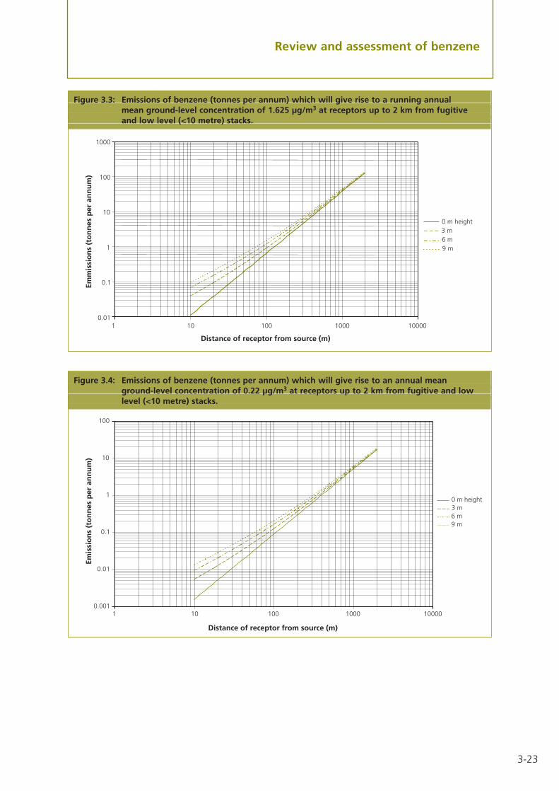
3-23
Review and assessment of benzene
Figure 3.4: Emissions of benzene (tonnes per annum) which will give rise to an annual meanground-level concentration of 0.22 µg/m3 at receptors up to 2 km from fugitive and lowlevel (<10 metre) stacks.
Figure 3.3: Emissions of benzene (tonnes per annum) which will give rise to a running annualmean ground-level concentration of 1.625 µg/m3 at receptors up to 2 km from fugitiveand low level (<10 metre) stacks.
0.01
0.1
10
100
1000
1 10 100 1000 10000
Distance of receptor from source (m)
0 m height3 m6 m9 m
Emm
issi
on
s (t
on
nes
per
an
nu
m)
1
0.001
0.01
0.1
1
10
100
1 10 100 1000 10000
Distance of receptor from source (m)
Emis
sio
ns
(to
nn
es p
er a
nn
um
)
6 m9 m
3 m0 m height
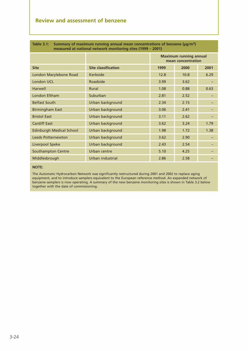
3-24
Review and assessment of benzene
Table 3.1: Summary of maximum running annual mean concentrations of benzene (µg/m3)measured at national network monitoring sites (1999 – 2001)
Maximum running annualmean concentration
Site Site classification 1999 2000 2001
London Marylebone Road Kerbside 12.8 10.8 6.29
London UCL Roadside 3.99 3.62 –
Harwell Rural 1.08 0.88 0.63
London Eltham Suburban 2.81 2.52 –
Belfast South Urban background 2.34 2.15 –
Birmingham East Urban background 3.06 2.41 –
Bristol East Urban background 3.11 2.62 –
Cardiff East Urban background 3.62 3.24 1.79
Edinburgh Medical School Urban background 1.98 1.72 1.38
Leeds Potternewton Urban background 3.62 2.90 –
Liverpool Speke Urban background 2.43 2.54 –
Southampton Centre Urban centre 5.10 4.25 –
Middlesbrough Urban industrial 2.86 2.58 –
NOTE:
The Automatic Hydrocarbon Network was significantly restructured during 2001 and 2002 to replace agingequipment, and to introduce samplers equivalent to the European reference method. An expanded network ofbenzene samplers is now operating. A summary of the new benzene monitoring sites is shown in Table 3.2 belowtogether with the date of commissioning.

3-25
Review and assessment of benzene
Table 3.2: Summary of benzene pumped samplers introduced into national networks during2001/2002
Site Site classification Commissioning date
Edinburgh Centre Urban centre 08/11/2001
Southampton Centre Urban centre 12/12/2001
Bristol Old Market Roadside 17/01/2002
Leicester Centre Urban centre 22/01/2002
Birmingham Roadside Roadside 29/01/2002
Middlesbrough Urban industrial 04/02/2002
Leeds Centre Urban centre 05/02/2002
Grangemouth Urban industrial 11/02/2002
Newcastle Centre Urban centre 12/02/2002
Oxford Centre Roadside 28/02/2002
Hove Roadside Roadside 27/02/2002
Haringey Roadside Roadside 26/02/2002
Manchester Piccadilly Urban centre 04/03/2002
Nottingham Centre Urban centre 05/03/2002
Northampton Urban centre 07/03/2002
Norwich Urban centre 12/03/2002
Southend-on-Sea Urban centre 14/02/2002
Leeds Roadside Roadside 20/03/2002
Sheffield Centre Urban centre 21/03/2002
Stoke Centre Urban centre 29/04/2002
Belfast Centre Urban centre 30/04/2002
Belfast Roadside Roadside 30/04/2002
Portsmouth Urban centre 09/05/2002
London Bloomsbury Urban centre 15/05/2002
Reading Urban centre 30/05/2002
Plymouth Urban centre 31/05/2002
Wigan Leigh Urban centre 05/06/2002
Liverpool Centre Urban centre 06/06/2002
Coventry Urban centre 10/06/2002
Leamington Spa Urban centre 10/06/2002
Cwmbran Urban background 26/06/2002
Yarm Roadside 08/07/2002
Hull Urban centre 09/07/2002
Barnsley Gawber Urban centre 10/07/2002
Bournemouth Urban centre 16/07/2002

3-26

Introduction 4.01 The Government and the Devolved Administrations have adopted a maximumrunning annual mean concentration of 2.25 µg/m3 as an air quality standard for 1,3-butadiene. The objective is for the standard to be achieved by the end of 2003.
4.02 This section of the guidance provides advice to local authorities on how toidentify areas within their locality, at risk of exceeding the Air Quality Objectives for 1,3-butadiene.
What areas are at risk of exceeding the objectives?
The national perspective
4.03 The main source of 1,3-butadiene in the United Kingdom is emissions frommotor vehicle exhausts. 1,3-butadiene is also an important industrial chemical and ishandled in bulk at a small number of industrial premises.
4.04 Concentrations of 1,3-butadiene are measured at a limited number of UKnational network sites. Maximum running annual mean concentrations of 1,3-butadiene measured at all urban background/centre and roadside locations arealready well below the 2003 objective of 2.25 µg/m3.
4.05 The increasing numbers of vehicles equipped with three way catalysts willsignificantly reduce emissions of 1,3-butadiene in future years. Recently agreed furtherreductions in vehicle emissions and improvements to fuel quality, including those aspart of the Auto-Oil programme, are expected to further reduce emissions of 1,3-butadiene from vehicle exhausts. These measures are expected to deliver the airquality objective by the end of 2003, and no further measures are thought to beneeded. Only those authorities with relevant locations in the vicinity of major industrialprocesses which handle, store or emit 1,3-butadiene, are expected to proceed beyondthe updating and screening assessment.
The local perspective – what conclusions have been drawn from the firstround of the review and assessment process?
4.06 There have been no AQMAs declared from the first round of reviews andassessments in respect of the air quality objective for 1,3-butadiene. This conclusionsupports the studies carried out at a national level.
4.07 Studies at a national level, based on both measured and modelling data, suggestthat there is little likelihood of the objective for 1,3-butadiene being exceeded by 2003.However, it is important that local circumstances are fully taken into considerationwithin the review and assessment process. All authorities are therefore required tocomplete the review and assessment for 1,3-butadiene. It is envisaged that this can beachieved without the need for further significant work, and it is highly unlikely that anyauthority will be required to proceed beyond the Updating and Screening Assessment.
Chapter 4 Review and assessment of 1,3-butadiene
4-1

Review and assessment of 1,3-butadiene
The Updating and Screening Assessment for 1,3-butadiene4.08 In completing the Updating and Screening Assessment, authorities areencouraged to maximise and build upon the data collation and assessments completedduring the first round of review and assessment.
4.09 All local authorities should undertake the Updating and Screening Assessmentfor 1,3-butadiene as part of the review and assessment process.
4.10 In order to complete the updating assessment, authorities should draw upon theinformation compiled as part of the First Stage report, completed in the first round ofreview and assessment.
4.11 This part of the review and assessment is based upon a checklist approach, asummary of which is provided in Box 4.1. Authorities may wish to consider formattingtheir reports for the Updating and Screening Assessment with these section headings inmind. A detailed checklist for each source or location is set out in Box 4.2 (at the endof the Updating and Screening Assessment section). This describes the information thatauthorities should collate for the review and assessment against the 2003 objective.The first column describes the source, location or data that need to be considered, andthe subsequent columns describe the steps that need to be taken.
Background concentrations
4.12 Estimated annual mean background concentrations for 2001 and 2003 havebeen mapped for the UK and can be accessed from the internet at the followingaddress: www.airquality.co.uk/archive/laqm/tools.php. Details of the mapping processcan also be found at this site. Factors to adjust measured background concentrations to2003 are provided in Box 4.3.
Box 4.3: Correction factors to estimate annual average 1,3-butadiene concentrations in future years measured data at background locations
Year Correction factor to Examplebe applied
1999 1.319
2000 1.136
2001 1.000
2002 0.872
2003 0.766
Box 4.1: Summary of the Updating and Screening checklist approach for 1,3-butadiene
Reference no. Source, location or data that need to be assessed
A Monitoring data
B New industrial sources
C Existing industrial sources with significantly increased emissions
1. Correction of measured background concentrations:Assume that the measured 1,3-butadiene concentration is 1.2µg/m3 in 2001. The corrected concentration for 2003 is then 1.2x 0.766 = 0.919 µg/m3.
Note: These factors do not apply to measured data where thesource is industrial.
4-2

Review and assessment of 1,3-butadiene
Monitoring data
4.13 Data collected from national monitoring networks, or from local monitoringcampaigns, are expected to give a more accurate indication of 1,3-butadieneconcentrations than modelling studies. Authorities are recommended to prioritise theuse of measured 1,3-butadiene concentrations wherever suitable data are available.It is emphasised that monitoring sites will need to be at locations relevant forpublic exposure, and where the maximum impact of the source (i.e. the highestconcentrations) are expected to be measured. In the case of fugitive emissions fromindustrial sources, then the highest relevant exposure will usually be at the closestresidential property in the downwind direction. In the case of emissions from chimneystacks, the highest concentrations may be some hundreds of metres downwind, andmay be determined by modelling.
4.14 Guidance on monitoring methods and strategies for 1,3-butadiene is set out inmore detail in Annex 1. Ideally, monitoring should have been carried out for a period ofone year, although a shorter period (e.g. 6 months) may be sufficient to demonstratethat the risk of exceedance of the objectives is negligible. Further guidance on howshort-term periods of monitoring data may be adjusted for assessment against therunning annual mean objectives is given in Annex 1.
4.15 Where measured data have been collected in the vicinity of an industrial source,concentrations should not be corrected for future years (2003), unless there issubstantive evidence that emissions will be reduced as a result of abatementtechnologies. If there is sufficient evidence to guarantee that emissions will be reducedby a quantified amount in future years, then this can be used to adjust the measuredvalues.
Screening assessment for industrial sources
4.16 A list of industrial processes with the potential to emit significant quantities of1,3-butadiene in 2003 is set out in Annex 2 (Appendix E). In the case of new industrialsources (since the last round of review and assessment), authorities are advised to checkwhether a Detailed Assessment has already been carried out as part of the planning orauthorisation process. This should certainly be the case for all Part A (and Part B inNorthern Ireland) regulated processes. If a suitably Detailed Assessment has beencompleted, then the authority may rely on these results, and should cite the conclusionsin the review and assessment report.
4.17 To simplify the assessment of industrial 1,3-butadiene emissions, twonomograms have been prepared1, which estimate the emission rate (in tonnes perannum) that would produce maximum running annual mean ground-levelconcentrations of 0.225 µg/m3, equivalent to 10% of the 2003 air quality objective.If the actual emission rate from the process exceeds the threshold, then it will benecessary to proceed to a Detailed Assessment.
1 Abbott J (2002) Review of pollutant specific guidance for industrial and domestic emissions. AEAT.
4-3

4-4
Review and assessment of 1,3-butadiene
4.18 The nomograms are shown at the end of this chapter. Authorities may alsodownload various LAQM Tools from the internet at the following address:www.airquality.co.uk/archive/laqm/tools.php which contain the calculations in an Excelspreadsheet form, which require the user to enter simple details on the emission rateand release conditions (stack height and diameter).
4.19 Where the process emits 1,3-butadiene from a stack of greater than 10 metresheight, the nomogram in Figure 4.1 should be used. Where the emissions arise from alow stack (less than 10 metres height) or from a fugitive source, then the nomogram inFigure 4.2 should be used.
4.20 To assist authorities in the compilation of data related to Part A (and Part B inNorthern Ireland) processes, the Environment Agency (EA), the Scottish EnvironmentProtection Agency (SEPA)2, and the Northern Ireland Environment and Heritage Service(EHS), have committed to provide information on any changes that may affectemissions from existing processes, and any new processes that have been, or will be,authorised. The information will be provided from the local office on request. A pro-forma request sheet for this information is provided in Annex 2 (Appendix F).
4.21 Authorities may also wish to consider checking information derived from the firstround of review and assessment if there were any doubts regarding their validity. If thisinformation was obtained from the regulatory agency, or directly from the PublicRegister, then there should be no need to undertake this task.
Stack emissions
4.22 To use the nomogram (Figure 4.1) it is necessary to estimate:
• the rate of emission of 1,3-butadiene in tonnes per annum
• the stack height
• the stack diameter
• the height of the tallest building within 5 stack heights of the chimney
4.23 The emission rate for Part A processes can be obtained from the regulatory agencies (see Para 4.20) or the operator directly. Emissions for processes in England and Wales are also posted on the internet at the following address:http://www.environment-agency.gov.uk. Emission rates for Part B (and Part C inNorthern Ireland) processes may be obtainable from the authority’s authorisationdocuments. Estimated emissions data and emissions factors are also available from theUK Emissions Factor Database www.naei.org.uk. Details of stack heights, diameters andbuilding heights can also be obtained from the regulator, the operator or theauthorisation documents, or may be estimated from a visual inspection.
2 SEPA have regulatory responsibility for Part B processes in Scotland.

4-5
Review and assessment of 1,3-butadiene
4.24 The nomogram uses the effective stack height. This can be assumed to beequal to the actual (physical) stack height unless:
• The height of release is greater than 3m above the building on which it sits, but lessthan 2.5 times the height of the tallest adjacent building. In this case the effectivestack height can be calculated from the following formula:
Ueff = 1.66(Uact – H)
where: H is the height (m) of the tallest adjacent building within 5 actual (physical)stack heights distance;
Ueff is the effective stack height; and
Uact is the actual (physical) stack height
4.25 To use the nomogram, identify the line that corresponds to the diameter of thestack under consideration, and locate the point on this line whose coordinates equalthe effective stack height. Read off the corresponding emission rate on the horizontalaxis, and compare this with the actual emission rate for the process. If the actualemission rate is greater than or equal to the emission rate derived from the chart, theauthority should proceed to a Detailed Assessment.
Short stack or fugitive emissions
4.26 To use the nomogram (Figure 4.2) it is necessary to estimate:
• the rate of emission of 1,3-butadiene in tonnes per annum
• the stack height (assumed to be zero for fugitive emissions)
4.27 The emission rate for Part A (and Part B in Northern Ireland) processes can beobtained from the regulatory agencies (see Para 4.20) or the operator directly. Emissionsfor processes in England and Wales are also posted on the Internet at the followingaddress: www.environment-agency.gov.uk. Emission rates for Part B (Part C in NorthernIreland) processes may be obtainable from the authority’s authorisation documents.Estimated emissions data and emissions factors are also available from the UK EmissionsFactor Database www.airquality.co.uk/archive/laqm/tools.php. Details of stack heights,diameters and building heights can also be obtained from the regulator, the operator orthe authorisation documents, or may be estimated from a visual inspection.
NOTE: If the stack height is less than any adjacent building within 5 actual (physical) stackheights distance, the authority should, in the first instance, undertake the assessmentassuming the release is from a low-level source (see Para 4.26). If this assessment indicates aproblem it will be necessary to proceed to a Detailed Assessment if the emission is greaterthan 0.05 tonne per annum.
Where there are multiple stacks at the same site, a precautionary approach may be taken byassuming the total emissions (from all stacks) are released from the smallest stack. Wherethere are complex sites, with many stacks, the above nomograms are unlikely to beapplicable, and authorities are advised to proceed to the Detailed Assessment.

4-6
Review and assessment of 1,3-butadiene
4.28 To use the nomogram, identify the line which corresponds to the height of thestack under consideration (assume zero for a fugitive emission), and locate the point onthis line whose coordinates equal the closest relevant receptor location. Read off thecorresponding emission rate on the horizontal axis, and compare this with the actualemission rate for the process. If the actual emission rate is greater than or equal to theemission rate derived from the chart, the authority should proceed to a DetailedAssessment.
4.29 The authority will need to consider the impact of emissions from stacks withinneighbouring areas, if there is a potential for these to be significant. As a guide, formedium size sources with chimneys between about 40 to 100 metres, impacts shouldbe considered at a distance up to about 5 km. For small sources with chimneysbetween about 20 to 40 metres, impacts should be considered at a distance up toabout 2 km. For fugitive emissions sources, impacts should be considered up to adistance of about 1 km. If there are several sources which line up, or are close to eachother, or there are doubts regarding the potential impact, the authority is advised totake a conservative view and proceed to a Detailed Assessment.
NOTE: Where there are multiple stacks or fugitive releases at the same site, a precautionaryapproach may be taken by assuming the total emissions (from all stacks or releases) arereleased from the smallest stack (or from a zero height source). Where there are complexsites, with many stacks or releases, the above nomograms are unlikely to be applicable, andauthorities are advised to proceed to a Detailed Assessment.
Box 4.2: Updating and Screening checklist
Monitoring
Overview
These steps will ensure you collate your 1,3-butadiene monitoring data andassess them appropriately to identify locations where exceedences of therunning annual mean objective might occur.
3. Calculate running annual meansfrom the data and identify thehighest value.
It is imperative that any localmonitoring data are ratified beforebeing used. Key steps will be toensure that you have screened andscaled the data – see Annex 1 fortechniques to do this.
2. Ratify your local monitoring data,if you have not already done so.
Include your own local monitoringdata and data from the nationalnetworks.
1. Collate all 1,3-butadienemonitoring data.
Approach
(A) Monitoring data
Notes relevant to each stepSteps that must be taken tocomplete the assessment
Source, location, ordata that need to be
assessed

4-7
Review and assessment of 1,3-butadiene
Box 4.2: Updating and Screening checklist (continued)
Monitoring (continued)
Industrial sources
Overview
No industrial sources were identified during the first round of review andassessment as likely to give rise to exceedences of the running annual meanobjective for 1,3-butadiene. You could, however, have new sources introducedinto your area or existing sources with substantially increased emissions. Thissection deals with these possibilities.
• Did the assessment predict anyexceedences of the objectives atrelevant locations?
Question
An assessment may already havebeen carried out as part of theplanning or authorisation process.If this is the case you should confirmthat the assessment is sufficient forreview and assessment purposes.
You only need to consider proposedsources for which planning approvalhas been granted.
1. Check whether an air qualityassessment has already beencarried out for the new industrialsource.
Approach 1(B) New industrialsources
The Detailed Assessment will be witha view to determining whether todeclare an AQMA.
If the answer is YES, proceed to aDetailed Assessment for 1,3-butadiene.
Action
Before you assess the measuredconcentrations check that themonitoring locations representrelevant exposure (see Paras 1.19 –1.21).
Use is made of currentconcentrations because there is nostraightforward way to projectfuture exceedences. Future estimateswould be part of any DetailedAssessment.
• Are any current running annualmeans greater than 2.25 µg/m3?
Questions
Notes relevant to each stepSteps that must be taken tocomplete the assessment
Source, location, ordata that need to be
assessed

4-8
Review and assessment of 1,3-butadiene
Box 4.2: Updating and Screening checklist (continued)
Industrial sources (continued)
See Para 4.20. If it is proving difficultto obtain the information on theemissions contact the EmissionsHelpdesk (Box 1.1).
2. Obtain updated information onthe total annual emission of 1,3-butadiene and the height of theemission.
A ‘substantial’ increase can be takento be one greater than 30%.
1. Determine whether any of thesources identified during the firstround of review and assessment aspotentially significant havesubstantially increased emissions.
Approach(C) Industrial sourceswith substantiallyincreasedemissions
If the answer is YES you shouldproceed to a Detailed Assessment for1,3-butadiene for this source.
Action
• Does the source exceed thethreshold in the nomogram?
Question
You will need to derive the effectivestack height. Details of how to dothis are provided in Para 4.24.
3. Use the nomograms described inPara 4.16 onwards to determine ifthe source requires furtherassessment.
See Para 4.20. If it is proving difficultto obtain the information on theemissions contact the EmissionsHelpdesk (Box 1.1).
2. Obtain information on the totalannual emission of 1,3-butadieneand the height of the emission.
1. Use the checklist in Annex 2 todetermine whether the sourceneeds considering further.
This approach should be followed ifthere has been no previous airquality assessment.
Approach 2
The Detailed Assessment may be nomore than relying on the findings ofthe air quality assessment. For this tobe the case the assessment will haveto meet the standards of a DetailedAssessment.
If the answer is YES you shouldproceed to a Detailed Assessment for1,3-butadiene for this source.
Action
Notes relevant to each stepSteps that must be taken tocomplete the assessment
Source, location, ordata that need to be
assessed

4-9
Review and assessment of 1,3-butadiene
The Detailed Assessment for 1,3-butadiene4.30 It is considered unlikely that any authority will need to proceed beyond thescreening assessment for 1,3-butadiene. Guidance on the Detailed Assessment hastherefore not been included in this document. In the event that any authority considersthat there is a significant risk of exceeding the 2003 objective, they are advised tocontact the relevant Helpdesk (see Box 1.1) for guidance.
Figure 4.1: Emissions of 1,3-butadiene (tonnes per annum) which will give rise to a running annual mean ground-level concentration of 0.225 µg/m3 (stacks >10 metres).
Box 4.2: Updating and Screening checklist (continued)
Industrial sources (continued)
If the answer is YES you shouldproceed to a Detailed Assessment for1,3-butadiene for this source.
Action
• Does the source exceed thethreshold in the nomogram?
Question
You will need to derive the effectivestack height. Details of how to dothis are provided in Para 4.24.
3. Use the nomograms described inPara 4.16 onwards to determine ifthe source requires furtherassessment.
Notes relevant to each stepSteps that must be taken tocomplete the assessment
Source, location, ordata that need to be
assessed
1
10
100
1000
0.1 1 10 100 1000
Emission (tonnes per annum)
Effe
ctiv
e st
ack
hei
gh
t (m
)
0.5 m diameter1 m2 m4 m8 m12 m

4-10
Review and assessment of 1,3-butadiene
Table 4.1: Summary of maximum running annual mean concentrations of 1,3-butadiene (µg/m3) measured at national network monitoring sites (1999 – 2001)
Maximum running annual mean concentration
Site Site classification 1999 2000 2001
London Marylebone Road Kerbside 2.25 1.92 1.63
London UCL Roadside 0.55 0.52 –
Harwell Rural 0.12 0.10 0.11
London Eltham Suburban 0.39 0.35 –
Belfast South Urban background 0.26 0.22 –
Birmingham East Urban background 0.39 0.34 –
Bristol East Urban background 0.36 0.29 –
Cardiff East Urban background 0.46 0.36 0.29
Edinburgh Medical School Urban background 0.21 0.19 0.20
Leeds Potternewton Urban background 0.41 0.31 –
Liverpool Speke Urban background 0.40 0.35 –
Southampton Centre Urban centre 0.60 0.55 –
Middlesbrough Urban industrial 0.32 0.22 –
Figure 4.2 Emissions of 1,3-butadiene (tonnes per annum) which will give rise to a running annual mean ground-level concentration of 0.225 µg/m3 at receptors up to 2 km from fugitive andlow level (stack <10 metre) sources.
0.001
0.01
0.1
1
10
100
1 10 100 1000 10000
Distance of receptor from source (m)
0 m height3 m6 m9 m
Emis
sio
ns
(to
nn
es p
er a
nn
um
)

Chapter 5: Review and assessment of lead
Introduction5.01 The Government and the Devolved Administrations have adopted an annualmean concentration of 0.5 µg/m3 as the air quality standard for lead, with an objectivefor the standard to be achieved by the end of 2004. In addition, a lower air qualityobjective of 0.25 µg/m3 to be achieved by the end of 2008 has also been set.
5.02 This section of the guidance provides advice to local authorities on how toidentify areas within their locality, at risk of exceeding the Air Quality Objectives forlead.
What areas are at risk of exceeding the objectives?
The national perspective
5.03 The agreement reached between the European Parliament and the EnvironmentCouncil on the Directive on the Quality of Petrol and Diesel Fuels (part of the Auto-OilProgramme) has led to the ban on sales of leaded petrol in the United Kingdom witheffect from 1 January 2000. Emissions of lead are now restricted to a variety ofindustrial activities, such as battery manufacture, pigments in paints and glazes, alloys,radiation shielding, tank lining and piping.
5.04 A summary of measured lead-in-air concentrations at UK national network sitesis shown in Table 5.1 for the period 1999-2001. Concentrations at all background andkerbside sites are well below the objectives for 2004 and 2008.
5.05 Detailed assessments of the potential impact of lead emissions from industrialprocesses have been undertaken by the Government and the Devolved Administrations,based upon both monitoring and sector analysis studies. The former has included a12-month monitoring survey in the vicinity of 30 key industrial sites in the UK, whichhas been used to supplement information already provided from the non-automaticmonitoring networks. These monitoring data have generally indicated no exceedancesof the 2004 or 2008 objectives, although locations in proximity to non-ferrous metalproduction and foundry processes were deemed to be at risk, and further monitoring isunder way. One exceedance of the 2004 objective was recorded in 2000 in the vicinityof the Brookside Metals plant (non-ferrous metals sector) in Willenhall.
The local perspective – what conclusions have been drawn from the reviewand assessment process?
5.06 There have been no AQMAs declared in respect of the 2004 or 2008 Air QualityObjectives, as a result of the first round of review and assessment. Only thoseauthorities with relevant locations in the vicinity of major industrial processes that emitsignificant quantities of lead, will need to progress beyond the Updating and ScreeningAssessment.
5-1

5-2
Review and assessment of lead
The Updating and Screening Assessment for lead5.07 This updating review is intended to identify any significant changes that may haveoccurred since the first round of review and assessment was completed. For lead, thiswill include new monitoring data, new or changed emissions sources (either locally or inneighbouring authorities), or other local changes that might affect air quality, etc.
5.08 In completing the Updating and Screening Assessment, authorities areencouraged to maximise and build upon the data and assessments work completedduring the first round of review and assessment.
5.09 It is recognised that some authorities will have completed Third Stage reportsduring the first round of review and assessment, and in doing so, will have set updetailed lists of emissions sources and used a variety of air quality dispersion models. Allauthorities should complete the updating assessment, but any subsequent screeningassessment may be carried out using models already established by the authority, if thisis the easier and preferred route.
5.10 This part of the review and assessment is based upon a checklist approach, asummary of which is provided in Box 5.1. Authorities may wish to consider formattingtheir reports for the Updating and Screening Assessment with these section headings inmind. A detailed checklist for each source or location is set out in Box 5.2 (at the endof the Updating and Screening Assessment section). This describes the information thatauthorities should collate for the review and assessment against the 2004 and 2008objectives. The first column describes the source, location or data that need to beconsidered, and the subsequent columns describe the steps that need to be taken.
Monitoring data
5.11 Data collected from national monitoring networks, or from local monitoringcampaigns, are expected to give a more accurate indication of lead concentrations thanmodelling studies. Authorities are recommended to prioritise the use of measured leadconcentrations wherever suitable data are available. It is emphasised that monitoringsites will need to be at locations relevant for public exposure (see Box 1.4), and wherethe maximum impact of the source (i.e. the highest concentrations) are expected to bemeasured. In the case of fugitive sources, then the highest relevant exposure is likely tobe at the closest residential property in the downwind direction. In the case ofemissions from chimney stacks, the highest concentrations may be some hundreds ofmetres downwind, and may be determined by simple dispersion modelling.
Box 5.1: Summary of the Updating and Screening checklist approach for lead
Reference no. Source, location or data that need to be assessed
A Monitoring data outside an AQMA
B New industrial sources
C Industrial sources with substantially increased emissions

5-3
Review and assessment of lead
5.12 Guidance on monitoring methods and strategies for lead is set out in moredetail in Annex 1. Ideally, monitoring should have been carried out for a period of oneyear, although a shorter period (e.g. 6 months) may be sufficient to demonstrate thatthe risk of exceedance of the objectives is negligible. Further guidance on how short-term periods of monitoring data may be adjusted for assessment against the annualmean objectives is given in Annex 1, or by contacting the relevant Helpdesk.
5.13 Where measured data have been collected in the vicinity of an industrial source,concentrations should not be corrected for future years (2004 and 2008), unless thereis substantive evidence that emissions will be reduced as a result of abatementtechnologies. If there is sufficient evidence to guarantee that emissions will be reducedby a quantified amount in future years, then this can be used to adjust the measuredvalues. For example, if the measured annual mean concentration in 2001 were 0.56µg/m3, and it were known that new abatement measures would reduce emissions by75% before 2003, then it could be assumed that ambient concentrations would fall to0.14 µg/m3 in 2004 and 2010.
Screening assessment for industrial sources
5.14 A list of industrial processes with the potential to emit significant quantities oflead is set out in Annex 2. In the case of new industrial sources (since the last round ofreview and assessment), authorities are advised to check whether an air qualityassessment has already been carried out as part of the planning or authorisationprocess. This should certainly be the case for all Part A (and Part B in Northern Ireland)regulated processes. If a suitably detailed assessment has been completed, then theauthority may rely on these results, and should cite the conclusions in the review andassessment report.
5.15 To simplify the assessment of industrial lead emissions, two nomograms havebeen prepared1 which estimate the emission rate (in tonnes per annum) that wouldproduce a maximum annual mean ground-level concentrations of 0.025 µg/m3,equivalent to 10% of the 2008 Air Quality Objectives. If the actual emission rate fromthe process exceeds these thresholds, then it will be necessary to proceed to a DetailedAssessment.
5.16 The nomograms are shown at the end of this chapter. Authorities may alsodownload various LAQM Tools from the internet at the following address:www.airquality.co.uk/archive/laqm/tools.php which contains the calculations in an Excelspreadsheet form, and require the user to enter simple details on the emission rate andrelease conditions (stack height and diameter).
5.17 Where the process emits lead from a stack of greater than 10 metres height, thenomogram in Figure 5.1 should be used. Where the emissions arise from a low stack(less than 10 metres height) or from a fugitive source, then the nomogram in Figure 5.2should be used.
1 Abbott J (2002) Review of pollutant specific guidance for industrial and domestic emissions. AEAT.

Review and assessment of lead
5.18 To assist authorities in the compilation of data related to Part A (Part B inNorthern Ireland) processes, the Environment Agency (EA), the Scottish EnvironmentProtection Agency (SEPA)2, and the Northern Ireland Environment and Heritage Service(EHS), have committed to provide information on any changes that may affectemissions from existing processes, and any new processes that have been, or will be,authorised. The information will be provided from the local office on request. A pro-forma request sheet for this information is provided in Annex 2 (Appendix F).
5.19 Authorities may also wish to consider checking information derived from the firstround of review and assessment if there were any doubts regarding their validity. If thisinformation was obtained from the regulatory agency, or directly from the PublicRegister, then there should be no need to undertake this task.
Stack emissions
5.20 To use the nomogram (Figure 5.1) it is necessary to estimate:
• the rate of emission of lead in tonnes per annum
• the stack height
• the stack diameter
• the height of the tallest building within 5 stack heights of the chimney
5.21 The emission rate for Part A (and Part B in Northern Ireland) processes can beobtained from the regulatory agencies (see Para 5.18) or the operator directly. Emissionsfor processes in England and Wales are also posted on the internet at the followingaddress: http://www.environment-agency.gov.uk. Emission rates for Part B (Part C inNorthern Ireland) processes may be obtainable from the authority’s authorisationdocuments. Estimated emissions data and emissions factors are also available from theUK Emissions Factor Database (www.naei.org.uk). Details of stack heights, diametersand building heights can also be obtained from the regulator, the operator or theauthorisation documents, or may be estimated from a visual inspection.
5.22 The nomogram uses the effective stack height. This can be assumed to beequal to the actual (physical) stack height unless:
• The height of release is greater than 3m above the building on which it sits, but lessthan 2.5 times the height of the tallest adjacent building. In this case the effectivestack height can be calculated from the following formula:
Ueff = 1.66(Uact – H)
where: H is the height (m) of the tallest adjacent building within 5 actual (physical)stack heights distance;
Ueff is the effective stack height; and
Uact is the actual (physical) stack height
2 SEPA have regulatory responsibility for Part B processes in Scotland.
5-4
Review and assessment of lead
5.23 To use the nomogram, identify the line that corresponds to the diameter of thestack under consideration, and locate the point on this line whose coordinates equalthe effective stack height. Read off the corresponding emission rate on the horizontalaxis, and compare this with the actual emission rate for the process. If the actualemission rate is greater than or equal to the emission rate derived from the chart, theauthority should proceed to a Detailed Assessment.
Short stack or fugitive emissions
5.24 To use the nomogram (Figure 5.2) it is necessary to estimate:
• the rate of emission of lead in tonnes per annum
• the stack height (assumed to be zero for fugitive emissions)
5.25 The emission rate for Part A (and Part B in Northern Ireland) processes can beobtained from the regulatory agencies (see Para 5.18) or the operator directly. Emissionsfor processes in England and Wales are also posted on the Internet at the followingaddress: http://www.environment-agency.gov.uk. Emission rates for Part B (Part C inNorthern Ireland) processes may be obtainable from the authority’s authorisationdocuments. Estimated emissions data and emissions factors are also available from theUK Emissions Factor Database (www.naei.org.uk). Details of stack heights, diametersand building heights can also be obtained from the regulator, the operator or theauthorisation documents, or may be estimated from a visual inspection.
5.26 To use the nomogram, identify the line which corresponds to the height of thestack under consideration (assume zero for a fugitive emission), and locate the point onthis line whose coordinates equal the closest relevant receptor location. Read off thecorresponding emission rate on the horizontal axis, and compare this with the actualemission rate for the process. If the actual emission rate is greater than or equal to theemission rate derived from the chart, the authority should proceed to a DetailedAssessment.
NOTE: If the stack height is less than any adjacent building within 5 actual (physical) stackheights distance, the authority should, in the first instance, undertake the assessmentassuming the release is from a low-level source (see Para 5.24). If this assessment indicates aproblem, it will be necessary to proceed to a Detailed Assessment if the emission is greaterthan 0.005 tonne per annum.
Where there are multiple stacks at the same site, a precautionary approach may be taken byassuming the total emissions (from all stacks) are released from the smallest stack. Wherethere are complex sites, with many stacks, the above nomograms are unlikely to beapplicable, and authorities are advised to proceed to the Detailed Assessment.
5-5

Review and assessment of lead
5.27 The authority will need to consider the impact of emissions from stacks withinneighbouring areas, if there is a potential for these to be significant. As a guide, formedium size sources with chimneys between about 40 to 100 metres, impacts shouldbe considered at a distance up to about 5 km. For small sources with chimneysbetween about 20 to 40 metres, impacts should be considered at a distance up toabout 2 km. For fugitive emissions sources, impacts should be considered up to adistance of about 1 km. If there are several sources which line up, or are close to eachother, or there are doubts regarding the potential impact, the authority is advised totake a conservative view and proceed to a Detailed Assessment.
NOTE: Where there are multiple stacks or fugitive releases at the same site, a precautionaryapproach may be taken by assuming the total emissions (from all stacks or releases) arereleased from the smallest stack (or from a zero height source). Where there are complexsites, with many stacks or releases, the above nomograms are unlikely to be applicable, andauthorities are advised to proceed to a Detailed Assessment.
Box 5.2: Updating and Screening checklist
Monitoring
Overview
These steps will ensure you collate all relevant lead monitoring data and assessthem appropriately to identify locations where exceedences of the annual meanobjectives for 2004 and/or 2008 might occur. You should focus on monitoringdata obtained since the last round of review and assessment, but it is also usefulto show longer-term trends where possible.
The annual means should represent acalendar year if possible. Where lessthan 9 months data are available,contact the Monitoring Helpdesk foradvice.
3. Calculate annual means from thedata.
It is imperative that any localmonitoring data are ratified beforebeing used. Key steps will be toensure that you have screened andscaled the data – see Annex 1 fortechniques to do this.
2. Ratify your local monitoring data,if you have not already done so.
Include your own local monitoringdata and data from the nationalmonitoring networks.
1. Collate all lead monitoring data.
Approach
(A) Monitoring dataoutside an AQMA
Notes relevant to each stepSteps that must be taken tocomplete the assessment
Source, location, ordata that need to be
assessed
5-6

Review and assessment of lead
Box 5.2: Updating and Screening checklist (continued)
Monitoring (continued)
Industrial sources
Overview
No industrial sources were identified during the first round of review andassessment as likely to give rise to exceedences of the annual mean objectivefor lead. You could however have new sources introduced into your area orexisting sources with substantially increased emissions. This section deals withthese possibilities. Particular attention should be paid to the combined impactof several sources, including those outside the local authority area.
The Detailed Assessment may be nomore than relying on the findings ofthe air quality assessment. For this tobe the case the assessment will haveto meet the standards of a DetailedAssessment.
If the answer is YES you shouldproceed to a Detailed Assessment forlead for this source.
Action
• Did the assessment predict anyexceedences of the objectives atrelevant locations?
Question
An assessment may already havebeen carried out as part of theplanning or authorisation process. Ifthis is the case you should confirmthat the assessment is sufficient forreview and assessment purposes.
You only need to consider proposedsources for which planning approvalhas been granted.
1. Check whether an air qualityassessment has already beencarried out for the new industrialsource.
Approach 1(B) New industrialsources.
The Detailed Assessment will be witha view to determining whether todeclare an AQMA.
If the answer is YES to either ofthese questions, proceed to aDetailed Assessment for lead.
Action
Before you assess the measuredconcentrations check that themonitoring locations representrelevant exposure (see Paras 1.19 –1.21).
Use is made of currentconcentrations because there is nostraightforward way to projectfuture exceedences (but see Para5.13). Future estimates would be partof any Detailed Assessment.
• Are any current annual meansgreater than 0.5 µg/m3?
• Are any current annual meansgreater than 0.25 µg/m3?
Questions
Notes relevant to each stepSteps that must be taken tocomplete the assessment
Source, location, ordata that need to be
assessed
5-7

Review and assessment of lead
Box 5.2: Updating and Screening checklist (continued)
Industrial sources (continued)
If the answer is YES you shouldproceed to a Detailed Assessment forlead.
Action
• Does the source exceed thethreshold in the nomograms?
Question
You will need to derive the effectivestack height. Details of how to dothis are provided in Para 5.22.
3. Use the nomograms described inPara 5.14 onwards to determine ifthe source requires furtherassessment.
See Para 5.21. If it is proving difficultto obtain the information on theemissions contact the EmissionsHelpdesk (Box 1.1).
2. Obtain updated information onthe total annual emission of leadand the height of the emission.
A ‘substantial’ increase can be takento be one greater than 30%.
1. Determine whether any of thesources identified during the lastround as potentially significanthave ‘substantially’ increasedemissions.
Approach(C) Industrial sourceswith substantiallyincreasedemissions
If the answer is YES you shouldproceed to a Detailed Assessment forlead for this source.
Action
• Does the source exceed thethreshold in the nomograms?
Question
You will need to derive the effectivestack height. Details of how to dothis are provided in Para 5.22.
3. Use the nomograms described inPara 5.14 onwards to determine ifthe source requires furtherassessment.
See Para 5.21. If it is proving difficultto obtain the information on theemissions contact the EmissionsHelpdesk (Box 1.1).
2. Obtain information on the totalannual emission of lead and theheight of the emission.
1. Use the checklist in Annex 2 todetermine whether the sourceneeds considering further.
This approach should be followed ifthere has been no previous airquality assessment.
Approach 2
Notes relevant to each stepSteps that must be taken tocomplete the assessment
Source, location, ordata that need to be
assessed
5-8

Review and assessment of lead
The Detailed Assessment for lead5.28 Where the screening assessment has indicated that there is a risk of the AirQuality Objectives for lead not being achieved by 2004 or 2008, then the authority willneed to carry out a Detailed Assessment. The aim of this Detailed Assessment is todetermine with reasonable certainty whether or not there is a likelihood of theobjectives not being achieved. The assumptions within this Detailed Assessment shouldbe considered in depth, and the data that are used or collected, quality-assured to ahigh standard. This is to allow the authority to have confidence in the decision that itreaches to declare, not declare, or revoke an Air Quality Management Area. Where alikely exceedance of the objectives is identified, then the authority will also need todetermine the magnitude and geographical extent, so that the AQMA boundary canbe set.
5.29 Because of the potential wide variety of sources and local circumstances thatmay prevail, it is not possible to set prescriptive guidance for the Detailed Assessment.However, wherever possible, lessons learnt from the First Round of review andassessment have been drawn upon. It is also expected that authorities will make use ofthe various Helpdesks that have been established (see Box 1.1).
5.30 Specific guidance related to monitoring, collation of emissions data anddispersion modelling, is provided in Annexes 1 to 3 of this document. Whilst importantaspects are highlighted in this section, authorities who are undertaking a DetailedAssessment are strongly advised to read the relevant sections of the Annexes beforecommencing their work.
5.31 In undertaking the Detailed Assessment it is important to give consideration tothe points of maximum relevant public exposure (i.e. those locations where the highestconcentrations of lead are expected). In the case of emissions from fugitive sources thehighest concentrations are generally likely to occur at the closest downwind point tothe facility. Where emissions are released from a stack or vent, then the point ofhighest concentration will occur some distance downwind. In the latter case, simpledispersion modelling may help identify this location.
Monitoring
5.32 As for the screening assessment, measured data are expected to give a moreaccurate indication of lead concentrations than modelling studies. This is particularlythe case where fugitive emissions are of the greatest significance.
5.33 Guidance on monitoring methods, monitoring strategies and suitable QA/QCprocedures are set out in greater detail in Annex 1 to this document. The followingpoints are highlighted:
• Monitoring should be undertaken at relevant locations (see Para 5.11 and Box 1.4).Specific consideration should be given to the locations of the lead-emitting processesin relation to public exposure.
5-9

Review and assessment of lead
• Ideally monitoring should be carried out for a period of a full year, with 90% datacapture, and any gaps evenly spread throughout the year. In some circumstances itmay be possible to curtail the period of monitoring, for example after 6 monthsconsecutive sampling. However, it should be noted that it will probably beimpractical to adjust locally measured data by comparison with national networksites, due to the local nature of the emissions. Where less than 9 months data areavailable, authorities are advised to contact the relevant Helpdesk.
5.34 Where monitoring indicates that the objectives are likely to be exceeded, then itmay be helpful to refine the monitoring strategy in order to more clearly identify thesource contributions. In such cases, authorities may find it useful to:
• Undertake monitoring of wind speed and direction to assist with the interpretationof results and any reported exceedances.
• Undertake monitoring at several locations including a site upwind of the source. Thiswill allow a more accurate assessment of the source contribution to the measuredexceedance to be carried out. Alternatively, ‘direction samplers’ which allowmonitoring to be carried out during pre-selected wind directions may also be used.
Modelling
5.35 For the Detailed Assessment, authorities will need to have confidence in theirresults, which will subsequently be used to determine whether there is a likelihood ofthe objectives being exceeded and the need to declare an AQMA.
5.36 Where emissions of lead can be accurately quantified from a stack or vent, thenthe impact can be determined using a suitable point source model. It is probably onlynecessary to determine the annual emission rate from the process even if there aresignificant daily or seasonal variations.
5.37 Issues regarding model validation and verification are discussed in further detailin Annex 3. Model validation generally refers to detailed, peer-reviewed studies thathave been carried out by the model supplier, or a regulatory agency (for example,USEPA). All models used in the Detailed Assessment should have an appropriatepedigree, and have been subject to detailed and documented validation trials.
5.38 Model verification refers to checks that are carried out on model performanceat a local level. This basically involves the comparison of predicted versus measuredconcentrations. Where there is a disparity between the predicted and measuredconcentrations, the first step should always be to check the input data and modelparameters in order to minimise the errors. If required, the second step will be todetermine an appropriate adjustment factor that can be applied. Whilst it is moredifficult to verify point source models at a local level, this is a more straightforwardprocess for annual mean concentrations, and is recommended for lead. Ideally, themonitoring location will have been selected with the aid of a dispersion model.
5-10

Review and assessment of lead
5.39 In all cases where model verification has been carried out, the approach shouldbe fully documented in the review and assessment report, and any adjustment factorapplied should be explicitly stated.
Meteorological data
5.40 The choice of meteorological data for use in the dispersion model can have anoutcome on the result, depending on whether a ‘worst case’ or ‘typical’ year isselected. A detailed discussion on the selection of meteorological data is provided inAnnex 3 and all authorities are advised to read this section prior to undertaking amodelling study. In summary, the guidance recommends that a single year of sequentialmeteorological data is generally used. If possible, meteorological, background andemissions data should all be derived from the same year.
5.41 In the case of emissions from point sources, the main effect of differentmeteorological years will be to affect the precise location of the maximum predictedconcentration. Authorities are advised to take into consideration the potential effects offluctuating wind directions in different years. A suggested means of dealing with this isto assume that the actual maximum concentration may occur within a 45 degree arccentred on the predicted maxima, and all properties lying within this arc should beconsidered. Where the authority decides to use multiple years (3 or more) ofmeteorological data, it is recommended that the results for all years are reported, butthat any decision is based upon the worst-case result.
Receptor spacing
5.42 The importance of giving due consideration to potential ‘hot spots’ has alreadybeen highlighted in Para 5.31. For the purpose of dispersion modelling, this requiresthe user to ensure that a suitable resolution for receptor grid spacing is used, or thatspecific receptors (representing the locations of maximum public exposure) are included.If the grid spacing is set to a low resolution (for example, several hundred metres) andno specific receptors are included, then there is the potential that the model will notpredict the highest concentrations relevant to public exposure. A more detaileddiscussion on receptor spacing is provided in Annex 3.
5-11

Review and assessment of lead
Figure 5.2 Emissions of lead (tonnes per annum) which will give rise to an annual mean ground-levelconcentration of 0.025 µg/m3 at receptor locations up to 2 km from fugitive and low level(stack <10 metre) sources.
Figure 5.1: Emissions of lead (tonnes per annum) which will give rise to an annual mean ground-levelconcentration of 0.025 µg/m3 (stacks >10 metres).
5-12
0.01 0.1 1 10 100
Emission (tonnes per annum)
Effe
ctiv
e st
ack
hei
gh
t (m
)
0.5 m diameter1 m2 m4 m8 m12 m
1
10
100
1000
0.0001
0.001
0.01
0.1
10
1 10 100 1000 10000
Distance of receptor from source (m)
0 m height3 m6 m9 m
Emis
sio
ns
(to
nn
es p
er a
nn
um
) 1

Review and assessment of lead
Table 5.1: Summary of annual mean lead-in-air concentrations at national network monitoring sites, 1999-2001 (µg/m3)
Annual mean lead-in-airconcentration (µg/m3)
Site Site classification 1999 2000 2001
London Cromwell Road 2 Kerbside 0.068 0.032 0.031
Cardiff Kerbside 0.074 0.029 0.028
Central London Urban Background 0.036 – –
Glasgow Urban Background 0.020 0.017 0.025
Leeds Urban Background 0.039 0.027 0.031
London Brent Urban Background 0.049 0.024 0.030
Motherwell Urban Background 0.016 0.009 0.016
Manchester Urban Background 0.051 0.022 0.023
Newcastle Urban Background 0.013 0.008 0.032
Brookside 1 Industrial 0.079 0.034 0.045
Brookside 2 Industrial 0.203 0.524 0.419
Elswick 1 Industrial 0.040 0.023 0.042
Elswick 2 Industrial 0.056 0.046 0.080
Elswick 6 Industrial 0.135 0.110 0.168
IMI 1 Industrial 0.367 0.055 0.043
IMI 2 Industrial 1.432 0.075 0.048
5-13

5-14

6-1
Chapter 6 Review and assessment of nitrogen dioxide
Introduction6.01 The Government and the Devolved Administrations have adopted two AirQuality Objectives for nitrogen dioxide, as an annual mean concentration of 40 µg/m3,and a 1-hour mean concentration of 200 µg/m3 not to be exceeded more than 18times per year1. The objectives are to be achieved by the end of 2005.
6.02 The first Air Quality Daughter Directive also sets limit values for nitrogen dioxide,which have been transposed into UK legislation. The Directive includes a 1-hour limitvalue of 200 µg/m3, not to be exceeded more than 18 times per year, and an annualmean limit value of 40 µg/m3, both to be achieved by 1 January 2010.
6.03 This section of the guidance provides advice to local authorities on how toidentify areas within their locality at risk of exceeding the Air Quality Objectives fornitrogen dioxide. Guidance is also provided to allow authorities to assess the likelihoodof the EU limit values not being achieved by 2010, although there is no statutoryrequirement on local authorities to carry out this additional assessment.
What areas are at risk of exceeding the objectives?
The national perspective
6.04 Nitrogen dioxide (NO2) and nitric oxide (NO) are both oxides of nitrogen, and arecollectively referred to as nitrogen oxides (NOx). All combustion processes produce NOxemissions, largely in the form of nitric oxide, which is then converted to nitrogendioxide, mainly as a result of reaction with ozone in the atmosphere. It is nitrogendioxide that is associated with adverse effects upon human health.
6.05 The principal source of nitrogen oxides emissions is road transport, whichaccounted for about 49% of total UK emissions in 2000. Major roads carrying largevolumes of high-speed traffic (such as motorways and other primary routes) are apredominant source, as are conurbations and city centres with congested traffic. Withinmost urban areas, the contribution of road transport to local emissions will be muchgreater than for the national picture. As an example, road transport is estimated toaccount for more than 75% of nitrogen oxides emissions in London.
6.06 The contribution of road transport to nitrogen oxides emissions has declinedsignificantly in recent years as a result of various policy measures, and furtherreductions are expected up until 2010 and beyond. For example, urban traffic nitrogenoxides emissions are estimated to fall by about 20% between 2000 and 2005, and by46% between 2000 and 20102.
1 The air quality standard for nitrogen dioxide is 286 µg/m3, expressed as the 1-hour mean, and is based upon theadvice of EPAQS. The 1-hour and annual mean objectives are consistent with the EU limit values. The limit valuesare derived from the WHO air quality guidelines (equivalent in concept to the UK standards).
2 Stedman J R, Bush T J, Murrells T P and King K (2001). Baseline PM10 and NOx projections for PM10 objectiveanalysis. AEAT/ENV/R/0726.

6-2
Review and assessment of nitrogen dioxide
6.07 Other significant sources of nitrogen oxides emissions include the electricitysupply industry and other industrial and commercial sectors, which accounted for about24% and 23% respectively in 1999. Emissions from both sources have also declineddramatically, due to the fitting of low nitrogen oxides burners, and the increased use ofnatural gas plant. Industrial sources make only a very small contribution to annual meannitrogen dioxide levels, although breaches of the hourly nitrogen dioxide objective mayoccur under rare, extreme meteorological conditions, due to emissions from thesesources.
6.08 A summary of measured nitrogen dioxide concentrations at UK national networksites is shown in Table 6.1 for the period 1999 to 2001. The annual mean objective of40 µg/m3 is currently widely exceeded at roadside sites throughout the UK, withexceedences also reported at urban background locations in major conurbations. Thenumber of exceedences of the 1-hour objective show considerable year-to-yearvariation, and are driven by meteorological conditions which give rise to winterepisodes of poor dispersion and summer oxidant episodes. In recent years, exceedencesof the short-term objective have generally only been recorded at roadside or kerbsidesites in close proximity to heavily-trafficked roads in major conurbations3.
6.09 In practice, meeting the annual mean objective in 2005, and the limit value in2010, is expected to be considerably more demanding than achieving the 1-hourobjective. National studies have indicated that the annual mean objective is likely to beachieved at all urban background locations outside of London by 2005, but that theobjective may be exceeded more widely at roadside sites throughout the UK in closeproximity to busy road links. Projections for 2010 indicate that the EU limit value maystill be exceeded at urban background sites in London, and at roadside locations inother cities.
The local perspective – what conclusions have been drawn from the reviewand assessment process?
6.10 The initial stages of the first round of the review and assessment process arenow complete, and it is useful to draw upon the conclusions reached at a local levelfrom this exercise. Of the 100-plus AQMAs that have been declared, the vast majorityare related specifically to road traffic emissions, where attainment of the annual meanobjective is considered unlikely. Of the anticipated AQMAs, 95% have traffic emissionsas the main, if not only, component. Exceedences of the objective have been identifiedwithin major conurbations, within smaller town centres with congested traffic, andalongside dual carriageways and motorways in more rural areas.
6.11 Exceedences have also been predicted in the vicinity of major airports, whereboth road traffic and aircraft nitrogen oxides emissions combine. Whilst industrialsources may make a contribution to local pollutant levels, no exceedences of theobjectives have been identified as a direct result of these emissions alone.
3 An exception was recorded at the Stockport urban background site in 2001, and was associated with unusualmeteorological conditions which caused an accumulation of emissions within the urban area. During this episode,there were 20 exceedences of the hourly objective in just 2 days. The potential for such unusual events willdiminish by 2005 due to lower NOx emissions.

6-3
Review and assessment of nitrogen dioxide
6.12 An analysis of monitoring data in the vicinity of roads throughout the UK hasbeen undertaken, and provides useful additional guidance to authorities on whereexceedences might occur4. The report concludes that, outside of major conurbations,exceedences of the annual mean objective are only likely to occur within about 10metres of the kerbside of single carriageway roads. This includes roads with relativelylow traffic flows (10000 – 20000 veh/day) if they are within congested town centres.This conclusion is particularly significant, as many market towns have narrow streets,with residential properties within 5 metres or so of the kerb. Despite higher trafficflows, exceedences of the annual mean objective are only likely within about 5 metresof the kerbside or hard shoulder of dual carriageways outside of major conurbations.
6.13 It is therefore critical that authorities focus upon those locations where theyexpect pollutant concentrations to be the highest (often referred to as ‘hot spots’).Focussing on these areas should ensure that potential exceedences are not missed. Thisapproach is also likely to be cost effective, particularly for updating reports preparedduring the first round of review and assessment. If there are no exceedences of theobjectives at the most polluted locations, then it can be reasonably concluded thatthere should be no exceedences elsewhere.
The Updating and Screening Assessment for nitrogendioxide6.14 This updating review is intended to identify any significant changes that mayhave occurred since the first round of review and assessment was completed. Fornitrogen dioxide, this will include new monitoring data, new or changed emissionssources (either locally or in neighbouring authorities), or other local changes that mightaffect air quality, etc.
6.15 Whilst there have been no changes to the Air Quality Objectives for nitrogendioxide, authorities will be aware that Government and the Devolved Administrationshave recently released new road traffic emissions factors. These new factors reflect theexpected higher nitrogen oxides emissions in future years from road transport. At anational level, these changes are expected to be relatively minor, but more significantchanges may be seen at a local level depending upon the traffic mix5.
6.16 The effect of these new factors will be to also change the predicted backgroundconcentrations in future years, as these are derived from our estimates of future fleetmix and vehicle emissions.
6.17 Whilst there is no statutory requirement to do so, authorities are alsoencouraged to extend their review and assessment to include the 2010 limit value. It isbelieved that in many cases this will add little additional work, and will provideauthorities with invaluable information, particularly when assessing the impact of local
4 Compilation of new roadside monitoring data obtained by local authorities as part of the review and assessmentprocess. A Report prepared by Air Quality Consultants Ltd and University of West of England on behalf of Defra,April 2002.
5 Emissions Toolkit available at http://www.stanger.co.uk/airqual/modelhlp.

6-4
Review and assessment of nitrogen dioxide
development proposals. It should be noted that, in the majority of cases, it is extremelyunlikely that the limit value in 2010 will be exceeded if the objective in 2005 is met.Emissions of nitrogen oxides are expected to continue to decline between 2005 and2010. Exceptions may occur at locations where emissions of nitrogen oxides have thepotential to increase between 2005 and 2010, for example close to major airportswhere significant expansion of air traffic movements is forecast. In such casesauthorities cannot automatically assume that the limit value in 2010 will be met if theobjective in 2005 is not exceeded.
6.18 In completing the Updating and Screening Assessment, authorities areencouraged to maximise and build upon the data and assessments work completedduring the first round of review and assessment.
6.19 It is recognised that many authorities will have completed Third Stage reportsduring the first round of review and assessment, and in doing so, will have set updetailed lists of emissions sources and used a variety of air quality dispersion models. All authorities should complete the updating assessment, but any subsequent screeningassessment may be carried out using models already established by the authority, if thisis the easier and preferred route.
6.20 In order to complete the Updating and Screening Assessment, authorities shoulddraw upon the information compiled as part of the First Stage report, completed in thefirst round of review and assessment.
6.21 This part of the review and assessment is based upon a checklist approach, asummary of which is provided in Box 6.1. Authorities may wish to consider formattingtheir reports for the Updating and Screening Assessment with these section headings inmind. A detailed checklist for each source or location is set out in Box 6.2 (at the endof the Updating and Screening Assessment section). This describes the information thatauthorities should collate for the review and assessment against the 2005 objective6.The first column describes the source, location or data that need to be considered, andthe subsequent columns describe the steps that need to be taken.
NOTE: Authorities will need to consider both NOx (comprising of NO and NO2) and nitrogendioxide (NO2) in the course of their reviews and assessments. It is strongly recommended thatNOx and NO2 concentrations are always expressed in units of µg/m3. Both emissions andconcentrations of NOx should always be expressed as NO2 equivalent (i.e. assuming that allof the NO present were as NO2). Emission rates are always expressed in this manner, anddispersion models require this assumption.
6 The approach set out in Box 6.2 for review and assessment of the 2005 objective may also be applied to the 2010limit value. Suitable tools for assessment of the limit value are also provided.

6-5
Review and assessment of nitrogen dioxide
Background concentrations
6.22 Estimated annual mean background nitrogen oxides and nitrogen dioxideconcentrations for 2001, 2005 and 2010 have been mapped for the UK, and can beaccessed from the internet at the following address:www.airquality.co.uk/archive/laqm/tools.php. Details of the mapping process can alsobe found at this site.
6.23 In using these maps, authorities are advised to take care to avoid ‘doublecounting’. For example, in rural areas where there is a section of heavily-trafficked roadit may be more appropriate to derive the background concentration from adjacent gridsquares. A recommended approach in such cases is set out in Box 1.5.
Monitoring data
6.24 Data collected from national monitoring networks, or from local monitoringcampaigns, are expected to give a more accurate indication of nitrogen dioxideconcentrations than modelling studies. Authorities are recommended to prioritise theuse of measured nitrogen dioxide concentrations wherever suitable data are available.It is emphasised that monitoring sites will need to be at locations relevant for publicexposure, and where the maximum impact of the source (i.e. the highestconcentrations) are expected to be measured (see Paras 6.12 and 6.13).
Box 6.1: Summary of the Updating and Screening checklist approach for nitrogen dioxide
Reference no. Source, location or data that need to be assessed
A Monitoring data outside an AQMA
B Monitoring data within an AQMA
C Narrow congested streets with residential properties close to the kerb
D Junctions
E Busy streets where people may spend 1-hour or more close to traffic
F Roads with high flow of buses and/or HGVs
G New roads constructed or proposed since first round of review and assessment
H Roads close to the objective during the first round of review and assessment
I Roads with significantly changed traffic flows
J Bus Stations
K New industrial sources
L Industrial sources with substantially increased emissions
M Aircraft

6-6
Review and assessment of nitrogen dioxide
6.25 Guidance on monitoring methods and strategies for nitrogen dioxide are set outin more detail in Annex 1. Monitoring using diffusion tubes is widely used in the UK tocharacterise ambient concentrations of nitrogen dioxide. Whilst this method canproduce data that are comparable to reference methods (chemiluminescence samplers)care must be taken with the storage, handling and analysis of the tubes. It is imperativethat suitable QA/QC procedures are employed, and that the diffusion tubes have beenvalidated against a reference method so that a ‘bias correction’ can be applied. Anapproach to the use of diffusion tubes, and a proposed method for bias correction isset out in Boxes 6.3 and 6.4 respectively. Note: the use of triplicate diffusion tubes isnot essential, except at sites which are co-located with chemiluminescent analysers.Guidance on the interpretation of triplicate exposures is given in Annex 1.
6.26 Ideally, monitoring should have been carried out for a period of one year,although a shorter period (for example, 6 months) may be sufficient to demonstratethat the risk of exceedence of the objectives is negligible. Further guidance on howshort-term periods of monitoring data may be adjusted for assessment against theannual mean objectives is given in Box 6.5.
Box 6.3: Use of nitrogen dioxide diffusion tubes
A recent study7 has looked at results from diffusion tube collocation studies carried out by a number oflocal authorities. This reveals considerable difference in the performance of tubes prepared by differentlaboratories. This is not a criticism of the laboratories, but emphasises that the laboratory bias must bedetermined and allowed for. So long as the laboratory performs consistently over time, then this biaswill not matter if it is allowed for. The bias adjustment factor should be based on collocation of tubeswith a chemiluminesence monitor. This could be part of a local survey or using a nearby long-term site.If unsure about how to proceed, contact the Monitoring or Review and Assessment Helpdesks.
When using diffusion tubes:
1. Determine the bias adjustment factor for the specific tube preparation method and specificlaboratory used. This bias adjustment factor should not be used for other preparation methods orlaboratories.
2. Provide details of the tube preparation method and the laboratory that prepared and analysed thetubes (these could be different laboratories) when reporting diffusion tube data.
3. Use a bias adjustment factor based on a collocation study over a full year when wanting to adjustresults from a full annual survey. As a minimum, the comparison should be based on 9 months data.This requirement is necessary because there can be seasonal variations in the bias.
4. For a diffusion tube survey of less than 9 months, use a bias adjustment factor based on a collocationstudy over the same time period as the survey, so as to allow for any seasonal variation in bias.
5. Only use a bias adjustment factor based on the same exposure periods (1-week, 2-weeks or monthly)as used for the survey. Thus a bias adjustment factor determined for a 2-week exposure periodshould not be applied to results for a survey with monthly exposure.
NOTE: there are four tube preparation methods in common use: 50% TEA in acetone; 50% TEA inwater; 20% TEA in water and 10% TEA in water.
7 Laxen D P H (2002) Compilation of diffusion tube co-location studies carried out by local authorities. Reportprepared for Defra and the Devolved Administrations.

6-7
Review and assessment of nitrogen dioxide
6.27 Where measured data have been collected, then the concentrations will need tobe adjusted for the relevant future year. Correction factors (using 2001 as the‘reference year’) are described in Box 6.6, and have been derived from the estimatedreduction in road traffic emissions in future years. These factors apply to the correctionof measured data at roadside or kerbside sites.
Box 6.4: Approach to bias correction of nitrogen dioxide diffusion tube data
Example
A collocation study produces an annual mean diffusion tube concentration, Dm, of 35 µg/m3 and anannual mean chemiluminesence concentration, Cm, of 39.5 µg/m3.
Bias adjustment
A bias adjustment factor A is calculated as follows:
A = Cm/Dm
For this example A = 39.5/35 = 1.129
The diffusion tube survey annual mean values are then multiplied by this bias adjustment factor.
[A common mistake is to increase the diffusion tube values by the bias, in this example this would beequivalent to multiplying by 1.114 (see below), which is wrong]
Diffusion tube bias B
It is not essential to calculate the diffusion tube bias B, but if required it can be done as follows:
B = (Dm – Cm) / Cm
For this example B = (35–39.5)/39.5 = –4.5/39.5 = –0.114, which is equal to –11.4% – in other words thetubes under-read by 11.4%.
[Bias should always be expressed relative to the chemiluminesence analyser result]
NOTES1. If there are fewer than 12 months of collocation results, then period means should be calculated for
matched periods, i.e. Dm and Cm should cover exactly the same time periods. In addition, datacapture for the chemiluminesence monitor should be >90% during each sample period to includethis period in the calculation.
2. If a bias adjustment factor is based on a period of less than 9 months, then this factor should not beapplied to the results of a 12-month survey.
3. A bias adjustment factor for a short period, e.g. 3-months can be applied to a survey over the samethree months, but remember that an adjustment will also be required to estimate the annual mean(see Box 6.5).
4. Bias adjustment factors should be applied to the diffusion tube measurement data to correct for anysystematic bias. These factors should be determined for the particular exposure time period and sitelocation type i.e. roadside or background. Authorities should explicitly state how any bias factorswere obtained, and report all original and corrected data.

6-8
Review and assessment of nitrogen dioxide
Box 6.5: Approach to the estimation of annual mean nitrogen dioxide concentrations fromshort-term monitoring data
Example
It is only possible to carry out a monitoring survey at site S for 6 months between June and November2002. The measured mean concentration M for this period is 38.0 µg/m3. How can this be used toestimate the annual mean for this location?
[This result could come from a chemiluminesence monitor or from a bias adjusted diffusion tube.]
Adjustment to estimate annual mean
The adjustment is based on the fact that patterns in pollutant concentrations usually affect a wideregion. Thus if a three month period is above average at one place it will almost certainly be aboveaverage at other locations in the region. The adjustment procedure is as follows:
1. Identify 2-4 nearby long-term monitoring sites, ideally those forming part of the national network.Ideally these should be background sites to avoid any very local effects. [These sites could be up to50 miles away depending on what is available.]
2. Obtain the annual means, Am, for the previous calendar year for these sites, 2001 in this example.
3. Work out the period means, Pm, for the period of interest, in this case June to November 2002.
4. Calculate the ratio, R, of the annual mean to the period mean (Am/Pm) for each of the sites.
5. Calculate the average of these ratios, Ra. This is then the adjustment factor.
6. Multiply the measured period mean concentration M by this adjustment factor Ra to give theestimate of the annual mean for 2001.
For this example the best estimate of the annual mean for site S in 2001 will be M x Ra = 38.0 x 0.951 =36.1 µg/m3.
NOTE: the estimated annual mean in this example is for 2001, even though the measurements wereduring 2002.
Long term site Annual mean Period mean Ratio2001 (Am) 2002 (Pm)
A 50.5 52.0 0.971
B 32.0 34.5 0.928
C 28.9 29.9 0.967
D 33.7 35.9 0.939
Average (Ra) 0.951
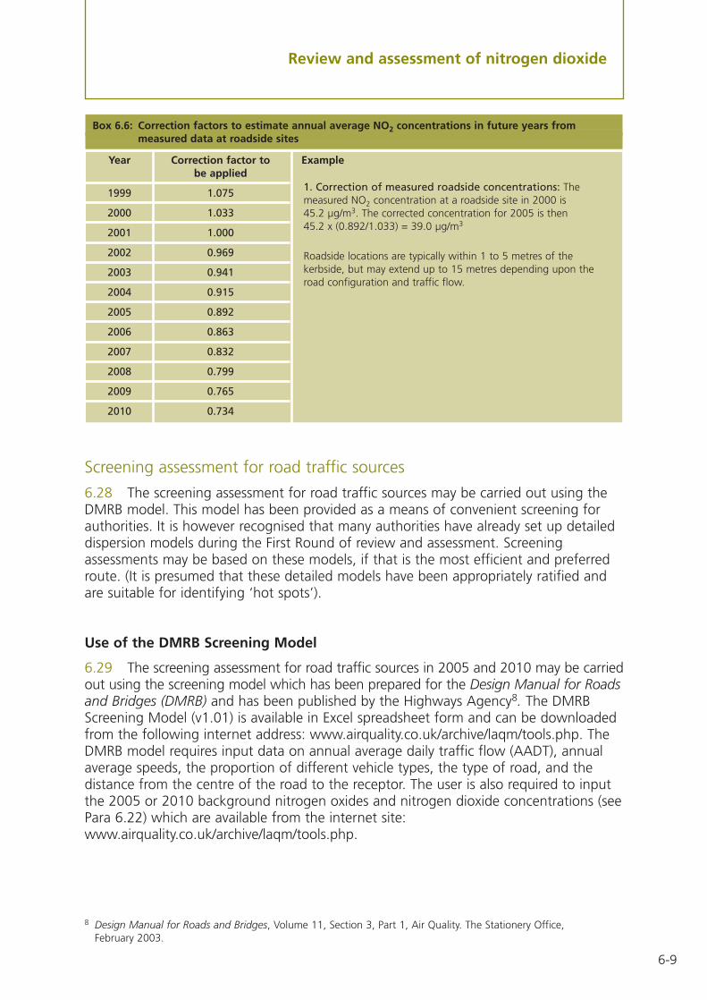
6-9
Review and assessment of nitrogen dioxide
Screening assessment for road traffic sources
6.28 The screening assessment for road traffic sources may be carried out using theDMRB model. This model has been provided as a means of convenient screening forauthorities. It is however recognised that many authorities have already set up detaileddispersion models during the First Round of review and assessment. Screeningassessments may be based on these models, if that is the most efficient and preferredroute. (It is presumed that these detailed models have been appropriately ratified andare suitable for identifying ‘hot spots’).
Use of the DMRB Screening Model
6.29 The screening assessment for road traffic sources in 2005 and 2010 may be carriedout using the screening model which has been prepared for the Design Manual for Roadsand Bridges (DMRB) and has been published by the Highways Agency8. The DMRBScreening Model (v1.01) is available in Excel spreadsheet form and can be downloadedfrom the following internet address: www.airquality.co.uk/archive/laqm/tools.php. TheDMRB model requires input data on annual average daily traffic flow (AADT), annualaverage speeds, the proportion of different vehicle types, the type of road, and thedistance from the centre of the road to the receptor. The user is also required to inputthe 2005 or 2010 background nitrogen oxides and nitrogen dioxide concentrations (seePara 6.22) which are available from the internet site:www.airquality.co.uk/archive/laqm/tools.php.
Box 6.6: Correction factors to estimate annual average NO2 concentrations in future years frommeasured data at roadside sites
Year Correction factor to Examplebe applied
1999 1.075
2000 1.033
2001 1.000
2002 0.969
2003 0.941
2004 0.915
2005 0.892
2006 0.863
2007 0.832
2008 0.799
2009 0.765
2010 0.734
1. Correction of measured roadside concentrations: Themeasured NO2 concentration at a roadside site in 2000 is45.2 µg/m3. The corrected concentration for 2005 is then 45.2 x (0.892/1.033) = 39.0 µg/m3
Roadside locations are typically within 1 to 5 metres of thekerbside, but may extend up to 15 metres depending upon theroad configuration and traffic flow.
8 Design Manual for Roads and Bridges, Volume 11, Section 3, Part 1, Air Quality. The Stationery Office,February 2003.

6-10
Review and assessment of nitrogen dioxide
6.30 The revised DMRB model is expected to provide a slightly conservativeassessment of the impact in most cases. This is appropriate for a screening model andshould prevent authorities unnecessarily proceeding to a Detailed Assessment. However,the validation work carried out by the Highways Agency has indicated that the modelmay significantly underpredict concentrations of nitrogen dioxide alongside urban city-centre roads classified as ‘street canyons’. In this context, a street canyon may bedefined as a relatively narrow street with buildings on both sides, where the height ofthe buildings is generally greater than the width of the road. To avoid missing potentialexceedences of the objective in such locations, the authority should multiply thepredicted annual mean NO2 ‘road traffic component’ concentration, in the ‘localoutput’ sheet in the DMRB, by a factor of 2, to take account of the modelunderprediction. This should then be added to the background concentration to givethe total concentration. Locations where this factor has been used should be clearlyidentified in the review and assessment report.
6.31 The DMRB model predicts the annual mean concentration for direct comparisonwith the annual mean objectives. If the annual mean objectives are not exceeded, theauthority may confidently assume that the short-term (1-hour) objectives will also bemet (see Para 6.09). However, if this approach is used, then care must be taken toinclude relevant locations where the hourly objectives might apply.
6.32 Where predicted concentrations exceed the annual mean objective, thenauthorities should proceed to a Detailed Assessment.
6.33 Authorities are reminded that for the review and assessment of the annual meanobjective, predictions should be carried out at relevant roadside locations (see Paras1.15 to 1.17).
Screening assessment for industrial sources
6.34 A list of industrial processes with the potential to emit significant quantities ofnitrogen oxides in 2005 and 2010 is set out in Annex 2, Appendix E. In the case of newindustrial sources (since the last round of review and assessment), authorities areadvised to check whether a Detailed Assessment has already been carried out as part ofthe planning or authorisation process. This should certainly be the case for all Part A(and Part B in Northern Ireland) regulated processes. If a suitably Detailed Assessmenthas been completed, then the authority may rely on these results, and should cite theconclusions in the review and assessment report.
6.35 To simplify the assessment of industrial nitrogen oxides emissions severalnomograms have been prepared9. These estimate the emission rate (in tonnes perannum) that would produce a 99.8th percentile ground-level concentration of 40µg/m3, equivalent to 20% of the short-term (hourly) 2005 air quality objective (and2010 limit value), and an annual mean ground-level concentration of 1 µg/m3,equivalent to 2.5% of the 2005 annual mean objective (and 2010 limit value). If theactual emission rate from the process exceeds the thresholds, then it will be necessaryto proceed to a Detailed Assessment.
9 Abbott J (2002) Review of pollutant specific guidance for industrial and domestic emissions. AEAT.

6-11
Review and assessment of nitrogen dioxide
6.36 To assist authorities in the compilation of data related to Part A (and Part B inNorthern Ireland) processes, the Environment Agency (EA), the Scottish EnvironmentProtection Agency (SEPA)10, and the Northern Ireland Environment and Heritage Service(EHS), have committed to provide information on any changes that may affectemissions from existing processes, and any new processes that have been, or will be,authorised. The information will be provided from the local office on request. A pro-forma request sheet for this information is provided in Annex 2 (Appendix F).
6.37 Authorities may also wish to consider checking information derived from theirfirst round of review and assessment if there were any doubts regarding their validity.If this information was obtained from the regulatory agency, or directly from the PublicRegister, then there should be no need to undertake this task.
6.38 The nomograms (Figures 6.1 and 6.2 for stack emissions and Figure 6.3 for shortstack or fugitive sources) are shown at the end of this chapter. Authorities may alsodownload various LAQM Tools from the internet at the following address:www.airquality.co.uk/archive/laqm/tools.php which contains the calculations in an Excelspreadsheet form, and requires the user to enter simple details on the emission rateand release conditions (stack height and diameter).
6.39 To use the nomograms it is necessary to estimate/derive:
• the rate of emission of NOx in tonnes per annum.
• the stack height.
• the stack diameter.
• the height of the tallest building within 5 stack heights of the chimney.
• the total oxidant concentration (NO2 + O3, as NO2) measured at the nearest nationalnetwork monitoring station (see Table 6.2).
• the annual mean background NO2 concentration.
6.40 The emission rate for Part A (and Part B in Northern Ireland) processes can beobtained from the regulatory agencies (see Para 6.36) or the operator directly. Emissionsfor processes in England and Wales are also posted on the internet at the followingaddress: http://www.environment-agency.gov.uk. Emission rates for Part B (Part C inNorthern Ireland) processes may be obtainable from the authority’s authorisationdocuments. Estimated emissions data and emissions factors are also available from theUK Emissions Factor Database www.naei.org.uk. Details of stack heights, diameters andbuilding heights can also be obtained from the regulator, the operator or theauthorisation documents, or may be estimated from a visual inspection.
Stack emissions
6.41 The nomograms use the effective stack height. This can be assumed to be equalto the actual (physical) stack height unless:
10 SEPA have regulatory responsibility for Part B processes in Scotland.

6-12
Review and assessment of nitrogen dioxide
• The height of release is greater than 3 m above the building on which it sits, but lessthan 2.5 times the height of the tallest adjacent building. In this case the effectivestack height can be calculated from the following formula:
Ueff = 1.66(Uact – H)
where: H is the height (m) of the tallest adjacent building within 5 actual (physical)stack heights distance;
Ueff is the effective stack height; and
Uact is the actual (physical) stack height
6.42 To use the short-term (1-hour) nomogram (Figure 6.1), the following procedureshould be used:
• Derive the total oxidant concentration (NO2 + O3, as NO2) at the nearest nationalnetwork monitoring station. Table 6.2 describes the 99.8th percentile values of(NO2 + O3, as NO2) for all sites in 1999-2001.
• Calculate the locally available ‘headroom’ as the objective value (200 µg/m3) minusthe 99.8th percentile of (NO2 + O3, as NO2).
• Divide the headroom by 0.05. This procedure assumes that 5% of the NOx emissionis released as NO2, and that the remaining NOx released is converted to NO2 up tothe limit of the available ozone.
• Divide the result by 4 (as a safety margin) to allow for the uncertainty in thisscreening nomogram. The result is the target concentration for screening. Divide theNOx emission from the stack (in tonnes/annum) by the target concentration andmultiply by 40 to scale the emission to the nomogram.
6.43 Identify the line that corresponds to the diameter of the stack underconsideration, and locate the point on this line whose coordinates equal the effectivestack height. Read off the corresponding emission rate on the horizontal axis, andcompare this with the scaled emission rate for the process. If the scaled emission rate isgreater than or equal to the emission rate derived from the chart, the authority shouldproceed to a Detailed Assessment.
6.44 To use the annual mean nomogram (Figure 6.2), the following procedure shouldbe used:
• Identify any sensitive receptors within 10 stack heights.
• Derive the background NO2 concentration at the receptor locations. Include anycontribution from local roads if this is likely to be significant.
• Calculate the locally available ‘headroom’ as the objective value (40 µg/m3) minusthe maximum background concentration.
• Divide the headroom by 4 (as a safety margin) to allow for the uncertainty in thisscreening nomogram. The result is the target concentration for screening. If the
6-13
Review and assessment of nitrogen dioxide
calculated target concentration is less than 0.25 µg/m3, set the target concentrationto 0.25 µg/m3. Divide the annual emission (in tonnes) by this target concentration, toscale the emission to the nomogram.
• Identify the line that corresponds to the diameter of the stack under consideration,and locate the point on this line whose coordinates equal the effective stack height.Read off the corresponding emission rate on the horizontal axis, and compare thiswith the scaled emission rate for the process. If the scaled emission rate is greaterthan or equal to the emission rate derived from the chart, the authority shouldproceed to a Detailed Assessment.
Short stack or fugitive emissions
6.45 To use the nomogram (Figure 6.3), the following procedure should be used:
• Identify the nearest sensitive receptors.
• Derive the background NO2 concentration at the receptor locations. Include anycontribution from local roads if this is likely to be significant.
• Calculate the locally available ‘headroom’ as the objective value (40 µg/m3) minusthe maximum background concentration.
• Divide the headroom by 4 (as a safety margin) to allow for the uncertainty in thisscreening nomogram. The result is the target concentration for screening. If thecalculated target concentration is less than 0.25 µg/m3, set the target concentrationto 0.25 µg/m3. Divide the annual emission (in tonnes) by this target concentration, toscale the emission to the nomogram.
• Identify the line that corresponds to the diameter of the stack under consideration,and locate the point on this line whose coordinates equal the effective stack height.Read off the corresponding emission rate on the horizontal axis, and compare thiswith the scaled emission rate for the process. If the scaled emission rate is greaterthan or equal to the emission rate derived from the chart, the authority shouldproceed to a Detailed Assessment.
NOTE: Where there are multiple stacks at the same site, a precautionary approach may betaken by assuming the total emissions (from all stacks) are released from the smallest stack.Where there are complex sites, with many stacks, the above nomograms are unlikely to beapplicable, and authorities are advised to proceed to the Detailed Assessment.
NOTE: If the emissions are non-continuous (i.e. a batch process); the point of discharge is lessthan 10 m above the ground or building on which it sits; or the stack height is less than anyadjacent building within 5 actual (physical) stack heights distance, the authority should, inthe first instance, undertake the assessment assuming the release is from a low-level source(see Para 6.45). If this assessment indicates a problem, it will be necessary to proceed to aDetailed Assessment if the emission is greater than 1 tonne per annum.
Where there are multiple stacks at the same site, a precautionary approach may be taken byassuming the total emissions (from all stacks) are released from the smallest stack. Wherethere are complex sites, with many stacks, the above nomograms are unlikely to beapplicable, and authorities are advised to proceed to the Detailed Assessment.

6-14
Review and assessment of nitrogen dioxide
Screening assessment for other transport sources
6.46 There is the potential for NOx emissions to arise from other forms of transport,such as aircraft and railways.
Airports
6.47 Information related to the potential impact of aircraft-generated NOx11 isavailable from a variety of sources, including Environmental Assessments that havebeen completed for new airport developments, and the recently published SERAS andRASCO studies12. These studies present a reasonably consistent picture. An airport witha throughput of 5 million passengers per annum (mppa) may contribute up to about25 µg/m3 NOx at the nearest receptor location. Some airports have a substantial freightcomponent which also needs to be taken into account; it may be assumed for thepurpose of this screening assessment that 100,000 tonnes of freight is equivalent to1 mppa13. (For example, an airport with 3.5 mppa, and an annual freight movementof 300,000 tonnes, is assumed to be 6.5 mppa equivalent).
6.48 Authorities need only consider airports that exceed 5 mppa or equivalent(in 2005 or 2010) and/or where the 2005 NOx background concentration exceeds25 µg/m3.
6.49 Where these criteria are exceeded, the authority will need to proceed to aDetailed Assessment.
Railways and shipping
6.50 NOx emissions from railways will only be associated with diesel trains. Emissionsare unlikely to have any significant impact alongside railway tracks, but there is thepotential for problems to occur in close proximity to large numbers of stationary, idlingengines, for example at depot or terminus. The impact is unlikely to extend beyond adistance of about 50 metres.
6.51 Where authorities have identified a significant potential for exceedence of theobjectives from railway sources, they will need to proceed to a Detailed Assessment.
11 The assessment of airport-related road traffic impacts should be carried out using the procedures described inParas 6.29 to 6.33 in this document.
12 Various reports related to the South East and East of England Regional Air Services Study (SERAS) and theRegional Air Services Co-ordination Study (RASCO) can be downloaded from the Government websitewww.airconsult.gov.uk.
13 The freight ‘mppa equivalence’ should only be used where freight is predominantly transported by non-passengeraircraft, for example, where there are freight terminals. If the majority of freight is transported in the hold ofpassenger aircraft, applying this factor would lead to double counting.

6-15
Review and assessment of nitrogen dioxide
6.52 Emissions from shipping movements at major ports would only be expected tobe significant in terms of the 1-hour objective and limit value. The First Round of reviewand assessment has provided no indication that shipping movements are likely to causean exceedence of the 1-hour objective and limit value, and under normal circumstancesthere should be no need to undertake further work. In the event that authorities haveconcern over shipping movements they are advised to contact the relevant Helpdesk(see Box 1.1).
Box 6.2: Updating and Screening checklist
Monitoring
Overview
These steps will ensure you collate all relevant nitrogen dioxide monitoringdata and assess them appropriately to identify locations where exceedences ofthe annual mean and/or 1-hour objectives might occur. You should focus onmonitoring data obtained since the last round of review and assessment, but itis also useful to show longer-term trends where possible.
The annual means should represent acalendar year if possible. Adjust theresult to estimate the annual mean ifyou have less that 9 individualmonthly means – see Box 6.5 for thetechnique to do this.
3. Calculate annual means from thedata.
It is imperative that any localmonitoring data are ratified beforebeing used. Key steps will be toensure that you have screened andscaled continuous monitoring data –see Annex 1 for techniques to dothis. Diffusion tube data should beappropriately ‘bias-corrected’– seeBox 6.4.
Recent national network data will belabelled ‘provisional’. They can stillbe used, as they have been scaled,but they have yet to be ratified. Donot base decisions on any provisionaldata alone.
2. Ratify your local monitoring data,if you have not already done so.
Include your own local monitoringdata and data from the nationalnetworks. Both continuous(chemiluminescent) and diffusiontube data should be included.
1. Collate all nitrogen dioxidemonitoring data.
Approach
(A) Monitoring dataoutside an AQMA
Notes relevant to each stepSteps that must be taken tocomplete the assessment
Source, location, ordata that need to be
assessed

6-16
Review and assessment of nitrogen dioxide
Box 6.2: Updating and Screening checklist (continued)
Monitoring (continued)
Overview
This step will determine whether there is evidence to suggest that an AQMApreviously declared may require reconsideration.
If the answer is NO to the secondquestion, it may still be appropriate toproceed to a Detailed Assessment ifyou expect that levels will be belowthe objectives by the relevant years.
The Detailed Assessment will be witha view to revoking the AQMA.
If the answer is YES to both of thesequestions, proceed to a DetailedAssessment for nitrogen dioxide.
Action
Before you assess the predictedconcentration check that themonitoring location representsrelevant exposure (see Para 1.19–1.21).
• Are all predicted annual means in2005 less than 40 µg/m3?
• Are there currently 18 or fewer1-hour exceedences of, or 99.8thpercentiles less than, 200 µg/m3?
Questions
This will be for monitoring carriedout within the previously definedarea of exceedence.
1. Carry out the data analysis as setout under (A) above.
Approach
(B) Monitoring datawithin an AQMA
The Detailed Assessment will be witha view to determining whether todeclare an AQMA.
If the answer is YES to either of thesequestions, proceed to a DetailedAssessment for nitrogen dioxide.
Action
Before you assess the measuredconcentrations check that themonitoring locations representrelevant exposure (see Paras 1.19–1.21).
Note that the 1-hour assessment isbased on current concentrations. Thisis because there is no straightforwardway to project future exceedences.
• Are any predicted annual meansin 2005 greater than 40 µg/m3?
• Are there currently more than 18exceedences of 200 µg/m3, or areany 99.8th percentiles greaterthan 200 µg/m3?
Questions
This step can only be completed ifyou have continuous monitoringdata. Where you have less than 90%data capture you should use the99.8th percentile rather than a countof exceedences.
5. Calculate the number of 1-hourexceedences of 200 µg/m3 in a fullyear, or the 99.8th percentile ofhourly means.
Box 6.6 provides the factors to do thisfor roadside and kerbside sites. Youshould summarise both current andfuture concentrations in a Table. It isalso advisable to project forward fromeach year of monitoring, to show therange of future concentrations. Youshould then use the highest value asthe basis for your decision.
4. Estimate the annual meanconcentrations in 2005.
Notes relevant to each stepSteps that must be taken tocomplete the assessment
Source, location, ordata that need to be
assessed

6-17
Review and assessment of nitrogen dioxide
Box 6.2: Updating and Screening checklist (continued)
Road traffic
Overview
Defra has examined the results from the last round of review and assessmentand looked for locations and levels of traffic that might lead to exceedences ofthe objective for nitrogen dioxide. This part of the assessment is structuredaround those conclusions.
NOTES1. To avoid missing potential exceedences of the objective in street canyons, the predicted annual mean
NO2 ‘road traffic component’ concentration, in the ‘local output’ sheet in the DMRB, should bemultiplied by a factor of 2. This should then be added to the background concentration to give thetotal concentration (see Para 6.30).
If there are monitoring data for theselocations, then you should use theseresults in preference to the DMRBscreening model to reach a decision.This assumes the data have beenquality assured (see Annex 1).
If the answer is YES, this indicates apotential exceedence of the annualmean objective. You should thenproceed to a Detailed Assessment fornitrogen dioxide at these locations.
Action
• Are any of the predicted annualmeans in 2005 greater than40 µg/m3?
Question
You will require information on thelocal background concentrations (seePara 6.22).
Information on the proportion ofvehicle types may be based on 2classes (HDV/LDV) or a more detailedbreakdown if data are available.
4. Use the DMRB screening model(Para 6.29) to predict the annualmean in 2005 at relevantlocations1. You will also needinformation on traffic flows,speeds and proportion ofdifferent vehicle types.
Obtain measured or modelled trafficdata where possible. If not make ajudgement based on local knowledgeof roads likely to have such flows.
3. Obtain information on trafficflows sufficient to list those roadsidentified above that have a flowgreater than 10,000 vehicles per day.
Use local knowledge to identify suchlocations. They could usefully bemarked on a map. Only include areaswhere the average speed is 50 kphor less. Only include roads where thecarriageway is less than 10 m wide.
2. Identify all general areas wherethere may be narrow congestedstreets with residential propertieswithin 5 m of the kerb.
If you specifically included thesetypes of location during the firstround, then there is no need toproceed further with this part.
1. Check whether these locationswere assessed during the firstround of review and assessment.
Concentrations are often higherwhere traffic is slow moving withstop/start driving, and wherebuildings either side reduce thedispersion. Such locations were notalways fully considered during thefirst round of review and assessment.
Approach(C) Narrow congestedstreets withresidentialproperties close to the kerb
Notes relevant to each stepSteps that must be taken tocomplete the assessment
Source, location, ordata that need to be
assessed

6-18
Review and assessment of nitrogen dioxide
Box 6.2: Updating and Screening checklist (continued)
Road traffic (continued)
NOTES1. Where 2 or more roads intersect, for example at a junction, the traffic flows from each road should
be added to give a combined total. For example at a crossroads with 2 roads intersecting, where road[A] has an AADT flow of 38000 vehicles per day, and road [B] has an AADT flow of 44000 vehicles perday, assume a combined flow of 82000 vehicles per day. If there are 3 links to the junction, then addthe flows and multiply by 2/3.
2. To avoid missing potential exceedences of the objective in street canyons, the predicted annual meanNO2 ‘road traffic component’ concentration, in the ‘local output’ sheet in the DMRB, should bemultiplied by a factor of 2. This should then be added to the background concentration to give thetotal concentration (see Para 6.30).
If there are monitoring data for theselocations, then you should use theseresults in preference to the DMRBscreening model to reach a decision.This assumes the data have beenquality assured (see Annex 1).
If the answer is YES, this indicates apotential exceedence of the annualmean objective in 2005. You shouldthen proceed to a DetailedAssessment for NO2 at theselocations.
Action
• Are any of the predicted annualmean concentrations in 2005greater than 40 µg/m3?
Question
You will require information on thelocal background concentrations (seePara 6.22).
4. Use the DMRB screening model topredict the annual meanconcentration in 2005 at relevantlocations2.
Information on the proportion ofvehicle types may be based on 2classes (HDV/LDV) or a more detailedbreakdown if the data are available.
3. Obtain detailed information ontraffic flows, speeds and theproportion of different vehicletypes.
A major conurbation may beconsidered to be a city with apopulation in excess of 2 million.
If there is no relevant exposure thenyou do not need to proceed further.
2. Determine whether there isrelevant exposure within 10mof the kerb (20m in majorconurbations).
A ‘busy’ junction can be taken to beone with more than 10000 vehiclesper day. Guidance on how to addflows at junctions is given below1.
1. Identify ‘busy’ junctions.
Experience from the first roundsuggests that junctions were oftennot considered adequately. Thisassessment is required where therewas no specific assessment ofjunctions during the First Roundagainst the 2005 objectives.
Approach(D) Junctions
Notes relevant to each stepSteps that must be taken tocomplete the assessment
Source, location, ordata that need to be
assessed

6-19
Review and assessment of nitrogen dioxide
Box 6.2: Updating and Screening checklist (continued)
Road traffic (continued)
NOTES1. To avoid missing potential exceedences of the objective in street canyons, the predicted annual mean
NO2 ‘road traffic component’ concentration, in the ‘local output’ sheet in the DMRB, should bemultiplied by a factor of 2. This should then be added to the background concentration to give thetotal concentration (see Para 6.30).
If there are kerbside monitoring datafor these locations, then you shoulduse these results in preference to theDMRB screening model to reach adecision. This assumes the data havebeen quality assured (see Annex 1).
If the answer is YES you shouldproceed to a Detailed Assessment fornitrogen dioxide at these locations.
Action
The DMRB screening model does notcalculate 1-hour concentrations. If the annual mean does not exceed40 µg/m3, then there should be nomore than 18 hours above 200 µg/m3.
• Are any of the predicted annualmeans in 2005 greater than 40µg/m3?
Question
You will require information on thelocal background concentrations (seePara 6.22).
4. Use the DMRB screening model(Para 6.29) to predict the annualmean in 2005 at relevantlocations1.
Information on the proportion ofvehicle types may be based on 2classes (HDV/LDV) or a more detailedbreakdown if data are available.
3. Obtain detailed information ontraffic flows, speeds andproportion of different vehicletypes.
A busy street can be taken to be onewith more than 10000 vehicles perday.
2. Identify all busy streets wheremembers of the public may beexposed within 5 m of the kerbfor 1-hour or more.
If you specifically included thesetypes of location during the firstround, then there is no need toproceed further with this part.
1. Check whether such locationswere assessed during first roundof review and assessment.
There will be some street locationswhere members of the public mayregularly spend 1-hour or more,e.g. streets with many shops, streetswith outdoor cafes/bars. You shouldnot include people occupationallyexposed in such locations.
Approach(E) Busy streets wherepeople may spend1-hour or moreclose to traffic
Notes relevant to each stepSteps that must be taken tocomplete the assessment
Source, location, ordata that need to be
assessed

6-20
Review and assessment of nitrogen dioxide
Box 6.2: Updating and Screening checklist (continued)
Road traffic (continued)
NOTES1. To avoid missing potential exceedences of the objective in street canyons, the predicted annual mean
NO2 ‘road traffic component’ concentration, in the ‘local output’ sheet in the DMRB, should bemultiplied by a factor of 2. This should then be added to the background concentration to give thetotal concentration (see Para 6.30).
If there are monitoring data for theselocations, then you should use theseresults in preference to the DMRBscreening model to reach a decision.This assumes the data have beenquality assured (see Annex 1).
If the answer is YES you shouldproceed to a Detailed Assessment fornitrogen dioxide at these locations.
Action
Annual mean predictions should alsobe carried out at locations where the1-hour objective only would apply, sothat an assessment of the short termobjective can be made as well.
• Are any of the predicted annualmeans in 2005 greater than40 µg/m3?
Question
You will require information on thelocal background concentrations (seePara 6.22).
5. Use the DMRB screening model(Para 6.29) to predict the annualmean in 2005 at relevantlocations1.
Items 3 and 4 could be carried out ineither order. There would be noneed to look for relevant exposure ifthe flow is less than 2,500 HDVvehicles per day.
4. Determine whether the flow ofheavy duty vehicles is greater than2500 vehicles per day.
Relevant exposure should be judgedagainst the annual mean and 1-hourcriteria (see Box 1.4).
A major conurbation may beconsidered to be a city with apopulation in excess of 2 million.
3. Determine whether there isrelevant exposure within 10mof these roads (20m in majorconurbations).
An unusually high proportion can betaken to be greater than 25%. Iftraffic data are not available, uselocal knowledge. Such roads couldinclude bus only streets or roadsleading to an industrial estate.
2. Identify all roads with anunusually high proportion ofheavy duty vehicles.
If you specifically included thesetypes of location during the firstround, then there is no need toproceed further with this part.
1. Check whether such locationswere assessed during first roundof review and assessment.
There will be some street locationswhere traffic flows are not high (lessthan 20000 vehicles per day) butthere is an unusually high proportionof buses and/or HGVs. These can be amajor source of nitrogen oxides.
Approach(F) Roads with highflow of busesand/or HGVs
Notes relevant to each stepSteps that must be taken tocomplete the assessment
Source, location, ordata that need to be
assessed

6-21
Review and assessment of nitrogen dioxide
Box 6.2: Updating and Screening checklist (continued)
Road traffic (continued)
• Are any of the predicted annualmeans in 2005 greater than 40 µg/m3?
Question
You will require information on thelocal background concentrations (seePara 6.22).
2. Use the DMRB screening model(Para 6.29) to predict the annualmean in 2005 at relevant locations1.
The aim is to establish whether thereis a risk of exceedences alongside thenew road, or existing roads with asignificant change in flows.
You should only proceed if there isrelevant exposure within 10m (20min major conurbations). A majorconurbation may be considered to bea city with a population in excess of2 million.
1. Establish whether the traffic flowon the new road is greater than10000 vehicles per day or whetherthe new road has increased trafficflow on existing roads previouslyidentified as having 2005 annualmean concentrations greater than36 µg/m3 or more than 15 1-hourexceedences of 200 µg/m3
This approach should be followed ifthere has been no previous airquality assessment.
Approach 2
The Detailed Assessment may be nomore than relying on the findings ofthe air quality assessment. For this tobe the case the assessment will haveto meet the standards of a DetailedAssessment.
If the answer is YES you shouldproceed to a Detailed Assessment fornitrogen dioxide at these locations.
Action
• Did the assessment predict anyexceedences of the objectives atrelevant locations?
Question
An assessment may already have beencarried out as part of the planningprocess. If this is the case you shouldconfirm that the assessment is sufficientfor review and assessment purposes.
You need only consider proposed roadsfor which planning approval has beengranted.
1. Check whether an air qualityassessment has already beencarried out for the new road.
Approach 1(G) New roadsconstructed orproposed sincefirst round ofreview andassessment
Notes relevant to each stepSteps that must be taken tocomplete the assessment
Source, location, ordata that need to be
assessed

6-22
Review and assessment of nitrogen dioxide
Box 6.2: Updating and Screening checklist (continued)
Road traffic (continued)
NOTES1. To avoid missing potential exceedences of the objective in street canyons, the predicted annual mean
NO2 ‘road traffic component’ concentration, in the ‘local output’ sheet in the DMRB, should bemultiplied by a factor of 2. This should then be added to the background concentration to give thetotal concentration (see Para 6.30).
Overview
This section addresses the changes to the emission factors in 2002. It appliesonly to the assessment against the 2005 objectives. It deals with locationswhere results were close to but just below the objective and for whichAQMAs were not declared.
This new assessment should use thenew emission factors.
If the answer is YES you shouldproceed to a Detailed Assessment fornitrogen dioxide at these locations.
Action
• Are there any roads with apredicted annual meanconcentration in 2005 above36 µg/m3 but below 40 µg/m3,which have not be reassessedusing the new emissions factors?
Question
The new factors might make adifference if locations were predictedto be close to the objective duringthe first round of review andassessment.
1. Identify any roads where annualmean concentrations in 2005 werepredicted to be above 36 µg/m3
but below 40 µg/m3 at relevantlocations, during the first roundof review and assessment.
Approach
(H) Roads close to the objectiveduring the firstround of reviewand assessment
If the answer is YES, this indicates apotential exceedence of the annualmean objective in 2005. You shouldthen proceed to a DetailedAssessment for nitrogen dioxide atthese locations.
Action
Notes relevant to each stepSteps that must be taken tocomplete the assessment
Source, location, ordata that need to be
assessed

6-23
Review and assessment of nitrogen dioxide
Box 6.2: Updating and Screening checklist (continued)
Road traffic (continued)
NOTES1. To avoid missing potential exceedences of the objective in street canyons, the predicted annual mean
NO2 ‘road traffic component’ concentration, in the ‘local output’ sheet in the DMRB, should bemultiplied by a factor of 2. This should then be added to the background concentration to give thetotal concentration (see Para 6.30).
If there are monitoring data for theselocations, then you should use theseresults in preference to the DMRBscreening model to reach a decision.This assumes the data have beenquality assured (see Annex 1).
If the answer is YES you shouldproceed to a Detailed Assessment fornitrogen dioxide at these locations.
Action
• Are any of the predicted annualmeans in 2005 greater than40 µg/m3?
Question
You will require information on thelocal background concentrations (seePara 6.22).
4. Use the DMRB screening model(Para 6.29) to predict the annualmean in 2005 at relevantlocations1.
Information on the proportion ofvehicle types may be based on 2classes (HDV/LDV) or a more detailedbreakdown if data are available.
3. Obtain detailed information ontraffic flows, speeds andproportion of different vehicletypes.
A road ‘at risk’ of exceeding theobjectives can be taken to be onepreviously identified with an annualmean above 36 µg/m3 at a relevantlocation.
2. Determine whether these roadshad previously been identified asbeing at risk of exceeding theobjectives.
A ‘large’ increase can be taken to bemore than 25% increase in traffic flow.You should also consider roads wheresuch an increase is identified due toimproved traffic data.
1. Identify any roads with more than10000 vehicles per day that haveexperienced ‘large’ increases intraffic.
Approach(I) Roads withsignificantlychanged trafficflows
Notes relevant to each stepSteps that must be taken tocomplete the assessment
Source, location, ordata that need to be
assessed

6-24
Review and assessment of nitrogen dioxide
Box 6.2: Updating and Screening checklist (continued)
Road traffic (continued)
If there are monitoring data for theselocations, then you should use theseresults in preference to the DMRBscreening model to reach a decision.This assumes the data have beenquality assured (see Annex 1).
If the answer is YES you shouldproceed to a Detailed Assessment fornitrogen dioxide at these locations.
Action
The DMRB screening model does notcalculate 1-hour concentrations. If theannual mean does not exceed 40µg/m3, then there should be no morethan 18 hours above 200 µg/m3.
• Are any of the predicted annualmeans in 2005 greater than 40µg/m3?
Question
You will require information on thelocal background concentrations (seePara 6.22).
When using the DMRB screeningmodel enter 100% into the ‘busesand coaches’ column.
4. Use the DMRB screening model(Para 6.29) to predict the annualmean in 2005 at relevantlocations.
Items 2 and 3 could be carried out ineither order. For instance, there is nopoint looking for relevant exposure ifthe flow is less than 1000 buses perday.
3. Determine whether the flow ofvehicles is greater than 1000 busesper day.
Relevant exposure should be judgedagainst the 1-hour criteria (see Box1.4). A major conurbation may beconsidered to be a city with apopulation in excess of 2 million.
2. Determine whether there isrelevant exposure within 10m ofthe bus station (20m in majorconurbations).
You should carefully define amovement. A bus coming into thebus station then going out againshould be treated as twomovements.
1. Collect information on the dailymovements of buses at the busstation.
This approach only applies to busstations that are not enclosed. Theassessment will be against the 1-hourobjective.
Approach(J) Bus stations
Notes relevant to each stepSteps that must be taken tocomplete the assessment
Source, location, ordata that need to be
assessed

6-25
Review and assessment of nitrogen dioxide
Box 6.2: Updating and Screening checklist (continued)
Industrial sources
Overview
Industrial sources will not make a significant local contribution to annual meanconcentrations, but could be significant in terms of the 1-hour objective. Theevidence from the work carried out during the first round is that very fewsources will require consideration.
If the answer is YES you shouldproceed to a Detailed Assessmentfor nitrogen dioxide for this source.
Action
• Does the source exceed thethreshold in the nomograms?
Question
You will need to derive the effectivestack height. Details of how to dothis are provided in Para 6.41.
3. Use the nomograms described inPara 6.34 onwards to determine ifthe source requires furtherassessment.
See Para 6.38. If it is proving difficultto obtain the information on theemissions contact the EmissionsHelpdesk (Box 1.1).
2. Obtain information on the totalannual emission of nitrogen oxidesand the height of the emission.
1. Use the checklist in Annex 2 todetermine whether the sourceneeds considering further.
This approach should be followed ifthere has been no previous airquality assessment.
Approach 2
The Detailed Assessment may be nomore than relying on the findings ofthe air quality assessment. For this tobe the case the assessment will haveto meet the standards of a DetailedAssessment.
If the answer is YES you shouldproceed to a Detailed Assessmentfor nitrogen dioxide for this source.
Action
• Did the assessment predict anyexceedences of the objectives atrelevant locations?
Question
An assessment may already have beencarried out as part of the planning orauthorisation process. If this is the caseyou should confirm that the assessmentis sufficient for review and assessmentpurposes.
You only need to consider proposedsources for which planning approvalhas been granted.
1. Check whether an air qualityassessment has already beencarried out for the new industrialsource.
Approach 1(K) New industrialsources
Notes relevant to each stepSteps that must be taken tocomplete the assessment
Source, location, ordata that need to be
assessed

6-26
Box 6.2: Updating and Screening checklist (continued)
Industrial sources (continued)
If the answer is YES you shouldproceed to a Detailed Assessment fornitrogen dioxide for these sources.
Action
• Does the source exceed thethreshold in the nomograms?
Question
You will need to derive the effectivestack height. Details of how to do thisare provided in Para 6.41.
3. Use the nomograms described inPara 6.34 onwards to determine ifthe source requires furtherassessment.
See Para 6.38. If it is proving difficultto obtain the information on theemissions contact the EmissionsHelpdesk (Box 1.1).
2. Obtain updated information onthe total annual emission ofnitrogen dioxide and the heightof the emission.
A substantial increase can be taken tobe one greater than 30%.
1. Determine whether any of thesources identified during the firstround of review and assessmentas potentially significant havesubstantially increased emissions.
Approach(L) Industrial sourceswith substantiallyincreasedemissions
Notes relevant to each stepSteps that must be taken tocomplete the assessment
Source, location, ordata that need to be
assessed
Review and assessment of nitrogen dioxide

6-27
Review and assessment of nitrogen dioxide
Box 6.2: Updating and Screening checklist (continued)
Other sources
Overview
Aircraft are significant sources of nitrogen oxides emissions, especially duringtakeoff. You should evaluate aircraft emissions at airports if they were notconsidered during the first round of review and assessment. Emissions fromaircraft once they are above about 200 m will make a negligible contribution toground-level concentrations.
NOTES• Diesel and Coal-Fired Locomotives: Both types of locomotive emit nitrogen oxides, but there is no
evidence to suggest that there is any risk of the 1-hour or annual mean objectives for nitrogendioxide in 2005 being exceeded. No further assessment is therefore required.
• Shipping: There are emissions of nitrogen oxides from the burning of oil in ship’s engines, but thereis no evidence to suggest that there is any risk of the 1-hour or annual mean objectives for nitrogendioxide in 2005 being exceeded. No further assessment is therefore required.
If there are monitoring data for worst-case relevant exposure locations nearthe airport boundary, then you shoulduse these results in preference to thepassenger throughput criteria to reacha decision. This assumes the data havebeen suitably quality assured (seeAnnex 1).
If the answer is YES you shouldproceed to a Detailed Assessmentfor nitrogen dioxide.
Action
• Is the predicted total equivalentpassenger throughput in 2005more than 5 mppa?
Question
You should convert the tonnes offreight to an equivalent number ofpassengers using 100000 tonnes =1 mppa. This only applies to freighttaken in ‘freight-only’ planes, notthat taken in passenger planes.
2. Obtain information on expectedannual throughput of passengersand tonnes of freight in 2005.Calculate the total equivalentpassenger numbers in millionpassengers per annum (mppa).
Concentrations fall-off rapidly onmoving away from the source, and areunlikely to make a significantcontribution beyond this distance.
If there is no relevant exposure, thenyou do not need to proceed further.
1. Establish whether there is relevantexposure within 1000m of theairport boundary.
This approach deals with aircraft as asource at airports. Road trafficimpacts associated with airportsshould be dealt with separately usingthe road traffic sections of Box 6.2.
Approach(M) Aircraft
Notes relevant to each stepSteps that must be taken tocomplete the assessment
Source, location, ordata that need to be
assessed

6-28
The Detailed Assessment for nitrogen dioxide6.53 Where the screening assessment has indicated that there is a risk of the AirQuality Objectives not being achieved by 2005, then the authority will need to carry outa Detailed Assessment. Authorities are also encouraged to carry out a DetailedAssessment for the 2010 limit values, if the screening assessment has indicated a risk ofexceedence. The aim of this Detailed Assessment is to determine with reasonablecertainty whether or not there is a likelihood of the objectives not being achieved. Theassumptions within this Detailed Assessment should be considered in depth, and thedata that are used or collected, quality-assured to a high standard. This is to allow theauthority to have confidence in the decision that it reaches to declare, not declare, orrevoke an Air Quality Management Area. Where a likely exceedence of the objectives isidentified, then the authority will also need to determine the magnitude andgeographical extent.
6.54 Because of the wide range of sources and local circumstances that may prevail,it is not possible to set prescriptive guidance for the Detailed Assessment. However,wherever possible, lessons learnt from the First Round of review and assessment havebeen drawn upon. It is also expected that authorities will make use of the variousHelpdesks that have been established (see Box 1.1).
6.55 Specific guidance related to monitoring, emissions data and dispersionmodelling, is provided in Annexes 1 to 3 of this document. Whilst important aspects arehighlighted in this section, authorities who are undertaking a Detailed Assessment arestrongly advised to read the relevant sections of the Annexes before commencing theirwork.
6.56 In undertaking the Detailed Assessment it is important to give consideration tothe points of maximum relevant public exposure (i.e. those locations where thehighest concentrations of nitrogen dioxide are expected). In the case of emissions fromroad traffic the highest concentrations are expected to occur at locations within closeproximity to the kerbside, particularly where traffic flows are high, or there is congestedtraffic along narrow streets. It is essential that authorities take these potential ‘hotspots’ into consideration within their review and assessment14.
6.57 In the course of the Detailed Assessment, authorities may need to adjustmapped or measured nitrogen dioxide and NOx concentrations at background sites to2005 or 2010. Suitable factors for these corrections are provided in Boxes 6.7 and 6.8respectively.
14 Attention is drawn to Box 1.4 which describes locations relevant for the Air Quality Objectives.Authorities should give consideration to potential exceedences of the 1-hour objective at kerbsidelocations. The highest annual mean concentrations are likely to be at roadside locations.
Review and assessment of nitrogen dioxide

6-29
Monitoring
6.58 As for the screening assessment, measured data are expected to give a moreaccurate indication of nitrogen dioxide concentrations than modelling studies.
6.59 Guidance on monitoring methods, monitoring strategies and suitable QA/QCprocedures are set out in greater detail in Annex 1 to this document. The followingpoints are highlighted:
Box 6.8: Correction factors to estimate annual mean NOx concentrations in future years frommeasured or mapped data at background sites
Year Correction factor to Examplebe applied
1999 1.098
2000 1.037
2001 1.000
2002 0.961
2003 0.926
2004 0.896
2005 0.869
2006 0.836
2007 0.800
2008 0.764
2009 0.728
2010 0.695
Box 6.7: Correction factors to estimate annual average NO2 concentrations in future years frommeasured or mapped data at background sites
Year Correction factor to Examplebe applied
1999 1.066
2000 1.025
2001 1.000
2002 0.973
2003 0.948
2004 0.927
2005 0.908
2006 0.884
2007 0.858
2008 0.831
2009 0.803
2010 0.778
Review and assessment of nitrogen dioxide
1. Correction of measured background concentrations: Themeasured NO2 concentration at a background site in 2000 is25.2 µg/m3. The corrected concentration for 2005 is then25.2 x (0.908/1.025) = 22.3 µg/m3.
1. Correction of measured background concentrations: Themeasured NOx concentration at a background site in 2000 is54.3 µg/m3. The corrected concentration for 2005 is then54.3 x (0.869/1.037) = 45.5 µg/m3.
6-30
• Some monitoring based on a continuous (chemiluminescent or equivalent) samplerwill normally be required for the Detailed Assessment. Ideally, sampling should becarried out for a full calendar year (particularly in respect of the short-term objective),with 90% data capture, and any gaps spread evenly throughout the year. In manycircumstances it may prove possible to use data from a shorter monitoring period(for example after 6 months consecutive sampling (3 months winter, and 3 monthssummer), by comparing the data with those measured at nearby, long-term sites(such as those operated in the UK Automatic Networks). An example of how thisdata analysis might be performed is set out in Box 6.5 and in Annex 1.
• Passive diffusion tubes have a useful role to play for the Detailed Assessment, inparticular providing improved spatial resolution15. However, it is essential that thetubes are adequately validated against a reference chemiluminescent sampler, andthat suitable ‘bias correction’ factors are applied to the data (see Box 6.4)16. Scalingfactors provided by the UK NO2 Diffusion Tube Survey Intercomparison Exercises arenot sufficient for this purpose, as the results are derived from only 1 monthsmonitoring. Bias adjustment factors produced by other authorities may be used,provided that the same laboratory, tube preparation method, exposure interval andsite type have been used.
• Sampling devices should be located at sites which are relevant in terms of publicexposure for the objectives (see Box 1.4). Ideally, monitoring should take place atlocal ‘hot spots’ so that likely exceedences of the objectives can be quantified. Thereis, for example, little point in carrying out a monitoring campaign which is solelyfocussed on kerbside sites, if the concern is with regard to the annual mean nitrogendioxide concentration, for which the building facade will be the relevant location.
• Monitoring strategies should take account of the potential requirements forsubsequent model verification at the outset of the study (see Para 6.66 and Annex 3).
Modelling
6.60 For the Detailed Assessment, authorities will need to have confidence in theirresults, which will subsequently be used to determine whether there is a likelihood ofthe objectives being exceeded and the need to declare an AQMA.
6.61 Issues regarding model validation and verification are discussed in further detailin Annex 3. Model validation generally refers to detailed, peer-reviewed studies thathave been carried out by the model supplier, or a regulatory agency (for example,USEPA). All models used in the Detailed Assessment should have an appropriatepedigree, and have been subject to detailed and documented validation trials.
6.62 Model verification refers to checks that are carried out on model performance ata local level. This basically involves the comparison of predicted versus measured
Review and assessment of nitrogen dioxide
15 Validated diffusion tubes are mainly useful as screening tools, or for providing additional information on spatialdistributions. They should not normally be used as the sole means of confirming the presence or absence of anexceedence of the objectives.
16 Triplicate exposures are not essential, apart from at sites co-located with chemiluminescent analysers. Guidanceon the interpretation of triplicate exposed tubes is given in Annex 1.

6-31
concentrations. Where there is a disparity between the predicted and measuredconcentrations, the first step should always be to check the input data and modelparameters in order to minimise the errors. If required, the second step will be todetermine an appropriate adjustment factor that can be applied. For the review andassessment of road traffic sources it is essential that model verification is carried out.For the review and assessment of point sources, verification of short-termconcentrations may be more difficult to carry out. In this case, the use of anappropriate validated model will be sufficient, provided that the source emissions canbe accurately quantified. However, in cases where there are local factors contributing touncertainty, such as certain types of batch processes, complex topography etc, thenlocal verification studies may be required, and/or an additional consideration ofuncertainties taken into account.
6.63 As indicated in Para 6.54 above, diffusion tubes are useful as screening tools,and can provide additional information on the spatial distribution of nitrogen dioxideconcentrations. The output of verified model predictions can be usefully compared tosuitably validated diffusion tube results, and this can provide an additional level ofconfidence in the results. However, diffusion tubes are not generally recommended asthe sole means of model verification.
6.64 In all cases where model verification has been carried out, the approach shouldbe fully documented in the review and assessment report, and any adjustment factorapplied should be explicitly stated.
Meteorological data
6.65 The choice of meteorological data for use in the dispersion model can have anoutcome on the result, depending on whether a ‘worst case’ or ‘typical’ year isselected. A detailed discussion on the selection of meteorological data is provided inAnnex 3 and all authorities are advised to read this section prior to undertaking amodelling study. In summary, the guidance recommends that a single year of sequentialmeteorological data is used. If possible, meteorological, background and emissions datashould all be derived from the same year.
6.66 In the case of emissions from point sources, the main effect of differentmeteorological years will be to affect the precise location of the maximum predictedconcentration. Authorities are advised to take into consideration the potential effects offluctuating wind directions in different years. A suggested means of dealing with this isto assume that the actual maximum concentration may occur within a 45 degree arc toeither side of the predicted maxima, and properties lying within this arc should beconsidered. Where the authority decides to use multiple years (3 or more) ofmeteorological data, it is recommended that the results for all years are reported, butthat any decision is based upon the worst-case result.
Review and assessment of nitrogen dioxide

6-32
Receptor spacing
6.67 The importance of giving due consideration to potential ‘hot spots’ has alreadybeen highlighted in Para 6.56. For the purpose of dispersion modelling, this requiresthe user to ensure that a suitable resolution for receptor grid spacing is used, or thatspecific receptors (representing the locations of maximum public exposure) areincluded17. If the grid spacing is set to a low resolution (for example, several hundredmetres) and no specific receptors are included, then there is the potential that themodel will not predict the highest concentrations relevant to public exposure. A moredetailed discussion on receptor spacing is provided in Annex 3.
6.68 In selecting specific receptors along roads, authorities are reminded to paycareful attention to the alignment of the road in their model. Some models maydescribe curved sections of road as straight-line links. In some instances this may causethe distance from the road to the specific receptor to be significantly distorted(distances over the first 10 metres or so from the kerbside are critical). Authorities areadvised to ensure that road alignments do not cause this type of problem.
Relationships between NOx and NO2
6.69 The Government and the Devolved Administrations are currently investigatingNOx and NO2 relationships in detail, and have tasked the Air Quality Expert Group(AQEG) to report in 2003. Further guidance on NOx and NO2 relationships will beissued to authorities if appropriate, once the AQEG report is available18.
Road traffic sources
6.70 There are a variety of approaches to dealing with NOx:NO2 relationships.A recommended approach19 that can be applied to road traffic sources, based upon anempirical relationship, is described in Box 6.9. The benefits of this approach are that itis simple to use, and does not require the user to apply different relationships forbackground and roadside sites. A potential disadvantage of this, and other empiricalapproaches, is that it assumes the derived empirical relationship will hold in futureyears. There is evidence to indicate that the NOx:NO2 relationship may change overtime. As annual mean ozone concentrations are expected to rise as NOx emissionsreduce in future years, this will result in higher levels of NO2 for a given NOxconcentration. Whilst such effects may not be so important by 2005 (in terms of the AirQuality Objectives) they may become more critical by 2010 (in terms of meeting thelimit values).
17 Some dispersion models allow the user to incorporate these specific roadside receptors automatically i.e. to placereceptors at a specified distance from the kerbside. Whilst this can be an acceptable approach, authorities shoulddocument that this option has been included, and ensure that the actual distances used in the model areconsistent with the distances of the closest receptors to the road.
18 For the purpose of the 2003 review and assessment, authorities may rely on the guidance given in this document.The outcome of the AQEG report will be used to prepare updated guidance for reviews and assessments in futureyears, if deemed appropriate.
19 Laxen D P H (2002) A new approach to deriving NO2 from NOx for assessment of roads. Air Quality Consultants.
Review and assessment of nitrogen dioxide

6-33
6.71 Other approaches to NOx:NO2 relationships are acceptable, and may bepreferred by the authority, depending upon the type of dispersion model that isemployed. Such approaches include ‘ozone-limited’ methods, the Generic ReactionSeries, or the Derwent-Middleton equation. Where the authority chooses to use adifferent approach to that set out in Box 6.9, then the method should be explicitlydefined.
6.72 Regardless of the approach taken, authorities are strongly recommended toverify their model predictions for NOx as well as for NO2 (see Box 6.10). This should becarried out separately for the background contribution (if modelled) and the source (i.e. the road traffic contribution). Once the NOx has been verified and adjusted asnecessary, a final check should be made against the measured NO2 concentrations.
Box 6.9: An approach to deriving NO2 from NOx for road traffic sources
A new empirical methoda has been developed to convert annual mean NOx to NO2. This is designed toavoid some of the problems that arose from the method in TG4(00) which relied on separatebackground and roadside empirical relationships derived from measured data. The new approach isalso derived from empirical data, but involves the addition of NO2 associated with the road traffic tobackground NO2 (the previous method relied on addition of background NOx to road NOx and thenconversion to NO2). The steps are thus to:
Step 1. Obtain the annual mean background NO2(background) and NOx(background) concentrations for thearea. These can be derived from the national 1x1 km background maps or from localmonitoring at background sites. (To avoid double counting of NOx and NO2 from very busyroads in rural areas you should use the method set out in Box 1.5).
Step 2. Calculate the annual mean contribution due to the road, NOx(road), at the location of interestb.This could be from any suitable model.
Step 3. Convert the NOx(road) to NO2(road) using the equation
NO2(road) = ((-0.068 x Ln(NOx(total))) + 0.53) x NOx(road)
where NOx(total) = NOx(background) + NOx(road), and Ln is log to the base e
Step 4. Add the NO2(road) to the NO2(background) to get the NO2(total) at the location of interest.
This methodology is built into the DMRB screening model. The conversion of road NOx to road NO2that takes place at step 3 essentially involves using a variable proportion of NO2 to NOx ranging fromabout 0.25 at low total NOx concentrations to around 0.12 at high total NOx concentrations.
NOTES:
(a) This method has been tested for road traffic sources, but is probably applicable for use with otherdiffuse emissions, such as airports. The method is not applicable to emissions from point sources,such as industrial chimneys, railway engines etc. In the case of doubt, authorities are advised tocontact the relevant Helpdesk for guidance.
(b) The NOx(road) contribution needs to be suitably verified before proceeding to the next stage.
Review and assessment of nitrogen dioxide
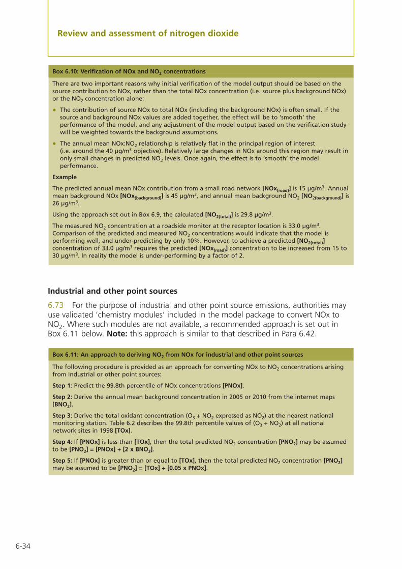
6-34
Industrial and other point sources
6.73 For the purpose of industrial and other point source emissions, authorities mayuse validated ‘chemistry modules’ included in the model package to convert NOx toNO2. Where such modules are not available, a recommended approach is set out inBox 6.11 below. Note: this approach is similar to that described in Para 6.42.
Box 6.11: An approach to deriving NO2 from NOx for industrial and other point sources
The following procedure is provided as an approach for converting NOx to NO2 concentrations arisingfrom industrial or other point sources:
Step 1: Predict the 99.8th percentile of NOx concentrations [PNOx].
Step 2: Derive the annual mean background concentration in 2005 or 2010 from the internet maps[BNO2].
Step 3: Derive the total oxidant concentration (O3 + NO2 expressed as NO2) at the nearest nationalmonitoring station. Table 6.2 describes the 99.8th percentile values of (O3 + NO2) at all nationalnetwork sites in 1998 [TOx].
Step 4: If [PNOx] is less than [TOx], then the total predicted NO2 concentration [PNO2] may be assumedto be [PNO2] = [PNOx] + [2 x BNO2].
Step 5: If [PNOx] is greater than or equal to [TOx], then the total predicted NO2 concentration [PNO2]may be assumed to be [PNO2] = [TOx] + [0.05 x PNOx].
Box 6.10: Verification of NOx and NO2 concentrations
There are two important reasons why initial verification of the model output should be based on thesource contribution to NOx, rather than the total NOx concentration (i.e. source plus background NOx)or the NO2 concentration alone:
• The contribution of source NOx to total NOx (including the background NOx) is often small. If thesource and background NOx values are added together, the effect will be to ‘smooth’ theperformance of the model, and any adjustment of the model output based on the verification studywill be weighted towards the background assumptions.
• The annual mean NOx:NO2 relationship is relatively flat in the principal region of interest(i.e. around the 40 µg/m3 objective). Relatively large changes in NOx around this region may result inonly small changes in predicted NO2 levels. Once again, the effect is to ‘smooth’ the modelperformance.
Example
The predicted annual mean NOx contribution from a small road network [NOx(road)] is 15 µg/m3. Annualmean background NOx [NOx(background)] is 45 µg/m3, and annual mean background NO2 [NO2(background)] is26 µg/m3.
Using the approach set out in Box 6.9, the calculated [NO2(total)] is 29.8 µg/m3.
The measured NO2 concentration at a roadside monitor at the receptor location is 33.0 µg/m3.Comparison of the predicted and measured NO2 concentrations would indicate that the model isperforming well, and under-predicting by only 10%. However, to achieve a predicted [NO2(total)]concentration of 33.0 µg/m3 requires the predicted [NOx(road)] concentration to be increased from 15 to30 µg/m3. In reality the model is under-performing by a factor of 2.
Review and assessment of nitrogen dioxide

6-35
Figure 6.2: Emissions of nitrogen oxides (tonnes per annum) which will give rise to an annual mean ground-level concentration of 1 µg/m3 (stacks > 10 metres)
Figure 6.1: Emissions of nitrogen oxides (tonnes per annum) which will give rise to a 99.8th percentile hourly mean concentration of 40 µg/m3
Review and assessment of nitrogen dioxide
0.5 m diameter1 m2 m4 m8 m12 m
1
10
100
1000
1 10 100 1000 10000 100000
Emission (tonnes per annum)
Effe
ctiv
e st
ack
hei
gh
t (m
)
10
100
1000
1 10 100 1000 10000
Emission, tonnes per annum
Effe
ctiv
e st
ack
heig
ht, m
0.5 m diameter1 m2 m4m

6-36
Figure 6.3: Emissions of nitrogen oxides (tonnes per annum) which will give rise to an annual mean ground-level concentration of 1 µg/m3 at receptor locations up to low level (stack<10 metre) sources
Review and assessment of nitrogen dioxide
0.01
0.1
100
1000
1 10 100 1000 10000
Distance of receptor from source (m)
Emis
sio
ns
(to
nn
es p
er a
nn
um
)
0 m height
9 m
3 m6 m
1
10

6-37
Table 6.1: Summary of annual mean nitrogen dioxide concentrations (µg/m3) and number of hourlyexceedences of 200 µg/m3 measured at national network sites, 1999-2001
Annual mean No. of hourlyexceedences of
200 µg/m3
Site Site classification 1999 2000 2001 1999 2000 2001
Camden Kerbside Kerbside 66 63 66 5 0 0
Glasgow Kerbside Kerbside 69 72 71 36 17 51
London Marylebone Road Kerbside 91 93 84 56 100 57
Bath Roadside Roadside 61 55 57 2 0 0
Brighton Roadside Roadside – – 36 – – 0
Bristol Old Market Roadside 55 55 57 5 7 93
Bury Roadside Roadside 73 70 69 0 5 10
Cambridge Roadside Roadside – 41 40 – 0 0
Dumfries Roadside – – 38 – – 0
Exeter Roadside Roadside 39 38 41 0 0 0
Haringey Roadside Roadside 51 51 48 6 0 0
Hounslow Roadside Roadside 60 52 54 0 0 0
Hove Roadside Roadside – 36 39 – 0 0
Lincoln Roadside Roadside 69 – – 11 – –
London A3 Roadside Roadside 59 55 54 4 0 0
London Bromley Roadside 65 63 61 0 0 0
London Cromwell Road 2 Roadside 93 88 76 12 12 1
Norwich Roadside Roadside 33 29 31 0 0 0
Oxford Centre Roadside 56 60 60 4 2 0
Southwark Roadside Roadside – 63 65 – 0 0
Stockton-on-Tees Yarm Roadside – – 40 – – 0
Sutton Roadside Roadside 43 40 44 0 0 3
Tower Hamlets Roadside Roadside 70 65 69 10 3 6
Harwell Rural – 12 17 – 0 0
Ladybower Rural 11 11 12 0 0 0
Lullington Heath Rural – 12 13 – 0 0
Rochester Rural 23 21 22 0 0 0
Wicken Fen Rural 14 14 14 0 0 0
London Bexley Suburban 37 35 36 0 0 0
London Eltham Suburban 36 33 34 0 0 0
London Hillingdon Suburban – 48 46 – 0 0
London Sutton Suburban 34 32 35 0 0 0
Manchester South Suburban – 18 22 – 0 0
Redcar Suburban 22 21 25 0 0 0
Walsall Willenhall Suburban 29 25 27 1 0 2
Review and assessment of nitrogen dioxide
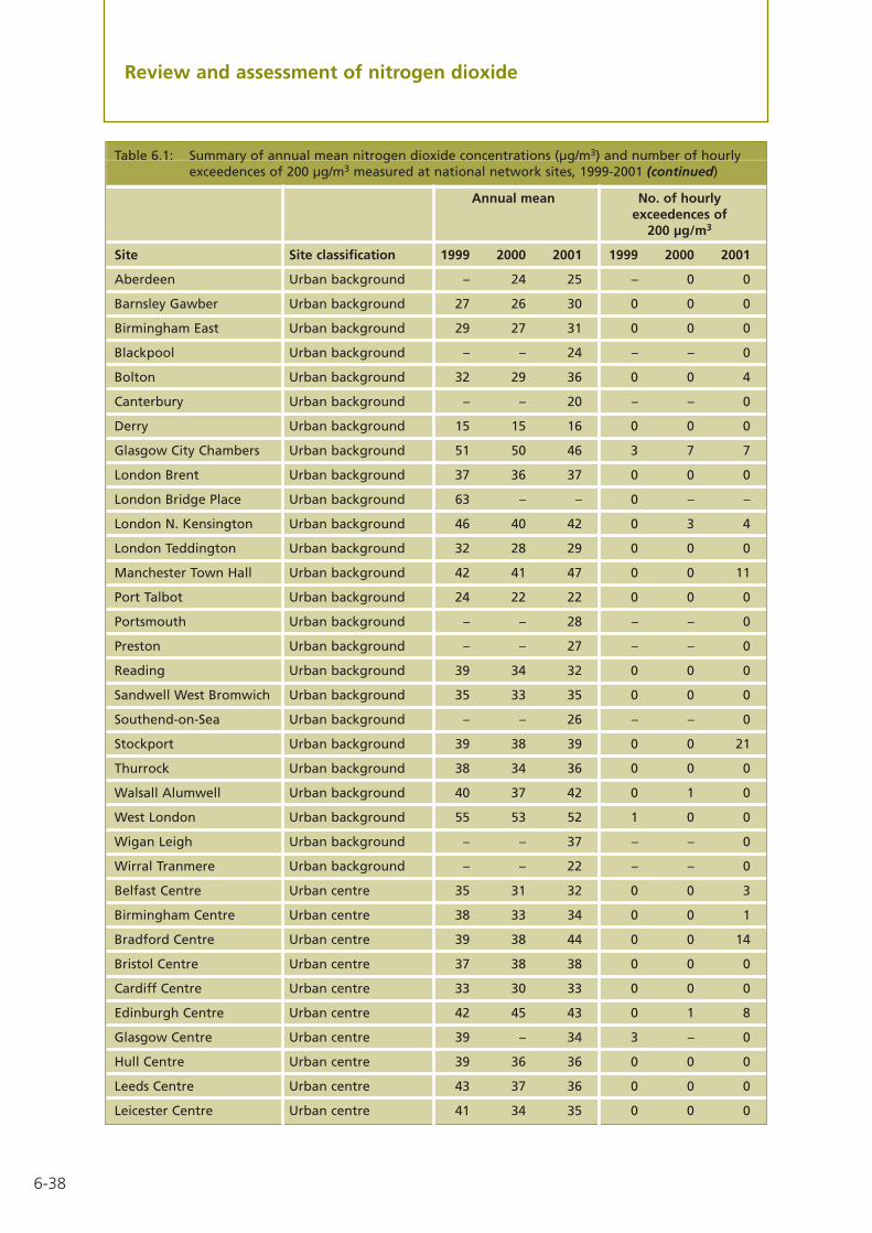
6-38
Table 6.1: Summary of annual mean nitrogen dioxide concentrations (µg/m3) and number of hourlyexceedences of 200 µg/m3 measured at national network sites, 1999-2001 (continued)
Annual mean No. of hourlyexceedences of
200 µg/m3
Site Site classification 1999 2000 2001 1999 2000 2001
Aberdeen Urban background – 24 25 – 0 0
Barnsley Gawber Urban background 27 26 30 0 0 0
Birmingham East Urban background 29 27 31 0 0 0
Blackpool Urban background – – 24 – – 0
Bolton Urban background 32 29 36 0 0 4
Canterbury Urban background – – 20 – – 0
Derry Urban background 15 15 16 0 0 0
Glasgow City Chambers Urban background 51 50 46 3 7 7
London Brent Urban background 37 36 37 0 0 0
London Bridge Place Urban background 63 – – 0 – –
London N. Kensington Urban background 46 40 42 0 3 4
London Teddington Urban background 32 28 29 0 0 0
Manchester Town Hall Urban background 42 41 47 0 0 11
Port Talbot Urban background 24 22 22 0 0 0
Portsmouth Urban background – – 28 – – 0
Preston Urban background – – 27 – – 0
Reading Urban background 39 34 32 0 0 0
Sandwell West Bromwich Urban background 35 33 35 0 0 0
Southend-on-Sea Urban background – – 26 – – 0
Stockport Urban background 39 38 39 0 0 21
Thurrock Urban background 38 34 36 0 0 0
Walsall Alumwell Urban background 40 37 42 0 1 0
West London Urban background 55 53 52 1 0 0
Wigan Leigh Urban background – – 37 – – 0
Wirral Tranmere Urban background – – 22 – – 0
Belfast Centre Urban centre 35 31 32 0 0 3
Birmingham Centre Urban centre 38 33 34 0 0 1
Bradford Centre Urban centre 39 38 44 0 0 14
Bristol Centre Urban centre 37 38 38 0 0 0
Cardiff Centre Urban centre 33 30 33 0 0 0
Edinburgh Centre Urban centre 42 45 43 0 1 8
Glasgow Centre Urban centre 39 – 34 3 – 0
Hull Centre Urban centre 39 36 36 0 0 0
Leeds Centre Urban centre 43 37 36 0 0 0
Leicester Centre Urban centre 41 34 35 0 0 0
Review and assessment of nitrogen dioxide

6-39
Table 6.1: Summary of annual mean nitrogen dioxide concentrations (µg/m3) and number of hourlyexceedences of 200 µg/m3 measured at national network sites, 1999-2001 (continued)
Annual mean No. of hourlyexceedences of
200 µg/m3
Site Site classification 1999 2000 2001 1999 2000 2001
Liverpool Centre Urban centre 41 35 38 0 0 1
London Bloomsbury Urban centre 67 59 51 6 0 0
London Hackney Urban centre 60 51 48 9 1 0
London Lewisham Urban centre 54 – – 0 – –
London Southwark Urban centre 56 52 55 0 0 0
London Wandsworth Urban centre 52 49 53 4 0 0
Manchester Piccadilly Urban centre 43 41 – 0 0 –
Newcastle Centre Urban centre 31 29 31 0 0 0
Norwich Centre Urban centre 27 25 28 0 0 0
Nottingham Centre Urban centre 44 40 35 0 0 0
Plymouth Centre Urban centre 22 24 33 0 0 0
Rotherham Centre Urban centre – 33 34 – 1 0
Sheffield Centre Urban centre 37 35 37 0 0 0
Southampton Centre Urban centre 42 38 38 0 0 0
Stoke-on-Trent Centre Urban centre 35 31 33 0 0 0
Swansea Urban centre 34 34 36 0 0 0
Wolverhampton Centre Urban centre 30 29 32 0 0 0
Billingham Urban industrial 33 36 32 0 2 2
Grangemouth Urban industrial – – 19 – – 0
Middlesbrough Urban industrial 25 24 24 0 0 1
Salford Eccles Urban industrial 43 37 42 1 0 12
Sheffield Tinsley Urban industrial 46 44 45 0 0 0
Review and assessment of nitrogen dioxide

6-40
Review and assessment of nitrogen dioxide
Table 6.2: Summary of 99.8th percentile of total oxidant concentrations (O3 + NO2) at nationalnetwork monitoring sites, 1999-2001 (µg/m3)
Annual mean total oxidantconcentration (µg/m3 as NO2)
Site Site classification 1999 2000 2001
London Marylebone Road Kerbside 241 249 253
Bury Roadside Roadside 200 184 196
Exeter Roadside Roadside 119 173 181
Harwell Rural 167 135 167
Ladybower Rural 174 137 132
Lullington Heath Rural 166 123 183
Narberth Rural 166 136 111
Rochester Rural 193 151 167
Wicken Fen Rural 178 137 160
London Bexley Suburban 185 143 184
London Eltham Suburban 184 155 183
London Hillingdon Suburban 154 150 179
London Sutton Suburban 163 138 180
Manchester South Suburban 153 159 123
Redcar Suburban 159 148 142
Barnsley Gawber Urban background 189 145 173
Birmingham East Urban background 173 129 163
Blackpool Urban background – 119 155
Bolton Urban background 179 151 163
Derry Urban background 146 137 113
Leamington Spa Urban background 181 148 171
London Brent Urban background 192 161 175
London Bridge Place Urban background 209 – –
London N. Kensington Urban background 199 166 178
London Teddington Urban background 208 151 190
London Westminster Urban background – 153 174
Port Talbot Urban background 175 139 160
Preston Urban background – 147 157
Reading Urban background 224 157 170
Sandwell West Bromwich Urban background 185 146 172
Southend-on-Sea Urban background – 155 176
Thurrock Urban background 189 149 185
Wirral Tranmere Urban background – 138 160
Belfast Centre Urban Centre 160 139 149
Birmingham Centre Urban Centre 174 137 165
Bradford Centre Urban Centre 159 143 215

6-41
Review and assessment of nitrogen dioxide
Table 6.2: Summary of 99.8th percentile of total oxidant concentrations (O3 + NO2) at nationalnetwork monitoring sites, 1999-2001 (µg/m3) (continued)
Annual mean total oxidantconcentration (µg/m3 as NO2)
Site Site classification 1999 2000 2001
Bristol Centre Urban centre 177 174 169
Cardiff Centre Urban centre 174 145 147
Coventry Centre Urban centre 113 102 177
Edinburgh Centre Urban centre 140 137 163
Glasgow Centre Urban centre 146 163 139
Hull Centre Urban centre 171 154 140
Leeds Centre Urban centre 172 142 137
Leicester Centre Urban centre 189 147 175
Liverpool Centre Urban centre 185 143 178
London Bloomsbury Urban centre 226 165 187
London Hackney Urban centre 248 176 165
London Lewisham Urban centre 168 129 –
London Southwark Urban centre 197 156 192
London Wandsworth Urban centre 187 148 185
Manchester Piccadilly Urban centre 172 105 200
Newcastle Centre Urban centre 162 155 125
Norwich Centre Urban centre 215 151 164
Nottingham Centre Urban centre 180 135 152
Plymouth Centre Urban centre 155 151 107
Rotherham Centre Urban centre 102 146 147
Sheffield Centre Urban centre 169 154 145
Southampton Centre Urban centre 188 139 168
Stoke-on-Trent Centre Urban centre 185 159 159
Swansea Urban centre 175 146 163
Wolverhampton Centre Urban centre 168 – 165
Middlesbrough Urban industrial 171 139 150
Salford Eccles Urban industrial 181 145 196

7-1
Chapter 7 Review and assessment of sulphur dioxide
7-1
Introduction7.01 The Government and the Devolved Administrations have adopted a 15-minutemean of 266 µg/m3 as an air quality standard for sulphur dioxide, with an objective forthe standard not to be exceeded more than 35 times in a year by the end of 2005.Additional objectives have also been set which are equivalent to the EU limit valuesspecified in the First Air Quality Daughter Directive. These are for a 1-hour meanobjective of 350 µg/m3, to be exceeded no more than 24 times per year, and a 24-hourobjective of 125 µg/m3, to be exceeded no more than 3 times per year, to be achievedby the end of 2004.
7.02 This section of the guidance provides advice to local authorities on how toidentify areas within their locality, at risk of exceeding the Air Quality Objectives forsulphur dioxide.
What areas are at risk of exceeding the objectives?
The national perspective
7.03 The main source of sulphur dioxide in the United Kingdom is power stations,which accounted for more than 71% of emissions in 2000. There are also significantemissions from other industrial combustion sources. Domestic sources now onlyaccount for 4% of emissions, but can be locally much more significant. Road transportcurrently accounts for less than 1% of emissions.
7.04 A summary of measured sulphur dioxide concentrations at UK national networksites is shown in Table 7.1 for the period 1999-2001. Concentrations have fallen at allsites in recent years, and the objectives were only exceeded at one site in Belfast duringthis period. This exceedence is associated with domestic coal burning which is stillwidespread in this area.
7.05 Local exceedences of the objectives (principally the 15-minute mean objective)may occur in the vicinity of small combustion plant (less than 20 MW) which burn coalor oil, in areas where solid fuels are the predominant form of domestic heating, and inthe vicinity of major ports.
The local perspective – what conclusions have been drawn from the firstround of the review and assessment process?
7.06 There have been a small number of AQMAs declared from the first round ofreview and assessment. These relate to emissions from coal-fired boilers at a cellophaneprocess and a food processing plant, a coal-fired boiler at a hospital, domestic coalburning, and shipping at a major port.
The Updating and Screening Assessment for sulphur dioxide7.07 This updating review is intended to identify any significant changes that mayhave occurred since the first round of review and assessment was completed. Forsulphur dioxide, this will include new monitoring data, new or changed emissionssources (either locally or in neighbouring authorities), or other local changes that mightaffect air quality, etc.

7-2
7.08 In completing the Updating and Screening Assessment, authorities areencouraged to maximise and build upon the data and assessments work completedduring the first round of review and assessment.
7.09 It is recognised that many authorities will have completed Third Stage reportsduring the first round of review and assessment, and in doing so, will have set updetailed lists of emissions sources and used a variety of air quality dispersion models. All authorities should complete the updating assessment, but any subsequent screeningassessment may be carried out using models already established by the authority, if thisis the easier and preferred route.
7.10 This part of the review and assessment is based upon a checklist approach, asummary of which is provided in Box 7.1. Authorities may wish to consider formattingtheir reports for the Updating and Screening Assessment with these section headings inmind. A detailed checklist for each source or location is set out in Box 7.2 (at the endof the Updating and Screening Assessment section). This describes the information thatauthorities should collate for the review and assessment against the 2004 and 2005objectives. The first column describes the source, location or data that need to beconsidered, and the subsequent columns describe the steps that need to be taken.
Background concentrations
7.11 Estimated annual mean background sulphur dioxide concentrations for 2001have been mapped for the UK, and can be accessed from the internet at the followingaddress: www.airquality.co.uk/archive/laqm/tools.php. Data files of 1km x 1km gridsquare estimated concentrations for each local authority can be downloaded along witha document illustrating the maps.
7.12 For the purpose of review and assessment, authorities may assume thatbackground annual mean sulphur dioxide concentrations at the end of 2004 and 2005will be 75% of the 2001 values.
Monitoring data
7.13 Data collected from national monitoring networks, or from local monitoringcampaigns, are expected to give a more accurate indication of sulphur dioxideconcentrations than modelling studies. Authorities are recommended to prioritise the
Box 7.1: Summary of the Updating and Screening checklist approach for sulphur dioxide
Reference no. Source, location or data that need to be assessed
A Monitoring data outside an AQMA
B Monitoring data within an AQMA
C New industrial sources
D Industrial sources with substantially increased emissions
E Areas of domestic coal burning
F Small boilers (>5MW(thermal)) burning coal or oil
G Shipping
H Railway Locomotives
Review and assessment of sulphur dioxide

7-3
use of measured sulphur dioxide concentrations wherever suitable data are available. Itis emphasised that monitoring sites will need to be at locations relevant for publicexposure, and where the maximum impact of the source (i.e. the highestconcentrations) are expected to be measured.
7.14 Guidance on monitoring methods and strategies for sulphur dioxide are set outin more detail in Annex 1. Monitoring using 8-port bubblers is still used in the UK, andwhilst their use has declined, the data may still prove useful. Guidance on the use ofdata from 8-port bubblers is provided in Box 7.3. Passive diffusion tube samplers havealso been developed for sulphur dioxide, but their use is not recommended for reviewand assessment. These diffusive samplers are only able to measure concentrations overa relatively long averaging period (one or two weeks) which cannot easily be comparedwith the shorter-term objectives.
7.15 Ideally, monitoring should have been carried out for a period of one year,particularly for assessment of the 15-minute mean objectives. A shorter period ofmonitoring (e.g. 9 months) may be sufficient to demonstrate that the risk ofexceedence of the objective is minimal, or of course, that an exceedence has occurred.In circumstances where authorities have less than 12 months data, they should contactthe relevant Helpdesk for assistance (see Box 1.1).
7.16 It should be noted that the assessment must be based on current measuredconcentrations, as there is no straightforward way to predict future exceedences of theshort-term objectives. An exception may be made where the authority is confident thatlocal emissions will reduce substantially by 2004 or 2005, for example due to aconfirmed proposal for emissions abatement by fuel or plant change, or plant closure.In such circumstances, the authority is again advised to contact the relevant Helpdesk(see Box 1.1).
Box 7.3: Use of 8-port bubblers for monitoring sulphur dioxide concentrations
8-port bubblers continue to be used to measure concentrations of sulphur dioxide at a number of sitesthroughout the UK, and these data can be of use for review and assessment. It is essential that suitableQA/QC procedures are used (see Annex 1). Ion chromatographic analysis should be used in preferenceto net acidity titration wherever possible. If net acidity measurements are made, the measuredmaximum daily mean concentration should be multiplied by 1.25 to take account of a general tendencyfor bubblers to under-read at high concentrations. This factor is open to uncertainty, and will tend tooverestimate the concentrations in most cases. If in doubt, the authority should contact the MonitoringHelpdesk (Box 1.1) for assistance.
The bubbler technique will provide measurements of daily mean sulphur dioxide concentrations whichcan be directly compared to the 24-hour mean objective. For comparison with the 15-minute and 1-hour objectives, authorities may use correction factors based upon empirical relationships with themeasured maximum daily mean:
99.9th percentile of 15-minute means = 1.8962 x maximum daily mean
99.7th percentile of 1-hour means = 1.3691 x maximum daily mean
To take account of the uncertainty in these relationships, it may be assumed that the 15-minute meanobjective is unlikely to be exceeded if the maximum daily mean concentration is less than 80 µg/m3, and the 1-hour mean objective is unlikely to be exceeded if the maximum daily mean concentration is less than 200 µg/m3.
Review and assessment of sulphur dioxide

7-4
Screening assessment for industrial sources
7.17 A list of industrial processes with the potential to emit significant quantities ofsulphur dioxide in 2004/2005 is set out in Annex 2, Appendix E. In the case of newindustrial sources (since the last round of review and assessment), authorities areadvised to check whether a Detailed Assessment has already been carried out as part ofthe planning or authorisation process. This should certainly be the case for all Part A(and Part B in Northern Ireland) regulated processes. If a suitably Detailed Assessmenthas been completed then the authority may rely on these results and should cite thereport in their Updating and Screening Assessment report.
7.18 Evidence from the first round of review and assessment has indicated thatemissions from small boiler plant (>5MWthermal) may give rise to exceedences of theobjectives. If they have not already done so, authorities must ensure that these boilersare included in the assessment.
7.19 If no other study has been carried out, then the authority will need to completea screening assessment. To simplify the assessment of sulphur dioxide emissions fromindustrial processes, a nomogram has been prepared which estimates the emission rate(in tonnes per annum) that would produce a 99.9th percentile ground-levelconcentration of 53.2 µg/m3, equivalent to 20% of the short-term (15-minute) 2005 airquality objective. If the actual emission rate from the process exceeds the threshold,then it will be necessary to proceed to a Detailed Assessment.
7.20 The nomogram (Figure 7.1) is shown at the end of this chapter. Authorities mayalso download LAQM Tools from the internet (www.airquality.co.uk/archive/laqm/tools.php) which contain the calculations in an Excel spreadsheet format, and requirethe user to enter simple details on the emission rate and release conditions (stack height and diameter).
7.21 To use the nomogram it is necessary to estimate/derive:
• the rate of emission of sulphur dioxide in tonnes per annum.
• the stack height.
• the stack diameter.
• the height of the tallest building within 5 stack heights of the chimney.
7.22 To assist authorities in the compilation of data related to Part A (and Part B inNorthern Ireland) processes, the Environment Agency (EA), the Scottish EnvironmentProtection Agency (SEPA)1, and the Northern Ireland Environment and Heritage Service(EHS) have committed to provide information on any changes that may affect emissionsfrom existing processes, or any new processes that have been, or will be, authorised.The information will be provided from the local office on request. A pro-forma sheet forthis information is provided in Annex 2 (Appendix F). Authorities may also wish toconsider checking information derived from their first round of review and assessmentif there were any doubts regarding their validity. If this information was derived fromthe regulatory agencies, or directly from the Public Register, then there should be noneed to undertake this task.
Review and assessment of sulphur dioxide
1 SEPA have regulatory responsibility for Part B processes in Scotland.

7-5
7.23 Emission rates for Part B (Part C in Northern Ireland) processes may beobtainable from the authority’s authorisation documents. Estimated emissions data and emissions factors are also available from the UK Emissions Factor Database(www.naei.org.uk). Details of stack heights, diameters and building heights can also be obtained from the regulator, the operator or the authorisation documents, or may be estimated from a visual inspection.
7.24 The nomogram uses the effective stack height. This can be assumed to beequal to the actual (physical) stack height unless:
• The height of release is greater than 3 m above the building on which it sits, but lessthan 2.5 times the height of the tallest adjacent building. In this case the effectivestack height can be calculated from the following formula:
Ueff = 1.66(Uact – H)
where: H is the height (m) of the tallest adjacent building within 5 actual(physical) stack heights distance;
Ueff is the effective stack height; and
Uact is the actual (physical) stack height.
7.25 To use the nomogram, identify the line that corresponds to the diameter of thestack under consideration, and locate the point on this line whose coordinates equalthe effective stack height. Read off the corresponding emission rate on the horizontalaxis, and compare this with the actual emission rate for the process. If the actualemission rate is greater than the emission rate derived from the nomogram, then theauthority will need to proceed to a Detailed Assessment.
Screening assessment for domestic sources
7.26 Coal and smokeless fuel burning for domestic heating has now largely beenreplaced by alternative fuels throughout most of the UK. However, there are a fewareas remaining where it is still predominant, and which may have the potential tocause exceedences of the objectives.
7.27 Evidence from the first round of review and assessment has indicated that coalburning tends to be concentrated into small areas or estates, which are generally lessthan 1 km2. The risk of exceedence in an area can be considered significant where the
NOTE: If the process is non-continuous (i.e. a batch process) the point of discharge is less than10m above the ground or the building on which it sits; or the stack height is less than anyadjacent building within 5 actual (physical) stack heights distance, the authority will need toproceed to a Detailed Assessment if the emission is greater than 1 tonne per annum.
Where there are multiple stacks at the same site, a precautionary approach may be taken byassuming the total emissions (from all stacks) are released from the smallest stack. Wherethere are complex sites, with many stacks, the above nomograms are unlikely to beapplicable, and authorities are advised to proceed to a Detailed Assessment.
Review and assessment of sulphur dioxide

7-6
density of ’coal’ burning (including coal, anthracite and smokeless fuels) houses exceeds100 properties per 500 by 500m area. In such cases, the authority will need to proceedto a Detailed Assessment.
7.28 Information on the number of properties burning coal may be available fromhouse condition surveys. If necessary, it may be appropriate to carry out a survey of thearea (see Box 7.4 for a case study from the first round of review and assessment).
Screening assessment for other transport sources
7.29 Whilst the transport sectors associated with aircraft and road traffic emit smallquantities of sulphur dioxide, evidence from the first round of review and assessment,and other sources, suggests that there is little risk of the objectives being exceeded dueto these emissions.
7.30 Shipping movements may also give rise to emissions of sulphur dioxide, andwhere there are significant movements within a major port, there is the potential forthe objectives to be exceeded. The authority should determine whether there is relevantpublic exposure (see Para 1.19) within 1km of the main berths and maneuvering areas.If there are more than 5000 shipping movements per year (restricted to large ships,such as cross-Channel ferries, container ships etc) the authority will need to proceed toa Detailed Assessment.
7.31 Diesel railway locomotives (and potentially coal fired steam locomotives) maygive rise to elevated sulphur dioxide concentrations. This is only likely to occur whenlocomotives are regularly stationary with their engines running for periods of around15-minutes or longer close to sensitive locations. It should also be noted that thecurrent maximum allowable sulphur content of rail locomotive diesel (2000 ppm) isexpected to reduce to 1000 ppm by 2008 as a result of forthcoming EU legislation (stillunder discussion). Current emissions of sulphur dioxide from rail locomotives aretherefore expected to decline in future years.
Box 7.4: Domestic coal burning – case study from first round of review and assessment
South Norfolk District is a predominately rural area South of Norwich City. It was realised during thereview and assessment process that domestic solid fuel burning within the largest parish Costesseycould have an impact on SO2 and PM10 within the district. This possibility was strengthened when theresults of a House Condition Survey undertaken in 1996 were examined. This survey indicated thatsome 12% of domestic dwellings in Costessey used solid fuel as a primary source of heating and 49% as a secondary source. Using the Technical Guidance LAQM TG4(00) it was confirmed that, if theprimary and secondary uses of solid fuel were aggregated, it was possible that the SO2 objective wouldbe exceeded, but unlikely that the PM10 objective would be exceeded.
After seeking advice from the Defra helpline a simple questionnaire was sent to all households in theCostessey area who had taken part in the original survey, and a very different picture emerged. Of the214 replies (56% of those surveyed) 1.6% still used solid fuel as a primary source of heating, and 4.7% as a secondary form of heating. Of those in the latter category only 2.4% used solid fuel to anysignificant extent (more than 10 days a year) the majority using it only 2-3 days. The vast majority ofthose surveyed used gas. On the basis of this new survey, it was determined that PM10 and SO2 fromdomestic solid fuel burning would be unlikely to cause exceedences of the objectives.
Review and assessment of sulphur dioxide

7-7
Review and assessment of sulphur dioxide
Box 7.2: Updating and Screening checklist
Monitoring
Overview
These steps will ensure you collate all relevant sulphur dioxide monitoring dataand assess them appropriately to identify locations where exceedences of the15-minute and/or 1-hour and/or 24-hour objectives might occur. You shouldfocus on monitoring data obtained since the last round of review andassessment, but it is also useful to show longer-term trends where possible.
If net acidity titration results havebeen used, contact the MonitoringHelpdesk. If desired you can use themaximum daily mean to estimate a99.9th percentile of 15-minute meansby multiplying by 1.8962.
6. For monitoring with bubblers in 8-port samplers identify themaximum daily mean.
Where you have less than 90% datacapture you should use the 99thpercentile rather than the number of 24-hour exceedences.
5. Calculate the number of 24-hourexceedences of 125 µg/m3 in a fullyear, or the 99th percentile.
Where you have less than 90% datacapture you should use the 99.7thpercentile rather than the number of 1-hour exceedences.
4. Calculate the number of 1-hourexceedences of 350 µg/m3 in a fullyear, or the 99.7th percentile.
Where you have less than 90% datacapture you should use the 99.9thpercentile rather than the number of 15-minute exceedences.
3. Calculate the number of 15-minuteexceedences of 266 µg/m3 in a fullyear, or the 99.9th percentile.
It is imperative that any localmonitoring data are ratified beforebeing used. For concentrationsrecorded by continuous monitors,the key step will be to ensure thatyou have screened and scaled thedata – see Annex 1. Box 7.3 providesinformation on how to treat datafrom bubbler samplers.
Recent national network data will belabelled ‘provisional’ (see Para 1.32).They can still be used, as they havebeen scaled, but they have yet to beratified. Do not base decisions onany provisional data alone.
2. Ratify your local monitoring data,if you have not already done so.
Include your own local monitoringdata (including data from 8-portbubbler samplers) and data from thenational monitoring networks. Donot include SO2 diffusion tube data.
1. Collate all sulphur dioxidemonitoring data.
Approach
(A) Monitoring dataoutside an AQMA
Notes relevant to each stepSteps that must be taken tocomplete the assessment
Source, location, ordata that need to be
assessed

7-8
Review and assessment of sulphur dioxide
Box 7.2: Updating and Screening checklist (continued)
Monitoring
Overview
This step will determine whether there is evidence to suggest that an AQMApreviously declared may require reconsideration.
If the answer is no to any of these, itmay still be appropriate to proceedto a Detailed Assessment if youexpect that levels will be below theobjectives by the relevant years.The Detailed Assessment will be witha view to revoking the AQMA. Thiswill have to take account of likelychanges between now and 2004/05.
If the answer is YES to all of thesequestions, proceed to a DetailedAssessment for sulphur dioxide.
Action
Before you assess the measuredconcentration check that themonitoring locations represent relevantexposure (see Paras 1.19 – 1.21).
• Are there currently 35 or fewer15-minute exceedences of, or99.9th percentiles less than, 266µg/m3?
• Are there currently 24 or fewer 1-hour exceedences of, or 99.7thpercentiles less than, 350 µg/m3?
• Are there currently 3 or fewer 24-hour exceedences of, or 99thpercentiles less than, 125 µg/m3?
Questions
This will be for monitoring carriedout within the previously definedarea of exceedence.
1. Carry out the data analysis as setout under (A) above.
Approach
(B) Monitoring datawithin an AQMA
The Detailed Assessment will be witha view to determining whether todeclare an AQMA.
If the answer is YES to any of thesequestions, proceed to a DetailedAssessment for sulphur dioxide.
Action
Before you assess the measuredconcentrations check that themonitoring locations represent relevantexposure (see Paras 1.19 – 1.21).
Use is made of currentconcentrations because there is nostraightforward way to projectfuture exceedences. Future estimateswould be part of any DetailedAssessment.
The bubbler criterion is related tothe risk of exceeding the 15-minuteobjective.
• Are there currently more than 35 15-minute exceedences of, or99.9th percentiles greater than,266 µg/m3?
• Are there currently more than 24 1-hour exceedences of, or99.7th percentiles greater than,350 µg/m3?
• Are there currently more than 3 24-hour exceedences of, or 99th percentiles greater than, 125 µg/m3?
• Does the maximum daily meanbubbler result exceed 80 µ/m3?
Questions
Notes relevant to each stepSteps that must be taken tocomplete the assessment
Source, location, ordata that need to be
assessed

7-9
Review and assessment of sulphur dioxide
Box 7.2: Updating and Screening checklist (continued)
Industrial sources
Overview
The first round confirmed that the 15-minute objective was the most stringentfor sulphur dioxide and that there are few sources that cause exceedences. It islikely that large coal burning boilers may be significant. The new regulationslimiting the sulphur content of fuel oil to less than 1% from 1 January 2003,mean that sources burning fuel oil are unlikely to be significant. However,particular attention should be paid to the combined impact of several sources,including those outside the local authority area.
You should take account of othersources that may affect the area.Plumes do not have to combine, butseparately they may add to thenumber of occasions with 15-minutevalues above 266 µg/m3.
If the answer is YES you shouldproceed to a Detailed Assessment forsulphur dioxide for this source.
Action
• Does the source exceed thethreshold in the nomograms?
Question
You will need to derive the effectivestack height. Details of how to dothis are provided in Para 7.24.
3. Use the nomograms described in Para 7.17 onwards to determine if thesource requires further assessment.
See Para 7.23. If it is proving difficult toobtain the information on the emissionscontact the Emissions Helpdesk (Box 1.3).
2. Obtain information on the totalannual emission of sulphur dioxideand the height of the emission.
1. Use the checklist in Annex 2 todetermine whether the sourceneeds considering further.
This approach should be followed ifthere has been no previous airquality assessment.
Approach 2
The Detailed Assessment may be nomore than relying on the findings of theair quality assessment. For this to be thecase the assessment will have to meetthe standards of a Detailed Assessment.
If the answer is YES you shouldproceed to a Detailed Assessment forsulphur dioxide for this source.
Action
• Did the assessment predict anyexceedences of the objectives atrelevant locations?
Question
An assessment may already havebeen carried out as part of theplanning or authorisation process. If this is the case you should confirmthat the assessment is sufficient forreview and assessment purposes.You only need to consider proposedsources for which planning approvalhas been granted.
1. Check whether an air qualityassessment has already beencarried out for the new industrialsource.
Approach 1
Notes relevant to each stepSteps that must be taken tocomplete the assessment
Source, location, ordata that need to be
assessed
(C) New industrialsources

7-10
Review and assessment of sulphur dioxide
Box 7.2: Updating and Screening checklist (continued)
Industrial sources (continued)
Domestic sources
Overview
There are still areas where domestic coal burning is being carried out. These canbe significant sources of sulphur dioxide. Consideration of the results from thefirst round has shown the need to focus on the density of houses burning coalover a smaller area of 500 x 500 m. There are other changes to the screeningcalculation, so even if carried out during the first round, a further screeningexercise may well be required.
For guidance on how to obtain thisinformation, including how to carryout a survey see Para 7.26. Do notcount houses with occasional use.
2. Collect information on the actualuse of domestic coal in theseareas.
You should take ‘significant’ to beany area of about 500 x 500 m wherethere may be more than 100 housesburning solid fuel as their primarysource of heating.
If necessary use professional judgementto identify such areas, includingexperience of coal burning odours inthe area on a winter’s evening.
1. Identify areas where significantcoal burning still takes place.Smokeless fuel has a similarsulphur content to coal so shouldbe treated in the same way.
(E) Areas of domesticcoal burning
Approach
You should take account of othersources that may affect the area.Plumes do not have to combine, butseparately they may add to thenumber of occasions with 15-minutevalues above 266 µg/m3.
If the answer is YES you shouldproceed to a Detailed Assessment forsulphur dioxide.
Action
• Does the source exceed thethreshold in the nomograms?
Question
You will need to derive the effectivestack height. Details of how to dothis are provided in Para 7.24.
3. Use the nomograms described inPara 7.17 onwards to determine ifthe source requires furtherassessment.
See Para 7.23. If it is proving difficultto obtain the information on theemissions contact the EmissionsHelpdesk (Box 1.3).
2. Obtain updated information onthe total annual emission ofsulphur dioxide and the height ofthe emission.
A ‘substantial’ increase can be takento be one greater than 30%.
1. Determine whether any of thesources identified during the lastround as potentially significanthave ‘substantially’ increasedemissions.
Approach
Notes relevant to each stepSteps that must be taken tocomplete the assessment
Source, location, ordata that need to be
assessed
(D) Industrial sourceswith substantiallyincreased emissions

7-11
Review and assessment of sulphur dioxide
Box 7.2: Updating and Screening checklist (continued)
Domestic sources (continued)
Boilers
Overview
The first round of review and assessment confirmed that larger boiler plant>5 MW(thermal) can give rise to high short-term concentrations, with the riskthat the 15-minute objective may be exceeded. The new regulations limitingthe sulphur content of fuel oil to less than 1% from 1 January 2003, meanthat boilers using fuel oil are unlikely to be significant on their own. Particularattention should be paid to the combined impact of several sources, includingthose outside the local authority area.
You should take account of othersources that may affect the area.Plumes do not have to combine, butseparately they may add to thenumber of occasions with 15-minutevalues above 266 µg/m3.
If the answer is YES you shouldproceed to a Detailed Assessment forsulphur dioxide at these locations.
Action
The nomogram is precautionary toallow for the possibility of othersources contributing to exceedences ofthe objective values.
• Does the source exceed thethreshold in the nomograms?
Questions
4. Use the nomograms described inPara 7.17 onwards to determine ifthe source requires furtherassessment.
You will need to derive the effectivestack height. Details of how to do thisare provided in Para 7.24.
3. Obtain information on totalannual emissions of sulphurdioxide and the stack height and diameter.
Near can be taken to be within 500 m.2. Establish whether there is relevantexposure ‘near’ to the source.
This could be plant in universities orhospitals, as well as in other largeinstitutional and commercialbuildings.
1. Identify all boiler plant >5 MW(thermal) that burn coal or fuel oil.
Approach
You should take account of othersources that may affect the area.Plumes do not have to combine, butseparately they may add to thenumber of occasions with 15-minutevalues above 266 µg/m3.
If the answer is YES you shouldproceed to a Detailed Assessment forsulphur dioxide at these locations.
Action
• Does the density of coal burningpremises exceed 100 per 500 x 500 m area?
Question
Notes relevant to each stepSteps that must be taken tocomplete the assessment
Source, location, ordata that need to be
assessed
(F) Small boilers > 5 MW(thermal)

7-12
Review and assessment of sulphur dioxide
Box 7.2: Updating and Screening checklist (continued)
Other sources
Overview
The fuels used in the transport sector contain varying amounts of sulphur. Thissection considers the range of possible transport related sources that mayrepresent a risk of exceeding the 15-minute objective.
You should take account of othersources that may affect the area.Plumes do not have to combine, butseparately they may add to thenumber of occasions with 15-minutevalues above 266 µg/m3.
If the answer is YES you shouldproceed to a Detailed Assessment forsulphur dioxide at these locations.
Action
• Are there more than 5,000movements per year?
Question
This should be confined to largeships, e.g. cross-Channel ferries, Ro-Ro, container ships, cruise liners.
Every visit from a ship will generatetwo movements. If possible useinformation on the number ofmovements in 2005.
2. Collect information on thenumber of ship movements peryear.
Modelling has shown that thegreatest risk of exceedence may bedownwind of the main alignment of berths.
1. Establish whether there is relevantexposure within 1 km of theberths and main areas ofmaneuvering.
Large ships generally burn oils with ahigh sulphur content in their mainengines (bunker oils). If there aresufficient movements in a port theycan give rise to short-termconcentrations above the objectives.Auxiliary engines used while berthed(hotelling) usually use a lowersulphur fuel, and are unlikely to besignificant.
Approach(G) Shipping
Notes relevant to each stepSteps that must be taken tocomplete the assessment
Source, location, ordata that need to be
assessed

7-13
Review and assessment of sulphur dioxide
Box 7.2: Updating and Screening checklist (continued)
Other sources (continued)
You should take account of othersources that may affect the area.Plumes do not have to combine, butseparately they may add to thenumber of occasions with 15-minutevalues above 266 µg/m3.
If the answer is YES you shouldproceed to a Detailed Assessment forsulphur dioxide at these locations.
Action
• Are there more than twooccasions a day when there mightbe a locomotive stationary forwith its engine running for 15-minutes or more?
Question
This might require a period ofobservation.
3. Obtain information on thenumber of trains per day thatmight affect these locations, andthe typical duration that they arestationary with their enginesrunning.
You should consider locations outsidethe station or depot, as well as onthe station. There will need to be the potential for exposure ofmembers of the public for periods of15-minutes or more. The exposureneeds to be ‘outdoors’ in the generalsense of the word.
If there is no relevant exposure thenyou need proceed no further.
2. Establish whether there is thepotential for regular outdoorexposure of members of thepublic within 15 m of thestationary locomotives.
This could be signals, goods loops,depots or stations.
1. Identify locations where diesellocomotives are regularlystationary for periods of 15-minutes or more.
Diesel and coal-fired locomotivesemit sulphur dioxide. Movinglocomotives do not make asignificant contribution to short-termconcentrations and do not need tobe considered further. Exposure tostationary locomotives may be moresignificant, but only in terms of the15-minute objective.
Approach(H) RailwayLocomotives
Notes relevant to each stepSteps that must be taken tocomplete the assessment
Source, location, ordata that need to be
assessed

7-14
The Detailed Assessment for sulphur dioxide7.32 Where the screening assessment has indicated that there is a risk of the AirQuality Objectives not being achieved by 2004 or 2005, then the authority will need tocarry out a Detailed Assessment.
7.33 The aim of this Detailed Assessment is to determine with reasonable certaintywhether or not there is a likelihood of the objectives not being achieved. Theassumptions within this Detailed Assessment should be considered in depth, and thedata that are used or collected, quality-assured to a high standard. This is to allow theauthority to have confidence in the decision that it reaches to declare, not declare, orrevoke an Air Quality Management Area. Where a likely exceedence of the objectives isidentified, then the authority will also need to determine the magnitude andgeographical extent.
7.34 Because of the wide range of sources and local circumstances that may prevail,it is not possible to set prescriptive guidance for the Detailed Assessment. However,wherever possible, lessons learnt from the first round of review and assessment havebeen drawn upon. It is also expected that authorities will make use of the variousHelpdesks that have been established (see Box 1.1).
7.35 Specific guidance related to monitoring, emissions data and dispersionmodelling, is provided in Annexes 1 to 3 of this document. Whilst important aspects are highlighted in this section, authorities who are undertaking a Detailed Assessmentare strongly advised to read the relevant sections of the Annexes before commencingtheir work.
7.36 In undertaking the Detailed Assessment it is important to give consideration tothe points of maximum relevant public exposure (i.e. those locations where thehighest concentrations of sulphur dioxide are expected). It is essential that authoritiestake these potential ‘hot spots’ into consideration within their review and assessment.
Monitoring
7.37 As for the screening assessment, measured data are expected to give a moreaccurate indication of sulphur dioxide concentrations than modelling studies.
7.38 Guidance on monitoring methods, monitoring strategies and suitable QA/QCprocedures are set out in greater detail in Annex 1 to this document. The followingpoints are highlighted:
• Monitoring for the Detailed Assessment should be based upon the UV fluorescentsampler, or equivalent. Ideally, sampling should be carried out for a full calendar year,with 90% data capture, and any gaps spread evenly throughout the year.
• 8-port bubblers may have a useful role to play for the Detailed Assessment inproviding improved spatial resolution, particularly where the emissions are associatedwith a low-level dispersed source, such as domestic heating. If monitoring for theDetailed Assessment is based solely on the use of 8-port bubblers, the authority willneed to provide a detailed justification to support this decision. In suchcircumstances, authorities are advised to contact the Monitoring Helpdesk (Box 1.1)at the outset of their monitoring campaign.
Review and assessment of sulphur dioxide

7-15
• Sampling devices should be located at sites that are relevant in terms of publicexposure for the objectives (see Box 1.4). Ideally, monitoring should take place atlocal ‘hot spots’ so that likely exceedences of the objectives can be quantified.
• Monitoring strategies should take account of the potential requirements forsubsequent model verification at the outset of the study (see Para 7.41 and Annex 3).
Modelling
7.39 For the Detailed Assessment, authorities will need to have confidence in theirresults, which will subsequently be used to determine whether there is a likelihood ofthe objectives being exceeded and a need to declare an AQMA.
7.40 Issues regarding model validation and verification are discussed in further detailin Annex 3. Model validation generally refers to detailed, peer-reviewed studies thathave been carried out by the model supplier, or a regulatory agency (e.g. USEPA). Allmodels used in the Detailed Assessment should have an appropriate pedigree, and havebeen subject to detailed and documented validation trials.
7.41 Model verification refers to checks that are carried out on model performance ata local level. This basically involves the comparison of predicted versus measuredconcentrations. Where there is a disparity between the predicted and measuredconcentrations, the first step should always be to check the input data and modelparameters in order to minimise the errors. If required, the second step will be todetermine an appropriate adjustment factor that can be applied. For the review andassessment of domestic heating and shipping sources it is essential that modelverification is carried out. For the review and assessment of point sources, verificationof short-term concentrations may be more difficult to carry out. In this case, the use ofan appropriate validated model will be sufficient, provided that the source emissionscan be accurately quantified. However, in cases where there are local factorscontributing to uncertainty, such as certain types of batch processes, complextopography etc, then local verification studies may be required, and/or an additionalconsideration of uncertainties taken into account.
7.42 In all cases where model verification has been carried out, the approach shouldbe fully documented in the review and assessment report, and any adjustment factorapplied should be explicitly stated.
Meteorological data
7.43 The choice of meteorological data for use in the dispersion model can have anoutcome on the result, depending on whether a ‘worst case’ or ‘typical’ year isselected. A detailed discussion on the selection of meteorological data is provided inAnnex 3 and all authorities are advised to read this section prior to undertaking amodelling study. In summary, the guidance recommends that a single year of sequentialmeteorological data is used. If possible, meteorological, background and emissions datashould all be derived for the same year.
Review and assessment of sulphur dioxide
7-16
7.44 In the case of emissions from point sources, the main effect of differentmeteorological years will be to affect the precise location of the maximum predictedconcentration. Authorities are advised to take into consideration the potential effects offluctuating wind directions in different years. A suggested means of dealing with this isto assume that the actual maximum concentration may occur within a 45 degree arc toeither side of the predicted maxima, and properties lying within this arc should beconsidered. Where the authority decides to use multiple years (3 or more) ofmeteorological data, it is recommended that the results for all years are reported, butthat any decision is based upon the worst-case result.
Receptor spacing
7.45 The importance of giving due consideration to potential ‘hot spots’ has alreadybeen highlighted in Para 7.36. For the purpose of dispersion modelling, this requiresthe user to ensure that a suitable resolution for receptor grid spacing is used, or thatspecific receptors (representing the locations of maximum public exposure) are included.If the grid spacing is set to a low resolution (for example, several hundred metres) andno specific receptors are included, then there is the potential that the model will notpredict the highest concentrations relevant to public exposure. A more detaileddiscussion on receptor spacing is provided in Annex 3.
Domestic coal use
7.46 The Detailed Assessment associated with domestic coal use is likely to focusupon:
• Determination of coal and smokeless fuel use in the area to allow calculation ofemissions;
• Application of detailed dispersion modelling; and
• Local monitoring to confirm existing concentrations.
7.47 As a first step, it is recommended that authorities should undertake a DetailedAssessment of coal use within the area of concern, characterising the different fuelsand combustion methods used in order to more accurately quantify the emissions.Guidance on emissions calculations is given in Annex 2, and additional advice may beobtained from the Emissions Inventory Helpdesk. These data may then be input to asuitable air quality dispersion model, in order to predict the ground-level impact.Guidance on the selection of suitable dispersion models is given in Annex 3, andadditional advice may be obtained from the Modelling Helpdesk (Box 1.1).
7.48 In the absence of local monitoring data of suitable quality, it is recommended thata monitoring programme is carried out in order to more accurately define current sulphurdioxide concentrations in the area of concern. It is suggested that monitoring equipmentis sited at relevant locations and ideally, monitoring carried out for a period of 12 months.As a minimum the monitoring should cover the main coal burning season.
Review and assessment of sulphur dioxide

7-17
Industrial emissions
7.49 The Detailed Assessment associated with Part A and Part B processes is likely tofocus upon:
• The application of detailed dispersion modelling; and
• The use of more detailed local monitoring to confirm existing concentrations.
7.50 There are a variety of dispersion models which can be used to assess the impactof emissions arising from elevated point sources (stacks). Guidance on the selection ofsuitable dispersion models is given in Annex 3, and additional advice may be obtainedfrom the Modelling Helpdesk (Box 1.1). Authorities are advised to consider a moreaccurate description of the sulphur dioxide emissions. Many processes operate wellwithin their emissions limits, and actual emissions data should be used if at all possible.For certain types of process, both seasonal and daily variations in emissions aresignificant, and should also be considered, wherever possible, and input to the model.
Emissions from shipping movements
7.51 Due to the uncertainty in emissions estimates for shipping operations, it is likelythat the Detailed Assessment will rely on a combination of modelling and monitoringstudies. Monitoring should be carried out at the locations of maximum public exposure,with dispersion modelling results initially used to inform the siting of monitoringequipment and subsequently to determine the geographic boundary of anyexceedences.
Figure 7.1: Emissions of SO2 which will give rise to a 99.9th percentile 15-minute ground-level mean concentration of 53.2 µg/m3.
Review and assessment of sulphur dioxide
1
10
100
1000
10 100 1000 10000 100000
Emission (tonnes per annum)
Effe
ctiv
e st
ack
hei
gh
t (m
)
0.5 m diameter 1 m2 m4 m8 m
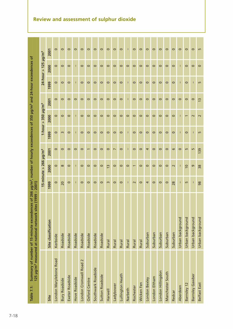
7-18
Review and assessment of sulphur dioxide
Tab
le 7
.1:
Sum
mar
y o
f n
um
ber
of
15-m
inu
te e
xcee
den
ces
of
266
µg
/m3 ,
nu
mb
er o
f h
ou
rly
exce
eden
ces
of
350
µg
/m3
and
24-
ho
ur
exce
eden
ces
of
125
µg
/m3
mea
sure
d a
t n
atio
nal
net
wo
rk s
ites
(19
99 –
200
1)
15-m
inu
te >
266
µg
/m3
1-h
ou
r >
350
µg
/m3
24-h
ou
r >
125
µg
/m3
Site
Site
cla
ssif
icat
ion
1999
2000
2001
1999
2000
2001
1999
2000
2001
Lon
do
n M
aryl
ebo
ne
Ro
ad
Ker
bsi
de
00
00
00
00
0
Bu
ry R
oad
sid
e R
oad
sid
e 20
80
30
00
00
Exet
er R
oad
sid
e R
oad
sid
e 0
00
00
00
00
Ho
ve R
oad
sid
e R
oad
sid
e –
–0
––
0–
–0
Lon
do
n C
rom
wel
l Ro
ad 2
Ro
adsi
de
00
00
00
00
0
Oxf
ord
Cen
tre
Ro
adsi
de
00
10
00
00
0
Sou
thw
ark
Ro
adsi
de
Ro
adsi
de
00
00
00
00
0
Sutt
on
Ro
adsi
de
Ro
adsi
de
00
00
00
00
0
Har
wel
lR
ura
l3
130
00
00
00
Lad
ybo
wer
Ru
ral
00
70
00
00
0
Lulli
ng
ton
Hea
thR
ura
l0
00
00
00
00
Nar
bet
hR
ura
l–
0–
–0
––
0–
Ro
ches
ter
Ru
ral
21
00
00
00
0
Wic
ken
Fen
Ru
ral
00
00
00
00
0
Lon
do
n B
exle
ySu
bu
rban
40
40
00
00
0
Lon
do
n E
lth
amSu
bu
rban
00
00
00
00
0
Lon
do
n H
illin
gd
on
Sub
urb
an0
00
00
00
00
Man
ches
ter
Sou
thSu
bu
rban
00
00
00
00
0
Red
car
Sub
urb
an28
26
00
00
00
Ab
erd
een
U
rban
bac
kgro
un
d–
–0
––
0–
–0
Bar
nsl
ey 1
2 U
rban
bac
kgro
un
d5
105
01
00
00
Bar
nsl
ey G
awb
er
Urb
an b
ackg
rou
nd
–9
5–
20
–0
0
Bel
fast
Eas
t U
rban
bac
kgro
un
d98
3813
95
213
50
5

7-19
Review and assessment of sulphur dioxide
Tab
le 7
.1:
Sum
mar
y o
f n
um
ber
of
15-m
inu
te e
xcee
den
ces
of
266
µg
/m3 ,
nu
mb
er o
f h
ou
rly
exce
eden
ces
of
350
µg
/m3
and
24-
ho
ur
exce
eden
ces
of
125
µg
/m3
mea
sure
d a
t n
atio
nal
net
wo
rk s
ites
(19
99 –
200
1)(c
on
tin
ued
)
15-m
inu
te >
266
µg
/m3
1-h
ou
r >
350
µg
/m3
24-h
ou
r >
125
µg
/m3
Site
Site
cla
ssif
icat
ion
1999
2000
2001
1999
2000
2001
1999
2000
2001
Bir
min
gh
am E
ast
Urb
an b
ackg
rou
nd
00
00
00
00
0
Bla
ckp
oo
l U
rban
bac
kgro
un
d–
–0
––
0–
–0
Bo
lto
n
Urb
an b
ackg
rou
nd
00
00
00
00
0
Bo
urn
emo
uth
U
rban
bac
kgro
un
d–
–0
––
0–
–0
Co
ven
try
Mem
ori
al P
ark
Urb
an b
ackg
rou
nd
––
0–
–0
––
0
Der
ry
Urb
an b
ackg
rou
nd
–19
0–
10
–0
0
Leam
ing
ton
Sp
a U
rban
bac
kgro
un
d0
00
00
00
00
Lon
do
n B
ren
t U
rban
bac
kgro
un
d0
00
00
00
00
Lon
do
n B
rid
ge
Plac
e U
rban
bac
kgro
un
d0
––
0–
–0
––
Lon
do
n N
. Ken
sin
gto
n
Urb
an b
ackg
rou
nd
00
00
00
00
0
Lon
do
n T
edd
ing
ton
U
rban
bac
kgro
un
d0
00
00
00
00
No
rth
amp
ton
U
rban
bac
kgro
un
d–
–0
––
0–
–0
Port
Tal
bo
t U
rban
bac
kgro
un
d–
00
–0
0–
00
Port
smo
uth
U
rban
bac
kgro
un
d–
–0
––
0–
–0
Pres
ton
U
rban
bac
kgro
un
d–
–0
––
0–
–0
Rea
din
g
Urb
an b
ackg
rou
nd
30
00
00
00
0
San
dw
ell W
est
Bro
mw
ich
U
rban
bac
kgro
un
d0
00
00
00
00
Sou
then
d-o
n-S
ea
Urb
an b
ackg
rou
nd
––
0–
–0
––
0
Sto
ckp
ort
U
rban
bac
kgro
un
d2
00
00
00
00
Sun
der
lan
d
Urb
an b
ackg
rou
nd
0–
00
–0
0–
0
Thu
rro
ck
Urb
an b
ackg
rou
nd
25
10
00
00
0
Wig
an L
eig
h
Urb
an b
ackg
rou
nd
––
0–
–0
––
0
Wir
ral T
ran
mer
e U
rban
bac
kgro
un
d–
–0
––
0–
–0
Bel
fast
Cen
tre
Urb
an c
entr
e 5
162
00
00
00
Bir
min
gh
am C
entr
e U
rban
cen
tre
00
00
00
00
0
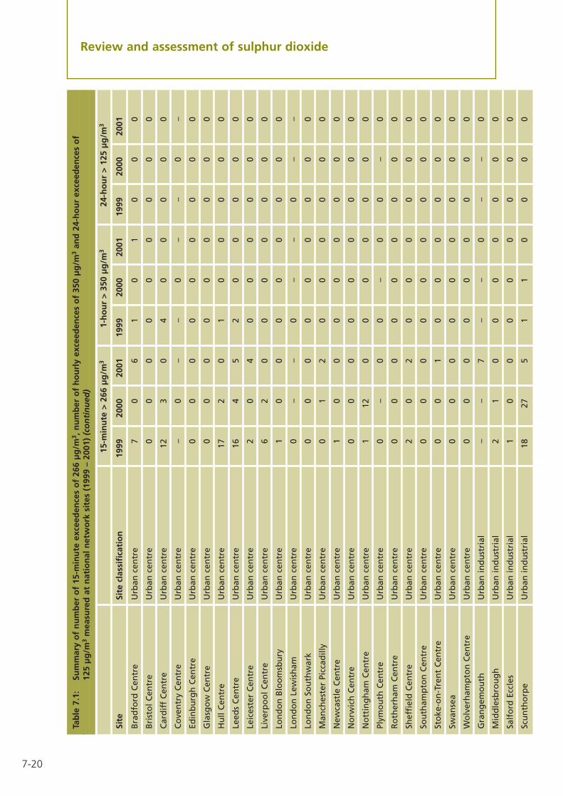
7-20
Review and assessment of sulphur dioxide
Tab
le 7
.1:
Sum
mar
y o
f n
um
ber
of
15-m
inu
te e
xcee
den
ces
of
266
µg
/m3 ,
nu
mb
er o
f h
ou
rly
exce
eden
ces
of
350
µg
/m3
and
24-
ho
ur
exce
eden
ces
of
125
µg
/m3
mea
sure
d a
t n
atio
nal
net
wo
rk s
ites
(19
99 –
200
1)(c
on
tin
ued
)
15-m
inu
te >
266
µg
/m3
1-h
ou
r >
350
µg
/m3
24-h
ou
r >
125
µg
/m3
Site
Site
cla
ssif
icat
ion
1999
2000
2001
1999
2000
2001
1999
2000
2001
Bra
dfo
rd C
entr
e U
rban
cen
tre
70
61
01
00
0
Bri
sto
l Cen
tre
Urb
an c
entr
e 0
00
00
00
00
Car
dif
f C
entr
e U
rban
cen
tre
123
04
00
00
0
Co
ven
try
Cen
tre
Urb
an c
entr
e –
0–
–0
––
0–
Edin
bu
rgh
Cen
tre
Urb
an c
entr
e0
00
00
00
00
Gla
sgo
w C
entr
e U
rban
cen
tre
00
00
00
00
0
Hu
ll C
entr
e U
rban
cen
tre
172
01
00
00
0
Leed
s C
entr
e U
rban
cen
tre
164
52
00
00
0
Leic
este
r C
entr
e U
rban
cen
tre
20
40
00
00
0
Live
rpo
ol C
entr
e U
rban
cen
tre
62
00
00
00
0
Lon
do
n B
loo
msb
ury
U
rban
cen
tre
10
00
00
00
0
Lon
do
n L
ewis
ham
U
rban
cen
tre
0–
–0
––
0–
–
Lon
do
n S
ou
thw
ark
Urb
an c
entr
e 0
00
00
00
00
Man
ches
ter
Picc
adill
y U
rban
cen
tre
01
20
00
00
0
New
cast
le C
entr
e U
rban
cen
tre
10
00
00
00
0
No
rwic
h C
entr
e U
rban
cen
tre
00
00
00
00
0
No
ttin
gh
am C
entr
e U
rban
cen
tre
112
00
00
00
0
Plym
ou
th C
entr
e U
rban
cen
tre
0–
00
–0
0–
0
Ro
ther
ham
Cen
tre
Urb
an c
entr
e 0
00
00
00
00
Shef
fiel
d C
entr
e U
rban
cen
tre
20
20
00
00
0
Sou
tham
pto
n C
entr
e U
rban
cen
tre
00
00
00
00
0
Sto
ke-o
n-T
ren
t C
entr
e U
rban
cen
tre
00
10
00
00
0
Swan
sea
Urb
an c
entr
e 0
00
00
00
00
Wo
lver
ham
pto
n C
entr
e U
rban
cen
tre
00
00
00
00
0
Gra
ng
emo
uth
Urb
an in
du
stri
al–
–7
––
0–
–0
Mid
dle
sbro
ug
hU
rban
ind
ust
rial
21
00
00
00
0
Salf
ord
Ecc
les
Urb
an in
du
stri
al1
00
00
00
00
Scu
nth
orp
eU
rban
ind
ust
rial
1827
51
10
00
0

Review and assessment for PM10
Introduction8.01 The Government and the Devolved Administrations have adopted two AirQuality Objectives for fine particles (PM10), which are equivalent to the EU Stage 1 limitvalues in the first Air Quality Daughter Directive. The objectives are 40 µg/m3 as theannual mean, and 50 µg/m3 as the fixed 24-hour mean to be exceeded on no morethan 35 days per year, to be achieved by the end of 2004. The objectives are basedupon measurements carried out using the European gravimetric transfer referencesampler or equivalent.
8.02 The EU has also set indicative limit values for PM10 which are to be achievedby 1 January 2010. These Stage 2 limit values are considerably more stringent, and are20 µg/m3 as the annual mean, and 50 µg/m3 as the 24-hour mean to be exceededon no more than 7 days per year. The Government, the Welsh Assembly Governmentand the Department of the Environment in Northern Ireland introduced provisionalobjectives to be achieved by the end of 2010, that are broadly in line with the Stage 2limit values, although it is not intended that these objectives will be brought intoRegulation for the purpose of Local Air Quality Management at this time1. Theprovisional objectives are:
• For all parts of England (except London), Wales and Northern Ireland, a 24-hourmean of 50 µg/m3 not to be exceeded more than 7 times per year, and an annualmean of 20 µg/m3, to be achieved by the end of 2010.
• For London, a 24-hour mean of 50 µg/m3 not to be exceeded more than 10 timesper year, and an annual mean of 23 µg/m3, to be achieved by the end of 2010. Anannual mean objective of 20 µg/m3 to be achieved by the end of 2015, has alsobeen set.
8.03 The Scottish Executive has incorporated new objectives for 2010 into theirRegulations, and authorities in Scotland will be required to review and assess air qualityagainst them. The prescribed objectives are as follows:
• A 24-hour mean of 50 µg/m3 not to be exceeded more than 7 times per year, andan annual mean of 18 µg/m3 to be achieved by the end of 2010.
8.04 This section of the guidance provides advice to local authorities on how toidentify areas within their locality, at risk of exceeding the prescribed Air QualityObjectives for PM10. Guidance is also provided to allow authorities in England andWales to assess the likelihood of the provisional objectives not being achieved by 2010,although there is no statutory obligation to do so.
Chapter 8 Review and assessment for PM10
8-1
1 The Government, the Welsh Assembly Government and the Department of the Environment in Northern Irelandwill consider whether the new particles objectives will be incorporated into Regulations as soon as practicable afterthe review of the EU First Air Quality Daughter Directive, which is due for completion in 2004.

Review and assessment of PM10
What areas are at risk of exceeding the objectives?
Sources of particles
8.05 There is a wide range of emission sources that contribute to PM10 concentrationsin the UK. The APEG report2 has confirmed that these sources can be usefully dividedinto 3 main categories. Primary particle emissions are derived directly from combustionsources, including road traffic, power generation, industrial processes etc. Secondaryparticles are formed by chemical reactions in the atmosphere, and comprise principallyof sulphates and nitrates. Coarse particles comprise of emissions from a wide range ofsources, including resuspended dusts from road traffic, construction works, mineralextraction processes, wind-blown dusts and soils, sea salt and biological particles.
8.06 It is important to bear in mind the different emission sources, and theirrespective contributions to PM10 concentrations, within the review and assessmentprocess for several reasons:
• The expected reduction in particle emissions in future years is different for each sourcetype. For example, emissions from road transport will be governed by new legislationon vehicle emission standards; emissions of secondary particles will be largelygoverned by controls on power generation, industrial and transport SO2 and NOxemissions, both in the UK and in Europe; emissions of coarse particles are largelyuncontrolled, and in general are not expected to decline in future years. In forecastingfuture emissions it is therefore essential to treat each source category separately.It should be noted that it is not appropriate to extrapolate measured PM10concentrations forwards to 2004 or 2010 using a simple trend analysis – a suitablemethodology for forecasting future concentrations is provided in later sections.
• The principal focus of Local Air Quality Management should be towards the controlof emissions at a local level. It is therefore important that the review and assessmentprocess identifies the contribution of local emission sources, so that the effectivenessof control policies or action plans can be evaluated.
8.07 A description of the different source categories, and their approximatecontribution to annual mean background concentrations is described in Box 8.1.A significant proportion of current annual mean PM10 is derived from regional(including long distance transport from Europe) background sources. The exact regionalbackground contribution at any site is variable, and will be dependent upon the precisegeographic location. Typical regional annual mean background contributions arecurrently within the range of about 14-21 µg/m3, gravimetric and are outside of thecontrol of local authorities. Where exceedences of the proposed objectives arepredicted, local authorities are strongly advised to focus their efforts on theidentification of the contribution of local sources to overall PM10 concentrations.
8-2
2 APEG (1999) Source apportionment of airborne particulate matter in the United Kingdom. Report of the AirborneParticles Expert Group. ISBN 0-7058-1771-7.
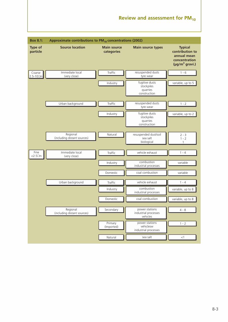
Review and assessment for PM10
Box 8.1: Approximate contributions to PM10 concentrations (2002)
Type of Source location Main source Main source types Typicalparticle categories contribution to
annual meanconcentration(µg/m3 gravi.)
8-3
Coarse2.5-10µm
Fine<2.5µm
Immediate local(very close)
Regional(including distant sources)
Immediate local(very close)
Regional(including distant sources)
Urban background
Urban background
resuspended duststyre wear
resuspended duststyre wear
combustionindustrial processes
power stationsindustrial processes
vehicles
power stationsvehiclesw
industrial processes
combustionindustrial processes
vehicle exhaust
coal combustion
vehicle exhaust
sea salt
coal combustion
resuspended dust/soilsea salt
biological
fugitive dustsstockpilesquarries
construction
fugitive dustsstockpilesquarries
construction
Traffic
Traffic
Traffic
Traffic
Secondary
Natural
Primary(Imported)
Domestic
Domestic
Industry
Industry
Industry
Industry
Natural
1 - 6
1 - 2
1 - 4
1 - 4
1 - 2
<1
4 - 8
2 - 31 - 2
1
variable, up to 5
variable, up to 2
variable
variable
variable, up to 8
variable, up to 8

8-4
Review and assessment for PM10
Policy measures and current PM10 concentrations
8.08 There has been significant progress in recent years in reducing emissions ofparticles from both the transport and industrial sectors, and total national annual UKemissions declined by nearly 40% in the period between 1990 and 1999. Furtherreductions are expected in future years as a result of agreed additional policies, or thosethat are currently under discussion. Within the industrial sector, particle emissions willbe further controlled through the EU Directive on Integrated Pollution Prevention andControl (IPPC) and the EU Waste Incineration Directive. In addition, a significantreduction in emissions of pollutants that lead to the formation of secondary particles isexpected as a result of the EU legislation on the Acidification Strategy. Emissions fromroad transport will also be reduced as a result of tightening emissions controls (Euro IIIand Euro IV standards) and by the reduction of the sulphur content of diesel fuel,which affects the emissions of particles from vehicles.
Box 8.2: Relationship between the European transfer reference sampler and other PM10sampling methods
Monitoring of PM10 in the UK networks has, to date, been largely founded on the use of the TEOManalyser. A concern with the TEOM instrument is that the filter is held at a temperature of 50˚C in orderto minimise errors associated with the evaporation and condensation of water vapour. This can lead toa loss of the more volatile particles (such as ammonium nitrate etc).
The EU limit values and the UK objectives are based upon measurements carried out using theEuropean transfer reference sampler, or equivalent. This is a gravimetric sampler, where the particulatematerial is collected onto a filter, and subsequently weighed. The filter is therefore held at fluctuatingambient conditions during the period of exposure. Whilst there will inevitably be some losses of volatilespecies from the filter (dependant upon the ambient temperature), these will be less than from theTEOM.
The Government and the Devolved Administrations have been investigating the relationship betweenthe TEOM and the reference sampler, using co-located instruments at 6 sites in the UK. These studieshave shown that the TEOM adjustment factor is site specific, and varies both from season to season,and from year to year. Because of this an interim default adjustment factor of 1.3 has been proposedfor the UK. This approach is supported by other studies carried out in other EU countries, and appearsto also apply to ß-attenuation instruments with a heated manifold.
For the purpose of the next round of review and assessment, authorities should bear in mind theissues set out below:
• Measurements of PM10 concentrations carried out using the European transfer reference sampler,or equivalent, are directly comparable with the UK objectives and EU limit values, and no datacorrection is necessary. There are, however, important QA considerations to bear in mind, regardingthe handling and weighing of filters.
• Measurements of PM10 concentrations carried out using a TEOM or ß-attenuation instrument,operating with a heated manifold, should be adjusted by multiplying the data by 1.3 to estimategravimetric equivalent concentrations.
• Measurements of PM10 concentrations carried out using other sampling methods (e.g. opticalanalysers, or gravimetric samplers that have not been certified as ‘equivalent’) will need to beconsidered carefully, particularly if they are being used in a Detailed Assessment, and theconcentrations measured are close to the objectives. Authorities with such analysers are advised tocontact the relevant Helpdesk (Box 1.1).
• It is not recommended that authorities carry out local intercomparison studies between the transferreference sampler and other samplers for the purpose of review and assessment. Where such studiesare carried out, it is essential to carry out the comparison over at least 6 months, including a summerand winter period. Any adjustment factors derived may be both season and site specific, and cannotsimply be used to adjust data at other sites, in other years. Authorities are advised to contact therelevant Helpdesk (Box 1.1) before embarking on intercomparison studies.
• The method of sampling is critical to the result. In all cases, authorities should explicitly state themethod of sampling, and report all original and ‘adjusted’ data.

8-5
Review and assessment for PM10
8.09 Concentrations of PM10 are currently measured at more than 60 nationalmonitoring sites in the UK. Data for the period 1999 to 2001 are described in Table 8.1.All of these data have been measured using a TEOM sampler, and have therefore beenmultiplied by 1.3 to give estimated concentrations expressed as µg/m3 gravimetric (seeBox 8.2). Concentrations are generally well below the 2004 annual mean objective (40 µg/m3 gravimetric) with the exception of the London Marylebone Road kerbsidesite. The 24-hour objective for 2004 (50 µg/m3, maximum of 35 exceedences per year)has been exceeded at a small number of sites, principally those in the vicinity of busyroads or close to industrial activities3.
8.10 The 2010 annual mean objectives are currently exceeded at the majority of siteswithin the network. Exceedences of the 24-hour objective for 2010 are also common,but vary from year to year, dependant upon meteorological conditions.
8.11 The data presented in Table 8.1 are current levels, and it is confidently expectedthat PM10 concentrations will continue to fall in future years. An analysis of PM10projections for 2004 is presented in the Air Quality Strategy. The assessment wascarried out using both 1995 and 1996 monitoring data, because 1996 wascharacterised by a much higher frequency of easterly winds associated with thetransport of polluted air from mainland Europe to the UK. The 1996 meteorologyoccurs about once every five to ten years and may therefore be described as ‘atypical’,and as such represents a worst-case, pessimistic scenario upon which to basepredictions of future PM10 concentrations. The analysis has indicated that with existingnational policy measures and atypical meteorology, exceedences of the 2004 objectivesmight be found in the following areas:
• urban background sites in central London;
• areas adjacent to busy roads, particularly within major urban areas;
• areas which have significant emissions from the domestic burning of solid fuels;
• areas in the vicinity of industrial plant, or which have significant uncontrolled orfugitive emissions (for example, quarrying, materials handling facilities etc.).
8.12 A similar analysis has also been carried out for the 2010 objectives4. Thisassessment indicates that, dependant upon meteorological conditions, exceedencesof the annual mean objectives at background locations are only likely to occur inSE England, and in London in particular. However, exceedences of the annual meanobjectives are still expected at some busy roadside sites throughout the UK.
3 Elevated PM10 concentrations were recorded at the Manchester Piccadilly urban centre site in 2001. Theseunusually high concentrations are believed to have been associated with the nearby construction activities inPiccadilly gardens.
4 Stedman J R, Bush T J, Murrells T P and King K (2001). Baseline PM10 and NOx projections for PM10 objectiveanalysis. AEAT/ENV/R/0726.

8-6
Review and assessment for PM10
The local perspective – what conclusions have been drawn from the reviewand assessment process?
8.13 More than 50% of the AQMAs declared in the UK have included exceedences ofthe 2004 24-hour mean PM10 objective, although the majority of these have been incombination with nitrogen dioxide, and are associated with road traffic sources. In mostof these cases the spatial extent of the 24-hour mean PM10 exceedence is smaller thanthat for the nitrogen dioxide annual mean objective. There are however other examplesof PM10 AQMAs. Industrial AQMAs for PM10 include a steel plant, unregulated coal-fired boilers and heating plant. In addition, fugitive sources of PM10 have been found tocause exceedences around a quarry and from port-handling activities. The declarationof an AQMA due to domestic coal burning is also under consideration.
8.14 It is critical that authorities focus upon those locations where they expectpollutant concentrations to be the highest, often referred to as ‘hot spots’. Focusing onthese areas should ensure that potential exceedences are not missed. This approach isalso likely to be cost-effective, particularly for updating reports prepared during the firstround of review and assessment. If there are no exceedences of the objective at themost polluted locations, then it can be reasonably concluded that there should be noexceedences elsewhere.
8.15 The highest PM10 concentrations associated with road traffic emissions will beclose to the road, with relevant locations for public exposure at the building façade (seeBox 1.4). For industrial emissions released from a tall stack, the maximum ground-levelconcentration may be many hundreds of metres downwind (this can be determined bydispersion modelling). In the case of fugitive and other ground-level releases (such asdomestic solid fuel), the highest concentrations may be expected close to the emissionsource.
The Updating and Screening Assessment for PM10
8.16 This updating review is intended to identify any significant changes that mayhave occurred since the first round of review and assessment was completed. This will,for example, include new monitoring data, new objectives, new or changed emissionssources (either locally or in neighbouring authorities), or other local changes that mightaffect air quality, etc.
8.17 Authorities will be aware that Government and the Devolved Administrationshave recently released new road traffic emissions factors. These new emissions factorswill affect PM10 emissions in future years from road transport. At a national level thesechanges are expected to be relatively minor, but more significant changes may occur ata local level depending upon the traffic mix5.
5 Emissions Factor Toolkit available at www.stanger.co.uk/airqual/modelhlp.

8-7
Review and assessment for PM10
8.18 In completing the Updating and Screening Assessment, authorities areencouraged to maximise and build upon the data and assessments completed duringthe first round of review and assessment.
8.19 All local authorities should undertake the Updating and Screening Assessmentfor the 2004 objective. Only those authorities in Scotland have a statutory requirementto undertake the Updating and Screening Assessment for the 2010 objective, althoughauthorities in England (including Greater London), Wales and Northern Ireland areencouraged to do so. It is believed that in many cases this will add little additionalwork, and will provide authorities with invaluable information, particularly whenassessing the impact of local development proposals. It should be noted that the 2010objectives are significantly more stringent. Authorities cannot assume that the 2010objectives will be met if there are no predicted exceedences of the 2004 objectives.
8.20 The monitoring data in Table 8.1 show that the 24-hour objective is morestringent than the annual mean objective in 2004. The opposite is true in 2010, andthe annual mean objectives are more stringent than the 24-hour objective. TheUpdating and Screening Assessment is therefore focused on the 24-hour meanobjective for 2004, and the annual mean objective for 2010.
8.21 This part of the review and assessment is based upon a checklist approach, asummary of which is provided in Box 8.3. Authorities may wish to consider formattingtheir reports for the Updating and Screening Assessment with these section headings inmind. A detailed checklist for each source or location is set out in Box 8.4 (at the endof the Updating and Screening Assessment section). This describes the information thatauthorities should collate for the review and assessment against the 2004 and 2010objectives. The first column describes the source, location or data that need to beconsidered, and the subsequent columns describe the steps that need to be taken.
Box 8.3: Summary of the Updating and Screening checklist approach for PM10
Reference no. Source, location or data that need to be assessed
A Monitoring data outside an AQMA
B Monitoring data within an AQMA
C Busy roads and junctions in Scotland
D Junctions
E Roads with high flow of buses and/or HGVs
F New roads constructed or proposed since first round of review and assessment
G Roads close to the objective during the first round of review and assessment
H Roads with significantly changed traffic flows
I New industrial sources
J Industrial sources with substantially increased emissions
K Areas with domestic solid fuel burning
L Quarries, landfill sites, opencast coal, handling of dusty cargoes at ports etc
M Aircraft

8-8
Review and assessment for PM10
Background concentrations
8.22 Estimated annual mean background PM10 concentrations for 2001, 2004 and2010 have been mapped for the UK, and can be accessed from the internet at thefollowing address: www.airquality.co.uk/archive/laqm/tools.php. Background maps forannual mean secondary PM10 in 2001 are also available. Details of the mapping processcan also be found at this site.
8.23 In using these maps, authorities are advised to take care to avoid ‘doublecounting’. For example, in rural areas where there is a section of heavily-trafficked roadit may be more appropriate to derive the background concentration from adjacent gridsquares. A recommended approach in such cases is set out in Box 1.5.
Monitoring data
8.24 Data collected from national monitoring networks, or from local monitoringcampaigns, are expected to give a more accurate indication of PM10 concentrationsthan modelling studies. Authorities are recommended to prioritise the use of measuredPM10 concentrations wherever suitable data are available. It is emphasised thatmonitoring sites will need to be at locations relevant for public exposure, and wherethe maximum impact of the source (i.e. the highest concentrations) are expected to bemeasured (see Para 8.15). All monitoring data used for review and assessment shouldbe quality-assured to a high standard. Details on QA/QC and ratification approaches areset out in Annex 1.
8.25 Guidance on monitoring methods and strategies for PM10 is set out in moredetail in Annex 1. Monitoring using continuous samplers (such as the TEOM or ß-attenuation samplers) is widely used in the UK to characterise ambient concentrationsof PM10. Whilst these methods have the advantage of providing short-term data forreporting to the public, the measured concentrations will need to be adjusted to unitsof µg/m3 gravimetric for comparison with the reference method (see Box 8.2). In somesituations the application of the interim 1.3 adjustment factor may lead to a significantover-estimation of the impact, for example if the predominant local source is mineralparticles, for example, near a quarry. Monitoring carried out using the referencesampler, or one that has been determined as equivalent, provides data that can bedirectly compared with the objectives. Measurements of PM10 concentrations usingother sampling methods (such as optical samplers, or gravimetric samplers that havenot been certified as equivalent to the reference method) will need to be consideredcarefully, particularly if the measured levels are close to the objectives. Authorities usingsuch samplers are advised to contact the Helpdesk (see Box 1.1) for advice.
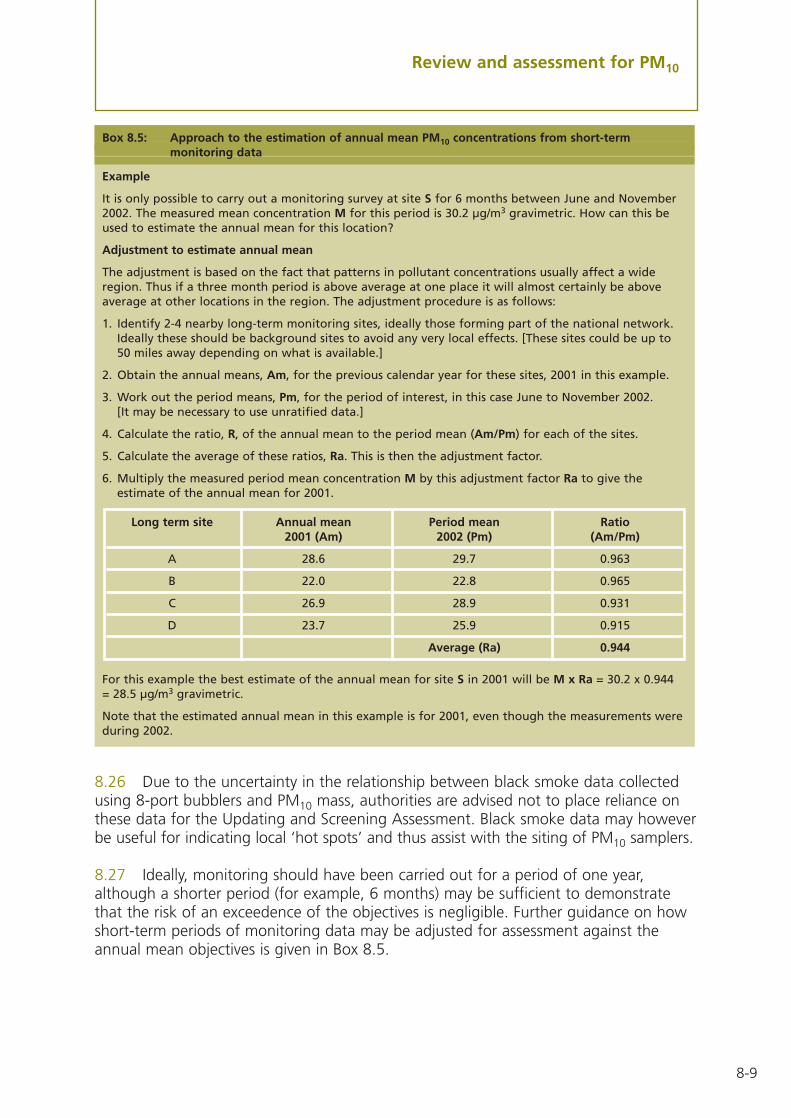
8-9
Review and assessment for PM10
Box 8.5: Approach to the estimation of annual mean PM10 concentrations from short-termmonitoring data
Example
It is only possible to carry out a monitoring survey at site S for 6 months between June and November2002. The measured mean concentration M for this period is 30.2 µg/m3 gravimetric. How can this beused to estimate the annual mean for this location?
Adjustment to estimate annual mean
The adjustment is based on the fact that patterns in pollutant concentrations usually affect a wideregion. Thus if a three month period is above average at one place it will almost certainly be aboveaverage at other locations in the region. The adjustment procedure is as follows:
1. Identify 2-4 nearby long-term monitoring sites, ideally those forming part of the national network.Ideally these should be background sites to avoid any very local effects. [These sites could be up to50 miles away depending on what is available.]
2. Obtain the annual means, Am, for the previous calendar year for these sites, 2001 in this example.
3. Work out the period means, Pm, for the period of interest, in this case June to November 2002. [It may be necessary to use unratified data.]
4. Calculate the ratio, R, of the annual mean to the period mean (Am/Pm) for each of the sites.
5. Calculate the average of these ratios, Ra. This is then the adjustment factor.
6. Multiply the measured period mean concentration M by this adjustment factor Ra to give theestimate of the annual mean for 2001.
For this example the best estimate of the annual mean for site S in 2001 will be M x Ra = 30.2 x 0.944= 28.5 µg/m3 gravimetric.
Note that the estimated annual mean in this example is for 2001, even though the measurements wereduring 2002.
Long term site Annual mean Period mean Ratio2001 (Am) 2002 (Pm) (Am/Pm)
A 28.6 29.7 0.963
B 22.0 22.8 0.965
C 26.9 28.9 0.931
D 23.7 25.9 0.915
Average (Ra) 0.944
8.26 Due to the uncertainty in the relationship between black smoke data collectedusing 8-port bubblers and PM10 mass, authorities are advised not to place reliance onthese data for the Updating and Screening Assessment. Black smoke data may howeverbe useful for indicating local ‘hot spots’ and thus assist with the siting of PM10 samplers.
8.27 Ideally, monitoring should have been carried out for a period of one year,although a shorter period (for example, 6 months) may be sufficient to demonstratethat the risk of an exceedence of the objectives is negligible. Further guidance on howshort-term periods of monitoring data may be adjusted for assessment against theannual mean objectives is given in Box 8.5.

8-10
Review and assessment for PM10
8.28 Where measured data have been collected, then the concentrations will need tobe adjusted for the relevant future year. An approach to adjusting measured annualmean PM10 data forwards to 2004 and 2010 is set out in Box 8.6. Correction factorsare described in Box 8.7. Authorities may also download various LAQM Tools from theinternet (www.airquality.co.uk/archive/laqm/tools.php) which contain the approach andthe factors in an Excel spreadsheet format6.
8.29 It should be noted that it is not possible to directly adjust the measured numberof 24-hour exceedences forward to a future year. The approach to this is to adjust themeasured annual mean concentrations in the first instance (see Box 8.6). The numberof 24-hour exceedences of 50 µg/m3 may then be estimated using the relationship withthe annual mean, which is described in Figure 8.1.
Box 8.6: Approach to correcting measured PM10 concentrations to 2004 or 2010
The contribution from different PM10 sources will not remain constant between the current year and2004 or 2010. It is therefore not appropriate to apply a single correction factor to measured data in thecurrent year, to estimate concentrations in the future year. The measured data must first be dividedinto the separate source categories (‘primary’, ‘secondary’ and ‘coarse’) and treated separately. Only the‘primary’ component is important in terms of local emissions – the ‘secondary’ and ‘coarse’ componentscan therefore be removed and added back in once future predictions from local sources have beenperformed.
Example
Monitoring data for 2000 are available for a calendar year. The data have been measured using aTEOM analyser. The annual mean concentration [CT2001] is 22.7 µg/m3.
Step 1: Adjust the TEOM data to estimate gravimetric values by multiplying by 1.3 [CG2000] = [CT2000] x 1.3, i.e. 22.7 x 1.3 which is equal to 29.5 µg/m3, gravimetric.
Step 2: Derive the local secondary PM10 concentration from the internet maps for 2001 [Csec2001].
Step 3: Estimate the local secondary PM10 concentration in 2000 [Csec2000] using the correction factorsin Box 8.7, i.e. [Csec2000] = [Csec2001] x 0.891.
Step 4: Estimate the local primary PM10 concentration in 2000 [Cprim2000] by subtracting the 2000secondary concentration and the PM10 coarse concentration (assumed to be 10.5 µg/m3 gravimetric)from the measured PM10 concentration, i.e. [Cprim2000] = [CG2000] – [Csec2000] – 10.5.
Step 5: Adjust the local primary PM10 concentration in 2000 to the future year of interest e.g. 2004[Cprim2004] using the correction factors in Box 8.7, i.e. [Cprim2004] = [Cprim2000] x (0.930/1.025).
Step 6: Calculate the secondary PM10 in the same future year [Csec2004], using the factors in Box 8.7, i.e. [Csec2004] = [Csec2001] x 0.932.
Step 7: Calculate the total estimated PM10 concentration in 2004 by adding the components together,i.e. [CG2004] = [Cprim2004] + [Csec2004] + 10.5 µg/m3 gravimetric.
6 The procedures described for correcting measured background data are based upon a simplified assumption thatthe ‘coarse’ component is uniform across the UK. In some circumstances this may lead to the calculation of‘negative’ concentrations. In such cases, authorities are advised to contact the Review and Assessment Helpdesk.

8-11
Review and assessment for PM10
Screening assessment for road traffic sources
8.30 The screening assessment for road traffic sources may be carried out using theDMRB Screening Model. The DMRB model has been provided as a means of convenientscreening for authorities. It is however recognised that many authorities have alreadyset up detailed dispersion models during the First Round of review and assessment.Screening assessments may be based on these models, if that is the most efficient andpreferred route. (It is presumed that these detailed models have been appropriatelyratified and are suitable for identifying ‘hot spots’.)
Box 8.7: Correction factors to estimate secondary PM10 and primary combustion PM10 concentrationsin future years from 2001 mapped data
Year Correction factor to be applied
Secondary PM10(a) Primary combustion PM10
1996 1.571 1.367
1997 1.340 1.289
1998 1.062 1.207
1999 0.972 1.158
2000 0.891 1.025
2001 1.000 1.000
2002 0.977 0.977
2003 0.955 0.954
2004 0.932 0.930
2005 0.909 0.907
2006 0.886 0.890
2007 0.864 0.870
2008 0.841 0.850
2009 0.818 0.832
2010 0.795 0.815
Example: If the estimated secondary PM10 Example: If the predicted primary PM10concentration in 2001 were 11 µg/m3 concentration in 2002 were 4 µg/m3, the(derived from the internet map, the primary PM10 concentration in 2004 would besecondary PM10 concentration in 2004 4 x (0.930/0.977) = 3.81 µg/m3.would be 11 x 0.932 = 10.25 µg/m3.
NOTE(a) Factors for secondary PM10 concentrations in all years up to and including 2001 are based upon
actual measurement data, and subject to variable meteorology. Factors for 2002 onwards are basedon modelled predictions using constant meteorology.

8-12
Review and assessment for PM10
Use of the DMRB Model
8.31 The screening model has been prepared for the Design Manual for Roads andBridges (DMRB) and has been published by the Highways Agency7. The DMRB (v1.01)model is available as an Excel spreadsheet and can be downloaded from the followinginternet address: www.airquality.co.uk/archive/laqm/tools.php. The DMRB modelrequires input data on annual average daily traffic flow (AADT), annual average speeds,the proportion of vehicle types, the distance from the centre of the road to thereceptor, and the road type. The user is also required to input the background PM10concentration (see Section 8.23) which is available from the internet site(www.airquality.co.uk/archive/laqm/tools.php).
8.32 The revised DMRB model is expected to provide a slightly conservativeassessment of the impact in most cases. This is appropriate for a screening model andshould prevent authorities unnecessarily proceeding to a Detailed Assessment. Thevalidation work carried out by the Highways Agency has indicated that the model maysignificantly underpredict concentrations of nitrogen dioxide and carbon monoxidealongside urban city-centre roads classified as ‘street canyons’. There is no clearevidence, however, that this is the case for PM10, thus no adjustment is required forstreet canyons in the case of PM10.
8.33 The DMRB model predicts the annual mean concentration and the number ofdays exceeding 50 µg/m3 for 2004 and 2010, which may be compared directly with theobjectives. Where predicted concentrations exceed the objectives, then authoritiesshould proceed to a Detailed Assessment.
8.34 Authorities are reminded that for the review and assessment of the annual meanobjective, predictions should be carried out at relevant roadside locations (see Paras1.19 to 1.21).
Screening assessment for industrial sources
8.35 A list of industrial processes with the potential to emit significant quantities ofPM10 in 2004 and 2010 is set out in Annex 2, Appendix E. In the case of new industrialsources (since the last round of review and assessment), authorities are advised to checkwhether an air quality assessment has already been carried out as part of the planningor authorisation process. This should certainly be the case for all Part A (and Part B inNorthern Ireland) regulated processes. If a suitably Detailed Assessment has beencompleted then the authority may rely on these results and should cite the report intheir Updating and Screening Assessment report.
8.36 To simplify the assessment of industrial PM10 emissions a series of nomogramshave been prepared8, which estimate the emission rate (in tonnes per annum) thatwould produce a 1 µg/m3 contribution to the 90th percentile of 24-hour concentrations,
7 Design Manual for Roads and Bridges, Volume 11, Section 3, Part 1, Air Quality. The Stationery Office, February 2003.
8 Abbott J (2002) Review of pollutant specific guidance for industrial and domestic emissions. AEAT.

8-13
Review and assessment for PM10
(for assessment against the short-term 2004 air quality objective), and an annual meanground-level concentration of 1 µg/m3 (for assessment against the annual mean 2010objectives). If the actual emission rate from the process exceeds the thresholds, then itwill be necessary to proceed to a Detailed Assessment.
8.37 To assist authorities in the compilation of data related to Part A (and Part B inNorthern Ireland) processes, the Environment Agency (EA), the Scottish EnvironmentProtection Agency (SEPA)9, and the Northern Ireland Environment and Heritage Service(EHS), have committed to provide information on any changes that may affectemissions from existing processes, and any new processes that have been, or willbe, authorised. The information will be provided from the local office on request.A pro-forma request sheet for this information is provided in Annex 2 (Appendix F).Authorities may also wish to consider checking information derived from their FirstRound of review and assessment if there were any doubts regarding its validity.If this information was derived from the regulatory agencies, or directly from thePublic Register, then there should be no need to undertake this task.
8.38 The nomograms are shown in Figures 8.2 to 8.7, and the procedures for theiruse described below. Authorities may also download various LAQM Tools from theinternet (www.airquality.co.uk/archive/laqm/tools.php) which contains the calculationsin the form of an Excel spreadsheet, and requires the user to enter simple details on theemission rate, release conditions (stack height and diameter) and background PM10concentrations where necessary.
2004 Objectives – Stack emissions
8.39 Emissions from combustion sources will need to be treated separately from lowtemperature (less than 100˚C) sources due to different buoyancy effects. To use thenomograms (Figures 8.2 and 8.3) it is necessary to estimate/derive:
• the rate of emission of PM10 in tonnes per annum.
• the stack height.
• the stack diameter.
• the stack exit temperature.
• the height of the tallest building within 5 stack heights of the chimney.
8.40 The emission rate for Part A (and Part B in Northern Ireland) processes can beobtained from the regulatory agencies or the operator directly. Emissions for processesin England and Wales are also posted on the internet at the following address:http://www.environment-agency.gov.uk.
9 SEPA has regulatory responsibility for Part B processes in Scotland.
8-14
Review and assessment for PM10
8.41 Emission rates for Part B (Part C in Northern Ireland) processes may be obtainablefrom the authority’s authorisation documents. Estimated emissions data and emissionsfactors are also available from the UK Emissions Factor Database (www.naei.org.uk).Details of stack heights, diameters and building heights can also be obtained from theregulator, the operator or the authorisation documents, or may be estimated from avisual inspection.
8.42 The nomograms use the effective stack height. This can be assumed to beequal to the actual (physical) stack height unless:
• The height of release is greater than 3 m above the building on which it sits, but lessthan 2.5 times the height of the tallest adjacent building. In this case the effectivestack height can be calculated from the following formula:
Ueff = 1.66(Uact - H)
where: H is the height (m) of the tallest adjacent building within 5 actual(physical) stack heights distance;
Ueff is the effective stack height; and
Uact is the actual (physical) stack height
8.43 Select either Figure 8.2 (for source temperatures greater than 100˚C) or Figure 8.3(for source temperatures less than 100˚C) – the use of the selected nomogram is thenidentical. To use the selected nomogram, identify the line which corresponds to thediameter of the stack under consideration, and locate the point on this line whosecoordinates equal the effective stack height. Read off the corresponding (threshold)emission rate on the horizontal axis, and compare this with the actual emission rate forthe process. If the actual emission rate is greater than or equal to the thresholdemission rate, the authority will need to proceed to a Detailed Assessment.
8.44 For PM10, the impact of an industrial source will be largely dependent upon thebackground concentration in 2004. A simplified (and precautionary) means of takingthis into account is as follows. Determine the permitted emission rate for the process asdescribed above, and then multiply by (32 minus the background). For example, if thepermitted emission rate were 4 tonnes per annum, and the 2004 background were24 µg/m3, the ‘background-adjusted’ permitted emission would be (32-24 = 8) x4 tonnes per annum = 32 tonnes per annum.

8-15
Review and assessment for PM10
2004 Objectives – Short stack or fugitive emissions
8.45 To use the nomogram (Figure 8.4) it is necessary to estimate/derive:
• the rate of emission of PM10 in tonnes per annum.
• the stack height (assumed to be zero for fugitive emissions).
8.46 The emission rate for Part A (and Part B in Northern Ireland) processes can beobtained from the regulatory agencies or the operator directly. Emissions for processesin England and Wales are also posted on the internet at the following address:http://www.environment-agency.gov.uk.
8.47 Emission rates for Part B (Part C in Northern Ireland) processes may be obtainablefrom the authority’s authorisation documents. Estimated emissions data and emissionsfactors are also available from the UK Emissions Factor Database (www.naei.org.uk).Details of stack heights, diameters and building heights can also be obtained from theregulator, the operator or the authorisation documents, or may be estimated from avisual inspection.
8.48 To use the nomogram, identify the line that corresponds to the height of thestack under consideration (assume zero for a fugitive emission), and locate the point onthis line whose coordinates equal the closest relevant receptor location. Read off thecorresponding emission rate on the horizontal axis, and compare this with the actualemission rate for the process. If the actual emission rate is greater than or equal to theemission rate derived from the chart, the authority should proceed to a DetailedAssessment. NOTE: The threshold emission may be adjusted to take account of the2004 background PM10 concentration – see Para 8.44.
NOTE: If the stack height is less than any adjacent building within 5 actual (physical) stackheights distance, the authority should, in the first instance, undertake the assessmentassuming the release is from a low-level source (see Para 8.45). If this assessment indicates aproblem, it will be necessary to proceed to a Detailed Assessment if the emission is greaterthan 0.01 tonne per annum.
Where there are multiple stacks at the same site, a precautionary approach may be taken byassuming the total emissions (from all stacks) are released from the smallest stack. Wherethere are complex sites, with many stacks, the above nomograms are unlikely to beapplicable, and authorities are advised to proceed to the Detailed Assessment.
8-16
Review and assessment for PM10
2010 Objectives – Stack emissions
8.49 To use the nomograms (Figures 8.5 and 8.6) it is necessary to estimate/derive:
• the rate of emission of PM10 in tonnes per annum.
• the stack height.
• the stack diameter.
• the stack exit temperature.
• the height of the tallest building within 5 stack heights of the chimney.
• the background PM10 concentration at receptor locations within a distance of up to10 stack heights.
8.50 The emission rate for Part A (and Part B in Northern Ireland) processes can beobtained from the regulatory agencies or the operator directly. Emissions for processesin England and Wales are also posted on the internet at the following address:http://www.environment-agency.gov.uk.
8.51 Emission rates for Part B (Part C in Northern Ireland) processes may beobtainable from the authority’s authorisation documents. Estimated emissions data andemissions factors are also available from the UK Emissions Factor Database(www.naei.org.uk). Details of stack heights, diameters and building heights can also beobtained from the regulator, the operator or the authorisation documents, or may beestimated from a visual inspection.
8.52 The nomograms use the effective stack height. This can be assumed to beequal to the actual (physical) stack height unless:
• The height of release is greater than 3 m above the building on which it sits, but lessthan 2.5 times the height of the tallest adjacent building. In this case the effectivestack height can be calculated from the following formula:
Ueff = 1.66(Uact - H)
where: H is the height (m) of the tallest adjacent building within 5 actual(physical) stack heights distance;
Ueff is the effective stack height; and
Uact is the actual (physical) stack height.
8.53 Select either Figure 8.5 (for source temperatures greater than 100°C) or Figure8.6 (for source temperatures less than 100°C) – the use of the selected nomogram isthen identical. To use the selected nomogram, the following procedure should be used:
• Identify sensitive receptors within 10 stack heights.
• Estimate the 2010 background concentration at these receptor locations. If thereceptor is close to a road (within 10 metres) then the road traffic contributionshould be included in this estimate.
8-17
Review and assessment for PM10
• Calculate the available ‘headroom’ as the objective minus the maximum backgroundconcentration at the sensitive receptors, for example, if the maximum estimatedbackground at a site in Scotland were 14 µg/m3, where the 2010 objective is 18µg/m3, the calculated headroom would be (18-14) 4 µg/m3.
• Divide the calculated headroom by a factor of 4 to take account of the uncertaintyin this screening method. From the above example this would be 1 and would bethe target value for the stack contribution to ground-level concentrations. Incircumstances where the target value is less than 0.25 µg/m3, the target valueshould be set at 0.25 µg/m3.
• Divide the annual emission rate (in tonnes per annum) by the target value, which willgive the scaled emission rate. Identify the line which corresponds to the diameter ofthe stack under consideration, and locate the point whose coordinates equal theeffective stack height. Read off the corresponding (threshold) emission rate on thehorizontal axis, and compare this with the scaled emission rate calculated above. Ifthe scaled emission rate is equal to or greater than the threshold emission rate, thenthe authority should proceed to a Detailed Assessment.
2010 Objectives – Short stack or fugitive emissions
8.54 To use the nomogram (Figure 8.7) it is necessary to estimate/derive:
• the rate of emission of PM10 in tonnes per annum.
• the stack height (assumed to be zero for fugitive emissions).
8.55 The emission rate for Part A (and Part B in Northern Ireland) processes can beobtained from the regulatory agencies or the operator directly. Emissions for processesin England and Wales are also posted on the internet at the following address:http://www.environment-agency.gov.uk.
8.56 Emission rates for Part B (Part C in Northern Ireland) processes may be obtainablefrom the authority’s authorisation documents. Estimated emissions data and emissionsfactors are also available from the UK Emissions Factor Database (www.naei.org.uk).Details of stack heights, diameters and building heights can also be obtained from theregulator, the operator or the authorisation documents, or may be estimated from avisual inspection.
NOTE: If the stack height is less than any adjacent building within 5 actual (physical) stackheights distance, the authority will need to proceed to a Detailed Assessment if the emissionis greater than 0.01 tonne per annum.
Where there are multiple stacks at the same site, a precautionary approach may be taken byassuming the total emissions (from all stacks) are released from the smallest stack. Wherethere are complex sites, with many stacks, the above nomograms are unlikely to beapplicable, and authorities are advised to proceed to the Detailed Assessment.

8-18
Review and assessment for PM10
8.57 To use the nomogram, identify the line that corresponds to the height of thestack under consideration (assume zero for a fugitive emission), and locate the point onthis line whose coordinates equal the closest relevant receptor location. Read off thecorresponding emission rate on the horizontal axis, and compare this with the actualemission rate for the process. If the actual emission rate is greater than or equal to theemission rate derived from the chart, the authority should proceed to a DetailedAssessment. NOTE: The actual emission rate should be scaled to take into account theavailable headroom using the procedure described in Para 8.53 above.
Screening assessment for domestic solid fuel sources
8.58 Solid fuel for domestic heating has been replaced by alternative fuels throughoutmost of the UK. However, there are a few areas where there is still a significant level ofsolid fuel (coal, smokeless fuels and wood) burning, which may cause an exceedence ofthe objectives. The risk of exceeding the objectives may be determined by calculatingthe density of ‘effective’ coal-burning houses, and then comparing these results withthe nomograms in Figures 8.8 and 8.9.
8.59 Evidence from the First Round of review and assessment has indicated that solidfuel burning tends to be concentrated into small areas or estates, which generally coverless than 1 km2. The procedure therefore requires authorities to identify the area withthe highest density of solid fuel-burning houses, and to then estimate the number ofhouses burning coal, anthracite, smokeless fuel or wood within a 500 m x 500 m gridsquare (solid fuels other than coal are weighted to give a ‘coal equivalent’). Theproportion of space in the 500 m x 500 m grid not occupied by solid fuel-burninghouses is also required, together with the annual mean background concentration for2004 and/or 2010 (see Para 8.22).
8.60 Three representative ‘area types’ are considered:
• A small village (approx 1 km2 area)
• A small town (approx 16 km2 area)
• A large town (approx 100 km2 area)
Users should select the area most appropriate to their location. Where there is doubt,the larger area should be chosen, for example, a solid fuel-burning area within a largevillage (8 km2) would be represented by a ‘small town’.
8.61 Figure 8.8 describes the density of effective coal-burning houses in a 500 x 500 mgrid which may give rise to an exceedence of the 24-hour mean objective in 2004 for aparticular estimated background PM10 concentration. If the actual density of effectivecoal-burning houses exceeds the threshold density of effective coal-burning housesshown in Figure 8.8, then the authority will need to proceed to a Detailed Assessment.

8-19
Review and assessment for PM10
8.62 Figure 8.9 describes the density of effective coal-burning houses in a 500 x 500m grid which may give rise to an exceedence of the annual mean objective of 20 µg/m3
in 2010 for a particular estimated background PM10 concentration. Where theassessment is being made against a different annual mean objective, the nomogrammay still be used by adjusting the background concentration (for example, forauthorities in Scotland where the annual mean objective is 18 µg/m3, the backgroundconcentration should be increased by 2 µg/m3. If the actual density of effective coal-burning houses exceeds the threshold density of effective coal-burning houses shownin Figure 8.9, then the authority will need to proceed to a Detailed Assessment.
8.63 A worked example is shown in Box 8.8.
Box 8.8: Screening assessment for domestic solid fuel burning and exceedence of the PM10 objectives
Step 1: The first step is to identify the area with the highest density of solid fuel burning houses. In thisexample, it is a housing estate in the north-west corner of a large village (12km2) in Scotland. Themajority of the solid fuel burning houses lie within a single 500 m x 500 m grid, with open space andnon-solid fuel burning premises taking up approximately 40% of the 500 m x 500 m area. Of the solidfuel burning houses, it is estimated that approximately 90% burn coal, whilst 10% burn smokeless fuel.
Step 2: Calculate the effective number of coal-burning houses [Ceff] in the 500 m x 500 m grid:
[Ceff] = [C] + (0.36*[A]) + (0.56*[S]) + (0.79*[W]), where:
Ceff is the effective number of coal-burning households;
[C] is the number of coal-burning households (in this example);
[A] is the number of anthracite-burning households (in this example, zero);
[S] is the number of smokeless-fuel-burning households (in this example 9); and
[W] is the number of wood-burning households (in this example, zero).
[Ceff] = 90 + (0.36*0) + (0.56*9) + (0.79*0) = 95
Step 3: The density of effective coal-burning houses [Deff] per 500 x 500 m area is then given by thefollowing equation:
[Deff] = [Ceff]/(1-L).
Where L = proportion of open space (in this case 40%) equal to 0.4.
[Deff] = 95/(1-0.4) = 158 houses per 500 x 500 m area.
Step 4: Estimate the 2004 and 2010 background concentrations from the internet maps [B2004] and [B2010](see Para 8.21). In this example [B2004] = 23 µg/m3 gravimetric, and [B2010] is 15 µg/m3 gravimetric.
Step 5: Using Figure 8.8, the threshold density of effective coal-burning houses in 2004, with an annualmean background of 23 µg/m3 is 180. The actual density of effective coal-burning houses [Deff] is 158,which is below the threshold number. It is unlikely that the 2004 objectives will be exceeded, and theauthority need proceed no further.
Step 6: The assessment for 2010 is against an annual mean objective of 18 µg/m3 as the authority lies inScotland. To use Figure 8.9, the threshold number of effective coal-burning houses in 2010 in Scotland,with an annual mean background of 17 (15+2) µg/m3 is 60. The actual number of effective coal-burninghouses [Deff] is 158, which is above the threshold number. There is therefore a potential that the 2010objectives will be exceeded. Unless there are suitable monitoring data available to demonstrate that anexceedence is unlikely (see Para 8.24) the authority will need to proceed to a Detailed Assessment.
8-20
Review and assessment for PM10
Screening assessment for fugitive and uncontrolled sources
8.64 There is the potential for dust emissions within the PM10 size fraction to arise froma number of uncontrolled and fugitive sources. These include, but are not limited to:
• Quarrying and mineral extraction sites.
• Landfill sites.
• Coal and material stockyards, or materials handling.
• Major construction works.
8.65 Emissions from these sources are not well quantified, and it is therefore difficultto predict PM10 concentrations with any accuracy. The screening assessment is thereforelargely based upon practical experience gained from studies in the vicinity of thesesources, and the results of the First Round of review and assessment. It should be notedthese fugitive sources will only impact upon the objectives if they are in operation in orafter 2004 or 2010. For this reason, short-lived construction sites will not normally needto be considered for the purpose of review and assessment.
8.66 The first step in the assessment is to determine whether there is relevant publicexposure near the sources of dust emission. It is important that distances to the actualsources of emission are considered (for example, the haul roads, crushers, stockpilesetc) and not the distances to the site boundary. Concentrations fall-off rapidly onmoving away from the source (see Annex 3).
8.67 In the absence of any local monitoring data, the following approach isrecommended:
• If there are no relevant locations for public exposure within 1000 metres of the dustemissions source then there should be no need to proceed further.
• If there are relevant locations for public exposure within 400 to 1000 metres of thedust emissions source, then there should be no need to proceed further if the 2004PM10 background is less than 27 µg/m3, or the 2010 background is less than 17 µg/m3
(Scotland).
• If there are relevant locations for public exposure within 200 to 400 metres of the dustemissions source, then there should be no need to proceed further if the 2004 PM10background is less than 26 µg/m3, or the 2010 background is less than 16 µg/m3
(Scotland).
• Where properties lie closer than 200 metres to the source, authorities are advised toinvestigate whether any dust nuisance complaints have been reported, as this maygive a guide to potential problems. The absence of complaints is not alone a basisfor saying that the objectives will not be exceeded, and authorities are advised totake account of local background levels and their own professional judgement basedon visual inspection of the operations.

8-21
Review and assessment for PM10
8.68 It must be emphasised that these criteria are subject to greater uncertainty thanthose prepared for other source types. In the case of doubt, authorities are advised touse local and professional judgement. For example, it is worth considering whetherdust nuisance complaints have been received from residential properties in the locality,or whether there is evidence from site inspections of dust emissions or dust deposits.In the event of any doubt, the authority should proceed to a Detailed Assessment.The basis for any decision should be clearly documented in the review andassessment report.
Screening assessment for other transport sources
8.69 There is the potential for PM10 emissions to arise from other forms of transport,such as aircraft, railway stations and depots, and shipping.
8.70 Aircraft are not major sources of PM10 emissions, but may make a contributionclose to the source. There is only a need to consider emissions if there is relevantexposure within 500 m of the airport boundary, and where the airport passengerthroughput exceeds 10 million passengers per annum (mppa) in 2004, or 5 mppa in201010. Where these criteria are exceeded, the authority will need to proceed to aDetailed Assessment.
8.71 Whilst diesel locomotives and coal fired steam engines emit PM10 there is noevidence to suggest that there is any risk of the 24-hour or annual mean objectivesbeing exceeded in 2004 or 2010. No further assessment is required.
8.72 The evidence that is currently available suggests that shipping makes a negligiblecontribution to both 24-hour and annual mean PM10 concentrations. No furtherassessment is required.
10 Airports with a substantial freight component also need to be considered. It may be assumed that 100000 tonnesof freight is equivalent to 1 mppa. This ‘mppa equivalence’ should only be used where freight is predominantlytransported by non-passenger aircraft. If the majority of freight is transported in the hold of passenger aircraft,this approach would lead to double counting.

8-22
Review and assessment for PM10
Box 8.4: Updating and Screening checklist
Monitoring
Overview
These steps will ensure you collate all relevant PM10 monitoring data and assessthem appropriately to identify locations where exceedences of the annual meanand/or 24-hour objectives might occur. You should focus on monitoring dataobtained since the last round of review and assessment, but it is also useful toshow longer-term trends where possible.
Box 8.6 describes the approach forthis. You should summarise bothcurrent and future concentrations ina table. It is also advisable to projectforward from each year ofmonitoring to show the range offuture concentrations. You shoulduse the highest value as the basis foryour decision.
5. Estimate the annual meanconcentrations in 2010 (Scotlandonly).
If necessary, estimate the number of24-hour exceedences of 50 µg/m3
using the relationship in Figure 8.1.Where you have less than 90% datacapture you should use the 90thpercentile rather than a count ofexceedences.
4. Estimate the number of 24-hourexceedences of 50 µg/m3 in 2004.
The annual means should represent acalendar year if possible. Adjust theresult to estimate the annual mean ifyou have less than 9 month’s data –see Box 8.5.
3. Calculate annual means and thenumber of 24-hour exceedencesof 50 µg/m3.
It is imperative that any localmonitoring data are ratified beforebeing used. Key steps are to ensurethat the data have been screened –see Annex 1. For data collected byTEOMs you should apply the default1.3 factor to estimate gravimetricconcentrations (see Box 8.2). SeePara 8.25 for information on how totreat data from other instruments.
Recent national network data will belabelled ‘provisional’ (see Para 1.32).They can still be used, as they havebeen scaled, but they have yet to beratified. Do not base decisions onany provisional data alone.
2. Ratify your local monitoring data,if you have not already done so.
Include your own local monitoringdata, and data from the nationalmonitoring networks.
1. Collate all PM10 monitoring data.
Approach
(A) Monitoring dataoutside an AQMA
Notes relevant to each stepSteps that must be taken tocomplete the assessment
Source, location, ordata that need to be
assessed

8-23
Review and assessment for PM10
Box 8.4: Updating and Screening checklist (continued)
Monitoring (continued)
Overview
This step will determine whether there is evidence to suggest that an AQMApreviously declared may require reconsideration.
In Scotland this would be insufficientground alone to revoke an AQMA, asconsideration will have to be given tothe new objectives for 2010 (seechecklist item (C)). The DetailedAssessment will be with a view torevoking the AQMA.
If the answer is YES proceed to aDetailed Assessment for PM10.
Action
Before you assess the predictedconcentration check that themonitoring location representsrelevant exposure (see Paras 1.19 –1.21)
The focus for 2004 is upon the 24-hrmean objective, as this is expected tobe more stringent than the annualmean objective.
For 2004 objectives:
• Are there 35 or fewer predicted24-hour exceedences of 50 µg/m3
in 2004?
Question
This will be for monitoring carriedout within the previously definedarea of exceedence.
1. Carry out the data analysis as setout under (A) above.
Approach
(B) Monitoring datawithin an AQMA
The Detailed Assessment will be witha view to determining whether todeclare an AQMA.
If the answer is YES to any of thesequestions, proceed to a DetailedAssessment for PM10.
Action
Before you assess the measuredconcentrations check that themonitoring locations representrelevant exposure (see Paras 1.19 –1.21).
The focus for 2004 is upon the 24-hrmean objective, as this is expected tobe more stringent than the annualmean objective.
The focus for 2010 in Scotland is uponthe annual mean objective, as this isexpected to be more stringent thanthe 24-hour objective.
For 2004 objectives:
• Are there more than 35 predicted24-hour exceedences of 50 µg/m3
in 2004 (or is the 90th percentilegreater than 50 µg/m3)?
For 2010 objectives (Scotland only):
• Are any predicted annual meansin 2010 greater than 18 µg/m3?
Questions
Notes relevant to each stepSteps that must be taken tocomplete the assessment
Source, location, ordata that need to be
assessed

8-24
Review and assessment for PM10
Box 8.4: Updating and Screening checklist (continued)
Road traffic
Overview
Defra has examined the results from the last round of review and assessmentand looked for locations and levels of traffic that might lead to exceedences ofthe objective for PM10. This part of the assessment is structured around thoseconclusions. It also covers the new objectives for Scotland.
NOTES1. Where 2 or more roads intersect, for example at a junction, the traffic flows from each road should
be added to give a combined total. For example at a crossroads with 2 roads intersecting, where road[A] has an AADT flow of 38000 vehicles per day, and road [B] has an AADT flow of 44000 vehicles perday, assume a combined flow of 82000 vehicles per day. If there are 3 links to the junction, then addthe flows and multiply by 2/3.
2. No adjustment is required for street canyons (see Para 8.32).
The focus for 2010 in Scotland is uponthe annual mean objective, as this isexpected to be more stringent thanthe 24-hour objective.
• Are any of the predicted annualmean PM10 concentrations in 2010greater than 18 µg/m3 (Scotlandonly)?
Question
You will require information on thelocal background concentrations (seePara 8.22).
4. Use the DMRB screening model topredict the annual mean in 2010at relevant locations2.
Information on the proportion ofvehicle types may be based on 2classes (HDV/LDV) or a more detailedbreakdown if the data are available.
3. Obtain detailed information ontraffic flows, speeds and theproportion of different vehicletypes.
A major conurbation may beconsidered to be a city with apopulation in excess of 2 million.
2. Determine whether there isrelevant exposure within 10m ofthe kerb (20 m in majorconurbations).
You should use the following criteriato define ‘busy’:
• Roads and/or junctions with morethan 5000 vehicles per day(AADT), where the annual meanbackground in 2010 is expected tobe above 15 µg/m3.
• Roads and/or junctions with morethan 10000 vehicles per day(AADT), where the annual meanbackground in 2010 is expected tobe below 15 µg/m3.
At junctions you should add flows1.
1. Identify ‘busy’ roads and junctions.
This approach is designed to assessbusy roads and junction against the2010 objectives that apply inScotland.
Approach(C) Busy roads andjunctions inScotland
Notes relevant to each stepSteps that must be taken tocomplete the assessment
Source, location, ordata that need to be
assessed

8-25
Review and assessment for PM10
Box 8.4: Updating and Screening checklist (continued)
Road traffic (continued)
NOTES1. Where 2 or more roads intersect, for example at a junction, the traffic flows from each road should
be added to give a combined total. For example at a crossroads with 2 roads intersecting, where road[A] has an AADT flow of 38000 vehicles per day, and road [B] has an AADT flow of 44000 vehicles perday, assume a combined flow of 82000 vehicles per day. If there are 3 links to the junction, then addthe flows and multiply by 2/3.
2. No adjustment is required for street canyons (see Para 8.32).
If there are monitoring data for theselocations, then you should use theseresults in preference to the DMRBScreening Model to reach a decision.This assumes the data have beenquality assured (see Para 8.24).
If the answer is YES, this indicates apotential exceedence of the 24-hourobjective in 2004. You should thenproceed to a Detailed Assessment forPM10 at these locations.
Action
• Are there more than 35, 24-hourexceedences of 50 µg/m3 predictedin 2004?
Question
You will require information on thelocal background concentrations (seePara 8.22).
4. Use the DMRB Screening Model topredict the number of 24-hourexceedences of 50 µg/m3 in 2004at relevant locations2.
Information on the proportion ofvehicle types may be based on 2classes (HDV/LDV) or a more detailedbreakdown if the data are available.
3. Obtain detailed information ontraffic flows, speeds and theproportion of different vehicletypes.
A major conurbation may beconsidered to be a city with apopulation in excess of 2 million.
If there is no relevant exposure thenyou do not need to proceed further.
2. Determine whether there isrelevant exposure within 10 m ofthe kerb (20 m in majorconurbations).
A ‘busy’ junction can be taken to beone with more than 10000 vehiclesper day. Guidance on how to addflows at junctions is given below1.
1. Identify ‘busy’ junctions.
Experience from the First Roundsuggests that junctions were often notconsidered adequately. This assessmentis required where there was no specificassessment of junctions during theFirst Round against the 2004objectives. The situation in Scotland iscovered under checklist item C.
Approach(D) Junctions
If there are monitoring data for theselocations, then you should use theseresults in preference to the DMRBScreening Model to reach a decision.This assumes the data have beenquality assured (see Para 8.24).
If the answer is YES, this indicates apotential exceedence of the annualmean objective for 2010. You shouldthen proceed to a DetailedAssessment for PM10 at theselocations.
Action
Notes relevant to each stepSteps that must be taken tocomplete the assessment
Source, location, ordata that need to be
assessed

8-26
Review and assessment for PM10
Box 8.4: Updating and Screening checklist (continued)
Road traffic (continued)
NOTES1. No adjustment is required for street canyons (see Para 8.32).
If there are monitoring data for theselocations, then you should use theseresults in preference to the DMRBScreening Model to reach a decision.This assumes the data have beenquality assured (see Para 8.24).
If the answer is YES you shouldproceed to a Detailed Assessment forPM10 at these locations.
Action
• Are there more than 35 24-hourexceedences of 50 µg/m3 predictedin 2004?
• Are any of the predicted annualmean PM10 concentrations in 2010greater than 18 µg/m3 (Scotlandonly)?
Questions
You will require information on thelocal background concentrations (seePara 8.22).
4. Use the DMRB Screening Model topredict the number of 24-hourexceedences of 50 µg/m3, in 2004(and for Scotland only, the annualmean for 2010) at relevantlocations1.
If the flow of HDVs is below 2000vehicles per day then you do notneed to proceed further.
3. Obtain detailed information ontraffic flows, speeds and theproportion of different vehicletypes.
Relevant exposure should be judgedagainst both the 24-hour (2004) andannual mean (2010) criteria (seePara 8.19).
A major conurbation may beconsidered to be a city with apopulation in excess of 2 million.
If there is no relevant exposure thenyou do not need to proceed further.
2. Determine whether there isrelevant exposure within 10 m ofthese roads (20 m in majorconurbations).
An ‘unusually high proportion’ canbe taken to be greater than 20% ofAADT flow. If traffic data are notavailable, use local knowledge. Suchroads could include bus-only streetsor roads leading to a quarry orfreight terminal.
1. Identify all roads with anunusually high proportion ofheavy duty vehicles.
There will be some street locationswhere there is an unusually highproportion of buses and/or HGVs.These can be an important source ofPM10.
Approach(E) Roads with highflow of busesand/or HGVs
Notes relevant to each stepSteps that must be taken tocomplete the assessment
Source, location, ordata that need to be
assessed

8-27
Review and assessment for PM10
Box 8.4: Updating and Screening checklist (continued)
Road traffic (continued)
You will require information on thelocal background concentrations (seePara 8.22).
2. Use the DMRB Screening Model topredict the number of 24-hourexceedences of 50 µg/m3, in 2004(and for Scotland, the annual meanfor 2010) at relevant locations1.
The aim is to establish whether thereis a risk of exceedences alongside thenew road or existing roads that willexperience increased traffic flows.
You should only proceed if there isrelevant exposure within 10 m (20 min major conurbations). A majorconurbation may be considered to bea city with a population in excess of2 million.
1. Establish whether the traffic flowon the new road is more than10000 vehicles per day (AADT) orwhether the new road hasincreased traffic flow on existingroads previously identified ashaving more than 30, 24-hourexceedences of 50 µg/m3 in 2004(or more than 6 exceedences in2010 in Scotland).
This approach should be followed ifthere has been no previous airquality assessment.
Approach 2
The Detailed Assessment may be nomore than relying on the findings ofthe air quality assessment. For this tobe the case the assessment will haveto meet the standards of a DetailedAssessment.
If the answer is YES you shouldproceed to a Detailed Assessment forPM10 at these locations.
Action
• Did the assessment predict anyexceedences of the objectives atrelevant locations?
Question
An assessment may already have beencarried out as part of the planningprocess. If this is the case you shouldconfirm that the assessment is sufficientfor review and assessment purposes.
If the assessment did not cover the new2010 objectives, then authorities inScotland will have to use the approachset out in checklist item (C).
You only need to consider proposedroads for which planning approval hasbeen granted.
1. Check whether an air qualityassessment has already beencarried out for the new road.
Approach 1(F) New roadsconstructed orproposed since lastround of reviewand assessment
Notes relevant to each stepSteps that must be taken tocomplete the assessment
Source, location, ordata that need to be
assessed

8-28
Review and assessment for PM10
Box 8.4: Updating and Screening checklist (continued)
Road traffic (continued)
NOTES1. No adjustment is required for street canyons (see Para 8.33).
Overview
This section addresses the changes to the emission factors in 2002. It appliesonly to locations where results were close to but just below the 2004 objectiveand for which AQMAs were not declared.
This new assessment should use thenew emission factors.
If the answer is YES you shouldproceed to a Detailed Assessment forPM10 at these locations.
Action
If the assessment was based on the90th percentiles then the question iswhether concentrations fall between45 to 50 µg/m3?
• Are there any roads with more than30 but fewer than 36, 24-hourexceedences of 50 µg/m3 in 2004,which have not been reassessedusing the new emissions factors?
Question
The new factors might make adifference if locations were predictedto be close to the objective duringthe first round of Review andAssessment.
1. Identify any roads where morethan 30 24-hour exceedences of50 µg/m3 were predicted atrelevant locations in 2004, duringthe first round of Review andAssessment.
Approach This only applies to the 2004objectives.
If the answer is YES you shouldproceed to a Detailed Assessment forPM10 at these locations.
Action
• Are there more than 35 24-hourexceedences of 50 µg/m3 predictedin 2004?
• Are any of the predicted annualmean PM10 concentrations in 2010greater than 18 µg/m3 (Scotlandonly)?
Questions
Notes relevant to each stepSteps that must be taken tocomplete the assessment
Source, location, ordata that need to be
assessed
(G) Roads close to theobjective duringthe first round of Review andAssessment

8-29
Review and assessment for PM10
Box 8.4: Updating and Screening checklist (continued)
Road traffic (continued)
NOTES1. No adjustment is required for street canyons (see Para 8.32).
If the answer is YES you shouldproceed to a Detailed Assessment forPM10 at these locations.
Action
• Are there more than 35 24-hourexceedences of 50 µg/m3 predictedin 2004?
Question
You will require information on thelocal background concentrations (seePara 8.22).
4. Use the DMRB Screening Model topredict the number of 24-hourexceedences of 50 µg/m3 in 2004at relevant locations1.
Information on the proportion ofvehicle types may be based on 2classes (HDV/LDV) or a more detailedbreakdown if the data are available.
3. Obtain detailed information ontraffic flows, speeds and theproportion of different vehicletypes.
A road ‘at risk’ of exceeding theobjectives can be taken to be onepreviously identified with more than30 24-hour concentrations above 50µg/m3 at a relevant location (or a90th percentile above 45 µg/m3).
2. Determine whether these roadshad previously been identified asbeing at risk of exceeding theobjectives.
A ‘large’ increase can be taken to begreater than 25% in AADT trafficflow. You should also consider roadswhere such an increase is identifieddue to improved traffic data.
1. Identify any roads with more than10000 vehicles per day (AADT)that have experienced ‘large’increases in traffic.
This only applies to the 2004objectives.
Approach(H) Roads withsignificantlychanged trafficflows
Notes relevant to each stepSteps that must be taken tocomplete the assessment
Source, location, ordata that need to be
assessed

8-30
Review and assessment for PM10
Box 8.4: Updating and Screening checklist (continued)
Industrial sources
Overview
Industrial sources will not make a significant contribution to annual meanconcentrations, but could be significant in terms of the 24-hour objective. Theevidence from the work carried out during the first round is that the focusshould be on fugitive sources, although coal-burning boilers and steel worksmay also be significant.
If the answer is YES you shouldproceed to a Detailed Assessment forPM10 for this source.
Action
• Does the source exceed thethreshold in the nomograms?
Question
You will need to derive the effectivestack height. Details of how to dothis are provided in Para 8.42.
3. Use the nomograms described inPara 8.35 onwards to determine ifthe source requires furtherassessment.
See Paras 8.40 and 8.41. If it isproving difficult to obtain theinformation on the emissions contactthe Emissions Helpdesk (Box 1.1).
2. Obtain information on the totalannual emission of PM10 and theheight of the emission.
1. Use the checklist in Annex 2 todetermine whether the sourceneeds considering further.
This approach should be followed ifthere has been no previous airquality assessment.
Approach 2
The Detailed Assessment may be nomore than relying on the findings ofthe air quality assessment. For this tobe the case the assessment will haveto meet the standards of a DetailedAssessment.
If the answer is YES you shouldproceed to a Detailed Assessment forPM10 for this source.
Action
In Scotland, you should proceed toApproach 2 if the assessment did notcover the 2010 objectives.
• Did the assessment predict anyexceedences of the objectives atrelevant locations?
Question
An assessment may already have beencarried out as part of the planning orauthorisation process. If this is the caseyou should confirm that the assessmentis sufficient for review and assessmentpurposes.
You only need to consider proposedsources for which planning approvalhas been granted.
1. Check whether an air qualityassessment has already beencarried out for the new industrialsource.
Approach 1(I) New industrialsources
Notes relevant to each stepSteps that must be taken tocomplete the assessment
Source, location, ordata that need to be
assessed

8-31
Review and assessment for PM10
Box 8.4: Updating and Screening checklist (continued)
Industrial sources (continued)
If the answer is YES you shouldproceed to a Detailed Assessment forPM10 for this source.
Action
• Does the source exceed thethreshold in the nomograms?
Question
You will need to derive the effectivestack height. Details of how to do thisare provided in Para 8.42.
3. Use the nomograms described inPara 8.35 onwards to determine ifthe source requires furtherassessment.
See Paras 8.40 and 8.41. If it isproving difficult to obtain theinformation on the emissions contactthe Emissions Helpdesk (Box 1.1).
2. Obtain updated information onthe total annual emission of PM10and the height of the emission.
A ‘substantial’ increase can be taken tobe one greater than 30%.
1. Determine whether any of thesources identified during the lastround as potentially significanthave ‘substantially’ increasedemissions.
Approach(J) Industrial sourceswith substantiallyincreasedemissions
Notes relevant to each stepSteps that must be taken tocomplete the assessment
Source, location, ordata that need to be
assessed
8-32
Review and assessment for PM10
Box 8.4: Updating and Screening checklist (continued)
Domestic sources
Overview
There are areas where domestic solid fuel burning still takes place. These can besignificant sources of PM10. Consideration of the results from the First Roundhas shown the need to focus on the density of houses burning solid fuel over asmaller area of 500 x 500 m. There are other changes to the screeningcalculation, so even if carried out during the First Round, a further screeningexercise may well be required.
If the answer is YES you shouldproceed to a Detailed Assessment forPM10 at these locations.
Action
• Does the density of effective coal-burning premises exceed thecriterion in the nomograms?
Question
The procedure for use of thenomograms is set out in Box 8.8 andParas 8.58 onwards.
3. Use the nomogram in Figure 8.8 todetermine the risk of exceedingthe objective. (In Scotland useFigure 8.9 as well to cover 2010.)
For guidance on how to obtain thisinformation, including how to carryout a survey Box 7.4.
Do not count houses with occasionaluse.
2. Collect information on the actualuse of solid fuel in these areas.
You should take ‘significant’ to be anyarea of about 500 x 500 m with morethan 50 houses burning solid fuel astheir primary source of heating.
Solid fuels include coal, anthracite,smokeless fuel and wood. These areused to calculate a number of ‘effective’coal-burning houses – see Para 8.57.
If necessary use professional judgementto identify such areas, includingexperience of smoke hanging over thearea on a winters evening.
1. Identify areas where significantsolid fuel burning still takes place.
Approach(K) Areas of domesticsolid fuel burning
Notes relevant to each stepSteps that must be taken tocomplete the assessment
Source, location, ordata that need to be
assessed

8-33
Review and assessment for PM10
Box 8.4: Updating and Screening checklist (continued)
Other sources
Overview
A number of other sources may be significant for PM10. They include fugitivedust and other transport sources. You should evaluate all these sources if theywere not considered during the last round. In Scotland, you will need toevaluate all these sources against the new 2010 objectives.
If the answer is YES to eitherquestion you should proceed to aDetailed Assessment for PM10 atthese locations.
Action
• Are there recent complaints aboutdust?
• Does visual inspection indicatesignificant dust?
Questions
Base this assessment on dustcomplaints and/or your experiencegained from site visits.
2. Determine whether there are dustconcerns associated with thefacility.
You should focus on unpaved haulroads, processing plant and materialshandling as the main sources.
Relevant exposure is as defined inParas 1.19-1.21.
‘Near’ should be defined as within1000m if the estimated 2004 (2010)annual mean background is greaterthan or equal to 27 (17) µg/m3,within 400 m if the 2004 (2010)background is greater than or equalto 26 (16) µg/m3, and within 200 m ifthe 2004 (2010) background is <26(<16) µg/m3. The distance should befrom the source, not the siteboundary. (The values in brackets arefor the 2010 objectives that apply inScotland).
If there is no relevant exposure nearto the source then you do not needto proceed further.
1. Establish whether there is relevantexposure ‘near’ to the sources ofdust emission.
This approach deals with fugitivesources of PM10. The focus is on theassessment of dust emissions, aswhere dust is emitted, a proportion,(typically around 20%), will bepresent as PM10.
Approach(L) Quarries/landfillsites/opencast coal/handling of dustycargoes at portsetc
Notes relevant to each stepSteps that must be taken tocomplete the assessment
Source, location, ordata that need to be
assessed

8-34
Review and assessment for PM10
Box 8.4: Updating and Screening checklist (continued)
Other sources (continued)
Overview
Aircraft are not major sources of PM10 emissions, but may make a contributionclose to the source. You should therefore evaluate aircraft emissions at airportsif they were not considered during the first round of review and assessment.Emissions from aircraft once they are above about 200 m will make a negligiblecontribution to ground-level concentrations.
NOTES• Diesel and Coal-Fired Locomotives: Both types of locomotive use fuels that cause PM10 emissions, but
there is no evidence to suggest that there is any risk of the 24-hour objective for 2004 (or 2010annual mean objective in Scotland) being exceeded. No further assessment is therefore required.
• Shipping: There are emissions of PM10 from the burning of oil in ship’s engines, but there is noevidence to suggest that there is any risk of the 24-hour objective for 2004 (or 2010 annual meanobjective in Scotland) being exceeded. No further assessment is therefore required.
If there are monitoring data for worst-case relevant exposure locations nearthe airport boundary, then you shoulduse these results in preference to thepassenger throughput criteria to reacha decision. This assumes the data havebeen suitably quality assured (seeAnnex 1).
If the answer is YES you shouldproceed to a Detailed Assessment forPM10.
Action
• Is the predicted total equivalentpassenger throughput in 2004more than 10 mppa?
• Is the predicted total equivalentpassenger throughput in 2010more than 5 mppa (Scotlandonly)?
Questions
You should convert the tonnes offreight to an equivalent number ofpassengers using 100000 tonnes = 1mppa. This only applies to freighttaken in ‘freight-only’ planes, notthat taken in passenger planes.
2. Obtain information on expectedannual throughput of passengersand tonnes of freight in 2004 (and2010 in Scotland). Calculate thetotal equivalent passengernumbers in million passengers perannum (mppa).
Concentrations fall-off rapidly onmoving away from the source, andare unlikely to make a significantcontribution beyond this distance.
If there is no relevant exposure thenyou do not need to proceed further.
1. Establish whether there is relevantexposure within 500 m of theairport boundary.
This approach deals with aircraft as asource at airports. Road trafficimpacts associated with airportsshould be dealt with separately usingthe Road Traffic sections of Box 8.4.
Approach(M) Aircraft
Notes relevant to each stepSteps that must be taken tocomplete the assessment
Source, location, ordata that need to be
assessed

8-35
Review and assessment for PM10
The Detailed Assessment for PM10
8.73 Where the screening assessment has indicated that there is a risk of the AirQuality Objectives not being achieved by 2004 (and 2010 in Scotland), then theauthority will need to carry out a Detailed Assessment. Authorities in England, Walesand Northern Ireland are also encouraged to carry out a Detailed Assessment againstthe provisional 2010 objectives, if the screening assessment has indicated a risk ofexceedence.
8.74 The aim of this Detailed Assessment is to determine with reasonable certaintywhether or not there is a likelihood of the objectives not being achieved. Theassumptions within this Detailed Assessment should be considered in depth, and thedata that are used or collected, quality-assured to a high standard. This is to allow theauthority to have confidence in the decision that it reaches to declare, not declare, orrevoke an Air Quality Management Area. Where a likely exceedence of the objectives isidentified, then the authority will also need to determine the magnitude andgeographical extent.
8.75 Because of the wide range of sources and local circumstances that may prevail,it is not possible to set prescriptive guidance for the Detailed Assessment. However,wherever possible, lessons learnt from the First Round of review and assessment havebeen drawn upon. It is also expected that authorities will make use of the variousHelpdesks that have been established (see Box 1.1).
8.76 Specific guidance related to monitoring, emissions data and dispersionmodelling, is provided in Annexes 1 to 3 of this document. Whilst important aspectsare highlighted in this section, authorities who are undertaking a Detailed Assessmentare strongly advised to read the relevant sections of the Annexes before commencingtheir work.
8.77 In undertaking the Detailed Assessment it is important to give consideration tothe points of maximum relevant public exposure (i.e. those locations where thehighest concentrations of PM10 are expected). It is essential that authorities take thesepotential ‘hot spots’ into consideration within their review and assessment.
Monitoring
8.78 As for the screening assessment, measured data are expected to give a moreaccurate indication of PM10 concentrations than modelling studies.
8.79 Guidance on monitoring methods, monitoring strategies and suitable QA/QCprocedures is set out in greater detail in Annex 1 to this document. The followingpoints are highlighted:
• Ideally, sampling should be carried out for a full calendar year (particularly in respectof the 24-hour objective), with 90% data capture, and any gaps spread evenlythroughout the year. In many circumstances it may prove possible to use data froma shorter monitoring period (for example after 6 months consecutive sampling:

8-36
Review and assessment for PM10
3 months winter, and 3 months summer), by comparing the data with thosemeasured at nearby, long-term sites (such as those operated in the UK AutomaticNetworks). An example of how this data analysis might be performed is set out inAnnex 1.
• Sampling devices should be located at sites which are relevant in terms of publicexposure for the objectives (see Box 1.4). Ideally, monitoring should take place atlocal ‘hot spots’ so that likely exceedences of the objectives can be quantified.
• Monitoring strategies should take account of the potential requirements forsubsequent model verification at the outset of the study (see Para 8.82 and Annex 3).
Modelling
8.80 For the Detailed Assessment, authorities will need to have confidence in theirresults, which will subsequently be used to determine whether there is a likelihood ofthe objectives being exceeded and the need to declare an AQMA.
8.81 Issues regarding model validation and verification are discussed in further detailin Annex 3. Model validation generally refers to detailed, peer-reviewed studies thathave been carried out by the model supplier, or a regulatory agency (for example,USEPA). All models used in the Detailed Assessment should have an appropriatepedigree, and have been subject to detailed and documented validation trials.
8.82 Model verification refers to checks that are carried out on model performance ata local level. This basically involves the comparison of predicted versus measuredconcentrations. Where there is a disparity between the predicted and the measuredconcentrations, the first step should always be to check the input data and modelparameters in order to minimise the errors. If required, the second step will be todetermine an appropriate adjustment factor that can be applied. For the review andassessment of road traffic sources it is essential that model verification is carried out.For the review and assessment of point sources, verification of short-termconcentrations may be more difficult to carry out. In this case, the use of anappropriate validated model will be sufficient, provided that the source emissions canbe accurately quantified. However, in cases where there are local factors contributing touncertainty, such as certain types of batch processes, complex topography etc, thenlocal verification studies may be required, and/or an additional consideration ofuncertainties taken into account.
8.83 In all cases where model verification has been carried out, the approach shouldbe fully documented in the review and assessment report, and any adjustment factorapplied should be explicitly stated.
Meteorological data
8.84 The choice of meteorological data for use in the dispersion model can have anoutcome on the result, depending on whether a ‘worst case’ or ‘typical’ year isselected. A detailed discussion on the selection of meteorological data is provided in
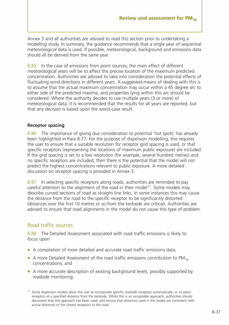
8-37
Review and assessment for PM10
Annex 3 and all authorities are advised to read this section prior to undertaking amodelling study. In summary, the guidance recommends that a single year of sequentialmeteorological data is used. If possible, meteorological, background and emissions datashould all be derived from the same year.
8.85 In the case of emissions from point sources, the main effect of differentmeteorological years will be to affect the precise location of the maximum predictedconcentration. Authorities are advised to take into consideration the potential effects offluctuating wind directions in different years. A suggested means of dealing with this isto assume that the actual maximum concentration may occur within a 45 degree arc toeither side of the predicted maxima, and properties lying within this arc should beconsidered. Where the authority decides to use multiple years (3 or more) ofmeteorological data, it is recommended that the results for all years are reported, butthat any decision is based upon the worst-case result.
Receptor spacing
8.86 The importance of giving due consideration to potential ‘hot spots’ has alreadybeen highlighted in Para 8.77. For the purpose of dispersion modelling, this requiresthe user to ensure that a suitable resolution for receptor grid spacing is used, or thatspecific receptors (representing the locations of maximum public exposure) are included.If the grid spacing is set to a low resolution (for example, several hundred metres) andno specific receptors are included, then there is the potential that the model will notpredict the highest concentrations relevant to public exposure. A more detaileddiscussion on receptor spacing is provided in Annex 3.
8.87 In selecting specific receptors along roads, authorities are reminded to paycareful attention to the alignment of the road in their model11. Some models maydescribe curved sections of road as straight-line links. In some instances this may causethe distance from the road to the specific receptor to be significantly distorted(distances over the first 10 metres or so from the kerbside are critical). Authorities areadvised to ensure that road alignments in the model do not cause this type of problem.
Road traffic sources
8.88 The Detailed Assessment associated with road traffic emissions is likely tofocus upon
• A compilation of more detailed and accurate road traffic emissions data;
• A more Detailed Assessment of the road traffic emissions contribution to PM10concentrations; and
• A more accurate description of existing background levels, possibly supported byroadside monitoring.
11 Some dispersion models allow the user to incorporate specific roadside receptors automatically i.e. to placereceptors at a specified distance from the kerbside. Whilst this is an acceptable approach, authorities shoulddocument that this approach has been used, and ensure that distances used in the model are consistent withactual distances of the closest receptors to the road.

8-38
Review and assessment for PM10
8.89 There are a wide variety of dispersion models available to authorities, which maybe used in addition to, or in support of, the DMRB Screening Model. Guidance on theuse and selection of these models, and the types of input data that are required, is setout in Annex 3, and further advice may be sought from the Modelling Helpdesk.
8.90 The emissions of PM10 are strongly related to vehicle speeds, and it isrecommended that more detailed information about traffic flow and speeds isobtained. For example, it may prove useful to split roads up into much smaller sections,which will then allow a more accurate definition of changing vehicle speeds, forexample, close to junctions. It may also prove important to take account of areas wherecold-start emissions are particularly important, such as in the vicinity of long-term carparks. PM10 emissions are also known to be affected by engine loading, for examplewhen vehicles are climbing steep hills, and specific speeds and emission factors forthese types of areas may need to be considered.
8.91 Where local traffic conditions are ‘unusual’ (for example, streets with diesel taxisand bus access only, HGVs travelling up steep hills etc), there may be some benefit indefining the vehicle types and operating conditions in more detail. Local emissionsestimates may be refined using the methods in Annex 2, and advice may be soughtfrom the Emissions Helpdesk.
8.92 The calculation of the ‘roadside enhancement’ to the 2004 or 2010 backgroundis of fundamental importance in predicting compliance with the objectives, and needsto be given detailed consideration at this stage. The APEG report has also indicated thatthe roadside enhancement to PM10 concentrations comprises of roughly equal halves offine particles (emitted from the vehicle exhausts) and coarse particles (generated byresuspension). Whilst vehicle emissions are confidently expected to decline by 2004 andfurther still by 2010, resuspended particle emissions are unlikely to reduce, unless trafficflows change substantially.
8.93 Whilst the resuspension component is widely considered to be significant, thereare currently no conclusive data to indicate what emissions rates should be applied. Forthe purpose of review and assessment, authorities are advised to ignore resuspension.For review and assessment of the 2004 objective, this is unlikely to cause a problem,provided that the model predictions are locally verified against monitoring data.However, this approach may cause predictions in 2010 to be underestimated, andauthorities may wish to bear this in mind in considering their conclusions.
Domestic solid fuel use
8.94 The Detailed Assessment associated with domestic solid fuel use is likely tofocus upon:
• An assessment of solid fuel use in the area to determine emissions;
• The application of detailed dispersion modelling; and
• Local monitoring to confirm existing concentrations.

8-39
Review and assessment for PM10
8.95 As a first step, it is recommended that authorities should undertake a DetailedAssessment of solid fuel use within the area of concern, characterising the differentfuels and combustion methods used in order to more accurately quantify the emissions.Guidance on emissions calculations is given in Annex 2, and additional advice may beobtained from the Emissions Helpdesk. These data may then be input to a suitable airquality dispersion model, in order to predict the ground level impact. Guidance on theselection of suitable dispersion models is given in Annex 3, and additional advice maybe obtained from the Modelling Helpdesk.
8.96 In the absence of local monitoring data of suitable quality, it is recommendedthat a monitoring programme is carried out in order to define more accurately currentPM10 concentrations in the area of concern. It is suggested that monitoring equipmentis sited at relevant locations and ideally, monitoring carried out for a period of12 months, although 6 winter months may also be suitable. It is not possible thoughto adjust shorter periods to estimate annual periods using the nearby monitoring sitesthat are not affected by domestic solid fuel use.
Industrial emissions
8.97 The Detailed Assessment associated with Part A and Part B processes is likely tofocus upon:
• The application of detailed dispersion modelling; and
• The use of more detailed local monitoring to confirm existing concentrations.
8.98 There are a variety of dispersion models that can be used to assess the impact ofemissions arising from elevated point sources (stacks). Guidance on the selection ofsuitable dispersion models is given in Annex 3, and additional advice may be obtainedfrom the Modelling Helpdesk. Authorities are advised to consider the following issues:
• Accurate description of PM10 emissions – many processes operate well within theiremissions limits, and actual emissions data should be used if at all possible. Forcertain types of process, both seasonal and daily variations in emissions aresignificant, and should also be considered wherever possible and input to the model.
• Elevated point sources will have little impact upon the annual mean concentration,and the assessment should focus upon an accurate prediction of the 24-hourconcentrations. The modelling approach should therefore seek to predict day-by-dayground-level concentrations arising from the stack(s), which will then be added tosuitable sequential daily background concentrations for 2004 or 2010. Whilst theapplication of single ‘uniform’ factors to correct current daily background ‘primary’,‘secondary’ and ‘coarse’ concentrations to 2004 or 2010 is not ideal (as these willchange from day to day) this may form a useful first step. Where a more detailedanalysis of the background component is required, authorities are advised to consultthe relevant sections of the APEG report, or to contact the relevant Helpdesk.

8-40
Review and assessment for PM10
Uncontrolled and fugitive emissions
8.99 Due to the uncertainties associated with PM10 emission rates from uncontrolledand fugitive sources, it is likely that the Detailed Assessment will need to focus upon adetailed monitoring programme. Whilst emissions data are available for a variety offugitive sources, for example those published within the Compilation of Air PollutionEmission Factors (USEPA-42), these factors are subject to a variable degree ofuncertainty, and frequently require default assumptions to be made. Their principalapplication lies in allowing predictions to be made for the impact of operations whichare currently not in existence, or which are expected to undergo significant change by2004 or 2010. If applicable, guidance on emissions data and dispersion models may besought from the relevant Emissions and Modelling Helpdesks.
8.100 It is suggested that in many cases a suitable monitoring programme will need tobe established to determine the impact of these uncontrolled sources. In addition tothose points discussed in paras 8.78 to 8.79 above, the following points should beborne in mind:
• Monitoring should be undertaken at relevant locations. Consideration should begiven to the siting of dust-emitting processes and their position in relation to theselocations.
• Monitoring should focus upon those relevant locations where exposure to dustemissions is likely to be highest (for example, downwind from the source based onthe prevailing wind direction).
• Ideally monitoring should be carried out for a period of at least 12 months. Wherethis is not possible, it is recommended that measurements should be carried out overthe summer months, when wind-blown resuspension is likely to be highest.
• In all cases, authorities are advised to compare the results of local monitoringprogrammes with data from national network sites, to assist with the interpretationof findings.
8.101 Where monitoring indicates that the objectives are likely to be exceeded, then itmay be helpful to refine the monitoring strategy, in order to more clearly identify thesource contributions. In such cases, authorities may find it useful to:
• Undertake monitoring of wind speed and direction to assist with the interpretationof results and any reported exceedences.
• Carry out monitoring at several locations, including an upwind site. This will allow amore accurate assessment of the source emission contribution to the measured data.Alternatively, ‘directional’ monitoring equipment (which allows measurements to becollected only within a pre-defined wind direction) can be employed.
• Consider the use of various speciation and chemical analysis methods, once again toassess the source emission contribution to the measured data.

8-41
Review and assessment for PM10
Figure 8.2: Particulate emissions (tonnes per annum) from combustion source emissions (>100°C) to give a 90th percentile 24-hour average concentration of 1 µg/m3 (stack >10 metres).
Figure 8.1: Relationship between the number of 24-hour exceedences of 50µg/m3 and the annualmean concentration (derived from UK Automatic Network Sites 1997-2001).
0
20
40
60
80
100
120
140 y = –18.5 + 0.00145 x annual mean3 + 206
160
0 5 10 15 20 25 30 35 40 45 50
Nu
mb
er o
f 24
-ho
ur
exce
eden
ces
of
50 µ
g/m
3
Annual mean PM10 (gravimetric) µg/m3
annual mean
1
10
100
1000
0.1 1 10 100 1000 10000
Effe
ctiv
e st
ack
hei
gh
t (m
)
0.5 m diameter1 m2 m4 m8 m
12 m
Emission (tonnes per annum)

8-42
Review and assessment for PM10
Figure 8.4: Particulate emissions (tonnes per annum) which will give a 90th percentile of 24-hourmean ground-level concentration of 1 µg/m3 at receptor locations up to 2 km from fugitive and low level sources (stack <10 metres).
Figure 8.3: Particulate emissions (tonnes per annum) from low temperature sources (<100°C) whichwill give a 90th percentile of 24-hour mean ground-level concentration of 1 µg/m3
(stack >10 metres).
1
10
100
1000
0.1 1 10 100 1000
Effe
ctiv
e st
ack
hei
gh
t (m
)
0.5 m diameter1 m2 m4 m8 m12 m
Emission (tonnes per annum)
0.0001
0.001
0.01
0.1
1
10
100
1 10 100 1,000 10,000
Distance of receptor from source (m)
Emis
sio
ns
(to
nn
es p
er a
nn
um
)
0 m height3 m6 m9 m

8-43
Review and assessment for PM10
Figure 8.6: Particulate emissions (tonnes per annum) from low temperature sources (<100°C) whichwill give an annual mean ground-level concentration of 1 µg/m3 (stack >10 metres).
Figure 8.5: Particulate emissions (tonnes per annum) from combustion source emissions (>100°C) to give an annual mean ground-level concentration of 1 µg/m3 (stack >10 metres).
1
10
100
1000
1 10 100 1000 10000 100000
Emission (tonnes per annum)
Effe
ctiv
e st
ack
hei
gh
t (m
)
0.5 m diameter1 m2 m4 m8 m
12 m
1
10
100
1000
0.1 1 10 100 1000 10000
Emission (tonnes per annum)
Effe
ctiv
e st
ack
hei
gh
t (m
)
0.5 m diameter1 m2 m4 m8 m12 m
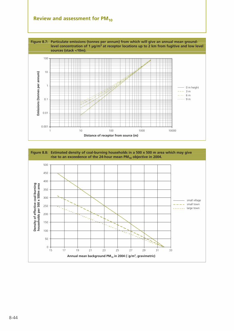
8-44
Review and assessment for PM10
Figure 8.8: Estimated density of coal-burning households in a 500 x 500 m area which may giverise to an exceedence of the 24-hour mean PM10 objective in 2004.
Figure 8.7: Particulate emissions (tonnes per annum) from which will give an annual mean ground-level concentration of 1 µg/m3 at receptor locations up to 2 km from fugitive and low level sources (stack <10m).
0.001
0.01
0.1
1
10
100
1 10 100 1000 10000
Distance of receptor from source (m)
Emis
sio
ns
(to
nn
es p
er a
nn
um
)
0 m height3 m6 m9 m
Annual mean background PM10 in 2004 (µg/m3, gravimetric)
0
50
100
150
200
250
300
350
400
450
500
15 17 19 21 23 25 27 29 31 33
small villagesmall townlarge town
Den
sity
of
effe
ctiv
e co
al-b
urn
ing
ho
use
ho
lds
per
500
x 5
00m
are
a

8-45
Review and assessment for PM10
Figure 8.9: Estimated density of coal-burning households in a 500 x 500 m area which may which may give rise to an exceedence of the 2010 annual mean PM10 objective.
0
20
40
60
80
100
120
15 16 17 18 19 20
small village
small town
large town
Annual mean background PM10 in 2010 (µg/m3, gravimetric)
Den
sity
of
effe
ctiv
e co
al-b
urn
ing
ho
use
ho
lds
per
500
x 5
00 m
are
a
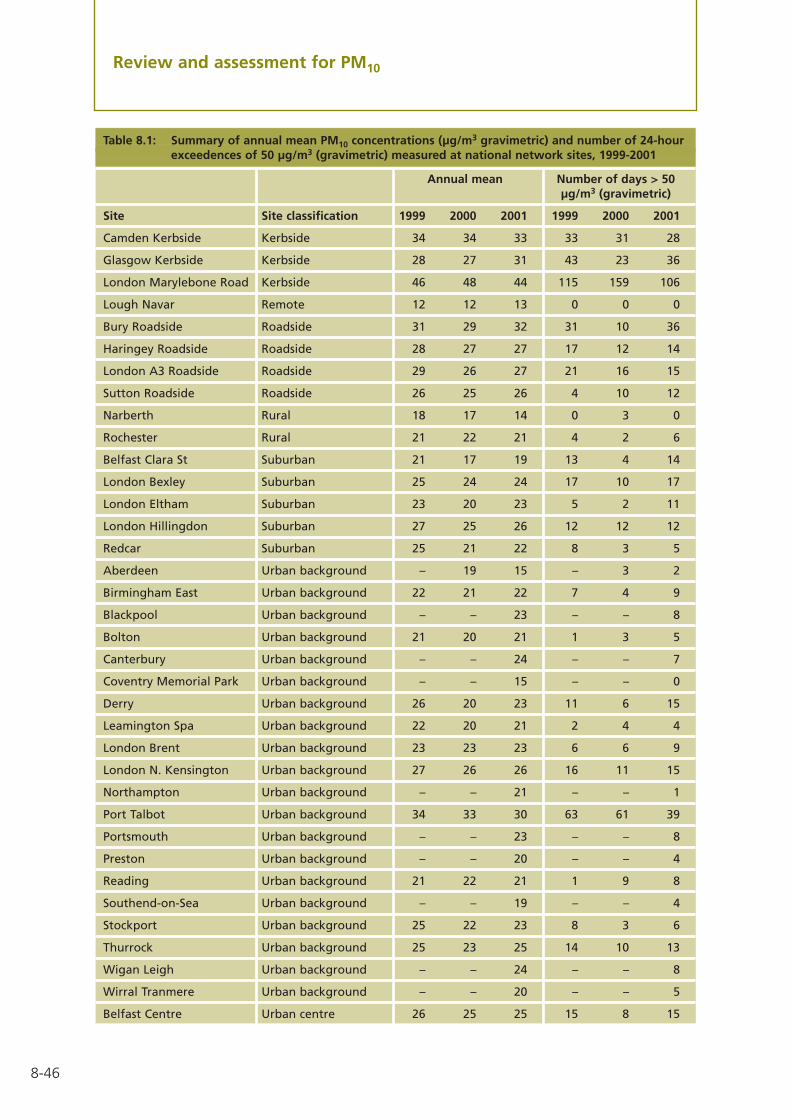
8-46
Review and assessment for PM10
Table 8.1: Summary of annual mean PM10 concentrations (µg/m3 gravimetric) and number of 24-hour exceedences of 50 µg/m3 (gravimetric) measured at national network sites, 1999-2001
Annual mean Number of days > 50µg/m3 (gravimetric)
Site Site classification 1999 2000 2001 1999 2000 2001
Camden Kerbside Kerbside 34 34 33 33 31 28
Glasgow Kerbside Kerbside 28 27 31 43 23 36
London Marylebone Road Kerbside 46 48 44 115 159 106
Lough Navar Remote 12 12 13 0 0 0
Bury Roadside Roadside 31 29 32 31 10 36
Haringey Roadside Roadside 28 27 27 17 12 14
London A3 Roadside Roadside 29 26 27 21 16 15
Sutton Roadside Roadside 26 25 26 4 10 12
Narberth Rural 18 17 14 0 3 0
Rochester Rural 21 22 21 4 2 6
Belfast Clara St Suburban 21 17 19 13 4 14
London Bexley Suburban 25 24 24 17 10 17
London Eltham Suburban 23 20 23 5 2 11
London Hillingdon Suburban 27 25 26 12 12 12
Redcar Suburban 25 21 22 8 3 5
Aberdeen Urban background – 19 15 – 3 2
Birmingham East Urban background 22 21 22 7 4 9
Blackpool Urban background – – 23 – – 8
Bolton Urban background 21 20 21 1 3 5
Canterbury Urban background – – 24 – – 7
Coventry Memorial Park Urban background – – 15 – – 0
Derry Urban background 26 20 23 11 6 15
Leamington Spa Urban background 22 20 21 2 4 4
London Brent Urban background 23 23 23 6 6 9
London N. Kensington Urban background 27 26 26 16 11 15
Northampton Urban background – – 21 – – 1
Port Talbot Urban background 34 33 30 63 61 39
Portsmouth Urban background – – 23 – – 8
Preston Urban background – – 20 – – 4
Reading Urban background 21 22 21 1 9 8
Southend-on-Sea Urban background – – 19 – – 4
Stockport Urban background 25 22 23 8 3 6
Thurrock Urban background 25 23 25 14 10 13
Wigan Leigh Urban background – – 24 – – 8
Wirral Tranmere Urban background – – 20 – – 5
Belfast Centre Urban centre 26 25 25 15 8 15

8-47
Review and assessment for PM10
Table 8.1: Summary of annual mean PM10 concentrations (µg/m3 gravimetric) and number of 24-hour (contd.) exceedences of 50 µg/m3 (gravimetric) measured at national network sites, 1999-2001
Annual mean Number of days > 50µg/m3 (gravimetric)
Site Site classification 1999 2000 2001 1999 2000 2001
Birmingham Centre Urban centre 24 23 22 10 10 10
Bradford Centre Urban centre 26 23 28 13 5 16
Bristol Centre Urban centre 26 26 24 12 11 16
Cardiff Centre Urban centre 28 25 27 13 11 12
Edinburgh Centre Urban centre 19 23 26 3 5 11
Glasgow Centre Urban centre 23 28 22 9 27 13
Hull Centre Urban centre 28 26 28 17 6 20
Leeds Centre Urban centre 26 23 24 19 5 8
Leicester Centre Urban centre 21 17 22 5 0 3
Liverpool Centre Urban centre 26 24 26 10 5 15
London Bloomsbury Urban centre 28 28 29 21 11 18
Manchester Piccadilly Urban centre 26 28 39 11 23 71
Newcastle Centre Urban centre 21 17 17 6 0 1
Norwich Centre Urban centre 23 22 20 6 1 1
Nottingham Centre Urban centre 25 24 26 9 5 14
Plymouth Centre Urban centre 21 20 20 0 3 4
Sheffield Centre Urban centre 26 25 24 9 4 11
Southampton Centre Urban centre 26 24 26 8 6 13
Stoke-on-Trent Centre Urban centre 22 21 22 7 5 8
Swansea Urban centre 22 26 26 1 13 7
Wolverhampton Centre Urban centre 23 23 23 8 11 10
Middlesbrough Urban industrial 23 23 29 20 5 9
Salford Eccles Urban industrial 20 22 28 6 6 11
Scunthorpe Urban industrial 21 24 32 46 31 50
NOTE: All data reported in this table have been measured using a TEOM sampler. The concentrationsreported by the TEOM have been multiplied by 1.3 to give PM10 concentrations expressed as µg/m3
gravimetric.

8-48

Monitoring
IntroductionA1.01 This section describes monitoring procedures that can be used for the followingpollutants in the Air Quality Strategy for England, Scotland, Wales and NorthernIreland1:
• Carbon monoxide (CO)
• Benzene (C6H6)
• 1,3-butadiene (CH2CHCHCH2)
• Lead (Pb)
• Nitrogen dioxide (NO2)
• Sulphur dioxide (SO2)
• Particulate matter (PM10)
A1.02 A summary of the main points to consider when setting up a monitoringprogramme is given in Box A1.1. Further information is available from the local authorityAir Quality Monitoring Helpdesk 01235 463356, email [email protected] orvia the LAQM section of the National Air Quality Information Archive web site athttp://www.airquality.co.uk. Monitoring questions can be posted and the answersviewed on the National Air Quality Information Archive web site.
A1.03 Monitoring fulfils a central role in the review and assessment process, providingthe necessary sound scientific basis for compliance measurement against the objectivesof the Air Quality Strategy. If monitoring is already being undertaken it is essential toestablish whether additional monitoring is necessary for review purposes.
• Is the existing monitoring adequate – is it being made over a suitable time periodand at the right location – and is the data capture appropriate?
• Are the methods and quality assurance and quality control (QA/QC) proceduresadequate to monitor for review and assessment purposes?
Monitoring can assist in demonstrating whether or not there is a significant risk of aprescribed Air Quality Strategy objective being exceeded in a relevant location, and toenable potential air quality management areas to be identified.
A1.04 Measurements made for the purpose of review and assessment often need tobe used in conjunction with other objective assessment techniques. In particular,monitoring will be required to verify and calibrate air quality models and air qualitymanagement systems to ensure that they are producing accurate and reliable estimatesof pollutant concentrations. It is, therefore, crucial that monitoring is carried out asaccurately as possible.
Annex 1 Monitoring
A1-1
1 The Air Quality Strategy for England, Scotland, Wales and Northern Ireland: CM 4548, HMSO Publications, 2000.
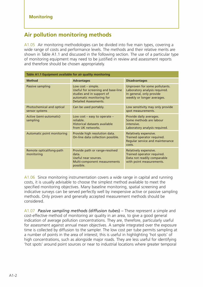
A1-2
Monitoring
Air pollution monitoring methods
A1.05 Air monitoring methodologies can be divided into five main types, covering awide range of costs and performance levels. The methods and their relative merits areshown in Table A1.1 and discussed in the following section. The use of a particular typeof monitoring equipment may need to be justified in review and assessment reportsand therefore should be chosen appropriately.
A1.06 Since monitoring instrumentation covers a wide range in capital and runningcosts, it is usually advisable to choose the simplest method available to meet thespecified monitoring objectives. Many baseline monitoring, spatial screening andindicative surveys can be served perfectly well by inexpensive active or passive samplingmethods. Only proven and generally accepted measurement methods should beconsidered.
A1.07 Passive sampling methods (diffusion tubes) – These represent a simple andcost-effective method of monitoring air quality in an area, to give a good generalindication of average pollution concentrations. They are, therefore, particularly usefulfor assessment against annual mean objectives. A sample integrated over the exposuretime is collected by diffusion to the sampler. The low cost per tube permits sampling ata number of points in the area of interest; this is useful in highlighting ‘hot spots’ ofhigh concentrations, such as alongside major roads. They are less useful for identifying‘hot spots’ around point sources or near to industrial locations where greater temporal
Table A1.1 Equipment available for air quality monitoring
Method Advantages Disadvantages
Passive sampling Low cost – simple. Unproven for some pollutants. Useful for screening and base-line Laboratory analysis required.studies and in support of In general, only provide automatic monitoring for weekly or longer averages.Detailed Assessments.
Photochemical and optical Can be used portably. Low sensitivity may only provide sensor systems spot measurements.
Active (semi-automatic) Low cost – easy to operate – Provide daily averages.sampling reliable. Some methods are labour
Historical datasets available intensive.from UK networks. Laboratory analysis required.
Automatic point monitoring Provide high resolution data. Relatively expensive.On-line data collection possible. Trained operator required.
Regular service and maintenancecosts.
Remote optical/long-path Provide path or range-resolved Relatively expensive.monitoring data. Trained operator required.
Useful near sources. Data not readily comparableMulti-component measurements with point measurements.possible.

A1-3
Monitoring
resolution is required for particular objectives. Diffusion tubes surveys are simple toundertake and minimal operator training is required. Diffusion tubes are available forthe following pollutants in the Air Quality Strategy:
• Nitrogen dioxide
• BTX (benzene, toluene, xylene)
• 1,3-butadiene
The tubes must be analysed by laboratories that can offer suitable quality assuranceand quality control measures to ensure the results meet the data quality objectivesdefined for the method (contact the Monitoring Helpdesk for a list of suppliers andanalysers of diffusion tubes). The diffusion tube data may be corrected for bias in theanalytical results.
A1.08 Active (semi-automatic) sampler methods – These methods collect pollutantsamples either by physical or chemical means for subsequent analysis in a laboratory.Typically, a known volume of air is pumped through a collector such as a filter orchemical solution for a known period of time, for subsequent laboratory analysis. Theseinclude bubbler samplers for sulphur dioxide and nitrogen dioxide and gravimetric filtersamplers for PM10 and lead. Sequential instruments with automatic sample changersare available.
A1.09 Automatic real-time point analyser methods – These produce high-resolution measurements (typically hourly or shorter period averages) for oxides ofnitrogen, sulphur dioxide, carbon monoxide and particulate matter (PM10). Gaschromatography (GC) analysers also provide high-resolution data on benzene, and 1,3-butadiene. The sample is analysed on-line and in real-time. In order to ensure thatthe data produced are accurate and reliable, a high standard of maintenance,calibration, operational and QA/QC procedures is required.
A1.10 Remote optical/long-path analysers – These are instruments that use a long-path spectroscopic technique to make real-time measurements of the concentration ofa range of pollutants integrated along a path between a light source and a detector.Instruments using the Differential Optical Absorption Spectroscopy (DOAS) system canbe used to monitor data for nitrogen dioxide, sulphur dioxide and benzene. In order toensure that the data produced are accurate and reliable, a high standard ofmaintenance, calibration, operational and quality assurance and quality controlprocedures is required.
A1.11 Photochemical and optical sensor systems – A range of relatively low-costautomatic analysers has been developed specifically for portable and personal exposuremonitoring applications. These are battery or mains operated electrochemical or solid-state sensor based systems which can continuously monitor a range of pollutants (carbon monoxide, nitrogen dioxide, sulphur dioxide) with a time average of 15-minutesor less. These sensors are of low sensitivity and mostly suitable for identifying hotspotsat roadsides and near point sources etc. Portable sensors using the light scatteringprinciple are available for PM10 monitoring.

A1-4
Monitoring
Planning, setting up and operating a monitoring campaignA1.12 Before embarking on a monitoring programme, it is important to have a clearunderstanding of what monitoring will achieve and how it will aid the review andassessment process. Box A1.1 lists some of the basic points to consider. It is importantthat the financial and other implications of embarking on a monitoring programme arefully understood before any action is taken. Local Authorities are advised to seekassistance from the Monitoring Helpdesk if they are uncertain about the best wayto proceed.
Selecting monitoring equipment
A1.13 A wide variety of equipment is commercially available for both sampler-basedand automatic point monitoring and a number of suppliers and manufacturers exist.Several different analysers may be suitable for the job and there may not necessarilybe an obvious best technical option. Monitoring equipment, particularly that used fordetailed monitoring, should have some independent verification of performance suchas the ambient MCERTS scheme operated by SIRA, the United States EnvironmentalProtection Agency (USEPA) Federal Register or German TUV designation. A list ofequipment suppliers is available on the National Air Quality Information Archive website and advice on monitoring equipment may be sought from the Monitoring Helpdesk.Table A1.2 gives a checklist of points to consider when selecting monitoring equipment.Table A1.3 gives specifications of typical automatic monitoring equipment used innational networks. These should be used when purchasing continuous analysers.
Box A1.1 Basic considerations for air quality monitoring
• What pollutants need to be monitored?
• What monitoring methods are appropriate?
• What monitoring equipment is needed?
• How much will it cost – to purchase and to operate?
• How long to monitor for?
• Where to monitor?
• How many monitoring sites are needed?
• What data quality is required?
• How to process and evaluate the data?
• How do the monitoring data relate to the requirement of the Air Quality Strategy?

A1-5
Monitoring
Table A1.2 Points to consider when choosing equipment
N/A = not available
A designated PM10inlet head must besupplied.
Accurate filterweighing andconditioningfacilities required.
Correction factor togravimetric standardshould be established.
A designatedPM10 inlet headmust besupplied.
N/APM10
N/ATime resolution must be suitable to measureagainst the 15-minuteobjective.
Not widelyavailable.
Not fully validated andshould be used withcaution.
SO2
N/ADual detection systemor fast cycling timeneeded for roadsidemonitoring.
Available inroadsidepollutionmonitors.
Use suppliers whoparticipate in the UKNO2 diffusion tubenetwork inter-comparison.
NO2
Gravimetric PM10monitors can be usedwith a suitableexposure period.
N/AN/AN/ALead
N/AAutomatic BTX analyseror full GC systems canalso be used.
N/ANot been fullyvalidated and should beused with caution.
1,3-butadiene
N/APumped samplers,automatic BTXanalysers available orfull GC systems can beused.
N/ADiffusion tubes over-read by ~30%compared with gaschromatography (GC)analysers.
Benzene
N/AGas correlation infra-red unitsrecommended.
Available inroadsidepollutionmonitors.
N/ACO
Accurate display/measurement systemfor flow raterequired.
Equipment should haveindependent typeapproval/designation.
Span range must besuitable to monitoragainst objectives.
RS232/Voltage outputor internal data loggingsystem required.
Suitable forscreening butnot for detailedmonitoring.
Tubes should besupplied and analysedby an accreditedlaboratory.
General
Gravimetric samplerContinuous samplersPortablesamplers
Diffusion tubes

A1-6
Monitoring
Other equipment
A1.14 In addition to the analysers, other site infrastructure will be required to set up afully automatic air quality monitoring station consisting of:
Equipment housing Electrical systemsAir conditioning/heating Telephone lines/modemCylinder storage facilities Air sample inlet systemAutocalibration facilities Data logging and acquisition facilities.Security systems Safety systems
Active samplers and diffusion tubes require a much lower level of site infrastructure.However, access to appropriate analytical facilities at a central laboratory may berequired. It is important to note that selecting, purchasing and commissioning theequipment for an automatic monitoring station can be a lengthy process (typically 2-3months) and time should be allowed for this at the planning stage.
Frequently Asked Questions on monitoring equipment
Can you supply contact details for the purchase of air quality monitoringequipment?
A1.15. A list of suppliers of all types air monitoring equipment is available from theMonitoring Helpdesk or via the LAQM section of the National Air Quality InformationArchive web site at http://www.airquality.co.uk. This is not a comprehensive list butincludes the leading UK suppliers of monitoring equipment.
Table A1.3 Typical specifications for UK automatic network-standard analysers
Pollutant measured by analyser NO2 SO2 O3 CO
Lower detectable limit 2 ppb 2 ppb 2 ppb 100 ppb
Precision as % of upper range limit < 1% < 1% < 1% < 1%
Noise Zero 1 ppb 1 ppb 1 ppb 50 ppbSpan 3 ppb 3 ppb 3 ppb 200 ppb
24-hour drift Zero 2 ppb 2 ppb 2 ppb 500 ppbSpan 2% FS 2% FS 2% FS 2% FS
Linearity Error* 2% 2% 2% 2%
95% Response Time (max) 180 secs 150 secs 150 secs 60 secs
* Linearity is a measure of the relationship of analyser response with changing concentration. Thisrelationship should be linear i.e. twice the concentration will produce twice the output signal etc.

A1-7
Monitoring
What are the recommended methods for making measurements ofcarbon monoxide?
A1.16 For screening studies, a number of portable electro-chemical carbon monoxideanalysers are available. They are generally of low sensitivity but can provide indicativemeasurements in monitoring areas of high concentration. For Detailed Assessments,automatic infra-red analysers are recommended.
What are the recommended methods for making measurements of benzeneand 1,3-butadiene?
A1.17 Benzene and 1,3-butadiene are sampled using a pumped sampling device on toa sorbent cartridge. Analysis is carried out by gas chromatographic determination.Diffusion tubes are also available for benzene. Several compact photo ionisationdetector based instruments are also available for continuous measurement of benzeneand 1,3-butadiene.
What are the recommended methods for making measurements of lead?
A1.18 Lead is monitored by collecting samples onto a filter using a suitable sampler.Devices commonly used are the ‘M Type’ sampler and the low volume gravimetricsampler. Analysis is by atomic absorption spectroscopy or inductively coupled plasmamass spectrometry. Samplers with PM10 inlets can be used for lead sampling for the AirQuality Strategy objective.
What are the recommended methods for making measurements ofnitrogen dioxide?
A1.19 For Updating and Screening Assessments, diffusion tubes or portable monitorscan be used. Diffusion tubes can also provide valuable data for more detailed studies.For Detailed Assessments, automatic chemiluminescent analysers are recommended.However, remote optical/long-path analysers are also suitable. Electrochemical cellanalysers are available on the market. The accuracy and precision of this equipmentis uncertain and they are only recommended for use in Updating and ScreeningAssessments. However, if monitoring with this type of analyser, it is advisable to co-locate the equipment with a fully calibrated continuous analyser to validate the data.For all monitoring it is important that a documented and traceable QA/QC scheme isimplemented.
What are the recommended methods for making measurements ofsulphur dioxide?
A1.20 For Updating and Screening Assessments, active samplers (bubblers) or portablemonitors can be used. Diffusion tubes should not be used, as they are unable to detectincreases in short-term concentrations attributed to emissions from point sources. ForDetailed Assessments, automatic ultra-violet fluorescent analysers are recommended.

A1-8
Monitoring
However, remote optical/long-path analysers are also suitable. Electrochemical cellanalysers are available on the market. The accuracy and precision of this equipmentis uncertain and they are only recommended for use in Updating and ScreeningAssessments. However, if monitoring with this type of analyser, it is advisable to co-locate the equipment with a fully calibrated continuous analyser to validate the data.For all monitoring it is important that a documented and traceable QA/QC scheme isimplemented.
What are the recommended methods for making measurements of PM10?
A1.21 For Updating and Screening Assessments, gravimetric samplers or portablemonitors can be used. If portable light scattering devices are used they should beproperly calibrated and be fitted with an appropriate PM10 inlet head. If black smokemeasurements are currently being undertaken, they can in some circumstances be usedas an indicator for likely PM10 ‘hot spots’. Note, however, there will not necessarily be aconsistent correlation between black smoke and PM10 which is applicable to all locationtypes and seasons.
For Detailed Assessments, gravimetric monitoring or automatic fixed-point monitors,such as TEOM, and ß-attenuation instruments can be used. Gravimetric monitorsproduce concentrations equivalent to that of the EU reference samplers and can bedirectly compared with the objectives2. Measurements of PM10 concentrations carriedout using a TEOM or ß-attenuation instrument, operating with a heated manifold,should be adjusted by multiplying the data by 1.3 to estimate gravimetric equivalentconcentrations.
Choosing a site
A1.22 Monitoring sites can be classified according to the type of environment in whichthey are located, in order to permit more meaningful evaluation of data. The sitedescription will generally reflect the influence of a particular pollutant source or ofoverall land use. Typical monitoring location types, as used in national automaticmonitoring networks, are shown in Table A1.4. More detailed definitions of siteclassification types are provided in Appendix A. It is important that detailed descriptionsof all monitoring site locations used are given in the review and assessment reportsincluding distance from kerbs etc.
2 BS EN 12341: 1999 Air Quality – Determination of the PM10 fraction of suspended particulate matter. Referencemethod and field test procedure to demonstrate reference equivalence of measurement methods.

A1-9
Monitoring
A1.23 In order to obtain useful air quality monitoring data for the purposes of reviewand assessment, the measurements made must be representative of the study area ofinterest. To achieve this, it is essential to choose the right site(s) for the monitoringequipment. A number of considerations need to be taken into account and it is worthinvesting reasonable effort in surveying possible sites before making a final choice. Theapproach taken to identify appropriate monitoring locations should be fullydocumented in the review and assessment report. The sites must be located wherethere is expected to be relevant exposure (see Box 1.4) or at least in a locationrepresentative of nearby exposure, for example, the same distance from a section ofroad as the façade of nearby residential properties.
A1.24 The site selection process must take into account the spatial distribution andvariability of gaseous pollutants. For example, concentrations of primary trafficpollutants such as carbon monoxide are highest at roadside locations, whereas sulphurdioxide concentrations may be highest at urban background or rural locations as aresult of emissions from a point source. For this reason, it is usually not possible tooptimise measurements for all pollutants at any one location, depending on thelocation of large point sources. In such circumstances, some degree of compromise maybe required or, several sites monitoring individual pollutants employed.
Table A1.4 Monitoring locations
Site type Description
Urban centre An urban location representative of typical population exposure intowns or city centres e.g. pedestrian precincts and shopping areas.
Urban background An urban location distanced from sources and therefore broadlyrepresentative of city-wide background conditions e.g. urbanresidential areas.
Suburban A location type situated in a residential area on the outskirts of a townor city.
Roadside A site sampling between 1m of the kerbside of a busy road and theback of the pavement. Typically this will be within 5m of the road, butcould be up to 15m.
Kerbside A site sampling within 1m of the kerb of a busy road.
Industrial An area where industrial sources make an important contribution tothe total pollution burden.
Rural An open countryside location, in an area of low population densitydistanced as far as possible from roads, populated and industrial areas.
Other Any special source-orientated or location category covering monitoringundertaken in relation to specific emission sources such as powerstations, car-parks, airports or tunnels.
A1-10
Monitoring
Identifying relevant locations
A1.25 The initial process in review and assessment is to determine likely ‘hot spots’,i.e. relevant locations where air quality may not meet the prescribed objectives. This canhelp refine the selection of suitable monitoring locations. The following information canbe used when screening for potential areas of concern:
A1.26 Existing air quality data. A range of monitoring activities is currentlyundertaken by local authorities and local data may be available to help assess futuremonitoring requirements. If monitoring has already been carried out in the area ofinterest, the data from previous studies may prove to be of use in targeting problemareas. Comprehensive monitoring of air quality is carried out on a national scale by theDefra and the Devolved Administrations. Many of the sites have accumulatedconsiderable historical data sets. All data are freely available to local authorities wishingto use this resource to assist in the appraisal of air quality in their area. Data fromthe networks can be obtained from the National Air Quality Information Archive:http://www.airquality.co.uk. Examples of the application of existing monitoring datainclude:
• Use of data from nearby national network sites or neighbouring local authority sitesto verify data obtained from short term or simple monitoring exercises.
• Estimating concentrations of pollutants with short term averaging periods. Forexample, the use of daily mean sulphur dioxide concentrations as an estimate ofexceedences per year of 15-minute means.
A1.27 Modelling. The results of dispersion modelling simulations can be used topredict pollutant dispersion and deposition patterns, thereby helping to identify areaswhere pollutant problems may occur. To be of real use, reliable emissions andmeteorological data are needed, together with an appropriate model. The modelshould be validated against data measured in the location of its application. Details ofdispersion modelling can be obtained from the Modelling Helpdesk.
A1.28 Sources and emissions. Compilation of emission data will help to identify themost polluted areas, as well as other location types where population exposure may besignificant. If a full emissions inventory is not available, then surrogate statistics such aspopulation density, location of industrial sources, traffic flows and fuel consumptionmay be of use in estimating likely pollution ‘hot spots’. Advice on emissions can beobtained from the Emissions Helpdesk.
Emissions data collated on a national basis is provided in the National AtmosphericEmissions Inventory (NAEI) http://www.naei.org.uk.
Details of industrial processes authorised by the Environment Agency can be found onthe Environment Agency web site – http://www.environment-agency.gov.uk/ under‘What’s in your backyard?’

A1-11
Monitoring
Details of industrial processes in Scotland can be obtained from the ScottishEnvironmental Protection Agency (SEPA) http://www.sepa.org.uk/.
Details of industrial processes in Northern Ireland can be obtained from theEnvironment And Heritage Service (EHS) http://www.ehsni.gov.uk/default.asp.
A1.29 Meteorology and topography. The prevailing weather conditions and localtopography will strongly influence the dispersion of air pollutants or, in the case ofsecondary pollutants, affect their production in the atmosphere. Meteorologicalmeasurements can be made on-site, or data purchased from the authorised agencies.
A1.30 Other information. Population and land-use information may be used totarget locations representative of both baseline and worst-case exposure. Advice onsiting for review and assessment can also be obtained from the Review and AssessmentHelpdesk.
Local siting criteria
A1.31 It is recognised that it is very difficult to identify a representative site, particularlyfor automatic sites when taking into account factors such as visual impact and planningpermission. However, in order to ensure meaningful comparisons of data betweendifferent areas, sites should be classified according to the scheme given in Appendix A.In selecting site locations recognised siting criteria should be employed as far aspossible (Box A1.2).
A1.32 The site should be located where relevant exposure is expected (see Box 1.4) orat least be representative of such exposure, for example, at the same distance from aroad as the facades of nearby residential properties. Details of site type and distance ofnearby sources should be provided whenever results are reported. Details of the typeand location of monitoring sites used in the national monitoring networks are on theSite Information Archive for the UK Automatic Urban and Rural Networks –http://www.stanger.co.uk/siteinfo/

A1-12
Monitoring
Site numbers
A1.33 Monitoring is normally undertaken in order to evaluate pollutant behaviour inboth space and time. A good programme design should therefore seek to optimiseboth spatial and temporal coverage, within available resource constraints. The numberand distribution of monitoring sites and samplers required for reviewing and assessingair quality depends on the degree of public exposure in the area to be covered, thespatial variability of the pollutants being measured and the required data usage. Ingeneral, automatic monitoring will only need to be carried out at one or twostrategically located sites. This monitoring can be supported by the use of diffusive orother simple samplers distributed over a wide area around the automatic site. It isrecommended that diffusion tubes are co-located with the automatic monitors toestimate any bias in the diffusion tube measurements. The most important locations arethose at which concentrations are expected to be high, and where the public may beexposed over the averaging times specified in the prescribed objectives.
Box A1.2 Local siting criteria
It should be in as open a setting as possible in relation to surrounding buildings.
Immediately above should be open to the sky, with no overhanging trees or buildings.
The sample intake should be no higher than 10 m above local ground level and ideally between1.4 m and 4 m.
For urban centre or background sites:There should be no major sources of pollution within 50 m. e.g. a large multi-storey car park.
There should be no medium sized sources within 20 m. e.g. petrol stations, ventilation outlets tocatering establishments etc.
Cars/vans/lorries should not be expected to stop with their engines idling within 5 m of the sample inlet.
The site should not be within:30 m of a very busy road (>30,000 vehicles/day).20 m of a busy road (10,000-30,000 vehicles/day).10 m of any other road (<10,000 vehicles/day).The surrounding area, within say 100 m, should not be expected to undergo major redevelopment, soas to avoid disruption and to allow long-term trends to be followed.
For traffic related sites:The site should be within 1 m of the kerb (kerbside sites).The site should be within 1-5 m of the kerb (roadside sites).
For industrial sitesWhere specific sources are being targeted, monitoring should be carried out at the point of maximumimpact as determined by modelling.

A1-13
Monitoring
Frequently Asked Questions on monitoring locations
Where should I try to locate my monitors to measure backgroundconcentrations?
A1.34 At urban locations distanced from major sources (typically greater than 50m)and therefore broadly representative of city-wide background conditions, for example,elevated locations, parks and urban residential areas.
Where should I try to locate my monitors for investigating road trafficemissions?
A1.35 Firstly look for areas of relevant public exposure (see Box 1.4). Initially, you couldcarry out a survey using passive or active samplers and/or portable monitors over avariety of roadside locations. For a more detailed study you would ideally monitor atroadside and background locations with ‘accurate’ monitors in conjunction withongoing passive or active samplers and portable monitoring. Try to site the monitors asnear to the point of relevant public exposure as possible, for example, at the buildingfaçade for residential housing. It is important (for model validation in particular) tocover a range of urban background and roadside or kerbside sites if possible. Highestconcentrations are likely to be recorded near busy roads, along congested streets or atcongested traffic junctions.
Where should I try to locate my monitors for investigating emissions frompoint sources?
A1.36 Firstly look for areas of relevant public exposure (see Box 1.4). Initially you couldcarry out a survey using passive or active samplers and/or portable monitors over avariety of locations including the point of modelled maximum impact. Then you wouldideally look at the modelled point of maximum impact with ‘accurate’ monitors inconjunction with ongoing sampler and portable monitoring. It will be difficult to ensurethat you monitor at the point of maximum impact, as this is likely to move from year toyear, and is unlikely to be identified accurately by modelling.
Once I’ve identified a suitable area for monitoring, what do I need to take intoconsideration when locating a specific site?
A1.37 For automatic analyser enclosures, visual impact or intrusion and noise may be aconsideration. Practical problems such as power and telephone connection, access andsecurity may also limit your choice. Assuming that these concerns are satisfied, amonitoring site should not be enclosed by surrounding buildings or covered byoverhanging vegetation. Ideally, sampling air at a height of between 1.4 m and 4 m isrecommended. Monitoring close to local or point source emissions, unless these havebeen specifically targeted for investigation, is not recommended.

A1-14
Monitoring
Do I need Planning Permission for my monitoring station?
A1.38 Planning permission is often required for monitoring enclosures. This is normallyobtained from the relevant local or district council or from the highways authority. ForNorthern Ireland a Street Works Licence is required3. It may also be necessary to obtainpermission from the relevant utility provider to site diffusion tubes on street lamps andtelegraph poles etc.
Monitoring period
A1.39 All surveys should ideally be carried out for a minimum of six months: three inthe summer and three in the winter consecutively (for example, January to June). Forpractical or budgetary reasons, local authorities may only be able to carry out three-month surveys using automatic monitors. These still provide extremely usefulinformation, particularly if levels can be compared with those from a nearby long-termair pollution monitoring site. An examination on the ratio of short-term to long-termaverage measurements at urban background sites shows that for nitrogen dioxide it isbest to start a six month campaign in January or July and a three month campaign inMarch or September. The six-monthly means show an average variability from theannual mean of up to 15% and for the three-monthly up to 20% – (Figure A1.1).Equivalent PM10 ratios do not show a marked seasonal variability.
3 Erection of Air Quality Monitoring Stations In Northern Ireland
Under Planning, General Development Order NI 1993 No. 273, part 12, page 30; District Councils can erect theequipment under Permitted Development if:
1. it is used for a function of the council i.e. environmental health;
2. it does not exceed 4m in height;
3. it does not exceed 200m3 in capacity
The placing of any apparatus in a street is subject to the provisions of the Street Works (Northern Ireland) Order1995 (hereinafter referred to as ‘the Order’) and the Regulations and Codes of Practice made or issuedthereunder. Copies of the Order, Regulations and Codes of Practice are available from HMSO.
A Street Works Licence is required by any person or organisation who wishes to place or retain apparatus in astreet, and thereafter inspect, maintain, adjust, repair, alter or renew the apparatus, change its position or removeit, unless the person or organisation has a statutory right to do so. Any person who carries out such workswithout a Street Works Licence or a statutory right is committing an offence and liable on summary conviction toa fine. The person granted a Street Works Licence, becomes an Undertaker for the purposes of the Order, andtherefore attracts the relevant duties and responsibilities imposed by the Order and its associated Regulations andCodes of Practice.
Under current legislation District Councils do not have a statutory right to erect air quality monitoring stations andtherefore require a Street Works Licence. In order to obtain a Licence the Council should initially contact the localRoads Service Development Control Section to agree the siting of the station. Following agreement, the applicantshould contact the local Roads Service Section Office to have a Licence issued. All applications should besubmitted at least one month in advance of the commencement of the proposed works and should beaccompanied by the relevant payment.

A1-15
Monitoring
The length of a monitoring survey may also depend upon the type of objective againstwhich you are comparing, and the results that you obtain. For comparison against theannual mean nitrogen dioxide objective, a three-month survey may be sufficient,whereas where you are trying to capture a peak concentration such as the 99.9th %ileof 15-minute means for sulphur dioxide then ideally you would measure for a full12 months. Also, if after only three months monitoring concentrations have proved tobe well below the objective then you could consider this to be sufficient data. If it is notthought possible to carry out monitoring for the required period then advice on thebest approach should be obtained from the Monitoring and Review and AssessmentHelpdesks.
A1.40 If long-term data sets are available from a nearby monitoring network then itshould be possible to estimate annual means from short-term data sets. An example ofhow to do this is given in Box A1.3. However, to produce any meaningful relationshipsbetween short and long-term data sets requires detailed statistical analysis and previousstudies have shown that derived scaling factors can be subject to considerable error.The longer the monitoring period used, the smaller the error on the scaling factor.
Figure A1.1 Ratio of short-term to annual means for nitrogen dioxide for an urban non-roadside site
0.6
0.7
0.8
0.9
1.0
1.1
1.2
1.3
1.4
Decem
ber
Novem
ber
Octobe
r
Sept
embe
r
Augus
tJu
lyJu
neMay
April
Mar
ch
Febr
uary
Janu
ary
6-Month3-Month
Decem
ber
Novem
ber
Octobe
r
Sept
embe
r
Augus
tJu
lyJu
neMay
April
Mar
ch
Febr
uary
Janu
ary
0.6
0.7
0.8
0.9
1.0
1.2
1.3
1.4

A1-16
Monitoring
A1.41 Diffusion tubes should be exposed for a minimum of one week and amaximum of four weeks dependant on ambient concentrations. Monitoring shouldbe evenly spaced during the year (for example, every 30 days) and encompass atleast three summer and three winter months consecutively where comparison withan annual mean objective is required. An examination on the ratio of short-term tolong-term average measurements for nitrogen dioxide diffusion tubes at urbanbackground sites shows that it is best to start a six-month campaign in January or Julyand a three-month campaign in February or July. The six-monthly means show anaverage variability from the annual mean of up to 20% and for the three-monthlymean up to 30%.
Box A1.3 An example of estimating a long-term average from a short-term measurement
Estimation of annual mean from short period surveys
ExampleIt is only possible to carry out a monitoring survey at site S for 3 months between September andNovember 2002. The measured mean concentration NO2 M for this period is 38.0 µg/m3. How can thisbe used to estimate the annual mean for this location?
[This result could come from a chemiluminesence monitor or from a bias adjusted diffusion tube.]
Adjustment to estimate annual meanThe adjustment is based on the fact that patterns in pollutant concentrations usually affect a wideregion. Thus if a three month period is above average at one place it will almost certainly be aboveaverage at other locations in the region. The adjustment procedure is as follows:
Step 1. Identify 2-4 nearby long-term monitoring sites, ideally those forming part of the nationalnetwork. Ideally these should be background sites to avoid any very local effects. [These sitescould be up to 50 miles away depending on what is available].
Step 2. Obtain the annual means, Am, for the previous calendar year for these sites, 2001 in thisexample.
Step 3. Work out the period means, Pm, for the period of interest, in this case September toNovember 2002. [It may be necessary to use unratified data.]
Step 4. Calculate the ratio, R, of the annual mean to the period mean (Am/Pm) for each of the sites.
Step 5. Calculate the average of these ratios, Ra. This is then the adjustment factor.
Step 6. Multiply the measured period mean concentration, M, by this adjustment factor, Ra, to givethe estimate of the annual mean.
Long-term site Annual mean Period mean Ratio2001 (Am) 2002 (Pm) (R)
A 50.5 52.0 0.971
B 32.0 34.5 0.928
C 28.9 29.9 0.967
D 33.7 35.9 0.939
Average(Ra) 0.951
For this example the best estimate of the annual mean for site S will be M x Ra = 38.0 x 0.951 = 36.1 µg/m3.
A1-17
Monitoring
A1.42 Gravimetric particulate samplers – Sampling should be carried out at thesame times for each day, normally from midnight to midnight. For lead, samples shouldbe changed every seventh or eighth day. Any time lost in the filter change over can beignored for the purpose of calculating daily average concentrations. For PM10, if asingle non-sequential sampler is used, monitoring should be carried out every other dayto maximise data capture preferably.
A1.43 Automatic samplers output a concentration every few seconds which isinterrogated and stored by the data logger typically every 10 seconds. These 10 secondvalues are then averaged up to the required interval. For some samplers, the dataoutput or data logging interval may be greater than 10 seconds but the logging intervalis not important as long as it is significantly less than the averaging period of theobjective. Advice should be sought from the Monitoring Helpdesk in case of doubt.Automatic samplers should be set to output average concentration data at least onceper hour and preferably every 15-minutes. In the case of sulphur dioxide, 15-minutedata are necessary for comparison with the 15-minute objective.
Screening surveys
A1.44 Wide-scale screening using simple monitoring techniques may be undertaken.Integrating measurement methods such as passive samplers, although fundamentallylimited in their time resolution, are useful for a variety of area-screening, exposureassessment, and network design functions. Site numbers and distribution should beselected so as to maximise data on the spatial distribution of pollutant concentrations.
A1.45 The sites selected may need to target both source-oriented monitoring locations(often synonymous with worst-case or ‘hot spot’ locations) and background locationsoptimised for quantifying general population exposure. Depending on the pollutantsunder assessment, data from a wide variety of location types may be necessary to buildup a reasonably complete picture of ambient exposure patterns. The general sitingcriteria given in Table A1.4 should be applied to the siting of individual samplers.
A1.46 Use of mobile monitoring stations – Automatic monitoring instruments maybe installed in a mobile vehicle or other portable monitoring facility and deployed forshort-term monitoring campaigns at a range of locations lasting a few days or weeks.The main application for mobile monitoring is for screening studies and to locate‘hot spots’. This type of study is particularly effective when carried out in conjunctionwith permanent fixed-site automatic monitoring studies. In practice in can be difficultto move the mobile station to a range of locations for short periods unless thenecessary services (for example electricity and telephone) are in place. The data requirecareful interpretation since very short-term monitoring can give a poor representationof longer-term averages.
A1-18
Monitoring
A1.47 Use of portable monitors – To help select suitable monitoring locations,portable hand-held monitors can be used to obtain a snap shot of pollutionconcentrations over a wide area. They are particularly useful for estimating impacts atsites of likely high concentration, for example, kerbsides and industrial point sources.Such monitors can be linked to GPS and GIS systems to provide further enhancedinformation.
Detailed monitoring
A1.48 If screening programmes indicate that pollutant concentrations may exceed theAir Quality Objectives, then measurement technologies must be selected which arecapable of time resolution consistent with the pollutant averaging times specified in theobjectives.
A1.49 Continuously operating automatic analysers may be used to make assessmentsagainst short or long-term objectives. Well-recognised semi-automatic methods such asbubbler-type smoke/sulphur dioxide samplers will be perfectly adequate for obtainingdaily concentration data for sulphur dioxide which will give a good general indicationof shorter term concentrations (for example, 15-minute averages) but cannot directlydemonstrate compliance with this objective. Screening assessments should provideinformation on the likely locations where the air quality objective for the pollutant ofconcern may be exceeded. This information can be used to select a monitoring site fordetailed studies using automatic monitors.
A1.50 In addition to the siting criteria listed in Box A1.2, a variety of practicalconsiderations also apply when selecting monitoring sites for automatic stations:
• It should be practical for power and telephone connections to be made.
• The site should be accessible for a vehicle to deliver the housing.
• It should be reasonably easy for gas cylinders to be delivered close to the site andtransferred to the housing without difficulty.
• There should be easy access to the site at all times.
• The site should be in an area where the risks of vandalism are minimal.
• Account will need to be taken of visual impact and opportunities to ‘hide’ thehousing using pre-existing structures.
The analysers can be housed in a free-standing enclosure or in a suitable building. Ineither case, the inlet manifold should be positioned so that any buildings or structuresdo not impede the free flow of air around the sampling inlet. The housing should useair conditioning, or other means, to maintain a temperature of approximately 20OC ±5.

A1-19
Monitoring
Routine site operations
A1.51 An on-going programme of routine site operations for automatic stations willinclude regular site visits to:
• carry out site checks on equipment, sampling systems, safety and security.
• perform manual equipment calibrations if necessary.
• carry out routine equipment maintenance and repair where necessary.
• change diffusion tubes or sampler solutions.
A1.52 The frequency and type of field calibrations required for automatic analysersshould be defined in a Quality Assurance Programme for the site or network. Acomprehensive calibration record and instrument checklist should be completed aftereach site visit and retained for subsequent QA/QC auditing. Details of calibrationprocedures and examples of suitable calibration sheets are available in the AutomaticUrban Network Site Operator’s Manual which is on the UK National Air QualityInformation Archive web site at http://www.airquality.co.uk/reports/lsoman/lsoman.html.
Monitoring costs
A1.53 As well as purchase of equipment there are other costs associated with amonitoring programme including:
• Staff costs – site operation – Frequent documented site visits are an essentialcomponent of air quality monitoring. The frequency of visits required will depend onthe type of monitor being used. For instance, certain PM10 monitors which use agravimetric sampler may require daily site visits. Filter changing and filter weighingfor gravimetric samplers can involve a lot of staff time. Passive samplers may need tobe replaced at 1,2 or 4 weekly intervals and returned to a laboratory for analysis.Telemetry systems can provide an efficient and cost-effective method for dataacquisition from automatic sites, but their adoption does not obviate the need forregular visits by operators. These should, in fact, be performed as frequently asoperational needs, geographical constraints and available manpower permit. TheNational Automatic Urban Network sites are visited routinely every two weeks.
• Staff costs – data processing – Automatic analysers produce large quantities ofdata, which need to be collected efficiently and stored for subsequent analysis.Although passive and active sampler methods produce much less data thanautomatic continuous methods, large monitoring surveys can soon accumulate largedatasets which become unmanageable if not efficiently processed and archived.
• Equipment maintenance – To ensure optimal performance from monitoring sites,all equipment should be fully serviced, preferably at six-monthly intervals, accordingto the instrument manufacturer’s recommendations. In addition to routine servicing,provision should be made for emergency ‘call out’ breakdown or repair visits fromthe service unit, in order to minimise equipment down-time.

A1-20
Monitoring
Frequently Asked Questions on monitoring procedures
How long do I need to monitor for?
A1.54 In general, monitoring should be carried out for as long as possible given theconstraints of time and resources. A year of monitoring is recommended. In particular,for pollutants with objectives based on short-term means over a year (for example, the 15-minute sulphur dioxide objective) a full year of monitoring is recommended. Forobjectives based on annual means, a minimum of six months monitoring isrecommended encompassing three summer and three winter months consecutively (forexample, December to June). If it is not possible to carry out monitoring for therequired period then advice on the best approach should be obtained from theMonitoring and Review and Assessment Helpdesks.
How many monitoring sites do I need?
A1.55 The number and distribution of monitoring sites and samplers required forreviewing and assessing air quality depends on the degree of public exposure in thearea to be covered, the spatial variability of the pollutants being measured and therequired data usage. In general, automatic monitoring will only need to be carried outat one or two strategically located sites. This monitoring can be supported by the useof diffusive or other simple samplers distributed over a wide area around the automaticsite. The most important locations are those at which concentrations are high andpeople may be exposed over the averaging times specified in the prescribed objectives.
Monitoring for individual pollutantsA1.56 The following methods are available for pollutants in the Air Quality Strategy:
Monitoring for benzene
A1.57 Diffusion tubes are available for benzene (toluene and xylene). Supply andanalysis of this type of tube for environmental monitoring is available from a number ofwell-established analytical laboratories. The sampler consists of a stainless steel tubepacked with a suitable absorbent for the material to be sampled. At present, automaticmonitoring techniques are based on gas chromatography (GC) systems. These fall intotwo categories:
• BTX or BTEX monitors; these measure concentrations of benzene, toluene,ethylbenzene and xylene isomers as well as 1,3-butadiene. This type of instrumentuses an adsorption tube for sample collection.
• A system designed to measure a range of hydrocarbons, with molecules containingfrom 2 carbon atoms up to and beyond 8 carbon atoms. The instruments utilise anadsorption tube that is cooled to sub-ambient temperatures for sample collection.

A1-21
Monitoring
A reference method is being developed by CEN for the EU Directive4. This requiressampling of benzene using a pumped sampling method on a sorbent cartridgefollowed by gas chromatographic determination.
Monitoring for 1,3-butadiene
A1.58 Diffusion tube samplers, similar to those for benzene, have been developed for1,3-butadiene. The performance of these tubes has not been fully validated but havebeen tested by the supplier (contact the Monitoring Helpdesk for more details).Automatic methods are as described for benzene.
Monitoring for carbon monoxide
A1.59 Diffusion tubes are not available for carbon monoxide. For screening studies, anumber of portable electro-chemical carbon monoxide analysers are available. They aregenerally of low sensitivity and not suitable for routine ambient monitoring. However,they can provide indicative measurements in monitoring areas of high concentration.A version of this sensor is incorporated into commercially available roadside pollutionmonitoring systems. Continuous carbon monoxide monitoring should preferably becarried out with a gas correlation analyser as used in national networks.
Monitoring for lead
A1.60 Sampling for lead is carried out by capturing fine ambient particulate matteronto a suitable filter media for subsequent analysis. The reference method for lead asgiven in the current EU Directive5 specifies the criteria for techniques used to monitorambient lead concentrations; these are recommended as the basis of lead monitoringagainst the prescribed Air Quality Objective. Two types of sampler are commonly usedfor lead monitoring, the ‘M Type’ sampler and the low volume gravimetric sampler.Glass fibre or membrane filters are recommended.
A1.61 The current reference method for lead does not require the use of a sizeselective sampling inlet but the First Air Quality Daughter Directive specifies that thePM10 reference method is to be used for lead measurement after 1 January 2005.Samplers with PM10 inlets can be used for lead sampling for the Air Quality Objective.This has the advantage that it might be possible to use one sampler to measure bothPM10 and lead. It should be noted that the quartz fibre filters often used for PM10monitoring are not suitable for lead analysis.
4 Council of the European Union. Directive 2000/69/EC of the European Parliament and of the Council of 16November 2000 relating to limit values for benzene and carbon monoxide in ambient air.
5 Council of the European Union. Council Directive of 22 April 1999 relating to a limit values for sulphur dioxide,nitrogen dioxide and oxides of nitrogen, particulate matter and lead in ambient air. (1999/30/EC).

A1-22
Monitoring
Monitoring for nitrogen dioxide
A1.62 Diffusion tubes are commonly used for measuring nitrogen dioxide. It isrecommended that these are supplied and analysed by an accredited laboratory. Anybias in measurement relative to the chemiluminescent method needs to be establishedwith a co-location study at the selected monitoring site. A number of portable electro-chemical nitrogen dioxide analysers are also available. They are generally of lowsensitivity and not suitable for routine ambient monitoring. However, these may haveapplications in monitoring areas of high concentration. A version of these sensors isincorporated into commercially available roadside pollution monitoring systems.
A1.63 Continuous nitrogen dioxide monitoring should be carried out preferably with achemiluminescent analyser as used in national networks. For use at kerbside locationswhere nitrogen oxides and nitric oxide concentrations may change rapidly, the analysermust make simultaneous measurements of nitrogen oxides and nitric oxide or else beengineered to compensate for possible effects of sequential sampling. Analysers withdual reaction chambers and detection systems are suitable for roadside/kerbsidemonitoring. Analysers with a single chamber must be configured so that negativenitrogen dioxide concentrations are not recorded during kerbside monitoring.Advice should be sought from the manufacturer or supplier on this.
A1.64 Remote optical sensor systems, such as the Differential Optical AbsorptionSystem (DOAS), can be used to measure nitrogen dioxide, but the methodology is lesswell established than that for automatic point monitors. Particularly careful attentionneeds to be paid to instrument calibration and quality assurance in order to obtainmeaningful data from remote sensing instruments.
Monitoring for PM10
A1.65 PM10 monitoring is fundamentally different from the measurement of gaseouspollutants, and the methods are generally less accurate than those for gaseouspollutants. A wide variety of different sampling and detection methodologies areavailable for ambient particulate measurements. The Air Quality Objective is based onmeasurements made using gravimetric samplers operated to a specified qualityassurance procedure which provide data that can directly be compared with objectives.It may be necessary to apply an adjustment factor to data measured using automaticsamplers to estimate the gravimetric equivalent concentration. For TEOM and ß-attenuation instruments with a heated inlet a factor of 1.3 should be applied. If agravimetric sampler is co-located with an automatic sampler then a local adjustmentfactor could be derived and applied to the data. Where such studies are carried out, itis essential to carry out the comparison over at least 6 months, including a summerand winter period. Any adjustment factors derived may be both season and sitespecific, and cannot simply be used to adjust data at other sites, in other years.Authorities are advised to contact the Monitoring Helpdesk (Box 1.1) before embarkingon intercomparison studies.
A1-23
Monitoring
• Low volume gravimetric samplers – Sequential instruments are available whichenable up to 40 samples to be exposed at a time. If single measurements are madethen samples should be exposed daily if possible or at least every alternate day(including weekend days). Filters should be weighed and conditioned as detailed inthe quality assurance section of this Annex.
• Tapered Element Oscillating Microbalance (TEOM) – Where TEOM monitors arecurrently in operation these can be used for Detailed Assessments. The data asmeasured by the TEOM should be multiplied by a factor of 1.3 to derive thegravimetric equivalent concentration.
• ß-attenuation analysers – These are available with heated and non-heated sampleinlets. The instruments with non-heated inlets may over-read due to entrapped wateron the filter but this should not apply if the filter is set to move regularly (forexample, every hour). For instruments with heated inlets, the data will require acorrection factor to be applied to estimate the gravimetric equivalent concentration.The data as measured should then be multiplied by a factor of 1.3.
• Light scattering systems – These are suitable for screening studies but notrecommended for Detailed Assessments. If light scattering devices are used, theyshould be properly calibrated. This is normally carried out by measuring the mass ofparticles deposited on an in-line filter in order to obtain a local calibration factor.
If any correction factor is used, the factor and how it was obtained should beclearly stated in the Review and Assessment report.
A1.66 If black smoke measurements are currently being undertaken, they can in somecircumstances be used as an indicator for likely PM10 ‘hot spots’. Note, however, therewill not necessarily be a consistent correlation between black smoke and PM10 which isapplicable to all location types and seasons.
Monitoring for sulphur dioxide
A1.67 The principle of active sampling methodologies is to draw ambient air through acollecting medium (typically a liquid bubbler), for a specified time, typically a 24-hourperiod. The analytical methods are detailed in the GEMS/AIR methodology reviewhandbook6. The UK networks use the total acidity method which is an acceptablemethod for air quality reviews7. However, more accurate results can be obtained usingion chromatographic analysis.
A1.68 Continuous sulphur dioxide monitoring should be carried out preferably with anultra-violet fluorescence (UVF) analyser as used in national networks. The DifferentialOptical Absorption System (DOAS), can be used to measure sulphur dioxide, describedbelow, but the methodology is less well established than that for automatic pointmonitors. Careful attention needs to be paid, particularly to instrument calibration andquality assurance in order to obtain meaningful data from remote sensing instruments.
6 UNEP/WHO, 1994 GEMS/AIR Methodology Reviews Vol. 4: Passive and Active Sampling Methodologies forMeasurement of Air Quality. WHOIEOS/94.4 UNEP/GEMS 94.A.S.
7 If this method is used the data must be multiplied by 1.25 – see Chapter 7.

A1-24
Monitoring
Examples of typical monitoring strategies
A1.69 Appropriate monitoring strategies will depend very much on localcircumstances. The following are examples of approaches that could be taken tomonitoring in specific cases.
Example 1: Monitoring of nitrogen dioxide in a city centre
A Screening Assessment has predicted an annual NO2 concentration in exceedence of the 40 µg/m3
Air Quality Objective for a major road using the DMRB Screening Model. Properties have beenidentified close to the road. In this case a typical monitoring strategy would be to make long-termmeasurements using a combination of automatic analysers and NO2 diffusion tubes.
Automatic monitoringA station close to the road in question is established to operate a chemiluminescent or long path DOASoxides of nitrogen analyser. The site is set up at the point of maximum exposure, close to the nearestreceptor (house or school etc.). The site should be established at approximately 3–5 metres from theroad edge ideally, but such considerations as the availability of electricity, site security and planningrequirements may mean the site is further away.
At kerbside or roadside locations where NOx and NO concentrations may change rapidly, the analysermust make simultaneous measurements of NOx and NO or else be engineered to compensate forpossible effects of sequential sampling. The equipment supplier is asked to demonstrate adequateperformance of the analyser at kerbside locations. A nearby automatic monitoring station operated aspart of a national or local network is used as a background reference for the review and assessmentprocess.
Diffusion tube monitoringMeasurements from sites close to a busy road will only be representative over a very small area as NO2concentrations close to sources vary considerably, even over short distances. Therefore, NO2 tubes forthese site types are positioned at sites along all roads estimated as most likely to exceed the Air QualityObjective. Tubes are also placed at sufficient background sites to obtain a representative backgroundconcentration for the area (3–4 sites typically). Tubes are exposed for one month at a time at each ofthe sites selected.
To validate the diffusion tube method, a set of triplicate tubes is also exposed at the automaticstation8. At the end of the first 6 months monitoring, the monthly averages from NO2 tubes and theautomatic analyser are compared. In the event of significant bias in diffusion tube measurement databeing identified, appropriate scaling factors may be defined from the co-exposure data and applied tothe diffusion tube measurement data to correct for any systematic bias. Any such correction factors andthe data used to derive them must be given in the review and assessment report. Details of correctionfor bias in diffusion tube measurements is given in Chapter 6. When the diffusion tube and automaticdata have been fully quality assured, they can then be used to estimate exceedences of the Air QualityObjectives, and also used to verify modelling undertaken as part of the review and assessment.
8 There are no robust statistical techniques for removing an outlier from a set of 3 data points, and unusual valueswill need to be considered carefully using a common sense approach and comparison with other nearbymonitoring. Contact the Monitoring Help Desk for more information.

A1-25
Monitoring
Example 3: Monitoring of PM10 around a quarry
Fugitive dust emissions represent a potential problem around a quarry. In order to determine whethera Detailed Assessment is required, a monitoring screening survey is undertaken.
If there are no receptors (houses, schools etc.) with 400 m of the quarry detailed monitoring will not berequired.
A suitable monitoring strategy is to set up samplers at 3-4 sites around the quarry source to makeindicative measurements. The samplers are located close to the nearest point of public exposure e.g. a house or school. For large quarries the receptor distance should be measured from the area ofmaximum activity during the survey period.
PM10 samplers are sited upwind and downwind of the quarry close to the nearest receptors. Any PM10sampler can be used. If electric power is not available at the sites then battery operated low volumegravimetric samplers or portable automatic monitors could be used. Wind speed and direction are alsomeasured at one site.
A nearby background site such as a national or local network site can be used as a reference, ifavailable.
If manual samplers are used they should be set to operate from midnight to midnight and samples arecollected every other day over a 3-month period. Daily average concentrations are compared to thosefrom the national network site in order to determine the contribution to total PM10 concentration ofbackground sources.
In order to further specify the source of the PM10 filters can be retained for scanning electronmicroscopic analysis to characterise the collected particles.
If no significant exceedences of the objectives are recorded then monitoring is terminated, otherwise adetailed monitoring study is undertaken.
Example 2: Monitoring of sulphur dioxide near a point source
The Environment Agency’s Guidance for Estimating the Air Quality Impact of Stationary Sources (GSS)9
has been used to calculate the distance of maximum impact of SO2 from a point source and theestimated concentration at that point. Results indicate that monitoring is required in order to carry outthe review and assessment.
In order to undertake the monitoring, the following strategy is adopted.
• A fixed or mobile monitoring station equipped with an automatic UVF or long path DOAS monitor islocated at the approximate distance from the source estimated by GSS as the point of maximumimpact. The automatic monitor is located in the prevailing downwind direction relative to the sourceand to the nearest receptor e.g. school or house. Wind speed and wind direction are alsocontinuously monitored. These need not be monitored if available from a local source.
• Ideally SO2 bubbler samplers should also be sited at 3 locations around the source including 1 upwind,1 crosswind and 1 co-located with the automatic sampler. Daily samples from the bubblers areanalysed and the data quality assured as detailed in the Quality Assurance and Quality Control section.
• The total monitoring period is 1 year. After six months, the validated data are examined. The numberof exceedences of the 15-minute standard and the validated daily average SO2 concentrationsmeasured by the UVF analyser is calculated. Daily average concentrations from the UVF analyser andco-located bubbler sampler are compared using regression analysis and correction factor derivedwhich is applied to the bubbler data for all sites. Any such correction factors and the data used toderive them must be given in the review and assessment report.
• The monitoring data can then be used to estimate exceedences of the Air Quality Objectives, and alsoused to verify modelling undertaken as part of the review and assessment process.
9 Guidance for Estimating the Air Quality Impact of Stationary Sources. GN 24. Environment Agency 1998.

A1-26
Monitoring
Quality assurance and quality control – QA/QCA1.70 A documented quality assurance and control programme must be followed inorder to ensure reliable and credible measurements. Typical QA/QC programmes includean established schedule of regular site calibrations, validation of data, anddocumentation of all procedures. Details of site quality assurance procedures are givenin the UK Automatic Network Site Operator’s Manual.http://www.aeat.co.uk/netcen/airqual/reports/lsoman/lsoman.html.
Collection, ratification and reporting of monitoring data
A1.71 An ongoing resource commitment to QA/QC is required in any monitoringsurvey, to ensure that measurements fully comply with the requirements of the airquality review and assessment and are therefore fit for purpose.
The fundamental aims of a QA/QC programme are as follows:
• Data should be representative of ambient concentrations existing in the area underinvestigation.
• Measurements need to be sufficiently accurate and precise to meet the definedmonitoring requirements.
• Data must be intercomparable and reproducible. Results from multi-site networksneed to be internally consistent and comparable with national, international or otheracceptable standards.
• Measurements should be consistent over time, particularly if long-term trend analysisis to be undertaken.
Data quality objectives
A1.72 Proper QA/QC practice is necessary to ensure data integrity and guarantee thedata quality required for meeting the overall monitoring objectives. Fundamental datarequirements are:
• Accuracy.
• Precision.
• Data capture.
• Traceability to national/international metrology standards.
• Long-term consistency.
A1.73 Accuracy may be defined as ‘the closeness of agreement between a singlemeasured value and the actual air quality characteristic or its accepted reference value’.Precision is the ‘closeness of agreement between mutually independent test resultsobtained by repeating a measurement several times under stipulated conditions’.

A1-27
Monitoring
A1.74 The overall uncertainty in any air quality measurement is the combination ofaccuracy and precision errors. Since accuracy is expressed as a percentage error, itssignificance for overall uncertainty increases at higher concentrations. At very lowconcentrations, close to the instrument baseline, the contribution of accuracy errors tototal uncertainty is reduced and the overall uncertainty estimate is dominated by theprecision error, which is constant at all concentrations.
A1.75 Data quality objectives for specific pollutants – taken from EU Directives – havebeen specified to help assess the overall confidence in the conclusions of any air qualityreview and assessment. It is not required for local authorities to calculate accuracylevels. They are intended to indicate the degree of confidence that can be placed in anyparticular monitoring result if the quality assurance and quality control procedures forthe method are properly undertaken. Accuracy percentages are for individualmeasurements averaged over the period of the Air Quality Objective expressed as twicethe standard deviation.
QA/QC of non-automatic data
A1.76 Although active and passive samplers are relatively simple to use, carefulattention must be paid to quality assurance and quality control procedures to ensurethat the data obtained are of defined and adequate quality. It is important to keepproper records of sample identifications, exposure dates and times etc. Any qualityassurance and control programme will also include QA/QC of the subsequentlaboratory analyses of samples collected.
QA/QC of passive samplers
A1.77 Quality assurance of the analysis of diffusion tubes includes activities such asuse of analytical and field blanks, checking the dimensions of the tubes and preparationof quality control charts for the analysis. Analytical laboratories should be accredited toa recognised standard, for example, WASP, UKAS or EN 45001. For detailed review andassessments diffusion tube data must be validated by the use of a co-located automaticmonitor.
Table A1.5 Data quality objectives
Pollutant Accuracy %
Benzene ±25
1,3-butadiene ±25
Carbon monoxide ±15
Lead ±25
Nitrogen dioxide ±15
PM10 ±25
Sulphur dioxide ±15

A1-28
Monitoring
Details of diffusion tube monitoring procedures are given in the UK NitrogenDioxide Diffusion Tube Network Instruction Manual –http://airquality.co.uk/reports/no2man/no2man.html. For diffusion tube and passivesampler methods, high data capture depends upon careful handling and transport ofsamples and correct laboratory analysis procedures.
A1.78 QA/QC Requirements for analytical laboratories – When selecting alaboratory for the supply and analysis of diffusive samplers, it is important to ensurethey follow the correct QA/QC procedures. Good laboratory practice and highstandards of cleanliness are required for accurate analysis. A regime of system blankand calibration runs must be incorporated into the analysis of exposed tubes. Thelaboratories should maintain quality control charts of calibration records. The localauthority should ask to see results of participation in interlaboratory round-robinexercises (for example, WASP) and details of formal accreditation to BS or UKASstandards for the analytical method when selecting a laboratory.
A1.79 Box A1.4 lists the information that should be obtained from the analyticallaboratory in order to ensure that the analytical results are properly calculated andreported.
A1.80 In the review and assessment report, the local authority should commentgenerally on the QA/QC of the analysis giving details of:
• name of the laboratory.
• results of participation in inter laboratory round-robin exercises (for example, WASP).
• formal accreditation to BS or UKAS standards for the analytical method.
When presenting diffusion tube results in the review and assessment report, thefollowing information should be included:
• Type of tube.
• Type of absorbent.
• Uptake rate (for benzene tubes).
• Monitoring site location.
• Annual mean concentrations (or period mean if less than full year).
Box A1.4: Information which should be obtained from the analytical laboratory
Type of tube
Type of absorbent
Uptake rate (for benzene tubes)
Method of tube preparation (for nitrogen dioxide tubes)
Monitoring site location
Exposure dates
Exposure duration
Measured concentrations

A1-29
Monitoring
A1.81 Ratification of benzene data obtained using diffusion tubes – The processof ratification should include the determination of the limit of detection (lod) and theuncertainty in the measurement technique. The lod and uncertainty may well dependon the supplier and the analytical laboratory, which may not necessarily be the same.The work required to undertake the ratification will probably not be cost effective forsmaller studies especially as diffusion tubes are viewed as a screening tool. The use of afew simple checks should however, increase confidence in the data obtained from theexposure of diffusion tubes.
A1.82 Most if not all benzene diffusion tubes also absorb toluene, ethylbenzene andthe xylenes i.e. they are BTEX diffusion tubes. The additional information should onlyadd a small percentage to the price but can be valuable in helping to determine thereliability of the reported benzene concentrations. The ratio of the reportedconcentrations of BTEX on each tube can be used to assess the reliability of the results.The ratio of concentrations of BTEX compounds in ambient air is of the order:benzene:toluene:ethylbenzene:(m+p)-xylene:o-xylene is approximately 1:3.5:1:2:1i.e if benzene is 1 µg/m3 then the toluene will be 3.5 µg/m3 etc. Should the results ofthe analysis of the tubes exhibit significant variations in the measured ratios or elevatedconcentrations for some of the analytes then the results should be treated with care.For example, elevated concentrations of toluene, ethylbenzene and the xylenes mayindicate a local source of the TEX compounds. Typical sources are some glue solventsand certain paint thinners. Elevated concentrations of a single component may wellindicate that the result is faulty.
A1.83 Comparison of reported benzene concentrations at a UK Hydrocarbon Networksite. If undertaking a larger study, for example, 10 or more monitoring locations, thepossibility of co-locating one of the diffusion tube sites with a UK HydrocarbonNetwork site should be considered. The UK Hydrocarbon Network now employs bothautomatic and non-automatic monitoring techniques. The increased number of sitesmay mean that there is a UK Hydrocarbon Network site relatively close to the proposeddiffusion tube survey. Comparison of the results from the diffusion tube survey and theHydrocarbon Network site will provide useful information on the performance of thediffusion tubes.
QA/QC of active samplers
A1.84 For active sampling systems, it is necessary to calibrate the volume or flow-metering device and the sampling/analytical procedures. Gas-meters used to determinesample volume, or flow meters used to check flow rate, should be calibrated againstprimary standards before use and regularly thereafter.
QA/QC procedures for gravimetric particulate samplers
A1.85 For PM10 gravimetric samplers, it is important that the filters used are properlyconditioned and weighed in a controlled environment before and after exposure.Weighing must be carried out using an accurate balance calibrated to nationalstandards. Sample flow rates must be checked to ensure that the sample volume isaccurately determined.

A1-30
Monitoring
QA/QC of automatic monitoring data
A1.86 The overall uncertainty of a given measurement is calculated from a summationof individual uncertainties for the monitoring method. For an automatic monitoringmethod these include:
• Precision of the analyser.
• Linearity errors of the analyser.
• Uncertainty of the gas standards.
• Stability of the output signal.
In order to minimise measurement uncertainty it is important to apply stringent QA/QCprocedures to monitoring programmes such as those laid down for the UK automaticmonitoring networks.
Calibration methods
A1.87 Automatic instruments generate electrical response signals corresponding to theconcentration of pollutants in the air. Calibrations can be conducted at a numberof levels:
• Daily ‘automatic’ calibration.
• Frequent (weekly/fortnightly/monthly) manual calibrations.
• Periodic (for example, 3-6-monthly) reference calibrations.
A two point calibration is used to quantify the analyser ‘zero’ and ‘span’ response.The ‘zero’ response is the response of the analyser when the pollutant species beingmeasured is not present in the sample airstream. The ‘span’ response is the response,of the analyser to a gas mixture of accurately known concentration.
Calibration standards
A1.88 In order to ensure reproducible data quality, automatic monitoring instrumentsmust be properly calibrated using reliable and traceable calibration standards. Gasmixtures at near-ambient concentrations should be used for on-site or remotecalibrations of point source monitoring equipment (see Box A1.5). These mixturesshould be verified independently by a suitable calibration laboratory. Themanufacturers’ certificates may not always offer the accuracy and traceability requiredfor the calibration of automatic monitoring instruments. Gas cylinders provide aconvenient means for calibrating nitric oxide, nitrogen dioxide, sulphur dioxide andcarbon monoxide instruments and are commercially available from a number ofestablished suppliers. Dilution systems can be used with high concentration gascylinders. A list of gas standard suppliers is available from the Monitoring Helpdesk.

A1-31
Monitoring
A1.89 The accuracy, precision and data capture requirements for screening-assessments are less stringent than those for Detailed Assessments. However, allcalibration gases and analytical techniques applied to monitoring methods should beaccredited to a recognised standard, for example, UKAS or EN 45001.
A1.90 Gas cylinders at low concentrations cannot be guaranteed to be stable over thelong-term. Hence, It is recommended that the concentration of these gases are checkedby independent audit every six months, as in the UK national monitoring networks.
Equipment service and maintenance
A1.91 To obtain meaningful long-term average measurements, it is important toensure that a high level of data capture is obtained. Any data loss should, wherepossible, be evenly distributed throughout the year. For this reason, equipment serviceengineers must undertake any necessary repairs promptly. Any sophisticated automaticmonitoring system will require an adequate programme of equipment maintenance andsupport. Maintenance schedules for the replacement of consumable parts, diagnosticchecks and equipment overhaul should in all cases follow manufacturer’srecommendations. Routine and non-routine service visits must be fully documented todescribe in detail any adjustments, modification or repairs undertaken. The exact serviceschedule and level of documentation should be agreed as part of the service contract.An example of a service contract specification for an automatic monitoring station canbe found in the UK Automatic Network Site Operator’s Manualhttp://www.aeat.co.uk/netcen/airqual/ reports/lsoman/lsoman.html.
A1.92 Results of the analyser tests or calibrations performed during the service shouldbe recorded. For active samplers, pumps, metres and valves etc. need to be regularlycalibrated and maintained. Routine service and maintenance activities should bescheduled outside periods when high pollutant concentrations may be expected inorder that the public may be alerted in the event of a pollution episode. More detailson equipment support are given in the subsequent sections of this annex.
Data capture
A1.93 Only if acceptable data quality and high capture rates are achieved can theperformance be regarded as fully satisfactory. A data capture rate of 90% for ratified(i.e. usable) data is recommended as a target for monitoring. For screening studies,75% data capture of ratified data is recommended provided the objectives of thesurvey are met. These data capture rates do not include losses due to regular calibrationor maintenance of the instrument. Any down-time for the samplers should be evenlyspaced through the monitoring period to ensure maximum temporal coverage.
Box A1.5: Convenient calibration gas mixtures for urban monitoring sites
0.5 ppm (parts per million by volume) NO in N2
0.5 ppm NO2 in air
0.5 ppm SO2 in air
20 ppm CO in air

A1-32
Monitoring
A1.94 Although some data loss due to analyser failure is unavoidable (short ofdeploying backup instruments), most other failure modes can be minimised by use ofthe correct procedures (Box A1.6).
Data processing
A1.95 Data processing – sampler systems – For diffusion tube and passive samplersystems, data processing is heavily dependent on manual recording of data on exposuretimes and sampling volumes. It is, therefore, important that the operators involved areproperly trained and accurately record the necessary information.
A1.96 Data processing – automatic systems – Automatic analysers record theconcentration of pollutants as a continuous analogue voltage or digital output signals.The signal is averaged over a certain time period (for example, 15-minutes or hourlyaverages). This averaging process can be implemented by a data logger which may bebuilt into the analyser or as a free-standing unit. The data stored on the logger can thenbe downloaded directly onto a computer or collected via a modem and telephone line.
A1.97 Once automatic data have been collected, they have to be converted from rawvalues to more useful pollutant concentrations. This may be carried out eitherautomatically on-site or after collection of data from the monitoring station. Theconversion is achieved using zero and span ‘calibration factors’. Calibration factors areestimated from the regular calibrations carried out by the site operator. The two-pointcalibration will quantify the analyser ‘zero’ and ‘span’ response.
A1.98 The ‘zero’ response, Vz, is the response in measurement units of the analyserwhen the pollutant species being measured is not present in the sample airstream.The ‘span’ response, Vs, is the response of the analyser to an accurately knownconcentration, c, in ppb, (volume parts per billion) of the pollutant species. Both the‘zero’ and ‘span’ responses will be taken on the concentration range at which theinstrument normally operates. Instrument ‘zero’ and ‘span’ factors are then calculatedusing these data as follows:
• Instrument zero = Vz.
• Instrument sensitivity, F = c/(Vs-Vz).
Box A1.6: Procedures to minimise data loss
• efficient data telemetry (enabling frequent checks of the data so that on-site problems to beidentified rapidly).
• backup data storage media on-site.
• rapid servicing, maintenance and repair.
• comprehensive and documented site operational protocols.
• regular application of these protocols.
• experienced site operators.
• proven site infrastructure and system backup.
• the deployment of proven analyser types.

A1-33
Monitoring
Ambient pollution data are then calculated by applying these factors to logged outputsignals as follows:
• Pollutant concentration (ppb) = F(Va-Vz).
where Va is the recorded signal from the analyser sampling ambient air. Application ofcalibration data in this way assumes that the instrument response is linear over thewhole concentration/voltage range in use. For comparison with the objectives,concentrations should be converted to the appropriate units using the factors inAppendix B.
Data ratification
A1.99 Data validation and ratification – After applying the calibration factors, it isessential to screen the data, by visual examination, to see if they contain spurious andunusual measurements: this is how equipment faults or episodes of exceptionally highpollution are detected. Errors in the data may occur as a result of equipment failure,human error, power failures, interference or other disturbances. Any suspicious data,such as large spikes or spurious high concentrations can be ‘flagged’ or marked to beinvestigated more fully. this process is known as validation. It is important to retain theoriginal ‘raw’ data-set in case it is necessary to re-examine the original measurements ata later date.
A1.100 Data validation must be followed by more thorough checking at 3 or 6-monthintervals to ensure that they are reliable and consistent. This latter process is called data‘ratification’. Essentially, the data ratification procedure involves a critical review of allinformation relating to a particular data set, in order to verify, amend or reject the data.A wide range of inputs need to be considered in the ratification process (Box A1.7).When the data have been ratified, they represent the final data set to be used in thereview and assessment process. It is therefore important that the ratification process isundertaken very carefully. Steps in the ratification process include:
• Examination of calibration records to ensure correct application of calibration factors.
• Examination of data for other pollutants and monitoring sites to highlight anyanomalies.
• Deletion of data shown from chart or other records to spurious, for example, spikesgenerated by the analyser.
• Correction of any baseline drift as indicated by examination of daily calibrationrecords.

A1-34
Monitoring
• Examination of any local scale changes to the site environment, for example,roadworks to account for any unexpected variations in concentration10.
• Application of correction factors from QA/QC audits.
Box A1.7: Factors to be taken into consideration during data ratification
Instrument history and characteristics. Has the equipment malfunctioned in this way before?
Calibration factors and drift. Rapid or excessive response drift can make data questionable.
Negative or out of-range data. Are the data correctly scaled? Figure A1.2 presents a time series of 15-minute SO2 data as raw millivolts from an urban site which shows a large zero baseline offset andstep changes in concentration following calibration visits. After correction has been made for these atthe data ratification stage the data are usable for comparison with the Air Quality Objective (Figure A1.3).
Rapid excursions or ‘spikes’. Are such sudden changes in pollution concentrations likely?
Characteristics of the monitoring site. Is the station near a local pollution sink or source which couldgive rise to these results?
Effects of meteorology. Are such measurements likely under these weather conditions?
Time of day and year. Are such readings likely at this time of day/week/year?
The relationship between different pollutants. Some pollutant concentrations may rise and falltogether (e.g. from the ‘same source’). Figure A1.4 shows a time series of data for a range of pollutantsfor CO, NOx, SO2, O3 and PM10 measured at an urban centre site). The patterns are generally consistentfor CO, NOx and PM10 which would be expected, for these vehicle derived pollutants.
Results from other sites in a network. These may indicate whether observations made at a particularsite are exceptional or questionable. Data from national network or other sites in the area can becompared for a given period to determine if measurements from a particular station are consistentwith general pollution concentrations. If any high concentrations are identified (seen as spikes) at thelocal site, further examination is required. Figure A1.5 shows a comparison of PM10 concentrationsmeasured in the London area in November 1998. The plots show that the pollution profile is generallyconsistent but occasional peaks are site specific.
QA Audit and Service reports. These will highlight any instrumental problems and determine if anycorrection of the data is necessary for long-term drift etc.
10 It is generally assumed that construction/demolition activities are short-lived. However, major infrastructure/construction works can last for more than a year, with many periods of intense activity. Certain constructionactivities can elevate 24-hour mean PM10 concentrations such as to cause breaches of the short-term objective.The Cardiff AURN station was within about 10m of construction works on a nearby retail development for muchof 1994. During this year there were 105 exceedences of 50 µg/m3 as 24-hour concentrations, as compared with39, 36 and 40 exceedences in 1995, 1995 and 1997 respectively. This shows the potential for constructionactivities to cause exceedences of the PM10 objectives. When all construction activity had ceased in December,there were no exceedences of 50 µg/m3 as a daily mean.
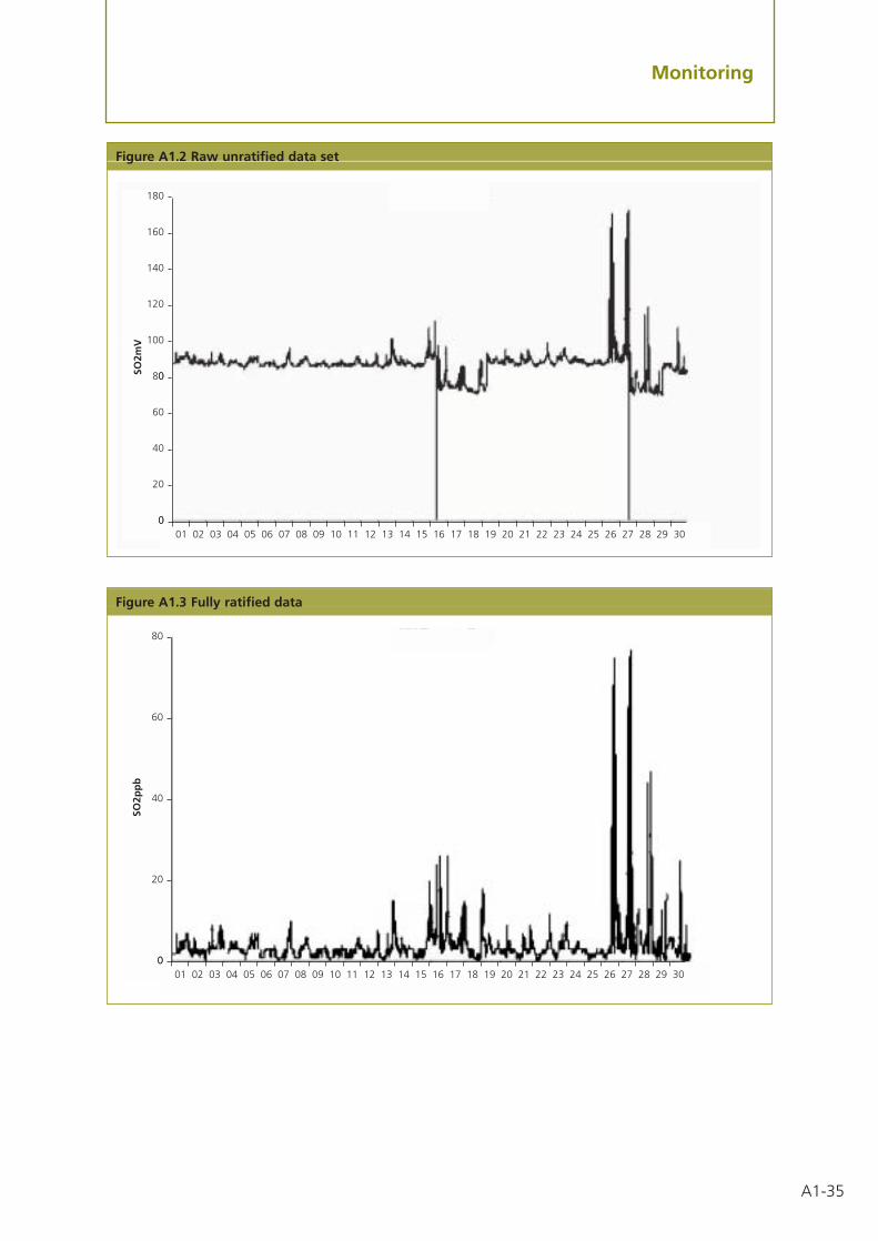
A1-35
Monitoring
Figure A1.3 Fully ratified data
Figure A1.2 Raw unratified data set
01 02 03 04 05 06 07 08 09 10 11 12 13 14 15 16 17 18 19 20 21 22 23 24 25 26 27 28 29 3000
20
40
60
080
100
120
140
160
180
SO2m
V
01 02 03 04 05 06 07 08 09 10 11 12 13 14 15 16 17 18 19 20 21 22 23 24 25 26 27 28 29 3000
80
60
40
20
SO2p
pb

A1-36
Monitoring
A1.101 Records of calibration and services visits should be used to aid interpretation ifanomalous peaks are seen. Records of daily automatic calibrations, if available, can beused to identify any long-term drift in the output of the instrument and correctionfactors applied as appropriate.
Figure A1.5 PM10 measurements at a range of automatic sites
Figure A1.4 Pollutants measured at an urban centre site
01 02 03 04 05 06 07 08 09 10 11 12 13 14 15 16 17 18 19 20 21 22 23 24 25 26 27 28 29 3040 ppb
500 ppb
400 ppb
80 ppb
8 ppb
80 ppb
150 µg/m3
OZONE
NOX
NO
NO2
CO
SO2
PM10
0
01 02 03 04 05 06 07 08 09 10 11 12 13 14 15 16 17 18 19 20 21 22 23 24 25 26 27 28 29 30
150 µg/m3
PM10
0 µg/m3
150 µg/m3
PM10
0 µg/m3

A1-37
Monitoring
A1.102 Ratification is an important data management process, ensuring measurementsare credible, reliable and fit for the purpose of review and assessment or any othermonitoring objectives. The effort and skill level required for data ratification should notbe under estimated. Several environmental consultancies can assist with this process,under contract, if required.
Reporting of monitoring data
A1.103 Even the simplest air quality monitoring programme can quickly produce alarge amount of data. Statistical summaries are therefore required to obtain a clearoverall picture and to minimise the amount of information needed to describe thepollution situation. These statistical summaries form the basis of calculations tocompare measured results with the objective.
The type of information required may include:
• hourly, daily, monthly, seasonal and annual mean concentrations of pollutants.
• exceedences of specified threshold or limit values.
• hourly, daily, monthly maximum values.
• variation of concentration with wind direction, and other meteorological factors.
• trends over time.
• mapped concentrations (of area diffusion tube surveys).
A selection of different ways to analyse and present air pollution data is given in Box A1.8.
A1.104 Calculation of exceedence statistics – Specific statistics need to becalculated from the ratified data for comparison with the Air Quality Objectives.The following definitions are commonly used:
• 15-minute mean – 15-minute mean is a mean calculated every 15-minutes for thepreceding 15-minutes, i.e. from 00:00 to 00:14; 00:15 to 00:29; 00:30 to 00:44 and00:45 to 00:59.
• Hourly mean – An hourly mean is the mean concentration for the following houri.e. the mean for 11:00 will be the mean for the period 11:00 to 11:59. If the hourlymean is calculated from 15-minute means than at least three valid 15-minute meansare required to produce a valid hourly mean.
• Running 8-hour mean – A running 8-hour mean is a mean which is calculated fromhourly average concentrations. The running 8-hour mean for a particular hour is themean of the hourly average concentrations for that hour and the preceding 7 hours.The averaging period is stepped forward by one hour for each value, so running meanvalues are given for the periods 00:00 -07:59, 01:00 – 08:59 etc. There are, therefore,24 possible 8-hour means in a day (calculated from hourly data). In order for arunning average to be valid, 75% data capture is required i.e. 6 hourly averages outof every 8 must be valid. The maximum daily running 8-hour mean is the maximum8-hour running mean measured on any one day, i.e. between 00:00 and 23:59 hours.

A1-38
Monitoring
• 24-hour mean – A 24-hour mean is the mean concentration for the preceding 24-hours. If the 24-hour mean is calculated from hourly means then at least 18 validhourly means are required to produce a valid 24-hour mean.
• Annual mean – An annual mean is a mean that is calculated from hourly averageconcentrations over a year, yielding one annual mean per calendar year, forautomatic data. The annual mean for non-automatic data is the mean of therelevant sampling period over a year. Annual means are based on 366 days for leapyears and 90% data capture is required.
• Running annual mean – A running annual mean is a mean which is calculated eachhour from hourly average concentrations over a year. The running annual mean isthe mean of the hourly average concentration for that hour and the preceding 8759hours (365 days). For leap years annual means are based on 366 days.
• Percentile – A value that is the rank at a particular point in a collection of data. Forinstance, a 98th percentile of values for a year is the value that 98% of all the datain the year fall below, or equal. Calculation of percentiles is described in theFrequently Asked Questions on QA/QC.
A1.105 Commercial software, often available from the equipment suppliers, can beused to produce standard reporting formats. In reporting data it is important to makeclear what concentration units have been calculated.
Box A1.8 Methods for analysis and reporting of air quality data
TablesData are presented in the form of lists e.g. tables of measured pollutant concentrations for differentintervals of time at selected measurement sites. Tables provide the largest sets of data for generalanalysis at minimal expense.
Time seriesA time series plot of concentrations against specified time intervals provides a very useful way toquickly visualise a large dataset. These can be used to identify possible data anomalies, to comparedata from different monitoring sites or fluctuations of different pollutants at the same site. Diurnal orseasonal variations in pollutant concentrations can also be readily viewed.
Trend analysisBy performing a regression analysis on statistics such as annual mean and 98th percentileconcentrations, it is possible to assess how air quality compares to previous years and identify whetherpollution concentrations are changing over time. Statistically significant trends, or even a reasonableoverview of how concentrations are changing, usually only become meaningful when complete datarecords extend over five years or more.
MappingMapping of concentration data or statistics, often using GIS systems, is invaluable in assessing spatialpatterns of pollution and exposure, identifying ‘hot spots’ and assisting in monitoring network design.This technique is particularly appropriate for area surveys with diffusion tube samples.
Wind/pollution rosesThese can be useful in determining the source of a given pollutant. The wind velocity rose indicatesaverage wind speed for wind directions recorded in each various sectors and the wind direction roseindicates the percentage of time wind was recorded from each particular direction. The pollution roseplots relate air pollution measurements to wind direction. These plots show the average pollutantconcentrations during periods when the wind was recorded in each of the sectors.

A1-39
Monitoring
Frequently Asked Questions on QA/QC
How do I ratify and report data?
A1.106 Screen the data, by visual examination, to see if they contain spurious andunusual measurements: this is how equipment faults or episodes of exceptionally highpollution are detected. This initial data validation must be followed by more thoroughchecking at 3 or 6-month intervals to ensure that they are reliable and consistent. Thislatter process is called data ‘ratification’. Essentially, the data ratification procedureinvolves a critical review of all information relating to a particular data set, in order toverify, amend or reject the data. When the data have been ratified, they represent thefinal data set to be used in the review and assessment process. The data reportedshould include:
• Simple statistics such as data capture, arithmetic and geometric mean of hourlyvalues, maximum hour, and 24-hour.
• Comparison of the results with relevant standards and objectives of the Air QualityStrategy.
• Site and equipment information.
It is import to record the measurement units that have been used and any correctionfactors which have been applied to the data.
How do I calculate percentiles?
A1.107 This is done by ranking the measurements by concentration value and canreadily be carried out using Excel or a similar spreadsheet. For example, to calculate the99.8th percentile of hourly nitrogen dioxide concentrations:
Step 1. Load the hourly average concentrations for a year into a spreadsheet.Step 2. Sort them into ascending order of concentration.Step 3. Calculate 99.8 percent of the total number of concentration values.Step 4. Round this number to the nearest integer.Step 5. The concentration in the row equivalent to this number is then the
99.8th percentile.Thus, if in calendar year there are 8760 values measured99.8 % of 8760 = 8742.48 = 8742The concentration at row 8742 in the spreadsheet is then the 99.8th percentile.
Alternatively the following spreadsheet functions can be used:In Excel: = percentile(address of first cell:address of final cell,0.XXX)In Lotus 123: &percentile(0.XXX. address of first cell:address of final cell)
where 0.XXX is the required percentile, for example, the 99.8th percentile = 0.998
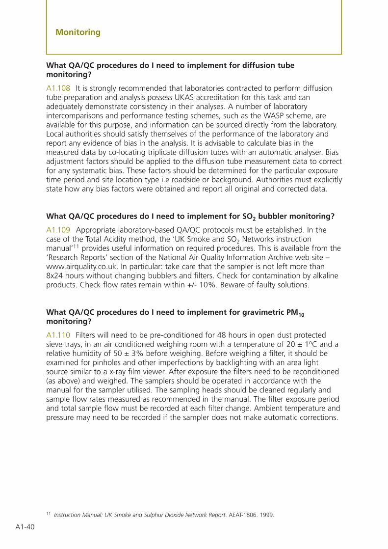
A1-40
Monitoring
What QA/QC procedures do I need to implement for diffusion tubemonitoring?
A1.108 It is strongly recommended that laboratories contracted to perform diffusiontube preparation and analysis possess UKAS accreditation for this task and canadequately demonstrate consistency in their analyses. A number of laboratoryintercomparisons and performance testing schemes, such as the WASP scheme, areavailable for this purpose, and information can be sourced directly from the laboratory.Local authorities should satisfy themselves of the performance of the laboratory andreport any evidence of bias in the analysis. It is advisable to calculate bias in themeasured data by co-locating triplicate diffusion tubes with an automatic analyser. Biasadjustment factors should be applied to the diffusion tube measurement data to correctfor any systematic bias. These factors should be determined for the particular exposuretime period and site location type i.e roadside or background. Authorities must explicitlystate how any bias factors were obtained and report all original and corrected data.
What QA/QC procedures do I need to implement for SO2 bubbler monitoring?
A1.109 Appropriate laboratory-based QA/QC protocols must be established. In thecase of the Total Acidity method, the ‘UK Smoke and SO2 Networks instructionmanual’11 provides useful information on required procedures. This is available from the‘Research Reports’ section of the National Air Quality Information Archive web site –www.airquality.co.uk. In particular: take care that the sampler is not left more than8x24 hours without changing bubblers and filters. Check for contamination by alkalineproducts. Check flow rates remain within +/- 10%. Beware of faulty solutions.
What QA/QC procedures do I need to implement for gravimetric PM10monitoring?
A1.110 Filters will need to be pre-conditioned for 48 hours in open dust protectedsieve trays, in an air conditioned weighing room with a temperature of 20 ± 1oC and arelative humidity of 50 ± 3% before weighing. Before weighing a filter, it should beexamined for pinholes and other imperfections by backlighting with an area lightsource similar to a x-ray film viewer. After exposure the filters need to be reconditioned(as above) and weighed. The samplers should be operated in accordance with themanual for the sampler utilised. The sampling heads should be cleaned regularly andsample flow rates measured as recommended in the manual. The filter exposure periodand total sample flow must be recorded at each filter change. Ambient temperature andpressure may need to be recorded if the sampler does not make automatic corrections.
11 Instruction Manual: UK Smoke and Sulphur Dioxide Network Report. AEAT-1806. 1999.

A1-41
Monitoring
What QA/QC procedures do I need to implement for automatic PM10monitoring?
A1.111 The analysers should be operated in accordance with the manual for theequipment utilised. The sampling heads should be cleaned regularly and sample flowrates measured as recommended in the manual. Suitable calibration factors need to becalculated for some monitors such as light scattering devices. Data from some analysersmay also need to be re-scaled in order to compare with standards and objectives of theAir Quality Strategy. The Monitoring or Review and Assessment Helpdesks should becontacted for more information.
What QA/QC procedures do I need to implement for automatic NOx and SO2monitoring?
A1.112 The analysers should ideally be housed in an air-conditioned room, hut ortrailer, and operated according to the manufacturers’ instructions. The analysers shouldbe calibrated at least once every two weeks for urban sites, monthly for rural sites. Thecalibration should be performed with zero air from a zero air cylinder or chemicalscrubber and certificated gas cylinders. 15-minute averaged data should be collectedand scaled using the best available calibration factors. Independent audit checks onmonitors, gas standards and site operational procedures may be beneficial when usingthese highly complex analysers.

A1-42
Monitoring
Appendix A: Definition of site classesKerbside (U1)A site sampling within 1m of the edge of a busy road.
Source influences Local traffic
Examples of objectives:Identifying vehicle pollution blackspotsAssessing worst case scenariosEvaluating impacts of vehicle emission control technologiesDetermining impacts of traffic planning/calming schemes
Roadside (U2)A site sampling between 1m of the kerbside of a busy road and the back of thepavement. Typically this will be within 5m of the road, but could be up to 15m.
Source influences Local traffic
Examples of objectives:Assessing worst case population exposureEvaluating impacts of vehicle emission controlsDetermining impacts of traffic planning/calming schemes
Urban Centre (U3)A non-kerbside site, located in an area representative of typical population exposure intown or city centres (for example, pedestrian precincts and shopping areas). This islikely to be strongly influenced by vehicle emissions, as well as other general urbansources of pollution. Sampling at or near breathing-zone heights will be applicable.
Source influences Vehicle, commercial, space heating
Examples of objectives:Identification of long-term urban trends
Urban Background (U4)An urban location distanced from sources and therefore broadly representative of city-wide background conditions, for example, elevated locations, parks and urbanresidential areas.
Source influences Vehicle, commercial, space heating
Examples of objectives:Trend analysisUrban planningTraffic and land-use planning

A1-43
Monitoring
Urban Industrial (U5)An area where industrial sources make an important contribution to the total pollutionburden.
Source influences Industrial, motor vehicles
Examples of objectives:Assessing local impacts on health and amenityProcess optimisationSource attribution/identificationProviding model input dataModel development/validationLocal planning and plant authorisation
Suburban (SU)A location type situated in a residential area on the outskirts of a town or city.
Source influences Traffic, commercial, space heating, regionaltransport, urban plume downwind of a city
Examples of objectivesTraffic and land-use planningInvestigating urban plumes
Rural (R1)An open country location, in an area of low population density, distanced as far aspossible from roads, populated and industrial areas.
Source influences Regional long-range transport, urban plume
Examples of objectivesEcosystem impact studiesAssessing compliance with critical loads and levels for crops and vegetationInvestigating regional and long-range transportIdentification of ozone ‘hot spots’
Remote (R2)A site in open country, located in an isolated rural area, experiencing regionalbackground pollutant concentrations for much of the time.
Source influences Regional/hemispheric background
Examples of objectivesAssessing ‘unpolluted’ global or hemispheric background conditionsLong-range transport studiesLong-term baseline trend analysis
Special (Sp)A special source-oriented category covering monitoring studies undertaken in relation tospecific emission sources such as power stations, petrol stations, car parks or airports.

A1-44
Monitoring
Appendix B: Conversion factorsConversion factors for gaseous pollutants at 20oc and 101.3 kPa
Benzene 1 ppb = 3.25 µg/m3
1,3-butadiene 1 ppb = 2.25 µg/m3
Carbon monoxide 1 ppm = 1.16 mg/m3
Nitric oxide 1 ppb = 1.25 µg/m3
Nitrogen dioxide* 1 ppb = 1.91 µg/m3
Sulphur dioxide 1 ppb = 2.66 µg/m3
Ozone 1 ppb = 2.00 µg/m3
*NOx in µg/m3 is expressed as NO2 i.e. (NOppb + NO2ppb)*1.91 = NOx µg/m3

Estimating emissions
IntroductionA2.01 This guidance is not intended to provide a single outline to compiling acomplete emissions inventory. Review and assessment is about assessing the potentialfor air quality exceedences and therefore is about identifying and understanding thesignificant sources contributing to poor air quality.
A2.02 These significant sources will be different for different local authorities and evenfor different areas within a local authority. In the majority of cases, road transport andstationary large point sources are likely to be the most common problems. Inaddition but probably in more isolated cases residential areas burning coal or solidfuel, large ship ports or airports may need Detailed Assessments. In many cases acomplete inventory is inappropriate and time consuming. However, where exceedencesare likely to result as a cumulative result of a large number of different sources then amore complete inventory is recommended.
A2.03 It is recommended that the significant sectors are assessed in detail first andthen if necessary (i.e. there is more than one significant sector or the combination oflocal sources are likely to have an impact on population) a combined assessment isundertaken.
A2.04 The emissions data necessary for a combined assessment should include thedata gathered for the sector specific assessments as detailed in the guidance below. Inaddition, background emissions data can be used to account for sectors not specificallyassessed in the detailed studies. These data can be obtained from the NAEI’s datawarehouse on www.naei.org.uk/datawarehouse and will include:
• Non point source commercial, industrial and residential emission maps.
• Road transport emission maps including major, minor, cold start, hot soak and break& tyre wear.
• Port emissions.
• Airport emissions.
A2.05 In addition point source and traffic data are available as background input forareas outside the LA boundary:
• Large point sources.
• Major road emissions.
Full details of the NAEI’s data warehouse is included in Appendix D.
Annex 2 Estimating emissions
A2-1

A2-2
Estimating emissions
Road transport
DMRB Screening Model assessment data
A2.06 It is important to try to improve on the general quality and reliability of thescreening data used for the DMRB Screening Model1 assessment. The DMRB ScreeningModel assessment should be done using the tools and approach specified in Annex 3,and the various chapters of the main document.
A2.07 The data necessary for screening is illustrated in Figure A2.1.
Traffic Flow: AADT242 is required for the measure of traffic flow and should besourced from the local traffic department or the Highways Agency regional officeswhere possible. The data collected for the Screening Assessment can be used as a basisfor the DMRB Screening Model assessment. However, effort should now be focused onidentifying the flows for each component link contributing to a junction of concern.Flows that had been assumed for certain links should be replaced with real counts for
Figure A2.1: DMRB Screening Model assessment data requirements
1 Design Manual for Roads and Bridges, Volume II, Section 3, Part 1, Air Quality. The Stationery Office, February 2003.2 AADT is the annual average daily traffic flow – sometimes referred to as AADT24.
Traffic flow
AADT24 and assumed flows where not available
Hourly, daily, seasonal variation
Traffic growth
NRTF index of growth
Traffic split
% HDV link specific
Detailed and link specific
Speed
Average by link/junction
Detailed by type and link section: daily average
Detailed by traffic type and sub section: hourly profile
Detailed AssessmentLocal information on future plans and capacities
% HDV road type average or link specific
Road link locations
Peak hourlysee modelling section for details
Annual averagesee modelling section for details
AADT24 and new counts if appropriate
Road geography
Road width
Tempro
Flow by link sub section
DMRB Screening Model
Use the DMRB Screening Model spreadsheet

A2-3
Estimating emissions
that link. If no data are available from a wider search then consider specific spot countsbut make sure that these are representative of AADT24 flows. Example 1: Derivation ofTraffic Flow Data in Appendix A provides a worked example.
Traffic split can remain as % HDV. However, it is recommended that local link specific,rather than national average, information is used as the % HDV can vary dramaticallyfor different links and junctions.
Traffic Growth: Estimates of traffic flow for future years are required. It isrecommended that local knowledge from the Highways Agency, Scottish Executive, theWelsh Assembly Transport Directorate, the Department of Regional Development(Northern Ireland), Roads Service Transportation Unit or Local Planning departmentsshould be used to apply growth factors to the current traffic count data. This isimportant where local factors such as planned housing development, or industrial, retailor leisure facilities may have an impact on the future traffic flow. Where local data arenot available and no planned local changes are expected the NRTF3 traffic growthfactors can be used.
Traffic Speed: For the DMRB Screening Model assessment basic daily average speedfor two-way flow is adequate for both road links and junctions. Where possible anemphasis should be placed on collecting or estimating more reliable local data ratherthan using national averages or speed limits. The likelihood and effect of congestionshould be built into the speed estimates for DMRB Screening Model assessments.A worked example: Example 2: Vehicle Splits and Speeds is included in Appendix A.The COBA (COst Benefit Analysis) manual also contains a methodology for estimatingvehicle speeds. See http://www.roads.dft.gov.uk/roadnetwork/heta/highway/pdfs/coba11part00.pdf.
Detailed Assessment data
A2.08 Detailed Assessment will involve some form of modelling, requiring high qualitytraffic flow and link location information. The possible approaches and tools formodelling are discussed in Annex 3. It is very important for Detailed Assessments thatthe data used is representative of the specific likely traffic flow, speed and typecharacterisation for the links being considered. Try to avoid using average or aggregatefactors for flow or traffic composition. Try also to incorporate possible slow speedsduring congestion and the likely impact of bus stops and steep hills. A2.10 ‘Speeds’provides information about calculating suitable speeds to use in the DetailedAssessment.
A2.09 The emissions for each link can be calculated using the Emission Factor Toolkit(see Annex 3). The Emission Factor Toolkit (EFT) requires link specific input data ofspeed, traffic composition and road type. From this input data emission factors for eachspecific link being assessed will be calculated and can be applied to the geographicmap of the roads and their AADT24 traffic flow. Alternatively, if not using the EFT thenthe raw emission factor data are available from the NAEI website onwww.naei.org.uk/datawarehouse.
3 National Road Traffic Forecast – the NRTF does not apply to Northern Ireland.

A2-4
Estimating emissions
A2.10 The data necessary for the Detailed Assessment is illustrated in Figure A2.2.
Traffic flows: For Detailed Assessments it is important to get accurate counts orestimates of traffic flow. The traffic flow data should be AADT24 but also include localdaily and day of the week variation information for peak hour exceedence calculations.These data should be available from the Local Transport Department, the County PlanningDepartment or the Highways Agency. Example 1: Derivation of Traffic Flow Data inAppendix A provides a worked example. Alternatively, UK average daily, weekly andmonthly traffic flow factors can be downloaded from www.naei.org.uk/datawarehouse.
Vehicle split and emission factors: For Detailed Assessments it is recommended thatthe EFT be used to estimate detailed vehicle split and emission factors for each link. TheEFT is preloaded with national average fleet compositions for different road types andcan disaggregate a coarser set of vehicle categories into those required for emissionestimation. However, where possible this split should be based on the link specificvehicle split for each road link being considered and should also be based on a moredetailed local split than used for DMRB Screening Model Assessment. Some trafficcount data will contain a basic vehicle split (cars, Light Goods Vehicles, Rigid HGV,Articulated HGV, Buses & Coaches and Motorcycles). Where possible this level of detailshould be used as the primary input data. For major roads this level of detail can alsobe obtained for a large number of specific count points from the NAEI data warehouse(www.naei.org.uk/datawarehouse).
Figure A2.2: Illustration of data requirements for Detailed Modelling Assessment
Traffic flow
AADT24 and assumed flows where not available
Hourly, daily, seasonal variation
Traffic growth
NRTF index of growth
Traffic split
% HDV link specific
Detailed and link specific
Speed
Average by link/junction
Detailed by type and link section: daily average
Detailed by traffic type and sub section: hourly profile
DMRB Screening Model
Use the DMRB Screening Model spreadsheet
Local information on future plans and capacities
% HDV road type average or link specific
Road link locations
AADT24 and new counts if appropriate
Road geography
Road width
Tempro
Flow by link sub section
Detailed Assessment
Peak hourlysee modelling section for details
Annual averagesee modelling section for details

A2-5
Estimating emissions
Traffic growth: Local knowledge from the Highways Agency, the Welsh Assembly,Scottish Executive or Local Planning departments must be used to apply growth factorsto the current traffic count data. This is important where local factors such as plannedhousing development, or industrial, retail or leisure facilities may have an impact on thefuture traffic flow. Where local data are not available and no planned local changes areexpected the NRTF traffic growth factors can be used.
Speeds: Estimation of appropriate traffic speed is important for modelling of roadtraffic sources. Unfortunately, it is usually difficult to obtain data on speeds that wouldbe ideal for air quality studies. Speed estimates for Detailed Assessment work must belink specific. At junctions, links will need to be broken down to their key elements asoutlined in Figure A2.3. A worked example (Example 2): Vehicle splits and speeds isincluded in Appendix A. An alternative approach is to estimate (or measure) theaverage time taken for vehicles to travel from one end to the other of the junctionsection and convert this to an average speed. You should allow for the different phasesof the lights and different levels of congestion during the day.
A2.11 Traffic models will usually include an estimate of average transit speed ofvehicles along modelled links. However, this will be for the time period considered bythe model network (for example, AM peak), and will not be available for discretesections of links. Generally, model-based speed estimates will be fairly crudeapproximations that will be heavily influenced by the nature and operation of theparticular model software from which they are derived (for example, do they include‘junction delays’, how do they relate to pre-determined speed/flow curves). Trafficcounts do not provide data on speed directly. The following provides further guidanceon an approach that can be used in the absence of better data.
Figure A2.3: Detailed speed data at junctions
HS = high speed
RS = reduced speedLS = low speed
LSRSRS
RS
RS
HS
HS
HS
HS

A2-6
Estimating emissions
• Speed data may be obtained directly from a traffic model (users should understandthe basis on which the model speeds are calculated), from ‘floating-car’ studies orfrom theoretical extrapolations based on speed limit/flow.
• The use of hourly speeds throughout the day are also likely to be necessary. This canoften be different for different roads and should be assessed locally if possible. Inaddition the more complex changing speeds on junctions should be considered.
• For junctions, there is no straightforward way to estimate speeds. Common senseand driving experience is therefore helpful. It is suggested that the aim should be toestimate average speeds over a 50m section of road – for example a 50m sectionleading up to traffic lights. The estimation of an average speed for two-way trafficon this 50m section requires consideration to be given to three conditions:
• traffic on the carriageway pulling away from the lights – probably travelling at40-50 kph.
• traffic on the carriageway approaching the lights when green – probablytravelling at 20-50 kph.
• traffic on the carriageway approaching the lights when red – probably having anaverage speed of 5-20 kph, depending on the time of day and how congestedthe junction is.
It is considered that the combined effect of these three conditions is likely in mostinstances to be a two-way average speed for all vehicles of 20-40 kph. Speeds insimilar ranges would also apply at roundabouts, although on sections of largeroundabouts, speeds may well average between 40-50 kph.
Dealing with congestion: Average vehicle speeds during traffic congestion will fall,and there is no simple factor that can be applied to the average speed to calculate aspeed applicable to congested periods. The preferred approach is to calculate theemission rate for the affected roads for each hour of the day or week on the basis ofthe road speeds and traffic flows for each hour. The calculated emissions profile couldthen be used in the dispersion model. However, many dispersion models will onlyaccept a single emission rate (normally expressed as grammes of pollutant emitted fromvehicles per second) for a road link, or section of a link. It may then be necessary tocalculate a weighted average emission factor (EF) to take account of the varying trafficflows and vehicle speeds throughout the day. If there is only a small section ofcongestion, the weighted EF should be only be used to model the emissions along thatsection of road, and not for large distances either side.

A2-7
Estimating emissions
The following illustration summarises the calculations needed:
where:
F = vehicle flow
E = emission factor
weighted EF = ∑ (F x E) (g/km/vehicle)∑ F
This weighted EF would be suitable to use in congested sections of road. Other modelsrequire the calculation of hourly factors to apply to the average emission rate. The lastcolumn of the above table illustrates the approach to employ in calculating the hourlyfactors. Remember, if there are more than several percent HDV travelling on a road link,emissions (and so indirectly, concentrations in air) may increase sharply as the speedfalls below 20 kph – this means your choice of speed and hence emission factor will beimportant in this situation.
Dealing with bus stops: Bus stops can locally slow traffic. If local knowledge suggeststhat traffic speeds are affected by bus stops, then you could split the road link into anumber of sections in a similar way to that shown in Figure A2.3 and attribute anappropriate speed to each link. To model bus stops properly, assuming a road withsimple two-way traffic, it is useful to model both parts of this traffic flow separately.This allows the effect of the bus stop on only one side of the road to be accounted forin the modelling. The modelling will be composed of two components – modelling theemissions from the moving traffic (the total traffic flow should be modelled here) andmodelling the emissions from the stationary buses at the bus stops. At the time,
Hour F E F x F 24 x F x E/∑ (F x E)
(vehicle/hr) (g/km/vehicle) (g/km/hr)
1
2
3
4
– “ – – “ – – “ – – “ –
22
23
24
∑ F ∑ (F x E)(over 24 hr period)

A2-8
Estimating emissions
emission factors for stationary vehicles are not readily available, so, EFs from very slowmoving vehicles (at say 5 km per hour) may be used. The effective emission factor for abus over the length of the bus stop section of the road may then be estimated from:
EF2 =EFL x VL x m/60
L
where:
EFL is the emission factor for buses at low speed, g per vehicle km.
VL is the speed corresponding to the emission factor, km per h.
m is the number of minutes each bus stays at the bus stop with its enginerunning.
L is the length of the bus stop section, in km.
Dealing with hills: Even hills with slight gradients may slow the traffic significantly,particularly if there is a large percentage of HDVs. As vehicles start to climb the hill, thepower demanded from the vehicle engine will increase, although the speed of thevehicles may remain similar. As the power demanded increases, emissions will increasealso. Therefore, using an emission factor for an assumed average speed on sections ofroads on steep hills (say greater than 1:10) may underestimate the actual emissions.A useful indication of whether a hill may be considered steep is that a high proportionof goods vehicles need to change gear to enable them to climb the hill. To identifysections of hills, you could introduce a ‘hill section’ in a similar way to the way the roadlinks are broken into different components as shown in Figure A2.3. This ‘hill section’would contain the hill and some distance of road after the hill. Local knowledge is thebest way to decide the length of road affected by the hill. Ideally on hills, the emissionsfrom the vehicles should be estimated using an emission factor specifically derived forvehicles climbing hills. At the time this guidance was written, no such factors wereavailable. One approach to account for the increased emissions as vehicle is to use thefollowing expression to derive an emission factor suitable for vehicles climbing a hill. Ina simple way, the expression accounts for the fact that the speeds are slower but theengines are under greater load:
EF2 = EF1 x (V1/V2)
where:
EF1 emission factor for vehicles travelling at the maximum permitted speedon that road (grammes per vehicles km).
V1 maximum vehicle speed (km per hour).
V2 assumed ‘hill speed’ (km per hour).
EF2 emission factor at speed V2, which is suitable for vehicles climbing the hill(grammes per vehicle km).

A2-9
Estimating emissions
Alternatively, you could account for the increased emissions by assigning a ‘reducedspeed’ section for the entirety of the ‘hill section’. Using an emission factor for slowermoving vehicles, particularly for slow moving HDVs, will result in increased estimates ofemissions and therefore increased ambient concentrations.
Link Locations: For the Detailed Assessment the traffic flow will be required on aspatial basis. Each link will require at least, a location (grid reference) for each end ofthe link so that its location in relation to nearby population can be accurately assessed.In cases where the road link is not simply a straight line between the two pointsadditional spatial detail will be required. Detailed centre lines and accurate road widthdata will also need to be collected for each link in the assessment to assess the impacton the nearby population. The ‘Planning Department’ of the Local Authority shouldhave the data on a spatial basis. In many cases the links will need to be split andjunctions modified to account for different speeds at or near to road junctions. Annex 3describes how to use this data for modelling exceedences.
Frequently Asked Questions
Who do I contact for traffic flow information?
A2.12 The relevant department within your local authority for traffic flow informationon most local roads will be the first point of contact. However, the Highways Agencymanages most trunk roads and motorways in England, the Welsh Assembly TransportDirectorate does so in Wales and the Scottish Executive does so in Scotland. Withinthese organisations, the relevant regional coordinator should be contacted. Personnelwithin your own traffic departments can often provide Highways Agency data.Alternatively, relevant contacts can be found in the Highways Agency website.(www.highways.gov.uk/roads/area/area_pages_home.htm). The NAEI holds a centralisedcollation of traffic count data on all ‘A’ roads and motorways. These data can be used asa starting point for traffic flows and count point locations. However these data do notcontain the geographic detail necessary for modelling and will have to be used inconjunction with more detailed geographic road maps.
A2.13 There are two possible types of traffic flow information:
• traffic counts are made either by human observation (‘manual counts’) or machine(‘automatic’ or ‘continuous’ counts). Essentially, traffic passing the observer iscounted and (usually) ‘classified’ (i.e. organised into sub-categories for each of themain vehicle types) over a time period, or sequence of related time periods. Theseshould be used in preference to traffic model data.
• traffic/transportation models: a computerised representation of the road network.Local Authority traffic engineering departments commonly use these to investigatethe likely impact of future road policies, such as infrastructure development.
A2-10
Estimating emissions
A2.14 Data from traffic models have been found to suffer from inaccuracies at thelevel of the individual link that may render it unsuitable for use in isolation for theDetailed Assessments. Use of data from this source is therefore more suited to‘screening’ and DMRB Screening Model studies. Traffic count data will usually be morereliable at the level of the individual link and should be used wherever possible forDetailed Assessments. The primary disadvantage of ‘Traffic Count’ data are that theyare resource-intensive to collect for other than a small number of links, and thatextreme care needs to be taken in extrapolating what are essentially point-basedobservations to whole ‘roads’.
A2.15 In obtaining, understanding and manipulating traffic activity data from eithertraffic models or traffic counts, it is very important that users thoroughly understandthe basis on which the data have been compiled. A large number of issues can arisehere, and the following should be used as a checklist. Close working liaison betweenenvironmental and transport practitioners will be required. The latter should be able toassist on all of the points in this list.
What years do I need to assess my traffic for?
A2.16 You need to project traffic flows forward to the relevant year depending on thepollutant being assessed (Chapters 2-8). Each traffic or transport department within alocal authority should have estimates of the expected growth on roads under theirjurisdiction. For trunk roads and motorways managed by the Highways Agency andScottish Executive, they can be contacted directly to obtain relevant growth factors.
A2.17 Specific future plans (either to reduce traffic congestion or to develop housingor commercial areas) will have an effect on the traffic flows and may even include theconstruction of new roads. Depending on the maturity of these plans there may alreadybe flow estimates and even impact assessment data available from the planningdepartment of the Local Authority or the County Council. This ‘Local’ informationshould be used in any Detailed Assessment of traffic impacts.
A2.18 You should ask for year by year growth factors based on road types – thegrowth on motorways is likely to be different to the growth on urban roads.
A2.19 You may be provided with growth factors based on HIGH, MEDIUM or LOWestimates. Ask your transport, traffic or planning department to indicate which one isthe most reasonable, and to provide you with a justification of which one you shoulduse, particularly when low or no growth is advised.
A2.20 The National Road Traffic Forecasts (NRTF) should be used to undertake thenecessary projections where local information is not available.

A2-11
Estimating emissions
The NRTF provides two basic types of data:
What is TEMPRO?
These pages contain detailed commentary on the derivation of the forecasts and theircorrect application. Where a five-yearly growth factor is given, factors for intermediateyears can be derived through interpolation. Consideration should be given to theappropriateness of NRTF-derived ‘global’ traffic growth forecasts for the roads understudy, particularly where (as is the case in many cities) roads are effectively alreadyoperating at ‘maximum capacity’. Please note the NRTF Index of Growth and TEMPROdo not apply in Northern Ireland. Information on traffic growth can be obtained, in thefirst instance, from the Department for Regional Development (NI), Roads ServiceTransportation Unit, Transport Planning Team.
A2.21 Traffic speed variations should also be reconsidered for future scenarios.
What kind of traffic count information can I use?
A2.22 There are a wide range of traffic count data available to local authorities. Theseinclude:
• 12-hour manual counts – generally available for one day between 7am and 7pm.This may include vehicle classification, but generally not speed.
• Automatic Traffic Count (ATC) data – generally available for at least a week, covering24-hour flows for each day. Can often provide a range of vehicle classifications andspeed data (where traffic is moving above a certain speed threshold).
Dataset Links
National-level See growth estimates, http://www.roads.dft.gov.uk/roadnetwork/nrpd/heta2/nrtf97/index.htmat five-yearly intervals, by basic road and area type
Estimates specific The ‘TEMPRO4’ program. The TEMPRO pages are located at to each local http://www.tempro.org.ukauthority district in the UK
What is TEMPRO?Seehttp://www.roads.dft.gov.uk/roadnetwork/heta/hetatemp.htm
4 TEMPRO – Trip End Model Presentation Program produced by the Department for Transport. At the time thisguidance was written, the latest version of the software was TEMPRO v4, and it was necessary to register yourdetails at the website above before being allowed to download the model. The model is free, and is split intoregional components.

A2-12
Estimating emissions
• Video data – CCTV used to film traffic flows on a road and manually counted at alater stage. Can provide information on vehicle classification but estimates of speedsare more difficult.
• Radar speed data – hand held or fixed instruments measure the speed across asection of road.
A2.23 In many cases, most counting systems are placed on free flowing sections ofroads away from junctions. However both manual counts and speed radar, and videofootage can be used at junctions.
A2.24 Any of the above information can be used as long as the AADT can beestimated (see A2.28 – A2.32).
What if no traffic figures have been made available?
A2.25 You can try to use your local knowledge to assess whether the road could besignificant in the first instance.
A2.26 If you are able to identify that flows could be significant, and that exposure isalso relevant you will need to gather some idea of the likely traffic flows. To do this,you can:
• Download major road traffic count data from the NAEI data warehouse onwww.naei.org.uk/maps/datawarehouse and check the flows for relevant or relatedlinks there and/or
• compare it with similar roads in your area and use your local knowledge.
A2.27 In the absence of any data, you may need to arrange for an initial traffic countto be undertaken from which you can estimate traffic flows. This should be done inconsultation with the Local Traffic department and aim at estimating the AADT andvehicle split (at least %HDV) for the links of interest. Additional vehicle split (Cars/Taxis,LGV, HGV Rigid and Articulated, Buses and Coaches and motorcycles) as well as thedaily and weekly variation should be recorded if the link is likely to require a DetailedAssessment.
My traffic flow data are not AADT what do I do?
A2.28 The DMRB Screening Model needs AADT traffic flows. Your transport/trafficdepartment or Highways Agency should be able to give you factors based on yourregion, to allow you move between:
• AM or PM peak to 12-hour flows and/or 24-hour flows.
• 18-hour flows (commonly used for noise assessments) and 24-hour flows.
A2-13
Estimating emissions
A2.29 It should be born in mind that you will generally have to apply the same factorsto total traffic flows and assume that vehicle split information is the same. You shouldcheck that this is a reasonable assumption, particularly where you are applying factorsto peak hour traffic flows.
A2.30 In addition, local factors from sets of traffic flow may be derived for a few roadsin an area and applied to other roads of a similar nature. An example of how to do thisis shown in A2.144.
A2.31 Local conversion factors should be used as first preference where available,particularly when estimating emissions for Detailed Assessments. ‘Default’ nationalfactors (see Table A2.1) can be used but will not reflect local conditions and aretherefore only recommended for estimating AADT24 for screening and DMRBassessments.
A2.32 In addition to the collection of AADT24 traffic flows additional temporal detailis recommended. This additional detail will provide modellers with an indication of thelevels and duration of peak flows for assessing peak hourly exceedences. Where acount is taken over a number of hours, the variation in the flow volume over the courseof a typical day can be obtained directly. An example (Example 1) of the derivation oftraffic flow data in Appendix A provides a worked example.
How do I know my flows are representative for the year?
A2.33 If you have used 12-hour traffic counts, these are often carried out on a singleday – therefore you should check if this day was typical or not. Some local authoritieswill need to consider seasonal patterns, particularly in tourist areas, when estimatingaverage traffic flows for the year. You can do this by comparing the flows on the day ofthe manual count with 24-hour flows from ATC or similar data over the same period.For instance, if your manual count was taken on a Friday:
• you should obtain ATC data for the same period on a road of similar use (i.e. there islittle point in comparing an urban road with motorway counts.
• compare the same Friday with the rest of the week to check if there were significantdifferences between the average on that day and the 7-day average.
Table A2.1 National default factors for expanding 12-hour traffic counts to AADT (annual average daily flow)
For roads within inner London 12-hour count multiplied by 1.45
For roads within outer London 12-hour count multiplied by 1.35
For roads within and including M25 (London) only 12-hour count multiplied by 1.30
For roads elsewhere within the UK 12-hour count multiplied by 1.15
Source: DETR, Transport Statistics Roads Division. Unpublished.

A2-14
Estimating emissions
• if the data from the ATC is available over a wider time period, you can also check tosee if that week was typical of the wider period or season,
• similarly you can use other long term traffic data to check that you are basing yourscreening assessments on reasonable estimates of traffic flows.
Fridays and Mondays counts are likely to over estimate while weekend counts are likelyto under estimate when used as averages for AADT.
Where can I get vehicle split data from?
A2.34 Basic vehicle split information should be available with the traffic flowinformation. As a minimum you should expect to be provided with a % HDV split fromtraffic counts and traffic model data. Manual traffic counts should have some moredetailed traffic type splits. However, these more detailed traffic splits are likely to be lesscommon. The NAEI’s data warehouse contains some current and forecasted nationaltraffic split information that can be used in the absence of local data.
How do I determine my vehicle splits?
A2.35 The DMRB Screening Model requires as a minimum the average percentage ofHDVs on a road. Traffic departments, the Scottish Executive or the Highways Agencycan be contacted to obtain basic proportions of vehicle classifications for some or allroads in an area. It is unlikely these data will be available for all roads so someconsideration to the types and nature of roads will be required in order to makereasonable assumptions. Example 2: Vehicle Splits and Speeds is included in Appendix A.The Emission Factor Toolkit will calculate on the basis of UK averages, a detailed trafficsplit from basic %HDV. Where basic vehicle split information (%HDV) is not available,the NAEI can be used to obtain an estimate by region and road type for the major roadtypes. Alternatively Transport Statistics GB contains UK average vehicle split by roadtype, see http://www.transtat.dft.gov.uk/roadtraf/index.htm. The LAQM helpdesks canbe contacted for advise on vehicle splits should information not be available.
Where can I get traffic speed data?
A2.36 Traffic speed information is not usually available with traffic count data. Thelocal transport department, the Scottish Executive or the Highways Agency may have information on speeds for specific links. Alternatively use the speed limit as an indication of the average speed. When making Detailed Assessments the effect of congestion on speed should be considered. A worked example: Example 2: VehicleSplits and Speeds is included in Appendix A. The COBA (COst Benefit Analysis) manual contains a methodology for estimating vehicle speeds – seehttp://www.roads.dft.gov.uk/roadnetwork/heta/highway/pdfs/coba11part00.pdf.In addition Transport Statistics GB contains some UK speed averages (see http://www.transtat.dft.gov.uk/roadtraf/index.htm). Some Local Authorities haveused GPS (Global Positioning System) based speed surveys to gather additionalinformation.

A2-15
Estimating emissions
How do I estimate speeds at junctions?
A2.37 For a busy junction, assume that traffic approaching the junction slows to anaverage of 20 km/hr (approximately 10 mph). These should allow for a junction whichsuffers from a lot of congestion and stopping traffic. In general, these speeds arerelevant for approach distances of approximately 25m.
• For other junctions (non-motorway) and roundabouts where some slowing of trafficoccurs, you should assume that the speed is 10 km/hr slower than the average freeflowing speed.
• For motorway or trunk slip roads you should assume average speeds of 40–45 km/hr(approximately 30 mph) close to the junction.
• You should use local knowledge of an area to help assess whether a junction suffersregularly from congestion. You may have speed data at only a few locations, butthese may be representative of other roads in your area.
A2.38 See A2.10 for detailed speed assessments. A worked example: Example 2:Vehicle Splits and Speeds is included in Appendix A. The COBA manual contains amethodology for estimating vehicle speeds(see http://www.roads.dft.gov.uk/roadnetwork/heta/highway/pdfs/coba11part00.pdf).
Background road data
A2.39 Background road emissions are those that are not the primary focus forconcern. However, they may collectively contribute materially to local ambient levels.This means that the contribution from these types of emission may need to be takeninto account in certain areas, particularly those considering wider than immediate majorroad corridors, or those where predicted compliance with objectives is in doubt. Thereare three categories of ‘background road emissions’:
• Roads that are not being assessed in detail (minor and less significant major roads).
• Cold start and evaporative.
• Brake and tyre wear.
A2.40 There are national datasets that can be used to provide background data forthese emissions from www.naei.org.uk/datawarehouse . However, these datasets aregeneralised and based on national spatial statistics at 1 x 1km such as population,employment, road density, car ownership etc. If the emission from any of the abovesources is likely to be significant in relation to air quality exceedences it isrecommended that more detailed local data are sought.

A2-16
Estimating emissions
Minor Roads
A2.41 Roads that are not being assessed in detail will include Minor roads as well asrural or more distant major roads. Minor roads will usually carry comparatively smallamounts of traffic that are not such as to give rise to the possibility of an exceedenceof Air Quality Objectives in their own right. A busy urban road that is the subject of thisround of review and assessment will typically be surrounded by smallerresidential/access roads. By their nature, data describing traffic flows on minor roads issparse, and this means that traffic will usually need to be estimated on the basis offairly crude surrogate statistics.
A2.42 The objective is to compile an area source type grid (usually of 1 x 1 kmresolution) of the roads that are not being assessed in detail. This grid will represent theemissions from hot exhausts from the network of roads not included in road link andjunction assessments. This grid needs to be based on the best available data.
A2.43 Using count data: In many cases there will be a number of road counts for themajor roads and some of the minor roads. For the minor roads where the counts arelikely to be sparse these data can be used to estimate an average flow per km of minorroad. Multiplied by the total km of minor roads to get an estimate of total vehicle kmon the minor road network. Distributing this vehicle km total across the area using roaddensity from OS maps or the ‘minor road’ distribution map from the NAEI will createdistribution of minor road vehicle km that can be used to calculate emissions grids. It isrecommended that a local traffic engineer be consulted when making these estimates.The other major roads can then be added to this or derived from the NAEI’s major roadmaps and subtracting the roads being assessed in detail.
A2.44 Without using count data: The NAEI holds average national 1 x 1 kmdistribution data sets for emissions on minor roads. These datasets distribute the UKtotal minor road emissions. They are based on average flow by road type and OS minorroad density maps. These datasets can be accessed from the Helpdesk but should onlybe used in the absence of more detailed local data. Consider carefully whether thecontribution from this source is likely to be material to the study being undertaken.
• Are the figures obtained in reasonable proportion to the ‘major’ roads?
• How might flows on these roads – in aggregate – change between the date of theestimation and the date of the Air Quality Objective (for example, imposition of area-wide traffic calming schemes etc.). If changes are planned, will these materially affectconclusions of a review and assessment?
Cold starts and evaporative emissions
A2.45 Cold start and trip-end hot soak emissions are usually estimated on the basis oftrips as these emissions can be considered as an additional emission resulting from acold engine at the beginning of each trip for cold start, and the evaporative componentfrom hot engines. The important spatial entity to estimate is the trip starts and the tripends. There are three possible sources of data describing the density of vehicle trip endsover a study area:

A2-17
Estimating emissions
• data from a traffic or transport model.
• data from a transport or travel survey.
• estimates based on surrogate statistics.
A2.46 A transport model, where available, will usually be able to provide an‘origin/destination’ (‘OD’) matrix which describes the pattern of trip starts over an areain terms of the number of vehicle trips originating across a system of ‘zones’ (smallpolygons). This source can be appropriate for area-wide studies.
A2.47 Some authorities will have recent travel surveys, from which similar data canbe obtained to that from the road transport models. These data will also be subject tothe limitations of the travel survey involved (for example, whether people or vehicles arecounted, sample size, etc.).
A2.48 Where neither of the above are available, an estimate can be made on the basisof surrogate statistics. The most appropriate approach here is to combine regional trip-rate data (i.e. number of trips per household, by mode, per day) from the DfT’sNational Travel Survey (NTS) with population density and/or employment densitydata. The precision that can be expected from this approach is clearly very limited.
A2.49 Emission factors for cold starts and hot soaks are given in the UK EFDB onthe NAEI website (www.naei.org.uk/emissions).
A2.50 Crude emission estimates on 1 x 1 km bases are compiled for the UK mapsbased on UK estimates of ‘cold start’ and ‘evaporative’ emissions. These datasets couldbe used in the absence of other data to provide a background map for these sources.(see www.naei.org.uk/datawarehouse).
A2.51 Particular consideration should be given to temporal patterns – the morningpeak period will see a lot of ‘starts’ in suburban areas, with a correspondingconcentration of starts in the centre of towns in the PM peak (and vice-versa for tripends). Emissions from cold starts can be calculated using the TRAMAQ5 EXEMPT excessemissions model. The EXcess Emissions Planning Tool (EXEMPT) is an empirical modelthat calculates excess emissions from cars running with cold engines. These ‘cold start’emissions would be important if many of the car journeys in an area were short trips.The model is freely accessible (as a spreadsheet) from:http://www.aeat.co.uk/netcen/airqual/reports/tramaq/exempt.xls. The Summary reportand User Guide can be opened at:http://www.aeat.co.uk/netcen/airqual/reports/tramaq/summary0638.pdf andhttp://www.aeat.co.uk/netcen/airqual/reports/tramaq/guide0639.pdf.
5 TRAMAQ (the TRAffic Management and Air Quality Research Programme) is a six year programme originallycommissioned by the Charging and Transport Division of the DETR. The programme now resides in the DfT(Department for Transport). The work is designed to assess effects of 1) traffic management schemes on air qualityand 2) vehicle emissions. The work is designed to provide technical advice and guidance for Local Authorities sothey can ‘better assess effects of traffic management on air quality in urban areas’.

A2-18
Estimating emissions
A2.52 The model can be used as a simple tool for assessing the effects of certain typesof developments, for example, a new out-of-town shopping complex where many carsmay make their journey with cold engines. The results are given as emissions (units ofmass), not concentrations (mass in air). Further work is required independently of themodel to calculate concentrations. To estimate emissions from the total journey, theexcess emissions from the EXEMPT model must be combined with normal runningemissions for the entire journey. Users are strongly advised to read the user guide andstudy the worked examples in this guide before they incorporate emissions from thismodel into a larger modelling study.
Brake & tyre wear
A2.53 Estimating emissions from brake and tyre wear should be done on the basis ofvehicle km by type of vehicle. This component can be added to the major road linkestimates using specific emission factors from the UK EFDB. Alternatively it can becalculated more generally by adding all vehicle km data into 1 x 1 km gridsquares (roadlinks and minor roads) for each basic vehicle type (cars, LGV, HGV, buses/coaches) andapplying an emission factor from the UK EFDB to these vehicle km.
A2.54 Emissions factors for fugitive PM10 from brake and tyre wear and re-suspendedroad dust are subject to a great degree of uncertainty. These factors are expressed perkilometre travelled, or as a percentage of the total PM10 emission, and need thereforeto be associated with vehicle-kilometrage data for the road under study. The NAEI has aUK wide dataset of break & tyre wear emissions based on 1 x 1 km grid of vehicle km andUK EFDB factors (see www.naei.org.uk/datawarehouse).
A2.55 Calculation Area grids: Where the road link data provides detail for roads orareas that do not need Detailed Assessment then the data can be simplified as a 1 x 1 kmarea source estimates of emissions grid. This will also be necessary for adding roadtraffic emissions to other sources within a GIS for a combined source assessment. Firstcalculate the emissions per km for each of the road links. Then using a GIS (GeographicInformation System) an area (1 x 1 km) grid should be overlaid on to the road network,and the road network split (cut) at the points of intersection with the grid. Theemissions from each of the link fragments can then be added up in each gridsquare togive a total emission for that gridsquare.
Point sources
Introduction
A2.56 Point sources should be considered as any stationary source likely to give rise tosignificant emissions of air pollutants.
A2.57 The initial stage for assessing point sources is to compile a list of relevant pointsource information, identifying the type of process at this early stage is key to ensuringthat effort can be focused at significant processes amongst a potential mass of otherin-significant processes. This can be done in the point source estimating tool

A2-19
Estimating emissions
spreadsheet (available from www.naei.org.uk/point_tool_guidance) where emissionsfrom some regulated processes can be inserted and calculated based on simple processdata.
A2.58 The list should include all potential point sources and must include all IPC Part Aand B processes6 in the Local Authority (under PPC, existing Part A processes willbecome A17). It should also include small boilers and certain un-regulated processessuch as some petrol filling stations, pottery kilns etc. It is also recommended that Part Aand B point sources near the borders of neighboring Local Authorities also are includedin this list.
In England and Wales6 under the Pollution Prevention and Control Act 1999 and thePollution Prevention and Control Regulations 2000, local authorities were newly givenresponsibility for Integrated Pollution Control over certain categories of industrialinstallation. This is known as Local Authority Integrated Pollution Prevention andControl (LA-IPPC), and the installations and activities are often referred to as Part A2.The existing Local Air Pollution Control regime also transfers into the Local Air PollutionPrevention and Control (LAPPC) system (Part B) under the new legislation.
Apart from a small number of new Part A installations and substantial changes to PartA2 installations, the new controls do not begin to come into force until April 2003, andthe systems are phased in over a period of years. Part A1 processes in England andWales will be regulated by the Environment Agency. For further information, seeinformation at the following web link:http://www.defra.gov.uk/environment/consult/ppc1002/index.htm.
A2.59 Where point sources have already been assessed in earlier review andassessment work changes or new processes should be identified. The existing list ofPart A process8 emissions can be reviewed by the Environment Agency and the ScottishEnvironment Protection Agency. To assist authorities in the compilation of data relatedto Part A (Part B in Northern Ireland) processes, the Environment Agency (EA), theScottish Environment Protection Agency (SEPA), and the Northern Ireland Environmentand Heritage Service (EHS), have committed to provide information on any changesthat may affect emissions from existing processes, and any new processes that havebeen, or will be, authorised. The information will be provided from the local office onrequest. A pro-forma request sheet for this information is provided in Appendix F andin the point source spreadsheet.
6 In Northern Ireland processes are regulated under the Industrial Pollution Control (NI) Order 1997 and categorisedas Part A, B and C. The Industrial Pollution and Radio Chemical Inspectorate (IPRI) regulate Part A and B processes.Part C processes are regulated by local district councils. In Scotland both Part A and B processes are regulated bySEPA.
7 Part I of the Environmental Protection Act has been the main mechanism for minimising air pollution fromindustrial sources for a number of years. This Act established two pollution control systems: 1) the Local AirPollution Control system (LAPC) and the Integrated Pollution Control system (IPC). The IPC system took account ofreleases to air, and also releases to land and water. The IPC and LAPC will be succeeded by a new PollutionPrevention and Control (PPC) regime implementing the EC Directive 96/61. This EC Directive is the IntegratedPollution Prevention and Control (IPPC) Directive. PPC is being phased in from late 1999 until 2007. The Directiverequires individual industrial plants to take any measures necessary to comply with relevant EC environmentalquality standards, which include the Limit Values in the first Air Quality Daughter Directive and Limit Values set insubsequent Daughter Directives.
8 IPRI will review changes in Part A and B process in Northern Ireland.

A2-20
Estimating emissions
A2.60 All point sources should be listed with the minimum required pre-screeningdetails of process descriptions (i.e. IPC or PPC process description, PG note descriptionetc). For processes that are likely to have a significant impact on local air quality a basicnomogram assessment must be undertaken.
A2.61 A template spreadsheet has been provided as part of the review andassessment information pack, to assist with the collection and evaluation of pointsources for review and assessment. This template identifies the key data needed foreach point source for the initial assessments (Blue and Green) and for more DetailedAssessments (Orange) should the source be significant and need to be considered inspecific modelling studies. Local Authorities are encouraged to use this spreadsheet formaintaining their point source details. The full guidance on using this spreadsheet isavailable on the internet at www.airquality.co.uk.
A2.62 The sheet ‘Point source data’ can be used to store all the point sourceinformation in a consistent format. This spreadsheet will make it easy for the data to beused in modelling studies. Each row of this table should containing the details of aspecific process (or site if there is only one significant process). The spreadsheet hasbeen pre-loaded with pollutant inventory data for processes reporting emissions in2000 and specific local authority emissions data can be extracted into the main sheet‘Point source data’ by selecting the appropriate local authority name. Where emissionsdata are un-available these can be calculated from the process type and any availablefuel use and process data. The nomograms have been incorporated into thespreadsheet so that once emissions and stack data have been entered an likelyexceedence can be highlighted.
A2.63 Figure A2.4 identifies a process for collecting appropriate point source emissionsdata.

A2-21
Estimating emissions
Figure A2.4: Collecting emissions data for point sources
Compile list ofprocesses
Are there any‘Processes’ likelyto contribute to anexceedance
Have yougot stackheightdata
Have yougotannualemissions
Have you gotmeasurementdata and flowrate
Have yougot emissionfactors &activity data
Have you got limit valuesfrom PGnotes
Good quality medium quality poor quality
No
Screen using nomograms(Annex 2/3)
Estimate emissionsusing measurementdata (Annex 2)
Estimate emissions usingfactors or mass balance(Annex 2)
Estimate emissionsusing limit values(Annex 2)
Canoperatorprovidedata
Canoperatorprovidedata
Do sitesshowpotential forexceedance
No
STOP
Gather operating profile data:Estimate peak emissionsModel emissions(see Annex 3)
See Appendix 5 Annex 2Local knowledgeThink about non contenteous processes
Public RegisterLocal knowledgeTemplate spreadsheet (part As)
Use localknowledgeNo
No STOP
Public RegisterOperatorPollution InventoryLocal Knowledge
No
Yes YesYes
Yes Yes
Yes
Yes Yes
Yes
Point source assessmentspreadsheetOr nomograms(see Annex 3)
Keep list for futurereference
Visual inspection
Keep list for futurereference
No
No No
A2-22
Estimating emissions
Identifying priority sectors and pollutants
A2.64 Significant emissions are likely from a number of different processes. This mayinclude either Part A1, A2 (under PPC), B and C regulated processes. It may also includesmaller unregulated processes including small boilers. As well as defined (stack)releases, industrial processes may also give rise to fugitive emissions. This is particularlyrelevant to emissions of benzene, 1,3-butadiene, particles and lead. Fugitive emissionsgenerally arise at ground level, for example from chemical storage and handling plant,quarries and some metal refining activities, and are more difficult to quantify usingsimple methods. As a result fugitive emissions from industrial source may need to beconsidered as area and/or volume sources. Appendix E identifies significant processesfor Part A and B processes as well as a list of the major fuel storage depots.
Point source data gathering
A2.65 There are a number of different point source data sources.
A2.66 Regulated Processes: A large quantity of data for regulated Part A and B(including Part C in NI) processes will be contained in the public register. The publicregister should be regarded as the starting point for compilation of an initial list ofnames, addresses and process descriptions of regulated processes. The local authoritymay want to use this opportunity to update the data and therefore wish to approachthe operator directly with a specific data request. In these cases the local authority mayfeel it is appropriate to request the full list of data necessary to consider the sitesimpact for all the phases of assessment and avoid having to return at a later date foradditional information. The data to request is laid out in the spreadsheet in the ‘Datarequest template’. Local Authorities might wish to contact the Environment Agency forthe data before contacting operators directly.
A2.67 The exact details of any data held in the register depends on a site-specificauthorisation, and this may not include all of the details required by local authoritiesbecause it was not specifically designed for the purposes of air quality management.Similarly, the register will document all substantial changes and variations as defined inregulations although this may not include changes such as an increase in throughput ifthis remains within the conditions of the authorisation, which specifies a range ratherthan an absolute value.
A2.68 Unregulated Processes: In addition to the large boilers that are a commonfeature of Part A and Part B industrial processes, a local authority may typically hostseveral additional sites operating smaller boilers not regulated under Part A, B (or Part C in Northern Ireland), such as:
• large schools and colleges.
• hospitals.
• office headquarters.
• district heating schemes.

A2-23
Estimating emissions
A2.69 There is evidence to suggest that localised exceedences of the 15-minute SO2objective may occur in the vicinity of coal- or oil-fired combustion plant of less than20MW rating.
A2.70 Information regarding boiler characteristics and operations is often difficult toacquire, and direct application to the boiler operators will usually be necessary. Oil isused in older small industrial boilers, or as a backup supply for non-guaranteed gassupply contracts. If the boiler is used as a backup boiler, while the boiler itself may beof a significant size, it may only be used for a few hours a year which could result in anexceedence.
Getting data from the Public Registers
A2.71 Public registers are an important source of information about emissions from,and operations at, authorised process. These registers should be continually updated.
A2.72 The information contained in the registers differs between England and Wales,Scotland, and Northern Ireland. In England and Wales, there are two public registers –the Environment Agency PCC public register (containing information about Part A1processes – processes regulated by the Environment Agency) and the Local Authorityregisters (containing information about Part B (IPC) and/or Part A2 processes). InScotland, the SEPA register holds information about PCC Part A1, Part A2 processesand Part B processes. In Northern Ireland the public register holds information aboutPCC Part A1, Part A2 and Part B processes and is maintained by the Industrial Pollutionand Radio Chemical Inspectorate of the Environment and Heritage Service. Part Cinformation is held by local district councils.
A2.73 Commissioning data (that is, data collected when a plant first starts to operate)will not be as accurate as data from a recent monitoring exercise.
Public register for Part A industrial processes
A2.74 Information on Part A processes is collated and held on a public register by therelevant enforcing authority as detailed below:
Region of the UK Organisation or body holding relevant information
England and Wales The Environment Agency (EA)
Scotland Scottish Environment Protection Agency (SEPA)
Northern Ireland Environment and Heritage Service (EHS)

A2-24
Estimating emissions
For each authorised process the following information should be present:
Public register entity Information included
*Possible additional information
• emissions reductions.Emission reduction plans.*
• emissions estimates.
• stack parameters (e.g. diameter, velocity, flowrate and temperature).
Modelling studies.*
• emission exceedences & operating problems.Revocation, variation and enforcement notices.
• emissions estimates.Annual emissions data.
• concentrations (mg/Nm3 or ppm).
• stack parameters (e.g. diameter, velocity, flowrate and temperature).
Compliance monitoring data.
• emission limits (annual/instantaneous).
• reporting requirements.
• definition of release points.
Authorisation conditions and details ofsubsequent variations to operating conditions.
• process description.
• details of process equipment – including anyarrestment plant.
• activity data – throughput/production rates.
• release points.
• stack parameters.
• potential releases to atmosphere.
• commissioning data (includingmonitoring/modelling data).
• modelling studies.
• operating hours.
• site plans – possibly detailing buildingdimensions.
Initial application for authorisation and details ofsubsequent variation to conditions ofauthorisation.
A2.75 The availability of data on the Part A public register tends to vary for differentprocess types. Combustion processes are tested regularly and information down tostack configuration and location is often readily available. Organic processes, on theother hand, are often less well documented and information may be available about alarge multitude of stacks and vents with no easily discernible differentiation. The publicregister does not contain information that is considered to be commerciallyconfidential.
A2.76 An additional source of information with regard to Part A processes maybeavailable through consultation with the appropriate local Environment Agency or SEPAinspector. The Environment Agency maintains access, via a web site, to a database ofreleases from the industrial processes it regulates. See the section ‘Getting Data fromthe Regulator’ below.

A2-25
Estimating emissions
Public register for Part B industrial processes
A2.77 Information on Part B or Part A2 processes is collated and held on a publicregister by the relevant enforcing authority as detailed below:
A2.78 The public register is continually updated and contains information on eachauthorised process (usually in the form of an individual file for each process). For eachauthorised process the following information should be present:
Region of the UK Organisation or body holding relevant information
England and Wales Local Authorities
Scotland Scottish Environment Protection Agency (SEPA)
Northern Ireland Environment and Heritage Service (EHS) and local District Councils (Part C)
Public register entity Information included
Emission reduction/upgrading plans.
Note: this is unusual for Part B processes.Modelling studies.
• operating profiles.Details of subsequent variations to operatingconditions.
• emission limits (annual/instantaneous).
• reporting requirements.
• definition of release points.
Authorisation conditions.
• brief process description.
• details of process equipment – including anyarrestment plant.
• activity data – throughput/production rates.
• release points.
• stack parameters.
• potential releases to atmosphere.
• commissioning data (includingmonitoring/modelling data).
• modelling studies.
• operating hours.
• site plans – possibly detailing building heights.
Initial application for authorisation and details ofsubsequent variation to conditions ofauthorisation.
A2.79 In general the Part B public registers are less comprehensive than their Part Acounterparts. In particular, information relating to release points and stack parameters islikely to be sparse.
A2.80 The Part B public registers will not contain information that is considered to becommercially confidential.

A2-26
Estimating emissions
A2.81 A brief summary of the level of information that can be obtained from the PartB public register for the main process types is given below:
• Combustion process operators may provide emission monitoring data for sulphurdioxide, oxides of nitrogen, carbon monoxide, particles and organic compounds,although a complete set of data would be unusual. Waste oil burners rarely reportemissions of fuel use data. When monitored data are not available emissions can becalculated, using the annual fuel use or boiler size with relevant emissions factors.
• Ferrous and non-ferrous metal process operators may provide some monitoredemissions data for sulphur dioxide, oxides of nitrogen, carbon monoxide, particles,organic compounds and lead/metals. Data are often incomplete and recourse willusually need to be made to emission factors, based on a description of the processcharacteristics.
• The cement and mineral industries are a potential source of particles but there isusually very little data relating to emissions. For some of these processes, use can bemade of the UK EFD provided that material throughput/production rates are known.
• Incineration process operators may provide emission monitoring data for sulphurdioxide, carbon monoxide, particles, metals and organic compounds. Whenmonitored data are not available emissions can be calculated for clinical wasteincinerators from emission factors. Currently there are no satisfactory emissionfactors for crematoria. As/when such factors are developed they will be available onthe UK EFD.
• Coating and timber process operators do not often provide monitored emissionsdata. Where particles or hydrocarbon emissions from these processes are of interest,these may be estimated on the basis of materials throughput. Where incinerators orother hydrocarbon arrestment equipment is employed oxides of nitrogen and carbonmonoxide emissions may be reported.
• The animal and vegetable processing industries vary greatly in the data supplied.Animal feed processors may have particle emissions data only, whereas the tobaccoindustry often has a reasonable set of monitored emissions data. A limited numberof emission factors are available for some of these processes. Details ofthroughput/output will be needed to calculate emissions.
A2.82 As yet Part B processes are not included in the Pollution Inventory in Englandand Wales. Currently there is no equivalent national database for Part B processreleases.
A2.83 Activity data such as throughput of raw materials/production rates andoperating hours given in the original application for authorisation may have changedsignificantly since the initial application. Although information concerning substantialchanges and variations to the original authorisation should be kept on the publicregister, relatively minor changes may not be documented. This is particularly the casefor Part B processes. As a result it is recommended that, for sites that are significant,data taken from the public register be checked with the operator.
A2-27
Estimating emissions
Getting data from the regulator
A2.84 The Pollution Inventory (PI) for England and Wales The specificrequirements for reporting releases from Part A processes are set out in the conditionsof each individual authorisation. From November 25th 1998 all Part A authorisationsinclude a condition that requires process operators to report annual releases of thesubstances listed in the Pollution Inventory where appropriate. Reported releases fromPart A processes are submitted to the relevant local Environment Agency office. The PI isavailable on the internet at (http://www.environment-agency.gov.uk)9.
• The PI identifies just over 200 substances that may be released to air, land or water.These substances include those identified in national/international legislation as wellas those associated with health and/or environmental effects. The reportingrequirements for the PI encompass emissions from an entire IPC process and thusaccount for both point source emissions (stack emissions), and fugitive emissions (forexample, material transfer/storage, cleaning and maintenance).
• Emissions data from IPC processes is submitted in a standard format against acommon list of substances. Each substance listed in the PI has a ‘threshold reportingvalue’. Operators are only required to report process emissions where they exceedthe threshold reporting values. Annual releases given on the pollution inventory forPart A processes are given for the entire plant. As a result the annual release figurescould relate to many distinct stacks and could include fugitive emissions. The PI doesnot allow dissemination of these data, nor does it provide details of the releasepoints that contribute to the total release of a substance. Releases are only reportedon the PI if they exceed the Environment Agency’s reporting threshold values. SomePart A processes may emit quantities of a substance that could be significant withregard to local air quality but fall below these thresholds. Such processes should notnecessarily be discounted from review and assessment solely on the basis of theirreleases being below the reporting thresholds. This is especially the case for locationswhere there are several sources of a pollutant in close proximity.
• Although Part A processes are required to report emissions of PM10 over 1 tonneper year to the Pollution Inventory, data for PM10 can be difficult to obtain forindustrial sources. Where required, particulate monitoring for Part A and Part Bprocesses is nearly always undertaken for total particulate. For certain processesPM10 emissions can be estimated from total PM emissions using emission factors forwhich particulate size distribution studies have been undertaken.
• The situation is similar for lead emissions. Part A processes are required to reportemissions of lead over 10 kg per year to the Pollution Inventory. Monitoring of leademissions is usually undertaken for total metals. Releases of lead from industrialsources are frequently reported as total metals for a defined group of metals/metalcompounds.
9 Reported releases from Part A and B processes and additional information in Northern Ireland can be obtained bycontacting IPRI.
A2-28
Estimating emissions
There will be some slight difference in collecting the Pollution Inventory data underPPC. The requirements under the IPPC Directive have been expanded upon by the EU10.Defra are required to report to the EPER from 2002.
A2.85 Authorisations and inspectors information: Additional information can befound for Part ‘A’ processes by contacting the Environment Agency directly.Environment Agency inspectors will have an in-depth knowledge of the Part ‘A’processes in their area and will be able to help with local knowledge.
A2.86 SEPA regulates Part A and B processes: Information can be obtained bycontacting the relevant unit in SEPA.
A2.87 Reported releases from Part A and B processes: Additional information inNorthern Ireland can be obtained by contacting IPRI.
Getting data from the operator
A2.88 A great deal of useful and up-to-date information can be obtained from theoperator. It is recommended that the operator be consulted when estimating emissionsand operating profiles. The extent of consultation will depend on both the detail andcurrency of the available data from the public register as well as the importance of thesource. It is unnecessary to approach an operator of a process unlikely to cause airquality exceedences as defined by the pre-screening assessment.
A2.89 Operators should have all the required information, however, the Public Registerand the Pollution Inventory and regulatory bodies such as the Environment Agency forEngland and Wales, SEPA for Scotland and DoE Northern Ireland should be consultedfirst. In cases where the sources are likely to be significant the operator should be askedto confirm the validity of the information used. They should also be asked to provideadditional information where necessary which is not available from the centralisedsources such as the public register or the regulatory bodies. The ‘Data request template’(See the point source spreadsheet or Appendix F) could be used as a starting point andpartially filled using pollution inventory or public register data prior to consultation withthe operator.
A2.90 Responses from operators are likely to take time and require pursuing. It ishowever worthwhile and should be started as early as possible.
10 Commission Decision 2000/479/EC on Implementation of a European Pollutant Emission Register (EPER) accordingto Article 15 of the IPPC Directive. The decision gives details of the substances that must be reported under EPER,the thresholds for such substances, the format for reporting, and the appropriate codes that should be used insuch reporting for individual sectors. The reporting requirements basically mean that any PPC Part A activity thatreleases quantities of substances above certain thresholds, must notify the Environment Agency or SEPA of thetotal amount released each year. The requirements cover 50 substances in total, 26 for releases to water, and 37for releases to air. For some substances reporting is required for releases to both air and water.

A2-29
Estimating emissions
Getting data from Process Guidance Notes
A2.91 Substances to be reported and/or those for which concentration limits apply aredetailed in the relevant Process Guidance (PG) Note(s). PG Notes also provide generalinformation concerning the frequency, method and format for reporting releases. Theexact reporting requirements for each individual Part B process are specified in theprocess authorisation.
A2.92 For IPC processes in England and Wales11 a series of 5 industry sectorguidance notes have been developed to give general guidance to the EnvironmentAgency on specific industry sectors. More detailed guidance is available in the form ofIPR (Integrated Pollution Regulation) Guidance Notes. IPR Notes include informationwith regard to environmental quality standards, European Union and internationalobligations that should be met and advice on compliance monitoring. IPR Notes arereviewed approximately every 4 years and the resulting revised notes have the prefix S2(Series 2). Additionally, Technical Guidance Notes have been published to provideguidance and background detail on a range of technical subjects (including variousmonitoring methods and standards). Sector Guidance Notes under PPC regulation willprogressively replace IPC and Series 2 notes over the coming years. The EC is alsoproducing sector BAT Reference Documents (BREFs) but not necessarily to the sametimescale.
A2.93 For LAPC processes the Secretary of State has issued a series of ProcessGuidance (PG) Notes which provide guidance for each category of Part B process andwhich usually include, inter alia, information relating to emission limits, monitoring andsampling requirements. Additionally, 5 General Guidance (GG) Notes and over 100Additional Guidance Notes (AQ Notes) have been published to supplement and clarifyinformation contained in the PG Notes and to provide additional guidance on the wayin which Part 1 of the EPA and its Regulations should be interpreted. PG Notes arereviewed approximately every 4 years and the revised notes supersede any earlierversions.
Emissions estimation
A2.94 In many cases the available data will be inadequate for estimating annualemissions. Many Part B process registers only contain information on spot stack/ventmeasurements or emissions estimates for only part of the process. Often there is nomonitoring data or estimates of annual emission available. In these cases it isrecommended that the emission estimates be derived in collaboration with theoperator. A quick focused discussion with the operator could save many hours ofuncertain calculation and guesswork. For the initial screening phase annual emissionshould be the focus of effort.
11 The Chief Inspector in Northern Ireland has issued a similar series for Part B processes.

A2-30
Estimating emissions
A2.95 Emission tests or continuous emission monitoring data, when available, areusually the preferred option for estimating the mass emissions from a process.Generally, process specific tests and/or continuous emissions monitoring programmesallow determination of the pollutant contribution from an existing source moreaccurately than the use of emissions factors. Even then, the results will be applicableonly to the conditions existing at the time of the testing or monitoring. To provide thebest estimate of longer term (i.e. yearly or typical day) emissions, these conditionsshould be representative of the process’s routine operations.
Using monitoring or emission limit data
Calculation of annual emission estimates using concentrations from monitoringor emissions limits data:
A2.96 Estimating annual emissions using stack/flue concentration data are done here intwo steps. Step one, calculating the mass emitted per second based on the measurementor limit values. Step two calculating the annual emission based on the operating profileof the plant. The following worked examples are included in Appendix 1:
• Example 3: Calculating the Volumetric Flow Rate.
• Example 4: Estimating Emission Data from Monitoring Data.
• Example 5: Use of Emissions Factors for Calculating Emissions for Industrial Processes.
Step One: Calculation emissions in g per s from concentration values
A2.97 Using monitoring data: There are two types of monitoring, continuous orperiodic. Continuous monitoring will measure the concentration continuously and anaverage of this measurement is adequate for estimating an annual emission. Periodicmonitoring exercises relate to a fixed instant in time. The release rate, exit velocity andexit temperature of efflux gases will relate specifically to the conditions under which themonitoring exercise was undertaken. For a continuous process, which continuallyoperates under the same conditions, variations from one monitoring exercise to anothershould be minimal. For batch process, processes that frequently change their operatingconditions and start up/shut down/emergency procedures a one-off annual monitoringexercise will not necessarily represent process emission accurately. Conditions ofauthorisation define the reporting conditions for monitoring data. The scope, frequencyand timing of periodic (annual/6 monthly) monitoring exercises should be carried outwith regard to local circumstances, operational practice and the scale of the operation.
A2.98 In many cases not all releases from a process will be monitored, generally onlythose specified in the conditions of authorisation will be reported on. The flow fromsimilar ducts and stacks that have not been measures should also be consideredassuming the same emission concentration as those measured.

A2-31
Estimating emissions
A2.99 Where monitoring data are used to derive long term average concentrations,typical or average emission rates should be adequate. For pollutants with short termaveraging periods a number of worst case scenarios should also be considered.
A2.100 Monitoring data for point sources are usually recorded as concentrations on amass or volumetric basis (either mg/m3 or ppm). Generally, releases are reported in unitsof milligrams per ‘normal’ (N) cubic metre. A normal cubic metre of gas is a cubic metreof dry gas at 273 K, 101.3 kPa. Where monitoring results are given in units of ppm(parts per million) it may be necessary to convert to units of mg/m3 or mg/Nm3.Conversion from ppm to mg/m3 or mg/Nm3 is briefly described in Appendix B. GSS12
also contains information for this conversion.
A2.101 Monitoring data from point sources are usually corrected to standard referenceconditions to take account of the effects of temperature, moisture content, oxygencontent and pressure. The standard reference conditions are different for differentprocesses. For example, pollutant concentrations in the discharge from a crematoriummay be expressed at reference conditions of 273 K, 101.3 kPa and 11% oxygen drygas. Volumetric flowrates in the discharge are also usually corrected to the samereference conditions. If the volumetric flowrate and the pollutant concentration areboth expressed at the same reference conditions then it is straightforward to calculatethe rate of emission as described in A2.106. However, significant errors may arise if theflowrate and concentration are expressed at different conditions. Seek expert advice ifin doubt - for Part A1 processes, check with the local EA, SEPA, or Industrial Pollutionand Radio Chemical Inspectorate of the Environment and Heritage Service.
A2.102 Using Emission limits. Where emission monitoring has not been done or dataare not available ‘emission limit’ values may be used to estimate emissions in place ofmonitored concentrations. Certain processes may have emission limits for variousreleases. Emission limits, where applicable, are usually stated in the conditions ofauthorisation. For Part B processes these limits are also given in the relevant ProcessGuidance Note. For Part A processes some of the IPR Process Guidance Notes containemission concentration limits. Care must be taken when estimating emissions in thismanner.
A2.103 Data relating to release limits will have obvious limitations in relation toaccurate quantification of emissions for review and assessment and, in particular,downstream modelling applications where a temporal description of emissions may berequired. Where limits apply over different time periods (for example, annual limits vs.concentration limits) care should be taken to distinguish between the maximumpermissible release over a short interval and the maximum permitted over a longerperiod. Many processes operate well within their specified emission limits. Thus, the useof release limits may lead to over estimation of emissions.
12 GSS is an Environment Agency model produced to support the First Round of air quality review and assessment(Guidance for Estimating the Air Quality Impact of Stationary Sources. EA Guidance Note 24, 1998). Although themodel is not formally used part of the Second Round of air quality review and assessment, it still contains usefulinformation to help estimate emissions and predict concentrations from large point sources.

A2-32
Estimating emissions
A2.104 For Part B processes the concentration release limits specified in the ProcessGuidance Notes generally relate to a specific unit within the process – for example, to 1spray booth, 1 print train or 1 incinerator. The process in question may operate morethan one of these units. Additionally, there is often more than one limit for a processaccording to what (if any) form of control/abatement technology is in place. Thus, somedetailed knowledge is required to use emission limits for the purpose of estimatingreleases.
A2.105 Calculation: To obtain emission rate in units of g per s the followinginformation will be required:
• release concentration (mg/Nm3 or mg/m3 at standard reference conditions)from monitoring data or emission limit.
• volumetric flow rate (Nm3/s or m3/s at the same reference conditions) orestimated ‘volumetric flow rate’ from stack diameter, temperature and velocity.
A2.106 The emission rate (g per s) can then be obtained from the following calculations:
Step two: Calculating the annual emission
A2.107 Annual emissions can be calculated from the emissions rate (g per s) and theoperating profile using the equation below. This profile will be based on the operationof the process over the course of the hours of the day, days of the week and months ofthe year. The template spreadsheets provides a framework for recording thisinformation as it is essential for estimating peak emission periods and generatingsuitable input for air quality assessment modelling. For more information on estimatingoperating profiles and using the default datasets see A2.122.
A2.108 When making such assumptions local authorities should be aware of, and takeinto consideration, the inaccuracies that are being introduced. Emissions can beestimated from emission limit concentrations following the methodology described inthis section. However, it is important to note that this calculation may only be used forscreening purposes and is likely to lead to an overestimation of actual emissions.
Estimating annual emissions
annual = emission x seconds x hours per x days per x weeks per x 0.000001emissions rate per hour day week year
tonnes/yr g/s g/h h/d d/week w/yr tonnes/g
Estimating emissions from release concentration and flow rate
release concentration at volumetric flow atemission rate = standard reference x the same reference x 0.001
conditions conditions
g/s mg/Nm3 Nm3/s g/mg
A2-33
Estimating emissions
Using emissions factors
A2.109 Example 5: Use of Emissions Factors for Calculating Emissions for IndustrialProcesses in Appendix A provides a worked example.
Calculating annual emissions using activity data and emission factors
A2.110 Emission factors can be used to calculate annual emissions from activity datasuch as fuel consumption, production, or consumption statistics. Emission factors canbe based on one or several sets of measurement from similar processes and can be verygeneralised (such as an average for coal combustion in boilers) or highly specific (suchas coal combustion in a tangential grate boiler).
A2.111 If you are using the point source estimating tool spreadsheet then thisspreadsheet contains emission factors for the significant processes. On entering theprocess details and specific activity data a screening emission estimate will becalculated. Follow the instructions in the introductory pages of the spreadsheet.
A2.112 The use of emission factors often requires a detailed knowledge of a processand it is important to consider the ‘appropriateness’ or ‘relevance’ of an emissionsfactor before applying it. Additionally, some emission factors are more robust thanothers, depending on how they were derived and how much test data was available,and this should be taken into account when considering the accuracy of emissionsestimated from emission factors.
A2.113 Emission factors have been used as fundamental tools for air qualitymanagement for a considerable time. Data from source-specific emission tests orcontinuous emission monitors are usually preferred for estimating emissions becausethe data provides the best representation of the tested source’s emissions. However,test data from individual sources are not always available and, even then, they may notreflect the variability of actual emissions over a prolonged period of time. Thus,emission factors are frequently used for estimating emissions, in spite of theirlimitations.
A2.114 The application of emission factors to estimate emission from an industrialprocess is the same, in principle, for both Part A, Part B and unregulated processes.However, some process types are better represented by emission factors than others:
• Combustion processes (Part A and Part B) have been well studied and a wealth ofemission factors are available for a large range of pollutants.
• The metal industries have generated a reasonable number of emission factors.Some of these are more applicable to the larger Part A processes than Part Bprocesses. Emission factors for this industry sector tend to be dominated byparticulate releases. Only a small number of factors are available for lead emissions.Some emission factors exist for fugitive releases from these processes. A relativelydetailed knowledge of the process itself and the process equipment (i.e. furnacetype, abatement technology) is required to use these factors effectively.

A2-34
Estimating emissions
• Mineral processes are reasonably represented by emission factors. For someprocesses, such as cement batching, factors are available for fugitive particulateemissions. However, particulate size distribution data are limited, hence estimationsof PM10 are generally difficult.
• There are relatively few emission factors for the chemical industries as theseprocesses tend to be unique. Engineering judgement or mass balance techniquescoupled with local knowledge are recommended for estimating emissions from thechemical industries sector.
• The waste disposal industries (with the exception of crematoria) are welldocumented. Emission factors are available for a large range of substances.
• For the ‘other industries’ processes emission factors are relatively sparse or rely onactivity data that may be difficult to obtain.
A2.115 Emission factors for industrial process generally relate the release of asubstance to an activity associated with that process. The actual activity data requiredto carry out emissions estimation varies depending on the process in question.
A2.116 For most processes raw material usage (throughput) data or production ratedata are necessary. For example, emission factors for combustion processes require fueluse data and factors for steel manufacturing process require steel production rates. Itcan be difficult to obtain the appropriate activity data from the public registers –especially for Part B processes. It may be best to approach the operator directly for themost up to data and reliable activity data.
A2.117 Many emission factors are very specific to particular equipment types, firingconfigurations, abatement/arrestment technologies etc. In order to ensure the mostappropriate factor is selected for use it is necessary to have a reasonably detailedknowledge of a process. A table listing the main sources of emission factor data areprovided in Appendix A.
Material balance (mass balance) and engineering judgement
Calculating annual emissions using ‘expert’ engineering judgement or massbalance
A2.118 A mass balance approach may provide reliable average emissions for specificsources. A pragmatic definition of mass balance is ‘what goes in comes out, unless itstays there!’. For some sources, a material balance may provide a better estimate offugitive emissions than emission tests alone. In general, material balances are appropriatefor use in situations where a higher percentage of material is lost to atmosphere viafugitive means (for example, storage tanks). In contrast, material balance may beinappropriate where a material is consumed or chemically combined in the process, orwhere losses to the atmosphere are a small portion of the total process throughput.

A2-35
Estimating emissions
A2.119 Engineering judgement: If no other reasonable option exists, releases can beestimated using best engineering judgement. This can be based on release data fromother similar processes (where releases are already known) combined with knowledgeof the physical and chemical properties of the materials involved. For example, forcertain processes, vapour pressure and/or equipment design information can be used tomake appropriate assumptions in order to estimate the amount of a substancereleased.
Estimating future emissions
A2.120 There will be very little information on future emissions in the public registerand getting this information from the operators is likely to be difficult. Where possibleget the regulatory body to provide details of likely future emissions from plant whichthey regulate. Alternatively the operator should be able to provide details of likelyfuture emissions. If this data is not available then forecast profiles for specific industrialsectors can be obtained from DTI.
Estimating fugitive emissions
A2.121 Fugitive emissions may also give rise to significant emissions for some largeprocesses or storage facilities. This is particularly relevant to emissions of benzene, 1,3-butadiene, particles and lead. Emissions can be calculated from mass balances orloss inventories for products or feedstock compiled by the operators. Where the fugitiveemissions are from a process and the release is not product or feedstock loss then it canonly be estimated using emission factors and activity data. Emission factors can befound on the UK EFDB website or in the point source estimating tool spreadsheet.
Operating profiles
A2.122 For detailed modelling it is important to understand the operating profile ofthe process. This is especially important for processes which do not operate at aconstant level all day, week or year. In these cases the annual emission may beconcentrated into only a few hours of the day, days of the week or months of the yearand will be far more likely to contribute to significant exceedences. The point sourceestimating tool spreadsheet provides space for these data to be added andrecommends the following format.
• Hours of the day: The number of operating minutes for each hour of the dayshould be added here. For a continual process then each hour should be assigned 60minutes.
• Days of the week: These profiles should be entered as % of a standard day (i.enormal working day = 100%).
• Months of the year: These profiles should be entered as % of a standard month(i.e. normal working month = 100%).
A2-36
Estimating emissions
A2.123 It is highly recommended that these data be compiled in consultation with theoperator especially for complex batch processes. If no data are available or theprocesses follow general patterns then default profiles can be used (see sheet ‘Defaultprofiles’ in the template spreadsheet). If this template spreadsheet is used the averageannual operating seconds can easily be calculated and used when estimating emissionsbased on measurement or limit value data.
Other stationary sourcesA2.124 In evaluating the possible contribution from this source, it is particularlyimportant that local authorities are clear about the definition of this group of emissions,so that the potential for double-counting is avoided. The definition of the scope ofthese emissions that is usually applied is ‘emissions arising from the combustion of theremaining fuel in an area-wide consumption statistic once fuel giving rise to emissionsalready identified as point- or line-based sources (particularly Part A/B processes andboilers treated explicitly as point sources) have been subtracted’.
A2.125 Emissions estimations for this source suffer particularly from difficultiesassociated with obtaining good activity data, and the relatively poor quality of theavailable emissions factors. A general method for estimating area-based emissionssources is given in Example 6 in Appendix A. Users should note that spatial re-apportionment across several different geographical bases may be required. Thefollowing sections confine themselves to a discussion of some of the more importantissues relating to activity data and emissions factors.
Low-level domestic and commercial combustion
A2.126 For sulphur dioxide and PM10, in areas that are particularly associated with thedomestic combustion of high solid or high sulphur liquid fuel, it is important to fullyassess the impact of these sources. For other pollutants it is unlikely that emissions fromlow-level domestic and commercial combustion will contribute a significant quantity ofemissions and will not warrant detailed treatment.
A2.127 Figure A2.5 shows a flow diagram for assessing non-point domestic/commercial combustion. In cases where local knowledge can show that there is nosignificant domestic or non-point source commercial combustion of coal or oil thenNAEI background grids for domestic and commercial emissions can be used and nofurther investigation is needed. The NAEI background grids can be obtained fromwww.naei.org.uk/datawarehouse.
A2.128 Where it is likely that there will be significant emissions from domestic orcommercial sources then a Detailed Assessment of the spatial emissions must be done.This should be at least at a 1 x 1 km emission map of domestic and commercialsolid/liquid burning for the current year and 2005 and 2010.

A2-37
Estimating emissions
A2.129 Identifying solid/liquid fuel burning areas: Using local knowledge andmaps highlight the areas where solid or high sulphur liquid is burned (estates,commercial areas etc). These areas will be used to constrain the distribution of solid andhigh sulphur fuel burning in the emission maps. If there are significant commercial sitesthen these should be treated as point sources and dealt with according the pointsource guidance.
A2.130 Getting activity data – in some cases coal/SSF or other solid fuel sales datamay be available from coal merchants, possibly on the basis of postcode or other salesareas. It is important to attribute these sales to the point of use, which is potentiallydifferent from point of sales. Population is a useful surrogate for distributing this salesdata within the areas defined as ‘solid/liquid fuel burning areas’. If the totalconsumption is known only then this can be distributed over the ‘these’ areas based onpopulation at 1 x 1 km from the NAEI www.naei.org.uk/datawarehouse.
Figure A2.5: Estimating residential and commercial emissions
Are there likely to be anysolid/high sulphur liquidfuel burning domestic or
commercial areas on2005/2010
Map out fuelburning areas andcalculate amount
burned for2005/2010
Get NAEI emissionfactors
1x1 kmmaps
Get NAEI 1x1 km emissionestimates for
domestic/commercialsources
Modelconcentration(see annex 3)
Yes
No
Local knowledgeHECA
Existing fuel surveys
NAEI website
Local knowledgeFuel survey
HECA
A2-38
Estimating emissions
A2.131 Local surveys under HECA (The Home Energy Conservation Act) can providedetailed postcode level survey data on domestic fuel consumption by fuel type. Thesedata if available can be obtained from the local authority Energy Conservation officers.These data can give quantitative as well as spatial activity data for solid, liquid andgaseous fuel consumption.
A2.132 Sometimes it is not possible to obtain sales data or consumption data. In thesecases estimates can be made based on the defined extent of solid/liquid fuelconsumption population on a 1 x 1 km grid square basis and assumptions about theenergy demand per capita either for the UK as a whole or from local data in the LocalAuthority. This is a last resort for domestic estimation before using the NAEI 1 x 1 kmdistribution grids, and has limitations.
A2.133 Basic emissions factors for combustion of the various types of coal and othersolid and liquid fuels are given on the UK EFDB(http://www.naei.org.uk/emissions/index.php). Emission factors for peat and some othersolid fuels may not currently be included on the website. Please contact the Helpdeskfor more information.
A2.134 It is not expected that emissions from the combustion of gaseous fuels willneed to be evaluated in detail. NAEI emission grids are available for emissions fromcommercial and domestic gas consumption, www.naei.org.uk/datawarehouse.
Other area sources
A2.135 There are a wide variety of other area-based sources that give rise to emissionsof pollutants for which objectives have been prescribed. An example of an area sourceis quarrying. Total emissions from these sources, and the data that is available toestimate them, are such as to not warrant detailed studies by local authorities.Background emission maps can be obtained from the NAEI onwww.naei.org.uk/datawarehouse.
A2.136 In some cases it may be necessary to estimate specific sources in more detaildepending on their significance. In the case of PM10, wind-blown dust, sea salt, fugitiveemissions from activities such as quarrying and bulk materials handling etc. may form asignificant component of ambient PM10 levels. These sources are not amenable toconventional emissions calculations, and local authorities interested in PM10 levels fromthis perspective are advised to contact the Helpdesk.

A2-39
Estimating emissions
Other mobile sources
Emissions from aircraft movements in the vicinity of airports
A2.137 Airports are complex and highly-visible activities which may be considered aspart of a review and assessment. In general, however, the contribution of aircraftmovements at the busier UK airports is unlikely to give rise in itself to an exceedence ofAir Quality Objectives in areas with residential or other non-occupational population.Nevertheless, the contribution from this source may combine with other activitiesassociated with the airport (particularly associated road traffic) to form the focus of aDetailed Assessment. The emissions from airports may also need to be scrutinised forwider purposes, such as the consideration of airport expansion plans.
A2.138 For the narrow purpose of review and assessment, detailed work should onlybe justified at the larger airports in the UK (in excess of 5 million passengers per year).In all of these cases, comprehensive and recent inventories have been provided from anumber of sources. To find out about existing work on emissions from significant airportscontact the Helpdesk. Appendix C contains a list of airports and their activity in 2000.
A2.139 For smaller airports aggregate datasets from the NAEI onwww.naei.org.uk/maps/datawarehouse can be used as background emission maps.
Emissions from inshore and estuarine shipping
A2.140 Shipping is unlikely to be the primary cause of a possible exceedence of AirQuality Objectives anywhere in the UK, and it is not expected that local authorities willneed to undertake detailed work on this source. Defra is currently sponsoring work toquantify emissions from all recognised ports within the UK, and further details of thiscan be obtained through the emissions helpdesk. Background emission maps ofshipping emissions can be obtained from the NAEI onwww.naei.org.uk/maps/datawarehouse.
A2.141 If it is deemed necessary to undertake a more Detailed Assessment, annualshipping movements at all recognised ports in three different tonnage bands are availablefrom the DETR publication ‘Transport Statistics Report, Maritime Statistics’, from theGovernment Statistical Service. More specific data on shipping movements may availablefrom the Harbour Master at the port of interest. The average time taken for vessels toberth at the dock is required, as is the time to travel either to the end of the study area,or a known point out to sea. These times are available from the Harbour Master.
A2.142 Pleasure and fishing vessel movements are not available from any data source.For more detailed work, the engine power rating of each vessel is required instead ofthe tonnage. These data can be purchased from Lloyds Maritime Information Servicesfor vessels other than ferries, and ferry data can be obtained from published timetablesand the ferry operators.
A2.143 Emissions factors applicable to various types of shipping movement data areavailable on the UK EFD. Emissions from shipping are best represented on a line-sourcebasis (i.e. along lines of rivers or shipping lanes).
A2-40
Estimating emissions
Appendix A: Worked examples
Example 1: Derivation of traffic flow data
A2.144 The following is an example of the traffic data available:
• 24-hour count data providing total volumetric flows for each hour has been providedby the local transport department for two roads. One road (ROAD A) is a main streetwith many shops, the other is an urban road (ROAD B) through the city. Detailedcounts are available and a summary over 10 weeks has been prepared.
• 12-hour manual counts at a number of locations throughout the town are availablefor one day.
• Peak hour counts covering the hours ending at 08:00, 09:00 and 10:00 and 16:00,17:00 and 18:00 for a number of locations.
• Vehicle classifications based on 12-hour counts for Road A and Road B.
• 24-hour speed profile of traffic on Road A and Road B.
Step 1:
A2.145 For initial screening and DMRB assessment the 24-hour AADT flow needs tobe determined for each road, along with an estimate of average speed and HDVpercentage.
A2.146 The 24-hour AADT for Road A and B can be determined directly from the 24-hour count data provided by the traffic department. The average 24-hour flow forthe period of 10 weeks for each road should be an appropriate estimate for the annualaverage. This can be confirmed by asking the local traffic department if there is asignificant seasonal factor for traffic in the area.
Step 2:
A2.147 Consider the roads for which only 12-hour and/or peak hour information isavailable. Divide the roads up into those which are of a similar nature to Road A, andRoad B using local knowledge.
A2.148 Using the detailed 24-hour counter data for Road A or B, calculate a factorbetween the 12-hour and 24-hour flow for each day of the week. At the same time,sum the traffic flows for each day for the hours ending at 08:00, 09:00 and 10:00 and16:00, 17:00 and 18:00 for each day. This enables a ratio between the total peak hourflow and the 24-hour total to be calculated. An example of this is shown below forRoad B. It is possible to derive other factors from the peak hour flow data. However,the approach taken in the example makes good use of the available data.
A2.149 Example detailed count data for 1 week for Road B.

A2-41
Estimating emissions
A2.150 From the data above, a factor of 1.27 has been derived to estimate the 24-hour count from a 12-hour count on road similar to Road B. In addition, a factor of2.46 has been derived to enable an estimate of the 24-hour flow from the peak countdata for Road B.
Hour end Monday Tuesday Wednesday Thursday Friday Saturday Sunday 7 day week
1 197 204 229 263 250 418 413 282
2 126 127 127 152 165 322 275 185
3 151 96 114 113 112 238 238 152
4 105 102 87 115 111 222 212 136
5 151 137 159 155 164 150 137 150
6 336 347 372 399 414 261 113 320
7 1,113 1,067 1,124 1,099 1131 523 271 904
8 2,5512 2,673 2,622 2,736 2,623 983 446 2,085
9 2,743 2,798 2,647 2,678 2,713 1,278 469 2,189
10 2,013 2,050 2,191 2,108 2,223 1,532 753 1,839
11 1,971 2,051 2,000 2,110 2,035 1,841 1,168 1,882
12 2,025 2,058 2,175 2,118 2,283 2,076 1,557 2,042
13 2,153 2,300 2,247 2,303 2,422 2,250 1,700 2,196
14 2,267 2,316 2,284 2,404 2,463 2,388 1,793 2,274
15 2,232 2,311 2,244 2,372 2,558 2,231 1,854 2,257
16 2,357 2,369 2,310 2,444 2,559 1,907 1,805 2,250
17 2,735 2,683 2,852 2,791 2,861 1,851 1,697 2,496
18 2,838 2,833 2,827 2,812 2,606 2,009 1,503 2,490
19 2,162 2,088 2,473 2,254 1,968 1,488 1,225 1,951
20 1,551 1,545 1,881 1,719 1,644 1,304 1,111 1,536
21 1,136 1,213 961 1,369 1,140 962 918 1,100
22 866 907 995 974 959 725 828 893
23 574 660 1,727 710 734 672 608 812
24 379 427 517 446 559 511 467 472
Total peak forhours ending 15,198 15,406 15,449 15,569 15,585 9,560 6,673 13,3498-10 and 16-18
12-hour 28,008 28,530 28,872 29,130 29,314 21,834 15,970 25,951
16-hour 32,674 33,262 33,833 34,291 34,188 25,348 19,098 30,385
18-hour 33,627 34,349 36,077 35,447 35,481 26,531 20,173 31,669
24-hour 34,693 35,362 37,165 36,644 36,697 28,142 21,561 32,895
Ratio 24-hour/ 1.24 1.24 1.29 1.26 1.25 1.29 1.35 1.2712-hour
Ratio 24-hour/ 2.28 2.30 2.41 2.35 2.35 2.94 3.23 2.46total peak
2,512
2,743
2,013
2,673
2,798
2,050
2,051
2,058
2,300
2,316
2,311
2,369
2,683
2,833
2,088
1,124
2,622
2,647
2,191
2,000
2,175
2,247
2,284
2,244
2,310
2,852
2,827
2,473
1,881
961
995
1,099
2,736
2,678
2,108
2,110
2,118
2,303
2,404
2,372
2,444
2,791
2,812
2,254
1,719
1,369
974
710
446
2,357
2,735
2,838
15,198
28,530
33,833
35,447

Step 3:
A2.151 Check that the 24-hour flow calculated from the detailed data for one week isrepresentative of the longer period of measurement. The 24-hour average flow over a10 week period on Road B was 32178 vehicles. Therefore the one of week detailedflow of 32895 would need to be multiplied by a factor of 0.98 (approx) to be correctedto 32178. This indicates that the week used for detailed flows is representative of thelonger term monitoring and that it is not necessary to further adjust the 24-hour flows.
A2.152 12-hour counts for roads similar to Type B should be multiplied by 1.27 toadjust to a 24-hour AADT estimate. The total peak hour counts (i.e. the sum of theflows for the hours ending at 08:00, 09:00 and 10:00 and 16:00, 17:00 and 18:00) forRoad B should be multiplied by 2.46 to estimate the 24-hour AADT on these roads.
Step 4:
The same exercise was carried out for Road A.
A2.153 A factor for 12-hour to 24-hour flows of 1.5 was derived, and a factor of 3.13for total peak hours to 24-hour flows. In addition, when the 24-hour flow for the weekof 18245 was compared to the longer term set of data, an average 24-hour flow of19350 was calculated, giving a ratio of 1.06. This additional factor should be applied tothe 24-hour flows to give an estimate of the 24-hour AADT for roads of similar natureto Road A.
A2.154 The derived factors indicate that the patterns of flows on Road A and Road Bare significantly different and highlight the importance of considering the nature ofroads when trying to determine a reasonable estimate of the 24-hour AADT flow.
A2.155 It can also be seen in the graphs below that there are differences to thepatterns of flows on the week days and weekends. Therefore, careful consideration totraffic patterns for the roads should be given when carrying out a Detailed Assessment.
A2-42
Estimating emissions
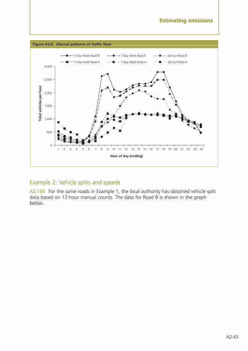
A2-43
Estimating emissions
Example 2: Vehicle splits and speeds
A2.156 For the same roads in Example 1, the local authority has obtained vehicle splitdata based on 12-hour manual counts. The data for Road B is shown in the graphbelow.
Figure A2.6: Diurnal patterns of traffic flow
0
500
1,000
1,500
2,000
2,500
3,000
1 2 3 4 5 6 7 8 9 10 11 12 13 14 15 16 17 18 19 20 21 22 23 24
Hour of day (ending)
Tota
l veh
icle
s p
er h
ou
r
5 Day Week Road B 7 Day Week Road B Sat-Sun Road B
5 Day Week Road A 7 Day Week Road A Sat-Sun Road A
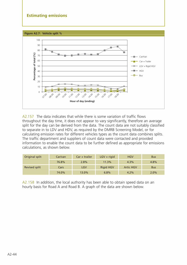
A2.157 The data indicates that while there is some variation of traffic flowsthroughout the day time, it does not appear to vary significantly, therefore an averagesplit for the day can be derived from the data. The count data are not suitably classifiedto separate in to LDV and HDV, as required by the DMRB Screening Model, or forcalculating emission rates for different vehicles types as the count data combines splits.The traffic department and suppliers of count data were contacted and providedinformation to enable the count data to be further defined as appropriate for emissionscalculations, as shown below.
A2.158 In addition, the local authority has been able to obtain speed data on anhourly basis for Road A and Road B. A graph of the data are shown below.
Original split Car/van Car + trailer LGV + rigid HGV Bus
76.8% 2.8% 11.3% 4.3% 4.8%
Revised split Cars LGV Rigid HGV Artic HGV Bus
74.0% 13.0% 6.8% 4.2% 2.0%
Figure A2.7: Vehicle split %
A2-44
Estimating emissions
0
10
20
30
40
50
60
70
80
90
100
07:0
008
:00
09:0
010
:00
11:0
012
:00
13:0
014
:00
15:0
016
:00
17:0
018
:00
Hour of day (ending)
Perc
enta
ge
of
tota
l (%
)
Car/Van
Car + Trailer
LGV + Rigid HGV
HGV
Bus

A2-45
Estimating emissions
A2.159 The speed graph shows that the two roads have different speed profiles, andthe average speed of Road A is much lower than Road B, particularly at night. Theaverage speed for the relevant road should be applied to roads of a similar nature. Fordetailed modelling in areas of exceedences, a variation in speed throughout the dayshould be considered. Using the shape of the profiles, a separate speed for the daytimeand one for night-time would sufficiently reflect the variation throughout the day.
Example 3: Calculating the volumetric flow rate
A2.160 The calculation of rates of emission from monitoring results requires ameasurement of the flowrate of the discharge at specified conditions of temperature,pressure, moisture content and oxygen content. When the flow rate is not reportedwith the monitoring results an approximate estimate can be calculated from the stackdiameter (m) and stack gas velocity (m/s) as follows:
However, this calculation may contain substantial errors if the actual temperature,oxygen content and moisture content of the discharge is markedly different from thespecified conditions. Seek expert advice if in doubt – for Part A1 processes, check withthe local Environment Agency, SEPA, or Industrial Pollution and Radio ChemicalInspectorate of the Environment and Heritage Service.
flow rate = area of stack x stack velocity
m3/s = m2 x m/s
Figure A2.8: Vehicle speed variation by time of day
0
10
20
30
40
50
60
1 2 3 4 5 6 7 8 9 10 11 12 13 14 15 16 17 18 19 20 21 22 23 24
Hour of day (ending)
Spee
d (
kph
)
Road A
Road B

A2-46
Estimating emissions
Worked example of how to obtain an approximate estimate of flow rate:
A 13 m high stack has a diameter of 0.4 m.
Stack gas velocity is 12 m/s
Example 4: Estimating emission data from monitoring data
A2.161 The following data has been obtained from the Public Register:
A2.162 This method can also be used to calculated release rates (g per s) frommonitoring data. In this case the annual operating hours are not required and thefollowing calculation would be carried out:
Annual carbon monoxide emissions
CO = 173 x 2.1 x 3600 x 2000 x 0.000001
kg/yr = mg/Nm3 x Nm3/s x s/hr x hr/yr x kg/mg
= 2616 kg/yr
Note: When using monitoring data from a batch process it is important to use the actual operatinghours (i.e. those for which the process is operating and not the opening hours of the facility) tocalculate annual emissions.
Process Crematoria, Part B process, 5.1
No of process units One
No of flues One
Stack height 15 m
Volumetric flow at reference conditions of temperature, pressure, moisture content and oxygen content 2.1 Nm3/s
CO emissions at reference conditions of temperature, pressure, moisture content and oxygen content 173 mg/Nm3
The following data has been assumed:
Operating hours 2000 hr/yr
Stack cross sectional area = πr2
= 3.14 x (0.4/2)2
= 0.126 m2
Flow Rate = 0.126 x 12
= 1.24 m3/s

A2-47
Estimating emissions
Example 5: Use of emissions factors for calculating emissions for industrialprocesses
A2.163 The following case study illustrates the general procedures used to calculateemissions from point-source processes using emission factors. Some of the featuresillustrated in this case study are:
• the scope of ideal activity data requirements from process operators.
• the limitations of activity data which is commonly available.
• the use of key engineering assumptions in completing the set of activity datarequired for the application of emission factors.
• the selection and use of emission factors.
Case Study 1
A2.164 This case study illustrates the use of emission factors where the operator hasprovided sufficient information such that no assumptions, regarding the process itself,need to be made.
A2.165 The following information has been obtained from the process operator:
Process Part B 1.3, waste oil combustion
No of flues One
Fuel use Waste oil
Sulphur content 1.8%
Ash content 0.1%
Oil consumption 76 m3/yr
Operating hours 1978 hours/year
Carbon monoxide emission rate (g per s)
CO = 173 x 2.1 x 0.001
g/s = mg/Nm3 x Nm3/s x g/mg
= 0.36 g/s
Note: When using monitoring data to estimate release rates (g per s), for pollutants with Air QualityObjectives with short term averaging periods, it is important to understand what operatingconditions the monitoring data represents. If the monitoring data are an average of manymonitoring runs, or typical of average conditions of operation it may not be representative ofworst case scenarios (e.g. start up/shut down).

A2-48
Estimating emissions
A2.166 The basic details supplied by the operator are sufficient for a simple emissionscalculation, using the emission factors from the UK EFDB. The emission factors for:sulphur monoxide, nitrogen oxides, carbon monoxide and PM and PM10 from the UK EFDB are as follows:
Using this information the following calculation can be made to estimate annualemissions for these pollutants:
Etot = F x T
Where:
Etot is the total annual emission for one of the case study pollutants (kg/yr).
F is the emission factor for a Part B waste oil combustion process (kg/m3).
T is the annual throughput of waste oil (m3/yr).
Application of the above equation results in the following annual emissions estimates:
Case Study 2
A2.167 This case study illustrates the use of emissions factors where the operator hasprovided insufficient information to enable a straight forward calculation of annualemissions from emission factors. This study highlights the limitations of activity dataand the nature of the assumptions that may be required in order to complete emissioncalculations. The following information has been obtained from the process operator:
Process Part B 1.3, waste oil combustion
No of flues One
Fuel use Waste oil
Thermal rating 0.5MW
Table A2.3: Annual emissions from waste oil burner (kg/yr)
Pollutant SO2 NOx CO PM PM10
Emission 2408 173 47 59 46
Table A2.2: Emission factors for waste oil combustion (units are kg per cubic metre of waste oil)
Pollutant SO2 NOx CO PM PM10
Factor 17.6 x S(a) 2.28 0.6 7.7 x A(b) 79% of PM
a S = weight % sulphur in fuelb A = weight % ash in fuel

A2-49
Estimating emissions
The throughput can be estimated from the thermal rating of a boiler. To calculate thethroughput the following information is required:
• annual operating hours and
• calorific value of the fuel.
In cases where the operating hours are not available, but are necessary to calculateannual emissions, it is reasonable to make an educated guess. The composition ofwaste oil varies according to its former use and, as such, it is difficult to provide fuelparameters that will be representative for all types of waste oil. In the absence of adetailed fuel specification it is possible to use fuel parameters for Heavy Fuel Oil(HFO)/residual oils. Average fuel parameters are provided in Appendix D.
Thus, to estimate fuel consumption the following assumptions have been made:
Using these assumed values the annual throughput can be calculated as follows:
T = (R x 3600 x H)/Cval
Where:
It should be noted that in calculating the throughput from the thermal rating of theboiler the following, additional, assumptions have been made:
The engine is continually operating at full load, and that fuel is consumed with 100percent efficiency.
T is the annual throughput of waste oil (m3/yr)
R is the thermal rating of the boiler (MW)
H is the annual operating hours (hr/yr)
Cval is the calorific value (of the waste oil) (MJ/m3)
In this instance:
R 0.5 MW
H 1920 hr/yr (assumed)
Cval 41808 MJ/m3 (assumed)
Thus,
T = (0.5 x 3600 x 1920)/41808
T = 83 m3/yr
Annual operating hours 8 hr/day, 5 day/week, 48 week/yr (1920 hr/yr)
Calorific value of oil 41,808 MJ/m3
A2-50
Estimating emissions
A2.168 Having calculated the annual throughput of waste oil the annual emissions canbe calculated as described above. For this case study the operator did not supply a fuelspecification thus, it will be necessary to make assumptions about the ash and sulphurcontent of the waste oil. In the absence of a detailed fuel specification it is possible touse fuel parameters for Heavy Fuel Oil (HFO)/residual oils. Average fuel parameters areprovided in Appendix D. It should be noted that waste oil generally has a lower sulphurcontent and a higher ash content than HFO/residual oil.
Assume:
This gives the following annual emissions:
Example 6: Area sources – emissions from coal combustion over aresidential areaA2.169 The following worked example illustrates the general procedures used tocalculate emissions from area-based sources. An example of emissions from generalcoal combustion over a small (hypothetical) residential area where there is high solidfuel or coal use is given. Particular features illustrated by this worked example are:
• the form of the base activity data commonly received from data suppliers.
• spatial re-apportionment using the capabilities of a mapping package/GIS.
• the importance of recognising and eliminating double-counting of emissions in area– source estimates.
A2.170 Activity data for area sources is often available only on a spatially-aggregatedbasis to protect commercial confidentiality, or simply due to the impracticality ofobtaining more detailed data. Where this is the case data needs to be re-apportionedfrom the original geography (which may typically be a postcode sector, electoral ward,county or even national level statistics) to the kilometre grid squares common to theother sources in the inventory. Data may also be estimated per household andapportioned per household. Coal sales data for an area were obtained from the severalcoal suppliers and merchants in the area for the last full year on a postcode-sectorbasis. Table A2.5 illustrates the typical form of the raw activity data. If the area inquestion is a smoke control area, so the solid fuel used will in fact be smokeless solidfuel (SSF).
Table A2.4: Annual emissions from waste oil burner (kg/yr)
Pollutant SO2 NOx CO PM PM10
Factor 2922 189 50 64 50
% sulphur in waste oil = 2.0%
% ash in waste oil = 0.1%

A2-51
Estimating emissions
A2.171 Industrial and commercial coal (for example, hospitals, council buildings)should be counted under point sources, where possible. If coal is accounted for as anarea source, care should be taken not to double-count.
A2.172 To be used in an emissions inventory, the original data (on a postcode sectorbasis) needs to be re-apportioned to the 1 by 1 km grid square geography. This can bedone using the capabilities of a mapping package. In this case, a simple re-apportionment based on area proportion is used (i.e. the individual grid squares areassigned values depending upon the extent to which they overlie postcode sectors withdifferent total values). More complex re-apportionments (for example, weighted byrelative population density or road length) can be devised if appropriate.
A2.173 The spatially re-apportioned fuel usage per kilometre grid square is thenmultiplied by the emissions factor to produce the emissions per grid square for eachpollutant. The emissions factors for domestic coal (as an example) are given in Table A2.7,and the final calculated emissions from domestic coal in Table A2.8, by multiplying thecoal used per square by the relevant emission factor.
Table A2.6: Coal sales data re-apportioned by kilometre grid square
Grid square (reference ID) Domestic coal (tonnes per year) Coke (tonnes per year)
354500,178500 17.97 1.60
355500,178500 12.38 0.68
356500,178500 6.14 0.05
354500,177500 16.89 1.20
355500,177500 14.72 0.07
356500,177500 18.99 1.58
354500,176500 12.35 0.06
355500,176500 14.96 0.09
356500,176500 17.68 1.20
Table A2.5: Coal sales data in tonnes per year, as received from fuel suppliers
Postcode sector Domestic coal (tonnes per year) Coke (tonnes per year)
BX8 3 102 19
BX9 1 38 2
BX9 2 45 0
BX9 3 57 5
BX10 7 62 0
BX11 0 110 10
BX11 8 54 3
BX11 9 81 2
BX20 0 70 0

A2-52
Estimating emissions
Table A2.8: Calculated emissions from domestic coal, in kg per year
Grid square Domestic SO2 NOx CO Benzene PM10(reference ID) coal burnt kg/yr kg/yr kg/yr kg/yr kg/yr
(tonnes/year)
354500,178500 17.97 377 536 24,114 6,945 72,226
355500,178500 12.38 260 369 16,613 4,784 49,758
356500,178500 6.14 129 183 8,239 2,373 24,678
354500,177500 16.89 355 504 22,665 6,527 67,885
355500,177500 14.72 309 439 19,753 5,689 59,163
356500,177500 18.99 399 566 25,483 7,339 76,326
354500,176500 12.35 259 368 16,572 4,773 49,638
355500,176500 14.96 314 446 20,075 5,782 60,128
356500,176500 17.68 371 527 23,725 6,833 71,060
Table A2.7: Emissions factors for domestic coal, in kg of pollutant per tonne of fuel
Pollutant SO2 NOx CO PM PM10
Factor 21 1.42 45 0.288 10.4

A2-53
Estimating emissions
Appendix B
Sources of emissions factors
A2.174 Although several sources of emission factors exist, the UK EFDB was developedto aid in the review and assessment procedure. (http://www.naei.org.uk/emissions). TheUK Emission Factor Database is based on emissions data used to derive the UK’sNational Atmospheric Emissions Inventory. The emission factors in this database are UKaverage factors for a large number of different source sectors including industrialprocesses, combustion, transport and residential and commercial combustion. Thedatabase also includes a number of screening factors based on employment, number ofprocesses and population.
Other information sources
Corinair, The Atmospheric Emission Inventory Guidebook(http://www.eea.int/aegb.indice.htm)
A2.175 This atmospheric emission inventory guidebook has been prepared by theexpert panels of the UNECE/EMEP Task Force on Emissions Inventories and is publishedand distributed by the European Environment Agency. The Guidebook is designed toprovide a comprehensive guide to atmospheric emission inventory methodology foreach of the emission-generating activities listed in the current version of the SelectedNomenclature for Air Pollution (SNAP 94), initially developed for the 1985 CorinairInventory.
US EPA AP 42 Compilation of Air pollutant Emission Factors(http://www.epa.gov/ttn/chief/ap42etc.html)
A2.176 The United States Environmental Protection Agency has developed a largecompendium of emission factors which is known as AP-42. AP-42 includes emissionfactors for most of the review and assessment pollutants The US EPA reviews andrevises its air pollutant emission factors every three years.
A2.177 Each AP-42 emission factor is given a rating from A through E, with A beingconsidered as being the most reliable. A factor’s rating is a general indication of thereliability, or robustness, of that factor. This rating is assigned based on the estimatedaccuracy of the tests used to develop the factor and on both the amount of dataavailable from tests and the representative characteristics of that data. In general,factors based on many observations, or on more widely accepted test procedures, areassigned higher rankings. Since ratings are subjective and only indirectly consider theinherent scatter amongst the data used to calculate factors, the ratings should be usedas approximations. An A rating should be considered an indicator of the accuracy andprecision of a given factor being used to estimate emissions from a large number ofsources.

A2-54
Estimating emissions
National Atmospheric Emissions Inventory (NAEI)www.naei.org.uk.
National Pollutant Inventory Guide, Australian Government (1998)http://www.environment.gov.au/net/npi.html.
Guide for Reporting to the National Pollutant Release InventoryIBSN 0-662-266129, 1997; http://www.ec.gc/pdb/npri/links.html.
United Nations Environment Programme; International and National PRTR Activities,Catalogue of Documents, 1998http://irptc.unep.ch/prtr/docs01.html.
World Health Organisation Internet web sitehttp://www.who.int.
Texas Natural Resource Conservation Commission (TNRCC) Permits Divisionhttp://www.tnrcc.com.
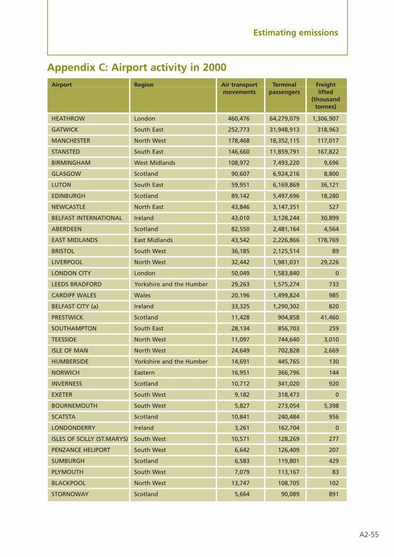
A2-55
Estimating emissions
Appendix C: Airport activity in 2000
Airport Region Air transport Terminal Freightmovements passengers lifted
(thousandtonnes)
HEATHROW London 460,476 64,279,079 1,306,907
GATWICK South East 252,773 31,948,913 318,963
MANCHESTER North West 178,468 18,352,115 117,017
STANSTED South East 146,660 11,859,791 167,822
BIRMINGHAM West Midlands 108,972 7,493,220 9,696
GLASGOW Scotland 90,607 6,924,216 8,800
LUTON South East 59,951 6,169,869 36,121
EDINBURGH Scotland 89,142 5,497,696 18,280
NEWCASTLE North East 43,846 3,147,351 527
BELFAST INTERNATIONAL Ireland 43,010 3,128,244 30,899
ABERDEEN Scotland 82,550 2,481,164 4,564
EAST MIDLANDS East Midlands 43,542 2,226,866 178,769
BRISTOL South West 36,185 2,125,514 89
LIVERPOOL North West 32,442 1,981,031 29,226
LONDON CITY London 50,049 1,583,840 0
LEEDS BRADFORD Yorkshire and the Humber 29,263 1,575,274 733
CARDIFF WALES Wales 20,196 1,499,824 985
BELFAST CITY (a) Ireland 33,325 1,290,302 820
PRESTWICK Scotland 11,428 904,858 41,460
SOUTHAMPTON South East 28,134 856,703 259
TEESSIDE North West 11,097 744,640 3,010
ISLE OF MAN North West 24,649 702,828 2,669
HUMBERSIDE Yorkshire and the Humber 14,691 445,765 130
NORWICH Eastern 16,951 366,796 144
INVERNESS Scotland 10,712 341,020 920
EXETER South West 9,182 318,473 0
BOURNEMOUTH South West 5,827 273,054 5,398
SCATSTA Scotland 10,841 240,484 956
LONDONDERRY Ireland 3,261 162,704 0
ISLES OF SCILLY (ST.MARYS) South West 10,571 128,269 277
PENZANCE HELIPORT South West 6,642 126,409 207
SUMBURGH Scotland 6,583 119,801 429
PLYMOUTH South West 7,079 113,167 83
BLACKPOOL North West 13,747 108,705 102
STORNOWAY Scotland 5,664 90,089 891

A2-56
Estimating emissions
Airport Region Air transport Terminal Freightmovements passengers lifted
(thousandtonnes)
KIRKWALL Scotland 9,339 86,790 736
SHEFFIELD CITY Yorkshire and the Humber 4,247 60,636 0
DUNDEE Scotland 2,468 49,667 0
ISLES OF SCILLY (TRESCO) South West 2,262 37,078 29
BENBECULA Scotland 3,537 35,516 311
ISLAY Scotland 1,567 20,579 171
WICK Scotland 2,937 20,484 5
CAMBRIDGE Eastern 1,643 19,845 43
CAMPBELTOWN Scotland 1,347 7,994 2
BARRA Scotland 1,247 7,689 40
KENT INTERNATIONAL South East 984 7,594 32,239
BATTERSEA HELIPORT London 2,237 6,452 0
BIGGIN HILL South East 1,323 6,168 1
TIREE Scotland 710 4,928 28
LERWICK (TINGWALL) Scotland 2,110 4,602 1
COVENTRY West Midlands 5,804 3,993 4,905
SOUTHEND South East 874 3,536 780
HAWARDEN North West 100 2,490 0
GLOUCESTERSHIRE South West 219 1,991 0
LYDD South East 267 1,522 5
UNST Scotland 682 1,429 0
SHOREHAM South East 665 1,379 13
CARLISLE North West 354 452 1
BARROW-IN-FURNESS North West 45 77 0

A2-57
Estimating emissions
Appendix D: The NAEI’s data warehouseA2.178 The NAEI’s data warehouse contains up-to-date emissions data for differentsources and pollutants. Data are available for download and e-mail delivery.
Emissions data warehouse
A2.179 This is an online archive of emissions and supporting mapping data availablefor use by local authorities (LAs), the wider scientific community and the public. Thedatasets provide LAs with the specific component emissions data that they need tosupplement their more detailed review and assessment studies.
Local authority data warehouse
A2.180 Data are stored on the warehouse for each local authority. The user can searchby keyword or can navigate through web pages listing the datasets available and selectthose required for download (the list below illustrates the data that are available).
By LA Boundary CSV files
Data type Sector Detail Notes
• Large point sources(by point location)
Point sources
All industrial sources excludingthe point sources in the datasetslisted below.
• Combustion
• Processes
Non-pointIndustry
Emissions grouped by the keyfuel types.
• Rail
• Shipping
• Mobile machinery
• Airports
Other transport
Emissions grouped by the keyfuel types.
• Coal
• Natural gas
• Oil
Domestic
Emissions broken down into theroad transport sectors necessaryfor review and assessment. ManyLA’s will be making DetailedAssessments for the major roadsand therefore will only requireother road transport emissionsform the system to completetheir picture.
• Major roads
• Cold starts
• Evaporative
• Minor roads
• Brake & tyre wear
Road transportNAEI calculatedemissions data (1 x 1 km*) forLAQM pollutants
A2-58
Estimating emissions
The browseable selection pages include brief descriptions of the datasets including: theyear of the dataset, description and assumptions and an expected update date.
By LA Boundary CSV files
Data type Sector Detail Notes
*Unless otherwise specified
• Ports activity
• Airports activity
Other transport
• AADF for majorroads by countpointlocation
• Minor roads AADF
Road transport
Emissions grouped by the keyfuel types.
• Coal
• Natural gas
• Oil
Domestic fueluse (GJ fuelconsumed)
• 1995 total number ofpeople
Population 1 x 1 km (totalnumber ofpeople)
Mapping datasets(1 x 1 km*)

A2-59
Estimating emissions
Appendix E: Significant point source processes lists
Part A processes likely to require review and assessment analysis
A2.181 The numbers below indicate how significant the process is likely to be for eachpollutant as a % of the total Part A emission in 2000. A blank cell indicates that theprocess can be ignored. 0 indicates an emission is likely but small in comparison toother Part A sources.
Processes are in order of general significance:
Process ID IPC process name CO NOx PM SO2 Lead Benzene 1,3-butadiene
2.1 Iron and steel 57 19 61 9 37
1.4 Petroleum processes 0 16 4 15 0 73 2
4.1 Petrochemical processes 0 0 0 2 95
1.3 Combustion processes 1 34 13 45 2 0 0
2.2 Non-ferrous metals 17 1 4 7 23
4.2 Manufacture and use of 0 0 0 0 35 0 3organic chemicals
1.2 Carbonisation and 2 6 2 10 2 12associated processes
3.1 Cement\lime manufacture and associated processes 1 9 7 3 1 7 0
4.4 Processes involving halogens 19 1 0 0 0
3.6 Ceramic production 1 0 4 9
1.1 Gasification and associated 0 4 0 5processes
4.5 Inorganic chemical processes 1 4 0 1
6.3 Tar and bitumen processes 0 0 3 1 1
4.6 Chemical fertiliser production 0 1 2
3.3 Other mineral fibres 0 1 1 0 0
5.1 Incineration 0 2 0 0 0
6.1 Paper and pulp manufacturing 0 0 0 0processes
4.3 Acid processes 0 0 0 0 0
3.5 Glass manufacture and 0 0production
5.2 Recovery processes 0 0 0 0 0 0
6.9 Treatment/processing of animalor vegetable matter 0 0
5.3 Production of fuel from waste 0 0
6.5 Coating processes and printing 0 0
3.2 Processes involving asbestos 0

A2-60
Estimating emissions
Part B/A213 processes likely to require review and assessment analysis
A2.182 The following table gives an indication (x) of those processes most likely torelease significant quantities of the specified substances to air. It should be noted thatthis table is not comprehensive, and authorities are advised to rely upon local,professional judgement. In the event of doubt, additional advice may be sought fromthe Emissions Helpdesk.
Process PG Carbon Benzene 1,3- Sulphur Nitrogen Lead PM10
note(s) monoxide butadiene* dioxide** oxides
Waste oil combustion 1/1, 1/2
Combustion plant 1/3, 1/4,20-50 mwth 1/5 x x
WDF combustion <3 mwth 1/10
Reheat furnaces 20-50 mwth 1/11 x x
Waste combustion 0.4-3 mwth 1/12
Processes for the storage, 1/13 xloading and unloading of petrol at terminals
Unloading of petrol into 1/14storage at service stations
Furnaces for extraction of 2/1 xnon-ferrous metals from scrap
Galvanising 2/2
Electrical and rotary furnaces 2/3 x
Foundry Processes 2/1
Hot land cold blast cupolas 2/5 x x
Aluminium and aluminium 2/6 x xalloy processes
Zinc and zinc alloy processes 2/7 x x
Process ID IPC process name CO NOx PM SO2 Lead Benzene 1,3-butadiene
6.2 Di-isocyanate processes 0 0
4.7 Pesticide production 0
2.3 Smelting processes 0 0 0 0
3.4 Other mineral processes 0
4.8 Pharmaceutical production
4.9 Storage of chemicals in bulk 0
6.4 Processes involving uranium
6.6 Manufacture of dyestuffs/ 0 0printing ink/coating mats
6.7 Timber processes
6.8 Processes involving rubber 0
7.0 Sewage treatment works
13 In Northern Ireland some of these processes may be Part C authorised by District Councils.

A2-61
Estimating emissions
Process PG Carbon Benzene 1,3- Sulphur Nitrogen Lead PM10
note(s) monoxide butadiene* dioxide** oxides
Copper and copper alloy 2/8 x xprocesses
Metal decontamination 2/9
Blending, packing, loading 3/1and use of bulk cement
Manufacture of heavy clay 3/2 xgoods and refractory goods
Glass (excluding lead glass) 3/3 x xmanufacturing processes
Lead glass manufacturing 3/4 x xprocesses
Coal, coke, coal product and 3/5 xpetroleum coke processes
Exfoliation of vermiculite and 3/7expansion of perlite
Quarry processes 3/8 x
Plaster processes 3/12
Lime processes 3/14
Roadstone coating 3/15 x x
China and ball clay processes 3/17 xincluding the spray drying of ceramics
Processes for the surface 4/1treatment of metals
Incineration processes 5/1, 5/3,5/4
Crematoria 5/2
Processes for the manufacture 6/4of particleboard and fibreboard
Textile and fabric coating 6/8processes (where nitrogen containing solvents are used)
Manufacture of coating 6/9 xpowder
Coil coating (where nitrogen 6/13 xsolvents are used)
Heat set web offset 6/16printworks
Rubber processes 6/28 x x
Powder coating processes 6/31
Metal and other thermal 6/35spraying process
*only if 1,3-butadiene is used as part of the process
**only if process burns coal or heavy fuel oil
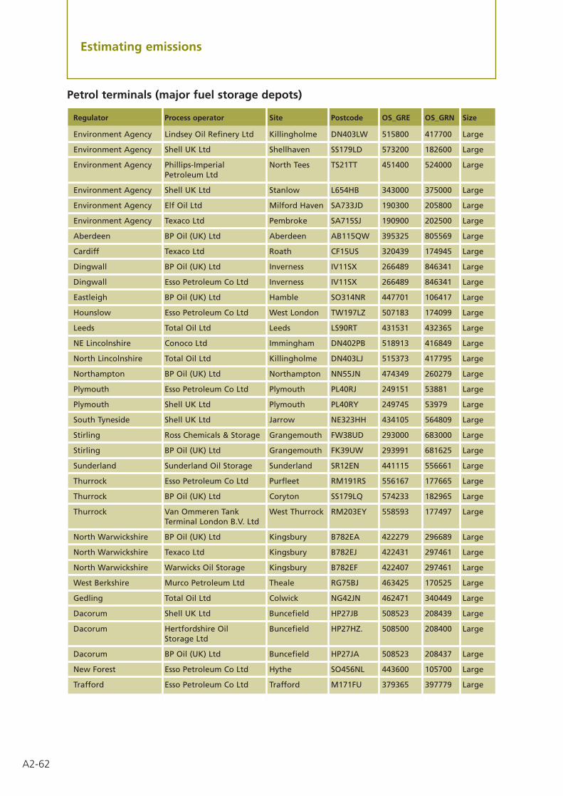
A2-62
Estimating emissions
Petrol terminals (major fuel storage depots)
Regulator Process operator Site Postcode OS_GRE OS_GRN Size
Environment Agency Lindsey Oil Refinery Ltd Killingholme DN403LW 515800 417700 Large
Environment Agency Shell UK Ltd Shellhaven SS179LD 573200 182600 Large
Environment Agency Phillips-Imperial North Tees TS21TT 451400 524000 LargePetroleum Ltd
Environment Agency Shell UK Ltd Stanlow L654HB 343000 375000 Large
Environment Agency Elf Oil Ltd Milford Haven SA733JD 190300 205800 Large
Environment Agency Texaco Ltd Pembroke SA715SJ 190900 202500 Large
Aberdeen BP Oil (UK) Ltd Aberdeen AB115QW 395325 805569 Large
Cardiff Texaco Ltd Roath CF15US 320439 174945 Large
Dingwall BP Oil (UK) Ltd Inverness IV11SX 266489 846341 Large
Dingwall Esso Petroleum Co Ltd Inverness IV11SX 266489 846341 Large
Eastleigh BP Oil (UK) Ltd Hamble SO314NR 447701 106417 Large
Hounslow Esso Petroleum Co Ltd West London TW197LZ 507183 174099 Large
Leeds Total Oil Ltd Leeds LS90RT 431531 432365 Large
NE Lincolnshire Conoco Ltd Immingham DN402PB 518913 416849 Large
North Lincolnshire Total Oil Ltd Killingholme DN403LJ 515373 417795 Large
Northampton BP Oil (UK) Ltd Northampton NN55JN 474349 260279 Large
Plymouth Esso Petroleum Co Ltd Plymouth PL40RJ 249151 53881 Large
Plymouth Shell UK Ltd Plymouth PL40RY 249745 53979 Large
South Tyneside Shell UK Ltd Jarrow NE323HH 434105 564809 Large
Stirling Ross Chemicals & Storage Grangemouth FW38UD 293000 683000 Large
Stirling BP Oil (UK) Ltd Grangemouth FK39UW 293991 681625 Large
Sunderland Sunderland Oil Storage Sunderland SR12EN 441115 556661 Large
Thurrock Esso Petroleum Co Ltd Purfleet RM191RS 556167 177665 Large
Thurrock BP Oil (UK) Ltd Coryton SS179LQ 574233 182965 Large
Thurrock Van Ommeren Tank West Thurrock RM203EY 558593 177497 LargeTerminal London B.V. Ltd
North Warwickshire BP Oil (UK) Ltd Kingsbury B782EA 422279 296689 Large
North Warwickshire Texaco Ltd Kingsbury B782EJ 422431 297461 Large
North Warwickshire Warwicks Oil Storage Kingsbury B782EF 422407 297461 Large
West Berkshire Murco Petroleum Ltd Theale RG75BJ 463425 170525 Large
Gedling Total Oil Ltd Colwick NG42JN 462471 340449 Large
Dacorum Shell UK Ltd Buncefield HP27JB 508523 208439 Large
Dacorum Hertfordshire Oil Buncefield HP27HZ. 508500 208400 LargeStorage Ltd
Dacorum BP Oil (UK) Ltd Buncefield HP27JA 508523 208437 Large
New Forest Esso Petroleum Co Ltd Hythe SO456NL 443600 105700 Large
Trafford Esso Petroleum Co Ltd Trafford M171FU 379365 397779 Large

A2-63
Estimating emissions
Regulator Process operator Site Postcode OS_GRE OS_GRN Size
Poole Texaco Ltd Poole BH154AJ 400561 90131 Large
Unknown Shell UK Ltd Londonderry BT487SH 60814 581770 Large
Unknown Esso Petroleum Co Ltd Belfast BT39EA 149039 531001 Large
Unknown BP Oil (UK) Ltd Wymondham NR189QY 613475 300773 Large
Unknown Esso Petroleum Co Ltd Erdington B248DN 411383 290193 Large
Unknown Esso Petroleum Co Ltd Avonmouth BS119BN 352095 180611 Large
Carlisle BP Oil (UK) Ltd Dalston CA57LX 336443 550441 Medium
NE Lincolnshire Simon Storage Co Ltd West Riverside DN402QU 519215 416829 Medium
South Gloucestershire Murco Petroleum Ltd Westerleigh BS378QE 370599 180461 Medium
Stockton-On-Tees Seal Sands Storage North Tees TS21UB 451495 524057 Medium
Thurrock ST Services Ltd Grays RM175YU 560381 178279 Medium
Kings Lynn Kings Lynn Storage Ltd Kings Lynn PE302HH 561861 321357 Small
Slough Total Oil Ltd Slough SL36ED 500839 179959 Small
Nuneaton and Murco Petroleum Ltd Bedworth CV79EJ 435865 285461 SmallBedworth
Adur Texaco Ltd Brighton BN411EL 526235 104871 Small
Isle of Wight Dominion Oils Ltd East Cowes PO326HF 450353 94595 Small
Unknown BP Oil (UK) Ltd Fort William PH336LR 211311 774411 Small
Unknown BP Oil (UK) Ltd Benbecula HS85NU 81245 843447 Small
Unknown BP Oil (UK) Ltd Orkney KW151LG 345079 1011249 Small
Unknown BP Oil (UK) Ltd Skye IV519XP 139745 864749 Small
Unknown BP Oil (UK) Ltd Lerwick ZE10LZ 447537 1141803 Small
Unknown BP Oil (UK) Ltd Stornoway HS12BS 142535 932659 Small
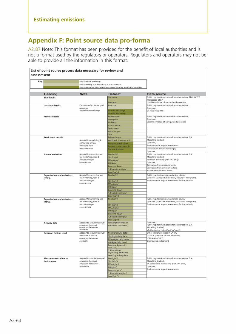
A2-64
Estimating emissions
Appendix F: Point source data pro-formaA2.87 Note: This format has been provided for the benefit of local authorities and isnot a format used by the regulators or operators. Regulators and operators may not beable to provide all the information in this format.
Key Required for Screening
Required only if primary data is not available
Required for detailed assessment and if primary data is not available
Heading Note Dataset Data sourceSite details Site name
Operator
Location details Can be used to derive grid reference
Postcode
OS Grid east (6fig)
OS Grid north (6fig)
Process details Process code
descriptionPG/Note
source sector
Sector notes
emission type
Year
Stack/vent details Release height
vent/stack diameter (m)
flue gass velocity (m/s)flue gas temperature ©
Stack restrictions Observation (Local Knowledge),Operator
Annual emissions Nox (kg/yr)
SO2 (kg/yr)
PM10 (kg/yr)CO (kg/yr)
Benzene (kg/yr)
1,3-butadiene (kg/yr)
Lead (kg/yr)
Expected annual emissions (2005)
Nox (kg/yr)
SO2 (kg/yr)
PM10 (kg/yr)CO (kg/yr)
Benzene (kg/yr)
1,3-butadiene (kg/yr)
Lead (kg/yr)
Expected annual emissions (2010)
Nox (kg/yr)
SO2 (kg/yr)
PM10 (kg/yr)CO (kg/yr)
Benzene (kg/yr)
1,3-butadiene (kg/yr)
Lead (kg/yr)
Activity data Needed to calculate annual emissions if annual emissions data is not available
consumption (mass or volume or number/yr)
Operator,Public register (Application for authorisation, EIA, Modelling Studies),sAuthorisation notes (Part “A” only)
Emission factors used Nox (kg/activity data)
SO2 (kg/activity data)
PM10 (kg/activity data)
CO (kg/activity data)
Benzene (kg/activity data unit)1,3-butadiene (kg/activity data unit)
Lead (kg/activity data)
Nox (g/m3)SO2 (g/m3)
PM10 (g/m3)
CO (g/m3)
Benzene (g/m3)
1,3-butadiene (g/m3)
Lead (g/m3)
Needed for screening and for modelling peak & annual average exceedences
Measurements data or limit values
Public register (emission reduction plans),Operator (Expected abatement, closure or new plant),Environmental impact assessments for future build
Other similar processes in LA list,UYEFDB (Emission factors database),USEPA (Air CHIEF),Engineering Judgement
Public register (Application for authorisation, EIA, Modelling Studies),EA compliance monitoring (Part “A” only),Operator,Environmental impact assessments.
Needed to calculate annual emissions if annual emissions data is not avaialable
Needed to calculate annual emissions if annual emissions data is not available
Needed for screening and for modelling peak & annual average exceedences
Public register (Application for authorisation, EIA, Modelling studies),Operator,Environmental impact assessments
Public register (Application for authorisation), Operator,Local knowledge of unregulated processes
Public register (Application for authorisation) REGULATED PROCESSES ONLYLocal knowledge of unregulated processes
Public register (Application for authorisation),Operator,OS map (1:50,000)
Public register (Application for authorisation, EIA, Modelling studies),Pollution Inventory (Part “A” only)Operator,Estimation from measurements,Estimation from emission factors,Estimation from limit values
Public register (emission reduction plans),Operator (Expected abatement, closure or new plant),Environmental impact assessments for future build
Needed for modelling
Needed for modeling & estimating annual emissions from measurements
Needed for screening and for modelling peak & annual average exceedences
List of point source process data necessary for review and assessmsent

A2-65
Estimating emissions
Heading Note Dataset Data sourceOperating profiles (Specific)
Hourly
01:00
02:00
03:0004:00
05:00
06:00
07:00
08:00
09:00
10:0011:00
12:00
13:00
14:00
15:00
16:00
17:00
18:0019:00
20:00
21:00
22:00
23:00
00:00
Mon
Tue
Wed
Thu
Fri
Sat
Sun
MonthlyJan
Feb
Mar
Apr
May
Jun
Aug
Sep
Oct
Nov
Dec
Needed for estimating emissions from concentration measurements and modelling peak emissions exceedences. Enter relative values into each profile
Public register (Application for authorisation, EIA, Modelling studies),Operator,Environmental impact assessments.

A2-66

Modelling
IntroductionA3.01 This Annex of the technical guidance provides advice to local authorities on theuse of air quality dispersion models1 for review and assessment. Dispersion models area valuable tool in the review and assessment process for a variety of reasons:
• pollutant emissions arising from different source types (for example, industrialchimneys, road traffic etc) can be taken into account in terms of their impact uponground-level concentrations.
• concentrations across a wide geographical area can be predicted, and assist with thedetermination of the geographic boundaries of any exceedences of the objectives.
• concentrations can be predicted for future years (i.e. the years in which theobjectives are to be achieved), taking into account emission controls and new orchanged source emissions.
• scenario testing can be effectively undertaken to determine source contributions andcontrol strategies.
A3.02 The purpose of this section of the technical guidance is:
• to promote best practice and efficient use of resources for dispersion modelling2.
• to provide local authorities with a clear and concise method for ensuring that thenecessary sources have been considered using a variety of nomograms and screening tools.
• to provide guidance which allows specific sources/sites at which there are potentialexceedences of the air quality objectives to be identified and focussed upon in detail.
• to help obtain as reasonable results as practicably possible to increase confidence inmodelling outputs.
• to aid in the sensible interpretation of results.
A3.03 In writing this guidance, feedback gathered during the evaluation of the firstround of review and assessment3 and from key users and suppliers of models(Appendices B and C) has been considered.
A3.04 It is recognised that many local authorities have already made an informedchoice regarding dispersion modelling tools during the course of the First Round ofreview and assessment. For future rounds of review and assessment, authorities maywish to ‘fine-tune’ the inputs (to improve the accuracy of the results) and carry out moreextensive verification (of the modelling results against a larger monitoring dataset).
Annex 3 Modelling
A3-1
1 Manual on Modelling: A Guide for Local Authorities, D. R. Middleton, Met O (APR) Turbulence and Diffusion NoteNo. 241 (to be made available on the Met Office website www.meto.gov.uk).
2 Royal Meteorological Society Policy Statement. Atmospheric Dispersion Modelling: Guidelines on the justification ofchoice and use of models, and the communication and reporting of results. Published in collaboration with theDepartment of the Environment, May 1995. The Royal Meteorological Society, Reading.
3 Evaluation of the First Round of Review and Assessment of the Local Air Quality Management Process. Report forDefra and the Devolved Administrations.

A3-2
Modelling
A3-2
Modelling
LAQM toolsA3.05 The amount of data management required through the process of review andassessment varies between local authorities. Some authorities have already set updetailed emissions inventories but these need to be reviewed periodically as objectiveschange, as new potential sources become relevant and when annual Progress Reportsare produced.
A3.06 A number of LAQM tools have been provided (available for download fromwww.airquality.co.uk) to help manage the data collected for review and assessment.The first step of updating and screening may be carried out using the LAQM tools asthey allow:
• an updateable pro-forma system for storing basic information on sources usinginformation set out in Annex 2 (Estimating Emissions).
• a link to the initial nomograms and screening tools for easy screening without theneed for a paper based assessment.
• quick and easy notification of significant sources.
A3.07 The LAQM tools have also been developed with requirements for yearly updatesin mind. The system can be easily updated by multiple users and stored, and shouldform a useful checklist when appraising the progress and outcomes of the review andassessment process.
A3.08 The LAQM tools have not been designed to negate the need for detailedemissions inventories but to be used as a checking system to focus more on areaswhere there have been significant changes that may not be highlighted in existingemission inventories. Where changes to, or additional sources, are identified, detailedemissions inventories should also be updated to reflect these.
A3.09 The use of the LAQM tools should make the management of the review andassessment process easier, particularly when different personnel have to pick up tasks atvarying stages of the process.
A3.10 The evaluation of the first round of review and assessment highlighted thatmore co-operation between different departments within local authorities would help.The LAQM tools may be easily accessed by other users, such as those in planning andtransport departments, to allow them to view information (such as those roads whichrequire Detailed Assessment), and to fill gaps in the information required.
A3.11 The LAQM tools are an additional aid for local authorities to use throughout theLAQM review and assessment process, but there is no requirement to use this facilityshould systems already be in place. However, for many, the LAQM tools will be a usefulresource.

A3-3
Modelling
A3-3
Source data requirementsA3.12 Previous experience from review and assessment has indicated that there aretwo main types of sources that need to be considered:
• road traffic sources.
• point sources (i.e. stacks).
A3.13 Other sources which may be treated as area sources (from domestic coalburning or agriculture), rail, air, shipping and fugitive sources may also be significant in some areas.
A3.14 The requirements for assessing all of these types of sources and information onscreening the potential significance of these sources are provided below.
Road traffic sourcesA3.15 For road traffic sources basic information which helps in the initialidentification and management of the source includes:
• the name of the road (for example, A27).
• a name for the section being assessed.
for example, single section between New Town and Old Town
for example, junction of A27 and B1069 in New Town
(It may also be useful at this stage to identify the road using grid references but this isnot essential when first determining the significance of roads.)
A3.16 The checklists in the main body of TG(03) should first be used to determinewhat general annual average daily traffic (AADT) flows are relevant for each pollutantbefore estimating the HDV percentage and speeds on roads. The Road TrafficInformation Spreadsheet (www.airquality.co.uk/archive/laqm/tools.php) also allows theinformation to be stored and contains an electronic version of the checklists in relationto road traffic.
A3.17 Once potentially significant roads have been identified, the DMRB screeningmethod can be used to further assess roads (www.airquality.co.uk/archive/laqm/tools.php).The DMRB Screening Model (v1.01) allows quick and easy assessment of road trafficsources. The DMRB Screening Model (v1.01) allows for the assessment of pollutantlevels at relevant receptors that are within 200 m of the centre of a road for therelevant year of the objective.
A3.18 Before using the DMRB Screening Model (v1.01), the following informationshould be collected:

A3-4
Modelling
1. the annual average daily traffic flow based on 24-hour flows (AADT24)4 – do not usethe peak hour traffic flow.
2. the average percentage split of vehicle categories as either:
• Heavy Duty Vehicles (HDV) and Light Duty Vehicles (LDV); or
• Passenger Cars, Light Good Vehicles (LGV), Rigid Heavy Good Vehicles (HGV), ArticHGV, and Buses/Coaches.
3. an estimate of the average speed of vehicles (km/hr).
4. growth factors to adjust traffic flows to the relevant year of assessment.
A3.19 As a guide, an HDV is any vehicles weighing over 3.5 tonnes, which can befurther split into Rigid vehicles (2 and 3 axles), Artic vehicles (3 or more axles), and Busesand Coaches. An LGV weighs less than 3.5 tonnes but is not a general passenger car.
A3.20 The information for individual roads can be collated in the Road TrafficInformation Spreadsheet (www.airquality.co.uk/archive/laqm/tools.php). This tool allowsthe user to collate information on relevant road links for assessment against thescreening criteria set out in the checklists in the main chapters and to identify if aDMRB screening exercise is required.
A3.21 The DMRB Screening Model (v1.01) can be used to predict the annual averageconcentrations of nitrogen oxides, nitrogen dioxide, PM10, carbon monoxide, benzeneand 1,3-butadiene. Through the use of empirical statistics derived from the analysis ofmonitored PM10 data in the UK, estimates of the concentrations over a 24-hour averagingperiod can be derived from the annual mean predictions to allow an assessment of theshorter-term AQS objective. Monitoring data indicates a poor relationship between theannual mean and the 8-hour carbon monoxide and 1-hour nitrogen dioxide objectivetherefore these short-term objectives are not predicted in the revised DMRB.
A3.22 The emissions factors calculated within the DMRB Screening Model (v1.01) arederived directly from the Emission Factors Toolkit (see section A3.43).
A3.23 For stand-alone roads (i.e. not a junction), the same information as detailed inA3.18 is required by the DMRB. In addition, the following will be required:
• the distance from the road centre line to the nearest receptor, which should allow anassessment of the worst-case location.
A3.24 For junctions the following additional information is required and may be storedin the Road Traffic Information Spreadsheet:
• is the junction an intersection or a roundabout?
• the number of arms at the junction or roundabout (this will typically be four).
4 In some cases, annual average daily traffic flows are provided based on 12, 16, 18 or 24-hour periods. The 24-hour AADT should be used.

A3-5
Modelling
• the AADT24 flow on each arm.
• the average speed on each arm.
• the percentage vehicle split (see section A3.18) on each arm.
• the distance to receptor (from centre of the road) to relevant arms.
• turning movements for each arm.
A3.25 The DMRB Screening Model (v1.01) contains advice on assessing junctions.Where complex junctions exist, and particularly where there is relevant exposure, theuse of monitoring (continuous or validated diffusion tubes) should not be overlooked as an effective method of assessment.
A3.26 Where street canyons or enclosed streets with buildings close to the road onboth sides are highlighted, the DMRB may not reasonably estimate concentrationswithin these environs, due the complex nature of pollution dispersion. In these cases,other screening tools such as AEOLIUS (produced by the Met Office5 and based on theDanish OSPM model), or monitoring should be considered.
A3.27 More information on the consideration of street canyons and complex roads is provided in the Detailed Assessment of Roads section A3.56.
A3.28 Where possible, the estimates from the DMRB should be compared against anylocal monitoring, provided it is of good quality, over a reasonable time period andrepresentative of the receptor locations that have been assessed.
A3.29 If the DMRB assessment indicates that exceedences of the AQS objectives mayoccur, it will be necessary to progress to a more Detailed Assessment. This may includethe use of more complex dispersion models, and/or the use of monitoring data.
A3.30 The main chapters of this document provide information regarding the currentpicture on where exceedences of the objectives due to road traffic are occurring. Ingeneral, where exceedences of the annual mean nitrogen dioxide and PM10 objectivesdue to road traffic are an issue, they are expected to occur within about 30 metres ofthe carriageway.
A3.31 In terms of the short-term objectives, there are only a handful of locationswhere an exceedence of the hourly objective of nitrogen dioxide and daily objective of PM10 is likely to occur due to road traffic, most being in central London or othermajor conurbations. Therefore, it is likely that most local authorities should focus on predictions of annual mean and 24-hour concentrations when progressing todetailed modelling.
A3.32 Annex 2 (Emissions Estimates) contains the answers to some common questionsregarding estimating traffic flows including:
• who do I contact for traffic flow information?
• what year of assessment do I use?
5 www.metoffice.gov.uk/environment/aeolius1.html
A3-6
Modelling (continued)
• what if no traffic figures have been made available?
• what type of traffic count information can I use?
• how do I estimate speeds at junctions?
• the DMRB needs AADT24 traffic flows – what if my data are not in this format?
• how do I know my flows are representative for the year?
Detailed Assessment of road traffic emissions
A3.33 Where potential exceedences of an AQS objective have been indicated by theDMRB, or where a particularly complex site such as a junction or a street canyon, whichwas not fully assessed using screening tools, has been identified, a Detailed Assessmentshould be carried out.
A3.34 Any Detailed Assessment may include modelling but monitoring also has animportant role to play. Data from continuous analysers, diffusion tubes or other long-term monitoring, can be used in a number of ways including:
• to provide further information on pollution levels in complex areas such as largeand/or congested junctions, and street canyons or similar that may not be assessedwell by dispersion models.
• to provide information that can be used to help verify any dispersion modelling thatis undertaken.
A3.35 It is expected that most local authorities proceeding to detailed modelling ofroad traffic will be concerned with potential exceedences of the annual mean (fornitrogen dioxide and/or PM10) and the 24-hour mean PM10 objectives.
A3.36 In general, the use of more complex dispersion models will require a certainamount of geographical information such as:
• the grid reference of the start and end points of a section of road.
• the width of the road being assessed.
• the grid reference of the specific receptors at which pollution levels need to beassessed.
so that the orientation of sources and receptors can be taken account of when winddirections are included in the modelling.
A3.37 The use of Geographical Information Systems (GIS) can be a quick and easy wayto retrieve the correct co-ordinates for sources that can be input directly into dispersionmodels.
A3.38 Most dispersion models allow more complex traffic patterns than a single AADTto be assessed including:
A3-7
Modelling
• basic AADT patterns varied by day of the week.
• diurnal patterns varying for each hour of the day, and also by day of the week.
A3.39 For either of these patterns, the speed and proportion of HDVs may also vary,therefore requiring a wide range of traffic patterns to be assessed.
A3.40 In addition, many models allow a wider vehicle split to be assessed, which mayinclude (but is not limited to) the following vehicle type classifications:
• Cars (petrol and diesel).
• LGV (petrol and diesel).
• HGV (rigid and artic).
• Buses and Coaches.
• Taxis (some times defined as a separate category when derived from traffic models).
A3.41 Some models also allow the details of Euro engine standard of vehicle types tobe defined by the user (Euro is a term used to link the relevant EC Directive that setslimit values on emissions from vehicles manufactured or first registered after certaindates. Further information is available on www.naei.gov.uk). These vehicle splits maybe supplied to a model through means of an emissions inventory, or may be input intothe model by using aggregated emissions factors that take account of the total flow ona road.
A3.42 The extent to which a detailed breakdown of sources is required for review andassessment is discussed in the next section.
Emission Factors Toolkit (EFT)
A3.43 For the purposes of review and assessment, all emissions estimations of roadtraffic tailpipe emissions should be based on the Emission Factors Toolkit(www.stanger.co.uk/airqual/modelhlp) which allow various sets of aggregated emissionfactors in terms of g/km.veh to be calculated. The data on which the EFT is based isprovided on the NAEI website (www.naei.org.uk) and were derived from recent updatesto road transport emission factors undertaken by TRL6. The EFT is available to modellersand model developers to ensure that the same set of emission factors are being usedby all local authorities.
A3.44 Generally, most people require a set of emission factors in terms of basic vehiclesplits such as Light Duty Vehicles (LDV), and Heavy Duty Vehicles (HDV) only, or moredetailed splits such as cars, Light Goods Vehicles, Heavy Goods Vehicles, and buses. Inorder to calculate emission factors for these vehicle splits the raw emission factors mustbe aggregated based on the relative proportions of each vehicle type. This aggregationalso needs to take account of the Euro classification of vehicle engines within particularvehicle classification.
6 TJ Barlow, A J Hickman, P Boulter. Exhaust Emission Factors 2001: Database and Emission Factors, TRL Limited.Project Report PR/SE/230/00.

A3-8
Modelling
A3.45 Box A3.1 below shows the variety of emission factors that can be calculated byusing the Emission Factors Toolkit.
A3.46 The road traffic emissions data within the EFT and NAEI should be used by alllocal authorities until further notice from DEFRA. Where a local authority is notplanning on using data from the EFT, they should contact the helpdesks to discussalternative approaches.
A3.47 If a model requires emission estimates in a format other than g/km.veh, youshould contact the model developer for guidance on adjusting the emissions to therequired format if the model does not automatically calculate them.
How detailed should my traffic flows be at the detailed modelling stage?
A3.48 The following level of detail is recommended:
• determine annual average traffic flows and use diurnal patterns where available.
• determine annual average speeds on roads and near junctions.
• determine average vehicle splits.
• focus your detailed modelling on specific areas and specific receptors to scales of 10sof metres as opposed to wider scale modelling that may miss out the details atroadside locations where exceedences are more likely.
Box A3.1: Types of emission factors calculated using the EFTFor each type of split, proportions of those in BOLD are user defined while those in Italicare based on defaults
Type 1 Type 2 Type 3 Type 4 Type 5
LDV CARS PETROL CARS PETROL CARS CARS
Petrol Cars Petrol Cars Petrol Cars
Diesel Cars Diesel Cars DIESEL CARS DIESEL CARS Diesel Cars
Petrol LGV
Diesel LGV LGV PETROL LGV PETROL LGV TAXIS+
Petrol LGV
Diesel LGV DIESEL LGV DIESEL LGV LGVHGV
Petrol LGV
Rigid HGV HGV HGV RIGID HGV Diesel LGV
Artic HGV Rigid HGV Rigid HGV
Buses Artic HGV Artic HGV ARTIC HGV HGV
Coaches Rigid HGV
BUSES/COACH BUSES/COACH BUSES/COACH Artic HGV
Buses Buses Buses
Coaches Coaches Coaches BUSES
COACHES
+ Assumed to be diesel LGV
A3-9
Modelling
A3.49 The level of detail of input data will depend on how much information isavailable for roads within an authority.
A3.50 Where possible include a diurnal pattern for traffic flows (see Annex 2 fordefault diurnal patterns). Also consider the difference between flows for Monday toFriday, and Saturday/Sunday as these can vary significantly.
A3.51 A diurnal pattern of average hourly speeds may also be available to use inmodelling predictions, but where it is not, average speeds can be used. Localauthorities may consider an estimate of speeds over the following periods in order toaccount for congestion during peak hours and more free flowing traffic at night (timesare inclusive and are for example only and may vary for different locations):
• morning peak (for example, 7am – 9am)
• inter-peak (for example, 10am – 4pm)
• evening peak (for example, 5pm – 7pm)
• night-time (for example, 8pm – 6am)
A3.52 Local authorities may have more detailed estimates of vehicle classificationssuch as proportions of diesel and petrol cars and LGVs, rigid and artic HGVs, along withseparate estimates of buses. Local estimates should be included in dispersion modellingwhere available. However, in the absence of local estimates, default vehicle splits (oncepercentage of HDV has been provided) are used within the EFT and can be viewed inthe output screen. In addition, full details of default vehicle splits used in the EFT, asderived in the NAEI along with further details of vehicle standards used (i.e. Eurostandards), are available on the NAEI website7.
A3.53 If good estimates of average splits of vehicles are available the aim should be touse a more detailed split than just HDV and LDV as these data may be useful for futurereviews, particularly where information is required on the relative contribution of vehicletypes to pollution levels (source apportionment) where exceedences are predicted andAQMAs declared.
A3.54 Source apportionment studies may be required in order to determine therelative contribution of vehicle types at specific receptor locations. If considering howthe hourly variations in traffic affect these contributions, for example, restricted accessand deliveries by HGVs at certain times of the day, accurate data should be used – inthis respect, it is unlikely to be of huge benefit unless consideration is given to how thecombination of vehicles numbers and the vehicle splits and speeds are related. It isrecommended that local profiles of speeds and particularly vehicle splits are obtainedfor this type of work. Consider using a single site (or type of site, urban junction, trunkroad, motorway) representative of a worst case for the assessment of action plans andthe effects of different traffic management options from which results of very detailedmodelling can be obtained and applied on a wider scale.
7 http://www.naei.org.uk/emissions/index.php

A3-10
Modelling
A3.55 For traffic management plans, potential schemes might be more general or theycould target the flows during specific hours. Considerable resources may be needed todetermine detailed traffic patterns over various hours of the day but improvinginformation on average vehicle splits would provide useful information.
Street canyons and complex junctions
A3.56 Many models cannot accurately predict concentrations within street canyonsdue to the complex nature of the dispersion in these environments. The dispersionpattern in a street canyon depends on a number of things including:
• the orientation of the street with respect to wind direction.
• wind speed.
• the height of buildings on either side of the street.
• the variation in the height of the buildings.
• the volume and speed of traffic on the roads.
• the distance from the roadside to the buildings.
• whether there are any gaps in buildings or roads junctions along sections of thestreet.
• other atmospheric conditions such as temperature.
A3.57 All of these physical parameters affect the pattern of dispersion within a streetcanyon such that very complicated wind flows and vortices may form under certainconditions making it very difficult to fully understand and to predict accurately theconcentrations at specific locations.
A3.58 The most characteristic feature of the wind flow within street canyons is theformation of a vortex, so that the direction of the wind at street level is opposite to theflow above roof level. This usually causes higher pollutant concentrations on theleeward (up-wind) side of the street and lower concentrations on the windward (down-wind) side, which is the opposite of what is expected in flat terrain.
A3.59 Locations on the windward side of a canyon can experience greater dispersionand ventilation leading to lower pollutant levels, while pollutants can become trappedon the leeward side, particularly when wind directions are perpendicular to theorientation of the street. However, over short time periods wind flows can reversehighlighting the level of complexity of dispersion in these circumstances.
A3.60 Studies involving monitoring campaigns on both sides of street canyons haveshown that background concentrations influence the level of concentrations withinstreet canyons because roof-top concentrations moving into street canyons can lead toincreased ventilation and a flushing out of pollutants. Similarly, gaps may allowincreased wind flows to enter the canyon and re-circulate pollutants away from thejunctions, but may cause increased concentration further away from the junction. Theopposite may occur though if the gap is a junction, where emissions from traffic are

A3-11
Modelling
carried into the canyon and the result can be higher concentrations at junctions. The re-circulation of pollutants is often used to describe the trapping of pollutants within awind vortex.
A3.61 Even when using very complex 3-dimensional models it is unlikely that mostcommonly available models would be capable of predicting concentrations while takinginto account such degrees of complexity. However there are some models available thatcan be used to assess concentrations in a typified street canyon (details of models areprovided on the Review and Assessment Helpdesk websites) but the uncertainties ofsuch predictions are difficult to quantify.
A3.62 Most studies seem to have shown that concentrations are highest at street leveland decrease with height above the ground. If the models are used to predictconcentrations at head height, and exceedences are not predicted (assumingpredictions are correct) then concentrations at greater height are likely to be lower.
A3.63 A number of models include options to predict concentrations within streetcanyons. Further information can be obtained from the Modelling Helpdesk and isprovided in published papers8.
A3.64 The use of computational fluid dynamic models (CFD) or wind tunnelsimulations may be considered in very contentious cases. However these tools are oftencomplex to use and may not be appropriate for the purposes of review and assessment.CFD is more often used to improve the understanding of the behaviour of a systemrather than for generation of results for comparison against Air Quality Objectives. Thelimitations of computerised, practical, dispersion models must be recognised in thesecircumstances and the use of monitoring data should not be overlooked.
A3.65 Local authorities are advised in most circumstances to monitor concentrations atthe roadside and building façade at a number of locations on both sides of a streetcanyon (see Annex 1). In the absence of widespread monitoring in a number of streetcanyons, the results from a single detailed study could be used to help assess similarareas on the basis of comparisons of traffic flows and to compare against thepredictions from models.
A3.66 The Highways Agency is considering further the issue of road tunnels andmonitoring at relevant locations near portals is currently recommended in order toassess existing tunnels. The Dispersion Modelling Helpdesk should be contacted forfurther information on modelling such locations.
8 Vardoulakis S., Fisher B.E.A., Pericleous K., Gonzalez-Flesca N., Modelling air quality in street canyons: a review.Atmospheric Environment 37, 155-182 (copies available from the authors).

A3-12
Modelling (continued)
Point sourcesA3.67 For point sources, Annex 2 provides information on what data to collect andhow to collate it.
A3.68 It is important to identify the emissions profiles for point sources, as these havean impact on the contributions to short-term concentrations. It is advisable for localauthorities to contact the regulatory agency for information on any previous modellingassessments and/or emissions data in order to avoid duplication of effort and ensureconsistency.
A3.69 For a process identified as having batch cycles that cannot be describedtemporally, more liaison with the operator and/or regulatory agency will be required.These processes can vary randomly, in terms of emissions, temperature and evenvelocity profiles and are very difficult to model. Some continuous monitoring of thesource emissions is required in order to determine the extent and nature of anyvariations. A basic profile may be determined and modelled by staggering emissionsover different periods to try to cover predictions when the batch profile is high at night,and during daytime. The modelling/ emissions helpdesks may be able to help forspecific situations, perhaps with regard to interpretation of fuel-use statistics orproduction logs, to help estimate the cycles.
A3.70 Random, infrequent events such as cleaning, start up/shut down and failureshould not be normally modelled for review and assessment. In general monitoring isnot available during these times. If these events are part of the normal operations,perhaps occurring every morning/evening/weekend or occur regularly, then they shouldbe included.
A3.71 Changes in fuel use should also be considered. Most operators have evidencethat shows how often they may have had to use alternative fuel sources such as heavyfuel oil (perhaps during disruption to gas supplies) – this may not occur every year, andwhile regulatory agencies require these to be considered for authorisations, these arenot required to be assessed for review and assessment. However, where an operatorcommonly switches fuel during certain times of years (some food/agricultural processesafter harvests) these can be considered normal operations and should be modelled.
A3.72 If information regarding future abatement, changes to feed quality or futureproduction are known, these should be considered for modelling of future years. It issuggested that any such information should be agreed with the regulatory agency priorto modelling.
A3.73 Particulate monitoring is nearly always undertaken for total particulates, notPM10. For certain processes, the PM10 emissions can be estimated from particle sizedistributions reported in the literature9 or the Modelling Helpdesk can be contacted.The available particle size distribution data are primarily from the US. The worst-caseassumption that all the particulate emissions will be in the PM10 fraction may be toopessimistic for detailed stack modelling where the contribution of the stack is
9 US EPA AP 42 Compilation of Air Pollution Emission Factors (http://www.epa.gov/ttn/chief/ap42etc.html).
A3-13
Modelling
significant (in relation to the background concentration and/or the Air QualityObjectives). Similarly, total metals are often monitored rather than specific species ofconcern for LAQM, for example, lead. Total VOCs are frequently measured in a stack,rather than specifically benzene.
A3.74 Use of emissions limits for authorised processes is often pessimistic and manyplants operate well below these. The modelling assumptions should be realistic but mayneed to err on the side of being conservative. The onus has to be on information fromthe operators. Useful data may also be obtained from the annual returns from processoperators to the regulatory agency (Inventory of Substances Released, ISR).
A3.75 There is a need to recommend minimum standards for stack modelling data –see Box A3.2 below. Temporal emissions data should be used if modelling using aconstant annual emission rate has indicated exceedences of the relevant objective (afterallowing for background). Local authorities should first find out about the variation inemissions (i.e. significant excursions/divergences from the mean value), if initialscreening fails. Otherwise, a scenario could arise where no exceedences are predictedon the annual average emission rate but the temporal patterns were not actuallychecked. Should data which meet these minimum standards not be available, andappropriate estimates from NAEI were not available, it would be a waste of resources torun a large number of Action Plan scenarios with a complex model. When theminimum data requirement for detailed modelling cannot be met, ambient monitoringcould be more useful.
A3.76 It is worth noting that when a large number of Action Plan scenarios are to bemodelled (or sensitivity analyses to be carried out), the speed of the model runs couldbecome a deciding factor in the choice of model.
Box A3.2: Data required for stack modelling
If theexcursionsabout theannual meanemission rateare greaterthan 100%
Annualemissions dataadequate
If theexcursionsabout theannual meanemission rateare greaterthan 100%,and are likelyto occur onmore than 35days in the year
If theexcursionsabout theannual meanemission rateare greaterthan 100%,and are likelyto occur onmore than 18hours in theyear
If theexcursionsabout theannual meanemission rateare greaterthan 100%,and are likelyto occur onmore than 9hours per year
Temporal data– whenrequired
Temperature, velocity, volumetric flow-rateStack emissionconditions
Stack height and diameterPhysical data
COBenzene and1,3-butadiene
PM10NO2SO2
Example: Temporal data are required for sulphur dioxide if the emission rate is morethan twice the annual mean value on more than 9 hours in the year.

A3-14
Modelling (continued)
Complex effects
A3.77 Buildings close to stacks and complex terrain can be modelled far more readilynow, due to improvements in model codes and faster run times. Terrain data files arereadily available at reasonable cost.
A3.78 However, validation of models for these circumstances is on-going and theresults of modelling such complex effects are still less robust than modelling simplesituations, for example, no nearby buildings and flat terrain. The results from differentnew-generation models when building wake effects and/or terrain effects are includedcan be very different, and caution must be exercised in the interpretation of thesepredictions10.
A3.79 Most models use different cut-off criteria for various complex effects. By way ofillustration, the proprietary models ADMS and AERMOD use different criteria to decidewhether a building will have a downwash effect on the plume. ADMS considersbuildings which are at least 30% of the stack height, and the BPIP algorithms inAERMOD include buildings if they are at least 40% of the stack height.
A3.80 Model improvements for complexities such as buildings and terrain are on-going mainly for point source models, i.e. industrial stack emissions. Road trafficmodelling often needs to take account of street canyon effects, though terrain is less ofan issue over the short distances within which concentrations are significant, within100 m of the kerb.
A3.81 No standard dispersion model will calculate concentrations inside or within thesurface of buildings.
A3.82 The difficulties with modelling terrain and building downwash effects should beborne in mind. The results obtained with the use of these algorithms should beconsidered carefully when deciding on a declaration of an AQMA. It is noteworthy thatterrain modelling is usually unnecessary if the slope is less than 10%.
A3.83 There are many other complexities at industrial sites which push dispersionmodels to their limits, and examples of these are given below. Under thesecircumstances, physical modelling (i.e. in a wind tunnel) or CFD modelling may beuseful tools with which to investigate the air quality impacts for certain meteorologicalscenarios. However, these require very specialist use and interpretation, as they aredifficult to set up and have limited use for review and assessment. Complexities atindustrial sites include:
• the use of ‘china-mans hats’ as rain shields on stacks. These hoods inhibit the verticalplume rise. It has been ‘custom and practice’ for some time to set the efflux velocityat the lowest value which the dispersion model will allow. This is often between0.1 – 1 m/s for such releases. The Environment Agency recommends 0.1 m/s. Thiseffectively allows only the thermal buoyancy of the efflux gases to affect plume rise.
10 R&D Technical Report P353: A review of dispersion model Intercomparison studies using ISC, R91, AERMOD andADMS. R&D Technical Report P362: An intercomparison of the AERMOD, ADMS and ISC dispersion models forregulatory applications.

A3-15
Modelling
• release points which are sometimes non-vertical i.e. a vent protruding from the sideof a wall. As well as the inability of many practical dispersion models to treat such arelease, complex entrainment between buildings is likely, which currently cannot bemodelled reliably by practical, short-range dispersion models. Contact the DispersionModelling Helpdesk for further information.
Atmospheric chemistry
A3.84 Estimation of secondary nitrogen dioxide and sulphate are treated on an urbanscale by models such as ADMS-Urban and AirViro. Estimation of secondary pollutantformation on a regional scale is outside the capability of practical models at the moment– such an investigation will require mesoscale plume chemistry models. An example, ofsuch a model is NAME, which uses the 3-dimensional wind field from the Met OfficeNWP model. However, for most local authorities, NAME is unlikely to be a practical toolfor local Review and Assessment air quality modelling in the foreseeable future.
Other sourcesA3.85 Other sources such as domestic solid fuel burning, and fugitive emissions mayneed to be assessed. Screening nomograms can be used to determine the localsignificance of solid fuel use and Annex 2 provides information on which pollutantsmay be significant.
A3.86 Sources other than Part A processes and road traffic may in many cases beaggregated in an emissions inventory to be included in detailed modelling as abackground contribution. A useful source is the national 1 km by 1 km emissions maps,although it will be necessary to subtract the specific sources being modelled to avoiddouble counting. An alternative approach is to rely on the national backgroundconcentration maps, also available to a scale of 1km by 1km. These maps include acomponent of rural background, thus if the dispersion model being used requires aseparate rural background, this must be subtracted from the national mappedbackground first (or the source will be double counted).
A3.87 Other sources such as aircraft, trains and shipping may also need to beconsidered. Refer to the checklists for each pollutant to determine their significanceand contact the Dispersion Modelling Helpdesk to discuss further input datarequirements.
Fugitive emissions
A3.88 As well as defined (stack) releases, leakages at industrial processes, and activitiesat mineral extraction sites may give rise to fugitive emissions. This is particularly relevantto emissions of benzene, 1,3-butadiene, particulate matter and lead (near secondarysmelters, for example). Fugitive emissions generally arise at ground level, and aredifficult to quantify. As a result, they can often be treated as area sources if, as aminimum, an annual emission rate can be estimated.
A3-16
Modelling
A3.89 For some of these processes, use can be made of the UK emission factordatabase, provided that material throughput/production rates are known. Annex 2provides further information on sources of data for fugitive emissions. Operators canoften carry out a mass balance calculation in order to estimate fugitive losses from asite/process. For some sources, a mass balance may provide a better estimate of fugitiveemissions than emissions tests alone. In general, material balances are appropriate foruse in situations where a higher percentage of material is lost to atmosphere viafugitive means (for example, storage tanks).
A3.90 It is noteworthy that if the fugitive emissions are very high, the impact of thecontrolled release from a stack within the same site may be insignificant and detailedmodelling of the stack would not be the most useful investigation for the overallimpact. If modelling of the fugitive source is not possible due to lack of adequate data,the focus of the assessment should be on monitoring.
A3.91 Case studies for different types of fugitive PM10 sources are detailed inAppendix A of this document. Close to grain handling activities at a port, dispersionmodelling has indicated that PM10 concentrations decline only with distance from theemission sources, falling to background levels within about 500m. On the basis ofmonitoring (near the largest mineral extraction sites in the UK) it was found that nobreaches of the year 2004 AQS PM10 objectives are likely as a result of fugitive dustemissions from mineral extraction, cement manufacture and lime works. However, nomodelling has been undertaken to support this finding. Monitoring data from veryclose to a construction site in Cardiff have shown the potential for constructionactivities to cause exceedences of the year 2004 PM10 objectives.
A3.92 Monitoring near a coal-handling plant has shown that airborne concentrationsfall off exponentially with distance from source, to less than 1% of the original sourcestrength at a distance of around 400m11. This empirical finding is consistent withdispersion modelling of various monodisperse aerosols which show a similar fall-off ofconcentrations with distance downwind, though the fall-off rate is a function ofprevailing wind speed and particle size distribution.
A3.93 The graph in Box A3.3 shows the PM10 concentration (normalised to theconcentration 1.0 at 10m from the emission source) as a function of distancedownwind, for a typical wind speed of 6 m/s. All particles were assumed to be of10µm aerodynamic diameter, i.e. a monodisperse aerosol. At distances of 100m and200m from the emission source, the ambient PM10 concentrations are 18% and 8%respectively of the value 10m from the source. The graph may be used to estimate, verycrudely, the fugitive, daily mean PM10 concentrations at specific properties near mineralworkings, from limited monitoring data at a single site (at a known distance from theemitting source).
11 Environment Agency Report, PM10 Survey Around “Worst Case” Coal Handling Plant, Andrew M King, 26 March 2001.
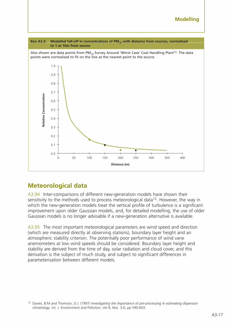
A3-17
Modelling
Meteorological dataA3.94 Inter-comparisons of different new-generation models have shown theirsensitivity to the methods used to process meteorological data12. However, the way inwhich the new-generation models treat the vertical profile of turbulence is a significantimprovement upon older Gaussian models, and, for detailed modelling, the use of olderGaussian models is no longer advisable if a new-generation alternative is available.
A3.95 The most important meteorological parameters are wind speed and direction(which are measured directly at observing stations), boundary layer height and anatmospheric stability criterion. The potentially poor performance of wind vaneanemometers at low wind speeds should be considered. Boundary layer height andstability are derived from the time of day, solar radiation and cloud cover, and thisderivation is the subject of much study, and subject to significant differences inparameterisation between different models.
Box A3.3: Modelled fall-off in concentrations of PM10 with distance from sources, normalisedto 1 at 10m from source
Also shown are data points from PM10 Survey Around ‘Worst Case’ Coal Handling Plant12. The datapoints were normalised to fit on the line at the nearest point to the source.
Rel
ativ
e C
on
cen
trat
ion
0.0
0.1
0.2
0.3
0.4
0.5
0.6
0.7
0.8
0.9
1.0
0 50 100 150 200 250 300 350 400
Distance (m)
12 Davies, B.M and Thomson, D.J. (1997) Investigating the importance of pre-processing in estimating dispersionclimatology. Int. J. Environment and Pollution, Vol 8, Nos. 3-6, pp 590-603.

A3-18
Modelling
Meteorology used in screening models
A3.96 Some screening models have built-in sample meteorological datasets, forexample, the Environment Agency GSS workbook13, and ADMS-Screen. However, thesemeteorological datasets are statistical frequency analyses. There is some concern thatstatistical meteorological data do not predict the high percentile values (though theyare adequate for the calculation of annual means), yet screening tools need to beconservative i.e. over-predict rather than under-predict.
A3.97 Statistical frequency analyses of meteorological observations (typically over a10-year period) have limited use for detailed modelling – computers are now fastenough to handle a full year of sequential meteorological data (which does not under-estimate peak concentrations, as statistical datasets had a tendency to do). A use forstatistical data is in comparing wind roses between sites for long-term changes.However, sequential datasets should be used for detailed modelling, and especially forthe calculation of high percentile values or maximum 1-hour means.
Inter-year variability of source contributions, as a result of differences inmeteorological data?
A3.98 A sensitivity analysis carried out during the compilation of the SupplementaryAssistance spreadsheet14 (using Birmingham sequential meteorological datasets)showed that of 5 years (1996, 1997, 1998 and 1999 and 2001), 1998 gave the highest99.9th percentile of 1-hour means, 24% higher than 2001 (which gave the lowestvalue). However, the trend for the annual means was different; 1999 gave the highestannual mean, 26% higher than 2001 (which gave the lowest value). So, the greatesteffect of different years of met data is not necessarily on the high percentiles. Thisstudy modelled only emissions from a single stack, with no account taken ofbackground concentrations.
A3.99 This investigation was repeated with other sequential meteorological datasetsfrom 4 different stations. The results suggest that Manchester shows less inter-yearvariability for predicted annual mean concentrations than other stations, and thatBirmingham shows more inter-year variability for predicted 99.9th percentileconcentrations than other stations.
A3.100 Further results of inter-year variability for ADMS3 point source modelling havebeen provided by the Environment Agency15, based on a modelling study of 23 powerstations across England and Wales, using a variety of meteorological observing stations.A maximum difference of 28% between met. years was found for the peak 99.9thpercentile predictions, over 5 meteorological years (1990 – 1994).
13 Guidance for estimating the air quality impact of stationary sources (1998), Environment Agency, National Centrefor Risk Analysis and Options Appraisal, report No. GN24.
14 Y. Vawda, J.S. Moorcroft, P. Khandelwal and C. Whall (2001), Sulphur dioxide emissions from small boilers –Supplementary Assistance on stack height determination, Clean Air, Volume 31, Autumn 2001.
15 Dispersion Calculations of Short Term Sulphur Dioxide Concentrations from UK Generating Stations using EmissionLevels for 2005, R&D Technical Report P395, D. Hall, A.M. Spanton, C.B. Powlesland and S. Walker.

A3-19
Modelling
A3.101 By definition, these inter-comparisons consider the primary pollutantcomponent only – no allowance for background is made, and therefore, noconsideration is given to the effect different meteorological years are having on thesecondary pollutant contribution.
A3.102 Results of inter-year variability (for the primary emissions, with no allowancemade for background) also provided by CERC, Stoke-on-Trent CC, AEAT and ARIC areas follows:
• Over a grid of receptors, CERC found that between 1996 and 2001 using Heathrowmeteorological data, there was a 26% difference between the highest (1998) andlowest (1996) annual mean maxima. They found that between 1996 and 1999 usingWaddington meteorological data, there was a 16% difference between the highest(1997) and lowest maxima (1996).
• AEAT found a difference of 11 – 25% between lowest and highest annual meanpredictions (Waddington meteorological data), over 5 meteorological years (1995 –1999). This range of difference is almost exactly the same as that found using pointsource modelling. Of the 4 receptor locations ARIC modelled, Manchester Airportmeteorological years 1995 – 1999 using the entire Manchester/Warrington emissionsinventory and a very large number of receptor locations. A consistent trend wasfound across all receptors, with 1999 predicting the highest nitrogen oxidesconcentrations, and 1995 the lowest concentrations. The range of differencebetween the highest and lowest concentrations is no more than 30% for the vastmajority of the receptor locations.
A3.103 The preceding discussion suggests that the use of 2 different meteorologicalyears should give a difference in modelled source contribution of no more than 30%.This is a useful statistics, for it allows a single year of meteorological data to be used forthe purposes of review and assessment, yet indicates the likely maximum variabilityabout the single year prediction.
How many years of meteorological data?
A3.104 Differences in predicted results may arise depending on the chosen year ofmeteorological data as described in paragraphs A3.98 – A3.103 and other factors suchas model used and receptor locations. For the purposes of review and assessment, oneyear of meteorological data may be used for dispersion modelling.
A3.105 Where possible and practicable for model verification, the following should allbe based on the same year:
• emission estimates.
• monitoring data.
• background estimates.
• meteorological data.

A3-20
Modelling (continued)
A3.106 However, in some cases this might not be possible, for example, where norecent meteorological data are available or particular years have large amounts ofmissing data. For review and assessment purposes, a minimum data capture of 90%is recommended for meteorological data. The Environment Agency is working withthe Met Office and NSCA to further examine the minimum data requirements fordispersion modelling. Missing lines of meteorological data could be interpolated, orfilled by data for those specific hours from a neighbouring site. Emissions andmonitoring data for these hours should not be ignored, as it is important to maintainas large a dataset of emissions and monitoring data as possible.
A3.107 If meteorological data for the year of model verification are not available,another year not more than 5 years old should be chosen. The user should check forchanges in instrumentation, observing station re-locations, and significant changes intopography/land use over the years. The modeller should also note the percentage ofmissing hours in the different years, and choose to model years with data capture highenough for valid use in the model.
A3.108 While it is recommended that the year of meteorological data should matchthe year of assessment (paragraph A3.105) this is not possible for future predictions.Whatever year of meteorological data is used to verify dispersion modelling, the sameyear should be used for future year predictions as the performance of the model maybe related to the chosen year of meteorological data. Some local authorities may havealready developed dispersion models based on a certain year of meteorological dataand have progressed to investigating source apportionment and action plans so theymay wish to continue with the current chosen year of meteorological data. If a localauthority changes the year of meteorological data, model verification should beundertaken again.
A3.109 A local authority may choose to use multiple years (3 or more) ofmeteorological data during the review and assessment process in order to determinethe significance of meteorological data on any predictions. The information provided inparagraphs A3.98 to A3.103 indicates that differences are unlikely to be greater than30%. The range of the results, including those at relevant roadside receptors, and thedifferences in relation to year of meteorological data should be provided if such studiesare undertaken. An explanation as to which set of predictions has been used for furtherdetailed modelling and production of concentration contours should also be provided.
A3.110 Information on the potential variation of concentrations between years canalso be determined from long-term monitoring data.
A3.111 Under general circumstances, where multiple years (three or more) ofmeteorological data have been modelled for road traffic sources, the typical year (i.e.not the best or the worst) is generally appropriate for decision-making purposes andfurther modelling, but some local authorities may decide to choose the worst case year.Local authorities in London should contact the Greater London Authority for updatedadvice on which years to use for review and assessment.

A3-21
Modelling
A3.112 For industrial sources, the use of 5 years of meteorological data is required bythe Environment Agency for detailed modelling16. The regulatory agency would haveconsidered the impact of its regulated processes on compliance with Air QualityObjectives in its determination and variation of authorisation. It is advisable for localauthorities to contact the regulatory agency for model predictions. Local authoritiesmight want to consider modelling these sources with multiple years of meteorologicaldata. Where point sources are thought to be the main contributor to a potentialexceedence of shorter-term objectives, decisions should be based on the worst-caseresults but all results should be reported.
A3.113 If the nearest observing station to the area being modelled is greater than30 km away, local authorities should consider the next nearest and appropriateobserving station. A range of approximately 30 km is the limit for the predictions ofa short-range, practical dispersion model. The Met Office can be contacted for adviceon representative sites.
A3.114 Where a local authority has serious cause for concern about the representivityof an observational station for the assessment area, as part of improved verification,they may consider running multiple years (3 or more) of meteorological data. In thiscase, it is recommended that the typical year is used for decision making purposes.A full description of the results from different years should be provided for comparison(section A3.109). The Modelling Helpdesk can be contacted for further advice.
Meteorological data and background
A3.115 Background concentrations can be accounted for in a number of ways duringdetailed modelling, including:
• using simple annual averages (either monitored or national maps).
• adding an hourly or daily background file to your modelled results (i.e. hour 1modelled is added to hour 1 background and so on).
• modelling hourly background concentrations based on ‘background sources’ andusing a rural background monitoring file.
A3.116 For the verification of modelled results (i.e. comparison against monitoringdata, and possible adjustment of modelling results) the year of meteorological datashould be the same as the year of background data. As described in paragraph A3.105,the year of meteorological data, monitoring data, emissions data and background datashould all be the same whenever possible but in some cases this might not be possible.
A3.117 The importance of the meteorological year used may not be so significant insome cases because the background year chosen may be the significant factor,particularly where local authorities are using years with high background and secondaryPM10 concentrations – see section A3.120.
16 The Air Quality Modelling and Assessment Unit, The Environment Agency.

A3-22
Modelling
A3.118 The factors provided in the main chapters of this document should be used toproject background concentrations (monitored or national maps) forward to therelevant years. In the absence of further information, if an hourly or daily backgroundfile is being added to the modelled concentrations, the same factors as those forprojecting annual averages should also be used.
Sources of meteorological data
A3.119 There are a number of providers of sequential meteorological data fordispersion modelling, examples of which are the Met Office and Trinity Consultants Inc.The datasets provided by any organisation, for the same site and year, are notnecessarily identical. However, year-by-year variations in meteorological data from onesource are greater than the differences between Trinity and Met Office data for aparticular year, for example. The different meteorological data sets provided by these 2suppliers have relatively little effect on the calculation of annual means17. So the choiceof supplier is not critical, despite slightly different parameters being measured.
Pollution episodes
A3.120 An informal analysis carried out by AEA (which did not systematically modeldifferent meteorological datasets) surmised that for nitrogen dioxide and PM10, year1997 meteorology would give high results and 2001 would give ‘ordinary’ or typicalresults, regardless of region. However, 1996 has been identified in the AQS as a ‘bad’year for PM10 exceedences, though this has been attributed to easterly winds bringingin secondary PM10 into south-eastern England, i.e. a secondary component caused theexceedences, not a primary pollutant.
A3.121 The Met Office has carried out some preliminary investigations into how‘typical’ years of met data differ, and how often pollution episodes could recur. No usewas made of emission inventories or dispersion modelling, and only the historicalarchives of Heathrow meteorological data and London monitoring data wereinspected18. The purpose was to try to identify the weather related variables thatcorrelate with different types of pollution episodes, the frequency of such weatherconditions, and the likely recurrence pattern. The study looked at the frequency ofcalms and light winds because they have special significance for urban air quality. Thisstudy showed that historically, episodes occurred during months with high incidences ofcalms. Paragraph A3.124 describes how some dispersion models treat calm conditions.
‘Lifetime’ of meteorological data sets
A3.122 Some meteorological data sets can be said to have a ‘lifetime’, but this isdependent on the changes in the vicinity of the station (for example, increasingurbanisation around Heathrow over the last 50 years, resulting in a change in the localmeteorology) and observing practice (for example, changes in the types of anemometer
17 Hall, D.J. and Spanton, A.M. (1999) Meteorological Data and Dispersion Modelling. Clean Air, Volume 29,September/October.
18 On the recurrence of air pollution episodes, D.R. Middleton and J. Dixon, 31st August 2001, The MeteorologicalOffice, Turbulence and Diffusion Note 269.

A3-23
Modelling
used, leading to slightly different frequencies of low wind speeds recorded). Themodeller should be aware of any changes to the observing station and recordingpractice which the site may have been subject to, before choosing the year of data toemploy in the modelling.
A3.123 Reports of meteorological data observations and conditions are availablefrom the Met Office. Data provided by the Met Office can also include roughnesslength, details of anemometer type, and the inclusion of any corrections foranemometer height.
Treatment of calm and missing meteorological data
A3.124 In calm conditions (i.e. wind speeds close to 0 m/s), a number of models havea mathematical discontinuity. This means that the concentration will not be calculatedfor such hours, unless some approximation is built into the model. The high percentilesof pollutants from ground level sources (for example, road traffic) often occur in suchcalm conditions, and are therefore difficult to model with confidence. Anemometersshould be capable of measuring very low wind speeds; ultrasonic anemometers areespecially well suited to this.
A3.125 Most Gaussian-type models do not use the lines in the meteorological data setwhich have calm winds in its calculations, so they will be missing the instances whenconcentration values may be at their highest. Alternatively, some models default to aminimum wind speed, for example, ADMS-Urban and ADMS-Roads set the minimumwind speed to 0.75 m/s.
A3.126 The US EPA type models assume that all wind speeds recorded as between0.5 – 1 m/s are treated as 1 m/s. For wind speeds less than 0.5 m/s, the following rulesare applied:
• if the averaging period is 1-hour, wind speeds less than 0.5 m/s are ignored andthose lines of met data are skipped.
• if the averaging period is 8 hours, at least 6 lines of met data out of 8 consecutivelines must have wind speeds greater than 0.5 m/s. The lines with winds less than0.5 m/s will be ignored, and the period average will be approximated to the 8-hourmean.
• if the averaging period is 24-hours, at least 18 lines out of 24 consecutive lines musthave wind speeds greater than 0.5 m/s. The lines with wind speeds less than 0.5 m/swill be ignored, and the period average will be approximated to the 24-hour mean.
A3.127 This treatment is often referred to as the 75% rule for US EPA models, and isused for calms and missing hours. In the case of a 24-hour averaging period, the modelwill ignore up to 6 invalid hours (18/24 real wind speeds = 75%). The resultingconcentration is calculated by summing those 18 valid hours and dividing by 18. If youhave 10 calms, then the model sums the 14 valid hours and divides by 18. This maytherefore produce a dilution effect.

A3-24
Modelling (continued)
A3.128 The Environment Agency is working with the Met Office and NSCA to examineminimum data capture rates to be acceptable for use in dispersion models.
Calculation of percentiles and/or number of exceedences
A3.129 Some of the objectives allow the air quality standard to be exceeded for acertain number of hours in the year. For example, the short-term objective for nitrogendioxide allows a concentration of 200 µg/m3 to be exceeded for 18 hours in the year.Such Air Quality Objectives are always expressed in terms of the number ofexceedences, and not percentile values.
A3.130 If a full year of sequential hourly meteorological data is available (8760 hours)for modelling, a predicted concentration of 200 µg/m3 (after allowing for background)may be exceeded on no more than 18 hours. If a dispersion model is run to calculatethe hourly mean concentrations, and assuming that the model does indeed carry outthe calculation for every single line of meteorological data (including the calms), the19th highest concentration equates to a 99.79th percentile. (This is analogous with amonitor measuring an hourly concentrations for every hour in the year without any lossof data or malfunction.)
A3.131 There are 2 issues to bear in mind with Air Quality Objectives which allow anumber of exceedences:
1. observational meteorological data often have many hours of data missing. If therecorder has managed to capture only 6000 hours (for example), the 19th highesthourly mean concentration will not be equivalent to the 99.79th percentile. In thiscase, the 19th highest concentration would equate to a 99.70th percentile of theavailable meteorological data (assuming a calculation is carried out for every line ofmeteorological data). The 99.79th percentile of the available meteorological datawould actually allow only 13 exceedences.
2. some models do not carry out a calculation for those lines which have inadequatedata, for example, missing wind direction or cloud cover. Using the example above,the 6000 hours of meteorological data may have contained 1000 hours which wereinvalid or inadequate. A model may be used which ignores these hours. The 19thhighest concentration of 5000 hours equates to a 99.64th percentile of themeteorological data processed. The 99.79th percentile of the available meteorologicaldata which can be processed by the model, would actually allow only 11exceedences.
A3.132 Therefore, it is important to know how the model employed treats missinghours of meteorological data, inadequate or invalid lines of data, and also how it treatsthe calms, particularly if predicting the number of exceedences.
A3.133 When there are data for less than 90% of hours in a year (including missing,invalid and calm hours), it would be useful if the modelled results are expressed aspercentiles, as well as exceedences. If there are more than 90% of hours in the yearavailable, then the results are most usefully expressed as the number of exceedences.

A3-25
Modelling
A3.134 Using the 90% valid meteorological data availability criterion, the percentilestatistic is constrained to no less than 99.78% for nitrogen dioxide. For other pollutantswhich have objectives expressed as a maximum permissible number of exceedences ofan air quality standard (for example, sulphur dioxide, PM10), the same guidance canapply. For example, for sulphur dioxide, if less than 90% of the hours are available formodel calculations, the 99.9th percentile should be calculated and reported, as well asthe number of exceedences of 266 µg/m3. For PM10, at least 90% of valid days need tobe available for modelling if allowing for 35 exceedence days (year 2004 objective);otherwise, the 90th percentile of the available meteorological days should also becalculated.
A3.135 The examples for nitrogen dioxide described above are summarised in BoxA3.4, with a few additional scenarios.
Urban meteorology
A3.136 The First Round of review and assessment identified road traffic as the primarycause of exceedences of the annual mean nitrogen dioxide objective in many urbanareas. This highlights the need for a greater understanding of urban meteorology inorder to improve the modelling of road traffic emissions.
A3.137 For urban pollution studies, it may be necessary to use measurements takenwithin the urban area, and this poses particular problems of instrument siting andexposure; some measurements may be unduly influenced by upwind buildings orstructures. Some models require a roof top wind; this is rarely available, so the modelswill rely on a 10m wind speed recorded at an observing station outside the town19.
A3.138 The Urban option in AERMOD gives higher concentrations than the Ruraloption because the urban heat island effect (which is represented by an adjusted heatflux, so the user has to define a population density) increases turbulence at night andmore of the plume is brought to ground. The user should be aware of differences ofthis nature when invoking similar Urban options in various models.
A3.139 Research is currently underway which will lead to recommendations on howairport meteorological data should be adopted for urban modelling, and on how urbanmeteorology should be observed routinely for managing air quality. A proper diagnosisof the heat flux and atmospheric stability is now being carried out for cities20. In urbanareas, the wind over increased surface roughness creates greater mechanicalturbulence. Stability is influenced by the urban heat island effect and its effect onthermally induced turbulence, which may lead to a delay in the onset of the eveningtransition to night-time stable conditions. In large cities, the stable conditions may notdevelop at all during the night, and this will affect the air quality. Many models do notaccount for this effect at all.
19 Meteorological Challenges in Urban Air Pollution. D. R. Middleton, Clean Air, Vol 32, Spring 2002.20 Uncertainties in met pre-processing for dispersion models (2003). D. R. Middleton and D.J. Thomson, Atmospheric
Dispersion Modelling Liaison Committee, NRPB (in press).
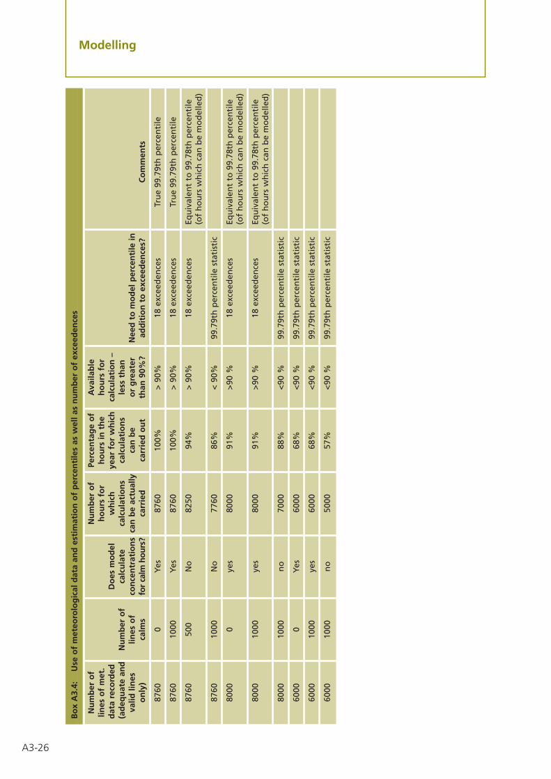
A3-26
Modelling (continued)
Bo
x A
3.4:
Use
of
met
eoro
log
ical
dat
a an
d e
stim
atio
n o
f p
erce
nti
les
as w
ell a
s n
um
ber
of
exce
eden
ces
Nu
mb
er o
fN
um
ber
of
Perc
enta
ge
of
Ava
ilab
lelin
es o
f m
et.
ho
urs
fo
rh
ou
rs in
th
eh
ou
rs f
or
dat
a re
cord
edD
oes
mo
del
wh
ich
year
fo
r w
hic
hca
lcu
lati
on
–(a
deq
uat
e an
dN
um
ber
of
calc
ula
teca
lcu
lati
on
sca
lcu
lati
on
sle
ss t
han
valid
lin
eslin
es o
fco
nce
ntr
atio
ns
can
be
actu
ally
can
be
or
gre
ater
Nee
d t
o m
od
el p
erce
nti
le in
on
ly)
calm
sfo
r ca
lm h
ours
?ca
rrie
dca
rrie
d o
ut
than
90%
?ad
dit
ion
to
exc
eed
ence
s?C
om
men
ts
8760
0Y
es87
6010
0%>
90%
18 e
xcee
den
ces
Tru
e 99
.79t
h p
erce
nti
le
8760
1000
Yes
8760
100%
> 9
0%18
exc
eed
ence
sTr
ue
99.7
9th
per
cen
tile
8760
500
No
8250
94%
> 9
0%18
exc
eed
ence
sEq
uiv
alen
t to
99.
78th
per
cen
tile
(o
f h
ou
rs w
hic
h c
an b
e m
od
elle
d)
8760
1000
No
7760
86%
< 9
0%99
.79t
h p
erce
nti
le s
tati
stic
8000
0ye
s80
0091
%>
90 %
18 e
xcee
den
ces
Equ
ival
ent
to 9
9.78
th p
erce
nti
le
(of
ho
urs
wh
ich
can
be
mo
del
led
)
8000
1000
yes
8000
91%
>90
%18
exc
eed
ence
sEq
uiv
alen
t to
99.
78th
per
cen
tile
(o
f h
ou
rs w
hic
h c
an b
e m
od
elle
d)
8000
1000
no
7000
88%
<90
%99
.79t
h p
erce
nti
le s
tati
stic
6000
0Y
es60
0068
%<
90 %
99.7
9th
per
cen
tile
sta
tist
ic
6000
1000
yes
6000
68%
<90
%99
.79t
h p
erce
nti
le s
tati
stic
6000
1000
no
5000
57%
<90
%99
.79t
h p
erce
nti
le s
tati
stic

A3-27
Modelling
A3.140 A comparison of urban meteorological measurements has been carried out forBirmingham for a 4-week period in winter 1999, with a rural synoptic station (atColeshill) and the output from the Met Office Unified Model (UM)21. Urban windspeeds at 30 m were found to be closest to rural 10 m wind speeds; the local urbanroughness length was 0 – 2 m. The urban temperature was about 1oC greater than therural temperature, with some lag. The UM results showed that it modelled well for arural synoptic station but the character of the urban site was not captured.
A3.141 There is a need to take care in the of siting of instruments for wind directionsand speeds in urban areas – tunnelling effects in a particular area of city may becompletely different to those in another.22 The Met Office should be contacted forfurther information.
Coastal effects
A3.142 The main regional differences in meteorology are stronger winds near thecoast (particularly towards the west). At inland locations, the wind speed is lower onaverage, and the more extreme low-level dispersion conditions occur more often.
A3.143 Modelling of coastal towns has relied on the observational meteorological datafrom a nearby station, often located a few tens of km inland. Different models can givevery different results for coastal situations.
Estimating background concentrations in modelling studiesA3.144 Short-range practical dispersion models can only predict the pollutantconcentrations contributed by the modelled source. There will always be an additionalcomponent arising from those sources which have not been modelled; these could beother nearby roads or stacks, or distant sources (regional or even transboundary). Theassessment of potential exceedences of the air quality objective must take account ofthe background pollutant level.
A3.145 When using data collected at nearby monitoring stations to estimatebackground levels, it is important to ensure that the measurement does not alreadyinclude a component due to the source being modelled, which could result in thesource contribution being counted twice.
A3.146 Similarly, maps of projected background concentrations in the Air QualityArchive include major roads, Part A and Part B processes in the grids, so this could leadto double-counting if one of these sources was included in the modelling scenario23.
21 Field Measurements and Modelling of Urban Meteorology in Birmingham, UK. N.L. Ellis and D.R. Middleton, 20thSeptember 2000, The Meteorological Office, Turbulence and Diffusion Note No.268.
22 Hough, M.N. and Nelson, N. (2000) The representivity of weather data for dispersion calculations. AtmosphericDispersion Modelling Liaison Committee report.
23 Stedman, J.R, Bush, T.J. and Vincent K.J. (2002) UK air quality modelling for annual reporting 2001 on ambientair quality assessment under Council Directives 96/62/EC and 1999/30/EC. AEA Technology, NationalEnvironmental Technology Centre. Report AEAT/ENV/R/1221.

A3-28
A3.147 It is important to understand how the National Air Quality Information Archivehas produced its estimates of background pollutant concentrations. Data frommonitoring sites representative of rural locations have been interpolated to produce amap of rural concentrations. The impact of local scale (< 20 km) emissions has thenbeen estimated using an empirical box modelling approach (applied to sources includedin the National Atmospheric Emissions Inventory, which is then superimposed on therural map. Hence, it is apparent that even the maps of ‘background’ concentrations willalready incorporate the air quality contribution of all emission sources. Care must betaken that sources are not ‘double-counted’ (Box 1.5).
A3.148 Annual mean background concentrations (estimated from National Air QualityInformation Archive data or local monitoring) can readily be added to the annual meancontribution from the modelled source. Similarly, hourly predictions could be added tohourly measurements from a suitable monitoring station, as long as the potential forincluding the source contribution twice is carefully considered, for example, byinspecting the hour-by-hour wind directions with respect to the relative positioning ofthe modelling source and the monitoring station; downwind monitoring stations havethe potential to be recording a signal from the source being modelled. Percentileconcentrations cannot be simply added, but must be calculated after adding hour-by-hour modelling and monitoring data.
How detailed should my modelled area be?A3.149 The aim of the review and assessment process is to gradually focus on morespecific sites/sources such as single roads or junctions at which potential exceedences ofthe AQS objectives are identified through the means of different levels of screeningexercises.
A3.150 If you are assessing roads that are 10 to 20 metres wide, you should bepredicting concentrations at either:
• specific receptors representative of exposure as identified using maps; and/or
• a receptor grid spaced at 5 to 10 metres near to the roadside to provide enoughdetailed prediction in the areas where exceedences are more likely to occur.
A3.151 The Environment Agency recommends the use of a grid resolution equal to 1.5times the stack height for the assessment of point sources. For review and assessment,if point sources are being assessed, model resolution should be in the order of 25 to50 metres. Greater spacing can result in areas of impact being missed (Box A3.5).
A3.152 The review and assessment process requires that contours of concentrations bedrawn for the areas where exceedences have been identified. This does not mean thatwhole urban areas need to be contoured, particularly at background locations. Specificreceptors should first be used for any detailed modelling at the roadside then contourscan be produced for relevant areas with exceedences.
Modelling (continued)

A3-29
Box A3.5: Difference in concentration based on modelling at 200 m (upper) and 50 m (lower) grid spacing. The lower plot clearly indicates that the impact area to the north of the stack is not represented at larger grid spacing. The area covered by each grid is the same.
20
10
25
3525 25
30402520
10
15 25
20
15
15
15
15
15
15
45
25
35
35
3525
5
2030
35 40
40
35
25
25
15
20
25
20
10
10
10
10
10
10
10
10
15
15
25
20
2020
20
3020
30
200 metre gridspacing(stack at centre)
50 metre gridspacing(stack at centre)
Modelling

A3-30
A3.153 When producing contours for a whole urban area, they should includelocations within 30 to 50 metres of roads (perhaps further for some motorway sites),and based on spacing of 5 to 10 metres. General background concentrations for mosturban areas are well known and do not require detailed contouring, however verifiedmodelled background based on local emission inventories may be useful for widerdecision making purposes.
A3.154 Modelling of large regions at low levels of spatial detail, for example, with a50 m grid spacing, can result in localised exceedences at junctions and within a fewmetres of roads being missed. This highlights the importance of predicting at specificreceptor locations or using a small grid spacing of 5 – 10 m, rather than large grids. Theuse of intelligent gridding which alters the spacing of receptors close to roads may alsobe useful.
Interpretation of concentration contours
A3.155 As shown in the example above, the grid spacing (i.e. the distance betweenpredictions points) affects the interpretation of the results. In addition the interpolationor contouring method can affect how the contours are drawn. Common methods usedto draw contours are Inverse Distance Weighting (IDW), Rectangular, Krigging andNatural Neighbour Analysis. The method to use depends on the spacing of thepredictions. If there is any doubt as to which to use, contact the model developers orthe Dispersion Modelling Helpdesk.
A3.156 A useful exercise is to predict concentrations at both specific locations and fora grid of receptors. Produce contours for the grids using some of the methods listedabove and check the agreement of results obtained at the specific receptors. You mayfind that a particular interpolation methods gives better agreement for the model set-up chosen. This will help to ensure that predictions at specific receptors within anAQMA match the contours drawn to define the area.
A3.157 Box A3.6 shows the predicted concentration of annual average nitrogendioxide at a number of specific receptors near a complex junction and those predictionsderived from modelled grids at spacing between 5 m and 100 m. The box indicatesthat there is better agreement at all receptors when a spacing of 5 m is used.
Box A3.6: Comparison of predicted concentration of annual average NO2 (µg/m3) at a number ofreceptors near a complex junction, and results derived from contouring based on regulargrids with grid spacing ranging between 100 m and 5 m. Surfer default Inverse DistanceWeighting Interpolation method used.
Specific 100 m 50 m 25 m 10 m 5 m
Receptor 1 39.2 38.6 41.6 41.1 40.1 39.3
Receptor 2 41.4 38.3 44.7 44.7 42.2 41.6
Receptor 3 43.7 38.1 45.8 47.0 44.7 43.9
Receptor 4 37.3 37.6 40.6 38.5 38.0 37.5
Receptor 5 39.1 38.8 41.7 42.2 40.3 39.4
Receptor 6 35.1 37.4 37.6 37.1 35.8 35.2
Receptor 7 40.3 38.4 42.8 42.8 41.2 40.5
Receptor 8 38.6 37.8 40.8 40.2 39.9 38.8
Modelling (continued)
A3-31
A3.158 In many cases, particularly for road traffic modelling, the orientation of grids is north-south/east-west which can lead to a ‘stepping’ of concentration contours,particularly where a single linear road in different orientation is modelled. For longsections of roads, the use of grids parallel to the orientation can produce neatercontours as shown below.
A3.159 Blobs and circles representing very high concentrations commonly appear oncontours for road traffic modelling. These can be reduced by using parallel grids.Blanking techniques can also be used to cover or hide the contours on the road but it is recommended that this is done after interpolation of contours and is only aesthetic.Parts of the grid should not be removed prior to interpolation as this will increase thedistance between the points and will generally remove those higher concentrationsclose to the road.
Model validation, verification, adjustment and uncertaintyA3.160 Validation of a model refers to the general comparison of modelled resultsagainst monitoring data carried out by the model developers. The models used inreview and assessment should have some form of published validation assessmentavailable and/or should be recognised as fit for purpose by regulatory authorities.
A3.161 The validation by model developers is unlikely to have been undertaken in thearea being considered. Therefore it is necessary to perform a comparison of modelledresults versus any local monitoring data at relevant locations. The results of thiscomparison must be included in the review and assessment report and is referred to asmodel verification in this document.
A3.162 Discrepancies between modelled and measured concentrations and resultsfrom a dispersion model may be due to a number of different reasons including:
• traffic flow uncertainties, including estimates of speeds, total flows and proportionsof vehicle types.
• emission estimates for vehicles and other sources such as domestic heating andindustrial stacks.
• estimates of background concentrations.
• meteorological data uncertainties.
• model input parameters such as roughness length, minimum Monin-Obukhovlength.
• overall model limitations.
A3.163 Verification is the process by which uncertainties such as those describedabove are investigated and minimised. Disparities between modelling and monitoringresults are likely to be as result of a combination of all of these aspects.
Modelling

A3-32
A3.164 Model verification may or may not result in an adjustment of modelled resultsdepending on the outcomes and/or the source types being considered. If modelledresults are adjusted the factors or amount of adjustment should be referred to as modeladjustment. This corrects for systematic error. The full details of how the modelverification and calibration is undertaken should always be provided. However,adjustment of the modelling results should only be carried out once other uncertaintieshave been minimised.
A3.165 The modelled results from industrial sources alone are not expected to beadjusted, as it is recognised that appropriate monitoring around stacks may not beavailable to allow verification of the modelled results. Where long-term monitoring isavailable it should be compared against the modelled results and commented upon.
A3.166 The verification of point source modelling should focus on the shorter-termconcentrations (particularly 1-hour and 15-minute means) as the impacts are greaterthan longer-terms concentrations such as the annual or 24-hour mean. Elevated pointsources usually have little impact on annual mean ground-level pollutantconcentrations. An example of verification of SO2 concentrations is shown in Box A3.7below as it may be of some use to local authorities.
A3.167 The results of dispersion modelling of point sources may not agree with theresults of monitoring. This may be due to a number of factors including an under orover estimation of the source emissions, and difficulties in determining emissionsprofiles, along with the different parameters of the dispersion model includingroughness length, building, terrain and meteorological data.
Box A3.7: Example of SO2 verification
For the purposes of verification, the measurements from a monitor at an industrial backgroundlocation have been used. The comparison of the modelled ‘industrial source contribution’, background,and total measured concentrations are shown below (all results are as µg/m3).
Modelled Total Total % Differenceindustrial source modelled monitored (-ve under-
contribution Background concentration concentrations predict)
1-hour objective 73.6 24.6 98.2 104.2 –6%
15-minute mean objective 213 24.6 237.6 225.3 +6%
In this case, the 15-minute objective has been derived from hourly modelling24 (i.e. the 15-minuteaverage was not directly predicted by the model). The under or over prediction in both cases is lessthan 10% and shows that at the monitoring location, the model is performing well for both averagingperiods.
It should be born in mind that the performance of the model is only relevant at the location wheremonitoring is available. The monitored location probably does not represent the worse case locationpredicted by the model and performance at this location may be different.
24 Beychok, M.R. (1994) Fundamentals of Stack Gas Dispersion. Published by Milton R. Beychok, 2233 Martin St,Unit 205, Irvine CA 92612, USA ISBN 0-9644588-0-2.
Modelling (continued)

A3-33
A3.168 If an exceedence of a short-term objective is predicted, for example in the 98thpercentile, a range of percentiles can also be predicted, for example, the 85th, 90thand 95th to 100th in the area of significant impacts to give an indication of the rangeof predicted concentrations at these levels. If the 98th percentile results in a predictedexceedence, as do the 95 to 97th, this suggests that there is a likely risk of exceedingthe objective given the dispersion modelling inputs. However, if the predictedconcentrations at lower percentile do not exceed, then it may be concluded that thereis less risk of exceeding the objective.
A3.169 It should also be noted that the predicted area of maximum impact from astack may not agree with the results of monitoring, and that the maximum impact areais likely to be more ‘fluid’ i.e. variable. If modelled predictions do not appear to agreewith the results of monitoring the user may contact the dispersion modelling helpdeskto discuss. Under these circumstances, it may be useful to model the stack withmultiple years of meteorological data and to consider further the emissions estimatedused in any modelling, for instance, reviewing information on any patterns of releases.For authorised processes, the regulatory agency should be contacted to determine whatlevel of assessment has already been carried out.
What sites should be included in verification and adjustment?
A3.170 As indicated above, monitoring data (of suitable quality) can be used to verifyboth modelling of stacks and roads. However, adjustment of modelled results isgenerally only required (if necessary) when road traffic modelling is included.
A3.171 All monitoring used for Verification and/or Adjustment of modelling resultsshould be undertaken to the standards described in Annex 1 (Monitoring). The errorsaround diffusion tube measurements should have also been assessed using co-locationexercises at a continuous monitor preferably placed at the roadside of an area requiringdetailed modelling.
A3.172 Where kerbside sites are used for the verification of long-term objectives,inclusion of these may lead to over-adjustment of modelled concentrations at othersites. Kerbside locations are relevant for shorter-term objectives and where relevantexposure is present.
A3.173 Dispersion models can perform differently at roadside and background sites,particularly when the background concentration has been predicted by the model.
• If background sources such as domestic heating have been modelled, the resultsshould be verified against background monitoring. It may therefore be necessary toadjust the modelled background concentrations.
• If national background maps have been used, these should first be compared againstany local monitoring to check they are representative of the area. In most cases thereis good agreement with monitoring, but some locations may not agree.
Modelling
A3-34
A3.174 There can be difficulty in deciding if roadside, and/or intermediate and/orkerbside sites should be included in the same verification. It is recommended that all ofthese sites are included in the first instance. It is possible to separate the site types bydistance from the road, but the levels monitored can indicate strong roadsidecontributions and some ‘intermediate’ sites may reflect typical roadside concentrations.Therefore, initial comparisons of the modelled versus monitored concentrations will beable to highlight if the performance of the model is significantly different between thedifferent site types.
A3.175 It should be recognised that undertaking verification at a large number ofdifferent site types can lead to complications if adjustment of the modelled results arerequired. It is recommended that site types should not be separated beyondbackground and roadside/intermediate. Where kerbside sites are available, these shouldbe treated separately, or where adjustment factors are comparable, combined withroadside and intermediate sites.
A3.176 In some cases, a local authority may have ‘roadside’ diffusion tubes sites within5m of small residential roads. The local authority should consider removing these sitesfrom the verification of roadside sites, but they may be useful for verification of urbanbackground sites.
A3.177 Wherever possible, motorways and other major trunk roads should beconsidered in a separate verification exercise to more general urban areas. Thecombination of these sites may lead to large over-predictions of concentrations nearmotorways.
A3.178 When only road traffic sources have been modelled the predictedconcentration from the model, without the background, should be referred to as the‘modelled roads or traffic contribution’. If other sources are included in the modellingrefer to the ‘source contribution’. Some consideration of the relevant contribution ofsource may be required – particularly where stacks are significant.
A3.179 Most verification exercises are only required for annual average concentrations.The annual average monitored roadside contribution of nitrogen oxides and PM10 willbe required at continuous monitoring sites. This can be derived by:
• subtracting a background concentration from the total roadside monitoredconcentration to estimate the ‘monitored roads or traffic contribution’. This may becarried out for nitrogen oxides, nitrogen dioxide and PM10.
[Monitored Total Roadside] NOx, NO2, PM10 – [Background] NOx, NO2, PM10= [Monitored Roadside Contribution] NOx, NO2, PM10
A3.180 The following sections provide further information on methods for verificationand adjustment of nitrogen oxides and nitrogen dioxides although the information canalso be applied to verification of PM10.
Modelling (continued)

A3-35
NOx/NO2 verification and adjustment
A3.181 Conversion of nitrogen oxides is required in order to estimate nitrogen dioxideconcentrations. Methods include:
• That described in the Chapter 6 of this document.
• Ozone limited methods available in various models.
• Generic reaction series.
• Derwent-Middleton function for hourly concentrations.
A3.182 In each case, the modelled roadside nitrogen oxides contributions are requiredto be verified and possibly adjusted before any conversion to nitrogen dioxide isundertaken. Where conversion to nitrogen dioxide is undertaken internally by a model,it is recommended that information on the modelled nitrogen oxides from road trafficand major point sources only (i.e. without background) is also extracted. It should bepossible to extract this information, as it is required for any source apportionment workundertaken during further assessments.
A3.183 Examples of nitrogen oxides and nitrogen dioxide verification are provided inthe following sections and they use the method described in Chapter 6. This methodshould not be considered to be exclusive of or better than any other method.
A3.184 It is recommended that some continuous NOx/NO2 monitoring from a roadsidelocation representative of locations at risk of exceedence should be available for modelverification on the basis of nitrogen oxides concentrations first, then nitrogen dioxide(See Chapter 6). The use of diffusion tubes can provide a wider picture of pollutantlevels and can be a useful tool in review and assessment once the measurements havebeen corrected for bias and uncertainty.
A3.185 Model verification of nitrogen dioxide concentrations may be carried out usingdiffusion tubes but the measurements should be corrected for bias as derived from co-location exercises alongside continuous monitoring locations. For the purposes ofmodel verification, it is recommended that:
• 12 months of collocated measurements are used to determine bias corrections.
• co-location is preferable at a continuous analyser located at the roadside rather thana background site (but it recommended that diffusion tubes are collocated at anyavailable continuous NOx/NO2 analyser).
• that at least 5 roadside diffusion tube sites are used during any model verification.
A3.186 For model verification, it is recommended that co-location is undertaken intriplicate at available continuous NOx/NO2 analysers. This allows an additional estimateof precision of monthly measurements to be undertaken which can provide informationon the reliability of measurements, in addition to a bias correction.
Modelling

A3-36
A3.187 Further information regarding requirements for the verification of nitrogenoxides is available in Chapter 6.
Methods of model verification and adjustment
A3.188 Various methods have been used to compare modelled and monitored resultsand these can be viewed on the Review and Assessment Helpdesk website. Localauthorities may contact the helpdesk for advice and review of verification exercises theyhave carried out.
A3.189 Methods of verification and possible adjustment depend on how a model isoperated and the parameters the model requires. Examples of methods of adjustmentof NOx/NO2 concentrations are provided below using the most current method forconverting nitrogen oxides to nitrogen dioxide as described in Chapter 6. This methodof conversion of nitrogen oxides to nitrogen dioxide does not exclude the use of otherforms of conversion as described in A3.181 where they are available.
A3.190 Example 1 may be used for scenarios where modelling is focussed on roadsidelocations and NETCEN estimate of backgrounds have been used. In this example it isassumed that the emphasis of the error of the modelling is placed on the road trafficcontribution. Example 2 provides a method where the errors are assumed to beassociated with emphasis of background concentrations. In reality errors are likely to bedue to a combination of different reasons as described in A3.162 but a combinedadjustment is difficult to obtain.
A3.191 It is useful to check the mapped background concentrations against availablemonitoring data and where necessary data from neighbouring authorities can also beused. If an adjustment factor is being considered, the following should also be takeninto account:
• Has the modelling taken into account all relevant local emission sources?
• Has potential double counting of the road contribution in the estimated backgroundbeen taken into account?
• Are the estimates of vehicle numbers, vehicle mix and road speeds used in themodelling well-founded?
• Is the dispersion of pollutants likely to be affected by unusual topography, forexample, street canyons, trees, cuttings?
• Are the local meteorological conditions markedly different from the data used(urban meteorological effects (A3.136))?
• Is the assumed NOx:NO2 relationship appropriate?
• Is the uncertainty in the assumed background significant compared to the roadcontribution?
A3.192 A number of assumptions are made when undertaking model adjustment andit should be recognised that any adjustment carried out is a reflection of the specificscenario and the availability and quality of local monitoring data.
Modelling (continued)

A3-37
Example 1: Adjustment of annual average NO2 based on a singlecontinuous monitoring site using a multiplication factor.
This example refers to modelling based on road traffic sources only, and backgroundnitrogen oxides and nitrogen dioxide obtained from national mapping. The followingdata are required:
Roadside total monitored NO2 concentration = 39.7 µg/m3 [NO2]TotMonRoadside total monitored NOx concentration = 92.4 µg/m3 [NOx]TotMonBackground NOx = 63.1 µg/m3 [NOx]BkgdBackground NO2 = 33.5 µg/m3 [NO2]BkgdModelled roadside NOx contribution = 17.4 µg/m3 [NOx]RoadsMod
Step 1: Calculate monitored roadside contribution for NOx and NO2 (µg/m3)
[NOx]TotMon – [NOx]Bkgd = [NOx]RoadsMon92.4 – 63.1 = 29.3
[NO2]TotMon – [NO2]Bkgd = [NO2]RoadsMon39.7 – 33.5 = 6.2
Step 2: Determine Adjustment Factor for modelled roadside contribution
[NOx]RoadsMon / [NOx]RoadsMod = NOx[AdjustmentRoadsMod]29.3 / 17.4 = 1.68
Therefore, all modelled roads contributions should be multiplied by 1.68 to give the corrected modelledcontribution, NOx[CorrRoadsMod].
NOx[CorrRoadsMod] = [NOx]RoadsMod x NOx[AdjustmentRoadsMod]29.3 = 17.4 x 1.68
Note, NOx[CorrRoadsMod] should equal the [NOx]TotMon for verification sites.
Step 3: Calculate Factor F (proportion of NOx converted to NO2)
F = –0.068 x LN([NOx]TotMon) + 0.53F = –0.068 x LN(92.4) + 0.53 = 0.22
The factor F varies between sites depending on the total NOx and must be calculate for all results.
Step 4: Calculate modelled roadside NO2 contribution (µg/m3)
[NO2]RoadsMod = NOx[CorrRoadsMod] x Factor F6.5 = 29.3 (Step 2) x 0.22 (Step 2)
Step 5: Calculate final NO2 concentration (µg/m3)
[NO2]TotMod = [NO2]RoadsMod + [NO2]Bkgd40 = 6.5 (Step 4) + 33.5
The concentration derived in this step should equal or closely approximate the total monitored NO2concentration, in this example 39.7 µg/m3. This additional check will show whether the assumedrelationship between NOx and NO2 is appropriate.
Modelling
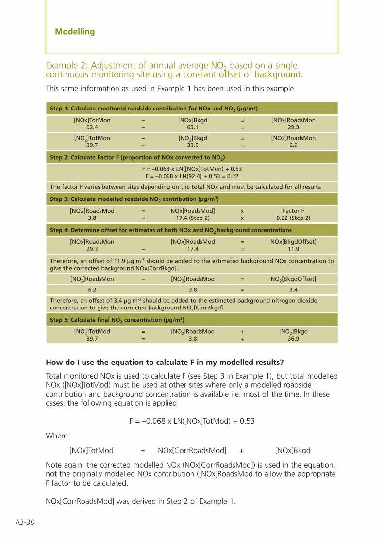
A3-38
Example 2: Adjustment of annual average NO2 based on a singlecontinuous monitoring site using a constant offset of background.
This same information as used in Example 1 has been used in this example.
How do I use the equation to calculate F in my modelled results?
Total monitored NOx is used to calculate F (see Step 3 in Example 1), but total modelledNOx ([NOx]TotMod) must be used at other sites where only a modelled roadsidecontribution and background concentration is available i.e. most of the time. In thesecases, the following equation is applied:
F = –0.068 x LN([NOx]TotMod) + 0.53
Where
[NOx]TotMod = NOx[CorrRoadsMod] + [NOx]Bkgd
Note again, the corrected modelled NOx (NOx[CorrRoadsMod]) is used in the equation,not the originally modelled NOx contribution ([NOx]RoadsMod to allow the appropriateF factor to be calculated.
NOx[CorrRoadsMod] was derived in Step 2 of Example 1.
Step 1: Calculate monitored roadside contribution for NOx and NO2 (µg/m3)
[NOx]TotMon – [NOx]Bkgd = [NOx]RoadsMon92.4 – 63.1 = 29.3
[NO2]TotMon – [NO2]Bkgd = [NO2]RoadsMon39.7 – 33.5 = 6.2
Step 2: Calculate Factor F (proportion of NOx converted to NO2)
F = –0.068 x LN([NOx]TotMon) + 0.53F = –0.068 x LN(92.4) + 0.53 = 0.22
The factor F varies between sites depending on the total NOx and must be calculated for all results.
Step 3: Calculate modelled roadside NO2 contribution (µg/m3)
[NO2]RoadsMod = NOx[RoadsMod] x Factor F3.8 = 17.4 (Step 2) x 0.22 (Step 2)
Step 4: Determine offset for estimates of both NOx and NO2 background concentrations
[NOx]RoadsMon – [NOx]RoadsMod = NOx[BkgdOffset]29.3 – 17.4 = 11.9
Therefore, an offset of 11.9 µg m-3 should be added to the estimated background NOx concentration togive the corrected background NOx[CorrBkgd].
[NO2]RoadsMon – [NO2]RoadsMod = NO2[BkgdOffset]
6.2 – 3.8 = 3.4
Therefore, an offset of 3.4 µg m-3 should be added to the estimated background nitrogen dioxideconcentration to give the corrected background NO2[CorrBkgd].
Step 5: Calculate final NO2 concentration (µg/m3)
[NO2]TotMod = [NO2]RoadsMod + [NO2]Bkgd39.7 = 3.8 + 36.9
Modelling (continued)
A3-39
Example 3: Verification of annual average NO2 based on two continuousroadside monitoring sites and 10 roadside diffusion tube sites.
This example refers to modelling based on road traffic sources only, and backgroundnitrogen oxides and nitrogen dioxide obtained from a background NOx/NO2 analyser.Box A3.8 shows the calculated concentrations at various stages of the verificationexercise for predictions near roads. Background nitrogen oxides is 46.5 µg/m3 andnitrogen dioxide is 23.3 µg/m3.
An adjustment factor for modelled roadside NOx was derived for each analyser usingthe method described in Steps 1 and 2 of example 1. The adjustment factor for eachsite was 1.8 and 2.3; this was averaged to obtain a combined modelled roadside NOxadjustment factor of 2.05.
The modelled roadside NOx at each verification site was therefore corrected by a factorof 2.05 [column 2 of Box A3.8].
The equation for F, (F = -0.068 x Ln(Total NOx) + 0.53) is used to determine theproportion of NOx converted to NO2 at each site. Total NOx at each site is derived byadding the corrected modelled roadside NOx to background NOx [column 3 Box A3.8].Background NOx is this case is 46.5 µg/m3 as derived from a continuous backgroundNOx/NO2 analyser. The F factor derived at each site [column 4] is applied to thecorrected roadside modelled NOx (column 2) to get the modelled roadside NO2concentration [column 5].
The monitored roadside NO2 [column 6] is derived by subtracting background NO2 fromthe total monitored NO2 concentration at each site. The modelled [column 6] andmonitored [column 5] roadside NO2 contributions are compared in a scatter graph anda trend line, along with its equation and regression co-efficient are derived (Graph 1).The equation of the trend line is used to correct the modelled roadside NO2 further[column 7]. [Note that the graph has been drawn with modelled on the x axis becausethe equation derived is in the form of monitored = slope*modelled and can thereforebe used to correct the modelled data to monitored.]
The corrected modelled roadside NO2 is then added to background NO2 to derive thetotal modelled NO2 concentration at each site [column 8]. Another scatter graph isdrawn to compare the total modelled NO2 against total monitored NO2 (Graph 2) andthe equation of this trend line can be used further adjust total modelled NO2. [Notethat the graph has been drawn with modelled on the x axis because the equationderived is in the form of monitored = slope*modelled + intercept and can therefore beused to correct the modelled data to monitored.]
The trend line on graph one for roadside contributions only, has been fitted throughzero to avoid producing negative roadside contributions, but Graph 2 for total NO2 isnot, as background NO2 is included and does not approach zero.
It should be noted that other forms of curves may be fitted to the data includinglogarithmic curves. The various relationships should be compared based on the availabledata. The graphs shown are for roadside locations and similar comparisons which includebackground locations (and generally lower concentrations) may also be undertaken.
Modelling

A3-40
Graph 2: Modelled vs monitored total roadside NO2 (annual average)
Graph 1: Modelled vs monitored roadside NO2 (annual average) – not including background
y = 1.0955x
R2 = 0.5114
0.0
5.0
10.0
15.0
20.0
25.0
30.0
35.0
40.0
0.0 5.0 10.0 15.0 20.0 25.0 30.0
Modelled roadside contribution NO2 (µg/m3)
Mo
nit
ore
d r
oad
sid
e co
ntr
ibu
tio
n N
O2
(µg
/m3 )
y = 2.2508x - 58.494
R2 = 0.7458
0.0
10.0
20.0
30.0
40.0
50.0
60.0
70.0
0.0 10.0 20.0 30.0 40.0 50.0 60.0
Modelled total roadside NO2 (µg/m3)
Mo
nit
ore
d t
ota
l ro
adsi
de
NO
2 (µ
g/m
3 )
Modelling (continued)
A3-41
Bo
x A
3.8:
Cal
cula
ted
res
ult
s fo
r Ex
amp
le 3
, Mo
del
ver
ific
atio
n w
ith
co
nti
nu
ou
s an
alys
ers
and
dif
fusi
on
tu
bes
at
road
sid
e lo
cati
on
s
12
34
56
78
910
Co
rrec
ted
%D
iffe
ren
cem
od
elle
db
etw
een
Tota
lM
on
ito
red
road
sid
eTo
tal
Co
rrec
ted
mo
del
led
an
dC
orr
ecte
dm
od
elle
d N
Ox
road
sid
eN
O2
(µg
/m3 )
mo
del
led
NO
2to
tal N
O2
mo
nit
ore
dTo
tal
mo
del
led
(µg
/m3 )
Mo
del
led
NO
2(µ
g/m
3 )ro
adsi
de
NO
x(µ
g/m
3 )(a
pp
lyto
tal N
O2
mo
nit
ore
dro
adsi
de
NO
x(2
+ b
ackg
roun
dC
alcu
late
Fro
adsi
de
(1 –
bac
kgro
und
app
ly e
qu
atio
n(7
+ b
ackg
roun
deq
uat
ion
(mo
d –
mo
n)
NO
2(µ
g/m
3 )(µ
g/m
3 )N
Ox)
fact
or
NO
2(µ
g/m
3 )N
O2)
Gra
ph
1)
NO
2)G
rap
h 2
)m
on
*100
37.8
86.9
133.
50.
197
17.1
14.5
18.8
42.1
36.2
–4.2
35.0
88.8
135.
30.
196
17.4
11.7
19.1
42.4
36.9
5.6
44.4
114.
816
1.3
0.18
421
.221
.123
.246
.546
.13.
8
44.4
136.
418
3.0
0.17
624
.021
.126
.349
.653
.119
.5
40.6
101.
114
7.6
0.19
019
.217
.421
.144
.441
.41.
9
52.9
133.
718
0.2
0.17
723
.629
.625
.949
.252
.2–1
.3
34.0
83.4
129.
90.
199
16.6
10.7
18.2
41.5
34.9
2.5
47.3
124.
417
1.0
0.18
022
.424
.024
.647
.949
.34.
3
44.4
110.
015
6.6
0.18
620
.521
.122
.545
.844
.50.
2
53.9
140.
418
6.9
0.17
424
.530
.626
.850
.154
.30.
8
60.6
142.
118
8.6
0.17
424
.737
.327
.050
.354
.8–9
.6
54.5
114.
716
1.3
0.18
421
.131
.223
.246
.546
.1–1
5.4
Modelling

A3-42
What if hourly results need assessing?
A3.193 In cases where hourly nitrogen dioxide concentrations have been identified asbeing at risk of exceedence based on monitored concentrations, some verification ofhourly modelled nitrogen dioxide may also be required. It is recommended thatverification of hourly results is only carried out when detailed daily traffic patterns andbackground concentrations (from a file of monitored background concentrations orwhen background is modelled) have been included.
A3.194 One method for verifying hourly nitrogen dioxide concentrations is to extractthe hourly contributions of nitrogen oxides from the model (i.e. hours 1 to 8760) andadd the continuous hourly background nitrogen oxides to each hour. This may be doneeasily in a spreadsheet, or it may be possible to extract the total hourly nitrogen oxidesfor each hour directly from the model.
A3.195 To compare the modelled hourly total nitrogen oxides (including background)against the total monitored nitrogen oxides concentrations, it is recommended thatrather than using a regression technique, total modelled nitrogen oxides and totalmonitored nitrogen oxides for each hour are sorted and the top 50 of each areselected. A regression line can be drawn through this set of nitrogen oxides data whichrepresents the correction of nitrogen oxides at around the 19th highest concentration.The top 50 hours are chosen as it is at these ranges of results that the correction isrequired for the hourly objective.
A3.196 Apply the equation derived from the regression to correct the modelled totalhourly nitrogen oxides to the monitored total hourly nitrogen oxides. The conversion ofnitrogen oxides to nitrogen dioxide concentrations is then applied, this may be thenDerwent-Middleton function or others.
A3.197 The top 50 modelled hourly nitrogen dioxide concentrations are then plottedagainst the top 50 hourly nitrogen dioxide monitored concentrations and a regressionline and equation is derived again. This new equation can be applied to the correctedmodelled nitrogen oxides concentrations to derive an estimate of hourly nitrogendioxides concentrations.
A3.198 The whole of the data set is not included in the regression because undermost circumstances the focus of exceedences will not lie with low results but at thosenear the objective. In addition, a ranked (sorted) approach is described because it isunlikely that modelled hour by hour concentrations will match monitored hour-by-hourbecause of error in traffic profiles, and because wind directions are averaged in themeteorological file and will not accurately reflect the variation in monitoring.
A3.199 The Dispersion Modelling Helpdesk can be contacted for further informationregarding verification of hourly concentrations.
Modelling (continued)

A3-43
Uncertainty estimates
A3.200 Additional uncertainty of adjusted results will arise from random errors – thatis errors that cannot be easily quantified. Local authorities should be aware of theseadditional uncertainties but are not expected to take account of them by furtheradjusting their modelling results. However these uncertainties are useful in assisting theauthority in its decision as to the extent of the boundary of an AQMA. Furtherinformation is provided in Chapter 1 (paragraph 1.24) and below.
A3.201 The NSCA document ‘Air Quality Management Areas: Turning Reviews intoAction’ available on (www.stanger.co.uk/airqual/model/hlp) provides a useful discussionon the uncertainty around the lines of exceedence and methods for calculating theuncertainty of modelled results. The document identifies a number of ranges ofuncertainty (based on the relevant objective) that may be used when there are only afew locations suitable for verification. As an example, Box A3.8 shows U (uncertainty)values as described for NO2 and PM10 objectives.
A3.202 Using a U value for the annual mean nitrogen dioxide concentration of 0.1,the standard deviation of the model (SDM), and therefore the uncertainty of the linesof exceedence would be:
SDM = 0.1 x 40 = 4 µg/m3.
A3.203 Therefore lines showing 32 µg/m3 (40 – 2SDM), 36 µg/m3 (40 – 1SDM) and40 µg/m3 can be drawn and used when deciding upon the area to be declared as anAQMA. It is however a local decision as to the level of uncertainty that is included inthe decision about where to draw an AQMA boundary.
A3.204 An additional method developed by NETCEN25 based on roadside monitoringand modelling at a series of London sites provides an indication of the likelihood ofexceeding an objective at different predicted levels for NO2 and PM10. This method maybe useful for decision making as concentrations are classified in terms of likelihood(very unlikely, unlikely probable, possible, likely and very likely) based on confidencelevels. Box A3.9 shows the confidence levels for modelled concentrations for 2005 forNO2, and 2004 for PM10 as derived from a statistical analysis. Local authorities may findthis method useful but the confidence limits should only be used with verifiedpredictions. The confidence limits were derived from modelling based on ADMS andshould not be used where point sources are being assessed. Their applicability to othermodels has not been tested.
Box A3.8: NSCA stock U values for assessing uncertainty
Air Quality Objective Stock U value
NO2, 1-hour mean 0.3 – 0.5NO2, annual average 0.1 – 0.2
PM10, 24-hour mean 0.3 – 0.5PM10, annual average 0.3
25 Stedman JR, Bush TJ and Vincent KJ (2002). UK air quality modelling for annual reporting 2001 on ambient airquality assessment under Council Directive’s 96/62/EC and 1990/30/EC. AEA Technology Report AEAT/ENV/R/1221.
Modelling

A3-44
A3.205 It is recognised that it is a difficult exercise for local authorities to determinethe uncertainty of modelling results and the confidence levels provide an indication ofthe what might be expected from modelling in the absence of other information.However, they are only strictly applicable to the scenario for which they were derived.
A3.206 Using Box A3.9 a modelled annual mean NO2 concentration of 44 µg/m3 in2005 would represent a probable exceedence of the annual mean objective and anunlikely overall exceedence of the hourly mean objective. Similarly, for PM10, apredicted annual mean concentration of 39 µg/m3 would represent a possibleexceedence of the annual average objective in 2004, and a modelled 90th percentile24-hour mean of 39 µg/m3 would represent an unlikely exceedence of the 24-hourPM10 objective in 2004.
*In terms of review and assessment, a ‘likely’ exceedence (see Chapter 1) would be any that is ‘probable’ or above.
Box A3.9: Example of confidence levels for modelled concentrations for year of objective (2005 – NO2, 2004 PM10)
NO2
Description of NO2 Annual No2 Hourly averageoccurrence of Chance of average based on modelledexceedence of exceeding objective annual average
objective* objective % (µg/m3) NO2 (µg/m3)
Very unlikely Less than 5 < 28 < 39
Unlikely 5 to 20 28 to 34 39 to 52
Possible 20 to 50 34 to 40 52 to 67
Probable 50 to 80 40 to 46 67 to 81
Likely 80 to 95 46 to 52 81 to 97
Very likely More than 95 > 52 > 97
PM10
Description of PM10 Annual PM10 90%ile 24-houroccurrence of Chance of average average (µg/m3)exceedence of exceeding objective based percentiles,
objective objective % (µg/m3) not annual mean)
Very unlikely Less than 5 < 33 < 36
Unlikely 5 to 20 33 to 37 36 to 44
Possible 20 to 50 37 to 40 44 to 50
Probable 50 to 80 40 to 43 50 to 56
Likely 80 to 95 43 to 47 56 to 64
Very likely More than 95 >47 > 64
Modelling (continued)
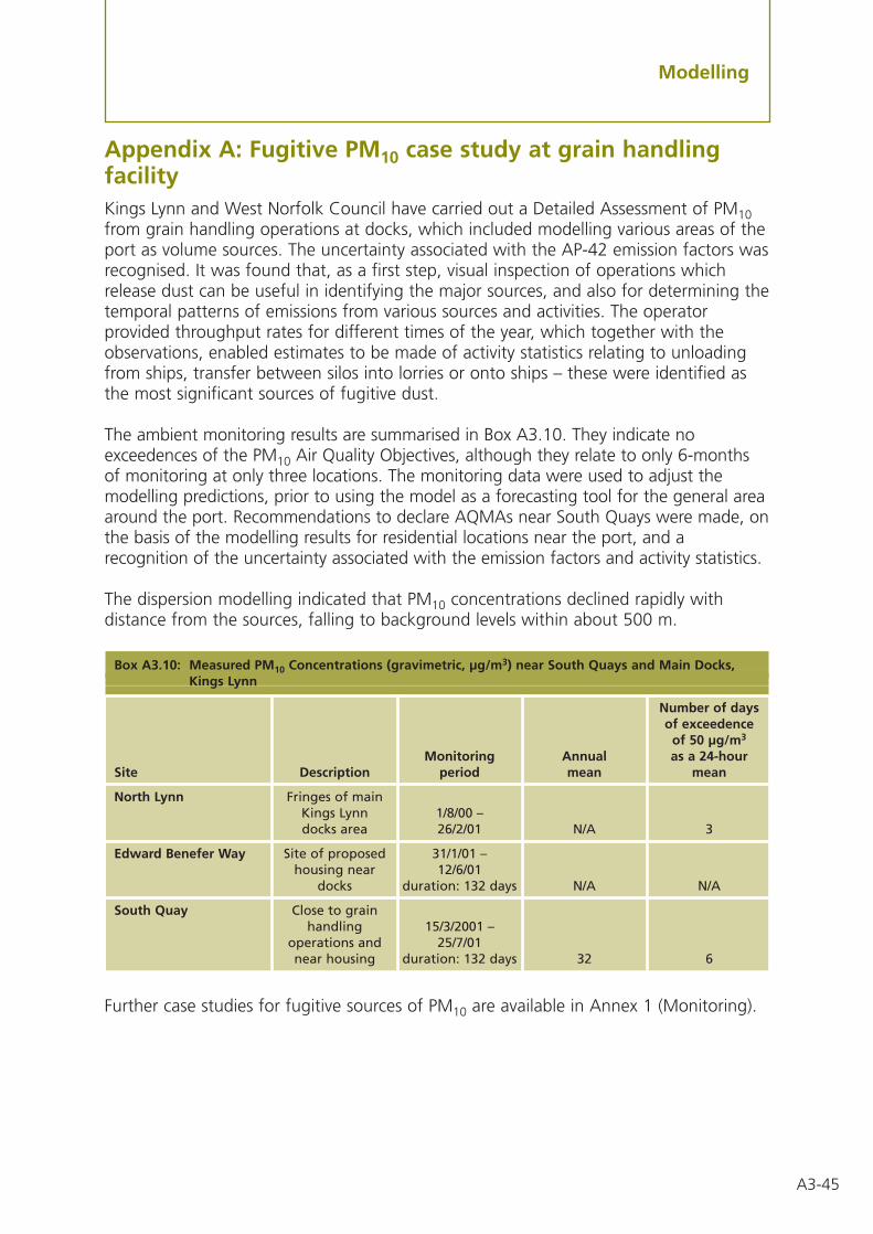
A3-45
Appendix A: Fugitive PM10 case study at grain handlingfacilityKings Lynn and West Norfolk Council have carried out a Detailed Assessment of PM10from grain handling operations at docks, which included modelling various areas of theport as volume sources. The uncertainty associated with the AP-42 emission factors wasrecognised. It was found that, as a first step, visual inspection of operations whichrelease dust can be useful in identifying the major sources, and also for determining thetemporal patterns of emissions from various sources and activities. The operatorprovided throughput rates for different times of the year, which together with theobservations, enabled estimates to be made of activity statistics relating to unloadingfrom ships, transfer between silos into lorries or onto ships – these were identified asthe most significant sources of fugitive dust.
The ambient monitoring results are summarised in Box A3.10. They indicate noexceedences of the PM10 Air Quality Objectives, although they relate to only 6-monthsof monitoring at only three locations. The monitoring data were used to adjust themodelling predictions, prior to using the model as a forecasting tool for the general areaaround the port. Recommendations to declare AQMAs near South Quays were made, onthe basis of the modelling results for residential locations near the port, and arecognition of the uncertainty associated with the emission factors and activity statistics.
The dispersion modelling indicated that PM10 concentrations declined rapidly withdistance from the sources, falling to background levels within about 500 m.
Further case studies for fugitive sources of PM10 are available in Annex 1 (Monitoring).
Box A3.10: Measured PM10 Concentrations (gravimetric, µg/m3) near South Quays and Main Docks, Kings Lynn
Number of daysof exceedence
of 50 µg/m3
Monitoring Annual as a 24-hourSite Description period mean mean
North Lynn Fringes of main Kings Lynn 1/8/00 – docks area 26/2/01 N/A 3
Edward Benefer Way Site of proposed 31/1/01 – housing near 12/6/01
docks duration: 132 days N/A N/A
South Quay Close to grain handling 15/3/2001 –
operations and 25/7/01near housing duration: 132 days 32 6
Modelling

A3-46
Appendix B: List of key model users whose views on theFirst Round have been sought
Organisation Contact
ADM Ltd David Harvey
Kings ERG (formerly SEIPH) Sean Beavers
NETCEN/AEA Beth ConlanJohn WattersonJohn StedmanJustin GoodwinJohn Abbott
ARIC Bethan OwenHazel Peace
The Met Office Doug MiddletonTony Ramsay
Environmental Consultancy Group (ECG)
Environment Agency Betty NgColin PowleslandBernard Fisher
Entec Chris Whall
Enviros Aspinall Mark Broomfield
Birmingham City Council and West Midlands Bob ApplebyRegional Group
CUBA Group, Bristol City Council Peter Fryer
Sheffield City Council Nick Chaplin
Mott Macdonald Ltd Matthew Ireland, Melanie Smith
Derbyshire Dales District Council Malcolm Chattwood
Kings Lynn and West Norfolk Borough Council Dave Robson
GLA David VowlesAlaric Lester
Envirobods David Hall
Southampton City Council Peter Barton
Slough Borough Council Nigel Dicker
Leicester City Council Neil Cooper
TRL Ian McCrae, Paul Boulter
Highways Agency Michele Hickman
Stoke-on-Trent City Council Rob Hannaby
Modelling (continued)

A3-47
Appendix C: List of key model suppliers whose views onthe First Round have been soughtThis list is not an exhaustive guide and any reference to models or software should beregarded as illustrative only and not as a recommendation.
Company Model supplied Contact
CERC ADMS Christine McHugh, Sarah Wilkinson
Fluidyn UK Fluidyn Panache Sharad Tripathi
The Met. Office Lakes software
Trinity AERMOD, ISC
SMHI AirViro
Enviro Technology EnviMan Mike WebleyServices plc
OPSIS EnviMan Hakan Tornevik
CES/Faber Maunsell AAQUIRE James Richer
HA/TRL DMRB Screening Model (v1.0) M. Hackman, I. McCrae, P. Boulter
Modelling

A3-48

A4-1
Annex 4 Abbreviations and glossary
Abbreviations AADT Annual Average Daily Traffic (vehicles per day)
ADMS Atmospheric Dispersion Modelling System
AQMA Air Quality Management Area
ATC Automatic Traffic Counts
AURN Automatic Urban and Rural (air quality monitoring) Network
BAM Beta Attenuation Monitor
BAT Best Available Techniques
CCTV Closed Circuit Television
CO carbon monoxide
CO2 carbon dioxide
COMEAP Committee on the Medical Effects of Air Pollutants
Defra Department for Environment, Food & Rural Affairs
DfT Department for Transport
DMRB Design Manual for Roads and Bridges Screening Model (v1.00)
EA Environment Agency
EFD (or EFDB) Emissions Factor Database
EfW Energy from Waste
EIA Environmental Impact Assessment
GSS Guidance for estimating the air quality impact of Stationary Sources
HECA Home Energy Conservation Act 1995
HDV Heavy Duty Vehicles (includes Rigid and articulated Heavy GoodsVehicles and Buses and Coaches)
Minor roads Non A roads or motorways
NAEI National Atmospheric Emissions Inventory
NAMAS National Accreditation of Measurement and Sampling
NO nitrogen monoxide, also termed nitric oxide
NO2 nitrogen dioxide
NOx nitrogen oxides
NRTF National Road Traffic Forecasts
NWS National Waste Strategy (Scotland)

A4-2
Abbreviations and glossary
OS Ordnance Survey
O2 oxygen
O3 ozone
PM10 particulate matter with an (equivalent aerodynamic) diameter of tenmicrons (10 µm) or less
PM2.5 particulate matter with an (equivalent aerodynamic) diameter of 2.5microns (2.5 µm) or less
SO2 sulphur dioxide
SEPA Scottish Environment Protection Agency
TEMPRO Trip End Model PROjections of growth in travel demand, and theunderlying car ownership and planning data projections
TEOM Tapered Element Oscillating Microbalance
TÜV German Accreditation Organisation
UKAS United Kingdom Accreditation Service
USA Updating and Screening Assessment
USEPA United States Environmental Protection Agency
WASP Workplace Analysis Scheme for Proficiency
WDF Waste Derived Fuel (or Refuse Derived Fuel)

A4-3
Abbreviations and glossary
GlossaryAccuracy A measure of how well a set of data fits the true value.
Area source Emission sources that are too diffuse to identify individually (for example,residential properties).
Air Quality Objective Policy targets generally expressed as a maximum ambientconcentration to be achieved, either without exception or with a permitted number ofexceedences within a specified timescale (see also air quality standard).
Air quality standard The concentrations of pollutants in the atmosphere which canbroadly be taken to achieve a certain level of environmental quality. The standards arebases on assessment of the effects of each pollutant on human health including theeffects on sensitive sub groups (see also Air Quality Objective).
Annual mean The average of the concentrations measured for each pollutant for oneyear. In the case of the Air Quality Objectives this is for a calendar year.
AQMA Air Quality Management Area, an area which a local authority has designatedfor action, based upon predicted exceedences of Air Quality Objectives.
Atmospheric dispersion model A mathematical, often computer-based method forcalculating pollutant concentrations from emissions data under a set of knownvariables. Models vary from screening models to detailed, ‘new-generation’ types.Annex 3 discusses their application in more detail.
AURN Automatic Urban and Rural Network of air pollution measurement sites,managed by contractors on behalf of Defra and the Devolved Administrations.
Concentration The amount of a (polluting) substance in a volume (of air), typicallyexpressed as a mass of pollutant per unit volume of air (for example, microgrammes per cubic metre, µg/m3) or a volume of gaseous pollutant per unit volume of air (partsper million, ppm).
Conservative Tending to over-predict the impact rather than under-predict.
Data capture The percentage of all the possible measurements for a given period thatwere validly measured.
Emissions inventory is a quantification and compilation of emission sources bygeography and time, usually including data covering one or several years.
Euro I Europe-wide vehicle standard that required vehicles manufactured after 1992 to achieve set emissions limits. For petrol cars this was achieved by the fitting of threeway catalysts.
Euro II, III, IV & V Europe-wide vehicle standards that are progressively stricter, foryears 1996, 2000, 2006 and 2008 respectively.
Exceedence A period of time where the concentration of a pollutant is greater thanthe appropriate Air Quality Objective.
A4-4
Abbreviations and glossary
Fine particles, particulate matter, PM10 Particles in air with an (equivalentaerodynamic) diameter of ten micrometres (10 µm, 10 micrometres) or less.
Line source Emission source considered to be mobile and to follow a well defined path(for example, road transport, shipping, railways).
Maximum hourly average The highest hourly reading of air pollution obtained duringthe time period under study.
Microgramme (µg), one millionth of a gramme.
Micrometre (µm), also referred to as a micron, one millionth of a metre.
Model adjustment Following model verification, the process by which modelled resultsare amended. This corrects for systematic error.
mg/m3 milligrammes per cubic metre of air. A unit for describing the concentration ofair pollutants in the atmosphere, as a mass of pollutant per unit volume of clean air.This unit is one thousand times larger than the µg/m3 unit listed below.
µg/m3 microgrammes per cubic metre of air. A measure of concentration in terms ofmass per unit volume. A concentration of 1 µg/m3 means that one cubic metre of aircontains one microgram (millionth of a gram) of pollutant.
nm nanometre 10-9 metres, one billionth of a metre.
Percentile A value that is the rank at a particular point in a collection of data. Forinstance, a 98th percentile of values for a year is the value that 98% of all the data inthe year fall below, or equal.
Point source Significant facility may include a number of stacks or large plant.
ppb parts per billion. The concentration of a pollutant in air in terms of volume ratio.A concentration of 1 ppb means that for every billion (109) units of air, there is oneunit of pollutant present.
ppm The concentration of a pollutant in air in terms of volume ratio. A concentrationof 1 ppm means that for every million (106) units of air, there is one unit of pollutantpresent.
Precision A statistical definition of how closely a range of readings are to one another(see accuracy).
Ratification (Monitoring) involves a critical review of all information relating to a dataset, in order to amend or reject the data. When the data have been ratified theyrepresent the final data to be used (see also validation).

A4-5
Abbreviations and glossary
Running mean is a mean – or series of means – calculated for overlapping timeperiods, and is used in the calculation of several of the National Air Quality Objectives.For instance, an 8-hour running mean is calculated every hour, and averages the valuesfor eight hours. The period of averaging is stepped forward by one hour for each value,so running mean values are given for the periods 00:00 – 07:59, 01:00 – 08:59 etc.By contrast a non-overlapping mean is calculated for consecutive time periods, givingvalues for the periods 00:00 – 07:59, 08:00 – 15:59 and so on. There are, therefore,24 possible running 8-hour means in a day (calculated from hourly data) and 3non-overlapping 8-hour means.
TEOM Tapering Element Oscillating Microbalance. Equipment used for measuring fineparticulate matter such as PM10.
Validation (Monitoring) screening monitoring data by visual examination to check for spurious and unusual measurements (see also ratification).
Validation (Modelling) refers to the general comparison of modelled results againstmonitoring data carried out by the model developers.
Verification (Modelling) comparison of modelled results versus any local monitoringdata at relevant locations.

PB7514
Nobel House17 Smith SquareLondon SW1P 3JR
About Defrawww.defra.gov.uk
Technical GuidanceLAQM. TG(03)
Part IV of the Environment Act 1995
Local Air Quality Management
Part IV of the Environm
ent Act 1995: Local A
ir Quality M
anagement: Technical G
uidance