List of CILC 2007 papers

List of CILC 2007 papers

Testing Logic Programs with Multiple ChancesFrancesco Buccafurri, Gianluca Caminiti and Rosario Laurendi

Rule-based e-mail annotationsMassimo Marchi, Giacomo Fiumara, Rosamaria Pagano and Fortunato Roto

Automatic Correctness Proofs for Logic Program TransformationsAlberto Pettorossi, Maurizio Proietti and Valerio Senni

Frame logic under answer set semanticsMario Alviano, Francesco Calimeri, Giovambattista Ianni and Alessandra Martello

Parallel Instantiation of ASP ProgramsFrancesco Calimeri, SImona Perri and Francesco Ricca

Implementation and Evaluation of Look-Back Techniques and Heuristics in DLVWolfgang Faber, Nicola Leone, Marco Maratea and Francesco Ricca

Towards Proof Theoretic Model GenerationCamillo Fiorentini, Alberto Momigliano and Mario Ornaghi

Web Site Verification: an Abductive Logic Programming ToolGiacomo Terreni, Paolo Mancarella and Francesca Toni,

Programmazione Logica Multi-valued, Sinonimia, ControlloDaniele Genito

Modeling CNF-formulae and formally proving the correctness of DPLL by Means of RefereeEugenio Omodeo and Alexandru Ioan Tomescu

A Dialogue Games Framework for the Operational Semantics of Logic LanguagesStefania Costantini and Arianna Tocchio

A Heuristic Approach for P2P NegotiationStefania Costantini, Arianna Tocchio and Panagiota Tsintza

Using Unfounded Sets for Computing Answer Sets of Programs with Recursive AggregatesMario Alviano, Wolfgang Faber and Nicola Leone

Extending Agent-oriented Requirements with Declarative Business Processes: a Computa-tional Logic-based ApproachVolha Bryl, Paola Mello, Marco Montali, Paolo Torroni and Nicola Zannone

A Tableau for Right Propositional Neighborhood Logic over TreesDavide Bresolin, Angelo Montanari and Pietro Sala

1

KLM Logics of Nonmonotonic Reasoning: Calculi and ImplementationsLaura Giordano, Valentina Gliozzi, Nicola Olivetti and Gian Luca Pozzato

Answer Set Programming with ResourcesStefania Costantini and Andrea Formisano

A Goal-Directed Calculus for Standard Conditional LogicsNicola Olivetti and Gian Luca Pozzato

Indexing Techniques for the DLV InstantiatorGelsomina Catalano, Nicola Leone and Simona Perri

Combination Methods for Model-Checking of Infinite-State SystemsSilvio Ghilardi, Enrica Nicolini, Silvio Ranise and Daniele Zucchelli

Multivalued Action Languages with Constraints in CLP(FD)Agostino Dovier, Andrea Formisano and Enrico Pontelli

SLDNF-Draw: a Visualisation Tool of Prolog Operational SemanticsMarco Gavanelli

Decision algorithms for fragments of real analysis. II. A theory of differentiable functionswith convexity and concavity predicatesDomenico Cantone and Gianluca Cincotti

On the satisfiability problem for a 3-level quantified syllogisticDomenico Cantone and Marianna Nicolosi Asmundo

Generalizzazione di Clausole Basata Su Un Nuovo Criterio di SimilaritaStefano Ferilli, Teresa Basile, Nicola Di Mauro, Marenglen Biba and Floriana Esposito

Constraint-based simulation of biological systems described by Molecular Interaction MapsLuca Bortolussi, Simone Fonda and Alberto Policriti

Interoperability Mechanisms for Ontology Management SystemsGallucci Lorenzo, Giovanni Grasso, Nicola Leone and Francesco Ricca

Some remarks on Rice’s and Rice-Shapiro Theorems and related problemsDomenico Cantone and Salvatore Cristofaro

2

Testing Logic Programs with Multiple Chances

Francesco Buccafurri, Gianluca Caminiti, and Rosario Laurendi

DIMET, Universita degli Studi Mediterranea di Reggio Calabria,via Graziella, loc. Feo di Vito, 89122 Reggio Calabria, Italy,

bucca, gianluca.caminiti, rosario.laurendi @unirc.it

Abstract. The extension of Answer Set Programming (ASP) to naturally rep-resent multi-chances reasoning is an issue recently studied in the literature byproposing logic programs with multiple chances (MC-programs). The importanceof the above issue derives from the consideration that traditional ASP does notallow us to naturally express forms of reasoning where different conditions, par-tially alternative and hierarchically structured, are mentally grouped in order toderive some conclusion. The hierarchical nature of such knowledge concerns withthe possible failure of a chance of deriving a conclusion and the necessity, insteadof blocking the reasoning process, of activating a subordinate chance. However,introducing an additional abstraction layer in order to improve the Knowledge-Representation capability of ASP, sometimes might result in an intolerable in-crease of solver execution time. This paper is aimed to study the above issue,by implementing MC-programs, evaluating them, and comparing them with themost suitable language (for multi-chance reasoning) existing in the literature, thatis Nested Logic Programming.

1 Introduction

The extension of Answer Set Programming (ASP) to naturally represent multi-chancesreasoning is an issue recently studied in the literature [4]. There, the authors start fromthe consideration that in human-like reasoning it often happens that different conditionsare mentally grouped in order to derive some conclusion. Such conditions represent dif-ferent chances (i.e., possibilities), partially overlapped, exploitable as alternative waysto go further in the reasoning steps. Moreover, following different kinds of ordering,like reliability, simplicity, cost, and so on, different chances are hierarchically struc-tured, and the failure of a chance of deriving a conclusion, caused by uncertainty condi-tions, enables the application of a subordinate chance. This way, the reasoning processis not necessarily blocked by uncertainty.

Consider for example the diagnostic medical reasoning. The doctor tries to recog-nize a classical clinical picture, in order to derive a diagnosis, but often such a pictureis unclear and incomplete. In this case he typically adopts subordinate ways in order toreach the same conclusion as consulting, ex-adiuvantibus treatments, tests and so on.

Such a situation can be easily generalized to the case where multiple possibilitiesof deriving yield the same conclusion, as represented in Figure 1. A conclusion can bederived by the joint occurring of a given set ofn basic conditions such that each, in caseof uncertainty, can be substituted by a suitable second-chance condition. Clearly, it is

2

Fig. 1. Basic and second-chance conditions required to yield the same conclusion.

possible that each second-chance condition is uncertain itself, hence being substitutedby a third-chance option, etc.

Answer Set Programming [7] does not allow us to express such situations in a syn-thetic fashion, since different chances of deriving a conclusion must be distributed overdifferent rules, and conditions enabling the switching among chances must be explicitlyrepresented.

In [4], a language is defined extending ASP by including a new modality, allowingus the representation, in a compact and natural fashion, of the multi-chances form ofreasoning described above. Therein, the language is compared by examples with otherformalisms, which are suitable to represent multiple chances. Among them we recallNested Logic Programming(NLP) [11], that is a well-known framework languagesallowing default reasoning with exceptions and prioritized rules [2, 14, 5, 3, 8].

An important question that is not addressed in [4], is that the high abstraction levelintroduced by the new modality, giving the language the capability of expressing multi-chances reasoning in a very natural and declarative fashion, has a heavy price in termsof evaluation time. Indeed, in [4], only an asymptotic complexity analysis is provided,showing that the complexity of the language is the same as plain ASP.

This paper address the above issue, by experimentally studying the performanceof MC-programs and by comparing the language with the most suitable language (formulti-chance reasoning) existing in the literature, that is NLP [11].

The plan of the paper is the following. Section 2 briefly recalls syntax and seman-tics of Logic Programs with Multiple Chances [4]. Then, in Section 3 we discuss anumber of experiments we have performed in order to evaluate the performance of theabove framework, and also we discuss a comparison with NLP. Finally, we draw ourconclusions in Section 4.

3

2 Logic Programs with Multiple Chances

In this section, we give an overview of logic programs with multiple chances [4], ref-erenced to asMC-programs, by briefly recalling the syntax and the semantics of thelanguage.

Recall [7] that anatom is an expressionp(t1, · · · , tn), wherep is a predicateofarity n andt1, · · · , tn are constants. Aliteral is either apositive literala or anegativeliteral ¬a, wherea is an atom and¬ is theclassical negationsymbol. Given a literala, ¬a is defined as¬p, if a = p andp if a = ¬p. A setL of literals isconsistentif∀l ∈ L,¬l 6∈ L. Given a literala, the formulanot a is thenegation as failure(NAF) ofa1.

Definition 1. Givenm ≥ 0 andk ≥ 0, anMC-formulaβ is a formula

(α1[γ1], · · · , αm[γm])T1, · · · , Tk

where:

(1) αj (1 ≤ j ≤ m) is (possibly the NAF of) a literal and may appear underlined,(2) Ti (1 ≤ i ≤ k) is a subset ofαj | αj(1 ≤ j ≤ m) is either underlined, or is not

the NAF of a literal, and(3) γj (1 ≤ j ≤ m) is a (possibly empty) conjunction of MC-formulas.

Each setTi (1 ≤ i ≤ k) is referenced to as theadmissibility constraintand the(possibly empty) setT1, · · · , Tk of admissibility constraints ofβ is denoted byS(β).γj (1 ≤ j ≤ m) is referenced to as thesecond-chanceof αj .

Observe that the recursive definition above is a generalization of the standard defini-tion of the conjunction of (possibly the NAF of) literals occurring in the body of an ASPlogic rule, where both (i) a second-chance is (possibly) associated to each literal, (ii)literals may appear underlined and (iii) a set of admissibility constraints is associated tothe conjunction.

Each second-chance may be viewed as a substitution of theαj to which is applied.Such a substitution is executed only whenαj is uncertain(the notion of uncertainty willbe introduced in the following – the underlining is relating with this notion). Due to therecursive structure of the above definition, a second-chance is, in turn, a conjunctionof MC-formulas, and thus may contain further subordinate chances (i.e., the nestingof chances is allowed). Intuitively, second-chances are subordinate conditions that arerequired, in order to satisfy the MC-formula, whenever the basic conditionsαis areuncertain. Actually, not all the possible configurations of values makingαis uncertainare allowed, in order to activate the substitution of the second-chance, but only thosesatisfying the admissibility constraints.

Example 1.Consider the following MC-formulas:β1 = (a, not b)[c] (denoted alsoby (a[c], not b[c])), whereS(β1) = ∅ andβ2 = (a, b)a, b[c], (denoted also by(a[c], b[c])a, b), whereS(β2) = a, b.

1 Observe that the NAF of negative literals is allowed.

4

Given a conjunction of MC-formulas∆, in favor of simplicity, we often write

(α1[γ1], · · · , αm[γm])T1, · · · , Tk[∆]

to denote the following MC-formula:

(α1[γ1[∆]], · · · , αm[γm[∆]])T1, · · · , Tk.

In particular, ifγ1 = · · · = γm = ∆, we write (α1, · · · , αm)T1, · · · , Tk[∆] todenote the MC-formula(α1[∆], · · · , αm[∆])T1, · · · , Tk. Clearly, square brackets ofempty second-chances are omitted.

Definition 2. An MC-ruler is a formulaa ← β1, · · · , βn (n ≥ 0), wherea is a positiveliteral andβi is an MC-formula, for each1 ≤ i ≤ n. The seta, denoted byhead(r),is referenced to as theheadof r, and the setβ1, · · · , βn, denoted bybody(r), isreferenced to as thebodyof r.

Note that since an MC-formula is a generalization of a standard conjunction of (theNAF of) literals, a standard ASP rule is a special case of an MC-ruler. Informally, anMC-rule is a logic rule allowing in the body the substitution of some literal with itssecond-chance (under uncertainty conditions).

Example 2.The following are examples of MC-rules:a ← (b, c, e)c, e, b, c[not d],anda ← b[c[d]], f [not g].

Definition 3. An MC-programis a finite set of MC-rules.

We introduce now the intended models of the semantics of MC-programs. First weneed some preliminary definitions.

Given an (MC-)programP , LitP is the set of literals occurring inP . An interpre-tationI of an (MC-)programP is a consistent subset ofLitP . A literal a is truew.r.t. Iif a ∈ I, it is falsew.r.t. I if ¬a ∈ I. A literal a is undefinedw.r.t. I if it is neither truenor false w.r.t.I. Given a literala, a formulanot a is true w.r.t. I if a 6∈ I, it is falsew.r.t. I otherwise (observe that the NAF of a literal cannot be undefined w.r.t. a giveninterpretation). From now on in this section, consider given an (MC-)programP and aninterpretationI of P .

We introduce now a basic notion of the framework, that is the notion ofuncertaintyof an element of an MC-formula. Indeed the mechanism of substitution of an elementof an MC-formula with its second-chance is founded on this property (this will be ex-plained in detail in the following).

Definition 4. Given an MC-formulaβ = (α1[γ1], · · · , αm[γm])T1, · · · , Tk, we saythatαj (1 ≤ j ≤ m) is uncertainw.r.t. the interpretationI if either:

(i) αj = a | a ∈ LitP ∧ a,¬a ∩ I = ∅,(ii) αj = a | a ∈ LitP ∧ a 6∈ I, or

(iii) αj = not a | a ∈ LitP ∧ a ∈ I.

5

The definition above arises from the following reasoning. We expect that an elementαj is uncertain if it is undefined. This is captured by the item (i) of the definition.Note that, correctly, this item does not include the case of the NAF of a literal, sincesuch a formula cannot be undefined. Now, when we want to interpret as uncertain alsothe false value ofαj , we require thatαj is underlined (items (ii) and (iii)). Thanks tothis mechanism, also the NAF of a literal can be uncertain, whenever it appears in anunderlined elementαj = not a, anda is true.

Example 3.For instance, given the interpretationI = ¬a, the MC-formulab[not d]is uncertain w.r.t.I sinceb,¬b ∩ I = ∅. Moreover, the MC-formulac[f ] is uncertainw.r.t. I sincec 6∈ I. Finally, the MC-formulaa[g] is not uncertain w.r.t.I because¬a ∈ I.

Moreover, Definition 4 above is extended by means of a flexible machinery suchthat we are able to specify which literals in an MC-formula cannot be uncertain at thesame time.

Definition 5. Given an MC-formulaβ = (α1[γ1], · · · , αm[γm])T1, · · · , Tk, S(β) istrue w.r.t. I if for eachTi ∈ S(β) (1 ≤ i ≤ k), there existsα ∈ Ti such thatα is notuncertain w.r.t.I.

In words, an admissibility constraintTi states that literals occurring in an MC-formulaβ cannot appear simultaneously in uncertainty configurations.

Example 4.Consider the following MC-rule:a ← (b, c, e)c, e, b, c[not d]. Givenan interpretationI = ¬b, e, it is easy to see thatS(β) = c, e, b, c is not truew.r.t. I, because bothc andb are uncertain w.r.t.I.

Now, we define the intended models of the semantics of MC-programs. First, weintroduce a transformation for MC-programs which produces an ASP program.

Definition 6. We define theMC-transformationof the programP w.r.t the interpreta-tion I as the ASP programP I , obtained fromP by executing Algorithm 1.

Algorithm 1 (The MC-transformation algorithm)repeat

for each MC-ruler ∈ P doif ∃β ∈ body(r) | S(β) is false w.r.t.I then deleterelse foreachβ = (α1[γ1], · · · , αm[γm])T1, · · · , Tk ∈ body(r) dodeleteS(β)for each1 ≤ j ≤ m doif αj is uncertain w.r.t.I then remove fromαj the underlining (if any)if γj is not emptythen replaceαj [γj ] by γj

end ifelseremove fromαj the underlining (if any); replaceαj [γj ] by αj

end ifend for

end for

6

end ifend for

until ∀r ∈ P,∀β ∈ body(r) ∃a ∈ LitP | β = a ∨ β = not a

The MC-transformation ofP consists of both (i) deleting all MC-rules ofP whose bodyincludes some MC-formula with false admissibility constraint, (ii) deleting all admissi-bility constraints from the remaining MC-formulas, (iii) for each uncertain elementαj

in the body of every MC-rule, removing the underlining (if any), and replacingαj by itssecond-chance (if any); (iv) for each remaining elementαj , removing the underlining(if any) and discarding its second-chance. The loop ends when only (possibly the NAFof) literals occur inP .

Definition 7. An interpretationJ of the programP is ananswer setof P if J is ananswer set2 of P J .

Example 5.For instance, consider the following MC-programP :

r1 : a ← (b, c, e)c, e, b, c[not d]r2 : d ← not a r3 : ¬b ← ar4 : c ← not d r5 : e ←

The intended answer sets ofP are:a,¬b, c, e, d, e. Indeed, givenI1 = a,¬b, c, e,the MC-transformation ofP w.r.t. I1 is P I1 = r′1, r2, r3, r4, r5, wherer′1 is a ←not d, c, e. Observe thatI1 is an answer set ofP I1 thought as an ASP program. Like-wise, it is easy to see thatI2 = d, e is an answer set ofP I2 = r2, r3, r4, r5 (r1 isdeleted due to the constraintb, c).

Remark. The formalism presented in [4] can be viewed as an extension of the ASPnegation by failure. Indeed, the ruleh ← not b can be rewritten in the form of a MC-rule ash ← ¬b[true]. According to the semantics of MC-programs,h is derived ifeitherb is false (i.e.,¬b is true) orb is undefined (since, in this case the subordinatecondition is activated and it corresponds to the constanttrue), exactly as the ASP ruleh ← not b.

3 Experiments

In this section we discuss the results of several experiments we have done in order toevaluate the language proposed in [4]. First, we describe our testbed. We have imple-mented an algorithm in Java which performs a source-to-source transformation fromMC-programs to Answer Set Programming. The code is based on a suitable linear-timetranslation algorithm, described in [4]. Briefly, a given MC-programP is translated,by means of such an algorithm, into an ASP programΓ (P ). Thus, we exploit nowa-days powerful ASP engines [9, 13] in order to compute the answer sets ofP in terms

2 The definition ofanswer setsof an ASP program can be found in [7]. We do not report it herefor space limitations. Note that, according to the definition of interpretation, we want to limitour focus only on consistent answer sets.

7

of answer sets of the logic programΓ (P ) that is produced by the translation. We havechosen the DLV System [9], that is widely accepted as a state-of-the-art ASP solver3.

Now, we describe two series of experiments we have performed:

1. The first series of experiments is aimed to study the impact of the features of MC-programs on the performance of the ASP solver.

2. In the second series of experiments we compare the performance of the frameworkof MC-programs with that of NLP.

3.1 First Series of Experiments: Evaluation of MC-Programs

Now we describe the first series of experiments we have performed. We have consideredthe following parameters that are associated to the syntax of MC-programs:

(1) The number of MC-formulas per rule (n);(2) The maximum level of nesting of MC-formulas (l);(3) The number of elements (possibly MC-formulas) that compose a second-chance of

a MC-formula (m); and(4) The activation of admissibility constraints (c).

Table 1 shows the values assigned to the parameters above. Observe that such val-ues have been chosen since we assume that a real programmer would represent multi-chance knowledge by means of human-readable MC-programs. Hence, the parametervalues are not arbitrary, but they correspond to realistic cases.

Parameter Set of Valuesn 1,2,3,4l 1,2m 1,2,3,4c disabled, enabled

Table 1.Parameter values used for the experiments.

Thus, for each different choice of the parameter values, we have generated a set ofMC-program instances. Each program in a given instance set is made of ten MC-rules,where each rule has a structure that corresponds to the parameter choice. The maximumnumber of literals occurring per each instance is fifteen.

In the next experiment we want to evaluate the impact of admissibility constraints.

3 We have used DLV release Jul 14 2006, running on a Pentium 4 @ 3.40 Ghz.

8

Experiment 1.In order to evaluate the effect of the admissibility constraints, we wantto compare the average times needed by the ASP solver to compute the answer sets ofeach program instance set, forc = disabled andc = enabled, respectively.

First, we consider the casel = 1. The results of the experiment are shown in Fig-ure 2. Each instance set is denoted by the pair〈i, j〉, wherei andj correspond to valuesassigned to the parametersn andm, respectively. Observe that we omit all instance sets〈1, j〉 such that1 ≤ j ≤ 4, since it is easy to see that in those cases there is just oneMC-formula in the body of a MC-rule and thus admissibility constraints cannot be usedfor such instances. Clearly, ifm is fixed, then the average time needed to compute theanswer sets grows asn increases. Conversely, ifn is fixed, different values ofm pro-duce slight differences w.r.t. the average times of computation. The reason is that, sincein this casel = 1, for each program instance, second-chances are simply conjunctionsof m (possibly NAF) literals.

Moreover, another effect caused by using only one level of nested chances is thatthe computational overhead introduced by admissibility constraints is, on average, verysmall.

Fig. 2. Effect of admissibility constraints on MC-programs (one level of nesting).

Experiment 2.In this experiment we evaluate the performance of MC-programs, underthe same setting as Experiment 1 above. The only parameter that changes here isl, i.e.l = 2. Figure 3 shows the results of the experiment after such a change. Considerationssimilar to those stated forl = 1 hold. However, observe that, now, the impact of ad-missibility constraints is, on average, more evident than the case above, since for each

9

level of nesting it is possible to enable the admissibility constraint. As a consequence,a bigger computational overhead is produced.

Moreover, concerning the instance sets〈i, j〉 (2 ≤ i ≤ 4, j = 1), note that theresults are comparable with those obtained forl = 1 (see Experiment 1). The reasonis that if j = 1, then each second-chance in a MC-formula is composed by only oneelement. As a consequence, regardless the two levels of nesting, in casej = 1 it ispossible to enable the admissibility constraints only on the first level (i.e., not insidesecond-chances).

0

1

2

3

4

5

6

7

8

9

10

á2,1ñ á2,2ñ á2,3ñ á2,4ñ á3,1ñ á3,2ñ á3,3ñ á3,4ñ á4,1ñ á4,2ñ á4,3ñ á4,4ñ

Instance Set

Avg

Tim

e(s

)

MC (constraints disabled)

MC (constraints enabled)

Fig. 3. Effect of admissibility constraints on MC-programs (two levels of nesting).

Experiment 3.Now, we are interested in discussing the results of an experiment thatis aimed to evaluate the effect of representing multi-chance knowledge by using MC-program with more than one level of nested chances.

Figure 4 shows the average times measured on instance sets in case admissibilityconstraints are disabled. This is done both for one level and for two levels of nestedsecond-chances. It is easy to see that the computational overhead due to the presence ofa second level of nesting inside MC-formulas is more evident as the parametersn andm increase.

Now, observe that similar considerations hold for the results shown by Figure 5,which represents the average times measured on instance sets such that the admissibil-ity constraints are enabled. Clearly, as mentioned in the paragraph above concerningExperiment 2, those instance sets such that no admissibility constraint can be intro-duced are omitted. Now, note that the presence of admissibility constraints inside MC-

10

formulas produces, on average, a computational overhead that is bigger than in the casesuch constraints are disabled. Concerning the instance sets such thatm = 1, we recallthat for such cases, the overhead is reduced because the structure imposed by the pa-rameters to the program instances does not allow to enable admissibility constraints atthe second level of nesting.

0

1

2

3

4

5

6

7

8

9

á1,1ñ á1,2ñ á1,3ñ á1,4ñ á2,1ñ á2,2ñ á2,3ñ á2,4ñ á3,1ñ á3,2ñ á3,3ñ á3,4ñ á4,1ñ á4,2ñ á4,3ñ á4,4ñ

Instance Set

Avg

Tim

e(s

)

MC (one level of nesting)

MC (two levels of nesting)

Fig. 4. Effect of the number of nesting levels on MC-programs (admissibility constraints dis-abled).

3.2 Second Series of Experiments: Performance Comparison with NLP

In this Section we compare the performance of MC-programs with that of Nested LogicProgramming (NLP). Recall that NLP [11] is a class of logic programs, where arbitrar-ily nested expressions – formed from literals by using negation as failure, conjunctionand disjunction (;) – are allowed in both the bodies and heads of rules. Given an MC-programP , a suitable translationP ′ into a suitable fragment of NLP (with neither NAFnor disjunction in heads of rules) exists. Informally, we can give a sketch of an easytranslation scheme of an MC-rule ofP into an equivalent NLP rule ofP ′. It sufficesto write, for each literalb occurring in a conjunction of a MC-rule, the disjunction ofthe following two conditions: (i) The first condition representsb in the standard case(i.e., no uncertainty), (ii) The second condition models the conjunction of both all theallowed(by means of admissibility constraints) conditions producing the uncertainty ofb and the second-chance associated tob.

Example 6.Consider, for instance, the MC-rulea ← (b[e], c[f ])b, c. An equiva-lent NLP rule obtained by the above translation method is:

11

0

1

2

3

4

5

6

7

8

9

10


Instance Set

Avg

Tim

e(s

)

MC (one level of nesting)

MC (two levels of nesting)

Fig. 5.Effect of the number of nesting levels on MC-programs (admissibility constraints enabled).

a ← (b; (not b, e, (c;¬c))), (c; (not c, not ¬c, f, b))

Clearly such a translation machinery, though it is simple, it is recursive in case thereis more than one level of nested second-chances inside MC-rules.

However, since in our experiments we have limited the maximum nesting level to asmall value, namely 2, it easy to see that such a translation is feasible.

Moreover, in [4] the authors have shown that encoding a multi-chance knowledgerepresented by MC-programs into NLP produces logic programs that are extremelytedious to write and difficult to read (i.e. they represent knowledge in fashion that isnot natural). This occurs especially in case the original MC-programs have two or morelevels of nested second-chances.

Now, we describe the testbed we have used for this series of experiments. For eachMC-program instance that we have generated (recall Table 1), we have produced thecorresponding NLP program, according to the translation scheme above. Then, we haveexploited an external NLP front-end for the DLV system [15] that runs under SICStusProlog [6] in order to obtain from each NLP instance, an equivalent ASP program thatwe have given in input to DLV.

Experiment 4.First we have evaluated the size of both MC- and NLP program instancesafter the translation into ASP. In detail, we have counted both the number of atoms andrules after the translation and we have measured the average per cent increase obtainedby the NLP instances relative to the corresponding MC ones, after the translation.

The following Tables 2 and 3 summarize the results of the experiment, showing thatthe increase in size of NLP program instances after the translation is very big. As we

12

will show in the following experiments, such a big increase in the size corresponds to abetter performance exhibited by the ASP solver on MC-programs.

Constraints Constraintsdisabled enabled

One levelof nesting 152.18% 161.75%Two levelsof nesting 123.56% 119.04%

Table 2.MC vs NLP: Percent increase of the number of atoms

The following figures show the performance comparison between MC-programsand equivalent NLP programs, run under DLV. Observe that, for each instance set, onlythe average times needed to compute the answer sets are presented. We do not considerhere the times required to perform the translation from either MC- or NLP programinstances to ASP.

Experiment 5.First, we discuss the comparison in the case of one level of nesting (l =1). The results of the experiment are reported both in case the admissibility constraintsare disabled (Figure 6) and in case they are enabled (Figure 7). Clearly, we have omittedin Figure 7 the instance sets denoted by the pairs〈i, j〉 such thati = 1, since suchinstance sets correspond to the casen = 1 (recall Table 1), and thus admissibilityconstraints cannot be enabled.

Observe that the performance of the solver is much better on the MC-programs thanon the corresponding NLP instances. This occurs especially in case the admissibilityconstraints are enabled, since the translation from NLP into ASP produces a programwhose size is much bigger than that obtained by translating the corresponding MC-program instance into ASP (recall the results of Experiment 4). As a consequence thecomputational overhead is bigger for NLP programs. In detail, Figure 7 shows thatin case admissibility constraints are enabled, the NLP instances are slower than thecorresponding MC instances by, on average, more than 200%.

Moreover, we have done the same comparison in case of two levels of nesting(l = 2). Figures 8 and 9 show the result of the experiment in case the admissibilityconstraints are disabled and enabled, respectively. Now, observe that the computationaloverhead due to the second level of nested chances is bigger than the case above. MC-programs exhibit better performance than NLP programs. Moreover, in case admissi-bility constraints are enabled, the computational overhead of NLP programs is moreevident than in the case they are disabled. Finally, an interesting result is shown byFigure 9, that is, on average, in case admissibility constraints are enabled, the NLPinstances are more than ten times slower than the corresponding MC instances.

13

Constraints Constraintsdisabled enabled

One levelof nesting 336.61% 369.14%Two levelsof nesting 251.76% 282.62%

Table 3.MC vs NLP: Percent increase of the number of rules

0

5

10

15

20

25


Instance Set

Avg

Tim

e(s

)

MC

NLP

Fig. 6. MC vs NLP (admissibility constraints disabled, one level of nesting).

4 Conclusions

The paper presents experimental evaluation of the implementation of MC-logic pro-grams. The language relies on Answer Set Programming and includes constructs usefulfor naturally representing some forms of reasoning where multiple chances of derivinga given conclusion occur. The results of the experiments we have performed give usvaluable information about the impact that the features of MC-programs have on theperformance of the ASP solver. Moreover, the results of the performance comparisonbetween MC-programs and NLP programs (having at least the same abstraction level)show the superiority of the former in terms of running time for their evaluation.

Finally, the good performance exhibited by the ASP solver on the MC-program in-stances confirms us in the feeling that a very interesting direction for our future researchis applying the formalism to hard problems such as planning [12, 16, 10, 1].

14

0

5

10

15

20

25

30


Instance Set

Avg

Tim

e(s

)

MC

NLP

Fig. 7. MC vs NLP (admissibility constraints enabled, one level of nesting).

References

1. M. Balduccini, M. Gelfond, R. Watson, and M. Nogueira. The USA-Advisor: A Case Studyin Answer Set Planning. InLPNMR, volume 2173 ofLCNS, pages 439–442. Springer, 2001.

2. G. Brewka and T. Eiter. Preferred Answer Sets for Extended Logic Programs.Artif. Intell.,109(1-2):297–356, 1999.

3. G. Brewka, I. Niemela, and M. Truszczynski. Prioritized Component Systems. InAAAI05,pages 596–601, 2005.

4. F. Buccafurri, G. Caminiti, and D. Rosaci. Logic programs with multiple chances. InG. Brewka et Al., editor,Proceedings of ECAI - European Conference on Artificial Intel-ligence, pages 347–351. IOS Press, 2006.

5. F. Buccafurri, N. Leone, and P. Rullo. Disjunctive Ordered Logic: Semantics and Expres-siveness. InProc. of KR’98, pages 418–431, 1998.

6. Swedish Institute for Computer Science. Sicstus prolog. http://www.sics.se/sicstus/.7. M. Gelfond and V. Lifschitz. Classical Negation in Logic Programs and Disjunctive

Databases.New Generation Computing, 9, 1991.8. M. Gelfond and T. C. Son. Reasoning with Prioritized Defaults. InLPKR, pages 164–223,

1997.9. N. Leone, G. Pfeifer, W. Faber, T. Eiter, G. Gottlob, S. Perri, and F. Scarcello. The DLV

System for Knowledge Representation and Reasoning.ArXiv Computer Science e-prints,pages 11004–+, 2002.

10. V. Lifschitz. Answer Set Programming and Plan Generation.Artif. Intell., 138(1-2):39–54,2002.

11. V. Lifschitz, L.R. Tang, and H. Turner. Nested Expressions in Logic Programs.Annals ofMathematics and Artif. Intell., 25(3-4), 1999.

15

0

10

20

30

40

50

60

70

80

90


Instance Set

Avg

Tti

me

(s)

MC

NLP

Fig. 8. MC vs NLP (admissibility constraints disabled, two levels of nesting).

12. A. Nareyek, E. C. Freuder, R. Fourer, E. Giunchiglia, R. P. Goldman, H. A. Kautz, J. Rin-tanen, and A. Tate. Constraints and AI Planning.IEEE Intelligent Systems, 20(2):62–72,2005.

13. I. Niemela and P. Simons. Smodels - an Implementation of the Stable Model and Well-founded Semantics for Normal Logic Programs. InProc. of the 4th LPNMR, LNCS, pages420–429. Springer, 1997.

14. C. Sakama and K. Inoue. Prioritized Logic Programming and Its Application to Common-sense Reasoning.Artif. Intell., 123(1-2), 2000.

15. V. Sarsakov, T. Schaub, H. Tompits, and S. Woltran. nlp: A compiler for nested logic pro-gramming. In V. Lifschitz and I. Niemela, editors,LPNMR, volume 2923 ofLNCS, pages361–364. Springer, 2004.

16. T. C. Son, P. H. Tu, M. Gelfond, and A. R. Morales. Conformant Planning for Domains withConstraints-A New Approach. InProc. of The XXth National Conf. on Artif. Intell. and the17th Innovative Applications of Artif. Intell. Conf., pages 1211–1216, 2005.

16

0

20

40

60

80

100

120


Instance Set

Avg

Tim

e(s

)

MC

NLP

Fig. 9. MC vs NLP (admissibility constraints enabled, two levels of nesting).

Rule-based e-mail annotations?

G.Fiumara1, M.Marchi2, R.Pagano1 and F.Roto1

1 Dept. of Physics, University of Messina,Sal. Sperone, 31. S. Agata di Messina. I-98166 Messina, Italy,

giacomo.fiumara,[email protected] DSI - University of Milan,

Via Comelico, 39/41. I-20135 Milan, Italy,[email protected]

http://mag.dsi.unimi.it/

Abstract. We present the RuBaST (Rule-Based Spam Termination)project, describe its theoretical underpinnings and some preliminary bench-mark results. RuBaST shows that hand-written rules that guide thespam-likeliness evaluation are effective on a relevant corpus that we haveassembled by collecting e-mails that have escaped detection by SpamAs-sassin.

1 Introduction

This article describes a rule-based personal e-mail annotator that works as aspam sentinel. The annotator applies ad-hoc set of annotation rules (calledanti-spam policy) by means of a Prolog inferential engine. Our program, calledRuBaST (Rule-Based Spam Terminator) is intended as a filtering layer betweena typical, site-wide SpamAssassin [1] and the user’s mailbox. RuBaST takes asinput e-mails and human-written annotation rules that give a score to certainaspects of the e-mail, e.g., the occurrence of specific words in the body text ora suspicious sender address. RuBaST works as follows. First, it reads the e-mailfile and applies ad-hoc regular expressions that de-obfuscate suspicious words,e.g., Ciaa11is is rendered as Cialis. Next the whole e-mail is converted into aset of Prolog facts; Prolog rules representing the user’s spam annotation policyare combined with those facts. The rules describe, essentially, a scoring system.The overall score is obtained as the sum of all scores given by the rules: it iscompared to a user-defined threshold and the e-mail is forwarded accordingly.The annotation rules in Prolog syntax are applied by means of the SWI-Prologinferential engine.

RuBaST has been developed in the context of our long-term research goal ofapplying rule-based policies to Web activities, e.g., Web service connection [2],Web data extraction [3] and Semantic Web composition [4]. It does not wishto replicate the excellent results obtained by Machine Learning and Bayesian

? A companion Web site to this article, with software, results and the corpus describedherewith are available at http://mag.dsi.unimi.it/rubast/

filtering, but rather to provide an interface where personal rules are providedand tuned to the particular type of spam one is receiving or indeed finds moreobnoxious.

Even though this application is in its infancy, it shows promising results w.r.t.a small but challenging corpus that we have assembled with e-mails that havenot been blocked by our campus-wide SpamAssassin filter3 then in version 3.1.1.

1.1 The idea

The basic idea of our project is to exploit rule-based reasoning to realize ananti-spam filter which assists in the onerous task of manually identifying andseparating spam from ham (i.e., non-spam) messages. In particular, our goal isto implement an intelligent agent which would assess spam somewhat in human-like fashion4. RuBaST filter receives and analyzes the messages acquiring thesame information perceived by the user. Every piece of information available tothe user, e.g., the sender, the addressee, the object and the text of the message,is relevant and should be considered.

1.2 Validation

We have tested the first implementation of RuBaSTagainst a corpus of e-mailsthat have been collected and prepared to this purpose. So far, the most e-mailsin the corpus are, beyond doubt, spam. It is important to notice that the re-cipient also wrote the annotation policy that was given to RuBaST during theexperiments. Few messages have been classified as ham or maybe by the recipient.The maybe case consists of unsolicited messages, e.g. conference announcements,that share, in the structure and content of the message, some similarity with realspam. For instance, the To: field is normally masked, the return address differsfrom the From:, the message is impersonal and almost always invites to visit aWeb site. To validate the effectiveness of RuBaST in weeding out spam messages,we have posed the problem in terms of Information Retrieval (IR) [6], i.e., asa challenge for RuBaST to select all and only the messages in the corpus thatwere deemed spam. Then, we have compared each annotation to that given by ahuman (other than the recipient) and measured the degree of similarity in termsof Precision, Recall and F1, rather than accuracy and error5.

2 The Implementation

The implementation of RuBaST consist mainly of a Java application with aProlog-based automated reasoning core. The interface between the two modules3 http://spamassassin.apache.org/4 In the Logical AI tradition of McCarthy (see, e.g., [5]), we take intelligent agents to

be computer systems that acts intelligently: what the agent does is appropriate forits circumstances and its goal, it is flexible to changing environments, it deduce fromexperience, and it makes appropriate choices given finite computational resources.

5 Please refer to [7] or to [8] for an introduction to this subject.

is performed by the JPL package provided by SWI-Prolog. Figure 1 summarizesthe architecture of our implementation. Such architecture addresses two mainconcerns that have emerged during our project. First, the current solutions thatintegrate inferential engines into a Java program (e.g., tuProlog [9]) were consid-ered not viable for this project or harder to use vis-a-vis SWI Prolog. Second, wewould like to retain the ability to experiment with different inferential engines inthe future. For instance, in the next phase of the project we will experiment withAnswer Set Programming6. Indeed, the annotation rules, which will be describedin the sequel, hardly use any function or built-in that are specific to SWI.

myaccounts.txtspamexpressions.txt

spamwords.txtspamwordsregxpr.txt

whitelist.txt

Frontend

JVM

RuBaST.jar kbwhitelist.plkbblacklist.plkbmail.pl

kbaccounts.pl

SWI-Prolog

rules.pl

result.txt

result.xml

mails.txtRuBaST

Fig. 1. The overall architecture

JPL [12] is a library that uses the SWI-Prolog7 foreign interface and theJava jni interface8to interleave Prolog and Java executions. The role of the Javamodule, then, is to prepare the message information for the Prolog engine. Wecall this preparation phase normalization. The main task of normalization is theso-called de-obfuscation of the mail body, i.e., spotting (and relative replacement)of terms that have been disguised by the spammer in order to hide them fromthe anti-spam softwares (please see [13] for a discussion and the latest results onde-obfuscation).

The following words are examples of obfuscation found in e-mails not detectedby SpamAssassin version 3.1.1:

– Viiagrra (for Viagra) and– Ci-iallis (for Cialis)

Our rule-based, then, applies to the normalized message the heuristic rules ofthe base of knowledge, assigning a positive score (spam clue) or a negative score(ham clue). The obtained value (SPAM VALUE) is compared to some thresholdsand will accordingly classify the message as SPAM, MAYBE-SPAM or HAM.The prior knowledge embedded in our system consists, essentially, of two list:

6 Answer Set Programming, in short, gives to Prolog rules a multiple models semantics,thus allowing to model reasoning by cases. Please refer to the pioneering work ofLifschitz and Gelfond [10] and to the survey in [11] for an introduction to the subject.

7 http://www.swi-prolog.org/8 http://java.sun.com/j2se/1.4.2/docs/guide/jni/

- black-words and black-expressions commonly used in the spam messages(commonly referred to as blacklist), and

- trusted email address (commonly referred to as whitelist).

2.1 The Java module and the de-obfuscation

The first task of the Java module is to locate and extract from the message thepieces of information that are subject of our analysis. For instance, the sender,the addressee, the object and the text of the message. Next, de-obfuscationstarts. RuBaST resorts to regular expressions, to analyze the text of the messagelooking for words and/or expressions that are present in blacklist, yet disguisedby spammers.

Sender

Adressee

Object

Text

Mail

RuBaST.jar

mail.txt Sender

Adressee

Object normalized

Text normalized

Mail

Normalizationspamwords.txt

spamwordsregexpr.txtspamexpressions.txt

kbmail.pl

spamwords.txtspamexpressions.txt

CreateBlacklist() kbblacklist.pl

myaccounts.txt CreateAccountList() kbaccounts.pl

whitelist.txt CreateWhitelist() kbwhitelist.pl

Fig. 2. Architecture of the front end

Attempts to mask the black-expressions are of different kind [13], for instance,misspelling, insertion, replacement (or removal) of non-alphabetical characters(e.g., extra spaces), to name a few.

RuBaST tries to pick all those obfuscations that, although complicated, areresolved by an average user at a glance. 9

RuBaST constructs two models of regular expressions for every black-expression.

Example 1. The two models for the word CIALIS are:

Model 1: [cC]1 .0,2 [iI]1 .0,2 [aA]1. 0,2 [lL]1 .0,2[iI]1 .0,2 [sS]1 .0,2 [\\s]1

Model 2: [cC]1 .0,2 [\\n]+ .0,2 [\\n]* .0,2 [\\n]* .0,2[iI]1 .0,2 [\\n]+ .0,2 [\\n]* .0,2 [\\n]* .0,2...

9 Spammers seems to be aware that very complex obfuscation risks, in fact, to remainunclear to the human eye, thus making the attempt of spamming useless.

The second model tries to find those black-expressions written one character forline; we found that several spam e-mails, which we have collected, present thiskind of structure.

2.2 The Prolog module

The Prolog module represents the core of our anti-spam filter. It applies twofilters:

WORDS FILTER (henceforth WF), which operates on the Subject and Bodyof the message, and

RULES FILTER (henceforth RF), which operates on envelope informationssuch as sender and addressee (From and To). The final score consists of the sumof the scores recommended by each filter (see Figure 3).

Rules.pl

kbaccounts.plkbwhitelist.pl

Words_filter

Score1kbmail.pl

Rules_filter

FindSpamWord()FindDistance() Score2

kbblacklist.pl

EvalutateFrom()

EvalutateTo()EvalutateProvider() Score4

Score5

Score3

ScoreW

ScoreR

+

Total Score

=

Fig. 3. Architecture of the Prolog module

The WORDS FILTER To advertise their products, be they of commercialor financial kind, spammers are often forced to use some word or expression thatis easily identifiable, e.g. the name of a popular medicine.WF exploits this aspect to look for unsolicited offerings. To be such, spam ad-vertisement should:

- describe the product and mention its name;- speak favorably of the product;- express clearly the sale offer;- provide references, normally URLs, where the product can be purchased.

To find this information out, our module takes as input 2 files:

- kbmail.pl - the representation of the message;- kbblacklist.pl - the internal “black words” archive.

The kbmail.pl file contains the relevant information of the message that arerepresented as Prolog facts:

- the sender:from(eml id, email addr).fromProvider(eml id, provider).

- the addressee:to(eml id, email addr).

- the object and the text are represented as a list of words by the fact:email(eml id, [W0, W1, . . . ,Wk])

For the sake of portability, the blacklist is organized as a simple set of facts.Each black-expression corresponds to a value which indicates the degree of spamassociated to its occurrence.For instance, consider the following selection from our rules:spam word(′buy′, 20).spam word(′viagra′, 100).spam word(′%guaranteed′, 70).spam word(′clickhere′, 70).

The first step of the WF execution consists of scanning the list inside the emailfacts to recognize the black-words. The list of found black-words (henceforthhitlist) is then analyzed to count the occurrence of every word detected and toassert in the knowledge base by:assert(wFind(eml id, expression, occurrence)).

A partial score is computed for every black-expression found by the formula:

words score(eml id) =|hitlist|∑

i=1

(V alue[Wordi] ∗Occ[Wordi]) (1)

Where Value is the spam value of the black-expression and Occ is its occurrencein the message. This score is of course too coarse as a measure of spam likelihood.

We have then considered the relative position of black-words in the subjectand in the message: the higher the distance between them, the lower the proba-bility that they are correlated. So, in the second step we compute the distancebetween each two black-expressions found and to assert record these informa-tions on the knowledge base:

assert(findDist(EmailID,Word1,Word2, Distance)).The relative score of the position of two black-words is defined as usual:

distance Score(eml id,Wordi,Wordj) =V ali + V alj

41

log(Dist + 2)(2)

Where Vali and Valj are the scores of Wordi and Wordj, respectively, and Distis the distance between the two words10.10 Sometimes we use the term words to refer to expressions. Consider for instance the

expression lowest price that is an entry of the blacklist.

Rules for analyzing the envelope The information related to sender and toaddressee is another element useful for the evaluation. Usually the user does notexpect spam messages from familiar email addresses while expects it. The RFmodule analyzes the envelope informations by using the knowledge base thatholds the white-list and the user’s self-defined profile information. The annota-tion assigned by each rule, whenever it applies, is recorded as a set of facts oftype: rule value(rule name, relative value).The following scores are given by the rules that most often get applied:rule value(′known From′, −60).rule value(′from myProvider′, −20).rule value(′unknown to′, 20).

The final annotation is defined as the sum of the values of the rules that didapply. The following is an example of the rules that analyze envelopes; if thesender of the mail is in the whitelist, then the rule gives a negative score (i.e.unlikely to be spam) to the e-mail.

/*PROCEDURE KNOWN_FROMit checks whether the sender is present in the white list,represented by knownAddress(X) facts.*/known_from(EmailID) :- from(EmailID,X),

knownAddress(X),rules_value(known_from,Y),

assert(rules_find(EmailID,known_from,Y)).

Rules for analyzing the content The following rules are simple examplesof how the e-mail content (or the Subject: field) can be analyzed. The first rulebelow annotates the e-mail according to the occurrence of black-words:

/* PROCEDURE FINDWORD.simply checks whether a backlist word appears in the message.Use findall to find the whole hit set.*/word(X):-spam_word(X,_).findWord(EmailID,X) :- email(EmailID,E),

word(X),member(X,E).

The next rule captures the following reasoning: if the body or the object ofthe mail contains two different spam words, then we give a positive score basedon the distance between them.

/* PROCEDURE FINDDIST2it finds the distance between two different words_spam thenasserts (findDist(_El2,_El1,Count)where _El1 e El2_ are different

spam_word and Count is the distance in between*/findDist2 :- email(EmailID,Email),

wFind(EmailID,X,N1),N1>0,wFind(EmailID,Y,N2),N2>0,(X)\==(Y),not(alreadyFound(EmailID,Y,X)),find_dist2(EmailID,X,Y,Email).

alreadyFound(EmailID,A,B) :- findDist(EmailID,A,B,_);findDist(EmailID,B,A,_).

find_dist2(EmailID,_El1,_El2,[],_,_):- fail.

find_dist2(EmailID,_El1,_El2,[_El2|T],_El1,Count) :-assert(findDist(EmailID,_El1,_El2,Count)),C is Count+1,!,find_dist2(EmailID,_El1,_El2,T,_El1,C).

find_dist2(EmailID,_El1,_El2,[_El1|T],_El2,Count) :-assert(findDist(EmailID,_El2,_El1,Count)),C is Count+1,!,find_dist2(EmailID,_El1,_El2,T,_El2,C).

find_dist2(EmailID,_El1,_El2,[_El2|T]) :- Count is 0,find_dist2(EmailID,_El1,_El2,T,_El2,Count).

find_dist2(EmailID,_El1,_El2,[_El1|T]) :-Count is 0,find_dist2(EmailID,_El1,_El2,T,_El1,Count).

find_dist2(EmailID,_El1,_El2,[_|T],_El1,Count) :-C is Count+1,find_dist2(EmailID,_El1,_El2,T,_El1,C).

find_dist2(EmailID,_El1,_El2,[_|T],_El2,Count) :-C is Count+1,find_dist2(EmailID,_El1,_El2,T,_El2,C).

find_dist2(EmailID,_El1,_El2,[_|T]) :-find_dist2(EmailID,_El1,_El2,T).

We can now see how the annotation works on one example of increasingly com-plexity .

3 Experimental assessment

This Section describes the experimental validation of the rules w.r.t. a corpusthat we assembled to this purpose. The messages collected into the corpus havebeen received by the same e-mail address over a period of several months between2005 and 2006.The considered address has been constantly shielded by the campus-wide Spa-mAssassin. Thus, these e-mails can be considered hard instances for spam detec-tion since they escaped SpamAssassin. The SpamAssasin score, which is alwaysattached to the meta field of the mail, has been saved for further analysis andcomparison. The 131 messages have been recorded and assigned to one of thesecategories

– total spam;– false positive;– false negative, and– valid.

Valid e-mails are only a very small selection of the e-mails received daily bythe considered address. We have selected those that showed features that couldindeed be considered evidence for a spam nature, thus are likely to provide afalse positives. These features were: the fact that the e-mail is impersonal, thatit shows multiple To: addresses and the fact that it has URLs in the body.We found that conference call-for-papers advertisements did have these featuresand could, subjectively, be considered spam. However, the large majority of theconsidered instances were true spams, as shown in Table 1.

ID Class Name # of e-mails

0 Spam 119

1 Maybe 5

2 Ham 7

Table 1. Human-made classification of the corpus

All the e-mails that compose the corpus were submitted to the human expertin one session. A simple Java interface would show the message, including the Toand From fields, and ask to press a button to assign to it a score: Spam, Maybeand Ham. At the end of the experiment, the Java program wrote out onto a filethe id and annotation of each e-mail.

3.1 Evaluation

We have evaluated the RuBaST annotation of the corpus against that of a human(other than the creator of the corpus) throughout the Information Retrieval (IR)[6] standard measures precision, recall and F1.

To define such measures, we need to work on four frequency scores:

tp RuBaST and the expert agree on the category assigned in the corpus;fp RuBaST disagress with the assigned category but the expert does not;fn the expert disagress with the category but RuBaST does not, andtn both disagree on the assigned category.

The above scores may be understood by looking at the organization of Table2.

Expert

Relevant Not RelevantRuBaST Retrieved tp fp

Not Retrieved fn tn

Table 2. Parameters used to compute precision and recall

We can now define the three measures:

precision =tp

tp + fp≤ 1 (3)

recall =tp

tp + fn≤ 1 (4)

F1 =2

1precision + 1

recall

(5)

The last definition is a simplification of the harmonic mean of the two measureswith α = 1/2.

3.2 Test execution

Our corpus, organized as a folder (one file per message, no classification), hasbeen fed to RuBaST, which generated an annotation file in the same format asthat described above. Next the exact classification, the human annotation andthe RuBaST score were consulted and compared and we computed the neededtp, fp, and fn frequencies ( tn is not really needed in what follows). The resultsare summarized in Table 3.For the considered experiment the frequencies were:

Spam Maybe Ham

Corpus 119 5 7

Expert 92 32 7

RuBaST 54 21 56

Table 3. Comparing the classification frequencies

tp = 51 (6)fp = 49 (7)fn = 7 (8)tn = 24 (9)

Finally, the scores could be computed:

precision =tp

tp + fp=

5151 + 49

= 0, 51 (10)

recall =tp

tp + fn=

5151 + 7

= 0, 879 (11)

F1 =2

1precision + 1

recall

=2

10,51 + 1

0,879

= 0, 645 (12)

That is, the percentages are (about) 51 %, 87 % and 64 %, respectively.

4 Discussion and Related Work

Even though RuBaST is a novel application of rule-based reasoning, our exper-imental assessment shows that it can be very effective in weeding out spame-mails. The assessment was done on a rather small corpus (as opposed to largeand diversified corpora, e.g., TREC11 [14] and SpamAssassin 12 ). Yet our corpusis relevant precisely for the reason that the annotation policies RuBaST enforcesare personal ones and need to be evaluated against the particular spam attackone recipient is under. Even though writing the Prolog-style annotation rulescan be tedious, this approach has the benefit of being compositional: rules canbe changed, added a different times, copied from others etc. without any furtherchange in the system, thus making it possible to react quickly, on a personal basis,to new classes of spam messages that would escape the standard Internet-levelfilters. Finally, it is possible to learn rules from corpora by applying InductiveLogic Programming, to the personal corpus, seen as a training set. This furtheractivity can be incorporated into RuBaST almost effortlessly.11 http://trec.nist.gov/12 Apache Foundation: The SpamAssassin Public Mail Corpus, Apache Foundation,

(http://spamassin.apache.org/publiccorpus/)

5 System-wide implementation

An improvement to RuBaST we are planning is a system-wide version. The aimis to put on the server-side of the scenario the burden of the computation ofHidden Markov Models (HMM) in order to gain de-obfuscation in a significantlydifferent way from regular expressions. Various advantages can be seen from thisimplementation. First, calculations are accomplished on the server, thus light-ening mail clients. Secondly, the de-obfuscation challenges that are common tovarious clients receiving similar e-mails can be done only once and for all. In

Fig. 4. Architecture of the system-wide implementation, first schema

Figure 4 we represent a possible architecture of the system-wide implementa-tion. Incoming e-mails are processed by SMTP server and sent to SpamAssassinwhich re-sends the accepted e-emails to SMTP server in order to be sent to re-cipients (namely, to RuBaST ). From here e-mails are sent to HMM (see actions2 and 3 in Figure 4). After the de-obfuscation phase, e-emails are finally sentto RuBaSTand rule-based reasoning starts (action 4 in Figure 4). Figure 5 il-lustrates a different architecture. The main difference from the previous schemaconsists in that the HMM is computed before the e-mails are sent to final recip-ients, that relieves client mail-tools even more than in the previous schema.

6 Acknowledgments

Thanks to Franco Salvetti for providing motivations and collaborating to the firstversion of this article. Rosamaria Pagano and Fortunato Roto are MSc studentsof Computer Science at The University of Messina.

Fig. 5. Architecture of the system-wide implementation, second schema

References

1. Sergeant, M.: Internet-level spam detection and spamassassin 2.50. In: SpamConference. (2003)

2. Marchi, M., Mileo, A., Provetti, A.: Declarative policies for web service selection.In: POLICY, IEEE Computer Society (2005) 239–242

3. Bernardoni, C., Marchi, M., Fiumara, G., Provetti, A.: Declarative web dataextraction and annotation. In: 20th Workshop on Logic Programming (WLP 2006).(2005) 137–144

4. Bertino, E., Provetti, A., Salvetti, F.: Reasoning about rdf statements with defaultrules. In: Rule Languages for Interoperability, W3C (2005)

5. Poole, D., Macworth, A., Goebel, R.: Computational Intelligence: a Logical Ap-proach (2nd ed). Oxford University Press (2007)

6. van Rijsbergen, C.J.: Information Retrieval (2nd ed.). Butterworths, London(1979)

7. Manning, C., Schutze, H.: Foundations of Statistical Natural Language Processing.MIT Press (1999)

8. Jurafsky, D., Martin, J.H.: Speech and Language Processing (2nd ed.). Prentice-Hall (2006)

9. Denti, E., Omicini, A., Ricci, A.: Multi-paradigm java-prolog integration in tupro-log. Sci. Comput. Program. 57 (2005) 217–250

10. Lifschitz, V., Gelfond, M.: The stable model semantics for logic programming.Proc. of 5th ILPS conference (1988) 1070–1080

11. Marek, V.W., Truszczynski, M.: Stable models and an alternative logic pro-gramming paradigm. The Logic Programming Paradigm: a 25-Year Perspective,Springer-Verlag (1999) 75–398

12. Wielemaker, J., Anjewierden, A.: An architecture for making object-oriented sys-tems available from prolog. In: Proc. of the 12th Int’l Workshop on Logic Pro-gramming Environments (WLPE2002). (2002)

13. Lee, H., Ng, A.Y.: Spam deobfuscation using a hidden markov model. In: Proc. ofthe Second Conference on Email and Anti-Spam (CEAS 2005). (2005)

14. Cormack, G.V., Lynam, T.R.: Spam corpus creation for trec. In: Proc. of theSecond Conference on Email and Anti-Spam (CEAS 2005). (2005)

Automatic Correctness Proofs forLogic Program Transformations?

Alberto Pettorossi1 and Maurizio Proietti2 and Valerio Senni1

(1) DISP, University of Roma Tor Vergata, Via del Politecnico 1, I-00133 Roma, Italypettorossi,[email protected]

(2) IASI-CNR, Viale Manzoni 30, I-00185 Roma, [email protected]

Abstract. The many approaches which have been proposed in the liter-ature for proving the correctness of unfold/fold program transformations,consist in associating suitable well-founded orderings with the proof treesof the atoms belonging to the least Herbrand models of the programs.In practice, these orderings are given by ‘clause measures’, that is, mea-sures associated with the clauses of the programs to be transformed. Inthe unfold/fold transformation systems proposed so far, clause measuresare fixed in advance, independently of the transformations to be provedcorrect. In this paper we propose a method for the automatic generationof the clause measures which, instead, takes into account the particularprogram transformation at hand. During the transformation process weconstruct a system of linear equations and inequations whose unknownsare the clause measures to be found, and the correctness of the transfor-mation is guaranteed by the satisfiability of that system. Through someexamples we show that our method is able to establish in a fully auto-matic way the correctness of program transformations which, by usingother methods, are proved correct at the expense of fixing sophisticatedclause measures.

1 Introduction

Rule-based program transformation is a program development methodologywhich consists in deriving from an initial program a final program, via the ap-plication of semantics preserving transformation rules [5]. In the field of logic(or functional) programming, program transformation can be regarded as a de-ductive process. Indeed, programs are logical (or equational, resp.) theories andthe transformation rules can be viewed as rules for deducing new formulas fromold ones. The logical soundness of the transformation rules easily implies that atransformation is partially correct, which means that an atom (or an equation,resp.) is true in the final program only if it is true in the initial program. How-ever, it is usually much harder to prove that a transformation is totally correct,

? This paper also appears in the Proceedings of the 23rd International Conference onLogic Programming (ICLP’07), Porto, Portugal, 8-13 September, 2007.

which means that an atom (or an equation, resp.) is true in the initial programif and only if it is true in the final program.

In the context of functional programming, it has been pointed out in theseminal paper by Burstall and Darlington [5] that, if the transformation rulesrewrite the equations of the program at hand by using equations which belong tothe same program (like the folding and unfolding rules), the transformations arealways partially correct, but the final program may terminate (w.r.t. a suitablenotion of termination) less often than the initial one. Thus, a sufficient conditionfor total correctness is that the final program obtained by transformation alwaysterminates. This method of proving total correctness is sometimes referred to asMcCarthy’s method [13]. However, the termination condition may be, in practice,very hard to check.

The situation is similar in the case of definite logic programs, where thefolding and unfolding rules basically consist in applying equivalences that holdin the least Herbrand model of the initial program. For instance, let us considerthe program:

P : p← q r ← q q ←The least Herbrand model of P is M(P ) = p, q, r and M(P ) |= p ↔ q. If wereplace q by p in r ← q (that is, we fold r ← q using p← q), then we get:

Q : p← q r ← p q ←The transformation of P into Q is totally correct, because M(P ) = M(Q).However, if we replace q by p in p ← q (that is, we fold p ← q using p ← qitself), then we get:

R : p← p r ← q q ←and the transformation of P into R is partially correct, because M(P ) ⊇M(R),but it is not totally correct, because M(P ) 6= M(R). Indeed, program R doesnot terminate for the goal p.

A lot of work has been devoted to devise methods for proving the totalcorrectness of transformations based on various sets of rules, including the foldingand the unfolding rules. These methods have been proposed both in the contextof functional programming (see, for instance, [5, 10, 17]) and in the context oflogic programming (see, for instance, [3, 4, 6–9, 11, 14–16, 19–21]).

Some of these methods (such as, [3, 5, 6, 11]) propose sufficient conditions fortotal correctness which are explicitly based on the preservation of suitable termi-nation properties (such as, termination of call-by-name reduction for functionalprograms, and universal or existential termination for logic programs).

Other methods, which we may call implicit methods, are based on conditionson the sequence of applications of the transformation rules that guarantee thattermination is preserved. A notable example of these implicit methods is pre-sented in [9], where integer counters are associated with program clauses. Thecounters of the initial program are set to 1 and are incremented (or decremented)when an unfolding (or folding, resp.) is applied. A sequence of transformations istotally correct if the counters of the clauses of the final program are all positive.

The method based on counters allows us to prove the total correctness ofmany transformations. Unfortunately, there are also many simple derivations

2

where the method fails to guarantee the total correctness. For instance, in thetransformation from P to Q described above, we would get a value of 0 for thecounter of the clause r ← p in the final program Q, because it has been derivedby applying the folding rule from clause r ← p. Thus, the method does not yieldthe total correctness of the transformation. In order to overcome the limitationsof the basic counter method, some modifications and enhancements have beendescribed in [9, 15, 16, 21], where each clause is given a measure which is morecomplex than an integer counter.

In this paper we present a different approach to the improvement of thebasic counter method: instead of fixing in advance complex clause measures,for any given transformation we automatically generate, if at all possible, theclause measures that prove its correctness. For reasons of simplicity we assumethat clause measures are non-negative integers, also called weights, and given atransformation starting from a program P , we look for a weight assignment tothe clauses of P that proves that the transformation is totally correct.

Our paper is structured as follows. In Section 2 we present the notion of aweighted transformation sequence, that is, a sequence of programs constructed byapplying suitable variants of the definition introduction, unfolding, and foldingrules. We associate the clauses of the initial program of the sequence with someunknown weights, and during the construction of the sequence, we generate aset of constraints consisting of linear equations and inequations which relatethose weights. If the final set of constraints is satisfiable for some assignmentto the unknown weights, then the transformation sequence is totally correct. InSection 3 we prove our total correctness result which is based on well-foundedannotations method proposed in [14]. In Section 4 we consider transformationsequences constructed by using also the goal replacement rule and we presenta method for proving the total correctness of those transformation sequences.Finally, in Section 5 we present a method for proving predicate properties whichare needed for applying the goal replacement rule.

2 Weighted Unfold/Fold Transformation Rules

Let us begin by introducing some terminology concerning systems of linear equa-tions and inequations with integer coefficients and non-negative integer solutions.

By PLIN we denote the set of linear polynomials with integer coefficients.Variables occurring in polynomials are called unknowns to distinguish them fromlogical variables occurring in programs. By CLIN we denote the set of linear equa-tions and inequations with integer coefficients, that is, CLIN is the set p1 =p2,p1 <p2, p1≤p2 | p1, p2 ∈ PLIN . By p1≥p2 we mean p2≤p1, and by p1 >p2 wemean p2 < p1. An element of CLIN is called a constraint. A valuation for a setu1, . . . , ur of unknowns is a mapping σ : u1, . . . , ur → N, where N is the set ofnatural numbers. Let u1, . . . , ur be the set of unknowns occurring in p ∈ PLIN .Given a valuation σ for (a superset of) u1, . . . , ur, σ(p) is the integer obtainedby replacing the occurrences of u1, . . . , ur in p by σ(u1), . . . , σ(ur), respectively,and then computing the value of the resulting arithmetic expression. A valuation

3

σ is a solution for the constraint p1 =p2 if σ is a valuation for a superset of thevariables occurring in p1 = p2 and σ(p1) = σ(p2) holds. Similarly, we define asolution for p1 <p2 and for p1≤p2. σ is a solution for a finite set C of constraintsif, for every c ∈ C, σ is a solution for c. We say that a constraint c is satisfiableif there exists a solution for c. Similarly, we say that a set C of constraints issatisfiable if there exists a solution for C. A weight function for a set S of clausesis a function γ : S → PLIN . A value of γ is also called a weight polynomial.

A weighted unfold/fold transformation sequence is a sequence of programs,denoted P0 7→P1 7→ · · · 7→Pn, such that n≥ 0 and, for k = 0, . . . , n−1, Pk+1 isderived from Pk by applying one of the following transformation rules: weighteddefinition introduction, weighted unfolding, and weighted folding. These rules,which will be defined below, are variants of the familiar rules without weights.For reasons of simplicity, when referring to the transformation rules, we will oftenomit the qualification ‘weighted’. For k = 0, . . . , n, we will define: (i) a weightfunction γk : Pk → PLIN , (ii) a finite set Ck of constraints, (iii) a set Defsk

of clauses defining the new predicates introduced by the definition introductionrule during the construction of the sequence P0 7→ P1 7→ · · · 7→ Pk, and (iv) aweight function δk : P0 ∪ Defsk → PLIN . The weight function γ0 for the initialprogram P0 is defined as follows: for every clause C ∈ P0, γ0(C) = u, where uis an unknown and, for each pair C and D of distinct clauses in P0, we havethat γ0(C) 6=γ0(D). The initial sets C0 and Defs0 are, by definition, equal to theempty set and δ0 = γ0.

For every k > 0, we assume that P0 and Pk have no variables in common.This assumption is not restrictive because we can always rename the variablesoccurring in a program without affecting its least Herbrand model. Indeed, inthe sequel we will feel free to rename variables, whenever needed.

Rule 1 (Weighted Definition Introduction) Let D1, . . . , Dm, with m > 0,be clauses such that, for i = 1, . . . ,m, the predicate of the head of Di doesnot occur in P0 ∪ Defsk. By definition introduction from Pk we derive Pk+1 =Pk ∪ D1, . . . , Dm.We set the following: (1.1) for all C in Pk, γk+1(C) = γk(C), (1.2) fori = 1, . . . ,m, γk+1(Di) = ui, where ui is a new unknown, (2) Ck+1 = Ck,(3) Defsk+1 = Defsk ∪ D1, . . . , Dm, (4.1) for all D in P0 ∪Defsk, δk+1(D) =δk(D), and (4.2) for i = 1, . . . ,m, δk+1(Di) = ui.

Rule 2 (Weighted Unfolding) Let C: H ← GL ∧ A ∧ GR be a clause inPk and let C1: H1 ← G1, . . . , Cm: Hm ← Gm, with m ≥ 0, be all clausesin P0 such that, for i = 1, . . . ,m, A is unifiable with Hi via a most generalunifier ϑi. By unfolding C w.r.t. A using C1, . . . , Cm, we derive the clausesD1: (H ← GL ∧G1 ∧GR)ϑ1, . . . , Dm: (H ← GL ∧Gm ∧GR)ϑm, and from Pk

we derive Pk+1 = (Pk − C) ∪ D1, . . . , Dm.We set the following: (1.1) for all D in Pk − C, γk+1(D) = γk(D), (1.2) fori = 1, . . . ,m, γk+1(Di) = γk(C) + γ0(Ci), (2) Ck+1 = Ck, (3) Defsk+1 = Defsk,and (4) δk+1 = δk.

4

For a goal (or set of goals) G, by vars(G) we denote the set of variablesoccurring in G.

Rule 3 (Weighted Folding) Let C1: H ← GL ∧ G1 ∧ GR, . . . , Cm: H ←GL ∧ Gm ∧ GR be clauses in Pk and let D1: K ← B1, . . . , Dm: K ← Bm

be clauses in P0 ∪ Defsk. Suppose that there exists a substitution ϑ such thatthe following conditions hold: (i) for i = 1, . . . ,m, Gi = Biϑ, (ii) there existsno clause in (P0 ∪Defsk)−D1, . . . , Dm whose head is unifiable with Kϑ, and(iii) for i = 1, . . . ,m and for every variable U in vars(Bi)− vars(K): (iii.1) Uϑis a variable not occurring in H,GL, GR, and (iii.2) Uϑ does not occur in theterm V ϑ, for any variable V occurring in Bi and different from U .By folding C1, . . . , Cm using D1, . . . , Dm, we derive E: H ← GL∧Kϑ∧GR, andfrom Pk we derive Pk+1 = (Pk − C1, . . . , Cm) ∪ E.We set the following: (1.1) for all C in Pk − C1, . . . , Cm, γk+1(C) = γk(C),(1.2) γk+1(E) = u, where u is a new unknown, (2) Ck+1 = Ck ∪ u≤ γk(C1)−δk(D1), . . . , u≤γk(Cm)−δk(Dm), (3) Defsk+1 = Defsk, and (4) δk+1 = δk.

The correctness constraint system associated with a weighted unfold/fold trans-formation sequence P0 7→ · · · 7→ Pn is the set Cfinal of constraints defined asfollows:Cfinal = Cn ∪ γn(C)≥1 | C ∈ Pn.

The following result, which will be proved in Section 3, guarantees the totalcorrectness of weighted unfold/fold transformations. By M(P ) we denote theleast Herbrand model of program P .

Theorem 1 (Total Correctness of Weighted Unfold/Fold Transforma-tions). Let P0 7→ · · · 7→ Pn be a weighted unfold/fold transformation sequenceconstructed by using Rules 1–3, and let Cfinal be its associated correctness con-straint system. If Cfinal is satisfiable then M(P0 ∪Defsn) = M(Pn).

Example 1. (Continuation Passing Style Transformation) Let us consider theinitial program P0 consisting of the following three clauses whose weight polyno-mials are the unknowns u1, u2, and u3, respectively (we write weight polynomialson a second column to the right of the corresponding clause):

1. p← u1

2. p← p ∧ q u2

3. q ← u3

We want to derive a continuation-passing-style program defining a predicatepcont equivalent to the predicate p defined by the program P0. In order to do so,we introduce by Rule 1 the following clause 4 with its unknown u4:

4. pcont ← p u4

and also the following three clauses for the unary continuation predicate contwith unknowns u5, u6, and u7, respectively:

5. cont(ftrue)← u5

6. cont(fp(X))← p ∧ cont(X) u6

7. cont(fq(X))← q ∧ cont(X) u7

5

where ftrue , fp, and fq are three function symbols corresponding to the threepredicates true, p, and q, respectively. By folding clause 4 using clause 5 we getthe following clause with the unknown u8 which should satisfy the constraintu8 ≤ u4−u5 (we write constraints on a third column to the right of the corre-sponding clause):

8. pcont ← p ∧ cont(ftrue) u8 u8 ≤ u4 − u5

By folding clause 8 using clause 6 we get the following clause 9 with unknownu9 such that u9 ≤ u8 − u6:

(∗) 9. pcont ← cont(fp(ftrue)) u9 u9 ≤ u8 − u6

By unfolding clause 6 w.r.t. p using clauses 1 and 2, we get:

(∗) 10. cont(fp(X))← cont(X) u6 + u1

11. cont(fp(X))← p ∧ q ∧ cont(X) u6 + u2

Then by folding clause 11 using clause 7 we get:

12. cont(fp(X))← p ∧ cont(fq(X)) u12 u12 ≤ u6 + u2 − u7

and by folding clause 12 using clause 6 we get:

(∗) 13. cont(fp(X))← cont(fp(fq(X))) u13 u13 ≤ u12 − u6

Finally, by unfolding clause 7 w.r.t. q we get:

(∗) 14. cont(fp(X))← cont(X) u7 + u3

The final program is made out of clauses 9, 10, 13, and 14, marked with (∗), andclauses 1, 2, and 3. The correctness constraint system Cfinal is made out of thefollowing 11 constraints.

For clauses 9, 10, 13, and 14: u9≥1, u6 + u1≥1, u13≥1, u7 + u3≥1.For clauses 1, 2, and 3: u1≥1, u2≥1, u3≥1.For the four folding steps: u8≤u4−u5, u9≤u8−u6, u12≤u6+u2−u7, u13≤u12−u6.This system Cfinal of constraints is satisfiable and thus, the transformation fromprogram P0 to the final program is totally correct.

3 Proving Correctness Via Weighted Programs

In order to prove that a weighted unfold/fold transformation sequence P0 7→· · · 7→Pn is totally correct (see Theorem 1), we specialize the method based onwell-founded annotations proposed in [14]. In particular, with each program Pk

in the transformation sequence, we associate a weighted program P k by adding aninteger argument n(≥ 0), called a weight, to each atom p(t) occurring in Pk. Hereand in the sequel, t denotes a generic m-tuple of terms t1, . . . , tm, for some m≥0.Informally, p(t, n) holds in P k if p(t) ‘has a proof of weight at least n’ in Pk. Wewill show that if the correctness constraint system Cfinal is satisfiable, then it ispossible to derive from P 0 a weighted program Pn where the weight argumentsdetermine, for every clause C in Pn, a well-founded ordering between the headof C and every atom in the body C. Hence Pn terminates for all ground goals(even if Pn need not) and the immediate consequence operator TP has a unique

6

fixpoint [2]. Thus, as proved in [14], the total correctness of the transformationsequence follows from the unique fixpoint principle (see Corollary 1).

Our transformation rules can be regarded as rules for replacing a set of clausesby an equivalent one. Let us introduce the notions of implication and equivalencebetween sets of clauses according to [14].

Definition 1. Let I be an Herbrand interpretation and let Γ1 and Γ2 be twosets of clauses. We write I |= Γ1 ⇒ Γ2 if for every ground instance H ← G2 ofa clause in Γ2 such that I |= G2 there exists a ground instance H ← G1 of aclause in Γ1 such that I |= G1. We write I |= Γ1 ⇐ Γ2 if I |= Γ2 ⇒ Γ1, and wewrite I |= Γ1 ⇔ Γ2 if (I |= Γ1 ⇒ Γ2 and I |= Γ1 ⇐ Γ2).

For all Herbrand interpretations I and sets of clauses Γ1, Γ2, and Γ3 thefollowing properties hold:

Reflexivity : I |= Γ1 ⇒ Γ1

Transitivity : if I |= Γ1 ⇒ Γ2 and I |= Γ2 ⇒ Γ3 then I |= Γ1 ⇒ Γ3

Monotonicity : if I |= Γ1 ⇒ Γ2 then I |= Γ1 ∪ Γ3 ⇒ Γ2 ∪ Γ3.

Given a program P , we denote its associated immediate consequence operatorby TP [1, 12]. We denote the least and greatest fixpoint of TP by lfp(TP ) andgfp(TP ), respectively. Recall that M(P ) = lfp(TP ).

Now let us consider the transformation of a program P into a program Qconsisting in the replacement of a set Γ1 of clauses in P by a new set Γ2 ofclauses. The following result, proved in [14], expresses the partial correctness ofthe transformation of P into Q.

Theorem 2 (Partial Correctness). Given two programs P and Q, such that :(i) for some sets Γ1 and Γ2 of clauses, Q = (P − Γ1) ∪ Γ2, and (ii) M(P ) |=Γ1 ⇒ Γ2. Then M(P ) ⊇M(Q).

In order to establish a sufficient condition for the total correctness of thetransformation of P into Q, that is, M(P ) = M(Q), we consider programswhose associated immediate consequence operators have unique fixpoints.

Definition 2 (Univocal Program). A program P is said to be univocal if TP

has a unique fixpoint, that is, lfp(TP ) = gfp(TP ).

The following theorem is proved in [14].

Theorem 3 (Conservativity). Given two programs P and Q, such that : (i) forsome sets Γ1 and Γ2 of clauses, Q = (P − Γ1) ∪ Γ2, and (ii) M(P ) |= Γ1 ⇐ Γ2,and (iii) Q is univocal. Then M(P ) ⊆M(Q).

As a straightforward consequence of Theorems 2 and 3 we get the following.

Corollary 1 (Total Correctness Via Unique Fixpoint). Given two pro-grams P and Q such that : (i) for some sets Γ1, Γ2 of clauses, Q = (P −Γ1)∪Γ2,(ii) M(P ) |= Γ1 ⇔ Γ2, and (iii) Q is univocal. Then M(P ) = M(Q).

7

Corollary 1 cannot be directly applied to prove the total correctness of atransformation sequence generated by applying the unfolding and folding rules,because the programs derived by these rules need not be univocal. To overcomethis difficulty we introduce the notion of weighted program.

Given a clause C of the form p0(t0)← p1(t1)∧. . .∧pm(tm), where t0, t1, . . . ,tm are tuples of terms, a weighted clause, denoted C(w), associated with C is aclause of the form:

C(w): p0(t0, N0)← N0 ≥ N1+· · ·+Nm + w ∧ p1(t1, N1) ∧ . . . ∧ pm(tm, Nm)where w is a natural number called the weight of C(w). Clause C(w) is denotedby C when we do not need refer to the weight w. A weighted program is a set ofweighted clauses. Given a program P = C1, . . . , Cr, by P we denote a weightedprogram of the form C1, . . . , Cr. Given a weight function γ and a valuation σ,by C(γ, σ) we denote the weighted clause C(σ(γ(C))) and by P (γ, σ) we denotethe weighted program C1(γ, σ), . . . , Cr(γ, σ).

For reasons of conciseness, we do not formally define here when a formulaof the form N0 ≥ N1 + · · · + Nm + w (see clause C(w) above) holds in aninterpretation, and we simply say that for every Herbrand interpretation I andground terms n0, n1, . . . , nm, w, we have that I |= n0 ≥ n1 + · · ·+ nm + w holdsiff n0, n1, . . . , nm, w are (terms representing) natural numbers such that n0 isgreater than or equal to n1 + · · ·+ nm + w.

The following lemma (proved in [14]) establishes the relationship betweenthe semantics of a program P and the semantics of any weighted program Passociated with P .

Lemma 1. Let P be a program. For every ground atom p(t), p(t) ∈ M(P ) iffthere exists n ∈ N such that p(t, n) ∈M(P ).

By erasing weights from clauses we preserve clause implications, in the sensestated by the following lemma (proved in [14]).

Lemma 2. Let P be a program, and Γ1 and Γ2 be any two sets of clauses. IfM(P ) |= Γ 1 ⇒ Γ 2 then M(P ) |= Γ1 ⇒ Γ2.

A weighted program P is said to be decreasing if every clause in P has apositive weight.

Lemma 3. Every decreasing program is univocal.

Now, we have the following result, which is a consequence of Lemmata 1, 3,and Theorems 2 and 3. Unlike Corollary 1, this result can be used to prove thetotal correctness of the transformation of program P into program Q also in thecase where Q is not univocal.

Theorem 4 (Total Correctness Via Weights). Let P and Q be programssuch that: (i) M(P ) |= P ⇒ Q, (ii) M(P ) |= P ⇐ Q, and (iii) Q is decreasing.Then M(P ) = M(Q).

By Theorem 4, in order to prove Theorem 1, that is, the total correctness ofweighted unfold/fold transformations, it is enough to show that, given a weightedunfold/fold transformation sequence P0 7→· · · 7→Pn, we have that:

8

(P1) M(P0 ∪Defsn) |= P0 ∪Defsn ⇒ Pn

and there exist suitable weighted programs P 0 ∪Defsn and Pn, associated withP0 ∪Defsn and Pn, respectively, such that:

(P2) M(P 0 ∪Defsn) |= P 0 ∪Defsn ⇐ Pn, and

(P3) Pn is decreasing.

The suitable weighted programs P 0 ∪Defsn and Pn are constructed as we nowindicate by using the hypothesis that the correctness constraint system Cfinal

associated with the transformation sequence, is satisfiable. Let σ be a solution forCfinal . For every k = 0, . . . , n and for every clause C ∈ Pk, we take C = C(γk, σ),where γk is the weight function associated with Pk. For C ∈ Defsk we takeC = C(δk, σ). Thus, P k = P k(γk, σ) and Defsk = Defsk(δk, σ).

In order to prove Theorem 1 we need the following two lemmata.

Lemma 4. Let P0 7→ · · · 7→ Pk be a weighted unfold/fold transformation se-quence. Let C be a clause in Pk, and let D1, . . . , Dm be the clauses derived byunfolding C w.r.t. an atom in its body, as described in Rule 2. Then:

M(P 0 ∪Defsn) |= C ⇔ D1, . . . , Dm

Lemma 5. Let P0 7→ · · · 7→ Pk be a weighted unfold/fold transformation se-quence. Let C1, . . . , Cm be clauses in Pk, D1, . . . , Dm be clauses in P0 ∪ Defsk,and E be the clause derived by folding C1, . . . , Cm using D1, . . . , Dm, as describedin Rule 3. Then:

(i) M(P0 ∪Defsn) |= C1, . . . , Cm ⇒ E(ii) M(P 0 ∪Defsn) |= C1, . . . , Cm ⇐ E

We are now able to prove Theorem 1. For a weighted unfold/fold transformationsequence P0 7→· · · 7→Pn, the following properties hold:

(R1) M(P0∪Defsn) |= Pk ∪ (Defsn−Defsk)⇒ Pk+1∪ (Defsn−Defsk+1), and

(R2) M(P 0 ∪Defsn) |= P k ∪ (Defsn−Defsk)⇐ P k+1 ∪ (Defsn−Defsk+1).

Indeed, Properties (R1) and (R2) can be proved by reasoning by cases on thetransformation rule applied to derive Pk+1 from Pk, as follows. If Pk+1 is de-rived from Pk by applying the definition introduction rule then Pk ∪ (Defsn −Defsk) = Pk+1 ∪ (Defsn − Defsk+1) and, therefore, Properties (R1) and (R2)are trivially true. If Pk+1 is derived from Pk by applying the unfolding rule,then Pk+1 = (Pk − C) ∪ D1, . . . , Dm and Defsk = Defsk+1. Hence, Prop-erties (R1) and (R2) follow from Lemma 2, Lemma 4 and from the mono-tonicity of ⇒. If Pk+1 is derived from Pk by applying the folding rule, thenPk+1 = (Pk−C1, . . . , Cm)∪E and Defsk = Defsk+1. Hence, Properties (R1)and (R2) follow from Points (i) and (ii) of Lemma 5 and the monotonicity of⇒.

By the transitivity of ⇒ and by Properties (R1) and (R2), we get Proper-ties (P1) and (P2). Moreover, since σ is a solution for Cfinal and Pn = Pn(γn, σ),Property (P3) holds. Thus, by Theorem 4, M(P0 ∪Defsn) = M(Pn).

9

4 Weighted Goal Replacement

In this section we extend the notion of a weighted unfold/fold transformationsequence P0 7→ P1 7→ · · · 7→ Pn by assuming that Pk+1 is derived from Pk byapplying, besides the definition introduction, unfolding, and folding rules, alsothe goal replacement rule defined as Rule 4 below. The goal replacement ruleconsists in replacing a goal G1 occurring in the body of a clause of Pk, by a newgoal G2 such that G1 and G2 are equivalent in M(P0 ∪Defsk). Some conditionsare also needed in order to update the value of the weight function and theassociated constraints. To define these conditions we introduce the notion ofweighted replacement law (see Definition 3), which in turn is based on the notionof weighted program introduced in Section 3.

In Definition 3 below we will use the following notation. Given a goal G :p1(t1)∧. . .∧pm(tm), a variable N , and a natural number w, by G[N,w] we denotethe formula ∃N1 . . .∃Nm(N ≥ N1+· · ·+Nm+w∧p1(t1, N1)∧. . .∧pm(tm, Nm)).Given a set X = X1, . . . , Xm of variables, we will use ‘∃X’ as a shorthand for‘∃X1 . . .∃Xm’ and ‘∀X’ as a shorthand for ‘∀X1 . . .∀Xm’.

Definition 3 (Weighted Replacement Law). Let P be a program, γ be aweight function for P , and C be a finite set of constraints. Let G1 and G2 be goals,u1 and u2 be unknowns, and X ⊆ vars(G1)∪ vars(G2) be a set of variables. Wesay that the weighted replacement law (G1, u1)⇒X (G2, u2) holds with respectto the triple 〈P, γ, C〉, and we write 〈P, γ, C〉 |= (G1, u1) ⇒X (G2, u2), if thefollowing conditions hold:(i) M(P ) |= ∀X (∃Y G1 ← ∃Z G2), and(ii) for every solution σ for C,

M(P ) |= ∀X∀U (∃Y (G1[U, σ(u1)])→ ∃Z (G2[U, σ(u2)]))where: (1) P is the weighted program P (γ, σ), (2) U is a variable, (3) Y =vars(G1)−X, and (4) Z = vars(G2)−X.

By using Lemma 2 it can be shown that, if C is satisfiable, then Condi-tion (ii) of Definition 3 implies M(P ) |= ∀X (∃Y G1 → ∃Z G2) and, there-fore, if 〈P, γ, C〉 |= (G1, u1) ⇒X (G2, u2) and C is satisfiable, we also have thatM(P ) |= ∀X (∃Y G1 ↔ ∃Z G2).

Example 2. (Associativity of List Concatenation) Let us consider the followingprogram Append for list concatenation. To the right of each clause we indicatethe corresponding unknown.

1. a([ ], L, L) u1

2. a([H|T ], L, [H|R])← a(T,L,R) u2

The following replacement law expresses the associativity of list concatenation:Law (α): (a(L1, L2,M) ∧ a(M,L3, L), w1)

⇒L1,L2,L3,L (a(L2, L3, R) ∧ a(L1, R, L), w2)where w1 and w2 are new unknowns. In Example 4 below we will show thatLaw (α) holds w.r.t. 〈Append , γ, C〉, where C is the set of constraints u1 ≥ 1,u2≥1, w1≥w2, w2 + u1≥1.

10

In Section 5 we will present a method, called weighted unfold/fold proof method,for generating a suitable set C of constraints such that 〈P, γ, C〉 |= (G1, u1)⇒X

(G2, u2) holds.Now we introduce the Weighted Goal Replacement Rule, which is a variant

of the rule without weights (see, for instance, [20]).

Rule 4 (Weighted Goal Replacement) Let C: H ← GL ∧ G1 ∧ GR be aclause in program Pk and let C be a set of constraints such that the weightedreplacement law λ : (G1, u1)⇒X (G2, u2) holds w.r.t. 〈P0 ∪Defsk, δk, C〉, whereX = vars(H,GL, GR) ∩ vars(G1, G2).By applying the replacement law λ, from C we derive D : H ← GL ∧G2 ∧GR,and from Pk we derive Pk+1 = (Pk−C)∪D. We set the following: (1.1) forall E in Pk−C, γk+1(E) = γk(E), (1.2) γk+1(D) = γk(C)−u1+u2, (2) Ck+1 =Ck ∪ C, (3) Defsk+1 = Defsk, and (4) δk+1 = δk.

The proof of the following result is similar to the one of Theorem 1.

Theorem 5 (Total Correctness of Weighted Unfold/Fold/ReplacementTransformations). Let P0 7→· · · 7→Pn be a weighted unfold/fold transformationsequence constructed by using Rules 1–4, and let Cfinal be its associated correct-ness constraint system. If Cfinal is satisfiable then M(P0 ∪Defsn) = M(Pn).

Example 3. (List Reversal) Let Reverse be a program for list reversal consistingof the clauses of Append (see Example 2) together with the following two clauses(to the right of the clauses we write the corresponding weight polynomials):

3. r([ ], [ ])← u3

4. r([H|T ], L)← r(T,R) ∧ a(R, [H], L) u4

We will transform the Reverse program into a program that uses an accumula-tor [5]. In order to do so, we introduce by Rule 1 the following clause:

5. g(L1, L2, A)← r(L1, R) ∧ a(R,A, L2) u5

We apply the unfolding rule twice starting from clause 5 and we get:6. g([ ], L, L)← u5 + u3 + u1

7. g([H|T ], L,A)← r(T,R) ∧ a(R, [H], S) ∧ a(S, A,L) u5 + u4

By applying the replacement law (α), from clause 7 we derive:8. g([H|T ],L,A)← r(L,R) ∧ a([H],A,S) ∧ a(R,S,L) u5 + u4 − w1 + w2

together with the constraints (see Example 2): u1≥1, u2≥1, w1≥w2, w2+u1≥1.By two applications of the unfolding rule, from clause 8 we get:

9. g([H|T ], L,A)← r(T,R) ∧ a(R, [H|A], L) u5+u4−w1+w2+u2+u1

By folding clause 9 using clause 5 we get:10. g([H|T ], L,A)← g(T,L, [H|A]) u6

together with the constraint u6 ≤ u4 − w1 + w2 + u2 + u1.Finally, by folding clause 4 using clause 5 we get:

11. r([H|T ], L)← g(T,L, [H]) u7

together with the constraint u7 ≤ u4 − u5.

11

The final program consists of clauses 1, 2, 3, 11, 6, and 10. The correctnessconstraint system associated with the transformation sequence is as follows.For clauses 1, 2, and 3: u1≥1, u2≥1, u3≥1.For clauses 11, 6, and 10: u7≥1, u5 + u3 + u1≥1, u6≥1.For the goal replacement: u1≥1, u2≥1, w1≥w2, w2 + u1≥1.For the two folding steps: u6 ≤ u4 − w1 + w2 + u2 + u1, u7 ≤ u4 − u5.This set of constraints is satisfiable and, therefore, the transformation sequenceis totally correct.

5 The Weighted Unfold/Fold Proof Method

In this section we present the unfold/fold method for proving the replacementlaws to be used in Rule 4. In order to do so, we introduce the notions of: (i) syn-tactic equivalence, (ii) symmetric folding, and (iii) symmetric goal replacement.

A predicate renaming is a bijective mapping ρ : Preds1 → Preds2, wherePreds1 and Preds2 are two sets of predicate symbols. Given a formula (or a setof formulas) F , by preds(F ) we denote the set of predicate symbols occurringin F . Suppose that preds(F ) ⊆ Preds1, then by ρ(F ) we denote the formulaobtained from F by replacing every predicate symbol p by ρ(p). Two programsQ and R are syntactically equivalent if there exists a predicate renaming ρ :preds(Q)→ preds(R), such that R = ρ(Q), modulo variable renaming.

An application of the folding rule by which from program Pk we derive pro-gram Pk+1, is said to be symmetric if Ck+1 is set to Ck ∪ u= γk(C1)−δk(D1),. . . , u=γk(Cm)−δk(Dm) (see Point 2 of Rule 3).Given a program P , a weight function γ, and a set C of constraints, we say thatthe replacement law (G1, u1) ⇒X (G2, u2) holds symmetrically w.r.t. 〈P, γ, C〉,and we write 〈P, γ, C〉 |= (G1, u1)⇔X (G2, u2), if the following condition holds:(ii*) for every solution σ for C,

M(P ) |= ∀X∀U (∃Y (G1[U, σ(u1)])↔ ∃Z (G2[U, σ(u2)]))where P , U , Y , and Z are defined as in Definition 3. Note that, by Lemma 2,Condition (ii*) implies Condition (i) of Definition 3. An application of the goalreplacement rule is symmetric if it consists in applying a replacement law thatholds symmetrically w.r.t. 〈P0∪Defsk, δk, C〉. A weighted unfold/fold transfor-mation sequence is said to be symmetric if it is constructed by applications ofthe definition and unfolding rules and by symmetric applications of the foldingand goal replacement rules.

Now we are ready to present the weighted unfold/fold proof method, whichis itself based on weighted unfold/fold transformations.

The Weighted Unfold/Fold Proof Method. Let us consider a program P , a weightfunction γ for P , and a replacement law (G1, u1)⇒X (G2, u2). Suppose that Xis the set of variables X1, . . . , Xm and let X denote the sequence X1, . . . , Xm.Step 1. First we introduce two new predicates new1 and new2 defined by the fol-lowing two clauses: D1: new1(X)← G1 and D2: new2(X)← G2, associatedwith the unknowns u1 and u2, respectively.

12

Step 2. Then we construct two weighted unfold/fold transformation sequencesof the forms: P ∪ D1 7→ · · · 7→Q and P ∪ D2 7→ · · · 7→R, such that thefollowing three conditions hold:(1) For i = 1, 2, the weight function associated with the initial program P ∪Diis γi

0 defined as: γi0(C) = γ(C) if C ∈ P , and γi

0(Di) = ui;(2) The final programs Q and R are syntactically equivalent; and(3) The transformation sequence P ∪ D2 7→· · · 7→R is symmetric.Step 3. Finally, we construct a set C of constraints as follows. Let γQ and γR bethe weight functions associated with Q and R, respectively. Let CQ and CR bethe correctness constraint systems associated with the transformation sequencesP ∪ D1 7→ · · · 7→ Q and P ∪ D2 7→ · · · 7→ R, respectively, and let ρ be thepredicate renaming such that ρ(Q) = R. Suppose that both CQ and CR aresatisfiable.(3.1) Let the set C be γQ(C)≥γR(ρ(C)) | C ∈ Q ∪ CQ ∪ CR. Then we infer:〈P, γ, C〉 ÙF (G1, u1)⇒X (G2, u2)

(3.2) Suppose that the transformation sequence P ∪D1 7→· · · 7→Q is symmetricand let the set C be γQ(C)=γR(ρ(C)) | C ∈ Q ∪ CQ ∪ CR. Then we infer:〈P, γ, C〉 ÙF (G1, u1)⇔X (G2, u2)

It can be shown that the unfold/fold proof method is sound.

Theorem 6 (Soundness of the Unfold/Fold Proof Method).If 〈P, γ, C〉 ÙF (G1, u1)⇒X (G2, u2) then 〈P, γ, C〉 |= (G1, u1)⇒X (G2, u2).If 〈P, γ, C〉 ÙF (G1, u1)⇔X (G2, u2) then 〈P, γ, C〉 |= (G1, u1)⇔X (G2, u2).

Example 4. (An Unfold/Fold Proof ) Let us consider again the program Appendand the replacement law (α), expressing the associativity of list concatenation,presented in Example 2. By applying the unfold/fold proof method we will gen-erate a set C of constraints such that law (α) holds w.r.t. 〈Append , γ, C〉.Step 1. We start off by introducing the following two clauses:

D1. new1(L1, L2, L3, L)← a(L1, L2,M) ∧ a(M,L3, L) w1

D2. new2(L1, L2, L3, L)← a(L2, L3, R) ∧ a(L1, R, L) w2

First, let us construct a transformation sequence starting from Append ∪ D1.By two applications of the unfolding rule, from clause D1 we derive:

E1. new1([ ], L2, L3, L)← a(L2, L3, L) w1 + u1

E2. new1([H|T ], L2, L3, [H|R])← a(T,L2,M) ∧ a(M,L3, R) w1 + 2u2

By folding clause E2 using clause D1 we derive:E3. new1([H|T ], L2, L3, [H|R])← new1(T,L2, L3, R) u8

together with the constraint u8 ≤ 2u2.Now, let us construct a transformation sequence starting from Append ∪ D2.By unfolding clause D2 w.r.t. a(L1, R, L) in its body we get:

F1. new2([ ], L2, L3, L)← a(L2, L3, L) w2 + u1

13

F2. new2([H|T ], L2, L3, [H|R])← a(L2, L3,M) ∧ a(T,M,R) w2 + u2

By a symmetric application of the folding rule using clause D2, from clause F2

we get:F3. new2([H|T ], L2, L3, [H|R])← new2(T,L2, L3, R) u9

together with the constraint u9 =u2.The final programs Append ∪ E1, E3 and Append ∪ F1, F3 are syntacticallyequivalent via the predicate renaming ρ such that ρ(new1) = new2. The trans-formation sequence Append ∪ D2 7→ · · · 7→ Append ∪ F1, F3 is symmetric.Step 3. The correctness constraint system associated with the transformationsequence Append ∪ D1 7→ · · · 7→ Append ∪ E1, E3 is the following:C1: u1≥1, u2≥1, w1 + u1≥1, u8≥1, u8≤2u2

The correctness constraint system associated with the transformation sequenceAppend ∪ D2 7→ · · · 7→ Append ∪ F1, F3 is the following:C2: u1≥1, u2≥1, w2 + u1≥1, u9≥1, u9 =u2

Both C1 and C2 are satisfiable and thus, we infer:〈Append , γ, C12〉 `UF

(a(L1, L2,M)∧a(M,L3, L), w1)⇒L1,L2,L3,L (a(L2, L3, R)∧a(L1, R, L), w2)where C12 is the set w1 + u1 ≥ w2 + u1, u8 ≥ u9 ∪ C1 ∪ C2.Notice that the constraints w1 +u1≥w2 +u1 and u8≥u9 are determined by thetwo pairs of syntactically equivalent clauses (E1, F1) and (E3, F3), respectively.By eliminating the unknowns u8 and u9, which occur in the proof of law (α)only, and by performing some simple simplifications we get, as anticipated, thefollowing set C of constraints: u1≥1, u2≥1, w1≥w2, w2 + u1≥1.

6 Conclusions

We have presented a method for proving the correctness of rule-based logic pro-gram transformations in an automatic way. Given a transformation sequence,constructed by using the unfold, fold, and goal replacement transformation rules,we associate some unknown natural numbers, called weights, with the clausesof the programs in the transformation sequence and we also construct a set oflinear constraints that these weights must satisfy to guarantee the total correct-ness of the transformation sequence. Thus, the correctness of the transformationsequence can be proven in an automatic way by checking that the correspondingset of constraints is satisfiable over the natural numbers. However, it can beshown that our method is incomplete and, more in general, it can be shown thatthere exists no algorithmic method for checking whether or not any unfold/foldtransformation sequence is totally correct.

As already mentioned in the Introduction, our method is related to the manymethods given in the literature for proving the correctness of program trans-formation by showing that suitable conditions on the transformation sequencehold (see, for instance, [4, 8, 9, 16, 20, 21], for the case of definite logic programs).

14

Among these methods, the one presented in [16] is the most general and it makesuse of clause measures to express complex conditions on the transformation se-quence. The main novelty of our method with respect to [16] is that in [16]clause measures are fixed in advance, independently of the specific transforma-tion sequence under consideration, while by the method proposed in this paperwe automatically generate specific clause measures for each transformation se-quence to be proved correct.

Thus, in principle, our method is more powerful than the one presentedin [16]. For a more accurate comparison between the two methods, we did somepractical experiments. We implemented our method in the MAP transformationsystem (http://www.iasi.cnr.it/~proietti/system.html) and we workedout some transformation examples taken from the literature. Our system runson SICStus Prolog (v. 3.12.5) and for the satisfiability of the sets of constraintsover the natural numbers it uses the clpq SICStus library.

By using our system we did the transformation examples presented in thispaper (see Examples 1, 3, and 4) and the following examples taken from theliterature: (i) the Adjacent program which checks whether or not two elementshave adjacent occurrences in a list [9], (ii) the Equal Frontier program whichchecks whether or not the frontiers of two binary trees are equal [5, 21], (iii) aprogram for solving the N -queens problem [18], (iv) the In Correct Positionprogram taken from [8], and (v) the program that encodes a liveness propertyof an n-bit shift register [16]. Even in the most complex derivation we carriedout, that is, the Equal Frontier example taken from [21], consisting of 86 trans-formation steps, the system checked the total correctness of the transformationwithin milliseconds. For making that derivation we also had to apply several re-placement laws which were proved correct by using the unfold/fold proof methoddescribed in Section 5.

Acknowledgements

We thank the anonymous referees for constructive comments.

References

1. K. R. Apt. Introduction to logic programming. In J. van Leeuwen, editor, Handbookof Theoretical Computer Science, pp. 493–576. Elsevier, 1990.

2. M. Bezem. Characterizing termination of logic programs with level mappings. InProc. of NACLP, Cleveland, Ohio (USA), pp. 69–80. MIT Press, 1989.

3. A. Bossi and N. Cocco. Preserving universal termination through unfold/fold. InProceedings ALP ’94, LNCS 850, pp. 269–286, Berlin, 1994. Springer-Verlag.

4. A. Bossi, N. Cocco, and S. Etalle. On safe folding. In Proceedings of PLILP ’92,Leuven, Belgium, LNCS 631, pp. 172–186. Springer-Verlag, 1992.

5. R. M. Burstall and J. Darlington. A transformation system for developing recursiveprograms. Journal of the ACM, 24(1):44–67, January 1977.

15

6. J. Cook and J. P. Gallagher. A transformation system for definite programs basedon termination analysis. In Proceedings of LoPSTr’94 and META’94, Pisa, Italy,LNCS 883, pp. 51–68. Springer-Verlag, 1994.

7. S. Etalle and M. Gabbrielli. Transformations of CLP modules. Theoretical Com-puter Science, 166:101–146, 1996.

8. M. Gergatsoulis and M. Katzouraki. Unfold/fold transformations for definite clauseprograms. Proceedings PLILP ’94, LNCS 844, pp. 340–354. Springer-Verlag, 1994.

9. T. Kanamori and H. Fujita. Unfold/fold transformation of logic programs withcounters. Technical Report 179, ICOT, Tokyo, Japan, 1986.

10. L. Kott. About transformation system: A theoretical study. In 3eme ColloqueInternational sur la Programmation, pp. 232–247, Paris (France), 1978. Dunod.

11. K.-K. Lau, M. Ornaghi, A. Pettorossi, and M. Proietti. Correctness of logic pro-gram transformation based on existential termination. In J. W. Lloyd, editor,Proceedings of ILPS ’95, pp. 480–494. MIT Press, 1995.

12. J. W. Lloyd. Foundations of Logic Programming. Springer, 1987. 2nd Edition.13. J. McCarthy. Towards a mathematical science of computation. Proceedings of IFIP

1962, pp. 21–28, Amsterdam, 1963. North Holland.14. A. Pettorossi and M. Proietti. A theory of totally correct logic program transfor-

mations. Proceedings of PEPM ’04, pp. 159–168. ACM Press, 2004.15. A. Roychoudhury, K. Narayan Kumar, C. R. Ramakrishnan, and I. V. Ramakr-

ishnan. Beyond Tamaki-Sato style unfold/fold transformations for normal logicprograms. Int. Journal on Foundations of Computer Science, 13(3):387–403, 2002.

16. A. Roychoudhury, K. Narayan Kumar, C. R. Ramakrishnan, and I. V. Ramakrish-nan. An unfold/fold transformation framework for definite logic programs. ACMTransactions on Programming Languages and Systems, 26:264–509, 2004.

17. D. Sands. Total correctness by local improvement in the transformation of func-tional programs. ACM Toplas, 18(2):175–234, 1996.

18. T. Sato and H. Tamaki. Examples of logic program transformation and synthesis.Unpublished manuscript, 1985.

19. H. Seki. Unfold/fold transformation of stratified programs. Theoretical ComputerScience, 86:107–139, 1991.

20. H. Tamaki and T. Sato. Unfold/fold transformation of logic programs. Proceedingsof ICLP ’84, pp. 127–138, Uppsala, Sweden, 1984. Uppsala University.

21. H. Tamaki and T. Sato. A generalized correctness proof of the unfold/fold logicprogram transformation. Technical Report 86-4, Ibaraki University, Japan, 1986.

16

Frame Logic under Answer Set Semantics

Mario Alviano and Francesco Calimeri and Giovambattista Ianni andAlessandra Martello

Dipartimento di Matematica, Universita della Calabria, I-87036 Rende (CS), Italy.alviano,calimeri,ianni,[email protected]

Abstract. Frame logic is well known as a useful ontology modeling for-malism, mainly appreciated for its object-oriented features and its non-monotonic variant, capable to deal with typical nonmonotonic featuressuch as object oriented inheritance.This paper presents a preliminary work defining a framework for copingwith frame-like syntax and higher order reasoning within an answer setprogramming environment. Semantics is defined by means of a transla-tion to an ordinary answer set program. A working prototype, togetherwith usage examples, is presented.The works paves the way to further deeper studies about the usage offrame logic-like constructs under Answer Set Semantics.

1 Introduction

Frame Logic (F-logic) [1, 2] is a knowledge representation and ontology lan-guage which combines the declarative semantics and expressiveness of deductivedatabase languages with the rich data modelling capabilities supported by theobject oriented data model.The basic idea behind F-logic is to consider complex data types as in object-oriented databases, combine them with logic and use the result as a programminglanguage. Some of the desirable features of F-logic are:

– it eases the burden of declaring properties of instance data. With respectto the flat relational model (and to its logic counterpart, where tables aremodelled as predicates), it is possible to “talk” about all the facts related toa single individual within a single structure, i.e. the molecule.

– it eases the burden of reasoning about classes. Higher order reasoning is na-tive in F-logic, so that the border between the notion of class and individualis smooth. With respect to the usual logic programming paradigm, it is thenpossible to reason about classes with the same ease of use as classic logicprogramming offers when it is necessary to reason on individuals.

On the other hand, Answer Set Programming (ASP) languages and systems(among the variety of such systems we recall here DLV [3] and GNT/smodels [4]),offer several other desirable features such as declarativity (they are fully compli-ant with a strongly assessed model-theoretic semantics [5]) and nondeterminism

(possibility to specify, in a declarative way, search spaces, strong and soft con-straints [6], and more). Also, ASP shares with F-logic the possibility to reasonabout ontologies using nonmonotonic constructs, included nonmonotonic inher-itance, as it is done in some ASP extensions conceived for modelling ontologies[7].Nonetheless, ASP misses the useful F-logic syntax and higher order reasoningcapabilities. This paper aims at extending answer set programming with someof the F-logic features. In particular, our contributions are:

1. We present the family of Frame Answer Set Programs (FAS programs), allow-ing usage of frame-like constructs, and of higher order atoms. Interestingly,frames may appear both in the head and in the body of rules and can benested. Nested frames might be negated, allowing, to some extent, the sameliberality in writing programs typical of nested logic programs [8].

2. We provide the semantics of FAS programs in terms of a translation to ahigher order answer set program.

3. We show some example describing the ease of use of the language.4. We present a system (DLT), able to deal with programs in F-logic like syntax,

and featuring higher order reasoning. DLT is a front-end, i.e., such programsare translated in the syntax accepted by several solvers, thus enabling F-logicfeatures under Answer Set Semantics.

The remainder of the paper is structured as follows: Section 2 introduces a “run-ning example” that will help the reader understanding our approach. Section 3introduces the syntax of the language FAS (Frame Answer Set). Section 4 con-tains a formalization of the semantics of FAS programs, while Section 5 describeshow to use frame-like syntax for modeling the running example. Eventually, thesystem supporting FAS programs is described in Section 6, and conclusions aredrawn in Section 7.

2 Running example

In order to make the capabilities of the system and the range of applicationsclearer, in the rest of this paper we will refer to an example herein introduced.The example refers to a typical team building problem. A leader of a given projectneeds to build a team from a set of employees, everyone having some skills. Theteam must be selected according to the following specifications:

s1. The team consists of a given fixed number of employees.s2. At least a given set of different skills must be present in the team.s3. The sum of the salaries of the employees working in the team must not

exceed a given budget.s4. The salary of each individual employee is within a specified limit.s5. The number of women working in the team has to reach at least a given

number.

s6. Possibly, overlappings on desired skills should be avoided, therefore at mostone of employee with some required skills is preferable.

s7. Possibly, employees with undesired skills should be not selected.

We decided to model employees by instances of the class named employee. Thisclass has properties corresponding to the actual employee description and skill.Properties are mapped to several binary predicates (gender, surname, married,skill, salary). A project is encoded by instances of the project class, while spec-ified properties of the project are stored in apposite predicates (name, budget,numEmployee, maxSalary, numFemale, wantedSkills, nonWantedSkills).

3 Syntax

We present here the syntax of FAS (Frame Answer Set) programs. We will as-sume the reader to be familiar with basic notions concerning with Answer SetProgramming (ASP) [5].Let C be a set of constant and predicate symbols. Let X be a set of variables.We conventionally denote variables with uppercase first letter (e.g. X, Project),while constant with lowercase first letter (e.g. x, brown, nonWantedSkill). AFrame Answer Set program (FAS program) is a set of rules, of the form

a1∨, . . . ,∨al ← b1, . . . , bk, not bk+1, . . . , not bm.

where a1, . . . , al and b1, . . . , bk are literals, not bk+1, . . . , not bm are naf-literals,and l ≥ 0, k ≥ 0, m ≥ k. An atom can be a standard or a frame atom. A standardatom is of the form t0(t1, . . . , tn), where t0, . . . , tn are terms, and t0 representsthe predicate name of the atom. A term is either a variable from X , or a constantsymbol from C. A literal is either an atom p, or an expression of the form ¬p(called “strongly negated” atom), where p is an atom. A naf-literal is either ofthe form b, or of the form not b, where b is a literal.A frame atom, or molecule, can be of one of the following three forms:

i. obj[a1, . . . , an]

ii. obj : class

iii. obj : class[a1, . . . , an]

where obj is a term, called the subject of the frame and used to define an object,class is a term that defines the class which obj belongs to, and a1, . . . , an is alist of attribute expressions used to define properties of objects.Informally, a frame molecule asserts that the object has some properties as spec-ified by the attribute expressions listed inside the brackets.An attribute expression defines an association between an attribute name and oneor multiple values than it can take. We use the auxiliary symbols “→” and “³”respectively to define the single value and the set-valued mapping. A positiveattribute expression a can be of one of the following three forms:

i. nameii. name op value [op ∈ →,³]iii. name ³ values

where name is a term (or a strongly-negated term) representing the name ofthe property, value is either a molecule or a term, and values is a non-emptyset of value. If more values are given for multi-valued attributes (e.g, case (iii)),the values must be enclosed in curly brackets. Note that, when only one elementappears inside curly brackets, we may omit these.A negative attribute expression is a negated positive attribute expression. An at-tribute expression is either a positive attribute expression or a negative attributeexpression.A plain higher order ASP program contains only standard atoms, while a plainASP program contains only standard atoms t0(t1, . . . , tn) where t0 is a constantsymbol.Every object name refers to exactly one object, although molecules starting withthe same subject may be combined. Since the value referred to an object attributecan be frames, molecules can be nested.As an example, the following is a frame molecule:

brown : employee[ surname → “Mr. Brown”,

skill ³ java, asp,salary → 800,

gender → male,

married → pink ]

This defines membership of the subject brown to the employee class and assertssome values corresponding to the properties bind to this object. This framemolecule says brown is male (as expressed by the value of the attribute gender),is married to another employee identified by the subject pink. brown knows javaand asp languages, as suggests the values of the skill property, while he has asalary equal to 800. We may define a new frame molecule, like this, collectinginformation about the employee encoded by the subject pink, but we can alsocombine this information nesting frame molecules, as follows:

brown : employee[ surname → “Mr. Brown”,skill ³ java, asp,salary → 800,gender → male,married → pink : employee[ surname → “Mrs. Pink”,

skill ³ html, asp, javascript,salary → 900,gender → female,married → brown ]

].

The following is an example of logic rule defining the profile a particular em-ployee must have in order to be selected for project p3. We encoded this ruleusing strong and naf nested negation:

E[inProject ³ p3] ∨ E[¬inProject ³ p3] ← X : employee,E : employee[skill ³ c + +, perl,not married → X : employee[not skill ³ c + +, perl ]].

This means that candidates to the project team p3 are employees knowing c++and perl programming languages, but not married to another employee not know-ing the same programming languages.

4 Semantics

We provide here the semantics of FAS programs in terms of a translation to ahigher order ASP program. Thus we first provide the semantics of plain higherorder ASP programs.

4.1 Semantics of plain higher order programs

Semantics of higher order programs is defined in terms of the traditional Gelfond-Lifshitz reduct for a ground disjunctive logic program with classical negation [5].Given a plain higher order program P , its ground version grnd(P ) is given bygrounding rules of P by all the possible substitutions that can be obtained us-ing consistently elements of C. A ground rule thus contains only ground atoms;the set of all possible ground atoms that can be constructed combining pred-icates and terms occurring in the program is usually referred to as Herbrandbase (BP ). We remark that the grounding process substitutes also nongroundpredicates names with symbols from C (e.g., a valid ground instance of the atomH(brown, X) is married(brown, pink)): however, grnd(P ) is a standard ASPground program.An interpretation for P is a set of ground atoms, that is, an interpretation is asubset I ⊆ BP . I is said to be consistent if ∀a ∈ I we have that ¬a 6∈ i. A groundpositive literal A is true (resp., false) w.r.t. I if A ∈ I (resp., A 6∈ I). A groundnegative literal notA is true w.r.t. I if A is false w.r.t. I; otherwise notA is falsew.r.t. I.Given a ground rule r ∈ grnd(P ), the head of r is true w.r.t. I if H(r) ∩ I 6= ∅.The body of r is true w.r.t. I if all body literals of r are true w.r.t. I (i.e.,B+(r) ⊆ I and B−(r) ∩ I = ∅) and is false w.r.t. I otherwise. The rule r issatisfied (or true) w.r.t. I if its head is true w.r.t. I or its body is false w.r.t. I.A model for P is an interpretation M for P such that every rule r ∈ grnd(P )is true w.r.t. M . A model M for P is minimal if no model N for P exists suchthat N is a proper subset of M . The set of all minimal models for P is denotedby MM(P ).

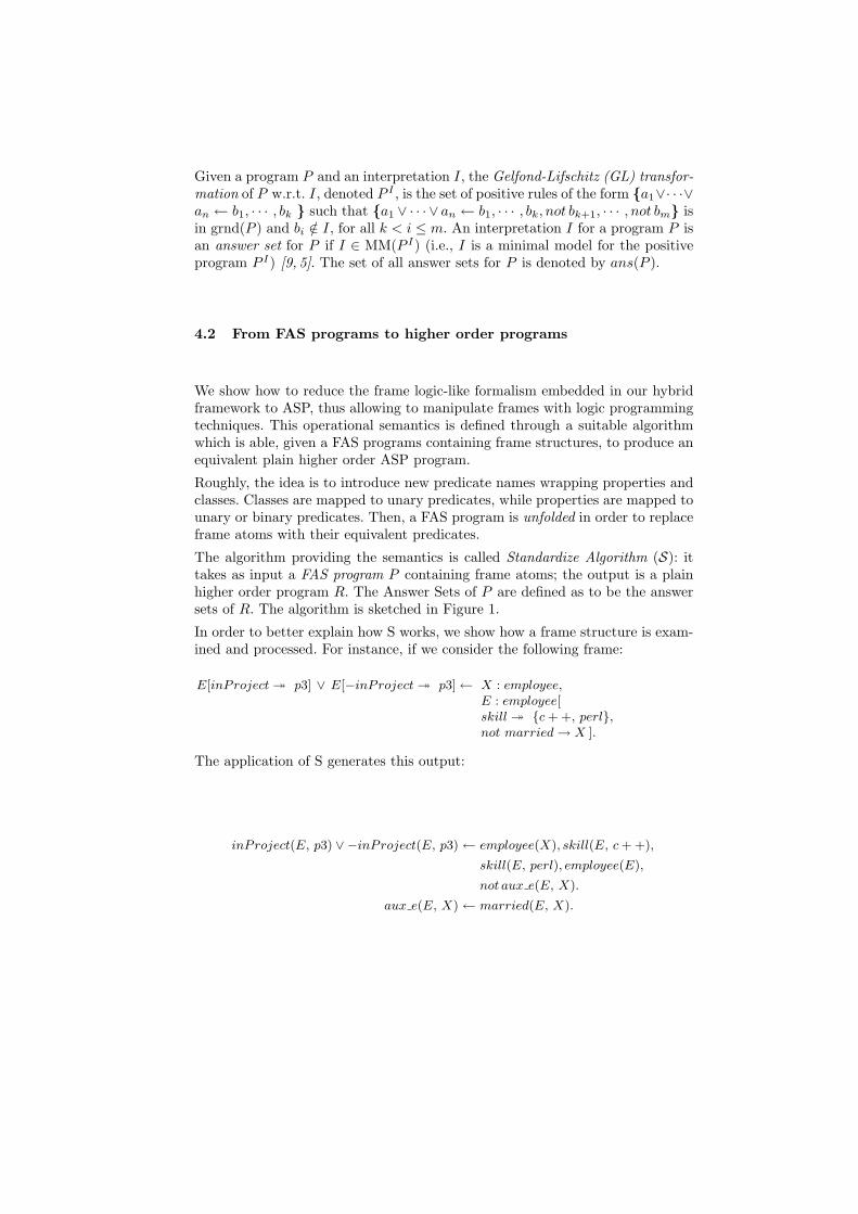
Given a program P and an interpretation I, the Gelfond-Lifschitz (GL) transfor-mation of P w.r.t. I, denoted P I , is the set of positive rules of the form a1∨· · ·∨an ← b1, · · · , bk such that a1 ∨ · · · ∨ an ← b1, · · · , bk, not bk+1, · · · , not bm isin grnd(P ) and bi /∈ I, for all k < i ≤ m. An interpretation I for a program P isan answer set for P if I ∈ MM(P I) (i.e., I is a minimal model for the positiveprogram P I) [9, 5]. The set of all answer sets for P is denoted by ans(P ).

4.2 From FAS programs to higher order programs

We show how to reduce the frame logic-like formalism embedded in our hybridframework to ASP, thus allowing to manipulate frames with logic programmingtechniques. This operational semantics is defined through a suitable algorithmwhich is able, given a FAS programs containing frame structures, to produce anequivalent plain higher order ASP program.

Roughly, the idea is to introduce new predicate names wrapping properties andclasses. Classes are mapped to unary predicates, while properties are mapped tounary or binary predicates. Then, a FAS program is unfolded in order to replaceframe atoms with their equivalent predicates.

The algorithm providing the semantics is called Standardize Algorithm (S): ittakes as input a FAS program P containing frame atoms; the output is a plainhigher order program R. The Answer Sets of P are defined as to be the answersets of R. The algorithm is sketched in Figure 1.

In order to better explain how S works, we show how a frame structure is exam-ined and processed. For instance, if we consider the following frame:

E[inProject ³ p3] ∨ E[−inProject ³ p3] ← X : employee,E : employee[skill ³ c + +, perl,not married → X ].

The application of S generates this output:

inProject(E, p3) ∨ −inProject(E, p3) ← employee(X), skill(E, c + +),

skill(E, perl), employee(E),

not aux e(E, X).

aux e(E, X) ← married(E, X).

Standardize (INPUT: P containing frames OUTPUT: R without frames)Let R = P ;while R contains frame literals do

let r ∈ R be a rule containing frame atoms;while r contains frame literals do

remove frame f from r;let o be the subject, L the set of attributes, and X the set of variables of f ;case f appeared in the body of r:

if f is positive thenif f has class c then

add c(o) to the body of r;for each attribute expression e ∈ L do

let a be the name, and V the set of values of e;if e is positive then

if V is empty thenadd a(o) to the body of r;

elsefor each term t ∈ V do

add a(o, t) to the body of r;for each molecule m ∈ V with subject s do

add a(o, s) and m to the body of r;else

let e be in the form not e′;add the frame not o[e′] to the body of r;

else (Let f in form not f ′)add to r a new fresh literal not auxf (X);add to R a new rule auxf (X) ← f ′;

case f appeared in the head of r:if f is in the form o : c (resp. in the form o[a → v]) then

add to the head of r the literal c(o) (resp. a(o, v));else

add to the head of r a new atom auxf (X);if f has class c then

add c(o) ← auxf (X) to R;for each attribute expression e ∈ L do

let a be the name, and V the set of values of e;if V is empty then

add a(o) ← auxf (X) to R;else

for each term t ∈ V doadd a(o, v) ← auxf (X) to R;

for each molecule m ∈ V with subject s) doadd a(o, s) ← auxf (X) and m ← auxf (X) to R;

Fig. 1. The Standardize Algorithm.

5 Examples

In this section we will provide several examples aiming at showing how to usethe frame-like language.

Higher order reasoning enables the possibility to quantify over predicate names.The rule

related(X, Y ) ← X[Z → Y ].

relates all the X and Y for which some property Z holds. Also higher orderreasoning enables the possibility to enforce axioms that must hold on predicates,

such asX : C : −subClassOf(C, D), X : D.

this enforces membership of an individual X to the class C when it is knownthat D is a subclass of C and that X is member of C.Ease of use of frames can be seen by looking at our running example. Employeesmight be encoded as:

brown : employee[ surname → “Mr. Brown”,

skill ³ java, asp,salary → 800,

gender → male,

married → pink ].

red : employee[ surname → “Mrs. Red”,

skill ³ java, php, perl, python,salary → 1200,

gender → female,

married → black ].

pink : employee[ surname → “Mrs. Pink”,

skill ³ html, asp, javascript,salary → 900,

gender → female,

married → brown ].

black : employee[ surname → “Mr. Black”,

skill ³ c + +, asp, asp, perl, php, python,salary → 1900,

gender → male,

married → red ].

While projects might be described as:

p1 : project[ name → “A System for a Really Nice Web Site”,

budget → 1800,

numEmployee → 2,

maxSalary → 1000,

numFemale → 1,

wantedSkills ³ html, java,nonWantedSkills ³ c + + ].

p2 : project[ name → “A Semantic-Web-Oriented Extension of DLV”,

budget → 3000,

numEmployee → 2,

maxSalary → 1800,

numFemale → 1,

wantedSkills ³ c + +, html,nonWantedSkills ³ java ].

Membership of a given employee E, in a given project P , can be guessed withthe following disjunctive rule:

E[inProject ³ P ] ∨ E[−inProject ³ P ] ← E : employee, P : project.

Conditions (s1), . . . , (s7) can be addressed by the following FAS constraints.

(s1) ← P : project[numEmployee → Nempl],not #countE : inProject(E, P ) = Nempl.

(s2) ← P : project[wantedSkills ³ Wsk],not #countE : skill(E, Wsk), inProject(E, P ) ≥ 1.

(s3) ← P : project[budget → B],not #sumS, E : salary(E, S), inProject(E, P ) ≤ B.

(s4) ← P : project[maxSalary → Msal],E : employee[inProject ³ P, salary → S], not S ≤ Msal.

(s5) ← P : project[numFemale → Nfem],not #countE : gender(E, female), inProject(E, P ) ≤ Nfem.

(s6) :∼ E1 : employee[skill ³ S, inProject ³ P [wantedSkill ³ S]],E2 : employee[skill ³ S, inProject ³ P ], E1 6= E2. [1 :]

(s7) :∼ E : employee[skill ³ S,inProject ³ P [nonWantedSkill ³ S]]. [1 :]

It is worth noting that in the above set of constraints we take advantage ofsome peculiar features of the DLV system, namely weak constraints [6] andaggregates [10].Intuitively, a weak constraint W induces an ordering among the answer sets of agiven program, depending on the number of ground instances that violate W (thelesser W is violated in an answer set A, the more A is preferred). The aggregatesatoms #count and #sum, on the other hand, are exploited in order to count thenumber of values a given conjunction of atoms may have, and for summing upnumeric terms appearing in a given conjunction of atoms, respectively. For thesake of simplicity, such constructs were not included in the formal syntax andsemantics definition given in Section 3 and 4. We refer the reader to the citedliterature for further details.

Fig. 2. Architecture of DLT System.

6 System Overview

FAS programs have been implemented within the DLT environment [11]. DLTextends the DLV system (and, to some extent, any other ASP solver) withTemplate predicates, Frame Logic and Higher Order predicates. The currentversion of the system is freely available on the DLT Web page1.The overall architecture of the system is shown in Figure 2. Roughly, the DLTsystem works as follows. A FAS program P is sent to a DLT pre-parser, whichperforms syntactic checks, converts frame syntax to plain syntax (by applyingthe algorithm S defined in Section 4), and builds an internal representationof P . The DLT Inflater produces an equivalent program P ′ by processing andeliminating other special constructs of the language, such as templates; P ′ ispiped towards an answer set solver. The answer sets ans(P ′) of P ′, computedby the solver are then converted in a readable format through the Post-parsermodule, which filters out from ans(P ′) information about predicates and rulesthat were internally generated.

Additional features of the system

As a front-end system, DLT features several other constructs that can be usedfor enriching an answer set solver. Furthermore, although the syntax of producedprograms is compliant with DLV, if special constructs of DLV (like disjunction,aggregate atoms, weak constraints) are avoided, DLT is compliant with anyother solver supporting the traditional, prolog-like, syntax. Among others, DLTfeatures are:

Template definitions. A DLT program may contain template atoms, that allow todefine intensional predicates by means of a subprogram, where the subprogram isgeneric and reusable. This feature provides a succinct and elegant way for quicklyintroducing new constructs using the DLT language. Syntax and semantics oftemplate atoms are described in [11].

Frame Spaces. A Frame Space directive tells how frames are mapped to regularatoms, and can be used for defining modules where each predicate has localscope within a given frame space. The directive has syntax @name. From thepoint after the directive each frame is interpreted as belonging to the framespace name, and local to this. For referring to a predicate or frame belonging to

1 http://dlt.gibbi.com.

a given frame space it is possible to use the syntax atom@framespace, like ine.g. person(gibbi)@local.Internally, a frame likeX[f → Y ] is rewritten as f(X,Y,name).When the directive “@.” is used, the systems switchs to the default frame space,thus triggering the traditional behavior of the system.

Solvers support. DLT can virtually support any solver that accepts inputs inthe format generated by DLT. Models produced by the external solver are thenparsed back to the DLT syntax. The -solver=[pathname] option allows tospecify the path of the solver. Compatibility with the systems DLV [3], DLV-EX [12], DLV-HEX [13] is provided; compatibility with S-models is guaranteedwithin a subset of the language. A detailed compatibility table is available onthe DLT web site.

Function Symbols. Besides constant and variable terms, the DLT parser allowsalso functional terms. Solvers allowing function symbols are thus ready to becoupled with DLT.

7 Conclusions

We have presented a framework that allows to enrich an Answer Set Program-ming language with frame-like syntax and higher order reasoning. While prelimi-nary, our work paves the way to a more formal investigation of possible semanticsfor F-logic under stable models semantics.

References

1. Kifer, M., Lausen, G., Wu, J.: Logical foundations of object-oriented and frame-based languages. Journal of the ACM 42(4) (1995) 741–843

2. Yang, G., Kifer, M.: Inheritance in Rule-Based Frame Systems: Semantics andInference. Journal on Data Semantics VII (2006) 79–135

3. Leone, N., Pfeifer, G., Faber, W., Eiter, T., Gottlob, G., Perri, S., Scarcello, F.:The dlv system for knowledge representation and reasoning. ACM Trans. Comput.Log. 7(3) (2006) 499–562

4. Janhunen, T., Niemela, I.: Gnt - a solver for disjunctive logic programs. In Lifschitz,V., Niemela, I., eds.: Proceedings of the Seventh International Conference on LogicProgramming and Nonmonotonic Reasoning (LPNMR-7). Volume 2923 of LectureNotes in AI (LNAI)., Fort Lauderdale, Florida, USA, Springer (2004) 331–335

5. Gelfond, M., Lifschitz, V.: Classical Negation in Logic Programs and DisjunctiveDatabases. New Generation Computing 9 (1991) 365–385

6. Buccafurri, F., Leone, N., Rullo, P.: Enhancing Disjunctive Datalog by Constraints.IEEE Transactions on Knowledge and Data Engineering 12(5) (2000) 845–860

7. Ricca, F., Leone, N., Bonis, V.D., Dell’Armi, T., Galizia, S., Grasso, G.: A dlpsystem with object-oriented features. In: LPNMR. (2005) 432–436

8. Lifschitz, V., Tang, L.R., Turner, H.: Nested Expressions in Logic Programs. An-nals of Mathematics and Artificial Intelligence 25(3–4) (1999) 369–389

9. Przymusinski, T.C.: Stable Semantics for Disjunctive Programs. New GenerationComputing 9 (1991) 401–424

10. Calimeri, F., Faber, W., Leone, N., Perri, S.: Declarative and ComputationalProperties of Logic Programs with Aggregates. In: Nineteenth International JointConference on Artificial Intelligence (IJCAI-05). (2005) 406–411

11. Calimeri, F., Ianni, G.: Template programs for disjunctive logic programming: Anoperational semantics. AI Communications 19(3) (2006) 193–206

12. Calimeri, F., Cozza, S., Ianni, G.: External sources of knowledge and value in-vention in logic programming. Annals of Mathematics and Artificial Intelligence(2007. To appear.)

13. Eiter, T., Ianni, G., Tompits, H., Schindlauer, R.: A uniform integration of higher-order reasoning and external evaluations in answer set programming. In: IJCAI-05,Proceedings of the Nineteenth International Joint Conference on Artificial Intelli-gence, Edinburh, UK August 2-5, 2005. (2005) 90–96

Parallel Instantiation of ASP Programs?

F. Calimeri, S. Perri, and F. Ricca

Dipartimento di Matematica, Universita della Calabria, 87036 Rende (CS), Italycalimeri, perri, [email protected]

Abstract. Most of the Answer Set Programming (ASP) systems are endowedwith an instantiation module, which generates a new program equivalent to theinput one, but not containing variables. The instantiation process may be com-putationally expensive, especially for solving real-world problems, where largeamounts of data have to be processed: this has been confirmed by recent appli-cations of ASP in different emerging areas, such as knowledge management orinformation extraction/integration, where also scalability has been recognized asa crucial issue.In this paper we present a new strategy for the parallel instantiation, that allowsto improve both performances and scalability of ASP systems by exploiting thepower of multiprocessor computers. Indeed, in the last few years, the micropro-cessors technologies have been moving to multi-core architectures; this makes thereal Symmetric MultiProcessing (SMP) finally available even on non-dedicatedmachines, and paves the way to the development of more scalable softwares.We have implemented such approach into the ASP system DLV, and carried outan experimental analysis which confirms the validity of the proposed strategy,expecially for real-world applications.

1 Introduction

ASP is a declarative approach to programming proposed in the area of nonmonotonicreasoning and logic programming [1–3]. The main advantage of ASP is its high ex-pressiveness; unfortunately, this comes at the price of a high computational cost, whichhas made the implementation of efficient ASP systems a difficult task. Several effortshave been spent to this end, and, after some pioneering work [4, 5], a number of mod-ern systems are now available. The most widespread ones are DLV [6], GnT [7], andCmodels-3 [8]; many other support various fragments of the ASP language. The ker-nel modules of ASP systems operate on a ground instantiation of the input program,i.e. a program that does not contains any variable, but is semantically equivalent to theoriginal input [9]. Consequently, any given program P first undergoes the so calledinstantiation process computing from P an equivalent ground program P ′. This pre-processing phase is computationally very expensive; thus, having a good and scalableinstantiation procedure is, in general, a key feature of ASP systems.

? Supported by M.I.U.R. within projects “Potenziamento e Applicazioni della ProgrammazioneLogica Disgiuntiva” and “Sistemi basati sulla logica per la rappresentazione di conoscenza:estensioni e tecniche di ottimizzazione.”

Many optimization techniques have been proposed for this purpose [10–12]; nev-ertheless, performances of instantiators are still not acceptable, especially in case ofreal-world problems, where the input data may be huge and also scalability is crucial.Indeed, the recent application of ASP in different emerging areas, such as knowledgemanagement or information extraction/integration [13–15], have confirmed the practi-cal need of more performant and scalable ASP systems.

Besides the other techniques, a technology that might be profitably exploited in thefield of Answer Set Programming (ASP) is Symmetric MultiProcessing (SMP). SMPis a computer architecture where two or more identical processors connect to a sin-gle shared main memory resource allowing simultaneous multithread execution. In thepast, only servers and workstations took advantage of it. However, recently, technologyhas moved to multi-core/multi-processor architectures also for entry-level systems andPCs; this permitted to enjoy the benefits of parallel processing on a large scale. Thesebenefits include better workload balances, enhanced performances, improved scalabil-ity, not only for systems that run many processes simultaneously, but also for single(i.e., multithreaded) applications.

In this paper we present a brand new strategy for the parallel instantiation, allowingto improve both performances and scalability of ASP systems by exploiting the powerof multiprocessor computers. The proposed technique exploits some structural proper-ties of the input program in order to detect subprograms of P that can be evaluated inparallel minimizing the usage of concurrency-control mechanisms, and thus minimiz-ing the “parallel overhead”. We implemented it in an experimental version of the DLVsystem, and performed several experiments which confirmed the effectiveness of ourtechnique especially in the evaluation of real-world problem instances.

The remainder of the paper is structured as follows: in Section 2 we introduce syntaxand semantics of ASP; in Section 3 we briefly describe the instantiation procedures ofDLV system; in Section 4 we present our parallel instantiation algorithm; in Section 5we report and discuss the results of the experiments carried out in order to evaluate theproposed technique; in Section 6, eventually, we look at related works and draw theconclusions.

2 Answer Set Programming

We next provide a formal definition of syntax and semantics of answer set programs.

2.1 Syntax

A variable or a constant is a term. An atom is a(t1, ..., tn), where a is a predicate ofarity n and t1, ..., tn are terms. A literal is either a positive literal p or a negative literalnot p, where p is an atom.

A disjunctive rule (rule, for short) r is a formula

a1 ∨ · · · ∨ an :– b1, · · · , bk, not bk+1, · · · , not bm. (1)

where a1, · · · , an, b1, · · · , bm are atoms and n ≥ 0, m ≥ k ≥ 0. The disjunctiona1 ∨ · · · ∨ an is the head of r, while the conjunction b1, ..., bk, not bk+1, ..., not bm

is the body of r. A rule without head literals (i.e. n = 0) is usually referred to as anintegrity constraint. A rule having precisely one head literal (i.e. n = 1) is called anormal rule. If the body is empty (i.e. k = m = 0), it is called a fact.

We denote by H(r) the set a1, ..., an of the head atoms, and by B(r) the setb1, ..., bk, not bk+1, . . . , not bm of the body literals. B+(r) (resp., B−(r)) denotesthe set of atoms occurring positively (resp., negatively) in B(r). A Rule r is safe if eachvariable appearing in r appears also in some positive body literal of r.

An ASP program P is a finite set of safe rules. A not -free (resp., ∨-free) programis called positive (resp., normal). A term, an atom, a literal, a rule, or a program isground if no variables appear in it.

Accordingly with the database terminology, a predicate occurring only in facts isreferred to as an EDB predicate, all others as IDB predicates.

2.2 Semantics

Let P be a program. The Herbrand Universe and the Herbrand Base of P are definedin the standard way and denoted by UP and BP , respectively.

Given a rule r occurring in P , a ground instance of r is a rule obtained from rby replacing every variable X in r by σ(X), where σ is a substitution mapping thevariables occurring in r to constants in UP . We denote by ground(P) the set of all theground instances of the rules occurring in P .

An interpretation for P is a set of ground atoms, that is, an interpretation is a subsetI of BP . A ground positive literal A is true (resp., false) w.r.t. I if A ∈ I (resp., A 6∈ I).A ground negative literal not A is true w.r.t. I if A is false w.r.t. I; otherwise not A isfalse w.r.t. I .

Let r be a ground rule in ground(P). The head of r is true w.r.t. I if H(r)∩ I 6= ∅.The body of r is true w.r.t. I if all body literals of r are true w.r.t. I (i.e., B+(r) ⊆ Iand B−(r)∩ I = ∅) and is false w.r.t. I otherwise. The rule r is satisfied (or true) w.r.t.I if its head is true w.r.t. I or its body is false w.r.t. I .

A model for P is an interpretation M for P such that every rule r ∈ ground(P) istrue w.r.t. M . A model M for P is minimal if no model N for P exists such that N is aproper subset of M . The set of all minimal models for P is denoted by MM(P).

Given a program P and an interpretation I , the Gelfond-Lifschitz (GL) transforma-tion of P w.r.t. I , denoted PI , is the set of positive rulesPI = a1 ∨ · · · ∨ an :– b1, · · · , bk | a1 ∨ · · · ∨ an :– b1, · · · , bk, not bk+1, · · · , not bm

is in ground(P) and bi /∈ I, for all k < i ≤ mLet I be an interpretation for a program P . I is an answer set for P if I ∈ MM(PI)

(i.e., I is a minimal model for the positive program PI )[16, 1]. The set of all answersets for P is denoted by ANS(P).

3 The DLV Instantiator

In this section we provide a description of the DLV instantiator. Given an input programP , it efficiently generates a ground instantiation that has the same answer sets as the

q

r s

p

¬

p,r q

s

GP GcP

Fig. 1. Dependency and Component Graphs.

full one, but is much smaller in general [6]. Note that the size of the instantiation is acrucial aspect for the efficiency of ASP systems, since the answer set computation takesan exponential time in the size of the ground program received as input (i.e., producedby the instantiator).

In order to generate a small ground program equivalent to P , the DLV instantiatorgenerates ground instances of rules containing only atoms which can possibly be de-rived from P , and thus avoiding the combinatorial explosion which can be obtained bynaively considering all the atoms in the Herbrand Base[11]. This is obtained by takinginto account some structural information of the input program, concerning the depen-dencies among IDB predicates.

We give now the definition the Dependency Graph of P , which, intuitively, de-scribes how predicates depend on each other.

Definition 1. Let P be a program. The Dependency Graph of P is a directed graphGP = 〈N, E〉, where N is a set of nodes and E is a set of arcs. N contains a node foreach IDB predicate of P , and E contains an arc e = (p, q) if there is a rule r in P suchthat q occurs in the head of r and p occurs in a positive literal of the body of r.

The graph GP naturally induces a partitioning of P into subprograms (also calledmodules) which allows for a modular evaluation. We say that a rule r ∈ P defines apredicate p if p appears in the head of r. A module ofP is the set of rules defining all thepredicates contained in a particular maximal strongly connected component (SCC) ofGP . Intuitively, a module includes (among others) all rules defining mutually dependentpredicates.

Example 1. Consider the following program P , where a is an EDB predicate:

p(X,Y ) ∨ s(Y ) :– q(X), q(Y ), not r(X, Y ) q(X) :– a(X)p(X, Y ) :– q(X), r(X,Y ) r(X,Y ) :– p(X, Y ), s(Y )

The graph GP is illustrated in Figure 1; moreover, the strongly connected componentsof GP are s, q and p, r. They correspond to the three following modules:

• p(X,Y ) ∨ s(Y ) :– q(X), q(Y ), not r(X, Y ). • q(X) :– a(X). • p(X,Y ) :– q(X), r(X, Y ). p(X,Y ) ∨ s(Y ) :– q(X), q(Y ), not r(X, Y ).

r(X,Y ) :– p(X, Y ), s(Y ).

It is possible to single out an ordered sequence C1, . . . , Cn of SCC components ofGP (which is not unique, in general) such that the evaluation of the program module

Procedure Instantiate (P : Program; GP : DependencyGraph;var Π: GroundProgram; var T: SetOfAtoms);

beginvar I: SetOfAtoms;var C: SetOfPredicates;T := EDB(P); I = EDB(P); Π := ∅;while GP 6= ∅ do

Remove a SCC C from GP without incoming edges;InstantiateComponent(P, C, T, I, Π);

end whileend Procedure;

Fig. 2. The DLV Instantiation Procedure.

corresponding to component Ci depends only on the evaluation of the components Cj

such that i < j (1 ≤ i < n, 1 < j ≤ n). Basically, this follows from the definitionof SCC which corresponds to a maximal subset of mutually dependent predicates. In-tuitively, this ordering allows one to evaluate the program one module at time, so thatall data needed for the instantiation of a module Ci have been already generated by theinstantiation of the modules preceding Ci.

We sketch now a description of the instantiation process based on this principle,omitting details on how a single module is grounded and providing a general idea of thewhole process.

The procedure Instantiate shown in Figure 2 takes as input a program P to be in-stantiated and the dependency graph GP and outputs a set of true atoms T and a setof ground rules containing only atoms which can possibly be derived from P , suchthat ANS(T ∪ Π) = ANS(P). As previously pointed out, the input program P ispartitioned in modules corresponding to the maximal strongly connected componentsof the dependency graph GP . Such modules are evaluated one at a time starting fromthose that do not depend on other components, according to the ordering induced by thedependency graph.

More in detail, the algorithm initially creates a new set of atoms I that will containthe subset of the Herbrand Base relevant for the instantiation. Initially, T = EDB(P),I = EDB(P), and Π = ∅. Then, a strongly connected component C, which has noincoming edge, is removed from GP , and the program module corresponding to C isevaluated by invoking InstantiateComponent which uses an improved version of thegeneralized semi-naive technique [17] for the evaluation of (recursive) rules.

Roughly, InstantiateComponent takes as input the component C to be instantiated,the sets T and I , and for each atom a belonging to C, and for each rule r defininga, computes the ground instances of r containing only atoms which can possibly bederived from P . At the same time, it updates both the set T with the newly generatedground atoms already recognized as true, and the set I with the atoms occurring in theheads of the rules of Π . The algorithm runs on until all the components of GP havebeen evaluated.

It can be shown that, given a program P , the ground program Π ∪ T generated bythe algorithm Instantiate is such that P and Π ∪ T have the same answer sets.

4 The Parallel Instantiation Procedure

In this Section we describe the new instantiation algorithm that computes a groundversion of a given program P by exploiting parallelism. It takes advantage of somestructural properties of the input program P in order to detect the modules that can beevaluated in parallel without using “mutexes” in the main data structures.

Roughly, the parallel instantiation of the input program P is based on a patternsimilar to the classical producer-consumers problem. A manager thread (acting as aproducer) identifies the components of the dependency graph of P that can be run inparallel, and delegates their instantiation to a number of instantiator threads (actingas consumers) that exploit the same InstantiateComponent function introduced inSection 3.

Once the general idea has been given, we introduce some formal definition in orderto detail the proposed technique. First of all, we define a new graph, called ComponentGraph, whose nodes correspond to the strongly connected components of the Depen-dency Graph GP . Then, we give the definition of a partial ordering among the nodesof Gc

P . Please note as, with a small abuse of notation, we will indifferently refer tocomponents of GP and corresponding nodes of the Component Graph.

Definition 2. Given a program P , let GP be the corresponding dependency graph. TheComponent Graph of P is a directed labelled graph Gc

P = 〈N,E, lab〉, where N is aset of nodes, E is a set of arcs, and lab : E → +,- is a function assigning to each arca label. N contains a node for each (maximal) strongly connected component of GP ; Econtains an arc e = (B,A) if there is a rule r in P such that q ∈ A occurs in the head ofr and p ∈ B occurs in a positive (resp., negative) literal of the body of r; lab(e) =“+”(resp., lab(e) =“-”).

Definition 3. For any pair of nodes A, B of GcP , A precedes B (denoted A ¹ B) if

there is a path in GcP from A to B; and A strictly precedes B (denoted A ≺ B), if

A ¹ B and B A.

Example 2. Consider the program P of Example 1. The component graph of P is il-lustrated in Figure 1. It easy to see that the node p, r precedes s, while q strictlyprecedes s.

Basically, this ordering guarantees that a node A strictly precedes a node B if theprogram module corresponding to A has to be evaluated before the one correspondingto B.1

We are now ready to describe the parallel instantiation procedures exploiting thisordering. As previously pointed out, we make use of some threads: a manager, and anumber of instantiators running the procedures Manager and Instantiator reportedin Figure 3, respectively.

1 Note that the presence of negative arcs in GcP only determines a preference among the admis-

sible orderings induced by the dependency graph, thus it does not affect the correctness of theoverall instantiation process.

Procedure Manager (P : Program; GcP : ComponentGraph;

var T: SetOfAtoms; var Π: GroundProgram);begin

var U :SetOfComponents ; var D:SetOfComponents; var R:SetOfComponents;var I: SetOfAtoms; var C: SetOfPredicates;

D = ∅; R = ∅; U = nodes(GcP)

T := EDB(P); I = EDB(P); Π := ∅;while ( U 6= ∅ )

for all C ∈ U ;if (canBeRun(C,U , R, Gc

P ))begin

R = R∪ C;Spawn(Instantiator, P, C,U ,R,D, T, I, Π);

end ifend

Procedure Instantiator (P : Program; C: Component; var U : SetOfComponents;var R: SetOfComponents; var D: SetOfComponents;var T: SetOfAtoms; var I: SetOfAtoms; var Π: GroundProgram);

beginInstantiateComponent(P, C, T, I, Π);D = D ∪ C;R = R− C;U = U − C;

end

Fig. 3. The Parallel Instantiation Procedures.

The Manager procedure takes as input both a program P to be instantiated and itsComponent Graph Gc

P ; it outputs both a set T of true atoms and a set of ground rulesΠ , such that ANS(T ∪Π) = ANS(P).

First of all, the sets T, I , and Π are initialized like in the standard DLV Instantiator.Moreover, three new sets of components are created: U (which stands for Undone)represents the components of P that have still to be processed, D (which stands forDone) those that have already been instantiated, and R (which stands for Running)those currently being processed.

Initially, D and R are empty, while U contains all the nodes of GcP . The manager

checks, by means of function canBeRun described below, whether components in Ucan be instantiated. As soon as some C is processable, it is added to R, and a new in-stantiator thread is spawned in order to instantiate C by exploiting the InstantiateCom-ponent function defined in Section 3. Once the instantiation of C has been completed,C is moved from R to D, and deleted from U . The manager thread goes on until all thecomponents have been processed (i.e., U = ∅).

The function canBeRun, as the name suggests, checks wether a component C canbe safely evaluated (i.e. without requiring “mutexes” in the main data structures) byexploiting the following definition:

A

B

D

C E

¬

Fig. 4. An example of Component Graph.

Definition 4. Let U be the set of components which still have to be processed. We saythat C ∈ U can be run if ∀A ∈ U at least one of the following conditions holds:

(i) C ≺ A;(ii) C ¹ A and @A′ ∈ U s.t. exists an arc e = (A′, C) of Gc

P with lab(e) =“+”, and∀K ∈ R, do not exist arcs e′, e′′ of Gc

P such that e′ = (R, C) and e′′ = (C,R).

Basically, this definition ensures that (i) a component C is not evaluated beforeall the components strictly preceding C (w.r.t. the partial ordering defined above) havebeen processed; and, (ii) if C appears in a cycle of Gc

P then it is selected only if it hasno positive incoming edges and does not directly depend on some currently runningcomponent. The two conditions of Definition 4 checked by function canBeRun guar-antee the correctness, since they respect the dependencies of GP (as for the standardinstantiation algorithm defined in Section 3).

Moreover, canBeRun singles out components that can be evaluated in parallel with-out using “mutex” locks in the data structures that implement the sets T and I; thisallows us to save resources and reduce the time spent in lock-contentions. It is easy tosee that two components C1 and C2 are “selected” only if any predicate p occurring inthe body of some rule of C1 does not appear in the head of some rule of C2, and viceversa. If the data structures implementing the sets T and I properly store the groundatoms in different containers (i.e., one for each predicate name, as in DLV), then no“mutex” lock is needed to protect them: during the evaluation of a rule, an instantiatorthread may write in the container of an atom a only when a rule defining a is processed;thus, it will never write in a location being accessed by another instantiator.

Interestingly, condition (ii) of Definition 4 allows one to run in parallel even compo-nents appearing in cycles of Gc

P (i.e., components that are, somehow, interdependent).This can be illustrated by the following example:

Example 3. Consider the Component Graph of Figure 4. All the nodes of the graph areinvolved in a cycle; thus, the evaluation of each component is somehow dependent onthe evaluation of each other. However, condition (ii) of Definition 4 allows to select Ato be evaluated first. While A is running, no other component can be processed, becauseboth conditions (i) and (ii) are violated for all of them. Once the instantiation of A hasended, component B can be run, because it satisfies condition (ii). At the same time, byvirtue of condition (ii), also components C and D can be run. Then, component E canbe evaluated only when the instantiations of all B, C and D have been completed.

It is important noting that the actual implementation is more involved, but onlybecause of technical reasons. First of all, the auxiliary control structures (like U , D andR) are properly protected by “mutex” locks, and the busy waiting is properly avoided.

Finally, we also have to deal with additional structures which allow the user to set themaximum number of instantiator threads. We do not believe that these technical issuesmay help to get a better insight, but they are rather lengthy in description; for this reason,we refrain from discussing them here.

5 Experiments

In order to consistently evaluate the parallel grounding technique described in Section 4,we have implemented it as an extension of the DLV system, and performed some ex-periments. We took into account several problems belonging to different applications,ranging from classical ASP benchmarks to “real-word” applications.

We have compared the prototype with the official DLV [18] release2 on which itis based. In addition, we considered the maximum number of concurrent instantiatorthreads as a parameter; thus, we deal with the following versions of DLV:

– dl.release: the original DLV system release without parallel grounding;– dl.thX: the modified DLV system with X indipendent working threads (X ranges

from 1 to 4).

All the binaries have been built with GCC 3.4 (the same used to build the originalDLV release), statically linking the Posix Thread Library.

Experiments have been performed on a machine equipped with two Intel Xeon HT(single core) CPUs clocked at 3.60GHz with 1 MB of Level 2 Cache and 3GB of RAM,running Debian GNU Linux (kernel 2.4.27-2-686-smp). This machine is capable ofsimultaneously run (i.e., each thread executed on a different processing unit) at most4 threads; with more, the system performs poorly because of the preemptive threadscheduling overhead. This has ben confirmed by the experiments; thus, we decided toomit here the results obtained by allowing more than 4 concurrent instantiator threads.Limiting to 4 concurrent instantiator threads does not eliminate the effects of preemp-tion, but, reasonably, they become negligible; indeed, we ran the tests on an “unloaded”machine, and the operating system always tries to schedule active threads on free CPUs.

Time measurements have been performed by means of the time command shippedwith the above cited version of Debian GNU Linux. Unfortunately, we could not con-sider the total CPU times3, because, in case of multi-threaded applications, they resultas the sum of the time spent by the process on each processing unit (e.g., when a processfully exploits simultaneously two processors for 5 minutes, the total reported CPU timeis 10 minutes). We decided to overcome the problem by considering the so called realtime, based on the system wall-clock time. Obviously, this measure is less accurate thanthe total CPU time, since it unavoidably includes the time spent by other processes inthe system (even by unrelated operating system routines). In order to obtain more reli-able information, we have repeated each test three times, and provide here both averageand standard deviation of the results.

2 Official DLV release, July 14th 2006.3 The sum of user and system time; we refer the reader to time manual pages for a detailed

description of these quantities [19].

In the following, we describe the benchmark problems, and finally report and dis-cuss the results of the experiments.

5.1 Benchmark Programs

We provide here a brief description of the problems considered for the experiments. Inorder to meet the space constraints, we refrain from showing the encodings (considerthat some are automatically generated, and are very long and involved). However, theyare available at http://www.mat.unical.it/parallel/cilc inst.tar.gz.

3-Colorability. This well-known problem asks for an assignment of three colors to thenodes of a graph, in such a way that adjacent nodes always have different colors.

Ancestor. Given a parent relationship over a set of persons, find the genealogy tree ofeach one. It is a classical deductive database problem exploiting recursive rules.

Knowledge Discovery. Given an ontology and a text document, an ASP program clas-sifies the document w.r.t. the ontology. Basically, the goal is to associate the documentcontents to one or more concepts in the given ontology: a document is associated tothe concepts it deals with. Problems have been provided by the company EXEURAs.r.l. [20].

Player. A data integration problem. Given some tables containing discording data, finda repair where some key constraints are satisfied. The problem was originally definedwithin the EU project INFOMIX [15].

Hypertree Decomposition. Compute a k-width complete hypertree decomposition [21]of a given query Q in a given predicate P.

ETL Workflow. In general, ETL stands for Extraction Transformation and Loading.Here the goal is to emulate, by means of an ASP program, the execution of a work-flow, in which each step constitutes a transformation to be applied to some data (inorder to query for and/or extract implicit knowledge). We considered the encoding ofthree different steps, automatically generated by a software working on some americaninsurance data. Problems have been provided by the company EXEURA s.r.l. [20].

Cristal. A deductive databases application that involves complex knowledge manipu-lations. The application was originally developed at CERN [22].

Timetabling. A real timetable problem from the faculty of Science of the University ofCalabria. We have considered for the evaluation the programs that the faculty exploitedfor two different academic years.

The above-mentioned problems can be roughly divided into two classes, with re-spect to their structure. One contains problems having very “dense” dependency graphs(meaning that there are only few components), like 3-Colorability or Ancestor. Theother contains problems featuring several rules belonging to independent componentsof the dependency graph, like ETLs or Timetablings. Therefore, the parallel instantia-tion of the first might only moderately be profitable, while the latter should be easiergrounded in parallel; having both classes of problems allows one to get a sharpen pic-ture of the behavior of our prototype.

Fig. 5. Average CPU usage.

5.2 Results

The results of the experimental activities are summarized in Table 1 and Table 2, show-ing average total execution times and average instantiation times, respectively, both inseconds. The first consists of the overall time spent by DLV, from the invocation by theOS to the end of the instantiation (including parsing, output printing, etc.)4, while thesecond takes into account exactly the time spent by the instantiation itself.

We wanted also to outline the amount of parallel computation resources actually ex-ploited; to this extent, in Figure 5 we report the average CPU usages5. The graph drawsthe CPU usage w.r.t. to the number of allowed threads: “1.00” means that the process“took” a single CPU, while higher values mean an higher rate of parallel execution. It isimportant recalling also CPU usages take into account the overall time spent by DLV.

We discuss now the results. At a first glance, it is easy to notice as, apart from fewexceptions, as the number of allowed threads increases, the performances get better.However, among all the considered problems, one can observe different behaviors.

First of all, 3col and Ancestor do not enjoy any improvement. This was expected,since their dependency graphs are almost composed by a single huge component, thuspreventing the possibility of taking advantage from our parallel techniques. Indeed,they settle at the bottom of the graph of Figure 5. Nevertheless, times are not affectedby noticeable overheads, even w.r.t. the official DLV release.

4 This means, both the parallel instantiation and the other non-parallel phases. It is worthwhilestating that the the component graph is computed by the old DLV version as well as the newone; in addition, we verified that the time spent in the computation is actually negligible.

5 Computed as ((User + System)/Real); see [19]. Please note that this does not rate paral-lelism, but the exploitation of the CPUs, thus giving us an idea about how much the executionhas actually been parallelized, even if it is machine-dependent.

It’s then possible to identify a set of instances (namely: Knowledge discovery,ETL1, ETL2, Player, Decomp) that, as soon as the number of allowed threads movesfrom one to two, show an appreciable gain in instantiation time, all above 20% (e.g.:Knowledge Discovery passes from 2.06s to 1.86s; ETL1 from 64.35s to 53.93s). Then,the advantage does not grow, in practice, with the number of allowed threads; as anexample, allowing more than three threads for solving Knowledge discovery is useless(1.86s, 1.53s and 1.65s with two, three and four threads, respectively). Almost the sameobservation can be made for ETL1, ETL2 and Decomp, while Player still exhibits alittle performance gain even with four threads. Indeed, looking at the graph of Figure 5,all these instances show an almost flat pattern over 2 allowed threads.

Unfortunately, we note that something strange happens when we look ad total av-erage times: for Decomp and Knowledge discovery, all the dl.thX executables show aclear degradation in the performances if compared with the DLV release. We have in-vestigated this strange phenomenon, and discovered that it is actually a technologicalissue, concerning the standard STL [23] multithreaded memory allocator. In fact, theDLV system heavily relies on STL data structures; these exploit a memory allocatorfunction that suffers from a dramatic performance degradation when linked against amultithreaded executable [24]. In our case, this sometimes neutralizes all the benefitsprovided by parallelism. Fortunately, in case of ETL1 and ETL2, this does not wasteall the gain, which still stands on about 23% also in the total execution times (ETL1,for instance, moves from 64.99s to 50.4s). This technological problem can be fixed, asindicated for instance in [24]; since the implementation takes quite some time, we leftit as a future work.

Finally, a last set of instances (namely: ETL3, Cristal, Timetabling 1, Timetabling2), clearly exhibits a performance gain growing as the number of allowed threads in-creases. Instantiation times improvements go from about 18% for Cristal (which passesfrom 4.17s with one thread to 3.58s with four) to about 40% for Timetabling 1 (from10.64s to 6.42s). In the graph of Figure 5 the patterns related to these problems aremonotonically increasing (in particular, when four threads are allowed, the exploitedcpu usage grows up to a factor of 2). These benefits still survive in the total executiontimes for all instances, apart from Timetabling 2. The difference with this is due to thesame memory allocation drawbacks previously discussed6.

Summarizing, best improvements have been observed within the last set of prob-lems; it is worthwhile noting that all of them come from concrete applications, thusconfirming that our approach can be profitably exploited to improve performances ofASP while dealing with real world problems.

For the sake of completeness, it is important noting that the Intel Hyper Thread-ing (HT) technology [25] (implemented by the machine exploited for the experiments)works by duplicating certain sections of the processor, but not all the main executionresources. Basically, each processor pretends to be two ”logical” processors in front ofthe host operating system which, thus, can schedule four threads or processes simulta-neously (two processes/threads per CPU); however, these will compete for some impor-tant execution resources (e.g., the cache). Consequently, there is only an approximation

6 Intuitively, these drawbacks increase their weight when memory allocation functions are morefrequently invoked.

Problem dl.release dl.th1 dl.th2 dl.th3 dl.th4Cristal 4.04 (0.07) 4.17 (0.08) 4.23 (0.08) 4.41 (0.12) 4.66 (0.36)Ancestor 51.78 (0.54) 52.15 (0.48) 52.23 (0.48) 52.68 (0.35) 52.16 (0.64)3Col 15.83 (0.35) 15.71 (0.05) 14.90 (0.30) 15.40 (0.69) 15.32 (0.35)Decomp 6.91 (0.00) 8.83 (0.01) 7.41 (0.77) 6.81 (0.07) 7.23 (0.25)TimeTab1 7.27 (0.10) 12.14 (0.04) 9.56 (0.56) 8.50 (0.06) 7.93 (0.34)TimeTab2 12.42 (0.46) 12.85 (0.42) 10.98 (1.99) 8.59 (0.55) 10.78 (3.43)KnoDisc 3.41 (0.00) 5.29 (0.00) 5.09 (0.00) 4.76 (0.00) 4.87 (0.15)Player 6.87 (0.02) 7.00 (0.02) 5.52 (0.47) 5.56 (0.46) 5.34 (0.06)ETL1 64.72 (0.35) 64.99 (0.61) 54.58 (2.77) 49.61 (0.61) 50.40 (0.11)ETL2 64.25 (0.22) 64.26 (0.42) 49.70 (0.56) 49.89 (0.13) 49.92 (0.53)ETL3 182.38 (0.38) 186.72 (0.43) 126.82 (10.21) 118.57 (1.53) 120.97 (2.42)

Table 1. Average Real Execution Times (standard deviations within parentheses).Problem dl.release dl.th1 dl.th2 dl.th3 dl.th4Cristal 3.96 (0.07) 4.03 (0.07) 3.31 (0.08) 3.33 (0.07) 3.44 (0.11)Ancestor 51.75 (0.54) 52.08 (0.48) 52.16 (0.48) 52.61 (0.35) 52.08 (0.64)3Col 15.67 (0.35) 15.40 (0.05) 14.59 (0.30) 15.10 (0.69) 15.01 (0.35)Decomp 6.65 (0.00) 8.33 (0.01) 6.92 (0.77) 6.32 (0.07) 6.73 (0.25)TimeTab1 6.51 (0.10) 10.64 (0.04) 8.06 (0.54) 6.99 (0.05) 6.42 (0.34)TimeTab2 11.46 (0.46) 10.97 (0.42) 9.08 (1.98) 6.70 (0.55) 8.90 (3.44)KnoDisc 1.88 (0.00) 2.06 (0.01) 1.86 (0.00) 1.53 (0.01) 1.65 (0.15)Player 6.76 (0.02) 6.79 (0.01) 5.31 (0.47) 5.36 (0.46) 5.13 (0.07)ETL1 64.32 (0.35) 64.35 (0.62) 53.93 (2.77) 48.96 (0.61) 49.75 (0.11)ETL2 64.00 (0.22) 63.88 (0.41) 49.31 (0.56) 49.50 (0.13) 49.48 (0.57)ETL3 180.83 (0.37) 184.17 (0.44) 124.24 (10.19) 115.96 (1.61) 118.41 (2.42)

Table 2. Average Grounding Times (standard deviations within parentheses).

of the behavior of a true four processor machine. This effect cannot be avoided with thestandard linux SMP kernel, since it is not aware of all the HT peculiarities. Thus, withpure multi-processor or multi-core machines, the performances of our technique shouldbe even better.

6 Related Work and Conclusions

In this paper, we proposed a new technique for the parallel computation of the instanti-ation of ASP programs. It exploits some structural properties of the input program P inorder to detect modules of P that can be evaluated in parallel.

As a matter of fact, the exploitation of parallel techniques for computing answersets is not new [26–28]; however, our approach is not comparable with the existingones, since the latter concern the model generation task, instead of the instantiation.Nonetheless, a lot of work has been done in the fields of logic programming and de-ductive databases [17, 29–39]; still, the techniques are comparable to a limited extentto the one illustrated here: some of them apply to syntactically restricted classes of pro-grams, and some others requires an heavy usage of concurrency-control mechanisms.The only one comparable to the present is the so-called stream parallelism, where all the

rules are evaluated simultaneously: basically, the information resulting from the eval-uation of each rule is passed to the ones depending on it, like in a pipeline. However,this scheme suffers from heavy communication overheads, while our approach mini-mizes the usage of “mutexes” in the main data structures, thus reducing the overheadintroduced by the concurrency-control constructs.

We have implemented our strategy producing an experimental version of the DLVsystem, and performed several experiments on a SMP-based machine. The obtainedresults confirmed, on the one hand, the effectiveness of our technique, which allowsone to save real (wall-clock) time, especially while evaluating real-world problem in-stances; on the other hand, they outlined some annoying technical issues due to theusage of the standard STL multithreaded memory allocator, which is widely consideredperformance-wise not optimal [24].

We plan to improve the current implementation by solving the problems concern-ing STL memory allocation performances; nonetheless, we want to extend our parallelgrounding technique as well, in order to exploit parallelism also during the instantiationof a single component.

References

1. Gelfond, M., Lifschitz, V.: Classical Negation in Logic Programs and Disjunctive Databases.NGC 9 (1991) 365–385

2. Eiter, T., Gottlob, G., Mannila, H.: Disjunctive Datalog. ACM TODS 22(3) (1997) 364–4183. Eiter, T., Faber, W., Leone, N., Pfeifer, G.: Declarative Problem-Solving Using the DLV

System. In Minker, J., ed.: Logic-Based Artificial Intelligence. Kluwer (2000) 79–1034. Bell, C., Nerode, A., Ng, R.T., Subrahmanian, V.: Mixed Integer Programming Methods for

Computing Nonmonotonic Deductive Databases. JACM 41 (1994) 1178–12155. Subrahmanian, V., Nau, D., Vago, C.: WFS + Branch and Bound = Stable Models. IEEE

TKDE 7(3) (1995) 362–3776. Leone, N., Pfeifer, G., Faber, W., Eiter, T., Gottlob, G., Perri, S., Scarcello, F.: The DLV

System for Knowledge Representation and Reasoning. ACM TOCL 7(3) (2006) 499–5627. Janhunen, T., Niemela, I., Seipel, D., Simons, P., You, J.H.: Unfolding Partiality and Dis-

junctions in Stable Model Semantics. ACM TOCL 7(1) (2006) 1–378. Lierler, Y.: Disjunctive Answer Set Programming via Satisfiability. In: LPNMR’05. LNCS

36629. Eiter, T., Leone, N., Mateis, C., Pfeifer, G., Scarcello, F.: A Deductive System for Non-

monotonic Reasoning. In J. Dix and U. Furbach and A. Nerode, ed.: LPNMR’97. LNCS1265

10. Faber, W., Leone, N., Mateis, C., Pfeifer, G.: Using Database Optimization Techniques forNonmonotonic Reasoning. In DDLP’99, Prolog Association of Japan (1999) 135–139

11. Leone, N., Perri, S., Scarcello, F.: Improving ASP Instantiators by Join-Ordering Methods.In: LPNMR’01. LNCS 2173

12. Leone, N., Perri, S., Scarcello, F.: BackJumping Techniques for Rules Instantiation in theDLV System. In: NMR 2004. (2004) 258–266

13. Ruffolo, M., Leone, N., Manna, M., Sacca’, D., Zavatto, A.: Exploiting ASP for SemanticInformation Extraction. In: Proceedings ASP05 - Answer Set Programming: Advances inTheory and Implementation, Bath, UK (2005)

14. Cumbo, C., Iiritano, S., Rullo, P.: Reasoning-based knowledge extraction for text classifica-tion. In: Discovery Science. (2004) 380–387

15. Leone, N., Gottlob, G., Rosati, R., Eiter, T., Faber, W., Fink, M., Greco, G., Ianni, G., Kałka,E., Lembo, D., Lenzerini, M., Lio, V., Nowicki, B., Ruzzi, M., Staniszkis, W., Terracina, G.:The INFOMIX System for Advanced Integration of Incomplete and Inconsistent Data. In:Proceedings of the 24th ACM SIGMOD International Conference on Management of Data(SIGMOD 2005), Baltimore, Maryland, USA, ACM Press (2005) 915–917

16. Przymusinski, T.C.: Stable Semantics for Disjunctive Programs. NGC 9 (1991) 401–42417. Ullman, J.D.: Principles of Database and Knowledge Base Systems. Computer Science Press

(1989)18. Faber, W., Pfeifer, G.: DLV homepage (since 1996) http://www.dlvsystem.com/.19. Debian: Manual pp. about using a GNU/Linux system http://packages.debian.

org/stable/doc/manpages/.20. Exeura s.r.l., Homepage http://www.exeura.it/.21. Gottlob, G., Leone, N., Scarcello, F.: Hypertree Decompositions and Tractable Queries.

JCSS (2002)22. CRISTAL project, homepage http://proj-cristal.web.cern.ch/.23. Stepanov, A., Lee, M.: The Standard Template Library. (Part of the evolving ANSI C++

standard. ftp://butler.hpl.hp.com/stl/.) (1995)24. Berger, E.D., McKinley, K.S., Blumofe, R.D., Wilson, P.R.: Hoard: A Scalable Memory

Allocator for Multithreaded Applications. In: ASPLOS. (2000) 117–12825. Koufaty, D., Marr, D.T.: Hyperthreading Technology in the Netburst Microarchitecture.

IEEE Micro 23(2) (2003) 56–6526. Finkel, R.A., Marek, V.W., Moore, N., Truszczynski, M.: Computing stable models in par-

allel. In: Answer Set Programming. (2001)27. Gressmann, J., Janhunen, T., Mercer, R.E., Schaub, T., Thiele, S., Tichy, R.: Platypus: A

Platform for Distributed Answer Set Solving. In: LPNMR. (2005) 227–23928. Pontelli, E., El-Khatib, O.: Exploiting Vertical Parallelism from Answer Set Programs. In:

Answer Set Programming. (2001)29. Wolfson, O., Silberschatz, A.: Distributed Processing of Logic Programs. In: SIGMOD

Conference. (1988) 329–33630. Wolfson, O.: Parallel Evaluation of Datalog Programs by Load Sharing. J. Log. Program.

12(3&4) (1992) 369–39331. Gupta, G., Pontelli, E., Ali, K.A.M., Carlsson, M., Hermenegildo, M.V.: Parallel execution

of prolog programs: a survey. ACM Trans. Program. Lang. Syst. 23(4) (2001) 472–60232. Clark, K.L., Gregory, S.: Parlog: Parallel Programming in Logic. ACM Trans. Program.

Lang. Syst. 8(1) (1986) 1–4933. Ramakrishnan, R.: Parallelism in Logic Programs. Ann. Math. Artif. Intell. 3(2-4) (1991)

295–33034. Leone, N., Restuccia, P., Romeo, M., Rullo, P.: Expliciting Parallelism in the Semi-Naive

Algorithm for the Bottom-up Evaluation of Datalog Programs. Database Technology 4(4)(1993) 245–158

35. de Kergommeaux, J.C., Codognet, P.: Parallel Logic Programming Systems. ACM Comput.Surv. 26(3) (1994) 295–336

36. Wu, Y., Pontelli, E., Ranjan, D.: Computational Issues in Exploiting Dependent And-Parallelism in Logic Programming: Leftness Detection in Dynamic Search Trees. In: LPAR.(2005) 79–94

37. Inoue, K., Koshimura, M., Hasegawa, R.: Embedding Negation as Failure into a ModelGeneration Theorem Prover. In: CADE. (1992) 400–415

38. Ramakrishnan, R., Ullman, J.D.: A Survey of Deductive Database Systems. JLP 23(2)(1995) 125–149

39. Zhang, W., Wang, K., Chau, S.C.: Data Partition and Parallel Evaluation of Datalog Pro-grams. IEEE Trans. Knowl. Data Eng. 7(1) (1995) 163–176

Implementation and Evaluation of Look-BackTechniques and Heuristics in DLV⋆

Wolfgang Faber1, Nicola Leone1, Marco Maratea1,2, and Francesco Ricca1

1 Department of Mathematics, University of Calabria, 87036 Rende (CS), Italyfaber,leone,maratea,[email protected]

2 DIST, University of Genova, 16145 Genova, [email protected]

Abstract. Answer Set Programming (ASP) is a programming paradigm based onlogic rules. It is purely-declarative and allows for both disjunction in the head ofthe rules and nonmonotonic negation in the body. ASP is very expressive: anyproperty whose complexity is in the second level of the polynomial hierarchycan be expressed with the language of ASP, thus it is strictlymore powerful thanpropositional logic under standard complexity conjectures. DLV is the state-of-the-artdisjunctiveASP system, and it is based on an algorithm using backtrackingsearch, like the vast majority of the currently available ASP systems. Despite itsefficiency, until recently, DLV did not incorporate any “backjumping” techniques(neither did other disjunctive ASP systems). Related, DLV could not use “look-back” information accumulated for backjumping in its heuristics, which have beenshown in related research areas to be crucial on large benchmarks stemming fromapplications. In this paper, we focus on the experimental evaluation of the look-back algorithms and heuristics that have been implemented in DLV. We have con-ducted a wide experimental analysis considering both randomly-generated andstructured instances of the 2QBF problem (the canonical problem for the com-plexity classesΣP

2 andΠP

2 ). The results show that the new look-back techniquessignificantly improve the performance of DLV, being performance-wise competi-tive even with respect to “native” QBF solvers.

1 Introduction

Answer Set Programming (ASP) [1, 2] is a purely-declarativeprogramming paradigmbased on nonmonotonic reasoning and logic programming. Theidea of answer set pro-gramming is to represent a given computational problem by a logic program whoseanswer sets correspond to solutions, and then use an answer set solver to find such solu-tions [3]. The language of ASP is very expressive, allowing for both disjunction in thehead of the rules and nonmonotonic negation in the body, and able to represent everyproperty in the second level of the polynomial hierarchy. Therefore, ASP is strictly morepowerful than propositional logic unlessP = NP .

DLV is the state-of-the-artdisjunctiveASP system, and it is based on an algorithmrelying on backtracking search, like most other competitive ASP systems. Until recently,

⋆ Supported by M.I.U.R. within projects “Potenziamento e Applicazioni della ProgrammazioneLogica Disgiuntiva” and “Sistemi basati sulla logica per larappresentazione di conoscenza:estensioni e tecniche di ottimizzazione.”

DLV did not incorporate any “look-back” techniques, like “backjumping” proceduresand “look-back” heuristics. By “backjumping” [4] we refer to an optimized recoveryupon inconsistency during the search where, instead of restoring the state of the searchup to the previous choice and then “flipping” its value, we tryto “jump over” choices thatare not relevant for the inconsistency we met. This is done bymeans of a reason calculus,which records information about the literals (“reasons”) whose truth has caused the truthof other derived literals.

Look-back heuristics [5] further strengthen the potentialof backjumping by usingthe information made explicit by the reasons. The idea of such family of heuristics isto preferably choose atoms which frequently caused inconsistencies, thus focusing on“critical” atoms. This significantly differ from classicalASP heuristics that use informa-tion arising from the simplification part (“look-head”) of the algorithm. Such look-backoptimization techniques and heuristics have been shown, onother research areas, to bevery effective on “big” benchmarks coming from applications, like planning and formalverification.

In this paper, we report on the analysis, implementation andevaluation of the back-jumping technique and look-back heuristics in DLV, and ultimately, about their effi-ciency in the disjunctive ASP setting. Such methods have been already used in otherASP systems which(i) do not allow for disjunction in the head of the rules [6, 7], or(ii)apply such methods only indirectly after a transformation to a propositional satisfiabilityproblem [8]. The resulting system, called DLVLB, is therefore the first implementationof disjunctive ASP featuring backjumping and look-back heuristics. Importantly, oursystem provides several options regarding the initialization of the heuristics and the truthvalue to be assigned to an atom chosen by the heuristics. In our experimental analysis,we provide a comprehensive comparison of the impact of theseoptions, and demon-strate how the new components of DLVLB enhances the efficiency of DLV. Moreover,we also provide a comparison to the other competitive disjunctive ASP systems GnT andCmodels, which are generally outperformed considerably byDLV LB on the consideredbenchmarks. Finally, we also present a comparison with respect to QBF solvers, whichalso allow for solving problems within the second level of the polynomial hierarchy.

2 Answer Set Programming Language

A (disjunctive) ruler is a formula

a1 ∨ · · · ∨ an :– b1, · · · , bk, not bk+1, · · · , not bm.

wherea1, · · · , an, b1, · · · , bm are function-free atoms andn ≥ 0, m ≥ k ≥ 0. Thedisjunctiona1 ∨ · · · ∨ an is theheadof r, while b1, · · · , bk, not bk+1, · · · , not bm isthe body, of which b1, · · · , bk is thepositive body, andnot bk+1, · · · , not bm is thenegative bodyof r.

An (ASP) programP is a finite set of rules. An object (atom, rule, etc.) is calledgroundor propositional, if it contains no variables. Given a programP , let theHerbrandUniverseUP be the set of all constants appearing inP and theHerbrand BaseBP be theset of all possible ground atoms which can be constructed from the predicate symbolsappearing inP with the constants ofUP .

Given a ruler, Ground(r) denotes the set of rules obtained by applying all possiblesubstitutionsσ from the variables inr to elements ofUP . Similarly, given a programP ,theground instantiationGround(P) of P is the set

⋃r∈P Ground(r).

For every programP , its answer sets are defined using its ground instantiationGround(P) in two steps: First answer sets of positive programs are defined, then areduction of general programs to positive ones is given, which is used to define answersets of general programs. A setL of ground literals is said to beconsistentif, for everyatomℓ ∈ L, its complementary literalnot ℓ is not contained inL. An interpretationIfor P is a consistent set of ground literals over atoms inBP .3 A ground literalℓ is truew.r.t. I if ℓ ∈ I; ℓ is falsew.r.t. I if its complementary literal is inI; ℓ is undefinedw.r.t.I if it is neither true nor false w.r.t.I. InterpretationI is total if, for each atomA in BP ,eitherA or not A is in I (i.e., no atom inBP is undefined w.r.t.I). A total interpretationM is amodelfor P if, for everyr ∈ Ground(P), at least one literal in the head is truew.r.t. M whenever all literals in the body are true w.r.t.M . X is ananswer setfor apositive programP if it is minimal w.r.t. set inclusion among the models ofP .

The reductor Gelfond-Lifschitz transformof a general ground programP w.r.t. aninterpretationX is the positive ground programPX , obtained fromP by (i) deleting allrulesr ∈ P the negative body of which is false w.r.t. X and (ii) deletingthe negativebody from the remaining rules. An answer set of a general programP is a modelX ofP such thatX is an answer set ofGround(P)X .

3 Answer Set Computation Algorithms

In this section, we describe the main steps of the computational process performed byASP systems. We will refer particularly to the computational engine of the DLV sys-tem, which will be used for the experiments, but also other ASP systems, employ asimilar procedure. In general, an answer set programP contains variables. The firststep of a computation of an ASP system eliminates these variables, generating a groundinstantiationground(P) ofP .4 The subsequent computations, which constitute the non-deterministic hearth of the system, are then performed onground(P) by the so calledModel Generator procedure.

In the following paragraphs, we illustrate the original model generation algorithmof DLV (which is based on chronological backtracking); then, we briefly describe abackjumping technique that has been implemented in the system[10]; and, we detailhow the model generation algorithm has been changed to introduce it. Finally, we reporta description of all the heuristics, including the new ones based look-back techniques,that have been implemented in the DLV system, so far.

The Standard Model Generator Algorithm. The computation of answer sets is per-formed by exploiting the Model Generator Algorithm sketched in Figure 1.5

3 We represent interpretations as set of literals, since we have to deal with partial interpretationsin the next sections.

4 Note thatground(P) is usually not the fullGround(P); rather, it is a subset (often muchsmaller) of it having precisely the same answer sets asP [9]

5 Note that for reasons of presentation, the description hereis quite simplified w.r.t. the “real”implementation. A more detailed description can be found in[11].

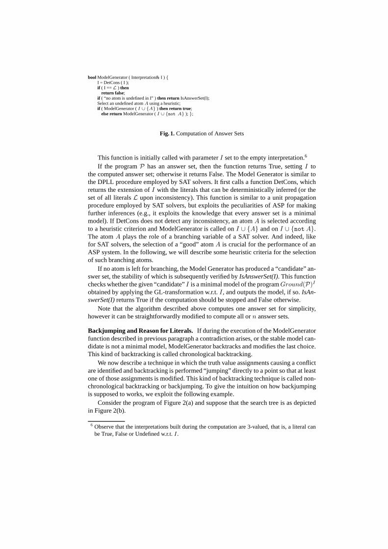
bool ModelGenerator ( Interpretation& I )I = DetCons ( I );if ( I == L ) then

return false;if ( “no atom is undefined in I” )then return IsAnswerSet(I);Select an undefined atomA using a heuristic;if ( ModelGenerator (I ∪ A ) then return true ;

else returnModelGenerator (I ∪ not A ); ;

Fig. 1. Computation of Answer Sets

This function is initially called with parameterI set to the empty interpretation.6

If the programP has an answer set, then the function returns True, settingI tothe computed answer set; otherwise it returns False. The Model Generator is similar tothe DPLL procedure employed by SAT solvers. It first calls a function DetCons, whichreturns the extension ofI with the literals that can be deterministically inferred (or theset of all literalsL upon inconsistency). This function is similar to a unit propagationprocedure employed by SAT solvers, but exploits the peculiarities of ASP for makingfurther inferences (e.g., it exploits the knowledge that every answer set is a minimalmodel). If DetCons does not detect any inconsistency, an atom A is selected accordingto a heuristic criterion and ModelGenerator is called onI ∪ A and onI ∪ not A.The atomA plays the role of a branching variable of a SAT solver. And indeed, likefor SAT solvers, the selection of a “good” atomA is crucial for the performance of anASP system. In the following, we will describe some heuristic criteria for the selectionof such branching atoms.

If no atom is left for branching, the Model Generator has produced a “candidate” an-swer set, the stability of which is subsequently verified byIsAnswerSet(I). This functionchecks whether the given “candidate”I is a minimal model of the programGround(P)I

obtained by applying the GL-transformation w.r.t.I, and outputs the model, if so.IsAn-swerSet(I)returns True if the computation should be stopped and False otherwise.

Note that the algorithm described above computes one answerset for simplicity,however it can be straightforwardly modified to compute all or n answer sets.

Backjumping and Reason for Literals. If during the execution of the ModelGeneratorfunction described in previous paragraph a contradiction arises, or the stable model can-didate is not a minimal model, ModelGenerator backtracks and modifies the last choice.This kind of backtracking is called chronological backtracking.

We now describe a technique in which the truth value assignments causing a conflictare identified and backtracking is performed “jumping” directly to a point so that at leastone of those assignments is modified. This kind of backtracking technique is called non-chronological backtracking or backjumping. To give the intuition on how backjumpingis supposed to works, we exploit the following example.

Consider the program of Figure 2(a) and suppose that the search tree is as depictedin Figure 2(b).

6 Observe that the interpretations built during the computation are 3-valued, that is, a literal canbe True, False or Undefined w.r.t.I .

Fig. 2. Backtracking vs Backjumping.

According to this tree, we first assumea to be true, derivingb to be false (fromr1

to ensure the minimality of answer sets). Then we assumec to be true, derivingd to befalse (fromr2 for minimality). Third, we assumee to be true and derivef to be false(from r3 for minimality) andg to be true (fromr4 by forward inference). This truthassignment violates constraintr5 (whereg must be false), yielding an inconsistency. Wecontinue the search by inverting the last choice, that is, weassumee to be false and wederivef to be true (again fromr3 to preserve minimality) andg to be true (fromr6 byforward inference), but obtain another inconsistency (because constraintr7 is violated,hereg must also be false).

At this point, ModelGenerator goes back to the previous choice point, in this caseinverting the truth value ofc (cf. the arc labelled BK in Fig. 2(b)).

Now it is important to note that the inconsistencies obtained are independent of thechoice ofc, and only the truth value ofa ande are the “reasons” for the encounteredinconsistencies. In fact, no matter what the truth value ofc is, if a is true then any truthassignment fore will lead to an inconsistency. Looking at Fig. 2(b), this means that inthe whole subtree below the arc labelleda no stable model can be found. It is thereforeobvious that the chronological backtracking search explores branches of the search treethat cannot contain a stable model, performing a lot of useless work.

A better policy would be to go back directly to the point at which we assumeda tobe true (see the arc labelled BJ in Fig. 2(b)). In other words,if we know the “reasons”of an inconsistency, we can backjump directly to the closestchoice that caused the in-consistent subtree. In practice, once a literal has been assigned a truth value during thecomputation, we can associate a reason for that fact with theliteral. For instance, given arulea :–b, c, not d., if b andc are true andd is false in the current partial interpretation,thena will be derived as true (by Forward Propagation). In this case, we can say thata is true “because”b andc are true andd is false. A special case arechosenliterals, astheir only reason is the fact that they have been chosen. The chosen literals can thereforebe seen as being their own reason, and we may refer to them as elementary reasons. Allother reasons are consequences of elementary reasons, and hence aggregations of ele-mentary reasons. Each literall derived during the propagation (i.e., DetCons) will havean associated set of positive integersR(l) representing the reason ofl, which are essen-tially the recursion levels of the chosen literals which entail l. Therefore, for any chosen

literal c, |R(c)| = 1 holds. For instance, ifR(l) = 1, 3, 4, then the literals chosen atrecursion levels 1, 3 and 4 entaill. If R(l) = ∅, thenl is true in all answer sets.

The process of defining reasons for derived (non-chosen) literals is calledreason cal-culus. The reason calculus we employ defines the auxiliary concepts of satisfying literalsand orderings among satisfying literals for a given rule. Italso has special definitions forliterals derived by the well-founded operator. Here, for lack of space, we do not reportdetails of this calculus, and refer to [10] for a detailed definition.

When an inconsistency is determined, we use reason information in order to under-stand which chosen literals have to be undone in order to avoid the found inconsistency.Implicitly this also means that all choices which are not in the reason do not have anyinfluence on the inconsistency. We can isolate two main typesof inconsistencies:(i)Deriving conflicting literals, and(ii) failing stability checks. Of these two, the secondone is a peculiarity of disjunctive ASP.

Deriving conflicting literals means, in our setting, that DetCons determines that anatoma and its negationnot a should both hold. In this case, the reason of the incon-sistency is – rather straightforward – the combination of the reasons fora andnot a:R(a) ∪R(not .a).

Inconsistencies from failing stability checks are a peculiarity of disjunctive ASP, asnon-disjunctive ASP systems usually do not employ a stability check. This situation oc-curs if the function IsAnswerSet(I) of ModelGenerator returns false, hence if the checkedinterpretation (which is guaranteed to be a model) is not stable. The reason for such aninconsistency is always based on an unfounded set, which hasbeen determined insideIsAnswerSet(I) as a side-effect. Using this unfounded set,the reason for the inconsis-tency is composed of the reasons of literals which satisfy rules which contain unfoundedatoms in their head (the cancelling assignments of these rules). The information on rea-sons for inconsistencies can be exploited for backjumping by going back to the closestchoice which is a reason for the inconsistency, rather than always to the immediatelypreceding choice.

In the next paragraph, we will describe a modified version of the ModelGeneratoralgorithm which implements the above-sketched backjumping technique.

The Model Generation Algorithm with Backjumping. In this paragraph we describeModelGeneratoBJ (shown in Fig. 3) a modification of the ModelGenerator function,which is able to perform non-chronological backtracking.

It extends ModelGenerator by introducing additional parameters and data structures,in order to keep track of reasons and to control backtrackingand backjumping. In par-ticular, two new parametersIR andbj level are introduced, which hold the reason ofthe inconsistency encountered in the subtrees of which the current recursion is the root,and the recursion level to backtrack or backjump to. When going forward in recursion,bj level is also used to hold the current level.

The variablescurr level, posIR, andnegIR are local to ModelGeneratoBJ andused for holding the current recursion level, and the reasons for the positive and negativerecursive branch, respectively.

Initially, the ModelGeneratorBJ function is invoked withI set to the empty inter-pretation,IR set to the empty reason, andbj level set to−1 (but it will become 0immediately). Like the ModelGenerator function, if the programP has an answer set,then the function returns true and setsI to the computed answer set; otherwise it returns

bool ModelGeneratorBJ (Interpretation& I, Reason& IR,int& bj level )

bj level ++;int curr level = bj level;

I = DetConsBJ ( I, IR );if ( I == L ) return false;if ( “no atom is undefined in I” )

if IsAnswerSetBJ( I, IR );return true ;else

bj level = MAX ( IR );return false;

Reason posIR, negIR;

Select an undefined atomA using a heuristic;

R(A)= curr level;if ( ModelGeneratorBJ(I ∪ A, posIR, bjlevel ) return true ;if (bj level< curr level)

IR = posIR;return false;

bj level = curr level;R(not A) = curr level;if ( ModelGeneratorBJ (I ∪ not A, negIR, bjlevel ) return true ;

if ( bj level< curr level )IR = negIR;return false;

IR = trim( curr level, Union ( posIR, negIR ) );bj level = MAX ( IR );return false;

;

Fig. 3.Computation of Answer Sets with Backjumping

false. Again, it is straightforward to modify this procedure in order to obtain all or up ton answer sets. Since these modification gives no additional insight, but rather obfuscatesthe main technique, we refrain from presenting it here.

ModelGeneratorBJ first calls DetConsBJ, an enhanced version of the DetCons pro-cedure. In addition to DetCons, DetConsBJ computes the reasons of the inferred literals,as pointed out in the paragraph for reasons. Moreover, if at some point an inconsistencyis detected (i.e. the complement of a true literal is inferred to be true), DetConsBJ (re-turns the set of all literalsL, and) builds the reason of this inconsistency and stores itin its new, second parameterIR. If an inconsistency is encountered, ModelGeneratorBJimmediately returns false and no backjumping is done. This is an optimization, becauseit is known that the inconsistency reason will contain the previous recursion level. Thereis therefore no need to analyze the levels.

If no undefined atom is left, ModelGeneratorBJ invokes IsAnswerSetBJ, an en-hanced version of IsAnswerSet. In addition to IsAnswerSet,IsAnswerSetBJ computesthe inconsistency reason in case of a stability checking failure, and sets the second pa-rameterIR accordingly. If this happens, it might be possible to backjump, and we setbj level to the maximal level of the inconsistency reason (or 0 if it isthe empty set)before returning from this instance of ModelGeneratorBJ. Indeed, the maximum level inIR corresponds to the nearest (chronologically) choice causing the failure. If the stabil-ity check succeeded, we just return true.

Otherwise, an atomA is selected according to a heuristic criterion. We set the reasonof A to be the current recursion level and invoke ModelGeneratorBJ recursively, using

posIR andbj level to be filled in case of an inconsistency. If the recursive callreturnedtrue, ModelGeneratorBJ just returns true as well. If it returned false, the correspondingbranch is inconsistent,posIR holds the inconsistency reason andbj level the recursionlevel to backtrack or backjump to.

Now, if bj level is less than the current level, this indicates a backjump, and wereturn from the procedure, setting the inconsistency reason appropriately before. If not,then we have reached the level to go to. We set the reason fornot A, and enter thesecond recursive invocation, this time usingnegIR and reusingbj level (which is reini-tialized before). As before, if the recursive call returns true, ModelGeneratorBJ immedi-ately returns true also, while if it returned false, we checkwhether we backjump, settingIR and immediately returning false. If no backjump is done, this instance of ModelGen-eratorBJ is the root of an inconsistent subtree, and we set its inconsistency reasonIRto the union ofposIR andnegIR, deleting all (irrelevant) integers which are greater orequal than the current recursion level (this is done by the function trim). We finally setbj level to the maximum of the obtained inconsistency reason (or 0 if the set is empty)and return false.

The actual implementation in DLV is slightly more involved,but only due to techni-cal details. Since we do not believe that these technical issues give any particular insight,but are instead rather lengthy in description, we have optedto not include them.

The information provided by reasons can be further exploited in a backjumping-based solver. In particular, in the following paragraph we describe how reasons for in-consistencies can be exploited for defining look-back heuristics.

Heuristics. In this paragraph we will first describe the two main heuristics for DLV(based on look-ahead), and subsequently define several new heuristics based on reasons(or based on look-back), which are computed as side-effectsof the backjumping tech-nique. We assume that a ground ASP programP and an interpretationI have been fixed.We first recall the “standard” DLV heuristichUT [12], which has recently been refined toyield the heuristichDS [13], which is more “specialized” for hard disjunctive programs(like 2QBF). These are look-ahead heuristics, that is, the heuristic value of a literalQdepends on the result of takingQ true and computing its consequences. Given a literalQ, ext(Q) will denote the interpretation resulting from the application of DetCons onI ∪ Q; w.l.o.g., we assume thatext(Q) is consistent, otherwiseQ is automatically setto false and the heuristic is not evaluated onQ at all.

Standard Heuristic of DLV (hUT ). This heuristic, which is the default in the DLVdistribution, has been proposed in [12], where it was shown to be very effective on manyrelevant problems. It exploits a peculiar property of ASP, namelysupportedness: Foreach true atomA of an answer setI, there exists a ruler of the program such that thebody ofr is true w.r.t.I andA is the only true atom in the head ofr. Since an ASP systemmust eventually converge to a supported interpretation,hDS is geared towards choosingthose literals which minimize the number ofUnsupportedTrue (UT)atoms, i.e., atomswhich are true in the current interpretation but still miss asupporting rule. The heuristichUT is “balanced”, that is, the heuristic values of an atomQ depends on both the effectof takingQ andnot Q, the decision betweenQ andnot Q is based on the same criteriainvolving UT atoms.

Enhanced Heuristic of DLV (hDS). The heuristichDS , proposed in [14] is based onhUT , and is different fromhUT only for pairs of literals which are not ordered byhUT .The idea of the additional criterion is that interpretations having a “higher degree ofsupportedness” are preferred, where the degree of supportedness is the average numberof supporting rules for the true atoms. Intuitively, if all true atoms have many supportingrules in a modelM , then the elimination of a true atom from the interpretationwouldviolate many rules, and it becomes less likely finding a subset of M which is a modelof PM (which would disprove thatM is an answer set). Interpretations with a higherdegree of supportedness are therefore more likely to be answer sets. Just likehUT , hDS

is “balanced”.

The Look-back Heuristics (hLB). We next describe a family of new look-back heuris-ticshLB. Different tohUT andhDS , which provide a partial order on potential choices,hLB assigns a number (V (L)) to each literalL (thereby inducing an implicit order). Thisnumber is periodically updated using the inconsistencies that occurred after the most re-cent update. Whenever a literal is to be selected, the literal with the largestV (L) willbe chosen. If several literals have the sameV (L), then negative literals are preferredover positive ones, but among negative and positive literals having the sameV (L), theordering will be random. In more detail, for each literalL, two values are stored:V (L),the current heuristic value, andI(L), the number of inconsistenciesL has been a reasonfor since the most recent heuristic value update. After having chosenk literals,V (L) isupdated for eachL as follows:V (L) := V (L)/2 + I(L). The motivation for the divi-sion (which is assumed to be defined on integers by rounding the result) is to give moreimpact to more recent values. Note thatI(L) 6= 0 can hold only for literals that havebeen chosen earlier during the computation.

A crucial point left unspecified by the definition so far are the initial values ofV (L).Given that initially no information about inconsistenciesis available, it is not obvioushow to define this initialization. On the other hand, initializing these values seems tobe crucial, as making poor choices in the beginning of the computation can be fatal forefficiency. Here, we present two alternative initializations: The first, denoted byhMF

LB , isdone by initializingV (L) by the number of occurrences ofL in the program rules. Theother, denoted byhLF

LB, involves ordering the atoms with respect tohDS , and initializingV (L) by the rank in this ordering. The motivation forhMF

LB is that it is fast to computeand stays with the “no look-ahead” paradigm ofhLB. The motivation forhLF

LB is to tryto use a lot of information initially, as the first choices areoften critical for the size ofthe subsequent computation tree. We introduce yet another option for hLB, motivatedby the fact that answer sets for disjunctive programs must beminimal with respect toatoms interpreted as true, and the fact that the checks for minimality are costly: If wepreferably choose false literals, then the computed answerset candidates may have abetter chance to be already minimal. Thus even if the literal, which is optimal accordingto the heuristic, is positive, we will choose the corresponding negative literal first. Ifwe employ this option in the heuristic, we denote it by addingAF to the superscript,arriving athMF,AF

LB andhLF,AFLB respectively.

4 Experiments

We have implemented the above-mentioned look-back techniques and heuristics in DLV;in this section, we report on their experimental evaluation.

Compared Methods. For our experiments, we have compared several versions of DLV[15], which differ on the employed heuristics and the use of backjumping. For having abroader picture, we have also compared our implementationsto the competing systemsGnT and CModels3, and with the QBF solver Ssolve. The considered systems are:• dlv.ut : the standard DLV system employinghUT (based on look-ahead).• dlv.ds: DLV with hDS , the look-ahead based heuristic specialized forΣP

2 /ΠP2 hard

disjunctive programs.• dlv.ds.bj: DLV with hDS and backjumping.• dlv.mf : DLV with hMF

LB .7

• dlv.mf.af: DLV with hMF,AFLB .

• dlv.lf : DLV with hLFLB.

• dlv.lf.af : DLV with hLF,AFLB .

• gnt [16]: The solver GnT, based on the Smodels system, can deal with disjunctive ASP.One instance of Smodels generates candidate models, while another instance tests if acandidate model is stable.• cm3 [8]: CModels3, a solver based on the definition of completionfor disjunctive pro-grams and the extension of loop formulas to the disjunctive case. CModels3 uses twoSAT solvers in an interleaved way, the first for finding answerset candidates using thecompletion of the input program and loop formulas obtained during the computation,the second for verifying if the candidate model is indeed an answer set.• ssolve[17]: is a search based native QBF solver that won the QBF Evaluation in 2004on random (or probabilistic) benchmarks (performing very well also on non-random, orfixed, benchmarks), and performed globally (i.e., both on fixed and probabilistic bench-marks) well in the last two editions.

Note that we have not taken into account other solvers like Smodelscc [6] or Clasp[7] because our focus is on disjunctive ASP.

Benchmark Programs and Data. The proposed heuristic aims at improving the per-formance of DLV on disjunctive ASP programs. Therefore we focus on hard programsin this class, which is known to be able to express each problem of the complexity classΣP

2 /ΠP2 . All of the instances that we have considered in our benchmark analysis have

been derived from instances for 2QBF, the canonical problemfor the second level of thepolynomial hierarchy. This choice is motivated by the fact that many real-world, struc-tured (i.e., fixed) instances in this complexity class are available for 2QBF on QBFLIB[18], and moreover, studies on the location of hard instances for randomly generated2QBFs have been reported in [19–21].

The problem 2QBF is to decide whether a quantified Boolean formula (QBF)Φ =∀X∃Y φ, whereX andY are disjoint sets of propositional variables andφ = D1 ∧ . . .∧Dk is a CNF formula overX ∪ Y , is valid.

7 Note that all systems withhLB heuristics exploit backjumping.

The transformation from 2QBF to disjunctive logic programming is a slightly al-tered form of a reduction used in [22]. The propositional disjunctive logic programPφ produced by the transformation requires2 ∗ (|X | + |Y |) + 1 propositional predi-cates (with one dedicated predicatew), and consists of the following rules. Rules of theform v ∨ v. for each variablev ∈ X ∪ Y . Rules of the formy ← w. y ← w. foreachy ∈ Y . Rules of the formw ← v1, . . . , vm, vm+1, . . . , vn. for each disjunctionv1∨ ...∨vm ∨¬vm+1∨ ...∨¬vn in φ. The rule← not w. The 2QBF formulaΦ is validiff PΦ has no answer set [22].

We have selected both random and structured QBF instances. The random 2QBFinstances have been generated following recent phase transition results for QBFs [19–21]. In particular, the generation method described in [21]has been employed and thegeneration parameters have been chosen according to the experimental results reportedin the same paper. First, we have generated 10 different setsof instances, each of whichis labelled with an indication of the employed generation parameters. In particular, thelabel “A-E-C-ρ” indicates the set of instances in which each clause hasA universally-quantified variables andE existentially-quantified variables randomly chosen from asetcontainingC variables, such that the ratio between universal and existential variablesis ρ. For example, the instances in the set “3-3-70-0.8” are 6CNFformulas (each clausehaving exactly 3 universally-quantified variables and 3 existentially-quantified variables)whose variables are randomly chosen from a set of 70 containing 31 universal and 39existential variables, respectively. In order to compare the performance of the systems inthe vicinity of the phase transition, each set of generated formulas has an increasing ratioof clauses over existential variables (from 1 to maxr). Following the results presentedin [21], maxr has been set to 21 for each of the sets 3-3-70-*, and 12 for eachof the 2-3-80-*. We have generated 10 instances for each ratio, thus obtaining, in total, 210 and 120instances per set, respectively. Then, because such instances do not provide informationabout the scalability of the systems w.r.t. the total numberof variables, we generatedother sets. We took the “2-3-80-0.8” and “3-3-70-1.0” sets,we fixed the ratio of clausesover existential variables to the “harder” value for the DLVversions and vary the numberof variablesC (from 5 to maxC, step 5), where maxC is 80 and 70, respectively. We havegenerated 10 instances for each point, thus obtaining, in total, 160 and 140 instances perset, respectively.

About the structured instances, we have analyzed:

– Narizzano-Robot - These are real-word instances encoding the robot navigationproblems presented in [23], as used in the QBF Evaluation 2004 and 2005.

– Ayari-MutexP - These QBFs encode instances to problems related to the formalequivalence checking of partial implementations of circuits, as presented in [24].

– Letz-Tree - These instances consist of simple variable-independent subprogramsgenerated according to the pattern:∀x1x3...xn−1∃x2x4...xn(c1∧ . . .∧cn−2) whereci = xi ∨ xi+2 ∨ xi+3, ci+1 = ¬xi ∨ ¬xi+2 ∨ ¬xi+3, i = 1, 3, . . . , n− 3.

The benchmark instances belonging to Letz-tree, Narizzano-Robot, Ayari-MutexP havebeen obtained from QBFLIB [18], including the 32 (resp. 40) Narizzano-Robot instancesused in the QBF Evaluation 2004 (resp. 2005), and all the∀∃ instances from Letz-treeand Ayari-MutexP.

Results. All the experiments were performed on a 3GHz PentiumIV equipped with1GB of RAM, 2MB of level 2 cache running Debian GNU/Linux. Time measurementshave been done using thetime command shipped with the system, counting total CPUtime for the respective process.

dlv.ut dlv.dsdlv.ds.bj dlv.mf dlv.mf.af dlv.lf dlv.lf.af gnt cm3 ssolve

2-3-80-0.4 119 120 120 120 120 120 120 3 57 1202-3-80-0.6 91 102 99 103 83 101 96 4 62 1202-3-80-0.8 88 99 99 99 79 97 92 5 73 1202-3-80-1.0 81 95 96 106 80 95 95 10 81 1202-3-80-1.2 84 99 101 109 85 101 102 6 93 120

3-3-70-0.6 159 174 168 172 157 164 166 4 76 2103-3-70-0.8 128 138 135 150 123 132 140 2 82 2103-3-70-1.0 114 128 127 149 112 128 125 7 96 2053-3-70-1.2 123 131 133 156 115 129 140 9 117 2093-3-70-1.4 124 139 142 161 117 142 141 9 131 210

#Total 1111 1225 1220 1325 1071 1209 1217 59 868 1644

Table 1.Number of solved instances within timeout for Random 2QBF.

We start with the results of the experiments with random 2QBFformulas. For everyinstance, we have allowed a maximum running time of 20 minutes. In Table 1 we report,for each system, the number of instances solved in each set within the time limit. Lookingat the table, it is clear that the new look-back heuristic combined with the ”mf” initializa-tion (corresponding to the system dlv.mf) performed very well on these domains, beingthe version which was able to solve most instances in most settings, particularly on the3-3-70-* sets. Also dlv.lf, in particular when combined with the “af” option, performedquite well, while the other variants do no seem to be very effective. Considering thelook-ahead versions of DLV, dlv.ds performed reasonably well. Considering GnT andCModels3, we can note that they could solve few instances, while it is clear that Ssolveis very efficient, being able to solving almost all instances.

Figures 4 (resp. 5) show the results for the “2-3-80-0.8” (resp. “3-3-70-1.0”) set,regarding scalability. For sake of readability, only the instances with an high numberof variables are presented: GnT, Cmodels3, Ssolve and all the DLV versions solve allinstances not reported. The left (resp. right) plot of each Figure contains the cumulativenumber of solved instances about all the DLV versions (resp.GnT, CModels3, Ssolveand the best version of DLV). Overall, on these particular sets, we can see that all the“look-back” versions of DLV scaled much better than GnT and CModels3, with verysimilar results among them (dlv.lf.af just solve one more instance (Fig. 5 left)). Ssolvemanaged to solve all instances, and in less time (not reported).

In Tables 2, 3 and 4, we report the results, in terms of execution time for findingone answer set, and/or number of instances solved within 20 minutes, about the groups:Narizzano-Robot, Ayari-MutexP and Letz-Tree, respectively. The last columns (AS?)indicate if the instance has an answer set (Y), or not (N), butfor Table 2 where it indicateshow many instances have answer sets. A “–” in these tables indicates a timeout. ForhLB heuristics, we experimented a few different values for “k”,and we obtained the

110

115

120

125

130

135

140

145

150

807570656055

#sol

ved

inst

ance

s

#variables

2-3-80-0.8 - hard region

dlv.utdlv.ds

dl.ds.bjdlv.mf

dlv.mf.afdlv.lf

dlv.lf.af

80

90

100

110

120

130

140

150

160

807570656055504540

#sol

ved

inst

ance

s

#variables


dlv.mfgnt

cm3ssolve

Fig. 4. Left: Number of solved instances by all DLV versions. Right:Number of solved instancesby dlv.mf, GnT, CModels3 and Ssolve.

100

102

104

106

108

110

112

114

7065605550

#sol

ved

inst

ance

s

#variables


dlv.utdlv.ds

dl.ds.bjdlv.mf

dlv.mf.afdlv.lf

dlv.lf.af

70

80

90

100

110

120

130

140

7065605550454035

#sol

ved

inst

ance

s

#variables


dlv.lf.afgnt

cm3ssolve

Fig. 5. Left: Number of solved instances by all DLV versions. Right:Number of solved instancesby dlv.lf.af, GnT, CModels3 and Ssolve.

best results fork=100. However, it would be interesting to analyze more thoroughly theeffect of the factork.

In Table 2 we report only the instances from the QBF Evaluation 2004 and 2005,respectively, which were solved within the time limit by at least one of the comparedmethods. In Table 2, dlv.mf was the only ASP and QBF solver able to solve all thereported 63 (23 for QBF Evaluation 2004 and 40 for QBF Evaluation 2005) instances,followed by Ssolve (60), CModels3 (58) and dlv.lf (47). Moreover, dlv.mf was alwaysthe fastest ASP system on each instance (sometimes dramatically, even if for lack ofspace we consider the instances on which it took more than 1 sec, and often faster thanSsolve, especially on the QBF Evaluation 2004 instances. Onthe QBF Evaluation 2005instances, dlv.mf, Cmodels3 and Ssolve solved all of them, with a mean execution timeof 228.07s, 189.74s and 76.91s, respectively. The “traditional” DLV versions could solve10 instances, while dlv.ds.bj solved 21 instances, and tookless execution time. Thisindicates the advantages of using a backjumping technique on these robot instances.

dlv.ut dlv.dsdlv.ds.bj dlv.mf dlv.mf.af dlv.lf dlv.lf.af gnt cm3 ssolve AS?

QBF Eval. 2004 10 10 11 23 12 15 12 5 18 20 5QBF Eval. 2005 0 0 10 40 34 32 22 0 40 40 0

#Total 10 10 21 63 46 47 34 5 58 60 5

Table 2.Number of solved instances on Narizzano-Robot instances asselected in the QBF Eval-uation 2004 and 2005. The last column indicates how many instances have answer sets.

dlv.ut dlv.dsdlv.ds.bj dlv.mf dlv.mf.af dlv.lf dlv.lf.af gnt cm3 ssolve AS?

mutex-2-s 0.01 0.01 0.01 0.01 0.01 0.01 0.01 1.890.65 0.03 Nmutex-4-s 0.05 0.05 0.05 0.06 0.05 0.06 0.05 – – 0.04 Nmutex-8-s 0.21 0.2 0.23 0.21 0.21 0.23 0.21 – – 0.07 Nmutex-16-s 0.89 0.89 0.98 0.89 0.89 1.01 0.9 – – 0.13 Nmutex-32-s 3.67 3.72 4.06 3.63 3.64 4.16 3.79 – – 0.3 Nmutex-64-s 15.3816.08 17.64 14.97 15.04 18.08 16.97 – – 0.81 Nmutex-128-s69.0779.39 90.92 62.97 62.97 92.92 93.05 – – 2.83 N

#Solved 7 7 7 7 7 7 7 1 1 7

Table 3.Execution time (seconds) and number of solved instances on Ayari-MutexP instances.

In Table 3, we then report the results for Ayari-MutexP. In that domain all the ver-sions of DLV and Ssolve were able to solve all 7 instances, outperforming both CMod-els3 and GnT which solved only one instance. Comparing the execution times requiredby all the variants of dlv we note that, also in this case, dlv.mf is the best-performingversion, while Ssolve scaled up much better. About the Letz-Tree domain, the DLVversions equipped with look-back heuristics solved a higher number of instances andrequired less CPU time (up to two orders of magnitude less) than all ASP competitors.

In particular, the look-ahead based versions of DLV, GnT andCModels3 could solveonly 3 instances, while dlv.mf and dlv.lf solved 4 and 5 instances, respectively. Interest-ingly, here the ”lf” variant is very effective in particularwhen combined with the “af”option, like in the random instances for testing scalability. It could solve the same num-ber of instances as Ssolve, with Ssolve having better scaling capabilities.

Summarizing, dlv.ds.bj showed (especially on same sets of the random programs,and on the Narizzano-Robot instances) improvements w.r.t.the “traditional” DLV ver-sions. Moreover, if equipped with look-back heuristics, DLV showed very positive per-formance, further strengthening the potential of look-back techniques. In all of the testcases presented, both random and structured, DLV equipped with look-back heuris-tics obtained good results both in terms of number of solved instances and executiontime compared to traditionals DLV, GnT and CModels3. dlv.mf, the “classic” look-back heuristic, performed best in most cases, but good performance was obtained alsoby dlv.lf. The results of dlv.lf.af on the some random and Letz-Tree instances show thatthis option can be fruitfully exploited in some particular domains. We also included inthe picture the QBF solver Ssolve: while often it showed verygood results, on samedomains, i.e., the Narizzano-Robot, dlv.mf performed better than Ssolve, both in termsof number of instances solved and CPU execution time. It should be also noted that the

dlv.ut dlv.ds dlv.ds.bj dlv.mf dlv.mf.af dlv.lf dlv.lf.af gnt cm3 ssolve AS?

exa10-10 0.18 0.17 0.17 0.04 0.1 0.06 0.06 0.12 0.03 0.01 Nexa10-15 7.49 7.09 7.31 0.34 0.71 0.48 0.38 6.46 0.73 0.01 Nexa10-20278.01264.53 275.1 12.31 17.24 5.43 2.86 325.2667.56 0.02 Nexa10-25 – – – 303.67 432.32 44.13 19.15 – – 0.02 Nexa10-30 – – – – – 166.93 129.54 – – 0.05 N

#Solved 3 3 3 4 4 5 5 3 3 5

Table 4.Execution time (seconds) and number of solved instances on Letz-Tree instances.

vast majority of the structured instances presented do not have answer sets, while thebigger advantages of dlv.mf over Ssolve on the Narizzano-Robot instances are obtainedon the instances with answer sets.

5 Conclusions

We have described a general framework for employing look-back techniques in disjunc-tive ASP. In particular, we have designed a number of look-back based heuristics, ad-dressing some key issues arising in this framework. We have implemented all proposedtechniques in the DLV system, and carried out a broad experimental analysis on hard in-stances encoding 2QBFs, comprising both randomly generated instances and structuredinstances. It turned out that the proposed heuristics outperform the traditional (disjunc-tive) ASP systems DLV, GnT and CModels3 in most cases, and a rather simple approach(“dlv.mf”) works particularly well, being performance-wise competitive with respect to“native” QBF solvers. A possible topic for future research is to further expand the rangeof look-back techniques in DLV by employing, e.g.,learning, i.e., the ability to recordreasons in order to avoid exploration of useless parts of thesearch tree which would leadto an inconsistency already encountered.

References

1. Gelfond, M., Lifschitz, V.: The Stable Model Semantics for Logic Programming. In: LogicProgramming: Proceedings Fifth Intl Conference and Symposium, Cambridge, Mass., MITPress (1988) 1070–1080

2. Gelfond, M., Lifschitz, V.: Classical Negation in Logic Programs and Disjunctive Databases.New Generation Computing9 (1991) 365–385

3. Lifschitz, V.: Answer Set Planning. In Schreye, D.D., ed.: Proceedings of the 16th Interna-tional Conference on Logic Programming (ICLP’99), Las Cruces, New Mexico, USA, TheMIT Press (1999) 23–37

4. Prosser, P.: Hybrid Algorithms for the Constraint Satisfaction Problem. Computational Intel-ligence9 (1993) 268–299

5. Moskewicz, M.W., Madigan, C.F., Zhao, Y., Zhang, L., Malik, S.: Chaff: Engineering anEfficient SAT Solver. In: Proceedings of the 38th Design Automation Conference, DAC2001, Las Vegas, NV, USA, June 18-22, 2001, ACM (2001) 530–535

6. Ward, J., Schlipf, J.S.: Answer Set Programming with Clause Learning. In Lifschitz, V.,Niemela, I., eds.: Proceedings of the 7th International Conference on Logic Programming andNon-Monotonic Reasoning (LPNMR-7). Volume 2923 of LNAI., Springer (2004) 302–313

7. Gebser, M., Kaufmann, B., Neumann, A., Schaub, T.: Conflict-driven answer set solving.In: Twentieth International Joint Conference on ArtificialIntelligence (IJCAI-07), MorganKaufmann Publishers (2007) 386–392

8. Lierler, Y.: Disjunctive Answer Set Programming via Satisfiability. In Baral, C., Greco,G., Leone, N., Terracina, G., eds.: Logic Programming and Nonmonotonic Reasoning —8th International Conference, LPNMR’05, Diamante, Italy,September 2005, Proceedings.Volume 3662 of Lecture Notes in Computer Science., SpringerVerlag (2005) 447–451

9. Faber, W., Leone, N., Mateis, C., Pfeifer, G.: Using Database Optimization Techniques forNonmonotonic Reasoning. In INAP Organizing Committee, ed.: Proceedings of the 7th In-ternational Workshop on Deductive Databases and Logic Programming (DDLP’99), PrologAssociation of Japan (1999) 135–139

10. Ricca, F., Faber, W., Leone, N.: A Backjumping Techniquefor Disjunctive Logic Program-ming. AI Communications – The European Journal on ArtificialIntelligence19(2) (2006)155–172

11. Faber, W.: Enhancing Efficiency and Expressiveness in Answer Set Programming Systems.PhD thesis, Institut fur Informationssysteme, Technische Universitat Wien (2002)

12. Faber, W., Leone, N., Pfeifer, G.: Experimenting with Heuristics for Answer Set Program-ming. In: Proceedings of the Seventeenth International Joint Conference on Artificial Intelli-gence (IJCAI) 2001, Seattle, WA, USA, Morgan Kaufmann Publishers (2001) 635–640

13. Faber, W., Ricca, F.: Solving Hard ASP Programs Efficiently. In Baral, C., Greco, G., Leone,N., Terracina, G., eds.: Logic Programming and Nonmonotonic Reasoning — 8th Interna-tional Conference, LPNMR’05, Diamante, Italy, September 2005, Proceedings. Volume 3662of Lecture Notes in Computer Science., Springer Verlag (2005) 240–252

14. Faber, W., Leone, N., Ricca, F.: Solving Hard Problems for the Second Level of the Polyno-mial Hierarchy: Heuristics and Benchmarks. Intelligenza Artificiale 2(3) (2005) 21–28

15. Leone, N., Pfeifer, G., Faber, W., Eiter, T., Gottlob, G., Perri, S., Scarcello, F.: The DLVSystem for Knowledge Representation and Reasoning. ACM Transactions on ComputationalLogic 7(3) (2006) 499–562

16. Janhunen, T., Niemela, I.: Gnt - a solver for disjunctive logic programs. In Lifschitz, V.,Niemela, I., eds.: Proceedings of the 7th International Conference on Logic Programming andNon-Monotonic Reasoning (LPNMR-7). Volume 2923 of LNAI., Springer (2004) 331–335

17. Feldmann, R., Monien, B., Schamberger, S.: A Distributed Algorithm to Evaluate QuantifiedBoolean Formulae. In: Proceedings National Conference on AI (AAAI‘00), Austin, Texas,AAAI Press (2000) 285–290

18. Narizzano, M., Tacchella, A.: QBF Solvers Evaluation page (2002) http://www.qbflib.org/qbfeval/index.html/.

19. Cadoli, M., Giovanardi, A., Schaerf, M.: Experimental Analysis of the Computational Cost ofEvaluating Quantified Boolean Formulae. In: Proceedings ofthe 5th Congress: Advances inArtificial Intelligence of the Italian Association for Artificial Intelligence, AI*IA 97. LectureNotes in Computer Science, Rome, Italy, Springer Verlag (1997) 207–218

20. Gent, I., Walsh, T.: The QSAT Phase Transition. In: Proceedings of the 16th AAAI. (1999)21. Chen, H., Interian, Y.: A model for generating random quantified boolean formulas. In:

Nineteenth International Joint Conference on Artificial Intelligence (IJCAI-05), ProfessionalBook Center (2005) 66–71

22. Eiter, T., Gottlob, G.: On the Computational Cost of Disjunctive Logic Programming: Propo-sitional Case. Annals of Mathematics and Artificial Intelligence15(3/4) (1995) 289–323

23. Castellini, C., Giunchiglia, E., Tacchella, A.: SAT-based planning in complex domains: Con-currency, constraints and nondeterminism. Artificial Intelligence147(1/2) (2003) 85–117

24. Ayari, A., Basin, D.A.: Bounded Model Construction for Monadic Second-Order Logics.In: Prooceedings of Computer Aided Verification, 12th International Conference, CAV 2000,Chicago, IL, USA, July 15-19, 2000, Chicago, IL, USA (2000)

Towards Proof Theoretic Model Generation

Camillo Fiorentini, Alberto Momigliano, Mario Ornaghi

Dipartimento di Scienze dell’InformazioneUniversita degli Studi di Milano

via Comelico 39, 20135 Milano–Italyfiorenti,momiglia,[email protected]

Abstract In recent years model generation tools have been developed in differ-ent areas, such as DLV or Smodels in the context of Answer Set Programming,or USE in the context of the UML modeling language. In the latter case thosemodels are known assnapshotsand represent possible system states. We are de-veloping COOML (Constructive Object Oriented Modeling Language), an OOmodeling language in the spirit of the UML, but based on a constructive seman-tics, in particular the BHK explanation of the logical connectives. We introduce ageneral notion of snapshot based on populations of objects and structured piecesof information, based on which snapshot generation algorithms can be designed.COOML’s underlying semantics allows the user to tune the appropriate amount ofinformation to the problem domain. In this paper we investigate the language suit-ability to represent general combinatorial problems and tosolve them by snapshotgeneration.

1 Introduction

The Constructive Object Oriented Modeling Language COOML has been developedas a specification language for OO systems. It is similar to UML, although it uses aconstructive semantics that allows the user to specify in a selective way the pieces ofinformation he/she wants. This is obtained through a semantics related to the BHKexplanation of logical connectives. In our formalisation,a piece of information is apair i : F , whereF is a formula andi an explanation of it. According to the BHK, anexplanation ofA∧B contains an explanation ofA and one ofB, an explanation ofA∨Bcontains an explanation ofA or one ofB, and so on. However, while in the BHK anexplanation ofF should give evidence for the validity ofF , in our casei : F representsa piece of information which may betrueor falsein a worldw. Thus, we have notion ofmodelof a piece of information based on classical logic. In particular, we usetrue : Fto indicate the truth ofF; in fact, true does not contain evidence forF , but representsa piece of information true in all the models ofF . This allows us to choose differentlevels of detail. For example, the piece of information[1, iA] : A∨B indicates thatA istrue according toiA : A, while true : A∨B simply means thatA∨B is true, but nothingis said aboutA or B. For more details on the logical aspects, we refer to [12].

A system state, orsnapshot, of an OO system is characterized by the populations ofthe currently live objects and their information content. COOML uses pieces of infor-mation to model snapshots. In fact, the former provide a general notion of snapshot andsnapshot generation algorithms can be designed. Snapshot generation is similar to:

– the analogous notion in the UML, as implemented e.g. in USE [7];– model generation in SAT [11] and in Answer Set Programming such as Smod-

els [13] and DLV [10].

Snapshot generation is interesting for at least two different reasons:

a) It is important for understanding and validating OO specification. In the UML, toolsbased on the OCL have been developed [8]. In [14] we have givena first sketch ofCOOML model generation in this direction.

b) Models have been proposed for the representation of combinatorial problems throughpropositional theories; thus model generation yields their solution [1]. Interestingexperiences have been developed, for example, in the area ofplanning [2,16,5].

The latter point suggests to exploit COOML as a language for representing combinato-rial problems and solving them by snapshot generation. Notethat UML snapshots, aswell as models in answer set programming are defined on a modeltheoretical ground.COOML snapshots are still based on the classical notion of model, but they have alsoa proof theoretic flavor, which enables selective information. The possibility of treat-ing information in a more selective way, with respect to a purely model-theoretic ap-proaches, has effects on the possibility ofselecting only the relevant information, andefficiency of thegrounding procedure.

In this paper, we present a first prototype for COOML snapshotgeneration. For ourdiscussion we have chosen the example of planning, since it is significant and is one ofthe examples where model generation has been intensively investigated (see [6,3,2] toname just a few). In the conclusions, we briefly discuss the possibility of integrating ourapproach with model-theoretic generation methods such as the one exploited by DLV.

2 COOML Specifications

The link between the data stored in a software system and their meaningin the “realworld” is the result of the abstractions performed in theanalysis phase. Typically (seee.g., [9]), the analysis has to produce adictionarycontaining the abstract concepts usedin specifications and choose thedata types(possibly depending on the implementationlanguage). The analysis phase should result in a language totalk about theworld andits states. We callproblem formulas(PF) the sentences of this language. In this paperworlds are formalized as classical interpretations, but other problem logics can be used,and even informal interpretations are allowed. We only require that problem formulascan be understood by the final user as properties that may or may not hold in a worldw; we writew |= S to denote that the PF formulaSholds inw.

Thus, COOML specifications distinguish two different layers: theCOOML layer,concerning the properties of the information stored in the system, and theproblem do-main (PD) layer, concerning the problem domain at hand. The logic of the COOMLlayer is a fragment of the constructive logicE∗ [12], while the choice of the problemdomain signature and logic is left open. In this section we explain the COOML layer,leaving the problem domain layer as understood, provided that it satisfies the aboveassumptions.

In the OO COOML syntax, a class specification has the following general form:

2

ClassC (*)ENVT e : ConstrC(this,e) ptyName :PtyC(this,e)Methods

whereC is the name of the class andPtyC(this,e) is its class property, specifying thestructure and the meaning in the problem domain of the data stored by its objects. Theclass property depends on the self-reference variablethis and on the possible environ-ment variablese. The latter are a distinguished feature of COOML: they referto valuesthat are defined outside ofC, but are used in its specification. We callConstrc(this,e)theenvironment constraintof C. Environment variables, as well as properties and con-straints, are illustrated in Example 1.

Sub-classing is defined in the usual way, together with the notions of inheritanceand overriding. Moreover, there areabstractclasses, i.e., such that cannot be used tocreate objects. Non abstract classes are calledconcreteclasses. A COOML specificationconsists in a set of class specifications.

The snapshot generation algorithm SG considered in this paper requires a compi-lation from a COOML specification into a suitable normal form. For lack of space wedo not introduce the OO COOML syntax, but we express COOML specifications andtheir semantics directly in the SG-representation (which turns out here to be Prolog).This section is organized as follows: firstly we give the basic COOML assumptions onclasses and objects and we introduce constraints; then we explain COOML specifica-tions and their semantics; finally, we define COOML populations of objects, represent-ing system states.

Classes and objectsIn a COOML system state there is a finite set oflive objects. Eachlive object is uniquely identified by a ground termo that we call theobject identi-fier. For object identifiers, we assume Clark’s equality theory [4]. By the SG-predicateclass(c,o,e) we denote thato is a live object with implementation classc (i.e. the classused to create it) and environmente. To take into account sub-classing, we also havethe SG-predicateconcreteSubclass(c′,e′,c,e), meaning thatc′ with environmente′ isa concrete subclass of the (concrete or abstract) classc with environmente, and theSG-predicateob jType(c,o,e), explicitly definedas follows:

∀c,o,e. ob jType(c,o,e) ↔ ∃c′,e′. concreteSubclass(c′,e′,c,e) ∧ class(c′,o,e′) (1)

Following the OO view, classes and objects are abstractionsof the modelled world.Thus, we treat both the above SG-predicates as part of the problem domain signatureand classes as first class citizens, i.e., individuals of thedomain of a worldw. In thiscontext, the class hierarchy is represented bysubclass axiomsof the form

∀e. concreteSubclass(c,e,c′,t(e)) (2)

wheret(e) are terms mapping the environment ofc into the one ofc′. We consider onlyconcrete subclasses, because abstract classes are not translated into a SG-representation.Abstract classes can be mentioned by the SG-predicateob jType, interpreted accord-ing to its definition (1). Inherited properties and methods are inserted in the concrete

3

(sub)classes by the compilation phase, which also takes into account overriding. In thisway, the SG algorithm directly finds the property and methodsof an object in its cre-ation class.

Constraints (CON)Constraints are the SG-representation of problem formulas. Theyare built on top of the atomic problem formulas, using the conjunction ‘&’, interpretedas usual:w |= C1& C2 iff w |= C1 andw |= C2. Open constraints are understood to beuniversally quantified. Other logical connectives are possible, depending on the problemdomain logic.

Class specifications and COOML formulas (CF)A specification of a classC is associ-ated with the environment constraint and the property ofC, as defined in (*):

envConstr(class(c,this,e), Constrc(this,e)).pty(class(c,this,e), Ptyc(this,e)).

The environment constraint is the SG-representation of theformula∀x,e.class(c,x,e)→Constrc(x,e). The property,Ptyc(this,e) is a COOMLformulaCF. The syntax of CF’sis as follows:

CF ::= CON | CF and CF | CF or CF | exi(x, CF) | f or(u : G(u), CF)

whereand, or are binary operators,x, u are lists of variables, andG(u) is ageneratorfor the universal variablesu. More precisely, a generator foru is a particular constraintG(u,y) such that, for every groundt and every worldw, the domain

Dom(G(u,t), w) = d | w |= G(d,t)

is finite. We distinguish betweendataandobject generators. A data generatorG(u,y)for u must have an associated procedure to generateDom(G(u,t),w) and the domaindoes not depend onw. In Example 1 we use the data generatorin(u,t1,t2), whereu isan integer variable andt1,t2 are integer terms that do not containu: for every instanceof t1, t2, in(u,t1,t2) generates the sequence of the integersu such thatt1 ≤ u≤ t2. Anobject generator has formclass(c,u,t) and depends on the current worldw. Since inevery worldw there are only finitely many objects of classc, we can enumerate all theo such thatclass(c,o,t) holds inw.

A CF defines a set of possibleinformation values, represented in SG by Prologlists. By IT(F) we indicate the set of the possible information values associated with apropertyF . It is defined as follows:

IT(CON) = trueIT(F1 and F2) = [i1, i2] | i1 ∈ IT(F1) andi2 ∈ IT(F2) IT(F1 or F2) = [k, i] | 1≤ k≤ 2 and i ∈ IT(Fk)IT(exi(x, F) = [exi(t), i] | t are ground terms andi ∈ IT(F)IT( f or(u : G(u), F) = [ [ for(t1), i1], . . . , [ for(tn), in] ] |

n≥ 0 and, for all j ∈ 1..n, t j are ground terms andi j ∈ IT(F)

4

A piece of informationis a pairi : F , with i ∈ IT(F). For every groundF , themeaningof i : F in a worldw is formalized by the relationw ||= i : F:

w ||= true : CON iff w |= CONw ||= [i1, i2] : F1 and F2 iff w ||= i1 : F1 andw ||= i2 : F2

w ||= [k, i] : F1 or F2 iff w ||= i : Fk

w ||= [exi(t), i] : exi(x, F(x)) iff w ||= i : F(t)w ||= [[for(t1), i1], . . . , [for(tn), in]] : f or(u : G(u), F(u)) iff Dom(G(u),w) = t1, . . . ,tn and

w ||= i j : F(t j) for all j ∈ 1..n

Example 1.Let us specify words of parametric lengthN. We need a classword withenvironmentN which collects theN bits of the word. SinceN is an environment variable,it is fixed externally and cannot be updated by the methods of the classword. Each bitis an object of classbitInAWord, a subclass of the abstract classbit. Since a bitboccurs in a positionPos of a wordW, W andPos are in the environment ofbitInAWord(whereasbit has empty environment). We also use the problem formulaslen(Word,N)(the length ofWord is N), contains(Word,Bit,Pos) (Bit is the bit ofWord in positionPos), low(Bit) (bit Bit has low value0) andhigh(Bit) (Bit has high value1). Usingthe Prolog SG-representation, the specification is:

concreteSubclass(bitInAWord, [W,Pos], bit,[]).envConstr(class(bitInAWord,This,[W,Pos]),

class(word,W,[N]) & contains(W,This,Pos)).envConstr(class(word,This,[N]), len(This,N)).pty(class(bit,This,[]), low(This) or high(This)).pty(class(bitInAWord,This,[W,Pos]), low(This) or high(This)).pty(class(word,This,[N]),

for(Pos:in(Pos,0,N-1),exi(Bit, class(bitInAWord,Bit,[This,Pos])))).

The propertylow(This) or high(This) of the classbit admits as information value[1,true], corresponding to a low bit, or[2,true], corresponding to a high bit. Such aproperty is explicitly shown also in the subclassbitInAWord, as this is the result of thecompilation phase. In the property of classword, thefor construct generates the bitsof the word, where each bit has a positionPos in 0..N− 1. For conciseness, we haveomitted further constraints, e.g., the fact that a bit cannot occur in two distinct positions.

COOML systems and their populationsA COOML system specification contains aset ofsubclass axioms, representing the class hierarchy, and a set ofclass specifica-tions, where each class is specified by its environment constraintand its class propertydefinition. Subclass axioms, environment constraints and their semantics have been ex-plained in the previous paragraphs. A class propertypty(class(c,this,e), Ptyc(this,e))is interpreted as the CF:

f or(x,e : class(c,x,e), Ptyc(x,e)) (3)

Thus, in a piece of information such asi : (3), i has the form

[ [ f or(o1,e1), i1], . . . , [ f or(on,en), in] ]

5

whereo1, . . . ,on are the live objects with classcand eachi j ∈ IT(Ptyc(x,e)). In COOMLwe represent the above piece of information as the set of the live objects of classc,together with their information content:

i1 : class(c,o1,e1), . . . , in : class(c,on,en). (4)

We writew |= i j : class(c,o j ,ej) to indicate thatw |= i j : Ptyc(o j ,ej). Clearly, (3) is truein a worldw iff w |= i j : class(c,o j ,ej) for every 1≤ j ≤ n. A set such as (4) is calleda population of class c. Thepopulation of a system Sis obtained as the union of thepopulation of its classes. The above discussion justifies the following definition:

Definition 1. Let Spec be a COOML system specification in a problem domain PD, Pbe a population of Spec, and w be a world for PD. Then we say thatP holds inw, andwe write w||= P , iff:

1. for every subclass axiom SubC of Spec, w||= true : SubC,2. for every environment constraint CON of Spec, w||= true : CON, and3. for every i: class(c,o,e) ∈ P , w ||= i : class(c,o,e).

If w ||= P , we also say thatw is amodelof P .

Example 2.Let us consider the following population (or snapshot)Pw2 of the specifi-cation in Example 1:

[2,true]: class(bitInAWord,b0,[w2,0]),[1,true]: class(bitInAWord,b1,[w2,1]),[[for(0),[exi(b0),true]], [for(1),[exi(b1),true]]]: class(word,w2,[2])

Let w be a model ofPw2. In w, w2 is an object of classword that represents the word10 of length 2 (the value of the environment variableN). Indeed, the information valueassociated withclass(word,w2,[2]) establishes that the bits ofw2 areb0 (in position0) andb1 (in position 1). Moreover,b0 is high (the information value of the corre-sponding class property is[2,true]), while b1 is low. We remark thatb0 andb1 areobjects of classbitInAWord and, by the subclass axiom,objType(bit,b0,[]) andobjType(bit,b1,[]) hold in w.

3 Snapshot Generation

Once a COOML specificationSpechas been translated into itsSG-representation, theuser has to specify a set ofgeneration requirementsand ageneration goal(g-goal). Thegeneration requirements are first-order formulae in the constraint language of SG andmust be satisfied by the generated population:

Definition 2. Let Spec be a COOML specification,P be a population of Spec, and GRbe a set of generation requirements. ThenP satisfiesGR iff, for every model w ofP ,w |= GR.

6

A g-goal is represented by a list[T1 : class(c1,o1,e1), . . . ,Tn : class(cn,on,en)], whereeveryclass(c j ,o j ,ej) is ground. In general, the termsTj in a g-goal are open. Groundg-goals coincide with populations. To define the solutions of a g-goal in a declarativeway, we introduce the following partial ordering on g-goalsGGk, where hereafter weuse set-theoretic operations for the sets underlying listsof populations:

GG1 GG2 iff there is a substitutionσ s.t.GG1σ ⊆ GG2 (5)

Definition 3. Let Spec be a COOML specification, GR be a set of generation require-ments, and GG a g-goal. Asolutionof GG is a populationP of Spec such thatP satisfiesGR and GG P .

We are interested in theminimal solutionswith respect to. A minimal solutionis representative of all the larger solutions in the following sense: ifGG1 GG2, thenevery modelw of GG2 is also a model ofGG1. If the generation requirements aresufficiently strong, we may obtain finitely many minimal solutions.

Example 3.Let us consider the specification of Example 1 and the following generationrequirements:

class(word,W, [N]) → W = w(N) ∧ member(N, [2,3])class(bitInAWord, B, [W,Pos]) → ∃N(class(word,W, [N]) ∧ B = b(W,Pos) ∧ 0≤ Pos≤ N−1)

This implies that the possible objects of classword arew(2) (of length 2) andw(3) (oflength 3) and the objects of classbitInAWord have the formb(W,Pos), whereW isw(2)orw(3) and 0≤Pos≤ length(W)−1. The g-goal[InfoW: class(word,w(2),[2])]has 4 minimal solutions, corresponding to the words00, 01, 10, 11. For instance, thepopulation of the second solution is:

[1,true]: class(bitInAWord, b(w(2),0), [w(2),0])[2,true]: class(bitInAWord, b(w(2),1), [w(2),1])[[for(0), [exi(b(w(2),0)),true]], [for(1),...]]: class(word,w2,[2])

On the other hand, the g-goal

[[1,true]: class(bitInAWord,B,[w(2),1]), InfoW: class(word,w(2),[2])]

has two minimal solutions corresponding to00 and10. As a matter of fact, any solu-tion has to satisfy[1,true]:class(bitInAWord,B,[w(2),1]), which forces the bitb(w(2),1) (the second bit ofw2) to 0.

The purpose of the SG algorithm is to generate all the minimalsolutions of a g-goal GG. The nodes of the search space are generation-states (g-states) of the formS= 〈PopS,ToDoS,ClosedS〉. The list PopS contains the currently generated popula-tion, ToDoS is the g-goal to be solved, whileClosedS is a list of atoms of the formclosed(c,e). An atomclosed(c,e) is inserted inClosedS as soon as SG generates acomplete piece of informationIn f o : f or(x : class(c,x,e),F) for a universally boundedCF. In this case, the domain ofclass(c,x,e) cannot be modified in subsequent searchsteps, because it is fixed byIn f o. We denote the domain ofclass(c,x,e) in a g-stateSby

DomS(c,e) = o | ∃ T (T : class(c,o,e) ∈ PopS∪ToDoS)

7

The meaning of the predicateclosed(c,e) in S is defined by the axiom

ClosureAx(S,c,e) = ∀x(class(c,x,e) ↔ x = o1∨ . . .∨x = om)

whereo1, . . . ,om are all the elements ofDomS(c,e). By ClosureAx(S) we denote theconjunction of all the axiomsClosureAx(S,c,e) such thatclosed(c,e) ∈ClosedS.

According to the above discussion, we extend the relation and the definition ofsolution to g-states, as follows. LetSpecbe a COOML specification. Then we say:

– 〈PopS1,ToDoS1,ClosedS1〉〈PopS2,ToDoS2,ClosedS1〉 iff:1. (PopS1 ∪ToDoS1) (PopS2 ∪ToDoS2),2. PopS1 ⊆ PopS2 andClosedS1 ⊆ClosedS2 and3. for everyclosed(c,e) ∈ClosedS1, DomS1(c,e) = DomS2(c,e).

– 〈PopS,ToDoS,ClosedS〉 is in solved formiff ToDoS is the empty list[ ].– 〈PopS, [ ],ClosedS〉 is asolution of Specwith generation requirementsGR iff

PopS is a population ofSpecandPopS satisfiesGR∪ClosureAx(S).

We now outline a non-deterministic generation algorithm NDGA.

NON-DETERMINISTIC GENERATION ALGORITHM

Input: A specificationSpec, a g-goalGG, a setGRof generation requirementsvar S: g-states;S:= 〈[ ],GG, [ ]〉;Repeat

1. Choose (non deterministically)T : class(c,o,e) ∈ ToDoS;2. STEP(T : class(c,o,e), S, S);

until S= 〈PopS,ToDos,ClosedS〉 is in in solved form.Output: PopS

STEP(+T : class(c,o,e), +S, −S′)build a S’ such that:1. S S′;2. PopS′ = PopS ∪ Tσ : class(c,o,e), with σ a ground substitution;3. PopS′ is a population ofSpecsatisfyingGR∪ClosureAx(S′);4. For every minimal g-stateS∗ such thatS S∗, there isS′ such thatS S′ S∗.

The STEP procedure has to generate a g-stateS′ starting fromS and a piece of in-formationT : class(c,o,e) (the class to be solved). We have formalized it as a non-deterministic procedure and we have only fixed the minimal requirements needed to getthe following:

Theorem 1. Let Spec be a COOML specification, GR be a set of generation require-ments, and GG be a g-goal. We have:

– (Correctness). If the SG algorithm halts with a solution PopS, then PopS is a mini-mal solution of GG.

– (Completeness). If P is a finite minimal solution of GG, then there is a computa-tion which outputsP and requiresn calls to the procedureSTEP, wheren are theelements ofP .

8

Such requirements are a guide to design correct and completedeterministic implemen-tations, which may employ differentgeneration strategies, i.e., ways of implementingthe generation step and of choosingT : class(c,o,e) ∈ ToDoS.

3.1 A Prototype SG Algorithm and its Generation Requirements

We have implemented a prototype of the NDGA algorithm. It is built on top of threemain procedures:

1. addConstrList checks the environment constraints and adds, when necessary,new goals to theToDo list;

2. info generates an information valueTσ ∈ IT(Ptyc(o,e)), whereT : class(c,o,e) isthe selected goal;

3. generateDomain is used byinfo when a CFf or(u : G(u),F) is encountered, togenerate the domain ofG(u) and update theClosed list.

All the procedures use the generation requirements to checkthe consistency of the gen-eration hypotheses and to instantiate existential goals. So far, we have not consideredefficiency aspects. The effort has been on correctness and completeness and on a kernellanguage to express computable generation requirements. We do not explain here thedetails of our implementation, as not relevant for the purposes of this paper. Rather, weprefer to explain the supported generation requirement language. It is a first rough ker-nel, which can be improved and expanded. However, it is already sufficient to expressnon trivial problems, as shown in the next section. We have three types of requirements:information type requirements, errors, and instantiationrequirements.

An information-requirementhas the form

〈name〉(This: class(c,o,e), T1 : class(c1,o1,e1), . . . , Tn : class(cn,on,en))

It can occur in a constraintConstrc of anenvConstr(class(c,This,e),Constrc). Its mean-ing is that the next g-stateS′ has to satisfy the requirement

PopS ∪ ToDos ∪ T1 : class(c1,o1,e1), . . . ,Tn : class(cn,on,en) S′

That is, whenever an objectThiswith classcand environmente is created, then the pop-ulation is expected to contain instances ofT1 : class(c1,o1,e1), . . . ,Tn : class(cn,on,en).

We have two kinds oferrors: localErr(A,S) andglobalErr(S). The former ischecked whenever theSGalgorithm in current g-stateS encounters an existential goal∃(A) and looks for an instanceAσ. If localErr(A,S) succeeds,A is treated as incon-sistent and refused. Otherwise, it is accepted as consistent. Instead,globalErr(S) ischecked only when a g-state in solved form is reached:S is accepted as a solution onlyif globalErr(S) fails. The user can definelocalErr(A,S) andglobalErr(S) usingthe predicateholds(K,S) implemented (and used) by SG, whereK is a constraint ofthe PD andS the current g-state. The semantics ofhold is defined as follows:

– For ground atomic constraints on live objects:class(c,o,e) holds (inS) iff there is aT s.t.T : class(c,o,e) ∈ PopS∪ToDoS;ob jType(c,o,e) holds iff class(c′,o,t) holds, for some concrete subclassc′ of c;closed(c,e) holds iff it belongs toClosedS.

9

– For the other ground atomic constraintsK:K holds inS iff it is true in every model of thealready generatedpopulationPopS.

Concerning non atomic constraints, so far we have implemented the conjunction ‘&’.The existential quantification is implicit in the fact thatholds(K,S) can be invoked onan openK and yields a computed answer substitution. We have the following mono-tonicity and non-monotonicity result:holds(K,S) andS S’ entailsholds(K,S’),while not(holds(K,S)) obtained by finite failure does not entailnot(holds(K,S’)).Thus, when programminglocalErr, the user should not use negation onholds atoms.However, there are cases where one can define a monotonicholds(not(K),S). In par-ticular:

holds(not(class(C,O,E),S) :-holds(closed(C,E),S), not(holds(class(C,O,E),S)).

Of course, the excluded-middle lawholds(K,S) or holds(not(K),S) may not beappropriate in general. The use ofholds in the definition oflocalErr will be exem-plified in the next section.

Finally, we haveinstantiation constraints, which are used for grounding purposes.The SG algorithm implements the following constraints:

class(c,o,e) → id(c,o,e)ob jType(c,o,e) → ∃c′,t (concreteSubclass(c′,t,c,e) ∧ id(c,o,e))K → cInstance(K,S) for the other atomic constraintsK

The user has to define the predicatesid(c,o,e) to generate the ground terms to be used aslive objectswhenclass andobjType predicates are instantiated, andcInstance(K,S)to generate the instances of the other atoms. To exemplify, the generation requirementsin Example 3 can be expressed as follows:

id(word,W,N) :- W=w(N), member(N, [2,3]).id(bitInAWord,B,[W,Pos]) :- id(word,W,N), B=b(W,Pos), 0<=Pos, Pos<N.

The use of instantiation constraints is also illustrated inthe next section.

4 Representing Combinatorial Problems: the Planning Example

In this section we illustrate the use of COOML specificationsto represent combinatorialproblems and of the generation algorithm to solve them. We represent a combinatorialproblemP at three levels:

1. We specify a set of COOML classes such that snapshots represent the possiblesolutions ofP.

2. We specify the general properties ofP, in the form of generation requirements thatmust be satisfied independently from the specific problem instance to be solved.

3. A specific instanceI of P to be solved is expressed by means of specific generationrequirements; the snapshots generated represent the solutions ofI .

10

To illustrate the above levels in the specification of a combinatorial problem, wehave chosen planning. At level 1 we use abstract classes to represent general featuresthat have to be specialized by concrete classes in the lower levels. Abstract classes arenot translated and do not occur in the SG representation. However, we need to showthem to explain this level. We denote (possible) super-types, constraints and propertiesof an abstract classc as follows:

subType(c, e, c′, t)envConstr(ob jType(c,this,e), Constrc(this, e) [& SubClassConstr])pty(ob jType(c,this,e), Ptyc(this,e) [and SubClassPty])

SubClassConstrandSubClassPtystand for (possible) generic sub-constraints and sub-properties, to be instantiated by the concrete subclasses.

Level 1. Representing conditional plansWe model a plan as a set of plan states (calledp-states, to distinguish them from the g-states of the SG algorithm) linked by actions.The plan begins with a start actionB, leading into an initial p-stateI , and ends witha stop actionE, exiting from a goal p-stateG. Each p-state has at least one entry ac-tion Aprecand at least one exit actionAnext. Entry and exit actions are formalized asenvironments.

pty(class(plan, This, []),exi(B,

exi(E,exi(I,

exi(G,objType(start, B, [I]) & objType(stop, E, [G]))

))))).

pty(objType(pstate, This, [Aprec,Anext]),PstateSubPty

))).

Actions can be modelled in different ways, depending on the kind of planning prob-lems at hand. Here we consider conditional plans. Accordingto [16], we distinguishsensing and non-sensing actions. In this formalisation, a non-sensing action correspondsto a unique arc exiting from a p-state, while a sensing actiongives rise ton≥ 2 exitingarcs, corresponding ton possible outcomes of the sensing action. An example with astart actionbeg, a stop actionend, a sensing actionsng and a non-sensing actionmv isshown in Fig.1.

In our COOML formalisation, each action links the p-states as environment. Forsimplicity, we assume that sensing actions have two outcomes, and we distinguish thefollowing types of (abstract) actions:

subType(move, [From, To], action, []).subType(sensing, [From, To1, To2], action, []).subType(start, [To], action, []).subType(stop, [From], action, []).

11

/0

s0 sng mv

s2

s1

beg

end

Figure1. A conditional plan

We explain only themove andsensing actions. Their properties and environmentconstraints are

pty(objType(move, This, [From, To]),out(This,From) & in(This,To)).

pty(objType(sensing, This, [From, To1, To2]),out(This,From) & in(This,To1) & in(This,To2)).

envConstr(objType(move, This, [From, To]),next(This:C, InfoFrom:class(pstate,From,[Aprec,This]),

InfoTo:class(pstate,To,[This,Anext]))).

envConstr(objType(sensing, This, [From, To1, To2]),branch(This:C, InfoFrom:class(pstate,From,[Aprec,This]),

InfoTo1:class(pstate,To1,[This,Anext1]),InfoTo2:class(pstate,To2,[This,Anext2]))).

wherenext and branch are information-requirements (see Section 3.1).InfoFrom,InfoTo, etc., have to be defined in the concrete subclasses ofpstate. The definition ofthe GR pertains at level 2. Here, it suffices that all the planswe are interested in can berepresented by a population. For example, the conditional plan in Fig. 1 is representedby the following snapshot.

[[exi(beg),[exi(end),[exi(s0),[exi(s2),true]]]]]:class(plan,p,[]),true:class(start,beg,[s0]), true:class(stop,end,[s2]),true:class(sensing,sng,[s0,s1,s2]), true:class(move,mv,[s1,s2]),true:class(pstate,s0,[beg,sng]), true:class(pstate,s1,[sng,mv]),true:class(pstate,s2,[sng,end]), true:class(pstate,s2,[mv,end])

Level 2. Establishing general problem domain propertiesIn this section we consider thegeneral problem domain properties, to hold in any instance,by means of the generationrequirements. We have three main steps, concerning the information-requirements usedin the environment constraints of level 1, the instantiation constraints, and possible error

12

constraints. In our example, this is illustrated as follows.The information-requirementsof the action-classesstart, stop, move andsensing define an action by means of itseffect on the information values of the p-states in its environment. In our example thisrefers to the concrete actions and will be done at level 3.

Concerning the instantiation constraints, we have to definethe predicatesid(C,O,E)andcInstance(K,S) (see Section 3.1). At level 2 we partially specifyid as follows:

id(plan, plan, []).id(start, start, [I]):- init(I).id(stop, stop, [G]):- goal(G).id(move,m(A,B),[A,B]) :- lt(A,B).id(sensing, s(A,B,C),[A,B,C]) :-

lt(A,B), lt(A,C), not(B==C).id(pstate, This, [Aprec,Anext]) :-

init(This); inState(This); goal(This).

The predicateslt(A,B) (A is less thanB), init(I) (I is the initial p-state),goal(G)(G is the goal p-state) andinState(This) (This is an intermediate p-state) have to befixed when a specific generation problem is established. We have a uniquestart actionand a uniquestop action. If thelt predicate is a well-founded order, then no cyclic pathcan be generated. Indeed, a cycle such as, for example,m(s0,s1),m(s1,s0), wouldrequirelt(s0,s1) andlt(s1,s0).

Finally, bycInstance we constrain the instantiation of atoms with predicates dif-ferent fromclass andobjType. We show only the following instantiation constraintfor the atomout. It imposes that the action exiting from a goal must bestop, while anaction exiting from a non-goal p-state must be either a sensing or a move action.

cInstance(out(Anext,From),State) :-goal(From) -> Anext=stop;

( id(sensing,Anext,[From,To1To2]);id(move,Anext,[From,To]) ).

Level 3. Formalizing and solving a problem instanceNow we show how, using theabove general formalisation of conditional plans, one can design a specific planningproblem. The information content of the specific p-states isspecified by a subclass ofpstate. Then the effect of the actions is specified by implementing the information-requirements ofstart, stop, move andsensing. Finally, by means oflt, one fixes afinite set of p-states and a (well-founded) ordering on them.

As an example, let us consider an instance of themedicateproblem [15]: “A patientis infected. He can take the medicine and get cured if he were hydrated; otherwise,the patient will be dead. To become hydrated, the patient candrink. Thecheck actionallows us to determine if the patient is hydrated or not”. We first specify the informationcontent of p-states by the concrete subclass:

concreteSubclass(patientstate,[Aprec,Anext],pstate,[Aprec,Anext]).pty(class(patientstate,This,[Aprec,Anext]),

( dead(This) or nonDead(This) ) and( infected(This) or nonInfected(This)) and( hydrated(This) or true ) )

13

An information value could be, for example,[[2,true],[1,true],[2,true]], indi-cating that the patient is not dead and infected, but we do notknow whether it is hy-drated or not (the piece of informationtrue:true holds in any state, i.e., it representscomplete ignorance).

Then we specify the moves and the sensing actions. We have thesensing actioncheck (checking whether the patient is hydrated or not), the movedrink (the patientdrinks and becomes hydrated), and the movemedicate (the patient is medicated andeither becomes non-infected or dead). Here we show the specification ofdrink. We donot have to specifypty andenvConstr, because they are inherited. We have only tospecify the abstract methodnext

concreteSubclass(drink,[From,To],move,[From,To]).next(This:class(drink,This,[From,To]),[DeadInfo, InfectedInfo, HydratedInfo]:class(patientstate,From,[Aprec,This]),[DeadInfo, InfectedInfo, [1,true]]:class(patientstate,To,[This,Anext]))

:- DeadInfo = [2,true].

that is, drinking makes the patient hydrated (the information value[1,true] is asso-ciated withhydrated(This) or true), while leavingDeadInfo andInfectedInfo(associated with the formulasdead(This) or nonDead(This) andinfected(This)or nonInfected(This) respectively) unchanged. This example also shows how wedeal with the frame problem. ByDeadInfo=[2,true] we express the enabling condi-tion of the action, i.e., that the patient is not dead.

The initial and final states are specified by the concrete subclasses ofstart andstop, implementing their information-constraints. Those affect initially, and imple-mentfinally. A possible implementation is:

initially([[2,true],[1,true],[2,true]],State).finally([[2,true],[2,true],X], State).

that is, initially the patient is non-dead and infected and we do not know whether he ishydrated or not. Finally, we aim for non-dead and non-infected.

Concerning the states, the relationlt is axiomatized by the usual order 0< 1 <

2 < 3. With this instantiation we have obtained both the conformant plan where thepatient drinks and then is medicated, and the conditional plan where the first action isthe sensing actioncheck and, according to the cases, either the patient is medicated(ifhydrated), or drinks and is medicated.

5 Conclusion

We have presented the semantics of the OO modelling languageCOOML, a languagein the spirit of the UML, but based on a constructive semantics, in particular the BHKexplanation of the logical connectives. We have introduceda general notion of snap-shot based on populations of objects and structured pieces of information, from whichsnapshot generation algorithms can be designed. More technically, we have introducedgeneration goals and the notion of minimal solution of such agoal in the setting of aCOOML specification, and we have outlined a non-deterministic generation algorithm

14

NDGA, showing that finite minimal solutions can be, in principle, generated. As faras implementation is concerned, one needs a decidable generation constraint languageGC in order to specify the general properties of the problem domain, as well as theinstantiation constraints.

Based on NDGA, we have developed a first prototype SG. At the moment, it has aminimal and low level GC. In particular, for information constraints, we use directly theinternal representation of information values. We are designing a higher level language,where one specifies the required information at a logical level, and the correspondinginformation constraint can be automatically generated. Wehave done few experimentswith our SG algorithm, including some planning examples: the one considered here, theblocks world and the bomb in a toilet problem. Although the GRlanguage is somewhatlow level, it was possible to express easily aspects relatedto instantiation (grounding)and to different kinds of complete or incomplete information. There are similaritieswith respect to the approaches based on propositional modelgeneration, in particularthose based on Answer Set Programming, in so much as an information value can beseen as a kind of answer set. The main difference is that information values are orientedto the kind of information one looks for. Moreover, to generate snapshots we needinstantiation constraints, which essentially play the role of grounding in ASP.

The research presented here is a work in progress. We are improving and extendingour prototype. Future work will mainly explore two directions.

– First, we want to study in a deeper way the relationship with generation methodsbased on Answer Set Programming, and the possibility of integrating the two ap-proaches.

– Secondly, we will exploit the possibility offered by CLP’s,in particular open con-straints.

In particular, we will consider the possibility of using DLVfor performing the propo-sitional level of snapshot generation. Roughly, the idea isto adapt our snapshot gen-eration algorithm for universal and existential quantifiers to get a kind of “groundingprocedure” which prepares the input for the DLV solver.

References

1. C. Baral. Knowledge Representation, Reasoning and Declarative Problem Solving. Cam-bridge University Press, 2003.

2. C. Baral, T. Eiter, and J. Zhao. Using SAT and logic programming to design polynomial-timealgorithms for planning in non-deterministic domains. In M. M. Veloso and S. Kambhampati,editors,Proceedings, The Twentieth National Conference on Artificial Intelligence and theSeventeenth Innovative Applications of Artificial Intelligence Conference, pages 578–583.AAAI Press, 2005.

3. C. Castellini, E. Giunchiglia, and A. Tacchella. Sat-based planning in complex domains:Concurrency, constraints and nondeterminism.Artif. Intell., 147(1-2):85–117, 2003.

4. K. L. Clark. Negation as failure. In M. L. Ginsberg, editor, Readings in NonmonotonicReasoning, pages 311–325. Morgan Kaufmann, Los Altos, California, 1987.

5. T. Eiter, W. Faber, N. Leone, G. Pfeifer, and A. Polleres. Alogic programming approach toknowledge-state planning, II: The DLVK system.Artif. Intell., 144(1-2):157–211, 2003.

15

6. M. Ghallab, D. Nau, and P. Traverso.Automated Planning: Theory and Practice. MorganKaufmann, 2004.

7. M. Gogolla, J. Bohling, and M. Richters. Validation of UMLand OCL models by automaticsnapshot generation. InUML, pages 265–279, 2003.

8. M. Gogolla, M.Richters, and J. Bohling. Tool support for validating UML and OCL modelsthrough automatic snapshot generation. InSAICSIT ’03, pages 248–257, 2003.

9. C. Larman.Applying UML and Patterns. Prentice Hall PTR, Upper Saddle River, NJ, 1998.10. N. Leone, G. Pfeifer, W. Faber, T. Eiter, G. Gottlob, S. Perri, and F. Scarcello. The DLV

system for Knowledge Representation and Reasoning.ACM Transactions on ComputationalLogic, 7(3):499–562, 2006.

11. Y. S. Mahajan, Z. Fu, S. Malik, Zchaff2004: An Efficient SAT Solver. LNCS 3542, SpecialVolume, pages 360–375, Springer Verlag 2004.

12. P. Miglioli, U. Moscato, M. Ornaghi, and G. Usberti. A constructivism based on classicaltruth. Notre Dame Journal of Formal Logic, 30(1):67–90, 1989.

13. I. Niemela and P. Simons. Smodels - an implementation ofthe stable model and well-foundedsemantics for normal LP. InLPNMR, pages 421–430, 1997.

14. M. Ornaghi, M. Benini, M. Ferrari, C. Fiorentini, and A. Momigliano. A constructive objectoriented modeling language for information systems.ENTCS, 153(1):67–90, 2006.

15. T. C. Son, P. Tu, and X. Zhang. Reasoning about sensing actions in domains with multi-valued fluents.Studia Logica, 79(1):135–160, 2005.

16. T. C. Son, P. H. Tu, and C. Baral. Planning with sensing actions and incomplete informationusing logic programming. InLogic programming and nonmonotonic reasoning, volume2923 ofLecture Notes in Comput. Sci., pages 261–274. Springer, Berlin, 2004.

16

Web Site Verification:an Abductive Logic Programming Tool

P. Mancarella1, G. Terreni1, and F. Toni2

1 Dipartimento di Informatica, Universita di Pisa, ItalyEmail: paolo,[email protected]

2 Department of Computing, Imperial College London, UKEmail: [email protected]

Abstract. We present the CIFFWEB system, an innovative tool for theverification of web sites, relying upon abductive logic programming. Thesystem allows the user to define web site requirements, i.e. rules that aweb site should fulfill. Their fulfillment is checked through abductive rea-soning, returning the parts of the web sites responsible for the violation.The rules are expressed by using (a fragment of) the rule-based semi-structured query language Xcerpt. Then, we give a mapping from Xcerptrules into abductive logic programs, that can be executed by means of thegeneral-purpose CIFF proof procedure for abductive logic programmingwith constraints. Thus, the resulting CIFFWEB system is a prototypesystem composed of (1) the CIFF System 4.0 and (2) a translator which,given rules expressed in Xcerpt and XML/XHTML pages of a web site,computes an abductive logic program with constraints that can be rununder CIFF 4.0 to identify violations of the rules.

1 Introduction

The exponential growth of the WWW raises the question of maintaining auto-matically web sites, in particular when the designers of these sites require themto exhibit certain properties at both structural and data level. The capabilityof maintaining web sites is also important to ensure the success of the SemanticWeb vision. As the Semantic Web relies upon the definition and the maintenanceof consistent data schemas (XML/XMLSchema, RDF/RDFSchema, OWL andso on [2]), tools for reasoning over such schemas (and possibly extending thereasoning to multiple web pages) show great promise.This paper introduces a tool, referred to as CIFFWEB, for verifying web sitesagainst sets of requirements which have to be fulfilled by a web site instancethrough abductive reasoning.We define an expressive characterization of rules for checking web sites’ errorsby using (a fragment of) the well-known semi-structured data query languageXcerpt [5]. With respect to other semi-structured query languages (like XQuery[4] and XPath [8]) which all propose a path-oriented approach for querying semi-structured data, Xcerpt is a rule-based language which relies upon a (partial)pattern matching mechanism allowing one to easily express complex queries

in a natural and human-tailored syntax. Xcerpt shares many features of logicprogramming, for example its use of variables as place-holders and unification.However, to the best of our knowledge, it lacks (1) a clear semantics for negationconstructs and (2) an implemented tool for running Xcerpt programs/evaluatingXcerpt queries. A by-product of this paper is the provision of both (1) and (2)for a fragment of Xcerpt, namely the subset of this language that we adopt forexpressing web checking rules.We map formally the chosen fragment of Xcerpt for expressing checking rulesinto abductive logic programs with constraints that can be fed as input to thegeneral-purpose CIFF proof procedure [10]. This proof procedure is an extensionof the IFF abductive proof procedure [12] allowing a more sophisticated handlingof variables and integrating a constraint solver for arithmetical operations. CIFFis proven sound with respect to the three valued completion semantics [13] andhas been implemented in the CIFF System 4.0 [14]. By mapping web checkingrules onto abductive logic programs with constraints and deploying CIFF for de-termining fulfillment (or identify violation) of the rules, we inherit the soundnessproperties of CIFF thus obtaining a sound concrete tool for web checking.CIFF is a general-purpose logic programming procedure and it is not able tohandle directly semi-structured data of the kind Xcerpt does. Thus, we alsodefine, as part of the CIFFWEB tool, a simple XML/XHTML translation intoa representation of the web pages suitable for CIFF, and we rely upon thatrepresentation in defining the translation function for the web checking rules.At the end of the translation process the CIFF System 4.0 can be successfullyused to reason upon the (translation of the) web checking rules finding thoseXML/XHTML instances not fulfilling the rules, and representing errors as ab-ducibles in abductive logic programs.

2 Motivation

When searching the web, it is easy to encounter web pages containing errors intheir structure and/or their data. The main goal of this section is to identifysome typical errors and define a rule pattern for checking these errors.We argue that, in most cases, considering an XML/XHTML web site instance,the errors can be divided into two main categories: structural errors and content-related (data) errors. Structural errors are those errors concerning the presenceand/or absence of tag elements and relations amongst tag elements in the pages.For example, if a tag tag1 is intended to be a child of a tag tag2, the occurrence inthe web site of a tag1 instance outside the scope of a tag2 instance is a structuralerror. Data errors, instead, are about the in-tag data content of tag elements.For example a tag3 could be imposed to hold a number greater than 100.To better exemplify the types of error we consider, we present here a very simpleXML web site instance of a theater company. The site is composed of two pagesrepresenting respectively a list of shows produced by the company and the listof directors of the company, given below

%%% showindex.xml %%% directorindex.xml

2

<showlist> <directorlist>

<show> <director>

<showname>Epiloghi</showname> dir1</director>

<dir_by>dir1</dir_by> <director>

</show> dir2</director>

<show> <director>

<showname>Black Comedy</showname> dir3</director>

</show> <director>

<show> dir2</director>

<showname>Confusioni</showname> </directorlist>

<dir_by>dir3</dir_by>

</show>

</showlist>

We can specify a number of rules which any such web site instance should fulfill.For example, we could specify that the right structure of a show tag in the firstpage must contain both a showname tag element and a dir by tag element asits child. In this case we have a structural error, due to the lack of a dir bytag element in the second show of the list. Moreover we could specify that twodirector tags in the second page must not contain the same data. In this casewe have a data error due to the double occurrence of the dir2 data.Requirements (and thus errors) can involve more than one web page. For exam-ple, a possible requirement for the theater company specification may be that

each director must direct at least one showThe above requirement can lead to content-related errors which involve bothpages. There is a simple way to check this requirement: for each director tagdata in the directorindex page, if there does not exist a matching data of adir by tag in the showindex page then a data-content error is detected. This isthe case for dir2 in the earlier example.In all examples in this section, we have assumed that an error instance is firedby a piece of XML/XHTML data which does not fulfill a certain requirement(or specification). We will first formalize any such requirement as a web checkingrule. For each such rule we need both a condition part and an error part. Foreach instance of the considered data such that the condition part is matched, anerror needs to be returned.

3 Web checking rules

In order to formalize and characterize requirements, such as the ones expressedin natural language in the earlier section, as web checking rules we first need aformal language. Our choice is to use the Xcerpt [5] language: a deductive, rule-based query language for semi-structured data which allows for direct access toXML data in a very natural way. Our characterization of web checking rulescan be accommodated straightforwardly in a fragment of the Xcerpt language.Here, we give some background notions about the Xcerpt fragment we use 3.3 The full Xcerpt language is much more expressive then the fragment we adopt here

for expressing web checking rules. For further information about Xcerpt see [5].

3

An Xcerpt program is composed of a GOAL part and a FROM part. The FROM partprovides access to the sources (XML files or other sources) via (partial) patternmatching among terms, while the GOAL part reassembles the results of the queryinto new terms. Variables can be used within either parts and act as placeholders(as in logic programming).As an example, the requirement, in the context of our earlier example pages,that each director must appear at most once in the director list [Rule1] can beexpressed in Xcerpt as follows:

GOAL

all err [var Dir1, var Dir2, "double director occurrence"]

FROM

in resource "file:directorindex.xml",

directorlist

director var Dir1,

director var Dir2

where Dir1 = Dir2

END

The main Xcerpt statement we use in the GOAL part is the all t statement(where t is a term, err in our example), indicating that each possible instanceof t satisfying the FROM part gives rise to a new instance of t returned by theGOAL part. In our methodology for writing web checking rules, all t will alwaysbe all err, where err stands for “error”.In the FROM part, an access to a resource is wrapped within an in statement.Multiple accesses must be connected by and indicating that all subqueries haveto succeed in order to make the whole query succeed. The main Xcerpt queryterms t which we use in our work are: (1) double curly brackets, i.e. t ,denoting partial term specification of t; the order of the subterms of t withinthe curly brackets is irrelevant; (2) variables, expressed by var followed by anidentifier (variable name); values for variables can be strings and numeric values;(3) a where statement for expressing constraints through standard operatorslike =, \=, <, >, <=; (4) subterms of the form without t denoting subtermnegation, illustrated within the following formulation of the requirement eachdirector directs at least one show [Rule2] :

GOAL

all err [var DirName,"director w/out show"]

FROM

and

in resource "file:directorindex.xml",

director var DirName ,

in resource "file:showindex.xml",

showlist

without show dir_by var DirName

END

4

without is only applicable to subterms t that do not occur at root level in theunderlying web pages (in our example, showlist and directorlist occur atroot level); all variables that occur within a without have to appear elsewhereoutside the without and finally a without subterm cannot occur nested.

4 A Xcerpt-like grammar for positive web checking rules

To simplify the presentation, we first focus our attention on positive web checkingrules, i.e. rules in which negation (the without statement in Xcerpt syntax) doesnot occur.In defining the syntax, we distinguish between basic syntactic categories andstructural syntactic categories. The basic categories are used to define the basiccomponents of the rules, namely variables, constants (strings and numbers),XML tags and constraints (e.g. X > Y ). The structural categories, instead, arethe main parts of the Xcerpt rules, as we have seen in the examples before: thequery part, the error part, the in construct and so on.For each syntactic category, we avoid stating explicitly the syntactic rules forsequences of elements derived from it. We use instead the following notationalconvention. Given a syntactic category C, C ? denotes the syntactic category forelements derived from C. The metarule for C ? is the following:

C ? ::= C, C ? | ε (ε denotes the empty string)

The grammar for the basic categories is the following:

Const ::= String | Number VarOrConst ::= Var | ConstTag ::= String Rel ::= < | > | ≤ | ≥ | = | \=VarName ::= String Constraint ::= Var Rel VarOrConstVar ::= var VarName

Notice that the Tag and the VarName categories generate simply strings. How-ever we keep them distinct categories to improve readability of the syntacticrules for the structural categories.In the second part of the grammar we define effectively the interesting con-structs of the web checking rules. Recall that a web checking rule is composedof two main parts: a query part and an error part. The error part gives the errorspecification, while the query part is a conjunction of queries represented by anand wrapping a list of in construct. Each element of the conjunction (i.e. eachin construct) expresses a query involving a specific resource. At the end of thewhole conjunction a set of constraints can be expressed by the where construct.

CheckRule ::= GOAL Error FROM Query END

Error ::= all err [ VarOrConst? , String ]

Query ::= InPart WhereInPart ::= In | and In?

In ::= in Resource Term Resource ::= resource file: String Term ::= Tag VarOrConst? Term? Where ::= where Constraint? | ε

We denote by α ∈ C that α is a string derived from the syntactic category C.

5

5 The (positive) translation process

In this section we show formally how to translate positive web checking rulesinto abductive logic programs suitable for the CIFF proof procedure. This sectionis organized as follows: first we give a brief background about abductive logicprograms, then we show how we represent the XML/XHTML pages in a usefulway for CIFF, then we show the formal translation function for the rules. Finallywe give some examples of translations.

5.1 Abductive logic programming with constraints

An abductive logic program with constraints (ALPC) consists of (1) a constraintlogic program P , referred to as the theory, namely a set of clauses of the formA ← L1∧ . . .∧Lm, where the Lis are literals (ordinary or abducible atoms, theirnegation, or constraint atoms in some underlying language for constraints), Ais an ordinary atom and whose variables are all implicitly universally quantifiedfrom the outside; (2) a finite set of abducible predicates, that do not occur inany conclusion A of any clause in the theory, and (3) a finite set of integrityconstraints (ICs), namely implications of the form L1∧· · ·∧Lm → A1∨· · ·∨An

where the Lis are literals and the Ajs are (ordinary, abducible, constraint orfalse) atoms, and whose variables are all implicitly universally quantified fromthe outside. The theory provides definitions for ordinary predicates, while con-straint atoms are evaluated within an underlying structure <, as in conventionalconstraint logic programming.A query is a conjunction of literals (whose variables are implicitly existentiallyquantified). An answer to a query specifies which instances of the abduciblepredicates should hold so that both (1) (some instance of) the query is entailedby the constraint logic program extended with the abducibles and (2) the ICs aresatisfied [10]. More precisely, chosen the three-valued completion semantics [13]as the underlying logic programming semantics, let |=3(<) denote the notion ofentailment in the 3-valued completion appropriately augmented, a-la-constraintlogic programming, with a notion of satisfiability for the underlying structure <for interpreting the constraint atoms in the abductive logic program. Then, ananswer for a query Q is a pair (∆, C) such that, for each substitution σ for thevariables in ∆∪C ∪Q such that σ |=3(<) C, it holds that (1) P ∪∆σ |=3(<) Qσand (2) P ∪∆σ |=3(<) ICs.The CIFF procedure computes such answers. It operates with a presentationof the theory as a set of iff-definitions, which are obtained by the (selective)completion of all predicates defined in the theory except for the abducible andthe constraint predicates. CIFF returns three possible outputs: (1) an abductiveanswer to the query (a set of possibly non-ground abducible atoms and a setof constraints on the variables of the query and of the abducible atoms); (2) afailure, indicating that there is no answer and finally (3) an undefined answer,indicating that a critical part of the input is not allowed. Allowedness relates toinput formulae with certain quantification patterns for which the concept of a(finite) answer cannot be defined [10].

6

A CIFF computation starts from a node composed of the query plus the ICs.Then the CIFF procedure repeatedly applies a set of rewrite rules (see [10]) tothe nodes in order to update them and to construct a proof search tree. A nodecontaining a goal false is called a failure node. If all branches in a derivationterminate with failure nodes, then the procedure is said to fail (no answer to thequery). A non-failure (allowed) node to which no more proof rules apply can beused to extract an abductive answer.The CIFF System 4.0 is a Prolog implementation of CIFF, available at

www.di.unipi.it/∼terreni/research.php.The system takes as input a list of files representing an ALPC. The abduciblepredicates Pred are declared explicitly in the form abducible(Pred) while theoperators representing clauses and ICs are respectively :- (Prolog-like syntax)and implies. Within clauses and integrity constraints, negative literals are rep-resented in the form not(Atom), constraint atoms are represented in the form#>, #<, #=, #\=..., and disequality atoms are represented as A\==B.

5.2 XML representation

To pave the way to writing, in a format suitable for the CIFF system, specifica-tion rules for properties of web sites, we first provide a suitable representationof web sites data. Obviously CIFF is not able to handle directly XML data andXML structure, hence we propose a translation whereby for each tag element ofthe original XML file, an atom pg el is generated having the following form:

pg_el(ID,TagName,IDFather)

where TagName is the name of the tag element, whereas ID and IDFather rep-resent the unique identifiers for the tag element and its father. They are neededfor keeping information about the structure of the XML page.Furthermore a data inside a tag element is represented by an atom of the form:

data_el(ID,Data,IDFather)

The following is the translation of the XML pages seen in section 2

xml_pg(’showindex.xml’,0). data_el(12,’Confusioni’,11).

pg_el(1,showlist,0). pg_el(13,dir_by,10).

pg_el(2,show,1). data_el(14,’dir3’,13).

pg_el(3,showname,2).

data_el(4,’Epiloghi’,3). xml_pg(’directorindex.xml’,15).

pg_el(5,dir_by,2). pg_el(16,directorlist,15).

data_el(6,’dir1’,5). pg_el(17,director,16).

pg_el(7,show,1). data_el(18,’dir1’,17).

pg_el(8,showname,7). pg_el(19,director,16).

data_el(9,’Black Comedy’,8). data_el(20,’dir2’,19).

pg_el(10,show,1). pg_el(21,director,16).

pg_el(11,showname,10). data_el(22,’dir3’,21).

For each page, we store also a fact of the form xml pg(FileName,ID), holdingthe name of the file and the unique identifier of the page

7

5.3 Positive translation function

We are now ready to show the formal translation function for positive web check-ing rules mapping them from Xcerpt-like syntax to abductive logic programs.We define inductively two functions, namely T JCK and T ′JαK(id) which, given astring α derivable from one of the syntactic categories defined in the previoussection, return a string, representing a part of an abductive logic program4. Theabductive logic program corresponding to a whole web checking rule is obtainedby applying the function T JRK to a rule R ∈ CheckRule. This abductive logicprogram with constraints is then suitable as input for CIFF. In particular thetranslation of a CheckRule gives rise to a single CIFF integrity constraint.The two translation functions differ in that T ′JαK(id) has one extra argument,id, representing a number. Intuitively, a call of the form T ′JαK(id) amounts attranslating the element α which is a component of another element, uniquelyidentified by id. This identifier id is needed in the translation of α to keep thecorrespondence between α and the element it is part of. In what follows weassume that the auxiliary function

newID()generates a fresh variable whenever called. This function will be used when a newidentifier id will be needed to uniquely identify the element being translated.For brevity we omit the specification of the translation of the basic syntacticelements, since they basically remain unchanged (e.g. the translation of a stringα representing a variable name is α itself).In Xcerpt, variables are used as in logic programming, that is they can be sharedbetween distinct parts of a rule by using the same name. In the translation,variable names are simply left unchanged, so that sharing is maintained.

We use a top-down approach in defining the translation functions. Hence, thefirst rule is for the CheckRule category.

CheckRuleT JGOAL Error FROM Query ENDK =

let Head = T JErrorKand Body = T JQueryK

inBody implies Head.

As we can see the result is a string representing a CIFF integrity constraint: thebody is the translation of the query part and the head is the translation of theerror part. Intuitively, each instance of the XML data matching the body willfire an instance of the head representing the corresponding error. We will seethat the predicate used in Head of such constraint is abducible, hence firing theconstraint will amount to abducing its head, constructed as follows:

ErrorT Jall err[Vars, Msg]K = [abd err([Vars],Msg)]

4 As usual, we use J·K to highlight the syntactic arguments of the translation functions

8

The predicate abd err/2 is defined as abducible. The two arguments are (1) thevariable list occurring in the error part of the rule and (2) the error message.For the query component, the translation produces the conjunction of the trans-lations of the InPart component and of the Where component of the query.QueryT JInPart WhereK =

let Conjunction = T JInPartKand Constraints = T JWhereK

in[Conjunction, Constraints]

The constraints in the Where part of a query are simply translated into the sameconjunction of CIFF constraints: we omit this part for space reasons.The translation of the InPart of a query results in the conjunction of the trans-lations of the single components.In-1T Jinresourcefile : Res TermK = T JTermKIn-2T JIn and InRestK =

let Conjunct = T JInKand OtherConjuncts = T JInRestK

inConjunct, OtherConjuncts

The following rules translate terms in Term, and produce the conjuncts in theconjunction constituting the body of the integrity constraint corresponding toa checking rule. Each term specifies a tag and hence the translation amountsat producing an instance of the pg el predicate, possibly in conjunction withother conjuncts corresponding to the translation of the subtags. A fresh variableis generated through the newID() function, to uniquely represent the tag beingtranslated. Note the usage of the function T ′J·K(·) for the translation of the dataelements (variables and constants) and of the subtags of the tag being translated.Term-1T JtagName VarOrConstSeq, TermSeqK =

let Id = newID()and DataElements = T ′JVarOrConstSeqK(Id)and SubTerms = T ′JTermSeqK(Id)and Ids = IdVars(DataElements) ∪ IdVars(SubTerms)and Constraints = all distinct(Ids)

inpg el(Id, tagName, ), DataElements, SubTerms, Constraints

In the above rule, we have introduced two new auxiliary functions:- IdVars(X) which is assumed to return the set of all Ids, generated by the

newID() function, occurring in its argument X;- all distinct(V ars) which is assumed to generate the constraint∧

x,y∈Varsx 6=y

x 6= y

9

Term-2.1T ′Jvar VarNameK(Id) =

let Id′ = newID()in

data el(Id′, VarName, Id)

Term-2.2 (A similar rule for constants which we omit for space reasons)Term-3T ′JsubTagName VarOrConstSeq, TermSeqK(Id) =

let Id′ = newID()and DataElements = T ′JVarOrConstSeqK(Id′)and SubTerms = T ′JTermSeqK(Id′)

inpg el(Id′, subTagName, Id), DataElements, SubTerms

Term-4T ′JX, XsK(Id) =

let Conjunct = T ′JXK(Id)and OtherConjuncts = T ′JXsK(Id)

inConjunct, OtherConjuncts

Cases Term-2.1 and Term-2.2 produce instances of the data el/3 predicate.Notice that the translation amounts at producing an instance data el(Id′, El,Id), where El is the actual data element, Id′ is the unique identifier assignedto it and Id is the unique identifier of the term the data element is part of.In the case Term-3 we have a translation similar to case Term-1, the onlydifference being that in the case Term-1 the third argument of pg el/3 is theanonymous variable, whereas in case Term-3 is the unique identifier of the termcontaining the subterm being translated. Finally, the case Term-4 correspondsto the translation of a sequence X, Xs in VarOrConst? or in Term?.

Example 1. Let us consider the web checking rule [Rule1] for the theater com-pany web site, seen in section 3. To simplify the presentation of the translationresults, let us identify the main syntactic components of the rule:

err1 = all err [ var Dir1, var Dir2, "double director occurrence"]

query1 = in1 , where1

in1 = in resource "file:directorindex.xml" root1 root1 = directorlist

director var Dir1, director var Dir2 where1 = where Dir1 = Dir2

Let us apply the translation function T to Rule1.T JRule1K = T Jquery1K implies T Jerr1K.T Jerr1K = abd err([Dir1,Dir2],"double director occurrence")

T Jquery1K = [T Jin1K T Jwhere1K]T Jin1K = T Jroot1KT Jwhere1K = Dir1 = Dir2

T Jroot1K = pg el(ID1,directorlist, ), ID2 #\= ID4,

pg el(ID2,director,ID1), data el(ID3,Dir1,ID2),

pg el(ID4,director,ID1), data el(ID5,Dir2,ID4)

10

Summarizing we have the following translation:

[pg el(ID1,directorlist, ), ID2 #\= ID4

pg el(ID2,director,ID1), data el(ID3,Dir1,ID2)

pg el(ID4,director,ID1), data el(ID5,Dir2,ID4), Dir1 = Dir2]

implies

[abd err([Dir1,Dir2], "double director occurrence")].

6 Adding negation to the translation process

The mapping of web checking rules considering also negative parts, i.e. withwithout statements in Xcerpt syntax, is a bit more complicated. The resultingabductive logic program is no longer a single integrity constraint but it includesalso a set of clauses which defines new (fresh) predicates needed for handlingcorrectly the negations. Also the grammar must be extended for covering thewithout construct on which we impose the following restrictions: (1) a withoutcould not appear at the top level of an in statement, (2) without statementscould not appear nested, and (3) variables appearing at any deep level in thescope of a without appear elsewhere outside a without in the query part. Theselimitations are directly borrowed from the Xcerpt specification.The modifications/extensions to the grammar are the following:

Term ::= Tag VarOrConst? Term? Without? Without ::= without PosTerm | without VarOrConstPosTerm ::= Tag VarOrConst? PosTerm?

Due to lack of space we omit the definition of the modified translation functionbut we show only how it works by means of a translation example. A completedefinition can be found at www.di.unipi.it/∼terreni/research.php.Let us consider again the theater company web site. We want to express thateach show has at least a director [Rule3]. The Xcerpt representation is as follows:

GOAL all err [ var ShowName, "show without a director"]

FROM in resource "file:showindex.xml",

show showname var ShowName,

without dir_by END

We show only the detailed translation of the interesting components:

root3 = show showname var ShowName wout3 wout3 = without dir by

The root3 element is translated as follows (note that now the output is composedof two parts: the conjuncts part and the clauses part resulting from wout3).

T Jroot3K =let 〈 wout conjs ; wout clauses 〉 = T ′Jwout3K(ID1)in 〈 pg el(ID1,show, ), pg el(ID2,showname,ID1),

data el(ID3,ShowName,ID2),wout conjs ; wout clauses 〉

11

Finally, we translate the wout3 part adding a negated atom (of a fresh predicatepred 1) into the body of the integrity constraint, and we define pred 1 withthe conjuncts derived from the term specification inside the without statement.The variables used as arguments for pred 1 are for keeping the right bindingsoutside the integrity constraint.

T ′Jwout3K(ID1) = 〈 not(pred 1(ID1)) ; pred 1(ID1) :- pg el(ID4,dir by,ID1) 〉

Roughly speaking, the definition of pred 1(ID1) gives the following meaning tonot(pred 1(ID1)): there exists no ID4 dir by tag that is a child of ID1.

7 Analysis

In this section we outline how our translation provides a semantics for the frag-ment of Xcerpt we have adopted for defining web checking rules, and CIFFWEBa sound mechanism for performing the checking, by virtue of the soundness ofCIFF for abductive logic programming with constraints. Given a web site W ,let X (W ) be the result of applying the translation given in section 5.2 to W .X (W ) is a set of ground unit clauses. Given a set of web checking rules R, letT JRK= T JrK|r ∈ R.T JRK is an abductive logic program with constraints 〈P, A, I〉 such that A con-sists of all atoms in the predicate abd err and P and I are given as in sec-tion 6. 5 Trivially, 〈P ∪X (W ), A, I〉 is an ALPC. Note that the abducible pred-icate abd err only occurs in the conclusions of integrity constraints in I.We say that the rules in R are fulfilled in W if and only if P ∪X (W ) |= I, where|= stands for consequence wrt the 3-value completion [13]. We also say that therules in R are violated in W if and only if P ∪X (W ) 6|= I and there exists ∆ ⊆ Asuch that P ∪ X (W ) ∪∆ |= I.Intuitively, due to the fact that the abducible atoms can appear only in the headof a rule, the need of abducible atoms (i.e. a non-empty ∆) for satisfying theintegrity constraints means that some web checking rule has been violated. Fur-thermore the abducible atoms in ∆ represent those violations. By soundness ofCIFF [10] we obtain that, with an empty query, if CIFFWEB succeeds returningan empty answer then all rules in R are satisfied in W ; if CIFFWEB succeedsreturning a non-empty answer then some rule in R is violated.

8 Running the System

In order to run the CIFFWEB system the web checking rules in Xcerpt syntaxand the XML/XHTML pages are needed. The system will compile all the rulesand the sources giving rise to the corresponding abductive logic program withconstraints. That ALPC can be used directly as input for the CIFF System 4.0.Detailed information on how to run the CIFFWEB System can be found atwww.di.unipi.it/∼terreni/research.php.5 T actually returns the representation of the ALPC in the format required by CIFF

System 4.0. We assume here the logical - rather than system - version of this ALPC.

12

Running the system with the three rules and the two XML pages seen above,the following abductive answer is produced:

[abd_err([’dir2’,’dir2’],’double director occurrence’),

abd_err([’Black Comedy’],’show without a director’),

abd_err([’dir2’],’director w/out a show’].

representing correctly (1) the fact that ’dir2’ appears twice in the directorlist, (2) that the show ’Black Comedy’ has been inserted without a directorassociated with it and finally (3) that ’dir2’ does not direct any show. As theresults show, the CIFFWEB system conjoins all the web checking rules and theabducibles in the answer correspond to all the error instances of all the rules.

9 Related Work, Future Work and Conclusions

In this paper we have illustrated the CIFFWEB system for verifying web sites byusing abductive logic programming and in particular the CIFF [10] proof proce-dure as computational counterpart. Despite the exponential WWW growth andthe success of the Semantic Web, there is limited work on web sites verification.Notable exceptions are [15] (which mainly inspired our work) [9] and [11]; theXLINKIT framework [7] and the GVERDI-R system [1, 3].The work more closely related to ours is the GVERDI-R system [1, 3] which veri-fies web sites against rules written in an ad-hoc language which allows the user tospecify both correctness and completeness rules to be fulfilled. The GVERDI-Rweb rule language is an ad-hoc language which relies upon a (partial) pattern-matching mechanism very similar to the Xcerpt one and its expressiveness iscomparable to our Xcerpt fragment. However we argue that our use of negationconstructs in the query part of the rules allows for a bit more expressiveness.Furthermore, it seems that queries like [Rule1] seen in section 3 are difficult toexpress in the GVERDI-R language due to the ordering imposed by its languagespecification in a subterm specification of a query.Another key difference is that the GVERDI-R system relies upon an ad-hoccomputational counterpart for its framework, while our system relies upon thegeneral purpose CIFF abductive proof procedure. This is an important issuebecause while the GVERDI-R system had to define both the language and itsformal properties, the CIFFWEB systems inherits all from the CIFF proof pro-cedure which has a well-defined syntax and has been proved sound.Conversely, the GVERDI-R system allows for the use of functions for managingstrings and data in a non-straightforward way, e.g. by matching strings to regu-lar expressions or using arithmetic functions on numbers. While the CIFFWEBsystem deals with arithmetic functions thanks to the underlying integrated con-straint solver, it lacks the use of other types of functions. As pointed out in [1],this is an important feature for a web verification tool.We chose Xcerpt [6, 5] as our specification language for web checking rules be-cause it is a well-recognized query language for semi-structured data as XMLand its human-tailored syntax allows us to express complex queries in a simplerway than other well-known query languages as, e.g., XPath [8] and XQuery [4].

13

Moreover, the possibility of expressing negation (through the without construct)makes Xcerpt a very expressive language and its similarities to logic program-ming, e.g. the use of variables as placeholders and its declarative and operationalsemantics based on the concept of unification, make Xcerpt very suitable to havea computational counterpart based itself on (abductive) logic programming. Weremark that there are a number of interesting features of Xcerpt which couldbe integrated in our framework, e.g. the possibility of representing aggregateddata, which are typical contents of web pages.Although we benefit from the choice of Xcerpt for representing web checkingrules for the reasons given above, note that our approach could be applied toany other formulation of web checking rules that can be mapped onto ALPCs.Finally, we give a hint of the main line of our ongoing work. We believe thatabductive reasoning could be exploited not only for checking errors of a website as we have shown in this paper, but also for repairing such errors. Theidea is to modify checking rules by adding new clauses and integrity constraintswhich could abductively suggest how to repair the site instead of simply detectingerrors. These suggestions can then be used by a human expert to perform repairs.In practice, the system should identify actions for repairing the web sites in theform of new elements to be integrated in the data. Obviously new problemsarise as the introduced data could interfere with the other checking/repairingrules. This means that a simple Xcerpt interpreter is not sufficient to evaluateweb repair rules: we need a computational tool which takes into account allthe possible rules interconnections. We give here a sketch of how our frameworkcould be extended for embracing repairing rules. The first idea is to introduce twonew abducible predicates, namely abd pg el and abd data el which intuitivelyrepresent the ”abducible versions” of the pg el and data el predicates. The keydifference is that atoms of the abducible versions can be dynamically introducedinto the framework giving a way for fixing the errors into the web pages.Let us consider again the requirement that each show has at least a director[Rule3]. The ALPC obtained after the translation process (as described in thispaper) is the following:

pred_3(ID0) :- pg_el(ID3,dir_by,ID0).

[pg_el(ID0,show,_), pg_el(ID1,showname,ID0),

data_el(ID2,ShowName,ID1), not(pred_3(ID0))]

implies

[abd_err([ShowName],’show without a director’)].

Instead of returning an error by means of an abd err atom, we could add a newdirector as a child of the interested show tag. This could be done by replacingthe head of the integrity constraint with [repair 3(ID0)] where:

repair_3(ID0) :- abd_pg_el(_,dir_by,ID0).

In this way the abductive process tries to add a dir by element as a child of theshow ID0 instead of displaying an error. This example can be run directly as anALPC on the CIFF System (although CIFFWEB does not handle repair rulesdirectly yet) which returns the answer: abd pg el( A,dir by,18). This answerrepresents a new element intended to be a child of the showname element whose

14

id number given by the CIFFWEB translation is 18. Being a new element, thesystem cannot instantiate an id number for the abduced dir by element and itmodels that situation through the unbound variable A. This is an example ofnot-straightforward, non-ground abduction which can be handled by CIFF.The above is a very simple example giving an idea of the possibilities of theabductive reasoning for repairing purposes. A characterization of web repairrules and a formal methodology for obtaining them from web checking rules isstill work in progress. It is also not totally clear if an Xcerpt-like language couldaccommodate straightforwardly web repair rules.Indeed, there are many issues to take into account when new atoms are abducedand added to the framework. In particular web checking rules must be aware ofthe fact that tag elements or data elements could be added to the framework inorder to check if those additions imply further violations to them.Also the GVERDI-R system seems to make some steps in this direction aspointed out in [3], but a repairing specification and a concrete tool are stillwork in progress. Also the XLINKIT system seems to be capable of some formof repairing actions but they are limited to broken links in web sites.

References

1. M. Alpuente, D. Ballis, and M. Falaschi. A rewriting-based framework for websites verification. Elect. Notes in Theoretical Computer Science, 124:41–61, 2005.

2. G. Antoniou and F. van Harmelen. A Semantic Web Primer. MIT Press, 2004.3. D. Ballis and D. Romero. Fixing web sites using correction stategies. In Proc.

WWV’06, 2006.4. S. Boag, D. Chamberlin, M. F. Fernandez, D. Florescu, J. Robie, and J. Simon.

XQuery 1.0: An XML query language, 2007.5. F. Bry, T. Furche, and B. Linse. Data model and query constructs for versatile web

query languages: State-of-the-art and challenges for Xcerpt. In Proc. PPSWR06,pages 90–104, 2006.

6. F. Bry and S. Schaffert. The XML query language Xcerpt: Design principles,examples, and semantics, 2002.

7. L. Capra, W. Emmerich, A. Finkelstein, and C. Nentwich. Xlinkit: a consistencychecking and smart link generation service. ACM Transac. on IT, 2:151–185, 2002.

8. J. Clark and S. DeRose. XML Path language (XPath) version 1.0, 1999.9. T. Despeyroux and B. Trousse. Semantic verification of web sites using natural

semantics. In Proc. CC-BMIA’00, 2000.10. U. Endriss, P. Mancarella, F. Sadri, G. Terreni, and F. Toni. The CIFF proof

procedure for abductive logic programming with constraints. In Proc. JELIA 2004,2004.

11. M. Fernandez, D. Florescu, A. Levy, and D. Suciu. Verifying integrity constraintson web site. In Proc. IJCAI 1999, 1999.

12. T. H. Fung and R. A. Kowalski. The IFF proof procedure for abductive logicprogramming. Journal of Logic Programming, 33(2):151–165, 1997.

13. K.Kunen. Negation in logic programming. Journal of LP, 4:231–245, 1987.14. P. Mancarella, F. Sadri, G. Terreni, and F. Toni. Programming applications in

CIFF. In Proc. LPNMR 2007, to appear, 2007.15. F. Toni. Automated information management via abductive logic agents. Journal

of Telematics and Informatics, 18(1):89–104, 2001.

15

PROGRAMMAZIONE LOGICA MULTI-VALUED, SINONIMIA, CONTROLLO

Daniele Genito

Dipartimento di Matematica ed Informatica Università di Salerno via Ponte don Melillo - 84084 - Fisciano (SA)

[email protected]

Abstract. In questo lavoro si espongono alcuni tratti di un progetto di ricerca relativo alla possibilità di utilizzare la programmazione logica classica (e in par-ticolare il Prolog) per implementare alcune forme di argomentazione tipiche della logica fuzzy.

1. Introduzione

All’interno della logica fuzzy [4], [7] si è sviluppato un interessante capitolo riguar-dante la possibilità di estendere la programmazione logica in modo da coinvolgere predicati vaghi [6], [9]. In questo lavoro viene esplorata l’idea per cui la programma-zione logica classica possa essere una metalogica con cui si descrive e si definisce la programmazione logica fuzzy. Un approccio interessante riguardante le metaregole viene considerato in [1] in cui si definiscono le nozioni di valori di support e confi-dence e li si associano ad ogni regola, trasformandola in una sorta di metaregola. In [8] viene analizzato un aspetto della programmazione logica relativo a come com-binare il concetto di Answer Set Programming (ASP) con la logica fuzzy nel contesto della Fuzzy Answer Set Programming (FASP), rendendo contemporaneamente più flessibile ed elegante tutto l’apparato. L’innovatività del nostro approccio consiste però nella possibilità di definire predicati che parlano di altri predicati (una sorta di metapredicati) siano essi classici o vaghi e di introdurre relazioni tra essi.Ciò permette di formalizzare forme di argomentazioni che utilizzano la nozione di sinonimia (intesa come relazione fuzzy), un tipico esem-pio di metapredicato di tipo fuzzy (si vedano ad esempio [2], [3]).

2. Il Prolog come metalogica della logica classica

Consideriamo il seguente programma che coinvolge una relazione binaria r e la sua estensione simmetrica esr: r(a,b). r(b,c). r(c,d). r(s,s).

esr(X,Y):- r(X,Y);r(Y,X). L’operazione che faremo è considerare i nomi di predicati r e esr come costanti accet-tando la possibilità che esistano predicati che parlano di predicati. Osserviamo che l’asserzione del fatto r(a,b) a livello metalinguistico si esprimerebbe nel modo se-guente: “la relazione r riferita alle costanti a e b definisce un’asserzione il cui grado di verità è 1”. Appare allora naturale introdurre un predicato val2 in modo che la formu-la val2(R,X,Y,V) significhi "il predicato binario R è verificato da X ed Y con grado V" per poi considerare il fatto val2(r,a,b,1). Così i primi quattro fatti del nostro pro-gramma saranno trasformati in: val2(r,a,b,1). val2(r,b,c,1). val2(r,c,d,1). val2(r,s,s,1). Per quanto riguarda la regola è possibile tradurla nella metaregola:

val2(Rel2,X,Y,1):-estende_simm(Rel2,Rel1),(val2(Rel1,X,Y,1);val2(Rel1,Y,X,1)). Questa regola è generale e indica il comportamento di una qualunque relazione Rel2 che estende simmetricamente una data relazione Rel1. A tale regola è necessario poi aggiungere il fatto che la relazione esr estende la relazione r: estende_simm(esr,r). Allo stesso modo possono essere considerate altri tipi di estensioni di una data rela-zione. Ad esempio, se al dato programma si volesse aggiungere la definizione dell’estensione riflessiva err di r, normalmente si dovrebbe aggiungere la regola err(X,Y) :- X = Y ; r(X,Y). Equivalentemente possiamo considerare la metaregola generale: val2(Rel2,X,Y,1):- estensione_rifl(Rel2,Rel1),(X =Y;val2(Rel1,X,Y,1)). a cui è necessario aggiungere il fatto estensione_rifl(err,r). Con considerazioni analoghe si può definire anche l’estensione transitiva.

3. Il prolog come metalogica della logica fuzzy

Vediamo ora come si possono estendere le tecniche del paragrafo precedente per im-plementare la logica fuzzy in Prolog. Ricordiamo che nella logica fuzzy usualmente il connettivo logico della congiunzione viene interpretato tramite una norma triangolare ⊗. Inoltre le regole di inferenza vengono opportunamente “fuzzyficate”. Ad esempio, il Modus Ponens, la regola di particolarizzazione e la ∧-introduzione vengono estese nel modo seguente α, α→β λ, μ ∀xα λ α, β λ, μ β λ⊗μ α(t) λ α∧β λ⊗μ Il significato di tali regole è ovvio. Ad esempio il Modus Ponens esteso assicura che se è stato provato α con grado λ ed è stato provato α→β con grado μ, allora è possibi-le concludere β con grado λ⊗μ. Una buona formalizzazione sull’uso di varie norme per associare valori di verità di tipo fuzzy (plausibilità) a regole di programmi si può trovare in [5], con un’attenta analisi di come si propaga l’incertezza dell’informazione utilizzando regole di programma. Applichiamo tale modo di procedere ad un programma fuzzy cioè ad un fuzzy insie-me di clausole di programma. Consideriamo il seguente esempio dove il valore scritto tra parentesi quadre rappresenta il grado con cui si accetta la relativa clausola. ama(carlo,luisa). [0.3]

; ;

- 3 -

ama(carlo,X)←giovane(X)∧bella(X). [0.9] bella(maria). [0.8] giovane(maria). [0.7] giovane(elena). [0.7] Data la domanda ama(carlo,maria), per particolarizzazione si ottiene la formula

ama(carlo,maria) ← giovane(maria)∧bella(maria) con grado 0.9. D’altra parte, per la ∧-introduzione si ottiene la formula

giovane(maria)∧bella(maria) con grado uguale a 0.8⊗0.7. Successivamente tramite il Modus Ponens si ottiene

ama(carlo,maria) con grado 0.9⊗0.8⊗0.7. Per implementare in Prolog una tale procedura si può agire in questo modo. Si trasformano tutti i predicati presenti nel programma in costanti, raggruppandoli a seconda della loro arità. Si definisce poi un nuovo predicato per ogni arità. Vediamo come si potrebbe trasformare il programma precedente:

teo2(ama,carlo,luisa,0.3). teo2(ama,carlo,X,V) :- teo1(giovane,X,V1),teo1(bella,X,V2), V is V1*V2*0.9 . teo1(bella,maria,0.8). teo1(giovane,maria,0.7). teo1(giovane,elena,0.7).

dove come norma si è usata la norma del prodotto. Osserviamo che i vecchi predicati sono stati trasformati in costanti e così facendo, si è passati ad un livello superiore, in cui gli oggetti sono i predicati stessi, sui quali si possono introdurre nuove relazioni. Inoltre si è implementato il metapredicato “essere un teorema” che per motivi compu-tazionale si è diviso in due predicati teo2 e teo1 relativi ad arità di tipo due o di tipo uno dei predicati coinvolti. Tuttavia se si effettua l’interrogazione teo2(ama,carlo,elena,V) la risposta non sarà V = 0 ma NO, espressione di un falli-mento. Aggiungiamo la regola per default per cui ogni asserzione è almeno un teo-rema con grado 0 teo1(R,X,0). Dopo ciò invece la risposta sarà V = 0. Così si è esaminato il caso di regole che siano congiunzione di letterali positivi. E’ possibile anche coinvolgere la disgiunzione con-siderando la regola: ama(carlo,X)←giovane(X)∨bella(X). [0.9] che verrà tradotta in

teo2(ama,carlo,X,V) :- teo1(giovane,X,V1),teo1(bella,X,V2), V is 0.9*max(V1,V2). In tale caso la regola per default è necessaria. Infatti, se si prova a chiedere teo2(ama,carlo,elena,V) la risposta sarà NO, cosa completamente contraria all’intuizione. Naturalmente in programmazione logica la disgiunzione può essere evitata spezzando ogni regola in più regole, nel nostro caso si avrebbe: teo2(ama,carlo,X,V) :- teo1(giovane,X,V1), V is V1*0.9 . teo2(ama,carlo,X,V) :- teo1(bella,X,V1), V is V1*0.9 . Così facendo si evita di inserire la regola per default nel caso della disgiunzione. Osserviamo che in questo modo si risolvono i possibili problemi dovuti relativi alla regola per default per tutte le regole che sono riconducibili a congiunzione o disgiun-zione di letterali positivi (cioè quelle che di solito sono utilizzabili in Prolog). Ovviamente teo2 e teo1 potrebbero non fornire un unico valore V. Infatti possono esi-stere diverse dimostrazioni della stessa formula ciascuna con un grado diverso.

Ciò è coerente con le idee della logica fuzzy che prevedono la “fusione” dei contributi forniti dalle diverse dimostrazioni. Questo fatto comporta l’esigenza di raccogliere in una lista tutti i valori forniti dalle diverse dimostrazioni per poi calcolare il massimo dei valori. Questo si può ottenere, ad esempio tramite la regola: teorema(R,X,Y,V):-findall(V1,teo2(R,X,Y,V1),L),massimo(L,V).

4. Sinonimia

Supponiamo che un commesso di una libreria abbia la richiesta, da parte di una clien-te, di un libro d’avventura che sia anche economico. Supponiamo inoltre che non trovi disponibile nessun libro che verifichi le proprietà di essere avventuroso ed economico, allora sarà portato a consigliarne altri che si avvicinino alle esigenze della cliente. Ad esempio potrebbe proporre un libro di fantascienza che non costi troppo. Questo atteggiamento è un tipico esempio d’uso della sinonimia che è applicato nella vita di tutti i giorni: il commesso sa che “libro di fantascienza” può essere considerato come sinonimo di “libro d’avventura” e quindi anche se il libro che è in grado di pro-porre non sarà esattamente (con grado 1) ciò che la cliente cercava, è comunque ragionevole proporlo. L’argomentazione che si vuole implementare è:

Regole e fatti Buono (X) ← Avventuroso (X)∧Economico (X) [1] Fantascienza(Io Robot) [1] Non caro(Io Robot) [1] Relazione di sinonimia sinonimo(Fantascienza,Avventuroso) [0.8] sinonimo(Economico,Non caro) [0.7] Conclusione Buono (Io Robot) [1 ⊗1 ⊗1 ⊗0.7⊗0.8]

N.b.: il simbolo ⊗ rappresenta una qualunque norma triangolare.

La spiegazione dello schema di sopra è che il libro X è buono con grado 1 per la cliente se è avventuroso ed economico, ma poiché essere di fantascienza è sinonimo di essere avventuroso con grado ad esempio 0.8, e non caro è sinonimo di economico con grado 0.7, un libro non caro e di fantascienza sarà buono per la cliente con grado [1 ⊗1 ⊗1 ⊗0.7⊗0.8]. I numeri 0.8 e 0.7 possono allora essere visti come il prezzo da pagare per forzare un’unificazione che altrimenti non sarebbe possibile. Supponiamo di voler introdurre la relazione di sinonimia tra due predicati qualsiasi, ad esempio per definire il predicato “economico” come sinonimo del predicato “non caro”, vediamo come poterlo fare: pred1(A,X,V):-sinonimo(A,B,V1),pred1(B,X,V2),V is V1*V2 . sinonimo(economico,noncaro,0.8). La prima riga è di carattere universale: essa stabilisce che se un qualsiasi predicato A è sinonimo del predicato B con grado di sinonimia V1, e il predicato B vale su X con grado V2, allora si avrà che anche il predicato A vale su X con un grado funzione di V1 e V2 (in questo caso particolare è stato utilizzato il prodotto). Notiamo che in

- 5 -

questo caso i predicati sono indicati come variabili, in modo che questa riga definisca il concetto di sinonimia tra due predicati generici. La seconda riga invece caratterizza semplicemente un possibile valore di sinonimia tra i due particolari predicati “econo-mico” e “non caro”. Un altro esempio è nella definizione di un predicato che ne neghi un altro già presente nel programma; vediamo come ottenerlo: not_pred1(P,X,V):-pred1(P,X,V1),V is 1-V1. pred1(brutta,X,V):-not_pred1(bella,X,V). Nella prima riga, è definita la generica negazione di un predicato P: se il predicato P vale su X col valore V1, allora il predicato not p varrà su X con il valore 1-V1; anche questa riga è del tutto generale e può essere utilizzata per un qualsiasi predicato di ari-tà 1 (nella seconda riga c’è un esempio di utilizzo per la definizione del predicato “brutta” come negazione del predicato “bella”). È immediato il vantaggio che si è conseguito con questo approccio: in precedenza la relazione di sinonimia tra predicati non era facilmente implementabile, invece ora è stata ottenuta modificando i predicati in veri e propri oggetti del programma. Il Prolog, con questo tipo di approccio, diventa una sorta di metalinguaggio, questo significa che i nomi di predicati sono considerati come costanti e quindi che si posso-no definire predicati che parlano di predicati. È come se si trattasse di logica del se-condo ordine in cui si può operare sui predicati come se fossero degli oggetti su cui stabilire nuove relazioni e operazioni; in altre parole siamo saliti di un livello. È importante osservare la grande duttilità di quest’approccio: tutto ciò che si poteva affermare prima nel Prolog standard, lo si può ottenere anche adesso, ma si sono potu-te introdurre nuove relazioni sui predicati in maniera efficiente e pulita, ampliando le possibilità e la potenza del programma. Un’ulteriore applicazione potrebbe essere un’estensione di quanto visto finora, al caso in cui i valori di verità dei predicati siano considerati in un bireticolo prodotto (ad e-sempio in [0,1] × [0,1] ) invece che nel reticolo [0,1].

Bibliografia

1. Ben-Eliyahu-Zohary R, Gudes E., Ianni G., Metaqueries: Semantics, complexity, and effi-cient algorithms, Artificial Intelligence, 149 (2003), pp. 61-87.

2. Fontana A., Formato F., Gerla G., Fuzzy unification as a foundation of fuzzy logic pro-gramming. In Logic Programming and Soft Computing, (T. P. Martin and F. Arcelli Fontana Eds.). Research Studies Press, 1998, pp. 51-68.

3. Formato F., Gerla G., Sessa M., Similarity-based unification, Fundamenta Informaticae, 41 (2000) 393-414.

4. Goguen J. A., The logic of inexact concepts, Synthese, 19 (1968/69) pp. 325-373. 5. Mateis C., Extending Disjunctive Logic Programming by T-norms, LPNMR 1999 pp. 290-

304. 6. Medina J., Ojeda-Arciego M., Vojtas P., Multi-adjoint logic programming with continuous

semantics. In Proc. LPNMR’01, 2001, to appear. 7. Pavelka J., On fuzzy logic I: Many-valued rules of inference, Zeitschr. f. math. Logik und

Grundlagen d. Math., 25 (1979) pp. 45-52. 8. Van Nieuwenborgh D., De Cock M., Vermeir D., Fuzzy Answer Set Programming. In Proc.

JELIA 2006, pp. 359-372. 9. Vojtas P., Fuzzy logic programming, Fuzzy Sets and Systems, 124 (2001) pp. 361-370.

Modeling CNF-formulae and formally provingthe correctness of DPLL by means of Referee

Eugenio G. Omodeo1, Alexandru I. Tomescu2

1University of Trieste, Dipartimento di Matematica e [email protected]

2University of Bucharest, Faculty of Mathematics and Computer [email protected]

Abstract. This paper reports on using the Referee proof-verificationsystem to formalize issues regarding the satisfiability of CNF-formulaeof propositional logic. We specify an “archetype” version of the Davis-Putnam-Logemann-Loveland algorithm through the THEORY of recur-sive functions based on a well-founded relation, and prove it to be cor-rect. Within the same framework, and by resorting to the Zorn lemma,we develop a straightforward proof of the compactness theorem.

Key words. Proof checking, program-correctness verification, set the-ory, satisfiability decision procedures, proof modularization.

1 Introduction

Referee, or Ref for short (see [7, 5, 6]), is a broad gauge proof-verification systembased on set theory; its design and implementation evolved hand-in-hand withthe development of a fully formalized proof scenario which will culminate in aproof of the Cauchy integral theorem on analytic functions. One virtue of Refis that the syntax of proofs is very close to natural mathematical notation: thisensures readable and reusable proofware.1

Formal methods of algorithm verification are a natural yield of proof checkingand automated deduction. Algorithms have often been examined formally withsystems such as Isabelle [2] or Coq [1], but the experience on which we will reportis the first verification of an algorithm carried out with Referee (ours could evenbe—as far as we know—the first fully formalized proof of correctness of theDavis-Putnam-Logemann-Loveland procedure, DPLL). Although Ref does not,up until today, encompass specific programming notation, this paper suggeststhat an integration of such notation with Ref’s logical notation is easy to conceive.

We will formalize the notion of model for a formula in conjunctive normalform, and will introduce an “archetype” version of DPLL. To encapsulate therelevant concepts in the Referee system, we will use the THEORY mechanism[7]. Like procedures in a programming language, theories have lists of formal

1 Proofware is the peculiar scripting code used to specify in absolute rigor proofs andproof schemes. Its primary application is not to describe algorithms.

parameters. Each theory requires its parameters to meet a set of assumptions.When applied to a list of actual parameters that have been shown to meet theassumptions, a theory will instantiate several additional output set, predicate,and function symbols, and then supply a list of theorems initially proved ex-plicitly (relative to the formal parameters) by the user inside the theory itself.These theorems will generally involve the new symbols. Roughly speaking, theassumptions met by the formal parameters can be regarded as preconditions,while the theorems supplied in the “theory” are postconditions. By the term in-terface we refer to the list of formal parameters of a THEORY, the assumptionsthey meet, and the statements of the theorems proved within the THEORY.

M. Davis and H. Putnam [3], and later M. Davis, G. Logemann, and D.Loveland [4], proposed an algorithm for determining whether a propositionalformula given in conjunctive normal form is satisfiable or not. A vast literaturehas evolved from this seminal paper [4] — before it, researchers in the Auto-mated Deduction field thought they had to reduce ground sentences to equiv-alent disjunctive normal form to be tested for validity [9], whereas nowadaysreduction to conjunctive normal form and satisfiability test have become ratherstandard steps.

The version of DPLL underlying our work is best specified in rather con-ventional imperative terms, like those seen in Figure 1 where the programminglanguage used is SETL [10]. But, in order to comply with the Ref notation, wemust formalize DPLL in purely logical, set-theoretical terms, as will be shownand explained at due time.

————

This paper is organized as follows. In Section 2 we discuss how to create, outof a given set of so-called “atoms”, a set of affirmative and negative literals (i.e.,sets which can act conveniently as pure symbols) of which the affirmative onesare equi-numerous with the atoms. Section 3 introduces CNF-formulae alongwith the pertaining notions of model and satisfiability. It also states lemmason how to reduce a CNF formula S, relative to a literal X occurring withinit: this reduction either produces a single CNF S′, simpler but equi-satisfiablewith S, or it produces two simpler CNFs, S′ and S′′, such that S is satisfiableif and only if either S′ or S′′ is satisfiable. In Section 4, the algorithm DPLL isspecified and shown to be correct. The specification is provided in such termsas to ensure termination, but grossly, in the sense that no criterion is indicatedfor selecting the literal X relative to which the CNF-formula S will be reduced(such a criterion, in fact, would have a bearing on efficiency but is immaterial asfar as correctness is concerned). The variant of DPLL is also shown to be correctwhich discards, at the outset, all tautological clauses from the input formula. InSection 5 we briefly report on how the compactness theorem about propositionallogic was proved with Ref.

The issues discussed in Sections 2, 3, 4 reflect into three Ref theories. Asthese consist of approximately 2000 lines of code altogether, we cannot afforddiscussing in full the various constructions and proofs which support our mathe-matical discourse: only the interfaces of the theories will be shown, in a dedicated

Appendix. Notwithstanding, we will provide examples and stress sensible pointsof the proof of correctness.

The interested reader should turn to [6], [7] and [11] for syntax, basic termi-nology and features of Ref.

2 The signedSymbols theory

The signedSymbols theory, whose interface is shown in Appendix A, receives viaits formal parameter a set atms not subject to any assumption. Out of this set,it creates a set litsΘ whose elements shall be regarded as literals. Internally, thistheory defines an injective affirmation operation, e.g.

affΘ(X) =Def X ,

converting every element x of atms into a positive literal. A negation operation,e.g.

negΘ(X) =Def

(X\ ∅

)∪

(∅\X

),

is also defined internally. Thus, if we regard each negΘ(affΘ(x)) as a negativeliteral and stick to the above definitions, the collection litsΘ of all positive andnegative literals constructed inside the signedSymbols theory turns out to be

litsΘ =Def

b ∪ x : b ⊆ ∅ , x ∈ atms

.

Along with affΘ( ), negΘ( ), and litsΘ, the signedSymbols theory returns a des-ignation for falsehood, e.g.

falseΘ =Def ∅ ,

such that the pair falseΘ, negΘ(falseΘ) of complementary truth values does notintersect litsΘ. Note that the theorems externalized by this theory include

〈∀x | negΘ

(negΘ(x)

)= x & negΘ(x) 6= x〉 ,

stating that the global function negΘ is a Galois correspondence.

We remark in passing that the above-shown precise definitions of affΘ( ),negΘ( ), litsΘ, and falseΘ, are devoid of interest outside the theory we are con-sidering and, as such, do not deserve appearing explicitly on the theory interface.Speaking in general, a theory should be designed in such a way that reworking ofits internals does not propagate outside the theory in question, to other theoriesthat make use of it.

Actually, a second-release implementation of the signedSymbols theory—motivated by the author’s desire to make signedSymbols more widely usable,e.g. for the development of a theory of freely generated groups—insists on thefact that all of the syntactic entities in the collection

x : x ∈ litsΘ ∪ falseΘ, negΘ(falseΘ)

Fig. 1. A procedural specification of the “archetype” DPLL algorithm

procedure dp0(s)-- s is a finite (conjunctive) set of disjunctive clauses of literals

t := c: c in s, h in c | neg(h) in c;-- tautological clauses within input conjunctionm := dp1(s - t);-- analyze the rest; if unsatisfiable, propagate fail,-- else enlarge its modelreturn

if fail in m then failelse m + arb(h,neg(h)): c in s, h in (c - m) | neg(h) in (c - m) end if;

procedure dp1(s);-- s is a finite set of disjunctive non-tautological clauses-- the model of s under construction will be-- enlarged repeatedly, and s will be simplified-- until s is either satisfied or blatantly false

if s = then return end if; -- obviousif in s then return fail; end if; -- absurd

h := selectLiteral(s);-- if the selected literal appears in a singleton clause,-- apply the unit literal rule

if h in s then-- the literal h was chosen within a unit clausereturn dp1(c - neg(h): c in s | h notin c) + h;

end if;

-- otherwise, proceed either to pure literal rule-- or to splitting rule

if (FORALL d in s | neg(h) notin d) then-- include the pure literal h in the modelreturn dp1(c in s | h notin c) + h;

end if;

-- splitm1 := dp1(c - neg(h): c in s | h notin c) + h;return

if fail notin m1 then m1else dp1(c - h: c in s | neg(h) notin c) + neg(h) end if;

end dp1;

procedure selectLiteral(s);-- Here we are assuming that s is a non-null set of non-null clauses-- we pick a literal in one of the clauses of s, and return itreturn arb(arb(s)); -- refined selection criteria can enhance efficiency

end selectLiteral;

end dp0;

have the same, transfinite, set-theoretic rank (see Figure 2).It may be worth recalling here that the global rank function (intuitively

speaking, a measure of how deeply nested every set is) has the recursive definition

rk(X) =Def

rk(y) ∪ rk(y) : y ∈ X

.

The new constraint about rank (entailing, among others, that falseΘ can nolonger equal ∅), as well as the modest changes needed inside the theory to meetthis constraint, have no bearing whatsoever on the exploitation of signedSymbolsdiscussed in the ongoing.

rk(x) : x ∈ litsΘ ⊆ rk(falseΘ)〈∀n ∈ N ∪ N | n ∈ rk(falseΘ)〉〈∀x | rk(x) /∈ rk(falseΘ) → rk

(negΘ(x)

)= rk(x)〉

Fig. 2. Addendun to the interface of the signedSymbols theory

3 The cnfModels theory

Any CNF-formulaS = c1 ∧ c2 ∧ · · · ∧ cn

of propositional calculus, where each clause ci is a disjunction

ci = hi,1 ∨ hi,2 ∨ · · · ∨ hi,#ci(#c being the cardinality of c)

of distinct literals, is conveniently represented as the set

S =h1,1, h1,2, . . . , h1,#c1, . . . , hn,1, hn,2, . . . , hn,#cn

.

In what follows, as we think of a “CNF-formula” in these set-theoretical terms,we shall say that the set M is a model of S if and only if:

i) M is not contradictory (i.e., M contains no complementary literals h, vh),ii) every set in S shares at least one literal with M.

We say that a formula S is satisfiable iff there exists a model of S.The cnfModels theory (see Appendix B) receives a global Galois correspon-

dence h 7→ vh, and introduces the notions of model and satisfiability of a CNF-formula as just explained:

Is cnfModelΘ(M) ↔Def h ∈ M |vh ∈ M = ∅ ;

Has cnfModelΘ(S,M) ↔Def Is cnfModelΘ(M) & c ∈ S |M ∩ c = ∅ = ∅ ;

Is cnfSatΘ(S) ↔Def 〈∃m | Has cnfModelΘ(S,m)〉.

The main purpose of this theory is to prove various lemmas enabling thereduction of an instance of the satifiability/modeling problem for conjunctivenormal forms to a simpler instance of the same problem.

Relative to a CNF-formula S, when c is a clause in S, and h is a literal in c,we shall say that

• c is a tautological clause iff

〈∃h′ ∈ c |vh′ ∈ c〉 (tautological clause)

• c is a unit clause and h is a unit literal iff

c = h (unit clause, unit literal)

• h is a pure literal iff

〈∀c′ ∈ S |vh /∈ c′〉 (pure literal)

Let us now examine the algorithm in Figure 1. To support the claims whichwe will provide as explanations during the analysis that follows, we will producethe statements of various theorems whose proofs have been written and verifiedwith Ref; note that variables written in upper case within such statements are,by convention, universally quantified. To be short, we denote by

⋃S the union-

set x : y ∈ S, x ∈ y, and by arb(X), where X is any set, an arbitrary memberof X (conventionally, arb(∅) = ∅).2 Relative to S, c, and h as above, we mustconsider the following cases:

(i) Both h and vh belong to c, and hence c is a tautological clause. In thiscase, if M is a model for S \ c then if M contains h or v h, it is a model for S aswell. If it does not contain h or v h, then adding either of h,v h will make Minto a model for S. To state this, one can introduce the following theorem:

Theorem. Has cnfModelΘ(S,M) → Has cnfModelΘ(S ∪ c :c ∈ S0, h ∈ c |vh ∈ c,M ∪ arb(h,vh) : c ∈ S0, h ∈ c\M |vh ∈ c\M).

(ii) h is a unit literal. Using the definition of Has cnfModelΘ, we have thath belongs to any model M of S. Therefore, any model of the simplified formulah ∪ c \ vh: c ∈ s | h /∈ c will also be a model of S.

Theorem. H ∈ S & Has cnfModelΘ(S,M) → H ∈ M & vH /∈ M;Theorem. Has cnfModelΘ(H ∪ c\ vH : c ∈ S | H /∈ c ,M) →

Has cnfModelΘ(S,M).

(iii) h is a pure literal. By the theorem below, establishing the satisfia-bility of S amounts to establishing the satisfiability of the reduced formula

2 One can think that arb( ) originates from Skolemization of the regularity axiom

〈∀x ∃ y ∀ v | v ∈ x → (v /∈ y & y ∈ x)〉 of the Zermelo-Fraenkel set theory.

h ∪ c ∈ S | h /∈ c. This formula, stripped of all clauses containing h, re-quires h to belong to its model, as discussed above.

Theorem. vH /∈⋃

S →(Is cnfSatΘ(S) ↔ Is cnfSatΘ(H ∪ c ∈ S | H /∈ c)

).

(iv) h is neither a unit literal nor a pure literal. Then vh ∈ S. Splitting theformula S on h means checking whether either of the two formulae

h ∪ c\ vh : c ∈ S | h /∈ c , vh ∪ c\ h : c ∈ S |vh /∈ c

has a model. As h or vh are unit literals here, this amounts to checking whetherh or vh can be put in a model of S.

Theorem. Is cnfSatΘ(S) ↔ Is cnfSatΘ(H ∪ c\ vH : c ∈ S | H /∈ c) ∨Is cnfSatΘ(vH ∪ c\ H : c ∈ S |vH /∈ c).

To exemplify the Ref proof-checking mechanism and its inference steps, weillustrate below how to prove the above splitting principle by resorting to thefollowing theorems, which must have been proved already:

Theorem cnfModels0. vvH = H & vH 6= H;Theorem cnfModels18. Has cnfModelΘ(S,M) →

Has cnfModelΘ(H ∪ c\ vH : c ∈ S | H /∈ c ,M ∪ H) ∨Has cnfModelΘ(vH ∪ c\ H : c ∈ S |vH /∈ c ,M ∪ vH);

Theorem cnfModels20. Is cnfSatΘ(H ∪ c\ vH : c ∈ S | H /∈ c) → Is cnfSatΘ(S).

The proof of the splitting principle runs as follows:

Theorem cnfModels21. Is cnfSatΘ(S) ↔ Is cnfSatΘ(H ∪ c\ vH : c ∈ S | H /∈ c) ∨Is cnfSatΘ(vH ∪ c\ H : c ∈ S |vH /∈ c). Proof:Suppose not(s, h0) ⇒ Auto

Let (s, h0) be a counterexample. We consider the direct implicationfirst:

Suppose ⇒ Is cnfSatΘ(s) & ¬(Is cnfSatΘ(h0 ∪ c\ vh0 : c ∈ s | h0 /∈ c) ∨

Is cnfSatΘ(vh0 ∪ c\ h0 : c ∈ s |vh0 /∈ c))

Use def (Is cnfSatΘ) ⇒ Stat1 : 〈∃m | Has cnfModelΘ(s,m)〉 &

Stat2 : ¬〈∃m |Has cnfModelΘ(h0 ∪ c\ vh0 : c ∈ s | h0 /∈ c ,m)〉 &

Stat3 : ¬〈∃m |Has cnfModelΘ(vh0 ∪ c\ h0 : c ∈ s |vh0 /∈ c ,m)〉〈m1〉→Stat1(Stat1, ?) ⇒ Stat4 : Has cnfModelΘ(s,m1)

Using Theorem cnfModels18 we can construct a model for one of thetwo sets in the hypothesis

〈s, m1, h0〉→T cnfModels18 (Stat4, ?) ⇒Has cnfModelΘ(h0 ∪ c\ vh0 : c ∈ s | h0 /∈ c ,m1 ∪ h0) ∨Has cnfModelΘ(vh0 ∪ c\ h0 : c ∈ s |vh0 /∈ c ,m1 ∪ vh0)

Both cases get discarded, as they contradict Stat2 or Stat3, respectively

Suppose ⇒ Stat5 : Has cnfModelΘ(h0 ∪ c\ vh0 : c ∈ s | h0 /∈ c ,m1 ∪ h0)〈m1 ∪ h0 〉→Stat2(Stat5, ?) ⇒ falseDischarge ⇒ Stat6 : Has cnfModelΘ(vh0 ∪ c\ h0 : c ∈ s |vh0 /∈ c ,m1 ∪ vh0)〈m1 ∪ vh0 〉→Stat3(Stat6, ?) ⇒ false; Discharge ⇒ Auto

We now consider the reverse implication, and suppose that the firststatement holds. By Theorem cnfModels20 we arrive at a contradiction

Suppose ⇒ Is cnfSatΘ(h0 ∪ c\ vh0 : c ∈ S | h0 /∈ c)〈h0, s〉→T cnfModels20 (?) ⇒ false; Discharge ⇒ Auto

It remains to be shown that the second statement holds. Given thatvvh0 = h0, we can again apply cnfModels20. We have discarded allpossible cases, hence the proof is complete.

〈h0〉→T cnfModels0 (?) ⇒ vvh0 = h0

EQUAL ⇒ Is cnfSatΘ(vh0 ∪ c\ vvh0 : c ∈ s |vh0 /∈ c)〈vh0, s〉→T cnfModels20 (?) ⇒ false; Discharge ⇒ Qed

Some readers may be perplexed about an apparent terminology misuse inwhat precedes: in spite of our indication that the notions of model and satis-fiability refer to formulae in conjunctive normal form, the formal definitions ofthe predicates Has cnfModelΘ(S, ) and Is cnfSatΘ(S) do not enforce any typingrestriction reflecting the idea that S should be a set of sets of literals. The veryrequirement that the correspondence v be defined globally (i.e., that v X yielda value for every set X) may look over-demanding, if one thinks that literalsshould be drawn from a specific set (say the set of non-null integer numbers)instead of from the class of all sets. The theory displayed in Figure 3 accommo-dates things for those who think that a better way of modeling negation wouldbe by means of a a self-inverse function whose domain is the specific set whoseelements represent literals and truth constants. As a matter of fact, it providesa mechanism for extending any such “toggling map” into a global Galois corre-spondence. Once this patch is available, one will probably convene that workingwithout the encumbrance of a typing discipline not only is safe but also offerssome advantages to the proof designer.3

3 To clarify the theory interface shown in Figure 3, we must say that a pairing functionx, y 7→ 〈x, y〉 and projections p 7→ p[1], p 7→ p[2] have been defined globally so that⟨∀x, y | 〈x, y〉[1] = x & 〈x, y〉[2] = y

⟩. By the notation Svm(F ) we indicate that F

is a map, i.e. a set satisfying the property F =〈p[1], p[2]〉 : p ∈ F

, and is also

single-valued in the sense that〈p, q〉 : p ∈ F, q ∈ F | p 6= q & p[1] = q[1]

= ∅ . The

notation F X, where F normally is a map—not a global function!—designates the

application of F to X, defined as follows: F X =Defarb(

p[2] : p ∈ F | p[1] = X)

.

Finally, the inverse F← and the domain of a map F are defined to be the respective

sets〈p[2], p[1]〉 : p ∈ F

and

p[1] : p ∈ F

.

Theory globalizeTog (T)

Svm(T) & T← = T &

p ∈ T | p[1] = p[2]

= ∅⇒

(togΘ

)〈∀x ∈ domain(T) | Tx 6= x & T(Tx) = x〉〈∀x ∈ domain(T) | togΘ(x) = Tx〉〈∀x | togΘ(x) 6= x & togΘ

(togΘ(x)

)= x〉

End globalizeTog

Fig. 3. A tool for globalizing a toggling map T to the entire universe of sets

4 The davisPutnam theory

After having developed the ability to construct a global Galois correspondence,a set of signed symbols, and an encoding of falsehood (to be passed on to ournext theory via its formal parameters vX, lits and fail), we can now proceed towriting an “archetype” version of the Davis-Putnam algorithm for propositionalformulae in conjunctive normal forms. We will define a recursive function dpΘ

that, given a set of clauses S, returns a model of S if S is satisfiable, otherwisereturns a fictitious model containing the element fail. Let us note that the nullset ∅ will represent falsehood when viewed as a clause, whereas it will representtruth when viewed as a set of clauses.

Within the davisPutnam theory (see Appendix C), we will apply the cnfModelstheory submitting as input parameter to it the same function vX, and renamingits output predicates as Has dpModelΘ and Is dpSatΘ, respectively.

A selection function sl(S) will be supplied to davisPutnam as a fourth pa-rameter: this is supposed to provide a literal appearing in S, unless S is a trivialformula (i.e., a blatantly satisfiable or unsatisfiable one). The simplest such func-tion is

sl(S) =Def arb(arb(S)).

A more efficient choice would be to select first literals within unit clauses, thenpure literals, and finally arbitrary literals from the formula. Ouyang [8] analyzesthe choice of branching rules, but such a discourse is beyond the scope of ourpaper.

The formulae which make sense as input for the satisfiability decision algo-rithm contain finitely many literals; accordingly, we define clauSetsΘ to be theset of all formulae with a finite number of literals, all belonging to lits:

clauSetsΘ =Def s ⊆ Plits | Finite(⋃

s) .

Let us introduce the notation settledΘ to represent, for any s ∈ clauSetsΘ, theset of all unit literals contained in s which are also pure literals:

settled(S)Θ =Def u : u ∈ S, h ∈ u | u = h & h,vh ∩⋃

(S\ u) = ∅ .

Using the definition of Has dpModelΘ, we can deduce that⋃

settledΘ(S) is in-cluded in any model of S; therefore, in order to simplify S, it suffices to selectliterals from S\settledΘ(S). Hence, we define the “picking” function:

pkΘ =Def

[x, sl

(x\settledΘ(x)

)]: x ∈ clauSetsΘ

.

In sight of defining the Davis-Putnam procedure recursively, we must singleout a well-founded relation over the family clauSets of all sets of clauses. (Inci-dentally, this approach will automatically ensure termination of the algorithm).A set of clauses is regarded as being “smaller” than another if its settled partis strictly included in the settled part of the other. The relation just defined isindeed a well-founded relation:

Theorem. G ⊆ clauSetsΘ & G 6= ∅ →⟨∃m ∈ G,∀v ∈ G |¬

(⋃(v\settledΘ(v)

)⊆

⋃(m\settledΘ(m)

)&⋃(

v\settledΘ(v))6=

⋃(m\settledΘ(m)

))⟩.

To be able to invoke the wellfounded recursive fcn theory already available inRef (cf. [7]), we define an operator f3 dpΘ and a predicate P3 dpΘ, both ternary,which will play the role of formal input parameters. The third argument ofthese is meant to designate a “picking” function like the one just defined. Asregards the operator f3 dpΘ, its first and second argument generally designate aset s of clauses and a doubleton collection of models, one modeling s ∪ psand one modeling s ∪ v(ps); the pseudo-model fail being used in placeof either when a genuine model does not exists. When s is trivially satisfiable(e.g. null), as it coincides with its obvious part, then f3 dpΘ(s, , ) supplies itsmodel

⋃s; when s is manifestly false, as flagged by the null clause present in it,

f3 dpΘ(s, , ) returns fail; when s is neither trivially satisfiable nor manifestlyfalse, f3 dpΘ(s,m, p) draws a model of s (if any) from m, giving priority to themodel of s ∪ ps if this exist but picking the model of s ∪ v(ps) whenthe former does not exist (of course if neither has a model, m = fail willhold).

f3 dpΘ(S,M,P) =Def if ∅ ∈ S then fail elseif settledΘ(S) ⊇ S then

⋃S else

arb(

w ∈M | (fail /∈⋃M → PS ∈ w) & (fail ∈ w → 〈∀v ∈M | fail ∈ v〉))

fifi

As regards the predicate P3 dpΘ, its first argument again designates a set sof clauses, and its second designates the set s′ resulting from the simplification ofs when either the literal h or its complement vh is assumed to be true, where his selected from s by the picking function. It would be pointless to carry out thesimplification relative to vh when h is a pure literal, namely one whose comple-ment does not occur in s: in this case the above-discussed operator f3 dpΘ willreceive a singleton, instead of a doubleton, set of models. There are situations

in which the picking function is not guaranteed to return anything significant,but they cause no problem because in such cases the satisfiability check for s isobvious and can be performed directly by the operator f3 dpΘ without reductionof s to a simpler s′ .

P3 dpΘ(S,S′ ,P) ↔Def

(v(PS) ∈

⋃S &

S′ = v(PS) ∪ c\ PS : c ∈ S |v(PS) /∈ c)∨

S′ = PS ∪ c\ v(PS) : c ∈ S | PS /∈ c

Let us note that in the case when PS is a pure literal, we havePS ∪ c\ v(PS) : c ∈ S | PS /∈ c = PS ∪ c ∈ S | PS /∈ c.

By applying the THEORY well recursive fcn, we obtain:

Theorem. 〈∀x, p | x ∈ clauSetsΘ → dp0Θ(x, p) =f3 dpΘ(x, dp0Θ(y, p) : y ∈ clauSetsΘ |(

⋃(y\settledΘ(y)) ⊆

⋃(x\settledΘ(x)) &⋃

(y\settledΘ(y)) 6=⋃

(x\settledΘ(x))) & P3 dpΘ(x, y, p), p)〉.

The following theorem states that the set resulting from the splitting ruleis a finite set of literals and that it is smaller with respect to the well-foundedrelation introduced above.

Theorem. X ∈ clauSetsΘ & H ∈⋃(

X\settledΘ(X))

&

Y = H ∪ c\ vH : c ∈ X | H /∈ c →Y ∈ clauSetsΘ &

⋃(Y\settledΘ(Y)

)6=

⋃(X\settledΘ(X)

)&⋃(

Y\settledΘ(Y))

⊆⋃(

X\settledΘ(X)).

We are now ready to state the key theorem of our correctness verification:

Theorem. S ∈ clauSetsΘ →if fail ∈ dp0Θ(S, pkΘ) then ¬Is dpSatΘ(S) else Has dpModelΘ

(S, dp0Θ(S, pkΘ)

)fi.

This assertion gets proved by mathematical induction on the numbern = #

⋃(s\settledΘ(s)

). If n = ∅, then s\settledΘ(s) = ∅ or s\settledΘ(s) = ∅ .

If the former alternative holds, then the value returned by dp0Θ will be⋃

s, andactually we know from cnfModels (recalling the definition of settledΘ) that thisis a model of s. If the latter alternative holds, we have also ∅ ∈ s and thus dp0Θ

will return the answer fail which is again correct by the definition of a model.If ∅ ∈ n, then pkΘ will pick a literal h from one of the clauses in s\settledΘ(s).

If v(pkΘs) /∈⋃

s then the only set that satisfies the predicate P3 dpΘ is s1 =pkΘs ∪ c ∈ s | (pkΘs) /∈ c. As it has one fewer literal than s, we canapply the induction hypothesis and deduce that the resulting set m1 is a modelfor s1.

Otherwise, both s1 = v(pkΘs) ∪ c\ pkΘs : c ∈ s |v(pkΘs) /∈ cand s2 = pkΘs ∪ c\ v(pkΘs) : c ∈ s | (pkΘs) /∈ c satisfy P3 dpΘ. Asthey have two fewer literals than s, by the induction hypothesis we deduce that

the models m1 and m2 returned by dp0Θ(s1) and dp0Θ(s2) are indeed models ofs1 and s2, respectively.

For all the cases above, using the theorems on the pure literal rule, unit literalrule and the splitting rule in cnfModels, we can prove the statement for s, andshow that the induction holds, which completes our proof.

To refine our results, we define the function dpΘ that applies dp0Θ to theinput formula deprived of all tautological clauses, and then enriches the model(if any) thus obtained, so that it becomes also a model of the initial formula.

Def. modelTautΘ(S,M) =Def if fail ∈ M then fail elseM ∪ arb(h,vh) : c ∈ S, h ∈ c\M |vh ∈ c\M;

Def. dpΘ(S) =Def modelTautΘ(S, dp0Θ(S\ c : c ∈ S, h ∈ c |vh ∈ c , pkΘ)

);

Theorem. S ∈ clauSetsΘ →(Is dpSatΘ(S) ↔ fail /∈ dpΘ(S)

);

Theorem. S ∈ clauSetsΘ →(Is dpSatΘ(S) ↔ Has dpModelΘ

(S, dpΘ(S)

)).

5 Proof of the Compactness Theorem

It is remarkable that a single proof-development environment can provide sup-port for the specification of a terminating algorithm (the Davis-Putnam proce-dure in our case-study), for the proof of its correctness, and also for the proof ofsuch a general fact as the compactness theorem. For propositional logic, this factcan be stated by first introducing the notion of finite satisfiability, whichrefers to a set Ψ of sets S of finite clauses: in order that Ψ be finitely satisfiable,for every finite subset F of Ψ there must exist a model M which simultaneouslysatisfies all S in F . The compactness theorem states that any Ψ which is finitelysatisfiable in this sense admits a model M which simultaneously satisfies all S inΨ . A short, well-known proof of this fact can be derived from the Zorn lemma.

In rough outline, the proof goes as follows: let us consider the set Σ of allfinitely satisfiable supersets Φ of Ψ such that

x : s ∈ Φ, c ∈ s, y ∈ c, x ∈ y, v y

=

x : s ∈ Ψ, c ∈ s, y ∈ c, x ∈ y,v y

.

It can be shown that every subset of Σ which is totally ordered by ⊆ has anupper bound (relative to ⊆) in Σ; therefore, by the Zorn lemma, Σ has at leastone ⊆-maximal element Φ0. It can be shown that for every finitely satisfiable setΦ and for each X ∈

x : s ∈ Φ, c ∈ s, y ∈ c, x ∈ y, v y

, either Φ∪X or

Φ∪v X is finitely satisfiable: which means, when Φ is maximal (e.g. whenΦ = Φ0), that either X or v X (and only one of the two, else the finitesatisfiability would be contradicted) belongs to it. Hence we can define a modelM0 by collecting all those X for which X ∈ Φ0. Consider now an S ∈ Φ0

and a clause c ∈ S. Assuming by contradiction that c does not intersect M0, wewould have v x ∈ Φ0 for every x ∈ c, but then S ∪ v x : x ∈ cwould not be satisfiable, contradicting the finite satisfiability of Φ0.

Carrying this argument out in Ref requires two proofs (one concerning theextensibility of finitely satisfiable sets, and one culminating in the compactness

theorem). We found that the natural placement for such proofs is within the cnf-Models theory discussed two sections ago. Approximately 220 lines of proofwarewere needed to formalize these proofs; their verification takes about 2 seconds.

Conclusions and Further Work

In this paper we have described how to prove the correctness of a well-known al-gorithm in the Referee theorem checker. The three theories introduced constitutethe actual proof, showing that Ref can be used to tackle algorithm verificationproblems. Many algorithms can be specified, very naturally and in compact,high-level terms, by means of an executable language grounded on set theory(cf. [10]). Hence it would be desirable to enhance Ref with programming-specificnotation, so that proving that a procedure behaves as desired could be done, infull, under the surveillance of the automated verifier.

This paper has also addressed, for the first time, the issue of how to “arith-metize” the syntax and the symbolic manipulations of a formal language; i.e.,how to encode by means of set-theoretic constructions the formation rules, des-ignation rules, deduction and/or rewriting rules of a formal system. The firststep having now been done, we are confident that many situations will arisewhich can be tackled similarly. Indeed, thanks to the set-theoretic counterpartprovided by the THEORY signedSymbols for the basic symbols of a language,∈-recursion can mimic structural recursion over the terms of its signature.

To give a quick example, let us denote by Vω the collection of all the heredi-tarily finite sets (namely, those sets whose rank is a finite ordinal). We can rep-resent the algorithm which reduces an arbitrary formula of propositional logicto negative-normal form as follows:

sgn(Op, P ) =Def if Op = 0 then P elseif P ∈ lits then v Pelse

1 \ (Op ∩ 1)

∪

sgn(1, y) : y ∈ P \ Vω

fi ;

nnf(P ) =Def if P ∈ lits then P

else sgn(

arb(P ∩ Vω), nnf(y) : y ∈ P \ Vω)

fi.

(Clue: P ∩Vω and P \ Vω represent opcode and argument of any set P , when Pis viewed as encoding a syntactic object).

And here is how to evaluate a sentence of a propositional mono-modal logicwith respect to a Kripke frame consisting of a set W of worlds and an accessibilityrelation R between worlds, and to a model M assigning a set of worlds to eachpropositional letter:

m vl(Op,U,W,R) =Def if Op = 0 then U elseif Op = 1 then W \ Uelse

x ∈ W | U ⊇ R x

fi ;

m eval(E,W,R, M) =Def if E ∈ domain(M ) then M E else

m vl(

arb(E ∩ Vω),⋃m eval(y, W, R,M) : y ∈ E \ Vω ,W,R, M

)fi .

Acknowledgements

The authors would like to thank Jacob T. Schwartz (New York University) forhis assistance with the development of the Referee system.

We had pleasant and fruitful discussions with Giovanna D’Agostino (Univ.of Udine) and with Marianna Nicolosi Asmundo (Univ. of Catania), who con-tributed to the “arithmetization” (set-theoretic rendering in our case) of seman-tic notions referring to propositional (even non-classical) logics and to the proofof compactness.

Research partially funded by the INTAS project Algebraic and deductionmethods in non-classical logic and their applications to Computer Science, andby the Italian MUR/PRIN project Large-scale development of certified mathe-matical proofs.

References

1. P. Letouzey and L. Thery, Formalizing Stalmarck’s algorithm in Coq, TPHOLs,2000.

2. T. Nishihara, Y. Minamide Depth First Search, The Archive of Formal Proofs,2004.

3. M. Davis, H. Putnam A Computing Procedure for Quantification Theory, Journalof the ACM, 7(3):201–215, 1960

4. M. Davis, G. Logemann, D. Loveland. A machine program for theorem-proving,Communications of the ACM, 5(7):394–397, 1962.

5. D. Cantone, E.G. Omodeo, J.T. Schwartz, P. Ursino. Notes from the logbook ofa proof-checker’s project. In N. Dershowitz ed., International symposium on ver-ification (Theory and Practice) celebrating Zohar Manna’s 10000002-th birthday.Springer-Verlag, LNCS 2772, pp. 182–207, 2003.

6. E.G. Omodeo, D. Cantone, A. Policriti, J.T. Schwartz. A Computerized Referee. InO. Stock and M. Schaerf (Eds.):Reasoning, Action and Interaction in AI Theoriesand Systems, Essays Dedicated to Luigia Carlucci Aiello, LNAI 4155, pp. 114–136,2006.

7. E.G. Omodeo, J.T. Schwartz. A ‘Theory’ mechanism for a proof-verifier basedon first-order set theory. In A. Kakas and F. Sadri (eds.), Computational Logic:Logic Programming and beyond, Essays in honour of Robert Kowalski, part II,Springer-Verlag, LNAI 2408, pp. 214-230, 2002.

8. M. Ouyang. How good are branching rules in DPLL?, Discrete Applied Mathemat-ics, 89(1-3):281–286, 1998.

9. D. Prawitz, H. Prawitz, N. Voghera. A Mechanical Proof Procedure and its Realiza-tion in an Electronic Computer, Journal of the ACM, 7(2)102–128, 1960, reprinted(with a commentary) in Automation of Reasoning 1, Classical Papers on Compu-tational Logic, pp. 202-28, J. Siekmann and G. Wrightson (eds), Springer-Verlag,1983.

10. J. T. Schwartz, R. K. B. Dewar, E. Dubinsky, and E. Schonberg. Programmingwith Sets: An introduction to SETL. Texts and Monographs in Computer Science.Springer-Verlag, New York, 1986.

11. http://www.settheory.com/Setl2/Ref user manual.html

Appendix

A The signedSymbols THEORY

Theory signedSymbols(atms)⇒ (affΘ, negΘ, litsΘ, falseΘ)

〈∀x, y | x 6= y → affΘ(x) 6= affΘ(y)〉〈∀x | negΘ

(negΘ(x)

)= x & negΘ(x) 6= x〉

〈∀x, y | affΘ(x) 6= negΘ

(affΘ(y)

)〉affΘ(x) : x ∈ atms ⊆ litsΘ

negΘ(x) : x ∈ litsΘ = litsΘ

falseΘ /∈ litsΘ

End signedSymbols

B The cnfModels THEORY

Theory cnfModels(vx)〈∀x |vvx = x & vx 6= x〉

⇒ (Has cnfModelΘ, Is cnfSatΘ)〈∀s | Has cnfModelΘ(∅, ∅) & Is cnfSatΘ(∅) &

(∅ ∈ s → ¬Is cnfSatΘ(s)

)〉〈∀s | h ∈

⋃s |vh ∈

⋃s = ∅ & ∅ /∈ s → Has cnfModelΘ(s,

⋃s) & Is cnfSatΘ(s)〉

〈∀s | u : u ∈ s, h ∈ u | u = h & h,vh ∩⋃

(s\ u) = ∅ ⊇ s →Has cnfModelΘ(s,

⋃s) & Is cnfSatΘ(s)〉

〈∀t, s,m | t ⊆ s & Has cnfModelΘ(s,m) → Has cnfModelΘ(t,m)〉〈∀t, s | t ⊆ s & Is cnfSatΘ(s) → Is cnfSatΘ(t)〉〈∀s,m | Has cnfModelΘ(s,m) → Has cnfModelΘ(s,m ∩

⋃s)〉

〈∀s,m, t | Has cnfModelΘ(s,m) →Has cnfModelΘ(∅,m ∪ arb(k,vk) : c ∈ t, k ∈ c\m |vk ∈ c\m)〉

〈∀s,m, t |Has cnfModelΘ(s,m) → Has cnfModelΘ(s ∪ c : c ∈ t, h ∈ c |vh ∈ c ,m ∪ arb(h,vh) : c ∈ t, h ∈ c\m |vh ∈ c\m)〉

〈∀s,m, h |Has cnfModelΘ(s,m) & ¬Has cnfModelΘ(h ∪ c\ vh : c ∈ s | h /∈ c ,m ∪ h) → vh ∈ m〉

〈∀s,m, h |Has cnfModelΘ(s,m) → Has cnfModelΘ(h ∪ c\ vh : c ∈ s | h /∈ c ,m ∪ h) ∨ Has cnfModelΘ(vh ∪ c\ h : c ∈ s |vh /∈ c ,m ∪ vh)〉

〈∀h, s,m | Has cnfModelΘ(h ∪ c\ vh : c ∈ s | h /∈ c ,m) → Has cnfModelΘ(s,m)〉〈∀h, s | Is cnfSatΘ(h ∪ c\ vh : c ∈ s | h /∈ c) → Is cnfSatΘ(s)〉〈∀s, h | Is cnfSatΘ(s) ↔ Is cnfSatΘ(h ∪ c\ vh : c ∈ s | h /∈ c) ∨

Is cnfSatΘ(vh ∪ c\ h : c ∈ S |vh /∈ c)〉〈∀h, s |vh /∈

⋃s →

(Is cnfSatΘ(s) ↔ Is cnfSatΘ(h ∪ c ∈ s | h /∈ c)

)〉〈∀h, s,m | h ∈ s & Has cnfModelΘ(s,m) → h ∈ m & vh /∈ m〉〈∀Ψ | Is cnfFinSatΘ(Ψ) ↔ 〈∀f ⊆ Ψ | Finite(f) → 〈∃m,∀s ∈ f | Has cnfModelΘ(s,m)〉〉〉〈∀Ψ | Is cnfFinSatΘ(Ψ) & 〈∀s ∈ Ψ, c ∈ s | Finite(c)〉→

〈∃m,∀s ∈ Ψ | Has cnfModelΘ(s,m)〉〉End cnfModels

C The davisPutnam THEORY

Theory davisPutnam(vx, lits, fail, sl(x)

)〈∀x |vvx = x & vx 6= x〉vx : x ∈ lits = litsfail /∈ lits〈∀s | s 6= ∅ & ∅ /∈ s → sl(s) ∈

⋃s〉

⇒ (clauSetsΘ,Has dpModelΘ, Is dpSatΘ, dpModelΘ, settledΘ, pkΘ, f3 dpΘ,P3 dpΘ, dp0Θ,modelTautΘ, dpΘ)

〈∀h, s |vh /∈⋃

s → c ∈ s | h /∈ c = c \ vh : c ∈ s | h /∈ c〉〈∀s | s ∈ clauSetsΘ →

(Finite(s) & Finite(

⋃s) &

⋃s ⊆ lits & fail /∈

⋃s & vfail /∈

⋃s)〉

〈∀s, c |(s ∈ clauSetsΘ & c ∈ s

)→ Finite(c)〉

〈∀s, t |(s ∈ clauSetsΘ & (t ⊆ s ∨

⋃t ⊆

⋃s)

)→ t ∈ clauSetsΘ〉

〈∀s,m | Has dpModelΘ(s,m) ↔ h ∈ m |vh ∈ m = ∅ & c ∈ s |m ∩ c = ∅ = ∅〉〈∀s | Is dpSatΘ(s) ↔ 〈∃m | Has dpModelΘ(s,m)〉〉〈∀g | (g ⊆ clauSetsΘ & g 6= ∅) → (∃m ∈ g | ∀v ∈ g | ¬

(⋃(v \ settledΘ(v)) ⊆

⋃(m \ settledΘ(m)) &⋃

(v \ settledΘ(v)) 6=⋃

(m \ settledΘ(m)))〉

〈∀x, p | x ∈ clauSetsΘ → dp0Θ(x, p) = f3 dpΘ

(x, dp0Θ(y, p) : y ∈ clauSetsΘ |(⋃(

y\settledΘ(y))

⊆⋃(

x\settledΘ(x))

&⋃(

y\settledΘ(y))6=

⋃(x\settledΘ(x)

))&

P3 dpΘ(x, y, p), p)〉

〈∀s | s ∈ clauSetsΘ → #⋃(

s\settledΘ(s))∈ Za〉

〈∀x, h, y | x ∈ clauSetsΘ & h ∈⋃(

x\settledΘ(x))

& y = h ∪ c\ vh : c ∈ x | h /∈ c →y ∈ clauSetsΘ &

⋃(y\settledΘ(y)

)6=

⋃(x\settledΘ(x)

)&⋃(

y\settledΘ(y))

⊆⋃(

x\settledΘ(x))〉

〈∀s | s ∈ clauSetsΘ & ∅ /∈ s & s 6⊆ settledΘ(s) → pkΘs ∈⋃(

s\settledΘ(s))

& pkΘs 6= fail &

v(pkΘs) 6= fail &(v(pkΘs) ∈

⋃s → v(pkΘs) ∈

⋃(s\settledΘ(s)

))〉〈∀s | s ∈ clauSetsΘ & ∅ ∈ s ∨ s ⊆ settledΘ(s) ∨ #

⋃(s\settledΘ(s)

)= ∅ →

if fail ∈ dp0Θ(s, pkΘ) then ¬Is dpSatΘ(s) else Has dpModelΘ(s, dp0Θ(s, pkΘ)

)fi〉

〈∀s | s ∈ clauSetsΘ →if fail ∈ dp0Θ(s, pkΘ) then ¬Is dpSatΘ(s) else Has dpModelΘ

(s, dp0Θ(s, pkΘ)

)fi〉

〈∀s | s ∈ clauSetsΘ →(Is dpSatΘ(s) ↔ fail /∈ dpΘ(s)

)〉〈∀s | s ∈ clauSetsΘ →

(Is dpSatΘ(s) ↔ Has dpModelΘ

(s, dpΘ(s)

))〉End davisPutnam

A Dialogue Games Framework for the OperationalSemantics of Logic Languages

Stefania Costantini Arianna Tocchio

Universita degli Studi di L’AquilaDipartimento di Informatica

Via Vetoio, Loc. Coppito, I-67010 L’Aquila - Italystefcost,tocchio @di.univaq.it

Abstract. We propose an approach to the operational semantics of agent-oriented logic programming languages based on the theory of dialogue games,that has its origin in the philosophy of argumentation. We define a formal dia-logue game framework that focuses on rules of dialogue that the players of thegame, i.e., the components of the language interpreter, can be assumed to adoptin interacting with each other. The operation of a component is thus modeledby means of the responses to utterances coming either from other componentsor from the outside. The approach leads to a natural, uniform and modular wayof modeling all the components of the interpreter, including the communicationcomponent and the communication protocol. The interpreter behavior can be ab-stracted from the operational rules so as to define and prove useful properties.

1 Introduction

Logic Programming languages have been since the very beginning characterized bya rigorous definition of their declarative and procedural semantics [22] [1], formallylinked to the operational semantics [12], [5]. As agents and multi-agent systems havebecome an emerging paradigm for programming distributed applications, several agent-oriented languages, formalisms and frameworks based on logic programming and com-putational logic have been proposed, among which [2], [18], [9], [29], [21], [10]. All ofthem have been developed with attention to the formal semantics, and to the complianceof the implementation w.r.t. the semantics.

Nevertheless, D’Inverno and Luck in [15] observe thatimplementations have typi-cally involved simplifying assumptions that have resulted in the loss of a strong theo-retical foundation for them, while logics have had small relation to practical problems.Though this fragmentation into theoretical and practical aspects has been noted, andseveral efforts made in attempting to address this fragmentation in related areas ofagent-oriented systems (for example, [14], [17], [23], [36]), there remains much to bedone in bringing together the two strands of work.An effort in this direction has beenmade via the formalization of operational semantics in an agent language. This hasresulted for instance in the definition of AgentSpeak(L), which can be viewed as an ab-straction of the implemented Procedural Reasoning System (PRS) [16] and the Distrib-uted Multi-Agent Reasoning System(dMARS) [13], and which allows agent programsto be defined and interpreted [29].

The effort of providing an abstract formalization of agent behavior is aimed at theapplication of formal methods in a rigorous definition and analysis of agents function-alities. This may allow one to demonstrate interesting properties related to system cor-rectness. Bracciali et al. in [8] synthesize the need of being able to prove agent behaviorcorrectness as follows:the ever-growing use of agents and multi-agent systems in prac-tical applications poses the problem of formally verifying their properties; the ideabeing that by verifying properties of the overall system we can make informed judge-ments about the suitability of agents and multi-agent systems in solving problems posedwithin application domains..

We can find a similar consideration in [6], where the authors explain the motiva-tions that have persuaded them to describe the AgentSpeak(L) behavior with Model-Checking techniques:...tools should be usable by a general computing audience, thereshould also be strong theoretical foundations for such tools, so that formal methodscan be used in the design and implementation processes. In particular, the verifica-tion of multi-agent systems showing that a system is correct with respect to its statedrequirements is an increasingly important issue, especially as agent.

Formal properties of agent systems should refer in general to multi-agent contexts,where the correctness of agent interactions assumes a relevant role. In [4] and [3], someinteresting properties are demonstrated via AUML. Wooldridge and Lomuscio in [37]present theVSK logic, a family of multi-modal logics for reasoning about the infor-mation properties of computational agents situated in some environment. Viroli andOmicini in [35] study the impact of thinking about agents and multi-agent systems interms of their observable behavior. Bracciali et al. in [8] define the semantics of a multi-agent system via a definition of stability on the set of all actions performed by all agentsin the system and specify properties of individual success of agents, overall success of amulti-agent system, robustness and world-dependence of a multi-agent system, as wellas a number of properties of agents within systems. Finally, we mention the work ofBordini and Moreira reported in [7]: they exploit an operational semantics in order toinvestigate properties of AgentSpeak(L) agents.

McBurney and Parsons, in [25] [26] [28] [27], study argumentation-based dialoguesbetween agents. They propose dialogue games as a formal framework for dialogues be-tween autonomous agents, The authors discuss how to prove some properties of dia-logues under a given protocol, in particular termination, dialogue outcomes, and com-plexity. Dialogue games are formal interactions between two or more participants, inwhich participants “move” by uttering statements according to pre-defined rules.

In this paper, we propose dialogue games as a general operational semantics ap-proach for agent-oriented logic programming languages. We have applied this approachto the DALI language [10] [11]. In particular, in [34] the behavior of the DALI inter-preter has been fully defined as a dialogue games whose players are the various modulescomposing the interpreter itself. I.e., the players are the component of the interpreter,considered as black boxes, that play an innocent game one towards the other.

A first advantage of the approach is that of being able to describe in a uniform wayall aspects of an agent-oriented language, including communication. A second advan-tage is modularity: as a language interpreter is seen as composed of modules which arethe players of a game, these modules can be composed, added, removed, replaced in

2

flexible ways provided that they respect the “rules” of the game. Another advantage isthat one can take profit of game theory for proving properties of the interpreter, amongwhich various properties of correctness. In [34], correctness of the DALI interpreterw.r.t. the declarative and procedural definition of DALI extended resolution is formallyproved.

This approach is elaboration-tolerant w.r.t. the communication protocol, that canbe specified via a separate set of transition rules. To demonstrate this point, we definecompliance w.r.t. a protocol and demonstrate compliance for the simple case of thefour-acts protocol introduced by Sadri et al. [31].

This research has been initiated in the context of the Ph.D. work of one of the au-thors, reported in [34]. Since then, the formal setting has been improved, and the effortreported in this paper has been that of generalizing the approach to logic languages ingeneral This has required to generalize and extend previous definitions.

The rest of the paper is organized as follows. In Section 2 we introduce dialoguegames. In Section 3 we propose formal dialogue games as a tool for defining the opera-tional semantics of agent-oriented logic programming languages, and introduce to thisaim a specific dialogue game framework. In Section 4 we illustrate some examples oflaws and rules of the proposed dialogue games, taken from the DALI language descrip-tion but general enough to be quite directly applicable to other languages/formalisms.In Section 5 we show how we can abstract aspects of the operational behavior fromgiven laws and rules, so as to define and prove useful properties. Finally, we concludein Section 6.

2 Dialogue Games as a formal framework for dialogues betweenautonomous agents

Formal dialogue games have been studied in philosophy since at least the time of Aris-totle. For a review of their history and applications see [25]. Recently, they have beenapplied in various contexts in computer science and artificial intelligence, particularlyas the basis for interaction between autonomous software agents. Dialogue game proto-cols have been proposed for agent team formation, persuasion, negotiation over scarceresources, consumer purchase interactions and joint deliberation over a course of actionis some situation ([20],[24],[32],[33]).

In particular, formal dialogue games are interactions between two or more players,where each player “moves” by making utterances, according to a defined set of rules.

In this section, we present a model of a generic formal dialogue game as reportedin [25]. We assume that the topics of discussion between the players can be representedin some logical language. A dialogue game specification then consists of the followingelements:

– Commencement Rules:Rules which define the circumstances under which a dia-logue commences.

– Locutions: Rules which indicate what utterances are permitted.– Combination Rules: Rules which define the dialogical contexts under which par-

ticular locutions are permitted or not, or obligatory or not.

3

– Commitments: Rules which define the circumstances under which participantsexpress commitment to a proposition.

– Termination Rules: Rules that define the circumstances under which a dialogueends.

For locutions, we will basically adopt (and illustrate in the following sections) theform proposed in [27]. The definition of a dialogue game is completed by the specifi-cation oftransition rulesthat define how the state of the system (composed of the setof players) changes as a result of a certain locution having been uttered (or, also, as aresult of a certain locution havingnot being uttered). Transition rules provide a formallinkage between locutions and their possible usages and effect, and make automateddialogues possible.

3 Operational Semantics as a Dialogue Game

We propose formal dialogue games as a tool for defining the operational semantics ofagent-oriented logic programming languages. The motivation of this proposal relies inthe nature of this languages, that reflects into the structure of the interpreter. Despite thedifferences, all agent-oriented languages have (at least) the following basic features:

– A logical “core” that for instance in both KGP and DALI is resolution-based.– Reactivity, i.e., the capability of managing external stimula.– Proactivity, i.e., the capability of managing internal “initiatives”.– The capability of performing actions.– The capability of recording what has happened and has been done in the past.– The capability of managing communication with other agents. This can be seen as

a composition of sub-capabilities: managing both out-coming and incoming mes-sages according to a given protocol, and possibly applying ontologies to understandmessage contents.

– A basic cycle that interleaves the application of formerly specified capabilities.E.g., in DALI the basic cycle is integrated with the logical core into an extendedresolution, while in KGP the basic cycle has a meta-level definition and thus can bevaried.

All these components can be seen as “players” that play together and make “moves”,so as to coordinate themselves to generate the overall interpreter behavior. This means,our players participate in an “innocent” game where their objective is not to win, butrather is that of respecting the rules of the game itself. Thus, we expect each playerto faithfully follow the laws and rules and produces a set of admissible moves. Thesemoves will influence the other players and will determine the global game.

Advantages of the approach are the following:

– Each component can be seen as a “black-box”. I.e., the corresponding locutionsand transition rules can be defined independently from the rest. Then, capabilitiescan be easily added/removed, at the expense of modifying only the basic cycledescription, which is however by its very nature quite modular.

4

– There is no different formalism for the communication capability. Then, one cangive the full description of the language interpreter in one and the same formalism.This has the positive consequence of elaboration-tolerance with respect of changesin the communication component. Moreover, properties that are not just related tocommunications, but rather involve communication in combination to other capa-bilities can be more easily proved.

We have experimented the proposed approach for defining thefull operational se-mantics of the interpreter of the DALI language [34]. DALI [10] [11] is a Horn-clauseagent oriented language, with a declarative and procedural semantics that have beenobtained as an extension of the standard one. The operational semantics that we havedefined has allowed us to prove some relevant properties. In particular, we have provedcorrectness of the interpreter w.r.t. DALI extended resolution, and compliance w.r.t.some communication protocols.

Below we propose how to define the operational semantics as a dialogue game.

First of all, we have to define what we mean by thestateof an agent.

Definition 1 (State of an agent).LetAgx be the name of the agent. We define the internal stateISAgx as the tuple< E, A, G > composed by the current sets of events perceived, actions to beperformed and goals to be achieved.

Then, we propose the definition of a law for the particular kind of dialogue game that we aredefining.

Definition 2 (Law). We define a lawLx as a framework composed by the following elements:

– Name:the name of law.– Locution: The utterance, that expresses the purpose of the application of the law.– Preconditions:The preconditions for the application the law.– Meaning: The informal meaning of the law.– Response:The effects of the application of the law.

Consider that, being the game innocent, the other player (and, ultimately, the overall inter-preter) are expected to behave as specified by a law whenever it is applied. In particular, a law isapplied with respect to the current state of the interpreter, which is defined as follows.

Definition 3. A state of the interpreter is a pair< Agx, SAgx > whereAgx is the name of theagent and theoperational stateSAgx is a triple< PAgx , ISAgx , ModeAgx >. The first elementis the logic program defining the agent, the second one is the agent current internal state, thethird one is a particular attribute, that we callmodality, which describes what the interpreter isdoing.

The application of laws is regulated by transition rules that specify how the state of theinterpreter changes when the laws are applied.

Definition 4 (Transition rule). A transition rule has the following form:

< Agx, < P, IS, Mode >>Li,...,Lj−→ < Agx, < NewP, NewIS, NewMode >>

whereLi, ..., Lj are the rules which are applied in the given state thus obtaining a new statewhere some elements have possibly changed. Namely,NewP , NewIS andNewMode indicate,respectively,P , IS andMode updated after applying the laws.

5

A transition rule can also describe how an agent can influence an other one. In this case, wewill have:

Definition 5 (Inter-Agent Transition rule). A transition rule involving two agents has the fol-lowing form:

< Agx, < PAgx , ISAgx , ModeAgx >>Li,...,Lj−→ < Agy, < PAgy , ISAgy , ModeAgy >>

where x 6= y

About the general features of the game, we may notice that:

– Commencement Ruleshere define the activation of an agent, and imply as precon-ditions the acquisition of a syntactically correct logic program and of the possibleinitialization parameters. The response consists in the creation of the initial stateand in the activation of the basic interpreter cycle.

– Combination Rulesdefine in which order the transition rules should be applied ifmore than one is applicable (i.e., the preconditions of the corresponding laws areverified). In our case, the only rule is that the component corresponding to the basicinterpreter cycle must regain the control after a predefined quantum of time. Thebasic cycle will then utter locutions that activate the other components according toits policy.

– Commitments are taken for granted, i.e., the players (components of the inter-preter) always accept to give the needed responses and thus make the expectedeffects of transitions actual.

– Termination Rules should define under which circumstances an agent stops itsactivity. They may be missing if the agent is supposed to stay alive forever (or, inpractice, as long as possible).

4 Examples of Laws and Transition Rules

In this Section we show some laws and rules that are taken from the operational seman-tics of DALI, but that are general enough to be easily adapted to other languages andformalisms. It is may be interesting to notice that the DALI interpreter is described by90 laws and 141 transition rules (fully reported in [34]).

4.1 Message Reception Player

We now present one of the players that belong to the DALI interpreter. Its function isthat of receiving the incoming messages, and thus we may say that it is fairly generalrather than specific of DALI. The only specific feature is that a DALI logic programincludes a set of meta-rules that define the distinguished predicatetold in order to spec-ify constraints on the incoming messages. A message consists in general of: a sender,a primitive, a content, the language in which it is expressed and the adopted commu-nication protocol. In DALI, if the message elements satisfy the constraints specified inthe told rules, then the message is accepted; otherwise, it is discarded. This is why thisplayer is called the TOLD player.

6

Below are the laws and rules for the TOLD player. Laws and rules are reported withthe numbers occurring in [34]. The first law connects the agent to the input messagespace. Each agent checks, from time to time, if in incoming message space (that, in thecase of DALI, is the Linda tuple space) there a message for it. In this case, it takes themessage and starts to inspect it. The first law describes this process and extracts fromthe whole message the parameters which are relevant for TOLD rules: the sender agentand the content of the message.

L12: TheL12 receivemessage(.)law:Locution: receive message(Agx, Agy, P rotocol, Ontology, Language, Primitive)Preconditions: this law can be applied when the agentAgx finds in input messagespace a message with its name.Meaning: the agentAgx receives a message fromAgy (environment, other agents,...).For the sake of simplicity, we consider the environment as an agent.Response:The player considers the information about the language and the ontologyand extracts the name of sender agent and the primitive contained in the message.

Law L13 verifies protocol compatibility. If the sender agent protocol is differentfrom that of the receiver agent, then the message is discarded “a priori”.

L13: TheL13 receivemessage(.)law:Locution: receive message(Agx, Agy, P rotocol, Ontology, Language, Primitive)Preconditions:The Protocol is compatible with the one of the receiver agent.Meaning: This law discards all messages that the agent could not understand correctlyconsidered the different protocols adopted. If the protocols coincide, then the messagegoes on.Response:The message enters into the TOLD level.

L14 verifies whether the constraints for the received message are all true and, onlyin this case, allows the message to move forward.

L14: TheL14 TOLD check true(.) law:Locution: TOLD check true(Agy, P rotocol, Primitive)Preconditions:The constraints of TOLD rules applicable to the name of the senderagentAgy and to the primitive and content must be true.Meaning: The communication primitive is submitted to the check represented byTOLD rules.Response:The primitive can be processed by the next step.

The TOLD player plays the game not only with itself and with other internal playersbut also with the environment. With itself, because it has an “its own opinion” (derivedby means of thetold rules) about the sender, primitive and content of the message (is thesender reliable? is the content compatible with its role and its knowledge base?) Withthe others, because it interplays moves with the META and interpreter players, where

7

the META player will apply ontologies for “understanding” the message contents. Fi-nally, with the environment because the message contains information influencing itsreception or elimination. For example, a non correct syntax of the message can deter-mine its elimination apart from the “opinion” of the component.

The transition rule below specifies that an agent which is in modalityman-ageperceptionsand finds an incoming message, will go into thereceived messagemodality. It applies lawL12, that incorporates the precondition that an agent canreceive a message only if a physical communication act has taken place in the server.We can see the neither the logic program nor the internal state of the agent change. Thisbecause theL12 law extracts the parameters from the message but does not involveinternal processes of the agent.

R45 : < Ag1, < P, IS,manage incoming messagesAg1 >>L12−→

< Ag1, < P, IS, received message(Message)Ag1 >>

The R46 transition rule verifies the message protocol compatibility and only inthe positive case allows the communicative act to go on. This initial filter is relevantbecause the protocol incompatibility can generate serious damages in the receiveragent. In fact, also if the primitive names are the same, the arguments can be differentand this may result in a misleading interpretation.

R46 : < Ag1, < P, IS, received message(Message)Ag1 >>L13−→

< Ag1, < P, IS, protocol compatible(Protocol, Message)Ag1 >>

Rule R47 forces the agent to eliminate a message with an incompatible protocol.The specificationnot(L13) means that this transition takes place only in case lawL13

cannot be applied.

R47 : < Ag1, < P, IS, received message(Message)Ag1 >>not(L13)−→

< Ag1, < P, IS, end manage incoming messagesAg1 >>

The R48 transition rule specifies how, once extracted the parameters Sender andContent and overcome the protocol control, the player invokes the correspondingTOLD rules.L14 acts in the situation where all constraints are verified and the messagecan be accepted by the agent. This step does not involve the logic program or the eventsqueues, thus only the modality changes.

R48 : < Ag1, < P, IS, protocol compatible(Message)Ag1 >>L14−→

< Ag1, < P, IS, TOLD(Sender, Content)Ag1 >>

If instead at least one constraint is not verified, the precondition ofL14 law becomesfalse and the expected response cannot be applied. This means that the message containssome information which is considered by the receiver agent to be either not interestingor harmful.

8

The move of the TOLD player that influences the behavior of META player is rep-resented by the modalityTOLD(Sender, Content). In the DALI actual architecture,this move corresponds to the message overcoming of the TOLD filter level. Only in thiscase the message reaches the META level where the agent will try to “understand” thecontents by possibly applying an ontology.

4.2 Communication Protocols

We have explicitly defined by means of suitable transition rules two communicationprotocols: the first one is the FIPA/DALI protocol, which is described in [34] by meansof theR120-R135 transition rules. The second one is the Four-acts protocol [31] and isdealt with by theR136-R141 transition rules. We have described this protocol becauseits simplicity allows us to show all the related laws and rules. We notice however thatthe proposed operational semantics framework is in principle able to accommodate anyother protocol.

In the Four-act protocol we have two agents, sayAg1 andAg2, each of which hasa set of rules that determine its role in the dialogue. The dialogue subject is the requestof a resourceR by Ag1 to Ag2. The agentAg1 will have the following protocol rules:

Ag1 protocol rulesask(give(Resource), Ag1) ⇐ init(Ag1) (p1)ok(give(Resource)Ag1) ⇐ accept(give(Resource), Ag2) (p2)ask(give(Resource), Ag1) ⇐ refuse(give(Resource), Ag2) (p3)

Ag2 is the agent that receives the request and must decide if the resource can be given. Its choicedepends on conditionC, according to the following protocol rules:Ag2 protocol rulesaccept(give(Resource), Ag2) ⇐ ask(give(Resource), Ag1) ∧ C (p4)refuse(give(Resource), Ag2) ⇐ ask(give(Resource), Ag1) ∧ ¬C (p5)

The requesting resource process goes on indefinitely if the agent does not obtain theresource, so the above definition of the protocol has only a theoretical sense because, inthe real world, the agents would presumably somehow put an end to the interaction.

Below are the laws and transition rules that operationally formalize this protocol.Notice that we have considered the original formulation of the Four-acts protocol, with-out trying either to extend it or to fix its problems, like e.g. termination. In fact, theFour-acts protocol is usually referred to in the literature as a simple example of “a”protocol, and not for its practical usability.

The first law makes the interpreter able to adopt this protocol (among the availableones), while the subsequent laws introduce the corresponding communication acts. Thelaws formalize both the asking and the responding roles, as an agent may alternativelytake any of them.

L84: TheL84 adopt four-acts protocol(.) law:Locution: adopt four act protocol(Protocol, Primitive, Content)Preconditions:No precondition.Meaning: This law allows an agent to adopt Four-act protocol.

9

Response:The Four-acts protocol will be used to process theContentof thePrimitive.

The R136 transition rule forces the interpreter to understand the communicationprimitive of incoming messages by using the Four-acts protocol:

R136 : < Ag1, < P, IS, choose protocol(Primitive, Content)Ag1 >>L84−→

< Ag1, < P, IS, process(Four − acts, Primitive(Content))Ag1 >>

Law L85 introduces the possibility for an agent to start the dialogue with theSender agent that has issued a corresponding request.L88 checks whether the agentis able to give the resource or not, whileL86 andL87 are respectively responsible foracceptance and refusal. Finally,L89 terminates the dialogue in case the requester agenthas obtained the resource.

L85: TheL85 process(Four-acts, init(.))law:Locution: process(Four − acts, init(Sender))Preconditions:No precondition.Meaning: This law allows an agent to process a dialogue propose.Response:The processing phase of this primitive continues.

L86: TheL86 process(Four-acts, ask(.))law:Locution: process(Four − acts, ask(Resource, Sender))Preconditions:The dialogue is started through theinit primitive.Meaning: The agentSenderasks for theResource.Response:The processing phase of this primitive continues, thus allowing the agent toeither accept or refuse this request.

L87: TheL87 process(Four-acts, accept(.))law:Locution: process(Four − acts, accept(Resource, Sender))Preconditions:The agent has sent to the Sender the request to have a certainResource.Meaning: The agentSenderhas accepted to give theResource.Response:The processing phase of this primitive continues, thus allowing the requesteragent to obtain theResource.

L88: TheL88 process(Four-acts, refuse(.))law:Locution: process(Four − acts, refuse(Resource, Sender))Preconditions: The agent has sent to theSender the request to obtain a certainResource.Meaning: The agentSenderhas refused to give theResource.Response:The processing phase of this primitive continues, but the requester agentcannot obtain theResource.

L89: TheL89 verify request(.)law:Locution: verify request(Resource, Sender)Preconditions:The Sender agent has required theResource.

10

Meaning: The agent verifies that it can give theResourceto the Senderagent andresponds positively.Response:The agent gives the resource.

L90: TheL90 process(Four-acts, ok(.))law:Locution: process(Four − acts, ok(Resource, Sender))Preconditions:The agent has obtained the resource.Meaning: This law allows an agent to conclude the dialogue having obtained thedesired resource.Response:The dialogue terminates.

The agent who wants to ask another agent for obtaining a resource starts thedialogue through theL85 law. In fact,init delineates the first communication step. Theagent, after the initialization process, asks for theResourceby sending the messagecontaining the actiongive(Resource). We will indicate this request generically withAction:

R137 : < Ag1, < P, IS, process(Four − acts, init(Sender)Ag1 >>L85,L23−→

< Ag1, < P, NIS, send(Four − acts, ask(Action, Sender))Ag1 >>

The agent receiving a resource request, accepts the proposal if the lawL89 permitsthis:

R138 : < Ag1, < P, IS, process(Four − acts, ask(Action, Sender)Ag1 >>L86,L89,L23−→

< Ag1, < P, NIS, send(Four − acts, accept(Action, Sender))Ag1 >>

If the internal state does not authorize the resource transfer, the agent sends arefusemessage.

R139 : < Ag1, < P, IS, process(Four − acts, ask(Action, Sender)Ag1 >>L86,not(L89),L23−→

< Ag1, < P, NIS, send(Four − acts, refuse(Action, Sender))Ag1 >>

A positive response to the assignment problem concludes the process and theinterpreter goes into theok modality.

R140 : < Ag1, < P, IS, process(Four − acts, accept(Action, Sender)Ag1 >>L90,L23−→

< Ag1, < P, NIS, send(Four − acts, ok(Action, Sender))Ag1 >>

An agent that receives a refuse, persists stubbornly in its intent by returning to theaskmodality:

R141 : < Ag1, < P, IS, process(Four − acts, refuse(Action, Sender)Ag1 >>L86,L23−→

< Ag1, < P, NIS, send(Four − acts, ask(Action, Sender))Ag1 >>

11

5 Abstracting Agent Properties

We now propose some abstractions over the operational semantics behavior, that canbe useful in order to define and prove properties. As a basic step, we define a functiondescribing the agent behavior as the composition of the application of a given set oftransition rules, starting from a specific agent operational stateSAgx

. This abstractionprocess consists in formalizing theOperational Semantics Call:

Definition 6 (Operational Semantic Call). Given a list of transition rules(R1, ..., Rn) andan initial operational stateS0

Agxof an agent, we define the Operational Semantics Call

Ψ[k,...,n](Agx, S0Agx

, (R1, ..., Rn)) as follows:

Ψ[R1,...,Rn](Agx, S0Agx

, (R1, ..., Rn)) = 〈Agx, SfAgx

〉such that〈Agx, S0

Agx〉 R1−→ 〈Agx, S1

Agx〉 R2−→ ...

Rn−→ 〈Agx, SfAgx

〉 whereAgx is the agent nameandSf

Agxis the final operational state determined by the subsequent application of the given

transition rules.

We then introduce a semantic functionBehavior, that allows us to explore agentcoherence by relating the perceptions that an agent receives in input to the actions thatthe agent performs, which constitute its observable output behavior. We consider theagent as a “black box” whose evolution is completely determined by theOperationalSemantics CallΨ computed on a given a list of transition rules and a given set of per-ceptions. Notice that the given perceptions are partly recorded in the “events” compo-nent of the initial state, and partly related to the laws which are applied by the giventransition rules: as we have seen, there are laws that are applicable if there is an incom-ing perception, for instance an incoming message. Perceptions can take different formsand can be described in different ways depending upon the specific agent-oriented lan-guage/formalism and the application context at hand. Thus, we will not commit to anyspecific description. We only notice that in general: (i) A particular kind of percep-tion consists in the reception of a message. (ii) A perception will be annotated with atime-stamp that indicates when the agent has become aware of it; then, perceptions areassumed to be totally ordered w.r.t. the time-stamp and can be compared on this basis.

The functionBehavioroperates an abstraction process that considers only the per-ceptions in input and the actions in output. As a preliminary step, we define theActionSemantic functionthat returns all operational statesSfAgx

whose modality indicatesthat an action has been performed. A particular kind of action consists in sending amessage.

Definition 7 (Action Semantic function). Given the Operational Semantics CallΨ computedon a list (R1, ..., Rn) of transition rules, we define the Action Semantic functionΞAgx as afunction that, givenΨ[R1,...,Rn], returns allSfAgx

’s related to performing an action:ΞAgx(p, Ψ[R1,...,Rn]) =SfAgx

|modality(SfAgx

) = made(Action) ∨ modality(SfAgx) = sent(Message/Action)

where the function “modality” extracts the modality fromSfAgx.

We now consider the set of actions that an agent performsin response to a certainperceptionp present in the initial state. It is obtained as the set of actions contained in

12

the states specified by the aboveAction Semantic Functionwhen the agent receives theperceptionp as input.

Definition 8 (Semantic Behavior with respect to the perceptionp). Let ΞAgx(p, ΨL) be theAction Semantic Function applied to a listL of transition rules and let the agent initial statecontain only the perceptionp. We define the Semantic BehaviorBehp

Agx(p, L) with respect the perceptionp as the set of actions belonging to theSfAgx

′sselected byΞ:Behp

Agx(p, L) =

A| A is an action where ∃ SfAgx∈ ΞAgx(p, ΨL) such that A ∈ SfAgx

Below we extend the definition to consider a setP of perceptions.

Definition 9 (Semantic Behavior).Let BehpAgx

(X, L) be the Semantic Behavior of the agentwith respect to the single perception, letL be a list of transition rules, letP = p1, ..., pnbe the set of perceptions contained in the agent initial state. We define the Semantic BehaviorBehAgx(P, L) with respect toP asBehAgx(P, L) =

⋃k=1,...,n

BehpAgx

(pk, L)

The definition of the agent behavior through the operational semantics allows us toconsider properties of our agents. An important property is conformance of an agentactual behavior with respect to the expected behavior (however defined, we do not enterinto details here). We can say that an agent iscoherentif it performs in response to aset of perceptions the set of actions that the designer expects from it.

Definition 10 (Coherent agent).LetBehAgx(P, L) be the behavior (set of actions) of the agentAgx with respect to a set of perceptionsP and a listL of transition rules. The agentAgx iscoherent with respect to the expected behaviorβAgx if βAgx ⊆ BehAgx(P, L).

Definition 11 (Strongly Coherent agent).A coherent agentAgx is strongly coherent with re-spect to the expected behaviorβAgx if βAgx = BehAgx(P, L).

Let us restrict the set of perception that we consider to the incoming messages, and theexpected behaviorβAgx to the out-coming message. Then, these two elements together may beassumes to describe the communication protocolPrtAgx that the agent is expected to follow byan external observer. Than, strong coherence coincides with compliance w.r.t. the protocol.

Definition 12 (Protocol Compliance).Consider a protocolPrtAgx = 〈P, βAgx〉where letP bea the set of incoming messages andβAgx the corresponding expected set of out-coming messages.Agx is compliant w.r.t.PrtAgx if it is strongly coherent w.r.t.P andβAgx .

Aa a simple example of protocol compliance, it is easy to see that, referring to the operationalsemantics laws and rules defined in the previous section asOP :

Theorem 1. AgentAgx whose semantic behaviorBehAgx is defined according to the transitionrules inOP is compliant w.r.t. the Four-act protocol.

Intuitively, this is the case as each rule defining the protocol has a direct correspondence witha transition rule and a corresponding applied law inOP .

13

6 Conclusions

We have proposed a new approach to the operational semantics of logic languages. We haveshown the effectiveness of the approach, and we have demonstrated how it allows useful proper-ties to be defined and proved.

We have experimented the approach in the formalization of the DALI language. In [34] thefull DALI interpreter is described, and such a complete working operational definition can hardlybe found for other languages. The definition has been the basis of the working implementation ofDALI.

We mean to consider in the future other languages/formalisms in order to emphasize, via theoperational description, similarities, differences and general properties. Of course, we mean toconsider formal properties of single agents or of multi-agent systems other less simple than thoseconsidered here.

References

1. K. R. Apt and R. Bol. Logic programming and negation: a survey. Journal of Logic Pro-gramming 19/20, 1994.

2. K. A. Arisha, F. Ozcan, R. Ross, V. S. Subrahmanian, T. Eiter and S. Kraus. IMPACT: aplatform for collaborating agents.IEEE Intell. Systems14(2), 1999.

3. M. Baldoni, C. Baroglio, A. Martelli and V. Patti. Reasoning about logic-based agent inter-action protocols. Proc. of the Italian Conference on Computational Logic, CILC’04, 2004.

4. M. Baldoni, C. Baroglio, A. Martelli, V. Patti and C. Schifanella. Verifying protocol confor-mance for logic-based communicating agents. Post Proc. of the Fifth International Workshopon Computational Logic in Multi-Agent Systems, CLIMAV, Springer-Verlag, 2005.

5. E. Boerger and D Rosenzweig. A mathematical definition of full Prolog. Science of Com-puter Programming 24, Elsevier, 1995.

6. R. H. Bordini, M. Fisher, C. Pardavila and M. Wooldridge. Model checking AgentSpeak.Second Int. Joint Conf. on Autonomous Agents and Multi-Agent Systems, ACM Press, 2003.

7. R. H. Bordini and A. F. Moreira. Proving BDI Properties of Agent-Oriented ProgrammingLanguages. Ann. Math. Artif. Intell. 42(1-3), 2004.

8. A. Bracciali, P. Mancarella, K. Stathis and F. Toni. On modelling declaratively multi-agentsystems. Proc. of Declarative Agent Languages and Technologies (DALT 2004), LNAI 3476,Springer-Verlag, 2004.

9. A. Bracciali, N. Demetriou,U. Endriss, A. Kakas, W. Lu, P. Mancarella, F. Sadri, K. Stathis,G. Terreni, and F. Toni. The KGP model of agency: Computational model and prototypeimplementation. Global Computing: IST/FET International Workshop, Revised SelectedPapers, LNAI 3267, Springer-Verlag, 2005.

10. S. Costantini and A. Tocchio. A Logic Programming Language for Multi-agent Systems.Logics in Artificial Intelligence, Proc. of the 8th Europ. Conf., JELIA 2002, LNAI 2424,Springer-Verlag, 2002.

11. S. Costantini, A. Tocchio. About declarative semantics of logic-based agent languages.Declarative Agent Languages and Technologies (Post-Proc.), LNAI 3229, Springer-Verlag,Berlin, 2006.

12. S.K. Debray and P. Mishra. Denotational and Operational Semantics for Prolog, Journal ofLogic Programming, 1988.

13. M. d’Inverno and D. Kinny and M. Luck and M. Wooldridge. Formal Specification ofdMARS. ATAL ’97: Proc. of the 4th Int. Works. on Intelligent Agents IV, Agent Theories,Architectures, and Languages, ISBN 3-540-64162-9, Springer Verlag, 1997.

14

14. M. d’Inverno and M. Luck. Formalising the Contract Net as a Goal-Directed System. AgentsBreaking Away: Proc. of the Seventh Europ. Works. on Modelling Autonomous Agents in aMulti-Agent World, Lecture Notes in Artificial Intelligence, 1038, Springer-Verlag, 1996.

15. M. d’Inverno and M. Luck. Engineering AgentSpeak(L): A Formal Computational Model.Journal of Logic and Computation 8(3), 1998.

16. M. P. Georgeff and A. L. Lansky. Reactive Reasoning and Planning. Readings in Planning,Morgan-Kaufmann, 1990.

17. R. Goodwin. A formal specification of agent properties. Journal of Logic and Computation5(6), 1995.

18. K. V. Hindriks, F. de Boer, W. van der Hoek, and J. C. Meyer. 1999. Agent programming in3APL. Autonomous Agents and Multi-Agent Systems 2(4), 1999.

19. R. A. Kowalski. How to be Artificially Intelligent - the Logical Way, Draft, revised February2004, Available on line, URLhttp://www-lp.doc.ic.ac.uk/UserPages/staff/rak/rak.html.

20. K. Larson and T. Sandholm. Bargaining with limited computation: Deliberation equilibrium.Artificial Intelligence 132(2), 2000.

21. J. A. Leite, J. J. Alferes and L. M. Pereira.MINERVA: A dynamic logic programmingagent architecture.Proc. ATAL01, LNAI 2333, Springer Verlag, 2002.

22. J.W. Lloyd. Foundations of Logic Programming, Second Edition. Springer-Verlag, Berlin,1987.

23. M. Luck, N. Griffiths and M. d’Inverno. From agent theory to agent construction: A casestudy. Intelligent Agents III: Proc. of the Third Int. Works. on Agent Theories, Architecturesand Languages, LNAI 1038, Springer-Verlag, 1997.

24. D. C. Parkes. Optimal auction design for agents with hard valuation problems. Agent-Mediated Electronic Commerce Works. at the Int. Joint Conf. on Artificial Intelligence,Stockholm, 1999.

25. P. McBurney and S. Parsons. Dialogue Games in Multi-Agent Systems. Informal Logic22(3), Special Issue on Applications of Argumentation in Computer Science, 2002.

26. P. McBurney and S. Parsons. Games that agents play: A formal framework for dialoguesbetween autonomous agents. Journal of Logic, Language and Information, 11 (3), SpecialIssue on Logic and Games, 2002.

27. P. McBurney, R. M. van Eijk, S. Parsons and L. Amgoud. A Dialogue Game protocol foragent purchase negotiation, Autonomuos Agents and Multi-Agent Systems, 7 (3), 2003.

28. S. Parsons, M. Wooldridge and L. Amgoud. Properties and complexity of some formal inter-agent dialogues. Journal of Logic and Computation,13 (3).

29. A. S. Rao AgentSpeak(L): BDI Agents speak out in a logical computable language. AgentsBreaking Away: Proc. of the Seventh Europ. Works. on Modelling Autonomous Agents in aMulti-Agent World, Lecture Notes in Artificial Intelligence, 1038, Springer-Verlag, 1996.

30. A. S. Rao and M. P. Georgeff. An Abstract Architecture for Rational Agents. KR - 1992,DBLP http://dblp.uni-trier.de.

31. F. Sadri, F. Toni and P. Torroni. Dialogues for negotiation: agent varieties and dialogue se-quences. Intelligent Agents VIII: 8th Inter. Works., ATAL 2001, Seattle, WA, USA, RevisedPapers,LNAI 2333 Springer-Verlag, 2002.

32. T. Sandholm Unenforced e-commerce Transactions IEEE Internet Computing 1(6), 1997.33. T. Sandholm, S. Suri, A. Gilpin and D. Levine. CABOB: A fast optimal algorithm for

combinatorial auctions. Proc. of IJCAI-0l, Seattle, WA, 2001.34. A. Tocchio. Multi-agent systems in computational logic, Ph.D. Thesis, Dipartimento di

Informatica, Universita degli Studi di L’Aquila, 2005.35. M. Viroli and A. Omicini. Multi-Agent Systems as Composition of Observable Sys-

tems WOA 2001 – Dagli oggetti agli agenti: tendenze evolutive dei sistemi software -http://lia.deis.unibo.it/books/woa2001/pdf/22.pdf.

15

36. M. Wooldridge and N. R. Jennings. Formalizing the cooperative problem solving process.Readings in agents, ISBN 1-55860-495-2, Morgan Kaufmann Publishers Inc., 1998.

37. M. Wooldridge and A. Lomuscio. A Logic of Visibility, Perception, and Knowledge: Com-pleteness and Correspondence Results. Logic Journal of the IGPL 9(2), 2001.

16

A Heuristic Approach for P2P Negotiation

Stefania Costantini, Arianna Tocchio, and Panagiota Tsintza

Dip. di Informatica, Universita di L’Aquila, Coppito 67100, L’Aquila, Italystefcost,tocchio,[email protected]

Abstract. In this paper we present a formal and executable approachto automated multi-issue negotiation between two competitive agents.In particular, this approach is based on reasoning in terms of projectionsin convex regions of admissibility values and is an extension of previouswork by Marco Cadoli in the area of proposal-based negotiation. Ourgoal is to develop a heuristic strategy to flexibly compute the offers andthe counter-offers so as to fulfill the agent objectives and minimize thenumber of the agents’ interactions. The proposed algorithm improvesa fundamental parameter of the negotiation process: the transaction’scomplexity.

1 Introduction

Nowadays, negotiation and particulary automated negotiation, becomes moreand more important as a consequence of the rapid development of web-basedtransactions and in particular of e-commerce. Negotiation is an important sub-ject of study in the branch of Distributed Artificial Intelligence (DAI) and MAS(Multi-Agent Systems) ([1–4]).

The negotiation process can be defined as a particular form of interactionbetween two or more agents. As mentioned by Walton e Krabbe in ([5]), ne-gotiation is a particular type of interaction in which a group of agents, with adesire to cooperate but with conflictive interests, work together in aim to reacha common goal. Governatori et al. emphasize that the negotiation can be seenas the process that involves at least two parts whose common goal is to achievean agreement that is acceptable from all parts in the process ([6]).

Jennings et al. ([7]) provide a more formal definition of the process accordingto which: “The negotiation can be defined as a distributed research in a spaceof potential agreements”. In this sense, each participant involves a portion ofthe geometric space that delimitates her individual areas of interest (also callednegotiation spaces). Therefore, each automated agent intends to reach all agree-ments in her area. Negotiation spaces can be represented by a set of constraintsand then finding an agreement can be modeled as a constraint satisfaction prob-lem (CSP). In particular, in multi-agent systems the negotiation process can berepresented as a distributed constraint satisfaction problem (DCSP), since theconstraints are distributed among different agents ([8]).

A large number of approaches to negotiation (e.g., game theoretic, auction-based, heuristic-based, argumentation-based([9])) has been recently developed.

We pay particular attention to proposal-based negotiation. In this case, theprocess involves a number of agents which usually have a limited common knowl-edge about the other’s constraints, i.e., about the negotiation spaces. In proposal-based negotiation the information exchange between the parties is in the form ofoffers (internal points of the negotiation spaces) rather than constraints, prefer-ences or argumentation. Each agent is able to compute the points of the individ-ual areas in order to reach an agreement. During the process each negotiationspace can evolve, for example expand or shrink, as a response to internal orexternal events. The negotiation terminates when the participants find a point,in the space of negotiation, that is mutually acceptable. Obviously, that pointhas to be included in the common area of all negotiation spaces (i.e., in theintersection of the areas of interests)([3]).

The agents, involved in the negotiation process need to interact and areusually self-interested, since each one has different constraints to satisfy anddifferent benefits, in terms of utility functions, to maximize (or minimize). Theutility functions can be represented as new constraints on the agents knowledge.The speed of the process, or time complexity, largely depends on the particularnegotiation strategy adopted by each agent.

The research work reported here is an extension of previous work by MarcoCadoli, introduced in ([10]). This paper presents an heuristic strategy for proposal-based negotiation, whose goal is to minimize the number of the interactions be-tween the automated agents involved in the process and thus to speed-up thesearch of an agreement. In this approach, the negotiation spaces are consideredas convex, i.e., all points between two acceptable variable assignments are accept-able as well. The admissible offers are internal points of the negotiation areas,and those will be the only exchangeable information among the involved agents.Moreover, the agents are able to reason in means of projections. As discussedbelow, reasoning by means of projection can help the agents to compute subse-quent offers as each one can exclude certain points of the individual negotiationareas.

The rest of this paper is structured as follows. Section 2 is an overviewof related work. In section 3 we present the theoretical background and thebasic approach to negotiation that we adopt, introduced by Marco Cadoli. InSection 4 we discuss our motivations for extending this basic approach. Section 5is devoted to the presentation of the features of the extended negotiation model.In section 6 we present the implementation of the proposed strategy and insection 7 we analyze a case study and the related experimental outcomes. InSection 8 we conclude and outline future work.

2 An overview

Numerous strategies have been propose in order to improve the efficiency, com-pleteness and robustness of the negotiation process(e.g., [10, 3, 11–20]). In [11] anumber of agent strategies designed for the 2002 TAC (Trading Agent Competi-tion) are reported. These techniques include machine learning, adapted, planning

and hybrid agents as well as heuristic-based strategies. The aim of [12], instead,is to determine how an agent (with firm deadlines) can select an optimal strategybased on an incomplete information about his opponent. STRATUM, reportedin [13], is a methodology for guiding strategies for negotiating agents in non-game-theoretic domains.

Gomes in [14] analyzes how a group of agents can deal in the presence ofexternalities. This has been done by adding to the worth of a bilateral coalitionthe amount of the negative externalities, that is created for the excluded player.The equilibrium values are increased or decreased in the presence of negativeor positive externalities. In [15] the line of research has produced a number ofresults on the hardness of dealing with positive and negative externalities andthe maximization of the social welfare. In [18] Matos et al. present an empiricalevaluation of a number of negotiation strategies in different types of automatedagents and environments. Moreover, this research presents a service-oriented ne-gotiation model and a number of tactics (as time-dependent, resource-dependentand behavior-dependent) as well as strategies capable to compute the offers andcounter-offers used by the agents during the process.

Rahwan et. al in [19] have developed a protocol-independent theory of strat-egy. In this approach, various factors that influence the generation of strate-gies are defined, used by the automated agents. In [20], instead, a negotiationmodel and two types of negotiation strategies, called concession and problemsolving strategies, are presented. This work considers three subclasses of strate-gies, called starting high and conceding slowly, starting reasonable and concedingmoderately and starting low and conceding rapidly. The first one models an op-timistic opening attitude and successive small concessions, the second one arealistic opening attitude and successive moderate concessions and, finally, thethird one models a pessimistic opening attitude and successive large concessions.

The negotiation process is considered as a constraint-based model in [10],[17],and [3]. In [17] and [3] negotiation is considered as a distributed constraint sat-isfaction problem. Moreover, the exchange of information between the involvedagents is limited to the offers. All other information items such as the negotiationspace or the utility function are private and are considered as local knowledgeof each agent. Each agent reduces the negotiation space by asserting new con-straints in the agent’s local knowledge. The mentioned research is focused onthe introduction of an architecture that supports one-to-one and one-to-manynegotiation.

3 Theoretical Background

In this paper, we discuss and extend the approach of reasoning by means ofprojections reported in ([10]). In this approach, negotiation is considered as adistributed constraint satisfaction problem and the negotiation spaces as convexregions: i.e., all points included in the individual regions are equally acceptable.The aspects that influence the definition of negotiation protocols are: 1) theobjects of the negotiation, 2) the models (or tactics) that an agent adopts for

computing the various decisions, 3) the agents cooperation level and 4) the costsof the communication and computation, in terms of time, space, etc.

The interactions among agents involve the following factors:

– Variables: it is assumed that, before the beginning of the negotiation, theagents agree on the number and on the nature of the variables consideredduring the process. Variables represent issues that the agents wish to takeinto account. Variables are numeric (or boolean as special cases of integers).In the examples that we consider, variables are all real.

– Constraints: the negotiation areas of each agent can be represented asa set of constraints. A proposal can be accepted only if it is included onthe individual negotiation area (that means that the set of constraints issatisfied). Note that the individual negotiation area (i.e. all the admissibleoffers) is private knowledge of each agent.

– Information exchange: it is assumed that the negotiation adopts a proposal-based mechanism. This means that the only information exchange amongagents consists in offers and counter-offers. Moreover, the agent’s interactionis vertex-based and therefore the agents are bound to select as offers onlythe areas vertices. I.e., this approach is applicable only in case of polyhedralnegotiation areas. All other information items, such as constraints or prefer-ences, will be considered as private. The agent’s response to each offer canbed either acceptance, that concludes the process, or rejection, that inducesa counter-offer (if existing).

– Protocols and agent’s cooperation level: the protocols can be consid-ered to be the rules that each part involved in the negotiation process hasto respect. In this context, the agents are bound to communicate only theoffers included in there individual areas and that they are really willing toaccept. In this sense, we consider the agents to be partially cooperative.

– Strategy: this approach adopts the strategy of concluding the process inthe minimum number of interactions. This means that the approach tries tofind an offer included in the common part of the negotiation areas by usingthe minimum number of interactions.

– Objective function: each agent is self-interested, which means that she/heignores the other agent’s preferences.

In [10] it has been proved that reasoning in terms of projections can lead toa protocol that always converges and in some cases allows for large savings interms of number of proposed vertices (in the worst case, the number of agent’sinteractions is exponential in the number of variables and in the number ofconstraints). More specifically, an agent that has her offer rejected is capableof constructing a projection: i.e., new constraints obtained by connecting theproposals made so far. Projections help her compute the subsequent offers. Infact, after the projection construction the agent understands that all pointsincluded in her projection area can’t be accepted from the opposer. In thisway, she excludes all vertices which belong to this particular area thus avoidingunnecessary proposals, and proceeds with the remaining ones. Note that thenumber of vertices of a convex region is finite: then, the negotiation process ends

either when a point of agreement in the intersection of the negotiation areas isfound or when it is proved that there is no such point.

3.1 Reasoning by means of projections

Below we introduce the main concepts related to negotiation by means of rea-soning on projections. For the sake of clarity, we explain the approach by meansof an example. Let as assume that the feasibility regions are finite, that meansthat they can be described by means of linear constraints. The example pro-posed here concerns a bilateral peer-to-peer negotiation process involving twoissues. We also note that the negotiation areas are considered as polyhedralfeasibility regions. This assumption enables a vertex-based interaction. For themoment in fact, let us assume that the only possible offers that an agent canmake are the vertices of her feasibility region. Let us consider two agents, saySeller and Buyer, involved in the negotiation process and represented by the re-spective negotiation areas reported in figure 1. In this example, the negotiation

X

Y

I (Intersection Area)

Buyer

Seller

B1

B2

B3

B4

A1

A2

s1

s2

PB (Projection Area)

Fig. 1. An example

area (indicated as RA) of agent Seller can be described by the set of constraintsCA = X º 4, X ¹ 20, Y º 13, Y ¹ 40, X º −3Y +49, X ¹ Y +4, X º (3/2)Y −50, X ¹ −(3/4)Y + 47. The negotiation area (indicated as RB) of the agentBuyer can be described by the set CB = X º 15, X ¹ 40, Y º 10, Y ¹ 25.

By resolving each set of constraints, we can conclude that each area has fourvertices that will be used as proposals during the agents interaction. Let VA =A1 = (10, 13), A2 = (17, 40), A3 = (4, 15), A4 = (17, 13), A5 = (20, 16), A6 =(20, 36), A7 = (4, 36), A8 = (10, 40) be the sets of possible proposals (set of ver-tices of the negotiation space) of the agents Seller and VB = B1 = (15, 10), B2 =(40, 25), B3 = (40, 10), B4 = (15, 25) be the possible proposals of the agentBuyer. The intersection area I = RA

⋂RB is clearly not empty, and therefore

there is a potential agreement between the two agents.

We assume that the negotiation process starts with a proposal from the agentBuyer and that the sequence of proposals is as follows: B1, A1, B2, A2. Eachinteraction has the side-effect of updating the knowledge base of the agents bystoring all proposals (both made and received) and possible new constraints.The subsequent steps of the negotiation are motivated as follows:

– Since agent Buyer has received as counter-offer point A1 not included intothe buyer’s negotiation area, she rejects the proposal.

– After two interactions, the agents have exchanged four proposals, namelyB1, A1, B2, A2. None of them has been accepted. At this point, the agentBuyer computes a projection area by binding the couples of points (B1, A2),(B2, A1) and (B1, B2) and by adding to her knowledge base the new linearconstraints that represent the new lines s1 and s2. The agent is able toconclude that the intersection of her negotiation area with the projectionarea (delimited by the lines s1, s2 and (B1, B2))is empty and therefore allpoints of projection area can’t be accepted from the counter part of theprocess. The agent exploits the updated knowledge to select the next offerto make, excluding all initial points that are included in the projection area.In this way, the agent Buyer understands that her vertex B3 can’t beenaccepted by the opposer, excludes this point from the set of proposals andproceeds by offering her point B4.

– Finally, this last offer is contained in the negotiation area of the agent Sellerand therefore this proposal will be accepted. In this case, we say that thenegotiation process terminated successfully.

In the case where the last offer is not contained in the negotiation area ofthe opposer, the agent Buyer would conclude that there is no further pointto propose and would terminate the negotiation process, having proved thatthe intersection of the two negotiation areas is empty and therefore there is nopossible agreement.

4 Limits of the Original Approach

We introduce an extension to the basic approach that we have previously de-scribed. The motivations of our extension are summarized in the following threepoints:

– Limiting the possible proposals to the vertices of the respective regions in([10])is efficient but, in some cases, inducts problematic trades, specially incases in which the intersection area is not empty but not includes vertices. Forexample, in figure 2 there are two agents, seller and buyer, whose individualnegotiation areas are expressed through convex regions. It is clear that theremight be a potential agreement amongst the agents, since the intersectionarea includes various points. However in this case, after six interactions (thesequence of proposals is B1, A1, B2, A2, B3, A3) the seller agent perceives thatthere is no other vertex to propose (as she has previously excluded vertex

seller agent

buyer agent

B1 B3

B4

exluded vertex

A3 A2

A4A1

B2

seller’s agent projection area

Fig. 2. A first problematic interaction

A4) and so she concludes the negotiation process with a proof that there isnot a point of agreement.

– Also when the intersection area contains one or more vertices determininga possible agreement, the exploration of the points internal to the area rep-resents a more realistic and sometime advantageous method for concludingthe negotiation process.

– The “flat” nature of proposals where all vertices are equally considered maylead in real applications to further problematic situations. In particular, it isnatural for us to consider that one or more issues considered by an agent havegreater priority than others. Let us assume that the agents try to reach anoptimal point with respect to an objective function. This objective functioncan be chosen according to the particular context. In fact, the algorithms isindependent of it. In figure 3 we consider two agents, Business and Client.We assume that Business desires to maximize the issue Y and that thesequence of interactions starts with a proposal (from Client) of the point B1

and continues with A1, B2 and A2. In this case, the approach of reasoning bymeans of projections does not allow us to obtain savings in terms of numberof proposed vertices.

– As mentioned in [10], a problem of the approach of reasoning by means ofprojections is that, since the agents have to remember all former proposals(made, received and subsequent), it is hard to find algorithms and datastructures which allow agents to store the entire sequence of proposals inpolynomial space.

We discuss below how to solve (at least to a certain extent) the problemsdescribed in the previous three points by extending the approach so that theproposals are not only vertices but also internal points of the convex regions.Those points will not be randomly selected. Their selection, instead, will bebased on the recent proposals made by the agent, which will be increased (ordecreased) by a δ margin. This margin can be chosen, for example, as proposed in[21]. Besides, we will no longer memorize all proposals but, rather, the projectionareas thus updating the agent’s knowledge base by adding new constraints.

X

Y

B4

B3

Client

Bussines

A1

A2

B2

B1

Fig. 3. A second problematic interaction

5 Extending the Approach

5.1 Model description

As mentioned in the previous section, we are going to introduce a formal andexecutable approach to automated multi-issue negotiation between two partially-cooperative agents. In this paper we present the approach for a 2-issue scenariobecause the multi-variables approach implies the exploitation of the projectionsin the space, a scenario on which we are working but that at this moment hasnot been evaluated. The adopted strategy overcomes a number problems thatcan be identified in the original formulation. To this aim, we define the set ofagents involved in the process as AS = A1, A2, ..., An. Agent i maintains missues, represented in terms of variables x1

i , x2i , ..., x

mii ∈ R+.

For the sake of simplicity and without loss of generality, we explain theextension by considering only two agents A and B. Then, the set of agents is AS =A1, A2. We assume that the agents have already agreed on the number and onthe nature of the variables to use during the process. Let us assume for instancethat the agents have agreed upon using two variables denoting real numbers. Inthis way, the two negotiation areas can be represented in the cartesian plane.They will be denoted as RA and RB . In general, as discussed above the twobidding agents can reach an agreement only in the case where RA

⋂RB 6= Ø.

In the proposed strategy the negotiation is considered to be interactive, thatis the bidding agents need several rounds of interactions (of offers and counter-offers) before they conclude in an agreement. The agents are considered to bepartially cooperative, in the sense that they cannot propose the same offer twiceand cannot make a proposal that they are not willing to accept. That means thatall offers have to be included in the individual negotiation areas. The extensionto ([10]) is based on the change of the nature of the proposals which will allowedto be internal points of the feasibility areas rather than just vertices.

The strategy takes further advantage from reasoning by means of projection.As before, during the process the bidding agents will never do proposals that are

included in the individual projection areas since those particular points will neverbe accepted from the antagonist. Furthermore, projection areas will be createddynamically during negotiation. In this way, the agents don’t need to use all theinternal points of the individual feasibility region: this will lead to a great savingin terms of offers. Note however that the number of offers remains exponentialin the worst case. Nevertheless, after a large number of experiments we areconfident about the fact that the proposed strategy speeds up the negotiationprocess in the average case.

5.2 The trade-off strategy in multi-variable regions

The tactic proposed in this paper thus tries to minimize the interaction com-plexity by excluding several points of the feasibility regions of agents. Assumethat the two negotiation areas RA and RB are those represented in figure 4. Thenegotiation process initiates with a proposal, for example by agent A. The firstproposal is assumed to be a random point of the individual convex region of theagent. The second proposal instead is identified as follows: each agent computes

Intersection Area

Agent A

Agent B

new constraints

A1

Α2δ

Β1

Fig. 4. The trade-off strategy in multi-variable regions

the circumference whose center corresponds to the point of the first proposaland whose radius is R = δ, where the choice of the margin δ will depend oneach specific application context and, chosen at the beginning of the negotiationphase, does not change at runtime. The proposal will be selected as a randompoint of the semi-circumference closer to the opposer’s proposal. Clearly, we re-quire it to be included on the individual feasibility region. In this way, the agenttries to approach the opposer’s offer by proposing a point that is more likelyto be accepted, and by adapting the individual profile to the one that can beassumed for the opposer. To do this, the agent has to add new constraints toher knowledge base. If no such point is found, then the next agent’s proposalwill be a new random point of the feasibility region. After that, each agent usesthe reasoning on projection in the same way as in [10]. The points included inthe projection area will be stored in the agents memory, by adding the newconstraint that represent the projection area to her knowledge base.

All subsequent proposals will be selected in the same way as the second oneand the center of the circumference will be the last proposal of the agent, addingone further constraint: the new proposals must not be included in the areas ofthe projection made so far. The projection areas may be described in terms of aset of linear dis-equations. In this way, the agent will find the new variables tooffer working out a new, or extended, DCSP problem.

An advantage is that the agent does not have to store all the potential pro-posals. Rather, the only information the agent needs in order to construct thenew projections (the constraints), are four trade-offs, that is the two most re-cently proposals from each agent. If a satisfactory contract has not been foundyet, the agent continues with the next proposal and so on. Below is the precisedefinition of the algorithm:

Algorithm:

1. Find the first proposal O1 = (x1, y1) as a random point of the feasibility regionand make the proposal.

2. If the counter-offer is not included in the region (no agreement is found),then do:(a) Propose a new offer O2 = (x2, y2) by using the trade-off strategy.(b) Generate the projections by using the reasoning by means of projection.(c) Add the new constraints which represent the projections area to the agent’s

knowledge base.else accept offer

3. do(a) Given the last offer of Oi =(xi, yi) proposed by the other agent, and while

no deadlock is observed, generate the projections by using the reasoning bymeans of projection.

(b) Add the new constraints which represent the projections area to the con-straints found so far.

(c) propose a new offer Oi+1 = (xi+1, yi+1) by using the trade-off strategy. while(the counter-offer is not included in the region (no agreement is found))

6 Implementation

6.1 The DALI language

The proposed approach has been implemented in the DALI language. DALI([22–26]) is an Active Logic Programming language designed in the line of [27]for executable specification of logical agents. DALI is a prolog-like logic program-ming language with a prolog-like declarative and procedural semantics [28]. Inorder to introduce reactive and proactive capabilities, the basic logic languagehas been syntactically, semantically and procedurally enhanced by introducingseveral kinds of events, managed by suitable reactive rules. All the events andactions are timestamped, so as to record when they occurred. These features aresummarized very briefly below.

An external event is a particular stimulus perceived by the agent from theenvironment. We define the set of external events perceived by the agent from

time t1 to time tn as a set E = e1 : t1, ..., en : tn where E ⊆ S. and the ei’sare atoms. indicated with postfix E in order to be distinguished from both plainatoms and other DALI events. External events allow an agent to react througha particular kind of rules, reactive rules, aimed at interacting with the externalenvironment. When an event comes into the agent from its external world, theagent can perceive it and decide to react. The reaction is defined by a reactiverule which has in its head that external event. The special token :>, used insteadof : −, indicates that reactive rules performs forward reasoning. A reactive rulehas the form:ExtEventE :> Body where Body has the usual (logic programming) syntax andintended meaning except that it may contain the DALI event and action atomswhich are introduced below.

The internal event concept allow DALI agents to be proactive independentlyof the environment by reacting to its own conclusion (which can be consideredas a form of introspection). More precisely: An internal event is syntacticallyindicated by postfix I and implies the definition of two rules. The first onecontains the conditions (knowledge, past events, procedures, etc.) that must betrue so that the reaction (in the second rule) may happen:IntEvent : −ConditionsIntEventI :> Body

Internal events are automatically attempted with a default frequency cus-tomizable by means of user directives in the initialization file that can tune alsoother parameters such as how many times an agent must react to the internalevent (forever, once, twice,. . . ) and when (forever, when triggering conditionsoccur, . . . ); how long the event must be attempted (until some time, until someterminating conditions, forever).

Actions are the agent’s way of affecting the environment, possibly in reactionto either an external or internal event. An action in DALI can be also a mes-sage sent by an agent to another one. An action atom is syntactically indicatedby postfix A. Clearly, when an atom corresponding to an action occurs in theinference process, the action is supposed to be actually performed by suitable“actuators” that connect the agent with its environment. In DALI, actions mayhave or not preconditions: in the former case, the actions are defined by actionsrules, in the latter case they are just action atoms. An action rule is just a plainrule, but in order to emphasize that it is related to an action, we have introducedthe new token :<. External and internal events that have happened (i.e., thathave been reacted to) and actions that have been performed are recorded as pastevents, that represent the agent’s memory, and the basis of its “experience”.

6.2 Implementation Outline

In this section, we present a snapshot of the code developed for the implemen-tation of the above-discussed negotiation algorithm, paying particular attentionto some reactive and proactive capabilities of the agents implemented in DALI.First of all, we note that all constraints (and therefore the representation ofthe negotiation area) as well as the margin δ to be used during the interaction

are stored in the agent profile and are loaded at runtime. This makes the im-plementation elaboration-tolerant w.r.t. changing the negotiation parameters.The proposals of the counter-part is received by the agent by means of a DALIreactive rule: offerE(X,Y, A) :> once(reconsider(X, Y, A)).

Whenever an agent receives an offer she controls if the offer is included in thenegotiation area and, if so, she responds. This is implemented via the followingrule:reconsider(X, Y, A) : −area(X, Y ), !, clause(agent(A), ),messageA(clientenew, send message(accept pr(X, Y, A), A)).

In the opposite case the agent chooses, by using the rule call random semicycle(X1, Y 1, X, Y ), a (random) point of the closer semi-circumference to the op-poser’s proposal that is included in the negotiation area and not included inthe projection area constructed so far. After that, the agent sends a messagecontaining the counter-offer by means of an action of the kind messageA.

Finally, she updates the knowledge base by adding the new constraints thatrepresent the projection areas and by updating the last four proposals (thosemade and received).reconsider(X, Y, A) : −out of area(X, Y ), (Az > X, Bz > Y, out( , , , , X, Y )),call random semicycle(X1, Y 1, X, Y ),messageA(clientnew, send message(new offert(X1, Y 1, A), A)),clause(agent(A), ), extract off1(offert1( , ), , ),extract off2(offert2( , ), Ac, Bc), update offert1(offert1( , ), Ac, Bc),update offert2(offert2( , ), X, Y ), update proposal1(proposal1( , ), Az, Bz),update proposta2(proposta2( , ), X1, Y 1), clause(offers(L), ), append([Y ], L, L1),append([X], L1, L2), assert(offers(L2)), retractall(offers(L)),clause(proposals(Lp), ), append([Y 1], Lp, L3), append([X1], L3, L4),assert(proposals(L4)), retractall(proposals(Lp)).

As an example of the pro-active capabilities of the agent, we show how theagent checks whether a point is included in the projection areas. This checkemploys an internal event, represented by a number of DALI rules. As mentionedabove, the conclusion of the first couple of rules is automatically attempted fromtime to time. If it is true (i.e., it has been proved), possibly returning somevalues for input variables, then the body of the second rule (the reactive one) isexecuted, after assigning the values to the variables.update history( , , X, Y ) : −offerP (X, Y, ).update historyI(Lo, Lp, X, Y ) : −[ , , Xo2, Y o2, Xo1, Y o1|L1] = Lo, [ , , Xp2, Y p2, Xp1, Y p1|L2] = Lp,new condition(X, Y, Xp2, Y p2, Xo2, Y o2, Xp1, Y p1, Xo1, Y o1),update constraints([Xo2, Y o2, Xo1, Y o1|L1], [Xp2, Y p2, Xp1, Y p1|L2], X, Y ).

new condition(X, Y, X1, Y 1, X2, Y 2, X3, Y 3, X4, Y 4) : −X4 > X1, X2 >= X4,Y 2 >= Y 4, X1 = X3, !, X1 >= X, coeff2(X1, Y 1, X2, Y 2, X3, Y 3, X4, Y 4, M2),Cost2isY 4− (M2 ∗X4), (M2 ∗X) + Cost2 >= Y, coeff3(X1, Y 1, X2, Y 2, X3,Y 3, X4, Y 4, M3), Cost3isY 2− (M3 ∗X2), Y >= (M3 ∗X) + Cost3.

Here, update historyI(Lo,Lp,X, Y )) is an internal event that is triggeredeach time the agent receives a new offer. The procedure new condition(X, Y, Xp2,Y p2, Xo2, Y o2, Xp1, Y p1, Xo1, Y o1) builds the new projection (by constructingthe new constraints) and the update constraints([Xo2, Y o2, Xo1, Y o1|L1], [Xp2, Y p2

, Xp1, Y p1|L2], X, Y ), updates the knowledge base of the agent by adding thenew constraints.

7 Experiments

We have experimented the performance of the application by putting at worktwo intelligent agents in the wearing market context. An agent plays the roleof the seller while the second one of the buyer. The exchanged products aredescribed simply by two attributes: the price and the delivery days. This choiceallows us to restrain to the cartesian plane.

In [29] we present many experiments, that have allowed us to elicit the impactof the main parameters on the algorithm performance. Here for the sake ofbrevity we present a single experiment.

Let us define some relevant experimentation parameters for the seller. Let Xand Y be variables indicating respectively the delivery days and the price, with3 < X < 33 and 370 < Y < 740 euros. For determining the area in which theoffers can be identified, we suppose that a discount of the 50% can be applied toeach product. The resulting area for the seller is 30 (days) for 370 (euros). Theδ parameter has been set to 12. For the buyer, we have set an area of 25 daysfor 130 euros that we move in the plane in order to vary the intersection areawith the one of the seller. The δ parameter for the buyer has been set to 10. Thenegotiation process is started by the buyer agent which proposes to the sellerthe next point in her area. The table 1 shows the results of the testing phase.The Intersection Area describes the size of the area where the seller and buyer

Intersection Area Average Max n. iterations Min n. iterations

8 d. x 30 euro 9,59 15 28 d. x 20 euro 10,55 15 28 d. x 10 euro 12,67 17 21 d. x 1 euro 50,81 152 2

Table 1. The results of the testing phase

agents can find an agreement. The Average synthesizes how many interactionsin average are necessary in order to conclude the negotiation process, while themax and min values represent respectively the highest and lowest number ofinteractions reached in the respective tests. The tests have been executed on aPentium IV with 225 MB RAM.

We have to notice that the number of interactions is no more proportionalin the number of vertices, as in the case of [10]. In our case, the number ofinteractions heavily depends upon the dimension of the intersection area andupon the distance between the first two offers. However, tests have showed thatin the case in which the negotiation area has a relevant number of vertices, the

approach proposed in this paper results to be more efficient with respect to theoriginal one, at least in average case. Note that in the best case, i.e., when thefirst (random) offer falls in the intersection area, the agreement is obtained afterone interaction. Even though the algorithm complexity, in some extreme cases,can be considered high we claim that the granularity of the search space canjustify this fact.

8 Conclusion and related work

The extension proposed in this paper to the original approach by Marco Cadoli isbased upon adopting a heuristic algorithm which considers not only the verticesas possible offers but also internal points of the feasibility regions.

By comparing the proposed algorithm with the one reported in [10] we con-clude that our work overcomes a number of problems, even though in our casethe number of interactions it is no more proportional to the number of vertices.However, experiments show that our algorithm has a reasonable complexity inthe average case, and in some cases it can be even more efficient than the originalone.

The additional complexity, according to the tests, is a reasonable price topay for the extra features and for the possibility of other extensions. In fact, theapproach can be further extended, e.g. by adding new protocols, objective andutility functions. Furthermore, the approach can be improved by studying a peer-to-peer negotiation where the parts involved in the process use more than twoissues, involving in such way a multidimensional space. We have been studyingthe possibility of considering as negotiation spaces not only convex areas butalso non-convex ones. This result can be obtained by converting a non-convexregion in a convex one and by excluding all points that are not part of theoriginal negotiation area [30]. The proposed approach can be adopted either asa stand-alone strategy of negotiation or as a constraint-based technique, in thecontext of many general architectures like for instance the one in [17].

There is basic difference between our approach and other related researchsuch as the one in [17]: these works introduce architectures that supports one-to-one and one-to-many negotiation, without however considering complexityissues. Instead, the nature of the offers and the selection of variables assignmentin our approach are mainly aimed at obtaining a reasonable complexity in termsof number of interactions steps.

Among the various other approaches that can be found in the literature,several consider negotiation via argumentation and take therefore ac differentpoint of view w.r.t. our proposal-based approach. In other works, such as [8]the negotiation is defined as a single-issue process. The speed of negotiation istackled in [31], but in this research variables are boolean while in our approachare real numbers.

Acknowledgments

This work started as a cooperation with Marco Cadoli. Unfortunately, Marcoleft us in November 2006 after a long illness. This paper is dedicated to him.

References

1. Guttman, R.H., Moukas, A.G., Maes, P.: Agent-mediated electronic commerce: asurvey. Knowl. Eng. Rev., Cambridge University Press, New York, NY, USA 13(2)(1998) 147–159

2. Guttman, R.H., Maes, P.: Cooperative vs. competitive multi-agent negotiations inretail electronic commerce. In: CIA ’98: Proceedings of the 2th International Work-shop on Cooperative Information Agents II, Learning, Mobility and ElectronicCommerce for Information Discovery on the Internet, London, UK, Springer-Verlag(1982) 135–147

3. Kowalczyk, R., Bui, V.: On constraint-based reasoning in e-negotiation agents.In: Agent-Mediated Electronic Commerce III, Current Issues in Agent-Based Elec-tronic Commerce Systems (includes revised papers from AMEC 2000 Workshop),London, UK, Springer-Verlag (2001) 31–46

4. Bozzano, M., Delzanno, G., Martelli, M., Mascardi, V., Zini, F.: Logic program-ming and multi-agent system: A synergic combination for applications and seman-tics (1999)

5. Walton, D.N., Krabbe, E.C.W.: Commitment in Dialogue: Basic Concepts of In-terpersonal Reasoning. Albany : State University of New York Press (1995)

6. Governatori, G., ter Hofstede, A.H., Oaks, P.: Defeasible logic for automatednegotiation. In Swatman, P., Swatman, P., eds.: Proceedings of CollECTeR, DeakinUniversity (2000) Published on CD.

7. Jennings, N.R., Parsons, S., Sierra, C., , Faratin, P.: Automated negotiation.In Proceedings of 5th International Conference on the Practical Application ofIntelligent Agents and Multi-Agent Systems (PAAM 2000)

8. Yokoo, M., Durfee, E.H., Ishida, T., Kuwabara, K.: The distributed constraint sat-isfaction problem: Formalization and algorithms. Knowledge and Data Engineering10(5) (1998) 673–685

9. Karunatillake, N.C., Jennings, N.R., Rahwan, I., Norman, T.J.: Argument-basednegotiation in a social context. In: AAMAS ’05: Proceedings of the fourth interna-tional joint conference on Autonomous agents and multiagent systems, New York,NY, USA, ACM Press (2005) 1331–1332

10. Cadoli, M.: Proposal-based negotiation in convex regions. In: CIA. (2003) 93–10811. Greenwald, A., The, E.: The 2002 trading agent competition: An overview of agent

strategies. Amy Greenwald (ed.), AI Magazine. (2002)12. Fatima, S.S., Wooldridge, M., Jennings, N.R.: Optimal negotiation strategies for

agents with incomplete information. Pre-proceedings of the Eighth InternationalWorkshop on Agent Theories, Architectures, and Languages (ATAL-2001),John-Jules Meyer and Milind Tambe, Pre-proceedings of the Eighth International Work-shop on Agent Theories, Architectures, and Languages (ATAL-2001), pp. 53-68(2001)

13. Rahwan, I., Sonenburg, L., Jennings, N.R., McBurney, P.: Stratum: A methodol-ogy for designing heuristic agent negotiation strategies. International Journal ofApplied Artificial Intelligence 21 (2007)

14. Gomes, A.R.: Valuations and dynamics of negotiations. Rodney L. White Centerfor Financial Research Working Paper No. 21-99 (July 2004)

15. Conitzer, V., Sandholm, T.: Expressive negotiation in settings with externalities.In Proceedings of the 20th National Conference on Artificial Intelligence (AAAI-05), pp. 255-260 (2005) Pittsburgh, Pennsylvania, USA.

16. Kazmer, D., Zhu, L., Hatch, D.: Process window derivation with an application tooptical media manufacturing. Journal of Manufacturing Science and Engineering123, Issue 2 (May 2001) 301–311

17. Rahwan, I., Kowalczyk, R., Pham, H.H.: Intelligent agents for automated one-to-many e-commerce negotiation. In: ACSC ’02: Proceedings of the twenty-fifthAustralasian conference on Computer science, Darlinghurst, Australia, Australia,Australian Computer Society, Inc. (2002) 197–204

18. Matos, N., Sierra, C., Jennings, N.R.: Determining successful negotiation strate-gies: An evolutionary approach. In Demazeau, Y., ed.: Proceedings of the 3rd In-ternational Conference on Multi-Agent Systems (ICMAS-98), Paris, France, IEEEPress (1998) 182–189

19. Rahwan, I., McBurney, P., Sonenberg, L.: Towards a theory of negotiation strat-egy. I. Rahwan, P. McBurney, and L. Sonenberg. Towards a theory of negotiationstrategy (a preliminary report). In S. Parsons and P. Gmytrasiewicz, editors, Pro-ceedings of the 5th Workshop on Game Theoretic and Decision Theoretic Agents(GTDT-2003), pages 73–80, 2003. (2003)

20. Lopes, F., Mamede, N.J., Novais, A.Q., Coelho, H.: Negotiation strategies forautonomous computational agents. In: ECAI. (2004) 38–42

21. Somefun, K., Gerding, E., Bohte, S., La, H.: Automated negotiation and bundlingof information goods. In: Proceedings of the 5th Workshop on AgentMediatedElectronic Commerce (AMEC V), Melbourne, Australia, July. (2003)

22. Costantini, S., Tocchio, A.: A logic programming language for multi-agent systems.In: Logics in Artificial Intelligence, Proc. of the 8th Europ. Conf.,JELIA 2002.LNAI 2424, Springer-Verlag, Berlin (2002)

23. Costantini, S., Tocchio, A.: The dali logic programming agent-oriented language.In: Logics in Artificial Intelligence, Proc. of the 9th European Conference, Jelia2004. LNAI 3229, Springer-Verlag, Berlin (2004)

24. Tocchio, A.: Multi-agent sistems in computational logic. Ph.D. Thesis, Diparti-mento di Informatica, Universita degli Studi di L’Aquila (2005)

25. Costantini, S., Tocchio, A.: About declarative semantics of logic-based agent lan-guages. In Baldoni, M., Torroni, P., eds.: Declarative Agent Languages and Tech-nologies. LNAI 3229. Springer-Verlag, Berlin (2006) Post-Proc. of DALT 2005.

26. Costantini, S., Tocchio, A., Verticchio, A.: A game-theoretic operational seman-tics for the dali communication architecture. In: Proc. of WOA04, Turin, Italy,December 2004, ISBN 88-371-1533-4. (2004)

27. Kowalski, A.: How to be artificially intelligent - the logical way.Draft, revised February 2004, Available on line (2006) http://www-lp.doc.ic.ac.uk/UserPages/staff/rak/rak.html.

28. Lloyd, J.W.: Foundations of Logic Programming (Second, Extended Edition).Springer-Verlag, Berlin (1987)

29. Costantini, S., Tocchio, A., Tsintza, P.: Experimental evaluation of a heuristicapproach for p2p negotiation. Submitted Paper (2007)

30. Siegel, A.: A historical review of the isoperimetric theorem in 2-d, and its place inelementary plane geometry ,http://www.cs.nyu.edu/faculty/siegel/SCIAM.pdf.

31. Wooldridge, M., Parson, S.: Languages for negotiation. In Proceedings of theFourteenth European Conference on Artificial Intelligence (ECAI 2000) pages 393-397, 2000.

Using Unfounded Sets for Computing Answer Sets ofPrograms with Recursive Aggregates

Mario Alviano, Wolfgang Faber, and Nicola Leone

Department of Mathematics, University of Calabria, 87030 Rende (CS), Italyalviano,faber,[email protected]

Abstract. Answer set programming with aggregates (ASP A) allows for mod-elling many problems in a more concise way than with standard answer set pro-gramming (ASP ). Previous works have focused on semantical and theoreticalissues, and only few works have addressed computational issues, such as present-ing algorithms and methods for implementingASP A.In this paper, we fix a richASP language supporting recursive aggregates, andstudy means for implementing a reasoning engine for it. In particular, we leveragework on unfounded sets forASP A, and show how they can be used for charac-terizing and computing answer sets. Furthermore, we introduce an operator foreffectively computing the greatest unfounded set (GUS), and study how it can beevaluated in a modular way, providing a means both for pruning the search spaceand for answer set checking. We have implemented these ideas and provide abrief sketch of the prototype architecture.

1 Introduction

The introduction of aggregate atoms [1–10] is one of the major syntactic extensions toAnswer Set Programming of the recent years. While both semantic and computationalproperties of standard (aggregate-free) logic programs have been deeply investigated,relatively few works have focused on logic programs with aggregates; some of theirsemantic properties and their computational features are still far from being fully clari-fied. In particular, there is a lack of studies on algorithms and optimization methods forimplementing recursive aggregates in ASP efficiently.

In this paper, we try to overcome this deficiency and make a step towards a more ef-ficient implementation of recursive aggregates in ASP. To this end, we first focus on theproperties of unfounded sets for programs with aggregates1. Unfounded sets are at thebasis of the implementation of virtually all currently available ASP solvers. Indeed,na-tiveASP solvers like, e.g., DLV and Smodels, use unfounded sets for pruning the searchspace (through the well-founded operators); andSAT-basedASP solvers like, e.g., AS-SAT and Cmodels, use the related concept of loop formulas [13, 14] for checking. Thus,an in-depth study of the properties of unfounded sets for programs with aggregates is avaluable contribution for the implementation efficientASPA systems.

We provide a new notion of unfounded sets forASPA, explain how unfounded setscan be profitably employed both for pruning the search space and for checking answer

1 We use the notion of unfounded sets in the sense of [11] rather than in the sense of [12]

sets inASPA computations. We then design an operator for computing the greatestunfounded set (GUS), and, in order to support a more efficientimplementation, weprovide a method for the modular computation of GUS, and sketch the architecture ofour implementation ofASPA.

We adopt theASPA semantics defined in [8], which seems to be receiving a con-sensus. Recent works, such as [15, 16] give further support for the plausibility of thissemantics by relating it to established constructs for aggregate-free programs. In partic-ular, [15] presented a semantics for very general programs,and showed that it coincideswith [8] on ASPA programs. We consider the richASPA fragment allowing for dis-junction, nonmonotonic negation, and both monotonic and anti-monotonic recursiveaggregates; we denote this language by DLPA

a,m.Roughly, the main contributions of the paper are the following.

– We define a new and intuitive notion of unfounded set for DLPAa,m, relate it to

previous notions showing also that it agrees with the standard notions of unfoundedsets on aggregate-free programs, and characterize its properties.

– We show that unfounded sets can be profitably employed for pruning the searchspace in DLPAa,m computations, by formally proving the properties of greatest un-founded sets (GUS) w.r.t. pruning.

– We demonstrate the formal properties allowing us to exploitgreatest unfoundedsets for answer-set checking in DLPA

a,m programs.– We specify an operatorRP,I for computing the greatest unfounded sets.– We design a modular evaluation technique for computingRP,I component wise to

allow for a more efficient implementation.– We implement the above results in DLV, obtaining a system supporting the DLPAa,m

language, which is available for experimenting with recursive aggregates.2

To the best of our knowledge, our work provides the first implementation of re-cursive aggregates in disjunctive ASP. Previous implementations of aggregates in ASPeither forbid recursive aggregates [5] or disallow disjunction [17, 18, 4, 10].3

2 Logic Programs with Aggregates

In this section, we recall syntax, semantics, and some basicproperties of logic programswith aggregates.

2.1 Syntax

We assume that the reader is familiar with standard LP; we refer to the respective con-structs asstandard atoms, standard literals, standard rules, andstandard programs.Two literals are said to be complementary if they are of the form p andnot p for someatomp. Given a literalL, ¬.L denotes its complementary literal. Accordingly, given asetA of literals,¬.A denotes the set¬.L | L ∈ A. For further background, see [20,21].

2 Note that before our extension DLV supported only nonrecursive aggregates.3 Note that Cmodels [19] disallows aggregates in disjunctive rules.

Set Terms.A DLPA set termis either a symbolic set or a ground set. Asymbolic setis a pairVars :Conj, whereVars is a list of variables andConj is a conjunction ofstandard atoms.4 A ground setis a set of pairs of the form〈t :Conj 〉, wheret is a list ofconstants andConj is a ground (variable free) conjunction of standard atoms.

Aggregate Functions.An aggregate functionis of the formf(S), whereS is a set term,andf is anaggregate function symbol. Intuitively, an aggregate function can be thoughtof as a (possibly partial) function mapping multisets of constants to a constant.

Example 1.In the examples, we adopt the syntax of DLV to denote aggregates. Aggre-gate functions currently supported by the DLV system are:#count (number of terms),#sum (sum of non-negative integers),#times (product of positive integers),#min

(minimum term),#max (maximum term)5.

Aggregate Literals.An aggregate atomis f(S) ≺ T , wheref(S) is an aggregatefunction,≺∈ =, <, ≤, >,≥ is a predefined comparison operator, andT is a term(variable or constant) referred to as guard. Also, anaggregate atommay have the formT1 ≺1 f(S) ≺2 T2, wheref(S) is an aggregate function,≺1,≺2∈ <, ≤, andT1

andT2 are terms.

Example 2.The following aggregate atoms are in DLV notation, where thelatter con-tains a ground set and could be a ground instance of the former:

#maxZ : r(Z), a(Z, V ) > Y #max〈2 : r(2), a(2, k)〉, 〈2 : r(2), a(2, c)〉 > 1

An atomis either a standard atom or an aggregate atom. Aliteral L is an atomA or anatomA preceded by the default negation symbolnot; if A is an aggregate atom,L isanaggregate literal.

DLPA Programs. A DLPA rule r is a construct

a1 ∨ · · · ∨ an :− b1, . . . , bk, not bk+1, . . . , not bm.

wherea1, . . . , an are standard atoms,b1, . . . , bm are atoms, andn ≥ 1, m ≥ k ≥ 0.The disjunctiona1 ∨ · · · ∨ an is referred to as theheadof r while the conjunctionb1, ..., bk, not bk+1, ..., not bm is the body of r. We denote the set of head atomsby H(r), and the setb1, ..., bk, not bk+1, ..., not bm of the body literals byB(r).B+(r) andB−(r) denote, respectively, the sets of positive and negative literals inB(r).Note that this syntax does not explicitly allow integrity constraints (rules without headatoms). They can, however, be simulated in the usual way by using a new symbol andnegation.

A DLPA programis a set of DLPA rules. In the sequel, we will often drop DLPA,when it is clear from the context. Aglobal variable of a ruler appears in a standardatom ofr (possibly also in other atoms); all other variables arelocal variables.

4 Intuitively, a symbolic setX : a(X, Y ), p(Y ) stands for the set ofX-values makinga(X, Y ), p(Y ) true, i.e.,X |∃Y s.t . a(X, Y ), p(Y ) is true.

5 The first two aggregates roughly correspond, respectively, to the cardinality and weight con-straint literals of Smodels.#min and#max are undefined for empty set.

Safety. A rule r is safe if the following conditions hold: (i) each global variable ofr appears in a positive standard literal in the body ofr; (ii) each local variable ofrappearing in a symbolic setVars : Conj appears in an atom ofConj ; (iii) eachguard of an aggregate atom ofr is a constant or a global variable. A programP is safeif all r ∈ P are safe. In the following we assume that DLPA programs are safe.

2.2 Answer Set Semantics

Universe and Base.Given a DLPA programP, let UP denote the set of constantsappearing inP, andBP be the set of standard atoms constructible from the (standard)predicates ofP with constants inUP .

Instantiation. A substitutionis a mapping from a set of variables toUP . A substitu-tion from the set of global variables of a ruler (to UP ) is aglobal substitution for r; asubstitution from the set of local variables of a symbolic set S (to UP ) is a local sub-stitution forS. Given a symbolic set without global variablesS = Vars : Conj, theinstantiation ofS is the following ground set of pairsinst(S):〈γ(Vars) : γ(Conj )〉 | γ is a local substitution forS.6

A ground instanceof a ruler is obtained in two steps: (1) a global substitutionσ forr is first applied overr; (2) every symbolic setS in σ(r) is replaced by its instantia-tion inst(S). The instantiationGround(P) of a programP is the set of all possibleinstances of the rules ofP.

Interpretations.An interpretationfor a DLPA programP is a consistent set of standardground literals, that isI ⊆ (BP ∪ ¬.BP) such thatI ∩ ¬.I = ∅. A standard groundliteral L is true (resp. false) w.r.tI if L ∈ I (resp.L ∈ ¬.I). If a standard groundliteral is neither true nor false w.r.tI then it is undefined w.r.tI. We denote byI+ (resp.I−) the set of all atoms occurring in standard positive (resp. negative) literals inI. Wedenote byI the set of undefined atoms w.r.t.I (i.e. BP \ I+ ∪ I−). An interpretationI is total if I is empty (i.e.,I+ ∪ ¬.I− = BP ), otherwiseI is partial. A totalizationof a (partial) interpretationI is a total interpretationJ containingI, (i.e.,J is a totalinterpretation andI ⊆ J).

An interpretation also provides a meaning for aggregate literals. Their truth value isfirst defined for total interpretations, and then generalized to partial ones.

Let I be a total interpretation. A standard ground conjunction istrue (resp. false)w.r.t I if all (resp. some) of its literals are true (resp. false). The meaning of a set, anaggregate function, and an aggregate atom under an interpretation, is a multiset, a value,and a truth-value, respectively. Letf(S) be a an aggregate function. The valuationI(S)of S w.r.t. I is the multiset of the first constant of the elements inS whose conjunctionis true w.r.t.I. More precisely, letI(S) denote the multiset[t1 | 〈t1, ..., tn :Conj 〉∈S∧Conj is true w.r.t. I ]. The valuationI(f(S)) of an aggregate functionf(S) w.r.t. I isthe result of the application off onI(S). If the multisetI(S) is not in the domain off ,I(f(S)) = ⊥ (where⊥ is a fixed symbol not occurring inP).

6 Given a substitutionσ and a DLPA objectObj (rule, set, etc.), we denote byσ(Obj) theobject obtained by replacing each occurrence of variableX in Obj by σ(X).

A ground aggregate atomA of the formf(S) ≺ k is true w.r.t.I if: (i) I(f(S)) 6= ⊥,and, (ii) I(f(S)) ≺ k holds; otherwise,A is false. An instantiated aggregate literalnot A = not f(S) ≺ k is true w.r.t.I if (i) I(f(S)) 6= ⊥, and, (ii)I(f(S)) ≺ k doesnot hold; otherwise,not A is false.

If I is apartial interpretation, an aggregate literalA is true (resp. false) w.r.t.I if itis true (resp. false) w.r.t.eachtotalizationJ of I ; otherwise it is undefined.

Example 3.Consider the atomA = #sum〈1:p(2, 1)〉, 〈2:p(2, 2)〉 > 1. Let S be theground set inA. For the interpretationI = p(2, 2), each extending total interpretationcontains eitherp(2, 1) or not p(2, 1). Therefore, eitherI(S) = [2] or I(S) = [1, 2] andthe application of#sum yields either2 or 3, henceA is true w.r.t.I, since they are bothgreater than1.

Our definitions of interpretation and truth values preserve“knowledge monotonic-ity”. If an interpretationJ extendsI (i.e.,I ⊆ J), then each literal which is true w.r.t.I

is true w.r.t.J , and each literal which is false w.r.t.I is false w.r.t.J as well.

Minimal Models. Given an interpretationI and a ground ruler, the head ofr is truew.r.t. I if some literal inH(r) is true w.r.t.I; the body ofr is true w.r.t.I if all literalsin B(r) are true w.r.t.I; rule r is satisfied w.r.t.I if its head is true w.r.t.I wheneverits body is true w.r.t.I. A total interpretationM is amodelof a DLPA programP ifall r ∈ Ground(P) are satisfied w.r.t.M . A modelM for P is (subset) minimal if nomodelN for P exists such thatN+ ⊂ M+. Note that, under these definitions, the wordinterpretationrefers to a possibly partial interpretation, while amodelis always a totalinterpretation.

Answer Sets.We now recall the generalization of the Gelfond-Lifschitz transformationand answer sets for DLPA programs from [8]: Given a ground DLPA programP anda total interpretationI, let PI denote the transformed program obtained fromP bydeleting all rules in which a body literal is false w.r.t.I. I is an answer set of a programP if it is a minimal model ofGround(P)I .

Example 4.Consider interpretationI1 = p(a), I2 = not p(a) and two programsP1 = p(a) :− #countX : p(X) > 0. andP2 = p(a) :− #countX : p(X) < 1..

Ground(P1) = p(a) :− #count〈a : p(a)〉 > 0. andGround(P1)I1 = Ground(P1),

Ground(P1)I2 = ∅. Furthermore,Ground(P2) = p(a) :− #count〈a : p(a)〉 < 1., and

Ground(P2)I1 = ∅, Ground(P2)

I2 = Ground(P2) hold.I2 is the only answer set ofP1 (sinceI1 is not a minimal model ofGround(P1)

I1 ),while P2 admits no answer set (I1 is not a minimal model ofGround(P2)

I1 , andI2 isnot a model ofGround(P2) = Ground(P2)

I2 ).

Note that any answer setA of P is also a model ofP becauseGround(P)A ⊆Ground(P), and rules inGround(P) \ Ground(P)A are satisfied w.r.t.A.

Monotonicity. Given two interpretationsI andJ we say thatI ≤ J if I+ ⊆ J+ andJ− ⊆ I−. A ground literalℓ is monotone, if for all interpretationsI, J , such thatI ≤ J ,we have that: (i)ℓ true w.r.t.I impliesℓ true w.r.t.J , and (ii) ℓ false w.r.t.J impliesℓ

false w.r.t.I. A ground literalℓ is antimonotone, if the opposite happens, that is, for allinterpretationsI, J , such thatI ≤ J , we have that: (i)ℓ true w.r.t.J impliesℓ true w.r.t.I, and (ii)ℓ false w.r.t.I impliesℓ false w.r.t.J . A ground literalℓ is nonmonotone, if itis neither monotone nor antimonotone.

Note that positive standard literals are monotone, whereasnegative standard literalsare antimonotone. Aggregate literals may be monotone, antimonotone or nonmonotone,regardless whether they are positive or negative. Nonmonotone literals include the sumover (possibly negative) integers and the average.

Example 5.All ground instances of#countZ : r(Z) > 1 andnot #countZ : r(Z) < 1

are monotone, while for#countZ : r(Z) < 1, andnot #countZ : r(Z) > 1 theyare antimonotone.

We denote by DLPAm,a the fragment of DLPA in which monotone and antimono-tone literals may occur. In the following, byprogramwe will usually refer to a DLPAm,a

program. Given a ruler of a DLPAm,a program, we denote withMon(B(r)) andAnt(B(r)),

respectively, the set ofmonotoneandantimonotoneliterals inB(r). Note that, as de-scribed in [22], many programs with nonmonotone literals can be polynomially rewrit-ten into DLPAm,a programs. Some important examples include programs containingaggregate atoms of the formT1 ≺1 f(S) ≺2 T2 andf(S) = T (which per se arenonmonotone independent off(S)), which can be rewritten to conjunctionsT1 ≺1

f(S), f(S) ≺2 T2 andf(S) ≥ T, f(S) ≤ T , respectively.

3 Unfounded Sets

We now give a definition of unfounded set for DLPA programs with monotone andantimonotone aggregates, extending the one of [16].

In the following we denote byS1 ∪ ¬.S2 the set(S1 \ S2) ∪ ¬.S2, whereS1 andS2 are sets of standard ground literals.

Definition 1 (Unfounded Set).A set X of ground atoms is an unfounded set for aDLPA

a,m programP w.r.t. an interpretationI if, for each ruler ∈P such thatH(r)∩X 6= ∅,at least one of the following conditions holds:

1. Ant(B(r)) is false w.r.t.I.2. Mon(B(r)) is false w.r.t.I ∪ ¬.X.3. H(r) is true w.r.t.I ∪ ¬.X.

While condition 1 declares that rule satisfaction does not depend on atoms inX,conditions 2 and 3 ensure that the rule is satisfied also if theatoms inX are switchedto false. Note that condition 3 is equivalent to(H(r) \ X) ∩ I 6= ∅, and∅ is always anunfounded set, independent of interpretation and program.

Example 6.Consider the following programP :

a(1) ∨ a(2). a(1) :− #count〈1:a(2)〉>1. a(2) :− #count〈1:a(1)〉>1.

and I = a(1), a(2). Thena(1) and a(2) are unfounded sets forP w.r.t. I.a(1), a(2) is not an unfounded set forP w.r.t. I, as for the first rule none of the threeconditions holds.

Theorem 1. A set X of ground atoms is an unfounded set for aDLPAa,m programP

w.r.t. an interpretationI according to Def. 1 iff it is an unfounded set forP w.r.t. I

according to Def. 1 of [23].

Proof. According to Def. 1 of [23], a setX of ground atoms is an unfounded set fora programP w.r.t. an interpretationI if, for each ruler in Ground(P) having someatoms fromX in the head, at least one of the following conditions holds: a) some literalof B(r) is false w.r.t.I, b) some literal ofB(r) is false w.r.t.I ∪ ¬.X, or c) some atomof H(r) \ X is true w.r.t.I.

First of all, let us observe that conditions 1 and 2 of Def. 1 trivially imply conditionsa) and b), respectively, and that, as noted earlier, condition 3 of Def. 1 is equivalent tocondition c).

Now, observe that if a monotone body literal is false w.r.t.I, it is also false w.r.t.I ∪ ¬.X. In a similar way, if an antimonotone body literal ofr is false w.r.t.I ∪ ¬.X,then it is false also w.r.t.I. Therefore, if condition a) holds for a monotone literal, con-dition 2 holds for this literal; if condition a) holds for an antimonotone literal, condition1 holds. Likewise, if condition b) holds for a monotone literal, condition 2 holds; ifcondition b) holds for an antimonotone literal, condition 1holds.

Thus, on DLPAm,a our definition of unfounded set specializes Def. 1 of [23] byimposing stricter properties in conditions 1 and 2.

From this equivalence and results in [23] it follows that unfounded sets as definedin Def. 1 also coincide with other definitions of unfounded sets for various languagefragments.

Corollary 1. For a non-disjunctive, aggregate-free programPand an interpretationI,any unfounded set w.r.t. Def. 1 is a standard unfounded set (as defined in [11]).

For an aggregate-free programP and interpretationI, any unfounded set w.r.t.Def. 1 is an unfounded set as defined in [24].

For a non-disjunctiveLPAm,a programPand an interpretationI, any unfounded set

w.r.t. Def. 1 is an unfounded set as defined in [16].

We next state an important monotonicity property of unfounded sets.

Proposition 1. Let I be a partial interpretation for aDLPAm,a programP andX an

unfounded set forP w.r.t. I. Then, for eachJ ⊇ I, X is an unfounded set forP w.r.t. Jas well.

Proof. If X is an unfounded set forP w.r.t. I, then for eacha ∈ X and for eachr ∈ P with a ∈ H(r), (1) Ant(B(r)) is false w.r.t.I, or (2)Mon(B(r)) is false w.r.t.I ∪ ¬.X, or (3)H(r) is true w.r.t.I ∪ ¬.X holds. Now, note that sinceI ⊆ J holds,then alsoI ∪ ¬.X ⊆ J ∪ ¬.X holds. So, if (1) holds, it holds also forJ , and if (2) or(3) hold, then they hold also forJ ∪ ¬.X.

We next define the central notion in the remainder of this work, theGreatest Un-founded Set(GUS), as the union of all unfounded sets.

Definition 2. LetI be an interpretation for a programP. Then, letGUSP(I) (the GUSfor P w.r.t. I) denote the union of all unfounded sets forP w.r.t. I.

From Proposition 1 it follows that the GUS of an interpretationI is always containedin the GUS of a superset ofI.

Proposition 2. LetI be an interpretation for a programP. Then,GUSP(I) ⊆ GUSP(J),for eachJ ⊇ I.

Note that despite its name, the GUS is not always guaranteed to be an unfoundedset. In the non-disjunctive case, the union of two unfoundedsets is an unfounded setas well, also in presence of monotone and antimonotone aggregates [16], and so forthese programs a GUS is necessarily an unfounded set. However, in the presence ofdisjunctive rules, this property does no longer hold, as shown in [24]. Therefore it alsodoes not hold for DLPAm,a, and as a consequence a GUS need not be an unfounded set.

Observation 2 If X1 and X2 are unfounded sets for aDLPAm,a programP w.r.t. I,

thenX1 ∪ X2 is not necessarily an unfounded set.

By virtue of Theorem 1, Proposition 1 of [23] carries over to unfounded sets ofDefinition 1.

Proposition 3. If X1 and X2 are unfounded sets for a programP w.r.t. I and bothX1 ∩ I = ∅ andX2 ∩ I = ∅ hold, thenX1 ∪ X2 is an unfounded set forP w.r.t. I.

This allows for defining the class of unfounded-free interpretations for which theGUS is guaranteed to be an unfounded set.

Definition 3 (Unfounded-free Interpretation). Let I be an interpretation for a pro-gramP. I is unfounded-free ifI ∩ X = ∅ for each unfounded setX for P w.r.t. I.

As an easy consequence we obtain:

Proposition 4. LetI be an unfounded-free interpretation for a programP. Then,GUSP(I)is an unfounded set.

Next, we show an interesting property for total interpretations.

Proposition 5. Let I be a total interpretation for a programP. Then,I is unfounded-free iff no non-empty setX ⊆ I+ is an unfounded set forP w.r.t. I.

Proof. (=⇒) If a non-empty subsetY of I+ is an unfounded set forP w.r.t. I, thenI

is not unfounded-free.(⇐=) If I is not unfounded-free, then there exists a non-empty subsetof I+ which isan unfounded set forP w.r.t. I. Let X be an unfounded set forP w.r.t. I such thatY = X ∩ I 6= ∅. Note thatI ∪ ¬.X = I ∪ ¬.Y , thenY is also an unfounded set forPw.r.t. I.

4 Answer Set Checking via Unfounded Sets

Unfounded sets can be used to characterize models and answersets; these characteriza-tions can be profitably used for answer set checking. Given Theorem 1, the followingresults are consequences of Theorem 4 and Corollary 6 of [23].

Proposition 6. Let M be a total interpretation for a programP. ThenM is a modelfor P iff M− is an unfounded set forP w.r.t. M .

Proposition 7. LetM be a model forP. M is an answer-set forP iff M is unfounded-free forP.

Furthermore, we can show that unfounded sets also characterize minimal models.

Proposition 8. LetM be a model for a positive programP. M is a minimal model forP iff it is unfounded-free.

Proof. (⇐=) If M is not minimal then there exists another modelM1 such thatM+1 ⊂

M+, and soX = M+ \ M+1 6= ∅. Then, for eachr ∈ P such thatH(r) ∩ X 6= ∅,

(i) H(r) ∩ M+1 6= ∅, or (ii) Ant(B(r)) is false w.r.t.M1, or (iii) Mon(B(r)) is false

w.r.t. M1. Note thatM1 = (M \ X) ∪ ¬.X = M ∪ ¬.X, and then: from (i) followsthat H(r) is true w.r.t.M ∪ ¬.X, from (ii) follows thatAnt(B(r)) is false w.r.t.M(becauseM1 ≤ M ), from (iii) follows thatMon(B(r)) is false w.r.t.M ∪ ¬.X. So,Xis an unfounded set forP w.r.t. M , and thenM is not unfounded-free.(=⇒) Assume, by contradiction, thatM is not unfounded-free. Then, by Proposition 5,there exists a non-emptyX ⊆ M+ which is an unfounded set forP w.r.t. M . Now, weshow that the total interpretationM1 = M ∪ ¬.X is a model forP (contradicting theminimality of M ). Let r be a rule ofP such thatH(r) is true w.r.t.M , andH(r) isfalse w.r.t.M1. Then,H(r) ∩ X 6= ∅. But X is an unfounded set forP w.r.t. M , then(1) Ant(B(r)) is false w.r.t.M (and then it is false w.r.t.M1, becauseM1 ≤ M ), or(2) Mon(B(r)) is false w.r.t.M ∪ ¬.X = M1, or (3)H(r) is true w.r.t.M ∪ ¬.X =M1. Note that (3) cannot holds by assumption. Then,r is satisfied w.r.t.M1 by body,contradicting the minimality ofM .

We next show that the condition of being unfounded-free is invariant for a programand its reduct.

Lemma 1. Let M be a total interpretation for a programP. M is unfounded-free forP iff it is unfounded-free forPM .

Proof. (=⇒) If X is not an unfounded set forP w.r.t. M , then for eacha ∈ X thereexistsr ∈ P such thatr violates all condition of Definition 1. Then, from condition(1)and (2),B(r) is true w.r.t.M . Therefore, the imager′ of r is inPM . Clearly,r′ violatesall conditions of Definition 1 forPM w.r.t. M. Now, if M is unfounded-free forP, then,by Proposition 5, every non-emptyX ⊆ M+ is not an unfounded set forP w.r.t. M ,and then it is not an unfounded set forPM w.r.t. M . So,M is unfounded-free forPM .(⇐=) Let X be an unfounded set forP w.r.t. M . Then, for eacha ∈ X and for eachr ∈ P with a ∈ H(r), (1)Ant(B(r)) is false w.r.t.M , or (2)Mon(B(r)) is false w.r.t.

M ∪ ¬.X, or (3)H(r) is true w.r.t.M ∪ ¬.X. Case (1) or (2) imply thatr has no imagein PM or condition (2) holds forr′. Case (3) imply that condition (3) holds also forr′.So,X is an unfounded set also forPM w.r.t.M . Therefore, ifM is not unfounded-freefor P, then it is not unfounded-free forPM . It follows thatM unfounded-free forPM

impliesM unfounded-free forP.

Furthermore,GUSP(I) permits to check whetherI is unfounded-free, and thenwhether it is an answer set.

Theorem 3. LetI be a total interpretation for a programP. I is unfounded-free if andonly if I− = GUSP(I).

Proof. (⇐=) It is easy to see that each unfounded setX for P w.r.t. I is a subset ofI−,and thenI ∩ X = ∅ holds.(=⇒) For each unfounded setX for P w.r.t. I, I ∩ X = ∅ holds. SinceI is total, thisis equivalent toX ⊆ I−, and thenGUSP(I) ⊆ I−. By Proposition 6, it follows thatI− ⊆ GUSP(I), and thenI− = GUSP(I).

Corollary 2. Given a total interpretationI for a programP, I is an answer set if andonly if I− = GUSP(I) andI− is an unfounded set w.r.t.P andI.

These results allow for checking whether a model or an interpretation is an answer setjust by using the notion of unfounded sets.

5 Pruning via Unfounded Sets

In this section we show some properties ofGUSP(I), which may be used during thecomputation of the answer sets, for pruning the search spaceand detecting uselessbranches of the computation.

Theorem 4. Given an interpretationI for a programP, if I ∩ GUSP(I) 6= ∅, then nototalization ofI is an answer set forP.

Proof. If I ∩ GUSP(I) 6= ∅, then there exists an unfounded setX for P w.r.t. I suchthatI ∩X 6= ∅. LetJ be a totalization ofI. Then, by Proposition 1,X is an unfoundedset forP w.r.t. J . Clearly,J ∩ X 6= ∅, soJ is not unfounded-free. By Proposition 7Jis not an answer-set forP.

Thus, during the construction of answer sets one may want to compute the GUSwith respect to the interpretation so far and test whether itcontains some element of theinterpretation. If so, one should abandon the constructionand backtrack, as no answerset can be found in the current branch. Moreover, the GUS alsoserves as an inferenceoperator for pruning the search space.

Theorem 5. Given an interpretationI for a programP, if J is an answer set contain-ing I, thenJ containsI ∪ ¬.GUSP(I) as well.

Proof. AssumeJ + I ∪ ¬.GUSP(I) thenJ ∩ GUSP(I) 6= ∅. From Proposition 2 itfollows thatJ ∩ GUSP(J) 6= ∅, and then, by Theorem 4,J is not an answer set forP.

In other words,¬.GUSP(I) is contained in all answer sets extendingI, so whenconstructing answer set candidates we can safely add these literals to the candidate.

6 Computing Greatest Unfounded Sets

We now define an operator for computing the Greatest Unfounded Set of aDLPA

m,a

programP w.r.t. an interpretationI: the operatorRP,I that, given a setX of groundatoms, discards the elements inX that do not satisfy any of the unfoundedness condi-tions of Definition 1.

Definition 4. LetP be aDLPA

m,a program andI an interpretation. Then we define theoperatorRP,I as a mapping2BP → 2BP as follows:

RP,I(X) = a ∈ X | ∀r ∈ ground(P) with a ∈ H(r), Ant(B(r)) is false w.r.t.I,

or Mon(B(r)) is false w.r.t.I ∪ ¬.X,

or H(r) is true w.r.t.I ∪ ¬.a

Given a setX ⊆ BP , the sequenceR0 = X, Rn = RP,I(Rn−1) decreases mono-tonically and converges finitely to a limit that we denote byRω

P,I(X). We next showthatRω

P,I(BP \ I) is an unfounded set, and we can therefore use this operator todetectundefined atoms that can be safely switched to false, reducing the search space.

Proposition 9. Given aDLPA

m,a programP and an interpretationI, RωP,I(BP \ I) is

an unfounded set forP w.r.t. I.

Proof. Let X = RωP,I(BP \ I). By definition ofRP,I , we haveX ⊆ BP \ I, and

henceX ∩ I = ∅. Now, for eacha ∈ X and for eachr ∈ P, a ∈ H(r) implies thatAnt(B(r)) is false w.r.t.I, or Mon(B(r)) is false w.r.t.I ∪ ¬.X, or H(r) is true w.r.t.I ∪ ¬.a. If the last holds, sinceX ∩ I = ∅, alsoH(r) is true w.r.t.I ∪ ¬.X. Then,X is an unfounded set forP w.r.t. I.

Importantly,RP,I does not discard any unfounded set contained in the input set.

Proposition 10. LetP be aDLPA

m,a program,I be an interpretation forP, andJ ⊆BP . Every unfounded set forP w.r.t. I which is contained inJ is also contained inRω

P,I(J).

Proof. Let X ⊆ J be an unfounded set forP w.r.t. I. For eacha ∈ X and for each ruler ∈ P such thata ∈ H(r), Ant(B(r)) is false w.r.t.I, or Mon(B(r)) is false w.r.t.I ∪ ¬.X, orH(r) is true w.r.t.I ∪ ¬.X holds. If the last holds, sincea ⊆ X, H(r) istrue w.r.t.I ∪ ¬.a as well. Then, from the definition ofRP,I , RP,I(X) = X holdsand, sinceX is monotonic andX ⊆ J , Rω

P,I(J) must containX.

Using the above propositions, we can prove thatRωP,I(BP\I) computes the greatest

unfounded set forP w.r.t. I.

Theorem 6. LetP be aDLPA

m,a program andI an unfounded-free interpretation forit. Then,Rω

P,I(BP \ I) = GUSP(I).

Proof. (⊇) SinceI is unfounded-free,I ∩ X = ∅ holds for each unfounded set forPw.r.t. I, and thenX ⊆ BP \ I. So, by Proposition 10, alsoX ⊆ Rω

P,I(BP \ I) holds,and thenGUSP,I(BP \ I) is contained inRω

P,I(BP \ I).(⊆) By Proposition 9,Rω

P,I(BP \ I) is an unfounded set forP w.r.t. I, and then, bydefinition of GUS, it is contained inGUSP(I).

Is is easy to see that the fixpoint of theRP,I operator is efficiently computable.Thus, from the above theorem one can employRP,I as powerful and efficient pruningoperator for unfounded-free interpretations. Actually, on the large class of head-cyclefree programs [25], theRP,I allows us to always compute the greatest unfounded set,even if the interpretation is not unfounded-free, and can betherefore employed both forpruning and answer-set checking. In the next section, we show how this can be done inan efficient way providing an algorithm for the modular computation of GUS viaRP,I .

7 Modular Evaluation of Greatest Unfounded Sets

In this section, we show how we can localize the computation of unfounded sets. To thisend, we define the notion ofdependency graph, the strongly connected components ofwhich define the modules, on which the local computation willwork.

With every ground programP, we associate a directed graphDGP = (N , E),called thedependency graphof P, in which (i) each atom ofP is a node inN and (ii)there is an arc inE directed from a nodea to a nodeb iff there is a ruler in P such thatb ∈ H(r) anda is a standard atom inMon(B(r)) or an atom appearing in the groundset of an aggregate literal inMon(B(r)).

An important and well-known class of programs arehead-cycle-free (HCF)pro-grams: A programP is HCF iff there is no ruler in P such that two predicates occur-ring in the head ofr are in the same cycle ofDGP . In our implementation for DLPAm,a,described in Section 8, we consider only HCF programs. This class of programs hasrecently been shown to be the largest class of programs for which standard reasoningtasks are still in NP (cf. [26]). The main result of this section, Theorem 7, is thereforealso stated for HCF programs.

We can partition the set of ground atoms occurring inP in strongly connected com-ponents. Two atomsa andb are in the same component if there is both a path froma tob and a path fromb to a in DGP . Also, we can define a partial order for components:C1 C2 iff there exista ∈ C1, b ∈ C2 such that there is a path froma to b. Moreover,the subprogramPC ⊆ P associated with a componentC consists of all rulesP whichcontain an atom ofC in their heads. Before introducing the algorithm, we show someproperties that hold for theRP,I operator.

Lemma 2. LetP be a program andI be an interpretation. For each setsX andY suchthatX ⊆ Y , Rω

P,I(X) ⊆ RωP,I(Y ) holds.

Proof. By induction. The only condition of Def. 4 that depends on thestarting setX is“Mon(B(r)) is false w.r.t.I ∪ ¬.X”. If this holds for some atom inRP,I(X) and someruler in P, thenMon(B(r)) is false also w.r.t.I ∪ ¬.Y , becauseI ∪ ¬.Y ≤ I ∪ ¬.X.So, RP,I(X) ⊆ RP,I(Y ). AssumingR(i)

P,I(X) ⊆ R(i)P,I(Y ), thenR

(i+1)P,I (X) =

RP,I(R(i)P,I(X)) ⊆ RP,I(R

(i)P,I(Y )) = R

(i+1)P,I (Y ).

Lemma 3. LetP be a program andI an interpretation,C a component ofP andPC

the subprogram associated toC. Then, for eachX ⊆ C, RPC ,I(X) = RP,I(X).

Proof. Clearly, each ruler of P with H(r) ∩ X 6= ∅ is also inPC .

Theorem 7. LetC1, C2, ..., Cn be a total order for the components of an HCF programP such thatCi Cj implies i ≤ j. Starting fromI0 := I and then, for eachi =1, ..., n, computingXi := Rω

PCi,Ii−1

(Ci \ I), Ii := Ii−1 ∪ ¬.Xi, it holds thatIn is

equal toI ∪ ¬.GUSP(I).

Proof. We prove that at each step of the computationXi = RωP,I(BP \ I) ∩ Ci holds.

Base(⊆). From Lemma 3 and Lemma 2 it follows thatX1 = RωPC1

,I(C1 \ I) =

RωP,I(C1 \ I) ⊆ Rω

P,I(BP \ I). So,X1 ⊆ RωP,I(BP \ I) ∩ C1, becauseX1 ⊆ C1.

Base(⊇). For eacha ∈ RωP,I(BP \ I) ∩ C1 and for eachr ∈ P with a ∈ H(r), (1)

Ant(B(r)) is false w.r.t.I, or (2)Mon(B(r)) is false w.r.t.I ∪ ¬.RωP,I(BP \ I), or (3)

H(r) is true w.r.t.I ∪ ¬.a. Note that, sinceP is HCF,a is the only atom inH(r) be-longing toC1, so from (3) it follows thatH(r) is true w.r.t.I ∪ ¬.(Rω

P,I(BP \ I) ∩ C1).Also, note thatMon(B(r)) depends only on atoms inC1. Then, from (2) it follows thatMon(B(r)) is false w.r.t.Rω

P,I(BP \ I)∩C1. So,RωP,I(BP \ I)∩C1 is an unfounded

set forPC1w.r.t. I and, by Def. 4, it is a subset ofX1.

Suppose thatXi = RωP,I(BP \ I) ∩ Ci.

(⊆) For eacha ∈ Xi+1 and for eachr ∈ PCi+1with a ∈ H(r), Ant(B(r)) is

false w.r.t.Ii (and w.r.t.I becauseIi ≤ I), or Mon(B(r)) is false w.r.t.Ii ∪ ¬.Xi+1

(= I ∪ ¬.(Xi+1 ∪ (I−i \ I−))), or H(r) is true w.r.t.Ii ∪ ¬.a (and therefore alsow.r.t. I ∪ ¬.(Xi+1 ∪ (I−i \ I−)) becauseI+

i = I+ anda is the only atom belongingto someCj , for j = 1, ..., i + 1). No other rule inP \ PCi+1

hasa in head, and thenXi+1 ∪ (I−i \ I−) is an unfounded set forP w.r.t. I. So, from Proposition 10,Xi+1 isa subset ofRω

P,I(BP \ I).(⊇) For eacha ∈ Rω

P,I(BP \ I) ∩ Ci+1 and for eachr ∈ P with a ∈ H(r), (1)Ant(B(r)) is false w.r.t.I (and so w.r.t.Ii becauseIi ⊇ I), or (2)Mon(B(r)) is falsew.r.t. I ∪ ¬.Rω

P,I(BP \ I), or (3)H(r) is true w.r.t.I (and so w.r.t.Ii). From (2) it fol-lows thatMon(B(r)) is false w.r.t.Y = I ∪ ¬.(Rω

P,I(BP \ I) ∩ (C1 ∪ C2 ∪ ... ∪ Ci+1)(becauseMon(B(r)) depends only from atoms inC1, . . . , Ci+1).But I ∪ ¬.(Rω

P,I(BP \ I) ∩ (C1 ∪ C2 ∪ ... ∪ Ci) = Ii andXi+1 ⊆ RωP,I(BP \ I) ∩

Ci+1. ThenY + = (Ii ∪ ¬.Xi+1)+ andY − ⊇ (Ii ∪ ¬.Xi+1)

−, soY ≤ Ii ∪ ¬.Xi+1

andMon(B(r)) is false also w.r.t.Ii ∪ ¬.Xi+1.

8 Prototype Architecture

We have implemented the approach described in Section 7, modifying the system DLV,which already processes nonrecursive aggregates. For a thorough description of theDLV architecture, we refer to [27]. The main structure of thesystem is reported inFigure 1.

The input, after having possibly been processed by some frontends, is handed tothe DLV core, in particular to the grounding, which producesa ground version of theinput, which is guaranteed to have the same answer sets as theinput. Control is thenhanded over to the model generator, which performs a backtracking heuristic searchfor models, which serve as answer set candidates. During this search, various pruningtechniques are employed, among them also unfounded set computations (cf. [28, 29]).Each of the found answer set candidates is then submitted to the model checker, which

User Interface

Diagnosis

Frontend

Inheritance

Frontend

SQL3

Frontend

Planning

Frontend

Intelligent

Grounding

Model

Generator

Model

Checker

Ground

Program

File

System

Relational

Database

Filtering

Output

User Interface

Diagnosis

Frontend

Inheritance

Frontend

SQL3

Frontend

Planning

Frontend

Intelligent

Grounding

Model

Generator

Model

Checker

Ground

Program

File

System

Relational

Database

Filtering

Output

DLV core

Fig. 1.DLV system architecture

verifies whether the model is an answer set (cf. [30]). When theinput program is HCF,this check need not be done, as any produced candidate is known to be an answer set.

Therefore, for our prototype we had to modify the grounding and generator mod-ules. In the grounding phase, in the case of non-recursive aggregates all instances ofpredicates inside an aggregate are known at the time the aggregate is instantiated. Whensupporting also recursive aggregates, this assumption no longer holds, and thereforea somewhat more complex grounding strategy has to be employed. Concerning themodel generator, a large part of the existing machinery for aggregates could be re-used.In order to treat recursive aggregates correctly, unfounded set computation involvingaggregates, which has not been present in DLV so far, is necessary. We have imple-mented unfounded set computations using an optimized implementation of the methoddescribed in Section 7, which further localize the computation by focusing only on thecomponents that have been affected by the last propagation step. The system prototypeis available athttp://www.dlvsystem.com/dlvRecAggr, and supports a su-perset of hcf programs, requiring head-cycle freeness onlyon the components with re-cursive aggregates. Preliminary results of experiments onCompanies Control examplesindicate that the implementation offers good performance on medium-size instances.

References

1. Kemp, D.B., Stuckey, P.J.: Semantics of Logic Programs with Aggregates. In: ISLP’91, MITPress (1991) 387–401

2. Denecker, M., Pelov, N., Bruynooghe, M.: Ultimate Well-Founded and Stable Model Seman-tics for Logic Programs with Aggregates. In Codognet, P., ed.: ICLP-2001, (2001) 212–226

3. Gelfond, M.: Representing Knowledge in A-Prolog. In: Computational Logic. Logic Pro-gramming and Beyond. LNCS 2408 (2002) 413–451

4. Simons, P., Niemela, I., Soininen, T.: Extending and Implementing the Stable Model Seman-tics. Artificial Intelligence138(2002) 181–234

5. Dell’Armi, T., Faber, W., Ielpa, G., Leone, N., Pfeifer, G.: Aggregate Functions in Disjunc-tive Logic Programming: Semantics, Complexity, and Implementation in DLV. In: IJCAI2003, Acapulco, Mexico,(2003) 847–852

6. Pelov, N., Truszczynski, M.: Semantics of disjunctive programs with monotone aggregates -an operator-based approach. In: NMR 2004. (2004) 327–334

7. Pelov, N., Denecker, M., Bruynooghe, M.: Partial stable models for logic programs withaggregates. In: LPNMR-7. LNCS 2923

8. Faber, W., Leone, N., Pfeifer, G.: Recursive aggregates in disjunctive logic programs: Se-mantics and complexity. In: JELIA 2004. LNCS 3229

9. Son, T.C., Pontelli, E.: A Constructive Semantic Characterization of Aggregates in ASP.Theory and Practice of Logic Programming (2007) Accepted for publication, available inCoRR as cs.AI/0601051.

10. Son, T.C., Pontelli, E., Elkabani, I.: On Logic Programming with Aggregates. Tech. ReportNMSU-CS-2005-006, New Mexico State University (2005)

11. Van Gelder, A., Ross, K., Schlipf, J.: The Well-Founded Semantics for General Logic Pro-grams. JACM38(3) (1991) 620–650

12. Aczel, P.: Non-well-founded sets. Number 14. CSLI Lecture Notes (1988)13. Lin, F., Zhao, Y.: ASSAT: Computing Answer Sets of a Logic Program by SAT Solvers. In:

AAAI-2002, Edmonton, Alberta, Canada, AAAI Press / MIT Press (2002)14. Lee, J., Lifschitz, V.: Loop Formulas for Disjunctive Logic Programs. In: Proceedings of the

Nineteenth International Conference on Logic Programming (ICLP-03), (2003) 451–46515. Ferraris, P.: Answer Sets for Propositional Theories.http://www.cs.utexas.edu/

users/otto/papers/proptheories.ps (2004)16. Calimeri, F., Faber, W., Leone, N., Perri, S.: Declarative and Computational Properties of

Logic Programs with Aggregates. In: Nineteenth International Joint Conference on ArtificialIntelligence (IJCAI-05). (2005) 406–411

17. Gebser, M., Kaufmann, B., Neumann, A., Schaub, T.: Conflict-driven answer set solving.In: Twentieth International Joint Conference on Artificial Intelligence (IJCAI-07). (2007) Toappear.

18. Lierler, Y., Maratea, M.: Cmodels-2: SAT-based Answer Set Solver Enhanced to Non-tightPrograms. In: LPNMR-7. LNCS 2923

19. Lierler, Y.: Disjunctive Answer Set Programming via Satisfiability. In: LPNMR’05. LNCS3662

20. Baral, C.: Knowledge Representation, Reasoning and DeclarativeProblem Solving. CUP(2003)

21. Gelfond, M., Lifschitz, V.: Classical Negation in Logic Programs and Disjunctive Databases.NGC 9 (1991) 365–385

22. Faber, W.: Decomposition of Nonmonotone Aggregates in Logic Programming. WLP 2006164–171

23. Faber, W.: Unfounded Sets for Disjunctive Logic Programs with Arbitrary Aggregates. In:LPNMR’05. LNCS 3662

24. Leone, N., Rullo, P., Scarcello, F.: Disjunctive Stable Models: Unfounded Sets, FixpointSemantics and Computation. Information and Computation135(2) (1997) 69–112

25. Ben-Eliyahu, R., Dechter, R.: Propositional Semantics for Disjunctive Logic Programs.AMAI 12 (1994) 53–87

26. Faber, W., Leone, N.: On the Complexity of Answer Set Programming with Aggregates.In: Logic Programming and Nonmonotonic Reasoning — 9th InternationalConference, LP-NMR’07, Tempe, Arizona, 2007, Proceedings. (2007) To appear.

27. Leone, N., Pfeifer, G., Faber, W., Eiter, T., Gottlob, G., Perri,S., Scarcello, F.: The DLVSystem for Knowledge Representation and Reasoning. ACM TOCL7(3) (2006) 499–562

28. Faber, W.: Enhancing Efficiency and Expressiveness in Answer Set Programming Systems.PhD thesis, TU Wien (2002)

29. Calimeri, F., Faber, W., Leone, N., Pfeifer, G.: Pruning Operators for Disjunctive LogicProgramming Systems. Fundamenta Informaticae71(2–3) (2006) 183–214

30. Koch, C., Leone, N., Pfeifer, G.: Enhancing Disjunctive Logic Programming Systems bySAT Checkers. Artificial Intelligence15(1–2) (2003) 177–212

Extending Agent-oriented Requirements withDeclarative Business Processes: a Computational

Logic-based Approach?

Volha Bryl1, Marco Montali2, Paola Mello2, Paolo Torroni2, and NicolaZannone1

1 DIT, University of Trento – Via Sommarive 14, 38050 Povo (TN), Italybryl | [email protected]

2 DEIS, University of Bologna – V.le Risorgimento 2, 40136 Bologna, Italypmello | mmontali | ptorroni @deis.unibo.it

Abstract. The analysis of business requirements and the specificationof business processes are fundamental for the development of informationsystem. The focus of this paper is on the combination of these two phases,that is, on linking the business goals and requirements to the businessprocess model. To this end, we propose to extend the Tropos framework,which is used to model system and business requirements, with declar-ative business process-oriented constructs, inspired by DecSerFlow andConDec languages. We also show how the proposed framework can bemapped into SCIFF, a computational logic-based framework, for prop-erties and conformance verification.

1 Introduction

Modeling and analyzing requirements of information systems in terms of agentsand their goals has been a topic of a considerable interest during the last decades[1]. Tropos [2] is one of the existing approaches to agent-oriented software engi-neering, which emphasizes the concepts of agent and goal from the early phasesof the system development. Agent-oriented requirements analysis helps to un-derstand the organizational setting in which a system will operate, to modelstakeholders’ strategic interests and thus to represent the rationale beyond theintroduction of the system and the design choices made.

The next step to be made after modeling and analyzing early system require-ments is defining the corresponding business process. As it was pointed out in [3],linking the “strategic” business goals and requirements to the business processmodel is an utmost important issue. In this setting, many problems arise fromorganizational theory and strategic management perspectives due to limits onparticular resources (e.g., cost, time, etc.). Business strategies have a fundamen-tal impact on the structure of enterprises leading to efficiency in coordination? This work has been partially funded by EU SENSORIA and SERENITY projects,

by the MIUR-FIRB TOCAI project, by the MIUR PRIN 2005-011293 project, andby the PAT MOSTRO project.

2

and cooperation within economic activities. However, one of the drawbacks ofTropos, as well as many other agent-oriented modeling approaches, is in that thepassage from a requirements model to a business process model is not clearlydefined. For example, Tropos does not allow modeling temporal and data con-straints between the tasks an agent is assigned to, which is essential when spec-ifying the partial ordering between activities of a business process. Ability torepresent start and completion times, triggering events, deadlines, etc. is strictlynecessary when defining a business process model.

To support the development, optimization, and management of enterpriseday-by-day activities, we propose a framework for facilitating the interactionbetween requirements analysis and the definition of business processes. In par-ticular, we propose to extend Tropos with declarative business process-orientedconstructs, inspired by two novel graphical languages, namely DecSerFlow [4]and ConDec [5]. In this way, the typical goal-oriented approach of Tropos agentsis augmented with a high-level reactive, process-oriented dimension. We refer tothe extended framework as to B-Tropos. Furthermore, we show how both thesecomplementary aspects could be mapped into a unique underlying formalism,called SCIFF [6], a computational logic-based framework for the specificationand verification of interaction protocols in an open multi-agent setting. Thanksto this mapping it is possible to exploit the possibility of directly using theSCIFF specification to implement logic-based agents [7], as well as to performdifferent kinds of verification, such as properties verification [8] or conformanceverification of a given execution trace w.r.t. the model it should follow [6]. Tomake the discussion more concrete, the proposed approach is applied to modelingand analyzing an intra-enterprise organizational model, focusing on the coordi-nation of economic activities among different units of an enterprise collaboratingto produce a specific product.

The structure of the paper is as follows. Section 2 briefly presents the Tro-pos methodology. Section 3 describes our process-oriented extensions of Tropos.The SCIFF framework is presented in Section 4, whereas Section 5 defines themapping of B-Tropos concepts to SCIFF specifications. The paper ends with theoverview of related work and conclusive remarks in Sections 6 and 7, respectively.

2 The Tropos Methodology

Tropos [2] is an agent-oriented software engineering methodology tailored to de-scribe and analyze socio-technical systems along the whole development processfrom requirements analysis up to implementation. One of its main advantages isthe importance given to early requirements analysis. This allows one to capturewhy a piece of software is developed, behind the what or the how.

The methodology is founded on models that use the concepts of actor (i.e.,agent and role), goal, task, resource, and social dependency. An actor is an ac-tive entity that has strategic goals and performs actions to achieve them. A goalrepresents a strategic interest of an actor. A task represents a particular course ofactions that produces a desired effect. A resource represents a physical or an in-

3

formational entity without intentionality. A dependency between two actors indi-cates that one actor depends on another to achieve some goal, execute some task,or deliver some resource. The former actor is called depender, while the latter iscalled dependee. The object around which the dependency centres is called de-pendum. In the graphical representation, actors are represented as circles; goals,plans and resources are respectively represented as ovals, hexagons and rectan-gles; and dependencies have the form depender → dependum → dependee.

From a methodological perspective, Tropos is based on the idea of building amodel of the system that is incrementally refined and extended. Specifically, goalanalysis consists of refining goals and eliciting new social relationships amongactors. Goal analysis is conducted from the perspective of single actors usingthree reasoning techniques: means-end analysis, AND/OR decomposition, andcontribution analysis. Means-end analysis aims at identifying tasks to be exe-cuted in order to achieve a goal. Means-end relations are graphically representedas arrows without any label on them. AND/OR decomposition combines ANDand OR refinements of a root goal or a root task into subparts. In essence,AND-decomposition is used to define the process for achieving a goal or a task,whereas OR-decomposition defines alternatives for achieving a goal or executinga task. Contribution analysis identifies the impact of the achievement of goalsand tasks over the achievement of other goals and tasks. This impact can bepositive or negative and is graphically represented as edges labeled with “+”and “−”, respectively.

Example 1. Figure 1 presents the requirements model of a product developmentprocess. In this scenario, different divisions of a company have to cooperate in or-der to produce a specific product. The Customer Care division is responsible fordeploying products to customers, which refines it into subgoals manufacture prod-uct, for which it depends on the Manufacturing division, and present product, forwhich it depends on the Sales division. In turn, Manufacturing decomposes theappointed goal into subgoals define solution for product, for which it depends onthe Research & Development (R&D) division, and make product that it achievesthrough task execute production line. To achieve goal define solution for product,R&D has to achieve goals provide solution, which it achieves through task designsolution, evaluate solution, and deploy solution, which it achieves through taskdefine production plan. The evaluation of the solution is performed in terms ofcosts and available resources. R&D executes task assess costs, which consistsin calculating bill of quantities and evaluating bill of quantities, to achieve goalevaluate costs, and depends on the Warehouse for evaluate available resources.The Warehouse either can query the databases to find available resources or askthe Purchases division to buy resources from external Supplier. In the latter case,Purchases searches in company’s databases for possible Suppliers and selects theone who provides the best offer.

4

Fig. 1. Product Development Process in Tropos

3 Towards declarative process-oriented annotations

How business processes can be obtained from requirements analysis is an urgentissue for the development of a system. Unfortunately, Tropos is not able to copewith this issue mainly due to the lack of temporal constructs. In this sectionwe discuss how Tropos can be extended in order to deal with high-level process-oriented aspects. The proposed extensions intend to support designers in definingdurations, absolute time, and data-based decision constraints of goals and tasksas well as declaratively specifying relations between them. The latter extension isbased on DecSerFlow [4] and ConDec [5], two novel graphical languages recentlyproposed by van der Aalst et al. to represent in a declarative and graphicalway service flows and flexible business processes. We call Tropos extended withdeclarative business process-oriented constructs B-Tropos.

5m i n / m a x d u r a t i o n t i m e i n t e r v a ls t a r t c o m p l e t i o nDO P D a t e O P D a t ei n p u t / o u t p u t d a t a a b s o l u t e t i m e c o n s t r a i n tFig. 2. Extended notation for tasks and goals

3.1 Some definitions

For the sake of clarity, we now give some informal definitions, which will be usedto describe the Tropos extensions introduced in this section.

Definition 1 (Time interval). A time interval is a definite length of timemarked off by two (non negative) instants (Tmin and Tmax), which could be con-sidered both in an exclusive or inclusive manner. As usually, we use parentheses( (. . .) ) to indicate exclusion and square brackets ( [. . .] ) to indicate inclusion.

Definition 2 (Relative time interval). A time interval is relative if initialinstant and final instant are defined in function of another instant. Given a timeinterval TI marked off by Tmin and Tmax and a time instant T , two relative timeintervals could be defined w.r.t. T

– TI+T to denote the time interval marked off by T + Tmin and T + Tmax;– TI−T to denote the time interval marked off by T − Tmax and T − Tmin.

For example, [10, 15)+T1 ≡ [T1 + 10, T1 + 15) and (0, 7]−T2 ≡ [T2 − 7, T2).

Definition 3 (Absolute time constraint). An absolute time constraint is aunary constraint of the form T OP Date, where T is a time variable, Dateis a date and OP ∈ at, after, after or at, before, before or at (with theirintuitive meaning).

Definition 4 (Data-based decision). A data-based decision formalizes a data-driven choice in terms of a CLP [12] constraint or Prolog predicate.

Definition 5 (Condition). A condition is a conjunction of data-based deci-sions and absolute time constraints.

3.2 Tasks/Goals extension

In order to support the modeling and analysis of process-oriented aspects ofsystems, we have annotated goals and tasks with temporal information such asstart and completion time (the notation is shown in Fig. 2). Each task/goal canalso be described in terms of its allowed duration (D in Fig. 2). This allows one toconstrain, for instance, the completion time to the start one: completion time ∈D+source time. Additionally, absolute temporal constraints can be used to definestart and completion times of goals and tasks. Tasks can also be specified interms of their input and output. Finally, goals and tasks can be annotated witha fulfillment condition, which defines when they are successfully executed.

6

relation weak relation negation

respondedpresence

co-existence 1 2 1 2 1 2response

T b T b T bprecedence

T b T b T bsuccession

T b1 2 1 2T b 1 2T bTable 1. Tropos extensions to capture process-oriented constraints (grouped negationconnections share the same intended meaning, as described in [4]).

3.3 Process-oriented constraints

To refine a requirements model into a high-level and declarative process-orientedview, we have introduced different connections between goals and tasks, namelyrelation, weak relation, and negation (see Table 1). These connections allow de-signers to specify partial orderings between tasks under both temporal and dataconstraints. To make the framework more flexible, connections are not directlylinked to tasks but to their start and completion time. A small circle is used todenote the connection source, which determines when the triggering conditionis satisfied (co-existence and succession connections associate the circle to bothend-points, since they are bi-directional).

Relation and negation connections are based on DecSerFlow [4] and ConDec[5] template formulas, extended with the possibility of bounding execution times(e.g., deadlines) and representing data-based and absolute time constraints. Con-ditions can be specified on both start and completion time and are delimited bycurly braces (see c, r and cri in Table 1); the source condition is a trig-gering condition whereas the target condition represents a restriction on timeand/or data.

The intended meaning of a responded presence relation is: if the source hap-pens s.t. c is satisfied, then the target should happen and satisfy r. The co-existence relation applies the responded presence relation in both directions, byimposing that the two involved tasks, when satisfying cr1 and cr2, should co-exist(namely either none or both are executed). Other relation connections extend theresponded presence relation by specifying a temporal ordering between sourceand target events; optionally, a relative time interval (denoted with Tb in Table1) could be attached to these connections, bounding when the target is expectedto happen w.r.t. the time at which the source happened.3

In particular, the response relation constrains the target to happen afterthe source. If Tb is specified, the minimum and maximum time are respectively3 If Tb is not specified, the default interval is (0,∞).

7

(a) A during B (b) A meets B

Fig. 3. Representation of two simple Allen’s intervals in B-Tropos

(a) Response relation (b) Weak response relation

Fig. 4. Integrating process-oriented and goal-directed dimensions in B-Tropos

treated as a delay and a deadline, i.e. the target should occur between the min-imum and the maximum time after the source (target time ∈ T+source time

b ).The precedence relation is opposite to response relation, in the sense that it con-strains the target to happen before the source. A succession relation is used tomutually specify that two tasks are the response and precedence of each other.By mixing different relation connections, we can express complex temporal de-pendencies and orderings, such as Allen’s intervals [9] (see Fig. 3). For example,Allen’s meets relation is formalized by imposing that A’s completion should beequal to B’s start (see Fig. 3(b)).

As in DecSerFlow and ConDec, we assume an open approach. Therefore, wehave to explicitly specify not only what is expected, but also what is forbid-den. These “negative” dependencies are represented by negation connections,the counter-part of relation connections. For example, the negation co-existencebetween two task states that when one task is executed, the other task shallnever be executed, either before or after the source.

Summarizing, through relation and negation connections designers can adda horizontal declarative and high level process-oriented dimension to the verticalgoal-directed decomposition of goals and tasks. It is worth noting that, in pres-ence of OR decompositions, adding connections may affect the semantics of therequirements model. The decomposition of task A in Fig. 4(a) shows that A canbe satisfied by satisfying D or E. On the contrary, the response relation betweenB’s completion and D’s start makes D mandatory (B has to be performed be-cause of the AND-decomposition, hence D is expected to be performed after B).This kind of interaction is not always desirable. Therefore, we have introducedweak relation connections that relax relation connections. Their intended mean-ing is: whenever both the source and the target happen, then the target mustsatisfy the connection semantics and the corresponding restriction. The maindifference between relations and weak relations is that in weak relations the ex-ecution is constrained a posteriori, after both source and target have happened.

8

fi n da v a i l a b l er e s o u r c e s b u yr e s o u r c e sf r o m e x t e r n a ls u p p l i e re v a l u a t ea v a i l a b l er e s o u r c e se v a l u a t es o l u t i o nR e s e a r c h a n dD e v e l o p m e n te v a l u a t ec o s t s A N D e v a l u a t er e s o u r c e sa s s e s s c o s t sc a l c u l a t e b i l lo f q u a n t i t i e s e v a l u a t e b i l lo f q u a n t i t i e sA N D

W a r e h o u s efi n dr e s o u r c e si n w a r e h o u s e[ 1 0 , 2 ]f u l fi l l m e n t : F o u n d = y e s O = F o u n d O = C B i l l I = E B i l l E B i l l = C B i l l

Fig. 5. Process-oriented extensions applied on a fragment of Fig. 1

Differently from Fig. 4(a), in Fig. 4(b) the response constraint between B andD should be satisfied only if D is executed.

Finally, B-Tropos permits to constrain non-leaf tasks, leading to the possi-bility of expressing some process-oriented patterns [10]. For instance, a relationconnection whose source is the completion of a task, which is AND-decomposedinto two subtasks, triggers when both subtasks have been executed. Therefore,the connection resembles the concept of a synchronizing merge on the leaf tasks.

To show how process-oriented constraints could be added to a Tropos model,we extend a fragment of the diagram represented in Fig. 1; the result is shownin Fig. 5. The first extension concerns the decomposition of task assess costs:the bill of quantities can be evaluated only after having been calculated. Such aconstraint could be modeled in B-Tropos by (1) indicating that the calculationproduces a bill of quantities, whereas the evaluation takes a bill as an input, and(2) attaching a response relation connection between the completion of task cal-culate bill of quantities and the start of task evaluate bill of quantities. The secondextension has the purpose of better detailing task find resources in Warehouse,namely representing that (1) task duration is at least of 10 time units, (2) thetask produces as an output a datum (called Found), which describes whether ornot resources have been found in the Warehouse, and (3) the task is consideredfulfilled only if resources have been actually found, i.e., Found is equal to yes.

4 SCIFF

SCIFF [6] is a formal framework based on abductive logic programming [11],developed in the context of the SOCS project4 for specifying and verifying inter-action protocols in an open multi-agent setting. SCIFF introduces the conceptof event as an atomic observable and relevant occurrence triggered at executiontime. The designer has the possibility to decide what has to be considered as an4 SOcieties of heterogeneous ComputeeS, EU-IST-2001-32530 (home page

http://lia.deis.unibo.it/research/SOCS/).

9

event; this generality allows him to decide how to model the target domain atthe desired abstraction level, and to exploit SCIFF for representing any evolvingprocess where activities are performed and information is exchanged.

We distinguish between the description of an event, and the fact that an eventhas happened. Happened events are represented as atoms H(Ev, T ), where Evis a term and T is an integer, representing the discrete time point at which theevent happened. The set of all the events happened during a protocol executionconstitutes its log (or execution trace). Furthermore, the SCIFF language sup-ports the concept of expectation as first-class object, pushing the user to thinkof an evolving process in terms of reactive rules of the form “if A happened, thenB is expected to happen”. Expectations about events come with form E(Ev, T )where Ev and T are variables, eventually grounded to a particular term/value.

The binding between happened events and expectations is given by means ofSocial Integrity Constraints (ICs). They are forward rules, of the form Body →Head, where Body can contain literals and (conjunctions of happened and ex-pected) events and Head can contain (disjunctions of) conjunctions of expecta-tions. CLP constraints and Prolog predicates can be used to impose relationsor restrictions on any of the variables, for instance, on time (e.g., by expressingorderings or deadlines). Intuitively, IC allows the designer to define how an in-teraction should evolve, given some previous situation represented in terms ofhappened events; the static knowledge of the target domain is instead formal-ized inside the SCIFF Knowledge Base. Here we find pieces of knowledge of theinteraction model as well as the global society goal and/or objectives of singleparticipants. Indeed, SCIFF considers interaction as goal-directed, i.e., envis-ages environments in which each actor, as well as the overall society, could havesome objective only achievable through interaction; by adopting such a vision,the same interaction protocol could be seamlessly exploited for achieving differ-ent strategic goals. This knowledge is expressed in the form of clauses (i.e., alogic program); a clause’s body may contain expectations about the behavior ofparticipants, defined literals, and constraints, while their heads are atoms. Asadvocated in [13], this vision reconciles in a unique framework forward reactivereasoning with backward, goal-oriented deliberative reasoning.

In SCIFF an interaction model is interpreted in terms of an Abductive LogicProgram (ALP)[11]. In general, an ALP is a triple 〈P,A, IC〉, where P is a logicprogram, A is a set of predicates named abducibles, and IC is a set of IntegrityConstraints. Roughly speaking, the role of P is to define predicates, the role of Ais to fill-in the parts of P that are unknown, and the role of IC is to control theway elements of A are hypothesized, or “abduced”. Reasoning in abductive logicprogramming is usually goal-directed (being G a goal), and it accounts to findinga set of abduced hypotheses ∆ built from predicates in A such that P ∪ ∆ |= Gand P ∪ ∆ |= IC. The idea underlying SCIFF is to adopt abduction todynamically generate the expectations and to perform the conformance checkingbetween expectations and happened events (to ensure that they are following theinteraction model). Expectations are defined as abducibles: the framework makeshypotheses about how participants should behave. Conformance is verified by

10

trying to confirm the hypothesized expectations: a concrete running interaction isevaluated as conformant if it fulfills the specification. Operationally, expectationsare generated and verified by the SCIFF proof procedure,5 a transition systemwhich has been proved sound and complete w.r.t. the declarative semantics [6].The proof procedure is embedded within SOCS-SI,6 a JAVA-based tool capableto accept different event-sources (or previously collected execution traces) andto check if the actual behavior is conformant w.r.t. a given SCIFF specification.

5 Mapping B-Tropos concepts to the SCIFF framework

In this section we present the mapping of B-Tropos concepts into SCIFF speci-fications, briefly describing how the obtained formalization is used to implementthe skeleton of logic-based agents.

Table 2 summarizes the formalization of the goal-oriented part of B-Troposin SCIFF. Tasks and goals refer to a whatsoever actor X. Being goal-oriented,all the concepts of such a part are modeled inside the SCIFF knowledge base.When formalizing this part, two fundamental concepts emerge: the achievementof a goal and the execution of a task. Both concepts are modeled in SCIFF byconsidering the actor who is trying to achieve the goal or executing the task andthe involved start and completion times; such times should satisfy both durationand absolute time constraints eventually associated to the goal/task. Further-more, by taking into account a specific goal, different (possibly overlapping)cases may arise:

– AND/OR-decompositions and means-end relations can be trivially trans-lated to Prolog.

– Positive contributions are implemented with a clause specifying that thetarget is achieved if the contribution’s source is achieved.

– Negative contributions are implemented as denials, by imposing that achiev-ing both the involved goals leads to inconsistency.

– In goal and task dependencies, it is expected that the depender will commu-nicate to the dependee that he/she requires the goal to be achieved insidea certain time interval. The communication of this kind of delegation is ex-plicit (i.e. observable), so it can be directly mapped to a SCIFF expectationabout depender’s behavior.

– In some cases the designer may prefer to keep the model at an abstract level,so goals can be neither refined nor associated to tasks. Abduction allowsus to face such a lack of information by reasoning on goal’s achievementin a hypothetical way; in particular, we introduce a new abducible calledachieved to hypothesize that the actor has actually reached the goal.

Task execution mainly differs from goal achievement in that task start andcompletion events are verified by a fulfillment condition. As for dependency

5 Available at http://lia.deis.unibo.it/research/sciff/.6 Available at http://www.lia.deis.unibo.it/research/socs si/socs si.shtml.

11

B-TroposGoal/ Task

D1 2 achieve(X, G, Ti, Tf )← Tf ∈ D+Ti , ac1, ac2, . . . .

1 2 execute(X, A, Ti, Tf )← Tf ∈ D+Ti , ac1, ac2, . . . .

ANDdecomposi-tion

achieve(X, G, Ti, Tf )←achieve(X, G1, Ti1, Tf1), . . . , achieve(X, Gn, Tin, Tfn),

Ti = minTi1, . . . , Tin, Tf = maxTf1, . . . , Tfn.execute(X, A, Ti, Tf )←

execute(X, A1, Ti1, Tf1), . . . , execute(X, An, Tin, Tfn),

Ti = minTi1, . . . , Tin, Tf = maxTf1, . . . , Tfn.

OR decom-position

achieve(X, G, Ti, Tf )←achieve(X, G1, Ti, Tf ).

. . .

achieve(X, G, Ti, Tf )←achieve(X, Gn, Ti, Tf ).execute(X, A, Ti, Tf )←execute(X, A1, Ti, Tf ).

. . .

execute(X, A, Ti, Tf )←execute(X, An, Ti, Tf ).

Means-end achieve(X, G, Ti, Tf )← execute(X, A, Ti, Tf ).

Positivecontribu-tion

achieve(X, G1, Ti, Tf )← achieve(X, G2, Ti, Tf ).

Negativecontribu-tion

achieve(X, G1, Ti, Tf ), achieve(X, G2, Ti, Tf )→⊥

Goal De-pendency

achieve(X, G, Ti, Tf )←E(delegate(X, Y, G, Tf ), Ti).

Task De-pendency

execute(X, A, Ti, Tf )←E(delegate(X, Y, A, Tf ), Ti).

Leaf goal achieve(X, G, Ti, Tf )←achieved(X, A, Ti, Tf ).

Leaf task

execute(X, A, Ti, Tf )←E(event(start, X, A), T i),

E(event(compl, X, A), T f),

fulfillment condition, Tf > Ti.Table 2. Mapping of the goal-oriented proactive part of B-Tropos in SCIFF.

relations, these events are mapped to expectations and should appear in theexecution trace.

The reactive part of B-Tropos encompasses both the reaction to a requestfor achieving a goal and process-oriented constraints. As already pointed out,process-oriented constraints are inspired by DecSerFlow/ConDec template for-mulas, for which a preliminary mapping to SCIFF has been already established

12

Response

T b hap(event(Ev, A, X), T1) ∧ c

→exp(event(Ev, A, X), T2) ∧ r ∧ T2 ∈ T+T1b .

Weak Re-sponse


∧hap(event(Ev, A, X), T2)→ r ∧ T2 ∈ T+T1b .

NegationResponse


∧hap(event(Ev, A, X), T2) ∧ r ∧ T2 ∈ T+T1b →⊥ .

Table 3. Mapping of B-Tropos response connections in SCIFF.

[14]. Connections belonging to the same family (i.e. relations, weak relationsand negations) are translated to very similar ICs: the only main difference isthe way in which the involved times are constrained, to reflect the connectionsemantics. An example is given in Table 3, where response connections have beenformalized; they specify in a straightforward way the informal description givenin Section 3.

Predicates hap and exp respectively represent the happening and the expec-tation of a complex or simple event (remember indeed that also non-leaf taskscould be constrained). Since the start and completion of leaf tasks are consideredas observable events, then for a leaf-task A (Ev ∈ start, completion):

hap(event(Ev, A, X), T )← H(event(Ev, A, X), T ).

exp(event(Ev, A, X), T )← E(event(Ev, A, X), T ).

Complex events recursively follows the AND/OR decomposition philosophy:

– the start/completion of an OR-decomposed task happen (resp. is expectedto happen) when one of its (sub)tasks start/completion happens (resp. isexpected to happen);

– the start of an AND-decomposed task happens (resp. is expected to happen)when its first (sub)task is started (resp. expected to started);

– the completion of an AND-decomposed task happens (resp. is expected tohappen) when its last (sub)task is completed (expected to be completed).

To model the reaction to a request for achieving a goal G, we simply assumethat when a dependee Y receives from depender X a request for achieving goalG, then Y should react by assuming the commitment of actually achieving G:7

H(delegate(X, Y,G, Tf ), Td) → achieve(Y, G, Ti, Tf ) ∧ Ti > Td.

Table 5.1 shows the SCIFF formalization corresponding to the B-Troposdiagram of Figure 5. Here Research & Development and Warehouse are respec-tively represented as r&d and wh, and the equality symbol = is used to denoteunification.

The provided formalization could be used to directly implement the skeletonof logic-based agents, as for example the ones described in [7]. Such agents follow7 Anyway, more complex dependency protocols should be seamlessly modeled inSCIFF.

13

Table 5.1 Formalization of the B-Tropos model fragment shown in Figure 5

KBr&d : achieve(r&d, eval solution, Ti, Tf )←achieve(r&d, eval costs, Ti1, Tf1),

achieve(r&d, eval resources, Ti2, Tf2),

min(Ti, [Ti1, Ti2]), max(Tf , [Tf1, Tf2]).

achieve(r&d, eval costs, Ti, Tf )←execute(r&d, assess costs, Ti, Tf ).

execute(r&d, assess costs, Ti, Tf )←execute(r&d, calc bill, Ti1, Tf1),

execute(r&d, eval bill, Ti2, Tf2),

min(Ti, [Ti1, Ti2]), max(Tf , [Tf1, Tf2]).

execute(r&d, calc bill, Ti, Tf )←E(event(start, r&d, calc bill), Ti),

E(event(compl, r&d, calc bill, [CBill]), Tf ), Tf > Ti.

execute(r&d, eval bill, Ti, Tf )←E(event(start, r&d, eval bill, [EBill]), Ti),

E(event(compl, r&d, eval bill), Tf ), Tf > Ti.

achieve(r&d, eval resources, Ti, Tf )←E(delegate(r&d, wh, eval resources, Tf ), Ti).

KBwh : achieve(wh, eval resources, Ti, Tf )←execute(wh, find resources, Ti, Tf ).

execute(wh, find resources, Ti, Tf )←execute(wh, find in wh, Ti, Tf ).

execute(wh, find resources, Ti, Tf )←execute(wh, buy, Ti, Tf ).

execute(wh, find resources, Ti, Tf )←E(event(start, wh, find in wh), Ti),

E(event(compl, wh, find in wh, Found), Tf ),

Tf ≥ Ti + 10, Found = yes.

execute(wh, buy, Ti, Tf )←E(event(start, wh, buy), Ti),

E(event(compl, wh, buy), Tf ), Tf > Ti.

ICsr&d : H(event(compl, r&d, calc bill, [CBill]), T1)→E(event(start, r&d, eval bill, [EBill]), T2)

∧ T2 > T1, EBill = CBill.

ICswh : H(delegate(r&d, wh, eval resources, Tf ), Ti)→achieve(wh, eval resources, Ti, Tf ).

the Kowalsky-Sadri cycle for intelligent agents, by realizing the think phasewith the SCIFF proof-procedure and the observe and act phases in JADE. Theproof-procedure embedded into SCIFF-agents is equipped with the possibilityto transform expectations about the agent itself into happened events, and witha selection rule for choosing a behavior when more different choices are available.

In particular, each actor represented in a B-Tropos model could be mappedinto a SCIFF-agent whose deliberative pro-active part (formalized in the agent’sknowledge base) is driven by the goal/task decomposition of its root goal, andwhose reactive behavior (formalized as a set of ICs) is determined by the del-egation mechanism and the process-oriented constraints. The agent that wantsto achieve the global goal (such as Customer Care in Figure 1) starts by decom-posing it, whereas other actors wait until an incoming request from a dependeris observed; in this case, the delegation reactive rule of the agent is triggered,and the agent tries to achieve its root goal. The root goal is decomposed untilfinally one or more expectations are generated. Such expectations could be eitherrequests or start/completions of tasks, and thus are transformed to happenedevents, i.e. actions performed by the agent.

14

Table 5.1 shows how the formalized SCIFF specification is assigned to thetwo agents under study, i.e., the Warehouse and R&D unit. To have an intuitionabout how the two agents act and interact, let us consider the case in which theR&D unit should achieve its top goal (because it has received the correspondingdelegation from the Manufacturing division). The unit will decompose the goalobtaining, at last, the following set of expectations about itself:8

E(event(start, r&d, calc bill), Tscb), . . . ,

E(event(compl, r&d, calc bill, [Bill]), Tccb), Tccb > Tscb,

E(event(start, r&d, eval bill, [Bill]), Tseb), Tseb > Tccb,

E(event(compl, r&d, eval bill), Tceb), Tceb > Tseb,

E(del(r&d, wh, eval resources, Tcer), Tser).

This set of expectations could be read as an execution plan, consisting of twoconcurrent parts: (1) a sequence about start/completion of leaf tasks, ordered bythe response relation which constrains the bill calculation and evaluation; (2) thedelegation of resources evaluation, which should be communicated to the Ware-house. In particular, when the expectation about the delegation is transformedto a happened event by the R&D agent, the Warehouse agent is committed toachieve the delegated goal inside the time interval (Tser, Tcer).

Besides the implementation of logic-based agents, SCIFF can also be usedto perform different kinds of verification, namely performance verification andconformance verification. Performance verification is devoted to prove that stake-holders can achieve their strategic goals in a given time. Such a verification canalso be used to evaluate different design alternatives in terms of system perfor-mances. Conformance verification [6] is related to the auditing measures thatcan be adopted for monitoring the activities performed by actors within the sys-tem. The idea underlying conformance verification is to analyze system logs andcompare them with the design of the system. This allows system administratorsto understand whether or not stakeholders have achieved their goals and, if itis not the case, predict future actions. For the lack of space, we do not discusshere the details of these kinds of verification.

6 Related Works

Several formal frameworks have been developed to support the Tropos method-ology. For instance, Giorgini et al. [15] proposed a formal framework based onlogic programming for the analysis of security and privacy requirements. How-ever, the framework does not take into account temporal aspects of the system.In [16] a planning approach has been proposed to analyze and evaluate designalternatives. Though this framework explores the space of alternatives and de-termines a (sub-)optimal plan, that is, a sequence of actions, to achieve thegoals of stakeholders, it does not permit to define temporal constraints among

8 By imposing, through a special integrity constraint, that two different expectationsabout the same event should be fulfilled by one happened event.

15

tasks. Fuxman et al. [17] proposed Formal Tropos that extends Tropos withannotations that characterize the temporal evolution of the system, describingfor instance how the network of relationships evolves over time. Formal Troposprovides a temporal logic-based specification language for representing Troposconcepts together with temporal constructs, which are verified using a model-checking technique such as the one implemented in NuSMV. This frameworkhas been used to verify the consistency of the requirements model [17] as wellas business processes against business requirements and strategic goal model [3].However, Formal Tropos does not support conformance verification.

The use of computational logic for the flexible specification and rigorousverification of agent interaction is adopted by many proposals. While other works[18] use temporal logics to model the temporal dimension of interaction, SCIFFexploits a constraint solver and adopts an explicit representation of time, makingit possible to specify and reason upon expressive temporal constraints (such asdeadlines). With [19, 20], SCIFF shares the vision of a multi-agent system as anopen society of heterogeneous and autonomous interacting entities. While in [20]Event Calculus is applied to commitment-based protocol specification, SCIFFsemantics is given in terms of an Abductive Logic Program. Many abductiveproof-procedures exist in literature (e.g., [13, 21]), but none of them deals withhypotheses confirmation used in SCIFF to verify if the abduced expectationshave indeed a corresponding happened event.

7 Conclusions

In this work we have proposed B-Tropos, an extension of Tropos with declar-ative process-oriented constraints, to the aim of making the first step towardsthe definition of a business process from an early requirements model. Morespecifically, we have introduced the possibility to mutually constrain task/goalexecution times, by using connections inspired by DecSerFlow and ConDec lan-guages. Augmenting a Tropos model with such constraints has the effect thatboth the proactive agents behavior and the reactive, process-oriented one couldbe captured within the same diagram.

We have also shown how both goal-oriented and process-oriented dimensionsof B-Tropos can be mapped into the SCIFF framework. Such a mapping makesit possible to directly implement logic-based agents following what is prescribedby the model, as well as to perform different kinds of verification, namely tocheck if the model satisfies a given property and to monitor if the executiontrace of a real system is actually compliant with the model.

The work presented here it is a first step towards the integration of a businessprocess in the requirements model. The next step will be the generation of ex-ecutable business process specifications (such as BPEL) from B-Tropos models.Moreover, we intend to better exploit the underlying SCIFF constraint solverby introducing more complex scheduling and resource constraints in order tocapture more details of business requirements and agent interactions.

16

References

1. Henderson-Sellers, B., Giorgini, P., eds.: Agent-Oriented Methodologies. IdeaGroup Publishing (2005)

2. Bresciani, P., Giorgini, P., Giunchiglia, F., Mylopoulos, J., Perini, A.: TROPOS:An Agent-Oriented Software Development Methodology. JAAMAS 8(3) (2004)203–236

3. Kazhamiakin, R., Pistore, M., Roveri, M.: A Framework for Integrating BusinessProcesses and Business Requirements. In: EDOC’04, IEEE Press (2004) 9–20

4. van der Aalst, W.M.P., Pesic, M.: DecSerFlow: Towards a truly declarative serviceflow language. In: WS-FM’06. Volume of LNCS 4184., Springer (2006)

5. van der Aalst, W.M.P., Pesic, M.: A declarative approach for flexible businessprocesses management. In: BPM’06. LNCS 4103, Springer (2006) 169–180

6. Alberti, M., Chesani, F., Gavanelli, M., Lamma, E., Mello, P., Torroni, P.: Ver-ifiable agent interaction in abductive logic programming: the SCIFF framework.TOCL (2007) Accepted for publication.

7. Alberti, M., Chesani, F., Gavanelli, M., Lamma, E., Mello, P.: A verifiable logic-based agent architecture. In: ISMIS’06. LNCS 4203, Springer (2006) 188–197

8. Alberti, M., Chesani, F., Gavanelli, M., Lamma, E., Mello, P., Torroni, P.: Secu-rity Protocols Verification in Abductive Logic Programming: A Case Study. In:ESAW’05. LNCS 3963, Springer (2005) 106–124

9. Allen, J., Ferguson, G.: Actions and events in interval temporal logic. Journal ofLogic and Computation 4(5) (1995)

10. van der Aalst, W.M.P., ter Hofstede, A.H.M., Kiepuszewski, B., Barros, A.P.:Workflow patterns. Distributed and Parallel Databases 14(1) (2003) 5–51

11. Kakas, A.C., Kowalski, R.A., Toni, F.: Abductive Logic Programming. Journal ofLogic and Computation 2(6) (1993) 719–770

12. Jaffar, J., Maher, M.: Constraint logic programming: a survey. Journal of LogicProgramming 19-20 (1994) 503–582

13. Fung, T.H., Kowalski, R.A.: The IFF proof procedure for abductive logic program-ming. Journal of Logic Programming 33(2) (1997) 151–165

14. Chesani, F., Mello, P., Montali, M., Storari, S.: Towards a decserflow declara-tive semantics based on computational logic. Technical Report DEIS-LIA-07-002,DEIS, Bologna, Italy (2007)

15. Giorgini, P., Massacci, F., Zannone, N.: Security and Trust Requirements Engi-neering. In: FOSAD 2004/20005. LNCS 3655, Springer (2005) 237–272

16. Bryl, V., Massacci, F., Mylopoulos, J., Zannone, N.: Designing Security Require-ments Models through Planning. In: CAiSE’06. LNCS 4001, Springer (2006) 33–47

17. Fuxman, A., Liu, L., Mylopoulos, J., Pistore, M., Roveri, M., Traverso, P.: Speci-fying and Analyzing Early Requirements in Tropos. REJ 9(2) (2004) 132–150

18. Venkatraman, M., Singh, M.P.: Verifying compliance with commitment protocols.JAAMAS 2(3) (1999) 217–236

19. Artikis, A., Pitt, J., Sergot, M.J.: Animated specifications of computational soci-eties. In: AAMAS’02. (2002) 1053–1061

20. Yolum, P., Singh, M.P.: Flexible protocol specification and execution: applyingevent calculus planning using commitments. In: AAMAS’02, ACM (2002) 527–534

21. Kakas, A., Mancarella, P.: On the relation between truth maintenance and abduc-tion. In: PRICAI’90. (1990) 438–443

A tableau for Right PropositionalNeighborhood Logic over trees

Davide Bresolin1, Angelo Montanari2, and Pietro Sala2

1 Department of Computer Science, University of Verona,Verona, Italy [email protected]

2 Department of Mathematics and Computer Science, University of Udine,Udine, Italy [email protected]

[email protected]

Abstract. Propositional interval temporal logics come into play in manyareas of artificial intelligence and computer science. Unfortunately, mostof them turned out to be (highly) undecidable. In the last years, variousdecidable fragments have been identified and systematically studied. Inthis paper, we address the decision problem for the future fragment ofPropositional Neighborhood Logic (Right Propositional NeighborhoodLogic) interpreted over trees and we positively solve it by providing asound, complete, and terminating tableau-based decision procedure.

1 Introduction

Interval temporal logics play an important role in many areas of computer sci-ence. Interval-based formal systems for representing and reasoning about timehave indeed been developed in artificial intelligence (reasoning about action andchange, qualitative reasoning, planning, and natural language processing), theo-retical computer science (specification and automatic verification of programs),and databases (temporal and spatio-temporal databases). A comprehensive andup-to-date survey on the main propositional and first-order interval temporallogics proposed in the literature can be found in [10]. In this paper, we restrictour attention to the class of propositional interval temporal logics, which includesHalpern and Shoham’s Modal Logic of Time Intervals (HS) [12], Venema’s CDTlogic, interpreted over linear and partial orders [8,11,19], Moszkowski’s Proposi-tional Interval Temporal Logic (PITL) [15], Propositional Neighborhood Logic(PNL), investigated by Goranko et al. [2,3,4,5,6,9], and the temporal logics ofsubinterval relations [1,17,18].

The most expressive propositional interval temporal logics, e.g., HS, CDT,and PITL, turned out to be (highly) undecidable, but various syntactic and/orsemantic decidable fragments of them have been identified and systematicallystudied. As pointed out in [13], different paths to decidability have been explored.One can get decidability by making a suitable choice of the interval modalities.This is the case with the 〈B〉〈B〉 (begins/begun by) and and 〈E〉〈E〉 (ends/ endedby) fragments of HS. Goranko et al. proved the decidability of 〈B〉〈B〉 (the case

2

of 〈E〉〈E〉 is similar) by embedding it into the propositional temporal logic oflinear time LTL[F,P] with temporal modalities F (sometime in the future) andP (sometime in the past) [10]. Formulae of 〈B〉〈B〉 are translated into formulaeof LTL[F,P] by a mapping that replaces 〈B〉 by P and 〈B〉 by F . LTL[F,P] hasthe finite model property and is decidable. Decidability can also be achievedby constraining the classes of temporal structures over which the interval logicis interpreted. This is the case with the so-called Split Logics (SLs) [14]. SLsare propositional interval logics equipped with operators borrowed from HS andCDT, but interpreted over specific structures, called split structures, where everyinterval can be ‘chopped’ in at most one way. The decidability of various SLs hasbeen proved by embedding them into first-order fragments of monadic second-order theories of time granularity, which are proper decidable extensions of thewell-known monadic second-order theory of one successor S1S. Finally, decid-ability can be achieved by constraining the relation between the truth value of aformula over an interval and its truth value over subintervals of that interval. Asan example, one can constrain a propositional letter to be true over an interval ifand only if it is true at its starting point (locality) or can constrain it to be trueover an interval if and only if it is true over all its subintervals (homogeneity).A decidable fragment of PITL extended with quantification over propositionalletters (QPITL) has been obtained by imposing the locality constraint [15]. Byexploiting such a constraint, decidability of QPITL can be proved by embeddingit into quantified LTL.

In this paper, we focus our attention on the class of propositional temporallogics of temporal neighborhood (PNLs for short). They features modalities forright and left interval neighborhoods, namely, the after operator 〈A〉 and itstranspose 〈A〉, such that 〈A〉ϕ (resp. 〈A〉ϕ) holds over [d0, d1] if ϕ holds over[d1, d2] (resp. [d2, d0]) for some d2 > d1 (resp. d2 < d0). The decidability ofvarious logics in this class has been proved by developing suitable tableau-baseddecision procedures. The decidability of the future fragment of PNL (RPNL forshort) over the natural numbers has been proved by Bresolin et al. in [4,6]. Theybasically show that an RPNL formula is satisfiable if and only if there exista finite model, or an ultimately periodic (infinite) one, with a finite represen-tation of bounded size. By exploiting this results, they devise a tableau-baseddecision procedure of optimal complexity (NEXPTIME). This result has beenlater extended to full PNL interpreted over the integers in [5], where an optimalNEXPTIME decision procedure is provided. Even though the solution for fullPNL exploits the same idea at the basis of the one for RPNL, its proof turns outto be much more difficult. A third decidability result is given in [2], where thesatisfiability problem for PNL has been shown to be decidable in NEXPTIMEwith respect to several classes of linear orders by reducing it to the satisfiabil-ity problem for the decidable 2-variable fragment of first-order logic extendedwith a linear order [16]. Here, we address the decision problem for RPNL inter-preted over trees and we positively solve it by providing a sound, complete, andterminating tableau-based decision procedure.

3

The paper is organized as follows. In Section 2 we introduce syntax and se-mantics of RPNL interpreted over trees. In Section 3 we illustrate the problemsthat one must face when linear structures are replaced with trees. Then, in Sec-tion 4 we develop a tableau-based decision procedure for RPNL interpreted overtrees, we determine its complexity, and we prove its soundness and complete-ness. Conclusions provide an assessment of the work and outline future researchdirections.

2 Right Propositional Neighborhood Logic over trees

According to a commonly accepted perspective [7], the temporal structure un-derlying branching-time temporal logics is a tree, where each time point mayhave many successor time points. We assume that the timeline defined by everypath in the tree is either finite or isomorphic to 〈N, <〉 and we allow a node inthe tree to have infinitely many (possibly, uncountably many) successors. It willturn out that, as far as our logic is concerned, such trees are indistinguishablefrom trees with finite branching.

Given a directed graph G = 〈G,S〉, a finite S-sequence over G is a sequenceof nodes g1g2 . . . gn, with n ≥ 2 and gi ∈ G for i = 1, . . . , n, such that S(gi, gi+1)for i = 1, . . . , n − 1. Infinite S-sequences can be defined analogously. We definea path ρ in G as a finite or infinite S-sequence. In the following, we shall takeadvantage of a relation S+ ⊆ G × G such that S+(gi, gj) if and only if gi andgj are respectively the first and the last element of a finite S-sequence. In sucha case, we say that gj is S-reachable from gi.

Infinite trees are defined as follows.

Definition 1. A tree is a directed graph T = 〈T, S〉, where T is the set ofnodes, called time points, and S ⊆ T ×T is the set of edges. The set T containsa distinguished element t0, called the root of the tree, and the relation S is suchthat:

– for every t ∈ T if t 6= t0 then S+(t0, t), that is, every time point is S-reachablefrom the root;

– for every t ∈ T if t 6= t0 then there exists at most one t′ ∈ T such thatS(t′, t) (together with the previous one, this condition guarantees that everytime point different from the root has exactly one S-predecessor);

– there exists no t′ such that S(t′, t0), that is, t0 has no S-predecessors.

Given a tree T = 〈T, S〉, we can define a partial order < over T such that,for every t, t′ ∈ T , t < t′ if and only if S+(t, t′). It can be easily shown that, forevery infinite path ρ in T, 〈ρ,<〉 is isomorphic to 〈N, <〉.

Given a tree T = 〈T, S〉, and the corresponding partial ordering 〈T,<〉, aninterval on T is an ordered pair [ti, tj ] such that ti, tj ∈ T and ti < tj . The setof all intervals will be denoted by I(T)−. We use the superscript − to indicatethat point-intervals [b, b] are excluded. The pair 〈T, I(T)−〉 is called an interval

4

structure. For every pair of intervals [ti, tj ], [t′i, t′j ] ∈ I(T)−, we say that [t′i, t

′j ] is

a right neighbor of [ti, tj ] if and only if tj = t′i.

The language of Right Propositional Neighborhood Logic (RPNL− for short)consists of a set AP of propositional letters, the classical connectives ¬ and ∨,and the modal operator 〈A〉.

The formulae of RPNL−, denoted by ϕ,ψ, . . ., are recursively defined by thefollowing grammar:

ϕ ::= p | ¬ϕ | ϕ ∨ ϕ | 〈A〉ϕ.

The remaining classical connectives, as well as the logical constants > (true)and ⊥ (false), can be defined as usual. Moreover we define a derived modaloperator [A] such that [A]ϕ ≡ ¬〈A〉¬ϕ. We denote by |ϕ| the length of ϕ, thatis, the number of symbols in ϕ (in the following, we shall use | | to denotethe cardinality of a set as well). Whenever there are no ambiguities, we call anRPNL− formula just a formula. A formula of the forms 〈A〉ψ or [A]ψ is called atemporal formula (from now on, we identify ¬〈A〉ψ with [A]¬ψ and ¬[A]ψ with〈A〉¬ψ), in particular, we call a formula of the form 〈A〉ψ a temporal request.

A model for an RPNL− formula is a pair M = 〈〈T, I(T)−〉,V〉, where 〈T, I(T)−〉is an interval structure and V : I(D) −→ 2AP is a valuation function assign-ing to every interval the set of propositional letters true on it. Given a modelM = 〈〈T, I(T)−〉,V〉 and an interval [di, dj ] ∈ I(T)−, the semantics of RPNL−

is defined recursively by the satisfiability relation as follows:

– for every propositional letter p ∈ AP , M, [ti, tj ] p iff p ∈ V([ti, tj ]);– M, [ti, tj ] ¬ψ iff M, [ti, tj ] 6 ψ;– M, [ti, tj ] ψ1 ∨ ψ2 iff M, [ti, tj ] ψ1, or M, [ti, tj ] ψ2;– M, [ti, tj ] 〈A〉ψ iff ∃tk ∈ T , tk > tj such that M, [tj , tk] ψ.

We place ourselves in the most general setting and we do not impose anyconstraint on the valuation function. In particular, given interval [di, dj ], it mayhappen that p ∈ V([di, dj ]) and p 6∈ V([d′i, d

′j ]) for all intervals [d′i, d

′j ] (properly)

included in [di, dj ].

3 RPNL− over linear vs. branching structures

As a preliminary step, we point out the differences between interpreting RPNL−

over linear structures and over branching ones. In [3], Bresolin and Montanaripropose a branching-time extension of RPNL−, called BTNL[R]−, that inter-leaves operators that quantify over possible timelines with RPNL− operatorsthat quantify over intervals belonging to a given timeline, and they develop adoubly-exponential tableau-based decision procedure for it. In this paper, wekeep the logic RPNL− unchanged, but we interpret it over trees instead of linearorders. It is not difficult to show that whenever an RPNL− formula is satisfiableover a linear structure it is also satisfiable over its branching variant. However,the opposite does not hold in general as shown by the following examples.

5

d0 d1

d2

d3 di dj

[A]>〈A〉[A][A]¬p

〈A〉[A][A]p [A][A]¬p

[A][A]p

¬p

p

Fig. 1. Unsatisfiability of the formula ϕ1 over a linear ordering.

As a first example consider the formula ϕ1 ≡ 〈A〉[A][A]p ∧ 〈A〉[A][A]¬p ∧[A]〈A〉> which states that there exists an interval in the future of the currentone such that p holds over every interval in its future (the double [A] allows usto refer to all intervals strictly to the right of the current one), there exists aninterval in the future of the current one such that ¬p holds over every intervalin its future and the model is infinite (last conjunct). The formula ϕ1 is clearlyunsatisfiable on a linear order, as shown in Figure 1, because it requests theexistence of an interval (in fact, infinite ones) over which both p and ¬p hold.On the contrary, one can easily satisfy ϕ1 on a branching structure imposingthat one condition holds on a given branch of the model and the other conditionholds on another one, as shown in Figure 2.

d0 d1

d2

d3 di dj

d′i

d′j

[A]>〈A〉[A][A]¬p

〈A〉[A][A]p [A][A]¬p

[A][A]p

¬p

p

Fig. 2. A branching structure satisfying ϕ1.

As another example, consider the formula ϕ2 = 〈A〉(〈A〉> ∧ [A]〈A〉>) ∧〈A〉[A]⊥. If we interpret it over an interval of a branching structure, it im-poses that such an interval belongs to both an infinite path and a finite one (seeFigure 3). On the contrary, such a formula is clearly unsatisfiable in a linearstructure.

The differences between interpreting an RPNL− formula over a branchingstructure instead of a linear one can be explained as follows. As we shall provein the next section, in any model for an RPNL− formula, atoms sharing their

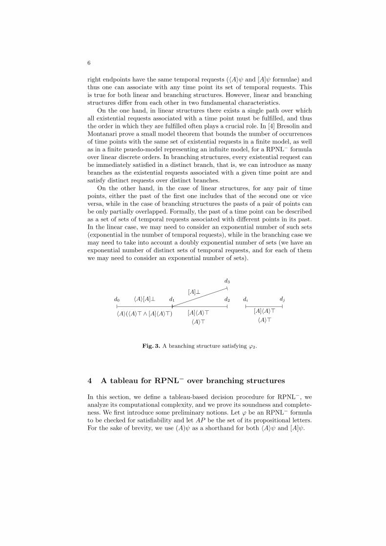
6

right endpoints have the same temporal requests (〈A〉ψ and [A]ψ formulae) andthus one can associate with any time point its set of temporal requests. Thisis true for both linear and branching structures. However, linear and branchingstructures differ from each other in two fundamental characteristics.

On the one hand, in linear structures there exists a single path over whichall existential requests associated with a time point must be fulfilled, and thusthe order in which they are fulfilled often plays a crucial role. In [4] Bresolin andMontanari prove a small model theorem that bounds the number of occurrencesof time points with the same set of existential requests in a finite model, as wellas in a finite psuedo-model representing an infinite model, for a RPNL− formulaover linear discrete orders. In branching structures, every existential request canbe immediately satisfied in a distinct branch, that is, we can introduce as manybranches as the existential requests associated with a given time point are andsatisfy distinct requests over distinct branches.

On the other hand, in the case of linear structures, for any pair of timepoints, either the past of the first one includes that of the second one or viceversa, while in the case of branching structures the pasts of a pair of points canbe only partially overlapped. Formally, the past of a time point can be describedas a set of sets of temporal requests associated with different points in its past.In the linear case, we may need to consider an exponential number of such sets(exponential in the number of temporal requests), while in the branching case wemay need to take into account a doubly exponential number of sets (we have anexponential number of distinct sets of temporal requests, and for each of themwe may need to consider an exponential number of sets).

d0 d1

d3

d2 di dj

〈A〉(〈A〉> ∧ [A]〈A〉>)

〈A〉[A]⊥[A]⊥

[A]〈A〉>〈A〉>

[A]〈A〉>〈A〉>

Fig. 3. A branching structure satisfying ϕ2.

4 A tableau for RPNL− over branching structures

In this section, we define a tableau-based decision procedure for RPNL−, weanalyze its computational complexity, and we prove its soundness and complete-ness. We first introduce some preliminary notions. Let ϕ be an RPNL− formulato be checked for satisfiability and let AP be the set of its propositional letters.For the sake of brevity, we use (A)ψ as a shorthand for both 〈A〉ψ and [A]ψ.

7

Definition 2. The closure CL(ϕ) of ϕ is the set of all subformulae of ϕ and oftheir negations (we identify ¬¬ψ with ψ).

Definition 3. The set of temporal requests of ϕ is the set TF(ϕ) of all temporalformulae in CL(ϕ), that is, TF(ϕ) = (A)ψ ∈ CL(ϕ).

By induction on the structure of ϕ, we can easily prove the following proposition.

Proposition 1. For every formula ϕ, |CL(ϕ)| is less than or equal to 2 · |ϕ|,while |TF(ϕ)| is less than or equal to 2 · (|ϕ| − 1).

The notion of ϕ-atom is defined in the standard way.

Definition 4. A ϕ-atom is a set A ⊆ CL(ϕ) such that:

– for every ψ ∈ CL(ϕ), ψ ∈ A iff ¬ψ 6∈ A;– for every ψ1 ∨ ψ2 ∈ CL(ϕ), ψ1 ∨ ψ2 ∈ A iff ψ1 ∈ A or ψ2 ∈ A.

We denote the set of all ϕ-atoms by Aϕ. We have that |Aϕ| ≤ 2|ϕ|. For any atomA we define the set of temporal requests of A as the set REQ(A) = A ∩ TF(ϕ).It’s easy to prove that given a model M = 〈〈T, I(T)−〉,V〉 for a RPNL− formulaϕ one can construct a unique function VA : I(T)− → Aϕ that associate to everyinterval [di, dj ] ∈ I(T)− an atom A such that for every ψ ∈ CL(ϕ), ψ ∈ A ifand only if M, [di, dj ] |= ψ. Now we prove the following theorem that constrainsatoms sharing the same endpoints.

Theorem 1. Let M = 〈〈T, I(T)−〉,V〉 a model for a RPNL− formula ϕ andde, di, dj ∈ T with di < de and dj < de, if VA([di, de]) = A and the atomassociated to VA([dj , de]) = A′ then REQ(A) = REQ(A′).

Proof. Suppose by contraddiction that REQ(A) 6= REQ(A′) then we can as-sume without loss of generality that exists 〈A〉ψ ∈ REQ(A) and 〈A〉ψ /∈ REQ(A′),by the definition of atom we have that [A]¬ψ ∈ REQ(A′), since M is a modelthere exists dh > de such that M, [de, dh] |= ψ (for 〈A〉ψ ∈ REQ(A)) and forevery dk > de M, [de, dk] |= ¬ψ (for [A]¬ψ ∈ REQ(A′)) then M, [de, dk] |= ¬ψthis leads to a contraddiction.

Atoms are connected by the following binary relation.

Definition 5. Let Rϕ be a binary relation over Aϕ such that, for every pair ofatoms A,A′ ∈ Aϕ, A Rϕ A

′ if and only if, for every [A]ψ ∈ CL(ϕ), if [A]ψ ∈ A,then ψ ∈ A′.

A tableau for RPNL− is a suitable decorated tree T . The decoration of eachnode n in T , denoted by ν(n), is a triple 〈[di, dj ], A,D〉, where D = 〈D,<〉 is aprefix of N, di and dj , with di < dj , belong to D, and A is an atom. The rootr of T is labeled by the empty decoration 〈∅, ∅〉. Given a node n, we denote byA(n) the atom component of ν(n).

Expansion rules. The construction of a tableau is based on the following expan-sion rules. Let n be a node in T , decorated with 〈[di, dj ], An,Dn〉. The followingexpansion rules can be possibly applied to n:

8

1. Step rule: if dj ≥ d for all d ∈ Dn and there exists at least one 〈A〉-formulain An, then choose a set of atoms A′1, .., A′k such that, An Rϕ A′i for everyA′i and for every 〈A〉ψ ∈ An there exists A′i such that ψ ∈ A′i. For every A′iadd an immediate successor n′ to n decorated with 〈[dj , dj+1], A′i,D′〉, whereD′ is obtained from Dn by adding a new point dj+1 after all points in Dn.

2. Fill-in rule: if there exists a point dk > dj such that there are no ancestorsn′ of n with decoration 〈[dj , dk], A′,D′〉, for some A′ and D′, then take anyatom A′′ such that An Rϕ A′′ and REQ(A′′) = REQ(A), for all ancestors nof n with ν(n) = 〈[d, dk], A,D〉 (since dk belongs to Dn, there exists at leastone of them), for some d,A, and D, and add an immediate successor n′′ ton, with ν(n′′) = 〈[dk, dj ], A′′,Dn〉.

Both rules add new successors to n. However, while the step rule decorates suchnodes with a new interval ending at a new point dj+1, the fill-in rule decoratesthem with a new interval whose endpoints were already in Dn.

From the definition of the Fill-in rule, it follows that all atoms associatedwith intervals ending at the same point d agree on their temporal requests.Hereinafter, we denote by REQ(d) their common set of requests.

Blocking condition. To guarantee the termination of the method, we need asuitable blocking condition to avoid the infinite application of the expansionrules in the case of infinite models. We say that a node n, decorated with〈[di, dj ], An,Dn〉 is blocked if there exists an ancestor n′ of n, decorated with〈[dk, dl], An′ ,Dn′〉, with dl < dj , such that:

– REQ(An) = REQ(An′);

– for all dh < dj there exists dm < dl such that REQ(dh) = REQ(dm).

Roughly speaking we block a node n if it has an ancestor n′ with the same setof temporal requests and every set of temporal requests that occurs in a pathfrom n′ to n occurs in an ancestor of n′.

Expansion strategy. Given a decorated tree T and a node n, we say that anexpansion rule is applicable to n if n is non-blocked and the application of therule generates at least one new node. The branch expansion strategy for a leafnode n, decorated with 〈[di, dj ], An,Dn〉, is the following one:

1. if the fill-in rule is applicable, apply the fill-in rule to n;

2. if the fill-in rule is not applicable and there exists a point dk < dj , suchthat there are no ancestors of n with decoration 〈[dk, dj ], A′,D′〉, for someA′ ∈ Aϕ, close the node n;

3. if the fill-in rule is not applicable, n is not closed, then apply the step ruleto n.

Tableau. Let ϕ be the formula to be checked for satisfiability, an initial tableaufor ϕ is a decorated tree with only one node 〈[d0, d1], A, d0 < d1〉, where A isan atom containing ϕ.

9

〈[d0, d1], A0, D1〉

〈[d1, d2], A0, D2〉blocked

〈[d1, d2], A1, D2〉×〈[d1, d2], A2, D2〉

×

〈[d1, d2], A3, D2〉〈[d1, d2], A4, D2〉

〈[d2, d3], A0, D3〉×

〈[d1, d3], A0, D3〉×


〈[d3, d4], A1, D4〉×

〈[d3, d4], A2, D4〉×

〈[d3, d4], A3, D4〉×


Fig. 4. A tableau for the formula ϕ2 ≡ 〈A〉(〈A〉> ∧ [A]〈A〉>) ∧ 〈A〉[A]⊥

A tableau for ϕ is any decorated tree T obtained by expanding the initial tableaufor ϕ through successive applications of the branch-expansion strategy to cur-rently existing branches, until the branch-expansion strategy cannot be appliedanymore.

Pruning the tableau. Given a tableau T for a formula ϕ, we apply the fol-lowing pruning procedure until no nodes can be removed:

1. remove any closed node from the tableau;2. remove any node n without successor such that the fill-in rule has been

applied to it in the tableau construction;3. remove any node n such that the step rule has been applied to it in the

tableau construction and there exists 〈A〉ψ ∈ An such that there are nosuccessors of n labeled with ψ;

4. remove any node that is not reachable from the root.

It will turn out that a formula ϕ is satisfiabile if and only if exists a finaltableau for it that is not empty.

4.1 An example

To understand how the tableau-based procedure works consider the formulaϕ2 ≡ 〈A〉(〈A〉> ∧ [A]〈A〉>) ∧ 〈A〉[A]⊥ introduced in Section 3. A non-empty

10

final tableau for ϕ2 is represented in Figure 4. We denote with ψ the for-mula 〈A〉> ∧ [A]〈A〉>. The atoms used int the tableau construction are A0 =〈A〉>, 〈A〉[A]⊥, 〈A〉ψ,¬ψ,ϕ2, A1 = [A]⊥, 〈A〉[A]⊥, 〈A〉ψ,¬ψ,ϕ2, A2 = [A]⊥, [A]〈A〉>, 〈A〉ψ,¬ψ,¬ϕ2, A3 = [A]⊥, [A]〈A〉>, [A]¬ψ,¬ψ,¬ϕ2, and A4 =〈A〉>, [A]〈A〉>, 〈A〉ψ,ψ,¬ϕ2. Di stands for the linear order d0 < ... < di.

The root of the tableau is the node 〈[d0, d1], A0,D1〉. We apply the step ruleon it choosing the set A0, A1, A2, A3, A4. The node 〈[d1, d2], A0,D2〉 satisfies〈A〉> and it is blocked since A0 is repeated. 〈A〉[A]⊥ is satisfied by the node〈[d1, d2], A3,D2〉. Since A3 does not contain 〈A〉-formulae this node is open andit is not expanded further. We satisfy 〈A〉ψ with the node 〈[d1, d2], A4,D2〉 that,as we will show later, is open. Every node containing A1 or A2 is closed becausethese atoms contain both the formula [A]⊥, that imposes on the current nodeto have no successors, and an 〈A〉-formula that imposes on the node to have atleast one successor. Consider now the node 〈[d1, d2], A4,D2〉: to satisfy 〈A〉> and〈A〉ψ, we apply the step rule choosing the set A0, A4. Then we apply the fill-inrule to the successor labeled 〈[d2, d3], A0,D3〉 and we add a successor labelled〈[d1, d3], A0,D3〉 to it. Now we have to apply the step rule on 〈[d1, d3], A0,D3〉: wechoose to use the same successors we used before for 〈[d0, d1], A0,D1〉. With thischoice for the successors, we can’t satisfy the formula 〈A〉[A]⊥ since the node〈[d3, d4], A3,D4〉 is closed because the fill-in rule is not applicable on [d2, d4]for this branch (an atom cannot contain both 〈A〉> and [A]⊥). For this reason〈[d1, d3], A0,D3〉 will be removed by the pruning procedure, as well as its prede-cessor 〈[d2, d3], A0,D3〉, and as well as the node 〈[d3, d4], A0,D4〉 (which will beremoved since it is no more reachable from the root). However, since the node〈[d2, d3], A4,D3〉 is blocked and satisfies all the 〈A〉-formulae of 〈[d1, d2], A4,D2〉,the latter node will not be removed. This shows that the final tableau depicted inFigure 4 is not empty, from which we can correctly conclude that ϕ2 is satisfiable.

4.2 Computational complexity

As a preliminary step, we show that the proposed tableau method terminates;then we analyze its computational complexity.

In order to prove termination of the tableau method, we give a bound on thelength of any branch B of any tableau for ϕ:

1. by the blocking condition, after at most O(22·TF (ϕ)) = O(22·n), with n =|ϕ|, applications of the step rule, the expansion strategy cannot be appliedanymore to a branch (REQ(d) can take 2TF (ϕ) different values and therecan be at most 2TF (ϕ) different sets of requests associated with time pointsd′ < d);

2. given a branch B, between two successive applications of the step rule, thefill-in rule can be applied at most k times, where k is the current number ofelements in the linear ordering Dn labelling the last node of B (k is exactlythe number of applications of the step rule up to that point).

Hence, the length of a branch is (at most) exponential in |ϕ|.

11

Theorem 2 (Termination). The tableau method for RPNL− terminates.

Proof. Given a formula ϕ, let T be a tableau for ϕ. Since, by construction, everynode of T has a finite outgoing degree and every branch of it is of finite length,by Konig’s Lemma, T is finite.

Since the outgoing degree of every node is bounded by the number of re-quests, that is, |REQ(ϕ)| ≤ n, the size of a final tableau is O(22n

). However,the proposed decision procedure does not need to explicitly generated the wholetableau. It can indeed keep track of a branch at a time and expand it in anon-deterministic way, until it is either blocked or closed (in this case the pro-cedure returns fail). Given that the length of any branch is at most O(22·n), theproposed decision procedure is in EXPSPACE.

4.3 Soundness and completeness

The soundness and completeness of the proposed method can be proved as fol-lows. Soundness is proved by showing how it is possible to construct a modelsatisfying ϕ from a non-empty final tableau T for ϕ. The proof must encompassboth the case of blocked nodes and that of non-blocked ones. Proving com-pleteness consists in showing that for any satisfiable formula ϕ there exists anon-empty final tableau for it.

Theorem 3 (Soundness). Given a formula ϕ and a final tableau T for ϕ, ifT is non-empty, then ϕ is satisfiable.

Proof. Let T be a non-empty final tableau for ϕ. We show that, by visiting T ,we can build up a model satisfying ϕ. We start from the root n0 of the tableau.Since T is not-empty, we choose one of the successors of n0. By the definitionof initial tableau, such a successor n is decorated with 〈[d0, d1], An, d0 < d1〉.Thus, we consider the two-nodes tree T0 = d0, d1 and we define the initialmodel M0 = 〈〈T0, I(T0)−〉,V0〉 where V[d0, d1] = p ∈ An. Now, suppose thatwe have built a partial model M and that we have reached a node n in the tableaudecorated with 〈[di, dj ], An,Dn〉. We proceed by induction on the expansion rulethat has been applied to n.

– No expansion rules have been applied to n, but n is not blocked. In this casethere are no 〈A〉-formulae in An and we do not need to expand the model.

– The step rule has been applied to n. For every formula 〈A〉ψ ∈ An we take asuccessor nψ of n such that ψ ∈ A(nψ), we add an immediate successor dψto dj in the tree and expand the model by putting V[dj , dψ] = p ∈ A(nψ).

– The fill-in rule has been applied to n. The successor of n is labelled withan interval [dk, dj ] and with an atom A′. We expand the model by puttingV[dk, dj ] = p ∈ A′.

– n is blocked. In this case there exists an ancestor n′ of n such that REQ(An) =REQ(An′) and for all dh < dj there exists dm < dl such that REQ(dh) =REQ(dm). Since no new atoms are introduced between n′ and n we canproceed with the construction from n repeating the construction that startsfrom n′.

12

At the end of such a (possibly infinite) construction, we have built a modelsatisfying ϕ.

Theorem 4 (Completeness). Given a satisfiable formula ϕ, there exists anon-empty final tableau T for ϕ.

Proof. Let ϕ be a satisfiable formula and let M = 〈〈T, I(T)−〉,V〉 be a modelfor it. We prove that there exists a non-empty final tableau T which corre-sponds to M. Since M is a model for ϕ, there exists an interval [d0, d1] suchthat M, [d0, d1] ϕ. Let A0 = ψ ∈ CL(ϕ) : M, [d0, d1] ψ. By the def-inition of initial tableau there exists a successor n0 of the root labelled with〈[d0, d1], A0, d0 < d1〉. We start the construction of the non-empty tableau forϕ from n0, and we proceed by induction on the expansion rules. Suppose that wehave built a partial tableau T and that we are considering a node n decoratedwith 〈[di, dj ], An,Dn〉. Three cases arise.

– The fill-in rule is applicable to n. Let dk be the point such that there areno nodes labelled with [dk, dj ]. We add a successor n′ to n labelled with〈[dk, dj ], A′,D′〉, where A′ = ψ ∈ CL(ϕ) : M, [dk, dj ] ψ, and we proceedin the construction from n′.

– The step rule is applicable to n. Hence, for every 〈A〉ψ ∈ An there existsan interval [dj , dψ] such that M, [dj , dψ] ψ. Let Aψ = θ ∈ CL(ϕ) :M, [dj , dψ] θ. For every 〈A〉ψ ∈ An we add a successor nψ to n decoratedwith 〈[dj , dψ], Aψ,Dn ∪ dψ〉 and we proceed inductively on such nψ.

– No rules are applicable to n. Since M is a model for ϕ, n cannot be a closednode. Hence, either there are no 〈A〉-formulae in An or n is blocked.

It can be proved that the tableau T obtained at the end of the above proce-dure is a non empty tableau for ϕ.

5 Conclusions

In this paper, we focused our attention on interval logics of temporal neighbor-hood. We addressed the satisfiability problem for the future fragment of strictNeighborhood Logic (RPNL−), interpreted over trees, and we showed how tosolve it by providing a sound and complete tableau-based decision procedure ofEXPSPACE complexity.

We do not know if our procedure is of optimal complexity or not. A firstdevelopment of this work will be the study of the complexity of the satisfiabilityproblem for the logic RPNL− interpreted over trees. A more valuable, yet moredifficult, development would be the extension of the proposed tableau method tothe case of full PNL interpreted over trees and over general partial orders withthe linear interval property (where intervals are always linear).

13

References

1. D. Bresolin, V. Goranko, A. Montanari, and P. Sala. Tableau systems for logics ofsubinterval structures over dense orderings. In Proc. of TABLEAUX 2007, volume4548 of LNAI, pages 73–89. Springer, 2007.

2. D. Bresolin, V. Goranko, A. Montanari, and G. Sciavicco. On Decidability andExpressiveness of Propositional Interval Neighborhood Logics. In Proc. of theInternational Symposium on Logical Foundations of Computer Science (LFCS),volume 4514 of LNCS, pages 84–99. Springer, 2007.

3. D. Bresolin and A. Montanari. A tableau-based decision procedure for a branching-time interval temporal logic. In H. Schlingloff, editor, Proc. of the 4th Int. Work-shop on Methods for Modalities, pages 38–53, 2005.

4. D. Bresolin and A. Montanari. A tableau-based decision procedure for right propo-sitional neighborhood logic. In Proc. of TABLEAUX 2005, volume 3702 of LNAI,pages 63–77. Springer, 2005.

5. D. Bresolin, A. Montanari, and P. Sala. An optimal tableau-based decision algo-rithm for Propositional Neighborhood Logic. In Proc. of the 24th InternationalSymposium on Theoretical Aspects of Computer Science (STACS), volume 4393 ofLNCS, pages 549–560. Springer, 2007.

6. D. Bresolin, A. Montanari, and G. Sciavicco. An optimal decision procedure forRight Propositional Neighborhood Logic. Journal of Automated Reasoning, 38(1-3):173–199, 2007.

7. E. Emerson and J. Halpern. Decision procedures and expressiveness in the temporallogic of branching time. Journal of Computer and System Sciences, 30(1):1–24,1985.

8. V. Goranko, A. Montanari, and G. Sciavicco. A general tableau method for propo-sitional interval temporal logic. In Proc. of TABLEAUX 2003, volume 2796 ofLNAI, pages 102–116. Springer, 2003.

9. V. Goranko, A. Montanari, and G. Sciavicco. Propositional interval neighborhoodtemporal logics. Journal of Universal Computer Science, 9(9):1137–1167, 2003.

10. V. Goranko, A. Montanari, and G. Sciavicco. A road map of interval temporallogics and duration calculi. Journal of Applied Non-Classical Logics, 14(1–2):9–54,2004.

11. V. Goranko, A. Montanari, G. Sciavicco, and P. Sala. A general tableau methodfor propositional interval temporal logics: Theory and implementation. Journal ofApplied Logic, 4(3):305–330, 2006.

12. Joseph Y. Halpern and Yoav Shoham. A propositional modal logic of time intervals.Journal of the ACM, 38(4):935–962, October 1991.

13. A. Montanari. Propositional interval temporal logics: some promising paths. InProc. of the 12th International Symposium on Temporal Representation and Rea-soning (TIME), pages 201–203. IEEE Computer Society Press, 2005.

14. A. Montanari, G. Sciavicco, and N. Vitacolonna. Decidability of interval temporallogics over split-frames via granularity. In Proc. of the 8th European Conferenceon Logics in AI, volume 2424 of LNAI, pages 259–270. Springer, 2002.

15. B. Moszkowski. Reasoning about digital circuits. Tech. rep. stan-cs-83-970, Dept.of Computer Science, Stanford University, Stanford, CA, 1983.

16. M. Otto. Two variable first-order logic over ordered domains. Journal of SymbolicLogic, 66(2):685–702, 2001.

17. I. Shapirovsky. On PSPACE-decidability in Transitive Modal Logic. In R. Schmidt,I. Pratt-Hartmann, M. Reynolds, and H. Wansing, editors, Advances in ModalLogic, volume 5, pages 269–287. King’s College Publications, London, 2005.

14

18. I. Shapirovsky and V. Shehtman. Chronological future modality in Minkowskispacetime. In P. Balbiani, N. Y. Suzuki, F. Wolter, and M. Zakharyaschev, editors,Advances in Modal Logic, volume 4, pages 437–459. King’s College Publications,London, 2003.

19. Y. Venema. A modal logic for chopping intervals. Journal of Logic and Computa-tion, 1(4):453–476, 1991.

KLM Logics of Nonmonotonic Reasoning:

Calculi and Implementations

Laura Giordano1, Valentina Gliozzi2, Nicola Olivetti3, and Gian Luca Pozzato2

1 Dipartimento di Informatica - Universita del Piemonte Orientale “A. Avogadro” -via Bellini 25/G - 15100 Alessandria, Italy

[email protected] Dipartimento di Informatica - Universita degli Studi di Torino, corso Svizzera 185 -

10149 Turin - Italygliozzi,[email protected]

3 LSIS - UMR CNRS 6168 Universite Paul Cezanne (Aix-Marseille 3), AvenueEscadrille Normandie-Niemen 13397 Marseille Cedex 20 - France

[email protected]

Abstract. We present proof methods for the logics of nonmonotonicreasoning defined by Kraus, Lehmann and Magidor (KLM). We intro-duce tableaux calculi (called T ST) for all KLM logics. We provide deci-sion procedures for KLM logics based on these calculi, and we study theircomplexity. Finally, we describe KLMLean 2.0, a theorem prover imple-menting the calculi T ST inspired by the “lean” methodology. KLMLean2.0 is implemented in SICStus Prolog and it also comprises a graphicalinterface written in Java1.

1 Introduction

In the early 90’ [13, 14] Kraus, Lehmann and Magidor (from now on KLM) pro-posed a formalization of non-monotonic reasoning that was early recognized asa landmark. Their work stemmed from two sources: the theory of nonmonotonicconsequence relations initiated by Gabbay [8] and the preferential semantics pro-posed by Shoham [16] as a generalization of Circumscription. Their works lead toa classification of nonmonotonic consequence relations, determining a hierarchyof stronger and stronger systems.

According to the KLM framework, defeasible knowledge is represented by a(finite) set of nonmonotonic conditionals or assertions of the form

A |∼ B

whose reading is normally (or typically) the A’s are B’s. The operator “|∼” isnonmonotonic, in the sense that A |∼ B does not imply A∧C |∼ B. For instance, a

1 This research has been partially supported by “Progetto Lagrange - FondazioneCRT” and by the projects “MIUR PRIN05: Specification and verification of agentinteraction protocols” and “GALILEO 2006: Interazione e coordinazione nei sistemimulti-agenti”.

2 L. Giordano, V. Gliozzi, N. Olivetti, and G.L.Pozzato

knowledge base K may contain football lover |∼ bet , football player |∼ football lover ,football player |∼ ¬bet , whose meaning is that people loving football typically beton the result of a match, football players typically love football but they typicallydo not bet (especially on matches they are going to play...). If |∼ were interpretedas classical (or intuitionistic) implication, one would get football player |∼ ⊥, i.e.typically there are not football players, thereby obtaining a trivial knowledgebase.

In KLM framework, one can derive new conditional assertions from theknowledge base by means of a set of inference rules. The set of adopted infer-ence rules defines some fundamental types of inference systems, namely, from thestrongest to the weakest: Rational (R), Preferential (P), Loop-Cumulative (CL),and Cumulative (C) logic. In all these systems one can infer new assertions with-out incurring the trivializing conclusions of classical logic: in the above example,in none of the systems, one can infer football player |∼ bet . In cumulative logics(both C and CL) one can infer football lover ∧ football player |∼ ¬bet , givingpreference to more specific information; in Preferential logic P one can also inferthat football lover |∼ ¬football player ; in the rational case R, if one further knowsthat ¬(football lover |∼ rich), that is to say it is not the case that football loversare typically rich persons, one can also infer that football lover ∧ ¬rich |∼ bet .

From a semantic point of view, to the each logic (R, P, CL, C) correspondsone kind of models, namely, possible-world structures equipped with a preferencerelation among worlds or states. More precisely, for P we have models with apreference relation (an irreflexive and transitive relation) on worlds. For thestronger R the preference relation is further assumed to be modular. For theweaker logic CL, the preference relation is defined on states, where a state canbe identified, intuitively, with a set of worlds. In the weakest case of C, thepreference relation is on states, as for CL, but it is no longer assumed to betransitive. In all cases, the meaning of a conditional assertion A |∼ B is that B

holds in the most preferred worlds/states where A holds.A recent result by Halpern and Friedman [6] has shown that preferential

and rational logic are quite natural and general systems: surprisingly enough,the axiom system of preferential (likewise of rational logic) is complete withrespect to a wide spectrum of semantics, from ranked models, to parametrizedprobabilistic structures, ǫ-semantics and possibilistic structures. The reason isthat all these structures are examples of plausibility structures and the truth inthem is captured by the axioms of preferential (or rational) logic. These results,and their extensions to the first order setting [7] are the source of a renewedinterest in KLM framework.

Even if KLM was born as an inferential approach to nonmonotonic reasoning,curiously enough, there has not been much investigation on deductive mecha-nisms for these logics. In short, the state of the art is as follows:

- Lehmann and Magidor [14] have proved that validity in P is coNP-complete.Their decision procedure for P is more a theoretical tool than a practical al-gorithm, as it requires to guess sets of indexes and propositional evaluations.They have also provided another procedure for P that exploits its reduction

KLM Logics of Nonmonotonic Reasoning: Calculi and Implementations 3

to R. However, the reduction of P to R breaks down if boolean combinationsof conditionals are allowed, indeed it is exactly when such combinations areallowed that the difference between P and R arises.

- A tableau proof procedure for C has been given in [1]. Their tableau proce-dure is fairly complicated; it uses labels and it contains a cut-rule. Moreover,it is not clear how it can be adapted to CL and P.

- In [11] it is defined a labelled tableau calculus for the conditional logic CEwhose flat fragment (i.e. without nested conditionals) corresponds to P.That calculus needs a fairly complicated loop-checking mechanism to ensuretermination. It is not clear if it matches complexity bounds and if it can beadapted in a simple way to CL.

- Finally, decidability of P and R has also been obtained by interpretingthem into standard modal logics, as it is done by Boutilier [4]. However, hismapping is not very direct and natural, as we discuss below.

In this work we present tableau procedures for all KLM logics called T ST, whereS stands for R,P,CL,C. Our approach is based on a novel interpretation ofP into modal logics. As a difference with previous approaches (e.g. Crocco andLamarre [5] and Boutillier [4]), that take S4 as the modal counterpart of P, weconsider here Godel-Lob modal logic of provability G (see for instance [12]). Ourtableau method provides a sort of run-time translation of P into modal logic G.The idea is simply to interpret the preference relation as an accessibility relation:a conditional A |∼ B holds in a model if B is true in all minimal A-worlds w

(i.e. worlds in which A holds and that are minimal). An A-world w is a minimalA-world if all smaller worlds are not A-worlds. The relation with modal logic G ismotivated by the fact that we assume, following KLM, the so-called smoothnesscondition, which is related to the well-known limit assumption. This conditionensures that minimal A-worlds exist whenever there are A-worlds, by preventinginfinitely descending chains of worlds. This condition therefore corresponds tothe finite-chain condition on the accessibility relation (as in modal logic G).Therefore, our interpretation of conditionals is different from the one proposedby Boutilier, who rejects the smoothness condition and then gives a less natural(and more complicated) interpretation of P into modal logic S4. We are able toextend our approach to the cases of CL and C by using a second modality whichtakes care of states. As a difference with P and CL, the calculus for C requiresa sort of (analytic) cut rule to account for the smoothness condition. We alsoconsider the case of the strongest logic R; as for the other weaker systems, ourapproach is based on an interpretation of R into an extension of modal logic G,including modularity of the preference relation (previous approaches [5, 4] takeS4.3 as the modal counterpart of R). As a difference with the tableau calculiintroduced for P, CL, and C, here we present a labelled tableau system, whichseems to be the most natural approach in order to capture the modularity of thepreference relation.

The tableau calculi mentioned above can be used to define a systematicprocedure which allows the satisfiability problem for R, P, and CL to be decidedin nondeterministic polynomial time; moreover, we obtain a complexity bound


for these logics, namely that they are coNP-complete. For R and P, this isin accordance with the known complexity results, whereas for CL this boundis new, to the best of our knowledge. The calculus T CT gives nonetheless adecision procedure for this logic too.

Finally, we present KLMLean 2.0, a theorem prover implementing T ST cal-culi in SICStus Prolog. KLMLean 2.0 is inspired by the “lean” methodology [3],and it also comprises a graphical interface written in Java. For the rational logicR, KLMLean 2.0 offers two different versions: 1. a simple version, where Pro-log constants are used to represent T RT’s labels; 2. a more efficient one, wherelabels are represented by Prolog variables, inspired by the free-variable tableaupresented in [2]. To the best of our knowledge, KLMLean 2.0 is the first theoremprover for KLM logics.

The plan of the paper is as follows: in section 2, we recall KLM logics, andwe show how their semantics can be represented by standard Kripke models.In section 3, we present the tableaux calculi T ST and we elaborate them inorder to obtain a terminating procedure. Also, we summarize complexity resultsobtained by analyzing T ST. In section 4 we present KLMLean 2.0, a theoremprover written in SICStus Prolog implementing the T ST calculi.

2 KLM Logics

We briefly recall the axiomatizations and semantics of the KLM systems. Forthe sake of exposition, we present the systems in the order from the strongest tothe weakest: R, P, CL, and C. For a complete picture of KLM systems, see [13,14]. The language of KLM logics consists just of conditional assertions A |∼ B.We consider a richer language allowing boolean combinations of assertions andpropositional formulas. Our language L is defined from a set of propositionalvariables ATM , the boolean connectives and the conditional operator |∼. We useA, B, C, ... to denote propositional formulas (that do not contain conditional for-mulas), whereas F, G, ... are used to denote all formulas (including conditionals);Γ, ∆, ... represent sets of formulas, whereas X, Y, ... denote sets of sets of formu-las. The formulas of L are defined as follows: if A is a propositional formula,A ∈ L; if A and B are propositional formulas, A |∼ B ∈ L; if F is a booleancombination of formulas of L, F ∈ L.

The axiomatization of R consists of all axioms and rules of propositionalcalculus together with the following axioms and rules. We use ⊢PC to denoteprovability in the propositional calculus, whereas ⊢ is used to denote provabilityin R:

– REF. A |∼ A (reflexivity)– LLE. If ⊢PC A ↔ B, then ⊢ (A |∼ C) → (B |∼ C) (left logical equivalence)– RW. If ⊢PC A → B, then ⊢ (C |∼ A) → (C |∼ B) (right weakening)– CM. ((A |∼ B) ∧ (A |∼ C)) → (A ∧ B |∼ C) (cautious monotonicity)– AND. ((A |∼ B) ∧ (A |∼ C)) → (A |∼ B ∧ C)– OR. ((A |∼ C) ∧ (B |∼ C)) → (A ∨ B |∼ C)


– RM. ((A |∼ B) ∧ ¬(A |∼ ¬C)) → ((A ∧ C) |∼ B) (rational monotonicity)

REF states that A is always a default conclusion of A. LLE states that thesyntactic form of the antecedent of a conditional formula is irrelevant. RW de-scribes a similar property of the consequent. This allows to combine default andlogical reasoning [6]. CM states that if B and C are two default conclusions ofA, then adding one of the two conclusions to A will not cause the retractionof the other conclusion. AND states that it is possible to combine two defaultconclusions. OR states that it is allowed to reason by cases: if C is the defaultconclusion of two premises A and B, then it is also the default conclusion oftheir disjunction. RM is the rule of rational monotonicity, which characterizesthe logic R: if A |∼ B and ¬(A |∼ ¬C) hold, then one can infer A ∧C |∼ B. Thisrule allows a conditional to be inferred from a set of conditionals in absenceof other information. More precisely, “it says that an agent should not have toretract any previous defeasible conclusion when learning about a new fact thenegation of which was not previously derivable” [14].

The axiomatization of P can be obtained from the axiomatization of R byremoving the axiom RM.

The axiomatization of CL can be obtained from the axiomatization of Pby removing the axiom OR and by adding the following infinite set of LOOPaxioms:

LOOP. (A0 |∼ A1) ∧ (A1 |∼ A2)...(An−1 |∼ An) ∧ (An |∼ A0) → (A0 |∼ An)

and the following axiom CUT:

CUT. ((A |∼ B) ∧ (A ∧ B |∼ C)) → (A |∼ C)

Notice that these axioms are derivable in P (and therefore in R). The weakestlogical system considered by KLM is Cumulative Logic C, whose axiom systemcan be obtained from the one for CL by removing the set of (LOOP) axioms.

The semantics of KLM logics is defined by considering possible world (orpossible states) structures with a preference relation w < w′ among worlds (orstates), whose meaning is that w is preferred to w′. A |∼ B holds in a modelM if B holds in all minimal worlds (states) where A holds. This definitionmakes sense provided minimal worlds for A exist whenever there are A-worlds(A-states): this is ensured by the smoothness condition defined below.

Definition 1 (Rational and Preferential models). A rational model is atriple

M = 〈W , <, V 〉

where W is a non-empty set of items called worlds, < is an irreflexive, tran-sitive and modular2 relation on W, and V is a function V : W 7−→ 2ATM ,which assigns to every world w the set of atoms holding in that world. The truthconditions for a formula F are as follows:

2 A relation < is modular if the following condition holds: for each u, v, w, if u < v,then either w < v or u < w.


– if F is a boolean combination of formulas, M, w |= F is defined as forpropositional logic, namely:• if F is an atom P ∈ ATM, then M, w |= P iff P ∈ V (w);• if F is a negation ¬G, then M, w |= ¬G iff M, w 6|= G;• if F is a conjunction G1 ∧G2, then M, w |= G1 ∧G2 iff M, w |= G1 andM, w |= G2;

• if F is a disjunction G1 ∨ G2, then M, w |= G1 ∨ G2 iff M, w |= G1 orM, w |= G2;

• if F is an implication G1 → G2, then M, w |= G1 → G2 iff M, w 6|= G1

or M, w |= G2.

Let A be a propositional formula; we define Min<(A) = w ∈ W | M, w |= A

and ∀w′, w′ < w implies M, w′ 6|= A. We define:

– M, w |= A |∼ B if for all w′, if w′ ∈ Min<(A) then M, w′ |= B.

We also define the smoothness condition on the preference relation: if M, w |=A, then w ∈ Min<(A) or ∃w′ ∈ Min<(A) s.t. w′ < w. Validity and satisfiabilityof a formula are defined as usual.

A preferential model is defined as the rational/preferential model, with theonly difference that the preference relation < is no longer assumed to be modular.

Observe that the above definition of rational model extends the one given byKLM to boolean combinations of formulas. Notice also that the truth condi-tions for conditional formulas are given with respect to single possible worlds foruniformity sake. Since the truth value of a conditional only depends on globalproperties of M, we have that: M, w |= A |∼ B iff M |= A |∼ B.

Models for (loop-)cumulative logics also comprise states:

Definition 2 (Loop-Cumulative and Cumulative models). A (loop-)cumulativemodel is a tuple

M = 〈S,W , l, <, V 〉

where S is a set of states and l : S 7→ 2W is a function that labels every statewith a nonempty set of worlds; < is defined on S, it satisfies the smoothnesscondition and it is irreflexive and transitive in CL, whereas it is only irreflexivein C.

For s ∈ S and A propositional, we let M, s |≡ A if ∀w ∈ l(s), then M, w |= A,where M, w |= A is defined as for propositional logic. Let Min<(A) be the setof minimal states s such that M, s |≡ A. We define M, s |≡ A |∼ B if ∀s′ ∈Min<(A), M, s′ |≡ B. The relation |≡ can be extended to boolean combinationsof conditionals in the standard way. We assume that < satisfies the smoothnesscondition.

The language of the tableau calculi that we will introduce in the next sectionextends L by formulas of the form A, where A is propositional, whose intuitivemeaning is that A holds in a world/state w if A holds in all the worlds/statespreferred to w (i.e. in all w′ such that w′ < w). We extend the notion of KLMmodel to provide an evaluation of boxed formulas as follows:


Definition 3 (Truth condition of modality ). We define the truth condi-tion of a boxed formula as follows:

– (R and P): M, w |= A if, for every w′ ∈ W, if w′ < w then M, w′ |= A

– (CL and C): M, s |≡ A if, for every s′ ∈ S, if s′ < s then M, s′ |≡ A

From definition of Min<(A) in Definitions 1 and 2 above, and Definition 3,it follows that for any formula A, w ∈ Min<(A) iff M, w |= A ∧ ¬A (resp.s ∈ Min<(A) iff M, s |≡ A ∧ ¬A).

3 Tableaux Calculi T ST

In this section we present analytic tableaux calculi T ST for KLM logics, whereS stands for R,P,CL,C. The basic idea is simply to interpret the preferencerelation as an accessibility relation. The calculi for R and P implement a sort ofrun-time translation into (extensions of) Godel-Lob modal logic of provability G.This is motivated by the fact that we assume the smoothness condition, whichensures that minimal A-worlds exist whenever there are A-worlds, by preventinginfinitely descending chains of worlds. This condition therefore corresponds tothe finite-chain condition on the accessibility relation (as in modal logic G). Thisapproach is extended to the cases of CL and C by using a second modality L

which takes care of states. For a broader discussion on those calculi, see [9, 15,10].

The rules of the calculi manipulate sets of formulas Γ . We write Γ, F as ashorthand for Γ ∪ F. Moreover, given Γ we define the following sets:

– Γ = ¬A | ¬A ∈ Γ

– Γ ↓

= ¬A | ¬A ∈ Γ– Γ |∼± = A |∼ B | A |∼ B ∈ Γ ∪ ¬(A |∼ B) | ¬(A |∼ B) ∈ Γ

– Γ L↓

= A | LA ∈ Γ.

As mentioned, the calculus for rational logic R makes use of labelled formulas(see Figure 1), where the labels are drawn from a denumerable set A; there aretwo kinds of formulas: 1. world formulas, denoted by x : F , where x ∈ A andF ∈ L; 2. relation formulas, denoted by x < y, where x, y ∈ A, representing thepreference relation. Rules of the calculus T RT also manipulate the following setof formulas: Γ M

x→y = y : ¬A, y : ¬A | x : ¬A ∈ Γ. The following definitionstates the truth conditions for labelled formulas:

Definition 4 (Truth conditions of formulas of T R). Given a model M =〈W , <, V 〉 and a label alphabet A, we consider a mapping I : A 7→ W. Given aformula α of the calculus T R, we define M |=I α as follows: M |=I x : F iffM, I(x) |= F ; M |=I x < y iff I(x) < I(y).We say that a set Γ of formulas of T R is satisfiable if, for all formulas α ∈ Γ ,we have that M |=I α, for some model M and some mapping I.


x newlabel

y new(!−)

z occurs in Γ and

x < z , z < y ∩ Γ = ∅(<)

Γ|∼±

,Γ!

↓

,A |∼ B ,LA,!¬LA Γ ,A |∼ B ,LA,!¬LA,LBΓ ,A |∼ B ,¬LA

T CLT

T CT

T PT

T RT

if Γ does not contain

negated L − formulas

label

ΓL

↓

,¬LA

Γ ,¬LA(L−)

Γ

ΓL

↓(L−)

Γ ,¬(A |∼ B)

Γ|∼±

,LA,!¬LA,¬LB

(|∼−)

Γ ,¬!¬LA

Γ!

,Γ|∼±

,Γ!

↓

,LA,!¬LA

(!−)

(|∼+)Γ ,A |∼ B

Γ ,A |∼ B ,¬LA Γ ,A |∼ B ,¬!¬LA Γ ,A |∼ B ,LB

ΓL

↓

,¬LA

Γ ,¬LA(L−)

Γ ,¬(A |∼ B)

Γ|∼±

,LA,!¬LA,¬LB

(|∼−)

(|∼+)Γ ,A |∼ B

(AX) Γ , x : P , x : ¬P with P ∈ ATM (AX) Γ , x < y , y < x

Γ , u : A |∼ B

Γ , u : A |∼ B , x : ¬!¬A Γ , u : A |∼ B , x : BΓ , u : A |∼ B , x : ¬A(|∼+)

Γ , u : ¬(A |∼ B)

Γ , x : A, x : !¬A, x : ¬B(|∼−)

Γ , x : ¬!¬A

Γ , y < x , y : A, y : !¬A,ΓMx→y

Γ , x < y

Γ , x < y , x < z ,ΓM

z→xΓ , x < y , z < y ,Γ

My→z

(AX) Γ ,P ,¬P with P ∈ ATMΓ ,A |∼ B ,¬!¬A Γ ,A |∼ B ,BΓ ,A |∼ B ,¬A

(|∼+)

Γ ,¬(A |∼ B)(|∼−)

Γ ,A |∼ B

Γ|∼±

,A,!¬A,¬B

(!−)Γ ,¬!¬A

Γ!

,Γ|∼±

,Γ!

↓

,A,!¬A

if Γ does not contain

negated L − formulas

Γ

ΓL

↓(L−)

Fig. 1. Tableau systems T ST. To save space, we omit the standard rules for booleanconnectives. For T CLT and T CT the axiom (AX) is as in T PT.

While the calculus for R makes use of labelled formulas, the calculi T ST for allother KLM logics, presented in Figure 1, do not make use of labels. A tableauis a tree whose nodes are sets of formulas Γ . A branch is a sequence of sets offormulas Γ1, Γ2, . . . , Γn, . . . , where each node Γi is obtained by its immediatepredecessor Γi−1 by applying a rule of T ST, having Γi−1 as the premise and Γi

as one of its conclusions. A branch is closed if one of its nodes is an instance of(AX), otherwise it is open. We say that a tableau is closed if all its branches areclosed.

The rules (|∼−) and (−) are called dynamic, since they introduce a new worldin their conclusions. The other rules are called static. In order to prove thatfootball lover |∼ ¬football player can be derived in preferential logic P from theknowledge base football lover |∼ bet , football player |∼ football lover , football player


×

× × ×

×

(|∼+)

(|∼+)

(|∼−)

(¬)

(!−)

(!−)

(!−)

L |∼ B,P |∼ L,P |∼ ¬B,¬(L |∼ ¬P )

L |∼ B,P |∼ L,P |∼ ¬B,L,!¬L,¬¬P

L |∼ B,P |∼ L,P |∼ ¬B,L,!¬L,P

. . . , L,¬L . . . ,¬!¬L,!¬L

. . . , L, !¬L,¬L

L |∼ B,P |∼ L,P |∼ ¬B,L,!¬L,P,B

. . . ,¬P, P L |∼ B,P |∼ L,P |∼ ¬B,L,!¬L,P,B,¬!¬P . . . ,¬B,B

L |∼ B,P |∼ L,P |∼ ¬B,¬L,P,!¬P

. . . ,¬P, P . . . ,¬L,L. . . , !¬P,¬!¬P

. . . ,¬P, P,!¬P

(|∼+)

×

×

Fig. 2. A derivation in T PT for football lover |∼ bet , football player |∼ football lover ,football player |∼ ¬bet ,¬(football lover |∼ ¬football player). To increase readability,we use P to denote football player , L to denote football lover and B for bet .

|∼ ¬bet, one needs to search a closed tableau in T PT for the set of formulasfootball lover |∼ bet , football player |∼ football lover , football player |∼ ¬bet ,¬(football lover |∼ ¬football player ). In Figure 2 a closed tableau in T PT forthe above unsatisfiable set of formulas is presented.

The calculi T ST are sound and complete wrt the semantics:

Theorem 1 (Soundness and completeness of T ST, [9, 15, 10]). Given aset of formulas Γ of L, it is unsatisfiable if and only if there is a closed tableauin T ST having Γ as a root.

3.1 Termination and Complexity Results

The calculi T ST do not ensure termination. However, we are able to turn theminto terminating calculi. In general, non-termination in tableau calculi can becaused by two different reasons: 1. dynamic rules can generate infinitely-manyworlds, creating infinite branches; 2. some rules copy their principal formula inthe conclusion, thus can be reapplied over the same formula without any control.

Concerning point 1, we are able to show that the generation of infinitebranches due to the interplay between rules (|∼+) and (−) cannot occur. Intu-itively, the application of (−) to a formula ¬¬A (introduced by (|∼+)) addsthe formula ¬A to the conclusion, so that (|∼+) can no longer consistently in-troduce ¬¬A. This is due to the properties of in G. Furthermore, the (|∼−)rule can be applied only once to a given negated conditional on a branch, thusinfinitely-many worlds cannot be generated on a branch.

Concerning point 2, we have to control the application of the (|∼+) rule, whichcan otherwise be applied without any control since it copies its principal formulaA |∼ B in all its conclusions, then the conclusions have a higher complexity thanthe premise. We can show that it is useless to apply (|∼+) more than once inthe same world/state, therefore the calculi T ST are modified to keep track ofpositive conditionals already considered in a world/state by moving them inan additional set Σ in the conclusions of (|∼+), and restrict the application ofthis rule to unused conditionals only. The dynamic rules (|∼−) and (−), whose


conclusions represent a different world/state wrt the corresponding premise, re-introduce formulas from Σ in order to allow further applications of (|∼+) in theother worlds/states. This machinery is standard. Concerning the labelled calcu-lus T RT, the same mechanism is applied by equipping each positive conditionalwith the list L of worlds-labels in which (|∼+) has already been applied, andrestricting its application by using worlds not belonging to L. In [15, 9, 10] itis shown that no other machinery is needed to ensure termination, except forT CT, which needs a further standard loop-checking machinery.

Theorem 2 (Termination of T ST, [9, 15, 10]). For all KLM logic S, T ST

ensures a terminating proof search.

We conclude this section by summarizing complexity results for T ST. In [9, 15,10], we have shown that for the logics R, P, and CL, the tableaux calculi abovecan be used to define a coNP decision procedure to check the validity of a setof formulas of L. The same cannot be done for the weakest logic C.

We can prove the following Theorem:

Theorem 3 (Complexity of R, P, and CL). The problem of deciding validityfor KLM logics R, P, and CL is coNP-complete.

Concerning R and P, this result matches the known complexity results for theselogics. Concerning the logic CL, this complexity bound is new, to the best ofour knowledge.

4 KLMLean 2.0: a Theorem Prover for KLM Logics

In this section we describe an implementation of T ST calculi in SICStus Prolog.The program, called KLMLean 2.0, is inspired by the “lean” methodology [3](even if it does not fit its style in a rigorous manner): the Prolog program consistsin a set of clauses, each one representing a tableau rule or axiom; the proofsearch is provided for free by the mere depth-first search mechanism of Prolog,without any additional ad hoc mechanism. KLMLean 2.0 can be downloaded athttp://www.di.unito.it/∼pozzato/klmlean 2.0.

Let us first describe the implementation of non-labelled calculi for P, CL,and C. We represent each node of a proof tree (i.e. set of formulas) by a Prologlist. The tableaux calculi are implemented by the predicate

prove(Gamma,Sigma,Tree).

which succeeds if and only if the set of formulas Γ , represented by the list Gamma,is unsatisfiable. Sigma is the list representing the set Σ of used conditionals, andit is used in order to control the application of the (|∼+) rule, as described inthe previous section. When prove succeeds, Tree contains a representation of a


closed tableau3. For instance, to prove that A |∼ B∧C,¬(A |∼ C) is unsatisfiablein P, one queries KLMLean 2.0 with the following goal: prove([a => (b and

c), neg (a => c)],[ ],Tree). The string “=>” is used to represent the condi-tional operator |∼, “and” is used to denote ∧, and so on. Each clause of prove

implements one axiom or rule of the tableaux calculi; for example, the clausesimplementing (AX) and (|∼−) are as follows:

prove(Gamma, ,tree(...)):-member(F,Gamma),member(neg F,Gamma),!.

prove(Gamma,Sigma,tree(. . . )):-select(neg (A => B),Gamma,NewGamma),

conditionals(NewGamma,Cond),append(Cond,Sigma,DefGamma),

prove([neg B|[box neg A|[A|DefGamma]]],[],. . . ).

The clause for (AX) is applied when a formula F and its negation ¬F belongto Γ . Notice that F is a formula of the language L, even complex; KLMLean2.0 extends (AX) to a generic formula F in order to increase its performances,without losing the soundness of the calculi. The clause for (|∼−) is applied when aformula ¬(A |∼ B) belongs to Γ . The predicate select removes ¬(A |∼ B) fromGamma, then the auxiliary predicate conditionals is invoked to compute the setΓ |∼± on the resulting list NewGamma; finally, the predicate prove is recursivelyinvoked on the only conclusion of the rule. Notice that, since (|∼−) is a dynamicrule, the conditionals belonging to Σ move to Γ in the conclusion (execution ofappend), in order to allow further applications of (|∼+). To search for a derivationof a set of formulas Γ , KLMLean 2.0 proceeds as follows: first of all, if Γ is aninstance of (AX), the goal will succeed immediately by using the clauses forthe axioms. If it is not, then the first applicable rule will be chosen, e.g. ifGamma contains a formula neg(neg F), then the clause for (¬) rule will be used,invoking prove on its unique conclusion. KLMLean 2.0 proceeds in a similar wayfor the other rules. The ordering of the clauses is such that the boolean rulesare applied before the other ones. In the case of cumulative logic C, KLMLean2.0 implements a loop-checking machinery by equipping the prove predicatewith an additional argument, called Analyzed, representing the list of sets offormulas already considered in the current branch. Clauses implementing T CT

are invoked only if the current set of formulas has not yet been considered, i.e.if it does not belong to Analyzed.

The theorem prover for rational logic R implements labelled tableau calculiT RT. It makes use of Prolog constants to represent labels: world formulas x :A are represented by a Prolog list [x,a], and relation formulas x < y arerepresented by a list [x,<,y]. As for the other systems, each clause of thepredicate prove implements a tableau rule or axiom. As an example, here is theclause implementing the rule (<), capturing the modularity of the preferencerelation:

3 More in detail, the argument Tree is instantiated by a functortree(Rule,F,G,SubTree1,[SubTree2]), tracing that the rule Rule has beenapplied to the principal formula F Rule G in the current set of formulas. SubTree1and SubTree2 are functors tree representing the closed tableau for each conclusionof the rule.


prove(Gamma,Labels,Cond,tree(. . . )):-

member([X,<,Y],Gamma),member(Z,Labels),X\=Z, Y\=Z,

\+member([X,<,Z],Gamma),\+member([Z,<,Y],Gamma),!,

gammaM(Gamma,Y,Z,ResLeft),gammaM(Gamma,Z,X,ResRight),

append(ResLeft,Gamma,LeftConcl),append(ResRight,Gamma,RightConcl),

prove([[Z,<,Y]|LeftConcl],Labels,Cond,. . . ),!,

prove([[X,<,Z]|RightConcl],Labels,Cond,. . . ).

The predicate gammaM(Gamma,X,Y,...) computes the set Γ Mx→y defined in the

previous section. In this system, Cond is used in order to control the applicationof the (|∼+) rule: it is a list whose elements have the form [x,a => b], repre-senting that (|∼+) has been applied to A |∼ B in the current branch by using thelabel x. In order to increase its performances, KLMLean for R adopts a heuris-tic approach (not very “lean”) to implement the crucial (|∼+) rule: the predicateprove chooses the “best” positive conditional to which apply the rule, and the“best” label to use. Roughly speaking, an application of (|∼+) is considered tobe better than another one if it leads to an immediate closure of more conclu-sions. Even if (|∼+) is invertible, choosing the right label in the application of(|∼+) is highly critical for the performances of the thorem prover. To postponethis choice as much as possible, for the logic R we have defined a more efficientversion of the prover, inspired by the free-variable tableaux introduced in [2].It makes use of Prolog variables to represent all the labels that can be used ina single application of the (|∼+) rule. This version represents labels by integersstarting from 1; by using integers we can easily express constraints on the rangeof the variable-labels. To this regard, the library clpfd is used to manage free-variables domains. In order to prove Γ, u : A |∼ B, KLMLean 2.0 will call proveon the following conclusions: Γ, u : A |∼ B, Y : ¬A; Γ, u : A |∼ B, Y : ¬¬A;Γ, u : A |∼ B, Y : B, where Y is a Prolog variable. Y will then be instanti-ated by Prolog’s pattern matching to close a branch with an axiom. PredicateY in 1..Max is used to define the domain of Y , where Max is the maximal in-teger occurring in the branch (i.e. the last label introduced). The list Cond herecontains elements of the form [a => b,Used], where Used is the list of free vari-ables already introduced to apply (|∼+) in the current branch. In order to ensuretermination, the clause implementing (|∼+) is applied only if |Used|< Max; thepredicate all different([Y|Used]) is then invoked to ensure that all variablesused to apply (|∼+) on the same conditional will assume different values. On theunsatisfiable set ¬(A∨D |∼ F ∨¬C ∨¬B∨A), (A∧B)∨ (C ∧D) |∼ E∧F,¬(P |∼

E ∧ F ),¬((A ∧ B) ∨ (C ∧ D) |∼ G), the free-variables version succeeds in lessthan 2 ms, whereas the “standard” version requires 1.9 s.

The performances of KLMLean 2.0 are promising. We have tested the imple-mentation for R over 300 sets of formulas: it terminates its computation in 236cases in less than 2.5 s (204 in less than 100 ms). The results for R and for theother KLM logics are reported in Table 1:

KLMLean 2.0 has also a graphical user interface (GUI) implemented in Java. TheGUI interacts with the SICStus Prolog implementation by means of the packagese.sics.jasper. Thanks to the GUI, one does not need to know how to call


KLM logic 1 ms 10 ms 100 ms 1 s 2.5 sR (with free-variables) 176 178 204 223 236

P 166 164 185 206 211CL 119 118 136 150 159C 76 77 92 110 123

Table 1. Some statistics for KLMLean 2.0.

the predicate prove, or if the program implements a labelled or an unlabelleddeductive system; one just introduces the formulas of a knowledge base K (or theset of formulas to prove to be unsatisfiable) and a formula F , in order to proveif one can infer F from K, in a text box and searches a derivation by clickinga button. Moreover, one can choose the intended system of KLM logic, namelyR, P, CL or C. When the analyzed set K ∪ ¬F of formulas is unsatisfiable,KLMLean offers these options:

– display a proof tree of the set in a special window;– build a LATEX file containing the same proof tree: compiling this file with

LATEX, one can obtain the closed tree in a pdf file, or ps, or dvi, and thencan print it.

The theorem prover for rational logic R offers another functionality. If the initialset of formulas K ∪¬F is satisfiable, i.e. the predicate prove answers no, thenKLMLean 2.0 also displays a model satisfying K ∪ ¬F.

Some pictures of KLMLean 2.0 are presented in Figure 3.

5 Conclusions and Future Work

In this paper, we have presented tableau calculi T ST for all the logics of the KLMframework for nonmonotonic reasoning. We have shown a tableau calculus forrational logic R, preferential logic P, loop-cumulative logic CL, and cumulativelogic C. The calculi presented give a decision procedure for the respective logics.Moreover, for R, P and CL we have shown that we can obtain coNP decisionprocedures by refining the rules of the respective calculi. In case of C, we obtaina decision procedure by adding a suitable loop-checking mechanism. In this case,our procedure gives an hyper exponential upper bound. Further investigation isneeded to get a more efficient procedure. On the other hand, we are not awareof any tighter complexity bound for this logic.

All the calculi presented in this paper have been implemented by a theoremprover called KLMLean 2.0, which is a SICStus Prolog implementation of T ST

inspired to the “lean” methodology, whose basic idea is to write short programsand exploit the power of Prolog’s engine as much as possible. To the best of ourknowledge, KLMLean 2.0 is the first theorem prover for KLM logics.

We plan to extend our calculi to first order case. The starting point will bethe analysis of first order preferential and rational logics by Friedman, Halpern


Fig. 3. Some pictures of KLMLean 2.0

and Koller in [7]. Moreover, we intend to increase the performances of KLMLean2.0 by experimenting standard refinements and heuristics.

References

1. A. Artosi, G. Governatori, and A. Rotolo. Labelled tableaux for non-monotonicreasoning: Cumulative consequence relations. J. of Logic and Computation,12(6):1027–1060, 2002.

2. B. Beckert and R. Gore. Free variable tableaux for propositional modal logics.In Proc. of TABLEAUX 1997 (Automated Reasoning with Analytic Tableaux andRelated Methods), volume 1227 of LNAI, Springer-Verlag, pages 91–106, 1997.

3. B. Beckert and J. Posegga. leantap: Lean tableau-based deduction. Journal ofAutomated Reasoning, 15(3):339–358, 1995.

4. C. Boutilier. Conditional logics of normality: a modal approach. Art. Int., 68(1):87–154, 1994.

5. G. Crocco and P. Lamarre. On the connection between non-monotonic inferencesystems and conditional logics. In Proc. of KR 92, pages 565–571, 1992.

6. N. Friedman and J. Y. Halpern. Plausibility measures and default reasoning.Journal of the ACM, 48(4):648–685, 2001.


7. N. Friedman, J. Y. Halpern, and D. Koller. First-order conditional logic for defaultreasoning revisited. ACM TOCL, 1(2):175–207, 2000.

8. D. Gabbay. Theoretical foundations for non-monotonic reasoning in expert sys-tems. Logics and models of concurrent systems, Springer, pages 439–457, 1985.

9. L. Giordano, V. Gliozzi, N. Olivetti, and G. L. Pozzato. Analytic Tableaux forKLM Preferential and Cumulative Logics. In Proc. of LPAR 2005, LNAI 3835,pages 666–681. Springer, 2005.

10. L. Giordano, V. Gliozzi, N. Olivetti, and G. L. Pozzato. Analytic Tableaux Calculifor KLM Rational Logic R. In Proc. of JELIA 2006, volume 4160 of LNAI, pages190–202. Springer, 2006.

11. L. Giordano, V. Gliozzi, N. Olivetti, and C. Schwind. Tableau calculi for preference-based conditional logics. In Proc. of TABLEAUX 2003, LNAI 2796, pages 81–101.Springer, 2003.

12. G.E. Hughes and M.J. Cresswell. A Companion to Modal Logic. Methuen, 1984.13. S. Kraus, D. Lehmann, and M. Magidor. Nonmonotonic reasoning, preferential

models and cumulative logics. Artificial Intelligence, 44(1-2):167–207, 1990.14. D. Lehmann and M. Magidor. What does a conditional knowledge base entail?

Artificial Intelligence, 55(1):1–60, 1992.15. G. L. Pozzato. Proof Methods for Conditional and Preferential Logics. PhD thesis,

2007.16. Y. Shoham. A semantical approach to nonmonotonic logics. In Proc. of Logics in

Computer Science, pages 275–279, 1987.

Answer Set Programming with Resources?

Stefania Costantini1 and Andrea Formisano2

1 Universita di L’Aquila, Dipartimento di Informatica. [email protected] Universita di Perugia, Dip. di Matematica e Informatica. [email protected]

Abstract. In this paper we propose an extension of Answer Set Pro-gramming (ASP) to support declarative reasoning on consumption andproduction of resources. We call the proposed extension RASP, standingfor Resourced ASP. Resources are modeled by specific atoms, to whichwe associate quantities that represent the available amount. The firing ofa RASP-rule can both consume and produce resources. We define the se-mantics for RASP programs by extending the usual answer set semanticsand we propose an implementation based on standard ASP-solvers.

Key words: ASP, quantitative reasoning, language extensions.

Introduction

Answer Set Programming (ASP) is a form of logic programming based onthe answer set semantics [7], where solutions to a given problem are repre-sented in terms of selected models (answer sets) of the corresponding logicprogram [10, 11]. Rich literature exists on applications of ASP in manyareas, including problem solving, configuration, information integration,security analysis, agent systems, semantic web, and planning (see [3, 17, 1]among many). The ASP formulations in these and other fields might takeprofit from the possibility of performing (at least to some extent) formsof quantitative reasoning like those that are possible in Linear Logics [8]and Description Logics [2]. In this direction, in this paper we propose anextension of ASP to support declarative reasoning on consumption andproduction of resources. We call the proposed extension RASP, standingfor Resourced ASP. Resources are modeled by specific atoms to which weassociate quantities that represent the available amount. Thus, an atomof the form q:n indicates a quantity n of resource q. The firing of a RASP-rule can both consume and produce resources. If several tasks require thesame resource, different allocation choices are possible.

We provide syntax of RASP programs (Sect. 1) by allowing amountatoms to occur as positive literals in both the head and the body of rules.Amount atoms in the body of rules indicate which resources are consumed? This research is partially supported by GNCS.

by that rule, and in which quantity. Correspondingly, amount atoms inthe head (as we will see, in the general case we will admit several amountatoms in the head of a rule) indicate which resources are produced by thatrule, and in which quantity.

Let us focus on a simple example that should clarify the motivationsof the approach. Consider a situation where, if one has three eggs, threehundred grams of flour and three hundred grams of sugar, then s(he) cancook a cake. Similarly, if s(he) has two eggs, three hundred grams of sugarand two hundred milliliters of milk, then s(he) can prepare an ice-cream.Depending on the number n of available eggs, it might be the case thatthe ingredients are sufficient to prepare both, one, or none of the desserts.This could be a RASP program encoding such a situation:

γ1: cake :- egg:3, flour:3, sugar:3.

γ2: ice cream :- egg:3, sugar:2, milk:2.

γ3: egg:n.γ4: flour:8.

γ5: sugar:6.

where the amounts occurring in the body of a rule correspond to resourceswhich are consumed whenever the rule is used. Facts describe initiallyavailable resources. Clearly, one could be interested in finding all possiblealternative allocations of resources, possibly subject to further specificconstraints or consumption policies (cf., Sect. 4).

Aemantics for RASP programs is provided in Sect. 2, by combiningusual answer set semantics with an interpretation of resource amounts,where different allocation choices correspond to different answer sets. Wediscuss extensions to the basic paradigm (Sect. 3) where, in the con-text of the same semantics, one can define both constraints on quantitiesand negative quantities. Also, we allow the same rule to be (optionally)fired more than once, if the available quantities of consumed resourcesare sufficient for constructing more than one instance of the producedresources. In Sect. 4 we discuss how to introduce a filter on the answersets of a RASP program, so as to specify different policies for productionand consumption of resources. Finally, an implementation of RASP basedon standard ASP-solvers is proposed in Sect. 5.

1 Syntax of RASP-programs

Let 〈Π, C,V〉 be a structure where Π = ΠP ∪ ΠR is a set of predicatesymbols such that ΠP ∩ ΠR = ∅, C = CP ∪ CR is a set of symbols ofconstant such that CP ∩ CR = ∅, and V is a set of symbols of variable.1

1 Intuitively, we are partitioning the symbols of the underlying language in P rogramsymbols and Resource symbols.

2

The elements of CR are said amount-symbols, while the elements ofΠR are said resource-symbols. A program-term is a variable or a constantsymbol. An amount-term is either a variable or an amount-symbol.

LetA(X,Y ) denote the collection of all atoms of the form p(t1, . . . , tn),with p ∈ X and t1, . . . , tn ⊆ Y . Then, a program-atom is an elementof A(ΠP , C ∪ V). An amount-atom is a writing of the form q:a whereq ∈ A(ΠR, C ∪ V) and a is an amount-term. As usual, a program-literalL is A or not A where A is a program-atom. If L = A (resp., L = not A)then L denotes not A (resp., A). A resource-literal (r-literal) is either aprogram-literal or an amount-atom.

A RASP-rule (rule, for short) γ is a writing of the form H ←B1, . . . , Bk where B1, . . . , Bk are r-literals and either H is a program-atom or a (non-empty) list of amount-atoms. If no amount-atom occursin γ, then γ is said to be a program-rule, otherwise it is a resource-rule(r-rule, for short). The head and the body of a rule are defined as usual.A rule with empty body (i.e. k = 0) is a fact. The case in which a ruleγ has an empty head is admitted only if γ is a program-rule (i.e. γ is anASP constraint). An r-program is a finite set of RASP-rules.

As customary, a term (atom, literal, rule, . . . ) is ground if no variableoccurs in it. The grounding of an r-program P is the set of all groundinstances of rules of P , obtained through ground substitutions over theHerbrand universe of P . In order to ensure finiteness of the groundingprocess we assume that each variable occurring as amount-term in a rule,also occurs in a program-atom of the body. In any r-program only a finitenumber of resource-symbols of CR occurs. Hence, as far as amount-atomsare concerned, a finite number of ground instances can be generated bythe grounding process. Let BH(X, Y ) denote the collection of all groundatoms built from predicate symbols in X and terms in Y .

2 Semantics of RASP-programs

In order to define semantics of r-programs, we have to fix an interpre-tation for amount-symbols. This is done by choosing a collection Q ofquantities, a natural choice being Q = Z, and the operations to com-bine and compare quantities. To this aim, we consider given a mappingκ : CR → Z that associate integers to amount-symbols. (Alternative op-tions for Q are possible. For instance, one could choose Q to be the setQ of rationals.) Positive (resp. negative) integers will be used to modelproduced (resp. consumed) amounts of resources.

3

Before going on, we introduce some useful notation. Given two setsX, Y , let FM(X) denote the collection of all finite multisets of elementsof X, and let Y X denote the collection of all (total) functions havingX and Y as domain and codomain, respectively. Given a collection Z ofintegers, Σ(Z) denotes their sum.

We introduce now the notion of r-interpretation for r-programs, byconsidering the ground case in the first place. As we will see, for anyfixed resource symbol, an interpretation of a (ground) r-program P mustdetermine an allocation of amounts for all occurrences of such symbol ineach rule of P . We restrain to those allocations having a non-negativeglobal balance. The collection SP of all potential allocations is the follow-ing set of mappings:

SP = F ∈ (FM(Q))P | 0 6 Σ( ⋃

γ∈P

F (γ)) (1)

Plainly, to interpret a r-program, further restrictions will be imposedto identify suitable elements of SP . Hence, an r-interpretation of a groundr-program P is defined by providing a mapping µ : ΠR → SP . Thefunction µ determines, for each resource-symbol q ∈ ΠR, a mappingµ(q) ∈ SP . In turns, such a mapping assigns to each rule γ ∈ P a (pos-sibly empty) multi-set µ(q)(γ) of quantities for each amount-symbols asuch that q:a occurs in γ. We have the following definition.

Definition 1. An r-interpretation for a (ground) r-program P is a pairI = 〈I, µ〉, with I ⊆ BH(ΠP , C) and µ : ΠR → SP .

Notice that an r-interpretation (and hence a model) for an r-programcan be seen after two different though related points of view. In fact,two aspect have to be taken into account: the truth of program literalsand the allocation of resources. Hence, the firing of a r-rule, involvingconsumption/production of resources. Then, the rule can be fired if andonly if the truth values of the program-literals satisfy the rule. We reflectthe fact that the satisfaction of a r-rule γ depends on the truth of itsprogram-literals by introducing a fragment of ASP program γ. Let ther-rule γ, having L1, . . . , Lk as program-literals and R1, . . . , Rh as amount-atoms. The ASP-program γ is so defined:

γ =

← L1, . . . ,← Lk if the head of γ consists of amount-atoms← L1, . . . ,← Lk, if the head H of γ is a program-atom

H ← L1, . . . , Lk and h > 0 γ otherwise.

4

Notice that if γ is a program-rule then γ = γ. The following definitionstates that in order to be a model, an r-interpretation that allocates non-void amounts to the resource-symbols of γ (i.e., γ is fired, see below), hasto model the ASP-rules in γ.

Definition 2. Let I = 〈I, µ〉 be an r-interpretation for a (ground) r-program P . I is an answer set for P if the following conditions hold:• for all rules γ ∈ P

(∀ q ∈ ΠR

(µ(q)(γ) = ∅)

)∨

(∀ q ∈ ΠR

(µ(q)(γ) = R(q, γ)

))(2)

where R(q, γ) is the multiset so defined:2

R(q, γ) = [ v ∈ Z | v = −κ(a) for q:a in the body of γ

or v = κ(a) for q:a in the head of γ ] (3)

• I is a stable model for the ASP-program P , so defined

P =⋃

γ

∣∣∣∣γ is a program-rule in P, orγ is a resource-rule in P and ∃ q ∈ ΠR

(µ(q)(γ) 6= ∅)

An r-rule γ in P is fired if ∃ q ∈ ΠR

(µ(q)(γ) 6= ∅) (i.e., through its satisfac-

tion, some resources are consumed and/or produced). Given an answer set〈I, µ〉 for an r-program P , the resource balance for P , w.r.t. 〈I, µ〉, is themapping ϕ : ΠR → Z defined as: ϕ(q) = ΣΣ(µ(q)(γ)) | γ ∈ P, whichsummarizes consumptions and productions of all resources.

An r-interpretation I is a answer set of an r-program P if it is a answerset for the grounding of P .

Example 1. Let us consider the simple r-program P made of the rulesγ1, . . . , γ5 mentioned in the Introduction, where we identify CR with Z andwe have ΠR = egg, flour, sugar, milk, ΠP = cake, ice cream. Puttingn = 4, an r-interpretation for P is 〈I, µ〉 with I = cake and µ such that

µ(egg)(γ1) = [ − 3 ], µ(egg)(γ3) = [ 4 ], µ(egg)(γi) = ∅ otherwise;µ(flour)(γ1) = [ − 4 ], µ(flour)(γ4) = [ 8 ], µ(flour)(γi) = ∅ otherwise;µ(sugar)(γ1) = [ − 3 ], µ(sugar)(γ5) = [ 6 ], µ(sugar)(γi) = ∅ otherwise;µ(milk)(γi) = ∅ for all i.

The program P is made of the fact cake (i.e., γ1). Hence, I is a stablemodel for P . This r-interpretation fires the rule γ1. The resource balanceϕ is such that ϕ(egg) = 1, ϕ(flour) = 4, ϕ(sugar) = 3, and ϕ(milk) = 0.2 As it will be clear in the sequel, the use of multisets allows us to handle multiple

copies of the same amount-atom. Each of these copies must be taken into account,since it corresponds to a different amount of resource.

5

The next example involves interactions between r-rules and ASP rules:through the use of variables, the values admitted for resource amounts canbe controlled by means of program predicate; also, compound programatoms and terms can be used to define different ground instance of r-rules(cf., the first rule of the program below).

Example 2. A simple example of a “toy heating system”. It is a dual-fuelsystem and comprises two fuel sources: electricity as a primary system andalternate fuel such as gas or fuel oil as a secondary source. The controlswitches the electric heat off and the backup fuel on during peak loadconditions, typically on the coldest days of the winter. We can model thissituation by the following RASP program (assuming a1, a2, a3 ∈ Z):

warm :- fuel(Type):Q, load(Load), requiredFuel(Load,Type), needed(Type,Q).

:- not warm. 1temperature(5), temperature(20)1.money:a3. is winter.

load(low) :- temperature(Celsius), Celsius>10, is winter.

load(high) :- temperature(Celsius), Celsius=<10, is winter.

load(none) :- not is winter.

requiredFuel(high,oil). requiredFuel(low,electricity).

needed(oil, a2). needed(electricity, a1).

fuel(oil):a1 :- money:a3. fuel(electricity):a2 :- money:a3.

There are two expected solutions, discriminated through a cardinalityconstraint (in the second line, [13]), which states that the temperaturecan be either 5 or 20 degrees. In the former case we have a high peakload (load(high) is true) and oil is used. The other solution, when thetemperature is 20 degrees (load(low) is true), involve using electricity.

As discussed in Sect. 5, a solver for RASP can be obtained by exploit-ing existing ASP-solvers through compilation into ASP. Once κ has beenchosen, it can be encoded in r-programs through program-predicates andusual ASP-rules. Alternatively, one can directly employ numerical termsand rely on the built-in features of the specific ASP-solver.

Example 3. We take advantage from having (multi)sets of amount-atomsas heads of rules, to model a chemical reaction. We consider a simplifieddescription of the photosynthesis in green plants. Photosynthesis usesthe energy of light to convert carbon dioxide (CO2) and water (H2O)into glucose (C6H12O6) and oxygen (O2). The process can be roughlydescribed as two interleaved phases, called respectively light-dependentreaction (which converts solar energy into chemical energy stored in spe-cific molecules, NADPH and ATP) and carbon fixation (which capturescarbon dioxide and makes the precursors of glucose). Simple general equa-tions that schematize the two phases are (adapted from [12]):

6

12H2O+ light energy +12NADP++18ADP+18Pi ⇒ 6O2+18ATP+12NADPH+12H+

6CO2+6O2+18ATP+12NADPH+12H+ ⇒ C6H12O6+6H2O+12NADP++18ADP+18Pi

The following rules encode such reactions:oxygen:A, atp:C, nadph:B, proton:B :- water:B, adp:C, nadp:B, pi:C,

light, B=2*A, C=3*A, A=6*Moles

reagents1(Moles,A,B,C,D).

glucose:D, water:A, adp:C, nadp:B, pi:C :- nadph:B, proton:B, atp:C, oxygen:A,

carbDioxide:A, A=6*D, B=2*A, C=3*A,

reagents2(A,B,C,D).

where we generically used the two predicates reagents1,2 (defined else-where in the program) to indicate that values for A,B,C,D,Moles can beobtained through other program-rules.

3 Extending the basic framework

Multiple firing of resource-rules. Let us enrich the RASP languageby admitting r-rules γ of the form

[N1, N2] : H ← B1, . . . , Bk (4)

(where H and the Bi are as before). The intended meaning is that, when-ever γ can be fired, this can be done any number n of times provided thatN1 6 n 6 N2 holds. Consequently, after grounding, N1 and N2 have tobe instantiated to positive integers (namely, N1, N2 ∈ N+ = N \ 0). Tothis purpose, both variables N1 and N2 have to occur in program atomsof the body. Notice that for N1 = N2 = 1 we obtain r-rules as introducedin Sect. 1. To deal with this extension it suffices to modify the definitionof r-interpretation as follows: An r-interpretation for a program P is atriple I = 〈I, µ, ξ〉, where I and µ are as before, while ξ is a mappingξ : P → N+. In view of this notion of r-interpretation, the definition ofanswer set is obtained from Def. 2 by replacing condition (2) with:3

∀ q ∈ ΠR

µ(q)(γ) = ∅

∨∀ q ∈ ΠR

µ(q)(γ) = ξ(γ)·R(q, γ)

∧ N16ξ(γ)6N2

.

Negative amount-atoms. A negative amount-atom is of the form - q:a,where q:a is an amount-atom. The easiest manner of interpreting negativeamount-atoms is through the inverse function on Z. Formally, it sufficesto modify the definition of R(q, γ) (cf., (3) in Def. 2) as follows:

R(q, γ) = [ v ∈ Z | v = −κ(a) for q:a in the body or - q:a in the head of γor v = κ(a) for q:a in the head or - q:a in the body of γ ]

3 Given a multiset S and n ∈ N, we are denoting by n·S the multiset [ n·s | s ∈ S ].

7

This use of the inverse function corresponds to imposing a duality betweenconsumption and production of resources. Hence, a negative amount-atom- q:a in the body of a fired rule models the consumption of −κ(a) unitsof resource q. This actually means that an amount κ(a) of resource q isproduced. A dual argument applies to negative amount-atoms appearingin the head of r-rules.

Constraints on global resource balances. In the framework intro-duced so far, one can easily express constraints on the consumption/pro-duction of amounts of resources. For instance, assume that an amount-atom q:X (with X ∈ V) occurs in a r-rule γ and that the firing of γshould be avoided for particular amounts of q. This can be ensured byusing program-literals in the body of γ that inhibit the firing of γ when-ever X assumes such values (as consequence of grounding). Constraintsof this kind are, in a sense, local to the specific rule being considered.

It is easy to extend the basic framework to allow the assertion of con-straints on the global resource balance. We describe now two simple formsof such global constraints. The (qualified) fact leaveAtLeast : q:a whereq:a is a ground amount-atom, can be used to weed-out all models in whichan amount of q smaller than κ(a) is left unused.4 A similar constraint isimposed through the fact leaveAtMost : q:a. In this case, in each answerset no more that κ(a) units of q can be left unused.

For a resource q, in order to fulfill the constraints leaveAtLeast : q:aq

and leaveAtMost : q:bq, we filter the potential r-interpretations for an r-program P by refining the definition of the mapping µ (cf., (1), page 4).In particular, we restrain its codomain SP as follows:

µ : ΠR → F ∈ (FM(Z))P | κ(aq) 6 Σ(⋃

γ∈P

F (γ)) 6 κ(bq)

Similarly, other constraint imposing different requirements on theglobal resource balance can be dealt with.

4 Budget Policies

As we have seen, a answer set for an r-program is constituted of a setof (true) program-atoms I and a mapping µ establishing the amountsfor each consumption/production of resources. There might be the casethat different answer sets agree on I but involve different mappings. I.e.,,

4 Notice that, for a given resource symbol q, it makes little sense to impose more thanone constraint of this kind. It suffices, in fact, to consider the most restrictive one.

8

fixed the set I, more that one mapping might satisfy the conditions ex-pressed in Def. 2. In such a situation, it could be valuable to apply somecriteria to filter the collection of all possible answer sets. In particular,different policies could be adopted in selecting a specific strategy for theconsumption/production of resources (i.e., in firing r-rules). We identifythree basic possibilities, among many (for the sake of simplicity, let usfocus on grounded programs):

Thrifty. An r-rule γ is fired only if this is forced. (For instance, becausethe truth of a program-atom occurring as head of γ is required byeffect of other parts of the program.)

Prodigal. Whenever an r-rule γ can be fired, it must be fired.Optional. This is the most general policy and it admits the solutions

obtained by the previous policies. In this case, different resource allo-cations can enable the firing of different rules, possibly in antitheticmanners. There is no preference among the different mappings.

Example 4. Recall the example mentioned in the Introduction (r-rulesγ1 . . . γ5), where we put n = 7 and add a further rule:

γ6: milk:3.Four potential solutions are possible: make none, one, or both the desserts.The Thrifty policy selects the answer set in which no dessert is made, sinceno firing of rules is forced. The Prodigal policy selects the answer set inwhich both desserts are made (this is possible because enough ingredientsare available for both recipes). Using the Optional policy all of the fourpossibilities are admissible.

The first two policies can be easily characterized by considering a par-tial order on the collection of mappings µ. Such an order can be di-rectly induced by a partial order v on FM(Z) simply defined as:∀m ∈ FM(Z) (∅ v m). Consequently, a partial order v′ on SP canbe so defined: ∀F1, F2 ∈ SP

(F1 v′ F2 ↔ ∀ γ ∈ P (F1(γ) v F2(γ))

).

Finally, a partial order v′′ on the collection of mappings turns out to beso definable: ∀µ1, µ2 ∈ (SP )ΠR

(µ1 v′′ µ2 ↔ ∀ q ∈ ΠR (µ1(q) v′ µ2(q))

).

Given an r-program P , consider the collection of those answer sets〈I, µ〉 of P which agree on I. The adoption of the Prodigal policy corre-sponds to focusing on answer sets that are maximal w.r.t. the order v′′.Conversely, the Thrifty policy selects v′′-minimal answer sets. Noticethat, for a given (ground) r-program, by Def. 2, fixing v as above im-plies that µ1 v′′ µ2 if µ2 fires all the rules in P fired by µ1. A refinedchoice for v, viable for instance in presence of multiple firings, could be:∀m1,m2 ∈ FM(Z) (m1 v m2 ↔ Σ(m1) 4 Σ(m2)).

9

5 Towards a running implementation of ground RASP

In this section we explore a way of characterizing the semantics of r-programs by describing a translation of ground r-programs into plainASP, so as to establish a correspondence between the answer sets ofan r-program and the answer sets of a suitable ASP-program. (Needlessto say that such a translation should be carried out by a compiler andthen it would be transparent to the user.) In what follows we deal withground r-programs only. We remark that the grounding process has totake care of multiple amount-atoms that could appear in a rule as effectof ground substitution. Multiple copies of the same amount-atom mustnot be deleted, since each occurrence of an amount-atom corresponds to adifferent amount of resource. Keeping track of multiple copies of amount-atoms reflects, in the translation into ASP code, the use of multisets indefining the semantics of r-programs.

In implementing RASP one have to render the group Z (or Q), to-gether with all needed operations and functions (namely, sum, inversion,comparison, etc.), as well as the mapping κ. All these ingredients couldbe realized in at least two ways (not necessarily antithetic). On the onehand, since, as mentioned, a finite portion of Z enters into play in aground program, we can encode it and the corresponding restrictions ofall the needed operations as fragments of ASP code (e.g., by explicittabulation). Alternatively, one could profit from some form of built-in orexternal source of computation. Examples of features supporting externalevaluation in ASP-solvers are the user-defined functions and the API oflparse [13], external evaluation in dlv [5, 4], or even the integration withother programming paradigms and tools [14].

ASP encoding of r-rules. In encoding resource handling in ASP, inorder to use solvers such as smodels or dlv, we have to cope with a limita-tion of these tools relative to dealing with negative numbers. Some solvers(e.g. dlv [9]) explicitly restrain the integers occurring in a program to benon-negative. Others, namely those based on the front-end lparse [15],do not explicitly impose such a restriction. Nevertheless, some unexpectedbehaviors may be experimented when negative quantities enter into playin the search/construction of answer sets.5 To overcome this limitation,we are forced to separate the treatment of negative (i.e., consumed) and

5 Consider, for instance, two variants of the following program obtained by substi-tuting i with 3 and −3, respectively. Lparse (vers. 1.0.17) produces unexpectedanswers: nump(i) belongs to the answer set only for the case of i = 3. (Similar

10

positive (i.e., produced) quantities. This slightly complicates the transla-tion of an r-program into an ASP program, that would be simpler if theASP-solver at hand treated negative integers directly.

Let γ be the a ground r-rule p ← L1, . . . , Ln, q1:a1, . . . , qk:ak (withk, n > 0), then its rendering in ASP code is made of these ASP rules:6

(1) p :- L1, ..., Ln, fired(nγ).

(2) :- Li, fired(nγ). for j = 1, . . . , n(3) fired(nγ) :- use n(nγ,1,q1,a1),...,use n(nγ,k,qk,ak).

(4) cons(nγ,j,qj,aj). for j = 1, . . . , k(5) :- 1use n(nγ,1,q1,a1),...,use n(nγ,k,qk,ak)k − 1.

where nγ is a new constant uniquely associated to γ. The cardinality con-straint used in rule (5) (see, [13] for a detailed description), imposes thateither none or all of the literals use n(nγ,1,q1,a1),...,use n(nγ,k,qk,ak)

are true. Notice the use of a specific argument of the predicate cons(namely, the second one) in order to distinguish among different occur-rences of identical amount atoms by indexing the amount atoms of therule; we assume defined a domain predicate idx(0..m), where m is themaximum number of amount-atoms in a rule. For a rule of the formq0:a0 ← L1, . . . , Ln, q1:a1, . . . , qk:ak, the encoding changes as follows:

(2’) :- Li, fired(nγ). for j = 1, . . . , n(3’) fired(nγ) :- use p(nγ,0,q0,a0), use n(nγ,1,q1,a1),...,use n(nγ,k,qk,ak).

(4’) prod(nγ,0,q0,a0). cons(nγ,j,qj,aj). for j = 1, . . . , k(5’) :- 1use p(nγ,0,q0,N), use n(nγ,1,q1,a1),...,use n(nγ,k,qk,ak)k.(Where (3’)-(5’) should be suitably generalized in case of rules havingmore that one amount-atom in the head.) Notice the separation betweenpositive/produced and negative/consumed amounts by means of the pred-icate symbols use p/prod and use n/cons. Negative amount-atoms - q:aare treated by exchanging the use of cons and prod. Ordinary program-rules are left unchanged.

Ensuring correct usage of resources. The following code imposescorrect usage of resources in firing a rule:

(10) use p(G,I,R,Q) :- fired(G), prod(G,I,R,Q).

(11) use n(G,I,R,Q) :- fired(G), cons(G,I,R,Q).

(12) :- use p(G,I,R,N), N!=Q, val(N), prod(G,I,R,Q).

(13) :- use n(G,I,R,N), N!=Q, val(N), cons(G,I,R,Q).

(where val encodes a domain predicate for quantities, needed by lparse

behaviors have been reported in [6, Sec. 3.1].)val(-5..8). nump(X) :- num(X), val(X).

g :- num( i ). num( i ) :- g. g.6 Here we are encoding assuming lparse as front-end of the solver.

11

for domain restriction during grounding). The balance for each resource isevaluated by the following fragment of code. Observe the rather counterin-tuitive programming trick exploited to evaluate sums (e.g., lines (16)-(18))due to limitations of lparse’s language.

(14) 0fired(G)1 :- rule(G). rule(nγ). for each resource-rule γ(15) res(qj). for each resource symbol qj

(16) #weight use n(X,Y,W,Z)=Z. #weight use p(X,Y,W,Z)=Z.

(17) consumed(R,N) :- N[use n(G,I,R,Q):val(Q):idx(I):rule(G)]N, res(R),val(N).

(18) 1consumed(T,N) : val(N)1 :- res(T).

(19) produced(R,N) :- N[use p(G,I,R,Q):val(Q):idx(I):rule(G)]N, res(R),val(N).

(20) 1produced(T,N) : val(N)1 :- res(T).

(21) :- consumed(R,N), produced(R,P), res(R), val(P;N), P<N.

Rules (16)-(20) evaluates the global consumed/produced amounts. Suchan involved use of weight literals to compute sums could be avoided insystems providing aggregate functions (e.g., dlv). Rule (21) imposes apositive global balance for each resource (cf., (1), page 4). To imposeother forms of global constraints on the balance of a specific resource,one has to introduce modified versions of rule (21).

Dealing with multiple firing. As regards multiple firing of r-rules, ifγ is of the form shown in (4), it suffices to add this fragment of code tothe resulting ASP-program:

(22) firings(nγ,N1..N2). for each rule [N1, N2] : γ(23) 1counter(G,N):firings(G,N)1 :- fired(G), rule(G).

(24) :- not fired(G), counter(G,N), firings(G,N), rule(G).

where counter encodes the mapping ξ which associates a number n offirings to each fired rule, subject to the restriction N16n6N2 (imposedby the predicate firings).

To take into account repeated firings in the resource’s balances, rules(3),(5),(10)-(13) (as well as (3’),(5’)) have to be slightly modified asfollows:

(3) fired(nγ):- use n(nγ,1,q1,C*a1), ..., use n(nγ,k,qk,C*ak),

counter(nγ,C), firings(nγ,C).

(5) :- 1 use n(nγ,1,q1,C*a1), ..., use n(nγ,k,qk,C*ak) k−1,counter(nγ,C), firings(nγ,C).

(10) use p(G,I,R,C*Q) :- fired(G), counter(G,C), firings(G,C), prod(G,I,R,Q).

(11) use n(G,I,R,C*Q) :- fired(G), counter(G,C), firings(G,C), cons(G,I,R,Q).

(12) :- use p(G,I,R,N), N!=C*Q, val(N), counter(G,C),

firings(G,C), prod(G,I,R,Q).

(13) :- use n(G,I,R,N), N!=C*Q, val(N), counter(G,C),

firings(G,C), cons(G,I,R,Q).

12

Rendering of budget policies. The translation described so far realizesthe Optional policy. The Prodigal policy is obtained by adding constraintsthat weed-out the answer sets in which a rule could be fired but it is not:

(30) balance(R,P-N) :- res(R),consumed(R,N),produced(R,P),P>=N,val(P;N).

(31) #weight cons(X,Y,W,Z)=Z. #weight prod(X,Y,W,Z)=Z.

(32) consumes(G,R,N) :- N [cons(G,Idx,R,Q) : val(Q) : idx(Idx)] N,

rule(G), res(R), val(N).

(33) 1consumes(G,T,N):val(N)1 :- rule(G), res(T).

(34) produces(G,R,N) :- N [prod(G,Idx,R,Q) : val(Q) : idx(Idx)] N,

rule(G), res(R), val(N).

(35) 1produces(G,T,N):val(N)1 :- rule(G), res(T).

(36) :- enabled(G), rule(G).

(37) enbld(G,R) :- balance(R,U), produces(G,R,P1), consumes(G,R,N1),

(U+P)>=N, val(U;N;P), rule(G), res(R).

and instances of (38) and (39) are added for each r-rule γ:(38) enabled(nγ) :- counter(nγ,C), firings(nγ,More), firings(nγ,C),

enbld(nγ,q1),...,enbld(nγ,qk), L1,...,Ln.

(39) enabled(nγ) :- not fired(nγ), enbld(nγ,q1), ..., enbld(nγ,qk),

L1, ..., Ln.

Note that the predicate balance encodes the component ϕ of the answerset of r-programs (see page 5).

An analogous treatment can be designed for other policies, such as theThrifty policy. It is also easy to single-out an answer set correspondingto maximal numbers of firings by using the maximize instruction offeredby lparse. For example (using num as auxiliary domain predicate):

#weight counter(X,Y)=Y. maximize[counter(G,C):num(C):rule(G)].

The above-outlined translation from RASP into ASP, has beenchecked on several examples. For the time being, the translation is doneby hand and the implementation of an automated compiler is part of ourfuture works. Let us conclude this section by reporting on the outputgiven by smodels for a short example.

Example 5. Different cakes require different amounts of ingredients:

egg:15. flour:15. sugar:13. chocolate:4.

[1,5]: cake(small):1 :- egg:2, flour:3, sugar:3.

[1,2]: cake(big):1 :- egg:7, flour:6, sugar:5, chocolate:2.

By translation into ASP, under the Prodigal policy, and by running theASP solver, we obtain the models:Answer 1: balance(cake(big),2) balance(cake(small),0)

balance(chocolate,0) balance(egg,1) balance(flour,3) balance(sugar,3)

fired(g1) counter(g1,2) ...

13

Answer 2: balance(cake(big),0) balance(cake(small),4)


fired(g2) counter(g2,4) ...

Answer 3: balance(cake(big),1) balance(cake(small),2)


fired(g1) fired(g2) counter(g1,1) counter(g2,2) ...

6 Concluding remarks

In this work we have introduced RASP, an extension of ASP with thepossibility of defining resources with their amounts. Resources can beproduced and consumed by rules’ firings, that can also be multiple, tak-ing into account various kinds of global constraints on resource consump-tion/production, as well as policies to customize and filter resource allo-cation. Semantics of resources’ amounts relies upon the algebraic struc-ture of Z which models quantities, operations, and relations among them.(Other choices for the domain of quantities are possible, e.g., Q in placeof Z.)

Different allocations of resources correspond to different answer sets.A compilation process into plain ASP has been outlined. This translationmakes use of specific features offered by the front-end lparse, but theapproach can be easily rephrased for other ASP solvers [16]. The exten-sion RASP can be useful to model more easily and directly several kindsof production processes and planning problems, including configurationproblems.

An envisaged extension of the framework consists in allowing amountsin amount-atoms to be described explicitly as intervals or sets of values.Similarly, explicit expressions or compound resource-terms could be con-sidered. Concerning negation-as-failure applied to amount-atoms, theremight be several approaches to assess their semantics. It is not clear whichis the most intuitive meaning of saying that “an amount-atom q:a is nottrue”. Should it mean that the resource p is not produced at all? Or itmeans that p can be produced in any amount but different from a? More-over, what should be considered as the scope of this constraint? A singlerule or the whole program? Actually, some of these approaches can besimulated by using the features described in Sect. 3 (cf., the constraintson global resource balance). For there reasons, it seemed more natural tous not to permit naf amount-atoms.

14

References

[1] C. Anger, T. Schaub, and M. Truszczynski. ASPARAGUS – the Dagstuhl Initia-tive. ALP Newsletter, 17(3), 2004. See also asparagus.cs.uni-potsdam.de.

[2] F. Baader, D. Calvanese, D. L. McGuinness, D. Nardi, and P. F. Patel-Schneider.The Description Logic Handbook. Cambridge University Press, 2003.

[3] C. Baral. Knowledge representation, reasoning and declarative problem solving.Cambridge University Press, 2003.

[4] F. Calimeri and G. Ianni. External sources of computation for answer set solvers.In C. Baral, G. Greco, N. Leone, and G. Terracina, editors, Proc. of the 8th Intl.Conference on Logic Programming and Nonmonotonic Reasoning, volume 3662of LNCS, pages 105–118. Springer, 2005.

[5] T. Eiter, G. Ianni, R. Schindlauer, and H. Tompits. A uniform integration ofhigher-order reasoning and external evaluations in answer-set programming. InL. P. Kaelbling and A. Saffiotti, editors, Proc. of the 19th Intl. Joint Conferenceon Artificial Intelligence, pages 90–96. Professional Book Center, 2005.

[6] P. Ferraris and V. Lifschitz. Weight constraints as nested expressions. Theoryand Practice of Logic Programming, 5(1-2):45–74, 2006.

[7] M. Gelfond and V. Lifschitz. The stable model semantics for logic programming.In Proc. of the 5th Intl. Conference and Symposium on Logic Programming, pages1070–1080, 1988.

[8] J.-Y. Girard. Linear logic. Theoretical Computer Science, 50:1–102, 1987.[9] N. Leone, G. Pfeifer, W. Faber, T. Eiter, G. Gottlob, S. Perri, and F. Scarcello.

The DLV system for knowledge representation and reasoning. ACM Trans. Com-put. Logic, 7(3):499–562, 2006.

[10] V. Lifschitz. Answer set planning. In Proc. of the 16th Intl. Conference on LogicProgramming, pages 23–37, 1999.

[11] V. W. Marek and M. Truszczynski. Stable logic programming - an alternativelogic programming paradigm, pages 375–398. Springer, 1999.

[12] D. Nelson and M. Cox. Lehninger Principles of Biochemistry. Freeman& Co.,2004.

[13] I. Niemela, P. Simons, and T. Syrjanen. Smodels: A system for answer set pro-gramming. In Proc. of the 8th Workshop on Non-Monotonic Reasoning, 2000.

[14] M. Osorio and E. Corona. The A-Pol system. In M. D. Vos and A. Provetti, ed-itors, Answer Set Programming, Advances in Theory and Implementation, Proc.of the 2nd Intl. ASP’03, volume 78 of CEUR Workshop Proc., 2003.

[15] P. Simons, I. Niemela, and T. Soininen. Extending and implementing the stablemodel semantics. Artificial Intelligence, 138(1-2):181–234, 2002.

[16] Web references for some ASP solvers. ASSAT: assat.cs.ust.hk; Ccalc: www.cs.utexas.edu/users/tag/ccalc; Cmodels: www.cs.utexas.edu/users/tag/

cmodels; DeReS and aspps: www.cs.uky.edu/ai; DLV: www.dbai.tuwien.ac.at/proj/dlv; Smodels: www.tcs.hut.fi/Software/smodels.

[17] WASP–WP5 Report: Model applications and proofs-of-concept, 2005. WorkingGroup on Answer Set Programming (WASP): www.kr.tuwien.ac.at/projects/WASP/report.html.

15

A Goal-Directed Calculus for Standard

Conditional Logics

Nicola Olivetti1 and Gian Luca Pozzato2

1 LSIS - UMR CNRS 6168 Universite Paul Cezanne (Aix-Marseille 3), AvenueEscadrille Normandie-Niemen 13397 Marseille Cedex 20 - France

[email protected] Dipartimento di Informatica - Universita degli Studi di Torino, corso Svizzera 185 -

10149 Turin - [email protected]

Abstract. In this paper we focus on proof methods for conditional log-ics. We present US’, a goal-directed calculus for the basic normal condi-tional logic CK and its standard extensions ID, MP, and ID+MP. US’ isderived from some labelled sequent calculi, called SeqS’, and it is basedon the notion of uniform proofs. We also introduce GoalDUCK, a simpleimplementation of US’ written in SICStus Prolog1.

1 Introduction

Conditional logics have a long history. They have been studied first by Lewis[26, 28, 3, 36] in order to formalize a kind of hypothetical reasoning (if A were thecase then B), that cannot be captured by classical logic with material implica-tion. In particular they were introduced to capture counterfactual sentences, i.e.conditionals of the form “if A were the case then B would be the case”, whereA is false. If we interpret the if...then in the above sentence as a classical im-plication, we obtain that all counterfactuals are trivially true. Nonetheless onemay want to reason about counterfactuals sentences and hence be capable ofdistinguishing among true and false ones [4].

In the last years, there has been a considerable amount of work on applica-tions of conditional logics to various areas of artificial intelligence and knowledgerepresentation such as non-monotonic reasoning, hypothetical reasoning, beliefrevision, and even diagnosis.

The application of conditional logics to nonmonotonic reasoning was firstlyinvestigated by Delgrande [8] who proposed a conditional logic for prototypicalreasoning; the understanding of a conditional A ⇒ B in his logic is “the A’shave typically the property B”. For instance, one could have:

∀x(Penguin(x) → Bird(x)), ∀x(Penguin(x) → ¬Fly(x)),∀x(Bird(x) ⇒ Fly(x))

1 This research has been partially supported by “Progetto Lagrange - FondazioneCRT” and by the projects “MIUR PRIN05: Specification and verification of agentinteraction protocols” and “GALILEO 2006: Interazione e coordinazione nei sistemimulti-agenti”.

2 Nicola Olivetti and Gian Luca Pozzato

The last sentence states that birds typically fly. Observe that replacing ⇒ withthe classical implication →, the above knowledge base is consistent only if thereare no penguins. The study of the relations between conditional logics and non-monotonic reasoning has gone much further since the seminal work by Kraus,Lehmann, and Magidor [24] (KLM framework), who proposed a formalization ofthe properties of a nonmonotonic consequence relation: their system comprisesnonmonotonic assertions of the form A |∼ B, interpreted as “B is a plausibleconclusion of A”. It turns out that all forms of inference studied in KLM frame-work are particular cases of well-known conditional axioms [6]. In this respectthe KLM language is just a fragment of conditional logics. We refer to [10] fora broader discussion on the application of conditional logics to nonmonotonicreasoning.

Conditional logics have also been used to formalize knowledge update andrevision. For instance, Grahne presents a conditional logic (a variant of Lewis’VCU) to formalize knowledge-update as defined by Katsuno and Mendelzon[23]. More recently, in [16] and [15], it has been shown a tight correspondencebetween AGM revision systems [1] and a specific conditional logic, called BCR.The connection between revision/update and conditional logics can be intuitivelyexplained in terms of the so-called Ramsey Test (RT): the idea is that A ⇒ B

“holds” in a knowledge base K if and only if B “holds” in the knowledge baseK revised/updated with A; this can be expressed by (RT) K ⊢ A ⇒ B iffK A ⊢ B, where denotes a revision/update operator.

Conditional logics have also been used to model hypothetical queries in de-ductive databases and logic programming; the conditional logic CK+ID is thebasis of the logic programming language CondLP defined in [12]. In that lan-guage one can have hypothetical goals of the form (quoting the old Yale’s Shoot-ing problem) Load gun ⇒ (Shoot ⇒ Dead) and the idea is that the hypotheticalgoal succeeds if Dead succeeds in the state “revised” first by Load gun and thenby Shoot2.

In a related context, conditional logics have been used to model causal in-ference and reasoning about action execution in planning [35, 22]. In the causalinterpretation the conditional A ⇒ B is interpreted as “A causes B”; observethat identity (i.e. A ⇒ A) is not assumed to hold.

Moreover, conditional logics have found some applications in diagnosis, wherethey can be used to reason counterfactually about the expected functioning ofsystem components in face of the observed faults [29].

In spite of their significance, very few proof systems have been proposedfor conditional logics. One possible reason of the underdevelopment of proof-methods for conditional logics is the lack of a universally accepted semanticsfor them. This is in sharp contrast to modal and temporal logics which have aconsolidated semantics based on a standard kind of Kripke structures.

Similarly to modal logics, the semantics of conditional logics can be definedin terms of possible world structures. In this respect, conditional logics can be

2 The language CondLP comprises a nonmonotonic mechanism of revision to preservethe consistency of a program potentially violated by an hypothetical assumption.

A Goal-Directed Calculus for Standard Conditional Logics 3

seen as a generalization of modal logics (or a type of multi-modal logic) wherethe conditional operator is a sort of modality indexed by a formula of the samelanguage. The two most popular semantics for conditional logics are the so-called sphere semantics [26] and the selection function semantics [28]. Both arepossible-world semantics, but are based on different (though related) algebraicnotions. Here we adopt the selection function semantics, which is more generaland considerably simpler than the sphere semantics.

With the selection function semantics, truth values are assigned to formulasdepending on a world; intuitively, the selection function f selects, for a worldw and a formula A, the set of worlds f(w, A) which are “most-similar to w” or“closer to w” given the information A. In normal conditional logics, the func-tion f depends on the set of worlds satisfying A rather than on A itself, so thatf(w, A) = f(w, A′) whenever A and A′ are true in the same worlds (normalitycondition). A conditional sentence A ⇒ B is true in w whenever B is true inevery world selected by f for A and w. Since we adopt the selection functionsemantics, CK is the fundamental system [28]; it has the same role as the systemK (from which it derives its name) in modal logic: CK-valid formulas are exactlythose ones that are valid in every selection function model.

In this paper we first present a sequent calculus for CK and for some of itsstandard extensions, namely ID, MP, ID+MP. This calculus is called SeqS’,and it makes use of labels following the line of [37] and [11]. Two types of for-mulas are involved in the rules of the calculi: world formulas of the form x : A

representing that A holds at world x and transition formulas of the form xA

−→ y

representing that y ∈ f(x, A). The rules manipulate both kinds of formulas.We then show that SeqS’ calculi can be the starting point to develop goal-

directed proof procedures, according to the paradigm of Uniform Proofs by Millerand others [27, 13]. Calculi of these kind are suitable for logic programming ap-plications. The basic idea of goal-directed proof search is as follows: given asequent Γ ⊢ G, one can interpret Γ as the program or database, and G as a goalwhose proof is searched. The backward proof search of the sequent is driven bythe goal G, in the sense that the goal is stepwise decomposed according to itslogical structure. In a goal-directed proof method, the logical connectives canbe interpreted operationally as simple and fixed search instructions. A proof ofthis sort is called a uniform proof. Given a sequent calculus for a logic L, ingeneral, not every provable sequent admits a uniform proof: one must identify asignificant fragment of L that allows uniform proofs. Usually, this fragment (inthe propositional case) is alike to the Harrop-fragment of intuitionistic logic (see[27]). To specify this fragment one distinguish between the formulas which canoccur in the database (D-formulas) and the formulas that can be asked as goals(G-formulas).

We present goal-directed proof procedures for a selected fragment of CK andits extensions with axioms ID and MP. We call these calculi US’, where S’ standsfor CK, ID, MP, ID+MP.

Finally, we introduce GoalDUCK, a very simple SICStus Prolog implemen-tation of the calculi US’. As far as we know, no other goal-directed theorem


prover for the above standard conditional logics has been previously describedin the literature.

The plan of the paper is as follows. In section 2 we introduce the conditionalsystems we consider, then we present the sequent calculi SeqS’ for conditionallogics in section 3. In section 4 we present the goal-directed proof procedure US’derived from SeqS’. In section 5 we present the theorem prover GoalDUCK. Insection 6 we discuss some related work and possible future research.

2 Conditional Logics

Conditional logics are extensions of classical logic by the conditional operator⇒. We restrict our concern to propositional conditional logics.

A propositional conditional language L is defined from: a set of propositionalvariables ATM ; the symbols of false ⊥ and true ⊤; a set of connectives ¬, →,∨, ∧, ⇒. We define formulas of L as follows:

– ⊥, ⊤, and the propositional variables of ATM are atomic formulas;– if A is a formula, then ¬A is a complex formula;– if A and B are formulas, A → B, A ∨ B, A ∧ B, and A ⇒ B are complex

formulas.

Similarly to modal logics, the semantics of conditional logics can be defined interms of possible world structures. In this respect, conditional logics can be seenas a generalization of modal logics (or a type of multi-modal logic) where theconditional operator is a sort of modality indexed by a formula of the samelanguage. The two most popular semantics for conditional logics are the so-called sphere semantics [26] and the selection function semantics [28]. Both arepossible-world semantics, but are based on different (though related) algebraicnotions. In this work, we adopt the more general solution of the selection functionsemantics. We consider a non-empty set of possible worlds W . Intuitively, theselection function f selects, for a world w and a formula A, the set of worldsof W which are closer to w given A. A conditional formula A ⇒ B holds in aworld w if the formula B holds in all the worlds selected by f for w and A.

Definition 1. A selection function model is a triple M = 〈W , f, [ ]〉 where:

• W is a non empty set of items called worlds;• f is the so-called selection function and has the following type:f : W × 2W −→ 2W

• [ ] is the evaluation function, which assigns to an atom P ∈ ATM the setof worlds where P is true, and is extended to the other formulas as follows:• [⊥] = ∅• [⊤] = W• [¬A] = W − [A]• [A → B]=(W − [A]) ∪ [B]• [A ∨ B] = [A] ∪ [B]• [A ∧ B] = [A] ∩ [B]


• [A ⇒ B]=w ∈ W | f( w, [A]) ⊆ [B]

Notice that we have defined f taking [A] rather than A; this is equivalent todefine f on formulas, i.e. f(w,A) but imposing that if [A]=[A

′

] in the model,then f(w, A)=f(w, A

′

). This condition is called normality.The semantics above characterizes the basic normal conditional system, called

CK. An axiomatization of the CK system is given by:

• any axiomatization of classical propositional logic

• (Modus Ponens)A A → B

B

• (RCEA)A ↔ B

(A ⇒ C) ↔ (B ⇒ C)

• (RCK)(A1 ∧ · · · ∧ An) → B

(C ⇒ A1 ∧ · · · ∧ C ⇒ An) → (C ⇒ B)

As in modal logic, extensions of the basic system CK are obtained by assum-ing further properties on the selection function. Here we consider the followingstandard extensions:

Name Axiom Model conditionID A ⇒ A f(w, [A]) ⊆ [A]MP (A ⇒ B) → (A → B) if w ∈ [A] then w ∈ f(w, [A])

3 Sequent Calculi SeqS’

In this section we present some sequent calculi for conditional logics. Thesecalculi are called SeqS’, where S’ stands for CK,ID,MP,ID+MP3, and theyare inspired to labelled deductive systems introduced in [11] and in [37].

In Figure 1 we present SeqS’; the calculi make use of labelled formulas, wherethe labels are drawn from a denumerable set A; there are two kinds of formulas:

• world formulas, denoted by x : A, where x ∈ A and A ∈ L;

• transition formulas, denoted by xA

−→ y, where x, y ∈ A and A ∈ L.

A world formula x : A is used to represent that A holds in the possible world

represented by the label x; a transition formula xA

−→ y represents that y ∈ f (x,[A]). A sequent is a pair 〈Γ, ∆〉, usually denoted with Γ ⊢ ∆, where Γ and ∆ aremultisets of labelled formulas. The intuitive meaning of Γ ⊢ ∆ is: every modelthat satisfies all labelled formulas of Γ in the respective worlds (specified by thelabels) satisfies at least one of the labelled formulas of ∆ (in those worlds). Therigorous definition of sequent validity is stated as follows:

3 In [33] sequent calculi SeqS’ are also extended to the normal conditional logics al-lowing axioms CS and CEM. These calculi are called SeqS.


Definition 2 (Sequent validity). Given a model M = 〈W , f, [ ]〉 for L, anda label alphabet A, we consider any mapping I : A → W.

Let F be a labelled formula, we define M |=I F as follows:

• M |=I x: A iff I(x) ∈ [A]

• M |=I xA

−→ y iff I(y) ∈ f(I(x), [A])

We say that Γ ⊢ ∆ is valid in M if for every mapping I : A → W, if M |=I F

for every F ∈ Γ , then M |=I G for some G ∈ ∆. We say that Γ ⊢ ∆ is valid ina system (CK or one of its extensions) if it is valid in every M satisfying thespecific conditions for that system (if any).

(AX) Γ , x : P ⊢ ∆, x : P (P ∈ ATM )

(A⊥) Γ , x : ⊥ ⊢ ∆ (A⊤) Γ ⊢ ∆, x : ⊤

Γ ⊢ ∆, x : A(¬R)

Γ ⊢ ∆, x : ¬A(¬L)

Γ , x : A ⊢ ∆

Γ , x : ¬A ⊢ ∆

(∧L)Γ , x : A ∧ B ⊢ ∆

Γ , x : A, x : B ⊢ ∆(∧R)

Γ ⊢ ∆, x : A ∧ B

Γ ⊢ ∆, x : A Γ ⊢ ∆, x : B

(∨L)Γ , x : A ⊢ ∆ Γ , x : B ⊢ ∆

Γ , x : A ∨ B ⊢ ∆

Γ ⊢ ∆, x : A, x : B(∨R)

Γ ⊢ ∆, x : A ∨ B

(→ L)Γ , x : A → B ⊢ ∆

Γ ⊢ ∆, x : A Γ , x : B ⊢ ∆(→ R)

Γ ⊢ ∆, x : A → B

Γ , x : A ⊢ ∆, x : B

(⇒ L)Γ , x : A ⇒ B ⊢ ∆

Γ , x : A ⇒ B ⊢ ∆, xA

−→ y Γ , x : A ⇒ B , y : B ⊢ ∆

(⇒ R)Γ ⊢ ∆, x : A ⇒ B

Γ , xA

−→ y ⊢ ∆, y : B

Γ , xA

−→ y ⊢ ∆, xB−→ y

u : A ⊢ u : B u : B ⊢ u : A(EQ)

Γ ⊢ ∆, xA

−→ x , x : A

Γ ⊢ ∆, xA

−→ x

(MP )Γ , x

A−→ y ⊢ ∆

(ID) Γ , xA

−→ y , y : A ⊢ ∆

Fig. 1. Sequent calculi SeqS’. Rules (ID) and (MP) are only used in correspondingextensions of the basic system SeqCK.

Systems combining two or more semantic conditions are characterized by allrules capturing those conditions.


As an example, in Figure 2 we present a derivation in SeqID of the validsequent ⊢ x : (P → Q) ⇒ (P → Q).

xP→Q−→ y, y : P ⊢ y : Q, y : P x

P→Q−→ y, y : Q, y :, P ⊢ y : Q

(→ L)x

P→Q−→ y, y : P → Q, y : P ⊢ y : Q

(ID)x

P→Q−→ y, y : P ⊢ y : Q

(→ R)x

P→Q−→ y ⊢ y : P → Q

(⇒ R)⊢ x : (P → Q) ⇒ (P → Q)

Fig. 2. A derivation in SeqID for ⊢ x : (P → Q) ⇒ (P → Q).

SeqS’ calculi are sound and complete with respect to the semantics:

Theorem 1 (Soundness and completeness [33]). A sequent Γ ⊢ ∆ is validif and only if Γ ⊢ ∆ is derivable in SeqS’.

4 Goal-directed Proof Procedure for Conditional Logics

In this section we investigate how SeqS’ calculi can be used in order to developgoal-directed proof procedures for conditional logics, following the paradigm ofUniform Proof by Miller and others [27, 13].

The paradigm of uniform proof can be seen as a generalization of conventionallogic programming. Given a sequent Γ ⊢ G, one can interpret Γ as the programor the knowledge base or the database, whereas G can be seen as a goal whoseproof is searched. Intuitively, the basic idea is that the backward proof of Γ ⊢ G

is driven by the goal G; roughly speaking, the goal G is stepwise decomposedaccording to its logical structure by the rules of the calculus, until its constituentsare reached. The connectives in G can be interpreted operationally as searchinstructions. To prove an atomic goal Q, the proof search mechanism checks ifΓ contains a “clause” whose head matches with Q and then tries to prove the“body” of the clause.

Given a sequent calculus, not every valid sequent admits a uniform proof ofthis kind; in order to describe a goal-directed proof search one must identify afragment of the corresponding logic that allows uniform proofs.

Here we present a simple goal-directed calculus US’, where S’ stands forCK, ID, MP, ID+MP. First of all, we specify the fragment of the conditionallanguage L we consider. We distinguish between the formulas which can occursin the program (or knowledge base or database), called D-formulas, and theformulas that can be asked as goals, called G-formulas.

Definition 3 (Language for uniform proofs). We consider the fragment ofthe conditional language L, called LUS’, comprising:


• database formulas, denoted with D

• goal formulas, denoted with G

• transition formulas of the form xA−→ y

defined as follows (Q ∈ ATM):

D = G → Q | A ⇒ D

G = Q | ⊤ | G ∧ G | G ∨ G | A ⇒ G

A = Q | A ∧ A | A ∨ A

We define a database Γ as a set of D-formulas and transition formulas.

It is worth noticing that formulas of kind A can be either atomic formulas orcombinations of conjunctions and disjunctions of atomic formulas.

The rules of the calculi US’ are presented in Figure 3. US’ ’s rules are able

to prove a goal which is either a formula x : G or a transition formula xA

−→ y;from now on we use γ to denote a goal of both kinds. Given a goal γ whose proofis searched from a database Γ , we call Γ ⊢GD γ a query. We write Γ ⊢GD γ

Γi ⊢GD γi to denote that the sequent Γ ⊢GD γ is reduced to sequents Γi ⊢GD γi.The rule (U prop) is used when D-formulas have the form A1 ⇒ A2 ⇒ . . . ⇒An ⇒ (G → Q), where G could be ⊤.

(U trans) Γ ⊢GD xA

−→ y Flat(u : A′) ⊢GD u : A and Flat(u : A) ⊢GD u : A′ if xA

′

−→ y ∈ Γ

(U⊤) Γ ⊢GD x : ⊤

if y : A1 ⇒ A2 ⇒ . . . ⇒ An ⇒ (G → Q)

(U ax) Γ ⊢GD x : Q if x : Q ∈ Γ

(U ∨) Γ ⊢GD x : G1 ∨ G2 Γ ⊢GD x : G1 or Γ ⊢GD x : G2

(U prop) Γ ⊢GD x : Q Γ ⊢GD yA1

−→ x1 ,Γ ⊢GD x1

A2

−→ x2 , . . . ,Γ ⊢GD xn−1

An

−→ x ,Γ ⊢GD x : G

(U ∧) Γ ⊢GD x : G1 ∧ G2 Γ ⊢GD x : G1 and Γ ⊢GD x : G2

∈ Γ

and x != y

(U ⇒)CK Γ ⊢GD x : A ⇒ G Γ, xA

−→ y ⊢GD y : G (y new)

(U ⇒)ID Γ ⊢GD x : A ⇒ G Γ, xA

−→ y, Flat(y : A) ⊢GD y : G (y new)

(U trans)MP Γ ⊢GD xA

−→ x Γ ⊢GD x : A

Fig. 3. Rules for the calculi US’.


The rule (U ⇒)CK belongs to UCK and UMP only, whereas (U ⇒)ID is usedin UID and UID+MP. The rule (U trans)MP only belongs to the calculi UMPand UID+MP.

A proof is a tree whose branches are sequences of nodes Γi ⊢GD γi, where γi

is a goal (i.e. either a formula x : G or a transition formula xA

−→ y). Each nodeΓi ⊢GD γi is obtained by its immediate predecessor Γi−1 ⊢GD γi−1 by applyinga rule of US’, i.e. Γi−1 ⊢GD γi−1 Γi ⊢GD γi. A branch is closed if one of itsnodes is an instance of (U ⊤) or of (U ax), otherwise it is open. A derivation is aproof whose branches are all closed. We give the following (standard) definition:

Definition 4. If Γ is a database and γ is a goal, then Γ ⊢GD γ is derivable inUS’ if there is a derivation in US’ starting with Γ ⊢GD γ.

Given a formula of type A, i.e. either an atomic formula or a boolean com-bination of conjunctions and disjunctions of atomic formulas, the operationFlat(x : A) has the effect of flatten the conjunction/disjunction into sets ofatomic formulas:

Definition 5 (Flat Operation).

• Flat(x : Q) = x : Q, with Q ∈ ATM;• Flat(x : F ∨ G) = Flat(x : F ) ∪ Flat(x : G)• Flat(x : F ∧ G) = SF ∪ SG | SF ∈ Flat(x : F ) and SG ∈ Flat(x : G)

This operation is needed when rules introducing a formula of type A in thedatabase are applied, since an A-formula might not be a D-formula. These rules,namely (U trans) and (U ⇒)ID, introduce a formula of type A in the left handside of the sequent, i.e. a formula possibly being a combination of conjunctionsand disjunctions of atoms. This formula needs to be decomposed in its atomiccomponents. Indeed, in order to search a derivation for a transition formula

xA

−→ y, when (U trans) is applied by considering a transition xA

′

−→ y in theprogram (or database), then the calculus leads to search a derivation for bothu : A′ ⊢GD u : A and u : A ⊢GD u : A′; intuitively, this step corresponds toan application of the (EQ) rule in SeqS’. As an example, suppose that A hasthe form Q1 ∧ Q2 ∧ . . . ∧ Qn; in this case, in order to prove u : A ⊢GD u : A′,we need to flat the database, thus proving the following sequent: u : Q1, u :Q2, . . . , u : Qn ⊢GD u : A′. In case A has the form Q1 ∨ Q2, then we need toprove both u : Q1 ⊢ u : A′ and u : Q2 ⊢ u : A′. The same happens when (U⇒)ID is applied to Γ ⊢GD x : A ⇒ B, and the computation steps to prove

Γ, xA

−→ y, y : A ⊢GD y : B, and y : A needs to be decomposed as defined hereabove.

As another example, suppose that the formula x : A is introduced in thedatabase, and that A = P ∨ (Q ∧ (R ∨ S)). The Flat operation returns thefollowing databases: Flat(x : A) = P, Q, R, Q, S.

Moreover, we write Γ, Flat(x : A) ⊢GD γ to denote that the goal γ can bederived from all the databases obtained by applying Flat to x : A (and addingformulas in Γ ), that is to say:


Definition 6. Given a database Γ , a formula A and a goal G, let Flat(x : A) =S1, S2, . . . , Sn. We write Γ, Flat(x : A) ⊢GD γ if and only if ∀i = 1, 2, . . . , n

we have that Γ, Si ⊢GD γ.

The goal-directed calculi US’ are sound and complete wrt to the semantics, thatis to say it can be shown that:

Theorem 2 (Soundness and Completeness of US’). If Γ is a database,

γ is a goal (i.e. either a formula x : G or a transition formula xA

−→ y), thenΓ ⊢GD γ is derivable in US’ if and only if Γ ⊢ γ is derivable in the correspondingsystem SeqS’.

In order to save space, we omit the proof, which is similar to the one of Theorem6.5 presented in [33]. Soundness and completeness wrt the semantics immediatelyfollow from the fact that SeqS’ calculi are sound and complete wrt selectionfunction models [33].

As an example of usage of the goal-directed proof procedures US’, considerthe following knowledge base Γ , representing the functioning of a simple DVDrecorder:

• (1) x : seton ⇒ ((pressRecButton ⇒ recording) → readyToRec)• (2) x : seton ⇒ pressRecButton ⇒ (sourceSelected → recording)• (3) x : seton ⇒ pressRecButton ⇒ (⊤ → sourceSelected)

We should interpret a conditional formula A ⇒ B as “if the current state isupdated with A then B holds” or, if A were an action, as “as an effect of A,B holds”, or “having performed A, B holds”. In this respect, clauses in Γ canbe interpreted as: (1) “having set the device on, it is ready to record wheneverit starts to record after pressing the REC button”; (2) “having set the deviceon and then having pressed the REC button, if the registration source has beenselected, then the device will start to record”; (3) “having set the device onand then having pressed the REC button, it results that the registration sourcehas been selected (the default source)”. For a broader discussion on plausibleinterpretations of conditionals, we remind the reader to [35, 22, 12]; here we justobserve that they have been widely used to express update/action/causation.

We show that the goal “Having set the DVD recorder on, is it ready torecord?”, formalized as x : seton ⇒ readyToRec derives from Γ in UCK. Thederivation is presented in Figure 4.

5 The Theorem Prover GoalDUCK

In this section we present GoalDUCK, a very simple implementation of thecalculi US’. GoalDUCK is a SICStus Prolog program consisting of only eightclauses (resp. nine clauses in systems allowing MP), each one of them implement-ing a rule of the calculus4, with the addiction of some auxiliary predicates and of

4 For technical reasons, GoalDUCK splits the rule (U prop) in two clauses, one takingcare of applying it to the specific case of a goal x : Q by using a clause x : G → Q.


Γ ⊢GD x : seton ⇒ readyToRec

Γ, xseton

−→ y ⊢GD y : readyToRec

Γ, xseton

−→ y ⊢GD y : pressRecButton ⇒ recordingΓ, xseton

−→ y ⊢GD xseton

−→ y

u : seton ⊢GD u : seton

(U ax)

Γ, xseton−→ y , y

pressRecButton−→ z ⊢GD z : recording

(1)



pressRecButton−→ z ⊢GD x

seton−→ y

(U ax)


pressRecButton−→ z ⊢GD y

pressRecButton−→ z

u : pressRecButton ⊢GD u : pressRecButton

(U ax)


pressRecButton−→ z ⊢GD z : sourceSelected



pressRecButton−→ z ⊢GD x

seton−→ y

(U ax)


pressRecButton−→ z ⊢GD y

pressRecButton−→ z

u : pressRecButton ⊢GD u : pressRecButton

(U ax)


pressRecButton−→ z ⊢GD z : ⊤

(U ⊤)

(3)

(2)

Fig. 4. A derivation of the goal x : seton ⇒ readyToRec. When (U prop) is applied,the corresponding edge is labelled with the number of the formula of the initial databaseused.

a predicate implementing the Flat operation. The SICStus Prolog program onlyconsists of 52 lines of code.

The goal-directed proof search is implemented by a predicate

prove(Goal,Gamma,Trans,Labels).

which succeeds if and only if the goal G, represented by Goal, derives from theknowledge base Γ , represented by the list of world formulas Gamma and by the listof transition formulas Trans. Labelled formulas (both world and transition for-mulas) are represented by Prolog lists [X,A] and [X,A,Y], respectively. Labelsis the list of labels occurring in the current branch of the proof.

For instance, to prove if x : A ⇒ B derives from the database x : A ⇒C ⇒ (⊤ → B), x : B ⇒ ((A ⇒ B) → C), one queries GoalDUCK withthe following goal: prove([x,a => b],[[x, a => c => (true -> b)], [x,b

=> ((a => b) -> c)]],[],[x]).

The predicate prove is also equipped with an additional argument Tree, instan-tiated by a functor tree and used to store the steps of a derivation and thengive a justification of the proof. As mentioned above, each clause of the predicateprove implements an axiom or rule of the calculus US’. Here below we presentthe clauses implementing (U ⇒)CK, (U prop), and (U trans) as examples:

prove([X,A => G],Gamma,Trans,Labels):-generateLabel(Y,Labels),

prove([Y,G],Gamma,[[X,A,Y]|Trans],[Y|Labels]).


prove([X,Q],Gamma,Trans,Labels):-member([Y,F=>(G->Q)],Gamma),atom(Q),

prove([X,G],Gamma,Trans,Labels),extract(F,List),

proveList(X,Y,List,Gamma,Trans,Labels).

prove([X,A,Y], ,Trans, ):-

member([X,AP,Y],Trans),flat(A,FlattenedA),flat(AP,FlattenedAP),

proveFlat([x,A],[],[],[x],x,FlattenedAP),

proveFlat([x,AP],[],[],[x],x,FlattenedA).

The clause implementing (U ⇒)CK is very intuitive: if A ⇒ G is the currentgoal, then the generateLabel predicate introduces a new label Y, then the pred-icate prove is called to prove the goal y : G from a knowledge base enriched

by the transition xA

−→ y. Obviously, in the versions of GoalDUCK support-ing CK+ID+MP, i.e. implementing the goal-directed calculi UID+MP, thisclause is replaced by the one implementing the rule (U ⇒)ID.The clause implementing (U prop) proceeds as follows: first, it searches for aclause y : F ⇒ (G → Q) in the database Γ , then it checks if Q is an atom,i.e. if Q ∈ ATM ; second, it makes a recursive call to prove in order to find aderivation for the goal x : G; finally, it invokes two auxiliary predicates, extractand proveList, having the following functions:

• extract builds a list of the form [A1, A2, . . . , An], where F = A1 ⇒A2 ⇒ . . . ⇒ An;

• proveList invokes recursively the predicate prove in order to find a uniform

proof for each goal xi

Ai+1

−→ xi+1 such that Ai+1 belongs to the list generatedby extract.

Given a goal [X,A,Y], the clause implementing (U trans) is invoked. It firstsearches for a transition formula [X,AP,Y] in the database (i.e. in the list Trans),then it calls the predicate flat on both formulas A and AP; this predicate im-plements the Flat operation, building a list of databases obtained by flatteningA (resp. AP) as defined in Definition 5. In order to prove Flat(u : A) ⊢GD u : AP

and Flat(u : AP ) ⊢GD u : A, another auxiliary predicate, called proveFlat,is finally invoked by the clause implementing (U prop); proveFlat recursivelyinvokes the predicate prove by using all different databases built by flat.

The performances of GoalDUCK are promising. We have tested its perfor-mances and compared them with CondLean’s. CondLean is a theorem proverimplementing SeqS’ calculi written in SICStus Prolog [30, 31]. We have imple-mented a SICStus Prolog program testing both GoalDUCK and CondLean,versions for CK, in order to compare their performances. This program ran-domly generates a database containing a specific set of formulas, obtained bycombining a fixed set of propositional variables ATM . Moreover, the programbuilds a set of goals, whose cardinality is specified as a parameter, that can beeither derivable or not from the generated database. Each goal is obtained froma set ATM of variables which is a subset of the set ATM of variables in thedatabase, in order to study situations in which several formulas in the database


are useless to prove a goal. GoalDUCK seems to offer better performances thanCondLean. We have tested the two theorem provers over 100 goals, obtainingthat GoalDUCK is able to prove 81 goals, whereas CondLean answers posi-tively in 72 cases. Moreover, GoalDUCK concludes its work in 97 cases over100 within the fixed time limit of 1 ms, even with a finite failure in 16 cases,whereas CondLean results in a time out in 28 cases.

We conclude this section by remarking that goal-directed proof methods usu-ally do not ensure a terminating proof search. GoalDUCK does not ensure ter-mination too. Indeed, given a database Γ and a goal x : G, it could happen that,after several steps, the goal-driven computation leads to search a derivation forthe same goal x : G from a database Γ ′ such that Γ ′ ⊇ Γ (that is to say: Γ ′

either corresponds to Γ or it is obtained from Γ by adding new facts). Thisproblem is also well known in standard logic programming. As an example, con-sider the database containing the fact x : (Q ∧ ⊤) → Q: querying GoalDUCKwith the goal x : Q, one can observe that the computation does not terminate:GoalDUCK tries to apply (U prop) by using the only clause of the program(database), then it searches a derivation of the two subgoals x : ⊤ (and the com-putation succeeds) and x : Q. In order to prove this goal, GoalDUCK repeatsthe above steps, then incurring in a loop.

6 Conclusions and Future Works

In this paper we have provided goal-directed calculi for normal conditional logicscalled US’. These calculi are sound and complete wrt to the semantics, if thelanguage considered is restricted to a specific fragment allowing uniform proofs.Moreover, we have presented GoalDUCK, a SICStus Prolog implementationof the calculi US’. GoalDUCK is a simple program, consisting of only sevenclauses. Each clause of GoalDUCK implements an axiom or rule of the calculiUS’. To the best of our knowledge, no other goal-directed calculi/theorem proversfor conditional logics have been previously proposed in the literature. Furtherinvestigation could lead to the development of extensions of logic programmingbased on conditional logics. Related works on proof methods for conditionallogics in the literature have concentrated on extensions of CK and do not presentimplementations of the deductive systems introduced.

De Swart [7] and Gent [14] give sequent/tableau calculi for the strong condi-tional logics VC and VCS. Their proof systems are based on the entrenchmentconnective ≤, from which the conditional operator can be defined.

Crocco and Farinas [5] give sequent calculi for some conditional logics in-cluding CK, CEM, CO and others. Their calculi comprise two levels of sequents:principal sequents with ⊢P correspond to the basic deduction relation, whereasauxiliary sequents with ⊢a correspond to the conditional operator: thus the con-stituents of Γ ⊢P ∆ are sequents of the form X ⊢a Y , where X, Y are sets offormulas.

Artosi, Governatori, and Rotolo [2] develop labelled tableau for the first-degree fragment (i.e. without nested conditionals) of the conditional logic CU


that corresponds to cumulative non-monotonic logics. In their work they uselabels similarly to SeqS’. Formulas are labelled by path of worlds containing alsovariable worlds.

Lamarre [25] presents tableau systems for the conditional logics V, VN, VC,and VW. Lamarre’s method is a consistency-checking procedure which tries tobuild a system of sphere falsifying the input formulas.

Groeneboer and Delgrande [9] have developed a tableau method for the con-ditional logic VN which is based on the translation of this logic into the modallogic S4.3.

In [19] and [20] a labelled tableau calculus for the logic CE and some ofits extensions is presented. The flat fragment of CE corresponds to the non-monotonic preferential logic P and admits a semantics in terms of preferentialstructures (possible worlds together with a family of preference relations). Thetableau calculus makes use of pseudo-formulas, that are modalities in a hybridlanguage indexed on worlds.

In [17, 18, 34] tableau calculi for nonmonotonic KLM logics are presented.These calculi, called T ST , are obtained by introducing suitable modalities tointerpret conditional assertions. Moreover, these calculi have been implementedin SICStus Prolog: the program, called KLMLean, is inspired by the “lean”methodology and follows the style of CondLean [32, 21].

In future research we aim to develop goal-directed calculi for other conditionallogics, in order to extend GoalDUCK to support all of them. We also intendto investigate a broader language allowing uniform proofs.

Finally, we intend to evaluate the performances of GoalDUCK by executingsome other tests. As a consequence, in our future research we plan to increaseits performances by experimenting standard refinements and heuristics.

References

1. C. E. Alchourron, P. Gardenfors, and D. Makinson. On the logic of theorychange: Partial meet contraction and revision functions. Journal of Symbolic Logic,50(2):510–530, 1985.

2. A. Artosi, G. Governatori, and A. Rotolo. Labelled tableaux for non-monotonicreasoning: Cumulative consequence relations. Journal of Logic and Computation,12(6):1027–1060, 2002.

3. B. F. Chellas. Basic conditional logics. Journal of Philosophical Logic, 4:133–153,1975.

4. T. Costello and J. McCarthy. Useful counterfactuals. ETAI (Electronic Transac-tions on Artificial Intelligence), 3:Section A, 1999.

5. G. Crocco and L. Farinas del Cerro. Structure, consequence relation and logic,volume 4. In D. M. Gabbay (ed.), What is a Logical System, Oxford UniversityPress, pages 239–259, 1995.

6. G. Crocco and P. Lamarre. On the connection between non-monotonic inferencesystems and conditional logics. In B. Nebel and E. Sandewall editors, Principlesof Knowledge Representation and Reasoning: Proceedings of the 3rd InternationalConference, pages 565–571, 1992.


7. H. C. M. de Swart. A gentzen-or beth-type system, a practical decision procedureand a constructive completeness proof for the counterfactual logics vc and vcs.Journal of Symbolic Logic, 48(1):1–20, 1983.

8. J. P. Delgrande. A first-order conditional logic for prototypical properties. ArtificialIntelligence, 33(1):105–130, 1987.

9. J. P. Delgrande and C. Groeneboer. A general approach for determining the va-lidity of commonsense assertions using conditional logics. International Journal ofIntelligent Systems, 5(5):505–520, 1990.

10. N. Friedman and J. Y. Halpern. Plausibility measures and default reasoning.Journal of the ACM, 48(4):648–685, 2001.

11. D. M. Gabbay. Labelled deductive systems (vol i). Oxford Logic Guides, OxfordUniversity Press, 1996.

12. D. M. Gabbay, L. Giordano, A. Martelli, N. Olivetti, and M. L. Sapino. Conditionalreasoning in logic programming. Journal of Logic Programming, 44(1-3):37–74,2000.

13. Dov M. Gabbay and Nicola Olivetti. Goal-directed Proof Theory. Kluwer AcademicPublishers, 2000.

14. I. P. Gent. A sequent or tableaux-style system for lewis’s counterfactual logic vc.Notre Dame Journal of Formal Logic, 33(3):369–382, 1992.

15. L. Giordano, V. Gliozzi, and N. Olivetti. Iterated belief revision and conditionallogic. Studia Logica, 70(1):23–47, 2002.

16. L. Giordano, V. Gliozzi, and N. Olivetti. Weak agm postulates and strong ramseytest: a logical formalization. Artificial Intelligence, 168(1-2):1–37, 2005.

17. L. Giordano, V. Gliozzi, N. Olivetti, and G. L. Pozzato. Analytic Tableaux forKLM Preferential and Cumulative Logics. In Geoff Sutcliffe and Andrei Voronkov,editors, Prooceedings of LPAR 2005 (12th Conference on Logic for Programming,Artificial Intelligence, and Reasoning), volume 3835 of LNAI, pages 666–681, Mon-tego Bay, Jamaica, December 2005. Springer-Verlag.

18. L. Giordano, V. Gliozzi, N. Olivetti, and G. L. Pozzato. Analytic Tableaux Calculifor KLM Rational Logic R. In Proceedings of JELIA 2006, volume 4160 of LNAI,pages 190–202. Springer-Verlag, September 2006.

19. L. Giordano, V. Gliozzi, N. Olivetti, and C. Schwind. Tableau calculi for preference-based conditional logics. In Proceedings of TABLEAUX 2003 (Automated Reason-ing with Analytic Tableaux and Related Methods), volume 2796 of LNAI, Springer,pages 81–101, 2003.

20. L. Giordano, V. Gliozzi, N. Olivetti, and C.B. Schwind. Extensions of tableaucalculi for preference-based conditional logics. In Proceedings of M4M-4, pages220–234. Informatik-Bericht 194, December 2005.

21. L. Giordano, V. Gliozzi, and G. L. Pozzato. KLMLean 2.0: a Theorem Prover forKLM Logics of Nonmonotonic Reasoning. In Proceedings of TABLEAUX 2007,volume to appear of LNAI. Springer-Verlag, 2007.

22. L. Giordano and C. Schwind. Conditional logic of actions and causation. ArtificialIntelligence, 157(1-2):239–279, 2004.

23. G. Grahne. Updates and counterfactuals. Journal of Logic and Computation,8(1):87–117, 1998.

24. S. Kraus, D. Lehmann, and M. Magidor. Nonmonotonic reasoning, preferentialmodels and cumulative logics. Artificial Intelligence, 44(1-2):167–207, 1990.

25. P. Lamarre. A tableaux prover for conditional logics. In Principles of KnowledgeRepresentation and Reasoning: Proceedings of the 4th International Conference,pages 572–580, 1993.


26. D. Lewis. Counterfactuals. Basil Blackwell Ltd, 1973.27. D. Miller, G. Nadathur, F. Pfenning, and A. Scedrov. Uniform proofs as a founda-

tion for logic programming. In Annal of Pure and Applied Logic, 51(1-2):125–157,1991.

28. D. Nute. Topics in conditional logic. Reidel, Dordrecht, 1980.29. N. Obeid. Model-based diagnosis and conditional logic. Applied Intelligence,

14:213–230, 2001.30. N. Olivetti and G. L. Pozzato. CondLean: A Theorem Prover for Conditional

Logics. In Proceedings of TABLEAUX 2003, volume 2796 of LNAI, pages 264–270. Springer, September 2003.

31. N. Olivetti and G. L. Pozzato. CondLean 3.0: Improving Condlean for StrongerConditional Logics. In Proceedings of TABLEAUX 2005, volume 3702 of LNAI,pages 328–332. Springer-Verlag, September 2005.

32. N. Olivetti and G. L. Pozzato. KLMLean 1.0: a Theorem Prover for Logics ofDefault Reasoning. In Proceedings of M4M-4, pages 235–245. Informatik-Bericht194, December 2005.

33. N. Olivetti, G. L. Pozzato, and C. B. Schwind. A Sequent Calculus and a TheoremProver for Standard Conditional Logics. ACM Transactions on ComputationalLogics (TOCL), to appear, 2007.

34. G. L. Pozzato. Proof Methods for Conditional and Preferential Logics. PhD thesis,2007.

35. C. B. Schwind. Causality in action theories. Electronic Transactions on ArtificialIntelligence (ETAI), 3(A):27–50, 1999.

36. R. Stalnaker. A theory of conditionals. In N. Rescher (ed.), Studies in Logical The-ory, American Philosophical Quarterly, Monograph Series no.2, Blackwell, Oxford,pages 98–112, 1968.

37. L. Vigano. Labelled non-classical logics. Kluwer Academic Publishers, Dordrecht,2000.

Indexing Techniques for the DLV Instantiator

Gelsomina Catalano, Nicola Leone, and Simona Perri

Department of Mathematics, University of CalabriaI-87030 Rende (CS), Italy

catalano,leone,[email protected]

Abstract. In Answer Set Programming (ASP) systems, the computationconsists of two main phases: (1) the input program is first simplified andinstantiated, generating a ground (i.e., variable free) program, (2) proposi-tional algorithms are then applied on the ground program to generate theanswer sets. The instantiation phase is much more than a simple variables-elimination; it performs the evaluation of relevant programs fragments, pro-ducing a ground program which has precisely the same answer sets as thetheoretical instantiation, but it is sensibly smaller in size. For instance, ifthe input program is disjunction-free and stratified, then its evaluation iscompletely done by the instantiator (there is no second phase at all). Theinstantiation phase may be computationally expensive; in fact, it has beenrecognized to be the key issue for solving real-world problems by using An-swer Set Programming.

In this paper, we propose to employ main-memory indexing techniques forenhancing the performances of the instantiation procedure of the ASP sys-tem DLV. In particular, in order to check the impact that indexing may haveon the performances of the system, we implemented a first argument indexingstrategy for the DLV instantiator, and we carried out an experimentationactivity on a collection of benchmark problems, including also real-worldinstances. The results of experiments are very positive and confirm the in-tuition that indexing can be very useful for improving the efficiency of theinstantiation process.

1 Introduction

Answer Set Programming (ASP) is a fully declarative programming style – proposedin the area of logic programming and nonmonotonic reasoning [1–3] – which has beenrecognized as a promising approach for dealing with problems requiring advancedmodeling capabilities for problem representation.

After many years of theoretical research and some years of considerable effortson developing effective implementations, there are nowadays a number of systemssupporting this programming style, like DLV[4], Smodels [5], GnT [6], and Cmodels[7], that can be utilized as advanced tools for solving real-world problems in a highlydeclarative way.

The computation of the answer sets in ASP systems consists of two main phases:the input program is first simplified and instantiated, generating a ground (i.e., vari-able free) program, and then propositional algorithms are applied on the groundprogram to generate the answer sets. The instantiation phase is much more than asimple variables-elimination; it performs the evaluation of relevant programs frag-ments, producing a ground program which has precisely the same answer sets asthe theoretical instantiation, but it is sensibly smaller in size. For instance, if theinput program is disjunction-free and stratified, then its evaluation is completely

done by the instantiation procedure (also called instantiator) which computes thesingle answer set without producing any instantiation.

Since the instantiation phase may be computationally expensive, having a goodinstantiator is crucial for the efficiency of the entire ASP system. The recent ap-plication of ASP systems in the areas of Knowledge Management, Security, andInformation Integration [8, 9], has made evident the need of improving ASP instan-tiators.

This paper focuses on the instantiator of DLV which is widely recognized tobe a very strong point of the DLV system. It already incorporates a number ofoptimization techniques [10–12] but, since ASP applications grow in size, the DLV

instantiator needs to efficiently handle larger and larger amount of data.A critical issue for the efficiency of the DLV instantiator is the retrieval of ground

instances from the extensions of the predicates. Indeed, the size of the extensionsmay be very large, and thus, in the absence of techniques for speeding-up the re-trieval, the time spent in identifying candidate instances can dramatically affect theperformances of the instantiator.

In this paper, we face this issue and, in this respect, we propose the use ofindexing techniques, that is techniques for the design and the implementation ofdata structures that allow to efficiently access to large datasets.

Main-memory indexing methods have been already profitably used in the logicprogramming area [13, 14]. Indeed, effective indexing has become an integral compo-nent of high performance declarative programming systems. Almost all the Prologimplementations support indexing on the main functor symbol of the first argumentof predicates, and some of them, like XSB [15], SWI-Prolog [16], support more so-phisticated indexing schemata.

In this work, in order to assess the impact of indexing on the performances of theDLV instantiator, we implemented a kind of first argument indexing strategy for theinstantiation procedure of DLV, and we carried out an experimentation activity on acollection of benchmark programs. The results of the experiments are very positive;we have obtained non-trivial speed-ups, ranging from a few percent to orders ofmagnitude, across a wide range of applications. Given these results, we believe thatit is of utmost importance the design of a technique for indexing any argument,that, hence, can be exploited also in those case in which first argument indexing isnot applicable or the first argument of a predicate is not the most appropriate forindexing.

2 The Language of Answer Set Programming

2.1 Syntax

A variable or a constant is a term. An atom is a(t1, ..., tn), where a is a predicate ofarity n and t1, ..., tn are terms. A literal is either a positive literal p or a negative literalnot p, where p is an atom.1 A (disjunctive) rule r has the following form:

a1 ∨ · · · ∨ an ← b1, · · · , bk, not bk+1, · · · , not bm,n ≥ 1, m ≥ k ≥ 0

where a1, · · · , an, b1, · · · , bm are atoms. The disjunction a1 ∨ · · · ∨ an is the head of r,while the conjunction b1, ..., bk, not bk+1, ..., not bm is the body of r.

We denote by H(r) the set a1, ..., an of the head atoms, and by B(r) the setb1, ..., bk, not bk+1, . . . , not bm of the body literals. B+(r) (resp., B−(r)) denotes the1 Without loss of generality, in this paper we do not consider strong negation, which is

irrelevant for the instantiation process; the symbol ‘not’ denotes default negation here.

set of atoms occurring positively (resp., negatively) in B(r). For a literal L, var(L)

denotes the set of variables occurring in L. For a conjunction (or a set) of literalsC, var(C) denotes the set of variables occurring in the literals in C, and, for a ruler, var(r) = var(H(r)) ∪ var(B(r)). A rule r is safe if each variable appearing in r

appears also in some positive body literal of r, i.e., var(r) = var(B+(r)).An ASP program P is a finite set of safe rules. A not -free (resp., ∨-free) program

is called positive (resp., normal). A term, an atom, a literal, a rule, or a program isground if no variables appear in it.

A predicate occurring only in facts (rules of the form a ←), is referred to asan EDB predicate, all others as IDB predicates. The set of facts in which EDBpredicates occur, is called Extensional Database (EDB), the set of all other rules isthe Intensional Database (IDB).

2.2 Semantics

Let P be a program. The Herbrand Universe and the Herbrand Base of P are definedin the standard way and denoted by UP and BP , respectively.

Given a rule r, a ground instance of r is a rule obtained from r by replacingevery variable X in r by σ(X), where σ : var(r) 7→ UP is a substitution mapping thevariables occurring in r to constants in UP . We denote by ground(P) the set of allthe ground instances of the rules occurring in P.

An interpretation for P is a set of ground atoms, that is, an interpretation isa subset I of BP . A ground positive literal A is true (resp., false) w.r.t. I if A ∈ I

(resp., A 6∈ I). A ground negative literal not A is true w.r.t. I if A is false w.r.t. I;otherwise not A is false w.r.t. I.

Let r be a ground rule in ground(P). The head of r is true w.r.t. I if H(r)∩I 6= ∅.The body of r is true w.r.t. I if all body literals of r are true w.r.t. I (i.e., B+(r) ⊆ I

and B−(r) ∩ I = ∅) and is false w.r.t. I otherwise. The rule r is satisfied (or true)w.r.t. I if its head is true w.r.t. I or its body is false w.r.t. I.

A model for P is an interpretation M for P such that every rule r ∈ ground(P) istrue w.r.t. M . A model M for P is minimal if no model N for P exists such that N

is a proper subset of M . The set of all minimal models for P is denoted by MM(P).Given a program P and an interpretation I, the Gelfond-Lifschitz (GL) trans-

formation of P w.r.t. I, denoted PI , is the set of positive rules

PI = a1 ∨ · · · ∨ an ← b1, · · · , bk | a1 ∨ · · · ∨ an ← b1, · · · , bk,¬bk+1, · · · ,¬bm

is in ground(P) and bi /∈ I, for all k < i ≤ mDefinition 1. [17, 1] Let I be an interpretation for a program P. I is an answer setfor P if I ∈ MM(PI) (i.e., I is a minimal model for the positive program PI). 2

3 Instantiation of Answer Set Programs: DLV’s Strategy

Using advanced database techniques ([10, 11]) and a clever backjumping algorithm[12], the DLV instantiator efficiently generates a ground instantiation of the inputthat has the same answer sets as the full program instantiation, but is much smallerin general. For example, if the input program is normal and stratified, the instan-tiator is able to compute the single answer set of the program, namely the set ofthe facts and the atoms derived by the instantiation procedure.

In this section, we provide a short description of the overall instantiation pro-cess of the DLV system, and focus on the “heart” procedure of this process whichproduces the ground instances of a given rule.

In Figure 1 we have depicted the general structure of the instantiator.An input program P is first analyzed by the parser, which also builds the ex-

tensional database from the facts in the program, and encodes the rules in theintensional database in a suitable way. Then, a rewriting procedure (see [10]), op-timizes the rules in order to get an equivalent program P ′ that can be instantiatedmore efficiently and that can lead to a smaller ground program. At this point,another module of the instantiator computes the dependency graph of P ′, its con-nected components, and a topological ordering of these components. Finally, P ′ isinstantiated one component at a time, starting from the lowest components in thetopological ordering, i.e., those components that depend on no other component,according to the dependency graph. During the instantiation of each component, forthe evaluation of recursive rules, an improved version of the generalized semi-naivetechnique [18] is used.

Input

ProgramParser Rewriter

Rule

Instantiator

DG

Builder

Component

InstantiatorGround

program

EDB

IDB

DG

Input

ProgramParser Rewriter

Rule

Instantiator

DG

Builder

Component

InstantiatorGround

program

Ground

program

EDBEDB

IDBIDB

DGDG

Fig. 1. Architecture of DLV’s Instantiator

3.1 Rule Instantiation

In this section, we describe the process of rule instantiation – the heart of the DLV

instantiator.The algorithm Instantiate, shown in Figure 2, generates the possible instantia-

tions for a rule r of a program P. When this procedure is called, for each predicatep occurring in the body of r we are given its extension, as a set Ip containing all itsground instances. We say that the mapping θ : var(r) → UP is a valid substitutionfor r if it is valid for every literal occurring in its body, i.e., if for every positiveliteral L (resp., negative literal not L) in B(r), θL ∈ IL

2 (resp. θL 6∈ IL) holds.Instantiate outputs such valid substitutions for r.

Note that, since the rule is safe, each variable occurring either in a negativeliteral or in the head of the rule appears also in some positive body literal. For thesake of presentation, we assume that the body is ordered in a way that any negativeliteral always follows the positive atoms containing its variables. Actually, DLV hasa specialized module that computes a clever ordering of the body [11] satisfying thisassumption.

Instantiate first stores the body literals L1, . . . , Ln into an ordered list B =(null, L1, · · · , Ln, last). Then, it starts the computation of the substitutions for r.To this end, it maintains a variable θ, initially set to ∅, representing, at each step,a partial substitution for var(r).

Now, the computation proceeds as follows: For each literal Li, we denote byPreviousVars(Li) the set of variables occurring in any literal that precedes Li in

2 Meaning the extension of the predicate occurring in L.

Algorithm InstantiateInput R: Rule, IL1 , · · · , ILn : SetOfInstances;Output S: SetOfTotalSubstitutions;var L: Literal, B: ListOfAtoms, θ: Substitution;begin

θ = ∅;(* return the ordered list of the body literals (null, L1,· · ·,Ln, last) *)B := BodyToList(R);L := L1; S := ∅;while L 6= null

if Match(L, IL, θ) thenif(L 6= last) then

L := NextLiteral(L);else (* θ is a total substitution for the variables of R *)

S := S ∪ θ;L := PreviousLiteral(L); (* look for another solution *)θ := θ |PreviousVars(L);

elseL := PreviousLiteral(L);θ := θ |PreviousVars(L);

output S;end;

Function Match (L:Literal, IL:SetOfInstances, var θ:Substitution):Booleanbegin

(* take a ground instance G from IL, if any *)while getInstance(IL,G)

(* if G is consistent with the current substitution θ, extend θ and exit *)if extend(G,θ) then

return true;return false;

end;

Fig. 2. Computing the instantiations of a rule

the list B, and by FreeVars(Li) the set of variables that occurs for the first time inLi, i.e., FreeVars(Li) = var(Li)− PreviousVars(Li).

At each iteration of the while loop, by using function Match, we try to find amatch for a literal Li with respect to θ. More precisely, we look in ILi for a groundinstance G which is consistent with the variables in PreviousVars(Li), and thenuse G in order to extend θ to the variables in FreeVars(Li). If there is no such asubstitution, then we backtrack to the previous literal in the list, or else we considertwo cases: if there are further literals to be evaluated, then we continue with the nextliteral in the list; otherwise, θ encodes a (total) valid substitution and is thus addedto the output set S. Even in this case, we backtrack for finding another solution.

Note that, for the sake of clarity, we described a simplified version of the instan-tiation procedure currently implemented in DLV. Indeed, the algorithm Instantiatereported above is based on a classical chronological backtracking schema while theactual DLV instantiation procedure exploits a more efficient backjumping technique(see, [12]).

4 An Indexing Technique for ASP Programs Instantiation

A critical issue for the efficiency of the DLV instantiator is the task accomplishedby function Match shown in Figure 2. This function takes as input a literal L, itsextension IL and a partial substitution θ and tries to find a ground instance in IL

matching θ.This task, in the absence of techniques for speeding-up the retrieval of candi-

date instances, may be very expensive. Indeed, the size of IL can be very large andthus, a simple approach based on linear search trough IL leads to a drop in perfor-mance of the instantiator (also because Match is invoked very frequently during theinstantiation).

In this Section, we describe a strategy for matching in a more efficient wayliterals whose first term is already instantiated. That is, this technique allows toefficiently match a literal L whose first term is either a constant or a variable Xsuch that X ∈ PreviousVars(L) and thus θ already contains a substitution for X.

The strategy relies on the exploitation of suitable hash index structures thatboost the retrieval of ground instances according to values of their first term.

For each predicate p, its extension Ip is implemented by means of a list storing,according to lexicographical order, the ground instances of p. We associate to eachextension Ip an hash map representing an index to Ip. More in detail, for eachpredicate p, let Ip be the extension of p and C ⊆ UP be the set of all the distinctconstants appearing as first argument of some instance in Ip. An index to Ip is anhash map Mp that associates to each c ∈ C (the key of the map) a pointer pt to Ip.In particular, pt identifies the first ground instance in Ip having c as first argumentand thus, due to the lexicographical order of Ip, facilitates the retrieval of all groundinstances in Ip with the same characteristic.

By using these structures, the match of a literal L whose first term is instantiatedwith a constant c can be performed as follows: first of all, we access to the indexcorresponding to L using c as key. Then, we simply follow the pointer associatedto c in order to retrieve all the ground instances having c as first term and try toextend θ by using, one after the other, such instances. Note that, since the indexis implemented by means of an hash map, looking up the pointer pt by its key isefficient. In particular, the average case complexity of this operation is constanttime.

For the implementation we used a STL hash map[19] and we simply needed toprovide it with a hash function. Since in DLV all the constants (both numbers andstring) are properly stored in an unique data structure, we could choose as hashfunction the one that assigns to each constant the respective index in the structure.This made the function both efficient to be computed and almost free from collisions.Moreover, the size of the map is also properly limited because of the way the STLsimplement it[19].

We remark that, in the original implementation of DLV there is only one case inwhich a literal is instantiated quite efficiently, i.e. when FreeVars=∅ and thus θL isa ground atom. Indeed, in this case, its match simply requires to look for θL in theextension IL and, since IL is lexicographically ordered, this can be performed by abinary search. However, by means of the indexes, we can get speed improvementsalso in this particular case, because indexes allow us to perform binary search on asubset of IL.

Note that, at present, DLV does not support indexes for recursive predicates.This is due to the fact that at the time of the evaluation of such predicates, theirextensions are not completely determined, rather, they are continuously updated.Consequently, keeping an index to the extension of a recursive predicate, would

require that every time a new instance is added to the extension, a new entry maybe added also to its associated index. Thus, intuitively, if on the one hand indexesspeed-up retrievals, on the other hand, they slow-down updates. We are currentlypondering about the possibility of using indexes also for recursive predicates, and inparticular we are evaluating, with the help of an experimental analysis, the measurein which slowdowns overshadow speedups.

As already stated in the previous Section, the DLV instantiator is endowed witha specialized module that, before the instantiation of a rule, computes a clever or-dering of the body [11]. Roughly, the reordering algorithm works as follows: at eachstep i > 1, we have already established which are the literals that have to be placedin the first i− 1 positions in the final ordering of the body, and we make a greedychoice to select the literal that has to be placed in the i-th position. This literal, sayit L, is chosen if it is minimal with respect to a selectivity criterion. In particular,the selectivity criterion that we exploit combines two factors: one is a measure ofhow much the choice of L reduces the search space for possible substitutions andthe other takes into account the binding of the variables of L (by preferring liter-als with already bound variables, we may quickly detect possible inconsistencies).Obviously, for maximizing the exploitation of this indexing, we could modify thereordering criterion in order to maximize the number of literals placed so that theirfirst argument is bound. However, this may considerably affect the overall orderingof the body, and since the instantiation time of a rule strongly depends on the orderof evaluation of literals, it is not clear if implementing this change can be reallyconvenient. Perhaps, this could be discovered by means of a proper experimentalanalysis, but we believe that major investigation should be preferably directed atthe development of a technique for indexing any argument, rather then at allowinga wider usage of the first argument indexing. Indeed, there are many cases in which,whatever the reordering criterion, the first argument indexing technique is not ap-plicable (for instance, when the first argument of a literal is a variable occurringsolely in it) or is not effective (for instance, when the number of different constantsappearing as first argument of the ground instances of a literal L is small w.r.t thesize of the extension of L).

5 Experimental Results

5.1 Benchmark Programs

In order to check the impact of the indexing technique on the DLV instantiator,we carried out an experimentation activity on a collection of benchmark problems,taken from different domains. For space limitation, we do not include the code ofbenchmark programs; however they can be retrieved, together with the binariesused for the experiments, from our web page: http://www.mat.unical.it/indexing/indexing.tar.gzip. Moreover, we give below a very short description of the prob-lems. In particular, the first three ones have been taken from Asparagus, the en-vironment for benchmarking of ASP systems [20], and we considered, for each ofthem, three different instances. GrammarBasedIE and Reachability have also beenused for The First Answer Set Programming System Competition.GrammarBasedIE The original name is GrammarBasedInformationExtraction. Itis a problem of information extraction from unstructured documents. The instanceswe have used are in 001.asp, in 020.asp, in 082.asp.Reachability The classical reachability problem. Instances: AL 12 2 E I (a tree with12 levels and 2 children), AL 14 2 E I (14 levels and 2 children) and AL 15 2 E I

Program DLV DLV+Indexing

GrammarBasedIE 1 12.04 9.10GrammarBasedIE 2 6.35 4.88GrammarBasedIE 3 10.35 7.26Reachability 12 14.99 2.60Reachability 14 331.16 38.76Reachability 15 – 165.89Samegen 40 21.43 0.36Samegen 50 66.41 0.75Samegen 60 165.64 1.33Scheduling 60.98 18.74Cristal 3.75 2.233COL-simplex – 23.253COL-ladder 871.42 3.20K-Decomp 6.37 6.07Ramsey(3,7) 6= 23 20.94 18.56Timetabling U 9.58 4.66Timetabling S 36.62 35.56InsuranceWorkflow1 72.60 58.65InsuranceWorkflow2 169.40 60.25DocClass – 14.06DataIntegration 7.03 0.22

Table 1. Execution Times

(15 levels and 2 children).Samegen Given the parent relationship, find all pairs of persons belonging to thesame generation. Instances: 40 generations, 50 generations and 60 generations.Scheduling A scheduling program for determining shift rotation of employees.Cristal A deductive databases application that involves complex knowledge manip-ulations on databases, developed at CERN in Switzerland [21].3COL-simplex The classical 3-colorability problem on a simplex graph with 540900edges and 180901 nodes.3COL-ladder 3-colorability on a ladder graph with 59848 edges and 79800 nodes.K-Decomp Decide if exists a hypertree decompositon [22] of a conjunctive queryhaving width≤K.Ramsey(3,7) 6= 23 Prove that 23 is not the Ramsey number Ramsey(3,7) [23].Timetabling U A timetable problem for the first year of the faculty of Science ofthe University of Calabria.Timetabling S An instance of the high-school timetabling problem.InsuranceWorkflow An ASP program emulating the execution of a workflow inwhich each step is a transformation to be applied to some insurance data (in orderto query for and/or extract implicit knowledge). We considered the encoding of twodifferent steps. Problems provided by the company EXEURA s.r.l. [24].DocClass A problem of document classification provided by EXEURA s.r.l. [24].DataIntegration Given some tables containing discording data, find a repair wheresome key constraints are satisfied. The problem was originally defined within theEU project INFOMIX [8].

5.2 Results

We implemented the indexing technique described in Section 4 in the Instantiatormodule of DLV and we compared our prototype with the official DLV release (July14th 2006) [25] by using the above benchmark problems. All binaries were producedby using the GNU compiler GCC 4.1.2, and the experiments were performed on aIntel CORE SOLO 1.8 GHz with 512 Mbytes of main memory.

Table 1 shows the results of our tests. Each test has been repeated three timesin order to obtain more trustworthy information. For each benchmark program Pdescribed in column 1, columns 2 and 3 report the times employed to instantiateP by using the standard DLV instantiator, and the instantiator DLV+Indexing,respectively. All running times are expressed in seconds. The symbol ‘−’ meansthat the instantiator did not terminate within 30 minutes.

The results confirm the intuition that the indexing technique can be very usefulfor improving the efficiency of the DLV instantiator. Indeed, it is clear from the tablethat, in general, DLV+Indexing outperforms the standard DLV instantiator. Inparticular, there are some cases in which the speed-up is really impressive. Consider,for instance, DocClass. Here, the standard DLV instantiator does not terminatewhithin 30 minutes, while DLV+Indexing takes 14.06s. A similar behavior can benoted in 3COL-simplex and Reachability 15. We have notable improvements alsofor Reachability 12, Reachability 14, Samegen 40, Scheduling, and DataIntegration,where times differ by one order of magnitude, for Samegen 50 and Samegen 60where the difference is of two orders of magnitude and for 3COL-ladder where thedifference is even of three orders of magnitude. However, also the other benchmarksshow some improvements even if not so high. Clearly, the speed-up reflects howintensively indexing is used for a given benchmark. For instance, K-Decomp andTimetabling S exhibit only a little performance gain because their encodings aresuch that first term indexing is exploitable only for the match of few literals. Forthis kind of programs, DLV could take advantage of more sophisticated indexingtechniques allowing the indexing of arguments other than the first.

6 Conclusions And Ongoing Work

In this paper, we present a first attempt in the direction of exploiting main-memoryindexing strategies for the instantiation of ASP programs. In particular, we imple-mented in DLV a first argument indexing technique and performed several experi-ments in order to check the impact of the indexes on the instantiator of DLV.

The results of the experiments are very positive and encourage further investiga-tion in this respect. Currently, we are pondering about the possibility to use indexesalso for recursive predicates. Moreover, we are working on the design of a technique,specialized for the DLV instantiator, allowing the indexing of any argument, andthus exploitable also in those case in which first argument indexing is not applicableor the first argument of a predicate is not the most appropriate for indexing.

References

1. Gelfond, M., Lifschitz, V.: Classical Negation in Logic Programs and DisjunctiveDatabases. New Generation Computing 9 (1991) 365–385

2. Eiter, T., Gottlob, G., Mannila, H.: Disjunctive Datalog. ACM Transactions onDatabase Systems 22(3) (1997) 364–418

3. Eiter, T., Faber, W., Leone, N., Pfeifer, G.: Declarative Problem-Solving Using theDLV System. In Minker, J., ed.: Logic-Based Artificial Intelligence. Kluwer AcademicPublishers (2000) 79–103

4. Leone, N., Pfeifer, G., Faber, W., Eiter, T., Gottlob, G., Perri, S., Scarcello, F.: TheDLV System for Knowledge Representation and Reasoning. ACM Transactions onComputational Logic 7(3) (2006) 499–562

5. Niemela, I., Simons, P., Syrjanen, T.: Smodels: A System for Answer Set Programming.In Baral, C., Truszczynski, M., eds.: Proceedings of the 8th International Workshopon Non-Monotonic Reasoning (NMR’2000), Breckenridge, Colorado, USA (2000)

6. Janhunen, T., Niemela, I.: Gnt - a solver for disjunctive logic programs. In Lifschitz,V., Niemela, I., eds.: Proceedings of the Seventh International Conference on LogicProgramming and Nonmonotonic Reasoning (LPNMR-7). Volume 2923 of LectureNotes in AI (LNAI)., Fort Lauderdale, Florida, USA, Springer (2004) 331–335

7. Lierler, Y.: Cmodels for Tight Disjunctive Logic Programs. In: W(C)LP 19th Work-shop on (Constraint) Logic Programming, Ulm, Germany. Ulmer Informatik-Berichte,Universitat Ulm, Germany (2005) 163–166

8. Leone, N., Gottlob, G., Rosati, R., Eiter, T., Faber, W., Fink, M., Greco, G., Ianni,G., KaÃlka, E., Lembo, D., Lenzerini, M., Lio, V., Nowicki, B., Ruzzi, M., Staniszkis,W., Terracina, G.: The INFOMIX System for Advanced Integration of Incompleteand Inconsistent Data. In: Proceedings of the 24th ACM SIGMOD InternationalConference on Management of Data (SIGMOD 2005), Baltimore, Maryland, USA,ACM Press (2005) 915–917

9. Massacci, F.: Computer Aided Security Requirements Engineering with ASP Non-monotonic Reasoning, ASP and Constraints, Seminar N 05171. Dagstuhl Seminar onNonmonotonic Reasoning, Answer Set Programming and Constraints (2005)

10. Faber, W., Leone, N., Mateis, C., Pfeifer, G.: Using Database Optimization Tech-niques for Nonmonotonic Reasoning. In INAP Organizing Committee, ed.: Proceedingsof the 7th International Workshop on Deductive Databases and Logic Programming(DDLP’99), Prolog Association of Japan (1999) 135–139

11. Leone, N., Perri, S., Scarcello, F.: Improving ASP Instantiators by Join-OrderingMethods. In Eiter, T., Faber, W., Truszczynski, M., eds.: Logic Programming andNonmonotonic Reasoning — 6th International Conference, LPNMR’01, Vienna, Aus-tria, September 2001, Proceedings. Volume 2173 of Lecture Notes in AI (LNAI).,Springer Verlag (2001)

12. Leone, N., Perri, S., Scarcello, F.: BackJumping Techniques for Rules Instantiationin the DLV System. In: Proceedings of the 10th International Workshop on Non-monotonic Reasoning (NMR 2004), Whistler, BC, Canada. (2004) 258–266

13. Demoen, B., Marien, A., Callebaut, A.: Indexing in Prolog. In: Proceedings of theNorth American Conference on Logic Programming, MIT Press (1989) 1001–1012

14. Carlsson, M.: Freeze, Indexing, and other implementation issues in the WAM. In:Proceedings of the Fourth International Conference on Logic Programming, MIT Press(1987) 40–58

15. Rao, P., Sagonas, K.F., Swift, T., Warren, D.S., Freire, J.: XSB: A System for Effi-ciently Computing Well-Founded Semantics. In Dix, J., Furbach, U., Nerode, A., eds.:Proceedings of the 4th International Conference on Logic Programming and Non-Monotonic Reasoning (LPNMR’97). Volume 1265 of Lecture Notes in AI (LNAI).,Dagstuhl, Germany, Springer Verlag (1997) 2–17

16. Wielemaker, J.: SWI-Prolog 5.1: Reference Manual, University of Amsterdam (1997-2003)

17. Przymusinski, T.C.: Stable Semantics for Disjunctive Programs. New GenerationComputing 9 (1991) 401–424

18. Ullman, J.D.: Principles of Database and Knowledge Base Systems. Computer SciencePress (1989)

19. Standard Template Library Programmer’s Guide http://www.sgi.com/tech/stl/.20. Asparagus, Homepage http://asparagus.cs.uni-potsdam.de/.21. CRISTAL project, homepage http://proj-cristal.web.cern.ch/.22. Gottlob, G., Leone, N., Scarcello, F.: Hypertree Decompositions and Tractable

Queries. In: Proceedings of the 18th ACM Symposium on Principles of DatabaseSystems – PODS’99. (1999) 21–32 Full paper in Journal of Computer and SystemSciences.

23. Radziszowski, S.P.: Small Ramsey Numbers. The Electronic Journal of Combinatorics1 (1999)

24. Exeura s.r.l., Homepage http://www.exeura.it/.25. Faber, W., Pfeifer, G.: DLV homepage (since 1996) http://www.dlvsystem.com/.

Combination Methods for

Model-Checking of Infinite-State Systems ⋆

Silvio Ghilardi1, Enrica Nicolini2, Silvio Ranise2, and Daniele Zucchelli1,2

1 Dipartimento di Informatica, Universita degli Studi di Milano (Italia)2 LORIA & INRIA-Lorraine, Nancy (France)

Abstract. Manna and Pnueli have extensively shown how a mixture offirst-order logic (FOL) and discrete Linear time Temporal Logic (LTL) issufficient to precisely state verification problems for the class of reactivesystems. Theories in FOL model the (possibly infinite) data structuresused by a reactive system while LTL specifies its (dynamic) behavior. Inthis paper, we give a decidability result for the model-checking of safetyproperties by lifting combination methods for (non-disjoint) theories inFOL. The proof suggests how decision procedures for the constraint sat-isfiability problem of theories in FOL and the exploration of a safetygraph (associated to the system) can be integrated. This paves the wayto employ efficient Satisfiability Modulo Theories solvers in the model-checking of infinite state systems. We illustrate our technique on twoexamples.

1 Introduction

In [10] and many other writings, Manna and Pnueli have extensively shown howa mixture of first-order logic (FOL) and discrete Linear time Temporal Logic(LTL) is sufficient to precisely state verification problems for the class of reactivesystems. Theories in FOL model the (possibly infinite) data structures used bya reactive system while LTL specifies its (dynamic) behavior. The combinationof LTL and FOL allows one to specify infinite state systems and the subtle waysin which their data flow influences the control flow. Indeed, the capability ofautomatically solving model-checking problems is of paramount importance forsupporting the automation of verification techniques using this framework. Ourapproach is to reduce this to a first-order combination problem over non-disjointtheories.

Preliminarily, we describe our framework for integrating LTL operators withtheories in FOL (Section 2.1): we fix a theory T in a first-order signature Σ andconsider as a temporal model a sequence M1,M2, . . . of standard (first-order)models of T and assume such models to share the same carrier (or, equivalently,the domain of the temporal model is ‘constant’). Following [12], we consider

⋆ An extended version of this paper entitled “Combination Methods for Satisfiability

and Model-Checking of Infinite-State Systems” will appear in the proceedings ofCADE 2007.

symbols from a subsignature Σr of Σ to be rigid, i.e. in a temporal modelM1,M2, . . . , the Σr-restrictions of the Mi’s must coincide. The symbols inΣ \ Σr are called ‘flexible’ and their interpretation is allowed to change overtime (free variables are similarly divided into ‘rigid’ and ‘flexible’). For model-checking, the initial states and the transition relation are represented by formu-lae, whose role is to non-deterministically restricting the temporal evolution ofthe model (Section 3).

In this framework, the safety model-checking problem turns out to be un-decidable even if the constraint satisfiability problem for the underlying theoryis decidable (this can be obtained by a standard reduction to the reachabil-ity problem for Minsky machines [11]). The main contribution (Theorem 3.1 inSection 3) of the paper is to identify suitable hypotheses (i.e. Tr-compatibilityand local finiteness [5]) to obtain the decidability of the related model-checkingproblem for quantifier-free safety properties. The proof of this result suggestshow decision procedures for the constraint satisfiability problem of theories inFOL and algorithms for exploring a safety graph associated to the system canbe integrated. This paves the way to employ efficient Satisfiability Modulo The-ories (SMT) solvers in the model-checking of infinite state systems, as previousproposals have suggested their use for bounded model-checking [2]. Finally, weillustrate our techniques on two examples (Example 3.1 and 3.2). As this con-tribution is meant for a presentation-only track, details and proof sketches havebeen omitted. The reader can find more information in [6] and full technicaldetails in [7].

2 Background

We assume the usual syntactic and semantic model-theoretic notions of first-order logic (see [7]). A Σ-theory T is a set of sentences in the signature Σ; thesentences in T are also called axioms. A theory is universal iff it has universalclosures of open formulas as axioms. We also assume the usual first-order notionsof interpretation, satisfiability, validity, and logical consequence. The equalitysymbol ‘=’ is interpreted as the identity. If Σ0 ⊆ Σ is a subsignature of Σ andif M is a Σ-structure, the Σ0-reduct of M is the Σ0-structure M|Σ0

obtainedfrom M by forgetting the interpretation of function and predicate symbols fromΣ \Σ0. A Σ-structure M is a model of a Σ-theory T (in symbols, M |= T ) iff allthe sentences of T are true in M. A Σ-theory T admits elimination of quantifiersiff for every formula ϕ(x) there is a quantifier-free formula ϕ′(x) such that T |=ϕ(x) ↔ ϕ′(x). Standard versions of Linear Arithmetics, Real Arithmetics, acycliclists, and any theory axiomatizing enumerated datatypes admit elimination ofquantifiers. The (constraint) satisfiability problem for the theory T is the problemof deciding whether a Σ-sentence (Σ-constraint, resp.) is satisfiable in a modelof T . We will use free constants instead of variables in constraint satisfiabilityproblems, so that we (equivalently) redefine a constraint satisfiability problemfor the theory T as the problem of establishing the satisfiability of T ∪ Γ (or,equivalently, the T -satisfiability of Γ ) for a finite set Γ of ground Σa-literals

2

(where Σa := Σ ∪ a, for a finite set of new constants a). For the same reason,from now on, by a ‘Σ-constraint’ we mean a ‘ground Σa-constraint’, where thefree constants a should be clear from the context.

A Σ-embedding (or, simply, an embedding) between two Σ-structures M =(M, I) and N = (N,J ) is any mapping µ : M −→ N among the correspondingsupport sets satisfying the condition

(∗) M |= ϕ iff N |= ϕ,

for all ΣM -atoms ϕ (here M is regarded as a ΣM -structure, by interpreting eachadditional constant a ∈ M into itself and N is regarded as a ΣM -structure byinterpreting each additional constant a ∈M into µ(a)).

The T0-compatibility notion is crucial for the completeness of combinationschemas [5].

Definition 2.1 (T0-compatibility [5]). Let T be a theory in the signature Σand T0 be a universal theory in a subsignature Σ0 ⊆ Σ. We say that T is T0-compatible iff T0 ⊆ T and there is a Σ0-theory T

⋆0 such that (1) T0 ⊆ T ⋆

0 ; (2) T ⋆0

has quantifier elimination; (3) every model of T0 can be embedded into a modelof T ⋆

0 ; and (4) every model of T can be embedded into a model of T ∪ T ⋆0 .

Local finiteness yields termination of combination schemas [5].

Definition 2.2 (Local Finiteness [5]). A Σ0-theory T0 is locally finite iffΣ0 is finite and, for every finite set of free constants a, there are finitely manyground Σ

a0 -terms t1, . . . , tka

such that for every further ground Σa0 -term u, we

have that T0 |= u = ti (for some i ∈ 1, . . . , ka). If such t1, . . . , tkaare effectively

computable from a(and ti is computable from u), then T0 is effectively locallyfinite.

If T0 is effectively locally finite, for any finite set of free constants a it is pos-sible to compute finitely many Σ

a0 -atoms ψ1(a), . . . , ψm(a) such that for any

Σa0 -atom ψ(a), there is some i such that T0 |= ψi(a) ↔ ψ(a). These atoms

ψ1(a), . . . , ψm(a) are the representatives (modulo T0-equivalence) and they canreplace arbitraryΣ

a0 -atoms for computational purposes. For example, any theory

in a purely relational signature is locally finite.

2.1 Temporal Logic

We assume the standard syntactic and semantic notions concerning Proposi-tional LTL (PLTL), such as PLTL-formula and PLTL-Kripke model. Follow-ing [10], we fix a first-order signature Σ and we consider formulae obtainedby applying temporal and Boolean operators (but no quantifiers) to first-orderΣ-formulae.

Definition 2.3 (LTL(Σa)-Sentences). Let Σ be a signature and a be a (pos-sibly infinite) set of free constants. The set of LTL(Σa)-sentences is inductivelydefined as follows: (i) if ϕ is a first-order Σa-sentence, then ϕ is an LTL(Σa)-sentence and (ii) if ψ1, ψ2 are LTL(Σa)-sentences, so are ψ1 ∧ ψ2, ¬ψ1, Xψ1,ψ1Uψ2.

3

We abbreviate ¬(¬ψ1 ∧ ¬ψ2),⊤Uψ,¬♦¬ψ as ψ1 ∨ ψ2,♦ψ and ψ, respectively.Notice that free constants are allowed in the definition of a LTL(Σa)-sentence.

Definition 2.4. Given a signature Σ and a set a of free constants, an LTL(Σa)-structure (or simply a structure) is a sequence M = Mn = (M, In)n∈N ofΣa-structures. The set M is called the domain (or the universe) and In is calledthe n-th level interpretation function of the LTL(Σa)-structure.

So, an LTL(Σa)-structure is a family of Σa-structures indexed over the naturals.When considering a backgroundΣ-theory T , these structures will also be modelsof T .

Definition 2.5. Given an LTL(Σa)-sentence ϕ and t ∈ N, the notion of “ϕbeing true in the LTL(Σa)-structure M = Mn = (M, In)n∈N at the instantt” (in symbols M |=t ϕ) is inductively defined as follows:

– if ϕ is a first-order Σa-sentence, M |=t ϕ iff Mt |= ϕ;– M |=t ¬ϕ iff M 6|=t ϕ;– M |=t ϕ ∧ ψ iff M |=t ϕ and M |=t ψ;– M |=t Xϕ iff M |=t+1 ϕ;– M |=t ϕUψ iff there exists t′ ≥ t such that M |=t′ ψ and for each t′′,t ≤ t′′ < t′ ⇒ M |=t′′ ϕ.

We say that ϕ is true in M or, equivalently, that M satisfies ϕ (in symbolsM |= ϕ) iff M |=0 ϕ.

Below, following [12], we partition the signature into a rigid (i.e. time inde-pendent) and a flexible (i.e. time dependent) part. There are various reasonssupporting this choice. The most important is that our framework allows usmore flexibility in solving certain problems: actions from the environment ona reactive systems are somewhat unpredictable and can be better modelled byflexible function symbols, as demonstrated by the following Example.

Example 2.1. Suppose we want to model a water level controller. To this aim,we need two functions symbols in(flow)/out(flow) expressing the water levelvariations induced by the environment and by the opening action of the valve,respectively: these functions depend both on the current water level and on thetime instant, thus the natural choice is to model them by just unary functionsymbols, which are then flexible because the time dependency becomes in thisway implicit. On the other hand, the constants expressing the alarm and theoverflow level should not depend on the time instant, hence they are modeled asrigid constants; for obvious reasons, the arithmetical binary comparison symbol< is also time-independent, hence rigid too. Having chosen these (flexible andrigid) symbols, we can express constraints on the behavior of our system byintroducing a suitable theory (see Example 3.1 below for details).

There is also a more technical (but still crucial) reason underlying our dis-tinction between rigid and flexible symbols: we can avoid some undecidabilityproblems by carefully choosing problematic function or predicates to be flexible.In fact, if we succeed to keep the rigid part relatively simple (e.g., a locally finitetheory), then we usually do not lose decidability.

4

Definition 2.6. An LTL-theory is a 5-tuple T = 〈Σ, T,Σr, a, c〉 where Σ is asignature, T is a Σ-theory (called the underlying theory of T ), Σr is a subsig-nature of Σ, and a, c are sets of free constants.

Σr is the rigid subsignature of the LTL-theory; the constants c will be rigidlyinterpreted, whereas the constants a will be interpreted in a time-dependentway. The constants a are also (improperly) called the system variables of theLTL-theory, and the constants c are called its system parameters. The equalitysymbol will always be considered as rigid. An LTL-theory T = 〈Σ, T,Σr, a, c〉 istotally flexible iff Σr is empty and is totally rigid iff Σr = Σ. For the semanticside, we introduce the following

Definition 2.7. An LTL(Σa,c)-structure M = Mn = (M, In)n∈N is appro-priate for an LTL-theory T = 〈Σ, T,Σr, a, c〉 iff we have

Mn |= T, In(f) = Im(f), In(P ) = Im(P ), In(c) = Im(c).

for all m,n ∈ N, for each function symbol f ∈ Σr, for each relational symbolP ∈ Σr, and for all constant c ∈ c.

Because of completeness issues, the following class of locally finite compatibleLTL-theories is introduced:

Definition 2.8. An LTL-theory T = 〈Σ, T,Σr, a, c〉 is locally finite compatibleiff there is a universal and effectively locally finite Σr-theory Tr such that T isTr-compatible and the constraint satisfiability problem for T is decidable.

3 The Model-Checking Problem

Given two signatures Σr and Σ such that Σr ⊆ Σ, we define the one-stepsignature as Σ⊕Σr

Σ := ((Σ \ Σr) ⊎ (Σ \ Σr)) ∪ Σr, where ⊎ denotes disjointunion. In order to build the one-step signature Σ⊕Σr

Σ, we first consider twocopies of the symbols in Σ \ Σr; the two copies of r ∈ Σ \ Σr are denoted byr0 and r1, respectively. Notice that the symbols in Σr are not renamed. Also,arities in the one-step signature Σ⊕Σr

Σ are defined in the obvious way: thearities of the symbols in Σr are unchanged and if n is the arity of r ∈ Σ \ Σr,then n is the arity of both r0 and r1. The one-step signature Σ ⊕Σr

Σ will be

also written as⊕2

Σr

Σ; similarly, we can define the n-step signature⊕n+1

Σr

Σ forn > 1 (our notation for the copies of (Σ \ Σr)-symbols extends in the obviousway, that is we denote by r0, r1, . . . , rn the n+ 1 copies of r).

Definition 3.1. Given two signatures Σr and Σ such that Σr ⊆ Σ, two Σ-structures M0 = 〈M, I0〉 and M1 = 〈M, I1〉 whose Σr-reducts are the same,the one-step (Σ⊕Σr

Σ)-structure M0 ⊕ΣrM1 = 〈M, I0 ⊕Σr

I1〉 is defined asfollows: (a) for each function or predicate symbol s ∈ Σ \Σr, (I0 ⊕Σr

I1)(s0) :=

I0(s) and (I0 ⊕ΣrI1)(s

1) := I1(s) and (b) for each function or predicate symbolr ∈ Σr, (I0 ⊕Σr

I1)(r) := I0(r).

5

If ϕ is a Σ-formula, the Σ⊕ΣrΣ formulae ϕ0, ϕ1 are obtained from ϕ by

replacing each symbol r ∈ Σ \Σr by r0 and r1, respectively. The one-step theoryT ⊕Σr

T is taken to be the combination of the theory T with a partially renamedcopy of itself: Given two signatures Σr and Σ such that Σr ⊆ Σ, the (Σ⊕Σr

Σ)-

theory T ⊕ΣrT is defined as ϕ0 ∧ϕ1 | ϕ ∈ T . We will write

⊕2

Σr

T instead of

T ⊕ΣrT ; the n-step theories

⊕n+1

Σr

T (for n > 1) are similarly defined.Let now T = 〈Σ, T,Σr, a, c〉 be an LTL-theory with finitely many param-

eters and system variables. A transition relation for the LTL-theory T is a(Σa,c ⊕Σ

c

r

Σa,c)-sentence δ: we write such formula as δ(a0, a1) to emphasize thatit contains the two copies of the system variables a (on the other hand, the sys-tem parameters c are not duplicated and will never be displayed). An initial statedescription for the LTL-theory T = 〈Σ, T,Σr, a, c〉 is simply a Σa,c-sentence ι(a)(again, the system parameters c will not be displayed).

Definition 3.2 (LTL-System Specification and Model-Checking). AnLTL-system specification is an LTL-theory T = 〈Σ, T,Σr, a, c〉 (with finitelymany system variables and parameters) endowed with a transition relation δ(a0, a1)and with an initial state description ι(a). An LTL(Σa,c)-structure M = Mn =(M, In)n∈N is a run for such an LTL-system specification iff it is appropriatefor T and moreover it obeys the initial state description ι and the transition δ,i.e. (1) M0 |= ι(a), and (2) Mn ⊕Σ

c

r

Mn+1 |= δ(a0, a1), for every n ≥ 0. Themodel-checking problem for the system specification (T , δ, ι) is the following:given an LTL(Σa,c)-sentence ϕ, decide whether there is a run M for (T , δ, ι)such that M |= ϕ.3 The ground model-checking problem for (T , δ, ι) is similarlydefined for a ground ϕ.

The (syntactic) safety model-checking problem is the model-checking problemfor formulae of the form ♦υ, where υ is a Σa,c-sentence. Since υ is intended todescribe the set of unsafe states, we say that the system specification (T , δ, ι) issafe for υ iff the model-checking problem for ♦υ has a negative solution. Thisimplies that ¬υ is true for all runs of (T , δ, ι).

In the literature about model-checking (especially, for finite-state systems),it is usually assumed the seriality of the transition relation: every state of thesystem must have at least one successor state (see, e.g., [1] for more details).

Definition 3.3. An LTL-system specification (T , δ, ι), based on the LTL-theoryT = 〈Σ, T,Σr, a, c〉, is said to be serial iff for every Σa,c-structure M0 = (M, I0)which is a model of T , there is another Σa,c-structure M1 = (M, I1) (still amodel of T ) such that (M0)|Σr

= (M1)|Σrand M0 ⊕Σ

c

r

M1 |= δ(a0, a1).

Although the notion of seriality defined above is non-effective, there exist sim-ple and effective conditions ensuring it. For example, if the transition relationδ consists of the conjunction of (possibly guarded) assignments of the formP (a0) → a1 = t0(a0) where P (a0) is the condition under which the assign-ment is executed, then δ is serial.The standard trick [1] of ensuring seriality bya 0-ary predicate describing error states works in our framework too.

3 In the literature, the model-checking problem is the complement of ours, i.e. it is theproblem of deciding whether a given sentence is true in all runs.

6

Definition 3.4. An LTL-system specification (T , δ, ι), based on the LTL-theoryT = 〈Σ, T,Σr, a, c〉, is locally finite compatible iff T is.

In the rest of this paper, besides assuming the decidability of the constraintsatisfiability problem of the theory underlying T , we require that any LTL-systemspecification (T , δ, ι) is serial and both ι and δ are ground. Unfortunately, thesehypotheses are not sufficient to guarantee decidability. In fact, it is possible toreduce the ground safety model-checking problem to the reachability problem ofMinsky machines, which is known to be undecidable (see, e.g., [7]).

Fortunately, the safety model-checking problem is decidable for locally fi-nite compatible LTL-system specifications. In the rest of this Section, let T =〈Σ, T,Σr, a, c〉 be a locally finite compatible LTL-theory, (T , δ, ι) be an LTL-system specification based on T , and υ(a) be a ground Σa,c-sentence. The re-lated safety model-checking problem amounts to checking whether there existsa run M = Mnn∈N for (T , δ, ι) such that M |=n υ(a) for some n ≥ 0: if thisis the case, we say that the system is unsafe since there is a bad run of length n.

We can ignore bad runs of length n = 0, because the existence of such runscan be preliminarily decided by checking the ground sentence ι(a) ∧ υ(a) forT -satisfiability. So, for n ≥ 1, taking into account the seriality of the transition,a bad run of length n+ 1 exists iff the ground (

⊕n+2

Σc

r

Σa,c)-sentence

ι0(a0) ∧ δ0,1(a0, a1) ∧ δ1,2(a1, a2) ∧ · · · ∧ δn,n+1(an, an+1) ∧ υn+1(an+1) (1)

is⊕n+2

Σc

r

T -satisfiable, where ι0(a0) is obtained by replacing each flexible symbol

r ∈ Σ \Σr with r0 in ι(a) (the system variables a are similarly renamed as a0);δi,i+1(ai, ai+1) is obtained by replacing in δ(a0, a1) the copy r0 and r1 of eachflexible symbol r ∈ Σ \ Σr with ri and ri+1 respectively (the two copies a0, a1

of the system variables a are similarly renamed as ai, ai+1); and υn+1(an+1) isobtained by replacing each flexible symbol r ∈ Σ \ Σr with rn+1 in υ(a) (thesystem variables a are similarly renamed as an+1). For the sake of simplicity,we will write formula (1) by omitting the superscripts of ι, δ, and υ (but wemaintain those of the system variables a).

Now, for a given n+1, an iterated application of the main combination resultin [5] and the fact that T0-compatibility is a modular property (see again [5])yield the decidability of the satisfiability of formula (1). Unfortunately, this isnot sufficient to solve the model-checking problem for LTL-system specificationssince the length of a bad run is not known apriori. To solve this problem, wereduce the existence of a satisfiable formula of the form (1) to a reachabilityproblem in a safety graph (see Definition 3.7 below).

Definition 3.5. A ground (Σa,c ⊕Σc

r

Σa,c)-sentence δ is said to be purely left(purely right) iff for each symbol r ∈ Σ \ Σr, we have that r1 (r0, resp.) doesnot occur in δ. We say that δ is pure iff it is a Boolean combination of purelyleft or purely right atoms.

Given a formula δ(a0, a1), it is always possible (see, e.g., [5]) to obtain an eq-uisatisfiable formula δ(a0, a1, d0) which is pure by introducing “fresh” constants

7

that we call d0 (i.e., d0 ∩ (a0 ∪ a1) = ∅) to name “impure” subterms. Usu-ally, δ is called the purification of δ. Let A1, . . . , Ak be the atoms occurringin δ(a0, a1, d0). A δ-assignment is a conjunction B1 ∧ · · · ∧ Bk (where Bi iseither Ai or ¬Ai, for 1 ≤ i ≤ k), such that B1 ∧ · · · ∧ Bk → δ is a proposi-tional tautology. Since δ is pure, we can represent a δ-assignment V in the formV l(a0, a1, d0) ∧ V r(a0, a1, d0), where V l is a purely left conjunction of literalsand V r is a purely right conjunction of literals. As a consequence, a bad run oflength n+ 1 exists iff the ground sentence

ι(a0) ∧n∧

i=0

(V li+1(a

i, ai+1, di) ∧ V ri+1(a

i, ai+1, di)) ∧ υ(an+1) (2)

is⊕n+2

Σr

T -satisfiable, where d0, d1, . . . , dn are n+1 copies of the fresh constants

d0 and V1, . . . , Vn+1 range over the set of δ-assignments. Since Tr is locally

finite, there are finitely many ground Σc,a0,a1,d0

r -literals which are representative

(modulo Tr-equivalence) of all Σc,a0,a1,d0

r -literals.

Definition 3.6 (Guessing). Let Σ be a signature Σ and S be a finite set ofΣ-atoms. An S-guessing G is a Boolean assignment to members of S. We alsoview G as the set ϕ | ϕ ∈ S and G(ϕ) is assigned to true ∪ ¬ϕ | ϕ ∈ S andG(ϕ) is assigned to false.

A guessingG(a0, a1, d0) over the finitely many representatives of the locally finitetheory Tr will be called a transition Σr-guessing.

Definition 3.7. The safety graph associated to the LTL-system specification(T , δ, ι) based on the locally finite compatible LTL-theory T is the directed graphdefined as follows:

– the nodes are the pairs (V,G) where V is a δ-assignment and G is a transitionΣr-guessing;

– there is an edge (V,G) → (W,H) iff the ground sentence

G(a0, a1, d0) ∧ V r(a0, a1, d0) ∧W l(a1, a2, d1) ∧H(a1, a2, d1) (3)

is T -satisfiable.

The initial nodes of the safety graph are the nodes (V,G) such that ι(a0) ∧V l(a0, a1, d0) ∧ G(a0, a1, d0) is T -satisfiable; the terminal nodes of the safetygraph are the nodes (V,G) such that V r(a0, a1, d0) ∧ υ(a1) ∧ G(a0, a1, d0) is T -satisfiable.

In (3) we still follow our convention of writing only the system variable re-namings (flexible symbols being renamed accordingly). More in detail: we makethree copies r0, r1, r2 of every flexible symbol r ∈ Σ \ Σr. Both V r and W l

might contain in principle two copies r0, r1 of r: the two copies in V r keep theiroriginal names, whereas the two copies in W l are renamed as r1, r2, respectively.However, V r is a right formula (hence it does not contain r0) and W l is a left

8

formula (hence it does not contain r1): the moral of all this is that only thecopy r1 of r occurs after renaming, which means that (3) is after all just a plain

Σa0,a1,a2,d0,d1

-sentence (thus, it makes sense to test it for T -satisfiable). Noticethat the Skolem constants d0 of V r are renamed as d1 in W l.

The decision procedure for safety model-checking relies on the following fact.

Proposition 3.1. The system is unsafe iff either ι(a) ∧ υ(a) is T -satisfiable orthere is a path in the safety graph from an initial to a terminal node.

The idea behind the proof is the following: by contradiction, assume there isa path from an initial to a terminal node and the system is safe. Repeatedly,compute Σr-ground interpolants of (2) between T and

⊕j

Σr

T (such interpolantsexist by Tr-compatibility), for j = n+1, . . . , 1. This yields the T -unsatisfiabilityof the final node (formula) in the graph; a contradiction.

Theorem 3.1. The ground safety model-checking problem for a locally finitecompatible LTL-system specification is decidable.

Example 3.1. Consider the water level controller in [14] where (i) changes in thewater level by in(flow)/out(flow) depend on the water level l and on the timeinstant; (ii) if l ≥ lalarm at a given state (where lalarm is a fixed value), then avalve is opened and, at the next observable instant, l′ = in(out(l)); and (iii) ifl < lalarm then the valve is closed and, at the next observable instant, l′ = in(l).

Let us now consider the LTL-theory T = 〈Σ, T,Σr, a, c〉 where l is the onlysystem variable (a := l) and there are no system parameters (c := ∅); Σr =lalarm, loverflow, <, lalarm, loverflow are two constant symbols and < is a binarypredicate symbol; Σ := Σr ∪ in, out; Tr is the theory of dense linear orderswithout endpoints endowed with the additional axiom lalarm < loverflow; and

T := Tr ∪

∀x (x < lalarm → in(x) < loverflow),∀x (x < loverflow → out(x) < lalarm)

It can be shown that the constraint satisfiability problem for T is decidable, Tr

admits quantifier elimination, and Tr is effectively locally finite. From these, itfollows that T is a locally finitely compatible LTL-theory. We consider now theLTL-system specification (T , δ, ι) where ι := l < lalarm and

δ :=(

lalarm ≤ l0 → l1 = in0(out0(l0)))

∧(

l0 < lalarm → l1 = in0(l0))

.

Notice that δ is a purely left (Σa ⊕ΣrΣa)-formula.

We consider the safety model-checking problem specified by the LTL-systemabove and whose unsafe states are described by υ := loverflow < l. Using theprocedure suggested by Theorem 3.1 we can prove that the system is safe, i.e.that there is no run M for (T , δ, ι) such that M |= ♦υ. We can observe thatthe task in practice is not extremely hard computationally. It is sufficient toconsider just 50 nodes (modulo T -equivalence) of the safety graph that are T -satisfiable (i.e. the nodes (V,G) such that V ∧G is T -satisfiable). Also, instead

9

of considering all the edges of the safety graph, it is sufficient to build just thepaths starting from the initial nodes or ending in a terminal node (namely toapply a forward/backward search strategy). In the first case, only 26 nodes of thesafety graph are reachable from an initial node. In the latter, just 12 nodes arebackward reachable from a terminal node. Hence the problem is clearly amenableto automatic analysis by using a decision procedure for T .

Example 3.2. The aim of this example is to use our techniques to analyze thesafety of the well-known Lamport’s mutual exclusion “Bakery” algorithm. If thenumber of involved processes is unknown, we can build for the problem an ap-propriate LTL-system specification T which violates our assumptions becauseit has universal (instead of ground) transition relation and initial state descrip-tion. More in detail, we use a language with two sorts, one for the individuals(i.e the involved processes), the other for the tickets. The tickets are ruled bythe theory of dense total order with named distinct (rigid) endpoints 0 and 1;moreover, a (flexible) function for the ticket assignment is constrained by an“almost-injectivity” axiom (i.e., people cannot have the same ticket with theexception of the ticket 1 that means being out of the queue). Finally, a flexibleconstant models the current ticket bound and a flexible predicate captures theserved individuals. The transition says the following: (i) the values of the cur-rent ticket bound are strictly increasing; (ii) every individual is removed fromthe queue immediately after being served; (iii) if an individual is in the queueand is not served, then its ticket is preserved; (iv) if an individual is not thefirst in the queue, it cannot be served; (v) if an individual is not in the queue,either remains out of the queue or takes a ticket lying in the interval betweentwo consecutive values of the current ticket bound (without being immediatelyserved). The initial state description says that no one is in the queue and thecurrent ticket bound is set to 0, whereas the unsafe states are the ones in whichat least two people are served at the same time.

By Skolemization and instantiation, we produce out of T a locally finitecompatible LTL-system specification T ′ which is safe iff T is safe. Safety of T ′

can then be easily checked through our techniques (see [7] for details). We pointout that the features of T that make the whole construction to work are purelysyntactic in nature: they basically consist of the finiteness of the set of terms ofcertain sorts in the skolemized Herbrand universe.

4 Related work

The literature on infinite state model-checking is extremely vast. For lack ofspace, we consider works which are closely related to ours. The paper [3] exten-sively reviews constrained LTL, which can be the basis for model checking ofinfinite state systems but it does not allow for flexible symbols (apart from sys-tem variables). Other results and techniques from [3] (and also from the recent[4]) should be taken into account for integration in our framework so to be ableto handle richer underlying theories such as Linear Arithmetic.

10

An integration of classic tableaux and automated deduction techniques ispresented in [13,9]. While using a similar approach, [13] only provides a uni-form framework for such an integration with no guarantee of full automation,while [9] focuses on the decidability of the model-checking problem of particularclasses of parametrized systems. Both works do not use combination techniques.The approach in [2] proposes the reduction of bounded model-checking prob-lems to SMT problems. Theorem 3.1 identifies precise conditions under whichour reduction yields a decision procedure: our safety graph is not just an approx-imation of the set of reachable states. With [2], we share the focus on using SMTsolvers, which is also a common feature of the “abstract-check-refine” approachto infinite-state model-checking (see the seminal work in [8]).

References

1. E. M. Clarke, O. Grumberg, and D. A. Peled. Model Checking. MIT Press, 2000.2. L. de Moura, H. Rueß, and M. Sorea. Lazy theorem proving for bounded model

checking over infinite domains. In CADE 2002, volume 2392 of LNCS, 2002.3. S. Demri. Linear-time temporal logics with Presburger constraints: An overview.

Journal of Applied Non-Classical Logics, 16(3–4), 2006.4. S. Demri, A. Finkel, V. Goranko, and G. van Drimmelen. Towards a model-checker

for counter systems. In Proc. of ATVA 2006, volume 4218 of LNCS, 2006.5. S. Ghilardi. Model theoretic methods in combined constraint satisfiability. Journal

of Automated Reasoning, 33(3-4), 2004.6. S. Ghilardi, E. Nicolini, S. Ranise, and D. Zucchelli. Combination methods for

satisfiability and model-checking of infinite-state systems. Accepted for publicationin CADE 2007.

7. S. Ghilardi, E. Nicolini, S. Ranise, and D. Zucchelli. Combination Methods for Sat-isfiability and Model-Checking of Infinite-State Systems. Technical Report RI313-07, U. degli Studi di Milano, 2007. Available at http://homes.dsi.unimi.it/

~zucchell/publications/techreport/GhiNiRaZu-RI313-07.pdf.8. S. Graf and H. Saıdi. Construction of abstract state graphs with PVS. In Proc. of

CAV 1997, volume 1254 of LNCS. Springer, 1997.9. M. Maidl. A unifying model checking approach for safety properties of parameter-

ized systems. In Proc. of CAV 2001, volume 2102 of LNCS, 2001.10. Z. Manna and A. Pnueli. Temporal Verification of Reactive Systems: Safety.

Springer-Verlag, 1995.11. M. L. Minsky. Recursive unsolvability of Post’s problem of “tag” and other topics

in the theory of Turing machines. Annals of Mathematics, 74(3), 1961.12. D. A. Plaisted. A decision procedure for combination of propositional temporal

logic and other specialized theories. Journal of Automated Reasoning, 2(2), 1986.13. H. B. Sipma, T. E. Uribe, and Z. Manna. Deductive model checking. Formal

Methods in System Design, 15(1), 1999.14. V. Sofronie-Stokkermans. Interpolation in local theory extensions. In Proc. of

IJCAR 2006, volume 4130 of LNCS, 2006.

11

http://homes.dsi.unimi.it/~zucchell/publications/techreport/GhiNiRaZu-RI313-07.pdf

http://homes.dsi.unimi.it/~zucchell/publications/techreport/GhiNiRaZu-RI313-07.pdf

Multivalued Action Languageswith Constraints in CLP(FD) ⋆

Agostino Dovier1, Andrea Formisano2, and Enrico Pontelli3

1 Univ. di Udine, Dip. di Matematica e [email protected] Univ. di Perugia, Dip. di Matematica e [email protected] New Mexico State University, Dept. Computer [email protected]

Abstract. Action description languages, such asA andB [6], are expressive in-struments introduced for formalizing planning domains andproblems. The paperstarts by proposing a methodology to encode an action language (with conditionaleffects and static causal laws), a slight variation ofB, usingConstraint Logic Pro-gramming over Finite Domains. The approach is then generalized to lift the use ofconstraints to the level of the action language itself. A prototype implementationhas been developed, and the preliminary results are presented and discussed.

1 Introduction

The construction of intelligent agents that can be effective in real-world environmentshas been a goal of researchers from the very first days of Artificial Intelligence. It haslong been recognized that such an agent must be able toacquire, represent, andreasonwith knowledge. As such, areasoning componenthas been an inseparable part of mostagent architectures in the literature.

Although the underlying representations and implementations may vary betweenagents, the reasoning component of an agent is often responsible for making decisionsthat are critical to its existence. Logic programming languages offer many attributes thatmake them suitable as knowledge representation languages.Their declarative nature al-lows the modular development of provably correct reasoningmodules [2]. Recursivedefinitions can be easily expressed and reasoned upon. Control knowledge and heuris-tic information can be declaratively introduced in the reasoning process. Furthermore,many logic programming languages offer a natural support for nonmonotonic reason-ing, which is considered essential for commonsense reasoning. These features, alongwith the presence of efficient solvers [1, 11, 15, 7], make logic programming an attrac-tive paradigm for knowledge representation and reasoning.

In the context of knowledge representation and reasoning, avery important appli-cation of logic programming has been in the domain of reasoning about actions andchange and planning [2]. Planning problems have been effectively encoded usingAn-swer Set Programming (ASP)[2]—where distinct answer sets represent different trajec-tories leading to the desired goal. Other logic programmingparadigms, e.g.,ConstraintLogic Programming over Finite Domains (CLP(FD)), have been used less frequently tohandle problems in reasoning about actions (e.g., [14, 17]). Comparably more emphasis

⋆ This paper will appear in Proc. of the 23rd Int. Conference on Logic Programming (ICLP07).

has been placed in encoding planning problems as (non-logicprogramming) constraintsatisfaction problems [10].

Recent proposals on representing and reasoning about actions and change have re-lied on the use of concise and high-level languages, commonly referred to asactiondescription languages, e.g., the languagesA andB [6]. Action languages allow one towrite propositions that describe the effects of actions on states, and to create queries toinfer properties of the underlying transition system. Anaction descriptionis a specifi-cation of a planning problem using the action language.

The goal of this work is to explore the relevance of constraint solving and con-straint logic programming [11, 1] in dealing with action languages and planning. Thepush towards this exploratory study came from a recent investigation [4, 5] aimed atcomparing the practicality and efficiency of answer set programming versus constraintlogic programming in solving various combinatorial and optimization problems. Thestudy indicated that CLP offers a valid alternative, especially in terms of efficiency, toASP when dealing with planning problems; furthermore, CLP offers the flexibility ofprogrammer-developedsearch strategies and the ability tohandle numerical constraints.

The first step, in this paper, is to demonstrate a scheme that directly processes anaction description specification, in a language similar toB, producing a CLP(FD) pro-gram that can be used to compute solutions to the planning problem. Our encoding hassome similarities to the one presented in [10], although we rely on CLP instead of CSP,and our action language supports static causal laws and non-determinism—while thework of Lopez and Bacchus is restricted to STRIPS-like specifications.

While the first step relies on using constraints to compute solutions to a planningproblem, the second step brings the expressive power of constraints to the level of theaction language, by allowing multi-valued fluents and constraint-producingactions. Theextended action language (namedBFD

MV ) can be as easily supported by the CLP(FD)framework, and it allows a declarative encoding of problemsinvolving actions withresources, delayed effects, and maintenance goals. These ideas have been developed ina prototype, and some preliminary experiments are reported.

We believe that the use of CLP(FD) can greatly facilitate thetransition of declarativeextensions of action languages to concrete and effective implementations, overcomingsome inherent limitations (e.g., efficiency and limited handling of numbers) of otherlogic-based systems (e.g., ASP).

2 An Action Language

“Action languages are formal models of parts of the natural language that are usedfor talking about the effect of actions”[6]. Action languages are used to defineactiondescriptionsthat embed knowledge to formalize planning problems. In this section, weuse a variant of the languageB, based on the syntax used in [16]. With a slight abuse ofnotation, we simply refer to this language asB.

2.1 Syntax of B

An action signature consists of a setF of fluent names, a setA of action names, and asetV of values for fluents inF . In this section, we consider Boolean fluents, henceV =

2

0, 1.1 A fluent literalis either a fluentf or its negationneg (f). Fluents and actions areconcretely represented bygroundatomic formulaep(t1, . . . , tn) from a logic languageL. For simplicity, we assume that the set of admissible terms is finite.

The languageB allows us to specify anaction descriptionD, which relates actions,states, and fluents using predicates of the following forms: executable(a, [list-of-conditions]) asserts that the given conditions have

to be satisfied in the current state in order for the actiona to be executable; causes(a, l, [list-of-conditions]) encodes a dynamic causal law, de-

scribing the effect (the fluent literall ) of the execution of actiona in a state satis-fying the given conditions; caused([list-of-conditions], l) describes a static causal law—i.e., the

fact that the fluent literall is true in a state satisfying the given preconditions;(where[list-of-conditions] denotes a list of fluent literals). Anaction descrip-tion is a set of executability conditions, static, and dynamic laws. A specificplanningproblemcontains an action descriptionD along with a description of theinitial stateand thedesired goal(O):

initially(l) asserts that the fluent literall is true in the initial state,

goal(f) asserts that the goal requires the fluent literalf to be true in the final state.

Fig. 4 reports an encoding of the three barrels problem usingthis language.

2.2 Semantics of B

If f ∈ F is a fluent, andS is a set of fluent literals, we say thatS |= f iff f ∈ SandS |= neg(f) iff neg(f) ∈ S. Lists of literals[ℓ1, . . . , ℓn] denote conjunctionsof literals. We denote with¬S the setf : neg(f) ∈ S ∪ neg(f) : f ∈ S.A set of fluent literals isconsistentif there are no fluentsf s.t. S |= f andS |=neg(f). If S ∪ ¬S ⊇ F thenS is complete. A setS of literals isclosedunder a setof static lawsSL = caused (C1, ℓ1), . . . , caused (Cn, ℓn), if for all i ∈ 1, . . . , nit holds thatS |= Ci ⇒ S |= ℓi. The setCloSL(S) is defined as the smallest set ofliterals containingS and closed underSL. CloSL(S) is uniquely determined and notnecessarily consistent.

The semantics of an action language on the action signature〈V ,F ,A〉 is givenin terms of a transition system〈S, v, R〉 [6], consisting of a setS of states, a totalinterpretation functionv : F × S −→ V (in this sectionV = 0, 1), and a transitionrelationR ⊆ S ×A× S. Given a transition system〈S, v, R〉 and a states ∈ S, let:

Lit(s) = f ∈ F : v(f, s) = 1 ∪ neg(f) : f ∈ F , v(f, s) = 0.

Observe thatLit(s) is consistent and complete. Given a set of dynamic lawsDL =causes (a, ℓ1, C1), . . . , causes (a, ℓn, Cn) for the actiona ∈ A and a states ∈ S,we define theeffect ofa in s as follows:E(a, s) = ℓi : 1 6 i 6 n,Lit(s) |= Ci.

LetD be an action description defined on the action signature〈V ,F ,A〉, composedof dynamic lawsDL, executability conditionsEL, and static causal lawsSL. The tran-sition system〈S, v, R〉 described byD is a transition system such that:

1 Consequently, we often say that a fluent is true (resp., false) if its value is1 (resp.,0).

3

• If s ∈ S, thenLit(s) is closed underSL;• R is the set of all triples〈s, a, s′〉 such that

Lit(s′) = CloSL(E(a, s) ∪ (Lit(s) ∩ Lit(s′))) (1)

andLit(s) |= C for at least one conditionexecutable (a, C) in EL.Let 〈D,O〉 be a planning problem instance, where∆ = ℓ | initially (ℓ) ∈ Ois a complete set of fluent literals. Atrajectory is a sequences0a1s1a2 . . . ansn s.t.〈si, ai+1, si+1〉 ∈ R (0 ≤ i < n). Given the corresponding transition system〈S, v, R〉,a sequence of actionsa1, . . . , an is a solution (aplan) to the planning problem〈D,O〉if there is a trajectorys0a1s1 . . . ansn in 〈S, v, R〉 s.t.Lit(s0) = ∆ andLit(sn) |= ℓfor eachgoal (ℓ) ∈ O. The plan is sequential and the desired length is given.

3 Modeling B and planning problems in CLP(FD)

Let us describe how action theories are mapped to finite domain constraints. We willfocus on how constraints can be used to model the possible transitions from each indi-vidual state of the transition system. Ifsv andsu are the starting and ending states of atransition, we assert constraints that relate the truth value of fluents insv andsu.

A Boolean variable is introduced to describe the truth valueof each fluent in a state.The value of a fluentf in sv (resp.,su) is represented by the variableIV v

f (resp.,EVuf ).

These variables can be used to build expressionsIV vl (EVu

l ) that represent the truth valueof each fluent literall . In particular, ifl is a fluentf , thenIV v

l = IV vf ; if l is the literal

neg(f) , thenIV vl = 1 − IV v

f . Similar equations can be set forEVl. In a similar spirit,given a conjunction of literalsα ≡ [l 1, . . . , l n] we will denote withIV v

α the expressionIV v

l1∧ · · · ∧ IV v

ln; an analogous definition is given forEVu

α. We will also introduce, foreach actionai, a Boolean variableAv

i , representing whether the action is executed ornot in the transition fromsv to su under consideration.

Given a specific fluentf , we develop constraints that determine whenEVuf is true

and false. Let us consider the dynamic causal laws that havef as a consequence:

causes (at1 , f, α1) · · · causes (atm, f, αm)

Analogously, we consider the static causal laws that assertneg (f):

causes (af1, neg(f), β1) · · · causes (afn

, neg(f), βn)

Let us also consider the static causal laws related tof

caused (γ1, f) · · · caused (γh, f)caused (ψ1, neg(f)) · · · caused (ψℓ, neg(f))

Finally, for each actionai we will have its executability conditions:executable (ai, δ

i1) . . . executable (ai, δ

ip)

Figure 1 describes the Boolean constraints that can be used in encoding the relationsthat determine the truth value of the fluentf . We will denote withCv,u

f the conjunctionof such constraints. Given an action specification over the set of fluentsF , the systemof constraintsCv,v+1

F includes:

• the constraintCv,v+1f for eachf ∈ F and for each0 ≤ v < N whereN is the

chosen length of the plan;

4

EVuf ↔ Posfired v,uf ∨ (¬Negfired v,u

f ∧ IV vf ) (2)

¬Posfired v,uf ∨ ¬Negfired v,u

f (3)

Posfired v,uf ↔ DynPvf ∨ StatP u

f (4)

Negfired v,uf ↔ DynNvf ∨ StatN u

f (5)

DynPvf ↔Wm

i=1(IV v

αi∧ Avti) (6)

StatP uf ↔

Wh

i=1EVuγi

(7)

DynNvf ↔Wn

i=1(IV v

βi∧ Avfi

) (8)

StatN uf ↔

Wℓ

i=1EVuψi

(9)

Fig. 1. The constraintCv,uf for the generic fluentf

• for eachf ∈ F and0 ≤ v ≤ N , the constraintsIV vf = EVv

f

• for each0 ≤ v < N , the constraint∑

aj∈A Avj = 1

• for each0 ≤ v < N and for each actionai ∈ A, the constraintsAvi →

∨p

j=1 IV vδi

j

This modeling has been translated into a concrete implementation using SICStus Pro-log. In this translation constrained CLP variables directly reflect the Boolean variablesmodeling fluent and action’s occurrences. Consequently, causal laws and executabilityconditions are directly translated into CLP constraints. The complete code and proofscan be found atwww.dimi.uniud.it/dovier/CLPASP . Let us proceed with a sketchof the correctness proof of the constraint-based encoding w.r.t. the semantics.

F ∪ ¬FS S′

E

Fig. 2. Sets of fluents involved in a state transition

Let S = Lit(sv) (resp.,S′ = Lit(sv+1)) be the set of fluent literals that holds insv (resp.,sv+1). We denote byE = E(a, s), and byClo = CloSL. Fig. 2 depicts theequationS′ = Clo(E ∪ (S ∩ S′)). From any specific, known,S (resp.,S′), we canobtain a consistent assignmentσS (resp.,σS′ ) of truth values for all the variablesIV v

f

(resp.,EVv+1f ) of sv (resp.,sv+1). Conversely, each truth assignmentσS (resp.,σS′ ) for

all variablesIV vf (resp.,EVv+1

f ) corresponds to a consistent set of fluentsS (resp.,S′).

Let σa be the assignment of truth values for such variables such that σa(Avi ) = 1 if

and only ifai occurs in the state transition fromsv to sv+1. Note that the domains ofσS , σS′ , andσa are disjoint, so we can safely denote byσS σS′ σa the compositionof the three assignments. Clearly,E ⊆ S′.

5

Theorem 1 states the completeness of the constraint-based modeling of the planningproblem. For any given action descriptionD, if a triple〈s, a, s′〉 belongs to the transitionsystem described byD, then the assignmentσ = σS σS′ σa satisfiesCv,v+1

F .

Theorem 1 (Completeness). If S′ = CloSL(E(ai, sv)∪ (S ∩ S′)) thenσS σS′ σa

is a solution of the constraintCv,v+1F .

Let us observe that the converse of the above theorem does notnecessarily hold. Theproblem arises from the fact that the implicit minimality inthe closure operation is notreflected in the computation of solutions to the constraint.Consider the action descrip-tion whereF = f , g, h andA = a, with predicates:

executable(a,[]). causes(a,f,[]). caused([g],h). cause d([h],g).

SettingS = neg(f) , neg(g) , neg(h) andS′ = f , g, h determines a solution ofthe constraintCv,v+1

F with the execution of actiona, butCloSL(E∪(S∩S′)) = f ⊂S′. However, the following holds:

Theorem 2 (Weak Soundness). LetσS σS′ σa identify a solution of the constraintCv,v+1

F . ThenCloSL(E(ai, sv) ∪ (S ∩ S′)) ⊆ S′.

Let us consider the set of static causal lawsSL. SL identifies adefinite propositionalprogramP as follows. For each positive fluent literalp, let ϕ(p) be the (fresh) pred-icate symbolp, and for each negative fluent literalneg(p) let ϕ(neg(p) ) be the(fresh) predicate symbolp. The programP is the set of clauses of the formϕ(p) ←ϕ(l1 ), . . . , ϕ(lm ), for each static causal lawcaused([l1,...,lm],p) . Notice thatpandp are independent predicate symbols inP . FromP one can extract the dependencygraphG(P ) in the usual way, and the following result can be stated.

Theorem 3 (Correctness). Let σS , σS′ , σa be a solution of the constraintCv,v+1F . If

the dependency graph ofP is acyclic, thenCloSL(E(ai, sv) ∪ (S ∩ S′)) = S′.

If the programP meets the conditions of the previous theorem, then the following holds.

Theorem 4. There is a trajectory〈s0, a1, s1, a2, . . . , an, sn〉 in the transition system ifand only if there is a solution for the constraintsC0,1

F ∧ C1,2F ∧ · · · ∧Cn−1,n

F .

4 The Action Language BFD

MV

Constraints represent a very declarative notation to express relationships between un-knowns; as such, the ability to use them directly in the action theory would greatlyenhance the declarative and expressive power of the action language, facilitating theencoding of complex action domains, such as those involvingmultivalued fluents.

Example 1 (Control Knowledge).Domain-specific control knowledge can be formal-ized as constraints that we expect to be satisfied by all the trajectories. For example, wemay know that if a certain action occurs at a given time step (e.g., ingest poison )then at the next time step we will always perform the same action (e.g.,call doctor ).This could be encoded asocc(ingest poison) ⇒occ(call doctor) 1 whereocc(a) is a fluent describing the occurrence of the actiona andf 1 indicates that thefluentf should hold at the next time step. The operator⇒ is an implication constraint.

6

Example 2 (Delayed Effect).Let us assume that the actiona (e.g.,req reimbursement )has a delayed effect (e.g.,bank account increased by $50 after 30 time units). Thiscould be expressed as a dynamic causal law:

causes(request reimbursement,incr(bank,50) 30,[])

whereincr is a constraint introduced to deal with additive computations.

Example 3 (Maintenance Goals).It is not uncommon to encounter planning problemswhere along with the type of goals described earlier (known as achievementgoals),there are alsomaintenancegoals, representing properties that must persist throughoutthe trajectory. Constraints are a natural way of encoding maintenance properties, andcan be introduced along with simple temporal operators. E.g., if the fluentfuel repre-sents the amount of fuel available, then the maintenance goal which guarantees that wewill not be left stranded could be encoded as:always(fuel > 0) .

Furthermore, the encoding of an action theory using multivalued fluents leads to morecompact and more efficient representations, facilitating constraint propagation duringplanning (with pruning of the search space) and better exposing non-determinism (thatcould be exploited, for example, by a parallel planner).

4.1 Syntax of BF D

MV

Let us introduce the syntax ofBFDMV . As forB, the action signature consists of a setF

of fluent names, a setA of action names, and a setV of values for fluents inF .In the definition of an action description, an assertion (domain declaration) of the

kind fluent (f, v1, v2) or fluent (f, v1, . . . , vk) declares thatf is a fluent and thatits set of valuesV is the interval[v1, v2] or the setv1, . . . , vk.2 An annotated fluent(AF) is an expressionfa, wheref is a fluent anda ∈ N

−.3 Intuitively speaking, anannotated fluentfa denotes the value the fluentf had in the past,−a steps ago. Suchfluents can be used influent expressions (FE), which are defined inductively as follows:

FE ::= n | AF | abs (FE) | FE1 ⊕ FE2 | rei(FC)

wheren ∈ Z,⊕ ∈ +,−, ∗, /,mod. rei(FC) is the reification of fluent constraintFC.Fluent expressions can be used to buildfluent constraints(FC), i.e., formulae of the

form FE1 op FE2, whereFE1 andFE2 are fluent expressions andop ∈ eq, neq , geq ,leq , lt , gt . The languageBFD

MV allows one to specify anaction description, whichrelates actions, states, and fluents using predicates of thefollowing forms:

axioms of the formexecutable (a, C) asserting that the fluent constraintC has tobe entailed by the current state in order for the actiona to be executable.

axioms of the formcauses (a, C,C1) encode dynamic causal laws. The actiona can be executed if the constraintC1 is entailed by the current state; the stateproduced by the execution of the action is required to entailthe constraintC.

axioms of the formcaused (C1, C2) describe static causal laws. If the fluent con-straintC1 is satisfied in a state, then the constraintC2 must also hold in such state.

2 Note that we could generalize the notion of domain to more complex and non-numeric sets.3 With N

− we denote the set0,−1,−2,−3, . . . . We will often denotef0 simply byf .

7

An action descriptionis a set of executability conditions, static and dynamic laws.Observe that traditional action languages likeB are special cases ofBFD

MV . For ex-ample, the dynamic causal law ofB:

causes(a, f, [f 1,...,f k, neg(g 1),..., neg(g h)])

can be encoded ascauses(a, f 0 eq 1,[f 0

1 eq 1,...,f 0

k eq 1, g 0

1 eq 0, ..., g 0

h eq 0])

A specific instance of a planning problem is a pair〈D,O〉, whereD is an action the-ory, andO contains any number of axioms of the forminitially (C) andgoal (C),whereC is a fluent constraint.

4.2 Semantics of BF D

MV

Each fluentf is assigned uniquely to a domaindom(f) in the following way: If fluent (f, v1, v2) ∈ D thendom(f) = v1, v1 + 1, . . . , v2. If fluent (f, Set) ∈ D, thendom(f) = Set.

A functionν : F → Z ∪ ⊥ is astateif ν(f) ∈ dom(f) for all f ∈ F . For a numbern ≥ 1, we define astate sequenceν as a tuple〈ν0, . . . , νn〉 where eachνi is a state.

Let us consider a state sequenceν, a step0 ≤ i < |ν|, a fluent expressionϕ, and letus define the concept ofvalueof ϕ in ν at stepi (denoted byν(ϕ, i)):• ν(x, i) = x if x is a number• ν(fa, i) = νi−|a|(f) if |a| ≤ i,⊥ otherwise• ν(abs(ϕ), i) = abs(ν(ϕ, i))

• ν(ϕ1 ⊕ ϕ2, i) = ν(ϕ1, i)⊕ ν(ϕ2, i)

We treat the interpretation of the various⊕ operations and relations as strict w.r.t.⊥.Given a fluent constraintϕ1 opϕ2, a state sequenceν and a time0 ≤ i < |ν|, the notionof satisfactionν |=i ϕ1 op ϕ2 is defined asν |=i ϕ1 op ϕ2 ⇔ ν(ϕ1, i) op ν(ϕ2, i).If ν(ϕ1, i) or ν(ϕ2, i) is ⊥, then ν 6|=i ϕ1 op ϕ2. |=i can be generalized to the caseof propositional combinations of fluent constraints. In particular, ν(rei(C), i) = 1 ifν |=i C, elseν(rei(C), i) = 0. The operations∩ and∪ on states are defined next:

ν1 ∪ ν2(f) =

ν1(f) if ν1(f) = ν2(f)ν1(f) if ν2(f) = ⊥ν2(f) if ν1(f) = ⊥

ν1 ∩ ν2(f) =

ν1(f) if ν1(f) = ν2(f)⊥ otherwise

Let ν be a state sequence; we say thatν is consistent if, for each0 ≤ i < |ν|, and foreach static causal lawcaused (C1, C2) we have that:ν |=i C1 ⇒ ν |=i C2.

Let a be an action andν be a state sequence. The actiona is executable inν at stepi (0 ≤ i < |ν| − 1) if there is an axiomexecutable (a, C) such thatν |=i C.

Let us denote withDyn(a) the set of dynamic causal law axioms for actiona. Theeffects of executinga at stepi in the state sequenceν, denoted byEff (a, ν, i), is

Eff (a, ν, i) =∧

C | causes (a, C,C1) ∈ Dyn(a), ν |=i C1

Furthermore, given a constraintC, a state sequenceν, and a stepi, the reductRed(C, ν, i)is defined as the constraint

Red(C, ν, i) = C ∧∧

f−j = νi−j(f) | f ∈ F , 1 ≤ j ≤ i

8

Let us denote withStat the set of static causal law axioms. We can defineClo(ν, i) as

Clo(ν, i) =∧

C2 | caused (C1, C2) ∈ Stat, ν |=i C1

A state sequenceν is a valid trajectory if the following conditions hold:• for each axiom of the forminitial (C) in the action theory we have thatν |=0 C

• for each axiom of the formgoal (C) we have thatν |=|ν|−1 C

• for each0 ≤ i < |ν| − 1 there is an actionai such that actionai is executable inν at stepi we have thatνi+1 = σ∪ (νi∩νi+1) (*) whereσ is a solution of the constraint

Red(Eff (ai, ν, i), ν, i+ 1) ∧Clo(ν, i+ 1)

Let us conclude with some comments on the relationship between the semantics ofBand ofBFD

MV . First of all, the lack of backward references inB allows us to analyze eachB transition independently. Conversely, inBFD

MV we need to keep track of the completetrajectory—represented by a sequence of states.

In B, the effect of a static or dynamic causal law is to set the truth value of a flu-ent. Hence, the setsE andClo can be deterministically determined (even if they canbe inconsistent) and the equation (1) takes care of these twosets and of the inertia. InBFD

MV , instead, less determined effects can be set. For instance,causes (a, f gt 1, [ ]), ifdom(f) = 0, 1, 2, 3, admits two possible values forf in the next state. One could ex-tend the semantics of Sect. 2, by working on sets of sets forE or Clo. Instead, we havechosen to encode the nondeterminism within the solutions ofthe introduced constraints.Equation (1) is therefore replaced by equation (*) above.

The concrete implementation ofBFDMV in SICStus Prolog is directly based on this

semantics. We omit the detailed description, which is a fairly mechanical extension ofthe implementation ofB (in this case the main difference w.r.t. what done in Sect. 3,isthat the set of the admitted values for multivalued fluents determines the domain of theCLP constrained variables), and relative proof of correctness due to lack of space.

4.3 Some Concrete Extensions

The languageBFDMV described above has been implemented using SICStus Prolog,as

a fairly direct generalization of the encoding described for the Boolean case. In addi-tion, we have introduced in the implementation some additional syntactic extensions,to facilitate the encoding of recurring problem features.

It is possible to add information about thecostof each action, fluent, and about theglobal cost of a plan. This can be done by writing rules of the form:

action cost(action,VAL) (if no information is given, the default cost is 1).

state cost(FE) (if no information is given, the default cost is 1) is the costof astate, whereFE is a fluent expression built on current fluents.

plan cost(plan op n) wheren is a number, adds the information about the globalcost admitted for the sequence of actions.

goal cost(goal op NUM) adds a constraint about the global cost admitted for thesequence of states.

9

minimize action to constrain the search to a plan with minimal global action cost.

minimize state which forces the search of a plan with minimal goal state cost.

The implementation of these cost-based constraints relieson the optimization featuresoffered by SICStus’ labeling predicate: the labeling phaseis guided by imposing anobjective function to be optimized.

The language allows the definition ofabsolute temporal constraints, i.e., constraintsthat refer to specific time instances in the trajectory. We define a timed fluent as a pairFLUENT @ TIME. Timed fluents are used to build timed fluent expressions (TE)andtimed primitive constraints (TC). E.g.,contains(5) @ 2 leq contains(5) @ 4

states that, at time 2, barrel 5 contains at most the same amount of water as at time 4.contains(12) @ 2 eq 3 states that, at time 3, barrel 12 contains 3 liters of water.These constructs can be used in the following expressions:

cross constraint(TC) imposes the timed constraintTC to hold.

holds(FC,StateNumber) It is a simplification of the above constraint. states thatthe primitive fluent constraintFC holds at the desired State Number (0 is the num-ber of the initial state). It is therefore a generalization of the initially primitive.It allows to drive the plan search with some point information.

always(FC) states that the fluent constraintsFC holds in all the states. Currentfluents must be used in order to avoid negative references.

The semantics can be easily extended by conjoining these newconstraints to theformulae of the previous subsection.

4.4 An Extended BF D

MVLanguage: Looking into the Future

We propose to extendBFDMV to allow constraints that reason about future steps of the

trajectory (along lines similar to [3]).

Syntax: Let us generalize the syntax presented earlier as follows: an annotated fluentis of the formfa, wheref ∈ Z. Constructing fluent formulae and fluent constraintsnow implies the ability of looking into the future steps of computation. In addition,we introduce another fluent constraint, that will help us encoding interesting problems:incr(fa, n) wherefa is an annotated fluent andn is a number. Theincr constraintprovides a simplified view of additive fluents [9].

Semantics: The definition of the semantics becomes a process of “validating” a se-quence of states to verify their fitness to serve as a trajectory. Given a fluent for-mula/constraintϕ and a time stepi, we define the conceptAbsolute(ϕ, i) as follows: if ϕ ≡ n thenAbsolute(ϕ, i) = n

if ϕ ≡ fa thenAbsolute(ϕ, i) = f i+a

if ϕ ≡ ϕ1 ⊕ ϕ2 thenAbsolute(ϕ, i) = Absolute(ϕ1, i)⊕Absolute(ϕ2, i)

if ϕ ≡ abs(ϕ1) thenAbsolute(ϕ, i) = abs(Absolute(ϕ1, i))

if ϕ ≡ rei(ϕ1) thenAbsolute(ϕ, i) = rei(Absolute(ϕ1, i))

if ϕ ≡ ϕ1 op ϕ2 thenAbsolute(ϕ, i) = Absolute(ϕ1, i) op Absolute(ϕ2, i)

if ϕ ≡ incr(ϕ1, n) thenAbsolute(ϕ, i) = incr(Absolute(ϕ1, i), n)

10

For a sequence of statesν = 〈ν0, . . . , νn〉 and actionsa = 〈a0, . . . , an−1〉, let us define

Global(a, ν) =

n−1∧

i=0

Absolute(Eff (ai, ν, i), i+ 1)

The sequence of statesν is a trajectory if• for each axiom of the forminitial (C) in the action theory we have thatν |=0 C

• for each axiom of the formgoal (C) in the action theory we have thatν |=|ν|−1 C

• there is a sequence of actionsa = 〈a0, a1, . . . , an−1〉with the following properties:for each0 ≤ i < n we have thatai is executable at stepi of ν and νi+1 =σ∪(νi∩νi+1), whereσ is a solution ofRed(Global(a, ν), ν, i+1)∧Clo(ν, i+1).

In particular, ifIncr(C, i) = n | incr(f i, n) ∈ C are all theincr constraints for anannotated fluentf i, thenθ is a solution of it w.r.t. a sequence of statesν if νi(f) =νi−1(f) +

∑

n∈Incr(C,i) n.

5 Experimental Analysis

The prototype, implemented on an AMD Opteron 2.2GHz Linux machine, has beenvalidated on a number of benchmarks. Extensive testing has been performed on theCLP encoding ofB, and additional results can be found atwww.dimi.uniud.it/

dovier/CLPASP . Here we concentrate on two representative examples.

5.1 Three-barrel Problem

We experimented with different encodings of the three-barrel problem. There are threebarrels of capacityN (even number),N/2 + 1, andN/2 − 1, respectively. At thebeginning the largest barrel is full of wine, the other two are empty. We wish to reacha state in which the two larger barrels contain the same amount of wine. The onlypermissible action is to pour wine from one barrel to another, until the latter is fullor the former is empty. Figure 4 shows the encodings of the problem (forN = 12)in B (where, it is also required that the smallest barrel is emptyat the end) andBFD

MV .Table 1 provides the execution times (in seconds) for different values ofN and differentplan lengths. TheB encoding has been processed by our CLP(FD) implementation andby two ASP solvers (Smodels and Cmodels)—the encoding of aB action description inASP is natural (see [5]). TheBFD

MV descriptions have been solved using SICStus Prolog.

5.2 2-Dimensional Protein Folding Problem

The problem we have encoded is a simplification of the proteinstructure folding prob-lem. The input is a chaina1a2 · · · an with ai ∈ 0, 1, initially placed in a verticalposition, as in Fig. 3-left. We will refer to eachai as anamino acid. The permissibleactions are the counterclockwise/clockwisepivot moves. Once one pointi of the chainis selected, the pointsa1, a2, . . . , ai will remain fixed, while the pointsai+1, . . . , an

will perform a rigid counterclockwise/clockwise rotation. Each conformation must be

11

Barrels’ Len. Ans. B BFDMV

capacities lparse SmodelsCmodels CLP(FD) unconstrainedplan cost

constrained plan cost(in parentheses)

8-5-3 6 N 8.95 0.10 0.85 0.16+0.36 0.02+0.11 (70) 0.01+0.108-5-3 7 Y 8.94 0.28 1.34 0.19+0.47 0.02+0.13 (70) 0.03+0.138-5-3 8 Y 9.16 0.39 2.07 0.18+2.66 0.03+0.85 (70) 0.01+0.798-5-3 9 Y 9.22 0.39 8.11 0.22+1.05 0.02+0.28 (70) 0.05+0.2812-7-5 10 N 35.63 18.31 325.28 0.45+26.86 0.05+7.79 (90) 0.03+6.7812-7-5 11 Y 35.70 45.91 781.28 0.52+28.87 0.05+9.46 (90) 0.04+5.0312-7-5 12 Y 35.58 81.12 4692.08 0.58+203.34 0.06+57.42(100) 0.04+35.3112-7-5 13 Y 35.67 18.87 1581.49 0.66+66.52 0.06+25.65(100) 0.03+23.2616-9-7 14 N 114.16 2018.65 – 1.28+2560.90 0.07+564.68(170) 0.07+518.7816-9-7 15 Y 113.53 2493.61 – 1.29+2833.97 0.07+688.84(170) 0.07+520.1416-9-7 16 Y 115.36 6801.36 – 1.37+17765.620.06+4282.86(170) 0.04+1904.1716-9-7 17 Y 114.04 2294.15 – 1.55+6289.060.06+1571.78(200) 0.06+1389.27Table 1. Experimental results with various instances of the three-barrels problem (For CLP(FD)andBFDMV we reported the time required for the constrain and the labelling phases).

10

10

19

urrurrurru pivot(2,clock)

pivot(3,clock)pivot(9,clock)pivot(8,clock)pivot(7,antick)pivot(6,clock)pivot(4,antick)pivot(5,clock)

1(001) 3-410

10 ur r

urru

rru

Instance Length Answer BF DMV

17-2 4 N 0.08+0.0017-2 5 Y 0.10+0.00113-4 4 N 0.46+13.18113-4 5 Y 0.64+25.58

1(001)2-2 4 N 0.08+0.051(001)2-2 5 Y 0.11+0.011(001)3-4 8 N 0.49+8882.131(001)3-4 9 Y 0.58+862.84

Fig. 3. On the left: Initial configuration, a plan, and final configuration with 4 contacts between1-amino acids. On the right: some results for different sequences, energy levels, and plan lengths.

a self-avoiding-walk, i.e., no two amino acids are in the same position. Moreover,thechain cannot be broken—i.e., two consecutive amino acids are always at points at dis-tance 1 (i.e., in contact). The goal is to perform a sequence of pivot moves leading toa configuration where at leastk non-consecutive amino acids of value 1 are in contact.Fig. 3 shows a possible plan to reach a configuration with 4 contacts. The figure alsoreports some execution times. Fig. 5 reports theBFD

MV action description encoding thisproblem. Since the goal is based on the notion of cost of a given state, for which reifiedconstraints are used extensively, a direct encoding inB does not appear viable.

Let us consider the resolution of the problem starting from the input chain1001001001.If N = 10, asking for a plan of8 moves and for a solution with cost≥ 4, our plannerfinds the plan shown in Fig. 3-center in 862.84s. Notice that,by adding the pair of con-straintsholds(x(3) eq 11,1) andholds(y(3) eq 11,1) the time is reduced to61.05s, and with the constraintholds(x(4) eq 11,2). holds(y(4) eq 10,2).

the plan is found in only 5.11s. In this case, multivalued fluents and the ability to intro-duce domain knowledge allowsBFD

MV to effectively converge to a solution.

12

(1) barrel(5). barrel(7). barrel(12).(2) liter(0). liter(1). liter(2). ... liter(11). liter(12 ).(3) fluent(cont(B,L)):- barrel(B),liter(L),L =< B.(4) action(fill(X,Y)):- barrel(X),barrel(Y), neq(X,Y).(5) causes(fill(X,Y),cont(X,0),[cont(X,LX),cont(Y,LY )]):-(6) action(fill(X,Y)), fluent(cont(X,LX)),(7) fluent(cont(Y,LY)), Y-LY >= LX.(8) causes(fill(X,Y),cont(Y,LYnew),[cont(X,LX),cont( Y,LY)]):-(9) action(fill(X,Y)), fluent(cont(X,LX)),(10) fluent(cont(Y,LY)), Y-LY >= LX, LYnew is LX + LY.(11) causes(fill(X,Y),cont(X,LXnew),[cont(X,LX),cont (Y,LY)]):-(12) action(fill(X,Y)), fluent(cont(X,LX)),(13) fluent(cont(Y,LY)), LX >= Y-LY, LXnew is LX-Y+LY.(14) causes(fill(X,Y),cont(Y,Y),[cont(X,LX),cont(Y,L Y)]):-(15) action(fill(X,Y)), fluent(cont(X,LX)),(16) fluent(cont(Y,LY)), LX >= Y-LY.(17) executable(fill(X,Y),[cont(X,LX),cont(Y,LY)]) :-(18) action(fill(X,Y)), fluent(cont(X,LX)),(19) fluent(cont(Y,LY)), LX > 0, LY < Y.(20) caused([ cont(X,LX) ], neg(cont(X,LY)) ) :-(21) fluent(cont(X,LX)), fluent(cont(X,LY)),(22) botte(X),liter(LX),liter(LY),neq(LX,LY).(23) initially(cont(12,12)). initially(cont(7,0)). ini tially(cont(5,0)).(24) goal(cont(12,6)). goal(cont(7,6)). goal(cont(5,0) ).

(1) barrel(5). barrel(7). barrel(12).(2) fluent(cont(B),0,B):- barrel(B).(3) action(fill(X,Y)):- barrel(X),barrel(Y), neq(X,Y).(4) causes(fill(X,Y), cont(X) eq 0, [Y-cont(Y) geq cont(X) ]):-(5) action(fill(X,Y)).(6) causes(fill(X,Y), cont(Y) eq cont(Y)ˆ(-1) + cont(X)ˆ( -1),(7) [Y-cont(Y) geq cont(X) ]):- action(fill(X,Y)).(8) causes(fill(X,Y), cont(Y) eq Y, [Y-cont(Y) lt cont(X)] ):-(9) action(fill(X,Y)).(10) causes(fill(X,Y), cont(X) eq cont(X)ˆ(-1)-Y+cont(Y )ˆ(-1),(11) [Y-cont(Y) lt cont(X)]):- action(fill(X,Y)).(12) executable(fill(X,Y), [cont(X) gt 0, cont(Y) lt Y]):-(13) action(fill(X,Y)).(14) caused([], cont(12) eq 12-cont(5)-cont(7)).(15) initially(cont(12) eq 12).(16) goal(cont(12) eq cont(7)).

Fig. 4. B description (above) andBFDMV description (below) of the 12-7-5 barrels problem

5.3 Other Examples

We report results from two other planning problems. The first(3x3-puzzle) is an en-coding of the 8-tile puzzle problem, where the goal is to find asequence of moves tore-order the 8 tiles, starting from a random initial position. In theCommunity-M prob-lem, there areM persons, identified by the numbers1, 2, . . . ,M . At each time step,one of the persons, sayj, provided (s)he owns more thanj dollars, givesj dollars tosomeone else. The goal consists of reaching a state in which there are no two personsi andj such that the difference between what is owned byi andj is greater than 1.Table 2 lists some results forM = 5 and for two variants of the problem: The personiinitially owns i+ 1 dollars (inst1 ) or 2 ∗ i dollars (inst2 ).

13

(1) length(10).(2) amino(A) :- length(N), interval(A,1,N).(3) direction(clock). direction(antick).(4) fluent(x(A),1,M) :- length(N), M is 2 * N, amino(A).(5) fluent(y(A),1,M) :- length(N), M is 2 * N, amino(A).(6) fluent(type(A),0,1) :- amino(A).(7) fluent(saw,0,1).(8) action(pivot(A,D)):- length(N), amino(A), 1<A,A<N, d irection(D).(9) executable(pivot(A,D),[]) :- action(pivot(A,D)).(10) causes(pivot(A,clock),x(B) eq x(A)ˆ(-1) +y(B)ˆ(-1) -y(A)ˆ(-1),[]):-(11) action(pivot(A,clock)),amino(B),B > A.(12) causes(pivot(A,clock),y(B) eq y(A)ˆ(-1)+x(A)ˆ(-1) -x(B)ˆ(-1),[]):-(13) action(pivot(A,clock)),amino(B),B > A.(14) causes(pivot(A,antick),x(B) eq x(A)ˆ(-1)-y(B)ˆ(-1 )+y(A)ˆ(-1),[]):-(15) action(pivot(A,antick)),amino(B),B > A.(16) causes(pivot(A,antick),y(B) eq y(A)ˆ(-1)-x(A)ˆ(-1 )+x(B)ˆ(-1),[]):-(17) action(pivot(A,antick)),amino(B),B > A.(18) caused([x(A) eq x(B), y(A) eq y(B)],saw eq 0) :-(19) amino(A),amino(B),A<B.(20) initially(saw eq 1).(21) initially(x(A) eq N) :- length(N), amino(A).(22) initially(y(A) eq Y) :- length(N), amino(A),Y is N+A-1 .(23) initially(type(X) eq 1) :- amino(X), X mod 3 =:= 1.(24) initially(type(X) eq 0) :- amino(X), X mod 3 =\= 1.(25) goal(saw gt 0).(26) state cost( FE ) :- length(N), auxc(1,4,N,FE).(27) auxc(I,J,N,0) :- I > N - 3,!.(28) auxc(I,J,N,FE) :- J > N,!,I1 is I+1,J1 is I1+3,auxc(I1, J1,N,FE).(29) auxc(I,J,N,FE1+type(I) * type(J) *(30) rei(abs(x(I)-x(J))+abs(y(I)-y(J)) eq 1)):-(31) J1 is J + 2, auxc(I,J1,N,FE1).(32) always(x(1) eq 10). always(y(1) eq 10).(33) always(x(2) eq 10). always(y(2) eq 11).(34) goal cost(goal geq 4).

Fig. 5. BFDMV Encoding of the HP-protein folding problem with pivot moveson input of the form1001001001. . . starting from a vertical straight line.

6 Conclusions and Future Work

The objective of this paper was to initiate an investigationof using constraint logicprogramming techniques in handling action description languages and planning prob-lems. In particular, we presented an implementation of the languageB using CLP(FD),and reported on its performance. We also presented the action languageBFD

MV , which

Instance LengthAnswer B BFDMV

lparse SmodelsCmodels CLP(FD) unconstrainedplan cost

3x3-puzzle 10 N 45.18 0.83 1.96 0.68+9.230.32+11.953x3-puzzle 11 Y 45.59 1.85 2.350.70+24.100.34+27.34

Community-5inst1 6 N 208.39 96.71 3.552.70+73.910.02+34.86Community-5inst1 7 Y 205.48 10.57 2.45 3.17+0.18 0.04+0.03Community-5inst2 6 N 204.40 54.20 3.152.67+61.680.03+19.40Community-5inst2 7 Y 208.48 3.69 1.07 3.17+0.17 0.04+0.02

Table 2. Excerpt of experimental results with different instances of various problems (ForCLP(FD) andBFDMV we reported the time required for the constrain and the labelling phases).

14

allows the use of multivalued fluents and the use of constraints as conditions and con-sequences of actions. We illustrated the application ofBFD

MV to two planning problems.Both languages have been implemented using SICStus Prolog.

The encoding in CLP(FD) allow us to think of extensions in several directions, suchas encoding of qualitative and quantitative preferences (apreliminary study has beenpresented in [12]), introduction of global action constraints for improving efficiency(e.g., alldifferent among states), and use of constraints to represent incomplete states—e.g., to determine most general conditions for the existence of a plan and to conductconformant planning [13]. We also believe that significant improvements in efficiencycould be achieved by delegating parts of the constraint solving process to a dedicatedsolver (e.g., encoded using a constraint platform such as GECODE).

Acknowledgments This work is partially supported by MIUR projects PRIN05-015491 andFIRB03-RBNE03B8KK, and by NSF grants 0220590, 0454066, and0420407. The authors wishto thank Tran Cao Son for the useful discussions and suggestions.

References

[1] K. Apt. Principles of Constraint Programming.Cambridge University Press, 2003.[2] C. Baral. Knowledge representation, reasoning and declarative problem solving. Cam-

bridge University Press, 2003.[3] C. Baral, T.C. Son, and L.C. Tuan. A Transition Function based Characterization of Actions

with Delayed and Continuous Effects.KRR, Morgan Kaufmann, 2002.[4] A. Dovier, A. Formisano, and E. Pontelli. A Comparison ofCLP(FD) and ASP Solutions

to NP-Complete Problems. In Proc. ofICLP05, LNCS 3668, pp. 67–82, 2005.[5] A. Dovier, A. Formisano, and E. Pontelli. An Empirical Study of CLP and ASP Solutions

of Combinatorial Problems.J. of Experimental & Theoretical Artificial Intelligence, 2007.[6] M. Gelfond and V. Lifschitz. Action Languages.Elect. Trans. Artif. Intell.2:193–210, 1998.[7] E. Giunchiglia, Y. Lierler, and M. Maratea. SAT-Based Answer Set Programming. In Proc.

of AAAI’04, pp. 61–66, AAAI/Mit Press, 2004.[8] A.K. Jonsson, P.H. Morris, N. Muscettola, K. Rajan, and B.D. Smith. Planning in Inter-

planetary Space: Theory and Practice. InAIPS, 2002.[9] J. Lee and V. Lifschitz. Describing Additive Fluents in Action Language C+.IJCAI, 2003.

[10] A. Lopez and F. Bacchus. Generalizing GraphPlan by Formulating Planning as a CSP. InProc. of IJCAI, 2003.

[11] K. Marriott and P. J. Stuckey.Programming with Constraints. MIT Press, 1998.[12] T. Phan, T.C. Son, E. Pontelli. CPP: a Constraint Logic Programming based Planner with

Preferences.LPNMR, Springer Verlag, 2007.[13] T. Phan, T.C.Son, C. Baral. Planning with Sensing Actions, Incomplete Information, and

Static Causal Laws using Logic Programming.TPLP(to appear).[14] R. Reiter.Knowledge in Action: Logical Foundations for Describing and Implementing

Dynamical Systems.MIT Press, 2001.[15] P. Simons. Extending and Implementing the Stable ModelSemantics. Doctoral dissertation.

Report 58, Helsinki University of Technology, 2000.[16] T.C. Son, C. Baral, and S.A. McIlraith. Planning with different forms of domain-dependent

control knowledge.LPNMR, Springer Verlag, pp. 226–239, 2001.[17] M. Thielscher. Reasoning about Actions with CHRs and Finite Domain Constraints. In

Proc. ofICLP02, LNCS 2401, pp. 70–84, 2002.

15

SLDNF-Draw: a Visualisation Tool of Prolog

Operational Semantics

Marco Gavanelli

Engineering Department, University of Ferrara,Via Saragat 1,

44100 Ferrara, Italy.http://www.ing.unife.it/docenti/MarcoGavanelli/

Abstract. Logic Programming is a programming paradigm widely usedfor teaching Artificial Intelligence in university courses. Also, learningit is propaedeutical for understanding formal specification languages,widely accepted tools in software engineering. Many widely used LogicProgramming languages (such as Prolog) adopt the SLDNF resolutionas operational semantics.However, after a first phase in which students learn how specificationscan be translated into executable code, a second phase is necessary forengineering the resulting program. In this second phase, having a clearpicture of the execution model is crucial.In this paper, SLDNF-Draw, a program that visualises the SLDNF oper-ational semantics, is presented. It has been successfully used in universitycourses to support teaching of Prolog.

1 Introduction

Logic programming languages are one of the most successful examples of declar-ative programming paradigms; besides the notable number of practical appli-cations, they are widely used in Artificial Intelligence, and are often used inuniversity courses as a valid tool to support learning of AI techniques [4].

In fact, many applications in AI represent the knowledge of the system inlogics, and tree-search is widely used to find a solution. Logic programminglanguages provide efficient tree-search algorithms, and have transparent back-tracking mechanisms. Moreover, in many logic programming languages (such asProlog), the user is not required to adopt the predefined search method, nor toblindly accept the other engineered choices adopted by the language develop-ers: the language lets the user easily redefine the interpreter by means of meta-interpretation. Practical applications range from solving combinatorial problems(for instance, Constraint Logic Programming is one of Logic Programming ribsand is effectively used by various companies, like British Airways, Cisco Systems,Airfrance, just to name a few) to typical Artificial Intelligence applications, likeexpert systems or machine learning.

However, learning Logic Programming requires a change in the approachto programming: while in imperative programming the focus is on algorithms

http://www.ing.unife.it/docenti/MarcoGavanelli/

(Algorithms + Data Structures = Programs [14]), in declarative programmingthe control is intrinsically embedded in the language, and the programmer hasonly to formally state the logics of the program (Algorithm = Logic + Control

[7]). Thus, algorithms become less important (at least at a first view), whilegiving correct specifications becomes crucial. This is exactly the goal of rapidprototyping: make specification and implementation (almost) coincide.

At a second view, however, the program must often be engineered and bewritten taking into account the underlying algorithm, in order to avoid infiniteloops, or frustrating inefficiencies.

The reasons are many. Many real-life logic programming languages (such asProlog and its dialects) are devised to let the user define efficient programs,possibly at the expense of completeness. Other logic programming languages(such as Answer Set Programming languages [11,8]) rely on a grounding of theprogram, so they are limited to programs that handle data structures of pre-defined size.

For example, Prolog skips the inefficient breadth-first search strategies, andprefers an incomplete but fast depth-first search strategy, that is prone to infiniteloops if the knowledge base is written naively, but can be almost as efficient asan equivalent program written in an imperative language if the program is well-engineered.

The story is not new: students have to face and learn the engineering art ofchoosing the right tradeoff, and exploit the available tools at their full capabili-ties.

The problem in teaching Prolog to engineering students is that they oftenadopt an imperative viewpoint; they are usually very skilled in writing programsin C, or C++, or Java. Thus, they often start imagining the operational behav-iour when they write a program, without thinking very much about the logicbehind it. They become quite skilled in optimising Prolog programs, before fullyunderstanding the logic programming style itself.

For instance, typically students think that the clause should be identifiedunivocally, and not simply non-deterministically selected. Thus they often askthe teacher if there is a language statement, or instruction, that the programmershould use to identify the intended clause. The answer is twofold. In a firstphase, the professor should convince the students that such a syntactic item isnot necessary for a correct specification of the program. In a second phase, theavailable syntactic tools (like mode declarations, indexing, and even the cut) canbe described, in order to improve the efficiency.

The learning process can be seen composed of two steps:

– learning to program in logics, forgetting about algorithms– figuring out the algorithm that has been developed, and improving it.

Hermenegildo [12] has a similar viewpoint, and suggested to use in the firststep a logic language with a complete search strategy, and to introduce standardProlog, with its efficiency issues, in a second phase.

Learning, in both of the two phases, relies on a good understanding of theoperational semantics. The operational semantics of Prolog is formalised through

2

SLDNF-resolution [1], i.e., SLD (Selected Literal Definite clause) resolution to-gether with Negation as Failure. In SLD resolution every state in the computa-tion is a node of a tree; the tree will be typically explored by depth-first searchwith backtracking. It is important, for students, to visualise such trees, under-stand which clauses will be selected, which will be cut. The Prolog tracer couldbe used, but its use is indeed limited for learning purposes.

This paper describes a tool that visualises SLDNF trees. The tool, calledSLDNF Draw, is extensively used in teaching Prolog, and a set of exercises arechosen to make the students try the trickiest parts of the operational seman-tics. By seeing wrong programs, and correcting them, the students learn moreefficiently the art, and engineering, of programming in Prolog.

The rest of the paper is organised as follows. First the specifications andfeatures of SLDNF Draw are given in Section 2. Some Prolog exercises thathave been proposed to students and visualised through SLDNF Draw are inSection 3. Related work is described (Section 4). Future extensions are reportedin Section 5. Conclusions follow.

2 SLDNF Draw

SLDNF Draw [5] is a program that visualises SLDNF trees given a knowledgebase and a goal. SLDNF Draw is a tool intended for teaching Prolog in engi-neering classes. Thus, the following requirements have been taken into account

Open source meta-interpretation SLDNF Draw should be a software thatstudents can download, and use freely. Moreover, teachers want students to beable to look at the source code and understand how the program works. Studentsare encouraged to modify and improve it, as looking at the source code canbe useful to learn techniques of Prolog programming. For this reason, it wasimportant to develop SLDNF Draw as a meta-interpreter. In this way, studentsget acquainted to the Prolog environment, can study a real-life example of meta-interpreter, and can propose or develop improvements for the next releases ofthe program.

Full Prolog Syntax Prolog is sometimes defined as SLD Resolution plus Nega-tion as Failure. Actually, Prolog is a full programming language with built-insthat can handle mathematics (the is predicate, relational operators, etc.), meta-predicates for aggregates (findall, setof, etc.), and various extra-logic pred-icates (like var, ==, copy term, etc.). All these constructs are part of the ISOProlog and of most Prolog dialects, and are used in almost every non trivial ap-plication. For these reasons, SLDNF Draw has been developed to handle built-inpredicates and easily extensible for other, future predicates.

Cut One of the difficult concepts for students to understand is the cut symbol(written “!”). This extra-logic predicate operationally removes some branches of

3

the SLDNF tree. Of course, cuts should be used as rarely as possible. The trendis to exclude the cut from new logic programming languages (even very efficientones, like Mercury [13]), and to prefer operators having a similar operationalsemantics but a more understandable behaviour (like, for example, the ->/3

meta-predicate).However, the cut is still part of almost all Prolog implementations, and of

ISO Prolog as well. The cut is still widely used in Prolog programming, so un-derstanding it is definitely important to understand existing software; moreover,it can be useful to engineer and profile the execution of a program.

For these reasons, it is important for students to understand the operationalsemantics of cut, and visualise the nodes that will be explored and the ones thatwill be not.

Output In order to be useful, the output format should be easy to visualise,and to zoom in case of large trees. It is desirable for the output format to beunderstandable and easy to convert to other graphic formats. LATEX was thechosen output format: it contains packets that visualise trees given the declar-ative representation, and it is easily convertible to Postscript and most vectorformats, as well as to bitmap formats useful for the web.

Thanks to the meta-interpretation facilities of Prolog, the implementation israther simple: it is a classical meta-interpreter that executes a Prolog programand, during execution of a node, saves on a file (as imperative side-effects) theLATEX instructions that generate the tree. In Fig. 1 we give a sketch of the meta-interpreter, where init_X, close_X (where X can be box, node or subtree)write on a file the LATEX instructions necessary for drawing the element X.

Some care was necessary to retrieve the names of the variables, in order tovisualize the bindings. We used the library var_name of ECLiPSe [3], that wasdeveloped for debugging purposes.

3 How to exploit SDLNF-Draw for understanding Prolog

A set of exercises are prepared for the students. Teachers provide the knowledgebase (the Prolog program) and ask the students to visualise the correspondingSLDNF tree. Then, students are asked to comment on the result: whether theprogram is correct, how to correct it if it is not, suggest improvements if it couldbe made more efficient, and so on. Some of the proposed exercises are shown inthe rest of this section.

3.1 Reversibility

One of the first examples in many Prolog courses is about the member predicateand Prolog reversibility. In logic programming, the predicate of membership ofa list

4

draw([],File):-

print_resolvent(File ,"true").

draw([not(A)|B],File):-

init_box(File),

draw(A,File),

close_box(File),

draw(B,File).

draw([A|B],File):-

init_subtree(File),

print_resolvent(File ,[A|B]),

clause(A,Body),

append(Body ,B,Resolvent),

init_node(File),

draw(Resolvent ,File),

close_node(File),

(draw(B,File) ; close_subtree(File), fail).

Fig. 1. Sketch of the SLDNF-Draw meta-interpreter.

member(X,[X|T]).

member(X,[H|T]):- member(X,T).

can be obviously used to check if an element belongs to a list (Figure 2 left), but

true

false

member(2,[])

member(2,[3])

TT

member(2,[2,3])

member(2,[1,2,3])

true

true

true

false

member(X0,[])

X0/3 TT

member(X0,[3])

X0/2 TT

member(X0,[2,3])

X0/1 TT

member(X0,[1,2,3])

true

true

true

false

member(1,[])

Z0/1 TT

member(1,[Z0])

!!!!!Y0/1 TT

member(1,[Y0,Z0])

X0/1 TT

member(1,[X0,Y0,Z0])

Fig. 2. member for checking membership, instanciating a variable, and buildinga list

can also be used to generate assignments (Figure 2 centre) for a variable (useful,for example, for implementing a generate-and-test pattern) or even for generatingthe elements of a list, or use lists as approximation of sets [10] (Figure 2 right).

3.2 Recursion and Last call optimisation

Most Prolog compilers are able to optimise tail-recursive predicates, with theso called last call optimisation. In this case, the SLD tree shows the difference

5

between a naively written predicate, like the following, that computes the lengthof a list (Figure 3 left):

len([],0).

len([H|T],N):- len(T,M), N is M+1.

and its tail recursive version (Figure 3 right):

lent([],N,N).

lent([H|T],Ni,No) :- Nt is Ni+1, lent(T,Nt,No).

true

N0/3

N0 is 2+1

M0/2

M0 is 1+1,N0 is M0+1

M1/1

M1 is 0+1,M0 is M1+1,N0 is M0+1

M2/0

len([],M2),M1 is M2+1,M0 is M1+1,N0 is M0+1

len([3],M1),M0 is M1+1,N0 is M0+1

len([2,3],M0),N0 is M0+1

len([1,2,3],N0)

true

N0/3

lent([],3,N0)

Nt2/3

Nt2 is 2+1,lent([],Nt2,N0)

lent([3],2,N0)

Nt1/2

Nt1 is 1+1,lent([3],Nt1,N0)

lent([2,3],1,N0)

Nt0/1

Nt0 is 0+1,lent([2,3],Nt0,N0)

lent([1,2,3],0,N0)

Fig. 3. Length of a list: recursive and tail recursive implementations

The differences are evident, and it is easy to convince students that the firstimplementation takes more memory by simply looking at the shapes of the trees:of course, the resolvent must be kept in memory in order to execute the program.Also, the resolvent shows the typical evolution of the stack in a recursive call:first all the activations are put in the stack, then the end condition is reached andthe activation records are popped out; so the tree has a diamond-like shape. Thetail-recursive implementation, instead, needs a constant number of activationrecords.

3.3 Cut

The cut is always difficult to understand fully, and even expert Prolog program-mers can make mistakes. One of the proposed exercises gives this definition ofthe minimum of two numbers:

6

minw(A,B,A) :- A < B, !.

minw(A,B,B).

Such a definition seems perfectly reasonable at a first sight: the minimum is A

if A < B and it is B otherwise. But the SLD tree shows very clearly that theanswers can be unsound: in Figure 4, the first tree shows how the answer to thequestion “what is the minimum between 1 and 2” is computed: there exists onlyone computed answer, which is 1. In the second tree of Figure 4, instead, thequestion is “is 2 the minimum between 1 and 2?”, and the answer, surprisingly,is yes.

true

!

1<2,! (cut)

X0/1bbb

minw(1,2,X0)

true

minw(1,2,2)

Fig. 4. Two invocations of the minimum predicate with cut give different (un-sound) results

When facing this program, students are able to find a correct implementationof the minw predicate. Some of them think that the problem stands in the factthat the second clause has a wrong meaning, thus the solution should give acorrect meaning to each of the clauses taken by themselves. In this way, theimplementation is correct even without cut, and propose this solution:

minw(A,B,A) :- A < B.

minw(A,B,B) :- A >= B.

Others have a more imperative viewpoint, and suggest that the problem is in thefirst clause: the assignment on the output variable (that provides the minimum)is done too early, before the test A < B. Remembering the if instruction ofimperative languages, they propose to postpone the assignment to the outputvariable after the test has been executed:

minw(A,B,M) :- A < B,!, M=A.

minw(A,B,B).

Both ideas are correct; students should be encouraged to propose alternativesolutions, and select their preferred one, knowing the pros and cons of the variousimplementations.

3.4 Negation

In some cases the specifications of the program coincide exactly with the defin-ition given in mathematics. Consider, for example, the minimum of a list. The

7

definition proposed to students in mathematics courses is the following: an ele-ment is the minimum of a set if it belongs to the set and there is no such elementbelonging to the set which is smaller.

min(S) = M ⇐⇒ M ∈ S ∧ ¬(∃X ∈ S,X < M).

The specifications are already executable:

minimumlist(M,L) :- member(M,L), not(smaller(L,M)).

smaller(L,M):- member(X,L), X<M.

If the specifications are correct, the program is already correct; logics sup-ports rapid prototyping. On the other hand, the execution model can be ineffi-cient, as can be seen from the SLDNF tree (Fig. 5).

true

false

2<2

false

4<2

false

member(X0,[]),X0<2

X0/4 @@

member(X0,[4]),X0<2

X0/2 JJ

member(X0,[2,4]),X0<2

smaller([2,4],2)

not(smaller([2,4],2))

false

true

2<4

false

4<4

false

member(X0,[]),X0<4

X0/4 l

l

member(X0,[4]),X0<4

X0/2 TT

member(X0,[2,4]),X0<4

smaller([2,4],4)

not(smaller([2,4],4))

false

member(M0,[]),not(smaller([2,4],M0))

M0/4

hhhhhhhhhhh

member(M0,[4]),not(smaller([2,4],M0))

((((((((((((M0/2

bbb

member(M0,[2,4]),not(smaller([2,4],M0))

minimumlist(M0,[2,4])

Fig. 5. Minimum of a list: implementation based on the definition.

Vast parts of the tree are evidently repeated, so one may think to optimiseit by cutting some branches. Since the minimum value is unique, one can stopthe search as soon as the minimum is found. Students are usually very keen inunderstanding which branches can be cut, and where the cut can be put in ordernot to change the semantics of the program (Figure 6).

As a second step, if the efficiency requirements are tight, it can be imple-mented with tail recursion, but this typically means figuring out an algorithm,not simply implementing specifications (Figure 7).

8

true

!

false

2<2

false

4<2

false

member(X0,[]),X0<2

X0/4 l

l

member(X0,[4]),X0<2

X0/2 c

c

member(X0,[2,4]),X0<2

smaller([2,4],2)

not(smaller([2,4],2)),! (cut)

M0/2

PPPPP

member(M0,[2,4]),not(smaller([2,4],M0)),!

minimumlist(M0,[2,4])

Fig. 6. Minimum of a list: implementation based on the definition, cuttingredundant branches.

9

minimumlistt([],M,M).

minimumlistt([H|T],Mi,Mo):- H<Mi,!, minimumlistt(T,H,Mo).

minimumlistt([H|T],Mi,Mo):- H>=Mi, minimumlistt(T,Mi,Mo).

false

4<2,!,minimumlistt([],4,M0)

true

M0/2

minimumlistt([],2,M0)

4>=2,minimumlistt([],2,M0)

XXXXXXX

minimumlistt([4],2,M0)

!,minimumlistt([4],2,M0)

2<10,!,minimumlistt([4],2,M0) (cut)

hhhhhhhhhhhh

minimumlistt([2,4],10,M0)

Fig. 7. Minimum of a list: tail recursive version.

3.5 Occur-check

Integer numbers can be defined in the very same way the students are taught inmathematics courses, i.e., from Peano axioms: an integer number is either zero(0) or a successor (s) of an integer number. Basic operations can be defined easily;for example the sum can be defined with two clauses, saying that X + 0 = X

and s(A) + B = s(C) whenever it is known that A + B = C:

sum(0,X,X).

sum(s(A),B,s(C)):- sum(A,B,C).

Given such a definition, simple equations can be solved, as conjunction ofgoals. For example,

X + Y = 3Y + 1 = X

is written as the goal sum(X,Y,s(s(s(0)))), sum(Y,s(0),X), and the Prologinterpreter correctly provides X = s(s(0)) and Y = s(0).

However, the interpreter can give wrong results if the occur-check is turnedoff, as the following example shows (Figure 8 left):

1 + Y = X

0 + X = Y

10

Seeing this example, students have different viewpoints: either they think thatthe result is infinite, or they think that the result is wrong (as a number cannotbe equal to its successor). It is worth to let students discuss in brainstormingsessions or in small groups if the provided result is correct. Finally, the professorexplains the occur-check: the interpreter can check that all the generated datastructures will be acyclic before performing unification. Of course, this has acost, so the user is warned. The occur-check can be switched on, and a correctresult is provided (Figure 8 right).

trueY0/s(s(s(s(s(s(s(s(s(s(s(s(s(s(s(. . . )))))))))))))))

sum(0,s(Y0),Y0)

C0/Y0,

sum(0,Y0,C0),sum(0,s(C0),Y0)

X0/s(C0),

sum(s(0),Y0,X0),sum(0,X0,Y0)

false

sum(0,s(Y0),Y0)

C0/Y0,

sum(0,Y0,C0),sum(0,s(C0),Y0)

X0/s(C0),

sum(s(0),Y0,X0),sum(0,X0,Y0)

Fig. 8. Equation solution without and with occurs check.

3.6 Arrays

Although Prolog programs are often based on lists, Prolog also has arrays, thatcan be extremely useful when engineering and optimising programs. In fact,all Prolog data structures are based on terms, that are built with a functorand a sequence of terms that are accessible in constant time. Thus, a term likea(X,Y,Z) can be seen as an array containing three variables. Such an array canbe generated with the goal functor(A, a, 3) and its elements can be accessedthrough unification: for example, to access the second element the unificationA = a( ,K, ) can be used. However, arrays should also let the user access then-th element for any computed n, not just for numbers predefined at compiletime. For this reason, Prolog contains the arg predicate, that can be used toaccess the single elements in constant time, as shown in the following example:

initarr(A,N,N).

initarr(A,I,N):- I<N, arg(I,A,I), J is I+1, initarr(A,J,N).

The code is quite self-explaining: the predicate creates an array containingthe natural numbers from 1 to N − 1. Note how the SLDNF tree in Figure 9shows the array being filled with values: the variables occurring in the terma(X0,X1,X2) in initarr are assigned the numbers from 1 to 3.

4 Alternative software

Other tools are available on the web for drawing SLD trees; some of them arereviewed in the following.

11

true

false

4<4,arg(4,a(1,2,3),4),J3 is 4+1,initarr(a(1,2,3),J3,4)

((((((((((( TT

initarr(a(1,2,3),4,4)

J2/4

J2 is 3+1,initarr(a(1,2,3),J2,4)

X2/3

arg(3,a(1,2,X2),3),J2 is 3+1,initarr(a(1,2,X2),J2,4)

3<4,arg(3,a(1,2,X2),3),J2 is 3+1,initarr(a(1,2,X2),J2,4)

initarr(a(1,2,X2),3,4)

J1/3

J1 is 2+1,initarr(a(1,2,X2),J1,4)

X1/2

arg(2,a(1,X1,X2),2),J1 is 2+1,initarr(a(1,X1,X2),J1,4)

2<4,arg(2,a(1,X1,X2),2),J1 is 2+1,initarr(a(1,X1,X2),J1,4)

initarr(a(1,X1,X2),2,4)

J0/2

J0 is 1+1,initarr(a(1,X1,X2),J0,4)

X0/1

arg(1,a(X0,X1,X2),1),J0 is 1+1,initarr(a(X0,X1,X2),J0,4)

1<4,arg(1,a(X0,X1,X2),1),J0 is 1+1,initarr(a(X0,X1,X2),J0,4)

initarr(a(X0,X1,X2),1,4)

A0/a(X0,X1,X2)

functor(A0,a,3),initarr(A0,1,4)

Fig. 9. Example with arrays

12

SLD Draw [9] draws on-screen the SLD tree of a goal. The source code is notprovided; it does not handle negation, although it can show the cut. However, agood understanding of negation is fundamental in Prolog programming, so usinga standard representation of negation in SLDNF trees is important for students.Moreover, having available the source code is useful in order to understand howthe program works.

CI Space [2] is a set of tools for learning computational intelligence. Amongothers, it contains a Java applet for drawing SLD trees. It has a limited supportfor negation and no support for built-ins.

Showing the behaviour of the full Prolog language is important. As noted byDucasse [12], especially for students who are not seeking academic careers, Prologis viewed as a toy language (too small and too simple) and is not appreciatedas as a real programming language. So, focusing only on SLD resolution withNegation as Failure without considering the built-ins could be too restrictive.Built-ins are important to show the full capabilities of Prolog. In particular,engineering students should know the built-ins that can improve efficiency: e.g.,handling arithmetics is a must, and arrays are very useful. A didactic programshould show how these built-in predicates behave, and how they interact withthe other predicates. Stated otherwise, a visualisation program should show thetrees for a full Prolog syntax, not just limit itself to SLD resolution.

5 Future work

In future work, we aim at extending the visualisation capabilities of SLDNFDraw. Some improvements have been proposed by students, and include con-straint propagation and branch-and-bound (in order to visualise ConstraintLogic Programming [6] derivations).

Another interesting extension would concern providing a more dynamic out-put: the exploration of the tree could be given incrementally, interactively orthrough animations. This could be performed by invoking a visualisation soft-ware from Prolog, or the animation could be saved in a SVG or Flash format.

6 Conclusion

This work presented SLDNF Draw, a program that draws the operational se-mantics of Prolog. It is developed as a meta-interpreter, and it is available forthe students to look at its source code. It can be freely downloaded from

http://www.ing.unife.it/software/sldnfDraw/

It has been used in university courses for teaching logic programming and, inparticular, the features of Prolog. SLDNF Draw handles the full syntax of Prolog,it is not restricted to SLD resolution, but can handle negation, cut, built-inpredicates (like arithmetic or aggregation predicates), which are necessary inreal-life applications.

13


In our experience, students find the program useful to understand the opera-tional semantics of Prolog: they use it for making experiments, for understandingwhich implementations are more efficient, and for visualising the Prolog execu-tion.

Acknowledgements

This work has been partially supported by the MIUR PRIN 2005 project n. 2005-015491 Constraints and preferences as a unifying formalism for system analysis

and solution of real-life problems.

References

1. K. L. Clark. Negation as Failure. In H. Gallaire and J. Minker, editors, Logic and

Data Bases, pages 293–322. Plenum Press, 1978.

2. M. Cline, W. Coelho, K. O’Neill, M. Pavlin, J. R. Santos, S. Sueda, L. Tung, A. Yap,C. Conati, P. Gorniak, H. Hoos, A. Mackworth, and D. Poole. CIspace: Toolsfor learning computational intelligence. http://www.cs.ubc.ca/labs/lci/CIspace/,Nov. 2003.

3. ECRC and IC-Parc. ECLiPSe User Manual, Release 5.2. IC-Parc, Imperial Col-lege, London, UK, 2001.

4. O. Garcia, R. Perez, B. Silverman, H. Austin, R. Baum, L. Brady, R. Cameron,S. Castaneda, J. Chen, P. Dey, G. DiCristina, A. Elmaghraby, R. Foster, C. Free-man, M. Kirch, A. Lawrence, A. Manesh, S. Manickam, C. Ramamoorthy, R. Rari-den, U. Reichenbach, S. Rosenbaum, F. Saner, F. Severance, C. Torsone, D. Valen-tine, H. V. Landingham, and R. Vasquez. On teaching AI and expert systemcourses. IEEE Trans. Educ., 36(1):193–197, Feb. 1993.

5. M. Gavanelli. SLDNF Draw web page. http://www.ing.unife.it/software/sldnfDraw/,2004.

6. J. Jaffar and M. Maher. Constraint logic programming: a survey. Journal of Logic

Programming, 19-20:503–582, 1994.

7. R. Kowalski. Algorithm = logic + control. Communications of the ACM, 22(7):424– 436, July 1979.

8. N. Leone, G. Pfeifer, W. Faber, T. Eiter, G. Gottlob, S. Perri, and F. Scarcello.The dlv system for knowledge representation and reasoning. ACM Transactions

on Computational Logic, 7(3):499–562, 2006.

9. F. G. Lopez. SLD draw. http://polaris.lcc.uma.es/∼pacog/sldDraw/, Oct. 2003.

10. T. Munakata. Notes on implementing sets in Prolog. Communications of the ACM,35(3):112–120, Mar. 1992.

11. I. Niemela and P. Simons. Smodels - an implementation of the stable model andwell-founded semantics for normal lp. In J. Dix, U. Furbach, and A. Nerode, editors,Logic Programming and Nonmonotonic Reasoning, 4th International Conference,

LPNMR’97, volume 1265 of Lecture Notes in Computer Science, pages 421–430.Springer, 1997.

12. E. Pontelli. Teaching (constraint) logic programming panel at ICLP 2003. ALP

Newslwtter, 17(1), Feb. 2004.

14


13. Z. Somogyi, F. Henderson, and T. Conway. The execution algorithm of Mercury,an efficient purely declarative logic programming language. Journal of Logic Pro-

gramming, 29(1-3):17–64, Oct.-Dec. 1996.14. N. Wirth. Algorithms + Data Structures = Programs. Prentice Hall PTR, Upper

Saddle River, NJ, USA, 1978.

15

Decision algorithms for fragments of real

analysis. II. A theory of differentiable functions

with convexity and concavity predicates⋆

Domenico Cantone and Gianluca Cincotti

Universita di Catania, Dipartimento di Matematica e Informatica,

Viale A. Doria, 6, I-95125 Catania, Italy

e-mail: cantone, [email protected]

Abstract. We address the decision problem for a fragment of real anal-ysis involving differentiable functions with continuous derivative. Theproposed theory, besides the operators of Tarski’s theory of reals, in-cludes predicates for comparisons, monotonicity, convexity and deriva-tive of functions over bounded closed intervals or unbounded intervals.Our decision algorithm is obtained by showing that satisfiable formulaeof our theory admit canonical models in which functional variables areintepreted as piecewise exponential functions. These can be implicitlydescribed within the decidable Tarski’s theory of reals.Our satisfiability test generalizes previous decidability results not involv-ing derivative operators.

Key words: Automated theorem proving, decision procedures, elemen-tary real analysis.

1 Introduction

Verification of floating point hardware and hybrid systems has given an impor-tant impulse to the formalization in computerized environments of the theoryof reals and some of its extensions. In this connection, among others, we citethe work on theorem proving with the real numbers using a version of the HOLtheorem prover [12], the mechanization of real analysis in Isabelle/HOL [9], inPVS [10], and in the interactive proof system IMPS [11], the ongoing efforts withthe Mizar system [1, 15], the attempt to formalize Cauchy’s integral theorem andintegral formula in the EtnaNova proof-verifier [20, 5, 16], and so on.

To keep within reasonable limits the amount of details that a user mustprovide to a verification system in proof sessions, it is necessary that the verifierhas a rich endowment of decision procedures, capable to formalize “obvious”deduction steps. Thus, a proof verifier for real analysis should include in itsinferential kernel a decision procedure for Tarski’s elementary theory of reals[22] as well as efficient decision tests for more specialized subtheories such as

⋆ Work partially supported by MIUR project “Large-scale development of certified

mathematical proofs” n. 2006012773.

2

the existential theory of reals [13], the theory of bounded and stable quantifiedconstraints [18], and other even more specific classes of constraints.

In some situations, one may also need to reason about real functions, repre-sented in the language as interpreted or uninterpreted function symbols.1 How-ever, one must be aware that the existential theory of reals extended with theinterpreted symbols log 2, π, ex, and sinx is undecidable [19]. On the otherhand, it has been shown in [14] that the first-order theory of the real numbersextended with the exponential function ex is decidable, provided that Schanuel’sconjecture in transcendental number theory holds [6, Chapter 3, pp. 145-176].

The existential theory of reals has been extended in [4] with uninterpretedcontinuous function symbols, function sum, function point evaluation, and withpredicates expressing comparison, monotonicity (strict and non-strict) and non-strict convexity of functions. Such decidability result has been further extendedin [3], where a decision algorithm for the sublanguage RMCF+ (augmented the-ory of Reals with Monotone and Convex Functions) of elementary analysis hasbeen given. The theory RMCF+ consists of the propositional combination ofpredicates related to certain properties of continuous functions which must holdin bounded or unbounded intervals. More precisely, the arguments of RMCF+’spredicates are numerical and functional terms. Numerical variables are inter-preted by real numbers, whereas functional variables are interpreted by every-where defined continuous real functions of one real variable. Furthermore, nu-merical terms are obtained by composing numerical variables through the basicarithmetic operations, whereas functional terms are obtained by composing func-tional variables through the addition (or subtraction) operator over functions.

In this paper, we consider a new theory, RDF (theory of Reals and Differen-tiable Functions), which in part extends the RMCF+ theory as it allows contin-uous and differentiable (with continuous derivative) real functions as interpreta-tion of functional variables. The RDF theory contains all RMCF+’s predicatesplus other predicates concerning first order derivative of functions.

The arguments of RDF’s predicates are numerical terms and functional vari-ables (this is the only restriction with respect to the theory RMCF+, sinceaddititive functional terms are not currently allowed in RDF).

We will show that the RDF theory is decidable by generalizing the prooftechniques used in [3, 4]. In particular, the decision algorithm is obtained byexploiting the fact that any satisfiable RDF-formula admits a model in whichfunctional variables are interpreted by parametric piecewise exponential func-tions. Since such functions can be implicitly described by existential formulae ofTarski’s theory of reals, the decidability of RDF follows.

1 Interpreted function symbols have a predefined interpretation (e.g., the exponentialand the sinus functions, ex and sin x, respectively), whereas uninterpreted functionsymbols have no predefined meaning attached to them and therefore they can beinterpreted freely (e.g. the “generic” function symbols f and g).

3

The paper is organized as follows. In Section 2 we present the syntax and se-mantics of RDF-formulae. Then in Section 3 we review the normalization processfor unquantified formulae of first order theory with equality and introduce thenotion of ordered RDF-formulae. Section 4 reports a decision algorithm for RDFtheory and a sketch proof of its correctness. Final remarks and open problemsare given in the last section.

2 The RDF theory

In this section we introduce the language of the theory RDF (Reals with Differ-entiable Functions) and give its intended semantics.

Two different kinds of variables can occur in RDF. Numerical variables, de-noted with x, y, . . ., are used to represent real numbers; whereas, functional vari-ables, denoted with f, g, . . ., are used to represent continuous and differentiable(with continuous derivative) real functions. RDF-formulae can also involve thefollowing constant symbols:

– 0,1, which are interpreted as the real numbers 0,1, respectively;

– 0,1, which are interpreted as the null function and the 1-constant function,respectively.

The language RDF includes also two distinguished symbols: −∞,+∞; they can-not occur everywhere in RDF formulae but only as “range defining” parametersas it will be clear from the following definitions.

Definition 1. Numerical terms are recursively defined by:

1. every numerical variable x, y, . . . or constant 0,1 is a numerical term;

2. if t1, t2 are numerical terms, then (t1 + t2), (t1 − t2), (t1 ∗ t2), and (t1/t2) arenumerical terms;

3. if t is a numerical term and f is a functional variable, then f(t) and D[f ](t)are numerical terms;

4. an expression is a numerical term only if it can be shown to be so on thebasis of 1,2,3 above.

In the following we will use the term “functional variable” to refer either toa functional variable or to a functional constant.

Definition 2. An extended numerical variable (resp. term) is a numerical vari-able (resp. term) or one of the symbols −∞ and +∞.

4

Definition 3. An RDF-atom is an expression having one of the following forms:

t1 = t2 , t1 > t2,

(f = g)[s1,s2] , (f > g)[t1,t2],

(D[f ] = t)[s1,s2] , (D[f ] > t)[s1,s2], (D[f ] ≥ t)[s1,s2],

(D[f ] < t)[s1,s2] , (D[f ] ≤ t)[s1,s2],

Up(f)[s1,s2] , Strict Up(f)[s1,s2],

Down(f)[s1,s2] , Strict Down(f)[s1,s2],

Convex(f)[s1,s2] , Strict Convex(f)[s1,s2],

Concave(f)[s1,s2] , Strict Concave(f)[s1,s2],

where t, t1, t2 are numerical terms, f, g are functional variables, and s1, s2 areextended numerical terms such that s1 6= +∞ and s2 6= −∞.

Definition 4. An RDF-formula is any propositional combination of RDF-atoms.

The semantics of RDF-formulae is defined as follows.

Definition 5. A real model for an RDF-formula is an interpretation M suchthat:

1. For any numerical variable x, the value Mx is a real number.2. For any functional variable f , (Mf) is an everywhere defined differentiable

real function of one real variable with continuous derivative.3. For any composite numerical term t1 ⊗ t2, M(t1 ⊗ t2) is the real number

Mt1 ⊗Mt2, where ⊗ ∈ +,−, ∗, /.4. For any numerical term f(t), M(f(t)) is the real number (Mf)(Mt).5. For any numerical term D[f ](t), M(D[f ](t)) is the real number D[(Mf)](Mt).6. Let t, t1, t2 be numerical terms, let f, g be functional variables and assume

that Mt,Mt1,Mt2, (Mf), (Mg) are respectively their interpretations by M .Let s1, s2 be extended numerical terms and let Ms1,Ms2 be their associatedinterpretations, where Msi, i = 1, 2 is a real number as above if si is anumerical term; otherwise Msi is the symbol −∞ (resp. +∞) if si = −∞(resp. +∞).RDF-atoms are interpreted by a given real model M according to the follow-ing rules:(a) t1 = t2 (resp. t1 > t2) is true if and only if Mt1 = Mt2 (resp. Mt1 >

Mt2);(b) (f = g)[s1,s2] is true2 if and only if Ms1 > Ms2, or Ms1 ≤ Ms2 and

(Mf)(x) = (Mg)(x) for every x ∈ [Ms1,Ms2];(c) (f > g)[t1,t2] is true if and only if Mt1 > Mt2, or Mt1 ≤ Mt2 and

(Mf)(x) > (Mg)(x) for every x ∈ [Mt1,Mt2];(d) (D[f ]⊲⊳ t)[s1,s2], with ⊲⊳ ∈ =, >,≥, <,≤, is true if and only if Ms1 >

Ms2, or Ms1 ≤Ms2 and D[(Mf)](x)⊲⊳ Mt for every x ∈ [Ms1,Ms2];

2 With some abuse of notation, bounded and unbounded intervals are representedwith the same formalism [a, b]. Furthermore, we assume −∞ < +∞.

5

(e) Up(f)[s1,s2] (resp. Strict Up) is true if and only if Ms1 ≥ Ms2, orMs1 < Ms2 and the function (Mf) is monotone nondecreasing (resp.strictly increasing) in the interval [Ms1,Ms2];

(f) Convex(f)[s1,s2] (resp. Strict Convex) is true if and only if Ms1 ≥Ms2,or Ms1 < Ms2 and the function (Mf) is convex (resp. strictly convex)in the interval [Ms1,Ms2];

(g) the truth value of Down(f)[s1,s2] (resp. Strict Down) andConcave(f)[s1,s2] (resp. Strict Concave) are defined in a manner com-pletely analogous to the above definitions (e) and (f).

One can not expect that any deep theorem of real analysis can be directlyexpressed by an RDF-formula, and therefore automatically verified. Indeed, ourdecidability result is to be regarded as just one more step towards the mechaniza-tion of the “obvious”, which is basic for the realization of powerful interactiveproof verifiers in which the user assumes control only for the more challengingdeduction steps (such as, for instance, the instantiation of quantified variables),otherwise leaving the burden of the verification of small details to the system.

We give next a few examples of statements which could be verified automat-ically by our proposed decision test for RDF.

Example 1 Let f be a real differential function in a closed interval [a, b] withcontinuous derivative such that f(a) = f(b), f ′(a) 6= 0, and f ′(b) 6= 0. Thenthere exists some a < c < b such that f ′(c) = 0. (This is a weakened version ofRolle’s theorem.)

A possible formalization of the above statement is given by the universalclosure of the formula:

(a < b ∧ f(a) = f(b) ∧D[f ](a) 6= 0 ∧D[f ](b) 6= 0)

−→ (∃c)(a < c < b ∧D[f ](a) = 0) ,

whose theoremhood can be tested by showing that the following RDF-formula isunsatisfiable:

(a < b ∧ f(a) = f(b) ∧D[f ](a) 6= 0 ∧D[f ](b) 6= 0)

∧(

(D[f ] > 0)[a,b] ∨ (D[f ] > 0)[a,b]

)

.

⊓⊔

Example 2 Let f be a real differential function in a closed interval [a, b] withconstant derivative in [a, b]. Then the function f is linear in [a, b].

A possible formalization of the above statement is given by the universalclosure of the formula:

(D[f ] = t)[a,b] −→

(

Convex(f)[a,b] ∧ Concave(f)[a,b]

)

,

6

whose theoremhood can be tested by showing that the following RDF-formula isunsatisfiable:

(D[f ] = t)[a,b] ∧(

¬Convex(f)[a,b] ∨ ¬Concave(f)[a,b]

)

.

⊓⊔

In the rest of the paper we will present a satisfiability test for RDF.

3 The normalization process

Our decidability test makes use of the following general normalization process(cf. [4]). Let T be an unquantified first order theory, with equality =, variablesx1, x2, . . ., function symbols f1, f2, . . . and predicate symbols P1, P2, . . ..

Definition 6. A formula ϕ of T is in normal form if:

1. every term occurring in ϕ is a variable or has the form f(x1, x2, . . . , xn),where x1, x2, . . . , xn are variables and f is a function symbol;

2. every atom in ϕ is in the form x = t where x is a variable and t is a term,or in the form P (x1, x2, . . . , xn), where x1, x2, . . . , xn are variables and P isa predicate symbol.

Lemma 1. There is an effective procedure to transform any formula ϕ in T intoan equisatisfiable formula ψ in normal form.

Proof. See [4, Lemma 2.2]. ⊓⊔

Definition 7. A normal form formula ϕ of T is in standard normal form if itis a conjunction of literals of the kinds:

x = y, x = f(x1, . . . , xn), x 6= y

P (x1, x2, . . . , xn), ¬P (x1, x2, . . . , xn).

where x, y, x1, x2, . . . , xn are variables, f is a function symbol, and P is a pred-icate symbol.

Let S be the class of all formulae of T in standard normal form. Then wehave:

Lemma 2. T is decidable if and only if S is decidable.

Proof. See [4, Lemma 2.4]. ⊓⊔

Next, we describe the standard normal form for the RDF theory.

7

First of all, we observe that the following equivalences hold:

t1 = t2 − t3 ≡ t2 = t1 + t3,

t1 = t2/t3 ≡ (t3 6= 0) ∧ (t2 = t1 ∗ t3),

t1 6= t2 ≡ (t2 > t1) ∨ (t1 > t2),

t1 6> t2 ≡ (t1 = t2) ∨ (t2 > t1),

t1 > t2 ≡ (t1 = t2 + v) ∧ (v > 0),

where t1, t2, t3 stand for numerical terms and v stands for a new numerical vari-able. Moreover, by recalling that function symbols are modeled by differentiablefunctions (with continuous derivative), the following equivalences hold:

Up(f)[s1,s2] ≡ (D[f ] ≥ 0)[s1,s2],

Down(f)[s1,s2] ≡ (D[f ] ≤ 0)[s1,s2],

where s1, s2 are extended numerical terms.3

By applying the elementary normalization process hinted to above, we canconsider, w.l.o.g., only formulae in standard normal form whose literals are ofthe following kinds:

x = y + w, x = y ∗ w, x > 0 , y = f(x), y = D[f ](x),

(f = g)[z1,z2], (f 6= g)[z1,z2],

(f > g)[w1,w2], (f 6> g)[w1,w2],

(D[f ]⊲⊳ y)[z1,z2], (D[f ] 6 ⊲⊳ y)[z1,z2], where ⊲⊳ ∈ =, >,≥, <,≤,

Strict Up(f)[z1,z2], ¬Strict Up(f)[z1,z2], (resp. Strict Down),

Convex(f)[z1,z2], ¬Convex(f)[z1,z2], (resp. Strict Convex),

Concave(f)[z1,z2], ¬Concave(f)[z1,z2], (resp. Strict Concave),

where x, y, w,w1, w2 are numerical variables, z1, z2 are extended numerical vari-ables,4 and f, g are functional variables.

The decision algorithm to be presented in Section 4 requires one more prepara-tory step.

Let ϕ be a formula of the RDF theory.

Definition 8. A domain variable for a formula ϕ is a numerical variable suchthat it is either the argument of some functional variable (e.g., x in f(x) or inD[f ](x)) or it is the argument of the range defining parameters of some intervalmentioned in ϕ (e.g., x and y in Convex(f)[x,y]).

We consider a strict linear ordering of the domain variables:

3 Observe that strict-monotonicity predicates can not be treated in the same way.4 By Definition 3, we have z1 6= +∞ and z2 6= −∞.

8

Definition 9. Let D = x1, x2, . . . , xn be the set of domain variables of ϕ. Aformula ϕ is said to be ordered if:

ϕ is satisfiable ⇐⇒ ϕ ∧

n−1∧

i=1

(xi < xi+1) is satisfiable.

The family RDFord of all the ordered formulae in RDF is a proper subset ofRDF. It is straightforward to prove that:

Lemma 3. RDF is decidable if and only if RDFord is decidable. ⊓⊔

In the rest of the paper, formulae of RDF will always be assumed to beordered and in standard normal form.

4 The decision algorithm

In this section we present a decision algorithm which solves the satisfiabilityproblem for RDF-formulae. The algorithm takes as input an ordered RDF-formula ϕ in standard normal form and reduces it, through a sequence of ef-fective and satisfiability preserving transformations ϕ ; ϕ1 ; ϕ2 ; ϕ3, into aformula ψ = ϕ3 of the existential Tarski’s theory of reals, i.e., an existentiallyquantified formula involving only real variables, the arithmetic operators +, ∗,and the predicates =, <.

From the decidability of Tarski’s theory of reals (see [22]; see also [7]), thedecidability of RDF follows immediately.

In the following, wi denotes a numerical variable, whereas zi denotes anextended numerical variable.

In view of the results mentioned in the previous section, without loss ofgenerality we can assume that our input formula ϕ is in standard normal formand ordered. The sequence of transformations needed to go from ϕ to ψ is givenby the following:

Reduction algorithm for RDF.– Input : an ordered formula ϕ of RDF in standard normal form.– Output : a formula ϕ3 of the Tarski’s theory of reals which is equisatisfiablewith ϕ.The algorithm involves the following three fundamental steps:

1. ϕ ; ϕ1: Negative clauses removal.Given an ordered formula ϕ of RDF in standard normal form, we constructan equisatisfiable formula ϕ1 involving only positive predicates. The generalidea applied in this step is to substitute every negative clause involving afunctional symbol with an implicit existential assertion.

9

For the sake of simplicity, in the following we use the relation x y as ashorthand for

x y ≡Def

x ≤ y if x and y are both numerical variables

true if x = −∞ or y = +∞

false if x = +∞ and y = −∞.

(a) For any literal of type (f 6= g)[z1,z2] occurring in ϕ, introduce three newnumerical variables x, y1, y2 and replace (f 6= g)[z1,z2] by the formula:

Γ ∧ y1 6= y2,

whereΓ ≡ (z1 x z2) ∧ y1 = f(x) ∧ y2 = g(x).

(b) Replace any literal of type (f 6> g)[w1,w2] occurring in ϕ by the formula:

Γ ∧ y1 ≤ y2,

whereΓ ≡ (w1 ≤ x ≤ w2) ∧ y1 = f(x) ∧ y2 = g(x).

and x, y1, y2 are new numerical variables.(c) Replace any literal of type (D[f ] 6= y)[z1,z2] (resp. 6>, 6≥, 6<, 6≤) occurring

in ϕ by the formula:

Γ ∧ y1 6= y (resp. ≤, <,≥, >),

whereΓ ≡ (z1 x z2) ∧ y1 = D[f ](x),

and x, y1 are new numerical variables.(d) Replace any literal of type ¬Up(f)[z1,z2] (resp. ¬Strict Up(f)[z1,z2]) oc-

curring in ϕ by the formula:

Γ ∧ y1 > y2 (resp. Γ ∧ y1 ≥ y2),

where

Γ ≡ (z1 x1 < x2 z2) ∧

2∧

i=1

yi = f(xi),

and x1, x2, y1, y2 are new numerical variables.The case of literals of the form ¬Down(f)[z1,z2] (resp. ¬Strict Down(f)[z1,z2])can be handled similarly.

(e) Replace any literal of type ¬Convex(f)[z1,z2] (resp. ¬Strict Convex(f)[z1,z2])occurring in ϕ by the formula:5

Γ ∧ (y2 − y1)(x3 − x1) > (x2 − x1)(y3 − y1)

5 The formula asserts the existence of three points x1, x2, x3, such that (x2, f(x2)) liesabove (resp. (x2, f(x2)) does not lie below) the straight line joining the two points(x1, f(x1)) and (x3, f(x3)).

10

(resp. Γ ∧ (y2 − y1)(x3 − x1) ≥ (x2 − x1)(y3 − y1)),

where,

Γ ≡ (z1 x1 < x2 < x3 z2) ∧

3∧

i=1

yi = f(xi)

and x1, x2, x3, y1, y2, y3 are new numerical variables.The case of of literals of the form ¬Concave(f)[z1,z2] (resp. ¬Strict Concave(f)[z1,z2])can be handled similarly.

It is straightforward to prove that the formulae ϕ and ϕ1 are equisatisfiable.

At this point, by normalizing ϕ1 and in view of Lemma 2, we can assumewithout loss of generality that ϕ1 is in standard normal form, i.e., it is aconjunction of literals of the following types:

x = y + w, x = y ∗ w, x > 0, y = f(x), y = D[f ](x),

(f = g)[z1,z2], (f > g)[w1,w2],

(D[f ]⊲⊳ y)[z1,z2], where ⊲⊳ ∈ =, >,≥, <,≤,

Strict Up(f)[z1,z2], Strict Down(f)[z1,z2],

Convex(f)[z1,z2], Strict Convex(f)[z1,z2],

Concave(f)[z1,z2], Strict Concave(f)[z1,z2].

Furthermore, in view of Lemma 3, we may further assume that ϕ1 is orderedwith domain variables v1, v2, . . . , vr.

2. ϕ1 ; ϕ2: Explicit evaluation of functions over domain variables.This step is in preparation of the elimination of functional clauses.For every domain variable vj and for every functional variable f occurring

in ϕ1, introduce two new numerical variables yfj , tfj and add the literals

yfj = f(vj) and tfj = D[f ](vj) to ϕ1. Moreover, for each literal x = f(vj)

already occurring in ϕ1, add the literal x = yfj ; likewise, for each literal

x = D[f ](vj) already occurring in ϕ1, add the literal x = tfj .In this way, we obtain a new formula ϕ2 which is clearly equisatisfiable toϕ1.

3. ϕ2 ; ϕ3: Functional variables removal.In this step all literals containing functional variables are eliminated.Let V = v1, v2, . . . , vr be the collection of the domain variables of ϕ2 withtheir implicit ordering, and let the index function ind : V ∪ −∞,+∞ 7−→1, 2, . . . , r be defined as follows:

ind(x) =Def

1 if x = −∞,

l if x = vl, for some l ∈ 1, 2, . . . , r,

r if x = +∞.

For each functional symbol f occurring in ϕ2, let us introduce the newnumerical variables γf

0 , γfr and proceed as follows:

11

(a) For each literal of type (f = g)[z1,z2] occurring in ϕ2, add the literals:

yfi = yg

i , tfi = tgi ,

for i ∈ ind(z1), . . . , ind(z2); moreover, if z1 = −∞, add the literal:

γf0 = γg

0 ;

likewise, if z2 = +∞, add the literal:

γfr = γg

r .

(b) For each literal of type (f > g)[w1,w2] occurring in ϕ2, add the literal:

yfi > yg

i ,

for i ∈ ind(w1), . . . , ind(w2).(c) For each literal of type (D[f ]⊲⊳ y)[z1,z2] occurring in ϕ2, where ⊲⊳ ∈

=, <,≤, >,≥, add the formulae:

tfi ⊲⊳ y ,

yfj+1 − yf

j

vj+1 − vj

⊲⊳ y,

for i, j ∈ ind(z1), . . . , ind(z2), j 6= ind(z2). Additionally, if ⊲⊳ ∈ ≤,≥add also the formulae:

(

yfj+1 − yf

j

vj+1 − vj

= y

)

−→ (tfj = y ∧ tfj+1 = y);

moreover, if z1 = −∞ , add the formula:

γf0 ⊲⊳ y,

and if z2 = +∞ , add the formula:

γfr ⊲⊳ y.

(d) For each literal of type Strict Up(f)[z1,z2] (resp. Strict Down(f)[z1,z2])occurring in ϕ2, add the formulae:

tfi ≥ 0 (resp. ≤),

yfj+1 > yf

j (resp. <),

for i, j ∈ ind(z1), . . . , ind(z2), j 6= ind(z2). Moreover, if z1 = −∞ , addthe formula:

γf0 > 0 (resp. <),


γfr > 0 (resp. <).

12

(e) For each literal of type Convex(f)[z1,z2] (resp. Concave(f)[z1,z2]) occur-ring in ϕ2, add the following formulae:6

tfi ≤yf

i+1 − yfi

vi+1 − vi

≤ tfi+1 (resp. ≥),

(

yfi+1 − yf

i

vi+1 − vi

= tfi ∨yf

i+1 − yfi

vi+1 − vi

= tfi+1

)

−→ (tfi = tfi+1),

for i ∈ ind(z1), . . . , ind(z2)−1; moreover, if z1 = −∞ , add the formula:

γf0 ≤ tf1 (resp. ≥),


γfr ≥ tfr (resp. ≤).

(f) For each literal of type Strict Convex(f)[z1,z2] (resp. Strict Concave(f)[z1,z2])occurring in ϕ2, add the following formulae:

tfi <yf

i+1 − yfi

vi+1 − vi

< tfi+1 (resp. >),

for i ∈ ind(z1), . . . , ind(z2)−1; moreover, if z1 = −∞ , add the formula:

γf0 < tf1 (resp. >),


γfr > tfr (resp. <).

(g) Drop all literals involving some functional variable.Let ϕ3 be the resulting formula.

Plainly, the formula ϕ3 involves only literals of the following types:

t1 ≤ t2 , t1 < t2 , t1 = t2 ,

where t1 and t2 are terms involving only real variables, the real constants 0 and1, and the arithmetic operators + and ∗ (and their duals − and /), so thatthe formula ϕ3 belongs to the decidable (existential) Tarski’s theory of reals.Thus, to show that our theory RDF has a solvable satisfiability problem, it isenough to show that even the latter transformation step preserves satisfiability.Such result, though not particularly deep, requires a quite technical and lenghtyproof, which will be provided in an extended version of the present paper.

Therefore we can conclude with our main result:

Theorem 1. The theory RDF has a decidable satisfiability problem. ⊓⊔

6 Observe that this group of formulae implicitly forces the relationsy

fj−y

fj−1

vj−vj−1≤

yfj+1

−yfj

vj+1−vjfor each j ∈ ind(z1) + 1, . . . , ind(z2) − 1. Geometrically, the point of

coordinates (vj , yfj ) does not lie above (resp. lies below) the straight line joining the

two points (vj−1, yfj−1) and (vj+1, y

fj+1).

13

5 Conclusions

In this paper we have shown that the satisfiability problem for the fragmentRDF of the theory of reals with differential functions and various predicates issolvable.

The result has been obtained through a sequence of effective reductions whichtransforms any RDF-formula into an equisatisfiable formula of the decidableTarski’s theory of reals. Our decidability result is based on the existence ofcanonical models of satisfiable RDF-formulae in which functional variables areinterpreted by parametric piecewise exponential functions.

By further generalizing canonical models, we expect that more elaborateconstructs (such as, for instance, function addition and derivation predicate overopen intervals) can be allowed without disrupting decidability.

References

1. E. Bonarska. An Introduction to PC Mizar, Fondation Philippe le Hodey, Brus-sels, 1990.

2. D. Cantone, A. Ferro, and E. G. Omodeo. Computable set theory, volume no.6Oxford Science Publications of International Series of Monographs on Computer

Science. Clarendon Press, 1989.

3. D. Cantone, G. Cincotti, G. Gallo. Decision algorithms for some fragments ofreal analysis: A theory of continuous functions with strict-convexity constructs.Journal of Symbolic Computation, Vol. 41(7), pp. 763–789, 2006.

4. D. Cantone , A. Ferro, E. Omodeo, J.T. Schwartz. Decision algorithms for somefragments of analysis and related areas. Communications on Pure and Applied

Mathematics, Vol.40, pp. 281-300, 1987.

5. D. Cantone, E.G. Omodeo, J.T. Schwartz, and P. Ursino. Notes from the Log-book of a Proof-Checker’s Project. In N. Dershowitz, editor, Proc. of the In-

ternational Symposium on Verification: Theory and Practice, LNCS 2772, pp.182–207, Springer-Verlag, 2003.

6. G.V. Chudnovsky. Contributions to the Theory of Transcendental Numbers.Amer. Math. Soc. Providence, RI, 1984.

7. G. Collins. Quantifier elimination for real closed fields by cylindrical algebraicdecomposition. In Second GI Conference on Automata Theory and Formal Lan-

guages, LNCS Vol. 33, Springer-Verlag, Berlin, 1975.

8. A. Ferro, E.G. Omodeo, J.T. Schwartz. Decision procedures for elementarysublanguages of set theory, I. Multi-level syllogistic and some extensions. Com-

munications on Pure and Applied Mathematics, Vol. 33, pp. 599–608, 1980.

9. J.D. Fleuriot. On the Mechanization of Real Analysis in Isabelle/HOL. In Proc.

of the 13th International Conference on Theorem Proving in Higher Order,LNCS 1869, pp. 145–161, Springer-Verlag, London, UK, 2000.

10. H. Gottliebsen. Automated Theorem Proving for Mathematics: Real Analysis in

PVS. PhD thesis, University of St. Andrews, 2001.

11. J.D. Guttman and F.J. Thayer. IMPS: An Interactive Mathematical Proof Sys-tem. Journal of Automated Reasoning, 11:213-248, 1993.

12. J. Harrison. Theorem Proving with the Real Numbers, Springer-Verlag, 1998.

14

13. J. Heintz, M.-F. Roy, and P. Solerno. On the theoretical and practical complexityof the existential theory of reals. The Computer Journal, Vol. 36 (5), pp. 427-431,1993.

14. A.J. Macintyre and A.J. Wilkie, On the decidability of the real exponentialfield. In P. Odifreddi, editor, Kreiseliana, pp. 441–467, A.K. Peters, Wellesley,MA, 1996.

15. M. Muzalewski. An Outline of PC Mizar, Fondation Philippe le Hodey, Brussels,1993.

16. E.G. Omodeo and J.T. Schwartz. A ‘theory’ mechanism for a proof-verifier basedon first-order set theory. In A. Kakas and F. Sadri, editors, Computational Logic:

Logic Programming and Beyond, LNCS 2408, pp. 214–230, Springer-Verlag,2002.

17. W.V. Quine. Methods of logic. Henry Holt, New York, 1950.18. S. Ratschan. Efficient solving of quantified inequality constraints over the real

numbers. To appear in ACM Transactions on Computational Logic. A pre-printis available at the arXiv.org e-Print archive at http://arxiv.org/.

19. D. Richardson. Some undecidable problems involving elementary functions of areal variable. Journal of Symbolic Logic, Vol. 33, pp. 514–520, 1968.

20. J.T. Schwartz, D. Cantone, and E.G. Omodeo. Computational logic and

set theory: The systematic application of formalized logic to the founda-

tions of analysis. Book in preparation, to appear in the series Textsin Computer Science, Springer-Verlag, 2008. A first draft is available athttp://www.settheory.com/intro.html .

21. G. Sutcliffe and C.B. Suttner, The TPTP Problem Library: CNF Release v1.2.1,Journal of Automated Reasoning, Vol. 21(2), pp. 177–203, 1998. (Availableonline at http://www.tptp.org)

22. A. Tarski. A Decision method for elementary algebra and geometry (2nd ed.rev.). University of California Press, Berkeley, 1951.

On the satisfiability problem for a 3-level

quantified syllogistic⋆

Domenico Cantone and Marianna Nicolosi Asmundo

Dipartimento di Matematica e Informatica, Universita di CataniaViale A. Doria 6, I-95125 Catania, Italy

e-mail: [email protected], [email protected]

Abstract. We present a fragment of multi-sorted set-theoretic formulae, called 3LQS,that admits a restricted form of quantification over individual and set variables, andshow that it has a solvable satisfiability problem.The proof is carried out by showing that the theory 3LQS enjoys a small model property,i.e., any satisfiable 3LQS-formula ψ has a finite model whose size depends solely on thesize of ψ itself.

1 Introduction

Computable set theory is a research field active since the late seventies. Theprincipal results achieved during the years, mainly regarding the study of thesatisfiability problem for several fragments of set theory, have been collected in[7, 8]. The most efficient decision procedures have been implemented in the proofverifier EtnaNova [10, 11] and within the system STeP [2].

The basic set theoretic language is MLS (Multi-Level Syllogistic), extendedin several ways by the introduction of operators, predicates and quantifiers.

Most of the decidability results regard one-sorted multi-level syllogistics, thatis languages with variables of one kind only, ranging over the Von Neumannuniverse of sets. On the other hand, few decidability results exist for multi-sorted stratified syllogistics, where variables of several kinds are allowed. This,despite of the fact that the need of proving theorems containing variables ofdifferent sorts often arises in many fields of mathematics and computer science.

In [9] an efficient decision procedure for the satisfiability of the language 2LS,a version of MLS with variables of two sorts (individuals, sets), is presented.Subsequently, in [4], the extension of 2LS with the singleton operator and thecartesian product operator is proved decidable. The result is obtained by em-bedding 2LS in the class of purely universal formulae of the elementary theoryof relations. In [6] Tarski’s and Presburger’s arithmetics extended with sets havebeen studied. In [5] the language 3LSSPU is proved decidable. 3LSSPU isa multi-sorted stratified syllogistic allowing variables of three kinds (individu-als, sets, sets of sets), and involving the singleton, powerset, and general unionoperators in addition to the operators and predicates in 2LS.

⋆ Work partially supported by MIUR project “Large-scale development of certified mathematicalproofs” n. 2006012773.

In this paper we present a decidability result for the satisfiability problem ofthe set-theoretic language 3LQS (3-level quantified syllogistic).

3LQS is a multi-sorted quantified syllogistic, whose language allows variablesof different kinds. In particular, analogously to 3LSSPU , it contains individualvariables, varying over the elements of a given nonempty universe D, set vari-ables, ranging over subsets of D, and collection variables, varying over collectionsof subsets of D.

The language of 3LQS admits a restricted form of quantification over indi-vidual and set variables. Its vocabulary contains only the predicate symbols =and ∈. In spite of that, 3LQS allows to express several constructs of set theory.Among them, the most comprehensive one is the set former, which in turn allowsto express other operators like the powerset operator, the singleton operator, andso on.

We will show that 3LQS enjoys a small model property by presenting aprocedure which allows to extract, out of a model satisfying a 3LQS-formulaψ, a finite model which also satisfies ψ. The procedure of construction of thefinite model is inspired to the algorithms described in [4] and [5]. In particularit extends the approach presented in [4] to handle quantifiers over set variablesand it is simpler and more efficient than the procedure introduced in [5].

The paper is organized as follows. In Section 2, we introduce the syntax andthe semantics of the 3LQS language and we illustrate its expressiveness. Sub-sequently, in Section 3 the machinery needed to prove the decidability result isprovided. In particular, a general definition of a restricted 3LQS-interpretation(relativized 3LQS-interpretation) is introduced, together with some useful tech-nical results. In Section 4, a decision procedure for the satisfiability problemof 3LQS is presented. We use notions and results introduced in Section 3 toconstruct a small 3LQS model and to prove the correctness of the decisionprocedure. Finally, in Section 5, we draw our conclusions.

2 The language 3LQS

2.1 Syntax

The language 3LQS (3-level quantified syllogistic) of our concern has

(i) a collection V0 of individual or level 0 variables, denoted by lower case lettersx, y, z, . . .;

(ii) a collection V1 of set or level 1 variables, denoted by final upper case lettersX, Y, Z, . . .;

(iii) a collection V2 of collection or level 2 variables, denoted by initial upper caseletters A,B,C, . . ..

The formulae of 3LQS are defined as follows:

2

(1) level 0 atomic formulae:• x = y, for x, y ∈ V0;• x ∈ X, for x ∈ V0, X ∈ V1;

(2) level 1 atomic formulae:• X = Y , for X, Y ∈ V1;• X ∈ A, for X ∈ V1, A ∈ V2;• (∀z1) . . . (∀zn)ϕ0, with ϕ0 a propositional combination of level 0 atoms;

(3) level 2 atomic formulae:• (∀Z1) . . . (∀Zm)ϕ1, where ϕ1 is a propositional combination of level 0 and

level 1 atoms(4) the formulae of 3LQS are the propositional combinations of atoms of level

0, 1, and 2.

2.2 Semantics

A 3LQS-interpretation is a pair M = (D,M), where

– D is any nonempty collection of objects, called the domain or universe ofM, and

– M is an assignment to variables of 3LQS such that• Mx ∈ D, for each individual variable x ∈ V0;• MX ∈ pow(D), for each set variable X ∈ V1;• MA ∈ pow(pow(D)), for all collection variables A ∈ V2.

1

Let

- M = (D,M), a 3LQS-interpretation- x1, . . . , xl ∈ V0,- X1, . . . , Xm ∈ V1,- A1, . . . , An ∈ V2,- u1, . . . , ul ∈ D,- U1, . . . , Um ∈ pow(D),- A1, . . . ,An ∈ pow(pow(D)).

By

M[x1/u1, . . . , xl/ul, X1/U1, . . . , Xm/Um, A1/A1, . . . , An/An] ,

we denote the interpretation M′ = (D,M ′) such that

M ′xi = ui , for i = 1, . . . , lM ′Xj = Uj , for j = 1, . . . , mM ′Ak = Ak , for k = 1, . . . , n

and which otherwise coincides with M on all remaining variables. Throughoutthe paper we use the abbreviations: Mz for M[z1/u1, . . . , zn/un] and MZ forM[Z1/U1, . . . , Zm/Um].

1 We recall that, for any set s, pow(s) denotes the powerset of s, i.e., the collection of all subsets ofs.

3

Definition 1. Let ϕ be a 3LQS-formula and let M = (D,M) be a 3LQS-interpretation. We define the notion of satisfiability of ϕ with respect to M(denoted by M |= ϕ) inductively as follows

1. M |= x = y iff Mx = My;2. M |= x ∈ X iff Mx ∈MX;3. M |= X = Y iff MX = MY ;4. M |= X ∈ A iff MX ∈ MA;5. M |= (∀z1) . . . (∀zn)ϕ0 iff M[z1/u1, . . . , zn/un] |= ϕ0, for all u1, . . . , un ∈

D;6. M |= (∀Z1) . . . (∀Zm)ϕ1 iff M[Z1/U1, . . . , Zm/Um] |= ϕ1, for all U1, . . . , Un ∈

pow(D).Propositional connectives are interpreted in the standard way:

7. M |= ϕ1 ∧ ϕ2 iff M |= ϕ1 and M |= ϕ2;8. M |= ϕ1 ∨ ϕ2 iff M |= ϕ1 or M |= ϕ2;8. M |= ¬ϕ iff M 6|= ϕ. 2

Let ψ be a 3LQS-formula, if M |= ψ, i.e. M satisfies ψ, then M is said to bea 3LQS-model for ψ. A 3LQS-formula is said to be satisfiable if it has a 3LQS-model. A 3LQS-formula is valid if it is satisfied by all 3LQS-interpretations.

2.3 Restriction over quantifiers

To guarantee the correctness of the decision procedure of Section 4.2, quantifiersover individual variables nested within quantifiers over set variables have to berestricted.

Let (∀Z1) . . . (∀Zm)ϕ1 be an atomic formula of level 2. We require that

¬ϕ0 →m∧

j=1

n∧

i=1

zi ∈ Zj

is valid for every level 1 atomic formula of the form (∀z1) . . . (∀zn)ϕ0 present inϕ1: in this case we say that the atom (∀z1) . . . (∀zn)ϕ0 is linked to the variablesZ1, . . . , Zm.

The condition above guarantees that, if a given interpretation assigns toz1, . . . , zn elements of the domain that make ϕ0 false, such values are containedin the subsets of the domain assigned to Z1, . . . , Zm. By the construction of therelativized model presented in Sections 3 (definition of relativized interpreta-tion) and 4.2 (definition of the finite domain), this is enough to make sure thatsatisfiability is preserved in the finite model.

Such constraint is not particularly restrictive as the examples in Section 2.4illustrate: when quantifiers over individual variables are nested within quantifiersover set variables, they are used to describe a property of the quantified setvariables (see for example the 3LQS version of the powerset operation).

4

2.4 Expressiveness of the language 3LQS

Several constructs of elementary set theory are easily expressible within thelanguage 3LQS. The most comprehensive one is the set former, which in turnallows to express other significant operators such as the powerset operator andits variants, the singleton operator, binary union, intersection, and set difference,etc.

Atomic formulae of type X = z : ϕ(z) can be expressed in 3LQS by theformula

(∀z)(z ∈ X ↔ ϕ(z)) (1)

provided that after transformation into prenex normal form one obtains a for-mula satisfying the syntactic constraints of 3LQS. In particular this is achievedwhenever ϕ(z) is any unquantified formula of 3LQS. Therefore the followingconstructs can be expressed in 3LQS:

– X1 = X2 ∪X3 [in 3LQS: (∀z)(z ∈ X1 ↔ z ∈ X2 ∨ z ∈ X3)];– X1 = X2 ∩X3 [in 3LQS: (∀z)(z ∈ X1 ↔ z ∈ X2 ∧ z ∈ X3)];– X1 = X2 \X3 [in 3LQS: (∀z)(z ∈ X1 ↔ z ∈ X2 ∧ z /∈ X3)];– X ⊆ Y [in 3LQS: (∀z)(z ∈ X → z ∈ Y )];– X = x [in 3LQS: (∀z)(z ∈ X ↔ z = x)];– etc.

The same remark applies also to atomic formulae of type A = Z : ϕ(Z).In this case, in order that a prenex normal form of

(∀Z)(Z ∈ A↔ ϕ(Z)) (2)

be in the language 3LQS, it is enough that

(a) ϕ(Z) does not contain any quantifier over level 1 variables, and(b) all quantified variables of level 0 in ϕ(Z) are linked to the variable Z.

Therefore one can express the following operators:

– A1 = A2 ∪ A3 [in 3LQS: (∀Z)(Z ∈ A1 ↔ Z ∈ A2 ∨ Z ∈ A3)];– A1 = A2 ∩ A3 [in 3LQS: (∀Z)(Z ∈ A1 ↔ Z ∈ A2 ∧ Z ∈ A3)];– A1 = A2 \ A3 [in 3LQS: (∀Z)(Z ∈ A1 ↔ Z ∈ A2 ∧ Z /∈ A3)];– A1 ⊆ A2 [in 3LQS: (∀Z)(Z ∈ A1 → Z ∈ A2)];– A = X [in 3LQS: (∀Z)(Z ∈ A↔ Z = X)];– A = pow(X) [in 3LQS: (∀Z)(Z ∈ A↔ (∀z)(z ∈ Z → z ∈ X))];– A = pow=h(X), where pow=h(X) = Z : Z ⊆ X and |Z| = h with h a

positive integer constant;– A = pow≤h(X), where pow≤h(X) = Z : Z ⊆ X and |Z| ≤ h with h a

positive integer constant;

5

– A = pow∗(X1, . . . , Xn), where pow∗(X1, . . . , Xn) = Z : Z ⊆⋃n

i=1Xi and Z∩

Xi 6= ∅, for all 1 ≤ i ≤ n [in 3LQS: (∀Z)(Z ∈ A ↔ ((∀z)(z ∈ Z → z ∈∨n

i=1z ∈ Xi) ∧

∧n

i=1(∃z)(z ∈ Z ∧ z ∈ Xi))];

– A = X1⊗· · ·⊗Xn, where X1⊗· · ·⊗Xn = x1, . . . , xn : xi ∈ Xi, for all 1 ≤i ≤ n;

– etc.

3 Relativized interpretations

We introduce the notion of relativized interpretation, to be used together withthe decision procedure of Section 4.2 to construct out of a model M = (D,M)for a 3LQS-formula ψ, a finite interpretation M

∗ = (D∗,M∗) satisfying ψ aswell.

Definition 2. Let M = (D,M) be a 3LQS-interpretation. Let D∗ ⊆ D, d∗ ∈D∗, and V ′

1 ⊆ V1. We define the relativized interpretation Rel(M, D∗, d∗,V ′1) of

M with respect to D∗, d∗, and V ′1 to be the interpretation (D∗,M∗), where

M∗x =

Mx , if Mx ∈ D∗

d∗ , otherwise

M∗X =MX ∩D∗

M∗A = ((MA ∩ pow(D∗)) \ M∗X : X ∈ V ′1) ∪ M∗X : X ∈ V ′

1, MX ∈MA .

2

We spend some words on the intuition behind the definition of M∗A. Anal-ogously to M∗X, M∗A is obtained from the intersection of the interpretationof A in M with the power set of the finite domain D∗. However, such op-eration may leave in MA ∩ pow(D∗) some sets J such that J = M∗X withMX /∈ MA. Such Js have to be removed from the restricted interpretation ofA in order to guarantee that satisfiability of ψ is preserved (this justifies the\M∗X : X ∈ V ′

1 in Definition 2). Further, there also may be some MX ∈ MAsuch that M∗X /∈MA∩pow(D∗). Again, to make the restricted model preservesatisfiability of ψ, such M∗X have to be added to the interpretation of A in therestricted model (this justifies the ∪M∗X : X ∈ V ′

1, MX ∈MA in Definition2).

For ease of notation, we will often omit the reference to the element d∗ ∈ D∗

and write simply Rel(M, D∗,V ′1) in place of Rel(M, D∗, d∗,V ′

1).The definition of relativized interpretation given above is inspired by the

construction of the finite model described in [5]. However, in our case the con-struction of the finite model results simpler: we don’t have to close the formulawith respect to the powerset operation and the general union operation, anddon’t have to construct a normalized model.

The following satisfiability result holds for unquantified atomic formulae.

6

Lemma 1. Let M = (D,M) be a 3LQS-interpretation. Also, let D∗ ⊆ D,d∗ ∈ D∗, and V ′

1 ⊆ V1 be given. Let us put M∗ = Rel(M, D∗, d∗,V ′1). Then the

following holds.

(a) M∗ |= x = y iff M |= x = y, for all x, y ∈ V0 such that Mx,My ∈ D∗;(b) M∗ |= x ∈ X iff M |= x ∈ X, for all X ∈ V1 and x ∈ V0 such that

Mx ∈ D∗;(c) M∗ |= X = Y iff M |= X = Y , for all X, Y ∈ V1 such that if MX 6= MY

then (MX∆MY ) ∩D∗ 6= ∅;(d) if for all X, Y ∈ V ′

1 such that MX 6= MY we have (MX∆MY ) ∩ D∗ 6= ∅,then M∗ |= X ∈ A iff M |= X ∈ A, for all X ∈ V ′

1, A ∈ V2.2

Proof.

Cases (a), (b) and (c) are easily verified. We prove only case (d).

(d) Assume that for all X, Y ∈ V ′1 such that MX 6= MY we have (MX∆MY )∩

D∗ 6= ∅. LetX ∈ V ′1 andA ∈ V2. IfMX ∈MA, then obviouslyM∗X ∈M∗A.

On the other hand, if MX /∈ MA, but M∗X ∈ M∗A, then necessarily wemust have M∗X = M∗Z, for some Z ∈ V ′

1 such that MZ ∈ MA. But then,as MX 6= MZ, we would have by our hypothesis that M∗X 6= M∗Z, whichis a contradiction.

3.1 Relativized interpretations and quantified atomic formulae

Satisfiability results for quantified atomic formulae are treated as shown in thefollowing. Let us put

Mz,∗ = Rel(Mz, D∗,V ′1)

M∗,z = M∗[z1/u1, . . . , zn/un]

MZ,∗ = Rel(MZ , D∗,V ′1 ∪ Z1, . . . , Zm)

M∗,Z = M∗[Z1/U1, . . . , Zm/Um].

The lemmas in the following provide useful technical results to be employedin the proof of Theorem 1. In particular Lemmas 2 and 3 are used to proveLemma 4.

Lemma 2. Let u1, . . . , un ∈ D∗ and let z1, . . . , zn ∈ V0. Then, for every x ∈ V0

and X ∈ V1 we have:

(i) M∗,zx = Mz,∗x,

2 We recall that ∆ denotes the symmetric difference operatore defined by s∆t = (s \ t) ∪ (t \ s).

7

(ii) Mz,∗X = M∗,zX

Lemma 3. Let M = (D,M) be a 3LQS-interpretation, D∗ ⊆ D, V ′1 ⊆ V1,

Z1, . . . , Zm ∈ V1 \ V′1, U1, . . . , Um ∈ pow(D∗) \ M∗X : X ∈ V ′

1.Then the 3LQS-interpretations M∗,Z and MZ,∗ coincide.

Lemma 4. Let M = (D,M) be a 3LQS-interpretation. Let D∗ ⊆ D, d∗ ∈ D∗,V ′

1 ⊆ V1 be given, and let M∗ = Rel(M, D∗, d∗,V ′1). Further, let (∀z1) . . . (∀zn)ϕ0

and (∀Z1) . . . (∀Zm)ϕ1 be two atomic formulae of level 1 and 2, respectively, suchthat Mx ∈ D∗, for every x ∈ V0 occurring in ϕ0 or in ϕ1. We have

(i) if M |= (∀z1) . . . (∀zn)ϕ0, then M∗ |= (∀z1) . . . (∀zn)ϕ0;(ii) if M |= (∀Z1) . . . (∀Zm)ϕ1, then M∗ |= (∀Z1) . . . (∀Zm)ϕ1, provided that

(MX∆MY ) ∩D∗ 6= ∅, for every X, Y ∈ V1 such that MX 6= MY .

4 The satisfiability problem for 3LQS-formulae

In this section we solve the satisfiability problem for 3LQS, i.e. the problem ofestablishing for any given formula of 3LQS whether it is satisfiable or not, byproving a small model property for 3LQS-formulae.

We begin by showing how the general satisfiability problem for 3LQS canbe reduced to a simpler instance of it.

4.1 Normalized 3LQS-conjunctions

Let ψ be a formula of 3LQS and let ψDNF be a disjunctive normal form ofψ. Then ψ is satisfiable if and only if at least one of the disjuncts of ψDNF issatisfiable. We recall that the disjuncts of ψDNF are conjunctions of level 0, 1,and 2 literals, i.e. level 0, 1, and 2 atoms or their negation. In view of the previousobservations, without loss of generality, we can suppose that our formula ψ isa conjunction of level 0, 1, and 2 literals. In addition, we can also assume thatno bound variable in ψ can occur in more than one quantifier or can occur alsofree.

For decidability purposes, negative quantified conjuncts occurring in ψ canbe eliminated as explained below. Let M = (D,M) be a model for ψ. ThenM |= ¬(∀z1) . . . (∀zn)ϕ0 if and only if M[z1/u1, . . . , zn/un] |= ¬ϕ0, for someu1, . . . , un ∈ D, and M |= ¬(∀Z1) . . . (∀Zm)ϕ1 if and only ifM[Z1/U1, . . . , Zn/Um] |= ¬ϕ1, for some U1, . . . , Un ∈ pow(D). Thus, each neg-ative literal of type ¬(∀z1) . . . (∀zn)ϕ0 can be replaced by ¬(ϕ0)

z1,...,zn

z′1,...,z′n

, where

z′1, . . . , z′n are newly introduced variables of level 0. Likewise, each negative lit-

eral of type ¬(∀Z1) . . . (∀Zn)ϕ1 can be replaced by ¬(ϕ1)Z1,...,Zn

Z′

1,...,Z′

n, where Z ′

1, . . . , Z′n

are newly introduced variables of level 1.Hence, we can further assume that ψ is a conjunction of literals of the fol-

lowing types:

8

(1) x = y, x 6= y, x ∈ X, x /∈ X, X = Y , X 6= Y , X ∈ A, X /∈ A;(2) (∀z1) . . . (∀zn)ϕ0, where n > 0 and ϕ0 is a propositional combination of level

0 atoms;(3) (∀Z1) . . . (∀Zm)ϕ1, where m > 0 and ϕ1 is a propositional combination of

level 0 and level 1 atoms, where atoms of type (∀z1) . . . (∀zn)ϕ0 in ϕ1 arelinked to the bound variables Z1, . . . , Zm.

We call such formulae normalized 3LQS-conjunctions.

4.2 A decision procedure

In view of the preceding discussion we can limit ourselves to consider the satis-fiability problem for normalized 3LQS-conjunctions only.

Thus, let ψ be a normalized 3LQS-conjunction and assume that M =(D,M) is a model for ψ.

We show how to construct, out of M, a finite 3LQS-interpretation M∗ =(D∗,M∗) which is a model of ψ. We proceed as follows. First we outline aprocedure to build a nonempty finite universe D∗ ⊆ D whose size dependssolely on ψ and can be computed a priori. Then, a finite 3LQS-interpretationM∗ = (D∗,M∗) is constructed according to Definition 2. Finally M∗ is provedto be a model of ψ.

Construction of the universe D∗. Let us denote by W0, W1, and W2 thecollections of the variables of level 0, 1, and 2 present in ψ, respectively. Thenwe compute D∗ by means of the procedure SmallDomain(ψ,M) illustrated inFigure 1 as follows.

Let ψ1, . . . , ψk be the conjuncts of ψ. To each conjunct ψi of the form(∀Zi1) . . . (∀Zimi

)ϕi we associate the collection ϕi1, . . . , ϕiℓiof atomic formulae

of type (2) present in the matrix of ψi and call the variables Zi1, . . . , Zimithe

arguments of ϕi1, . . . , ϕiℓi. Then we put

Φ = ϕij : 1 ≤ i ≤ k and 1 ≤ j ≤ ℓi.

For every pair of variables X, Y in W1 such that MX 6= MY let uX,Y beany element in the symmetric difference of MX and MY and put ∆1 = uXY :X, Y in W1 and MX 6= MY .We initialize D∗ with the set Mx : x in W0 ∪∆1. Then, for each ϕ ∈ Φ of the form (∀z1) . . . (∀zn)ϕ0 having Z1, . . . , Zm asarguments and for each ordered m-tuple (Xi1 , . . . , Xim) of variables in W1, ifMϕZ1 ,..., Zm

Xi1,...,Xim

= false we insert in D∗ elements u1, . . . , un ∈ D such that

M[z1/u1, . . . , zn/un]ϕ0Z1 ,..., Zm

Xi1,...,Xim

= false ,

otherwise we leave D∗ unchanged.

9

It is clear that after that a formula ϕ ∈ Φ of the form (∀z1) . . . (∀zn)ϕ0 witharguments Z1, . . . , Zm has been treated, the size of D∗ can increase of at mostn|V1|

m elements. This gives a bound of O(|ψ|q+2) on the final size of D∗, whereq is the maximal length of quantifiers prefixes over level 1 variables present inψ.

procedure SmallDomain(ψ,M)1. Φ := ∅;2. for i = 1, . . . , k do3. if ψi is of kind (∀Zi1), . . . , (∀Zimi

)ϕi then4. for j = 1, . . . , iℓi do

//ϕij are the atomic formulae of type (2) present// in the matrix of ψi

5. Φ := Φ ∪ ϕij;6. endfor;7. endif;8. endfor;9. ∆1 := ∅;10. for X,Y ∈ W1(ψ) such that MX 6= MY do11. if uXY ∈MX∆MY then

//just take one uXY

12. ∆1 := ∆1 ∪ uXY ;13. endif;14. endfor;15. D∗ := Mx : x ∈ W0 ∪∆1;16. for every ϕ ∈ Φ do17. if ϕ is of kind (∀z1) . . . (∀zn)ϕ0

with arguments Z1, . . . , Zm then18. for every (Xi1, . . . ,Xim) ∈ Wm

1 do

19. if MϕZ1,...,Zm

Xi1,...,Xim= false then

//u1, . . . , un are elements of D such that

//M[z1/u1, . . . , zn/un]ϕ0

Z1,...,Zm

Xi1,...,Xim= false.

20. D∗ := D∗ ∪ u1, . . . , un;21. endif;22. endfor;23. endif;24. endfor;25. return D∗;end procedure

Fig. 1. Procedure of construction of D∗.

Correctness of the procedure. Now we put M∗ = Rel(M, D∗,W1). We haveto show that, if M |= ψ, then M∗ |= ψ.

10

Theorem 1. Let M be a 3LQS-interpretation satisfying a normalized 3LQS-conjunction ψ. Further, let M∗ = Rel(M, D∗,W1) be the 3LQS-interpretationdefined according to Definition 2, where D∗ is constructed as described in theprocedure depicted in Figure 1, and let W1 be defined as above. Then M∗ |= ψ.

Proof.

We have to prove that M∗ |= ψ′ for every literal ψ′ in ψ. Each ψ′ is of one ofthe three kinds introduced in Section 4.1. By applying Lemma 1 or 4 to everyψ′ in ψ (according to the kind of ψ′) we obtain the thesis.

Notice that the hypotheses of Lemma 1 and of Lemma 4 are fulfilled by theconstruction described by the procedure SmallDomain in Figure 1:

– Mx ∈ D∗, for every variable x ∈ V0. Furthermore, (MX∆MY ) ∩ D∗ 6= ∅for every X, Y ∈ V1 such that MX 6= MY (see line 15 of the procedureSmallDomain, where the generic set of individual variables V0 is substitutedwith W0 and V1 with W1);

– the constraint introduced in Section 2.1 for atomic formulae of level 2, con-cerning links between quantified variables of level 0 and 1, is satisfied (lines16 − 24).

5 Conclusions and future work

We have presented the multi-sorted stratified set-theoretic language 3LQS andhave provided a decision procedure for its satisfiability problem.

Our next step will be to exploit the procedure for the construction of thefinite model (in particular of the universe D∗ and of the interpretation M∗) tobuild a tableau-based decision procedure for 3LQS in the flavour of [3, 1], inorder to obtain a more efficient decision procedure that could be embedded inautomated theorem provers and proof verifiers.

References

1. B. Beckert and U. Hartmer. A Tableau Calculus for Quantifier-free Set Theoretic Formulae. InTABLEAX ’98: Proceedings of the International Conference on Theorem Proving with AnalyticTableaux and Related Methods, LNCS 1397, pages 93–107, Oisterwijk, The Netherlands, 1998.Springer.

2. N. S. Bjørner, A. Browne, E. S. Chang, M. Colon, A. Kapur, Z. Manna, H. B. Sipma, and T. E.Uribe. STeP: Deductive-algorithmic verification of reactive and real-time systems. In Proc. Intl.Conference on Computer Aided Verification, volume 1102 of LNCS, pages 415–418. Springer, 1996.

3. D. Cantone. A fast saturation strategy for set-theoretic tableaux. In TABLEAUX ’97: Proceed-ings of the International Conference on Automated Reasoning with Analytic Tableaux and RelatedMethods, pages 122–137, London, UK, 1997. Springer-Verlag.

4. D. Cantone and V. Cutello. A decidable fragment of the elementary theory of relations and someapplications. In ISSAC ’90: Proceedings of the international symposium on Symbolic and algebraiccomputation, pages 24–29, New York, NY, USA, 1990. ACM Press.

11

5. D. Cantone and V. Cutello. Decision procedures for stratified set-theoretic syllogistics. In ManuelBronstein, editor, Proceedings of the 1993 International Symposium on Symbolic and AlgebraicComputation, ISSAC’93 (Kiev, Ukraine, July 6-8, 1993), pages 105–110, New York, 1993. ACMPress.

6. D. Cantone, V. Cutello, and J. T. Schwartz. Decision problems for Tarski and Presburger arith-metics extended with sets. In CSL ’90: Proceedings of the 4th Workshop on Computer ScienceLogic, pages 95–109, London, UK, 1991. Springer-Verlag.

7. D. Cantone, A. Ferro, and E. Omodeo. Computable set theory. Clarendon Press, New York, NY,USA, 1989.

8. D. Cantone, E. Omodeo, and A.Policriti. Set Theory for Computing - From decision procedures todeclarative programming with sets. Springer-Verlag, Texts and Monographs in Computer Science,2001.

9. A. Ferro and E.G. Omodeo. An efficient validity test for formulae in extensional two-level syllo-gistic. Le Matematiche, 33:130–137, 1978.

10. E. G. Omodeo, D. Cantone, A. Policriti, and J. T. Schwartz. A Computerized Referee. In Reason-ing, Action and Interaction in AI Theories and Systems, Lecture Notes in Artificial Intelligence,vol. 4155, pages 117–139, 2006.

11. J. Schwartz, D. Cantone, and E. Omodeo. Computational Logic and Set Theory (Texts in Com-puter Science). Springer-Verlag New York, Inc., Secaucus, NJ, USA. In preparation.

12

Generalizzazione di Clausole Basata su unNuovo Criterio di Similarita

S. Ferilli, T.M.A. Basile, N. Di Mauro, M. Biba, and F. Esposito

Dipartimento di InformaticaUniversita di Bari

via E. Orabona, 4 - 70125 Bari - Italiaferilli, basile, ndm, biba, [email protected]

Abstract. Pochi lavori in letteratura sono stati dedicati alla definizionedi criteri di similarita tra formule della Logica del Prim’Ordine, dove lapresenza di relazioni fa sı che diverse porzioni di una descrizione possanoessere mappate in molti modi differenti su un’altra descrizione. Quindi, eimportante individuare dei criteri generali che siano in grado di support-are il confronto tra formule. Questo potrebbe avere molte applicazioni;questo lavoro tratta il caso di due descrizioni (ad es., una definizione eduna osservazione) che devono essere generalizzate, dove il criterio di sim-ilarita potrebbe aiutare a concentrarsi sulle sottoparti delle descrizioniche sono piu simili e quindi piu probabilmente corrispondenti tra loro,basandosi sulla loro struttura sintattica. Sperimentazioni su dataset realidimostrano l’efficacia dell’approccio proposto e l’efficienza di una imple-mentazione in una procedura di generalizzazione.

1 Introduzione

La Logica del Prim’Ordine e un potente formalismo in grado di esprimere re-lazioni tra oggetti, il che gli consente di superare le limitazioni delle rappresen-tazioni proposizionali o attributo-valore. Tuttavia, la presenza di relazioni fa sıche varie porzioni di una descrizione possano essere mappate in molti possibilimodi differenti su un’altra descrizione. Questo pone un importante problema disforzo computazionale quando due descrizioni devono essere confrontate tra diloro. D’altra parte, le tecniche per il confronto tra due descrizioni del prim’ordinepotrebbero avere molte applicazioni, in particolare in Intelligenza Artificiale:per esempio, aiutare una procedura di sussunzione a convergere velocemente;valutare il grado di similarita tra due formule; implementare una procedura dimatching flessibile; supportare tecniche di classificazione del tipo instance-basedoppure il clustering concettuale.

Per quanto riguarda l’apprendimento supervisionato, molti sistemi si basanosulla generalizzazione delle definizioni rispetto alle osservazioni, ed una funzionedi similarita potrebbe aiutare la procedura a concentrarsi sulle componenti chesono piu simili e che quindi e piu probabile che corrispondano. Ovviamente,questo riguarda gli aspetti semantici del dominio e quindi non esiste un modo

preciso (algoritmico) per riconoscere le (sotto-)formule giuste. Quindi, il prob-lema deve essere affrontato euristicamente, sviluppando qualche metodo che puoipotizzare quali parti di una descrizione si riferiscono a quali parti di un’altradescrizione, basandosi esclusivamente sulla loro struttura sintattica. Per questomotivo, e necessario cercare similarita parziali tra le componenti delle descrizioni.

In particolare, molti sistemi di Apprendimento Automatico nel Prim’Ordineinducono teorie sotto forma di Programmi Logici, una restrizione della Logicadel Prim’Ordine a insiemi di Clausole di Horn, ossia formule logiche della formal1 ∧ · · · ∧ ln ⇒ l0 dove gli li sono atomi, spesso rappresentate in stile Prologcome l0 :- l1, . . . , ln da interpretarsi come “l0 (detto testa della clausola) evera, se l1 e ... e ln (detto corpo della clausola) sono tutti veri”. Senza perditadi generalita [8], nel seguito si trattera il caso di clausole Datalog connesse.

Nei paragrafi seguenti verranno presentati alcuni criteri ed una formula suiquali basare le considerazioni sulla similarita tra clausole del prim’ordine. Dopoaver effettuato una panoramica dei lavori connessi nel paragrafo 4, il 5 mostracome la formula proposta e in grado di guidare in maniera efficace una proceduradi generalizzazione. Infine, il paragrafo 6 conclude l’articolo presentando spuntiper lavori futuri.

2 La Formula di Similarita

Intuitivamente, la valutazione della similarita tra due entita i′ ed i′′ potrebbeessere basata sia sulla presenza di caratteristiche comuni, che dovrebbero in-cidere positivamente sulla valutazione della similarita, sia sulle caratteristichedi ciascuna entita non possedute dall’altra (definiamo questo come residuo dellaprima entita rispetto alla seconda), che dovrebbe incidere negativamente sulvalore complessivo della funzione di similarita [5]. Quindi, possibili parametri disimilarita sono:

n , il numero delle catteristiche possedute da i′ ma non da i′′ (residuo di i′

rispetto a i′′);l , il numero delle catteristiche possedute sia da i′ che da i′′;m ,il numero delle catteristiche possedute da i′′ ma non da i′ (residuo di i′′

rispetto a i′).

Si e quindi sviluppata una nuova funzione che esprime il grado di similaritatra i′ ed i′′ basato su tali parametri:

sf (i′, i′′) = sf(n, l, m) = 0.5l + 1

l + n + 2+ 0.5

l + 1l + m + 2

(1)

La funzione restituisce valori in ]0, 1[, il che richiama la teoria della probabilitae quindi puo aiutare gli esseri umani ad interpretare il valore risultante. Unasovrapposizione completa del modello sull’osservazione tende al limite di 1 alcrescere del numero delle caratteristiche in comune. Il valore di similarita totale1 non viene mai raggiunto, il che e coerente con l’intuizione che l’unico casoin cui questo deve succedere e l’esatta identita tra le due entita, ossia i′ = i′′

(in seguito, assumeremo i′ 6= i′′). Al contrario, nel caso di non-sovrapposizione,la funzione tende a 0 al crescere del numero delle caratteristiche non condi-vise. Questo e coerente con l’intuizione che non esiste un limite al numero dicaratteristiche differenti in due descrizioni che contribuiscono a renderle diverse.Inoltre, nel caso in cui non ci siano caratteristiche che descrivono le due en-tita (n = l = m = 0, cioe il confronto di due oggetti che non hanno nessunacaratteristica) la funzione assume il valore di 1/2, che puo essere consideratointuitivamente corretto per rappresentare il caso di massima incertezza. Per es-empio, un tale caso si verifica quando un modello include un oggetto privo diproprieta da soddisfare: confrontandolo con un altro oggetto osservato, privoanch’esso di proprieta, non si e in grado di capire se la sovrapposizione e totaleperche le due descrizioni non hanno realmente nessuna proprieta da soddisfare,oppure perche precedenti generalizzazioni hanno rimosso dal modello tutte lecaratteristiche di cui prima disponeva. Va notato che ciascuno dei due terminisi riferisce in particolare ad una delle due entita che si stanno confrontando, equindi si potrebbe introdurre un peso per attribuire diversa importanza a cias-cuna di esse (questo potrebbe essere tipicamente necessario quando il confrontoriguarda un modello rispetto ad una osservazione); questo, comunque, travalicagli scopi di questo articolo.

3 Criteri di Similarita

Nelle formule del prim’ordine, i termini rappresentano oggetti specifici; i predi-cati unari in generale rappresentano proprieta dei, mentre i predicati n-ari esp-rimono relazioni fra termini. Quindi, si possono definire due livelli di similaritaper coppie di descrizioni del prim’ordine: il livello degli oggetti, relativo alla sim-ilarita tra termini nelle descrizioni, e il livello strutturale, che si riferisce a comei grafi delle relazioni nelle descrizioni si sovrappongono:

Example 1. Consideriamo come esempio illustrativo nel resto dell’articolo, leseguenti due clausole (in questo caso una regola C ed una osservazione classificataE):

C : h(X) :- p(X, Y ), p(X,Z), p(W,X), r(Y,U), o(Y,Z), q(W,W ), s(U, V ),π(X), φ(X), ρ(X), π(Y ), σ(Y ), τ(Y ), φ(Z), σ(W ), τ(W ), π(U), φ(U).

E : h(a) :- p(a, b), p(a, c), p(d, a), r(b, f), o(b, c), q(d, e), t(f, g),π(a), φ(a), σ(a), τ(a), σ(b), τ(b), φ(b), τ(d), ρ(d), π(f), φ(f), σ(f).

3.1 Similarita tra Oggetti

Consideriamo due clausole C ′ e C ′′; chiamiamo A′ = a′1, . . . , a′n l’insieme deitermini in C ′, e A′′ = a′′1 , . . . , a′′m l’insieme dei termini in C ′′. Quando si con-frontano una coppia (a′, a′′) ∈ A′ × A′′, ossia un oggetto preso da C ′ e uno daC ′′, rispettivamente, si possono distinguere due tipi di caratteristiche: le pro-prieta espresse dai predicati unari (attributi caratteristici), e i modi in cui questisono relazionati ad altri oggetti in base ai predicati n-ari (attributi relazionali).

Piu precisamente, gli attributi relazionali sono definiti dalla posizione che glioggetti occupano tra gli argomenti dei predicati n-ari, poiche posizioni diversesi riferiscono a ruoli diversi svolti dagli oggetti. In seguito, intenderemo un ruolocome una coppia R = (predicato, posizione) (scritto in maniera compatta comeR = predicato/arieta.posizione). Per esempio, attributi caratteristici possono es-sere maschio(X) o alto(X), mentre attributi relazionali possono essere espressida predicati come genitore(X,Y), dove in particolare l’argomento in prima po-sizione identifica il ruolo di genitore (genitore/2.1), e il secondo rappresenta ilruolo di figlio (genitore/2.2).

Due valori di similarita possono quindi essere associati ad a′ e a′′: una simi-larita caratteristica, dove (1) e applicata ai valori relativi agli attributi caratter-izzanti, e una similarita relazionale, basata sul numero di volte che due oggettisvolgono lo stesso ruolo nei predicati n-ari.

La similarita caratteristica tra a′ e a′′, sfc(a′, a′′), puo essere calcolata con-siderando l’insieme P ′ delle proprieta relative ad a′ e l’insieme P ′′ delle proprietarelative ad a′′ come sf(nc, lc,mc) per i seguenti parametri:

nc = |P ′ \ P ′′| e il numero delle proprieta possedute dall’oggetto rappresentatodal termine a′ in C ′ ma non dall’oggetto rappresentato dal termine a′′ in C ′′

(residuo caratteristico di a′ rispetto ad a′′);lc = |P ′ ∩ P ′′| e il numero di proprieta in comune tra l’oggetto rappresentato

dal termine a′ in C ′ e l’oggetto rappresentato dal termine a′′ in C ′′;mc = |P ′′ \ P ′| e il numero di proprieta possedute dall’oggetto rappresentato

dal termine a′′ in C ′′ ma non dall’oggetto rappresentato dal termine a′ in C ′

(residuo caratteristico di a′′ rispetto ad a′)

Una tecnica simile si puo usare per calcolare la similarita relazionale tra a′

ed a′′. In questo caso, poiche un oggetto puo svolgere piu volte lo stesso ruolo inrelazioni differenti (ad esempio, un genitore di molti figli), bisogna considerare imulti insiemi R′ e R′′ dei ruoli svolti da a′ ed a′′, rispettivamente. Quindi, la simi-larita relazionale tra a′ ed a′′, sfr(a′, a′′), puo essere calcolata come sf(nr, lr,mr),dove

nr = |R′ \R′′| esprime quante volte a′ svolge in C ′ ruoli che a′′ non svolge inC ′′, (residuo relazionale di a′ rispetto ad a′′);

lr = |R′ ∩R′′| e il numero di volte che sia a′ in C ′ che a′′ in C ′′ svolgono glistessi ruoli;

mr = |R′′ \R′| esprime quante volte a′′ svolge in C ′′ ruoli che a′ non svolge inC ′, (residuo relazionale di a′′ rispetto ad a′).

Complessivamente, la similarita di oggetti tra due termini si puo definirecome sfo(a′, a′′) = sfc(a′, a′′) + sfr(a′, a′′).

Example 2. Le proprieta e ruoli per lo stesso termine in C e E, e il confrontoper alcune delle possibili coppie, sono riportate in Tabella 1.

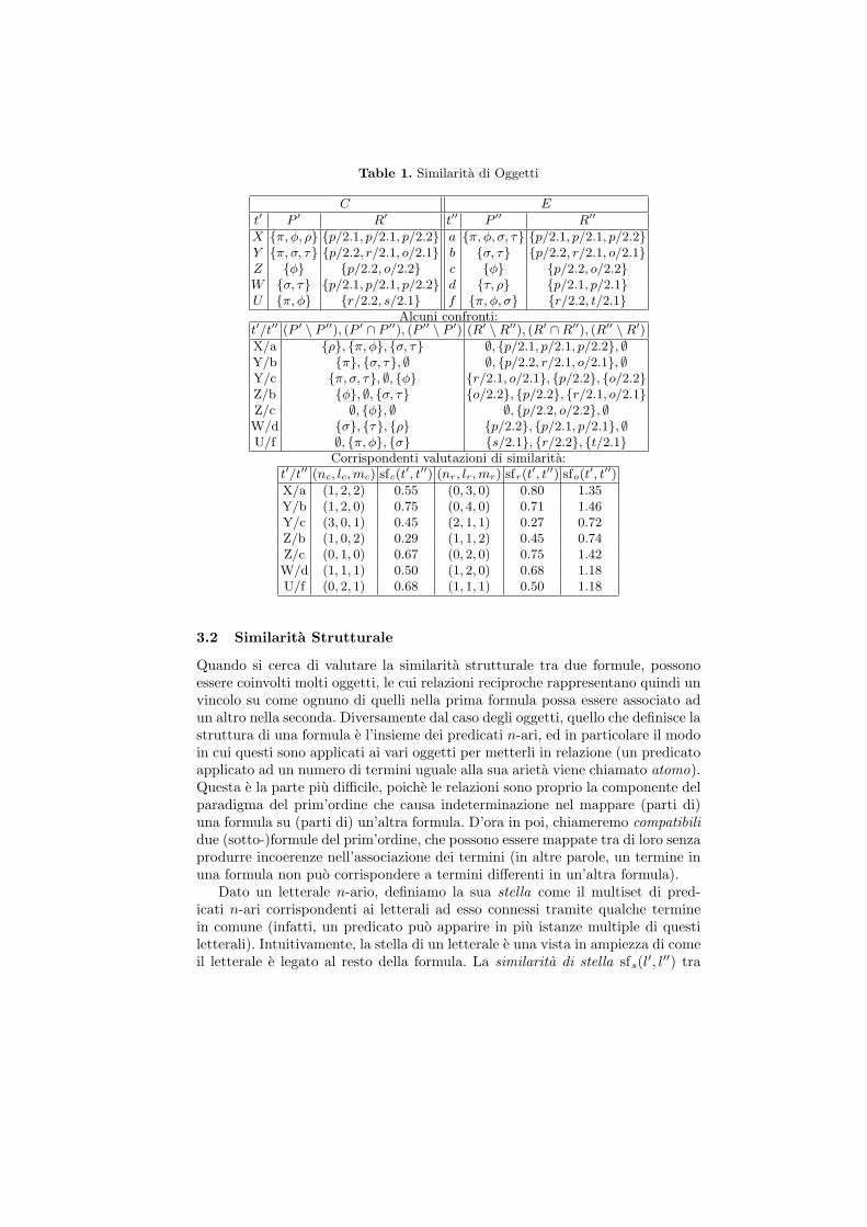
Table 1. Similarita di Oggetti

C E

t′ P ′ R′ t′′ P ′′ R′′

X π, φ, ρ p/2.1, p/2.1, p/2.2 a π, φ, σ, τ p/2.1, p/2.1, p/2.2Y π, σ, τ p/2.2, r/2.1, o/2.1 b σ, τ p/2.2, r/2.1, o/2.1Z φ p/2.2, o/2.2 c φ p/2.2, o/2.2W σ, τ p/2.1, p/2.1, p/2.2 d τ, ρ p/2.1, p/2.1U π, φ r/2.2, s/2.1 f π, φ, σ r/2.2, t/2.1

Alcuni confronti:t′/t′′ (P ′ \ P ′′), (P ′ ∩ P ′′), (P ′′ \ P ′) (R′ \R′′), (R′ ∩R′′), (R′′ \R′)X/a ρ, π, φ, σ, τ ∅, p/2.1, p/2.1, p/2.2, ∅Y/b π, σ, τ, ∅ ∅, p/2.2, r/2.1, o/2.1, ∅Y/c π, σ, τ, ∅, φ r/2.1, o/2.1, p/2.2, o/2.2Z/b φ, ∅, σ, τ o/2.2, p/2.2, r/2.1, o/2.1Z/c ∅, φ, ∅ ∅, p/2.2, o/2.2, ∅W/d σ, τ, ρ p/2.2, p/2.1, p/2.1, ∅U/f ∅, π, φ, σ s/2.1, r/2.2, t/2.1

Corrispondenti valutazioni di similarita:t′/t′′ (nc, lc, mc) sfc(t

′, t′′) (nr, lr, mr) sfr(t′, t′′) sfo(t

′, t′′)X/a (1, 2, 2) 0.55 (0, 3, 0) 0.80 1.35Y/b (1, 2, 0) 0.75 (0, 4, 0) 0.71 1.46Y/c (3, 0, 1) 0.45 (2, 1, 1) 0.27 0.72Z/b (1, 0, 2) 0.29 (1, 1, 2) 0.45 0.74Z/c (0, 1, 0) 0.67 (0, 2, 0) 0.75 1.42W/d (1, 1, 1) 0.50 (1, 2, 0) 0.68 1.18U/f (0, 2, 1) 0.68 (1, 1, 1) 0.50 1.18

3.2 Similarita Strutturale

Quando si cerca di valutare la similarita strutturale tra due formule, possonoessere coinvolti molti oggetti, le cui relazioni reciproche rappresentano quindi unvincolo su come ognuno di quelli nella prima formula possa essere associato adun altro nella seconda. Diversamente dal caso degli oggetti, quello che definisce lastruttura di una formula e l’insieme dei predicati n-ari, ed in particolare il modoin cui questi sono applicati ai vari oggetti per metterli in relazione (un predicatoapplicato ad un numero di termini uguale alla sua arieta viene chiamato atomo).Questa e la parte piu difficile, poiche le relazioni sono proprio la componente delparadigma del prim’ordine che causa indeterminazione nel mappare (parti di)una formula su (parti di) un’altra formula. D’ora in poi, chiameremo compatibilidue (sotto-)formule del prim’ordine, che possono essere mappate tra di loro senzaprodurre incoerenze nell’associazione dei termini (in altre parole, un termine inuna formula non puo corrispondere a termini differenti in un’altra formula).

Dato un letterale n-ario, definiamo la sua stella come il multiset di pred-icati n-ari corrispondenti ai letterali ad esso connessi tramite qualche terminein comune (infatti, un predicato puo apparire in piu istanze multiple di questiletterali). Intuitivamente, la stella di un letterale e una vista in ampiezza di comeil letterale e legato al resto della formula. La similarita di stella sfs(l′, l′′) tra

due letterali n-ari compatibili l′ e l′′ che hanno stelle S′ ed S′′, rispettivamente,puo essere calcolata come sf(ns, ls,ms) per i seguenti parametri:

ns = |S′ \ S′′| che esprime quante relazioni l′ ha in piu in C ′ rispetto a quelleche l′′ ha in C ′′ (residuo di stella di l′ rispetto a l′′)

ls = |S′ ∩ S′′| che e il numero delle relazioni che hanno in comune l′ in C ′ ed l′′

in C ′′;ms = |S′′ \ S′| che esprime quante relazioni l′′ ha in piu in C ′′ rispetto a quelle

che l′ ha in C ′ (residuo di stella di l′′ rispetto a l′).

Complessivamente, una valutazione piu adeguata della similarita tra l′ e l′′ puoessere ottenuta aggiungendo a questo risultato la similarita caratteristica e strut-turale per tutte le coppie dei loro argomenti in posizioni corrispondenti:

sfs(l′, l′′) = sf(ns, ls, ms) + Σt′/t′′∈θsfo(t′, t′′)

dove θ e l’insieme delle associazioni dei termini che mappanno l′ su l′′.Ogni formula del prim’ordine puo essere rappresentata come un grafo in cui

gli atomi sono i nodi e gli archi connettono due nodi se e solo se questi sonorelazionati in qualche modo. Ne consegue che un confronto tra due formule pervalutare la loro similarita strutturale corrisponde al calcolo di un omomorfismofra (sotto-)grafi, un problema noto essere NP -difficile in generale a causa dellapossibilita di mappare un (sotto-)grafo su un altro in molti modi differenti. Diconseguenza, si e interessati ad euristiche che possano dare suggerimenti signi-ficativi sulla sovrapposizione della struttura tra due formule con basso sforzocomputazionale. In realta, poggiando sul fatto che le clausole contengono ununico atomo nella testa ed una congiunzione di atomi nel corpo, si puo sfruttareuna rappresentazione a grafo piu semplice rispetto a quella per formule generali,come descritto nel seguito. In particolare, si tratteranno solo clausole connesse(cioe il cui grafo associato e connesso), e si costruira il grafo sulla base di unacaratteristica semplice (per quanto riguarda i dettagli che esprime circa una for-mula), ma al tempo stesso potente (per quanto riguarda l’informazione che essaconvoglia), che e la condivisione dei termini tra coppie di atomi.

Data una clausola C, definiamo il suo grafo associato come GC = (V, E) con

– V = l0 ∪ li|i ∈ 1, . . . , n, li costruito su predicati k-ari, k > 1 e– E ⊆ (a1, a2) ∈ V × V | terms(a1) ∩ terms(a2) 6= ∅

dove terms(a) denota l’insieme dei termini che appaiono come argomenti dell’a-tomo a. La strategia di selezione degli archi da rappresentare, schematizzatanell’Algoritmo 1, si basa sulla presenza di un unico atomo nella testa, che forniscesia un punto di partenza che precise direzioni per attraversare il grafo, al finedi scegliere, tra le tante possibili, una prospettiva unica e ben definita sullastruttura della clausola. Piu precisamente, costruiamo un grafo orientato aciclico,stratificato (cioe con l’insieme dei nodi partizionato) in modo tale che la testasia l’unico nodo al livello 0 (primo elemento della partizione) ed ogni livello(elemento della partizione) successivo sia composto da nuovi nodi (non ancora

Algorithm 1 Costruzione del grafo associato a CRequire: C = l0 : −l1, . . . , ln: Clause

i← 0; Level0 ← l0; E ← ∅; Atoms← l1, . . . , lnwhile Atoms 6= ∅ do

i← i + 1Leveli ← l ∈ Atoms | ∃l′ ∈ Leveli−1s.t.terms(l) ∩ terms(l′) 6= ∅E ← E ∪ (l′, l′′) | l′ ∈ Leveli−1, l

′′ ∈ Leveli, terms(l′) ∩ terms(l′′) 6= ∅Atoms← Atoms \ Leveli

end whilereturn G = (

Si Leveli, E): graph associated to C

h(X)

p(X,Y) p(X,Z) p(W,X)

r(Y,U) o(Y,Z) q(W,W)

s(U,V)

h(a)

p(a,b) p(a,c) p(d,a)

r(b,f) o(b,c) q(d,e)

t(f,g)

Fig. 1. Grafi associati alle clausole C (a sinistra) ed E (a destra)

raggiunti dagli archi) che hanno almeno un termine in comune con nodi dellivello precedente. In particolare, ogni nodo nel nuovo livello e connesso tramiteun arco entrante ad ogni nodo al livello precedente che ha tra i suoi argomentialmeno un termine in comune con esso.

Example 3. Costruiamo il grafo GC , riportato in Figura 1. La testa rappresentail livello 0 della stratificazione. Quindi, degli archi orientati possono essere in-trodotti da h(X) a p(X,Y ), p(X, Z) e p(W,X), che sono i soli atomi ad avereX come argomento, il che produce il livello 1 della stratificazione dei termini.Adesso, il prossimo livello puo essere costruito, aggiungendo archi orientati chevanno da atomi al livello 1 ad atomi non ancora considerati che condividono unavariabile con loro: r(Y, U) – fine di un arco che parte a p(X, Y ) –, o(Y,Z) – finedi archi che partono da p(X, Y ) e p(X, Z) – e q(W,W ) – fine di un arco che parteda p(W,X). Il terzo (e ultimo) livello del grafo include l’unico atomo rimasto,s(U, V ) – avente un arco entrante da r(Y, U).

Adesso, tutti i possibili cammini che partono dalla testa e raggiungono nodifoglia (quelli senza archi uscenti) possono essere interpretati come le componenti

base della struttura complessiva della clausola. Essendo questi cammini univo-camente determinati, si riduce la quantita di indeterminazione nel confronto.Intuitivamente, un cammino descrive in profondita una porzione delle relazionidescritte nella clausola.

Date due clausole, C ′ e C ′′, definiamo intersezione tra due cammini p′ =<l′1, . . . , l

′n′ > in GC′ e p′′ =< l′′1 , . . . , l′′n′′ > in GC′′ la coppia delle piu lunghe

sottosequenze inziali compatibili di p′ e p′′:p′ ∩ p′′ = (p1, p2) = (< l′1, . . . , l

′k >,< l′′1 , . . . , l′′k >) s.t.

∀i = 1, . . . , k : l′1, . . . , l′i compatibile con l′′1 , . . . , l′′i ∧

(k = n′ ∨ k = n′′ ∨ l′1, . . . , l′k+1 incompatibile con l′′1 , . . . , l′′k+1)

e i due residui come le parti incompatibili restanti.p′ \ p′′ =< l′k+1, . . . , l

′n′ >, p′′ \ p′ =< l′′k+1, . . . , l

′′n′′ >)

Quindi, la similarita di cammini tra p′ e p′′, sfs(p′, p′′), puo essere calcolataapplicando (1) ai seguenti parametri:

np = |p′ \ p′′| = n′ − k e la lunghezza della sequenza finale incompatibile di p′

rispetto a p′′ (residuo di cammino di p′ rispetto a p′′);lp = |p1| = |p2| = k e la lunghezza della massima sequenza iniziale compatibile

di p′ e p′′;mp = |p′′ \ p′| = n′′ − k e la lunghezza della sequenza finale incompatibile di p′′

rispetto a p′ (residuo di cammino di p′′ rispetto a p′).

piu la similarita di stella di tutte le coppie di letterali nelle sequenze iniziali:

sfp(p′, p′′) = sf(np, lp,mp) + Σi=1,...,ksfs(l′i, l′′i )

Example 4. Poiche la testa e unica (e quindi puo essere associata univocamente),in seguito tratteremo solo i letterali del corpo per mostrare i criteri strutturali.La Tabella 2 riporta i confronti delle stelle per un campione di letterali in C edE, mentre la Tabella 3 mostra alcuni confronti tra cammini.

Va notato che nessun criterio e di per se nettamente discriminante, ma la lorocooperazione riesce con successo a distribuire i valori di similarita e a rendere ledifferenze sempre piu chiare man mano che ciascuno viene composto con quelliprecedenti.

Una generalizzazione puo essere ora calcolata considerando le intersezioni deicammini in base alla similarita decrescente, e aggiungendo alla generalizzazioneparziale generata finora i letterali in comune per ogni coppia ogni volta chequesti sono compatibili (vedere l’Algoritmo 2). Ulteriori generalizzazioni pos-sono essere ottenute tramite backtracking. Questo permette anche, nel caso losi desideri, di tagliare la generalizzazione quando si raggiunge una certa sogliadi lunghezza, assicurando che solo le porzioni con similarita meno significativevengano rimosse.

Example 5. L’intersezione dei cammini con il piu alto valore di similarita eC.3/E.3, e quindi la prima generalizzazione parziale risulta p(X, Z), o(Y,Z),

Table 2. Similarita di stelle

C E

l′ S′ l′′ S′′

p(X, Y ) p/2, p/2, r/2, o/2 p(a, b) p/2, p/2, r/2, o/2p(X, Z) p/2, p/2, o/2 p(a, c) p/2, p/2, o/2r(Y, U) p/2, o/2, s/2 r(b, f) p/2, o/2, t/2

Alcuni confronti:l′ l′′ (S′ \ S′′), (S′ ∩ S′′), (S′′ \ S′)

p(X, Y ) p(a, b) ∅, p/2, p/2, r/2, o/2, ∅p(X, Y ) p(a, c) r/2, p/2, p/2, o/2, ∅p(X, Z) p(a, c) ∅, p/2, p/2, o/2, ∅p(X, Z) p(a, b) ∅, p/2, p/2, o/2, r/2r(Y, U) r(b, f) s/2, p/2, o/2, t/2

Corrispondenti valutazioni di similarita:l′ l′′ (ns, ls, ms) sf(ns, ls, ms) sfo sfs(l

′, l′′)p(X, Y ) p(a, b) (0, 4, 0) 0.71 sfo(X, a) = 1.35 sfo(Y, b) = 1.46 3.52p(X, Y ) p(a, c) (1, 3, 0) 0.73 sfo(X, a) = 1.35 sfo(Y, c) = 0.72 2.80p(X, Z) p(a, c) (0, 3, 0) 0.80 sfo(X, a) = 1.35 sfo(Z, c) = 1.42 3.57p(X, Z) p(a, b) (0, 3, 1) 0.73 sfo(X, a) = 1.35 sfo(Z, b) = 0.74 2.82r(Y, U) r(b, f) (1, 2, 1) 0.60 sfo(Y, b) = 1.46 sfo(U, f) = 1.18 3.24

con associazioni X/a, Y/b, Z/c. Subito dopo si considera C.2/E.2, le cui as-sociazioni sono compatibili con quelle attuali, cosicche esso contribuisce conp(X,Y ) alla generalizzazione (non ci sono nuove associazioni). Poi viene C.1/E.1,che essendo compatibile estende la generalizzazione aggiungendo r(Y, U) e leassociazioni con U/f. A questo punto tocca a C.1/E.2 e quindi a C.2/E.1, chesono compatibili ma ridondanti, e quindi non aggiungono niente alla generaliz-zazione attuale (ne alle associazioni). In seguito viene considerato C.4/E.4, chee compatibile ed estende la generalizzazione e le associazioni attuali, rispettiva-mente, con p(W,X) e W/d. Infine, vengono considerati C.3/E.2, C.2/E.3,C.3/E.1 e C.1/E.3, che pero vengono scartati perche le relative associazioni sonoincompatibili.

4 Lavori correlati

Molte misure di distanza sono state sviluppate per rappresentazioni attributo-valore, ma pochi lavori hanno affrontato la definizione di misure di similaritao di distanza per descrizioni del prim’ordine. In [4], viene proposta una misuradi distanza basata sulla teoria delle probabilita applicata alle componenti dellaformula. Rispetto a questa misura, la nostra funzione non richiede assunzioni oipotesi semplificative (come per esempio indipendenza statistica, mutua esclu-sione), il che facilita la gestione delle probabilita, ne alcuna conoscenza a prioridel linguaggio di rappresentazione (come per esempio i tipi del dominio). Inoltre,il nostro approccio non necessita che l’utente imposti dei pesi sull’importanzadei predicati e non e basato sulla presenza di relazioni obbligatorie, come per lasottoclausola G1 in [4].

Table 3. Similarita di cammini

Path No. C E

1. < p(X, Y ), r(Y, U), s(U, V ) > < p(a, b), r(b, f), t(f, g) >2. < p(X, Y ), o(Y, Z) > < p(a, b), o(b, c) >3. < p(X, Z), o(Y, Z) > < p(a, c), o(b, c) >4. < p(W, X), q(W, W ) > < p(d, a), q(d, e) >

p′ p′ ∩ p′′ p′ \ p′′ θp′∩p′′ (n, l, m)p

p′′ p′′ \ p′ sfp(p′, p′′)

C.1 < p(X, Y ), r(Y, U) > < s(U, V ) > X/a, Y/b, U/f (1, 2, 1)E.1 < p(a, b), r(b, f) > < t(f, g) > 7.36

C.1 < p(X, Y ) > < r(Y, U), s(U, V ) > X/a, Y/b (2, 1, 1)E.2 < p(a, b) > < o(b, c) > 3.97

C.2 < p(X, Y ) > < o(Y, Z) > X/a, Y/b (1, 1, 2)E.1 < p(a, b) > < r(b, f), t(f, g) > 3.97

C.2 < p(X, Y ), o(Y, Z) > <> X/a, Y/b, Z/c (0, 2, 0)E.2 < p(a, b), o(b, c) > <> 7.95

Algorithm 2 Generalizzazione basata sulla similaritaRequire: C: Rule; E: Example

PC ← paths(C); PE ← paths(E);P ← (pC , pE) ∈ PC × PE |pC ∩ pE 6= (<>, <>);G← ∅; θ ← ∅while P 6= ∅ do

(pC , pE)← argmax(pC ,pE)∈P (sf(pC , pE))P ← P \ (pC , pE)(qC , qE)← pC ∩ pE

θq ← substitution s.t. qC = qE

if θq compatible with θ thenG← G ∪ qC ; θ ← θ ∪ θq

end ifend whilereturn G: generalization between C and E

Molti sistemi di apprendimento supervisionato dimostrano l’importanza diuna misura di similarita. Per esempio, KGB [1] usa una funzione di similarita,parametrizzata dall’utente, per guidare la generalizzazione; le nostre idee di sim-ilarita caratteristica e relazionale sono molto simili a questa, ma il calcolo dellasimilarita e piu immediato. Mentre KGB non puo gestire informazione negativanelle clausole, il nostro approccio puo essere facilmente esteso a questo scopo.Il classificatore k-Nearest Neighbor RIBL [2] e basato su una versione modifi-cata della funzione proposta in [1]. L’idea di base e che la similarita di oggettidipende dalla similarita dei valori dei loro attributi (la similarita della loro di-mensione), e, ricorsivamente, dalla similarita degli oggetti a questi connessi. Talepropagazione pone il problema della indeterminazione (incertezza) nelle associ-azioni, che il nostro approccio evita grazie al diverso approccio strutturale.

[9] presenta un approccio per l’induzione di distanze su esempi in logica delprim’ordine, che dipende dal pattern che discrimina i concetti-obiettivo. Si se-lezionano k clausole e i valori di verita che esprimono se la clausola copre o menol’esempio sono utilizzati come k componenti di una distanza tra gli esempi nellospazio 0, 1k. [6] organizza i termini in una gerarchia in base all’importanza epropone una distanza tra termini basata su interpretazioni ed una funzione chemappa ogni espressione semplice in un numero naturale. [7] presenta una fun-zione di distanza tra atomi basata sulla differenza rispetto alla loro lgg e usa lafunzione per calcolare distanze tra clausole. La funzione consiste in una coppia:la prima componente estende la distanza in [6] ed e basata sulle differenze tra ifuntori nei due termini, mentre la seconda componente e basata sulle differenzenelle occorrenze delle variabili e permette di differenziare casi che la prima com-ponente non puo discriminare.

5 Sperimentazioni

All scopo di verificare se i criteri proposti siano in grado di produrre indizisignificativi sulla similarita tra due strutture, la procedura di generalizzazioneguidata dalla similarita e stata confrontata con una versione precedente (nonguidata) utilizzata nel sistema INTHELEX [3]. Il sistema e stato impostato inmaniera tale che, quando la prima generalizzazione prodotta dalla proceduraguidata non era coerente con tutti gli esempi negativi, il sistema poteva cer-care generalizzazioni piu specifiche in backtracking1. Per valutare l’accuratezzapredittiva e stata usata la 10-fold cross-validation.

Un primo confronto ha riguardato il classico dataset ILP della Mutagenesi,sul quale il sistema ha raggiunto un’accuratezza predittiva leggermente migliore(87%) rispetto alla versione non guidata (86%) sfruttando solo il 30% del tempodi esecuzione (4035 secondi anzich 13720). E’ importante notare che la primageneralizzazione trovata era sempre corretta, e quindi non e stato mai necessariofare backtracking per cercare altre alternative, mentre la versione non guidataha dovuto calcolare 5815 ulteriori generalizzazioni per gestire quei casi in cui laprima generalizzazione trovata era incoerente con gli esempi pregressi. Questoconferma che la misura di similarita e in grado di guidare la corretta identifi-cazione delle sotto-parti corrispondenti nelle descrizioni chimiche.

Altre sperimentazioni sono state condotte su un dataset2 contenente de-scrizioni del layout della prima pagina di 122 articoli scientifici appartenentia 4 classi diverse. Da questi sono stati ricavati 488 esempi posititi/negativi perapprendere regole di classificazione dei documenti, e 1488 esempi per appren-dere regole che identificano 12 tipi di (etichette per le) componenti logiche dei

1 Per evitare che il sistema impiegasse troppo tempo in generalizzazioni difficili, e statoimpostato in maniera da abbandonare la generalizzazione attuale e cercare di gener-alizzare un’altra clausola (se presente) non appena venivano trovate in backtracking500 (sotto-)generalizzazioni ridondanti oppure ne venivano calcolate 50 nuove maincoerenti

2 http://lacam.di.uniba.it:8000/systems/inthelex/index.htm#datasets

Table 4. Risultati sperimentali

Ratio Time (sec.) Cl Gen Exc+ Spec+ Spec− Exc− Acc

ClassificazioneSF 90.52 579 8 47(+0) 0 2 0 0 0.94I 70.22 137 7 33(+100) 0 1 1 1 0.97

S80 73.63 206 7 33(+13) 0 0 1 1 0.97

EtichettaturaSF 91.09 22220 36 180(+0) 0 8 3 3 0.89I 68.85 33060 39 137(+5808) 0 15 11 12 0.93

S80 71.75 15941 54 172(+220) 0 14 8 2 0.93

documenti (per esempio, titolo, autore, abstract etc). I risultati sono riportatinella Tabella 4.

La prima questione e se la funzione di similarita proposta fosse in grado diguidare la procedura di ricerca verso l’identificazione delle sotto-parti appro-priate da mettere in corrispondenza nelle due descrizioni che si stavano con-frontando. Poiche l’associazione corretta non e nota, questo puo essere valutatosolo indirettamente. Un modo per far cio e valutare il fattore di compressionedella generalizzazione guidata, ossia la porzione di letterali nelle clausole dageneralizzare che e preservata dalla generalizzazione. Infatti, poiche ogni gener-alizzazione in INTHELEX deve essere un sottoinsieme di ciascuna delle clausoleda generalizzare (a causa della assunzione di Object Identity), piu letterali ven-gono preservati da queste clausole dalla generalizzazione, meno generale sarala generalizzazione. Piu formalmente, valutiamo la compressione come il rap-porto tra la lunghezza della generalizzazione e quella della clausola piu corta dageneralizzare: piu grande e questo valore, piu sicuri si puo essere che le associ-azioni corrette siano state trovate grazie ai criteri e alla formula di similarita.Ovviamente, piu grande e la differenza in lunghezza tra due clausole da gener-alizzare, piu grande sara l’incertezza presente, e quindi piu difficile sara identi-ficare appropriatamente le parti corrispondenti tra loro. E interessante notareche sul dataset dei documenti la generalizzazione guidata dalla similarita (SF)ha preservato in media piu del 90% dei letterali della clausola piu corta, conun massimo di 99,48% (193 letterali su 194, contro un esempio da 247) e solo0,006 di varianza. Di conseguenza, ci si puo aspettare che le generalizzazioniprodotte siano effettivamente le meno generali (o le approssimino molto). Perverificarlo, invece di calcolare la vera generalizzazione meno generale per ognigeneralizzazione effettuata e confrontarla con quella prodotta dalla proceduraguidata, il che sarebbe stato computazionalmente pesante e avrebbe richiesto dimodificare il comportamento del sistema, si e calcolato quanti backtracking ilsistema doveva calcolare per raggiungerne una piu specifica. Il risultato e statoche, entro il limite dato, non e stata trovata nessuna altra generalizzazione, il chesuggerisce che la prima generalizzazione trovata e probabilmente molto vicina a(ed in effetti molto spesso e) la generalizzazione meno generale. Da notare cheapplicando della formula di similarita di Tverski [10] (che rappresenta lo statodell’arte nell’attuale letteratura) allo stesso problema, si sono ottenute sempregeneralizzazioni piu corte di quelle ottenute utilizzando la nostra formula.

Comunque, essendo tali generalizzazioni molto specifiche, la loro accuratezzapredittiva risulta piu bassa di quelle ottenute dall’algoritmo INTHELEX nonguidato (I), il che probabilmente e dovuto alla necessita di un maggior numero diesempi per convergere a definizioni predittive oppure all’overfitting. Per questomotivo, la procedura di generalizzazione guidata dalla similarita e stata im-postata per scartare almeno il 20% dei letterali della piu corta clausola originale(S80): questo ha portato alla stessa accuratezza predittiva di I, ed ha ridottodrasticamente il tempo di esecuzione rispetto alla versione senza vincoli (ed an-che rispetto ad I nel caso del compito di etichettatura). Anche il numero dellegeneralizzazioni decresce, sebbene al costo di uno sforzo maggiore di special-izzazione (anche per mezzo di letterali negativi che sono gestiti come spiegatonella sezione precedente), che e in ogni caso piu efficace rispetto a I (in parti-colare per quanto riguarda le eccezioni negative). Nel compito di classificazioneil numero delle clausole decresce leggermente, mentre in quello di etichettaturail numero cresce di 15, ma viene equilibrato da 10 eccezioni negative in meno.E importante notare che le generalizzazioni trovate sono ancora molto aderentiagli esempi, come suggerisce il fatto che nelle sperimentazioni di classificazionesono state trovate in backtracking (e testate per verificarne la correttezza) solo13 generalizzazioni piu specifiche (delle quali solo 1 corretta), mentre I ne hatrovate 100, di cui 6 corrette. Nel task di etichettatura, S80 ha trovato 220 ulteri-ori generalizzazioni candidate (di cui 6 corrette) contro 5808 (di cui 39 corrette)di I. Questo dimostra che si potrebbe anche evitare il backtracking con pocaperdita in S80, ma non in I.

Un altro importante parametro per valutare l’utilita della funzione proposta edella relativa strategia e il tempo di esecuzione. La Tabella 4 mostra che, nel taskdi etichettatura, utilizzando la funzione di similarita si raggiunge un risparmioche va da 1/3 fino a 1/2 del tempo totale, dell’ordine di ore. Le prestazioni neltask di classificazione sono in ogni caso confrontabili (differenze dell’ordine didecimi di secondo) il che si puo probabilmente spiegare col fatto che tale task emolto piu facile, per cui resta poco spazio per miglioramenti e il tempo necessarioper cacolare la formula annulla il risparmio.

6 Conclusioni

Le relazioni, in Logica del Prim’Ordine, portano ad indeterminazione nel map-pare porzioni di una descrizione su un’altra descrizione. In questo articolo si sonoidentificati un insieme di criteri ed una formula per il confronto tra clausole, esono stati utilizzati per guidare una procedura di generalizzazione indicando lesottoparti delle descrizioni che piu verosimilmente corrispondo l’una all’altra,basandosi solo sulla loro struttura sintattica.

Stando ai risultati sperimentali, la generalizzazione basata sulla similaritae in grado di catturare le associazioni corrette e puo produrre la stessa accu-ratezza predittiva della versione non guidata, ma producendo teorie piu ‘pulite’e riducendo drammaticamente la quantita di tempo necessario per convergere (ilrisparmio di tempo cresce al crescere della complessita del problema).

Come lavoro futuro si potrebbe raffinare la metodologia di calcolo della sim-ilarita. Inoltre, la nuova misura di similarita potrebbe essere messa alla provacon altre applicazioni, quali il matching flessibile, il clustering concettuale oppurel’instance-based learning.

References

[1] G. Bisson. Learning in FOL with a similarity measure. In W.R. Swartout, editor,Proc. of AAAI-92, pages 82–87, 1992.

[2] W. Emde and D. Wettschereck. Relational instance based learning. In L. Saitta,editor, Proc. of ICML-96, pages 122–130, 1996.

[3] F. Esposito, S. Ferilli, N. Fanizzi, T. Basile, and N. Di Mauro. Incremental multi-strategy learning for document processing. Applied Artificial Intelligence Journal,17(8/9):859–883, 2003.

[4] F. Esposito, D. Malerba, and G. Semeraro. Classification in noisy environmentsusing a distance measure between structural symbolic descriptions. IEEE Trans-actions on PAMI, 14(3):390–402, 1992.

[5] Dekang Lin. An information-theoretic definition of similarity. In Proc. 15th In-ternational Conf. on Machine Learning, pages 296–304. Morgan Kaufmann, SanFrancisco, CA, 1998.

[6] S. Nienhuys-Cheng. Distances and limits on herbrand interpretations. In D. Page,editor, Proc. of ILP-98, volume 1446 of LNAI, pages 250–260. Springer, 1998.

[7] J. Ramon. Clustering and instance based learning in first order logic. PhD thesis,Dept. of Computer Science, K.U.Leuven, Belgium, 2002.

[8] C. Rouveirol. Extensions of inversion of resolution applied to theory completion.In Inductive Logic Programming, pages 64–90. Academic Press, 1992.

[9] M. Sebag. Distance induction in first order logic. In N. Lavrac and S. Dzeroski,editors, Proc. of ILP-97, volume 1297 of LNAI, pages 264–272. Springer, 1997.

[10] A. Tversky. Features of similarity. Psychological Review, 84(4):327–352, 1977.

Constraint-based simulation of biological systemsdescribed by Molecular Interaction Maps

Luca Bortolussi1, Simone Fonda4, and Alberto Policriti2,3

1 Dept. of Mathematics and Computer Science, University of Trieste, Italy.2 Dept. of Mathematics and Computer Science, University of Udine, Italy

3 Istituto di Genomica Applicata, Udine, Italy4 Dept. of Computer Science, University of Pisa, Italy.

Abstract. We present an application of stochastic Concurrent Con-straint Programming, defining an encoding of biochemical networks de-scribed by the graphical notation of Molecular Interaction Maps. Suchmaps are compact, as they represent implicitly a wide set of reactions,and therefore not easy to simulate with standard tools. With our encod-ing, we are able to stochastically simulate these maps implicitly, withoutgenerating the full list of reactions.

1 Introduction

The aim of this work is the simulation of biological regulatory networks describedby the graphical notation of Molecular Interaction Maps (MIM) [19]. In order toachieve this goal, we define an encoding of such maps in stochastic ConcurrentConstraint Programming (sCCP) [2], a stochastic, concurrent, and constraint-based programming language.

In scientific literature, many mathematical tools have been proposed to de-scribe, model, and simulate the behaviors of biological systems, all sharing thecommon goal of organizing and analyzing the available knowledge and under-standing of such systems [7, 14, 15]. As happens with computer programminglanguages, one formalism could be better suited than another for a specificpurpose, depending on the features it provides to its users. When choosing aformalism many parameters must be taken into account: continuous or discreterepresentation of the entities, expressivity, availability of mathematical analysistechniques, possibility of a computer aided simulation and visualization, and soon. Other important properties of a modeling language concern the process ofwriting and maintaining a model: compositional languages are usually prefer-able for systems composed of many interacting parts, like biological ones [23].Formalisms can also differ in the size of produced models; generally, the morecompact the better. Moreover, the same system can be modeled at different lev-els of detail; for example, a cell can be described as a functional black box orspecifying its internal behaviors and mechanisms in detail.

As the focus of modeling in biology is to understand dynamical properties of bi-ological systems, most of the modeling languages have a semantic based on ordi-nary differential equations [29] or stochastic processes [30]. Stochastic processes,usually continuous-time Markov Chains [21], have been used in biochemistryand biology since a long time, especially after the publishing of a simple andefficient simulation algorithm by Gillespie [11, 12]. These models are generallymore realistic than the ones based on Ordinary Differential Equations (ODEs),as they represent molecules as discrete quantities (compared to the continuousapproximation of ODEs) and, moreover, they have a noisy evolution (comparedto the determinism of ODEs), an important issue in biology [20, 30].

Generally, both stochastic and differential models can be obtained in a canon-ical way when the list of reactions of the system is fully specified [8, 30] (i.e., weneed to specify all the possible ways of reacting of all the possible reactants).A big problem with this approach is the cost of the notation: in some cases,the effort required for a complete specification can be overwhelming; this is trueespecially for bio-regulatory networks, due to the central role played by multi-molecular complexes and protein modifications [16, 17, 19, 9, 1]. In fact, even asmall set of proteins can potentially generate a big number of different com-plexes, of which only a few different kinds may be present at a certain time.Manually listing all these complexes can be a very hard task.

In order to tackle this problem, we need a formalism that can work at anhigher level of abstraction, representing entities and behaviors in an implicitway. One possibility is offered by the Molecular Interaction Maps [17, 19]: theyare a compact graphical notation proposed by Kohn, with the goal to be clear,easy to use, compact, unambiguous, and (hopefully) widespread. In the author’sexpectations, the equivalent of electronic circuit diagrams for biologists.

The contribution of this work is the definition of an encoding of MIM insCCP, a stochastic extension of Concurrent Constraint Programming [2], alreadyused to model biological systems at different degrees of complexity [4, 3]. Thecrucial ingredient of such an encoding will be the implicit representation ofcomplexes and reactions. Essentially, molecular complexes will be representedby graphs, modified locally by reactions. The idea of this approach originatesfrom the work of Danos and Laneve [6] and from the attempt of encoding theirκ-calculus in sCCP [3]. Before presenting the encoding we discuss MolecularInteraction Maps in more detail (Section 2) and address some issues related totheir semantic (Section 3). Then, after briefly recalling sCCP (Section 4), wepresent the main ideas of the implicit simulation of MIMs in sCCP (Section 5).This is the core of the paper where we try to maintain in the encoding—and,consequently, in the implementation—the feature characterizing MIMs (namelytheir implicitness) providing, at the same time, a stochastic based engine fortheir simulation. Preliminary experimental results on applicatin of our technique(Section 6) and a comparison of our approach with some related work (Section 7)are then presented. Finally, conclusions and future directions of work can befound in Section 8.

2 Molecular Interaction Maps

(a) (b)

Fig. 1. Two very simple MIMs

We briefly introduce the MIM notation; the interested reader is referredto [19] for a detailed presentation. A MIM is essentially a graph, where nodescorrespond to different (basic) molecular species, linked by different kinds ofconnecting lines, see Figure 1 for an example. The notation follows few generalprinciples: to keep the diagram compact an elementary molecular species, likeA, B or C in Figure 1(a), generally occur in only one place on a map. Differentinteractions between molecular species, instead, are distinguished by differentlines and arrowheads; for instance, the double line in Figure 1(a) represents acovalent modification of B (in this case a phosphorylation, i.e. the attachmentof a phosphate group at a specific place in the protein), while the single double-barbed arrows denote complexation operations. Complex molecular species, orsimply complexes, are created as a consequence of interactions and are indicatedby small circles on the corresponding interaction line; e.g. in Figure 1(a) x rep-resents the complex A : B, the result of a complexation between A and B, whiley represents the phosphorylated B molecule (denoted hereafter with pB).

In general, there are two types of interaction lines: reactions and contingen-cies. The former operate on molecular species, the latter on reactions or othercontingencies. The red line with a T-shaped end of Figure 1(b) is an inhibitionline; it states that phosphorylated B (indicated by y) cannot bind to C, (infact the line terminates on the barbed arrow connecting B and C). Anothercontingency symbol of Figure 1(b) is the arrow with a bar preceding its emptyarrowhead, terminating in x. This line represents a requirement : B must be phos-phorylated in order to bind to A. Note that multiple nodes on an interactionline represent exactly the same molecular species. In Figure 2 we list a subset ofarrows, taken from [19].

In order to fully explain the differences between Figure 1(a) and Figure 1(b),we need to introduce the interpretations of MIMs. The MIM notation, in fact,can be equipped with two different interpretations: explicit and combinatorial.In the explicit interpretation, an interaction line applies only to the molecularspecies directly connected to it. Looking again at Figure 1(a), we can say that

Fig. 2. A restricted list of reaction and contingency arrows of MIMs.

B can bind to A (forming the complex A : B) or to C (forming the complexB : C) but there is no way the complex A : B : C will be formed. Moreover, ifB is phosphorylated it cannot bind neither to A nor to C.In the combinatorial interpretation, an interaction line represents a functionalconnection between domains or sites that (unless otherwise indicated) is inde-pendent of the modifications or bindings of the directly interacting species. Inthis way the map of Figure 1(a) states that A can bind to B, independently ofthe state of B. For instance, B could be phosphorylated and thus forming theA : pB complex, or it could be bound to C, resulting in the A : B : C complex.The first interpretation needs every interaction to be explicitly defined, in a“what is depicted is what happens” fashion, and this requires the use of manyreaction lines. On the other hand, the combinatorial interpretation takes theopposite point of view, i.e. “what is not explicitly forbidden does happen”. Inthis case the behavior can be specialized by means of contingency lines.5

In Table 1 we summarize the differences between the two interpretations.While the two interpretations of the map of Figure 1(a) are different, the mapof Figure 1(b) has exactly the same behavior under both interpretation, thanksto the use of inhibition and requirement symbols. Moreover, the combinatorialinterpretation represents implicitly a large number of molecules: a single com-plexation arrow usually handles, on both sides, a big set of reactants. Consider,for example, the arrow connecting A to B in Figure 1(a); in the combinatorialinterpretation it represents four reactions, namely the complexation of A withB, pB, B : C and pB : C.

In principle, it is always possible to create an explicit MIM with the samebehaviors of a combinatorial MIM, introducing more reaction arrows and con-

5 There is also a third layer of interpretation, called heuristic in [18], used mainly tostructure and organize available knowledge of biological systems. In this interpreta-tion, all interactions possible in the combinatorial case and forbidden in the explicitone are left unspecified, thus representing incomplete knowledge.

ComplexesFigure 1(a) Figure 1(b)Expl. Comb. Expl. Comb.

A:B X XB:C X X X XA:pB X X XpB:C XA:B:C XA:pB:C X

Table 1. Different interpretations of MIMs of Figure 1

tingencies. Explicit MIMs can be easily translated into a set of ODEs or intoan explicit stochastic model for computer simulation, see [16]. Unfortunately,expliciting a combinatorial MIM is a non-trivial job, due to the combinatorialexplosion of reaction arrows and contingencies needed in the map. In addition,an explicit ODE-based (or stochastic) simulation, like the one described in [16],requires to consider all possible molecular complexes that can be generated inthe system as reactants or products of some reaction. However, at a given time,usually only a small subset of these complexes is present, hence the effort neededto generate explicitly this large number of complexes is largely unmotivated.

Our goal is precisely to define a simulation operating directly at the level ofthe combinatorial interpretation of MIMs, hence this is the interpretation we willconsider in the rest of the paper. The advantages of this choice are clear: duringeach stage of a simulation, we need to represent only the complexes present inthe system at that time. Moreover, models can be defined using the compactnotation of combinatorial MIMs, hence the resulting map is usually smaller,thereby easier to build and understand.

3 Removing ambiguity from MIMs

The biggest obstacle towards the definition of an implicit simulation is, unfortu-nately, in the MIM notation itself. In fact, the combinatorial interpretation is farfrom being a rigorous semantic: combinatorial MIMs are intrinsically ambiguous,as there are many cases in which the exact behavior of the map is not defined.Moreover, some arrows in the MIM notation are just “syntactic sugar”, as theirbehavior can be defined in terms of other arrows. To tackle these problems, wehave defined a set of graph rewriting rules, disambiguating some cases in whatwe deem a biologically plausible way and removing redundant arrows. This canbe seen as the first step towards the definition of a formal semantic for MIMs.We discuss some examples in the following.

The MIM of Figure 3(a) represents a situation in which A can bind to B,forming a complex (A : B) that can bind to C. Writing this in the standard, self-explanatory, chemical notation, we obtain A + B → A : B and (A : B) + C →A : B : C. Biologically, every complex formed this way can, in principle, be

(a) Removing de-complexation ambiguity (b) Removing stimulation arrow

Fig. 3. An example of graph rewriting rules for MIMS

de-complexed, meaning that the map of Figure 3(a) describes also the inversereactions A : B : C → (A : B) + C and A : B → A + B. It is not clear, however,if the link between A and B in A : B : C could be broken or not. We assumethat this is not possible, because the map states that C can bind only to A : Band not to A nor B alone, thus it plausibly describes a biological mechanismin which C binds to a modified structure containing A and B, a structure thatcannot disappear while bound to C.6

In order to make this choice explicit, we add an inhibition symbol from the noderepresenting the A : B : C complex to the A : B complexation arrow, thuspreventing de-complexation of A : B when C is bound. This is an example of avery simple graph rewriting rule in order to eliminate ambiguity.

Figure 3(b) left, shows a MIM where the A : B complex stimulates the B : Cbond (stimulation is represented with an arrow with empty arrowhead). Theintended meaning of stimulation is that B is more likely to bind to C when itis complexed with A. We can see this mechanism in an alternative way, usingtwo complexation arrows between B and C, one representing the slower reactionand the other one representing the faster reaction. These arrows need to bemutually exclusive, see Figure 3(b) right. This second rewriting rule reduces thenumber of symbols of maps, simplifying the encoding in sCCP. Therefore, thetwo examples given are representative of two classes of rewriting rules: the firsttackling ambiguity, the second simplifying the notation.

4 Stochastic Concurrent Constraint Programming

Concurrent Constraint Programming (CCP [27]) is a process algebra havingtwo distinct entities: agents and constraints. Constraints are interpreted first-order logical formulae, stating relationships among variables (e.g. X = 10 orX + Y < 7). Agents in CCP, instead, have the capability of adding constraints(tell) into a “container” (the constraint store) and checking if certain relations

6 Note that different behaviors can be obtained changing the topology of the map. Forinstance, if C binds only to A instead of binding to A : B, the complex A : B : Ccan be broken also in (A : C) + B.

Program = D.A

D = ε | D.D | p(x) : −A

A = 0 | tell∞(c).A | M | local x.A | A ‖ AM = π.G | M + M

π = tellλ(c) | askλ(c)G = 0 | tell∞(c).G | p(y) | M | local x.G | G ‖ G

Table 2. Syntax of of sCCP.

are entailed by the current configuration of the constraint store (ask). The com-munication mechanism among agents is therefore asynchronous, as informationis exchanged through global variables. In addition to ask and tell, the languagehas all the basic constructs of process algebras: non-deterministic choice, paral-lel composition, procedure call, plus the declaration of local variables. Moreover,constraints of the store can be defined using the computational machinery ofProlog [28, 27].

The stochastic version of CCP (sCCP [2, 4]) is obtained by adding a stochasticduration to all instructions interacting with the constraint store C, i.e. ask, tell.Each instruction has an associated random variable, exponentially distributedwith rate given by a function associating a real number to each configurationof the constraint store: λ : C → R+. Its syntax is defined by the grammar ofTable 2.

The underlying semantic model of the language (defined via structural oper-ational semantic, cf. [2]) is a Continuous Time Markov Chain [21] (CTMC), i.e.a stochastic process whose temporal evolution is a sequence of discrete jumpsamong states in continuous time. States of the CTMC correspond to configu-rations of the sCCP-system, consisting in the current set of processes and inthe current configuration of the constraint store. The next state is determinedby a race condition between all active instructions such that the fastest one isexecuted, like in stochastic π-calculus [22] or PEPA [13]. More details on sCCPand on its operational semantics can be found in [3].

Time-varying quantities, an important ingredient to deal with biological sys-tems [4], are modeled as stream variables, i.e. growing lists with an unboundedtail.

In [3, 4] we argued that sCCP can be conveniently used for modeling a widerange of biological systems, like biochemical reactions, genetic regulatory net-works, the formation of protein complexes, and the process of folding of a protein.In fact, while maintaining the compositionality of process algebras, the presenceof a customizable constraint store and of variable rates gives a great flexibilityto the modeler.

5 Encoding MIMs in sCCP

In this section we present the basic ideas for the direct simulation of MIM insCCP. The starting point is the definition of a suitable representation of mole-cules and complexes. Actually, with respect to other process algebras like π-calculus [22], sCCP offers a crucial ingredient in this direction, namely the pres-ence of the constraint store. In fact, the store is customizable and every kindof information can be represented by the use of suitable constraints, i.e. logicalpredicates. Manipulating and reasoning on such information can be performedin a logic programming style [27]. These ingredients make the constraint store anextremely flexible tool that can be naturally used to represent the data structuresneeded to operate on MIMs.

The idea to simulate MIMs is simple: we operate directly on the graphicalrepresentation. Of course, a MIM contains all possible interactions of the system,hence the graphical representation used in the simulation must be specialized tosingle molecules and complexes. Complexes, in particular, can be seen as graphs,with nodes representing the basic molecules (i.e. the proteins) of the complex,and with edges representing the chemical bonds tying them together. Such graphswill be referred in the following as complex-graphs.

Recalling Figure 1 and the combinatorial interpretation of Section 2, we caneasily convince ourselves that molecular species are defined by the collectionof their interaction sites. In our encoding, these sites are represented by ports,having the following properties:

– each port (or better, port-type) is the terminating point of one single arrowin the MIM7;

– each port-type is characterized by an unique identifier, called port type id,and by a boolean variable, INHp, storing the state of the port. In fact,each port can be active (INHp = false), meaning that it can take partto the corresponding reaction, or inhibited (INHp = true) by biologicalmechanisms specified in the map;

Molecular-types correspond to nodes of the MIM or to points in the middleof an arrow (i.e., terminating points of reaction arrows). They consist of anunique identifier, molecular type id, of a list of port-types, implicitly determiningall the possible reactions the molecule can be involved into, and of a list ofcontingencies starting from it (we present the treatment of contingencies at theend of the section). For instance, in Figure 1(a), A and x nodes define twodistinct molecular-types.

Each graph of a complex can contain, in principle, several instances of thesame molecular-type, just think of the case in which two copies of the samemolecule are bound together (the so-called homodimers). In order to distinguishamong these different copies, we introduce an unambiguous naming system insideeach complex, enumerating each node of a complex-graph with an integer, local7 This condition can always be made true by the application of suitable rewriting rules

to the map.

molecular type(molecular type id,port list,contingency list)node(molecular type id, mol id)

edge([mol id1, port type id1],[mol id2, port type id2])complex type(complex type id, node list,edge list, contingency list)

complex number(complex type id, X)port number(port type id, X)

Table 3. Predicates describing MIM structures and counting their occurrences.

to that complex, called mol id. Moreover, each different complex graph that canbe constructed according to the prescription of the MIM, identifies a complex-type; complex-types are also given an unique id, complex type id, assigned atrun-time whenever a new complex-type is created.

Complex-graphs and molecular-types can be easily represented in sCCP. Infact, we just need to store all the characterizing information in suitable logi-cal predicates, listed at the beginning of Table 3. Note that each molecule in acomplex-type is unambiguously identified by the pair (complex type id,mol id).8

Such pairs are called coordinates of the molecule.Another important class of predicates, crucial for the run-time engine, are thosecounting the number of objects of a certain type. Specifically, at run-time we needto count how many complexes we have for each different complex-type (predi-cate complex number), and how many active ports we have, for any port-type(predicate port number). The variable X used in these predicates is a streamvariable, defined in Section 4.

The reason for updating the number of ports or complexes at run-time, liesin the definition of the stochastic model for the simulation of MIMs. We adopta classical approach, defining the speed of a reaction according to the principleof mass action [12]: the speed of each reaction is proportional to the quantityof each reactant. In our encoding, each reaction involves one or two port-types,hence its speed will be proportional to the number of active instances of suchport-types.

The simulation algorithm of such stochastic model is based on the celebratedGillespie algorithm [11, 12], extended in order to manage all the additional infor-mation of graphs and complexes. Essentially, we can see it as a loop composedof 4 basic steps:

1. choose the next reaction to execute;2. choose the reactants;3. create the products;8 molecular type id can be recovered from mol id and the predicate

node(molecular type id, mol id).

complexation(port id1,port id2, rate) :-local complex id1,complex id2,mol id1,mol id2,nodes,

edges,contingencies,new complex id.ask[rate·#port id1·#port id2](

are greater than zero(port id1,port id2)∧ are reactions unlocked).

tell∞(lock reactions).tell∞(activate port manager(port id1)).askF (is port manager done(port id1)).tell∞(activate port manager(port id2)).askF (is port manager done(port id2)).tell∞(get chosen complex(port id1,complex id1,mol id1)).tell∞(get chosen complex(port id2,complex id2,mol id2)).tell∞(build complex(complex id1,mol id1,complex id2,

mol id2,nodes,edges,contingencies)).tell∞(add complex(nodes,edges,contingencies,

new complex id)).tell∞(update numbers(complex id1,complex id2,

new complex id,port id1,port id2)).tell∞(apply contingencies(new complex id)).tell∞(unlock reactions).complexation(port id1,port id2, rate)

port manager(port id) :-local complex id,mol id.askF (is port manager active(port id)).tell∞(choose complex(port id,complex id,mol id)).tell∞(complex chosen(port id,complex id,mol id)).tell∞(port manager done(port id)).port manager(port id)

Table 4. Two sCCP agents used in the simulation of MIMs.

4. apply contingency rules to products.

We give now some details of its sCCP implementation. The choice of thenext reaction can be seen as a stochastic race among all the enabled reactions.In sCCP, this effect is obtained associating an agent to each reaction arrow of themolecular interaction map, called reaction agent. For instance, in Table 4 we showthe agent dealing with complexation. This agent tries to execute at a rate definedaccording to the principle of mass action (ask[rate·#port id1·#port id2]). If the agentwins the competition, it gets control of the whole system (lock reactions)and then it activates two auxiliary agents in order to identify the reactantsactually involved (activate port manager). In fact, a reaction involves twocomplexes with available ports of the required port-type. However, as differentcomplex-types can have such ports available, we must identify the ones reallyinvolved in the reaction. Essentially, we need to pick, with uniform probabil-

ity, one complex among all those having an active port of the required type.This operation is performed by port managers (see again Table 4): there isone agent for each port-type, keeping an updated list of all complex types con-taining active ports of its type and choosing one of them upon request from areaction agent (choose complex). Port agents keep the information about ac-tive ports in a list stored in a dedicated predicate, whose elements are pairs(complex type id,mol id) identifying the molecule in a complex-type containingthe port (we omitted these details from the code of Table 4).

When reactants have been chosen by port agents, the reaction agent gener-ates the products of the reaction (build complex). For instance, in case of acomplexation reaction, the agent has to merge two complexes into one, addingnodes and edges to the complex description and marking as bound the portsinvolved in the reaction (i.e. removing them from lists of the corresponding portagents).

If, after these operations, a new (i.e. not present in the system) complex-type is obtained, then all the necessary predicates are added to the constraintstore. Otherwise, the value’s variable counting the number of complexes of thegenerated type is increased, while those of the two reactants are decreased(add complex,update numbers). Checking if a complex-type is already presentis, in fact, a problem of graph isomorphism. For the subclass of complex-graphs,this problem is quadratic in their description, thanks to the fact that ports areunique for each edge, see [26] for further details.

The last point of the simulation algorithm consists in the application of con-tingencies (apply contingencies). These are the inhibition and requirementarrows, briefly introduced in Section 2. To grasp the rationale behind their im-plementation, consider again Figure 1(b). The inhibition arrow from y (the headof the contingency rule) to A-B complexation line (the tail) was used to forbidcomplexation between phosphorylated B and A. This essentially means that, ifB is phosphorylated (i.e., the corresponding edge e is in the complex descrip-tion), then B cannot bind to A, and so the port pB−A connecting B to A, mustbecome inactive.This example suggests that contingencies are nothing but logical implications ofthe form:

IF (a set of edges E is in the complex)THEN (some ports must become active/inactive)

Rules of this kind are stored in each molecular-type descriptor, so that eachcomplex-type has associated a set of contingency rules potentially applicable.When a new complex type is created in a reaction, then the reaction agent checkswhat rules among those listed in the complex can be applied, and it modifiesaccordingly the value of INHp of ports and their associated global counters, likethe predicate port number and the lists used by port agents.

6 Experimental Results

In this section we present some preliminary tests of the framework just pre-sented. Before discussing a simple example in detail, we briefly comment on theimplementation. At the moment, we have a first prototype implementation ofsCCP, based on SICStus prolog [10]. Essentially, we have a meta-interpreter forthe language, coded using SICStus’s Constraint Logic Programming libraries tomanage the constraint store, cf. [3] for further details.

The interpreter accepts arbitrary sCCP programs, and it can also be extendedwith external libraries, defining sCCP agents and constraints. Hence, to test theencoding of MIMs in sCCP, we simply defined the templates of all agents andpredicates needed; in this way, a MIM can be described simply by the collectionof agents associated to reactions and ports and by the description of moleculartypes.

Unfortunately, the interpreter based on Prolog lacks computational efficiency.In the future, we plan to write a more efficient implementation of the wholelanguage.

(a) MIM interpreted explic-itly

(b) MIM interpreted combi-natorially

(c) Combinatorial MIMequivalent to Figure 4(a)

Fig. 4. Molecular Interaction Maps for a simple subnetwork of the G1/S phase transi-tion network.

The example we consider is a very simple MIM taken from [16], where Kohnfirst introduced the MIM notation in order to study the mammalian G1/S cell-cycle phase transition. In that paper, Kohn studied this system using an evo-lutionary perspective: he started from a small subnetwork and extended it toinclude further details at each step. Here we consider the simplest system, com-posed by three proteins. One is the transcription factor E2F , involved in theregulation of several genes active in the replication of DNA (the S phase of thecell cycle). The second is a protein Rb, belonging to the Retinoblastoma family,inhibiting E2F activity when complexed to it. The third is a Protease P involved

in the degradation of E2F . The corresponding map, as taken from [16], is shownin Figure 4(a). As we can see, there is also an external feeding of E2K. The prob-lem with this map is that in [16] Kohn interpreted it explicitly. This means thatthe bindings of E2F are exclusive. In the combinatorial interpretation, instead,these two bindings can coexist in the same complex. However, in both maps thedegradation of E2F can happen when E2F is bound only to protease P . This isa choice that we make explicit introducing a suitable inhibition arrow, see Fig-ure 4(b). If we want to obtain the same behavior of the explicit interpretation,we need to make the bindings exclusive: this can be obtained simply adding twoinhibition symbols in the map, ending up with Figure 4(c).

The differences between the two interpretations are not confined to the topol-ogy of the maps, but they obviously propagate to the dynamical behavior. InFigure 5, we show the simulation of the map of Figure 4(b) (Figure 5(a)) andof that of Figure 4(c) (Figure 5(b)). As we can see, the dynamics and the stablevalues of the complex Rb:E2F are different. In fact, in the less restrictive systemof Figure 4(b), part of the Rb : E2F complex is also bound to protease P , hencethe stationary value of pure Rb : E2F is lower.

This example, despite its simplicity, shows two things: the feasibility of ourencoding, which is able to simulate the maps implicitly, and the fact that definingpossible interaction in combinatorial MIMs is a matter of forbidding unwantedor unrealistic behaviors.

(a) sCCP Simulation of MIM of Fig-ure 4(b)

(b) sCCP Simulation of MIM of Fig-ure 4(c)

Fig. 5. sCCP simulation of MIMs of Figures 4(b) and 4(c). Parameters are as in [16].

7 Related Work

We briefly review some related work, focused on the simulation of MIMs. Firstof all, Kohn himself in [16] uses the explicit version of MIMs to generate theassociated mass action ODEs. Of course, this requires all possible reagents to bedefined, giving rise to the combinatorial explosion discussed in Section 2.

Other approaches, closer to ours, are based on the κ-calculus [6] and on β-binders [5]. κ-calculus is a process algebra with an operational semantic basedon rewriting rules, having complexation and activation (i.e. phosphorylation) asbasic primitives. However, κ-calculus does not have a stochastic semantics, andthe operation of de-complexation is not supported. It follows that MIMs canonly be partially described and they cannot be simulated.

β-binders [24], instead, are a modification of stochastic π-calculus [22] inwhich π-processes are contained into boxes, having interaction capabilities ex-posed in their surface (the so called binders). Processes in different boxes cancommunicate through typed channels having an high affinity provided by anexternal function. Boxes can also be split and merged at run-time. MIMs canbe described as β-binders [5] using the same basic assumptions we made in Sec-tion 5: molecules are represented as boxes and characterized by the collectionof their interaction sites (i.e. of their binders). However, this encoding differsfrom ours as it follows the principles put forward in [25]: each basic moleculepresent in the system will be described by a dedicated box. The description ofcomplexes, instead, is stored in the external environment. Clearly, different basicmolecules have different descriptions in terms of boxes (they differ in the innerπ-processes and in their binders), hence the addition of new interaction capa-bilities requires the modification of all boxes involved. Our encoding, instead,associates an agent to each reaction arrow of the map (plus an agent to eachport type); moreover, adding arrows requires just to put in parallel an agent ofthe corresponding type (plus the port managers for the new ports). The additionof new basic molecular species requires the addition in the store of the predi-cates describing them. Another substantial difference with β-binders is that weare not developing a new language, but we are simply programming an existingone, without even exploiting all its features. For instance, the functional ratescan be used, as in [4, 3], to encode chemical kinetics different from mass action,like Michaelis-Menten one, resulting in a simplification of models (we need onereaction instead of three).

8 Conclusions

In this paper we presented an implementation in stochastic concurrent constraintprogramming of an algorithm to simulate biologically regulatory networks de-fined by means of Molecular Interaction Maps. This notation is implicit, as eachedge in such a diagram represents a set of reactions potentially very large. OursCCP-simulation, instead of generating the full list of reactions, is able to simu-late the map implicitly, generating only those complexes that are actually presentin the system at run-time. This is achieved using a graph-based representationof complexes, so that new complexes are dynamically constructed merging andsplitting other complex-graphs. A prototype implementation has been writtenin SICStus prolog [10] and used to perform some preliminary tests.

The choice of sCCP as a language to describe (implicitly) such maps is mo-tivated by different reasons. First of all, the details of the stochastic evolution

are dealt automatically by its (stochastic) semantics. In addition, the power ofconstraints allows to represent and reason directly on the graph-based repre-sentation of complexes, separating this description from the definition of agentsperforming the simulation. Another important motivation is that the model builtin such way is compositional w.r.t. the addition of new edges (and nodes) in aMIM, see the discussion of the previous section. Finally, the sCCP descriptionof a MIM is proportional in size to the number of symbols needed to write themap itself, thus taming the combinatorial explosion of possible reactions.

Currently, we are planning to realize a more efficient implementation, in-terfacing it with graphical tools to design MIMs, in order to analyze big bio-regulatory networks.

References

1. M.L. Blinov, J. Yang, J.R. Faeder, and W.S. Hlavacek. Graph theory for rule-based modeling of biochemical networks. Transactions of Computational SystemsBiology, 2007.

2. L. Bortolussi. Stochastic concurrent constraint programming. In Proceedings of4th International Workshop on Quantitative Aspects of Programming Languages,QAPL 2006, ENTCS, volume 164, pages 65–80, 2006.

3. L. Bortolussi. Constraint-based approaches to stochastic dynamics of biological sys-tems. PhD thesis, PhD in Computer Science, University of Udine, 2007. Availableat http://www.dmi.units.it/ bortolu/files/reps/Bortolussi-PhDThesis.pdf.

4. L. Bortolussi and A. Policriti. Modeling biological systems in concurrent constraintprogramming. In Proceedings of Second International Workshop on Constraint-based Methods in Bioinformatics, WCB 2006, 2006.

5. F. Ciocchetta, C. Priami, and P. Quaglia. Modeling kohn interaction maps withbeta-binders: an example. Transactions on computational systems biology, LNBI3737:33–48, 2005.

6. V. Danos and C. Laneve. Formal molecular biology. Theor. Comput. Sci.,325(1):69–110, 2004.

7. H. De Jong. Modeling and simulation of genetic regulatory systems: A literaturereview. Journal of Computational Biology, 9(1):67–103, 2002.

8. L. Edelstein-Keshet. Mathematical Models in Biology. SIAM, 2005.9. J.R. Faeder, M.L. Blinov, B. Goldstein, and W.S. Hlavacek. Rule-based modeling

of biochemical networks. Complexity, 10:22–41, 2005.10. Swedish Institute for Computer Science. Sicstus prolog home page.11. D.T. Gillespie. A general method for numerically simulating the stochastic time

evolution of coupled chemical reactions. J. of Computational Physics, 22, 1976.12. D.T. Gillespie. Exact stochastic simulation of coupled chemical reactions. J. of

Physical Chemistry, 81(25), 1977.13. J. Hillston. A Compositional Approach to Performance Modelling. Cambridge

University Press, 1996.14. H. Kitano. Foundations of Systems Biology. MIT Press, 2001.15. H. Kitano. Computational systems biology. Nature, 420:206–210, 2002.16. K. W. Kohn. Functional capabilities of molecular network components controlling

the mammalian g1/s cell cycle phase transition. Oncogene, 16:1065–1075, 1998.17. K. W. Kohn. Molecular interaction map of the mammalian cell cycle control and

dna repair systems. Molecular Biology of the Cell, 10:2703–2734, August 1999.

18. K. W. Kohn, M. I. Aladjem, S. Kim, J. N. Weinstein, and Y. Pommier. Depictingcombinatorial complexity with the molecular interaction map notation. MolecularSystems Biology, 2(51), 2006.

19. K. W. Kohn, M. I. Aladjem, J. N. Weinstein, and Y. Pommier. Molecular in-teraction maps of bioregulatory networks: A general rubric for systems biology.Molecular Biology of the Cell, 17(1):1–13, 2006.

20. H. H. Mcadams and A. Arkin. Stochastic mechanisms in gene expression. PNASUSA, 94:814–819, 1997.

21. J. R. Norris. Markov Chains. Cambridge University Press, 1997.22. C. Priami. Stochastic π-calculus. The Computer Journal, 38(6):578–589, 1995.23. C. Priami and P. Quaglia. Modelling the dynamics of biosystems. Briefings in

Bioinformatics, 5(3):259–269, 2004.24. C. Priami and P. Quaglia. Beta binders for biological interactions. In Proceedings

of Computational methods in system biology (CMSB04), 2005.25. A. Regev and E. Shapiro. Cellular abstractions: Cells as computation. Nature,

419, 2002.26. A. Romanel, L. Dematte, and C. Priami. The beta workbench. Technical Report

TR-03-2007, Center for Computational and Systems Biology, Trento, 2007.27. V. A. Saraswat. Concurrent Constraint Programming. MIT press, 1993.28. L. Shapiro and E. Y. Sterling. The Art of PROLOG: Advanced Programming

Techniques. The MIT Press, 1994.29. S. H. Strogatz. Non-Linear Dynamics and Chaos, with Applications to Physics,

Biology, Chemistry and Engeneering. Perseus books, 1994.30. D. J. Wilkinson. Stochastic Modelling for Systems Biology. Chapman & Hall, 2006.

Interoperability Mechanisms for Ontology

Management Systems⋆

Lorenzo Gallucci, Giovanni Grasso, Nicola Leone, Francesco Ricca

Department of Mathematics, University of Calabria, 87036 Rende (CS), Italygallucci|grasso|leone|[email protected]

Abstract. The Ontology Web Language (OWL) is a W3C recommen-dation which has been conceived to enrich Web pages with machine-understandable descriptions of the semantics of the presented contents(i.e. Web Ontologies). OWL is based on the Open World Assumption(OWA), and indeed, it is suitable for describing and sharing Web in-formation. However, OWL is unpractical in some cases (for examplein applications dealing with Enterprise Ontologies) where different as-sumptions, like the Closed World Assumption (CWA), are better suited.Conversely, the OntoDLP language, an extension of Disjunctive LogicProgramming with the most important constructs of ontology specifi-cation languages, is based on the CWA and can be fruitfully exploitedin such cases. Nevertheless, it may happen that enterprise systems haveto share or obtain information from the Web. This means that suitableinteroperability tools are needed.In this paper we present a pragmatic approach to the interoperabilitybetween OWL and OntoDLP. Basically, we provide a couple of syntac-tic transformations that allow one to import an OWL ontology in acorrispondent one specified in OntoDLP and vice versa. The proposedtechnique is based on an intuitive translation and preserves the seman-tics of the original specification when applied to interesting fragments ofthe two languages.

1 Introduction

The OWL (Ontology Web Language) [1] is a recommendation of the World WideWeb Consortium (W3C) which is playing an important role in the field of Seman-tic Web. Indeed, OWL has been conceived to enrich Web pages, now presentinginformation for humans, with machine-readable content. Thus, it aims at pro-viding a common way for specifying the semantic content of Web information(i.e.Web Ontologies). OWL is built on-top of other preexisting Web languages,such as XML [2] and RDF(S) [3], and, its semantics is based on expressiveDescription Logics (DL)[4]. Essentially, the idea behind all the DLs (and, conse-quently, behind OWL) is the one of representing relationships among concepts

⋆ Supported by M.I.U.R. within projects “Potenziamento e Applicazioni della Pro-grammazione Logica Disgiuntiva” and “Sistemi basati sulla logica per la rappresen-tazione di conoscenza: estensioni e tecniche di ottimizzazione.”

II

of a domain. Thus, the basic constructs of DLs allows one to specify restrictionson relationships, like e.g. ∀R.C denotes the class of all individuals that are in therelationship R with only individuals belonging to the concept C. The semanticsof DLs are usually given by exploiting a set-theoretic interpretation of concepts,i.e. a concept is interpreted as a set of individuals and roles (which are binary re-lationships among individuals) are interpreted as sets of pairs of individuals. Thenon-finiteness of the domain of interpretation and the Open World Assumption(OWA) are distinguishing features of Description Logics with respect to othermodeling languages which have been developed in the study of non-monotonicreasoning, logic programming, and databases. These characteristics makes DLs,and thus OWL, particularly well suited for defining and sharing data in the Web,i.e. for defining Web Ontologies. However, there are many other application do-mains in which the data belongs to more conventional and structured sources(such as relational databases), and in which the specification of the knowledgemust be considered complete. For example, this happens very often when en-terprises share data for business purpose; a typical scenario is the one of banksor insurance companies sharing information about behavior and/or reliabilityof customers. In this scenario, Enterprise Ontologies (i.e ontologies containingspecifications of terms and definitions relevant to business enterprises), are oftenused for sharing information stored in relational databases. It is straightforwardto see that, in this settings, (i) the nature of the domain makes the CWA anessential tool; and, (ii) rule-based formalisms (permitting sophisticated formsof reasoning and querying) can be fruitfully applied. Thus, OWL may be un-practical to use and, conversely, OntoDLP [5] a novel ontology representationlanguage based on Answer Set Programming (ASP) [6, 7], which presents boththe above-mentioneed features, can be fruitfully applied. Indeed, OntoDLP addsto an expressive logic programming language the most common ontology spec-ification constructs (e.g. classes, relations, inheritance, axioms etc.); and moregenerally, OntoDLV can be suitably used when one has to deal with domainsrequiring the CWA, and/or the the reasoning capabilities of an expressive rule-based language.

It is worth noting that, even if the world of enterprise ontologies and theWeb have very different requirements (e.g. open vs closed world assumption) itmay happen that the enterprise applications need to exploit information madeavailable in a Web site and vice versa. In this scenario, it is important to provideinteroperability tools which make the systems able to simultaneously deal withboth OWL and OntoDLP ontologies, or, at least, they must be able to shareand/or exchange the information expressed in one of the two formalism with theother and vice versa.

In this paper, we propose a pragmatic approach to the problem of interop-erability between a OntoDLP and OWL. In particular, we designed a generalstrategy (i) for “importing” an OWL ontology in OntoDLP; and (ii) for “export-ing” an OntoDLP specification in an OWL one. We obtained an import and anexport transformations which tries to “translate” each construct of the originallanguage in an intuitively equivalent one on the destination language (for some

III

constructs the obtained behavior is only intuitively approximated). Moreover,we studied the theoretical properties of the above-mentioned transformationsand we identified some fragments of the languages for which the semantic equiv-alence between the original OWL (resp. OntoDLP) ontology and the obtainedOntoDLP (resp. OWL) ontology is guaranteed (i.e. the consequences entailed bythe original specification under the source language semantics are the same ofthe ones entailed by the obtained specification under the destination languagesemantics).

The rest of the paper is organized as follows: Section 2 briefly describes theOntoDLP language; Section 3 presents the import and export transformations;Finally, in Section 5 we draw our conclusions.

2 The OntoDLP Language

In this section we informally describe the OntoDLP language, a knowledge rep-resentation and reasoning language which allows one to define and to reasonon ontologies. For a better understanding, we will describe each construct in aseparate paragraph and we will exploit an example (the living being ontology),which will be built throughout the whole section, thus illustrating the featuresof the language.

OntoDLP is actually an extension of (disjunctive) Answer Set Programmingunder the stable model semantics, and hereafter we assume the reader to befamiliar with ASP syntax and semantics (for further details refer to [7]).

Classes. A (base) class1 can be thought of as a collection of individuals thatbelong together because they share some properties.

Classes can be defined in OntoDLP by using the the keyword class followedby its name, and class attributes can be specified by means of pairs (attribute-name : attribute-type), where attribute-name is the name of the property andattribute-type is the class the attribute belongs to.

Suppose we want to model the living being domain, and we have identifiedfour classes of individuals: persons, animals, food, and places.

For instance, we can define the class person having the attributes name, age,father, mother, and birthplace, as follows:

class person( name:string, age:integer, father:person, mother:person,birthplace:place).

Note that, this definition is “recursive” (both father and mother are of typeperson). Moreover, the possibility of specifying user-defined classes as attributetypes allows for the definition of complex objects, i.e. objects made of other ob-jectsMoreover, many properties can be represented by using alphanumeric strings

1 For simplicity, we often refer to base classes by omitting the base adjective, whichhas the sole purpose of distinguishing this construct of the language from anotherone called collection class that will be described later in this section.

IV

and numbers by exploiting the built-in classes string and integer (respectivelyrepresenting the class of all alphanumeric strings and the class of non-negativenumbers).

In the same way, we could specify the other above mentioned classes in ourdomain as follows:

class place(name:string).class food(name:string, origin:place).class animal(name:string, age:integer, speed:integer).

Objects. Domains contain individuals which are called objects or instances.Each individual in OntoDLP belongs to a class and is univocally identified

by using a constant called object identifier (oid) or surrogate.Objects are declared by asserting a special kind of logic facts (asserting that

a given instance belongs to a class). For example, with the following two facts

rome : place(name:”Rome”).john:person(name:”John”, age:34, father:jack, mother:ann, birthplace:rome).

we declare that “Rome” and “John” are instances of the class place and person,respectively. Note that, when we declare an instance, we immediately give anoid to the instance (e.g. rome identifies a place named “Rome”), which may beused to fill an attribute of another object. In the example above, the attributebirthplace is filled with the oid rome modeling the fact that “John” was born inRome; in the same way, “jack” and “ann” are suitable oids respectively fillingthe attributes father, mother (both of type person).

The language semantics (and our implementation) guarantees the referentialintegrity, both jack, ann and rome have to exist when john is declared.

Relations. Relations are declared like classes: the keyword relation (instead ofclass) precedes a list of attributes, and model relationships among objects. As anexample, the relation friend, which models the friendship between two persons,can be declared as follows:

relation friend(pers1:person, pers2:person).

In particular, to assert that two persons, say “john” and “bill” are friends (ofeach other), we write the following logic facts (that we call tuples):

friend(pers1:john, pers2:bill). friend(pers1:bill, pers2:john).

Thus, tuples of a relation are specified similarly to class instances, that is, byasserting a set of facts (but tuples are not equipped with an oid).

Inheritance. OntoDLP allows one to model taxonomies of objects by using thewell-known mechanism of inheritance.

Inheritance is supported by OntoDLP by using the special binary relationisa. For instance, one can exploit inheritance to represent some special cate-gories of persons, like students and employees, having some extra attribute, likea school, a company etc. This can be done in OntoDLP as follows:

V

class student isa person(code:string,school:string,tutor:person).

class employee isa person(salary:integer,skill:string,company:string,tutor:employee).

In this case, we have that person is a more generic concept or superclass andboth student and employee are a specialization (or subclass) of person. Moreover,an instance of student will have both the attributes: code, school, and tutor,which are defined locally, and the attributes: name, age, father, mother, andbirthplace, which are defined in person. We say that the latter are “inherited”from the superclass person. An analogous consideration can be made for theattributes of employee which will be name, age, father, mother, birthplace, salary,skill, company, and tutor.

An important (and useful) consequence of this declaration is that each properinstance of both employee and student will also be automatically considered aninstance of person (the opposite does not hold!).

For example, consider the following instance of student:

al:student(name:”Alfred”, age:20, father:jack, mother:betty, birthplace:rome,code:”100”, school:”Cambridge”, tutor:hanna).

It is automatically considered also instance of person as follows:

al:person(name:”Alfred”, age:20, father:jack, mother:betty, birthplace:rome).

Note that it is not necessary to assert the above instance.In OntoDLP there is no limitation on the number of superclasses (i.e. multi-

ple inheritance is allowed). Moreover, there are two more built-in classes in On-toDLP. The first one, called individual, is the superclass of all the user-definedclasses; and the second one, called object (or ⊤), is the only (direct) superclass ofindividual, string, and integer (thus, objectis the most general OntoDLP type).2

We complete the description of inheritance recalling that OntoDLP allowsone to organize also relations in taxonomies. In this case, relation attributesand tuples are inherited following the same criteria defined above for classes.Clearly, the taxonomies of classes and relations are distinct (class and relationsare different constructs).Collection Classes and Intensional Relations. The notions of base class and baserelation introduced above correspond, from a database point of view, to the theextensional part of the OntoDLP language. However, there are many cases inwhich some property or some class of individuals can be “derived” (or inferred)from the information already stated in an ontology. In the database world, theviews allows to specify this kind of knowledge, which is usually called “inten-sional”. In OntoDLP there are two different “intensional” constructs: collectionclasses and intensional relations.

As an example, suppose we want to define the class of peoples which are lessthan 21 years old and have less than two friends (we name this class youngAnd-Shy). Note that, this information is implicitly present in the ontology, and the“intensional” class youngAndShy can be defined as follows:

2 For a formal description of inheritance we refer the reader to [5].

VI

collection class youngAndShy(friendsNumber: integer) X : youngAndShy(friendsNumber : N) :− X : person(age : Age),

Age < 21, #countF : friend(pers1 : X, pers2 : F ) < 2.

Note that in this case the instances of the class youngAndShy are “borrowed”from the (base) class person, and are inferred by using a logic rule. Basically,this class collects instances defined in another class (i.e. person) and performsa re-classification based on some information which is already present in theontology. Thus, in general, the collection classes neither have proper instancesnor proper oid’s while they “collect” already defined objects.

In an analogous way we specify “intensional relations” by using the keywords intensional relation followed by a logic program defining its tuples. Itis worth noting that the programs which define collection classes and intensionalrelations must be normal and stratified ([7]).

Thus, in general, collection classes and intensional relations are both morenatural and more expressive than relational database views, because they exploita powerful language that allows recursion and negation as failure.

It is important to say that both collection classes and intensional relationscan be organized in taxonomies by using the isa relation. Importantly, the in-heritance hierarchy of collection classes (resp. intensional relations) and the oneof base classes (resp. relations) are distinct (i.e a collection class cannot be su-perclass or subclass of a base class and vice versa).

Axioms and Consistency. An axiom is a consistency-control construct modelingsentences that are always true (at least, if everything we specified is correct).Axioms can be used for several purposes, such as constraining the informationcontained in the ontology and verifying its correctness. As an example supposewe declared the relation colleague, which associates persons working together ina company, as follows:

relation colleague (emp1:employee, emp2:employee).

It is clear that the information about the company of an employee (recall thatthere is an attribute company in the scheme of the class employee) must beconsistent with the information contained in the tuples of the relation colleague.To enforce this property we assert the following axioms:

(1) :− colleague(emp1 : X1, emp2 : X2), not colleague(emp1 : X2, emp2 : X1)(2) :− colleague(emp1 : X1, emp2 : X2),

X1 : employee(company : C), not X2 : employee(company : C).

The above axioms states that, (1) the relation colleague is symmetric, and (2) iftwo persons are colleagues and the first one works for a company, then also thesecond one works for the same company.

If an axiom is violated, then we say that the ontology is inconsistent (that is,it contains information which is, somehow, contradictory or not compliant withthe intended perception of the domain)3.

3 Note that, OntoDLP axioms are consistency control constructs (intended for con-

straining the ontology to the intended specification) and, thus they are radicallydifferent from OWL axioms.

VII

Reasoning modules. Given an ontology, it can be very useful to reason aboutthe data it describes. Reasoning modules are the language components endowingOntoDLP with powerful reasoning capabilities. Basically, a reasoning module isan ASP program conceived to reason about the data described in an ontology.Reasoning modules in OntoDLP are identified by a name and are defined by aset of (possibly disjunctive) logic rules and integrity constraints.

Syntactically, the name of the module is preceded by the keyword modulewhile the logic rules are enclosed in curly brackets (this allows one to collect allthe rules constituting the encoding of a problem).

As an example, suppose that the living being ontology contains a base relationthat models the roads connecting neighbor places. The following module can beused to know wethere exists a route connecting two places.

module(connections)route(X,Y ) :− road(start : X, end : Y ).route(X,Y ) :− road(start : X, end : Z), route(Z, Y ).

The above rules basically computes the transitive closure of the relation road;moreover, the “ouptut” relation route has been used in this reasoning module,without the need of defining its scheme. We did not declare the (auxiliary)predicate route in the ontology, because it is related only to this computation(we simply used it) Note that, the information about routes is implicitly presentin the ontology and the reasoning module just allows to make it explicit.

It is worth noting that, since reasoning modules have the full power of (dis-junctive) Answer Set Programming, they can be also used to perform complexreasoning tasks on the information contained in an ontology. In practice, theyallow one to solve problems which are complete for the second level of the poly-nomial hierarchy.

Querying. An important feature of the language is the possibility of askingqueries in order to extract knowledge contained in the ontology, but not directlyexpressed. As in DLP a query can be expressed by a conjunction of atoms, which,in OntoDLP, can also contain complex terms.

As an example, we can ask for the list of persons having a father who is bornin Rome as follows:

X:person(father:person(birthplace:place(name: “Rome”)))?

Note that we are not obliged to specify all attributes; rather we can indicateonly the relevant ones for querying. In general, we can use in a query both thepredicates defined in the ontology and the auxiliary predicates in the reasoningmodules. For instance, consider the reasoning module connections defined in theprevious section, the query route(rome,milan)? asks whether there is a routeconnecting Rome and Milan.

It is worth noting that in presence of disjunction or unstratified negation inmodules, we might obtain multiple answer sets; in this case the system supportsboth brave and cautious reasoning (see [5]).

VIII

3 Interoperability between OWL and OntoDLP

In this section we describe a pragmatic strategy that allows one to import anOWL-DL [1]4 ontology in OntoDLP, and to export an OntoDLP ontology inOWL. Hereafter, we assume the reader to be familiar with with both syntax andsemantics of OWL[1] and Description Logics[4].

3.1 Importing OWL in OntoDLP

In the following we provide a description of the import strategy by exploitingsome examples. Each group of OWL constructs is described in a separate para-graph.

OWL Thing (⊤) and OWL Nothing (⊥). The OWL universal class Thing cor-responds to the OntoDLP class individual (because both are the set of all indi-viduals). Conversely, in OntoDLP we cannot directly express the empty class ⊥,but we approximate it as follows:

class Nothing. ::− X:Nothing().

Note the axiom imposes that the extension of Nothing is empty.

Atomic classes and class axioms (C, C ⊑ D). Atomic classes are straightfor-wardly imported in OntoDLP. For example, we write: class Person()to importthe specification of the atomic class Person.

Inclusion axioms directly correspond to the isa operator in OntoDLP. Thus,the statement Student ⊑ Person (asseting that student is a subclass of person)is imported by writing: class Student isaPerson.

In OWL one can assert that two or more atomic classes are equivalent (i.e.they have the same extension) by using an equivalent class axiom (≡). OntoDLPdoes not have a similar construct, but we can obtain the same behavior byusing collection classes and writing suitable rules to enforce the equivalence.For example, USPresident ≡ PrincipalResidentOfWhiteHouse is importedas follows:

collection class USPresident X:USPresident() :− X: PrincipalResidentOfWhiteHouse().

collection class PrincipalResidentOfWhiteHouse X:PrincipalResidentOfWhiteHouse() :− X:USPresident().

Another class axiom provided by OWL, called disjointWith, asserts that twoclasses are disjoint. We approximate this behavior by using an axiom in On-toDLP. For example:

Man ⊓ Woman ⊑ ⊥

4 OWL-DL is the largest decidable fragment of OWL which directly corresponds to apowerful Description Logics.

IX

in represented in OntoDLP using the axiom:

::− X:Man(), X:Woman().

which asserts that an individual cannot belong to both class Man and classWoman.

Enumeration classes a1, ..., an. A class can be defined in OWL by exhaustivelyenumerating its instances (no individuals exist outside the enumeration).

For example, if we model the RGB color model as follows:

RGB ≡ red, green, blue

we will import it in OntoDLP by using a collection class in this way:

collection class RGB green : RGB(). red : RGB().green : RGB(). blue : RGB().

and we also add to the resulting ontology, the axiom ::− #count X: X:RGB() > 3. in order to correctly fix the number of admissible instances of the class.

Properties and Restrictions (∀, ∃, ⋚ nR). One of the main features of OWL(and, originally of Description Logics) is the possibility to express restrictionon relationships. Mainly, relationships are represented in OWL by means ofproperties (which are binary relations among individuals) and, three kinds ofrestrictions are supported: ∃R.C (called some values from), ∀R.C (called allvalues from) and restrictions on cardinality ⋚ nR. While properties are naturally“imported” in OntoDLP by exploiting relations, the restrictions on propertiesare simulated by exploiting logic rules.

We start considering ∃R.C, and for example, we define the class Parent asfollows: Parent ⊇ ∃hasChild.Person, which means that parent contains theclass of all individuals which are child of some instance of person. Importing thisfragment of OWL in OntoDLP we obtain:

collection class Parent X:Parent() :− hasChild(X,Y), Y:Person().

The rule allows one to infer all individuals having at least one child.Also for the ∀R.C property restriction we use a simple example, in which we

define the concept HappyFather as follows:

HappyFather ⊑ ∀hasChild.RichPerson

In practice, an individual is an happy father if all its children are rich. The abovestatement can be imported in OntoDLP in the following way:

collection class RichPerson Y:RichPerson() :− hasChild(X,Y), X:HappyFather().

Similarly, we import the property restriction ∃R.o. For example we candescribe the class of persons which are born in Africa as follows:

X

African ≡ ∃ bornIn.africa

where africa is a specific individual representing the mentioned continent. Toimport it in OntoDLP, we write:

collection class Afrincan X:Afrincan() :− bornIn(X,africa).

intensional relation bornIn (domain:object, range:object).bornIn(X, africa) :− X : Afrincan().

Note that, in this case the import strategy is more precise than the oneused of ∃R.C; in fact, we could also “fill” the bornIn (intensional) relation withexactly all the individuals belonging to class African.

We now consider the cardinality constraints that allow one to specify for acertain property either an exact number of fillers (= nR.C), or at least n / atmost n different fillers (respectively ≥ nR.C and ≤ nR.C). In order to describethe way how ≤ nR.C is imported, we define the class ShyPerson as a Personhaving at most five friends:

ShyPerson ≡≤ 5hasFriend

To import it in OntoDLP we write:

collection class ShyPerson X:ShyPerson() :− hasFriend(X, ),

#countY:hasFriend(X,Y)<= 5.

Note that, the aggregate function #count(see [5]) allows one to infer all theindividuals having less than (or exactly) five friends.

The remaining cardinality constraints can be imported by only modifyingthe operator working on the result of the aggregate function (with >= and =for ≥ nR.C and = nR.C, respectively).

OWL also allows to specify domain and range of a property. As an example,consider the property hasChild which has domain Parent and range Person.

⊤ ⊑ ∀hasChild−.Parent ⊤ ⊑ ∀hasChild.Person

when we import this in OntoDLP we obtain:

relation hasChild (domain:Parent, range:Person ).

It is worth noting that consistently with rdfs:domain and rdfs:range semantic,we can state that an individual that occurs as subject (resp. object) of the rela-tion hasChild, also belongs to the Parent (resp. Person) class. To simulate thisbehavior, the definition of the collection classes Parent and Person is modifiedby introducing the following rules (the first for Parent, the second for Person):

X:Parent() :− hasChild (X, ).Y:Person() :− hasChild ( ,Y).

XI

Moreover, in OWL properties can be organized in hierarchies, can be definedequivalent (by using the owl:equivalentProperty construct), functional, transitiveand symmetric. Property inheritance is easily imported by exploiting the corre-sponding OntoDLP relation inheritance, while the remaining characteristics ofa property (like being inverse of another) are expressed in OntoDLP by usingintensional relations with suitable rules. For example if the relation hasChild isdeclared inverse of hasParent, when we import it in OntoDLP we have:

intensional relation hasChild (domain: Parent, range: Person) hasChild(X,Y ) :− hasParent(Y,X).

intensional relation hasParent (domain: Person, range: Parent) hasParent(X,Y ) :− hasChild(Y,X).

Similarly, the transitive property ancestor, is imported in OntoDLP as:

intensional relation ancestor (domain: Person,range: Person) ancestor(X,Z) :− ancestor(X,Y ), ancestor(Y,Z).

A classic example of symmetric property is the property marriedWith. We canimport such a property into OntoDLP as:

intensional relation marriedWith (domain:Person, range:Person) marriedWith(X,Y ) :− marriedWith(Y,X).

Moreover, OWL functional and inverse functional properties are encoded byusing suitable OntoDLP axioms. For example, consider the functional propertyhasFather and its inverse functional property childOf ; they are importd in On-toDLP as:

::− hasFather(X, ), #countY:hasFather(X,Y)> 1.::− childOf ( ,Y), #countX:childOf(X,Y)> 1.

Intersection, Union and Complement (⊓, ⊔, ¬). In OWL we can define a classhaving exactly the instances which are common to two other classes. Consider,for example the class Woman which is equivalent to the intersection of the classesPerson and Female; in OWL we write:

Woman ≡ Person ⊓ Female

This expression is imported in OntoDLP as:

collection class Woman isa Person, Female() X:Woman() :− X:Female(), X:Person().

Note that we use inheritance in OntoDLP in order to state that each instanceof class Woman is both instance of Person and Female; and, conversely, thelogic rule allows one to assert that each individual that is common to Personand Female is an instance of class Woman.

In a similar way we deal with the class union construct. For instance, if wewant to model the Parent class as the union of Mother and Father, then in OWLwe write:

XII

Parent ≡ Mother ⊔ Father

and the following is the result of the import of this axiom in OntoDLP:

collection class Parent X:Parent() :− X:Mother().X:Parent() :− X:Father().

Another interesting construct of OWL is called complement-of, and is anal-ogous to logical negation. An example is the class InedibleFood defined as com-plement of the class EdibleFood, as follows:

InedibleFood ≡ ¬EdibleFood

and, we import it in OntoDLP by using negation as failure as follows:

collection class InedibleFood X:InedibleFood() :− X:individual(), not X:EdibleFood().

Individuals and datatypes. The import of the ABox of a OWL ontology isstraightforward; and actually, the A-Box assertions are directly imported in On-toDLP facts. For example, consider the following

Person(mike) hasFather(mark,mike)

which are, thus imported in OntoDLP as:

mike:Person(). hasFather(mark,mike).

OWL makes use of the RDF(S) datatypes which exploit the XMLSchemadata-type specifications[8].

OntoDLP does not natively support datatypes other than integer and string.To import the others OWL datatypes we encode each datatype property fillerin an OntoDLP string that univocally represents its value.

3.2 Exporting OntoDLP in OWL

In this section, we informally describe how an OntoDLP ontology is exported inOWL by using some example.

Classes. Exporting (base) classes (with no attribute), and inheritance it is quiteeasy since they can be directly encoded in OWL . For instance:

class Student isa Person. becomes simply: Student ⊑ Person

However, OntoDLP class attributes do not have a direct counterpart in OWL,and we represent them introducing suitable properties and restrictions. Supposethat the class Student has an attribute advisor of type Professor. To export it inOWL, we first create a the functional property advisor, with Student as domainand Professor as range; and, then we export the class Student as Student ⊑∀advisor.Professor.5

5 If a class C has more than one attribute, we create a suitable property restrictionsfor each attribute of C and we impose that C is the the intersection of all the definedproperty restrictions.

XIII

Relations. We can easily export binary (base) relations and inheritance hierar-chies in OWL, since the destination language natively supports them. In par-ticular, isa statements are translated in inclusion axioms, and domain andrange description allowed us to simulate the attributes. For relations having ar-ity greater than two, we adopt the accepted techniques described in the W3CWorking Group Note on n-ary Relations [9].6

Instances. As we have seen for the import phase, also instances exporting isstraightforward. For instance, if we have:

john:Person(father : mike). friends(mark,john).

then we can export it in OWL as:

Person(john) person father(john,mike) friends(mark, john)

Note the person father property, created as explained above for class attributes.

Collection classes and intensional relations. These constructs, representing the”intensional” part of the OntoDLP language, do not have corresponding lan-guage feature in OWL. Moreover, collection classes and intensional relations areexploited in the import strategy to “simulate” the semantics of several OWLconstructs. Since we want to preserve their meaning as much as possible in ourtranslation, we implemented a sort of “rule pattern matching” technique thatrecognizes wether a set of rules in a collection class or in an intensional relationcorresponds to (the “import” of) an OWL construct. For example, when wedetect the following rule (within a intensional relation):

ancestor(X,Z) :− ancestor(X,Y ), ancestor(Y,Z).

we can assert that the relation ancestor is a transitive property. This can bedone for all the supported OWL feature, because the correspondence inducedby the import strategy between OWL constructs and corresponding collectionclasses is direct and not ambiguous.

In case of rules that do not “correspond” to OWL features, we export them asstrings (using an auxiliary property). In this way, we are able to totally rebuild acollection class (intensional relation) when (re)importing a previously exportedOWL ontology.

Axioms and Reasoning Modules. OWL does not support rules, thus we decided toexport axioms and reasoning modules only for storage and completeness reasons.To this end, we defined two OWL classes, namely: OntoDLPAxiom and OntoDL-PReasoningModule. Then, for each reasoning module (resp. axiom) we create aninstance of the OntoDLPReasoningModule (resp. OntoDLPAxiom) class repre-senting it; and we link the textual encoding of the rules (resp. axioms) to thecorresponding instances of the OntoDLPReasoningModule (resp. OntoDLPAx-iom) class.

6 Basically, to represent an n-ary relation we create a new auxiliary class having nnew functional properties.

XIV

4 Theoretical Properties

In this section we show some important properties of out import/output strate-gies. In particular, we single out fragments of OWL DL and OntoDLP whereequivalence between the input and the output of our interoperability strategiesis guaranteed.

Syntactic Equivalence. Let import(Oowl) and export(Odlp) denote, respectively,the result of the application of our import and export strategies to OWL ontologyOowl and OntoDLP ontology Odlp.

Theorem 1. Given a OWL DL ontology Oowl, and an OntoDLP ontology Odlp

without class attributes and n-ary relations, we have that:(i) export(import(Oowl)) = Oowl, and(ii) import(export(Odlp)) = Odlp.

This means that if we import (resp. export) an ontology, we are able to syntacti-cally reconstruct it by successively applying the export (resp. import) strategy.Intuitively, the property holds because we defined a bidirectional mapping be-tween the primitives of the two languages (actually, there is no ambiguity sincewe use a syntactically different kind of rule for each construct).

Semantic Equivalence. We now single out a restricted fragment of OWL DL inwhich the import strategy preserves the semantics of the original ontology (i.e.the two specifications have equivalent semantics).

Theorem 2. Let Γ , ΓR and ΓL be the following sets of class descriptors: Γ =A,B ⊓ C,∃R.o, ΓR = Γ∪ ∀R.C , ΓL = Γ ∪ ∃R.C, ⊔, and, let Oowl bean ontology containing only:

– class axioms A ≡ B where A,B ∈ Γ ;

– class axioms C ⊑ D where C ∈ ΓL and D ∈ ΓR;

– property axioms: domain, range, inverse-of, symmetry and transitivity;

– ABox assertions

then import(Oowl) under the OntoDLP semantic entails precisely the same con-sequences as Oowl.

Intuitively, the equivalence property holds because7 the the First Order The-ories equivalent to the admitted fragment of OWL only contains Horn equality-free formulae whose semantics corresponds to the one of the produced logicprogram.

7 According to the approach of Borgida [10], also used in [11].

XV

5 Conclusion and Related Work

In this paper, we proposed a pragmatic approach to the problem of interoperabil-ity between OntoDLP and OWL. In particular, we designed and implementedin the OntoDLV system two transformations which are able to import an OWLontology in OntoDLP, and export an OntoDLP specification in an OWL one.

Moreover, we studied the theoretical properties of the above-mentioned trans-formations and we obtained some interesting results. The first one regards asyntactic property of the two transformations. Basically, it is guaranteed thatapplying the import (resp. export) transformation to an OWL (resp. OntoDLP)ontology O, we can rebuild O by applying the “inverse” export (resp. import)transformation. Furthermore, we identified some fragments of OWL for whichthe semantic equivalence between the original OWL ontology and the obtainedOntoDLP ontology is guaranteed.

Our approach is, somehow, connected with the effort of combining OWLwith rules for the Semantic Web (see [12] for an excellent survey). Indeed, onemight think to import an OWL ontology in OntoDLP in order to exploit thelatter to perform reasoning on top of the original specification. This simple ideahas the drawback (from the Semantic Web viewpoint) of relaxing importantassumptions like both open-world and unique name assumption. Conversely,one of the major problems existing in the interaction of rules and descriptionlogics with strict semantic integration is retaining decidability (which is, instead,ensured in our framework) without loosing easy of use and expressivity. Forinstance, the SWRL[13] approach is undecidable; while, in the so-called DL-saferules [14] a very strict safety condition is imposed to retain decidability. Notably,this safety condition has been recently weakened in some works [15, 16] thusobtaining a more flexible environment. However, the goal of the above-mentionedapproaches is different from the one achieved in this paper; where we introducedsome interoperability mechanisms to combine OWL and OntoDLP ontologies.Conversely, the techniques exploited to obtain our import transformation aresimilar to (even if more pragmatic and less general than) the ones used forreducing description logics to logic programming (see [17, 18, 11, 19, 20]).

References

1. Smith, M.K., Welty, C., McGuinness, D.L.: OWL web ontology language guide.W3C Candidate Recommendation (2003) http://www.w3.org/TR/owl-guide/.

2. Bray, T., Paoli, J., Sperberg-McQueen, C.M.: Extensible Markup Language (XML)1.0. W3C Recommendation (2000) http://www.w3.org/TR/REC-xml/.

3. Brickley, D., Guha, R.V.: Rdf vocabulary description language 1.0: Rdf schema.w3c recommendation (2004) http://www.w3.org/TR/rdf-schema/.

4. Baader, F., Calvanese, D., McGuinness, D.L., Nardi, D., Patel-Schneider, P.F.,eds.: The Description Logic Handbook: Theory, Implementation, and Applications.CUP (2003)

5. Ricca, F., Leone, N.: Disjunctive Logic Programming with Types and Objects:The DLV+ System. Journal of Applied Logics 5 (2007)

XVI

6. Gelfond, M., Lifschitz, V.: Classical Negation in Logic Programs and DisjunctiveDatabases. NGC 9 (1991) 365–385

7. Leone, N., Pfeifer, G., Faber, W., Eiter, T., Gottlob, G., Perri, S., Scarcello, F.:The DLV System for Knowledge Representation and Reasoning. ACM TOCL 7

(2006) 499–5628. T.Paul, V. Biron, K.P., Malhotra, A.: XML Schema Part 2: Datatypes Second

Edition. (2004) http://www.w3.org/TR/xmlschema-2/.9. Noy, N., Rector, A.: Defining N-ary Relations on the Semantic Web. W3C Working

Group Note (2006) http://www.w3.org/TR/swbp-n-aryRelations/.10. Borgida, A.: On the relative expressiveness of description logics and predicate

logics. Artificial Intelligence 82 (1996) 353–36711. Grosof, B.N., Horrocks, I., Volz, R., Decker, S.: Description logic programs: Com-

bining logic programs with description logics. In: Proc. of the International WorldWide Web Conference, WWW2003, Budapest, Hungary. (2003) 48–57

12. Antoniou, G., Damsio, C.V., Grosof, B., Horrocks, I., Kifer, M., Maluszynski, J.,Patel-Schneider, P.F.: Combining Rules and Ontologies. A survey. (2005)

13. Horrocks, I., Patel-Schneider, P.F., Boley, H., Tabet, S., Grosof, B., Dean, M.: Swrl:A semantic web rule language combining owl and ruleml (2004) W3C MemberSubmission. http://www.w3.org/Submission/SWRL/.

14. Motik, B., Sattler, U., Studer, R.: Query answering for owl-dl with rules. J. WebSem. 3 (2005) 41–60

15. Rosati, R.: Integrating ontologies and rules: Semantic and computational issues.In: Reasoning Web. (2006) 128–151

16. Rosati, R.: Dl+log: Tight integration of description logics and disjunctive datalog.In: KR. (2006) 68–78

17. Belleghem, K.V., Denecker, M., Schreye, D.D.: A strong correspondence betweendescription logics and open logic programming. In: ICLP. (1997) 346–360

18. Swift, T.: Deduction in ontologies via asp. In: LPNMR. (2004) 275–28819. Heymans, S., Vermeir, D.: Integrating semantic web reasoning and answer set

programming. In: Answer Set Programming. (2003)20. Hustadt, U., Motik, B., Sattler, U.: Reducing shiq-description logic to disjunctive

datalog programs. In: Principles of Knowledge Representation and Reasoning:Proceedings of the Ninth International Conference (KR2004), Whistler, Canada.(2004) 152–162

Some remarks on Rice’s and Rice-Shapiro

theorems and related problems⋆

Domenico Cantone and Salvatore Cristofaro

Dipartimento di Matematica e InformaticaUniversita di Catania

Viale Andrea Doria N. 6, I-95125 Catania, Italycantone,[email protected]

Abstract. We present some extensions of the well-known theorems byRice and Rice-Shapiro, which are particularly useful for proving non-recursiveness and nonrecursive enumerability of wide classes of sets ofnatural numbers. Our extensions do not require that the sets be indexsets, as the above cited theorems do, and, in most cases, they allow forsimple and quick proofs of undecidability results. We also discuss someproblems concerning sequences of classes of partial recursive functions.

Key words: Rice’s theorem, undecidable problems, theory of recursivefunctions.

1 Introduction

Rice’s theorem [1] is a very powerful tool for proving the nonrecursiveness of awide class of sets of natural numbers. We recall the usual form in which Rice’stheorem is stated.

Theorem 1 (Rice’s theorem). Let C be a class of 1-ary partial recursive func-tions. Then, for any acceptable programming system φ, the set x : φx ∈ C isrecursive if and only if C is trivial, namely, if and only if C is empty or it containsall the 1-ary partial recursive functions.1

Thus, if A is a set of natural numbers, and the characteristic function of Ais expressible in the form “φx ∈ C ”, for some class C of 1-ary partial recursivefunctions, then, in order to show that A is nonrecursive, it is enough to “ exhibit ”

⋆ Work partially supported by MIUR project “Large-scale development of certified

mathematical proofs” n. 2006012773.1 We will use the symbols φ,ϕ, ψ, . . . to denote variables ranging over acceptable pro-

gramming systems. See the Appendix for a brief explanation of some of the termsand notations used in the paper as well as for some basic results of Recursion Theory(such as the s-m-n Theorem, the Recursion Theorem, etc.) which are particularlyrelevant to the present paper. The reader is referred to textbooks such as [5], [4]and [6] for a comprehensive introduction to the subject of Recursion Theory. Ournotations follow closely those in [5] and [6], with some minor modifications.

two 1-ary partial recursive functions f and g such that f ∈ C and g /∈ C.2. In sucha case f and g are witnesses of the fact that C is nontrivial. However, althoughRice’s Theorem characterizes a wide class of nonrecursive subsets of N, and issimple to apply, it has a limited range of application. Namely, it can be appliedonly if the set A under consideration is an index set, meaning that for no pairof natural numbers x and y it is the case that x ∈ A, y /∈ A and φx = φy. (Thisis, indeed, a necessary and sufficient condition for the characteristic function ofA to be expressible in the form “φx ∈ C, ” for some class C of 1-ary partialrecursive functions.)

A more general case in which membership to classes of partial recursivefunctions is involved is that of sets whose characteristic functions are expressiblein the form “φx ∈ Γx, ” where Γ0, Γ1, Γ2, . . . is an enumeration of classes of 1-arypartial recursive functions.3 For instance, the characteristic function of the setA = x : φx(0) = x can be expressed as “φx ∈ Γx, ” where Γx is the class of all1-ary partial recursive functions f such that f(0) = x.4

We notice that the characteristic function of every subset A of N is alwaysexpressible in the above form. Indeed, if one sets

Γx =

φx, if x ∈ A

∅, otherwise ,

then it is immediate to see that A = x : φx ∈ Γx. In general, we give thefollowing definition:

Definition 1. Let Γ0, Γ1, Γ2, . . . be an enumeration of classes of 1-ary partialrecursive functions. The diagonal set of Γ0, Γ1, Γ2, . . . relative to φ, or, briefly,the φ-diagset of Γ0, Γ1, Γ2, . . ., is the set

pΓ qφ = x : φx ∈ Γx .

Thus, for any subset A of N, there is an enumeration Γ0, Γ1, Γ2, . . . of classes of1-ary partial recursive functions such that A = pΓ qφ.

In the spirit of Rice’s and Rice-Shapiro theorems, our aim is to single outa number of “ easily verifiable ” conditions on an enumeration Γ0, Γ1, Γ2, . . . ofclasses of 1-ary partial recursive functions, which are sufficient for its φ-diagsetto be nonrecursive (or nonrecursively enumerable).

To begin with, let Γ0, Γ1, Γ2, . . . be an enumeration of classes of 1-ary partialrecursive functions. We notice that if the set pΓ qφ is nonrecursive, then plainly

2 Notice that, if f and g satisfy the additional condition that f ⊆ g or that θ /∈ C,for every finite restriction θ of f , then, by Rice-Shapiro Theorem ([2], [3]), A is alsononrecursively enumerable.

3 Formally speaking, an enumeration of classes of partial recursive functions is a func-tion Γ which maps every natural number x into a class Γ (x) of partial recursivefunctions. The (x+ 1)-st term in the enumeration Γ , i.e., the class Γ (x), is denotedas Γx. In the sequel we will denote an enumeration Γ of classes of partial recursivefunctions as Γ0, Γ1, Γ2, . . .

4 Observe that A is not an index set.

there must exist an infinite subset B of N such that Γx is nontrivial, for allx ∈ B. However, the converse is easily seen to be false. Indeed, if one setsΓx = φx, for all x, then each Γx is nontrivial, but pΓ qφ = N. Therefore,for the nonrecursiveness of pΓ qφ we need stronger conditions, other than, forinstance, the fact that infinitely many of the classes Γ0, Γ1, Γ2, . . . are nontrivial.A possibility would be that of requiring that the enumeration Γ0, Γ1, Γ2, . . . isuniformly nontrivial, in the sense of the following definition:

Definition 2. Let Γ0, Γ1, Γ2, . . . be an enumeration of classes of 1-ary partialrecursive functions. We say that Γ0, Γ1, Γ2, . . . is uniformly nontrivial with re-spect to φ (abbreviated as φ-u.n.t.) if there are 1-ary recursive functions α andβ such that, for almost all x,5

(1) φα(x) ∈ Γx, and(2) φβ(x) /∈ Γx.

Thus, if Γ0, Γ1, Γ2, . . . is φ-u.n.t. then, for almost all x, not only the class Γx isnontrivial, but we can effectively find (the indices of) two witnesses φα(x) andφβ(x) of this fact. As a simple corollary of Theorem 3 in Section 2 we get

Property 1. Let Γ0, Γ1, Γ2, . . . be an enumeration of classes of 1-ary partial re-cursive functions. If Γ0, Γ1, Γ2, . . . is φ-u.n.t. then pΓ qφ is nonrecursive.

Remark 1. Notice that, from Roger’s Isomorphism Theorem it follows that theproperty of an enumeration Γ0, Γ1, Γ2, . . . of classes 1-ary partial recursive func-tions of being φ-u.n.t. does not depend on the particular acceptable programmingsystem φ we have under consideration; i.e., if ψ is any other acceptable program-ming system, then Γ0, Γ1, Γ2, . . . is φ-u.n.t. iff Γ0, Γ1, Γ2, . . . is ψ-u.n.t. Due tothis fact, in the sequel we will speak sometimes of enumerations of classes of 1-ary partial recursive functions which are u.n.t. without specifying the acceptableprogramming system.

The crucial property of a u.n.t. enumeration Γ0, Γ1, Γ2, . . . of classes of 1-arypartial recursive functions is that, given x one can effectively find (an index for)a partial recursive function which is different from φx, in either cases in whichx ∈ pΓ qφ or x /∈ pΓ qφ. For, if α and β are as in Definition 2, then, for almost allx, we have that x ∈ pΓ qφ implies φx 6= φβ(x), and x /∈ pΓ qφ implies φx 6= φα(x).As we shall see in Example 1 below, there are enumerations of classes of partialrecursive functions which are not u.n.t. but which satisfy the property mentionedabove. To include this case in our discussion, we give the following definition.

Definition 3. Let Γ0, Γ1, Γ2, . . . be an enumeration of classes of 1-ary partialrecursive functions. We say that Γ0, Γ1, Γ2, . . . is weakly uniformly nontrivialwith respect to φ (abbreviated as φ-w.u.n.t.) if there are 1-ary recursive functionsα and β such that, for almost all x,

(1) x ∈ pΓ qφ implies that φx 6= φβ(x), and

5 We recall that a property P (x) holds for almost all x, if there is an n such that P (x)holds for all x ≥ n.

(2) x /∈ pΓ qφ implies that φx 6= φα(x).

From Theorem 3 in Section 2, the following property follows:

Property 2. Let Γ0, Γ1, Γ2, . . . be an enumeration of classes of 1-ary partial re-cursive functions. If Γ0, Γ1, Γ2, . . . is φ-w.u.n.t. then pΓ qφ is nonrecursive.

In Section 2 we will see that, by “strengthening” the conditions (1) and (2) ofDefinition 3, we may derive more than just the nonrecursiveness of the diagonalset pΓ qφ (cf. Theorems 4 and 5).

The essential difference between the properties of an enumeration Γ0, Γ1, Γ2, . . .of classes of 1-ary partial recursive functions of being φ-u.n.t. and that of being φ-w.u.n.t, is that, while in the first case it is required that the condition φα(x) ∈ Γxholds for almost all x (cf. (1) of Definition 2), in the latter case it is required thatthe same condition holds for all but finitely many x which are fixpoints6 of thefunction α (cf. (1) of Definition 3), and similarly for the condition φβ(x) /∈ Γx.Since the set of fixpoints of a recursive function depends on the particular accept-able programming system one has under consideration,7 we expect that there areenumerations Γ0, Γ1, Γ2, . . . of classes of 1-ary partial recursive functions whichare w.u.n.t. with respect to some given acceptable programming system, butnot w.u.n.t. with respect to some other acceptable programming system, and,indeed, this is the case, as is illustrated in the following example.

Example 1. Let us suppose that the acceptable programming system φ is suchthat φ2x = f∅, for all x, and let Γx be the class of all 1-ary partial recursivefunctions f whose domain is a subset of the domain of φx+1. Notice that

pΓ qφ = x : Domain(φx) ⊆ Domain(φx+1) .

By implicit use of the s-m-n Theorem, let α and β be 1-ary recursive functionssuch that φα(x) = f∅ and φβ(x) = λy.1, for all x. Then, it is easy to verify

that, for all x, x ∈ pΓ qφ implies that φx 6= φβ(x), and x /∈ pΓ qφ implies thatφx 6= φα(x). Thus Γ0, Γ1, Γ2, . . . is φ-w.u.n.t. However, Γ0, Γ1, Γ2, . . . cannot beφ-u.n.t. since, otherwise, we would have that φf(x) 6= φx+1 for almost all x, wheref is some recursive function. By the Recursion Theorem this is impossible.

We notice also that, although the enumeration Γ0, Γ1, Γ2, . . . is φ-w.u.n.t.there is an acceptable programming system ψ with respect to which it is notw.u.n.t. In fact, if we set ψ = λxy.φ(x+ 1, y), then ψ is an acceptable program-ming system (as it follows from Rogers’ Isomorphism Theorem), but now therecannot be a recursive function β such that x ∈ pΓ qψ implies ψx 6= ψβ(x), simply

because the condition x ∈ pΓ qψ holds for all x, and thus the existence of such afunction β would contradict the Recursion Theorem.

One may have noticed that the fact that the particular enumeration Γ0, Γ1, Γ2, . . .in the previous example is φ-w.u.n.t. depends essentially on the assumption that

6 By a fixpoint of a recursive function f we mean an x such that φx = φf(x).7 In other words, for a given recursive function f and a given acceptable programming

systems ϕ and ψ, one has, in general, x : ϕx = ϕf(x) 6= x : ψx = ψf(x).

the acceptable programming system φ satisfies the condition that φ2x = f∅, forall x. It is not difficult to see that there is, indeed, one such φ which satisfiesthis condition. For, let ϕ be any acceptable programming system, and let p be arecursive, increasing function such that, for all x, ϕp(x) = f∅ (such a function pexists by the Padding Lemma), and let R be the range of p. Since R is recursive,its complement, ∁R, is recursive too. Moreover, ∁R is also infinite, and so letq be a recursive, increasing function whose range is ∁R. Let ρ be the functiondefined by

ρ(x) =

p(x/2), if x is even

q((x− 1)/2), otherwise .

Plainly, the function ρ is recursive and bijective. Therefore, by Rogers’ Iso-morphism Theorem, φ =Def λxy.ϕ(ρ(x), y) is an acceptable programming sys-tem and we have that φ2x = f∅, for each x. In a similar way, it can beshown that there is an acceptable programming system φ such that, for allx, φ3x = f∅ and φ3x+2 = λy.1. Then, if we assume that the φ in Exam-ple 1 satisfies these last two conditions, it is immediate to verify that the enu-meration Γ0, Γ1, Γ2, . . . can not be φ-w.u.n.t. since, in this case, we have thatpΓ qφ = x : (∃y ≤ x)(3y ≤ x ≤ 3y + 1), a recursive set. Thus, the fact thatΓ0, Γ1, Γ2, . . . is φ-w.u.n.t. (and, in general, the fact that the diagonal set pΓ qφ isnonrecursive), depends on the “nature” of the acceptable programming systemφ, and indeed each class Γx is defined in terms of φ. However, we may observethat the membership problem for pΓ qφ, namely the problem of determining, forany given x, whether x ∈ pΓ qφ, can be considered as an instance of a moregeneral membership problem in which enumerations of classes of 2-ary partialrecursive functions are involved. Indeed, for x ∈ N, let Ωx be the class of all 2-ary partial recursive functions f such that Domain(fx) ⊆ Domain(fx+1). Then,φ ∈ Ωx iff Domain(φx) ⊆ Domain(φx+1), and thus pΓ qφ = x : φ ∈ Ωx. Ingeneral we give the following definition.

Definition 4. Given an enumeration Φ0, Φ1, Φ2, . . . of classes of 2-ary partialrecursive functions and given a 2-ary partial function f , we put

〈Φ〉f = x : f ∈ Φx .

Thus pΓ qφ = 〈Ω〉φ.

Now, so far we have shown that, for the particular enumerationΩ0, Ω1, Ω2, . . .defined above, the recursiveness of the set 〈Ω〉φ depends on the nature of theacceptable programming system φ. Similarly, one can easily show that the samewould also hold if Ωx were, for instance, the class of all 2-ary partial recursivefunctions f such that Domain(fx) ⊆ ∁Domain(fx+1), whose corresponding set is〈Ω〉φ = x : Domain(φx) ∩ Domain(φx+1) = ∅, or also if Ωx were such that〈Ω〉φ = x : Domain(φx) ∪ Domain(φx+1) = x.

We observe that in all of the cases above, the membership problem for 〈Ω〉φ

essentially involves comparing the domains of the two “consecutive” functions φxand φx+1, by means of elementary set-theoretic operations, and so it is natural

to ask whether the reason why the recursiveness of 〈Ω〉φ depends upon φ is aconsequence of this fact. But the answer is easily seen to be negative, as thefollowing example shows.

Example 2. Let Ω0, Ω1, Ω2, . . . be such that

〈Ω〉φ = x : Domain(φx) ∪ x+ 1 ⊆ Domain(φx+1) .

We claim that 〈Ω〉φ is nonrecursive. Indeed, for x ∈ N, let Γx be the class of all1-ary partial recursive functions f such that Domain(φx−1) ∪ x ⊆ Domain(f).Observe that x ∈ 〈Ω〉φ iff φx+1 ∈ Γx+1. Since the enumeration Γ0, Γ1, Γ2, . . . isplainly u.n.t., its diagonal set, pΓ qφ, is nonrecursive. Then, we have x ∈ 〈Ω〉φ

iff x+ 1 ∈ pΓ qφ, i.e., 〈Ω〉φ = x : x+ 1 ∈ pΓ qφ, and thus our claim is correct.

An interesting question would be that of characterizing families F of enumera-tions of classes of 2-ary partial recursive functions containing only enumerationsΦ0, Φ1, Φ2, . . . such that the recursiveness of the set 〈Φ〉φ does not depend uponthe acceptable programming system φ.

This question can be made more precise by introducing the notion of safenessof an enumeration of classes of 2-ary partial recursive functions, as follows.

Definition 5. Let Φ0, Φ1, Φ2, . . . be an enumeration of classes of 2-ary partialrecursive functions. We say that Φ0, Φ1, Φ2, . . . is safe with respect to a class C

of subsets of N, if for any two acceptable programming systems ϕ and ψ,〈Φ〉ϕ ∈ C iff 〈Φ〉ψ ∈ C .

Then, the question posed above can be rephrased as the problem of character-izing families of enumerations of classes of 2-ary partial recursive functions interms of safeness (with respect to the class of all recursive sets) of their members.

A (relatively) small family of enumerations of classes of 2-ary partial recur-sive functions for which the above question admits a simple partial solution isthat involving enumerations Φ0, Φ1, Φ2, . . . such that, for all φ, the membershipproblem for the set 〈Φ〉φ can be expressed as “φr(x) ∈ Γx ”, where r is a recur-sive, increasing function and Γ0, Γ1, Γ2, . . . is a u.n.t. enumeration of classes of1-ary partial recursive functions. For instance, if Φx is the class of the functionsf such that f(2x, 0) = x, then 〈Φ〉φ = x : φ2x(0) = x = x : φ2x ∈ Γx, whereΓx is the class of the functions g such that g(0) = x.

For this case we have the following result.

Theorem 2. Let Φ0, Φ1, Φ2, . . ., r and Γ0, Γ1, Γ2, . . . as above. If the complementof the range of r is infinite then the enumeration Φ0, Φ1, Φ2, . . . is not safe withrespect to the class of all recursive sets.

Proof. Suppose that ∁Range(r) is infinite. Let us assume, without any loss ofgenerality, that the enumeration Γ0, Γ1, Γ2, . . . is φ-u.n.t. (see Remark 1), andlet α and β be as in Definition 2. Specifically, let n be such that φα(x) ∈ Γx andφβ(x) /∈ Γx hold for all x ≥ n. Let p be a padding function for φ, and let thefunction q be defined by the following primitive recursive equations:

q(0) = α(0),

q(x+ 1) = p(α(x + 1), q(x) + 1) .

Notice that the function q is recursive and increasing, and moreover

(1) the complement of the range of q is recursive and infinite, and(2) φq(x) = φα(x), for all x.

Thus, let r and q be recursive, increasing functions such that Range(r) = ∁Range(r)and Range(q) = ∁Range(q), and let δ and σ be the functions defined by

δ(x) =

q(r−1(x)), if x ∈ Range(r)

q(r−1(x)), otherwise ,and σ(x) =

q(r−1(x)), if x ∈ Range(r)

q(r−1(x)), otherwise ,

where r−1 = λx.(µy ≤ x)(r(y) = x), and similarly for r−1.8

Plainly, the functions δ and σ are recursive and, moreover, they are also bijec-tive. Therefore, by Rogers’ Isomorphism Theorem, ϕ =Def λxy.φ(δ(x), y) andψ =Def λxy.φ(σ(x), y) are acceptable programming systems. We claim that theset 〈Φ〉ϕ is recursive, whereas 〈Φ〉ψ is not. To begin with, notice that, for all x,we have that ϕr(x) = φδ(r(x)) = φq(x) and ψr(x) = φσ(r(x)) = φq(x), and thus

〈Φ〉ϕ = x : φq(x) ∈ Γx and 〈Φ〉ψ = x : φq(x) ∈ Γx.Since φα(x) ∈ Γx for each x ≥ n, from (2), it follows that 〈Φ〉ϕ ⊇ x : x ≥ n,

and therefore 〈Φ〉ϕ is a recursive set. Concerning 〈Φ〉ψ , let us suppose, by theway of contradiction, that it is recursive. Let s by the function defined by

s(x) =

q−1(x), if x ∈ Range(q)

q−1(x), otherwise ,

and let Ωx = Γs(x), for each x. Then, it is easy to verify that

pΩq φ = (Range(q) ∩ s−1(〈Φ〉ϕ)) ∪ (Range(q) ∩ s−1(〈Φ〉ψ)) ,

where s−1(A) = x : s(x) ∈ A, for any set A. Thus, since s is a recursivefunction, the set pΩq φ is recursive. But this is in contrast with Property 1 sincethe enumerationΩ0, Ω1, Ω2, . . . is φ-u.n.t. as φα(s(x)) ∈ Ωx and φβ(s(x)) /∈ Ωx, foreach x ≥ n, with λx.α(s(x)) and λx.β(s(x)) recursive functions. This concludesthe proof of the Theorem

In the next section we present some results which can be used to obtain quickproofs of the nonrecursiveness or nonrecursive enumerability of certain sets ofnatural numbers, based on the idea of regarding a set of natural numbers as thediagonal set of an enumeration of classes of 1-ary partial recursive functions, asdiscussed before. However, for expository reasons, we shall not mention explicitly

8 In general, given a recursive function f , we put f−1 = λx.(µy ≤ x)(f(y) = x), i.e.,

f−1(x) =

(

the least y ≤ x such that f(y) = x, if one such y exists

x+ 1, otherwise .

Notice that if f is increasing, then f−1(f(x)) = x, for all x, and additionallyf(f−1(x)) = x, provided that x ∈ Range(f).

that the sets we have under consideration are to be regarded as diagonal setsof enumerations of classes of 1-ary partial recursive functions, although, in somecases, we shall emphasize this fact. Moreover, we introduce also the new andintermediate concept of FIP-reduction which turns out to be useful for simplifyingproofs.

2 Technical Results

We present a technique to show that certain subsets of N are nonrecursive (ornonrecursively enumerable), which make use, basically, of the Recursion Theo-rem with parameters. Our technique has a wide range of applications and is opento possible extensions. In addition it requires only very minimal assumptions.

In the sequel we assume that φ is a fixed acceptable programming systemand, for x ∈ N, we denote with Wx and Ex the domain and the range of thefunction φx, respectively. Moreover, we put K = x : x ∈ Wx. If f is a 2-arypartial function, we put FIP(f) = x : φx = fx. Given a r.e. set W , an indexfor W is an x such that Wx = W . Similarly, if f is a 1-ary partial recursivefunction, an index for f is an x such that f = φx.

We begin with an example illustrating our main idea.

Example 3. Let A = x : φx(0) = x. Let us show that A is nonrecursive. Weproceed as follows. Let g and h be the 2-ary partial recursive functions such thatg(x, y) = x and h(x, y) = x + 1, for all x and y. Notice that FIP(g) ⊆ A andFIP(h) ⊆ ∁A. Now, suppose by way of contradiction, that A is recursive. Let thefunction f be defined as follows

f(x, y) =

g(x, y), if x ∈ ∁A

h(x, y), otherwise .

Then, since A is recursive, the function f is partial recursive and we have that

∁A ∩ FIP(f) ⊆ A and A ∩ FIP(f) ⊆ ∁A . (1)

By applying the s-m-n Theorem we get a 1-ary recursive function k such thatφk(x) = fx, for all x, and therefore, by the Recursion Theorem, there is a numbere such that φe = fe, i.e., e ∈ FIP(f). By (1) above we have that e ∈ ∁A iff e ∈ A,which is a contradiction.

We notice that in the proof that set A of the previous example is nonrecursive,the starting point was to find the 2-ary partial recursive functions g and h suchthat FIP(g) ⊆ A and FIP(h) ⊆ ∁A, and then a subsequent application of thes-m-n Theorem and the Recursion Theorem did the rest. A similar argumentcan be used to show that many other sets are nonrecursive. This is the case,for instance, of the set B = x : x2 ∈ (Wx ∩ Ex), where one can choose thefunctions g and h such that g = λxy.x2 and h = λxy.(x2+1). The above idea canbe suitably generalized to obtain stronger undecidability results, by introducingparameters at the appropriate place. This point is illustrated in the followingexample.

Example 4. Let

A = x : Wx = x,B = x : Wx = N and Ex = x, x+ 1, x+ 2, . . ., andC = (E ∩A) ∪ (O ∩B),

where E is the set of the even numbers and O the set of odd numbers. Considerthe following proofs that ∁K ≤m A, ∁K ≤m B and ∁K ≤m C. Let f be the3-ary partial function defined by

f(x, y, z) =

1, if (z ≥ y) and (x ∈ K or z = y)

↑, otherwise .

Since f is plainly partial recursive, by the s-m-n Theorem there is a 2-ary recur-sive function s such that φs(x,y)(z) = f(x, y, z), for all x, y and z. Since s is recur-sive, by the Recursion Theorem with parameters there is a 1-ary recursive func-tion k such that φk(x)(z) = φs(x,k(x))(z), for all x and z, i.e., φk(x) = φs(x,k(x)).By the definition of the function f , it is immediate to verify that, for all x, x /∈ Kiff Wk(x) = k(x), i.e., x ∈ ∁K iff k(x) ∈ A. Therefore ∁K ≤m A.To show that ∁K ≤m B, let

g(x, y, z) =

y + z, if ¬STP (e, x, z)

↑, otherwise ,

where e is an index for K. Then, as before, if we apply the s-m-n Theorem tog first, and then apply the Recursion Theorem with parameters, we get a 1-ary recursive function l such that x ∈ ∁K iff l(x) ∈ B, for all x, showing that∁K ≤m B, as required. Finally, to show that ∁K ≤m C, it is enough to considerthe function

h(x, y, z) =

f(x, y, z), if y ∈ E

g(x, y, z), otherwise ,

and then to use similar arguments as before.

What do the three proofs in Example 4 have in common? Let us call the sets A,B and C of Example 4 the target sets, and let us denote them with T . A carefulinspection reveals that in proving the generic reduction ∁K ≤m T we startedby constructing a 3-ary partial recursive function ϕ (ϕ = f in the case T = A,ϕ = g in the case T = B and ϕ = h in the case T = C) such that, for all x,

x ∈ ∁K implies that FIP(ϕx) ⊆ T and x /∈ ∁K implies that FIP(ϕx) ⊆ ∁T .

After that, we have used the s-m-n Theorem and the Recursion Theorem withparameters to obtain a recursive function r such that r(x) ∈ FIP(ϕx), for all x.Such function r provides the desired many-one reduction from ∁K to T . Noticealso that the function h has been constructed by combining the functions f andg, as suggested by the observation that, for all x,

x ∈ ∁K implies FIP(fx) ⊆ ∁E ∪ C and x /∈ ∁K implies FIP(fx) ⊆ ∁E ∪ ∁C ,

and similarly for the function g.9

The above considerations are formalized in the following definition.

Definition 6. Given sets A,B,X ⊆ N, we say that A is FIP-reducible to B withrespect to X, and write A ⊳X B, if there is a 3-ary partial recursive function fsuch that, for all x,

(1) if x ∈ A then FIP(fx) ⊆ ∁X ∪B;

(2) if x /∈ A then FIP(fx) ⊆ ∁X ∪ ∁B.

We write A ⊳ B to mean that A ⊳ N B.

Before we go further, let us state the following elementary property which willbe useful to simplify proofs.

Property 3. Let A, B and X be subsets of N. Then, A ⊳X B iff there is a 2-aryrecursive function r such that, for all x and y,

(a) if x ∈ A and φy = φr(x,y), then y ∈ (∁X ∪B);

(b) if x /∈ A and φy = φr(x,y), then y ∈ (∁X ∪ ∁B).

Proof. Simply note that if f satisfies conditions (1) and (2) of Definition 6 then,by the s-m-n Theorem, there is a recursive function r such that, for all x, yand z, we have that φr(x,y)(z) = f(x, y, z). Then, observe that φy = φr(x,y) iffy ∈ FIP(fx).

Next, we give the following definition.

Definition 7. A 2-ary recursive function r satisfying conditions (a) and (b)of Property 3 is called a FIP-reduction from A to B relative to X. We writeA ⊳ r

X B to mean that r is a FIP-reduction from A to B relative to X. We writealso A ⊳ r B to mean that A ⊳ r

NB.

In the following lemma we present some properties of the relation of FIP-reduction.

Lemma 1. Let A, B, X and Y be subsets of N. Then,

(1) if A ⊳X B and Y ⊆ X, then A ⊳Y B;

(2) if X is finite, then A ⊳X B;

(3) if A ⊳X B, A ⊳Y B and X (or Y ) is recursive, then A ⊳ (X∪Y ) B;

(4) if A ⊳ B then A ≤m B;

(5) if A ≤m B and B ⊳X Y , then A ⊳X Y ;

(6) if A ⊳X B then A ⊳X (B ∩X);

(7) if A ⊳X B and Y ∩X = ∅, then if A ⊳X (B ∪ Y ).

9 See the proofs of Theorems 4 and 5 to understand the idea underlying the con-struction of the functions f and g, whose definition may seem a bit mysterious atfirst.

Proof. Properties (1), (6) and (7) are immediate consequences of the definitionof FIP-reduction, so we give only the proofs of (2), (3), (4) and (5).

(2): Assume that X is finite, and let n be such that X∩x ∈ N : x > n = ∅.Moreover, let e ∈ N be such that φe 6= φx, for all x ≤ n, and let r be the 2-aryrecursive function defined by r(x, y) = e, for all x and y. Then, if φy = φr(x,y),we must have that y ∈ ∁X . This implies that A ⊳ r

X B.(3): Suppose that A ⊳X B, A ⊳Y B, and also suppose that X is recursive.

Let r and s be 2-ary recursive functions such that A ⊳ rX B and A ⊳ s

Y B. Lett(x, y) be the function defined as follows:

t(x, y) =

r(x, y), if y ∈ X

s(x, y), otherwise.

Plainly, t is a recursive function, and it is immediate to verify that A ⊳ t(X∪Y ) B.

(4): Assume that A ⊳ B, and let r be such that A ⊳ r B. Then, since r isrecursive, by the Recursion Theorem with parameters, there is a 1-ary recursivefunction k such that, for all x, φk(x) = φr(x,k(x)). Plainly, A = x : k(x) ∈ B,and thus A ≤m B.

(5): Let A ≤m B via a function k and let r be a FIP-reduction from B to Yrelative to X . Then it is immediate to verify that the function λxy.r(k(x), y) isa FIP-reduction from A to Y relative to X , and thus A ⊳X Y .

Definition 8. Let F be a family of subsets of N, and let A and X be subsets ofN. We say that F is FIP-reducible to A with respect to X, and write F <⊳X A,if B ⊳X A, for all B ∈ F . Moreover, we write F <⊳ A to mean that F <⊳ N A.

Lemma 2. Let A and X be subsets of N, and let F be a family of subsets of N.If X is co-finite and F <⊳X A, then F <⊳ A and ∁A /∈ F . Therefore, if F isclosed under complementation, then A /∈ F .

Proof. Plainly, if X is co-finite and F <⊳X A, then, by (2) and (3) of Lemma 1,it follows that F <⊳ A. Thus, let us assume that F <⊳ A.

Suppose, by way of contradiction, that ∁A ∈ F . Then, ∁A ⊳ A. So, let r bea 2-ary recursive function such that ∁A ⊳ r A. By the Recursion Theorem thereis an n such that φn = φr(n,n). Then, we have that n ∈ ∁A iff n ∈ A, which is acontradiction. Therefore ∁A cannot be a member of F .

The following theorem generalizes the idea used in the proof of Example 3.

Theorem 3. Let A and X be subsets of N. Suppose that there are 2-ary partialrecursive functions f and g such that

(1) X ∩ FIP(f) ⊆ A;(2) X ∩ FIP(g) ⊆ ∁A.

Then, REC <⊳X A.Moreover, if X is co-finite, then REC <⊳ A and A is nonrecursive.

Proof. Given a recursive set B, we define the function

h(x, y, z) =

f(y, z), if x ∈ B

g(y, z), otherwise.

Plainly, h(x, y, z) is partial recursive, and thus, by the s-m-n Theorem, there isa recursive function r(x, y) such that φr(x,y)(z) = h(x, y, z), for all x, y and z. Itis immediate to verify that r is a FIP-reduction from B to A relative to X , andthus B ⊳X A. This proves the first part of the theorem. The second part followsat once from Lemma 2 and the fact that REC is closed under complementation.

Remark 2. Notice that if A and X are subsets of N, with X co-finite, thenthe condition on the existence of two 2-ary partial recursive functions f and gsatisfying (1) and (2) of Theorem 3, is equivalent to the condition that A equalsthe diagonal set of some φ-w.u.n.t. enumeration Γ0, Γ1, Γ2, . . . of classes of 1-ary partial recursive functions (see Section 1). To see that this is the case, it isenough to set, for all x,

Γx =

φx, if x ∈ A ∩ ∁X

P \ gx, if x ∈ A ∩X

∅, if x ∈ ∁A ∩ ∁X

fx, otherwise .

Then, observe that A = pΓ qφ. Moreover, the s-m-n Theorem ensures that thereare recursive functions α and β such that φα(x) = fx and φβ(x) = gx, for all x. Itis then a simple matter to show that conditions (1) and (2) of Definition 3 aresatisfied for almost all x, namely for all x ∈ X .

The two theorems which follow generalize the proofs in Example 4.

Theorem 4. Let A and X be subsets of N. Suppose that there are 2-ary partialrecursive functions f and g such that

(1) X ∩ FIP(f) ⊆ A;(2) X ∩ FIP(g) ⊆ ∁A;(3) fx ⊆ gx, for all x ∈ X ∩ ∁A.

Then, CO−RE <⊳X A. Moreover, if X is co-finite, then CO−RE <⊳ A and A isnonrecursively enumerable.

Proof. Let h be the 4-ary partial function defined as follows:

h(t, x, y, z) =

g(y, z), if x ∈Wt ∨ f(y, z)↓

↑, otherwise.

Plainly, h is partial recursive, and thus, by the s-m-n Theorem, there is a 3-aryrecursive function s such that h(t, x, y, z) = φs(t,x,y)(z), for all t, x, y and z.

Notice that, if x ∈ Wt, then φs(t,x,y) = gy, for each y. Moreover, if x /∈ Wt andy ∈ X ∩ ∁A, then φs(t,x,y) = fy, since fy ⊆ gy, since y ∈ X ∩ ∁A.

Now, let W be a r.e. set and let e be an index for W , i.e., We = W . Letr = λxy.s(e, x, y). We claim that ∁W ⊳ r

X A. Indeed, let x and y be such thaty ∈ X and φy = φr(x,y). We have to show that:

(a) x ∈ ∁W implies that y ∈ A, and(b) x ∈ W implies that y ∈ ∁A.

Assume first that x ∈ ∁W and suppose, by way of contradiction, that y /∈ A,i.e., y ∈ ∁A. Then, since y ∈ X , we have that y ∈ X ∩ ∁A. Moreover, x ∈ ∁Wimplies that x /∈ We, and hence φs(e,x,y) = fy, i.e., φr(x,y) = fy. This impliesthat y ∈ X ∩ FIP(f), and thus, from (1), it follows that y ∈ A: a contradiction.Therefore (a) holds. Concerning (b), assume that x ∈ W . Then, x ∈ We. Thisimplies that φs(e,x,y) = gy (i.e., φr(x,y) = φy), and so y ∈ X ∩ FIP(g), which inturn implies that y ∈ ∁A.So far we have shown that ∁W ⊳X A. Since W is an arbitrary r.e. set, weconclude that CO−RE <⊳X A. This proves the first part of the Theorem. Thesecond part follows from Lemma 2.

Theorem 5. Let A and X be subsets of N. Suppose that there is a 2-ary partialrecursive function f such that

(1) X ∩ FIP(f) ⊆ A;(2) if φx ⊑ fx and x ∈ X, then x ∈ ∁A.

Then, CO−RE <⊳X A and CO−RE <⊳X ∁A. Moreover, if X is co-finite, thenCO−RE <⊳ A and CO−RE <⊳ ∁A and neither A nor ∁A are recursively enumer-able.

Proof. Let g be the 4-ary partial function defined as follows:

g(t, x, y, z) =

f(y, z), if ¬STP(t, x, z)

↑, otherwise.

Since g is plainly partial recursive, by the s-m-n Theorem there is a 3-ary recur-sive function s such that φs(t,x,y)(z) = g(t, x, y, z), for all t, x, y and z. Noticethat, if x /∈ Wt then z : ¬STP(t, x, z) = N, and thus φs(t,x,y) = fy. Moreover,if x ∈ Wt then there is a z∗ such that z : ¬STP(t, x, z) ⊆ z : z < z∗, andthus φs(t,x,y) ⊑ fy.

Now, let W be a r.e. set, and let e be an index for W , i.e., We = W . Letr = λxy.s(e, x, y). Moreover, let x and y be such that y ∈ X and φy = φr(x,y).Then, by using a reasoning similar to that in the proof of Theorem 4, it is easyto verify that x ∈ ∁W implies that y ∈ A, and x ∈W implies that y ∈ ∁A.Thus r is a FIP-reduction from ∁W to A relative to X , and so ∁W ⊳X A. SinceW was an arbitrary r.e. we conclude that CO−RE <⊳X A.

To show that CO−RE <⊳X ∁A, we observe that if g(x, y) = f∅ then, from(2), it follows that X ∩ FIP(g) ⊆ ∁A. Moreover, gx ⊆ fx, for each x. From thesefacts and (1), by applying Theorem 4, we get the desired result. The first partof the theorem is thus proved. The second part follows again from Lemma 2.

The following example presents some applications of Theorems 4 and 5.

Example 5. Let

A = x : Wx = x, andB = x : Wx = N and Ex = x, x+ 1, x+ 2, . . . (cf. Example 3).

Let f , g and h be the partial recursive functions such that, for all x and y:

f(x, y) =

1, if y = x

↑, otherwise ,g(x, y) =

1, if y ≥ x

↑, otherwise ,h(x, y) = y + x .

Then, it is immediate to verify that the following conditions hold:

(1) FIP(f) ⊆ A;(2) FIP(g) ⊆ ∁A;(3) fx ⊆ gx, for all x;(4) FIP(h) ⊆ B;(5) if φx ⊑ hx then x /∈ B.

Therefore, by (1), (2) and (3), from Theorem 4, it follows that CO−RE <⊳ A.Similarly, from (4) and (5), using Theorem 5, it follows that CO−RE <⊳ B. Thus,∁K ≤m A and ∁K ≤m B. Observe also, that φx = gx implies that x /∈ B (i.e.,FIP(g) ⊆ ∁B), and thus, by Theorem 4, we get ∁K ≤m (A ∪ B). Furthermore,if X and Y are disjoint subsets of N (e.g., X = E and Y = O, see Example 3),then by (1), (6) and (7) of Lemma 1, we get

CO−RE <⊳X (A ∩X) ∪ (B ∩ Y ) and CO−RE <⊳Y (A ∩X) ∪ (B ∩ Y ) .

Therefore, if X (or Y ) is recursive and, in addition, X ∪ Y is co-finite, then by(3) and (2) of Lemma 1 it follows that CO−RE <⊳ (A ∩X) ∪ (B ∩ Y ), and thus∁K ≤m ((A ∩X) ∪ (B ∩ Y )).

3 Conclusions

We have presented some extensions of Rice’s and Rice-Shapiro theorems whichturn out to be useful for proving the nonrecursiveness and nonrecursive enu-merability of many sets of natural numbers. Our extensions are based on theidea of regarding a set of natural numbers as the diagonal set of an enumerationof classes of partial recursive functions, a new concept which we have intro-duced in the paper, which, in many cases, is perhaps the most natural way ofregarding a set. By extending this idea, we have also considered problems con-cerning the membership of acceptable programming systems to classes of partialrecursive functions, and we have introduced the related notion of safeness of anenumeration of classes of partial recursive functions. Moreover, we have raisedthe question of characterizing families of safe enumerations. A partial solution tothis question has been provided for a restricted family of enumerations of classesof partial recursive functions. We plan to further investigate the above ques-tion (and other related ones) more deeply in the future and to provide extendedsolutions.

References

1. H. Gordon Rice: Classes of Recursively Enumerable Sets and Their Decision Prob-lems. Transactions of the American Mathematical Society, Vol. 74(2), 358–366, 1953.

2. H. Gordon Rice: On Completely Recursively Enumerable Classes and Their KeyArrays. Journal of Symbolic Logic, Vol. 21(3), pp. 304–308, 1956.

3. Norman Shapiro: Degrees of Computability. Transactions of the American Mathe-

matical Society, Vol. 82(2), pp. 281–299, 1956.

4. Hartley Rogers, Jr.: Theory of recursive functions and effective computability. 2ndedn. MIT Press, Cambridge, MA, 1987.

5. Nigel Cutland: Computability: an introduction to recursive function theory. Cam-bridge University Press, Cambridge, 1980.

6. Carl H. Smith: A recursive introduction to the theory of computation. Springer-Verlag, New York, Inc., Secaucus, NJ., 1994.

Appendix: Basic definitions

Let A be a subset of N. We denote with ∁A the complement of A, i.e., ∁A = N\A.The characteristic function of A is the 1-ary total function χA such that, for allx, χA(x) = 1, if x ∈ A and χA(x) = 0, otherwise. We say that A is recursiveif χA is a recursive function; A is recursively enumerable (abbreviated r.e.) ifA is the range of a partial recursive function; A is co-recursively enumerable(abbreviated co-r.e.) if its complement is r.e. Additionally, we say that A is co-finite if its complement is a finite set. We denote with RE, REC and CO−RE theclasses of all recursive sets, of all r.e. sets, and of all co-r.e. sets, respectively.

If A and B are subsets of N, we say that A is many-one reducible to B,and write A ≤m B, if there is a 1-ary recursive function f such that x ∈ A ifff(x) ∈ B, for all x. In such a case, we say that A is many-one reducible to B viaf , and write A ≤fm B.

Let f be an (n + 1)-ary partial function, with n > 0. For x ∈ N, we denotewith fx the n-ary partial function such that, for all y1, . . . , yn,

fx(y1, . . . , yn) = f(x, y1, . . . , yn) .

The domain and the range of a partial function f are denoted with Domain(f)and Range(f), respectively. The everywhere undefined function, i.e., the functionwith empty domain, is denoted with f∅. The class of all 1-ary partial recursivefunctions is denote with P .

If f is an n-ary partial function and x1, . . . , xn ∈ N, we write f(x1, . . . , xn)↓ tomean that f(x1, . . . , xn) is defined (i.e., (x1, . . . , xn) ∈ Domain(f)). Similarly, wewrite f(x1, . . . , xn)↑ to mean that f(x1, . . . , xn) is undefined (i.e., (x1, . . . , xn) /∈Domain(f)).

If f and g are partial functions we write f ⊆ g to mean that f is a restrictionof g, and f ⊑ g to mean that f is a finite restriction of g.

An acceptable programming system is a 2-ary partial recursive function φsatisfying the following conditions:

(1) for any 1-ary partial recursive function f there is an x such that φx = f ;(2) there is a 2-ary recursive function c such that φc(x,y) = λz.φx(φy(z)), for all

x and y.

Next, we recall some basic results in the Theory of Recursive Functions.

Theorem 6. (Step-counter Theorem) If φ is an acceptable programming system,then there is a 3-ary recursive predicate STP such that, for all x, y and u,

(1) φx(y)↓ iff there exists a z such that STP(x, y, z) holds;(2) if STP(x, y, u) holds then STP(x, y, z) holds for all z ≥ u.

Theorem 7. (The s-m-n Theorem) Let φ be an acceptable programming sys-tem. If f is an (n+ 1)-ary partial recursive function, then there exists an n-aryrecursive function s such that, for all x1, . . . , xn and y,

f(x1, . . . , xn, y) = φs(x1,...,xn)(y) .

Theorem 8. (Recursion Theorem) Let φ be an acceptable programming system.If f is a 1-ary recursive function, there are infinitely many numbers n such that

φf(n) = φn .

Theorem 9. (The Recursion Theorem with parameters) Let φ be an acceptableprogramming system. If f is a 2-ary recursive function, then there is a 1-aryrecursive function k such that, for all x,

φf(x,k(x)) = φk(x) .

Theorem 10. (Rogers’ Isomorphism Theorem) Let φ be a fixed acceptable pro-gramming system, and let ψ be a 2-ary partial recursive function. Then, thefollowing conditions are equivalent:

(1) ψ is an acceptable programming system;(2) there are recursive functions τ1 and τ2 such that, for all x,

φx = ψτ1(x) and ψx = φτ2(x) ;

(3) there is a recursive, bijective function ρ such that, for all x,

φx = ψρ(x) .

Theorem 11. (Padding Lemma) Let φ be an acceptable programming system.Then, there is a 2-ary recursive function p, called a padding function for φ, suchthat, for all x and y, φp(x,y) = φx and p(x, y) > y.

List of CILC 2007 papers

Documents

Transcript of List of CILC 2007 papers