Leonardo De Paoli Cardoso deCastro

Forecasting Industrial Production inBrazil using many Predictors

DISSERTAÇÃO DE MESTRADO

DEPARTAMENTO DE ECONOMIA

Programa de Pós-graduação em Macroeconomia eFinanças

Rio de JaneiroMay 2016

Leonardo De Paoli Cardoso de Castro

Forecasting Industrial Production in Brazilusing many Predictors

Dissertação de Mestrado

Dissertation presented to the Programa de Pós–Graduação emMacroeconomia e Finanças of the Departamento de Economia,PUC-Rio as a partial fulfillment of the requirements for the degreeof Mestre em Macroeconomia e Finanças.

Advisor: Prof. Marcelo Cunha Medeiros

Rio de JaneiroMay 2016

Leonardo De Paoli Cardoso de Castro

Forecasting Industrial Production in Brazilusing many Predictors

Dissertation presented to the Programa de Pós–Graduação emMacroeconomia e Finanças of the Departamento de Economia,PUC-Rio as a partial fulfillment of the requirements for thedegree of Mestre em Macroeconomia e Finanças. Approved bythe following comission:

Prof. Marcelo Cunha MedeirosAdvisor

Departamento de Economia – PUC-Rio

Prof. Carlos Viana de CarvalhoPontifícia Universidade Católica do Rio de Janeiro – PUC-Rio

Prof. Eduardo Fonseca MendesUniversity of New South Wales – UNSW

Prof. Monica HerzCoordinator of the Centro de Ciências Sociais – PUC-Rio

Rio de Janeiro, May 30th, 2016

All rights reserved.

Leonardo De Paoli Cardoso de Castro

Graduated in Economics from PUC-Rio in 2012.

Bibliographic datade Castro, Leonardo De Paoli Cardoso

Forecasting Industrial Production in Brazil using manyPredictors / Leonardo De Paoli Cardoso de Castro; Advisor:Marcelo Cunha Medeiros. – Rio de Janeiro : PUC-Rio, Depar-tamento de Economia, 2016.

v., 42 f: il. ; 29,7 cm

1. Dissertação (mestrado) - Pontifícia Universidade Ca-tólica do Rio de Janeiro, Departamento de Economia.

Inclui referências bibliográficas.

1. Economia – Tese. 2. Produção industrial. 3. Proje-ções. 4. LASSO. 5. Encolhimento. 6. Seleção de modelos.7. Indicadores antecedentes. I. Medeiros, Marcelo Cunha. II.Pontifícia Universidade Católica do Rio de Janeiro. Departa-mento de Economia. III. Título.

CDD: 620.11

Acknowledgment

To my advisor, Marcelo Cunha Medeiros, for his continued patience,guidance and advice.

To the members of my committee, professors Carlos Viana de Carvalhoand Eduardo Fonseca Mendes, for their comments and suggestions.

To my friends (and mostly, mentors), Pedro Castro and Gabriel Hartung,for the lessons and experiences shared over the years.

To my mother, and my sister, for the kindness and support at all times. ToLuiz and to Dudu, my brothers and best friends. To my two fathers, Fernandoand Marco Antonio, which will always be my greatest examples of dedicationand perseverance.

To Camila, who after 8 years finally decided to become part of my life.

Abstract

de Castro, Leonardo De Paoli Cardoso; Medeiros, MarceloCunha (Advisor). Forecasting Industrial Production in Brazilusing many Predictors. Rio de Janeiro, 2016. 42p. MSc. Disserta-tion – Departamento de Economia, Pontifícia Universidade Católicado Rio de Janeiro.

In this article we compared the forecasting accuracy of unrestrictedand penalized regressions using many predictors for the Brazilian industrialproduction index. We focused on the least absolute shrinkage and selectionoperator (Lasso) and its extensions. We also proposed a combinationbetween penalized regressions and a variable search algorithm (PVSA).Factor-based models were used as our benchmark specification. Our studyproduced three main findings. First, Lasso-based models over-performed thebenchmark in short-term forecasts. Second, the PSVA over-performed theproposed benchmark, regardless of the horizon. Finally, the best predictivevariables are consistently chosen by all methods considered. As expected,these variables are closely related to Brazilian industrial activity. Examplesinclude vehicle production and cardboard production.

KeywordsIndustrial production; Forecasting; LASSO; Shrinkage; Model se-

lection; Leading indicators;

Resumo

de Castro, Leonardo De Paoli Cardoso; Medeiros, MarceloCunha (Orientador). Prevendo a Produção IndustrialBrasileira usando muitos Preditores. Rio de Janeiro, 2016.42p. Dissertação de Mestrado – Departamento de Economia, Pon-tifícia Universidade Católica do Rio de Janeiro.

Nesse artigo, utilizamos o índice de produção industrial brasileira paracomparar a capacidade preditiva de regressões irrestritas e regressões su-jeitas a penalidades usando muitos preditores. Focamos no least absoluteshrinkage and selection operator (LASSO) e suas extensões. Propomos tam-bém uma combinação entre métodos de encolhimento e um algorítmo deseleção de variáveis (PVSA). A performance desses métodos foi comparadacom a de um modelo de fatores. Nosso estudo apresenta três principais re-sultados. Em primeiro lugar, os modelos baseados no LASSO apresentaramperformance superior a do modelo usado como benchmark em projeções decurto prazo. Segundo, o PSVA teve desempenho superior ao benchmark in-dependente do horizonte de projeção. Finalmente, as variáveis com a maiorcapacidade preditiva foram consistentemente selecionadas pelos métodosconsiderados. Como esperado, essas variáveis são intimamente relacionadasà atividade industrial brasileira. Exemplos incluem a produção de veículose a expedição de papelão.

Palavras-chaveProdução industrial; Projeções; LASSO; Encolhimento; Seleção

de modelos; Indicadores antecedentes;

Contents

List of Abreviations 8

1 Introduction 9

2 Shrinkage regressions and the Lasso 132.1 Penalized Regressions 132.2 Penalized Variable Selection Algorithm (PSVA) 16

3 Data and Period of Analysis 18

4 Main Results 21

5 Conclusion 25

References 27

A Estimation Procedures 30

B Data 32B.1 Candidate Variables 32B.2 Sources 36

C Figures 37

List of Abreviations

ADALASSO – Adaptive Least Absolute Shrinkage and Selection OperatorADF – Augmented Dickey-FullerAR – Auto-RegressiveARIMA – Auto-Regressive Integrated Moving AverageBIC – Bayesian Information CriteriaDFA – Dynamic Factor AnalysisDM – Diebold-MarianoFGV - Fundação Getúlio VargasGDP – Gross Domestic ProductIBGE – Instituto Brasileiro de Geografia e EstatísticaIPI – Industrial Production IndexLASSO – Least Absolute Shrinkage and Selection OperatorMA – Moving AverageMAE – Mean Absolute ErrorMDIC – Ministério da Indústria, Comércio Exterior e ServiçosNTD – National Treasury DepartmentOLS – Ordinary Least SquaresPCA – Principal Component AnalysisPIM – Produção Industrial MensalPVSA – Penalized Variable Search AlgorithmRMSE – Root Mean Squared ErrorVAR – Vector Auto regression

1Introduction

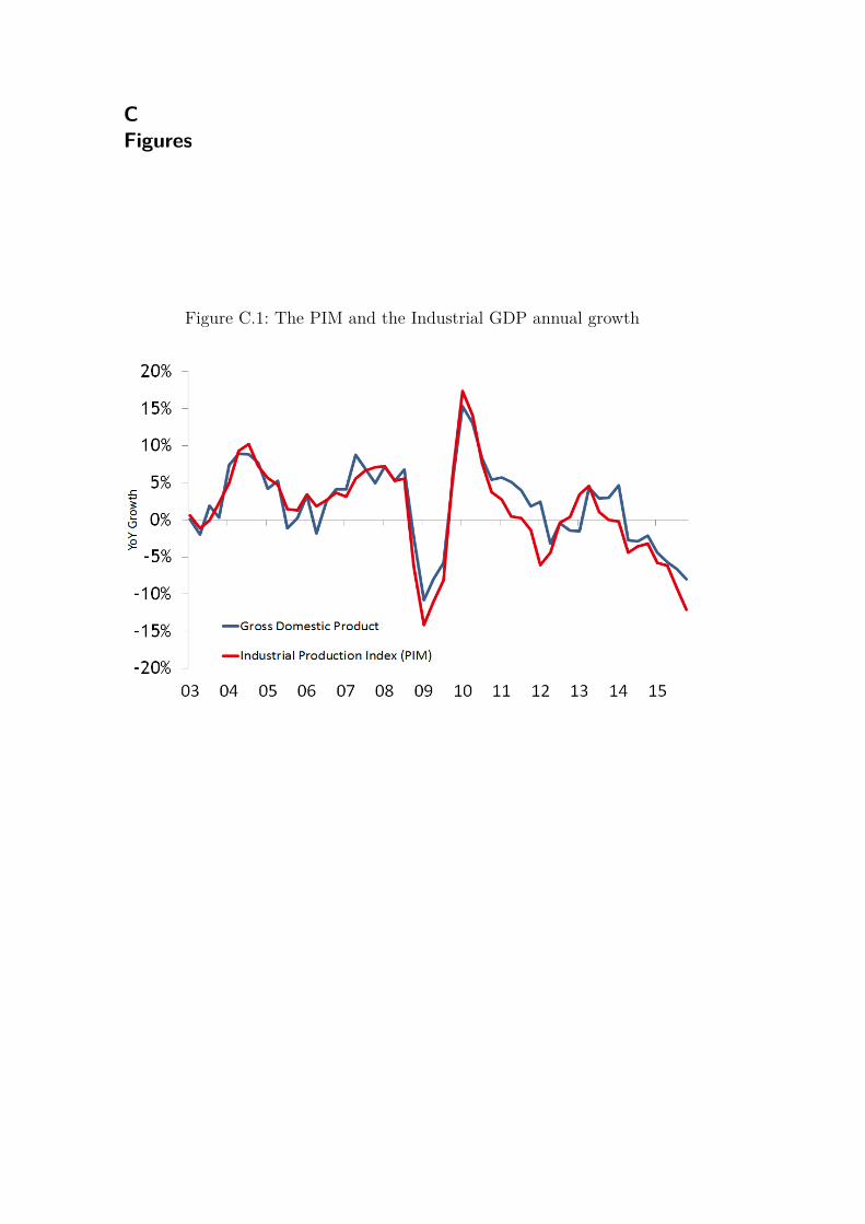
After GDP, the industrial production index (IPI) is the most importantbusiness cycle indicator for a given country. One of the main advantages ofusing the IPI in comparison to GDP is that the latter is usually disclosed in aquarterly manner while the former is released on a monthly basis. This givesus reliable high-frequency updates on the economic situation and helps marketagents to assess current and future developments. Thus, it’s safe to say thatthe IPI is a reliable indicator of the overall level of economic activity. In Brazil,the industrial sector accounts for over 17 percent of the economy’s total GDP.Therefore, accurately forecasting short-term activity is essential for aiding thedecision-making processes not only of industry-related companies but also ofcentral bankers and other policy makers.

In this work, we addressed different methods for predicting both short-and long-term developments of the Brazilian industrial production index in adata-rich environment. While an extensive literature has focused on forecastingactivity in real time for developed countries, few studies have been done forthe Brazilian economy. Stock and Watson (2002) used factor-based modelsto forecast different real variables in the United States, including industrialproduction, over both short- and long-term horizons. Their results showed thathigh-dimensional forecasting methods over-performed simpler linear models inmost cases. Bulligan, Golinelli and Parigi (2010) compared different forecastingmethods for the Italian IPI series and found that factor models over-performedstandard ARIMA regressions. Acedanski (2013) applied a similar methodologyto the Polish industrial production index and concluded, contrary to Bulligan,Golinelli and Parigi’s (2010) result, that simpler models often over-performedfactor models. Lupi and Bruno (2001) used VAR models to forecast Italianindustrial production and concluded that current leading indicators providegood predictive ability for not only short-but also long-term horizons. Apartfrom pursuing the best forecasting method, these authors also demonstratedthe benefits of model combination following Stock and Watson (2006). Finally,Cunha (2010) used a diffusion index to anticipate future movements of theslack in Brazilian industrial production. His results show that factor modelsbased solely on financial variables over-perform more complex models. This

Chapter 1. Introduction 10

result goes accords with those found by Hollauer, Issler and Notini (2008) andcontradicts common wisdom, which states that hard-data variables are thosemost likely to present higher predictive power. Our main objective in this paperis to forecast Brazilian IPI’s monthly growth by considering a large number ofpotential variables, using both soft and hard data.

Forecasting economic activity is not an easy task, especially when work-ing with a large number of potential predictors. Since most candidates are mereapproximations of reality, the uncertainty over the correct choice of regressorsgrows with the number of available candidates. Model specification is thereforean issue that is not readily resolved.

Standard variable selection algorithms usually rely on some type ofinformation criteria, such as the Bayesian Information Criterion (BIC), asequential testing procedure, such as forward stepwise selection, or some sortof model selection algorithm. The main problem with these approaches isthat their ability to provide reliable forecasts is limited to small datasets.There are two reasons for this: first, the number of available models growsexponentially with the number of candidate variables, making these methodscomputationally costly or even unfeasible to evaluate all possible combinations;second, when the number of covariates is larger than the number of availableobservations (k > T ), models become under-identified, making ordinary leastsquares estimation impossible. Thus, estimating high-dimensional models usingstandard procedures does not seem to be a good choice.

Empirical evidence helps us by providing priors on which leading eco-nomic indicators are most likely to anticipate the movements of other variables.In this work, our prior is that a small number of variables are relevant in de-termining future developments of the Brazilian Industrial Production Index(PIM). This implies the use of a sparse (small number of relevant variables)rather than dense (many relevant variables) dataset. The statistical methodused in each of these two representations varies. Standard estimation methodsfor dense matrices are Principal Component Analysis (PCA), Dynamic Fac-tor Analysis (DFA) and other variations. These methods capture the commonvariance between the explanatory variables and narrow these variables to asmall number of factors. Despite providing good predictive results, they pro-vide no information on which variables best describe the model and are alsosubject to bad quality data. Sparse matrix estimation, by contrast, is generallyachieved using penalized regressions. The introduction of a penalty parameterinto standard linear regressions helps to diminish model complexity by forcingthe coefficients of irrelevant variables toward zero. The Ridge Regression pro-posed by Hoerl and Kennard (1970) and the Elastic Net regression proposed

Chapter 1. Introduction 11

by Zou and Hastie (2005) are examples of penalized least squares.Statistical data on the Brazilian economy have only recently begun to

be gathered. Therefore, forecasting the country’s economic variables can beproblematic since we face a “fat” shaped dataset (many variables but not asmany observations, k > T ). Model selection in this type of dataset is subjectto various issues, e.g., over-fitting and constant revisions. Our main goal in thispaper is to forecast the Brazilian industrial production index by consideringa large number of potential explanatory variables. We use three differentapproaches to cope with this problem. First, we use factor-based models as ourbenchmark. Second, we use shrinkage regressions (or penalized regressions),using the Lasso (Least Absolute Shrinkage and Selection Operator) proposedby Tibshirani (1994) and the Adalasso (Adaptive Least Absolute Shrinkageand Selection Operator) proposed by Zou (2006). Shrinkage regressions aredesigned to select the most parsimonious model while preserving the truerepresentation of data generating process of the response variable. Third,we combine penalized regressions with a variable selection algorithm thatwe will henceforth refer to as PVSA (Penalized Variable Search Algorithm).This methodology reduces the number of potential explanatory variables usingshrinkage regressions and then uses a variable search algorithm to select themodel with the best out-of-sample performance. Finally, we also assess thepredictive ability of the simple mean of all forecasts produced by the PSVA.We will henceforth refer to this forecast combination as POOL.

Our results demonstrate that shrinkage regressions over-perform ourbenchmark in short-term forecasts. The combination of penalized regressionswith a variable selection model (PVSA) over-performed the Lasso, the Adalassoand the proposed benchmark at all forecasting horizons. Furthermore, pool-ing forecasts using the Lasso as a first-step variable filter (POOL) achievedthe best forecasting accuracy in our exercise. Diebold-Mariano tests of sta-tistical equivalence corroborate this outcome. Moreover, the shrinkage modelspredictive ability and variable selection consistency worsened as we increasedthe number of candidates, revealing a methodological limitation. The resultsalso show that long-term forecasts exhibit inferior performance compared withshorter horizons and are often beaten by the response variable’s historicalmean. A possible explanation for this result is that the available leading indi-cators seem to contain little information about long-run investment decisionsand, consequently, future production.

Finally, although our main objective is to select the most accuratemodel independent of the forecasting horizon, all methods yielded similar setsof candidate variables. As we would expect, those most frequently selected

Chapter 1. Introduction 12

were related to economic activity and production. Individually, explanatoryvariables related to the auto industry were by far the most common in ouranalysis, suggesting that Brazilian industrial production is highly dependenton this segment. Another interesting result is that business sentiment surveysalso exhibited high predictive power and were frequently selected in both short-and long-term forecasts. This corroborates the results observed in Hollauer,Issler and Notini (2008) and Mello, E. (2014) that show that the industry’scapacity utilization index and business sentiment surveys significantly enhanceforecasting power.

This paper is organized as follows. Section 2 introduces the penalizedregression framework, focusing on the Lasso and its variants. Section 2 alsopresents the PSVA. In Section 3, we briefly discuss the Brazilian IPI and thecandidate variables available in our dataset. In Section 4, we present our mainresults, and we conclude our analysis in Section 5.

2Shrinkage regressions and the Lasso

Approximating complex inter-correlations between real-world variablesusing small, semi-structural models is a difficult task. For instance, an econ-omy’s transmission mechanisms are determined by a huge number of differentvariables - which may or may not be directly related to the economy itself.Given the underlying uncertainty, accurate variable selection plays a substan-tial role in the pursuit of a single model that can simplify reality using a smallnumber of candidates. Sequential testing procedures such as forward stepwiseselection and complete subset regression analysis (Elliot, Gargano and Tim-mermann, 2012) achieve good results when working with small datasets byproviding a parsimonious model with good predictive performance. However,these methods become inefficient and, eventually, unfeasible when using a largenumber of predictors, as when the number of covariates exceeds the numberof observations (k > T ), models become under-identified. Penalized regres-sions such as the Lasso are a fast and reliable alternative for high-dimensionalestimation and forecasting.

In this chapter, we introduce the penalized regression framework. Wealso present a variant of penalized regression called the PSVA (PenalizedVariable Selection Algorithm), which combines shrinkage methods and avariable selection algorithm.

2.1Penalized Regressions

Shrinkage regressions such as the Lasso can be viewed as a penalizedfunctional form of standard ordinary least squares estimation. There are twomain objectives motivating the introduction of tuning parameters into OLSregressions: (i) reducing model complexity by shrinking the estimates of theregression coefficients toward zero relative to their OLS estimates and (ii)improving accuracy by trading bias to reduce estimator variance. By producingsome coefficients that are exactly zero, the Lasso provides interpretable modelsand is therefore an efficient alternative when working with high-dimensionaldatasets. The Lasso estimator is defined as follows:

Chapter 2. Shrinkage regressions and the Lasso 14

b̂ = arg minb̂

||Y −Xb||22 + λP∑p=1|bp|, (2-1)

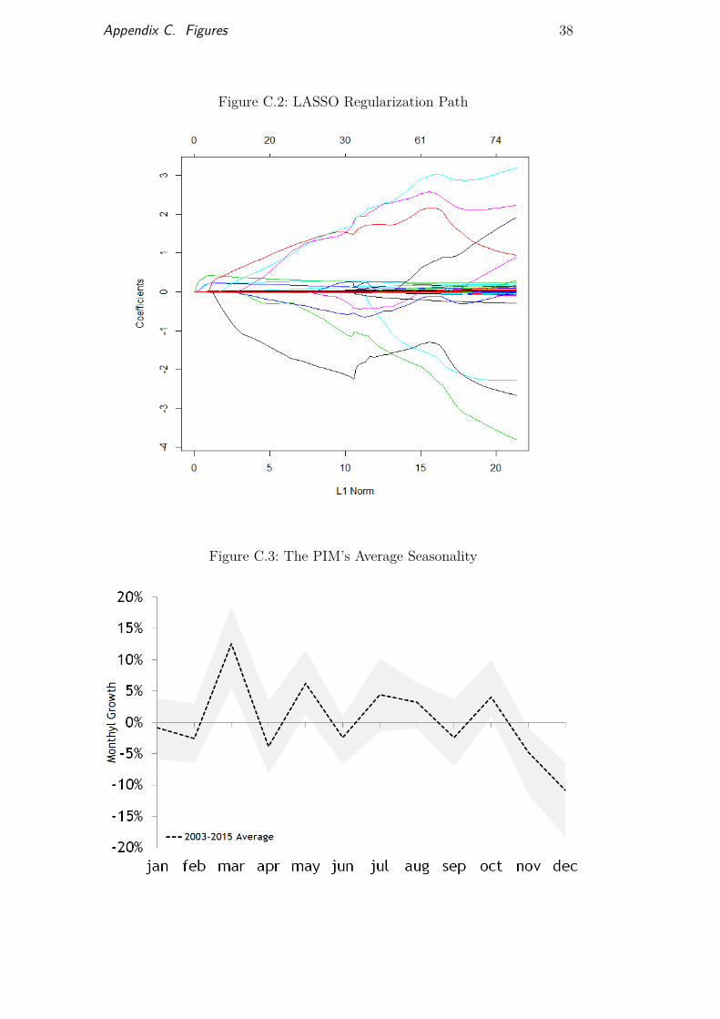
where b is the N × 1 vector of parameters, Y = (y1, ..., yt)′ is theresponse variable, X is the P × n data matrix, and λ is a non-negativeregularization parameter. In penalized regressions, model complexity becomesa function of its regularization parameter (λ). As the tuning parameterincreases in size, penalties become more conservative and reduce the modelspecification by shrinking irrelevant variables coefficients toward zero (λ =∞makes all coefficients equal to zero). Figure 2 illustrates this relationship byshowing the sensitivity between the Lasso’s penalization parameter (x axis)and the candidate regressors coefficients (y axis). Most studies select thetuning parameter using cross-validation1 or some information criteria suchas the Bayesian Information Criterion (BIC). The former is not always thebest choice since it is not robust to inter-temporal dependence. In otherwords, cross-validation does not provide the expected results when the dataare not independent and identically distributed (i.i.d.). Thus, regularizationparameters selected through information criteria appear to work best for time-series datasets.

Although capable of efficiently handling large datasets, the Lasso alsofaces limitations. Zou (2006) and Meinshausen and Bühlmann (2006) showedthat there are scenarios in which the model selection determined by the Lassois inconsistent and does not achieve the oracle property (Fan and Li, 2001).In other words, the Lasso is not always capable of selecting the correct set ofrelevant variables, and even if it is, the Lasso estimator will most likely presenta different asymptotic distribution than that provided by the OLS estimator(oracle). Zou (2006) suggested a two-step procedure called the adaptive Lasso(Adalasso), whereby individual weights are used to further constrain variablecoefficients in the l1 penalty. This modification allows the Adalasso to achievevariable selection consistency. Moreover, Medeiros and Mendes (2015) derivedconditions under which the Adalasso presents both model selection consistencyand enjoys the oracle property. The Adalasso estimator is defined as follows:

β̂ = arg minβ̂

||Y −Xβ||22 + λP∑p=1wp|βp|, (2-2)

where β is the N × 1 vector of parameters, λ is the first-step Lassoregularization parameter, w is a weight vector defined as wp = |β̂Lasso|

−γ, with1A model validation technique.

Chapter 2. Shrinkage regressions and the Lasso 15

βLasso as a first-step Lasso estimator to β, and γ is a non-negative weightingparameter (γ > 0).

The main challenge in applying this approach is to correctly tune theadaptive Lasso or, in other words, to retrieve the optimal pair of parameters(γ, λ) that will yield the model with the closest representation to the truedata generation process. Both parameters are often selected through theminimization of some sort of loss function, e.g., root mean squared error ormean absolute error, using cross-validation methodology. As mentioned above,this method does not perform well in frameworks with serially correlated data.To address this issue, practitioners have resorted to the use of out-of-sampleevaluation or information criterion, such as the BIC. Zhang et al (2010),Wang et al (2007) and Zou et al (2007) showed that the BIC is a reliablealternative to cross-validation in time-series frameworks. Finally, Medeirosand Mendes (2015) used the BIC as the selection method for both the first-step Lasso regularization parameter (λ) and the Adalasso weighting parameter(γ). They showed that this flexible version of the Adalasso is asymptoticallyconsistent and enjoys the oracle property (selects the correct variable subset)even when the number of candidate variables is much larger than the numberof observations.

In addition to the Lasso, there are also other types of penalized regres-sions that are worth highlighting. The Lasso is a particular case in which astandard ordinary least squares estimator is constrained by a linear absolutevalue penalty term. Other shrinkage methods such as the Ridge Regressionand the Elastic Net also use quadratic penalties. Let us consider a generic lossfunction (l) that contains both linear (l1) and quadratic penalties (l2). Thelatter can be defined as follows:

l1,2 = λP∑p=1

[(1− α)|bp|+ α|bp|2], (2-3)

where λ is a positive regularization parameter, bp represents the pth

independent variable coefficient, and α represents the share of each penalty(l1 or l2) in the minimization procedure. The Lasso is a particular case inwhich α = 0. As α increases toward unity, the quadratic penalty gainsimportance and may not necessarily shrink irrelevant variables to zero but,instead, to a very small value. In contrast to the Lasso, the Ridge Regression(the particular case in which α = 1) does not produce a parsimonious model,as it always retains all the predictors in the model. When α is in between theseparticular cases, the following regression is known as the Elastic Net (Zou andHastie, 2005), which uses a combination of both linear (l1) and quadratic (l2)

Chapter 2. Shrinkage regressions and the Lasso 16

penalties. By combining the effects of both the Lasso and the Ridge Regression,the Elastic Net produces a sparse model with good predictive accuracy whileencouraging a grouping effect (it selects highly correlated regressors).

2.2Penalized Variable Selection Algorithm (PSVA)

Testing all possible variable combinations in high-dimensional datasets isa costly and sometimes unfeasible task. We propose a variation of the CompleteSubset Regression method proposed by Elliot, Gargano and Timmermann(2013) by combining shrinkage regressions and a variable selection algorithm.We also propose a set of constraints that reduce the required computationaleffort and makes variable selection more efficient.

The methodology applied consists of two main parts. First, we reduce thenumber of available candidates to a few targeted predictors2 by applying theLasso as a first-step variable filter. Since our procedure involves re-estimatingthe model for each out-of-sample prediction (in our work, we consider a 36-step forecast sample), the Lasso may ultimately select heterogeneous models.The variables selected through the procedure compose a new set of candidatesthat is used in the second part of our proposed algorithm. By employing alower-dimension dataset we are able to address conventional model selectionmethods such as sequential testing procedures and information criterion.

The second part of the algorithm uses a slightly different approach fromordinary variable selection methods by imposing two additional constraints.The first further reduces the set of candidates selected by the Lasso by imposinga cap (k) on the number of variables available to our algorithm. Second,instead of estimating all available variable combinations (2k), we also limitthe maximum number of variables that can be included in each model (p).Both modifications make our algorithm more efficient by eliminating from theanalysis variables that may have been incorrectly selected by the Lasso andprecluding model over fitting. Our results consider k = 20 and p = 6.

The top-k most selected variables are considered the most likely to bestrepresent the response variable’s data generating process and are thereforeincluded as candidates by our algorithm. If a number of variables greater than kpresent the same (and highest) selection rate, all will be assigned as candidates.For example, assume that k=10 and that the Lasso selected 12 of the totalavailable variables in its estimation procedure with the same selection rate.In this case, k will be reset to 12, thus considering all selected variables aspossible candidates.

2See Bai & Ng (2008) for more on targeted predictors.

Chapter 2. Shrinkage regressions and the Lasso 17

Having selected n≤k variables, we estimate every possible variable com-bination that respects the p-maximum variable constraint using ordinary leastsquares. The total number of different model specifications is then given bythe following equation:

tot =p∑i=1

n!(n− i)!i! , (2-4)

where n is the number of available candidates, and i is the number ofvariables combined in each individual model.

Finally, each individual model produces one-step-ahead forecasts within amoving window of j periods. This procedure is repeated Z times, and in eachiteration, the moving window shifts backward by one period. To illustrate,suppose that in the first iteration, models are tested for their performance inthe window between t1,1 = v and t2,1 = v+ z. The best model in this iteration,denoted m1, will be the model with the best out-of-sample RMSE error withinthis window. Then, in the second iteration, the moving window would shiftbackward by one. As a result, models would be tested for their out-of-sampleRMSE performance in the window between t1,2 = v − 1 and t2,2 = v + z − 1.We would then have another model, denoted m2, which performed the bestin this second window. Notably, m1 and m2 may or may not be the same.After z iterations, we would have Z best models, each of which had the topperformance in its respective moving window. These models are then used toproduce the “true performance” of our proposed algorithm. Considering theexample above, m1 would give us the forecast for period v + z + 1, while m2

would produce the forecast for period v + z. The idea is to always predictusing the model that had the best out-of-sample performance up to the lastobservation of a given moving window. Within each moving window, we alsoconsider not only individual models but also model averages, such that m1

forecasts may be an average over the tot models rather than one single model.

3Data and Period of Analysis

The PIM is Brazil’s monthly industrial production index (IPI) andrepresents the product of both manufacturing and extractive industries. Theindex is calculated by the Brazilian Institute of Geography and Statistics(IBGE) and was first compiled in the 1970s. In May 2014, the IPI receivedits second methodological revision, updating the industries’ activities andtheir index weights to the latest classification of the National Classificationof Economic Activities (CNAE 2.0). Despite having changed its methodologyin 2014, the IBGE updated the IPI in January 2012 and linked it to its previousversion, creating a series that begins in 2002.

Since the available data were subject to a methodological revision, it isvery unlikely that the IPI’s data generating process has remained the sameover time. Therefore, the choice of which sample to use in our analysis was nottrivial. We had three possible options:

(1) Use only the new version (with the methodological update) of the IPI,running from January 2012 until September 2016. This would give us asample with 48 observations.

(2) Use the old version (without the methodological update) of the IPI,running from January 2002 until September 2016. This would give us asample with 120 observations.

(3) Test whether the coefficients suffered significant changes after themethodological update. If the test result were negative, we could esti-mate our models using the entire available sample, running from January2002 until September 2016. This would give us 177 observations.

As estimating models with a small number of observations and a largenumber of candidates is a problem that lacks a simple solution, we chosethe option that provided us with the largest sample available (option 3). Toassess whether there was a significant change between periods, we estimateda regression with seasonal dummies and an additional control variable thatrepresented the updated series period1. The results indicated that we could not

1A dummy equal to 0 from January 2002 to December 2011 and equal to 1 from January2012 to September 2016.

Chapter 3. Data and Period of Analysis 19

significantly reject that the two periods presented the same seasonal effects. Inlight of this result, option 3 seemed to be the best choice for our analysis.

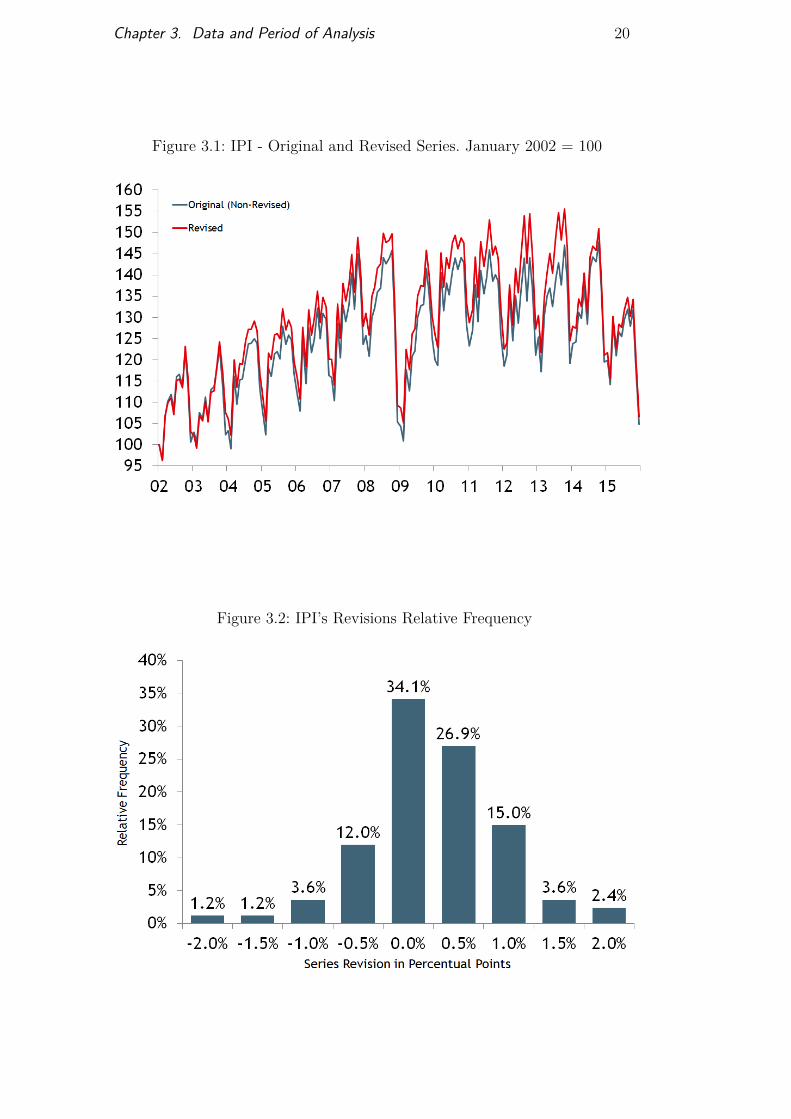
There is an additional consideration that needs to be made: our mainobjective is to perform real-time forecasts of the IPI’s monthly growth. Thismeans attempting to replicate the exact conditions (with the same informationset) faced by forecasters or, in other words, considering only the preliminarynature of the data and discarding possible revisions. Therefore, our responsevariable was constructed by linking the non-revised realizations of the IPI’smonthly growth from January 2002 until our last available observation inSeptember 2016. Figure 3.1 compares the original (non-revised) and the revisedindustrial production index using January 2002 as our initial point2. Figure3.2 shows the relative frequency of revisions made to the IPI over the years.

Following the methodology applied to construct our real-time IPI series,we selected over 70 candidate variables, of which we also include two lags. Thelagged response variable is also included as a candidate variable in our dataset.All variables were tested for the presence of a unit root and transformed(first differentiated) when necessary. To account for the seasonality of theseries, monthly dummies were also included as candidate regressors. Theexplanatory variables are both soft and hard data and are detailed in AppendixB. Our dataset contains variables that cover the manufacturing of intermediary,durable and non-durable goods, government debt, taxes, foreign trade, wages,unemployment, confidence indexes, sales, leverage, interest rates, etc. Allcandidate variables possess the same time span as the IPI (January 2002 toSeptember 2016).

Our sources are Bloomberg, the Brazilian Institute of Geography andStatistics (IBGE), the Getúlio Vargas Foundation (FGV), the National Trea-sury department, the Brazilian Central Bank, the Ministry of Development,Industry and Foreign Trade, the Ministry of Labor, and the Industry Federa-tion of the state of São Paulo (FIESP).

2January 2002 = 100.

Chapter 3. Data and Period of Analysis 20

Figure 3.1: IPI - Original and Revised Series. January 2002 = 100

Figure 3.2: IPI’s Revisions Relative Frequency

4Main Results

This section presents the performance of three forecasting methods usedto predict the monthly growth of the Brazilian industrial production index(IPI) ( PIMt

PIMt−1−1). The first method is based on principal components analysis

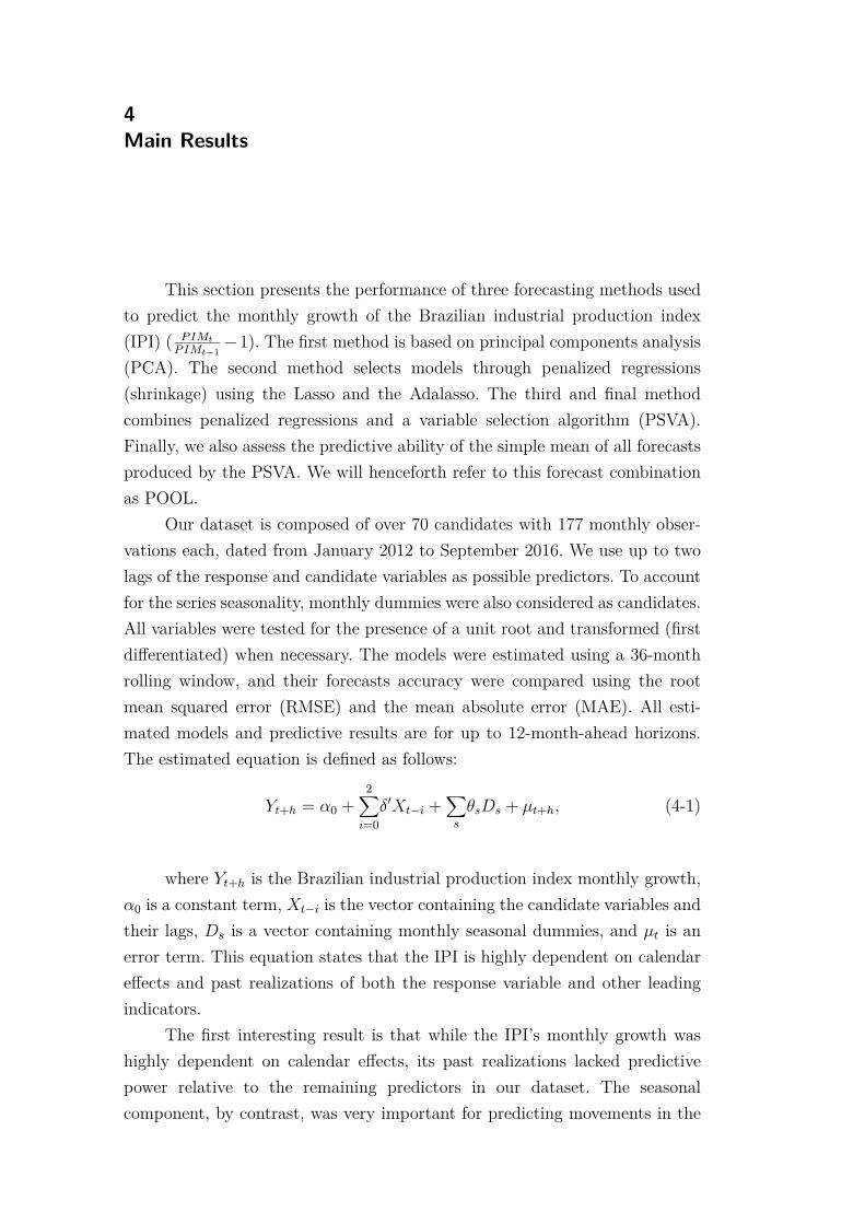
(PCA). The second method selects models through penalized regressions(shrinkage) using the Lasso and the Adalasso. The third and final methodcombines penalized regressions and a variable selection algorithm (PSVA).Finally, we also assess the predictive ability of the simple mean of all forecastsproduced by the PSVA. We will henceforth refer to this forecast combinationas POOL.

Our dataset is composed of over 70 candidates with 177 monthly obser-vations each, dated from January 2012 to September 2016. We use up to twolags of the response and candidate variables as possible predictors. To accountfor the series seasonality, monthly dummies were also considered as candidates.All variables were tested for the presence of a unit root and transformed (firstdifferentiated) when necessary. The models were estimated using a 36-monthrolling window, and their forecasts accuracy were compared using the rootmean squared error (RMSE) and the mean absolute error (MAE). All esti-mated models and predictive results are for up to 12-month-ahead horizons.The estimated equation is defined as follows:

Yt+h = α0 +2∑i=0δ′Xt−i +

∑s

θsDs + µt+h, (4-1)

where Yt+h is the Brazilian industrial production index monthly growth,α0 is a constant term, Xt−i is the vector containing the candidate variables andtheir lags, Ds is a vector containing monthly seasonal dummies, and µt is anerror term. This equation states that the IPI is highly dependent on calendareffects and past realizations of both the response variable and other leadingindicators.

The first interesting result is that while the IPI’s monthly growth washighly dependent on calendar effects, its past realizations lacked predictivepower relative to the remaining predictors in our dataset. The seasonalcomponent, by contrast, was very important for predicting movements in the

Chapter 4. Main Results 22

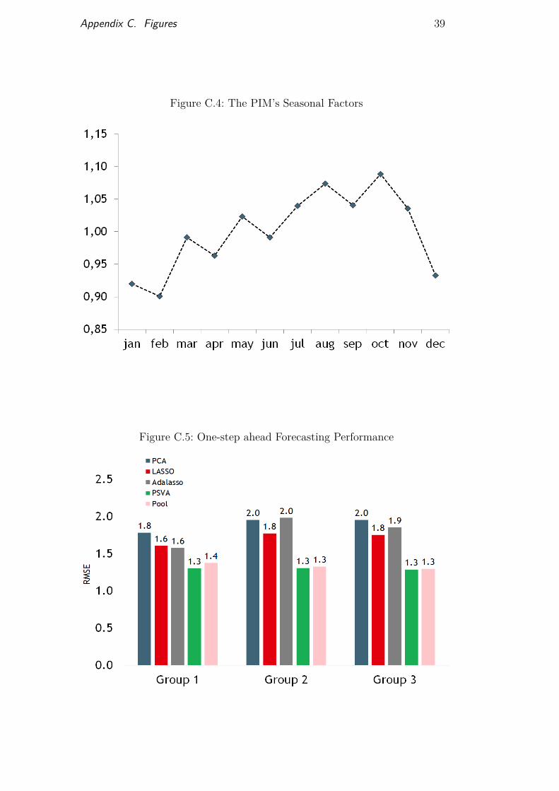
responses variable. Figure 3 shows that the series monthly results behave in asimilar way over time. Moreover, when tested formally, the results indicatedthat the IPI exhibits strong seasonality. Figure 4 shows how the seasonal factorsare spread across the year. This result led us to include monthly dummies ascandidate regressors to address this seasonal behavior. Note that imposingdummies as candidates while using shrinkage methods can be problematic.For instance, it is unlikely that they will always be selected by the algorithmsince other variables can capture part of the seasonality, thus causing thedummies to be regarded as irrelevant. Nevertheless, results have shown thatboth the Lasso and the Adalasso recurrently considered the seasonal dummiesas relevant regressors.

By providing good forecasting results in the presence of a very largenumber of variables, penalized regressions out-perform factor-based modelswhen exposed to a large number of irrelevant variables. For comparisonpurposes, we tested the Lasso, Adalasso and the PSVA using three differentdatasets:

(1) Dataset composed of the most relevant variables selected following ourown prior. Total of 59 candidates.

(2) Dataset 1 plus 20 candidates (includes lagged variables). Total of 79candidates.

(3) Dataset 1 plus 60 candidates (includes lagged variables). Total of 119candidates.

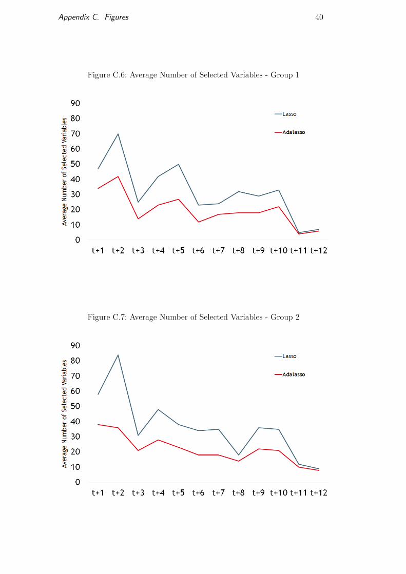
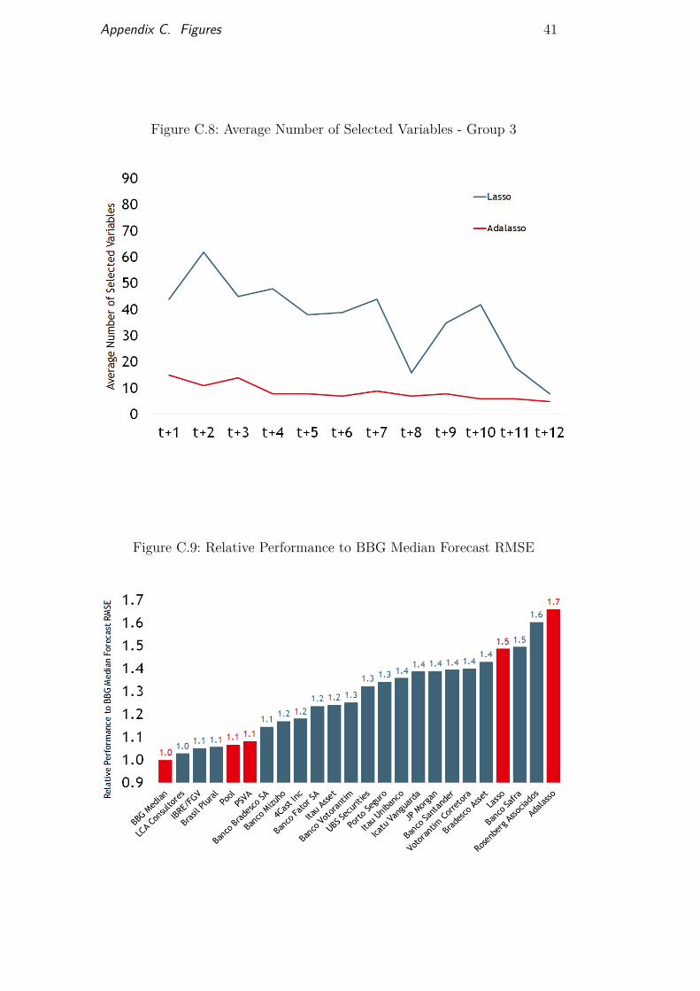
The result of this exercise was that both the Lasso and the Adalasso be-came more conservative as we included a larger number of irrelevant variablesas potential candidates. This becomes more clear in longer-term forecasts, inwhich only a small number of variables are considered relevant. By becomingmore conservative, the forecasting performance at any given horizon deterio-rated as the size of the dataset increased. Appendix B presents the variablesused in each of the three previously mentioned groups. Figure 5 compares themethods one-step-ahead forecasting performance using each dataset. Figures6, 7 and 8 depict the average number of selected variables at each forecastinghorizon using the Lasso and the Adalasso, each with a different set of variables.

Using dataset number 2 as the available group of variables, the proposedmethods achieved strong results in short-term forecasting, which is the mostrelevant horizon for econometric models. This outcome highlights the potentialbenefits of shrinkage regressions in data-rich environments. When compared tothe one-step ahead forecasts disclosed by other market participants, the PSVA

Chapter 4. Main Results 23

and POOL were included among the top-10 best-performing predictors. Thisis another strong result, especially as market participants are able to introducepriors into their forecasts to cope with movements that are not captured bythe available regressors. Figure 9 shows the top-ranked market participantsforecasting performance and the ranking of the Lasso, the Adalasso, thePVSA and the POOL model. Furthermore, another interesting result was thatthe POOL’s forecasting performance improved as the number of irrelevantvariables grew. This leads us to two conclusions: first, shrinkage regressionswere unable to efficiently discard all irrelevant variables; second, variables thatwere presumed to be orthogonal to the IPI captured part of the movementthat other candidates were not able to capture.

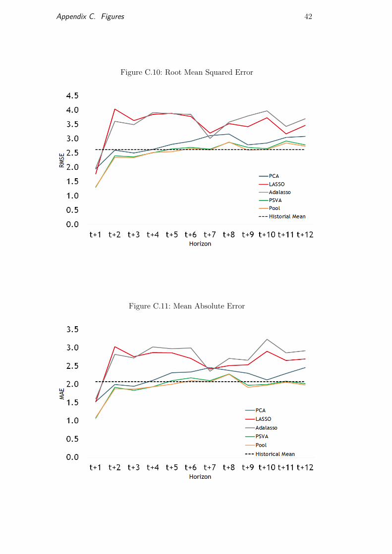
The results also indicate that long-term forecasts exhibit considerablyworse performance than those at shorter horizons and are often out-performedby the response variable’s historical mean. A possible explanation for this resultis that the available leading indicators seem to contain little information aboutlong-run investment decisions and, consequently, future production. Figures10 and 11 show the root mean squared error (RMSE) and the mean squared(MAE) at different forecasting horizons using the Lasso, the Adalasso, thePSVA, the POOL and a model using principal components (our benchmark).

It’s worth noting that all of the proposed methods were efficient in choos-ing variables consistent with economic theory, regardless of forecasting horizon.Examples of recurrently selected variables in long-term forecasts were laggedinterest rates and spread rates. A possible transmission mechanism regardingthese variables is that long-term investments are negatively influenced by a costeffect, i.e., higher interest rates. At short-term horizons, the best-performingmodels regularly selected variables related to vehicle production, highway traf-fic, cardboard sales and working days. This result suggests that Brazilian in-dustrial production is highly dependent on the country’s auto industry.

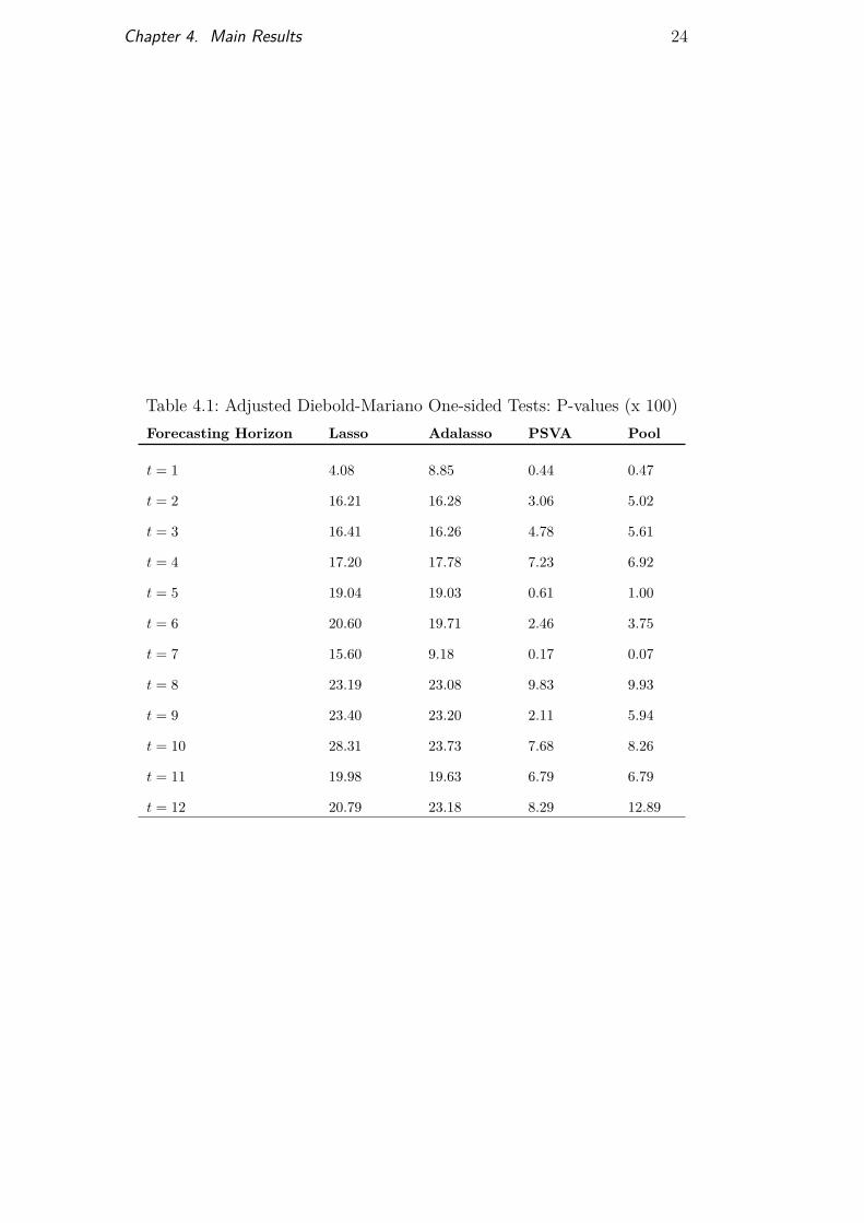
To assess the statistical relevance of the various forecasts generated by theproposed methods, we used the Diebold-Mariano test for predictive equality.All forecasts were compared against our benchmark. These tests revealedthat one-step-ahead predictions were statistically superior to the proposedbenchmark’s performance. Tests of the longer-term forecasts (h > 1), bycontrast, did not reject the null hypothesis of statistical equality. This resultpersisted even after adjusting the DM test to improve small-sample properties,as proposed by Harvey, Leybourne, and Newbold (1997). Table 2 illustratesthis analysis by presenting the adjusted DM test’s p-values for 1- to 12-month-ahead forecasts.

Chapter 4. Main Results 24

Table 4.1: Adjusted Diebold-Mariano One-sided Tests: P-values (x 100)Forecasting Horizon Lasso Adalasso PSVA Pool

t = 1 4.08 8.85 0.44 0.47

t = 2 16.21 16.28 3.06 5.02

t = 3 16.41 16.26 4.78 5.61

t = 4 17.20 17.78 7.23 6.92

t = 5 19.04 19.03 0.61 1.00

t = 6 20.60 19.71 2.46 3.75

t = 7 15.60 9.18 0.17 0.07

t = 8 23.19 23.08 9.83 9.93

t = 9 23.40 23.20 2.11 5.94

t = 10 28.31 23.73 7.68 8.26

t = 11 19.98 19.63 6.79 6.79

t = 12 20.79 23.18 8.29 12.89

5Conclusion

Forecasting economic variables in rich, high-dimensional environmentsis a difficult task. In this paper, we address this issue and compare differentforecasting methods when applied to Brazilian data, specifically the industrialproduction index (IPI). Since standard linear models tend to become ineffi-cient as our dataset enlarges, we utilized shrinkage methods to address thedimensionality problem. Here, we consider the Lasso and the Adalasso. Wealso propose a combination of penalized regressions and a variable search al-gorithm, which we refer to as PVSA. Finally, we also assess the predictiveability of the simple mean of all forecasts produced by the PSVA, which wecall POOL. The forecasts produced by these previously mentioned methodswere compared to a principal component model, our benchmark.

The results demonstrated that shrinkage methods over-performed theproposed benchmark in short-term forecasts, regardless of the number ofavailable candidates. Furthermore, the PSVA and the POOL excelled thegreater part of market participants predictions. This is a strong result giventhat individuals are able to introduce their priors to cope with movements thatare not captured by the available regressors. Long-run forecasts, by contrast,exhibit considerably worse performance and often under-perform the responsevariable’s historical mean.

Finally, all methods considered selected similar sets of explanatory vari-ables. Short-term predictions were usually dominated by the auto industryrelated variables, highway traffic, cardboard sales, business days, and so forth.Long-term forecasting, by contrast, exhibited greater variability and selectedvariables such as interest rates, spread rates, confidence indexes and so forth.Moreover, the shrinkage models’ predictive ability and variable selection con-sistency worsened as we increased the number of candidates, revealing a clearlimitation of the minimization algorithm. The merger between penalized re-gressions and a deterministic variable selection algorithm addressed this prob-lem by consistently selecting the same variable subset regardless of the numberof available regressors. The short-term forecast results suggest that Brazil’s in-dustrial production is highly dependent on the country’s auto industry andother related sectors. Medium-term determinants, by contrast, were unclear,

Chapter 5. Conclusion 26

suggesting both methodological and data limitations.

References

[1] ACEDÁNSKI, J.. Forecasting industrial production in poland – acomparison of different methods. Ekonometria Econometrics, 39:40–51, 2013.

[2] ARTHUR E. HOERL, R. W. K.. Ridge regression: Biased estimationfor nonorthogonal problems. Technometrics, 12(1):55–67, 1970.

[3] BAI, J.; NG, S.. Forecasting economic time series using targetedpredictors. Journal of Econometrics, 146(2):304–317, October 2008.

[4] BATES, M. J.; GRANGER, J. C. W.. The combination of forecasts.Journal of the Operational Research Society, 20(4):451–468, 1969.

[5] BRUNO, G.; LUPI, C.. Forecasting euro-area industrial productionusing (mostly) business surveys data. ISAE Working Papers 33, ISTAT- Italian National Institute of Statistics - (Rome, ITALY), 2003.

[6] BULLIGAN, G.; GOLINELLI, R. ; PARIGI, G.. Forecasting monthlyindustrial production in real-time: from single equations tofactor-based models. Empirical Economics, 39(2):303–336, 2010.

[7] CUNHA, F. C. S.. Previsão da Produção Industrial do Brasil: UmaAplicação do Modelo de Índice de Difusão Linear. Dissertaçãode mestrado, Departamento de Engenharia Elétrica da PUC-Rio, PontifíciaUniversidade Católica do Rio de Janeiro, Rio de Janeiro, 2010.

[8] DE MELLO, E. P. G.; FIGUEIREDO, F. M. R.. Assessing the Short-termForecasting Power of Confidence Indices. Working Papers Series 371,Central Bank of Brazil, Research Department, Dec. 2014.

[9] ELLIOTT, G.; GARGANO, A. ; TIMMERMANN, A.. Complete subsetregressions. Journal of Econometrics, 177(2):357–373, 2013.

[10] FAN, J.; R., L.. Variable selection via nonconcave penalized like-lihood and its oracle properties. Journal of the American StatisticalAssociation, 96:1348–1360, 2001.

References 28

[11] FRANCIS X. DIEBOLD, R. S. M.. Comparing predictive accuracy.Journal of Business & Economic Statistics, 13(3):253–263, 1995.

[12] HARVEY, D.; LEYBOURNE, S. ; NEWBOLD, P.. Testing the equality ofprediction mean squared errors. International Journal of Forecasting,13(2):281–291, 1997.

[13] HOLLAUER, G.; ISSLER, J. A. V. ; NOTINI, H. H.. Prevendo o cresci-mento da produção industrial usando um número limitado decombinações de previsões. Economia Aplicada, 12:177 – 198, 2008.

[14] MEDEIROS, M. C.; MENDES, E. F.. l1-Regularization of High-Dimensional Time-Series Models with Flexible Innovations. Jour-nal of Econometrics, 191:255 – 271, 2016.

[15] MEINSHAUSEN, N.; BÜHLMANN, P.. High dimensional graphsand variable selection with the lasso. ANNALS OF STATISTICS,34(3):1436–1462, 2006.

[16] STOCK, J. H.; WATSON, M.. Forecasting with many predictors.volumen 1, chapter 10, p. 515–554. Elsevier, 1 edition, 2006.

[17] STOCK, J.; WATSON, M.. Macroeconomic forecasting using diffu-sion indexes. Journal of Business and Economic Statistics, 20(2):147–162,2002.

[18] TIBSHIRANI, R.. Regression shrinkage and selection via the lasso.Journal of the Royal Statistical Society, Series B, 58:267–288, 1994.

[19] WANG, H.; LI, G. ; TSAI, C.-L.. Regression coefficient and autore-gressive order shrinkage and selection via the lasso. Journal of theRoyal Statistical Society Series B, 69(1):63–78, 2007.

[20] ZHANG, Y.; LI, R. ; TSAI, C.-L.. Regularization parameter selectionsvia generalized information criterion. Journal of the AmericanStatistical Association, 105(489):312–323, 2010.

[21] ZOU, H.. The adaptive lasso and its oracle properties. Journal ofthe American Statistical Association, 101(476):1418–1429, 2006.

[22] ZOU, H.; HASTIE, T.. Regularization and variable selection via theelastic net. Journal of the Royal Statistical Society, Series B, 67:301–320,2005.

References 29

[23] ZOU, H.; HASTIE, T. ; TIBSHIRANI, R.. On the “degrees of freedom”of the lasso. Ann. Statist., 35(5):2173–2192, 10 2007.

AEstimation Procedures

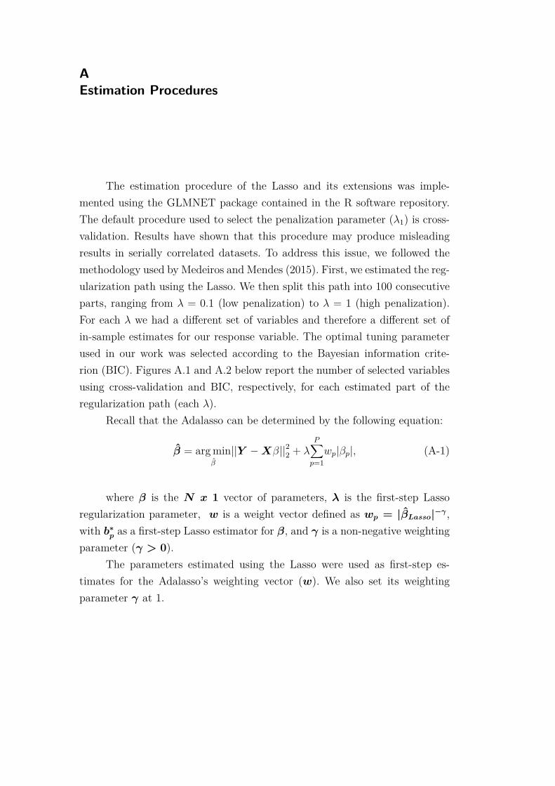
The estimation procedure of the Lasso and its extensions was imple-mented using the GLMNET package contained in the R software repository.The default procedure used to select the penalization parameter (λ1) is cross-validation. Results have shown that this procedure may produce misleadingresults in serially correlated datasets. To address this issue, we followed themethodology used by Medeiros and Mendes (2015). First, we estimated the reg-ularization path using the Lasso. We then split this path into 100 consecutiveparts, ranging from λ = 0.1 (low penalization) to λ = 1 (high penalization).For each λ we had a different set of variables and therefore a different set ofin-sample estimates for our response variable. The optimal tuning parameterused in our work was selected according to the Bayesian information crite-rion (BIC). Figures A.1 and A.2 below report the number of selected variablesusing cross-validation and BIC, respectively, for each estimated part of theregularization path (each λ).

Recall that the Adalasso can be determined by the following equation:

β̂ = arg minβ̂

||Y −Xβ||22 + λP∑p=1wp|βp|, (A-1)

where β is the N x 1 vector of parameters, λ is the first-step Lassoregularization parameter, w is a weight vector defined as wp = |β̂Lasso|−γ ,with b∗p as a first-step Lasso estimator for β, and γ is a non-negative weightingparameter (γ > 0).

The parameters estimated using the Lasso were used as first-step es-timates for the Adalasso’s weighting vector (w). We also set its weightingparameter γ at 1.

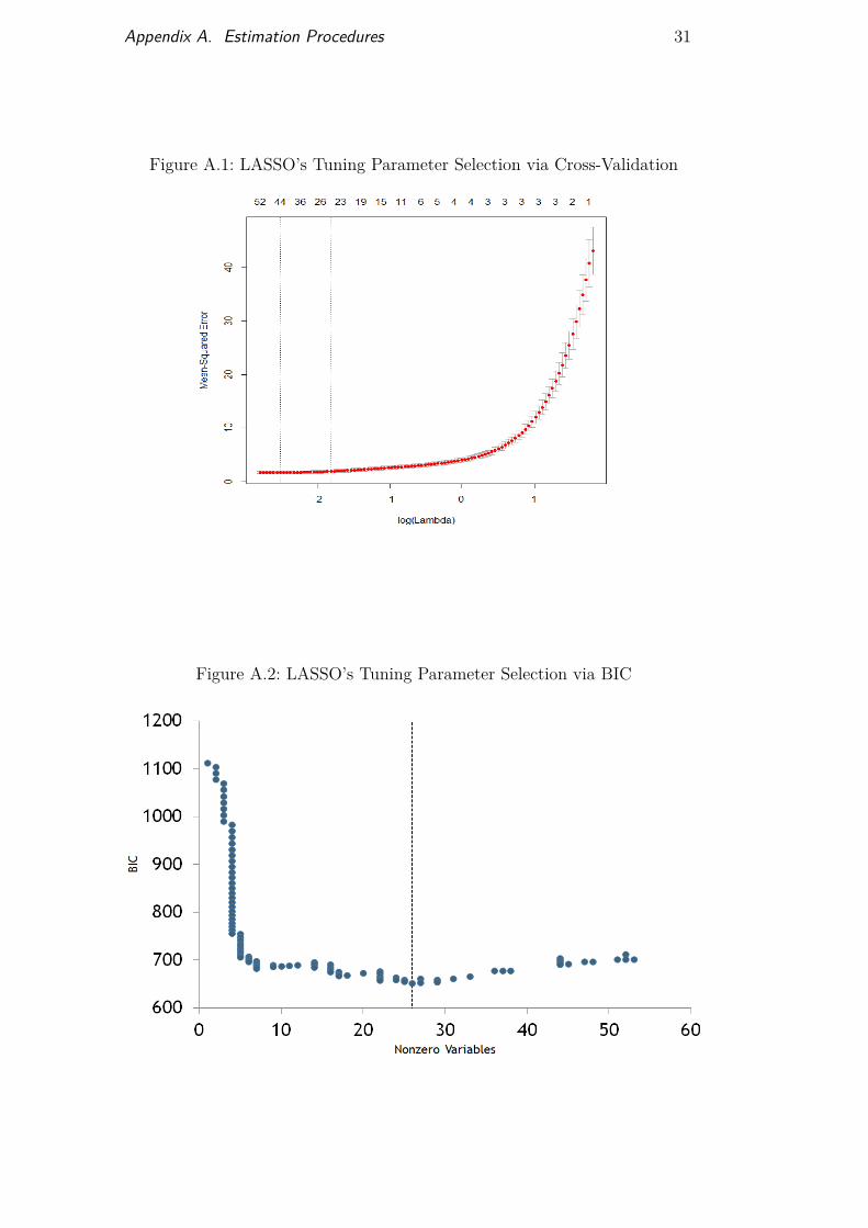
Appendix A. Estimation Procedures 31

Figure A.1: LASSO’s Tuning Parameter Selection via Cross-Validation

Figure A.2: LASSO’s Tuning Parameter Selection via BIC

BData

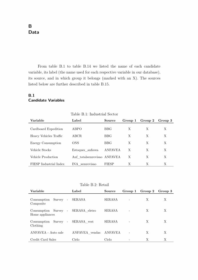
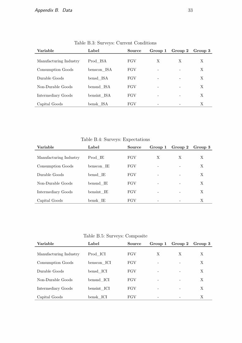
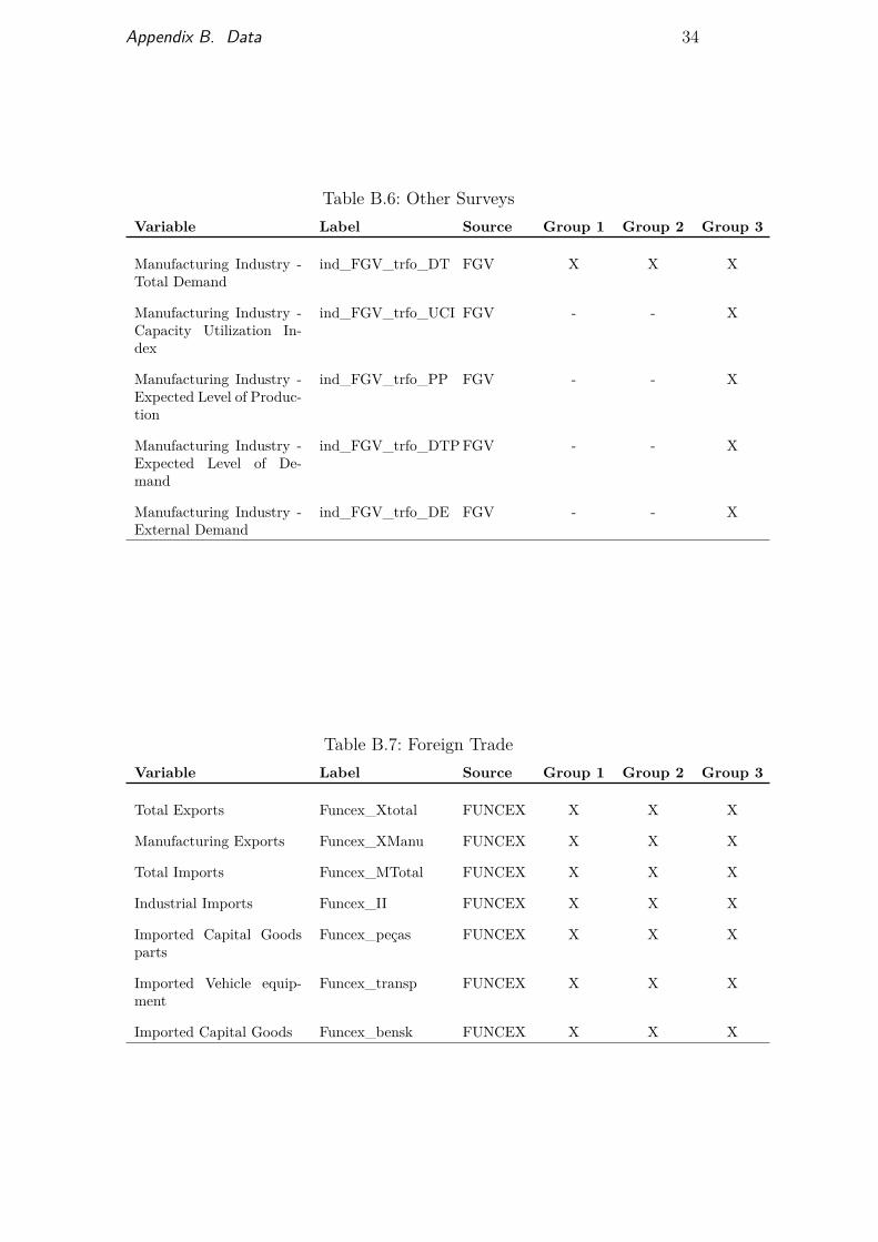
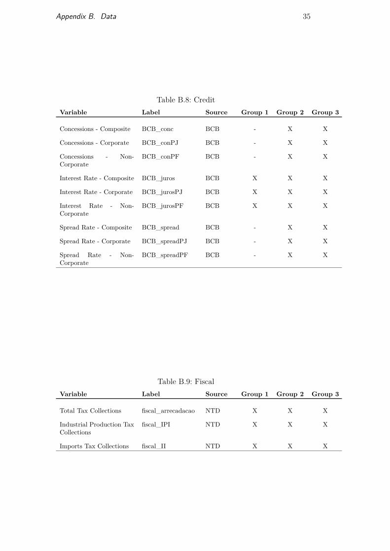
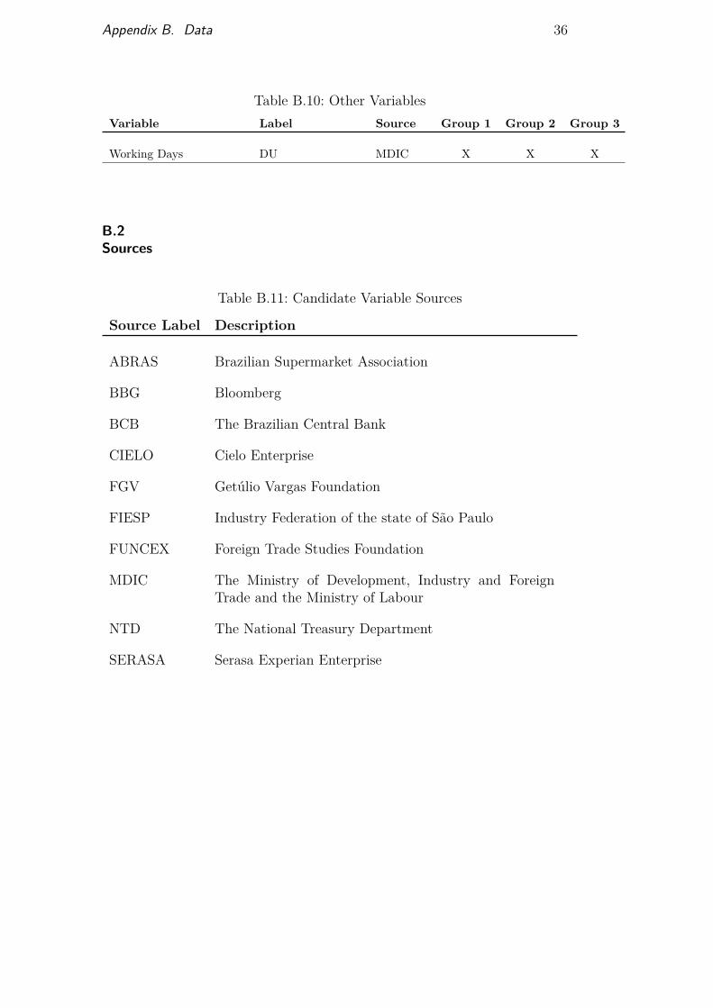
From table B.1 to table B.14 we listed the name of each candidatevariable, its label (the name used for each respective variable in our database),its source, and in which group it belongs (marked with an X). The sourceslisted below are further described in table B.15.

B.1Candidate Variables

Table B.1: Industrial SectorVariable Label Source Group 1 Group 2 Group 3

Cardboard Expedition ABPO BBG X X X

Heavy Vehicles Traffic ABCR BBG X X X

Energy Consumption ONS BBG X X X

Vehicle Stocks Estoques_anfavea ANFAVEA X X X

Vehicle Production Anf_totalsemrevisao ANFAVEA X X X

FIESP Industrial Index INA_semrevisao FIESP X X X

Table B.2: RetailVariable Label Source Group 1 Group 2 Group 3

Consumption Survey -Composite

SERASA SERASA - X X

Consumption Survey -Home appliances

SERASA_eletro SERASA - X X

Consumption Survey -Clothing

SERASA_vest SERASA - X X

ANFAVEA - Auto sale ANFAVEA_vendas ANFAVEA - X X

Credit Card Sales Cielo Cielo - X X

Appendix B. Data 33

Table B.3: Surveys: Current ConditionsVariable Label Source Group 1 Group 2 Group 3

Manufacturing Industry Prod_ISA FGV X X X

Consumption Goods benscon_ISA FGV - - X

Durable Goods bensd_ISA FGV - - X

Non-Durable Goods bensnd_ISA FGV - - X

Intermediary Goods bensint_ISA FGV - - X

Capital Goods bensk_ISA FGV - - X

Table B.4: Surveys: ExpectationsVariable Label Source Group 1 Group 2 Group 3

Manufacturing Industry Prod_IE FGV X X X

Consumption Goods benscon_IE FGV - - X

Durable Goods bensd_IE FGV - - X

Non-Durable Goods bensnd_IE FGV - - X

Intermediary Goods bensint_IE FGV - - X

Capital Goods bensk_IE FGV - - X

Table B.5: Surveys: CompositeVariable Label Source Group 1 Group 2 Group 3

Manufacturing Industry Prod_ICI FGV X X X

Consumption Goods benscon_ICI FGV - - X

Durable Goods bensd_ICI FGV - - X

Non-Durable Goods bensnd_ICI FGV - - X

Intermediary Goods bensint_ICI FGV - - X

Capital Goods bensk_ICI FGV - - X

Appendix B. Data 34

Table B.6: Other SurveysVariable Label Source Group 1 Group 2 Group 3

Manufacturing Industry -Total Demand

ind_FGV_trfo_DT FGV X X X

Manufacturing Industry -Capacity Utilization In-dex

ind_FGV_trfo_UCI FGV - - X

Manufacturing Industry -Expected Level of Produc-tion

ind_FGV_trfo_PP FGV - - X

Manufacturing Industry -Expected Level of De-mand

ind_FGV_trfo_DTPFGV - - X

Manufacturing Industry -External Demand

ind_FGV_trfo_DE FGV - - X

Table B.7: Foreign TradeVariable Label Source Group 1 Group 2 Group 3

Total Exports Funcex_Xtotal FUNCEX X X X

Manufacturing Exports Funcex_XManu FUNCEX X X X

Total Imports Funcex_MTotal FUNCEX X X X

Industrial Imports Funcex_II FUNCEX X X X

Imported Capital Goodsparts

Funcex_peças FUNCEX X X X

Imported Vehicle equip-ment

Funcex_transp FUNCEX X X X

Imported Capital Goods Funcex_bensk FUNCEX X X X

Appendix B. Data 35

Table B.8: CreditVariable Label Source Group 1 Group 2 Group 3

Concessions - Composite BCB_conc BCB - X X

Concessions - Corporate BCB_conPJ BCB - X X

Concessions - Non-Corporate

BCB_conPF BCB - X X

Interest Rate - Composite BCB_juros BCB X X X

Interest Rate - Corporate BCB_jurosPJ BCB X X X

Interest Rate - Non-Corporate

BCB_jurosPF BCB X X X

Spread Rate - Composite BCB_spread BCB - X X

Spread Rate - Corporate BCB_spreadPJ BCB - X X

Spread Rate - Non-Corporate

BCB_spreadPF BCB - X X

Table B.9: FiscalVariable Label Source Group 1 Group 2 Group 3

Total Tax Collections fiscal_arrecadacao NTD X X X

Industrial Production TaxCollections

fiscal_IPI NTD X X X

Imports Tax Collections fiscal_II NTD X X X

Appendix B. Data 36

Table B.10: Other VariablesVariable Label Source Group 1 Group 2 Group 3

Working Days DU MDIC X X X

B.2Sources

Table B.11: Candidate Variable Sources

Source Label Description

ABRAS Brazilian Supermarket Association

BBG Bloomberg

BCB The Brazilian Central Bank

CIELO Cielo Enterprise

FGV Getúlio Vargas Foundation

FIESP Industry Federation of the state of São Paulo

FUNCEX Foreign Trade Studies Foundation

MDIC The Ministry of Development, Industry and ForeignTrade and the Ministry of Labour

NTD The National Treasury Department

SERASA Serasa Experian Enterprise

CFigures

Figure C.1: The PIM and the Industrial GDP annual growth

Appendix C. Figures 38

Figure C.2: LASSO Regularization Path

Figure C.3: The PIM’s Average Seasonality

Appendix C. Figures 39

Figure C.4: The PIM’s Seasonal Factors

Figure C.5: One-step ahead Forecasting Performance

Appendix C. Figures 40

Figure C.6: Average Number of Selected Variables - Group 1

Figure C.7: Average Number of Selected Variables - Group 2

Appendix C. Figures 41

Figure C.8: Average Number of Selected Variables - Group 3

Figure C.9: Relative Performance to BBG Median Forecast RMSE

Appendix C. Figures 42

Figure C.10: Root Mean Squared Error

Figure C.11: Mean Absolute Error