Lectures on the differential geometry of curves and surfaces
564
-
Upload
khangminh22 -
Category
Documents
-
view
0 -
download
0
Transcript of Lectures on the differential geometry of curves and surfaces

Cornell University
Library
The original of this book is in
the Cornell University Library.
There are no known copyright restrictions in
the United States on the use of the text.
http://www.archive.org/details/cu31924060289141
CORNELL UNIVERSITY LIBRARY
924 060 289 14

Production Note
Cornell University Library pro-duced this volume to replace theirreparably deteriorated original.It was scanned using Xerox soft-ware and equipment at 600 dotsper inch resolution and com-pressed prior to storage usingCCITT Group 4 compression. Thedigital data were used to createCornell's replacement volume onpaper that meets the ANSI Stand-ard Z39. 48-1984. The productionof this volume was supported in
part by the Commission on Pres-ervation and Access and the XeroxCorporation. Digital file copy-right by Cornell UniversityLibrary 1991.

COkNELLUNIVERSITYLIBRARIES
Mathematics
Library
White Ha!l


LECTURES
ON THE
DIFFERENTIAL GEOMETRYOF CURVES AND SURFACES
CAMBRIDGE UNIVERSITY PRESS
Honfton: FETTER LANE, E.C.
C. F. CLAY, Manager
SESinbuteb : 100, PRINCES STREET
ISrtlin: A. ASHER AND CO.
leipjig: F. A. BROCKHAUS
litis Bora: G. P. PUTNAM'S SONS
Bumbag anD Calcutta: MACMILLAN AND CO., Ltd.
Ail rights reserved
LECTURES
ON THE .
DIFFERENTIAL GEOMETRYOF CURVES AND SURFACES
BY
A. R. FORSYTH,ScD., LL.D., Math.D., F.R.S.,
SOMETIME SADLERIAN PROFESSOR OF PURE MATHEMATICS
IN THE UNIVERSITY OF CAMBRIDGE
Cambridge :
at the University Press
IQI2

CamfatiSge
:
PRINTED BV JOHN CLAY, M.A.
AT THE UNIVERSITY PRESS
PREFACE.
rriHE material of the present volume consists of the substance
of lectures delivered, from time to time, during my tenure
of the Sadlerian professorship of pure mathematics in the University
of Cambridge. The last occasion, when such lectures were given
by me, was during the Michaelmas Term of 1909.
As the volume does not pretend to be a complete treatise on
differential geometry, and as it is restricted to the contents of mylectures, readers will find that not a few sections of the vast range
of the subject are discussed only shortly and that some are left
undiscussed. In lectures, my aim was to expound those elements
with which eager and enterprising students should become ac-
quainted ; they could thus, in my opinion, be best prepared for
the penetrating consideration, which is suited for the private study
rather than for the lecture-room or the examination-room. No
lack of individual interest was implied in omitted branches of the
subject ; to give an instance of a purely personal kind, my lectures
never even mentioned the application of Lie's theory of continuous
groups to the construction of the differential invariants for space
and for surfaces in space—a matter to which, elsewhere, I had
devoted some attention. One ofmy ideals, in lecturing to students,
was to provide them with some of the instruments for research
;
consequently this volume is mainly intended for students who,
later, may devote themselves to original work.

VI PEEFACE
The book can be regarded as composed of three main sections
;
its divisions are only partially indicated by the chapters, which are
numbered consecutively. Throughout, it deals solely with con-
figurations in ordinary Euclidean space.
In the first section, consisting of a single chapter, the properties
of skew curves and of their associated lines and planes are ex-
pounded, without regard to any family or families of surfaces upon
which the curves may happen to lie.
In the second section, consisting of chapters II—vi, the subject-
matter is the properties of curves upon any general surface in space.
Some classes of these curves (e.g. lines of curvature) are organically
connected with the surface ; they are completely determined by
the elements of the surface to which they belong. Other curves,
such as geodesies, have an equally organic relation with the surface
;
but they are not determined solely by the elements of the surface,
for they can satisfy some arbitrarily assigned condition or conditions.
Again, quite arbitrary curves and families of curves can be assumed
upon a surface ; not a little attention has been devoted to methods
for constructing differential invariants which, being in value in-
dependent of parameters of reference, express the geometrical
magnitudes of the curves, subject, of course, to the dominance
of the intrinsic magnitudes of the surface containing the curve
or curves.
In the third section, consisting of chapters vn—xi, the subject-
matter is surfaces in general, rather than particular configurations
on surfaces. The most ordinary methods of point-to-point corre-
spondence and comparison of surfaces are explained. Surfaces,
which are defined (wholly or partially) by intrinsic properties,
are considered, special attention being paid to minimal surfaces.
Families of surfaces are discussed, according to the respective
definitions that ultimately establish the families ; the most
obvious instance relates to those surfaces which have plane or
spherical sets of lines of curvature. Lastly, a brief sketch of
PREFACE Vll
the simplest fundamental properties of triply orthogonal systems
is given.
The book concludes with a single chapter that contains an
introduction to the elementary theory of congruences of curves,
specially of straight lines and of circles.
Scattered throughout the book, examples (over two hundred
in number) will be found ; many of them are extracted from
memoirs by various authors. At the end, there is a set of
miscellaneous examples collected from Cambridge examination
papers in recent years ; for the collection, I am indebted to
Mr K. A. Herman.
To facilitate reference, I have constructed a customary table
of contents at the beginning of the book and a customary subject-
index at the end ; and, because a more or less persistent significance
is assigned to many of the symbols that are used, I have given (at
the end of the table of contents) a list of these symbols with the
passages where the significance is first stated.
From the frequent references throughout, as well as in the
references in the brief half-historical introductions to most of the
chapters, it will be seen that one of my special desires has been to
direct students to the work of the mathematician who, I think,
would be generally hailed as the greatest living master of the
subject. The treatise by Darboux must remain, at least for this
generation, the classical exposition of Differential Geometry.
In exposition, it may have been rash on my part to restrict
myself throughout to a treatment, which is based mainly upon the
analysis used by Gauss and by those who followed him in its use.
Certainly I have made no attempt to give what could only have
been a rather faint reproduction of Darboux's treatment, which
centres round the tri-rectangular trihedron at any point of a curve
or surface or system. My hope is that students may experience
an added stimulus of interest when they find that different methods
combine in the development of growing knowledge.
Vlll PREFACE
Of course, in so extensive a subject, indebtedness naturally is
not confined to one great worker alone. The names quoted in the
course of my pages (and all have been quoted, whose work has
been used by me) will give some hint of the multitude of workers
who, through the long sequence of years, have constructed the
immense fabric of acquired knowledge. Great as many of those
names are, I wish here to place on record my own sense of gratitude
to Darboux and to his work. My tribute of homage is gladly
rendered in this year, the jubilee of his doctorate at Paris.
For valuable help given to me in many ways during the revision
of the proof-sheets, as well as for suggestions and criticisms that
proved useful to me, I tender my most cordial thanks to myfriend Mr R. A. Herman, Fellow and Lecturer of Trinity College,
Cambridge, and University Lecturer in Mathematics.
Finally, in past years and on other occasions, it has been mygood fortune to receive the unfailing assistance of the staff of the
University Press at Cambridge. On this occasion, their assistance
has been forthcoming in the same generous and unstinted measure
as before. To them, as only is their due, my thanks once more are
given.
A. R. F.
February, 1912.
TABLE OF CONTENTS.
CHAPTER I.
CURVES IN SPACE.
§§ PAGE
1. Two modes of defining curves in space 1
2. Analytical definition of a curve by expressions for its coordinates in terms
of a parameter 2
3. Equations of the tangent, the normal plane, the osculating plane, the
principal normal, the binormal 3
4. The circular curvature of a curve ; the angle of contingence 4
5. The trihedron at a point ; convention as to positive directions ... 4
6. Torsion ; the angle of torsion, the radius of torsion 5
7. Use of spherical indicatrix 6
8. Sphere of curvature ; its radius 7
9. Distance of a consecutive point from the tangent, the osculating plane, the
sphere of curvature ; coordinates of the consecutive point in terms of
the arc .... 8
10. The moving trihedron ; Routh's diagram j screw curvature ... 10
11, 12. Locus of centre of circular curvature;
polar line ; rectifying plane
;
rectifying line 12
13. Polar developable ; polar line ; its edge of regression, being the locus of
the centre of spherical curvature 13
14, 15. Rectifying developable ; its generators and edge of regression ; used to
determine curves which have their curvatures in an assigned variable
ratio 13
16. Osculating developable ; Serret's formulae when a curve is defined by its
osculating plane 16
17, 18. ".'he Serret-Frenet formulae ; a Riccati equation 17
19. A skew curve is defined uniquely, save as to position and orientation, by
its two curvatures 21
20. Curves whose curvatures are in a constant ratio 23
21. Curves with assigned torsion 25
22. Curves with assigned circular curvature 27
Examples 28
CONTENTS
CHAPTER II.
GENERAL THEORY OF SURFACES.
§§ PAGE
23. Coordinates of a point on a surface expressed in terms of two parameters 32
24. Fundamental magnitudes of the first order, E, F, G . . . . 33
25, 26. Elementary formulae for curves on a surface 34
27. Direction-cosines X, T, Z of the normal to the surface ; a differential
equation of the surface 36
28. Fundamental magnitudes of the second order, L, M, N . 37
29. Derivatives of X, T, Z . . 39
30. Integrability of the differential equation of a surface (§ 27) . 40
31. Curvature of a normal section of a surface 41
32. Lines of curvature and principal radii ; their equations .... 41
33. The mean curvature, H, and the Gauss measure of curvature, K, at
any point ... 44
34. The Gauss characteristic equation ; the measure K is expressible in terms
of the magnitudes E, F, G and their derivatives 44
35. The two Mainardi-Codazzi relations .... ... 46
36. Variation of the angle between the parametric curves ... 49
37-39. Bonnet's theorem that a surface is determined uniquely, save as to orien-
tation and position, by the three fundamental magnitudes of the first
order and the three of the second order 50
40. Derived magnitudes ; those of the third order P, Q, R, S . . . 56
41. Derived magnitudes of the fourth order and higher orders ... 57
42. Variations of the measures of curvature expressed in terms of P, Q, H, S . 58
43. Derivatives of x, y, z of the third order .... 59
Examples . 60
CHAPTER III.
ORGANIC CURVES OF A SURFACE.
44. Orthogonal systems of parametric curves . .... 63
45. Conditions that the parametric curves should be lines of curvature 63
46. Theorems of Meunier and of Euler on curvature of sections 64
47. Conjugate directions ; the general equation .... .6548. Condition that the parametric curves should be conjugate ... 67
49, 50. Laplace's linear equation of the second order satisfied by the coordinates
when the parametric curves are conjugate, with examples . 6851. Asymptotic (self-conjugate) lines ; inflexional tangents 7052. Analytic determination of asymptotic lines, on a sphere, on FreBnel's
wave-surface.... 7X
53. Conditions that the parametric curves should be asymptotic lines 7254. Pseudo-spheres (2T= - l//i2) 74
55. Nul lines ; conditions for parametric curves ; determination of nul lines
on a surface .... 75
CONTENTS XI
§§ PAGE
56. Equations for a surface with nul Hues as parametric variables ... 76
57. Surfaces with constant mean curvature (ff=2/h) 77
58, 59. Lie's construction for nul lines in space, and their association with
minimal surfaces .... 78
60. Isometric lines .... ... 80
61. Range of isometric variables .... .8162. Examples of isometric lines . . 82
63. Equations, and conditions, when the parametric curves are isometric . 83
64. Surfaces having isometric lines of curvature, with example ... 84
65, 66. Geodesies ; characteristic property ; also, when they are lines of curvature,
they are plane curves . . 87
67. Geodesic parallels . 88
68. Geodesic polar coordinates ; equations for the surface .... 88
69. Summary of results relating to parametric curves, when they belong to
some class of organic curves 90
Examples 91
CHAPTER IV.
LINES OF CURVATURE.
70. The differential equations of the lines, (i) ordinary, (ii) partial ... 93
71. Umbilici 94
72. Equation for lines of curvature near an umbilicus; its integral in the
immediate vicinity 95
73. Configuration of the lines when all the roots of the critical cubic are real
.
97
74. Configuration when only one root is real 98
75. Form of the differential equation for the lines in general when the surface
is given by a Cartesian equation . .* 99
76. Particular method for determining an integral equation of the lines on
special classes of surfaces ... 100
77, 78. Equations for the surface when the lines of curvature are the parametric
curves ; with application to the case of a central quadric . . . 102
79. Hirst's theorem on the conservation of lines of curvature under inversion,
with other results.... . ... 105
80. Surface of centres ; simple geometrical properties 107
81. Analytical formulae; equations, and' fundamental magnitudes for the two
sheets 108
82, 83. Ribaucour's theorems, as to surfaces when the lines of curvature on the
two sheets of the centro-surface are given by the same equation, and
when the asymptotic lines on the two sheets are given by the same
equation . . ... ... Ill
84. The centro-surface of an ellipsoid ; its configuration 113
85. Surfaces derived by measuring any variable distance along the normal ; the
equations in general . 117
86. The middle evolute ... 119
87. Remark on parallel surfaces 120
Examples . 121
62
XU CONTENTS
CHAPTER V.
GEODESICS.
§§ ^QEReferences to authorities 123
88. Three distinct ranges of investigation ... ... 123
89. Some fundamental theorems from the calculus of variations, applicable
to geodesies; the complete set of tests that secure the minimumproperty 124
90. Two of the variation tests are always satisfied 128
91. The characteristic variation equation leads to the general equations of
geodesies ; the significance of these equations 129
92. Different forms of the general equations of geodesies ; some inferences ;
nul lines satisfy the equations ... .... 130
93. Geodesies on surfaces of revolution ; a first integral, and the primitive . 132
94. Geodesies in the vicinity of a parallel of minimum radius ; three kinds
.
134
95, 96. Geodesies in the vicinity of a parallel of maximum radius ; condition
that it is a closed curve . 134
97. Limitation of range within which a geodesic is actually the shortest
distance ; conjugate points, when the curve is not a meridian . 136
98. Geodesies, that are not meridians, on an oblate spheroid . . . 138
99. Conjugate points on a geodesic when it lies in a meridian ; the general
test, with examples . . 142
100. Geodesies in general ; characteristic equation derived from the property
that its principal normal is the normal to the surface . . 144
101. Geodesies on an ellipsoid . . 145
102. The Gauss general equation of a geodesic 148
103. Geodesic curvature of curves ; its measure . ... 149
104. Liouville's expression for geodesic curvature 151
105. The two measures of geodesic curvature are equal ; a third expression,
due to Bonnet 153
106. Circular curvature and torsion of any curve on the surface . 154
107. Torsion of the geodesic tangent . 155
108. Families of geodesies and geodesic parallels ; form of arc-element on the
surface ; special case, when geodesic polar coordinates arise . . 156109,110. Curves geodesically parallel on a surface . 157111-113. Total curvature of a geodesic triangle ... 160
114. Geodesic ellipses and hyperbolas on a surface 162115. Determination of geodesic parallels by a partial equation A<£= 1 of the
first order............ 163116. Deduction of geodesies orthogonal to geodesic parallels . . . 165117. When geodesies are known, the geodesic parallels can be obtained by
quadrature; examples of theorems in §§ 115, 116 .... 168
118. Geodesies and geodesic parallels when the parametric curves are nullines ; Beltrami's theorem ... ... 172
119. Polynomial integrals of A<£= 1 for the construction of geodesic parallels 175

CONTENTS Xlll
§§ PAGE120. Surfaces, admitting a linear integral of A<f> = l, are deformable into
surfaces of revolution 177121. Surfaces admitting a quadratic integral of A0= 1 ; Liouville surfaces ;
Lie surfaces ... . 178
122. Liouville surfaces, admitting different quadratic integrals ... 181
123. But different quadratic integrals cannot be combined ; each, by itself,
leads to a family of geodesies 183
124. Surfaces, admitting a linear integral, do not admit a quadratic integral
that can be combined with the linear integral ... . 185
Examples 186
CHAPTER VI.
GENERAL CURVES ON A SURFACE ; DIFFERENTIAL INVARIANTS.
Scope of the chapter 189
125. Curves in general ; some analytical results, already obtained and nowassociated with binary forms 189
126. The circular curvature and the torsion of a curve and of its geodesic
tangent, and the geodesic curvature of the curve, when position on
the curve is denned by the arc 192
127. Similarly when the curve is defined by a relation = 0, together with
the measures for the parametric curves 194
128. Some properties of lines of curvature .... 196
129. Some properties of asymptotic lines ... ... 198
130. Some properties of geodesies 200
131. Combinations of characteristic properties of organic curves 202
132. Differential invariants ; references to authorities 203
133. Some simple examples of differential invariants, exhibiting the nature
of the invariants . 204
134. Beltrami's differential parameters, connected with curves on the surface
and the arc-element of the surface . 206
135. Illustrations of the use of differential parameters 208
136. Differential invariants in general ; the magnitudes that can occur, up
to the third order ; relative and absolute invariants . . 209
137. The infinitesimal transformation, after Lie, of all the arguments retained 210
138. Formation of the partial differential equations of the first order satisfied
by an invariant 213
139. The independent integrals of one block of these equations ; transfor-
mation of the remainder, which are a complete Jacobian system . 215
140. Association of these equations with the concomitants of a system of
simultaneous binary forms ; an algebraically complete set of inde-
pendent integrals, in terms of which every integral can be expressed 217
141. Significance of Beltrami's differential operators, as-used by Darboux . 218
142. Geometrical significance of all the invariants included in the alge-
braically complete system 220
XIV CONTENTS
PAGE
143. Examples of other invariants expressible in terms of members of the
system . . . ... . 225
144. Some further simple examples, leading to relations among the geo-
metrical magnitudes ... 226
145. The simplest invariants belonging to two curves on the surface simul-
taneously considered ; a complete system within the lowest order
of derivation . . .... ... 228
146. Geometrical significance of all the invariants of two curves within that
lowest order, together with some relations between the geometrical
magnitudes . . . • .... 230
Examples .... 232
CHAPTER VII.
COMPARISON OF SURFACES.
147. Various methods of comparing surfaces 234
148. Conformed representation . .235
149. Planes ... .238150. Surfaces of revolution in general . 238
151. Spheres; maps and projections . 239
152. Examples ..... .242153. Other projections, not conformal 243
154. Geodesic representation; Beltrami's theorem on surfaces that can be
represented geodesically on a plane 243
155. The three families of surfaces of constant curvature, with their geodesies
that become straight lines in the plane representation . . . 245
156. Tissot's theorem 248
157. Dini's theorem that surfaces which can be geodesically represented on
one another are Liouville surfaces ..... 250
158. Two exceptions to Tissot's theorem ; Lie's theorem 251
159. Spherical representation; usually it is not conformal .... 254
160. Some properties of spherical images, of orthogonal lines, of lines of
curvature, of conjugate lines ; Joachimsthal's theorems on lines of
curvature that are plane or spherical 255
161. Various magnitudes connected with the spherical representation of a
surface 258
162. Introduction of tangential coordinates ; equations of second order
satisfied by them; the fundamental magnitudes of the surface
in terms of them 260
163. Equations which determine a surface when a spherical representation
is given 261
164. Spherical representation when the parametric curves are images of
asymptotic lines ; example of pseudo-sphere 262
165. Some special cases 263
Examples ... 267
CONTENTS XV
CHAPTER VIII.
MINIMAL SURFACES.
§§PAGE
Historical notice 268
166. Definition of minimal surface; construction, by the calculus of varia-
tions, of the characteristic equation 268
167. Another establishment of the characteristic equation ; the second
variation for the surface-integral; conditions for a minimum . 270
168. Some general properties of minimal surfaces 272
169. Properties of the spherical representation 273
170. Forms of the intrinsic equation for the arc-element . 277
171. Integral equations expressing the Cartesian coordinates in terms of two
parameters (after Monge) 279
172. The Weierstrass equations for a minimal surface 280
173. Discussion of some tacitly omitted cases ; Lie's theorem 282
174, 175. The fundamental magnitudes for a minimal surface in terms of the
Weierstrass coordinates ; and the organic lines of the surface . 284
176. Tangential coordinates (§ 169) 286
177. Some examples of minimal surfaces; Enneper's surface; Henneberg's
surface ; helicoids ; the catenoid (being the only minimal surface of
revolution) ... ... 287
178. Conditions that the Weierstrass equations should give an algebraic
surface ... 290
179. Conditions that the Weierstrass equations should give a real surface 292
180. Arbitrary functions in the Weierstrass equations determine a surface
;
but a given surface may be representable by two forms of arbitrary
functions ... 293
181-183. Lie's double minimal surfaces, with examples 294
184. Deformation of minimal surfaces so that they always are minimal
;
associated surfaces 297
185. Bonnet's surface, adjoint to a minimal surface ; Schwarz's results . 298
186, 187. Schwarz's method of determination of a minimal surface made to pass
through an assigned curve and to touch a developable along the
curve; with examples 300
188. Note on conjugate curves on a minimal surface, limiting the range
within which it is a minimum 305
Examples .307
CHAPTER IX.
SURFACES WITH PLANE OB SPHERICAL LINES OF CURVATURE;
WBINGARTEN SURFACES.
189. Surfaces having plane or spherical lines, of curvature .... 310
190. Reason for restriction to these classes 311
191. Remark as to developable surfaces, and surfaces with circular lines of
curvature 313
XVI CONTENTS
§§ PAGE
192, 193. Serret-Cayley treatment of plane lines and spherical lines together
;
critical condition among the parametric functions, and its double
significance 314
194. Surfaces with two systems of plane lines of curvature 317
195. Dupin's cyclides;properties, and equations 324
196. Statement as to limiting cases of Dupin's cyclides . 327
197,198. Rouquet's method, by means of the spherical image 328
199. Surfaces having one plane system and one spherical system of lines of
curvature ; seven critical cases . 332
200. Discussion of one critical case . 333
201. Equations for a surface when the systems of lines of curvature are
assigned families of curves 338
202. Reference to investigations on surfaces having only one system of lines
of curvature plane or spherical . 343
203, 204. Weingarten surfaces ; some general formulae, and examples . 343
205-207. Centro-surface of a Weingarten surface ; it is deformable into a surface
of revolution 347
208. Lie's theorem that the lines of curvature on a Weingarten surface can
be obtained by quadrature 351
Examples .... 352
CHAPTER X.
DEFORMATION OF SURFACES.
Preliminary statement 364209, 210. Deformation and applicability ; fundamental test, with example . 356211, 212. Surfaces with a constant Gaussian measure of curvature are applicable
upon themselves in an infinite variety of ways .... 350213. Surfaces of constant Gaussian curvature that are surfaces of revolution,
as applicable upon themselves 358214. Simple formulae for surfaces of revolution that deform into surfaces of
revolution 361215. Deformation in general ; a preliminary geodesic equation 361216. The equation of the second order connected with deformation; its
characteristics are the asymptotic lines 362217. Some special forms of the equation.; for a surface *=/(#, y); for
surfaces such that cW= i\dudv, (V=dv!'+I3*cW .... 363218. Bonnet's solution of the general problem .... 366219. Darboux's method of forming the critical equation, with the subsequent
procedure;some examples, from a plane, a sphere, a paraboloid of
revolution 367220. The critical Monge-Ampere equation of the second order for deforma-
tion; the Ampere method of integration .... 371
221. Cauchy's existence-theorem for integrals .... 373222. Can a surface be deformed while some curve on the stjrface is kept
W* 1374
223. Deformations of a surface so that some curve on the surface ia deformedinto a given curve in space 37*
CONTENTS XV11
(^ PAGE
224. Deformation of scrolls ; Bonnet's preliminary theorem on the deforma-
tion of a ruled surface so that it remains a ruled surface . . 378
225. Deformation of a ruled, surface in general ; the fundamental equations
and magnitudes ; the asymptotic lines .... 380
226-229. Line of striction on a ruled surface ; its intrinsic equation and someproperties .... 383
230,231. Howfar does a given arc-element determine a ruled surface'/ Beltrami's
theorem on the two associated ruled surfaces 387
232. Beltrami's method, where special regard is paid to a directrix curve
during the deformation ; with examples .... 391
233. Two methods of considering deformations; infinitesimal deformations,
and their critical equation 394
234, 235. Infinitesimal deformations in general for z—/{t, y) . 396
236. Infinitesimal deformations in general for ds2= 4\dudv, with the equa-
tions for a minimal surface 398
237. Weingarten's method ; the middle surface between a surface and anysurface derived by deformation 400
238. The equations determining the central deformation function, according
as the middle surface is developable or is not developable
;
its
significance 402
239. Deformation of a surface while a curve remains rigid (§ 222) 404
240. Weingarten's theorems 405
Examples . 407
CHAPTER XI.
TRIPLY ORTHOGONAL SYSTEMS OF SURFACES.
Preliminary statement 408
241. Curvilinear coordinates in space, after Lame, orthogonal systems of
surfaces being used; fundamental magnitudes of the first order;
with Dupin's cyclides and their orthogonals as an example . . 408
242. Fundamental magnitudes of the second order, with complete table
for the three families .... . . 412
243. Dupin's theorem 414
244. The second derivatives of x, y, z, xi+y% +ii, and the equations satisfied
by them 414
245. The principal (Gaussian) curvatures of the surfaces .... 417
246. Lame (or Gauss and Mainardi-Codazzi) relations satisfied, in two
sets, by Hu Hit H3 418
247. Two questions propounded as to the fundamental magnitudes . 420
248-251. The three quantities B\, Bt , H3 determine a triply orthogonal system,
save as to orientation and position; with example as to the con-
formal representation of space 421
252. The degree of generality to be expected in a complete solution of the
equations of orthogonality 429
253. A family of surfaces, belonging to a triply orthogonal system, must
satisfy a partial differential equation of the third order 430
254. Partial equations of the first order for the associated families . 432
xviii CONTENTS
§§PA0B
255. Darboux's construction of the critical equation to be satisfied by the
parameter of the family 433
435
437
439
444
446
448
453
455
456
458
462
464
256. Cayley's form cf the critical equation
257. Darboux's form for a family of surfaces <f>(x, y, z, «)=0
258. Special arithmetical form of the equation, with some examples
259. Puiseux's construction of the arithmetical form of the equation
260. Lame" surfaces ; Darboux's theorem ....261. Bouquet surfaces ii = J[+Y+Z; with examples .
262. The critical equation for coaxial central quadrics
263. The critical equation for a family of coaxial paraboloids
264. Lame isothermic surfaces
265, 266. Isometric triply orthogonal systems ....267. Two examples of isometric triply orthogonal systems .
Examples
CHAPTER XII.
CONGRUENCES OF CURVES.
268. Preliminary explanations as to congruences of curves 466
269. Equations of a congruence ; its surfaces 468
270. The focal points on a curve; focal surface of a congruence, with some
properties ; envelope of grouped curves . .... 469
271, 272. Limitations upon a congruence of curves that they may admit orthogonal
section by a surface or family of surfaces 471
273. Rectilinear congruences ; their equations ; fundamental quantities 475
274. Shortest distance between two selected rays 477
275. Limits (limiting points) of a ray ; Hamilton's theorem .... 478
276. Foci of a ray ; focal planes of a ray ; the developable surfaces in a
rectilinear congruence 480
277. Normal rectilinear congruences ; the single condition.... 482
278. The Malus-Dupin theorem that a system of rays, once normal, remains
normal after refractions and reflexions 484
279. Isotropic rectilinear congruences 485
280. The middle surface of an isotropic rectilinear surface is minimal . 486
281. Congruences of circles; their equations; fundamental magnitudes . 488
282, 283. The four focal points on a circle, and the four consecutive intersecting
circles 490
284. Congruences such that two consecutive circles each determine two foci
.
492
285, 286. Canonical equations of these congruences ; Darboux's theorem 494287. The focal chords 497288. Shortest distance between any two selected circles 498289. Cyclical systems ... 499
Examples 601
Miscellaneous Examples 503
General Index 512
SYMBOLS USED, AND THEIR SIGNIFICANCE.
The following list of symbols has been framed for convenience of reference. Themeanings assigned are those which are most frequently used ; they are given in the
definitions on the respective pages indicated by the numbers. It should be understood,
however, that other meanings are occasionally and temporarily assigned to them ; and it
will be found that some symbols, such as those which have a significance limited to a
special investigation, are not included.
A binary form connected with the curvature of a normal section, 190.
A magnitude for a ruled surface, 380.
A, B, G =EM-FL, EN-OL, FN-GM, 95.
A, B, C, F, G, S quantities connected with triply orthogonal systems, 432.
a, a', a" direction-cosines of the tangent to a skew curve, 20.
a, b, c parameters of plane or spherical lines of curvature, 310.
a, b, c direction-cosines of generator of a ruled surface, 380.
a, b, V, c quantities connected with a rectilinear congruence, 475.
B magnitude for a ruled surface, 380.
B, B' [B= <fy/dn= {& (0)}4], covariants, 219, 230.
6, b', b" direction-cosines of the principal normal to a skew curve, 20.
c, c', e'' direction-cosines of the binormal to a skew curve, 20.
-O multiplier connected with geodesic polar coordinates, 89.
D magnitude for a ruled surface, 380.
D, Dlt D2 quantities in the equations of geodesies, 190.
E, F, G fundamental magnitudes of the first order for a surface, 33.
E, F, Q fundamental magnitudes of first order for first sheet of centro-surface
110.
£', F', G' fundamental magnitudes of first order for second sheet of centro
surface, 110.
<& excess-function in calculus of variations, 127.
e, /, g fundamental quantities for a spherical image, 254.
e, /, g quantities connected with a rectilinear congruence, 476.
/ a relative invariant, 210.
/i critical function for range of geodesies, 126.
(/, A) Jacobian magnitude in partial differential equations, 175.
/=0, g<=0 equations of congruences of curves, 467.
g multiplier connected with geodesic polar coordinates, 89.
H mean curvature of a surface at a point, 44.
XX SYMBOLS USED
H, H measures of mean curvature for centro-surfaee, 111.
Sx , H2 , Hz magnitudes for triply orthogonal surfaces, 410.
h binary form connected with two curves on a surface, 230.
h\, h%, A3 magnitudes for triply orthogonal surfaces, 409.
/ zero or unity, in connection with a binary form, 190.
/ an invariant connected with a curve, 217.
di-fti geodesic contingence of a curve on a surface, 149.
i, j angles between geodesic and parametric curves, 148.
J Jacobian in a congruence, 470.
J binary form connected with a curve on a surface, 230.
J, J', J" three binary forms connected with a curve, 217, 218, 229.
J Jacobian for two sets of parametric variables, 204.
K specific (or Gauss measure of) curvature of a surface at a point, 44.
K, K' measures of specific curvature for centro-surfaee, 111.
I parameter of plane or spherical lines of curvature, 310.
f1 , h focal lengths along a ray, 480.
L, M, N fundamental magnitudes of the second order for a surface, 38.
L, M, N fundamental magnitudes of second order for first sheet of centro-surfaee,
111.
L', M', N' fundamental magnitudes of second order for second sheet of centro-
surfaee, 111.
I, m, n direction-cosines of binormal of a skew curve, 5.
m, m', m" derivatives of magnitudes of first order for a surface, 44.
-3-, -j-, differentiation along geodesic normals to curves on a surface, 218, 230.
n, n', n" derivatives of magnitudes of first order for a surface, 44.
P (sometimes) an arbitrary function of p only.
p, q quantities proportional to direction-cosines of the normal to a plane,
16, 60.
p, q parameters of a current point on a surface, 32.
p, q parameters of congruences of curves, 468.
p, q, r coordinates of point on directrix curve of a ruled surface, 380.
P, Q, R, S derived magnitudes of third order for a surface, 56.
Q (sometimes) an arbitrary function of q only.
R radius of spherical curvature of a skew curve, 7.
r distance of a point on a surface of revolution from the axis, 82.
r, *, t second derivatives of z with respect to x and y, 60.
dS element of arc in a spherical image, 254.
* arc along a curve, 2.
ds element of arc along a curve, in space, 2, on a surface, 33.
^r , jjdifferentiation along curves on a surface, 218, 230.
T =(LN- M*p, a magnitude of the second order for a surface, 38.
AND THEIR SIGNIFICANCE XXI
T tangential coordinate of a surface, 260.
t parameter along a curve, 2.
-j differentiation along a geodesic tangent to a curve on a surface, 223.
t, tx , t% distances along a ray, 478, 479.
u length along generator of ruled surface, 380.
u parameter of plane or spherical lines of curvature, 310
.
du shortest distance between two consecutive rays in a congruence, 477.
u, v! binary forms connected with a curve, 229.
wmB double-suffix notation for derivatives, 210.
«i, 11%, k3 , ... derivatives of u, 409.
u, v, w parameters of triply orthogonal surfaces, 409.
u, v Weierstrass parameters for minimal surface, 280, 291 foot-note.
\u, v] connected with Lame relations, 419.
{u, v) connected with Lame relations, 419.
u, v parameters of nul lines (symmetric variables) on a surface, 76 ; or lines
of curvature, 93.
V =(EG—F2)*, a magnitude of the first order for a surface, 34.
v a fundamental quantity for a spherical image, 257.
v, v' binary forms connected with a curve on a surface, 230.
W binary form connected with lines of curvature, 190.
w binary form connected with two curves, 229.
w a complex variable in a relation F(w, z) = Q, 238.
, w3 four binary forms connected with a curve, 217.
derivatives along a curve with regard to the arc, 2.
derivatives with regard to parameters, 33.
derivatives of x, 409.
direction-cosines of the normal to a surface, 36, 471, coordinates in
spherical image, 254, tangential coordinates, 260.
(sometimes) functions of x alone, of y alone, of z alone.
direction-cosines of a ray in a congruence, 475, 484.
elements for infinitesimal deformation of a surface, 394, 396.
coordinates of a point on a curve or a surface.
point on an adjoint minimal surface, 298.
(=x+ iy, x — iy) conjugate complex variables in a plane, 236.
radius of curvature of surface along one line of curvature, p= constant,
64.
direction -angles of the tangent to a skew curve, 17.
parameters of plane or spherical lines of curvature, 310.
derived magnitudes of the fourth order for a surface, 57.
radius of curvature of surface along one line of curvature, q= constant,
64.
W2 , W2 , W2
XX11 SYMBOLS USED
r, r', r" quantities connected with magnitudes of first order for a surface, 45.
y radius of geodesic curvature of any curve, 149, 192.
yty'
ty'
1
quantities connected with fundamental quantities for a spherical
image, 259.
y\ y" radii of geodesic curvature of parametric curves, 150.
A, a', A" quantities connected with magnitudes of first order for a surface, 45.
a<£ Beltrami's first differential parameter, 164.
A2 (<£) Beltrami's second differential parameter, 207.
V binary form connected with two curves, 229.
A (0, >//) a covariant intermediate to two curves, 206.
8,8' two binary forms connected with a curve, 217.
fy J' g" quantities connected with fundamental quantities for a spherical
image, 259.
dt angle of contingence of a skew curve, 4.
e = (Efa* - IFfrfy+QWfi, 153.
6 angle between tangent to a curve on a surface and a line of curvature,
192.
6 inclination of generator of ruled surface to directrix curve, 380.
e ((, tg)critical function for range of geodesies, 126.
A binary form connected with two curves on a surface, 230.
X quantity of first order when a surface is referred to its nul lines, 80.
X angle at which two curves intersect, 230.
X parameter of plane or spherical lines of curvature, 314.
A, A', A", A'" quantities connected with derived magnitudes of the third order for a
surface, 59.
X, X', X", X'" quantities connected with derived magnitudes of the third order for a
surface, 59.
direction-angles of the binormal to a skew curve, 17.
derivatives of fundamental quantities for a spherical image, 259.
derivatives of fundamental quantities for a spherical image, 259.
direction-angles of the principal normal to a skew curve, 17.
centre of curvature on first sheet of centro-surface, 108.
centre of curvature on second sheet of centro-surface, 108.
quantities in infinitesimal transformation, 210.
radius of circular curvature of a skew curve, 4, of a curve on a surface,
192.
radius of curvature of a normal section of a surface, 41.
radius of curvature of normal section of a surface, 151, 192.
radius of curvature of a second normal section of a surface, 230.
quantities connected with derived magnitudes of the third order for asurface, 59.
radius of torsion of a skew curve, 5, of a curve on a surface, 192.
radius of torsion of geodesic tangent, 192, 230.
X, /*, "

AND THEIR SIGNIFICANCE XXU1
At angle of torsion of a skew curve, 5.
dr' angle of torsion of geodesic tangent to a curve, 154.
v parameter of plane or spherical lines of curvature, 314.
* quantity connected with geodesies, 191.
<f>azimuth of point on a surface of revolution, 132.
<j> central function in Weingarten deformations, 401.
<f>=b family of geodesic parallels, 165.
$0°) ?)= c equation of curve on surface, 34, 194, 210.
* (#> ^) a covariant intermediate to two curves, 207.
yfr = J!-=c family of geodesies, 166.
dx angle of screw curvature of a skew curve, 12.
Q binary cubic connected with variation of curvature, 1 92.
a> angle between parametric curves on a surface, 34.
m inclination of principal normal of curve on a surface to normal of the
surface, 151, 192.
a angle between parametric curves in a spherical image, 257.

CHAPTER I.
Curves in Space.
Among the books to be consulted on tbe matter of this chapter, one is the classical
treatise by Monge, Applications de Paralyse a la geome'trie ; the most useful edition is that
by Liouville (1850), which also contains the famous memoir by Gauss on the general
theory of surfaces, as well as various Notes by Liouville, Serret, and others.
The portions of Darboux's great treatise*, Tkeorie gdn&ale des surfaces, that should be
consulted, are the first four chapters of the first volume and Note IV appended to the
fourth volume. Of Bianchi's treatise +, Lezioni di geometria diferenziale, which also is
excellent, the first chapter will repay reference in the present connection.
This chapter deals solely with real curves in space. Certain imaginary curves in
space (such as minimal or nul lines, and some curves of constant torsion) have important
relations with real surfaces. The consideration of such curves, other than nul lines,
belongs to a discussion of differential geometry more extensive than is here possible ; but
nul lines will be considered later (§§ 55—59) in connection with surfaces.
1. Curves in space, when they are not plane, are called skew, or twisted,
or curves of double curvature (of flexion or circular curvature, and of torsion)
;
when an epithet is necessary, the word skew will be used.
Skew curves occur in various manners. The two simplest of these modes
arise by analytical definition and by the expression of organic properties.
When a curve is defined analytically, the coordinates of a current point
are usually expressed in terms of a variable parameter. Sometimes an
equivalent (but more cumbrous) definition is adopted when the curve is
the whole, or a part, of the intersection of two surfaces ; it is then given
by combining the equations of the surfaces.
When a curve is defined by an organic property, that property is often
relative to some surface upon which the curve lies. Thus lines of curvature,
asymptotic lines, geodesies, are families of curves, characterised by their
respective relations to the surfaces on which they exist. Consequently it is
necessary to deal with surfaces in general, before the adequate expressions
* It will usually be cited as Thiorie generate or as Darboux.
f It will usually be cited as Geometria differenziale or as Bianchi ; the references will be to
the second (Italian) edition.
F. 1
2 LINES AND PLANES [CH. I
for curves defined by organic properties can be obtained ; only the elements
of the general theory are required for the purpose.
We shall be concerned with intrinsic properties of curves and of surfaces,
almost without exception. The position in space, and the orientation, of
curves and of surfaces retain in this theory nothing of the significance and
the importance that usually belong to them in algebraic geometry. The
properties and relations are obtained by means of the differential coefficients
of the magnitudes connected with the curves and the surfaces; hence the
subject is often called differential geometry.
Moreover, except in rare instances, we shall avoid singular points of all
kinds on curves and surfaces, and also singular lines on surfaces, in spite of
their importance in other branches of geometry and in the theory of
algebraic functions. Our purpose is the formulation of the fundamental
properties of the curves and surfaces within a range of the geometrical
configuration that is devoid of singularities.
Principal Lines and Planes of a Curve.
2. Let the coordinates of a current point on a skew curve be expressed
in terms of a parameter t in the form
x = x(t), y = y(t), z = z(t).
As we are dealing with an ordinary range of the curve, the functions x(t),
y(t), z(t) are taken to be regular throughout the range of the parameter;
and we assume the positive direction of currency along the curve to be that
which is given by increasing values of t.
The arc measured along the curve from some fixed point is denoted by s ;
we have
dt~ \\dtj \dt)
+[dtj j
'
where the positive sign is taken for the square root. Occasionally the arc s
is the dependent variable in an investigation ; then it is usually convenient
to keep s a function of t. Otherwise, there is convenience in making the
arc s the actual parameter ; in all such cases, we denote the first derivatives
of x, y, z by x', y', z' ; and similarly for derivatives of higher orders. Clearly
«'» + y'* + J* - 1.
If £ V> K are the coordinates of a point Q on the curve, whose arc-distance
from P is u, then
v = y + uy" + \u*y" + \u*y'" +...
£ = z + uz' + \u*z" + bu'S" +...
where the coefficients of the powers of u are the values of the derivatives at P.
3] CONNECTED WITH A SKEW CUKVE 3
3. The tangent is the limiting position of a secant through P and a
consecutive point ; hence the equations of the tangent are
X-x _Y-y Z-zx' y' ~ V '
where X, Y, Z are current coordinates along the line. The direction-cosines
of the tangent at P are x', y1
, z' ; the positive direction of the tangent is taken
to be that in which s and t increase.
The plane through P perpendicular to the tangent at P is the normal
plane ; its equation is
(X - x)x' + (Y- y)y' + (Z-z)z' = 0.
Every line passing through P in this plane is a normal to the curve.
Any number of planes pass through the tangent at P; their general
equation is
(X - x)l + (Y - y)m + (Z - z)n = 0,
with the condition
lx' + my' + nz' — 0.
The osculating plane at P is denned as the one of these planes through the
tangent at P which also contains the tangent at a consecutive point; as
the direction-cosines of this consecutive tangent are proportional to
x' + ux"+..., y' + uy"+..., z" + uz" + ...,
we have, for the osculating plane,
l(x' + ux" + ...) + m(y' + uy" +...) + n(z' + uz" + ...) = 0,
that is, using lx1 + my' + nz
1 = 0, we have
lx" + my" + nz" =
in the limit. Hence the equation of the osculating plane is
X-x, Y-y, Z-z =0.
x', y ,
z'
Ioo"
,y" ,
*"
As the tangent at P is the limiting position of a secant through P and a
consecutive point P1
, and the tangent at P' is the limiting position of
a secant through P" and another consecutive point P", the osculating plane
at P is the limiting position of a plane through P and two consecutive
points. Three points usually suffice to determine a plane uniquely ; and so
the osculating plane at P is the plane which, of all the planes through P,
has the closest contact with the curve. Moreover, through three points a
unique circle can be drawn ; hence, lying in the osculating plane, there is a
circle which is the limiting position of the circle through P and two points
on the curve consecutive to P. It is sometimes called the osculating circle
;
its radius is definite in position and magnitude, and is called the radius of
circular curvature (sometimes the radius of flexion, sometimes the radius of
1—2
4 CURVATURE [CH. I
curvature simply), while the curvature of the circle is called the circular
curvature of the curve (sometimes the flexion, sometimes the curvature
simply).
It is easy to see that the intersection of two consecutive osculating planes
is a tangent to the curve.
4. Among the normals at P to the curve, there is one which lies in
the osculating plane; it is called the principal normal. The centre of
circular curvature lies on this principal normal, and is the intersection of
two consecutive normal planes and the osculating plane; hence it is
given by
(f-*)^ + (ij-y)y' + (r-*)*'-o,
(Z-x)x" + (v -y)y" + (Z-z)z" = x'* + y'* + z*=l,
(f - *) W*" - »'f) + (v - y)W - x'
z") + (f- *)W - y'x") = °-
It follows that
f-a tj-y t-z 1
*" ~ y" ~ z" x"* + f* + z"*'
and therefore, denoting the radius of circular curvature by p, so that
p, = tf- xy + (v
-y? + (i;-z)\
we have
i = x"> + y"* + z">.
P*
We select the positive sign for (x"2 + y"* + z"*)~ ^ as giving the value of p.
The positive direction of the principal normal is taken as towards the centre
of curvature from the point on the curve ; and therefore the direction-cosines
of the principal normal are px", py", pz".
Further, let de be the angle between two consecutive tangents at P and
P1
, and let ds denote the arc PP. Then
p ds'
so that
©'-H" + *'* + '"'
The angle de, being the angle between consecutive tangents, is sometimescalled the angle of contingence ; and the circular curvature is sometimes called
the curvature of contingence.
5. Among the normals at P to the curve, there is one which is perpen-
dicular to the osculating plane; as it is perpendicular to two consecutive
tangents, it is called the binormal. The equations of the binormal at P are
X-x = Y-y Z-ztfz" - *y ~ *V - x'z" ~ x'f - y'x"
'
6] TORSION 5
and its direction-cosines are
± p (yV - /y"), + p (*V - *V), ± p (x'y" - y'x").
The direction-cosines of any line are customarily taken to be the direction-
cosines of its positive direction. For the tangent and for the principal normal,
these have been settled; the binormal is merely perpendicular to the
osculating plane, and so the choice between the two possibilities for the
positive direction is a matter of convention. We shall choose the positive
direction of the binormal so that the positive direction of the tangent PT,
the positive direction of the principal normal PN (the curve being concave
to N), and the binormal PB, stand to one another in the same way as do
the coordinate axes Ox, Oy, Oz in the usual rectangular configuration ; and
then the direction-cosines of the binormal are
p(y'z"-z'y"), p (z'x" -x'z"), p (x'y" - y'x").
The figure formed by the three lines and the three planes is' called the
trihedron of the curve at P (sometimes the principal trihedron, sometimes
the moving trihedron) ; and the lines are sometimes called the principal axes
or lines of the curve at the point.
6. The angle of torsion is the angle between consecutive osculating
planes or between consecutive binormals. If this angle be denoted by dr,
the quantity dr/ds measures the rate per unit of arc at which the
osculating plane turns round the tangent. It is usually denoted by 1/cr,
so that
l = dr
a- ds'
and a is usually called the radius of torsion, while I /a- is often called the
curvature of torsion, or simply the torsion. But there is no circle of torsion
associated with the curve in the same kind of way as the circle of curvature
;
the radius of torsion is devoid of direction, though the torsion itself has
a sign that will be used (§ 9) with the foregoing convention. If I, m, n be
the direction-cosines of the binormal at P, and I + dl, m + dm, n + dn be
those of the consecutive binormal, then
that is,
Now
sin2 dr = 2 (m (n + dn) — n(rn + dm)}',
~ =J= {{mn' - m'nf + (nV - n'lf + (Im - I'm)1
}
*
m = p (z'x" - x'z"), m' = P (z'x'" - x'z'") + p' (z'x" - x'z"),
n = p (x'y" - y'x"), n' = p (x'y'" - y'x'") + p' (x'y" - y'x");

6
hence
TORSION OF A CURVE [CH. I
mn' - m'n = p' {(z'x" - x'z") {x'y'" - y'x'") - (x'y" - y'x") {six'" - x'z'")}
x' , y , z'= pix'
y
v , y ,z
Similarly for the other two quantities in the expression for l/o\ Substituting,
and taking the positive sign for the square root, we have
p*a* , y
*", y"
z
z"
*'", y"\ *"'
thus leading to an expression for the torsion.
Also, as IV + mm + nn'= 0, we have
a-
NowV = p(y'z"'-z'y"') + p(y'z"-zY),
and so for the others ; substituting, and evaluating, we have
I-A.(^ + !r +^)-I_^ >
another expression for a, which will be deduced otherwise in another
connection.
7. These particular results as regards the expressions for de and dr,
and other results specially relating to inclinations of lines organically related
to any curve, can be obtained by the use of the spherical indicatrix. Throughthe centre of a sphere of radius unity, let a radius be drawn parallel to a
line whose direction-cosines are a, /9, 7 ; the extremity of the radius can beregarded as representing the line. Thus, corresponding to all the tangents
of the curve, there will exist a continuous curve upon the sphere whichconsequently provides an image of the sheaf of tangents.
Let another radius be drawn parallel to a consecutive line whosedirection-cosines are a + da, £ + d$, y + dy. The angle between this line,
and the line that has a, y3, 7 for its direction-cosines, is equal to the lengthof the arc between the representative points on the spherical indicatrix
;
hence it is equal to
{(da)> + (dl3Y + (dyy\i
Thus the angle of contingence is
= \(dxy + (dyy + (dz'Y}i
= (x"* + y"*+ z"*)ids;
8] SPHERE OF CURVATURE
and the angle of torsion is
= {(diy+(dmy + (dny\i
= (r2 + ro'2 + ra'2)*ds
= \(mn' - m'ny + (nV - niy + (lm'- I'rrCffi ds,
as above.
8. Through the circle of curvature at P, any number of spheres can be
drawn ; their centres lie on a straight line, through the centre of curvature
at P and perpendicular to the osculating plane; and each of the spheres
contains the three consecutive points which determine the circle of curvature.
A sphere is, in general, uniquely determined by four points ; hence, when we
choose that one of the spheres which passes through four consecutive points
on the curve, we have the sphere which has the closest contact with the
curve. It is called the sphere of curvature ; its centre is called the centre
of spherical curvature ; and its radius is the radius of spherical curvature.
Let X„, Y , Z be the centre of the sphere of curvature, and R its radius
;
then the equation
(Z - x„y + (F- Y y + (Z- z y = b?
must be satisfied at P and at three points consecutive to P. Thus
(x-x„y +(y-Yl,y +(z-z y = r\
(x-X )x' +(y-Y )y' + (z-Z )z' = 0,
(x - X„) x" +{y- Y )y" +{z- Z ) z" afl -y'"—z'* = -l,
(x - Z ) x" + (y- F )y'" + (z- Z ) z'" = - x'x" - y'y" - z'z" = 0.
From the last three equations, we have
(x-X )\ x', y' , z'
! x", y", z"
x"\ y"\ z'"
0, y', z
-i. y"> *"
0, y'", z'"
that is,
and similarly
x-X = p*(y'z'"-z'y'");
y-Y = p*<T(z'x'"-x'z'"),
z-Z =p*<r(x'y"'-y'x").
The first of the equations then gives
R1 =pW {{j/z"' - z'y'J + (z'x'" - x'z"J + (x'y'" - y'x'J]
= p'o* {(ff's + y*> + z'
2
) (a'"2 + y'"> + z'"*) - (x'x'" + y'y'" + z'z"J
= p'o* (a;"'2 + y'"1 + z'"*) - <r
2,
8
because
Again,
SPHERE OF CURVATURE
x'x" + y'y" + z'z" = 0,
x'x'" + y'y'" + z'z"' = - x"' - y"«- - z"* = - \\p\
[CH. I
1
pV~~
9] ORDERS OF CONTACT
The normal distance of the point Q on the curve from the sphere of
curvature at P being n, we have
(R + ny = (f- x,y +(V - Yy +^-z y.
Retaining only the lowest power of n, and the lowest power of u that is
significant, we find
2Rn = ^u4n,
where
fi = p'a|
x , y , z
* » y > z
.x
, y , z
Denoting this determinant by D, we have
D
~Vp*-
p2<7
10 routh's [ch. I
taken as axes of reference, the most important terms* in the expressions for
the coordinates of Q are
When a is positive, the current point of the curve passes at P from the
negative to the positive side of the osculating plane; when o- is negative,
the passage of the current point is from the positive to the negative side of
that plane.
Routh's Diagram.
10. The association of the kinematics of a rigid system with geometry
is of ancient occurrence ; and it has been much used by writers on geometry,
very specially by Darbouxf. A simple and effective use of the notion in
discussing the properties of skew curves has been made by Routh +.
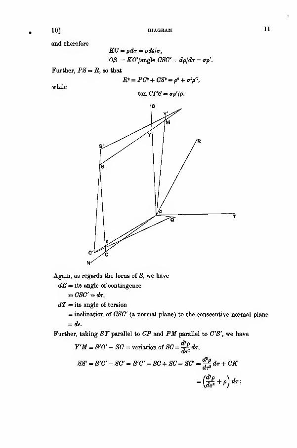
In the accompanying figure, drawn for the case of positive torsion,
PT, PN, PB are the tangent, the principal normal, and the binormal, of a
curve at a point P, so that BPN is the normal plane, TPN is the osculating
plane, and TPB is the rectifying plane ; G is the centre of circular curva-
ture, and S is the centre of spherical curvature, so that OS is perpendicular
to the osculating plane TPN. The principal normal at a consecutive point
Q distant ds from P is QC\ which does not meet PC because it lies in the
consecutive osculating plane at Q ; the centre of circular curvature at Q is
C ; and PQC is the osculating plane at Q. The centre of spherical curvature"
at Q is S' ; so that C'S', which is the intersection of two consecutive normal
planes at Q (and therefore passes through S, the intersection of three
consecutive normal planes at P), is perpendicular to the plane PQC ; thus
S, C, C, P lie on a circle, for both the angles SGP and SC'P are right.
Then
PC = P ,QC' = p + dP = PC, KC' = dP ,
neglecting powers of small quantities higher than those retained. Also
de = angle of contingence
= inclination of the consecutive normal planes SC'P, SC'Q
= angle PC'Q,
anddr = angle of torsion
= inclination of the consecutive osculating planes CPQ, C'PQ
= angle CPC = angle CSC;
* For higher terms, see Mathews, Quart. Journ. Math., vol. xxvi (1893), pp. 27—SO.
T It is made fundamental in his treatment of the subject : see, passim, his treatise Thforie
gfntrale.
X Quart. Journ. Math., vol. vii (1866), pp. 37—44.
10]
and therefore
DIAGRAM 11
KG = pdr = pds/a,
CS - KC/aagle CSC = dp/dr = ap.
Further, PS = R, so that
E 2 = PC + CS* = p2 + a*p\
tan. CP8=ap'Ip.
IB
while
Again, as regards the locus of S, we have
dE = its angle of contingence
= CSC = dr,
dT = its angle of torsion
= inclination of CSC (a normal plane) to the consecutive normal plane
= de.
Further, taking SY parallel to CP and PM parallel to CS', we have
Y'M = S'C -SC = variation of SC_d*p
dr,
SS' = S'C-SC=S'C-SC + SC-SC' =^dT + CK
(d>
-©+')*'
12 routh's diagram [ch. I
and therefore, for the locus of S,
d?pthe radius of circular curvature (pt) = p + -=-^
,
the radius of torsion (o-,) = - ( p + -r^J
.
11. The use of the diagram can be developed. Thus PC and QC do not
intersect; so the principal normals of the curve have no envelope. Let dc
be the arc-element of the locus of C ; then
(dcf = (CKf + {CKf = (pdrf + (dp)* = R*(dr)\
so that
/dcV = -R* = ,
\ds) o-2 ~~
.
while, if <p denotes the inclination of the tangent CC to the principal normal
at P (being equal to the angle CSP), we have
cot <p = ap'/p.
Next, denoting by dx the angle between PC and QC, we have, from the
spherical indicatrix,
dx = {(dey + (dry}iand so
ds \p* o*)'
a magnitude sometimes called the screw curvature of the curve at the point.
12. Two consecutive normal planes at P intersect in the line CS, which
is called the polar line. The plane TPB, perpendicular to the principal
normal PC, is called the rectifying plane ; it contains the binormal PB, but
two consecutive rectifying planes do not intersect in the binormal. Their
intersection, a line PR through P, is called the rectifying line; it can be
obtained as follows. The equations of QC, the radius of curvature at Q, are
X-ds _Y Z.
-de 1~ dr
'
and therefore the equation of the rectifying plane at Q, which is perpendicular
to QC, is
-(X-ds)de+Y+Zdr = 0.
Where this plane cuts 7=0, the rectifying plane at P, we have
-(X-ds)de + Zdr = 0,
or, ultimately,
-Xde + Zdr = 0;
hence the equations of the rectifying line PR are
7=0, Z=Xd€/dT = X<r/p.
Thus the inclination of PR to the binormal is tan-1 (p/a).

14] ASSOCIATED DEVELOPABLES 13
Associated Developables.
13. The equation of any plane, organically connected with a skew curve,
contains a single parameter ; the envelope of the planes is therefore a develop-
able surface. Among these, the most interesting are the envelopes of the
principal planes of the curve.
On the surface, which is the envelope of the osculating planes, the original
curve is the edge of regression (or cuspidal locus). To the consideration of
this developable we shall return in § 16.
The envelope of the normal plane is called * the polar developable. Its
equation is obtained by eliminating the parameter between
{X-x)x' +<J-y)y' + {Z-z)z' =0,
(X-x)x" + (Y- y)y" + {Z-z)z" = x'* + y'* + zJ* = \.
When these equations are taken together, without elimination of the variable,
they are the equations of the polar line; they can be changed into the
form
X-(x + P*x") _ Y-(y + p>y") _ Z-(z + P*z")
y'z"-z'y" ~ z!x"-x'z' ~ x'y"-y'x"'
verifying the property that it passes through the centre of circular cur-
vature and is perpendicular to the osculating plane; and any point on it
is a pole of the circle of curvature. Moreover, being the intersection of two
consecutive planes which are tangent planes to the polar developable, the
polar line is a generator of that surface.
The edge of regression of the polar developable is the locus of the centres
of spherical curvature ; and therefore (by § 8) its equations are
X-x Y-y _ Z-z _ t
y'z'" - z'y'"~
z'x"' - m'z'" x'y" - y'x'"P "'
Also, the osculating plane of the edge of regression at X, Y, Z is the normal
plane of the original curve at x, y, z; and the normal plane of the edge
of regression at X, Y, Z is parallel to the osculating plane of the original
curve at x, y, z.
14. The envelope of the rectifying plane TPB is usually called the
rectifying developable.
The reason for using the epithet arises from an intrinsic property of the
surface. The principal normal of the original curve is PN, perpendicular to
the plane TPB, and therefore coinciding with the normal to the rectifying
developable; hence the original curve is a geodesic (a line of shortest
distance) upon the surface. When a surface is deformed without stretching
* The names of the various surfaces were assigned by Monge, Applications de Vanalyse a la
giometrie (1795), quoted on p. 1.
14 ASSOCIATED [CH. I
or tearing, there is no change in the length of any portion of aDy curve
;
when a developable surface is developed into a plane, every geodesic becomes
a straight line. Thus, when the rectifying developable is developed into
a plane, the original curve becomes a straight line ; hence the name of
the surface.
The equation of the surface can be obtained by eliminating the parameter
between the equations
(X-x)x" + (Y-y)y"+(Z-z)z"=0,
(X - x) x'" + (Y-y) y"> + (Z-z) z'" = x'x" + y'y" + z'z" = 0.
When these equations are taken together, without elimination of the variable,
they are the equations of the rectifying line through P. They can be taken
in the equivalent form
X-x Y-y _Z-y"z'" - z"y'" z"x'" - x"z'"
~ x"f - y"x'"
'
Since
(y"z'" - z"y"J + (z"x" - x"z"J + (x"y'" - y"x"J
= (x"' + y"> + z"*) (x'"* + y'"* + /"») - (x"x'" + y"y'" + z"z"J
p'o* '
the cosine of the inclination of the rectifying line to the tangent is
PV(p*+o*)l
*', V", *'
*", y", *"
y'", *'"X
which is equal to p (ps + a3) ^, agreeing with a former result.
The edge of regression of the rectifying developable is given by theequations
(X-x)x" +(Y-y)y" +{Z-z)z" =0,
(X-x)x'" +(J-y)y"' +(Z-z)z'" =x'x" + y'y" + z'z" =0,
(X - x) x"" + (F - y)y"" + (Z-z) z"" = x'x'" + y'y'" + z'z'" = - l/p»
;
and therefore the point corresponding to P is given by
Z-zX-x Y-yy"z'" - z"f ~ z"~x
irr^x7^r'°-x"y"'-y"x"'
'
1
p*E'
where E is the determinant
«", y", z"
<»'", y'", z"'
x"", y"", z""
15] DEVELOPABLES 15
The value of E can be found in the same way as the value of D in § 9.
We have
1
p"aE = tx'x"
Ix'x"
Ix'x'"
2«"2, 2x"x'"
Xx"x'", Sx"">
lx"x"". 2x'"x""
When the values of the constituents in this determinant are substituted, wefind*
Ep" ds \ov
16. The rectifying developable can be usedf to determine curves the
ratio of whose curvatures is a known variable^ function of the arc.
Take any such curve, and construct its rectifying developable. Thecurve is a geodesic upon this surface and cuts the rectifying line at anangle ^r, where
p = a cot yfr,
while the rectifying line is a generator of the developable.
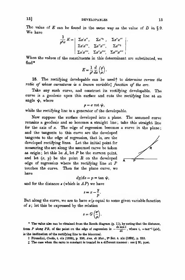
Now suppose the surface developed into a plane. The assumed curve
remains a geodesic and so becomes a straight line; take this straight line
for the axis of x. The edge of regression becomes a curve in the plane
;
and the tangents to this curve are the developed
tangents to the edge of regression, that is, are the
developed rectifying lines. Let the initial point for
measuring the arc along the assumed curve be taken
as origin ; let this be A, let P be the current point,
and let (x, y) be the point R on the developed
edge of regression where the rectifying line at Ptouches the curve. Then for the plane curve, we
havedy/dx = p = tan yfr,
and for the distance s (which is AP) we have
Vs = x--.
PBut along the curve, we are to have er/p equal to some given variable function
of s ) let this be expressed by the relation
'-*©•
* The value also can be obtained from the Bouth diagram (p. 11), by noting that the distance,
from P along PR, of the point on the edge of regression is -p— , where i, =tan-1 (p/<r),
is the inclination of the rectifying line to the binomial.
t Pirondini, Crelle, t. cix (1893), p. 238, Ann. di Mat., 2* Ser. t. xix (1892), p. 213.
X The case when the ratio is constant is treated in a different manner : see § 20, post.

16 OSCULATING DEVELOPABLE [CH. I
Then the plane curve into which the edge of regression has been developed
satisfies the equation
x-V- = G(P).
The primitive of this Clairaut equation is
y = cx — cG(c),
giving the aggregate of tangents; and the singular solution, being their
envelope, is given by the equations
y = ex — cG (c)1
= x-G(c)-cG'(c)j'
which thus is the equation of the developed edge of regression. Hence we
have the result :
—
To construct skew curves satisfying the relation s= G (<r/p), form the plane
curve
x = G(c) + cG'(c), y = c2 (?'(c);
bend the plane about the tangents to this curve, according to any assigned
law, so as to form a developable surface; the original axis of x in the plane
becomes, on the developable surface, a skew curve having the required property.
16. The osculating developable is the envelope of the osculating plane
of the curve. Its generators are the tangents to the curve ; and its edge
of regression is the curve itself.
This property suggests another method of analytical definition of a curve
in which the initial element is not a point of the curve as in the preceding
investigations, but is the variable osculating plane. This method was adopted
by Serret*, who has deduced by its means a number of results. The equation
of the osculating plane is taken in the form
z = px + qy — u,
where p and q are functions of the single parameter u. The envelope is, of
course, a developable surface ; its generators are given by the equations
z =px +qy — u\
= p'x 4- q'y — 1 J'
which thus are the equations of the tangent to the curve; and its edgeof regression is given by the equations
z = px + qy - u\
= p'x + qy -1
J
i)=p"x+q"y
* Liouville's Journal, t. xiii (1848), p. 353.
17] OSCULATING DEVELOPABLE 17
Thus the current point on the curve is given by the equations
x _ y z +u 1
q"--p"-pq"-qp"-p'q"-q'p"-Let
* = (q"p'"-p"q'")(p'q"-q'p")-°, T = {jfl + q» + (pq> - qp'f}ithen
dx , Ay ,. Az . , .. A ds mA
Hence the direction-cosines of the tangent are given by the equations
cos a = q'lT, cos @ = - p'/T, cos y = (pq' - gp')/^
and the direction-cosines of the binormal by the equations
cosX. cosu cos v ., „ „. _JL
We at once find
and therefore (§ 7) the radius of circular curvature is given by
P = r»A (i +p* + 5T* (pY' - s'p")-1,
while the radius of torsion is given by
o- = (l+_p2 + ga)A.
Serret-Frenet formulas.
17. The preceding results are conclusions derived from the analytical
definition of a curve by means of the coordinates of a current point. Another
method is founded upon certain differential relations belonging to all curves
;
and these relations are made precise, generically for families of curves,
individually for particular curves, by the assignment of some intrinsic
property or properties.
These general relations exist between the derivatives of the direction-
cosines of the edges of the principal trihedron at any point: sometimes
they are called * after Serret, sometimes after Frenet. They can be obtained
as follows.
The direction-cosines of the principal lines at any point of the curve
possess many notations; we shall take
cos a, cos 0, cos 7, (and a, a, a") as the direction-cosines of the tangent,
cos f, cos % cos f, (and b, b', b") „ „ „ principal normal,
cos \, cos /*, cos v, (and c, c', c") „ „ „ binormal,
* They are given in a memoir by Serret, Liouville'i Journal, t. zvi (1851), p. 193 : also in a
memoir (which had been a thesis) by Frenet, 16., t. xvii (1852), p. 437.
F. 2
18 SERRET-FRENET [CH. I
with the convention already adopted (§ 5), whereby these lines could be
displaced into coincidence with a set of coordinate axes without changing
the sense of any line*. Then
]cos a, cos /3, cos 7 = 1
:
I cosf, cosjj, cosf
ICOS X, COS fl, cos V
and each constituent of the determinant is equal to its minor. Also
cos o, cos f, cos X are the direction-cosines of the axis of x,
cos yS, cos i), cos /* „ „ „ „ y,
cos 7, cosf, cosi> „ „ „ „ z,
when the principal lines of the curve are taken as the axes of reference. Now
cos a = x', cos f = px";
henced cos a _ cos fds p
together with two similar relations for the derivatives of the other two
direction-cosines of the tangent. Again, we have
cos a cos X + cos /3 cos /x + cos 7 cos v = 0,
so that, becauseCOS f COS X + C08 7} cos p. + cos f cos v = 0,
it follows that
dcosX, _dcosu dcos;/
,a~s~ +008^-ar- +cos v~cos I
Also
hence
that is,
ds
d cos v
= 0.
. dcosX dcosu „, u»cos X —j— + cos u —j—- + cos v—;
— =;
ds ds ds
= ... = ...=0,dcos\ 1
ds cos fi cos 7 — cos v cos /3
d cosXI d cos /i. _ 1 d cos 1/
But
hence
cosf ds cos 17 rfs cosf cfe
coa\ = p(y'z"-z'y");
p {y'z"' - z'y'") + p'(j,V - *>") = ^",
p (z'x'" - x'z'") + p' (z'x" - x'z") = 0py",
PW ~ y'x'") + P' (x'y" - y'x") = Bpz".
Multiplying by x", y", z" respectively, and adding, we find
-p x', y', z' = -,
*", y", z"p
' *'", y", z"'
* The alternative convention leads to a change in the sign of <r throughout.
17] FORMULAE 19
so that
hence
d cos X _ cos £ds a
together with two similar relations for the derivatives of the other two
direction-cosines of the binormal. Further,
cos (?= cos /m cos 7 — cos v cos 8,
and therefore
d cos P d cos 7 d cos 8 d cos u.—j—- = cos /*—
-j—- — cos v —-j—1- + cos 7—-~- — cos 8
ds ^ ds ds ds ds
= - (COS fl COS f — COS V COS 1)) (cos 7 cos 1) — cos 8 cos f
)
cos a cos \
9 <r
together with two similar relations for the derivatives of the other twodirection-cosines of the principal normal.
These are the Serret-Frenet formulae satisfied by the derivatives of the
direction-cosines of the principal lines. They are taken by Darboux in the
form*da _b db _c a dc b
ds p' ds (T p' ds <r
'
Particular sets of simultaneous solutions of these equations are
a, b, c — cos a, cos f, cos \,
a, b, c = cos 8, cos t), cos /i,
a, b, c = cos 7, cos f, cos v.
The complete resolution of the equations can be made to depend upon
that of a single equation. Letf. _ a + ib
where i denotes V— 1 ; then
dl 1dl _ 1 Ida . db\ a +ds 1 — c \ds ds) (1 —(1 - c)a ds
~2» pl
2a'
* As compared with Darboux's earlier form, there is a change of the sign of <r (or of c), due
to the convention concerning the axes. But Darboux's later preference, Tkgorie giniraU, t. iv,
p. 428, is for the form here adopted.
f This combination of direction-cosines is of frequent use in differential geometry ; its effec-
tive introduction appears to be due to Weierstrass, though it occurs earlier in the work of
Lagrange and of Gauss on the conformal representation of a spherical surface upon a plane.
2—2
20 SERRET-FRENET FORMULA [CH. I
which is an equation for I of the Riccati form *, when p and a are regarded as
known functions of s. When I is known, however it has been obtained, the
complex quantity conjugate to I is known ; hence, writing
a + ib 1 a — ibZ =
1-c' m 1-c '
we have
a =1 — Im
I — m 'b = i
1 + lm
l-m ' c =I +ml — m'
18. These Frenet-Serret formulae can be obtained by another processf,
which is based directly upon their significance in relation to the curvature
and the tortuosity.
We take the direction-cosines of the principal lines at a point according
to the tableau
(a, a', a")
b, b', b"
c, c', c"
The direction-cosines of the principal lines at a consecutive point, referred to
the principal lines at the original point, are given by
1 , de , , for the tangent,
-de, 1 , dr, „ „ principal normal,
, — dr, 1 , „ „ binormal.
Hence
and therefore
a + da = a + bde,
b+ db = — ode+b + cdr,
c + dc = - bdr + c ;
da
dl
b db _c a dc _ b
p' ds a p' ds a-'
with similar relations between a', 6', c' ; and a", b", c".
These relations are of fundamental importance in the theory of skewcurves. The present process of establishing them is independent of theearlier analysis ; and so they can be used to obtain, easily, many of the results
already given. Thus
dz
and therefore
6 =d*x
_dx , _dyds
: ~ ds
-J*y
a =
"a?-"-"' v-pH-nr. *"-p5S-^,ds1
* For some of the properties of this equation, gee my Treatiie on Differential Equation,,(3rd ed.), § 110.
*
+ I am indebted to Mr R. A. Herman for this process.
19]
so that
Similarly
APPLICATIONS 21
p*(x"* + y"*+/'*) = l.
„, _d1a _ d (b\_ 1 /c _a\ _ b ,
X ~d^~d8 \p)~p[a p)~? P '
and so for y'" and z'"; thus

22 INTRINSIC DEFINITION OF A CURVE [CH. I
there in direction. Then at the point we have o = a,,', f = &'. *<> = V. and
so the constant is equal to unity at the point ;that is,
cos a cos a' + cos f cos £' + cos X cos X' = 1.
Alsocos" a + cos2 f + cos8 X = 1,
cos" a' + cos'f'+cos2 X'= 1
;
hence,
cos a = cos a', cos £ = cos £', cos X = cos X,
the first of which is
Similarly, we have
dx _da^
ds ds
'
dy dy dz _ dz'
ds~ ds ' ds ds'
and therefore
x — x = constant, y — y' = constant, z — z = constant.
The initial point has the same coordinates for the two curves, so that each
of these constants is zero ; hence
x - x = 0, y - y = 0, z - z = 0,
and therefore the two curves everywhere coincide. But the only changes
made in the second curve were in its position and its orientation in space
;
thus the two curves were originally the same, save for position and
orientation in space. Hence the proposition.
We can at once infer one result. It is known that both the curvatures
of a helix on a circular cylinder are constant ; hence every curve, which has
both its curvatures constant, is a helix on a circular cylinder.
More generally, it follows that all magnitudes, intrinsically belonging to
the curve, can be expressed in terms of p and <r and of their derivatives.
The main inference from the general proposition is that, for the intrinsic
and unique specification of a curve, we need to have the values of p and a given
as functions of s ; any complete equivalent of such data would also be needed,
if they were not provided ; and the.data are sufficient. If then only a single
equation is given, of any form, between p, a, s, we must expect some arbitrary
element to exist in the equations of the most general curve which satisfies
the condition implied by the single equation. In other words, we shall have
a family of curves : and a curve will be selected from the family by the
assignment of some special form to the arbitrary element.
Thus it has been seen that curves can be constructed satisfying an
equation 8 = (<r/p). For the purpose, it is sufficient to have a family of
developable surfaces bound by the property that, when the surfaces are
developed, the edges of regression become one and the same curve in the
20] SPECIAL FAMILIES OF CURVES 23
plane ; and the curves, satisfying the equation, are given by taking one curve
upon each member of the family of surfaces.
We shall now take a number of other examples* of this general result.
Curves having their Curvatures in a Constant Ratio f.
20. Let p/<r= k= tan A, suppose, where A is a constant. The Serret-
Frenet equations now are
da _b db _ a c _ — (a — ck) dc _ b _ bk
ds p' ds p a p ' ds a p'
which are linear in a,b,c; hence
d i-y (a cos A — c sinA + ib) = -. (a cos A — c sin A + ib).ds^ p cos A
Let
rds' P
'u = sec A
P
so that u is a real quantity, being a function of s ; then
a cos A — c sin A 4- ib = Re~iu ,
where R is an arbitrary constant. We must suppose that R is complex ; let
R = Per",
where P and 8 are real ; then
a cos A — c sin A + ib = Pe-»<«+8>.
Consequentlya cos A — c sin A — i& = Pe* (u+8)
;
and a2 + 62 +c2 =l.
Solving these three equations, we find
a cos A — c sin A = P cos (m + 8) = sin p cos (u + 8)
— b = P sin (it + 8) = sin jp sin (w + 8) ,
rt sin .4 + ccos.4 = (1 — P2)- =cosp
giving the values of a, b, c, the cosines of the inclinations of the three
principal lines to the axis of as.
Similarly, let p and 8' be the constants of integration for a, V, c, and
p" and 8" be the constants of integration for a", b", c", the respective cosines of
the inclinations of the three principal lines to the axis of y and the axis of z.
* The reader would do well to consider Darboux's treatment of these examples, and of others,
in his Theorie generate, t. i, §§ 6—12, 32—39.
t This is the one case not covered by the example in § 15. It appears to have been discussed
first by Puiseux, LiomiiUe's Journal, t. vii (1842), pp. 65—69. The analysis, which follows, is more
detailed than the treatment in Darboux and in Bianchi ; it is given so as to secure the most
explicit form of the analytical definition of the curves.

24 CURVATURES IN CONSTANT RATIO [CH. I
Then
a cos A - c' sin A = sin p' cos (u + 8')\ a"cos A — c" sin A = sin p"cos (u + 8")
-b' = sin p sin (u + 8'),
-b" = sinp" sin (« + 8").
a' sin .4 + c' cos 4 = cosp' ) a" sin .4 + c" cos .4 = cosp"
The primitive of all the three sets of equations, in this form, apparently
involves six constants; but they reduce to three. The three lines having
a, b, c; a', b', c' ; a", b", c" ; for their direction-cosines are perpendicular
to one another; the necessary conditions are satisfied by the relations
cot p cot p' _ cotp' cotp" _ cot p" cot p _ _ ,
cos (8 - 8')~
cos (S' - 8") ~ cos (S" - 8)~
To obtain the analytical definition of the curve, we note that
a = cos .A sinpcos(w + 8) + cospsin^4,
so that
x — x = s cosp sin A + cosA sinp I cos (u + 8) ds,
and similarly
y — y = s cosp' sin A + cos A sinp'J
cos (u + 8') ds I'
z— z„ — s cosp" sin A + cos A sinp" I cos (u + 8") ds
where
u = sec 4if*.J P
and a;, y0> z are arbitrary constants. The new arbitrary constants
xo, y<>, Zo affect the position of the curve in space: the surviving constants
8, 8\ 8" affect its orientation.
There is nothing in the problem to limit the value of p. Hence it maybe taken to be an arbitrary function of s ; and so, for the range of variation of
this arbitrary function, we have a family of curves intrinsically distinct from
one another. But all the curves of the family have two properties in common.
We have
a sin A+ c cos A = cosp, a' sin .4 + c' cos .4 = cosp', a" sin4+c" cos .4 = cosp";
hencesin A = a cosp + a cos p' + a" cos p",
cos A = c cosp + c cosp' + c" cosp".
The first of these two relations shews that the tangent to the curve is at a
constant inclination ^tt — A to the line whose direction-cosines are cosp,
cosp', cosp'' (for 2 cos*p= 1), that is, to a fixed line; and the second shews
that the binormal is at a constant angle A to the same line. Moreover
= b cos p + b' cos p' + b" cos p",
that is, the principal normal is perpendicular to the same line. It therefore

21] CURVES HAVING ASSIGNED TORSION 25
follows that this line is the rectifying line of the curve : that is, along any
curve the rectifying line has a constant direction, and the rectifying developable
is a cylinder. The generators are the rectifying lines: and the curve is a
geodesic on the surface.
A curve on a surface which makes a constant angle with a fixed direction
is called a helix. It therefore follows from the preceding investigation that
a curve, having the ratio of its curvatures constant, is a helix. The establish-
ment of the converse proposition—that a helix has its curvatures in a constant
ratio—is left as an exercise.
Curves having assigned Torsion, variable or constant.
21. Let the torsion be given as a function of the arc. With a, a', a"
;
b, b', b" ; c, c', c" ; as the direction-cosines of the principal lines, we have
t./ >, in i dc V dc" b"a = oc —be, -j- =
, —j- = .
as a- as aTherefore
(„ dc' , dc"\Cds-
C-ds-)'
with two similar equations ; so that
dx = ads = - a- (c"dc' - c' dc")
dy = a'ds = — a(c dc"— c"dc ) -.
dz = a"ds = — <r(c'dc — c dc )
Also we have
c2 + c's + c"2 = 1
;
and from the value of the torsion in general, we have
fdcV fd&y (djy _ 1_
\ds)+
{ds)+\ds) ~
a*'
Now, when the torsion is given, a is a known function of s ; and therefore
the quantities c, c, c" are three functions of s, subject to these two equations,
that is, one arbitrary element survives among the three functions.
The first of the equations is satisfied by taking
c = sin 8 cos<f>,
c = sin 6 sin<f>,
c" = cos 6,
for any values of 8 and tf> : and then the second of the equations is satisfied,
provided
(d0)! + sin20(tty)
2 =(^Y.
With these values, we have
dx = — a (cos 8 cos<f>
sin 8d<f> + sin <f>d8)'
dy = — a (cos 8 sin <j> sin 8d<j> — cos <f>dd)
dz = a sin20d<f>
26 CURVES OF CONSTANT TORSION [CH. 1
All the magnitudes involved are functions of one parameter, which can be
chosen at will ; we choose z to be the parameter. As already indicated, an
arbitrary element will remain in the equations ; accordingly, we assume
tan $ =/(*)>
where / is an arbitrary function of z. Then
fd
<t>=
l
Z£Ji
dz >
sin»*=l±A co^. ST-1-/' ;
and therefore
de -(ff 1 f" Idads^f 1+f \»rf
Consequently
JL ,
i+/8i ff i/" id*ds\>_(idsY
<r(l +/2) «/' - 1 -p \l +/» 2 /' 2 ds dW U <**/
'
a relation between z and s, involving the arbitrary function /; in particular,
it expresses ds/dz in terms of z and s. Also
dx + idy = - e* cot (dz - io- tan 0d0)"l
dx - idy = - e~<* cot (dz + ia tan 0d0)J'
which are the (integrable) analytical equations of the curve when substitution
is made for tf>, tan 0, dd ; and they involve an arbitrary function /, while z is
the parameter of the equations.
As is to be expected, the simplest case arises when the torsion is constant.
It is not necessary, for the construction of the analytical equations of the
curve, that the equation giving ds/dz should be retained. We have
as the equations of the curve ; or, substituting for<f>,
we find
dx= -*f"-f'-wr dz]
dy = - W"-ff Jas the analytical equations of curves of constant torsion l/<r, where /, =f(z),is arbitrary in the equations*.
* This is Serret'a form of the equations of curves of constant torsion: see Liouville'B editionof Monge (quoted p. 1), p. 566.
22] CURVES HAVING ASSIGNED CURVATURE 27
Curves of constant torsion have formed a subject of many investigations
in comparatively recent years, especially those which are algebraic curves.
Thus taking the formulae
dx=-a(c"dc'-c dc")
dy=-a(c dc"— c"dc ) -,
dz = — a (c' dc — c dc')
where a now is supposed constant, Fabry assumes that c, c', c" are integral
functions of sines and cosines of integer multiples of a parameter t, such that
each of the quantities on the right-hand side is devoid of a term not involving
sines or cosines when expressed as a sum of terms each involving only one
sine or cosine. Again, Fouche takes the Weierstrass expressions (§ 17)
_ 1 -afi , _ . l+q/3 „ _ a + /3
with o and /8 as algebraic functions of a parameter: and imposing the
conditions that dx, dy, dz must be the exact differentials of some algebraical
functions, he obtains a critical equation that admits many evident solutions*.
And from the relation
*"'-®"it can be proved that no algebraic curve of constant non-zero torsion exists
on a sphere.
Curves having assigned Circular Curvature.
22. Let the radius of circular curvature be given as a function of the arc.
Then the quantities a, a', a" satisfy the relations
a2 + a'2 + a"3 = 1,
/da\2. /daV fda"\/day /dory /dory _ i
\ds)+{ds)
+\ds)
~P
!
where p is a known function of s ; and therefore a, a', a" are three functions
of s, subject to these two equations, that is, one arbitrary element survives
among the three functions. Also
dx = ads = apdS, dy = a'ds = a'pdS, dz = a"ds = a"pdS,
where S is a new parameter related to s by the equation
^ = dS;P
* References to the memoirs by Fabry and by Fouche as well as to other papers on the
subject are given by Darbouz, Thiorie ggnerale, t. iv, p. 429, in the course of a Note on the
torsion of skew curves, which is specially commended to the reader's attention.
28 EXAMPLES [CH. I
and then
x - a;„ = I apdS, y - y„ =J
a'pdS, z-z =J
a"/jd/S,
where a, a', a" are functions of S such that
a2 + a'8 + a"2 =l,
day /do'y /da'V _
,
ds)+\ds)
+ Us)_1 -
The case, when p is constant and equal (say) to k, is not analytically
simpler than the case when p is variable ; the parameter 8 is merely s/k.
EXAMPLES.
1. When the circular curvature of a curve is zero at all points, the curve is a
straight line ; and when the curvature of torsion is zero at all points, the curve is plane.
2. Shew that the determinant
*", y", s"
*'", y, *•"
srt f", r
vanishes for a helix ; and conversely.
3. Prove that the radius of circular curvature of the locus of the centre of spherical
curvature of a curve is R -j- ; and indicate analogies between the formulae of plane
curves, connecting the magnitudes usually denoted by ;•, p, <p, ijr, p, with the formulae of
skew curves connecting the magnitudes denoted in the text by R, p, <p, t, pi-
Prove that, for any curve drawn upon a sphere, the relation
P
is satisfied.
S+a(-J)-°. or ' + S=°-
4. A helix is drawn on a circular cylinder of radius a and cuts the generators at a
constant angle a ; shew that both the circular curvature and the torsion are constant, that
the rectifying line at any point is the generator of the cylinder, and that the locus of the
centre of circular curvature is another helix upon a coaxial cylinder.
Hence shew how to construct the circular cylinder which contains the helix having at
a point the closest (three-point) contact with a curve.
5. Prove that, if a curve be drawn so that its tangent has a constant inclination to a
fixed direction in space, the ratio of its curvatures is constant.
6. Shew that, for a spherical helix,
p=a sec a (cos2 a -cos2 dp, o-=a cosec a (cos2 a -cos2 0)i,
and that the cross-section of its rectifying developable is an epicycloid.
7. A loxodrome is drawn on a sphere of radius a, cutting a set of meridians ata constant angle a. Shew that, at an angular distance from the pole, its radius of
circular curvature is a (1 - cos2 6 cos2 a)~ * sin 6, and its radius of torsion is
a (1 - cos2 6 cos2 a) sec a cosec a.
EXAMPLES 29
8. Prove that the radius of circular curvature of the edge of regression of the recti-
fying developable at the point corresponding to P is sec i-p( cos2£-3-.
J, where i is the
inclination of the rectifying line to the binormal at P ; and that the radius of torsion is
d ( „ .ds\
9. Prove that the circular curvature of the locus of the centre of circular curvature of
a skew curve is
1 2 o'M"|4ripV d /y\ if ^>\_\W ds\p ) R\ p
2A4 J
10. Obtain the direction-cosines of the rectifying line in the form
{ptf+po- (yV - jCjO} (p2+*2
)~ *.
with two similar expressions.
11. Denoting -=-tby x
t , and similarly for derivatives of y and z, prove that
zl i *m >2n
are independent of the axes of reference.
12. Shew that the torsion of the curve
and
x={bc{b-c)}i j {(&-*) (c-*)}-4*
y= {co(c-a)}4
\ {(c-t){a-t))~^dt
z={a6(a-6)}4 f{(a-<)(&-0}~ 4cfc
is constant. Indicate the character of the spherical indicatrix of its tangents and of its
binomials.
13. Prove that the radii of curvature and torsion of an involute of a curve are
a _ p2 +o'i
(p2+*2
)
:
14. In the Serret-Frenet formulae, let
4 ' p{<rp'-p<r's.
a+ib _ (ti-e)i
1 -c_ e
where e denotes the integral \p~ 1ds; shew that v satisfies the equation
dv i .
-r = - sin (v - 1).as cr
15. In a particular curve, the direction-cosines of the binormal are given by
c=Acos0+ jiCOs30, c'=X'sin0+ /*sin30, c"= K+2rfcos20,
where 8 is a current parameter, and X, X', p., k, d are constants such that
" l --*** v-l'+V-vA -<£4V-v>*,A--— + -(<** -3M*)*, X'
Prove that the curve, if of constant torsion, is algebraic.

30 EXAMPLES [CH. I
16. Curves (often called Bertrand curves*) are such that the relation
5 + 5-1p *
is satisfied, where m and n are constants : shew that the curve is analytically defined by
the relations
dx= mAdS-n(.A"dA'-A-dA")
rfy= mA'dS-n(AdA"-A"dA ) ,
dz=mA"dS-n(A'dA -AdA'),
where A, A', A" are three functions of a parameter subject to the conditions
A*+A'2+A"*=l,
(dS)* ={dAf+ (dA'f+ (dA"f.
17. Proye that, if two curves have the same principal normals, their osculating planes
cut at a constant angle a ; and shew that they are Bertrand curves.
Also prove that, if c denote the common distance of corresponding points,
<r<r'*=<?cosec2 a.
18. Shew that a curve, intrinsically defined by the equations
p = ks, <r= Is,
where k and I are constants, lies on a circular cone, and is a helix on that cone.
19. Prove that, for any skew curve,
*"'= - \* - p- x"+ i (yV - //').
with corresponding expressions for y"', «"'; also
with corresponding expressions for y"", *""; and indicate a method of obtaining the
general form of the expressions for the rath derivatives of x, y, z with regard to *.
Shew that the value of a""*+y""2+*"" 2 is
20. Denoting four consecutive points, at equal small intervals da on a curve, by 1, 2,
3, 4, by 12 the chord joining the points 1 and 2, and so for the other chords, prove that
12 . 34 + 23 . 14-13 . 24= i ^-. (<&)«.6 pV
21. A helix is drawn on a surface making a constant angle a with the axis of z. Shewthat its curvature is given by the equation
sin „ =„ picosx-p)^}* f(p-ftcosx)ft)*ni
\ p(ft-ft) )+n
*\ p(ft-ft) I '
where ft and ft are the radii of curvature of the principal sections, ra, and n^ are thedirection-cosines with regard to the axis of z of the tangents to the sections, and x is givenby the equation
cosaeinx=M3,
where cos-1 n3 is the angle between the axis of 2 and the normal to the surface.
* After Bertrand's memoir, Liouville's Journal, t. xv (1850), p. 332.
EXAMPLES 31
22. The six coordinates of the principal lines of a curve with regard to fixed rect-
angular axes are a, a', a", a, a, a" ; b, V, b", /3, /3', 0" ; c, c', c", y, y', y" ; the first three, in
each case, being the direction-cosines. Prove that
da_§ds p
' j — — — -fttjas a- p as a
23. A curve is given as the intersection of two surfaces
<t> (*. y, »)=o, V' (*i y. *)=°
;
the quantities D, E, F denote the determinants
D, E, F=<f>x> <ps , <p.
k denotes (D^+E^+F2)
-^, and a derivative of any quantity U is denoted by U',
where
Obtain the following results* for the curve at any point :
—
(i) The equation of the osculating plane is
(X-x)(EF'-E'F)+(Y-y) {FD' -F'D)+{Z-z) (DE'-D'E)=0 ;
(ii) The radius of circular curvature and the radius of torsion are given by the
relations
±=k*{(EF'-E'F)l +(1FD'-F'DF+(DE'-&EW,
P
J-=*°| D , E , FjD', E', F'
| D ,,^ E,^pn
* Other results are given by FroBt, Solid Geometry, (3rd ed., 1886), §§ 628 et seq.
CHAPTEK II.
General Theory of Surfaces.
Much of the present chapter is founded upon the memoir by Gauss, Disquisitwnes
generates circa superficies curvas, (Ges. Werke, t. iv, pp. 217 et seq.); and some account of
the memoir is given in Salmon's Analytical Geometry of Three Dimensions.
Frequent reference should be made to portions of the first volume and the third
volume of Darboux's treatise. Much of chapter in and chapter iv of Bianchi's treatise
will be found useful, as also will the first section of Knoblauch's Einleitung in die
allgemeine Theorie der krummen Flachen.
It is unnecessary to give copious references in detail ; the subject-matter is bound to
be treated in any book on differential geometry.
Fundamental Magnitudes of the First Order.
23. In the discussion of the intrinsic properties of a surface, the position
of the surface relative to coordinate axes is not of importance ; and therefore
there is convenience in substituting, for the equation of the surface in
Cartesian form, other equivalent equations that shall have more direct refer-
ence to variation upon the surface itself. This usually is effected by expressing
the coordinates of any point on the surface in terms of two independent
parameters p and q, through relations
x = x(p,q), y = y(p,q), z = z(p,q);
the elimination of p and q between these relations leads to the equation
of the surface, if it should be required. We shall assume, unless there is
explicit statement to the contrary, that we have to deal with surfaces or
portions of surfaces, which are regular in character, and within the range of
which no singularities (whether of point or line) occur. The parameters pand q are not necessarily real ; often it will be expedient to take conjugate
or other complex variables as the parameters of reference. Within the
range considered, the functions x (p, q), y (p, q), z (p, q) are finite and
continuous, usually uniform ; if they are multiform, we shall usually restrict
the variations to regions which admit no interchange of branches of
the functions. Also, a representation in terms of two parameters is not
unique; for if we make p and q two independent functions of two new
24] FUNDAMENTAL MAGNITUDES 33
parameters p' and q', we shall have x, y, z given as functions of p' and q, of
the same type as before.
A curve drawn upon the surface can be represented by some relation
between p and q, say
<f> (p. q) = 0,
whether the relation be integral or differential. Sometimes the curve can
be obtained by making p and q functions of a single parameter ; for instance,
geodesies are discussed by this method of representation among others.
A notation for derivatives with respect to p and q will be required;
we write
dx _ dx
Tp-*1' dq
= X*'
&x _ d*x d2x _dp"*"' dpdq'*1*' dq1
'*"'
and so on, with corresponding symbols for derivatives of y and of z. The
notation will occasionally be used for derivatives of other magnitudes as
they arise.
24. Take any point on the surface, determined by p and q ; a»d consider
a neighbouring point, also on the surface, determined by the values p + dp and
q + dq. When we retain only the first powers of small quantities, the distance
between the two points measures the infinitesimal arc on the surface ; denoting
it by ds, we have*ds2 = da? + dy- + dz"
= Edp* + ZFdpdq + Gdtf,where
E= xit + y1
i + z1i =Xxl
i\
F = xt x„ + y^y2 + ztzt = l,x^x2
G = x,2 + y? + zf = 1x?
These quantities E, F, G are independent of the particular selection of
perpendicular coordinate axes; for when we effect an orthogonal trans-
formation
x' — a + \x + fiy +vz,
y' = b + \'x + fiy + v'z,
z' = c + \"x + fi"y + v"z,
we have
E' = 2#/a
= a^SX2 + 2xryi 2\/i + 2a;,^ 1\v + y? 2/*2 + 2ylz1 2/u; + z? Xv*
= otf + y?+z? = E,
* We shall always write dx- instead of {dx)2, and similarly lor other powers and lor other
quantities.
F. 3
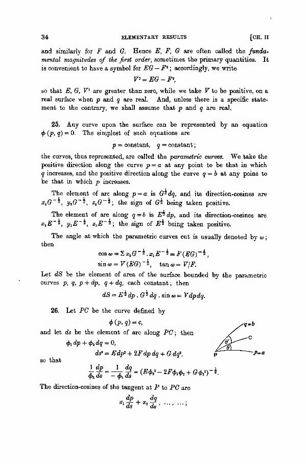
34 ELEMENTARY RESULTS [CH. II
and similarly for F and G. Hence E, F, G are often called the funda-
mental magnitudes of the first order, sometimes the primary quantities. It
is convenient to have a symbol for EG — F3; accordingly, we write
V2 = EG - F\
so that E, G, V- are greater than zero, while we take V to be positive, on a
real surface when p and q are real. And, unless there is a specific state-
ment to the contrary, we shall assume that p and q are real.
25. Any curve upon the surface can be represented by an equation
4>(p, q) = 0. The simplest of such equations are
p = constant, q = constant
;
the curves, thus represented, are called the parametric curves. We take the
positive direction along the curve p = a &t any point to be that in which
q increases, and the positive direction along the curve q = b at any point to
be that in which p increases.
The element of arc along p — a is G^dq, and its direction-cosines are
xs (t~2, y2G~~, ZzG~*; the sign of G% being taken positive.
The element of arc along q = b is E*dp, and its direction-cosines are
Xii?-*, yxE~', 2,^
_5; the sign of E$ being taken positive.
The angle at which the parametric curves cut is usually denoted by w;
then
cos to = 2 x2G~$ .
x
xE~ i = F(EG)~^
,
sin a> = V (EG) ~i, tan a> = V/F.
Let dS be the element of area of the surface bounded by the parametriccurves p, q, p + dp, q + dq, each constant ; then
dS = E$dp. G^ dq . sin a = Vdpdq.
26. Let PC be the curve defined by
and let ds be the element of arc along PC; then
0! dp + <\>i dq = 0,
ds> = Edp*+2Fdpdq + Gdq\ p~ P=aso that
£J- =^ £-<**- **•** +**.'>-*.
The direction-cosines of the tangent at P to PC are
x ^P + xdSCl
ds+X
'ck' -' -'

26] FOR CURVES ON A SURFACE 35
and so, if 6 is the angle (taken as in the figure) at P between PC and p = a,
we have
sin0 = (?-*F^as
= V^\G (E<f>2* - 2F<j>1 fr + G#)} ~ *
Similarly, if & be the angle (taken as in the figure) at P between PCand q = b, so that
8 + d' = tD,
we have
sin0' = ^-*F$as
= - Vfr {E {Etf - iFhfr + G^)}-i.
Next, let another curve PC be given by
•
-f (P. 4) = c'.
and let 8s, Sp, Sq represent small variations along the curve at the point P.
Let x denote the angle at P between PC and PC ; then
ds Ss cos % = 2,(x1 dp + x2 dq) fa Sp + x2 Sq)
= Edp Sp + F(dp Sq + dq Sp) + Gdq Sq,
ds Ss sin ^ = V(dp Sq — Sp dq),
so that
cog = Efcfa - F(<fh^ + foifr) + Qfrfi
* (## - 2/^, + G0,*)* (£f22 - 2/>2^ + G^,2)*
'
sin = V(<fr.^i--^.^i)
(E& - 2F<j>l <f>1+ G<t>$ {Etyi - 2^1^! + GW)*
It follows that too directions, given by dp : dq, and Sp : Sq, are perpen-
dicular, if
Edp Sp + F(dp Sq + dq Sp) + GdqS.q = 0;
and that, if two directions are given by the quadratic equation
®dps + 2$ dp dq + Vdq"~ = 0,
3—2
36 SOME ANALYTICAL [CH.II
their inclination x *s given by
sin x C0S X2F(#a -0¥)* FW-2F&+G®'
so that they are perpendicular if
EV - 2^0) + G® = 0.
Thus the curves orthogonal to a family f(p, q) = a, for varying values of
at, are given by the differential equation
27. Let X, F, Z be the direction-cosines of the normal to the surface
at P. It is perpendicular to every tangent line to the surface and therefore,
in particular, to the tangents at P to the parametric curves ; hence
Xxx + Yyx + Zzx= 0, Xx2 + Yy2 + Zz2
= 0.
Also
X 2 + Y" + Z* = 1 :
consequently*
X = (y1 zi -y1 z1)V-\ Y=(z1 x2 -z2 x1)V~1, Z = (x1 y2-x2 y1)V-\
or, with a customary notation,
X, Y, Z= ^
The following relations, capable of easy verification, may be noted for
future use
:
V=
:\x
lY-y
1X = (z1F-z2E)V
ytZ -z,Y = (xlF-x2E)Vz
lX-x1Z=(ylF-y2E)V
dVdxx
dV<>yi
dv^- = x2 Y-y2X j
= y2Z-z2Y\
= z2X — x2Z
X, Y, Z
xit 2/i > zi
xv> Vii zi
x2 Y- y2X = (>,(? - z2F) V'1
y2Z-z2 Y =(xiG-x2F)V~1
z2X-x2Z =(ylG-yiF)V->}
gz— **+*r
dVdy~r~
ZiX+XiZf
;
d^- = -xl Y + yiX)
* As V is taken positive, the signs given to A, Y, Z are effectively a definition of the positivedirection of the normal.
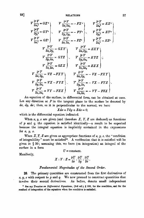
28] RELATIONS 37
°y*
dx^dyx
dxi dx2
y *r
dz1 dz2
= GXY\
= -FX*
= - FY* \
,
= -FZ*
V'lA-^EX*
r 5Z~ SZt
d*Vdx2 dys
= EXY
3sVV^-Z-= GYZ
V ±L- = OZXOZl OXi
V£-4-=VZ -FXY\
V^-^ = VX-FYZ
V J?-i-=VY-FZXoz1 ax2
V^- = EZXdz3 dx2
d*VStfjSy,
= -VZ -FXY\
V £-L- = -VX- FYZ
V^-4- = -VY-FZX0Z3 OX!
An equation of the surface, in differential form, can be obtained at once.
Let any direction at P in the tangent plane to the surface be denoted bydx, dy, dz; then, as it is perpendicular to the normal, we have
Xdx + Ydy + Zdz = 0,
which is the differential equation indicated.
When x, y, z are given (and therefore X, Y, Z are deduced) as functions
of p and q, the equation is satisfied identically—a result to be expected
because the integral equation is implicitly contained in the expressions
for x, y, z.
When X, Y, Z are given as appropriate functions of x, y, z, the " condition
of integrability " must be satisfied*. A verification that it is satisfied will be
given in § 30; assuming this, we have (on integration) an integral of the
surface in a formU= constant.
Manifestly,
X-Y-Z=— — —dx ' dy ' dz
'
Fundamental Magnitudes of the Second Order.
28. The primary quantities are constructed from the first derivatives of
x, y, z with respect to p and q. We now proceed to construct quantities that
involve their second derivatives. As before, denote small independent
* See my Treatiie on Differential Equations, (3rd ed.), § 152, foi the condition, and for the
method of integration of the equation when the condition is satisfied.
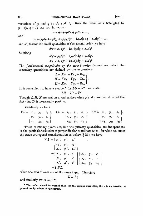
38 FUNDAMENTAL MAGNITUDES [CH. II
variations of p and q by dp and dq ; then the value of x belonging to
p + dp, q + dq has two forms, viz.
x + dx + %d?x + %d*x + ...,
andx + (x,dp + x2dq) + % (xn dp* + 2xndpdq + x^dq*) + ...;
and so, taking the small quantities of the second order, we have
d*x = xu dp* + 2xKdpdq + x^dqK
Similarly
d*y = yndp* + 2yKdpdq + ywdq\
d'z = zu dp* + 2z12dpdq + z^dq*.
The fundamental magnitudes of the second order (sometimes called the
secondary quantities) are defined by the expressions
L = Xxn + Yyn + Zzu"
M = Xxn + Yy12 + Zz12
N = Xxa + Yy22 +Zza _
It is convenient to have a symbol * for LN - M 2; we write
LN-M° = T>.
Though L, M, N are real on a real surface when p and q are real, it is not the
fact that T* is necessarily positive.
Manifestly we have
VL = rt ,

29] OF THE SECOND ORDER 39
29. The quantities X, Y, Z are functions ofp and q ; their first derivatives
with respect to p and q can be expressed by means of L, M, N. For
Xx! + Fy2 + Zzx- 0,
and therefore
Z,«i + F.y, + Zsz, = - (X#„ + Yylx + Zzn ) = -L.
Similarly, from Xar2 + Fy2 + Zz%= 0, we have
X,xt + Y1y1 + Z1z2 = - (Xxa + YyK + Zz^) = -M;
and, as X2+ F2+ Z2 = 1, we have
X1X + F1F+ 1Z=0.
Solving these three equations for Xx , Yit Zu we have
X1V=-L(y2Z-zaY)-M(zlY-y1Z),
and therefore (§ 27)
X^2 = - L (xxG - x2F) - M(- a^F+ x^E)
= x, (FM - GL) + x2 (- EM+ FL)'
Y1 V* = y1 (FM-GL) + y2(-EM+ FL)
£,F2 = zx (FM - GL) + z2 (- EM+ FL)
In the same way, we find
X2F2 = x, (FN- GM) + x2 {- EN + FM)Y2 V* = y, (FN- GM) + y, (-EN + FM)
.
ZJT* = *, (FN -GM) + z,(- EN + FM)
From these, we have
x^ = X1 (-EN + FM) + X2 (EM- FL),
xtT* = X, (- FN + GM) + X2 (FM- GL);
and similarly for yx and y2 in terms of F and F2 , and for z, and z.2 in terms
of Zx and Z2 .
and similarly
Also we have
V'(Y1Zi-YiZi)= yi, y* FM-GL, -EM + FL
FN-GM, -EN + FM= VX.V*T*,
and so for the others ; thus
V(Y1Zt -Y2Z1)=T"XV(Z
1X2 -ZSX1 ) = T*Y
F(XlF2-X2F1) = T^,
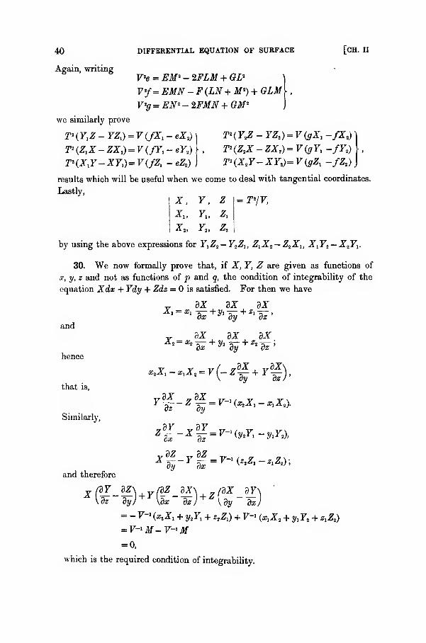
40
Again, writing
DIFFERENTIAL EQUATION OF SURFACE [CH. II
V*e = EM" - 2FLM + GL*
F 8/= EMN - F(LN + M8) + GLM
\,
V*g = EN* - 2FMN + GM2
we similarly prove
r (YXZ - YZ,) = V (/X, - eX2)j
T2( Y*Z - YZ,) = V (gX, -/X2) }
T* (Z>X - ZX,) = F(/F - eY2) , T*(Z2X - ZX,) = V(gYx -/F2)
T'iX.Y-XY^ V(fZx- eZ,) ) T8 (X2F-XF2)= F((^ -fZ,) J
results which will be useful when we come to deal with tangential coordinates.
Lastly,
X, Y, Z =T*/V,
Xu Yu Zx
X2 , F2 , A>
by using the above expressions for YXZ2— Y„Zlt ZlXi — Z2X1 , XJT^ —X2YX .
30. We now formally prove that, if X, Y, Z are given as functions of
x, y, z and not as functions of p and q, the condition of integrability of the
equation Xdx + Ydy + Zdz = is satisfied. For then we have
and
hence
that 19,
Similarly,
„ dX dX dXX^x^+y^ + z^,dx
dX,
dxdXdx
YTz~
Z% = ^{xiX1-xiX2).
dx
and therefore
fdY dZ
BZ
dxx %-y di-y-^ ^
x (dY dZ\ fdZ dX\ fdX dY\A\dz dy)
+ y\dx--^) +
Z{dy--dx)dy
= - F-' faX, + y2Yx + z2Zx) + F"1 faX2 + y,F2 + z,Z2)
= 0,
which is the required condition of integrability.
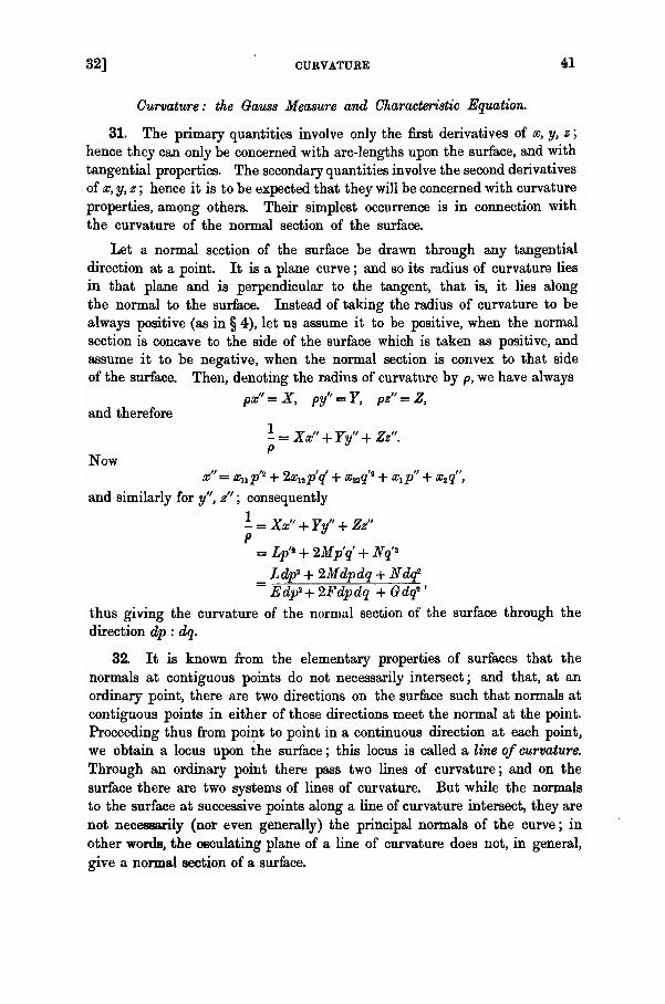
32] CURVATURE 41
Curvature: the Gauss Measure and Characteristic Equation.
31. The primary quantities involve only the first derivatives of x, y, z;
hence they can only be concerned with arc-lengths upon the surface, and with
tangential properties. The secondary quantities involve the second derivatives
of x, y, z ; hence it is to be expected that they will be concerned with curvature
properties, among others. Their simplest occurrence is in connection with
the curvature of the normal section of the surface.
Let a normal section of the surface be drawn through any tangential
direction at a point. It is a plane curve ; and so its radius of curvature lies
in that plane and is perpendicular to the tangent, that is, it lies along
the normal to the surface. Instead of taking the radius of curvature to be
always positive (as in § 4), let us assume it to be positive, when the normal
section is concave to the side of the surface which is taken as positive, and
assume it to be negative, when the normal section is convex to that side
of the surface. Then, denoting the radius of curvature by p, we have always
px"=X, py" = Y, pz"=Z,and therefore
Now
- = Xx" + Yy" + Zz".P
x"= Xitp'2 + Ix^p'q' + x^q' 11 + x^p" + x2 q",
and similarly for y", z" ; consequently
- = Xx" + Yy"+Zz"
= Lp'i +2Mp'q' + Nq'i
Ldpi + 2Mdpdq + Ndq*~ Edp*+ IFdpdq + Gdq*
'
thus giving the curvature of the normal section of the surface through the
direction dp : dq.
32. It is known from the elementary properties of surfaces that the
normals at contiguous points do not necessarily intersect; and that, at an
ordinary point, there are two directions on the surface such that normals at
contiguous points in either of those directions meet the normal at the point.
Proceeding thus from point to point in a continuous direction at each point,
we obtain a locus upon the surface ; this locus is called a line of curvature.
Through an ordinary point there pass two lines of curvature; and on the
surface there are two systems of lines of curvature. But while the normals
to the surface at successive points along a line of curvature intersect, they are
not necessarily (nor even generally) the principal normals of the curve; in
other words, the osculating plane of a line of curvature does not, in general,
give a normal section of a surface.
42 PRINCIPAL RADII [CH. II
The intersection of consecutive normals along a line of curvature is called
a centre of curvature of the surface ; as there are two lines of curvature at
each point, there are two centres of curvature and both of them lie upon the
normal. As we pass over the surface, we have two such points associated
with each point on the surface ; the locus of these points is called the surface
of centres. The distance between the point and a centre of curvature, with
its proper sign, is called a radius of curvature of the surface ; thus at any
point there are two radii of curvature, sometimes called the principal radii.
They are the radii of curvature (as defined in § 31) of normal sections
through the respective directions.
At a point x, y, z, let r be a radius of curvature, and let f, 77, f denote the
corresponding centre of curvature ; then
f = x + rX, 7) = y + rY, f= z + rZ.
For a normal at a consecutive point on a line of curvature, the quantities
f, i), £ r are unaltered ; hence first variations along the line of curvature are
such that
= dx + rdX, = dy + rdY, = dz + rdZ,
and therefore, for the line of curvature, we have
= (a;, + rX,) dp + {x2 + rX2) dq,
= (y, + rY,) dp + (y, + rYt) dq,
= (*, + rZ,) dp + (sa + rZt) dq.
These are apparently three equations ; in reality, they are equivalent to only
two equations because, multiplying them by X, Y, Z respectively and adding,
we have a nul result.
Multiplying the equations by xlt ylt zx respectively and adding, we have
= (E + rlx.X,) dp + (F+ rZx^,) dq
= {E- rL) dp + (F-rM)dq;
and multiplying them by xlt y3 , z3 respectively and adding, we have
= (F + rXx^XJ dp + (G + rZx2X2) dq
= (F-rM)dp + (G- rN) dq,
so that along any line of curvature we have
= (E-rL) dp + (F-rM)dq= (F-rM)dp + (G-rN)dq
'
These two equations, combined, determine the directions of the lines of
curvature and the radii of curvature at any point.
For the directions, we have
= Edp + Fdq -r(Ldp + Mdq),
= Fdp + Gdq - r (Mdp + Ndq) ;
32] OF CURVATURE 43
they are given by
Edp + Fdq , Fdp + Odq = 0,
Ldp + Mdq, Mdp + Mdqthat is, by
(EM- FL) dp* + (EN- GL) dpdq + (FN - GM) dq*= 0.
Unless the equation is evanescent, it is quadratic in the ratio dpjdq; andtherefore at any point of a surface there are generally two lines of curvature.
Moreover, as
E(FN-GM)-F(EN- GL) + G (EM - FL) = 0,
the two lines are perpendicular to one another (§ 26) at the point.
Exception to the conclusion, that there are two lines of curvature at
a point, occurs when the equation giving those directions is evanescent.
We then have
L_M_N _1E F~G'~k'
say. The radius of curvature of a normal section of the surface through anydirection, being
Edp* + 2Fdpdq + Gdq*
Ldp* + 2Mdpdq + Ndq2 '
is equal to k, independent of the direction and therefore the same for all
directions through the point. Such a point is an umbilicus on the surface
;
the character of the surface in the vicinity of such a point will be considered
later.
To determine the magnitude of the radii, we eliminate dpjdq between
the equations. Then
E-rL, F-rM =0,
F-rM, G-rNthat is,
TV - (GL - 2FM+EN) r + V* = 0,
so that there are two values, respectively corresponding to the two directions.
These must be associated correctly. Should a value of r be given, the value
of dp/dq (which determines the direction) is equal to either of the fractions
_ F-rM _G-rNE-rL ' F-rM'
Should a direction be given, the radius of curvature of the surface (which, in
general, is not equal to the radius of curvature of the curve) is equal to either
of the fractions
Edp + Fdq Fdp + Gdq
Ldp + Mdq : Mdp + Ndq
'
44 MEAN CURVATURE [CH. II
33. A pair of symmetric combinations of the radii are of importance.
These are the mean curvature H, where
and the total curvature (or the specific curvature or Gauss measure) K, where
1 T*
the quantities a and /3 denoting the two radii. It will be proved that T' is
expressible in terms of derivatives of E, F, G, so that the total curvature
depends only upon the fundamental magnitudes of the first order. The same
property does not belong to the mean curvature.
Later, it will be seen that, for a minimal surface (that is, the surface of
least area with any assigned boundary), the mean curvature H is zero, so that
the equation
GL-2FM+EN=0is characteristic of a minimal surface. But this equation may be satisfied
along a line or lines, on any surface.
The Gauss measure of curvature is positive for a synclastic surface or for
the synclastic portions of a surface, that is, at places where all the surface near
the point lies on the same side of the tangent plane; familiar instances of
synclastic surfaces are provided by the inside of a bowl, a closed soap-bubble,
and the palm of a hand. The Gauss measure of curvature is negative for an
anticlastic surface or for the anticlastic portions of a surface, that is, at places
where different adjacent parts of the surface lie on different sides of the tangent
plane ; familiar instances are provided by a saddle-back, the top of a mountain
pass, and a ridge between two fingers of a hand. The Gauss measure of
curvature is zero for a developable surface ; familiar instances are provided by
the rolling shutter of a desk, and a crumpled piece of paper.
34. To establish the result just stated as regards the total curvature, as
well as to establish the intrinsic significance of the six fundamental magni-
tudes which have been introduced, it is necessary to obtain further relations
;
and then it will appear that the six magnitudes are not functionally
independent of one another. Let quantities m, m', m", n, n, n" be dennedby the equations
m = x1xu +y1yn + z1zll = $E1
m' = xtfn + y^y-a + z^K = %E2
m" = x&n + yiyia + zlZa = F2- £G,
n = x2xu + y2yn + z2zn = F,- \E2
n = xtx12 + y2y13 + z2z12= £(?,
>>
n = x^Xn + y2ys + ziZi2 = \G2

34] gauss's measure of curvature 45
other quantities I\ T', T"; A, A', A"; will be required, as defined by the
equations
V'T =mG -nF} V"A = nE -mF\VT' = m'G -n'F\, FaA' = n'E -m'F\,
FT" = m"0 - n"F) F2A" = ri'E- m"F)
which also give
m = ET + FA) m' = ET' + FA'\ m" = ET" + FA"\
n = FT + GA j'
ri = FT' + GA') ' n" = FT" + GA" J
'
Solving the equations
Xxu + Yyn + Zzn = L,
*i«n + yij/ii + 21*11 = w,
aWi + yayn + ^n = n,
for xu , yn , zn , we have
Ftu = Z, (y^a- z1y2) + m {y2Z - z2Y) + n(z-J- y^Z)
= LVX + y(x1G-xiF)+^. (- «,F + «^),
that is,
xu = LX + #!r + x2A.
Similarly for yu and zn ; the values are
a;u = LX + a^T + #3A^
yu^ZF+ y.r + y.Al.
^ = i^ + *,r +«2aJ
We proceed in the same way to obtain the other second derivatives of
x, y, z; their values are
xu = MX + atj" + a;2A")
yli = MY + y1 T' + y2A'\,
zn =MZ + ZiT' + z2A')
xw =NX + XjT" + x2 A"\
y^ = NY+y1 T" + y1A"\.
zm = NZ+zlT" + z2A")
For the moment, let
I =xnx!a + yuy!a + z11 zxl ,
l' = x]23 +y12
* +v;then
m2— ml' = V —I, «,' — w2
= V — I,
and the common value gives
l'-l = $(Ev-2FK + Gu).
46 gauss's characteristic equation [ch. II
Now
a,.5 + y»* + *i»* = M (
Xx» + 7V" + Zz^ + r ' ^XlXli + yiVvi + ZlZl^
+ A' (x2xl2 + y2y,2 + z2z12)
= Ma +mT + n'^
= M* + (Eri* - 2Fn'm + Om' 1) V~*
= M" + (ET' 1 + 2FT'A' + GA' 2),
and
xuxa + ytlya + zaza = L (Xx^ + 7ya + Zz&) + T (x,xw + y^y* + z,za)
+ A (x2x^ + y2ysB + z2z^= 2,2V+m'T + n"A
= LN + {Enn" - F (nm" + ri'm) + Gmm") V^= LN + {ETT" + F (rA" + T"A) + GAA"J
;
hence
LN-M'+ {E (ran" -n'^-F (nm" - 2rim + nm) + (mm" - m *)} P"2
= 1-1'
= ~h(Ea -2Fu + G11 ),
and therefore
LN - M2 = V*K= - i (En - 2F12 + Gn)
- {E (ran" - n'2) - F(nm" - 2n'm' + n"m) + (mm" - m' 2
)} F"2
= - $(Ea-2F12+ Gn) + (E, F, G$T', A')2 - (E, F, G$T, A$r", A").
This is sometimes called* the Gauss characteristic equation. Its chief
significance lies in the fact that LN— M* is expressible in terms of E, F, Gand their derivatives of the first and the second order; hence it follows
that the total curvature is expressible in terms of the fundamental magnitudes
of the first order and their derivatives, a result that is important in connection
with the deformation of surfaces.
Mainardi-Codazzi relations.
35. There are also two relations of a differential type. We have
3 _ a
dq^'dp*12 '
and so, substituting for xn and xVi their values that are linear in X, xly xt
(§ 34), we find
LX2 + a^r2 + x2A2 + XL2 + xnr + x^A
= MX, + «JY + a,A,' + XM, + xnT' + ar12A'.
On substitution for Xu X2 , xn , xn , x^ in terms of X, xu x2 (§§ 29, 34), this
equation becomes
X® + an® + xjd" = 0,
It was obtained first by Gauss in his celebrated memoir of 1827 already (p. 32) quoted.
35] MAINARDI-CODAZZI RELATIONS 47
where= L2
-Mx + Mr + NA - LV - MA'
& =FK+r2- iy + r"A - fa'
©" = - EK + A2- A,' + TA' - l
vA + AA" - A' 2
Proceeding similarly from yn and yw , and from zn and z12 , we have
F© + ^0' + y2@" = 0,
Z® + ^@' + «„©" = 0.
It follows, from these three relations linear in ®, ©', ©", that
© = 0, ©' = 0, ©" = 0,
as their determinant is not zero.
When the same process is applied to xa and xx ; to y12 and ym ; and to z12
and zw ; three relations are obtained which similarly lead to
$ = 0, <I>' = 0, <D" = 0,
where4> =N1 -M, + MA" + LV" - MY' - NA'
<*>' = - gk + r," - iy + rr" - r' 2 + r'A" - r"A'
<£>" = FK + A," - A2' + T"A - T'A'
Apparently, there are six relations; we proceed to shew that all of them
are satisfied in virtue of
(i) the Gauss equation,
(ii) the relations © = 0, 4> = 0,
(iii) necessary identities.
The last are connected with the derivatives of various quantities that occur,
and they are as follows.
Because
%El= m = ET + FA, \E2 =m' = ET' + FA',
it follows that
^-(ET + FA) = ~ (ET' + FA').
When this is expanded, and we substitute for ra — IY and A2 — A/ in terms
of 0' and 0", we find
E& + F&' = 0.
Similarly, proceeding from
JG, = n' = JT' + GA', $0, = n" = FT" + GA",
we find
FV + G*" = 0.
48 MAINARDI-CODAZZI [CH. II
Again, becauserul— nl
' =F1S— \E&— $Gn ,
when we expand the left-hand side and use the Gauss equation, we find
F®' + G®" = 0.
Lastly, because
m" — m.2 = Fu — %Ea — $GU ,
when we expand the left-hand side and use the Gauss equation, we find
E& + F<&" = 0.
Hence, retaining the Gauss equation, we have the relations
m' + F®" = 0] E& + FQ>" = 0\
F& + G&' = OJ' F& + GQ>" = j
'
which are satisfied in virtue of our necessary identities ; that is, we have
0'=O, 0" = O, 3>' = 0, <D" = 0,
because V2,= EG — F%
, is not zero.
It therefore follows that the relations to be retained are the Gauss charac-
teristic equation, together with the relations @ = 0, <& = 0. These two
new equations are
L2 +TM +bN = ikf, + T'L + A'M'L + A'M)
"L + A"M)'
they frequently are called the Mainardi-Codazzi relations* In all, therefore,
there are three differential equations which the six fundamental magnitudes
of the first and the second order must satisfy. It remains to be seen what
element, if any, of generality is possessed by a surface if and when it is
determined by six magnitudes, which are given initially and which satisfy
the three differential equations.
The Mainardi-Codazzi relations can be expressed in a different (but
equivalent) form. We have
dq\VJ~V * V* 2
= ix2 -^(r' + A"),
\v)~v Ml v Vldp
1 M-4*.-f(r + A');
* They were given, though not in the adopted form, by Mainardi, Giorn. 1st. Lomb., t. ix
(185G), p. 395; and, in the adopted form, by Codazzi, Ann. di Mat., t. ii (1868), p. 273.
36]
hence
RELATIONS 49
d (L\ d (M\ 1 , T ... L ,„, A „v if /ri A ,.
V= 4.(-XA"+21fA'-jyA)
and similarly
4(tH(t)-t<-«-*»«"-Hwhich are the Mainardi-Codazzi relations in another form.
36. The necessary identities used in establishing the relations can be
used also to obtain two other results, connected with the angle o> between
the parametric lines. We have
3 (VA} _ d_f7A'\
dq \ E ) dp\ E_VA~ E
VA' VA(r' + A")+j_(A2-A/)-^(r + A')- — Ei+E E E"
VA'
EiE>
E (A, - A/ + AA" - A' 2 + TA' - T'A)
= VK, in virtue of 6" = 0.
Similarly, in virtue of <£" = 0, we have
d(VT"\ d(Vr\_dj>\-G-)-dq\-G)-
VK-
Now the angle w between the parametric lines is given by tan a> = V/F;
henceFdV-VdF
day = EG
Consequently
and therefore
and similarly
so that
= -^Q-yiFGdE - 2EGdF + EFdG).
2EGVO}, = FGE, - 2EGFX + EFG,
= FG.2m- 2EG (n + m!) + EF . 2n'
= - (2ET' + 2GA) V\
(VA VT'\ai = -{-E
+-G-)''
(VA' VT"\w>=-\-E-
+-<r)>
(VA Vr'\, /FA' 7T"\ ,
dm = tojdp + m2dq = - l-^- + —gJdp - I -^- +
—q~J«?•
F.

50 BONXET S [CH. II
Moreover,'FA VV
and
"3pl G ) dq\E r .
which are the two results in question. The second of them gives Liouville's
form for the total curvature.
&»12
Bonnet's Theorem.
37. We now come to the theorem which is the essential justification for
considering the differential geometry of surfaces in connection with the six
fundamental magnitudes. It was proved * first by Bonnet, and may be
enunciated as follows:
—
When six fundamental magnitudes are given, and when they satisfy the
Gauss characteristic equation and the two Mainardi-Codazzi relations, they
determine a surface uniquely save as to its position and orientation in space.
The equations, satisfied by X, xlt x, when they are regarded as three
dependent variables, are
and
Xn — lj\
x,, — MX
-~{FM-GL)xi -yi{-EM-^FL)xt =
— rx1
— r'xt
- Axa=
f
- A'*. = J
(i).
P = X2 -y2(FN- Gil)*, ~yA~ EN + FM)x2 =
Q = x12 -MXR = xa -NX
...(ii).-T'x, -A'a^O- r>, - a>, = o )
Both sets are linear in the dependent variables ; derivatives with regard to poccur only in set (i) and with regard to q only in set (ii).
The primitivef of the linear set (i) is of the form
X = %A+r,B + ZC
«i = ?<h + vbi +& (iii),
*a = %<h + yba + fc,
• Journ. Ec. Polytech., eah. xlii (1867), p. 81.
t See my Treatite on Differential Equations, (3rd ed.), § 173.

37] FUNDAMENTAL THEOREM 51
where f, rj, £ are arbitrary constants so far as concerns derivation with respect
to p, that is, are arbitrary functions of q so far as concerns set (i). Also
X, #1, x2 = A, o„ (h;
X, a>u a:2 = B, 6,, 6a ;
£. , Xi , a;2 = o, Cj , c2 ;
are particular sets of integrals of the equations, linearly independent of one
another ; and any linear combination of them with coefficients, that are inde-
pendent ofp and that combine them as in (iii), is also a set of integrals of the
equations (i).
But the equations (ii) are to be satisfied simultaneously with (i). Con-
sequently they must be satisfied by the quantities (iii) ; and the variables at
our disposal for this purpose are f, % f, which are functions of q alone.
Accordingly, for the equations (ii), £, -q, f become the dependent variables
while q is the independent variable. Let
P, Q, R take values* P„ Q„ J2, when X, xit x2 = A, a,, «2 ;
Pi, Qi, Ri = 2?, 6,, 62 ;
-P31 Q31 -K3 = C, Ci, c2 ;
then when the expressions (iii), which must satisfy the equations (ii), are
substituted in those equations, we have
dl; , drj d%a2
dq'+ b2
dq~+C
*dq~= (ZRt + vRt+SR,)
These equations (iv), regarded as determining f, 77, f, must provide a primitive
involving those quantities and expressing them as functions of q alone, even
though the coefficients in these equations involve the quantity p, which now
is parametric. The requirement will be met if the values of f, i), £, as given
by (iv), also satisfy the relations
dA d£ 35 drt , dC dt,+„ _. +
dC dX (t?£i T ,._dp dq dp dq dp dq \dp~r
''dp~r*dpj+ V-5Z + b
dP,\
3a, df 36, dp 3c, df = _ U dQi dQt ^dQ3\
dp dq dp dq dp dq \ dp dp dp)•(v);
dp dq dp dq dp dq
Sajdf 36a dy 3cjdf / .. dRi 322, y,dRs\
dp dq dp dq dp dq \ dp dp dp
)
and these relations will be satisfied if it can be shewn that they are conse-
quences of equations (iv) and of the earlier equations, regard being paid to
the three differential relations satisfied by the fundamental magnitudes.
* The values Q x , Qt , Q3 actually are zero because the third equation in (i) is the same as
Q= ; the symbols are retained for symmetry.
4—2
52 bonnet's [ch. ii
The three equations in (v) can be- taken separately and the process is
mainly the same for each of them ; we therefore set out the details in con-
nection with the first.
Because of the first of equations (i), we have
F*M = (FM - GL)a, + (-EM + FL)a,op
say; and
op
V 3- = «Ci + tca .
dp
Multiply the second of the equations in (iv) by s, the third by t, add, and use
the immediately preceding results ; we have
.)•^f +|^ +fi)--f<* +,*>-'<*- +,«- f('ft+ <*
This will be the same as the first of the equations (v)—which accordingly
will be a consequence of earlier equations—if
V^ = sQi + tRu
op
We proceed to shew that these relations are satisfied. We have
Pi =d
4~ Yi(FN ' GM)ai -V' (
- EN+FM)a'
say ; and, similarly,
dq
R1= d-^-NA-r"a1 -X%.
dq
HencedP, _ VA
Butdp dpdq ^dpyv) ai dp\vv v*dP v*dp-
dA s
so thatdp ~ V'^ + V'
*'
d*A s 3a, t da
dp~dq~~T*dq'+V*~dq'^
Uldq \V*J
^ U*d~q
+ ^(?>) +a4(r°)'
37] THEOREM 53
and therefore
3-Pi _ s 3aj t 3a2
lp ~T*dq~+ Vt
~dq
+ a, {4(T*)"|W} + 0i {4(^)"|(W}-~ (LA + Fa, + Aa2)
-~ (MA + Fa, + A'aa)
+ a's (f) - 1(£) + <r
'
s - vw + <r'< - ™>/ 7i}
+~(sM^tN-s'L-HM).
When the coefficient of a, is evaluated, it is found to vanish in virtue of the
Mainardi-Codazzi relations. The coefficient of a2 vanishes in the same way.
And the coefficient of A vanishes identically. Hence
V^ = sQ1 + tR1 .
Similarly
V^^sQ. + tR,,
V^-p^sQs + tR,.dp
Consequently, the first of the equations in (v) is satisfied in virtue of
earlier equations and of the differential relations among the fundamental
magnitudes.
Next, to obtain the second of the equations in (v), we multiply the three
equations in (iv) by L, T, A, and add. After corresponding calculations
similar to those just given, and by using the relations in § 35, satisfied in
virtue of the Gauss equation and the Mainardi-Codazzi relations, we find
that the result reduces to the required second equation in (v).
And to obtain the third of the equations in (v), we multiply the three
equations in (iv) by M, T', A', and add. Calculations similar to those for the
second equation are required; the result reduces to the required third
equation in (v).
Thus the equations (v) are satisfied, in virtue of earlier equations that
are retained, and in virtue of the differential relations among the fundamental
magnitudes. Consequently the equations (iv) possess a primitive which
expresses f, t], f as functions of q alone even though the coefficients in the
54 ESTABLISHMENT OF [CH. II
equations, in the form in which they actually occur in the general investiga-
tion, may involve p parametrically. This primitive is of the type
f = X£, + M& + v%t
'
t) = \7)1 + fify + VI),
where X, fi, v are arbitrary constants; fn t}u £,, being functions of 3 alone,
are a special set of integrals; and likewise for £,, t?2 , £2 ; &» Vs> ?a5 the three
special sets being linearly independent. When these values of f, 17, f are
substituted in the expressions (iii), we have
X = XA + jjB + vC \
x, = Xa, + /ib, + vc, I (vi)i,
#2= Xa, + ^b2 + vc«
)
whereA = f4 + 77lJB + ?1C,
as= £ia2 + %&2 + ^Cj,
and so for B, b,, b2 ; and C, c„ c2 . Thus A, a^ a,; B, b,, b2 ; C, c,, c2 ; are
three particular sets of solutions of the original six differential equations to
be satisfied ; and the values of X, xit sc2 in (vi^ constitute the primitive of the
six equations.
The equations, determining Y,yu yit are precisely the same in form as the
six which determine X, xx , a2 ; and likewise those for Z, zu z2 . Hence the
primitive of the equations for Y, yu y2 is
F=X'A + /B+»/C
y1= \'a1 + fi'b1 + v'c1
(viy,
y2 = X'aj + /u/b2 + v'c?
and the primitive of the equations for Z, zt , z» is
Z = X"A + Al"B + v"Czt= \"a, + /t"b, + i/'c, (vi)s ;
z.2= X"a2 + /i"b2 + v c2
where, in (vi)2 , X', fi, v; and, in (vi)a , X", /*", v"; are arbitrary constants.
38. Thus the complete primitive appears to contain nine arbitrary
constants which are produced in sets of three by the integration of the
equations. But these equations are themselves merely inferences from
earlier fundamental equations, among which are
Z2 + F2 + Z* = 1, *,« + y* + z? = E,
Xx1 + Yy1 + Zz1= 0, x1 x.2 + yly2 +z1zi
= F,
Z«2 + Fys +^2 = 0, orf + y* + z? =G;and therefore these equations must be satisfied.

38] bonnet's theorem 55
Now, substituting in X* + Y* + Z2 = l the values given by the primitives,
we have
Aa2\a + 2ABSV + B2V + 2AC2X.I/ + 2BC2fii> + C a2*2 = 1.
But A = X, B =Y, C = Z are particular solutions, so that
A2 + Ba + C 2 = 1.
Hence writing
k,, ks , k3 , kt , kt , ke= S\2 - 1, t\/i, 2/jl
2- 1, 2A.i>, 2^i>, 2v2 - 1,
we have
A2*! + 2AB&2 + B2
fc3 + 2ACfc4 + 2BC)fc5 + C 2&6 = 0.
Similarly from Xa:, +Tyx + Zz1= 0,v/e have
Aa,&, + (Ab, + a,B) fa+ Bb,k3 + (Ac, + a,C) kt + (Be, + b,C) ka + Cc,&6= ;
and from the other four relations in turn, we have
Aa,&, + (Ab2+ ftjB) kt + Bb2fcs + (Ac2 + a„C) kt + (Bc2 + b2C) k, + Cc2&« = 0,
a,2&, + 2a,b,fc2 + b,2^ + 2a,c,A4 + 2b,cA + c,a&6 = 0,
a,ajA;, + (a,b2 + aub,) kt + b,b2A;3 + (a,c2 + a,c,) kt + (b,ea + b2c,) k5 + CjCjfc, = 0,
a^jfc, + 2a2b2 fc2 + tyk3 + 2a2C2A;4 + 2b2e2&6 + c22A;6 = 0.
Thus there are six equations linear and homogeneous in the six constants k.
The determinant of the coefficients on the left-hand sides is equal to
A, B, C
a,, b,, c,
a^ d2 , o2
that is, to V*, and so it does not vanish. Hence all the constants k are zero,
that is,
2\2 -l = 0, 2/w = 0,
Iff - 1 = 0, 2i>\ = ,
Si/2 -1 = 0, 2\/t = 0;
and therefore the nine constants \, fi, v are the direction-cosines of three
perpendicular lines.
Finally, we have, for the surface itself,
dx = x1dp + x3dq,
that is,
x — I = \ I (a,dp + &idq) + p I (b,dp + b2dq) + v I (c,dp + o2dq),
= \u + fiv + vw;
and similarly
y — V =\'u + fi'v +v'w,
z-l" = \"u + p"v + v"w,
where I, V, I" are additive arbitrary constants of integration.

56 DERIVED [CH. II
The relations between the constants \ leave the orientation of the surface
undetermined ; the existence of the constants I, V, I" leaves the position of the
surface undetermined.
And so we have Bonnet's theorem as enunciated.
39. It follows from this theorem that the six fundamental magnitudes
E, F, G, L, M, N, together with their derivatives, are sufficient for the
expression and the determination of all magnitudes and all properties that
are intrinsically possessed by the surface. Later we shall see that, as is to be
expected, some properties are common to all those surfaces which (roughly
at the moment) may be*described as having E, F, G in common without any
regard to L, M, N other than the Gauss characteristic equation. At present,
the important result is that the six magnitudes give uniquely the intrinsic
determination of a surface and that therefore they suffice for the expression
of all properties of the surface which are independent of its position and its
orientation.
Derived Magnitudes.
40. It has just been stated, as an inference from Bonnet's theorem, that
properties and magnitudes intrinsically possessed by a surface are expressible
in terms of the three fundamental magnitudes E, F, G of the first order,
of the three fundamental magnitudes L, M, N of the second order, andof their derivatives. Now it happens, as might be expected, that certain
combinations involving first derivatives of L, M, N have relations with deri-
vatives of x, y, z of the third order similar to those possessed by L, M, N withderivatives of x, y, z of the second order. Similarly certain combinationsinvolving second derivatives of L, M, N have corresponding relations withderivatives of x, y, z of the fourth order ; and so with the respective ordersin succession. The combinations, which thus arise, are sometimes calledfundamental magnitudes; having regard to the essential significance of thefundamental magnitudes of the first order and the second order, the newcombinations may be called derived magnitudes of the various orders.
The derived magnitudes are perhaps most simply defined in connectionwith the variation of the curvature of the normal section of the surfacealong a curve * In particular, those of the third order are defined by therelation
Ts [p)= pp's + bqp*v' + 3iW + s<p.
The values of P, Q, R, S are obtained as follows. As before (§ 31), we have
-X = x" = xu p'* + 2x,iP'q' +x^ + xiP" + x2q",
* This will be seen, at a later stage, to imply the consideration of geodesic tangents to the
41] MAGNITUDES 57
with two similar equations. Multiplying them by a;,, yx , zlt and adding, wehave
Ep" + Fq" + vip'* + 2m'p'q' + m"q'1 = ;
multiplying them by x^, y2 , z2 , and adding, we have
Fp" + Gq" + np'* + 2n'p'q' + ri'q'* = 0.
Hence
Now
- p" = I>'2 + 2T'p'q' + T'Y2
- q" = Ap'a + 2A'pV + A"9'2
- = Lp* + 2Mp'q' + Nq'\
and therefore
jg (-) = LlP* + (Z, + 2JfI)j>V +W +^.W + ^9*
+ 2 (Zp' + %')l>" + 2W + -^V) 9"
= (Z, - 2Zr - 2MA)p'3
+ (Z„ + 2JIT, - 4>LV - 2MT - 4MA' - 2NA)p'*q'
+ (2iWs + N, - 2LT" - 4MT' - 2MA" - *NA')p'q'*
-r (Ni -2MV" -2NA")q'\
on substitution for p" and q". Having regard to the Mainardi-Codazzi
relations, and reverting to the definitions of P, Q, R, S, we have values of the
derived magnitudes of the third order in the form
P = Ll -2(LT + MA)
Q = Z2 -2(Zr + ilfA')
= Jf, - (Zr' + MA') - (MT + FA)
R = M,- (Mr' + NA') - (LV + MA")= if, - 2 (Mr + NA')
S = N1 -2(MT" + NA")
It is not difficult to verify that these derived magnitudes of the third order
satisfy the differential relations
P, - Qi = 2 (Pr + QA') - 2 (Qr + -RA) + 2K(FL - EM),
Q%- R,= PT" + QA" - (RT +SA) + K (GL - EN),
R2 -S,=2 (QT" + RA") - 2 (RT' + SA') + 2K(GM- FN).
41. The derived magnitudes of the fourth order are defined* in con-
nection with the second derivative of the curvature along the normal section
from point to point of any curve ; they are such as to give
d?
VSee a paper by the author, Messenger of Math., vol. xxxii (1903), pp. 68—80.
.
,(!) = («. A 7 , &,eW,q'Y-
58 DERIVED [CH. II
By a process similar to that used for the investigation of the values of
P, Q, R, S, we find
o = P,-3(Pr+QA)= P> - 3 (PT' + QA') - §K (FL - EM)= Q. - 2 (Qr + RA) - (PV + QA') + $K (FL - EM)
7 - Q* - 2 (QI" + RA') - (PT" + QA") - \K (GL -EN) \
= R, - 2 (QI" + JJA') - (i?r + SA) + %K (GL - EN)
8 = ^-2 (QT" + RA")-(RV + SA') - \K (GM - FN)=
(S1-3(Er' + SA') + %K(GM-FN)
e = Si-3(Rr"+SA")
The derived maguitudes of any order m, thus defined, involve derivatives
of x, y, z of order m.
42. The first derivatives of the Gauss measure of total curvature, and of
the measure of mean curvature, can be expressed in terms of the derived
magnitudes of the third order. We have
V*K=LN-M-\and therefore
V'Kl= L,N + LN, - 2MMX
- 2^ (LN - M*).
When we substitute for Z,,Mlt iV, in terms of P, Q, R and other magnitudes,
also for Vu and reduce, we find
V*KX = NP- 2MQ + LR\and, similarly,
V*Kt = NQ-2MR + LS
In the same way for H, the measure of mean curvature, we find
V*HX= GP - 2FQ + ER
V*Hi = GQ-2FR + ES''
Cor. When a surface has the property that there is a functional relation
between its principal radii of curvature, the relation can be expressed in
a form
f(H,K) = 0,
or in the Jacobian form
thus its fundamental magnitudes must satisfy the equation
GP-2FQ + ER GQ-2FR + E8NP-2MQ+LR NQ-2MR+LS'
Such a surface is usually called a Weingarten surface, and referred to as
a surface W : some of the properties will be discussed hereafter (§§ 203—208).
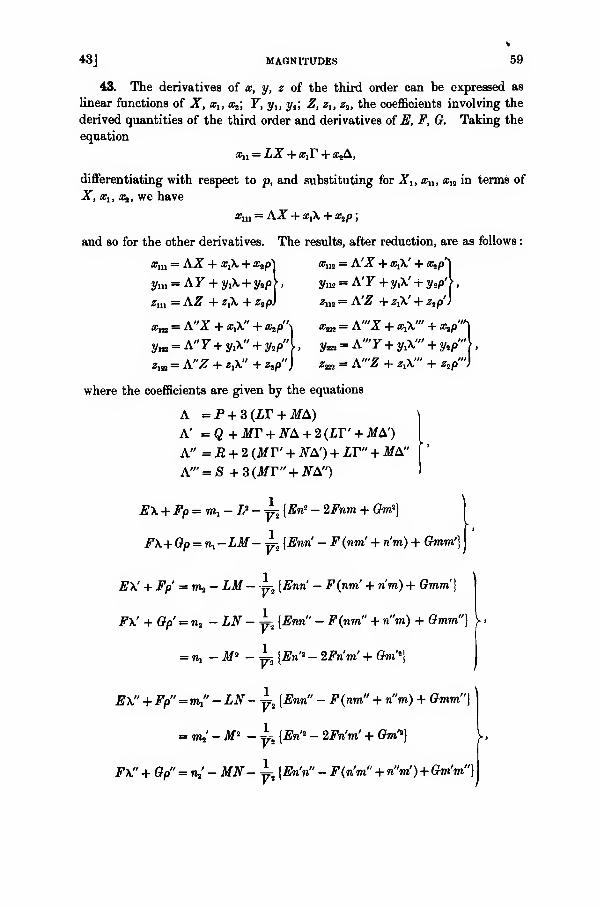
43J MAGNITUDES 59
43. The derivatives of x, y, z of the third order can be expressed as
linear functions of X, xlt x2 ; Y, ylt t/2 ; Z, zx , z„, the coefficients involving the
derived quantities of the third order and derivatives of E, F, G. Taking the
equation
xu = LX + <r,r + XjA,
differentiating with respect to p, and substituting for Xlt xn , xw in terms of
X, Xi, Xz, we have
xul = AX + x{X + x2p ;
and so for the other derivatives. The results, after reduction, are as follows
:
xm = AX + x{X + xtp\ x112 = A'X + xX + x2p"\
ym = A'Y +yX + y^p'},
zm = A'Z + zX + ztp')
xm = A'"X + xX" + x*p"*
y** = A'"Y+ yX" + y,p"
z^ « A'"Z + zX" + z,p"
ym^AY + yJ^+ ytp
zm = AZ + z{X + zt p.
xva = A"X + xX + a<w"
yla = A"Y+y1\" + y,p"
zw = A"Z + zX' + V.where the coefficients are given by the equations
A = P + S(LV + MA)
A' =Q+Mr + NA + 2(LT' + MA')
A" = R + 2 (Mr + NA') + LT" + MA"
A'" = S + 3(MT" + NA")
EX +Fp=m1 -L*- y* {En* - 2Fnm + Gm?)
F\+Gp = 71,-LM- y2\Enri -F(nm' + n'm) + Gram'}
EX' + Fp = m2 -LM- y2[Enn' - F(nm' + n'm) + Gmm'}
FX' + Gp = n2 -LN-y2{Enn" - F(nm" + n"m) + Gmm"
= m, - M* - ~ {En'1 - iFnm' + Gm'*\
EX" + Fp" = m,"-LN-y2{Enn" - F(nm" + n"m) + Gmm"\
= rrh'-M* -~ {En'1 - 2Fn'm' + Gm'*} \
,
FX" + Gp"^n.'-MN-y {En'n" - F(n'm" + n"m')+ Gm'm"}
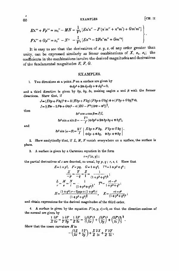
gQ EXAMPLES [CH. II
E\"' + Fp'" = ml' -MN - yt[Erin" -F {rim" + ri'iri) + Gm'm"}
F\>" + GP'" = «," -N* -yt
[En'"- - 2Fn"m" + Gm">)
It is easy to see that the derivatives of x, y, z, of any order greater than
unity, can be expressed similarly as linear combinations of X, xu x2 ;the
coefficients in the combinations involve the derived magnitudes and derivatives
of the fundamental magnitudes E, F, G.
EXAMPLES.
1. Two directions at a point P on a surface are given by
edpi+ 2<t>dpdq+irdqi=0,
and a third direction is given by bp, 8q, 8s, making angles a and with the former
directions. Shew that, if
J=(Ebp+ FBq)i*- 2 (Ebp + Fdq){F&p+ Gbq)* + (Fbp + GSq)t 8,
/= {(E* -2F* + Qe? -4 (EG- F*)(e* - *2)}*,
then8«2 cos a cos /3
=
J/1,
V 2
S*2 sin a sin 0= —j (ebpi+2*8pbq+ frbqi),
and2V
8*2 sin(a-/3)= =^E8p+ F8q, F8p+ G8q
e8p+*bq, *8p+*bq
2. Shew analytically that, if L, M, N vanish everywhere on a surface, the surface is
plane.
3. A surface is given by a Cartesian equation in the form
*=/(*> y) ;
the partial derivatives of z are denoted, as usual, by p, q ; r, s, t. Shew that
E=l+p\ F=pq, G= \ + qt, V*=l+p* + q*;
-V -9 1(i +ps+ ?
«)4'
L M N 1 _2_ rt-$
r s i2-L/>! '
t Q +pa+tf)V\+p*+ q
„ (l+q*)r-2pqs+ (l+p*)t rt-*
and obtain expressions for the derived magnitudes of the third order.
4. A surface is given by the equation F(x, y, z)=0, so that the direction-cosines of
the normal are given by
^_F_l}_F_\_^F_\(^FY fijy /3F\*>*Xdx~Fdy~Zdz~ \\dx)
+\dy) +
\dz~)\'
Shew that the mean curvature H is
_fdX 27\ XdX YdT\dx
+ty )
+ Z dz+ Z dz'
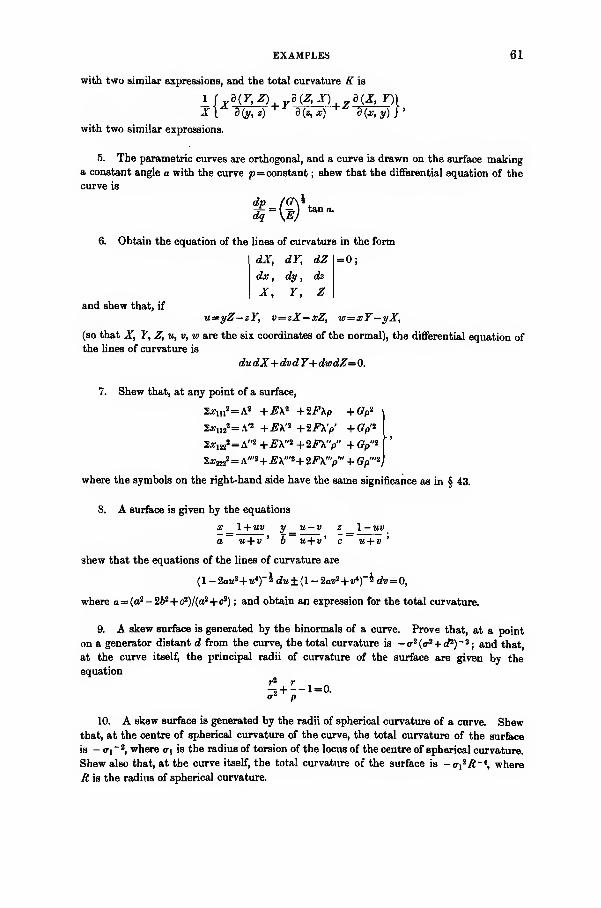
EXAMPLES 61
with two similar expressions, and the total curvature K is
1\ V Z{Y,Z) d {Z, X ) 3(iT, Y
)\
x\A d(j,,z)+I
d(*,xf s(^y)7'
with two similar expressions.
5. The parametric curves are orthogonal, and a curve is drawn on the surface makinga constant angle a with the curve p= constant ; shew that the differential equation of the
curve is
(G\idp _ (GY-
dq-\E)tan <
6. Obtain the equation of the lines of curvature in the form
dX, dV, dZ =0;
dx , dy , dz
X, Y, Zand shew that, if
u**yZ—zY, v=zX—xZ, w=xY—yX,
(so that X, Y, Z, u, v, w are the six coordinates of the normal), the differential equation ofthe lines of curvature is
dudX+dvdY+dwdZ=0.
7. Shew that, at any point of a surface,
2j:,u2=A2 +E\* + 2FXp +Gpz
2x1)22 =A'2 +EX* +2F\'P ' + Gp'2
2tfj222=A"2 +E\"* +2F\"p" +GP"*
|
2xm<>
=
A"'2+ EW'*+ 2F\'"p'" + GP'"Vwhere the symbols on the right-hand side have the same significance as in § 43.
8. A surface is given by the equations
x _\+uv y _u — v z _\-uva u+v ' b u+ v' c u+ v
'
shew that the equations of the lines of curvature are
(1 - 2aM2+M«)"* du± (1 -2ai>2+i^)"4 dv=0,
where a=(o2 - 262+c2)/(a2+c2) ; and obtain an expression for the total curvature.
9. A skew surface is generated by the binomials of a curve. Prove that, at a point
on a generator distant d from the curve, the total curvature is — o-^cr' + rf2)-2
; and that,
at the curve itself, the principal radii of curvature of the surface are given by the
equationr2 r
„2+ --1=0.
P
10. A skew surface is generated by the radii of spherical curvature of a curve. Shewthat, at the centre of spherical curvature of the curve, the total curvature of the surface
is - a\ ~ 2, where <r\ is the radius of torsion of the locus of the centre of spherical curvature.
Shew also that, at the curve itself, the total curvature of the surface is - o-j2.ft-4
, where
ft is the radius of spherical curvature.

62 EXAMPLES
11. A surface is generated by straight lines which meet the lines y= ±xta.na,
2=±i e > and the intercepts between the axis of z and the points where the generator
meets the lines are u and v, functions of a parameter. Shew that, at a point on the
surface in the plane of xy, the total curvature is
-16cW'ain»2u,
{<* («' 8+2uV cos 2a+v' 2)+ (tM/+ u'v)2 sin2 2a}2 '
and that, at a point on the surface in the first line, the principal radii of curvature are
given by the equation
1 2c sin 2a u — v cos 2a dv c2 sin2 2a (*Y-a\dJr2 r (c2+
a
2 sin2 2a)* du (c2+^ sin2 2a)2 \lu
12. A surface is given by the equations
x= sin u (cosh2 v - cos a cos u cosh e — 2 cos2 a),
y= sinh v (cos2 a cos2 u — cos a cos u cosh v — 2),
z— sin a cos u cosh v (cosh v — cos a cos a).
Prove that the curves of reference are the lines of curvature, and that the principal
radii of curvature are
(2 cos a cos u — cosh v) (cosh v+ cos a cos u)! cosec a,
(2 cosh v - cos a cos u) (cosh i>+ cos a cos uf cosec a.
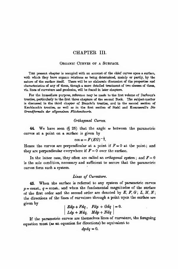
CHAPTER III.
Organic Curves of a Surface.
The present chapter is occupied with an account of the chief curves upon a surface,
with which they have organic relations as being determined, mainly or partly, by the
nature of the surface itself. There will be no elaborate discussion of the properties and
characteristics of any of them, though a more detailed treatment of two classes of them,
viz. lines of curvature and geodesies, will be found in later chapters.
For the immediate purpose, reference may be made to the first volume of Darboux's
treatise, particularly to the first three chapters of the second Book. The subject-matter
is discussed in the third chapter of Bianchi's treatise, and in the second section of
Knoblauch's treatise, as well as in the first section of Stahl and Kommerell's Die
GrundforTneln der allgemeinen Flachentheorie.
Orthogonal Curves.
44. We have seen (§ 25) that the angle w between the parametric
curves at a point on a surface is given by
cos cd = F(EG)~k
Hence the curves are perpendicular at a point if F = at the point ; and
they are perpendicular everywhere if F = over the surface.
In the latter case, they often are called an orthogonal system ; and F=0is the sole condition, necessary and sufficient to secure that the parametric
curves form such a system.
Lines of Curvature.
45. When the surface is referred to any system of parametric curves
p = const., q = const., and when the fundamental magnitudes of the surface
of the first order and the second order are denoted by E, F,Q; L,M,N;
the directions of the lines of curvature through a point upon the surface are
given byEdp + Fdq, Fdp + Gdq =0.
Ldp + Mdq, Mdp + Ndq
If the parametric curves are themselves lines of curvature, the foregoing
equation must (as an equation for directions) be equivalent to
dpdq = 0.

64 meunier's and euler's theorems [ch. hi
Hence we must haveEN-GL^O,
EM-FL = 0, FN-GM = Q.
From the last two equations, we have
(EN-GL)M = 0, (EN-GL)F = 0,
and therefore
M=0, F=0,
are the conditions that the parametric curves should be lines of curvature.
When the conditions are satisfied, the radius of curvature for p = constant,
say a, and the radius of curvature for q = constant, say /9, are
a=GjN, = E/L.
The conditions ^=0, M = 0, are necessary and sufficient to secure that
the parametric curves are lines of curvature. The condition F = makes the
parametric curves an orthogonal system ; the new condition M = makes
them the special orthogonal system constituted by lines of curvature.
46. Two well-known theorems can be stated in connection with the
general formulae of the preceding chapter.
Take any curve on the surface. Let 1/r be its circular curvature ; and
let 1/p be the curvature (defined as in § 31) of the normal section of the
surface through the tangent to the curve. The direction-cosines of the
principal normal to the curve are rx", ry", rz"; hence, if 6 be the angle
between this principal normal and the normal to the surface, we have
cos 6 = X . rx" + Y. ry" + Z.rz".But
x" = xnp" + 2xKp'q' + xaq'a + x,p" + x2q",
and similarly for y" and z" ; hence
^ = Xx" + Yy" + Zz" = Lp* + 2Mp'q + Nq'* = -
.
This is Meunier's theorem.
Next, at any point take a normal section of the surface through a direction
making an angle i/r with the line of curvature p = constant. Let the surface
be referred to the lines of curvature as parametric curves, so that ^=0,M=0; then
cos*=(rt, sm + = Elf.ds' r
ds
The radius of curvature of the normal section is given by
l-rfM 1
, xrfdqY L N cos* yjr sins yfrp- L {ds)+N
[ds)=£Sin^ + £COS^= f+-f-,

47] CONJUGATE DIRECTIONS 65
which is Euler's theorem on the curvature of a normal section through anydirection not coinciding with a line of curvature*.
The relations of the indicatrix
«
to the curvature are at once suggested ; they are discussed in text-books onsolid geometry. Only one remark need be made here, for ulterior use. If the
indicatrix is an ellipse, p is finite for every normal section. If the indicatrix
is a hyperbola, p is infinite for each of the directions i/r = tan-1 (- /3/a)i, whichare the directions of the asymptotes of the indicatrix.
The detailed development of the analysis connected with lines of curvature
and with associated properties will be deferred until the next chapter.
Conjugate Directions.
47. The familiar notion of conjugate diameters (or conjugate directions)
in a central conic can be extended, through the indicatrix, so as to give rise
to the notion of conjugate directions (and conjugate lines) on a eurfacef. In
the case of a conic with centre G, a direction given by two points P and Q on
the curve is conjugate to GR, where the tangents at P and Q intersect in R;
and the definition makes an asymptote of the conic conjugate to itself.
In the case of a surface, let a line PR be drawn through a point Pparallel to the intersection of the tangent plane at P with the tangent plane
at a point Q ; when Q tends to coincide with P (or becomes a point con-
secutive to P), the limiting positions of PQ and PR are called conjugate
directions at P.
The condition that two directions dp, dq; and dp, dq; are conjugate can
be deduced from the definition. Let PQ be the direction dp, dq ; and let PRbe the direction dp', dq', so that PR is parallel to the ultimate intersection
of the tangent planes at P and at Q. Let P be the point x,y,z; the tangent
plane at P is
^- x)X + (v -y)Y + ^-z)Z = 0,
where f, v, f are current coordinates. The tangent plane at Q, say x + dx,
y + dy, z + dz, is
(£ - x - dx) (X + dX) + (v - y - dy) (F + dY) + (£
-
1 - dz) (Z + dZ) = 0.
ButXdx + Ydy + Zdz = 0,
and therefore the latter equation can be taken in the form
2 {(f- x) (X + dX) - dxdX) = 0.
* The result can be established from the quite general formulae, without any special choice of
parametric curves.
t The extension originated with Dupin, Diveloppementt de geomitrie (1813), p. 91.
66 CONJUGATE [CH. HI
The quantity dxdX is of the second order ; hence the line of intersection of
the two planes is given by
(£-*)* +(v-y)Y +{Z-z)Z -01
(£ - x)dX + (v - y)dY + (? - z)dZ = 0j'
Let a point x + dx', y + dy', z + dz' be taken on the surface, so that it lies
ultimately on the direction PR ; thus dx', dy', dz' determine the direction PR,
and for that direction
g — x:7i — y:£—z = dx' : dy' : dz'.
The first equation is satisfied identically. The second equation is
dx'dX + dy'dY + dz'dZ = 0,
which accordingly is the equation to be satisfied by the direction conjugate
to PQ. Nowdx'' = Xjdp' + x2dq'', dX = X^p + X2dq;
and therefore
(Sa^X,) dpdp' + (2#2X,) dpdq' + (Zx^X,) dqdp' + (2#2X2) dqdq' = 0,
that is,
. Ldpdp' + M (dpdq' + dqdp) + Ndqdq' = 0.
This is the condition that the two directions should be conjugate to one another.
As the analysis manifestly is reversible, the condition is seen to be sufficient
as well as necessary.
The symmetry of the condition between dp, dq ; and dp', dq'\ justifies the
assumption in the phraseology that the conjugate property is reciprocal.
When written in the form
(Ldp + Mdq) dp + (Mdp + Ndq) dq' = 0,
the condition shews that the two directions are conjugate diameters of the
indicatrix ; for the equation of the indicatrix is
A (EGy- <*
Thus only a single condition requires to be satisfied in order that two
directions may be conjugate. Hence one direction can be taken arbitrarily,
and the other is then determined by the condition ; and it is uniquely deter-
mined, for the condition is lineo-linear in the quantities dpjdq, dp'jdq'. Thuslet a curve be
4> (P> l) = constant,
so that we have a family of curves when the constant is parametric; the
direction of the curve at a point is given by
op r dq *
But the direction dpjdq, conjugate to Bp/Bq, is given by
(Ldp + Mdq) Bp + (Mdp + Ndq) Sq = 0;
48] DIRECTIONS 67
that is, the conjugate direction at the point satisfies the equation
(Ldp + Mdq)^ - (Mdp + Ndq) |£ = 0,
or, what is the same thing,
oq op \ oq op) dp
an ordinary differential equation of the first order, the primitive of which
gives a family of lines conjugate to the family ^> (p, q) = constant. If this
conjugate family be -^(p, q) = constant, then
dq oq \dp dq dq dp J dp dp
48. When two directions Bp, Bq; Bp', Bq'; satisfy an equation
Adp* + 2Bdpdq + Gdq* = 0,
thenBpBp' _ BpBq' + BqSp' _ BqSq'
~G~ ~ ^2B ~ A '
and therefore the condition that the two directions should be conjugate is
CL- 2BM+AN = 0.
The condition is sufficient, as well as necessary, to secure the conjugate
character.
The parametric curves p = a, q = b, where a and b are constant, are
given bydpdq = 0.
Taking A=0, (7 = 0, and B not zero, we infer that the condition necessary
and sufficient to make the parametric curves a conjugate system is
M=0.In particular, the lines of curvature are conjugate to one another. This is a
consequence of the fact that when the lines of curvature are made parametric
curves, then one of the conditions is M= 0, which makes them conjugate ; and
it can also be verified from their general equation
(EM- FL) dp* + (EN - GL) dpdq + (FN- GM) dq" = 0,
by making A,B,G= EM-FL, EN-GL, FN-GM, respectively, in the
foregoing relation.
The direction dp', dq', which is conjugate to dp, dq, is given by
dp dq _.Mdp + Ndq " - (Ldp + Mdq) ~ '
say, where
^- = (EM » - 2FLM + GL*) dp*
+ 2 (EMN -FLN- FM* + GLM) dpdq
+ (EN* - 2FMN + GM*) dq* = &*,
5—2
68 CONJUGATE LINES AS [CH. Ill
so that
Let x denote the angle between the two conjugate directions ; then
dsds' cos x = Edpdp + F(dpdq + dqdp') + Gdqdq'
= 6 {(Edp + Fdq) (Mdp + Ndq) - (Fdp + Gdq) (Ldp + Mdq)},
that is,
®ds cos x = (EM - FL) dp' + (EN - GL) dpdq + (FN - GM) dq\
Manifestly the only conjugate directions perpendicular to one another are the
lines of curvature.
49. The equations relating to surfaces in general, as obtained in the
preceding chapter, were constructed for any unspecified system of parametric
curves. When any particular specification is introduced, some corresponding
simplification in the equations may be caused. When the parametric curves
are conjugate, we haveM=0
in all the equations. This causes a special simplification in three of the
partial differential equations (of § 34) satisfied by the coordinates, viz. those
involving x12 , yl2 , za . When the parametric curves are conjugate, these
equations are
x12 = x1 T' + x3 A', y12 = y,r + y2 A', za = ^r' + ^A';
that is, x, y, z are three solutions of the equation
dpdq dp dq
'
This is a linear partial differential equation of the second order, and usually
is called Laplace's equation, being written in the form (with the customarynotation for partial differential equations)
s = ap + bq,
where a and b are functions of the independent variables.
The primitive* of this equation involves two arbitrary functions; hencethe most general values of x, of y, and of z, obtained solely as integrals of theequations, are expressions each of which involves linearly an arbitrary functionofp and an arbitrary function of q. The arbitrary functions are not unrelated
;
for assuming T' and A' known, we have
Vr = JGE2 -lFQlt 7*A' - \EG l- $FE2 ,
as well as the Gauss characteristic equation and the Mainardi-Codazzi
* For the general theory of Laplace's linear equation, and for the special construction of theprimitive when the latter can be expressed in finite terms involving the two arbitrary functions,see the author's Theory of Differential Equations, vol. vi, chap. xiii.
50] PARAMETRIC CURVES 69
relations; and all these conditions must be satisfied when the values of
x, y, z are substituted.
Even so, a large amount of arbitrary generality will survive in the
complete solution which, through this stage at least, is rather an investigation
in partial equations than in geometry. Geometrical applications arise by the
assignment of further conditions; and illustrations of these, in connection
with particular surfaces or families of surfaces, will be given from time to
time.
The amplest discussion of the equation, together with many compre-
hensive applications to surfaces, will be found in the second volume of
Darboux's treatise.
50. One particular family of surfaces, referred to conjugate lines as
parametric curves, is instanced by Darboux* in the form
x = A(p-a)m (q-a)n, y = B(p-b)m (q-b)n , z= G(p-c)m (q-c)n,
where A, a, B, b, C, c, m, n are constants. It is easy to verify that
(q — p) xv, = nxx— rnxz
{q-p)yn = nyx -mya
{q — p) zu = nzi — mz2
so that, multiplying these equations by X, Y, Z respectively, and adding, wehave
M = 0;
and therefore the parametric curves given by p = constant, q = constant, are
conjugate.
More generally, the direction on the surface given by Bp, 8q is conjugate
to the direction given by dp, dq, if
m(m—l)dpSp n(n—l)dqSq(p -a)(p- b) (p - c) ~ (q-a)(q-b(q^cj
-
The family includes many important sets of surfaces. When m = n, wehave the " tetrahedral " surfaces
/ T\\lm /w \l/j» / 2 \l/m
(z)(6_C) +
(I)(c_o) +
fo)^-b) = (a-b)(b-c)(c-a),
special cases of which arise, in Steiner's surface for m = n = 2, in a well-
known cubic surface for m = n = — 1, and in the trivial plane for m= w=l.When wi = f, n = J, we have (as will be seen later) the surface of centres of
the ellipsoid; when m = £, n = \, we have an ellipsoid; and so for other
special values of m and n.
* ThSorie ginirale, t. i, p. 142.

70 ASYMPTOTIC [OH. Ill
Asymptotic Lines.
51. Various definitions of asymptotic lines are given, according to the
property selected to characterise them. They are associated simply with
conjugate directions; an asymptotic line is then defined as a curve on the
surface whose direction at any point is self-conjugate. The direction dp'/dq'
must then be the same as dp/dq ; that is, a self-conjugate direction is given
by either of the equations
dxdX + dydY + dzdZ = 0,
Ldp* + 2Mdpdq + Ndq1 = 0.
Consequently there are generally two asymptotic directions at any point of
a surface. When the total curvature is positive (so that LN > M"), the
directions are imaginary and different ; when it is negative, they are real
and different ; when it is zero (so that the surface is developable), there is
only a single asymptotic line through a point, and it is the generator.
The curvature of the normal section of a surface through the tangent to
an asymptotic line, beingLp'* + 2Mp'q' + Nq'\
is zero. The tangent to the line then coincides with an asymptote of the
indicatrix at the point; hence the name.
Consider the tangent plane at a point (x, y, z) on the surface. The
distance of a neighbouring point x + dx, y + dy, z + dz from that plane
= Xdx+Ydy + Zdz
= %(Ldpi + 2Mdpdq + Ndq1) + other terms,
the other terms being of the third and higher orders in dp and dq. Thus
any tangent to the surface, being a straight line in the tangent plane, meets
the surface in two consecutive points; but a tangent to the surface in the
direction of an asymptotic line meets the surface in three consecutive points.
The directions of the asymptotic lines are therefore often called the inflexional
tangents at the point.
Another method of stating the last result is to declare that the asymptotic
directions are the tangents to the curve of intersection (which has the point
for a double point) of the surface by its tangent plane. On a hyperboloid of
one sheet, they are of course the generators.
Let x denote the angle between the asymptotic lines
Ldp* + 2Mdpdq + Ndq* =
at any point ; then (§ 26)
2V(M*-LN)$tan X ~ EN-2FM + GL
52] LINES 71
or writing
K- 1 H- 1 ^ 1
where a and /3 are the principal radii of curvature at the point, we have
cos y = '-z.
.
If the asymptotic lines are everywhere perpendicular on a surface, so that
X = \t, then
EN-2FM + 6L = 0,
that is, the surface is minimal.
52. The analytic determination of the asymptotic lines upon a surface
can be made to depend upon the integration of the differential equation
Ldp2 + 2Mdpdq + Ndtf = 0,
of the first order and second degree. For any surface, what is required in
this mode of determination of the asymptotic lines is the preliminary con-
struction of the quantities L, M, N.
Ex. 1. On a sphere, we can take,
#=cos/>cos5, #= cosj»sin j, z=ainp;
and then, by simple calculations, we have
L=-\, Jf=0, N=-l,
so that the asymptotic directions (being imaginary, for the sphere is synclastic) are given by
dp2+dq2=0,that is, they are
p+tq= const., p— iq= const.
Ex. 2. Prove that, at the origin on any surface
2z=ax2+2hxy+by2+ terms of higher order in x and y,
the asymptotic directions are
ax2 + 2hxy+by2=0.
Ex. 3. As a last example, consider the asymptotic lines on Fresnel's wave-surface*
x2y
2 22
Is — a r2— b r2 — c'
where ts=x2+y2+z2
. We have
ax2 by2 cz2
^-. a+
r2-b + ri-c '
and so we takeri=x2+yi+z2=q,
ax2ty
2 _&?_ _ abc (8-p)(.8-q)6-a + 6-b + 0-c~ p (6-a){8-b)(6-cY
as equations defining the parameters p and q, the latter equation being satisfied identically
for all values of 6.
* For a fall discussion, see Note vm at the end of Darboux's fourth volume.
72 ASYMPTOTIC LINES AS [CH. Ill
We then have
^= bc (a-q)(a-p)
p (a - 6) (a - c)
'
with similar expressions for y and z ; hence
xt1 a
x 2p(a —p)
#2 11x 2a — q
xJt _ 1 (4p-3a) g
a:
—4 pi (a—p)2
#12 1 a
x ip(a —p)(a — q)
#22 1 1
x 4 (a — j)2
Xx= W{b- c){bc-(b+c)p+pq}(a-p)(a-q),
where Hr
is a multiplier, common to X, Y, Z, the value of which is immaterial at present.
Then, writing
U={a-b)(b-c)(c-a),we have
X= S^i^ii
:2Xxxn
__. wup* {q* - (a+ b+c) q+ab+ bc+ ca} + abc (q-2p)
p(a-p)(b-p){fi-p)M=2Xxl2
iWU,
N=2Xzn_ , w„ -abc+ (ab+bc+ca)p-(a+b+c)pi-pq(q-2p)
t °{a - q){b -q)(c-q)
Inserting the values of L, M, N, we at once have the differential equation for the
asymptotic lines.
Darboui (I.e.) shews that, by introducing a parameter » in place of p, denned by the
relation
p(p-q)(p-»)=(p-a)(p-t>)(p-c),
the differential equation can be obtained in the form
di? dq*
(s-a)(s-b)(S -c)-{q-a){q-b)(q-c)'
the primitive of which can be expressed algebraically.
53. The conditions that the parametric curves should be asymptotic
lines are easily derived from their general equation
L dp2 + 2Mdpdq + Ndq* = 0.
If these are the parametric curves p = a,q = b, the equation must effectively
be the same as
dpdq = 0,
and therefore we must have
Z = 0, iV = 0, Jlf + 0.

54] PARAMETRIC CURVES 73
(The complete difference between the condition, that the parametric curves
should be two different conjugate directions, and the conditions, that they
should be two self-conjugate directions, will be noticed.)
Moreover, as the analysis manifestly is reversible, the conditions are
sufficient as well as necessary.
As the asymptotic lines are a couple of systems of curves distinct from
one another on all surfaces which are not developable, it frequently is
convenient to choose them as the parametric curves of reference. In that
choice, we make Z = and N~=0 in all the general equations which have
been obtained; consequently there is much simplification in the forms of
those equations. Thus the Mainardi-Codazzi relations take the form
MX= (T-M)M, M2
= (b"-T')M.
The equation of the lines of curvature (on dropping the non-zero factor M )
becomesEdp>-Gdq* = Q.
We haveY— = r+A'
74 PSEUDOSPHERE [CH. Ill
and
$-y'-0, thatis,r' = 0.
Reverting to the definitions of V and A', we have
m'G-n'F=0, n'E-m'F=0,
and therefore
m = 0, 11 = 0,
that is,
E2 = 0, G, = 0.
Consequently E is a function of p only ; by changing the variable p to p'
where ^^dp = dp', the new quantity in place of E is unity, and therefore
without any loss of generality, we can take E = 1 for the surface. Similarly,
as G is a function of q only, we can take G=l without any loss of generality
for the surface.
The angle between the parametric curves has been denoted by w ;hence
in the present case
F—aosco, V= sin co,
and therefore
„ V sin coM= — =.
Now for any surface we have (§ 36)
a>» _ a /ta'\ a /EE'Uf/t-
and therefore, in the present case, we have
Woo 1 .
^—3~ = — sin a),
where /a is a real constant.
Upon the integration of this equation, the determination of the most
general pseudosphere rests. When any solution is found giving co in terms
ofp and q, we then know
E(=l), G(=l), Z(=0), iV(=0), ^(=cosq>), M(=fi-i sin a);
that is, by Bonnet's theorem, we have a pseudosphere completely determined
save as to position and orientation. Thus, as so often happens in the
differential geometry of surfaces, the solution of the problem depends upon
the integration of a partial differential equation of the second order. Theprimitive of the equation
has not yet been obtained.
d*co 15-5- = — sin codpoq f?
55] NUL LINES 75
The lines of curvature upon the pseudosphere are given by
dp2 - dq1 = 0,
that is, they are given by
p + q = u = constant, p — q = v = constant.
When the surface is referred to the lines of curvature as parametric
curves instead of the asymptotic lines, so that u and v are the variables of
reference, the preceding differential equation of the surface becomes
9wdu* dv*
=Sam<°-
Nul Lines.
55. The nul lines (or minimal lines) on a surface are denned in connectionwith arcs of zero length ; they are given, as to their variables, by
Edp* + 2Fdpdq +Gdq*= 0.
On any real surface, the nul lines are imaginary ; and their parameters are
conjugate complex variables, unless V is zero, a case which usually is
excluded* from consideration. But it will appear that, though the variables
are imaginary, they have definite and important relations with real isothermic
systems of lines upon the surface.
In order that the parametric curves may be nul lines, the equation
Edf + 2Fdpdq +Gdq* = 0,
which is the defining equation of such lines, must effectively be the same as
dp dq = 0,
which is the general equation of parametric curves. Hence
# = 0, G = 0, 2? +0,
(and therefore ^4=0). The expression for any arc then becomes
ds*=2Fdpdq.
To determine the nul lines on a surface when they are not the parametric
curves, we have to integrate the equation
Edp* + 2Fdpdq + Gdq* = 0,
that is, the equations
Edp + (F+iV)dq = 0, Edp + (F-iV)dq = 0,
where we shall assume that p and q are real. Let the primitive of the first
of these two equations linear in dqjdp be
u = <p (p,q) = constant,
so that u is a complex function ofp and q. \iv is the conjugate to u,
v = -^r(p,q) = constant
* Darboux (t. i, p. 148) shews that, when V=0, the surface is a developable circumscribed to
the imaginary circle at infinity.
76 NUL LINES AS PARAMETRIC CURVES [CH. Ill
is the primitive of the second of the equations linear in dq/dp. Then
du = fi{Edp + (F+iV)dq],
dv = v{Edp + (F-iV)dq},
where fi and v are conjugate quantities ; hence
ds2 = Edp- + 2Fdp dq+G dq>
=—=, du dv = Xdudv,fivhj
where X. is a real quantity on a real surface.
The nul lines then are given by the equations
u = a, v = b.
These variables u and v are often called the symmetric variables. Later it
will be seen that, while symmetric variables are not unique for a surface,
the choice of such variables possessing the symmetric character is narrow.
56. When a surface is referred to nul lines as parametric curves, the
various equations in the general theory are much simplified. We then have
E = 0, G=0, V' = -F';
t = f1/f, r'=o, r"=o,
A = 0, A'=0, A" = F,/F.
The Mainardi-Codazzi relations become
which can be written
1 T d U M\
and the Gauss equation becomesF1 F,
The mean curvature is
and the total curvature is
LN-M> = F12-'-J±-\
*-«*
K = LN-M*
-F^q-^nThe differential equation of the lines of curvature is
-Ldp1 + Ndq* = 0;
and the equation of the asymptotic lines is unaffected, being
Ldpi+ 2M dpdq + Ndq* = 0.

57] SURFACES OF CONSTANT MEAN CURVATURE 77
It will appear that the discussion of the geodesies upon a surface is
simplified, so far as their equations are concerned, by referring the surface to
nul lines as parametric curves ; for only a single fundamental magnitude (F)
of the first order then occurs in the equations, instead of all three when the
parametric curves are any general unspecified curves.
57. As a passing example of the use of nul lines as parametric curves,
consider surfaces with a constant mean measure of curvature, say 2/A, where
A is a constant. ThenM_2
l F~h :
so that
Mh = F.
From the Mainardi-Codazzi equations, we have
L2= 0, iV, = 0.
Thus £ is a function ofp only, if it is not zero; when we change the variable
to p' where IPdp = dp', the new quantity L is unity, that is, we can take
L = l without loss of generality. Similarly we can take N=l without loss
of generality, when it is not zero.
The Gauss equation now becomes
l-M^ = Fn -^p,
that is,
&(\ogF) _ 1 _ Fdpdq ~F h?'
a partial equation of the second order to determine* F. Suppose that some
integral of this equation is known ; it gives F, and therefore also M which
is equal to F/h. Thus we know E, F, G, L, M, N; that is, by Bonnet's
theorem, there is a surface uniquely determined by these quantities, save as
to position and orientation in space.
The lines of curvature upon the surface satisfy the equation
- dp* + dq* = ;
that is, they are given by
p + q = constant, p — q = constant.
• Writing
F=kem, h=-2^,the equation becomes
8'fl _ 1gin
dp dq ~ ii? '
which is the same equation as occurred (§ 54) in the discussion of surfaces having the Gaussian
measure of curvature constant.
78 lie's theorems on [ch. tii
The asymptotic lines on the surface satisfy the equation
Fdp1 + dq2 +2jdpdq = 0,
that is, they are given by the equations
hdp+{F ±(F*-h*fi\dq = 0.
58. It is possible to have nul lines in space, as well as nul lines on any
given surface; and they possess the important property that, from them, it is
possible to construct minimal surfaces analytically.
One method of constructing nul lines in space is given by Lie as follows.
Take any plane
tx + uy + vz = 1,
subject to a specific relation
P + tt2 + V2 =
and to any arbitrary non-homogeneous relation
f(t,u,v) = 0.
The two relations determine (say) u and v as functions of t; thus the
equation of the plane contains only a single parameter, and therefore the
envelope of the plane is a developable surface. The edge of regression of
this surface is a nul line ; and so, by taking any number of different relations
/= 0, we have any number of nul lines.
The verification of the statement is easy. A point on the edge of
regression is given by
tx+ uy + vz = 1 \
x + u'y + v'z =J-,
u"y + v"z = 0)
with the conditions
f + m2 + v1 = 0, t + uu' + vv =;
and these equations give x, y, z as, variable functions of t, so that dx, dy, dz
are not zero. But along the edge, we have
tdx + udy + vdz + (x + u'y + v'z) dt = 0,
dx + u'dy + v dz + (u"y + v"z) dt = 0,
that is,
and therefore
tdx + udy + vdz = 0,
dx+u'dy + v'dz=0,
dx dy dz
uv' - u'v ~ v - tv'~
tu' -u ~ '*'

59] NUL LINES 79
where /i is not zero because x, y, z are variable quantities. Hence the
element of arc ds is given by
- ds2 = (mi/ - u'vy + (v- tv'f + (tu - u)2
= (1 + w's + v'*) \v? (1 + m'2) + v" (1 + v'1) + 2uvu'v'},
on substituting — (uu + vv) for t. The second factor is
u* + i? + (uu + vv'f
= u* + a2 + P = 0,
and so
ds = 0,
thus verifying* the statement that the edge of regression is a nul line in
space.
59. These nul lines in space are used+ by Lie to construct minimal
surfaces, according to the theorem
:
Let JV, and N~s be two nul lines in space; let P, be any point on Nu and
P2 any point on N3 ; then the locus of the middle point of the straight line
P^P^is a minimal surface.
The coordinates of P, can be represented by
x1= 2A 1 (t) = 2Au y1
= 2B1 (t) = 2B1 , z, = 2(7, (0 = 2(7,,
whereAp + B^ + W-O,
because iV, is a nul line. The coordinates of P2 can be represented by
*2 = 24 2 (0) = 24 2 , y2 = 2B2 (0) = 2Bi , *a = 2(7a (0) = 2(72 ,
where4 2
'2 +P2
'2 + (72'2 = 0,
because i\T2 is a nul line. The coordinates of the middle point of PXP2 are
x = A 1 (t) + A,(6),
y = B1 (t) + B2 (0),
* = (7,(0 + (7,(0);
and therefore, for its locus, we have
E= 2a:,s =A 1"> + £,'2 + (7,'2 = 0,
G = 2<caa = A? + B? + G2
" = 0.
* For the purpose, the Serret formula of § 21 can also be used ; in them, we write
t ur v v
while the u of those formulas now becomes - l\v. Then we verify that T, which is equal to
{p't+ql+ ipq'-p'q)*}*,
vanishes ; and so ds = 0.
t Math. Ann., t. xiv (1879), p. 337. Lie chooses the middle point; the locus of a point, that
divides P\Pz in any constant ratio, also is a minimal surface.
80 ,MINIMAL SURFACES AND NUL LINES [CH. Ill
Also
ais = 0, y,2 = 0, zn = 0,
and therefore
M=0.Consequently
EN-2FM + GL = 0,
the equation characteristic of a minimal surface.
It thus appears that minimal surfaces can be derived from any two
minimal curves.
If A,, Bu C, are algebraic functions, and also A it Blt G2 are algebraic
functions, then x, y, z are algebraic functions of t and 6 ;that is, the minimal
surfaces then are algebraic. Hence if the arbitrary relation /(t, u, v) =
be chosen as an algebraic function in each case, we shall have a succession
of algebraic nul lines ; and thence a succession of algebraic minimal surfaces
can be constructed.
In particular, if A,(t) and A 2 (0), B,(t) and B^d), d(«) and Cs (0) are
conjugate pairs of complex quantities, the minimal surface is real though
both the initiating nul lines are imaginary. For instance, let
t = a + /3i, d = a-8i,
where a and 8 are real. An algebraic minimal curve is given by
x, = St- 13, y, = - i (St + t') y
z, = St\
and another byx1 = 30-d>, y2 = i(3e + 0>), *2= 302
;
the minimal surface derived from these as initiating curves is Enneper's
minimal surface* (also algebraical, and of order 9)
x=Sa+SaBi -a?, y = 3/9 + 3a?B - 8\ z = 3(a?-8*).
Isometric Lines.
60. In connection with the determination of nul lines upon a surface, wesaw that the element of arc could be taken in the form
ds2 = Xdudv,where \ is a real constant,
du = fi {Edp + (F+ iV) dq], dv=v [Edp + (F- iV) dq},
H and v being magnitudes independent of differential elements. On a real
surface, these symmetric parameters are conjugate complex variables ; so wecan take
u = P+iQ, v = P-iQ,where P and Q are real variables. We now have
ds* = \(dP1 + dQ>);
and the curves P = constant, Q = constant, are parametric and real.
* First obtained by Enneper, Zeitschr. f. Math. u. Phytik, t. ix (1864), p. 108.
61] ISOMETRIC LINES 81
Because there is no term in ds2 which involves dPdQ, the parametric
curves are orthogonal to one another.
Now take a number of parametric curves in succession, such that the
variations dP and dQ in passing from any curve to the next curve are
equal to one another, the common value of all of them being k. Then the
element of arc along Q = constant intercepted between two successive
P-curves is equal to \*k, and the element of arc along P = constant
intercepted between two successive Q-curves is also equal to X*/c; and
the curves are orthogonal to one another. Thus the selected rectangle is a
square; and so, by the parametric curves as chosen, the surface is divided
into small squares. Such a system of parametric curves is called isometric,
sometimes isothermic, sometimes orthogonal and isometric, the division of
the surface into small squares being the distinguishing property.
61. Isometric variables are not unique. Take any function, say
f (P + iQ), of two variables given as isometric for a surface ; and separate
f{P + iQ) into its real and imaginary parts, so that
f(P + iQ) = P' + iQ'.
Let g(P — iQ) be the conjugate of f(P + iQ)—should all the coefficients in
f(P + iQ) be real, g (P - iQ) is f(P - iQ) ; then
g{P-iQ) = P'-iQ\Hence
(dP + idQ)f (P + iQ) = dP' + idQ,
(dP - idQ) g' (P - iQ) =dP - idQ';
and therefore
ds* = \(dP* +dQ2
)
= X'(dP* + dQ'%where
\ = X'f'(P + iQ)g'(P-iQ),
so that X' is a real quantity. Consequently, the new parametric curves
P = constant, Q' = constant, are an orthogonal isometric system.
Moreover P' and Q' constitute the aggregate of isometric variables when
complete variety of form is permitted to the function /, a property which can
be established as follows. Reverting to the initial symmetric variables u and
v, connected with the isometric variables P and Q, we have the element of
arc upon the surface in the form
ds2 = X du dv.
Let any other reduction for the arc-element, expressed by means of symmetric
variables connected with other isometric variables, be represented by
ds^ — X'dudv.
f. 6
82 ISOMETRIC [CH. Ill
Then u and v are independent functions of the first parametric variables;
hence we must have
\dudv = \'(^- du + -~- dv) (^-du + j-dv) ,
for all variations of u and v. Consequently
du dv' _ „ du dv' _ _
dudu~ ' dv dv ~ '
hence either
(i) =- = 0, so that u is a function of u only, and then 5— = 0, so that vdv ou
is a function of v only ; or
(ii) =- = 0, so that «' is a function of v only, and then ^- = 0, so that v'ou ov
is a function of u only.
The two cases differ only in an interchange of variables ; effectively they are
only a single case, represented by
u'=f(u), v'=g(v).
As u and v are conjugate variables, g (v) is the conjugate of f(u). The
foregoing relations between P + iQ and P' + iQ' therefore produce the
aggregate of isometric variables.
It will appear later, in the discussion of the representation of a surface
upon other surfaces, that the relations express the conformal representation
of the surfoxe upon itself; and further, that the reference of a surface to an
isometric surface implies the conformal representation of the surface upon
a plane, the coordinates in the plane being the parametric variables.
62. Simple systems of isometric lines are provided by the lines of
curvature upon a surface of revolution and by the lines of curvature upona central quadric.
For a surface of revolution, the lines of curvature are the meridians andthe parallels of latitude. Let r denote the distance of any point from the
axis of revolution,<f>
its longitude from some meridian of reference, and let
z = f{r)
be the equation of any meridian curve ; then
ds* = dr1 + r* d<f>* + dz*
= (l+f'")dr> + r*d<l>*.
Let
4p-(l+/'.)i^;T
then
ds* = r*(dp* + dtfyl).
An isometric system is therefore provided by the curves = constant (whichare the meridians) and r = constant (which are the parallels).
63J LINES 83
In the second case, it is known, from the theory of confocal central
quadrics, that the coordinates of any point on the surface
^/a + flb + z'/c = l
can be expressed in the form
- fiya? = a(a+p)(a + q),
-yaf=b(b + p)(b+q),
-a0z* = c(c+p) (c + q),
where a, ft, y = b — c, c-a, a-b. Then
ZKil q, \(a+p)(b+p)(c+p) (a + q)(b + q)(c + q)\'
so that the curves p= constant, q = constant (that is, the lines of curvature)
are an isometric system.
63. The conditions that any original parametric curves should be anisometric system are easily obtainable.
In the first place, they must be orthogonal ; hence
F=0.
Next, the element of arc must be expressible in the form
\(dP> + dQ>),
and p = constant, q = constant, are to be the same effectively as P = constant,
Q = constant; hence
E= \f(p), G = \g(q),
where /and g are any functions ofp and q respectively. Thus
E_f(p)& 9(q)'
and therefore
which is the other necessary condition.
When an element of arc is given in the form
Edp'+Odq',
and the necessary condition is satisfied, an appropriate change in the variables
leads to the form
X(dP2 + dQa);
and then the necessary condition is
E = G.
But it must be remembered that, for this form of the condition, one special
isometric system has been chosen.
6—2
84 SURFACES HAVING ISOMETRIC [CH. Ill
Assuming this special choice made, the conditions are
F = 0, E=G = \.
We then have
1=2X" ~2\' 2\*
A2X' 2X' 2X'
The Mainardi-Codazzi equations are
The Gauss equation is
Z^-Jf»--^(Xu + X»)+^(Xl, + Xi«)
1 fdHogX d'logXN~ 2 \ dp
+a?
» ;•
The mean curvature is given by
and the total curvature is given by
_ 1_ /ffilogX d" log X\
2X\. dp*+
da" )dp* dq"
64. The reference of any surface to isometric lines as parametric curves
affects the form of the expression for the arc, and therefore affects the forms
of E, F, G; but, beyond the necessity of satisfying the Gauss equation
which gives a value for LN — M', no condition is thereby imposed upon
the determination of L, M, N; consequently we cannot expect to have any
unique determination of a surface. Any postulation of further conditions,
of course, modifies the problem.
Accordingly (and especially after the two examples just given in § 62)
we proceed to consider those surfaces whose isometric curves include the
lines of curvature. Let the surface be referred to the special isometric
lines such that we can take
E = G = \,
of course with the condition F= 0. As the parametric lines now are lines
of curvature, we have (§ 45) both F= 0, M= ; thus the aggregate of
conditions is
E=G = \, F=0, M = 0.
64] LINES OF CURVATURE 85
What is required is the determination (as far as may be possible) of the
quantities X, L, N. The equations which they have to satisfy are
Z2= \^(L + N),
so that
Writing
we have
dp\XJ X
dq\Xj X
A = N*/X, B = DfX, p. = log X,
£"**• fr^' AB - Vi
we must eliminate A and B between these three equations. Now
B~= 23*2 - A/tfr, A™ = 2%% - Bfr%,
But
, 9A = dB dAdpdq dp dq
+ 23% + 23,3, - A (/*A + ^,3) - ftPi*1.
&Adpdq
= /*1,^ + /i1&2 ;
hence, equating these values ofa , substituting for ^— and -=— , and
reducing, we find
= 23*12- 23A - 23=/*,/*, + J. (/i,*, - /%*) + 5 (/^- /t,23).
Let

86 SURFACES HAVJNG ISOMETRIC [CH. Ill
ButBAdp= fr*
B d^ = 2%%-A^
A^=2^x-B^dBa7
=^Using the values of A and B just obtained, taking account of the value of
A, and reducing, we find that only two independent relations survive, viz.
3^ + A,
2/ y D + A J y
dp 2/A~^ + A **1 + A Jl+ D-AIA* 11
dDD-Adq 2JA
From these, by the relation
we have3AD + A
= ^-^**2
B-A ID + AJA-f-r yrJv
~~ T » 2
A^^-4/^y,
2/ r
SA2) - A=^-^^ +fcAi^d D + AJD Ddq 2JD
For either pair, we thus have two simultaneous partial differential
equations ; they are of the fifth order in the derivatives of \. When a value
of \ is known, we find A and B from the equations
2AI=D + A, 2BJ = D-A.Then E(=\), F(=0), G(=\), L, Jf(=0), N, are known; and so, by Bonnet's
theorem, the surface is determinate save as to position and orientation. Thusthe solution of the problem depends upon the resolution of the two equa-
tions of the fifth order.
In connection with surfaces of this character, reference may be madeto a memoir* by Weingarten and to §§ 435—437 (vol. ii) of Darboux'streatise.
As an example, we can verify that a surface of constant mean curvature has thespecified character.
We have seen (§ 57) that, when a surface of constant mean curvature is referred to its
nul lines as parametric curves, so that its arc-element is given by
<M>=2Fdpdq,
the lines of curvature are given by the equationsp ± q= constant. Write
p+q=2u, p-q=2iv;then u and v are parameters of the lines of curvature, and
ds?=2F(du?+dv*),
shewing that the lines of curvature are a parametric system.
Sitzungsb. Berl., t. ii (1883), p. 1163.
66] LINES OF CURVATURE 87
Geodesies.
65. Among the important lines upon a surface, one class is constituted
by the curves called geodesies. Unlike lines of curvature, asymptotic lines,
and nul lines, they are not determined uniquely or in pairs at a point bythe surface itself. A direction taken at a point determines uniquely a
geodesic having that direction at the point. The detailed consideration of
their properties will be deferred until a later chapter. They are mentioned
here solely because they provide a system of coordinates for the representation
of the surface, corresponding in notion to the system of polar coordinates in
a plane; in consequence, these are sometimes called geodesic polar coordinates,
sometimes geodesic orthogonal coordinates.
The original definition of a geodesic on a surface is that it is the shortest
distance measured along the surface between two points on its course. It
is therefore a curve along which a tightly stretched string would lie at rest
between the two points on a smooth surface. At any element, the internal
forces due to the tensions at the two extremities lie in the osculating plane
of the curve, while the external force is the pressure which acts along the
normal to the surface; as these balance because the string is at rest, the
osculating plane of the curve at any point contains the normal to the surface
at the point. This property, characteristic of geodesies, will later be derived
also from non-statical considerations.
Later (Chap, v) we shall see that there may be a limit to the range of the
curve when it is to be the shortest distance from any initial point to every
other along its course. When such a limit exists, each extremity of the
range is called the conjugate of the other; and then, as will also be seen, it
is possible to draw more than one geodesic between two points when either
lies beyond the conjugate of the other. For our immediate purpose, we shall
assume the domain of the surface in the vicinity of a point to be so far
restricted that it shall not include the conjugate (if any) of the point along
any geodesic.
66. Without waiting for the full discussion of the general equation of
geodesies, it is desirable to notice one simple and important property, viz.
if a geodesic be a plane curve (which is not merely a straight line), or if it
be a line of curvature, then it is both a plane curve and a line of curvature.
When a geodesic is a plane curve, its principal normals intersect, save
only when it is a straight line. These principal normals are the normals to
the surface along its course ; they therefore intersect, and so the curve is
a line of curvature.
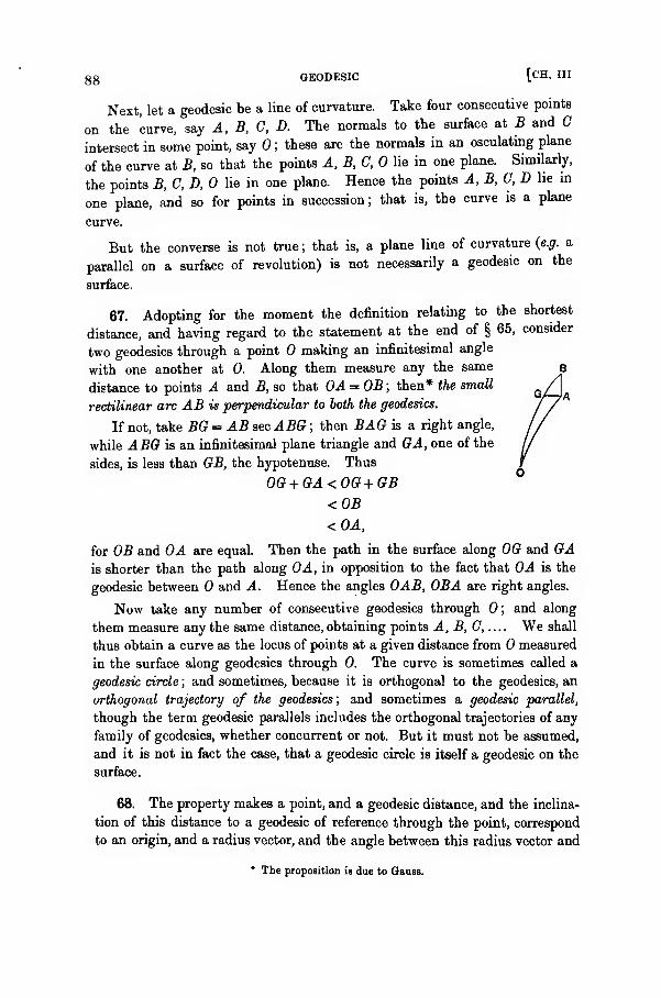
88 GEODESIC [CH. Ill
Next, let a geodesic be a line of curvature. Take four consecutive points
on the curve, say A, B, C, D. The normals to the surface at B and C
intersect in some point, say 0; these are the normals in an osculating plane
of the curve at B, so that the points A, B, C, lie in one plane. Similarly,
the points B, C, D, lie in one plane. Hence the points A, B, C, D lie in
one plane, and so for points in succession; that is, the curve is a plane
curve.
But the converse is not true ; that is, a plane line of curvature {e.g. a
parallel on a surface of revolution) is not necessarily a geodesic on the
surface.
67. Adopting for the moment the definition relating to the shortest
distance, and having regard to the statement at the end of § 65, consider
two geodesies through a point making an infinitesimal angle
with one another at 0. Along them measure any the same
distance to points A and B, so that 0A = 0B; then* the small
rectilinear arc AB is perpendicular to both the geodesies.
If not, take BO = AB sec ABG ; then BAG is a right angle,
while ABO is an infinitesimal plane triangle and OA, one of the
sides, is less than OB, the hypotenuse. Thus
0G + GA<00 + GB<0B<0A,
for OB and OA are equal. Then the path in the surface along OG and GAis shorter than the path along OA, in opposition to the fact that OA is the
geodesic between and A. Hence the angles OAB, OBA are right angles.
Now take any number of consecutive geodesies through 0; and along
them measure any the same distance, obtaining points A, B, 0, We shall
thus obtain a curve as the locus of points at a given distance from measured
in the surface along geodesies through 0. The curve is sometimes called a
geodesic circle ; and sometimes, because it is orthogonal to the geodesies, an
orthogonal trajectory of the geodesies; and sometimes a geodesic parallel,
though the term geodesic parallels includes the orthogonal trajectories of any
family of geodesies, whether concurrent or not. But it must not be assumed,
and it is not in fact the case, that a geodesic circle is itself a geodesic on the
surface.
68. The property makes a point, and a geodesic distance, and the inclina-
tion of this distance to a geodesic of reference through the point, correspond
to an origin, and a radius vector, and the angle between this radius vector and
* The proposition is due to Gauss.
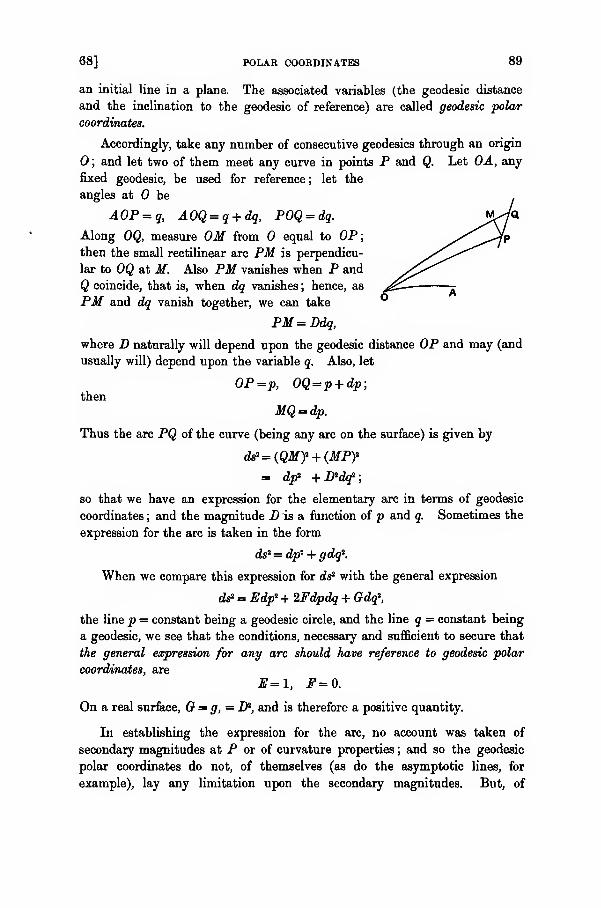
68] POLAR COORDINATES 89
an initial line in a plane. The associated variables (the geodesic distance
and the inclination to the geodesic of reference) are called geodesic polar
coordinates.
Accordingly, take any number of consecutive geodesies through an origin
; and let two of them meet any curve in points P and Q. Let OA, any
fixed geodesic, be used for reference; let the
angles at be
AOP = q, AOQ = q + dq, POQ = dq.
Along OQ, measure OM from equal to OP;then the small rectilinear arc PM is perpendicu-
lar to OQ at M. Also PM vanishes when P and
Q coincide, that is, when dq vanishes ; hence, as
PM and dq vanish together, we can take
PM=Ddq,
where D naturally will depend upon the geodesic distance OP and may (and
usually will) depend upon the variable q. Also, let
OP=p, OQ=p + dp;then
MQ = dp.
Thus the arc PQ of the curve (being any arc on the surface) is given by
ds*=(QMy + (MPy
= dp* + D2d?a;
so that we have an expression for the elementary arc in terms of geodesic
coordinates ; and the magnitude D is a function of p and q. Sometimes the
expression for the arc is taken in the form
ds1 = dp1 + gdq".
When we compare this expression for ds* with the general expression
ds2 = Edf + 2Fdpdq + Odq\
the line p = constant being a geodesic circle, and the line q = constant being
a geodesic, we see that the conditions, necessary and sufficient to secure that
the general expression for any arc should have reference to geodesic polar
coordinates, are
E=\, F=0.
On a real surface, G = g,=Ifi, and is therefore a positive quantity.
In establishing the expression for the arc, no account was taken of
secondary magnitudes at P or of curvature properties ; and so the geodesic
polar coordinates do not, of themselves (as do the asymptotic lines, for
example), lay any limitation upon the secondary magnitudes. But, of
90 GEODESIC POLAR COORDINATES [CH. Ill
course, the Gauss equation and the Mainardi-Codazzi relations must be
satisfied. We have
r=o, r=o, r"—yu
A = 0, A'=£<fr/<7, A" = i^;so that the Mainardi-Codazzi relations are
The Gauss equation is
LN-M* = -\gn +l 9l»;z 9
and therefore the total curvature is
9
= --£f(h99*-9?)
ydp*
When we use the quantity D in place of g, and we write K=—z, where a andaP
£ are the principal radii of curvature at the point, the last equation becomes
dp"-+
a/3 '
a property first established by Gauss.
The mean curvature is given by
H= L + l.9
One property of the quantity D may be noticed. When P is near 0, thegeodesic OP is appreciably a straight line so that PM=pdq; hence, whenp is very small, we have
D=p+ higher powers of small quantities,
and so, at 0, we have
dp
As already stated, the detailed developments of the analysis, connectedwith geodesies and their properties, will be deferred until Chapter V.

69] SUMMARY OF RESULTS AS TO CURVES 91
Summary.
69. It may be convenient to make a summary statement of the different
sets of conditions satisfied by the fundamental magnitudes when the para-
metric curves belong to one or other of the various classes of curves
considered in this chapter. The curves are
(i) orthogonal, ifF= ;
(ii) lines of curvature, ifF= 0, M —;
(iii) conjugate, ifM= ;
(iv) asymptotic, if L = 0, N=;
(v) nul,HE=0, G = 0;
(vi) isometric (or isothermic) orthogonal, if E = G, F = (with a special
selection among the variables); if the special selection is not
made, then F=0, ^- log (E/G) = ;
(vii) geodesic polar, ifE = 1, F= 0.
EXAMPLES.
1. Obtain an equation of asymptotic lines of the surface given by the equations
x*=>(b-c)(p-a)(q-a), f=(c-a)(p-b)(q-b), z^=(.a-b)(p-c)(q-c).
2. Shew that the asymptotic lines of the tetrahedral surface
(xla)m+ (ylb)m+(z/c)m= 1
are determined by the equation
a (*/a)im +)3 (y/6)*m+7 (s/c)4
m=0,
where a, ft y are arbitrary constants such that a2+^2+y2= 0.
3. Prove that a conjugate system of curves on a surface remains conjugate when the
surface is submitted to any projective transformation.
4. Prove that the condition, necessary and sufficient to secure that the parametric
curves are conjugate, is that all the four coordinates in a homogeneous system should
satisfy an equation
where A, B, C are functions of p and q only.
Shew that an equation of the same form (though with different values of J, B, C)
must be satisfied by each of the coordinates in a tangential system.
5. Two families of spheres are defined by the equations
x2+yi+zi-p1x-p2y-p3i-Pi=0, a^+yi+zi-qlx-qiy-qaz-qi =0,
where px , ..., pt are functions of p only and qu ..., j4 are functions of q only ; shew that
the envelope of the radical plane of any sphere of the first system and any sphere of the
second system is a surface possessing two families of conjugate plane curves.
92 EXAMPLES [CH. Ill
6. A sphere of radius unity is referred to nul lines as parametric curves. Shew that
the parameters u and v can be chosen so as to give
F=2(\+uv)-*=-M, Z=0, N=0;
so that the nul lines are also asymptotic, and the equation for the lines of curvature is
evanescent.
Prove also that the equations of geodesies on the sphere then are
u'' _ 2» v" 2u
v!*~
l + uv ' V2 ~ 1 + uv
'
where u'=dujdt and i/=dv/ds; and obtain a primitive, other than the integral
4uV= (1+m»)2, in the form
au+ bv=uv— 1.
Verify that the curve so determined is part of a great circle.
7. Shew that the only developable surfaces which have isometric lines of curvature
are either conical or cylindrical.
8. Shew that the variables of the nul lines satisfy the equation
9. A surface is given by the equation
d>2={f<j>+q)-9(p-q)}<ipdq;and its Gaussian measure of curvature is constant, and not zero. Prove that either
(0 f(p+q)=*1P(p+q), g{p-q)=«1?(,p-q),
where j? denotes the Weierstrass elliptic function ; or
(ii) f(p+ q)= K<soaeci(p+q), g(p-q)= K cosec*(j>-q); or
(iii) f(p+q)= K(p+q)-*, g(p-q)= ic(p-q)- i.
10. Shew that the developable surfaces, given by the equation
d»2={f(p+ q)-g(p-q)}dpdq,can have one or other of the following expressions
:
(i) f(p+ q)= KCoah(p+ q), g(p-q)= K coah(p-q);
(ii) f(p+ q)= KeV + «, g (p-q)= Ke"-";
(iii) f(p+ q)= K{p+qf, g{p-q)= >c(p-q)2;
(iv) f(p+ q)= *{p+q), g(p-q)= *{p-q);and obtain the most general form.
11. Shew that the circumference of a small geodesic circle of radius ^> is 2»rp(l - £2r p!),
and that its area is wp* (1 - frR\p*\ where K is the total curvature of the surface at thecentre of the circle.
CHAPTER IV.
Lines of Curvature.
Concerning the topics about to be discussed—viz., the determination of the lines of
curvature on a surface, the configuration of the lines of curvature near an ordinary
umbilicus on a surface, and some properties of the double-sheeted centro-surface belonging
to an ordinary region of any surface,—some references are given in the course of the
chapter. The student should also consult Darboux's treatise, t. iii, pp. 334—356, and
Bianchi's treatise, chapter IX.
70. Some of the immediate and elementary characteristics of lines of
curvature have already been given, mainly to fix them individually in the
scheme of organic curves upon a surface. Among these are the properties
that, along a line of curvature, consecutive normals to the surface intersect
;
that, at any general point, there are two lines of curvature which are perpen-
dicular to one another, and that there is a centre of curvature for each of the
lines at each point of the surface; that there is a surface of centres, being the
double-sheeted locus of the centres of curvature; and so on. We now proceed
to consider some developments of such results, as well as other properties of
the surface which are specially controlled by the lines of curvature.
In the first place, it is important to obtain an integral equation or integral
equations for their analytical expression. We know that, when the surface
is referred to two parametric curves, the directions of the lines of curvature
at any point satisfy the equation
(EM- FL) dp* + (EN - GL) dpdq + (FN - GM) dq* = 0,
which is definitely non-evanescent except at an umbilicus. Accordingly, it is
necessary to integrate (directly or indirectly) this equation which, being of
the first order and the second degree, is equivalent to the two equations
2 (EM- FL) dp + {EN-GL-V* (H* - 4Z )*} dq = 0,
2 (EM- FL) dP + {EN-GL + V* (H* - 4K)*} dq = 0,
each being of the first order and the first degree. Let the respective
primitives of these equations be
u= constant, v = constant
;
then these primitive equations give the lines of curvature. Thus the deter-
mination depends upon the solution of a couple of ordinary equations of the
first order, when we know a parametric representation of the surfaces.
94 UMBILICI [CH. IV
The same result can otherwise be expressed in terms of partial differential
equations of the first order. When a line of curvature is given by
u = constant,
its direction at any point is given by
utdp + utdq = ;
and the ratio of dp/dq thus determined must satisfy the general equation.
Hgiicg(FN-GM)^"- (EN - GL) «,«, + (EM - FL) u? = 0.
The same equation is satisfied by v, when the other line of curvature is
given byv = constant.
Hence the lines of curvature are given by two functionally independent
integrals of
(FN- GM)6?-(EN-GL)e,6s + (EM-FL)e? = 0,
which is a partial differential equation of the first order, in two independent
variables. This has to be integrated (say) by Charpit's method ; when the
solution admits analytical completion, we have equations for the lines of
curvature.
Umbilici.
71. The equation for the directions of the lines of curvature thus leads
definitely to equations for the lines after some process of integration, always
on the assumption that the equation exists. But the result cannot be inferred
when the equation ceases to exist through becoming evanescent ; and so this
possibility must be considered further.
At such a place on a surface, called an umbilicus, we have
L_M_N _1E~ F~ Q' ~k :
say. The curvature of a normal section of the surface through any direction
dp/dq, being
Ldf +2Mdpdq + Ndq2
Edpi + 2Fdpdq + Gdq"'
there becomes \/k, and consequently is independent of the direction. Thus
the two principal radii of curvature at the point become l//e—it will be
remembered that a principal radius of curvature of the surface usually is not
the radius of circular curvature of the corresponding line of curvature itself
—
and the radius of curvature of every normal section also is 1/k. Thus there
seems no specific line of curvature at the point ; and so we inquire into the
form of the lines of curvature in the immediate vicinity *.
* The subject was first investigated by Cayley, for the umbilicus of an ellipsoid, Coll. Math.Papers, vol. v, pp. 115—130 : and more generally by Darboux, in Note vn, at the end of the fourth
volume of bis treatise. See also, in a note by the author, Messenger of Math., vol. xxxii (1903),
pp. 75—80.

72] ON A SURFACE 95
72. At first sight, it might appear convenient to take the lines of curva-
ture as parametric curves, because F and M would then be zero over the
surface and the equations would be simplified. But the lines of curvature at
and near an umbilicus have not yet been determined, and their determination
is the matter at issue; we must therefore choose other parametric curves.
It is equally impossible to choose asymptotic lines for the purpose; being
the asymptotes of the indicatrix-conic, which is a circle at an umbilicus,
they are not definite there. We might choose isometric orthogonal lines. Weshall however leave the parametric curves quite general and unspecified,
merely noting the simplification which would arise had isometric orthogonal
lines been chosen.
Writing dpjdq = t, and
A = EM-FL, B= EN-GL, C = FN-GM,so that A, B, G vanish at an umbilicus p , q , we have
Ai? + Bt + C =as the equation of the lines of curvature. At a point p +p, q + q, very near
an umbilicus, we have
A = A^p + A2q + £ (Aatf+ 2AKpq + Aaq>) + ...,
B = BlP + B,q + \ (Bup* + 2BliPq + Ba q*) + ...,
C=ClP + C2q+$ (Cnf + 2C12 pq + Cuf) + ...,
where the coefficients of the various powers of p and q are the values, at the
umbilicus, of the derivatives of A, B, G. For the present purpose, the first
derivatives are critically important. Now
A, = EJI+ EMX- FJL - FL,
= EQ-FP,
on substituting for Mt and Lt in terms of the derived magnitudes of the third
order (§ 40) and using the umbilical relations LIE = M/F= N/G ; and similarly
A,= ER-FQ,B^ER-GP, B^ES-GQ,C^FR-GQ, G2=FS-GR.
We have, always,
EC-FB+GA=0;and therefore, at an umbilicus,
EG.-FB. + GA^O, EC2 -FB, + GA 3= 0.
(Had special isometric orthogonal lines been chosen as parametric curves, we
should have had E=G, F = 0; and then A 1 + G1= 0, A 2 + C2 = Q. These
special relations give no essential simplification.)
Owing to the form of the occurrence of t in the differential equation and
to the fact that full variation of some variable is needed, we make t the
independent variable. Following Darboux, we use a contact-transformation
96 LINES OF CURVATURE [CH. IV
8o that q = df/#, p =tdW - f ; and p and 9 are to be expressed as functions
of t. We are to have p and q small; and so £ and d?/<ft must be small.
Substituting in the differential equation, we find
(A 1 t> + B1t+Cl)(tf
t
-i;)+(A>V + B1 t + Ci)§t + ...=0,
where the unexpressed terms contain squares and higher powers of £ and
df/cft; and therefore the terms of lowest order in the equation* are
{A 1 t? + (B1+ A i)f> + (Cl + B2)t+C1}§t
= (As + B1 t + C1)i;+....
Consequently, when we require values of f that are small (given in the
present case by having an arbitrary constant small), so that we keep in
the immediate vicinity of the umbilicus, the governing part of £ satisfies the
equation ,,.
{AS + (Br + A,) t* + (G, + B,)t + C>]ft
= (AS + BJ + 0,) f.
1
AS + (Bl + A i)f + (G, + Bi)t + G2= A 1 (t-ti
)(t-ti)(t-t3);
and suppose that the quantities tu U, <s are unequal, and that no one of them
is a root of AS + B,t + 0,. Then let
AS + BJ + C* = mi_+ JHh_ + J0±_
Afi + (Br + A 2) t* + (G\ +BJt + C2 t-tt t-t, t-ts
'
we haverrh + wij + ms
= 1.
The governing part of £, say f , is then given by
£ = c(< -O""^ -<*)"*(<- *3)m
'..
where c is an arbitrary constant ; and, as £ is to be small for the investigation,
we take c to be small. Then
_ d| / Wi m2 m3 \ j.'
9 ~ dt Kt-U t-t, t-tj i
^~*dt s-Kt-tit-tit-tjs
it being always remembered that c is a small quantity.
* For the general properties of such equations, see the author's Theory of Differential Equa-
tion!, vol. ii, chap. v.
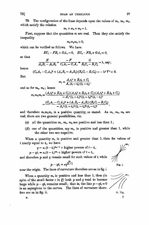
73] NEAR AN UMBILICUS 97
73. The configuration of the lines depends upon the values of wij, m*, tw,,
which satisfy the relation
First, suppose that the quantities m are real. Then they also satisfy the
inequality
w^w^m, > 0,
which can be verified as follows. We have
so that
hence
But
ECl -FB1 + OA l = 0, EG.-FB.+ GA^O,
E -F GAA - ArB,
~ C.A, - G,A, ~ B& - B.Cr *say '
(C1A1 -ClAiy + (A 1Ba -A 1B1)(B1C1 -BiCa) = -\'V*<0.
A 1 t13 + B1 tl + G1
ma TOam3 = -
and so for m,, mt ; hence
(Atf + B^ + C) (jj,tf + B1 tt + fl) (^i<s3 + Bl tt + Cx)
_ (C^A, - CU,)' + (AXB* - A&)(B& - B.C,)
-ASfr-Wfa-ttYitt-ty
and therefore imiw,iml is a positive quantity, as stated. As m,, m^, m, are
real, there are two general possibilities, viz.
(a) all the quantities m^, wij, wi, are positive and less than 1
;
(yS) one of the quantities, say w^, is positive and greater than 1, while
the other two are negative.
When a quantity m^ is positive and greater than 1, then for values of
t nearly equal to t1 , we have
q = Kl (t — <1)m'~ 1 + higher powers of t — U,
p — qtj = K2 (t- ti)"
1' + higher powers of t — ty,
and therefore p and q remain small for such values of t, while
p — qt1= «gm >
_1
near the origin. The lines of curvature therefore are as in fig. i.
When a quantity wij is positive and less than 1, then (in
spite of the small factor c in f) both p and q tend to become
large while p — qti remains small ; that is, the line p — qt1 =is an asymptote to the curves. The lines of curvature there-
fore are as in fig. ii.
F.
Fig. i.
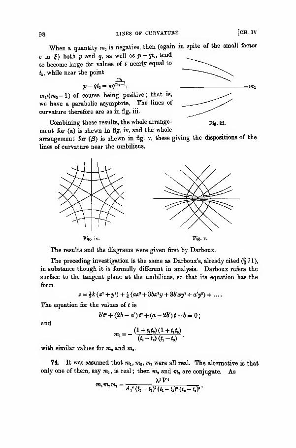
98 LINES OF CURVATURE [CH. IV
When a quantity m, is negative, then (again in spite of the small factor
c in £) both p and q, as well as p - qU, tend
to become large for values of t nearly equal to
(,, while near the point
p-qU = *?m,_1
.
mj/(m,-l) of course being positive; that is,
we have a parabolic asymptote. The lines of
curvature therefore are as in fig. iii.
Combining these results, the whole arrange-
ment for (a) is shewn in fig. iv, and the whole
arrangement for (£) is shewn in fig. v, these giving the dispositions of the
lines of curvature near the umbilicus.
Fig. iii.
Pig. iv. Fig. v.
The results and the diagrams were given first by Darboux.
The preceding investigation is the same as Darboux's, already cited (§71),
in substance though it is formally different in analysis. Darboux refers the
surface to the tangent plane at the umbilicus, so that its equation has the
form
z=^k(x2 + y,) + ^(aic!
' + 3bxiy + Sb'xf + a'y!l)+ ....
The equation for the values of t is
V? + (2b- a')t* + (a-2b')t-b = 0;
and
mi = —(l+fA)(l + <A)
(<i-<2) (<i-<,)
with similar values for m, and m,.
74 It was assumed that 7%, m^, m, were all real. The alternative is that
only one of them, say wij , is real ; then m* and tw, are conjugate. As
m^m^mt =^{ti-krik-unt, -t,y

75] NEAR AN UMBILICUS 99
it follows that miWi2m3 is negative. Now m2ra3 is the product of two con-
jugate quantities and therefore is positive ; hence ml is negative.
Then for values of t nearly equal to tlt we have p, q, p — tx q all large,
while there is a parabolic asymptote
p—qt1= /eg"1 '
-1;
and so the configuration of the lines of curvature is as in fig. vi.
Fig. vi.
75. The suggested determination of the lines of curvature, by means of
the differential equation of the first order which they satisfy, presupposes
a knowledge of the fundamental magnitudes ; and this may be neither given
nor obtainable easily in the absence of obviously suitable parameters. Yet
it may be necessary to have some integral equation giving the lines of curva-
ture ; and we can then proceed in one or other of two modes.
By the first, we make two of the Cartesian coordinates the parameters
—
say x and y ; the parametric curves are then not orthogonal (save at special
places), though their projections on the plane of z are orthogonal. Then
with the usual notation for derivatives of z with respect to x and y, the
fundamental magnitudes* are
E=\+p*, F=pq, G = l + qi,
and so the differential equation of the lines becomes
{(1 +p*)s -pqr] da? + {(1 + tf) t - (1 + q*)r} dxdy + [pqt - (1 + ga)«} dy* = 0.
The primitive of this equation will give the projection of the lines of curva-
ture upon the plane z = ; when it is combined with the equation of the
surface, we have equations sufficient for the analytical expression of the lines
of curvature.
* See Ex. 3, p. 60.
7—2
100 INTEGRAL EQUATIONS OF THE [CH. IV
76. The other mode of proceeding depends upon the use of another form
of the equation ; and it is effective with some special classes of surfaces.
Let u, v, w denote three quantities proportional to the direction-cosines
of the normal, so that
u:v:w =X:Y:Z =Tx
.
Yy.
Yz ,
if the equation of the surface is<f>
(x, y,z) = 0; then any point on the normal
is given by
%=x + lu, r)=y + lv, £=z+lw,
where I is a variable parameter. Take the consecutive normal at a point
along a line of curvature ; denote by £, i), % the point where the two normals
meet, and by f + df, 77 + dr/, £+ df the point where the second normal is
met by the normal at a second consecutive point along the line of curvature.
Then df, dt), df is an element of the normal, so that
say; hence
that is,
and similarly
Hence
df _ drj _ d%_u v w
fiu = dx+ Idu + udl,
= dx+ Idu + u(dl — p);
= dy+ Idv + v (dl — fi),
= dz + Idw + w (dl — fi).
= 0,I dx, dy, dz
du, dv, dw
!u , v , w
an equation satisfied in connection with variations along a line of curvature
;
it is a differential equation of the lines of curvature.
If, with the concurrent use of<f>
(x, y,z) = and derivatives from it, we
can obtain a couple of independent integrals
f(x,y,z)=p, g(x,y,z) = q,
where p and q are arbitrary quantities, these are the equations of the lines of
curvature; p and q are the parametric variables of the lines. The difficulty,
of course, lies in obtaining such integrals; there is no general process by
which the integration is reduced to mere quadratures.
As an example, let us find equations for the lines of curvature on the cubic surface
aryz=l.
We can take
1
76] LINES OF CURVATURE 101
The differential equation is
dx, dy, dz
dx dy dz
a5 ' f' ~z*111x' y' z
and so quantities A and B exist such that
=0,
l'(A+S)^ l-(A+?)*' \={A+$ d>>
that is, if B=\A,
. dxA — 1
ady _ 1 . dz _ 1
x~x*+\' y~y>+\' z~W+\-
But any direction on the surface is such that
dx dy+
dz=()
x y z
Hence there are two values of X, each associated with a line of curvature ; and they are
given by the equation
a^+X^V+ X z2+X~
Take the line of curvature d'x, d'y, d'z which is perpendicular to dx, dy, dz, so that
dxd'x+dyd'y+dzd'z=0;
then, along that line,
xd'xj_
yd'y zd'z
Also
^+x +^+x +22+x~a
d\ d\ d\
adding and effecting a quadrature, we have
(**+ X) (y8+ X) (?
+
X)= constant.
Let Xi and X2denote the roots of the equation
1
+.tfW + ^U=0,#2+x v+x 22+X
regarded as a quadratic in X ; then the lines of curvature on the surface xyz= l are given
by(*HX1
)(y+X1)(*1!+X1)=?M
(*2+X2)(y
!!+Xi!)(*2+X2)=}i'
wherep and q are the parametric variables.
Changing p and q into 4p and 4j, Cayley shewed that these equations are equivalent
to
x*+ayi+oW=3(pi +9^)3
1
x*+ a>y+ uz*= 3 (p* - 2* )$ I
'
where <•> is an imaginary cube root of unity.
102 LINES OF CURVATURE AS [CH. IV
77. We have already seen that the conditions necessary and sufficient
to make the parametric curves lines of curvature are
F=0, M = 0,
the first of which makes them perpendicular and the second of which makes
them conjugate. We then have
r=
77]
But
PARAMETRIC CORVES 103
dq \fi) dq \EJ
L, L
and similarly
— _?_ _ w~ E E* a
~2E\G E)
2E\a fi)'
dp \u) 2G\I3 a)'
hence the Mainardi-Codazzi relations can be written
d /i\ 1/1 i\ aiogg '
dpW ~ 2 [fi a) dp
3/l\ 1/1_ 1\ 91og.g
dq\fi) 2\o /Sj fy J
The Gauss characteristic equation is
But
LN— i {En + Gu) +^ (E,Q, + flfl +^ (^G, + E*).
3p
1 /J_ <wh = '
• JE»1 E.
dq \q\ dq ) 2E^O^ ° 4 #£(?*
and therefore the Gauss equation becomes
\E +GJ'
d_fj_
dG^),d_ /_!_ a^\ _ LN3p \^i 3p / 8? \G<i 3? /
E^Gfc
a{3 '
which can also be obtained directly from Liouville's form (§ 36).
The derived magnitudes of the third order are
«-A-5*-«e-a)-*4(a)
*-*.-f*-*(r3- es©
104 FORMULAE FOR CENTRAL QUADRICS [CH. IV
78. Consider, in particular, the formulae for a central quadric
& V1 z"
,
a o c
they will be required later in dealing with its surface of centres. We know
that the lines of curvature are the intersections of the quadric with the
confocal quadrics
x>+ f
;= 1,
a? fa+p^b+p^c+p a+q b + q c+q
so that p and q are the parametric variables of the lines of curvature upon
the given quadric. The coordinates of a point on the quadric are given by
- fi*/a? =a(a+p)(a + q)
-yay'=b(b + p)(b + q) .
- a0z2 = c (c + p) (c + q) )
whereo, /8, 7 = b — c, c — a, a — b.
' + ?))
' + ?).
Then, if r is the distance of a point on the quadric from the centre, and
if m is the perpendicular from the centre on the tangent plane at the point,
7^ = ^ + f +z* = a + b+c + p + q)1 a? y' z* pq^>
=a»+
6a+
c2_
a6c
We have
E= p(p-q) \
4,(a + p)(b+p){c+p)
q(q-p)= 1-4>(a+q)(b + q)(c+q)
F=0Also
and
xr_ f be (a+p)(a + g))i
\ @y pq
Y-\ ca (b+p)(b + q))i
1 7« pq J
Ia& pq )
q-p~4>\pq) {a+p)(b+p)(c+p)
N= 1 /abc\i p- q4\pq) {a + q)(b+q)(c+
M=0q)
79] INVERSION AND LINES OF CURVATURE 105
The principal radii of curvature (say a and fi') are
1 = JV; = _/a6c\il
a? Q \pq) q
The umbilici are given by
p = q;
but the quantities p and q are separated in general by — a, — b, — c, according
to the values of these quantities ; and so, at an umbilicus, p = q = — a or — b
or — c. Thus, on an ellipsoid for which a > b > c> 0, the umbilici are given
by p = q = — b.
The magnitudes of the third order are
3L 1L IN 3NP -~2p' Q = ~2q> R= ~2^> /S=_ 29-
79. Among the many simple properties of relation between a surface
and the surfaces derived from it by inversion, we have the property* that
when a surface is inverted, its lines of curvature are transformed into lines of
curvature.
Let c be the radius of inversion, and take the centre of inversion as origin.
Denoting by f, ij, f the point which is the inverse of a;, y, z, we have
f= c3 £, V=c^, ?=c>J„ »--tf + jf + *«.
Then
with similar values for 7}lt r)lt f„ £a ; while
TVi = arc, + yyx + «„ rrs= xxt + yyt + zz% .
Hence, for the inverse surface,
and therefore
cr-K+vf+U^G;
r*
:".t appears to have been noted first by Hirst, Ann. di Mat., t. ii'(1859), p. 164.

106 INVERSION OF SURFACES [CH. IV
For the direction-cosines X', Y', Z' of the normal to the inverse surface, we
have
where
and W is the perpendicular from the origin on the tangent plane. Also
Again,
r2
with corresponding values of iju , f„, while
ttu = <ca:u + yj/n + zzn + E-r?\hence
r4 r2
Similarly
Consequently
^'if' - F'L' = - p (tfif- JX),
tf'JV' - G'Z'— £ (EN - OL),
F'N' -Q'M'= - ^(FN- OM) ;
and therefore the lines of curvature of the inverse surface, being given by
(E'M' - F'L') dp* + (E'N - O'L) dp dq + (F'N' - Q'M') dq* = 0,
that is, by
(EM - FL) dp* + (EN - OL) dp dq + (FN- OM) dq1 = 0,
are the same as the lines of curvature upon the original surface. The pro-
position therefore stands.
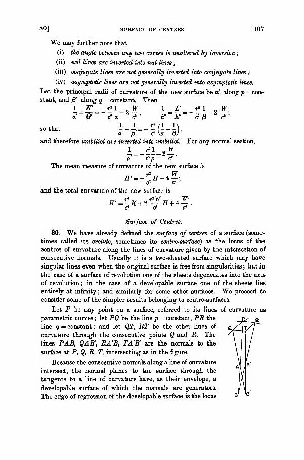
80] SURFACE OF CENTRES 107
We may farther note that
(i) the angle between any two curves is unaltered by inversion
;
(ii) nul lines are inverted into nul lines
;
(iii) conjugate lines are not generally inverted into conjugate lines ;
(iv) asymptotic lines are not generally inverted into asymptotic lines.
Let the principal radii of curvature of the new surface be a', along p = con-
stant, and f¥, along q = constant. Then
I =^ = _!?I_9Z i-:*L__I?I_9 Zof 0' c2 a c2 ' &~ E'~
c2 /3 c2 '
4.u 41 1 r2 /l 1\
so that - — —, = ( -),a' j3' c2 \a £/'
and therefore umbilici are inverted into umbilici. For any normal section,
1 HI .Fp &p c2 '
The mean measure of curvature of the new surface is
r2 WH' ^fT-4-";
c2 c2
and the total curvature of the new surface is
r4 r2W W"
c* c* <r
Surface of Centres.
80. We have already denned the surface of centres of a surface (some-
times called its evolute, sometimes its centro-surface) as the locus of the
centres of curvature along the lines of curvature given by the intersection of
consecutive normals. Usually it is a two-sheeted surface which may have
singular lines even when the original surface is free from singularities ; but in
the case of a surface of revolution one of the sheets degenerates into the axis
of revolution; in the case of a developable surface one of the sheets lies
entirely at infinity; and similarly for some other surfaces. We proceed to
consider some of the simpler results belonging to centro-surfaces.
Let P be any point on a surface, referred to its lines of curvature as
parametric curves ; let PQ be the line p = constant, PR the
line q = constant ; and let QT, RT be the other lines of
curvature through the consecutive points Q and R. The
lines PAB, QAF, RA'B, TA'B' are the normals to the
surface at P, Q, R, T, intersecting as in the figure.
Because the consecutive normals along a line of curvature
intersect, the normal planes to the surface through the
tangents to a line of curvature have, as their envelope, a
developable surface of which the normals are generators.
The edge of regression of the developable surface is the locus
108 SUJtFACE OF [CH. IV
of the intersection of the normals, that is, a curve upon the centro-surface.
and so it is the intersection of the centro-surface and the developable
surface. At the point P, we have
It will be convenient to call the sheet of the centro-surface given by the
centres of curvature along the lines p — constant the first sheet, this being
the locus of the points A for all the points on all these lines ; and similarly
the sheet for the centres of curvature along the lines q = constant will be
called the second sheet, this being the locus of the points B.
The normals at P and R, meeting at a point B on the second sheet, touch
the first sheet at A and A' respectively ; thus AA' is a tangent line to the
first sheet. Also PAB is a tangent line to the first sheet ; consequently the
plane PBR is the tangent plane at A to the first sheet. The normal at Ato the first sheet is perpendicular to this plane and is therefore parallel to
PQ at P. Similarly the plane PA Q is the tangent plane at B to the second
sheet; and the normal at B to the second sheet is parallel to PR at P.
Hence the normal at any point on either sheet is parallel to the tangent to
the corresponding line of curvature ; and the normals to the two sheets at
the two centres belonging to any point on the surface are perpendicular to
one another.
But A A' is not necessarily nor generally parallel to PR, nor is BB'
necessarily or generally parallel to PQ. We are not therefore in a position
to assert that AA' and BB' are perpendicular to one another ; as will be seen
later, it is only exceptionally (in one or other of two directions on the surface
at P) that associated arcs on the two sheets of the centro-surface are perpen-
dicular.
Next, consider the osculating plane of the edge of regression at A. It
contains two consecutive tangents to that edge; that is, it contains two consecu-
tive normals to the original surface along the line of curvature and therefore it
contains the tangent to its line of curvature. But at the point on the sheet,
the normal to the sheet is parallel to that tangent to the line of curvature.
Consequently, the osculating plane at any point of the edge of regression
that lies on the first sheet contains the normal to the sheet ; it is therefore
(§ 65) a geodesic on the sheet. The same holds for the second sheet. Hence
the edge of regression on the developable surface generated by the normals
to the given surface along a line of curvature is a geodesic on the corre-
sponding sheet of the centro-surface.
81. As regards the analytical formulae, let f, r\, £" be the coordinates of
A, a point on the first sheet ; and let f, rj, f be the coordinates of B, a point
81] CENTRES 109
on the second sheet; A and B being the associated centres for P. Thenwe have
a;, + /3Z1=
Ja2 + aX2
= 0,
yl + $7l = 0, y2 + aF2 =0,
*! + /8Z, = 0, *2 + a22 =0.
But
hence
and so
% = x + aX, f = * + /8X;
df = (aij + aXi) dp + Xda
= #i (l — gj dp + Xda,
d? = (x* + pX2)dq + Xdp
= x2 (l-@)dq + XdP;
d^xJl-^jdp + Xda \ dg^Xtfl-^dq + Xdp '
di- yi (l-?)dp+Yda L dn' = yt (l-?)dq+Ydl3
d?=zJl-?\dp + ZdcLj
dS' =z*(l-^dq +Zdpj
In the first place, we notice that
dfdf ' + dijdi?' + dfd£' = dad/S;
and therefore associated arcs on the two sheets are perpendicular only if da
or d/3 is zero, that is, only for directions
Pdp + Qdq = 0, Rdp + Sdq = 0,
on the original surface (§ 77).
In the second place, we notice that along the geodesic on the first sheet,
which is the edge of regression of the developable surface generated by the
normals along p = constant, we have
Sf = XSa, 8V = YBa, Sf = ZSa.
If the orthogonal trajectory of this curve on the sheet be given at the point
by the foregoing values of df, dt}, df, then the necessary and sufficient
condition
d^ + dv Brj + d^=0leads to
da = 0;
that is, the orthogonal trajectories of the regressional geodesies are given by
110 THE TWO SHEETS OF A [CH. IV
the curves on the sheet corresponding to the loci on/ the surface at which the
curvature of the associated line of curvature is constant.
We can at once verify from the formulas that the normal at any point to
a sheet is parallel to the tangent to the associated line of curvature. Thus,
for the first sheet, we have
ih=»yi(i-|)+y«i.
%a= Xav,
at the point, the direction-cosines of the normal to the sheet are propor-
tional to
&» Vi> fti
&, V2, ft !
that is, to
3-1) V\> z\'
X, T,Z\
that is, to a;s , yt , z2 , which are proportional to the direction-cosines of the
line of curvature p = constant. Similarly, for the other sheet. Let these
direction-cosines be A, B, C for the first sheet, and be A',B', C for the second
sheet; then
A = (?-**, B = G-iy2 ,
0=G~lg,\
A' = E~ixu B=E-i yi , C' = E-\zx
)'
Let da denote an elementary arc on the first sheet, and E, P, G denote
the fundamental magnitudes of the first order for that sheet ; and let da',
E', P', G' have the similar significance for the second sheet. Then
da* = df 2 + d-rf + d? = E(\- |) dp" + da",
do-'* = dp + dv'* + dft2 =dp + G(l-Pf dq\
) E'=A2!
It is to be noted, from the form of the expression for do; that the curves
p = constant are geodesies upon the first sheet, while the curves a = constant
are their orthogonal trajectories—in agreement with former results ; and
similarly for the curves q = constant and /8 = constant on the second sheet.
so that
E =
P
Gr = CLi

82] CENTRO-SUBFACE 111
Let L, M, N denote the fundamental magnitudes of the second order for
the first sheet ; and let L', M', N' have the similar significance for the second
sheet. Then
L-^ft1 + Ata + Cr,I --iG-i(l-|)^ =^|A,
a
and similarly for L', M', N'. The whole set of values is
E a ^
M = M' = >.
V = -Ei §1
The values of the fundamental magnitudes for either sheet are deducedfrom the set for the other sheet by interchanging simultaneously p and q,
E and G, L and N, a and y9.
Manifestly, neither P = nor P' = save in the special circumstances
that a principal radius of curvature is a function of one of the parameters
only. But M = and M' = ; hence the two curves on either sheet, that
correspond to lines of curvature on the original surface, are conjugate to one
another, but in general are not lines of curvature on the sheet.
The total curvatures for the two sheets are
K=- 7 K' = -
and the measures of mean curvature are
1 er& GbafPH =
(*-&&'
Gh
Gi(a-$y Ekutia-Pf a«2
'
/3a, &&* Ei
82. The lines of curvature on the first sheet, being in general
(EM - PL) dp* + (EN - GL) dpdq + (FN - GM) dq* = 0,
are, on substitution, given by the equation
[('•+4-J)'K +fJ^->ds -°-
112 RIBAUCOUR'S THEOREMS [CH. IV
The lines of curvature on the second sheet similarly are given by the
equation
]^ + (?(i-f)J
}M| +|§ aiA.]^? = o.
These two equations are the same if the coefficients are proportional to one
another. Writing them momentarily in the form
adp3 + bdpdq + cdq1 = 0,
a'dpf + b'dpdq + c'dq* = 0,
we have the necessary conditions given by
c' =6'= a'
c b a
'
c' aThe condition - = — leads to a relation
c a
& = ft.
a, di
'
LI I
and, when this relation is used, the condition T = — leads to a relationo a
«, = A;that is, we have
0,-^ = 0, o,-A= 0.
Consequently we must have
a — /3 = constant,
and so we have the theorem due to Ribaucour*:
When the lines of curvature on one sheet of the centro-surface correspond
to the lines of curvature on the other sheet (that is, when they are determined
by the same analytical relation for the two sheets), the difference of the principal
radii of curvature of the original surface is constant.
Moreover, we then have
(a -firthat is, the Gauss measure of curvature is constant and negative and the
same everywhere on each of the sheets.
83. The asymptotic lines on the first sheet, being in general
Ldp" + 2Mdpdq + Ndqt = 0,
are, on substitution, given by the equation
Ea'fodp' - Gpcitdq* = 0.
Those on the second sheet are given by
Ea'fadp'-Gpa^dq^O.
* Comptes Rendus, t. lxxiv (1872), p. 1399.
84] CENTRO-SURFACE OF AN ELLIPSOID 113
These two equations are the same if
«*!ft - Ojft = 0,
that is, if a relation
/(a,/8)-0
subsists between the principal radii of curvature of the original surface
without the occurrence of other variable quantities. Such surfaces are called
Weingarten surfaces (§ 42) and are to be discussed later. Meanwhile, wehave the result* that the asymptotic lines on the two sheets of the centro-
swrface of a Weingarten surface correspond to one another ; and, conversely,
if the asymptotic lines on the two sheets of a centro-surface correspond to one
another, the original surface is a Weingarten surface.
84. As an example of the general theory, consider the centro-surface of
an ellipsoid
^ + ? + ^-l.a o c
and suppose that a >b >c, all three quantities being positive. The expressions
for x, y, z, X, Y, Z, and for the principal radii of curvature have already (§ 78)
been obtained. The radii of curvature are positive on the concave side of
the surface (§ 31) ; hence the centres of curvature are
V =y-^7=i[
-^(b+ Py(b + q)^
?=*-/3'Z = {-^g(c + p)»(c + ?)}
f = *-«tt«{-^(a+p)(a+g}>j
?= z - tt>Z=\-±(c+p)(c + qYf t
Elimination of p and q among the values of f, r\, £ leads to a relation
between f, i\, £ which is the equation of the first sheet. But elimination of
p and q among the values of f , rj', f' manifestly leads to the same equation
;
that is, there is a single equation representing the two sheets of the surface.
Now we have
(a + pfqg2
+(b+p)'
bn1
(o+py
+(c + p)-
= 0,
= i;(a+py^(b + pY* The result is also due to Ribaucour (I.e.).
114 CENTRO-SURFACE [CH. IV
and the equation would be obtainable by the elimination of p between these
two relations. The elimination can be effected as follows. Take the
equation
a+t
'
b+t '
c+t
where is a disposable parameter. It is a quartic in t ; and the two pre-
ceding equations express the two conditions that the quartic should have a
triple root. Write the quartic in the form
P + MJ* + 6/c2 «2 + ik3 t + kt = 0,
where4Jfc1
= +A-X,
6ka = 6A+B-Y,
4ik3 = dB + C-Z,
z-p+v+r,Y=(b + c)£* + (c + a) v* + (a + b)?,
Z=bd- i + carf + ab?.
The conditions that the quartic should have a triple root are that the quadrin-
variant and the cubinvariant should vanish ; hence
kt - 4kjc3 + 3&S," = 0,
1, ku kt = 0.
Kit K% , K3
A = a+b + c,
B =bc + ca + ab,
C = abc,
X.,02 + Xjtf + X4= 0,
The former gives
and the latter gives
where X and ft are of degree 0, X2 and ^ of degree 2, X4 and fit of degree 4,
and yn, of degree 6, in the variables, each of them being an even function in
its own degree. Eliminating 8, we have
X, \>, X4 , , =0, Xo, X,, \,
, , X , X,, X,
Mo, Ma, M<> M«>
, Mo, Ma, M«, M»
as the equation of the centro-surface. Manifestly it is a surface of the twelfth
order.

84] OF AN ELLIPSOID 115
To obtain a notion of the form of the centro-surface, consider it near the
plane £= and, in particular, its section by that plane. In that plane wemust have —p = c, or -q = c. When —p = c, then
-byar,' = (b-c)3 (b + q) = a3 (b + q),so that
/32+
a?~ '
an ellipse, being the locus of points where the normal to the ellipsoid along
the principal section is met by the normal at an adjacent point on the other
line of curvature. For small values of £ near that ellipse, we take c + p = — Pwhere P is small ; then, approximately,
£ f(& + g)ff j*/ 3P\1 «7 J V 2/3)'
" = 1 by
(b + q)aa}i ( 3 PPHI)-
?
so that there is a cuspidal edge of the centro-surface at the ellipse. When— q = c, then
(o^)* = a + p, (- &71?2)* = 6 + p,
so that
(of)4 + (67;!!)i = 7i
the evolute of the principal section of the ellipsoid. For small values of f
near that evolute, we take c + q = — Q where Q is small ; then
-a/3y?={a+Py(-l3-Q), - byav* = (b +pf (a - Q), - cap? = - (c + p)> Q,
so that the plane f= is normal to the surface and the evolute section is an
ordinary curve upon the surface. As regards the degree of the intersection,
the degree of the ellipse must be counted thrice because of the cuspidal edge,
and the degree of the evolute is six ; hence the degree of the intersection is
twelve, as is to be expected.
Similarly for the other coordinate planes. The sections are
:
in ?=0,

116 CENTRO-SURFA.CE OF AN ELLIPSOID [CH. IV
corresponds to an umbilicus on the ellipsoid. The dotted line OH is a nodal
curve where the sheets intersect ; and they touch one another at Q.
The nodal curve is given by the equality of £, 17, £ for one set of values
oip and q to f ', t\, £" for another set of values p' and q'. Thus
(a +pY (a+q) = (a + p') (a + qj,
(b+pY(b + q)=(b+p')(b + qy,
(c +pf (c + 9) = (c + p') (c + qj ;
and sop, q,p' could be expressed in terms of q; or all four quantities p,q,p', q'
could be expressed in terms of one parameter. As q and p' occur linearly in
the equations, they can be eliminated at once ; we have
a(a + qJ-a(a+pY, (a + q'f, (a+pY =0.
b(b + qy-b(b+PY, (b + qy, (b+ Pyc(c + qj -c(c +p)\ (c + q')3
,(c +pf
Removing a non-vanishing factor (a — b) (b — c) (c — a) ( p — q')4, and writing
A = a + b + c, B = ah 4 be + ca, C = abc,
we find
3^' (p+q') + A{(p+ qj + 2pq'\ + SB(p + q') + 2C= 0,
as a relation giving p in terms of q1
. To express them in terms of a single
parameter a, we take
3pq' + A(p + q') + B = 2<r,
and then
Apq'+B(p + q')+C=-<r(p + q')
85] DERIVED SURFACES 117
that is,
Apq'+(B + a)(p + q')+C = 0.
Hence
m' p+q'AC -& + Br - 2a* AB-2Aa-3C 3B + 3a-A*'
thus p and q' are the roots of the equation in P(SB - A* + 3<t) P2+ (30- AB + 2Aa)P + AC - B* + B<r - 2a3 = 0.
The values of q and p' are then given linearly by the original equations
;
they are
9 PiC(2q'-p) -(A+p + q')q'* G (2p - q') - (A +p + q')p*
(3C-AB + 2A<r)<r'
There are two nodal lines, each closed, each passing through the centres of
curvature at two umbilici; they are symmetrical with reference to the surface;
and they do not intersect upon the centro-surface unless a + c = 26, in which
case they touch at two points.
For further details and properties of the centro-surface of an ellipsoid, a
memoir* by Cayley may be consulted.
Derived Surfaces.
85. In addition to the surface of centres, there are various surfaces
specially connected with the centres of curvature which suggest themselves
for consideration. Thus there is the middle evolute, which is the locus of the
point midway between the two centres. There are also the parallel surfaces,
being the loci of points taken at a constant distance along the normal from
the given surface.
Consider, generally, a derived surface obtained by measuring along the
normal a variable distance I from the surface ; thus I will be a function of pand q and, unless the surface be a Weingarten surface, I can be regarded as a
function of a and #. Let the point thus associated with x, y, z be denoted by
f , % f ; then
% = x + lX, r) = y + lY, %= z + lZ.
We have
h = ^ + lZ, + Xl2=-(l-a)-2
+ Xk,a.
Coll. Math. Papers, vol. viii, paper 520, where other references are given.
1 18 DERIVED [CH. IV
and similarly for derivatives of rj and \. Let E, F, denote the fundamental
magnitudes of the first order ; then
e = (
1 ~/Xe+u>
a - a>*
Also let X, Y, Z be the direction-cosines of the normal to the new surface,
,- /*;_/-•,, ^(l-vyy-PY + l'^jG+V^jE-,and write
,„ ,-,. EG
then
-<!¥*- ") (^-*)-C-^*-*) (^»-*)y Z-a G , J-/9 E .
-^(J-aKJ-flX+J,— ^.s, + *,-£- ^2
When the normal to the derived surface coincides with the normal to the
original surface, we have X =X, Y=Y,Z=Z; and so
Z1= 0, Z2 = 0,
except for special surfaces and special values of I such that
l = a, l2 =0; or lt= 0, 1 = 0.
Thus, in general, 1 = constant; or a surface parallel to the given surface is
the only surface, which is derived by taking points along the normal and has
its tangent plane parallel to the original tangent plane.
When the normal to the derived surface is perpendicular to the normal
to the original surface, we have XX + YY + ZZ = ; and so
(l-a)(l-/8)«0.
The centro-surface is therefore the only surface thus derived, which has its
tangent plane perpendicular to the original tangent plane.
And generally, the inclination <£ of the two normals to one another is
given by
Vcos<f>= ^ (I -a) (I -/3).
86] SURFACES 119
For the fundamental magnitudes of the second kind, say L, M, W, wehave
f11= — <&n Xl
di\&)+ Xln + X1 l1
on reduction (§§ 34, 77) ; also
= y,(E2 l-a l2\ (G1 l-P k\
2<? /3 '
S* = x
with corresponding values for the second derivatives of 17, f. Thus
= l11 ^(l-*Hl-/3)-l1>^(2l-2a)-^(l-a)(l-0y
(Ifr Ex l-fi\ l-*„. (l-Py VE,
VM=la^(l- a)(l-0)-l1 lll(2l-a-l3)
fl-aY VE,2G-iffiS-iffi**
VN = l^(l-a)(l-P)-l^{2l-2p)-^<!-aLr(!-$)
fl-ay VG.. (la, Gt l-a\ 1-0 v+ h \~a~) ~2E +k W~2G ~a~) ~0~ V '
It is clear that, in general, the lines on a surface thus derived, which
correspond to the lines of curvature, are not perpendicular, for F is not zero
;
and they are not conjugate, for M is not zero. If however I is a function of
only one of the two parametric variables, then F is zero while M is not zero
;
then the lines, which correspond to the lines of curvature on the original
surface, are perpendicular to one another. And if I be constant, so that the
derived surface is a parallel surface, then both F and M are zero ; that is, the
lines of curvature on all parallel surfaces correspond to one another.
86. Various simplifications arise in regard to these derived surfaces when
special values are assigned to the quantity I.
We have already considered the cases when I is made equal to one or
other of the principal radii of curvature ; the derived surface is the centro-
surface.
120 PARALLEL SURFACES [CH. IV
When I = $ (a + yS), the derived surface is the middle evolute ; it was
apparently first considered by Ribaucour* and discussed subsequently as
to its properties by Appell and by Goursat. The latter, in particular, dis-
cussed the inverse problem of determining a surface or surfaces which have
an assigned surface as their middle evolute; the resolution of the problem
f
depends, as many inverse problems in differential geometry depend, upon
a knowledge of the most general integral of a partial differential equation
of the second order.
For a Weingarten surface such that a + yS = constant, the middle evolute
is a parallel surface. A minimal surface is its own middle evolute. But for
surfaces not of special character such as Weingarten surfaces, the properties
of the middle evolute are not of conspicuous importance.
87. One property of parallel surfaces—the persistence of the lines of
curvature through all the surfaces which are parallel to a given surface
—
has already been indicated. The normals at associated points coincide ; and
the lines of curvature on the two surfaces correspond. But the asymptotic
lines do not correspond, nor do the nul lines.
As regards the measures of curvature, we have
l—'-=£e, tf-o, Jf-- l~a.The principal radii of curvature, being G/N and EjL, axe a— I and # — I, as
is to be expected. Also
1 1 H-21KH =
K =
n particular, if 1
then
a-rp-l 1-lH+PK'
1 K(a-0G8-Q 1-lH +lW
In particular, if K be constant and equal to l/as, and we take I = + a,
a
that is, a surface parallel to a surface of constant total curvature 1/a2 at
a distance a is a surface of constant mean curvature. This result, one morelink between surfaces having constant measures of curvature, is due to
Bonnet.
* Liouville's Journal, 4°" S^r. t. vii (1891), pp. 5—108, 219—270. Other references are givenby Darbonx, TMorU ginirale, t. iv, p. 327.
t Goursat, Amer.Journ. Math., vol. x (1888), p. 187.
EXAMPLES 121
EXAMPLES.
1. Obtain the lines of curvature on the surface xy=az, where a is constant, in the
form
p=(zi +aP)b+(z2+f)b, q=(z2+x2)^-(zi+yi)K
2. Shew that the lines of curvature upon the surface
xx
ym zn=a,
where I, m, n are constant, and a is a parameter, are given by the equations
(H'eH"(H"=» (w^rw-*where X and /i are the roots of the equation
I . m , n
%+6 y-+ 6 -+6
regarded as a quadratic in 8, the parametric variables of the lines of curvature being
p and q; and prove that the principal radii of curvature are pk and qk, where
k = (l2lx2 + m?ly2 + n1/z2)*. Prove also that the surfaces a = constant, p = constant,
q = constant, are orthogonal to one another.
3. Shew that the ellipsoid xi/a2+y2/l^+z2jci=l has real umbilici at the points
y=0, x*= -
a*-<? ' a?-c2 '
on the assumption that a>b>c. Discuss the lines of curvature in the vicinity of any
one of these points; and shew that they have the configuration in fig. vi (p. 99).
4. Verify that the lines of curvature on the quadric
y2 z2
a c
are the intersections by the confocal quadrics
-^- +——4(*-p).a—p c—p r
Trace their course upon the surface ; and find the principal radii of curvature in terms of
the parameters of the confocal quadrics.
5. A surface is inverted with respect to any centre. Shew that the quantity r/p+p/r
is unaltered, save as to sign, where r is the distance of a point from the centre of inversion,
p is the perpendicular upon the tangent plane, and 1/p is the curvature of the normal
section at the point in any direction.
6. A surface is referred to its lines of curvature as the parametric curves ; shew that
EXn= - IPX - (P+LT) X! - ZAx2 '
-EX12= - (Q+LV) xx- Lb'Xi
GXi2= - N?*! -(R+ NA') x2
0X22= -N^X-NV'xt-iS+N^Xi.
with corresponding formulae for derivatives of Y and Z.
122 EXAMPLES [CH. IV
7. A sphere of diameter a rolls on the outside of a closed oval surface of volume Vand area S; and the parallel surface, which is its outer envelope, has volume V and area S'.
Shew that
8. A surface, parallel to a given surface, is generated as the envelope of a sphere of
constant diameter a rolling on the surface. With the customary notation for magnitudes
on the given surface, shew that the fundamental magnitudes for the parallel surface are
F'= (l -cfiK) F+(a?H-2a)M I, M'=(l-aH)M+aKF I .
0'= (l-a*K) G+(a?H-2a)N} N'={\-aH)N+aKG J
9. A distance I, equal to the harmonic mean of the principal radii of curvature, is
measured along the normal to the surface; and da- denotes an elementary arc on the
surface, which is the locus of the point so obtained. Prove that
*,-*,
+(l5f)
,
* ,»
and give a geometric interpretation of the result.
10. Prove that each sheet of the evolute of a pseudo-sphere is applicable to a catenoid.

CHAPTER V
Geodesics.
The literature connected with geodesics is very copious. Only a few importantreferences will be given here ; fuller references will be found in the authorities quoted.
For geodesics on surfaces of revolution in particular, a full treatment will be found inthe first chapter of the sixth book in vol. iii of Darboux's treatise ; and reference shouldalso be made to Halphen's Fonctions elliptiques, ch. vi.
For the general properties of geodesics and the use of the notion of geodesic curvature,
the fundamental memoir is that of Gauss*; and full treatment is given, as usual, byDarbouxt.
The method of determining geodesics by means of the solution of partial differential
equations of the first order is expounded by Darboux in his third volume, pp. 1—39 and
pp. 66—85. At the end of the fourth volume he has appended a Note (il) by Koenigs,
dealing specially with geodesics which can be obtained through quadratic integrals andsummarising a number of results deduced in another memoir J.
One portion of the subject-matter has been omitted deliberately—the analogy between
theoretical dynamics and the theory of geodesics. It was developed first by Jacobi § ; andan excellent account is given by Darboux in the last two chapters of the second volume of
his treatise.
Reference may also be made throughout to the sixth chapter of Bianchi's treatise.
At the beginning of this chapter, various propositions from the calculus of variations
are stated. In their application to the theory of geodesics, they are used especially in
connection with the range along which a geodesic is actually the shortest distance on the
surface.
88. The definition and a few elementary properties of geodesics have
already been given ; these curves will now be discussed in fuller detail, and
three main methods of discussion will be indicated.
A geodesic upon a surface has been defined as a curve of shortest length
measured in the surface between two points ; and a descriptive property was
deduced to the effect that the osculating plane of the curve contains the
normal to the surface. The curve may be produced to any length on the
* Disquisitiones generates circa superficies airvas, Ges. Werke, t. iv, pp. 217—258.
t See, in particular, the second volume of his treatise, pp. 402—437 ; and the third volume,
pp. 113—192.
t Mem. des Sav. Etr., t. xxxi, No. 6, (1894).
§ See his Vorlesungen iiber Dynamik.
124 GEODESICS [CH. V
surface, and the deduced descriptive property will be possessed at every
point; but the curve is not necessarily the shortest distance between any
two points however far it is produced. Thus on a sphere a great circle is
a geodesic curve ; the shortest distance on the sphere between two points is
the smaller arc of the great circle through the points, and not the greater
arc, though the latter everywhere possesses the deduced property. Hence
we must possess some method of determining the limits, if any, between
which a geodesic curve is actually the shortest distance, and outside which it
may cease to be the shortest distance, though it possesses everywhere the
deduced property. For this purpose (as for other connected purposes) the
calculus of variations will be used; fortunately, the expression of an arc
involves only derivatives of the first order, and so only the simplest
propositions will be required.
In a second range of investigation, the property (which will sometimes be
called the geodesic property) that the osculating plane of the curve contains
the normal to the surface is used, initially to obtain equations for the geodesic,
and later to determine their properties, especially when the geodesies are
drawn as tangents to non-geodesic curves. For this purpose (as also for
other connected purposes), the Gaussian analysis for surfaces will be used.
In a third range of investigation, the analytical association with theoretical
dynamics is used. Thus, to take only the simplest instance, we know that a
particle, moving on the concave side of a smooth surface under the influence
of no forces other than the pressure, describes a geodesic. More generally,
the Lagrangian equations of motion of a particle in a conservative field
have the form characteristic of the equations of a geodesic as deduced bythe calculus of variations. The theory of partial differential equations of thefirst order is much used in the developments of those Lagrangian equations
;
and so it may be expected that the theory will be useful in deriving someproperties of geodesies. Some illustrations, especially as connected with theactual determination of the curves, will be given in due course.
Application of the Calculus of Variations.
89. Without pretending to give a full summary of the results obtainedin the calculus of variations for problems of the first order, it will be sufficientfor our purpose to state the essentially useful propositions, as they can beapplied to geodesies on a surface*. It is the length of the arc between two
• The proofs will be found, with varying elaboration, in any one of the more modern text-
sl« nfV ?D8 °f Variationa
'8Uch « 'hose by Bolza, Hadamard, Hancock, Kneser.
1™
t
I r^0DB!re
°f °ld Btttnding-Thns the BimPleBt caBe °f the tot (or, what is the
Z fn^g
' / I".dUe t0 Eul6r
-The 8eCOnd is dne t0 Le^dre, and the third to Jacobi.ine fourth is due to Weierstrass, who reconstructed the subject and whose lectures, in authority
trre form, are not yet published.
89] CALCULUS OF VARIATIONS 125
points on the surface which is to be made a minimum; so we have to consider
integrals
f(Ep'* + 2Fp'q' + Gq'rf dt, f(E+ 2F6 + G6*f dp,
where, in the first, p and q are to be made appropriate functions of t, while
p' = dp/dt and q' — dqjdt ; and, in the second, 6 = dq/dp, and q is to be made
an appropriate function of p ; always so as to secure the minimum. The
propositions are as follows.
I. When the quantity to be made a minimum is
\f{P> <1>P> l')dt,\>
where the function / is homogeneous, and of the first order, in p and q, the
quantities p and q must satisfy the equations
dp dt\dp'J ' dq dt\dq'J"•
dp dt\dp'J ' dq dt\dq.
Because / is homogeneous and of the first order in p' and q, these two
equations are equivalent to the single equation
^=aW- 9W +(pV'-
?y'
)/l=0 '
owing to the relations
dp dt\dp')~ q' dq dt\dq')~ P '
the quantity /j being
. __i__ayp'q'dp'dq"
Thus either equation can be treated alone. In any of the forms, it is the
characteristic equation ; the primitive gives a possible minimum.
It is an addition to the proposition that, even if the curve should suffer a
sudden change of direction at a free (and not fixed) point in its course, the
values of df/dp' and df/dq' are continuous in the passage through the free
point.
II. The preceding quantity /i must be positive everywhere along the
curve if a minimum is to exist.
This condition is necessary, though not sufficient, to make the second
variation positive. The preceding condition is necessary and sufficient to
make the first variation zero.
Ill (i). When the primitive of the characteristic equation can be deter-
mined, let it be denoted by
p=<f>(t, a, b), q = i/r (t, a, b),
126 PROPOSITIONS FROM THE [CH. V
where a and b are arbitrary constants ; and write
£-*•<* £-*<* £-*<«.
Construct the functions
«. = *'(«) *. (') - f (0 ti (<) = X! (0.
«, = *'(*) fr (0 - <f>' (') +. <*) = te (0.
e (*,«,)= xi (Ox. ft.) -»(0xi«.);
and take the independent variable t as increasing throughout the range of
integration. Then a range of integration, beginning at < , must not extend
so far as the root of ® (t, ta) = which is next greater than t„.
A geometric expression of the condition is due to Jacobi. Take a curve
satisfying the characteristic equation and passing through the lower limit of
the integral represented by t„ ; and take a consecutive curve (that is, one which
makes an infinitesimal angle at t„ with the preceding curve) also satisfying the
characteristic equation and passing through the same initial point. Let the
first point after the initial point at which these two curves ultimately inter-
sect (if they do intersect) be called the conjugate of the initial point. Then
the range must not extend as far as the conjugate of the initial point.
Ill (ii). When the primitive of the characteristic equation is not known,
it may happen that some special integral is known. In that case, the critical
function @ (t, t„) must be obtained by another process. Let
and form the equation
d ( , du\ ,
TtV>-dt)- ufl=0 '
where u is the dependent variable, inserting the values ofp, q, p", q" derivedfrom the special integral. This linear equation in u of the second order hasto be completely integrated ; its primitive is
u = cu1 + c'u,
= cXl {t) + c%(t),
where c and c are arbitrary constants. The critical function is ® (t, <„),
where
®<*.«-xi(0x.«.)-x.(*)x.(M;
the condition, as regards the range of integration, has already been stated.

89] CALCULUS OF VARIATIONS 127
IV. Let
g£>= 9* (p> q> p'> q)> £ = 92 (p, q, p, q) ;
and construct the function <& such that
<& = {£», (p, q, F, Q) - 9l (p, q, p', q)\ F+ [g, (p, q, F, Q') - g2 (p, q, p', q')} Q'.
This function (& must be positive everywhere along the geodesic curve for all
directions given by P' and Q', other than F =p' and Q' = q. The functions
gx and g2 are homogeneous of order zero in p' and q; for the function €E, the
independent variable can be taken to be s, the arc of the curve.
These tests are sufficient and necessary to secure that the curve provides
a minimum ; that is, the integral receives a positive increment for small
variations of p and q. These variations are called weak, when Bp, Sq, Sp', Sq'
are small and tend to zero; they are called strong when Bp' and Sq' are
not small, though Sp and Bq are small and tend to zero. The first three
tests are sufficient to secure the minimum property for weak variations ; the
additional fourth test (the excess-function test) is necessary and sufficient to
secure the minimum property also for strong variations.
V. When the integral, which has to be made a minimum, has the form
r
W(p,q,6)dp,/'
where 6 = dq/dp, the first three tests have a simpler form; and they represent
the older stage of the calculus of variations, when the variations considered
admissible were of the type called weak.
The characteristic equation in (I) is
d /dW\ dW_dp\de) dq
The test contained in (II) is that the quantity
d*Wd6*
must be positive everywhere.
For the test in (III), let the primitive of the characteristic equation be
q = g(p,a,b).
Then the quantity
Ada+ B
db'
where A and B are arbitrary constants, must not again acquire in the course
of the range the value that it has at the beginning; so that the range is thus
128 APPLICATION TO GEODESICS [CH. V
limited. But if the primitive is not known, while some special integral is
known, then the equation
\d-W d f^W\) d (d*Wdu\
1 dq* dp \dqde)
]
Udp\ d& dp)
~
(when for q and 6 their values derived from the special integral are substi-
tuted) must be completely integrated. Let the primitive be
u — Au^ + But.
Then the quantity Au, + But must not again acquire in the course of the
range the value that it has at the beginning.
Such are the tests needed for our purpose. We proceed to apply them,
first, in general to all geodesies as far as possible and then, later, to some
particular geodesies when they can be applied only upon a knowledge of
details.
90. The element of arc upon the surface is, as usual,
ck2 = Edp* + 2Fdpdq + Gdq\
When the curve is a geodesic, some relation must exist between p and q so
as to define the curve; or, what is the same thing, p and q must be expressible
in terms of a single parameter, say t. Then ifp' = dp/dt, q' = dq/dt, 8 = dq/dp,
the arc is given in either of two forms, viz.
fa = (Ep'< + 2Fp'q' + Gq'*) dt\ ds?= (E+2F0 + Gff') dp';
and therefore, when the arc on the surface between two points has a minimumlength, the integrals
J(Ep"- + 2Fp'q' + Gq'rf dt, j(E+i2F6 + Gfrf dp,
must satisfy the minimum tests provided by the calculus of variations.
Two of the tests are satisfied for all geodesies on all surfaces, it beingremembered that we are dealing with portions of surfaces which are devoid
of singularities.
Consider the test in (II). When we write
/=/(/>> 9,P', 2') = (Sp" + 2Fp'q' + Gqrf,
where we naturally take the positive sign for the real radical, we have
p'q dp'dq'
Yl
on reduction This is always positive on a real surface ; and so the necessarycondition is satisfied.
91] TESTS SATISFIED 129
When we write
W = W (p, q, 0) = (E + 2F6 + GPfl,
again taking the positive sign for the real radical, we have
d>W_ Vdffi W3 '
which always is positive ; so that the condition is satisfied for this form also,
as is to be expected when it is satisfied for the other form. It follows that,
in the discussion of geodesies, we need pay no further attention to the test
in (II).
Next, consider the excess-function test in (IV). We have
_ Ep' + Fq dp dq91 J—-E
ds+F
ds'
_ Fp' + Gq' _ F dp dq.
and therefore
(& - {EP' +Fq - (Ep + Fq1
)] F + {FP' + GQ' - (Fp + Gq')} Qf
= i — cos n,
where il is the angle between the direction p', q and the direction P', Q'.
Thus the excess-function is positive for all directions given by P' and Q', other
than P' =p' and Q'=q'. The test is satisfied for all geodesies on all surfaces;
and therefore we need pay no further attention to the test in (IV).
Accordingly, we now have only to consider the characteristic equation
and the determination of conjugate points.
91. When we develop the characteristic equation
dt Kdp'J dp '
where/= (Ep' + 2Fp'q' + Gq'*f, we have
^|i (Ep' + Fq')
}- 1 (ElP* + 2FlP'q' + <?1?") = 0,
that is,
and so
that is,
v.
*^S-(t)"+ 2»'tS-"(S)'=°-

130 GENERAL EQUATIONS OF [CH. V
Similarly, when we develop the characteristic equation
dt {dq'J dq '
we find
^.+"S-(t)'+-it-"(sy--These two equations are the equations of geodesies in general. They serve
to determine p and q in terms of s, taken as a parameter; when s is
eliminated between the determinate values of p and q, a single relation
survives which is the integral equation of geodesies on the surface.
As regards the significance of the equations, we note that
d8*-Xll
\ds)+2Xl
>dsds+ X
"{ds)+Xl
ds>+X
° <fc"
with similar expressions for dty/ds1 and d'zjds*, these relations holding for
any curve. Hence
*3? +*»d*x d2y d?z
= 0,
when the curve is a geodesic ; and similarly
Hence
that is,
d>x d?y d*z n
1 dte_ \__<&y_ 1 <&z
Vi z* ~ Z\ Vi ds2 zlx2 -x^ ds* ~ x^-yjc^ ds1 '
X ds*_Y ds*
~ Z d?
'
so that the principal normal of the curve coincides with the normal to thesurface, in accordance with the earlier inference (§ 65) that the osculatingplane of the curve contains the normal to the surface.
We may remark here that this property is sometimes made the basis
of a definition of a geodesic.
92. Other forms can be given to the general equations. In their first
form, they are

92] GEODESICS 131
when they are resolved for -^ and -rf , we find
S^(S)"-^is+ r»(|)--o|
as1 \ds/ as as \ds/ I
These also are therefore general equations of a geodesic, and they prove more
useful than the general equations in their initial form.
Moreover, we are to expect that the two characteristic equations are
equivalent to one only ; and we know that the integral equation of a geodesic
is a single relation between p and q, so that the single characteristic equation
ought to be a relation between p and q which (owing to the form of the
general equations) should be an ordinary differential equation of the second
order. Nowdpdq _dq /dp\* d?q dp d'q dqdtp.
dsdp~ds' \ds) dp" ~ ds d& ds ds"
'
Q6DC6
$='"'(|)"^'-^>(|)' + <r- 2i'>|- i'
which is the (single) general equation of geodesies on a surface.
One important inference can be made from this form of the equation.
Consider a region of the surface devoid of singularities ; then the quantities
R r", T", A, A', A" are finite and (even when they are not uniform functions
ofp and q) have regular branches in that region. It is known* that a unique
solution of an ordinary differential equation of the foregoing form exists, which
gives q as a uniform function of p and is such that, for an assigned value of p,
both q and dq/dp have arbitrarily assigned values ; in other words, a geodesic
through any ordinary point on a surface is uniquely determined by its direction
through the point. Thus we have a justification (among other things) for the
use of geodesic polar coordinates.
It is to be noted that all the forms of the general equations of geodesies
involve, among the fundamental magnitudes of the surface, only those of the
first order and their derivatives. Hence when a surface is deformed in anyway, without stretching and without tearing, so that the arc-element is
unaltered, the geodesies remain geodesies on the deformed surface; for the
quantities E, F, are unaltered during any such process. And the result is
essentially contained in the deformations of the type indicated.
Further, it is to be expected that the nul lines on a surface will possess
analytically the geodesic property of being the shortest distance between twopoints on a surface ; thus the relation
/= (Ep* + 2Fp'q + Gq'rf =* See the author's Theory of Differential Equations, vol. iii, § 209.
9—2
132 GEODESICS ON [CH. V
should satisfy the characteristic equations. It is easy to verify that, from the
first form of the characteristic equations, we have
(Ep + Fq)| = {Ep" + Fq" +Wp* + E.p'q' + (F, - *©,) ?''}/>
(Fp' + Gq')ft
= {Fp" + Gq" + (F, - $E2)p'* + GlP'q' + W*q'*}f,
which clearly are satisfied by/=0,
that is, by the nul lines on the surface.
Geodesies on Surfaces of Revolution.
93. The general equation of geodesies does not appear to admit of
integration in finite terms for all surfaces. But it is possible to integrate,
wholly or partially, the equation for many classes of surfaces ; and special
methods, sometimes individual to a class of surfaces, sometimes general in
scope and effective in particular cases, are used to obtain the primitive.
If by any method we can obtain an integral equation containing two
independent arbitrary constants, it is effectively the primitive of the general
characteristic equation. All that then remains, in order to complete the
process at present under consideration, is the determination of the range
between conjugate points.
Among surfaces which thus admit integral expression for their geodesies,
one conspicuous class is constituted by surfaces of revolution. We proceed
to consider them briefly in this regard.
Take the axis of z as the axis of revolution ; and let the equation of the
surface be7" = a? + y
2 = 2u (z) = 2m.
Let x = rcos<f>, y = r sin<f>,
so that <f> is the azimuth of a point on the
surface ; and let the geodesic cut the meridian at an angle sfr ; then
, d<f>sm+ = rds--
Also, we have
rdr= u'dz,
so that
ds2 = dri + r*d<f>2 +dz2
-^+(£+i)*'.
Thus, for the characteristic equations in <j> and z, we have
93] SURFACES OF REVOLUTION 133
This quantity / does not involve<f>
explicitly, so that df/dA = ; thus the
characteristic equation in cf> becomes
dt \d6'J '
hence
that is,
r*^ = Ads '
where A is an arbitrary constant. (When we are dealing with the motion
of a particle upon the surface, as indicated in § 88, the quantity A is a
constant multiple of the moment of its momentum round the axis.) Wethus have a first integral of the equations ; it can also be written
r sin yfr = h.
Further, we have
ds2 =f ds* + (£- +lW2u \2u )
and therefore
Hence
*- (£30** -(£*)**
dS = —idsT ,.2
'^-hdz
so that
/r* + u 3yhdz\r"- - AV ~^ '
fr- + u'-\i dz
= Z,
say, where 7 is an arbitrary constant of integration. We now have an
integral equation containing two independent arbitrary constants A and 7 ; it
is the general integral equation of geodesies on surfaces of revolution.
When a geodesic curve between two given points on the surface is
required, the constants h and 7 for the curve are obtained from the
conditions which result from substituting the coordinates of the points in the
integral equation.
In order that the curve may be real, we must have
r>A.If and when r = h, we have
sin 1/r = 1
;
that is, the geodesic touches the parallel at the point which thus is a highest
point or a lowest point on the geodesic.
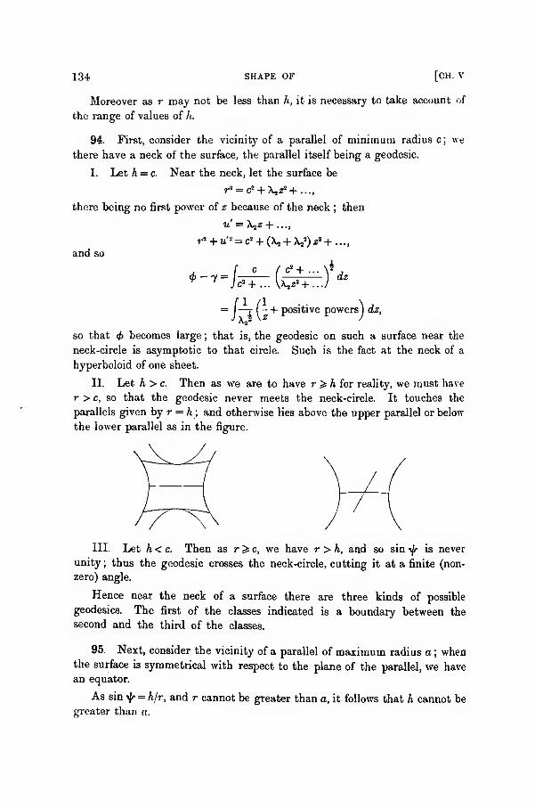
134 SHAPE OF [CH. V
Moreover as r may not be less than h, it is necessary to take account of
the range of values of h.
94. First, consider the vicinity of a parallel of minimum radius c ; we
there have a neck of the surface, the parallel itself being a geodesic.
I. Let h = c. Near the neck, let the surface be
7-a = c2 + A,s2 + ...,
there being no first power of z because of the neck ; then
and so
= I—r ( - + positive powersJdz,
so that 4> becomes large ; that is, the geodesic on such a surface near the
neck-circle is asymptotic to that circle. Such is the fact at the neck of a
hyperboloid of one sheet.
II. Let h > c. Then as we are to have r > h for reality, we must have
r > c, so that the geodesic never meets the neck-circle. It touches the
parallels given by r = h ; and otherwise lies above the upper parallel or below
the lower parallel as in the figure.
III. Let h < c. Then as r^c, we have r > h, and so sin yjr is never
unity ; thus the geodesic crosses the neck-circle, cutting it at a finite (non-
zero) angle.
Hence near the neck of a surface there are three kinds of possible
geodesies. The first of the classes indicated is a boundary between the
second and the third of the classes.
95. Next, consider the vicinity of a parallel of maximum radius a ; whenthe surface is symmetrical with respect to the plane of the parallel, we havean equator.
As sin i/r = h/r, and r cannot be greater than a, it follows that h cannot be
greater than «.
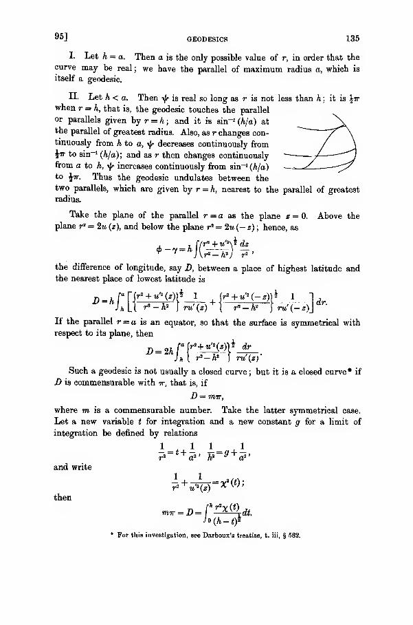
9g] GEODESICS 135
I. Let h = a. Then a is the only possible value of r, in order that the
curve may be real; we have the parallel of maximum radius a, which is
itself a geodesic.
II. Let h < a. Then i/r is real so long as r is not less than h ; it is \ir
when r = h, that is, the geodesic touches the parallel
or parallels given by r = h ; and it is sin-1
(h/a) at
the parallel of greatest radius. Also, as r changes con-
tinuously from h to a, yfr decreases continuously from$ir to sin
-1(h/a); and as r then changes continuously
from a to h, yjr increases continuously from sin-1 (h/a)
to Jw. Thus the geodesic undulates between the
two parallels, which are given by r = h, nearest to the parallel of greatest
radius.
Take the plane of the parallel r = a as the plane z = 0. Above the
plane r" = 2m (z), and below the plane r* = 2m (- z) ; hence, as
, , [fr* +mM dz
the difference of longitude, say D, between a place of highest latitude andthe nearest place of lowest latitude is
D=h!a n** +«*(*))* 1
+ [
** +*»(-«)]* i i rfrJ * L l * - A2
J"*' (*) V r2 - A2
Jru'(- z)\
ar-
If the parallel r = a is an equator, so that the surface is symmetrical with
respect to its plane, then
Ji lr*-h* ) rw'(0>
Such a geodesic is not usually a closed curve ; but it is a closed curve* if
D is commensurable with it, that is, if
-D = 77177,
where m is a commensurable number. Take the latter symmetrical case.
Let a new variable t for integration and a new constant g for a limit of
integration be defined by relations
1.1 1 .1
and write
= t +a*> h*
= g + a"
then
m7r = D=[h
^c(^dt.
* For this investigation, see Darboux's treatise, t. iii, § 582.

136 CLOSED GEODESICS [CH. V
Now m is purely numerical ; consequently* we must have
that is,
1 1 . «v
fdzV _ t
\dr)~
u'»f»j 0?-r*'
and therefore
dzy (m' -^a' + r'
a2 -?-2
But ^ is a maximum or minimum (so that dz = 0) when r = h; hence m is
less than unity, and/dzV _ r'-A2
WW "a2 -?-2 '
which is the equation defining the surface of revolution that possesses closed
geodesies undulating across the equator.
As regards this surface, its element of arc ds is
dsi = dra + ra d(f>t + dz1
n2 — h*= \-^dr* + r*dp.a2 — r2
NowA!= a'(l-7n'); let
r = asinw, ^>=m<£';
thends2 = m'a" (du2 + sin8w d<£'2).
But the last expression is the square of the arc-element on a sphere of radius
ma ; hence the surface of revolution in question is deformable into a sphere,
which is Darboux's result.
96. But it may happen that, in the vicinity of the parallel of maximumradius a, there is no parallel given by r = h ; as our only condition is that
h < a, it might happen that on the whole surface there is no parallel given
by r = h. In either case, the geodesic crosses the parallel given by r = a at
a finite non-zero angle ; in its march away from that parallel across parallels
of decreasing radius, it crosses the meridians at a constantly increasing angle,
which however remains less than a right angle unless and until it reaches
a parallel given by r = h.
97. It now becomes necessary to investigate the range along the geodesic
curve for which the curve is actually the shortest distance between the
extreme points, or, what is the same thing, to determine the conjugate of
a given point.
* The result can easily be established. It is an example of a theorem given by Abel ((Euvres
computes, 1881, vol. i, pp. 14, 15) in a memoir now regarded as a pioneer in the subject which,under the name integral equations, has attracted many investigators in recent years.
97] CONJUGATE POINTS ON GEODESICS 137
There are two cases to consider. In the first, h is not zero and the curve
is not a meridian ; in the second, h is zero and the curve is a meridian.
In the former case, we have
/2\* dz, . [If + tt'Y dz*-V = h
){f=h>) f-
provided that the geodesic curve is not given by the very special case r = h,
dz = 0, that is, provided it is not a parallel of maximum or minimum radius
(in which event, the method of treatment is similar to that adopted for the
case of geodesic meridians). Then
and the condition is that, in the range, the quantity
shall not again attain the value which it has at the beginning of the range
;
that is, the quantity
dh
must not again attain its initial value.
Suppose that there is no parallel given by r = h (so that every point on
the surface is at a distance from the axis greater than h). Then the subject
of integration in d(j>/dh is always finite and positive, and dz has the same sign
along the curve ; thus d<f>/dh is always increasing or always decreasing along
the geodesic, and so it cannot again acquire its initial value. There is no
finite limit to the range of shortest distance along the curve ; no point on the
geodesic has a conjugate at a finite distance.
Suppose that there is a parallel given by r = h. Then from the initial
point of the range until the parallel is neared, the subject of integration is
finite and of the same positive sign while dz is of uniform sign. In passing
through contact with the parallel, the relations
«*-a(S±^. d(m=^±^dz,T \f-hV f \dhj(r«_^«)|
shew that =?- passes through an infinite value and always increases as cf>
increases in passing through the contact; that is, ^? changes its sign in
passing through the infinite value and begins to increase from — oc . After
some stage it will increase to its initial value; at that stage, we have the
conjugate of the initial point. But the actual analytical determination of the
conjugate in precise expression depends upon the particular surface.

138 CONJUGATES ON GEODESICS [CH. V
The same result can be obtained by regarding the conjugate of the
initial point as the ultimate position of the next intersection with a con-
secutive curve through the initial point. In order to have such a consecutive
curve, we need values h + dh, y + dy of the arbitrary constants; in the
figure, let this curve be represented by the dotted lines (for positive and
negative values of dh respectively), while the original curve is represented
by the continuous line. Then the point G is the conjugate of A for the
direction A C ; and a range along the geodesic, beginning at A , is the shortest
distance for all points from A to G short of G. Similarly B is the conjugate
of A for the direction AB.
Note. In dealing with the critical function
/-. dz,
(rz - ft2)*
it proves necessary to exercise care in the choice of the current variable for
the integral, so that it shall admit of continuous increase (or continuous
decrease) throughout the range of integration that corresponds to the con-
tinuous range of the curve.
98. Consider, for example, the non-meridian geodesies on an oblate
spheroid*. The surface is
«? + y* <*_1
a2 c2 '
so that we can take
z = c cos 6, r = asmd, x = a sin 6 cos<f>, y = asind sin
<f>.
* See two noteB by the author, Messenger of Math., vol. xxv (1896), p. 84, p. 161. Referencesto Jacobi, Halphen, and Cayley are given on pp. 94, 95, {I.e.).

98] GEODESICS ON OBLATE SPHEROID 139
We know that a non-meridian geodesic undulates between two parallels;
so let E be the highest point of our geodesic EP,and let CE, OP be the meridians through E and P. c
We thus have a geodesic triangle CEP, right-angled
at E ; the angle EGP is<f>.
Let CPE =^ ; and let
a be the value of 6 at E. Then (§§ 93, 95)
and therefore
ysin20. </>' = &;
n d<j>a sin* -J- = sin a,
as
which is a first integral of the characteristic equation.
This leads to
<i4>={i -" ain' d)ir a
de,(sin2 - sin2a)2 sin
which can be regarded as the differential equation of the geodesic. Theexplicit integration requires elliptic functions and can be effected as follows.
Letcos = cos a en u,
where u is a new variable vanishing when 6 = a, and where the modulus k
of the elliptic functions is given by
e2 cosa a
Then
so that
d<f>=
<#>=
k' = —l-e2 sin2 o'
(l-e'sin'a)^ dn2 w__
sin o 1 + cot2 o sn2 u
(1 -e2 sin2 a)£ f» dn2 w
du,
sin a Jol + cot2 a sn2 udu
= U,
say.
The general equation of geodesies, without the initial choice of the
meridian of reference, would be
containing two arbitrary constants a and 7.
As regards the arc of the geodesic, we have
ds sin2 6
ad<p
sin a
= (1 - e2 sin2 a)^ dn2 u du,
140
and therefore
GEODESICS ON [CH. V
s = a(l-ea sins a)^(M),
where E is the second elliptic integral ; the arc being measured from the
place u = 0, that is, from the point E.
As CPE = f, we have (§ 93)
r sin i}r = h = a sin a
;
hence
Hence
and
sin sin yfr = sin a.
tan yjr =sin a tana
(sin2 - sin2 a)* snu
tan cos yfr = tn w.
Manifestly, some of the relations for the parts of the geodesic triangle
CPE on the spheroid are similar to those of a right-angled triangle on a
sphere; for the respective surfaces they are
sin sin yfr = sin o "] sin sin $• = sin a*
en u cos a = cos
tan fsnii= tan a
tan#cosi/r= tnw
s (1 - e2 sins a)~£ = a£(w)_
cos u cos a = cos
tan >Jr sin u = tan o
tan cos^r= tan«
But it should be noted that, on the spheroid, is not the angle subtended
by CP at the centre, as it is on a sphere ; nor is a the angle subtended by
CE at the centre, as it is on a sphere.
On the auxiliary sphere of the spheroid (that is, a sphere having the same equator),
take the projection of the spheroid orthogonal to the equator. Let C", E', P' be the
projections of C,E,P; the great circles CP' and CE' are the projections of the meridians
CP and CE ; while E'P', the projection of the geodesic EP, is not a great circle. Theangles subtended by CE' and CP' at the centre are a and 6; also E'C'P' is
<f>,and
C'E'P' is a right angle. Let the angle E'P'C be denoted by \j/, and the arc E'P' by s'
;
then we have the equations
s'=a (1 - ^sin2 a)' am u,
sin 6 sin i|/= sin a dn v,
tan i/r' sn u= (1 - e2 sin2 a)' dn « tan a,
tan 6 cos ^'= ( 1 - e2 sin2 a) ~ $ tn u.
The establishment of these relations is left as an exercise.

98] OBLATE SPHEROID 141
Also, we have
j./i * • * \-i , ,ftnu\ 1 f" dnw-dn'w ,
6(1 — e2 sma a) ^tan-1 !-— —:— -m\sin a/ sm a J o 1 + cot2 a sns u
on the spheroid, and
\sino/on the sphere.
The geodesic undulates between the two parallels determined by 6= a,
= 7r — a. Where it cuts a parallel determined by d = f3, we have
cos /8 = cos acnu;
thus the successive points are u = ult u = 4iK—u1 , u = 4<K + ult and so on.
The difference in longitude between the highest point and the nearest lowest
point of the geodesic is
/-. , • , n* f 1 (iK dn u - dn2 u , }
v '{ smaJo 1+ cot2 a sn2 u
J
and is therefore less than tt.
To find the conjugate of any point on the geodesic, we take the general
integral equation in the form
(l-e2 sin2 0)*sina6-*,= - de = i.
' (sin2 6 - sin2 «)$ sin 6
Then
8a—
9a ' dy~
The critical function A -=— + B -^- is not again to acquire its initial value, that
is, =- is not again to acquire its initial value. Now
dl__ /"(I - e2 sin2 6f sin cos a
da '
(sin 2 6- sin2 a)*
_ (l-e2 sinii a)^ fdn2 M ,
cos a J sn2 w '
on introducing the elliptic functions ; and
d8
/;
dn3w 7 ,.„ _. . cnwdnudu = k'2u-E(u)-
fsn2 M sn u
Hence, if ux be the conjugate of u , we have
,. „. . cnitidnMj ... „. . cnM dn«k 'Mj-EM l = « 8Mo - -Q (Mo) ,1 x ' snt*! snu„
so that
ECii! — u ) - A 2(«i - m ) = — •v ' v ' snWjSnM,,
142 CONJUGATES ON [CH. V
The required value of Wj is the root of this equation, regarded as an equation
in w,, which is next greater than u . By tracing the curves
J snxsnu,
it is easy to verify that, when < u„ < IK, then
4,K>u i >u + 2K.
99. In the second case mentioned in § 97, when the curve is a meridian,
h is zero, and <£ is constant. We cannot deduce the critical function from
the value of<f>,
and must proceed to obtain it as the primitive of the linear
equation of the second order given in § 89, III (ii). Returning to the general
surface of revolution, we have always
the arc being ifdz; hence, denoting d<j>/dz by<f>',
we have
-^ = -?/ =0dp •
d<f>di>' '
for /does not explicitly involve<f>;
and
d'/ = f
when we insert the zero value of<f>'.
The equation for the critical function
U is
)i dz i
_ "'
and therefore
d_\ j^_
U=B + AJ(u* + rrfC
^.
The range is limited by the condition that U must not again acquire the
value which it has at the beginning of the range ; in other words, the
quantity
/'
dz(u" + r°jt
^
must not again in the range acquire its initial value.
Another form of the function is
[(„* + r*)*dr
h r'u
It will be noticed that the form of the function coincides with the critical
function in the earlier case when h is made zero therein.

99] GEODESICS 143
Note. As before, so here, in dealing with the critical function
/<
it proves necessary to exercise care in the choice of the current variable for
the range of the integral, so that it may increase continuously (or decrease
continuously) throughout the range.
Ex. 1. In the case of a circular cylinder ?•= constant, u'=0 ; the critical function is
-j , and along a (rectilinear) meridian this function never resumes its initial value. There
is no limit to the shortest-distance property.
Similarly for a circular cone.
Ex. 2. In the case of a sphere, we have
r2= a2— z2, u'=— z,
so that the critical function is
/,
adz
(a2 -z2)*'
that is, - tan-
* -. Hence the conjugate of any point z on the meridian is given by z + aw,a a
that is, the diametrically opposite point on the meridian ; and therefore (as is to be
expected) a great circle is the shortest distance for any length less than half the circle.
Ex. 3. In the case of a paraboloid of revolution, the axis of the parabola being the
axis of revolution, we haver2 =2fe, u'=l,
so that the critical function is
/'<*+»->*£•
that is,
-M* + }*nh-.rrl
TI I
•
Hence any arc of the meridian, whatever its length when it does not include the
vertex, is a shortest distance. When an arc of a meridian does include the vertex, and r^
is the distance of any point from the axis, then the shortest distance along the arc must
not extend so far as a point distant r2 from the axis, where
sinh-i^-f sinh- 1r
-f= - («
2+r12)*+- (P + rf)*.
Ex. 4. In the case of an anchor-ring, we have
z= a sin 6, r=c+acosfl.
The critical function becomes I .
geo3 ^\2 1which is
~ ." » (c*-«sinf),(cr'-as2)*
where
(c — a\*
144 THE METHOD OF GAUSS [CH. V
and, in the function, iff has to lie between - £jt and + £*-. In the march of the function
with the increase of 6, the angle ty increases ; when it increases beyond $ir, we must take
\|r — it in its place.
Thus the conjugate of a point on the meridian is the point half-way round the
meridian.
Ex. 5. A meridian is drawn on an oblate spheroid ; and any point on it is denoted by
r= a sin 6, z= c cos 8. Shew that, if 6X be the conjugate of 8 , then
wheream «!= #!, amwo
=0o ,
and where e, = (a1 - (?)^ja, is the modulus of the elliptic functions.
The Gauss Theory of Geodesies.
100. We proceed now to the discussion of geodesies upon a surface and
their relation to other curves on the surface, without any special regard to
the range within which they are the shortest distance between two points.
The fundamental property is that the principal normal of the curve coincides
with the normal to the surface at any point. This property is sometimes used
as the explicit definition of the curve (§91); it has been derived (§ 65) from
statical considerations; it has been shewn to be a consequence (§ 91), under
the calculus of variations, of the definition by the shortest arc-distance.
Under the last method, it was deduced from the characteristic equations
in the calculus of variations. It is important, however, that the establish-
ment of these characteristic equations should not be based solely upon that
method ; so, accepting the geodesic property (whether as a definition, or as
derived from statical considerations), we can establish the general equations
as follows. Nowx" = xn p'
2 + 2xK p'q' + xa q' 2 + x^p" + x2 q",
where dashes now denote differentiation with regard to s ; and therefore, on
the assumption of the characteristic property, and taking the sign of the
radius of curvature of a normal section as in § 31, we have
= xnp* + 2xKp'q' + Xnq'* + xxp" + x2 q",
and similarlyP
Y- = ynP'1 + tyvp'q' + y»<p +yy + y*q",
- = Znp'* + Zznp'q' + za q'* + z,p" + e,q".
Multiplying by X, Y, Z, and adding, we have
- = Lp'* + 2Mprq' + Nq'*,
the customary formula for the curvature of a normal section; it therefore
101] FOR GEODESICS 145
gives the circular curvature of the geodesic at the point. Again, multiplying
by Xi, yx , *i, and adding; and multiplying by xit y2 , zit and adding; we have
Ep"+ Fq" + mp'* + 2m'p'q'+ m"q" = 0\
Fp" + Gq" + np'* + 2n'p'q' + ri'q* = 0j'
which are the general equations of a geodesic on a surface.
From these, as before (§§ 91, 92), we have
$- r"(g)'+<2r'-*"Hg)"+<
r-^>!-*.
as the single general equation of geodesies on the surface.
In all the forms of the equations as given in § 92, the parametric variables
are general and the parametric curves are completely unrestricted. Somesimplification arises when the parametric curves are specialised.
101. As an example, consider the geodesies upon the quadric*
a? y* z* .- + % + - = l.a o c
Let the quadric be referred to its lines of curvature as usual ; then (§ 78)
we haveE = \{p-q)P, F=0, G = t(q-p)Q,
where
P E Q= 9
{a +p)(b+p){e+pY V(a + q)(b + q)(c + q)-
Hence (§ 77)
r- 1(JL + S). a= i *2\p-q
,
Pj' *(q-p)Q'
2p-q' 2q-p'
2(p-q)P'a
2\q-p +Q)>
where P' = dP/dp, Q' = dQ/dq. Writing
o'=^ „" = *£H dp' H dp''
we have the equation of the geodesies in the form
2 (p ~q) PQq" =W - P)(Qq'-P)- (P - q)PQq'(^ "yTo integrate this equation, introduce a new quantity u such that
P ^ Qq'* _ Qq'*-Pu+p u+q q-p
* For a discussion of geodesies upon quadrics not of revolution, see a paper by the author,
Proc. Lond. Math. Soc., vol. xxvii (1896), pp. 250—280.
P. 10
146
Then
GEODESICS ON A
Z _ *+l - <2V - 2 £ + H!±«' =
[CH. V
Substituting for «, and inserting the value of q" from the differential equation,
we have
0,
Let
u + q u+pthat is,
u'=0,
and so
u = constant = 6.
Thus a first integral of the equation of geodesies on the quadric is
Pd£ = Qdq*
6+p d + q'
R(p) = p{a + p)(b + p)(c +p)(6 + p),
R(q) =q(a + q)(b + q)(c + q)(0 + q);
then the equation is
pdpL
qdq =0{R(p)}l-{R(q)}l
where the lower sign is chosen for a geodesic along which p and q increase
together or decrease together, and the upper sign is chosen in the alternative
cases. Nowpdpi qdq* 4dsa
(a+p)(b + p)(c + p) _ (a+q)(b+q)(c + q) p^q6+p + q p-q'
and therefore
2ds pdp _ _ qdq
P^ ~fii (/>))*
~ +{#(?)}*
Let the upper sign be chosen ; then
dp ^ dq ds /l l\__dspq
J= 2^-( 1- 1
-) = -2<5 p — q\pqj j[R(p)}$ {R(q)}
Accordingly, the first integral of the equation of the geodesies can be taken in
the form
dp- +
dqdv
2{R(prf 2{R(qtf
PdP,
qdq _ Q2{R(p)}i 2{R(q)}i

101] CENTRAL QUADRIC 147
being the canonical equations for hyperelliptic integrals; and*
ds= —pqdv.Also we have
dr Jb + P)(o + p) (b + q)(c + g)
2{R{p)}* * 2{R(q)\i
= (be — pq) dv,
so that
ds = dT— bedv,that is,
s — s = T — be v.
The integration of the equations thus requires the use of hyper-
elliptic functions of the simplest classf ,just as elliptic functions are required
for the oblate spheroid, and circular functions are required for the sphere.
Let the quadric be an ellipsoid, so that a, b, c are positive ; and suppose
that
a>b>c.Then we have
a >—p >b> — q>c.
The curves, p = constant, are the intersection of the ellipsoid with the
confocal hyperboloids of two sheets ; and the curves, q = constant, are the
intersection of the ellipsoid with the confocal hyperboloids of one sheet. Tosecure real values, we must have R (p) > 0, R (q) > ; hence
-p > > - q,
and so
a>—p>0, b> — q>c.
Because and 6 lie between —p and — q, there are three cases according
as 6 = b, 6<b, 6>b.
(i) When = b, the geodesic passes through an umbilicus and, whencontinued, through the diametrally opposite umbilicus.
(ii) When < b, the geodesic touches (but does not cross) a line of
curvature given by = — q ; it undulates between the two lines of curvature
given by q = — 0, and these are lines upon the confocal hyperboloid of one
sheet.
(iii) When > b, the geodesic touches (but does not cross) a line of
curvature given by 0= —p; it undulates between the two lines of curvature
given by p = — 8, and these are lines upon the confocal hyperboloid of two
sheets.
* This agrees with the form given by Weierstrass in 1861 ; Ges. Werke, t. i, p. 262. See also
Cayley, Coll. Math. Papers, vol. vii, p. 493, vol. viii, p. 156, p. 188.
t The expressions for the coordinates and the length of the arc in terms of the current
parameter v are given in the author's paper, already quoted. It may be added that only elliptic
functions are required for the equations of umbilical geodesies.
10—2

148 INCLINATION TO PARAMETRIC CURVES [CH. V
Ex. Let nr denote the perpendicular from the centre of the ellipsoid upon the tangent
plane at any point ; and let D', D" denote the semi-diameters of the ellipsoid, parallel to
the respective directions of any geodesic through the point and of a line of curvature
through the point. Prove that or/)' is constant along the geodesic and that ssD" is
constant along the line of curvature. Is the converse true for either line or for both ?
Discuss the configuration of the curves
xaD=k2,
where it is a parametric constant, and D is the semi-diameter of the ellipsoid parallel to
the tangent to the curve at the point.
102. Returning now to the general equation of geodesies, let i denote the
angle, made by a geodesic with the parametric curve q = b through the point,
and measured towards the curve p = a. Then (§ 26, 6' now being denoted
by i, and 8 later by j), we have
E$ cos i = Ep' + Fq',
and therefore
^ ( JSjp' + Fq') = *tf" * (ElP' + E,q') cos i - E*pg sin i
= ±(E1p' + E2q')(Ep' + Fq')-Vq'^;
consequently, along a geodesic, we have
i (EiP '* + 2FlP'q' + G, 3'a) -^ (ElP' +E3q') (Ep + Fq') -Vq'fg
.
Hence
'S-GS*'!*-'.)'^.*-!*)'F2A , F2A' ,= -~E~P-^-^
Thus, along a geodesic, we have
Eydi = — Adp — A'dq,
together with
ds cosi = E~i (Edp + Fdq), ds sin i = E~$Vdq,
where i is the inclination of the geodesic to the parametric curve q = b.
Similarly, if j is the inclination of the geodesic to the parametric curve
p = a through the point, measured towards the curve q— b, we have
ydj T'dp-Y-dq,
together with
dscoBJ = G~$(Fdp + Gdq), dsBinj = G~^Vdp.
103] GEODESIC CURVATURE OF CURVES 149
These results are in accord with the relation (§ 36)
do, /A T'\, /A' r"\,V=-{E +
G)dp -[E +
-G)d<*'
for the variation of the angle between the parametric curves.
Geodesic Curvature of Curves.
103. We now are in a position to develope a notion as to another curvature
of curves on a surface. We have already considered the circular curvature
and the torsion of any twisted curve, and therefore of any curve upon a
surface. In the case of a plane curve, we regard the curvature in connection
with the deviation of the curve from its tangent. Geodesies on a surface
have much analogy with straight lines in a plane, even when the surface is
not developable ; and so it is natural to consider a curvature of a curve
upon the surface in connection with the deviation of the curve from its
geodesic tangent.
Accordingly, let a curve at any point cut the parametric curve q = b at an
angle i; and at the point draw the geodesic tangent to the curve. At a
consecutive point on the curve, let i + di be the inclination of the curve to
the parametric curve, q = constant, through the point ; and let i + Bi be the
inclination of the consecutive geodesic tangent at the consecutive point to
that consecutive parametric curve. Then the angular deviation (measured
from the parametric curve q = b towards the curve p = a) of the curve from
its geodesic tangent is di — Si, that is,
,. FA, FA'di + -g- dp + —g- dq.
This is called the angle of geodesic contingence of the curve ; the rate of arc-
variation of this angle is called its geodesic curvature. Denoting* the latter
by I/7, we haveds ,. FA, FA'
Similarly, we haveds /,. VT'
,VT", \- = -(dj +— dp+-Q-dq),
where j is the inclination to the parametric curve p = a, and the geodesic
contingence as measured from that curve is Sj — dj.
Of course, when the curve itself is a geodesic, its geodesic curvature is
zero; hencedi FA dp FA' dq
ds+ E ds
+ E ds
* Sometimes the symbol p„ is used, instead of 7.
150 LIOUVILLE'S EXPRESSIONS FOR [CH. V
is the equation of a geodesic. When the value of t is inserted, this equation
reduces to the earlier general equation of geodesies.
Let I/7" be the geodesic curvature of p = a, and I/7' be the geodesic
curvature of q = b. The element of arc along p = a is G*dq; hence
G$dq , ,FA'—^ = dm + -5- dq,E
G*dp_ VT"G
dq,
that is,
Similarly,
i = -7r"<?-?
7
7" 9? EG*.
-, = VkE-%7
1_ g_ t 3« VT'
V dp e^GNow, in general, we have
l_diL
VAdp VA'dq
7 ds E ds E ds
di G*A . . A'= t +• -g-sinj+^Hini.
The simplest case arises when the parametric curves are orthogonal. Then
i+j = 0, = j7T, V* = EG,
1 _ A'=
Gt 1_G*A_ Ei
7" E* 2GE*' 7 E 2EG*'and so
1 _ di cos i sin i
y~ds +~Y
+ "7r '
which effectively is Liouville's formula*.
Further simplification would occur if we could choose the parametric
curves so that I/7' and 1/7" are zero, that is, if there were two orthogonal
families of geodesies on the surface. In that case G^= 0, Et=
; that is, E* In his edition of Monge's Application de VAnalyse a la Giomitrie, p. 575. The signs ol
7, -/, 7" in the text differ from those in Liouville's formula ; they agree, when the geodesic
contingence is taken to be Si - di instead of di - di.
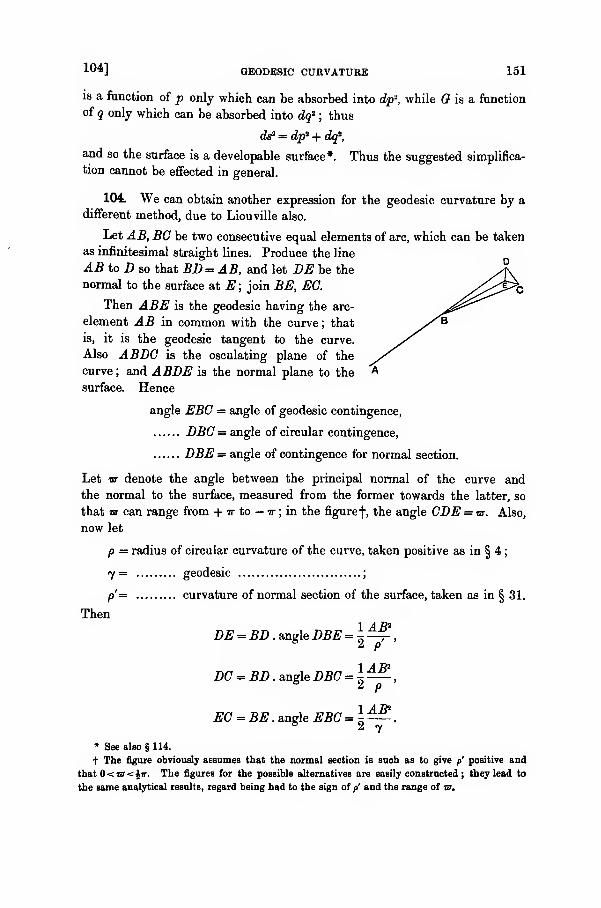
104] GEODESIC CURVATURE 151
is a function of p only which can be absorbed into dp 2, while is a function
of q only which can be absorbed into dq2; thus
ds2 = dp1 + dq*,
and so the surface is a developable surface*. Thus the suggested simplifica-
tion cannot be effected in general.
104. We can obtain another expression for the geodesic curvature by a
different method, due to Liouville also.
Let AB, BG be two consecutive equal elements of arc, which can be taken
as infinitesimal straight lines. Produce the line
AB to D so that BD=AB, and let DE be the
normal to the surface at E; join BE, EG.
Then ABE is the geodesic having the arc-
element AB in common with the curve; that
is, it is the geodesic tangent to the curve.
Also ABDG is the osculating plane of the
curve; and ABDE is the normal plane to the
surface. Hence
angle EBG = angle of geodesic contingence,
DBC = angle of circular contingence,
DBE = angle of contingence for normal section.
Let -as denote the angle between the principal normal of the curve and
the normal to the surface, measured from the former towards the latter, so
that ra- can range from + tt to — ir ; in the figure f, the angle GDE = &. Also,
now let
p = radius of circular curvature of the curve, taken positive as in § 4
;
7= geodesic ;
p'= curvature of normal section of the surface, taken as in § 31.
Then
DE = BD. angle DBE=\^-
,
DC = BD . angle DBG = \—
,
5 2 p '
EC = BE. angle EBC = 1— .
* See also § 114.
t The figure obviously assumes that the normal section is such as to give p positive and
that 0<E7<^ir. The figures for the possible alternatives are easily constructed ; they lead to
the same analytical results, regard being had to the sign of p' and the range of sr.

152
But
hence
GEODESIC CURVATURE
DE = DCcos*r, EC= DC sinw,
1 cos nr 1 sin w
[CH. V
p p 1 p
The first of these two results is Meunier's theorem. The second is a new
expression for the geodesic curvature.
The direction-cosines of the binormal of the curve are
p (y'z" - z'y"), p (z'x" - xz"), p (x'y" - y'x"),
and the direction-cosines of the principal normal are px", py", pz" ;hence
cos « = Xpx" + Ypy" + Zpz",
so that
1 cos or
P'
=~P~
= Xx"+Yy" + Zz"
= Lp'* + 2Mp'q' + Nq'\
the familiar result. Also
sin v = Xp (y'z" - z'y") + Yp (z'x" - x'z") +Zp (x'y" - y'x"),
so that
1
7~
105] bonnet's fobm 153
and these should be equal to one another. Now
E$ cos i = Ep' + Fq', E$ sin i = Vq'
;
hence
Ep" + Fq" = -Etp* - (E2 + J*,) p'q'-F^
+ %E-$ (Erf +E2 q') cos i -E$ sin i j^
,
Vq" = - Fy?' - V2
q'*+ ^E~i (E,p' + E2 q') sin i +# cos i^
.
Multiply the latter by E* cos i, the former by E* sin i, and subtract ; then
di
dsEV(p'q" - q'p") =E^- (VlP'q + V^) {Ep' + Fq')
+ {ElP* + (2?2 + Fx)p'q' + F,f] Vq'.
Now (§ 34)
V1=V(r + A'), T2 = V(T' + A"),
EX = 2(ET + FA), Fl= ET'+F{r +A') + GA,
#s = 2 (#P + FAT), F*= #r" + F(V + A") + <?A'
;
substituting and reducing, we find
diEV (p'q" - q'p") =Ejg+ V&p' (2Fp'q' + Gq'1) + VA'q (Ep'" + 2Fp'q' + Gq'>)
- EV(2A' - T)p'2q' - EV(A" - 2r')p'q'* + EVV'q'*,
which proves the equality of the two expressions for the geodesic curvature.
Another expression, due to Bonnet, for the geodesic curvature of a curve
is required when the equation of the curve is given in the form<f> (p, q) = 0.
Let ® denote the positive square root of E<f>f — 2F<f>1 cf>1 + G<f>i* ; then, as
we take
thus assigning the direction along the curve that is positive. Also
4>ip" + <f>*q" + <f>»p'2 + Zfa.p'q' + <£m?
'2 = 0,
and therefore
© (p'q" - q'p") + fap*+ 2^p'q' + fc,j* = 0.
Now
dp\ ) dq\ © )
= v* {p'q"- q'p" +V + (2A' - T)P'*q' + (A" - 2r')pY2 - r'Y'l.

154 TORSION OF A [CH. V
on using the preceding relations ; and therefore
1 _ 1 (d_ /F& - G<p{\ d_ (Ffa - E+,\
y~'V\dp\ ) dq\ © ))'
which is Bonnet's expression for the geodesic curvature * of the curve
*0»,g)-0.
106. From the two relations
1 cos bt 1 _ sin «7 P
we haveP
1-1 1-P3
P 7
consequently, inserting the values of p' and 7 that have been obtained, we
have an expression for the circular curvature of any curve on the surface.
Thus, for the curve p=a, we have
rn -— v*r"*
ip*u a -G*'
and for the curve q = b, we have
1"
+<?
3
_ L3 F2A2
The curvature of torsion of the curve could be derived from the formula
fa'x
x" y", z"
"> y .
*'
but the expression is complicated, requiring the use of the derived magnitudes
of the third order. Another and more convenient (but equivalent) expression
for the torsion, connecting it with the torsion of the geodesic tangent to the
curve, can be obtained as follows. Let dr' be the angle of torsion for the
geodesic tangent ; so that, in passing to a consecutive point, its osculating
plane (being the normal plane to the surface) turns through an angle dr
about the tangent. The inclination of the osculating plane of the curve at
the point to the osculating plane of the geodesic is ra-; the inclination at
a consecutive point is ts + dvi, so that the osculating plane of the curve has
turned, round the tangent, through an angle dtr relative to the osculating
plane of the geodesic; and these rotations are in the same sense. Hencethe angle through which the osculating plane of the curve has turned in
space round the tangent is dr — dvs ; and therefore
1 _ dr dis
«r ds ds'
the expression in question.
* See also §§ 135, 142.

107] GEODESIC 155
dr'107. The quantity -j- is the torsion of the geodesic ; sometimes (but less
often than formerly) it is called the geodesic torsion of the curve. The analogy
of this name with the geodesic curvature of a curve (which is the arc-rate of
deviation of the curve from its geodesic tangent) is not justified by any
intrinsic property of the magnitude ; so we shall not use this descriptive
name which implies that the magnitude specifically belongs to the curve.
The actual magnitude of the torsion of the geodesic can be expressed
analytically in a simple form as follows. At a point on the surface, let the
configuration be referred to the indicatrix with the lines of curvature as the
directions at the point of the axes of reference ; and suppose (as in § 46) that
the geodesic makes an angle yfr with the line of curvature associated with
the principal radius a. The circular curvature of the geodesic (being the
curvature of the normal section through the tangent) is given by
1 _ cos* •v/r sin2yjr
The equation of the surface in the vicinity of P is
2z =—h ^ + higher powers.
The direction-cosines of the tangent to the geodesic at P are cos ^r, sin ifr, ;
the direction-cosines of its principal normal (being the normal to the surface)
are 0, 0, 1 ; hence the direction-cosines of the binormal are sin i/r, — cos yfr, 0.
The direction-cosines of its principal normal at a neighbouring point, distant
ds from P, are
ds , ds . , ,-— cosijr, --gsmifr, 1;
hence the direction-cosines of the consecutive binormal (which, of course, is
perpendicular to the first tangent) are
sin yjr, — cos ^r, ds ( -5) sin >Jr cos i/r.
The last of these direction-cosines is cos (%ir + dr'), when we take the tangent
to the curve, the positive direction (§ 31) of the normal to the surface, and
the binormal to the geodesic as a set of lines similar to the customary
rectangular configuration. Hence
^=(^-l) coa ^ ain^which is the expression for the torsion of the geodesic.
Manifestly the torsion vanishes at a point on a geodesic where the
geodesic touches a line of curvature ; and it vanishes at an umbilicus for
every geodesic through the umbilicus. Manifestly also two geodesies at
right angles have equal and opposite torsions.

156 GENERAL FAMILIES OF [CH. V
Families of Geodesies and Geodesic Parallels.
108. We have seen that, when geodesic polar coordinates are used upon
a surface, the element of arc on the surface can be expressed in the form
dsi = df + D2dq";
in this form, the parametric lines q = b are a family of geodesies. But it
so happens that, in the deduction of this form, the geodesies are a family of
concurrent curves ; and it might be desirable to have one set of parametric
curves composed of a family of non-concurrent geodesies.
Accordingly, consider generally the possibility of having one set of para-
metric curves, say q = constant, constituted by geodesies. Then the relations
q=b, p' = E~l,
where b is an arbitrary constant, must satisfy the general equations, which
are characteristic of geodesies, viz.,
2 | (Ep' + Fq') = (Elt Flt G&p', q')\
2 ± (Fp' + Gq') = (Et , Fit G&p', qj.
The former becomes an identity. The second equation gives
and therefore some function 6 ofp and q exists such that
dp' $ dq'
Thus, for the element of arc on the surface, we have
ds2 = Edp* + 2Fdpdq + Gdq3
<I)'*:+2
|34^+s^
= dfr+gdq\where
It is manifest, from the form of the expression for the arc, that the curves
6 = constant, q = constant,
are perpendicular to one another. The curves q = b are geodesies ; the curves
6 = a are the orthogonal trajectories of the geodesies. But, further, the
element of arc along any geodesic q = b is given by
ds = dd;
109] GEODESICS 157
that is, the geodesic distance between two 0-curves, given by
= lt 6 = 0,,,
is 0j — O , and so is the same for all geodesies q = constant (which, of course,
cut the 0-curves orthogonally). The curves = a are called a family of
geodesic parallels. The members of the family are given by the parametric
values of a ; and the geodesic distance between two members of the family
is the difference between the values of their parameters.
The equations are thus the same as when we use geodesic polar co-
ordinates. In other words, the arc-element and everything that depends
upon the expression for the arc-element are the same whether the geodesies
are concurrent or not concurrent ; and the orthogonals of the geodesies are,
in both cases, geodesic parallels.
Note. The question as to whether the orthogonal geodesies of any family
of geodesic parallels are, or are not, concurrent, can be settled by proceeding
to form their envelope, if any. They are concurrent, if the envelope is a point.
Thus it is found that, on the surface
ds2 = 4f(p — q) dpdq,
geodesic parallels are given by
a (P + 2) ~ |{aa —/(')} dt = constant,
where a is an arbitrary constant ; the orthogonal geodesies are
1 (p + q) _ Aa= -/(«)]~ * dt = constant
;
where, in both equations, t denotes p — q.
Along the geodesies, we have
/ a2 \^dp + d
9.-[tfZrf)(.dp-dq) = 0,
so that, if f = dq/dp, we haveo'-/_ a - gy
a? U + Vas the differential equation of the first order, satisfied by geodesies. The
envelope (if any) of the curves is obtained by assigning equal roots to f
;
hence it is given by/=a2
,
which in general is a curve (real or imaginary) and not a point. Thus the
geodesies in the family indicated are not concurrent in general ; when they
happen to be concurrent, we have geodesic polar coordinates.
The meridians on a surface of revolution are a family of concurrent
geodesies when the axis of revolution meets the surface in real points.
109. One remark, partly in connection with the general notion of parallel
curves on a surface, may be made here. It is not possible to take any
arbitrarily assigned family of curves (p, q) = a, where a is the parameter, as

158 PARALLEL [CH. V
a family of geodesic parallels ; and the reason is simple. Measure a small
distance Bn along the surface normal to any curve of the family 6 {p, q) = c
;
as the tangential direction along the curve is given by 6^dp + 6adq = 0, the
direction of the normal distance Bn is given by
Bp Bq Bn
G0.-F0,=EOz-Fdi ~~
v {E6? - 2F01 0, + Gdrf
'
If the other extremity of this normal distance lies on a curve of the same
family, then, as
0(p + 8p,q + Bq) = (p, q) + 1Bp + 0>Bq
= c + ~ (E0f - 2F6A + Gdtf,
we must have
y (E8? - 2F6A + Gdrf = function of 0,
in order that it may belong to the same family. This condition is not
generally satisfied, either by the equation of a family of curves, or by the
equation of any member of the family taken in the foregoing form.
The matter however suggests the general idea of curves, parallel to any
assigned curve of the family; but the parallel curves, thus derived from
any curve, form another distinct family which, as will be seen, are geodesic
parallels.
110. Take any curve ; and through successive points on the curve draw
the geodesies which cut it orthogonally. Whenwe measure a length t along the curve from a
fixed point 0, say to M, and take a length I
along the geodesic normal at M, say to P, wehave a uniquely determined point P on the
surface. The locus of P, for a constant length I
measured along the geodesic normals, is said to
be parallel to the original curve ; and, by taking
any number of different lengths I, we obtain any number of curves parallel
to the original arbitrarily assumed curve.
All these parallel curves cut orthogonally the geodesic lines drawn as
normals to the original curve; and so the parallel curves form a family of
geodesic parallels. The property can be established as follows.
Let a consecutive point N be taken ; and along the geodesic normal at
N, let another length l + dl be measured, so that MN = dt, QN = l + dl.
Taking RN=l, we have QR = dl. Denote the angle QRP by <a ; and let
PR, which is not necessarily equal to MN, be denoted by rdt, where the
variable quantity r is equal to unity when 1 = 0. Then the arc PQ on the
surface is given bydiP=dli - Irdtdl cos m + r*dt*.
110] CURVES 159
Now the equation t = constant, under our construction, gives a geodesic
;
hence as E= 1, the condition in § 108 becomes
jn(rcos<»)= 0,
so that r cos to is a function of t alone. To find this function of t, consider
the position at M ; we there have m = ^'ir, r = l,so that the function of t is
zero. Thus <o = ^ir, and the locus of P is normal to the geodesies MP.Moreover,
thus the curves I = constant, being the curves parallel to the original curve,
are a family of geodesic parallels.
Ex. Consider a sphero-conic given by
xi+y2+z2=r2, ax2+by2+cz2=0,
assuming that no one of the quantities a, /9, y(= b — c, c— a, a — b respectively) vanishes.
On the sphere, draw great circles orthogonal to the sphero-conic ; and along the great
circles measure any the same distance subtending an angle ^ at the centre of the sphere.
A new curve is thus obtained, parallel to the sphero-conic ; let x', y', z' denote the point
on the parallel curve corresponding to the point x, y, z on the sphero-conic;prove that
x" -+$'-+* -=0, x'x+y'y+Jz=r* cos ijr,
and verify from these equations that the locus of x', y1
, z1cuts orthogonally the great
circles orthogonal to the sphero-conic. Shew also that the locus of x', if, z is not a
sphero-conic ; so that the family of curves on the sphere, parallel to the sphero-conic, are
not a family of sphero-conics.
It thus appears that any assigned curve can be taken as initiating a
family of geodesic parallels. The result is not in contradiction with the
result of § 109 ; for the locus of P is given by an equation of the family of
parallels, while the equation of the original curve is not generally, as given
initially, some particular case of this equation. Let the equation of the
original curve be 6 (p, q) = ; and let the equation of the family of parallels
be<f> (p, q)= I, where I has the same significance as before. The equations
= 0, = 0, can be simultaneously satisfied, though there is no functional
relation between 6 and ^ alone ; the condition of § 109 is satisfied for
<f>= I or 0, while it usually is not satisfied for 6 = 0.
Ex. In a plane, E=\, F=0, G=l. The equation of a parabola 6=y2—4x=0 does
not satisfy the condition of § 109, for 8i2+62
2 is not a function of 6 alone.
Let the curves parallel to the parabola be drawn ; the curve at a distance c is given by
the equations
H? +ll (2-x)-y=0, H?(2-x)-3w+x*+y2 -c2=0,
(i being a parameter, and also by the equation
<;«-«! c'+WisC2- (y2-4#)2 {y+(x- 1)2}=0,
where the values of utand w2 ,
polynomials in x and y, are not immediately important.
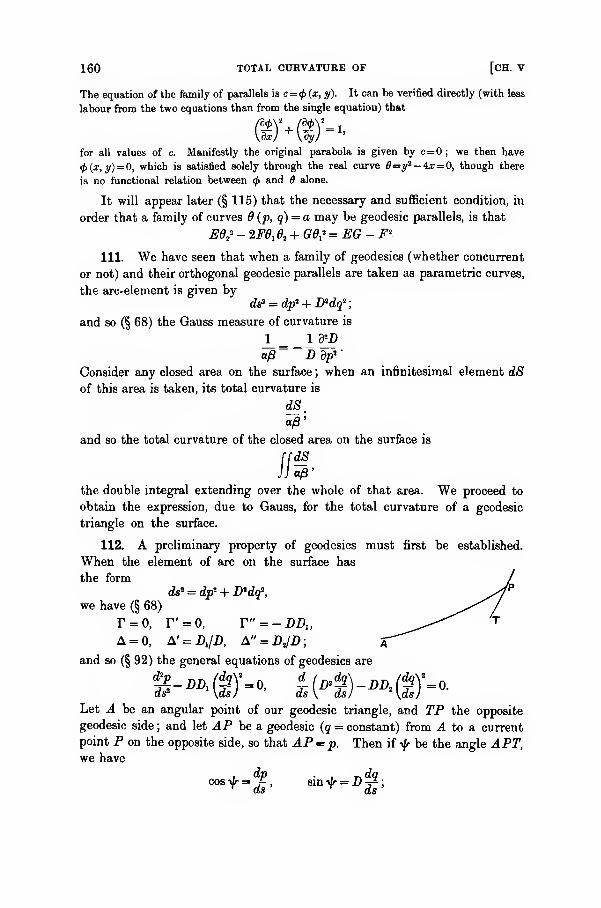
160 TOTAL CURVATURE OF [CH. V
The equation of the family of parallels is c= (j>(x, y). It can be verified directly (with less
labour from the two equations than from the single equation) that
©'OS'"-for all values of c. Manifestly the original parabola is given by c=0 ; we then have
(f>(x,y) = 0, which is satisfied solely through the real curve 8=y2 — 4r=0, though there
is no functional relation between(f>
and 6 alone.
It will appear later (§ 115) that the necessary and sufficient condition, in
order that a family of curves 6 (p, q) = a may be geodesic parallels, is that
Ed,1 - 2F6, B2 + G<V = EG - F*-
111. We have seen that when a family of geodesies (whether concurrent
or not) and their orthogonal geodesic parallels are taken as parametric curves,
the arc-element is given bydsl = dpi + Didqi
;
and so (§ 68) the Gauss measure of curvature is
a/3~ D dp*
'
Consider any closed area on the surface ; when an infinitesimal element dSof this area is taken, its total curvature is
dSa/3'
and so the total curvature of the closed area on the surface is
{dS
«P'
the double integral extending over the whole of that area. We proceed to
obtain the expression, due to Gauss, for the total curvature of a geodesic
triangle on the surface.
112. A preliminary property of geodesies must first be established.
When the element of arc on the surface has
the form
ds* = dp + D*dq\we have (§ 68)
r = o, r' = o, r" = -DA,a = o, a' = a/A A" = A/i>; X
and so (§ 92) the general equations of geodesies are
Let A be an angular point of our geodesic triangle, and TP the opposite
geodesic side ; and let AP be a geodesic (q = constant) from A to a current
point P on the opposite side, so that AP =p. Then if f be the angle APT,we have
cos* = g, sin* = i)g;
m
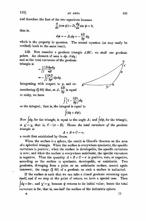
113] AX AREA 161
and therefore the first of the two equations becomesd tin
^(cos^)-A^sinf =0,
that is,
dyfr = -J)ldq=- -^-dq,
which is the property in question. The second equation (as may easily beverified) leads to the same result.
113. Now consider a geodesic triangle ABC; we shall use geodesicpolars. An element of area is dp.Ddq;and so the total curvature of the geodesic
triangle is
= [[DdPd1«/8-IS'-
-IS^dpdq.Integrating with respect to p, and re-
membering (§ 68) that, at A, ^- is equal
to unity, we have
as the integral ; that is, the integral is equal to
J(dq + dijr).
Now \dq, for the triangle, is equal to the angle A; and \difr, for the triangle,
is x' ~ X> *^at *s> G—(tt — B). Hence the total curvature of the geodesic
triangle is
A + B + C-ir,
a result first established by Gauss.
When the surface is a sphere, the result is Girard's theorem on the area
of a spherical triangle. When the surface is everywhere synclastic, the specific
curvature is positive ; when the surface is developable, the specific curvature
is zero ; and when the surface is everywhere anticlastic, the specific curvature
is negative. Thus the quantity A + B + C — it is positive, zero, or negative,
according as the surface is synclastic, developable, or anticlastic. Twogeodesies, diverging from a point on an anticlastic surface, cannot again
intersect; the range (§ 89) of a geodesic on such a surface is unlimited.
If the surface is such that we can take a closed geodesic returning upon
itself, and if we stop at the point of return, we have a special case. Then
dq — 2-Tr; and ^' =X> because -<Jr returns to its initial value ; hence the total
curvature is 2tt, that is, one-half the surface of the indicatrix sphere.
11
/'

162 GEODESIC COORDINATES [CH. V
114. It is reasonable to expect that, through the notion of geodesic
distance, it will be possible to construct for a surface relations which have
some analogies with relations in a plane.
Thus, suppose a family of geodesies given, and let them be cut by any
two curves. Let PQ and P'Q" be two neighbouring
geodesies of the family, cut by the curves PP' and QQ';
and let the geodesic parallels through P and Q be PMand QN. Then ifp and p + dp be the geodesic-distance
coordinates for P and P', while p and p + dp are those
for Q and Q', we have
PQ=p-po = MN,
ds = FQ'-PQ= {p + dp - (p„ + dp )} - (p -p„)
= dp- dp .
But if PP' = dt, QQ" = dt , we have
dp = P'M = dt cos PP'M, dp = Q'N = dt„ cos QQ'N;
and therefore
ds = dt cos PP'M - dt cos QQ'N,
being the expression for the increment of the geodesies cut by the curves.
Again, let P be any point on the surface ; and from P drop two geodesic
perpendiculars PM andPN upon a couple
of selected curves, one belonging to one
given family of geodesic parallels and the
other belonging to another given family
of geodesic parallels. When P describes
a locus on the surface such that
PM + PNis constant, then, if P' be a consecutive point on the locus, we have
dPM±dPN=0,so that
PP' cos PP'M' ± PP' cos P'PN = 0,and therefore
cos PP'M' ± cos P'PN= 0.
Hence the tangent in the surface to the locus of P bisects the angle MPN,either externally or internally. Such loci are known as geodesic ellipses (for
external bisection) and geodesic hyperbolas (for internal bisection).
To give analytical expression to this descriptive property, we chooseinitially, as coordinates of P, the geodesic distances u and v from the twocurves; then
ds2 = edit? + 2/dudv + gdv\

115] A PARTIAL DIFFERENTIAL EQUATION 163
Let u' = constant represent the geodesies which are orthogonal to the geodesic
parallels u = constant ; then we have
ds? = dv? + D*du'\
so that dtf — du* is a perfect square, when regarded as a function of the
differential elements, that is,
(e - 1) du* + 2fdudv + gdv*
is a perfect square, when regarded as a function of du and dv. Hence
f = g{e-l).
Similarly, because v is a geodesic distance,
f* = e(g-l).Consequently
e = g, f* = e(e-l);
and thus, taking e = cosec2at, so that /= cos to cosec2 a>, the arc-element
becomesds* = (du* + dv* + 2dudv cos o>) cosec' m.
To indicate more explicitly the analogy between ellipses in a plane and
geodesic ellipses, we take
u + v = 2U, u-v = 2V;
then the arc-element takes the form
. , dU* dV*sina ^eo cos2 £a>'
The quantity a> depends upon the particular geodesic parallels chosen as the
base of the geodesic perpendiculars, as well as upon the surface itself.
We have a special result (originally due to Liouville) to the following
effect : if a surface admits two families of geodesies which cut at a constant
angle, the surface is developable. For if to is constant, e, f, g are constant
;
their derivatives are zero, and so LN—M* vanishes; that is, the specific
curvature vanishes, which establishes the result.
The Equation A<£ = 1.
115. We have seen that, in one method of determining the integral
equation of geodesies upon a surface, it is necessary to integrate the general
equation, which is an ordinary non-linear ordinary differential equation of the
second order between p and q. But the fact, that the arc-element on the
surface can be expressed differentially in a form which arises most simply
when geodesic polar coordinates are used, can be employed to determine
systems of geodesic parallels and the associated systems of orthogonal
geodesies.
11—2

164 BELTRAMI'S [CH. V
Let a family of geodesic parallels on a surface be represented by the
equation
$ (P> ?)= constant
;
and let the equationyjr (j>, q) = constant
represent the family of orthogonal geodesies. Then, after preceding ex-
planations, we know that the arc-element on the surface can be expressed
in the formd<f>*+D*df*,
where D is free from differential elements ; hence
Edp2 + 2Fdpdq + Gdq* = d</>2 + lPdty\
and therefore
G=& -t-D2^-
(E - #) (G - &) -(^-^-0;
. GW-2F<f>i& + E$l&<t>
= yi ,
Consequently
or, if we write
we have
as a necessary condition.
It is also a sufficient condition. For, when the relation
(E- *,*) (G - <fc2) -(F-frW =
is satisfied, we have
ds2- d<p = (E - aV) dp* + 2 {F- <£, </>2) dpdg + (G - aV) dg2.
The right-hand side, regarded as a function of differential elements, is a
perfect square because of the relation ; and therefore
ds* - d$> = (A dp + Bdqf = D'dyfr*.
The condition therefore is sufficient as well as necessary ; and so we have the
result :
—
The general solution of the equation A<f> = 1 determines a family of geodesic
parallels cut orthogonally by afamily of geodesies.
The function A<f> is called* the first differential parameter of the
function<f>.
Now this equation A<£ = 1 is a partial differential equation of the first
order in two independent variables. To integrate it, we can always use
Charpit's method, though in special cases we may use simpler methods all
* After Beltrami who introduced it in his Bologna memoir of 1869, hereafter to be quoted.
116] FIRST DIFFERENTIAL PARAMETER 165
of which can be exhibited as special standard forms of the general method*.The procedure in the general method is as follows. The subsidiary set of
equations
dp _ dq _ dfa dfa
~(Qfa-Ffa) -^{Efa-Ffa) -|(A</») -|(A4>)
is constructed. One integral of the set is required which, while distinct from
A<f> = 1, must contain fa or fa or both ; let it be
f(P> 1> 0i> fa)=a-
This relation is combined with A(f> = 1 to express fa and fa in terms ofp and
q ; when their values are substituted in
dtf> = fadp + fadq,
the right-hand side becomes an exact differential ; and the integral of this
equation is obtained, by quadratures merely, in the form
<f>= <ji(p
t q, a) = 6.
Here a and b are arbitrary constants. Our desired geodesic parallels are
given by
4>(P> <1> a) = b.
It will be noticed that, for their complete expression, we need one integra-
tion of a set of ordinary equations and one quadrature.
116. When a family of geodesic parallels, satisfying the equation A<£ = 1,
has been obtained, the family of orthogonal geodesies can be constructed in
two ways.
It might happen that a somewhat special family of geodesic parallels is
obtainable in a form
<f>(p, q)=b,
where <p contains no arbitrary constant a. Then
2ty = (£-#)* D^ = {G-fa^;and so the corresponding family of orthogonal geodesies, yfr = constant, is
given by
(F - farf dp + {G- </>/)* dq = 0.
The integral equation of the special family of geodesies is then obtained, not
by a mere quadrature but by the integration of this equation.
When, however, it happens that the general families of geodesic parallels
are obtained in the form
<j>(p, q, a) = b,
where <j> now contains an arbitrary constant a, the orthogonal geodesies can
be constructed by a direct process. We have
dsi = dfai + Did^.
* See the author's Treatise on Differential Equations, 3rd ed., § 201.
16(3 QEODESICS DETERMINED THROUGH [CH. V
On the right-hand side occur the quantities p, q, dp, dq, which are current
variables, and also a, which is a parametric variable; while ds" does not itself
explicitly involve a. Hence
o-*m£ + (£*+«!!)w*all over the surface. Along each geodesic, we have
dyjr = 0;
and therefore, along each geodesic, we have
so that
dij>d^ = 0,da
dd> = 0, or d|^ = 0.da
Now we cannot have dyjr = and d<j> = together, for yfr and are
functionally independent of one another. We therefore have
df-0. dfa = o,
simultaneously ; so that yfr is a function of -^- alone. Merging the derivative
function in the multiplier D, we can take
+ = da>
in other words, the geodesies, which are orthogonal to the general families
of geodesic parallels </> (p, q, a)= 6, are given by
da~ C>
where c is an arbitrary constant. Moreover, as a is not a purely additive
constant in<f>,
this equation of the orthogonal geodesies contains two arbitrary
constants a and c.
Further, the inference has already been drawn (§ 92) from the theory of
ordinary equations of the second order that a geodesic through an ordinary
point on the surface is uniquely determined by its direction at the point. Theinference can be established as follows, without recourse to that theory.
For the purpose, it will be sufficient to shew that the geodesic parallel
<j>(p, q, a)=b can be made, at the point, to adopt an assigned direction
—
of course, perpendicular to the assigned direction of the geodesic. Thedirection of the geodesic parallel is settled by the ratio 4>i/<£2 ; if this ratio
were independent of a, so that
^i = <£2X,
where X is a function of p and q alone and is not a function of a, the twoequations
A£ = 1, fa = $aX,
116] PARTIAL DIFFERENTIAL EQUATIONS 167
would determine fa and fa as quantities independent of a ; and then
4>(p, q, a) would not involve a, contrary to hypothesis. Thus fa/fa involves
the arbitrary constant a ; this ratio can be made to assume any value, by
taking all possible values for a ; and so the geodesic parallel (and conse-
quently the geodesic) through the point can be made to lie in any assigned
direction at the point.
As regards the multiplier D, we have
everywhere on the surface. But
substituting, and dividing out by difr, we have
on the surface. Hence
n ^ ^n 9 -09*^™ 9*^
ft J n dDdfa n„d2fa-^+D dH-S
+D, -£''
and therefore, writing
and so on, we have
ni _J(fafa) n dD J(fa',fa)"
~J(fa, fa')' da J (fa, fa')'
where J (u, v) is the Jacobian of u and v with respect to p and q. Con-
sequently
d_(J(faJ)\_ J(faVfada\J(fa, fa
7
)\
LJ(fa, fa')'
and therefore
$j(fa fa')J(fa, fa')= J (fa fa) J (fa, o
A first integral, proper to the surface, of this equation of the third order
in a, is
J*(fafa) _ ViJ (fa, fa
1)'* '
which can be established independently.
It is easy to verify that the curves
debd> = constant, ^- = constant,
oa
are orthogonal. The direction dp/dq of the former is such that
fadp + fadq = 0.
168 GEODESICS AND [CH. V
The direction Bp/Bq of the latter is such that
These directions on the surface are perpendicular if
But we have
and E, F, G, V do not contain a ; hence the condition, necessary for ortho-
gonality, is satisfied.
117. One other result may be noted. Suppose that the general equation
of geodesies is given in the form
f(p, q, a) = c,
where a does not occur in a merely additive form in iff, it is desirable to have
the geodesic parallels. Now along any geodesic, we have
faBp + faBq = ;
consequently the orthogonal direction dpjdq, being that of the geodesic
parallel, is given by
(Eyfrz - F^) dp + (*V* - Gfy) dq = 0.
Thus a quantity jjl, independent of differential elements, must exist such
that
fi {(E+i - FfJ dp + (Fyfr2 - Chfr,) dq} = d<j>;
and <j> is such that A<f> = 1. Hence
/* (Eyjr2 - Ffr) = *. . /* (F+* - G*,) = fc,
V? (EW - 2F+&, + (?ti2) = i
;
therefore
<f>,= (E^ - F^) (E+* - 2FW, + GW)-$,
t/>2 = (***,- Gf,) (E+f - 2Ff1 yjr1+ GW)
~
*
so that, with these values inserted, the equation
$xdp + <f>2dq =
represents the geodesic parallels, when i/r = c represents the orthogonal geodesies.
A quadrature alone is necessary in order to have the integral equation
<f> (p, q, a) = b.
A simple equivalent form can be given to the expressions forty, ^ and
<f>2.
Along the geodesic we have
yftiBp + yfrs Bq = 0,
and therefore
Bp _ Bq Bs
*i ~ +* (E+f - <LFf^2 + G+&
'
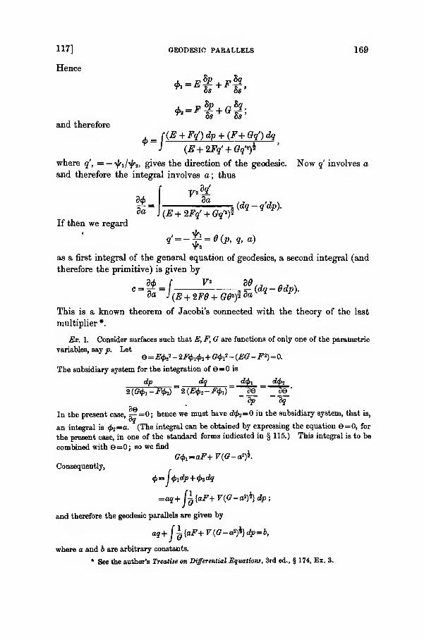
117] GEODESIC PARALLELS 169
Hence
*.-'i + oi:and therefore
Bs:
f (jg + Fq') dp + (F+ Gq') dq
J (E+2Fq' + Gq'rf
where q', = — ^,
i/^,
2 ,gives the direction of the geodesic. Now q' involves a
and therefore the integral involves a; thus
da
If then we regard
daa (^3 _ Q'dp)-
(E+2Fq' + Gq'rf
9'=-^ = Hp, q,a)
da J/
as a first integral of the general equation of geodesies, a second integral (and
therefore the primitive) is given by
l(E + 2Fd+G8*js da
This is a known theorem of Jacobi's connected with the theory of the last
multiplier *.
Ex. 1. Consider surfaces such that E, F, G are functions of only one of the parametric
variables, say p. Lete=E(j>
:i
2-2F<l>l<t>i +O(l)1
i-(EG-Fi)=0.
The subsidiary system for the integration of 6=0 is
dp _ dq d<f>x d(f>2
2 (0<fa- Ffc)
~2 (.fffo - /y>i) ~ 3e 5e
•
dp dq
In the present case, ^-=0; hence we must have d<j>2=0 in the subsidiary system, that is,
an integral is<f>2
=a. (The integral can be obtained by expressing the equation e=0, for
the present case, in one of the standard forms indicated in § 115.) This integral is to be
combined with 8=0; so we find
G^=aF+V{G-a^.Consequently,
</>= Ifadp+fadq
and therefore the geodesic parallels are given by
aq+j±{aF+V(G-arf}dp= b,
where a and b are arbitrary constants.
* See the author's Treatise on Differential Equations, 3rd ed., § 174, Ex. 3.

170 EXAMPLES OF GEODESICS DETERMINED BY [CH. V
The orthogonal geodesies are
30
that is,
8a~C'
where a and c are arbitrary constants ; and this equation accordingly is the general
equation of geodesies upon the particular surface.
Let
VO 5 dp=du, dq+-~dp=dv;
then the element of arc on the surface becomes
dsi=dui+Gdv\
where O, a function ofp alone, is a function therefore of u and not of v. Thus the surface
is deformable into a surface of revolution.
The equation of the geodesies becomes
( adu _•/{£(<? -a2
)}*
- "'
Let u be the angle at which the geodesic cuts the meridian ; then
dssin a)=6- dv, ds cos o> = du,
so that
tan<fl=G*du (G-arf'
or
which (§ 93) was the former first integral of geodesies on a surface of revolution.
Ex. 2. Consider the geodesies on the Liouville surfaces given by
oV= (P - Q) (IP dp2+ S* df),
where P and It are functions of p only, while Q and S are functions of q only. (It is
clear that the parametric curves yield an isometric system.)
The differential equation A(f>= 1 is now
7r^(i<fc 2
+i«fc2
)= i>
so that
a standard form of equation. An integral is known to be
this result being derivable also from the subsidiary system in § 115. Hence
fc=Jl(P-a)*t <h=S(a-Q)l;therefore
<t>= {r (P - a)* dp+ JS (a - Q)i dq.
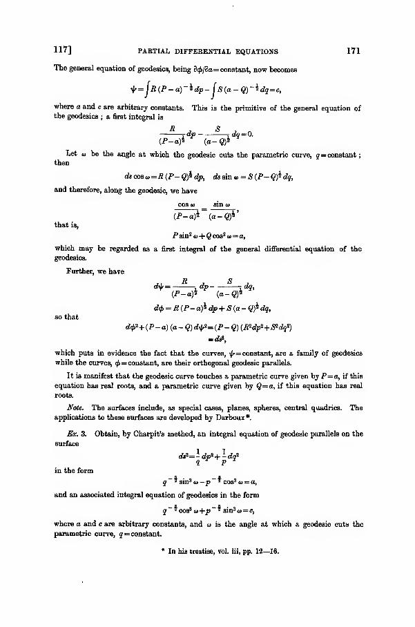
117] PARTIAL DIFFERENTIAL EQUATIONS 171
The general equation of geodesies, being 8<£/3a= constant, now becomes
^=JR(P-a)-idp- (S(a-Q)-Idq=c,
where a and c are arbitrary constants. This is the primitive of the general equation ofthe geodesies ; a first integral is
rdp j dq= 0.
(P-a)4 (a-§)4
Let o> be the angle at which the geodesic cuts the parametric curve, q= constant
;
then
ds cosa=R(P-Q)i dp, ds sin a = S(P-Q)^dq,
and therefore, along the geodesic, we have
cos a> sin <o
(jP-a)4 ~(a-<2)4'
that is,
P sin2 <•>
+
Q cos2 a= o,
which may be regarded as a first integral of the general differential equation of the
Further, we have
df= dp dq,
(P-a)* (a-©4
<fy = R (P- a)4 dp + S (a - §)4 dq,
so that
d$i+ {P-a){a-Q)dyi={P-Q){R*dp*+Sidq'1)
= tfs2,
which puts in evidence the fact that the curves, ^= constant, are a family of geodesies
while the curves, <f>= constant, are their orthogonal geodesic parallels.
It is manifest that the geodesic curve touches a parametric curve given by P=a, if this
equation has real roots, and a parametric curve given by Q=a, if this equation has real
roots.
Note. The surfaces include, as special cases, planes, spheres, central quadrics. Theapplications to these surfaces are developed by Darboux*.
Ex. 3. Obtain, by Charpit's method, an integral equation of geodesic parallels on the
surface
ds*=±dp2+-dq*? V
in the form
q ~ * sin3 <<> -p ~ * cos3 a = a,
and an associated integral equation of geodesies in the form
q ~ * cos3 a)+p ~ * sin3 «a = c,
where a and e are arbitrary constants, and <> is the angle at which a geodesic cuts the
parametric curve, q = constant.
* In his treatise, Vol. iii, pp. 12—16.
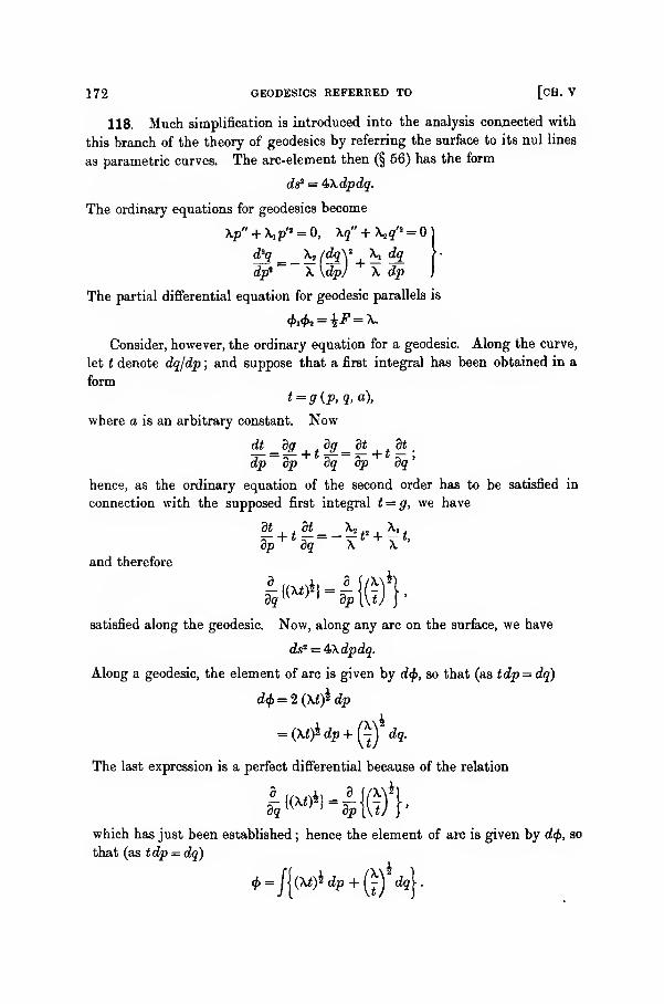
172 GEODESICS REFERRED TO [CH. V
118. Much simplification is introduced into the analysis connected with
this branch of the theory of geodesies by referring the surface to its nul lines
as parametric curves. The arc-element then (§ 56) has the form
ds2 = i\dpdq.
The ordinary equations for geodesies become
\p" + X, p" = 0, \q" + X2g'2 =
j
<Pq \t /dq\ 2 X, dq \-
dp3 ~ X \dp] X dp J
The partial differential equation for geodesic parallels is
</>i#2 = i-F = X.
Consider, however, the ordinary equation for a geodesic. Along the curve,
let t denote dq/dp ; and suppose that a first integral has been obtained in a
form
t=g(p,q,a),
where a is an arbitrary constant. Now
dp dp dq dp dq'
hence, as the ordinary equation of the second order has to be satisfied in
connection with the supposed first integral t = g, we have
— + t — = - - «2 + - t,
dp dq \ \ '
and therefore
satisfied along the geodesic. Now, along any arc on the surface, we have
dsl = ^\dpdq.
Along a geodesic, the element of arc is given by d<f>, so that (as tdp = dq)
d<f> = 2 (Xt)$ dp
= (\t)idp+(j) dq.
The last expression is a perfect differential because of the relation
which has just been established ; hence the element of arc is given by d<f>, so
that (as tdp = dq)
*-/{(w)*c«p+g) dqy
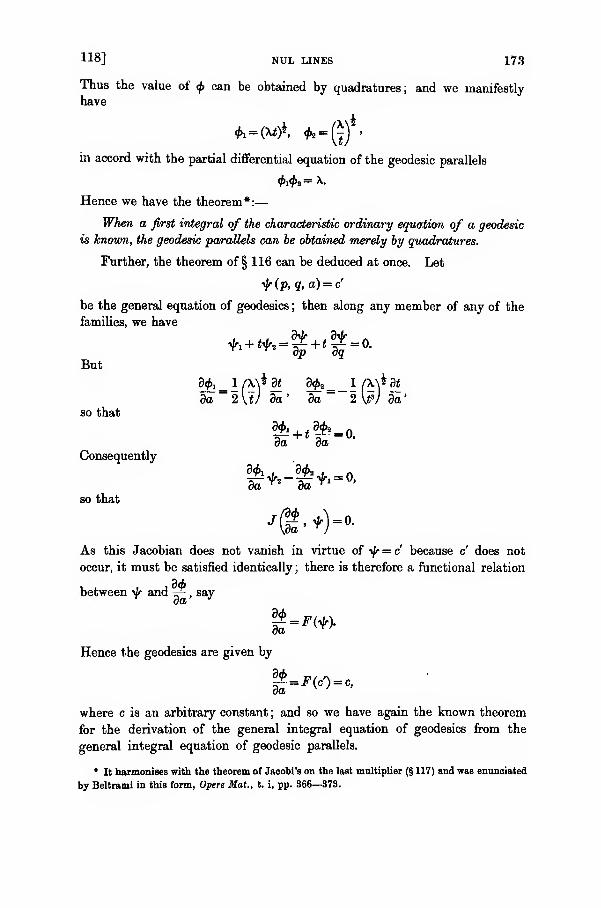
118] NUL LINES 173
Thus the value of </> can be obtained by quadratures; and we manifestly
have
*, = (X*)i, fr«g) >
in accord with the partial differential equation of the geodesic parallels
Hence we have the theorem*:
—
When a first integral of the characteristic ordinary equation of a geodesic
is known, the geodesic parallels can be obtained merely by quadratures.
Further, the theorem of § 116 can be deduced at once. Let
yfr(p, q,a) = c'
be the general equation of geodesies ; then along any member of any of the
families, we have
But
so that
Consequently
so that
da ~ 2\t) da' da ~ 2W da'
da da
As this Jacobian does not vanish in virtue of i}r=c because c does not
occur, it must be satisfied identically ; there is therefore a functional relation
between ^r and ~ , say
£-'<»
Hence the geodesies are given by
where c is an arbitrary constant ; and so we have again the known theorem
for the derivation of the general integral equation of geodesies from the
general integral equation of geodesic parallels.
* It harmonises with the theorem of Jacohi's on the last multiplier (§ 117) and was enunciated
by Beltrami in this form, Opere Mat., t. i, pp. 366—373.

174 EXAMPLES [CH. V
Ex. 1. Consider the surface for which
X=/(p-?).
The general ordinary equation for the geodesies becomes
while
hence
|{log/(P - ?)}=d-0f =^4and therefore
{\+tf _a4* "/'
where a is an arbitrary constant. Hence
t
qt-(B-/)*;
«* + («-/)*'
consequently
)» = {a* -(a -/)*}*, {={«*+(«"/)¥.
so that the arc along the geodesic is given by
<t>= j(ft)ldp+ (P) dq
= j{a* (dp +<fy) - (a -/)* (rfp - dq)}
=al (p+q)- f(a-e)l d0,
where 6=p-q, Q=f{6). Thus the geodesic parallels are
al(p + q)- l(a-efidd= b;
and the geodesies themselves are given by
P+»-/(jTTe) d6=c-
Ex. 2. Obtain the integral equation of the geodesies on the surface
ds2= if{pq) dp dqin the form
, p [/ a \*d6,
where 6=pq, e=f(6) ; and deduce the equation of the geodesic parallels.
Ex. 3. Shew that the geodesies on the surface
dii= \{f{p-q)-g(p+ q)}dpdqare given by the equation
[d(p-q)
±f d(p+ q) _ g
Note. This form, together with all derived from it by transformation of the variables,
includes the cases, at present known, in which an integral equation of the geodesies can be
expressed in finite terms.
119] POLYNOMIAL INTEGRALS 175
Polynomial Integrals of A0 = 1.
119. We have seen that geodesies can always be deduced from a
primitive integral equation of geodesic parallels. The latter can be obtained
if we have an equation
fifa, 0a > p, q)=a,
where a is an arbitrary constant, together with the equation
A=A(/)-l = 0.
The condition of coexistence is the Jacobian relation
(/,A) = 0,
which, in full, is
s£3A_3/;aAy9A_a/;aA = .
dp dfa 30! dp dq dfa d<f>2 dq '
and any integral of the subsidiary system (being the subsidiary system in
Charpit's method, § 115)
dfa dfa dp dq
dp dq 30! 302
which involves 0! or fa or both, can be used for the function /(01 , fa, p, q).
The two equations A = 0, /= a are to coexist ; so the form of/ is always
modifiable by means of the equation A = 0.
Now the number of cases in which an integral of the subsidiary system
can be obtained (by which we usually mean that it can be obtained in finite
terms) is comparatively small. Among these, some special attention has
been devoted* to the cases when /is polynomial in fa and fa; the conditions,
necessary and sufficient for the existence of such a function/, can be obtained
in the simplest instances.
Accordingly, suppose that / is polynomial of order n in fa and fa ; and let
the terms in/ of the same order m be gathered together and denoted by/m ,
so that /is expressible in a form
/=/» +/»-! +/»-* +...+/, +/, +/.,
where the coefficients in /„, /„_i, ... are (or may be) functions of p and q.
The actual expression of / can be modified by the use of the equation
A0= 1 ; as A0 is quadratic in fa and fa, a set of even terms in/ will remain
even, and a set of odd terms will remain odd, after such modification. The
equation
(/, A)-0
* See Darboux'a treatise, vol. Hi, pp. 23—39, 66—85, where (p. 66) references are given; and
a note by Koenigs at the end (pp. 368—404) of the fourth volume.
176 POLYNOMIAL INTEGRALS OF THE [CH. V
is to be satisfied, always concurrently with the equation A<f> = 1 ; that is, the
equation
(/», A) + (/„_, , A) + (/„_„ A) + . . . =
is to be satisfied concurrently with A$ = 1. Hence the even terms in / by
themselves satisfy the equation, and the odd terms in/ by themselves satisfy
the equation, in the form
(/n,A) + (/„_a,A)+ = 0,
(/_1 ,A) + (/M , A)+ =0,
each concurrently with A$ = l. Consequently, the odd powers of/ taken
together constitute an integral, and the even powers of / taken together
constitute an integral.
Consider the aggregate of even powers
/•+/»+/«+ •+/»;
it can be transformed into
/„(aw +/. (^y-1
+u(wy-2 +.»+/»,
that is, into a homogeneous polynomial of even order 2/u. Similarly the
aggregate of odd powers
/i+/t +/.+ ...+/**»
can be transformed into
/, (A</>y +/, (A<^- +
f
t (WY-*
+
• • +/«.that is, into a homogeneous polynomial of odd order 2/i + 1. We are
therefore led to inquire what are the integrals / in the form of homogeneous
polynomials in fa and fa, of the lowest orders in succession.
We do not consider the case (if any) when /is of order zero, that is, when
it does not involve fa or fa. It cannot effectively be combined with A<f>= 1 to
determine fa and fa, so as to lead to the quadrature necessary for the
determination of fa
As in § 118, we refer the surface to its nul lines, so that the arc-
element is
dsa = 4t\dpdq;
and then
A.
so that the differential equation for geodesic parallels becomes
& = fafa-\=0.When
f(<f>i, <f>2, p, q) = a
120] PARTIAL DIFFERENTIAL EQUATION 177
is an equation to be associated with A = 0, the condition of coexistence
(/, A) = becomes
We are concerned with integrals of this equation that are polynomial and
homogeneous in fa and fa.
120. When there is a linear integral, homogeneous in fa and fa, it mustbe of the form
f=afa + /3fa = 2a,
where a and /3 are functions ofp and q. In order that it may be an integral,
the equation
a\ + &\2 +fa (a.fa + fafa) + fa (asfa + fofa) =
must be satisfied concurrently with
fafa = \.
Hence
From the first two, we have
a = P, /3=Q,
where P is a function of p only and Q is a function of q only. Now o occurs
in the combination afa, that is, a^; hence, if P is not zero, by takingop
a new variable dp' = dp/P, we do not alter the character of the arc-element
and we make the new a equal to unity. Similarly, if Q is not zero, we can
change the variable so as to make /8 equal to unity without altering the
character of the arc-element. Also, P and Q do not vanish together, for
otherwise/would be evanescent. Hence there are two cases effectively, viz.,
(i), a=P = l, = Q=1,
(ii), a=P = 0, /3 = Q = 1.
For (i), the third condition becomes
X1 + \2 = 0,
so that
hence
We have
hence
and so
X = k (p - q)
;
ds* = 4>k (p — q) dpdq.
fa + fa= 2a, fafa= X = k ;
fa-fa=±2(a"-k)K
d<f> = {a ± (a" - k$\ dp + {a + (a2 - &)*} dq.
12
178 POLYNOMIAL INTEGRALS OF [CH. V
Consequently the geodesic parallels are given by
a(p + q)± j(a2 -k)$(dp-dq) = b;
and the geodesies are given by
p+q±a](a? - k)~$ (dp - dq) = c.
Moreover, writing
p = £ (» + «?). q = £ (« ~ «?)> {* (*^)1*^ = dw> * (^) = U
>
the arc-element is
ds2 = dw2 + C/cfo2,
so that the surface can be deformed into a surface of revolution ; and with
these variables, the geodesic parallels and the geodesies are given by the
respective equations
av±j(U-arf~=b, v + af(U-a')-$p = c.
For (ii), the third condition is \, = 0, so that \ = F(p), a function of ponly. Writing
F(p)dp = dp',
(for modification of the variable p still is possible), we have the arc-element in
the form
ds2 = ^dp'dq.
This is a special form of the preceding case. Thus the surfaces which
provide a linear integral of the equation (/, A) = are deformable into
surfaces of revolution.
121. When the equation (/, A) = has a quadratic integral other than
A0, let it be
/= a0,2 + 200,4, + 70/ = *«•
In order that it may be an integral at all, the equation
2 (a0, + £02)\ + 2 (£0, + 7 2) x,
+ <M«i&2 + 2/S,0,02+ 7,022) + 0, (o,# + 2/3,0,0, + 72 2
s) =
must be satisfied concurrently with 0,02 = \ ; the necessary conditions are
«, = 0, 7, = 0,
2o\, + 20X,, + >.«, + 2X/3, = 0,
2£\, + 27X2 + 2\/3x + \y, = 0.
Hence«=P. 7=Q,
where P is a function of p only and may be zero, and Q is a function of gonly and may be zero ; but a and 7 do not vanish together, for then f would
be a multiple of A0—a possibility which is to be excluded. Thus there are
two cases :
—
(i), ol = P, not zero; 7 = Q, not zero
;
(ii), a = P, not zero ; 7 = 0.
121] THE GEODESIC EQUATION 179
Case (i). The other two conditions are
|<W + «*|(X«*).0, |(V3) + 7»|(XT»).0 ;
^h^-WrM-hence
d_
dpLet
P~$dp = dp', Q-idq = dq', \P^ = M ;
then the equation is
d"ft _ 5>dp'^dq't'
so that
e=9(p' + q') + h(P'-q'),
where # and h are any functions whatever. Also
-£<*>-! -£<">-£consequently
\/3 g(p' + q>) + h(p'-q').
The element of arc is
as" = 4>\dpdq
= 4:fidp'dq'
= 4{g(p> + q') + h(p'-q')}dp'dq',
&>a' » M = £ (/ + 3') + h (p' - q').
= 4>i'2 + #» - 25- (p' + q') + 2h(p'- q'),
<f>1'-<t>2' = 2{a-h(p'-q')}i-,
<f>l' +
<t>1' = 2{a + g(p' + q')}
i-;
and
Also, as
we obtain
and therefore
<£ =/(&'<¥ + &'<*?')
= j{a+g(p'+ 9')}*W + dqJ)+j{a-h (p' - q')$ (dp' - dq').
Consequently the geodesies are
fdp' + dq'
|
f dp'-dq' = g
J{a + g(p' + q')}i J {a - h (p' - qrf '
where a and c are arbitrary constants, and the radicals clearly can have either
sign.
Surfaces, which have their arc-element of the foregoing form, are often
called Liouville surfaces (Ex. 2, § 117).
12—2

180 QUADRATIC INTEGRALS [CH. V
Case (ii). The other two conditions now are
Changing the variable p so that
p-^dp = a~$dp = dp',
we have
ai (x/9)+
!?(xa*)=0> |,^)=o.
Hence\£ = -Q,
x«i =/Q' + Q = /i,
where Q and Q are any functions of q. Thus
ds1 = 4 (jpV + Q) dp'cty,
a surface first given by Lie* ; and
</>/' = a - 2X/3 = a + 2Q,
Consequently
<f>= jifa'dp' + fadq)
= (a + 2Q)V+l"®
hdr,
J (a + 2Qfand therefore the geodesies are
p'f Q<k _
c
where a and c are arbitrary constants.
iVote. If the surface is real, then efo2 must be real and positive ; hence p
and q are conjugate variables, and
P'Q' + Q = qQo' + Qo
where Q„ is the conjugate of Q and Q„' is the conjugate of Q'. Each side of
the equation manifestly must be bilinear in p' and q ; hence
ft, = ap'q + bp' + cq + e,
where a and e must be real, while b and c are conjugate. When a is not
zero, linear transformations lead to
fi = p'q + l;writing
p' = ueiv, q = ueriv
,
we have
d& = 4 (<i2 + 1) {dv? + uWtf).
* In his investigations on geodesies that admit infinitesimal transformations, Math. Ann.,
t. xx (1882), pp. 337—454.
122] LIOUVILLE SURFACES 181
When a is zero, linear transformations lead to
t*=p'+q;writing
p' = u + iv, q = u — iv,
we have
di? = 8u(du?+dv'>).
Both surfaces are deformable into surfaces of revolution.
122. Returning to the Liouville surfaces, which constitute the moregeneral case, we have
« = P, y = Q, p-idp = dp', Q-idq = dq',
XP*Q* = 9(p' + q') + h(p'-q'),
\/3 = -g(p' + q>) + h(p'-q').
The simplest instance of all arises when o == 1, y = 1, so that p' =p, q' = q;and then
^=9(p+q) + h{p-q).
The geodesies are now given by
Idp+dq f dp-dq ^
c
M»+0(P + ?)}* '{o-ACp-gr)}*
Conversely, when X is given in the form
^ = g(p + q) + h(p-q),
we manifestly can have
a = 1, 7 =1, \/3 = - g {p + q) + h (p - q),
as a set of coefficients satisfying all the conditions for the existence of a
quadratic integral of the equation (/ A) = 0, and so leading to the deter-
mination of general families of geodesies. But the question arises :—can
there be more than one set of coefficients o, /S, y satisfying all the conditions
for the existence of a quadratic integral, so that there would be more than
one set of general families of geodesies upon the surface ? To answer the
question, we return to the conditions
2a\, + a,X + 2/3\„ + 2\& = 0, 27X2 + \y2 + 2/3X, + 2X.fr = ;
eliminating /9, we have
2aXn + 3a! X] + an\= 27X32 + 372X, + 7iaX.
This equation, in which
*=9(p + q) + h (p-q)>
is to be satisfied by a. = P, 7 = Q, where P is a function of p alone, and Qa function of q alone.

182 KCENIGS ON THE [CH. V
For the full discussion of this relation, reference should be made to the
investigations by Koenigs already (p. 123) quoted. Some simple examples
may be adduced.
I. LetX = (p + 5)™,
where m is a constant. Then the equation becomes
2m(m - 1)(« - 7) + 3wi(a'
-
y')(p + q) + (a"
-
y")(p + g)» = 0,
where a' is written for a^ and 7' for y2 . Operating twice in succession with
, we havedpdq'
(3m + 2) (a" - 7") + 2 (a'" - 7'") (p + q) = 0,
a — 7 =0.
As a = 7 when p + q = 0, the last relation gives
a = c„p* + 4ci2>3 + QcuP
2 + 4csi> + c*>
7 i= c 5* — 4dgs + 6c22s — 4sc,q + c4 .
When these are substituted in the last relation but one, we find
m = — 2;
and then the critical equation is satisfied without any further condition.
Hence on a surface for which
^ =(p-Tqy
dpdq'
we have
P = c p* + 4c,ps + 6c2p2 + 4c8p + cA
Q = c q*- 4C1J3 + 6c2?
2 - 4Cs? + °J
'
in other words, there are five distinct sets of coefficients for quadratic
integrals of the equation (/, A) = for this surface, and there are five
distinct general families of geodesies. Also
in this case ; so that the quadratic integral is
P^-2P^*^^ + Q^ = a,
that is, it is the square of a linear integral ; nevertheless, the five constants
Co 1 clt c2 , c8 , c4 remain unconditioned.
II. Let
* = p (p + q)-f?(p-q),
where p denotes the Weierstrass elliptic function. The critical equation is
2a\„ + 3a% + a"\ = 27^ + 37'\
2 + 7"X
;
123] QUADRATIC INTEGRALS 183
it is satisfied by a = 1, y = 1. It is not difficult to verify that the equationis also satisfied by
and therefore, when regard is paid to the periodicity of \, the equation is also
satisfied by
a = p(p + a>i ), y = p(q + a>1),
a = p(p + a>2), y = jp(q + a>!l),
a = p(p + a>3), y = p(q + (os);
in other words, we can take
^ = c<) +c1 ^(p) + c^(p + u,1) + c3 jp(p+a,i) + cl fp(p + a3),
rY = Co + c1 jp(q)+ci p(q+a) 1) + c3 p(q+<oi) + c4 p(q + e»3).
The five constants c , c„ c2 , c3 , c4 are unconditioned ; they occur in the general
integral equation, which therefore includes five distinct general families of
geodesies.
Ex^ 1. Shew that, on a surface for which
ds* = {(p-q)-*+ b\dpdq,
where b is a constant,
a= ca+ clp+ c2pi,y=c + cl q+ c2q
2.
Ex. 2. Shew that, on a surface for which
ds*={(p+q)-*-(p-q)-*}dpdq,we have
a= c p ~ 2+ c, + c2p2 +
c
3p*+
c
tp° i
y= C j'- 2+ C1 + C2g2+ C334+ C4 56
J
'
Note. These examples are due to Koenigs, who gives tables of the
various cases. All these surfaces, which admit five distinct families of
geodesies, have their specific curvature constant (or zero).
123. The preceding investigation has related to the use which can be
made of a single integral of the subsidiary system of (/, A) = in the
construction of the function(f>
which determines the geodesic parallels and
the geodesies. It is conceivable that two integrals of that subsidiary system,
/ and k, both involving fa and <)>.,, should be known and that they could
coexist. In that case, they must satisfy not merely the relations
(/,A) = 0, (*,A) = 0,
as they will unconditionally because they are integrals of the subsidiary
system, but the further relation
(f,k) = 0,

184 INDEPENDENT [CH. V
which is the condition of coexistence* of /and k. We then should have
three equations
A<£ = 1, f=a, k = b,
which coexist; eliminating oSj and fa we obtain a relation involving two
arbitrary constants which would be an equation of geodesic parallels.
But can the combination occur ? We have seen that distinct quadratic
integrals can exist for an appropriate surface; they will coexist if the
Jacobian condition (/ k) = is satisfied.
Accordingly, consider the surface
ds? = 4Xdpdq = 4 [g (p -f q) + h (p — q)} dpdq.
We know that there is a quadratic integral
f=fa + 2/3fafi2 + fa,where
\f3 = -g(p + q) + h(p-q).
Let another quadratic integral be
k=afa+2pfaf1 + yfa,where a= P, 7 = Q, and
2oX, + a'\ + 2 (\Pl+ \p) = 0,
27\j + 7'X + 2 (\p, + X,/}) = 0.
If/ and k coexist, then (/ k) = ; that is,
(0, + fifa (faa' + 2Pl^fa - (00, + pfa 2ft 0, 3
+ 0801 + fa (2/>a0,<k + fay') - (pfr + yfa 2fo<pl <p2 = 0,
which must be satisfied concurrently with<f>1fa=\. Hence
a' = 0, 7' = 0,
P2-V& + Ppi-pfr = 0.
From the first two of these we have
a = constant = a', y = constant = b'.
The relations, which allow k to be an integral, are now
a'\1 +|(V) = 0, b%+l(\p) = 0,
and therefore
aX, - 6'Xjj = 0.
* We are not here dealing with the question of merely distinct integrals of (/, A)=0, but ofcoexistent integrals. When the integrals f=a,k=b are distinct but not coexistent, the relations
A0=1, f=alead to one family of geodesic parallels, while the relations
, ,A#=l, k= b
lead to another family.

124] QUADRATIC INTEGRALS 185
But Xu = Xa ; hence
a' = b', = c,
say. Thus we have
c\1 + g-(\p) = 0, c\i+ ^-(XP) = 0,
and therefore
\p = - eg (p + q) + ch (p-q) = cX/3,
so that
P = cj3.
The remaining conditions for the coexistence of/and g are satisfied. But
k = afa* + 2p fa fa + yfa* = c/;
therefore the integrals, when they coexist, are not independent.
It therefore follows that, if there are two independent quadratic integrals,
they cannot he combined to give the equation of geodesies. Each of them, byitself, leads to a family of geodesies ; the two integrals determine two distinct
families of geodesies.
124. As another example, leading to a similar conclusion, consider the
surface
ds2 = 4>\dpdq = 4sf(p — q) dpdq.
It possesses a linear integral
g = fa + fa.
Can it possess a quadratic integral, independent of fafa/\ and of g* ? If so,
let it be
h = afa- + 2@fa fa + yfa\where a = P, y = Q,
2a\! + a,\ + 2 (/3X2 + Xft) = 0,
2y\ + 7sX + 2 (/3X, + Xfr) = 0.
The condition of coexistence is (g, h) = ; that is, the equation
o^,3 + Zfrfafa + y2 fao + 2&fafa = 0,
must be satisfied concurrently with fafa = X. Hence
«. = 0, 7a = 0) 0, + ft-O.
From the first two, we have
a = constant = a', 7 = constant = b'.
Now \j +\= ; hence the earlier conditions give
a' = b', =c,say. Then
cXj + ^Xs + X/S^O,that is,
cX! = /SXj + X/3,
;
andcX2 + 0A» + X& = 0,

186 EXAMPLES [CH. V
that is,
c\a = ySXj + X,/82 ;
thus
/3\ = c\ + k,
where k is a constant. Hence
h = c^j2 + c<f>2s + 2c\ + 2k
= c? + 2k+£;
in other words, h is not independent of g and A(£.
It follows that the coexistent integrals are not independent. The in-
dependent integrals determine distinct families of geodesies ; but they cannot
be combined to determine one and the same family.
EXAMPLES.
1. Representing the surface of an anchor-ring by the equations
x=rcos(j>, y= rsm<p, z= asin0, r= c+ acos0,
obtain the equation of geodesies in the form
<*£= ?**:
where h is an arbitrary constant ; and find an equation for determining the conjugate of
any point on the geodesic.
2. Discuss the geodesies on a hyperboloid of one sheet, not of revolution ; and describe
their course on the surface. In particular shew that, when the parameter 6 of integration
(§ 101) vanishes, the geodesies are the generators of the surface.
3. On an ellipsoid taken as in § 101, a geodesic through an umbilicus cuts the section
of the surface through the real umbilici at an angle v ; shew that the arc-element at anypoint on the surface can be expressed in the form
ds^dut+ J^dv*,sin2 v
where y is the distance of the point from the umbilical section, and
Shew that an umbilical geodesic does not return upon itself; and obtain equations forthe lines of curvature through a point in the form
tan ty tan Ji/= constant, tan £i> cot £i/= constant,
where v and v' are the angles at which the geodesies from the point to two umbilici, thatare not diametrically opposite, cut the umbilical section.

EXAMPLES 187
4. Obtain a first integral of the equation of geodesies on the quadric
y2ja+z2jc=4x
in the form
P~lpdp+ Q~%qdq=Q, P~^p2dp+Q~ iq2dq=ds,
where(c-a)y2= la(a+p)(a+ q), (a-c)z2=4c(c+p)(c+q),
P=p(a+p)(c+p)(6+p), Q=q(a+q)(c+q)(6+q),
6 being a constant of integration.
Trace the geodesies.
5. Shew that, through any point on a surface, there passes at least one geodesic such
that four consecutive points of the curve lie on its circle of curvature; and obtain an
equation for the direction in the form
Pdp3+3Qdp2dq+SRdpdq2+ Sdq3=0,
where P, Q, R, S are the derived magnitudes of the third order.
6. Shew that an equation of geodesies on the surface
dp2, dq2
ds2=—f-j- + , , ,
,
ap+bq ap+ bqis given by
n {(a'p+ b'q) ~ 4 cos a - tT (ap + bq) ~ * sin a>}°r= constant,r=i
where m is the angle at which the geodesic cuts the curve p= constant, and tu t%, t3 ,
au °2i «3 are constants such that
a+ a'u2 ai a2 ,03
6 — au+ b'u2 — a'v? u — tx u — t^ u-t3
'
7. Let the equation (/, A)=0 have a cubic homogeneous integral of the subsidiary
system in the form
Afas+Bfas+ Zafa2fa+ 2fifafa
2=a,
the equation A= being fafa
—
X= 0. Shew that
A=P, B=Q,where P is a function of p only and § is a function of q only, which may not vanish
together for a proper cubic integral.
When neither P nor Q vanishes, so that new variables pf and }' can be taken in the
form
P~*dp=dp', Q-*dq=dq',shew that
Aa/^ ~ dp12 'A V ~^%" *"* ~dq'2 '
where u satisfies the equation
d_(d*u d2u \ 3 / d2u S%\dp' [dp12 dp'dq
1
)+
dq" [dp'dq1
dq12)
'
When Q vanishes but not P, so that a new variable p' can be taken in the form
P~"dp=dp', shew that
W=Q,where Q is a function of q only. Shew also that
^=-|. ^-H|>where v satisfies the equation
dp' \dp' dq)+
dq \V
dq)

188 EXAMPLES [CH. V
8. The equation (/, A)=0 has a quartic homogeneous integral of its subsidiary system
in the form
<fo4+ 40$,S(fo+ 6y<h
!<fe
!,
+4/9'ch<ki
8+ <fe4=a,
the equation A= being <j>r <fe- X= 0. Shew that, if
X*y=r,then
3% WuXfl,__3^
hfi-~dp2 ' dpdq'P ~ dq2 '
3 3r JPu 9% d2u 3%2 dp ~ dq2 dpdq2 dpdq dq3 '
3dT d2u d3u d2u 3%2dq~ dp2 dp2dq dpdq dp3 '
so that u satisfies an equation of the fourth order.
If the equation has a quartic integral of its subsidiary system in the form
<^ 1
4+ 4^(/)1S0
2+ 6y^)12
22+4^l ^2
3= a,
then, denoting X^y by r, shew that
*>-! »-|. *-*
3 3r= 3a 3% 3m dhi
2 3j 3p 3p3y dq dp2 '
where § is a function of q only, m satisfying an equation of the third order.
9. The equation (/, A) = has a polynomial integral of its subsidiary system ex-
pressible in the form
an^>in+ Cn^2" + an -2</>i
n" 2+ Cn-2</>2""2 +---=constant,
the equation A=0 being 1 ^>2=X. Shew that an cannot involve q, and that cn cannot
involve p ; and obtain the relations satisfied by the remaining coefficients in the integral.
10. When the equation (/, A)= 0, where A =<f>l <j>2 -\=0, has an integral of its sub-
sidiary system in the form
<"t>i±0</>2 _y<t>i+<t>2
where no one of the quantities a, /3, y vanishes, shew that
a= Py, 0=fcP being a function of p only, and Q a function of q only. Shew also that X and y satisfy
the equations
|,{Xy(P-e)}+ X§' = o"
|{x-(^)} +XP' =
and obtain the geodesic parallels in the form
(\a-Q\i
/IGJ3) *(*£?)*}-*
CHAPTEE VI.
General Curves on a Surface: Differential Invariants.
The present chapter consists of two connected parts, and relates to curves that haveno particular organic relation to the surface but are specified by some assigned analytical
definition.
In the first part, the expressions for the various geometric magnitudes are obtained
in connection with simultaneous binary forms, associated at once with the curve and the
surface ; and it proves possible to obtain some relations among the magnitudes.
In the second part, there is a discussion of certain functions Called differential in-
variants (sometimes differential parameters). They maintain their values unaltered
through all changes in the superficial variables of reference, and so they represent
geometrical magnitudes of the curve and the surface. Their expressions are constructed,
and their geometrical significance is established.
Various methods have been devised for these differential invariants ; and references to
some of the authorities are given in § 133. The method here adopted is based upon Lie's
theory of continuous groups and, in the form adopted, was the subject of a memoir by the
author which is quoted in § 133. The reason for the adoption of this method, in spite of
its laborious detail, which however becomes mechanically easier as soon as its algorithm
is recognised, and in spite of its initial non-geometrical aspect, lies in its compelling
quality. Besides giving the expressions of the covariants, it indicates how many of them
are independent, and indicates also a merely algebraical method of expressing all the
covariants in terms of an algebraically independent set ; consequently, when once the
geometrical significance of all the covariants is established, we know how many of the
geometrical magnitudes are independent and we have all the relations (up to any order
of derivation) that exist among the magnitudes.
General Curves on a Surface.
125. We now proceed to consider general curves on the surface, rather
than special curves as in preceding chapters, especially for the purpose
of obtaining the analytical expressions for the more important geometrical
magnitudes. As the actual values of these magnitudes for a given curve
must be the same whatever system of superficial coordinates be adopted, it
follows that the various expressions must have an invariantive character
under all changes of the coordinates. Hence connected with the surface,
W=—w V
190 SOME BINARY FORMS [CH. VI
and with a curve or curves on the surface, there will exist covariants and
invariants persisting through all transformations of the parameters; so it
becomes necessary to construct all such invariantive functions and to establish
their geometric significance.
As before, we use p and q to denote the current parameters on the
surface ; the parametric curves are not assumed to be an orthogonal system.
A curve on the surface can be selected either by some relation between pand q of the form
<f>(p, q) = 0,
or by having p and q given, explicitly or implicitly, as functions of someparameter, say s, the arc of the curve measured from a fixed point. We shall
use the latter method first, and shall denote derivatives of p and q with
regard to s by p', p", ..., q', q", ....
It is convenient to recall some earlier results. Let
I=Ep'*+2Fp'q'+Gq'\
A=Lp'*+ 2Mp'q' + Nq'\
1
Ep'+Fq', Fp'+Gq
Lp' + Mq', Mp' + Nq'
A = I>'2 + 2T'p'q' + r'q'> +p",
A = <V2 + 2A'p'g' + A"?'2 + q",
B=V(p'Di -q'D1)
= v {p'q" - q'p"
+
Ap'3 + (2A' - r>y + (a"- 2r> Py - ry3},
V* = EG-F\T"- =LN-M\U=EN-2FM + GL;
and write, temporarily,
VW=C.For all curves that are not nul lines, 1=1; for nul lines, 1=0. Theasymptotic lines are given by A =0; the lines of curvature by (7=0 orW = ; the geodesic lines by D, = or Z)2 = or i) = 0.
Also we have
dsu'
so that
(Ep' + Fq')A + (Fp' + Gq)A =;
hence
A _ A DEp' + Fq1 -(Fp'+Gq')~V

125] CONNECTED WITH A SURFACE 191
so that
A = (Ep' + Fq') £ , A = - (ft? + Gq') y,and therefore
D2 = ED? + 2FL\D, + GD2\
Now I and A are a couple of simultaneous quadratic forms ; and their
asyzygetically complete concomitant system (that is to say, the aggregate of
linearly independent quantities that are invariantive for linear transformations
of p' and q') is constituted by the set I, A,G, V2, T', U. By a known result
—
which also can easily be verified directly—in the theory of binary forms, we
haveC* = IAU-T*P-V*A*,
so that (introducing the mean measure of curvature and the Gaussian
measure)
W* = IAH-KI*-A\
Thus, in the case of nul lines (the importance of which is analytical), we
haveW=±iA.
In the case of asymptotic lines, we have
W=±iKl=±iT/V.
In the case of all lines, other than nul lines, we have
W*=-A* +AH-K
-C-'X'-D-Again, we have
WD=\ Ep'+Fq', Fp' + Gq I
j
/, q' <
I
Lp'+Mq', Mp' + Nq'\, A, A
= 1, A\
= <f>-AV,
V. <i? i
where
Also
¥ = (Ep' + Fq')A + (Fp' + Gq')A = 0,
4> = (Lp' + Mq')A + (Mp' + Nq')A=p'3 (LT + MA) +p'*q' (2LV + 2MA' + MV + NA)
+p'q'* (LT" + MA" + 2MV + 2NA') + q'3 (MT" + NA")
+ (Lp' + Mq')p" + (Mp' + Nq') q".
^ = 2 (Lp' + Mq')p" + 2 (Mp' + Nq') q"
+ pU, +p'*q' (L2 + 2M,) +p'q'* (2M2 + NJ + q'*N2 ;
192 CURVATURES OF A GENERAL CURVE [cH. VI
and therefore
^ _ 2* = Pp'3 + 3Qp'*q + 3Rp'q'* + Sq'*
=n,
say, on reduction and after introducing the derived magnitudes of the third
order. We thus have
as
where fl now is a cubic form associated with the former system.
126. The circular curvature and the torsion of the curve, the circular
curvature and the torsion of the geodesic tangent to the curve, and the
geodesic curvature of the curve, can be brought into analytical relation with
the foregoing magnitudes. These geometrical quantities will be denoted by
the following symbols, all the conventions (§§ 103, 104) as to signs of magni-
tudes and as to directions in which angles are measured remaining unaltered :
—
p = radius of circular curvature of the curve'
a = radius of torsion of the curve )
p' = radius of circular curvature of the geodesic tangent, being the\
radius of circular curvature of the normal section of the surface
through the tangent,
<x' = radius of torsion of the geodesic tangent,
7 = radius of geodesic curvature of the curve.
Also we write
a = inclination of the principal normal of the curve to the normal to the
surface,
6 = inclination of the tangent of the curve to the line of curvature for
which 1/a is the principal curvature of the surface.
Nowx" = xup* + 2x12p'q + x^q'2 + xx
p" + xjf
^AX + x^ + x^,
on substituting for xn , xn , xK , their values (§ 34) in terms of X, xx ,xi ; and
similarly
y'^AY+y^+y^,z" = AZ +z1D1 +z2Di .
By Meunier's theorem, we have
cos a 1= -, = A.
P P
126] ITS TORSION 193
Let \, (i, v be the direction-cosines of the binormal of the curve ; then
\ = p(y'z"-z'y")
= pA (Zy - Yz') + pA (if*.~ z'y,) + PD, (y'z.2 - z'y,)
= Sp (*, {Fp' + Oq') - x, {Ep' + Fq')} + pXD,
on reduction ; and similarly for p. and v. Hence
sin w = \X + /jlY+ vZ
= PD,so that
1 sin cr n7 P
To obtain the torsion of the curve, we use the third Serret-Frenet formulae
d\ I dfi _ m dv _ n
ds <t' ds a ' ds a '
where I = px", m = py", n = pz". Now
sin *t = \X + fiY + vZ;
hencedvr v v d\ _, dX
cos xr -=— = ZA -J- + ZK - j-as as as
cos ot ,_. _ ,_. „= + plXXt + q2\Xi.c
But with the values of Zj and X 2 , as given in § 29, we have
Z\x t= Sp {#(^' + *y> - z (*y
+
Gq%
1\X2 = ^{N {Ep' + Fq') - M {Fp' + Gq')} ;
and therefore
dir cos vt pA TrT„ cos m ,ITcos sr -=- = +V K W = 1- lr cos «.
as <r K a
Proceeding similarly from the equation
cos sr = XI + Ym + Zn,
and using the second Serret-Frenet formulae, we find
d«r sin is pD rrn7 sin a ._. .
-,— = ^W KW = W sin w.- sin «j j Trds a V <r
Thus, from these relations, we have
as a
f. 13
194 TORSION [CH. VI
Further, this result shews that - + -3- is the same for all curves through
the point on the surface which have the same tangent as the given curve.
Take the geodesic tangent ; for that particular curve, w is always zero, and -
is the torsion of the geodesic; hence
1 dur ,1T
a as
1 dw = 1
a ds cri
in agreement with the result of § 106.
Also, we have1 _ cos8 6 sin'fl
— =(-p.— ) cos sin 8<r \)8 a/
For the radius of spherical curvature, we have
= p> + pW(AA' +DDJ,
Again, from the equation
cos ST= A,
we have
sin rs dm cos is dp _ dAp ds p* ds ds
= 2DW+il
and therefore
_ sintr /do- 1\
p \ds aJ
dvr\ sin is cos a dp _ds) p p
2 ds~
127. We shall need the expressions for the various geometrical magni-
tudes belonging, to the curve when it is given by an equation between
p and q, say
<l>(p, ?) = 0.
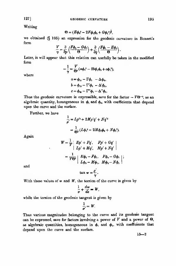
127J GEODESIC CURVATURE 195
Writing
we obtained (§ 105) an expression for the geodesic curvature in Bonnet's
form
y dp\ J+dqK /'
Later, it will appear that this relation can usefully be taken in the modified
form
where
-^ = @8 (ra^2 - 2^A + c^2).
b = <J>i2- r'<£, - A'<£„
c = 2S -F>1 -A"0s .
Thus the geodesic curvature is expressible, save for the factor — V®~', as an
algebraic quantity, homogeneous in <£, and 2 , with coefficients that depend
upon the curve and the surface.
Further, we have
-, = Lp* + 2Mp'q' + Nq'*
Again
W =
and
= ^(£^-2^,^ + ^).
Ep + Fq, Fp' + Gq'
Lp' + Mq', Mp' + Nq'
E<f>i — F<f>i , Ffa — G<f>i
L<f>2 -M<f>u Mfc — Nfa
tan w = —
.
1
F0*
With these values of vs and W, the torsion of the curve is given by
W,1 dwa ds
while the torsion of the geodesic tangent is given by
\.w.a
Thus various magnitudes belonging to the curve and its geodesic tangent
can be expressed, save for factors involving a power of V and a power of 0,
as algebraic quantities, homogeneous in #, and fa, with coefficients that
depend upon the curve and the surface.
13—2
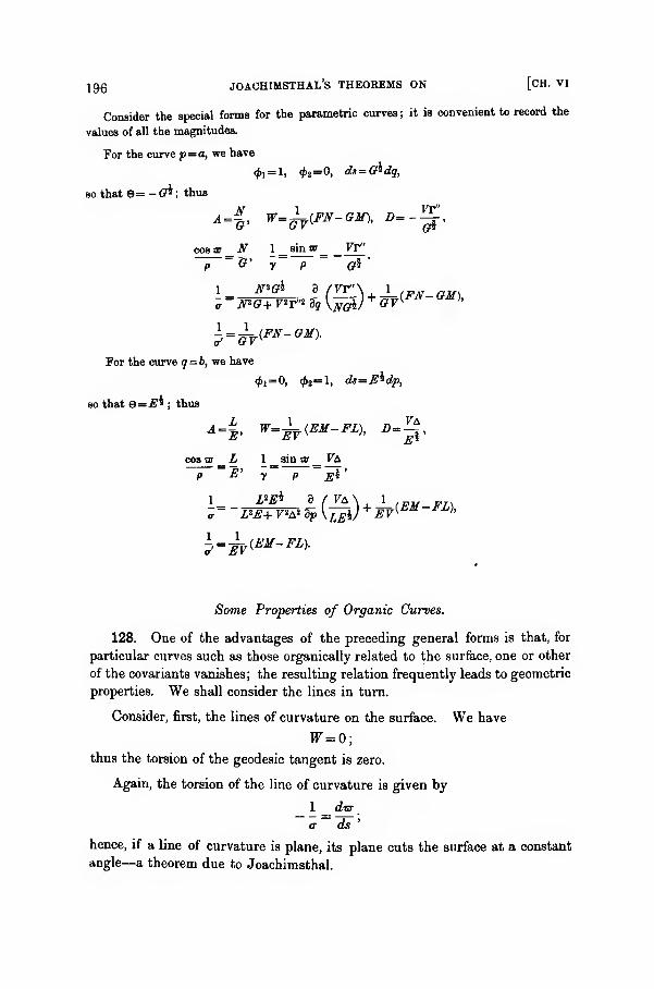
196 joachimsthal's theorems on [ch. VI
Consider the special forms for the parametric curves; it is convenient to record the
values of all the magnitudes.
For the curve p=a, we have
0, = 1, 02=0, ds = G^dq,
so that 6= -0*; thus
A-%. W=±(FN-GM), D—%.cosar_iV
r
1 _ sin w Vt"
~~P G' y~ P G*'
1 N*G* d fvr'\, 1 _ rm
<r'~GV
For the curve q= b, we have
i^^FN-Gm.
^1=0, 02=1, dt=E^dp,
so that e=E^ ; thus
cos sr L 1 _ sin or _ FA
P ^' y p ^4
'
1 Z'JE* 3 /FAN 1 „
l^iEM-FL).
Some Properties of Organic Curves.
128. One of the advantages of the preceding general forms is that, for
particular curves such as those organically related to the surface, one or other
of the covariants vanishes; the resulting relation frequently leads to geometric
properties. We shall consider the lines in turn.
Consider, first, the lines of curvature on the surface. We have
TT=0;
thus the torsion of the geodesic tangent is zero.
Again, the torsion of the line of curvature is given by
1 _ dis
a ds'
hence, if a line of curvature is plane, its plane cuts the surface at a constant
angle—a theorem due to Joachimsthal.

128] LINES OF CURVATURE 197
Again, if the line of curvature be also a line of curvature on another
surface so that it is the intersection of two surfaces, we have
1 _ dm 1 _ dvr'
<r ds ' a- ds'
for the two surfaces. Then
w' — i? = constant
;
hence the two surfaces cut at a constant angle—a theorem also due to
Joachimsthal.
Similarly, if two surfaces cut at a constant angle, and if the curve of
intersection be a line of curvature on one surface, it is a line of curvature on
the other also. For, as
er' — «t = constant,
we have
and therefore
dur' _ dvr
ds ds'
--+W' = --+W,<r a
so that
W'=W.If then either W or W vanishes, both vanish—which establishes the pro-
position.
Further, if a plane cut a surface at a constant angle, the curve of inter-
section is a line of curvature on the surface. For
^ =ds
u*
owing to the constancy of the angle, and
t-o,a
because the curve is plane ; hence
W=0,shewing that the curve is a line of curvature.
We have seen that inversion with respect to any centre conserves lines
of curvature (§ 79); and we know that inversion changes a plane into a
sphere. Hence we may expect some properties of spherical lines of curvature
similar to the preceding properties of plane lines of curvature.
Suppose, then, that a line of curvature lies on a sphere. Its geodesic
tangent is a great circle, that is, a plane curve ; and therefore the torsion of
the geodesic tangent is zero, so that, on the sphere, we have
1 dvr'
a ds
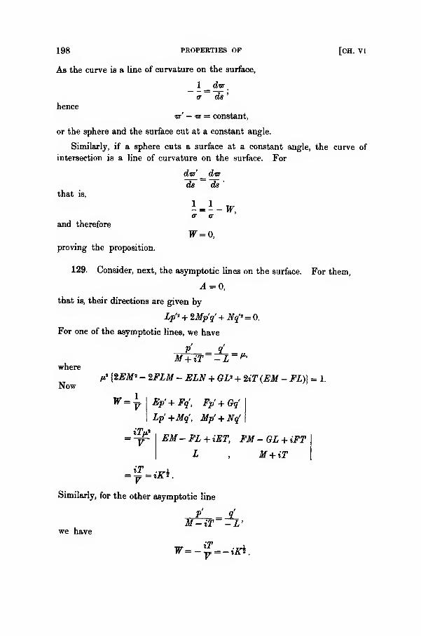
198 PROPERTIES OF [CH. VI
As the curve is a line of curvature on the surface,
1 d«r
a ds'
hencets' — a = constant,
or the sphere and the surface cut at a constant angle.
Similarly, if a sphere cuts a surface at a constant angle, the curve of
intersection is a line of curvature on the surface. For
dur' dtsr
that is,
and therefore
proving the proposition.
ds ds
a a
W=0,
129. Consider, next, the asymptotic lines on the surface. For them,
4 = 0,
that is, their directions are given by
Lp'3 + 2Mp'q'-hNq'' = 0.
For one of the asymptotic lines, we have
where
Now
M+ iT -L~*'
/*• {2EM> - 2FLM - ELN + GL* + 2iT(EM - FL)} = 1.
W=
~ V
Ep'+Fq, Fp' + Oq
Lp'+Mq', Mp' + Nq'
EM-FL + iET, FM-GL + iFT
L, M+ iT
Similarly, for the other asymptotic line
we have
P JL_r-iT -L'
iTW=- l± = -iKi.
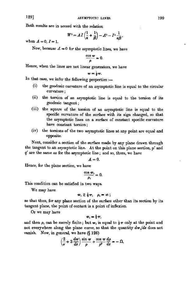
129] ASYMPTOTIC LINES 199
Both results are in accord with the relation
when A — 0, /= 1.
Now, because A = for the asymptotic lines, we have
COS 1ST -
p
Hence, when the lines are not linear generators, we have
sr= \tt.
In that case, we infer the following properties :
—
(i) the geodesic curvature of an asymptotic line is equal to the circular
curvature
;
(n) the torsion of an asymptotic line is equal to the torsion of its
geodesic tangent
;
(iii) the square of the torsion of an asymptotic line is equal to the
specific curvature of the surface with its sign changed, so that
the asymptotic lines on a surface of constant specific curvature
have constant torsion;
(iv) the torsions of the two asymptotic lines at any point are equal and
opposite.
Next, consider a section of the surface made by any plane drawn throughthe tangent to an asymptotic line. At the point on this plane section, p' andq' are the same as for the asymptotic line ; and so, there, we have
4 = 0.
Hence, for the plane section, we have
cos «•, _ .
Pi
This condition can be satisfied in two ways.
We may have
»i < \ir, Pi= °° ;
so that then, for any plane section of the surface other than its section by its
tangent plane, the point of contact is a point of inflexion.
Or we may have
«i = £"",
and then p, can be merely finite ; but •al is equal to J w only at the point and
not everywhere along the plane curve, so that the quantity dvrjds does not
vanish. Now, in general, we have (§ 126)
/ 2 _ d«r\ sin vt cos w dp
\a ds) p p3 ds~

200 GEODESICS [CH. VI
so that, for the asymptotic line, we have
1—
a
pa
At the point, ft is the same for the asymptotic line and the plane section,
being Pp'' + 3Qp''q' + 3Rp'q'i + Sq'*; and for the plane section, we have
l/o-, = 0. Hence, for the plane section,
as p 1
so that
2 3 rf-or,
pa /a, ds
Again, at the point, W is the same for the asymptotic line and the plane
section. Hence for the asymptotic line
1
and for the plane section
so that
Consequently
a result due to Beltrami.
= W,a
= ^!-F,as
dax _ 1
ds a'
2Pl = 3p,
130. Consider, next, geodesies on the surface. We then have
D = o, A = o, A = o.
No value of the ratio p'/q' is determined by these equations ; but we know
(§ 92) that any value of the ratio at the point determines uniquely a geodesic
on a part of the surface enclosing no singularity.
The direction of the geodesic through the point having maximum or
minimum curvature is obtained by making
Lfii + 2Mfi+NEp>+ 2Ffi+G'
where p.=p'\q\ a maximum or minimum. The necessary condition is
|
Efi + F, Ffi + Q|
= 0,
Lfi + M, Mfi + N\
that is,
lf = 0;
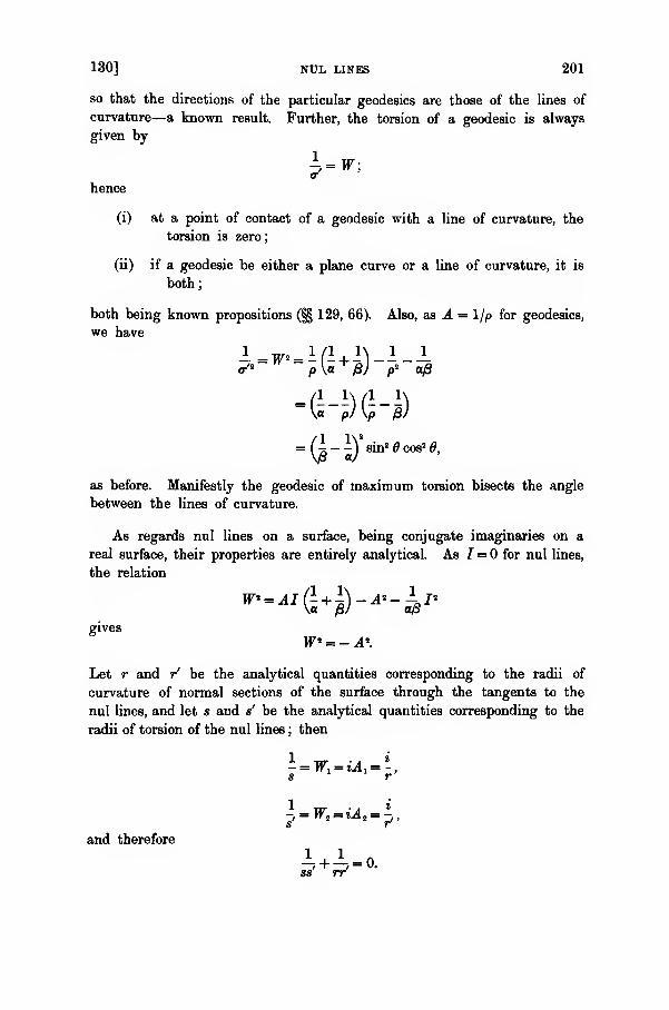
130] NUL LINES 201
so that the directions of the particular geodesies are those of the lines of
curvature—a known result. Further, the torsion of a geodesic is always
given by
l-,-W;a
hence
(i) at a point of contact of a geodesic with a line of curvature, the
torsion is zero;
(ii) if a geodesic be either a plane curve or a line of curvature, it is
both;
both being known propositions (§§ 129, 66). Also, as A = 1/p for geodesies,
we have
l=Tr> = I(l + l)_l_l</!
np\a + Bj p* a/3
=\a~p)\p~~p)
= (±-iysin°0cos20,
as before. Manifestly the geodesic of maximum torsion bisects the angle
between the lines of curvature.
As regards nul lines on a surface, being conjugate imaginaries on a
real surface, their properties are entirely analytical. As I= for nul lines,
the relation
W* = Al(± + ±\-A*-±I*\a B) a/3
gives
IT 2 = - A".
Let r and r' be the analytical quantities corresponding to the radii of
curvature of normal sections of the surface through the tangents to the
nul lines, and let s and s be the analytical quantities corresponding to the
radii of torsion of the nul lines ; then
s r
-, = W2 = iA t = ^,
and therefore
1+^ = 0.ss rr
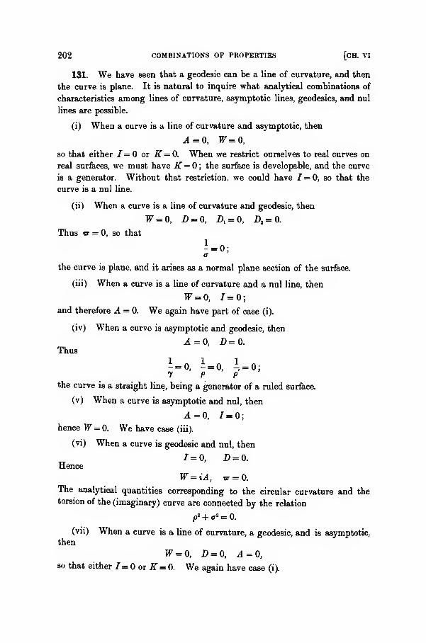
202 COMBINATIONS OF PROPERTIES [CH. VI
131. We have seen that a geodesic can be a line of curvature, and then
the curve is plane. It is natural to inquire what analytical combinations of
characteristics among lines of curvature, asymptotic lines, geodesies, and nul
lines are possible.
(i) When a curve is a line of curvature and asymptotic, then
4=0, W=0,so that either 1= or K= 0. When we restrict ourselves to real curves on
real surfaces, we must have K = ; the surface is developable, and the curve
is a generator. Without that restriction, we could have 1=0, so that the
curve is a nul line.
(ii) When a curve is a line of curvature and geodesic, then
W=0, D = 0, A = o, A = o.
Thus «r = 0, so that
1-.the curve is plane, and it arises as a normal plane section of the surface,
(iii) When a curve is a line of curvature and a nul line, then
F = 0, 7 = 0;
and therefore A = 0. We again have part of case (i).
(iv) When a curve is asymptotic and geodesic, then
A=0, D = 0.
Thus
*-0, 1 = 0, I, = 0;7 P P
the curve is a straight line, being a generator of a ruled surface.
(v) When a curve is asymptotic and nul, then
A=0, 1=0;hence IF = 0. We have case (iii).
(vi) When a curve is geodesic and nul, then
1 = 0, D = 0.
Hence
W = iA, vr = 0.
The analytical quantities corresponding to the circular curvature and the
torsion of the (imaginary) curve are connected by the relation
pp + a2 = 0.
(vii) When a curve is a line of curvature, a geodesic, and is asymptotic,
then
W = 0, D = 0, 4=0,so that either I= or K= 0. We again have case (i).

132] DIFFERENTIAL INVARIANTS 203
Differential Invariants.
132. The preceding results shew that many of the quantities connected
with a surface and with curves on the surface are expressed as functions
connected with binary forms. But a set of parameters on a surface can be
changed at will, while the quantities themselves are unaltered in value;
hence the expression in terms of the new parameters must be equal to the
earlier expression. In other words, we have an invariant or a covariant of
the forms.
Now it is important to know all the invariants and covariants which can
occur, as well as their geometrical significance. It is equally important to
know what relations may exist among them, for these will be relations
among the geometrical quantities themselves. Moreover, it is desirable to
know the tale of invariants of different kinds, such as those involving the
fundamental magnitudes of the surface without reference to any assigned
curve, and those involving the fundamental magnitudes of the first kind
(but not the magnitudes of the second kind) and any assigned curve or
curves on the surface.
Differential invariants (or differential parameters) were introduced byLame" for relations of space. The association with the theory of surfaces
was first made* by Beltrami, to whom many of the early results are due.
Another method, based more definitely on the pure algebra of the theory
of forms, was initiated by Christoffelf, and has led the way to manyinvestigations^.
Differential invariants of the type considered must belong to the general
class of differential invariants which constitute Lie's generalisation of the
theory of the concomitants of homogeneous forms. It proves possible to
adapt Lie's methods, used in the theory of continuous groups, for the con-
struction of the functions required §; and so, as the process also indicates the
amount of independence among the magnitudes constructed, we shall use it
for the immediate purpose.
* In his memoir, Mem. Ace. Bologna, 2d* ser., t. viii (1869), pp. 549—590. Beltrami there
gives also a sketch of the early history of the subject. An account of the theory, developed on
the basis of Beltrami's researches, is given by Darboux in his third volume, pp. 193—217.
+ CrelU, t. lxx (1869), pp. 46—70.
t Special mention should be made of a memoir by Ricci and Levi-Civita, Math. Ami., t. liv
(1901), pp. 126—201.
§ It was first effected by Zorawski for one class of the invariants ; see his memoir, Acta
Math., t. xvi (1893), pp. 1—64. The method was modified to some extent, and the construction
of all classes of the invariants up to a certain order, was effected in a memoir by the author,
Phil. Tram., (1903), pp. 329—402 ; and certain new relations among the geometrical magnitudes
of a surface are there given.
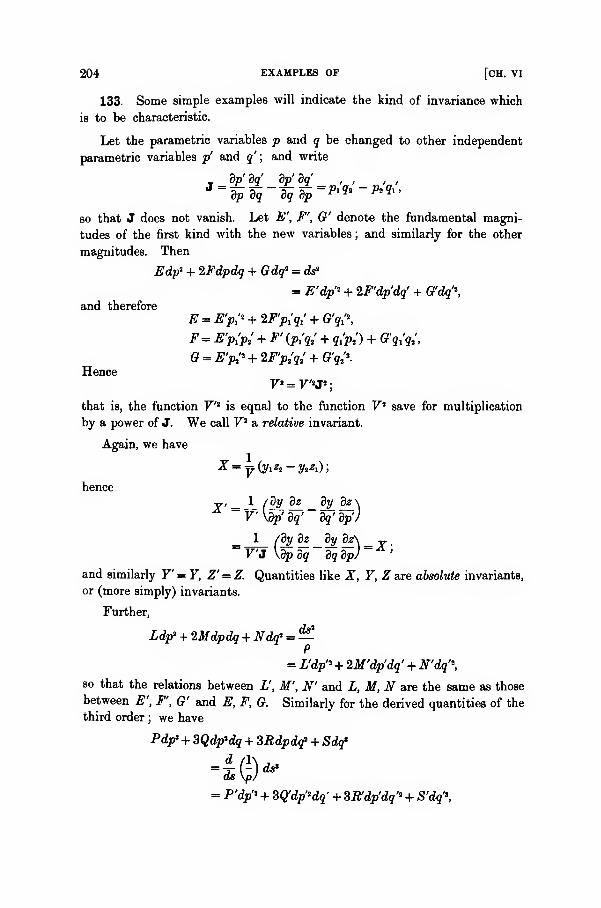
204 EXAMPLES OF [CH. VI
133. Some simple examples will indicate the kind of invariance which
is to be characteristic.
Let the parametric variables p and q be changed to other independent
parametric variables p' and q'; and write
_ dp'dq' dp'dq , , , ,
so that J does not vanish. Let E', F', G' denote the fundamental magni-
tudes of the first kind with the new variables; and similarly for the other
magnitudes. Then
Edp1 + 2Fdpdq + Gdq1 = ds*
= E'dp'* + 2F'dp'dq' + G'dq'\
and therefore
E - E'Pl'° + 2F'p1
'q1' + G'q,\
F = E'pipi + F' (p,'ft' + 9lX) + GVfc',
G = E'pt'* + 2F'pi'q
3' + G'q2
'*-
HenceF» = F'sJa
;
that is, the function V'2is equal to the function V' save for multiplication
by a power of J. We call V2 a relative invariant.
Again, we have
hence
V \dp' dq' dq' dp')
1 /dy dz dy dz\ _ ~
.
"r'j \d^dq~dqdp)~ '
and similarly F = 7, Z' = Z. Quantities like X, 7, Z are absolute invariants,
or (more simply) invariants.
Further,
Ldp* + 2Mdpdq + Ndq* =—P
= L'dp" + 2M'dp'dq' + N'dq'\
so that the relations between L', M', N' and L, M, N are the same as those
between E', F', G' and E, F, G. Similarly for the derived quantities of the
third order ; we have
Pdp> + 3Qdp>dq + SRdpdq1 + Sdq*
= P'dp'' + SQdp'dq- + 3R'dp'dq'* + S'dq'>,
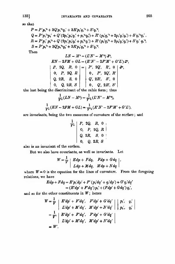
133] INVARIANTS AND COVARIANTS 205
so that
P = P'p? + SCftV + SKjH'q? + S'q,'*,
Q = P'p,v + Q' (2ftW + Pi1
*J.1
) + B'(ftV + V?iV) + sW
.
12 = P'Pl'K2 + <2'(VftV +ft'V) +# (ftV + V?iV) + «'?.'fc'
2>
s = pV + 8QbV + aB^v + SV-Then
LN-M* = (L'N' - M'*) J2,
## - 2PM + 02/ = (tf'iV - 2P'if ' + G'L') J',
P, 2Q', R',
0, P'(2Q', R'
Q', 2R', 8',
0, q, 2R\ S'
P, 2Q, R,
0, P 2Q, RQ, 2R, S,
0, Q, 2R, 8the last being the discriminant of the cubic form ; thus
±{LN-M*) = ±{L>N'-M>%
Y,(EN - 2FM + GL) =^ (E'N' - 2F'M' + G'L'),
are invariants, being the two measures of curvature of the surface ; and
V* P 2Q, R, ,
0, P, 2Q, R i
Q, 2R, S, :
0, Q, 2R, S
also is an invariant of the surface.
But we also have covariants, as well as invariants. Let
W =y ! Edp + Fdq, Fdp + Gdq
\ Ldp + Mdq, Mdp + Ndq
where W = is the equation for the lines of curvature. From the foregoing
relations, we have
Edp+ Fdq = E'p.'dp' + F' fa'dq' + qjdp) + G'q.'dq'
= (E'dp' + F'dq')Pl' + (Fdp' + Gdq') j,',
and so for the other constituents in W ; hence
w V
V
E'dp + F'dq', F'dp' + G'dq'
L'dp' + M'dq', M'dp' + N'dq'
E'dp' + F'dq', F'dp' + G'dq'
L'dp' + M'dq', M'dp' + N'dq'
Pi> 9i
Pi, 9a'
= W.

206 FIRST DIFFERENTIAL PARAMETER [CH. VI
Thus W is an absolute covariant or (more simply) a covariant. The in-
variantive character of W is to be expected ; for the lines of curvature must
be the same, whatever parameters be used.
134. But there are other types of covariants. Take any curve
<f> (p, q) = constant
;
in the new variables, let it be
$' (P >?') = same constant,
so that
tip, q) = <i>'{p',q)-
Then
0i = &P\ + fa'qi,
4>a = 4>\Pz + fa'qi,
and therefore
Ety-ZF^ + GW=
<f>1'*(Ep^-2Fp
l'p
2' + Gp1
'*)
+ 2^>s' [Ep^qi - F(p'q,' +p2
'
qi')+ GPl'q,'}
+ W(Eqi'*-2Fq1'q
2'+Gq1'*)
= J'iEW - 2F>1>2' + <?>,'»).
Consequently
y3(E& - 2^a *, + Gtf) =~ (E'fc* - 2F'<f>'&+ G'W) ;
and therefore, if
A(<f>)
= ~ (E& - ZFfrh + Gtf),
then A (<£) is an absolute covariant, connected with the curve upon the surface.It is Beltrami's first differential parameter.
As A(<f>) is an absolute covariant, so also is A(0 + X^) for all arbitraryconstant values of X. Now
A(<f> + \i/r) = A {$) + 2\ A (</>, -f) + \*A (f) t
where
A (<*>> +]= y, {£&*, - F(h+, + Vr^2) + G^f,}.i ,
Hence A(</>, f) is another absolute covariant, connected with two curves,
f = constant and + = constant, upon the surface. Sometimes it is called anintermediate covariant, sometimes a mixed covariant.
134] SECOND DJFFERENTIAL PARAMETER 207
Further, let
then
so that 4> (<£, ^r) is another absolute covariant, intermediate to the two curves.
But it is to be noted that the covariants so far obtained are not algebraically
independent of one another ; they are connected by the relation
A (*) A (f) - A2(<*», +) = 4>*
(<l>, *).
Again, we have
Gfr - F<f>2 =# (Op,' - Jfc,') +# (Gg/ - J-g.')
G<f>t— Ffa _ , G'ft/ — F'fa' , F'fa' — E'fa'= - «» ="= r Pi — bss— .
so that
G<f>! — Ffa / Gjfa
y — ?a y TV* VSimilarly
JVft, — Efa _ , G'4>\ — F'fa' , F'fa' — E'<j>2'
y — ?i y + P\ y,
Hence
d fGf} -F<f>i\_d_fF^l-E4>i\
dp\ V 1 dq\ V J
( , 3 , 3 \ (Ofr - Ffa ( . 3 . , 3 \ (Ftj-Efa.
_ 3 fG'ti-F'&\ d (F'ti-E'ti\=
*dp~'\ T )~ ihq'\ V )'
on reduction and substitution. Let
a tjL\1 d (G+i- Fk\ . ! 3
(-f<f>i + E^\ .
AaW = F^l F )+
Vd~q\ V )'
thenA2 (tf>)
= A2 (</>'),
that is, Av(<f>) is an absolute covariant. It is Beltrami's second differential
parameter.

208 USE OF [CH. VI
We thus have the set of covariants
*(<f>,^), A(tf>), A (*,*), M#By repeating the operations, we have other covariants
A(A<£), A($,A$), *(^A^),
and so on, to any extent. Darboux proves* that any covariant, which involves
two or more functions<f>,
ifr, ... and their derivatives, with E, F, G and
their derivatives, can be obtained through the adequate repetition of the
symbolical operations A and <t>.
135. To illustrate the use of these differential parameters and other
covariants, let p = ^ (p, q), q = ^ (p, q), be taken as new parametric
variables; then any arc-element upon the surface can be expressed in the
form _ds2 = Edp + 2Fd<j>difr + Gd^\
Now _ _ _
on substitution ; then
1/ F° = A (<*>) A (*) - A2
(i>, yft) = & {<j>, +),
and so
p_ A(f) - A(4»,^)ff_ A(0)
4>°(<f>,t)'~ *=(*, +)' *(*.+)'
Consequently the arc-element upon the surface becomes
, A(Vr)rfft>-2A(<ft, yfr) d4>dyfr + A(<ft) <ty
a
When the new parametric curves are nul lines for the surface, we must
have
A(^) = 0, A(</>) = 0;
that is, the nul lines for a surface are obtainable by taking two functionally
independent solutions of the equation
A(*) = 0.
When the new parametric curves are an orthogonal isometric system for
the surface, we must have
A (*)-*(*), *(«/,,*) = 0;
that is, an orthogonal isometric system for a surface is obtainable by taking
two functionally independent solutions of the equations
A(0) = A(*), A(0,*) = O;
and then the arc-element is given by
dP + dS*
* Treatiie, t. Hi, pp. 203, 204.
136] DIFFERENTIAL PARAMETERS 209
The variables for the isometric system are connected with the variables for
the nul lines by the customary relation (§ 60) ; for, writing x = ± ^> whereand S- are real, we have
A (x) = A (0) - A (&) + 2iA (0, *),
so that the equation for the variables of the nul lines leads to the equations
for the variables of the isometric lines.
Again, by direct substitution in the expression for the second differential
parameter, we haveA2 (0) = O, A2 (*) = 0;
thus both the parametric variables for an orthogonal isometric system satisfy
the equation Aa (/u) = 0.
Ex. Taking the arc-element on a surface in the form
ds2=(l +p2) efo;
2+ 2pqdxdy+ (1 +g2) dy\
prove that parallel planes cut a minimal surface in isometric curves.
Lastly for the purpose of immediate illustration, we can prove, by the
method adopted in § 134 for \(tf>), that
I JA (H*-&<t>i\ , 1 (Ffr- E^\\
V\dp\ J dq\ @ /J*
where ® denotes {Efa* — 2F<j>l <f>2
+ Cr<£i2)* is an absolute covariant. In order
to obtain its geometrical significance, we specialise one of the new parametric
curves, and we take tj> (p, q) = q. Then $, = 0, tf>2= 1, ® = E* ; the absolute
covariant becomes
,T-ftthat is, VAE 2
. But (§ 127) this quantity is the geodesic curvature of the
curve q = constant ; hence we again have Bonnet's result
1 _ _1 f1 /JVfc - g&\, 1 (Fh-E&\\
y~V\dp\ @ /+9oA e /J'
136. The results in § 134 stir a larger question. We are challenged
with the problem of finding and interpreting all the invariants upon a surface,
and all the covariantive functions, which are connected with curves upon the
surface and involve E, F, G, L, M, N as well as their derivatives. Merely for
purposes of finite enumeration, we shall take derivatives only up to a finite
order ; and for purposes of precise illustration, we shall take only low orders
of the derivatives of the various quantities. Moreover, we only want those
covariants which are algebraically independent of one another; our quest
is not for an asyzygetically complete system.
f. 14

210 ALGEBRAICAL AGGREGATE OF [CH. VI
As regards the quantities to be included, we shall take E, F, G and their
derivatives of the first order ; in place of these derivatives, we shall take the
six equivalent quantities T, A, F, A', T", A" of § 34, as convenient for our
purpose, though not convenient if higher derivatives were required. The
transformations of these quantities under the transformations of the variables
involve the first and the second derivatives of p' and q' with respect to pand q. The laws of change for L, M, N are the same as those for E, F,G;
and therefore to the retained order of derivatives of p' and q', we take
L, M, N and their derivatives of the first order. But the last are not inde-
pendent of one another, owing to the Mainardi-Codazzi relations ; in place of
them, we shall take the four derived magnitudes of the third order P, Q, R, 8.
We can take one curve,<f>= constant, on the surface; or we can take two
independent curves,<f>= constant, and yfr = constant, on the surface ; it is no
use taking three curves<f>, -ty, x = constants, for there is a functional relation
between three functions of two variables. In the first instance, we shall
take one curve,<f>= constant, for the present purpose. The quantity </> itself
will not occur ; the relation <£ = </>' contains no derivatives of p' and q', but it
provides the means of obtaining relations between the derivatives of <£ and <£'.
Clearly we shall have derivatives of<f>
of the first and the second orders,
as these involve the retained order of derivatives of p' and q'. Thus our
invariantive functions involve E, F, G, I\ A, I", A', T", A", L, M, N, P, Q, R, S,
<f>io> <£oi. <t>x>, 0ii, 0m, where*
_ dm+nuUmn
~dp^q»'
for all quantities u, and for all values of m and n.
Ultimately we require absolute invariants. These can be obtained as
ratios of relative invariants ; as the analysis for relative invariants is simpler
than for absolute invariants, we construct the relative invariants. If/ be
any such function, and if /' be the same function under the new variables,
our definition is that the relation
/=JTmust be satisfied for some integer value of the index fi.
137. To utilise this equation we have recourse to Lie's theory of con-
tinuous groups, particularly to the fundamental proposition! tnat a continuousgroup is determined by the aggregate of infinitesimal transformations whichit contains. Accordingly, we shall deal only with infinitesimal transformations
of p and q which (in Lie's notation) are
p' = p + £ (p, q) dt, q' = q + v(p,q)dt,
* Thin double-suffix notation is convenient for the expression of derivatives of all orders,though it is less convenient than the earlier notation for derivatives of the first order alone.
+ Theorie der Berllhrungstransformationen, vol. iii, p. 597; see also Campbell, Continuousgroupi, p. 80.
137] CONCOMITANTS 211
where powers of dt above the first are neglected; and then, to secure all
kinds of relations between p', q', p, q, we take f and i) to be completely
arbitrary functions of p and q. As the quantities retained for our invariants
involve derivatives of p' and q' up to the second order, we shall have deri-
vatives of £ and 17 of the first and second orders.
As regards J, we have
J = (1 + fiodt) (1 + Vndt) - gndtVwdt
= l+(f)0+ 1? l)<^.
on neglecting dt3. Also
hence our defining relation becomes
which is to be satisfied for all functions £ and i\. We thus need the increment
of /; and this arises through the increments of the various quantities it
contains.
We have £ = $, and therefore
<£io = Pi$m + qi'<f>oi = (1 + ijiodt)<f>10
' + r)1B dt<f>m',
4>*> - |(1 + &»dt) g-? + viodt g-;| {(1 + %wdt) <f>10' + viodtfu'}
= (1 + 2f„A) &»' + 2Vw dt<f>n' + (£»&„' + 7in$n) dt,
on neglecting squares of dt, and so for other derivatives of <j>. Hence
tyw' — #10 = — (£10^10' + ^io^o/) dt.
On the right-hand side we can replace<f>10
' and ^>01' by <£,„ and <pm respectively,
as we neglect squares of dt ; hence
d't'w fc JL I J.
Similarly for the other derivatives ; the required tale of results is :
—
d<jho _dt
= fio^io + %o<£oi
-yr — ?oi&o + ^oi^oidt
- -$* = 2f10 <£a, + 2»7,o</>ii + ^<fho + ^so^oi
d<j>n
dt
d<j>m _'
dt
= £lO011 + foi^H) + %0$02 + »?01 011 + fll&O + ^ll^Ol
= 2f i<|>u + 2»7oi0o2 + loa^io + VibQoi
14—2

212 THE METHOD OF [CH. VI
To obtain the increments of the magnitudes of the surface, we proceed in
the same way. We have
E = E'p1'* + 2F'p1
'q1'+G
,
q1
'*
= (l + 2£10dt)E'+2VlodtF',
which at once gives dE/dt. Similarly for all the magnitudes ; the required
tale of results is :
—
dEdt
~

138] CONTINUOUS GROUPS 213
drdt
dA''
dt
dT"dt
cZA"'
dt
f«(r-A')+,1§r"+ ifar + ft,
= ft.A' + fcA +1?10 (A"-r') + „„
= - f.»r" + 6.(21*- a") + 2%1r"+ f.
2f01 A' -VnT"+ 7701 A" + 7,0,
138. The arguments that can occur in a covariantive function / are
twenty-one in number, viz. <£„, <£01 , <£„, <£„, <£„; E, F, Q, T, A, T', A', T", A";
L, M, N\ P, Q, R, S. Denoting any one of them by u, we have
d/"_„9/ du
dt v du dt
'
ditThe value of -5- has been obtained for each argument; hence the critical
equation becomes
The equation must be satisfied for all arbitrary functions if and 17 whatever
;
and therefore the coefficients of all the derivatives of £ and of 17 on the two
sides must be respectively equal to one another. We thus obtain ten
equations in all, arising through the coefficients of fw , ?ra > Vw, Vm J £». j?n> £02!
Vx,,Vn,Vw They are:—
9$io Cpso dpn
M/=^ +^ + ilf^ + 2iv^ + Q| +2E^ +34
•(i),
dF
A3A
+ 1dT'
+ar"
+ A3A"
9<S
+*£ + *-s£ +*i£ <ia

214 THE CHARACTERISTIC [CH. VI
coming from the coefficients of f10 and ^01respectively; and
+ *»l +^ +**"l
(I)'
+ 2r| + (2A--r)| +r^ +<A»-n3|,-r»
3
V
+*•&**&+*•£ (H)'
*-% +*•& (m>'
•-£ + *•& (m
•-£ +*-£ (V >'
»-I +*»^ <VI>'
o-I- + *«af,
<VII)
'
°-£ + *s£ <vm>'
coming from the remaining coefficients. This is the aggregate of equations
arising out of the critical equations.
Conversely, a function /, that satisfies these equations in connection with
a suitable integer value of fi, possesses the property
/=jy,
that is, it is a covariant. Hence what is required for our purpose is the
aggregate of algebraically independent functions satisfying these ten equa-
tions, the last eight of which are homogeneous and linear in the derivatives
of f.
139] PARTIAL DIFFERENTIAL EQUATIONS 215
The theory of such equations, as well as the method of integration, is
known* ; so we proceed first to integrate them, and then apply the theory to
indicate an independent aggregate.
139. Consider the last six of the equations, viz. (Ill)—(VIII), by them-
selves. All the Poisson-Jacobi conditions of coexistence are satisfied
identically. Hence they form, a complete Jacobian system. The total numberof variables, with respect to which derivatives of/ occur, is nine—viz., the
three second derivatives of <j>, and the six quantities V, A, V, A', T", A".
Thus the total number of algebraically independent integrals, involving
some or other of these nine variables, is three; for the number of such
integrals is the excess of the number of such variables over the number of
equations in a complete Jacobian system. Now it is easy to verify that the
quantities
<fat>— r^io
—
a$01 , <£u — r '<f>w — A'^oi » <£<n — r"0io— a"#01 ,
satisfy the equations; and it is manifest that they are algebraically inde-
pendent of one another. Hence, writing
a=<f>w — V<f>10
— A<f>01 -j
b = <f>n- r" <j>10
- A' <j>m I
,
c = 4>m — r"<£io — a"<£oi J
we have a, b, c as the three integrals above indicated.
If, then, we take / to be any function of a, b, c, and of<f>10 , <£01 , E, F, G,
L, M, N, P, Q, R, 8, then the six equations are satisfied; and the most
general function of those arguments is the most general integral of those six
equations. We therefore now limit / to be a function of those arguments
;
and we need take no further notice of the six equations. To avoid confusion,
we denote the function /, in its new form, by g.
Let the
216 INTEGRATION OF THE [CH. VI
Then as f, now denoted by g, has become a function of a, b, c, $] . #01 >
E, F, G, L, M, N, P, Q, R, S only, the four equations take the form
W BET
dF BL2E% + F d
S, + 2LdS +Mli+3P^ + 2Q^ + R^
dP dQ dR
da db
dff+ *a* + h%+^ (i).
•(").
•*+»t +*-&'96•(I).
.(II).+ »i+'i+*&These four equations satisfy the Poisson-Jacobi conditions of coexistence, and
so they are a complete system. When we take
equation (i) — equation (ii) =
with (I) and (II), we have a complete Jacobian system, each being linear andhomogeneous in the derivatives of /. The arguments, with respect to whichderivatives are taken, are fifteen in number ; this complete Jacobian system
contains three equations ; and therefore, by the customary theorem, there are
twelve algebraically independent solutions.
Further, we take a new equation, given by
equation (i) + equation (ii) = 0,
so that we have substituted two equivalent equations for (i) and (ii). Thesolutions to be obtained will be homogeneous in certain groups of the
quantities ; let any one of them be
of degree r^ in E, F, G,
L, M, N,
P, Q, R, S,
a, b, c,
£10. $01
;
140] CHARACTERISTIC EQUATIONS 217
then this new equation is satisfied if
2fi = 2?ii + 2n2 + 3ns + 2n4 + n6 ,
so that 7»3 + ws must be an even integer.
140. Now the three equations
(I), (II), equation (i) — equation (ii) = 0,
are the complete Jacobian system of the differential equations for the
invariants and covariants of the simultaneous system of binary forms
w, = (E, F, G%fa, - ^o)2,
wi = (L, M, N$fa, -fa)*,
wi' = (a, b, c^fa, -fa)*,
w3 = (P,Q,R,S$fa,-fa)>;
and we therefore require an algebraically complete (not an asyzygetically
complete) set of concomitants of these binary forms, the set to contain twelve
members. An algebraically complete set is not unique ; it can be modified
by exclusion and inclusion, provided it remains an algebraically complete
set of twelve members.
Such a set can be taken initially as follows :
—
wa = (E,F,G%fa,-fa)*,
V* = EG-F*,
w2' = (L,M,N%fa,-fa)*,
T* = LN-M*.
\<poi, — <pw
= (EM - FL) fa* - (EN - GL) fa fa + (FN - GM) fa*,
w2" = (a, b, cQfa, - fay,
I = Ec-2Fb + Ga,
= (Eb - Fa) fa*- (Ec - Ga) fafa + (Fc - Gb) fa*,
wi = (P,Q,R,Slfa,-fay,
8 = {E*S - 3EFR + (EG + 2F*) Q - FGP) fa
- {EFS - (EG + 2F*) R + SFGQ - G 2P} fa,
V = (ER - 2FQ + GP) fa - (E8 - 2FR + GQ) fa,
218 AN AGGREGATE OF CONCOMITANTS [CH. VI
\</>oi> —fay
= (EQ - FP) <$»? - (2ER -FQ- GP) *»»*»
+ (ES + FR- 20Q) frfa* - (FS - OR) <£103.
In terms of the members of this algebraically complete set, every other
concomitant of the system can be expressed; and each member of the set
is a relative invariant or covariant.
To obtain the absolute invariants and covariants, we require the index fi
of each of the foregoing quantities, as given by
H = n 1 + n2 + ni + ^ (3n„ + n6).
We easily find
ft.= 2, for w» V2
, <, T\ wf, I ;
fi = 3, for J, J', w3 ,8'
;
/t«4, for 8, J";
and therefore an algebraically complete set of absolute invariants and
covariants, eleven in number, is given by
5 5( ?! ^' I i £ !5 i i ^ys> y-2> ya> y« y*' y»> y>> ys> ys> y*> yf
As already indicated, the system can be modified by the exclusion of
some of the retained concomitants and the subsequent inclusion of some of
the omitted concomitants, the same in number, and independent of one
another when the set is restored to completeness.
Some instances of concomitants, omitted from the system and expressible
in terms of its members, can easily be given ; they will be deferred until the
geometrical significance of the retained concomitants has been established, so
that their geometrical significance can be given simultaneously.
141. Two directions at any point of a curve on a surface are specially
determined by the curve, viz. the tangent to the curve, and the direction
which lies in the tangent plane to the surface and is normal to the curve.
These two directions may be denoted by -~ , -^ ; and -^- , -=2 ; respectively.
Now we have, for the tangent,
<f>1°ds-
+*"ds
=°'
together with the universal equation
141] GEOMETRICAL INTERPRETATION 219
as in §§ 26, 105, we take
Again, for the direction of the normal in the tangent plane, we have
E dp<ty + F /<tyfy + fydq\ + Gdqdq
!=0ds dn \ds dn dn ds) ds dn '
and, as dn is an element of arc on the surface, we have
E(d/U2Ff£^ + G m=l;\dnj dn dn \dnj
therefore
l»-l(^ +eS)-^ (-^+GM
Before proceeding to the identification of the invariants, we obtain the
simple interpretation of the Beltrami operators A and 4>. We have
ds
Next, we haved4> dp dq
dn
w£
220 GEOMETRICAL [CH. VI
di/r , dp dq
^ = **Tn + *"dn
Vw}
ds and dn in the differentiation being determined by the curve<f>= constant.
Hence (except as to the invariant factor - B) Beltrami's invariant <J> (tf>, yfr) is
-^ tand (except as to the factor E) his invariant A (<j>, yfr) is -3-=- ; and
repetitions of the Beltrami differential operators <I> and A are, effectively,
repetitions of the operators -3- and -5-. Moreover, we have
*p = E-K *-e-*,asq asp
dp___& dp _ F dq = F dq = F$dnp V ' dn
q ygk ' dnp ygi ' dnq
V '
Hence we infer at once the theorem (§ 134) of Darboux, that any covariant,
which involves two or more functions<f>, -ty,
... and their derivatives, with
E, F, G and their derivatives, can be obtained through the adequate
repetition of the symbolical operations A and «1>.
142. Coming more directly to the significance of the invariants in the
retained complete aggregate, we shall denote the various geometrical magni-
tudes by the same symbols as in § 126. We already have
where
Next,
dn
and therefore
w2 .

142] INTERPRETATION 221
Next,?'* LN-M*V*~ EG- F*
-'-h-the Gaussian measure of curvature. Further,
/= (EM - FL) <j>01* - (EN - GL) </>„,&„ + (FN - GM) fa*
= w.lVW
O"
and therefore
V a"Next, we have
<}>iop" +M' +<t>*>p'' + tyup'g' + <f>W = o
;
so that
«b* (pY ~ 9P") + - (<Moi! - 2</>„0oi^o + <M.o2) = o.
Hence, using the symbol D of § 125, we have
awz
2
and therefore
Consequently,
[^- Ap* - (2A' - r>i>v - (A" - 2rv?'a -rys
+ <^»0I)12 — 20U0O101O + #02^>10
2= 0;

222 GEOMETRICAL SIGNIFICANCE [CH. VI
so, operating on the equation
we have
W* 2B-^ = fa g- [y)- fa g-
[y
)
— yi J >
142] OF THE CONCOMITANTS 223
curvature of the tangent geodesic. Accordingly, let arc-variation along the
d
dt'geodesic be denoted by -j
', if a quantity u does not relate to contact, then
du _duds~dt'
because the curve and the geodesic touch ; if u relates to contact of any
order, thendu du
ds dt
is usually not zero because usually there is a non-vanishing geodesic con-
tingence. Examples will occur later. Meanwhile, we have
£(?)-<"«.*«£. 8"
= wa
-f (P, Q,i*,<Sf$(/>01J -</>10)
3
= w1~*w3 ;
and therefore
V3 dt[P')-
Next, for H, which denotes the measure of mean curvature of the
surface, we have (§ 42)
V'j!- = GP-2FQ + ER, V*d-^- = GQ-2FR + ES.
HenceidH , BH . dH
and therefore
Similarly
Wh&>
&__ dH7s ds
Vw^ d^= (GI*»
" F<f>m) -§ + {E^ ~ **»> if
- l8-- yi°'
and therefore
V*~ dn'
Proceeding as before, we have
_wa 2 wa'J' — wJ'J
224 SUMMARY OF RESULTS FOR [CH. VI
on reduction, so that we have no unidentified covariant on the right-hand
side. But, substituting the values of all the covariants as known, we have
ds{p')~dt\p')+ya"
an illustration of the foregoing statement that arc-variation of a quantity,
connected with the contact between a curve and its geodesic tangent, is
not the same along the curve as along the geodesic tangent.
The result could also have been derived from the relation
given in § 125 ; for when the values of A, fi, D, W are inserted, we have
ds \p') dt [p'J+
ycr'
Similarly, we have
V^ Tn (f)= {<**" " **> I + <** "^ j|}t
Substituting the values of the covariants already known, we find
V* " dn\p')+ Z
* ds'
This result completes the establishment of the significance of the covariants
in the algebraically complete set as retained.
The following is the aggregate of the results which have been obtained :—
^ _ a _ my
143] ALGEBRAICAL AGGREGATE 225
V* dt\p'J " \ds\p') ye'}'
±__ R dHV* dn'
8__ ndHV»~ ds
•
V*~a
dn\p')+
a' ds'
143. To illustrate the theorem that, to the order of derivation included,
this system is algebraically complete, some examples will be taken.
The quantity EN — 2FM + GL is the intermediate invariant of w3 and
wt', and its index is 2 ; so we write
H=±-a(EN-2FM+GL),
H being the mean curvature as usual; thus H is an absolute invariant.
NowJ1 = (EN- 2FM + GL)waW - T*wf - V*w,'* ;
and therefore, when the values of the quantities are substituted from the
above set, and a factor B'V is removed,
1 -E-jr-1*'*-
P' p'*'
shewing that H is expressible in terms of the retained quantities. A more
familiar form of the relation is
cr'a \a p')\p' fi)-
The quantity Lc — 2Mb+ Na is the intermediate invariant of w,' and w3",
with index 2 ; thus (Lc — 2Mb + Na) V~3 is an absolute invariant. Now
wt (Lc - 2Mb + Na) = Iw,' + HV'w," --JJ'-- V'wa'w3",W2 1V2
and H is expressible as above ; consequently the new absolute invariant is
expressible in terms of members of the system. When the values of the
invariants are inserted, we find
1 ,r n ,« v- x 1 fdB B\ B „ 2 dB
~p'dn a' ds yW* a/3J~
The quantity ac-b* is the one invariant of w9", regarded as a binary
form, and its index is 2 ; hence (ac — b3) V~* is an absolute invariant of the
system. NowJ'» = Iwtwa
" -(ac- b') «;,» - V'w,"*,
f. 15
226 OTHER INVARIANTS [CH. VI
=— + —.. V'w2'J' - - V*HJ' - -- V'Jv>t",Wo M>, MV
so that (ac — 6s) V~* is expressible in terms of members of the system. When
their values are inserted, we find
1 (dB\» BdB
There is an invariant intermediate to w2 , w2', u/a", viz.,
E, F, GL, M, Na, b, c
and its index is 3. It must be expressible in terms of members of the
system; in fact,
E, F, GL, M, Na, b, c
and H is expressible in terms of members of the system. When the values
of the invariants are inserted, we find
* ' " —(?-H)£+ ($M)?-L, M, Na, b, c
The cubic wa has the quadricovariant Ha , where
Ht = {PR - (?) fa - (PS - QR) fafa + (QS - BJ>) fa,and its index is 4. Now
J"" = w2w,B' - Vwf - wfHt ,
and therefore
Similarly, it has a cubicovariant 3>3 , where
<J>, = (P»S - 3PQR + 2Q») fa - (3PQS - 6PR> + 8QR) fa"fa+ (- 3PRS + 6Q>S - SQR*) fafa - (PS' - 3QRS + 2R>) fa,
and its index is 6. Now
w.'^a = waw,2S - 3wawt8'J" + 2 V'wfJ" - 2/"'
;
insertion of the values of the known covariants leads to the value of <!>,.
144. These examples indicate a way of obtaining the value of a covariant
of the system. It is sufficient to express the covariant in terms of thefundamental members of the algebraically complete system and then to
substitute, in the expression, the values of those members which occur.
But the process can be used, in the same way, for another purpose. It
may happen that geometrical magnitudes exist, which lie within the order
144] GENERAL MODE OF INTERPRETATION 227
of derivation retained and which do not occur in the set of those which have
occurred. They necessarily are covariants of the system, and consequently
are expressible in terms of members of the system; thus they can be
evaluated in terms of the set of magnitudes retained. Hence we are led
to relations among the geometrical magnitudes.
As an example, consider the Gaussian measure of curvature K. Both
the quantities dK/ds and dK/dn lie within the order of derivation retained.
NowdK -*/. 3 , 3W> riov
so that (§ 42)
w$V>dJ^ = (NP- 2MQ + LB)
<J>0]- (NQ - 2MB + LS) <f>lt
Also
so that
W$V°^ = [SEL - B (2EM + FL) + Q(EN + 2FM) - PFN] <pmdn
- [SFL - B (2FM+GL) + Q (FN + 20M) - PGN} <f>w .
When we express these covariants in terms of the members of the complete
system, we have
Substituting the values of the covariants which are known, this gives
dKldH („ 2\ d (l\ 2 d (1\ 4 dB~d7~p'~dJ
+\ p'J dt \p'J
+<r' dn \p'J B<t'* ds
'
the relation required. Other forms can be given to it. We have
1 - H K 1
2 da = dK_\dM_/H _2\dL /1\
ds p' ds \ p'J ds \p'J
so that
ds ds p
2\ [d /1\ d /1\) 2 d (1\ 4 dB= \E
and therefore
that is,
[H ~
p'J \dt [p'J ds \p')\ a dn (p'J
1 d° - (tj-IW-^C^-——V> ~ds~
~\ p'J 7 dn [p'J Ba' ds
'
dl\a')~B<T'd8+dn\p'}
+\a p'J y
Ba'* ds
15—2

228 SYSTKM OF CONCOMITANTS FOR [CH. VI
Proceeding similarly with the covariantive expression for w^V* -*—
,
we find
(tt l\jL(l\ _2^/l\+ V1
p'J dn \p'J+
a' dt \p)
dK = l_dHdn p dn ' V." p'J dn \p'J ' a' dt \p'
_4_ dB 2 dH 2H dBBp'a' ds a ds
+Ba' ds
'
and this can similarly be changed to a relation
dn\a'J ds\p'J+ya' \a
+p'J
1 dB dHB ds ds
And so for other instances »
146. The preceding investigation is concerned with invariants which
arise in connection with a single curve upon the surface. It was pointed out
(§ 136) that we might consider two, but that we could not consider profitably
more than two, independent curves upon the surface. The method adopted
for invariants connected with a single curve is applicable to the construction
of invariants connected with two curves
<f>= constant, ^r = constant.
We shall develop the results only for the simplest case—when the order of
differentiation among the equations of transformation is only the first, instead
of the second as in the preceding analysis.
In that simple case, the arguments which can occur in an invariant f are
E, F, G, L, M, N,<f>10 ,
<f>01 ,^r
10 ,^r01 . Every such invariant /satisfies four partial
equations constructed in the same way as the ten equations in § 137 ; the
four equations are
These equations satisfy the Poisson-Jacobi conditions of coexistence. Takingthe equation, which arises from the difference of the first two equations, andassociating it with the last two, the set of three equations thus constituted
is a complete Jacobian system. The number of variables, with respect to
which differentiation occurs, is ten, being the total of the arguments whichcan occur in /; hence the number of independent solutions is seven, beingthe excess of the number of variables over the number of equations in the
complete Jacobian system. Every solution of the equations, that is, every
* Several are given in the memoir by the author already (§ 132) cited.
145] TWO CURVES ON A SURFACE 229
covariant within the order of differentiation of the relations of transformation,
can be expressed in terms of those seven solutions. Moreover, if a solution
is homogeneous andof order nt] in E, F, G,
m2 ... L, M, N,
»w3 ...<f>lf>
, <f>(U,
mt ... ^,0, Vta,
the equation, which arises by taking the sum of the first two equations, is
satisfied if
li = m1 + rni + \(m3 + «i4).
Now the four equations shew that every solution is a concomitant of the
system of binary forms(E,f, cnafa-boY,
or, what is the same thing in an algebraically complete system, is a con-
comitant of the system of binary forms
(E,F, G^ou -+„)*,
(<£io. ^oi^oi- - fio)-
We shall take them as concomitants of the first of these two systems.
An algebraically complete set of solutions (each one of which is a relative
covariant) is made up of the set
:
u = (E,F,G1<f>0U -&„)*,
u, = {L,M,N\4>«u-<i>wy,
V* = EG-F\T* = LN-M\W = (-^io, "^oi^oi. - &o).
/= E+a-Ffa, F<j>m - G<l>w
L<j>m - M<f>10 , Mfa - N(f>10
E<j>m -F<j>1<t , F<f>01 - G<f>w j.
^10, ^01
For these relative covariants, we find
(i = l, for w,
/i= 2,for«,«', V\ T\V,
fi = 3, for /:
and therefore an algebraically complete set of absolute covariants within the
order retained is made up of the six functions
w JL JL H — —y> yi' yi' yf y*' V'
raA(<f>, ^) = v =
230 CONCOMITANTS FOB [CH. VI
146. The symbols already used to denote the geometrical quantities
related to the curve<f>= constant, will be retained. An elementary arc along
the curve i/r = constant will be denoted by ds', and one in the surface normal
to that curve will be denoted by dri. We write
and take
p" = radius of circular curvature of the geodesic tangent to the curve
yfr = constant,
a" = radius of torsion of that geodesic tangent,
X = angle between the two curves,<f>, yfr = constants.
Also other simple covariantive forms occur, within the order of variation
retained ; among them, we note the following :
—
v = (E, F, <?$^01 > -^]0)a>
*-(L.M,NTfru , -+„?,
Li/r01- M-»frw , Myfrm - Nyfri0
h = L<f>m ifro,-M (^oi^io + ^io^oi) + -fltyio^io,
A = (EM- FL)<t>m+m -$(EN- GL) (<paf„ +^rB ) + (FN- GM) <M^o-
Each of these must, of course, be expressible in terms of the members of the
algebraically complete set already retained.
In proceeding to the geometrical interpretation of the foregoing covariants,
we shall as far as possible use the earlier results applying in the case of a
single curve.
As before, we have
146] TWO CURVES 231
and similarly for the curve i]r = constant, we have
x _ Fdp^ tdpdq dpdq\ n dqdqdsds'
+r\d8d8'
+ds'ds)
+^dsds'
= u~K~$V;
V
Also
cos
hence
Similarly
Vi=BE cos\.
sin
hence
It follows at once that
x=v (dpdq_dqdp\\ds ds' ds ds'j
y = -BB' sinX.
giving the expression for v in terms of the members of the algebraically
complete aggregate.
Again, we have
uV = u'V2- 2wJV - wV
F
s + uw* (EN- 2FM + GL) ;
when the values of the various quantities are inserted, the equation
reduces to
1 cos 2X sin 2\ /l 1 \ . „
„
p p ff \a p/
Similarly, we have
u*J= JV2 + Vw {2 7 s u - u (EN- 2FM + GL)} - Wit?;
when the values of the various quantities are inserted, the equation reduces to
1 cos2\ (1 1/1 1Y| - „%?-' = -v--^-2U +M sm2x-
Both these results can be verified, by using Euler's theorem on the curvature
of a normal section and the equation for the torsion of a geodesic given
in § 107. Moreover, we at once have
cos \ sin \ _ cos X, sin \papacos\
,(1 1/1
,l\l . . cos\ fl 1/1
, 1\] . ,
232 SIMULTANEOUS INVARIANTS [CH. VI
Next, we have
and therefore
We also have
leading to
uh — u'V — Jw,
h DD , /cosX sinX\
vh = v'V + Jw,
h n n, /cos X sin X\
the two expressions for h being equal.
AIbouA = JV + V*wu' -%vm (EN- 2FM+ GL),
and therefore
A^ _BFcosX
We also have
and therefore
{H(H)}M—vA = JV - V*wv' + $wv(EN - 2FM+ GL),
'cosX (1 1 /l , 1\1 DD, . .
l^ + p-2{; +]3)\
BBamX>
A_ .85' cos X
the two expressions for A being equal.
Some of the corresponding results relating to differential invariants
within the next order of derivation of the equations of transformation of the
independent variables, which lead to relations between the geometrical
magnitudes involved, are given in the author's memoir cited (§ 132). Andfurther results are derivable, in this field of research, by the use of the same
method.
EXAMPLES.
1. Shew that, if two systems of orthogonal curves have constant geodesic curvatures,
they are isometric curves.
2. With the notation adopted in § 146, for the circular curvature and the torsion of
two curves<f>= constant and \^ = constant, and for other magnitudes connected with the
curves, prove that
_1 sin* A /cosX sin A\ !
99 op \ 9 * I9i
l 1/1 iv
3. The orthogonal trajectories of the curves <j> (p, q) = c are drawn ; denoting by 1/y
the geodesic curvature of one of these trajectories, prove that
where J' is the covariant of § 142. Interpret this result for the case when the curves
<p = c are geodesic parallels.

EXAMPLES 233
4. Prove that
dsdn dnds ~ y ds B ds dn~ y ds y dn '
where Y is any absolute invariant of the surface, \jy is the geodesic curvature of the
orthogonal trajectory of the curves <f>— constant, and the other quantities in the equation
have the customary significance. Prove the result also when t=B.
5. Shew that, if Y denotes any quantity (such as H or K), which is related to anyposition on the surface and the expression of which is independent of any direction
through that position,
cPY cPt^ldY<W dt*~ydn'
where ds, dn, dt are elementary arcs, along any curve, normal to the curve, and along its
geodesic tangent, respectively.
6. With the notation of § 142, whereby djds denotes arc-variation along any curve,
<b— constant, while d/dt denotes arc-variation along its geodesic, shew that
ds*\p'J dP\p')~Sds\y<r')
+ ydt\o>)'
where the quantities p', a, y have the customary significance in connection with the curve
and the surface. Shew also that
ds (dt \p')f dt \dt \p')} ~y3 dt\af)'
7. Writing ut= -Ffa + Gfo, vt=E<p01 -F<l>w , «a'= - M<p i+N<pw , v2'=L<p01 -Jlf<p10 ,
obtain the following results, as interpretations of the respective covariants :
—
(L, M, Nfa, v2)*=V*B*(ff-±?);
(E, F, ffluj, vtf-VW^-Ky,
(a, b, ofe, »a)2=F*2^i
(EM- FL, EN- GL, FN-GM^, vtf= - F6^
;
(Lb-Ma,Lc- Na, Mc - Nb J<p01 ,- <pi0?= V* (^g + £
) ;
(p, q, r, n*. »,)*= - v>{*l g) +2 J S-* S} :
(LQ-MP, 2LR-MQ-NP, LS+MR-2NQ, MS-NR^H<t>oi,-<b10f
(aQ-bP, 2aR-bQ-cP, aS+bR-2cQ, bS-eR\<f>oi,-<pi )3
Evaluate also the following covariantive magnitudes :
—
{L*S-ZLMR+(LN+2M*) Q-MNP) ^-{LMS-^N+Zif^R+ZMNQ- N*P} <p10 ;
(P, Q, R,SM,vtf;(aR-2bQ+cP)<p01 -(aS- 2bR+cQ)<pw ;
and the discriminant (§ 133) of the cubic form (P, Q, R, Sltfioi.-^io)3
-
CHAPTER VII.
Comparison of Surfaces.
The present chapter deals with three methods used for the comparison of surfaces.
The process of conformal representation had its origin in Lagrange's theory of maps of
surfaces of revolution. It was generalised by Gauss, and now has become an important
feature in the theory of functions of a complex variable*.
The theory of geodesic representation of surfaces, whereby geodesies are to be
conserved, proves to be of somewhat limited range. It was initiated by Beltrami, and
has been developed t by Dini and Darboux.
For spherical representation of surfaces and for the use of tangential coordinates,
special reference should be made to Darboux's Treatise (Book ii, ch. vii, in vol. i ; and
Book viii, ch. viii, in vol. iv) and to Bianchi (ch. v, in vol. i).
147. We now pass from the discussion of curves on surfaces to the more
direct consideration of surfaces themselves; and we begin with the repre-
sentation of surfaces on one another. This comparison of surfaces is important
alike in practice and in theory. In practice, it includes the whole matter of
maps, on whatever principle they are constructed. In theory, it admits the
derivation of classes of properties of a surface, by assigning one or other of
the simpler surfaces on which a surface can be represented under postulated
laws and conditions.
In all the representations, that will be considered, a surface and its
representation correspond point by point ; and even of such representations,
only some will be discussed. Such theories as those of inversion and polar
reciprocation belong mainly to the domain of non-differential geometry, and
will find no place here. We shall limit the immediate discussion to three
kinds of representation, called conformal, spherical, and geodesic respectively.
In conformal representation, the aim is to secure the detailed arrangement
of two surfaces so that, when they are compared, there shall be the greatest
amount of similarity possible. Thus two spherical surfaces can be coordinated
so that the only element lacking from complete similarity is the scale ; and
even the scale is uniform. But a spherical surface and a plane cannot be
coordinated to that degree of similarity.
For references, see the chapters on conformal representation in the author's Theory
of functions.
t References are given in §§ 154, 156.
148] CONFORMAL REPRESENTATION OF SURFACES 235
In the geodesic representation of one surface upon another, the purpose
is to relate the surfaces in such a way that geodesies on one of them always
correspond to geodesies upon the other. Thus if a surface can be geodesically
represented upon a plane, its geodesies are derived from straight lines by the
equation of relation. But, as will be seen, it is not always possible to makeany two surfaces geodesic representatives of one another.
Of spherical representation, we have already had one particular instance
in the spherical indicatrix connected with a skew curve. General attention
is concentrated more upon the tangent plane at its point of contact than
upon the point itself; for we draw, through the centre of a sphere of radius
unity, a line parallel to the normal, and we take the point, where this line
cuts the spherical surface, as the image of the point on the surface. Thusany configuration on the original surface will have its representation in a
configuration on the spherical surface ; and the question has to be solved as
to how far a spherical image can be substituted for the original configuration
or can determine it. It will appear (§ 159), however, that developable
surfaces do not admit of spherical representation.
There is still one other correspondence of surfaces of the utmost
importance; it occurs when a surface is deformed in any manner that
excludes stretching or tearing. The theory of deformation is reserved for
a separate chapter.
Conformal Representation.
148. In general, it is impossible to depict two surfaces so that all the arcs
upon one of them correspond exactly to all the arcs upon the other; the
relation would require that, subject to a uniform scale of change, the one
surface would be deformable into the other. But it is possible to bring them
into relation with one another so that all the infinitesimal arcs at a point on
one shall correspond to all the infinitesimal arcs at a point on the other, the
magnification between the arcs being the same for all of them at the two
points. The magnification will, however, vary from point to point; so the
similarity between the surfaces exists between infinitesimal areas, and is not
uniform over the whole surface. It follows from elementary geometry that,
because of the uniform magnification at a point, the angle between two
corresponding infinitesimal arcs is unaltered; in other words, the indicated
relation conserves angles. This relation is called a conformal representation.
It is essential to the constitution of a geographical map, made as perfect as
possible ; it secures similarity in detail, even when similarity at large cannot
be obtained.
When two surfaces are conformally related to one another, and one of
them is conformally related to a third, the other also is conformally related
to that third surface, because at corresponding points the three surfaces are
236 CONFORMAL [CH. VII
similar to one another. Hence, in order to bring any two surfaces into
conformal relation with one another, it is sufficient to have each of them
couformally related to some standard surface ; and the simpler this standard
surface is, the simpler the equations for conformation. We therefore take a
plane as the standard surface ; and so our problem is the construction of an
equation (or of equations) which shall represent a surface conformally on
a plane.
Accordingly, at a point P take any arc ds on the given surface ; and in
the plane at a point P', made arbitrarily to correspond with P, take any arc
ds'. Then if
mds— ds',
where the magnification m is some function of position, not involving the
differential elements ds or ds' in any way, and if this relation holds for all
arcs at P and P', we secure detailed similarity at the points between the
surface and the plane. It is a differential equation ; its integral gives a
conforming relation; and we have to see what elements of generality it
contains that may be at our disposal. Denoting the point in the plane by
x and y, the equation is
Edp*+ IFdpdq + Odqi = m"* (da? + dtf).
In the first place, it is clear that the lines x = a', y = V, give a double set of
orthogonal isometric lines ; and we therefore, in effect, have to determine the
orthogonal isometric lines of the surface as a practically equivalent problem.
Let u = a, v = b be nul lines through P, so that (§ 60)
du = /* {Edp + (F+ iV) dq], dv = fi, [Edp + (F- iV) dq],
where fi and fj.are free from differential elements ; then u and v are conjugate
complex variables ; and p and /x„ are conjugate magnitudes, which may be
entirely real in special cases. Also, let
z = x + iy, z<t= x-iy;
then our differential equation has the form
Edudv =—— dzdz = \dzdz
,
where X is a real positive quantity.
When du vanishes, dzdz„ also vanishes, that is, either dz vanishes or
dz„ vanishes. Suppose that du and dz vanish together; then u and z are
constant together. But u is a function of two variables p and q, and z is afunction of two variables x and y ; hence u and z can be constant together,
only if some functional relation of the form
148] REPRESENTATION 237
exists, / denoting any unrestricted function of its argument. Let g (z ) be
the conjugate of f(z); then
which now is a consequence of the relation between the complex variables
u and z.
Had we taken dz instead of dz as the magnitude vanishing with du, weshould have had a relation
u = F(ze),
with a conjugate consequence v = G(z). The effect is only to change the
sign of y, or to take a reflexion of the configuration in the axis of x—a process
that does not affect conformation ; and so we can regard the first relation as
covering both cases.
Moreover, as regards the result, no limitation has been imposed on the
function /. Hence we have the theorem:
—
A surface is conformally represented on a plane by the relation
u =f(x + iy),
where f is any function whatever, and u is a parameter of nul lines of
the surface.
And we infer that every conformal representation of the surface must be
derived through some appropriate form of the function/. Also, we have
v = g(x-iy),
where g is the conjugate of /; hence
dudv =/' (x + iy)g' (x — iy) (da? + dy"),
so that
^^f'{x + iy)g'(x-iy),
giving the magnitude m associated with the function/.
Different functions / give different conformal representations of the
surface on the plane. All these representations on the plane are conformal
with one another ; that is, different functions f lead to conformal representa-
tions of the plane upon itself.
In the above result, the function / is general. It may be made special
by the assignment of appropriate conditions or requirements, additional to
the conformal quality of the representation.
Ex. Consider the surface
<fo2=p2 (dp2 +e»>dg*),
manifestly deformable into a surface of revolution, p being a constant. The Gaussian
measure of curvature is -ft~ 2, so that the surface is a pseudo-sphere (§ 54).

238 CONFORMAL REPRESENTATIONS [CH. VII
The nul lines are given bydp±ie"dq=0 ;
that is, we may take
for any form of the function/ ; and then we have a copy of the surface on the plane.
The general equation of geodesies on the surface is easily found, by the method of
S§ 115, 116, to bee-2p+ (?
-a)S= 6,
where a and b are arbitrary constants.
If we take f(x+iy)=x+iy, then the figures in the map corresponding to geodesies are
x* + (y-a)*=6,
that is, circles having their centres on the axis of y.t
149. The simplest class of cases, in its analytical aspect, arises when the
surface to be represented conformally on a plane is itself a plane. When wis the complex variable of any point in the plane to be represented, the
conforming relation is
w=f(z);
or, as/ is any function of its argument, the conforming relation can be taken
to beF(w,z) = 0,
where F is a quite general function of its two arguments.
Round this equation, and specially connected with the particularisation
of the function F, so as to satisfy one or other of special conditions, there has
grown a vast body of investigations belonging to the theory of functions of
complex variables; and a multitude of functional properties find their
elucidation through the conformal representation of the two planes of w and
of z. As such investigations really belong to the theory of functions and
only secondarily to differential geometry, an account of them must be sought
elsewhere*.
150. An extensive class of important cases, which really were the base
of Lagrange's investigations into maps and map-making, is provided by
surfaces of revolution.
Let r denote the distance of a point on the surface from the axis of
revolution, z its height above some plane perpendicular to the axis of
revolution, oi the longitude (relative to some fixed meridian) of the meridian
through the point, and da the element of arc of the meridian at the point.
We have
da* = dr* + dz\
* An account of the functional theory of oonformal representation of planes will be found in
the author's Theory offunctions of a complex variable, (tod ed.), chapters xix and xx.
151] maps 239
so that r, z, da are functions of the current parameter of the meridian ; and
ds" = (da" + r'dp)
= r3(<ty
a + d<^),
where
r
so that yfr is a function of the current parameter of the meridian only. Thenthe relation
<t>+ isfr=f(x + iy),
for any form of the function /, gives a conformal representation of the surface
of revolution upon the plane ; and the magnification m, being the ratio of an
elementary arc on the surface to an elementary arc on the plane, is given by
1 = TO'r2/' (x + iy) g' (x - iy),
where g (x— iy) is the conjugate of f(x + iy).
If we take the conforming relation to be
x + iy = F(<f> + ty),
thenm»r» = F' (<f> + fy) Q'
(<f>- 1».
Manifestly the lines in the map, that represent the meridians on the surface,
are given by the equation
f(x + iy) + g(x — iy) = constant
;
and the lines in the map, that represent the parallels of latitude on the
surface, are given by the equation
f(x + iy) — g(x — iy) = constant.
151. The surface of revolution which occurs most frequently in this
connection, through geographical and astronomical problems, is the sphere.
The natural current parameter to choose for the meridian is the latitude \,
so that
r = a cos \, da = adX,
where a is the radius of the sphere ; and then
, , da d\T r cos \
so thatsech ^r = cos X,
the constant of integration being chosen so that \ and yfr vanish together.
The conforming relation is
<t> + »> =/(* + iy) ;
240 CONSTRUCTION OF [CH. VII
= f'(x + iy)g'(x-iy)\
the magnification to is given by
1
m?a3 cos* \
and various conformal representations are given by various forms of the
function /.
There are three forms of / which are of special importance—two for
geographical maps, and one for star-maps.
For the first form, we take f(u) = u/k, where A; is a real constant ; then
k((f> + iyfr) = x + iy,
so that
x = k<f>, y = kyfr.
Thus the meridians(<f>= constant) and the parallels of latitude (^r = constant)
are two sets of straight lines in the map; they are perpendicular to one
another, as is to be expected under the conservation of angles. Meridians,
with a constant difference of longitude, become equidistant parallel straight
lines. Parallels of latitude, with a constant difference of latitude and lying
on the same side of the equator, become parallel straight lines whose distance
from one another increases towards the pole. Also g(x — iy) = t(x — iy);
hence
to = - sec \.a
Thus the magnification is uniform along a parallel of latitude; and it
increases along a meridian away from the equator, the increase being very
rapid towards the pole. This map is known as Mercator's projection.
But though the meridians become straight lines, no other great circles
become straight lines.
For the second form, we take
x + iy = JfcB*(*+*»
= ke~*+i*,so that
Also
so that
hence
and therefore
x = ke'* cos<f>, y = ke~* sin
<f>.
f(x + iy)= 7 logX-jy^
1 , x — iy_g(x-iy) = --:log—j-
m'a1 cosa \ = a? + y*,
k k 1to = - e~* sec \ = -
a - o 1 + 8in\'
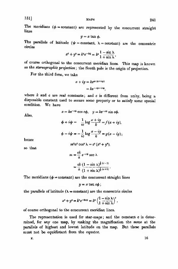
151] MAPS 241
The meridians (<£ = constant) are represented by the concurrent straightlines
y = x tan<f>.
The parallels of latitude (^ = constant, X = constant) are the concentriccircles
a? + «s = fre-** = k*l —i5-
X*
1 + sin X
'
of course orthogonal to the concurrent meridian lines. This map is knownas the stereographic projection ; the South pole is the origin of projection.
For the third form, we take
x + iy = Ice* i*"1"**)
= ke~ c^+^where k and c are real constants; and c is different from unity, being adisposable constant used to secure some property or to satisfy some special
condition. We have
Also,
hence
so that
x = ke'"* cos c<f>, y = ke~"* sin c<f>.
<f> + if= - log-^ =f(x + iy),
m?a? cos8 X = c2 (a? + y2),
c& „,m = — e~ c* sec A.
a
_c&(l-sin\)* (c -"
~ a(1 + sin X)*
(c+1)'
The meridians(<f>= constant) are the concurrent straight lines
y = x tan c<f> ;
the parallels of latitude (X = constant) are the concentric circles
/\ — sin XVa? +f = ^e-8c* = * f?
Sm,V
,
* Vl+sinX/
of course orthogonal to the concurrent meridian lines.
The representation is used for star-maps; and the constant c is deter-
mined, for any one map, by making the magnification the same at the
parallels of highest and lowest latitude on the map. But these parallels
must not be equidistant from the equator.
f. 16
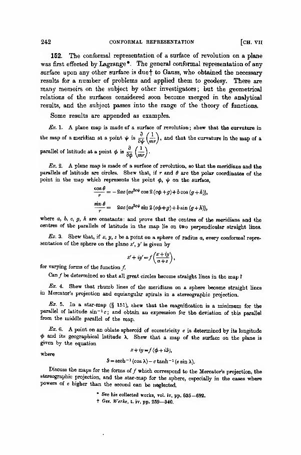
242 CONFORMAL REPRESENTATION [CH. VII
152. The conformal representation of a surface of revolution on a plane
was first effected by Lagrange*. The general conformal representation of any
surface upon any other surface is duef to Gauss, who obtained the necessary
results for a number of problems and applied them to geodesy. There are
many memoirs on the subject by other investigators; but the geometrical
relations of the surfaces considered soon become merged in the analytical
results, and the subject passes into the range of the theory of functions.
Some results are appended as examples.
Ex. 1. A plane map is made of a surface of revolution; shew that the curvature in
the map of a meridian at a point ^ is =-j- ( — 1 , and that the curvature in the map of a
parallel of latitude at a point<f>
is 5-7 (— )
.
Ex. 2. A plane map is made of a surface of revolution, so that the meridians and the
parallels of latitude are circles. Shew that, if r and 8 are the polar coordinates of the
point in the map which represents the point<fi, ty on the surface,
— = - 2oc {ae20* cos 2 (c0 +g)+ b cos (g+ k)},
^-= 2ac{aeie+iiiTi2(c<l>+g) + b&in(g+h)},
where a, 6, c, g, h are constants : and prove that the centres of the meridians and thecentres of the parallels of latitude in the map lie on two perpendicular straight lines.
Ex. 3. Shew that, if x, y, z be a point on a sphere of radius a, every conformal repre-
sentation of the sphere on the plane x1
,y' is given by
for varying forms of the function/.
Can / be determined so that all great circles become straight lines in the map 1
Ex. 4. Shew that rhumb lines of the meridians on a sphere become straight lines
in Mercator's projection and equiangular spirals in a stereographic projection.
Ex. 5. In a star-map (§ 151), shew that the magnification is a minimum for theparallel of latitude sin-»c; and obtain an expression for the deviation of this parallel
from the middle parallel of the map.
Ex. 6. A point on an oblate spheroid of eccentricity e is determined by its longitude
<p and its geographical latitude X. Shew that a map of the surface on the plane is
given by the equation
where*+*-/<*+*;.
S= sech " ' (cos X) - e tanh "» (e sin X).
Discuss the maps for the forms of/ which correspond to the Mercator's projection, thestereographic projection, and the star-map for the sphere, especially in the cases wherepowers of e higher than the second can be neglected.
* See his collected works, vol. iv, pp. 635—692.t Get. Werke, t. iv, pp. 259—340.
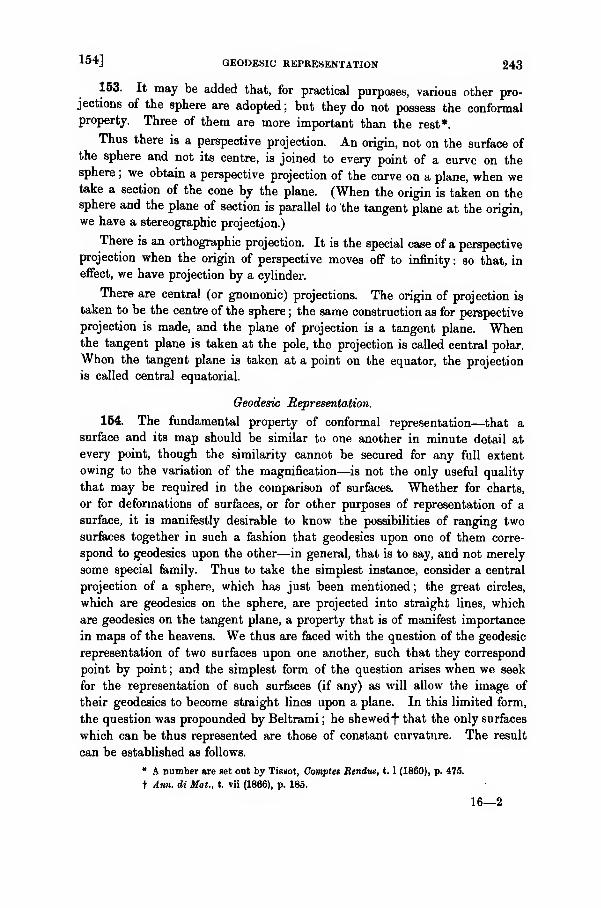
!54] GEODESIC REPRESENTATION 243
153. It may be added that, for practical purposes, various other pro-jections of the sphere are adopted ; but they do not possess the conformalproperty. Three of them are more important than the rest*.
Thus there is a perspective projection. An origin, not on the surface ofthe sphere and not its centre, is joined to every point of a curve on thesphere
;we obtain a perspective projection of the curve on a plane, when we
take a section of the cone by the plane. (When the origin is taken on thesphere and the plane of section is parallel to the tangent plane at the origin,
we have a stereographic projection.)
There is an orthographic projection. It is the special case of a perspective
projection when the origin of perspective moves off to infinity : so that, in
effect, we have projection by a cylinder.
There are central (or gnomonic) projections. The origin of projection is
taken to be the centre of the sphere ; the same construction as for perspective
projection is made, and the plane of projection is a tangent plane. Whenthe tangent plane is taken at the pole, the projection is called central polar.
When the tangent plane is taken at a point on the equator, the projection
is called central equatorial.
Geodesic Representation.
154. The fundamental property of conformal representation—that asurface and its map should be similar to one another in minute detail at
every point, though the similarity cannot be secured for any full extent
owing to the variation of the magnification—is not the only useful quality
that may be required in the comparison of surfaces. Whether for charts,
or for deformations of surfaces, or for other purposes of representation of a
surface, it is manifestly desirable to know the possibilities of ranging two
surfaces together in such a fashion that geodesies upon one of them corre-
spond to geodesies upon the other—in general, that is to say, and not merely
some special family. Thus to take the simplest instance, consider a central
projection of a sphere, which has just been mentioned ; the great circles,
which are geodesies on the sphere, are projected into straight lines, which
are geodesies on the tangent plane, a property that is of manifest importance
in maps of the heavens. We thus are faced with the question of the geodesic
representation of two surfaces upon one another, such that they correspond
point by point ; and the simplest form of the question arises when we seek
for the representation of such surfaces (if any) as will allow the image of
their geodesies to become straight lines upon a plane. In this limited form,
the question was propounded by Beltrami ; he shewedf that the only surfaces
which can be thus represented are those of constant curvature. The result
can be established as follows.
* A number are set out by Tissot, Comptes Rendun, 1. 1 (1860), p. 475.
t Ann. di Mat., t. vii (1866), p. 185.
16—2
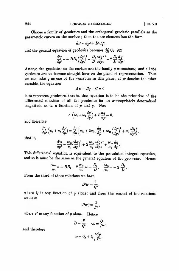
244 SURFACES REPRESENTED [CH. VII
Choose a family of geodesies and the orthogonal geodesic parallels as the
parametric curves on the surface : then the arc-element has the form
dt?=dp>+D'dqi,
and the general equation of geodesies becomes (§§ 68, 92)
dpa ~ "^{dp) D\dp) ' D dp'
Among the geodesies on the surface are the family q = constant ; and all the
geodesies are to become straight lines on the plane of representation. Thus
we can take q as one of the variables in this plane ; if w denotes the other
variable, the equation
Aw + Bq + C=0
is to represent geodesies, that is, this equation is to be the primitive of the
differential equation of all the geodesies for an appropriately determined
magnitude w, as a function of p and q. Now
and therefore
that is,
<Pq = Wn /dq\ 3
+ 2w^ (dqy w^dq
dp1 Wj \dp) «>! \dp) w, dp
'
This differential equation is equivalent to the postulated integral equation,
and so it must be the same as the general equation of the geodesies. Hence
W, w, D ' wt DFrom the third of these relations we have
where Q is any function of q alone; and from the second of the relations
we have
where P is any function ofp alone. Hence
n p Q
and therefore
w = Q> + QJ%
155] GEODESICALLY ON A PLANE 245
where Q, is any function of q alone. In order that the first relation may besatisfied, we must have
Q" + Q'\% = w~
= - DAwjF
-P(?1
;
and in this form the relation must be satisfied identically, for otherwise therewould be a relation between the independent variables. Differentiating
with respect to p, we have
P» s dp \p)
'
that is,
and so each side of this equation must be equal to a constant, say a. Thus
and therefore
/P'Y a .
(p)=-pi+ 6>
where 6 is a constant ; hence
and so
P" = 6P.
The Gauss measure of curvature of the surface is given by
K !«>
= --p=-6,
and so is constant; hence we have Beltrami's result that the only surfaces,
which can be geodesically represented on a plane, are those with a constant
measure of curvature.
155. There are three cases to consider, according as the constant measure
is zero, positive, or negative.
First, let the constant measure be zero. Then
P" = 0,
and so
P = a'p,
246 GEODESIC [CH. VII
where a' is a constant; no generality is lost by making the unexpressed
additive constant of integration equal to zero. Also
QsQ'' = _ pp" + ps = a '2_
and therefore
™ a*
hence
(c'Q?-a'*)$=c'q,
again making the additive constant of integration equal to zero without any
loss of generality. Hence the surface is
= dp1 + p^dq' 2,
on changing the variable q. Also we had
Q."+Q"jpi =-]PQ3 '
which, on substitution for P and Q, gives
er=o,so that
Q1= a"q+b".
But Q, is an additive part of w, which appears in the equation
Aw+ Bq + C= 0;
hence no generality is lost by taking a" = 0, b" = 0. Thus
W V]P> a'YNow
c'a'dq , ,
that is,
c'q = a' tan q,and
c'Q1 = a'2 sec2 q'.
Hence, except as to constant factors,
1w = - sec q , q = tan gr
;
and therefore the geodesies on the surfaces, having their arc-element in the'form
ds? = dp' + p2dq'1,
are given by the equation
Aw + Bq + C = 0,that is, by the equation
A'p sin q + Fp cos q' +C = 0.
155] REPRESENTATION 247
Secondly, let the measure of curvature be positive and equal to a-2 .
Then1 dlP 1
D dp2 ~ a2 '
so that
But
D = Q3 sm£ + Qt cos¥.
no generality is lost by taking
Also
and therefore
leading to
Q»Q" = -PP" + P'2 =\,
a2c'Qt = \ + (ac'q + b')2
= 1 + a2c'Y.
without loss of generality. Let
, , _ 1 dq _ ac'dqq ~ a Q2" ~ 1 + a*cY
'
so that
acq = tan q,
rfc'ty = sec2 q'.
Write
p = ap';
then the arc-element is
P*ds2 = dp2 +^ cfy
2
= a2 (dp'2 + sin2 //dq'2).
Also
„ «, f^ = _ZlJ P1 PQS '
which, on substitution for P and Q, gives
Q." = 0.
As Qi is an additive part of w, no loss of generality (so far as the geodesies
are concerned) is incurred by taking Q, = 0. Then
rdp
P2«-G + q/J
= — aQ cot - = — aQ cotp'.
248 GEODESIC REPRESENTATION [CH. VII
The geodesies on the surfaces, having their arc-element in the form
ds2 = a2 (dp 1 + sitfp'dq'*),
are given by the equation
A' smq' smp + B' cosy' sinp + C cos p' = 0.
The sphere, of course, is one of the included surfaces ; the last equation shews
that the geodesies on the sphere lie on planes through the centre, that is,
are great circles.
Thirdly, let the measure of curvature be negative and equal to a-2. The
analysis is the same as for the second case, save that hyperbolic functions
occur instead of circular functions. The result is that geodesies on the
surfaces, having their arc-element in the form
dsi = a2 (dp* + sinh2 p'dq'%
are given by an equation
A' sin q sinh p + B' cos q' sinh p' + C cosh p' = 0.
The Cartesian coordinates for the plane upon which the geodesies are
represented as straight lines are
at^psinq', y= pcosq';
x=smq' tan p', y = cos q' tanp';
a; = sin q tanh p'
,
y = cos q tanh p';
in the respective cases.
156. It thus appears that the variety of surfaces which can be represented
geodesically upon a plane is gravely limited ; and so it is natural to enquire
what surfaces can be represented geodesically upon one another, without any
restriction to a particular surface as that upon which the representation is to
be effected. A solution of the problem, though initially not complete, wasgiven* by Dini; a lacuna was supplied f by Lie; and another solution has
been given % by Darboux.
In order to effect the geodesic representation of one surface upon another,
it is necessary and sufficient to secure that the general equation of the
geodesies, viz.,
$ = r1$)'^'-*">(g)' +™t-4.should be the same for the two surfaces. This requires that the quantities
r", 2r-A", r-2A', a,
* Ann. di Mat., 2' Ser., t. iii (1869), pp. 269—293.t Math. Ann., t. xx (1882), p. 421.
t In the chapter, pp. 40—65, of the third volume of his treatise.
156] tissot's theorem 249
should be the same for the two surfaces. The equations thus obtained are
considerably simplified, if the same parametric curves are orthogonal on either
surface; still greater is the simplification if those parametric curves are
orthogonal on both surfaces.
But is this possible ? The answer to the question is to be found in the
following theorem, due* to Tissot :
—
In any birational correspondence between the real points of two real
surfaces, an orthogonal system on one surface exists having an orthogonal
system on the other as its homologue; and the system is unique, unless the
correspondence is conformal, or unless nul lines are homologous to nul lines.
Let the arc-elements on the two surfaces be
dss = Edp* + 2Fdpdq + Gdq\ ds'1 = E'dp* + 2F'dpdq + G'df.
When the correspondence between the surfaces is a conformal representation,
we must have
ds'* = m?ds*,
where m is independent of the differential elements ; hence, in that case, weshould have
~E~ F~ G'or, if we write
F'G-FG' = A, G'E-GE' = B, E'F-EF' = G,
the conditions for conformal representation are
4=0, B = 0, 0=0.
When the nul lines of one family on the first surface are homologues of
the nul lines of one family on the second surface, the equations ds2 = and
<2s'2 = have one root dp/dq common ; its value is given by
dp1 2dpdq dq*
F'G - FG' ~ G'E - GE' ~ E'F- EF'
'
that is, bydp3 _ 2dpdq _ dq"
A~ B ~ C'and the condition is
#-44C = 0.
We need not consider the case when both families of nul lines are homologous
with both families of nul lines ; for then
Edtf + 2Fdpdq + Gdq* - 0, E'df + 2F'dpdq + G'dq2 = 0,
would be the same equations, and we should have
W_F_ £'
E ~ F~ G'
that is, we should have the preceding case of conformal representation.
* Nouv. Ann. Math., 2m« Sit., t. xvii (1878), p. 151.
250 GEODESIQ [CH. VII
If possible, then, let Bp, Bq ; and S'p, B'q ; represent an orthogonal pair of
directions on both surfaces. We have
E BpB'p + F (BpB'q + BqB'p) + G SqB'q = 0,
E'BpB'p + F\BpB'q + BqB'p) + G'BqB'q = ;
and therefore
BpB'p = 6A,
BpB'q + BqB'p = 6B,
BqB'q = 6C.
Hence the directions Bq/Bp and B'q/S'p are the roots of the quadratic
At'-Bt + C=0.
We thus have a unique pair of orthogonal corresponding lines, unless either
the quadratic is evanescent so that A,B,G vanish, or the quadratic has equal
roots so that B*=4>AC. The former exception gives rise to conformal
representation. The latter requires that one set of nul lines should be
homologous, a correspondence that is imaginary for real surfaces. Hence wehave Tissot's theorem.
157. Deferring for the moment the two possible exceptions, let us
assume that the two surfaces have, in common, a unique system of orthogonal
curves. We take them as parametric curves, so that the arc-elements on the
two surfaces are
ds> = Edp> + Gdq\ ds'' = E'df + G'dq\
The general equation of geodesies on the first surface is
#q _ [dq\* -G, (dq\»(E* _ G,\ dq ( E, _ Ga E±dp* \dp) 2E^\dp)\E 2GJ
+dp\2E GJ
+2G'
and the general equation of geodesies on the second surface has the same
form. If the two surfaces can be represented geodesically upon one another,
the two general equations must be the same ; so the necessary and sufficient
conditions are
E E"Et G2 E2 C?2
~E~2G~ W~2G"
2E G 2E' G"Ea _ Eq
~G~ G7 '
From the second of these, we have
G~ G' '
158] REPRESENTATION OF SURFACES 251
where P is a function ofp only; and from the third, we have
E~ E' v'
where Q is a function of q only. Thus
E=E'P*Q, G=G'PQ>.
When we substitute these values of E' and G' in the first condition, it
becomes
G,(P-Q)=GPl ;
and then
G = QHP-Q),
where Q is a function of q only. When the values of E' and G' are substi-
tuted in the last of the conditions, it becomes
Ea_(Q-P) = EQi ;
and then
E=P*{P-Q),
where P is a function ofp only.
Hence the two surfaces are
ds2 = (P - Q) (P"dp2 + Q*dq%
and these are Liouville surfaces (§§ 117, 121). Consequently, a Liouville sur-
face can be represented geodesically upon an associated Liouville surface.
We have seen (p. 171) that geodesies on the first are given by
P(P-a)-$dp-Q(a-Q)-*dq = 0.
This equation is unaltered if we change P into — P~\ Q into — Q~\
P into PP~^, Q into QQ~K a into -1/a'. These changes turn the first
surface into the second; and so there is a direct verification that the two
Liouville surfaces can be represented geodesically upon one another.
158. We have to deal with the two exceptions to which Tissot's theorem
does not apply.
In the first of them, there is conformal representation, so that
ds' = mds.
Thus the nul lines on the two surfaces are the same. Let them be chosen
as the parametric curves ; then
ds1= 4\dpdq, ds'3 = 4i\'dpdq,
and therefore
V = m2\.
252 GEODESIC [CH. VII
The general equation of geodesies on the former surface is
<p£ _ X, dq _ Xj (dqy.
dp* X dp X \dp''
and on the latter it is
dp2 ~ X' dp X' \dp)'
When the two surfaces can be represented geodesically on one another, these
two general equations must be the same ; hence
A.J A.) A*2 A^
A. A, A. A.
and therefore
— = constant,
that is, m is constant. Thus the two surfaces are similar to one another in a
constant magnification.
In the second of the exceptions not included in Tissot's theorem, the
homologues of a family of nul lines on one surface are a family of nul lines
on the other.
Let one surface be referred to its nul lines as parametric curves; its
arc-element is
ds2 = 4>Xdpdq.
Let q = constant be the family of nul lines, of which the homologues are a
family of nul lines on the other surface ; then its arc-element has the form
ds'<> = IFdpdq + Gdq\
For the latter surface, we have
r = $, a =0,
r" = ^ a' -2F' '
Gt
~2F jiiFt-WJ, A" = -±(^ -££,);
and the general equation of geodesies is
On the former surface, the general equation of geodesies is
d!l = _h(d2\\h dldp2 X\dp) +
X. dp'
158] REPRESENTATION OF SURFACES 253
When the two surfaces can be represented geodesically on one another, these
two general equations are the same ; hence
$-&-&)— %.
F~ \-
The third of these conditions yields the relation
F=XQ,
where Q is a function of q only. When this relation is substituted in the
second condition, the latter becomes
The first condition now gives
G, _ X, 2 Q'
1G \+ SQ'
so that
where, so far as the condition is concerned, P is a function ofp only, and a is
a disposable constant. Substituting this value of G in the modified form of
the second condition, we find
hence
* = Q + lQQSJPdp,
where Q is a function of q only.
Now let
Pdp = du, \ = fiP, Q = R~3,
so that B, is a function of q only, and u is a new variable ; then
u. = Q--uR\r aor, choosing a= — 1,
Also
Thus the first surface is
fi = Q + uR.
F=fiPR-3,
G = - /SR-'.
ds2 = i/idudq
= 4 (Q + uR) dudq,
254 SPHERICAL [CH. VII
where Q and R are any functions of q alone ; and the second surface* is
ds'- = 2/LR-3dudq - fji>R-*dq2
,
where _fi,= Q + uK,
These two surfaces can be represented upon one another so that their
geodesies correspond. Now (§ 121) the geodesies on the surface
dsi = i(Q + uR')dudq
are given by the equation
» of M - c
(a+2B)* J (a+<2Rf-
where a and c are arbitrary constants ; this equation therefore gives also the
geodesies upon the geodesically associated surface.
Spherical Representation ; Tangential Coordinates.
159. We now come to the representation of a surface on a sphere,
already indicated in § 147 ; it frequently is called the spherical representation
of the surface, and it is due to Gauss originally. We take a sphere of radius
unity and through its centre draw a line parallel to the positive direction of
the normal to the surface ; the point on the surface has its image in the point
where the sphere is cut by the line. It thus follows that, in the represen-
tation, we are partly considering the tangent plane to the surface ; and so, in
using the direction-cosines of the normal, we are in effect using three of the
tangential coordinates of the surface. We shall therefore find it convenient
to deal with equations, expressed as far as possible, in terms of tangential
coordinates; for they are essential to the resolution of the question as to
how far a surface is determined by a given spherical representation.
The coordinates of the spherical image of a point on the surface, where
the direction-cosines of the normal are X, Y, Z, are themselves X, Y, Z, which
are subject to the condition X2 + Y2 + Z2= 1. Let dS be an arc-element on
the sphere ; then
dS* = dX°- + dY* + dZ* = edp* + 2fdpdq + gdq\where
e= XS + 7,2 + Z,2 =-EK+ LH,
/= Z,Z 2 + y, F2 + Z,Z2= - FK + ME,
g= Xi + IV + Z? =-GK + NH,
on substituting the values of the derivatives of X, Y, Z given in § 29.
We have
eg-f*= V'K";
* The result is due to Lie ; Bee § 156.
160] REPRESENTATION 255
and therefore, as eg-f">Q, the surface to be represented cannot be adevelopable surface.
Manifestly we have
dS* = - Kdf + H— ,
P
with the usual notation for the curvature of the normal section. Now
v H 1 /l 1 \ /cos2-Jr sin2 iK
cos2yfr sin2
1^~a* r '
where $• is the angle between the tangent to the curve and a line ofcurvature; and therefore
,„., /cos'2 !^ sin2-Jr. ,
,
Hence the spherical image usually is not a conformal representation.. Butthere are two classes of surfaces for which spherical representation is con-
formal. For one class, we have a = 0; its Cartesian equation, in the mostgeneral range, is
y + fix =<f>
(ji)\
z-ix(l+/j.
!')b = ty(fl))'
where<f>
and yfr are arbitrary functions. For the other class, we havea + £ = 0; they are minimal surfaces, and will be discussed later (in
Chap. viii).
160. Some simple properties can be established at once.
I. When the parametric curves on the surface are orthogonal, we have
When they are orthogonal on the sphere also, then
/=0;
and therefore, unless H = 0, we have M=0.
Further, when F=0, M=0, we have/=0 whether H vanishes or not.
Hence the spherical image of the lines of curvature is an orthogonal system
;
and the lines of curvature are the only orthogonal system whose spherical
image is orthogonal, unless the original surface is a minimal surface—in
which case the spherical representation happens to be conformal also, so that
any orthogonal system remains orthogonal in the representation.
II. But further, the spherical image of a line of curvature is parallel
(directly or reversely) to the line ; and if the spherical image of a curve is
parallel to the curve, then the curve is a line of curvature.

256 SPHERICAL [CH. VII
For the first part, take the lines of curvature as the parametric curves,
so that
F=0, M = 0.
We then have (§ 29), for the respective lines,
X-i = -' = ?1 = - -
"h Hi Zi E'
X* = Y1 = Z2 = _N
x„ y2 z2 G'
proving the statement.
For the second part, keep the parametric curves general ; and suppose
that the spherical image dX, d Y, dZ of da:, dy, dz is parallel to it. Then
Xidp + X2dq _Yidp+ Y2dq _ Zxdp + Z2dq
xtdp + x2dq yxdp + y2dq Zjdp + z2dq'
Let the common value of these fractions be fi ; then
Xj dp + X2dq = n fadp + x2dq),
Yjdp + Y2dq = fi (yrfp + y2dq),
Ztdp + Z2dq = fi (zxdp + z2dq).
Multiply these equations by as,, yit z, respectively, and add; and by x2 , y2 , z2respectively, and add ; we have
- Ldp- Mdq =fj,(Edp + Fdq),
- Mdp - Ndq = p (Fdp + Gdq)
;
and therefore
(EM - FL) dp* + (EN - GL) dpdq + (FN - GM) dq*= 0,
giving the directions of the lines of curvature.
III. A direction dx, dy', dz' on the original surface, which is conjugate
to a given direction dp, dq, is such (§ 47) that
dx'dX + dy'dY+dz'dZ=0,
where dX, dY, dZ are determined by dp, dq, that is, are the spherical imageof the given direction. It therefore follows that, when two directions are
conjugate on the surface, the spherical image of each direction is perpen-dicular to the other direction.
Moreover, as an asymptotic line is self-conjugate, it follows that the
spherical image of an asymptotic line is perpendicular to the line.
IV. The preceding result, relating to conjugate lines, can be stated in
another form, viz. the inclination of the spherical images of two conjugatelines is either equal to, or supplementary to, the inclination of the conjugatelines.
160] REPRESENTATION 257
This can be established independently as follows. Taking the conjugate
lines as the parametric curves, we have M = ; and therefore
f=-FK.As usual, denote by a the inclination of the parametric curves on the surface
which now are conjugate ; and denote by o>' the inclination of their spherical
images. Then (§ 25)
cot a> = FjV, cot a =f(eg -/»)"*.
Now
and we take v positive, just as V has been taken positive (§ 24) ; hence
v=±VK,the upper or the lower sign being used, according as the surface is synclastic
or anticlastic. Thuscot a =±f/VK,
that is,
cot to' = + cot <o,
which gives the property in question.
V. We can, by means of the spherical representation, prove Joachim-
sthal's theorems (§ 128) as to plane lines of curvature and spherical lines of
curvature.
In the case of a plane line of curvature, let a, b, c be the direction-
cosines of the normal to the plane. If at any point, or is the angle between
the normal to the surface and the principal normal to the curve, we have
sin vs = aX + bY+ cZ;
and therefore
d
ds
,. . / dX ,.dY,
dZ\dS(sm ^ =
(a dS+ b
dS +Cds)ds
l dx ,dy dz\ dl~ ~\ ds ds ds) dt
because the spherical image of a line of curvature is parallel to the line.
Now a, b, c are the direction-cosines of the normal to the plane in which
the line of curvature lies; thus
dx,,dy dz _
ads-
+ bI + Cds= °-
Consequently, sin ra- = constant ; or the plane and the surface cut everywhere
at a constant angle—which is the theorem as to plane lines of curvature.
Moreover, the equationaX + bY + cZ = sin sr
now shews that the spherical image of the line of curvature is a small circle,
unless the line of curvature is also a geodesic, in which case its spherical
image is a great circle.
f. 17
258 SPHERICAL [CH. VII
Also, if a family of lines of curvature is composed of plane curves, their
spherical image is a family of small circles. If both families of lines of
curvature are plane curves, then (because the spherical image of two lines of
curvature is two orthogonal lines) the spherical images are two families of
orthogonal small circles. We shall return later (§§ 197, 198) to this matter.
Next, consider a spherical line of curvature. Let the sphere be of radius r
and have its centre at x , y , z ; then, denoting by x the angle between the
normal to the surface and the normal to the sphere at a point on the line of
curvature, we have
cos x = X °^-° + F^^o + zz-_
fo
Consequently
d /w, \1 (t <**
±. v dy .. r dz\ ,
dS fdX x-x dY y-y,
dZz-z„\
_,dS /x-x„ dx y-y dy z-z„ dz\
~ ds \ r ds r ds r ds)
'
because the spherical image of a line of curvature is parallel to the line.
The quantity within the brackets on the right-hand side is zero because the
line of curvature lies on the sphere ; hence
cos x = constant,
and therefore the sphere and the surface cut at a constant angle along the
line of curvature—which is the theorem as to spherical lines of curvature.
(The angle x ig the angle or' — w of § 128.)
161. The fundamental magnitudes of the second order, say L', M', N',
for the sphere can be obtained simply. Denoting the direction-cosines of
the positive direction of the normal to the sphere by X', Y', Z', we have (in
accordance with §§ 27, 29)
X' -I(FA-Ft2i)- 1 KVX = ±X,
according as the surface is synclastic or anticlastic ; and similarly Y'= ±Y,Z' =±Z, the upper signs being used together and the lower signs being usedtogether. Thus
L' = X'Xu +Y'Yu + Z'Zn= ±(XX11 + YY11 + ZZ11 )
= + ^ (XX, + FF, + ZZt )- (X,* + Yf + Z?)
and similarly M' = +f, N'=5g. The radius of curvature of any normalsection of the sphere, being
edp* + 2/dpdq + gdq*
L'df + 2M'dpdq + N'dq*
'
161] REPRESENTATION 259
is numerically equal to unity, as was to be expected; it is positive or negative,
according as the normal to the positive side of the sphere has to be drawn
inwards or outwards.
Thus only the fundamental magnitudes of the first order for the sphere
need be taken into account. It is convenient to have the relations between
them and the fundamental magnitudes of the surface. Substituting for Kand H in the expressions for e, /, g, we find (see also § 29)
7'e = EM 2 - 2FLM + GL\
V*f= EMN - F (LN + M*) + GLM,
V'g = EN" - 2FMN + GM> ;
and therefore
t?E = eM° - 2/LM + gL\
v*F = eMN-f{LN + M<) + gLM,
v*G = dV! - 2/MN + gMa-
We require quantities corresponding to T, V, T", A, A', A". Let
H-= i«i, /*' = ie2 , ft" =/2 - \gu
v =/, - £e2 , v = \g* , v" = £&.
Then we take
t)a8 =ve — /if
'
vsS' =v'e -ft'f ;
v'y" = n"g-v"f) v'S" = v"e-fi"f
and we thus have the quantities required. Moreover, they give
fi = ey +/B \ v = fy +gS ^
S = ey' +/V , v' =fy' +gh'
V."=ey"+f&") v'=fy"+g$")
corresponding to the relations in § 34.
As the values of the quantities e,f, g involve all the magnitudes E, F, G,
L, M, N, these quantities fi, fi, /i", v, v, v" must be expressible in terms of
the derived magnitudes of the third order for the surface. We have
^ =4 {2mM°- 2 (n + m')LM+ 2n'D) + i{2M1(EM-FL)+ 2L1{GL-FM)}
dp V "
-^ (r+ A') {EM» - 2FLM + GD)
= 2{((?i _m
)
p +^_^ Q + 7' (er +/A)}
;
"s7 =W ~ vftfy' =fi'g-v'f r
= u"a-v"f\
17—2
260 TANGENTIAL [CH. VII
and similarly for the others. The aggregate of results is :
—
p =± {(GL -FM)P + (EM - FL) Q] + eT +/A
fi' =^-2{(GL -FM)Q + (EM - FL) R} + eT' +/A'
H-"= ^i {(OL -FM)R + (EM - FL) S] + eT" +/A"
v = y-% {(GM-FN)P + (EN- FM) Q] +/T + gb
v' =± \(GM -FN)Q + (EN - FM) R}+fT' +g*
„" = *. {(GM -FN)R +(EN-FM) 8} +/T" + gb"
and it is easy to shew that
V*K(y -T ) =PN-QM \ V*K(8 -A ) = -PM+QLV*K(y' -T') = QN-RM ,
V*K(8' -&') = -QM + RL .
V'K(y"-T") =RN-SM ) V*K(S"-b") = -RM + SL
162. The tangential coordinates connected with the surface are defined,
as usual, in connection with the tangent plane. Let x, y, z be the coordinates
of any point on the surface, and let T (with, of course, a new significance for
the symbol, different from the significance adopted in § 28) be the distance*
of the tangent plane from the origin ; then the equation of the plane is
xX + yY + zZ=T.The quantities X, Y, Z, T are the tangential coordinates of the surface.
We require various quantities, and some of our established equations,
expressed in terms of the tangential coordinates. For x, y, z, we have
xX +yY +zZ =T,
xX. + yY. + zZ^T,,
xXt + yYz + zZ^T,.Now (§ 29)
X, Y, Z =VK,Xit Ylf Zi
-"2» -*2» ^2
YtZt- Y,Z, = VKX,
Y2Z-YZ, = R (gX1 -fXi),
YZt-YJ-^-fXt + eX,);
* Sometimes W ie used (as in § 79, and regularly by Biancbi).
163]
hence
COORDINATES 261
x = TX + ± {eX2T2 -f{X,T2 + X2T,) + gX.T,)\
y=TY + ± {eY2T2 -/(F.r, + 7^) + gY^}
z=TZ + ± \eZ2T2 -f{ZxT2 + Z2Ty) + gZ.T,},
giving the point-coordinates of the surface in terms of the tangential
coordinates.
It therefore follows that, when the tangential coordinates are given, the
surface is completely determinate even as to position and orientation.
163. Again, we have (§ 161)
XXn + YY11 + ZZU = -e.
Also, from the definitions of the quantities /i and v, it follows that
XJv+YiYn + ZA^p,X2XU + Y2Yn + Z?Zn = v
;
hence, solving for Xu , Yu , Zn , we find
Xn — — eX + yXj + SX2 ;
and similarly for Yu , Zu . Thus
X,! = — eX + yXx + BX2
F„ = -eY+yY1 +BY2 .
Zn = -eZ + yZ1 + BZ2 .
Similarly
and
X12= —fX + y'Xi + B'X2
Y12= -fY+y'Y1 + B'Y2 \
Z^-fZ + y'Z.+B'Z,
X„ gX + y"X, + B"X2 \
Y^-gY + y"Y^B"Y2
Za gZ + y"Z1+B"Z2
These are the equations of the second order satisfied by X, Y, Z.
There are corresponding equations for T. We proceed from
T^wX. + yYr + zZ,;
Tn =xXn +yYu + zZu + x,Z, + y, F, +z&
= -eT+ yT1 + ST2 -L.
then
262 RANGE OF A [CH. VII
Ta ,
165] SPHERICAL REPRESENTATION 263
the quantities E, F, G become functions of known quantities, of T, and of
the derivatives of T up to the second order inclusive. Now, for every surface,
the six fundamental magnitudes must satisfy the Gauss characteristic equation
and the two Mainardi-Codazzi relations, viz.
LN-M*--±(Em - 2F13 + Gn)
- y^ {E (nn" - n'a) - F(nm" - 2«W + n"m) + G (mm" - m'%
L2 +TM+AN=M1 + T'L + A'Jf,
M, +r'M+A'N= JV, + T"L + A"4f.
When the foregoing values of E, F, G are substituted in these equations
—
the algebra is exceedingly laborious—and then, when substitution is made for
L, M, N in terms of the quantity T and the given magnitudes, the first of
these relations gives a partial differential equation for T which is of the
third order. (Owing to the presence of E„ — 2Fa+6u , the equation might
have been expected to be of the fourth order ; but the terms of that order
cancel.) The second of the relations gives another partial differential equation
for T of the third order; and the last of them gives yet another partial
differential equation for T of the third order. (In both of these equations,
the terms of the third order disappear from Lt —Mx , and Ma — N-^, respectively;
but they arise from the values of T, T', T", A, A', A", and they do not
disappear.)
Thus in general, when a spherical representation of a surface is given, it
is necessary to solve three simultaneous partial equations of the third order
if the surface itself is to be determined thereby.
165. But simplifications of this complicated result can be secured by the
assignment of particular conditions—these conditions really being limitations
upon some of the arbitrary functions that occur in the primitive of the three
simultaneous partial equations of the third order.
Let there be an assigned condition that the parametric curves on the
sphere shall be the images of asymptotic lines on the surface. Instead of
dealing with the specialised forms of the equations of the third order, it is
simpler to deal with the original equations that are fundamental; so we
assume the condition that the asymptotic lines are to be parametric, viz.,
Z = 0, N=0,
and then the Mainardi-Codazzi relations are
(r-b')M=Mlt (b"-r')M=Mt .
Moreover, we have
(r + A^F-F,, (A" + r')F=F8 ;

264 SUPPLEMENTARY [CH. VII
bo that
or- ^ +^ 2A"- ^ + ^
Consequentlyar = 3A^' 3A' = ar;
dq dp ' dq dp'
differential relations which, of course, are isolated under the special system
of parametric curves.
Having regard to these curves, the values of P, Q, R, S (as given in § 40)
are
P = -2ifA, Q= -2A/A\ R = -2MV, S=-2MT".
Also we now have
&E= eM\ v*F= -fM\ v*Q =gM\so that
vV=M\and
V -~ M *
- - 1 _ iiV " F~ AT2'
As regards the quantities 7, 7', 7", 8, 8', 8", there are simple relations
connecting them with T, T', T", A, A', A" under this system. We have
(§ 161)
7-r — p^OJf-J— 2A',
y-r'— ^fiif-J— sr,
^"- r"=-T4^4=- 2r'
8 - A =-t4 pji/=¥=- 2a-
8'-A'=-T4Qilf = | = -2A',
X" - A" = — KM = — - - 2F" •
V*K M~ '
and therefore
7 = r-2A', 8" = A"-2r',
y I", 7"=-r", 8 A, 8' A'.
Consequently we also have (always under this system of parametric curves)
dq dp' dp ~ dq'

165] CONDITIONS 265
as relations identically satisfied ; thus the spherical representation cannot bechosen arbitrarily. Also
E .«*!__.• F-f G _ 9.
therefore the arc-element on the surface is expressible in the form
ds8 = - ™ (edp1 - 2fdpdq + gdq*).
And then the quantity T is an integral common to the two equations of the
second order
Tm -y"T1 -B"T1 +gT=0\
Ex. Let these results be applied to a pseudo-spherical surface. We have, for all
surfaces referred to asymptotic lines as parametric curves (§ 42),
V2K1= -2MQ, V2Kt=-2MR;and therefore, for a pseudo-sphere,
Q=0, R=0.Thus
y'=r'=0, 8-=A'=0, y = r, 8"=A".Now
2V2r=E2G- G1F = ±(e2g+glf),
in this case; and so
«2=0, g1= o.
The same inferences follow from the conditions S'= A'=0. Hence e is a function of ponly ; it can therefore be made unity, because it can be absorbed into the term edp2
.
Similarly g is a function of q only ; it can therefore be made unity, because it can be
absorbed into the term gdq2. Thus the arc-element on the sphere is
dS2— dp2— 2dpdq cos <> -(- dq2,
and on the pseudo-sphere is
da2= - ={dp2 - 2dpdq cos a
+
dq2).
The parametric curves are asymptotic lines ; so that, over an ordinary region of the
surface, asymptotic lines of the same family do not meet. We thus do not have an
asymptotic triangle (like a spherical triangle on a sphere, or a geodesic triangle on any
surface); but we do have an asymptotic quadrilateral. If <>
denote the angle between the parametric curves, we have (§ 36)
in general
dpdq~dp\ E )+dq\ Q )
+y& '<
and therefore, in the present case,
a2o> .
5—5-= Sin<B.opoq
266 SPECIAL [CH. VII
Now the area of the quadrilateral is
dpdqsin a
= -•= {o)c -(«•-<»j,) -(ir — <aB)+<o^}
where 5 is the sum of the internal angles of the quadrilateral on the surface.
Other simplifications can be suggested; the results are left for detailed
working.
When the parametric curves are required to be orthogonal on the surface,
we must have F= 0, that is,
eMN-f(LN + M') + gLM = 0.
When the values of L, M, N in terms of T and its derivatives are substituted,
we have a non-linear partial equation for T of the second order.
When the parametric curves are required to be conjugate on the surface,
we have M = 0, that is,
Tlt-y'T1 -S'Ti +fT = 0.
We have a linear partial equation of the second order ; it is of the Laplace
type*
When the parametric curves are required to be both orthogonal and
conjugate on the surface, that is, are required to be lines of curvature on
the surface, we have F= 0, M — 0. Then
/•=0 -v' =— S' = -2i-
and the linear partial equation for T is
rp fis rp fill rp _ n
again of the Laplace type. When T is known, then
e
N*=— .
9* See the author's Theory of Differential Equation/, vol. vi, ehap. xiii.
165] CONDITIONS 267
When the surface is to have its mean curvature constant, then the partial
equation for T is
(LN-M*) H= eN- 2/M + gL,
of the second order and the Monge-Ampere type.
In all these cases, we have to integrate a partial differential equation of
the second order. Its primitive contains two arbitrary functions ; and so
there is, in each instance, a double family of surfaces with the assigned
spherical representation.
EXAMPLES.
1. Any two stereographic projections of a sphere are inverses of each other, the origin
of inversion in either being the origin of projection for the other.
2. Shew that the spherical images of the asymptotic lines on a minimal surface, as
well as the asymptotic lines themselves, are an orthogonal isometric system.
3. Two surfaces have the same spherical representation. A family of spheres is
drawn having their centres on one of the surfaces and the envelope of the spheres is
constructed; shew that the other surface is normal to the chords of contact.
4. Shew that, if
v U+ V v i(v-u) _ UV-l .mi , ,sX= —, T= —.- , z=——r, t=T(uv+l),
uv+1' uv+ 1 uv+ 1' v "
the lines of curvature on the original surface are given by
dud =
—
dvd ^-=0.ou ov
Also shew that, if another surface is given by the equations
3* dtx=di>
y= v>
° = -t+udu>
its asymptotic lines are given by the foregoing differential equation.
5. Prove that, when e, f, g, T are known, the lines of curvature on the original surface
are given by the equation
dq2,
—dqdp,
dp2 =0.
e / 9
Tn-yTi-iTt, Tn-M-STt, T^-y-T.-H'T,
6. Shew that the surfaces, which have one system of lines of curvature in parallel
planes, are given by the equations
x=/(») cos v-f'(v) sin v+ {g (it) sin u+gl(u) cos v) cos r,
y=f(v) sin v +/' (») cos v+{g (it) sin u+g' (it) cos it} sin v,
z=g (u) cos it —g' (it) sin «,
where/and g are any functions whatever.

CHAPTER VIII.
Minimal Surfaces.
The amount of mathematical literature, devoted to the subject of minimal surfaces, is
of vast extent.
The theory was initiated by Lagrange, mainly in his non-geometrical treatment of the
stationary values of double integrals. It attracted the fruitful attention of other great
mathematicians such as Monge, who was the first to give a general solution of the
question ; and of Legendre, who first applied what now is called a contact-transformation
to the partial differential equation of the second order that is characteristic of the surfaces.
All this work belonged to the later part of the eighteenth century. Its progress continued
intermittently in the earlier half of the nineteenth century until the researches of Bonnet,
published in 1853 and later, which marked an entirely new development in the deter-
mination of real surfaces. Soon there followed the investigations of Weierstrass, whogave the useful forms to the equations obtained by Monge and from them constructed
the generalities of the theory of minimal surfaces that are real and of surfaces that are
algebraic ; the significance of the theory of real surfaces being due to the fact that the
analysis is bound up with functions of complex variables. Moreover, the researches of
Weierstrass inspired the work of Schwarz who has contributed many important develop-
ments to the subject, on its geometrical side and its functional side. And Lie's work added
substantially to the theory of algebraic minimal surfaces that are subjected to assigned
conditions.
Mention also should be made of the memoirs of Beltrami who made notable additions
to the subject and, in one of his early memoirs, gives a survey of the progress made downto 1860.
Above all, there is the section (Book iii, vol. i) in Darboux's treatise dealing with the
whole matter, its history, its development, its later issues, problems half-solved or unsolved.
That section is practically a complete treatise at the time of its publication (1887) ; what-ever advances in detail may have been made since that date, Darboux's exposition shouldbe studied carefully by every student of the subject.
The Critical Equation 27 = 0.
166. We now proceed to consider one particular class of special surfaces,
usually called minimal surfaces. For many reasons, they are important.
They are related to the calculus of variations, as providing the simplest
significant example of a condition for the minimum of a double integral ; it
was in this relation, that they arose in investigations of Lagrange. They are
related, in their analytical expression, to the theory of functions of a complexvariable
; implicitly beginning in results due to Monge, the association has
been developed in many researches that have their foundation in somememoirs of Weierstrass, supplemented by the work of Schwarz and of lie.
166] MINIMAL SURFACES 269
They are connected with problems in mathematical physics, of which the
most picturesque is that of the soap-bubble.
Let surfaces be drawn so as to pass through an assigned closed curve
(whether continuous in direction or not) and be required, along the curve, to
touch an assigned developable surface passing through the curve. For the
moment we are not concerned with the limitations imposed upon surfaces bythese requirements, or with the extent of further condition that may be
imposed simultaneously with the limitations. Among all these surfaces, let
a surface be selected such that its area is a minimum—in the sense that,
when small variations of any kind upon the surface are effected subject to
the limitations, the result is to give an increase of area for the modified
surface. The original surface is called minimal. It may or may not be
unique. It may even be non-existent, owing to the complication of the
conditions.
We have seen (§ 25) that the element of area on the surface can be
represented by the quantity Vdpdq ; and therefore the area of the surface
bounded by some assigned curve is
// Vdpdq,
where the double integral is taken over the range limited by the curve. If
then the area of the surface is to be a minimum among the areas of all
surfaces which can be drawn through the curve, this double integral must be
a minimum.
The conditions that the first variation should vanish (a condition which
secures a stationary value for the double integral) are that the equations
dx dp\dxj dqxdfyj '
dX _ LfiL\ - A (®X.\ =0dy dp\dyj dq\dyj
<*Z"_ A fil\ _ A fiZ\ =dz dpKdZi) dq\dzj
should be satisfied. Now, as a function of the variables, V explicitly involves
xu x2 , yi, y», *i, z2 ; but it does not involve x, y, or z, so that
Again (§ 27)
?r.o ^=o ^=o.dx ' dy dz
hence the first equation becomes
y^ - *,F, - y*Zt + ZjTt= 0,
that is, on substitution for the derivatives of Y and Z (§ 29),
VX(EN-2FM + GL) = 0.
270 CHARACTERISTIC EQUATION [CH. VIII
The second and the third equations similarly give
VY {EN - 2FM + GL)= 0, VZ{EN - 2FM + GL) = 0;
hence all the conditions, required in order to make the first variation vanish,
are satisfied by the single relation
EN-2FM+GL = 0.
Thus H, the mean measure of curvature, vanishes ; the two principal radii of
curvature are equal and opposite, and therefore the indicatrix is a rectangular
hyperbola.
When, instead of parametric curves, the coordinate axes are used for
reference, the area is
{1 + p* + q'fi dxdy,//<
[P } + 1 1 2 4 = o
where p and q now denote the derivatives of z. The condition for a stationary
value is
dx]
which becomes(1 +q*)r- 2pqs + (1 +p
2) t = 0,
in accordance with the preceding relation when the values (Ex. 3, p. 60) of
the fundamental magnitudes are inserted.
167. The result can also be obtained without recourse to the general
formulae of the calculus of variations; and the process* leads to one condition,
critical as regards a minimum, which is important for weak variations (§ 89)
of the variables x, y, z of a point on the surface.
Let a length I, chosen as an arbitrary function of p and q, be measured
along the normal to any surface; and suppose the surface referred to its
lines of curvature. Then (§ 85) the quantity Ffor the surface, derived as the
locus of the extremity of this length I, is given by
v^{i-*)>{i-ey +i^J G + k>(-^)'E,
For the present purpose, the length I determines a small variation under
which the surface is to be minimal ; hence I itself is small, and (when we
assume the small variation to be weak) the quantities Zj and lt are small, of
the same order as I. Expanding V in powers of the small quantities /, lu l2 ,
and neglecting powers of these quantities higher than the second, we have
= V'\l-2lH + l> {H* + 2K) +l *
•
l>*
E + Gso that
V=
* It is substantially due to Daibouz, t. i, §§ 184, 185
167] SECOND VARIATION 271
The area of the derived surface, corresponding to an area 1 1 Vdpdq of the
original surface, is 1 1 Vdpdq ; hence the variation of area, being
jivdpdq-JJvdpdq,
is given by the expression
-jjlVHdpdq+ljf(2Kl> +l±+ l
£) Vdpdq.
If the original surface is to be minimal, this quantity must be positive for all
arbitrary small quantities I, on the understanding that 2, and l^ also are small
of the same magnitude as I. In the expression, the term of the first order
governs the rest unless it vanishes; and when it does not vanish, we can
make the sign of the term positive or negative at will by changing the sign
of I, and then the condition for a minimum would not be satisfied. Hence
the term of the first order must vanish ; as I is arbitrary, this requirement
can only be satisfied if the equation
5 =
holds everywhere on the surface. (If H does not vanish everywhere, we can
make the first term positive or negative at will, by choosing I everywhere of
the same sign as IT or everywhere of the opposite sign.) We thus have the
former result as to the equation, which is characteristic of minimal surfaces.
Thus for weak variations of minimal surfaces, the most important term in
the variation of the area (it is usually called the second variation) is
llfem+V + ^Vdpdq.
In this expression E, G, V are positive, while K is negative ; in order that
the surface may be a real minimum, the quantity must be positive for all
non-vanishing weak variations. As I is arbitrary, subject only to the
condition that it must vanish along the closed curve through which the
minimal surface is bound to pass, the requirement of a positive sign for the
second variation provides a test for a real minimum.
It is easy to prove that, when general parametric curves are selected
instead of the lines of curvature, the second variation is
ifj^KP + ytW ~ 2*V2+ 0y)| Vdpdq.
Ex. Taking weak variations #+£, y+i;, z+£ of x, y, z, bo that £, i;, f and their
derivatives are small, substituting and using the formulae of § 27, shew that the second
variation of the area can be expressed in the form
| ff^(El*>-2F\p+G\!
>)dpdq+fl(kXdvd(+ FdCd£+Zd£dr,),
where\=Xi1 +Till+ZCu n=Xh+rvs+Z(f

272 GENERAL PROPERTIES OP [CH. VIII
We shall see (in § 188) that the requirement of a positive sign for the
second variation, in order to secure a real minimum, causes a limitation of
the range over which the integration can extend; we shall have the conjugate
of an initial curve, when it is associated with an initial tangent developable.
But its discussion must be deferred until we have indicated other conditions
which make a minimal surface precise.
When strong variations are taken into consideration (that is, variations
which keep f, 17, f small and do not demand that f„ f„ 17, , nj^, £i, f2 shall be
small), it is necessary to construct the excess-function, as in § 89, IV.
Both investigations, in their general form, belong more to the domain of
the calculus of variations* than to that of differential geometry; it maysuffice to mention that the excess-function for a surface given by H=0 is
positive, and so the minimal surface satisfies another test for a true minimum.
For our purpose, the important property is that the relation
H=EN-2FM + GL =is satisfied at every point of a minimal surface.
Some General Properties.
168. Before proceeding to obtain integral equations, which shall be
equivalent to the characteristic equation H=0, whether they give the surface
intrinsically or express the coordinates of a point explicitly, it is worth while
to notice some simple properties generally common to all minimal surfaces.
(i) The nul lines on a minimal surface are conjugate. Let them be
taken as the parametric curves for the surface ; then E=0, G=0, and F is
not zero. But always
EN-2FM+GL = 0;
hence, in this representation, M = 0. Thus the parametric curves, being the
nul lines, are conjugate.
(ii) The asymptotic lines on a minimal surface are perpendicular. Let
them be taken as the parametric curves for the surface ; then L = 0, N=0,and M is not zero. Again, always
EN-2FM+GL = 0;* A fall discussion for any double integral
//'F(x, y, z, xi, y,, *,, xit y2 , z2)dpdq
was first given by Kobb, Acta Math., t. xvi (1893), pp. 65—140. The particular result in the text
agrees with Kobb's general result (I.e., p. 114) when the integral is / fVdpdq ; his quantities
F1,F„F
s,Fi then are
^F,= G/K, F3=EIV, Ft=-FIV, Ft=2KV.
Also, the excess-funotion (Z.c, pp. 121—123, 139) becomes equal to 1 -cos J, where $ denotes theangle at which the strong-variation surface cuts the minimal surface. Thus of the full tale ofthree tests—viz., the characteristic equation, the positive sign of the second variation, and thepositive sign of the excess-function—there remains only the test as regards the second variation;it will be considered in § 188.

169] MINIMAL SURFACES 273
hence, in this representation, F=-0. Thus the parametric curves, being the
asymptotic lines, are perpendicular.
The property follows also from the fact that the asymptotic lines are
always the asymptotes of the indicatrix which, in the case of a minimal
surface, is a rectangular hyperbola.
(iii) The converses of the two preceding propositions are valid ; that is,
if the nul lines are conjugate, or if the asymptotic lines are perpendicular, the
surface is minimal. The result is obtained by verifying that the relation
EN-2FM+GL =holds in each case.
(iv) Let the lines of curvature on a minimal surface be taken as the
parametric curves. We then have .F=0, M=0; and the characteristic
equation of the surface becomes
EN+GL = 0,
that is,
EG a
Now, with this representation, the Mainardi-Codazzi relations are
x,-i(§ + £)*,-o, *-$ + S)ft-aHence
Zj= 0, #, = 0;
that is, L is a function ofp only and N is a function of q only. As
E__GL~ N'
we now havea'log^a'loggdpdq dpdq '
which is the condition that the parametric curves are isometric (§ 63).
Thus the lines of curvature on a minimal surface are isometric.
But, as is known (§§ 62, 64), the converse is not valid ; that is, a surface
can have its lines of curvature an isometric system without being minimal.
Thus it may be a surface of revolution, or a central quadric, or a surface of
constant (non-zero) mean curvature.
169. Some properties of a simple character belong to the spherical
representation of a minimal surface.
The fundamental quantities e, f, g in any spherical image are given by
e = -EK + LH, f=-FK + MH, g = -GK + NH;
hence, for the image of a minimal surface, we have
e EK, f=-FK, g=-GK.The following properties may be noted.
f. 18

274 SPHERICAL IMAGE OF A [CH. VIII
(i) The spherical image of a minimal surface is a conformal representa-
tion of the surface (§ 159). For the arc-element on the surface is given by
ds1 = Edp3 + 2Fdpdq + Gdtf,
and the arc-element in the spherical image is given by
dS1 = edp* + 2/dpdq + gdq* ;
hencedS* = - Eds'.
Thus the magnification is the same in all directions at a point—which is the
test for conformal representation.
(ii) The converse of the last proposition is partly valid ; that is to say,
if the spherical image of a surface is a conformal representation, the surface
either is minimal or has its principal radii of curvature equal to one another.
When the spherical image of a surface is a conformal representation, we
have
-EK + LH=pE, -FK +MH = nF, -GK+NH = pG,
where fi is independent of the differentials in the arc-elements ; hence
LH = E(K + p), MH = F(K+ (i), NH=G(K + p).
Multiply by N, - 2M, L, and add ; we have
2KH =H(K + p),that is,
H(ti-K) = 0.
Multiply by G, — 2F, E, and add ; we have
H* = 2(K + p).
Hence either
H = 0, »— K;
so that either the surface is minimal, or
and so
that is, the surface has its principal radii of curvature equal at every point.
The latter alternative follows at once from the original equations. For,
whenfj.
is not equal to — K, they give
L_M_NE~ F~G'
and therefore, at every point, the curvature of the normal section is inde-
pendent of the direction of the section. This can happen only when the
169] MINIMAL SURFACE 275
principal radii of curvature are equal to one another at every point of the
surface. Its integral equation* has already (§ 159) been given in the form
z-ix{\+n*fi = -fy 0*)-''
the only real surface with the property is the sphere, and it is given bytaking
<t>(ji) = b + afi + R(l+/i")K yfr(fi) = c-iRfi-ia(l+nt^,
where a, b, c, R are real.
Hence, if there be a restriction to real surfaces, we can declare that, whenthe spherical image of a surface is a conformal representation of the surface,
the surface is either minimal or spherical.
(iii) The spherical images of nul lines on a minimal surface are nul lines
on the spherical image.
Taking nul lines as parametric curves on the original surface, we have
£ = 0, = 0.
Hence, in the spherical image of a minimal surface, we have
e = 0, g = 0;
that is, the parametric curves are nul lines on the spherical image.
(iv) The nul lines are also asymptotic lines in the spherical image. For,
taking them as parametric curves, we have (§ 161)
L'= + e = 0, N'= + g = 0;
that is, the parametric curves (being the nul lines) are asymptotic lines in
the spherical image.
(v) The converse of the proposition in (iii) is partly valid; that is to
say, if the spherical images of nul lines on a surface are themselves nul lines,
the surface either is minimal or has its principal radii of curvature equal to
one another.
Take the nul lines on the surface as the parametric curves ; then E= 0,
O = 0. Nowe = -EK + LH, g = -GK + NH;
hence, when these parametric curves are nul lines on the sphere, we have
LH=0, NH = 0.
We may have H= ; the surface then is minimal. Or we may have H not
zero ; and thenL = 0, N=0.
* See a note by the author,- Menenger of Math., vol. xzvii (1898), pp. 129—137.
18—2
276 SPHERICAL IMAGE OF A [CH. VIII
Thus„. -2MF_
eiM „ -M* _M\
a - —^y, ~ lF' -F*~ F1 '
hencejys -4Jir=o,
and the principal radii of curvature are equal.
The same remark about the latter alternative, as was made at the end of
the discussion of the property in (ii), holds in the present case.
(vi) The images of isometric lines on a minimal surface are themselves
isometric lines.
Take the isometric lines as the parametric curves for the surface ; then
where P is a function o(p only, and Q is a function of q only. Hence, in the
spherical image of the minimal surface, we have
/=0 1=9--' ' P Q'
that is, the parametric curves in the spherical image of the minimal surface
are isometric lines.
The property also follows as an immediate consequence of the fact that
the spherical image of a minimal surface is also a conformal representation of
the surface.
(vii) The converse of the proposition in (vi) is partly valid; but the
range of alternatives, when no extra condition is imposed, is wider than in
the preceding converse propositions.
Suppose that the spherical images of isometric lines on a surface are
themselves isometric lines. On the surface, take isometric lines as parametric
curves; then
F=0 *-*' P Q'
where P is a function of p alone, and Q is a function of q alone. As the
parametric curves are isometric in the spherical image, we have
T' -P, &'
where Pt is a function of p alone, and Q, is a function of q alone. Let
E= P\, G = Q\, e = Plfi, g = Q1,x;
then we have
P1 /x = -P\K+ LH,=MH,
!70] MINIMAL SURFACE 277
The middle relation can be satisfied by H=0; and the other two relations
can then be satisfied by
p Q-j5 = ^ = constant.
The surface is minimal; but there must be a specialised relation between
the isometric lines on the surface and the isometric quality of their image.
When the surface is not minimal, so that H is not zero, we must have
M = 0. As F=0, M=0, the isometric lines are lines of curvature on the
surface ; the surface accordingly belongs to the class of surfaces which have
isometric lines of curvature (§ 64). The other two conditions remain ; they
impose limitations upon these surfaces.
As an illustration of the latter case, consider the specialised relation
between the isometric lines on the surface and the isometric quality of
their image given byP Q-^ = ^ = constant
;
we shall have once more the class of surfaces with their principal radii of
curvature equal. For, choosing the special isometric system (§ 63) such that
we then have
Pi = c, Qi = c,
where c is a constant. The two conditions now are
and, by the present hypothesis, H is not zero. Hence
L = N.
Thus E=G, F=0, L = N, M = 0; and then the principal radii of curvature
are equal.
In the last alternative, the same remark applies as in (ii) and in (v).
170. The general intrinsic equations of minimal surfaces can be deduced
from some of the preceding results. After Bonnet's theorem, we know that
any surface is determinate intrinsically (that is, save as to orientation and
position) when the six fundamental magnitudes, satisfying the necessary
equations of universal condition, are known.
Let the nul lines be taken as the parametric curves ; then
E = Q, G = 0,
and, because the surface is minimal,
4f=0.
278 bonnet's form [ch. VIII
Then (§ 56) the Mainardi-Codazzi equations are
consequently ^ p n=q>
where P is a function of p alone, and Q is a function of q alone. Also the
specific curvature is
that is,
F dpdqK s '
Let F=PQ&;
then the equation for <S> is
ttylog* ,l.dpdq
This is a well-known partial equation of the second order ; its primitive (first
given hy Liouville) is
1 =-2- W* (P. +W
where Pj is any arbitrary function ofp alone and Qi is any arbitrary function
of q alone. Thus
We now have the values of E, F, G, L,M,N; hence the surface is intrinsically
determinate.
The arc-element
= 2Fdpdq
--j^APi + QiYdpdq.
The lines of curvature are given by the equation
Pdp*-Qdq*=0,
and the asymptotic lines are given by the equation
Pdf+Qdq* = 0;
in the case of both systems of lines, the integral equation is obtainable by
quadrature.
Denoting by r and — r the principal radii of curvature, we have
r* =H =iPQ (ll±MLN t WP/'Q," '
pidp = id£, Qdq = idv, P, = B, <2, = H,
171] INTEGRAL EQUATIONS 279
so that
If we change the parametric variables so that
p-,dp = idii
the arc-element is given by
the form used by Bonnet.
Integral Equations, after Monge and Weierstrass.
171. We now proceed to a more explicit determination of the integral
equations of the minimal surface, by obtaining expressions for the Cartesian
coordinates of a point upon it in terms of two parameters. These expressions
have a variety of useful forms.
Still taking the nul lines as parametric curves, we have
r" = 0, A'=0;
and so three of the equations (§ 34) satisfied by the Cartesian coordinates are
<Ei2= MX, yw= MY, zlt= MZ.
When the surface is minimal, and the nul lines are parametric,
M = 0;
and therefore the equations are
«i2 = 0, yJ2 =0, Zn= 0.
x=Ul+V1 ,
y=U2+V„ z=Us+Vs ,
where £7j, U„ Ua are functions of p alone, and Vl3 Vit V3 are functions of q
alone, all arbitrary so far as the particular equations of the second order are
concerned. But we must have E=0, G = 0, all the equations of the second
order having been deduced from values of E, F, G among other relations; hence
Subject to these two relations, the functions U and F are arbitrary functions
ofp and q respectively.
These equations have already (§ 59) been obtained, though in the inverted
sequence, during the establishment of Lie's theorem that a minimal surface
is the locus of the middle point of a straight line joining any point on one
nul line in space to any point on another nul line in space. That theorem,
indeed, is the interpretation of the preceding equations and conditions.
280 THE MONGE EQUATIONS [CH. VIII
The variables p and q are the parametric variables of the nul line ; but
we can take any function of p, instead of p itself, and any function of q,
instead of q itself, and still have parametric variables of the nul lines. Thus
p and q are not uniquely determinate quantities ; and so some simplifications
can be introduced by making the variables more precise. Accordingly, take
then the conditions are satisfied if
u,' = i (i + f*>*, r; =
i
(i+ -f2)*-
Then the integral equations become
x = p + q
y = <t> + +
z = i|(1 + $*)* dp + ij(l + ^'=)i dq
where(f>
is any function of p alone and yjr is any function of q alone, both of
them arbitrary. This form of the integral equations of a minimal surface is
usually associated with the name of Monge, by whom they were first
obtained *
172. Another method of satisfying the two conditions, to which the
functions U and V are subject, is as follows. Let a new variable u beintroduced, defined by the relation
Ut' + iU^-uUJ;manifestly u can be taken as the parametric variable for one set of nul lines.
The condition among the functions U is satisfied if
u
which accordingly can be used instead of the condition. From these twolinear equations, we have
W - W ^ lF(]Adu
say;
as the one relation affecting the quantities U (which are arbitraryfunctions of p) is satisfied, the function F(u) is arbitrary. Thus
I7I =i[(l-us)iT
(«)du,
U,=fuF(u)du.
Application de VAnalyu a la giomitrie, p. 211.
172] THE WEIERSTRASS EQUATIONS 281
Next, let a new variable v, conjugate to u, be introduced by the relation
rl
, -ivt'--vv$\
which is conjugate to the former relation ; manifestly v can be taken as the
parametric variable for the other set of nul lines. The condition governing
the functions V is satisfied if
F.' + tT.'-JjV,
which accordingly can be used instead of the condition. Proceeding as
before, we have
F,= ij\l-*)G (»)*>,
V3— ±if(l+tf)G(v)dv,
Vs =jvO(v)dv,
where the function (v) is arbitrary. Hence the integral equations of the
minimal surface become
x = lf(l-u*)F(u)du + lj(l-&)G(v)dv '
y = £i f (l + u*)F(u)du - \%U\ + tf)G (v) dv
z = I uF(u) du + jvG(v) dv
where F(u) is any arbitrary function of u alone, and G(v) is any arbitrary
function of v alone.
If x, y, z are to be real—that is, if we are to deal with only the real sheets
of the surface—G (v) must be the conjugate of F(u). Denoting by Rw the
real part of a complex variable w, we can write the foregoing equations in
the form
x = R[(\-v?)F{u)du, y = Rij(l + v?)F(u)du, z = R2 JuF(u)du.
Both forms suffer from the disadvantage of appearing to require quadra-
tures; but the disadvantage can be removed by changing the arbitrary
functions. LetF(u)=f'"(u), G(v) = g'"(v),
where f(u) and g (v) are new arbitrary functions of u alone and of v alone
respectively ; then the quadratures can be effected, with the result
x =4(i-nr («)+«/'<«)-/(«) \
+ \{X-rf)g"(y) + vg,
{v)-g{v) I
y = }i (1 + w2)/" (u) - iuf (u) + if(u)
- 4 i (1 + 1>8)g" (v) + ivg
1(v) - ig (v)
z= uf"{u)-f'{u) + vg"(v)-g'{v)
282 EXCEPTIONS TO THE [CH. VIII
As before, if x, y, z are to be real, so that then we should be dealing with
only the real sheets of the surface, g (y) must be the conjugate of /(«). In
that case, the last set of equations can be written in the form
x = R {(1 - «)/" («) + 2m/' (u) - 2/(u)J
y = R [i (1 + «»)/" (a) - 2tu/' (») + 2./ («)}
z = i2{2M/"(«)-2/'(«)}
All these forms are due* to Weierstrass, though the first suggestion of
satisfying the conditions for the functions U and V in the preceding manner
was madef by Enneper.
173. Before proceeding to use these forms of the integral equations of a
minimal surface, it should be noticed that one assumption has tacitly been
made and two possible exceptions have tacitly been ignored. It has been
assumed
(i) that the nul lines are distinct
;
(ii) that u, as defined, is variable and not constant
;
(iii) that v, as defined, is variable and not constant.
Account must be taken of the cases, if any, in which these assumptions are
not justified.
(i) Let us enquire whether it is possible to have a minimal surface on
which the nul lines are coincident. When the arc-element, as usual, is
ds2 = Edtf + 2Fdpdq + Gdq*,
the condition that the nul lines should coincide is
EG-F* = 0.
Let this single direction be taken for the parametric curve q = constant ; in
order that this curve may be a nul line, we must have
E=0.The former condition thus gives
F=0.As the surface is minimal, we have *
EN-2FM+GL = 0;
and therefore, as G is not zero because the arc-element is given by
dt?=Gdq\we have
Z = 0;that is,
E = 0, F=Q, L = 0.
* Bert. Monatsber., (1866), pp. 612—625, 855—856.
t Zeittchnftf. Math. u. Phy$ik, t. ix (1864), pp. 96—125.
173] GENERAL METHOD 283
Then r = 0, r= 0, T" = -£(?(?,; A = 0, A'= 0, A" = 0; and so one of the
sets of equations in § 34 becomes
#n = 0, y„ = 0, *„ = 0.
Hence
x=pAl +A i , y = pB1 +Bl , z=pC1 + C2 ,
where the functions A, B, C are functions of q alone. But we are to have
E = 0, F=0;hence
A 1' + B1
i + C1i = Q,
A, (pA,' + A,') + Bx (pBS + B2') + G, (pC,' + C2') = 0.
From the former we have
A^' + BA' + C&'-O;
and so the latter becomes
A 1A 2' +B1Bi
' + 0,0^0.
By another of the sets of equations in § 34, we have, for the present case
MX = xa= Ax
MY=y„ = B>MZ=zli
= C1'
J
so that the direction-cosines of the tangent plane to the surface are propor-
tional to A(, Bx, Cx'. Let the current Cartesian coordinates in space be
momentarily denoted by f, 17, J; then the Cartesian equation of the plane is
(Z-w)Ax' + (v-y)Bx' + (l;-z)Cx'=0,that is,
f4/ + f,Bi + ?C,' = AtAx' + BA' + CA'-
Thus the equation to the tangent plane to the surface contains only one
parameter. Hence the surface is a developable; and manifestly it is
imaginary.
Also
\%y* - a^yxf + (y^- ytztf + (*,a^ - ^atf = Vs
= 0,
in the present case ; hence
X'+ 7'+Z1 = 0,
that is,
A 1* + Bl
* + Cl*-0;
or the imaginary developable surface touches the circle at infinity*.
* See § 55, note.

284 GENERAL EQUATIONS FOR A [CH. VIII
(ii) Next, suppose that one (but not both) of the quantities u and v is
constant. Let u be constant ; then take
1 - M2i (1 + m!
) 2w
= \dp2 dp'
where P is a function of p only. The integral equations of the minimal
surface become
x = £ (1 - m8) P + £ f (1 - v1
) (v) dv'
y = ±i(l + ui)P- \i 1(1 + »*) (v) dv
z= uP + I vO (v) dv
The curves, v = constant, on the surface are straight lines meeting the circle
at infinity ; the surface is an imaginary cylinder.
(hi) Lastly, if both u and v are constant, we find similarly
x=l(l-u')P + b(l-v*)Q
y=li(l+u*)P-$i(l+v*)Q •
z = uP + vQ
The surface manifestly is a plane.
174 These exceptions may now be set aside. We return to the general
integral equations of a minimal surface ; when it is referred to nul lines as
parametric curves, these equations are
x = * (1 - «')./ " («) + «/' («) -/(«)
+ ±{l-*)g"(v) + vg'(v)-g(v)
y = }t (1 + O/" (m) - iuf (u) + if(u)
- J i (1 + tf) g" (v) + ii^' (t>) - ig (v)\
z = uf"(u)-f(u)+vg"(v)-g'(v)
where, for the present, the arbitrary functions /(«) and g (v) will not be
limited by the condition of being conjugate to one another.
We write a;, for dx/du, x2 for dx/dv, and so for all the derivatives. Wehave
and therefore
^ = i(i-^)/", ^-^(l+t^'", ik-V;
.0 = 0, ^=^(1 + uvff'"g'", G = 0, V=iF;
175]
thus the arc-element is
Further,
MINIMAL SURFACE
<te = (l+uvYf'"g'"dudv.
285
X = u + v
1 + uv'Y=i
and therefore
u =X + iY\-Z '
V —
286 SPHERICAL REPRESENTATION OF [CH. VIII
The geodesies on the surface are given (§ 118) by
d*u h\ (du\ 3 d*v F* /dv\" _d?
+ F\ck)~V
' ds>+F\ds)
~"'
<v__F?(dv\" Fi dv
u'~ F\du)+ Fdu
(The equations are satisfied by
u = constant, v = constant,
thus verifying the theorem (§ 92) that the nul lines satisfy the equations for
geodesies.) When the value of F is inserted, the third of the equations
DGCO 1116S
dh> _ /_2u_ £\ ldv\* /_2w_ A dv
du< ~ U + «» sT > U«/ VI + «» /'"/ du•
The lines of hyperosculation are
176. Three of the tangential coordinates, X, Y, Z, have been obtained
in terms of u and v. For the remaining coordinate T, we have
T=Xx+Yy + Zz
on substitution and reduction.
For the spherical representation of the minimal surface, we have
K LN 4
""-F*~ (1 +uvYf'"g""a ~ v '
and therefore constructing the coefficients in dS', which gives the element of
arc on the sphere, we find
4dS' = pi rr dudv.
(1 +uv)3
The spherical representation is manifestly conformal, as is known; the
magnification m of the surface on the sphere,, being (— K)*, is such that
-^ = i(i+w)»/'Y".
Also
2t>
1 + uv, 7
' = o, 7" = 0,
2m8 = 0, S' = 0, 8»„--^_;
1 + utr
177] MINIMAL SURFACES 287
and so (§ 163) X, Y, Z, T are four solutions of the equation
»*I
2g = Q
dudv (1 + uvy
Since the foregoing expression for T involves two arbitrary functions, the
primitive of this equation is given by 0—T. The quantities X, Y, Z are
special solutions, derivable by assigning special forms to the arbitrary
functions / and g in T; thus
T becomes X, when/= — ^, g = — \,
y, /=-K 9= K£, /=-!«, 0=-£i>.
Moreover, the tangential equation of the minimal surface can be obtained
at once ; for
X + iY X-iYU ~ \-Z '
V ~ \-Z '
so that
_-<*-**(££)-<*+">» (££)•being the tangential equation in question.
When we deal with only the real sheets of real surfaces, u and v are
conjugate, while f(u) and g (v) also are conjugate ; and then some simplifi-
cation arises in the expression of the tangential equation. Thus for
Enneper's surface (§177), given by
f=u\ g = tf,
we have
t = 4 ~ 2^(X1 - rn
an equation of the sixth class, when made homogeneous and rational; for
Henneberg's surface (§ 177), given by
f=\{\-v?y, g = l(l-v%
we have
(T-4Z)(X' + Fs)a = \Z(X} - F a)(3X 3 + 3Yt + 2Z"),
an equation of the fifth class.
177. Some special examples of minimal surfaces may be taken in
illustration of the formulae.
288 enneper's surface [ch. viii
Ex. 1. Enneper's surface* has already (§ 59) been mentioned. We take
and sox=3u-u3+3v-v3
y= t'(3u+tt3)-i(3i>+ »s) .
z= 3 (tf+ v1)
Since the expressions for x, y, z in terms of the parameters are algebraic and rational, the
surface is algebraic and unicursal. When the parameters are eliminated, the Cartesian
equation of the surface is found to be
2(2«3 -27x2+27ys +216?)3=27«{27(^+y!i)2+24^+162(jr!! -yi!)+864«} li
;
and the surface (known to be of the sixth class) is clearly of the ninth order.
The equation of the lines of curvature is dut -dvi= ;hence when we write
M= a+ t|3, »=a-t(3,
the quantities a and are the parameters of the lines of curvature. We then have
ar=6a+ 6a/3»-2a3
-y= 6/3+6o2/3-2/33 -.
2= 6o2 -6l81!
These givex+az= 00+40"
y+j&=-6/3-4j33j
'
these are the equations of the lines of curvature, which are plane.
The equation of the tangent plane is
2otf+2j3y+(o2+ |92 - l)z=2a«-2j3«+ 6a2-602
;
and therefore
Y- 2° v- 2g „_ a2 +fl2 -l
o2 +j32+r o2 +/32+r a*+/3»+r
Taking the plane lines of curvature as parametric curves, we find
£=0= 36(l + aJ+ /3")», -F=0;
L = -12, M=0, JV=12.
The asymptotic lines are given by flte2+aV=0, that is, by
o+0= c,, a-/3=c„
where C, and c2 are constants; along the former, we have
x= 6c, - 2c,3 - 6 (1 - c,2) - 4jS3,
-y= 6(l+c,2),3-12c,/32+4/33,
z=6ct2 -12c,/3,
bo that the line is a twisted cubic, and similarly for the other ; and their spherical images
are small circles
X+Y= Cl {\-Z), X-T=C2{\-Z).
The spherical images of the lines of curvature are the small circles
Z=o(l-2T), F-/3(l-^).
• ZeiUchriftf. Math. u. Phyrik, t. ix (1864), p. 108.
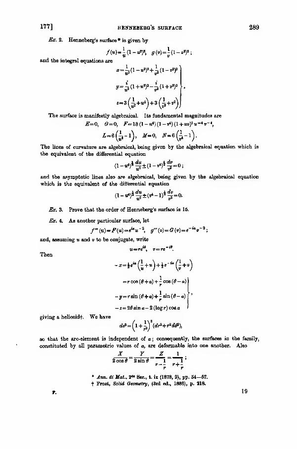
177] HENNEBERGS SURFACE 289
Ex. 2. Henneberg's surface* is given by
/<«
and the integral equations are
/M=ia-«8)2, g{v)=\(\-v*f;
*=I(1 -»*)*+ J(l_„»)3
,=3(I2+^) + 3 (I2+^)
The surface is manifestly algebraical. Its fundamental magnitudes are
E=0, G=0, F=l8(l-u*)(l-Vi)(l+uv)i 'u-*v- 1,
X=6(I4-l), M-0, *-e@-i).
The lines of curvature are algebraical, being given by the algebraical equation which is
the equivalent of the differential equation
and the asymptotic lines also are algebraical, being given by the algebraical equation
which is the equivalent of the differential equation
(i-^$±(^-«»*-a
Ex. 3. Prove that the order of Henneberg's surface is 15.
Ex. 4. As another particular surface, let
/'"(«)=/'(M)=«ia«- 2,
g"'(v)=0(v)=e- iav-
and, assuming u and v to be conjugate, write
Then*-«*, v=re'a.
=rcos(0+a) + -cos(0— a)
giving a helicoidf. We have
-y=rsin(0+ a)+ -sin(0-a)
- z= 25 sin a - 2 (log r) cos a
<fo»= (l + ^Y(eZr>+rW),
>.
so that the arc-element is independent of a ; consequently, the surfaces in the family,
constituted by all parametric values of a, are deformable into one another. Also
X Y Z 1
2 cos 6 ~ 2 sin 6 ~ \~ 1'
r-- r-\—r r
* Ann. di Mat., 2"» Ser., t. ix (1878, 9), pp. 54—57.
t Frost, Solid Geometry, (3rd ed., 1886), p. 218.
F. 19
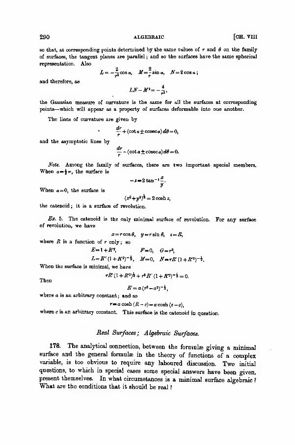
290 ALGEBRAIC [CH. VIII
so that, at corresponding points determined by the same values of r and 6 on the family
of surfaces, the tangent planes are parallel ; and so the surfaces have the same spherical
representation. Also
and therefore, as
2 2L=—scoso, J/=-sina, ^=2008(1;
LN-M*=-^,
the Gaussian measure of curvature is the same for all the surfaces at corresponding
points—which will appear as a property of surfaces deformable into one another.
The lines of curvature are given by
and the asymptotic lines by
drl-(cota±coseca)cW= 0,
(cota + coseca)d0=O.
Note. Among the family of surfaces, there are two important special members.
When a"\n, the surface is
-2=2tan-'-.y
When a=0, the surface is
(jp2+y2)4 = 2coshz,
the catenoid ; it is a surface of revolution.
Ex. 5. The catenoid is the only minimal surface of revolution. For any surface
of revolution, we have
x=rcos6, y= rsm6, z=R,
where R is a function of r only; so
£=l+R'*, F=0, G=r>,
L=R"(l+R'*)-t, M=0, N=rR (1 +#*)-*.
When the surface is minimal, we have
rR' (1 + R'i)h + r2R" (1 + Ri)~l = 0.Then
R'=a(rt-a?)-h,
where a is an arbitrary constant ; and so
r=ocosh(7J-c)=acosh(z-c),
where c is an arbitrary constant. This surface is the catenoid in question.
Real Surfaces; Algebraic Surfaces.
178. The analytical connection, between the formulae giving a minimalsurface and the general formulae in the theory of functions of a complexvariable, is too obvious to require any laboured discussion. Two initial
questions, to which in special cases some special answers have been given,present themselves. In what circumstances is a minimal surface algebraic ?
What are the conditions that it should be real ?
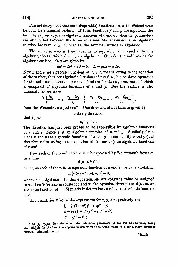
178] MINIMAL SURFACES 291
Two arbitrary (and therefore disposable) functions occur in Weierstrass's
formulae for a minimal surface. If these functions f and g are algebraic, the
formulae express x,y,z as algebraic functions of u and v ; when the parameters
are eliminated between the three equations, the eliminant is an algebraic
relation between x, y, z; that is, the minimal surface is algebraic.
The converse also is true; that is to say, when a minimal surface is
algebraic, the functions / and g are algebraic. Consider the nul lines on the
algebraic surface ; they are given by
da? + dyi + dz* = 0, dz =pdx + qdy.
Now p and q are algebraic functions of x, y, z, that is, owing to the equation
of the surface, they are algebraic functions of x and y ; hence these equations
for the nul lines determine two sets of values for dx : dy : dz, each of which
is composed of algebraic functions of x and y. But the surface is also
minimal; so we have
x1 + iy1 _ x1- iy} ^ 1 xa
- ty, _ x3 + iy, _l*"~ U. ' —
]— Vf —
y
.*! Zy U Zi Za V
from the Weierstrass equations* One direction of nul lines is given by
Xjdu : y-idu : zx du,
that is, bys, : y, : *,.
The direction has just been proved to be expressible by algebraic functions
of x and y ; hence u is an algebraic function of x and y. Similarly for v.
Thus u and v are algebraic functions of x and y ; consequently x and y (and
therefore z also, owing to the equation of the surface) are algebraic functions
of u and v.
Now each of the coordinates x, y, z is expressed, by Weierstrass's formulap
in a form
hence, as each of them is an algebraic function of u and v, we have a relation
A{6(u) + ^(v), u, v}=0,
where A is algebraic. In this equation, let any constant value be assigned
to v ; then ^ (v) also is constant ; and so the equation determines (u) as an
algebraic function of u. Similarly it determines ^ (v) as an algebraic function
of v.
The quantities 6 (u) in the expressions for x, y, z respectively are
£= Hi -*)/" + "/'-/>
V = li(l+u>)f"-iuf' + if,
* As (£i + tyi)/'i has the same value whatever parameter of the nul line is need, being
(dx + idy)jdz for the line, the expression determines the aotual value of u for a given minimal
surface. Similarly for v.
19—2
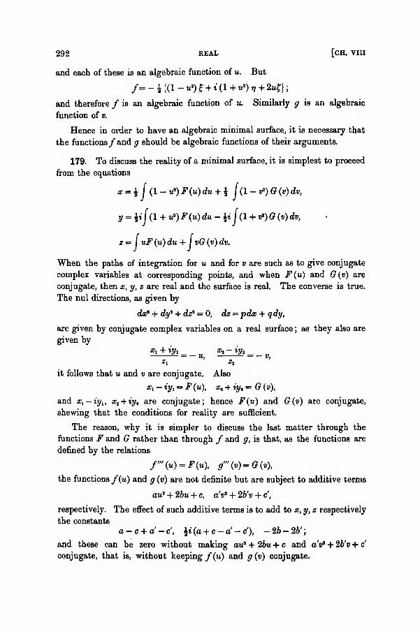
292 REAL [CH. VIII
and each of these is an algebraic function of u. But
/=-i;(l- W»)f + i(l+«a)i7+2Mf};
and therefore / is an algebraic function of u. Similarly g is an algebraic
function of v.
Hence in order to have an algebraic minimal surface, it is necessary that
the functions/and g should be algebraic functions of their arguments.
179. To discuss the reality of a minimal surface, it is simplest to proceed
from the equations
x = % j (l-u*)F(u)du + $ ((l-r?)G(v)dv,
y = bif(l + u*)F(u)du - fr f(l + &)G(v)dv,
z = I uF(u) du+ I vG (v) dv.
When the paths of integration for u and for v are such as to give conjugate
complex variables at corresponding points, and when F(u) and G(v) are
conjugate, then x, y, z are real and the surface is real. The converse is true.
The nul directions, as given by
dxa + dy' + dz' = 0, dz = pdx + qdy,
are given by conjugate complex variables on a real surface; as they also are
given byx1 + iy
} _ x, - iy, _
it follows that u and v are conjugate. Also
«i - iyi = F (w), x2 + iy2 = G (v),
and xl—iy
x , xi -\-iyi are conjugate; hence F(u) and G(v) are conjugate,
shewing that the conditions for reality are sufficient.
The reason, why it is simpler to discuss the last matter through the
functions F and G rather than through / and g, is that, as the functions are
defined by the relations
f'"(u) = F{u), g'"(v) = G(v),
the functions /(w) and g (v) are not definite but are subject to additive terms
au1 + 2bu + c, aV + 2b'v + c',
respectively. The effect of such additive terms is to add to x, y, z respectively
the constants
a — c + a'-c', ^i(a + c-a'-c'), -26-26';
and these can be zero without making av? + 26u + c and aV + 26'« + c'
conjugate, that is, without keeping f(u) and g (v) conjugate.
180] MINIMAL SURFACES 293
180. It is clear that, when functions F(u) and G(v) are given, the
values of x, y, z are determinate and unique save as to additive arbitrary
constants that arise in the quadratures; hence given functions F and
determine a minimal surface uniquely save as to its position in space.
It is not, however, the fact that a minimal surface leads to a unique
determination of functions F(u) and G(v), in connection with nul lines as
parametric curves. The quantities u and v are determined as a pair of
magnitudes, being the joint parameters of the nul lines. Accordingly, let
•«' and v' be another pair of magnitudes as parameters of nul lines, and let
A (u') and B {v') be the corresponding functions in the expressions for x, y, z.
Then we have two cases :—(i) when u is a function of u, and v' is a function
of v;
(ii) when u' is a function of v, and v' is a function of u.
In the former case, we have
(1 - «!
)F (u) du = (1 - u") A (v!) du', {l-v>)G (v) dv = (l- v'*) B (v) dv',
(1 + u>)F (u) du = (1 + m'2)A (u') du', (1 + vs
) G (v) dv = (1 + 1>") B (i/) dv',
uF(u) du = u'A («') du', vG (y) dv= v'B (v') dv' ;
and these relations can only be satisfied if
u = u', F(u) = A(u), v = v', G(v>= B (»')•
No new expressions for x, y, z are given in this case.
In the latter case, we have
(l-u*)F(u)du= (l-v'*)B(v')dv, (1 - V) G (v) dv = (1 -u'*)A (u')du',
( 1 + «») F(u) du = -(l + v'*) B (v) dv', (1 + «') G (v) dv = - (1 + u") A (u') du,
uF (u) du = v'B (v) dv, vG(v)dv = u'A («') du';
and these relations can only be satisfied if
uv' = -l, F(u) = -v"B{v), u'v = -l, G(v) = -u'A(u').
When the surfaces are real, F and G are conjugate, and A and B are
conjugate; and
A(u') = -±G(v)
~i*(-7)-
Thus there are two forms of function, F (u) with its conjugate, and
__ Q (- -\ with its conjugate, for the expressions of x, y, z as a point on au'* \ uj
given real minimal surface.
294 DOUBLE [CH. VIII
Consider, further, this double analytical representation of a real minimal
surface. The direction-cosines of the normal in the first representation are
given by_ u +v „ . v — u „ uv — 1JL — z - I = l: , ill = z ;
1 + uv'
1 + uv 1 + uv
and in the second representation the direction-cosines of the normal are
given by
_, u +v' „, v'-u' _, u'v' - 1
1 + u v 1+ uv 1 + u v
Butuv' = — 1, u'v = — 1
;
henceX' = -X, Y' = -Y, Z' = -Z.
Consequently, the normals are in opposite directions in the two repre-
sentations.
Double Surfaces.
181. One interesting set of surfaces arises when the functions in the
expressions for a real minimal surface are such that
j.(O-l0(-J), G{t) = -l F (-]),
being of course only a single relation. The first representation then gives
tdx= (l-u>)F(u)du+ (l-v*)G(v)dv\
Idy = i (1 + u*) F(u)du-i(l+ «') (v) dv
dz = uF(u) du + vO (v) dv
The second representation then gives
Idx = (1 - it'*) A (u') du + (1 - v'a) B (»') dv
= (1 - «'»)F (w') du + (1 - v'*) G (v') dv',
and similarly for the others ; that is, the second representation gives
Mx= (l-u'i)F(u')du'+ (1 - v'*) G (v) dv'
2dy = t (1 + u") F(u') du' - i (1 + v'3) G (v') dv'
dz = u'F(u) du + v'G{v) dv' J
Now1 , 1u = --, v =--;v u
and therefore the surface, in the vicinity of the point u, v, has exactly the
-(!-«'*)
181] MINIMAL SURFACES 295
same variations as in the vicinity of the point — , — . The values of theJ r v u
parameters at any point are determinate functions of the position of the
point ; hence, when the integration for x, y, z is effected, either
(i) the values of x, y, z in the first representation differ from those in the
second by constants ; or
(ii) the values of x, y, z in the first representation are the same as those
in the second.
In the first case, a suitable bodily translation (determined by the constants)
will make the two sets of values of x, y, z the same ; that is to say, a suitable
translation of the surface will bring the part of the surface in the vicinity of
the point u, v to coincide with the part of the surface in the vicinity of the
point— , — . Such a surface is periodic and therefore not algebraical.
In the second case, the part of the surface in the vicinity of the point u, v
coincides (without any translation) with the part of the surface in the vicinity
of the point— , — . When the function F is algebraical, such a surface Fis algebraical.
Now the normals at these two different parametric points, which geo-
metrically coincide on the surface, lie in opposite senses on the same line.
Accordingly if we trace a path on the surface from the point u, v to the point
, — , we return to the same geometrical position on the surface while,
at the end of the path, the normal assumes a position directly opposite to its
initial position. Thus it is possible, without any breach of continuity, to
pass from any position to the same position as though the surface were
pierced at that place ; in other words, the surface has only one side*, instead
of the familiar two sides. The notion of these minimal surfaces is due to
Lief who called them double surfaces. The test that a surface should be
double is that, if F and G are conjugate functions in the quadrature
expressions for the coordinates of a point on a real minimal surface, the
relation
should be satisfied identically.
* The simplest example, in model form, of a one-sided surface occurs when a long rectangular
strip of paper ABCD (of which AC and BD are the diagonals) is twisted once, or an odd
number of times, and then joined into a twisted ring by making the edge AB coincide with the
edge CD so that A coincides with C and B with D.
t Math. Ann., t. xiv (1878), pp. 331—416 ; ib., t. xv (1879), pp. 465—506.
296 DOUBLE SURFACES [CH. VIII
182. Special examples of double surfaces can be obtained directly by
solving (either generally or specially) this functional equation. Let
PF(t) = <f>(t),
and let<f><,
be the function conjugate to<f> ; then the equation is
*<*)— *»(- J)-
A solution of this equation is given by
<f>(t) = ia,
where a is a real constant ; then
*<o-S.
and we have the helicoid (§ 177, Ex. 4), a periodic surface.
Another solution is given by
*(*)««(«+J).where a is a real constant ; then
and we have another periodic surface.
Another solution is given by
<*>(*) = « (<'-^)>
where a is a real constant ; then
F(t)-a(l-l),
and then we have Henneberg's algebraic surface (§177, Ex. 2).
The general solution is given by
4>(t) = ial>+ 2 cM+,((»+lei'»ti + f*-,ri»«)m=0
+ 2 Cw, (PV-s- - <-»"e-fa«m)I
m= l
where the quantities c and a are real.
183. We have already (§ 59) dealt with Lie's method of generating
minimal surfaces by taking them as the locus of the middle point of the
chord joining any point on one nul line in space to any point on another nul
line in space. This method of generation (which really is an interpretation
of the Monge formulae and the Weierstrass formulae) is the foundation of Lie's
researches on minimal surfaces.
184] DEFORMATION OF MINIMAL SURFACES 297
When the nul lines are one and the same, the chord comes to be a chord
joining any two points on the nul line in space ; the locus of its middle point
still is a minimal surface ; and it is the fact that this minimal surface is a
one-sided or double surface. The proof of this theorem, which is due to
Lie, is left as an exercise.
Deformation of minimal surfaces.
184. The general discussion of the deformation of surfaces has been
reserved for a separate chapter. But the deformation of minimal surfaces,
limited by the restriction that the surface is to remain minimal, is so
particular that it may fitly be discussed here, especially as the detailed
results lead to other issues.
Accordingly, let a minimal surface be deformed without stretching or
tearing so as to remain minimal if that be possible. The arc-element must
remain unaltered ; and therefore, if m, and vt be the parameters of the nul
lines in any deformed configuration, we must have
(1 + uvf FGdvdv = (1 + «!«,)» F&diiidih,
where F and G are the functions in the Weierstrass equations, being func-
tions of u alone and v alone, respectively, and likewise for Fj and Gi with
regard to w, and », respectively. Now
and therefore
, 3m, , du, , , dv, . dv, ,du, =— du + -=— dv, dv1
= -=- du + -=-* dv;tiu dv du dv
du du'
3u 3w
Hence either u, is a function of u only and v, is a function of v only, or u^ is a
function of v only and v, is a function of u only. The alternatives are
effectively the same ; so we take
Ul = \ (u) = \, v1= /i (v) = m,
and then
(1 + mi;)2 FG = (1 + XM)
S F&X'/j.'.
32
Taking logarithms of both sides and then operating with =—=- , we find
i xy(i + uvy (i + Xfiy
that is,
dudv _ du^dvj
(1 + uvf (1 + u^y"
Hence the arc-elements in the spherical representations of the minimal
surface in its different stages are the same ; and so the spherical representa-
tions either are equal to one another or are symmetrical. But the deformation
is continuous and the spherical representations begin by being the same;
298 ASSOCIATED SURFACES [CH. VIII
hence the spherical representation at any stage is equal to the initial
spherical representation. Consequently, choosing an appropriate location of
the two forms of the minimal surface, we have
X, = X, ¥,= 7, Z^Z,that is,
m, = u, v, = v.
ThenFG = FXG,.
Now F and Fx are functions of u alone, while and (?, are functions of v
alone ; hence
F-a = tt = constant = e*",t (jTi
say, where at is any constant ; that is,
Fj = Feu , 0, = Ge-»
Minimal surfaces thus determined are called surfaces associated with the
minimal surface; and so we have Bonnet's theorem that the only minimal
surfaces, which can be deformed into a given minimal surface, are its
associated surfaces.
185. Among the associates of a minimal surface, there is one of special
importance. It is given by taking a = \ ir, so that
F, = iF, Gt= -iG;
and it is called the adjoint surface (sometimes Bonnet's adjoint surface).
Let x, y , z„ be the point on it which corresponds to the point x, y, z on the
original minimal surface ; then, writing
x = A(u) + A'(v), y = B(u) + B'(v), z = (u) + C (v),
we have
xt =iA{v)-iA'(v), y = iB(u)-iB'(v), zc - iC (u) - iC (v).
When the original minimal surface is real, the adjoint surface is real.
The two surfaces are algebraical together. And the same holds for every
associate of a minimal surface.
The adjoint of the adjoint is not the original minimal surface; it is
symmetrical with that original through the origin of coordinates.
The adjoint surface is not definite in position. For we can write A (u) + a
and A'(v) — a in place of A (u) and A'(v), without altering the original
surface ; but the effect is to add a term 2t'a to x . Similarly for y„ and z„.
And the same holds for every associate.
We have
x — ixt = 2A (w), y—iy = 2B (u), z-iz = 20 («),
x + ix = 2A'(v), y + iy, = 2B'(v), z + it, = 2(7' (v) ;
185] ADJOINT MINIMAL SURFACES 299
and therefore, if f, 17, f are the coordinates of the point which, on the associate
determined by a, corresponds to x, y, z, we have
= x cos a + x sin a
77 = y cos a + y sin a
£= .z cos a + z„ sin a
Again, we have
da; = %Xidu — ixtdv.
But (§ 27) we have, in general,
Yzx - Zy, = (x2E - x,F) V~\ Yzt- Zyt
= (xaF- x,0) F"1
;
and therefore, in the present case, as E = 0, G = 0, V = iF,
Yzl— Zyl
= ix1 , Yza—Zyi = — ixa .
Consequently
dx = ( Yzj — Zyx) du + ( Yz2— Zya) dv
= Ydz-Zdy,
and similarly for the others ; that is, we have
dx = Ydz — Zdy \
dy = Zdx — Xdz> •
dzt= Xdy — Ydx)
These results are due to Schwarz; and they again shew that the adjoint
surface, being obtainable through quadratures, is not definite in position.
Further, we have
dx„ _ . dx„ _ .
du'**1' dv'
1*"
and similarly for the other coordinates ; hence the direction-cosines of the
normal to the adjoint surface are the same as those of the normal to the
original surface, that is, the tangent planes to the two surfaces are parallel.
Alsodxdx,, + dydy„ + dzdz„ = 0,
on substituting the values of dx , dy , dz ; that is, corresponding curves on a
minimal surface and its adjoint are perpendicular to one another at corre-
sponding points.
The first of these results (but not the second) holds for any associate
surface. For
W u dA » 3? -u dA ' -»du~
6du~ Xl6
' dv~e
dv~ XlC
•
and similarly for the other coordinates; thus the direction-cosines of the

300 MINIMAL SURFACES UNDER [CH. VIII
normal to the associate are the same as for the original minimal surface,
and so the tangent planes are parallel. But
dxdl; + dydr) + dzd£= (Stic2) cos a + (IdxdxJ) sin a
= ds* cos a,
which vanishes only if o = %tt ; and
dx dl- + dy9dr) + dz„d%= ds<? sin a
= ds* sin a,
which vanishes only if a is or tr.
The lines of curvature on the original minimal surface are
Fdu"-Odv'=0
(F and being the functions in Weierstrass's expressions), and its asymptotic
lines are
Fdu*+Odif-0.
On the adjoint surface the lines of curvature are
iFdu' - (- iG) dif = 0,
which therefore correspond to the asymptotic lines of the original ; and the
asymptotic lines are
iFdu*-iGdvl = 0,
which therefore correspond to the lines of curvature of the original. And so
for other properties.
Minimal surfaces under assigned conditions.
186. The special results just proved and due to Schwarz, which relate to
the adjoint surface and determine it by a process of quadrature, have been
applied by him to a problem of greater importance in the theory of minimal
surfaces.
From any of the integral equations of a minimal surface, it appears that
they contain a couple of arbitrary functions in their expression ; and it is
natural to consider alike the character and the extent of the conditions which
the functions can help to satisfy. On the other hand, we know that the
differential equation of minimal surfaces is substantially a partial differential
equation of the second order, whether it occurs in the intrinsic form
EN-2FM+GL = 0,
or in the explicit form
(1 + q')r - 2pqs + (1 +f)t = 0,
with the customary notation.
187] ASSIGNED CONDITIONS 301
Now as regards such partial equations of the second order, the funda-
mental existence-theorem* (due to Cauchy) establishes the result that a
unique uniform integral z of the partial equation exists which is determined
by the conditions :
—
(i) that, along any assigned curve (not being one of the 'characteristic'
curves), the quantity z assumes an assigned value, and
(ii) that, along the same assigned curve, one of the derivatives of z
assumes an assigned value.
In the case of the partial equation for minimal surfaces, the characteristic
curves are given by
(1 + q') dy"+ 2pqdxdy + (1 +p1) da? = 0,
that is, bydo? + dy1 + dz* = 0,
which are the nul lines on the surface. Therefore, in applying Cauchy's
theorem, it is necessary to exclude the nul lines from the curves along which
external conditions can be assigned Further, along any non-excluded curve
the value of z is given, as also is that of one of its derivatives, say p ; thus, as
we everywhere havedz = pdx + qdy,
and as we are given z and p along the curve, we know q also ; that is, we
know p and q along the curve. Now at any point on the surface, the
quantities p and q determine the direction-cosines of the normal to the
surface, and therefore determine the tangent plane. We therefore can
restate Cauchy's general theorem for partial equations of the second order,
when it is applied to the equation of minimal surfaces, as follows :
—
A minimal surface is uniquely determinate by the condition that it passes
through an assigned curve and that, along the curve, it touches an assigned
developable surface through the curve, provided the curve is not a nul line upon
the surface.
To have the surface explicitly determinate, it is necessary to find the
forms of the arbitrary functions which shall satisfy the assigned conditions
;
for that end, Schwarz's results can be used.
187. Without entering into all the cases, let us assume that the assigned
curve is such that, along its range, the coordinates of a point x, y, z and the
direction-cosines X, Y, Z of the tangent plane to the assigned developable
surface, can be expressed in terms of a current parameter. We have :
x — ix — 2A, x + ix = 2A',
* See the author's Theory of Differential Equation*, vol. vi, chaps, zii, xx.
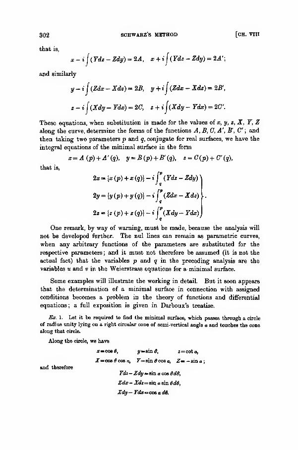
302 SCHWARZ'S METHOD [CH. VIII
that is,
x - i [(Ydz - Zdy) = 24, x + if(Ydz - Zdy) = 2A'\
and similarly
y-if (Zdx - Xdz) =25, y + ij(Zdx - Xdz) = 2B',
z - i f(Xdy- Ydx) = 2C, z + iUxdy - Ydx) = 2C.
These equations, when substitution is made for the values of x, y, z, X, Y, Zalong the curve, determine the forms of the functions A,B,C,A', B, C ; and
then taking two parameters p and q, conjugate for real surfaces, we have the
integral equations of the minimal surface in the form
x-A(p) + A'(q), y = B(p)+ B'(q), z = C(p)+ G'(q),
that is,
2x= [x (/>) + x (q)} -ijP
( Ydz - Zdy) 'k
J q
2y = {y (p) + y (?)} - » ("(Zdx - Xdz)
2z = [z (p) + z (g)} - i (\xdy - Ydx)
One remark, by way of warning, must be made, because the analysis will
not be developed further. The nul lines can remain as parametric curves,
when any arbitrary functions of the parameters are substituted for the
respective parameters ; and it must not therefore be assumed (it is not the
actual fact) that the variables p and q in the preceding analysis are the
variables u and v in the Weierstrass equations for a minimal surface.
Some examples will illustrate the working in detail. But it soon appears
that the determination of a minimal surface in connection with assigned
conditions becomes a problem in the theory of functions and differential
equations ; a full exposition is given in Darboux's treatise.
Ex. 1. Let it be required to find the minimal surface, which passes through a circle
of radius unity lying on a right circular cone of semi-vertical angle a and touches the cone
along that circle.
Along the circle, we have
x=cob6, y = 8in#, 2=cota,
J = cos5cosa, Y= sin $ cos a, Z=>— sin a;
and therefore
Ydz - Zdy= sin a cos 6d8,
Zdx- Xdz = sin a sin 6d6,
Xdy— r<£r«=cos a d6.
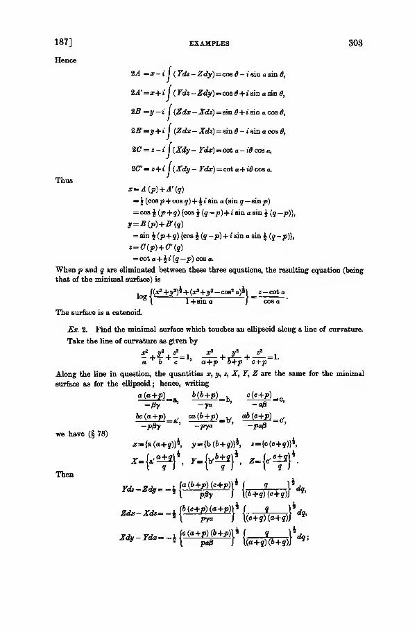
187]
Hence
EXAMPLES 303
2A =x - i
2A'=x+i
%B=y-
2B'=y+ i
2C = z-i
2C'=z+ i
Thus
i I(Tdz - Zdy)= cos 8 - i sin a sin 8,
iJ(Fdz - Zdy)=cos 8 + i sin a am 8,
i I (Zdx — Xdz) = sin 6 + i si n a cos 8,
iJ(^cte — Xdz)= sin — i sin a cos 8,
i I (Xdy— Ydx)=col a - J# cos a,
iJ(Xdy - Ydx)= cot a+ iO cos a.
*-4 0»)+J'(?)
= \ (cos p+cos y)+ Jisin a (sin q — sin jd)
= cos \ (p +q) {cos £ (g -/>)+i sin a sin J (j -p)},
y=B(p)+B(q)
= ain$(p+ q){coa$(q-p)+ isin a sin J (q-p)},
z=C(p)+ C'(q)
= cot a+^ i (g —p) cos a.
When jo and q are eliminated between these three equations, the resulting equation (being
that of the minimal surface) is
. f(x*+y8)*+ (a?+y*- cos8 o)h _ z-cota
I 1+sina )~ cos a
The surface is a cateuoid.
Ex. 2. Find the minimal surface which touches an ellipsoid along a line of curvature.
Take the line of curvature as given by
a b c ' a+p b+p c+p
Along the line in question, the quantities x, y, z, X, T, Z are the same for the minimal
surface as for the ellipsoid; hence, writing
o(o+p) b(b+p) c(c+p)_-/3y ^ -ya -a/3
bc(a+p)^_ , ca(b+p)
^_v db(c+p)^ c,
—pfly " ' -py°- ' -jPa/8
*={a(a+j)}4, y={° (&+?)}*> *={c(c+s#,
x.{,°_±i}', r-^}1, z.f.£±J}
4.
we have (§ 78)
Then
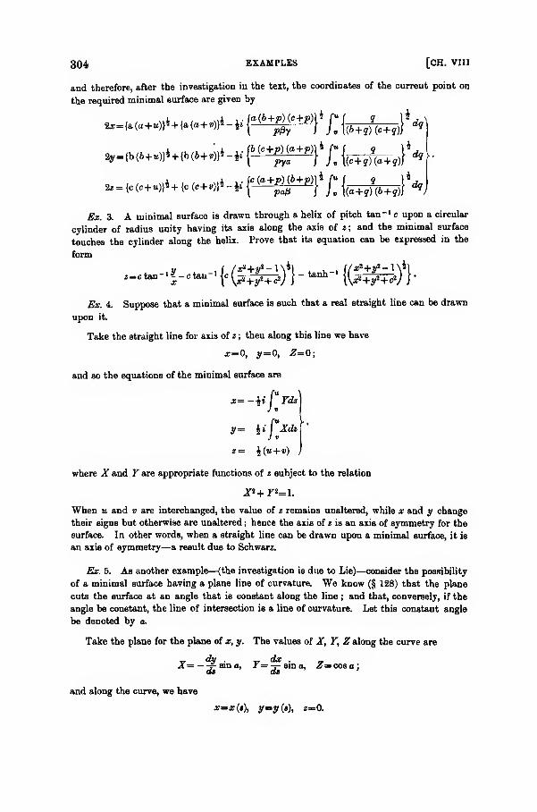
>
304 EXAMPLES [CH. VIII
and therefore, after the investigation in the text, the coordinates of the current point on
the required minimal surface are given by
».iM.»)iuWMli-li(»^) ,
|;js t,)f*
Ex. 3. A minimal surface is drawn through a helix of pitch tan -1 c upon a circular
cylinder of radius unity having its axis along the axis of i; and the minimal surface
touches the cylinder along the helix. Prove that its equation can be expressed in the
form
Ex. 4. Suppose that a minimal surface is such that a real straight line can be drawn
upon it.
Take the straight line for axis of z ; then along this line we have
x=0, y= 0, Z=0;
and so the equations of the minimal surface are
y= J* I Xdzl
z = i(u+v) j
where X and T are appropriate functions of z subject to the relation
When u and v are interchanged, the value of z remains unaltered, while x and y change
their signs but otherwise are unaltered ; hence the axis of z is an axis of symmetry for the
surface. In other words, when a straight line can be drawn upon a minimal surface, it is
an axis of symmetry—a result due to Schwarz.
Ex. 5. As another example—(the investigation is due to Lie)—consider the possibility
of a minimal surface having a plane line of curvature. We know (§ 128) that the plane
cuts the surface at an angle that is constant along the line ; and that, conversely, if the
angle be constant, the line of intersection is a line of curvature. Let this constant angle
be denoted by a.
Take the plane for the plane of x, y. The values of X, Y, Z along the curve are
_. dy . _ dx . _X=— -j-sma, l=j-ama, Z^cosa;
and along the curve, we have
Ydz\
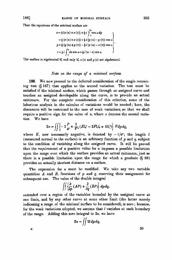
188] RANGE OF MINIMAL SURFACE 305
Then the equations of the minimal surface are
[v.
x=lt{x(u)+x(v)}+ ^i I cosady \
J V
=i{% (»)+* (»)} +ii {y (») -y (»)} cos a
y ,
y=$ {y (u)+y (v)} - $i{x (11) -x(v)} con a
z= \i I dsama=^i(u — v)sina
The surface is algebraical if, and only if, x (*) and y (*) are algebraical.
Note on the- range of a minimal surface.
188. We now proceed to the deferred consideration of the single remain-
ing test (§ 167) that applies to the second variation. The test must be
satisfied if the minimal surface, which passes through an assigned curve and
touches an assigned developable along the curve, is to provide an actual
minimum. For the complete consideration of this criterion, some of the
laborious analysis in the calculus of variations would be needed; here, the
discussion will be restricted to the case of weak variations, so that we shall
require a positive sign for the value of u, where u denotes the second varia-
tion. We have
2u =lj
j- 2 £ + ^ {El? - tFkk + GlA Vdpdq,
where K, now necessarily negative, is denoted by — l/aa ; the length I
(measured normal to the surface) is an arbitrary function of p and q, subject
to the condition of vanishing along the assigned curve. It will be proved
that the requirement of a positive value for u imposes a possible limitation
upon the range over which the surface provides an actual minimum, just as
there is a possible limitation upon the range for which a geodesic (§ 89)
provides an actually shortest distance on a surface.
The expression for u must be modified. We take any two variable
quantities A and B, functions of p and q, reserving their assignment for
subsequent use. The value of the double integral
I\{l-P{AP) +
Iq{m
)dp(k '
extended over a region of the variables bounded by the assigned curve at
one limit, and by any other curve at some other limit (the latter merely
indicating a range of the minimal surface to be considered), is zero ; because,
for the weak variations adopted, we assume that I vanishes at each boundary
of the range. Adding this zero integral to 2m, we have
=11 Vdpdq,2u--
v. 20
306 RANGE OF A [CH. VIII
where
U = y (Elf - ZFkh + Glf) + V (A, + B, - 2 ?) + 2AO, + 2BU2 ;
and U is expressible in the form
"=-^Hi-M- 24-K')(i-x') + "('-^y}'
provided the quantities X, A, B satisfy the relations
. FXz G X,
**' V\ + V\'
A _i_ R 9 ^ 9 '^I
V EXf aFX.X,,GV
a2
Obviously .4 and 5 can be regarded as known, when X is known. Eliminating
A and B between the three relations, we have the equation for X in the
form
d (F\, G\\ 3/ E\, F\,\ a V E\f a F\1Xi GVty\V\~V\) + &l\V\ + V\)~a*-V\° *V X*
~t"FX2 '
that is,
EX* - 2F\2 + G\n - (ST" - 2FT' + GT) X,
- (EA" - 2FA' + GA)\ + 2 ^ X = 0,
a partial differential equation of the second order.
The characteristics for the solution of this equation are
Edp* + 2Fdpdq + Gdq* = 0,
that is, are the nul lines of the surface, neither of which (§ 186) can be an
assigned boundary of the surface. Hence, by Cauchy's theorem already
quoted (§ 186), a unique regular integral of this equation exists, satisfying
the conditions :
—
(i) the magnitude \ shall, like I, vanish along the assigned curve
through which the minimal surface must pass
;
(ii) along the assigned curve, X, and X, shall differ from ^ and Za
respectively by relatively infinitesimal quantities.
When X is thus determined, the equation X = % (p, q), for parametric values
of X, gives curves on the surface, one of them coinciding with the assigned
curve when X = 0.
The subject U, in the modified integration for the second variation, is
everywhere positive for real surfaces, because
E>0, G>0, V>0,
188] MINIMAL SURFACE 307
unless it should happen that the quantities
I -hit / _ *a/
could vanish together, that is, unless the relation
l = cX
(where c is a pure constant) could hold, for variations I over the considered
range of the surface. The relation holds at the initial stage of the range,
because both I and X vanish there. If, therefore, after the initial stage,
X could again vanish either at or before the final stage, the relation could
hold over the whole considered range of the surface. The second variation
then would be zero, for an assumed choice I = cX ; disregarding variations
of higher orders, we could not declare that the included range of the minimalsurface provides an actual minimum area.
Accordingly, we trace upon the surface the family of curves
for parametric values of X; we call the assigned curve, given by \ = at the
boundary of the integral, the initial curve. As \ varies, positively and
negatively, it may again assume a zero value upon the surface ; we call the
curves, nearest to the initial curve in either sense along the surface, conjugate
to the initial curve. We therefore infer the result :
—
In order that an actual minimum area may be provided by a minimal
surface, which is required to pass through an assigned curve and to touch an
assigned developable along the curve, the range of the surface must not extend
sofar as the conjugate (if any) of the assigned curve on the surface.
It follows therefore that the range of a minimal surface must not extend
so far as the conjugate of any curve upon it, if the area of the surface is to be
an actual minimum for small variations. If only the descriptive property
—
that the mean curvature is zero—is required, it would be possessed by the
surface over its whole extent ; just as in the case of geodesies, the geodesic
property—that its principal normal is the normal to its surface—is possessed
along its whole course without any reference to conjugate points.
The more detailed consideration of the conjugate of any curve on a
minimal surface belongs to the region of the calculus of variations.
EXAMPLES.
1. Shew that the surface
cos ay
is minimal ; that it is the locus of the middle point of a chord joining any two points ona particular nul curve in space ; and that it is the only minimal surface such that
*= /(#) +#(#)•
20—2
308 EXAMPLES [CH. VIII
Obtain the equation of the adjoint surface in the form
si n az = sinh ax sinh ay.
2. Two surfaces can be deformed into one another, and their tangent planes at
corresponding points are parallel ; shew that they are associated minimal surfaces.
3. Two surfaces can be deformed into one another and corresponding arc-elements
are inclined to one another at a constant angle ; shew that they are associated minimal
surfaces.
4. Shew that for a minimal surface, given by the equations
2£(l-c2)*= c(0+</>) + sin0+sinc£ \
2y (1 - c2)4 = i {6- <j>+c (sin 6 - sin<f>)}
Y,
2z= -costf— cos<f> J
the lines of curvature become two families of circles in the spherical representation.
5. In Weierstrass's equations for a minimal surface, take
F(u)=auk, G(v)= a'ifi,
where k is a real constant, while a and a' are conjugate constants ; shew that the surface
can be deformed into a surface of revolution.
6. A minimal surface possesses a plane geodesic ; shew that the plane of the geodesic
is a plane of symmetry for the surface.
7. A minimal surface (Catalan's) is given by the equations
x=am2 u+sm2 v,
y= 2i (sin u — sin v),
2z=2M+sin2tt+ 2tf+8in 2v;
shew that it contains one geodesic which is a parabola, and another which is a cycloid.
8. Shew that the (Henry Smith) surface
z(a?+y*)=a;2has only one side.
9. In Weierstrass's equations for a minimal surface, take
™=(H*(H'i.where is an odd integer ; shew that the minimal surface is a " double " surface.
10. Given two associated minimal surfaces ; shew that the lines of curvature oneither of them correspond to isogonal trajectories of the lines of curvature on the other.
11. On two adjoint surfaces, corresponding geodesies are drawn; shew that thecircular curvature of one at any point is equal to the torsion of the other at thecorresponding point.
CHAPTER IX.
Surfaces with Plane oe Spherical Lines of Curvature;Weingarten Surfaces.
The present chapter is devoted to some special classes of surfaces, other than minimal
surfaces. The vast variety of modern investigations leads to an extraordinary amountof detailed result. Here, we shall deal with only some of the principal classes of such
surfaces.
Liouville surfaces have already been discussed, from the point of view of their most
important property—that they can be geodesically represented upon one another, and
that (for the explicit equation of their geodesies) they admit quadratic integrals of the
critical equation of geodesies (§ 157).
Reference (to the extent of constructing the essential partial differential equation of
the second order which serves for their construction) has also been made to surfaces
having a constant measure of curvature—whether the Gauss measure, or the meanmeasure (§§ 54, 57).
We have also dealt, briefly, with surfaces which possess lines of curvature of the
isometric type (§ 64). They will occur, later, under the discussion of triply orthogonal
systems of surfaces in space.
Thus, for various reasons, a selection of two special systems of surfaces is made for the
present chapter.
One of these systems is characterised by the property that the lines of curvature (in
either or in both the sets) are composed of plane curves or of curves that lie upon a
sphere. The special restriction to plane curves or to spherical curves is due to a
theorem of Joachimsthal's (§ 128) which facilitates the construction of integral equations
of the surfaces. The subject has been the cause of many investigations in the past
;
special note should be made of the memoirs by Serret*, Cayleyt, RouquetJ, of portions
of Darboux's treatise§, and of Bianchi's treatise||. The literature of this part of the
subject is so great that no attempt at a comprehensive bibliography can here be made
;
many references will be found in the authors just quoted.
* Liouville's Journal, t. xviii (1853), pp. 113—162.
+ Coll. Math. Papers, vol. xii, pp. 601—638.
t Mint, de VAc. des Sciences, Toulouse, 8* Ser., t. ix (1887), t. x (1888).
§ Vol. i, pp. 114—118 ; vol. iv, pp. 198—266.
IIVol. ii, chap. xxi.
310 SURFACES WITH PLANE OR SPHERICAL [CH. IX
The other of the systems of surfaces is characterised by the property that a functional
relation—as arbitrary as can be chosen—exists between the principal radii of curvature.
Such surfaces are called Weingarten surfaces ; special instances, such as those which have
one or other of the measures of curvature equal to a constant, are already known;the
more general investigation of such surfaces is due to Weingarten, to whose memoirs (as
to other investigations) detailed reference is given in Darboux's sections dealing with the
subject*.
Surfaces with Plane or Spherical Lines of Curvature.
189. We have seen (§ 129) that, if a line of curvature on a surface is a
plane curve, the plane cuts the surface at a constant angle ; and that, if a
line of curvature is a spherical curve (that is, if it lies on a sphere), the
sphere and the surface cut at a constant angle; the two results being
connected with one another owing to the property (§ 79) that inversion
conserves lines of curvature. In each case, the constancy of the angle is
maintained along the particular line of curvature. When there is a family
of plane lines, or when there is a family of spherical lines, the angle that is
constant along any one line can (and usually does) vary from one line to
another. The simplest illustration is provided by surfaces of revolution.
The property, originally discovered by Joachimsthal, can be used to
obtain a first integral of some associated differential equations of the surface
;
and the two cases—according as the lines of curvature are plane or are
spherical—can be treated together analytically.
Let an equation
k (a? + y2 + zl
) = 2 {ax + by + cz + u)
be taken; it represents a sphere if k=l, and a plane if A = 0. It is to be
the sphere or the plane, as the case may be, containing the line of curvature
;
and therefore the quantities a, b, c, u will be functions of one parameter,
which will be constant along the line and will vary from one line to another.
The property, that the sphere or the plane cuts the surface at a constant
angle, is analytically expressed by a relation
(kx-a)X + (ky-b)7+(kz-c)Z=l,
where I is constant along the line of curvature and usually varies from one
line to another ; that is, I also is a function of the parameter of the lines of
curvature in the family.
* See his treatise, vol. iii, Book vii, chape, vii, ix, x.
190] LINES OF CURVATURE 311
190. Before proceeding further with the discussion of the problem, wemay note one reason (chiefly of manipulative ease) why consideration is
restricted mainly to those classes of lines of curvature which are either plane
or spherical. It is not inconceivable that a family of lines of curvature
should be curves lying on a family of quadrics ; thus they might be helices
on a family of circular cylinders. The analysis, however, in all such cases
becomes more complicated ; for the first integral, similar to the Joachimsthal
property for planes and spheres, appears to be unobtainable.
To see the distinction between the cases, let the surface be referred to its
lines of curvature as parametric curves. We then have
F = 0, Jf = 0;
and then (§ 29)
EX^-Lxu EY^-Ly,, EZ^-Lz,,
QX2 = -Nxi7 GYt= -Ny% , OZt
= -Nz^.
Now suppose that the line of curvature, given by p = constant, lies upon a
surface
tf> (*. y, z, p) = 0.
The direction-cosines of the line at any point are proportional to x3 , yit z2 ;
so we have
i^dy-^+i 2*-
along the line, that is, we have
along the line. What is required, to secure some progress in the investigation,
is some less differentiated equivalent relation.
Let the surfaces <j> (x, y, z,p) = 0he& family of planes
ax + by + cz + u = 0,
where a, b, c, u are functions ofp only ; the foregoing equation is
aXt + bYv + cZ^O,
and therefore an integral is
aX + bY + oZ = l,
where I is a function ofp only. This gives Joachimsthal's theorem concerning
plane lines of curvature.
Next, let the surfaces<f>
(x, y, z, p) = be a family of spheres
a?+f+ «2 - 2aa; - Iby - 2cz - 2« = 0,

312 ASSIGNED FAMILIES OF [CH. IX
where again a, b, c, u are functions of p only ; the foregoing general equation
DGC0ID6S
Oc-a)X2 + (y-&)72 + (*-c)£s=0.
But we always have
Xxi + Yyz + Zz, = 0;hence
l{(x -a)X + (y-b)Y+ (z-c)Z}=0,
and therefore
(x - a) X + (y -b)Y + (z - c) Z = I,
where I is a function ofp only. This gives Joachimsthal's theorem concerning
spherical lines of curvature.
In each case, the surface of which the line in question is a line of
curvature, and the surface (plane or spherical) on which the line lies, cut
at an angle that is constant along the line. If there were the same integral
for any other surface, we should have
('8^i^»i(S8,+
(ss)
,+©r- ta-- rf'*
^y)by the relation
<f>(x, y, z, p) = ; but the plane and the sphere appear to be
the only surfaces which allow the integral.
It is conceivable that we could have an integral
where the factor|(^-J
+( 3 ) + (3 ) [
mav De capable of simplification
X -3- +Y Jf- + Z J?- = function ofp only,
equivalent to the general relation
X'te
+r*dy~
+ Z>Tz-°-
In that case, we must have
Y (&$ &$ 8ty \
* \teXi+
dx~dy~yi+
dxdzZV
+ Y(*+x+?*v+**-z)+ r\dxdy
X* +dy*
yi+dydz
ZV
Now this equation will be satisfied if a quantity p exists such that
da? dxdy dxdz"'
!91] LINES OF CURVATUKE 313
When the surfaces <j> (x, y, z,p) = are quadrics, say
aa?+ by* + cz* + 2fyz + 2gzx + 2hxy + 2lx + 2my + 2nz + u = 0,
where the coefficients are functions ofp alone, we have
a ~P> K g 1=0,
h, b-p, f
9> /> c-pso that p is a function of p only. In the case of a plane, the three equationsare evanescent, for p = 0. In the case of a sphere, we have
/-g = h = 0, a = b-c = p;
the three equations are satisfied identically. In other cases, the three
equations, combined with
Z 2 +F2 + Z2 = l,
determine X, Y, Z as functions of p alone. Thus
X, = 0, F2 = 0, Z2 = 0,
and so
Nx2 = 0, Ny2 = 0, Nz2 =0;
and therefore as we cannot have x2 , y2 , z2 all zero (for the surface would then
be a curve), we must haveiV = 0,
in addition to M =0. The Mainardi-Codazzi relations become
z2 = rz, o = r"z,
and we cannot now have L = ; hence T" = 0, that is, Gt- so that O is a
function of q only which can easily be made unity. Thus the arc is
dt? = dq' + Edp\
and the surface is developable; the lines of curvature, p = constant, are
geodesies and so are plane. There is no new case.
We thus, in the main, restrict ourselves for the present purpose to lines
of curvature that are plane or spherical.
191. Two remarks may be made in passing.
In the case of a developable surface (but not in the case of any other
ruled surface) one system of lines of curvature is made up of the generators,
all of which touch the edge of regression ; and the other system is made up
of their orthogonal trajectories, which are the superficial involutes of that
edge. A generator, however, does not lie in a definite plane; and so it is
simpler to consider developable surfaces apart.
Again, one system of lines of curvature may be circles. When a circle is
regarded as a plane curve, its plane is definite ; when it is regarded as a

314 PLANE OB SPHERICAL [CH. IX
spherical curve, its sphere may be indefinite. Accordingly, unless the family
of spheres is given, it is usually simpler to discuss circular lines of curvature
as plane curves than to discuss them as spherical curves.
>
Serret-Cayley Treatment of the Two Gases.
192. We now resume the analysis of § 189 ; and we assume that the
other system of lines of curvature also is composed of curves that are plane
or spherical. Let the family of surfaces, upon which they lie, be
*(«"- + y2 + z") - 2ttx - 2/3y - 2yz - 2v = 0,
where k is either or 1, and where a, yS, 7, v are functions of q alone ; then
we have(,cx-a)X+(Ky-^)Y+(KZ-y)Z=X,
where \ also is a function of q alone. Hence, for the whole surface, we have
the equations
= k(a? + y2 + z2
) - 2ax - 2by - 2cz - 2u \
1 = (kx-a)X + (ky-b)Y + (kz -c)Z
= ic(x2 + y2 + z2)- 2ax-2@y-2yz-2v
\ = (kx - a)X + (icy - 0)Y+(kz - 7) Z
1 = X s + F2 + Z*
= Xdx + Ydy + Zdz
where k and k are or 1 independently of one another, a, b, c, u, I are
functions of p alone, and a, $, 7, v, \ are functions of q alone. The first
five of these equations determine five of the quantities x, y, z, X, Y, Z, p, q
in terms of the other three, say X, Y, Z, p, q in terms of x, y, z. When the
values are substituted in the sixth and it is integrated—we shall prove that
the " condition of integrability "(§ 30) is satisfied—we have a new equation
I = 0, say ; we then have six equations and can regard them as determining
x, y, z, X, Y, Z in terms of p and q. We thus require this integrated
equation.
Let the direction-cosines of the two lines of curvature through a point
x, y, z on the surface be proportional to dx, dy, dz for the line along which pis constant, and to Sx, 8y, hz for the line along which q is constant. Then
(kx — a)dx + (ky — b)dy + (kz — c)dz = 0,
Xdx + Ydy + Zdz = 0,
and therefore
dx : dy : dz = kx — a,
X ,
ky-b,
Y .
kz — c
Z
193] LINES OF CURVATURE 315
Similarly
Sx : Sy : 8z = II kx — a, Ky — 0, xz — y t
.
\\X , 7 , Z
\
The two directions are perpendicular to one another ; hence
*y - P, KZ-y =0,
7 , Z2 I ky - b, kz — c
\ 7 , Zand therefore
(X2 + 7* + Z») {(kx - a) (kx - a) + (ky - b) (kV -fi) + (kz - c) (kz - y)}
= {X (kx-a) + 7(ky - b) + Z(kz - c)} {X (kx - a) + F(*y - /3) + Z(kz - <y)}.
Consequently
$k {k (a? + y2 + z2) - 2ax - 2by - 2cz]
+ $k {k (a? + y2 + s2
) - 2ax - 2/3y - 2yz] + aa + b^ + cy = l\;
and so
aa + b/3 + cy + UK + kv= ZX»
It therefore appears that the parametric coefficients in the equations of the
two families of surfaces, upon which the lines of curvature lie, cannot all be
taken arbitrarily.
193. As regards the integrability of the equation, when X, 7, Z are
determined by the first five of the equations, we have
(kx -a)dX + (ky - b) d7+ (kz -c)dZ= (Xax + 76, + Zc, + /,) dp,
and
(kx — a)dx+ (ky — b)dy+ (kz — c)dz= (xa^ +yh + zc^ + Uj) dp
;
hence, writing. _ Xa, + 7bx + Zcr + l,
xa Y + y\ + zcj + m,
we have
(kx -a)dX + (ky-b)d7 + (kz - c) dZ
= A {(kx — a)dx + (ky — b)dy + (kz — c) dz]
say. Similarly we have
(kx -a)dX + (Ky-0)d7+ (kz - y) dZ
= B {(kx — a)dx + (Ky — f3)dy + (kz — y) dz]
= V,
say, where
B _Xa,+ 7& + Zyt + \2a*2+ y/Si+sya + fs
316
And
Let
THE PARAMETER RELATION [CH. IX
XdX+YdY + ZdZ = 0.
fl = kx — a, ky — b, kz — c
KX — a, icy —ft, kz — 7
X , Y , Z
where £2 is not zero (for otherwise the normal to the surface would be
coplanar with the normals to the parametric surfaces); then
ildX = U{(*y-I3) Z-(kz- 7) 7} + V{(kz - c) Y-{ky -b) Z],
ndY=U{(Kz-y)X-(KX-a)Z\ + V{(kx-a)Z-(kz-c)X},
{ldZ = U{(Kx-a) Y-{Ky-p)X} + V{(ky-b)X-(kx-a)Y}.
Hence
n d-£-= A{kz - c)[(kz-i)X- {«x-a) Z} + B{KZ-<y)\{kx-a) Z-{kz - c)X},
n d
^ = A(ky-b){(Kx-a)Y-(Ky-/3)X} + B(Ky-/3){(ky-1>)X-(kx-a)Y}.
LetP = {kx- a) {kx — a) + {ky - b) {Ky — /8) + {kz — c) {kz — 7)
= aa + 6yS + C7 + kv + uk,
as before ; then
nr^-^\ = A{PX-{KX-a)l}-B{PX-{kx-a)X}.By
^{i--§)=^\PY-^y-m-B{PY-{ky-b)\),
dX dY\
Similarly
^{^--d-)= ^{PZ -{KZ-y)l}-B {PZ -{kz-c)\}.
Multiplying by X, Y, Z respectively and adding, we have
°Wl^f)^(g-g) +<-£)H.-w-*>.But the analytical expression of the orthogonality of the lines of curvature
was shewn to be
P = IX,
and fl is not zero ; hence
The condition of integrability (§ 30) of the equation Xdx + Ydy + Zdz = in
our set of six equations is therefore satisfied.

194] TWO PLANE SYSTEMS 317
The foregoing analysis shews that the necessary relation
aa + 6yS + cy + kv + uk = IX
gives the orthogonality of the lines of curvature and the condition of
integrability ; also it shews that these two properties are analytically
equivalent to one another.
It is the resolution of this relation, combined with the general equations,
that gives rise to the various surfaces.
Surfaces with Two Plane Systems.
194. In the first place, consider surfaces having plane curves for both
their systems of lines of curvature. Then
k = 0, *=0;
the equations involving the determination of X, Y, Z are
ax + by + cz = u, ax + (3y + yz = v,
aX + bY+ cZ=l, «X+ BY+yZ=\Xi +Y1 + Z2 = l,
aa + b8 + cy = l\,
while a differential equation of the surface as usual is
Xdx + Ydy + Zdz = 0.
Sometimes it will prove convenient to denote the first derivatives of z with
regard to x and yhyp and q ; so a change of notation will be made. On the
surface, we shall take m, and fi as the current parameters of the lines of
curvature ; and we shall assume that a, b, c, u, I are functions of m alone,
while a, #, y, v, \ are functions of fi alone.
I. If possible, let I = 0, X = 0, so that the plane of every line of curvature
is perpendicular to the tangent plane of the surface ; thus all the lines of
curvature are geodesies. Hence there are two families of geodesies cutting
at right angles; therefore (§114) the surface must be developable. Then
aa + 6/8 + cy = 0.
Now a, b, c cannot all vanish ; let a be different from zero, so we can make it
unity, and the relation becomes
a + b8 + cy = 0.
Also /8 and y cannot both vanish, for then o would vanish also ; so let /3 be
different from zero. Then we can take* /8 = 1, and thus the relation becomes
* In effect, we can divide by a in the former case and by /3 in the latter case ; the homogeneous
equations are substantially unchanged.
318 TWO PLANE SYSTEMS OF [CH. IX
In this relation, b and c at the utmost are functions of m alone, while a and 7at the utmost are functions of /i alone. Hence :—either b is a pure constant,
c is a pure constant, and a + cy is a pure constant; or o and 7 are pure
constants, and b + cy is a pure constant. The alternatives are interchanged
by an interchange of parameters ; we choose the first. Thus one family of
the planes is
x + by + cz — u,
that is, by a change of axes, it is
X = 11,
so that we can take 6 = 0, c = 0. The relation now gives a = ; and so the
other family of planes is
y + yz = v,
where 7 and v are functions of fi alone, or (what is the same thing) where v
is a function of 7, say
v= (l + y^F'(y).
The equations for X, Y, Z now are
X = 0, Y+yZ = 0;
hence the differential equation Xdx + Ydy 4- Zdz = of the surface now is
dz = ydy
= 7 (dv — ydz — zdy),
that is,
Thus(1 + 7
s) dz + zydy = ydv.
z (l + 7*)i =J 7 (l + rf)~i dv
= y(l+y*)F'(y)-F(y).
The tangent plane to the surface is perpendicular to the planes
x = u, y + yz = v,
at the point ; hence its equation is
yy-z = (l + y*)lF(y),
containing one parameter. The surface is a cylinder, having its generators
perpendicular to the plane x — 0\ its section by the plane x = 0, or by any
plane parallel to x= 0, is the envelope of the straight line
z = yy-(l + y*)*F(y).
II. In the second place, let only one of the two quantities I and \vanish. Let I be zero ; so that the planes of the lines of curvature in that
system contain the normal to the surface, and the lines of curvature in the
194] LINES OF CURVATURE 319
system are geodesies. The most obvious example is that of a surface of
revolution.
The analysis of the preceding case applies in its initial stage; we can
take a=l, /S=l, and the critical relation is
a + b + cy = 0.
Now consider the alternative rejected in the preceding case ; without loss of
generality, we take
a = 0, 7 = 0, 6 = 0;
the equations become
x + cz = u, y=v,
X + cZ=0, Y= \,
where u and c are functions of m alone, while v and X are functions of \i
alone. Thus we can regard u as a function of c, and v as a function of X, say
u =/(c) = (1 + c*)*F' (c), v = g (\) - (1 - \*)f G' (X).
Then
'-•G^t '--('i^f- '^and so the equation of the surface, Xdx + Ydy + Zdz— 0, becomes
cdx — dz X<jr'(X) , A
(1 + c2)* (1 - X2)*
that is,
Jfli°\dc-(l + c>)idz-z^ i+^»
idx = 0,
(1 + c2)* (1 + c2)* (1 - X2)*
on substituting from x + cz =/(c). Integrating, we have
« (1 + c2)* = c (1 + c2 ) J" (c) - ^(c) + X (1 - X2) G' (X) - G (X)
;
this equation, and
x + cz =/(c) = (1 + c*)%F'(c),
y = g(\) = (l-\°fG'(\),
are the equations of the surface.
When we take
r= _i-Lc^ Xy
(I + c2)* (1 - X2)*
the equations of the surface are
T=0 — = — =
320 TWO PLANE SYSTEMS [CH. IX
giving it as the envelope of its tangent plane, the equation of which contains
two parameters.
The special case, when F(c) = 0, gives the general surface of revolution.
Some exceptional cases must be noted. It might happen that \ is a
constant. The equation of the surface then is
cdx — dz X , n
(1 + c2)* (1-X2)*
leading to
z(l + erf - c (1 + c2)* F'(c) -F(c)+
X
tiy,
together with
x + cz = (l + crfF'(c).
When we take
r = Z -c* X
(1 + erf (1 - X2)*
the surface is given byPIT
7'
T'=°> i = °>
it is the envelope of a plane containing one parameter, and therefore it is a
developable surface.
It might happen that c is a constant. The equation of the surface then is
cdx-dz Xg\X)0>
(1 + erf (1 - X2)*
leading to
-^—-. + X (1 - X2) G' (X) - G (X) = 0,
(1 + erftogether with
y = (l-xrfG'(X).When we take
jr-?*—? , + _**- gcx),(1 + c2)* (1 - Xs)*
the surface is given by
7lT"T" = — = •1 u
' axUi
and so it is a developable surface.
III. Now suppose that neither I nor X vanishes ; the critical relation is
aa. + 6/S + C7 = IX.
As a,b, c cannot all vanish, suppose that a is not zero ; we can take it equal
194] DOUBLE PLANE SYSTEM 321
to unity, as before. Also, as a, /3, 7 cannot all vanish, suppose that # is notzero
; we can take it equal to unity as before. Thus
a + b + cy = IX,
where b, c, I are functions of one parameter m, and a, 7, X are functions of the
other parameter p.
We have
b' + c'y = I'X,
c'y = I'X',
where b' is the derivative of b; and similarly for the other quantities. If c' is
not zero and 7' is not zero, we have
v-p.
>'-(4-,>
Hence X —, — y is a constant or is zero, and so there is a linear relationA.
between b and c. Thus either c is constant, or 7 is constant, or there is a
linear relation between b and c ; that is, the planes of one of the families are
parallel to a fixed line. Let it be the family determined by the parameter m,
and take the fixed line for axis of y ; then
6 = 0,
and the critical relation becomes
a + 07 = l\.
Hencec'y = I A..
If c were constant, we should either have X = 0, which is excluded, or I' = 0, so
that the family of planes would be only a single plane ; thus
7= -A,
a = (l-l
-,c)\.
Hencea c'— — 1 -j, — c,
7 I
and each must therefore be a constant ; so the planes of the second family
are parallel to a line in the plane of xz. Take this line as the axis of x;
then we have a = 0, and the critical relation becomes
cy = IX,
f. 21
322 SURFACES WITH TWO SYSTEMS OF [CH. IX
that is,
<y I
where g is a constant. Writing /"=-, we now have the equations
and
Let
the equation
gives
and then
x + cz = u, y + yz = v,
X + cZ=gc, Y+yZ=fy,
X*+Y* + Z*=l.
c*(g-Z? + y*(f-Z? + Z*=\
z _fO-gT,
yl u-rNow
dx = — cdz — zdc + tide,
dy= — ydz — zdy + v'dy;
and the differential equation of the surface is
Xdx+ Ydy + Zdz = 0,
that is,
- cCdx -yVdy +^~ gFdz = 0.
f-9Substituting for dx and dy, and reducing, we find
(J-1) dz + (f-g) z (cCdc + yTdy) - (/- g) (cCu'dc + yTv'dy) = 0,
and therefore
* (b " r)- (/_ 9) l
(cCu'
dc + yTv'
dy) = °-
To have the integral free from quadratures, let
F' .<E>'
u =9Qi< v =ffi>
where F is any function of c alone, and <J> is any function of 7 alone, so that
the generality of u and of v is conserved ; then we have
19*] PLANE LIKES OF CURVATURE 323
Substituting this value of z in the equations
F' 4>'
we find
y(S-r)+(/-^(-7(/+*)+w5}+ (i-^)*;=o.
These three equations for x, y, z are the parametric equations of the surface.
Other forms can be given to them. Eliminating F', <l>' ; and F, <£' ; and
F', <I> ; in turn, we have
P=-cCx-yry +J^^-z + F+<t> = 0,J if
*£=-/&(<* + cz) + F'= Q,
o^=-gr'(y + yz) + ^' = 0,
equations which represent the surface as the envelope of the plane P = 0.
Moreover, the equations
du ' dv
are the planes of the lines of curvature of the two systems ; the inclination
of the former to the tangent plane at x, y, z is
cos-1—
—
(1 + m2)5
and the inclination of the latter to that tangent plane is
-, Acos l—-1 ,
(1 + v2)*
while the inclination of the two planes to one another is
uvcos
—
,
(1 +I*J*(1 + !»*)*'
When we take new parameters a and /3, and new functions A and B of
them respectively, where
ka = -cC, kfi--ir, F=kA, <& = kB,
k = (f-9)-K A*-/*,
21—2

324 dupin's [ch. ix
the plane P = becomes
«* + fiy + z [X(l - a8)* - (X3 -1)*(1- /3s)*} + 4 + £ = 0.
The surface is the envelope of this plane, a and £ being the parameters.
The earlier form is the form obtained by Serret and Cayley ; the later is
the form obtained by Darboux.
Dupin's Gyclides.
195. One of the most interesting examples of surfaces, having both its
systems of lines of curvature in the form of plane curves, is provided by
Dupin's cyclide*. The name cyclide was originally given to surfaces all
whose lines of curvature are circles ; it now is given to all surfaces of the
fourth order which have the circle at infinity for a double line, and to all
surfaces of the third order which contain the circle at infinity.
Dupin's cyclide is defined as the envelope of a sphere which has its centre
on one conic and passes through any one assigned point on another conic;
the two conies are to lie in perpendicular planes, and each of them is to pass
through the foci of the other. Also, the generation is double ; either pf the
conies can be taken as the locus of the centre of the moving sphere, but
there is a relation between the fixed points on the respective conies through
which the moving spheres are required to pass.
That the envelope surface, under the double generation, has circular lines
of curvature can easily be seen. Take either generation. Where the surface
envelopes a sphere, the normals to both are the same; because they are
normals to the sphere, they intersect ; and so, as these normals to the surface
meet one another, the curve of contact is a line of curvature. The curve of
contact is the intersection of two consecutive spheres, and therefore it is
a circle ; and so the lines of curvature in the system are circular. Similarly
for the lines of curvature in the other system.
The analysis is simple. Let the two conies be
a3 * 6a I , c2 ¥~
* = 0j 2/ = 0j
the condition that each of them passes through the foci of the other is
c" = a2 - b\
* See Dapio's Applications de giomftrie et de mtchanique, p. 200 ; Cayley, Coll. Math. Papert,
vol. ix, pp. 64—78 ; Darboux, Lecons sur la systemes orthogonaux, 2me ed. (1910), pp. 481—498.
195] CYCLIDES 325
Denote by a cos 6, b sin 6, 0, the centre of the sphere on the first conic, and bya, 0, 7, the fixed point on the second conic through which the sphere is to
pass ; the equation of the sphere is
a:2 + f + z* - 2 (x - a) a cos d - Iby sin 6 - a2 - y
1 = 0.
The envelope of the sphere is
(X«- + y°- + 22 _ tf _ y*f = 4a2 (p. _ ay + 4j2y, .
thus one system of the circular lines of curvature, being the intersections of
these consecutive spheres, is given by the equations
x2 4 y2 + z1 - 2 (x - a) a cos 6 - 2by sin d - a2
->f = 0]
(x — a) a sin 6 — by cos 0=0/
For the other generation of the cyclide, denote by ccos<f>, 0, i&sin<£, the
centre of the sphere on the second conic, and by a', 8', 0, the fixed point on
the first conic through which the sphere is to pass; the equation of the
sphere is
a? + y* + z1 - 2 (x - a') c cos<f>- 2ibz sin cj> - a'
2 - /3'2 = 0.
The envelope of the sphere is
(a? + y* + z* - a'2 - /3'2
)2 = 4c2 (x - a')2 - 4&V
;
thus the other system of circular lines of curvature, being the intersections of
these consecutive spheres, is given by the equations
a?+ y* + z" - 2 (x - a) c cos <£ - 2ibz sin <}> - a'2 - /3'2 = 1
(x — a') c sin <j> — ibz cos <j>— I
Moreover, among the constants, we have the relations
a2-v2 a'2 B'1
c2¥~ y
'
a2+ 62lf C a °-
The two envelopes of the two sets of moving spheres are to be one and the
same surface. When the two equations are compared and these relations are
used, we find that the two equations are the same, provided the additional
relation
a2a = c2 a'
is satisfied. We take a new quantity fi such that
and then the equation of the cyclide has the equivalent forms
(x2 + y2 + z* - fi* + 62)
2 = 4, (ax- c/x)2 + 4&2
y2
(a? + y2 + z* - (i* - 62)
2 = 4 (ex - a/*)2 - 46s*2
I
326 dopin's [ch. ix
Let pe be the radius of the circle
a? + y* + z* — ff+b1 -2 (ax - Cfi) cos — 2by sin 0=0,
(ax — Cfi) sin — by cos 0=0,
which are the equations of one system of lines of curvature ; and let ® be
the inclination of the radius to the normal to the cyclide, <f$ being constant
(by Joachimsthal's theorem) along the line. Then
(fi — c cos ff) b
(a2 sin' + 6* cos* 0)*'
sin cos © 1
c sin b(a
* sms e + b*cos* 0)^
and therefore the principal radius of curvature of the cyclide along this line
of curvature is given byRt = ft — c cos 0.
In the equations of the other system of lines of curvature, the quantity<f>
is imaginary ; taking real arguments, write
cos<f>= sec ijr, sin
<f>= i tan y ;
then the equations of the lines are
a?+ y*+ z* -ft* - V- 2 (ex- a/i) sec^ + 2bz tan ^ = 0,
(ex — a/i) sin ifr — bz = 0.
Let p+ be the radius of this circle, and let ^ be the inclination of its radius
to the normal to the cyclide, ^ being constant along the line ; then
(fi cos yfr — a) b •
(a1 sin2 yfr + b* cos2 fpsin V cos¥ 1
a sin ifr bcoaY(a
» sm» ^. + J» cos» ^.)*
'
and therefore the principal radius of curvature of the cyclide along this line
of curvature is given by
R^, — ft — a sec Y-
The coordinates of any point on the surface, given as the intersection of
two lines of curvature, are
fia b* c cos 8 — p. v
x= — H
—
c c a—c cos COS Yb (a — u cos •Jr) . .
y = —
*
°-a— . sma — c cos cos yb (c cos — u)
z =—J 3
—
^-r sin ya— c cos cosy

!96] cyclides 327
The fundamental quantities of the first order are
E=(d~¥ +(dl\* +(d-\* ^(fi COS yfr-af\de)
+\d0J
"l"W (a-ccos^cos^)2 '
Vty/ \dyfr) \dyfrj (a - c cos cos -\/r/
'
and the fundamental quantities of the second order are
j- _ .E _b*(/ji cos y}r — a) cos
^
iJ^ (a — c cos COS ^r)a '
jrr_G^_ b*(fi- c cos fl)
Re (a — ccos0cosi/r)a '
JI/ = 0.
The direction-cosines X, F, Z of the normal to the cyclide, being the same as
those of the enveloped sphere at the point, are
Y _ a cos cos ty — c
a — c cos 8 cos ^r
'
— _ b sin cos ijr
a—c cos cos yfr
:
„ — b sin ijr
a — c cos tf cos ^
'
Two spheres of different systems touch ; the centre of one of them is
acos#, 6sin#, 0, and its radius is \fi — c cos 0\; the centre of the other of
them is c sec ifr, 0, — b tan yfr, and its radius is \fi— a sec ^r|; and so the distance
between the centres is equal to the difference of the radii. The point of
contact is a point on the surface, which therefore lies on the line joining the
centres ; and this line is normal to the spheres and therefore normal to the
surface. (It is easy to verify that its direction-cosines are X, F, Z.) Hence
any straight line, meeting the initial ellipse and the initial hyperbola, is a
normal to the cyclide.
For other properties of Dupin's cyclides, reference may be made to the
authorities already quoted.
Ex. Shew that, for parametric values of /i, the Dupin cyclides are a family of parallel
surfaces.
196. A limiting case of the preceding investigation has to be noted ; and
one case has not been included. The results will merely be stated, and
their establishment left as an exercise.
The limiting case arises, when the ellipse becomes a circle and the
hyperbola degenerates into the straight line through the centre of the circle
perpendicular to its plane. The cyclide then becomes an anchor-ring, of
which the circle is the central thread ; and the only parametric element in
the equation of the surface is the radius of the core.
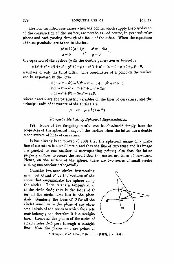
328 ROUQUETS USE OF [CH. IX
The non-included case arises when the conies, which supply the foundation
of the construction of the surface, are parabolas—of course, in perpendicular
planes and each passing through the focus of the other. When the equations
of these parabolas are taken in the form
y2 = 4i(a; + 0) z* = -Mx\
z = f' y = >'
the equation of the cyclide (with the double generation as before) is
x (a? + y* + z*) + (a? + y2) (I - ft) - z* (I + fi) - (x - I - /*) (I + fif = 0,
a surface of only the third order. The coordinates of a point on the surface
can be expressed in the form
x (1 + 1* + &>) = I (ffi -
1
1 + 1) + fi (d* + 1* + 1),
y (1 + t1 + ffi) = 21(0* + 1) t + 2fit,
z(l+P + i) = 2Wt* - 2fi0,
where t and 6 are the parametric variables of the lines of curvature ; and the
principal radii of curvature of the surface are
li - lt\ /j. + 1(1 + P).
Rouquet's Method, by Spherical Representation.
197. Some of the foregoing results can be obtained* simply, from the
properties of the spherical image of the surface when the latter has a double
plane system of lines of curvature.
It has already been proved (§ 160) that the spherical image of a plane
line of curvature is a small circle, and that the line of curvature and its image
are parallel to one another at corresponding points; also that the latter
property suffices to secure the result that the curves are lines of curvature.
Hence, on the surface of the sphere, there are two series of small circles
cutting one another orthogonally.
Consider two such circles, intersecting
in m ; let and P be the vertices of the
cones that circumscribe the sphere along
the circles. Then mOis a tangent at mto the circle dmb ; that is, the locus of
for all the circles amc lies in the plane
dmb. Similarly, the locus of for all the
circles amc lies in the plane of any other
small circle of the series to which the circle
dmb belongs ; and therefore it is a straight
line. Hence all the planes of the series of
small circles dmb pass through a straight
line. Now the planes amc are polars of
* Bouquet, Toul. Mim., 8« S<5r., t. ix (1887), t. x (1888).
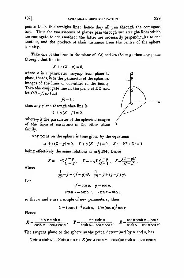
197] SPHERICAL REPRESENTATION 329
points on this straight line ; hence they all pass through the conjugate
line. Thus the two systems of planes pass through two straight lines which
are conjugate to one another ; the latter are necessarily perpendicular to one
another, and the product of their distances from the centre of the sphere
is unity.
Take one of the lines in the plane of YZ, and let OA = g; then any plane
through that line is
X + c(Z-g)=0,
where c is a parameter varying from plane to
plane, that is, it is the parameter of the spherical
images of the lines of curvature in the family.
Take the conjugate line in the plane of XZ, andlet OB =/, so that
then any plane through that line is
Y+y{Z-f) = 0,
where y is the parameter of the spherical images
of the lines of curvature in the other plane
family.
Any point on the sphere is thus given hy the equations
X + c(Z-g) = 0, Y + y(Z-f) = 0, X>+Y* + Z* = \,
being effectively the same relations as in § 194 ; hence
where
Let
Y--cc£^- Y- „vf- g 7--fG- gT
/= cos a, g = sec a,
c tan a = tanh u, y sin a = tan v,
so that u and v are a couple of new parameters ; then
C = (cosa) 2 COSnM; r=(cosa)'cosv.
Hence
X = sin a sinh u F= sin a sin vZ =
cos a cosh u — cos v
cosh u — cos a cos v
'
cosh u — cos a cos v'
cosh u — cos a cos v
'
The tangent plane to the sphere at the point, determined by u and v, has
X sin o sinh u + Fsin o sin v + Z(coa a cosh u — cos v) = cosh u — cos a cos v
330 BOUQUET'S [CH. IX
for its equation; and therefore the equation of the tangent plane to the
surface (which is parallel to this plane) is
x sin o sinh u + y sin a sin v + z (cos a cosh u — cos v) = F(u, v),
where F(u, v) is some function of u and v. The point x, y, z on the surface
is given by combining this relation with
u dFx sm a cosh u + z cos a sinh u = 5- ,
du
dFy sin a cos v + z sin v = -s-
.
ButT7. . . sin a sin w _ sin2 a cos v . ,
F, = - sinh m .—r ^ , ^1 = ;—r ^ sinh u,(cosh m — cos a cos »)
2 (cosh w — cos a cos vf
so that
F, sin a cos v + Z, sin v = 0.
The parametric curves are lines of curvature, so that
EX1= -Lxl , EYX
= -Lyx , EZx= -Lzx ;
hence
xr sin a cos v + ^i sin v = 0.
Hence, from the third of the equations that give the values of x, y, z, we have
dudv'
and the same result follows from constructing X t and Z„ and using the
second of those equations. Thus
F= U+ V,
where U is a function of u only, and V is a function of v only ; and now the
equations of the surface are
«sin sinh w + y sin o sin t> + 2 (cos a cosh w — cos»)= U + Vx sin a cosh u+z cos a sinh u=U'
y sin a cos v + z sin v = Vwhich are easily seen to be in accordance with the results previously
obtained (§ 194).
The second and the third of these equations, taken separately, are the
equations of the planes of the lines of curvature.
Note. We may also proceed from the equations for the tangential
coordinates, as given in § 163.
It is easy to prove that
sin' a .e = '1—
l r. = 9, f= J
(cosh u — cos a cos vf *
198] METHOD 331
and so, with the equation
xX + yY+zZ=Tin general, and the equation
T»—yT-ST.-Oin this case, where
7 "2V *"ty'
32
(.Dr) = DT1S + DaTr + D.T, + TASdudv
= 0,
D = cosh u — cos a cos v.
we have
when
Thus
£>T=U+ V,
where # is a function of w only, and V is a function of v only ; that is, the
equation of the tangent plane to the surface is
*sinasinh u+ y sin a sin v + z (cos a cosh u— cosi>)= U+V,as before.
jEr. Shew that, if
U=a sinh it + 6 cosh tt -f c, F= £ sin « + 1 cos »,
where a, 6, c, i, 2 are constants, the equation of the surface is
{(6 - z cos a)2- (* sin a - a)2}*+ {(y sin a - 1)2+ (z+ J)
8}*+ c= 0.
Prove that the surface is a Dupin cyclide, having its centre at the point
a cosec a, h cosec a, (J+ 6 cos a) cosec2 a ;
and find the smallest value of|c
jwhich allows the cyclide to be real. (When c—0, the
surface is a point-sphere duplicated.)
198. The general result is ineffective in the special case when
/-0-1-The equations then are
x + c(z-i)=o, r+7(£-i)=o, Z»+F*+Z»-l;so that
Z = F = Z 1
2c 27 cs+7J -l c, + 7»+l'
The tangent plane of the surface is
2ca;+27y + (cJ+71, -l)^ = ^,(c, 7),
where F is some function of c and 7. The coordinates of a point on the
surface are obtainable by joining this equation to the other two equations
ldF
idF
y+7*=2V
332 ONE PLANE SYSTEM WITH [CH. IX
Also
r,- "?*. *— 4
so that
Hence
and therefore
(c' + r' + l)3'
(c! + 7s + l)s
*
F, + 7^1 = 0.
y, + yz1= 0,
dcBy
Hence F is of the form C+Y, where C is any function of c alone, and V is
any function of y alone ; and now the equations of the surface are
2cx + 2yy + (c1 + y2 -l)z=G + Vx + cz = |C
The second and third of these equations are, as before, the planes of the two
systems of lines of curvature.
Ex. 1. Shew that the surface
o— Z 0—
z
has plane curves for its systems of lines of curvature.
Ex. 2. Shew that, in the general case for any values of C and of r as functions of c
and of y respectively, the surface can be generated as the envelope of spheres having their
centres on the parabola
y=0, a*-*-*,
and as the envelope of spheres having their centres on the parabola
x=0, y2=£+ 2z.
Obtain the relation between the two families of spheres when both generations are
effective.
One Plane System and one Spherical System.
199. The preceding discussion of surfaces, when both systems of lines
of curvature are plane curves, gives a sufficient indication of one of the
methods of proceeding in the case of surfaces, having one or both systems of
lines of curvature given as spherical curves. For the full detail of cases,
reference may be made to the memoirs of Serret* and of Cayleyf; the
developments, naturally, are mainly of an analytical character.
* Liouville't Journal, t. xviii (1853), pp. 113—162.
t Coll. Math. Papert, vol. xii, pp. 601—638.
200] ONE SPHERICAL SYSTEM 333
In particular, when we deal with surfaces having a set of plane curves for
one system of lines of curvature and a set of spherical curves for the other
system, there are seven substantially distinct cases to be set out, according to
Serret's investigations. The fundamental equations (with merely changes of
sign from the general case) are
X*+Y* + Z* = l
aX + bY+cZ + l =
ace + by + cz + u = V
,
os" + y" + 2* - 2aai - 20y - 2yz - 2v =
(x - a) X + (y - 0) Y+ (z - y) Z - X =
where a, b, c, I, u are functions of one parameter m, and o, 0, 7, \, v are
functions of the other parameter p; and the double condition, at once of
orthogonality for the lines of curvature and of integrability for the equation
of the surface, becomesaa + b0 + cy — IX + u = 0.
The seven cases of the critical equation just indicated are as follows,
account always being taken of simplification without loss of generality :
—
I, I = 0, u = 0, a = 0, = 0, 7 = ;
II, u — ml, \ = m
;
III, I = — mc, u = 0, a = 0, = 0, 7= mX ;
IV, c = 0, u = ml, a = 0, = 0, X = m ;
V, c = 0, I = 0, u = 0, a = 0, = ;
VI, a = 0, c = 0, u = ml, = 0, X = m;
VII, c = 0, 1 = ma, u = 0, = 0, a= — «i\
;
where, throughout, m denotes an arbitrary constant, and so remains an
arbitrary function of its argument.
200. Among these, consider specially the case where
(i) the quantities a, b, c, are unrestricted by conditions, while u = ;
(ii) the quantities a and vanish.
The critical equation of orthogonality becomes
cy=lX,
and therefore we may take
y- l-i,
where k is an arbitrary constant. It may be zero, or it may be infinite ; the
latter case is merged in the former, by interchange of parameters. The lines
of curvature of one system lie on concentric spheres.
334 ONE PLANE SYSTEM WITH [CH. IX
I. Take the special sub-case, when the constant k is zero. The funda-
mental equations then are
X>+Y* + Z>=1,
aX + bY + cZ = 0, xX + yY+ zZ*=\,
ax + by + cz = 0, a? + y + z* = v
;
and the critical equation is satisfied.
The equations are homogeneous in a,b,c; so we may assume
a" + b' + c2 = 1.
Also, a, b, c being functions of u alone, let
a' = a, (oj1 + 6,1 + c,
3)
-* V = 6, (a,2 + 6,
2 + Cl!)" * c = c, (a,8 + i,
2 + c,2)~ *
;
thus<ta' + bb' + cc'= 0,
a'2 + b'1 + c'
2 = 1.
Further, if
we have
v i." ~"O , , c = a , b , c
a', b', c'
aa"+ bb"+ cc" = 0,
a'a" + b'b" + c'c" = 0,
a"*+ V't+c"* = 1.
The aggregate of relations is
X>+Y* + Z* = l, aX + bY+ cZ = 0,
a"2 + b"' + c"2 = 1, a"a' + b"V + c'V = 0,
a'2 + 6'2 + c'2 = 1, o"a + 6"6 + c"c = 0,
a* + 6s + c2 = 1, a'a + b'b + c'c = 0.
Hence we may take
X = a cos t — a" sin t, Y=b'cost — b"smt, Z=c' cost — c" sin t,
where t is a new variable ; these satisfy the two equations in which X, Y, Zoccur. Take other three magnitudes
X' = a' siiit + a" cost, Y' = 6'sin£ + b" cost, Z' = c' sin t + c" cos t,
which obviously are such that
X'" + F'2 + Z'2 = 1, aZ' + bY' + cZ' =;
moreover,
XX'+FF' + ££' = 0.
Now consider quantities
S=Xa + X'/3, v=Ya+Y'0, Z=Za + Z'&:
and writing
we have
Thus
200] ONE SPHERICAL SYSTEM 335
then
af + 617 + C? = 0.
Comparing these with
xX+yY+ zZ = X,
a?+ y' + z" = v,
ax+ by + cz =;
o = \, a8 + /S2 = v
,
* = %, V=V, z=t
x = X\ + X'(v-\rf,
y=Y\+Y'(v-\rf,
z = Z\+Z' (u-\s)*,
which are expressions for x, y, z involving three variables, viz. m (through
the quantities a, b, c), ft (through \ and v), and t (through X, Y, Z, X', Y', Z').
These three variables can be reduced to two as follows.
We have
a"da + b"db + c"dc = (oV + b"V + c'V) (a,*+ bf + cffi du
= 0;
hence, as a"a + b"b + c"c = 0, it follows that
ada" + bdb"+cdc" = 0.
a"da" + b"db" + c"dc" = 0.
Also
Consequently
da" db" dc"
that is,
be" - b'c ca" - c"a ab" - a"b
'
dar_dV_<Wa ~ b'
~c'
say, where is a function of m only. Thus
a'da" + b'db" + c'dc = d6;
and therefore
a"da' + b"db' + c"dc' = -de.
336 PLANE AND SPHERICAL [CH. IX
HenceIXda = d6 . sin t,
2Xda" =d6.cost,
2ZdZ' = 2X (Xdt + da' .sint + da" . cos t)
= dt + d6.
Now along the surface, we have
Xdx+Ydy + Zdz = 0;
and the foregoing values of x, y, z must satisfy this relation. Substituting,
we find
dX + {v - X2)* (dt + dd) = 0,
that is,
- dt = (v -\*)~$d\ + dd.
With this value of t, the equations of the surface are
x = {a" (v - X2)* + a'\] cos t + {a' (v - X2)* - a"\} sin t
'
y = j6" (v - X2)* + b'x} cos t+[b'(v- X2)* - b"\] sin <
^ =[c" (v - \2)^ + c'X) cos t + {
c' (v - X2)* - c"X} sin t
.
II. Now take the less special case, when the constant k is not zero.
The equations are
X 2+F2 + Z2 = l ,
aX+bY+cZ=-ckxX + yY+(z-k\)Z=\
ax + by + cz =
x* + y*+z°-2k\z=2v 1
The equations are homogeneous in a,b, c ; so we can take c= - 1. Following
Serret*, let
X = -p(l+2>2 + g2)"*, F=- ? (l+^2 + 9
2)
-*, Z = (l+pa + g
2)-*
where p and g now denote the derivatives of z with respect to x and y. The
first equation is satisfied identically. The remaining equations become
ap + bq + 1 = - k (1 +f + qrf
z -px- qy= {k+ (l + p* + qrf}\
z — ax — by =
x* + y"+ zi -2k\z = 2v
where X and v are functions of /a, so that X is a function of v. From the
second of these, we have
- xdp - ydq = {k + (1 +ps + qrf] X'dv + (1 +f + q*)~$\(pdp + qdq);
* Liouville't Journal, t. xviii (1853), p. 141.
200] LINES OF CURVATURE 337
so that, when p and q are taken as the parametric variables, we find
y = -{k + (l+p* + q>)l}\'d^- q (i+p* + q>)-lx,
and therefore
Substitute in
z = ax+ by,
and take account of the first equation ; then
Substitute also in
a? + y* + z"- -2k\z = 2v,then
Consequently,
^-(6-S)A, |= -(a-p)A,
where
AX'= {(#- 1)X» + 2v}* (1 +p» + gsr*(a2 + 6= + 1 -A?)
-* {* + (l +p2 + g»)*}-*.
The relation
, dv , dv ,dv=d-p
dp +dq
dq'
for the determination of v, now becomes
X'dv (b — q)dp — (a- p) dq
{(k>-l)\<l + 2v}l (l +p* + q*)-l(ai + b1 +l-li?)l{k + (l+p1 + q'')l}
Z
together with
ap + bq + 1 = - fc (1 +f + qrf.
As the left-hand side of the differential relation is a perfect differential, the
right-hand side also must be a perfect differential. To evaluate it, write
_ /q»+6»+l-fr\* l + kjl+pt + q1)*
.
'
\ a2 + 6> J k + (i +p* + q*)i
'
then, after reduction, we find
sin
\'dv (a'b-ab')dm ,, ,„\_i ,. rt+ 1 + (1 - A8) * dj> = 0,
{()fc> -l)Xs
-|-2t;}* (a'+^(a*-t-i*+l-^f. 22
338 GENERAL EQUATIONS FOR [CH. IX
where the variables are separated. We thus have<f>
as a function of to and v;
and then from the equation for sin<f>, together with the relation between
a, b, p, q, we have p and q as functions of to and v, that is, we have x, y, z
expressed as functions of to and v, which are the parametric variables of the
lines of curvature.
For a more detailed development of this result, reference may be made to
the memoir by Serret already quoted* and to the memoirf by Cayley.
Ex. 1. Shew that, when u= ml, X= m, a=0, /3=0, y=0, where m is a constant, the
surface is developable.
Ex. 2. Shew that, when all the quantities c, I, u, a, /3 vanish, the surface is one of
revolution.
Ex. 3. Shew that, when the relations
a=0, c=0, u=ml, 0=0, \=m,
are satisfied, the surface is tubular.
General Equations for Arbitrarily Assigned Curves.
201. In the preceding discussion of surfaces possessing assigned classes
of curves as their lines of curvature, there has been a limitation to curves
that are plane or spherical ; the main reason (other than the comparative
simplicity of the curves) for the limitation was that it facilitated the
construction of integral results by the method of investigation adopted. It
is at least worth while formulating the problem in its most general type,
when the assigned lines of curvature are any two families of curves whatever,
subject of course to such necessary conditions as are demanded by the
equations.
Let the surface be referred to the lines of curvature as parametric curves,
so that
-F=0, Jf = 0;
then the Gauss characteristic equation is
iLNEO = E(E&+ Gf) + G (E& + Ef) - 2EG (Ea + Gu),
while the Mainardi-Codazzi relations are
Let s denote the arc along the line of curvature, p = constant, the arc being
measured from some director curve; and let t denote a similarly measured
arc along the line of curvature, q = constant ; then
ds=G$dq, dt = E$dp.
• l.c, p. 144.
+ Coll Math: Papen, vol. lii, p.-624.
201] ASSIGNED LINES OF CURVATURE 339
The lines of curvature are to belong to known families of curves, so that (§ 19)
it is sufficient to know the circular curvature 1/p and the torsion l/<r. Then pand <r will be functions of s and, as they may vary from line to line, they maybe functions oip also; let
P=f(s>P)> <r = h(s,p).
Further, at the point in question, let nr denote the angle between the normal
to the surface and the principal normal to the line of curvature ; then (§ 126)
1 _ dsr
a ds''
and therefore, as
%-* «•
we have
dq a h(s,p)''
By the known results, giving the curvature of a normal section of the surface
through the tangent to p = constant and the geodesic curvature of the line
p — constant (§ 127), we have
iv" cosct cosw .....
G=^T =fM (m)'
(?i sine- .. .
Denoting the circular curvature and the torsion of the other family of
lines of curvature by 1/p and lja', we have p and a as functions of t and q,
say
p'=g(t,q), cr' = k(t,q).
Also, at the point in question, we denote by w' the angle between the normal
to the surface and the principal normal to the line of curvature ; then we
have the relations
%-* wdvr' _ E* ' . ..
~~d~p~-Wq~) W '
L coser' . ..,
E=^M) <vu>'
Et sinw' . ....
1=
t,.—
\
(VU1 )-
2EG* 9(t>9)
In the last eight equations, there are initially eight unknown quantities, viz.
s, fir, t, sr', E, G, L, N, the independent variables being p and q ; the equations
22—2
340 GENERAL SYSTEMS OF [CH. IX
are potentially sufficient for the determination of the magnitudes, and will
give expressions that involve arbitrary elements. But the quantities E, G,
L, N must satisfy the characteristic equation and the Mainardi-Codazzi
relations ; and so there will be conditions to be satisfied not merely by the
arbitrary elements, but also by the quantities f, h, g, k, or, w'. In the
simplest instance, when the two families of lines of curvature are plane or
spherical, we saw that the parameters and other magnitudes connected with
the lines are certainly subject to one relation and so cannot all be taken
arbitrarily; the relation is additional to the limitation that the curves are
plane or spherical. A fortiori it is to be expected that, when curves are
assigned initially without the specialising limitation, they will have to satisfy
some condition or conditions, in order that they may provide the two systems
of lines of curvature for a surface.
Ex. 1. To illustrate the analysis, let it be required to determine surfaces having
circles for both sets of lines of curvature. Then
P=f(j>), v-^O,
P'=ff(9), o'->-0;hence
dw dw' .
dq~ ' dp~Consequently
a=P, w'=ft
where P is a function of p only that may be constant or zero, and § is a function of qonly that may be constant or zero ; these two results are, of course, Joachimsthal's
theorem on plane lines of curvature.
Suppose that neither P nor Q vanishes in general The special equations (other than
the intrinsic relations for all surfaces) are
tf coaPo=m (m)
'
g> ainP ..,,
2GE* f(P)(1V) '
L cos§
~E~m C™)'
Ei sing
ii£4= -^) (vm)
'
potentially sufficient to determine L, N, E, G. The equations (iv)' and (viii)' suffice to
determine E and O ; their primitive is
E-iH>=(H+K)f£y
where H is an arbitrary function of p and H' is its derivative, while K is an arbitrary
function of q and K' is its derivative. Then L is determined by (vii)' and N by (iii)'.
201] LINES OF CURVATURE 341
These quantities are to satisfy the intrinsic equations common to all surfaces.
Substituting in the Mainardi-Codazzi relation
we have
Li=l\E+ a) Ei '
cos_P _ coaQ_ _ff+K d_(cos gl
/(/») *(«)£'
is H is a function of p only and K of q only, while p and y are independent variables, we
uist have1 d fcosCT . . .
--p-, j- \—7-^ }= constant= a ',
, and the foregoing equation then gives
„ cosP C coaQ\
Each side of this equation must be a constant, say — /3 ; then
cosPE~ "7(rt"A
which satisfy all these equations. The same result follows from substituting in the other
Mainardi-Codazzi relation.
There remains the Oauss characteristic equation. Writing
cos P_ D cos Q_ n755" " ate)'*
1 '
so that
E-*P,'-(Pi-Qi)P» -fl'"*«i'-(/'l -«i)ft,
and substituting in the Gauss equation, we have
PiQi+PiQ^.+QiPtjf^A+B,
wherer t
A-PxPt j%-Pt, B=Q1 Q2 ^,-Q2*,
so that A is a function ofp only, and B is a function of j only. Hence
'.'i(*+*8)+*'*(^> ft
From the last of these derived relations, we have
342 EXAMPLES [CH. IX
where a' is a constant ; and therefore
where V and c" are constants. Consequently
Qi3+Qi2=a'Ql
*+ 2b'Q1 + m,
P2!=-o'Pl
i!+2c'PI +m'.
Instead of using the other derived relations, we substitute these values in the modified
form of the Gauss equation ; it becomes
6'Pi+c'§,= -cfPj-b'Qi-im+vi'),so that
6'= — c', m + m'=0.
Accordingly, all the necessary equations are completely satisfied by the set of values
P22= - a'Pf+ 2c'
P
t- m I
H= aP,-/3 rtf=-a§, + /3 j
These values are required for the expressions of E, G, L, N. When these are formed,
a and |3 disappear; so that, in the forms obtained, three arbitrary constants a', c', mappear.
The expressions can be simplified by changing the independent variables/ Let newvariables
<f>and 8 be introduced, defined by the equations
1 1-p =li-a cob (j>, q- = h-ccos6;
then
A ° j ft c . ,
p;=i68in
*' |;=& 8in *'
provided
m=-p, d=mli=m.
li\ a'=»i(/i2 -a2)=H-TO(/x'! -c2
).
The last conditions are satisfied, provided
/i=//, c2=o2—
6
2;
and thus, instead of the three constants a', c', p, we have four constants a, b, c, p, tied bythe relation
c2=o2-62
Let E and O, L and N, be the fundamental quantities when <j> and 6 are made theindependent variables, instead of p and q ; then
*=-<%)' "«©'.and so for the others. After simple reduction, we find
f- fr2O*-CCOS0)2
(acoB<j>-ccoad)2 '
p_ ffc-acosift)2
(acos^ — ccosd)2 '
-ff E fi — c cos £
1 ..... &=F= 1
(? (? fi— acoa<j>
2°3] WEINGARTEN SURFACES 343'
These (together with ^=0, M=0) are the fundamental magnitudes, of the first order andthe second order, belonging to a Dupiii cyclide. Hence, by Bonnet's theorem (§ 37), thesurface is a Dupin cyclide.
Ex. 2. In the preceding analysis, it has been assumed that both P and Q are generallydifferent from zero.
'
Shew that, when one of the two quantities vanishes, say P=0, the surface is an anchor-ring, given by the intrinsic equations
E<=(c+cosqy, F=0, G= \)
L=c+coaq, M=0, JV=1)'
Ex. 3. Shew that when both P and Q vanish, the surface is a developable surface*.
202. On the main line of development, especially when one of the
families of lines of curvature is plane, much simplification comes whenl/o- is zero, so that or is constant and may be zero. The most direct
illustration arises in connection with tubular surfaces ; that is, surfaces
which are the envelopes of spheres, having their centres on any given curve
in space, and having their radii any assigned continuous function of the arc.
Reference in general to surfaces, having one (but only one) system of
plane lines of curvature, may be made to Darbouxf and to BianchiJ.
Weingarten Surfaces.
203. One or two incidental references to Weingarten surfaces have
already been made; and some special examples have arisen, particularly
surfaces having a constant Gaussian measure of curvature and surfaces
having a constant mean curvature (including minimal surfaces). We proceed
to obtain some properties of these surfaces in general, defining them as
surfaces whose principal curvatures are connected by some functional relation^
i*(a,/8>=0.
We refer the surface to its lines of curvature, so that
F=0, M = 0.
The Mainardi-Codazzi relations are
*-,(*+$.* *-i(S+5K* As regards these results, a note-by the author, Messenger of Math., vol. xxxviii (1909),
pp. 33—14, may be consulted.
t See his treatise, t. iv, pp. 198—266.
J Geometria Differentiale, t. ii, chap. xxi.
§ They were first discussed in general by Weingarten, Crelle, t. lxii (1862), pp. 160—173.
344 WEINQARTEN [CH. IX
Now
hence
and therefore
so that
a -° s- E -
'P*~2E\B+
'G/ E* *
~ 2E\E 0)
__E1(\_l\
2#V/S a)'
a
Et ft o2E~7^ Pi '
where P is a function of p only. Taking a new variable p such that
dp' = P*dp, we effectively make P equal to unity ; so we can, without loss
of generality, write
E=e J*«-0.
daSimilarly, we can take
Also
= e J«0—.
r E „ G
thus the fundamental magnitudes of the surface are known, because the
integrals in E and C? are complete through the relation F(a, /3)= 0.
Ex. 1. In the case of a minimal surface, we have
a+ /3=0,so that
E=p, G=a> i=l, iV=l.
The lines of curvature are the parametric curves ; the asymptotic lines are given by
dp*+dq2=0.
Ex. 2. In the case of a surface having its Gaussian measure of curvature equal to aconstant, we have
aP = c,
where c is constant ; then
a—p p—aso that the fundamental magnitudes are known in terms of a and 0. As before, the lines
of curvature are the parametric curves ; the asymptotic lines are given by
dpi -dq2=0.

204] SURFACES 345
Ex. 3. In the case of a surface having its mean measure of curvature constant (butnot zero), so that
1 + 1 = 1a P c
'
we have
a—p p — a
As these satisfy the condition that
p-? (
los?)=°>
the lines of curvature form an isometric system*—a known property of surfaces having aconstant mean measure of curvature (§ 64).
204. Returning to the general equations for the Weingarten surface, wecan express the fundamental magnitudes in terms of a single parameter. Let
f*L i
so that
and therefore
Now we easily find
so that
hence
0'
E = p*e
da
0-a
346 WEmGARTEN [CH. IX
in general, say
then we have
205] surfaces 347
so that, on one sheet, the lines 6= constant andp= constant (that is, the lines a= constant
and p= constant), and, on the other sheet, the lines 6= constant and y= constant (that is,
the lines 0= constant and q= constant), are isometric orthogonal systems on the surface of
centres.
= sin£w, -^= cos£o>,
so that
Then
Ex. 2. Let
d$
(£)-«•
da= ^cos2 jto>da=i (1 + C08a>) da>,
and therefore
a=J(o>+sino>).Similarly
/3=J(<b— sino>).
Hence the functional equation of the Weingarten surface is
2(„-/9)= sin2(a+/3);
and the arc-elements on the sheets of its centro-surface are
da2 =cos4 4<a (Jcfo)2+ sin4 £<> (dpf,
da12= sin* &a (|efc>)2+ cos4 i o> (dq)*.
Ex. 3. Obtain expressions for the principal radii of curvature in terms of a single
parameter for each of the surfaces
1+1=?.
205. It follows from the functional equation F(a, £)=0, defining a
Weingarten surface, that
a^-ers/S^O.
As regards its two-sheeted surface of centres, the Gaussian measure of
curvature for one of them is (§ 81)
jr ! §t
(a-zS)^'
and for the other of them is
1 a,K'=-{*-&&'
hence for the Weingarten surface the product of the specific curvatures for
the sheets of its centro-surface is such that
KK' =
Again, assuming that the original surface is referred to its lines of

348 PROPERTIES OF [CH. IX
curvature as parametric curves, we have the asymptotic lines on the first
sheet given by the equation (§ 81)
and the asymptotic lines on the second sheet given by the equation
-E^dp' + G^dq'-O.
When the original surface is any Weingarten surface, these two equations
are the same ; hence the asymptotic lines on the two sheets of the centro-
surface of a Weingarten surface correspond to one another—a result due to
Ribaucour (§ 83).
The asymptotic lines on the original surface are given by
Ldf + Ndq* = 0,
that is,
If the asymptotic lines on the centro-surface correspond to the asymptotic
lines on the original surface, their equations must substantially be the same
;
that is,
®1 — _ ?? §1 = _ "'
fi a" fi«'
and therefore
a/3 = constant.
Hence the only Weingarten surfaces, such that the asymptotic lines on the
centro-surfaces correspond to the asymptotic lines on the original surfaces,
are those which have a constant Gaussian measure of curvature.
As another result, also due to Ribaucour (§ 82), we have the theorem
that the only surface, such that the lines of curvature on the centro-surface
correspond to one another, is a Weingarten surface such that
o — /3 = constant
;
but these lines of curvature are easily seen, from the analysis used (I. c.) in
establishing the result, not to correspond to the lines of curvature upon the
original surface.
206. Consider any elementary arc on either sheet—say the first sheet
—
of the centro-surface of a Weingarten surface. In general, (§ 81), it is
given by
do* = E (l - |Y dpt + dd?;
and therefore, for the Weingarten surfaces F(ol, /S) = 0, we have
daa =da3 +f(a)dp1,
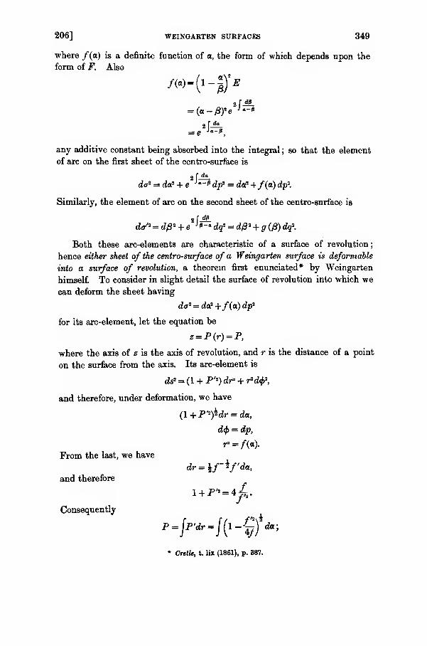
206] WEINGARTEN SURFACES 349
where /(a) is a definite function of a, the form of which depends upon the
form of F. Also
= (a-/S)2 ej —p
any additive constant being absorbed into the integral ; so that the element
of arc on the first sheet of the centro-surface is
d<x2 = da3 + e'— ^ dp2 = da2 + /(a) dp2
.
Similarly, the element of arc on the second sheet of the centro-surface is
do-'2 = dp* + e
} ^- a dqi = d0' + g (£) dg2.
Both these arc-elements are characteristic of a surface of revolution
;
hence either sheet of the centro-surface of a Weingarten surface is deformable
into a surface of revolution, a theorem first enunciated* by Weingarten
himself. To consider in slight detail the surface of revolution into which we
can deform the sheet having
dff2= da2 +/(a)dp2
for its arc-element, let the equation be
z = P{r) = P,
where the axis of z is the axis of revolution, and r is the distance of a point
on the surface from the axis. Its arc-element is
ds2 = (l + P'2)dr'-|-r2dtf>
2,
and therefore, under deformation, we have
(1+P'2)*dr = da,
d<j> = dp,
r- = /(«).
From the last, we have
dr=hf-if'da,and therefore
Consequently
1 + P'2 = 4 2.
p-/p'*-/(i-9**i
CrelU, t. lix (1861), p. 387.
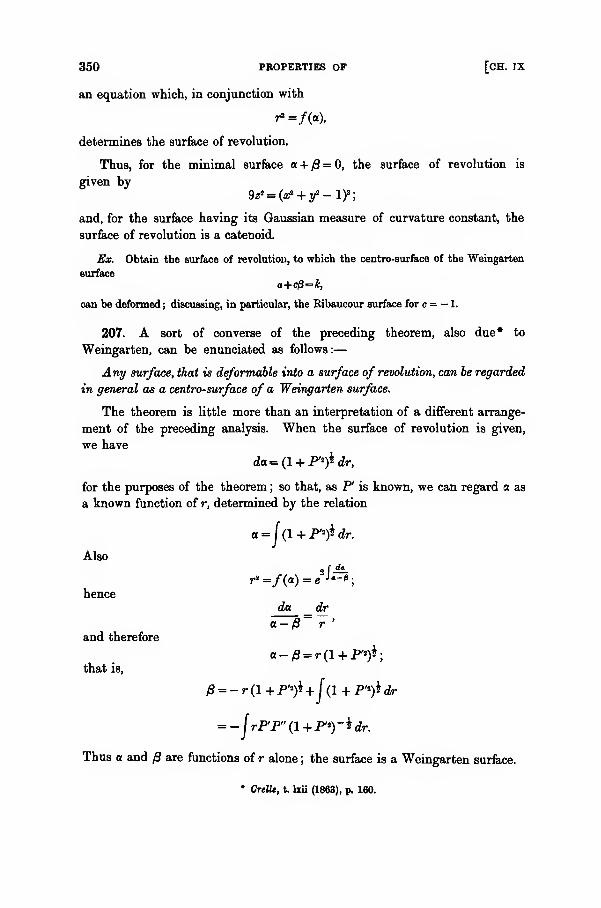
350 PROPERTIES OF [CH. IX
an equation which, in conjunction with
determines the surface of revolution.
Thus, for the minimal surface a + y3 = 0, the surface of revolution is
given by9z* = (x? + tf-iy>;
and, for the surface having its Gaussian measure of curvature constant, the
surface of revolution is a catenoid.
Ex. Obtain the surface of revolution, to which the centro-surface of the Weingarten
surface
a+cj3=£,
can be deformed ; discussing, in particular, the Ribaucour surface for c = — 1.
207. A sort of converse of the preceding theorem, also due* to
Weingarten, can be enunciated as follows:
—
Any surface, that is de/ormable into a surface of revolution, can be regarded
in general as a centro-surface of a Weingarten surface.
The theorem is little more than an interpretation of a different arrange-
ment of the preceding analysis. When the surface of revolution is given,
we have
da=(l + F*fidr,
for the purposes of the theorem ; so that, as P is known, we can regard a as
a known function of r, determined by the relation
Also
hence
a =j(i + p'>)i dr.
r'=/(a) = e '-*;
da dr
and therefore
that is,
«-/3 r*
a-0 = r(l+P*)*;
= - r(l +P*)*+f(1 + P'*)l dr
= -jrP'P"(l+P'*)-ldr.
Thus a and £ are functions of r alone ; the surface is a Weingarten surface.
* CreUe, t. liii (1863), p. 160.
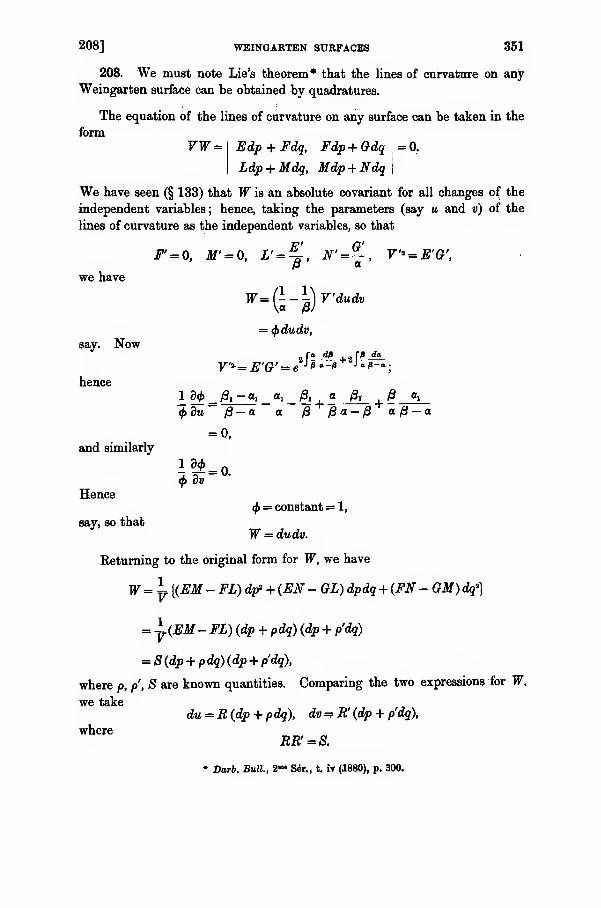
208] WEINGARTEN SURFACES 351
208. We must note Lie's theorem* that the lines of curvature on any
Weingarten surface can be obtained by quadratures.
The equation of the lines of curvature on any surface can be taken in the
form
VW= Edp + Fdq, Fdp + Gdq = 0.
Ldp + Mdq, Mdp + Ndq\
We have seen (§ 133) that W is an absolute covariant for all changes of the
independent variables; hence, taking the parameters (say u and v) of the
lines of curvature as the independent variables, so that
F'=0, Jf' = 0, L' = %, N' =~, V'* = E'G',
we have
say. Now
hence
and similarly
fi' a
"(B)-
Hence
say, so that
= <f>dudv,
= f*d*
i 2 f"da
<f>du /3 - a a /8/3a-/8«0-a= 0,
<£ = constant = 1,
W = dudv.
Returning to the original form for W, we have
W= y {(EM - FL) dp* + (EN - GL) dpdq + (FN - GM) dq3}
= ±(EM- FL) (dp + pdq) (dp + p'dq)
= S(dp + p dq) (dp+ p'dq),
where p, p, S are known quantities. Comparing the two expressions for W.
we takedu = R(dp + pdq), dv == R' (dp + p'dq),
whereRR' = S.
* Darb. Bull., 2°" S«5r., t. iv (1880), p. 300.
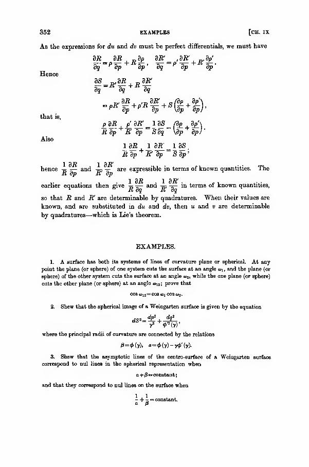
352 EXAMPLES [CH. IX
As the expressions for du and dv must be perfect differentials, we must have
Hence
that is,
Also
dR dR p dp dR' _ , dR' p, dp'
dq dq dq
p^djt P_dR = ldS_/dp_ d/\
Rdp + R'dp Sdq \dp dp)'
Rdp +R' dp Sdp'
I 2D 1/1 7?'
hence -= — and -5-/ -=- are expressible in terms of known quantities. TheK op K op
earlier equations then give -p ^— and -~; -=- in terms of known quantities,
so that R and R' are determinable by quadratures. When their values are
known, and are substituted in du and dv, then u and v are determinable
by quadratures—which is Lie's theorem.
EXAMPLES.
1. A surface has both its systems of lines of curvature place or spherical. At any
point the plane (or sphere) of one system cuts the surface at an angle o>, , and the plane (or
sphere) of the other system cuts the surface at an angle <u2 , while the one plane (or sphere)
cuts the other plane (or sphere) at an angle o>12 ;prove that
COS U12= cos a>i cos a>2
.
2. Shew that the spherical image of a Weingarten surface is given by the equation
where the principal radii of curvature are connected by the relations
0=<My). *=<Ky)-y4>'(y)-
3. Shew that the asymptotic lines of the centro-surface of a Weingarten surface
correspond to mil lines in the spherical representation when
a +/3*= constant;
and that they correspond to uul lines on the surface when
- + j: = constant.a &
EXAMPLES 353
4. Shew that, for a Weingarten surface
ci-|3= e,
the geodesic curvature of the parametric curve p= constant on the first sheet of its ceutro-
surface and the geodesic curvature of the parametric curve q = constant on the second
sheet of its centro-surface are equal to one another, the common value being 1/c.
5. The arc-element on a class of surfaces, referred to lines of curvature as parametric
curves, is such that
and the Gauss measure of curvature is given by
<f> (#*){$(£*) -.£*<?*};
prove that the surfaces are of the Weingarten type.
6. Shew that, if a minimal surface has plane curves for one system of lines of
curvature, its other system of lines of curvature also is plane. Illustrate the result
in connection with Enneper's minimal surface by shewing that every line of curvature
is a plane cubic; and verify that its asymptotic lines are skew cubics.
7. A surface has one system of its lines of curvature spherical;prove that the
radius of circular curvature of the lines is
where P and Q are functions of the parameter q of the lines, while e and g belong to the
spherical image of the surface which is supposed referred to its lines of curvature as
parametric curves.
F. 23
CHAPTER X.
Deformation of Surfaces.
The problem of the deformation of surfaces has attracted many investigators. In
its most general form, the discussion was initiated in the famous memoir by Gauss,
so often quoted ; and other investigations of the utmost importance for surfaces in
general are due to Bour, Bonnet, Darboux, and Weingarten, among others. References
to the original authorities will be found in Darboux's treatise, vol. iii, Book vii,
chapters ii—iv. Reference may also be made to chapter vii in voL i of the treatise by
Bianchi ; and important analytical developments are contained in the third volume of
this treatise, published in 1909.
Among surfaces that are subjected to deformation, special interest attaches to the class
of ruled surfaces. This problem seems first to have been considered by Minding* ; among
later writers, special mention should be made of Bonnet t and Beltrami J. References are
given by Darboux § and by Bianchi ||.
Among the deformations of surfaces which have secured much attention from
mathematicians, there is one considerable class, viz. infinitesimal deformations, important
alike on account of their intrinsic interest and the variety of results (as well as of methods)
connected with them. Moreover, while some of the results are of long standing, much of
the body of known doctrine belongs to more recent years. Full references are given by
Darboux IT and by Bianchi**, both of whom have made important contributions to the
subject ; and no lack of appreciation of the work of Beltrami, Guichard, Kcenigs and
Ribaucour is implied, because a special reference is made solely to two memoirs ft by
Weingarten. Only the briefest account of the elements of this interesting part of the
theory will be given in this chapter; the authorities just quoted should be consulted
for fuller discussion.
* CreUe, t. xviii (1838), pp. 297—302.
+ Jtmrn. &e TEc. Poly., cah. xlii (1867), pp. 1—151.* Ann. di Mat., t. vii (1865), pp. 105—138.
§ In the chapter occupying pp. 293—315 of vol. iii of his treatise.
|| See his treatise, ch. viii.
IF Treatise, practically throughout, vol. iv.
** Geometria Differentiate, vol. ii, pp. 1 et seq., 172 et geq.
tt Crelle, t. c (1887), pp. 296—310 ; Acta Math., t. xx (1897), pp. 159—200.
209] DEFORMATION AND APPLICABILITY 355
Deformation and Applicability ; Initial Conditions.
209. Let a surface be supposed flexible; and let it be changed in anymanner and within any limits, provided there is neither stretching nortearing. Any such change is called a deformation of the surface.
Again, let two surfaces be given such that either of them can suffer a
deformation into the other, or (what is the same thing) that both of them can
suffer deformations into some one and the same third surface. The twogiven surfaces are said to be applicable to one another. The mathematical
theory of the applicability of two surfaces is usually (but not always) the
same as that of the deformation of one surface; so it will usually be
convenient to speak of the latter alone.
Imagine any curve or curves drawn upon a surface ; and let the surface
be deformed. As there is no stretching or tearing, the distance between any
two points on a curve remains unaltered when the distance is measured
along the curve; in particular, any infinitesimal arc at a point remains
unaltered. The angle between two curves through a point remains unaltered
—a property secured by having every infinitesimal arc at a point conserved
in length throughout a deformation. If, then, an arc-element on a surface is
given bytils
2 = Edp* + iFdpdq + Gdq\
and the deformed arc-element on the surface, however deformed, is given by
ds'*= E'dp''+ 2F'dp'dq' + G'dq'\
the necessary and sufficient condition is that, for all variations of the
parameters, we must have
ds = ds'.
This comprehensive condition must be translated into more amenable forms.
Manifestly, geodesies (being the shortest distance on a surface between
two points) remain geodesies through any deformation ; and similarly, the
geodesic curvature of any curve (being the arc-rate of deviation of the curve
from a geodesic tangent) remains unaltered. In fact, any absolute covariant,
which involves only the equation of a curve or curves and the fundamental
magnitudes of the first order (being those which occur in the arc-element),
remains unaltered in a deformation. In particular, the Gaussian measure of
curvature of a surface is expressible in terms of E, F, G and of their
derivatives of the first and second orders ; accordingly, it remains unaltered
during all deformations. The latter property is a condition necessary to
secure that one surface can be deformed into another; it is not, however,
a generally sufficient condition. But it is sufficient to prevent a sphere or
23—2
356 DEFORMATION OF SURFACES OF [CH. X
a hyperboloid of one sheet from being deformed into a developable surface
;
sufficient, also, to prevent an ellipsoid or a spheroid from being deformed
into a sphere. Even a surface of constant curvature cannot be deformed into
another surface of constant curvature, unless the constants are the same.
210. As an example of the deformation of one surface into another,
tested by the invariability of the arc-element, consider the catenoid of revolu-
tion
r = (xi +J/
2)- = c cosh -
.
Taking
we have
x=r cos <j>, y=r sin<f>,
= dr* + r'cfa>a +~ ,drl
r' — c
r*= - -dri + riidd>\
r* — cs
Let
then
Now consider the helicoid
p = (r*-c2)*;
dsa = dpa +(/>s + ca)(ty>2
.
w z2 = tan -
.
Takingy= « sin », x = u cos v, z — av,
we haveds'2 = dv? + (u2 + a2
) dv2.
Manifestly the arc-elements are the same, for all variations, if
u=p, v=<f>,
a = c ;
in other words, the catenoid
r = c cosh -
c
can be deformed into the helicoid
= tanx c
We leave, as an exercise, the verification of the property that the Gaussian
measure of curvature is the same for the two surfaces at corresponding points.
211. Owing to a specially individual property of surfaces of constant
Gaussian measure of curvature—that such a surface is applicable upon itself
in an infinite variety of ways— , we shall discuss them first of all.
211] CONSTANT CURVATURE 357
Take such a surface; and choose, for its parametric curves, a family of
concurrent geodesies and the family of their geodesic parallels. Then the
arc-element of the surface is given by
cte2 = dp* + I?dq\
where the curves q = constant are the geodesies, and the quantity p is the
distance along the geodesic measured from any selected directrix geodesic
parallel. Then, ifK be the Gaussian measure of curvature, we have (§ 68)
Ddp*'
moreover, when p = 0, the general conditions (§ 68) require the limitations
f- >*for any non-singular part of the surface. When K is constant, there are
three typical cases according as K is zero, positive, or negative.
When K=0, we must have
S-^ =dp" '
so that
D = p<j>(q) + f(q).
The conditions, when p = 0, require that (j> (q) = 1, ty (q) = ; thus
D=p.
Hence the arc-element is given by
ds? = dp2 + p2dq2
.
When K is positive, let its value be \ja2; then
ld*D = _}_Ddp-~ a2 '
so that
£=£(?) COS ^ + ^(9)8^.
The conditions, when p = 0, require that
<j>(q) = 0, f(q) = a.
The arc-element is given by
ds2 =c^2 + a2 sin2 ^d9»,
or (what effectively is the same thing) by
ds*= a? (dp* + sia?pdq").
When K is negative, let its value be - 1/a2;then
D dp2 a1 '
358 DEFORMATION OF SURFACES [CH. X
so that
<r = <j>(q) cosh - + ^ (?) sinn
The conditions, when p = 0, require that
Henee the arc-element is given by
ds2 = dps + a2 sinh!^d92,
or (what is effectively the same thing) by
ds*=a* (dp* + sinh2pd?a).
Thus (as before, § 155) the surfaces of constant curvature have their arc-
element of one or other of the forms
ds*= dp*+p*dq*,
ds" = a2 (dp* + sin8pdq%
ds2 = a* (dp*+ sinh2pdg2).
212. Now take two surfaces of the same constant Gaussian curvature.
On them choose any two points and 0'; and through each of these points
draw a geodesic in any direction, measuring any distance p along the two
geodesies. Let the surfaces be referred to the geodesies and geodesic parallels
as parametric curves ; the elements of arc on the two surfaces are given by
<&= dp* +f(p) dq*. ds'* = dp* +f(p) dq'\
for one or other of the three forms of f(p). The arc-elements will be equal,
and so the two surfaces will be applicable to one another, if
dq*=dq'\that is, if
q-qo = q'-<?o'>
a relation which conserves the angle between corresponding pairs of geodesies
through and 0'.
Hence two surfaces of the same constant Gaussian curvature are applicable
to one another, by making an arbitrary point on one coincide with an arbitrary
point on the other and a second arbitrary point on the first coincide with a
second arbitrary point on the second, the geodesic distances between the
point-pairs on the two surfaces being the same. Thus two surfaces of the
same constant Gaussian curvature are applicable to one another in an
infinitude of ways. In particular, a surface of constant Gaussian curvature
can be deformed over itself in an infinitude of ways.
213. Among the surfaces of constant Gaussian curvature, which thus
are deformable each upon itself, it is convenient to know those that are
surfaces of revolution. We refer the surface to its meridians and parallels of
213] OP CONSTANT CURVATURE 359
latitude ; the former are geodesies which are not necessarily concurrent, and
so the analysis in § 211 does not apply; we take the arc-element in the form
ds2=du1 + ridv\
where du is the arc-element of a meridian and r, the distance of a point on
the surface from the axis, is a function of u only. Denoting hy K the measure
of curvature, we have
r du2
and therefore, for a pseudo-sphere having - 1/a2 for its measure of curvature,
we have<Pr_r_
du?~a;2 '
so thatu u
r = Ae a + Be ",
where A and B are constants. There are three cases :
—
(i) when A and B have the same sign ; by adding a constant to u (which
only means changing the origin of measurement along the meridian),
we can make A =B, and then the arc-element is
while
also
ds* = du2 + c2 cosh2 - dif,a
r = c cosh -
;
a
di? = di" + dz\
so that
-J(l-J«nh»g dn;
(ii) when A and B have opposite signs; in the same way as in the first
case, we can take A = - B, and then the arc-element is
ds2 = dn2 + c- sinh2 - dr",a
while
r — c sinh -
,
a
and
H(1_S cosh
1)du]
(iii) when one of the two constants .4 and B vanishes (both cannot
vanish); let B = 0, and (as is permissible in the same way as
before) take A = 1 ; then the arc-element is
2m
ds* = du2 + e a dv-,
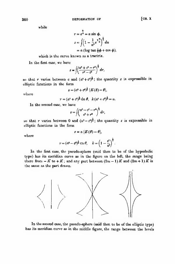
360 DEFORMATION OF [CH. X
while
r = e° = a sin<f>,
J
= a (log tan £</> + cos <j>),
which is the curve known as a tractrix.
In the first case, we have
'-J(-^7-)dr
'
so that r varies between c and (a2 + c2)^; the quantity z is expressible in
elliptic functions in the form
z = (a? + ti>)${E(0)-0},
where
r = (a* + <?)ldn6, /fc(a2 + cl)* = a.
In the second case, we have
* + .- J*"'
so that r varies between and (a2 -^)-; the quantity z is expressible in
elliptic functions in the form
z = a{E(0)-8},where
»\i• = (tf-eF)*cn0, *-(l~^)
In the first case, the pseudo-sphere (said then to be of the hyperbolic
type) has its meridian curve as in the figure on the left, the range being
there from — K to +K ; and any part between (2m — l)K and (2m + 1) K is
the same as the part drawn.
\
In the second case, the pseudo-sphere (said then to be of the elliptic type)
has its meridian curve as in the middle figure, the range between the levels
215] SURFACES OF REVOLUTION 361
of the cusps being from to 2K; and any part between 2mK and (2m + 2)Kis the same as the part drawn.
In the third case, the pseudo-sphere (said then to be of parabolic type) has
its meridian curve as in the figure on the right; it has cusps for = \ir, and the
axis of z is an asymptote, the range for the curve being from ^» = to<f>= tr.
214. ' The formulae for surfaces of revolution, as regards those deformations
which always leave them surfaces of revolution, can be obtained very simply
as follows*. Denoting the element of meridian arc by da, and the axial
distance by r, we havedai = dr* + dz\
ds' = da1 + rid<f>
t.
For the deformed surface, when it remains a surface of revolution, we have
ds?= da'i +r'1d<f>'
i.
All arcs are to correspond ; hence
r'd$ — rd<f>, da = da.
The former is satisfied byr' = kr,
and the latter gives
dz'* + dr'2 = dr* + dz-,
that is,
dz'i = dzi + {l-kl)dr"--
The required surfaces of revolution are given by
r'=kr, j=J{d* + (l-V
Thus in the case of a sphere, z = sin 6, r = cos 8 ; so
r = k cos 6,
e, = [(\-k--smi d)^de,
in agreement with the preceding result.
Ex. Obtain the deformations of a hyperboloid of revolution of one sheet, discussing
the configuration of the generators.
Deformation; General Equations.
215. From the essential property, that geodesies remain geodesies
throughout any deformation of the surface, we can deduce one equation
relating to all deformations.
Let the arc-element on the surface be given by
ds!l = dui + gidi/i,
* Frost, Solid Geometry, p. 350.
362 GENERAL EQUATIONS [CH. X
where g may be regarded as a known function of m and v such that, for small
values of u, we have
g = u-%K u3 + ...,
where K„ is the measure of curvature at the geodesic pole u = 0. In any
deformation, let the arc-element be given by
ds'* = dU* + G*dV°-;
then we must havedU1 + G-d V* = du2 + g'dv1
,
and the deformations will be given by the knowledge of all values of U, V, Gwhich satisfy this relation. We must have
du dv 3m dv
three relations involving the three quantities U, V, G. When we eliminate
G and the derivatives of V, we find
a partial equation of the first order for U containing the function g.
Should, however, g be unobtainable, some other method must be used
;
accordingly, we shall adopt a more generally effective method.
216. By Bonnet's theorem (§ 37) we know that, when the magnitudes
E, F, G, L, M, N are known, the surface is determinate save as to position
and orientation. But if only E, F, G are known, so that the arc-element is
given, the surface is determinate save as to position, orientation, and deforma-
tion. We proceed to indicate the equations for this limited determination of
the surface.
We have
xu -a-,r -#2A = LX,
xy2- a;,!
1' - x.i A' = MX,
x.„ - x,Y" - x,A" = NX,
LN-M* = KV\where the quantities V, T', V", A, A', A". K, V are known functions of E, F, Gand their derivatives. Also
V*X"- = (y,z., - y2zt)-
= (y.2 + z?)W + z?) - (m* +
z
t z.2y= (E- x?) (G - x?) -{F- xlXiy= V- - (Gx? - 2Fx,x.2 + Ex}).
217] FOR DEFORMATION 363
Consequently we have
(*,, - a;,r - x2A) (tea - xj"' - x2A") - (as,2- x,F' - x^'f
=K { V* - (Qxi1 - 2Fxlxi + Ex?)),
a partial differential equation, of the second order and the Monge-Amperetype, for the determination of x.
The same partial differential equation is satisfied by y and by z.
Connected with the solution of an equation of this type, and especially
with the process of obtaining an integral to satisfy assigned conditions, there
is a subsidiary equation (commonly called the equation of characteristics*
of the differential equation) which is of fundamental importance. Denote an
equation byil = ;
its characteristics are given by
an , an anft
Thus, for our equation, the characteristics are
X (Ndq* + 2Mdpdq + Ldf) = 0,
and similarly for the equations satisfied by y and by z ; that is, the charac-
teristics are given by
Ldf + 2Mdpdq + Ndq2 = 0.
Hence the characteristics of the equation for the determination of the surface
are its asymptotic lines, a result that will be seen to bring these lines into
specially significant relation with conditions that may be assigned as governing
all deformations of the surface.
217. Some forms of the equation are of special importance ; we shall
consider three of these forms.
I. Let the equation of the surface be
*=/(*> y);
and give to p, q, r, s, t their customary significance as the first and the
second derivatives of z with respect to x and y. We require the equation of
the second order, satisfied by every surface into which the given surface can
be deformed ; so we take x and y to be the independent variables throughout,
and we denote by Z the ordinate of the deformed surface, and by P, Q, R, S, T
* See the author's Theory of Differential Equations, vol. vi, chap. xx.

364 GENERAL EQUATIONS [CH. X
its first and its second derivatives with respect to x and y. Now, for the
given surface, we have (p. 60)
E=l+p\ F = pq, G-l+fl8,V*=l+p*+q\
VT = pr, V-V =ps, VT" = pt,
V*&=qr, F2A' = qs, F2A" = qt,
(1+pt + q*)*'
hence the equation, which is
(R - PT - QA) (T - PT" - QA") - (S - PT' - QA')2
= K 1
F
2 - (GP1 - 2FPQ + ffQ2)),
becomes
(RT - &) (1 + p2 + 9
s) - (rT -Mfl - 2aS) (pP + qQ) + (f* + Q2 - 1) (r* - s2) = 0.
The general value of Z, satisfying this equation, will give the general set of
surfaces derivable from
*=/(*. y)
by deformation. It ought to include (and manifestly it does include) the
possibility
Z=z.
II. Let the surface be referred to nul lines as parametric curves. The
arc-element then has the form
ds2 = 4ikdudv;
also
r=^, r'=o, r"=o,
A=0, A'= 0, A"=^,
2X dudv
Then, using to denote a; y, or z, we have the equation for in the form
(t>» -e,^) («„-«, £)-«,<•
To adopt the customary notation for partial differential equations with twoindependent variables, we write
e,=p, 8, = q, 0„= r , 12= s, e =*;
218] FOK DEFORMATION 305
and then, if
X, _ Xa _ 32 log X _ .
\~ U' \~ C
' dudv'~ b
'
our equation for surfaces, deformable into a given surface, is
rt — s'2 — cqr — apt = b(\-pq)- acpq,
the parametric curves being nul lines on the surfaces. Manifestly we have,
among the coefficients a, b, c and the quantity \, the relations
9 log\
_ d log X
dv
. _ da _ 3c _ d2 log X,
dv du dudv
The variables u and v are conjugate quantities, known (§ 55) to be derivable
by integrating an ordinary equation of the first order; the quantity X is then
a factor, obtainable by merely direct operations.
III. Let the surface be referred to geodesic polar coordinates. The arc-
element then has the form
ds* = du? + IPdv1.
With corresponding changes of notation, the equation, which determines
surfaces that are deformable into a given surface, is
r(« +i,i)A-2§)-(s-?§)2
+ 5-, (^-i)r-?8
) = 0,
the form being due to Bour. The equation naturally is equivalent to the
equation in the preceding type of representation of the surface; but it is
dependent upon the determination of the variables u and v, which requires
the integration of an ordinary differential equation of the second order.
218. Two other methods of constructing a critical equation—always of
the second order, for the surfaces that arise by the deformations of a given
surface, should be noted. One of them is due to Bonnet*, the other to
Darbouxf.
In Bonnet's method, the surface again is referred to its nul lines as
parametric curves, and the arc-element is taken in the form
ds2 = iX'dudv.
All the surfaces, into which it can be deformed, are given by
da? -t- dy* + dz* = iX'du do,
* Journ. Ec. Polytechn., cah. xlii (1867), p. 3.
f See his treatise, vol. iii, p. 253.
366 THE CRITICAL [CH. X
so that
«V + y? + z? = 0, x? + ys- + z? = 0,
«ia»i + yiyt + z1z2 = 2\\
The first two of these equations are satisfied by taking
xx= i (to2 + n2
), y, = to2 — n2, z
t= 2m»i,
«s,= i (to'8 + n'2), y2 = m- - n'2, £2 = 2m'ri,
for any values of to, n, m', n ; and then the third equation is satisfied if
nm' — vi'n = i\.
But we must have
and therefore
Hence
say. Also
and therefore
hence
Similarly
Now
9a;, _ 3a'2 9y, _ dy2 dzx _ dz,
dv du ' dv du ' dv du
'
mm? = m'rrii,
nn.1 = n «,
,
«m, + TOftj = w'to/ + ra'n/.
Wtj _ TO,' «/ _ «2
m' to n w'
to'2 3 /n'\
— i\ du \m'j
- Tl iL (Hl\ - ui\ dv \m) '
~'
»' n i\—, = - + —
,
m TO TOTO
to • ou\mJ
du \m) to' du \m) to to'5
d_ rn\ i 9 (\\ i\ .
du \m) to' du \m) to'2'
9m \to/ to' 9m \to/'
1. /^ - ^l fl — ^ f^\dv \m) m? m' dv \vi)
'
m' = i (yi - Mi) = ?i = jo, say,
m'J = i (yi - «i) = & = ?> say,
219] EQUATION FOR DEFORMATION 367
where p and q have an altered significance, which correspondingly will be
associated with r, s, t. Thus
au \mj t au \M*/
i _ i\ d /l \
and therefore
a» \piqi)+
8v l?y au [pi)
~ du \qi) dvy)
•
3d'
becoming, on expansion,
X (rt - s2) - 2\,gr - 2\1p« + 4*pq\n = 0.
This is the required equation; its difference, from the earlier equation in
form, is due to the fact that the dependent variable now is \ (y — ix).
When this equation is integrated so that £ is known, we know m and m';
and then, by quadrature through the above relations, we find n/m, that is, we
know to. The value of n' follows from mn — m'n = ik. Substituting in
dx = i (m2 + n2) du + i (m'2 + ril) dv,
dy = (m2 - »i2) du+ (m'2 - n'
2) dv,
dz = 2»»TOdM + 2m'n'dv,
and effecting the quadratures, we have the equations of all surfaces derivable
from the given surface by deformation.
219. Next, consider Darboux's method of constructing the critical
equation—always of the second order— for surfaces deformable into a given
surface. The latter still is referred to its nul lines so that the arc-element is
given byds1 = Qkdudv
;
all the required surfaces are such that
da? + dyt + dz2 = 4>\dudv.
Thusda? + dy" = 4>\dudv — (pdu + qdvf
= - p'du2+ 2 (2\ -pq) dudv - q*dv*.
The surface, of which the arc-element is given by
da? = -p'du2 + 2 (2\ -pq) dudv - q'dv1,
is thus deformable into a plane; consequently, its Gaussian measure of
curvature is zero. We have
E= -f, F=2\-pq, G = -q2, V* = 4,\(pq-\);
368 DARBOUX'S CRITICAL EQUATION [CH. X
and therefore
i (E„ - 2FK +Gu ) = rt- a* - 2\12 .
Also, with the notation of § 34, we have
m = — pr, ml = — ps, in" = 2X., - pt,
n = 2X, - qr, n' = -qs, n" = -qt;
and therefore
mi" - n'a = - 2\t qt + g2 (rt - s2),
am" - 2nm' + mn" =i\Xi- 2X.pt - 2\.qr + 2pq (rt -
s
2),
mm" - m- = - 2\pr + p* (rt - s2).
In order that the Gaussian measure of curvature may be zero, we must have
\(E^-2Fl,+ Gu)V'
= - E (nn" - «'2) + F(nm" - 2n'm' + mn") - G {mm" - to'
2),
which, when we substitute and reduce, becomes
rt-^-\ qr-^pt = (X-pq)2-^--— pq ,
the equation in question. Manifestly it is a partial differential equation of
the second order, being of the Monge-Ampere type; of course, the dependent
variable is not the same as in Bonnet's equation.
Moreover, supposing the value of z known, we have
da? + dy*=- p'dii1 + 2 (2\ - pq) dudv - </'ch>2
,
so thatx? + y?=-p\
i,x.2 + y1y2 =2\-pq,
x? + yi=- t ;
and therefore
(p2 + a.,
2) (f + x/) = (2\ - pq - xxx2)\
that is,
q-x? - 2 (2\ — pq)
x
1xi +pi
x.j! = 4\2 - 4<\pq,
an equation of the first order for x.
When x is known from this equation, then
;*/i
2 = - Pi - *i
2. 2/iyi=2\- pq - a^
,
and so the value of y is derivable by quadrature.
It thus appears that, whatever process be adopted, an essential and critical
condition—in the form that leads to surfaces which are deformable into a
given surface—is a Monge-Ampere partial differential equation of the second
order. The limitations of sufficiency of the equation, in varied possibilities,
will be discussed later ; we shall now deal with some special examples.
219] EXAMPLES OF DEFORMATION 369
Ex. 1. Consider the surfaces deformable into a plane. The square of the arc-elementis equal to chP+dy3
, that is,
dudv,
where u=x+ iy, »=x-iy. Thus, for Darboux's equation, X = J; and so the equation is
rt-8*=0.The intermediate integral is
JiU ... ?=/(/>);and the primitive is
z—au + vf (a) +<(> (o)'
0= u+vf'(a)+ <t>'(a))
'
where/and<f>
are arbitrary functions.
The equation for x now is
<?x? - 2 (8X - ac) xix2+a?x22=4k*- 4Xac,
where c=f(a) ; and its primitive is
x=au+fiv + ty(<a) \
W n61*G
cV - 2 (2X - ac) a0+ a2j92=4X2-4Xac.
The equations for y are
yi2= —pi— xii— — a2 —
a
2 =/i2,
and so the most general value is
y=/*M+i'i>+p.
The equations can be simplified by taking x and y as the independent variables, say
x=u, y= v; thenz= ax+yf (a) + (a)|
0= x+#/'(a)-r<*>'(«0J'
. being a developable surface, as was to be expected.
Ex. 2. Consider the deformations of a sphere, not restricted (as in § 213) to give
surfaces of revolution.
When the surface is referred to its nul lines as parametric curves, the arc-element is
4
~(l+uv)'ds2=
,, , ., dudv,
so that
x-l
(1 + w)2 '
for Darboux's equation. Thus
Xi _ -2v X2 _ -2tt
X-l+w»' \~l + UV'
52jogX_ -2dudv ~ (i+uv)'*'
and so the differential equation, which governs all the deformations, is
24

370 EXAMPLES OF DEFORMATION [CH. X
It is easy to verify that this equation is satisfied by
Z=/(W)=/(W),where
7 ~(w+\)*^ wiw + l)*'
the sphere itself being given by
Ex. 3. Consider the surfaces into which the paraboloid of revolution
2z=x*+y*
can be deformed. To represent the surface, let
z=^X, j-'=X'cosfl, y=X'sinfl;
the parameters of the nul lines are
2u=±f±(l+\)ld\+ i6, 2»=| J^(l+X)idX-^,
and the arc-element is
dsi=4\dudv.We take
f««+»-Hi(l+X)*A
=(x+ i)i_i iog (A±I)i±l,(X + l)4-l
though the integrated form will not be used. Writing X'= dX/rf£, we have
_2X_ 4X+ 2X'
(1+X)*' "(i+xv 5
and therefore
Ai A2 2
* * (1 + X)*'
3MogX= 2X
dudv (1+X)2 '
so that the Darboux equation is
4pj 4X2
~"(T+xj2"(T+x)2'
the customary partial differential equation of the second order and the Monge-Ampere type.
Ex. 4. When we retain x and y as the independent variables, and again consider the
deformations of the paraboloid of revolution
1z=x*+y\so that
p=x, q=y, r=\, s= 0, <= 1,
then the critical equation of the deformed surface is
(RT- S*) (1 +**+jr«) -(R+T) (xP+yQ)+P'+Qi - 1 =0,
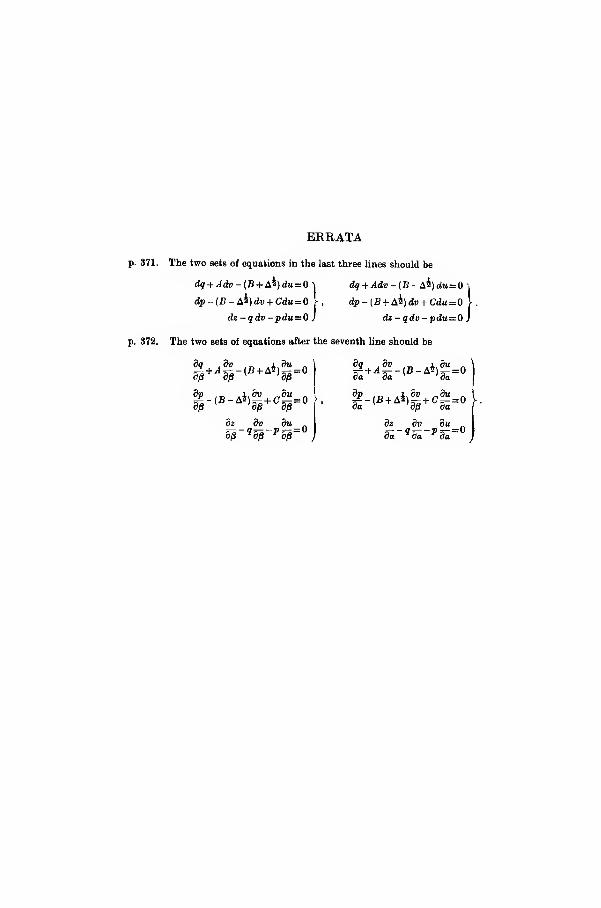
ERRATA
p. 371. The two seta of equations in the last three lines should be
dq + Adv-(B + &b)du=0 -j dq + Adv-{B- A^)du=
dp-(B-A^)dv + Cdu= Q r,
dp- (B + A^) dv + Gdu-
dz-qdv-pdu=0 J dz-qdo-pdu=
p. 372. The two sets of equations after the seventh line should be
dq .dv ,_ .l.du .
da da 'da
dp
dp-(B-A*)^+ o2S=0
dp dp'
,3d „ du
dz dv 5u_„dp 9 dp' p ap~
£-***%+<>«dz dv
3a_3
0a"
du
'Ta2
=o y

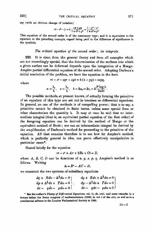
220] THE CRITICAL EQUATION 371
say (with an obvious change of notation)
tt 8 (»+»J1+J),+jfi- 1+a,+y|-
This equation of the second order is of the customary type ; and it is equivalent to the
equation in the preceding example, regard being paid to the difference of significance in
the symbols.
The critical equation of the second order ; its integrals.
220. It is clear, from the general theory and from all examples which
are not exceedingly special, that the determination of the surfaces into which
a given surface can be deformed depends upon the integration of a Monge-
Ampere partial differential equation of the second order. Adopting Darboux's
initial resolution of the problem, we have the equation in the form
rt — si— cqr — apt =b(X— pq) — acpq,
vhere
a -h c -h &-Sa.-gr -g 83l°g X
The possible methods, at present known, of actually forming the primitive
of an equation of this type are set out in treatises on differential equations.
In general, no one of the methods is of compelling power ; that is to say, a
primitive cannot be obtained in finite terms, unless some special form or
other characterises the quantity \. It may at once be said that no inter-
mediate integral (that is, an equivalent partial equation of the first order) of
the foregoing equation can be derived by the method of Monge or the
equivalent method of Boole ; nor can an intermediate integral be derived by
the amplification of Darboux's method for proceeding to the primitive of the
equation. All that remains therefore is to see how far Ampere's method,
which is perfectly general in idea, can prove effectively manipulative in
particular cases*.
Stated briefly for the equation
rt - s2 + Ar + 25s + Ct = D,
where A, B, C, 1) can be functions of x, y, z, p, q, Ampere's method is as
follows. WritingA =B*-AC-D,
we construct the two systems of subsidiary equations
dq+ Rdv-&tdu =
dp + &ldv + Tdu =
dz — qdv — pdu =
dq + Rdv + A^dw =
dp-^dv-r Tdu =
dz — qdv — pdu —
* See the author's Theory of Differential Equation!, vol. vi, ch. xvii; and some remarks in a
lecture before the Borne congress of mathematicians (1908) in vol. i of the Atti, ae well as in a
presidential address to the London Mathematical Society in 1906.
24—2

372 ampere's method [ch. x
We attempt to frame some integrable combination of the first set ; let it be
f(p, q, z, u, v, \) = a,
where a is an arbitrary parameter of integration. We attempt also to frame
some integrable combination of the second set ; let it be
g(p, q,z, u,v,\) = P,
where /3 is another arbitrary parameter of integration. The quantities a and
/9 are then made the independent variables ; and we form the equations
9,8+
9/3 9/3
9/3+
9/3+
9/3
dz _ dv _ 9m _
y.
da*

221] cauchy's integral 373
221. But, though there is the customary impossibility of integrating the
critical equation in finite terms, there exists the important theorem due to
Cauchy which governs the existence of integrals of partial differential
equations. When it is applied to an equation of the second order, the
theorem affirms the existence of a uniform integral, which is uniquely
determined by the properties that z and one of its derivatives—say p—acquire assigned values along any given curve that is not a characteristic.
The properties can be stated in another form. Let the curve be
<f>(u, v) = 0,
so that
au dv
Nowdz = pdu + qdv,
while z and p are given along the curve ; hence q also is known along the
curve, and therefore the properties can be regarded as giving the values of
p, q, z along the curve. When u and v are x and y, as in the equation in
§ 217 (I.), we can say that a surface exists as an integral of the equation,
uniquely determined by the requirements of passing through an assigned
curve and touching a given developable surface along the curve. But the
assigned curve must not be a characteristic ; in the present case, therefore, it
must not belong to either of the families of asymptotic lines.
In the most general form, the quantities x, y, z satisfy one and the same
equation of the second order. Suppose that, when u = a, where a is a
parameter and u is not the variable of an asymptotic line, the values of
x, y, z are required to be A (v), B(v), C(v\ and the values of a?,, y„ z, are
required to be o (w), b (v), c (v). Then
a?+ 62 + c2 =.E
aA' + bB' + cC' = FA'*+B'*+C'* = G
where E, F, G are given quantities ; thus, in the least restricted assignment
of conditions, three arbitrary elements appear to survive. The two inde-
pendent variables are unassigned and arbitrary, yet they would have to
disappear when the surface is represented by a single equation ; so they may
be considered as absorbing two out of three arbitrary elements. It follows
therefore that one arbitrary element certainly survives, when all requirements
are met and the surface is given by a single equation; and so a question
arises as to the use which can be made of this disposable arbitrary element.
Some instances are given in the propositions which follow.
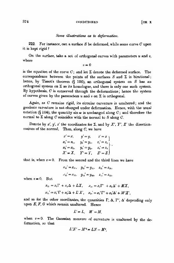
374 CONDITIONED [CH. X
Some illustrations as to deformation.
222. For instance, can a surface 8 be deformed, while some curve C uponit is kept rigid ?
On the surface, take a set of orthogonal curves with parameters u and v,
where
w =
is the equation of the curve C ; and let 2 denote the deformed surface. Thecorrespondence between the points of the surfaces S and 2 is birational
;
hence, by Tissot's theorem (§ 156), an orthogonal system on S has an
orthogonal system on 2 as its homologue, and there is only one such system.
By hypothesis, C is conserved through the deformations ; hence the system
of curves given by the parameters u and v on 2 is orthogonal.
Again, as C remains rigid, its circular curvature is unaltered ; and the
geodesic curvature is not changed under deformation. Hence, with the usual
notation (§ 104), the quantity sin is- is unchanged along G; and therefore the
normal to 2 along C coincides with the normal to S along C.
Denote by x', y', z' the coordinates for 2, and by X', Y', Z' the direction-
cosines of the normal. Then, along C, we have
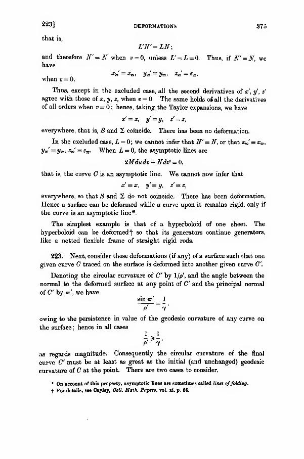
223] DEFORMATIONS 375
that is,
L'N' = LN;
and therefore i\r'=iV when i> = 0, unless Z' = Z = 0. Thus, if N' = N, we
have
a!K = xw , ya = yw , zw = z^,when v = 0.
Thus, except in the excluded case, all the second derivatives of x, y', z
agree with those of x, y, z, when v = 0. The same holds of all the derivatives
of all orders when v = ; hence, taking the Taylor expansions, we have
x' = x, y' = y, z' = z,
everywhere, that is, S and 2 coincide. There has been no deformation.
In the excluded case, L = 0; we cannot infer that N' = N, or that xa' = X&,
Vis = y-a, 3h' = z-a- When L = 0, the asymptotic lines are
2Mdudv + Ndi)> = 0,
that is, the curve C is an asymptotic line. We cannot now infer that
x' = x, y'= y, z' - z,
everywhere, so that 8 and 2 do not coincide. There has been deformation.
Hence a surface can be deformed while a curve upon it remains rigid, only if
the curve is an asymptotic line*.
The simplest example is that of a hyperboloid of one sheet. The
hyperboloid can be deformedf so that its generators continue generators,
like a netted flexible frame of straight rigid rods.
223. Next, consider those deformations (if any) of a surface such that one
given curve G traced on the surface is deformed into another given curve C.
Denoting the circular curvature of C by 1/p', and the angle between the
normal to the deformed surface at any point of C and the principal normal
of C" by -a', we havesin -a' _ 1
7—
>
P 7
owing to the persistence in value of the geodesic curvature of any curve on
the surface ; hence in all cases
W-.P 7
as regards magnitude. Consequently the circular curvature of the final
curve C must be at least as great as the initial (and unchanged) geodesic
curvature of C at the point. There are two cases to consider.
* On account of this property, asymptotic lines are sometimes called lines offolding.
t For details, see Cayley, Coll. Math. Papers, yol. xi, p. 66.
376 CONDITIONED [CH. X
I. Let1 1- >- •
P 7
On the deformed surface, take an orthogonal system of curves determined by
parameters u and v, such that the final curve C" is given by v = ; as any
function of u can be substituted for u, let the magnitude of u be chosen
so that, along v = 0, the arc of C" measured from some fixed point is equal to
u. Then the arc-element on the deformed surface is given by
ds2 = Edu? + Gdtf,
where E=\ when v = 0. Also, du is the arc-element of C on the undeformed
surface ; and E and G are known throughout.
The principal trihedron of C is known at every point. Hence the values
°f x\> Vi, Z\ are known when v — 0, for they are the direction-cosines of the
tangent to C". The values of p'xu , p'yn , p'zn are known when v = 0, for they
are the direction-cosines (say cos f, cos t), cos J) of the principal normal to C',
thus, as p' is known, the values of xa , yn , zn are known when v = 0. And the
direction-cosines (say cos \, cos p., cos v) of the binormal to C are known, that
is, when v = 0.
As «' is the angle between the normal to the deformed surface and the
principal normal to C", it follows that fa-isr' is the angle between the line
whose direction-cosines are G~*a;a , G~*yt, 6~*z2 ; hence
G ~ -#2= sin a-' cos f — cos «r' cos \,
G_'y2
= sin «•' cos 7; — cos •ar' cos /*,
6r~ *z2
= sin w' cos £ — cos w' cos v.
Thus the values of xit y2 , zt are known when v = ; and so also the values of
#12. Vm za are known when v = 0. Moreover, the variable x satisfies the
equation
/ Ex ,Et \( G, G2 \ I Et G, y
(*»- 2EX
>+2G
Xi) K^ + 2E^-2G Xi)-
\x"- 2E
X>~ 2GX*)
= K{EG-(Gx1" + Ext%
while y and z satisfy the same equation ; hence the values of x&, y.a , z& are
known when v = 0. Thus, partly from the data and partly from the nature
of the case, all the first and second derivatives of x, y, z are known along the
curve C. And similarly for all the higher derivatives; e.g., the values of
#ui» ahu. *uz. when v = 0, are the w-derivatives of xu , xlit xn , and therefore are
known, while the value of xm is obtained by differentiating the critical
equation with respect to v and then inserting in the derived equation the
values of the other quantities which are known.
223] DEFORMATIONS 377
Now consider deformations of the surface in general. For the purpose,
we require integrals of the foregoing critical equation which are such that,
when v = 0,
y = y, y^y-2
z = z', Zi = zl I
They exist, and they are uniquely determined by these relations. Thus the
curve on the deformed surface, given by v = 0, coincides with C" ; in other
words, the deformation of the original surface is possible. A curve, originally
given by v = 0, is deformed so as to coincide with C.
Moreover, in the present case, we have
sin -as _ 1
9 1
so that there are two (supplementary) values of is'. Thus we have the
result :
—
It is 'possible (in two different ways) to deform a surface, so that a
given curve C traced upon it can be deformed into a given curve C,
provided the circular curvature of C is greater than the geodesic curva-
ture of G on the original surface.
II. The other case arises when
1 _1p'~V
We must then have ts' = \ir. Also, when v = 0, we have
L _ cos w' _E o
and E=l, when v = 0; consequently
L = 0,
and therefore the curve C is an asymptotic line. Hence, as in the preceding
case, we are led to the theorem :
—
It is possible to deform a surface so that a given curve C should become
an asymptotic line C in the deformed surface, provided the geodesic
curvature of C is equal to the circular curvature of C.
These results will suffice to indicate the manner, in which the external
arbitrary data in Cauchy's existence-theorem concerning integrals of the
critical equation can be used to obtain some conditioned deformations of a
given surface. Further developments will be found in Darboux's discussion
of the subject*.
* See his treatise, vol. iii, especiall)' pp. 253—292.

378 DEFORMATION OF [CH. X
Deformation of Scrolls.
224. Among the surfaces which can be subjected to deformation, a special
interest attaches to scrolls, thereby meaning surfaces which are ruled and are
such that their rectilinear generators of any one system do not meet, the
surface not being developable. Hitherto, all the deformations under considera-
tion have related to the conservation of the arc-element, so that only the
fundamental magnitudes of the first order have been involved; we now
proceed to deformations limited, more or less, by fundamental magnitudes of
the second order.
Some hints have been given that a ruled surface can be deformed, while
each single generator is kept rigidly straight, though these generators are
not kept rigidly connected with one another. Accordingly, we first consider
those deformations, which allow a ruled surface to be changed into a ruled
surface.
Suppose that, if possible, such a deformation exists under which the
generators of one surface (being, of course, asymptotic lines of one system,
and also geodesies on the surface) do not deform into the generators of the
other surface (being also, of course, asymptotic lines of one system, and also
geodesies on the surface). Let p be the parametric variable of the uncon-
served generators on the first surface, and q the parametric variable of the
unconserved generators on the second surface; and take p and q as the
parametric variables of reference for both surfaces. As the arc-elements of
the two surfaces are the same, we have
Edp°- + 2Fdpdq + Gdq* = E'dp- + 2F'dpdq + G'dq",
for all variations ofp and q; hence
E = E', F=F', G = G'.
The asymptotic lines of the first surface are, as to one set, given by
p = constant, and the general equation is
Ldp* + 2Mdpdq + Ndq* = 0.
Hence we have
N=0.
The asymptotic lines of the second surface are, as to one set (not being the
set of the first surface), given by q = constant, and the general equation is
L'df + 2M'dpdq + N'dq* = 0.
Hence we have
I' = 0.
The measure of curvature for the two surfaces is the same ; hence
L'N'-M'* = LN-M*,
2241 SCROLLS 379
that is,
M' = + M.
Next, p = constant is a geodesic on the tirst surface, because the asymptoticlines of the system are generators ; hence
T" = 0.
Again, q = constant is a geodesic on the second surface, for the same reason;
hence
A = 0.
For the first surface, we have N = 0, r" = 0, A = 0; hence its Mainardi-Codazzi relations are
Z2 + YM=
M
, + T L + A'M, &"M = M, + V'M.
For the second surface, we have L = 0, V" = 0, A =; hence its Mainardi-
Codazzi relations are
VM'= MS + A'Jf ', N,' + A"M' = Mi + V'M' + A'iV'.
When the condition M ' = + M is used, the first two of these relations give
z2 =rz,and the other two give
iVY = A'JV'.
The quantity V is the same for both surfaces, and the final value of L after
deformation (being L') vanishes ; hence the former inference leads to
Z=0.
The quantity A' is the same for both surfaces, and the initial value of N'before deformation (being iV) vanishes ; hence the latter inference leads to
JV" = 0.
Thus there is a third surface which has its asymptotic lines (being geodesies)
given by p= constant, q = constant; that is, the surface is a ruled quadric.
Each of the two surfaces can be deformed into this quadric, on the hypothesis
that the generators of the first do not deform into the generators of the
second ; and a quadric is the only proper surface with two systems of linear
generators, for the intersection of a ruled surface of order n by its tangent
plane is composed of a generator and a proper curve of order n — 1. Hence
we have the theorem* :
—
When two ruled surfaces are deformable into one another, then either
:
—(i) the system of generators of one of them deforms Into the system of
generators of the other ; or
* It is due to Bonnet, Joura. de I'tlc. Poly., cah. xlii (1867), p. 44.
380 DEKORMATION OF [CH. X
(ii) each of them can be deformed into a ruled qvadric, the generators
of one surface deforming into one set of quadric generators, and
those of the other surface deforming into the other set of quadric
generators.
225. We now proceed to consider the more general deformation of ruled
surfaces; for this purpose, it is sufficient to obtain the surfaces which
have the same arc-element as a ruled surface. The discussion will be
restricted to real surfaces.
On a given ruled surface, let a curve G (to be called the directrix) be
drawn so as to meet all the generators. The position of a point on the
surface is uniquely determined by
(i) the arc of the directrix measured from a fixed point on the curve,
say v;
(ii) the direction-cosines (say a, h, c) of the generator of the surface that
passes through the point of C ;
(iii) the distance (say u) along the generator from the point where it
meets C;
and the coordinates of the point on the surface then are
x = p + au, y = q + bu, z= r + cu,
where p, q, r are the coordinates of the point on C through which the
generator passes. In these expressions, the quantities p, q, r, a, b, c are
functions of v only. As p', q', r are the direction-cosines of the tangent to C,
we have
e('-'-|- bf + c- = 1,
p- + q- + r'-= 1,
up' + bq + cr = cos 6 = D,
where 6 is the angle between the tangent to C and the generator ; and then,
when we write
a'- + b'2 + c'- = A,
a'p + b'q' + c'r = B,
where A, B, D are functions of v alone, the arc-element on the ruled surface
is given byds2 = du- + 2Ddudv + (Ani + 2Bu + l)dv*.
Accordingly, al' the surfaces into which the ruled surface can be deformed
must have thisM-c-element; and so, for the general equations relating to all
surfaces, we have
E=l, F= D, G = Au* + 2Bu + l,
V 2 = Au'+2Bu + l-D*.
225]
Also
and therefore
RULED SURFACES
Xj — a, i/l= b, z, = c,
x3=p' + ua, i/i = q' + ub', z.,= r' + uc
;
381
VX = br' - cq + it (be - eb'),
VY = cp — ar + tt (ca'—ac),
VZ = aq' — bp' + u (ah'— ba).
The quantities T, V, T", A, A', A', are such that
V*V =-(Au + B)D,
FT" = (D' -An - B)(Aur + 2Bu + L)-(itrA' + 2uB') D,
V2A =0,
F2A' =Au + B,
FaA" = u?A' + 2uB' -(U - An- B) D.
Further, we have
J?n = 0, yn = 0, zn = <),
xvl = a', yn = 6', za = c',
«a2 =p" + Ma"> #« = q" + ub", z-a= r" + «c"
;
and therefore
L = Xxu +Yyu + Zzn = 0,
VM = VXx12 + VYyu + VZzu
a, b, c
p', q, r'
a', b', c'
Ftf = VXx„ + VYy* + VZz.„
a , b c
p' + ua', q + ub', r' + uc'
p"+m", q" + ub", r'- + uc"
where f, q, £ are functions of v alone. Squaring the determinant which gives
M, we have
V'M' = l, A o
A l, 5
o, A 4
-il-il^-ZP;
382 DEFORMATION OF RULED SURFACES [CH. X
and therefore the Gaussian measure of curvature is
M i 1
a result also obtainable from Gauss's characteristic equation by inserting the
values
m = 0, in = 0, m" = D - Au - B,
/( = 0, h' = Au+B, n"=ii!A'+2uB',
A'H = 0, F,., = 0, G it= 2A.
As the general equation of asymptotic lines is
Ldu* + 2Mdudv + Ndv2 = 0,
and as 1 = for our ruled surface, one system of the asymptotic lines is
given by
v = constant,
that is, by the generators, as is to be expected. The other system of
asymptotic lines is given by the equation
2Mdu + Ndv = 0,
that is, by
du = _N^ V £u* j- 2yu+ £
dv 2M 2 (A-AIfi-B^'
As the coefficients of the powers of u on the right-hand side are functions of
v alone, the equation is of the Riccati type ; its primitive is of the form
where \ is an arbitrary constant, and o, ft, y, 8 are known functions of v.
Accordingly, this is the integral equation of the non-generator family of
asymptotic lines ; and the members of the family are given by the varying
values of the parameter \.
Take four values X,, Xj, X,, X4 of X, thus choosing four non-generator
asymptotic lines; and let «,, «j, «,, u4 be the corresponding values of u.
Then we verify at once that
(«! -ih)(ut-
u
t) = (X, - X.,) (X a -
X
4 )
(w, - «,) (wj- ut) (X, - Xs) (X, - X4)
'
a constant for the same four lines. Now u is the distance along a generator
;
and therefore the anharmonic ratio of the four points, where any generator
intersects four given non-generator asymptotic lines, is constant.
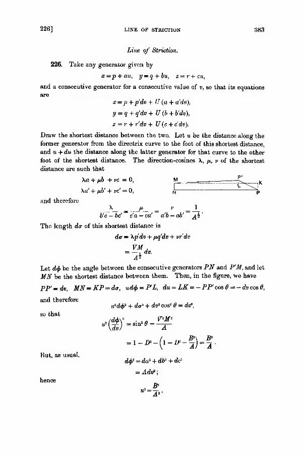
226] LINE OF STRICTION 383
Line of Striction.
226. Take any generator given by
x=p + au, y = q + bu, z=r+cu,
and a consecutive generator for a consecutive value of v, so that its equations
are
oc = p + p'dv + U (a + a'dv),
y — 1 + q'dv + U(b+ b'dv),
z — r + r'dv + U(c+ c'dv).
Draw the shortest distance between the two. Let u be the distance along the
former generator from the directrix curve to the foot of this shortest distance,
and u + du the distance along the latter generator for that curve to the other
foot of the shortest distance. The direction-cosines \, fi, v of the shortest
distance are such that
\a + fib +vc = 0, *^_ K
\a' + fib' + vc' = 0, n f>
and therefore
\ ft, v 1
b'c — be' c'a — ca' a'b — ab' ^ji
'
The length da of this shortest distance is
da = Xp'dv + fjq'dv + vr'dv
VM,= r dV.
A*
Let d<f> be the angle between the consecutive generators PN and P'M, and let
MN be the shortest distance between them. Then, in the figure, we have
PP' = dv, MN=KP = da, ud<f> = P'L, du = LK = -PP' cos 6 = -dv cos d,
and therefore
iC'dtjy1 + da* + dvs cos3 6 = dv*,
so that
W.*,.,.™:-©"-&\ B>
But, as usual,
hence
-i-a-(i-i-5)-!
(>J = du2 + db- + dc-
= Adtf;

384 PROPERTIES OF THE [CH. X
and therefore
•-*!
The sign must be determined. When we take the spherical image of the
generators, the quantities a', b', c' are proportional to the direction-cosines of
the spherical arc which makes an obtuse angle with PP', and the direction-
cosines of PP' are p\ q', r' ; hence B, which is equal to a'p' + b'q + c'r, is
negative. The quantity A is necessarily positive ; and u is taken positive
along the direction a, b, c. Hence*
B
The limiting position of the foot of the shortest distance between two
consecutive generators is called the centre of the generator (sometimes, also,
the centre of greatest density). The locus of this centre is called the line of
striction of the ruled surface. Obviously the shortest distance between two
consecutive generators is not itself part of the line of striction.
The equation of the line of striction in terms of the parameters of the
surface is
Au + B=0.
As A is not zero for real surfaces, the line is determinate ; and it is the
directrix curve, if B = 0.
227. We know (§ 105) that the geodesic curvature of any curve<f>
(u, v) =on a general surface is given by
V _d_ /Ffa-G+A d_ /Ffr -_E<f>,\
where
© = (E<f>.? - 2F<f>1(f>1 + Gtffi.
Now the directrix curve is given by a = 0, so that ^i = 1 and <£2 = ; hence
its geodesic curvature is given by
h-l^+lQ-* The result is obtained, without reference to any figure, by Darboux (t. iii, p. 299) as
follows. The shortest distance between two given generators will be obtained by making <b2 ,
dti= du? + 'IDdudv + {Au3 + 2Bu + 1) d»s ,
a minimum when u and du are regarded as variables, while v and dv are fixed. Hence
Au+ B=0, du + Ddv=0.
The former in the required result ; the latter is the incidental relation
du= -dvcoeS.

228] LINE OF STRICTION 385
For the ruled surface in general, we have
E=\, F = cos6, G= Au 2 + 2Bu + l,
V* = Au- + 2Bu + sin2;
and therefore
d r x Au+B
= B>
for the directrix curve, and
-(—) = - *^ — -JL (A'u* 2B'u)dv\Qi) gb dv 2G%
a de= — sin 8 t- ,
dv
for the directrix curve. Hence the geodesic curvature of the directrix
curve is given by1 B dd
7 sin dv'
Also the curve is chosen arbitrarily, subject to the condition that it intersects
the generators ; and so we have the theorem :
—
When a curve is drawn upon a ruled surface so as to intersect all
the generators, and when it has any two of the three properties
:
—(i) that it is a geodesic
;
(ii) that it is a line of striction
;
(iii) that it cuts the generators at a constant angle
;
it has the third property also.
228. Next, consider the orthogonal trajectories of the generators. Onthe surface, the family of generators is given by
Sv=Q.
The orthogonal trajectory of this family upon any surface in general is given
by the equation (§ 26)(Edu + Fdv)Bu = 0;
and therefore on the ruled surface it is given by
du + cos 6dv — 0,
that is, as 6 is a function of v only, by
cos ddv — constant.«+/c
Now suppose that one of these orthogonal trajectories is chosen as the
directrix curve; we then have
f. 25

386
so that
LINE OF STRICTION [CH. X
F = 0, <k = l, <k = 0, V1 = Au* + 2Bu + l = G,
and so the geodesic curvature of the curve is
1_ Au +B_7~ Aur+ 2Bu + 1
*
Thus the line of striction is the locus of points on the ruled surface where the
geodesic curvature of the orthogonal trajectories of the generators vanishes.
229. When an orthogonal trajectory of the generators is chosen as the
directrix curve, 8 = i ir ; the arc-element of the surface is then given by
Let
then
d& = du* + (»!+2^«+]] Adv\
Adtf = dt\ -j = a, j(A - B*)* = ft
;
ds2 = dt«s + {(« - a)2 + £»} dt-.
The centre of the generator is given by u = a. Let the normal to the surface
at any point on the generator make an angle fi with the normal to the
surface at the centre of the generator. At any current point, we have
VX = br'-cq' + u(bc'-cb')
VY= cp' — ar' + u (ca — ac') r
,
VZ= aq'-bp'+u (ab' - ba').
while the corresponding quantities at the centre are given by
V„X =br'-cq' + a (be' - cbj
V Y = cp' — ar' + a (ca' — ac') ,
,
V Z = aq' — bp + a (ab' — ba)
where
V' = Au' + 2Bu + l =(u-ay + >
V, = Aa> + 2Ba+l = /S"
Now•02
'
VV cos fl = XX, + YY + ZZ„
= 2 (br' - cqj+ (u + a) 2 (br' - cq)(bc' - cb') + u*Z (be' - cb'f
= l+(u + a)B + uaA
J? •
230] beltrami's theorem 387
hence
cos ft = ^{(«-«)* +
and therefore
u — a — ft tan ft,
giving the angle between the normals at the points u and a on the samegenerator.
Let the tangent plane at the centre of a generator be turned round the
generator through an angle<f>.
In its displaced position, it is the tangent
plane at a point on the generator given by
u1— a = ft tau $ ;
and it is the normal plane at a point on the generator given by
u2— a = —
ft cot <f> ;
thus
(M,-a)(M2 -o) + /92 = 0.
Hence any plane through a generator is a tangent plane at some point on the
generator and is a normal plane at some other point on the generator; and,
for different planes, the two points generate an involution having its centre
on the line of striction.
Beltrami's theorem on ruled surfaces.
230; The preceding general properties are necessary to facilitate the
discussion of our main question as to how far a ruled surface is determined
by a given arc-element.
When the element is given, the quantities A, B, D are known. We then
havea2 + b* + c2 =1
a". + W +c '°- =Ap'i + q
'i + r'i = l
ap + bq' + cr' = D \
,
a'p' + b'q' + c'r' = B!
five equations in all, consistent with one another and satisfied by six functions
of v. Hence one of the six functions can be taken arbitrarily, or an arbitrary
relation among them can be postulated; hence there is an infinitude of
ruled surfaces, which possess an assigned arc-element of the form, proper to
a given ruled surface.
Accordingly, let a relation
/(a, b, c) =25—2
388 beltrami's applicable [ch. x
be chosen arbitrarily. This relation, together with the first of the preceding
equations, determines b and c as functions of a; when these values are
substituted in the second equation, the determination of a as a function of v
is a matter of quadrature. Thus we can regard a, b, c as known functions
of v.
For the determination of p, q, r, we have
ap + bq'+ cr'=B,
a'p' + b'q' + c'r' = B,
(be' - b'c)p + (co' - c'a) q' + (aV - a'b) r' = -VM
say, where J has either sign of the radical. When these three equations,
linear in p', q', r, are solved, we find
d jp' = Da + -j a' + -7 (be - b'c),
q' = Db + -j b' + -r (ca' - c'a),
r'=Dc+~c' + j(ab'-a'b),
while the equationp'1 + q'3 + r's = 1
is satisfied in virtue of the value of J\ The determination of p, q, r is then,
again, a matter of quadrature.
As a! +6a + cJ = l, the values of a, b, c give a spherical image of the
generators, through the radii of the sphere which are parallel to them;
the aggregate of these radii forms a cone which is called the director cone.
Hence as the equation
/(a, b, c) =
was taken arbitrarily, and as no condition was subsequently imposed on the
equation, it follows that the director cone of a ruled surface possessing an
assigned arc-element of the proper form can be taken arbitrarily.
Thus there remains a disposable element through which some added
external condition can be satisfied.
231. One property of the preceding solution, first rendered significant
by Beltrami *, is to be noted. When a, b, c are regarded as known, there are
three linear equations for p', q', r' ; but the quantity J in those equations can
have either sign. Hence, given a ruled surface, there is another (and different)
ruled surface applicable in such a way that the corresponding generators are
parallel and in the same sense.
' Ann. di Mat., t. vii (1865), pp. 139—150.
231] RULED SURFACES 389
As an illustration, consider the paraboloid
a? y*
I m(where I and m have the same sign), so as to obtain the associated ruled
surface.
The generators can be taken in the form
x= \ {P 4- Imp tan 8 + u cos 8 cos a
y = — \ (?n2 + Imp tan 8 + u cos 8 sin a.
z= u sin 8
where
thus
As
we have
so that
Thus
tan i
/mya=w ;
a — cos 8 cos a, b = cos 8 sin a, c = sin 8,
p = \(t>+lmpten8, q = -k(m?+ Imp ten8, r=0.
&=t^— cos20,
( + m
4A = .-= r, cos4
8,(l + mf
B=-yff^ Cos*8 Sm8,(l + rnf
D = -, cos 6 ;
I + mand therefore
B .„ .sin 8 J ,(lmp
Z= _ * (^ m) co^' A
= ± ^8-
Substituting these values, we find
so that
p = %(P + lmpten8, 9 = - £ (wi2 + Zm)* tan 0, r = .0,
leading to the original surface ; or else
, / I \$l-3m ,_( m \$3l-m ,
390
so that
EXAMPLES [CH. X
p = l(ihn) c- 8")**'. «-i(r^i)(«-«>t«^ *-«
Thus the associated ruled surface is given by
a.'= s (i I (i — 3m) tan fl + a cos 5 cos o2\l+mJ v '
y = jr(j—- )"
(3< — m) tan 6 + u cos 6 sin a
z = u sin
its Cartesian equation is
„ x _i la*3l-m lyU-Smz = xy (lm) - ~aT T~. a T~,— 'Jy 2 1 l+m 2 m I +m
and therefore it is another ruled paraboloid.
Ex. 1. Shew that the ruled surface, which can be applied to the hyperboloid of
revolution
t±2? _ t - l
so that corresponding generators are parallel, is the helicoid defined by the equations
x u v a2 — <? . v\- = 1 cos - H—=-—jSin -a (at+c*)* " a+<? a
y u . v a2 — c2 v- = j sin =-—„ cos -
u+ 2
a
r(a? + crf (a' + e8)*
Ex. 2. Obtain equations of the generators of the cubic scroll
A=/(y-l),in the form
p=--v. 9 = 1. ,=0,
1
where
= (l+»« + «8)i;
and shew that the ruled surface associated with the cubic scroll, so that corresponding
generators are parallel, depends upon the equations
P' = _?!.
w»+9»*-4 \2v -4v3 j^+9^+ 4'
Ex. 3. Discuss similarly the cubic scrolls*
a?z+y2w = 0, x(yw+ xz)+y3 = 0,
where w is a linear function of x, y, »-.
* These equations give the two diBtinet kinds of cubic scrolls ; see Cayley, Coll. Math. Papers,
vol. v, pp. 211—213. It may be added that there are no undegenerate cubic scrolls of revolution.
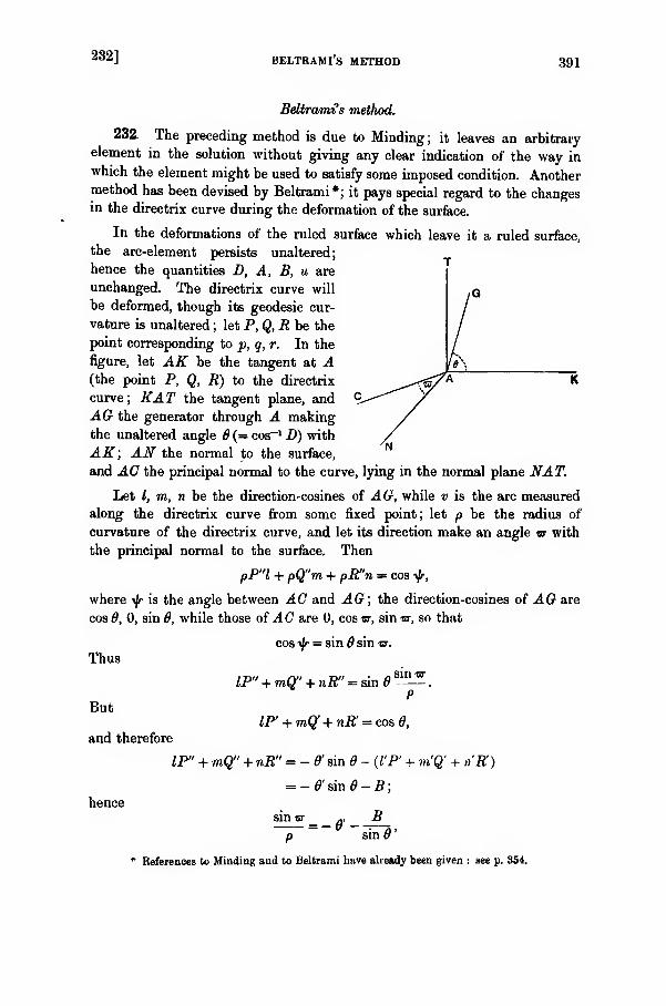
232] BELTRAMI'S METHOD 391
Beltrami's method.
232. The preceding method is due to Minding; it leaves an arbitrary
element in the solution without giving any clear indication of the way in
which the element might be used to satisfy some imposed condition. Anothermethod has been devised by Beltrami*; it pays special regard to the changesin the directrix curve during the deformation of the surface.
In the deformations of the ruled surface which leave it a ruled surface,
the arc-element persists unaltered;
hence the quantities D, A, B, u are
unchanged. The directrix curve will
be deformed, though its geodesic cur-
vature is unaltered ; let P, Q, R be the
point corresponding to p, q, r. In the
figure, let AK be the tangent at A(the point P, Q, R) to the directrix
curve; KAT the tangent plane, and
AG the generator through A making
the unaltered angle 6 (= cos-1 D) with
AK; AN the normal to the surface,
and AC the principal normal to the curve, lying in the normal plane NAT.
Let I, m, n be the direction-cosines of AG, while v is the arc measured
along the directrix curve from some fixed point; let p be the radius of
curvature of the directrix curve, and let its direction make an angle w with
the principal normal to the surface. Then
pP"l + pQ"m + pR"n = cos i/r,
where ^r is the angle between AC and AG; the direction-cosines of AG are
cos 6, 0, sin 6, while those of AC are 0, cos zr, sin w, so that
cos i]r = sind sin w.
Thus
But
and therefore
IP" + mQ" + nR" = sinsinw
IP' + mQf + nR' = cos 0,
IP" + mQ" + nR" = - & sin - (I'P' + m'Q' + n'R)
= -6'sm6-B;hence
sin or=-6- B
p sin 6
'
References to Minding and to Beltrami have already been given : see p. 354.
•392 beltrami's method [ch. x
in accordance with the result of § 227. The equation expresses the property
that the geodesic curvature of the directrix curve remains unaltered.
Let the direction-cosines of AK be cos a, cosyS, cos 7; those of AC be
cosf, cos 17, cosf; and those of the binormal to the directrix curve be cosX,
cos /*, cos v. As the generator AG makes an angle 8 with AK, an angle
cos-1 (sin 8 sin «) with AC, and an angle cos-1
(sin 6 cos or) with the binormal,
we have
I = cos 8 cos a + sin 8 sin or cos f + sin 8 cos er cos X \
in = cos 8 cos /8 + sin 6 sin or cos 17 + sin 8 cos or cos p. [ .
?j = cos 8 cos 7 + sin 6 sin or cos f + sin cos or cos 1/ J
For the directrix curve, the Serret-Frenet formulae are
d cos a _ cos fdc
232] " KXAMPLES 393
When it is satisfied, we can regard p and a (and then «r from the first
equation) as known functions of v. The Serret-Frenet formulae would then
be satisfied, as the curve is given, so that the direction-cosines of the
principal lines are known; and then the values of I, m, n are known.
In that case, the surface can be deformed.
Ex. 1. Consider the possibility of deforming a ruled surface, so that it shall remain
ruled and that any curve drawn upon it becomes an asymptotic line.
The curve is, of course, taken as the directrix curve. In its deformed shape, it is an
asymptotic line. The osculating plane of the latter is the tangent plane to the surface, so
that
hence
Alsop sin 6
. D2 /cosfl y siA —B2=l \-ffcos8j + —
and thereforea"
1 (A sin'fl-
sin^
sin'tf
sin2(9
Thus the ruled surface can be deformed, remaining ruled, so that a given curve upon it
can be deformed into an asymptotic line, provided the curvatures of the asymptotic line
are given (and therefore the asymptotic line is defined) by the preceding equations, where
the quantities 8, A, B are defined in connection with the original given curve on the
undeformed surface.
Ex. 2. When the directrix curve is chosen so as to be a geodesic, in all deformations
of the surface it remains a geodesic. Hence
sin or .- »= u,
P
for its geodesic curvature is zero ; hence or=0 for all deformed shapes unless one of them
is a straight line when -=0, while or is not settled by this equation.
In general, therefore, we have
•A-*so that
B=iy.
Also, in general (so that the deformed geodesic is not a straight line), the final shape of
the geodesic is such that
A -B*-fi^ -*¥)'+*«**.
that is,
/cos 8 _ 8ingy_ . _ «,j,
\P~ ' /
394 INFINITESIMAL [CH. X
Ex. 3. Shew that, when a ruled surface is deformed, remaining ruled, while some
assigned geodesic becomes a straight line, the equations of the surface in its final form are
x^uamBcoayff, y = u sin 8 sin i^, z=v+ uco&6,
where
* =
J am 6
Ex. 4. Determine the condition that must be satisfied by the quantities A, B, 6, in
order that a given curve on a ruled surface may, in the deformations which leave it ruled,
assume the form of a plane line of curvature.
Other illustrations will be found in Beltrami's memoir and in Darboux's treatise (vol. iii).
Infinitesimal Deformations.
233. When we come to consider the whole aggregate of deformations of
surfaces, there are two modes of approaching the subject.
In the first of them, we can have the coordinates of any point on the
surfaces expressed in a form
T =/(?> 9- *>> V = 9 (P> 9. 0. * = h (P. 9< 0.
where p and q are current variables on a surface, and t is a parameter
varying from one surface to another. Should t survive in the eliminant
which results from eliminating p and q between the three equations, that
eliminant represents a family of surfaces which, for continuous values of t,
can change into one another in continuous succession. If the fundamental
quantities E, F, G, defined as usual by the relations
E = x? + y* + zx\ F = xixi + y1y2 + z,zi , G = xt' + ya
! + z2\
are independent of t, then any two of the surfaces are applicable to one
another; they are usually (but not always*) deformable into one another.
In particular, when two surfaces arise from values of t that differ only
infinitesimally from one another, each of the surfaces is regarded as an
infinitesimal deformation of the other.
In the second of the methods of discussion, the actual infinitesimal
displacement of a point on the surface (subject, of course, to the persisting
conditions of deformation of surfaces) is considered, rather than the whole
body of the surface. We take
x' = x+eX, y =y + eY, z' = z + eZ,
where e is a small constant of negligible square, and X, Y, Z are functions of
the current superficial variables ; and then any arc-element of the surface is
to remain unaltered, either actually, or subject to changes of small quantities
* An exception occurs in the case of Beltrami's associated ruled surfaces which, owing to the
difference in the sign of J for the two surfaces (§ 230), are not deformable into one another.
233] DEFORMATIONS 395
that are of the second or higher orders. Such an instance of infinitesimal
deformation is provided by a small rotation of the surface given by
x' = x+ ey, y' = y — ex, z'= z.
The question, as to how far the two modes are equivalent, belongs mainlyto the theory of continuous groups of transformation. As we are concernedwith continuous deformations, rather than with the applicability of surfaces
(whether deformed or not), we shall deal with the second mode.
In either case, the essential and sufficient condition of applicability of twosurfaces is that the relation
dx'* + dy'1+ d/1 = da? + dy* + dz*
should be satisfied ; when the deformations to be considered are infinitesimal,
this relation is also essential and sufficient. When the values
af = x + eX, y' = y + e Y, z''= z + eZ
are substituted, and when the terms multiplied by ea are neglected because
the deformation is infinitesimal, then (on the removal of a factor e) we have
the equation
dxdX + dydY+dzdZ = 0,
which is critical for our purpose. It is the resolution of this equation
which contains the solution of the problem ; and there are various ways of
resolving it.
Before proceeding to two of the ways, we may note an interpretation of
the equation which shews that our problem is analytically tantamount to
another of an apparently quite different kind. The quantities X, Y, Z, being
functions of the two parameters in x, y, z, are the coordinates of a point on
an (unknown) surface; and dX, dY, dZ determine an arc-element on the
unknown surface, just as dx, dy, dz determine an arc-element on the given
surface. The critical equation
dxdX + dydY+dzdZ=0expresses the condition that the two arc-elements on the two surfaces are
always perpendicular to one another: and so the problem of infinitesimal
deformation is analytically equivalent to the problem of determining a surface
that is associated with a given surface by means of orthogonal arc-elements*.
* It may be added that a corresponding result applies in the case of deformations which are
not infinitesimal. Let two surfaces be deformable into one another, so that
<te* + dy* + dz*= Ac'2 + dy '2 + dz'*
;
then, writing
X=x+x', Y=y + y', Z=z + z',
X'=x-x', Y'=y-y\ Z'= z-z',
the two new surfaces are such that
dXdX' + dYdY' + dZdZ'=0,
and therefore they correspond by orthogonal arc-elements. The transformation is the basis of
one of Weingarten's methods ; see § 237.
396 INFINITESIMAL [CH. X
234. We have seen that, when a surface
* =/(*. V)
is referred to x and y as the parametric variables, and when the ordinate of
the surface (however deformed) is denoted by Z, the equation for the
determination of Z is (§ 217)
(RT- S*) (1 + p* + 92) - (rT+ tR - 2sS) (pP + qQ) + (P 1 + Q a - 1) (rt - *) = 0.
Now consider an infinitesimal deviation, represented by
Z=z + eZ\
where the square of e can be neglected ; denoting the derivatives of Z' by
P, Qf, R, S', T', we have
RT - S" = rt - s2 + e {rT + tR' - 2sS'),
rT + tR- 2sS = 2 (rt - s2) + e (rT + tR' - 2sS'),
pP + qQ =f + q* + eipP1 + qQ),
P*+Q>-l=p* + q*-l + 2e (pP' + qQ).
The critical equation, after substitution, rejection of cancelling terms, and
division by e, gives
rT' + tR'-2sS' = 0.
235. The preceding infinitesimal deformation gives the variation of an
ordinate alone. Consider a more general infinitesimal deformation, repre-
sented by
Z=z + eZ", X = x+eX', Y=y + eY',
governed by the critical relation
dxdX' + dydY' + dzdZ" = 0.
The quantity Z" can be taken the same function of X and Y, as Z' is of
x and y ; as Z" is multiplied by e, while X and Y differ from x and from yby small quantities, we can substitute Z' for Z" in the expression for Z.
Thus Z' is determined by the equation
rT' + tR'-2sS' = 0;
the infinitesimal deformation is represented by
Z = z+eZ', X = x + eX', Y=y + eY',
while we have
dxdX' + dydY' + dzdZ' = 0.
The latter gives
/dX' dX' \ iTiY' 7)Y' \dx(^ dx +
y
- dy) + dy{^dx + ^-dyj + (pdx + qdy)(P'dx + Q'dy) = 0,
235] DEFORMATION 397
for all variations of x and y ; hence
three equations to be satisfied by Z' and Y\ when Z' is known. Let
Then
%+"-" S+f^-tt
while, from the first,
so that
Again,
while, from the third,
so that
Hence
leading to
dU d*X' _, /v
dx-=tedy
+ P8+rQ >
rT'-2sS' + «iJ'=0,
the equation* which is satisfied by Z'. Consequently, when Z' is known, we
determine X' (save as to an additive function of y) and Y' (save as to an
additive function of x) from the equations
and then these arbitrary functions must be such as to satisfy the equations
dX' n fdY' \
-dy-+ PQ= ~[-dX-
+ «F
)
= U=
J
{Q' (rdx + sdy) - P' (sdx + tdy)}
= f(Q'dp-P'dq).
* This analysis is another establishment of the equation for Z' deduced from the equation
tlxdX +dydY+dtdZ=0.
398 EXAMPLES OF [CH. X
Ex. 1. Consider the infinitesimal deformations of the paraboloid of revolution
2z=x*+y*.We have
p= x, q=y, r=l, *= 0, < = 1.
The equation for Z' is
R'+T'=0,so that
Z'=$ (x+iy) +f {x-iy),
where <p and f are arbitrary functions of their arguments, and their derivatives are taken
in the expression for Z' to avoid transformations needed to effect subsequent quadratures.
Then- X' = x<t>' (j:+ ii/)- <j> (x + i'/) + xf' (./• - iy) - f (x - iy) + A (y),
-Y' = yp (x + iy) + uj> (x+ iy) +yf (x - iy) - if (x -iy)+ B (x),
CJ= i<j>' (x+ iy) - if (x - iy),
where A (y) and B (x) are arbitrary functions of their arguments. When we substitute,
wc find
A'(y) = 0, 5'(*)= 0,
so that A is a constant, as is B. These quantities occurring in X' and Y' merely give an
infinitesimal uniform displacement of the surface perpendicular to the axis of revolution.
Neglecting this displacement, we have the infinitesimal deformation given by the equations
- X'= x{<f>' (x+iy)+f (x-iy)}- {<£ (x+iy)+f (x- iy)},
- Y'= y{<t>'(x+iy)+ f'(x-iy)', + i{<f>(x+ iy)-f(x-iy)),
Z' = <f>'(x+ iy)+f (x- iy),
where <j> and f are arbitrary functions of their arguments.
Ex. 2. Shew that the infinitesimal deformations of the paraboloid
z= xyare given by
*=*+ «(* + ,'),
X=x+ t {2v -y(g + ny„
where £ is any function of x, and r) is any function of y.
236. In various investigations, we have seen that it can be convenient to
refer a surface to its nul lines as parametric curves, the arc-element being
given by the relation
da' = Qkdudv.
Then, denoting the derivatives of z with respect to u and v by p, q, r, s, t, we
obtained the equation characteristic of any deformed z in the shape (§ 217)
We proceed, as in § 234, to obtain the equations for the infinitesimal deforma-
tion of the surface. Writing
x = x +eX'. y = y + eY', z = z +eZ',
where xt ,y„, z„ are the coordinates of the point on the undeformed surface
and the square of e is to be neglected, we denote the derivatives of Z' with
respect to u and v by P', ty, it', 8', T', and similarly for the derivatives of z„
236] INFINITESIMAL DEFORMATION 399
Substituting, omitting the terms which cancel, and removing a factor e, wehave the equation for Z' in the form
UR - 2s S' + rX - £ (q R' + rJt) - \ (p,T + t„F)
The governing equation
dx„dX' + dy dY' + dz„dZ' = 0,
on the supposition that Z' is known, thus gives the (consistent) equations
for X' and Y' in the form
du du du du ^°
d3> dT +dysdr
+ udv du dv du *°
dxsdX^
+dy1 dT + q = _ n
du dv du dv "
3a%^|^ dY '
| g Q' = pdv dv dv dv "
These are the general equations for the infinitesimal deformation of the
surface. The result depends primarily on the integration of the Mongeequation of the second order, whatever be the surface.
As an illustration, take the case of the general minimal surface ; we have
(§ 174)\ = \(l + uvyf'"g'",
where/ is any function of u only, while g is any function of v only. Also
z, = uf"-f + vg"-g',
so that
P<,= uf , q<> = w ,
n = uf""+f", s = 0, t,= vg"" + g'",
\_ 2v /"" \>_ 2u g'^\~1 + uv
+f'~"
' \ l + uv+
g'"'
When these values are substituted and reduction takes place, the equations
for the infinitesimal deformation become
iT«+rr + 9'"(^-f)
r +/'"(^ -f)
Q' = o,
(1 _ u*)^ + t-(l + u.)^ + 2«F =
(!-«»)
du
dT_
dui(1 +^ + 2vF^
(l- tt')^-' + i(l+«')^ + 2«Q' = -|g
(l- v>)d-*-i(l + v>)
d-£.+2vQ=0
•
400 WKINUARTEN'S [CH. X
the quantity U ultimately dropping out of any particular solution, when
it has been completed.
Hence, in order to obtain the full expression of the infinitesimal deforma-
tion of a minimal surface in general, it is necessary to solve the foregoing
partial differential equation which is of the Monge type in the second order*,
as well as equations of the first order ultimately integrable by quadratures
alone.
Ex. Thus, for Enneper's surface (§ 177, Ex. 1), we have
f=u3,g=v3
;
and so the equation for Z' is
1 —uv
of which a particular solution is
Z' = k{\-uv)3,
where k is a constant. When we introduce new variables v! and v', such that
u'= u+iv, v' =u— iv,
the differential equation becomes a Laplace equation, with equal invariantst ; it can be
expressed in the form
&Z" 8«VZ
,
du'di/ {4 -»(•*- «"*)}»
whereZ'= {4-t (tf* -«'*)} Z
Weingarten's Method.
237. We now come to Weingarten's method^. He discusses, not merely
the surfaces into which a given surface can be deformed but also two other
surfaces which, at each stage of the deformation, can be associated with the
surface.
Suppose that S' and S" are two surfaces in space, such that S' can be
deformed continuously into S". Let x', y, z be any point on S' ; and let
x", y", z" be the corresponding point on 8". The necessary and sufficient
condition for the deformational correspondence of the surfaces is that the
relation
dx'* + dy* + dz'* = dx"1 + dy"- + dz"2
shall be satisfied everywhere for all variations along the surfaces.
* See Darboux, vol. iv, §§ 913—915.
t This is a special illustration of the general theory : see Darboux, vol. iv, ch. ii.
* Only an elementary sketch will be given here. His chief memoirs have already beenmentioned (p. 354). References have already (J.c.) been given to the accounts and developmentsof his investigations which are to be found in the treatises by Darbonx and by Bianchi.
237] METHOD 401
Now let
x = $(x' + x"), y~W + !/')> z = %(z' + z"),
«=£(-*'+*"), »=h{-y' + y"l *>-*(-*'+*");
the point «, y, z describes a surface /S, which can be regarded as a middle
between S' and S". This surface £ is made the clue to the whole development.
Clearly
dxdu + dydv + dzdiv = ;
and so, with p and q as the parametric variables, we have
:r1n
i + y1 v1 + zlw1 =0,
a\u.j + a\,M, + j/,v2 + y„i\ + z1w2 + z2w1= 0,
x2u2 + y2 v.2 + z2 w.j = 0.
We use the customary notation for the magnitudes of the first order and the
second order connected with the surface S ; and, for the purpose of dealing
with these equations, we introduce a central function<f>
under the definition
2 V<f> = XiUz + yxv„_ + ZjW2— (xjW, + ytvx + z2w^).
Then the foregoing equations are
xlu
1 +y1v1 + z1w1=
x2ut + y2Vi + z2w-i = — V<f>
x2ut + y2v2 + z3w2=
From the first of these, we have
Sa5,Mi2 + Sxiji*, = ;
and, from the second, wc have
Ix^Un + %xnu2= £- ( V<f>),
so that
g- ( V<f>) = SttyZj, - Su,x„.
Similarly, from the third and the fourth,
jr ( V<f>) = 2u^r„ - 2m,xk .
Also, as usual (§ 34), we have
xu = a^F + #2A + Z/.AT,
xn = a;^' + a;2A' + MX,
x,i = xxr" + x^" + NX,
and similarly for the derivatives of y and of z; all the coefficients concerned
belonging to the middle surface S. Then substituting, we find
J. ( V6) = V$T + LlXu2 + V<f>& - MlXut.dp
26
402 weingarten's [ch. x
But we have
p-r + A';
and therefore
h-yiLXXUt-MlXUi).
Similarly
fr = ^.(MIXiH - NIXu,).
238. Two cases occur, according as the Gaussian measure of curvature of
our middle surface S is zero or is not zero.
When the Gaussian measure of curvature is zero everywhere, then
LN-M* = 0;and so we have
N<f>, - Mfa= 0, - Mb + L^ = 0,
equivalent to only a single equation. The central function <j> satisfies a partial
differential equation of the first order.
When the Gaussian measure of curvature is not zero everywhere, the two
equations can be resolved ; they give
S-Xw, = - -gy(L<f>2- Mfa),
Hence
2Xu2= - ~(M4>„ - iVty).
d~p { KT~ )+
dq \ KV )~ ~ 1A 'Ul + iA '"2 '
3p'
Now (§ 29)
V'X, = (FM-GL) x,+ (FL-EM)x„
V*X, = (FN-GM)xl + (FM-EN)x1 ,
and similarly for the derivatives of Y and of Z ; hence
V'XXm = - (FM - EN) V<f>,
V*ZX1ut = (FM-GL)V<f>,
and therefore
d /Nh-Mfa , d (L^-M^,EN-2FM+GL^ n
d-p{ KV j+ ^l KV )
+ V * = -
The central function p satisfies a partial differential equation of the second
order and the Monge type.

238] MIDDLE SURFACE 403
As regards the quantities u, v, w, we have
x',«! + y2 «, + z.,Wl = - tf) V,
X, tl + VVl + Zw, = - ~ (L& - #<£,),.
which can be solved for «,, a,, /«,. There is a similar set for «,, ?„, w... Theresulting values are easily found to be
"i = gy{- L (X<j>, - </>X,) + J/ (Z0, - 0JT,)}\
«.= #V {
~ i¥ (Z^ _ ^Z2) + ^ {X^ - *X$
v, =~{-M(Y^ - 0F3) + N(Y<f>1 -<l>Y1)\
w'= FF l_^ (^2 " ^Zi) + N {Z<i>i " +ZM !
Thus, when<f>
is known, the determination of the quantities u, v, w is effected
by a process of quadratures.
We therefore have the following result :
—
Take any surface S and, in connection with it, determine a function tf>, by
the appropriate partial equation of the first order when S is developable, and
by the appropriate partial equation of the second order when S is not develop-
able ; and construct the quantities u, v, w. Then there are two surfaces S' and
S", given by the equations
x" = x + a, y" = y + v, z" = z + w,
x =x— u, y =y — v, z' = z — w,
such that each can be deformed into the other.
Ex. 1. Let the surface be referred to its asymptotic lines as parametric curves, so that
L=0, N=0.
We do not then have M=0, so that the function <j> satisfies a partial equation of the second
order. This equation is easily found to be
^12 ~4 ( ~R<t>2+ ~g <j>A+FK<l>=0,
a Laplace equation with equal invariants which, on the transformation
4>= *A'i,
26—2
404 weingarten's [ch. x
acquires the canonical form
*, 2+e*=o,where
A 12 5 AY/T2 _,_
This is the simplest form of the partial equation of the second order which, ultimately
in some form or other, must be solved before the central function<f>
can be determined.
Ex. 2. Shew that, if the. parametric curves on the surface <S are such that
L = N, M=0,
the equation for the function <£ can be transformed to
*H + *22=©'*,where
<£ = *A'i,
and 6' depends solely upon the surface.
239. Consider, under the new analysis, a question already (§ 222) discussed;
can a surface be deformed while some curve upon it remains rigidly fixed ?
As the parametric variables are at our disposal, again choose them so that
one of them is constant along the rigid curve, say p = a. Now along this
curve, we havetl f ft I tr t
x =x, y =y, z = z,
that is,
m = 0, v = 0, iv = 0,
when p = (i ; and therefore also
m.j =0, t)2= 0, w2
= 0,
when p = a. We shall assume that we are dealing with real surfaces
throughout ; the assumption, that V does not vanish, then is no limitation.
We haveX
lM i + ill
V-l + Z
\W-2 = V$,
in general ; hence we have
4 = 0, </>2 =0, ^, = 0, ...,
when p = a. Again, we have
SZ«S = - gy.(M<}>2 - i\ty,),
in general ; and therefore, if the middle surface S is not developable, wehave
iV<k = 0,
when p = a.
Suppose that N does not vanish (the influence of the alternative to each
of the suppositions can be considered later) ; so we have
24°] METHOD 405
when p = a, and therefore
<#>ia=
when p = a.
The differential equation satisfied by if> is
8 fJfy, - M<j>»\ c(L^-M<L\ EN-2FM+GL , .
dp{ ~V )+d^\—v~) + v *"s °
in general ; hence
<*>,. = 0,
when p = a, and so all the g-derivatives of<f>u vanish when p = a. Differentiate
the general characteristic differential equation with respect to p, and then
make p = a ; we have
when p = a, and so all the ^-derivatives of <£m vanish when p = a.
Similarly for all the derivatives of <j> when p = a—each of them vanishes.
Taking a Taylor expansion of<f>
in any non-singular region round the rigid
curve, we see that<f)
vanishes everywhere in such a region. Hence, whenregard is paid to the expressions for the derivatives for u, v, w, and to the
fact that «, v, w vanish when p = a, it is clear that
u=0, v = 0, w = 0,
everywhere in the region. Consequently
a'W, y"=y\ z"=z\
everywhere ; and so there is no deformation between S' and S". It therefore
follows that usually a surface cannot be deformed while a curve upon it is
kept rigid.
240. The negative conditions, under which the preceding result has been
obtained, are three. It was assumed that the surface 8 is real—the quantity
V was supposed not to vanish ; the surface S was assumed not to be
developable ; and the magnitude N was supposed not to vanish.
We shall maintain the first condition. If V= 0, the two nul lines through
a point coincide ; so that not merely would the surface be imaginary, but it
would belong to a very special class of imaginary surfaces.
Consider the possibility that N should vanish ; in that case, we should
have (along p = a)
Xxa + Yya + Zz& = 0.
And we always haveXtct + Yyt +Ztt =0;
henceA I X * Zt — 3/2^22 ^23/22 ^2*^22 ^2^22 • ^22/22 3^2*^22
= y'z" - z'y" : z'x" - x'z" : x'tf - y'x",
where dashes denote differentiation along the curve p = a. When this curve
is not a straight line, it has a definite direction for its binormal ; hence our
406 weingarten's theorems [ch. x
assumption implies that the normal to the surface coincides with the binormal
to the rigid curve along the whole length of the curve. Now when N is zero,
we cannot infer that <£, = along the curve, and so we should have a function
<f>satisfying the equation of the second order, vanishing along the rigid curve,
but not vanishing everywhere on the surface. Thus the analytical condition
N= is necessary for the conclusion.
When the surface S is developable, the function <^> satisfies a partial
equation of the first order
Nfr - Mfa = 0.
An argument similar to the earlier argument shews that, if N is not zero,
the function <j>, which satisfies this equation and vanishes along the rigid
curve, vanishes everywhere ; and then there is no deformation. Thus the
condition is unnecessary, when N is not zero; and the latter condition has
just been retained.
Summing up, we have Weingarten's theorems*:
—
When two surfaces deformable into one another coincide along a curve,
which is not a straight line and the points of which are self-congruent in
any deformation, the whole surfaces coincide unless the normals to the
rhiddle surface of the two surfaces constitute the binomials of the commoncurve.
When the measure of curvature of a real surface is everywhere positive,
N cannot vanish ; and so the exception cannot arise. Hence :
—
Surfaces of a positive measure of curvature cannot be deformed, if
a curve or part of a curve (not being a straight line) on the surface is
kept rigid.
Also :
—
Surfaces of a negative measure of curvature cannot be deformed, if a
curve or part of a curve other tluin an asymptotic line on the surface
is kept rigid.
If the curve, which is to be kept rigid, is an asymptotic line on the surface,
we can have N = ; we may have </> = along the line, where <j> satisfies the
equation of the second order, and yet we may have <£ different from zero
elsewhere. The surface may be deformable. The definite establishment of
a theorem, that it is deformable, would require the derivation, from the
equations, of the set of deformable surfaces which have their Gaussianmeasure of curvature everywhere negative and which possess one asymptoticline in common.
For further developments of the subject, reference should be made to thememoirs by Weingarten.
* Crelle, t. c (1887), p. 307 ; the earliest (but only partial) establishment of the second of
tliem was made by Jellett.
EXAMPLES 407
EXAMPLES.
1. Shew that it is possible to deform a surface so that a given curve becomes a line of
curvature on the deformed surface. Are there any conditions to be satisfied ?
2. Shew that a surface cannot be deformed so that a whole system of asymptotic
lines remains asymptotic, unless it is a ruled surface of which the asymptotic lines are
generators.
3. Prove that the Gaussian measure of curvature of a ruled surface is greater at the
line of striction than elsewhere along a generator.
4. Spheres are drawn according to any law, which makes the centres lie upon a
surface and their radii a function of the position of the centre upon the surface; and
their envelope is formed. Shew that the normals to the spheres at the points of contact
with their envelope remain rigidly connected with the surface on which their centres lie
when this surface is deformed.
5. Shew that a scroll can always be deformed into another scroll so as to make the
generators of the first become the principal normals of any one of their orthogonal
trajectories.
6. Shew that, if a scroll can be deformed into another scroll so that its generators
become the principal normals of two of their orthogonal trajectories, the equation
a2+ j32+ 2aa+ 26/3
+
e= 0,
(where a, b, c are constants, and a, p are the magnitudes of § 229), must be satisfied.
7. Shew that when a hyperboloid of revolution of one sheet is deformed, while its
generators remain rectilinear, its principal circular section becomes a (Bertrand) curve
such that
where A and k are constants.
8. Prove that the only real ruled surfaces, which can be deformed into surfaces of
revolution, are the one-sheeted hyperboloid of revolution and the minimal helicoid.
9. Prove that a pseudo-sphere can be deformed in an unlimited number of ways so as
to leave an asymptotic line rigid and to conserve the principal radii of curvature along the
line ; and that it can be deformed in one way so that any two lines through a point on the
surface become asymptotic lines for the deformed surface.
10. A given surface can be deformed into a ruled surface, a family of geodesies
becoming the generators. At the points where this family meets an asymptotic line,
the rectilinear tangents to the geodesic are drawn; prove that they generate a ruled
surface into which the given surface can be deformed.
CHAPTER XI.
Triply Orthogonal Systems of Surfaces.
The present chapter is devoted to triply orthogonal systems in ordinary space. Noaccount will be taken of multiply orthogonal systems in space of more than three
dimensions.
The first important theorem—that the intersections of three triply orthogonal surfaces
are lines of curvature on the surfaces—was obtained by Dupin in 1813. Later, the subject
attracted the attention of a multitude of mathematicians, among whom particular mention
of Lame' should be made ; the theory of curvilinear coordinates in space, and a large body
of developed results, owe their origin to him. Later, in 1846, it was pointed out by Bouquet
that any arbitrarily chosen surface cannot belong to a triply orthogonal system. In 1862,
Bonnet had shewn that the determination of- such a system must depend upon a partial
differential equation of the third order; and this equation of the third order was first
obtained by Cayley in 1872. Soon there followed the researches of Darboux, on orthogonal
systems, as on so many parts of differential geometry ; and many workers, among whomBianchi may be specially named, have laboured in the field.
It is unnecessary to set out detailed references to the many memoirs that are concerned
with the subject. The reader, who wishes to obtain a comprehensive grasp of the theory,
must refer to Darboux's treatise Lecons sur les systimes orthogonaux et les coordornnie*
cvrvilignet, published (in its completed form) in 1910. He will there find a systematic
exposition of the theory, which deals with all the important matters and includes manyof the latest developments. In that work, ample references to the original memoirs are
given.
Curvilinear coordinates in space; fundamental magnitudes.
241. Just as a point on a surface can be determined by two variables
which are taken as the parameters of two families of curves on the surface,
so a point in ordinary space can be determined by three variables which are
the parameters of three families of surfaces in the space. We shall assume
that, in any region which will be considered, the surfaces are uniform, regular,
and free from singularities ; hence through any ordinary point of space there
will pass three surfaces, one (and only one) belonging to each of the three
families.
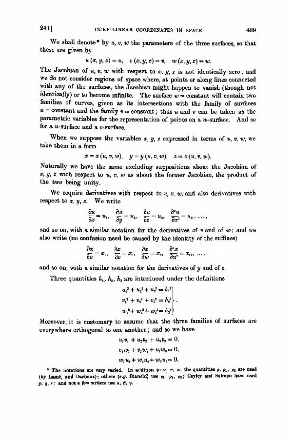
241J CURVILINEAR COORDINATES IN SPACE 409
We shall denote* by u, v, w the parameters of the three surfaces, so thatthese are given by
u (*. V> z) = m. v (x, y, z) = v, w (x, y, z) = w.
The Jacobian of u, v, w with respect to x, y, z is not identically zero ; andwe do not consider regions of space where, at points or along lines connectedwith any of the surfaces, the Jacobian might happen to vanish (though not
identically) or to become infinite. The surface w = constant will contain twofamilies of curves, given as its intersections with the family of surfaces
u = constant and the family v = constant ; thus u and v can be taken as the
parametric variables for the representation of points on a w-surface. And so
for a w-surface and a v-surface.
When we suppose the variables x, y, z expressed in terms of u, v, w, wetake them in a form
x = x (u, v, w), y = y (u, v, w), z = z (u, v, w).
Naturally we have the same excluding suppositions about the Jacobian of
x, y, z with respect to u, v, w as about the former Jacobian, the product of
the two being unity.
We require derivatives with respect to u, v, w, and also derivatives with
respect to x, y, z. We write
du _ du du 32 u
and so on, with a similar notation for the derivatives of v and of w ; and we
also write (no confusion need be caused by the identity of the suffixes)
dx dx dx &x
and so on, with a similar notation for the derivatives of y and of z.
Three quantities A,, h2 , h* are introduced under the definitions
?>,s + Vf + Vs
" = hf
iOjs+ w.?+ Wjf= hi
Moreover, it is customary to assume that the three families of surfaces are
everywhere orthogonal to one another ; and so we have
M,t>, +tt2 t>2 +US VS = 0,
VtWt + fl2M>2 + V3Wa = 0,
W]!*, + W2M2+ W3US= 0.
* The notations are very varied. In addition to u, v, to, the quantities p, pi, & are used
(by Lame, and Darbouz); others (e.g. Bianchi) use pi, p%, ps\ Cayley and Salmon have used
p, q,r; and not a few writers use a, j8, y.
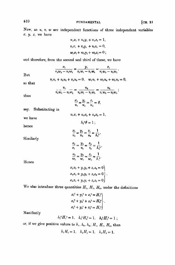
*10 FUNDAMENTAL [CH. XI
Now, as u, v, w are independent functions of three independent variables
x, y, z, we have
«,#, + w„y, + ysz1- 1,
»,.r, + v2yi + i>3 2i = 0,
w1a;,+ iw2y 1 + w3z,= 0;
and therefore, from the second and third of these, we have
x, yt z,
But
so that
thus
V2W3— V3W.2 V3W, — VXW3 «,W2
— W.W,
V,M, + V3U2 + V3U3 = 0, W,W, + W2M2 + W3 tts = 0,
Uj Uj V*
v.2w3 — y3 ?<;2 v3iv1
— v^ws v,w2— v2wx
'
say. Substituting in
we have
hence
Similarly
Hence
u, u2 w, '
«,», + M2*2 + "3*3 = 1,
we = 1
;
-' = ^i = ^- = —M, H2 M3 A,2
'
^2 _ y_2 ^2 a
Vi i>. w3 hf
'
®*_y2 _z1=: 2_w, w„ w-. h.y
XiX» + y 1 y.J + z1z2=
[
x„x, + y2y, + z.2z2= V .
x*xi + 2/32/1 + *3 «i =
We also introduce three quantities Hu H2 , Hs , under the definitions
a:,2 + y,
2 + *,•-' = #,=
«s2 + 3/2= + *,' =#2
2•
x.j> + yj + zs* = Hs\
Manifestly
V#»*-l, hJHi=l, kfHf=l;or, if we give positive values to h„ k2 , h3 , Hu H,, H3 , then
/*,#, = 1, h,H.2 =l, h sHa =l.
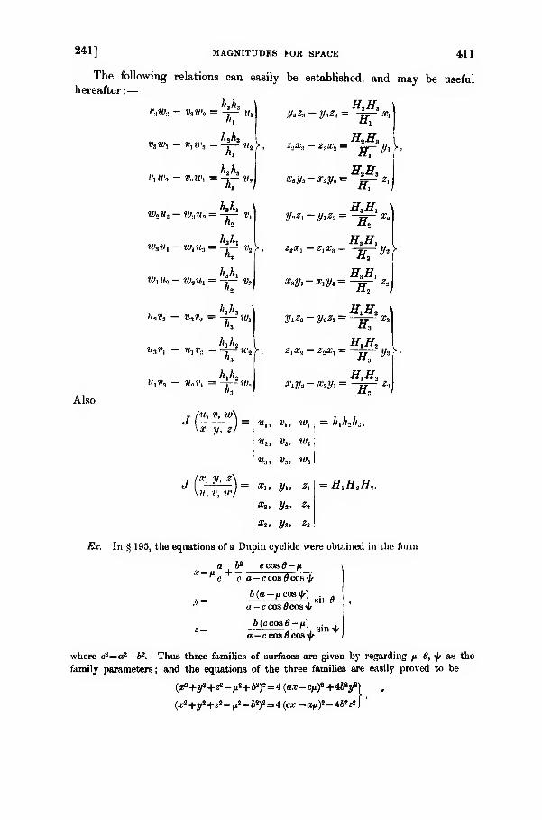
241] MAGNITUDES FOB SPACE 411
The following relations can easily be established, and may be useful
hereafter:
—
Also
III
Iuha
«i
thhac, it'., — v.,u\ = -£-= v3
h-x I
W«U.. — W,«„ = ——- Vfin
Half,
H2Haz,x.,-z3x„ =ff~ .V^>
®«y3~°rsy2= H2H3
y^i-y^t- -jj
w3 «, - w,?t3 = -j-l vtJ>
, zsx, -z,x3=
h2
Ik
hju \
K"
lij's
J'"'
W, Hi — W2M, = -~ Vs
U,V3— «3
?'., = -J—"wh
u3 v, - ?*it-
:. ='-phv,y
HtH,
H3Ht
>,
^y,-on,y3=~ Z;
HiH* \y,z,- y*z, = -^j- x3
_ H\H~.
2] #5 — ZaX) — „
H,H„
y*
u, v,w\ .
x, y, zj]
«2, v-i, w2j
U3 ,Vs , W3 \
• x»t yi> ziI
!
XSl 2/3, Z3
Ex. In ij 195, the equations of a Dupin cyclide were obtained in the form
a.
.v= n - +cco&O — Lt
.'/=
c c o-ecosflcos^
ft(a — ueosJr) . . \
u - c cos ecos i/r :
b(ccos6-u),2= * — r', 8111^
a-c cos cos ifr I
where c2=a2 -62. Thus three families of surfaces are given by regarding /1, 6, yff as the
family parameters ; and the equations of the three families are easily proved to be
(«a+y2+22 -/*2+61!
)2=4 (ar-cp)8 +46»y»)
(^2+y2 +j2-^_62)2= 4(c^-a^)2-462 22 j
'
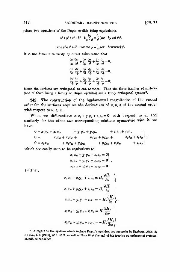
412 SECONDARY MAGNITUDES FOR [CH. XI
(these two equations of the Dupin cyclide being equivalent),
.r2+y2+22 +ft2 _ 2 _^' = i lax -by cot 6)*,•'
sin 6 c2J
x2+y2+zi+ bi - 2bz cot ^ = —2(ex— bz cosec tyf.
It is not difficult to verify by direct substitution that
dx dx dy dy dz cz _d^ d6
+ t^d6 + FH. d6 '
dx dx dy dy dz dz
d6 ty+
d6 ty+d6 3f '
dx dx dy dy dz dz
dyfr dfi rfy vp dty 3/i
hence the surfaces are orthogonal to one another. Thus the three families of surfaces
(one of them being a family of Dupin cyclides) are a triply orthogonal system*.
242. The construction of the fundamental magnitudes of the second
order for the surfaces requires the derivatives of x, y, z of the second order
with respect to u, v, w.
When we differentiate x^x„ + yx y„ + zx z^ = with respect to w, and
similarly for the other two corresponding relations symmetric with it, we
have
= ,r,xa + .Tj^s + y, y.a + y«.yn + z, z^ + z^yi
j
= x„xi3 + x3xK + y2 ?/,3 + y3yK + z„_zn + z3zK \ ;
= x,Xn + x3xK + y1ya + y3yv! + ziz23 + z3zn )
which .are easily seen to be equivalent to
x2x3l + y3y3X + z,zm = 0\ .
^#12 + y3yv > + z3 z x» = 0)
Further,
x1xll +y1yu +z,z„ = H
1
•»!*)» + yiyi! + «i«i-=^i
3/7,
du
dv
XiXn + y3yn + ztzu — — /i,dv
_ TT dHi&1&U + 3/1^13 + ZjZ13
— /I] -Tj—
«s*u + yay» + z3zu = -Ht
3/7,
dw
* In regard to the systems which include Dupin'e cyclides, two memoirs by Darboux, M€m. de
VAcad., t. li (1908), n* 1, n° 2, as well as Note iii at the end of his treatise on orthogonal systems,
should be consulted.

242]
*2*i! + y-tUn + Za2u =H2 -^
rlJf*'iffa + V^y-a. + ZXZ^ = -H.-^
x«xa + y«y.a+ z2za=H.~ \-
TRIPLY ORTHOGONAL SYSTEMS 413
««*u
+
y3yw + z,z„ = if;
8#3
3du
*i«s3 +y,yx> + Z1Z33=-Htdu
X.&U. + ys^ffl + z„jm= H„
dv
dH2
dw
*'s*ai + y3ya + ZiZv = -H.aff„
bw
XzX-a + y3ya + Z3Za =H3 -^
«2*S8 + ##33 + 3j3b =-H,
dH>
V
oH3
h
dv
TiJT
«3#3S + 2/3^33 + ZzZn =H3 -g—
*
The direction-cosines of the normals to the three surfaces are given by
7l =A l
=Fl
a _ ~^i _ ys_ _W% Za
h3 U3" h3 H3 i
«1 #1
''fh'H/
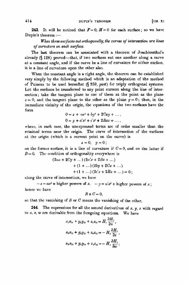
114 dupin's theorem [ch. XI
243. It will be noticed that F=Q, M=0 for each surface; so we have
Dupin's theorem :
—
When three surfaces cut orthogonally, the curves of intersection are lines
of curvature on each surface.
The last theorem can be associated with a theorem of Joachimsthal's
already (§ 128) proved—that, if two surfaces cut one another along a curve
at a constant angle, and if the curve be a line of curvature for either surface,
it is a line of curvature upon the other also.
When the constant angle is a right angle, the theorem can be established
very simply by the following method which is an adaptation of the method
of Puiseux to be used hereafter (§ 259, post) for triply orthogonal systems.
Let the surfaces be transferred to any point current along the line of inter-
section; take the tangent plane to one of them at the point as the plane
z=0, and the tangent plane to the other as the plane y = ; then, in the
immediate vicinity of the origin, the equations of the two surfaces have the
form= z + ax- + by2 + 2Cxy + ...
,
= y + a'a? + c'z1 + IBxz + ...
,
where, in each case, the unexpressed terms are of order smaller than the
retained terms near the origin. The curve of intersection of the surfaces
at the origin (which is a current point on the curve) is
z = 0, y = 0;
on the former surface, it is a line of curvature if (7=0, and on the latter if
B — 0. The condition of orthogonality everywhere is
(2ax + 2Cy+ ...)(2a'x+2Bz + ...)
+ (l + ...)(2by + 2Gx+...)
+ (l + ...)(2cz + 2Bx+ ...) = 0;
along the curve of intersection, we have
- z = as? + higher powers of x, - y = uV + higher powers of x;
hence we have
B + C = 0,
so that the vanishing of B or C means the vanishing of the other.
244. The expressions for all the second derivatives of x, y, z with regardto u, v, w are derivable from the foregoing equations. We have
*y»u + ytyn + ^zxx = - #,—'
,
&w

244]
and therefore
SECOND DEUIVATIVES 415
1 dH, I H, MT,\,
/ Hl dH,\
^11 — 2t "J
Again,
1 3-ff, / #, dUAH3
* dioj!
9#2
dw
and therefore
i a/f., i 8if3 \
i bh. i a#3 ,
i dH2 i a/£Z*- Z
*~H% dw+ Z*H3 dv)
It may be noted that the last three equations are the forms of equations of
conjugate systems on the w-surface; as they are also orthogonal, they are
necessarily lines of curvature. Similarly for the other surfaces.
The corresponding results for the other derivatives can be obtained by
the cyclical interchange of variables. The remaining formulae which, with
those already given, constitute the full aggregate of second derivatives, are
as follows:
—
/ H, dH.\ I 1 dH.,\ l R. dH,\\x"- Xi
[ H? du)+ ** \H, 'dv J
+ a '
3 1~ H} ~to)
**-**[ Hf du)+ Zi \Hi dv)
+ Za\ H3*dw)
1
J_ dH3 J_ dH,\X"- Xi H3 du
+Xl H1 dw
i a#, 1 dH,y*~ y* H> lu~
+ yi H\ dw
1 dH3 1 dHjZ»- Za H3 du
+Zl H,dw
>;
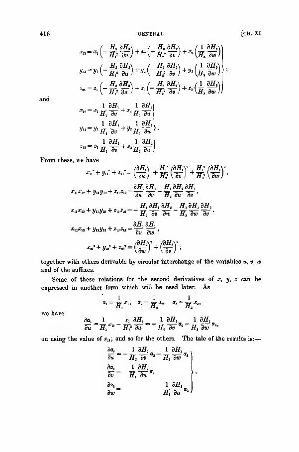
416 GENERAL [CH. XI
and
/ H, BHa t H, dHt\ / 1 3x7,\\
(x73 3x73\ / H3 dH2\ / 1 3x7,\ .
*-*\~W *) +*\-WtW) +*\M, to) ['
i 3#, i 3^,\
1 dH,
to
1 3x7, 1 a#s )
i 3#, i dH.Z"~ Zl
H, dv+ *iH1 du
From these, we have
3/z , 37i , ifi 3xf», 3xiiXnXa + y,,yB + Zn*12
="sir "air
~ f, as-
"ar
il , 3^J3X1
a
X7, 3/7, 3xi 3
3x7,3x7,
together with others derivable by circular interchange of the variables u, v, wand of the suffixes.
Some of these relations for the second derivatives of x, y, z can be
expressed in another form which will be used later. As
1 1 10, — "IT fl> ai~ W "*»> a3~ TJ Xl>
//, -"4 -"a
3a,_J_ J£L 3^_ 1_3#, 1 3xf,
3» "if,"*" H? du "//. 3i>
"»x7, 3w
a*'
we have
on using the value of a;,,; and so for the others. The tale of the results is:
—
5a,

245] FOKMULiE 417
3as
du
dv
da,
div
±dH,H3 dw
1 dH3
"s-W
H, dvUl
1 327,,
if, 9u'
= tt -rr-asJ7, 9v
1 3tf,9a»
3« * #3 3w"'
—3 = i aff,
?* = _ L ^s i 9-g3dw ~H, du~* H2 dv
'
together with corresponding results for ft, &, & and 7,, yt , y,.
Further, it is important (especially for some of the equations of triply
orthogonal systems) to associate a magnitude
= a? + y" + z1
with x, y, z, and to have the corresponding equations ; these are
«.-W-«(-§»*) +*£«5 + *(-gg) ['
and
3ff3
ft* \_ fl
1 3/r2 . 1 air.,--Hs dw-
+ °3 Hs ^dV
°S1 ~ °* h\ "air+ "• h\ ~dw~
_ 1 dH, iaff,Pl2 " Pl
/f1 "3ir+ t'2
jy2 "aT
It will be noticed that the forms of the last three equations are the same as
the forms of the corresponding equations for x, y, z—a property to be
compared with the corresponding property, noted in § 77, for surfaces when
they are referred to lines of curvature as parametric curves.
245. As the fundamental magnitudes of the three surfaces are known,
and as the parametric curves are lines of curvature on each of the surfaces,
the principal curvatures can be written down at once.
For the surface u= a, the principal curvature along v = b is N/G, that is,
1 9#s .
HXE% du
F, 27
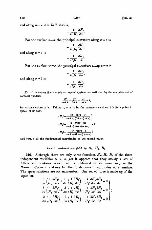
418 lam£ [ch. xi
and along w = c it is LjE, that is,
1 BH,
H& du"
For the surface v = b, the principal curvature along w = c is
j aff,
and along it = a is
HA dv'
For the surface w = c, the principal curvature along u= a is
j_ affa
and along v = 6 is
j_aff,#,#, aw
"
/sir. It is known that a triply orthogonal system is constituted by the complete set of
confocal quadrics
a+X + 6+X + c+X '
for various values of X. Taking u, v, w to be the parametric values of X for a point in
space, shew that
1(a+ u)(b+u)(c+u)
A ffJ(»-«)(»-«)
;
(a+v)(b+ v)(c+»)*2"
3 (a+w)(b+w){c+,
and obtain all the fundamental magnitudes of the second order.
Lame relations satisfied by Hx , Hit H3 .
246. Although there are only three functions Hlt Hit Hz of the three
independent variables u, v, w, yet it appears that they satisfy a set of
differential relations, which can be obtained in the same way as the
Mainardi-Codazzi relations for the fundamental magnitudes of a surface.
The space-relations are six in. number. One set of three is made up of the
equations
} dw dwdu \H, du) dv KH, dv) Hf
dv UT3 dv )+ dw\Hs dw) H? du du
'
d_
dw(1 *JL\ + A (1 aJL»U J_ dlL a-^i - n I
\H, dw)^du\H1 du)+Hi 9i> 9» /
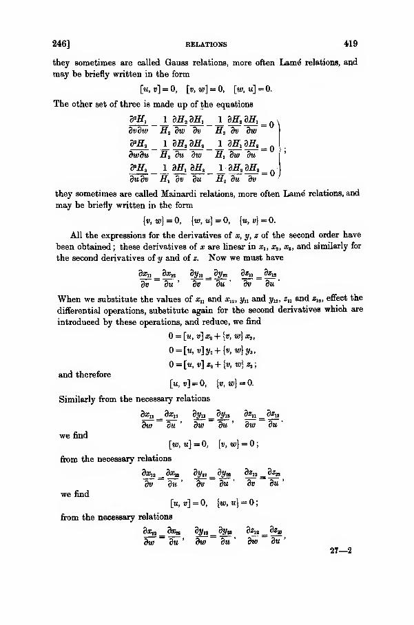
246] RELATIONS 419
they sometimes are called Gauss relations, more often Lame" relations, and
may be briefly written in the form
[m, v] = 0, [v, w] - 0, [w, u] = 0.
The other set of three is made up of the equations
d°H, 1 dH2 dH, 1 dHs dHx
dvdw Hi dw dv H3 dv dw
d*H2 1 dH3 dH2 1 dHdH2
dwdu H3 du dw Hx dw du
d>H„ 1 dHx dH3 1 dH3 dH3
=
=
=du dv H dv du H2 du dv
they sometimes are called Mainardi relations, more often Lame relations, and
may be briefly written in the form
{v, w) = 0, [w, u] = 0, {u, v} = 0.
All the expressions for the derivatives of x, y, z of the second order have
been obtained ; these derivatives of x are linear in x,, xit x3 , and similarly for
the second derivatives of y and of z. Now we must have
dxn _ 9xi2 dyn _ dya dfn _ (ten
dv du ' dv du dv du'
When we substitute the values of xn and as,,, yu and yw , zn and za , effect the
differential operations, substitute again for the second derivatives which are
introduced by these operations, and reduce, we find
= [w, v]x2 +{v, w}x3 ,
= [u,v]y2 + [v,w}y3 ,
= [u, v] z2 + {v, w\ z,;
and therefore
[m, v] = 0, {v, w\ = 0.
Similarly from the necessary relations
dxu _ dxn dyn _ dy^ dz^ _ dza
dw du ' dw du dw du
we find
[w, u] = 0, {v, w\ - ;
from the necessary relations
dxw _ dx& dyn _ dyn j^i? _ 9fa
Hv ~ du ' dv du ' dv du'
we find
[u, v\ = 0, {w, u) = ;
from the necessary relations
dx^ _ dxn <tyia _ tyln 3*» _ <^»
dw ~ du ' dw ~ du ' dw du'27—2
420 LAME RELATIONS [CH. XI
we find
[w, u] = 0, [w, u} = ;
from the necessary relations
dxa _ da^ dy„ _ dya dz^ _ dz^
dw ~ dv ' dw dv ' dw dv'
we find
[v, w] = 0, [v, w] = ;
from the necessary relations
dxu _ dx^, 92/js _ dy& dz^ _ dz&
dv~ du ' dv du ' dv du
'
we find
[u,v] = 0, {u,v} = 0;
from the necessary relations
9#jj_3a^ dyia_djfa d£a_dz^dw du. ' dw du dw du
we find
[w,u] = 0, {u, v} = 0;
from the necessary relations

248] EXTENSION OF BONNET'S THEOREM 421
But the equations are special in form, and have (in the two sets) a circular
symmetry in the variables; and so they may possess common solutions.
Thus a question arises as to whether any conditions must be satisfied in
order that the equations may coexist. Our concern, however, is rather withsystems of surfaces than with systems of equations ; and so the question will
rather relate to the conditions that may be required of families which canbelong to triply orthogonal systems.
The two questions will be taken in turn.
Extension of Bonnet's theorem (§ ,37) to space.
248. Accordingly, we proceed to investigate how far a triply orthogonal
system is determined by three quantities 27, , 272 , Hs , which are given in
value and satisfy the six characteristic partial equations of the second order.
The equations to be satisfied by the coordinates of a point in space, beingthe intersection of particular members of the three families (if they exist),
are three sets for each coordinate. One of these sets is
/ 27, 322,\ ( 27,327a _,
27, du'
1 327, 1 dH2
** XlH1 ~to~a:°H2W ~°
1 32/, 1 327s _„
being a set linear in x1} x2 , x3 , and in their first derivatives with regard to w.
The other two sets for x also are linear in xlt x2 , x3 , and in their first
derivatives with regard to v and to w respectively. The three sets coexist,
after the earlier analysis of § 246, provided the six characteristic equations are
satisfied by 27,, H*, H3 .
As the foregoing set of equations is linear in xu x2 , x3 , the primitive is of
the form
#i = foi + vh + ?c,
x2= fan + i)bi + fcjj
x3= ^a3 + t)bs + fc3
where f, 17, f are arbitrary functions of v and w, and where three linearly
independent sets of particular solutions are given by
= b1 , b2 , b3 ;
= c,, c2 , c3 .
Also, no limitations upon f, 17, f are imposed by the above set of differential
equations.
422 EXTENSION OF [CH. XI
249. The second set of equations in the derivatives of x is
Xj, Xj -
1 35, 1 dHt ='Htdv *H*du
( H2 dHt\ 1 dH, / H*dH3\'
a;B #H1 3#2 1 dff3
Ht dw 'H3 dv=
if the triply orthogonal system exists, this set must be satisfied by the
primitive of the first set. When
are substituted in the left-hand sides of these equations, let the latter become
Au A 3 , A, respectively* ; and similarly let them become Bj, B2 , B3 when
xlt xa , x3= bi, b2 , b3
are substituted, and become C,, Ct , C3 when
xlt xlt x3= C], c2 , c3
are substituted. Then, in order that the foregoing set may be satisfied by
the primitive of the first set, it is necessary and sufficient that the equations
3f9av
ft, ar-, + 6
« s=
+
c*g = - (?^« +^ +
?
c=)v
should be satisfied by values of f , 77, f which are independent of u. This last
requirement will be satisfied if, at the same time, the equations
3a, 3f db.dr, 3c, 3? /„34, ,35,
,
„3C,\\
3m du 3u 3u 3u * 3u /
3-B2 . ..SCV3a,3| 36j3j 3c2 3f _ _ /j.3_4j gi*, ^3C'a
3m 9w 3m 3v 3m dv \ du du du)
3a, 3| 36s 3^ 3c8 3? /\.dA 3 dB3+ ^dC^= _(>^.„3u dv ' du dv
T3m dv \ du
"^' du
""" b 3m A
also are satisfied. That they are so satisfied, in connection with the equations
which now define f, 77, f, can be established as follows.
Take the set of equations now defining f, 17, £i and multiply them by
_i_m, .&, 3#, _M± dJL-
Ex du' H? dv
' H3> dw '
then adding, and remembering that xlt x2 , x3= a,, Oj, a, constitute a particular
* The quantity J, formally is zero : it is retained for the sake of symmetry.
2*9] bonnet's theorem 423
system of solutions for the first set of three equations in x, and similarlyfor «,, asj, x3 = bu ba , ba , and for xu xs , x3
= c,, cit cs , we have
d^d^ dbidr) dcjd^
du dv du dv du dv
--p(A ±**l-A *l dE> AH> dHA? V11H
r duA2H3*-to~-
As Hj ~fa)
(n 1 dHx Hx BHt Hx 3JTA
'I'l, du ~"*W"to~ *H}fa)
Similarly for the second and the third of the set of equations for f, y, £Accordingly, they all will be satisfied, if only nine relations of the type
dAl- A 1 dJ*l- A Ml ^Ml i Ml dJLdu
l Hx du *H* dv "Hf dw
are satisfied. Now
so that
. _ 13ff, 1 dHt
dA}_da^_ J^dHi ±dH* If 1 dMl\ _ A (1. dM?\
du ~ duaaHl dv ""H* du ^ du Iff, dv) ^duKHzdu)-
But
du dv
1 dHx= <h
I Hx dHx\ I Hx dHx\
Hx du+ a*\~H* dv )
+a»{~ Hi fa)
d /j_ affA ^ /^ mta ^ (Mi dMi\+ a' 8v Ur, du) ^dvW2
2 3r /a° dv \H3
* dw )'
In the expression for ^—i, insert this value for -^— ; substitute for an , a12
from the original equations which they satisfy;gather together the terms in
0^, tij,, and substitute for affl , aw from 4 2 , -A a : then, after reductions which
are merely laborious, we find
dA. i. Hx dHx , Hi dHx
fa= ~ *K?-dT~ 3H}dw -
Also A x= 0. Hence the first of the nine relations is satisfied.
In precisely the same way, the other eight of those relations can be
proved to be satisfied.
424 EXTENSION OF [CH. XI
Consequently the three equations defining £, 77, f possess a primitive
in which f, 77, f occur as functions that do not involve u. As those equations
are homogeneous and linear in f , 77, ? and their derivatives with regard to v,
the primitive is of the form
/ ,it . a
V = P7) + <"? + T1?
? = />£'+*-?" + <'
where p, <r, t are arbitrary constants so far as derivation with respect to v is
concerned ; and where £', 77', £" are one special set of solutions, f", 77", f" are
another special set, and f '", 77'", f"' are a third special set, these three sets
being linearly independent of one another. When these values of f, 77, f are
substituted in a?,, x2 , x:„ we have
,r, = pot, + a/9, + T7,)
a'2 = pa, + <ry3o + T72 )
#3 = pa3 + 0783 + T7Sj
as the simultaneous primitive of the first two of the three sets of equations
satisfied by x ; and p, <r, t are (so far as concerns these two sets) arbitrary
functions of w. AlsoX,, X2 , £3 ~ &l> ®2> ^3 J
= &> A. A;= 7i. 7s> 7a;
are special simultaneous sets of solutions of the two sets of equations.
250. The third set of equations for x, viz.
1 as,1
H, dtv~ «^a ttH3 du
= 0\
1 dH> - o
#3 9^f3 ,1 Stf,
Xi H3 dw ~ °i
1 dH2
H2 dw
H3 dH3
H2* dv
must be satisfied. All that remains at our disposal for satisfying them are
three arbitrary (and so disposable) functions p, <r, t, of w. The procedure is
similar to the procedure for the preceding set ; the difference lies in the fact
that, when the linear equations of the first order for p, a, t are formed, two
subsidiary systems have to be satisfied instead of one alone. All the necessary
tests are satisfied in virtue of the six relations between Hu H2 , H3 ; and the
result is that the most general values of p, a, r are
p = \p, + fip2 + vp31
a = Xtr, + fia2 + va3 >;
T = XT, + flT2 + VT3 J
251] BONNETS THEOREM 425
where \, p, v are arbitrary constants; and where the other quantities are
functions of w only, forming linearly independent sets of solutions of the
equations for p, a, r.
When these values are substituted in the expressions for x1: x2 , x3 , wehave (as the ultimate primitive of the nine equations satisfied by x) the
expressions
xi= \X 1 + fiY1 + vZl
x2 = \X2 +pY2+ vZ2.
x3 = \X3 + fiY3 + vZ3
The quantities X, ft, v are arbitrary constants; the other quantities are
functions of u, v, w, which combine to form special sets of simultaneous
solutions of the equations.
The equations determining yl , y„, y3 are precisely the same as those for
xx , ,r2 , x3 ; hence their primitive is
y^X'X. + ^'Y + v'Z,
y2 = \'X2 + fi'Y2 + v'Z2 -.
y3 = \'X3 + fi Y3 + v'Z3
where X', /j,', v are arbitrary constants. Likewise as to the equations
determining zu z2 , z3 ; their primitive is
zx = X"Xi + (i"Yi + v"Zi
z2 — \"X2 + fi"Y2 + v"Z2
z3 = \"X3 + /i"Ya + v"Z%
where X", ji", v" are arbitrary constants.
251. Thus the complete primitive of all the equations together appears
to contain nine arbitrary constants. But these equations are not independent
of one another ; they are differential inferences from the earlier equations,
viz. from
#i2 + y? + z? = Hf, x2x3 + y2y3 + z« z» - P,
x<? + yi + z£- H^, x3xx + y3yx + z3zx= 0,
«»5 + y* + z*=Hs, «;lx1 + yxy2 + z1z2= 0;
consequently the complete primitive, which has been obtained, must satisfy
these equations also. When substitution takes place in the first of them, we
have
XflX- + 2Z1F1 2x,t + 2X xZ^\v + Yx-V + 2Y1Zllt
iv + Z&v* = Hf.
But Xlt Yi, Zx= xx , yu zu constitute a special solution, so that
Z,« + F,» + *,•-&,*;
hence, writing
*, = 2Xa -l, k2= S\fi, k3 = 2\i>, k-lfP-l, k^lfiv, £, = 2i»*-l,
426
we have
EXTENSION OF BONNETS THEOREM [CH. XI
IA 4 2Z 1F1 /fc!! + 2Z1 £,/fcs + Yfa + 2YXZX + Z,% = 0.
Treating the other equations in the same way, we find
XtXtk + (X,Y, + X.Y^k, + (X& + X&) k3+ Y.Y.k,
+ ( Y,Zt + 7A) ks + Z>Ztk, = 0,
2r Iz,t,+(ZI r,+x,FI)*i+(2rIz,+^IzI)*b+FlFIt,
+ (YyZs + Y3Z,) k„ + Z,Z3k3= 0,
X,% + 2XiYiki + 2Jr,£l£b + FA + 2Y2 Z„ks + Zt% = 0,
XtX,k + (X,YS + -YSFS)L + {X2Z3 +XSZ2) k3 + Y,Y3kt
+ (Y2Z3+ F,Z2) fc5 + Z,Z3ks= 0,
A',2*, + 2X3Y3k, + 2Ar3Z(fcs + Y3% + 2Y3Z& + Z,% = 0.
Thus there are six equations, homogeneous and linear in the six quantities
&,, ks , k,, kt , JfcB , ke . The determinant of the coefficients of the six quantities
in these equations is equal to
x»
251] CONFORMAL REPRESENTATION OF SPACE 427
The theorem is the extension, to triply orthogonal surfaces in space, of
Bonnet's theorem (§ 37) concerning the determination of a surface in general
by its fundamental magnitudes. After the theorem, a knowledge of appro-
priate quantities Hu Ht , Hs is sufficient to ensure the existence of a triply
orthogonal system ; the difficulty is to obtain this knowledge.
Ex. As an illustration of the use of these equations, consider the conforms! repre-
sentation of space upon itself.
Let x, y, z be the coordinates of a point in space ; and let u, v, w be the coordinates of
the associated point in the conformal representation. The arc-elements are given by
d#=dxt+dy*+df, di(*=dui + dvi+dwl.
As the representation is conformal, we must have
ds'=~Kds,
where X is any variable function free from differential elements ; hence
dxt+df+dz^^dtf+difi+drf).
Consequently
Let these values be substituted in the three relations of the type
8»2Ti _ J_ 3#2 dHi _ J_ aff3 dj?i =0 .
dvdw H2 dw dv £T3 dv dw '
they give
_^_ 1L=0 ^=odvdw ' dwdu ' dudv
'
so thatX=U+V+W,
where (so far as these relations are concerned) U is any function of u alone, V of v alone,
and W of w alone.
Let the values of Hu H2 , H3 be substituted in the three relations of the type
hi \H\ lu) +dv {Hi dv J
+J73
2 ?'" 3» '
they give three equations of the form
dtf+ dv*-\ \\du) * \dv)
T\dw) J
Inserting the value of X, we find
U"+ V"= V"+ W"= W"+ U"
U'2 + V'2 + W'°-—u+v+w •
HenCCV'-V'-W;
and therefore, as U, V, W are functions of it alone, v alone, and w alone, respectively, we
must have
U"= F'= W'"= - or 0,a
where a is a finite constant.
428 CONFORMAL REPRESENTATION OF [CH. XI
Taking the common value of U", V", W" to be 2/a, we have
Vml (t-btf+b,,
W=l{W - ei)Hct,
where the new quantities a, 6, c are constants. But
TJ-i a. y* + W*+ U+V+W '
when the values are substituted, we must have
a2+fe2+c2= 0.
Hence, changing the origin for u, v, w (which amounts only to a displacement in space),
we have
X = U+ T+ W=l («*+ »*+«*),
while
Hx= Ht = H% = ^ .
Let this value, common for #,, Ht , H3 , be substituted in the equations for the
derivatives of a,, a2 , a3 , obtained in § 244. They become
3a, 2.^- = - {Vai+Wa3),
252] SPACE UPON ITSELF 429
Similarly
'M'+ flS+W2 '
._£_ «WU3+ W2+M2-
These equations express an inversion with respect to the sphere
v?+v2+wi=a.
Next, taking the common value of V", V", W" to be zero, and noting the relation
+ u+v+iv '
we have U\ V, W zero. Hence U, V, W, A, Hu Ht , Hz are constant, and so theequations for x, y, z, when integrated, give
x—A, y-B, z-C=( a, a', a" \u, v, w),
b, V, b" I
c, c', c"I
where the constants a, 6, c on the right-hand side are proportional to the direction-cosines
of three perpendicular straight lines. These equations express displacement and rotation,
with constant magnification.
Hence there are only two independent methods of representing space conformally
upon itself, viz.
(i) by displacement and rotation, together with constant magnification,
(ii) by inversion.
The two methods can be repeated and combined in any manner and any number of times.
252. The difficulty of determining Hlt H2 , H3 does not depend solely
upon the fact that, by one method of procedure, we should be obliged to solve
a number of simultaneous partial equations of the second order. An added
complexity is caused by the fact that the number of independent equations
in the system is greater than the number of dependent variables involved
;
and so even Cauchy's existence-theorem cannot be applied to the system.
A preliminary investigation reveals the degree of generality which is the
utmost to be expected among such solutions as exist. In order that three
surfaces
u(x, y, z) = u, v(x, y, z) = v, w{x, y, z) = w,
may be orthogonal to one another (the quantities u, v, w on the right-hand
sides being parametric), the equations
VtW, + DjWa + vswa = '
Witt, + W2Ut + Wjtta =
must be satisfied. Let
-Sl= v1wl + v2wt , -S3 = w1 ri1 + wtut , -S3 = u
lv1 + uivi ;
430 EQUATION OF THE THIRD ORDER [CH. XI
then resolving the equations for w,, v„ w3 , we find
/S,S,\l /&SA* /s,srf
This is a set of three partial equations of the first order in three dependent
variables, and so we can apply Cauchy's theorem, as follows. Take any
arbitrary (constant) value of z, say* z = ; and let o, /8, 7 denote three
arbitrary functions of x and y, such that no two of the curves
a= constant, /S = constant, 7 = constant,
in the plane of z cut orthogonally. Then the quantities Slt S2 , <S„ do not
vanish when z = ; and so, within some range of values of z, the values of
the branches of «s, vs , w3 are uniform and continuous. Then Cauchy's theorem
declares that unique uniform functions v, v, w exist, satisfying the partial
equations, and acquiring the values a, £, 7 when z = ; in other words, a
triply orthogonal system exists, determined by the condition that three surfaces
pass through any three assigned curves in the plane of z, provided no two of
these three curves cut one another orthogonally. (The same limitation must
hold for any set of three curves in the plane through which any three of
the surfaces would pass.)
We have taken any plane z = 0. A corresponding theorem, with corre-
sponding limitations, would hold if we chose curves in any plane in space or
curves on any surface in space.
The importance of the result is obvious. The utmost degree of generality
that can be expected from solutions of the six characteristic equations corre-
sponds to the generality represented by the assignment of three arbitrary
functions of two variables.
The critical equation of the third order.
253. To make some nearer approach to the actual determination of
triply orthogonal systems, we proceed once more from the conditions of
orthogonality as follows. From two of them, we have
% ¥2 ¥,'
where
^i = W2U,- W3 U2, ^fi=wzui— w^ul , ^3 = w1u2 —w2u1 .
In order that the function v may exist, it is necessary and sufficient that the
equationV1dx + Vidy + -Vtdz = Q
* This particularisation involves no lose of generality ; it only implies a change of origin of
coordinates.
253] FOB ORTHOGONAL SURFACES 431
should have a single equation as its integral equivalent ; hence the condition
of integrability
must be satisfied. Now
-gy - aJT= "i^w -w^u - («,«;„ + «2wls + %%) + (w1uil + w2it„ + u>j«,3),
where
da? By* dz2'
Moreover, the remaining equation of orthogonality is
«!«>! + w2w2 + u3wt= 0,
so that
UlWll + M2Wj2 + V^WK + W,M„ + W2M,2 + «V«M= J
hence
Similarly for the other quantities of the same kind. When the values are
substituted, the condition of integrability becomes
W1 Uu + WsUn + «>,«!„ W,, tt, =0,
which, on multiplication by 2, can be written
Aw? + Bwf + Cwt* + 2Fw*wa + 2Gwiw1 + 2ifw,w2 = 0,
whereA =2(M2 ttlil -u,ww), F = ii1ua —u2uxl + ti3u13 — u1um
B = 2 (MjMsi - Wiltjs), 6r = KaMx, - ItaMas + "lWji ~ MsMn " •
C = 2 (WjMsj - WjMjn). E = MjMn - tt, M,i + U,Ub - tt3M„
Manifestly the same equation would be satisfied, if we write «,, v2 , t>3 in place
of w„ w2,w3 .
When we associate the equation
«,«/,+ MjW, + w3w3=
with the preceding relation which is homogeneous and quadratic in wit w2 , ws ,
and resolve the two equations for w, : w2 : w„, we find
«,,:«/,:«,, = £7: 17' : U",
where J/", £/', 17" are two-signed functions of A, B, C, F, G, H, «„ it,, it,.
(For one of the signs, we have w, : w2 : wt , while the other gives the values of
w, : »2 : flj.) In order that the function w may exist, the equation
Udx+U'dy+U"dz =
432 CRITICAL EQUATION OF [CH. XI
must satisfy the condition of integrability ; hence
\oz dy / \dx oz
)
\oy ox /
This relation is not evanescent. It remains as a partial differential equation
of the third order satisfied by v (x, y, z). Moreover, all the foregoing analysis
is reversible; hence this condition is sufficient as well as necessary. So wehave the theorem :
—
In order that a family of surfaces, represented by
u (x, y, z) = constant,
mayform part of a triply orthogonal system, it is necessary and sufficient
thai u should satisfy a partial differential equation of the third order.
254. Should the equation be satisfied by u (x, y, z), it still is necessary
to determine v(x, y, z) and w(x, y, z), in order to have the full system.
These two functions satisfy the same equation of the third order as u (x, y, z);
but it is unnecessary to take further solutions of that equation. We have
seen that quantities U, U', U" in the preceding analysis arise, as two-
signed functions ; let U, U', U" denote one set, and T, T', T" the other set,
all of them involving derivatives of u alone. Then
w1 :w2 :Ws=U: U' : U",
v, : v, : v, = T : T' : T".
The condition of orthogonality ought to be satisfied, so that we ought to
haveUr+U'T'+U"T" = 0.
Now the two sets of ratios are given by the equations
Ap + Bv* + C? + 2FVZ+ 2G&+ 2H&, = 0,
fit, + ijMa + fM3 = ;
hence
UT U'T__
U"T"Bui1 + Cuf - 2J^U3
=Cu,s + Av-f- 26rM,M,
~~ Au? + Bvf - 2'ffu^u3
'
It is easy to verify that
A + B + C= 0,
AuS + Buf + Omj2 + 2Fum, + 2GUJW! + 2i7u,M2= :
henceur + u'?'+ U"r" = o,
so that the condition of orthogonality is satisfied without any further
conditions.
The surface, w (x, y, z) = constant, is obtained by the integration of the
equation
Udx+U'dy+U"dz = 0;
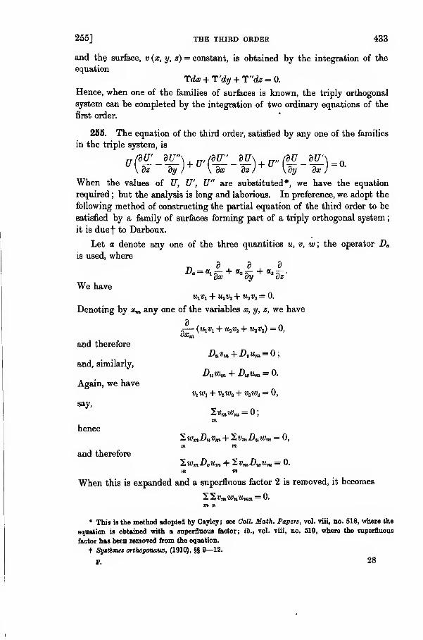
255] THE THIRD ORDER 433
and the surface, v (x, y, z) = constant, is obtained by the integration of the
equation
Tdx + T'dy + T"dz = 0.
Hence, when one of the families of surfaces is known, the triply orthogonal
system can be completed by the integration of two ordinary equations of the
first order.
255. The equation of the third order, satisfied by any one of the families
in the triple system, is
\az dy j \ ox dz
)
\oy ox J
When the values of U, U\ U" are substituted*, we have the equation
required ; but the analysis is long and laborious. In preference, we adopt the
following method of constructing the partial equation of the third order to be
satisfied by a family of surfaces forming part of a triply orthogonal system
;
it is duef to Darboux.
Let a denote any one of the three quantities u, v, w; the operator D*
is used, where
D-= a^ +a
*dy+
"°dz-
We haveitji), + u2v2 + uavs= 0.
Denoting by xm any one of the variables x, y, z, we have
- (it,!)! + «3«s + U3V3) = 0,
and therefore
and, similarly,
Again, we have
say,
hence
and therefore
dx„
Duvm +Dv um = 0;
Duwm + D„Um = 0.
!),«/, + ViW2 + V3WS — 0,
Svmw,„ = ;
m
1wmDuvm + *ZvmDuwm = 0,m m
lwmDvum + 1vmDwum = 0.
When this is expanded and a superfluous factor 2 is removed, it becomes
m n
* This is the method adopted by Cayley ; see Coll. Math. Papers, vol. viii, no. S18, where the
equation is obtained with a superfluous factor; ib., vol. viii, no. 519, where the superfluous
factor has been removed from the equation.
+ Systemes orthogonaux, (1910), §§ 9—12.
F. 28
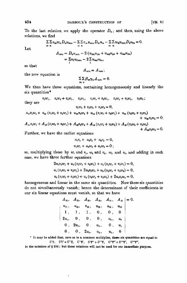
434 DARBOUX S CONSTRUCTION OF [CH. XI
To the last relation, we apply the operator Du ; and then, using the above
relations, we find
Z1vmwnDu'umn - 2,Svm umnDwun - S%wnumnDvum = 0.
m n vi » m nLet
"run = D„ltmH ~ 2 {UmiUln + Um<M->„ + Uva^an)
so that
the new equation is
= 2MJMiIB„-22«miMi„,i i
"mn — -"n?n >
S2y9m7„il,nn = 0.
We thus have three equations, containing homogeneously and linearly the
six quantities*
»,«;,, v1w1 + v2wi , v2iv», vlw3 + viw1 , v2w3 + v3w2 , v3w3 ;
they are
VjWj + v3w2 + v3w3— 0,
"li^iWi + itj2 (t>,tt/2 + U2Wj) + MaVjWa + M,3 (vtW3 + V3Wi) + U^ (v2W3 + V3W2)
+ u33v3w3= 0,
-diifiW, + A 12 (VjW2 + VtfVi) + AaV2W2 + A 13 (t^H/, + VaWt) + An (v2w3 + V3W2)
+ AnVnW, = 0.
Further, we have the earlier equations
UiV1 + U2V2 + lljl's = 0,
?*,«>! + u^w% + u3w3=
;
so, multiplying these by w, and vlt tv2 and v2 , ws and v3 , and adding in each
case, we have three further equations
2u 1ViW1 + Ms (V,W2 + »,«;,) + H3 (fl,W3 + W3Wi) = 0,
«, (i;,w>, + t^w/,) + 2u2v2w2 + u3 (v2w3 + v3w2) = 0,
it, (d,w3 + v3w,) + «2 (w2w3 + v3w2) + 2u3V3w3= 0,
homogeneous and linear in the same six quantities. Now these six quantities
do not simultaneously vanish; hence the determinant of their coefficients in
our six linear equations must vanish, so that we have
"11 > -"22> •"33> "23> -"81) -"-12
|"11 >"l
1 ,
2u„
1 ,
0,
, 2w2 ,
1 ,
0,
.
0, 2w3 , Ma
**31 > **12
,
u3 , Uj
. M,
Ml,
= 0.
* It may be added that, save as to a common multiplier, these six quantities are equal to
err, irt'+vr, err, ur"+u"r, vt'+vt, vr",in the notation of § 254 ; but these relations will not be used for our immediate purpose.
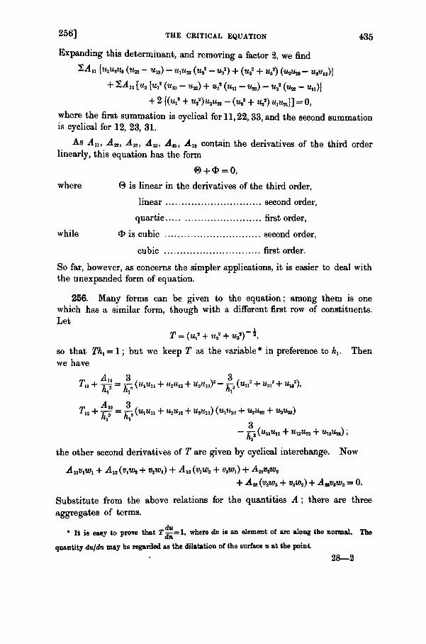
256] THE CRITICAL EQUATION 435
Expanding this determinant, and removing a factor 2, we find
2A„ {ujMjM, (l^ - Uaa) - M,«a (u* - «32) + («2
2 + U32) (i^lt,, - «,«„)}
+ 24 12 [m3 \u? («„ - «„) + u* («,, - «„) - «,» («„ - u,,)}
+ 2 {(w,2 + uflu&, - (l*,2 + M,3) MAl }] = 0,
where the first summation is cyclical for 11, 22, 33, and the second summationis cyclical for 12, 23, 31.
As Au , A&, j4jb, A&, An , An contain the derivatives of the third order
linearly, this equation has the form
@ + <I> = 0,
where © is linear in the derivatives of the third order,
linear second order,
quartic first order,
while $ is cubic second order,
cubic first order.
So far, however, as concerns the simpler applications, it is easier to deal with
the unexpanded form of equation.
256. Many forms can be given to the equation; among them is one
which has a similar form, though with a different first row of constituents.
Let
r =(«," + «,* + «,*)"*.
so that Thi = 1 : but we keep T as the variable* in preference to A,. Then
we have
A 3 3Tn + -^ =^ (w,w„ + «,«,, + u3u 13f - j-3 (u,,
2 + «,./ + U,32)>
A 3TK + -j-j = j-s (tt,Uu + U2M12 + M3?«is) («l«l'i + 1*2^ + M3W2,)
-J-„
("iiMit + «u«a + «13«2>) S
the other second derivatives of T are given by cyclical interchange. Now
AiMWx + Anfaw, + «2w,) + -A 13 (viWs + w3w,) + Aav2w2
+ Aa (v2w3 + v3w2) + Amv3w3 = 0.
Substitute from the above relations for the quantities A ; there are three
aggregates of terms.
* It is easy to prove that T-j-=l, where dn is an element of are along the normal. The
quantity dufdn may be regarded as the dilatation of the surface u at the point.
28—2

436 FORMS OF [CH. XI
In one aggregate, we have a set involving the second derivatives of T,
the same in form as the left-hand side of our equation with a factor hr*.
The aggregate of terms with the factor 3Ai-5
is
dhi 8Aj 3AA / dht3A, 9A,
Now
3y 3w
The aggregate of terms with the factor — 3h~3is
(ViMn + KjWa + tf3U31 ) (w,2*n + W£t,a + W3MSi)
+ («i«i2 + «2«ss + *Wh) («>iMi2 + Wtfln + WjMjb)
+ (v,Ua + Vtlla + V3M33) (Wi"i3 + w-iuw + ws>h>)-
= h2*U 2h*+ ^hi^J
Un + Wjln + M/„M3, = A,2 ( ^/h 5 *3 T" g- ) 5
and similarly for the others. Hence the aggregate is
Thus the second and third aggregates cancel ; and so the equation becomes
TnVjWj +2'li(tf1m! + !>9tt>,) + Tu^w, + v^) +Tav2wt+
T
n(vtws+ vaw2) + T^v%w% =0.
also
Wy
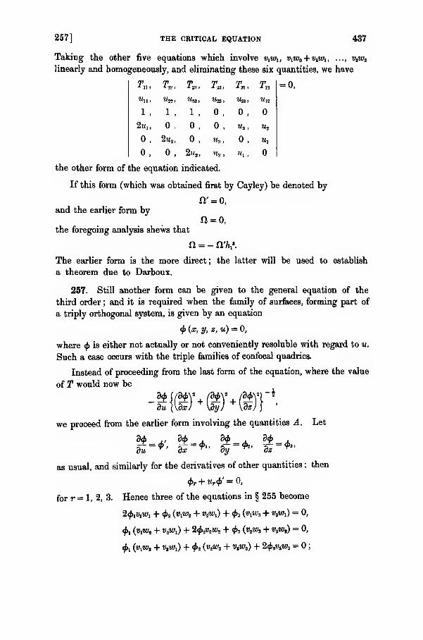
257] THE CRITICAL EQUATION 437
Taking the other five equations which involve v1wl , vlv)2 + v1wl vaw3
linearly and homogeneously, and eliminating these six quantities, we have
= 0,Tn ,

438 GENERAL FORMS OF [CH. XI
and the equation
VXWy + VjW2 + v,ws =is unaltered.
Again, we have
— urt <f>= <£„ + «>•#«' + us <f>r + ur u,4>" ;
hence, substituting in the equation
«,,»,«/, + M,S(«,W2 + l>aW>i) + M13(tW, + tf3W,) + UaV2W, + Ut,(vsWa + V3W2) + Us,V)W3 = 0,
after multiplication by —«f>',
the coefficient of <f>"
= 2w,i>, . l.UiW,,
and therefore is zero ; the coefficient of <£/
and therefore is zero. Likewise for the coefficients of <j>,' and <£/. Hence
the equation becomes
^lAW, + faifaWz + VsWt)+ ^(VjWj+ t>3Wi) 4- ^Kw,w. + <j>^(v.2ws+ V310Z) + <^S3?'3W3= 0.
There remains the sixth equation
A ul'jW, + A K(v,W» + t)2Wi) + j1, 3(w,«'3 + fljWi) + A-nVfiUz
+ An{V#U3 + V3W2) + AssVaWs = 0.
Now
- "«.(<£' = 4>r»t + Unfa' + Utt <f)r' + U tr <f>s
' + (ur,V, + tlstUr + UtrUs) <f>"
+ UrU,Ut<t>'" + UrU,<f>t" + U„Ut <l>r" + VtUr<f>s" + U,.lj)M' + U8<f>rt
' + «<<£,./ ;
as corresponding to the quantities A r„, we introduce quantities 4>„ under the
definitions
where the summation in each case (as for the quantities A rs) is for t = 1, 2, 3
:
and we substitute in the A -equation for the various quantities urtt , un , urt , utt ,
after multiplying by<f>'
3. In the resulting equation, the coefficient of <f>" is
which is zero ; the coefficient of <f>"° is
— 2^'2w (
22tt1fl,Sw)w 1 ,
which also is zero ; and similarly for all the aggregates of terms which contain
<f>"as a factor. Gathering together the remainder, we have the resulting
equation in the form
*„«,«/, + <J>12 (l),W2 + MjW,) + *,„ (v.W, + V,Wt ) + ^jjDjWj
+^ (vsWt + ViW2) + *jst)3W3= 0.
Thus, as before, we have six equations, homogeneous and linear in the six
258] THE CRITICAL EQUATION 439
*,.,
440 SPECIALISED FORM [CH. XI
shall be satisfied at the point; thus if f = ?;, so that y = vi , or if f= m>i so
that 7? = w2 , the requirement is necessarily and sufficiently satisfied, unless
^22 ^33 = "j
which also will satisfy the second equation, without limitations upon t) and £
Thus all the conditions required, in order to secure the lines selected as
axes, are satisfied except only when
W22 ^33 = ^ >
and the directions are definite and unique at the point, save for the possible
existence of this relation (which will be found to be a current characteristic
of a sphere).
In these circumstances, and with these values at the point, the terms
involving Au , Aa , A&, A 12 , Au in the general expanded equation become
evanescent as aggregate coefficients ; and thus the general equation becomes
Aau1
3 (um -u!a) = 0.
Inserting the value of A& at the point, and rejecting the non-vanishing
power of M,, the equation of the third order degenerates at the point into the
critical test represented by the relation
(«a - M33) (ttiWia - 2m,2W1s) = 0.
But, as already remarked, this test is arithmetical at a current point ; it is
not a differential equation.
Ex. 1. A family of parallel planes can belong to a triply orthogonal system. For the
family can be taken in the formx=u,
so thattt12= 0, tt,3= 0, M]23= 0;
the test is satisfied.
The determination of the other families in the system must be effected specially ; for
the general method of § 254 is ineffective, because all the quantities A, B,C, F, G, H vanish.
The u-surfaces are known ; they are such that
t*i = l, tt2= 0, M3 = 0.
The w-surfaces must satisfy the equation
Ui Vi +U2Vi+ U3V3= 0;hence we must have
»i=0,and therefore
v=<f>(y, z),
where<f>
is any arbitrary function. Thus the ^-surfaces are a family of cylinders having
their generators perpendicular to the plane of x, that is, perpendicular to the ?/ -surfaces.
The w-surfaces must satisfy the equations
From the former, we have

258] EXAMPLES 441
from the latter, we have
Let an integral of the equation
dd> 36
gf^+ gf^O.
**dz Jjk dy=0
oy dzJ
be given by
tytyt z) = constant;
then we can take the w-surfaces in the form
yf,(y, z)= w.
(We could take w equal to an arbitrary function of ^ ; but no generality is gained thereby.)
These w-surfaces also are cylinders having their generators perpendicular to the plane of x.
Ex. 2. A family of concentric spheres can belong to a triply orthogonal system.
The family can be taken in the form
x'i+yi+z2=u,so that
"12=0, uu= 0, um= Q;the test is satisfied.
As uu = U22=ic33 =2, w,2=tt23=ze3i=0, all the quantities A, B, C, F, G, H vanish; so
again the determination of the other families in the system must be specially effected.
We havew1= 2.r, ?<2
= 2i/, «3 = 2z;
hence the ^-surfaces satisfy the equation
xv1+yvi +zv3=0,
so that their equation is
•-(J-i)
say, where<f>
is an arbitrary function of its arguments.
The w-surfaces must satisfy the two equations
xv>\ +yv>2+zw3 = 0,
From the former, it follows that w can be any function of ij and f.Making 17 and f the
independent variables, we have the second equation in the form
Let an integral of the equation
be
V'O/j f)= constant;
then we can take the w-surfaces in the form
+ (>>, f)=w-
As an illustration, let d>(ij, f)=>j; then f (17, C)=(1+ij2K~ 2
- The triple system then is
x2+y2+z2=u \
y— vx \ .
a?+y2= wzi >
442 EXAMPLES OF [CH. XI
Ex. 3. A family of spheres, touching one another at the same point, can belong to a
triply orthogonal system.
The family can be taken in the form
x '
then2
the test is satisfied.
Once more, the method of § 254 cannot be applied* ; for the equations are
and the left-hand side of the latter is a factor of the left-hand side of the former, so that
the equations do not determine two sets of values for f : i) : {.
The v-surfaces must satisfy the equation
that is,
/, yJ+A 2w 2z(1-^- )vl + ^r, +-v3 = 0.
\ X- / .V XHence, writing
we have
<t>(l, f)= »,
as the equation of the r-surfaces, <p being any arbitrary function of its arguments.
The w-surfaces must satisfy the two equations
l( , Wx + U? W-2+% Wj= 0,
3>1 JPj +Jjltj+ l':i W-i = 0.
The former equation is the same as the equation for the p-surfaces ; hence w must be some
function of 17 and £ alone. When we take 17 and f as the independent variables, the second
of these equations becomes
(*%+«%)* + {«%+ ll +n%}*~°-
Let an integral of the equation
be given by
^(l, f)=constant;
then the ^-surfaces are given by
* The explanation of the failure in this example and in the preceding examples is simple.
The two equations determine the directions of the lines of curvature on the a-surfaee ; these are
not definite when the snrface is a plane or a sphere, and so the two equations must cease to beeffective.
258] TRIPLE SYSTEMS 443
As a special illustration, let
9i'l,()=1= 1 ;
then we find
, _r, _ xi+yi+z"
YC « ''
so that we have a triply orthogonal system given by
x2+y2+z2
x
2 —vy
aP+yt+z*^ =wz
Another triply orthogonal system is given by
.Tp+ lfi+ Z22 =UX
-=»y f
(pP+yZ+ Z2)*
y2+z2
J2!r. 4. As a last example for the present, consider a family of parallel surfaces.
The quantity u, in the equation of a family of parallel surfaces given by
u(x, y, z) = u,
satisfies a simple partial differential equation of the first order. To find it, measure
a small constant distance p along the normal ; the consecutive surface is given by the
equation
, / Mi u« «. \v + J« = u[x+I
-P, y + ^p, , + j-pj
= ?« + /), p,so that
, du/„ = --.
As p is constant, A, depends upon u alone ; and so we may take
tt,2 + tt2
2+ «32=/(M)i
as an equation characteristic of parallel surfaces.
Hence
«I«I2+ «2«22+ '«3«32= i/'(M) M2i
Ut M13+ «2 tt23 + M3«33=\f («) tt3 ;
and therefore, for our arithmetical test at the point, we have
«12 = 0, M13 =0.Again,
«lMl23+ ai3«|2+«23M22+M2'"223+''33"23+ w3M2a,
!=i/"(") w2 M3+i/'('0"2:l.
so that, at the point, we have"133 = 0.
444. PUISEUX'S [CH. XI
The arithmetical test is satisfied ; and so any family* of parallel surfaces can belong to a
triply orthogonal system.
It is easy to infer geometrically that the other members of the triple system are the two
sets of developables generated by the normals along the lines of curvature.
259. Proceeding by another method, Puiseux obtains -]* a number of
arithmetical results applicable at a current point—among them, the more
important factor of the arithmetical test which has just been considered.
He refers a triply orthogonal system to any point as origin, taking the
normals to the three surfaces as the axes of reference; then, by adjusting the
values of the parameters, he takes the surfaces near the origin in the form
u = x + aa? + dy2+ gz2 + 2Ayz + 2Fzx + 2Hxy + terms of higher orders
v = y + hx2 + by2 + ez2 +2Iyz + 2Bzx + 2Dxy +w= z +fx2 + iy2 + cz2 + 2Eyz+2Gzx + 2Cxy + ,
Now the equations
w,v, + ti.,v2 + u3v3 = 0,
VyWi + ttaM/2 + V3W3= 0,
w,u, + tv2u2 + W3U3= 0,
have to be satisfied along the lines of intersection ; hence
= (H + h) x + (D + d) y + (A + B) z + terms of order higher than the first,
= (B+C)x+ (I + i)y + (E+e)z+ ,
= (F+f)x + (C + A)y + (O+g)z+
The terms of the various orders must vanish separately; in order that the
terms of the first order may vanish, we must have
H + h = 0, D + d = 0, A+B = 0,
l + i=0, E+e=0, B + C = 0,
G + g = 0, F +f = 0, C + A = 0.
The last column of three relations gives
A = 0, B = 0, C=0,
which effectively is Dupin's theorem. Using all the relations, we can take
the surfaces in the form
v = x + aa? + dy2+ gz* — 2fzx — 2lixy
+JX* + my3 + pz3 + ay'z + 8yz* + r\z2x + kzo? + va?y + pxy2 + vxyz + ...,
v = y + ha? +by* + ez2 — 2iyz — 2dxy
+ qa? + ky>+ nz* + l-y2z + ayz2 + /3z2x + ezx2 + 6x2
y + Xxy2 + <j>xyz + ...,
w = z +/X2 + iy2 + cz* — 2eyz — 2gzx
+ sx3 + ry3 + Iz3 + my2z + fiyz2 + az2x + tzx2 + ya?y + %xy2 + %xyz + ...,
* We already have had examples, in a family of parallel planes, a family of concentric
spheres, and a family of Dnpin cyolides.
t Liouville, 2"« Ser., t. viii (1863), p. 33G.
259] METHOD 445
the unexpressed terms being of the fourth and higher orders. When wesubstitute in the equation
ViWi + V.iW2 + v3w3= 0,
the terms of the first order disappear ; the terms of the second order, which
are unaffected by the unexpressed terms, are to vanish by themselves, and so
we have= 4/7t+ 7 + e,
= ibi + 4et* + 3r + f
,
= ice + 4ei+ 3n + p,
= 2dg - 2be - lei - 2e2 - 2i2 + m + a,
= 4de - 4egr - &gh + 20 + %,
= 4,gi- Uf- *di + 2?+ <f>.
Similarly from w^ + w,u, + w3u3= 0, we have
= 4di + a + %,
= 4c<7 + 4fg + Sp + zt,
= 4a/+ 4tfg + 3s + k,
= 2eh-2cf- 2ag-2f* - 2$r2 + ij + t,
= 4e/- 4/A - U,i + 27 + v,
= 4>gh -4de - 4&g + 28 + x;
and from mm + u^Vj + MsV3= 0, we have
= 4egr + /8 + 8,
= 4iah + 4dh + 3q + v,
= 4ibd + 4idh+Sm+ \,
= 2fi- 2ad - 2bh - 2d 2 - 2A2 + 6 + p,
= 4df- 4di - fyi + 2a +<f>,
= Ahi - 4e/- 4fh + 2e + v.
From the fifth of the second set, we have
7= - 2ef+ 2fh + 2hi - Ju
;
and from the sixth of the third set, we have
e = 2e/+ 2fh - 2hi - £w.
When these are substituted in the first of the first set, it becomes
v = 8fh.
But in the present case, taking the values at the origin, we have
tt, = l, /=-iMi«, h = — \ua , t/ = M,s],;
446 LAMtf [CH. XI
so that the relation is
M1lt,23 -2l/MMiS =0,
being one of the factors of the arithmetical test in § 258.
Similarly
<j> = 8di, x = 8e9>
which are the corresponding tests for the ^-surface and the w-surface.
The equations are turned to other uses by Puiseux; for these uses, reference
should be made to his memoir. In particular, he shews that they contain
the Gauss and the Mainardi-Codazzi relations (§§ 34, 35).
Lame families of surfaces.
260. Whichever form of the equation be adopted, we now have explicitly
the partial equation of the third order which must be satisfied by the
parameter of a family of surfaces belonging to a triply orthogonal system.
Such a family is called* a Lame family.
As the equation is of the third order, it is to be expected (from the
general theory of partial differential equations) that its primitive will contain
three arbitrary functionsf which (after Cauchy's existence-theorem) may be
taken as (say) the values of u, us , us when z = 0, so that they are then
arbitrary functions of x and y. But the general equation appears too
complicated to admit of explicit integration in finite terms ; so we have to
deal with specialised cases. Nevertheless, these cases have some real degree
of generality. Among them, one of the most important is contained in a
theorem* by Darboux, dealing with a large family of Lame surfaces.
Having regard to the form of the partial equation of the third order
satisfied by such a family u (x, y, z) = u, we consider the equation
i »ni »». 0j3. $°3> $3i> @n = 0.
Mil-
26°] FAMILIES 447
for substituting, multiplying the second row by/", the fourth by \uj', thefifth by \u.J', the sixth by %uaf, and subtracting the sum of these multipliedrows from the first, we have a row of zeros.
Similarly, it is satisfied by
= xg (u), = yh (u), 0=zk (tt)
;
the process of verification is the same, save that the respective factors are
x9\ yh', zk', for the second row;
\xuxg" + g, \yujk" + h', \zu3k" + k', for the fourth row;
%mhg", hyuzh", %zutk", for the fifth row
;
\xu%g", \yihh" , %zus k", for the sixth row.
Similarly, it is satisfied by
= (a? + tf + z*)l(u),
the process of verification being the same, but with the multipliers
{a? + y* + z") I', for the second row,
21, for the third row,
£ (a? + y- + z*) it/' + 2x1', for the fourth row,
H*2 + y* + z>) «/' + 2yV, for the fifth row,
\ {a? + y- + 22) usl" + 2zV, for the sixth row.
Now the equation quoted is linear in the derivatives of 0, and therefore the
sum of any number of integrals with constant coefficients is an integral ; thus
@ = (it,2 + m2
2 + u?)~% - (of + y1 + z-) I - xg - yh - zk -f
is an integral. Bute=o
satisfies the equation; and so we have Darboux's theorem*:
—
Anyfamily of surfaces u(x, y, z) = u, satisfying the equation
- -, = (a;
2 + y- + z") l + xg+yh + zk +/(uf + uf+ufj*
where f, g, h, k, I are any arbitrary functions of u, is a Lame family
belonging to a triply orthogonal system.
For the development, and for some applications, of the theorem, reference
should be made to Darboux's treatise f.
* Apparently, there are five arbitrary functions in the integral, instead of three ; but the five
can be reduced to four, by taking a new variable u', such that ldu=du'. The four functions
involve only one parameter u ; each of the three functions in the primitive (after the statement
of Canchy's existence-theorem in § 252) contains two independent parametrio variables.
t Systemes orthogonaux, Book i, chap. iii.

448 BOUQUET [CH. XI
Bouquet surfaces.
261. As the general primitive of the equation of the third order has not
been obtained, it is worth while considering some special classes of surfaces
that belong to triply orthogonal systems. Among these are the w-surfaces,
whose equation* has, or can be made to have, the form
u = X+Y+Z,where X is a function of x only, Y of y only, Z of z only. Then
un = X", ua - 0,
An=XX'"-2X"\ Aa= 0,
and similarly for the others; hence the equation of the third order, when
expanded, is
ITT2(ZT'" - 2X"a) (Y" -Z") = 0.
Manifestly the factor X'Y'Z' can be dropped; and so the equation becomes
(X'X '" - 2X "») (Y"-Z") + (Y' Y'" - 2 F"») (Z" -X ")
+ (Z'Z'" - 2Z"*) (X"- Y") = 0.
The equation can be established ab initio by the following method which
also contributes some knowledge of the other families in the triple system.
Assuming that the it-surface does belong to a triply orthogonal system, the
other families are given by
X'v, + Y% + Z'v3= 0,
X'w,+ Y'w2 + Z'w3 = 0,
»!»! + MjW2 + V3W3 = 0.
As regards the first two of these equations, we take two independent integrals
of the subsidiary set
dx _dy _dzX'~Y'~Z"
say_[dx fdy Q_[d% fdz
a ~JT'~jt" P~)x'~JZ~'''
and then the first two equations are satisfied in complete generality, by
taking v and w as any two functions of a and /S only. Let these functions
be substituted in the third equation ; it becomes
'dv,dv\ (dw dw\ 1 dvdw 1 dv dw _
that is,
'.'"dvdw X^dv^dw~dada
+Z'*d$dP
X ,Afa+d0){c
(dv dv\ /dw dw\ X'2 ov ow a. ov ow _
* They were first considered by Bouquet, Liouville, t. zi (1846), pp. 446—450.
261] SUKFACES 449
There are three independent variables, though v and w are functions of only
two independent combinations of them. Change the independent variables,
choosing them to be a, £, x ; then y is a function of a and x, while z is a
function of # and x, such that
dy T dz_Zidx X" dx~ X"
Differentiating the modified equation with respect to x, and noting that v
and w now do not involve x but only a and fi, we have
X"-Y"dvdw X"-Z"dv_dw_Yh 9a 9a
+Z'- 9/3 9/3
~
Differentiating again, we have
X'X '" - Y'T" - 2 Y" (X" - Y") dv dw
Y'* da da
X'X'"-Z'Z'"-2Z"(X" -Z^) fodw_+ " Z* 9yS 9/8
Eliminating the derivatives of v and «/ between the last two relations, we find
(X'X '" - 2X "*)( Y" - Z") + ( Y' Y'" - 2 F"a
) (Z" - X")+ (Z'Z'" - 2Z"*) (X" - Y") = 0,
which is the equation in question.
When we use the earlier of the two derived relations to eliminate Y'2 from the
a-/9 equation, we find
/dv dv\ low bw\ „dv dw_
whereX'" Z"-Y"
It is not difficult to verify, through the critical equation of the third order, that P is a
function of a and j3 only.
Suppose that the w-surface does satisfy the Bouquet form of the critical
equation. Then, for the other two families, we have
|g -MY- (Z--X~),
where M is a quantity whose exact value is not required. Thus 5-/3—
and 53 /5o are tne roots of the quadratic equationdpi dp
PY'*(Z"-X") + 0{Y ,:i(Z"-X") + Z'*(X"-Y")-X'*(Y"-Z")}+ Z'*(X"-Y") = 0.
f. 29

450 bouquet's form of critical equation [ch. XI
One of the linear factors gives a homogeneous linear equation of the first
order for v; the other of the linear factors similarly supplies w. Whenthese equations are integrated, the values of v and of w are known; and
so we have the triple system.
Accordingly, the first step is the determination of values ofX , Y, Z which
shall satisfy the critical equation of the third order. It may be written
% + AX" + B = 0,
where A and B are independent of x, while
£ = X'X'"-2X"\
Differentiating with respect to x, we have
£' + AX"'=0,so that
J^— A-•y in — -*1 )
consequently both sides of this equation must be constant, so that
£' = aX'", A = -a.The former gives
X'X'" - 2X"> = ? = aX" + b,
where b is an arbitrary constant ; and then
B = b.
The relations A + o = 0, 5 — 6 = 0, give
Y'Y'"-2Y"* = aY" + b, Z'Z'" -2Z"*=aZ" + b.
Hence the most general resolution of the critical equation is constituted by
the set of equations
X'X'"-2X"*=aX" + b)
Y'Y'"-2Y"*=aY" + b
Z'Z"' -2Z n' = aZ" + b
Ex. 1. Consider the case when o=0, 6=0. Then
x'X"'-2X"*=o, rr-2f"! =o, z ,z ,"-zn*=o.
The primitives of these equations are
X=m log (x— m')+ m",
Y= n log (y - »') + n",
^= P l0g (2 -p')+p",
where all the quantities m, ..., p" are arbitrary constants. No generality is lost by
annihilating to', »', p', m", n", p" ; so we have
X=m\ogx, F=nlogy, Z=p\ogz.
The u-surface has therefore the simple form
U=eu=ex+r+z=xmymz''.

261] EXAMPLES 451
For the other two families in the triple system, we first deal with the equations
- Vl+ Vl+£ V3 = 0i* y •>
m n v- Wl +-w2+Zw
3 = 0.
Hence, ifa
both v and w are functions of a and alone. The equation
v1w1 +viwi+v3w3=0then becomes
if« dv^.^ dv\L dw^ ^ ,3»3*>. 8* Bart ,
/ dv dw, a dv dw\
Hence
dv dw dv dw
The equation satisfied by v is
sj +iV—^sap-"W =0;
and the same equation is satisfied by w. Let
da \ n P / 3/3
Oa \ » P /«>0
/2±m a _ !L±i» A
da_\ n p ]
(£±^a-^±^/3-Ai)rfa-2arf/3=0,
then we can take
Let integrals of
and
be
g(a, 0) = constant, A (a, /3)= constant,
respectively ; the two other families of the system are
g{a,ft)=v,
h(a, /3) = w.
Ex. 2. Shew that a triply orthogonal system is given by the equations :
—
(i) the hyperbolic paraboloids %-=u;
(ii) the closed sheets of the surface
(3,2_ 22)2 _ 2a (y»+ z»+ &p>)+
a
2- ;
(iii) the open sheets of the same surface.
29—2
452 EXAMPLES OF BOUQUET SURFACES [CH. XI
Ex. 3. Obtain the families, to be associated with the family
xyz = u
so as to give a triply orthogonal system, in the form
V= (X*+ ay1'+
a
1 «*)*+ (x*+ aiyi+azrf,
W=(3?+ay2+ aHrf -(xt+Jf+ azrf,
where a is an imaginary cube root of unity.
Ex. 4. Shew that the critical equation of the third order is satisfied for the surface
u = X+c(y*+z*),
where X is any function of x. Shew also that the families of surfaces to be associated with
it in a triply orthogonal system are
-!•[dx
w=(y2+i2)e J.x\
Ex. 5. It was shewn that a general resolution of the critical equation leads to three
equations of the formX'X"'-2X"i = aX"+b.
Thus we haveX'X'"=2X"3+aX"+ b
= 2(Z"-p)(Z"-<r))
where p and <r are constants. Assuming them unequal, let
X = j* _1_.
p — a p — <r'
then
so that\X"-p + X"-a) ~ X"
(X"-pf(X"-*r=(?x'2,an equation that usually is transcendental. Now
dX"dx= -g„
'
;dX"-2(X"-p)(X"-^y
= ±(X"-p)^-*(X"-<r)*»- l dX>\
so that
*-**»=s/(jr""'')|x
" 1 (X"~ <r)4"" 1 dX"-
If it were possible to invert this relation, so that
v„_d?f{x-xa , c)A - sp— '
then
X=f(x—x ,c) +Ax.Similarly
^=/(y-yo, d) +A'y,
Z=f{z-Zo,J')+ A"z.
But, in general, the relation cannot be inverted so as to give an explicit form for/.
262] TRIPLY ORTHOGONAL CENTRAL QUADRICS 453
Ex. 6. Integrate the equation, so as to obtain the w-surface in the following cases :
—
(i) when 6=0,
(ii) when a=0,
(iii) when a2 =86.
262. Now consider the possibility of having a family of central coaxial
(but not necessarily confocal) quadrics as a family belonging to a triply
orthogonal system. Their equation will have the form
a? v2 z1
<j>(<c,y,z,u) = j +^+ q-1 = 0,
where A, B, C are functions of the family parameter u. We have
9n — ^ . 9a — g > 9ss = q >
9» = 0, ^, = 0, 912 = 0;
while
9, = 2| ) 9» = 2|, 9= = 2j;
and so for the values of the other quantities 4>„ by cyclical rotation of the
indices. Substituting in the Darboux equation of § 257, and evaluating, we
find (on the rejection of a merely numerical factor)
xyz
(M+aHG-iMa-aWG-JW-*A'&C*
Hence, rejecting irrelevant factors and non-vanishing factors, we have
A(B - C)A' + B(C -A)B' + C(A- B)C = 0,
as a differential equation to be satisfied by the quantities A, B, C, which are
functions of the family parameter u. And then, for any values of A, B, C as
functions of the parameter it which satisfy the equation, the family of
quadrics
a? y* z* , .
belongs to a triply orthogonal system.
454 EXAMPLES OF CENTRAL QUADRICS [CH. XI
Ex. 1. The simplest solution is given by
A'=l, B"=l, C'=\,so that
A=a+u, B=b+u, C=c+u,
where a, 6, c are any constants. The equation of the family of surfaces is
x2 y2 z2 ,
a+u b+u c+u '
the family is composed of confocal quadrics of the same kind. The other two families in
the system are the two sets of confocal quadrics of the other two kinds.
Ex. 2. Manifestly, a somewhat general solution is given by
AA'= Ah+g\
BB=Bh+g\,
CC'= Ch+g)
where A and g are any disposable functions of u. We have one set of solutions of this
character by taking
A = (u+ b){u + c), B = (u+c)(u+a), C=(u+a){u+ b),
if
h=3u+a+ b+ c, g-=(u+ a)(u+b)(u+c);
and the family of quadrics, forming part of the triply orthogonal system, has the equation
(u+a)xi+(u+b)yi+(ii+c)zi={u-i-a)(u+b)(u+c).
The other families of the triple system satisfy the equations
x(u+a) vi+y(u+ b) i>2+ 2(u+ c) i>s =
x(u+ a) v>i+y(u+ b)w2+ z(u+c)w3= .
i>i v>i+Wi+ V3W3 =
The first step in the construction of these families is made by integrating the equations
dx dy dz
x(u+a)~ y(u+b)~ z(u+c)'
being the characteristics of the first two partial equations of the first order. When we
equate each of these functions to f"(u)du, where / is another unknown function, the
integral of these characteristics can be taken in the form
y=Bdu + b)/'(»)-/(») I
z- C(tu + «)/»-/<«)J
where A, B, C are arbitrary constants ; and then the value of/(«) satisfies the equation
Ai (u+a)el lu + a)''M+B2 (u+b)ei lu + b)''W+Ci (u+ c)e2 l''+ c)''W
= («+ a) (u+ 6) («
+
c) e^M.
When this value of /(«) is regarded as known, we can take the two integrals a and /3 of
the subsidiary characteristic equations in the form
a=xb-'yc - a za- h
,
^= xa^-e)yb{c-a)^{a-b)^a-b){b-c){e-a)f{«).
and then v and w are appropriate functions of a and /3, satisfying the equation
(6-c)sf
3» dv a(u+b+c)-bc\ ( dw dw a(u+b+c)-bc\2 -*- {"da+t3^ ~ "i+i } \
afa
+fide 5+5 J
-0 '
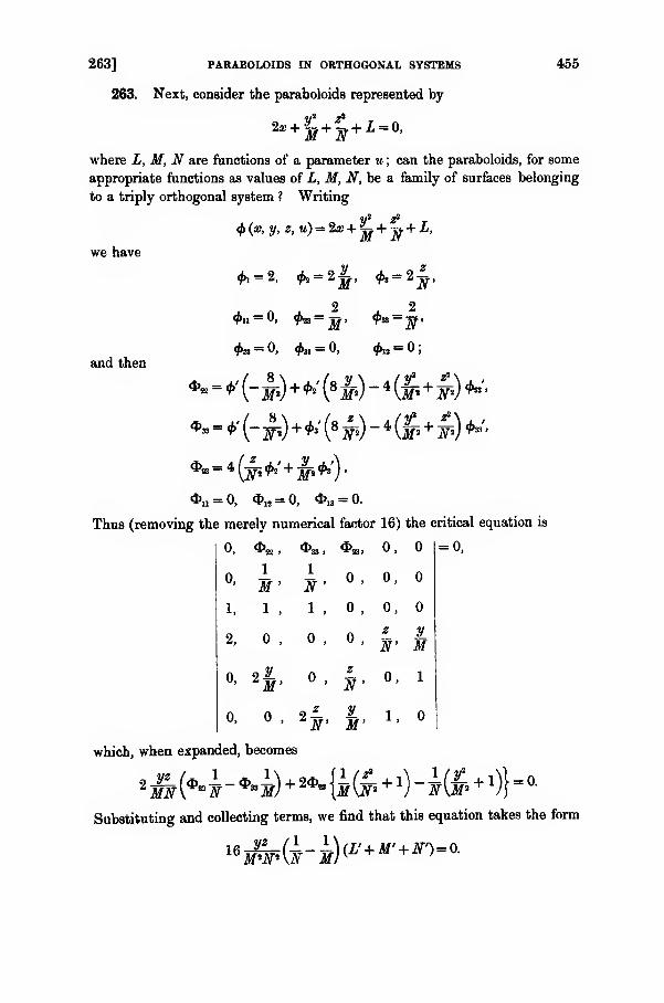
263] PARABOLOIDS IN ORTHOGONAL SYSTEMS 455
263. Next, consider the paraboloids represented by
V2 Z*
where L, M, N are functions of a parameter u ; can the paraboloids, for some
appropriate functions as values of L, M, N, be a family of surfaces belonging
to a triply orthogonal system ? Writing
we have
y3 £s#(a;, y, z,u) = 2x +
jjj+
-ff+ L,
<J>i= 2, #2 = 2-^, #3 = 2-^,M'
and then#23 = 0» #31 = 0,
8
'N'
#l2 = ;
^ = ^'(-^) +^(8i)- 4(|-» +^)^
^-'(-yi) + ^'(8 yi)- 4 (t +P^^ = 4(f2 #2
' + |-s #3') >
*.i = 0, *12 = 0, <fr13 = 0.
Thus (removing the merely numerical factor 16) the critical equation is
= 0,o,
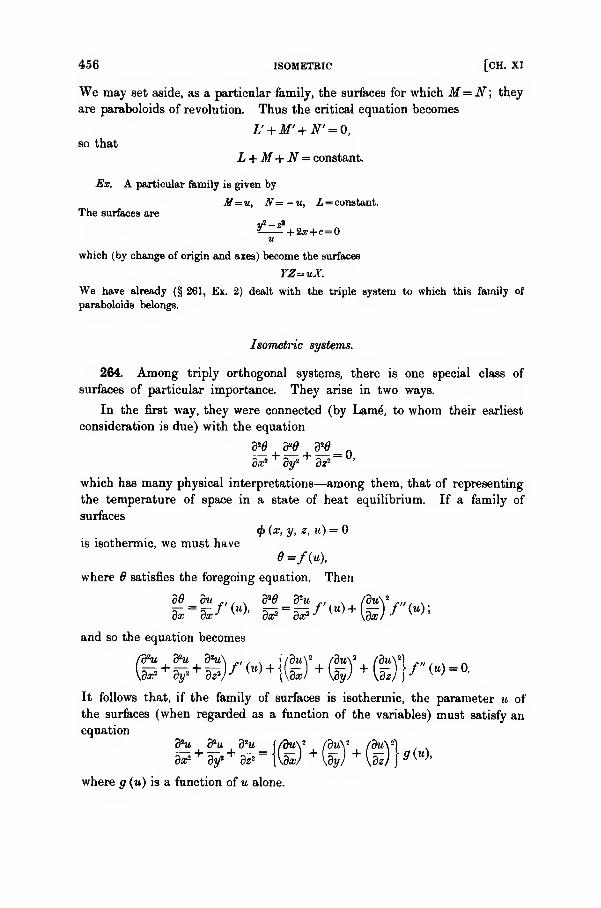
456 ISOMETRIC [CH. XI
We may set aside, as a particular family, the surfaces for which M=N\ they
are paraboloids of revolution. Thus the critical equation becomes
L' + M' + N' = 0,
so that
L +M+N= constant.
Ex. A particular family is given by
M=u, N= — u, Z= constant.The surfaces are
* h2#+c=0u
which (by change of origin and axes) become the surfaces
YZ=uX.
We have already (§ 261, Ex. 2) dealt with the triple system to which this family of
paraboloids belongs.
Isometric systems.
264. Among triply orthogonal systems, there is one special class of
surfaces of particular importance. They arise in two ways.
In the first way, they were connected (by Lam6, to whom their earliest
consideration is due) with the equation
which has many physical interpretations—among them, that of representing
the temperature of space in a state of heat equilibrium. If a family of
surfaces
<f>(x, y, z, u) =
is isothermic, we must have
where 6 satisfies the foregoing equation. Then
and so the equation becomes
/dhi,&u
,d*u\ ,, .
,\/du\ l /dux 1 /Buy) ,„, , n
It follows that, if the family of surfaces is isothermic, the parameter u of
the surfaces (when regarded as a function of the variables) must satisfy an
equation
dhi &u dhi {/du\ 2 fduV /duV) , s^ +^ + a?=iy +y +(sj }'<«>•
where g (u) is a function of u alone.
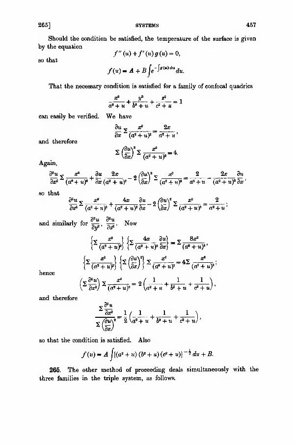
265] SYSTEMS 457
Should the condition be satisfied, the temperature of the surface is given
by the equation
/"(«)+/'(«)*(«) -0,so that
/(«)=4+£JWff(")dB
du.
That the necessary condition is satisfied for a family of confocal quadrics
a?, f z2 _
a? + u ¥ + u c? + u
can easily be verified. We have
du -, a? 2x
dx (a2 + uf a?+u'and therefore
Z\dx) ^iat+uf-*-
Again,
d*u - Xs du 2x _ /8u.y v 'e2 2 2x du
da? (tf+uf dx(a? + uY \dx) ~(a* + uf~ a2 + u (a2 + ufdx'
so that
3%2_^_ 4a: du /g«y s
a? 2__.da? (a?+uY
+(a? + uYdx \dx) (a2 + uf~ a? + u'
and similarly for ^— , — . Now
^ a? I f„ 4a_ 9«) ==s _8^_
rWf"(o! + »)! (a2 +u)3 '
a?1
(a* + uf)hence
/ »«N 3* / 1 1 1 \
V 3W (a2 +w)2 \a* + u ¥ + u <?+uJ'
and therefore
v /9m\ 2 2\a2+w &* + « c2 + m/'
so that the condition is satisfied. Also
/(it) = 4 f{(a2 + «) (62 + w) (c2 + w)}~ - dw + -B-
265. The other method of proceeding deals simultaneously with the
three families in the triple system, as follows.
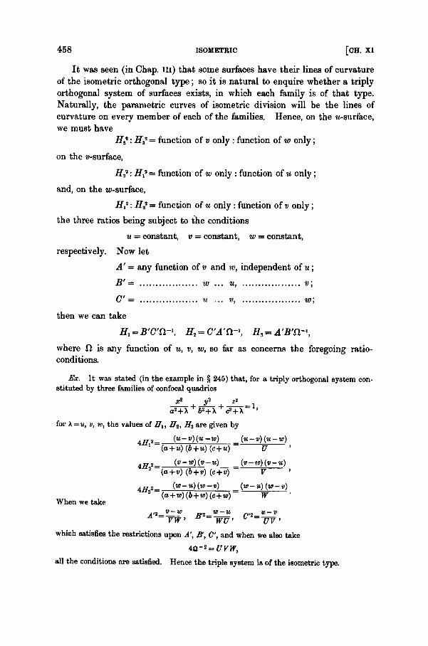
458 ISOMETRIC [CH. XI
It was seen (in Chap, in) that some surfaces have their lines of curvature
of the isometric orthogonal type ; so it is natural to enquire whether a triply
orthogonal system of surfaces exists, in which each family is of that type.
Naturally, the parametric curves of isometric division will be the lines of
curvature on every member of each of the families. Hence, on the M-surface,
we must have
H.* : H3* = function of v only : function of w only
;
on the v-surface,
Hf : Hf= function of w only : function of u only
;
and, on the w-surface,
2?,* : H£ = function of u only : function of v only
;
the three ratios being subject to the conditions
u = constant, v = constant, w = constant,
respectively. Now let
A' = any function of v and w, independent of u;
B' = w ... m, v;
C = u ... v w\
then we can take
i 1 =5'C"fl-^ H,-CA'n-«, H3 =A'B'n-\
where fi is any function of u, v, w, so far as concerns the foregoing ratio-
conditions.
Ex. It was stated (in the example in § 245) that, for a triply orthogonal system con-
stituted by three families of confocal quadrics
a? iA 22J--2— -J- = 1,«*»+A
T4*+X
T«*+ A
for \ = u, v, w, the values of Hu Ht , H3 are given by
\H*- <,v—v){u-w) = (u-v)(u-w)1
(a+ u) (b+u) (e+ u) U
^jya, {v-w)(v-u) _ (v-w)(v-u)2 (a+v) (b+v) (c+ v) V '
iH t- (v-u)(v-v) = (w-u)(w-v)3 (a+w)(b+w)(c+w) W
When we take
A ,2_vz w Rl_v>-u p,i_u-vVW ° ~ WU' ~~ffV'
which satisfies the restrictions upon A', ff, C, and when we also take
4Q-2 =UVW,all the conditions are satisfied. Hence the triple system is of the isometric type.
265] systems 459
The quantities HltHit H, have to satisfy the Lame' relations. Following*
Darboux, we write
#j=eB+c-i<*n H2=ec+A-\og n> Ha = eA+B-\0S a>
where
log A'=A, logR = B, log G' = C.
When we substitute in the second set of these relations, we have
n* = nB-4 3 + n3At + n<s,
n31 = QsS, + n,B3 + as.,
n^n,^ 4-fi.c, + ns3
where
Sl= (B3 -A 3)(C1 -A,)-A 3A2
$ = (0,-5,) {A, -B3) -BrB3 .
Ss = (Ai-Ci)(B1 -Cl)~C2C1 ,
The equations for ila , ft,, , fl Vi should lead to one and the same value for
n]i!3 . Differentiating the first with respect to u, and substituting for fl, s and
n, 3 from the second and third, we have
nIffl= h.b.c, + nscu„
+
iisA.B, + n& + s,A t+ s3a 3^j ;
and similarly from the others. Hence
-=—h S2A 2 + S3A 3 = -=—i- S3B3 + StBi = »— + St C, + S2C2 .
Nowo 2 j4 2 + S3A 3 = — A 3B3 Cj — A 3 B} C 2
= /S3jB3 + (Si^!
thus the foregoing conditions become
3S1 = 3S2= 3S3
3m dv dw'
Let the values of Slt S2 , S3 be substituted in these conditions ; then
C12 (fij — il 3) + 5^ (C2 — At)
= Cn (A 3 -B3) + A!S (C3-B3)
^Aa (B3 -C3) + Ba (A i -C\)
= 0,
by taking each of the three equal expressions as equal to one-third of their
sum. Thus
—' = -— = ~ =
3m ' dv ' dw
* Ann. ic. Norm. Sup., 1" S6r„ t. Hi (1866), p. 131.
460 DARBOUX's TREATMENT OF [CH. XI
so that /S, is a function of v and w only, S, of w and w only, and Ss of « and v
only. Thus
(fis - A,) (C, - 4.) = tf,,
(C, - 5.) (4, - £,) =K2 ,(A 2 - Cs) (5, - CO= tf3)
where Kxis a function of v and w only, 7f„ of w and u only, and K3 of it and
v only.
266. To find Ku let w have any constant value, say zero, an assignment
which does not affect Kx . Then
B3 becomes a function of w only, = w3 say,
C2v only, =vt say;
and let
w3— A 3
= J, v2 — A2 = I,
B3-w3= Tlt Gi -vi =TS .
ThenJI =KU (J+T2)(I + T3) = KU
so that
Now 7 and ./ do not involve u; hence
} [tj <m \tJ3m1
du \t) du \fj
But T2 does not contain v, and T3 does not contain m; ; hence both fractions
are functions of u only, say
V(u)b'(u)'
then
Y = b (w) c («) + a (a) = 6,c2 + Oj,
=r = 6 (w) c' («/) + a' (w) = &iC3 + 03.
Substituting in
y3
+5l+ i=o,
we have
bx (fyl+ c3J) + aj + a3J+ 1 = 0.
Now / and J are functions of v and w only; hence
0,7 + 03./+ 1 =0, cJ + c3J=0,so that
I J 1
C3 C% C^Cj "~ ^3^2
266] ISOMETRIC SYSTEMS
Consequently
A 2 = v2— I = v3 H -
,
ttaCg ~~ (X3C2
A 3 = w3 -J = w3 ,
&2C3 "" &3C2
B3 =w3 + T2 = w3 + 1 ,
„ _ 1
Change the variables from u, v, w to U, V, W, where
b^U, ^ V, -8= -F;then
3F 2 + F-F' 3TT~ 3 F- V"
dC -y 1e dB _ w> 1
where
^2' = "s tb . a function of V only,
^'=i».g^. IT only,
= -5rr V only at the utmost,CiOV
A- 1 dW W*-c3W W
But
A (dA
\a
(dA
\dW\dV)~dV\dW)'
therefore
6 = <j>=h,
where A is a pure constant. Thus
A = V, + W3 -h\og(W-V).Similarly
B=W3+U1-h\og(U-W),
C=U1 + V,-hlog(V-U);and so
= 1 ev,+r,+ fr,-hiri. (7 _ {j)-h(W- U)-k eu'.
H, = i «oi+r,+ ir,-*«(i|r_ F)-*(tf- 7)-*eF>,
461
462 ISOMETRIC [CH. XI
Returning now (as is permissible) to our old variables, we have
(y — «)~* (w — u)-hH> = QU„ _ (« — v)~h (w — v)~h
8 QV '
„ _ (u — w)~h (v— w)~ku* w •
Instead of modifying the equations, we substitute once more in the second
set of Lame relations ; then
(v-w)Q2a = h(Qt -Q,y
(w-u)Qn = h(Q3 -Q1 ) ,
(u-v) Q12 = A (&-&).
the conditions of compatibility being satisfied.
Thus, for confocal quadrics
Q = 2, A = -i,where
f7' = (a + w)(6 + «)(c + M);
and V and W are the same functions of v and of w as U is of u.
267. We now must have regard to the first set of three Lame relations
of § 246 which have to be satisfied by Hlt Ht , H3 . For simplicity, we shall
take
Q = constant = 1,
so that the equations for Q are satisfied. One of the relations is
du \H] du )+dv\Hi dv )
+ H? dw dwthat is,
J_ 3^ 1 dPHi _ J_ dH., 3£a _ 1_ dHi dB^, 1 dH.dH,H, du1
+Ht dv> H? du du Hf dv dv+
#,' dw dw ~ '
Now
L dJL = J}- + A_ _?' dJ*} = hrr
Hi du v — u w—u U ' dw w—u 1 '
M? = _ JL U d—' - h" +hTT
dv v-u " ~dv> (v-uf ,;
and similarly for the others. Inserting these values in the foregoing relation,
and reducing, we have
J_ W _ J_ VR? U HJV
= (Jt *_^_L + (_! LU+/J l_\±\w-u w-v) H} \u-v u-wl H? \v-w v-u) H?
'
267] systems 463
The other two relations similarly give
I. E _ _L EH? V H3
2 W_f h lL_\_L./J A_\ J_ / h 1 \ 1
\u-v u-w/Hi \v^w v-u)H? + \w-u w-vJHf
J_ El _ J_ ElHa2 W H2 U
= (Jl a_\JL + (_J *_\.i+ (_A L\i
\v-w v-u] Hf \w-u w-vJHi \u-v u-wJHi'The sum of the left-hand sides of these three equations is zero ; hence the
sum of their right-hand sides must be zero, that is,
(1 + 2h) {fc^ " W^v) Hi + {^Tv -^u) E7 + fc^ - V^) Htf= °-
Now the variable factor, being
-1
r^K-?)*^)](w - v) (v — w) (w — u)
is not zero. Hence1 +2h = 0,
so that h — — % ; and therefore
gi_ (ii-it)(w-tt) Irt _ (u-v)(w-v) Ui _ (u-w)(v-w)a i—
jjt > -"" yi. a > jps •
The first of the three equations now is
(w-v)UU'+(u-w)VV
= i (»-»y w,
2(v — w)(w — u)
1 (3u - v - 2w)(v— w) tt, _ 1 (3v — 2w - u)(w — u) Vi2 (m — v) (w— u) 2 (v — w) (u — v)
'
and the other two are obtainable by cyclical interchange of the three
variables.
The equations, in this form, are linear and homogeneous in U2, V2
, W2
and their derivatives of the first order. The symmetry suggests an ex-
pectation that U2, V", W are similar polynomials in u, v, w or, at least, that
solutions of this type certainly exist. If n be the common degree of these
polynomials, it is easy to see that
n = 3;
and it is easy to verify that
U2 = Kit3 + cm2 + &u +y\
V2 = kv2 + atf + &v + 7 !•
,
W2 = «• + aw2+ 0w+ 7J
464 TRIPLY ORTHOGONAL SYSTEMS [CH. XI
where k, a, y3, y are arbitrary constants, of which only the ratios are essential.
As a matter of fact, these relations constitute the primitive of the three
equations.
The values of Hu H2 , Hs thus obtained belong to the triply orthogonal
system of confocal quadrics.
Darboux shews that a general triply orthogonal isometric system is given
by the triple set of families of surfaces having the equation
4rfs— a2
4a*2 — fc
2 id* — c2
(x' + y* + z>y + ax> + by* + cz* + d? +—-^— a? + -j—— y* + -— z* = 0,
for X = u, v, w. The equation for the arc-element in space is
ds>=M^u - vKu - w)
dU>+(v - w
yv - uhv> + (w - u
^w - vhw>},
whereU= (u + a) (u + b) (u + c) (u* - 4da
)
V = (v + a) (v + b) (v + c) (v* - 4da)
.
W = (w + a) (w + b) (w + c) (up - 4d')
For this result, and for further developments, reference should be made to
his memoir already cited and, above all, to his treatise on orthogonal
systems.
EXAMPLES.
1. Let p and a- be the radii of curvature and torsion of the intersection of the surfaces
*>(*, #. 2)= »> w(x, y, z)= w,
in a triply orthogonal system;prove that
p* Hi'Xdv)+ff3t\dw) '
^=itan-^^!-^2. A family of surfaces is given by the equation
<p(x, y, z, »)=0,
and x and y are regarded as the independent variables. Shew that the critical equation
of the third order, which must be satisfied if the family belongs to a triply orthogonal
system, is
where
r=(i+P8
+?')-*J.
3. Shew that any family of planes, the equation of which contains one parameter,can form part of a triply orthogonal system.
In any one of the planes, let two sets of curves be drawn cutting one anotherorthogonally. Let the plane be moved so as always to touch the developable surface
which is the envelope of the family of planes;prove that the two families of surfaces
generated by the two sets of curves complete a triply orthogonal system.
EXAMPLES 465
4. Circles are drawn, cutting a given surface orthogonally and also a given planeorthogonally. Shew that there is a Lame' family of surfaces cutting the circles
orthogonally.
5. In the Bouquet surface u = X+Y+Z, denote the equation which X mustsatisfy by
X'X'"=2(X"-a)(X"-b);
and let X and fi be the roots of the equation
Also let
X'i Y'2 Z'*
6=X + 6=Y+ 6=Z= °-
/A _£_ _L_ / V'2 Y'2 5"2 \
shew that the u-surface, the v-surface, and the w-surface thus obtained, are a triply
orthogonal system.
6. Obtain equations for the orthogonal systems of which the surfaces
aa?+ by3+ cz3+ X (.r2+y%+ «2)= «,
ax*+ by*
+
cs4+ X (s2+y2+
«
2)
=
u,
(where a, 6, c, X are constants) respectively form part.
7. The envelope of the family of surfaces
(x+3
m
(x+lT(x+3
,'
x'=con8tant'
where X is the parameter for the family, constitutes a triply orthogonal system, provided
m+n+p+q is not zero.
Discuss the case when m+n+p+q— 0, obtaining a triply orthogonal system partly
through the envelope.
8. A particular Lame family consists of surfaces of constant negative curvature — ™
,
where U may be a function of u. Shew that we may take
ffl=U^-, #2=cosQ, ZT3 =8infl,
where Q must satisfy the four equations (due to Bianchi)
d2a 3*0 sin O cos Q3»2 duP U*
=0
&a da 3aO . „ da 32Q , „ .— s~ o n cot 0+5- 5—5- tanQ=dudvdw dv dwdu dw dudv
1 3 /sinQ\ 3 /3>0 \,da 32Q „ .
'! (*£)+* fj^-coseco) +f 22-mta-OUdu\ U J dw \dwdu J dv dvdu J
Prove that a solution of these equations is given by
^ ir - O=am {cv +/(«)},
where /(») is any arbitrary function of u, c is a pure constant, and the modulus of the
elliptic functions is 1/ctf ; and verify that these w-surfaces are surfaces of rotation.
30F.

CHAPTER XII.
Congruences of Curves.
The present chapter deals solely with the elements of the theory of congruences of
curves ; and within the range of that theory, attention is restricted to curves which are
either straight lines or circles.
The simplest example of rectilinear congruences (in which, moreover, there is direct
application to a physical subject) occurs when the straight lines are composed of a set
of lines that can be cut orthogonally by a family of surfaces—such as the rays of light
issuing from a centre. They were considered at an early stage by Malus, Dupin, and
Hamilton.
The theory of congruences of plane curves, and particularly of circles, owes its early
systematic development to Ribaucour.
Detailed references to many of the numerous writers on the subject will be found in
the second volume of Darboux's Theorie generate des surfaces, book iv, chapters i, xii, xiii,
xv, and in chapters x and xviii of Bianchi's Geometria Differenziale.
268. In almost all the preceding investigations, whether surfaces or
space constituted the subject of investigation, the discussion has been based
upon point-coordinates by taking a point as the initial element. Twoexceptions arose; for each of them, the discussion was based upon plane-
coordinates, by taking a plane as the initial element. In one of these
exceptions, the equation of the osculating plane of a skew curve was taken
as the analytical definition of the curve (§ 16) ; in the other of them, the
coordinates of the tangent plane to a surface were used, to complete the
spherical representation of the surface (§ 162).
Now, in algebraic geometry, it proves convenient to use line-coordinates
by taking a straight line as the element of space, instead of a point or a
plane ; more generally, we could take a curve, plane or skew, as the element
of space. For this purpose, we note that space may be regarded as containing
oo » points. For our purposes, a curve through a point will have a definite
direction (or one of a limited number of definite directions) ; so that the
curve will associate, with the point, oo » other points or a finite multiple of
oo ' other points ; consequently, we should have x 2 curves for our investigation.
As they are curves in space, they require two independent equations for
their analytical expression ; as they are oo 2 in numerical range, these equations
must involve two independent parameters. Such an aggregate of curves is
268] CONGRUENCES OF CURVES 467
called a congruence of curves, sometimes a congruence, sometimes a congruence
with a prefixed epithet (rectilinear, cyclical, or the like).
Examples of congruences of curves are frequent enough. Thus the
a££regat'e °f the normals to a surface is a rectilinear congruence, as is the
aggrega*e of tangents from a twisted curve to a surface in space. Systems
of rays in theoretical optics have been the subject of many investigations
;
and the importance of the congruence of characteristic curves in connection
with the primitives of partial differential equations is well known.
To illustrate the origin of a congruence, consider two similar problems,
one of which leads to a congruence, while the other does not. Take any two
algebraical surfaces and, for greater definiteness, suppose that they are not
parallel ; let it be required to find the aggregate, (i) of straight lines which
are orthogonal to both surfaces, (ii) of circles which are orthogonal to both
surfaces. The equations of the surfaces are taken to be
f(x,y,z) = 0, g(x,y,z) = 0.
(i) If x„, y , z be a point on the former surface; and if xx , yu zx be a
point on the latter surface ; where the straight line
x-qcq _ y-y* = z- za
#i-#o yi-y<> Zi-z*
is normal to both surfaces, we have
/(*o. yo, ^o) = 0, g(xu yu z1 ) = 0,
1 3/ = 1 a/ = 1 yxl -xn dx<l yj-yndyo zx
- zt dza'
1 dg _ 1 dg _ 1 dg
a, - x„ dxi y-i- y„ "byx zY
- z„ dzx
'
Thus there are six equations for the determination of the six quantities
#oi y<>, Zo, *i. Vi, Z\- In the absence of special relations between the surfaces
(such as parallelism, which would identify the last two pairs of equations), it
can be inferred that they furnish a limited number of solutions, real or
imaginary. Thus there is only a limited number of straight lines, normal
to the two surfaces ; they do not constitute a congruence.
(ii) Any circle in space can be represented by equations
(a _ a)* + (y -£)» + (*- 7)* = pi
I (x - a) +m (y - /8) + n (z - 7) = \
Let this circle cut the surface f(x, y,z)=0 orthogonally at x„, y , z„, and the
surface g (x, y, z) = orthogonally at #,, yv , e%. Then the equations
f(x , 2/o. *o) = 0, g(xx , yt , zl ) = 0,
(x -aY + (y,-P)> + (z<,-vY = p\ l(xo -a) + m(yo -0)+n(za -y) = O,
(x1-a? + (y1 -l3y + (z1 -yY = p
1, l(a:1 -a.) + m(yl -^) + n(z1 -y) = 0,
30—2
468 CONGRUENCES OF CURVES [CH. XII
dx ' dy„ ' dz„#o-«. !/o-P, Zo — y
I , to , n
\l , 711 , n
must be satisfied. Thus, in general, there are ten equations (some of them
not homogeneous) involving the twelve quantities x„, y , z , «i,yi,^i, a, @,y,p,
I : to, I : n; hence two of these quantities may be regarded as ultimately
independent parameters. They do constitute a congruence; such a double
system of circles is often called a cyclical congruence.
But it does not, of course, follow that a congruence of circles is necessarily
orthogonal to two independent surfaces.
269. Accordingly, we take a congruence of curves represented by two
equations
f(<v,y,z,p,q) = 0, g(a>,y,z,p,q) = 0,
where p and q are two parameters ; and we shall assume that the equations
are algebraical. When full variation is allowed to p and q independently of
one another, we have a double infinitude of curves in the congruence. The
curves, passing through a given point x, y„, z„ in space, are determined by
values of p and q which satisfy the equations
/(*<>, 2/o, *o. p, q) = o, g (a>o, J/o, e„ p, q) ~ 0.
Usually, these provide only a limited number of values of p and q, so that
then the number of curves passing through the assigned point in space is
limited. But it may happen that the two equations only determine a
relation between p and q, so that p is not restricted to any definite value
or values ; in that case, a simple infinitude of curves pass through the point.
The double infinitude of curves can be grouped so as to constitute
surfaces. Taking any relation
q = >f>(pl
and eliminating p and q between this equation and the equations of the
curves, we have a surface ; and by taking an infinitude of forms for<f>,
so as
to exhaust the congruence, we obtain a simple infinitude of surfaces. These
are called the surfaces of the congruence.
When any direction dx, dy, dz is taken at a point on the surface in the
tangent plane, we have
27°] FOCAL POINTS OF A CONGRUENCE 469
and therefore
where
" !+!*-«Thus the direction-cosines of the tangent plane are proportional to
dg_df Jg_df Jg_df*dx dx' ^dy dy' ^dz dz'
The curve of the congruence, passing through the point of contact of this
tangent plane, lies on the surface; and so its tangent lies in the tangent planeto the surface.
270. The equations /= and g = are independent of one another, so
far as concerns variables and parameters ; hence their Jacobian with regard
to any two of the arguments involved {e.g. with regard to p and q) does not
vanish identically. Thus the equation
Vd_9_dfdg =0dp dq dq dp
is usually a new equation, satisfied independently of the equations of the
curve /= and g = ; taken simultaneously with them, it determines a
finite number of sets of values of x, y, z, that is, it determines a finite
number of points on the particular curve, which are independent of the
existence of any assigned relation between p and q. For all such points,
the value of /* is independent of the form of <f>'(p); and so all the surfaces
of the congruence, which pass through the particular curve, have the same
tangent plane at each of the points in question. These points upon the
curve are called its focal points.
It has been remarked that the number of focal points is limited, being
the points given by the (usually) limited number of sets of simultaneous
solutions of
f=0 </ =dl dl- dl dl=07 "' 9 "' dpdq dqdp
a
For a rectilinear congruence, f= and g = are planes ; so the equations
are of order 1, 1, 2 respectively. The number of focal points upon any line
of the congruence usually is two ; on particular lines, the two focal points
may coincide.
For a congruence of circles, /= is a sphere and g = is a plane ; so the
equations are of order 2, 1, 2 respectively. The number of focal points upon
any circle of the congruence usually is four ; for particular circles, coincidences
among the focal points may occur.
470 FOCAL SURFACE OF A CONGRUENCE [CH. XII
For a congruence of conies, the number of focal points upon each conic
effectively is six. For sphero-conics, the number is twelve. For quadri-
quadric curves, the number is sixteen. For plane curves of order n, the
number is n(n+l). In the last case, there may be decrease of the
number of focal points in the finite part of space, owing to some speciality
in the form of the curve. In all the cases, there may be apparent decrease
in the number owing to coincidences among the focal points in the general
aggregate.
The focal points of any curve are given by the equations
/•_0 «-0 r- 8 (/>g)-Qf-0, g-O, J-
d{p ^-0,
whatever law between p and q is postulated. When p and q are eliminated
between the three equations, usually a single relation between x, y, z is the
eliminant. The surface, which is represented by this equation, is the same
whatever values may have been assigned to p and q ; thus it is the locus of
all the focal points of all the curves, and so it is called the focal surface of
the congruence.
Any surface of the congruence meets the focal surface at the focal points
of any of its curves. At any point on the focal surface, we have
and a corresponding equation derived from J=Q, which (with these two)
would give the direction-cosines of the normal to the tangent plane. Corre-
sponding to the focal points on the curve, we have
da da ' db db'
so that
as the equation for directions in the tangent plane of the focal surface. But
at these points on the surface of the congruence derived through our curve,
we have ft,= * ; so that the direction-cosines of the normal to the tangent
plane to the latter at these points are proportional to
KdA- dl K%Jf &J1dx dx ' dy dy' dz dz
'
and therefore are the same as those of the normal to the tangent plane to
the focal surface at the point. Hence any surface of a congruence touches
the focal surface at the foci of any of its curves ; and any two surfaces, con-
taining a particular curve, touch one another at the foci of the curve.
27 1 ] SURFACES NORMAL TO A CONGRUENCE 471
The last result suggests the consideration of envelopes of the curves inthe congruence. We cannot usually have
/* '-* I" ' I" ' I" ' I--
So we imagine a family selected according to some law between p and q; andthen its envelope is given by
/=0, ,.0, Z +¥<
r = °< ¥+¥¥=<>dp dqdp dp dq dp
When we eliminate x, y, z, we have an ordinary equation
of the first order ; this will determine the required law. Also, the equationsare included in, but are not so extensive as, the set of equations
/=0, g = 0, J=0;and so the envelope of the selected curves lies upon the focal surface, touching
the curves at their focal points.
Surfaces normal to a congruence.
271. Consider the possibility, that the curves in a congruence should benormal to some surface. Along the curve
f(x, y, z, p, q) = 0, g (x, y, z, p, q) = 0,
we have
dx dy dz
\y, z) \z, x) \x, y)
and so a surface, cutting the curve at right angles, is given by
If the surface is to cut all the curves of the congruence at right angles, the
values of p and q must be imagined as obtained from /= and g — 0, and
then be substituted in J (£-*), J {£-*), /(— ), wherever they occur.\y, zi \z, xj \x, yj
Let the resulting values of these quantities, which now are functions of
the variables alone, be denoted by X, Y, Z; our equation is
Xdx + Ydy + Zdz= 0.
In general and unconditionally, this differential relation is not integrable,
in the sense that its integral equivalent consists of only a single equation
;
and therefore there is no surface orthogonal to all the curves of an arbitrarily
assigned congruence.
472 SURFACES NORMAL TO A CONGRUENCE [CH. XII
But the differential relation has an integral equivalent consisting of a
single equation, if the condition of integrability is satisfied, viz. we must have
\dz dyj \dx dz I \dy dx/
As regards this equation there are two possibilities.
First, it may happen not to be an identity. In that event, it is a relation
between x, y, z, which is algebraical in form and so can be regarded as pro-
viding one or several values of z. If, for any one of these, the equation
Xdx + Ydy + Zdz =
is satisfied, then the equation giving the value of z in terms of x and yprovides a surface orthogonal to all the curves of the congruence. But it is
not usually the case that values of z thus obtained do satisfy the differential
relation; even those, which do satisfy it, only provide isolated surfaces
orthogonal to the curves; and the number of these isolated surfaces is
limited, so that it cannot be greater than the degree of the function I.
Secondly, the condition of integrability may happen to be satisfied
identically. In that event, the relation
Xdx + Ydy + Zdz =
has an integral equivalent consisting of an equation
N (x, y, z) = a,
where a is an arbitrary constant ; the integral equivalent is obtained in the
customary fashion. The integral equation gives a family of surfaces. All the
curves of the congruence are cut orthogonally by the family.
Further, we have assumed that the congruence is represented by integral
equations /= and g = 0, which are algebraical. It may be given initially by
differential equations
dx _dy _ dz
X~~Y~~Z'
the primitive of which contains the two necessary parameters and consists
of two integral equations. These two integral equations are, however, not
necessarily algebraical, even when X, Y, Z are algebraical. The argument is
otherwise unaltered ; and so we have the result :
—
A congruence of curves is usually not capable of orthogonal section
by a surface; but there may be isolated surfaces normal to the curves
in particular congruences, the number being limited when the curves are
algebraical; and it may happen (under the condition indicated) that acongruence is cut normally by a family of surfaces.
272] EXAMPLES 473
Ex. 1. For the congruencedx dy dz
.. 4y(«+l)
_z(aH-l)~^+l)'
so that
JT=y(*+l), ?"«.»(*+ 1), 2=sr(y + l).
The equation /=0 is not satisfied identically, being
yz+zx+xy+x+y+z=0.
The value of z given by this relation does not satisfy the equation
Xdx+Ydy+Zdz=Q;
there is no surface orthogonal to the congruence.
Ex. 2. For the congruence
dx _ dy _ dz
y—z z—x x-y'being a congruence of circles
x +y +z =p
x2+yi+z2=q)
the equation 7=0 is satisfied identically. Hence the circles can be cut orthogonally by a
family of surfaces, whose differential equation is
(y-z)dx+(z-x)dy+ (x-y)dz= 0;
the integral equation of the family is easily found to be
y-z=a(x-z).
Ex. 3. Shew that the congruence
py-qx=0, x2 +yi+z2 -2px—2qy+\=0,
being a congruence of circles orthogonal to the two particular surfaces
2=0, *»+y»+«*=l,has
dx _dy _ 2zdz
x y zi—xi—yi+ \
for its differential equations. Prove that the condition of integrability is satisfied; and
verify that all the curves of the congruence are cut orthogonally by the family of spheres
xi +yi+zi -\=az,
where a is the parameter of the family.
272. The general condition of integrability is
When- the congruence is given by the equations
f(x, y, z, p, q) = 0, g (x, y, z, p, q) = 0,
of the most general type, then
T _ 3(/,g) r 3(/.y) rJ(f.9) .A-d(y,z)' *-d{z,x)> * d(x,y)'
474 CONGRUENCES AND ORTHOGONAL SURFACES [CH. XII
and the values of p and q, in terms of x, y, z from/= and g = 0, have to be
inserted, explicitly or implicitly, in X, Y, Z before the" partial derivatives are
framed. Let
— = X — + Y- +Z—ds dx dy dz'
so that djds represents derivation along the curve of the congruence; and
write
dx dx dy dy dz dz
'
°-©•©©•Then the foregoing general condition can be expressed in the form
*dxds\dx)' ds\dp)' ds\dq)
B
\dp)'
273] RECTILINEAR CONGRUENCES 475
Ex. 2. Find the congruence of curves, lying in parallel planes and upon the surfaces
which can be cut orthogonally by a family of surfaces; and determine the orthogonalfamily.
Rectilinear congruences.
273. We now proceed to consider in some detail the properties of
congruences composed of straight lines, commonly called rectilinear con-
gruences. Their equation has the form
js-x _ y-y _ K-zX ~ 7 ~ Z •
where x, y, z, X, Y, Z are functions of two independent parameters p and q.
The point x, y, z may be regarded as a point on a director surface ; the
quantities X, Y, Z are the direction-cosines of the line (often called the ray)
through x, y, z, and, on the sphere
Z2 + Y* + Z*=l,
they give a spherical image of the congruence.
Distinction must be made between a congruence of lines, thus defined,
and a complex of lines. The equation of a complex has the above form
f-s _ y-y _ %-zX ~ Y ~ Z '
where now x, y, z is any point of space, and the direction-cosines X, Y, Z are
any definite functions ; so that the complex involves three parameters, while
the congruence involves two. We shall deal only with congruences.
Take any distance I from x, y, z along the ray through that point on the
director surface ; the coordinates of the point so obtained are
x + lX, y + lY, z + lZ.
The square of an arc-element in space at the point is
Sda? + 2dltXdx + 2l2dxdX + dP + P&ZX'.
Of the quantities which occur in this expression, Xdx2is the square of the
arc-element on the surface ; its form has been amply studied in earlier
chapters, and the significance is of minor importance for the lines in the
congruence. The quantity 2Xdx will occur from time to time ; its
evanescence is the condition that the lines are normals to a surface. The
quantity IdxdX is a new quadratic form; we write
a = 1x1Xl , 6 = 2a;2Z,, b' = '2x1X2 , c= "%x2 X«,
where x, = ^, xt= r- , and so for the other quantities ; then
op oq
2dxdX = adp"+ (b + b') dpdq + cdq\
476 RECTILINEAR [CH. XII
The quantity dl is merely an element of length along the ray ; it is, of course,
independent of p and q. The quantity 2dZ2is the square of the arc-element
in the spherical image ; we write (as before, § 159)
«»£*,', f=lXiXi , g = ZXi\
andIdX2 = dffi= edp* + 2fdpdq + gdq\
so that dd is the angle between the rays (p, q) and (p + dp,q + dq).
The parameters p and q are at our choice ; the choice can be exercised so
as to make/=0, b + b' = Q.
To prove this, take two new independent variables u and v, which are
functions of p and q to be determined. The new quantity / is
azaz byby dzdzdu dv du dv du dv
'
that is,
dpdpf/dpdq dpdq\ dqdq.
dudv^J \dudv dvdu)'ry
dudv'
and so the new quantity / will vanish if p and q, as functions of u and v,
satisfy the equation
(hidv \dudv dvduJ dudv
The new quantity 6 + 6' is
_ /dxdX dxdX\
\dv du du dv /'
that is,
a&& + (b + b')fe% +%%)+&%du dv ' \du dv dv du) du dv
'
and therefore the new quantity b + b' will vanish, if p and q satisfy the
equation
ad-P dP + (b + b')(
d-£ d2 +d-£ d
-2) + cd-l d
-2 = 0.dudv \du dv dv du) du dv
Thus two relations have to be satisfied.
Two cases arise. Firstly, let the relations be different from one another
;
then we have two partial equations of the first order involving two dependent
variables ; by the general existence-theorem for such equations, they possess
integrals which even satisfy assigned conditions. Thus the transformation is
possible. Secondly, let the relations be the same ; then the single relation
can be satisfied by taking q any function of u and v, and using the modified
relation to determine p. Thus the transformation is possible in an infinitude
of ways, whene :/: g = a : b + b' : c ;
such a congruence is called isotropic (§ 279).

274] CONGRUENCES 477
In both cases, therefore, we can make /= 0, 6 + b' = 0, without loss of
generality.
274. Take two consecutive rays determined by (p, q) and (p + dp,q + dq).
Let dn denote the shortest distance between them, and cos or, cos /8, cos y its
direction-cosines ; then
Z cos a + Fcos /3 + Z cos 7 = 0,
(Z + dX) cos a + ( Y+ dY) cos £ + (Z + dZ) cos 7 = 0,
so that
where
Then
so that
M cos a = YdZ-ZdY = (YZ1 -ZY1) dp+ (YZ2 -ZY2) dq\
M cos /3 = ZdX- XdZ= (ZX, - XZ,) dp + (ZX.2 - XZt) dq I
,
M cos 7 = XdY- YdX - (Z F, - YXJ dp+ (X Y, -YX2) dq)
M* = dX* + dY*+dZ*=dP.
dn = dx. cos u + dy. cos /8 + dz . cos 7,
dQdn = 1 [fadp + x^dq) {(YZX
- ZYX) dp + (YZ2- ZY*) dq}].
On the right-hand side, the coefficient of dp* is
Sx^YZ,- ZYX).
X.Y.-X.Y^vZ, Z.X.-Z.X^vY,
where v = (eg —/*)* 5 and so the coefficient of dp2
= - 2*. {£, (£,Z8- Z2Z,) - F, (X,
F
2 - X.F,)}
Now (§ 162)
b'-fa).
Similarly, the coefficient of dpdq is
-(ec-fb+fb'-ga),
and the coefficient of dq1is
1(fc-gb).
We thus have
dfldra = - \(eb' -fa) df+ (ec -fb +fb' - ga) dpdq + (/c - gb) dq'
edp+fdq, fdp + gdq
adp + bdq, b'dp + cdq

478 RECTILINEAR CONGRUENCES [CH. XII
Further, let t denote the distance along the ray (p, q) between the point
x, y, z and the foot of the shortest distance dn between the consecutive
rays under consideration ; and let t f dt denote the distance along the ray
(p + dp, q + dq) between the point x + dx, y + dy, z + dz and the foot of the
same shortest distance. Then
x+ tX + dn . cos a = x + dx + (t + dt) (X + dX)
= x + dx+ tX + Xdt + tdX,
when infinitesimal quantities of the second order are neglected ; thus
dn cos a = dx + Xdt + tdX.Similarly
dn cos /8 = dy + Ydt + tdY,
dn cos 7 = dz + Zdt + tdZ.
Multiplying by X, Y, Z, and adding, we have
dt + lXdx = 0;
multiplying by dX, dY, dZ, and adding, we have
ZdxdX + tZdX'^O,that is,
adp*+(b + b') dpdq + cdq*
edp" + Ifdpdq + gdq*
These results are general, whatever be the parametric variables (p and q) that
may originally have been selected.
The first relation shews that, if the congruence is normal to the director
surface, it is normal to any parallel surface ; for dt and IXdx vanish together.
275. The latter relation makes t a function of the ratio dp : dq. There
are two values of this ratio for which t has a stationary (maximum or
minimum) value ; and there is a corresponding quadratic giving the two
stationary values of t.
When t is a maximum or minimum,we have (denoting the ratio dp : dq by /i)
t (e/i +/) + Ufi + \ {b + b') =
t(fp + g) + Hb + b')p + c = 0.''
When ft, is eliminated, we have the quadratic giving the stationary values of
t ; it is
I
et + a , ft + £ (6 + b')j
= 0,
\ft + $(b + b'), gt + c
that is,
(eg -/») t> + [ec -f(b + b') + ga}t + ac-\(b + bj = 0.
The directions, determined by the ratio dp : dq on the director surface, for
which t has one or other of these two stationary values, are obtained byeliminating t ; they are given by the equation
{2/b -e(b + b')} dp + 2(ga- ec) dpdq +{g(b + b') - 2/c} dq* = 0.
275] LIMITS OF A RAY 479
Now v*, = eg —
/
s, is not zero; so we may take the directions of the parametric
curves to be given by the quantities u and v (of § 273) ; that is, without loss
of generality, we may take
/=0, 6 + 6' = 0;
and then the rays that give the maximum or minimum value of t are
p = constant, q = constant.
Let ti and (, denote the maximum and minimum values of t along the ray
;
say, let
c uh——-, h = — -
,
9 e
so that
_ eUdf + fadq*
edp'+gdqf1 '
As to the form of this result, particular consecutive rays are chosen through
the parameters of reference, the ray p = constant giving the value t^ and
the ray q — constant giving the value t2 .
Let cos o„ cos &, cos 71 denote the direction-cosines of the shortest
distance between the former ray and the current ray; and let cosa2 , cos/S2 ,
cos72 denote those of the shortest distance between the latter ray and the
current ray ; then, as
d61 cos a, = (YZt-ZYt) dq, d0, cos a, = (YZX
- ZYX) dp,
and similarly for the other quantities, we have
d01d02 2 cos a, cos as = {2 (YZ2- ZY2) ( YZ, - ZY,)\ dpdq
= {SX22XA- SZZ.SZZ,} dpdq
= 0,
with our curves of reference. Thus the two shortest distances are perpen-
dicular to one another.
Further, let w denote the angle which the shortest distance between the
ray (p + dp, q + dq) and the ray (p, q) makes—on the special reference—with
the shortest distance between the rays (p, q + dq) and (p, q). Then, as
dOdd, 2 cos a cos a, = 2 {(YZ2- ZY2) dq} ft
YZX- ZYJ dp + ( YZS - ZY2) dq]
= {2(YZ.-ZYiJ)df
on our reference, we haved0dd1 cos to = gdq*.
ButdOi>=gdq\
and therefore
d8 cos a = g* dq.
Similarly
d6 sin a> — e* dp,
480 FOCI OF A RAY [CH. XII
the two equations being consistent with
dd1 = edp' + gdq\Hence we have
t = t, cosso) + fcj sin5 w,
a result due to Hamilton.
The analytical analogy with Euler's theorem as to the curvature of normal
sections of a surface is obvious.
The two points determined by £, and t, are called the limits of the ray.
The two planes through the ray and the two directions, associated with the
limits, are called the principal planes of the ray ; manifestly they are perpen-
dicular to one another.
276. Next, consider the foci of the ray. We know that the foci of a
curve in a congruence
f(x, y, z, p, q) = 0, g (x, y, z, p, q) = 0,
can be obtained by associating the equations
dl =K ¥ di = Kdi
dp dq' dp dq'
with the equations of the curve. In the case of the ray, its equations are
l- — x = lX, T)— y = lY, ^— z=lZ,
where / is independent of p and q ; thus the equations to be associated
with them are
Xj + IXt = k (a;2 + IXt),
yi + lY^/cfa + lYz),
Zj + IZx =k (z2 + lZt).
Multiplying by X lt Yu Z, and adding, we have
a + le = K(b+lf);
multiplying by X2 , Y„ Zit and adding, we have
b' + lf=K(c + lg);
and therefore the positions of the foci on the ray are given by the equation
I
a + fe, b + lf = 0,
I b'+lf, c+lgthat is,
(eg -f) P + {ec -f(b + b') + ga}l + ac- W = 0,
the roots of which are their distances along the ray from the director surface.
Thus, in general, there are two foci ; let their distances from the director
surface be 2, and L.
Then. . ec-f(b+b') + ga _ ac-bb'
.
2*6] FOCAL PLANES 481
and, from the equation for the limits, we have
t j-* - eo-fjb + b^ + ga ac-±(b+bJ^ „=? • «*-eg _p ;
hence
e9-f*Thus the point midway between the foci is midway between the limits ; andwhen the foci are real, they lie between the limits.
When the ray was referred to its principal planes, we had
t = tt cos2o) + tf, sin' a>,
so that in passing along the ray between the two limits, the magnitude of a>
varies from to \tr. Let its values for J, and £, be o>i and «a2 ; then
k = U cos2 o»i + 1, sin2a>j , J2 = <i cos
2o>a + <„ sin2 o>2 ,
and
v\ + 6g = ti + C2 .
Hence
cos2e»i + cos2
o)3 = 1
;
and therefore, as o>i and o>2 are not negative and as neither of them is greater
than far, we have
to1 + ta2 = £tt.
The planes, through the ray and the two directions determined by these
angles oij and o)a associated with the foci, are called the focal planes. Theyare not perpendicular to one another ; but, because w1 + a2= fyir, it follows
that the plane through the ray bisecting the angle between the focal planes
bisects also the angle between the principal planes.
It is natural to consider which rays (if any) meet one another. Theshortest distance dn between the two rays (p, q) and (p + dp, q + dq) is given
by the equation
vdddn=\ edp+fdq, fdp+gdq !;
adp+bdq, b'dp + cdqj
and therefore the two rays will meet if dp : dq satisfies the equation
iedp+fdq, fdp + gdq
j
= 0.
adp + bdq, b'dp + cdq\
Hence there are two rays, which are consecutive to a given ray and intersect
it ; and therefore two of the surfaces of a rectilinear congruence are develop-
able surfaces.
f. 31
482 ASSOCIATED SURFACES [CH. XII
Moreover, the intersections of the two rays with a given ray are the foci
of the latter. For the intersections are on the edge of regression of the
developables, which is given by
= dx + ldX+Xdl,that is,
= (xs + IXi) dp + (<c2 + lXt) dq + Xdl;
and similarly
0-bfr + lYJdp + (ya + lY,)dq + Ydl.
= (*, + IZJ dp + (z2 + IZS) dq + Zdl.
Multiplying first by Xlt Ylt Zx and adding, and next by X2 , Y2 , Z2 and adding,
we have
(a + le) dp + (b + If) dq = 0,
(V + If) dp + (c + Ig) dq = 0,
and therefore
\ a + le, b + If|
= 0,
| b' + lf, c + lgI
being the equations for the focal distances.
Clearly the focal planes of a ray are the tangent planes to the developable
surfaces of the congruence that contain the ray ; and it is easy to shew that,
if n be the angle between the focal planes through the ray,
sinfl =^.Thus on any ray in the congruence there are five special points, viz., the
two limits, the two foci, and the middle point (that is, the point midwaybetween the limits and midway between the foci).
When we take all the rays in the congruence, each of these points
generates a surface as its locus ; and so we have the limit surfaces, the focal
surfaces, and the middle surface. The two limit surfaces are two sheets of
one and the same surface ; it is called the limit surface. The two focal
surfaces are two sheets of one and the same surface ; it is called the focal
surface. Each ray touches the two sheets of the focal surface at the respective
foci ; the focal planes of the ray are tangent planes to the focal surface at the
foci.
Normal rectilinear congruences.
277. Among rectilinear congruences, which are defined by the equations
£ = a; + lX, V = y + IY, Z=z + lZ,
special interest attaches (through various physical theories) to those which
are capable of orthogonal intersection by a surface and therefore (excluding
exceptional cases such as those indicated in § 272) by a family of surfaces.
Such congruences are called normal.
277] NORMAL RECTILINEAR CONGRUENCES 483
If the property is possessed by the rectilinear congruence, then there mustbe variations of f, % J representing directions perpendicular to X, Y,Z; andthese, accordingly, are such that
Xd£+Ydt, + ZdS=0.
When the values of £, n, f are substituted, this relation becomes
Xdx + Ydy + Zdz + dl = 0,
so that Xdx + Ydy + Zdz is a perfect differential as it stands. The analysis
is reversible; and therefore it is necessary and sufficient, that the quantity
Xdx + Ydy + Zdz should be a perfect differential, in order to secure that the
rectilinear congruence should be normal—a theorem due to Hamilton.
Much analytical and geometrical simplification in the general formulae
arises, when we deal with these special rectilinear congruences. We have
-dl = Xdx+ Ydy + Zdz,
while X, Y, Z, x, y, z are functions of p and q ; hence, writing
P=tXa>!, Q=1Xx1 ,
we have
-dl = Pdp + Qdq.
The right-hand side must be a perfect differential : thus
dP = BQ &l,
dq dp'
dpdq'and so
2,X2Xi = Xx1Xs .
Thusb = V;
and therefore (§ 276)fc]
~~ tg — tj """»•_>.
Consequently, as
U+t^k + k,
for all congruences, we have
V\ ^— tj t C2 ^ ^2
for a normal congruence.
Again, all the analysis is reversible. It follows therefore that, for a normal
congruence, the focal surface is also the limit surface ; and the focal planes,
becoming the principal planes, are perpendicular to one another.
Further, as we have-dl=Pdp + Qdq,
the right-hand side being a perfect differential, the integral determines I save
as to an additive constant, which is arbitrary; hence a normal congruence
of rays is cut orthogonally by a family of surfaces—a result to be expected
(after § 274), since the surface given by a definite value of I does not arise
through any singular condition.
31—2
484 THEOREM OF MALUS AND DUPIN [CH. XII
The simplest example of a normal congruence occurs when it is composed
of the aggregate of normals to a surface. The foci are the centres of principal
curvature ; and the focal surface is the centro-surface of the original surface.
278. One of the most interesting theorems relating to normal rectilinear
congruences is connected with a system of rays, subjected to any number of
reflections and refractions, viz.:
—
the system, ones normal, remains normal
throughout*. To establish the theorem, consider the effect of any refracting
or reflecting surface on the system. We take the surface as the director
surface ; x, y, z is any point upon it ; we denote by X, Y, Z the direction-
cosines of the incident ray, by X', Y', Z' the direction-cosines of the refracted
(or reflected) ray, and by X", Y", Z" the direction-cosines of the normal to
the surface at x, y, z. Then as the incident ray, the refracted (or reflected)
ray, and the normal to the surface, lie in one plane, we have
X", Y", Z" = 0,
X, Y, Z
X' , T , Z'
and therefore quantities \ and p exist such that
X = \X" + pX')
Y = \Y" + pY'
Z = \Z" + pZ'
YZ" - ZY" =p(Y'Z" - Z'Y"),
ZX" - XZ" = ft (Z'X" - X'Z"),
XY"- YX"= p(X'Y"- Y'X"),and therefore
{(YZ" - ZY'J + (ZX" - XZ'J + (XY" - YX'Jjl
= fi \(Y'Z" - Z'Y'J + (Z'X" - X'Z'J + (X'Y" - Y'X"Y}K
The left-hand side is the sine of the angle between the incident ray and the
normal to the surface ; the radical on the right-hand side is the sine of the
angle between the normal to the surface and the emerging ray ; hence /jl is
the constant index when there is refraction, and is - 1 when there is reflexion
—
in either case, fi is a constant.
Now for variations along the director surface, we have
X"dx+ Y"dy + Z"dz = 0;and therefore
Xdx + Ydy + Zdz = /*, (X 'dx + Y' dy + Z'dz).
The quantity Xdx + Ydy + Zdz is a perfect differential, because the incident
system can be cut orthogonally by a family of surfaces ; and ft is a constant.
The theorem usually is connected with the names of Mains and Dnpin ; see Darboux, t. ii,
pp. 280, 281.
Consequently

279] ISOTROPIC CONGRUENCES 485
Hence X'da;+ Y'dy + Z'dz is a perfect differentia] ; that is, the emerging
system can be cut orthogonally by a family of surfaces. This result happens
at every refracting or reflecting surface ; and so a system of rays, if normal,
remains normal after any number of refractions and reflexions.
It is easy to deduce the property that, along any ray in a heterogeneous
medium, the value of I fids between two points of its course is less than the
value of the same integral along any other path between the same two points.
279. In connection with rectilinear congruences, it was shewn that a
transformation of the variables so as to make /= and b + b' = is always
possible ; and such a transformation is possible in an infinite number of ways, if
a : b + b' : c = e : 2/ : g.
For a congruence of this type, (called isotropic), we have
t] — Sj = t,
so that the limits of a ray coincide and its foci are imaginary. The feet of
the shortest distances, between the ray and consecutive rays, coincide in the
point which is the single limit; and all these shortest distances lie in the
plane through the single limit. The two limits coincide with the middle
point ; and the two limit surfaces (or principal surfaces) coincide. This single
surface can be called the middle surface of the isotropic congruence ; it is the
envelope of the plane through the middle point perpendicular to the normal,
as well as the locus of the middle point*.
When we have any rectilinear congruence, we have ruled surfaces in the
congruence. For those sets of two which correspond to the variables of the
principal planes of the ray, the lines of striction coincide with the loci of the
limits. For any ruled surface in an isotropic congruence, the line of striction
coincides with the locus of the middle point ; and so the middle surface of an
isotropic congruence contains all the lines of striction of all the ruled surfaces
in the congruence.
Now choose as the parameters of reference the parameters of the mil lines
in the spherical representation ; we have, as usual,
v U + V ,7 . V — V „ uv — 1X. — i > i =% i , & = ,—
,
1 + uv 1 + uv 1 + uv
so that
e =' '-(TTSr *
= a
Our congruence is to be isotropic ; hence
a = 0, c = 0,
* A middle surface, taken as the envelope of the plane through the middle point of a ray
normal to the ray in any rectilinear congruence, also may be considered, in addition to
the middle surface in § 276 ; it is of direct importance in the case of isotropic congruences.

486 MIDDLE SURFACE OF AN [CH. XII
and the position of the middle point of the ray is given by
l ~ 2/ '
The director surface is at our disposal ; let it be chosen so as to be the unique
middle surface of the congruence. Then we always have t=0, that is, b +
V
=;
hence, with the middle surface of the isotropic congruence as its director
surface, we have
a = 0, b + b' = 0, c = 0.
It at once follows that
dxdX + dydY + dzdZ = ;
and therefore any arc on the middle surface is orthogonal to the corresponding
arc in the spherical representation. But the ray is normal to its middle
surface ; and so the spherical representation of the congruence is a spherical
representation of the middle surface. As corresponding arcs on the middle
surface and the sphere are always orthogonal to one another, the spherical
representation is also conformal ; and therefore (§ 169) it is possible, though
not certain from this property, that the middle surface is a minimal surface.
280. The property that
dxdX + dydY+ dzdZ^O,
for the middle surface of an isotropic congruence, also suggests an association
with Weingarten's method for considering the deformation of surfaces and
specially the infinitesimal deformation of surfaces ; but the consequences will
not be developed here.
The theorem, that the middle surface of an isotropic congruence actually
is a minimal surface, is due to Ribaucour*; it can be established as follows.
We denote by E, F, 6, L, M, N, as usual, the fundamental magnitudes for
the middle surface.
Because the congruence is isotropic and because we are dealing with the
middle surface, we have
a = 0, b + b' = 0, c = 0,
and therefore
as.X.+y, F, + *,£, = (),
#1^2 + y, F2 + z,Z2 = -p,
xtXi + yt Y,+ z^Zi = p,
ajjZ., + y1Y2 + z2Zt = 0.
Also
Z,a + F,2 + Z? = 0, X? + 722 + Zf = 0,
Z.Z.+ F.F. + ^Z,-/.
* M€m. Acad. Ray. Belg., t. xliv (1882), pp. 1—236.
280] ISOTROPIC CONGRUENCE 487
Combining the first of the above relations with
XX, + YYi + ZZ1= 0,
we have
X, : 7, : Z, = Yzx- Zyx : Zx, - Xzx : Xy, - Yxx .
X16HC6
( Yzx- Zyxf + (Zx, - Xzxy + {Xy, - Yxtf= ;
and so, as
Xx,+ Yy^ +Zz^Obecause the ray is normal to the middle surface, we have
E = x? + yi= +^ = 0.
Similarly, combining the fourth with
XXi+YY^ + ZZ^O,we have
G = xi + y? + z? = 0.
Again, resolving the equations
ar1X1 + y1 F1 + .s1£1= 0,
x? +y? + *.2 = °>
^Xt + y1Yi + z1Z2= - p,
we have
Similarly, from
we have
Manifestly
Thus
rrr, zr /*
ajjlj + y2F2 + ^^2 = 0,
<** +J/22 + ** =0.
xlXl-\-yt Yx + zlZl
= p,
Xs F2 Zt f
Hence
a;,= \Z„ j/,= XF„ *L « XZi,
x2= - \Z2 , 2/2 = - XF2 , ^ = - ^^is-
ar12 = ^Jf12 + Xs-^i . ^12 = — "k-Xn ~^^!
and therefore, by addition,
2a?i2 = Xja i— Xi Jf2.
Similarly _
2«M = Xn^i — XiZj.
Multiplying by X, 7, Z and adding, we have
M=Xxl2+Yya + Zz„= 0.
488 CONGRUENCES OF CIRCLES [CH. XII
Consequently, as E=0, M=0, = 0, we have
EN-2FM+ GL = 0;
and so the middle surface of the isotropic congruence is a minimal surface *-
Ex. The extremities of a straight line, the length of which is constant and the direction
of which depends upon two parameters, are made to describe two surfaces applicable to
one another ; shew that the middle point of the line generates an isotropic congruence.
Congruences of circles.
281. Another set of congruences of considerable importance is constituted
by those congruences which are composed of circles. When all the circles in
a congruence can be cut orthogonally by a family of surfaces, the congruence
is said to be normal ; and it usually is called a cyclical system. The elements
of the theory of cyclical systems, the initiation of which is due to Ribaucour,
can be stated in a form somewhat similar to that adopted for rectilinear
congruences.
Any circle in space is given by two equations
(a: - of + (y - by + (z - cf = r1,
X (.x-a) + Y(y -b) + Z(z - c) = 0,
whereX 3 + Y* + Z*=l.
When a, b, c, r, X, Y, Z are functions of two parameters, we have a congruence
of circles, by allowing unlimited variations to the parameters. Any point on
the circle is given by'the equations
x=a + lr, y = b + mr, 2 = c + nr,
whereli + mi + nt =l,
Xl+Ym + Zn = 0;
and I, m, n are functions ofp and q, as well as of a current variable along the
circumference, say the arc rd measured from a fixed point. Let the radius
through this fixed point have direction-cosines X, ft., v, and let a perpendicular
radius have direction-cosines \', ft, v ; then
l\ + m/i + nv = cos 8,
tk' + mji + nv = sin 0,
where\* + fi* + v1 =l, W + up + vv = 0, X'2 4V2 + "'i! = 1 -
Hence
I = X cos + \' sin 6
'
m = fi cos 8 + ft sin 6
n = v cos 8 + v sin 8
X = ftV — ftV, Y =v\' — v'\, Z=\ft —\'ft.
* For farther developments, see Darboux, t. ii, § 260.
281 ] CYCLICAL SYSTEMS 489
Thus the point on the circle is given by
as = a + r (X cos + X' sin 0)
'
y = b + r (p cos + p sin 0)
,
z = c + r (v cos + i/ sin 0)where
2X! =1, 2XX' = 0, 2X'S = 1;
and the quantities a, 6, c, r, X, /*, i/, X', /*', i/ are functions of the two parameters
of the congruence, viz. p and q, while is the current variable along the
circle.
Both sets of equations will be used, as may be found convenient. Forthe purposes of the analysis, derivatives of a with regard to p and q will be
denoted by a, and a?, and so for other magnitudes. The derivative of I with
regard to will be denoted by i8) and so for m and n ; these quantities, andtheir derivatives, alone involve 0, in addition to p and q.
Certain combinations of the derivatives are occasionally useful, par-
ticularly the combinations connected with the variations with respect to
p and q. We take
2V=e, 2x1 X,' = e" , 2X1
'2= e'
2X1XS =/, 2X,X2'= ^, 2x/x 2 = -f, 2\'K'=f
2V= £, 1W = 9", ^ 2V2
=5-'J
where the summation is for the cyclical interchange of X, fi, v among one
another, and for the simultaneous cyclical interchange of X', ft,', v among one
another. We take
X'X! + /*'/*, + v'vx= — t, XX/ + /*j»,' + w/ = t \
X'X, + fi'fio + v'vt =-f, XX,' + mm*' + w.' =<J
'
and then we easily find
Thus
\n_= -t'\' + (g-t't^XM2 = -«>' + (<?-*")* 7
Vi = -t'v' + {g-t'*fz,
X2'= t'\-(g'-t'rfx
*'- t'?-(g' -?>)*¥
v2'= tv-{g'-
\ = -t\' + (e-vfiX
/*,--*/»' + (•-!)* F
X,' = ^-(e'-^Z1
Ml'= tfi-(e'-t?)$Y
*,' = tv-(e?-trfZ
e" = X,X/ + frfr' + vm = - (e - <s)* (c' - «)*
/« XjX, + p,/t, + vlVi = (e - <")* ($r - *'8)* + «'
4> = X.V
+
Ml/i2' + iW = - (• - *•)* (j/ - «'«)*
^r = X/X,+ ^'m. + ".'"* - - (e' - <>)* (^ - *")*
/'= X/V+MiW+".V= (*' - **)* (^ - «*)* + «'
5," = X,V + M.M*' + **' (<7 " *")* (9' ~ <")*
490
and
Also
CYCLICAL SYSTEMS [CH. XII
2J,S = e cos8 6 + 2e" cos d sin 6 + e' sina 6
2J,Z2 =/coss +(tf> + ^)cos0sin0+/'sins
2 It* = g cos' 6 + 1g" sin 6 cos d + g' sin1
x,-x'(«r-ff)*-x («-*)*'
F1 = /*'(e'-«')i- At (e-«!
)i
Z1 = v'(e'-<a)i -v(e-*!!
)^
Z2= \'(^-^-\(flf-^
282. According to the general theory, the foci that lie upon any curve
of a congruence
f(x, y, z, p, q) = 0, g (x, y, z, p, q) = 0,
are given by combining these equations with the equation
dp dq dq dp
Consequently, the foci of a circle of the congruence
/= (a - af + (y - bf + {z - cf - r* = 0,
g=X(x-a) + Y(y-b) + Z(z-c) = 0,
are its intersections with the surface
1 7-r, + (x—a) Oi + (y—b)b1 + (z—c) c, , rr1 + (x — a) a2+ (y — b)
b
2 + (z — c)
c
2 = 0.
i2(# — a)Xx
— 2Jfa, , 2 (a — a)X2 — 2.Xa2
As this equation is of the second order, the number of sets of values of x, y, z
satisfying the three equations is equal to four (§ 270) ; but if a, b, c are
constant (so that all the circles of the congruence pass through a fixed
point), the new equation is only of the first order, and so the number of
sets of solutions x, y, z of the three equations is only two.
When the alternative form of the equations of the circle is used, the
third equation becomes
r, + 2Ja,, r2 + 2Za2 =0,
-SXc + rSJX,, -IXot + rtlXz
in the general case ; in the special case when the fixed point is common to
all the circles of the congruence, the equations for the foci are
a*+y* +z> = r",
Xx + Yy + Zz = 0,
r,2«X2 -r22iZ, = 0.
We shall deal only with the general case. Let
2Xo, = a, 2\Oj=/8, 2\Xt =7, 2\X2 =8 )
2\'a1 = a', 2\'o2 = ?, 2VX1= 7', 2\XS = 8',
283] FOCI 491
so that
y = - (e - «»)i 7' = _
(e' _ *)*,
« = -(</-**)*. «' = -(<;'-*")*;also, let
2Xa! = p, 2Xct2 — a.
Then the equation giving the foci of the circle in question is
r, + acos0 + «'sin0 , r, + # cos + 0' sin = 0,
_P + r (7 cos + y sin 0), -<r + r(S cos + $' sin 0)
an equation manifestly giving the values of which settle the foci of the
circle. The equation leads to four values of in general, so that there are
four foci upon a circle in a general congruence; when the circles all pass
through a fixed point, o, a', yS, f3! vanish, and then the equation leads to two
values of determining two foci upon each such circle.
The equations of the focal surface of the congruence of circles are
x = a + r(\ cos + \' sin 0),
y = b + r (ft cos + ft! sin 0),
z = c +r (v cos + v sin 0),
together with the above determinantal equation ; its explicit equation results
from eliminating p, q, and 0, among the four equations. Manifestly, the
focal surface is four-sheeted.
283. We know that, in rectilinear congruences, certain selected con-
secutive rays intersect one another; the points of intersection of any ray
with the (two) different rays, which meet it, are the foci of the ray. It is
natural to enquire which circles (if any), consecutive to a given circle, do
intersect it ; we easily find that there are four such consecutive circles, and
that each of the four points of intersection is a focus for the circle.
The proof is simple. Any circle
x = a + Ir, y = b + mr, z = c + nr,
intersects a consecutive circle if
= da+ Idr + rdl,
= db + mdr + rdm,
= dc + ndr + rdn,
that is, if the equations
(o,+ Zr,+ rll)dp + (ai + /r2 + rl2)dq+ rlsd0 = O\
(6, + mrj + nra,) dp + (62 + mra + vm?) dq + rm»d0 = >
(c, + w,+ mi)dp + (c2 + nrz+ rnt)dq+ rnad0 = O)
are satisfied at the point. Multiplying the equations by I, in, n, adding, and
remembering that
492 FOCI IN [CH. XII
we have(r, + Sifli) dp + (r2 + SZrtj) dq = 0.
Multiplying the equations by - X ,- Y, — Z, adding, and remembering that
Xl+Ym + Zn = 0,
so that
SZ^-SUT,, IXl^-ZlXt, 2*4 = 0,
we have(- IXa, + rXlX,) dp + (- Uo, + rtlXt) dq = 0.
Eliminating dp : dq, we have
r, + 2Za,, r2 + 2ia2i = 0,
I- SXa, + rtlX, ,
- 2Xa2 + rllX2 1
which is the equation giving the four foci of the circle. Hence the inter-
sections of the circle with consecutive circles are its four foci.
The circles, that are consecutive and intersect, are determined by the
quantities p + dp, q + dq; and the point common with the consecutive circle
is given by the value + dd on that consecutive circle. Now our two
equations are
Ttdp + r^dq + (adp + fidq) cos 6 + (a'dp + &dq) sin 8 = 0,
- pdp — <rdq + r (ydp + Sdq) cos 6 + r (y'dp + B'dq) sin = ;
hence
r2 adp + fldq, a'dp + fi'dq
ydp+ Sdq, y'dp + S'dq
adp + /3dq, n\dp + rr,dq
ydp + Sdq, —pdp + adq
2 + a'dp + fi'dq, rr^p + rridq
y'dp + 8'dq, — pdp — <rdq
This is an equation of the fourth order in dp:dq; its coefficients are functions
of p and q only ; and therefore it determines four consecutive values of pand q, which give consecutive values of a, b, c, r, X, Y, Z, and therefore give
four consecutive intersecting circles. And then the value of d8 is given by
the expression
rd6 = (t + a sin - a cos 8) dp + (t' + /S sin - £' cos 6) dq,
for each of the ratios of dp : dq.
284. These results are general ; and they belong to any congruence of
circles, without any limitations upon the congruence. Every circle meets
four other consecutive circles ; it intersects each of the circles in a single
point, the four points being the foci of the circle.
Now the greatest number of points in which two circles can intersect is
two ; and so it is conceivable that a congruence of circles may be such as to
allow two of the four foci of a circle to lie on one consecutive circle, and the
other two to lie on another consecutive circle. In that event, there will be
284] CONGRUENCES OF CIRCLES 493
two (and not four) values of dp : dq, which give consecutive intersecting
circles; for each of these two values of dp.dq, there will be two values
of 0, giving the two points upon the consecutive circle which are foci of the
first. In order that this distribution of the foci may be possible, the twoequations
dr + SXda cos 6 + t\'da sin 6 = 0,
- 2 Xda + rlXdX cos + rl\'dX sin = 0,
cannot be independent ; for, if independent, they would determine cos andsin uniquely for an assigned value of dp : dq, and so there would be only a
single focus on the consecutive circle. Accordingly, we must have
- ZXda S.XdX ZX'dXrdr "S,\da SVcfa
and these equations are to determine two values of dp : dq. Let p. denote
either of these values of dp :dq; then our equations are
— pfi—a _ 7/i + 8 y'fi + 8'
n-jfi + rr2~ a/i + ~ a> + j8'
'
The condition, that only two values of fi are thus to be provided, requires
that the third fraction shall be unconditionally equal to each of the other
two; and so quantities / and J must exist such that
Iy + Jy = — p
I8 + J8' = -tr
la + Ja' = rrl
I0+Jff=rr2
Consequently, the two conditions, represented by the equations
= 0,a,
494 SPECIAL [CH. XII
and therefore the quantities a, b, c, X, 7, Z satisfy the single condition
d_ (p (a'S - «o") + <r jar/' - ay))
dq \ yo" — y'$)
dp\ y&'-y'S
while, when this condition is satisfied, r2is given by a quadrature in the form
**"=/^7« Up <°'s" aS'> + *W ~ «?>' dP+ {p(P*-l3S')+ «0*/- ^7)1 dq].
The two values of p, are the roots of the quadratic
(ay' - a'y) p? + (iff - a'S + £y' - ffy) fi + 0V - ffh = ;
let them be /t, and fu, and let the primitives of the equations
dq _ dq _~dp~
lh '
dp-
*4"
respectively be
p = constant, p = constant,
so that p and p are two independent functions of the two parameters of the
congruence.
285. Now let these two quantities p and p be taken as the parameters
;
in other words, we may take p and q to be p and p'. Then the equations
- IXda = 2XriZ Ix'dXrdr ~ 2Xo*a
-"ZX'du
are to be satisfied by dp = and dq = 0. Let the common value of the
fractions be Q when dp = 0, and be P when dq = ; so that Q is a function
of q only, and P is a function ofp only. Then we have
2Xa,= -Prr,
2XX,=P2Xo1
2X'X,= P2X'a1
From the first set, we at once have
IX a? =-Qrra \
1\X2= QlXaS
2x%=Q2x'J
F.-Pfo-ySXa.)Z, = P(c1 -Z2Xa1)
and from the second set, we have
X2= Q(a3 — 2^2Za2)
,
F2 = (2(6,-72X0,)
Z,=Q(c, -Z2XO,),
285] CONGRUENCES 495
Then
i (X - aP) aPt- X (PIXad,
^(Y-bP) = -bP1 -Y(PXXa1
),'
jL(Z-cP) = -cP1 -Z(P2Xal),
<|{(SXo)-i(a«+&» + e?-r-)P}
= - 1 (a2 + ¥ + cs - r*) P, - (S Xa) (P^Xa,).
Now our congruence of circles is given initially by the equations
•j? + f + z- - 2ax- 2by - 2cz + as + ¥ + c2- t* =
Xa;+Fy+£z-2Xa = ('
it can therefore be expressed, in an equivalent form, by the equations
£P (^ + y2+ a2)-{(SXa)-i(o!! +62 + cs -ra)P}
+ (X-aP)x + (Y-bP)y + {Z-cP)z = 0\
£P1 (a? + ys + ss) + (2Xa)(2XuO +Ha2 + &2 +cs -ri!)P1
- x {aPt + X(P2Xa1 )}- y [bP, + Y(PZXai)} - z {cP, + Z(PlXa1)} = 0>
Comparing these two forms of equation with the preceding relations, that
follow from the relations connecting derivatives of X, Y, Z, a, b, c with
respect to p, we can express the result in the following form :
—
When a congruence of circles is such that each circle, of the set along
directions given by a constant value of the parameter q, is intersected in
two points by a consecutive circle of the same set, the equations of the
congruence can be taken in the form
P (a?+y* + z*)-2ax -2&y -2yz +28 =01
P, (a? + f + z*) - 2a,« - 2/3,y - 2y,z + 28, = 0J
'
Equations, connecting the derivatives of the quantities P, o, #, 7, 8 with
respect to q, also exist. Writing
a -A i-B 1-G --Dp — Ay P~ ' P~ P~we can take the equations of the congruence in the form
& + y* + & - 2Ax-2By - 2Cz + 2D = 0\
A lx+Bly + GlZ-D1= 0\
,
and again there are relations involving the derivatives of A, B, C, D.
A corresponding form could be obtained by using the equations involving
X2 , F2 , Zlt a,,, b„ ca ; and its parametric magnitudes would be subject to
relations connecting their derivatives with respect to p.

496 SPECIAL [CH. XII
286. Instead of developing the limitations which are imposed by these
relations for either of the forms, we shall now assume that the congruence
is given by the foregoing pair of equations. Should the congruence be given
initially by more general equations, the determination of the appropriate
variables p and q can be effected (§ 284) by the integration of two isolated
ordinary differential equations, each of the first order ; and so no generality is
lost by the immediate adoption of the pair of equations, so that we may take
a = A, b =B, c =G,
X = 6A X , Y=0Blt Z=6G„ 1Xa = eDl .
Now two of the foci of the circle lie upon another circle given by a consecutive
value ofp ; the equations for these two foci are
a? + y* + z2- 2Ax - 2By - 2Cz + 2D= 0,
A xx + Bty + CjZ -A =0,
Anx+Bny+Cnz-Dn = 0,
and therefore the equations of the line joining them are
A,x + Bxy + Ctz - A = 0\
Aux + Buy + Cuz - Dn = Oj'
As the other two foci are to lie upon a consecutive circle, for which p is
unaltered and q has a consecutive value, these other two foci must satisfy
the equations
a? + f+ *»- 2Ax - 2By - 2Cz + 2D = 0,
A tx + Bxy + G,z -A =0,
A 2x + Bsy + C2z - A = 0,
A 12x + Bay + Cnz - As = 0.
The equations are to provide two points ; hence the last three equations are
not independent, and so two relations are satisfied, viz.
A x , A, Ci, A =0.
A>i , .Do , Cg , x/2
An-, Bn , C,j, AsThese relations can also be expressed in the form
A lt =pA l + <rA i ,
B12 = pBj + «A
,
CK = pCx + <rCs ,
D„ = pD1 + aDt ,
where the quantities p and a can be any functions ofp and q. The equations
of the line through the two foci are
Ajx + Bxy + Ctz -A =
A 7x + B2y + C2z-D2 = 0\
287] CONGRUENCES OF CIRCLES 497
Gathering together the various results, we have the theorem* :
—
Let four quantities A, B, C, D be taken as solutions of an equation
&d de dd,=p^ + '
dpdq r dp dq'
where p and a are any functions of p and q ; then on each circle of the con-
gruence
xs+ y* + zi -2Ax-2By-2Oz+2D = 0\
dp y dp dp dp J
two of the foci lie on one consecutive circle, given by the same value of q and a
consecutive value of p, and the other two foci lie on another consecutive circle,
given by the same value ofp and a consecutive value of q.
The result may also be stated in the form :
—
Let any five functions A, B, C, D, E of p and q be chosen from among
integrals of an equation
M0U + N8n + PS* + M% + N'0*+P' = O;
also let m : n be chosen so that
Mri>-Nmn + Pm' = 0;
then the equations
A {a? +f + z1) + Bx + Cy + Dz + E = "|
define a congruence of circles of the foregoing type.
287. The surfaces, generated by consecutive circles which intersect, have
a relation to the congruence of circles similar to that which is borne to a
rectilinear congruence by its developables ; and the two-fold locus of the foci
of the circles (which, from their equations, manifestly lie upon the envelope
of the circles) is a double curve on these surfaces, corresponding to the edge
of regression of the developables in the rectilinear congruence. The equations
of this two-fold locus for one system of circles are obtained by eliminating p
between the equations
tf + yi + zi- 2Ax- 2By- 2Gz + 2D = '
A^ +B^+CtZ-D^O ;
Aux + Buy + Gaz - D„ = .
F.
* Darbouz, t. ii, p. 316.
32
498 CONGRUENCES OF CIRCLES [CH. XII
and for the other system of circles through the elimination of q between the
equations
a? + f + z* - 2Ax- 2By -2Cz + 2D =*
A 1x+Bly + C1z-D1 = .
A i2x + B12y + CKz — D,2 =
Also, the equations of the two surfaces, generated by consecutive circles, are
obtained by eliminating p and q respectively between the two equations
of the congruence.
288. The equations for obtaining the magnitude, direction, and position
of the shortest distance between any two consecutive circles (p, q) and
(p + dp, q + dq) of the congruence are as follows. Let its magnitude be dr
and its direction-cosines L, M, N; then
Ll3 + Mm<,+ Nn3 = 0,
Ldk + Mdm3 + Ndn3 = 0.
Also, let d$ be the angle between the tangents to the two circles at the feet
of the shortest distance, so that
then«a
s;d^3 = dl3
a + dm3i + t
Ld<f> = vi3dn 3— n3dm3
|
Md(j> = v3dl3— l3dn3 r
.
Ndtf>= Isdma — madls J
Again, by projection on the axes of reference, we have
a + lr+ Ldt = a + da + (l + dl)(r + dr),
Ldr = da + rdl + Idr
;
Mdr = db + rdm + mdr,
Ndr = dc + rdn + ndr.
that is,
and similarly
We at once have
d<j>dr= da + rdl + ldr, l3 , dl3
db + rdm + mdr, m^, dm^
dc +rdn +ndr, n3 , dn 3
which gives an expression for dr involving functions of and also dO.
Multiplying the equations for Ldr, Mdr, Ndr by %, m3 , r^, and adding,
we have
2l3da + rlltdl + drlll3= 0.
NowSM3 = 0, 2l3dl=dd- tdp - t'dq,
2891 CYCLICAL SYSTEMS 4-99
so that
(- a sin + a' cos - rt) dp + (-0 sin6 + & cos - rt') dq + rd8 = 0,
an equation expressing d0 in terms of dp, dq, and functions of 0.
Multiplying the same three equations by dl3 , drr^, dm*, and adding, wehave
2dadl3 + r"Zdldl3 + dr%ldl3 = 0.Now
%dadl3 = - dOtlda - sin 02dad\ + cos 0Xdad\',
2dldl3 = dpa2Ui3+ dpdql(lX + kL) + dqlXlt lw ,
Xldl, = — d0 + tdp + t'dq.
Inserting these values and substituting from the former equation for d0, weobtain an equation of the form
A cos 20+Bam 20 + Ccos + B ain0+E = O,
where A, B, C, D, E are quadratic functions of the ratio dp : dq; they donot involve 0, and they have magnitudes connected with the congruence for
their coefficients.
Accordingly, this is the equation for 0. When an appropriate value is
found, the earlier equation gives d0 in terms of dp and dq ; and then d<f> is
known. We thus have the value of dr in terms of dp and dq, and of knownmagnitudes that do not involve dp or dq.
Cyclical Systems.
289. Just as special importance centres in those rectilinear congruences
which can be cut orthogonally by a family of surfaces, so also it is necessary
to take particular account of congruences of circles which can be cut ortho-
gonally by a family of surfaces. Such congruences are called cyclical
systems.
The direction-cosines of the tangent to any circle of a congruence repre-
sented byx=a + lr, y = b + mr, z = c + nr,
are proportional to l3 , m 3 , n3 ; hence every direction dx :dy : dz at the point,
perpendicular to the tangent to the circle, must satisfy the relation
kdx + m3dy + n3dz = 0.
If the circles of the congruence can be cut orthogonally, this differential
relation must have a single equation as its integral equivalent, the single
equation representing of course the family of orthogonal surfaces ; and the
condition, necessary and sufficient to secure the result, is the customary
condition of integrability. When we write
P = %l3 (al + rl1 + Irt) = - a sin + a' cos — rt,
Q = 2i,(a2 + rl3 + Jr8) = -/3 sin 0+ /3'cos 0-rt',
32—2
500 CYCLICAL SYSTEMS [CH. XII
(with the notation of §§ 281, 282), the foregoing differential relation becomes
Pdp + Qdq + rd0=O.
The condition of integrability is
^-MX- 8
D-(f-fH.which, when the values of P and Q are substituted, becomes
2T cos0+T'sin0+@ = O,
whereT= r («£ - t'a) +r^ - rsa' - rft' + ra2
'
T' = r(tp- t'a') - n/S + r2a + rft - ra2
0= a/3' -a'/3 + rV-»%T, T', <5> manifestly being independent of 8.
The condition of integrability may be satisfied identically, so that
T=0, T' = 0, © = 0.
In that case, let
ft = constant
be the integral equivalent of the differential relation ; it is the equation of
the family of surfaces cutting the congruence of circles orthogonally.
If the condition is not satisfied identically, it may provide no value of 6,
or one value of 0, or two values of 6. In the first case, there is no surface
orthogonal to the congruence. In the second case, if (and only if) the value
of 6 satisfies the differential relation, there is one special surface orthogonal
to the congruence. In the third case, if (and only if) one of the values of
satisfies the differential relation, there is a special surface orthogonal to the
congruence ; there can, at the utmost, be two special surfaces thus orthogonal
to the congruence.
Ex. 1. Consider the congruence of circles, which lie in the tangent planes to a surface
and have their centres at the point of contact of the tangent plane with the surface.
Let the surface be referred to the lines of curvature as the parametric curves ; then
we can take these directions as the axes of reference in the planes of the circles, so that
\=axE~\ /t =&!#-*, v=cl E~*,
X^ojff-*, M'=62 (?-4, v'=c2G-kThen
a=2\al= E^, |3=2Xa2=0,
a'=SX'a,=0, |3'=SX'ai=<?i.
Also-<=SX'X,
=2aiG~i(aliE~l-$a
1E-*E1)
_ _ !• Ey.
\EG)i'
289] EXAMPLES 501
and, similarly,
r—*-*Hence
(EG)*'
T'=r2E*,
e={EO)i-i-^^Ou+E22 -^{0,(OE,+ OlE)+E2 {EiO+OE^
where K is the Gaussian measure of curvature of the surface.
In order that the congruence of circles may be a cyclical system, we are to have
r=o, 7"=0, e=0.Hence we must have
r= constant,
and therefore on a surface, whose Gaussian measure of curvature is constant and equal
to — -j , the congruence of circles of constant radius r, which lie in the tangent planes to
the surface and have their centres at the point of contact of the tangent plane with the
surface, constitutes a cyclical system.
It is not difficult to prove that the surfaces, orthogonal to these circles, are themselves
surfaces of constant negative curvature — 1/r2.
Ex. 2. Shew that, when any four of the orthogonal surfaces of a cyclical system are
taken, the anharmonic ratio of the four points in which they cut any circle of the system
is the same for all the circles.
EXAMPLES.
1. Three surfaces, independent of one another, are given by equations
f(x, y, z, p, ?)=0, g (x, y, z, p, y)=0, h (x, y, z, p, q)=0
;
and Xi, x2 denote the derivatives of x with regard tap, q, and similarly for y and z. Prove
that
with two similar relations; and verify that the direction-cosines of the normal to the
focal surface of the congruence
/=0, 0=0,at any point are proportional to
fc 3/

502 EXAMPLES [CH. XII
4. When the two sheets of the focal surface of a rectilinear congruence are the same,
the Gaussian measure of curvature of the focal surface at the point where it is touched by
the ray is
1
with the notation of § 275.
5. In a normal rectilinear congruence, the distance between the foci of a ray is the
same for all rays ; shew that the two sheets of the focal surface have their Gaussian
measure of curvature constant and negative.
6. Shew that, if the rectilinear congruence
ay—bx+d=0, cx—az+ b'=0, bz-cy+ a'=0
is normal, the expression
(a2+62+<?)"*|
da, db, dc
a, b, c
b',
must be an exact differential
7. Prove that the rectilinear tangents to a family of geodesies traced upon a surface
constitute a normal congruence.
8. Rays are incident upon a reflecting surface, and the developables of the incident
congruence are reflected into the developables of the reflected congruence ; shew that they
cut the surface in a conjugate system.
9. Shew that, if a congruence of circles normal to two surfaces is such that each of
them is met in two points by one of the consecutive circles, the congruence is normal.
10. The envelope of a sphere depending upon a couple of parameters is formed ; and
the lines of curvature on the two sheets of the envelope correspond. Circles are drawn,
each cutting a sphere normally at its two points of contact with its envelope ; shew that
they form a cyclical system.
11. Shew that with a given rectilinear congruence it is generally possible to associate
a unique cyclical system, so that the rays in the former are the axes of the circles in the
latter.
12. Shew that, if the planes of all the circles in a cyclical system pass through a fixed
point, the circles are cut orthogonally by a sphere having its centre at that point, unless
the point is at infinity when the circles are cut orthogonally by a plane.
13. Prove that the family of surfaces, orthogonal to a cyclical system, belongs to a
triply orthogonal system.
14. In a normal congruence of plane curves, the envelope of the planes is a surface
;
shew that, when the surface is deformed so as to carry its tangent planes with it while the
curves in the planes are unaltered, the congruence remains normal.
MISCELLANEOUS EXAMPLES.
1. A cubic helix has the plane at infinity for an osculating plane. Shew that it can
be represented by the equations
z=\(a*t-$P), y=\at\ 2=/i(o8«+J<3).
2. In a skew curve of constant torsion, the direction-cosines of the binormal have
the forma cos 8 + b cos id, a'sin 6+b'sva 40, ccosftf.
Find constants a, b, a', b', c so that the curve may be algebraic ; and obtain its equations.
3. Shew that the binormals of a skew curve generate a scroll on which the curve is
the line of striction ; that the principal radii of curvature of the scroll at a point on the
curve are o-tan^/3 and -<rcot£j3, where a- is the radius of torsion of the curve and
tan j3= 2p/<r ; and that the other inflexional tangent at the point makes an angle with
the generator.
4. Prove that any skew curve is a geodesic on some developable surface ; and find the
angle between the curve and the generator of the developable at any point.
When a linear relation or a quadratic relation exists between s and pia, the edge of
regression becomes a point or a conic respectively when the surface is developed into a
plane.
Shew also that, if the lines of curvature on a developable are spherical curves, the edge
of regression is a geodesic on a cone and so belongs to the first class of curves indicated.
5. Denoting by k and t the curvature and tortuosity at the origin of the line of
curvature of the surface
when it is referred to plane 2=0 as a tangent plane, prove that
9(3a-b)AB-3aBC a|3
K^~{a-bf a-b'
6. The tangent lines to two skew curves are conjugate with respect to a sphere. The
distances of their points of contact from the centre of the sphere are r and r' ; the
perpendiculars upon the tangents from the centre of the sphere are p and p' ; and the
radii of curvature and of torsion are p, <r, and p, a-', for the two curves respectively.
Prove that
pjypfe'3
and that rr'(tra')~* is equal to the radius of the sphere.
504 MISCELLANEOUS
7. Two skew curves are such that their tangent lines at corresponding points are
polar conjugates with regard to the paraboloid x2+y*=2z. Denoting by n1 and n^' the
cosines of the angles between those tangents and the axis of z, by v and v the moments
of the tangents about that axis, by na and n3' the cosines of the angles between the
binomials and the axis, and the tortuosities by a and <r', prove that
w'= — njin', <r<r'= -n^i^'2.
8. When a surface is represented in cylindrical coordinates by the equation z=f{r, 6),
its Gaussian measure of curvature is
dr>\dffi+ r
dr) \drd6 Z6)
h-(tMStff'
9. Points P„ ..., Pn move in such a way, that their mean centre is a fixed point and
the tangent planes to their loci at corresponding points are parallel. Let RT and H,' be
the principal radii of curvature of the locus of PT ; and let ar be the angle which a line of
curvature makes with a line in the tangent plane parallel to a fixed plane ; shew that
2 (^r +iJr')=0, 2 (Rr-Rr')cos2ar=0, 2 (fl,- .ft,') sin 2»r =0.r=l r=l r=l
10. The surface z=f(x, y) has ux+vy+wz= l for. a tangent plane, where w is some
function of u and v. Shew that
dw
z*
x+z^=0, y+.s -0,
(&z&z_ ( 32z \*\ . (&w <Pw _ /jPw VI _,
and apply the last result to compare the measures of curvature of a surface and of its polar
reciprocal at corresponding points.
11. When a surface is defined as the envelope of a plane
ux+vy+\>z=l,
where w is a function of u and v, its principal curvatures are the values of k given by
k (u2+v2+v?)*= \ (uu>i+vwi— w),
the values of X being roots of the equation
Aiou+Wi'+I, Xtt>,2+ «>iM>2, u-\-wwx=0.
XWn+WtWj, Xufe+W^+ l, V+tCWn
u+wwu v+vru>2, vP+ iP+v?
12. Skew surfaces are generated by drawing normals to a given surface at points
which lie on different curves traced upon it. Shew that, for surfaces containing an
assigned normal, the Gaussian measure of curvature at the centres of principal curvature
of the original surface is constant; and that, for surfaces touching along an assigned
normal, the principal radii of curvature at the centres of principal curvature of the
original surface are the same.
13. The generators of a ruled surface all belong to a linear complex; prove that the
asymptotic lines can be determined by a single quadrature. Shew that, for the surface
{yz-x¥=*y2 (x*+y*),they are given by
xv 2—— + -= constant.yz-x y
EXAMPLES 505
14. On a surface represented by
*=tfi^i, y=Ui Vi , z=U3 V3 ,
where Ux ,Uit U3 are functions of u only, and P„ V2 , V3 are functions of v only, such that
the parametric curves are a conjugate system, shew that the asymptotic lines can bedetermined by quadratures. Obtain them for the surface
x=A(u-a)m (v-ay, y=B(u-b)m (v-b)m, z=C{u-c)m {v-c)m.
15. On the surface
2Ax=(a+uf+(a+v)3
2By=(b+v,f+(b+v)3 -,
2Cz=(c+u)3 + (c+v)3
which is the locus of middle points of the chords of the curve
Ax={a+u)3, By=(b+u)\ Cz=(c+u)3
,
the asymptotic lines are given by u±v= constant.
16. Prove that the curvature of an asymptotic line on any surface is
(-00)* I d ( q\t 3/_g\*l
where a and j3 are the principal radii of curvature, and where u, v are the parametersof the lines of curvature.
17. The necessary and sufficient condition, that the lines of curvature may divide asurface into infinitesimal squares, is that the quantity
should be a perfect differential, k and k' denoting the circular curvatures of the lines of
curvature on the surface.
18. At any point P on a pseudosphere (of constant curvature -1) a unit length PQis taken along a tangent, drawn in such a direction that the tangent plane at Q to the
locus of Q passes through PQ and is perpendicular to the tangent plane at P. Shew that
the locus of Q is also a pseudosphere.
19. Prove that, on a surface of constant negative curvature - 1/r2, the area of the
maximum triangle, which can be formed with two of its sides of given lengths a and b, is
Sr^sin -1 ( tanh„- tanh =-).
20. Obtain the general equation of geodesies on the surface
2x= Hi -Ma)«"- 1rfM+ 1(1 -®2
) if-^dv,
2yi= - Ul +w2) un -*du+ Kl +t>!) V»~ ldv,
z=—7 (wB+1 +fln+1 ),«+l v
where n is a constant, in the form
log^=aJ{«'+<9-(l+*)}-4f.
6 denoting vv, and a and c being arbitrary constants.
506 MISCELLANEOUS
21. Shew that one system of the lines of curvature on the surface
#=/(X) cos X -/' (X) sin \+F(n) cos X,
y =/(X) sin X+/' (X) cos X +F(jt) sin X,
is composed of curves in parallel planes.
22. A point in space is determined by the parameters X, /i, v of the quadrics, which
pass through it and are confocal with x2la+yilb+zilc=l. Obtain the equations of a
straight line in the form
* [=0, , ^ ,=0,{(X-a)(X-0)/(X)}* " {(X-a)(X-/3)/(X)}*
where/(X)= (a+X)(6+X)(c+X),
and a, /3 are constants. Hence shew that the tangent lines, common to the quadrics of
parameters a and /3, are normals to a family of parallel surfaces given by
23. The coordinates of a point on a quadric a:2/a+y2/6+;52/c=l are given in the form
x2 a-b „ . v2 b — a „ „ z2 c — a , , , ,— = sn2 «sn2», t- = t cn2 ucn2 v, - =—rdtfwdu'B,
a a—c b o—c c c—o
where the modulus of the elliptic functions is (a - bfi (a-c)~ i. Shew that the equations
of the lines of curvature are
u= constant, v
=
constant
;
and that those of the generators are
u+
v
= constant, u-v= constant.
24. A point on the ellipsoid x2la?+y2/b2+z2/c2=l is represented by
.r= asnttdni,
1 y= b en u en v, z—cdnusnv,
where the modulus is 2 ~ * , and the ellipsoid is such that 262=a2+c2. Shew that u and v
are the parameters of its lines of curvature ; discuss the surface of centres ; and prove
that the curve u +v=y is the intersection of the ellipsoid with the quadric
ac(y2 - V) en y - 2b2xz dn2 y+ obey sn2 y=0.
25. Find the geodesies on the surface d&= {u+v)- 2 dudv ; and use the integral
equation to shew that, on a surface generated by rotating a tractrix about its asymptote,
the geodesies lie upon the cylinders
r'((t>i+ A<b+B)+ a2=0,
and cut the cuspidal edge at an angle a, where
c2
^=sec2 a-4)2.
26. A pseudosphere is represented by the equations
x = ak cos <> cos <p, y= ale cos a sin <p, z=a I (1— k2 ains 0)*dd ;
Jo
obtain the integral equation of its geodesies in the form
tan o = A sin k (<j> + /3).
Prove also that the equation of the geodesic parallel, having its centre at &>=a, <f>=0, and
having ^ an- for its radius, is
cos £<£ + tan u tan a = 0.
EXAMPLES 507
27. A closed circuit of given perimeter is drawn on a surface, so as to cut off a
maximum area of the surface. Prove that the geodesic curvature of the circuit is
constant ; and shew that, in general, only a limited number of such circuits of the same
perimeter can be drawn through any assigned point of the surface.
28. The geodesic distances of any point on a surface from two fixed points on the
surface, geodesically distant c from one another, are r and r'. The surface is such that
the curves
(l + a)i*+(l-a)r'*=a
are parallel curves (a being the parameter of the family) ; shew that the angle between
the curves
r=constant, r' = constant,at a point of intersection is
ta+r>2_ eiC08" —2^- •
29. Obtain the equation of geodesies on Enneper's minimal surface in the form
du dv „ ... _ i (dv, dv\
u v l v " \u v J
where a is an arbitrary constant.
30. The line of striction of a scroll is one of its asymptotic curves ; prove that the
angle at which it cuts any generator is equal to its angle of contingence t, and that the
asymptotic curves cut the generators at a distance r from the curve measured along the
generators, where
—- =a+Jt* cos tds,
r being the tortuosity of the curve at the point.
31. A skew curve has assigned terminal points and assigned directions for its
tangents at the terminal points ; and it is to have the property thatjK2ds along the
curve has a stationary value, where « is the circular curvature at any point. Denoting
the torsion at the point by r, prove that
«V=a,
! (JY+o2+6«>+J«e =0,
where a and b are constants.
32. The arc-element on a surface is given by
where m2+»2+w2=1.
Shew that the geodesies are given by linear equations between u and v.
Denoting the geodesic distance between two points u, v, w and u', v', v) by p, prove
that4w'sinh*(p/2a)= (f-?)*+(.,-,')
2.
where,_ ail _ aw
and so for £' and if. Obtain the arc-element in terms of £ and i; ; and determine the
curves in the plane of £, i\ which correspond to geodesies on the surface.
Prove that the Gaussian measure of curvature for the surface is constant.

508 MISCELLANEOUS
33. All surfaces, whose lines of curvature can be spherically represented by two
systems of orthogonal circles, can be generated as envelopes of the plane
, ,./n-cosa\ _/l — racosa\ nIx+my+nz+lfl —j j+mFl —J=0,
where P+m^+rfi—l, a is a constant depending upon the particular set of orthogonal
circles, and the axes of x and 2 are parallel to the lines through which the planes of the
two circles pass.
34. When a surface is geodesically represented on a plane, curves of finite constant
geodesic curvature on the surface do not in general become circles on the plane.
35. Prove that the surface, represented (in the ordinary notation of elliptic functions)
by the equations
2ic2^=^(m)+ ^'(«)- (1 - k*) (u+v)
2ic2y=i{.£(«)-.E(i>)-(l+ Ks)(«-»)}j
e"*=(dn u- k en u) (dn »-«cn v)
is minimal, and that its principal curvatures are
±2(cnudnucu »dni>)*(l+snasn »)-2
.
36. Prove that the surface
x= Xcosa+ sin X cosh /t,
y= P +cosacosXsinh/i,
z
=
sin a cos X cosh /*,
is a minimal surface ; that the parametric curves are plane lines of curvature ; and that
the Gaussian measure of curvature is
- (cosh 11 + cos a cos X) ~ 4 sin2 a.
37. A rigid boundary consists of two finite perpendicular straight lines OP and OQ,
and two infinite straight lines through P and Q perpendicular to the plane POQ drawn
in the same sense. Shew that the minimal surface with this boundary is obtained by
takingF(u)= -ik (I +2v? cos a+ u*)- 1
in the Weierstrass equations, where k and a are real, and OP, OQ are the axes of x and y.
Obtain relations between i, a, and the lengths of OP and OQ.
38. Taking the conies subsidiary to the construction of a Dupin cyclide as the focal
conies of a system of confocal quadrics, prove that the equation of the cyclide can be
expressed in the forma
1 + a2+ «3 = constant,
where a, , a2 , a 3 are the primary semi-axes of the confocals through any point.
39. When the fundamental magnitudes E, F, O are (i) functions of one parameter
only, or are (ii) homogeneous functions of two parameters of degree - 2, the surface is
applicable on a surface of revolution.
40. A portion of a sphere is deformed, and 6 is the angle which the normal to the
/32« 32 «\deformed surface makes with the axis of z
;prove that H ( 5-^ +^ I sec 8 cannot be
negative for the deformed surface, H denoting the mean measure of curvature.
EXAMPLES 509
41. A surface is generated by the revolution of the curve
x=k(a+ bcnu), y= bE(u),
round the axis of y, where k is the modulus and a>b. Prove that the zone between theplanes u=2iTand u= -2ff is applicable to a portion of an anchor ring.
Shew that the real branches of the asymptotic lines upon the surface are closed
curves, if
pg/ bVsa v \i _to
Jo \adn»-6/f snty—nw'
where m and n are integers.
42. Prove that helicoids of a special type exist, which are applicable to scrolls of a
special type so that the helices of the former coincide with the orthogonal trajectories of
the generators of the latter.
Prove also that the surfaces of revolution to which the helicoids in question can be
applied are generated, by rotation round the axis of y, of one or other of the curves
j i i?i \ ...snacnw
#dnw=l, y=u-H(u)+ Ki—3;
' * v ' dnw
1 / i> / \ .sn « du k
xcnu=l, Ky=u-£,(u)+ .
' " en u
43. A geodesic circle is denned as the locus of points on a surface at a constant
geodesic distance from a centre. It might also be denned as a curve of constant geodesic
curvature. Prove that, if the definitions agree for one centre, the surface is applicable to
a surface of revolution ; if they agree for all centres, the Gaussian measure of curvature
is constant.
44. Prove that an infinite number of scrolls can usually be found applicable to a
given scroll, so that their generators correspond ; and that scrolls, with their generators
parallel to those of a given cone, can be found similarly applicable to the given scroll.
Let the given scroll be the cylindroid
x=ucosv, y= usvav, z=psmiv,
and the given cone be x2+y2=z2 cot2 a ; shew that the equations of the line, on the scroll
applicable as above to the cylindroid, which corresponds to the axis of z on the cylindroid,
[cos {(sec a+2) 0+0} ,co8{(seca-2)»+0}~|—
-5S.+I + Sc-^2 J-
. Tsin {(sec a
+
2) v
+
0} ,sin {(sec a - 2)d+/3}~|
y= +p 8in a|_
—"sic^+2— +—SST^ J
»
z—±p cos a sin 2»,
where j3 is an arbitrary constant. Shew also that this line is the line of striction on its
scroll.

510 MISCELLANEOUS
45. Prove that the ruled surface, which is applicable to the hyperboloid
:r*/a*+ys/6,-*s/c!= 1,
and has its generators parallel to those of the hyperboloid in the same sense, is given by
the equations
x u 26c- -cos »= sin v-- tan ' {— '-, sin v\,
l6(a»+c*)« >a ^ (a»+c»)* (o»-6«)* l6(a»+c*)«
V u . 2act , . fc^-fr2)*
\i sin w=-cosi>+ r -.tanh -1 \— '-r cost;},
z u 2a6
where
c A (a^+ c2)* (62+c2)*
A8=a2 cos2 «+62 sin2 w+c2.
tan ' \— '-jtanvV,l6 (a*+<?fi I
46. The quadric z = xy is deformed into a surface
Z=f(x,V\ X=g{x,y), Y=h(x,y);
prove that a solution of the partial equation of the second order for Z is
Z= (*2y2+ axyfi + a log {(*y)*+ (a +*!>)*},
where a is an arbitrary constant ; and obtain the values of X and Y to be associated with
this value of Z.
47. Three quantities a, ft y connected with the parameters X, p, i> of three quadrics,
passing through a point in space and confocal with x2la+y'i/b + z2lc, are defined by the
relations
2(a+X)~JflfX= rfa, 2(6+X)-»(a+ X)~4rfX= dft 2(c+X)- 1 (a+ X)"*rfX= dy.
Prove that the surfaces denned by a, ft y as parameters are a triply orthogonal system
;
and obtain the arc-element in space as given by
4tW=cW+£Qd(P+{@ dy>,C-0 b-c '
where
f(6)=V+\)(6+,>.)(6 + v ).
48. Obtain the equation of confocal cyclides in the form
a?,W
,<*' i
a+X^ft+X^c+X '
where X is the parametric variable, and f, >/, ( are the parameters (to be replaced by the
functions of the variables) of a system of triply orthogonal spheres.
Shew that the cyclides constitute a triply orthogonal system.
49. Obtain a triply orthogonal system of surfaces such that
jBr,=l, J72=l, Hs=Au+Bv+C,
where A, B, C are functions of w alone.
EXAMPLES 511
50. Shew that the surfaces
are a triply orthogonal system.
51. The coordinates of a point in space are given by the equations
x= 2a —7 .. . „ {coB»-(iB-i))9in»},l+(w-i>)2 sin2 w l v
' "
y=2a1—-j ro-.-o {sin»+(«»-v)smi;},J1 +(«—»)* sin* u l x ' "
fi i * 2cosw )
[' 1 + (w - v? sin2 u)
Shew that the u-surface is a sphere having its centre on the axis of z, that the re-surface
is a pseudosphere having its measure of curvature equal to -1/a2, and that the ^-surface
is a surface of revolution round the axis of z. Verify that the parametric surfaces are a
triply orthogonal system, by obtaining the arc-element in space in the form
<fe2=°2c0S^'"
[fl - (w - vf sin2 u\ dv?+4(io- vf sin4 u oV+4 sin2 u <*»*].l + (w-»)2 sm2 a Ll v
''
INDEX.
(The numbers refer to the pages.)
Abel, 136.
Adjoint minimal surface (Bonnet's), 298
;
properties of, 299; correspondence of or-
ganic curves on, 300.
Algebraic curves of constant torsion, 27, 29.
Algebraic minimal surfaces, constructed from
algebraic nul lines in space, 80; in general,
291; example of, 305.
Algebraically complete aggregate of integrals
of the equations characteristic of differential
invariants for one curve, 217 ; the geometri-
cal significance of these invariants, 224
;
other integrals, and their significance, ex-
pressible in terms of this aggregate, 225,
233;
for two carves, 229, with their signifi-
cance, 230-232.
Ampere's method of solving partial differential
equations of the second order, 371.
Anchor-ring, as surface with circular lines of
curvature in both systems, 343.
Angle between parametric curves, 34, and
variation of, 50 ; between any two curves,
35, and any two directions, 36.
Appell, 120.
Applicability of surfaces, in general, 355
;
see deformation of surfaces.
Arc-element of space, referred to rectilinear
congruence, 475 ; canonical form of, 476.
Assigned systems of lines of curvature, general
equations of surfaces which have, 338.
Associated minimal surfaces, 298; special
example, 308.
Asymptotic lines, can be real, imaginary, or
single, 70 ; equation for (with examples),
71 ; conditions that parametric ourves maybe, 72 ; not conserved under inversion,
107 ;general properties of, as connected
with binary forms, 199, 200, 202 ; Beltrami's
property of, 200 ; in any spherical repre-
sentation, 256;
Asymptotic lines (cont.
)
on two sheets of a centro-surface corre-
spond, if and when the original surface
is any Weingarten surface, 113;
on minimal surface, 71, 272 ; spherical
representation of, 275; equation of,
on general surface, 285 ; on Enneper's
surface, 353
;
on Weingarten surfaces, 352
;
are the characteristics of the equation
for the deformation of surfaces, 363;
as rigid curves during a deformation
of a surface, 374, 405; as final
shape (after deformation) of an as-
signed curve, 377
;
other than generators on a ruled surface,
anharmonic property of, 382.
Beltrami, 164, 173, 200, 203, 206, 207, 234,
243, 245, 268, 354, 388, 391, 394.
Beltrami's differential parameters, the first,
164, 206, 219 ; the second, 207, 222 ; whenthe first vanishes, it gives nul lines, 208
;
when the second vanishes, it gives iso-
metric variables, 209.
Beltrami's method for deformation of ruled
surfaces, 391.
Beltrami's theorems, on geodesio parallels,
173; on the geodesic representation of a
surface on a plane, 245 ; on a ruled surface
applicable to another ruled surface, the
generators being parallel, 387, with examples,
389, 390.
Bertrand curves, 30, 407.
Bianchi, 1, 23, 32, 63, 93, 123, 234, 260,
309, 343, 354, 400, 408, 409, 465, 466.
Binary forms (simultaneous), oonneoted with
curves on a surface, 190, 194 ; some relations
between them, 191 ; their geometrical sig-
nificance, 192, 195; their expressions as
invariants, 204;
INDEX 513
Binary forms (cont.)
as leading to differential invariants of
one curve, 217, 225, with their sig-
nificance, 218, 225 ; and to differential
invariants of two curves, 229, with
their significance, 230-232.
Binormal to a skew curve, 4, 17.
Bolza, 124.
Bonnet, 50, 153, 195, 209, 268, 298, 354,
365, 379, 408, 421.
Bonnet's adjoint minimal surface, 298.
Bonnet's equation for the deformation of
surfaces, 365.
Bonnet's expression for the geodesic curvature
of a curve, 153, 195, 209, 221.
Bonnet's theorem on the deformation of
scrolls, 379.
Bonnet's theorem, that the fundamental mag-
nitudes of the first order and the second
order give the complete intrinsic determi-
nation of a surface, 50-56; extended to
space, 421-427.
Boundary condition (as to curve and tangent
developable) for minimal surface under
Cauchy's theorem (q. v.), 301 ; but the
boundary of the surface must not be a
nul line, 301 ; method of Schwarz for using,
to determine arbitrary functions in the
Weierstrass equations, 302 ; conjugate of
assigned boundary, 307.
Bouquet surfaces in triply orthogonal system,
448 ; equation to be satisfied by, 449, with its
resolution, 450, and examples, 450-452, 465.
Bour's equation for the deformation of sur-
faces, 354, 365.
Calapso, 372.
Calculus of variations, propositions relating to
a, fnnction of a single variable as required
for geodesies, 124-128 ; relating to functions
of two variables as required for minimal
surfaces, 269-271.
Campbell, 210.
Catalan minimal surface, 308.
Catenoid, the only minimal surface of revolu-
tion, 290; as satisfying given boundary
conditions, 302 ; deformation of, 356.
Canchy, 301, 430, 446, 447.
Cauchy's ex : stence-theorem, for the integral
of a partial differential equation of the
second order, 301, 373 ; used to define the
assigned boundary conditions for a minimal
surface, 301 ; for integrals of partial differ-
ential equations of the first order, applied
to triply orthogonal systems, 429, 447.
F.
Cayley, 94, 101, 117, 138, 147, 309, 314,
324, 332, 338, 375, 390, 408, 409, 433.
Central function in Weingarten's method for
deformation of surfaces, 401 ; satisfies anequation of the first or the second order,
402; leads to deformable surfaces, 403.
Central projections of a sphere, 243.
Central quadric, fundamental magnitudes andmeasures for, when it is referred to its
lines of curvature as parametric curves,
104 ; surface of centres for, 113, and the
configuration of its sheets, 116.
Centre of circular curvature of a skew curve,
4 ; of spherical curvature, 7 ; in Bouth's
diagram, 11.
Centre of generator of a ruled surface, andthe line of striction as its locus, 384.
Centres of curvature of a surface, 42, 109.
Centro-surface, see surface of centres.
Characteristic curves, equation for, must not
give nul lines for minimal surfaces so far as
boundary conditions are concerned, 301
;
of equation for the deformation of surfaces
are the asymptotic lines, 363 ; of equations
of the second order in general, 373.
Characteristic equation, for geodesies, 129
;
involves the geodesic property (q.v.), 130;
various forms of, 131 ; satisfied by nul lines,
132 ; deduced from the definition by the geo-
desic property, 145
;
for minimal surfaces, and its geome-
trical significance, 270.
Charpit's method for integrating partial differ-
ential equations of the first order, 164, 175
;
applied to obtain geodesic parallels and
families of geodesies, 169-171, and to discuss
polynomial integrals, 175.
Christoffel, 203.
Circle of curvature of skew curve, 3.
Circles, congruence of, 467; number of its
focal points, 469; see congruence of circles.
Circular curvature of curve on a surface and
associated binary forms, 192, 195.
Circular curvature of geodesic, same as that
of normal section of the surface through
the tangent, 144 ; its measure and associated
binary forms, 192, 195, 224; derivatives of
its measure, 223, 225.
Circular curvature of skew curve, 3 ; its
analytical expression and the direction-
cosines of the radius, 4; when the curve
is defined by its osculating plane, 17
;
when known, how far it defines a curve,
27.
Circular lines of curvature, surfaces which
33
514 INDEX
possess only, are Dupin cyolides or anchor.
rings, 342.
Closed geodesic, when possible on a surface
of revolution, 135 ; total curvature of portion
of surface bounded by, 161.
Codazzi, 48, 419.
Complex of lines and congruence of lines, 475.
Condition of integrability, for surfaces in
general, 37, 40; for surfaces with plane
or spherical lines of curvature, 316; ana-
lytically is equivalent to the condition of
orthogonality of the lines of curvature,
317; in triply orthogonal systems, 432.
Confooal quadrics as triply orthogonal system,
418; are also isometric, 457, 458.
Conformal representation of space upon itself,
427-429.
Conformal representation of surfaces, its
fundamental property, 235 ; adequately given
by representation upon a plane, 236, with
the conforming relation, 237 ; of planes on
planes, 238; of surfaces of revolution on
planes, 238, 242 ; various projections of
spheres, 239 ; of oblate spheroid on plane,
242; is also geodesic, only if the magnifi-
cation is constant, 252.
Congruence of circles, number of focal points,
469 ; general equations for, 488 ; funda-
mental magnitudes for, 489; special class
of, with particular disposition of the four
foci, 492, 493 ; magnitude, position, and
direction, of shortest distance between any
two consecutive circles, 498 ; see cyclical
systems.
Congruence of straight lines, 467; tee recti-
linear congruence.
Congruences, of curves in general, 467; illus-
tration of, 467; general equations of, 468;
surfaces of, 468 ; focal points of, 469 ; focal
surface of, 470 ; not usually capable of ortho-
gonal section by a surface, but there maybe particular orthogonal surfaces or even an
orthogonal family, 472 ; tee congruence of
circles, cyclical systems, rectilinear con-
gruence.
Conjugate of an assigned boundary on a
minimal surface, 307.
Conjugate lines and directions on a surface,
65 ; condition that two directions should
be conjugate, 66 ; equations for direction
conjugate to given direction, 67; condition
that parametric curves are conjugate, 67,
91; lines of curvature are the only ortho-
gonal directions which are conjugate, 68 ; in
a spherical representation, 256.
Conjugate points on a geodesic, 87, 126
;
when the geodesic is drawn on a surfaoe
of revolution, 138; on an oblate spheroid,
142, 144 ; on a sphere, paraboloid of re-
volution, anchor-ring, 143.
Contact of a skew curve with its tangent,
osculating plane, sphere of curvature, 8, 9.
Contingence, angle of, for a skew curve, 4;
in Bouth's diagram, 10.
Continuous groups, see Lie's theory of.
Coordinates of point, on a skew curve, at a
small arc-distance from any assigned point,
10 ; when the curve is defined by its oscu-
lating plane, 17;
on a surfaoe, equations satisfied by,
45.
Coordinates x, y, z, of a point in spaoe, as
connected with triply coordinate system,
equations satisfied by, 415, and by x* + y* + z5 ,
417.
Correspondence of surfaoea, point-to-point,
234; TisBot's theorem on conservation of a
single orthogonal system, 249.
Critical equation for range of minimal surface,
306.
Critical function for range of geodesic, on
surface of revolution, 137, 138, 142, 143;
on an oblate spheroid, 142; on a sphere,
143 ; on a paraboloid of revolution, 143
;
on an anchor-ring, 144.
Cubic integral of the equation A<t>= l for
geodesic parallels, 187.
Cubic scrolls, ruled surfaces associated with,
under Beltrami's theorem, 390.
Curvature of normal section of a surface
through a tangent, 41.
Curvatures of skew curve, when completely
given, define the curve intrinsically, 21
;
if given as to ratio, or either alone, how
far they define a curve, 15, 23, 25, 27.
Curve of curvature on a surface, see lines
of curvature.
Curves, in space: definition by current co-
ordinates, current parameter, arc, 2; by
means of osculating plane, 16; by some
organic property, 21-28; uniquely deter-
mined by the assignment of the two cur-
vatures, 21 ; having curvatures in a variable
ratio, 15, and in a constant ratio, 23 ; with
assigned torsion, 25 ; assigned circular cur-
vature, 27.
Curvilinear coordinates in space, 409.
Cyclical systems, 467, 468, 499 - general
equations for, 500; example oi, 501.
Cyclides, 324.
INDEX 515
Darboux, vii, viii, 1, 10, 19, 23, 27, 33, 63, 69,
71, 76, 86, 93, 94, 95, 120, 123, 135, 171,
175, 203, 208, 234, 248, 268, 270, 302,309, 310, 324, 343, 354, 365, 377, 384, 394,
400, 408, 409, 412, 433, 437, 439, 446, 447,
459, 464, 466, 484, 488, 497.Darboux, on surfaces with two plane systems
of lines of curvature, 324, 330 ; the equationfor the deformation of surfaces, 368; theequation of the third order satisfied by theparameter of a family of surfaces in a triply
orthogonal system, 433; on Lam<5 families
(S.w.)i 447 ; on isometric triply orthogonalsystems, 459-464.
Deformation of a curve assigned in deformationof a surface, 375.
Deformation of surfaces, in general, 131, 355
;
leaves Gauss measure of curvature unaltered,
355 ; of surfaces of revolution with constant
Gaussian curvature, 358; partial differential
equation of second order, with the use of the
integral, 363-368;
with one curve rigid, is possible whenthe curve is an asymptotic line, 375,
405 ; so that a given curve is deformed
into another given curve, 375, or into
an asymptotic line, 377, 393, or into
a plane line of curvature, 394;
by Weingarten's method, 395, 400;
central function in, 401, satisfying
an equation of the second order, 402
;
construction of, 403.
Deformation of minimal surfaces into minimal
surfaces, 297; conservation of spherical re-
presentation throughout, 298 ; associated
surfaces, and adjoint surfaces, 298; special
example, 308.
Deformation of particular surfaces; catenoid,
356; centro-surface of a Weingarten surface,
349, 350; helicoids, 289, 356; paraboloid of
revolution, 370, 372 ; plane, 369 ; pseudo-
sphere, 356; spheres, 369.
Deformations that are infinitesimal, see infini-
tesimal deformation.
Demartres, 345.
Derivatives of x, y, z of the second order, 45;
of X, Y, Z of the first order, 39 ; of x, y, z
of the third order, 59, 61 ; of X, ¥, Z of the
second order, 121.
Derived magnitudes, of the third order, 56,
and relations between them, 57 ; used to
express derivatives of x, y, z of the third
order, 59 ; variations of, under infinitesimal
transformations, 212
;
pf the fourth order, 57, and relations
Derived magnitudes (emit.)
between them, 58; expressions for,
when surface is referred to lines of
curvature as parametric curves, 103;
for a central quadric, 105 ; for mini-
mal surfaces, referred to nul lines, 285.
Derived surfaces, 117 ; fundamental magnitudes
for, 118; special cases (centro-surface, middle
evolute, parallel surfaces), 119, 120, 122.
Differential equation of a surface, 37, is in-
tegrate, 40; tee condition of integrability.
Differential invariants for one curve in general,
possible arguments in, 210 ; definition of, by
a relation, 210; partial differential equations
characteristic of, constructed after Lie's
theory of continuous groups, 210-214 ; ex-
pressions for, as solutions of these equations
in an algebraically complete aggregate, 217
;
geometrical significance of, 218-225;
for two curves in general, with partial
differential equations characteristic of,
228 ; algebraically complete aggregate
of integrals, 229, with their signifi-
cance, 230-232.
Differential invariants, methods for, 203
;
simple examples of, directly constructed,
204, 209; Beltrami's two differential para-
meters, 206, 207 ; illustrations of use, 208.
Differential parameters, Beltrami's first, 164,
206; Beltrami's second, 207; see differential
invariants.
Differentiation, along a curve and along a
geodesic tangent, difference between, with
examples, 223, 224, 233; along a geodesic
normal to a curve, 218 ; significance of these,
in construction of differential invariants by
Darboux's method, 220.
Dini, 234, 248.
Direction-cosines of a line, Weierstrass complex
combination of, 19.
Direction-cosines (X, ¥, Z) of the normal to
a surface, 36; first derivatives of, 39 ; second
derivatives of, 121.
Directrix curve on a ruled surface in deformation
taken to be an asymptotic line, 393 ; geode-
sic, 393, 394 ; plane line of curvature, 394.
Double surfaces (minimal), after Lie, 294;
examples, 296, 307, 308.
Dupin, 65, 324, 408, 414, 466, 484.
Dupin's cyclides, 324 ; the general equation of
order four, 325, lines of curvature and para-
metric equations, 326 ; fundamental magni-
tudes, 327 ; family of, are parallel surfaces,
327; limiting case of, when the general
equation is of order three, 328, 332; example
33—2
516 INDEX
of, 331 ; derived from general equations, 343
;
part of a triply orthogonal system, 411.
Dnpin's theorem on lines of curvature as
intersections of triply orthogonal systems
of surfaces, 414, 444;
theorem on normal congruences, 484.
Elliptic functions, and geodesies on an oblate
spheroid, 140 ; and umbilical geodesies on
an ellipsoid, 147.
Elliptic type of pseudo-sphere, 360.
Enneper on integral equations of minimal
surface, 282.
Enneper's minimal surface, tangential equation
of, 287 ; is of class six and order nine, 288
;
properties of, 288 ; lines of curvature on,
353 ; iufinitesimal deformation of, 400.
Envelope of curves in * congruence, lying
upon the focal surface, 471.
Equations characteristic of differential in-
variants constructed after Lie's theory of
continuous groups, 210-214 ; integration of
these equations, 215 ; algebraically complete
aggregate of their integrals, 217 ; examplesof other integrals, 225.
Euler's theorem on the curvature of the normalsection of a surface, 65, 124.
Evolute, of a curve does not exist as a locus
of centres of curvature, 10; of a surface, 107.
Excess-function, for a single independentvariable, 127; the test satisfied for all geo-
desies, 129, and for a minimal surface, 272.
Fabry, 27.
Family of curves, arbitrarily assumed, are notgeodesic parallels, 158 ; any curve of sucha family can be made the foundation ofa family of geodesic parallels, 158, but theform of its equation must be changed, 159.
Family of surfaces in triply orthogonal system,their parameter muBt satisfy a partial differ-
ential equation of the third order, 432 ; de-
termination of the associated families, 433.First order, fundamental magnitudes of the,
tee fundamental magnitudes.
Flexion, radius of; see radius of circular
curvature.
Focal planes of a ray, 481 ; in a normal
congruence are the principal planes, 483.
Focal points of a congruence of curves, 469
;
property of the surfaces of the congruence,
469 ; number of, for lines, circles, conies,
sphero-conics, quadri-quadric curves, 469,
470; tee foci.
Focal surface, of a congruence of curves, as
the loans of the fooal points, 470 ; contains
the envelope of selected families of curves in
the congruence, 471 ; of a rectilinear con-
gruence, 482; coincides with limit surfaoe
from normal congruence, 483; of a con-
gruence of circles, 490.
Foci of a congruence of circles, 490; are
intersections with four selected consecutive
circles, 491 ; may lie, in two pairs, on two
consecutive circles, 492, with conditions, 493.
Foci of a ray in a rectilinear congruence, 480
;
how related to the limits, 481 ; are inter-
sections with two selected consecutive rays,
482 ; coincide with limits in a normal con-
gruence, 483 ; in isotropic congruence, 485.
Forsyth, 37, 50, 57, 68, 94, 96, 131, 138, 145,
147, 165, 169, 189, 203, 215, 228, 232, 234,
238, 266, 275, 301, 343, 363, 371, 372.
Fouche, 27.
Fourth order of derived magnitudes, tee
derived magnitudes.
Frenet, 17.
Fresnel's wave-surfaoe, asymptotic lines on, 71.
Frost, 31, 289, 361.
Fundamental magnitudes, connected with a rec-
tilinear congruence, in canonical form, 476
;
connected with a congruence of circles, 489
;
for triply orthogonal systems of surfaces,
409, 410 ; give the fundamental mag-
nitudes for each family, 413 ; for con-
focal quadrics, 418, Lame relations
satisfied by, 418; when given, they
determine the system except as to
orientation and position, 421-427
;
Gauchy's existence-theorem for in-
tegrals applied to, 430
;
in a spherical representation, 254, 258
;
quantities associated with, 259
;
of a surface, of the first order, 33; of
the second order, 38 ; are invariantive
for all orthogonal transformations of
Cartesian axes of reference, 33, 38
;
satisfy the Gauss characteristic equa-
tion, 46, and the Mainardi-Codazzi
relations, 48 ; when known, give
unique intrinsic determination of a
surface, 50-56; of higher orders, tee
derived magnitudes ; expressions for,
when the surface is given by »
Cartesian equation, 60;
for a central quadric, 104; for the
sheets of a centro-surface, 110; for
minimal surface, 284; for a Wein-
garten surface, 344; for each family
in a triply orthogonal system, 413.
INDEX 517
Gauss, vii, 1, 19, 32, 46, 88, 123, 161, 234,
242, 254, 354, 419.
Gauss characteristic equation between the
fundamental magnitudes of a surface, 46,
76, 84, 85, 90, 103.
Gauss measure of curvature, K, for a surface,
44; expressible in terms of magnitudes of
the first order, 46 ; its first derivatives, 58
;
expression for, when the surface is given by
a Cartesian equation, 60 ; expression for,
when parametric lines are (i) asymptotic,
73, (ii) nul, 76, (iii) isometric, 84, (iv) geo-
desic polar, 90, (v) lines of curvature, 102
;
for an inverted surface, 107 ; for each sheet
of a centro-Burface, 111
;
as a differential invariant, 205, 221
;
derivatives of, 227; when constant
(positive, zero, or negative) surface canbe geodesically represented on a plane,
246 ; unaltered by deformation, 255.
Gaussian curvature, see Gauss measure.
General equations for a surface, 45 ; when the
parametric curves are (i) conjugate, 68
;
(ii) asymptotic) lines, 73 ; (iii) nul lines, 76
;
(iv) isometric lines, 84 ;(v) geodesic polars,
89; (vi) lines of curvature, together with
measures and derived magnitudes, 102,
specially for a central quadric, 104.
Generators of scrolls, how deformed whenscroll is deformed into a scroll, 379 ; their
orthogonal trajectories, 385, 386; property
of any plane through, 387.
Geodesic circles, as depending upon a theorem
due to Gauss, 88 ; expressions for circumfer-
ence and area, when small, 92.
Geodesic contingence of a curve, angle of, 149
;
connected with geodesic curvature, 149.
Geodesic coordinates, whether families are
concurrent or not, lead to same equations
for surface, 156 ; determination of con-
currence or non-concurrence, 157.
Geodesic curvature, of a curve, 149 ; of para-
metric curves, 150 ; Liouville's expressions
for, 150, 152 ; another expression for, 152
;
the two expressions are equal, 153 ; a third
expression, due to Bonnet, and equal to each
of the other two, 153; of a curve and as-
sociated binary forms, 193, 195, 221 ; of any
curve on a ruled surface, 385.
Geodesic, denned as shortest distance and so
is curve of a tight string on a surface, 87,
123; its osculating plane contains normal
to surface, 87 ; can be limited in range, 87,
124 ; when a plane curve, is a line of curva-
ture, and conversely, 87.
Geodesic ellipses and hyperbolas, 162, 163.Geodesic on ruled surface, property of, when
also a line of striction, 385; made a
directrix curve, 393.
Geodesic parallels, family of, 88, 157; signifi-
cance of the parameter, 457 ; limitation in
form of equation, 158 ; determined by the
equation A0= 1, 164 ; lead to the orthogonal
geodesies, 165 ; Beltrami's theorem on, 173
;
equation for, when the parametric curves
are nul lines, 172.
Geodesic polar coordinates, 88 ; conditions that
parametric curves may give, 89, 156, 157
;
properties of vector multiplier D in, 90,
161.
Geodesic property, that the osculating plane
contains the normal to the surface, defined,
124; involved in the characteristic equa-
tion, 130; used as a definition, 130, 144,
and leads to the characteristic equation,
145.
Geodesic representation of surfaces, upon a,
plane, 243 ; only possible when the Gauss
measure of curvature is constant, 245, with
the three cases, 246-248 ; upon one another,
when the surfaces are Liouville surfaces (with
the equations of the corresponding geodesies),
251, and when they are Lie surfaces, 254
;
is conformal, only if magnification is
constant, 252.
Geodesically parallel curves, see geodesic
parallels, parallel curves.
Geodesies and associated binary forms, 200,
202.
Geodesies connected with theoretical dynamics,
123, 133, and with the theory of partial differ-
ential equations, 124.
Geodesies, family of, derived from family of
geodesic parallels in connection with the
equation A<f> = 1, 165 ; connected with Jacobi's
theorem on last multiplier, 169 ; when para-
metric curves are nul lines, 173.
Geodesies, general (characteristic) equations
of, 129-131, shewing that geodesies through
a point are uniquely determined by their
directions at the point, 131, 161 ; are con-
served under deformation, 131 ; Gauss
expression for variation of inclination to
parametric curves, 148 ; equation obtained
through the vanishing of the geodesic curva-
ture, 149, 152.
Geodesies, on central quadrics, 145 ; first
integral of the general equation, 146
;
primitive of the general equation, 147
;
various forms of, 147, 186; on Liouville
518 INDEX
surfaces, 181 ; on a hyperboloid of one
sheet, 186 ; umbilical, on ellipsoid, 186
;
on non-central quadrics, 187 ; on minimal
surfaces, 286, 308.
Geodesies on surfaces of revolution, 132 ; the
primitive of the' differential equations, 133 ;
three kinds of geodesies near the neck, 134
;
away from the neck, a geodesic undulates
between two parallels, 13S ; when they can
be closed curves, 136 ; investigation of range,
137; on an oblate spheroid, 138, and
through an umbilicus on an ellipsoid, are
expressible by elliptic functions, 140, 147;
on a sphere, 143; on an anchor-ring, 186.
Gnomonic projections of a sphere, 243.
Goursat, 120.
Guiohard, 354.
Hadamard, 124.
Halphen, 123, 138.
Hamilton's theorems on systems of rays, 466,
480, 483.
Hancock, 124.
Helical curves, denned, 25 ; properties of,
28, 30.
Helicoids, as minimal surfaces, 289; family
of, defonnable into one another, 289; are
double and periodic, 296 ; deformation of,
356.
Henneberg's surface, tangential equation of,
287; is of class five, 287, and of order
fifteen, 289 ; properties of, 289 ; is double,
296.
Herman, vii, viii, 20.
Hirst, 105.
Historical notes, 1, 19, 27, 32, 46, 63, 65, 93,
120, 189, 203, 234, 242, 268, 309, 354, 371,
408, 466, 484.
Hyperbolic paraboloids as a family in a triply
orthogonal system, with the associated sur-
faces, 451.
Hyperbolic type of pseudo-sphere, 360.
Hyperboloid, deformation of, 375.
Hyperboloid of revolution, ruled surface as-
sociated with, under Beltrami's theorem,
390.
Hyperelliptic functions and geodesies on anellipsoid, 147.
Invariants and covariants of simultaneous
binary forms connected with a surface and
curves on the surface ; see differential in-
variants, binary forms (simultaneous).
Inversion, as conform ally representing space
upon itself, 429.
Inversion of surfaces, 105 ; conserves lines of
curvature, 106, also orthogonal curves in
general, nnl lines, umbilici, but not asym-
ptotic lines, 107 ; relation between measures
of curvature after, 107, 121.
Isometric lines, on a surface, 80; relation to
the surface, 81 ; parametric variables, though
not unique, are restricted in range, 81 ; their
aggregate gives the conformal representation
of a surface on itself, and on a plane, 82
;
conditions that parametric curves should be,
83 ; on minimal surface, spherical represen-
tation of, 276.
Isometric lines of curvature, on surface of
revolution, 82 ; on central quadric, 83
;
general equations for surfaces having, 84-
86 ; on surface of constant mean curvature,
86 ; on developable surfaces, 92.
Isometric triply orthogonal systems, 456;
confocal quadrics, 457, 458; Darboux's
general investigation of, 469.
Isothermic lines on a surface, see isometric
lines.
Isotropic rectilinear congruences, 476, 485
;
the limits on a ray ooincide and the foci
on a ray are imaginary, 485 ; properties of,
485, 486.
Jacobi, 123, 124, 138, 169, 173.
Jacobi's theorem on last multiplier connected
with equation of families of geodesies, 169,
173.
Jellett, 406.
Joachimsthal's theorems on plane or spherical
lines of curvature, 196, 197, 309, 311, 312,
340.
Eneser, 124.
Knoblauch, 32.
Kobb, 272.
Kcenigs, 123, 175, 182, 183, 354.
Kommerell, 63.
Infinitesimal deformation of surfaces, 394
;
critical equation of second order for, 396,
399 ; of paraboloids, 398 ; of minimal sur-
faces, 399; of Enneper's surface, 400.
Inflexional tangents, 70.
Integral equations, examples of, 136.
Lagrange, 19, 234, 238, 242, 268.
Lagrange's theorem on minimal area, 268,
270.
Lame, 203, 408, 409, 418, 419, 446, 456.
Lame's curvilinear coordinates in space, 409;
isometric triply orthogonal systems, 456.
INDEX 519
Lame famUy of surfaces (in a triply orthogonalsystem), 446; Darboux's theorem on, 447.
Lame relations (in two sets) satisfied by thethree fundamental magnitudes for triply
orthogonal systems, 418-420; degree ofgenerality possible in their primitive, 430.
Laplace equation, satisfied by coordinates of
a point on a surface, 68; in infinitesimal
deformation of surfaces, 400 ; in Weingarten'smethod for general deformation, 403.
Last multiplier (Jacobi's), and families of
geodesies, 169.
Legendre, 124, 268.
Levi-Civita, 203.
Lie, v, 79, 180, 189, 203, 210, 248, 254, 268,
295, 296, 351.
Lie double minimal surfaces, 294 ; associatedwith a single nul line in space, 297.
Lie surfaces, admitting a quadratic integral
of the equation A0=1 for geodesic parallels,
180; are deformable into surfaces of revolu-
tion, when real, 181 ; geodesically represent-
able on one another, 254.
Lie's construction of nul lines in space, 78,
and of minimal surfaces by means of nul
lines, 79, 279, 297.
Lie's theorem concerning lines of curvature
on a Weingarten surface, 351.
Lie's theory of continuous groups, used to
construct the equations characteristic of
relative differential invariants, 189, 203,
209-214, 228.
Limit surface, of rectilinear congruence, 482
;
coincides with focal surface in a normal
rectilinear congruence, 483 ; of isotropic
congruence, 485.
Limits of a ray, in n rectilinear congruence,
480; how related to the foci, 481; coincide
with foci in a normal congruence, 483; in
isotropic congruence, 485.
Line of striction on ruled surfaces, 383; pro-
perty of, if also geodesic, 385; how related
to the orthogonal trajectories of generators,
386 ; in an isotropic congruence, 485.
Linear integral of the equation A^= l for geo-
desic parallels, 178, 182; does not coexist
with independent quadratic integral, 186.
Lines of curvature, assigned systems of, equa-
tions for surfaces which have, 338 ; examples,
in Dupin's cyclides, 342, and in anchor-ring,
343;
of a surface, 41 ; the equation for their
directions, shewing that they are
orthogonal to one another, 43; con-
ditions that parametric curves may
Lines of curvature (cant.)
be, 64; are the only perpendicular
directions which are conjugate, 68;
if geodesic, are plane (but not con-
versely), 88;
in a spherical representation, 255, 257
;
when the distance T also is given,
equation of, 267;
on a surface of revolution, and on a
central quadric, are isometric, 82 ; onsurfaces afym2B=a, 121; on non-
central quadrics, 121;
on minimal surface, 273 ;general equa-
tion of, 285; when plane, 353; on a
Weingarten surface, 351 ; as intersec-
tions of triply orthogonal surfaces,
Dupin's theorem on, 414;
on two sheets of a centro-surface corre-
spond, if and when the original surface
is a special Weingarten surface, 112
;
plane or spherical, Joachhnsthal's theo-
rems on, 196, 197; some general
properties of, 197, 198, 202; whyspecially considered, 311 ; cannot have
all their parameters arbitrary, 315
;
surfaces with one system plane, other
spherical, 332
;
primitive of differential equation for,
and the parametric variables, 93;
become indefinite at an umbilicus,
94 ; configuration of, in immediate
vicinity of an umbilicus, 95-99
;
determination of, when the surface
is given by a Cartesian equation, 99,
with example, 100 ; conserved under
inversion, 106.
Lines of folding, asymptotic lines as, 375.
Liouville, 1, 26, 150, 151, 163.
Liouville's expressions for geodesic curvature,
150, 152.
Liouville surfaces, that are pseudo-spheres, 92
;
that are developable surfaces, 92 ; geodesic
parallels and families of geodesies on, 170,
179; course of a geodesic, 171; admit a
quadratic integral of the equation A<p = l for
geodesic parallels, 181 ; examples of, due to
Koenigs, 182 ; can be geodesically represented
on one another, 251.
Liouville's theorem that surfaces, with families
of geodesies cutting at a constant angle, are
developable, 151, 163.
Mainardi-Codazzi relations between the funda-
mental magnitudes of a surface, 48, 73, 76,
84, 85, 90, 102, 103.
520 INDEX
Malus, theorem of, on normal congruences,
466, 484.
Mathews, 10.
Mean curvature, H, of a surface, 44 ; vanishes
for a minimal surface, 44, 272 ; its first deri-
vatives, 58 ; expression for, when the surface
is given by a Cartesian equation, 60; ex-
pression for, when parametric lines are
(i) asymptotic, 73, (ii) nul, 76, (iii) isometric,
84, (iv) geodesic polar, 90, (v) lines of
curvature, 102 ; for an inverted surface, 107
;
for each sheet of a centro-surface, 111 ; as a
differential invariant, 205, 225; derivatives
of, 227.
Mean curvature constant, central equation for
surface having, 77 ; related to pseudo-sphere,
77, 120 ; asymptotic lines on, 78 ;possesses
isometric lines of curvature, 86; as Wein-
garten surfaces, 345.
Measures of curvature, see Gauss measure,
mean curvature.
Mercator's projection of spheres on planes,
240.
Meunier's theorem on curvature of curves on
a surface, 64.
Middle evolute of a surface, 117, 120; harmonic
middle evolute, 122.
Middle surface of rectilinear congruence, 482;
of isotropic congruence, 485, is a minimal
surface (Bibaucour's theorem), 486, and
connected with Weingarten's method for
deformation of surfaces, 486.
Minding, 354, 391.
Minding's method for deformation of ruled
surfaces, 387.
Minimal lines, see nul lines.
Minimal surface constructed by means of nul
lines in space, 79, 279.
definition of, 269; characteristic pro-
pertythat the mean curvature vanishes
,
obtained by calculus of variations,
270, and by properties of derived
surfaces, 271; second variation, for
weak variations, 271;
deformation of, into associated and
adjoint minimal surfaces, 298; in-
finitesimal, 399;
integral equations of, 279 ; after Monge,
280; after Weierstrass, 282, 284;
fundamental magnitudes of, 284
;
derived magnitudes of third order,
285; of revolution is a catenoid,
290;
intrinsic equations of, 278;
organic lines on, 272;
Minimal surface (cont.)
range over which it is a least area, 305
;
conjugate of a boundary curve, 307
;
spherical representation of, is conformal,
255, 274; image of asymptotic lines,
267; image of nul lines, 275; image
of isometric lines, 276
;
tangential equation of, 287;
that is algebraic, 80, 291; that is real,
292; that is double, 294; that is
periodic, 295, 296;
uniquely determined by passing through
an assigned curve (if not a nul line)
and touching an assigned developable
along the curve, 301; this property
used by Schwarz, to determine the
arbitrary functions in the Weierstrass
equations, 302; touching an ellipsoid
along a line of curvature, 303 ;passing
through a straight line, has the line
for axis of symmetry, 304; having
plane line of curvature, 305, 353.
Monge, 1, 13, 26, 150, 268, 279, 280.
Monge-Ampere equation for the deformation
of surfaces, 363 ; its characteristics are
asymptotic lines, 363 ; is the essential
condition, 368.
Monge's integral equations of minimal surface,
280.
Nodal curves on centro-surface of an ellipsoid,
117.
Normal plane of a skew curve, its equation, 3.
Normal rectilinear congruences, 482; Hamil-
ton's condition of their existence, 483 ; cut
orthogonally by a family of surfaces, 483;
example of, in the normals to a surface, 484
;
remain normal through reflexion and refrac-
tion in any heterogeneous medium (theorem
of Malus and Dupin), 484.
Normal section of a surface through a tangent,
expression for its curvature, 41.
Normal to a surface, direction-cosines of, 39 ; co-
incides with principal normal of ageodesic, 87.
Nul line in space, 78; Lie's construction of,
78; used by Lie to construct minimal
surfaces, 79, 279; leads to Lie's double
surfaces, 296, 297, with example, 307.
Nul lines on a surface, 75 ; conditions that
parametric curves may be, 75 ; their para-
metric variables, 76 ; equations for a sphere,
when nul lines are parametric, 91 ; conserved
under inversion, 107; analytical properties
of, connected with associated binary forms,
201, 202; on a Weingarten surface, 352;
INDEX 521
Nul lines {cant.)
as parametric carves, used to determinegeodesic parallels and families of
geodesies, 172;on minimal surface, 272; their spherical
representation, 275 ; are the convenient
parametric curves, 277, 279, 280, (with
possible, but limited, exceptions, 282)
;
parameters of, 291 ; must not beboundary for conditions assigned
under Cauchy's theorem, (q.v.), 301;connection with conjugate of an as-
signed boundary, 307.
Oblate spheroid, geodesies on, 139; a right-
angled geodesic triangle on, compared withright-angled triangle on a sphere, 140; un-dulation of, 141; range of, 142;
conformally represented on a plane, 242.
One-sided surfaces, see double surfaces ; exampleof, 308.
Organic curves, of surfaces, 63-91 ; on minimalsurfaces, 272; spherical representation of,
274; their equations in general, 285; and onadjoint surface, with correspondence, 300.
Orthogonal curves, condition for parametriccurves, 63; are conserved under inversion,
107; in a spherical representation, 255.
Orthogonal section of a congruence of general
curves, when possible, 472, 474; with ex-
amples, 473.
Orthogonal system in birational correspondence
of surfaces, Tissot's theorem on conservation
of unique, 249.
Orthogonal trajectories of generators on ruled
surfaces, 385; properties of, 386;
of geodesies, see geodesic parallels.
Orthographic projection, 243.
Osculating circle of a skew curve; see circle
of curvature.
Osculating developable of a skew curve, 16.
Osculating plane, of geodesic contains the
normal to the surface, 87;
of a Bkew curve, 3 ; used to define the
curve, 16, 78, 79.
Parabolic type of pseudo-sphere, 361.
Paraboloid of revolution, deformation of, 370.
Paraboloids, ruled surface associated with,
under Beltrami's theorem, 389 ; infinitesimal
deformation of, 398
;
as a family in a triply orthogonal
system, 455.
Parallel curves on a surface, 158 ; family based
on any arbitrarily assumed initial curve, 159
;
equation of family satisfies a differential
equation, 158.
Parallel generators, applicable ruled surfaces
possessing, 388.
Parallel surfaces, 117, 120; special pair of, in
pseudo-sphere and a particular surface of
constant mean measure, 120; properties,
121; Dupin's cyclides as example of, 327;
as a family in a triply orthogonal system,
443.
Parameter of family of surfaces in a triply
orthogonal system, 409; must satisfy a
partial differential equation of the third
order, 432, which has various forms, 434-
440.
Parameters of lines of curvature, which are
plane or spherical, are subject to one con-
dition, 315, which is the condition of
integrability of the differential equation of
the surface, 316;
nul lines in the Weierstrass equations
of h minimal surface, 291.
Parametric curves on a surface, 34; variation
of angle between, 50; may be orthogonal,
63; lines of curvature, 63; conjugate, 68;
asymptotic lines, 72 ; nul lines, 75 ; isometric,
83 ;geodesic polars, 89 ; summary of results,
90; and their geodesic tangents, curvatures
and torsions of, 196.
Partial differential equation A<j>-1, and its
connection with geodesic parallels and families
of geodesies, 164-171 ; form of, when para-
metric curves are nul lines, 172 ;polynomial
integrals of, 175.
Partial differential equations of the first order,
in the deformation of surfaces, 368.
Partial differential equations of the second
order, Ampere's method of solving, 371;
Cauchy's existence-theorem for, 373 ; charac-
teristics of, 373;
for the deformation of surfaces, 363;
the characteristics are the asymptotic
lines, 363; forms of, 364, 365, 367,
368; for infinitesimal deformation,
396, 399, 400 ; forWeingarten's central
function, 402.
Partial differential equation of the third order,
satisfied by parameter of a family in a triply
orthogonal system, 432; Darboux's construc-
tion of, 433; various forms of, 434-440; for
Bouquet surfaces X+Y+Z=u, 449; for
surfaces <t>(x, y, z, u) = 0, 437, 464.
Periodic minimal surfaces, 295, 296.
Perspective projections, 243.
Pirondini, 15.
522 INDEX
Plane lines of curvature, families of surfaces
possessing, chapter ix; minimal surfaces
possessing, 304 ; tee Joachimsthal's theorems.
Plane throngh generator of a ruled surface,
property of, 387.
Planes, deformation of, 369.
Planes (parallel) as a family in a triply ortho-
gonal system, with the associated families,
440; any family of, when the equation
contains one parameter, 464.
Polar developable of a skew curve, 13.
Polar line of a skew carve, 12.
Polynomial integrals of the equation A<f>=l
for geodesic parallels, 175; can be taken
either odd or even, 176; form of, whenparametric curves are nul lines, 177; if
linear, surface is deformable into surface of
revolution, 178; quadratic, 178; but simul-
taneous quadratic integrals, independent of
one another, do not coexist, 184 ; nor linear
and quadratic, 185; cubic, 187; quartic, 188;
of any order, 188.
Primary quantities, see fundamental magni-
tudes.
Principal axes of a curve, 6.
Principal curvatures of families in triply
orthogonal systems, 417.
Principal lines of a curve, 5; tee binormal,
principal normal, tangent.
Principal normal of a curve, 4.
Principal planes of a ray in a rectilinear
congruence, 480; are the focal planes in a
normal congruence, 483; in an isotropic
congruence, 485.
Principal radii, tee radii of curvature.
Projections of spheres), conformal, 239; Mer-
cator's, 240; stereographic, 241; for star-
maps, 241 ; non-conformal (perspective,
orthographic, gnomonio), 243.
Pseudo-sphere (surface having the Gaussmeasure of curvature constant and negative),
73; central equation for, when parametriccurves are asymptotic lines, 74, when para-
metric curves are lines of curvature, 75
;
connected with surface of constant meancurvature, 77, 120; forms of equation for,
when they are Liouville surfaces, 92; evolute
of, 122;
and spherical representation, 265; area
of a quadrilateral bounded by asym-ptotic lines, 265;
as a Lame family (q.v.), 465;as a Weingarten surface, 344, 348;
congruence of certain circles in tangent
planes to, form a cyclical system, 501
;
Pseudo-sphere (cont.)
deformable into itself in an unlimited
number of ways, 356; which are
surfaces of revolution, 358, 360;
hyperbolic, elliptic, parabolic, types,
360, 361; other deformations, 406,
407;
geodesically represented on a plane,
247;
one particular class, of which the geo-
desies are conformally represented by
a double family of circles on a plane,
237.
Puiseux, 23, 414 ; on triply orthogonal systems,
444.
Quadratic integral of the equation A0= 1 for
geodesic parallels, 178-183 ; does not co-
exist with an independent quadratic integral,
184, nor with an independent linear integral,
186.
Quadrics, central and coaxial, as a family in
a triply orthogonal system, 453; examples
of, with associated surfaces, 454.
Quartic integral of the equation A0=1 for
geodesic parallels, 188.
Radii of curvature of a surface, 42 ; the equa-
tion for their magnitudes, 43 ; associated with
the respective lines of curvature, 43, 64.
Radius of circular curvature of skew curve, 3;
its analytical expression and its direction-
cosines, 4 ; when the curve is denned by its
osculating plane, 17.
Radius of torsion of a skew curve, 6 ; when the
curve is denned by its osculating plane, 17.
Range (for least area) of a minimal surface,
305.
Range of geodesic, as shortest distance between
two points along a surface, may be limited,
126; on surface of revolution in general,
investigation of, 136, with critical function
for, 137, 142; on an oblate spheroid, 142,
144 ; on a sphere, paraboloid of revolution,
anchor-ring, 143; is unlimited on an anti-
clastic surface, 161.
Rays of a rectilinear congruence, 475; length
and position of shortest distance between
consecutive, 477; limits of, 480, principal
planes of, 480; foci of, 480, 481, and re-
lation to limits, 481; focal planes of, 481.
Real minimal surfaces, 292.
Rectifying developable of a skew curve, 13;
used to determine curves which have their
curvatures in an assigned variable ratio, 15.
INDEX 523
Rectifying line of a skew curve, 12.
Rectifying plane of a skew curve, 12.
Rectilinear congruence, 467; number of focal
points of, 469 ; equations of, in general, 475;
fundamental magnitudes connected with,
475, with their canonical form, 476 ; length
and position of shortest distance between
consecutive rays of, 477; limits, principal
planes, foci, focal planes, of rays in, 480,
481 ; focal surface of, 482 ; limit surface of,
482 ; middle surface of, 482 ; when capable of
orthogonal section by a surface, see normalrectilinear congruences.
Representation of surfaces upon one another,
general character, 234 ; see conformal repre-
sentation, geodesic representation, spherical
representation, deformation of surfaces.
Ribaucour, 112, 113, 120, 354, 466, 486, 488.
Ribauconr's theorem on the correspondence
(i) of lines of curvature, (ii) of asymptotic
lines, on the sheets of a centro-surface, 112,
348;
that the middle surface of an isotropic
congruence is minimal, 486.
Riccati equation, connected with Serret-Frenet
formulas, 20; another form, 29; for asym-
ptotic lines on ruled surface, 382.
Ricci, 203.
Right-angled geodesic triangle on oblate sphe-
roid, 140.
Rigid curve in deformation of surfaces, 373,
404; when the surfaces have their Gaussmeasure of curvature constant, 406.
Rouquet's method (by spherical representation)
of constructing the equation of surfaces that
have two plane systems of lines of curvature,
309, 328-332.
Routh's diagram for a skew curve, 10, 15.
Ruled surface, applicable to ruled surface with
parallelism of generators, 388; examples,
389, 390;
general deformation of, 380; general
equations for, 382; line of striction
on, 383; when an assigned curve
becomes an asymptotic line, 393;
see scrolls.
Salmon, 32, 409.
Schwarz, on properties of surface adjoint to
minimal surface, 268, 299; uses them to
determine a minimal surface under assigned
boundary conditions, 301.
Screw curvature of a skew curve, 12.
Scrolls, deformation of, into scrolls, 378;
generators of, how deformed, 379; if de-
formable into one another, may be deform-
able into ruled quadrio, 380 ;properties of,
when deformable into one another, 407;
see ruled surface.
Second order, fundamental magnitudes of the,
see fundamental magnitudes.
Second variation for weak variations of mini-
mal surface, 271, 305.
Secondary quantities, see fundamental magni-
tudes.
Self-conjugate directions, 70.
Serret, 1, 16, 17, 26, 309, 314, 324, 332,
336, 338.
Serret-Cayley treatment of surfaces with plane
or spherical lines of curvature, 314, 323,
330, 336-338.
Serret-Frenet formula, 19 ; applications of,
21-28 ; used to determine torsion of curve
on a surface, 193.
Significance of differential invariants of one
curve, 224, of two curves, 232.
Skew curves defined, 1 ; see curves, in space.
Smith (Henry) double surface, 308.
Space conformally represented upon itself, 427.
Special congruence of circles such that each
circle is intersected twice by a circle in the
same set, 492-498.
Specific curvature of a surface, see Gauss
measure.
Spheres, deformation of, 369; as a family in
a triply orthogonal system, with the as-
sociated families if concentric, 441 ; if they
touch one another, 442.
Spherical curvature of a skew curve, 7, 8
;
properties of locus of centre of, 11, 12, 28 ; on
a surface and associated binary forms, 194.
Spherical indicatriz, connected with a skew
curve, 6.
Spherical lines of curvature, families of sur-
faces possessing, chapter ix ; see Joachim-
sthal's theorems.
Spherical representation, of surfaces, 254 ; the
fundamental magnitudes, 254, 258 ; inap-
plicable to developable surfaces, 255; usually
is not conformal, 255 ; of minimal surfaces,
is conformal, 255 ; of orthogonal lines,
lines of curvature, conjugate lines, asym-
ptotic lines, 255; used to prove Joachim-
sthal's theorems, 257
;
how far it determines a surface, with
various cases, 262, 266; of minimal
surfaces, and their organic lines, 273-
277; of a Weingarten surface, 352;
of an isotropic congruence of rays,
485, 486;

524 INDEX
Spherical representation (cant.)
used (by Rouquet) to obtain the equa-
tions of a surface with two plane
systems of lines of curvature, 328.
Stahl, 63.
Star-maps, as conformal projections of a.
sphere on a plane, 241.
Steiner's surface, 69.
Stereo-graphic projections, 241, 243.
Striction, line of, see line of striction.
Strong variations, and the test by the excess-
function, 127; satisfied for all geodesies,
129 ; satisfied for all minimal surfaces,
272.
Surface of centres, for any surface, 42, 107
;
is two-sheeted in general, 107 ; relations
of the two sheets, 108 ; coordinates of
points (as centres of curvature) correspond-
ing to the original point, 109 ; fundamental
magnitudes of the first order, 110, and of
the second order, 111 ; the two measures
of curvature for each of the sheets, 111
;
conditions of correspondence of lines of
curvature and of asymptotic lines, 112
;
of an ellipsoid, in parametric represen-
tation, 69, 113; is a surface of order
twelve, 114 ; sections of, by principal
planes, 115; configuration of the
sheets, 116 ; nodal curves on, 117 ;
of Weingarten surface, deformable into
surface of revolution and other pro-
perties, 349-3S2.
Surface W, see Weingarten surfaces.
Surfaces derived by measuring a variable
distance along normals to a surface, see
derived surfaces.
Surfaces having plane or spherical lines of
curvature, Serret-Cayley discussion of, 315;
with two plane systems, 317, and their
general equation, 323, constructed also from
the spherical representation, 328 ; with
one system plane and the other spherical,
332.
Surfaces having positive constant Gauss
measure of curvature, not deformable if
any curve is kept rigid, 406.
Surfaces of a congruence of curves, 468
;
property of, at the focal points, 469.
Surfaces of revolution, with constant Gauss
measure of curvature, deformable upon
themselves, 358; in general, when deform-
able into surfaces of revolution, 361 ; the
only real ruled surfaces deformable into,
407.
Surfaces orthogonal to a congruence of curves,
when they exist, 472 ; to a congruence of
lines, 483; to a congruence of circles, 499,
500.
Symbols used, and their significance, xix.
Symmetric variables, parametric for nul lines
on a surface, 76; are conjugate for isometric
lines, 80.
Systems of surfaces, triply orthogonal, see
triply orthogonal systems.
Tangent to a skew curve, its equations, 3, 16
;
is the intersection of consecutive osculating
planes, 4.
Tangential coordinates X, Y, Z , T of a surface,
260 ; when given, they determine the surface
completely, 261 ; equations satisfied by, 261
;
when a spherical representation and the dis-
tance T are given, the surface is determinate
except as to orientation and position, 262,
with equation of its lines of curvature, 267
;
how far a surface is determined by a know-
ledge of X, Y, Z, or of a spherical repre-
sentation, 262, with illustrations of, 266.
Tangential equation of minimal surface in
general, 286 ; of Enneper's surface, and of
Henneberg's surface, 286.
Theoretical dynamics and geodesies, 123, 133.
Third order of derived magnitudes, see derived
magnitudes.
Third order, partial differentia] equation of
the, satisfied by parameter of a family in
a triply orthogonal system, 432, in various
forms of, 434-440.
Tissot, 243, 249.
Tissot's theorem on conservation of a single
orthogonal system under the birational
correspondence of surfaces, 249 ; two ex-
ceptions to, 251.
Torsion, angle of, for a skew curve, 5, 7
;
analytical expression for, 6 ; in Bouth's
diagram, 10 ; when a curve is defined by
its osculating plane, 17 ; when known,
whether variable or constant, how far it
defines a curve, 25.
Torsion of a curve on a surface, how related
to the torsion of its geodesic tangent, 154
;
the associated binary forms, 193, 195.
Torsion of a geodesic, 155 ; and associated
binary forms, 194, 195, 221 ; expressions
for, 225 ; derivatives of, 227.
Total curvature, of a surface at a point, see
GausB measure ; of closed area on a surface,
160; of a geodesic triangle, 161; of portion
of a surface bounded by a closed geodesic,
161 ; of an area on a pseudo-sphere, 265.

INDEX 525
Trihedron of a skew curve, 5.
Triply orthogonal systems of surfaces, 408;
the three parameters, 409 ; the three funda-
mental magnitudes of, 409, 410; example,
in Dupin cyclides and associated surfaces,
411 ; curves of intersection are lines of
curvature, 414; general equations for, 415;
principal curvatures of, 417; determined,
save as to orientation and position, by the
three fundamental magnitudes, 421-427
;
under Cauchy's existence-theorem for in-
tegrals, 429; Puiseux's discussion of, 444;
examples of, 411, 418, 440-443, 447,
450-452, 454, 464, 465;
that are isometric, 456; Darboux's in-
vestigation of, 459-464.
Umbilical geodesies on an ellipsoid, 147; do
not return upon themselves, 186.
Umbilicus on a surface, 43, 94 ; lines of curva-
ture indefinite at, 94; forms of lines of
curvature in immediate vicinity of, 95-99
;
on a central quadric, 105, 121; conserved
under inversion, 107; on an ellipsoid,
121.
Undulation of geodesies between parallels, on
a surface of revolution, 134; on an oblate
spheroid, 141 ; between lines of curvature on
an ellipsoid, 147.
Weak variations, 127, and the tests, 125-128;
one of the tests satisfied by all geodesic
curves, 128; for minimal surfaces, 271.
Weierstrass, 19, 124, 147, 268, 279, 282.
Weierstrass combination of direction-cosines,
19;
integral equations of minimal surface,
282, 284 ; on algebraic, and on real,
minimal surfaces, 291.
Weingarten, 86, 310, 343, 349, 350, 354, 395,
400, 406.
Weingarten's method for deformation of sur-
faces, 395, 400 ; central function in, 401,
satisfying an equation of the first or the
second order, 402 ; on deformable surfaces
associated with any arbitrarily assumed
surface, 403-406 ; connected with middle
surface of an isotropic congruence, 486.
Weingarten surfaces denned, 58 ; some pro-
perties of, 112, 113, 120 ; in general, 343;
fundamental magnitudes for, 344 ; examples
of, in surfaces with constant measures of
curvature, 345 ; minimal surface, with
centro-surface, 346 ; other examples, 347
;
centro-surface in general, 348 ; Lie's theorem
as to lines of curvature on, 351; spherical
representation, 352.
Zorawski, 203.
cambbidoe: printed by john clay, m.a. at the university press.