Lecture 3. Stochastic-Equilibrium in Network Expansion ...
83
Lecture 3. Stochastic-Equilibrium in Network Expansion Planning under Uncertainty, SE-NEP Laureano F. Escudero Universidad Rey Juan Carlos (URJC), M· ostoles (Madrid), [email protected] Laureano F. Escudero Universidad Rey Juan Carlos (URJC), M· ostoles (Madrid), [email protected] SE-NEP.Bilevel
-
Upload
khangminh22 -
Category
Documents
-
view
4 -
download
0
Transcript of Lecture 3. Stochastic-Equilibrium in Network Expansion ...

Lecture 3. Stochastic-Equilibrium in NetworkExpansion Planning under Uncertainty,
SE-NEP
Laureano F. EscuderoUniversidad Rey Juan Carlos (URJC), Mostoles (Madrid),
Laureano F. Escudero Universidad Rey Juan Carlos (URJC), Mostoles (Madrid), [email protected]
Program. Course on Stochastic-Equilibrium in NetworkExpansion Planning under uncertainty, SE-NEP
Lecture 1. Introduction to Network Expansion Planning.Deterministic version.Lecture 2. Stochastic multistage NEP: Strategic scenariotrees, multi-period Tactical scenario graphs andOperational two-stage trees. Scenario reduction. RiskNeutral.Lecture 3. Stochastic-Equilibrium in NetworkExpansion Planning under Uncertainty, SE-NEP.Lecture 4. Risk averse policies in stochastic optimization.Lecture 5. Matheuristic Nested Stochastic Decomposition.
Laureano F. Escudero Universidad Rey Juan Carlos (URJC), Mostoles (Madrid), [email protected]

Outline
Aim and ScopeMath Optim under uncertaintyPilot case: An extension of the classical static Bilevel TollAssignment Problem (TAP)Single-level equivalent multi-period stochasticequilibrium-based optimization model for networkexpansion planning. Primal-dual modelComputational experienceConclusions
Laureano F. Escudero Universidad Rey Juan Carlos (URJC), Mostoles (Madrid), [email protected]
Stochastic Optimization. Some elements
A period of a given time horizon is a time unit where therealization of the uncertain parameters takes place.
A scenario is a realization of the uncertain parameters alongthe periods of a given time horizon.
A scenario group for a given period is the set of scenarios withthe same realization of the uncertain parameters up to theperiod:Non-anticipativity principle should be satisfied.
A scenario group has one-to-one correspondence with a nodein the scenario tree.
Laureano F. Escudero Universidad Rey Juan Carlos (URJC), Mostoles (Madrid), [email protected]
t = 1 t = 2 t = 3 t = 4 t = 5 t = 6 t = 7
1 2 3
4
5
6
7
8
9
10
11
12
13
14
15
16
17
18
19
20
21
22
23
24
25
26
27
28
29
30
31
32
33
T = 1, . . . , 7
Ω = Ω1 = 18, 19, . . . , 33
A6 = 6, 4, 3, 2, 1
t6 = 5
σ6 = 4
S6 = 10, 11, 18, 19, 20, 21
S61 = 10, 11
N = 1, . . . , 33
N6 = 10 . . . , 17
Ω7 = 22, . . . , 25
Figura: Multi-period scenario tree
Laureano F. Escudero Universidad Rey Juan Carlos (URJC), Mostoles (Madrid), [email protected]
Scenario tree notation
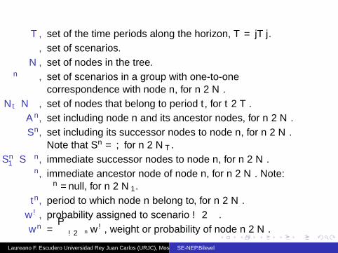
T , set of the time periods along the horizon, T = |T |.Ω, set of scenarios.N , set of nodes in the tree.
Ωn ⊆ Ω, set of scenarios in a group with one-to-onecorrespondence with node n, for n ∈ N .
Nt ⊂ N , set of nodes that belong to period t , for t ∈ T .An, set including node n and its ancestor nodes, for n ∈ N .Sn, set including its successor nodes to node n, for n ∈ N .
Note that Sn = ∅ for n ∈ NT .Sn
1 ⊆ Sn, immediate successor nodes to node n, for n ∈ N .σn, immediate ancestor node of node n, for n ∈ N . Note:
σn =null, for n ∈ N1.tn, period to which node n belong to, for n ∈ N .
wω, probability assigned to scenario ω ∈ Ω.wn =
∑ω∈Ωn wω, weight or probability of node n ∈ N .
Laureano F. Escudero Universidad Rey Juan Carlos (URJC), Mostoles (Madrid), [email protected]

Multiperiod Mixed 0-1 DEMfor Network Expansion Planning (NEP)
z = max∑n∈N
wn(anxn + bnyn)
s.t. xn ∈ 0,1nx(n), xσn ≤ xn ∀n ∈ N
Anxn + Bnyn = hn ∀n ∈ Nyn ∈ Y n ∀n ∈ N ,
where xn is a vector included by the so-named 0-1 step vars,and Y n is a feasible set of mixed 0-1 vectors.
Let xn, yn: Value vectors of the vectors xn, yn, resp., in a (full orpartial) solution, if any, for n ∈ N .
Laureano F. Escudero Universidad Rey Juan Carlos (URJC), Mostoles (Madrid), [email protected]
Stochastic Equilibrium-based NEP optimization. TAP:Sets
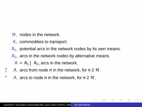
N , nodes in the network.
K, commodities to transport.
A1, potential arcs in the network nodes by its own means.
A2, arcs in the network nodes by alternative means.
A = A1 ∪ A2, arcs in the network.
Γn+ ⊂ A, arcs from node n in the network, for n ∈ N .
Γn− ⊂ A, arcs to node n in the network, for n ∈ N .
Laureano F. Escudero Universidad Rey Juan Carlos (URJC), Mostoles (Madrid), [email protected]
Stochastic Equilibrium-based NEP optimization. TAP:Deterministic parameters
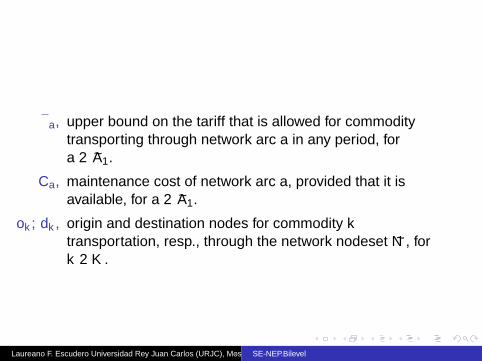
θa, upper bound on the tariff that is allowed for commoditytransporting through network arc a in any period, fora ∈ A1.
Ca, maintenance cost of network arc a, provided that it isavailable, for a ∈ A1.
ok , dk , origin and destination nodes for commodity ktransportation, resp., through the network nodeset N , fork ∈ K.
Laureano F. Escudero Universidad Rey Juan Carlos (URJC), Mostoles (Madrid), [email protected]

Stochastic Equilibrium-based NEP optimization. TAP:Stochastic parameters for scenario tree node n ∈ N
Una , investment cost for building network arc a, for a ∈ A1.
Un, available budget for network expansion planning.
V nk , commodity k volume to be transported for origin to
destination, for k ∈ K.
Bna , commodity transport unit cost through non-network arc a,
for a ∈ A2.
Laureano F. Escudero Universidad Rey Juan Carlos (URJC), Mostoles (Madrid), [email protected]
Stochastic Equilibrium-based NEP optimization. TAP:Variables xn
a in the upper-level model for scenarionode n, for n ∈ N
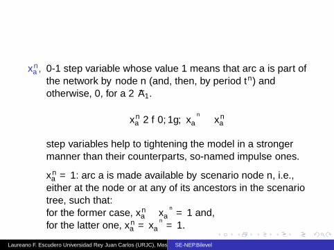
xna , 0-1 step variable whose value 1 means that arc a is part of
the network by node n (and, then, by period tn) andotherwise, 0, for a ∈ A1.
xna ∈ 0,1, xσ
n
a ≤ xna
step variables help to tightening the model in a strongermanner than their counterparts, so-named impulse ones.
xna = 1: arc a is made available by scenario node n, i.e.,
either at the node or at any of its ancestors in the scenariotree, such that:for the former case, xn
a − xσn
a = 1 and,for the latter one, xn
a = xσn
a = 1.
Laureano F. Escudero Universidad Rey Juan Carlos (URJC), Mostoles (Madrid), [email protected]

Stochastic Equilibrium-based NEP optimization. TAP:Variables θn
a in the upper-level model for scenario noden, for n ∈ N
θna , unit toll price (i.e., tariff) for commodity transport through
network arc a, for a ∈ A1.
0 ≤ θna ≤ θa
It is not active in case that arc a is not available, i.e.,xn
a = 0.
Laureano F. Escudero Universidad Rey Juan Carlos (URJC), Mostoles (Madrid), [email protected]
Variables in (each) dupla (commodity k , scenario noden)-based lower-level model, for k ∈ K, n ∈ N
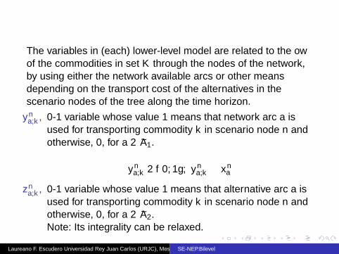
The variables in (each) lower-level model are related to the flowof the commodities in set K through the nodes of the network,by using either the network available arcs or other meansdepending on the transport cost of the alternatives in thescenario nodes of the tree along the time horizon.
yna,k , 0-1 variable whose value 1 means that network arc a is
used for transporting commodity k in scenario node n andotherwise, 0, for a ∈ A1.
yna,k ∈ 0,1, yn
a,k ≤ xna
zna,k , 0-1 variable whose value 1 means that alternative arc a is
used for transporting commodity k in scenario node n andotherwise, 0, for a ∈ A2.Note: Its integrality can be relaxed.
Laureano F. Escudero Universidad Rey Juan Carlos (URJC), Mostoles (Madrid), [email protected]
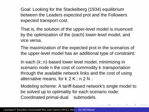
Goal: Looking for the Stackelberg (1934) equilibriumbetween the Leaders expected profit and the Followersexpected transport cost.
That is, the solution of the upper-level model is influencedby the optimization of the (each) lower-level model, andvice versa.
The maximization of the expected profit in the scenarios ofthe upper-level model has an additional type of constraint:
In each (k ,n)-based lower level model, minimizing inscenario node n the cost of commodity k transportationthrough the available network links and the cost of usingalternative means, for k ∈ K, n ∈ N .
Modeling scheme: A tariff-based network’s single model tobe solved up to optimality for each scenario node:Coordinated primal-dual submodels.
Laureano F. Escudero Universidad Rey Juan Carlos (URJC), Mostoles (Madrid), [email protected]
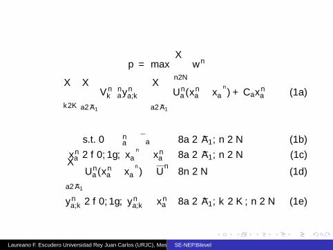
Upper-level model
p = max∑n∈N
wn
[∑k∈K
∑a∈A1
V nk θ
nayn
a,k −∑a∈A1
(Un
a (xna − xσ
n
a ) + Caxna)]
(1a)
s.t. 0 ≤ θna ≤ θa ∀a ∈ A1, n ∈ N (1b)
xna ∈ 0,1, xσ
n
a ≤ xna ∀a ∈ A1, n ∈ N (1c)∑
a∈A1
Una (xn
a − xσn
a ) ≤ Un ∀n ∈ N (1d)
yna,k ∈ 0,1, yn
a,k ≤ xna ∀a ∈ A1, k ∈ K, n ∈ N (1e)
Laureano F. Escudero Universidad Rey Juan Carlos (URJC), Mostoles (Madrid), [email protected]

(k ,n)-scenario node-based lower-level model, fork ∈ K, n ∈ N
cnk = min
(∑a∈A1
V nk θ
nayn
a,k +∑a∈A2
V nk Bn
azna,k)
(2a)
s.t.∑
a∈Γn+∩A1
yna,k +
∑a∈Γn
+∩A2
zna,k −
∑a∈Γn
−∩A1
yna,k −
∑a∈Γn
−∩A2
zna,k
= ρn,k ∀n ∈ N (2b)
0 ≤ yna,k ∀a ∈ A1 (2c)
0 ≤ zna,k ∀a ∈ A2, (2d)
where for n ∈ N : ρn,k = 1 for n = ok , ρn,k = −1 for n = dk andotherwise, ρn,k = 0.
Laureano F. Escudero Universidad Rey Juan Carlos (URJC), Mostoles (Madrid), [email protected]

It is well-known that there is an optimal solution for model(2) where the (y , z)-variables take 0-1 values.
So, no upper bound should be imposed on those variables,but bound 1 could reinforce the model.
Notice that there is a submodel for each dupla (scenarionode, commodity) in TAP.
In other types of applications there is only a submodel foreach scenario node.
As an Illustrative example, the lower-level reacts to each(θ, x)-offering from the upper-level solution until getting atariff equilibrium.
Applications: Open market in energy, good selling,transportation, etc. where both type of agents havealternatives for pursuing their aims.
Laureano F. Escudero Universidad Rey Juan Carlos (URJC), Mostoles (Madrid), [email protected]

The primal-dual approach is chosen in this work, sinceprovisional results on the KKT approach requiredunaffordable computing effort for instances underconsideration.
That big effort, probably, was due to the big M-parametersthat are required for the linearly representation of thequadratic complementary slackness conditions for eachscenario node.
Let δnn,k be the free dual variable of the conservation flow
constraint (2b) of the primal-dual model below, for thetriplet given by network node n, commodity k and scenarionode n.
Laureano F. Escudero Universidad Rey Juan Carlos (URJC), Mostoles (Madrid), [email protected]

Variable f na,k : Mixed 0-1 bilinear function θn
ayna,k , for
a ∈ A1, k ∈ K, n ∈ N , to be equivalently replaced with theFortet inequalities:
f na,k ≤ θayn
a,kθn
a − θa(1− yna,k ) ≤ f n
a,k ≤ θna + θa(1− yn
a,k )(3)
Laureano F. Escudero Universidad Rey Juan Carlos (URJC), Mostoles (Madrid), [email protected]
Single deterministic equivalent model tothe multi-period stochastic equilibrium-basedprimal-dual optimization model for network expansionplanning
Laureano F. Escudero Universidad Rey Juan Carlos (URJC), Mostoles (Madrid), [email protected]
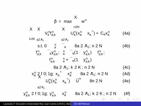
Upper level primal model
p = max∑n∈N
wn
[∑k∈K
∑a∈A1
V nk f n
a,k −∑a∈A1
(Un
a (xna − xσ
n
a ) + Caxna)]
(4a)
s.t. 0 ≤ θna ≤ θa ∀a ∈ A1, n ∈ N (4b)
f na,k ≤ θayn
a,k , θna − θa(1− yn
a,k ) ≤ f na,k ,
f na,k ≤ θ
na + θa(1− yn
a,k )
∀a ∈ A1, k ∈ K, n ∈ N (4c)xn
a ∈ 0,1, xσn
a ≤ xna ∀a ∈ A1, n ∈ N (4d)∑
a∈A1
Una (xn
a − xσn
a ) ≤ Un ∀n ∈ N (4e)
yna,k ∈ 0,1, yn
a,k ≤ xna ∀a ∈ A1, k ∈ K, n ∈ N (4f)
Laureano F. Escudero Universidad Rey Juan Carlos (URJC), Mostoles (Madrid), [email protected]

s.t. constraints of the (k ,n)-based lower models, for k ∈ K, n ∈ N
Primal model constraints:∑a∈Γn
+∩A1
yna,k +
∑a∈Γn
+∩A2
zna,k −
∑a∈Γn
−∩A1
yna,k −
∑a∈Γn
−∩A2
zna,k
= ρn,k ∀n ∈ N , k ∈ K (4g)
0 ≤ zna,k ≤ 1 ∀a ∈ A2, k ∈ K (4h)
Dual model constraints:V n
k θna − δn
n,k + δnn′,k≥ 0 ∀a = (n, n′) ∈ A1, k ∈ K (4i)
V nk Bn
a − δnn,k + δn
n′,k≥ 0 ∀a = (n, n′) ∈ A2, k ∈ K (4j)
Equating the (k ,n)-based primal and dual objective functions:(∑a∈A1
V nk f n
a,k +∑a∈A2
V nk Bn
azna,k)
= δnok ,k − δ
ndk ,k (4k)
Laureano F. Escudero Universidad Rey Juan Carlos (URJC), Mostoles (Madrid), [email protected]
Nested Stochastic Decomposition methodologoy.Some refs.
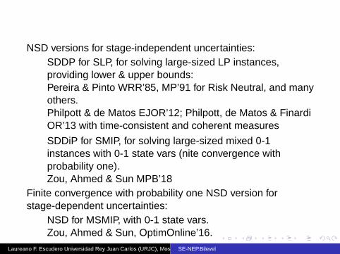
NSD versions for stage-independent uncertainties:SDDP for SLP, for solving large-sized LP instances,providing lower & upper bounds:Pereira & Pinto WRR’85, MP’91 for Risk Neutral, and manyothers.Philpott & de Matos EJOR’12; Philpott, de Matos & FinardiOR’13 with time-consistent and coherent measuresSDDiP for SMIP, for solving large-sized mixed 0-1instances with 0-1 state vars (finite convergence withprobability one).Zou, Ahmed & Sun MPB’18
Finite convergence with probability one NSD version forstage-dependent uncertainties:
NSD for MSMIP, with 0-1 state vars.Zou, Ahmed & Sun, OptimOnline’16.
Laureano F. Escudero Universidad Rey Juan Carlos (URJC), Mostoles (Madrid), [email protected]

Some refs. on NSD methodology (c)
Matheuristic NSD versions for mixed 0-1 state vars withstage-dependent uncertainties, for MSMIP:
Case w/ influential vars from immediate ancestor node:NSD-RN. Aldasoro, LFE, Merino, Monge & Perez TOP’14,among others. Continuous state vars.NSD-BILEVEL-NEP, for Stochastic Equilibrium in NetworkExpansion Planning. 0-1 state vars.LFE, Monge & Rodrigez-Chıa. Submitted, 2019.
Case w/ influential var from ancestor nodes:NSD-TSD, with Time in-consistent Stochastic Dominancefunctional.LFE, Monge & RomeroMorales COR’15NSD-ECSD, with Time consistent Expected ConditionalStochastic Dominance functional.LFE, Monge & RomeroMorales COR’18
Laureano F. Escudero Universidad Rey Juan Carlos (URJC), Mostoles (Madrid), [email protected]
NSD matheuristic, Nested Stochastic Decomposition
NSD starts by partitioning the set of time periods intomodeler-driven so-named stages each one is a subset ofconsecutive periods, creating thus a collection ofsubtrees/subproblems.The subproblems are not independent but each one islinked by the 0-1 step vars to the immediate ancestorsubproblem.NSD solves the subproblems at each iteration, byexecuting first a front-to-back scheme and after aback-to-from scheme.
Laureano F. Escudero Universidad Rey Juan Carlos (URJC), Mostoles (Madrid), [email protected]
Front-to-Back (FtB)
Back-to-Front (BtF)
t = 1 t = 2 t = 3 t = 4 t = 5 t = 6 t = 7
e = 1 e = 2 e = 3
First stage Intermediate stages Last stage
1 2 3
4
5
6
7
8
9
10
11
12
13
14
15
16
17
18
19
20
21
22
23
24
25
26
27
28
29
30
31
32
33
T = 1, . . . , 7,E = 1, 2, 3
Ω = Ω1 = 18, 19, . . . , 33
A6 = 6, 4, 3, 2, 1
t6 = 5
σ6 = 4
S6 = 10, 11, 18, 19, 20, 21
S61 = 10, 11
G2 = 4, 5, 6, 7, 8, 9
R2 = 4, 5
C4 = 4, 6, 7
L15 = 28, 29
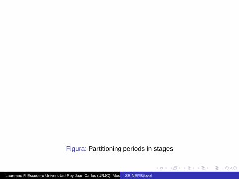
Figura: Partitioning periods in stages
Laureano F. Escudero Universidad Rey Juan Carlos (URJC), Mostoles (Madrid), [email protected]
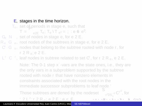
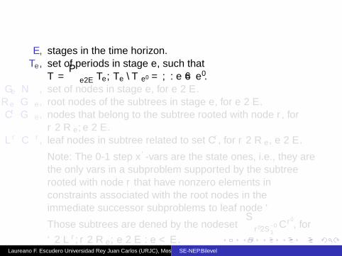
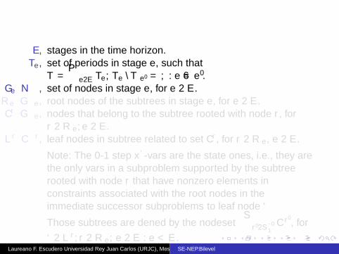
Scenario subtrees supporting the NSD subproblems.Sets
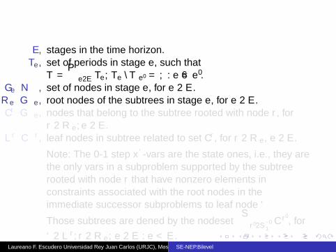
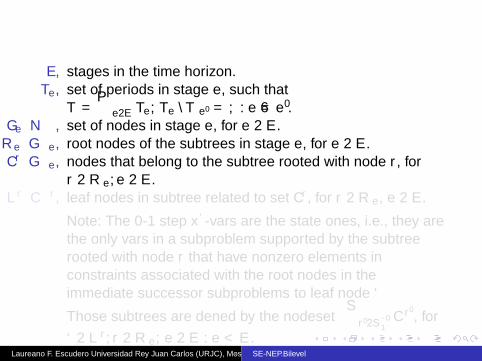
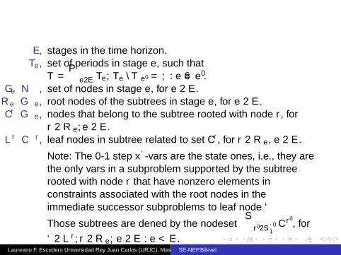
E , stages in the time horizon.Te, set of periods in stage e, such that
T =∑
e∈E Te, Te ∩ Te′ = ∅ : e 6= e′.Ge ⊆ N , set of nodes in stage e, for e ∈ E .Re ⊆ Ge, root nodes of the subtrees in stage e, for e ∈ E .Cr ⊆ Ge, nodes that belong to the subtree rooted with node r , for
r ∈ Re,e ∈ E .Lr ⊆ Cr , leaf nodes in subtree related to set Cr , for r ∈ Re, e ∈ E .
Note: The 0-1 step x`-vars are the state ones, i.e., they arethe only vars in a subproblem supported by the subtreerooted with node r that have nonzero elements inconstraints associated with the root nodes in theimmediate successor subproblems to leaf node `
Those subtrees are defined by the nodeset⋃
r ′∈S`′1Cr ′ , for
` ∈ Lr , r ∈ Re, e ∈ E : e < E .Laureano F. Escudero Universidad Rey Juan Carlos (URJC), Mostoles (Madrid), [email protected]
Scenario subtrees supporting the NSD subproblems.Sets
E , stages in the time horizon.Te, set of periods in stage e, such that
T =∑
e∈E Te, Te ∩ Te′ = ∅ : e 6= e′.Ge ⊆ N , set of nodes in stage e, for e ∈ E .Re ⊆ Ge, root nodes of the subtrees in stage e, for e ∈ E .Cr ⊆ Ge, nodes that belong to the subtree rooted with node r , for
r ∈ Re,e ∈ E .Lr ⊆ Cr , leaf nodes in subtree related to set Cr , for r ∈ Re, e ∈ E .
Note: The 0-1 step x`-vars are the state ones, i.e., they arethe only vars in a subproblem supported by the subtreerooted with node r that have nonzero elements inconstraints associated with the root nodes in theimmediate successor subproblems to leaf node `
Those subtrees are defined by the nodeset⋃
r ′∈S`′1Cr ′ , for
` ∈ Lr , r ∈ Re, e ∈ E : e < E .Laureano F. Escudero Universidad Rey Juan Carlos (URJC), Mostoles (Madrid), [email protected]
NSD matheuristic. EFV curves
Let the so-named Expected Future Value (EFV) curve ofthe subproblem supported by the subtree given by nodesetCr ′ , whose root node r ′ is an immediate successor of leafnode `, for r ′ ∈ S`1, ` ∈ Lr , r ∈ Re, e ∈ E : e < E , whereremember Lr ⊆ Cr .
EFV curves estimate the impact of the state vars(decisions) of the leaf nodes in the objective function ofsuccessor subproblems.
(.), current solution of the variables’ vector (.).
Laureano F. Escudero Universidad Rey Juan Carlos (URJC), Mostoles (Madrid), [email protected]

For easing the exposition, let a set of variables in the originalmodel (4) be notated as vector Z n, for n ∈ N . It can beexpressed
Z n ≡(yg ∀g ∈ An; xg ∀g ∈ An \ n
)(5)
Laureano F. Escudero Universidad Rey Juan Carlos (URJC), Mostoles (Madrid), [email protected]
EFV curve λ′r ′(x `), forr ′ ∈ S`1, ` ∈ Lr , r ∈ Re, e ∈ E : e < E
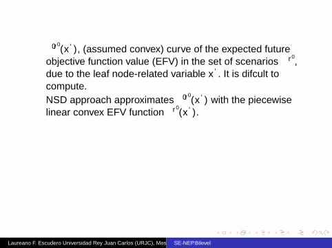
λ′r′(x`), (assumed convex) curve of the expected future
objective function value (EFV) in the set of scenarios Ωr ′ ,due to the leaf node-related variable x`. It is difficult tocompute.NSD approach approximates λ′r
′(x`) with the piecewise
linear convex EFV function λr ′(x`).
xℓ1b
b
b
b
b
b
b
b
b
b
b
b
b
b
xℓ3b
b
b
b
b
b
b
b
b
b
b
b
b
b
b
b
b
b
b
b
b
b
b
b
xℓ2
λr′3(x) = µr′3 + πr′3x
λr′1 (x) = µr′1 + πr′1x
λr′2(x) = µr′2 + πr′2x
λr′
xℓ
Laureano F. Escudero Universidad Rey Juan Carlos (URJC), Mostoles (Madrid), [email protected]

Objective function value F ′r of subproblem defined bynode set Cr , r ∈ Re, e ∈ E
F ′r = max∑`∈Lr
w `[∑
n∈A`
(anxn + bnyn) +∑
r ′∈S`1
w r ′
w `λ′r′(
x`)]
s.t. Anxn + Bnyn = hn, yn ∈ Y n ∀n ∈ Cr
xn ∈ 0,1nx , xσn ≤ xn ∀n ∈ Cr
Zσr= Zσr
xσr − xσ
r= 0
(6)
Laureano F. Escudero Universidad Rey Juan Carlos (URJC), Mostoles (Madrid), [email protected]

Elements definition of EFV function λr ′, forr ′ ∈ S`1, ` ∈ Lr , r ∈ Re, e ∈ E : e < E
Let Q` denote the set of indices q, such that the referencelevels indexed with q define the EFV function λr ′ .Each qth reference level is composed by vector(
x`q; µr ′q , πr ′q ∀r ′ ∈ S`1
),
where vector x`q
is the value of the vars in vector x`q, for
q ∈ Q`, retrieved from the subproblem related to scenario noder , andconstant µr ′q and vector πr ′q define a linear function of vector x`
obtained from the solution of the subproblem related to theimmediate successor node r ′ of scenario leaf node `, i.e.,q ∈ Q`, r ′ ∈ S`1, ` ∈ Lr .
λr ′ = minq∈Q`
µr ′q + πr ′q x`
.
Laureano F. Escudero Universidad Rey Juan Carlos (URJC), Mostoles (Madrid), [email protected]

EFV function λr ′, forr ′ ∈ S`1, ` ∈ Lr , r ∈ Re, e ∈ E : e < E
λr ′ = minq∈Q`
µr ′q + πr ′q x`
.
It is required that it is a valid cut for EFV curve λ′r′(·) as well as
a tight one, such that λ′r′(x`
q) = µr ′q + πr ′q x`
q.
Laureano F. Escudero Universidad Rey Juan Carlos (URJC), Mostoles (Madrid), [email protected]

Objective function value F r of subproblem defined bynode set Cr , r ∈ Re, e ∈ E : e < E , where EFV curveλ′r(x `) is replaced with EFV (piecewise linear) functionλr ′(x `), for r ′ ∈ S`1, ` ∈ Lr
F r = max∑`∈Lr
w `[∑
n∈A`
(anxn + bnyn) +∑
r ′∈S`1
w r ′
w `λr ′] (7a)
s.t. Anxn + Bnyn = hn, yn ∈ Y n ∀n ∈ Cr (7b)xn ∈ 0,1nx , xσ
n ≤ xn ∀n ∈ Cr (7c)
Zσr= Zσr q
(7d)
x` − xσr q
= 0 (7e)λr ′ ≤ µr ′q + πr ′q x` ∀q ∈ Q`, r ′ ∈ S`1, ` ∈ Lr . (7f)
Laureano F. Escudero Universidad Rey Juan Carlos (URJC), Mostoles (Madrid), [email protected]

xℓ1b
b
b
b
b
b
b
b
b
b
b
b
b
b
xℓ3b
b
b
b
b
b
b
b
b
b
b
b
b
b
b
b
b
b
b
b
b
b
b
b
xℓ2
λr′3(x) = µr′3 + πr′3x
λr′1 (x) = µr′1 + πr′1x
λr′2(x) = µr′2 + πr′2x
λr′
xℓ
Laureano F. Escudero Universidad Rey Juan Carlos (URJC), Mostoles (Madrid), [email protected]

NSD approach. Front-to-Back scheme from stagee = 1 to last stage e = E
Subproblems (7) from stage 1 to last one E are solved bypassing the values of linking x-vars onto the subproblemsin the next stage.
λ-values are zero in iteration q = 1.
In case of infeasibility of subproblem (7) for r ∈ Re, e ∈ E :merging scheme of stages e-1 and e.
Building a feas solution for original model (4)(xn, yn ∀n ∈ N ).
Obj fun value F =∑
n∈N wn(anxn + bnyn)
In that case, a testing is performed to analyze whether itimproves the incumbent solution.
Laureano F. Escudero Universidad Rey Juan Carlos (URJC), Mostoles (Madrid), [email protected]

Laureano F. Escudero Universidad Rey Juan Carlos (URJC), Mostoles (Madrid), [email protected]

Front-to-Back (FtB)
Back-to-Front (BtF)
t = 1 t = 2 t = 3 t = 4 t = 5 t = 6 t = 7
e = 1 e = 2 e = 3
First stage Intermediate stages Last stage
1 2 3
4
5
6
7
8
9
10
11
12
13
14
15
16
17
18
19
20
21
22
23
24
25
26
27
28
29
30
31
32
33
T = 1, . . . , 7,E = 1, 2, 3
Ω = Ω1 = 18, 19, . . . , 33
A6 = 6, 4, 3, 2, 1
t6 = 5
σ6 = 4
S6 = 10, 11, 18, 19, 20, 21
S61 = 10, 11
G2 = 4, 5, 6, 7, 8, 9
R2 = 4, 5
C4 = 4, 6, 7
L15 = 28, 29
Laureano F. Escudero Universidad Rey Juan Carlos (URJC), Mostoles (Madrid), [email protected]

NSD approach. Front-to-Back scheme from stagee = 1 to last stage e = E (c)
Upper bound of the solution value of the original model (4):solution value F r of model (7) for r = 0 (i.e., e = 1).
OG: Optimality gap of a given feasible solution value F ofthe original model (4) with respect to F 0 at iteration, say q.
Laureano F. Escudero Universidad Rey Juan Carlos (URJC), Mostoles (Madrid), [email protected]
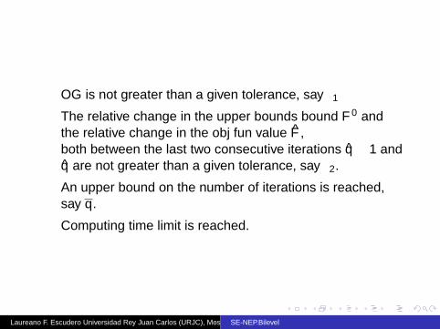
NSD approach. Stopping criteria
1 OG is not greater than a given tolerance, say ε12 The relative change in the upper bounds bound F 0 and
the relative change in the obj fun value F ,both between the last two consecutive iterations q − 1 andq are not greater than a given tolerance, say ε2.
3 An upper bound on the number of iterations is reached,say q.
4 Computing time limit is reached.
Laureano F. Escudero Universidad Rey Juan Carlos (URJC), Mostoles (Madrid), [email protected]

NSD approach. Back-to-Front scheme from last stagee = E to stage e = 2
It aims to refining the EFV functions λr ′ in the subproblemssupported by the subtrees rooted with the nodeset r ′ inRe, e ∈ E \ 1 around the feasible soln (Z n, xn ∀n ∈ NT )built in the front-to-back scheme at the current iteration q.
The subproblems in a given stage are solved, passing therefinement of the EFV functions onto the subproblems inthe previous stage.
Laureano F. Escudero Universidad Rey Juan Carlos (URJC), Mostoles (Madrid), [email protected]

NSD approach. On EFV function λr ′, forr ′ ∈ S`1, ` ∈ Lr , r ∈ Re, e ∈ E : e < E
Generating and appending a new set S`1 of linear functionsλr ′q
λr ′ ≤ µr ′q + πr ′q x` (8)
to the collection (7f):
λr ′ ≤ µr ′q + πr ′q x` ∀q ∈ Q` \ q, r ′ ∈ S`1, ` ∈ Lr
in model (7) related to the solution x`q, retrieved from the
front-to-back scheme, where q is the last iteration.
Laureano F. Escudero Universidad Rey Juan Carlos (URJC), Mostoles (Madrid), [email protected]

On obtaining vector (µr ′q , πr ′q)
It is worth to pointing out that some state-of-the-art optimizers(as CPLEX and others) do not provide the duals of theconstraints for fixed vars in MIP models.So, some alternatives:
Benders cut, B (Benders NM’62).
Lagrangean cut, L(Zou, Ahmed & Sun OptimOnline’16, MPB’18).
Strengthened Benders cut, SB(Zou, Ahmed & Sun OptimOnline’16, MPB’18).
Heuristic Benders cut, HB.
A mixture of SB cuts for later sages and L cuts for earlierstages, in particular, stage e = 1. Work-in-Progress.
Laureano F. Escudero Universidad Rey Juan Carlos (URJC), Mostoles (Madrid), [email protected]

Approximation schemes for EFV curve λ′r ′(x `): L-,SB-, B- and HB-based cuts for obtaining EFV functionλr ′(x `)
L: Valid and tight
SB: Valid and no-guarantee it is tight.
B: Valid and ’almost’ sure it is not tight.
HB: No guarantee it is valid, and sure it is tighter than B.
That is, there it not any guarantee that the EFV functionλr ′(x`) does not cut any feasible solution of the originalmodel (4).
So, no guarantee that the NSD incumbent solution is theoptimal one for, nor an upper bound is obtained.
Laureano F. Escudero Universidad Rey Juan Carlos (URJC), Mostoles (Madrid), [email protected]

HB-based cut for approximating EFV curve λ′r ′(x `) viaEFV function λr ′(x `)
No guarantee that the EFV function λr ′(x`) does not cutany feasible solution of the original model (4).
So, no guarantee that the NSD incumbent solution is theoptimal one for, nor an upper bound is obtained.
xℓ1b
b
b
b
b
b
b
b
b
b
b
b
b
b
xℓ3b
b
b
b
b
b
b
b
b
b
b
b
b
b
b
b
b
b
b
b
b
b
b
b
xℓ2
λr′3(x) = µr′3 + πr′3x
λr′1 (x) = µr′1 + πr′1x
λr′2(x) = µr′2 + πr′2x
λr′
xℓ
Laureano F. Escudero Universidad Rey Juan Carlos (URJC), Mostoles (Madrid), [email protected]
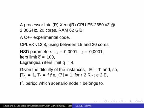
Computational experience. Computing HW/SW
A processor Intel(R) Xeon(R) CPU E5-2650 v3 @2.30GHz, 20 cores, RAM 62 GiB.
A C++ experimental code.
CPLEX v12.8, using between 15 and 20 cores.
NSD parameters: ε1 = 0,0001, ε2 = 0,0001,iters limit q = 100,Lagrangean iters limit q = 4.
Given the difficulty of the instances, E = T and, so,|Te| = 1, Te = t r, |Cr | = 1, for r ∈ Re, e ∈ E ,
t r , period which scenario node r belongs to.
Laureano F. Escudero Universidad Rey Juan Carlos (URJC), Mostoles (Madrid), [email protected]
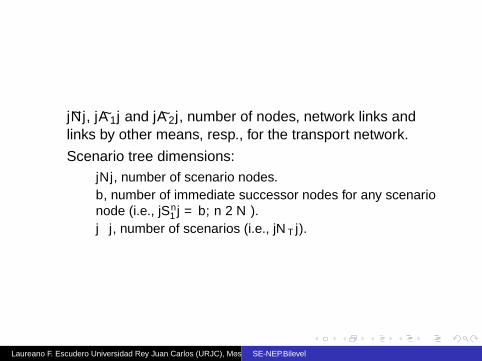
4 Testbeds
|N|, |A1| and |A2|, number of nodes, network links andlinks by other means, resp., for the transport network.Scenario tree dimensions:
|N|, number of scenario nodes.b, number of immediate successor nodes for any scenarionode (i.e., |Sn
1 | = b, n ∈ N ).|Ω|, number of scenarios (i.e., |NT |).
Laureano F. Escudero Universidad Rey Juan Carlos (URJC), Mostoles (Madrid), [email protected]
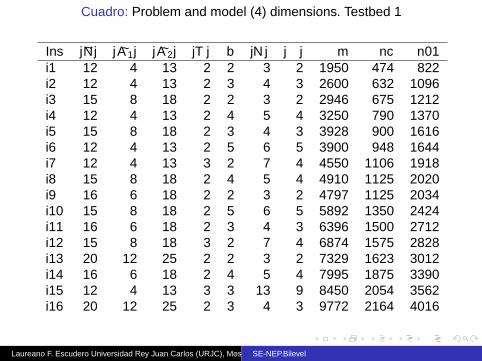
Cuadro: Problem and model (4) dimensions. Testbed 1
Ins |N| |A1| |A2| |T | b |N | |Ω| m nc n01i1 12 4 13 2 2 3 2 1950 474 822i2 12 4 13 2 3 4 3 2600 632 1096i3 15 8 18 2 2 3 2 2946 675 1212i4 12 4 13 2 4 5 4 3250 790 1370i5 15 8 18 2 3 4 3 3928 900 1616i6 12 4 13 2 5 6 5 3900 948 1644i7 12 4 13 3 2 7 4 4550 1106 1918i8 15 8 18 2 4 5 4 4910 1125 2020i9 16 6 18 2 2 3 2 4797 1125 2034i10 15 8 18 2 5 6 5 5892 1350 2424i11 16 6 18 2 3 4 3 6396 1500 2712i12 15 8 18 3 2 7 4 6874 1575 2828i13 20 12 25 2 2 3 2 7329 1623 3012i14 16 6 18 2 4 5 4 7995 1875 3390i15 12 4 13 3 3 13 9 8450 2054 3562i16 20 12 25 2 3 4 3 9772 2164 4016
Laureano F. Escudero Universidad Rey Juan Carlos (URJC), Mostoles (Madrid), [email protected]
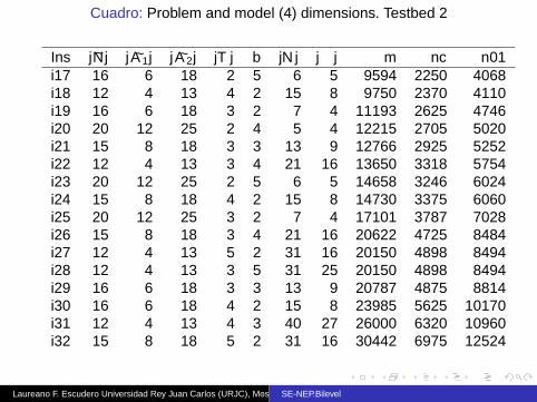
Cuadro: Problem and model (4) dimensions. Testbed 2
Ins |N| |A1| |A2| |T | b |N | |Ω| m nc n01i17 16 6 18 2 5 6 5 9594 2250 4068i18 12 4 13 4 2 15 8 9750 2370 4110i19 16 6 18 3 2 7 4 11193 2625 4746i20 20 12 25 2 4 5 4 12215 2705 5020i21 15 8 18 3 3 13 9 12766 2925 5252i22 12 4 13 3 4 21 16 13650 3318 5754i23 20 12 25 2 5 6 5 14658 3246 6024i24 15 8 18 4 2 15 8 14730 3375 6060i25 20 12 25 3 2 7 4 17101 3787 7028i26 15 8 18 3 4 21 16 20622 4725 8484i27 12 4 13 5 2 31 16 20150 4898 8494i28 12 4 13 3 5 31 25 20150 4898 8494i29 16 6 18 3 3 13 9 20787 4875 8814i30 16 6 18 4 2 15 8 23985 5625 10170i31 12 4 13 4 3 40 27 26000 6320 10960i32 15 8 18 5 2 31 16 30442 6975 12524
Laureano F. Escudero Universidad Rey Juan Carlos (URJC), Mostoles (Madrid), [email protected]
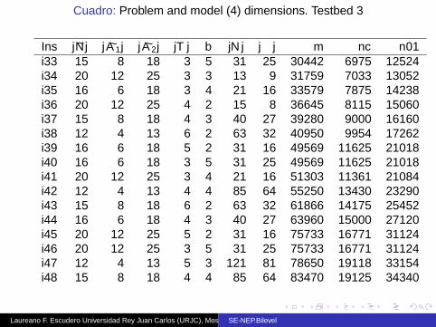
Cuadro: Problem and model (4) dimensions. Testbed 3
Ins |N| |A1| |A2| |T | b |N | |Ω| m nc n01i33 15 8 18 3 5 31 25 30442 6975 12524i34 20 12 25 3 3 13 9 31759 7033 13052i35 16 6 18 3 4 21 16 33579 7875 14238i36 20 12 25 4 2 15 8 36645 8115 15060i37 15 8 18 4 3 40 27 39280 9000 16160i38 12 4 13 6 2 63 32 40950 9954 17262i39 16 6 18 5 2 31 16 49569 11625 21018i40 16 6 18 3 5 31 25 49569 11625 21018i41 20 12 25 3 4 21 16 51303 11361 21084i42 12 4 13 4 4 85 64 55250 13430 23290i43 15 8 18 6 2 63 32 61866 14175 25452i44 16 6 18 4 3 40 27 63960 15000 27120i45 20 12 25 5 2 31 16 75733 16771 31124i46 20 12 25 3 5 31 25 75733 16771 31124i47 12 4 13 5 3 121 81 78650 19118 33154i48 15 8 18 4 4 85 64 83470 19125 34340
Laureano F. Escudero Universidad Rey Juan Carlos (URJC), Mostoles (Madrid), [email protected]

Cuadro: Problem and model (4) dimensions. Testbed 4
Ins |N| |A1| |A2| |T | b |N | |Ω| m nc n01i49 12 4 13 7 2 127 64 82550 20066 34798i50 20 12 25 4 3 40 27 97720 21640 40160i51 16 6 18 6 2 63 32 100737 23625 42714i52 12 4 13 4 5 156 125 101400 24648 42744i53 15 8 18 5 3 121 81 118822 27225 48884i54 15 8 18 7 2 127 64 124714 28575 51308i55 16 6 18 4 4 85 64 135915 31875 57630i56 15 8 18 4 5 156 125 153192 35100 63024i57 20 12 25 6 2 63 32 153909 34083 63252i58 16 6 18 5 3 121 81 193479 45375 82038i59 20 12 25 4 4 85 64 207655 45985 85340i60 16 6 18 7 2 127 64 203073 47625 86106i61 16 6 18 4 5 156 125 249444 58500 105768i62 20 12 25 5 3 121 81 295603 65461 121484i63 20 12 25 7 2 127 64 310261 68707 127508i64 20 12 25 4 5 156 125 381108 84396 156624
Laureano F. Escudero Universidad Rey Juan Carlos (URJC), Mostoles (Madrid), [email protected]

Results. CPLEX plain use and NSD in in L4, SB, HB
of i and ti , incumbent soln value for original model (4) andcomputing time (secs) for i = 1,3, wherei = 1 (CPLEX plain use w/ computing time as NSD;i = 3 (NSD).
of 1, CPLEX upper bound of opt sol, in L4, SB.
OG1 %, CPLEX optimality gap, 100.of 1−of 1of 1
, in L4, SB.
of 3, NSD estimation of upper bound of opt sol in L4, SB.
OG3 %, NSD estimation of the optimality gap, as
100. of 3−of 3of 3
in HB.
GR1, goodness ratio of NSD over CPLEX plain use, as of 3of 1
.
Laureano F. Escudero Universidad Rey Juan Carlos (URJC), Mostoles (Madrid), [email protected]
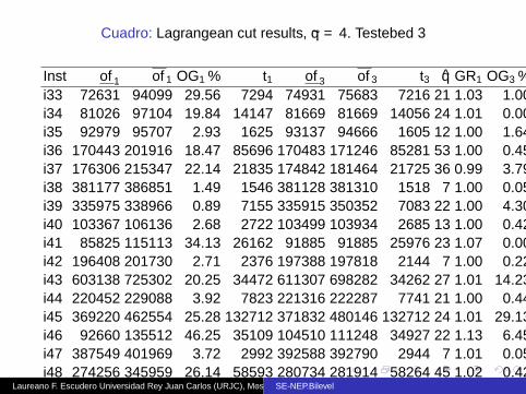
Cuadro: Lagrangean cut results, q = 4. Testebed 3
Inst of 1 of 1 OG1 % t1 of 3 of 3 t3 q GR1 OG3 %i33 72631 94099 29.56 7294 74931 75683 7216 21 1.03 1.00i34 81026 97104 19.84 14147 81669 81669 14056 24 1.01 0.00i35 92979 95707 2.93 1625 93137 94666 1605 12 1.00 1.64i36 170443 201916 18.47 85696 170483 171246 85281 53 1.00 0.45i37 176306 215347 22.14 21835 174842 181464 21725 36 0.99 3.79i38 381177 386851 1.49 1546 381128 381310 1518 7 1.00 0.05i39 335975 338966 0.89 7155 335915 350352 7083 22 1.00 4.30i40 103367 106136 2.68 2722 103499 103934 2685 13 1.00 0.42i41 85825 115113 34.13 26162 91885 91885 25976 23 1.07 0.00i42 196408 201730 2.71 2376 197388 197818 2144 7 1.00 0.22i43 603138 725302 20.25 34472 611307 698282 34262 27 1.01 14.23i44 220452 229088 3.92 7823 221316 222287 7741 21 1.00 0.44i45 369220 462554 25.28 132712 371832 480146 132712 24 1.01 29.13i46 92660 135512 46.25 35109 104510 111248 34927 22 1.13 6.45i47 387549 401969 3.72 2992 392588 392790 2944 7 1.01 0.05i48 274256 345959 26.14 58593 280734 281914 58264 45 1.02 0.42
Laureano F. Escudero Universidad Rey Juan Carlos (URJC), Mostoles (Madrid), [email protected]

Cuadro: Lagrangean cut results, q = 4. Testebed 4
Inst of 1 of 1 OG1 % t1 of 3 of 3 t3 q GR1 OG3 %i49 790692 833771 5.45 3058 813920 814102 3004 7 1.03 0.02i50 239974 318446 32.70 133110 246084 278280 132360 29 1.03 13.08i51 708116 734970 3.79 7457 719978 772717 7348 11 1.02 7.33i52 225544 309677 37.30 4017 298530 299633 3957 7 1.32 0.37i53 572181 734620 28.39 84470 588962 694614 84043 39 1.03 17.94i54 1335404 1591737 19.20 131115 1378708 1415879 131115 51 1.03 2.70i55 340948 363425 6.59 20946 348936 349436 20682 26 1.02 0.14i56 404471 531153 31.32 102128 424072 432277 101547 45 1.05 1.93i57 1055410 139126 830580 1582535 139126 11 90.53i58 650253 733051 12.73 47672 707648 710406 47152 37 1.09 0.39i59 301048 507319 68.52 134385 384553 503137 133665 16 1.28 30.84i60 1366863 1595141 16.70 30628 1556647 1565923 30190 24 1.14 0.59i61 449334 542291 20.69 47286 515729 515729 46644 32 1.15 0.00i62 523257 1062376 103.03 133379 825055 1729673 132765 5 1.58 109.64i63 2387036 142238 1877392 7209842 142238 6 284.03i64 336794 779913 131.57 136197 595635 921531 135417 7 1.77 54.71
Laureano F. Escudero Universidad Rey Juan Carlos (URJC), Mostoles (Madrid), [email protected]
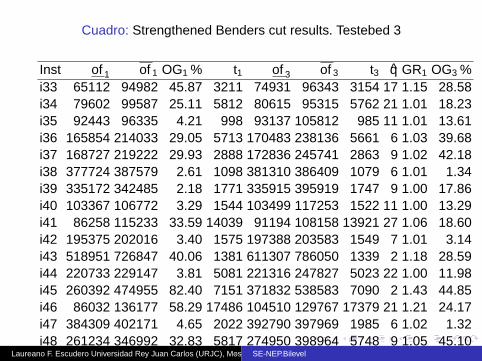
Cuadro: Strengthened Benders cut results. Testebed 3
Inst of 1 of 1 OG1 % t1 of 3 of 3 t3 q GR1 OG3 %i33 65112 94982 45.87 3211 74931 96343 3154 17 1.15 28.58i34 79602 99587 25.11 5812 80615 95315 5762 21 1.01 18.23i35 92443 96335 4.21 998 93137 105812 985 11 1.01 13.61i36 165854 214033 29.05 5713 170483 238136 5661 6 1.03 39.68i37 168727 219222 29.93 2888 172836 245741 2863 9 1.02 42.18i38 377724 387579 2.61 1098 381310 386409 1079 6 1.01 1.34i39 335172 342485 2.18 1771 335915 395919 1747 9 1.00 17.86i40 103367 106772 3.29 1544 103499 117253 1522 11 1.00 13.29i41 86258 115233 33.59 14039 91194 108158 13921 27 1.06 18.60i42 195375 202016 3.40 1575 197388 203583 1549 7 1.01 3.14i43 518951 726847 40.06 1381 611307 786050 1339 2 1.18 28.59i44 220733 229147 3.81 5081 221316 247827 5023 22 1.00 11.98i45 260392 474955 82.40 7151 371832 538583 7090 2 1.43 44.85i46 86032 136177 58.29 17486 104510 129767 17379 21 1.21 24.17i47 384309 402171 4.65 2022 392790 397969 1985 6 1.02 1.32i48 261234 346992 32.83 5817 274950 398964 5748 9 1.05 45.10
Laureano F. Escudero Universidad Rey Juan Carlos (URJC), Mostoles (Madrid), [email protected]

Cuadro: Strengthened Benders cut results. Testebed 4
Inst of 1 of 1 OG1 % t1 of 3 of 3 t3 q GR1 OG3 %i49 744545 834413 12.07 1082 814102 819551 1056 4 1.09 0.67i50 196564 320987 63.30 33648 246084 347831 33435 16 1.25 41.35i51 669308 735607 9.91 3973 719978 780192 3904 9 1.08 8.36i52 222571 309679 39.14 3228 299164 306235 3173 8 1.34 2.36i53 556944 745055 33.78 2086 588962 877015 2058 2 1.06 48.91i54 1082307 1621786 49.85 2875 1378708 1554399 2830 2 1.27 12.74i55 339253 363568 7.17 11144 348936 405605 10985 24 1.03 16.24i56 402302 532103 32.26 8126 423602 621672 8015 7 1.05 46.76i57 1077435 14943 830581 1197268 14250 2 44.15i58 476227 764845 60.61 1507 705704 922217 1451 2 1.48 30.68i59 233723 507319 117.06 55427 384553 567263 55099 14 1.65 47.51i60 1654596 8265 1556647 1616861 8053 9 3.87i61 379202 564082 48.75 1674 513926 721819 1605 2 1.36 40.45i62 582338 1062812 82.51 32982 825055 1238422 32745 3 1.42 50.10i63 2411878 32193 1877393 2779655 31248 2 48.06i64 336794 779913 131.57 75776 595635 904444 75291 11 1.77 51.85
Laureano F. Escudero Universidad Rey Juan Carlos (URJC), Mostoles (Madrid), [email protected]
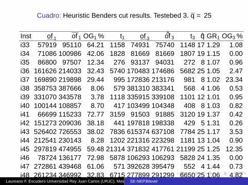
Cuadro: Heuristic Benders cut results. Testebed 3. q = 25
Inst of 1 of 1 OG1 % t1 of 3 of 3 t3 q GR1 OG3 %i33 57919 95110 64.21 1158 74931 75740 1148 17 1.29 1.08i34 71086 100986 42.06 1828 81669 81669 1807 19 1.15 0.00i35 86800 97507 12.34 276 93137 94031 272 8 1.07 0.96i36 161626 214033 32.43 5740 170483 174686 5682 25 1.05 2.47i37 169890 219898 29.44 995 172836 213176 981 8 1.02 23.34i38 358753 387666 8.06 579 381310 383341 568 4 1.06 0.53i39 331070 343578 3.78 1118 335915 339108 1101 12 1.01 0.95i40 100144 108857 8.70 417 103499 104348 408 8 1.03 0.82i41 66699 115233 72.77 3159 91503 91885 3120 19 1.37 0.42i42 151273 209036 38.18 441 197818 198338 429 5 1.31 0.26i43 526402 726553 38.02 7836 615374 637108 7784 25 1.17 3.53i44 212541 230143 8.28 1202 221316 223298 1181 13 1.04 0.90i45 297819 474955 59.48 21314 371832 417761 21199 25 1.25 12.35i46 78724 136177 72.98 5878 106293 106293 5828 24 1.35 0.00i47 272861 439468 61.06 571 392628 395479 552 4 1.44 0.73i48 261234 346992 32.83 6715 277899 291299 6650 25 1.06 4.82
Laureano F. Escudero Universidad Rey Juan Carlos (URJC), Mostoles (Madrid), [email protected]
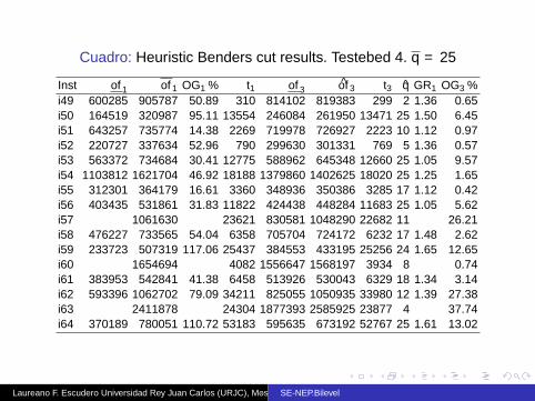
Cuadro: Heuristic Benders cut results. Testebed 4. q = 25
Inst of 1 of 1 OG1 % t1 of 3 of 3 t3 q GR1 OG3 %i49 600285 905787 50.89 310 814102 819383 299 2 1.36 0.65i50 164519 320987 95.11 13554 246084 261950 13471 25 1.50 6.45i51 643257 735774 14.38 2269 719978 726927 2223 10 1.12 0.97i52 220727 337634 52.96 790 299630 301331 769 5 1.36 0.57i53 563372 734684 30.41 12775 588962 645348 12660 25 1.05 9.57i54 1103812 1621704 46.92 18188 1379860 1402625 18020 25 1.25 1.65i55 312301 364179 16.61 3360 348936 350386 3285 17 1.12 0.42i56 403435 531861 31.83 11822 424438 448284 11683 25 1.05 5.62i57 1061630 23621 830581 1048290 22682 11 26.21i58 476227 733565 54.04 6358 705704 724172 6232 17 1.48 2.62i59 233723 507319 117.06 25437 384553 433195 25256 24 1.65 12.65i60 1654694 4082 1556647 1568197 3934 8 0.74i61 383953 542841 41.38 6458 513926 530043 6329 18 1.34 3.14i62 593396 1062702 79.09 34211 825055 1050935 33980 12 1.39 27.38i63 2411878 24304 1877393 2585925 23877 4 37.74i64 370189 780051 110.72 53183 595635 673192 52767 25 1.61 13.02
Laureano F. Escudero Universidad Rey Juan Carlos (URJC), Mostoles (Madrid), [email protected]

L4, SB, HB cut option results in NSD.Summary for SE-NEP
SE-NEP: Very difficult M01QP multistage problem w/large-scale model dimensions.
Weakness of original model (4): high range that is allowedto tariff θn
a , given the big θa-based constraints that arerequired for equivalently linearising θn
ayna,k .
Sharing the incumbent solution value of 3 in 23 out of the32 instances of Testbeds 3 and 4 (including the largestone, i64).
There are small differences in those values for most of theother instances.
The EFV functions λr ′ in SB and HB only differ in theconstant µr ′q .
Laureano F. Escudero Universidad Rey Juan Carlos (URJC), Mostoles (Madrid), [email protected]
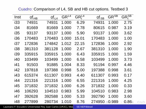
Cuadro: Comparison of L4, SB and HB cut options. Testbed 3
Inst of HB of L4 GRL4 GRL4t of SB GRSB GRSB
t
i33 74931 74931 1.000 6.29 74931 1.000 2.75i34 81669 81669 1.000 7.78 80615 0.987 3.19i35 93137 93137 1.000 5.90 93137 1.000 3.62i36 170483 170483 1.000 15.01 170483 1.000 1.00i37 172836 174842 1.012 22.15 172836 1.000 2.92i38 381310 381128 1.000 2.67 381310 1.000 1.90i39 335915 335915 1.000 6.43 335915 1.000 1.59i40 103499 103499 1.000 6.58 103499 1.000 3.73i41 91503 91885 1.004 8.33 91194 0.997 4.46i42 197818 197388 0.998 5.00 197388 0.998 3.61i43 615374 611307 0.993 4.40 611307 0.993 0.17i44 221316 221316 1.000 6.55 221316 1.000 4.25i45 371832 371832 1.000 6.26 371832 1.000 0.33i46 106293 104510 0.983 5.99 104510 0.983 2.98i47 392628 392588 1.000 5.33 392790 1.000 3.60i48 277899 280734 1.010 8.76 274950 0.989 0.86
Laureano F. Escudero Universidad Rey Juan Carlos (URJC), Mostoles (Madrid), [email protected]
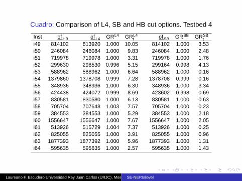
Cuadro: Comparison of L4, SB and HB cut options. Testbed 4
Inst of HB of L4 GRL4 GRL4t of SB GRSB GRSB
ti49 814102 813920 1.000 10.05 814102 1.000 3.53i50 246084 246084 1.000 9.83 246084 1.000 2.48i51 719978 719978 1.000 3.31 719978 1.000 1.76i52 299630 298530 0.996 5.15 299164 0.998 4.13i53 588962 588962 1.000 6.64 588962 1.000 0.16i54 1379860 1378708 0.999 7.28 1378708 0.999 0.16i55 348936 348936 1.000 6.30 348936 1.000 3.34i56 424438 424072 0.999 8.69 423602 0.998 0.69i57 830581 830580 1.000 6.13 830581 1.000 0.63i58 705704 707648 1.003 7.57 705704 1.000 0.23i59 384553 384553 1.000 5.29 384553 1.000 2.18i60 1556647 1556647 1.000 7.67 1556647 1.000 2.05i61 513926 515729 1.004 7.37 513926 1.000 0.25i62 825055 825055 1.000 3.91 825055 1.000 0.96i63 1877393 1877392 1.000 5.96 1877393 1.000 1.31i64 595635 595635 1.000 2.57 595635 1.000 1.43
Laureano F. Escudero Universidad Rey Juan Carlos (URJC), Mostoles (Madrid), [email protected]

Headings of tables for L4, SB, HB comparison
of c , incumbent solution of cut option c, resp, forc ∈ L4,SB,HB.GRc and GRc
t , goodness ratio of of c and tc of cup option cover HB, computed as of c
of HB, for c ∈ L4,SB;
Note: Obviously, a ratio above 1 means that the cut optionc expected profit or computing time is higher that the onein HB.
Laureano F. Escudero Universidad Rey Juan Carlos (URJC), Mostoles (Madrid), [email protected]
Observations in tables for L4, SB, HB comparison
L4, SB and HB share the incumbent solution value of 3 inmany of the 32 instances (including the largest ones).
The goodness ratios GRL4 and GRSB over HB vary from0.983 and 1.012.
So, it seems that OG3 is a good estimation of the optimalitygap in the difficult original SE-NEP model (4).
The goodness ratios GRL4t and GRSB
t in the computingtime have a high variability.
In fact, the ratio goes from 2.67 to 22.15 in L4 and from0.16 to 4.46 in SB, both over HB.
Laureano F. Escudero Universidad Rey Juan Carlos (URJC), Mostoles (Madrid), [email protected]
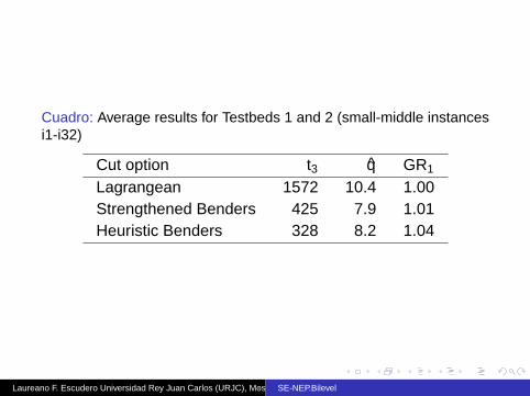
Cuadro: Average results for Testbeds 1 and 2 (small-middle instancesi1-i32)
Cut option t3 q GR1
Lagrangean 1572 10.4 1.00Strengthened Benders 425 7.9 1.01Heuristic Benders 328 8.2 1.04
Laureano F. Escudero Universidad Rey Juan Carlos (URJC), Mostoles (Madrid), [email protected]
Boxplot Radarchat
Heuristic Benders cut Lagrangean cut Strengthened Benders cut
010
2030
4050
OG3Time
Iter
GR1
GR2
Heuristic Benders cutStrengthened Benders cutLagrangean cut
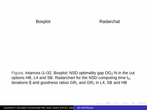
Figura: Intances i1-i32. Boxplot: NSD optimality gap OG3 % in the cutoptions HB, L4 and SB. Radarchart for the NSD computing time t3,iterations q and goodness ratios GR1 and GR2 in L4, SB and HB
Laureano F. Escudero Universidad Rey Juan Carlos (URJC), Mostoles (Madrid), [email protected]
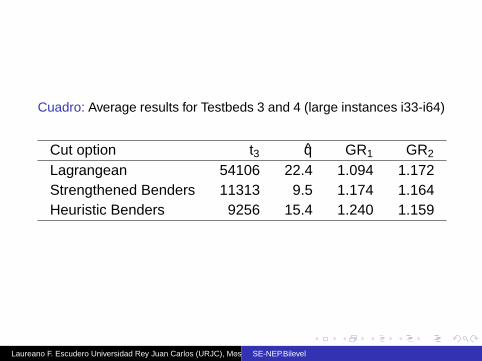
Cuadro: Average results for Testbeds 3 and 4 (large instances i33-i64)
Cut option t3 q GR1 GR2
Lagrangean 54106 22.4 1.094 1.172Strengthened Benders 11313 9.5 1.174 1.164Heuristic Benders 9256 15.4 1.240 1.159
Laureano F. Escudero Universidad Rey Juan Carlos (URJC), Mostoles (Madrid), [email protected]
Boxplot Radarchat
Heuristic Benders cut Lagrangean cut Strengthened Benders cut
020
4060
8010
0
OG3Time
Iter
GR1
GR2
Heuristic Benders cutStrengthened Benders cutLagrangean cut
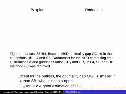
Figura: Intances i33-i64. Boxplot: NSD optimality gap OG3 % in thecut options HB, L4 and SB. Radarchart for the NSD computing timet3, iterations q and goodness ratios GR1 and GR2 in L4, SB and HB.Instance i63 was removed
Except for the outliers, the optimality gap OG3 is smaller inL4 than SB, what is not a surprise.OG3 for HB: A good estimation of OG3
Laureano F. Escudero Universidad Rey Juan Carlos (URJC), Mostoles (Madrid), [email protected]
Conclusions. SE-NEP, Stochastic-Equilibrium inmulti-period Network Expansion Planning
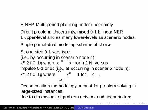
E-NEP, Multi-period planning under uncertainty
Difficult problem: Uncertainty, mixed 0-1 bilinear NEP,1 upper-level and as many lower-levels as scenario nodes.
Single primal-dual modeling scheme of choice.
Strong step 0-1 vars type(i.e., by occurring in scenario node n):xn ∈ 0,1 where xσ
n ≤ xn for n ∈ N versusimpulse 0-1 ones (i.e., at occurring in scenario node n):xn ∈ 0,1 where
∑n∈Aω
xn ≤ 1 for ω ∈ Ω.
Decomposition methodology, a must for problem solving inlarge-sized instances,due to dimensions of problem network and scenario tree.
Laureano F. Escudero Universidad Rey Juan Carlos (URJC), Mostoles (Madrid), [email protected]

Conclusions. NSD, Nested Stochastic Decomposition
For single primal-dual model, NSD proposal: Good resultsversus CPLEX, a M01LP/M01QP state-of-the-art solver.
Better for state variables only in consecutive two periods .
NSD performance improving: only step 0-1 vars
NSD: A good tool for helping to solve large-sized verydifficult problems, by considering,as a future research work,an `2-norm Regularized scenario Clustering SimplicialDecomposition Progressive algorithm (RCSDPA), see LFE,Garın, Monge & Unzueta Sub’19, for solving theF ′r -related subproblem (7).
Laureano F. Escudero Universidad Rey Juan Carlos (URJC), Mostoles (Madrid), [email protected]

REFERENCES on BILEVELH.G. Akdemir and F. Tiryaki. Bilevel stochastic transportation problem withexponentially distributed demand. Journal of Science and Technology, 2:32-37,2012.
G. Allende and G. Still. Solving bilevel programs with the KKT-approach.Mathematical Programming Ser A, 138:309-332, 2013.
S.M. Alizadeh, P. Marcotte and G. Savard. Two-stage stochastic bilevelprogramming. Transportation Research Part B, 58:92-106, 2013.
S. Avraamidou, N. A. Diangelakis and E.N. Pistikopoulos. Mixed Integer BilevelOptimization through multi-parametric Programming. In Foundations ofComputer Aided Process Operations/Chemical Process Control, 2017.
Ch. Audet, J. Haddad and G. Savard. A note on the definition of a linear bilevelprogramming solution Applied Mathematics and Computation, 181:351-355.2006.
L. Brotcorne, M. Labbe, P. Marcotte and G. Savard. A bilevel model and solutionalgorithm for a freight tariff-setting problem. Transportation Science, 34:289-302,2000.
L. Brotcorne, M. Labbe, P. Marcotte and G. Savard. A bilevel model for tolloptimization on a multicommodity transportation network. TransportationScience, 35:1-14, 2001.
L. Brotcorne, M. Labbe and G. Savard. Joint Design and Pricing on a Network.Operations Research, 56:1104-1115, 2008.
M. Caramia and R. Mari. Enhanced exact algorithms for discrete bilevel linearproblems. Optimization Letters, 9:1447-1468, 2015.
Laureano F. Escudero Universidad Rey Juan Carlos (URJC), Mostoles (Madrid), [email protected]

M. Carrion, J.M. Arroyo and A.J. Conejo. A bilevel stochastic programmingapproach for retailer futures market trading. IEEE Transactions on PowerSystems, 24:1446-1456, 2009.
S. DeNegre. Interdiction and discrete bilevel linear programming. PhD thesis,Lehigh University, Leigh, Penn, USA, 2011.
S. Dempe, V. Kalashnikov, G. Perez-Valdes and N. Kalashnikova. Natural gasbilevel cash-out problem: Convergence of a penalty function method. EuropeanJournal of Operational Research, 215:532-538, 2011.
S. Dempe, V. Kalashnikov, G. Perez-Valdes and N. Kalashnikova. The classicalKKT transformation. Bilevel Programming: Theory, Algorithms and Applicationsto Energy Networks, Section 3.5. Springer, 2015.
L.F. Escudero, J.F. Monge and A.M. Rodrıguez-Chıa. On pricing-basedequilibrium for network expansion planning. A multi-period bilevel approachunder uncertainty. Submitted 2019.
F. Facchinei, H. Jiang and L. Qi. A smoothing method for mathematical programswith equilibrium constraints. Mathematical programming, 85:107-134, 1999.
M. Fischetti, I. Ljubic, M. Monaci and M. Sinnl. On the use of intersection cuts forbilevel optimization. Mathematical Programming, Ser B, 172:77-103, 2018.
J. Fortuny-Amat and B. McCarl. A representation and economic interpretation ofa two-level programming problem. Journal of Operations Research Society,32:783-792, 1981.
V.V. Kalashnikov, V. Alexandrov and N.I. Kalashnikova. A stochatic approach forsolving bilevel natural gas cash-out problmes. Procedia Computer Science,80:1875-1886, 2016.
Laureano F. Escudero Universidad Rey Juan Carlos (URJC), Mostoles (Madrid), [email protected]
V.V. Kalashnikov, G. Perez-Valdes, A. Tomasgard and N.I. Kalashnikova. Naturalgas cash-out problme: Bilinear stochastic programming approach. EuropeanJournal of Operational Research, 206:18-33, 2010.
K. Kim and V. Zavala. Algorithmic innovations and software for the dualdecomposition method applied to stochastic mixed-integer programs.Mathematical Programming Computation, 10: 225-266, 2018.
R.M. Kovacevic and G.Ch. Pflug. Electricity Swing Option Pricing by StochasticBilevel Optimization: a Survey and New Approaches, European Journal ofOperational Research, 237:389-403, 2014.
M. Labbe, M. Leal and J. Puerto. New models for the location of controversialfacilities: A bilevel programming approach. Computers and OperationsResearch, in press, 2019.
M. Labbe, P. Marcotte and G. Savard. A bilevel model of taxation and itsapplication to optimal highway pricing. Management Science, 44:1608-1622,1988.
Z. Li and Ch. Floudas. Optimal scenario reduction framework based on distanceof uncertainty distribution and output performance: II. Sequential reduction.Computers and Chemical Engineering, 84:599-610, 2016.
Y. Liu, H. Xu and G. Lin. Stability analysis of two stage stochastic mathematicalprograms with complementarity constraints via NLP-pregularization. SIAMJournal on Optimization, 213:669-705, 2011.
G. Londono and A. Lozano. A Bilevel Optimization Program with EquilibriumConstraints for an Urban Network Dependent on Time. Transportation ResearchProcedia, 3:905-914, 2014.
Laureano F. Escudero Universidad Rey Juan Carlos (URJC), Mostoles (Madrid), [email protected]

P. Marcotte and D. Zhu. Exact and inexact penalty methods for the generalizedbilevel programming problem. Mathematical Programming, 74:141-157, 1996.
A. Philpott, M. Ferris and R. Wets. Equilibrium, uncertainty and risk inhydro-thermal elecrricity systems. Mathematical Programming, Ser. B,157:483-513, 2016.
S. Pineda, H. Bybling and J.M. Morales. Efficiently solving linear bilevelprogramming problems using off-the-shelf optimization software Optimizationand Engineering, 19:187-211, 2018.
S. Rebennack. Combining sampling-based and scenario-based nested Bendersdecompostion methods: Applications to stochastic dual dynamic programming.Mathematical Programming, Ser. A, 156:343-389, 2016.
E. Roghanian, S.J. Sadjadi and M.B. Aryanezhad. A probabilistic bi-level linearmulti-objective programming problem to supply chain planning. AppliedMathematics and Computation, 188:786-800, 2007.
G.K. Saharidis, A.J. Conejo and G. Kozanidis. Exact solution methodologies forlinear and (mixed) integer bilevel programming. In E-G. Talbi (ed.),Metaheuristics for Bi-level Optimization. Springer, pp. 221-245, 2013.
G.K. Saharidis and M.G. Ierapetritou. Resolution mehod for mixed integerbi-level linear problems based on decomposition techniques. Journal of GlobalOptimization, 44:309-318, 2009.
A. Sinha, P. Malo and K. Deb. A Review on Bilevel Optimization: From classicalto evolutionary approaches and applications. IEEE Transactions on EvolutionaryComputation, 22: 276-295, 2018.
Laureano F. Escudero Universidad Rey Juan Carlos (URJC), Mostoles (Madrid), [email protected]

A.S. Werner. Bilevel stochastic programming: Analysis and application totelecommunications. PhD Thesis. Norwegian University of Science andTechnology. Trondheim, Norway, 2004.
P. Xu and L. Wang. An exact algorithm for the bilinear mixed integer linearprogramming problem under three simplifying assumptions. Computers &Operations Research, 41:309-318, 2014.
J. Zhang and O.Y. Ozaltin A Branch-and-Cut algorithm for discrete bilevel linearprograms. Optimization Online, 2017.
D. Zhang and H. Xu. Two stage stochastic equilibrium problems with equilibriumconstraints: modeling and numerical schemes.Optimization-online,doi.org/10.1080/02331934.2011.632418, 2011.
D. Zhang, H. Xu and Y. Wu. A stochastic two stage equilibrium model forelectricity markets with two way contracts. Mathematical Methods of OperationsResearch, 71:1-45, 2010.
Laureano F. Escudero Universidad Rey Juan Carlos (URJC), Mostoles (Madrid), [email protected]

REFERENCESJ. Benders. Partitioning procedures for solving mixed variables programmingproblems. Numerische Mathematik 4:238-252, 1962.U. Aldasoro, L.F. Escudero, M. Merino, J.F. Monge and G. Perez. Onparallelization of a Stochastic Dynamic Programming algorithm for solvinglarge-scale mixed 0-1 problems under uncertainty. TOP, 23:703-742, 2015.M.P. Cristobal, L.F. Escudero and J.F. Monge. On Stochastic DynamicProgramming for solving large-scale tactical production planning problems.Computers & Operations Research 36:2418-2428, 2009.L.F. Escudero, M.A. Garın, J.F. Monge and A. Unzueta. On multistage stochasticmixed 0-1 bilinear optimization based on endogenous uncertainty and timeconsistent stochastic dominance risk management. Submitted 2019.L.F. Escudero and J.F. Monge. On capacity expansion planning under strategicand operational uncertainties based on stochastic dominance risk aversemanagement. Computational Management Science, 15:479-500, 2018.L.F. Escudero, J.F. Monge, A.M. Rodrıguez-Chıa. On pricing-based equilibriumfor network expansion planning. A multi-period bilevel approach underuncertainty. Submitted 2019.L.F. Escudero, J.F. Monge, D. Romero Morales and J. Wang. Expected FutureValue Decomposition Based Bid Price Generation for Large-Scale NetworkRevenue Management. Transportation Science, 47:181-197, 2013.L.F. Escudero, J.F. Monge and D. Romero-Morales, An SDP approach formultiperiod mixed 0–1 linear programming models with stochastic dominanceconstraints for risk management. Computers & Operations Research, 58:32-40,2015.
Laureano F. Escudero Universidad Rey Juan Carlos (URJC), Mostoles (Madrid), [email protected]

L.F. Escudero, J.F. Monge and D. Romero-Morales. On the time-consistentstochastic dominance risk averse measure for tactical supply chain planningunder uncertainty. Computers & Operations Research, 100:270-286, 2018.
J. Zou, S. Ahmed and X.A. Sun. Stochastic Dual Dynamic intger Programming.Optimization Online, 2016.
J. Zou, S. Ahmed and X.A. Sun. Multistage stochastic unit commitment usingStochastic Dual Dynamic integer Programming. Mathematical Programming,doi.org/10.1007/s10107-018-1249-5, 2018.
Laureano F. Escudero Universidad Rey Juan Carlos (URJC), Mostoles (Madrid), [email protected]