6.006- Introduction to Algorithms6.006 Introduction to AlgorithmsLecture 18

Dynamic Programming IProf Manolis KellisProf. Manolis Kellis

CLRS 15.3, 15.4

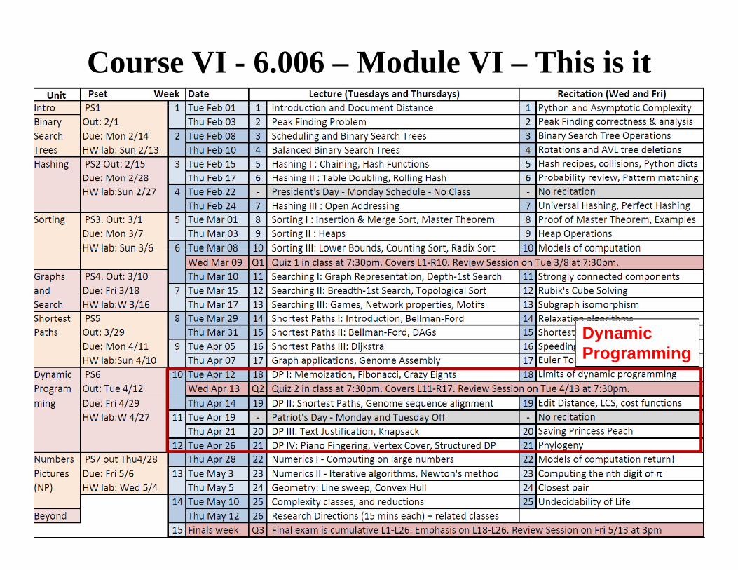
Course VI - 6.006 – Module VI – This is it

Dynamic Programming

2

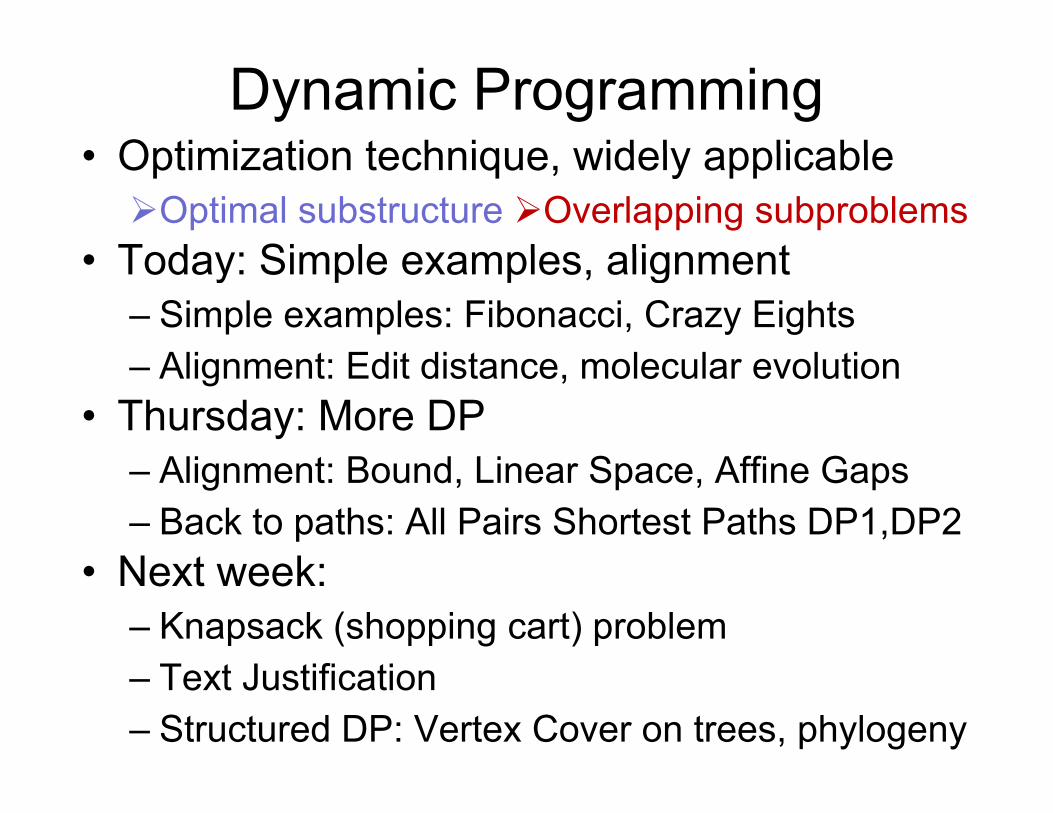
Dynamic Programming• Optimization technique widely applicable• Optimization technique, widely applicableOptimal substructure Overlapping subproblems

Today: Simple examples alignment• Today: Simple examples, alignment– Simple examples: Fibonacci, Crazy Eights

Ali t Edit di t l l l ti– Alignment: Edit distance, molecular evolution• Thursday: More DP

Ali t B d Li S Affi G– Alignment: Bound, Linear Space, Affine Gaps– Back to paths: All Pairs Shortest Paths DP1,DP2

N t k• Next week: – Knapsack (shopping cart) problem

f– Text Justification– Structured DP: Vertex Cover on trees, phylogeny

Today: Dynamic programming

• Fibonacci numbers– Top-down vs. bottom-up

• Principles of Dynamic programmingp y p g g– Optimal sub-structure, repeated subproblems

• Crazy EightsCrazy Eights– One-dimensional optimization

• Sequence alignment• Sequence alignment– Two-dimensional optimization

1 Fibonacci Computation1. Fibonacci Computation

(not really an optimization problem, but similar intuition applies))

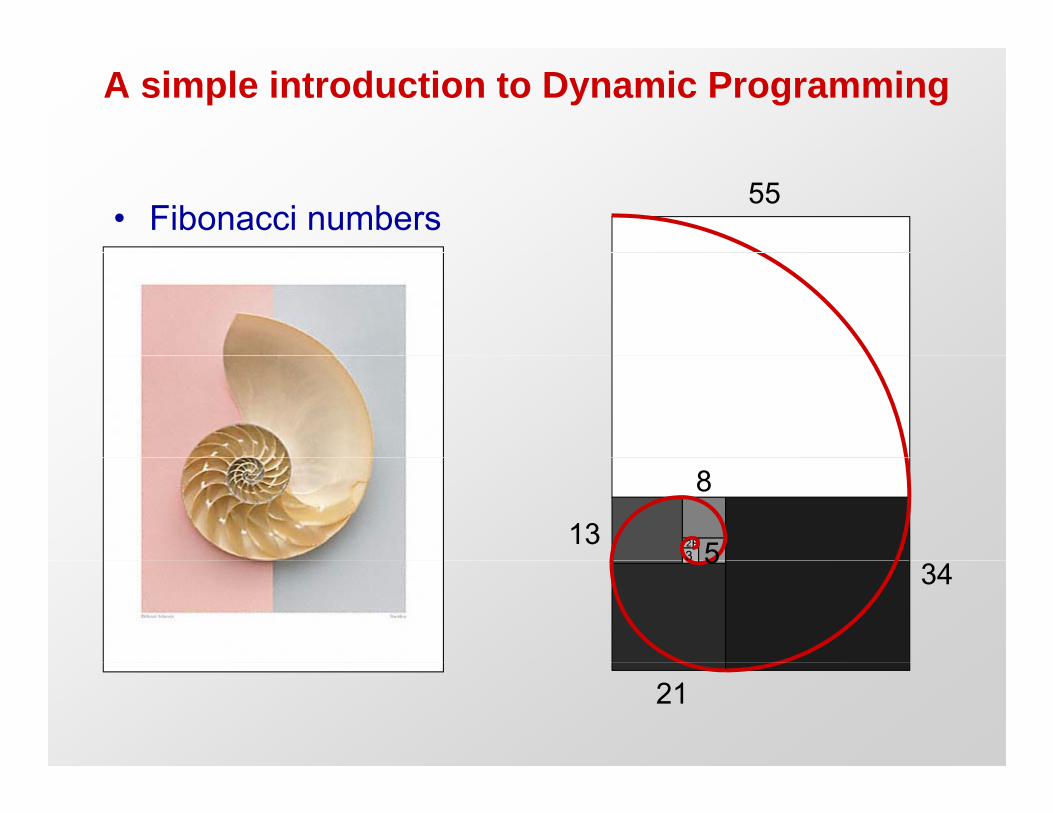
A simple introduction to Dynamic Programming

• Fibonacci numbers55

5

8

1332 5

34

21

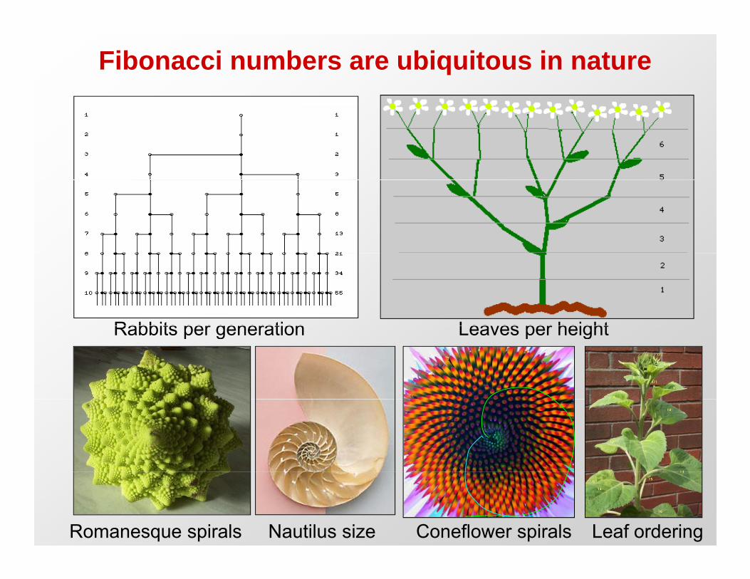
Fibonacci numbers are ubiquitous in nature

Rabbits per generation Leaves per heightRabbits per generation Leaves per height

Romanesque spirals Nautilus size Coneflower spirals Leaf ordering

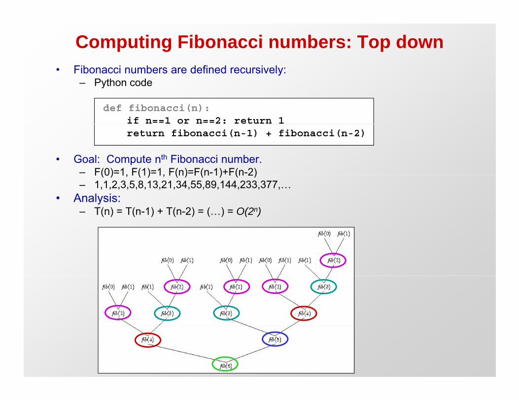
Computing Fibonacci numbers: Top down• Fibonacci numbers are defined recursively: y

– Python code

def fibonacci(n): if n==1 or n==2: return 1return fibonacci(n-1) + fibonacci(n-2)

• Goal: Compute nth Fibonacci number. – F(0)=1, F(1)=1, F(n)=F(n-1)+F(n-2)F(0) 1, F(1) 1, F(n) F(n 1) F(n 2)– 1,1,2,3,5,8,13,21,34,55,89,144,233,377,…

• Analysis: – T(n) = T(n-1) + T(n-2) = (…) = O(2n)

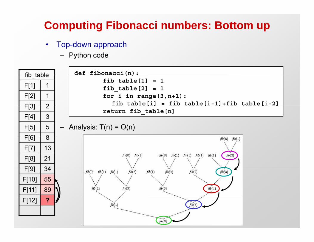
Computing Fibonacci numbers: Bottom up• Top-down approach• Top-down approach

– Python code

def fibonacci(n): fib table ( )fib_table[1] = 1fib_table[2] = 1for i in range(3,n+1):

fib table[i] = fib table[i-1]+fib table[i-2]2F[3]1F[2]1F[1]

fib_table

– Analysis: T(n) = O(n)

_ [ ] _ [ ] _ [ ]return fib_table[n]

8F[6]5F[5]3F[4]2F[3]

34F[9]21F[8]13F[7]8F[6]

89F[11]55F[10]34F[9]

?F[12]

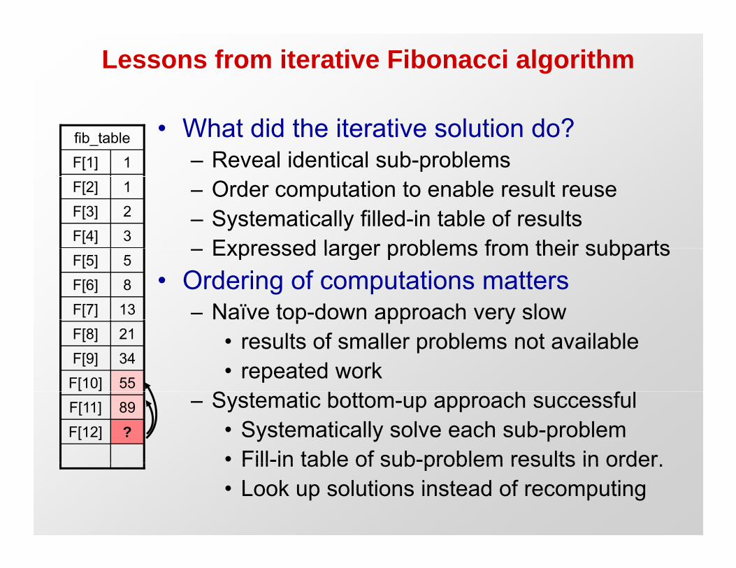
Lessons from iterative Fibonacci algorithm

• What did the iterative solution do?– Reveal identical sub-problems1F[1]

fib_table

– Order computation to enable result reuse– Systematically filled-in table of results

Expressed larger problems from their subparts3F[4]2F[3]1F[2]

– Expressed larger problems from their subparts• Ordering of computations matters

– Naïve top-down approach very slow13F[7]8F[6]5F[5]

p pp y• results of smaller problems not available• repeated work

S f55F[10]34F[9]21F[8]

– Systematic bottom-up approach successful• Systematically solve each sub-problem• Fill-in table of sub-problem results in order

?F[12]89F[11]

Fill in table of sub problem results in order. • Look up solutions instead of recomputing

Dynamic Programming in Theory

H ll k f D i P i• Hallmarks of Dynamic Programming– Optimal substructure: Optimal solution to problem

(instance) contains optimal solutions to sub-problems( ) p p– Overlapping subproblems: Limited number of distinct

subproblems, repeated many many timesTypically for optimization problems ( )• Typically for optimization problems (unlike Fib example)– Optimal choice made locally: max( subsolution score)– Score is typically added through the search spaceScore is typically added through the search space– Traceback common, find optimal path from indiv. choices

• Middle of the road in range of difficulty– Easier: greedy choice possible at each step– DynProg: requires a traceback to find that optimal path

Harder: no opt substr e g subproblem dependencies– Harder: no opt. substr., e.g. subproblem dependencies

Hallmarks of optimization problemsGreedy algorithms Dynamic Programming

1. Optimal substructureAn optimal solution to a problem (instance)

Greedy algorithms Dynamic Programming

An optimal solution to a problem (instance) contains optimal solutions to subproblems.

2. Overlapping subproblemsA recursive solution contains a “small” number

f di ti t b bl t d tiof distinct subproblems repeated many times.

3 G d h i3. Greedy choice propertyLocally optimal choices lead to globally optimal solution

Greedy Choice is not possibleGlobally optimal solution requires trace back through many choicesg y

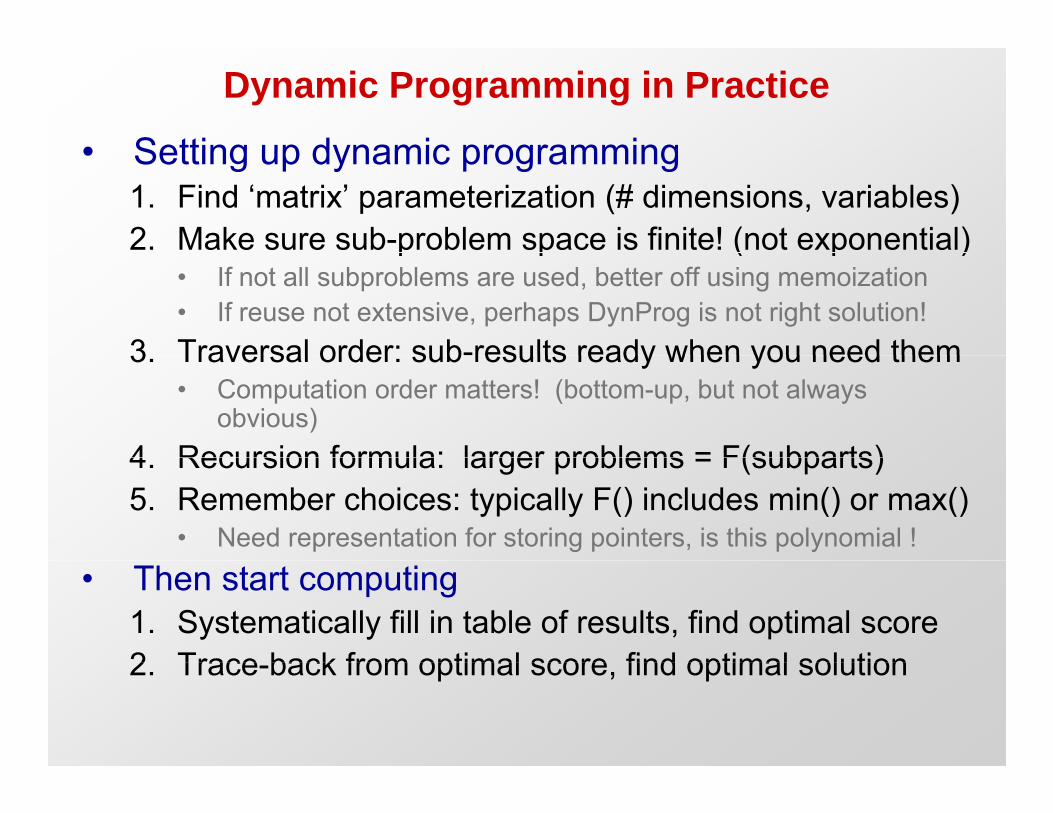
Dynamic Programming in Practice

• Setting up dynamic programming• Setting up dynamic programming1. Find ‘matrix’ parameterization (# dimensions, variables)2. Make sure sub-problem space is finite! (not exponential)p p ( p )

• If not all subproblems are used, better off using memoization• If reuse not extensive, perhaps DynProg is not right solution!

3 Traversal order: sub-results ready when you need them3. Traversal order: sub results ready when you need them• Computation order matters! (bottom-up, but not always

obvious)4 Recursion formula: larger problems = F(subparts)4. Recursion formula: larger problems = F(subparts)5. Remember choices: typically F() includes min() or max()

• Need representation for storing pointers, is this polynomial !• Then start computing

1. Systematically fill in table of results, find optimal score2 Trace back from optimal score find optimal solution2. Trace-back from optimal score, find optimal solution

2 Crazy Eights2. Crazy Eights

One-dimensional Optimization

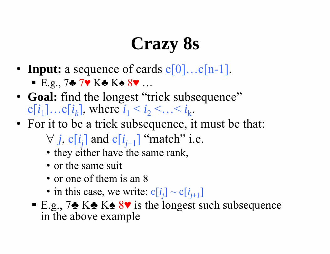
Crazy 8sCrazy 8s• Input: a sequence of cards c[0]…c[n-1].

8 E.g., 7♣ 7♥ K♣ K♠ 8♥ … • Goal: find the longest “trick subsequence”

c[i1] c[ik] where i1 < i2 < < ikc[i1]…c[ik], where i1 < i2 <…< ik.• For it to be a trick subsequence, it must be that:

j, c[ij] and c[ij+1] “match” i.e. j, [ j] [ j+1]• they either have the same rank, • or the same suit

f h i 8• or one of them is an 8 • in this case, we write: c[ij] ~ c[ij+1]

E g 7♣ K♣ K♠ 8♥ is the longest such subsequenceE.g., 7♣ K♣ K♠ 8♥ is the longest such subsequence in the above example

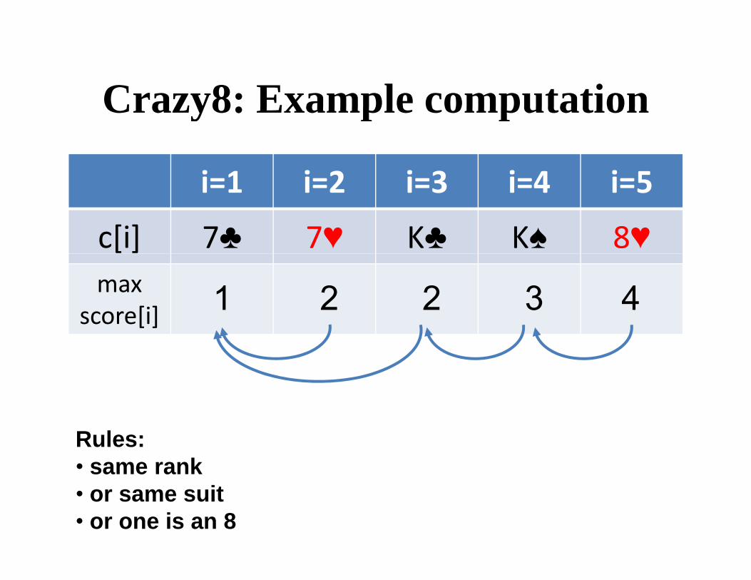
Crazy8: Example computationCrazy8: Example computation

i=1 i=2 i=3 i=4 i=5i=1 i=2 i=3 i=4 i=5

c[i] 7♣ 7♥ K♣ K♠ 8♥max 

score[i] 1 2 2 3 4[ ]

Rules: • same ranksame rank• or same suit • or one is an 8

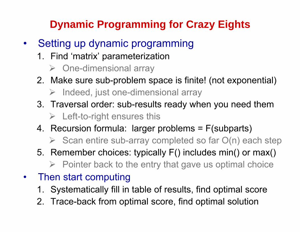
Dynamic Programming for Crazy Eights

• Setting up dynamic programming• Setting up dynamic programming1. Find ‘matrix’ parameterization One-dimensional arrayy

2. Make sure sub-problem space is finite! (not exponential) Indeed, just one-dimensional array

3 T l d b lt d h d th3. Traversal order: sub-results ready when you need them Left-to-right ensures this

4. Recursion formula: larger problems = F(subparts)4. Recursion formula: larger problems F(subparts) Scan entire sub-array completed so far O(n) each step

5. Remember choices: typically F() includes min() or max() Pointer back to the entry that gave us optimal choice

• Then start computing1 Systematically fill in table of results find optimal score1. Systematically fill in table of results, find optimal score2. Trace-back from optimal score, find optimal solution

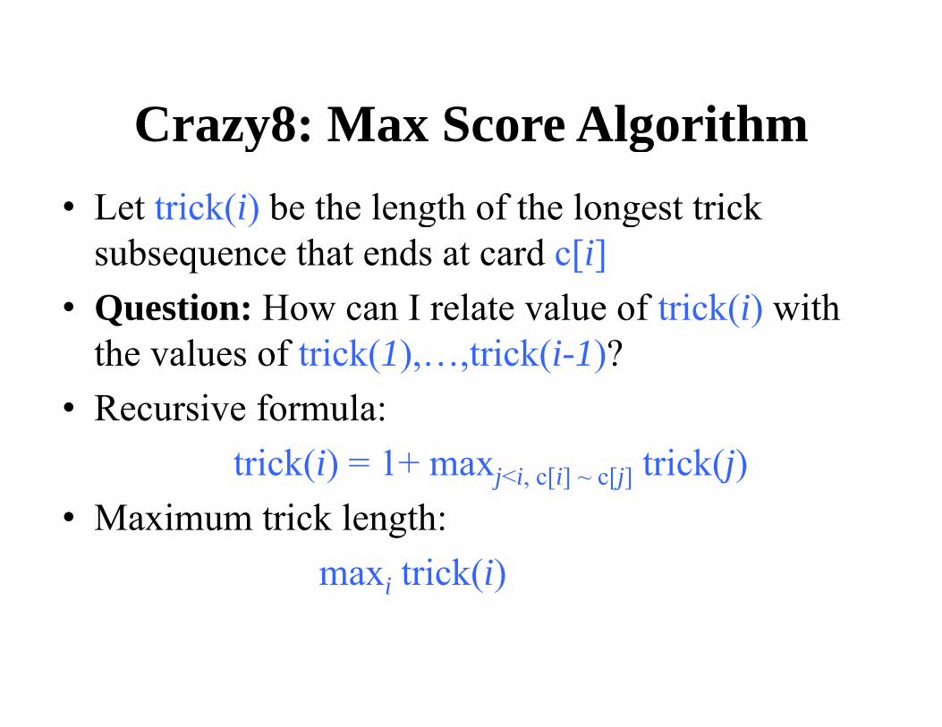
Crazy8: Max Score AlgorithmCrazy8: Max Score Algorithm• Let trick(i) be the length of the longest trick ( ) g g

subsequence that ends at card c[i]• Question: How can I relate value of trick(i) withQuestion: How can I relate value of trick(i) with

the values of trick(1),…,trick(i-1)?• Recursive formula:• Recursive formula:

trick(i) = 1+ maxj<i, c[i] ~ c[j] trick(j)• Maximum trick length:

maxi trick(i)i

ImplementationsImplementationsRecursive

• memo = { } • trick(i): if i in memo: return memo[i] else if i=1: return 1 else

• f := 1+maxj<i, c[i] ~ c[j] trick(j)• memo[i] : f• memo[i] := f• return f

• call trick(n)• call trick(n) • return maximum value in memo

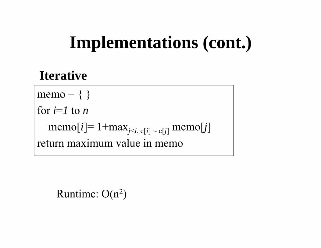
Implementations (cont.)Implementations (cont.)

Iterativememo = { } f i 1 t

Iterative

for i=1 to nmemo[i]= 1+maxj<i, c[i] ~ c[j] memo[j]

i l ireturn maximum value in memo

Runtime: O(n2)

Dynamic ProgrammingDynamic Programming• DP ≈ Recursion + Memoization• DP works when: the solution can be produced by combining solutions ofOptimal substructurethe solution can be produced by combining solutions of

subproblems; the solution of each subproblem can be produced by

Optimal substructure An solution to a problem can be obtained by

solutions to subproblems.the solution of each subproblem can be produced by combining solutions of sub-subproblems, etc;

moreover….

solutions to subproblems.trick(i) = 1+ maxj>i, c[i] ~ c[j] trick(j)

the total number of subproblems arising recursively is polynomial.

Overlapping SubproblemsA recursive solution contains a “small” number of p y

distinct subproblems (repeated many times)trick(0), trick(1),…, trick(n-1)

3 Sequence Alignment3. Sequence Alignment

Two-dimensional optimization

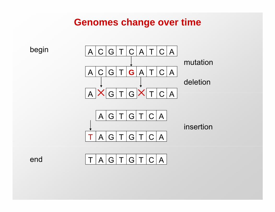
Genomes change over time

A C G T C A T C Amutation

begin

A C G T G A T C A

A G T G T C Adeletion

A G T G T C A

A G T G T C A

A G T G T C ATinsertion

A G T G T C ATend

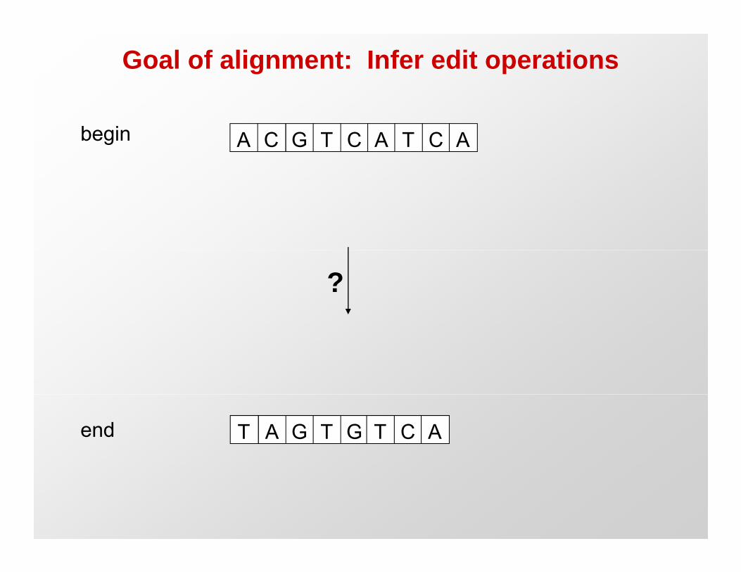
Goal of alignment: Infer edit operations

A C G T C A T C Abegin

?

A G T G T C ATend

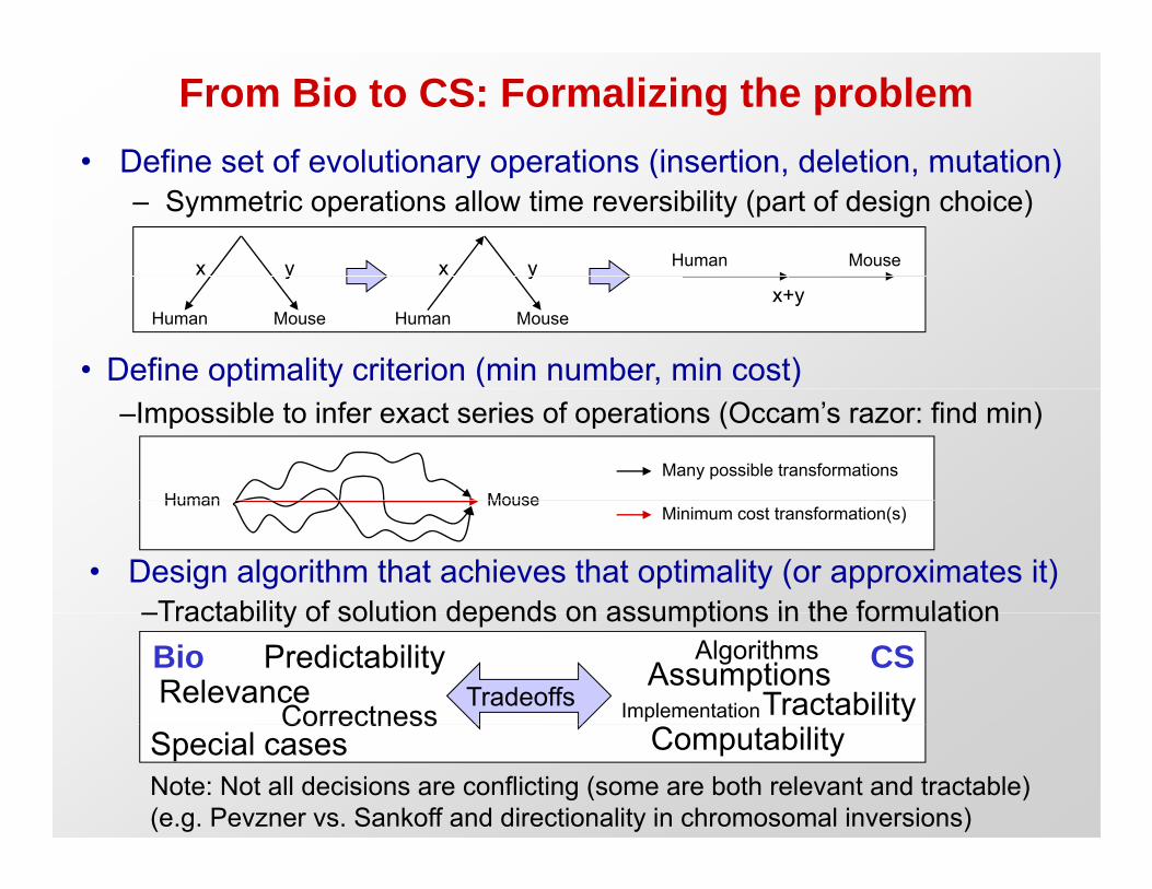
From Bio to CS: Formalizing the problem• Define set of evolutionary operations (insertion deletion mutation)• Define set of evolutionary operations (insertion, deletion, mutation)

– Symmetric operations allow time reversibility (part of design choice)

Human Mousex y x y

• Define optimality criterion (min number, min cost)

Human Mouse Human Mouse

y yx+y

Human Mouse

Many possible transformations

–Impossible to infer exact series of operations (Occam’s razor: find min)

Human MouseMinimum cost transformation(s)

• Design algorithm that achieves that optimality (or approximates it)–Tractability of solution depends on assumptions in the formulation–Tractability of solution depends on assumptions in the formulationBio CSRelevance Assumptions

TractabilityTradeoffs

Algorithms

Implementation

Predictability

CorrectnessSpecial cases Computability

Correctness

Note: Not all decisions are conflicting (some are both relevant and tractable)(e.g. Pevzner vs. Sankoff and directionality in chromosomal inversions)

Formulation 1: Longest common substring• Given two possibly related strings S1 and S2• Given two possibly related strings S1 and S2

– What is the longest common substring? (no gaps)

A C G T C A T C AS1 A C G T C A T C A

T A G T G T C A

S1

S2

A C G T C A T C AS1

offset: +1

S2 T A G T G T C A

offset: -2

A C G T C A T C AS1

S2 T A G T G T C AS2 T A G T G T C A

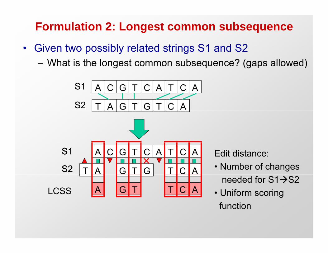
Formulation 2: Longest common subsequence

• Given two possibly related strings S1 and S2• Given two possibly related strings S1 and S2– What is the longest common subsequence? (gaps allowed)

A C G T C A T C A

T A G T G T C A

S1

S2

A C G T C A T C A

T A G T G T C A

S1

S2

A C G T C A T C A

T A G T G T C A

S1

S2

Edit distance: • Number of changes

A G T T C ALCSSneeded for S1S2

• Uniform scoringfunctionfunction

Formulation 3: Sequence alignment

• Allow gaps (fixed penalty)• Allow gaps (fixed penalty)– Insertion & deletion operations– Unit cost for each character inserted or deletedUnit cost for each character inserted or deleted

• Varying penalties for edit operations– Transitions (PyrimidinePyrimidine, PurinePurine)( y y , )– Transversions (Purine Pyrimidine changes)– Polymerase confuses Aw/G and Cw/T more often

A G T CA +1 ½ 1 1

Scoring function:Match(x x) = +1

Transitions: AG CT commonA +1 -½ -1 -1

G -½ +1 -1 -1T -1 -1 +1 -½

Match(x,x) = +1Mismatch(A,G)= -½Mismatch(C,T)= -½

AG, CT common(lower penalty)

Transversions:

C -1 -1 -½ +1Mismatch(x,y) = -1 All other operations

purine pyrimid.

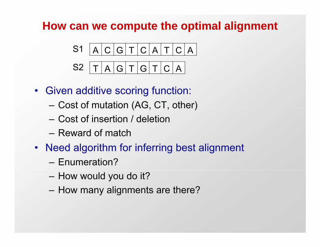
How can we compute the optimal alignment

S1 A C G T C A T C A

T A G T G T C A

S1

S2

• Given additive scoring function:– Cost of mutation (AG, CT, other)Cost of mutation (AG, CT, other)– Cost of insertion / deletion– Reward of match

• Need algorithm for inferring best alignment– Enumeration? – How would you do it?– How many alignments are there?

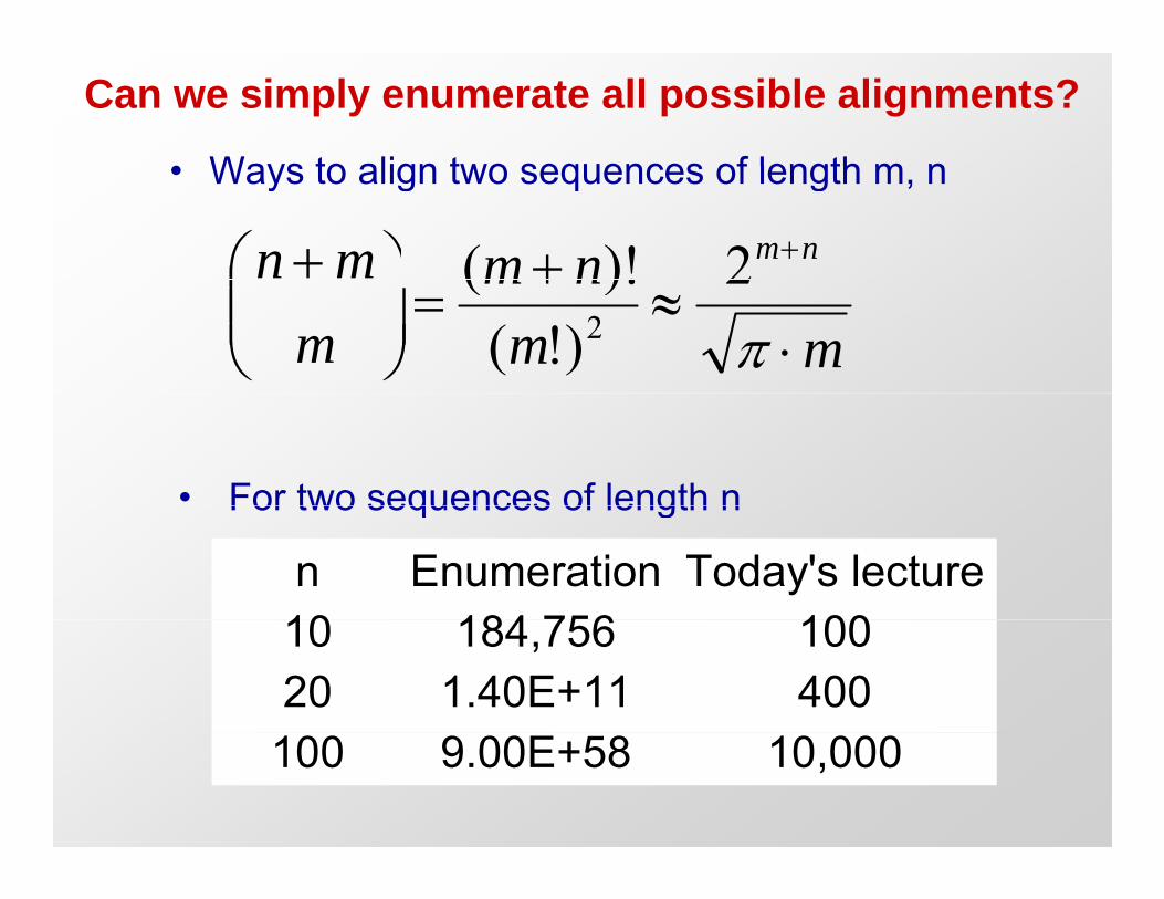
Can we simply enumerate all possible alignments?

• Ways to align two sequences of length m n• Ways to align two sequences of length m, n

nmmn nm

2)!(

mmnm

m

2

)!()!(

2

• For two sequences of length n

n Enumeration Today's lecture10 184 756 100

For two sequences of length n

10 184,756 10020 1.40E+11 400

100 9.00E+58 10,000

Key insight: score is additive!i

A C G T C A T C A

T A G T G T C A

S1

S2

i

• Compute best alignment recursively

T A G T G T C AS2

jCompute best alignment recursively– For a given aligned pair (i, j), the best alignment is:

• Best alignment of S1[1..i] and S2[1..j]• + Best alignment of S1[ i..n] and S2[ j..m]

i i

A C G T C A T C A

T A G T G T C A

S1

S2

j j

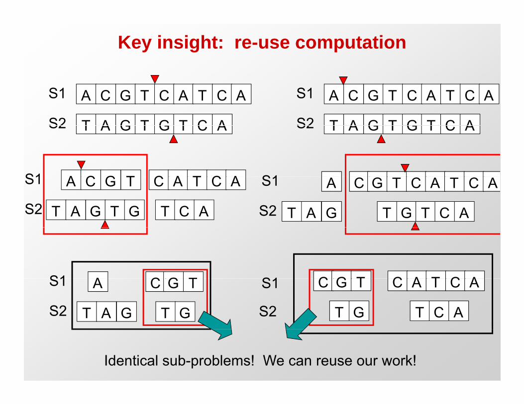
Key insight: re-use computation

A C G T C A T C A

T A G T G T C A

S1

S2

A C G T C A T C A

T A G T G T C A

S1

S2T A G T G T C AS2 T A G T G T C AS2

A C G T C A T C AS1 S1

S2

A C G T C A T C A

T A G T G T C A

S1

S2

A C G T C A T C A

T A G T G T C A

S1

A C G TS1 C G T C A T C AS1A C G T

T A G T G

S1

S2

C G T C A T C A

T G T C A

S1

S2

Identical sub-problems! We can reuse our work!

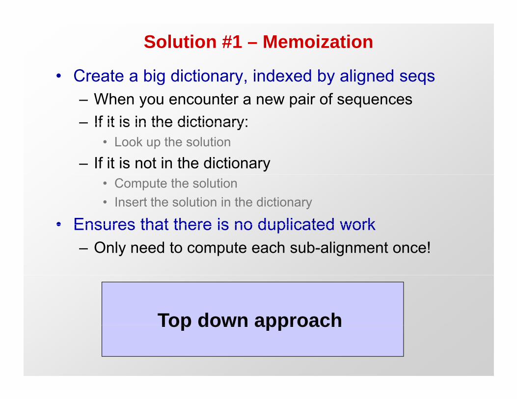
Solution #1 – Memoization

• Create a big dictionary indexed by aligned seqs• Create a big dictionary, indexed by aligned seqs– When you encounter a new pair of sequences– If it is in the dictionary:If it is in the dictionary:

• Look up the solution

– If it is not in the dictionary• Compute the solution• Insert the solution in the dictionary

• Ensures that there is no duplicated work• Ensures that there is no duplicated work– Only need to compute each sub-alignment once!

Top down approachTop down approach

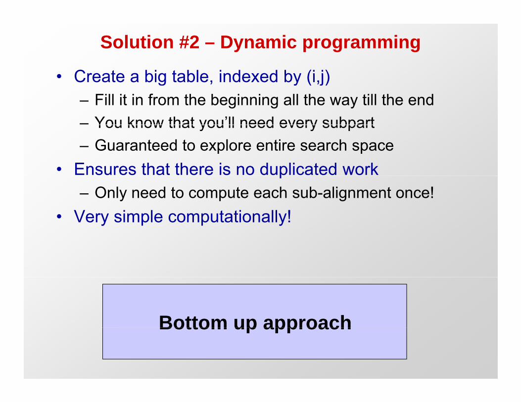
Solution #2 – Dynamic programming

• Create a big table indexed by (i j)• Create a big table, indexed by (i,j)– Fill it in from the beginning all the way till the end– You know that you’ll need every subpartYou know that you ll need every subpart– Guaranteed to explore entire search space

• Ensures that there is no duplicated workp– Only need to compute each sub-alignment once!

• Very simple computationally!

Bottom up approachBottom up approach

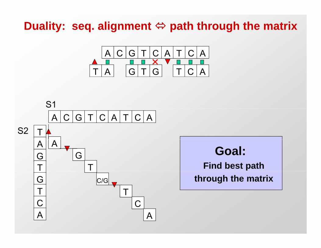
Duality: seq. alignment path through the matrix

A C G T C A T C A

T A G T G T C A

S1A C G T C A T C A

TS2AGT

AG

T

Goal: Find best path

GTC

C/G

TC

through the matrix

CA

CA

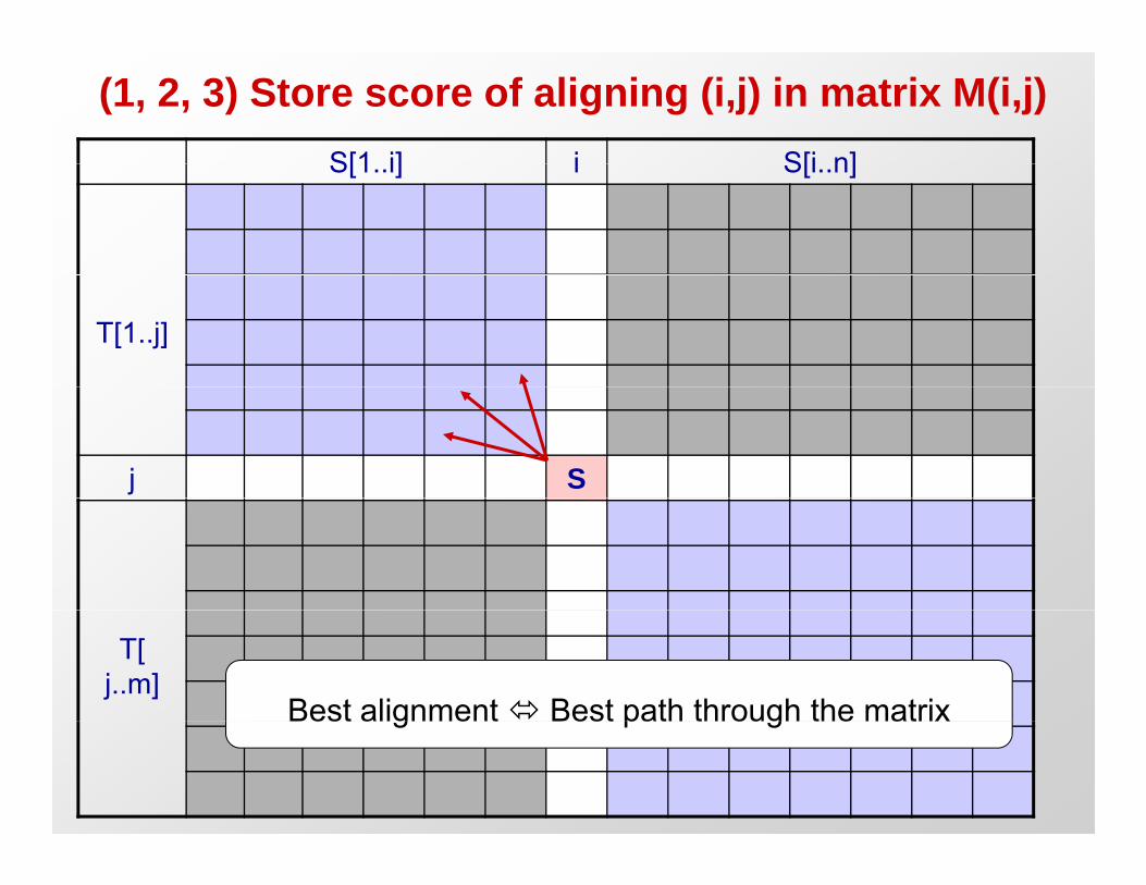
(1, 2, 3) Store score of aligning (i,j) in matrix M(i,j)S[1 i] i S[i n]S[1..i] i S[i..n]

T[1..j]

j S

T[ j..m]

Best alignment Best path through the matrixg p g

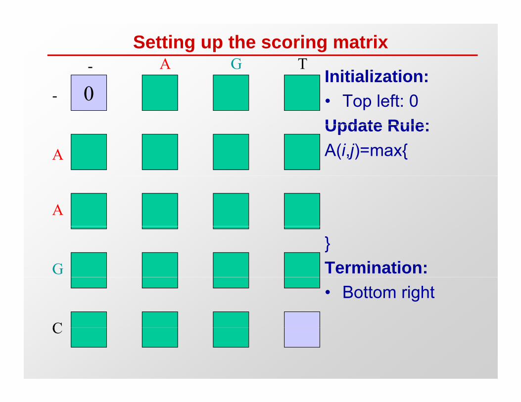
Setting up the scoring matrix- A G T

Initialization:- 0

Initialization:• Top left: 0Update Rule:

A

Update Rule:A(i,j)=max{

A

G}Termination:

C

• Bottom right

C

Setting up graph of scores- A G T

Initialization:- 0 -2 -4 -6

1-1 -1

Initialization:• Top left: 0Update Rule:

1

A -2 -1 -3 -5-1

-1 -1

Update Rule:A(i,j)=max{

• A(i-1 j ) - 21 gap

A -4 -3 -2 -4-1

-1 -1 A(i 1 , j ) 2• A( i , j-1) - 2• A(i-1 , j-1) -11 i t h

gapgap

G -6 -5 -4 -3-1-1 -1

( , j )• A(i-1 , j-1)+1

}

1 mismatch

match

C

6 5 4 3

8 7 6 5

-1 -1 -1 Termination:• Bottom right

C -8 -7 -6 -5

Dynamic Programming for sequence alignment

• Setting up dynamic programming• Setting up dynamic programming1. Find ‘matrix’ parameterization

• Prefix parameterization. Score(S[1..i],T[1..j]) F(i,j)• (i,j) only prefixes vs. (i,j,k,l) all substrings simpler 2-d matrix

2. Make sure sub-problem space is finite! (not exponential)• It’s just n2, quadratic (which is polynomial, not exponential)It s just n , quadratic (which is polynomial, not exponential)

3. Traversal order: sub-results ready when you need themColsLR

Rowst b t

Diagst Rb tL

4. Recursion formula: larger problems = F(subparts)• Need formula for computing F(i,j) as function of previous results

LR topbot topRbotL

• Single increment at a time, only look at F(i-1,j), F(i,j-1), F(i-1,j-1) corresponding to 3 options: gap in S, gap in T, char in both

• Score in each case depends on gap/match/mismatch penalties5. Remember choices: typically F() includes min() or max()

• Remember which of three cells (top,left,diag) led to maximum

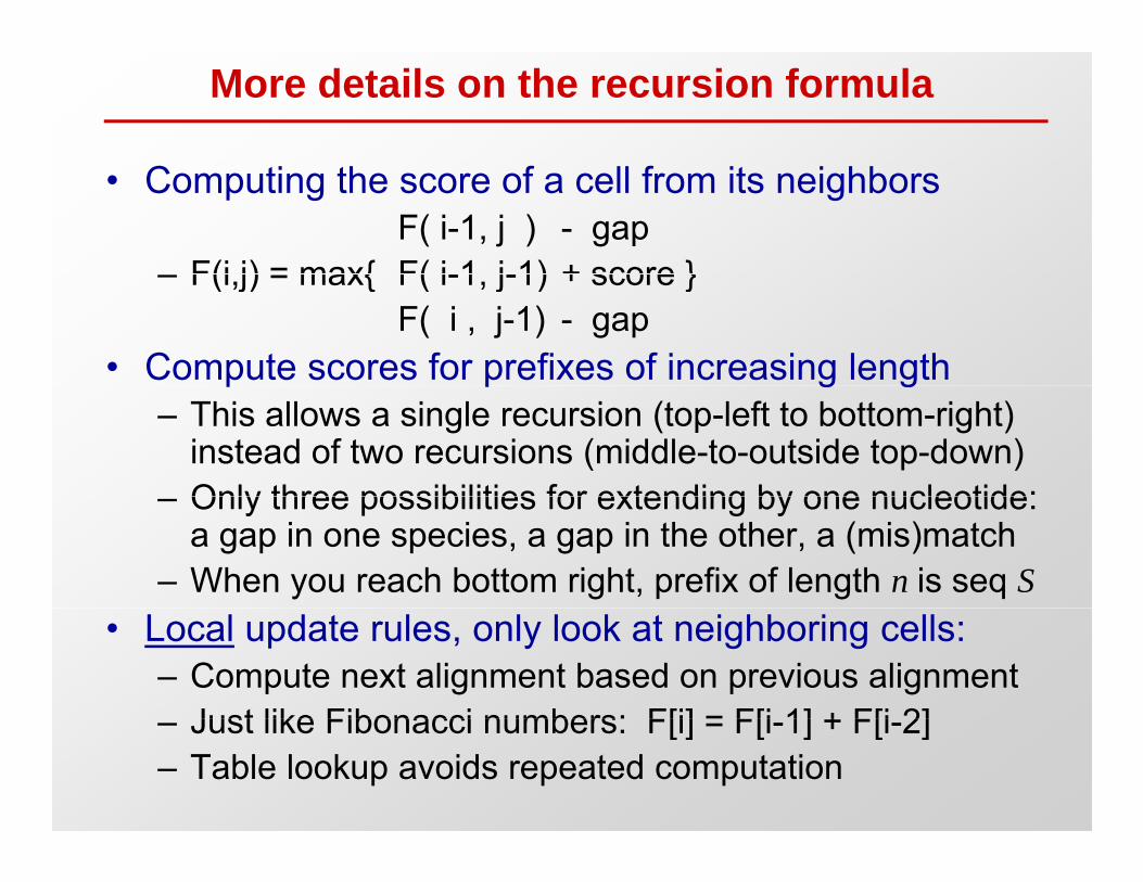
More details on the recursion formula

• Computing the score of a cell from its neighborsF( i-1, j ) - gap

F(i j) = max{ F( i 1 j 1) + score }– F(i,j) = max{ F( i-1, j-1) + score }F( i , j-1) - gap

• Compute scores for prefixes of increasing lengthp p g g– This allows a single recursion (top-left to bottom-right)

instead of two recursions (middle-to-outside top-down)Only three possibilities for extending by one nucleotide:– Only three possibilities for extending by one nucleotide:a gap in one species, a gap in the other, a (mis)match

– When you reach bottom right, prefix of length n is seq S• Local update rules, only look at neighboring cells:

– Compute next alignment based on previous alignmentJust like Fibonacci numbers: F[i] = F[i 1] + F[i 2]– Just like Fibonacci numbers: F[i] = F[i-1] + F[i-2]

– Table lookup avoids repeated computation

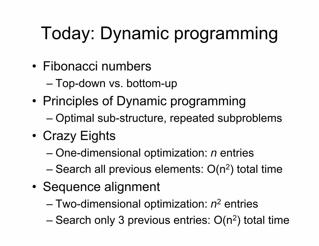
Today: Dynamic programming

• Fibonacci numbers– Top-down vs. bottom-up

• Principles of Dynamic programmingp y p g g– Optimal sub-structure, repeated subproblems

• Crazy EightsCrazy Eights– One-dimensional optimization: n entries– Search all previous elements: O(n2) total time– Search all previous elements: O(n ) total time

• Sequence alignmentT di i l ti i ti 2 t i– Two-dimensional optimization: n2 entries

– Search only 3 previous entries: O(n2) total time

Dynamic Programming module• Optimization technique widely applicable• Optimization technique, widely applicableOptimal substructure Overlapping subproblems

Today: Simple examples alignment• Today: Simple examples, alignment– Simple examples: Fibonacci, Crazy Eights

Ali t Edit di t l l l ti– Alignment: Edit distance, molecular evolution• Thursday: More DP

Ali t B d Li S Affi G– Alignment: Bound, Linear Space, Affine Gaps– Back to paths: All Pairs Shortest Paths DP1,DP2

N t k• Next week: – Knapsack (shopping cart) problem

f– Text Justification– Structured DP: Vertex Cover on trees, phylogeny

Course VI - 6.006 – Module VI – This is it

Dynamic Programming

43