Lecture 06Power calculation and Introduction to Smith chart

Hello and welcome, to NPTEL MOOC on electromagnetic guided waves, electromagnetic waves inguided and wireless media, this is module six, where we continue our discussion on transmission lines, Iwill just show you this

Refer slide time :( 0:29)

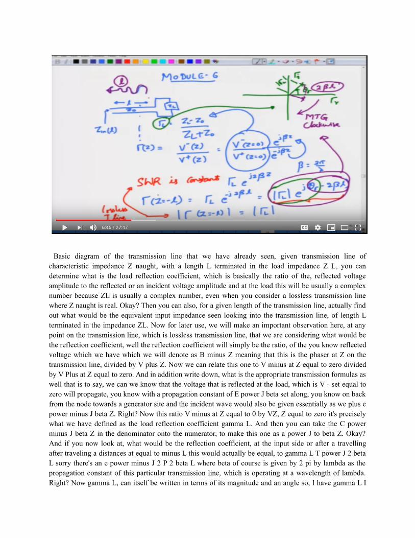
Basic diagram of the transmission line that we have already seen, given transmission line ofcharacteristic impedance Z naught, with a length L terminated in the load impedance Z L, you candetermine what is the load reflection coefficient, which is basically the ratio of the, reflected voltageamplitude to the reflected or an incident voltage amplitude and at the load this will be usually a complexnumber because ZL is usually a complex number, even when you consider a lossless transmission linewhere Z naught is real. Okay? Then you can also, for a given length of the transmission line, actually findout what would be the equivalent input impedance seen looking into the transmission line, of length Lterminated in the impedance ZL. Now for later use, we will make an important observation here, at anypoint on the transmission line, which is lossless transmission line, that we are considering what would bethe reflection coefficient, well the reflection coefficient will simply be the ratio, of the you know reflectedvoltage which we have which we will denote as B minus Z meaning that this is the phaser at Z on thetransmission line, divided by V plus Z. Now we can relate this one to V minus at Z equal to zero dividedby V Plus at Z equal to zero. And in addition write down, what is the appropriate transmission formulas aswell that is to say, we can we know that the voltage that is reflected at the load, which is V - set equal tozero will propagate, you know with a propagation constant of E power J beta set along, you know on backfrom the node towards a generator site and the incident wave would also be given essentially as we plus epower minus J beta Z. Right? Now this ratio V minus at Z equal to 0 by VZ, Z equal to zero it's preciselywhat we have defined as the load reflection coefficient gamma L. And then you can take the C powerminus J beta Z in the denominator onto the numerator, to make this one as a power J to beta Z. Okay?And if you now look at, what would be the reflection coefficient, at the input side or after a travellingafter traveling a distances at equal to minus L this would actually be equal, to gamma L T power J 2 betaL sorry there's an e power minus J 2 P 2 beta L where beta of course is given by 2 pi by lambda as thepropagation constant of this particular transmission line, which is operating at a wavelength of lambda.Right? Now gamma L, can itself be written in terms of its magnitude and an angle so, I have gamma L I

power J theta gamma minus 2 beta L. Okay? I will put that one into the exponential and if you now lookat, what is the magnitude of the reflection coefficient at Z equal to minus L that is as you move towardsthe generator. Right? So, this is the movement towards the generator what would be the magnitude of thereflection coefficient along the line, the magnitude of the reflection coefficient along the line, will beexactly equal to the magnitude of the reflection coefficient at the load, this property will apply only forlossless transmission line. If the line is lossy then the magnitude will actually change, in fact it willusually be smaller compared to the reflection coefficient magnitude at the load. Okay? So, because thisyou know, the magnitude of the reflection coefficient remains the same, it also follows immediately thatyes W R also remains the same. So, as W R is constant along the line on a transmission line which islossless. So, on a lossless transmission line both the magnitude of the reflection coefficient, is constant aswell as the SWR is constant. Okay?

Now coming to this other part. Right? The complete reflection coefficient you will actually see that, if Iwere to come up with you know an interesting graphical picture for this one, I know that this gamma at Zequal to minus L, is a complex number, which has been written in the polar form by giving its magnitudeas well as the angle. So, let's first consider the value, at L equal to zero meaning that we are consideringgamma L at the load plane that is Z equal to 0 plane, then that will simply be magnitude gamma L, timesE power J theta gamma which in the so-called,’ Complex Plane’ or the argon plane can be expressed as apoint. Okay? Whose radius is magnitude gamma L and whose angle with respect to the real axis is givenby theta gamma, do you agree with this take a minute to appreciate this graphical picture, all that we aredoing with this graphical picture, is to represent this gamma L which we calculate at the load, on to a nicevector or a point whose distance from the origin gives you the magnitude of gamma L and whose angle asmeasured from the real axis is given by theta gamma. Now what happens as you move towards thegenerator, well as you move towards the generator and you reach say Z equal to minus L the total anglehas actually reduced. Right? So, the angle has actually, reduced meaning the new point is locatedsomewhere at this point on the same circle, of the same radius but then since the angle is reduced youhave essentially moved, by moving a length of L you moved a total angle change, of 2 beta L. Okay? So,this is what means when we say, this is moving towards generator. So, I have actually moved towardsgenerator by going clockwise. Okay? So, the overall angle, is now reduced so, this is what I am actuallyplotting now and this would correspond to the reflection coefficient, after moving a distance L towardsthe generator. Now please note, you have moved a distance of L, but in terms of an angle you have moved2 beta L. Right?

Refer slide time :( 06:49)

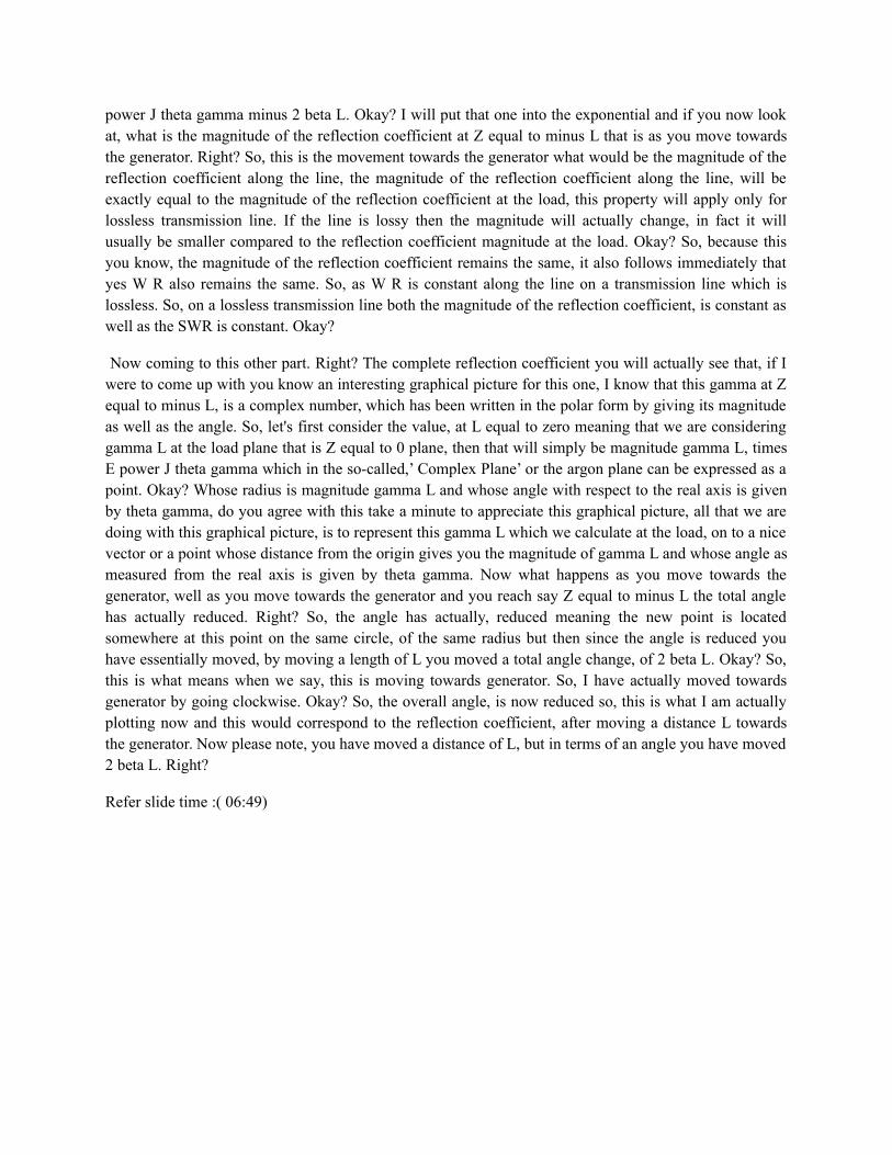
So, clearly if you move a total length of L equal to say lambda by 2 that is when you measure Lenz interms of the wavelength of the signal, then if you move a length of lambda by two you would actuallymove on the organ plane, you will your angle will change by an amount of to beta times L, which is 2 into2 pi by lambda because beta is 2 pi by lambda and L you have moved a distance of lambda by 2. So, youcancel lambda on both sides, will cancel 2 and then what you see is just 2 pi. Right? Of course you don'thave to just move lambda by 2 any multiple of lambda by 2 you move an integral multiple of lambda by 2you move you're going to move a distance change the angle by an amount of 2 M pi which essentiallymeans that if you started off at this point. Right? This is the origin you actually, have come back to thesame point and you come back, to the same point again and again so, physically on a losslesstransmission line, if the line, of you know line is actually of length say 3 lambda by 2 the properties that itwould see, at the load would essentially be the same properties, that it would see at this point as wellbecause you have taken an integral number, of lambda by 2 distance on the other hand if the length is, 3lambda by 2 plus say some point 1 lambda then the properties, that you would see would only bedetermined by this excess length 0.1 lambda, of course this is true because, we have assumed a losslesstransmission line and therefore there is no power changes, there is no voltage amplitude changes that ishappening out there and therefore gamma L is actually a constant. So, on the transmission line allproperties on a lossless transmission line all properties are repeating or they will repeat every lambda, by2 distance. Okay? So, if the physical length of the transmission line is when you represent in terms oflambda is given by an integral multiple of lambda by 2, plus some additional length then the propertiesimpedance transformation and everything is dependent only on this excess length. Okay? So, keep this inmind because, very shortly we are going to use this application. Okay?

Refer slide time :( 08:57)

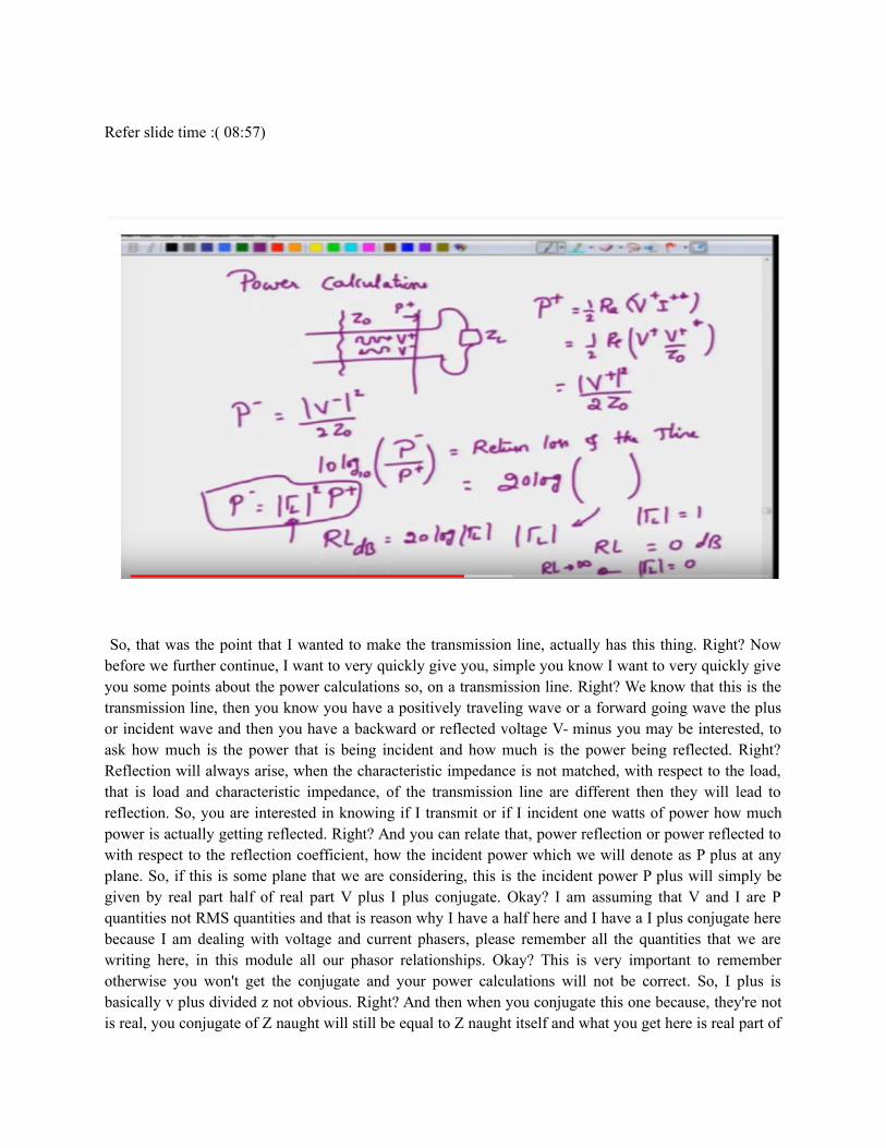
So, that was the point that I wanted to make the transmission line, actually has this thing. Right? Nowbefore we further continue, I want to very quickly give you, simple you know I want to very quickly giveyou some points about the power calculations so, on a transmission line. Right? We know that this is thetransmission line, then you know you have a positively traveling wave or a forward going wave the plusor incident wave and then you have a backward or reflected voltage V- minus you may be interested, toask how much is the power that is being incident and how much is the power being reflected. Right?Reflection will always arise, when the characteristic impedance is not matched, with respect to the load,that is load and characteristic impedance, of the transmission line are different then they will lead toreflection. So, you are interested in knowing if I transmit or if I incident one watts of power how muchpower is actually getting reflected. Right? And you can relate that, power reflection or power reflected towith respect to the reflection coefficient, how the incident power which we will denote as P plus at anyplane. So, if this is some plane that we are considering, this is the incident power P plus will simply begiven by real part half of real part V plus I plus conjugate. Okay? I am assuming that V and I are Pquantities not RMS quantities and that is reason why I have a half here and I have a I plus conjugate herebecause I am dealing with voltage and current phasers, please remember all the quantities that we arewriting here, in this module all our phasor relationships. Okay? This is very important to rememberotherwise you won't get the conjugate and your power calculations will not be correct. So, I plus isbasically v plus divided z not obvious. Right? And then when you conjugate this one because, they're notis real, you conjugate of Z naught will still be equal to Z naught itself and what you get here is real part of

V Plus V Plus conjugate by Z naught into half which is basically V plus magnitude square divided by 2 Znaught but following, the same lines you can easily show that P - will be V - magnitude square by 2 Znaught, now you look for the ratio of P minus 2 P plus. Right? And then express this ratio in terms of log,the base-10 in our course. So, you have 10 log of this quantity, which we will call as return loss of thedevice or return loss of the transmission line, of course there is nothing specific about transmission line inthis definition you can always take any you know device and then call its return loss, for example even ifyou go to a low frequency scenario, you put a load you have a source, you know equivalent source and a17 register, then you can always calculate what would be the power that is incident or power that is that isavailable from the transmitter and the power that is actually dissipated, by the resistor and then thedifference between the two is what we can think of as a reflected power. Right? So, this concept of returnloss is quite general, but it is used widely in high frequency or transmission line and microwaveapplications. So, this is your return loss of the transmission line, well so, far so, good I can use theexpressions for P minus and P plus 2Z naught is a common thing that gets cancelled. So, what I get is 20log. Right? Because the square in V plus magnitude square and V minus magnitude square will be takenout so, you get V minus magnitude by, V plus magnitude but this is nothing but the quantity in thisbracket is nothing but magnitude of gamma and for a transmission line, the magnitude of gamma for alossless transmission line that is simply equal to magnitude of gamma L. Right? So, the return loss, in DBis given by 20 log of magnitude of gamma L. So, when you have the return loss expressed in DB in thismanner. So, for the completely mismatched case where gamma magnitude of gamma L will be equal to 1the return loss is equal to 0 DB and when gamma L magnitude is equal to 0 for the case of losslesstransmission line, the return loss will be equal to infinity meaning. So, it's, it's really I mean we should have thought about it a little carefully, nevertheless what it actuallyshows is that when you I know you have your incident power, then the reflected power P plus can alwaysbe expressed as the magnitude of gamma L square, times the incident this is the reflected power. Right?So, the reflected power can be expressed as, of gamma n square times P plus and therefore this quantitymagnitude of gamma L Square, will tell you, how much is the power that is actually getting reflected so,when gamma L is equal to 1, which will be completely the case where you have complete mismatch thenall of the power is reflected back. Okay? And when gamma L equal to zero, then none of the powerincident has will be reflected back everything will be transmitted. So, it could be related to thetransmission coefficient, which we can relate as to the power that is delivered to the load, to the powerthat is actually being incident. So, if you think of the transmission, then having very high written loss isactually good because, that means there will be nothing coming back from the load. Okay? By the waythis can be used, to denote the incident and reflected powers or you can use no like talk about, thereturned losses at any plane on the transmission line

Refer slide time :( 14:34)

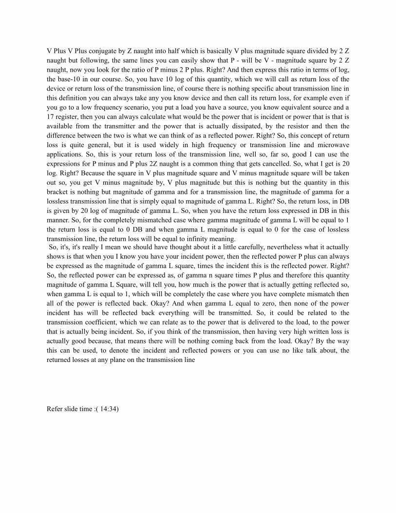
Sometimes you will also encounter scenario where one transmission line, will be connected to anothertransmission line, which itself may be connected to another transmission line and finally terminated withsome load. Okay? So, I just short-circuited here, but you can take any load here. Okay? And then at eachplane, you can I mean you will have some incident power and some reflected power and you're more orless quite, often interested in knowing what is the overall return loss Okay? The way to solve this problemwould be to first transform the impedance, seen looking at this edge and because, in this case it is just thelast transmission line. So, you move it to the transmission line before here you find out what would be theequivalent load impedance, say after transforming the load here. So, we will attach a load now so, wehave a load here, which we'll call and said L and after attaching a load ZL of the transmission line whoselength is L 1 with the characteristic impedance said 1, you find out what is the equivalent load impedanceonce you find the equivalent load impedance that L 1 here you find out what would be the equivalent loadimpedance ZL 2. Okay?

Which would be the impedance seen, at this plane. Okay? For a transmission line of length L 2, with acharacteristic impedance Z 2 connected to this transmission line. So, you can successively transform theimpedances, to obtain final ZL equivalent calculate what is gamma L equivalent and from this calculateits magnitude and calculate the overall equivalent return loss. Okay? so, you can do that one and if you'reinterested in knowing how much power is being transmitted from the first transmission line, to the secondtransmission line no problem here you calculate, what is gamma L 2 similarly, you calculate what isgamma L1 and then work towards this thing. Right? You may already have seen that you knowtransforming the impedances calculating magnitude of gamma L, may seem very tiresome infer it is truethat they are actually going to be tiresome if you have multiple such lines to be connected and if forexample if I simply change that L to some other values at n Prime, then you have to repeat thecalculations those things are not quite easy and intuitive there is a nice graphical method which actually,

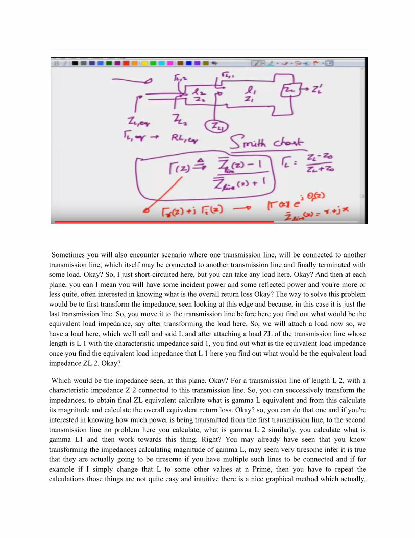
can be applied to solve these type of transmission line problems and that graphical method is called as,’Smith Chart’, We are going to build up to Smith chart so, all these that we discussed in the last 10-15minutes was actually to introduce you to Smith chart, where we will start with two basic assumptions thatat any point on the transmission line. Right? You can describe what is gamma of Z and at that gamma ofZ; you can actually obtain an equivalent Z of z Okay? I know the notations are getting a little confusingso, I will what I am going to write here is Z line of Z .Okay? Just to indicate that this is the lineimpedance, that I am saying at the Z plane. Okay? And there is a one-to-one relationship between, thesetwo Y remember gamma L is given by ZL minus Z naught by Z L plus Z naught and gamma any Z cansimilarly be expressed, by writing this as the line impedance at that load point or the load plane Z dividedminus Z not divided by Z line of Z plus Z naught. Okay? So, there is a one-to-one relationship betweengamma and the line impedances and because, we don't know what transmission line characteristicimpedance will be used, in many problems we in fact can work with what is called as,’ NormalizedImpedances’, when you work with normalized impedances you simply divide every impedance by thetransmission line, characteristic impedance. Okay? Or some reference impedance if you think of this wayso, you have this one-to-one relationship which forms the basis of Smith chart which allows you to solveproblems that I described earlier like this multiple connected transmission line problems. And this we willnot develop the equations, that is something that we can do it in a different course, but I will give you thebasic idea of Smith chart. Okay? How it would come about for that again we go back to the graphical method, of course this is a graphicalmethod and we realize how we can represent Gamma at any Z. Right? How do you represent this you canrepresent this in terms of its gamma real part and the imaginary part so, for example I can represent thisone as, gamma R of Z plus J gamma I of Z equivalently, I can represent this one by giving its magnitudeand the corresponding angle J theta gamma of Z. Okay? Meaning that at every point on the transmissionline, I can give the reflection coefficient by giving its magnitude, as well as its angle. Now on the sameyou know using this relationship, for every reflection coefficient at any point Z, I can calculate theequivalent normalized line impedance, which also can be written in terms of its real and imaginary parts,which we will denote as R plus J X. Okay? R is for small R you know capital R is usually used forresistor, small capital X is used for reactances, we have used small or and small X to denote that these arenormalized components. So, if I have this

Refer slide time :( 19:46)

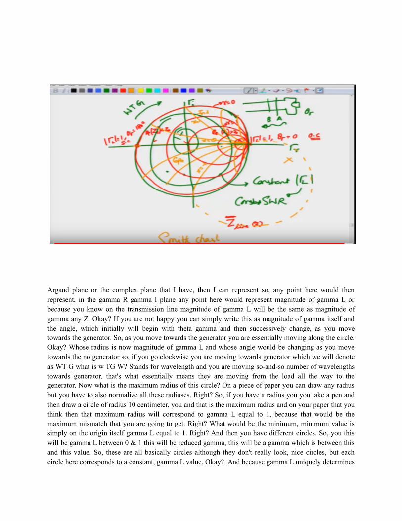
Argand plane or the complex plane that I have, then I can represent so, any point here would thenrepresent, in the gamma R gamma I plane any point here would represent magnitude of gamma L orbecause you know on the transmission line magnitude of gamma L will be the same as magnitude ofgamma any Z. Okay? If you are not happy you can simply write this as magnitude of gamma itself andthe angle, which initially will begin with theta gamma and then successively change, as you movetowards the generator. So, as you move towards the generator you are essentially moving along the circle.Okay? Whose radius is now magnitude of gamma L and whose angle would be changing as you movetowards the no generator so, if you go clockwise you are moving towards generator which we will denoteas WT G what is w TG W? Stands for wavelength and you are moving so-and-so number of wavelengthstowards generator, that's what essentially means they are moving from the load all the way to thegenerator. Now what is the maximum radius of this circle? On a piece of paper you can draw any radiusbut you have to also normalize all these radiuses. Right? So, if you have a radius you you take a pen andthen draw a circle of radius 10 centimeter, you and that is the maximum radius and on your paper that youthink then that maximum radius will correspond to gamma L equal to 1, because that would be themaximum mismatch that you are going to get. Right? What would be the minimum, minimum value issimply on the origin itself gamma L equal to 1. Right? And then you have different circles. So, you thiswill be gamma L between 0 & 1 this will be reduced gamma, this will be a gamma which is between thisand this value. So, these are all basically circles although they don't really look, nice circles, but eachcircle here corresponds to a constant, gamma L value. Okay? And because gamma L uniquely determines

SW R these are also called as,’ Constant SW R Circles’, S WR is VSWR circles. Okay? So, any point asyou keep moving would correspond to different points on the transmission line starting from some youknow initial load point. So, these are all different loads, I mean the different, different planes on thetransmission line. So, if I have this transmission line here, terminated with the load, say this planecorresponds to point A this plane corresponds to point B. And so, on I am moving towards the generatorand that corresponds to clockwise movement, on the appropriate constant SWR circle or a constantgamma L circle. However interestingly, every point that I consider say for example I consider at thispoint. Okay? This point would have an equivalent line impedance. Right? So, this point would actuallyhave an equivalent line impedance, because on this point you have a certain gamma Z. Okay? On somepoint on the transmission line that I don't know, but because I have this gamma of Z by knowing theangle, as well as the radius I will be able to obtain an equivalent line impedance. Okay? so, any point orall the points on this, I know on the on this circle within this circle, would correspond to equivalent lineimpedances, from the one-to-one relationship that we have this corresponds to normalized lineimpedances, of course what would be the line impedance for a point, let's say gamma L equal tomagnitude gamma L equal to 1 and an angle theta gamma equal to 0, this of course would correspond tothe open circuited point and that will be then so, normalized or unnormalized the value is always youknow infinity here. So, this point that we have written with the cross mark, that corresponds to opencircuit interestingly, if you go to this point which is gamma L magnitude still equal to 1 but an angle equalto 180 degrees. Right? Theta gamma equal to 180 degrees, this corresponds to short-circuit termination.Right? So, the point here, with coordinates 1 and 180 degrees or 1 and D Bar minus JP Bar J PI wouldactually correspond to a normalized impedance of 0 interesting. Right? In fact you can now extend thissuperimpose all the points, on this transmission line. Okay? All the points on this plane, with constantvalues of R and constant values of X meaning, I can actually have different circles, along those circles thevalue of gamma can change, but the value of R will always be constant. So, this corresponds to what iscalled as R equal to 1 or the unit circle or unity circle, the circle on the outer line that you have you knowwould correspond to a circle which we will call as R equal to 0 because that would b have a impedance of0 there. Okay? And then you have a well this one I have drawing, this circle would have an R value whichis between zero to one please remember R is normalized impedance, meaning that this is the case wherethe real part of Z L is actually less than Z naught. Okay?

So, the real part of Z L is less than Z naught similarly this case or this region corresponds to real part of ZL greater than Z naught and that would be these curves or these circles you can notice that the radius ofthe circle keeps on dropping as the real part of Z L keeps on increasing that is as you move from shortcircuit to open circuit the radius of the circle shrinks Center actually keeps moving away. So, the centerfor this one will be somewhere here the center for this one is here, the center for this one is here so, thecenter keeps shifting towards the. Right? It’s not towards .Right? And Right? And so, on and then thecircle radius also starts to shrink we are not done yet please note that we already on this graph, we havetwo kinds of circles one circles where we have constant gamma value, where the value of smaller andsmaller can change, however the magnitude of gamma L will remain the same and then you have thesered circles where the value of R will be constant R is real part of the impedance will be constant, whereasother values can actually change, I mean you can have different values of X, you can have differentvalues of gamma those things will change. Now I am about to draw, another set of circles, they are reallynot circles they're actually R is because, to make them circles you have to complete them outside thischart. Okay? We don't normally deal with region outside this chart, unless we are dealing with activecircuits. Okay? Which is not in this particular course so, therefore this region is forbidden for us. So, what

you have are these R is this straight line in fact is the R where you know you have X equal to 0 nosusceptance and then this arc is X equal to minus 1, this corresponds to capacitive region this correspondsto inductive region, because the susceptance is here are all positive this is X equal to 1, this is X less than1 this is X greater than 1 and so, on so, forth. Okay? So, you have these different R is so, this is your fullSmith chart it may look very the way I have written but please go to net and download this chart calledSmith chart keep it ready for the next module, because this is what we are going to use, I mean this willbe we will use to show you how to solve many transmission line problems. Okay? So, until then. Thankyou very much.