Leave-one-out kernel density estimates for outlier detection

Department of Econometrics and Business Statistics

http://monash.edu/business/ebs/research/publications

Leave-one-out kernel density

estimates for outlier detection

Sevvandi Kandanaarachchi, Rob J. Hyndman

February 2021

Working Paper 02/2021

ISSN 1440-771X



Sevvandi KandanaarachchiRMIT UniversityEmail: [email protected] author

Rob J. HyndmanMonash UniversityEmail: [email protected]

6 February 2021

JEL classification: C55, C65, C87

mailto:[email protected]

mailto:[email protected]



Abstract

This paper introduces lookout, a new approach to detect outliers using leave-one-out kernel

density estimates and extreme value theory. Outlier detection methods that use kernel density

estimates generally employ a user defined parameter to determine the bandwidth. Lookout

uses persistent homology to construct a bandwidth suitable for outlier detection without any

user input. We demonstrate the effectiveness of lookout on an extensive data repository by

comparing its performance with other outlier detection methods based on extreme value theory.

Furthermore, we introduce outlier persistence, a useful concept that explores the birth and the

cessation of outliers with changing bandwidth and significance levels. The R package lookout

implements this algorithm.

Keywords: anomaly detection, topological data analysis, persistent homology, extreme value

theory, peak over thresholds, generalized Pareto distribution

1 Introduction

Outliers, anomalies and novelties are often interchangeably used to describe the same concept:

data points that are unusual compared to the rest. The existence of multiple words to describe

similar concepts arise from the growth of outlier detection and applications in multiple research

areas. Indeed, outlier detection is used in diverse applications ranging from detecting security

breaches in the Internet of Things networks to identifying extreme weather events. Consequently,

it is important to develop robust techniques to detect outliers, which minimize costly false

positives and dangerous false negatives.

This diverse literature can be divided into approaches that use probability densities to define

outliers, and those that use distances to define outliers. Outlier detection methods that use prob-

ability densities treat outliers as observations that are very unlikely given the other observations.

Outlier detection methods that use distances treat outliers as observations that lie far from other

observations.

2

Leave-one-out kernel density estimates for outlier detection

In this paper, we take a probability density approach to outlier detection. We propose a new

outlier detection algorithm that we call lookout, which uses leave-one-out kernel density estimates

to identify the most unlikely observations. We address the challenge of bandwidth selection by

using persistent homology — a concept in topological data analysis — and use extreme value

theory (EVT) to identify outliers based on their leave-one-out density estimates.

The main challenge in using kernel density estimates for outlier detection is the selection of the

bandwidth. Schubert, Zimek & Kriegel (2014) employ kernel density estimates to detect outliers

using k-nearest neighbor distances where k is a user-specified parameter, which determines

bandwidth. Qin et al. (2019) employ kernel density estimates to detect outliers in streaming

data. They too have a radius parameter, which is equivalent to the bandwidth that needs

to be specified by the user. Tang & He (2017) use reverse and shared k nearest neighbors to

compute kernel density estimates and identify outliers. They also have a user defined parameter

k that denotes the reverse k nearest neighbors. The oddstream algorithm (Talagala et al. 2020)

computes kernel density estimates on a 2-dimensional projection defined by the first two

principal components, and so bandwidths need to be selected. We avoid subjective user-choice,

and the inappropriate use of bandwidths optimized for some other purpose, by proposing the

use of persistent homology as a new tool for bandwidth selection.

Extreme Value Theory has been gaining popularity in outlier detection because of its rich,

theoretical foundations. Burridge & Taylor (2006) used EVT to detect outliers in time series data.

Clifton et al. (2014) used Generalized Pareto Distributions to model the tails in high-dimensional

data and detect outliers. Other recent advances in outlier detection that use EVT include the

stray (Talagala, Hyndman & Smith-Miles 2021), oddstream (Talagala et al. 2020) and HDoutliers

(Wilkinson 2017) algorithms. Of these three methods, stray is an enhancement of HDoutliers and

both use distances to detect outliers, while oddstream uses kernel density estimates to detect

outliers in time series data. Our approach is closest to oddstream in that we also apply EVT to

functions of kernel density estimates. However, we use a different functional, and we avoid the

need for an outlier-free training set.

A brief introduction to persistent homology and EVT is given in Section 2. In Section 3 we

introduce the algorithm lookout and the concept of outlier persistence, which explores the birth

and death of outliers with changing bandwidth. We show examples illustrating the usefulness

of outlier persistence and conduct experiments using synthetic data to evaluate the performance

of lookout in Section 4. Using an extensive data repository of real datasets, we compare the

performance of lookout to HDoutliers and stray in Section 5.

Kandanaarachchi, Hyndman: 6 February 2021 3


We have produced an R package lookout (Kandanaarachchi & Hyndman 2021) containing this

algorithm. In addition, all examples in this paper are available in the supplementary material at

https://github.com/sevvandi/supplementary_material/tree/master/lookout.

We have used the R packages TDAstats (Wadhwa et al. 2018) and ggtda (Brunson, Wadhwa &

Scott 2020) for all TDA and persistent homology computations and related graphs. We have

used the R package evd (Stephenson 2002) to fit the Generalized Pareto Distribution.

2 Mathematical background

In this section we provide some brief background on three topics that we will use in our proposed

lookout algorithm.

1. topological data analysis and persistent homology;

2. extreme value theory and the peaks-over-threshold approach; and

3. kernel density estimation.

2.1 Topological data analysis and persistent homology

Topological data analysis is the study of data using topological constructs. It is about inferring

high dimensional structure from low dimensional representations such as points and assembling

discrete points to construct global structures (Ghrist 2008). Persistent homology is a method

in algebraic topology that computes topological features of a space that persist across multiple

scales or spatial resolutions. These features include connected components, topological circles

and trapped volumes. Features that persist for a wider range of spatial resolutions represent

robust, intrinsic features of the data while features that sporadically change are perturbations

resulting from noise. Persistent homology has been used in a wide variety of applications

including biology (Topaz, Ziegelmeier & Halverson 2015), computer graphics (Carlsson et al.

2008) and engineering (Perea & Harer 2015). In this section we will give a brief overview

of persistent homology without delving into the mathematical details. Readers are referred

to Ghrist (2008) and Carlsson (2009) for an overview and Wasserman (2018) for a statistical

viewpoint on the subject.

Simplicial complex

Consider a data cloud representing a collection of points. This set of points is used to construct

a graph where the points are considered vertices and the edges are determined by the distance

between the points. Given a proximity parameter ε, two vertices are connected by an edge if the

distance between these two points is less than or equal to ε. Starting from this graph, a simplicial


https://github.com/sevvandi/supplementary_material/tree/master/lookout


complex — a space built from simple pieces — is constructed. A simplicial complex is a finite

set of k-simplices, where k denotes the dimension; for example, a point is a 0-simplex, an edge a

1-simplex, a triangle a 2-simplex, and a tetrahedron a 3-simplex. Suppose S denotes a simplicial

complex that includes a k-simplex γ. Then all non-empty subsets of β ⊂ γ are also included in

S. For example, if S contains a triangle pqr, then the edges pq, qr and rs, and the vertices p, q

and r, are also in S.

The Vietoris-Rips complex and the Cech complex are two types of k-simplicial complexes. We will

construct a Vietoris-Rips complex from the data cloud as it is more computationally efficient

than the Cech complex (Ghrist 2008). Given a set of points and a proximity parameter ε > 0,

k + 1 points within a distance of ε to each other form a k-simplex. For example, consider 5 points

p, q, r, s and t and suppose the distance between any two points except t is less than ε. Then we

can construct the edges pq, pr, ps, qr, qs and rs. From the edges pq, qr and rp we can construct

the triangle pqr, from pq, qs and sp the triangle pqs and so on, because the distance between any

two points p, q, r and s is bounded by ε. By constructing the 4 triangles pqr, qrs, rsp and spq

we can construct the tetrahedron pqrs. The vertex t is not connected to this 3-simplex because

the distance between t and the other vertices is greater than ε. The simplicial complex resulting

from these 5 points consists of the tetrahedron pqrs and all the subset k-simplices and the vertex

t. Figure 1 shows this simplicial complex on the left and another example on the right.

p

qr

s

t

0.0

0.4

0.8

y

0.0 0.4 0.8x

−2

−1

0

1

2

y

−2 −1 0 1x

Figure 1: The figure on the left shows the points p, q, r, s and t with a proximity parameter ε = 0.5 andthe resulting Rips complex consisting of the tetrahedron pqrs, triangles pqr, qrs, rsp, pqs,edges pq, qr, rs, sp, qs, pr and vertices p, q, r, s and t. The figure on the right shows 8 pointsand the resulting Rips complex with ε = 4/3.



Persistent homology

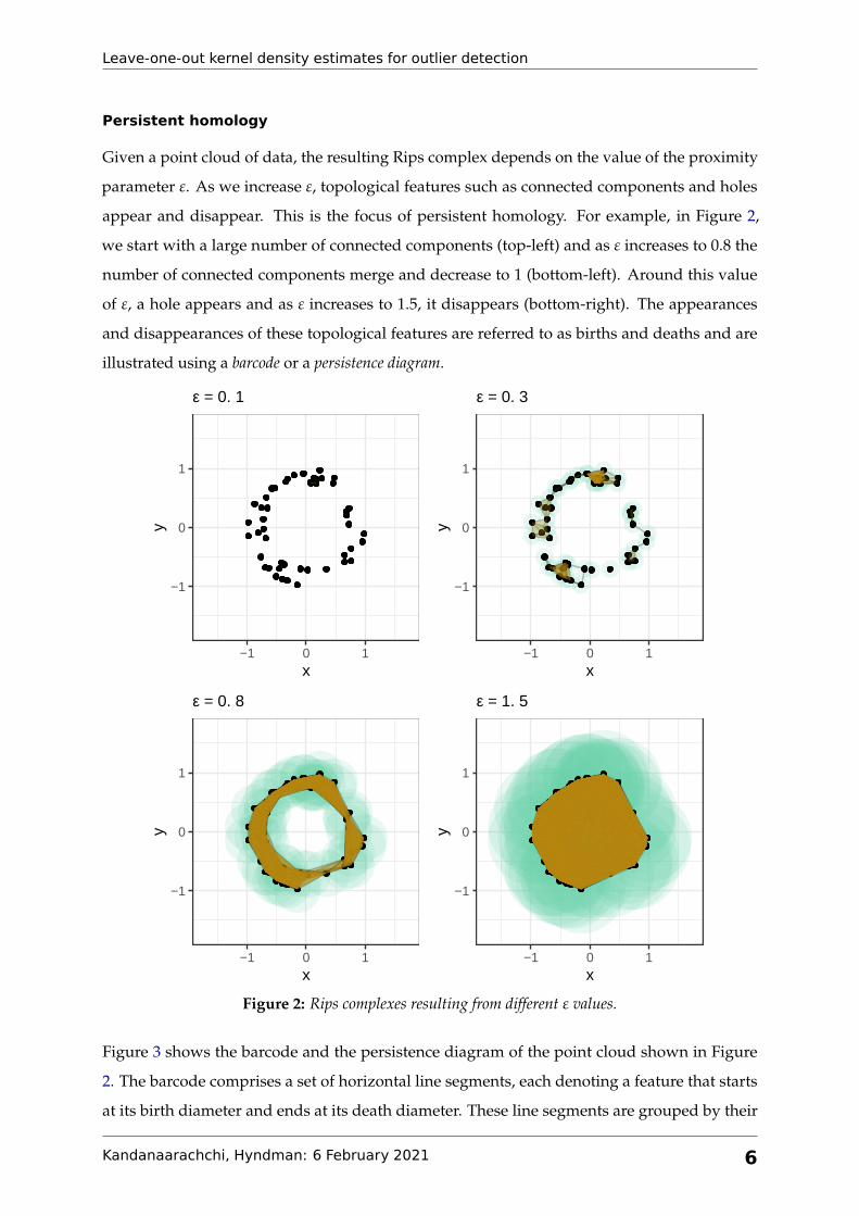
Given a point cloud of data, the resulting Rips complex depends on the value of the proximity

parameter ε. As we increase ε, topological features such as connected components and holes

appear and disappear. This is the focus of persistent homology. For example, in Figure 2,

we start with a large number of connected components (top-left) and as ε increases to 0.8 the

number of connected components merge and decrease to 1 (bottom-left). Around this value

of ε, a hole appears and as ε increases to 1.5, it disappears (bottom-right). The appearances

and disappearances of these topological features are referred to as births and deaths and are

illustrated using a barcode or a persistence diagram.

−1

0

1

y

−1 0 1x

ε = 0. 1

−1

0

1

y

−1 0 1x

ε = 0. 3

−1

0

1

y

−1 0 1x

ε = 0. 8

−1

0

1

y

−1 0 1x

ε = 1. 5

Figure 2: Rips complexes resulting from different ε values.

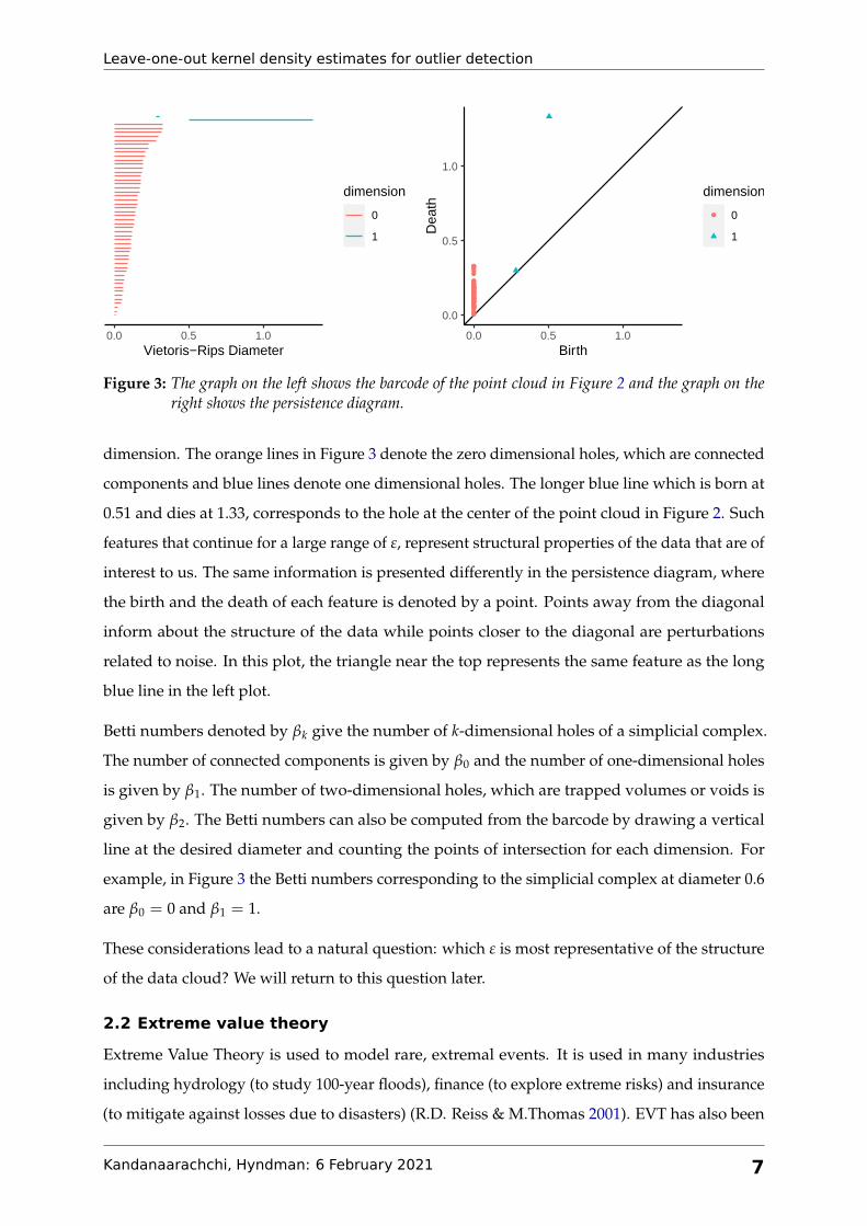
Figure 3 shows the barcode and the persistence diagram of the point cloud shown in Figure

2. The barcode comprises a set of horizontal line segments, each denoting a feature that starts

at its birth diameter and ends at its death diameter. These line segments are grouped by their



0.0 0.5 1.0Vietoris−Rips Diameter

dimension

0

1

0.0

0.5

1.0

Dea

th

0.0 0.5 1.0Birth

dimension

0

1

Figure 3: The graph on the left shows the barcode of the point cloud in Figure 2 and the graph on theright shows the persistence diagram.

dimension. The orange lines in Figure 3 denote the zero dimensional holes, which are connected

components and blue lines denote one dimensional holes. The longer blue line which is born at

0.51 and dies at 1.33, corresponds to the hole at the center of the point cloud in Figure 2. Such

features that continue for a large range of ε, represent structural properties of the data that are of

interest to us. The same information is presented differently in the persistence diagram, where

the birth and the death of each feature is denoted by a point. Points away from the diagonal

inform about the structure of the data while points closer to the diagonal are perturbations

related to noise. In this plot, the triangle near the top represents the same feature as the long

blue line in the left plot.

Betti numbers denoted by βk give the number of k-dimensional holes of a simplicial complex.

The number of connected components is given by β0 and the number of one-dimensional holes

is given by β1. The number of two-dimensional holes, which are trapped volumes or voids is

given by β2. The Betti numbers can also be computed from the barcode by drawing a vertical

line at the desired diameter and counting the points of intersection for each dimension. For

example, in Figure 3 the Betti numbers corresponding to the simplicial complex at diameter 0.6

are β0 = 0 and β1 = 1.

These considerations lead to a natural question: which ε is most representative of the structure

of the data cloud? We will return to this question later.

2.2 Extreme value theory

Extreme Value Theory is used to model rare, extremal events. It is used in many industries

including hydrology (to study 100-year floods), finance (to explore extreme risks) and insurance

(to mitigate against losses due to disasters) (R.D. Reiss & M.Thomas 2001). EVT has also been



used in outlier detection (Wilkinson 2017; Talagala et al. 2020). In this section we will give a

brief introduction to EVT using the notation in Coles (2001).

Consider n independent and identically distributed random variables X1, . . . , Xn with a dis-

tribution function F(x) = P{X ≤ x}. Then the maximum of these n random variables is

Mn = max{X1, . . . , Xn}. If F is known, the distribution of Mn is given by (Coles 2001, p45)

P{Mn ≤ z} = (F(z))n. However, F is usually not known in practice. This gap is filled by

Extreme Value Theory, which studies approximate families of models for Fn so that extremes

can be modeled and uncertainty quantified. The Fisher-Tippet-Gnedenko Theorem states that

under certain conditions, a scaled maximum Mn−anbn

can have certain limit distributions.

Theorem 2.1 (Fisher-Tippett-Gnedenko). If there exist sequences {an} and {bn} such that

P{(Mn − an)

bn≤ z}→ G(z) as n→ ∞,

where G is a non-degenerate distribution function, then G belongs to one of the following families:

Gumbel : G(z) = exp(− exp

[−( z− b

a

)]), −∞ < z < ∞,

Fréchet : G(z) =

0, z ≤ b,

exp(−(

z−ba

)−α)

, z > b,

Weibull : G(z) =

exp

(−(−[

z−ba

])α), z < b,

1, z ≥ b,

for parameters a, b and α where a, α > 0.

These three families of distributions can be further combined into a single family by using the

following distribution function known as the Generalized Extreme Value (GEV) distribution,

G(z) = exp

{−[

1 + ξ( z− µ

σ

)]−1/ξ}

,

where the domain of the function is {z : 1 + ξ(z − µ)/σ > 0}. The location parameter is

µ ∈ R, σ > 0 is the scale parameter, while ξ ∈ R is the shape parameter. When ξ = 0 we

obtain a Gumbel distribution with exponentially decaying tails. When ξ < 0 we get a Weibull

distribution with a finite upper end and when ξ > 0 we get a Fréchet family of distributions

with polynomially decaying tails.



The Generalized Pareto Distribution and the POT approach

The Peaks Over Threshold (POT) approach regards extremes as observations greater than a

threshold u. We can write the conditional probability of extreme events as

P {X > u + y | X > u} = 1− F(u + y)1− F(u)

, y > 0,

giving us

P {X ≤ u + y | X > u} = F(u + y)− F(u)1− F(u)

, y > 0.

The distribution function

Fu(y) = P {X ≤ u + y | X > u} ,

describes the exceedances above the threshold u. If F is known we could compute this probability.

However, as F is not known in practice we use approximations based on the Generalized Pareto

Distribution (Pickands 1975).

Theorem 2.2 (Pickands). Let X1, X2, . . . , Xn be a sequence of independent random variables with a

common distribution function F, and let Mn = max{X1, . . . , Xn}. Suppose F satisfies Theorem 2.1 so

that for large n, P{Mn ≤ z} ≈ G(z), where

G(z) = exp

{−[

1 + ξ( z− µ

σ

)]−1/ξ}

,

for some µ, ξ ∈ R and σ > 0. Then for large enough u, the distribution function of (X− u) conditional

on X > u, is approximately

H(y) = 1−(

1 +ξyσu

)−1/ξ, (1)

where the domain of H is {y : y > 0 and (1 + ξy)/σu > 0}, and σu = σ + ξ(u− µ).

The family of distributions defined by equation (1) is called the Generalized Pareto Distribution

(GPD). We note that the GPD parameters are determined from the associated GEV parameters.

In particular, the shape parameter ξ is the same in both distributions.

For a chosen threshold u, the parameters of the GPD can be estimated by standard maximum

likelihood techniques. As an analytical solution that maximizes the likelihood does not exist,

numerical techniques are used to arrive at an approximate solution. We use the R package evd

to fit a GPD using the POT approach.



2.3 Kernel density estimation

For a sample x1, x2, . . . , xn ∈ Rp, the kernel density estimate is given by

f̂ (x; H) =1n

n

∑i=1

KH (x− xi) , (2)

where H denotes a p× p positive definite bandwidth matrix, KH(z) = H−1/2K(H−1/2z), and

K is a kernel function. For consistency, we scale the kernels so that∫‖z2‖K(z)dz = 1. The

multivariate Gaussian kernel is given by

K(x) =1

(2π)p/2 exp(‖x‖2/2),

and the multivariate scaled Epanechnikov kernel by

K(x) =p + 2

cp(1− ‖x‖2/5)+, (3)

where cp is the volume of the unit sphere in Rp and u+ = max(0, u).

We will use the leave-one-out kernel density estimator given by

f̂−j(x; H) =1

n− 1 ∑i 6=j

KH(x− xi),

which can be simplified to

f̂−j(xj; H) =[n f̂ (xj; H)− H−1/2K(0)

]/(n− 1)

when evaluated at the observation omitted.

A major challenge in using kernel density estimates for outlier detection is selecting the appropri-

ate bandwidth. There is a large body of literature on kernel density estimation and bandwidth

selection (Scott 1994; Wang & Scott 2019) that focuses on computing density estimates that

represent the data as accurately as possible, where measures of accuracy have certain asymptotic

properties. However, our goal is somewhat different as we are interested in finding outliers

in the data, rather than finding a good representation for the rest of the data. Often the usual

bandwidth selection methods result in bandwidths that are too small and can cause the kernel

density estimates of the boundary and near-boundary points to be confused with outliers. In

high dimensions this problem is exacerbated due to the sparsity of the data. Thus, we need a



bandwidth that assists outlier detection. A too small bandwidth causes everything to be outliers,

while too large a bandwidth will lead to outliers being hidden.

3 Methodology

3.1 Bandwidth selection using TDA

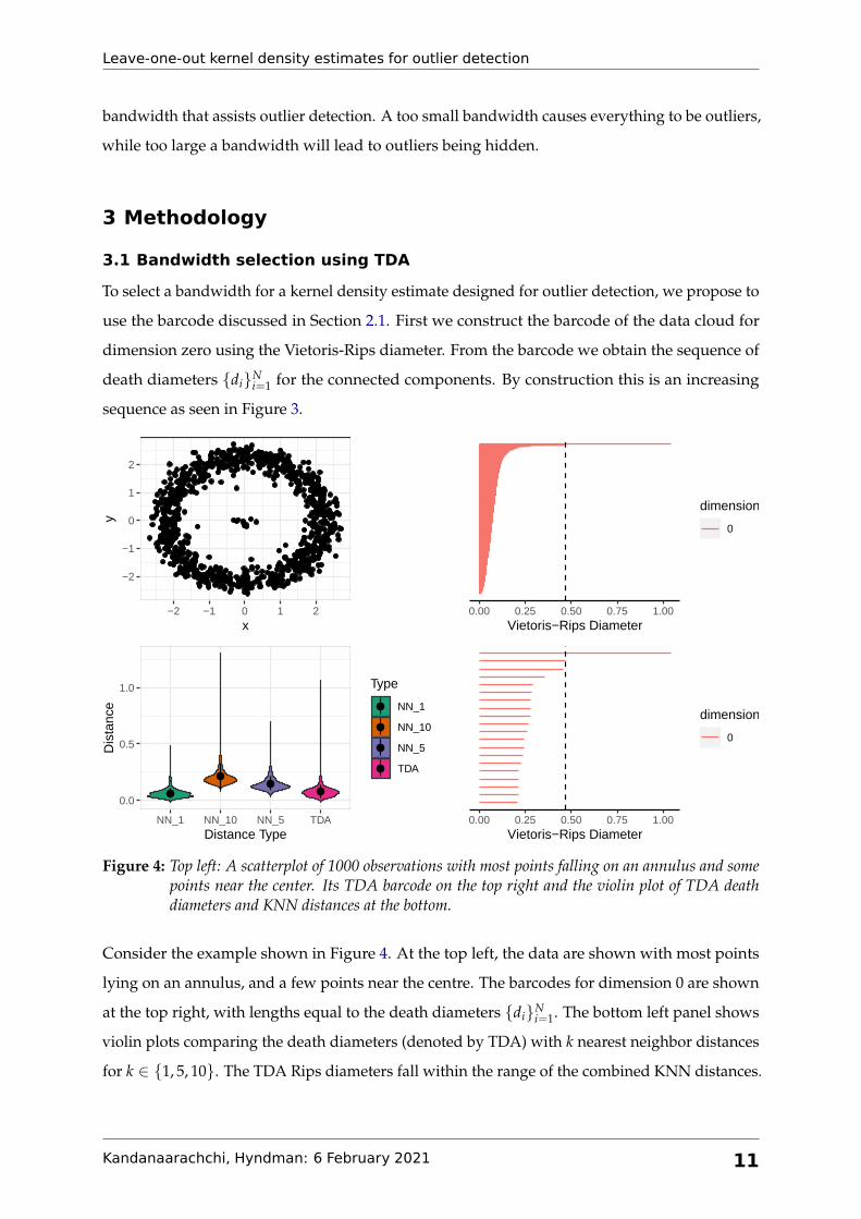
To select a bandwidth for a kernel density estimate designed for outlier detection, we propose to

use the barcode discussed in Section 2.1. First we construct the barcode of the data cloud for

dimension zero using the Vietoris-Rips diameter. From the barcode we obtain the sequence of

death diameters {di}Ni=1 for the connected components. By construction this is an increasing

sequence as seen in Figure 3.

−2

−1

0

1

2

−2 −1 0 1 2x

y

0.0

0.5

1.0

NN_1 NN_10 NN_5 TDADistance Type

Dis

tanc

e

Type

NN_1

NN_10

NN_5

TDA

0.00 0.25 0.50 0.75 1.00Vietoris−Rips Diameter

dimension

0

0.00 0.25 0.50 0.75 1.00Vietoris−Rips Diameter

dimension

0

Figure 4: Top left: A scatterplot of 1000 observations with most points falling on an annulus and somepoints near the center. Its TDA barcode on the top right and the violin plot of TDA deathdiameters and KNN distances at the bottom.

Consider the example shown in Figure 4. At the top left, the data are shown with most points

lying on an annulus, and a few points near the centre. The barcodes for dimension 0 are shown

at the top right, with lengths equal to the death diameters {di}Ni=1. The bottom left panel shows

violin plots comparing the death diameters (denoted by TDA) with k nearest neighbor distances

for k ∈ {1, 5, 10}. The TDA Rips diameters fall within the range of the combined KNN distances.



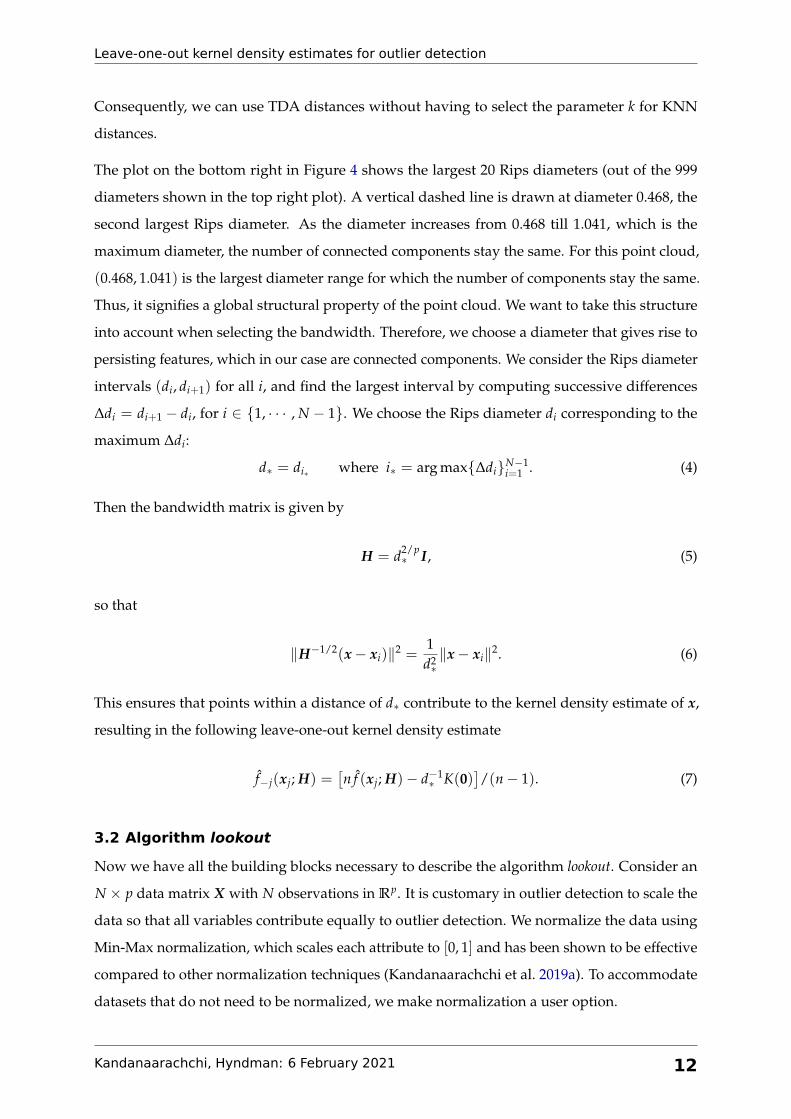
Consequently, we can use TDA distances without having to select the parameter k for KNN

distances.

The plot on the bottom right in Figure 4 shows the largest 20 Rips diameters (out of the 999

diameters shown in the top right plot). A vertical dashed line is drawn at diameter 0.468, the

second largest Rips diameter. As the diameter increases from 0.468 till 1.041, which is the

maximum diameter, the number of connected components stay the same. For this point cloud,

(0.468, 1.041) is the largest diameter range for which the number of components stay the same.

Thus, it signifies a global structural property of the point cloud. We want to take this structure

into account when selecting the bandwidth. Therefore, we choose a diameter that gives rise to

persisting features, which in our case are connected components. We consider the Rips diameter

intervals (di, di+1) for all i, and find the largest interval by computing successive differences

∆di = di+1 − di, for i ∈ {1, · · · , N − 1}. We choose the Rips diameter di corresponding to the

maximum ∆di:

d∗ = di∗ where i∗ = arg max{∆di}N−1i=1 . (4)

Then the bandwidth matrix is given by

H = d2/p∗ I, (5)

so that

‖H−1/2(x− xi)‖2 =1d2∗‖x− xi‖2. (6)

This ensures that points within a distance of d∗ contribute to the kernel density estimate of x,

resulting in the following leave-one-out kernel density estimate

f̂−j(xj; H) =[n f̂ (xj; H)− d−1

∗ K(0)]/(n− 1). (7)

3.2 Algorithm lookout

Now we have all the building blocks necessary to describe the algorithm lookout. Consider an

N × p data matrix X with N observations in Rp. It is customary in outlier detection to scale the

data so that all variables contribute equally to outlier detection. We normalize the data using

Min-Max normalization, which scales each attribute to [0, 1] and has been shown to be effective

compared to other normalization techniques (Kandanaarachchi et al. 2019a). To accommodate

datasets that do not need to be normalized, we make normalization a user option.



We compute the kernel density estimates defined by (2) and the leave-one-out kernel density

estimates defined in (7), with the bandwidth matrix (5), and the scaled Epanechnikov kernel (3).

Denote the kernel density estimate of xi by yi and the leave-one-out kde of xi (by leaving out

xi) by y−i. Then we fit a Generalized Pareto Distribution to − log(yi) using the POT approach

discussed in Section 2.2. We use the 90th percentile as the threshold for the POT approach as

recommended by Bommier (2014). Using the fitted GPD parameters, µ, σ and ξ, we declare

points with P (− log(y−i)|µ, σ, ξ) < α to be outliers. We summarize these steps in Algorithm 1.

Algorithm 1: lookout.input : The data matrix X, parameters α and unitize.output : The outliers, the GPD probabilities of all points, GPD parameters and bandwidth

1 If unitize = TRUE, then normalize the data so that each column is scaled to [0, 1].2 Construct the persistence homology barcode of the data.3 Find d∗ as in equation (4).4 Using H = (d∗)2/p I, compute kernel density estimates (2) and leave-one-out kernel

density estimates (7) using the scaled Epanechnikov kernel (3).5 Denote the kde of xi by yi and leave-one-out kde by y−i.6 Using the POT approach, fit a GPD to {− log(yi)}N

i=1 and estimate µ, σ and ξ.7 Using the GPD estimates µ̂, σ̂ and ξ̂, find the probability of the leave-one-out kde values{− log(y−i)}N

i=1, i.e., P (− log(y−i)|µ, σ, ξ) for all i.8 If P (− log(y−i)|µ, σ, ξ) < α, then declare xi as an outlier.

The output probability of lookout is the GPD probability of the points, so that low probabilities

indicate likely outliers and high probabilities indicate normal points. Note that the scaling factor

of the kernel K(x) does not affect the GPD parameters as it is just an offset after taking logs of yi

or yi.

The algorithm lookout has only 2 inputs, α and unitize. The parameter α determines the threshold

for outlier detection and unitize gives the user an option to normalize the data. We set α = 0.05

and unitize = TRUE as default parameter values. We use the Epanechnikov kernel in lookout due

to ease of computation. However, any kernel can be incorporated as long as the variances are

matched.

3.3 Outlier persistence

Lookout identifies outliers by selecting an appropriate bandwidth using TDA. If the bandwidth

is changed, will the original outliers be still identified as outliers by lookout? We explore this

question by varying bandwidth values in lookout. Similar work is discussed by Minnotte & Scott

(1993), who introduce the Mode Tree, which tracks the modes of the kernel density estimates



with changing bandwidth values. Another related idea is the SiZer map (Chaudhuri & Marron

1999), a graphical device that studies features of curves for varying bandwidth values.

1001

100210031004

1005

−3

−2

−1

0

1

2

3

−2 −1 0 1 2 3x

y

0

250

500

750

1000

0.0 0.1 0.2 0.3 0.4Bandwidth

Obs

erva

tion

Figure 5: Outliers at the center of the annulus in the left plot showing the outlier labels 1001–1005. Theoutlier persistence diagram on the right with the y-axis denoting the labels. The dashed lineshows the lookout bandwidth d∗.

If a point is identified as an outlier by the lookout algorithm for a range of bandwidth values,

then it increases the validity of that point as an outlier. Consider an annulus with some points

in the middle as shown in the left plot of Figure 5. The plot on the right, which is similar

to a barcode, shows the outliers identified by lookout for different bandwidth values. Each

horizontal line segment shows the range of Rips diameter values that has identified each point

as an outlier. With some abuse of notation, we label the x axis “bandwidth”, even though it

actually represents the Rips diameter d∗ = hp/2, where the bandwidth matrix H = hI. This is

motivated from equation (6), as we only consider points xi within a distance d∗ of every point

x when computing kernel density estimates using the Epanechnikov kernel. In this plot, the

y-axis corresponds to the point index. We call this plot the outlier persistence diagram signifying

the link to topological data analysis.

In the example in Figure 5, we see that the points 1001–1005 are identified as outliers in the

outlier persistence diagram for a large range of bandwidth values. The Rips diameter d∗ selected

by lookout is shown by a vertical dashed line. Many points are identified as outliers for small

bandwidth values but do not continue to be outliers for long; these outliers are born at small

bandwidth values and die out after a relatively short increase in bandwidth. Some points are

never identified as outliers, even at small bandwidths.

The outlier persistence diagram is a tool to observe the persistence of outliers with changing

bandwidth values. We vary the bandwidth values while keeping the GPD parameters fixed

at the values obtained using d∗ as in equation (4). The death diameter sequence di is used to



construct the set of bandwidth values used in this plot. We use ` bandwidth values starting

from the βth percentile of sequence {di} ending at√

5×maxi di. The parameters ` and β are

user-defined with default values ` = 20 and β = 90. Increasing ` gives better granularity but

increases the computational burden. As the death diameters are tightly packed, the default

value of 90th percentile gives a small enough starting bandwidth and√

5 maxi di gives a large

ending bandwidth. We summarize these steps in Algorithm 2.

Algorithm 2: outlier persistence for fixed α.input : The data matrix X, parameters α, unitize and bandwidth range parameters ` and

β

output : An N × ` binary matrix Y where N denotes the number of observations and `

denotes the number of bandwidth values with yik = 1 if the ith observation isidentified as an outlier for bandwidth index k.

1 Initialize matrix Y to zero.2 Run Algorithm 1 to determine the death diameter sequence {di} and the GPD parameters

µ0, σ0 and ξ0.3 Construct an equidistant bandwidth sequence of length ` starting from the βth percentile

of {di} to√

5 maxi di. Call the bandwidth sequence {bk}`k=1.4 for k from 1 to ` do5 Using h = (bk)

2/p and H = hI compute kernel density estimates and leave-one-outkernel density estimates using the scaled Epanechnikov kernel.

6 Denote the kde of xi by yi and leave-one-out kde by y−i.7 Using the GPD parameters µ0, σ0 and ξ0 find the GPD probability of the leave-one-out

kde values {− log(y−i)}Ni=1, i.e., P (− log(y−i)|µ0, σ0, ξ0) for all i.

8 If P (− log(y−i)|µ0, σ0, ξ0) < α, then declare xi as an outlier and let yik = 1.

Next, we extend this notion of persistence to include significance levels α ∈ {0.01, 0.02, . . . , 0.1}.

We define the strength of an outlier based on its significance level. Let xj be an outlier identified

at significance level α, where α is the smallest significance level for which xj is identified as an

outlier. Then

strength(xj) =(0.11− α)+

0.01(8)

Thus, if a point is identified as an outlier with a significance level α = 0.01, then it has strength

10, and an outlier with α = 0.1 has strength 1. To compute persistence over significance levels,

the only modification that needs to be done to Algorithm 2 is to fix α = 0.1 and to record the

minimum significance level if P (− log(y−i)|µ0, σ0, ξ0) < 0.1. Then we can use equation (8) to

compute its strength.

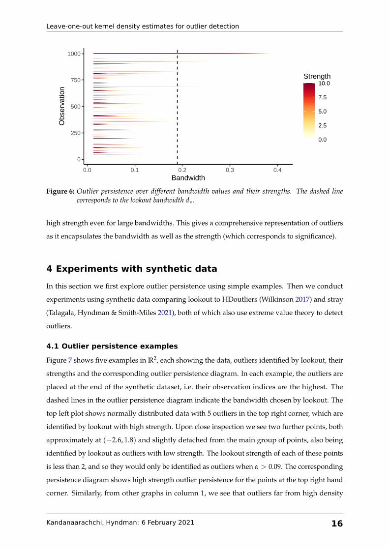
Figure 6 shows the persistence of outliers over different bandwidth values and significance

levels for the dataset in Figure 5. We see that points 1001–1005 are identified as outliers with



0

250

500

750

1000

0.0 0.1 0.2 0.3 0.4Bandwidth

Obs

erva

tion

0.0

2.5

5.0

7.5

10.0Strength

Figure 6: Outlier persistence over different bandwidth values and their strengths. The dashed linecorresponds to the lookout bandwidth d∗.

high strength even for large bandwidths. This gives a comprehensive representation of outliers

as it encapsulates the bandwidth as well as the strength (which corresponds to significance).

4 Experiments with synthetic data

In this section we first explore outlier persistence using simple examples. Then we conduct

experiments using synthetic data comparing lookout to HDoutliers (Wilkinson 2017) and stray

(Talagala, Hyndman & Smith-Miles 2021), both of which also use extreme value theory to detect

outliers.

4.1 Outlier persistence examples

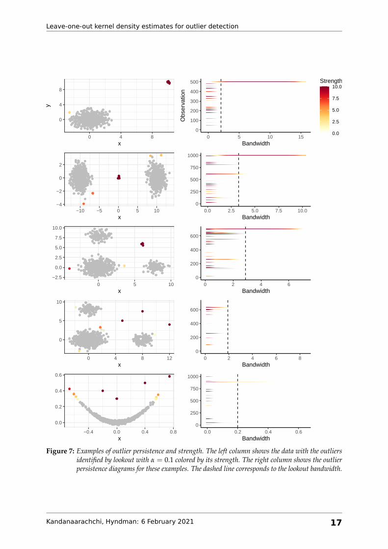
Figure 7 shows five examples in R2, each showing the data, outliers identified by lookout, their

strengths and the corresponding outlier persistence diagram. In each example, the outliers are

placed at the end of the synthetic dataset, i.e. their observation indices are the highest. The

dashed lines in the outlier persistence diagram indicate the bandwidth chosen by lookout. The

top left plot shows normally distributed data with 5 outliers in the top right corner, which are

identified by lookout with high strength. Upon close inspection we see two further points, both

approximately at (−2.6, 1.8) and slightly detached from the main group of points, also being

identified by lookout as outliers with low strength. The lookout strength of each of these points

is less than 2, and so they would only be identified as outliers when α > 0.09. The corresponding

persistence diagram shows high strength outlier persistence for the points at the top right hand

corner. Similarly, from other graphs in column 1, we see that outliers far from high density



0

4

8

0 4 8x

y

−4

−2

0

2

−10 −5 0 5 10x

−2.5

0.0

2.5

5.0

7.5

10.0

0 5 10x

0

5

10

0 4 8 12x

0.0

0.2

0.4

0.6

−0.4 0.0 0.4 0.8x

0

100

200

300

400

500

0 5 10 15Bandwidth

Obs

erva

tion

0.0

2.5

5.0

7.5

10.0Strength

0

250

500

750

1000

0.0 2.5 5.0 7.5 10.0Bandwidth

0

200

400

600

0 2 4 6Bandwidth

0

200

400

600

0 2 4 6 8Bandwidth

0

250

500

750

1000

0.0 0.2 0.4 0.6Bandwidth

Figure 7: Examples of outlier persistence and strength. The left column shows the data with the outliersidentified by lookout with α = 0.1 colored by its strength. The right column shows the outlierpersistence diagrams for these examples. The dashed line corresponds to the lookout bandwidth.



regions are identified by lookout with high strength and points outside high density regions,

but not so far away are identified with low strength. For the example in row 3, lookout has

identified a cluster of outliers approximately at (6, 6) with high strength as well as individual

points slightly away from high density regions with low strength. The example in row 5 has

single outliers rather than clusters, which are again identified by lookout. For the last example

in the bottom row, lookout has identified a cluster of outliers at (−0.6, 0.35) with low strength

and the remaining outliers with high strength. From the persistence diagrams we see that many

points are identified as outliers for low bandwidth values, but only a small number of outliers

persist until the bandwidth is large. In addition, some outliers persist at low strength values.

For example, the persistence diagram in row 5 has outliers around index 500 with low strength

persisting until large bandwidth values.

From the examples in Figure 7 we see that lookout selects a bandwidth appropriate for outlier

detection that is neither too small nor too large. In addition, lookout identifies outliers correctly.

The outlier persistence diagram gives a snapshot of the outliers for varying bandwidths and

significance levels increasing our understanding of the dataset and its outliers.

4.2 Comparison Study

In this section we conduct three experiments with synthetic data. Each experiment considers

two data distributions; the main distribution and a handful of outliers which are distributed

differently. There are several iterations to each experiment. The iterations serve as a measure of

the degree of outlyingness of the small sample. The outliers start off with the main distribution

and slowly move out of the main distribution with each iteration. Consequently, in the initial

iterations the points in the outlying distribution are not actual outliers as they are similar to

the points in the main distribution, while in the later iterations they are quite different from the

main distribution. We repeat each iteration 10 times to account for the randomness of the data

generation process.

We compare the results of lookout with 2 other algorithms; HDoutliers (Wilkinson 2017) and

stray (Talagala, Hyndman & Smith-Miles 2021), as both these algorithms also use extreme value

theory for outlier detection. For all three algorithms we use α = 0.05. We use two evaluation

metrics suited for imbalanced datasets: the F-measure and the geometric mean of sensitivity

and specificity denoted by Gmean. The F-measure is defined as

F-measure = 2precision× recall(precision + recall)

,



where

precision =tp

tp + fp, and recall =

tptp + fn

,

where tp, fp and fn denote true positives (predicted = true, actual = true), false positives (predicted

= true, actual = false) and false negatives (predicted = false, actual =true) respectively. The

F-measure is undefined when both precision and recall are zero, which occurs when the true

positives tp are zero. This happens when the outlier detection algorithm does not identify any

correct outliers. We assign zero to the F-measure in such instances.

Sensitivity and specificity are similar evaluation metrics more frequently used in a medical

diagnosis context:

sensitivity =tp

tp + fn, and specificity =

tntn + fp

,

and

Gmean =√

sensitivity× specificity,

where tn denotes the true negatives (predicted = false, actual = false). In fact, sensitivity and

recall are two different terms denoting the same quantity of interest.

Experiment 1

For this experiment we consider two normally distributed samples in R6; one large and one

small starting at the same location with the small sample slowly moving out in each iteration.

The set of points belonging to the small sample are considered outliers. We consider 400 points

in the bigger sample and 5 in the outlying sample, placed at indices 401–405. The points in the

larger sample are distributed in each dimension as N (0, 1). The outliers differ from the normal

points in only one dimension; i.e. they are distributed as N (2 + (i− 1)/2, 0.2), where i denotes

the iteration. In the first iteration the outliers are distributed as N (2, 0.2) in the first dimension

and in the tenth iteration they are distributed as N (6.5, 0.2). Each iteration is repeated 10 times

to account for randomness.

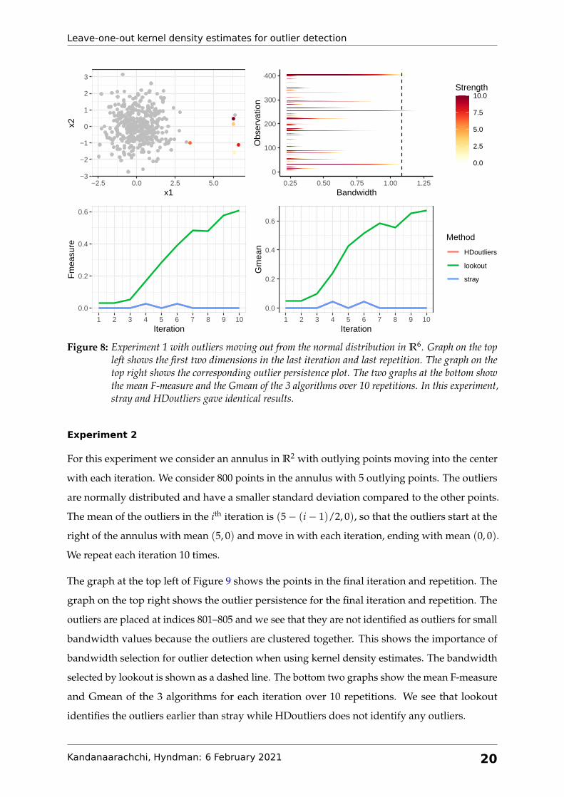
The top left graph of Figure 8 shows the first two dimensions of this experimental dataset in its

last iteration and repetition with outliers identified by lookout shown in different colors. The top

right graph shows the corresponding outlier persistence plot for this data with the dashed line

denoting the lookout bandwidth. The graphs at the bottom show the performance of lookout,

HDoutliers and stray with α = 0.05. The mean F-measure of the 10 repetitions for each iteration

is shown in the graph at the bottom left and the mean Gmean is shown at the bottom right. We

see that for each iteration lookout surpasses HDoutliers and stray significantly.



−3

−2

−1

0

1

2

3

−2.5 0.0 2.5 5.0x1

x2

0

100

200

300

400

0.25 0.50 0.75 1.00 1.25Bandwidth

Obs

erva

tion

0.0

2.5

5.0

7.5

10.0Strength

0.0

0.2

0.4

0.6

1 2 3 4 5 6 7 8 9 10Iteration

Fm

easu

re

0.0

0.2

0.4

0.6

1 2 3 4 5 6 7 8 9 10Iteration

Gm

ean

Method

HDoutliers

lookout

stray

Figure 8: Experiment 1 with outliers moving out from the normal distribution in R6. Graph on the topleft shows the first two dimensions in the last iteration and last repetition. The graph on thetop right shows the corresponding outlier persistence plot. The two graphs at the bottom showthe mean F-measure and the Gmean of the 3 algorithms over 10 repetitions. In this experiment,stray and HDoutliers gave identical results.

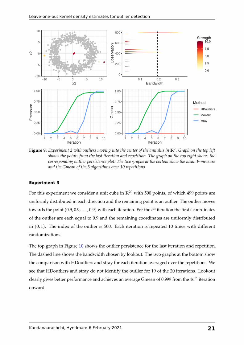
Experiment 2

For this experiment we consider an annulus in R2 with outlying points moving into the center

with each iteration. We consider 800 points in the annulus with 5 outlying points. The outliers

are normally distributed and have a smaller standard deviation compared to the other points.

The mean of the outliers in the ith iteration is (5− (i− 1)/2, 0), so that the outliers start at the

right of the annulus with mean (5, 0) and move in with each iteration, ending with mean (0, 0).

We repeat each iteration 10 times.

The graph at the top left of Figure 9 shows the points in the final iteration and repetition. The

graph on the top right shows the outlier persistence for the final iteration and repetition. The

outliers are placed at indices 801–805 and we see that they are not identified as outliers for small

bandwidth values because the outliers are clustered together. This shows the importance of

bandwidth selection for outlier detection when using kernel density estimates. The bandwidth

selected by lookout is shown as a dashed line. The bottom two graphs show the mean F-measure

and Gmean of the 3 algorithms for each iteration over 10 repetitions. We see that lookout

identifies the outliers earlier than stray while HDoutliers does not identify any outliers.



−10

−5

0

5

10

−10 −5 0 5 10x1

x2

0

200

400

600

800

0.1 0.2 0.3Bandwidth

Obs

erva

tion

0.0

2.5

5.0

7.5

10.0Strength

0.00

0.25

0.50

0.75

1.00

1 2 3 4 5 6 7 8 9 10Iteration

Fm

easu

re

0.00

0.25

0.50

0.75

1.00

1 2 3 4 5 6 7 8 9 10Iteration

Gm

ean

Method

HDoutliers

lookout

stray

Figure 9: Experiment 2 with outliers moving into the center of the annulus in R2. Graph on the top leftshows the points from the last iteration and repetition. The graph on the top right shows thecorresponding outlier persistence plot. The two graphs at the bottom show the mean F-measureand the Gmean of the 3 algorithms over 10 repetitions.

Experiment 3

For this experiment we consider a unit cube in R20 with 500 points, of which 499 points are

uniformly distributed in each direction and the remaining point is an outlier. The outlier moves

towards the point (0.9, 0.9, . . . , 0.9) with each iteration. For the ith iteration the first i coordinates

of the outlier are each equal to 0.9 and the remaining coordinates are uniformly distributed

in (0, 1). The index of the outlier is 500. Each iteration is repeated 10 times with different

randomizations.

The top graph in Figure 10 shows the outlier persistence for the last iteration and repetition.

The dashed line shows the bandwidth chosen by lookout. The two graphs at the bottom show

the comparison with HDoutliers and stray for each iteration averaged over the repetitions. We

see that HDoutliers and stray do not identify the outlier for 19 of the 20 iterations. Lookout

clearly gives better performance and achieves an average Gmean of 0.999 from the 16th iteration

onward.



0

100

200

300

400

500

1.5 2.0 2.5 3.0 3.5Bandwidth

Obs

erva

tion

0.0

2.5

5.0

7.5

10.0Strength

0.0

0.2

0.4

0.6

2 4 6 8 10 12 14 16 18 20Iteration

Fm

easu

re

0.00

0.25

0.50

0.75

1.00

2 4 6 8 10 12 14 16 18 20Iteration

Gm

ean

Method

HDoutliers

lookout

stray

Figure 10: Experiment 3 with an outlier moving to (0.9, 0.9, . . . ). Graph on the top shows the outlierpersistence plot for the last iteration and repetition. The two graphs at the bottom show themean F-measure and the Gmean of the 3 algorithms over 10 repetitions. In this experiment,stray and HDoutliers gave identical results.

5 Results on a data repository

For this section we use the data repository used in Kandanaarachchi et al. (2019b). This repository

has more than 12000 outlier detection datasets that were prepared from classification datasets.

Dataset preparation involves downsampling the minority class in classification datasets, con-

verting the categorical variables to numerical and accounting for missing values, all of which is

detailed in Kandanaarachchi et al. (2020).

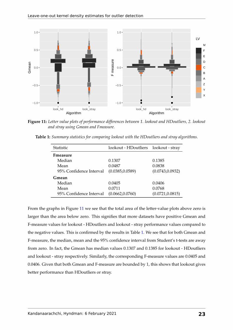
Figure 11 shows the letter-value plots (Hofmann, Wickham & Kafadar 2017) of performance

differences between (a) lookout and HDoutliers and (b) lookout and stray, using Gmean and

Fmeasure after removing the entries that have zero values for all three algorithms. Letter-

value plots enhance traditional box-plots by including more detailed information making them

suitable for large datasets. The letter-value plots in Figure 11 are area adjusted, that is, the area

of each box represents the number of points/datasets in it. The median is represented by a white

line and each black box represents a fourth of the population denoted by F in the legend. The

next box represents a eighth denoted by an E and each successive box represents half of the

previous one.



−1.0

−0.5

0.0

0.5

1.0

look_hd look_strayAlgorithm

Gm

ean

−1.0

−0.5

0.0

0.5

1.0

look_hd look_strayAlgorithm

F m

easu

re

LV

M

F

E

D

C

B

A

Z

Y

X

Figure 11: Letter value plots of performance differences between 1. lookout and HDoutliers, 2. lookoutand stray using Gmean and Fmeasure.

Table 1: Summary statistics for comparing lookout with the HDoutliers and stray algorithms.

Statistic lookout - HDoutliers lookout - stray

FmeasureMedian 0.1307 0.1385Mean 0.0487 0.083895% Confidence Interval (0.0385,0.0589) (0.0743,0.0932)

GmeanMedian 0.0405 0.0406Mean 0.0711 0.076895% Confidence Interval (0.0662,0.0760) (0.0721,0.0815)

From the graphs in Figure 11 we see that the total area of the letter-value plots above zero is

larger than the area below zero. This signifies that more datasets have positive Gmean and

F-measure values for lookout - HDoutliers and lookout - stray performance values compared to

the negative values. This is confirmed by the results in Table 1. We see that for both Gmean and

F-measure, the median, mean and the 95% confidence interval from Student’s t-tests are away

from zero. In fact, the Gmean has median values 0.1307 and 0.1385 for lookout - HDoutliers

and lookout - stray respectively. Similarly, the corresponding F-measure values are 0.0405 and

0.0406. Given that both Gmean and F-measure are bounded by 1, this shows that lookout gives

better performance than HDoutliers or stray.



6 Conclusions

Lookout uses leave-one-out kernel density estimates and EVT to detect outliers. Outlier detec-

tion methods that use kernel density estimates generally employ a user-defined parameter to

construct the bandwidth. Selecting a bandwidth for outlier detection is different from selecting

a bandwidth for general data representation, because the goal is to make outliers have lower

density estimates compared to the non-outliers. In addition, it is a challenge to select an appro-

priate bandwidth in high dimensions. To make outliers have lower density estimates compared

to the rest, a reasonably large bandwidth needs to be chosen. We introduced an algorithm called

lookout that uses persistent homology to select the bandwidth.

We compared the performance of lookout with HDoutliers and stray, two algorithms that also

use EVT to detect outliers. Our results on experimental data and on a large data repository

showed that lookout achieves better performance.

We also introduced the concept of outlier persistence, exploring the birth and death of outliers

with changing bandwidth and significance values. Outlier persistence gives a bigger picture,

taking a step back from fixed parameter values. It explores the bandwidth and significance

parameters and highlights the outliers that persist over a range of bandwidth values and their

significance levels. We suggest that it is a useful measure that increases our understanding of

outliers.

7 Supplementary materials

The R package lookout is available at https://github.com/sevvandi/lookout. The outlier

detection data repository used in Section 5 is available at Kandanaarachchi et al. (2019b). The

programming scripts used in Sections 4 and 5 are available at https://github.com/sevvandi/

supplementary_material/tree/master/lookout.

References

Bommier, E (2014). “Peaks-over-threshold modelling of environmental data”. MA thesis. De-

partment of Mathematics, Uppsala University.

Brunson, JC, R Wadhwa & J Scott (2020). ggtda: ’ggplot2’ Extension to Visualize Topological Persis-

tence. R package version 0.1.0. https://github.com/rrrlw/ggtda.

Burridge, P & AM Taylor (2006). Additive outlier detection via extreme-value theory. Journal of

Time Series Analysis 27(5), 685–701.


https://github.com/sevvandi/lookout



https://github.com/rrrlw/ggtda


Carlsson, G (2009). Topology and data. Bulletin of the American Mathematical Society 46(2), 255–308.

Carlsson, G, T Ishkhanov, V De Silva & A Zomorodian (2008). On the local behavior of spaces of

natural images. International journal of computer vision 76(1), 1–12.

Chaudhuri, P & JS Marron (1999). SiZer for Exploration of Structures in Curves. Journal of the

American Statistical Association 94(447), 807.

Clifton, DA, L Clifton, S Hugueny & L Tarassenko (2014). Extending the generalised pareto

distribution for novelty detection in high-dimensional spaces. Journal of Signal Processing

Systems 74(3), 323–339.

Coles, S (2001). An introduction to statistical modeling of extreme values. Vol. 208. Springer Series in

Statistics. London UK: Springer.

Ghrist, R (2008). Barcodes: the persistent topology of data. Bulletin of the American Mathematical

Society 45(1), 61–75.

Hofmann, H, H Wickham & K Kafadar (2017). Letter-Value Plots: Boxplots for Large Data.

Journal of Computational and Graphical Statistics 26(3), 469–477.

Kandanaarachchi, S & RJ Hyndman (2021). lookout: Leave One Out Kernel Density Estimates for

Outlier Detection. R package version 0.0.0.9000. https://github.com/sevvandi/lookout.

Kandanaarachchi, S, MA Muñoz, RJ Hyndman & K Smith-Miles (2019a). On normalization and

algorithm selection for unsupervised outlier detection. Data Mining and Knowledge Discovery,

1–46.

Kandanaarachchi, S, MA Muñoz, RJ Hyndman & K Smith-Miles (2020). On normalization and

algorithm selection for unsupervised outlier detection. Data Mining and Knowledge Discovery

34(2), 309–354.

Kandanaarachchi, S, MA Munoz Acosta, K Smith-Miles & RJ Hyndman (2019b). Datasets for

outlier detection. https://doi.org/10.26180/5c6253c0b3323.

Minnotte, MC & DW Scott (1993). The Mode Tree: A Tool for Visualization of Nonparametric

Density Features. Journal of Computational and Graphical Statistics 2(1), 51.

Perea, JA & J Harer (2015). Sliding windows and persistence: An application of topological

methods to signal analysis. Foundations of Computational Mathematics 15(3), 799–838.

Pickands, J (1975). Statistical Inference Using Extreme Order Statistics. The Annals of Statistics

3(1), 119–131.

Qin, X, L Cao, EA Rundensteiner & S Madden (2019). Scalable kernel density estimation-based

local outlier detection over large data streams. Advances in Database Technology - EDBT

2019-March, 421–432.


https://github.com/sevvandi/lookout

https://doi.org/10.26180/5c6253c0b3323


R.D. Reiss & M.Thomas (2001). Statistical Analysis of Extreme Values with Applications to Insurance,

Finance, Hydrology and Other Fields. 3rd ed. Birkhäuser, p. 516.

Schubert, E, A Zimek & HP Kriegel (2014). Generalized outlier detection with flexible kernel

density estimates. SIAM International Conference on Data Mining 2014, SDM 2014 2, 542–550.

Scott, DW (1994). Multivariate Density Estimation: Theory, Practice, and Visualization. Vol. 89. 425,

p. 359.

Stephenson, AG (2002). evd: Extreme Value Distributions. R News 2(2), 31–32. https://CRAN.R-

project.org/doc/Rnews/.

Talagala, PD, RJ Hyndman & K Smith-Miles (2021). Anomaly Detection in High-Dimensional

Data. Journal of Computational and Graphical Statistics. in press.

Talagala, PD, RJ Hyndman, K Smith-Miles, S Kandanaarachchi & MA Muñoz (2020). Anomaly

Detection in Streaming Nonstationary Temporal Data. Journal of Computational and Graphical

Statistics 29(1), 13–27.

Tang, B & H He (2017). A local density-based approach for outlier detection. Neurocomputing

241, 171–180.

Topaz, CM, L Ziegelmeier & T Halverson (2015). Topological data analysis of biological aggrega-

tion models. PloS ONE 10(5), e0126383.

Wadhwa, RR, DFK Williamson, A Dhawan & JG Scott (2018). TDAstats: R pipeline for computing

persistent homology in topological data analysis. Journal of Open Source Software 3(28), 860.

https://doi.org/10.21105/joss.00860.

Wang, Z & DW Scott (2019). Nonparametric density estimation for high-dimensional

data—Algorithms and applications. Wiley Interdisciplinary Reviews: Computational Statistics

11(4). arXiv: 1904.00176.

Wasserman, L (2018). Topological data analysis. Annual Review of Statistics and Its Application 5,

501–532.

Wilkinson, L (2017). Visualizing big data outliers through distributed aggregation. IEEE transac-

tions on visualization and computer graphics 24(1), 256–266.


https://CRAN.R-project.org/doc/Rnews/

https://CRAN.R-project.org/doc/Rnews/

https://doi.org/10.21105/joss.00860

https://arxiv.org/abs/1904.00176

Leave-one-out kernel density estimates for outlier detection

Documents

Transcript of Leave-one-out kernel density estimates for outlier detection