Learning To Be Overcondent

Learning To Be Overconfident∗

Simon Gervais

University of Pennsylvania

and

Terrance Odean

University of California at Davis

First Version: 10 May 1996

This Version: 7 June 1999

∗The authors would like to thank Roger Edelen, Hayne Leland, Andrew Lo, Ananth Madhavan, DavidRomer, Matthew Spiegel, Brett Trueman, Greg Willard, and two anonymous referees, as well as seminarparticipants at l’Ecole des Hautes Etudes Commerciales (Montreal), Rutgers University, the University ofTexas at Austin, the 1998 meetings of the American Finance Association, and the UCLA conference onthe “Market Efficiency Debate” for their comments and suggestions. All remaining errors are the authors’responsibility. Address correspondence to Simon Gervais, Finance Department, Wharton School, Universityof Pennsylvania, Steinberg Hall - Dietrich Hall, Suite 2300, Philadelphia, PA 19104-6367, (215) 898-2370.

Abstract

We develop a multi-period market model describing both the process by which traders learn

about their ability, and how a bias in this learning can create overconfident traders. A trader in

our model initially does not know his own ability. He infers this ability from his successes and

failures. In assessing his ability the trader takes too much credit for his successes, and this leads

him to become overconfident. A trader’s expected level of overconfidence increases in the early

stages of his career. Then, with more experience, he comes to better recognize his own ability. The

patterns in trading volume, expected profits, price volatility, and expected prices resulting from

this endogenous overconfidence are analyzed.

Your herds and flocks may increase, and you may amass much silver and gold — ev-

erything you own may increase. But your heart may then grow haughty, and you may...

say to yourself, ‘It was my own strength and personal power that brought me all this

prosperity.’

Deuteronomy 8:13-14,17

The Living Torah

translation by Rabbi Aryeh Kaplan

An old Wall Street adage advises “Don’t confuse brains with a bull market.” The need for such

wisdom stems from traders’ willingness to attribute too much of their success to their own abilities

and not enough to their good fortune. Successful traders are, thus, prone to become overconfident

in their abilities.

It is a common feature of human existence that we constantly learn about our own abilities

by observing the consequences of our actions. For most people there is an attribution bias to this

learning: we tend to overestimate the degree to which we are responsible for our own successes

(Wolosin, Sherman and Till, 1973; Miller and Ross, 1975; Langer and Roth, 1975). As Hastorf,

Schneider and Polifka (1970) write, “we are prone to attribute success to our own dispositions and

failure to external forces.” People recall their successes more easily than their failures and “even

misremember their own predictions so as to exaggerate in hindsight what they knew in foresight”

(Fischhof, 1982).

In this paper, we develop a multi-period market model describing both the process by which

traders learn about their ability and how a bias in this learning can create overconfident traders.

Traders in our model initially do not know their ability. They learn about their ability through

experience. Traders who successfully forecast next period dividends improperly update their beliefs;

they weight too heavily the possibility that their success was due to superior ability. In so doing

they become overconfident.

In our model, a trader’s level of overconfidence changes dynamically with his successes and

failures. A trader is not overconfident when he begins to trade. Ex ante, his expected overconfidence

increases over his first several trading periods and then declines.1 Thus the greatest expected

overconfidence in a trader’s lifespan comes early in his career. After this he tends to develop a

progressively more realistic assessment of his abilities as he ages.

1More precisely, this will happen for insiders with learning biases that are not too large, where “not too large” isprecisely defined in section 3.

1

One criticism of models of non-rational behavior is that non-rational traders will underperform

rational traders and eventually be driven to the margins of markets if not out of them altogether.2

This is, however, not always the case. De Long, Schleifer, Summers and Waldmann (1990) present a

model where non-rational traders in an overlapping generations model earn higher expected profits

than rational traders by bearing a disproportionate amount of the risk that they themselves create.

Rational traders are unwilling to take long-term arbitrage positions to eliminate these higher profits

because of the risk that they may die before the arbitrage pays off.

In our model, the most overconfident and non-rational traders are not the poorest traders. In

fact, for any given level of learning bias and trading experience, it is successful traders, though not

necessarily the most successful traders, who are the most overconfident. Overconfidence does not

make traders wealthy, but the process of becoming wealthy can make traders overconfident.

The model also shows that success affects traders’ conditional future expected profits in two

ways. First, success is indicative of higher ability and, therefore, greater expected future prof-

its. Second, success can increase overconfidence and thereby lower expected future profits through

suboptimal decision-making. The detrimental effect of the more successful traders’ greater overcon-

fidence on their future expected profits may, on occasion, more than offset their greater probable

ability.

Most models of financial market microstructure assume that all trader characteristics are com-

mon knowledge; in particular, traders’ risk aversion, their wealth, and the distribution of their infor-

mation are known by all market participants. Exceptions include Blume, Easley and O’Hara (1994),

Gervais (1996), and Subramanyam (1996). In these papers, the precision of the traders’ information

is random. Each traders’ precision is known to himself but is uncertain to other market participants

who must infer it from his actions. Our model builds on these works by extending this uncertainty

to the trader himself. He initially does not know the precision of his own information, and must

infer it by observing his signals and subsequent outcomes.

A large literature demonstrates that people are usually overconfident and that, in particular,

they are overconfident about the precision of their knowledge.3 Benos (1998), Odean (1998), Kyle

and Wang (1997), and Wang (1997) examine models with statically overconfident traders. In these

models greater overconfidence leads to greater expected trading volume and greater price volatility.4

2Early proponents of this view include Alchian (1950), and Friedman (1953). More recently, Blume andEasley (1982, 1992) have reinforced these ideas analytically.

3See for example Alpert and Raiffa (1982), and Lichtenstien, Fischhoff and Phillips (1982). Odean (1998) providesan overview of this literature.

4In one exception, Odean (1998) shows that an overconfident, risk-averse market-maker may reduce marketvolatility.

2

In our model, a greater learning bias causes greater expected overconfidence, which leads to greater

expected trading volume and greater price volatility.

Daniel, Hirshleifer and Subrahmanyam (1998) look at trader overconfidence in a dynamic model.

Our paper differs from theirs in that we concentrate on the dynamics by which self-serving attribu-

tion bias engenders overconfidence in traders, and not on the joint distribution of trader ability and

the risky security’s final payoff.5 Our approach has the advantage of being analytically tractable.

Our analysis differs from that of Daniel, Hirshleifer and Subrahmanyam in that we are interested

in the dynamic effects of biased learning on overconfidence, trading volume, price volatility and

trading profits, whereas their main objective is to show that overconfidence implies different price

correlation patterns in the short run and the long run. Nevertheless, we show that expected prices

exhibit the same humped-shape patterns through time in both models.

Overconfidence is determined, in our model, endogenously and changes dynamically over a

trader’s life. This enables us to make predictions about when a trader is most likely to be over-

confident (when he is inexperienced and successful) and how overconfidence will change during a

trader’s life (it will, on average, rise early in a trader’s career and then gradually fall). The model

also has implications for changing market conditions. For example, most equity market partici-

pants have long positions and benefit from upward price movements. We would therefore expect

aggregate overconfidence to be higher after market gains and lower after market losses. Since, as we

show, greater overconfidence leads to greater trading volume, this suggests that trading volume will

be greater after market gains and lower after market losses. Indeed, Statman and Thorley (1998)

find that this is the case. We would expect aggregate overconfidence to be particularly high in

a market with many young traders who have experienced only a long bull run. Thus, our model

predicts that trading volume and volatility should be higher in the late stages of a bull market than

in the late stages of a bear market.

Rabin and Schrag (1999) develop a model of confirmatory bias, the tendency to interpret new

information as confirming one’s previous beliefs. In as much as people tend to have positive self-

images, confirming bias and self-serving attribution bias are related. Our paper differs considerably

from Rabin and Schrag’s, in that we analyze the effect of attribution bias on the overconfidence of

traders in financial markets.

The rest of this paper is organized as follows. In section 1, we introduce a one-security multi-

period economy with one insider, one liquidity trader and one market maker. In section 2, we

develop the conditions under which there is a unique linear equilibrium in our economy. This

linear equilibrium is used in section 3 to analyze the effects of the insider’s learning bias on his

5This is because the risky security’s dividend is publicly revealed at the end of every trading round in our model.

3

overconfidence and profits, as well as on the market’s trading volume, volatility, and price patterns.

Section 4 discusses the empirical implications of the model and, finally, section 5 concludes. All

the proofs are contained in the appendices.

1 The Economy

We study a multi-period economy in which only one risky asset is traded among three market

participants: an informed trader, a liquidity trader, and a market maker. At the end of period t,

the risky asset pays off a dividend vt, unknown to all the market participants at the beginning of

the period.6

At the beginning of each period t, the risk-neutral informed trader (also called insider) observes

a signal θt which is correlated with vt. In particular, the signal θt is given by

θt = δtvt + (1− δt)εt, (1)

where εt has the same distribution as vt, but is independent from it. The variable δt takes the

values 0 or 1. Since εt is independent from vt, the insider’s information will only be useful when δtis equal to one. We assume that this will happen with probability a, i.e.

δt | a =

1, prob. a

0, prob. 1− a.(2)

This last equation shows that, the higher a is, the more likely that δt will be equal to one. For

this reason, we call a the insider’s ability.7 We assume that nobody (including the insider himself)

knows precisely the insider’s ability a at the outset (i.e. at time zero). Instead, we assume that, a

priori, the insider’s ability is drawn from the following distribution:

a =

H, prob. φ0

L, prob. 1− φ0,(3)

6Throughout the whole paper, we use a “hat” over a variable to denote the fact that it is a random variable.7Equivalently, we could call a the insider’s information precision.

4

where 0 < L < H < 1, and 0 < φ0 < 1. Of course, since the security dividend vt is announced at

the end of every period t, the insider will know at the end of every period whether his information

for that period was real (δt = 1) or was just pure noise (δt = 0).8 For tractability reasons, we also

assume that the market maker observes θt at the end of period t, so that his information at the end

of every period is the same as the insider’s.9 This information will be useful to both the insider

and the market maker in assessing the insider’s ability a.

In making this last assumption, we are essentially saying that the insider’s informational ad-

vantage over the market maker is one of market timing. Indeed, the insider’s information set at

the beginning of every period is always exactly one period ahead of the market maker’s. Since our

goal is not to explain the differences between these two information sets, we reduce the information

gap between the insider and the market maker to only (and exactly) one period. Our analysis is

then simplified in that both the insider and the market maker perform the same one-period up-

dating at the end of every period, except that the insider’s updating will be biased. Preventing

the market maker from observing θt at the end of period t would simply result in a more complex

(non Markov) updating process for the market maker, but would not affect the insider’s updating

process, in which we are ultimately interested. It would, however, increase the insider’s expected

profits since the market maker’s informational disadvantage would then be greater.

As mentioned above, our model seeks to describe the behavior of an informed trader with a

learning bias. In particular we want to model the phenomenon that traders usually think “too much

of their ability” when they have been successful at predicting the market in the past. In statistical

terms, this will mean that traders update their ability beliefs too much when they are right. Before

we formally include this behavior into our model, let us describe how a rational/unbiased insider

would react to the information he gathers from past trading rounds.

Let st denote the number of times that the insider’s information was real in the first t periods,

that is

st =t∑

u=1

δu. (4)

It can be shown, using Bayes’ rule, that, at the end of t periods, a rational insider’s updated beliefs

8This will be the case since εt = vt happens with zero probability with the continuous distributions that we willspecify later.

9As will become clear below, we could have equivalently assumed that every trader’s order and identity (insidervs liquidity trader) are revealed at the end of every period.

5

about his own ability will be given by

φt(s) ≡ Pra = H | st = s =Hs(1−H)t−sφ0

Hs(1−H)t−sφ0 + Ls(1− L)t−s(1− φ0). (5)

We denote this rational insider’s updated expected ability by

µt(s) ≡ E[a | st = s] = Hφt(s) + L[1− φt(s)]. (6)

In fact, since we do not assume any kind of irrational behavior on the part of the market maker,

and since the market maker’s information set is the same as the insider’s at the end of every period,

this will be the market maker’s updated belief at the end of period t.

In modeling the self-serving attribution bias (which we simply refer to as the learning bias from

now on), we assume that a trader who successfully forecasts a dividend, weights this success too

heavily when applying Bayes’ rule to assess his own ability. In choosing our updating rule we seek

to accurately model the behavior psychologists have observed, to create a simple, tractable model,

and to choose an updating rule that departs gradually from rational updating, and can therefore

be used to describe traders with different degrees of bias, including unbiased traders. Psychologists

find that when people succeed, they are prone to believe that success was due to their personal

abilities rather than to chance or outside factors; when they fail, they tend to attribute their failure

to chance and outside factors rather than to their lack of ability. They also find that “self-enhancing

attributions for success are more common than self-protective attributions for failure” (Fiske and

Taylor, 1991; also see Miller and Ross, 1975). This observed behavior can be modeled by assuming

that, when a trader applies Bayes’ rule to update his belief about his ability, he overweights his

successes, he underweights his failures, and he overweights successes more than he underweights

failures. The model is simpler and the qualitative results unchanged if one simply assumes, as we

do, that successes are weighted too heavily and failures are weighted correctly.

More precisely, we assume that when evaluating his own ability the insider overweights his

successes at predicting the security’s dividend (i.e. every time that δt = 1) by a learning bias factor

γ ≥ 1 (γ = 1 representing a rational insider). For example, at the end of the first period, if the

insider finds that θ1 = v1 (i.e. δ1 = 1), the insider will adjust his beliefs to

φ1(1) ≡ Prba = H | s1 = 1 =γHφ0

γHφ0 + L(1− φ0), (7)

6

where the subscript to “Pr” denotes the fact that the probability is calculated by a biased insider.

This updated probability is larger than that of a rational insider, i.e. φ1(1) ≥ φ1(1). Also, as can

be seen from (7), φ1(1) will be higher the larger γ is, and φ1(1) → 1 as γ → ∞; in other words,

the learning bias dictates by how much the insider adjusts his beliefs towards being a high ability

insider. Moreover, our model departs continuously from rationality in the sense that φ1(1)→ φ1(1)

as γ → 1. It is easily shown that, in this case,

φt(s) ≡ Prba = H | st = s =(γH)s(1−H)t−sφ0

(γH)s(1−H)t−sφ0 + Ls(1− L)t−s(1− φ0), (8)

and the (biased) insider’s updated expected ability is given by

µt(s) ≡ Eb[a | st = s] = Hφt(s) + L[1− φt(s)]. (9)

At the beginning of every period t, the risk-neutral insider observes his signal θt; he then chooses his

demand for the risky security in order to maximize his expected period t profits,10 πt, conditional

on both his signal and his ability beliefs µt−1(st−1) (which only depend on st−1). We denote this

demand by

xt = Xt(θt, st−1). (10)

The other trader in the economy is a trader who trades for liquidity purposes in every period.

This liquidity trader ’s demand in period t is given exogenously by the random variable zt. Both

orders, xt and zt, are sent to a market maker who fills the orders. As in Kyle (1985), we assume

that the market maker is risk-neutral and competitive, and will therefore set prices so as to make

zero expected profits. So, if we denote the total order flow coming to the market maker in period t

by

ωt = xt + zt, (11)

10As we mention above, both the risky dividend and the insider’s signal are announced at the end of every period,so that the market maker is always exactly one period behind the insider in terms of information at the beginningof the next period. This implies that the insider never finds it optimal to suboptimally choose his demand for oneperiod in order to maximize longer-term profits.

7

the market maker will set the security’s price equal to

pt = Pt(ωt, st−1) ≡ E[vt | ωt, st−1] (12)

in period t. An equilibrium to our model is defined as a sequence of pairs of functions (Xt, Pt),

t = 1, 2, . . . , such that the insider’s demand in period t, Xt(θt, st−1) maximizes his expected profits

(according to his own beliefs) for that period given that he faces a price curve Pt, while the market

maker is expecting zero profit in that period.

As it will become obvious later, the main results of this paper are driven by the insider’s

updating dynamics. As such, the liquidity trader and the market maker only play minimal roles

in this model. In fact, their role is essentially one of market clearing. Indeed, the presence of the

liquidity trader introduces noise that will prevent the “no trade equilibrium” described by Milgrom

and Stokey (1982) from occurring. The competitive market maker assumption is simply made

out of convenience; the presence of a risk-neutral rational trader would serve a similar purpose,

as in Daniel, Hirshleifer and Subrahmanyam (1998). Appendix D presents a brief synopsis of

alternative specifications that in turn avoid the presence of the liquidity trader and the market

maker, introduce the possibility for the market maker to maximize profits, and increase the number

of market participants. As argued in that appendix, these specifications do not affect the nature

of the insider’s (or insiders’) updating and, therefore, do not change the main results of the paper.

2 A Linear Equilibrium

In this section, we show that, when vt, εt, and zt are jointly and independently normal, there is

a linear equilibrium to our economy. We use that linear equilibrium in section 3 to illustrate the

properties of the model. More precisely, for this and the next section, we assume that

vt

εt

zt

∼ N

0

0

0

,

Σ 0 0

0 Σ 0

0 0 Ω

, t = 1, 2, . . . , (13)

and that each such vector is independent of all the others. Note that it is crucial that Var(vt) =

Var(εt), since we do not want the size of θt to reveal anything about the likelihood that δt = 1

until vt is announced. In other words, ability updating is only possible when both θt and vt become

8

observable.

Let us conjecture that, in equilibrium, the function Xt(θ, s) is linear in θ, and that the function

Pt(ω, s) is linear in ω:

Xt(θ, s) = βt(s) θ, (14a)

Pt(ω, s) = λt(s) ω. (14b)

Our objective is to find βt(s) and λt(s) which are consistent with this conjecture. We start with

the following result.

Lemma 2.1 Assume that a linear equilibrium exists in period t, that is assume that (14a) and (14b)

hold. Then, in period t, the insider’s demand for the risky security is given by

xt =µt−1(st−1)θt

2λt(st−1), (15)

and the market maker’s price schedule is given by

pt =µt−1(st−1)βt(st−1)Σβ2t (st−1)Σ + Ω

ωt. (16)

Proof : See Appendix A.

This lemma establishes that we can indeed write xt = βt(st−1)θt with

βt(s) =µt−1(s)2λt(s)

, (17)

and pt = λt(st−1)ωt with

λt(s) =µt−1(s)βt(s)Σβ2t (s)Σ + Ω

. (18)

However, the result relies on the assumption that a linear equilibrium exists. It turns out that this

assumption is not always satisfied given the insider’s learning bias. In fact, the following lemma

derives the exact condition under which such an equilibrium will exist in a given period t.

9

Lemma 2.2 In any given period t, there exists a linear equilibrium of the form conjectured in (14a)

and (14b) if and only if µt−1(st−1) ≤ 2µt−1(st−1).


This condition essentially states that the biased insider’s beliefs about his ability cannot exceed

those of the rational market maker by too much for an equilibrium to exist. It effectively ensures

that the insider will on average be making profits, even though he may not be optimizing correctly

due to his biased beliefs.11 Were this condition not satisfied, the market maker would know that

the insider will take a position that will on average result in negative profits. Our condition that

the competitive market maker quotes a price schedule earning him on average zero profits can then

never be satisfied. This results in a market breakdown. The following lemma derives a condition

that is both necessary and sufficient to always avoid such outcomes.

Lemma 2.3 A necessary and sufficient condition for µt−1(st−1) > 2µt−1(st−1) to be avoided for

any history up to any period t and any γ > 1 is that H ≤ 2L.


Note that, for a given fixed value of γ, H ≤ 2L is too strong a condition to avoid market

breakdowns for any history, i.e. the condition is then sufficient but not necessary. However, since

market breakdowns are outside the scope of this paper, we assume that H ≤ 2L is always satisfied

in the rest of our analysis.12 Such an assumption allows us to vary γ throughout the paper without

having to worry about the existence of an equilibrium, but does not affect the qualitative aspects

of our results.13 We finish this section with the following characterization of the equilibrium.

Lemma 2.4 Assuming that H ≤ 2L, there is always a unique linear equilibrium to the economy

described in section 1. In this equilibrium, the insider’s demand and the market maker’s price

11Note that this condition does not violate the absence of arbitrage results established by Bossaerts (1999) forsecurity prices, and by De Finetti (1937) for subjective probabilities. Indeed, although the insider’s learning biascould introduce profit opportunities for other informed traders (were they present in the economy), they do not leadto riskless arbitrage opportunities. In fact, the beliefs of the market maker in our model correspond to the marketbeliefs in Bossaerts’ work. Note also that, if the insider is risk-averse, this existence condition is not needed; however,the model then loses tractability.

12For a formal analysis of market breakdowns, consult Bhattacharya and Spiegel (1991).13In fact, although this assumption guarantees the survival of the insider by making his expected profits positive,

it does not guarantee the survival of overconfidence for an individual, as we show in section 3.2.

10

schedule are given by (14a) and (14b) with

βt(s) =

√ΩΣ

µt−1(s)2µt−1(s)− µt−1(s)

, and (19a)

λt(s) =12

√ΣΩµt−1(s) [2µt−1(s)− µt−1(s)]. (19b)


In what follows, we use this equilibrium to study the effects of the insider’s learning bias on the

economy.

3 Properties of the Model

In this section, we analyze the effects of the insider’s learning bias on the properties and dynamics of

the economy in equilibrium. We introduce a measure of overconfidence analogous to that found in

static models and show that the learning bias results in dynamically evolving insider overconfidence.

We then look at the effect of this changing overconfidence on trading volume, trader profits, price

volatility, as well as the expected price patterns.

3.1 Convergence

If this financial market game is played to infinity, we would expect both the insider and the market

maker to eventually learn the exact ability a of the insider. This in fact would be true for a rational

insider (γ = 1). However, since our insider learns his ability with a personal bias, this result is not

immediate; in fact, as we shall see, this result is not true for a highly biased insider.

When a = H, we expect the insider to correctly guess the one-period dividend a fraction H of

the time. So, as we play the game more and more often (as t tends to ∞), we expect his updated

posteriors

φt(s) =(γH)s(1−H)t−sφ0

(γH)s(1−H)t−sφ0 + Ls(1− L)t−s(1− φ0)=

1

1 +(LγH

)s (1−L1−H

)t−s 1−φ0φ0

11

to behave like

1

1 +(LγH

)Ht (1−L1−H

)t−Ht 1−φ0φ0

=1

1 +[(

LγH

)H (1−L1−H

)1−H]t 1−φ0φ0

.

This last quantity will converge to 1 as desired if

[(L

γH

)H ( 1− L1−H

)1−H]t→ 0 as t→∞,

or equivalently if

(L

γH

)H ( 1− L1−H

)1−H< 1.

The following lemma shows that this is indeed the case.

Lemma 3.1 When a = H, the updated posteriors of the insider φt(st) will converge to 1 almost

surely as t→∞.

Proof : See Appendix B.

So both the insider and the market maker will eventually learn the insider’s ability precisely

when it is high (when a = H). Let us now turn to the case where a = L. In this case, we expect

the insider to correctly guess the one-period dividend a fraction L of the time. So, as we play the

game more and more often (as t tends to∞), we expect his updated posteriors φt(s) to behave like

1

1 +(LγH

)Lt (1−L1−H

)t−Lt 1−φ0φ0

=1

1 +[(

LγH

)L (1−L1−H

)1−L]t 1−φ0φ0

.

As the following lemma shows, this quantity only converges to zero when γ is close enough to 1.

This means that the market maker will always learn the insider’s ability when it is low (when

a = L),14 but the insider will only do so if his learning bias is not too large.

14This is due to the fact that we assume that the market maker’s learning is unbiased.

12

Lemma 3.2 When a = L, the updated posteriors of the insider φt(st) will converge as follows:

φt(st)a.s.−−→

0, if γ < γ∗

φ0, if γ = γ∗

1, if γ > γ∗,

where γ∗ = LH

(1−L1−H

)(1−L)/L.


One implication of this lemma is that a low ability insider whose learning bias is sufficiently

extreme may never acknowledge his low ability, no matter how much experience he has.15 To

illustrate this, we show in Figures 1(a) and 1(b) how we expect an insider to adjust his beliefs

about his own ability (φt) when his actual ability is high, and when it is low respectively. As seen

in these figures, the biased insider’s beliefs are always on average larger than those of an unbiased

but otherwise identical insider. Since unbiased insiders always eventually learn their ability, it is

therefore not surprising to find that high ability insiders also always learn their own ability:16 they

naturally tend to update towards that high ability. However, as shown in Figure 1(b), a biased

insider may not always give in to his observations: more precisely, if γ > γ∗, he will never find out

if he is a low ability insider.

3.2 Patterns of Overconfidence

As we show in section 3.1, the insider will eventually learn his own ability, provided that his learning

is not too biased (i.e. provided that γ is not too large). This means that, when the insider’s ability

is low, the insider eventually comes to his senses, and recognizes the fact that he is a low ability

insider. However, it is always the case that the insider thinks too highly of himself relative to an

otherwise identical unbiased insider. This section introduces a measure for this discrepancy; we

call it the insider’s overconfidence. The evolution of the insider’s overconfidence throughout his life

is central to our study, as this overconfidence essentially measures by how much our model departs

from a purely rational setup in any given period.

15Bossaerts (1999) shows that prior beliefs that are correctly updated using Bayes’ law converge to the rightposterior beliefs, whether the priors are biased or not. In contrast, our result shows that correct priors updatedincorrectly may not lead to the correct posteriors.

16In fact, they will do so faster the more biased they are.

13

5 10 15 20 25Period t

0.6

0.7

0.8

0.9

1.0

5.0

25 9

1.5

1.0

E[t(s t

)|a=H

]-

ˆˆ

(a) Convergence when a = H.

5 10 15 20 25

0.1

0.2

0.3

0.4

0.5

0.6

0.7

5.0

25 9

1.5

1.0

Period t

E[t(s t

)|a=L

]-

ˆˆ

(b) Convergence when a = L.

Figure 1: Convergence patterns of the insider’s expected beliefs about his own ability when (a) a =H; (b) a = L. Both figures were obtained with H = 0.9, L = 0.5, φ0 = 0.5, and Σ = Ω = 1. Eachline was drawn with a different γ, shown in the legends. Note that, with these parameter values,γ∗ = 25/9 ≈ 2.78.

In our model, an insider is considered very overconfident at the end of a particular period t if his

updated expected ability at that time (µt(st)) is large compared to the updated expected ability

that a rational insider would have reached with the same past history of successes and failures

(µt(st)). To measure the insider’s overconfidence at the end of t periods, we therefore define the

random variable

κt ≡ Kt(st) ≡ µt(st)µt(st)

. (20)

14

Of course, when the insider is rational (γ = 1), the numerator is exactly equal to the denominator

of this expression, and κt = 1 for all t = 1, 2, . . . . On the other hand, when the insider’s learning

is biased (γ > 1), we have µt(st) ≥ µt(st), and κt ≥ 1 for all t. As the next proposition shows,

the insider’s overconfidence in period t is greater when the insider’s learning bias is large. In other

words, the insider’s overconfidence is directly attributable to his learning bias.

Proposition 3.1 The function Kt(s) defined in (20) is increasing in γ.


Our measure of overconfidence at any point in time is therefore increasing in the insider’s

learning bias, but is it also increasing in the number of his past successful predictions? Since

the insider’s overconfidence results from his learning bias when he is successful, it is tempting to

conclude that the more successful an insider is, the more overconfident he will be. As we next show,

this intuition is wrong.

First, since the insider updates his beliefs incorrectly only after successful predictions, it is always

true that µt(0) = µt(0), and therefore Kt(0) = 1. However, as soon as the insider successfully

predicts one risky dividend, his learning bias makes him overconfident,17 and µt(1) > µt(1), so

that Kt(1) > 1. So, it is always true that the insider’s first successful prediction makes him

overconfident.18 However, it is not always the case that an additional successful prediction always

makes the insider more overconfident.

To see this, suppose that we are at the end of the second period. The insider will then have

been successful 0, 1 or 2 times. We already know that K2(1) > K2(0) = 1 for any value of the

insider’s learning bias parameter γ. Now, suppose that γ is large. This means that if the insider

is successful in the first period, he will immediately (and perhaps falsely) jump to the conclusion

that he is a high ability insider, i.e. µ1(1) is close to H. Since this one successful period has already

convinced the insider that his ability is high, the second period results will not have much of an

effect on his beliefs, whether he is successful or not in that period, i.e. µ2(2) is close to µ2(1).

On the other hand, if the insider had been rational (γ = 1), he would have adjusted his expected

ability beliefs more gradually. In particular, after a first period success, a rational insider does

17In our model, traders are not overconfident when they begin to trade. It is through making forecasts and tradingthat they become overconfident. This leads market participants to be, on average, overconfident. In real markets,selection bias may cause even beginning traders to be overconfident. Indeed, since not everyone trades, it is likelythat people who rate their own trading abilities most highly will seek jobs as traders or will trade actively on theirown account. Those with actual high ability and those with high overconfidence will rate their own ability highest.Thus, even at the entry level, we would expect to find overconfident traders.

18Also, as section 3.1 shows, he will remain so for the rest of his life.

15

not automatically conclude that his ability is high. Instead, he adjusts his posterior expected

ability beliefs towards H, and uses the second period result to further adjust these beliefs: upward

towards H if he is successful, and downward towards L otherwise. As a result, µ2(2) will be

somewhat larger than µ2(1). Therefore, since µ2(2) ≈ µ2(1) and µ2(2) > µ2(1), we have

K2(2) ≡ µ2(2)µ2(2)

<µ2(1)µ2(1)

≡ K2(1),

and we see that K2(s) decreases when s goes from 1 to 2.

In short, the biased insider adjusts his beliefs non-rationally with every successful prediction,

making him overconfident. However, when the insider’s past performance is sufficiently good (large

number of successful predictions), it is the case that even an unbiased insider would reach the

conclusion that he is a high ability insider. In other words, the significance of the insider’s past

performance overweights the significance of his learning bias. The following proposition describes

this phenomenon in more details.

Proposition 3.2 The function Kt(s) defined in (20) is increasing over s ∈ 0, . . . , s∗t and de-

creasing over s ∈ s∗t , . . . , t, for some s∗t ∈ 1, . . . , t.


Intuitively, this result says that a trader who has been very successful in only a few rounds of

trading or one who has been moderately successful in several rounds of trading will have a greatly

inflated opinion of his ability. But a trader who has been very successful over many rounds of

trading probably does have high ability. And while he may overestimate his expected ability, he

does not do so by as much as do moderately successful traders.

In this model, traders are rational in all respects except that they have a common learning

bias: they tend to attribute their successes disproportionately to their own ability. This leads

successful traders to become overconfident. Other learning biases can also lead to overconfidence.

For example, it is well known that, when updating beliefs from sequential information, people tend

to weight recent information too heavily and older information too little (Anderson, 1959, 1981;

Hogarth and Einhorn, 1992).19 We do not introduce this recency effect into our model because

19In experimental studies, subjects sometimes also exhibit a “primacy effect,” weighting the earliest observationsof a time series heavily (Anderson, 1981). This happens most often in situations where subjects lose interest in thedata (Hogarth and Einhorn, 1992). It is unlikely that traders would lose interest in their own successes and failures,and so we would not expect to find a large primacy effect in their updating.

16

doing so would negate the Markov property of the insider’s (and the market maker’s) updating

process. It is clear though that, if traders weight recent outcomes more heavily than older ones,

recently successful traders will tend to become overconfident.

The last two propositions describe how the insider’s overconfidence in a particular period de-

pends on his learning bias and on his previous performance. Let us now turn to how his overcon-

fidence is expected to behave over time. To do this, we calculate the ex ante expected period t

overconfidence level of the insider, E [κt]. Since

Prst = s = Pr st = s | a = HPr a = H+ Pr st = s | a = LPr a = L=

(t

s

)Hs(1−H)t−sφ0 +

(t

s

)Ls(1− L)t−s(1− φ0), (21)

we have

E [κt] =t∑

s=0

(t

s

)[Hs(1−H)t−sφ0 + Ls(1− L)t−s(1− φ0)

] µt(s)µt(s)

, (22)

where µt(s) and µt(s) are as in (6) and (9). Figure 2 shows the patterns in the expected level of

overconfidence for different values of γ. When γ is relatively small (γ < γ∗), the insider will on

average be overconfident at first but, over time, will converge to a rational behavior.

This can be explained as follows. Over a small number of trading periods a trader’s success

rate may greatly exceed that predicted by his ability. Very successful traders will overestimate the

likelihood that success is due to ability rather than luck. But over many trading periods a trader’s

success rate is likely to be close to that predicted by his ability. Only those traders with extreme

learning bias (or with very unlikely success patterns) will fail to recognize their true ability. Indeed,

as γ increases, the insider tends to put more and more weight on his past successes, and so takes a

little more time to rationally find his ability. However, if γ is too large (more precisely, if γ > γ∗),

it is possible that the insider puts so much weight on his past successes in the stock market that

he never becomes rational. It can be shown that E [κt] then converges to φ0 + (1− φ0)HL .

Thus our model predicts that more inexperienced traders will be more overconfident than ex-

perienced traders. Less experienced traders are more likely to have success records which are

unrepresentative of their abilities. For some, this will lead to overconfidence. By the law of large

numbers, older traders are likely to have success records which are more representative of their

abilities; they will, on average, have more realistic self assessments. In a sufficiently large group

17

0 20 40 60 80 100

1.00

1.05

1.10

1.15

1.20

1.25

1.30

5.00

25 9

2.25

1.75

1.25

Period t

E[t]ˆ

Figure 2: Ex ante expected patterns in the level of overconfidence of the insider over time. Thefigure was obtained with H = 0.9, L = 0.5, φ0 = 0.5, Σ = Ω = 1. Each line was obtained with adifferent value of γ shown in the legend. Note that, with these parameter values, γ∗ = 25/9 ≈ 2.78.

of traders,20 however, there will be some successful, older, low-ability traders with whom the odds

have not yet caught up. These traders are likely to make large mistakes in the future.

As we see in Figure 2, on average, a trader’s overconfidence increases during the first part of his

trading experience and decreases during the latter part. It is natural to ask what factors determine

the point at which a trader’s overconfidence is likely to peak. All other things being equal, the

greater a trader’s learning bias, γ, the longer it is likely to take for his overconfidence level to peak.

Figure 3 illustrates this effect.

In addition to the degree of learning bias, how quickly a trader’s overconfidence peaks (and

how quickly he ultimately learns his true ability) depends on the frequency, speed, and clarity

of the feedback he receives. A trader who receives frequent, immediate, and clear feedback will,

on average, peak in overconfidence early, and quickly realize his true ability. One who receives

infrequent, delayed, and ambiguous feedback will peak in overconfidence later, and more slowly

realize his true ability. In general, financial markets are difficult environments for learning, as

feedback is often ambiguous and comes well after a decision was made. We would expect those who

trade most frequently, such as professional traders, and those who keep careful records rather than

relying on memory to learn most quickly. In our model a trader receives immediate feedback each

period. The greater the difference between the high (H) and the low (L) ability levels, the clearer

20Appendix D.3 presents an extension of the model with multiple insiders. The learning and overconfidencedynamics are essentially the same as in this single insider model.

18

1.25 1.50 1.75 2.00 2.25 2.50 2.75

5

10

15

20

25

30

35

40

Learning bias (g)

Per

iod

of m

axim

umex

pect

ed o

verc

onfid

ence

Figure 3: Period of maximum expected overconfidence as a function of the insider’s learning bias γ.The figure was obtained with H = 0.9, L = 0.5, and φ0 = 0.5.

0.15 0.2 0.25 0.3 0.35 0.4 0.45

20

40

60

80

100

Per

iod

of m

axim

umov

erco

nfid

ence

Dispersion of priors (H-L)

Figure 4: Period of maximum expected overconfidence as a function of the dispersion H − L ofthe insider’s prior ability beliefs. The figure was obtained with φ0 = 0.5, γ = 1.1, and keeping theinsider’s ex ante expected ability φ0H + (1− φ0)L constant at 0.7.

the feedback. Figure 4 illustrates how long it takes on average for the insider’s overconfidence to

peak as a function of H − L.

19

3.3 Effects of the Insider’s Learning Bias

Section 3.2 shows that the insider’s learning bias has a dynamic impact on his beliefs about his

ability and on the way he interprets future private information. This in turn affects the future

trading process. In this and the next section, we describe how this trading process, as measured

by trading volume, trader profits, and price volatility, is affected.

Since the insider’s learning bias is unaffected by his success rate and vice versa,21 our model

allows us to analyze the effects of the learning bias on the insider’s behavior and on the properties

of the economy in two different ways. First, given a fixed past history of the insider’s successes and

failures, we can vary the size of his learning bias to get an idea of the impact of that bias. This is

the focus of the current section. Second, we can fix the insider’s learning bias, and determine the

effects of different trading histories on the insider and the economy in general. We will turn to this

in section 3.4.

Before embarking on the effects of the insider’s learning bias, we calculate the three quantities

that will help us measure these effects: trading volume, expected insider profits, and price volatil-

ity.22 Let ψt denote the trading volume in period t. Since this trading volume comes from both

the insider and the liquidity trader, it is given by

ψt ≡ 12

(|xt|+ |zt|) . (23)

The following lemma shows how the expected one-period trading volume, expected insider profits

and price volatility are calculated, conditional on the insider having been successful s times in the

first t periods.

Lemma 3.3 Conditional on the insider having been successful s times in the first t periods (i.e.

conditional on st = s), the expected volume, the expected insider profits, and the price variance in

period t+ 1 are given by

E[ψt+1

∣∣ st = s]

=1√2π

[√Σβt+1(s) +

√Ω], (24)

21The learning bias γ is constant in every period, i.e. it does not change based on the insider’s past successes. Also,the insider’s successes, on which his updating is correctly based, are the direct results of his ability whatever theinsider’s learning bias may be, i.e. his success rate (unlike his profits) is not affected by his learning bias.

22We will study the effects of the learning bias on the patterns of prices in a separate section 3.5.

20

E [πt+1 | st = s] =12

√ΣΩ

√µt(s) [2µt(s)− µt(s)], (25)

and

Var [pt+1 | st = s] =Σ2µt(s)µt(s), (26)

respectively.


Recall from equation (14a) in section 2 that the insider will multiply his period t + 1 signal,

θt+1, by βt+1(s) to obtain his demand for the risky asset in that period. In other words, βt+1(s)

represents the insider’s trading intensity in period t+ 1 after having been successful s times in the

first t periods. As the above lemma shows, greater average insider intensity leads to larger expected

volume.

Moreover, as shown in section 3.2, a biased insider, who has had at least one success, is always

overconfident. In other words, the insider thinks that his signal θt+1 in period t + 1 is more

informative than it really is. This leads him to use his information more aggressively than he

should and leads to higher expected trading volume in the risky security. As the next proposition

demonstrates, the greater the learning bias the greater this trading.

Proposition 3.3 Given that st = s, the expected volume in period t+1 is increasing in the insider’s

learning bias parameter γ.


As mentioned above, expected volume in a particular period will be larger the larger the ex-

pected insider trading intensity is for that period. Notice that we can rewrite βt+1(s) given in (19a)

as

βt+1(s) =

√ΩΣ

[2

Kt(s)− 1]−1

, (27)

where Kt(s) is as defined in equation (20). This tells us that the trading intensity βt+1(s) of

the insider in period t + 1 given that he has been successful s times in the first t periods is a

21

monotonically increasing function of the insider’s overconfidence Kt(s) after t periods. Since we

showed in Proposition 3.1 that the insider’s overconfidence in any period, given any number of past

successes, is increasing in γ, it is natural to find that expected volume in a particular period will

also be increasing in γ.

Let us now look at the effect of the learning bias on the insider’s profits. We know that the

biased insider trades too aggressively on his information; in other words, the insider’s learning bias

makes him act suboptimally. It is therefore not surprising that the insider’s expected profits in any

given period are decreasing in his learning bias parameter γ.

Proposition 3.4 Given that st = s, the expected insider profits in period t + 1 are decreasing in

the insider’s learning bias parameter γ.


The more overconfident the insider, the more he trades in response to any given signal. This

increases his expected trading relative to that of the liquidity trader. Therefore the signal to noise

ratio in total order flow increases and the market-maker is able to make better inferences about

the insider’s signal. The market-maker is then able to set prices that vary more in response to θtand are closer to the expected dividend conditional on the insider’s signal (E[vt | θt]) and further

from its unconditional expectation (zero). This increases price volatility.

Proposition 3.5 Given that st = s, the expected price volatility in period t + 1, as measured by

the price’s variance, is increasing in the insider’s learning bias parameter γ.


3.4 Effects of the Insider’s Past Performance

The effects described in section 3.3 are static in the sense that they do not depend on the insider’s

past performance. Given any success history, the next period’s trading volume and price volatility

are expected to be larger and the next period’s insider profits are expected to be lower when γ

is large. These results are analogous to the results documented by Odean (1998) who shows that

trader overconfidence has these effects in a one-period economy. Since, as documented in section 3.2,

the insider’s learning bias eventually makes him overconfident, our results are natural extensions

of Odean’s static results.

22

However, we also know from section 3.2 that the insider’s overconfidence changes dynamically

with his past performance. In this section we look at how, for an insider with a particular learning

bias, the economy is affected by that insider’s past performance.

The monotonic relationship between βt+1(s) and Kt(s) described in (27) also helps us charac-

terize the conditional expected volume in a particular period t+ 1, given different past histories at

the end of t periods. It is not surprising to find that the expected one-period volume given s insider

successes in the first t periods has the same shape as Kt(s) as a function of s, which we described

in Proposition 3.2.

Proposition 3.6 The expected volume in period t + 1, conditional on the insider having been

successful s times in the first t periods (i.e. given st = s), is increasing over s ∈ 0, . . . , st and

decreasing over s ∈ st , . . . , t, for some st ∈ 1, . . . , t.


In section 3.3, we saw that the insider’s profits are reduced by his learning bias. As we shall see

next, this learning bias can cause a successful insider’s expected future profits to be smaller than

a less successful insider’s. This is because two forces affect an insider’s expected future profits: his

overconfidence and his expected ability.

To disentangle these two forces, let us describe the insider’s expected profits in period t+1 after

he has been successful s times in the first t periods. We know from section 3.2 that the insider’s

overconfidence at the end of t periods is at a minimum of 1 when s = 0. We also know from

Proposition 3.2 that overconfidence increases with the number s of past insider successful dividend

predictions (up to s∗t ). This means that the insider’s decision in period t+ 1 will be more and more

distorted as s increases.23

At the same time, as s increases, it becomes increasingly likely that the insider’s ability is high,24

though not as likely as the insider thinks. A biased insider who becomes sufficiently overconfident

may act so suboptimally that he more than offsets the potential increase in expected profits coming

from his probably higher ability. As the insider’s overconfidence comes back down (s > s∗t ),

successes decrease the insider’s overconfidence while increasing his expected ability. Thus both

forces lead to additional expected future profits.

Figures 5(a) and 5(b) illustrate how the insider’s overconfidence and expected ability counter-

balance each other. In Figure 5(a), we look at the insider’s expected profits in period 11, as a

23This was seen to be true in equation (27), where we show that βt+1(s) is monotonically increasing in Kt(s).24Result C.1 of Appendix C shows that more past successes increase the likelihood φt(s) that the insider’s ability

is high.

23

function of the number of successes he has had in the first 10 periods; we do this for three different

values of γ (1, 2, and 5), and otherwise use the same parameters as in Figures 1 and 2. It is clear

from that figure that an unbiased insider always benefits from an additional past success, since

his expected ability is higher. However, when the insider’s learning is biased, it is possible that

his overconfidence (which we plot in Figure 5(b)) prevents him from benefiting from the boost in

expected ability that results from an additional success. In fact, for this example, we can see that

an insider with γ = 2 or γ = 5 who has had six successes in the first 10 periods does worse than an

insider who has yet to predict one dividend correctly! This simple numerical example can in fact

be generalized as follows.

Proposition 3.7 Given that st = s, the expected insider profits in period t+ 1 are increasing over

s ∈ 0, . . . , s′t and s ∈ s′′t , . . . , t, but are decreasing over s ∈ s′t, . . . , s′′t for some (s′t, s′′t ) ∈1, . . . , t2 such that s′t ≤ s′′t .


Since the insider can only be perfectly right or completely wrong in any given period, the correct

measure of his past performance at the beginning of period t + 1 in this model is the number of

his past successes (st). In reality, traders can be right or wrong to different extents, and so the

measure that is typically used to measure their performance is past profits. It is easily shown that,

in our model, expected past profits are monotonically increasing in the number of past successes.

Figure 5(c) illustrates this for the above numerical example. Therefore future expected insider

profits, as a function of past profits, are first increasing, then decreasing, and then increasing again.

Corollary 3.1 Conditional on the insider’s cumulative profits π in the first t periods, the expected

insider profits in period t+ 1 are increasing over π ∈ (−∞, π′t] and π ∈ [π′′t ,∞), but are decreasing

over π ∈ [π′t, π′′t ] for some (π′t, π′′t ) ∈ R2 such that π′t ≤ π′′t .

In our model traders trade on their own account. We do not model the agency issues associated

with money managers investing for others nor do we model the relationship between an individual

money manager and the fund for which he may work. These issues may greatly influence money

managers’ decisions. Nevertheless, Proposition 3.7 along with Figure 5 may provide some guidance

about the choice of managers. We show that a trader with more past successes may have lower

expected future profits than a trader with fewer successes. This is because the more successful

trader, though objectively more likely to possess high ability, will not make maximum use of his

ability due to his overconfidence. An investor choosing a money manager cannot usually observe

24

0 2 4 6 8 10

Number of past successes (s)

0.20

0.25

0.30

0.35

0.40

0.45

5

2

1

E[|s

=s]

ˆˆ

(a) Expected insider profits.

0 2 4 6 8 101.0

1.1

1.2

1.3

1.4

1.5

1.6

1.7

5

2

1


K

(s)

(b) Overconfidence.

0 2 4 6 8 10

-2

0

2

4

6

5

2

1


E[

t|s

=s ]

ˆˆ

t=

(c) Expected past profits.

Figure 5: Expected insider profits in period 10 (a), expected overconfidence in that period (b), andexpected past insider profits (c) as functions the insider’s successes in the first 10 periods. Thefigure was obtained with H = 0.9, L = 0.5, φ0 = 0.5, Σ = Ω = 1. Each line was obtained with adifferent value of γ shown in the legend.

25

that manager’s level of overconfidence. If the investor has personal contact with a manager he

may try to assess that manager’s overconfidence through social cues, but when such cues are not

available, our model suggests that a manager’s success record will be indicative of his overconfidence.

Using a manager’s success record as a measure of his overconfidence creates a dilemma for the

investor since the investor uses the same success record to assess the manager’s ability. While a

trader would always prefer to have as good a success record as possible it is not clear that, when

choosing a money manager, an investor will always prefer the one with the best past record. A

very successful trader may be too overconfident and therefore trade too aggressively. The effects

of overconfidence on trading are likely to be exacerbated when risk aversion and agency issues

are introduced to the picture. An overconfident money manager may take risks with his client’s

money which the client would not endorse. Investors can try to protect themselves from choosing

the most overconfident managers by avoiding managers who are successful but underexperienced.

They should also judge managers on their long term performance, rather than their most recent

successes.25

In our model, all insiders, even those with low ability, earn positive expected profits from trading

with liquidity traders. In real markets traders who have experienced repeated failures are likely

to lose their jobs, their money, or their confidence, and quit trading. The traders who remain will

be those with the greatest ability and the greatest overconfidence. This survivorship bias, like the

selection bias mentioned in footnote 17, will make the overconfidence level of those active in the

marketplace higher than that of the general population. This is in contrast to the results of the

natural selection literature,26 which argue that overconfident and irrational traders will be driven

out of financial markets over time. This does not happen here, since trading profits are what make

insiders overconfident.

We finish this section by looking at the volatility of prices conditional on the insider’s past

performance. Expected volatility is not affected by the insider’s successes in the same way as

are overconfidence and volume. Although expected overconfidence and expected trading volume

can both be non-monotonic in the number of past insider successes, expected volatility is always

increased by one more insider success. More precisely, large posteriors by the biased insider (µt(s))

and the rational market maker (µt(s)) both contribute to more expected volatility: the former by

25As discussed in section 3.2, while we can identify the factors that determine on average how much time it willtake for a trader to achieve his maximum overconfidence, we are unable to say how long this time is for any class oftraders such as money managers. Furthermore, since our model allows for only two ability levels, there is not muchroom for a trader who has a long and successful track record to overestimate his ability. That is, he thinks he is ofability type H, and he is probably right. In real markets, traders can always believe themselves to have more abilitythan they have. Thus even those with long histories of success may fall prey to hubris.

26See, for example, Blume and Easley (1982, 1992), and Luo (1998).

26

his unwarranted aggressiveness, and the latter by his steeper price schedule.27

Proposition 3.8 At the end of period t, the conditional expected volatility in period t + 1 is in-

creasing in the number of past successful predictions by the insider in the first t periods.


3.5 Price Patterns

Daniel, Hirshleifer and Subrahmanyam (1998) argue that a trader’s overconfidence in his private

information can result in positive (negative) price autocorrelation in the short (long) run. In

their model, overconfident traders initially overreact to their long-lived private information about

a security’s payoff, but eventually realize their mistakes through the gradual public revelation of

that payoff.

In contrast, the information in our model is short-lived, in the sense that each signal obtained

by the insider is advantageous to him for one and only one period. In other words, the insider

can profit from each piece of information by trading only once, after which the information is

instantaneously made public. As a result, consecutive market-clearing prices are independent in

our model: Cov(pt, pt+1) = 0, for all t = 1, 2, . . . . Furthermore, this implies that the returns (i.e.

the price changes) are spuriously negatively autocorrelated through a bid-ask bounce, an effect

originally documented by Roll (1984):

Cov(pt+1 − pt, pt+2 − pt+1) = −Var(pt+1).

We know from the last two sections what effects the insider’s learning bias and past performance

have on the variance of prices; these effects are thus simply reversed for the return autocovariances.

We can still reconcile our results with those of Daniel, Hirshleifer and Subrahmanyam (1998),

and gain some insight into the effects of the insider’s learning bias on the price process by looking

at the expected evolution of prices for a given dividend size. In an economy where the insider’s

ability is known ex ante (i.e. H = L = µ), the expected price in any period t given a subsequent

27It should be noted that the increase in volatility is the result of the overconfident insider revealing, throughaggressive trading, more of his signal to the market maker than is optimal. This allows the market maker to setprices closer to the actual forthcoming dividend, vt, and further from its unconditional mean. If, as here, the insider’sinformation is revealed in the next period, this increase in volatility is short-lived and will not even be detected ifprices are measured only in the periods following public revelations.

27

announcement of vt = v is constant at E(pt|vt = v) = vµ2

2 . As we next show, this is not true when

the insider learns about his own ability through time (when H > L), in which case

E(pt|vt = v) =v

2

t−1∑s=0

(t− 1s

)[Hs(1−H)t−1−sφ0 + Ls(1− L)t−1−s(1− φ0)

]µt−1(s)µt−1(s).

First, when the insider learns his ability without a bias (γ = 1), the expected price in period t

for a given subsequent positive dividend28 will be increasing (decreasing) when his ability turns out

to be high (low). This is not surprising since the insider learns that he should use his information

more (less) aggressively over time. Unconditionally, the expected price starts at vµ2

2 and increases

to its long-run value. These effects are illustrated by the dotted lines in Figure 6 for the same set

of parameters as in previous figures.

When the insider learns with a bias, the expected price for a given dividend is always higher than

when he learns without the bias. Moreover, it is still the case that the expected price increases to the

correct/unbiased value when the insider’s ability turns out to be high. However, when the insider’s

ability is low, convergence to the unbiased long-run expected price only occurs for reasonable levels

of self-attribution bias (i.e. γ < γ∗); however, if the insider is so biased as to refuse to acknowledge

his low ability despite persistent poor performance (i.e. γ ≥ γ∗), the expected price stays too high.

Unconditionally, the expected price for a given dividend will therefore converge to the unbiased

value for reasonable levels of bias (i.e., γ < γ∗). All these effects are illustrated in Figure 6.

Note that in Figure 6(c), even when expected prices converge to their unbiased long-run value,

they have a humped-shape pattern similar to that of expected overconfidence in Figure 2, and sim-

ilar to that found by Daniel, Hirshleifer and Subrahmanyam (1998). The overconfidence developed

over time by the insider causes him to push prices too far in the short run but, in the long run, his

learning drives prices back to their correct values.

4 Discussion

Our model predicts that overconfident traders will increase their trading volume and thereby lower

their expected profits. To the extent that trading is motivated by overconfidence, higher trading

will correlate with lower profits. Barber and Odean (1998a) find that this is true for individual

investors.

28All the effects are reversed for a negative dividend.

28

10 20 30 40 50

0.25

0.30

0.35

0.40

g=5.0

g=25/ 9

g=1.5

g=1.0

Legend

Period t

E[pt|v

t=1,a

=H

]ˆ

ˆˆ

(a) Expected prices when a = H.

10 20 30 40 50

0.14

0.16

0.18

0.20

0.22

0.24

g=5.0

g=25/9

g=1.5

g=1.0

Legend

Period t

E[pt|v

t=1,a

=L

]ˆ

ˆˆ

(b) Expected prices when a = L.

10 20 30 40 50

0.25

0.26

0.27

0.28

0.29

0.30

g=5.0

g=25/9

g=1.5

g=1.0

Legend

Period t

E[pt|v

t=1]

ˆˆ

ˆ

(c) Unconditional expected prices.

Figure 6: Expected patterns of prices for a given dividend size of $1 per period (a) conditional ona = H; (b) conditional on a = L; (c) unconditionally. All three figures were obtained with H = 0.9,L = 0.5, φ0 = 0.5, and Σ = Ω = 1. Each line was drawn with a different γ, shown in the legends.Note that, with these parameter values, γ∗ = 25/9 ≈ 2.78.

29

While this evidence supports our model, our model does more than simply posit that investors

are overconfident. We also describe a dynamic by which overconfidence may wax and wane, both

on an individual level and in the aggregate (though the latter is not modeled formally). In times

when aggregate success is greater than usual, overconfidence will be higher. In our model, success

is measured by how well a trader forecasts dividends. This formulation allows us to present closed

form solutions. In many markets, returns will be a trader’s metric of success. Traders who attribute

returns from general market increases to their own acumen will become overconfident and therefore

trade more actively. Therefore, we would predict that periods of market increases will tend to be

followed by periods of increased aggregate trading. Statman and Thorley (1998) find this is so for

monthly horizons.29 Taking a longer view, overconfidence and its principal side effect, increased

trading, are likely to rise late in a bull market and to fall late in a bear market. A bull market

may also attract more investment capital, in part, because investors grow more confident in their

personal investment abilities. This increase in investment capital could cause price pressures that

sent market prices even higher.30

In our model, investors are most overconfident early in their careers. With more experience, self-

assessment becomes more realistic and overconfidence more subdued. Barber and Odean (1998b)

find that, after controlling for gender, marital status, children, and income, younger investors

trade more actively than older investors while earning lower returns relative to a buy-and-hold

portfolio. These results are consistent with our prediction that overconfidence diminishes with

greater experience.

A further testable empirical prediction of our model is that, on an individual level, investors who

realize abnormally good returns in one period will, on average, trade more actively in the next period

and in so doing lower their net returns. While the same prediction could be made for professional

money managers, their trading decisions will also be influenced by agency considerations that may

be difficult to disentangle from overconfidence.

Finally, it is worth noting that if other behavioral biases affect asset prices, then overconfidence

is likely to magnify those effects by giving investors the fortitude to act more aggressively on their

biased impulses.

29We were informed of Statman and Thorley’s results after writing this paper.30Of course other factors can lead to similar results. Investors might upwardly revise their estimate of the market’s

expected return during a bull market and therefore invest more. Or a bull market might benefit from demographicallydriven changes in aggregate savings.

30

5 Conclusion

We go through life learning about ourselves as well as the world around us. We assess our own

abilities not so much through introspection as by observing our successes and failures. Most of us

tend to take too much credit for our own successes. This leads to overconfidence. It is in this way

that overconfidence develops in our model. When a trader is successful, he attributes too much of

his success to his own ability and revises his beliefs about his ability upward too much. In our model

overconfidence is dynamic, changing with successes and failures. Average levels of overconfidence

are greatest in those who have been trading for a short time. With more experience, people develop

better self assessments.

Since it is through success that traders become overconfident, successful traders, though not

necessarily the most successful traders, are most overconfident. These traders are also, as a result

of success, wealthy. Overconfidence does not make traders wealthy, but the process of becoming

wealthy can make them overconfident. Thus overconfident traders can play an important long-term

role in financial markets.

As shown in our model, an overconfident trader trades too aggressively, and this increases ex-

pected trading volume. Volatility is increasing in a trader’s number of past successes (for a given

number of periods). Both volume and volatility increase with the degree of a trader’s learning

bias. Overconfident traders behave suboptimally, thereby lowering their expected profits. A more

successful trader is likely to have more information gathering ability but he may not use his infor-

mation well. Thus the expected future profits of a more successful trader may actually be lower

than those of a less successful trader. Successful traders do tend to be good, but not as good as

they think they are.

The principal goal of this paper is to demonstrate that a simple and prevalent bias in eval-

uating one’s own performance is sufficient to create markets in which investors are, on average,

overconfident. Unlike models such as De Long et al. (1990), in which biased traders survive by

earning greater profits, our model describes a market in which overconfident traders realize, on

average, lower profits. Though overconfidence does not lead to greater profits, greater profits do

lead to overconfidence. A particular trader’s overconfidence will not flourish indefinitely; time and

experience gradually rid him of it. However, in a market in which new traders are born every

minute, overconfidence will flourish.

31

Appendix A

Proof of Lemma 2.1

Assume that Pt(ωt, st−1) = λt(st−1) ωt. This means that the insider’s expected period t profits,

when sending a market order of xt to the market maker, are given by

Eb[πt | θt, st−1, xt] = Ebxt[vt − Pt(ωt, st−1)]

∣∣ θt, st−1, xt

= Eb

xt[vt − λt(st−1)ωt]


= Eb

xt[vt − λt(st−1)(xt + zt)]


= xt

[Eb(vt | θt, st−1)− λt(st−1)xt

], (28)

where the last equality follows from the fact that zt is independent from both θt and st−1, and has

a mean of zero. Differentiating this last expression with respect to xt and setting the result equal

to zero yields

xt =Eb(vt | θt, st−1)

2λt(st−1). (29)

Also, a simple use of iterated expectations and the projection theorem for normal variables31 shows

that

Eb(vt | θt, st−1) = Eb[Eb(vt|θt, st−1, δt)

∣∣ θt, st−1

]= Eb

[δtθt + (1− δt) · 0

∣∣ θt, st−1

]= Eb

[δt | st−1

]θt

= Eb [a | st−1] θt

= µt−1(st−1)θt, (30)

31The projection theorem for normal variables is as follows: suppose that[xy

]∼ N

([µxµy

],[ Σ11 Σ12

Σ12 Σ22

]).

Then E[x|y] = µx + Σ12Σ22

(y − µy).

32

where the third equality results from the fact that θt, without vt does not contain any information

about δt (or, equivalently, about a).32 This yields (15).

Next, Assume that Xt(θt, st−1) = βt(st−1) θt. As discussed in section 1, the market maker’s

price is a function of the information he gathers from the order flow that is sent to him. More

precisely,

pt = E[vt | ωt, st−1]

= E[E(vt | ωt, st−1, δt)

∣∣ ωt, st−1

]= E

δtE

[vt∣∣ ωt = βt(st−1)vt + zt, st−1

]+ (1− δt) · 0

∣∣ ωt, st . (31)

Use of the projection theorem for normal variables shows that

E[vt∣∣ ωt = βt(st−1)vt + zt, st−1

]=

βt(st−1)Σβ2t (st−1)Σ + Ω

ωt,

so that we can rewrite (31) as

pt = E[δt


ωt

∣∣∣ ωt, st−1

]= E[δt | st−1]


ωt

= E[a | st−1]βt(st−1)Σ

β2t (st−1)Σ + Ω

ωt

=µt−1(st−1)βt(st−1)Σβ2t (st−1)Σ + Ω

ωt, (32)

as in (16).

Proof of Lemma 2.2

To see this, recall from (28)-(30) that the insider chooses xt so as to maximize his expected

32Again, this is the case since both vt and εt have the same distribution.

33

profits in period t, which can be written as

Eb[πt | θt, st−1, xt] = xt

[Eb(vt | θt, st−1)− λt(st−1)xt

]= xt

[µt−1(st−1)θt − λt(st−1)xt

]. (33)

Assuming that the slope λt(st−1) of the market maker’s linear price schedule is positive,33 we can

maximize this expression with respect to xt to obtain the insider’s demand:

xt =µt−1(st−1)θt

2λt(st−1). (34)

Of course, this demand is not the same as that of a rational but otherwise identical insider, who

instead would be maximizing unbiased expected profits:

E[πt | θt, st−1, xt] = xt

[µt−1(st−1)θt − λt(st−1)xt

]. (35)

Since the maket maker is rational in this model, he knows that the (biased) insider’s correct expected

profits are given by (35), using the suboptimal demand xt as calculated in (34):

E[πt | θt, st−1, xt] =µt−1(st−1)θt

2λt(st−1)

[µt−1(st−1)θt − λt(st−1)

µt−1(st−1)θt2λt(st−1)

]

=µt−1(st−1)θ2

t

4λt(st−1)

[2µt−1(st−1)− µt−1(st−1)

]. (36)

Suppose first that the market maker quotes a price schedule with a positive slope. On average, he

then expects to profit from the liquidity trader; in fact, his expected profits against the liquidity

trader can be shown to be equal to λt(st−1)Ω. To perform his market clearing duties competitively,

it must therefore be the case that the market maker loses that same amount to the insider on

average, i.e. it must be the case that (36) is positive. However, when 2µt−1(st−1) < µt−1(st−1), this

is not the case, so that an equilibrium with a positively sloped price schedule is impossible.

What happens if the market maker quotes a price schedule with a negative slope? From (33),

33This is needed in order to satisfy the second-order condition. If the slope of the price schedule is negative, thenthe insider will want to trade an infinite number of shares.

34

we see that the insider’s problem degenerates, as he would then choose an infinite demand. This

would not only make his biased expected profits infinite (and positive), but would also make his

unbiased expected profits in (35) infinite (and negative). More than that, any negatively sloped

price schedule implies that the market maker will also lose against the liquidity trader; his expected

losses are given by −λt(st−1)Ω. It is therefore impossible for the market maker to perform his duties

competitively with any negatively sloped price schedule.

Proof of Lemma 2.3

The sufficiency part of the argument is obvious as H ≤ 2L implies that

2µt−1(st−1) ≥ 2L ≥ H ≥ µt−1(st−1).

To show necessity, we show that if 2L < H, then 2µt(s) < µt(s) for some integers s and t such that

0 < s ≤ t, and some γ > 1. So, suppose that 2L < H. For any ε > 0, it is possible to find integers

s and t such that 0 < s ≤ t and

µt(s) ≤ L+ ε.

Since µt(s) increases to H as γ increases to infinity, it is also possible to find γ > 1 such that

µt(s) ≥ H − ε.

By choosing ε to be strictly smaller than H−2L3 , we have

2µt(s) ≤ 2(L+ ε) < H − ε ≤ µt(s).

This completes the proof.

Proof of Lemma 2.4

By using (18) in (17) and rearranging, we obtain

2µt−1(s)Σβ2t (s) = µt−1(s)Σβ2

t (s) + µt−1(s)Ω,

35

which is quadratic in βt(s). As long as 2µt−1(s) ≥ µt−1(s), we can solve for βt(s) and obtain (19a),

as desired.34 Also, as argued above, a necessary and sufficient condition for this inequality to be

satisfied for any integers s and t such that 0 ≤ s < t and any γ > 1 is that H ≤ 2L. Finally,

using (19a) for βt(s) in (18) yields (19b).

34The other root is rejected, since it represents a minimum, not a maximum.

36

Appendix B

Proof of Lemma 3.1

As discussed in the paragraph preceding the lemma, all we need to show is that

(L

γH

)H ( 1− L1−H

)1−H< 1.

By taking log’s of both sides and rearranging, this can be shown to be equivalent to showing that

fγ,L(H) ≡ (1−H) log(1− L)− (1−H) log(1−H)−H log γ −H logH +H logL < 0 (37)

for all H ∈ (L, 1]. First, note that fγ,L(L) = −L log γ ≤ 0. So, if we can show that f ′γ,L(H) < 0 for

all H ∈ (L, 1], we will have the desired result. Indeed,

f ′γ,L(H) = − log(1− L) + log(1−H)− log γ − logH + logL

= − log γ − log(H(1− L)L(1−H)

)< 0,

since γ ≥ 1 and H(1−L)L(1−H) > 1.

Proof of Lemma 3.2

As t → ∞, since a = L, we expect the insider to correctly guess the one-period dividend a

fraction L of the times. So, as we play the game more and more often (t tends to ∞), we expect

his updated posteriors φt(s) to behave like

1

1 +(LγH

)Lt (1−L1−H

)t−Lt 1−φ0φ0

=1

1 +[(

LγH

)L (1−L1−H

)1−L]t 1−φ0φ0

.

So φt(s) will converge to 0, φ0, or 1 according to whether the expression in square brackets is

37

greater than, equal to, or smaller than 1. By taking log’s, this is equivalent to finding whether

gγ,H(L) ≡ (1− L) log(1− L)− (1− L) log(1−H)− L log γ − L logH + L logL

is greater than, equal to, or smaller than 0. Let us first check that g1,H(L) > 0 for all L ∈ [0, H),

which we do by verifying that g1,H(H) = 0, and g′1,H(L) < 0 for all L ∈ [0, H). The first part is

easily verified, and

g′1,H(L) = − log(1− L) + log(1−H)− logH + logL

= − log(H(1− L)L(1−H)

)< 0,

since H(1 − L) > L(1 −H). Now, observe that ∂∂γ gγ,H(L) = −L

γ < 0, so that g1,H(L) > gγ,H(L)

for all γ ∈ (1,∞) and limγ→∞ gγ,H(L) = −∞. Since g1,H(L) > 0, this means that there will always

be a value γ∗ such that

gγ,H(L)

> 0, if γ < γ∗

= 0, if γ = γ∗

< 0, if γ > γ∗.

This value γ∗ solves gγ∗,H(L) = 0, and it is easily shown to be given by

γ∗ =L

H

(1− L1−H

)(1−L)/L

.

This completes the proof.

Proof of Proposition 3.1

Since the denominator of Kt(s) in (20) is not a function of γ, ∂Kt(s)∂γ will have the same sign as

∂µt(s)∂γ . We show in Result C.2 of Appendix C that ∂µt(s)

∂γ > 0.


In our model, the number of successes in the first t periods is obviously an integer in 0, 1, . . . , t,

38

0.2 0.4 0.6 0.8 1.0

0.2

0.4

0.6

0.8

1.0

Kt(s)=K6

Kt(s)=K5

Kt(s)=K4

Kt(s)=K3

Kt(s)=K2

Kt(s)=K1=1t(s)

t(s)

t(s), t(s)ts=0

Figure 7: This figure shows φt(s) as a function of φt(s). For any s ∈ [0, t], we have φt(s) ≥ φt(s),so that all the points φt(s), φt(s)ts=0 must lie in the grey area. The thin solid lines represent the“iso-confidence” curves Kt(s) = Ki, i = 1, . . . , 6 for 1 = K1 < K2 < · · · < K6. The thick solid linerepresents the parametric curve φt(s), φt(s)ts=0, where φt(s) and φt(s) are given in (5) and (8)respectively.

but the function Kt(s) is well defined for any s ∈ [0, t]. We first show that this function is increasing

for s ∈ [0, s0] and decreasing for s ∈ [s0, t] for some s0 ∈ [0, t].

To show this, recall that

Kt(s) =µt(s)µt(s)

=L+ (H − L)φt(s)L+ (K − L)φt(s)

.

If we define an “iso-confidence” curve by Kt(s) = Ki for some constant Ki ≥ 1, each of these curves

can then be written as a straight line in a φt(s)-φt(s) diagram. More precisely, each iso-confidence

curve can be expressed as

φt(s) =1Ki

[φt(s)− (Ki − 1)L

H − L].

These lines are shown as thin solid lines for 1 = K1 < K2 < · · · < K6 in Figure 7.

From Result C.1 in Appendix C, we know that the parametric curve φt(s), φt(s)ts=0 starts at

(0, 0) and is increasing. This curve is shown as a thick solid line in Figure 7. Since the iso-confidence

39

curves are linear in this φt(s)-φt(s) diagram, we only need to show that φt(s) in first concave and

then convex as a function of φt(s). Indeed, it will then be the case that each iso-confidence curve

is crossed at most twice or, equivalently, that Kt(s) is increasing and then decreasing as a function

of s.

To show this, we use Result C.1 in Appendix C to obtain

∂φt(s)∂φt(s)

=∂φt(s)/∂s∂φt(s)/∂s

=φt(s)[1− φt(s)] log

(HL

1−L1−H

)φt(s)[1− φt(s)] log

(γHL

1−L1−H

) , (38)

and

∂

∂s

(∂φt(s)∂φt(s)

)= (39)

log(HL

1−L1−H

)log(γHL

1−L1−H

) φt(s)[1− φt(s)]φt(s)[1− φt(s)]

[1− 2φt(s)] log

(H

L

1− L1−H

)− [1− 2φt(s)] log

(γH

L

1− L1−H

).

Using standard calculus results along with (39) and Result C.1 in Appendix C, we have

∂2φt(s)∂φt(s)2 =

∂∂s

(∂φt(s)∂φt(s)

)∂φt(s)/∂s

=

φt(s)[1− φt(s)]φt(s)[1− φt(s)]

2

[1− 2φt(s)] log(HL

1−L1−H

)− [1− 2φt(s)] log

(γHL

1−L1−H

)log(HL

1−L1−H

) .

This last expression will always have the same sign as

D(φt(s), φt(s)

) ≡ [1− 2φt(s)] log(H

L

1− L1−H

)− [1− 2φt(s)] log

(γH

L

1− L1−H

). (40)

Since γ ≥ 1, (40) is negative for (φt(s), φt(s)) = (0, 0) and, since φt(s) ≥ φt(s), it is positive for

φt(s) ≥ 1/2. Therefore, if we can show that D(φt(s), φt(s)

)is increasing in φt(s) for φt(s) ∈ [0, 1/2],

40

we will have the desired result. Using (38), we have

dD(φt(s), φt(s)

)dφt(s)

=∂D

(φt(s), φt(s)

)∂φt(s)

∂φt(s)∂φt(s)

+∂D

(φt(s), φt(s)

)∂φt(s)

= −2 log(H

L

1− L1−H

) φt(s)[1− φt(s)] log(HL

1−L1−H

)φt(s)[1− φt(s)] log

(γHL

1−L1−H

) + 2 log(γH

L

1− L1−H

).

This last expression is nonnegative if and only if

φt(s)[1− φt(s)] log2(γH

L

1− L1−H

)≥ φt(s)[1− φt(s)] log2

(H

L

1− L1−H

).

Since γ > 1, this is definitely true for 0 ≤ φt(s) ≤ φt(s) ≤ 1/2. This shows that Kt(s) is first

increasing and then decreasing as a function of s.

To complete the proof, we must deal with the fact that, in our problem, we only care about

Kt(s) for s ∈ 0, 1, . . . , t. However, the result is immediate from the shape of Kt(s).

Proof of Lemma 3.3

First, a standard result for normal variables is that, if y ∼ N(0, σ2), then

E |y| =√

2σ2

π.

We can therefore write

E[ψt+1

∣∣∣ st = s]

=12

E[|xt+1|+ |zt+1|

∣∣∣ st = s]

=12

E[|xt+1|

∣∣∣ st = s]

+12

√2Ωπ

=12βt+1(s) E

[|θt+1|

∣∣∣ st = s]

+

√Ω2π

=12βt+1(s)

√2Σπ

+

√Ω2π

=1√2π

[βt+1(s)

√Σ +√

Ω],

41

and this last expression is equal to (24). The expression for expected profits is derived as follows:

E [πt+1 | st = s]

= E [xt+1(vt+1 − pt+1) | st = s]

= E(βt+1(st)θt+1

vt+1 − λt+1(st)

[βt+1(st)θt+1 + zt+1

] ∣∣∣ st = s)

= E[E(βt+1(st)θt+1

vt+1 − λt+1(st)


] ∣∣∣ θt+1, st = s) ∣∣∣ st = s

]= E

βt+1(s)θt+1

[µt(s)θt+1 − λt+1(s)βt+1(s)θt+1

] ∣∣∣ st = s

= βt+1(s)[µt(s)− λt+1(s)βt+1(s)

]E(θ2t+1∣∣ st = s

)= βt+1(s)

[µt(s)− λt+1(s)βt+1(s)

]Σ.

Finally, using the expressions derived for βt(s) and λt(s) in Lemma 2.4, it is easy to show that

βt+1(s) [µt(s)− λt+1(s)βt+1(s)] =12

√ΩΣµt(s) [2µt(s)− µt(s)],

so that

E [πt+1 | st = s] =12

√ΣΩ

√µt(s) [2µt(s)− µt(s)],

as in (25). In this economy, the security price in a period reflects only the dividend paid at the end

of that period. Since the dividend’s unconditional mean is zero, the price’s unconditional mean is

also zero. Therefore,

Var(pt+1 | st = s)

= E(p2t+1 | st = s

)= E

[λ2t+1(st) ω2

t+1∣∣ st = s

]= E

[λ2t+1(st)(xt+1 + zt+1)2 ∣∣ st = s

]= E

λ2t+1(st)


]2 ∣∣∣ st = s

= λ2

t+1(s)[β2t+1(s)E(θ2

t+1 | st = s) + 2βt+1(s)E(θt+1zt+1 | st = s) + E(z2t+1 | st = s)

]= λ2

t+1(s)[β2t+1(s)Σ + Ω

].

42

Now, using the expressions derived for βt(s) and λt(s) in Lemma 2.4, it is easy to show that

λ2t+1(s)

[β2t+1(s)Σ + Ω

]=

Σ2µt(s)µt(s),

so that

Var (pt+1 | st = s) =Σ2µt(s)µt(s),

as in (26).


Given the expression for the conditional expected volume in (24), it is sufficient to prove that

∂βt(s)∂γ

> 0.

Straighforward differentiation of the expression for βt(s) in equation (19a) of Lemma 2.4 results in

∂βt(s)∂γ

=

√ΩΣ

2µt−1(s)− µt−1(s)µt−1(s)

µt−1(s)[2µt−1(s)− µt−1(s)]2

∂µt−1(s)∂γ

,

which in turn shows that it is sufficient to show that

∂µt−1(s)∂γ

> 0.

This is shown to be true in Result C.2 of Appendix C.


To show the desired result, we only need to show that µt−1(s) [2µt−1(s)− µt−1(s)] is decreasing

in γ. This is straightforward to show since

∂

∂γµt−1(s) [2µt−1(s)− µt−1(s)] = −2 [µt−1(s)− µt−1(s)]

∂

∂γµt−1(s),

43

and ∂∂γ µt−1(s) is shown to be positive in Result C.2 of Appendix C.


The result easily follows from the fact that ∂∂γ µt−1(s) > 0, which is shown to be true in

Result C.2 of Appendix C.


As shown in Lemma 3.3, the expected volume in period t + 1 is proportional to the expected

trading intensity βt+1(s) of the insider in that period. Since βt(s) is monotonically increasing in

Kt(s) (see equation (27)), the result of Proposition 3.2 immediately implies this result.


This result is shown in essentially the same way that Proposition 3.2 was shown earlier, except

that the “iso-profit” curves are now quadratic.


In view of (26), this amounts to showing that the product µt(s)µt(s) is increasing in s. However,

since both these quantities are increasing in s (see Result C.2 in Appendix C), the result follows

easily.

44

Appendix C

This appendix contains a few results that are used in the proofs of some propositions in section 3.

Result C.1 The partial derivatives of φt(s) in (8) with respect to γ and s are respectively equal to

∂φt(s)∂γ

=s

γφt(s)

[1− φt(s)

] ≥ 0, (41)

and

∂φt(s)∂s

= φt(s)[1− φt(s)

]log(γH

L

1− L1−H

)≥ 0. (42)

Proof : Staightforward differentiation of φt(s) yields

∂φt(s)∂γ

=sγs−1Hs(1−H)t−sφ0

[(γH)s(1−H)t−sφ0 + Ls(1− L)t−s(1− φ0)

]−(γH)s(1−H)t−sφ0sγ

s−1Hs(1−H)t−sφ0

÷ [(γH)s(1−H)t−sφ0 + Ls(1− L)t−s(1− φ0)

]2=

sγ (γH)s(1−H)t−sφ0L

s(1− L)t−s(1− φ0)

[(γH)s(1−H)t−sφ0 + Ls(1− L)t−s(1− φ0)]2

=s

γφt(s)

[1− φt(s)

],

which is obviously greater than or equal to zero. Now, since we can write

φt(s) =1

1 +(LγH

1−H1−L

)s (1−L1−H

)t 1−φ0φ0

,

45

we have

∂φt(s)∂s

=(−1)

(LγH

1−H1−L

)slog(LγH

1−H1−L

)(1−L1−H

)t 1−φ0φ0[

1 +(LγH

1−H1−L

)s (1−L1−H

)t 1−φ0φ0

]2

= φt(s)[1− φt(s)

]log(γH

L

1− L1−H

).

Since γH > L and 1−L > 1−H, this last quantity is obviously greater than or equal to zero.

Result C.2 The partial derivatives of µt(s) in (9) with respect to γ and s are respectively equal to

∂µt(s)∂γ

= (H − L)∂φt(s)∂γ

= (H − L)s

γφt(s)

[1− φt(s)

] ≥ 0, (43)

and

∂µt(s)∂s

= (H − L)∂φt(s)∂s

= (H − L)φt(s)[1− φt(s)

]log(γH

L

1− L1−H

)≥ 0. (44)

Proof : Since we have

µt(s) = Hφt(s) + L[1− φt(s)

]= L+ (H − L)φt(s)

and H > L, this result follows immediately from Result C.1 above.

46

Appendix D

In this appendix, we present a few alternative specifications for the model. These specifications show

that the results of section 3 are robust to different trading crowds and market clearing mechanisms.

The reason why the results of the model are unaffected by these changes is because the learning

by the insider(s) is independent from the trading process. More precisely, an insider’s strategy

in each period depends directly on who he trades with and on the market clearing mechanism.

However, once the end-of-period dividend is announced, this insider updates his beliefs based on

that dividend, not based on that period’s trading. In the interest of space, the formal derivations

of these alternative models are not included here; however, the derivations are available from the

authors upon request.

D.1 Hedgers

The model of section 1 assumes that some traders will trade randomly for purely exogenous reasons.

Of course, since the market maker in that model makes zero profits on average, these liquidity

traders fuel the insider’s profits. In this section, we replace these liquidity traders by rational

traders who have a hedging motive for trading. The specification we adopt is similar to that of

Glosten (1989).

Suppose that, at the beginning of every period t, a trader (whom we will refer to as the hedger)

receives a random endowment zt of the risky security. Suppose also that this trader has negative

exponential utility U(πt) = −e−Rπt with respect to his profits πht in period t. It can be shown that,

if (vt, εt, zt)′ is distributed as in (13), the demand of this hedger in period t will be proportional to

zt.35

The rest of the model is solved as before, that is the market maker absorbs the total order

flow coming from both the insider and the hedger.36 It can be shown that the equilibrium will be

achieved as long as the hedger’s risk aversion coefficient R and the variances Σ and Ω are large

enough. Of course, the insider’s updating is exactly the same as in our original model, and all the

results of section 3 obtain.

35Of course, given that this hedger is rational, the proportionality constant is decreasing in the slope of the marketmaker’s price schedule.

36In fact, in this model, we can even consider a monopolist market maker who seeks to maximize his expectedprofits, as in Glosten (1989). This extra layer of generality obtains from the elasticity of the hedger’s demand, asopposed to the liquidity trader’s inelastic demand.

47

D.2 A Rational Expectations Economy

The presence of the market maker is also not essential to our model. Instead, the market clearing

price in each period could be obtained from a rational expectations equilibrium similar to that of

Grossman (1976), and Grossman and Stiglitz (1980).

Suppose that the economy consists of two risk-averse traders with negative exponential utility

function U(πt) = −e−Rπt with respect to their period t profits π1t and π2

t . Suppose that the first

trader, the insider, is endowed with the private information and learning bias described in section 1,

but that the second trader has no private information. Of course, this second trader can infer some

of the insider’s information through the market clearing price. As in Grossman and Stiglitz (1980),

we assume that the risky asset supply in period t is a random variable zt.

If (vt, εt, zt)′ is distributed as in (13), it can be shown that the market clearing price in period t

for this economy is given by

pt = at(st−1)θt − bt(st−1)zt,

for some positive functions at(·) and bt(·). Moreover, the demand xt for the risky asset by the

insider is linear in the signal θt and the price pt, and the demand yt for the risky asset by the

uninformed trader is proportional to pt:

xt = βt(st−1)θt − αt(st−1)pt;

yt = −ηt(st−1)pt,

where βt(·), αt(·), and ηt(·) are positive functions. As in Grossman (1976), these traders do not

trade when they are both rational, that is as long as the insider remains unsuccessful. However,

as discussed in section 3.2, the insider’s first successful prediction makes him overconfident for the

rest of his existence. Starting then, the two traders will start trading nonzero quantities of the

risky asset. In fact, it can even be shown that they would do so without a noisy supply of the risky

asset, as they agree to disagree. Also, since the insider’s updating is unaffected by this alternative

market-clearing mechanism, all the results from section 3 continue to hold.

48

D.3 Multiple Insiders

A potential criticism of the paper’s main model is the fact that only one trader possesses information

about the risky security’s dividend process. For example, our results in sections 3.1 and 3.2 show

that a (moderately) biased trader will on average be overconfident early in his career, and well

calibrated later on. Can we conclude that an economy’s overconfident traders will consist mainly

of young traders? Although it is tempting to answer this question in the affirmative from the

results derived so far, our one-insider model only addresses this issue indirectly. In this section,

we construct a multi-insider version of the model, which will allow us to tackle this question more

directly.

Suppose that a new insider is born every period t with an ability at, and lives for T periods.

During period t, these insiders are indexed by their age τ = 0, . . . , T − 1 at the beginning of the

period. Suppose also that every period consists of N trading rounds (indexed by n), each of which

coincides with a dividend payment by the risky security. As in our main model, we assume that

a liquidity trader participates in each such trading round, and that orders are cleared through a

competitive market maker. This means that, in every period, T insiders, a liquidity trader and the

market maker trade a risky security N times.

To simplify the analysis without affecting the results, we assume that at most one of the insiders

receives valuable information in each trading round. This trader is denoted by tn:

tn | (at, at−1, . . . , at−T+1) =

0, prob. atT

1, prob. at−1T

...

T − 1, prob. at−T+1T

T, prob. 1− 1T

∑T−1τ=0 at−τ .

The signal θτtn received by each trader is given by

θτtn = 1tn=τvtn +(1− 1tn=τ

)ετtn,

where vtn is the risky security’s dividend at the end of the trading round, and ετtn, τ = 0, 1, . . . , T−1,

are pure noises. The rest of the model is similar to our main one-insider model in that, at the

beginning of every trading round n in period t, the T insiders and the liquidity trader send their

49

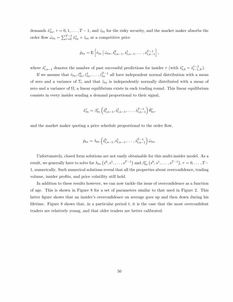
demands xτtn, τ = 0, 1, . . . , T − 1, and ztn for the risky security, and the market maker absorbs the

order flow ωtn =∑T−1

τ=0 xτtn + ztn at a competitive price

ptn = E[vtn∣∣ ωtn, s0

t,n−1, s1t,n−1, . . . , s

T−1t,n−1

],

where sτt,n−1 denotes the number of past successful predictions for insider τ (with sτt,0 = sτ−1t−1,N ).

If we assume that vtn, ε0tn, ε

1tn, . . . , ε

T−1tn all have independent normal distribution with a mean

of zero and a variance of Σ, and that ztn is independently normally distributed with a mean of

zero and a variance of Ω, a linear equilibrium exists in each trading round. This linear equilibrium

consists in every insider sending a demand proportional to their signal,

xτtn = βτtn

(s0t,n−1, s

1t,n−1, . . . , s

T−1t,n−1

)θτtn,

and the market maker quoting a price schedule proportional to the order flow,

ptn = λtn

(s0t,n−1, s

1t,n−1, . . . , s

T−1t,n−1

)ωtn.

Unfortunately, closed form solutions are not easily obtainable for this multi-insider model. As a

result, we generally have to solve for λtn(s0, s1, . . . , sT−1

)and βτtn

(s0, s1, . . . , sT−1

), τ = 0, . . . , T−

1, numerically. Such numerical solutions reveal that all the properties about overconfidence, trading

volume, insider profits, and price volatility still hold.

In addition to these results however, we can now tackle the issue of overconfidence as a function

of age. This is shown in Figure 8 for a set of parameters similar to that used in Figure 2. This

latter figure shows that an insider’s overconfidence on average goes up and then down during his

lifetime. Figure 8 shows that, in a particular period t, it is the case that the most overconfident

traders are relatively young, and that older traders are better calibrated.

50

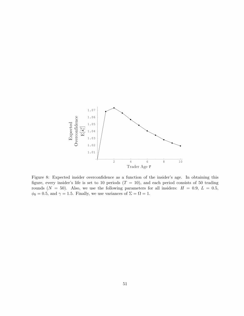
2 4 6 8 10

1.01

1.02

1.03

1.04

1.05

1.06

1.07

Trader Age t

Exp

ecte

dO

verc

onfid

ence

E[ktt]

ˆ

Figure 8: Expected insider overconfidence as a function of the insider’s age. In obtaining thisfigure, every insider’s life is set to 10 periods (T = 10), and each period consists of 50 tradingrounds (N = 50). Also, we use the following parameters for all insiders: H = 0.9, L = 0.5,φ0 = 0.5, and γ = 1.5. Finally, we use variances of Σ = Ω = 1.

51

References

Alchian, A. A., 1950, “Uncertainty, Evolution, and Economic Theory,” Journal of Political Econ-

omy, 58, 211-221.

Alpert, M., and H. Raiffa, 1982, “A Progress Report on the Training of Probability Assessors,”

in D. Kahneman, P. Slovic, and A. Tversky (eds.), Judgment Under Uncertainty: Heuristics and

Biases, Cambridge University Press, Cambridge and New York, 294-305.

Anderson, N., 1959, “Test of a Model for Opinion Change,” Journal of Abnormal and Social

Psychology, 59, 371-381.

Anderson, N., 1981, Foundations of Information Integration Theory, Academic Press, New York.

Barber, B., and T. Odean, 1998a, “The Common Stock Investment Performance of Individual

Investors,” working paper, University of California, Davis.

Barber, B., and T. Odean, 1998b, “Boys will be Boys: Gender, Overconfidence, and Common Stock

Investment,” working paper, University of California, Davis.

Benos, A., 1998, “Aggressiveness and Survival of Overconfident Traders,” Journal of Financial

Markets, 1, 353-383.

Bhattacharya, U., and M. Spiegel, 1991, “Insiders, Outsiders, and Market Breakdowns,” Review of

Financial Studies, 4, 255-282.

Blume, L., and D. Easley, 1982, “Learning To Be Rational,” Journal of Economic Theory, 26,

340-351.

Blume, L., and D. Easley, 1992, “Evolution and Market Behavior,” Journal of Economic Theory,

58, 9-40.

Blume, L., D. Easley, and M. O’Hara, 1994, “Market Statistics and Technical Analysis: The Role

of Volume,” Journal of Finance, 49, 153-181.

Bossaerts, P., 1999, “The Dynamics of Limited-Liability Securities Prices in Fallible Markets,”

working paper, California Institute of Technology.

Daniel, K., D. Hirshleifer, and A. Subrahmanyam, 1998, “Investor Psychology and Security Market

Under- and Overreactions,” Journal of Finance, 53, 1839-1885.

52

De Finetti, B., 1937, “La prevision: ses lois logiques, ses sources subjectives,” Annals of the Institut

Henri Poincare, 7, 1-68.

De Long, J., A. Shleifer, L. Summers, and R. Waldmann, 1990, “Noise Trader Risk in Financial

Markets,” Journal of Political Economy, 98, 703-738.

Fischhoff, B., 1982, “For Those Condemned to Study the Past: Heuristics and Biases in Hindsight.”

In D. Kahneman, P. Slovic, and A. Tversky (eds.), Judgment Under Uncertainty: Heuristics and

Biases, Cambridge University Press, Cambridge and New York, 335-351.

Fiske, S., and S. Taylor, 1991, Social Cognition (2nd ed.), McGraw-Hill, New York.

Friedman, M., 1953, Essays in Positive Economics, University of Chicago Press, Chicago.

Gervais, S., 1996, “Market Microstructure with Uncertain Information Precision: A Multi-Period

Analysis,” working paper, Wharton School, University of Pennsylvania.

Glosten, L., 1989, “Insider Trading, Liquidity, and the Role of the Monopolist Specialist,” Journal

of Business, 62, 211-235.

Grossman, S. J., 1976, “On the Efficiency of Competitive Stock Markets Where Traders Have

Diverse Information,” Journal of Finance, 31, 573-585.

Grossman, S. J., and J. E. Stiglitz, 1980, “On the Impossibility of Informationally Efficient Mar-

kets,” American Economic Review, 70, 393-408.

Hastorf, A. H., D. J. Schneider, and J. Polefka, 1970, Person Perception, Addison-Wesley, Reading,

Massachusetts.

Hogarth, R., and H. Einhorn, 1992, “Order Effects in Belief Updating: The Belief-Adjustment

Model,” Cognitive Psychology, 24, 1-55.

Kyle, A., 1985, “Continuous Auctions and Insider Trading,” Econometrica, 53, 1315-1335.

Kyle, A., and F. A. Wang, 1997, “Speculation Duopoly With Agreement to Disagree: Can Over-

confidence Survive the Market Test?,” Journal of Finance, 52, 2073-2090.

Langer, E., and J. Roth, 1975, “Heads I Win, Tails It’s Chance: The Illusion of Control as a

Function of the Sequence of Outcomes in a Purely Chance Task,” Journal of Personality and

Social Psychology, 32, 951-955.

53

Lichtenstein, S., B. Fischhoff, and L. Phillips, 1982, “Calibration of Probabilities: The State of the

Art to 1980,” in D. Kahneman, P. Slovic, and A. Tversky (eds.), Judgment Under Uncertainty:

Heuristics and Biases, Cambridge University Press, Cambridge and New York, 306-334.

Luo, G. Y., 1998, “Market Efficiency and Natural Selection in a Commodity Futures Market,”

Review of Financial Studies, 11, 647-674.

Milgrom, P., and N. Stokey, 1982, “Information, Trade and Common Knowledge,” Journal of

Economic Theory, 26, 17-27.

Miller, D., and M. Ross, 1975, “Self-serving Biases in Attribution of Causality: Fact or Fiction?,”

Psychological Bulletin, 82, 213-225.

Odean, T., 1998a, “Volume, Volatility, Price, and Profit When All Traders Are Above Average,”

Journal of Finance, 53, 1887-1934.

Roll, R., 1984, “A Simple Implicit Measure of the Effective Bid-Ask Spread in an Efficient Market,”

Journal of Finance, 39, 1127-1139.

Statman, M., and S. Thorley, 1998, “Overconfidence and Trading Volume,” working paper, Santa

Clara University.

Subramanyam, K. R., 1996, “Uncertain Precision and Price Reactions to Information,” The Ac-

counting Review, 71, 207-220.

Wang, A., 1997, “Overconfidence, Delegated Fund Management, and Survival,” working paper,

Columbia University.

Wolosin, R. J., S. J. Sherman, and A. Till, 1973, “Effects of Cooperation and Competition on

Responsibility Attribution After Success and Failure,” Journal of Experimental Social Psychology,

9, 220-235.

54

Learning To Be Overcondent

Documents

Transcript of Learning To Be Overcondent