KR-20 and KR-21 for some non-dichotomous data(It’s not just Cronbach’s alpha)

Robert C. Foster

Bettis Atomic Power Laboratory

Abstract

This paper presents some equivalent forms of the common Kuder-RichardsonFormula 21 and 20 estimators for non-dichotomous data belonging to certainother exponential families, such as Poisson count data, exponential data, or ge-ometric counts of trials until failure. Using the generalized framework of Foster(2020), an equation for the reliability for a subset of the natural exponentialfamily have quadratic variance function is derived for known population param-eters, and both formulas are shown to be different plug-in estimators of thisquantity. The equivalent Kuder-Richards formulas 20 and 21 are given for sixdifferent natural exponential families, and these match earlier derivations in thecase of binomial and Poisson data. Simulations show performance exceedingthat of Cronbach’s alpha in terms of root mean squared error when the formulamatching the correct exponential family is used, and a discussion of Jensen’sinequality suggests explanations for peculiarities of the bias and standard errorof the simulations across the different exponential families.

Keywords— Reliability, KR-20, KR-21, Cronbach’s Alpha, Exponential Families

1

1 Introduction

Formulas 20 and 21 of Kuder and Richardson (1937), abbreviated throughout this paperas KR20 and KR21, are some of the earliest and most well-known formulas in assessingreliability of a test. For dichotomous data, the formulas are given by

KR20 =k

k − 1

(1−

∑kj=1 pj(1− pj)

σ2X

)

KR21 =k

k − 1

(1− kp(1− p)

σ2X

)where k is the test length, σ2X is the variance of sum test scores, pj is the proportionof correct responses to test item j, and p is the average correct response over all items.The most common estimator of reliability, Cronbach’s alpha, is often seen as a generalversion of KR20 (Cronbach, 1951). Beyond Cronbach’s alpha, there does not seem to havebeen many attempts to determine equivalent variants of KR20 and KR21 to specific typesnon-dichotomous data, such as count data. Allison (1978) derived a KR21 equivalent forPoisson distributed data, but most have stuck to Cronbach’s alpha as a general estimatorof reliability.

The topic of reliability estimation, and Cronbach’s alpha in particular, has been asubject of much recent debate within the psychometric literature. Alpha has been criti-cized as having assumptions which are not realistic in practice (McNeish, 2018; Schmitt,1996; Sijtsma, 2009). Criticisms have focused on alpha’s assumptions of tau equivalenceand uncorrelated errors. McNeish (2018) claims that normality is an assumption of Cron-bach’s alpha, but Raykov and Marcoulides (2019) rebut that no assumptions of normalityare made in the derivation of alpha and consistency as an estimator does not depend onan assumption of normality. However, Zumbo (1999) notes that though the classical testtheory derivation of alpha makes no assumptions of normality, estimators of alpha oftendo, in agreement with Bay (1973) who noted in his time that early derivations of statisticalproperties of estimators such as Cronbach’s alpha and KR20 as in L. S. Feldt (1965) weredeveloped using an ANOVA model which includes an assumption of normality. More re-cent research in Zyl, Neudecker, and Nel (2000) on the sampling distribution of cronbach’salpha using maximum likelihood techniques also assumes normality, though nonparametricmethods have been developed for psychometric calculations using techniques like the boot-strap as in Raykov (1998). The statistical properties of alpha and other estimators havebeen little explored outside of these assumptions of normality, with simulation studies inSheng and Sheng (2012) and Zimmerman, Zumbo, and Lalonde (1993). Beyond classicaltest theory, Geldhof, Preacher, and Zyphur (2014) explicitly state that non-normal data isa limitation for reliability estimation in a multilevel confirmatory factor analysis frameworkAs Zinbarg, Yovel, Revelle, and McDonald (2006) note, properties of alternatives to Cron-bach’s alpha based on a factor analysis are not well known under non-normality, despitemost psychological data being non-normal. It is clear that there is a need for analysis ofreliability for non-normal data.

The purpose of this paper is to make a contribution towards the analysis of reliabilityunder non-normality by reversing direction from Cronbach’s alpha once again to derive

2

formulas to estimate test reliability in special cases – to find equivalent forms of KR20 andKR21 which can be used to assess reliability of tests for specific types of non-dichotomousdata. For example, chapter 21 of Lord, Novick, and Birnbaum (1968), discussing the workof Rasch (1960), notes that the number of an examinee’s misreadings in an oral reading testmay be modeled as a Poisson random variable. If the response of interest were instead thetime between misreadings, an exponential distribution would then be appropriate. Meredith(1971) also showed that a Poisson process is appropriate for tests of speed, and notedthat under certain assumptions the distributions of observed scores ought to be negativelybinomial distributed. The key idea is this: KR20 and KR21 can be seen as a specificversion of an estimator for reliability for Bernoulli distributed item responses where themean-variance relationship of the Bernoulli distribution is exploited for variance calculationsrather than using standard sample variances. Other exponential family distributions alsohave mean-variance relationships. By working within the generalized framework of Foster(2020) and deriving a formula for reliability in exponential families which uses the mean-variance relationship and which matches traditional KR20 and KR21 in the binomial case,equivalent versions of KR20 and KR21 are obtained for data from other exponential familydistributions. The KR20 and KR21 equivalent formulas are shown for when sum testscores can be said to follow one of the six natural exponential family distributions withquadratic variance function (NEF-QVF): the normal, the binomial, the Poisson, the gamma,the negative binomial, or the natural exponential family generated by a convolution ofgeneralized hyperbolic secant functions (NEF-GHS).

Section 2 describes the properties of the generalized framework for reliability de-scribed in Foster (2020) which form the basis for derivations of the formulas and definitionof reliability as parallel-test correlation, and states which assumptions are slightly modifiedfor the purposes of this paper. Section 3 shows how the mean-variance relationship canbe exploited to obtain test reliability and derives the general KR20 and KR21 formulas asestimators of this relationship, giving the formulas for each NEF-QVF distribution. Theseare shown to match the traditional KR20 and KR21 of Kuder and Richardson (1937) in thebinomial case, and the Poisson KR21 of Allison (1978) in the Poisson case. The conditionsfor algebraic equivalence between KR20 and Cronbach’s alpha are also discussed. Section4 performs a simulation study showing that these formulas do appear to converge to thepopulation reliability as the number of subjects and test length increases and comparing theequivalent KR20 and KR21 formulas to Cronbach’s alpha and each other in terms of rootmean squared error, bias, and standard deviation. Results indicate that when the formulasare used for data following the appropriate exponential family, performance is improved overCronbach’s alpha in terms of RMSE, though whether KR20 or KR21 is superior dependson the variance function of the exponential distribution. A brief discussion of Jensen’s in-equality indicates a possible explanation for why one formula is superior to another for agiven distribution.

2 Framework

This paper follows the generalized framework of Foster (2020), where “generalized” is usedin the same sense of a generalized linear model which may deal with non-normal exponential

3

family data. A complete theoretical description of the framework is given in Foster (2020),but this paper will only state without proof elements which are necessary. One major differ-ence is that while the framework of Foster (2020) applies to the entire natural exponentialfamily, this paper focuses only on the members of the exponential family having quadraticvariance function so that the variance is a polynomial function of the mean up to degree two.For example, a Bernoulli distribution with success probability p has mean p and variancep(1 − p) = p − p2, so the variance is a quadratic function of the mean. Such distributionsand their properties are extensively described in Morris (1982) and Morris (1983), whichserve as a general reference. Furthermore, while the framework of Foster (2020) allowsthe test length to vary between subjects, this paper assumes a common test length for allsubjects for the sake of simplicity. The framework of Foster (2020) is most closely relatedto the strong true-score theory found in chapters 21 through 24 of Lord et al. (1968) andassociated papers such as Lord (1965) and Keats and Lord (1962) in deriving propertiesof reliability when specific distributional forms can be assumed, but rather than dealingindividually with the binomial and Poisson distributions, the framework of Foster (2020)derives properties for the exponential family in general. The framework makes assumptionsof true score distributions in such a way as to ensure that the regression of true score onobserved score is linear, though the observed scores are non-normal.

Let i = 1, 2, . . . , n index test subject and let j = 1, 2, . . . , k index test item. In thisframework, each test item for each subject Yij is assumed to identically follow a naturalexponential family distribution with quadratic variance function (NEF-QVF), with inde-pendence conditional on subject ability θi. The six NEF-QVF distributions which may beused as generator distributions in this fashion are the normal, Bernoulli, Poisson, exponen-tial, geometric, and generalized hyperbolic secant densities. Each of these distributions isclosed under convolution. For example, the normal is a sum of normals, the binomial is thesum of Bernoullis, and the gamma is a sum of exponentials. Let Xi =

∑kj=1 Yij be the sum

score for subject i, summing over all k test items. The six possible distributions for Xi arethen the normal, binomial, Poisson, gamma, negative binomial, and NEF-GHS.

Furthermore, let abilities θi follow the corresponding conjugate prior g(θi|µ,M) forthe natural exponential family distribution, where µ = E[θi] and M = E[V (θi)]/V ar(θi).For example, if the test items Yij are Bernoulli distributed with mean given by subject abilityθi, then subject sum scores Xi are binomial distributed, and abilities θi themselves follow abeta distribution with parameters µ = α/(α+ β) and M = α+ β. A complete descriptionof several common NEF-QVF distributions, their conjugate priors, and the appropriateparameterizations in terms of µ and M is given in the appendix of Foster (2020). Themodel can be thought of as a hierarchy, with observed scores at the top level and abilitiesat the bottom level.

For natural exponential family distributions with quadratic variance function, thevariance is a polynomial function of the mean of up to degree two.

V ar(Yij |θi) = V (θi) = v0 + v1θi + v2θ2i (1)

For example, the Bernoulli distribution has V (θi) = θi(1− θi) = θi − θ2i , so v0 = 0, v1 = 1,and v2 = −1. The normal distribution, which assumes the variance around each itemresponse is known to be σ2, has V (θi) = σ2 constant.

4

In this framework, the conditional and unconditional expectations of test item Yijare given by

E[Yij |θi] = θi

E[Yij ] = µ(2)

where µ is the population mean ability. The conditional expectation being equal to abilityθi in Equation (2) is an implicit assumption that each item is of equal difficulty conditionalon subject with ability θi, the necessity of which is discussed in Section 6. The conditionaland unconditional variances are given by

V ar(Yij |θi) = V (θi)

V ar(Yij) = E[V (θi)] + V ar(θi)(3)

where V (θi) is the variance function in Equation (1) applied to abilities θi. Then sum scoresXi have conditional and unconditional expectations

E[Xi|θi] = kθi

E[Xi] = kµ(4)

Correspondingly, the conditional and unconditional variances of Xi are given by

V ar(Xi|θi) = kV (θi)

V ar(Xi) = kE[V (θi)] + k2V ar(θi)(5)

Within this framework, the test reliability is defined as the correlation betweenparallel tests, where parallel means that each test consists of identical, conditionally inde-pendent items Yij following the same exponential family model with means and variancesgiven by Equations (2), (3), (4), and (5). As shown in Foster (2020), when this conditionis met the test reliability is equal to

ρ =k

M + k

where k is the test length and M = E[V (θi)]/V ar(θi) is the parameter of the underlyingdistribution of abilities g(θi|µ,M). This is also one minus the shrinkage parameter in theBayesian posterior distribution. Cronbach’s alpha reduces to this quantity in the framework.

Because the response to each test item Yij is conditionally independent and identicalon ability θi, this framework is unidimensional. As shown in Equation (3) and in Foster(2020), the unconditional variances of each test item and unconditional covariances betweentest items are equal. The variance-covariance matrix between test items implied in thisframework is thus tau-equivalent with equal variances, though the variance around eachtest item Yij is different for each subject i because of the mean-variance relation given inEquation (1).

5

3 KR20 and KR21 as Estimators of Reliability

Conjugate priors for natural exponential families have a close relationship between theirmean µ and their variance V ar(θi), connecting to the variance function of the originalexponential family distribution they are conjugate to. From Morris (1983), the variance ofthe conjugate prior for natural exponential families with a quadratic variance function is

V (µ) = V ar(θi)(M − v2) (6)

where V (µ) is the variance function of Equation (1) applied to the mean µ, M is theparameter of the conjugate distribution of abilities g(θi|µ,M), and v2 is the coefficient of thequadratic term of the variance function in Equation (1). For example, a beta distribution forθi with parameters µ = α/(α+β) and M = α+β has variance V ar(θi) = µ(1−µ)/(M+1).With V (θi) = θi(1− θi) for the Bernoulli distribution, this gives V (µ) = (M + 1)V ar(θi).

Define the the quantity R as

R =k

k + v2

(1− kV (µ)

V ar(Xi)

)(7)

where V ar(Xi) is the unconditional variance. Using the mean-variance relationship givenin Equation (6) and the variances given in Equation (5), this quantity becomes

R =k

k + v2

(1− kV (µ)

V ar(Xi)

)=

k

k + v2

(1− kV ar(θi)(M − v2)

kE[V (θi)] + k2V ar(θi)

)=

k

k + v2

(kE[V (θi)] + k2V ar(θi)− kV ar(θi)(M − v2)

kE[V (θi)] + k2V ar(θi)

)=

k

k + v2

(M + k − (M − v2)

M + k

)=

k

k + v2

(k + v2M + k

)=

k

M + k

= ρ

(8)

The last line in Equation (7) is the parallel-test reliability, as previously stated. For di-chotomous, Bernoulli distributed item responses, which have V (θi) = θi − θ2i and v2 = −1,substitution into the quantity R in Equation (7) gives

R =k

k − 1

(1− kµ(1− µ)

V ar(Xi)

)which is strikingly similar to the original KR20 and KR21 estimators of Kuder and Richard-son (1937), but depends on known population parameters rather than sample quantities.

The parameters in Equation (7) are unknown, however, or else there would be noneed to administer any sort of test. The question is then, is it possible to construct a

6

consistent estimator for Equation (7) from sample quantities? The answer is yes. Givena consistent estimator for V (µ) and a consistent estimator for V ar(Xi), then by Slutsky’stheorem, using these as plug-ins for the numerator and denominator of Equation (7) willproduce a consistent estimator for the population test reliability.

For V ar(Xi), the standard unbiased variance moment-based estimator of varianceis used for raw sum scores xi.

s2x =1

n− 1

n∑i=1

(xi − x)2

A note on the equivalence of KR20 and Cronbach’s alpha for dichotomous data: theseare often stated to be exactly equal; however, algebraic equivalence only occurs when thebiased estimator of the sample variance which divides by the number of subjects n is usedfor V ar(Xi) rather than the unbiased estimator which divides by n − 1 (for Cronbach’salpha itself, either estimator of variance yields identical estimates so long as it is usedconsistently). For all calculations in this paper, the unbiased estimator of sample variance isused. The historical reason for introducing bias into the denominator of the KR20 estimatorof reliability appears to be obtaining algebraic equivalence Cronbach’s alpha. As the resultsof the simulation study in Section 4 show, however, using the unbiased estimator of varianceproduces improved performance over alpha.

For the quantity V (µ), more than one estimator is possible. Because V (θi) is acontinuous polynomial for all six distributions considered, any consistent estimator for µ isconsistent for V (µ) by the continuous mapping theorem. The simplest estimator is to notethat from Equation (4), E[Xi] = kµ, and so 1

k times the sample mean of sum scores hasexpectation E[ 1k x] = 1

k (kµ) = µ. Hence, 1k x is a consistent estimator for µ by the law of

large numbers, and so V ( 1k x) is a consistent estimator for V (µ).An alternative estimator is constructed by observing that the terms in the mean of

sum scores x can be rearranged to equal the sum of test item means.

x =1

n

n∑i=1

xi =1

n

n∑i=1

k∑j=1

yij =1

n

k∑j=1

n∑i=1

yij =k∑

j=1

yj (9)

From Equation (2), a single test item Yij has E[Yij ] = µ. By the law of large numbers,the item sample mean yj converges to µ for each item j. Then V (yj) is also a consistentestimator for V (µ).

In Equation (7), the desired quantity is not V (µ), but kV (µ). Because the variancefunction applied each item mean V (yj) is independently consistent for V (µ), a sum of V (yj)over all k items gives the desired result. Plugging this into Equation (7) with unbiasedsample variance s2x for the denominator yields the generalized form of KR20:

KR20 =k

k + v2

(1−

∑kj=1 V (yj)

s2x

)(10)

For dichotomous, Bernoulli distributed item responses with V (θi) = θi−θ2i so that v2 = −1,this gives:

7

k

k − 1

(1−

∑kj=1 yj(1− yj)

s2x

)which is the traditional KR20 formula, with yj = pj as the proportion of correct responseson item j.

The alternative is to use kV ( 1k x) as a consistent estimator for kV (µ). Plugging thisand s2x into Equation (7) yields the generalized form of KR21:

KR21 =k

k + v2

(1−

kV ( 1k x)

s2x

)(11)

For dichotomous, Bernoulli distributed item responses, this is

k

k − 1

(1−

k( 1k x)(1− 1k x)

s2x

)which is the traditional KR21 formula, as x is the average sum score and so 1

k x is theaverage proportion correct p.

The difference between KR20 and KR21, as far as this framework is concerned,is whether the variance function V (·) is applied “inside” the sum of item means on theright-hand side of Equation (9), yielding KR20, or “outside” the sum, yielding KR21. Atable showing the six different NEF-QVF distributions for item responses, their variancefunctions, and their corresponding KR20 and KR21 estimators is given in Table 1. Asshown, the binomial formulas match the formulas originally derived in Kuder and Richard-son (1937). The Poisson KR21 formula here exactly matches equation thirteen of Allison(1978), which originally derived KR21 for Poisson count data. This paper shows that it isalso the Poisson KR20 equivalent because the variance function for the Poisson distributionis simply the identity V (θi) = θi, and so applying Equation (9) gives equality. The restof the formulas are new, so far as can be determined. For the normal distribution, theerror variance σ2 around the response to each item is assumed known. As this is extremelyunlikely to be the case in practice, Cronbach’s alpha is recommended instead.

4 Simulation Study

4.1 Simulation Method

A reasonable question is, why use these generalized KR20 or KR21 estimators when Cron-bach’s alpha is available? What advantage do these estimators have? This question isanswered with a simulation study.

The purpose of this simulation study is to show that when data is simulated fromthe correct NEF-QVF model, the generalized KR20 and KR21 estimators correspondingto that family both converge to the population reliability as the test length and numberof subjects increase, and that they do so as or more efficiently than Cronbach’s alpha. Itis not a simulation study to determine all properties of the estimators or to investigate allpotential sources and magnitudes of bias, though several are discussed. For data generation,

8

the method described in the appendix of Foster (2020) is used, which is identical to thesimulation method of Huynh (1979) in the case of the binomial-beta model. Test data issimulated using the following algorithm:

1. Choose the appropriate NEF-QVF distribution for test item responses yij , the meanability µ, the number of subjects n, the number of test items k, and desired populationreliability ρ.

2. Calculate the M required to obtain the desired population reliability ρ as

M =

(1− ρρ

)k

3. Simulate n abilities θi from the conjugate prior g(θi|µ,M), one for each subject i.The appropriate parameterization of the prior in terms of µ and M is given in theappendix of Foster (2020)

4. For each θi, simulate k responses from the NEF-QVF distribution p(yij |θi). The sumscore xi for each subject i is calculated as the sum of these responses over the k items.

This algorithm implies the underlying distribution of talent levels g(θi|µ,M) is dif-ferent for each (k, ρ) pair, as the parameter M of the distribution is calculated anew foreach. Hence, it is difficult to directly compare simulation results across two identical kvalues if ρ differs, or across identical ρ values if k differs. Again, the primary goal is to showconvergence. The alternative is to keep the distribution of talent levels constant by keepingM constant and varying the the reliability through the test length k, but this was not chosenbecause it limits the potential values of the desired population reliability ρ and preliminarysimulations indicated that the shape of the distribution of talent levels g(θi|µ,M) was lessinfluential than the value of ρ, with the exception of extremely skewed distributions whichmay be of interest in other simulations. The balance of choices in producing a desired pop-ulation reliability ρ is delicate and it is not possible within this framework to have completefreedom in all choices. A more complete simulation study might achieve a desired ρ throughdifferent methods in order to determine the effect of each. Though the mean ability µ doesnot affect the population reliability directly, it does have the potential to affect the sam-pling distribution of reliability through manipulating aspects of the distribution of abilitiesg(θi|µ,M) such as skew and kurtosis. In particular, preliminary simulations indicated thatµ values near the edges of the distribution support may lead to very skewed g(θi|µ,M) dis-tributions which could potentially have a large influence, but these were not considered forfurther study by simulation in this paper. The mean µ is instead kept constant throughoutthe simulation studies to avoid yet another quantity which could potentially affect results,though it could be of interest in a further simulation study. This algorithm also producesitems which are of equal difficulty conditional on subject with ability θi, though items mayhave different algebraic means.

For the choice of exponential family model, the Poisson-gamma, gamma-inversegamma, negative binomial-F, and binomial-beta distributions are used, where the first dis-tribution named is the distribution of sum scores xi and the second is the conjugate prior

9

g(θi|µ,M). The binomial-beta distribution corresponds to the Kuder and Richardson (1937)coefficients and has been extensively studied, but is also shown here for completeness andcomparison to results for other estimators. The normal-normal assumes the variance σ2 isknown, and as such is not of practical use. The distribution in the last row of Table 1,the natural exponential family generated by a convolution of generalized hyperbolic secantdistributions, is neither common nor easy to simulate from.

For population ability ρ, the values 0.3, 0.6, and 0.8 are used, representing low,moderate, and high reliability. For test length, the values k = 5, 10, and 30 are used,representing a short, medium, and long test. For number of subjects, the values n = 30, 75,and 500 are used, representing a small, moderate, and large number of subjects. The valueof the mean ability µ is constant within each set of simulations at µ = 1 for the Poisson-gamma model and the gamma-inverse gamma model, µ = 1.01 for the negative binomial-Fmodel, and µ = 0.5 for the binomial-beta model. These were simply chosen as reasonablevalues which worked well in simulation.

This gives a total of 27 sets of (ρ, k, n) values for each exponential family model andfour models. Details of the implied variance-covariance matrix are given in the Appendix.For each set of values, a total of Nsims = 1, 000, 000 data sets were simulated and Cronbach’salpha and the KR20 and KR21 equivalents given by Equations (10) and (11) were calculatedfor each. To judge the estimator for a given set of estimated reliabilities ρ, the sample rootmean squared error is used.

RMSE(ρ) =

√√√√ 1

Nsims

Nsims∑s=1

(ρ− ρs)2

The root mean squared error is further decomposed into the traditional bias and variance(squared standard deviation) of the estimator.

RMSE(ρ) =√Bias2(ρ) + V ar(ρ) =

√√√√( 1

Nsims

Nsims∑s=1

(ρ− ρs)

)2

+1

Nsims

Nsims∑s=1

(ρs − ρs)2

where ρs is the sample mean of the ρs. Note that decomposition requires the biased varianceformula for exact algebraic equivalence, but for Nsims = 106 total simulations using eitherthe biased or unbiased variance estimate gives identical results within the first three decimalplaces. The decomposition allows for further inspection of results in order to determine exactproperties of the estimator and answer questions about why a particular estimator mightbe performing better or worse than another.

The results of the simulation study are shown in Table 2 and Figure 1 for thePoisson-gamma model, Table 3 and Figure 2 for the gamma-inverse gamma model, Table 4and Figure 3 for the negative binomial-F model, and Table 5 and Figure 4 for the binomial-beta model. In the results the sample standard deviation is given rather than the samplevariance because the sample variance was often extremely small. Results are reported tothree decimal places. The largest sample variance reported for any estimator is 0.2512 forCronbach’s alpha in the first row of Table 3; thus, the approximate Monte Carlo standarderror is less than or equal to 0.251/

√106 = 0.000251, and quite often much smaller. For

10

this reason, the reporting of three decimal places in results is appropriate. Again, note thatthe unbiased estimator of sample variance s2x which divides by n − 1 is used in all cases.Furthermore, intervals around derived quantities are small. A 99% bootstrap interval for theRMSE of Cronbach’s alpha in the first row of Table 3, based on 10,000 bootstrap samplesof the one million simulated alpha values, is (0.251, 0.252). The standard error of the pointestimate of RMSE is thus smaller than the rounding amount 0.001, so confidence intervalssurrounding the point estimates are not included.

4.2 Analysis of Results

The results of Tables 2, 3, 4, and 5 show that the primary aims of the simulation study aremet. Both Cronbach’s alpha and the estimators in Table 1 decrease in RMSE and appear tobe converging towards zero as the test length k and the number of subjects n increase. Thiscan be seen for ρ = 0.3 in Figures 1, 2, 3, and 4. Furthermore, the estimators in Table 1 arenearly universally superior to Cronbach’s alpha, answering the initial question posed of whythey might be preferred over alpha. It is only in high-data situations with a relatively largenumber of test items k and large number of subjects n that all estimators are nearly equaland the root mean squared error is approximately the same no matter which estimator youchoose. In general, it appears that increasing the number of subjects n can greatly leadto a reduction in RMSE through reduction of both bias and variance. For shorter testswith a smaller number of subjects, the generalized estimators provided by Equations (10)and (11) often strongly outperform alpha in terms of RMSE. However, there are noticeabledifferences in the exact manner the increase occurs. For example, the generalized KR21estimator outperforms the generalized KR20 estimator for the gamma-inverse gamma andnegative-binomial F results in Tables 3 and 4, but the reverse occurs for the binomial-betamodel results given in Table 5. The bias of all three estimators is also generally negative,except for KR20 and KR21 in the binomial-beta model results given in Table 5. There arealso differences in variances of the estimators across models. Though formal proof is notoffered, some probability theory may help to explain the idiosyncrasies within each tableand between tables.

First, it is noticeable that in all three sets of simulations the bias is negative forCronbach’s alpha in all cases, though converging to zero as the number of subjects n in-creases. Why? From Foster (2020), Cronbach’s alpha is estimating the quantity

α =k

k − 1

(1−

∑kj=1 V ar(Yj)

V ar(X)

)using plug-in estimates of the sample variances s2yj and s2x, though as in Foster (2020) thispaper assumes V ar(Yj) is identical for all test items j. Essentially, it is a ratio of samplevariances, and ratios of sample variances tend to be biased upwards. For independentvariances, Jensen’s inequality shows that the bias is always high, as 1/s2x is a convex functionof s2x and so E[1/s2x] ≥ 1/E[s2x] = 1/V ar(X); however, the lack of independence between s2xand

∑s2yj in the calculation of Cronbach’s alpha makes precise determination of the bias

for alpha difficult. When the bias of the ratio is positive, then the act of subtracting theratio from one in the calculation of Cronbach’s alpha flips the bias of the estimator as a

11

whole to underestimation.Also noticeable is that the bias of the KR21 and KR20 estimators is often larger

than the bias of Cronbach’s alpha for the gamma-inverse gamma and negative-binomial Fmodels, identical for the Poisson-gamma model, and smaller for the binomial-beta model.Why? Though is it difficult to state exactly the reasons, as Equations (10) and (11) areslightly different than alpha due to the presence of the k/(k + v2) in front and becausethe two estimators are estimating the reliability using different quantities, a very strongclue is offered by Jensen’s inequality. The numerators of KR20 and KR21 in Equations(10) and (11) are still estimating variances similarly to alpha, only in an indirect manner.From Equation (7), the mean-variance relationship for exponential family random variablesis being exploited to estimate the variance through estimation of the variance functionV (µ). Because V (µ) is not available, however, the plug-in estimate V ( 1k x) is used forthe KR21 estimator. By Jensen’s inequality, E[V ( 1k x)] ≥ V (E[ 1k x]) = V (µ) for convexfunctions V (·). In Table 1, the variance function V (µ) for both the exponential (gamma-inverse gamma model) and geometric (negative binomial-F model) distributions is convex.Hence, additional bias is introduced to the numerator of the ratio estimate, as the expectedvalue of the variance function of the sample mean is larger than the variance function of thepopulation mean. This is seen in the increased bias over Cronbach’s alpha in Tables 3 and 4.A similar argument applies for the KR20 estimator. The bias for the Poisson-gamma modelin Table 2, however, is equal for both Cronbach’s alpha and the KR20 and KR21 equivalents.This is because the variance function for the Poisson distribution V (µ) = µ is linear, andthus E[V ( 1k x)] = V (E[ 1k x]) = V (µ). The bias for KR20 and KR21 in the binomial-betamodel is smaller than the bias of Cronbach’s alpha, as seen in Table 5, because the variancefunction V (µ) = µ − µ2 is concave, and so E[V ( 1k x)] ≤ V (E[ 1k x]) = V (µ) by Jensen’sinequality. For most estimators, a downward bias would be a disadvantage. However, thebias of the standard binomial KR20 and KR21 appear in the numerator of a ratio estimatorthat is already biased upwards. By all accounts, it appears that the downward bias for thetraditional KR20 and KR21 from the use of the variance function applied to the samplemean acts as a counterweight to the upward bias coming from taking the ratio of samplevariances, which is a rather remarkable idea.

It has long been noted that in the standard binomial case, KR21 serves as a lowerbound for KR20 (Kuder & Richardson, 1937). This is also easily seen as an applicationof Jensen’s inequality in its algebraic form. Because V (θ) = θ − θ2 is concave, Jensen’sinequality gives

kV

(1

kx

)= kV

1

k

k∑j=1

yj

≥ k(1

k

) k∑j=1

V (yj) =k∑

j=1

V (yj)

and once again, the act of subtracting from one in Equations (10) and (11) flips the in-equality to obtain the standard result for the inequalities as a whole. Conversely, for convexvariance functions, as is the case with the exponential (gamma-inverse gamma model) andgeometric (negative binomial-F model) data, the inequality is reversed and KR20 servesas a lower bound to KR21. For Poisson data with identity variance function, the two es-timators are equal, as previously discussed. Because KR20 and KR21 are both generallyunderestimating the reliability, this has the effect that KR20 is less biased than KR21 for

12

the binomial-beta model, with a smaller variance, mirroring the traditional wisdom thatKR20 is superior to KR21 for dichotomous data. KR20 is more biased than KR21 for thegamma-inverse gamma and negative binomial-F models, with a larger variance.

Lastly, even though the bias of the KR20 and KR21 estimators is sometimes larger,it compensates for this by a greatly decreased variance. What is the reason for this decreasein variance? A possible explanation is that it comes from using sample means in combinationwith the mean-variance relationship of exponential families to estimate a variance ratherthan using sample variances themselves. Sample means converge to population means ata rate of

√n, where n is the number of test subjects, while sample variances converge to

population variances at a rate of n (Casella & Berger, 2002). Simply put, sample meansconverge faster than sample variances. Hence, estimating item variances using samplemeans in combination with a mean-variance relationship should tend to be more efficientthan using sample variances alone.

4.3 Alternative Reliability Estimators

Cronbach’s alpha, though popular is far from the only estimator available, and its usehas been criticized (McNeish, 2018; Sijtsma, 2009) and alternatively defended (Raykov &Marcoulides, 2019). One alternative based on analysis of a factorial structure is McDon-ald’s omega (McDonald, 1999), which has been proposed as preferable to Cronbach’s alpha(Hayes & Coutts, 2020; McNeish, 2018). Different estimators called omega exist, but twoin particular, omega hierarchical (ωH) which calculates the general factor saturation of atest and omega total (ωT ) which also includes specific factors, have been a focus of interest(Revelle & Zinbarg, 2009; Savalei & Reise, 2019). Another commonly proposed alternativeis the greatest lower bound (Sijtsma, 2009; Trizano-Hermosilla & Alvarado, 2016), but Rev-elle and Zinbarg (2009) note that it is potentially smaller than ωT , and its performance hasbeen examined in Trizano-Hermosilla and Alvarado (2016). It is, however, worth comparingthe generalized estimators of Table 1 to ωH and ωT to evaluate performance. Because thedata is tau-equivalent, omega will equal reliability and the simulation study will evaluateperformance as an estimator.

To do so, a smaller simulation study similar to that of Section 4.1 was performed.The Poisson-gamma (P-G), gamma - inverse gamma (G-IG), and binomial-beta (B-B) mod-els were used to simulate data with a desired population reliability of ρ = 0.8, chosen toavoid possible numerical issues with low reliabilities. Test lengths of k = 5, 10 and num-ber of subjects n = 30, 75 were chosen to present results with large root mean squarederrors so that differences between the estimators are more easily observed. A total ofNsims = 1, 000, 000 data sets were generated for each model. The generalized KR21 esti-mator was chosen for comparison because it performed the best on the Poisson-gamma andgamma-inverse gamma models, as seen in Tables 2 and 3. Calculation of ωH and ωT wasperformed using the psych package in R (Revelle, 2020). Root mean squared error and bothbias and variance of KR21, ωH , and ωT are shown in Table 6.

The results of the study generally show that ωH has the worst performance interms of root mean squared error, including both elements of bias and variance, while thegeneralized KR21 formulas of Table 1 are competitive with ωT for superior RMSE. In somescenarios one is larger, while in the others the second is larger. Noticeably, it occasionally

13

occurs that one estimator has a larger RMSE but a lower standard deviation, suggesting thatbias correction could be a worthwhile strategy to improve the estimator. Also noticeable isthat the bias of ωT is generally small, but positive. One possible explanation for the smallbias is that ωT may be overfitting the model, which causes an upward bias in estimationof reliability that counters the general downard bias from ratios of sample statistics seenin other estimators. However, as Savalei and Reise (2019) note, further study regardingthe properties of reliability coefficients such as ωH and ωT is needed to determine theirstatistical properties.

5 Example

A small example shows how and why these formulas can be applied in practice. The data inTable 7 are taken from Table 3 of Moore (1970) and represent a count of the number of timesa specific letter was seen in a clerical speed test, for which the time has been subdivided intoblocks of 10 units. Only the first 9 blocks of time are used in Table 7 in order to keep testlength equal for all subjects. Chi-squared goodness of fit tests performed by Moore (1970)show that a Poisson process is a good fit to the data, and so the number of responses in eachblock of time may be treated as an independent and identical Poisson random variable withmean θi for subject i. The data may therefore also be treated as unidimensional and tau-equivalent. If the data were larger, either in terms of number of subjects or number of items,a regression of sample variance on sample means could indicate a linear relationship whichwould indicate that the Poisson model is appropriate. For small data, recognizing that theobservation is a count should draw attention to the Poisson distribution for responses.

The reliability of this test represents the theoretical correlation of the sum scores xiwith sum scores on a parallel test. Ideally, this correlation will be high to indicate that thesum scores are accurately capturing each subject’s counting ability under time constraints.However, the data contains only k = 9 responses for each of n = 10 subjects, and the datais discrete and non-negative. Cronbach’s alpha for this data set is α = 0.079, which is low.A problem is that the small number of responses per subject indicates that item variancesare not being efficiently estimated. McDonald’s omega for this data set gives ωH = 0.726and ωT = 0.802, but factor analysis on a small, exceedingly non-normal data set shouldcall for caution with respect to the statistical properties, and the results of Table 6 indicatethat this could be an overestimate.

The generalized KR20 and KR21 estimators of Table 1, originally derived in Allison(1978) and which are equal in this case, resolve this issue by utilizing the mean-variancerelationship for Poisson data to obtain reliability. For Poisson data, the variance of asubject’s response for each item is equal to their mean ability. The generalized KR21estimator therefore uses sample means to obtain an estimate of ρ = 0.626. The simulationresults of Table 2 indicate that this estimate is likely still biased downwards, but is a moreefficient estimator than alternatives.

14

6 Conclusion, Suggestions, and Future Research

Directions

This paper has introduced formulas which may be seen as the equivalent of the classicalKR20 and KR21 formulas of Kuder and Richardson (1937) for some non-dichotomous data,extending to data which may be modeled using an NEF-QVF distribution. Simulationsshow that when the model is satisfied, the KR20 and KR21 equivalent formulas appear toconverge to the population reliability and are generally a more efficient estimator of relia-bility than Cronbach’s alpha. Exponential families are defined by mean-variance relations,so these formulas may be considered when a quadratic relationship between subject meanand subject variance appears to be present, as in Equation (1), which can be checked withanalysis of sample variances as a function of sample means, exactly in the way a general-ized linear model is chosen. Certain types of data such as dichotomous data (binomial),count data (Poisson), or data measuring time between events (exponential) also naturallyfit this framework, especially when each response may be assumed to have roughly the samedifficulty.

It is important to state the assumptions made in the derivation of these estimators:that the response to each test item identically follows a natural exponential family con-ditionally independent given ability θi for subject i, implying that all item difficulties areequal for a subject, and that abilities themselves follow the corresponding conjugate priordistribution. Not all of these assumptions are made in the derivations of the traditionalbinomial KR20 and KR21 in Kuder and Richardson (1937) and the Poisson KR21 in Allison(1978), suggesting that some assumptions may be superfluous, particularly the assumptionthat abilities follow the conjugate prior distribution. L. J. Feldt (1984) also derives thetraditional binomial KR20 and KR21 formulas simply from the binomial error model. Itis likely that these generalized KR20 and KR21 formulas may similarly be derived usinga general error model from the mean-variance relationship of natural exponential families,and possibly for exponential families without quadratic variance functions. Furthermore,the difference in use between KR20 and KR21 in Kuder and Richardson (1937) is takento be whether or not all items have equal difficulties. Zimmerman (1972) showed that thetraditional binomial KR21 does not equal reliability when item difficulties are unequal, andit seems incredibly likely that some similar property may hold for the generalized KR20 andKR21 estimators of Table 1. How these estimators perform with items of varying difficulty,and whether there exist theoretical guarantees of performance, remains unknown exceptingthe case of the traditional binomial KR20 and KR21 formulas.

As stated in Section 2, the data in this framework are implied to be unidimensionaland tau equivalent. If either of these assumptions are incorrect, none of KR20, KR21, oralpha are appropriate, and a reliability estimator based on analysis of a factorial structure,such as ωT of McDonald (1999), is more appropriate. Unidimensionality should be testedbefore reliability is calculated using these formulas. When assumptions are appropriate,Section 4.3 shows that the KR20 and KR21 values are competitive with ωT in terms of rootmean squared error.

The advantage of these formulas is that when the data can be assumed to comefrom the correct model, use of distribution-specific formulas will generally provide a su-

15

perior estimate of the test reliability as measured by mean-squared error as compared toCronbach’s alpha. This reduction occurs primarily through a reduction of the variance ofthe estimator, though for some estimators with an increase in bias. In general, for negativebinomial and gamma data, the KR21 estimator outperforms the KR20 estimator and hasless bias, though both generally outperform Cronbach’s alpha. For Poisson data, the twoestimators are equal, and both outperform Cronbach’s alpha. For binomial data, simula-tions agree with conventional wisdom that the traditional KR20 estimator is superior toKR21. This is verified through simulations in Section 4. Notably, it is only in the case ofdichotomous data, assumed to come from a binomial distribution, that KR20 outperformsKR21. Though it is not fully clear the reasons for this, Jensen’s inequality provides a strongclue.

Cronbach’s alpha can be used when no assumptions are made regarding the distri-bution of responses. Simulations show that while it is not the most efficient estimator ofreliability, it is a consistent estimator that performs well over all the exponential familiestested. The use of distribution-specific formulas such as KR20 and KR21 can then be seenas a riskier method of estimating reliability – when the parametric assumption is correct,the distribution-specific formula provides improved performance; however, if an incorrectdistribution is assumed, performance may be disastrously worse. This raises the obviousquestion of how “wrong” a parametric assumption must be in order for an estimate basedon it to be worse than Cronbach’s alpha, which could potentially be the subject of a futuresimulation study.

Bias is present in both Cronbach’s alpha and the equivalent KR20 and KR21 estima-tors. Noticeably, the bias is universally negative for alpha and almost universally negativefor both KR20 and KR21, excepting only a few instances of positive bias for KR20 in thebinomial-beta model. As discussed in Section 4, Jensen’s inequality may help to explain thedirection of the bias, though further study is needed. As noted in Section 4.3, bias correc-tion of the estimator could lead to improved performance. In general, a strategy to fix biasin an estimate of reliability could be to perform a bootstrap, parametric or otherwise, toobtain an estimate of the bias and then bias correct the original estimate of reliability. Theaccuracy of this procedure would depend on whether the bias the same at both the true andestimated values of reliability, which is not yet known; however, even an inaccurate boot-strap bias corrected estimate may prove to be more useful than an uncorrected estimate.As the RMSE of KR20 and KR21 for the gamma-inverse gamma and negative-binomial Fmodels is smaller than the RMSE of alpha despite the increase in bias, a bootstrap biascorrected version of the generalized KR20 and KR21 estimators for these models mightprove incredibly useful.

Lastly, Section 4.3 showed that ωT remains a strong estimator of reliability in thepresence of non-normality, sometimes superior to the KR21 estimates, but other timesinferior. The exact mechanism for this remains unknown, and the framework of Section 2could potentially be used to analyze statistical properties of estimators of factorial structuresin the presence of non-normality. It could also potentially be possible to derive estimators ofthe factorial structure which utilize the mean-variance relationship of exponential familieswith improved performance when the distribution of responses is known to take a certainform.

These formulas have been shown to be strong estimators of reliability in the scenario

16

of perfect match to the assumed exponential model, and represent a small step towards thederivation of a more complete theory for properties of reliability estimators in the presenceof non-normality. However, questions still remain about their use in the presence of itemsof unequal difficulty, lack of unidimensionality, and what their properties are both when thedata does and does not not perfectly fit the assumed exponential model. Further researchis needed, and these formulas offer many fruitful avenues for such research.

17

Yij Distribution V (θ) KR20 KR21

Normal σ2

(1−

∑kj=1 σ

2

s2x

) (1− kσ2

s2x

)

Bernoulli θ − θ2 k

k − 1

(1−

∑kj=1 yj(1− yj)

s2x

)k

k − 1

(1−

k( 1kx)(1− 1

kx)

s2x

)

Poisson θ

(1−

∑kj=1 yj

s2x

) (1− x

s2x

)

Exponential θ2k

k + 1

(1−

∑kj=1 yj

2

s2x

)k

k + 1

(1−

1kx2

s2x

)

Geometric θ + θ2k

k + 1

(1−

∑kj=1(yj + yj

2)

s2x

)k

k + 1

(1−

x+ 1kx2

s2x

)

GHS 1 + θ2k

k + 1

(1−

∑kj=1(1 + yj

2)

s2x

)k

k + 1

(1−

k(1 + 1k2x2)

s2x

)

Table 1: Natural exponential family distributions with quadratic variance functions and their cor-responding KR20 and KR21 estimators, given by Equations (10) and (11), respectively. The sumscores xi for subject i have sample mean x and sample variance s2x, where sample mean and varianceare calculated over subjects. Each test item has response yij, with i indexing subject and j indexingitem, and where yj is the mean response for item j, again averaging over subjects. The test lengthis k items and the number of subjects is n. Note that the use of the normal density assumes thatthe noise variance σ2 around each test item is known, which is unlikely to be the case in practice.Cronbach’s alpha is recommended when the data are believed to be normal. Where possible, termsare cancelled to simplify formulas, except in the case of the binomial so as to preserve KR20 andKR21 in their original forms. Also note that because

∑kj=1 yj = x as shown in Equation (9), the

Poisson estimator is identical for both KR20 and KR21. The binomial estimators were first derivedin Kuder and Richardson (1937) and the Poisson estimator was first derived in Allison (1978).

18

Poisson-GammaParameters Cronbach’s Alpha KR20 KR21

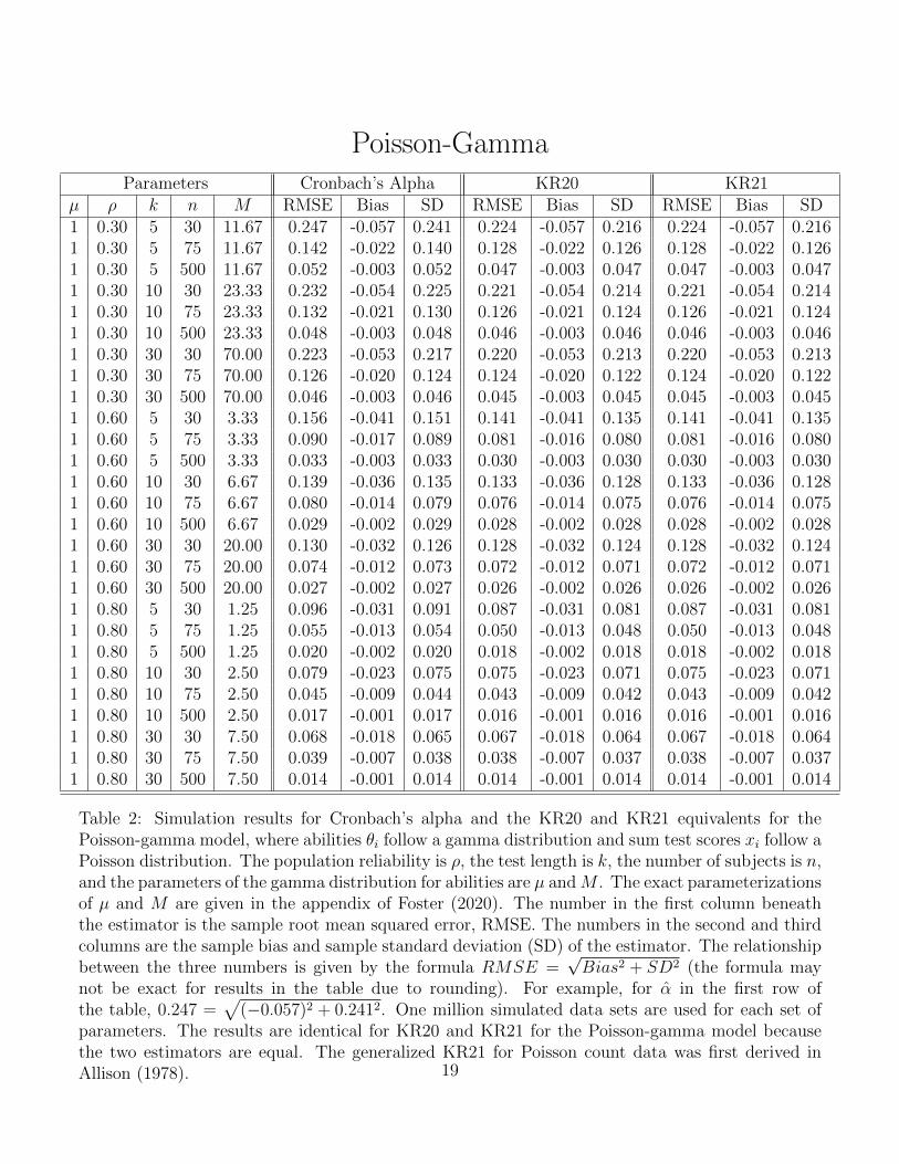
µ ρ k n M RMSE Bias SD RMSE Bias SD RMSE Bias SD1 0.30 5 30 11.67 0.247 -0.057 0.241 0.224 -0.057 0.216 0.224 -0.057 0.2161 0.30 5 75 11.67 0.142 -0.022 0.140 0.128 -0.022 0.126 0.128 -0.022 0.1261 0.30 5 500 11.67 0.052 -0.003 0.052 0.047 -0.003 0.047 0.047 -0.003 0.0471 0.30 10 30 23.33 0.232 -0.054 0.225 0.221 -0.054 0.214 0.221 -0.054 0.2141 0.30 10 75 23.33 0.132 -0.021 0.130 0.126 -0.021 0.124 0.126 -0.021 0.1241 0.30 10 500 23.33 0.048 -0.003 0.048 0.046 -0.003 0.046 0.046 -0.003 0.0461 0.30 30 30 70.00 0.223 -0.053 0.217 0.220 -0.053 0.213 0.220 -0.053 0.2131 0.30 30 75 70.00 0.126 -0.020 0.124 0.124 -0.020 0.122 0.124 -0.020 0.1221 0.30 30 500 70.00 0.046 -0.003 0.046 0.045 -0.003 0.045 0.045 -0.003 0.0451 0.60 5 30 3.33 0.156 -0.041 0.151 0.141 -0.041 0.135 0.141 -0.041 0.1351 0.60 5 75 3.33 0.090 -0.017 0.089 0.081 -0.016 0.080 0.081 -0.016 0.0801 0.60 5 500 3.33 0.033 -0.003 0.033 0.030 -0.003 0.030 0.030 -0.003 0.0301 0.60 10 30 6.67 0.139 -0.036 0.135 0.133 -0.036 0.128 0.133 -0.036 0.1281 0.60 10 75 6.67 0.080 -0.014 0.079 0.076 -0.014 0.075 0.076 -0.014 0.0751 0.60 10 500 6.67 0.029 -0.002 0.029 0.028 -0.002 0.028 0.028 -0.002 0.0281 0.60 30 30 20.00 0.130 -0.032 0.126 0.128 -0.032 0.124 0.128 -0.032 0.1241 0.60 30 75 20.00 0.074 -0.012 0.073 0.072 -0.012 0.071 0.072 -0.012 0.0711 0.60 30 500 20.00 0.027 -0.002 0.027 0.026 -0.002 0.026 0.026 -0.002 0.0261 0.80 5 30 1.25 0.096 -0.031 0.091 0.087 -0.031 0.081 0.087 -0.031 0.0811 0.80 5 75 1.25 0.055 -0.013 0.054 0.050 -0.013 0.048 0.050 -0.013 0.0481 0.80 5 500 1.25 0.020 -0.002 0.020 0.018 -0.002 0.018 0.018 -0.002 0.0181 0.80 10 30 2.50 0.079 -0.023 0.075 0.075 -0.023 0.071 0.075 -0.023 0.0711 0.80 10 75 2.50 0.045 -0.009 0.044 0.043 -0.009 0.042 0.043 -0.009 0.0421 0.80 10 500 2.50 0.017 -0.001 0.017 0.016 -0.001 0.016 0.016 -0.001 0.0161 0.80 30 30 7.50 0.068 -0.018 0.065 0.067 -0.018 0.064 0.067 -0.018 0.0641 0.80 30 75 7.50 0.039 -0.007 0.038 0.038 -0.007 0.037 0.038 -0.007 0.0371 0.80 30 500 7.50 0.014 -0.001 0.014 0.014 -0.001 0.014 0.014 -0.001 0.014

Table 2: Simulation results for Cronbach’s alpha and the KR20 and KR21 equivalents for thePoisson-gamma model, where abilities θi follow a gamma distribution and sum test scores xi follow aPoisson distribution. The population reliability is ρ, the test length is k, the number of subjects is n,and the parameters of the gamma distribution for abilities are µ andM . The exact parameterizationsof µ and M are given in the appendix of Foster (2020). The number in the first column beneaththe estimator is the sample root mean squared error, RMSE. The numbers in the second and thirdcolumns are the sample bias and sample standard deviation (SD) of the estimator. The relationshipbetween the three numbers is given by the formula RMSE =

√Bias2 + SD2 (the formula may

not be exact for results in the table due to rounding). For example, for α in the first row ofthe table, 0.247 =

√(−0.057)2 + 0.2412. One million simulated data sets are used for each set of

parameters. The results are identical for KR20 and KR21 for the Poisson-gamma model becausethe two estimators are equal. The generalized KR21 for Poisson count data was first derived inAllison (1978). 19

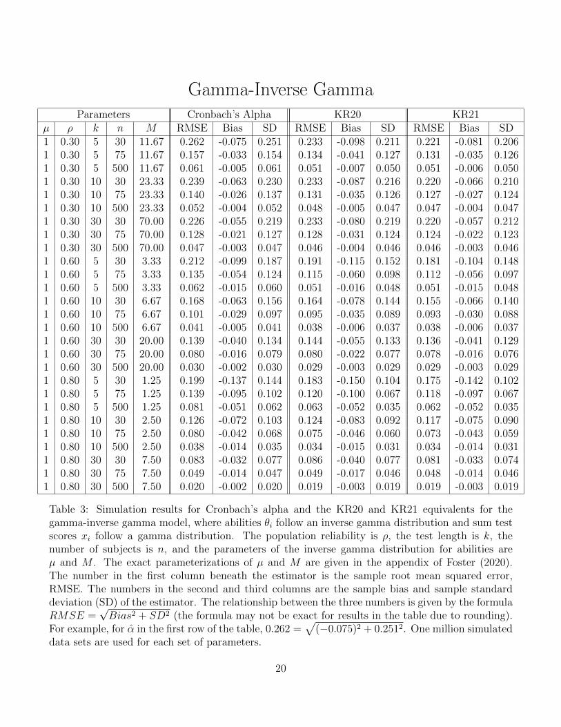
Gamma-Inverse GammaParameters Cronbach’s Alpha KR20 KR21

µ ρ k n M RMSE Bias SD RMSE Bias SD RMSE Bias SD1 0.30 5 30 11.67 0.262 -0.075 0.251 0.233 -0.098 0.211 0.221 -0.081 0.2061 0.30 5 75 11.67 0.157 -0.033 0.154 0.134 -0.041 0.127 0.131 -0.035 0.1261 0.30 5 500 11.67 0.061 -0.005 0.061 0.051 -0.007 0.050 0.051 -0.006 0.0501 0.30 10 30 23.33 0.239 -0.063 0.230 0.233 -0.087 0.216 0.220 -0.066 0.2101 0.30 10 75 23.33 0.140 -0.026 0.137 0.131 -0.035 0.126 0.127 -0.027 0.1241 0.30 10 500 23.33 0.052 -0.004 0.052 0.048 -0.005 0.047 0.047 -0.004 0.0471 0.30 30 30 70.00 0.226 -0.055 0.219 0.233 -0.080 0.219 0.220 -0.057 0.2121 0.30 30 75 70.00 0.128 -0.021 0.127 0.128 -0.031 0.124 0.124 -0.022 0.1231 0.30 30 500 70.00 0.047 -0.003 0.047 0.046 -0.004 0.046 0.046 -0.003 0.0461 0.60 5 30 3.33 0.212 -0.099 0.187 0.191 -0.115 0.152 0.181 -0.104 0.1481 0.60 5 75 3.33 0.135 -0.054 0.124 0.115 -0.060 0.098 0.112 -0.056 0.0971 0.60 5 500 3.33 0.062 -0.015 0.060 0.051 -0.016 0.048 0.051 -0.015 0.0481 0.60 10 30 6.67 0.168 -0.063 0.156 0.164 -0.078 0.144 0.155 -0.066 0.1401 0.60 10 75 6.67 0.101 -0.029 0.097 0.095 -0.035 0.089 0.093 -0.030 0.0881 0.60 10 500 6.67 0.041 -0.005 0.041 0.038 -0.006 0.037 0.038 -0.006 0.0371 0.60 30 30 20.00 0.139 -0.040 0.134 0.144 -0.055 0.133 0.136 -0.041 0.1291 0.60 30 75 20.00 0.080 -0.016 0.079 0.080 -0.022 0.077 0.078 -0.016 0.0761 0.60 30 500 20.00 0.030 -0.002 0.030 0.029 -0.003 0.029 0.029 -0.003 0.0291 0.80 5 30 1.25 0.199 -0.137 0.144 0.183 -0.150 0.104 0.175 -0.142 0.1021 0.80 5 75 1.25 0.139 -0.095 0.102 0.120 -0.100 0.067 0.118 -0.097 0.0671 0.80 5 500 1.25 0.081 -0.051 0.062 0.063 -0.052 0.035 0.062 -0.052 0.0351 0.80 10 30 2.50 0.126 -0.072 0.103 0.124 -0.083 0.092 0.117 -0.075 0.0901 0.80 10 75 2.50 0.080 -0.042 0.068 0.075 -0.046 0.060 0.073 -0.043 0.0591 0.80 10 500 2.50 0.038 -0.014 0.035 0.034 -0.015 0.031 0.034 -0.014 0.0311 0.80 30 30 7.50 0.083 -0.032 0.077 0.086 -0.040 0.077 0.081 -0.033 0.0741 0.80 30 75 7.50 0.049 -0.014 0.047 0.049 -0.017 0.046 0.048 -0.014 0.0461 0.80 30 500 7.50 0.020 -0.002 0.020 0.019 -0.003 0.019 0.019 -0.003 0.019

Table 3: Simulation results for Cronbach’s alpha and the KR20 and KR21 equivalents for thegamma-inverse gamma model, where abilities θi follow an inverse gamma distribution and sum testscores xi follow a gamma distribution. The population reliability is ρ, the test length is k, thenumber of subjects is n, and the parameters of the inverse gamma distribution for abilities areµ and M . The exact parameterizations of µ and M are given in the appendix of Foster (2020).The number in the first column beneath the estimator is the sample root mean squared error,RMSE. The numbers in the second and third columns are the sample bias and sample standarddeviation (SD) of the estimator. The relationship between the three numbers is given by the formulaRMSE =

√Bias2 + SD2 (the formula may not be exact for results in the table due to rounding).

For example, for α in the first row of the table, 0.262 =√

(−0.075)2 + 0.2512. One million simulateddata sets are used for each set of parameters.

20

Negative Binomial - F

Parameters Cronbach’s Alpha KR20 KR21µ ρ k n M RMSE Bias SD RMSE Bias SD RMSE Bias SD

1.01 0.30 5 30 11.67 0.251 -0.067 0.242 0.220 -0.090 0.201 0.210 -0.073 0.1971.01 0.30 5 75 11.67 0.151 -0.028 0.149 0.126 -0.037 0.120 0.123 -0.030 0.1191.01 0.30 5 500 11.67 0.058 -0.005 0.058 0.047 -0.006 0.047 0.047 -0.005 0.0471.01 0.30 10 30 23.33 0.235 -0.061 0.227 0.228 -0.084 0.212 0.215 -0.064 0.2061.01 0.30 10 75 23.33 0.137 -0.024 0.135 0.127 -0.033 0.123 0.124 -0.025 0.1221.01 0.30 10 500 23.33 0.051 -0.004 0.051 0.046 -0.005 0.046 0.046 -0.004 0.0461.01 0.30 30 30 70.00 0.225 -0.055 0.218 0.232 -0.080 0.218 0.219 -0.057 0.2121.01 0.30 30 75 70.00 0.128 -0.021 0.126 0.128 -0.031 0.124 0.124 -0.022 0.1221.01 0.30 30 500 70.00 0.047 -0.003 0.047 0.046 -0.005 0.046 0.046 -0.003 0.0451.01 0.60 5 30 3.33 0.164 -0.053 0.155 0.132 -0.068 0.113 0.125 -0.058 0.1111.01 0.60 5 75 3.33 0.103 -0.024 0.100 0.076 -0.030 0.070 0.074 -0.026 0.0691.01 0.60 5 500 3.33 0.042 -0.004 0.042 0.029 -0.005 0.029 0.029 -0.005 0.0291.01 0.60 10 30 6.67 0.142 -0.043 0.136 0.135 -0.058 0.122 0.128 -0.046 0.1191.01 0.60 10 75 6.67 0.085 -0.018 0.083 0.077 -0.024 0.073 0.075 -0.019 0.0721.01 0.60 10 500 6.67 0.032 -0.003 0.032 0.028 -0.004 0.028 0.028 -0.003 0.0281.01 0.60 30 30 20.00 0.132 -0.036 0.127 0.136 -0.050 0.126 0.128 -0.037 0.1221.01 0.60 30 75 20.00 0.076 -0.014 0.074 0.075 -0.019 0.073 0.073 -0.014 0.0721.01 0.60 30 500 20.00 0.028 -0.002 0.028 0.027 -0.003 0.027 0.027 -0.002 0.0271.01 0.80 5 30 1.25 0.114 -0.032 0.109 0.064 -0.043 0.048 0.060 -0.038 0.0461.01 0.80 5 75 1.25 0.080 -0.014 0.079 0.029 -0.018 0.022 0.027 -0.016 0.0221.01 0.80 5 500 1.25 0.042 -0.003 0.042 0.009 -0.004 0.009 0.009 -0.003 0.0091.01 0.80 10 30 2.50 0.075 -0.026 0.070 0.065 -0.035 0.055 0.061 -0.029 0.0531.01 0.80 10 75 2.50 0.047 -0.012 0.045 0.037 -0.015 0.033 0.035 -0.013 0.0331.01 0.80 10 500 2.50 0.019 -0.002 0.019 0.014 -0.003 0.014 0.014 -0.002 0.0141.01 0.80 30 30 7.50 0.066 -0.020 0.063 0.068 -0.027 0.062 0.063 -0.021 0.0601.01 0.80 30 75 7.50 0.038 -0.008 0.038 0.038 -0.011 0.036 0.037 -0.008 0.0361.01 0.80 30 500 7.50 0.014 -0.001 0.014 0.014 -0.002 0.014 0.014 -0.001 0.014

Table 4: Simulation results for Cronbach’s alpha and the KR20 and KR21 equivalents for thenegative binomial - F model, where abilities θi follow an F distribution and sum test scores xi followa negative binomial distribution. The population reliability is equal to ρ, the test length is k, thenumber of subjects is n, and the parameters of the F distribution for abilities are µ and M . The exactparameterizations of µ and M are given in the appendix of Foster (2020). The number in the firstcolumn beneath the estimator is the sample root mean squared error, RMSE. The numbers in thesecond and third columns are the sample bias and sample standard deviation (SD) of the estimator.The relationship between the three numbers is given by the formula RMSE =

√Bias2 + SD2 (the

formula may not be exact for results in the table due to rounding). For example, for α in the firstrow of the table, 0.251 =

√(−0.067)2 + 0.2422. One million simulated data sets are used for each

set of parameters.

21

Binomial-BetaParameters Cronbach’s Alpha KR20 KR21

µ ρ k n M RMSE Bias SD RMSE Bias SD RMSE Bias SD0.50 0.30 5 30 11.67 0.240 -0.048 0.235 0.228 -0.015 0.228 0.238 -0.039 0.2350.50 0.30 5 75 11.67 0.136 -0.018 0.135 0.133 -0.005 0.133 0.136 -0.015 0.1350.50 0.30 5 500 11.67 0.050 -0.003 0.050 0.050 -0.001 0.050 0.050 -0.002 0.0500.50 0.30 10 30 23.33 0.229 -0.050 0.223 0.217 -0.021 0.216 0.228 -0.046 0.2230.50 0.30 10 75 23.33 0.129 -0.019 0.128 0.126 -0.008 0.126 0.129 -0.017 0.1270.50 0.30 10 500 23.33 0.047 -0.003 0.047 0.047 -0.001 0.047 0.047 -0.002 0.0470.50 0.30 30 30 70.00 0.221 -0.051 0.216 0.210 -0.025 0.208 0.221 -0.050 0.2150.50 0.30 30 75 70.00 0.125 -0.019 0.124 0.122 -0.009 0.122 0.125 -0.019 0.1240.50 0.30 30 500 70.00 0.045 -0.003 0.045 0.045 -0.001 0.045 0.045 -0.003 0.0450.50 0.60 5 30 3.33 0.134 -0.023 0.132 0.127 -0.001 0.127 0.132 -0.015 0.1310.50 0.60 5 75 3.33 0.077 -0.009 0.077 0.076 0.000 0.076 0.077 -0.005 0.0770.50 0.60 5 500 3.33 0.028 -0.001 0.028 0.028 0.000 0.028 0.028 -0.001 0.0280.50 0.60 10 30 6.67 0.127 -0.025 0.124 0.121 -0.007 0.120 0.126 -0.022 0.1240.50 0.60 10 75 6.67 0.072 -0.009 0.072 0.071 -0.003 0.071 0.072 -0.008 0.0720.50 0.60 10 500 6.67 0.026 -0.001 0.026 0.026 0.000 0.026 0.026 -0.001 0.0260.50 0.60 30 30 20.00 0.125 -0.028 0.122 0.118 -0.012 0.118 0.125 -0.026 0.1220.50 0.60 30 75 20.00 0.071 -0.010 0.070 0.069 -0.004 0.069 0.071 -0.010 0.0700.50 0.60 30 500 20.00 0.026 -0.001 0.026 0.026 -0.001 0.026 0.026 -0.001 0.0260.50 0.80 5 30 1.25 0.068 -0.009 0.067 0.065 0.006 0.065 0.067 -0.001 0.0670.50 0.80 5 75 1.25 0.040 -0.003 0.040 0.039 0.003 0.039 0.040 0.000 0.0400.50 0.80 5 500 1.25 0.015 0.000 0.015 0.015 0.000 0.015 0.015 0.000 0.0150.50 0.80 10 30 2.50 0.061 -0.010 0.061 0.059 0.000 0.059 0.061 -0.007 0.0600.50 0.80 10 75 2.50 0.036 -0.004 0.035 0.035 0.000 0.035 0.035 -0.002 0.0350.50 0.80 10 500 2.50 0.013 -0.001 0.013 0.013 0.000 0.013 0.013 0.000 0.0130.50 0.80 30 30 7.50 0.061 -0.012 0.059 0.057 -0.004 0.057 0.060 -0.011 0.0590.50 0.80 30 75 7.50 0.034 -0.005 0.034 0.034 -0.001 0.034 0.034 -0.004 0.0340.50 0.80 30 500 7.50 0.013 -0.001 0.013 0.013 0.000 0.013 0.013 -0.001 0.013

Table 5: Simulation results for Cronbach’s alpha and KR20 and KR21 for the binomial - beta model,where abilities θi follow a beta distribution and sum test scores xi follow a binomial distribution.The population reliability is equal to ρ, the test length is k, the number of subjects is n, and theparameters of the beta distribution for abilities are µ and M . The exact parameterizations of µand M are given in the appendix of Foster (2020). The number in the first column beneath theestimator is the sample root mean squared error, RMSE. The numbers in the second and thirdcolumns are the sample bias and sample standard deviation (SD) of the estimator. The relationshipbetween the three numbers is given by the formula RMSE =

√Bias2 + SD2 (the formula may

not be exact for results in the table due to rounding). For example, for α in the first row ofthe table, 0.240 =

√(−0.048)2 + 0.2352. One million simulated data sets are used for each set of

parameters. The KR20 and KR21 estimators for this model are the traditional ones derived inKuder and Richardson (1937).

22

Parameters ωH ωT KR21Model µ ρ k n M RMSE Bias SD RMSE Bias SD RMSE Bias SDP-G 1 0.80 5 30 1.25 0.201 -0.153 0.130 0.090 0.061 0.066 0.087 -0.031 0.081P-G 1 0.80 10 30 2.50 0.310 -0.281 0.131 0.077 0.050 0.059 0.075 -0.023 0.071P-G 1 0.80 5 75 1.25 0.145 -0.114 0.088 0.060 0.041 0.045 0.050 -0.013 0.048P-G 1 0.80 10 75 2.50 0.250 -0.230 0.096 0.053 0.039 0.036 0.043 -0.009 0.042G-IG 1 0.80 5 30 1.25 0.309 -0.248 0.183 0.116 0.034 0.110 0.175 -0.142 0.102G-IG 1 0.80 10 30 2.50 0.355 -0.317 0.159 0.090 0.035 0.083 0.118 -0.076 0.090G-IG 1 0.80 5 75 1.25 0.270 -0.221 0.156 0.091 0.030 0.085 0.118 -0.097 0.066G-IG 1 0.80 10 75 2.50 0.331 -0.306 0.124 0.068 0.035 0.059 0.073 -0.043 0.059B-B 0.5 0.80 5 30 1.25 0.173 -0.135 0.108 0.084 0.066 0.052 0.067 -0.001 0.067B-B 0.5 0.80 10 30 2.50 0.296 -0.272 0.118 0.073 0.055 0.048 0.061 -0.007 0.061B-B 0.5 0.80 5 75 1.25 0.124 -0.101 0.071 0.054 0.041 0.035 0.040 0.000 0.040B-B 0.5 0.80 10 75 2.50 0.231 -0.215 0.084 0.049 0.040 0.029 0.035 -0.002 0.035

Table 6: Simulation results for the KR21 equivalent for the Poisson-gamma (P-G), gamma - inversegamma (I-G), and binomial-beta (B-B) models compared to omega hierarchical and omega total, ωH

and ωT , as measured by root mean squared error. The omega reliability calculations are performedby the psych package in R (Revelle, 2020). The number in the first column beneath the estimatoris the sample root mean squared error, RMSE. The numbers in the second and third columns arethe sample bias and sample standard deviation (SD) of the estimator. The relationship betweenthe three numbers is given by the formula RMSE =

√Bias2 + SD2 (the formula may not be

exact for results in the table due to rounding). For example, for ωH in the first row of the table,0.201 =

√(−0.153)2 + 0.1302. One million simulated data sets are used for each set of parameters.

Subject 0-10 10-20 20-30 30-40 40-50 50-60 60-70 70-80 80-90 xi1kxi s2

1 13 10 12 8 12 10 9 16 8 98 10.89 6.862 14 9 9 13 10 10 14 9 11 99 11.00 4.503 11 10 5 12 12 8 12 11 5 86 9.56 4.504 12 13 4 8 7 10 14 1 14 83 9.22 21.195 16 8 9 7 11 12 16 8 11 98 10.89 11.116 11 13 7 8 9 7 8 7 4 74 8.22 6.697 13 11 10 9 15 9 18 10 5 100 11.11 14.368 11 5 9 9 9 13 11 15 6 88 9.78 9.949 13 8 10 11 11 12 8 7 4 84 9.33 8.0010 12 9 12 9 14 8 12 10 7 93 10.33 5.25

Table 7: Data from Moore (1970) showing the count of the number of responses for each of tensubjects in consecutive intervals of transformed time. This data may be treated as a Poisson process,where each response is a realization of a Poisson random variable with mean given by a subject’sability θi.

23

Figure 1: Difference in RMSE (Alpha - KR21) for tests of different lengths for the poisson-gammamodel with ρ = 0.3, grouped by number of subjects. The plot clearly shows that α has a largerRMSE than KR21, but this effect decreases towards zero as both the test length k and number ofsubjects n increases. The data in this plot are from Table 2.

24

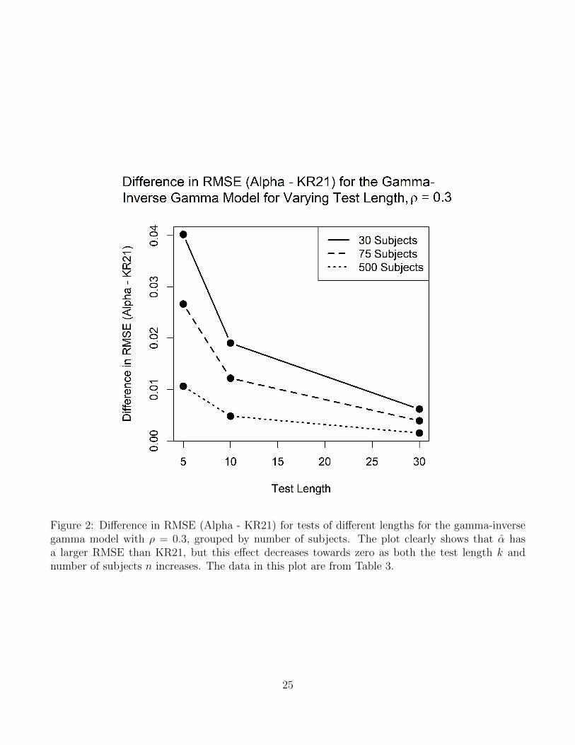
Figure 2: Difference in RMSE (Alpha - KR21) for tests of different lengths for the gamma-inversegamma model with ρ = 0.3, grouped by number of subjects. The plot clearly shows that α hasa larger RMSE than KR21, but this effect decreases towards zero as both the test length k andnumber of subjects n increases. The data in this plot are from Table 3.

25

Figure 3: Difference in RMSE (Alpha - KR21) for tests of different lengths for the negative binomial-F model with ρ = 0.3, grouped by number of subjects. The plot clearly shows that α has a largerRMSE than KR21, but this effect decreases towards zero as both the test length k and number ofsubjects n increases. The data in this plot are from Table 4.

26

Figure 4: Difference in RMSE (Alpha - KR21) for tests of different lengths for the binomial-betamodel with ρ = 0.3, grouped by number of subjects. The plot clearly shows that α has a largerRMSE than KR21, but this effect decreases towards zero as both the test length k and number ofsubjects n increases. The data in this plot are from Table 5.

27

References

Allison, P. D. (1978). The reliability of variables measured as the number of eventsin an interval of time. Sociological Methodology , 9 , 238 –253.

Bay, K. S. (1973). The effect of non-normality on the sampling distribution ofstandard error of reliability coefficient estimates under an analysis of variancemodel. British Journal of Mathematical and Statistical Psychology , 26 (1), 45-57.

Casella, G., & Berger, R. (2002). Statistical inference, second edition. DuxburyPress.

Cronbach, L. J. (1951, September). Coefficient alpha and the internal structure oftests. Psychometrika, 16 (3), 297 – 334.

Feldt, L. J. (1984). Some relationships between the binomial error model and classicaltest theory. Educational and Psychological Measurement , 44 (4), 883 – 891.

Feldt, L. S. (1965, September). The approximate sampling distribution of kuder-richardson reliability coefficient twenty. Psychometrika, 30 (3), 357 – 370.

Foster, R. C. (2020, June). A generalized framework for classical test theory. TheJournal of Mathematical Psychology , 96 .

Geldhof, G. J., Preacher, K. J., & Zyphur, M. J. (2014). Reliability estimation ina multilevel confirmatory factor analysis framework. Psychological Methods ,19 (1), 72-91.

Hayes, A. F., & Coutts, J. J. (2020). Use omega rather than cronbach’s alpha forestimating reliability. but. . . . Communication Methods and Measures , 14 (1),1-24.

Huynh, H. (1979). Statistical inference for two reliability indices in mastery testingbased on the beta-binomial model. Journal of Educational Statistics , 4 (3),231-246.

Keats, J. A., & Lord, F. M. (1962, March). A theoretical distribution for mental testscores. Psychometrika, 27 (1), 59 – 72.

Kuder, G. F., & Richardson, M. W. (1937). The theory of the estimation of testreliability. Psychometrika, 2 (3), 151 – 160.

Lord, F. M. (1965, September). A strong true-score theory, with applications. Psy-chometrika, 30 (3), 239 – 270.

Lord, F. M., Novick, M. R., & Birnbaum, A. (1968). Statistical theories of mentaltest scores. Oxford, England: Addison-Wesley.

McDonald, R. (1999). Test theory: A unified treatment. Taylor & Francis.McNeish, D. (2018). Thanks coefficient alpha, we’ll take it from here. Psychological

Methods , 23 (3), 412-433.Meredith, W. (1971, 08). Poisson distributions of error in mental test theory. British

Journal of Mathematical and Statistical Psychology , 24 , 49 - 82.Moore, W. E. (1970, November). Stochastic processes as true-score models for highly

speeded mental tests (Tech. Rep.). Princeton, New Jersey: Educational Testing

28

Service.Morris, C. N. (1982). Natural exponential families with quadratic variance functions.

The Annals of Statistics , 10 (1), 65 – 80.Morris, C. N. (1983). Natural exponential families with quadratic variance functions:

Statistical theory. The Annals of Statistics , 11 (2), 515 – 529.Rasch, G. (1960). Probabilistic models for some intelligence and attainment tests.

Danmarks Paedagogiske Institut.Raykov, T. (1998). A method for obtaining standard errors and confidence intervals of

composite reliability for congeneric items. Applied Psychological Measurement ,22 (4), 369-374.

Raykov, T., & Marcoulides, G. A. (2019). Thanks coefficient alpha, we still need you!Educational and Psychological Measurement , 79 (1), 200-210.

Revelle, W. (2020). psych: Procedures for psychological, psychometric, and person-ality research [Computer software manual]. Evanston, Illinois. Retrieved fromhttps://CRAN.R-project.org/package=psych (R package version 2.0.12)

Revelle, W., & Zinbarg, R. (2009, 03). Coefficients alpha, beta, omega, and the glb:Comments on sijtsma. Psychometrika, 74 , 145-154.

Savalei, V., & Reise, S. P. (2019). Don’t forget the model in your model-basedreliability coefficients: A reply to mcneish (2018). Collabra:Psychology , 5 (1).

Schmitt, N. (1996). Uses and abuses of coefficient alpha. Psychological Assessment ,8 , 350-353.

Sheng, Y., & Sheng, Z. (2012, February). Is coefficient alpha robust to non-normaldata? Frontiers in Psychology .

Sijtsma, K. (2009, 2009). On the use, the misuse, and the very limited usefulness ofcronbach’s alpha. Psychometrika, 74 (1), 107 – 120.

Trizano-Hermosilla, I., & Alvarado, J. (2016, 05). Best alternatives to cronbach’salpha reliability in realistic conditions: Congeneric and asymmetrical measure-ments. Frontiers in Psychology , 7 .

Zimmerman, D. W. (1972). Test reliability and the kuder-richardson formulas:Derivation from probability theory. Educational and Psychological Measure-ment , 32 (4), 939 – 954.

Zimmerman, D. W., Zumbo, B. D., & Lalonde, C. (1993). Coefficient alpha as anestimate of test reliability under violation of two assumptions. Educational andPsychological Measurement , 53 (1), 33-49.

Zinbarg, R., Yovel, I., Revelle, W., & McDonald, R. (2006, 03). Estimating generaliz-ability to a latent variable common to all of a scale’s indicators: A comparisonof estimators for ωh. Applied Psychological Measurement , 30 , 121-144.

Zumbo, B. (1999). A glance at coefficient alpha with an eye towards robustness studies: Some mathematical notes and a simulation model. (Paper No. ESQBS-99-1). Prince George, B.C.: University of Northern British Columbia. EdgeworthLaboratory for Quantitative Behavioural Science.

Zyl, J., Neudecker, H., & Nel, D. (2000, 09). On the distribution of the maximum

29

likelihood estimator of cronbach’s alpha. Psychometrika, 65 , 271-280.

30

Appendix

The elements of the variance-covariance matrices used in the simulations of Section 4 areeasily obtained through applying the formulas of Foster (2020). For an individual test itemyj or pair of test items yj,1, yj,2, the unconditional variance and covariance in this frameworkare

V ar(yj) = E[V (θi)] + V ar(θi) = V ar(θi)(M + 1) =

(V (µ)

M − v2

)(M + 1)

Cov(yj,1, yj,2) = V ar(θi) =V (µ)

M − v2

These equalities hold for all natural exponential family distributions except for the last line,which depends on the mean-variance relationship given in Equation (6) and holds only forthose with quadratic variance function, as discussed in this paper. The function V (µ) is thevariance function of the natural exponential family applied to the underlying populationmean, several of which are shown in Table 1, and v2 is the coefficient of the quadratic termof the quadratic variance function, as shown in Equation (1).

If the parameter M is defined by the desired population value of Cronbach’s alphaρ and test length k by the relation M = [(1−ρ)/ρ]k as in Section 4, these formulas reduce to

V ar(yj) = V (µ)

[(1− ρ)k + ρ

(1− ρ)k − ρv2

]Cov(yj,1, yj,2) = V (µ)

[ρ

(1− ρ)k − ρv2

]Within the variance-covariance matrix, all test items have identical variances and all covari-ances between them are equal. The variances and covariance for the simulations in Section4 are as follows.

Poisson-Gamma

For the Poisson-gamma model, the variance function is V (θ) = θ with v2 = 0. This yieldsvariance and covariance elements as

V ar(yj) =µ

M(M + 1)

Cov(yj,1, yj,2) =µ

M

31

ρ k µ M V (yj) Cov(yj,1, yj,2)

0.3 5 1 11.67 1.0857 0.08570.3 10 1 23.33 1.0429 0.04290.3 30 1 70 1.0143 0.01430.6 5 1 3.33 1.3 0.30.6 10 1 6.67 1.15 0.150.6 30 1 20 1.05 0.050.8 5 1 1.25 1.8 0.80.8 10 1 2.5 1.4 0.40.8 30 1 7.5 1.1333 0.1333

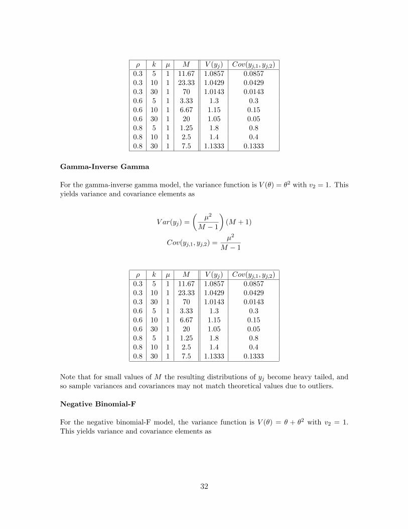
Gamma-Inverse Gamma

For the gamma-inverse gamma model, the variance function is V (θ) = θ2 with v2 = 1. Thisyields variance and covariance elements as

V ar(yj) =

(µ2

M − 1

)(M + 1)

Cov(yj,1, yj,2) =µ2

M − 1

ρ k µ M V (yj) Cov(yj,1, yj,2)

0.3 5 1 11.67 1.0857 0.08570.3 10 1 23.33 1.0429 0.04290.3 30 1 70 1.0143 0.01430.6 5 1 3.33 1.3 0.30.6 10 1 6.67 1.15 0.150.6 30 1 20 1.05 0.050.8 5 1 1.25 1.8 0.80.8 10 1 2.5 1.4 0.40.8 30 1 7.5 1.1333 0.1333

Note that for small values of M the resulting distributions of yj become heavy tailed, andso sample variances and covariances may not match theoretical values due to outliers.

Negative Binomial-F

For the negative binomial-F model, the variance function is V (θ) = θ + θ2 with v2 = 1.This yields variance and covariance elements as

32

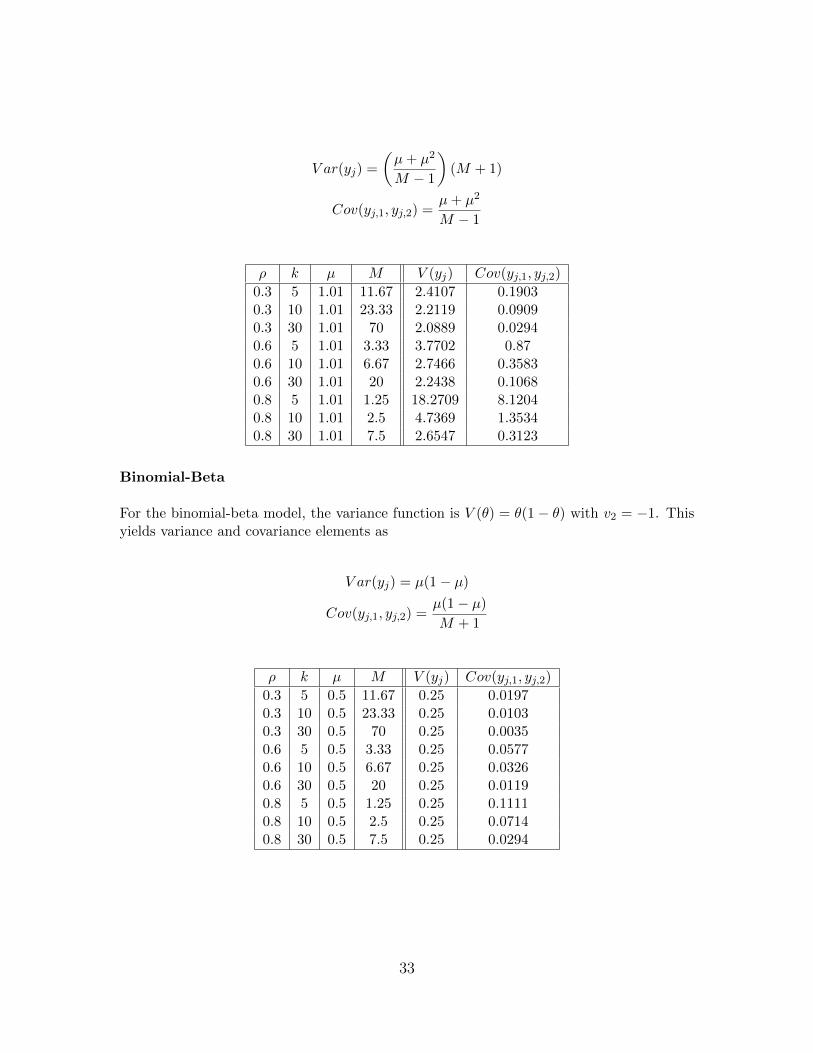
V ar(yj) =

(µ+ µ2

M − 1

)(M + 1)

Cov(yj,1, yj,2) =µ+ µ2

M − 1

ρ k µ M V (yj) Cov(yj,1, yj,2)

0.3 5 1.01 11.67 2.4107 0.19030.3 10 1.01 23.33 2.2119 0.09090.3 30 1.01 70 2.0889 0.02940.6 5 1.01 3.33 3.7702 0.870.6 10 1.01 6.67 2.7466 0.35830.6 30 1.01 20 2.2438 0.10680.8 5 1.01 1.25 18.2709 8.12040.8 10 1.01 2.5 4.7369 1.35340.8 30 1.01 7.5 2.6547 0.3123

Binomial-Beta

For the binomial-beta model, the variance function is V (θ) = θ(1− θ) with v2 = −1. Thisyields variance and covariance elements as

V ar(yj) = µ(1− µ)

Cov(yj,1, yj,2) =µ(1− µ)

M + 1

ρ k µ M V (yj) Cov(yj,1, yj,2)

0.3 5 0.5 11.67 0.25 0.01970.3 10 0.5 23.33 0.25 0.01030.3 30 0.5 70 0.25 0.00350.6 5 0.5 3.33 0.25 0.05770.6 10 0.5 6.67 0.25 0.03260.6 30 0.5 20 0.25 0.01190.8 5 0.5 1.25 0.25 0.11110.8 10 0.5 2.5 0.25 0.07140.8 30 0.5 7.5 0.25 0.0294

33