KNOWING WHO TO TRUST AND WHAT TO BELIEVEIN THE PRESENCE OF CONFLICTING INFORMATION

BY

JEFFREY WILLIAM PASTERNACK

DISSERTATION

Submitted in partial fulfillment of the requirementsfor the degree of Doctor of Philosophy in Computer Science

in the Graduate College of theUniversity of Illinois at Urbana-Champaign, 2011

Urbana, Illinois

Doctoral Committee:

Professor Dan Roth, Chair & Director of ResearchProfessor Yolanda Gil, University of Southern CaliforniaProfessor Jiawei HanProfessor ChengXiang Zhai

Abstract

The Information Age has created an increasing abundance of data and has, thanks to the rise of

the Internet, made that knowledge instantly available to humans and computers alike. This is not

without caveats, however, as though we may read a document, ask an expert, or locate a fact nearly

effortlessly, we lack a ready means to determine whether we should actually believe them.

We seek to address this problem with a computational trust system capable of substituting for

the user’s informed, subjective judgement, with the understanding that truth is not objective and

instead depends upon one’s prior knowledge and beliefs, a philosophical point with deep practical

implications.

First, however, we must consider the even more basic question of how the trustworthiness of

an information source can be expressed: measuring the trustworthiness of a person, document,

or publisher as the mere percentage of true claims it makes can be extraordinarily misleading

at worst, and uninformative at best. Instead of providing simple accuracy, we instead provide a

comprehensive set of trust metrics, calculating the source’s truthfulness, completeness, and bias,

providing the user with our trust judgement in a way that is both understandable and actionable.

We then consider the trust algorithm itself, starting with the baseline of determining the truth

by taking a simple vote that assumes all information sources are equally trustworthy, and quickly

move on to fact-finders, iterative algorithms capable of estimating the trustworthiness of the source

in addition to the believability of the claims, and proceed to incorporate increasing amounts of

information and declarative prior knowledge into the fact-finder’s trust decision via the General-

ized and Constrained Fact-Finding frameworks while still maintaining the relative simplicity and

tractability of standard fact-finders.

ii

Ultimately, we introduce Latent Trust Analysis, a new type of probabilistic trust model that

provides the first strongly principled view of information trust and a wide array of advantages over

preceding methods, with a semantically crisp generative story that explains how sources “generate”

their assertions in claims. Such explanations can be used to justify trust decisions to the user,

and, moreover, the transparent mechanics make the models highly flexible, e.g. by applying reg-

ularization via Bayesian prior probabilities. Furthermore, as probabilistic models they naturally

support semi-supervised and supervised learning when the truth of some claims or the trustworthi-

ness of sources is already known, unlike fact-finders which are perform only unsupervised learning.

Finally, with Generalized Constrained Models, a new structured learning technique, we can ap-

ply declarative prior knowledge to Latent Trust Analysis models just as we can with Constrained

Fact-Finding.

Together, these trust algorithms create a spectrum of approaches that trade increasing com-

plexity for greater information utilization, performance, and flexibility, although even the most

sophisticated Latent Trust Analysis model remains tractable on a web-scale dataset. As our trust

algorithms improve our ability to separate the wheat from the chaff, the curse of modern “informa-

tion overload” may become a blessing after all.

iii

Acknowledgements

Thank you to my parents, Kathleen and Barry Pasternack, for their generous support over theyears, although given the technology work items that they queue for me between visits I am fairlycertain that they believe “Doctor of Computer Science” means “Computer Surgeon” (I do, however,enjoy counseling people to “take 2GB of RAM and call me in the morning”). I would also like tothank my advisor, Dan Roth, to whom I am especially grateful for providing invaluable guidancethroughout my (extensive) time as a graduate student, and the rest of my committee, Yolanda Gil,Jiawei Han, and Cheng Zhai, all of whom have provided insightful comments and feedback (withspecial thanks to Yolanda for her detailed help in improving this document). Finally, thanks to thefellow students of my research group, with whom I have shared many enjoyable discussions, bothfanciful and pragmatic, along with a variety of other misadventures.

iv

Table of Contents

Chapter 1 Introduction . . . . . . . . . . . . . . . . . . . . . . . . . . . . . . . . . . 11.1 Background . . . . . . . . . . . . . . . . . . . . . . . . . . . . . . . . . . . . . . . . . 31.2 Overview . . . . . . . . . . . . . . . . . . . . . . . . . . . . . . . . . . . . . . . . . . 5

Chapter 2 Survey of Computational Trust . . . . . . . . . . . . . . . . . . . . . . . 92.1 Policy-based . . . . . . . . . . . . . . . . . . . . . . . . . . . . . . . . . . . . . . . . . 92.2 Theoretical . . . . . . . . . . . . . . . . . . . . . . . . . . . . . . . . . . . . . . . . . 102.3 Reputation-based . . . . . . . . . . . . . . . . . . . . . . . . . . . . . . . . . . . . . . 122.4 User-driven . . . . . . . . . . . . . . . . . . . . . . . . . . . . . . . . . . . . . . . . . 14

2.4.1 Databases . . . . . . . . . . . . . . . . . . . . . . . . . . . . . . . . . . . . . . 152.4.2 Structured User Analysis . . . . . . . . . . . . . . . . . . . . . . . . . . . . . 152.4.3 Provenance Systems . . . . . . . . . . . . . . . . . . . . . . . . . . . . . . . . 15

2.5 Information-based . . . . . . . . . . . . . . . . . . . . . . . . . . . . . . . . . . . . . 162.5.1 Identifying Source Dependence . . . . . . . . . . . . . . . . . . . . . . . . . . 162.5.2 Fact-Finding . . . . . . . . . . . . . . . . . . . . . . . . . . . . . . . . . . . . 172.5.3 Specialized Information-based Systems . . . . . . . . . . . . . . . . . . . . . . 18

2.6 Information Filtering and Recommender Systems . . . . . . . . . . . . . . . . . . . . 182.7 Conclusion . . . . . . . . . . . . . . . . . . . . . . . . . . . . . . . . . . . . . . . . . 20

Chapter 3 Comprehensive Trust Metrics . . . . . . . . . . . . . . . . . . . . . . . . 223.1 Summary . . . . . . . . . . . . . . . . . . . . . . . . . . . . . . . . . . . . . . . . . . 223.2 Introduction . . . . . . . . . . . . . . . . . . . . . . . . . . . . . . . . . . . . . . . . . 223.3 Background . . . . . . . . . . . . . . . . . . . . . . . . . . . . . . . . . . . . . . . . . 24

3.3.1 Homogenous (Reputation) Networks . . . . . . . . . . . . . . . . . . . . . . . 243.3.2 Heterogeneous Networks . . . . . . . . . . . . . . . . . . . . . . . . . . . . . . 25

3.4 The Metrics . . . . . . . . . . . . . . . . . . . . . . . . . . . . . . . . . . . . . . . . . 263.4.1 The Components of Trustworthiness . . . . . . . . . . . . . . . . . . . . . . . 263.4.2 Truthfulness . . . . . . . . . . . . . . . . . . . . . . . . . . . . . . . . . . . . 273.4.3 Completeness . . . . . . . . . . . . . . . . . . . . . . . . . . . . . . . . . . . . 273.4.4 Bias . . . . . . . . . . . . . . . . . . . . . . . . . . . . . . . . . . . . . . . . . 283.4.5 From Collections to Sources . . . . . . . . . . . . . . . . . . . . . . . . . . . . 293.4.6 Relativity . . . . . . . . . . . . . . . . . . . . . . . . . . . . . . . . . . . . . . 29

3.5 User Study . . . . . . . . . . . . . . . . . . . . . . . . . . . . . . . . . . . . . . . . . 293.5.1 The Article . . . . . . . . . . . . . . . . . . . . . . . . . . . . . . . . . . . . . 29

v

3.5.2 Setup . . . . . . . . . . . . . . . . . . . . . . . . . . . . . . . . . . . . . . . . 303.5.3 Overall Trustworthiness Assessments . . . . . . . . . . . . . . . . . . . . . . . 303.5.4 The Claims . . . . . . . . . . . . . . . . . . . . . . . . . . . . . . . . . . . . . 323.5.5 Calculated Metrics . . . . . . . . . . . . . . . . . . . . . . . . . . . . . . . . . 333.5.6 User Metric Preference . . . . . . . . . . . . . . . . . . . . . . . . . . . . . . . 34

3.6 Conclusion . . . . . . . . . . . . . . . . . . . . . . . . . . . . . . . . . . . . . . . . . 35

Chapter 4 Standard, Generalized, and Constrained Fact-Finders . . . . . . . . . 364.1 Summary . . . . . . . . . . . . . . . . . . . . . . . . . . . . . . . . . . . . . . . . . . 364.2 Introduction . . . . . . . . . . . . . . . . . . . . . . . . . . . . . . . . . . . . . . . . . 374.3 Related Work . . . . . . . . . . . . . . . . . . . . . . . . . . . . . . . . . . . . . . . . 38

4.3.1 Theoretical . . . . . . . . . . . . . . . . . . . . . . . . . . . . . . . . . . . . . 384.3.2 Fact-Finders . . . . . . . . . . . . . . . . . . . . . . . . . . . . . . . . . . . . 394.3.3 Comparison to Other Trust Mechanisms . . . . . . . . . . . . . . . . . . . . . 39

4.4 Fact-Finding . . . . . . . . . . . . . . . . . . . . . . . . . . . . . . . . . . . . . . . . 404.4.1 Priors . . . . . . . . . . . . . . . . . . . . . . . . . . . . . . . . . . . . . . . . 414.4.2 Fact-Finding Algorithms . . . . . . . . . . . . . . . . . . . . . . . . . . . . . . 42

4.5 Generalized Fact-Finding . . . . . . . . . . . . . . . . . . . . . . . . . . . . . . . . . 444.5.1 Encoding Information in Weighted Assertions . . . . . . . . . . . . . . . . . . 444.5.2 Rewriting Fact-Finders for Assertion Weights . . . . . . . . . . . . . . . . . . 474.5.3 Groups and Attributes as Layers . . . . . . . . . . . . . . . . . . . . . . . . . 50

4.6 Constrained Fact-Finding . . . . . . . . . . . . . . . . . . . . . . . . . . . . . . . . . 524.6.1 Propositional Linear Programming . . . . . . . . . . . . . . . . . . . . . . . . 534.6.2 The Cost Function . . . . . . . . . . . . . . . . . . . . . . . . . . . . . . . . . 544.6.3 From Values to Votes to Belief . . . . . . . . . . . . . . . . . . . . . . . . . . 554.6.4 LP Decomposition . . . . . . . . . . . . . . . . . . . . . . . . . . . . . . . . . 554.6.5 Tie Breaking . . . . . . . . . . . . . . . . . . . . . . . . . . . . . . . . . . . . 564.6.6 “Unknown” Augmentation . . . . . . . . . . . . . . . . . . . . . . . . . . . . 56

4.7 Experiments . . . . . . . . . . . . . . . . . . . . . . . . . . . . . . . . . . . . . . . . . 574.7.1 Data . . . . . . . . . . . . . . . . . . . . . . . . . . . . . . . . . . . . . . . . . 574.7.2 Experimental Setup . . . . . . . . . . . . . . . . . . . . . . . . . . . . . . . . 594.7.3 Generalized Fact-Finding . . . . . . . . . . . . . . . . . . . . . . . . . . . . . 604.7.4 Constrained Fact-Finding . . . . . . . . . . . . . . . . . . . . . . . . . . . . . 644.7.5 The Joint Framework . . . . . . . . . . . . . . . . . . . . . . . . . . . . . . . 67

4.8 Conclusion . . . . . . . . . . . . . . . . . . . . . . . . . . . . . . . . . . . . . . . . . 68

Chapter 5 Generalized Constrained Models . . . . . . . . . . . . . . . . . . . . . . 705.1 Summary . . . . . . . . . . . . . . . . . . . . . . . . . . . . . . . . . . . . . . . . . . 705.2 Introduction . . . . . . . . . . . . . . . . . . . . . . . . . . . . . . . . . . . . . . . . . 715.3 Related Work . . . . . . . . . . . . . . . . . . . . . . . . . . . . . . . . . . . . . . . . 72

5.3.1 Structured Learning . . . . . . . . . . . . . . . . . . . . . . . . . . . . . . . . 725.3.2 Constrained Learning and Prediction . . . . . . . . . . . . . . . . . . . . . . . 735.3.3 Constrained Conditional Models and Constraint Driven Learning . . . . . . . 745.3.4 Posterior Regularization (PR) . . . . . . . . . . . . . . . . . . . . . . . . . . . 75

5.4 Likelihood-Maximizing Metrics . . . . . . . . . . . . . . . . . . . . . . . . . . . . . . 765.5 The Generalized Constrained Model . . . . . . . . . . . . . . . . . . . . . . . . . . . 78

vi

5.5.1 Compact & Convex Metrics . . . . . . . . . . . . . . . . . . . . . . . . . . . . 795.5.2 Hard and Soft Constraints . . . . . . . . . . . . . . . . . . . . . . . . . . . . . 815.5.3 First-Order Logic as Linear Constraints . . . . . . . . . . . . . . . . . . . . . 81

5.6 Iterated GCMs for Semi-Supervised Learning . . . . . . . . . . . . . . . . . . . . . . 835.6.1 Soft and Hard IGCMs . . . . . . . . . . . . . . . . . . . . . . . . . . . . . . . 84

5.7 Experiments . . . . . . . . . . . . . . . . . . . . . . . . . . . . . . . . . . . . . . . . . 855.7.1 Synthetic . . . . . . . . . . . . . . . . . . . . . . . . . . . . . . . . . . . . . . 855.7.2 Information Extraction from Ads . . . . . . . . . . . . . . . . . . . . . . . . . 865.7.3 Prior Knowledge in Fact-Finders . . . . . . . . . . . . . . . . . . . . . . . . . 88

5.8 Conclusion . . . . . . . . . . . . . . . . . . . . . . . . . . . . . . . . . . . . . . . . . 89

Chapter 6 Latent Trust Analysis . . . . . . . . . . . . . . . . . . . . . . . . . . . . . 906.1 Summary . . . . . . . . . . . . . . . . . . . . . . . . . . . . . . . . . . . . . . . . . . 906.2 Introduction . . . . . . . . . . . . . . . . . . . . . . . . . . . . . . . . . . . . . . . . . 916.3 Related Work . . . . . . . . . . . . . . . . . . . . . . . . . . . . . . . . . . . . . . . . 92

6.3.1 Reputation Networks . . . . . . . . . . . . . . . . . . . . . . . . . . . . . . . . 926.3.2 Fact-Finders . . . . . . . . . . . . . . . . . . . . . . . . . . . . . . . . . . . . 926.3.3 Representations of Uncertainty . . . . . . . . . . . . . . . . . . . . . . . . . . 93

6.4 LTA Fundamentals . . . . . . . . . . . . . . . . . . . . . . . . . . . . . . . . . . . . . 946.5 Simple-LTA . . . . . . . . . . . . . . . . . . . . . . . . . . . . . . . . . . . . . . . . . 94

6.5.1 Learning the Model . . . . . . . . . . . . . . . . . . . . . . . . . . . . . . . . 966.5.2 Using Simple-LTA . . . . . . . . . . . . . . . . . . . . . . . . . . . . . . . . . 102

6.6 HEAD-LTA . . . . . . . . . . . . . . . . . . . . . . . . . . . . . . . . . . . . . . . . . 1026.6.1 Observations and Parameters . . . . . . . . . . . . . . . . . . . . . . . . . . . 1036.6.2 Constructing the Model . . . . . . . . . . . . . . . . . . . . . . . . . . . . . . 1056.6.3 Learning a HEAD-LTA Model . . . . . . . . . . . . . . . . . . . . . . . . . . 108

6.7 Experiments . . . . . . . . . . . . . . . . . . . . . . . . . . . . . . . . . . . . . . . . . 1126.8 Conclusion . . . . . . . . . . . . . . . . . . . . . . . . . . . . . . . . . . . . . . . . . 114

Chapter 7 Conclusion . . . . . . . . . . . . . . . . . . . . . . . . . . . . . . . . . . . 115

References . . . . . . . . . . . . . . . . . . . . . . . . . . . . . . . . . . . . . . . . . . . 118

vii

Chapter 1

Introduction

The Information Age has created an increasing abundance of data and has, thanks to the rise

of the Internet, made that knowledge instantly available to humans and computers alike. This

information explosion is not without its caveats, however, as though we may read a document,

ask an expert, or locate a fact nearly effortlessly, we lack a ready means to determine whether we

should actually believe them, particularly when different sources make contradictory claims and

each has their own, sometimes hidden, motivations in providing them. Ideally, we would like to

identify those sources, documents and facts whom we would trust if we had the time and ability

to consider all the information that is available to us, both for direct human consumption (e.g.

selecting which news article to read) and as a component of a larger artificial intelligence system

(e.g. an automated trader determining which stocks to buy and sell). Considering the innumerable

heuristics we already use everyday–choosing the top page in search results, accepting the claim

with the most votes, trusting the user with the best feedback, etc.–and how readily these can be

confounded (e.g. via “search engine optimization” or Sybil attacks), it is clear that an effective

system for ascertaining trustworthiness already has the immediate potential to greatly improve

existing applications, and will become even more vital with time.

Since a comprehensive analysis of the abundant information available is clearly an infeasible

task for any one person, we must seek a computational model that will reason about and assign

trust and belief as the user’s proxy. Indeed, my thesis is that such a computational trust system

can be reliably and effectively substituted for the user’s own informed and subjective judgement,

especially in domains where being fully informed is human-infeasible. By analogy, one cannot read

every document on the web, but we can still use Google to search (most of) them. And, just as

1

Google considers the user’s history and profile in selecting which documents to present, we must

consider the user’s prior knowledge and beliefs in determining which claims to believe.

Pragmatically, while subjective accuracy is the chief measure of a trust proxy, other concerns

must also be addressed. Often the corpora of interest are web-scale, large enough to not only exceed

human feasibility, but also computational feasibility should the algorithm require exponential or

even super-linear time (in extreme cases). Furthermore, we must also (perhaps ironically) consider

the user’s confidence in the trust system itself, more readily accomplished, for example, with a

principled generative story and semantically-meaningful parameters than with a set of mechanical

update functions run until convergence.

In this thesis we pursue a progression from less-informed, simple and somewhat ad hoc “fact-

finder” trust models to, ultimately, a highly-informed, sophisticated and principled Latent Trust

Analysis model. However, no model along this path wholly supersedes any other, with tractability

and simplicity exchanged for completeness and accuracy; consequently, every model has its niche

and they, collectively, allow us to perform trust analysis in a broad range of settings.

It should be emphasized, however, that the contributions presented are much broader than

building a specific high-performing trust system. Our Constrained Fact-Finding framework for

incorporating prior knowledge is extendable to all fact-finders, while the subsuming learning frame-

work this inspired, Generalized Constrained Models, can be widely applied to other structured

learning tasks, including the probabilistic Latent Trust Analysis model. Similarly, enhancing fact-

finding algorithms with weighted-edge, deepened information networks and similarity measures can

be done systematically, creating an entire family of new Generalized Fact-Finders. Furthermore, the

performance metrics we have developed provide a formal, standardized method for the direct and

comprehensive evaluation of the trustworthiness of sources and documents regardless of the infor-

mation trust system used; we also concretely establish through experiments that the fundamental

subjectivity of truth and trustworthiness has vital practical importance in many domains.

2

1.1 Background

Outside of the digital world, trust is essential, at some level, for almost everything we do. If we

define trust as our belief in the reliability of a resource in serving a desired function, then we can

see how pervasive it is in our daily lives: we trust our alarm clock to awaken us (but not so much

that we do not set a redundant alarm the night before an important meeting), trust our vehicle to

convey us to the office (but not so much that we do not carry auto club membership and a spare

tire), trust our recollection that we have filled the gas tank (but not so much that we do not glance

at the fuel gauge), and so on. Ronald Reagan was fond of the saying “trust, but verify”, which

certainly seems to hold true in many of these everyday actions. As [52] demonstrates, however,

blind trust can often be the best strategy so long as someone else can be trusted to do the necessary

policing; for instance, we assume that our food will not poison us because the government takes

steps to inspect and regulate it. Certain assumptions are also built into the human psyche; e.g. a

baby’s innate fear of heights [74] reflects an implicit belief in the physical phenomenon of gravity.

Indeed, most people have total trust that their next jump over a puddle will not send them flying

into space, strong trust that their salad does not harbor dangerous E. Coli, and reasonable trust

that their alarm clock will not be reset by a power failure in the middle of the night. The level

of trust people insist upon, of course, varies with how easy it is to ascertain as well as its relative

value (as reflected by the confidence policies of [11]). A person buying an inkjet printer may take

the salesman at his word, but a home buyer will hire a home inspector.

Online, trust is equally pervasive. Users regularly place faith in the accuracy of news articles

on nytimes.com, but are generally more guarded with respect to the content of an unfamiliar blog.

Search logs also demonstrate that, when searching for a numerical answer such as the height of a

skyscraper or fuel efficiency of a car, users are likely to examine multiple sources before accepting

an answer [84], showing that not only do they recognize the potential for inaccuracy, they can and

do take steps to mitigate it through their own heuristics. One of the simplest reputation systems for

establishing trust among users, and arguably among the most successful, is eBay’s simple positive-

neutral-negative rating system [22]. Though effective, both of these mechanisms, user heuristics

3

and trinary peer recommendations, are clearly flawed–a user can only check some small subset of

the top results (as ranked by their search engine), and eBay’s peer recommendations system is

quite vulnerable to abuse (e.g. a group of conspirators exchanging false recommendations amongst

themselves to boost their reputations). Previous work has addressed both of these issues; this in-

cludes algorithms such as TruthFinder [86, 85] for finding facts across large numbers of websites, and

Eigentrust [46] which can moderate (somewhat) the effects of a self-recommending malicious clique.

However, there is still a great deal of progress that needs to be made: TruthFinder, for example,

is oblivious to any peer recommendations or recommendations between the sources (which can be

implicit, e.g. a New York Times article citing the Chicago Tribune), while Eigentrust conversely

limits itself to recommendations alone, ignoring other available data, such as the comment that ac-

companies (and perhaps clarifies) a rating in eBay’s system. Consequently, one of the goals of our

work is the incorporation of as much relevant data as possible into the trust decision, going beyond

the trust network and factual assertions to include other observations, such as the sophistication

of the design of a source website (which, among many other factors, is known to influence human

trust judgements [28, 29, 30, 80, 8]).

Approximating the judgement of the user is important because ultimately a human (or other

agent) is employing our trust system as his proxy, to determine how much to trust a given entity

or claim would have if he were to examine all the relevant information himself with unlimited

cognitive resources and his own prior knowledge. Of course, this presumes a rational user, which

is known to be false in general [42], but we can reasonably assume that the user would nonetheless

prefer (and expect) a rational judgment. Idiosyncratic prior knowledge among users, however,

still makes the “correct”, rational trust decision a deeply subjective and thus individual exercise.

Consider two people, user A who believes that man landed on the moon in 1969 with 99% certainty,

and user B who believes the moon landing was a hoax with 99% certainty; given a collection of

documents concerning space exploration and their authors, the trust placed in each entity will vary

considerably, and we can reasonably expect user A to place high trust in NASA scientists and very

low trust in conspiracy theorists, whereas for user B this would be reversed. Note that neither user

is “wrong”; no “ground truth” is assumed—from our perspective, we merely have divergent prior

4

Comprehensive Trust Metrics

Fact-Finding Generalized Constrained

Generalized Constrained Models

Latent Trust Analysis

+ Declarative Knowledge+ Non-Declarative Prior Knowledge

Abstracted by

Adds Declarative Knowledge to

Measures Trustworthiness

Calculated by

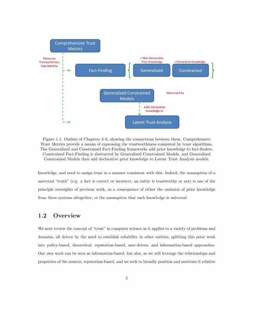
Figure 1.1: Outline of Chapters 3–6, showing the connections between them. ComprehensiveTrust Metrics provide a means of expressing the trustworthiness computed by trust algorithms.The Generalized and Constrained Fact-Finding frameworks add prior knowledge to fact-finders.

Constrained Fact-Finding is abstracted by Generalized Constrained Models, and GeneralizedConstrained Models then add declarative prior knowledge to Latent Trust Analysis models.

knowledge, and need to assign trust in a manner consistent with this. Indeed, the assumption of a

universal “truth” (e.g. a fact is correct or incorrect, an entity is trustworthy or not) is one of the

principle oversights of previous work, as a consequence of either the omission of prior knowledge

from these systems altogether, or the assumption that such knowledge is universal.

1.2 Overview

We next review the concept of “trust” in computer science as it applies to a variety of problems and

domains, all driven by the need to establish reliability in other entities, splitting this prior work

into policy-based, theoretical, reputation-based, user-driven, and information-based approaches.

Our own work can be seen as information-based, but also, as we will leverage the relationships and

properties of the sources, reputation-based, and we seek to broadly position and motivate it relative

5

to the broader context, although we will save more detailed comparisons for the individual Related

Work sections of the subsequent chapters.

One of the first questions that we must then address is how we can even measure a source

or document’s trustworthiness; certainly, when we evaluate a trust algorithm, we are concerned

with its ability to correctly identify true claims, but extending such a simple accuracy metric to

the providers of claims can be both misleading and disappointingly uninformative—the user may

not wish to read a highly biased and incomplete document merely because it is factually correct.

Rather, we propose a set of three comprehensive trust metrics, truthfulness, completeness, and

bias, that are able to materially inform the user of the quality of a source or document and help

them decide whether and how to rely upon them, and we are able to quantify this advantage, albeit

only coarsely, with a small user study. Furthermore, while these metrics are orthogonal to the

construction of the trust systems themselves, they nonetheless both aid in framing the problem as

a whole and reinforce the recurring theme of the subjectivity of trust which permeates our work.

Following this, we begin considering the families of algorithms that may be used to determine

belief and trust, starting with fact-finders. Fact-finders view the trust problem as a bipartite graph

of the information sources and the claims they assert, iteratively updating the trustworthiness

score of each source based on the believability of the claims it asserts, and updating the belief

score of each claim based on the trustworthiness of the sources asserting it. These algorithms are

extremely fast (linear time), more effective than simple voting, and fairly easy to implement. We

explore the family of fact-finding algorithms as a whole, and additionally introduce three novel,

high-performing algorithms: Average·Log, Investment, and PooledInvestment. The performance of

these new fact-finders compares very favorably to state-of-the-art fact-finders from the literature

on several real-world datasets, and we will revisit the same setup throughout our later experiments.

One limitation of fact-finders is their sole reliance on the source-claim graph; they are unable

to exploit any information beyond “who says what”. However, there is a great deal of valuable,

additional information that could better inform our trust decision if only we were able to take

advantage of it, such as: the properties of the sources (their degrees, professional associations,

quality of writing, etc.), the uncertainty of information extraction (deriving from either inherent

6

ambiguities in the underlying text or an imperfect information extraction engine), and similarities

among the claims (a source claiming the birthplace of Obama as “California” disagrees less with

someone else claiming “Hawaii” than they would someone claiming “Kenya”). We introduce a new

framework that generalizes fact-finding algorithms from unweighted, bipartite source-claim graphs

to weighted, k-partite graphs that are capable of encoding a wide variety of auxiliary information,

while still leveraging the diversity and performance of existing fact-finding algorithms. Moreover,

our experiments demonstrate that even small amounts of additional information can dramatically

improve the accuracy of Generalized Fact-Finders over their standard variants, and the modifi-

cations necessary to generalized existing fact-finding algorithms can be applied in a mechanistic,

rule-driven matter.

Despite the power of Generalized Fact-Finders, however, they do still omit one very key as-

pect: the user’s prior knowledge. For example, a user might know that ∀xLegalPresident(x) ⇒

BornIn(x, US);∀x,yBornIn(x, y) ∧Within(y, US) ⇒ BornIn(x, US);¬Within(Kenya, US), al-

lowing us to reject the claim BornIn(Obama,Kenya) if we also believe LegalPresident(Obama).

With Constrained Fact-Finders, we interleave updating the beliefs in the claims via the underlying

fact-finding algorithm with a “correction” of those beliefs in accordance with the declarative prior

knowledge we are provided, finding a corrected set of beliefs that satisfies our constraints while

minimizing the distance from the original beliefs. Our experiments demonstrate that not only does

prior knowledge, like Generalized Fact-Finding, further increase accuracy by incorporating more

information, it is also absolutely essential when the subjective truth of the user differs from the

majority. Further, Constrained Fact-Finding remains tractable by enforcing its constraints via a

polynomial-time linear program rather than an exponential-time integer linear program, as other

research into the application of declarative constraints has often used. As it is orthogonal to Gen-

eralized Fact-Finding, both techniques may be used jointly to create a tractable, highly informed

fact-finding framework, capable of greater performance than either approach on its own, and far

surpassing the standard fact-finders they supersede.

Inspired by the Constrained Fact-Finding approach, we introduce a subsuming method, General-

ized Constrained Models, to enforce prior knowledge in problems far beyond fact-finders, with very

7

broad applicability to supervised, semi-supervised and unsupervised structured learning problems.

For supervised learning, Generalized Constrained Models improves upon Constrained Conditional

Models [16] to enforce declarative constraints during inference with an underlying probabilistic

model, with GCMs selecting the (truly) most probable distribution over the latent variables that

satisfies the constraints, while CCMs instead find the satisfying distribution that is merely most

probable according to the underlying model. In semi-supervised and unsupervised problems, Iterated

Generalized Constrained Models are a modified-EM approach that can be seen as generalizing tech-

niques such as Constraint Driven Learning [15] and Posterior Regularization [33], combining the

best properties of both: the use of declarative constraints, ease of implementation, and polynomial

complexity, all while maintaining similar or better performance in our experiments.

Finally, we consider a new class of principled, probabilistic Latent Trust Analysis models for

determining the trustworthiness of sources and the belief in claims. We initially “bridge the gap”

between fact-finders and LTA by introducing a simple LTA fact-finder, a model where P (claim|X, θ)

may be taken as the claim’s “belief score”, and each source has only a single parameter corresponding

to its scalar trustworthiness score, and the update rules are derived (in closed form) from EM, such

that running the fact-finder performs EM on the model. Afterwards, we break from the fact-

finding paradigm entirely, presenting a sophisticated model capable of capturing all the phenomena

of Generalized Fact-Finders and more, modeling parameters corresponding to user truthfulness

and expertise as well as the “difficulty” of choosing the correct claim from each particular group

of alternatives. This provides a number of important advantages over fact-finders, including far

greater expressiveness and “explainability” (the ability to tell the user why a particular claim is

to be believed or a particular source to be trusted, and tell them the overall generative story that

the model represents); the tradeoff is that, since maximizing the expected (log) likelihood cannot

be done in closed form, performing expectation-maximization to learn the model requires Quasi-

Newton or Gradient Descent methods at a greater (though still quite feasible) computation cost

than fact-finders.

8

Chapter 2

Survey of Computational Trust

In this chapter we explore the field of computational trust, focusing on the work most relevant to

ours but also surveying other areas that help situate our research in the larger picture. We divide the

field into five areas: policy-based, theoretical, reputation-based, user-driven, and information-based,

partially borrowing from the division proposed by [5] (and see also [73] for another survey from a

different and more focused perspective), and additionally consider the related topic of recommender

systems.

2.1 Policy-based

Policy-based trust methods ([45, 88, 64, 51], to name only a few) tend to depend on cryptographic

and credential-oriented means to establish trust in another party, often concerned with with regu-

lating access to a resource as a security policy. Typically credentials are backed by a third-party

authority (e.g. as Thawte does for SSL certificates). These mechanisms are often essential building

blocks for informational trust decisions; e.g. if a malicious user can forge the identity or signature of

an author, he may create untrustworthy documents under his name, either lowering the trust others

place in the victim or, worse, use a high-trust author to propagate falsehoods. With credentials,

however, an author can sign his work cryptographically, and forgery becomes much harder. As an

example, when we employ data provided by Wikipedia in our experiments, we are relying upon

Wikipedia’s own authentication scheme to ensure that each revision is correctly associated with its

true author.

9

2.2 Theoretical

One of the early detailed looks at trust from a computational perspective can be found in [59], which

makes the important observation that trust can be global (as per eBay’s trust score), personal (each

person assigns their own trust values to other entities), or situational (personal and specific to a

given context); situational trust in particular has been poorly studied, although it seems natural to

trust a biologist’s description of mitosis more than his assessment of quantum tunneling, as entities

clearly have varying degrees of expertise and dependability for a given task. [73] observes that the

simple solution of merely creating separate models for each context is flawed, particularly when

data is scarce–while we may not trust our biologist’s physics expertise, for example, a seemingly

good-faith effort that at least loosely approximates the truth suggests he may be trusted to provide

accurate assertions within the domain of biology.

Trust is also key in many game theory strategies. Consider, for instance, an iterated prisoner’s

dilemma. Interestingly, tit-for-tat [7], whereby betrayal is punished with betrayal, and cooperation

rewarded with cooperation, is generally considered the most effective strategy for the game, but

never requires the agent to trust the opponent–betrayal can be identified and punished immediately,

eliminating any incentive to cheat, so the tit-for-tat strategist need only believe that the opponent

is rational. However, when checking for betrayal has a cost [52], trust becomes significant, as a

tit-for-tat strategist verifying his opponent’s action each time will incur a large verification penalty.

Instead, it would be better to check up on an opponent only “once in a while”, but employ more

draconian punishment for betrayal (but less severe than [6]’s absolute ”grim trigger”) such that he

sees no net gain. The occasional verification penalty can be viewed as the cost of establishing and

maintaining trust. Ironically, in the presence of such trust-but-verify agents, purely honest agents do

better, implying that such policing has strong positive externalities and the honest agents are free-

riders (in a real-world context, trust would therefore be a public good whose cost should be shared

by all, as it is with government safety agencies). [62] also examines the game-theoretic elements of

trust, using it to analyze and construct a reputation system where agents learn from the history

of past games and the reputations of other agents, showing (unsurprisingly) that establishing trust

10

has a net benefit to the parties involved. Game theory is important to our work for two reasons:

it provides a theoretical basis for estimating the value for trust and its costs (and, perhaps, how

they should be distributed), and it helps us understand the motivations and potential strategies of

those who “cheat”. [22] investigates the practical applications of this, finding that traditional trust

mechanisms (such as contract law) are largely unenforceable online, but reputation and trust are

even more vital due to the higher exposure the Internet provides (if a buyer rates you badly on

eBay, everyone will know, not just the buyer’s friends).

Additionally, a large amount of work from fields such as human-computer interaction, economics,

psychology and other social sciences looks at how trust is created and used by people, which has

direct implications for our work developing a trust system that can take into account the full breadth

of relevant information. Much research as it pertains to human-computer interaction specifically has

been done by Fogg’s Persuasive Technologies Lab [80, 8, 28, 30, 29], demonstrating that, besides

factors traditionally considered by trust systems such as recommendations and past reliability,

humans are superficial, placing more faith in a site with a “.org” domain name or a modern,

sophisticated design for example. We note that, though stereotypes, these are nonetheless useful

features, as “.org” websites are often non-profits that may be more truthful than a website trying to

sell a product, and a sophisticated design implies a high degree of investment by the website creator

who has much more at stake if he loses his visitors’ trust than someone whose website was prepared

in an hour. [34] similarly identifies 19 factors that influence trust in the context of the semantic web,

including user expertise (prior knowledge), the popularity of a resource (the [arguable] wisdom of

crowds), apparent bias (similar to “.org” vs. ”.com”) and recency (more recent information is more

likely to be up-to-date and correct). Separately, Fogg et al.’s work also provides insight in the trust

labels and accuracy that a human user would prefer; users with little knowledge about a subject

may desire a “true, false or maybe” judgement of a particular claim, while a domain expert might

require an exact probability–since computing exact trust scores may be expensive, understanding

when approximation is acceptable can potentially offer considerable savings.

Finally, probabilistic logics have been explored as an alternate method of reasoning about trust.

[57] utilizes fuzzy logic [65], an extension of propositional logic permitting [0,1] belief over proposi-

11

tions. [87] employs Dempster-Shafer theory [75], with belief triples (mass, belief, and plausibility)

over sets of possibilities to permit the modeling of ignorance, while [44] uses the related subjective

logic [43] which reasons about belief quadruples (belief, disbelief, uncertainty and base rate), where

base rate is an a priori estimate of belief given uncertainty. Directly modeling ignorance provides

an elegant alternative to ad hoc solutions like smoothing, but this must be weighed against its

complexity, and alternatives exist–in our constrained and generalized fact-finders, for example, we

can accomplish the same end by explicitly assigning weight to the unknown. We can also consider

the admitted ignorance of emphsources: for instance, in our Latent Trust Analysis model, we allow

for sources asserting a distribution of belief over the claims with a [0, 1] certainty “weight”.

2.3 Reputation-based

Reputation systems and trust metrics are frequently employed in P2P applications and social

groups. Alternatively, PageRank [13] can be seen as a reputation system where the links im-

ply recommendation, while [49] is similar but employs a dichotomy between hubs and authorities

such that authorities are trusted if they are recommended by many hubs and hubs are trusted if

they recommend many trustworthy authorities. In these and other reputation systems that em-

ploy a (often implied) trust network, there is a core principle of transitivity: if you trust Bob with

T (you,Bob) = 0.9, and he trusts Jane with T (Bob, Jane) = 0.5, then, in the absence of another path

and using a very simple transitivity scheme you might trust Jane T (you, Jane) = 0.5× 0.9 = 0.45.

Of course, transitivity can be much more complex with this; [44] uses the relatively complex op-

erators of subjective logic, while many other systems depend upon an iterative algorithm for trust

propagation. [39] is notable as it features a transitive distrust, which is far from straightforward

(do I trust those distrusted by those I distrust?); however, though negative trust effectively implies

that we “trust” the other entity to betray us, it may be of limited utility: if a user I strongly

distrust claims that the sky is blue, as does someone I trust moderately, should I assume that the

sky is some other color instead? This question of what can be inferred from an untrusted source’s

assertions will reappear with pragmatic importance when we construct the Latent Trust Analysis

12

model.

More generally, a major challenge in all transitive trust networks is thwarting manipulation by

malicious users. Eigentrust [46] is capable of reducing their impact on the network by essentially

using pre-selected trustworthy users as a “fount of trust”, such that trust flows from this initial

seed group out to the other peers, forcing malicious users—if they wish to be trusted—to at least

sometimes behave appropriately; the authors found that, in the context of file sharing, malicious

cliques of self-recommending users could deliver the most invalid files to others if they also delivered

the correct file 50% of the time. Sybil attacks [26], where one malicious individual or group can

control a large number of identities in the network, are also often very effective, both because

they allow a large portion of the entities in the network to be coordinated by a single malicious

party and because they allow for the use of disposable sock puppets, online identities that, when

they become distrusted or banned, can be abandoned with a new, clean account taking its place

(creating a sort of “whac-a-mole” game for legitimate users and administrators). There are two

principle ways to mitigate these problems [17, 54], either by verifying the user’s identity or imposing

a cost for creating or maintaining an account to prevent or discourage false user accounts, or by

adopting an asymmetric trust network. Most trust networks are symmetrical, and every user is (a

priori) equally trusted and equally influential. However, an asymmetric trust network such as the

online community Advogato [53] typically has a small core of trusted users (Advogato currently

has four). Because of this, only a chain of recommendations (or “certifications” in Advogato’s

terminology) from the trusted core can impart trust in a user, and, if discounting of transitive trust

is used, that user must be reasonably close to the core. Consequently, collaborating malicious users

acting independently cannot recommend themselves into a higher position of trust regardless of

their number. As an asymmetric counterpart to PageRank and Hubs and Authorities, we also have

TrustRank [40], a link analysis algorithm that starts with a small core of hand-selected, trusted

pages, and then crawls outwards, with the intent of sidestepping self-linking collections of spam

pages. Unfortunately, there are serious weaknesses of asymmetric networks, as a compromised core

user (or someone highly trusted by a core user) can wreak havoc on the system, and individuals

outside the “inner circle” have relatively little power (Advogato assigns global trust, although in

13

principle there is no reason this could not be combined with a subjective, per-user trust algorithm to

create a composite score). Note also that some asymmetric networks are more readily compromised

than others: while Eigentrust is also asymmetric, it remains vulnerable because trust scores are

updated automatically and frequently over the course of multiple interactions, allowing malicious

users who are merely sometimes cooperative to capture some of the trust flowing from the trusted

core. It is also worth observing that even Advogato weaknesses have been exploited in practice [79],

as both deceived and complicit high-trust users outside of the inner circle were able to also impart

high trust to another user widely claimed to be a “crank”.

Finally, we point out that not all reputation-based trust schemes are necessarily complex; as

previously mentioned, eBay allows only -1, 0, and +1 ratings (together with a short comment) for a

partner in a transaction, which are summed to obtain a global trust score–although there is a strong

economic incentive for cheating under this system (high trust allows a user to defraud others), it

is still widely considered successful [46, 22], presumably due to a combination of human policing

and buyers performing significant trust assessment of their trading partner beyond the single scalar

score, e.g. by evaluating past auctions, examining photographs of the product, considering the

grammar and spelling used by the seller, etc.

2.4 User-driven

Unlike reputation networks, where trust judgements in the form of recommendations are stated

or implied amongst entities, user-driven trust systems extrapolate from their users’ specific trust

judgements of information sources and the data they provide. This has the disadvantage of requiring

a great deal of user effort (and often expertise) to build a database or semantic web, although this

may be mitigated by software tools and by “piggybacking” on existing annotation tasks where the

additional effort is marginal (e.g. by qualifying “Address = 123 Acme Road” with “P = 0.95” to

express confidence in that claim).

14

2.4.1 Databases

Typical elements in a database trust system are data provenance (where data comes from, a “chain

of custody”), access control (credential-based trust), and data conflict resolution to handle con-

tradictions in the data [11]. [19, 18] consider both path similarity and data conflict. They detect

conflict through if-then conditions, reducing the trust score of those data found inconsistent. Path

similarity compares the provenance of the data under consideration by reasoning that if the same

claim comes from two distinct, independent data paths it is more trustworthy than if it had come

from data paths that share entities; this notion of multiple independent sources establishing more

trust than dependent sources also motivates work in inferring duplication among sources in other

domains (such as websites), but here the provenance is assumed to be given in its entirety.

2.4.2 Structured User Analysis

The TRELLIS system [37, 36] is an interface for structuring and annotating the synthesis of con-

clusions from underlying facts, where the reliability and credibility of a source and a claim may be

specified by the user, or inferred by how the claim is used: for example, if a user cites a claim as

support for his ultimate conclusion, this suggests that it is credible, and, conversely, if the claim

is cited but dismissed in the process of building to the conclusion, it may be taken as considered

and refuted by the user. Such structured analysis trees can be queried and exploited by other users

facing the same or similar questions and, when many such trees are considered, the general implied

trustworthiness of information sources and claims may be calculated. This idea is generalized to

arbitrary relations in [34], which also demonstrates the concept via a number of user-simulating

synthetic experiments.

2.4.3 Provenance Systems

A more abstract view are core provenance recording and querying mechanisms. These be specific to

tracking the originator and handlers of a workflow [48] or even a more basic, universally applicable

data format [61, 35]. By us to annotate items with their chain of creation, publication, and revision,

15

a user can, for example, decide whether to believe a magazine article by asking if he believes the

cited sources, the author and the publisher. Such reasoning reflects the heuristics people employ

when they, in essence, leverage name recognition to make their decisions—e.g. a Tom Cruise fan

might choose a movie because it stars Tom Cruise, or a Catholic might believe a cited claim because

it was made by the Pope. The catch is, of course, that not only must these provenance annotations

be researched and recorded, but that they themselves be trustworthy, and both of these are difficult

problems in practice: manually researching the provenance of existing documents at web-scale is

infeasible, and even if publishers provided this metadata themselves, we would still be unsure of

whether to trust them.

2.5 Information-based

A number of trust systems establish trust not by user input or implicit or explicit recommendations

among entities but rather by the information that the entities provide, which may be, for instance,

a set of documents or a set of search results. The methods tend to be varied, as are the domains

to which they are applied.

2.5.1 Identifying Source Dependence

In those cases when manually annotated provenance is impractical, we would still like to determine

dependencies among our information sources, but we typically we only have the name of the pub-

lisher or author who provided the information to us. Copying on the World Wide Web is a common

occurrence, and while some sources produce independent, original content exclusively, there are a

myriad of sites that do just the opposite, aggregating data from other sources and republishing it

(e.g. Google News and some blogs), with many sites somewhere in between (Wikipedia contains

a myriad of pages automatically generated from U.S. census data). [24, 25]’s solution is to ob-

serve that, if one source is dependent upon another, they will share the same mistakes along with

a consistent time delay (the copier can only publish after the original has been published), and

that–under the assumption that wrong answers are uniformly distributed–sharing many mistakes

16

is very unlikely if two sources are independent. Additionally, [84] considers trust in the context

of numerical search queries (“how old is John Smith?”), observing that two pages that claim the

same fact but are otherwise dissimilar provide better evidence than pages that are nearly identical

of each other because they are more likely to be independent.

There are two chief problems with the assumptions made by such approaches: first, mistakes are

not uniform and independent. Many errors are widely shared (e.g. that Shakespeare was born on

April 23rd, 1564), and if two sources share one mistake, they are more likely to share another, since

they are more likely to share the same assumptions or decision processes and thus arrive at the

same conclusions independently of one other, right or wrong. Second, a closed world is assumed:

if one source produces the same claims as another source but at a later time, he must have copied

that information from the other source. However, outside of scientific literature, very few of the

underlying claims are independently generated by the sources; even in the case of eyewitness reports

(e.g. of a car accident), the underlying event is observable to many parties, and in general people

tend to repeat things (e.g. “the world is round”) that they have not personally verified.

2.5.2 Fact-Finding

Given a large set of sources making conflicting claims, fact-finders determine “the truth” by iter-

atively updating their parameters, calculating belief in facts based on the trust in their sources,

and the trust in sources based on belief in their facts. TruthFinder [86] is a straightforward imple-

mentation of this idea. AccuVote [24, 25] improves on this by using calculated source dependence

(where one source derives its information from another) to give higher credibility to independent

sources. [32]’s 3-Estimates algorithm incorporates the estimated “hardness” of a fact, such that

knowing the answer to an easy question earns less trust than to a hard one (for instance, William

Shakespeare’s birthday is a much trickier question than William Clinton’s). However, fact-finders

fail to incorporate the user’s prior knowledge and the wealth of additional data available for a

particular domain (the information extractor’s confidence level in each source-claim pairing, group

membership of a source, etc.), shortcomings we address in a general, tractable way in Chapter 4,

allowing us to continue to leverage the diversity of existing fact-finders while also overcoming their

17

deficiencies.

2.5.3 Specialized Information-based Systems

Many trust systems are specialized for a particular domain, such as wikis. [89] is a relatively simple,

document-level approach, learning a dynamic Bayesian network across the flow of wiki revisions,

using the author and the number of inserted/deleted text fragments as features. Wikitrust [1, 2]

estimates the trustworthiness of edits (at the word level) by considering implicit endorsements by

other editors who make nearby edits or refinements without destroying the original text. These sys-

tems are ultimately intended to help readers of wikis determine which documents (or parts thereof)

to trust, but unfortunately lack the required claim-level granularity and general applicability of

fact-finding systems.

Additionally, many algorithms exist for combining multiple classifiers to make a final prediction.

Where weights are applied to these classifiers in an equitable fashion (i.e. not as in AdaBoost [31]

where the α weights are set sequentially) they can be considered relative degrees of trust: a highly-

weighted classifier, for example, presumably returns the correct answer more frequently than its

less-preferred brethren. A concrete example of this is [50], where the output of multiple rankers is

aggregated by weighted voting, and each ranker’s weights are determined by its agreement with the

others on (unlabeled) training examples. Highly-weighted rankers are taken as the most credible

and therefore contribute the most to the final prediction. Although the weights in such ensemble

classifiers are essentially a side effect of the learning algorithms, they can be correctly interpreted

as trust scores for the underlying classifier “sources”.

2.6 Information Filtering and Recommender Systems

In computational trust our task is to “recommend” trustworthy sources and true information; in a

sense, then, recommendation systems can in principle be seen as addressing a subsuming task. In

practice, of course, the actual methods used and the concrete problems they are applied to are quite

dissimilar, but the extensively studied field of recommender systems still warrants consideration,

18

partly for contrast and perspective and partly for cross-task insight.

Information filtering may be content-based, collaborative, or both; see [3] a survey of the field.

Content-based methods compare the objects to be recommended with the user’s demonstrated

preferences, and must thus have some understanding of the domain in which they operate; for

example, [66] represents documents with a set of keywords and uses these to match against profiles

established with explicit user feedback (ratings). There are, however, a few problems with such

systems. First, as with collaborative filtering, users must somehow construct a profile first, either

explicitly by, say, rating the quality of documents, or implicitly, by tracking the time a user spends

looking at documents. In either case, the system cannot provide personalized recommendations

without first being “trained”. One solution is to take an active learning approach and ask the user

to rate those that will best improve performance, as in [4]. A second, similar problem arises from

“overspecialization”, where a user is shown only items similar to those he has seen before; this can be

addressed by either filtering out redundant documents [90] or through some additional randomness

in selection. Finally, the third problem is intrinsic: where similarity is not easily measured (e.g.

photographs) these systems cannot function.

Collaborative filtering, however, avoids this last issue by treating the items as “black boxes”

(as most trust analysis systems treat claims); recommendations are established by determining the

similarity with other users and using these to weight each of their ratings of the item in question.

An example of this is the Google News recommender [20], which relies on implicit user preferences

(which stories they click on) and computes recommendations based upon the stories viewed by

other users who viewed a similar set of stories to the user in the past. These systems may be

“memory based” or “model based” [12], where memory-based systems directly rely upon similarity

to other users or cluster membership while model-based methods instead learn model parameters.

Still, as with content-based systems, there are problems unique to the collaborative approach.

First, assigning a user to a single cluster may be counterproductive; one person may have unique,

diverse sets of interests, such as miniature golf and simulated annealing. Second, it is difficult or

impossible to recommend new items, because these have no user ratings. Third, there is a “sparsity

problem”, where the number of users or the number of ratings is too small to make an accurate

19

recommendation, especially when the user is unusual and has few like-minded peers.

Given the hundreds of information filtering systems, and, indeed, recommender systems in

general, there is also the question of evaluation and robustness. Evaluations fall into three categories

[41]: predictive (e.g. predict a user’s movie rating), classification (predict whether a user will like a

movie or not), and rank (predict a preference-ordered list of movies for the user); consequently, the

apparent performance of a recommender varies depending upon which evaluation metric is selected.

Note that, in trust, these are all possible: we can predict the specific belief distribution, mark

each mutually exclusive assertion as “plausible” or ”not plausible”, ”trusted” or ”not trusted”, or

simply rank assertions in the order of believability. Also of interest is that, as with trust algorithms,

there is a need for the user to trust the recommender system, but unlike in trust algorithms, this

may require something beyond superficially correct output: for a book recommender system, for

instance, it seems inappropriate to recommend a book the user has already bought, but, on the other

hand, a user might interpret such a recommendation of something he likes as a sign of dependable

performance.

Also, for systems with a collaborative element, we must again concern ourselves with Sybil-

like attacks whereby many users (or, rather, their sock puppets) alter their behavior to affect the

recommendations other users obtain (e.g. an author creating many ratings “profiles” on a book

review site and then ranking his own books very highly). Some work, such as [60], has already

begun to consider this, and there may be the opportunity to borrow such strategies to counteract

the analogous threats to trust systems.

2.7 Conclusion

Our task is to determine which information sources are trustworthy and which claims can be be-

lieved. Unfortunately, user-driven approaches such as manually labeling credibility and reliability

do not scale well. Reputation networks can in many cases be discovered by inferring implied rec-

ommendations, but can, at best, only tell us which sources are trustworthy without specifically

addressing the claims they make. Instead, we will adopt a primarily information-based approach,

20

examining and comparing what sources actually say, but still leverage other aspects of compu-

tational trust to aid us, much like hybrid recommender systems that combine both content and

collaborative filtering. Indeed, our approaches will cross over numerous boundaries, with policy-

based trust establishing attribution during information extraction, entity recommendations and

attributes coloring our trustworthiness judgements of sources, and user-provided prior knowledge

constraining and qualifying our belief in the claims. Just as no user would ignore such a breadth

of features in his trust decision, nor can we do so if we hope to succeed as his proxy.

21

Chapter 3

Comprehensive Trust Metrics

3.1 Summary

Trust systems can analyze information networks to determine the “trustworthiness” of the nodes,

but the scalar values they produce are both opaque and semantically variable, and knowing only

that the trustworthiness of a website is “27” is not helpful to the user. Moreover, the simplistic

means by which they are typically calculated can yield misleading results, sometimes dramatically

so. We present a new, standardized set of trust metrics that instead compute the trustworthiness

of an information source as a triple of truthfulness, completeness, and bias scores, and argue that

these must be calculated relative to the user to be meaningful. We then explore these new metrics

with a user study. As these metrics make no assumptions about the internals of the underlying

trust algorithm they may be applied universally to all information-based trust systems, including

those we introduce in later chapters.

3.2 Introduction

Information-based trust systems [5] are algorithms that, given an information network containing

information sources (e.g. authors, publishers, websites, etc.) making a variety of claims (“the

atomic mass of gold is 42”), determine how much a user should trust the former and believe the

latter (a highly trusted source reliably provides trustworthy documents and a highly believed claim

is likely to be true). As data has become more abundantly available to us, the importance of such

systems has grown tremendously, particularly following the mass adoption of blogs, wikis, message

22

boards and other collaborative media; however,the high entry barrier (and enforced journalistic

standards) of older, established media such as newspapers and television is gone. Similarly, with

growing scale, reduced budgets, and instant communication, this “information overload” also vexes

those algorithms that seek to harness it, with an ever-increasing need to sift out the true from the

spurious.

Unfortunately, the assessments produced by these algorithms are simplistic, assigning a proba-

bility or arbitrary weight as the scalar trustworthiness of a source, based upon the accuracy of their

claims. For example, TruthFinder [86] calculates a source’s trustworthiness as the arithmetic mean

of the probabilities of its claims. Consider a short document authored by Sarah: “John is running

against me. Last year, John spent $100,000 of taxpayer money on travel. John recently voted to

confiscate, without judicial process, the private wealth of citizens.” If all of these statements are

true, Sarah and her document would thus be considered highly trustworthy.

However, if we know more about the background, we might find that Sarah is misleading us

and is, in fact, quite untrustworthy despite her factuality (i.e. we should not consider her to be

a reliable source of information). If “John is running against Sarah” is a well-known, “easy” fact

[32], Sarah’s correct assertion thereof is unimportant (taken to the extreme, one could otherwise

pad a document with banalities like “1+1=2, 1+2=3...” to produce a seemingly-trustworthy docu-

ment, regardless of its other content). Further, if $100,000 in travel expenses is par for John’s office

because it necessitates a great deal of travel, Sarah has conveniently neglected to mention this,

instead inviting the reader to compare his costs to their own prior expectation of what “typical”

travel expenses should be and conclude, incorrectly, that John has enjoyed gratuitously luxurious

accommodation. Similarly, Sarah’s “wealth confiscation” typically goes by the slightly more in-

nocuous term “taxation”, but her biased language suggests to the reader that John has approved

of something unusually nefarious.

To counter these problems, we propose assessing trustworthiness not as a scalar, but rather

three separate values: truthfulness, completeness, and bias. Decomposing trust into these three

components allows the trust system’s user to meaningfully assess the extent to which a document

or information source can be relied upon, and calculating them consistently across algorithms

23

permits the output of competing trust systems to be directly compared and evaluated. We also

find that the user himself is essential in calculating the trustworthiness of a source, in addition to

the prior knowledge he may bring to the trust system itself (e.g. as we will explore in Chapter

4); for example, if an investor and a politician are each reading about House debates on a new

corporate tax bill, the investor may not care who introduced the bill, while the politician may not

care about the fine-grain details of the tax. An author that occasionally flubs those details may

thus nonetheless still be trusted by the politician, but not the investor. By considering the relative

importance of information and preexisting beliefs of the user, we can better approximate the user’s

own judgment and provide a more accurate trust analysis.

3.3 Background

Broadly speaking, information networks can be categorized as homogeneous and heterogeneous

networks; our metrics apply the latter, but we also briefly discuss the former below for contrast.

3.3.1 Homogenous (Reputation) Networks

Homogeneous reputation networks have only a single type of entity, with edges forming recommen-

dations, votes, or other relationship between two entities in the graph; these are more commonly

known as reputation networks. As discussed in Chapter 2, reputation systems are frequently em-

ployed in P2P applications and social groups, such as Eigentrust [46] and Advogato [53]. Alterna-

tively, PageRank [13] and [49]’s Hubs and Authorities can be seen as reputation systems where links

imply recommendation. However, the amount of information that can be encoded in homogeneous

networks is limited; for news websites we might add edges corresponding to links between them

(again on the basis that these are implicit recommendations), but we would not look at the actual

articles on those websites, or the claims they contain. Thus, while the semantics of trustworthiness

within a reputation network are often relatively straightforward (based on “flows” of trust among

entities) they are a poor choice for information sources, where recommendations among the sources

(if present) are much less important than what the source actually says.

24

3.3.2 Heterogeneous Networks

The heterogenous networks seen in trust problems comprise of a number of (possibly hierarchical,

e.g. document→ author→ publisher) information sources, each asserting a number of claims. The

trust system seeks to both find the trustworthiness of these sources and the believability of their

claims, although in the user’s interest may be specific, e.g. determining the atomic weight of gold

or finding trustworthy articles about Bill Clinton.

Fact-finders are the predominant class of algorithms for finding trust in these networks; these

take as input a bipartite graph of sources and claims, with edges connecting each source to the claims

it asserts, and output a trustworthiness score for each source and a belief score for each claim (with

the semantics of these scores varying with the particular algorithm). We will discuss these at length

in Chapter 4; a straightforward example is TruthFinder [85, 86], though some reputation systems

(like Hubs and Authorities [49]) can be adapted to heterogeneous networks with relatively little

effort.

One important observation is that, regardless of the algorithm, we can readily standardize the

believability of each claim as the probability that the claim is true. However, source trustworthi-

ness scores are computed differently from algorithm to algorithm, and the most immediate choice,

used by TruthFinder and others, is to calculate this as the probability of the source producing a

true claim (the arithmetic mean of the probabilities of the claims made by the source) a measure

which, as already discussed, is readily misled. While the trustworthiness score remains an internal

parameter within the trust system, we can nonetheless report a more meaningful trustworthiness

evaluation using our own metrics, which (among other advantages) provide consistency by virtue

of being derived directly from the (standardized) belief in the claims rather than the arbitrary

trustworthiness score used by each particular algorithm.

25

3.4 The Metrics

3.4.1 The Components of Trustworthiness

Besides inconsistent and problematic semantics, existing scalar trust scores for information sources

suffer from being overly broad–trustworthiness cannot always be summarized with a single number.

Consider, for example, two news articles about a topic, both of which consist of entirely true

claims. One article may omit a number of important details, while the other may be strongly

biased towards one position. A human reader interested in only the gist of the topic would be

satisfied by the incomplete article, while an information extraction system building a knowledge

base would not take bias into account.

We therefore view the trustworthiness of an information source as three interrelated, but sepa-

rate, [0, 1] components: truthfulness, completeness, and bias. This has a number of advantages for

information consumers:

• It allows them to moderate their reading by factoring in the source’s inaccuracy, incomplete-

ness or bias (and, for example, questioning claims from a somewhat inaccurate source, or

carefully maintaining objectivity when confronted with a biased source).

• They can select information sources appropriate to their needs: completeness and bias may

not be important to every user.

• Similarly, when a single score is preferred as a “summary” of a source’s trustworthiness, this

can be computed from the truthfulness, completeness and bias with respect the user’s needs.

• Each component may be explained separately to the user: a low truthfulness score is explained

by inaccurate claims, low completeness by listing some of the important claims the source does

not mention, and bias by listing claims supporting the source’s favored position together with

a list of counterpoint claims they omitted.

26

3.4.2 Truthfulness

Given a single, atomic assertion, truthfulness is simply our belief in the claim; that is, T (c) = P (c).

For simplicity we restrict ourselves to Bayesian belief, but our definitions may readily be extended

to Dempster-Shafer or subjective logic, allowing us to qualify our belief with the ignorance or

uncertainty arising from insufficient evidence. For a collection of assertions C, such as documents,

we define

T (C) =

∑c∈C P (c) · I(c, P (c))∑

c∈C I(c, P (c))

where I(c, P (c)) is the subjective importance of a claim given its truth, as determined by the

user. Declaring “Dewey Defeats Truman” is more significant than an error reporting the price of

corn futures–unless the user happens to be a futures trader. The truth of a claim also affects its

importance; e.g. given the claim “tech stocks will be highly volatile over the next five years”, an

investor would be indifferent to this claim if true (since it is in line with market expectations) but

would definitely want to know if it was false (since it would mean the risk penalty incorporated

into the price of these stocks is undeserved).

3.4.3 Completeness

We are also concerned with how thorough collections of claims (and their providers) are: a reporter

who reports the military casualties of a battle but ignores civilian losses cannot be trusted as a

source of information about the war. While incompleteness is often symptomatic of bias, this is not

always the case—it is possible to provide an incomplete view on a topic without attempting to sway

the reader to a particular position. If a collection C purports to cover a topic t (e.g. “the war”),

and A is the collection of all claims in the corpus, we can calculate completeness with respect to t

as

C(C) =

∑c∈C P (c) · I(c, P (c)) · R(c, t)∑c∈A P (c) · I(c, P (c)) · R(c, t)

27

where R(c, t) is the [0, 1] relevance of a given claim c to the topic t. Thus, completeness is the

proportion of the topic’s true, importance- and relevance-weighted claims in a given collection. A

collection that omits true, important and highly relevant claims will have a low completeness, but

omitting untrue, unimportant or irrelevant claims will have no effect.

3.4.4 Bias

Bias results from supporting a favored position with either untruthful statements or a targeted

incompleteness (“lies of omission”). A single claim may also have bias depending on its represen-

tation; e.g. “freedom fighter” and “terrorist” can refer to the same person, but with very different

connotations. Like truthfulness and completeness, the degree of bias depends on the user—a politi-

cal conservative, for example, may find Fox News less biased than MSNBC, with the converse being

true for a liberal. Here we will restrict ourselves to considering a finite, discrete set S of possible

positions for the topic (e.g. pro- and anti-gun control), where S(c, s) is the [0, 1] degree to which a

claim c supports a position s ∈ S, and∑s∈S S(c, s) ≤ 1. Let us also denote the user’s support for

each position as S(s), where∑s∈S S(s) = 1. Now we can calculate the bias of a single claim c and

collection of claims C as

B(c) =∑s∈S

|S(s)− S(c, s)|

B(C) =

∑s∈S |

∑c∈C P (c) · I(c, P (c)) · (S(s)− S(c, s))|∑

c∈C P (c) · I(c, P (c)) ·∑s∈S S(c, s)

A collection of claims that, on the whole, matches the user’s belief among the possible positions

thus has no bias, whereas a collection whose claims, on the whole, contradict the user’s stance is

held to have high bias. Notice that a collection need not contain claims that each match the user’s

belief in the positions to to be considered unbiased, but rather must be balanced so that, taken

together (and weighted by truth and importance) these claims collectively support each position to

the same degree the user does.

28

3.4.5 From Collections to Sources

From our metrics over single-topic collections of claims such as documents, we can calculate of

trustworthiness of the information source P (such as an author or publisher) providing them:

X (P) =∑

C∈P X (C)·W(C)∑C∈PW(C) , where W is the relative weight of each constituent collection (e.g. the

importance of the collection’s topic t to the user), and X is the measure of interest (T , C, or B).

3.4.6 Relativity

Notice that we rely upon the subjective importance of claims to the user, as well as his stance

on the positions of each topic. Trustworthiness cannot be assessed “globally”, but—as we have

seen—must be calculated with respect to each user’s viewpoint to be meaningful. When evaluating

the performance of an algorithm relative to the user’s judgment, we have two choices: solicit the

user’s estimates of S(s) and I(c, T (c)), or obtain his opinion of the truthfulness, completeness and

bias of each collection directly; the former method is generally more tedious, but better suited to

large datasets where many collections share relatively few claims and topics.

3.5 User Study

We wished to explore our new metrics, and specifically to contrast our new trust metrics with

the simplistic trustworthiness scores calculated by existing trust systems, such as the arithmetic

mean (Tm(C) = |C|−1∑c∈C P (c)). To do this, we needed to evaluate these alternatives relative to

human trustworthiness judgments over a given collection of claims.

3.5.1 The Article

We selected a news article from the English version of The People’s Daily on the topic of the effec-

tiveness of China’s family planning policy (commonly referred to as the “one-child policy”, although

this is an inaccurate oversimplification). The People’s Daily is of particular interest because it is

operated by the Chinese Communist Party (CPC) and thus has a definite bias and yet tends to

29

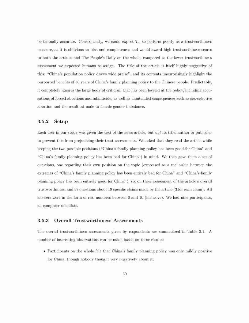
be factually accurate. Consequently, we could expect Tm to perform poorly as a trustworthiness

measure, as it is oblivious to bias and completeness and would award high trustworthiness scores

to both the articles and The People’s Daily on the whole, compared to the lower trustworthiness

assessment we expected humans to assign. The title of the article is itself highly suggestive of

this: “China’s population policy draws wide praise”, and its contents unsurprisingly highlight the

purported benefits of 30 years of China’s family planning policy to the Chinese people. Predictably,

it completely ignores the large body of criticism that has been leveled at the policy, including accu-

sations of forced abortions and infanticide, as well as unintended consequences such as sex-selective

abortion and the resultant male to female gender imbalance.

3.5.2 Setup

Each user in our study was given the text of the news article, but not its title, author or publisher

to prevent this from prejudicing their trust assessments. We asked that they read the article while

keeping the two possible positions (“China’s family planning policy has been good for China” and

“China’s family planning policy has been bad for China”) in mind. We then gave them a set of

questions, one regarding their own position on the topic (expressed as a real value between the

extremes of “China’s family planning policy has been entirely bad for China” and “China’s family

planning policy has been entirely good for China”), six on their assessment of the article’s overall

trustworthiness, and 57 questions about 19 specific claims made by the article (3 for each claim). All

answers were in the form of real numbers between 0 and 10 (inclusive). We had nine participants,

all computer scientists.

3.5.3 Overall Trustworthiness Assessments

The overall trustworthiness assessments given by respondents are summarized in Table 3.1. A

number of interesting observations can be made based on these results:

• Participants on the whole felt that China’s family planning policy was only mildly positive

for China, though nobody thought very negatively about it.

30

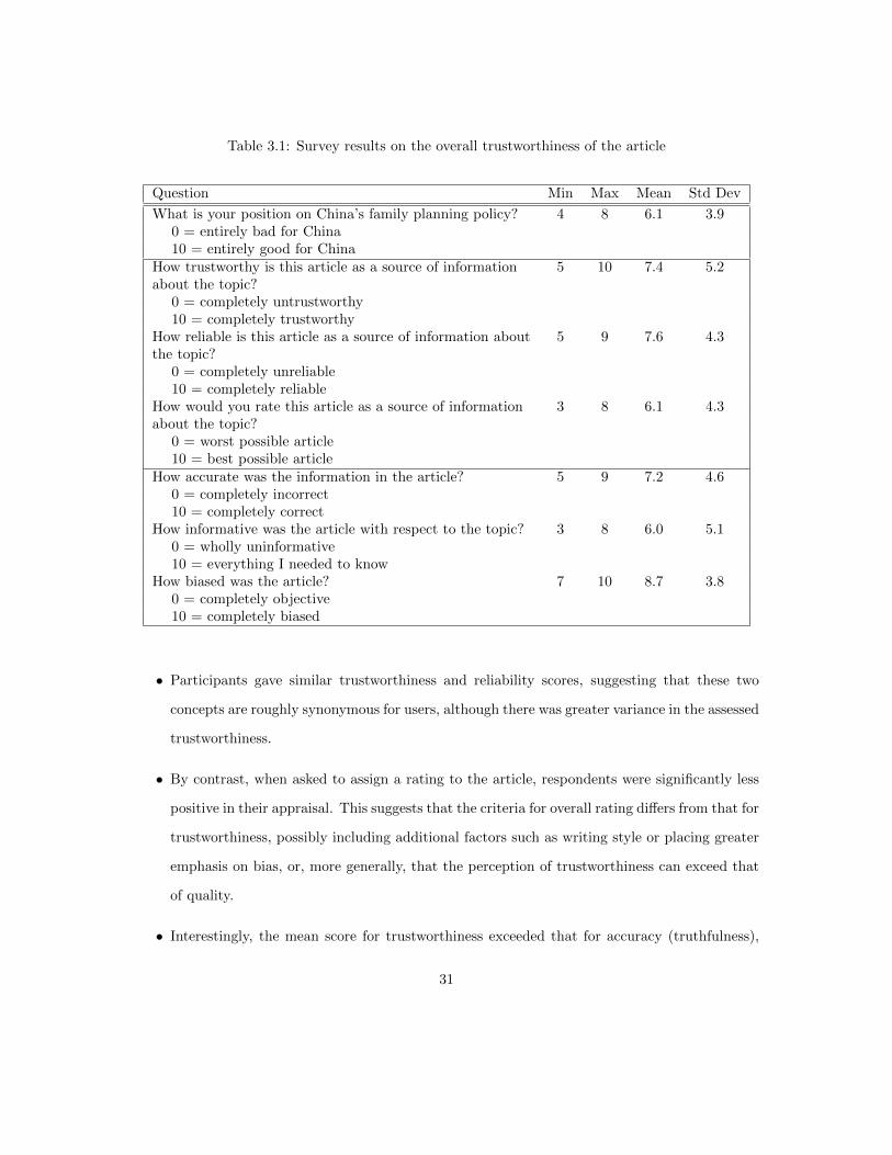
Table 3.1: Survey results on the overall trustworthiness of the article

Question Min Max Mean Std Dev

What is your position on China’s family planning policy? 4 8 6.1 3.90 = entirely bad for China10 = entirely good for China

How trustworthy is this article as a source of information 5 10 7.4 5.2about the topic?

0 = completely untrustworthy10 = completely trustworthy

How reliable is this article as a source of information about 5 9 7.6 4.3the topic?

0 = completely unreliable10 = completely reliable

How would you rate this article as a source of information 3 8 6.1 4.3about the topic?

0 = worst possible article10 = best possible article

How accurate was the information in the article? 5 9 7.2 4.60 = completely incorrect10 = completely correct

How informative was the article with respect to the topic? 3 8 6.0 5.10 = wholly uninformative10 = everything I needed to know

How biased was the article? 7 10 8.7 3.80 = completely objective10 = completely biased

• Participants gave similar trustworthiness and reliability scores, suggesting that these two

concepts are roughly synonymous for users, although there was greater variance in the assessed

trustworthiness.

• By contrast, when asked to assign a rating to the article, respondents were significantly less

positive in their appraisal. This suggests that the criteria for overall rating differs from that for

trustworthiness, possibly including additional factors such as writing style or placing greater

emphasis on bias, or, more generally, that the perception of trustworthiness can exceed that

of quality.

• Interestingly, the mean score for trustworthiness exceeded that for accuracy (truthfulness),

31

informativeness (completeness), and unbiasedness (1 - bias), suggesting that users may be

more generous in their assessment of overall trustworthiness than they are in its specific

components.

• The perceived high bias did not seem to preclude a reasonable overall trustworthiness; this

may indicate that the participants (highly educated computer scientists) consider themselves

savvy enough to correct for bias themselves, or it may be an artifact of the survey’s phrasing—

asking how trustworthy the article is “as a source of information about the topic” may have

implied that only the quantity and accuracy of the information, and not its bias, was to be

considered.

3.5.4 The Claims

From the news article we extracted 19 claims, ranging from unimportant details (“Carl Haub is

a senior demographer at the Population Reference Bureau”) to broad claims that directly address

the topic (“China’s family planning policy has alleviated problems from overpopulation in China”).

For each claim, we asked three questions:

1. To what degree do you believe this claim [0 = definitely not true, 10 = definitely true]?

2. How important would it be to you if this claim were true [0 = I wouldn’t care at all, 10 = I

would care a lot]?

3. How important would it be to you if this claim were false [0 = I wouldn’t care at all, 10 = I

would care a lot]?

Question 1 essentially asks for the user’s estimate of the probability of the claim, P(c). The

answers to questions 2 and 3 (A2 and A3) allow us to estimate I(c, P (c)) as P (c)·A2/10+(1−P (c))·

A3/10. We found respondents gave somewhat similar answers for these two questions (the mean

difference was 1.2), although for the claim “China is the most populous country in the world” the

difference was relatively large (means of 4.4 and 7.6, respectively) reflecting the value of a surprising

contradiction of the user’s expectations: if this claim were false, it would mean that a large number

of trusted sources of information (such as major mass media outlets and textbook publishers) had

32

been incorrect.

When we researched these 19 claims ourselves, we found sixteen to be true with high certainty.

The remaining three claims were speculative (such as “India’s population will surpass China’s in

2040”) and found to be reasonable, but obviously not provable. This suggests a mean accuracy of at

least 84%, which would then also be the minimum Tm simple trust score reported by a trust system

(assuming it determined the truth of the claims correctly). Our survey respondents, however,

were limited to their existing background knowledge and the article itself, and did not conduct

any additional research before making their accuracy assessment. Consequently, their average

estimate of the claims’ accuracy is a significantly lower 75% (7.5/10), reflecting their greater level

of uncertainty.

3.5.5 Calculated Metrics

We estimated R(c, t) and S(c, s) for each claim, and, taken together with the surveyed values for

P (c) and I(c, P (c)), we are able to calculate the truthfulness and bias of the document for each

participant. Computing completeness, on the other hand, is not possible since we are looking at a

single document rather than a corpus, and thus do not have A and do not know which claims we

are missing. The question on informativeness instead captured this from the users directly, giving

the article a mean of 6.0, which at first seems rather generous given the brevity and one-sidedness

of the article. However, as respondents did not, on the whole, have a strong interest in China’s

family planning policies, only the broad details were important to them, and thus an absence of

detail need not necessitate a low completeness.

We calculate a truthfulness of 0.77 and a bias of 0.58. The slightly higher truthfulness versus

the simple mean accuracy of the respondents’ claim beliefs (0.75) indicates that users were more

confident in the truth value of those claims which were more important to them. Unfortunately, as

the article is consistently factually accurate, there is little room for differentiation between these

two measures here; a more interesting example would be an article that gets the important claims

correct but fine details wrong. Our calculated bias, however, is much lower than than the bias

assigned by the respondents, 0.87 (8.7/10). In this particular article, the coverage is clearly and

33

uniformly one-sided, but our bias measure assumes that participants will perceive less bias when a

collection of claims (on the whole) agrees with their position on the topic. This is reasonable when

the bias level is moderate and somewhat subtle (e.g. in MSNBC and Fox News) but apparently

does not hold when bias is extreme and blatant, as the user can no longer “ignore” it. Interestingly,

when we calculate an “absolute” bias, setting S(s) = 1/|S|, we find a bias of 0.82, which is much

more in line with our users judgement. This suggests, perhaps, that when absolute bias is high, it

should be preferred to (or interpolated with) relative bias.

3.5.6 User Metric Preference

After conducting the survey and calculating our metrics, we wanted to know which trustworthiness

scores users would actually prefer in practice: our new metric triple, or a scalar rating. The

exact question we asked our survey participants was “which of these do you think best capture

the trustworthiness of the article you read in the survey (i.e. which set of metrics would be most

helpful to you if you were researching China’s family planning policy and were considering reading

the article)?”. We gave four choices. “The trustworthiness of the article is 7.4 (out of 10)”,

based on the mean overall trustworthiness given by the respondents, was preferred by 28%. “The

trustworthiness of the article is 8.7 (out of 10)”, selected as a moderately higher value, was preferred

by 11%. “The trustworthiness of the article is 10 (out of 10)”, based on the mean accuracy Tm

(taking the three speculative claims as true), was (predictably) preferred by 0%. Finally, the

composite “the truthfulness of the article is 7.7 (out of 10), the completeness of the article was 6 (out

of 10), and the bias of the article was 8.2 (out of 10)”, based on the calculated truthfulness, the mean

“informativeness” rating assigned by respondents, and the calculated absolute bias, respectively,

was preferred by the remaining 61% of respondents. Note that one respondent was undecided and

so split his vote between the first and last choices. Overall, our respondents preferred the new

metrics by a wide margin.

34

3.6 Conclusion

We have introduced three new metrics for measuring the trustworthiness of information sources:

truthfulness, completeness, and bias, and shown that these are able to convey a more useful and

more robust idea of how much (and in what way) an information source should be trusted than

the current practice of presenting the user with a single, trust algorithm-dependent scalar value.

By computing trustworthiness consistently across algorithms, we also enable direct cross-system

performance comparisons, and the evaluation of computed trustworthiness against human judgment.

However, as our survey shows, human perceptions of trustworthiness are not simple to capture.

Strikingly, survey participants assigned the news article a trustworthiness score that exceeded their

opinion of its accuracy, completeness, and unbiasedness! We also found that perception of bias, in

particular, was difficult to predict; the very high bias did not seem to be reflected to a significant

degree in the overall trustworthiness assessment, and could not be estimated relative to the user as

we had expected but instead required an objective estimate.

As our survey was limited in size and scope, further analysis of our metrics may be useful.

Future work should approach an entire corpus to allow calculation (or at least estimation) of the

set of all claims (A) to allow completeness to be calculated directly, should use domain experts to

ensure accurate estimates of P (c), and should include articles with varying levels of accuracy and

bias to allow for more thorough comparison.

Still, it is nonetheless already clear that predicting consistent, semantically well-defined compo-

nents of trust is a dramatic improvement; in its absence, a trust system might have assigned our

newspaper article a perfect trustworthiness score based upon its factual accuracy, completely ignor-

ing the incompleteness and bias that proved obvious to human readers. Our new metrics avoid this

trap and allow us to express a more complete picture of an information source’s trustworthiness.

35

Chapter 4

Standard, Generalized, andConstrained Fact-Finders

4.1 Summary

The Information Age has made publishing, distributing and collecting information easier, resulting

in the exponential growth of information available to us. Databases were once ledgers written

by hand by a single person; today they can be vast stores of data agglomerated from a myriad of

disparate sources. The mass media, formerly limited to newspapers and television programs held to

strict journalistic standards, has expanded to include collaborative content such as blogs, wikis, and

message boards. Documents covering nearly every topic abound on the Internet, but the authors

are often anonymous and the accuracy uncertain.

To cope with this new abundance, we employ information retrieval to suggest documents, and

information extraction to tell us what they say, but how can we determine what we should actually

believe? Not all information sources are equally trustworthy, and simply accepting the majority

view often leads to errors: a Google search for “water runs downhill” returns 36K documents, while

”water runs uphill” yields 88K. Consequently, a diverse set of trust algorithms collectively known

as fact-finders have been proposed that iteratively calculate the belief in a claim as a function of

the trustworthiness of the information sources asserting it and the trustworthiness of a source as a

function of the belief in the claims it makes.

Fact-finders, however, ignore the wealth of additional knowledge available, such as axiomatic

(“common-sense”) and specific declarative knowledge about claims, attributes of the sources, and

the quality of the information extraction. To incorporate this knowledge, we propose a new frame-

work that both generalizes the fact-finding algorithms to admit more informative inputs and enforces

36

declarative constraints over the fact-finding process. Each of these two (orthogonal) innovations

significantly improves results both individually and in conjunction, yielding far more accurate trust

decisions than standard fact-finders on real-world data. Furthermore, by modeling the user’s prior

knowledge and beliefs, we can find subjective truth, avoiding the assumption of a non-existent

objective truth made by previous trust analysis work, often with dramatic practical benefit.

4.2 Introduction

When we consider a collection of data with various authorship, we may view it as a set of infor-

mation sources each making one or more claims. Sources often make claims that are contradictory

(“Shakespeare was born on April 26th, 1564” and “Shakespeare was born on April 23rd, 1564”)

and, even in the absence of contradiction, we have no guarantee that the sole presented claim is

true. How, then, can we know which claims to believe, and which sources to trust? The typical

approach is simple: take a vote and choose the claim provided by the largest number of sources.

However, this implicitly assumes that all sources are equally trustworthy, which is rarely the case.

A class of algorithms known as fact-finders eliminate this implausible assumption by estimating the

trustworthiness of the sources in addition to the believability of the claims. Still, fact-finders are

themselves limited by the assumption of an objective, universal “ground” truth and by blindness

to anything beyond the source-claim graph, despite the plethora of additional knowledge available.

If one author claims that Mumbai is the largest city in the world, and another claims that it is

Seoul, who do we believe? One or both authors could be intentionally lying, honestly mistaken or,

alternatively, of different viewpoints of what constitutes a “city” (the city proper? The metropolitan

area?) Even here, truth is not objective: there may be many valid definitions of “city”, but we

should believe the claim that accords with our user’s viewpoint. Rarely is the user’s or author’s

perspective explicit (e.g. an author will not fully elaborate “the largest city by metropolitan area

bounded by...”) but it is often implied (e.g. a user’s statement that “I already know the population

of city A is X, city B is Y...” implies that his definition of a city accords with these figures). A

standard fact-finder, however, knows nothing about the user’s prior knowledge and presumes instead

37

to find the (frequently non-existent) objective truth that holds for everyone.

Of course, domain knowledge is not limited to specific knowledge statements such as “Los Angeles

is more populous than Wichita”, but also includes axiomatic knowledge of general rules such as

“cities usually grow over time”. We may also know something about the information sources (e.g.

“John works for the U.S. census”), the source’s own certainty in their claim (“I am 60% certain

that...”), the information extraction system’s certainty in the claim (”it is 70% certain that John

claimed he was 60% certain that...”), and the similarity between mutually exclusive claims (if John

thinks the population of a city is 1,000, he disagrees less with a claim that the population is 1,200

than a claim that it is 2,000).

Motivated by this, we introduce a framework that both generalizes fact-finding to incorporate

non-declarative source and similarity knowledge and constrains it to enforce the user’s axiomatic

and specific declarative knowledge about the claims. As these aspects are orthogonal and comple-

mentary, we introduce them separately, verifying their individual contribution to performance in the

experiments before combining them into a single system able to leverage a very broad range of rel-

evant information into making the trust decision while building upon the diversity and tractability

of existing state-of-the-art fact-finding algorithms.

4.3 Related Work

4.3.1 Theoretical

Recall from Chapter 2 that trust can be global (e.g. eBay’s feedback scores), personal (each

person has their own trust values), or situational (personal and specific to a context) [59]. Fact-

finding algorithms are based on global trust, while our framework establishes personal trust by

exploiting the user’s individual prior knowledge. Further, while our belief in a claim is decidedly

Bayesian (corresponding to the probability that the claim is true), “unknowns” (discussed later)

allow us to reason about ignorance as subjective logic [43] and Dempster-Shafer [75] do, but with

less complexity.

We are also concerned with factors that influence our trust decision beyond the simple “who

38

claimed what” assertions that are the sole input to standard fact-finders, features such as the

user’s prior knowledge, the source’s popularity, the source’s grammatical correctness, and so on, as

explored by Fogg [80, 8, 28, 30, 29] and Gil & Artz [34]. These hitherto exotic factors help motivate

our trust framework’s ability to incorporate a broad spectrum of prior knowledge such that it may

be leveraged in the context of generalized, constrained fact-finding.

4.3.2 Fact-Finders

Fact-finders consider a set of sources, each of which makes a set of claims. Often, sets of claims

are mutually exclusive with one another (e.g. putative Shakespeare birth dates), and the goal of

the fact-finder is to determine which of these alternatives is correct. They do this by iteratively

calculating the trustworthiness of each source given the belief in the claims it makes, and the belief

in each claim given the trustworthiness of the sources asserting it. TruthFinder [86], for example,

calculates the trustworthiness of a source as the mean belief in its claims. Hubs and Authorities [49],

while generally considered to be a reputation-based algorithm, is also readily adapted to fact-finding

as the simple Sums algorithm. Other fact-finders enhance this basic formula. AccuVote [24, 25]

computes source dependence (where one source copies another) and gives greater credence to more

“independent” sources, while 3-Estimates [32] estimates the “difficulty” of claims in its calculation,

and correctly asserting a difficult claim (for which there is a high degree of disagreement) confers

more trustworthiness for a source than asserting something that is “obvious”. In addition to these,

we will also introduce several new fact-finding algorithms, some offering substantially improved

performance in our experiments.

4.3.3 Comparison to Other Trust Mechanisms

Reputation-based systems and trust metrics determine trust among peers, with each peer providing

recommendations (or disapproval) for other peers; this may be implicit as in PageRank [13], where

the “recommendation” is in the form of a link, or explicitly, as in Advogato [53]. Reputation

algorithms thus tend to focus on the transitivity of these recommendations, whereas fact-finders

specify the relationship between sources and claims and derive their graph structure from corpora.

39

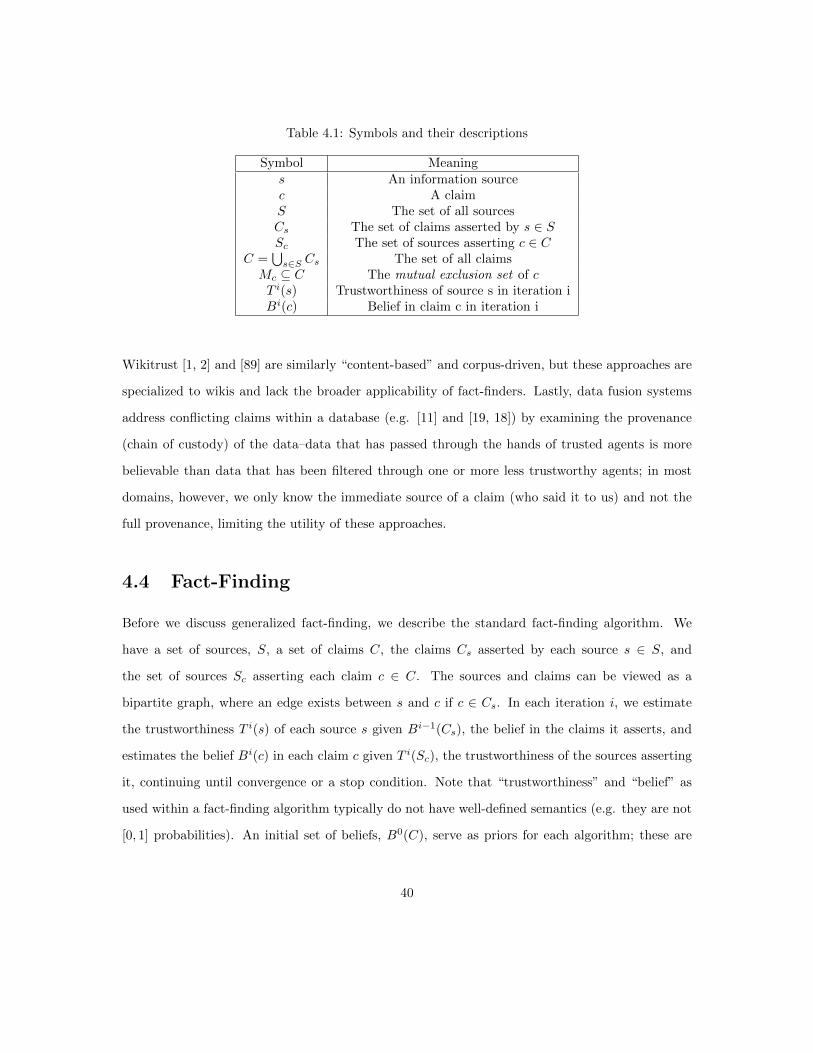
Table 4.1: Symbols and their descriptions

Symbol Meanings An information sourcec A claimS The set of all sourcesCs The set of claims asserted by s ∈ SSc The set of sources asserting c ∈ C

C =⋃s∈S Cs The set of all claims

Mc ⊆ C The mutual exclusion set of cT i(s) Trustworthiness of source s in iteration iBi(c) Belief in claim c in iteration i

Wikitrust [1, 2] and [89] are similarly “content-based” and corpus-driven, but these approaches are

specialized to wikis and lack the broader applicability of fact-finders. Lastly, data fusion systems

address conflicting claims within a database (e.g. [11] and [19, 18]) by examining the provenance

(chain of custody) of the data–data that has passed through the hands of trusted agents is more

believable than data that has been filtered through one or more less trustworthy agents; in most

domains, however, we only know the immediate source of a claim (who said it to us) and not the

full provenance, limiting the utility of these approaches.

4.4 Fact-Finding

Before we discuss generalized fact-finding, we describe the standard fact-finding algorithm. We

have a set of sources, S, a set of claims C, the claims Cs asserted by each source s ∈ S, and

the set of sources Sc asserting each claim c ∈ C. The sources and claims can be viewed as a

bipartite graph, where an edge exists between s and c if c ∈ Cs. In each iteration i, we estimate

the trustworthiness T i(s) of each source s given Bi−1(Cs), the belief in the claims it asserts, and

estimates the belief Bi(c) in each claim c given T i(Sc), the trustworthiness of the sources asserting

it, continuing until convergence or a stop condition. Note that “trustworthiness” and “belief” as

used within a fact-finding algorithm typically do not have well-defined semantics (e.g. they are not

[0, 1] probabilities). An initial set of beliefs, B0(C), serve as priors for each algorithm; these are

40

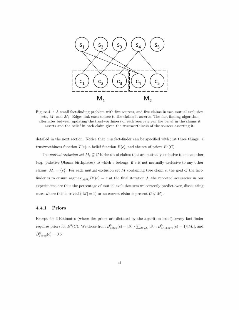
s1 s2 s3 s4 s5

c1 c2 c3 c4 c5

M1 M2

Figure 4.1: A small fact-finding problem with five sources, and five claims in two mutual exclusionsets, M1 and M2. Edges link each source to the claims it asserts. The fact-finding algorithm

alternates between updating the trustworthiness of each source given the belief in the claims itasserts and the belief in each claim given the trustworthiness of the sources asserting it.

detailed in the next section. Notice that any fact-finder can be specified with just three things: a

trustworthiness function T (s), a belief function B(c), and the set of priors B0(C).

The mutual exclusion set Mc ⊆ C is the set of claims that are mutually exclusive to one another

(e.g. putative Obama birthplaces) to which c belongs; if c is not mutually exclusive to any other

claims, Mc = {c}. For each mutual exclusion set M containing true claim c, the goal of the fact-

finder is to ensure argmaxc∈McBf (c) = c at the final iteration f ; the reported accuracies in our

experiments are thus the percentage of mutual exclusion sets we correctly predict over, discounting

cases where this is trivial (|M | = 1) or no correct claim is present (c /∈M).

4.4.1 Priors

Except for 3-Estimates (where the priors are dictated by the algorithm itself), every fact-finder

requires priors for B0(C). We chose from B0voted(c) = |Sc|/

∑d∈Mc

|Sd|, B0uniform(c) = 1/|Mc|, and

B0fixed(c) = 0.5.

41

4.4.2 Fact-Finding Algorithms

We consider Sums (Hubs and Authorities), TruthFinder, and 3-Estimates. Additionally, we intro-

duce three novel fact-finders that proved to be highly competitive in our experiments: Average-Log,

Investment, and PooledInvestment.

Sums (Hubs and Authorities)

Hubs and Authorities [49] gives each page a hub score and an authority score, where its hub score

is the sum of the authority of linked pages and its authority is the sum of the hub scores of pages

linking to it. This is adapted to fact-finding by viewing sources as hubs (with 0 authority) and

claims as authorities (with 0 hub score):

T i(s) =∑c∈Cs

Bi−1(c) Bi(c) =∑s∈Sc

T i(s)

We normalize to prevent T i(s) and Bi(c) from growing unbounded (dividing by maxs Ti(s) and

maxcBi(c), respectively), a technique also used with the Investment and Average·Log algorithms

(discussed next); this avoids numerical overflow. B0fixed priors are used.

Average·Log

Computing T (s) as an average of belief in its claims overestimates the trustworthiness of a source

with relatively few claims; certainly a source with 90% accuracy over a hundred examples is more

trustworthy than a source with 90% accuracy over ten. However, summing the belief in claims

allows a source with 10% accuracy to obtain a high trustworthiness score by simply making many

claims. Average·Log attempts a compromise, while still using Sums’ Bi update rule and B0fixed

priors.

T i(s) = log |Cs| ·∑c∈Cs B

i−1(c)

|Cs|

42

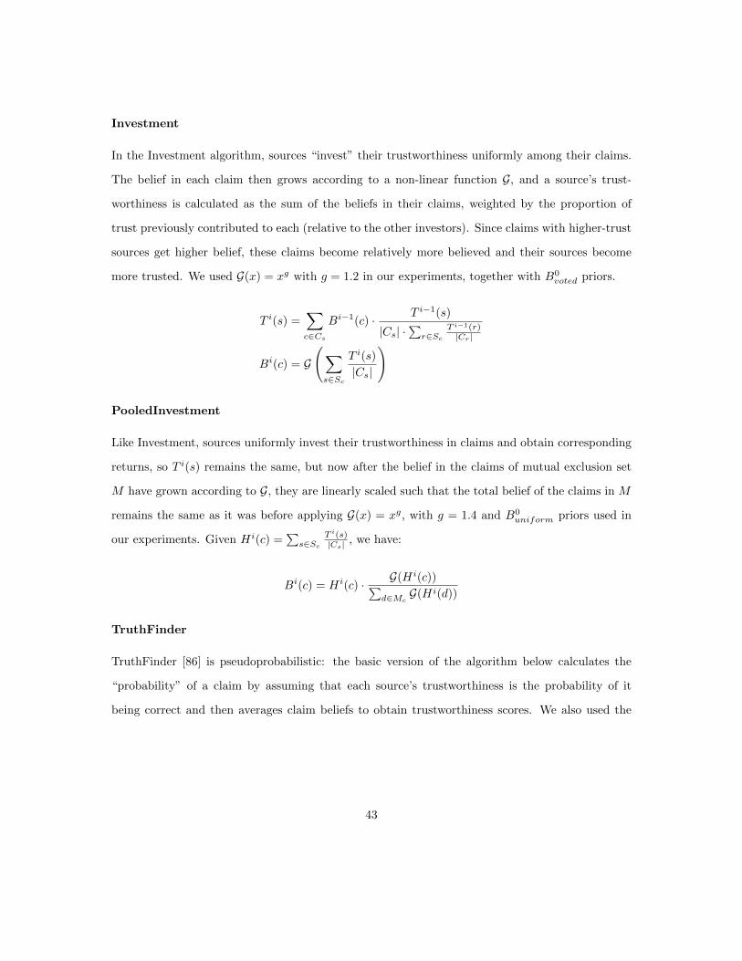
Investment

In the Investment algorithm, sources “invest” their trustworthiness uniformly among their claims.

The belief in each claim then grows according to a non-linear function G, and a source’s trust-

worthiness is calculated as the sum of the beliefs in their claims, weighted by the proportion of

trust previously contributed to each (relative to the other investors). Since claims with higher-trust

sources get higher belief, these claims become relatively more believed and their sources become

more trusted. We used G(x) = xg with g = 1.2 in our experiments, together with B0voted priors.

T i(s) =∑c∈Cs

Bi−1(c) · T i−1(s)

|Cs| ·∑r∈Sc

T i−1(r)|Cr|

Bi(c) = G

(∑s∈Sc

T i(s)

|Cs|

)

PooledInvestment

Like Investment, sources uniformly invest their trustworthiness in claims and obtain corresponding

returns, so T i(s) remains the same, but now after the belief in the claims of mutual exclusion set

M have grown according to G, they are linearly scaled such that the total belief of the claims in M

remains the same as it was before applying G(x) = xg, with g = 1.4 and B0uniform priors used in

our experiments. Given Hi(c) =∑s∈Sc

T i(s)|Cs| , we have:

Bi(c) = Hi(c) · G(Hi(c))∑d∈Mc

G(Hi(d))

TruthFinder

TruthFinder [86] is pseudoprobabilistic: the basic version of the algorithm below calculates the

“probability” of a claim by assuming that each source’s trustworthiness is the probability of it

being correct and then averages claim beliefs to obtain trustworthiness scores. We also used the

43

“full”, more complex TruthFinder, omitted here for brevity. B0uniform priors are used for both.

T i(s) =

∑c∈Cs B

i−1(c)

|Cs|Bi(c) = 1−

∏s∈Sc

(1− T i(s)

)

3-Estimates

3-Estimates [32], also omitted for brevity, differs from the other fact-finders by adding a third set

of parameters to capture the “difficulty” of a claim, such that correctly asserting a difficult claim

confers more trustworthiness than asserting an easy one; knowing the exact population of a city

is harder than knowing the population of Mars (presumably 0) and we should not trust a source

merely because they provide what is already common knowledge.

4.5 Generalized Fact-Finding

The key technical idea behind generalized fact-finding is that we can quite elegantly encode a variety

of prior knowledge by replacing the bipartite graph of standard fact-finders with a new weighted k-

partite graph, transitioning from binary assertions to weighted ones (“source s claims c with weight

x”) and adding additional “layers” of nodes to the graph to represent source groups and attributes.

We then need only modify the fact-finding algorithms to function on this new graph.

4.5.1 Encoding Information in Weighted Assertions

Weighted assertions, where each source s asserts a claim c with weight ω(s, c) = [0, 1], allow us to

incorporate a variety of factors into the model:

• Uncertainty in information extraction: we have a [0, 1] probability that source s asserted claim

c.

• Uncertainty of the source: a source may qualify his assertion (“I’m 90% certain that...”)

• Similarity between claims: a source asserting one claim also implicitly asserts (to a degree)

similar claims.

44

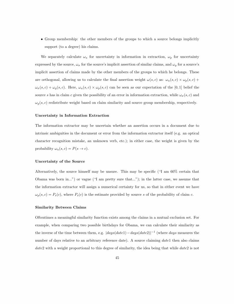
• Group membership: the other members of the groups to which a source belongs implicitly

support (to a degree) his claims.

We separately calculate ωu for uncertainty in information in extraction, ωp for uncertainty

expressed by the source, ωσ for the source’s implicit assertion of similar claims, and ωg for a source’s

implicit assertion of claims made by the other members of the groups to which he belongs. These

are orthogonal, allowing us to calculate the final assertion weight ω(s, c) as: ωu(s, c) × ωp(s, c) +

ωσ(s, c) + ωg(s, c). Here, ωu(s, c) × ωp(s, c) can be seen as our expectation of the [0, 1] belief the

source s has in claim c given the possibility of an error in information extraction, while ωσ(s, c) and

ωg(s, c) redistribute weight based on claim similarity and source group membership, respectively.

Uncertainty in Information Extraction

The information extractor may be uncertain whether an assertion occurs in a document due to

intrinsic ambiguities in the document or error from the information extractor itself (e.g. an optical

character recognition mistake, an unknown verb, etc.); in either case, the weight is given by the

probability ωu(s, c) = P (s→ c).

Uncertainty of the Source

Alternatively, the source himself may be unsure. This may be specific (“I am 60% certain that

Obama was born in...”) or vague (“I am pretty sure that...”); in the latter case, we assume that

the information extractor will assign a numerical certainty for us, so that in either event we have

ωp(s, c) = Ps(c), where Ps(c) is the estimate provided by source s of the probability of claim c.

Similarity Between Claims

Oftentimes a meaningful similarity function exists among the claims in a mutual exclusion set. For

example, when comparing two possible birthdays for Obama, we can calculate their similarity as

the inverse of the time between them, e.g. |days(date1)−days(date2)|−1 (where days measures the

number of days relative to an arbitrary reference date). A source claiming date1 then also claims

date2 with a weight proportional to this degree of similarity, the idea being that while date2 is not

45

what he claimed, he will prefer it over other dates that are even more dissimilar. Given a [0, 1]

similarity function σ(c1, c2), we can calculate:

ωσ(s, c) =∑

d∈Mc,d 6=c

ωu(s, d)ωp(s, d)σ(c, d)

Notice that a self-consistent source will not assert multiple claims in mutual exclusion set M

with∑c∈M ωu(s, c)ωp(s, c) > 1, and thus the addition of ωσ(s, c) to ω(s, c) will never result in

ω(s, c) > 1; it is possible, however, that∑c∈M ω(s, c) > 1 for a given source s. One way to avoid

this is to redistribute weight rather than add it; we introduce the parameter α to control the degree

of redistribution and obtain:

ωασ (s, c) =∑

d∈Mc,d6=c

(αωu(s, d)ωp(s, d)σ(c, d)∑

e∈Md,e6=d σ(d, e)

)− αωu(s, c)ωp(s, c)

This function ensures that only a portion α of the source’s expected belief in the claim,

ωu(s, c)ωp(s, c), is redistributed among other claims in Mc (proportional to their similarity with c),

at a cost of αωu(s, c)ωp(s, c).

[86] previously used a form of additive similarity as “Implication” functions in TruthFinder;

however, our formalization generalizes this idea and allows us to apply it to any fact-finder.

Group Membership via Weighted Assertions

Oftentimes a source belongs to one or more groups; for example, a journalist may be a member of

professional associations and an employee of one or more publishers. Our assumption is that these

groups are meaningful, that is, sources belonging to the same group tend to have similar degrees of

trustworthiness. A prestigious, well-known group (e.g. the group of administrators in Wikipedia)

will presumably have more trustworthy members (in general) than a discredited group (e.g. the

group of blocked Wikipedia editors). The approach discussed in this section encodes these groups

using ωg; a more flexible approach, discussed later, is to use additional “layers” of groups and

attributes instead.

46

Let Gs be the set of groups to which a source s belongs. If a source s and source u are both

members of the same group g, we interpret this as an implicit assertion by u in Cs, and by s in Cu—

that is, group members mutually assert each others’ claims to a degree. We use a redistribution

parameter β such that the original weight of a member’s assertion is split between the member

(proportional to 1− β) and the other members of the groups to which he belongs (proportional to

β). This gives us:

ωβg (s, c) = β∑g∈Gs

∑u∈g

ωu(u, c)ωp(u, c) + ωσ(u, c)

|Gu| · |Gs| ·∑v∈g |Gv|−1

− β(ωu(s, c)ωp(s, c) + ωσ(s, c))

∑v∈g |Gv|−1 in the denominator gives greater credence to “small” groups (where members

belonging to many other groups weigh less heavily), with the intuition that smaller groups have

more similar members. Note that in the worst case (where all sources belong to a single group and

each assert a unique set of k claims) this can effectively create as many as (k · |S|)2 − k · |S| new

assertions, with a corresponding increase in computational cost when running the fact-finder.

4.5.2 Rewriting Fact-Finders for Assertion Weights

After calculating the weight functions ω(s, c) for all s ∈ S and c ∈ C, we need to rewrite each

fact-finder’s T (s), B(c) and B0(c) functions to use these weights in the generalized fact-finding

process by qualifying previously “whole” assertions as “partial”, weighted assertions. We start by

redefining Sc as {s : s ∈ S, ω(s, c) > 0}, and Cs as {c : c ∈ C,ω(s, c) > 0}. The basic rewriting

rules are:

• Replace |Sc| with∑s∈Sc ω(s, c)

• Replace |Cs| with∑c∈Cs ω(s, c)

• In T i(s), replace Bi−1(c) with ω(s, c)Bi−1(c)

• In Bi(c), replace T i(s) with ω(s, c)T i(s)

These rules suffice for all the linear fact-finders we encountered; one, TruthFinder, is instead log-

linear, so an exponent rather than a coefficient is applied, but such exceptions are straightforward.

47

Generalized Sums (Hubs and Authorities)

T i(s) =∑c∈Cs

ω(s, c)Bi−1(c) Bi(c) =∑s∈Sc

ω(s, c)T i(s)

Generalized Average·Log

Average·Log employs the same B function as Sums, so we provide only the trustworthiness function:

T i(s) = log

(∑c∈Cs

ω(s, c)

)·∑c∈Cs ω(s, c)Bi−1(c)∑

c∈Cs ω(s, c)

Generalized Investment

The Investment algorithm requires sources to “invest” their trust uniformly in their claims; we

rewrite this such that these investments are weighted by ω.

T i(s) =∑c∈Cs

ω(s, c)Bi−1(c)T i−1(s)∑c∈Cs ω(s, c) ·

∑r∈Sc

ω(r,c)T i−1(r)∑b∈Cr ω(r,b)

Bi(c) = G

(∑s∈Sc

ω(s, c)T i(s)∑c∈Cs ω(s, c)

)

Generalized PooledInvestment

PooledInvestment utilizes the same T i(s) function as Investment, and instead alters the belief

function, which we generalize below.

Hi(c) =∑s∈Sc

ω(s, c)T i(s)∑c∈Cs ω(s, c)

Bi(c) = Hi(c) · G(Hi(c))∑d∈Mc

G(Hi(d))

Generalized TruthFinder

TruthFinder [86] has both a “simple” and “complete” version, with the latter making a number

of adjustments to the former. We specify only the simple version below, as the modifications to

48

s1 s2 s3 s4

c1 c2 c3 c4

g1 g2 g3

L1

L2

L3

Figure 4.2: A fact-finding problem with a single group layer. Edges between sources and groupsdenote membership.

the complete variant are similar. Both models calculate claim belief non-linearly, and in either

case we have the option of using logarithms to obtain a log-linear function. This is what we do in

practice, since it avoids underflow in the floating-point variables; for clarity, however, we present

the “multiplicative” version below. Note that using ω(s, c) as an exponent here is equivalent to its

use as a coefficient in the log-linear function.

T i(s) =

∑c∈Cs ω(s, c)Bi−1(c)∑

c∈Cs ω(s, c)Bi(c) = 1−

∏s∈Sc

(1− T i(s)

)ω(s,c)

Generalized 3-Estimates

3-Estimates [32] incorporates an additional set of parameters to model the “hardness” of each

claim (referred to as ε(F)) that can be incorporated into the B and T functions to fit our common

model. We omit the full algorithm here for brevity, but generalizing it is quite straightforward–

when calculating a summation over sources for a given claim or a summation over claims for a

given source, we simply weight each element of the sum by the relevant assertion weight between

the particular source and claim in question.

49

4.5.3 Groups and Attributes as Layers

Instead of using weighted assertions, we can add additional “layers” to represent groups and at-

tributes directly. Each node in these layers will represent a group or attribute, with edges linking

to its adjoining layers (either the sources or other groups/attributes), creating a k-partite graph

(with k > 3 used to encode meta-groups and meta-attributes.) An standard fact-finder iteratively

alternates between calculating the first layer (the claims) and the second layer (the sources), using

the B and T functions, respectively. Now we replace these with generic “up” and “down” functions

for each layer. For a k-partite graph with layers L1...k, we define U ij(Lj) over j = 2...k and Dij(Lj)

over j = 1...k − 1, with special cases U i1(L1) = Di−11 (L1) and Di

k(Lk) = U ik(Lk). The Uj and Dj

functions may differ for each j, or they may be the same over all layers. In each iteration i, we

calculate the values U ij(Lj) for layers j = 2 to k, and then calculate Dij(Lj) for layers j = k − 1 to

1. For example, to extend Sums to k layers, we calculate Uj(e) and Dj(e) as follows for e ∈ Lj :

U ij(e) =∑

f∈Lj−1

ω(e, f)U ij−1(f)

Dij(e) =

∑f∈Lj+1

ω(e, f)Dij+1(f)

Where ω(e, f) = ω(f, e) is the edge weight between nodes e and f ; if e or f is a group or

attribute, ω(e, f) is 1 if e has attribute or group f or vice-versa, and 0 otherwise. In many cases,

though, we may benefit from using an existing fact-finder over the claim and source layers, while

using a different set of functions to mediate the interaction between the source and group/attribute

layers. In particular, an information bottleneck often exists when calculating trustworthiness of a

source in the “down phase”, as it will be wholly dependent upon the trustworthiness of the groups to

which it belongs: a source belonging to one overall-mediocre group may make many correct claims,

but still be assigned a low trustworthiness score by the D function because of its group membership.

This type of problem can be resolved by incorporating both the layer below and the layer above

in each calculation; for example, for a given Dj(e), we can define ωchildren =∑f∈Lj−1

ω(e, f) and

Dsmoothj (e) = (1 + ωchildren)−1Dj(e) + ωchildren(1 + ωchildren)−1Uj(e), which returns a mixture

50

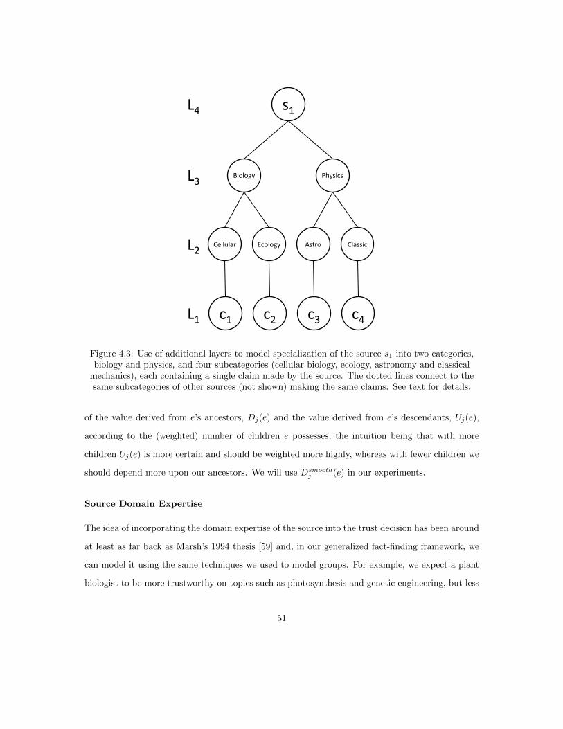
Cellular Ecology Astro Classic

c1 c2 c3 c4

Biology Physics

L1

L2

L3

s1L4

Figure 4.3: Use of additional layers to model specialization of the source s1 into two categories,biology and physics, and four subcategories (cellular biology, ecology, astronomy and classical

mechanics), each containing a single claim made by the source. The dotted lines connect to thesame subcategories of other sources (not shown) making the same claims. See text for details.

of the value derived from e’s ancestors, Dj(e) and the value derived from e’s descendants, Uj(e),

according to the (weighted) number of children e possesses, the intuition being that with more

children Uj(e) is more certain and should be weighted more highly, whereas with fewer children we

should depend more upon our ancestors. We will use Dsmoothj (e) in our experiments.

Source Domain Expertise

The idea of incorporating the domain expertise of the source into the trust decision has been around

at least as far back as Marsh’s 1994 thesis [59] and, in our generalized fact-finding framework, we

can model it using the same techniques we used to model groups. For example, we expect a plant

biologist to be more trustworthy on topics such as photosynthesis and genetic engineering, but less

51

reliable on topics outside his expertise, such as fusion and computational complexity. Still, these

aspects are not entirely separate: if we have two plant biologists A and B, and A gives accurate

information about plant biology while B gives inaccurate information, we will tend to assign greater

credence to A with respect to other domains (such as physics) as well–that is, we assume A is more

“generally trustworthy” overall.

To implement this, we may create additional layers to represent our trustworthiness in a source

for various domains. In Figure 4.3, we see that source s1 has made claims in four different domains:

cellular biology, ecology, astronomy, and classical mechanics. Each node shown in layers 2 and 3

is specific to s1, representing his trustworthiness in that particular field or subfield, such that the

sources are actually s1’s “Cellular”, “Ecology”, “Astro” and “Classic” nodes, which belong to two

groups corresponding to s1’s biology and physics trustworthiness, which themselves belong to a

metagroup corresponding to s1’s general trustworthiness.

Additional Layers versus Weighted Edges

Relative to adding edges to represent groups, expanding our model with additional layers increases

the complexity of the algorithm, but prevents the quadratic expansion of the number of edges and

corresponding increase in time complexity. More importantly, though, the flexibility in specifying

the U and D functions for high layers representing groups and attributes allows us to augment an

existing fact-finder to take advantage of this additional information in an arbitrary way.

4.6 Constrained Fact-Finding

To apply the user’s specific and axiomatic “common-sense” declarative prior knowledge over claims

to a fact-finding algorithm, we translate it into a linear program. We then iterate the following

until convergence or other stopping criteria:

1. Compute T i(s) for all s ∈ S

2. Compute Bi(c) for all c ∈ C

3. “Correct” beliefs Bi(C) with the LP

52

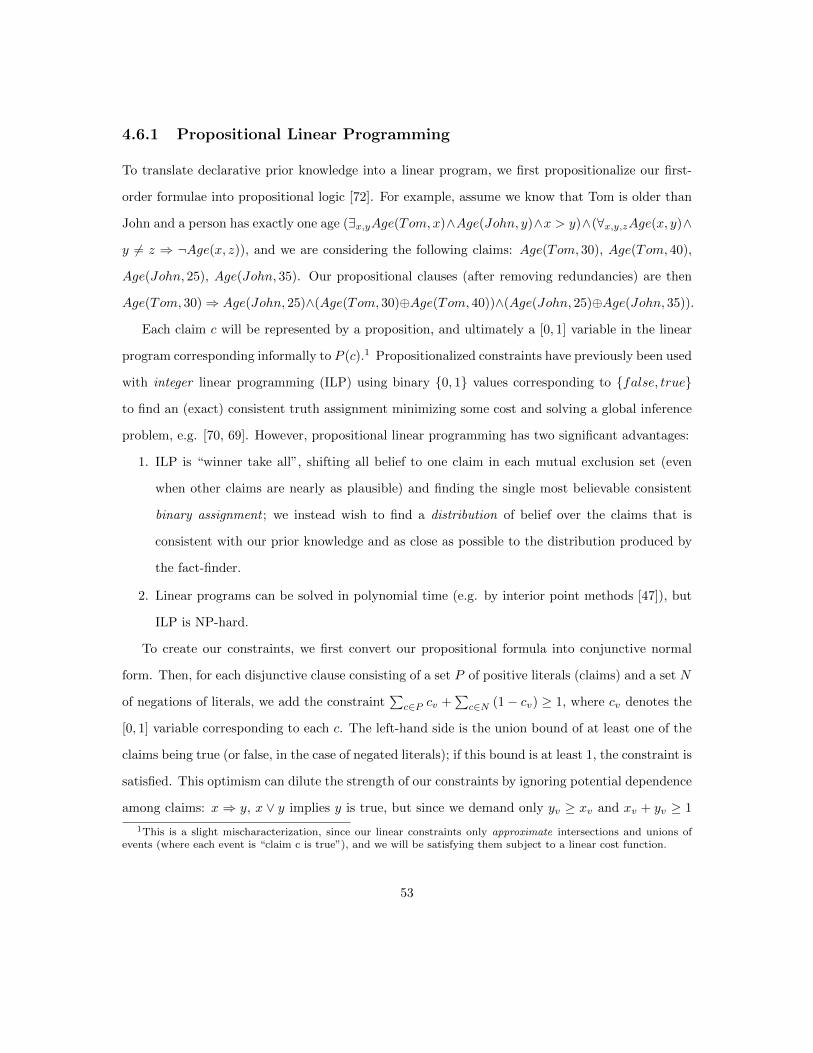
4.6.1 Propositional Linear Programming

To translate declarative prior knowledge into a linear program, we first propositionalize our first-

order formulae into propositional logic [72]. For example, assume we know that Tom is older than

John and a person has exactly one age (∃x,yAge(Tom, x)∧Age(John, y)∧x > y)∧(∀x,y,zAge(x, y)∧

y 6= z ⇒ ¬Age(x, z)), and we are considering the following claims: Age(Tom, 30), Age(Tom, 40),

Age(John, 25), Age(John, 35). Our propositional clauses (after removing redundancies) are then

Age(Tom, 30)⇒ Age(John, 25)∧(Age(Tom, 30)⊕Age(Tom, 40))∧(Age(John, 25)⊕Age(John, 35)).

Each claim c will be represented by a proposition, and ultimately a [0, 1] variable in the linear

program corresponding informally to P (c).1 Propositionalized constraints have previously been used

with integer linear programming (ILP) using binary {0, 1} values corresponding to {false, true}

to find an (exact) consistent truth assignment minimizing some cost and solving a global inference

problem, e.g. [70, 69]. However, propositional linear programming has two significant advantages:

1. ILP is “winner take all”, shifting all belief to one claim in each mutual exclusion set (even

when other claims are nearly as plausible) and finding the single most believable consistent

binary assignment ; we instead wish to find a distribution of belief over the claims that is

consistent with our prior knowledge and as close as possible to the distribution produced by

the fact-finder.

2. Linear programs can be solved in polynomial time (e.g. by interior point methods [47]), but

ILP is NP-hard.

To create our constraints, we first convert our propositional formula into conjunctive normal

form. Then, for each disjunctive clause consisting of a set P of positive literals (claims) and a set N

of negations of literals, we add the constraint∑c∈P cv +

∑c∈N (1− cv) ≥ 1, where cv denotes the

[0, 1] variable corresponding to each c. The left-hand side is the union bound of at least one of the

claims being true (or false, in the case of negated literals); if this bound is at least 1, the constraint is

satisfied. This optimism can dilute the strength of our constraints by ignoring potential dependence

among claims: x ⇒ y, x ∨ y implies y is true, but since we demand only yv ≥ xv and xv + yv ≥ 1

1This is a slight mischaracterization, since our linear constraints only approximate intersections and unions ofevents (where each event is “claim c is true”), and we will be satisfying them subject to a linear cost function.

53

we accept any yv ≥ 0.5 where yv ≥ xv ≥ 1− yv. However, when the claims are mutually exclusive,

the union bound is exact; a common constraint is of the form q ⇒ r1 ∨ r2 ∨ . . ., where the r literals

are mutually exclusive, which translates exactly to r1v + r2

v + . . . ≥ qv. Finally, observe that mutual

exclusion amongst n claims c1, c2, . . ., cn can be compactly written as c1v + c2v + . . .+ cnv = 1.

4.6.2 The Cost Function

Having seen how first-order logic can be converted to linear constraints, we now consider the cost

function, a distance between the new distribution of belief satisfying our constraints and the original

distribution produced by the fact-finder.

First we determine the number of “votes” received by each claim c, computed as ωc = ω(B(c)),

which should scale linearly with the certainty of the fact-finder’s belief in c. Recall that the semantics

of the belief score are particular to the fact-finder, so different fact-finders require different vote

functions. TruthFinder has pseudoprobabilistic [0,1] beliefs, so we use ωinv(x) = min((1−x)-1,minv)

with minv = 1010 limiting the maximum number of votes possible; we assume 1/0 = ∞. ωinv

intuitively scales with “error”: a belief of 0.99 receives ten times the votes of 0.9 and has a tenth

the error (0.01 vs. 0.1). For the remainder of the fact-finders whose beliefs are already “linear”, we

use the identity function ωidn(x) = x.

The most obvious choice for the cost function to minimize might be “frustrated votes”, computed

as∑c∈C ωc(1 − cv). Unfortunately, this results in the linear solver generally assigning 1 to the

variable in each mutual exclusion set with the most votes and 0 to all others (except when constraints

prevent this), shifting all belief to the highest-vote claim and yielding poor performance. Instead,

we wish to satisfy the constraints while keeping each cv close to ωc/ωMc, where ωMc

=∑d∈Mc

ωd,

and thus shift belief among claims as little as possible. We use a weighted Manhattan distance

called VoteDistance, where the cost for increasing the belief in a claim is proportional to the

number of votes against it, and the cost for decreasing belief is proportional to the number of votes

54

for it:

∑c∈C

max

(ωMc − ωc) · (cv − ωc/ωMc),

ωc · (ωc/ωMc− cv)

Thus, the belief distribution found by our LP will be the one that satisfies the constraints while

simultaneously minimizing the number of votes frustrated by the change from the original distri-

bution. Note that for any linear expressions e and f we can implement max(e, f) in the objective

function by replacing it with a new [−∞,∞] helper variable x and adding the linear constraints

x ≥ e and x ≥ f .

4.6.3 From Values to Votes to Belief

Solving the LP gives us [0, 1] values for each variable cv, but we need to calculate an updated belief

B(c). We propose two methods for this:

Vote Conservation: B(c) = ω−1(cv · ωMc)

Vote Loss: B(c) = ω−1(min(ωc, cv · ωMc))

ω−1 is an inverse of the vote function: ω−1idn(x) = x and ω−1

inv(x) = 1 − (1 + y)−1. Vote

Conservation reallocates votes such that the total number of votes in each mutual exclusion set,

ωM , remains the same after the redistribution. However, if the constraints force c to lose votes,

should we believe the other claims in Mc more? Under Vote Loss, a claim can only lose votes,

ensuring that if other claims in Mc become less believable, c does not itself become more believable

relative to claims in other mutual exclusion sets. We found Vote Loss slightly better on average

and used it for all reported results.

4.6.4 LP Decomposition

Frequently our linear programs can be decomposed into smaller problems that can be solved inde-

pendently. If there exists a subset of linear constraints L′ ⊂ L that contain a set of variables V ′ ⊂ V

55

such that ∀v∈V ′,l∈L/L′ v 6∈ l, then L′ together with the terms in the cost function containing the

variables V ′ can be solved as a separate LP.

We can also reduce running time by observing that, for any such “sub-LP”, it is easy to set each

variable cv to ωc/ωMc (yielding the minimum possible cost of 0) and check if the constraints are

satisfied—if they are, the optimal solution is found without invoking the linear solver. Together,

these techniques allowed us to solve most LPs one or two orders of magnitude faster in our experi-

ments (almost always within a matter of seconds), taking more than a minute to solve on a modest

desktop machine only when the presence of tens of thousands of constraints prevented meaningful

decomposition.

4.6.5 Tie Breaking

We must also address “ties” between claims with the same number of votes. If the linear solver is

allowed to break these arbitrarily, the results may vary from solver to solver. This is of particular

concern when using a chain of solvers (our experiments used Microsoft Solver Foundation (MSF)

simplex → lp solve simplex → MSF interior point) to enable “fallback” when one solver fails and

consistent behavior is required. We handled this by, within each decomposed LP, identifying pairs

of claims with the same number of votes, multiplying the votes of one by 1 + 10−10 and repeating

until no pair of claims is tied. Which claim gets slightly boosted depends upon a “precedence” that

is assigned randomly at the start of the experiment.

4.6.6 “Unknown” Augmentation

Augmenting our data with “Unknown” claims ensures that every LP is feasible and can be used to

model our ignorance given a lack of sufficient information or conflicting constraints. An Unknown

claim UM is added to every mutual exclusion set M (but invisible to the fact-finder) and represents

our belief that none of the claims in M are sufficiently supported. Now we can write the mutual

exclusion constraint for M as UM +∑c∈M cv = 1. When propositionalizing FOL, if a disjunctive

clause contains a non-negated literal for a claim c, then we add ∨UMcto the clause. For example,

Age(John, 35) ⇒ Age(Tom, 40) becomes Age(John, 35) ⇒ Age(Tom, 40) ∨ Age(Tom,Unknown).

56

The only exception is when the clause contains claims from only one mutual exclusion set (e.g.

“I know Sam is 50 or 60”), and so the LP can only be infeasible if the user directly asserts a

contradiction (e.g. “Sam is 50 and Sam is 60”). The Unknown itself has a fixed number of votes

that cannot be lost; this effectively “smooths” our belief in the claims and imposes a floor for

believability. If Age(Kim, 30) has 5 votes, Age(Kim, 35) has 3 votes, and Age(Kim,Unknown) is

fixed at 6 votes, we hold that Kim’s age is unknown due to lack of evidence. The number of votes

that should be given to each Unknown for this purpose depends, of course, on the particular fact-

finder and ω function used; in our experiments, we are not concerned with establishing ignorance

and thus assign 0 votes.

4.7 Experiments

To evaluate our extensions to fact-finding, both the generalization of the fact-finders themselves

and the application of declarative constraints, we experimented over a number of state-of-the-

art fact-finding algorithms using both real-world and semi-synthetic datasets. We considered both

extensions separately, finding each was independently able to improve the accuracy of trust decisions

by incorporating different types of prior knowledge into the fact-finding process, and then combined

these orthogonal components into a joint model able to achieve significantly better results than were

possible using either alone.

4.7.1 Data

We used a number of real-world datasets in our experiments, including two (Population and Biog-

raphy) extracted from Wikipedia infoboxes [83] (semi-structured tables with various fields within

Wikipedia articles). An example of an infobox for the city of Laguna Beach is shown in Figure 4.4.

57

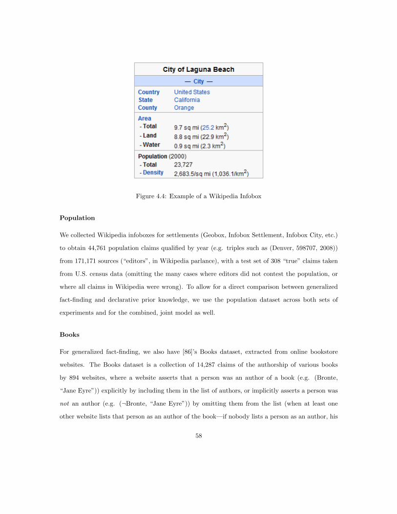
Figure 4.4: Example of a Wikipedia Infobox

Population

We collected Wikipedia infoboxes for settlements (Geobox, Infobox Settlement, Infobox City, etc.)

to obtain 44,761 population claims qualified by year (e.g. triples such as (Denver, 598707, 2008))

from 171,171 sources (“editors”, in Wikipedia parlance), with a test set of 308 “true” claims taken

from U.S. census data (omitting the many cases where editors did not contest the population, or

where all claims in Wikipedia were wrong). To allow for a direct comparison between generalized

fact-finding and declarative prior knowledge, we use the population dataset across both sets of

experiments and for the combined, joint model as well.

Books

For generalized fact-finding, we also have [86]’s Books dataset, extracted from online bookstore

websites. The Books dataset is a collection of 14,287 claims of the authorship of various books

by 894 websites, where a website asserts that a person was an author of a book (e.g. (Bronte,

“Jane Eyre”)) explicitly by including them in the list of authors, or implicitly asserts a person was

not an author (e.g. (¬Bronte, “Jane Eyre”)) by omitting them from the list (when at least one

other website lists that person as an author of the book—if nobody lists a person as an author, his

58

non-authorship is not disputed and can be ignored). The test set is 605 true claims collected by

examining the books’ covers.

Biography

For our declarative prior knowledge experiments, we created the Biography dataset by scanning

Wikipedia infoboxes to find 129,847 claimed birth dates, 34,201 death dates, 10,418 parent-child

pairs, and 9,792 spouses as reported by 1,167,494 editors. To get “true” birth and death dates, we

extracted data from several online repositories (after satisfying ourselves that they were independent

and not derived from Wikipedia!), eliminating any date these sources disagreed upon, and ultimately

obtained a total of 2,685 dates to test against.

American vs. British Spelling

Finally, we examined a domain where the truth was plainly subjective and thus the user’s prior

knowledge is essential: identifying the “correct” spelling of words given 209,189 articles from the

British National Corpus, The Washington Post and Reuters written by 9,387 distinct authors.

4.7.2 Experimental Setup

For our experiments we used a number of state-of-the-art fact-finding algorithms: Sums / Hubs

and Authorities (Sum), 3-Estimates (3Est), simplified TruthFinder (TFs), “full” TruthFinder

(TFc), Average·Log (A·L), Investment with g = 1.2 (Inv1.2), and PooledInvestment with g = 1.4

(Pool1.4). The voting baseline (Vote) simply chooses the claim asserted by the most sources. The

number of iterations used for each fact-finder was fixed at 20. To evaluate accuracy, after the final

iteration we looked at each mutual exclusion set M and predicted the highest-belief claim c ∈ M

(other than uM , if applicable), breaking ties randomly, and checked if it was the true claim tM . We

omitted any M that did not contain a true claim (all known claims are false) and any M that was

trivially correct (containing only one claim [other than uM , if applicable]).

59

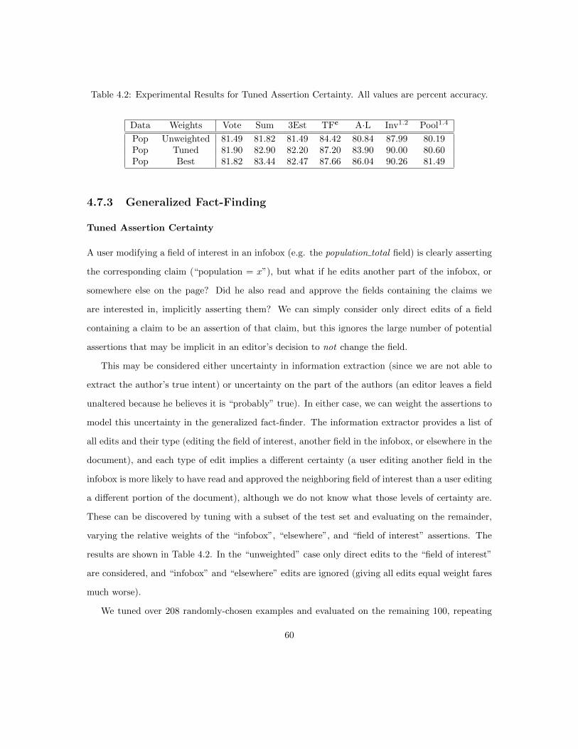
Table 4.2: Experimental Results for Tuned Assertion Certainty. All values are percent accuracy.

Data Weights Vote Sum 3Est TFc A·L Inv1.2 Pool1.4

Pop Unweighted 81.49 81.82 81.49 84.42 80.84 87.99 80.19Pop Tuned 81.90 82.90 82.20 87.20 83.90 90.00 80.60Pop Best 81.82 83.44 82.47 87.66 86.04 90.26 81.49

4.7.3 Generalized Fact-Finding

Tuned Assertion Certainty

A user modifying a field of interest in an infobox (e.g. the population total field) is clearly asserting

the corresponding claim (“population = x”), but what if he edits another part of the infobox, or

somewhere else on the page? Did he also read and approve the fields containing the claims we

are interested in, implicitly asserting them? We can simply consider only direct edits of a field

containing a claim to be an assertion of that claim, but this ignores the large number of potential

assertions that may be implicit in an editor’s decision to not change the field.

This may be considered either uncertainty in information extraction (since we are not able to

extract the author’s true intent) or uncertainty on the part of the authors (an editor leaves a field

unaltered because he believes it is “probably” true). In either case, we can weight the assertions to

model this uncertainty in the generalized fact-finder. The information extractor provides a list of

all edits and their type (editing the field of interest, another field in the infobox, or elsewhere in the

document), and each type of edit implies a different certainty (a user editing another field in the

infobox is more likely to have read and approved the neighboring field of interest than a user editing

a different portion of the document), although we do not know what those levels of certainty are.

These can be discovered by tuning with a subset of the test set and evaluating on the remainder,

varying the relative weights of the “infobox”, “elsewhere”, and “field of interest” assertions. The

results are shown in Table 4.2. In the “unweighted” case only direct edits to the “field of interest”

are considered, and “infobox” and “elsewhere” edits are ignored (giving all edits equal weight fares

much worse).

We tuned over 208 randomly-chosen examples and evaluated on the remaining 100, repeating

60

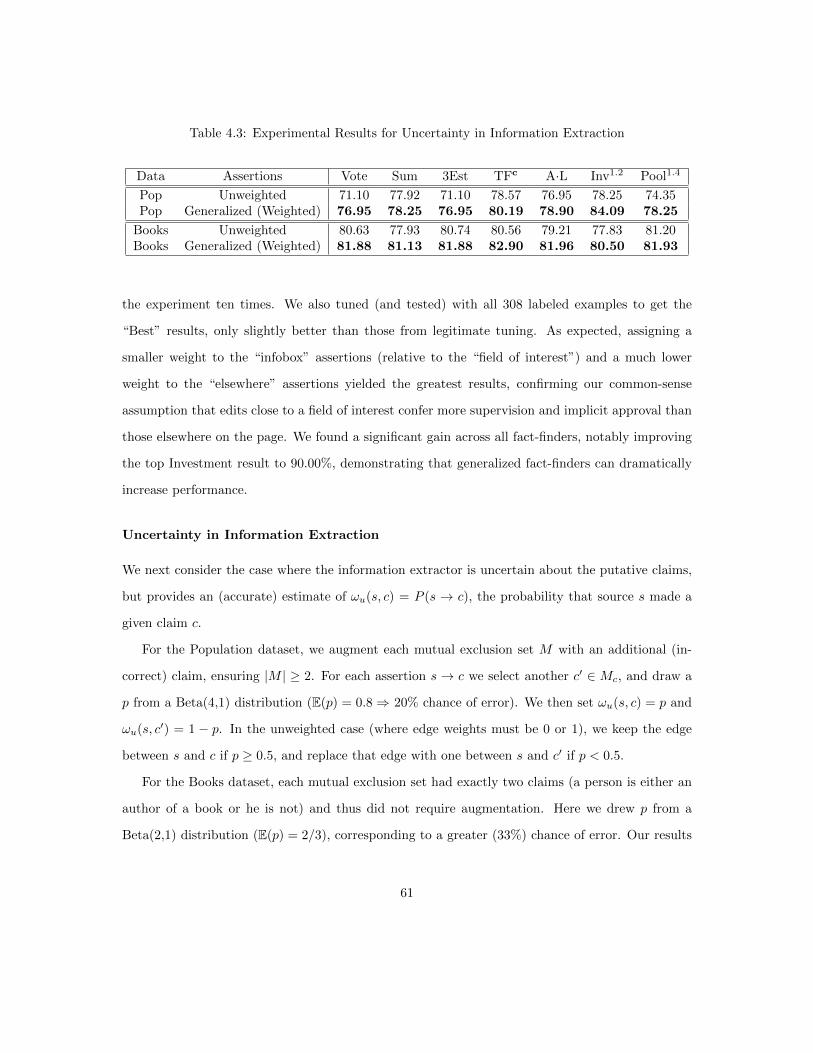
Table 4.3: Experimental Results for Uncertainty in Information Extraction

Data Assertions Vote Sum 3Est TFc A·L Inv1.2 Pool1.4

Pop Unweighted 71.10 77.92 71.10 78.57 76.95 78.25 74.35Pop Generalized (Weighted) 76.95 78.25 76.95 80.19 78.90 84.09 78.25

Books Unweighted 80.63 77.93 80.74 80.56 79.21 77.83 81.20Books Generalized (Weighted) 81.88 81.13 81.88 82.90 81.96 80.50 81.93

the experiment ten times. We also tuned (and tested) with all 308 labeled examples to get the

“Best” results, only slightly better than those from legitimate tuning. As expected, assigning a

smaller weight to the “infobox” assertions (relative to the “field of interest”) and a much lower

weight to the “elsewhere” assertions yielded the greatest results, confirming our common-sense

assumption that edits close to a field of interest confer more supervision and implicit approval than

those elsewhere on the page. We found a significant gain across all fact-finders, notably improving

the top Investment result to 90.00%, demonstrating that generalized fact-finders can dramatically

increase performance.

Uncertainty in Information Extraction

We next consider the case where the information extractor is uncertain about the putative claims,

but provides an (accurate) estimate of ωu(s, c) = P (s → c), the probability that source s made a

given claim c.

For the Population dataset, we augment each mutual exclusion set M with an additional (in-

correct) claim, ensuring |M | ≥ 2. For each assertion s → c we select another c′ ∈ Mc, and draw a

p from a Beta(4,1) distribution (E(p) = 0.8⇒ 20% chance of error). We then set ωu(s, c) = p and

ωu(s, c′) = 1 − p. In the unweighted case (where edge weights must be 0 or 1), we keep the edge

between s and c if p ≥ 0.5, and replace that edge with one between s and c′ if p < 0.5.

For the Books dataset, each mutual exclusion set had exactly two claims (a person is either an

author of a book or he is not) and thus did not require augmentation. Here we drew p from a

Beta(2,1) distribution (E(p) = 2/3), corresponding to a greater (33%) chance of error. Our results

61

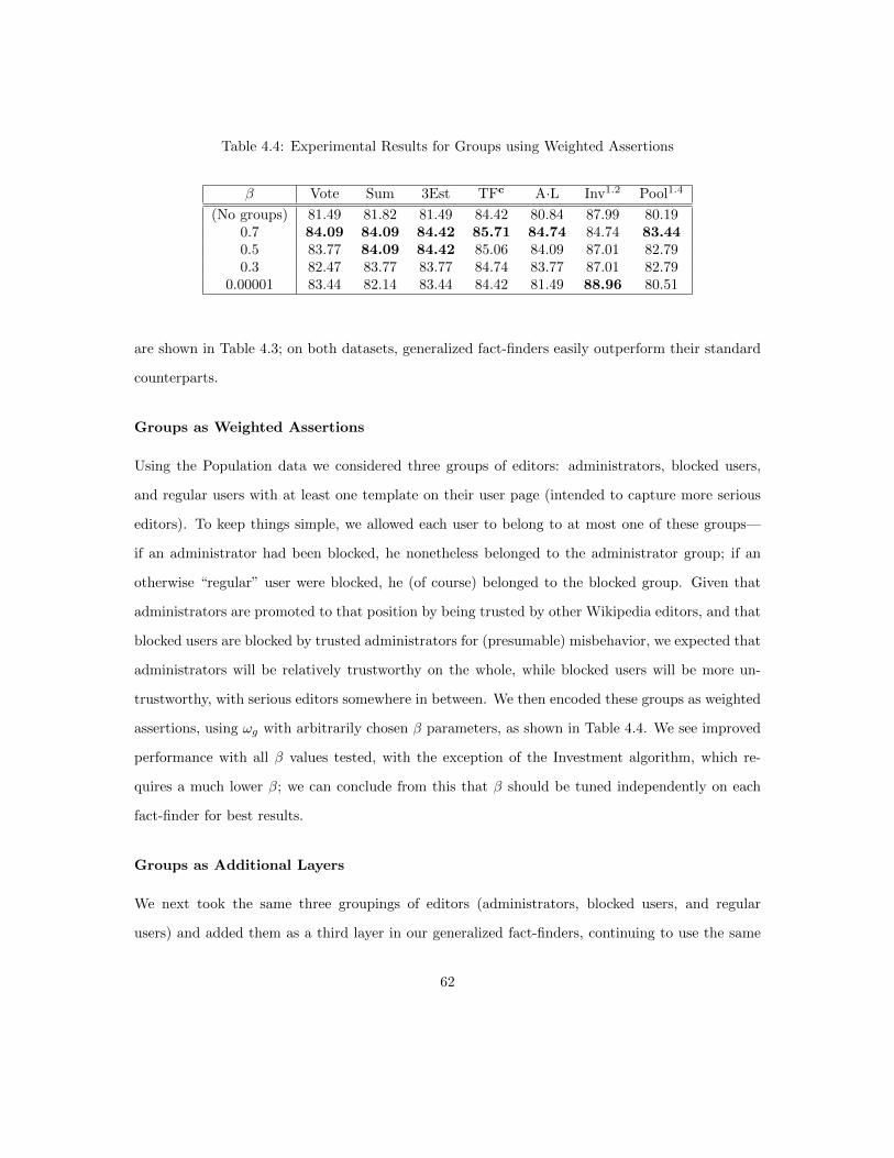
Table 4.4: Experimental Results for Groups using Weighted Assertions

β Vote Sum 3Est TFc A·L Inv1.2 Pool1.4

(No groups) 81.49 81.82 81.49 84.42 80.84 87.99 80.190.7 84.09 84.09 84.42 85.71 84.74 84.74 83.440.5 83.77 84.09 84.42 85.06 84.09 87.01 82.790.3 82.47 83.77 83.77 84.74 83.77 87.01 82.79

0.00001 83.44 82.14 83.44 84.42 81.49 88.96 80.51

are shown in Table 4.3; on both datasets, generalized fact-finders easily outperform their standard

counterparts.

Groups as Weighted Assertions

Using the Population data we considered three groups of editors: administrators, blocked users,

and regular users with at least one template on their user page (intended to capture more serious

editors). To keep things simple, we allowed each user to belong to at most one of these groups—

if an administrator had been blocked, he nonetheless belonged to the administrator group; if an

otherwise “regular” user were blocked, he (of course) belonged to the blocked group. Given that

administrators are promoted to that position by being trusted by other Wikipedia editors, and that

blocked users are blocked by trusted administrators for (presumable) misbehavior, we expected that

administrators will be relatively trustworthy on the whole, while blocked users will be more un-

trustworthy, with serious editors somewhere in between. We then encoded these groups as weighted

assertions, using ωg with arbitrarily chosen β parameters, as shown in Table 4.4. We see improved

performance with all β values tested, with the exception of the Investment algorithm, which re-

quires a much lower β; we can conclude from this that β should be tuned independently on each

fact-finder for best results.

Groups as Additional Layers

We next took the same three groupings of editors (administrators, blocked users, and regular

users) and added them as a third layer in our generalized fact-finders, continuing to use the same

62

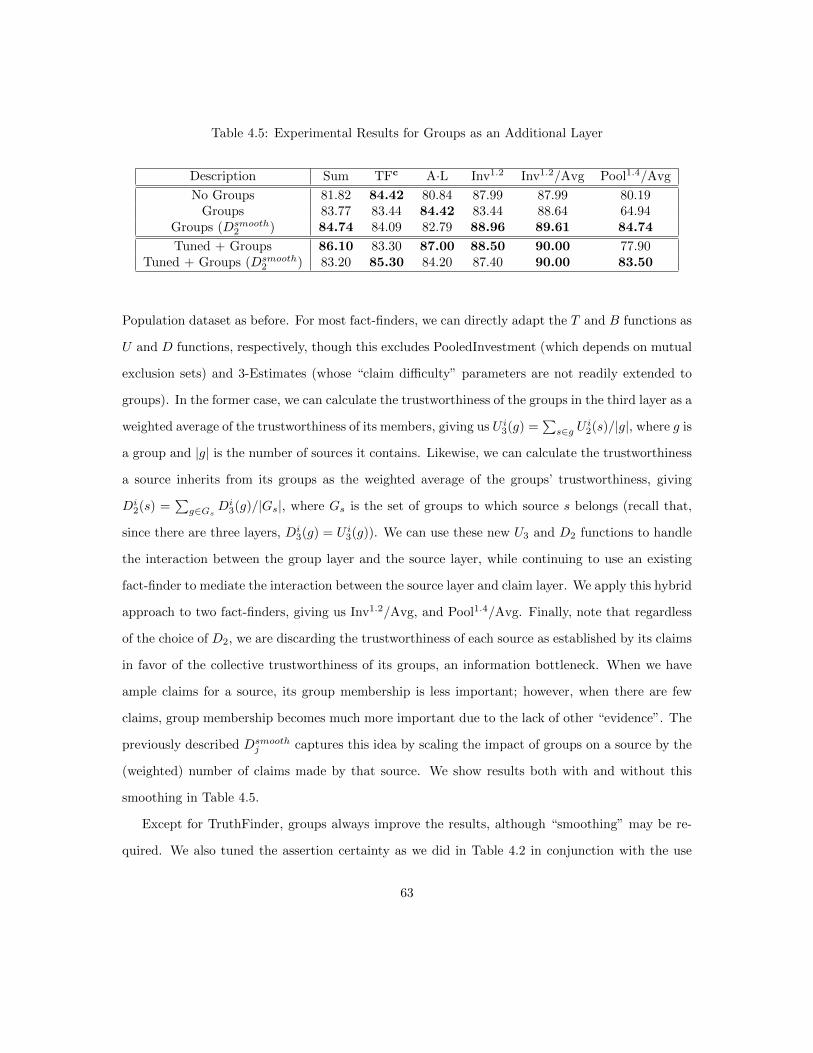
Table 4.5: Experimental Results for Groups as an Additional Layer

Description Sum TFc A·L Inv1.2 Inv1.2/Avg Pool1.4/Avg

No Groups 81.82 84.42 80.84 87.99 87.99 80.19Groups 83.77 83.44 84.42 83.44 88.64 64.94

Groups (Dsmooth2 ) 84.74 84.09 82.79 88.96 89.61 84.74

Tuned + Groups 86.10 83.30 87.00 88.50 90.00 77.90Tuned + Groups (Dsmooth

2 ) 83.20 85.30 84.20 87.40 90.00 83.50

Population dataset as before. For most fact-finders, we can directly adapt the T and B functions as

U and D functions, respectively, though this excludes PooledInvestment (which depends on mutual

exclusion sets) and 3-Estimates (whose “claim difficulty” parameters are not readily extended to

groups). In the former case, we can calculate the trustworthiness of the groups in the third layer as a

weighted average of the trustworthiness of its members, giving us U i3(g) =∑s∈g U

i2(s)/|g|, where g is

a group and |g| is the number of sources it contains. Likewise, we can calculate the trustworthiness

a source inherits from its groups as the weighted average of the groups’ trustworthiness, giving

Di2(s) =

∑g∈Gs D

i3(g)/|Gs|, where Gs is the set of groups to which source s belongs (recall that,

since there are three layers, Di3(g) = U i3(g)). We can use these new U3 and D2 functions to handle

the interaction between the group layer and the source layer, while continuing to use an existing

fact-finder to mediate the interaction between the source layer and claim layer. We apply this hybrid

approach to two fact-finders, giving us Inv1.2/Avg, and Pool1.4/Avg. Finally, note that regardless

of the choice of D2, we are discarding the trustworthiness of each source as established by its claims

in favor of the collective trustworthiness of its groups, an information bottleneck. When we have

ample claims for a source, its group membership is less important; however, when there are few

claims, group membership becomes much more important due to the lack of other “evidence”. The

previously described Dsmoothj captures this idea by scaling the impact of groups on a source by the

(weighted) number of claims made by that source. We show results both with and without this

smoothing in Table 4.5.

Except for TruthFinder, groups always improve the results, although “smoothing” may be re-

quired. We also tuned the assertion certainty as we did in Table 4.2 in conjunction with the use

63

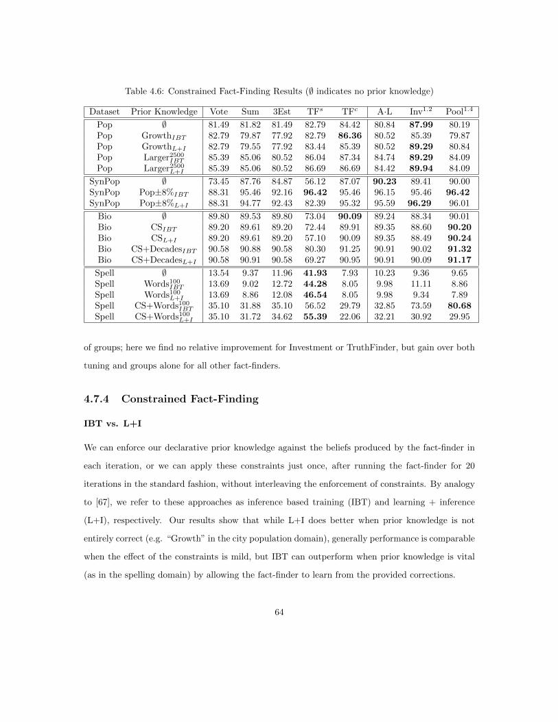
Table 4.6: Constrained Fact-Finding Results (∅ indicates no prior knowledge)

Dataset Prior Knowledge Vote Sum 3Est TFs TFc A·L Inv1.2 Pool1.4

Pop ∅ 81.49 81.82 81.49 82.79 84.42 80.84 87.99 80.19Pop GrowthIBT 82.79 79.87 77.92 82.79 86.36 80.52 85.39 79.87Pop GrowthL+I 82.79 79.55 77.92 83.44 85.39 80.52 89.29 80.84Pop Larger2500

IBT 85.39 85.06 80.52 86.04 87.34 84.74 89.29 84.09Pop Larger2500

L+I 85.39 85.06 80.52 86.69 86.69 84.42 89.94 84.09

SynPop ∅ 73.45 87.76 84.87 56.12 87.07 90.23 89.41 90.00SynPop Pop±8%IBT 88.31 95.46 92.16 96.42 95.46 96.15 95.46 96.42SynPop Pop±8%L+I 88.31 94.77 92.43 82.39 95.32 95.59 96.29 96.01

Bio ∅ 89.80 89.53 89.80 73.04 90.09 89.24 88.34 90.01Bio CSIBT 89.20 89.61 89.20 72.44 89.91 89.35 88.60 90.20Bio CSL+I 89.20 89.61 89.20 57.10 90.09 89.35 88.49 90.24Bio CS+DecadesIBT 90.58 90.88 90.58 80.30 91.25 90.91 90.02 91.32Bio CS+DecadesL+I 90.58 90.91 90.58 69.27 90.95 90.91 90.09 91.17

Spell ∅ 13.54 9.37 11.96 41.93 7.93 10.23 9.36 9.65Spell Words100

IBT 13.69 9.02 12.72 44.28 8.05 9.98 11.11 8.86Spell Words100

L+I 13.69 8.86 12.08 46.54 8.05 9.98 9.34 7.89Spell CS+Words100

IBT 35.10 31.88 35.10 56.52 29.79 32.85 73.59 80.68Spell CS+Words100

L+I 35.10 31.72 34.62 55.39 22.06 32.21 30.92 29.95

of groups; here we find no relative improvement for Investment or TruthFinder, but gain over both

tuning and groups alone for all other fact-finders.

4.7.4 Constrained Fact-Finding

IBT vs. L+I

We can enforce our declarative prior knowledge against the beliefs produced by the fact-finder in

each iteration, or we can apply these constraints just once, after running the fact-finder for 20

iterations in the standard fashion, without interleaving the enforcement of constraints. By analogy

to [67], we refer to these approaches as inference based training (IBT) and learning + inference

(L+I), respectively. Our results show that while L+I does better when prior knowledge is not

entirely correct (e.g. “Growth” in the city population domain), generally performance is comparable

when the effect of the constraints is mild, but IBT can outperform when prior knowledge is vital

(as in the spelling domain) by allowing the fact-finder to learn from the provided corrections.

64

City Population

Our axiomatic “common-sense” knowledge is that population grows over time (“Growth” in table

4.6); therefore, ∀v,w,x,y,zpop(v, w, y) ∧ pop(v, x, z) ∧ y < z ⇒ x > w. Of course, this often does

not hold true: cities can shrink, but performance was nevertheless superior to no prior knowledge

whatsoever. The L+I approach does appreciably better because it avoids forcing these sometimes-

incorrect constraints onto the claim beliefs while the fact-finder iterates (which would propagate the

resulting mistakes), instead applying them only at the end where they can correct more errors than

they create. The sparsity of the data plays a role—only a fraction of cities have population claims

for multiple years, and those that do are typically larger cities where the correct claim is asserted by

an overwhelming majority, greatly limiting the potential benefit of our Growth constraints. We also

considered prior knowledge of the relative sizes of some cities, randomly selecting 2500 pairs of them

(a, b), where a was more populous than b in year t, asserting ∀x,ypop(a, x, t) ∧ pop(b, y, t)⇒ x > y.

This “Larger” prior knowledge proved more effective than our oft-mistaken Growth constraint, with

modest improvement to the highest-performing Investment fact-finder, and InvestmentL+I reaches

90.91% with 10,000 such pairs.

Synthetic City Population

As our real-world data was sparse, we created a synthetic dataset to determine how effective

common-sense knowledge would be in the presence of “dense” data. We chose 100 random (real)

cities and created 100 authors whose individual accuracy a was drawn uniformly from [0, 1]. Be-

tween 1 and 10 claims (also determined uniformly) were made about each city in each year from 2000

to 2008 by randomly-selected authors. For each city with true population p and year, four incorrect

claims were created with populations selected uniformly from [0.5p, 1.5p], each author claiming p

with probability a and otherwise asserting one of the four incorrect claims. Our common-sense

knowledge was that population did not change by more than 8% per year (also tested on the

Wikipedia dataset but with virtually no effect). Like “Growth”, “Pop±8%” does not always hold,

but a change of more than 8% is much rarer than a shrinking city. These constraints greatly im-

proved results, although we note this would diminish if inaccurate claims had less variance around

65

the true population.

Basic Biographies

Our axiomatic common-sense (“CS”) knowledge was: nobody dies before they are born, people are

infertile before the age of 7, nobody lives past 125, all spouses have overlapping lifetimes, no child

is born more than a year after a parent’s (father’s) death, nobody has more than two parents, and

nobody is born or dies after 2008 (the “present day”, the year of the Wikipedia dump). Applying

this knowledge roughly halved convergence times, but had little effect on the results due to data

sparsity similar to that seen in the population data—while we know many birthdays and some

death dates, relatively few biographies had parent-child and spouse claims. To this we also added

knowledge of the decade (but not the exact date) in which 15,145 people were born (“CS+Decades”).

Although common sense alone does not notably improve results, it does very well in conjunction

with specific knowledge.

American vs. British Spelling

Prior knowledge allows us to find a truth that conforms with the user’s viewpoint, even if that

viewpoint differs from the norm. After obtaining a list of words with spellings that differed between

American and British English (e.g. ”color” vs. ”colour”), we examined the British National Corpus

as well as Washington Post and Reuters news articles, taking the source’s (the article author’s) use

of a disputed word as a claim that his spelling was correct. Our goal was to find the “true”

British spellings that conformed to a British viewpoint, but American spellings predominate by

far. Consequently, without prior knowledge the fact-finders do very poorly against our test set

of 694 British words, predicting American spelling instead in accordance with the great majority

of authors (note that accuracy from an American perspective is 1−“British” accuracy). Next we

assumed that the user already knew the correct spelling of 100 random words (removing these

from the test set, of course), but with little effect. Finally, we added axiomatic common-sense

(“CS”) knowledge: if a spelling a is correct and of length ≥ 4, then if a is a substring of b, a ⇔ b

(e.g. colour ⇔ colourful). Furthermore, while we do not know a priori whether a spelling is

66

American or British, we do know if e and f are different spellings of the same word, and, if two

such spellings have a chain of implication between them, we can break all links in this chain (while

some American spellings will still be linked to British spellings, this removes most such errors).

Interestingly, common sense alone actually hurts results (e.g. PooledInvestment (IBT) gets 6.2%),

as it essentially makes the fact-finders more adept at finding the predominant American spellings!

However, when some correct spellings are known, results improve greatly and demonstrate IBT’s

ability to spread strong prior knowledge, easily surpassing L+I. Results improve further with more

known spellings (PooledInvestment gets 84.86% with CS+Words200IBT ).

4.7.5 The Joint Framework

Our final experiments combine generalized and constrained fact-finding to create the full, joint

framework, capable of leveraging a very broad set of background and domain knowledge in our trust

decision. We again use the Population dataset, applying the Larger2500 declarative prior knowledge

set to generalized fact-finders using the Wikipedia editor group information (administrator, normal

user, blocked user) encoded as an additional layer. The results in Table 4.7 show a significant

and consistent gain using the joint framework with Dsmooth2 across all fact-finders (with IBT; L+I

results [not shown] were only slightly lower). The top result from the Investment fact-finder rises

to 90.58%, up from 89.61% using only group information, or 89.94% using only declarative prior

knowledge, while even the very simple Sums fact-finder achieves a respectable 87.99% performance,

up from 81.82% with no background knowledge of any kind.

Discussion

Because generalized and constrained fact-finding are orthogonal, they are easily merged by sim-

ply constraining the generalized fact-finder as we would a standard fact-finder. As both of these

approaches are polynomial time, so too is their joint application.

Additionally, there is also a broader lesson that may be taken away from these results: not

only are generalized and constrained fact-finding orthogonal, but so are the contributions of the

different types of knowledge they represent. Combining the source attributes, claim similarities, and

67

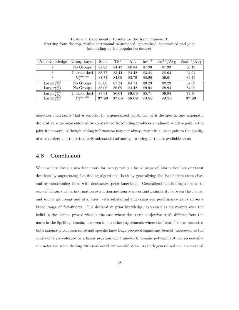
Table 4.7: Experimental Results for the Joint Framework.Starting from the top, results correspond to standard, generalized, constrained and joint

fact-finding on the population dataset.

Prior Knowledge Group Layer Sum TFc A·L Inv1.2 Inv1.2/Avg Pool1.4/Avg

∅ No Groups 81.82 84.42 80.84 87.99 87.99 80.19

∅ Unsmoothed 83.77 83.44 84.42 83.44 88.64 64.94∅ Dsmooth

2 84.74 84.09 82.79 88.96 89.61 84.74

Larger2500IBT No Groups 85.06 87.34 84.74 89.29 89.29 84.09

Larger2500L+I No Groups 85.06 86.69 84.42 89.94 89.94 84.09

Larger2500IBT Unsmoothed 87.34 86.04 86.69 85.71 89.94 72.40

Larger2500IBT Dsmooth

2 87.99 87.66 86.69 90.58 90.26 87.99

assertion uncertainty that is encoded by a generalized fact-finder with the specific and axiomatic

declarative knowledge enforced by constrained fact-finding produces an almost additive gain in the

joint framework. Although adding information may not always result in a linear gain to the quality

of a trust decision, there is clearly substantial advantage to using all that is available to us.

4.8 Conclusion

We have introduced a new framework for incorporating a broad range of information into our trust

decisions by augmenting fact-finding algorithms, both by generalizing the fact-finders themselves

and by constraining them with declarative prior knowledge. Generalized fact-finding allow us to

encode factors such as information extraction and source uncertainty, similarity between the claims,

and source groupings and attributes, with substantial and consistent performance gains across a

broad range of fact-finders. Our declarative prior knowledge, expressed as constraints over the

belief in the claims, proved vital in the case where the user’s subjective truth differed from the

norm in the Spelling domain, but even in our other experiments where the “truth” is less contested

both axiomatic common-sense and specific knowledge provided significant benefit; moreover, as the

constraints are enforced by a linear program, our framework remains polynomial-time, an essential

characteristic when dealing with real-world “web-scale” data. As both generalized and constrained

68

fact-finding are orthogonal, they may be readily used together, achieving better results than were

possible with either method alone and allowing the full breadth of the information available to be

jointly leveraged in determining the oft-subjective truth in the presence of a morass of conflicting

information.

69

Chapter 5

Generalized Constrained Models

Fact-finding can be understood to be a structured learning problem where the source trustworthiness

and truth of the claims are the latent variables. Building upon our work in Constrained Fact-

Finding, we can abstract from efficiently applying declarative knowledge to constrain the belief

in claims to constraining latent variables on arbitrary structured learning tasks, introducing a

framework known as Generalized Constrained Models. Indeed, Constrained Fact-Finding can be

understood to be a specific instance of (Iterated) GCMs, and from the relatively narrow perspective

of trust, the primary benefit of this is that GCMs allow us to apply the kind of declarative knowledge

used in Constrained Fact-Finding to other trust algorithms, including the Latent Trust Analysis

model in the next chapter, but the applications are actually far broader, extending to the extremely

varied problems addressed by structured learning in general.

5.1 Summary

Structured learning allows us to jointly predict multiple, interdependent labels in problems as diverse

as information extraction, vision, and, of course, information trustworthiness. However, complex

dependencies among the output variables demand require complex models to be captured directly,

often resulting in intractable learning and inference. Consequently, methods such as Constrained

Conditional Models (CCMs) [70], Posterior Regularization (PR) [33], and Constraint Driven Learn-

ing (CODL) [15] have been introduced, combining relatively simple models with prior knowledge

in the form of declarative constraints. However, when the simple model’s prediction violates the

constraints, these methods do not find the most likely constraint-satisfying alternative, but instead

70

rely on a specific, essentially arbitrary selection function (the metric). We show that the correct,

probability-maximizing metric depends on the character of the model’s error, and introduce the

metric-agnostic Generalized Constrained Model (GCM) to leverage it. When this metric is diffi-

cult to obtain analytically, or computationally infeasible, a GCM may alternatively use a compact,

convex metric; this class of metrics allows both the polynomial complexity of PR and the ease of

implementation of CCMs and CODL, with our experiments demonstrating comparable or improved

accuracy.

5.2 Introduction

There are often non-local dependencies that can be learned by a supervised structured learning

algorithm, but only at the cost of a possibly exponential number of new features and parameters:

for example, in named entity recognition we may know that all mentions of the same entity must

be the same type (if “George Washington” is a person in one sentence, he is still a person in the

next). These dependencies are thus often ignored in favor of simpler models requiring fewer training

examples. There may also be a variety of background knowledge (e.g. a name preceded by “USS”

refers to a ship, not a person, as in “USS George Washington”) that is likewise highly informative,

but, again, difficult to encode within a model or its parameters.

However, when dependencies and background knowledge are expressed as declarative constraints

(“all mentions of the same entity are the same type”, “each face has exactly one nose”, “all U.S.

presidents must be at least 35”, etc.), we can maintain a simple model (e.g. a Markov model

capturing only “local” dependencies among variables) and add an additional “global” inference

step to enforce the constraints by correcting the model’s prediction. When we choose the highest-

probability constraint-satisfying label according to the underlying supervised model (an NP-hard

task), this is a Constrained Conditional Model. Perhaps counterintuitively, this rarely results in

the truly most likely satisfying label, as discussed later. Posterior Regularization takes a different

approach, at each step correcting the predicted distribution over the latent variables by finding a

new distribution that satisfies the constraints in expectation and minimizes the KL-divergence with

71

the original prediction; while this is polynomial-time, the min-KL-divergence distribution, like the

max-probability label, is not the most likely distribution.

Instead, the appropriate metric to optimize depends on the error of the underlying model: when

its prediction violates our constraints, we need to know which of the alternate constraint-satisfying

labels (or label distributions) is most likely. Ideally, we can determine this metric analytically;

however, as error derives from a complex interplay of insufficient or noisy training examples and

the inherent limits of a model’s expressive power, we may instead empirically select a “best-fit”

metric for the problem, e.g. by testing different metrics on a development set.

These observations motivate Generalized Constrained Models, which generalize and subsume

both the supervised CCMs and the semi-supervised Constraint Driven Learning (iteratively-applied

CCMs) and PR (iteratively-applied KL-divergence minimization), abstracting from specific to arbi-

trary metrics and allowing the constraint of both discrete labels and label distributions. For convex

metrics with a polynomial length description (convex and compact), GCMs maintain CCMs’ (and

CODL’s) treatment of the underlying model as a “black box”, with minimal implementation effort

and, like PR, enjoy polynomial-time complexity.

In the remainder of this chapter, we first show that minimizing KL-divergence (PR), maximizing

probability (CCMs and CODL), or optimizing any other particular metric is improper because

the correct metric depends on the error exhibited by the underlying model. This motivates our

formulation of Generalized Constrained Models, and we describe compact, convex metrics that have

computational and implementation advantages over PR, CCMs and CODL and can be used when

the correct metric is hard to derive or infeasible. We also adapt GCMs to obtain an iterative semi-

supervised algorithm, and then perform experiments comparing GCMs with existing approaches.

5.3 Related Work

5.3.1 Structured Learning

In learning a structured classifier [9], we wish to obtain a function h : X → Y for observed

variables X and latent variables Y , where each yi ∈ Y ’s value depend on both X and on the

72

other labels Y \ yi. This can range from sequence models such as Hidden Markov Models (HMMs)

[10] to the more sophisticated Markov Random Fields [71] to non-probabilistic models such as

Structured Perceptron [21] and Structured SVM [81]. In these models, the dependencies among

the yi’s are captured within the features and parameters; for example, the relationship between

two adjacent states in an HMM are captured by a transition matrix specifying P (statet|statet−1).

Unfortunately, as the degree of dependency increases, the number of required parameters tends

to increase exponentially; for example, a fourth-degree HMM, where each state depends on the

four states preceding it (P (statet|statet−4, statet−3, statet−2, statet−1)), requires a transition matrix

|states|3 times as large as a first-degree HMM.

5.3.2 Constrained Learning and Prediction

Constrained approaches can be broadly divided into two types. The first restricts model parameters

directly, e.g. [38]’s diagonal transition models which alter the conditional probabilities of an HMM’s

transition matrix. However, such methods are limited in that they can only restrict those “local”

dependencies (e.g. between two adjacent states) that are already parameterized by the model,

and the actual encoding of prior knowledge into the parameters can be a difficult (and very model-

specific) task. This is because prior knowledge almost invariably concerns variables, not parameters:

we may know “x⇒ y ∨ z”, but how does that translate to an entry in a transition matrix?

Constraining the values of the latent variables directly by “correcting” the model’s output,

rather than its parameters, eliminates this problem. This makes enforcing the prior knowledge

straightforward, allowing truly “global” constraints without the need to augment the underlying

model, to the point where even quite simple unstructured classification models can be collated to

make structured predictions, with the dependencies among the latent variables enforced entirely

by constraints. In the supervised setting, the predominant method for applying constraints is

the aforementioned CCM [16], though a number of more specialized approaches such as [76] have

been proposed, targeted to a particular domain or learning algorithm. In the semi-supervised and

unsupervised settings, CODL and PR are of primary interest, although there are other approaches.

In Chapter 4 we applied constraints in expectation to a class of non-probabilistic models called

73

fact-finders, and we examined this setting in our third set of experiments. Generalized Expectation

[58, 27] penalizes the likelihood of a parameter set θ by how far the expectation of a function

deviates from its “target” value f , 4(f , Eθ[f ]). These are “soft”, as opposed to “hard”, constraints:

parameters θ violating the target value are penalized, but not forbidden. [55] takes a Bayesian

approach with “measurements” (akin to target values) which the model is supposed to satisfy

under θ, with the model’s objective function rewarding those θ that are likely to do so. Interestingly,

[33] argues that both of these, General Expectation and Bayesian measurements, can be restated as

specific instances of PR, and all three systems share strengths and weaknesses, including polynomial-

time approximation and difficulty porting to new models.

5.3.3 Constrained Conditional Models and Constraint Driven Learning

In CCMs [16] and their iterative semi-supervised variant, CODL [15], the opposite is true: learn-

ing and inference are NP-hard, but the underlying model is a “black box” and thus adapting to

new models is basically effortless. A CCM takes an underlying model θ and produces a label

Y = argmaxY ∈YKPθ(Y |X), where YK is the set of labels satisfying the constraints K. The semi-

supervised CODL simply iterates this process: given a supervised learning algorithm an initial set

of parameters θ0, labeled examples L, and unlabeled examples U , for each u ∈ U a tentative label

Yu = argmaxY ∈YKPθt(Y |Xu) is predicted. New parameters θt+1 are learned from L and U (using

the provisional labels), and we then continue iterating a predetermined number of times in a manner

similar to “hard” (truncated) Expectation-Maximization (EM) [78].

For both CCMs and CODL, prediction can be implemented with an Integer Linear Program

(ILP): if the model factors as Pθ(Y |X) ∝∏c∈C ψ(X,Yc), where C is the set of “cliques” (though

the model not need be graphical) and Yc is the set of latent variables in clique c ∈ C, then

we can encode the constraints K as linear constraints [68] and maximize the log-linear objective∑c∈C logψ(X,Yc). Soft constraints can be incorporated by adding a slack term sk to each linear

constraint taking the value 0 if k is satisfied and 1 otherwise, and augmenting the objective function

as∑c∈C logψ(X,Yc)−

∑k∈K ρksk, where ρk is the penalty for violating k (if ρk =∞ the constraint

is hard and must be satisfied).

74

The principal advantage of CCMs and CODL is the ease of implementation, requiring only data,

a learning algorithm and clique factorization, and constraints. However, it is also intractable: [15]

attempts to sidestep this by using beam-search, but this approximation cannot effectively enforce

the long-distance, non-local constraints which are often the most important. Fortunately, the ILP

can often be solved reasonably quickly in practice so long as the number of latent variables |Y |

and number of constraints K are relatively small. Still, while maximizing the probability of an

error-prone local model subject to constraints does ensure that no Y inconsistent with K will be

predicted, this does not guarantee that the consistent Y selected will actually be the most likely, or

even have a lower Hamming loss (the typical measure of accuracy) than the unconstrained prediction

would have, as we will later discuss.

5.3.4 Posterior Regularization (PR)

As CODL adds constraints to hard EM, PR adds constraints to soft EM. Here the modified

E-step is minimizing the KL-divergence between the predicted distribution q(Y ) and the distri-

bution Pθ(Y |X) provided by the model, minq,ξKL(q(Y )||pθ(Y,X)), subject to the constraints∑c∈C(Eq[φc(X,Yc)]) − b ≤ ξ and ||ξ||β ≤ ε, where c ∈ C is a clique in the model, Eq[φc(X,Y )]

is the expected value of a “feature function” for that clique returning a vector of values, b is the

vector of “desired maximums” for the sum of the clique functions, and β and b adjust the degree

to which these maximums may be exceeded. The M-step, as with standard EM, then uses the

predicted distribution q(Y ) to learn a new θ. Unlike CODL, PR constrains the distribution of the

latent variables q in expectation, rather than constraining a discrete labeling exactly. For instance,

given the constraint y1 + y2 ≤ 1 where y1 and y2 are {0, 1} binary independent variables in the

underlying model, the constraint is satisfied by q if q(y1) = q(y2) = 0.5, despite the fact that we

can draw y1 = 0 ∧ y2 = 0 from q (which factors according to the model) 25% of the time. The

advantage is that PR can be run in polynomial time, though it may still be expensive in practice:

as KL-divergence is convex, the E-step minimization (done in the dual) can be performed in poly-

nomial steps, but at each step the evaluation of the gradient requires inference in the underlying

model. Another serious practical concern is model “portability”: PR requires a distinct, non-trivial

75

implementation for each model, whereas CODL works universally because the model is a black

box. Finally, just as with CODL, the specific metric used by PR, KL-divergence, is essentially used

arbitrarily and cannot be expected to select the most likely distribution q given the particular error

exhibited by the underlying model.

5.4 Likelihood-Maximizing Metrics

As we will demonstrate, neither finding the constrained label distribution minimizing PR’s KL-

divergence nor finding the label maximizing CCM or CODL’s max-model-probability will yield the

most likely result. Clearly, if the label or distribution produced by θ violates our constraints, it

cannot be correct, but which label or distribution should we prefer instead?

We use constraints because the underlying model Pθ(Y |X) makes errors. We want to find the

true distribution of Y given X, P ∗(Y |X). If the error is characterized by a probability density

function (PDF) F such that F (q(Y )|Pθ(Y |X)) is proportional to the likelihood of distribution

q(Y ) = P ∗(Y |X) given that the model predicts distribution Pθ(Y |X), then F can be used to find

the most likely satisfying alternative when the model’s prediction violates the constraints.

Consider a simple example where each y ∈ Y is an independent binary variable and our

model θ predicts Pθ(Y |X) with marginal probabilities Pθ(y|X) sampled from a probability dis-

tribution defined by the PDF Fy(Pθ(y|X) = αy) ∝ e−|αy−P∗(y|X)|, giving us FY (Pθ(Y |X) =

α) ∝∏y∈Y e

−|αy−P∗(y|X)|. Notice that this is symmetric, so that given Pθ(Y |X) the likelihood

of “q(Y ) = P ∗(Y |X)” ∝ F (q(Y )|Pθ(Y |X)) =∏y∈Y e

−|q(y)−Pθ(y|X)|. When Pθ(Y |X) satisfies our

constraints, we can maximize this by simply setting q(Y ) = Pθ(Y |X). However, if Pθ(Y |X) does

not satisfy our constraints K, it cannot be correct, and we must seek a new distribution q ∈ Q

(where Q is the set of all distributions satisfying K) that maximizes F (q(Y )|Pθ(Y |X)). q(Y ) is thus

P (Y |X,K, θ): the most likely distribution of Y given the data, the constraints and the underlying

model.

For convenience, we can instead minimize the negated log of F , M(q, Pθ(Y,X)) =∑y∈Y |q(y)−

Pθ(y|X)|, such that in this exampleM is simply the L1 (Manhattan) distance between the marginals.

76

We refer to M as our metric. Note that minimizing this L1 distance uniquely finds the most likely

q(Y ) = P (Y |X,K, θ) for our model; other metrics, such as PR’s KL-divergence, yield different, less

likely q(Y ) 6= P (Y |X, θ,K). Moreover, as the error varies from model to model, there cannot be a

single correct metric for all models. In some cases, this error (and corresponding metric) can be de-

termined analytically (for example, when the model is trained on sensor values X, and the error of

each sensor value x is well-characterized, e.g. by a normal distribution); in other instances, a metric

can be selected empirically using a development set, e.g. from the set of efficient polynomial-length

convex metrics we introduce later.

To provide a concrete illustration with discrete labels, let us further assume Pθ(y1|X) =

Pθ(y2|X) = 0.9, Pθ(y3|X) = 0, and our constraint is “y1 = y2 = y3”. A CCM will find the maximum

probability constraint-satisfying label, which sets all three latent variables to false (as y1 = y2 =

y3 = T has probability 0.9·0.9·0 = 0). However, when the model’s error (characterized by F ) is con-

sidered, the event where all latent variables are true P (y1 = y2 = y3 = T ) ∝ e−|0.9−0|−|0.9−0|−|0−0| =

e−1.8 is less likely than all being false, P (y1 = y2 = y3 = F ) ∝ e−|0.9−1|−|0.9−1|−|0−1| = e−1.2. The

most likely consistent label is thus argmaxY P (Y |X, θ,K) = (y1 = T, y2 = T, y3 = T ). The CCM

predicted the consistent label (y1 = F, y2 = F, y3 = F ), which had maximum probability according

to the underlying model, but this faith is misplaced: if the model were accurate there would be no

need to constrain it!

However, there is one situation where finding the maximum probability label is the correct

thing to do. Let us say that we have a model θ that accurately predicts the latent variables in an

unconstrained domain, where labels are drawn from the true distribution P ∗(Y |X). Furthermore,

assume that we have another domain which is identical, except that P ∗K(Y |X) is constrained such

that for each Y P ∗K(Y |X) ∝ P ∗(Y |X) if Y satisfies K, and P ∗K(Y |X) = 0 if it does not (this

is equivalent to sampling Y from P ∗ and resampling when the drawn Y violates K). Here, the

maximum probability label according to θ that also satisfies K is indeed the maximum probability

label in the constrained domain. Still, while this is good news for CCMs (albeit only in a limited

transfer learning scenario), it is largely irrelevant for CODL, since if our unlabeled examples U are

taken from the unconstrained domain we should run unconstrained EM and then apply a CCM

77

to the result, and if our U are from the constrained domain the model θ we induce from them

will no longer reflect the unconstrained domain and (assuming that our model cannot capture the

constraints K within its parameters or there are too few examples to do so) the model will then

exhibit error that cannot be rectified by simply discarding those labels not satisfying K and choosing

the highest-probability label that remains.

Interestingly, even with an incorrect choice of metric, constraints often still improve the results.

This may be because the metric happens to find a distribution close to P (Y |X,K, θ), but perhaps

more frequently the underlying model’s prediction of Pθ(Y |X) is simply far from the space of

feasible distributions Q: here, moving to any q ∈ Q is likely to be an improvement. Similarly, when

Q is small (due to strict constraints), all q ∈ Q are close, so again moving to any q ∈ Q helps.

This may explain why past approaches have improved performance versus unconstrained baselines

despite using arbitrary metrics.

5.5 The Generalized Constrained Model

GCMs have two variants, “hard” and “soft”. A soft GCM predicts a distribution such that q(Y ) =

P (Y |X, θ,K) where q(Y ) satisfies constraints K in expectation. Hard GCM predicts a single,

discrete label Y satisfying K exactly. For brevity, we treat a hard label as a “distribution” q(Y )

satisfying the additional constraints ∀y∈Y q(y) ∈ {0, 1}. Soft GCM requires polynomial time with a

compact, convex metric, whereas hard GCM is NP-hard (by reduction from boolean satisfiability).

In a GCM, an underlying model θ is trained on labeled data. This allows us to predict a dis-

tribution over the latent Y , Pθ(Y |X), for observed variables X. This distribution, however, does

not take our constraints K into account: if Pθ(Y |X) violates K, it cannot be correct (we relax this

when using soft constraints, where violation is unlikely rather than impossible). By considering

the model’s error expressed as F (q(Y )|Pθ(Y |X)), how relatively likely that q(Y ) is the true distri-

bution given Pθ(Y |X), we obtain a metric M(q(Y ), Pθ(Y |X)) = −log(F (q(Y )|Pθ(Y |X)) such that

argminq(Y )∈QM(q(Y ), Pθ(Y |X)), where Q is the space of distributions satisfying K, produces a

satisfying q(Y ) = P (Y |X, θ,K), the most likely distribution given the data, the underlying model

78

θ, and the constraints. Notice that M need not be a true metric (with properties of symmetry,

subadditivity, etc.); we assume only M(q(Y ), q(Y )) ≤ M(q(Y ), q′(Y )) for all q′(Y ), ensuring that

if Pθ(Y |X) already satisfies K then q(Y ) = Pθ(Y |X).

Finally, we address soft constraints (soft and hard constraints are distinct and orthogonal to

soft and hard GCMs); unlike hard constraints, a soft constraint k ∈ K may be violated, but such

a violation means that a particular distribution q(Y ) is a factor of 1− P (k) relatively less likely to

be the true distribution. We assume each violation is independent. The full model is then:

P (Y |X, θ,K) = argmaxq(Y )

F (q(Y )|Pθ(Y |X))∏k∈K

(1− P (k))νk(q(Y ),X)

= argminq(Y )

− log

(F (q(Y )|Pθ(Y |X)) ·

∏k∈K

(1− P (k))νk(q(Y ),X)

)

= argminq(Y )

M(q(Y ), Pθ(Y |X)) +∑k∈K

ρkνk(q(Y ), X)

Where ρk = log(1−P (k)) and νk(q(Y ), X) is the degree to which a given q(Y ) violates constraint

k given observations X; in hard GCM violations are binary (a constraint is fully violated or fully

satisfied), so νk(q(Y ), X) ∈ {0, 1}, while soft GCM’s constraints in expectation yield a [0, 1] degree

of violation, examined in more detail when we later discuss constraints. Notice that for hard

constraints (which must be satisfied), we set P (k) = 1, so ρk =∞: no violation is permitted.

5.5.1 Compact & Convex Metrics

When the model’s error, and thus the metric, cannot be determined analytically, or when it cannot

be optimized in polynomial time, we use a development set to select the best-performing metric

from a set of candidates. Metrics having two properties—convexity and “compactness” (polynomial

length in the number of variables)—can be both optimized in polynomial time (when constraints

are enforced in expectation) and optimized in a primal form that allows the underlying model to be

treated as a black box. Like CCMs, CODL, and PR, we assume that the probability Pθ(Y |X) can be

factored as the product of clique-potentials. Given this, CCM and CODL’s maximum-probability

metric can be written compactly as a linear function of length O(|C| · 2maxc∈C |c|), where |c| is the

79

number of variables in clique c, although as the optimization is done with exact constraints (like

hard GCM) it is still exponential time. PR, on the other hand, applies constraints in expectation,

and though its KL-divergence metric has a number of terms exponential in the number of variables,

PR is able to optimize it in the dual, where it becomes tractable as gradient descent–however, this

requires calculating Pθ(Y |X) each time the gradient is evaluated, and, perhaps more significantly,

requires tailoring PR to each underlying model. Compact metrics (which may be exponential in

the size of largest clique, but max |c| is assumed to be small) ensure that the optimization can

be performed directly, in primal form, without reference to the underlying model—only the clique

potentials are relevant, maintaining the “plug-and-play” nature of CCMs and CODL.

Experimental Metrics

Our experiments use compact and convex metrics that can be expressed within a linear or quadratic

program, solvable with off-the-shelf, highly optimized linear programming and quadratic program-

ming packages rather than slower general purpose convex programming tools. In the equations

below, q(Y ) = P (Y |X, θ) and v refers to a possible assignment to a clique of variables Yc or a single

variable y. Some experimental metrics are omitted for brevity.

∑Yc∈Y

∑v

|q(Yc = v)− q(Yc = v)| (L1)

∑y∈Y

∑v

|q(y = v)− q(y = v)| (L1-Marginals)

∑Yc∈Y

∑v

q(Yc = v) · |q(Yc = v)− q(Yc = v)| (WeightedL1)

∑Yc∈Y

∑v

log(q(Yc = v)) · |q(Yc = v)− q(Yc = v)| (LogWeightedL1)

∑Yc∈Y

∑v

−q(Yc = v)q(Yc = v) (WeightedSum)

∑Yc∈Y

∑v

(q(Yc = v)− q(Yc = v))2 (SquaredL2)

∑Yc∈Y

∑v

(log(q(Yc = v)) · (q(Yc = v)− q(Yc = v)))2 (SquaredLogWeightedL2)

80

∑Yc∈Y

∑v

max

q(Yc = v)(q(Yc = v)− q(Yc = v)),

(1− q(Yc = v))(q(Yc = v)− q(Yc = v))

(VoteDistance)

5.5.2 Hard and Soft Constraints

Recall that in hard GCM constraints are enforced exactly : the corrected label q(Y ) (where all

marginals q(y) ∈ {0, 1}) always satisfy hard constraints and have binary satisfaction of soft con-

straints. In soft GCM, we seek a distribution q(Y ) satisfying the constraints in expectation. Consider

a model over two {0,1} independent variables, y1 and y2. If our model then predicts Pθ(Y |X) with

factors Pθ(y1|X) = 0.4 and Pθ(y2|X) = 0.6, but we have a constraint that y1 = y2, we could find

a corrected q(Y ) with factors q(y1) = q(y2) = 0, or q(y1) = q(y2) = 1 satisfying the constraint

exactly. However, both of these alternatives are far from our original Pθ(Y |X). Instead, we can

ask that Eq[y1] = Eq[y2], where q(Y ) is as close as possible to Pθ(Y |X) according to metric M .

This may give us (depending on M) a q(Y ) with factors q(y1) = q(y2) = 0.5; notice that the set of

distributions satisfying K in expectation is a superset of those satisfying K exactly.

5.5.3 First-Order Logic as Linear Constraints

In GCMs, our knowledge is ultimately encoded as linear constraints over variables corresponding to

cliques in the (factorized) model, where each possible assignment to the variables of clique c takes

a [0, 1] (soft GCM) or {0, 1} (hard GCM) marginal probability value q(Yc). These constraints,

along with the minimized sum of the metric and constraint violation penalties, constitute a convex

programming problem, assuming the metric is itself convex. Oftentimes, though, our constraints

are provided in first-order logic (FOL). [68] and Constrained Fact-Finding provide methods for

converting FOL into linear constraints where the convex programming variables are binary or

continuous, respectively, and correspond to single-variable marginals in q (i.e. q(y)). In our case

the convex programming variables correspond to clique-marginals (i.e. q(Yc)).

To achieve the constraint-feature type constraints of PR, where φk(Yc) is the feature value for a

particular assignment to a particular clique for a particular constraint k (with∑c∈C

∑Ycφk(Yc) ≤

81

bk), we simply add, for each constraint k, the linear constraint∑c∈C

∑Ycφk(Yc)vqYc ≤ bk, where

vqYc is a variable corresponding to the probability of a particular assignment of Yc in the convex

program.

We first propositionalize the FOL with respect to each unlabeled example, obtaining specific

propositional formulae such as TRUE⇒ (ϕy5=a ⇒ ϕy6=b) from FOL ∀ixi = d⇒ (yi = a⇒ yi+1 =

b) (assuming the example has observed variable x5 = d). Since the truth of “xi = value” for each

example is constant, it is replaced with TRUE or FALSE as appropriate. However, notice that the

propositional variables ϕ that remain correspond to assignments to individual output variables, not

assignments to cliques like our convex program’s variables.

We next combine these propositional variables where possible. We replace any conjunction

or disjunction of ϕ’s corresponding to y’s sharing the same clique with a new, combined ϕ. For

example, if there exists a clique Yc such that {y1, y2, y3} ⊆ Yc, (ϕy1=a ∧ ¬ϕy2=b) ∨ ϕy3=b becomes

(ϕy1=a∧y2 6=b)∨ϕy3=b and then ϕ(y1=a∧y2 6=b)∨y3=b. When there is a choice as to which ϕ’s to combine,

the selection minimizing the final number of ϕ should be made (this can be done in polynomial

time via dynamic programming).

Now we simplify any negated non-literals within the propositional formulae (e.g. ¬(ϕy1=a ∨

ϕy2=b) becomes ¬ϕy1=a ∧ ¬ϕy2=b). Each formula can be thought of as a tree where each node is

either the disjunction or conjunction of its children, with (possibly negated) literals as leaves. Each

node will create one linear constraint; we start at the leaves and work our way up.

To begin, we have ϕκ propositional variables, where κ are the sets of variable assignments ϕκ

corresponds to, specified as a propositional formula; for example, ϕ(y1=a∧y2 6=b)∨y3=b corresponds to

assignments κ = {y3 = b}∪⋃ω 6=b{y1 = a, y2 = ω}. We calculate the associated convex programming

variable vκ =∑Yc:Yc∩κ6=∅ q(Yc), where Yc ∩ κ 6= ∅ denotes an assignment to the clique Yc that

contains one or more of the assignments given by κ. For a negated literal, ¬ϕκ we calculate v¬κ =

1−vκ. Using our previous κ example, if we assume the yi’s take only values a and b, using q(ω1ω2ω3)

as shorthand for q(y1 = ω1, y2 = ω2, y3 = ω3) we have vκ = q(aab)+q(abb)+q(bab)+q(bbb)+q(aaa).

Moving up the tree, we may find a disjunction η =∨i vi, where the vi variables correspond to

literals, nested disjunctions, and nested conjunctions, respectively. We then add a linear constraint

82

vη = min(1,∑i vi), where v = min(a, b) is implemented in the convex program with “helper

constraints” v ≥ a and v ≥ b and adding the term v · r to the (minimized) objective function,

where r > ε−1 max M(q, Pθt−1(Yu|Xu)) +∑k∈K:ρk<∞ log ρ

νK(q,Xu)k , i.e. r is a constant larger than

the greatest possible sum of the distance and soft constraint penalties for the given example u. This

ensures min(a, b) ≤ v ≤ min(a, b)(1 + ε), since the cost of increasing r beyond min(a, b)(1 + ε) will

have a cost greater than any reduction in distance and constraint costs; very low ε results in trivial

error.

We may also see a conjunction of ζ =∧i vi; here, to create our conjunction variable vζ we simply

add one constraint for each conjoined variable vi, vζ ≤ vi, ensuring vζ = mini(vi) (there are no

negated non-literals, so a higher vζ will always be preferred by the convex program as maximizing

the value of the formula).

Finally, at the top of the tree, we are left with a single variable vk corresponding to the highest-

level conjunction, disjunction or propositional variable (if the formula consisted solely of a single

such variable). We now simply require that vk ≥ 1− νk, that is, that the formula is satisfied with

degree of violation νk ∈ {0, 1} (hard GCM) or νk ∈ [0, 1] (soft GCM).

In hard GCM, every v ∈ {0, 1}, and our set of linear constraints will enforce the constraints

exactly. In soft GCM, however, we have created what can be seen as an optimistic interpretation

of the FOL in expectation; in particular, if a constraint can be satisfied given a certain dependency

between two clique assignments, it is taken to be satisfied. For example, if we have two cliques each

consisting of single variables a and b, then we enforce a∨ b with the linear constraint equivalent to

a+ b ≥ 1: if a = b = 0.5, the constraint is satisfied as mutual exclusion is implicitly assumed

5.6 Iterated GCMs for Semi-Supervised Learning

CODL performs semi-supervised learning by iterative application of a CCM. Similarly, an iterated

GCM (IGCM) repeatedly learns a parameter set θ, predicts a distribution q(Y ) via a GCM, learns

a new θ, and iterates until convergence. Six inputs are required: labeled data L = (XL,YL),

unlabeled data U = (XU), a supervised learning algorithm producing a model θ, a metric M ,

83

constraints K, and constraint weights ρK . When |L| = 0, CDL is unsupervised. Like CODL and

PR, an IGCM can be viewed as a modified form of EM:

Expectation :qt = argminq

M(q, Pθt−1(YU|XU)) +∑k∈K

ρkνk(q,XU)

Maximization :θt = argmaxθ

γ logPθ(YL|XL) + Eqt [logPθ(YU|XU)]

Here, qt = qt(YU) represents the distribution over YU, the latent variables of the unlabeled

data. νk(q,XU) =∑u∈U νk(q(Yu), Xu) is the [0, |U|] degree to which q violates k, summed over

all instances u ∈ U. In the M-step, γ is the relative weight of the labeled to unlabeled examples,

matching an identical γ parameter in CODL. In practice, the supervised learner calculates the

updated θ given the (γ-weighted) labeled data L and the tentatively labeled U = (XU,qt(YU))

just as it would in standard EM: no modification to the learning algorithm is required.

The expectation step predicts q(Y ) via a GCM. Using a soft (q(Y ) is a distribution) or hard

(q(Y ) is a label) GCM yields soft or hard iterated GCM, respectively, analogous to soft and hard

EM [78]. When we have finished iterating, we have the option of either using the learned θ to predict

q(Y ) for a new example X, or using our constraints to correct that prediction as a GCM. Using a

GCM in the final inference usually yields significantly higher accuracy, but at the computational

cost of performing another optimization, which may be important when hard GCM is used and the

number of examples to be labeled is large.

5.6.1 Soft and Hard IGCMs

Soft and hard IGCMs are analogous to soft and hard EM [78], and iteratively predict q(YU) via

soft and hard GCMs, respectively. Notice also that CODL, which trains θ on discrete maximum-

probability labels YU, is a hard EM approach, while PR, which trains θ on a satisfying distribution

q(YU) over the labels, is akin to soft EM. In hard IGCM, we require the q(YU) found in the E-step

to be a discrete labeling, such that ∀u∈U∀y∈Yu∀valuesq(y = value) = {0, 1}. The principal advantage

of hard CDL, like CODL and hard GCCMs, is that the constraints can be enforced exactly (all

84

Y drawn from q(Y ) must satisfy K, assuming hard constraints), but, also like CODL, hard CDL

“loses” information by selecting a single discrete label as compared to finding a label distribution.

Soft CDL, like soft GCCMs and PR, runs in polynomial-time, but enforces constraints in expectation

rather than exactly, which avoids the information loss of hard GCCM but constrains the latent

variables less strictly than hard CDL. In our experiments we find that hard CDL does generally

outperform soft CDL, but in some situations, such as in our third set of experiments, predicting a

distribution rather than a specific label proves more valuable than enforcing the constraints exactly;

moreover, as soft CDL can be run (very efficiently) in polynomial-time, it may be preferable for

larger-scale problems even at the cost of accuracy.

5.7 Experiments

5.7.1 Synthetic

We begin with a simple set of semi-supervised, synthetic problems, where a small number of labeled

and large number of unlabeled examples is available for each problem. In each problem, each latent

variable yi ∈ Y is dependent upon 10 corresponding observed features Xi (each x ∈ Xi taking one of

5 values) according to a Naive Bayes model, such that P (yi = v|Xi) ∝ P (yi = v)∏x∈Xi P (x|yi = v).

This leaves the yi independent of each other; however, we also constrain Y . In the elementary

“same” problem we have two binary y which always take the same value (y1 = y2). In “close3”, we

have three y taking integer values in [0, 4], where |y1−y2| ≤ 3 and |y2−y3| ≤ 3; the similar “close1”

has the stricter restriction that |y1 − y2| ≤ 1 and |y2 − y3| ≤ 1. In each problem, examples (X,Y )

are drawn according to the Naive Bayes model for each yi; those that do not satisfy the relevant

constraint on Y are discarded and redrawn.

Our results (table 5.1) in the supervised setting cover the unconstrained Naive Bayes model

with no metric (“none”), PR’s minimized KL-divergence, CCMs, and three instantiations of soft

GCMs using metrics VD2 (squared VoteDistance), L22 (squared L2 distance), and LVD2 (squared

Log-VoteDistance). In the semi-supervised case, we have unconstrained EM, PR, CODL, and

three instantiations of soft iterated GCMs. The accuracies reported are the percent of y’s whose

85

Table 5.1: Synthetic Experiment Results. |L| and |U| are labeled and unlabeled examples.

Constraints |L| |U| Setting None PR CCMCODL VD2 L22 LVD2

Same 5 100 Supervised 72.70 76.20 76.80 76.80 76.80 76.80Same 5 100 Semi-Supervised 88.10 94.70 88.20 96.40 96.40 95.90Same 5 200 Supervised 72.00 76.15 76.70 76.70 76.70 76.70Same 5 200 Semi-Supervised 89.40 95.25 90.55 95.70 95.85 96.20

Close1 5 100 Supervised 39.97 42.87 42.80 42.20 41.67 42.40Close1 5 100 Semi-Supervised 53.90 65.30 54.60 66.87 64.30 62.57Close1 10 100 Supervised 48.03 51.17 51.03 51.03 50.47 51.40Close1 10 100 Semi-Supervised 60.07 70.50 60.80 72.23 70.33 69.07

Close3 5 100 Supervised 40.60 40.83 40.87 40.80 40.70 40.80Close3 5 100 Semi-Supervised 51.97 54.10 48.10 54.73 54.67 54.27Close3 10 100 Supervised 46.73 46.90 46.90 46.97 46.80 46.93Close3 10 100 Semi-Supervised 60.83 60.93 53.67 61.30 61.87 61.40

value was correctly predicted (Hamming loss), with argmaxvq(yi = v) as our label for each yi.

Each experiment was run 10 times with randomly-generated Naive Bayes models, and the results

averaged.

Interestingly, CCMs do relatively well as they enforce the constraints exactly in their predictions,

unlike EM, PR and soft GCMs. However, this advantage disappears in the semi-supervised setting,

with CODL sometimes significantly underperforming even unconstrained EM. PR, on the other

hand, demonstrates fairly strong performance; we modified the PR algorithm slightly to enforce

constraints on the final prediction, minimizing KL-divergence with what the PR-trained underlying

model original predicted. Compared to “standard” PR, this change improved accuracy by an

average of 1.2%. Still, (I)GCMs using squared VoteDistance significantly outperform PR overall,

while maintaining the practical advantages of treating the underlying model as a black box.

5.7.2 Information Extraction from Ads

To further compare with CCMs and CODL, we follow [15], which predicted fields in a set of 8,767 San

Francisco area apartment listings from June 2004 (here our constraints were encoded in FOL and

thus inapplicable to PR). The twelve possible fields identify what attributes (if any) are described

by the text, such as the amount of rent or the size of the dwelling. The underlying model is a first

86

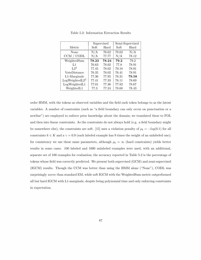
Table 5.2: Information Extraction Results

Supervised Semi-SupervisedMetric Soft Hard Soft Hard

None N/A 76.62 78.62 N/ACCM / CODL N/A 77.77 N/A 78.12

WeightedSum 78.23 78.24 79.2 79.2L1 76.63 78.02 77.8 78.91L22 77.45 78.02 79.18 78.91

VoteDistance 76.35 78.02 76.41 78.91L1-Marginals 77.36 77.95 78.31 79.58

LogWeightedL22 77.41 77.33 78.11 78.69LogWeightedL1 77.01 77.36 77.82 78.67

WeightedL1 77.3 77.24 78.68 78.43

order HMM, with the tokens as observed variables and the field each token belongs to as the latent

variables. A number of constraints (such as “a field boundary can only occur on punctuation or a

newline”) are employed to enforce prior knowledge about the domain; we translated these to FOL

and then into linear constraints. As the constraints do not always hold (e.g. a field boundary might

be somewhere else), the constraints are soft. [15] uses a violation penalty of ρk = −log(0.1) for all

constraints k ∈ K and a γ = 0.9 (each labeled example has 9 times the weight of an unlabeled one);

for consistency we use these same parameters, although ρk = ∞ (hard constraints) yields better

results in some cases. 100 labeled and 1000 unlabeled examples were used, with an additional,

separate set of 100 examples for evaluation; the accuracy reported in Table 5.2 is the percentage of

tokens whose field was correctly predicted. We present both supervised (GCM) and semi-supervised

(IGCM) results. Though the CCM was better than using the HMM alone (“None”), CODL was

surprisingly worse than standard EM, while soft IGCM with the WeightedSum metric outperformed

all but hard IGCM with L1-marginals, despite being polynomial time and only enforcing constraints

in expectation.

87

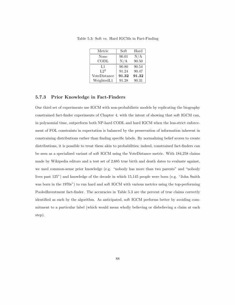
Table 5.3: Soft vs. Hard IGCMs in Fact-Finding

Metric Soft Hard

None 90.01 N/ACODL N/A 90.50

L1 90.80 90.54L22 91.24 90.47

VoteDistance 91.32 91.32WeightedL1 91.28 90.31

5.7.3 Prior Knowledge in Fact-Finders

Our third set of experiments use IGCM with non-probabilistic models by replicating the biography

constrained fact-finder experiments of Chapter 4, with the intent of showing that soft IGCM can,

in polynomial time, outperform both NP-hard CODL and hard IGCM when the less-strict enforce-

ment of FOL constraints in expectation is balanced by the preservation of information inherent in

constraining distributions rather than finding specific labels. By normalizing belief scores to create

distributions, it is possible to treat them akin to probabilities; indeed, constrained fact-finders can

be seen as a specialized variant of soft IGCM using the VoteDistance metric. With 184,258 claims

made by Wikipedia editors and a test set of 2,685 true birth and death dates to evaluate against,

we used common-sense prior knowledge (e.g. “nobody has more than two parents” and “nobody

lives past 125”) and knowledge of the decade in which 15,145 people were born (e.g. “John Smith

was born in the 1970s”) to run hard and soft IGCM with various metrics using the top-performing

PooledInvestment fact-finder. The accuracies in Table 5.3 are the percent of true claims correctly

identified as such by the algorithm. As anticipated, soft IGCM performs better by avoiding com-

mitment to a particular label (which would mean wholly believing or disbelieving a claim at each

step).

88

5.8 Conclusion

We have introduced Generalized Constrained Models for the supervised and semi-supervised set-

tings, encoding background knowledge and non-local dependencies of the latent variables in the

form of constraints on top of a simpler underlying model. While past approaches such as PR, CCM

and CODL have arbitrarily committed to a particular metric to choose a satisfying label or distri-

bution, we have shown that the correct choice—and thus, the correct metric—depend on the error

exhibited by the underlying model. When this error cannot be readily analyzed, we can empirically

select from a set of compact, convex metrics that allow any underlying model to be easily used as

“black box” (unlike PR) and can be optimized in polynomial-time (unlike CCMs and CODL), with

experiments demonstrating that GCMs with such metrics regularly outperform existing algorithms.

89

Chapter 6

Latent Trust Analysis

6.1 Summary

A fact-finder may be viewed as having semantics defined by its update rules, essentially creating a

system of transitive voting. There is no attempt to explain or model why sources make the claims

they do, but rather there are “votes” that flow from sources to claims and back to sources according

to mechanics set by domain experts in a manner that is expected to ultimately transfer more votes to

true claims than untrue claims and more votes to trustworthy sources than untrustworthy sources.

While this results in highly efficient algorithms and often works well in practice, particularly

when additional information is provided via Generalized and Constrained Fact-Finding, there are a

number of important limitations of fact-finders: they do not tell a “generative story” that can ex-

plain how a trust decision was obtained to users (and researchers), they cannot perform supervised

or semi-supervised learning of source trustworthiness and claim belief outside of ad hoc modifica-

tions, and they can be difficult to modify or analyze in a principled way. In this chapter we address

these shortcomings by introducing Latent Trust Analysis (LTA), a strongly principled, probabilistic

type of trust model where the truth of a claim is treated as a latent variable and the trustworthi-

ness of a source is captured by a set of model parameters. In conjunction with the Generalized

Constrained Models of the previous chapter, LTA models are able to capture all of the information

a joint Generalized Constrained Fact-Finder can (and more) with well-justified Bayesian semantics.

90

6.2 Introduction

Previous trust algorithms such as reputation networks and fact-finders have, at their heart, been

based upon some form of transitive voting; in a reputation network, this may mean trusting B

because you trust A and A trusts B, while in fact-finders this may mean believing claim C made by

source A because A also claims D, E and F , which you already believe. Explaining precisely how

sources decide which claims to assert is, of course, impossible to do exactly—particularly where

sources are people, their underlying psychology and reasoning would be far too difficult to model

even for an individual, and a given problem often involves thousands of sources or more. However,

by making judicious assumptions and simplifications, we hope to approximately model this process

and, in so doing, provide a digestible explanation that will allow users to understand the trust

algorithm and thus trust it more than they would one of the more opaque methods of previous

work; after all, even an accurate trust system is useless if users refuse to trust the system itself!

Moreover, once we establish a mathematical “story”, it may be readily modified: the Latent Trust

Analysis approach we present is not a single model, but rather a principled probabilistic method of

approaching the trust problem (much as fact-finders can be seen as a broad family of algorithms

that use a pair of rules for iteratively updating source trustworthiness and claim belief), and the

extensions we suggest later are far from exhaustive.

Fundamentally, a Latent Trust Analysis model is a probabilistic model where the truth of a claim

(or, equivalently, the one true claim from among a mutual exclusion set of claims) is a latent variable,

the trustworthiness of a source (its capacity and inclination for making true claims) is captured

by one or more parameters, and each assertion (“source s states P (c) = x”) is an observation.

More sophisticated LTA models can augment these basic elements with additional parameters (e.g.

measuring the “difficulty” of a mutual exclusion set) and observations (e.g. observed properties of

the source, such as its grammatical correctness or credentials). However, simple LTA models may

have significant computational advantages: the aptly-named Simple-LTA model we present in this

chapter can perform the unsupervised learning needed to induce the trustworthiness parameters

and claim probabilities using quickly-calculable closed-form expectation-maximization [23] E and

91

M steps which, in fact, correspond exactly to a fact-finder’s update rules, which means that Simple-

LTA can also be seen as the first well-justified probabilistic fact-finder, bridging the fact-finding and

LTA families of trust algorithms. In general, however, when closed-form M step cannot be derived,

as in the relatively complex HEAD-LTA model (Honesty, Expertise, Attribute and Difficulty-based

LTA), we must use a more computationally demanding method to maximize the expected log-

likelihood, such as gradient descent, Netwon’s method [77], or a Quasi-Newton method like L-

BFGS [56]; however, by using generalized expectation-maximization [63] we need only improve,

rather than maximize, our log-likelihood in each step, allowing us to tractably apply our model to

large real-world datasets, as our experiments on the Population dataset demonstrate.

6.3 Related Work

6.3.1 Reputation Networks

Some reputation networks have probabilistic interpretations: in PageRank [13], for example, the

score of a particular page is determined by link network topology, but can be viewed as how often

a random walk visits that page given some restart frequency. However, unlike a generative LTA

model, this does not explain how links are made, nor does it explicitly determine the trustworthiness

of the page, but rather finds the probability of being on a particular page after a random walk long

enough to ensure the mixing of the Markov chain. By contrast, other reputation approaches, such

as Hubs and Authorities [49], explicitly seek to obtain a trustworthiness value (or equivalent, such

as hub and authority scores) but despite the often-simple rules for trust transference, the ultimate

result of such systems (and how they arrived there) is difficult to explain, lacking ready semantics

or a probabilistic “story” of any kind.

6.3.2 Fact-Finders

Several fact-finders contain probabilistic elements; for example, TruthFinder [86] calculates claim

belief as 1 −∏s:s→c 1 − T (s), with the idea that T (s) is the probability that s tells the truth, so

92

the probability that a claim is wrong is the probability that all the (independent) sources are liars.

However, this probabilistic explanation falls apart when there are other, mutually exclusive claims,

which usually results in assigning “probabilities” over mutually exclusive possibilities summing to

more than 1. Perhaps more interestingly, [82] explicitly seeks to provide a Bayesian justification for

a fact-finder, but this depends on unrealistic assumptions, the chief being that P (s→ c|c)/P (s→

c) ≈ 1, that is, the probability of a source making a claim given that the claim is true divided by

the unconditional probability of the source making the claim is close to 1. In general this is not

the case: if half of all claims are true such that P (c) = 0.5, a source that tells the truth 90% of

the time such that P (c|s → c) = 0.9, and asserts 1% of claims such that P (s → c) = 0.01, then

P (s → c|c) = 0.018, almost double P (s → c). There is, however, no fundamental reason that a

fact-finder cannot capture a full probabilistic model, and indeed, the Simple-LTA model we will

present has Expectation-Maximization steps that can be viewed as corresponding to a fact-finder’s

T (s) and B(c) update rules.

6.3.3 Representations of Uncertainty

Our observations are not necessarily the unqualified “source s makes claim c” assertions of standard

fact-finders, and instead allow for the same detail provided by generalized fact-finders, where the in-

formation extractor’s confidence and the source’s certainty were captured by weighting by weighting

the assertions. In LTA, however, we view the source as providing a distribution over the claims in a

mutual exclusion set (e.g. “source s states claim c has probability x”) and consider the confidence

weight (as professed by either the source or the information extractor) separately. This confidence

is analogous to the gap between belief and plausibility in Dempster-Shafer theory [87, 75] or the

equivalent-but-explicit “uncertainty” of subjective logic [44, 43] (equal to 1 − belief − disbelief).

In our case, however, the confidence qualifies a classical Bayesian distribution with facile, natural

semantics (for example, two identical distributions asserted with confidence 0.5 are equivalent to

the same distribution asserted with full confidence [1]), a major advantage over more nuanced al-

ternatives given that we must both interpret the statements of sources (and simple probabilities of

information extractors) and explain our decisions to users accustomed to traditional probabilistic

93

reasoning.

6.4 LTA Fundamentals

In Latent Trust Analysis, sources assert distributions over the claims in each mutual exclusion set

(e.g. “President Obama was born in 1961 with 90% probability, and in 1962 with 10% probability”),

each with a degree of confidence from the source itself (e.g. “I am 50% confident in this distribution”)

or from information extraction (e.g. “I am 50% confident that the source asserted this distribution”).

The asserted probability of a particular claim c by source s is bs,c, and for each mutual exclusion

set m,∑c∈m bs,c = 1; we will use Ds,m to refer to the distribution over a mutual exclusion set as

a whole, such that Ds,m = {bs,c : c ∈ m}. The confidence of the source (or information extractor)

in the distribution over the claims in mutual exclusion set m is then ws,m. The distributions are

observed variables ({Ds,m} ⊆ X), while the confidences can be better described as conditioning

variables or constants which are, from the model’s perspective, given and not generated.

The distributions selected by the sources depend on the given {ws,m} values (a distribution

produced by a less confident source—or extracted by a less confident information extractor—will

tend to be less concentrated) as well as the trustworthiness of a source (a set of parameters ⊂ θ

corresponding to each source s) and, of course, which claim in mutual exclusion set m is actually

true, denoted ym ∈ Y , where Y are our latent variables (if c is the true claim in m, ym = c).

For observed variables X, latent variables Y , and parameters θ, we define the LTA model as the

joint probability of all three: P (X,Y, θ) = P (X,Y |θ)P (θ). An LTA model can thus be learned by

finding argmaxθ P (X, θ) = argmaxθ∑Y P (X,Y, θ) = argmaxθ

∑Y P (X,Y |θ)P (θ), the maximum

a posteriori (MAP) estimate of θ.

6.5 Simple-LTA

Assume there are only two claims in a mutual exclusion set, and ∀s,c bs,c ∈ {0, 1} (in real-world

domains, this case—where the source asserts only a single claim as having probability 1—is com-

94

mon); if we characterize the source’s trustworthiness as a single parameter θs then the probability

of asserting the true claim is just the source’s trustworthiness θs, and the probability of asserting

the false claim is just 1 − θs. Extending this basic idea to additional claims and bs,c ∈ [0, 1] gives

us the Simple-LTA model.

In Simple-LTA, if we assume that there is full confidence in a source’s asserted distribution

(ws,m = 1), the source asserts the true claim c ∈ m with belief bs,c with probability P (bs,c|ym =

c, θs) ∝ (θs)bs,c , and similarly asserts a false claim with probability P (bs,c|ym 6= c, θs) ∝ (1−θs)bs,c .

When there is less than full confidence (ws,m < 1) the distribution of belief asserted by the source

is likely to be less concentrated; incorporating ws,m into our probability estimates then gives:

P (bs,c|ym = c, θs) ∝ (θs)bs,cws,m

P (bs,c|ym 6= c, θs) ∝ (1− θs)(1−bs,c)ws,m

P (Ds,m|ym = c, θs) ∝

(θs)bs,c

∏bs,c ∈ Ds,m\bs,c

(1− θs)bs,cws,m

∝(

(θs)bs,c(1− θs)(1−bs,c)

)ws,m

The last equation gives the probability of the entire distribution asserted by s over m, with the

simplification in the last line due to the distributionality of Ds,m; since the beliefs over the claims

of m must sum to 1, we know that∑bs,c ∈ Ds,m\bs,c bs,c = 1 − bs,c. Because the distributions are

“generated” independently by the sources, given the truth and their trustworthiness parameters,

we can calculate the probability of generating all the distributions for a given mutual exclusion set

as:

P (Xm =⋃s

Ds,m|ym, θ =⋃s

θs) ∝∏s

P (Ds,m|ym, θs)

Finally, noting that the Xm are independent given the true claims Y and the source trustwor-

thiness parameters, the probability of all the observed distributions for all the mutual exclusion

95

sets is:

P (X =⋃m

Xm|Y =⋃m

ym, θ) ∝∏m

P (Xm|ym, θ)

To get the joint probability of the truth Y and the observations X given the parameters, we

apply Bayes’ Rule: P (X,Y |θ) = P (X|Y, θ)P (Y |θ). Without knowing the claimed distributions X,

the trustworthiness of the sources θ tells us nothing about the truth Y , and thus P (Y |θ) = P (Y ).

Taking everything together, we can now state the full joint probability of the model:

P (X,Y |θ) ∝ P (Y )∏m

∏s

((θs)

bs,ym (1− θs)(1−bs,ym ))ws,m

6.5.1 Learning the Model

To get the MAP estimate for θ in our model (and the implied distribution over Y ) we find

argmaxθ∑Y P (X,Y |θ)P (θ). This optimization would be very difficult to do directly, so we in-

stead apply the technique of Expectation Maximization, iteratively improving our estimate of θ at

each time step t by setting:

θt+1 = argmaxθ

EY |X,θt [log(P (Y,X|θ)P (θ))] = argmaxθ

∑Y

P (Y |X, θt) log(P (Y,X|θ)P (θ))

This can be split into an expectation step, the straightforward calculation of P (Y |X, θt) (since the

ym are conditionally independent this amounts to finding the conditional distributions of each ym

independently), and the maximization step, where we find θt+1 using the conditional distribution

over the Y from the expectation step.

96

Deriving the M-Step

We find the next θt+1 maximizing our expected log-likelihood as:

θt+1 = argmaxθ

∑Y

P (Y |X, θt) log(P (Y,X|θ)P (θ))

= argmaxθ

∑Y

(P (Y |X, θt)

· log

((P (Y )

∏m

∏s

((θs)

bs,ym (1− θs)(1−bs,ym ))ws,m)

P (θ)

)= argmax

θ

∑Y

P (Y |X, θt)

·

(log(P (θ)) + log(P (Y )) +

∑m

∑s

log((

(θs)bs,ym (1− θs)(1−bs,ym )

)ws,m))= argmax

θlog(P (θ)) +

∑Y

P (Y |X, θt)

·

(log(P (Y )) +

∑m

∑s

ws,m (bs,ym log(θs) + (1− bs,ym) log(1− θs))

)

If we assume that the prior probabilities on the true claim in each mutual exclusion set are

independent such that P (Y ) =∏m P (ym), we can further simplify:

= argmaxθ

log(P (θ)) +∑Y

P (Y |X, θt)

·

(log(

∏m

P (ym)) +∑m

∑s

ws,m (bs,ym log(θs) + (1− bs,ym) log(1− θs))

)= argmax

θlog(P (θ)) +

∑Y

P (Y |X, θt)

·∑m

(log(P (ym)) +

∑s

ws,m (bs,ym log(θs) + (1− bs,ym) log(1− θs))

)

Recalling that the latent variables are independent such that P (Y |X, θt) =∏m P (ym|X, θt),

97

and numbering the n mutual exclusion sets as m1,m2, . . . ,mn:

= argmaxθ

log(P (θ)) +∑Y

P (Y |X, θt)

·∑m

(log(P (ym)) +

∑s

ws,m (bs,ym log(θs) + (1− bs,ym) log(1− θs))

)= argmax

θlog(P (θ)) +

∑ym1

∑ym2

· · ·∑ymn

∏m

P (ym|X, θt)

·n∑i=1

(log(P (ymi)) +

∑s

ws,mi(bs,ymi log(θs) + (1− bs,ymi ) log(1− θs)

))= argmax

θlog(P (θ)) +

∑ym1

P (ym1|X, θt)

∑ym2

P (ym2|X, θt) · · ·

∑ymn

P (ymn |X, θt)

·n∑i=1

(log(P (ymi)) +

∑s

ws,mi(bs,ymi log(θs) + (1− bs,ymi ) log(1− θs)

))

98

Pulling out the inner summation∑ni=1 gives us:

= argmaxθ

log(P (θ)) +

n∑i=1

∑ym1

P (ym1 |X, θt)∑ym2

P (ym2 |X, θt) · · ·∑ymn

P (ymn |X, θt)

·

(log(P (ymi)) +

∑s

ws,mi(bs,ymi log(θs) + (1− bs,ymi ) log(1− θs)

))= argmax

θlog(P (θ))

+∑ym1

P (ym1|X, θt)

(log(P (ym1

)) +∑s

ws,m1

(bs,ym1

log(θs) + (1− bs,ym1) log(1− θs)

))·∑ym2

P (ym2|X, θt) · · ·

∑ymn

P (ymn |X, θt)

+∑ym2

P (ym2|X, θt)

(log(P (ym2

)) +∑s

ws,m2

(bs,ym2

log(θs) + (1− bs,ym2) log(1− θs)

))·∑ym1

P (ym1|X, θt)

∑ym3

P (ym3|X, θt) · · ·

∑ymn

P (ymn |X, θt)

+ . . .

+∑ymn

P (ymn |X, θt)

(log(P (ymn)) +

∑s

ws,mn(bs,ymn log(θs) + (1− bs,ymn ) log(1− θs)

))·∑ym1

P (ym1 |X, θt)∑ym2

P (ym2 |X, θt) · · ·∑ymn−1

P (ymn−1 |X, θt)

= argmaxθ

log(P (θ))

+∑ym1

P (ym1 |X, θt)

(log(P (ym1)) +

∑s

ws,m1

(bs,ym1

log(θs) + (1− bs,ym1) log(1− θs)

))

+∑ym2

P (ym2 |X, θt)

(log(P (ym2)) +

∑s

ws,m2

(bs,ym2

log(θs) + (1− bs,ym2) log(1− θs)

))+ . . .

+∑ymn

P (ymn |X, θt)

(log(P (ymn)) +

∑s

ws,mn(bs,ymn log(θs) + (1− bs,ymn ) log(1− θs)

))

Finally, we also assume that the prior probabilities over the trustworthiness of the sources are

99

independent, such that P (θ) =∏s P (θs):

= argmaxθ

∑s

log(P (θs))

+∑m

∑ym

P (ym|X, θt)

(log(P (ym)) +

∑s

ws,m (bs,ym log(θs) + (1− bs,ym) log(1− θs))

)

To find the maximizing θ, we look for the extrema of the expected log-likelihood where all the

partial derivatives are simultaneously 0, i.e. ∀s δδθs

∑s log(P (θs)) +

∑m

∑ymP (ym|X, θt) (. . .) = 0.

The partial derivative with respect to θs is:

δ

δθs

(∑t

log(P (θt)) +∑m

∑ym

P (ym|X, θt)

·

(log(P (ym)) +

∑t

wt,m (bt,ym log(θt) + (1− bt,ym) log(1− θt))

))

=δP (θs)

δθsP (θs)

−1 +∑m

∑ym

P (ym|X, θt)ws,m(bs,ymθs

+bs,ym − 1

1− θs

)

=δP (θs)

δθsP (θs)

−1 +

∑m

∑ymP (ym|X, θt)ws,m(bs,ym − θs)

θs − (θs)2

The roots of this partial derivative vary, of course, with the prior probability density function

P (θs). For the simplest case of uniform probability (P (θs) = 1), we have δP (θs)δθs

= 0, and can easily

100

find the unique maximizing root:

∑m

∑ymP (ym|X, θt)ws,m(bs,ym − θs)

θs − (θs)2= 0∑

m

∑ym

P (ym|X, θt)ws,m(bs,ym − θs) = 0

∑m

∑ym

P (ym|X, θt)ws,mbs,ym =∑m

∑ym

P (ym|X, θt)ws,mθs∑m

∑ym

P (ym|X, θt)ws,mbs,ym = θs∑m

ws,m∑ym

P (ym|X, θt)∑m

∑ym

P (ym|X, θt)ws,mbs,ym = θs∑m

ws,m

θs =

∑m

∑ymP (ym|X, θt)ws,mbs,ym∑

m ws,m

The M-Step’s argmaxθ is thus obtained when we set each θs to∑m

∑ym

P (ym|X,θt)ws,mbs,ym∑m ws,m

,

assuming a uniform prior over θ.

The EM Algorithm

To learn a Simple-LTA via EM, we simply iterate the following two steps until convergence:

E− Step : ∀m, P (ym|X, θt) ∝ P (Xm|ym, θt)P (ym)

M− Step : ∀s, θt+1s =

∑m

∑ymP (ym|X, θt)ws,mbs,ym∑

m ws,m

Here the E-step can be derived by first noting that P (ym, |X, θt) = P (ym|Xm, θt) because ym

is independent of all other assertions X \Xm about other mutual exclusion sets given Xm and θt.

Further, P (ym|Xm, θt) = P (Xm, ym|θt)P (Xm|θt)−1, so P (ym|Xm, θ

t) ∝ P (Xm, ym|θt). Finally,

given that P (ym|θ) = P (ym), P (Xm, ym|θt) = P (Xm|ym, θ)P (ym).

Interestingly, the M-step has an intuitive interpretation of setting the source’s trustworthiness

to the weighted average (weighted by ws,m · bs,ym) of the claims it asserted correctly according to

101

our current estimate of the truth P (Y |X, θt).

6.5.2 Using Simple-LTA

Connection to Fact-Finding

Simple-LTA is highly tractable: we have closed-form EM update steps, and each EM iteration takes

time O(|S| · |C|), the number of sources times the number of claims. Moreover, the E- and M-steps

of the EM learning algorithm can also be viewed as the Belief and Trust functions, respectively,

of a fact-finder. Notably, in addition to being a Latent Trust Analysis model, Simple-LTA is thus

also the first principled, generative fact-finding algorithm, providing the very low computational

demands of fact-finding algorithms as well as the benefits of LTA models in general (probabilistic

explanation of trust decisions, semi-supervised and supervised learning, etc.)

Discussion

The tradeoff for such amenable computation complexity is, of course, expressivity: Simple-LTA is

unable to capture aspects of the problem such as a source’s difficulty in choosing the true claim

from a mutual exclusion set (as in the HEAD-LTA model). However, Simple-LTA also requires

fewer assumptions and allows us to tell a very natural story that is, essentially, “a source with

trustworthiness θs tells the truth with probability θs”. Furthermore, rather than making the model

more expressive (and complex) to improve accuracy, we can instead regularize it via our P (Y )

and P (θ) priors, or apply declarative knowledge via Generalized Constrained Models; Simple-LTA

may be especially useful when there is too little data to learn the myriad parameters of more

sophisticated LTA models.

6.6 HEAD-LTA

Compared to Simple-LTA, the HEAD (Honesty, Expertise, Attributes and Difficulty) LTA model

has a more complex generative story; now, instead of a single trustworthiness parameter, a source

has an intrinsic honesty, intrinsic expertise, and observed attributes that correspond with honesty

102

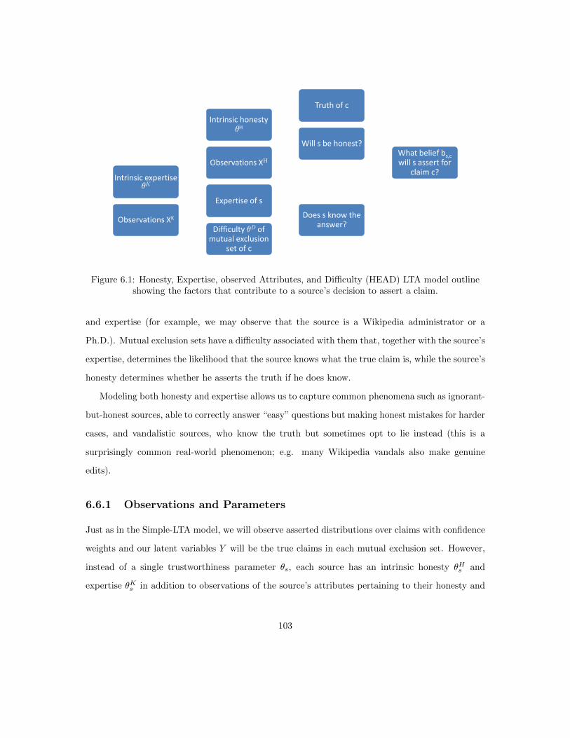
What belief bs,c

will s assert for claim c?

Truth of c

Will s be honest?

Intrinsic honesty µH

Observations XH

Does s know the answer?

Expertise of s

Intrinsic expertise µK

Observations XK

Difficulty µD of mutual exclusion

set of c

Figure 6.1: Honesty, Expertise, observed Attributes, and Difficulty (HEAD) LTA model outlineshowing the factors that contribute to a source’s decision to assert a claim.

and expertise (for example, we may observe that the source is a Wikipedia administrator or a

Ph.D.). Mutual exclusion sets have a difficulty associated with them that, together with the source’s

expertise, determines the likelihood that the source knows what the true claim is, while the source’s

honesty determines whether he asserts the truth if he does know.

Modeling both honesty and expertise allows us to capture common phenomena such as ignorant-

but-honest sources, able to correctly answer “easy” questions but making honest mistakes for harder

cases, and vandalistic sources, who know the truth but sometimes opt to lie instead (this is a

surprisingly common real-world phenomenon; e.g. many Wikipedia vandals also make genuine

edits).

6.6.1 Observations and Parameters

Just as in the Simple-LTA model, we will observe asserted distributions over claims with confidence

weights and our latent variables Y will be the true claims in each mutual exclusion set. However,

instead of a single trustworthiness parameter θs, each source has an intrinsic honesty θHs and

expertise θKs in addition to observations of the source’s attributes pertaining to their honesty and

103

expertise.

Observed Attributes

A source may have observable attributes that tell us how honest it is (e.g. whether the source

has been blocked from Wikipedia) and how much expertise it has (e.g. educational attainment).

These attributes are provided as vectors of features XHs (honesty) and XK

s (expertise). Not every

feature need be known for every source (missing values are permissible), and each feature may be

binary, multinomial, or continuous; we will henceforth assume binary features for simplicity, but

the extension to other types is straightforward.

As we will see, these features are treated as being caused or generated independently as a result

of the source’s honesty or expertise, essentially becoming the features and labels of a Naive Bayes

classifier.

Parameters

θHs is the [0, 1] probability of a source telling the truth in the absence of any observed evidence;

when we compute the probability of the source being honest, θHs can be thought of as the prior

probability of honesty used in the Naive Bayes prediction. However, θHs itself has a prior, P (θHs ),

which essentially determines the likelihood that the actual honesty of a source deviates from the

honesty predicted from its observed attributes (spelling and grammar, academic degrees, etc.).

A very concentrated P (θHs ) distribution, such as Beta(90, 10), means that θHs is unlikely to vary

much and, in effect, variation among the honesty of sources will depend almost entirely on their

attributes. A relatively flat P (θHs ) distribution such as Beta(1.09, 1.01), on the other hand, allows

θHs to vary widely, and the observed attributes become less important than our estimate of the

source’s individual, innate tendency towards honesty.

For the Naive Bayes honesty prediction, we also need to know the probability of the observation

conditioned on the sources’ honesty. These conditional probabilities are the same across all the

sources, so, assuming binary features, we need 2|XHs | parameters: {θP (x|H) : x ∈ XH

s }∪{θP (x|¬H) :

x ∈ XHs }. Note that since these parameters are shared, the conditional probability of a particular

104

feature value given that a source is honest or dishonest is the same for everyone.

θEs ∈ R is the “expertise” of a source is a real number that is compared against the “difficulty”

θDm ∈ R of a mutual exclusion. Distinguishing the “difficulty” of a mutual exclusion set is important:

determining that the sky is blue is much easier than determining the mass of the Higgs boson, for

example. Together, these two parameters give us the prior in our Naive Bayes prediction of whether

source s knows the true claim in mutual exclusion set m. As with honesty, we also need 2|XKs |

parameters for the probability of our expertise observations conditioned on the source knowing the

answer: {θP (x|K) : x ∈ XKs } ∪ {θP (x|¬K) : x ∈ XK

s }.

6.6.2 Constructing the Model

For each source s and each mutual exclusion set m, the HEAD-LTA model essentially calcu-

lates the probability that source s knows the true claim in m and the probability that source

s chooses to assert what it thinks is the true claim in m. These events (Ks,m and Hs, respec-

tively) are taken as independent, and together give us the distribution over the four possibili-

ties: (Ks,m, Hs), (Ks,m,¬Hs), (¬Ks,m, Hs)and(¬Ks,m,¬Hs). Each of these joint events then cor-

responds to a probability that source s asserts a particular distribution Ds,m over the claims in

m.

Opting for Honesty

A source may decide to lie, asserting a distribution Ds,m that does not accord with his actual belief.

We assume that the observed honesty-related features XHs are independent, so the probability that

a source opts to tell the truth is given by a Naive Bayes model:

P (Hs|XHs , θ) =

θHs∏x∈XHs

P (x|H, θP (x|H))

θHs∏x∈XHs

P (x|H, θP (x|H)) + (1− θHs )∏x∈XHs

P (x|¬H, θP (x|¬H))

Because we assume binary {0, 1} features, P (x|H, θP (x|H)) = xθP (x|H) + (1− x)(1− θP (x|H)).

Note that Hs (and Ks,m) are not explicitly modeled as latent variables; rather, we are only

interested in finding the probability of these events as a subcomponent of our larger model.

105

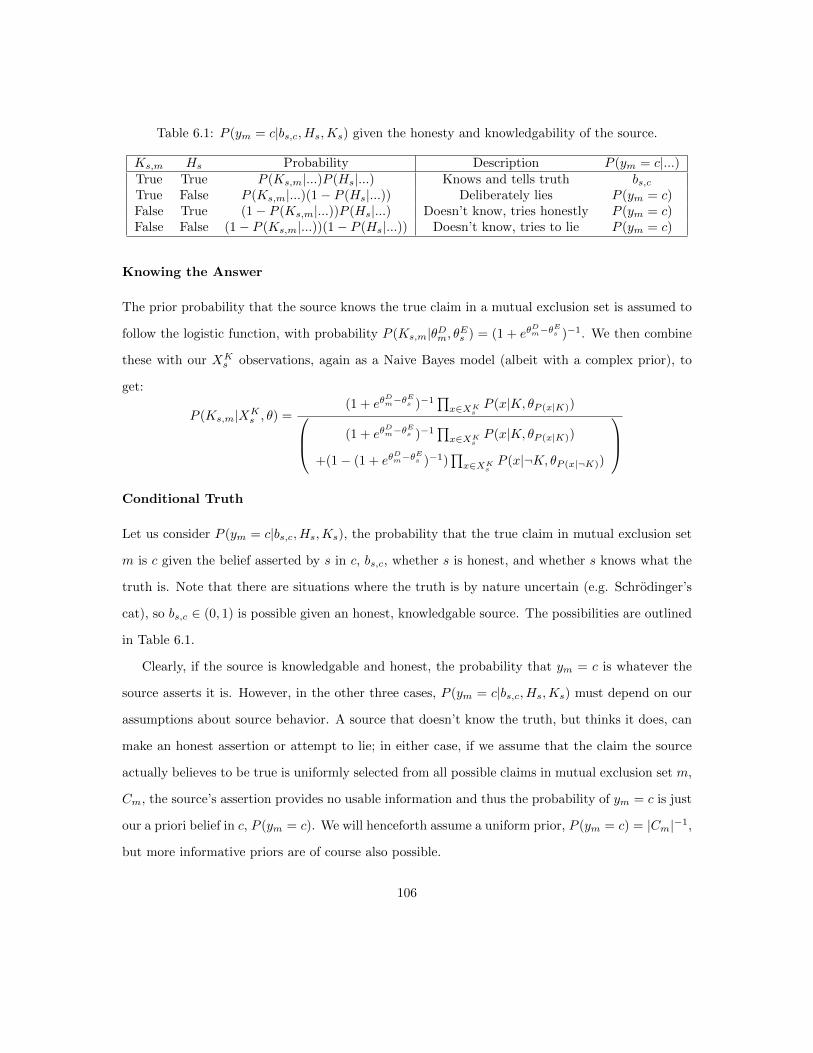
Table 6.1: P (ym = c|bs,c, Hs,Ks) given the honesty and knowledgability of the source.

Ks,m Hs Probability Description P (ym = c|...)True True P (Ks,m|...)P (Hs|...) Knows and tells truth bs,cTrue False P (Ks,m|...)(1− P (Hs|...)) Deliberately lies P (ym = c)False True (1− P (Ks,m|...))P (Hs|...) Doesn’t know, tries honestly P (ym = c)False False (1− P (Ks,m|...))(1− P (Hs|...)) Doesn’t know, tries to lie P (ym = c)

Knowing the Answer

The prior probability that the source knows the true claim in a mutual exclusion set is assumed to

follow the logistic function, with probability P (Ks,m|θDm, θEs ) = (1 + eθDm−θ

Es )−1. We then combine

these with our XKs observations, again as a Naive Bayes model (albeit with a complex prior), to

get:

P (Ks,m|XKs , θ) =

(1 + eθDm−θ

Es )−1

∏x∈XKs

P (x|K, θP (x|K)) (1 + eθDm−θ

Es )−1

∏x∈XKs

P (x|K, θP (x|K))

+(1− (1 + eθDm−θ

Es )−1)

∏x∈XKs

P (x|¬K, θP (x|¬K))

Conditional Truth

Let us consider P (ym = c|bs,c, Hs,Ks), the probability that the true claim in mutual exclusion set

m is c given the belief asserted by s in c, bs,c, whether s is honest, and whether s knows what the

truth is. Note that there are situations where the truth is by nature uncertain (e.g. Schrodinger’s

cat), so bs,c ∈ (0, 1) is possible given an honest, knowledgable source. The possibilities are outlined

in Table 6.1.

Clearly, if the source is knowledgable and honest, the probability that ym = c is whatever the

source asserts it is. However, in the other three cases, P (ym = c|bs,c, Hs,Ks) must depend on our

assumptions about source behavior. A source that doesn’t know the truth, but thinks it does, can

make an honest assertion or attempt to lie; in either case, if we assume that the claim the source

actually believes to be true is uniformly selected from all possible claims in mutual exclusion set m,

Cm, the source’s assertion provides no usable information and thus the probability of ym = c is just

our a priori belief in c, P (ym = c). We will henceforth assume a uniform prior, P (ym = c) = |Cm|−1,

but more informative priors are of course also possible.

106

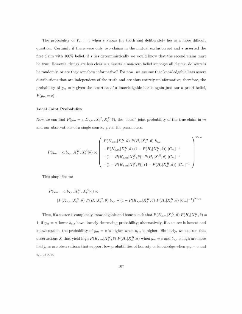
The probability of Ym = c when s knows the truth and deliberately lies is a more difficult

question. Certainly if there were only two claims in the mutual exclusion set and s asserted the

first claim with 100% belief, if s lies deterministically we would know that the second claim must

be true. However, things are less clear is s asserts a non-zero belief amongst all claims: do sources

lie randomly, or are they somehow informative? For now, we assume that knowledgable liars assert

distributions that are independent of the truth and are thus entirely uninformative; therefore, the

probability of ym = c given the assertion of a knowledgable liar is again just our a priori belief,

P (ym = c).

Local Joint Probability

Now we can find P (ym = c,Ds,m, XHs , X

Ks |θ), the “local” joint probability of the true claim in m

and our observations of a single source, given the parameters:

P (ym = c, bs,c, XHs , X

Ks |θ) ∝

P (Ks,m|XKs , θ) P (Hs|XH

s , θ) bs,c

+P (Ks,m|XKs , θ) (1− P (Hs|XH

s , θ)) |Cm|−1

+(1− P (Ks,m|XKs , θ)) P (Hs|XH

s , θ) |Cm|−1

+(1− P (Ks,m|XKs , θ)) (1− P (Hs|XH

s , θ)) |Cm|−1

ws,m

This simplifies to:

P (ym = c, bs,c, XHs , X

Ks |θ) ∝(

P (Ks,m|XKs , θ) P (Hs|XH

s , θ) bs,c + (1− P (Ks,m|XKs , θ) P (Hs|XH

s , θ) |Cm|−1)ws,m

Thus, if a source is completely knowledgable and honest such that P (Ks,m|XKs , θ) P (Hs|XH

s , θ) =

1, if ym = c, lower bs,c have linearly decreasing probability; alternatively, if a source is honest and

knowledgable, the probability of ym = c is higher when bs,c is higher. Similarly, we can see that

observations X that yield high P (Ks,m|XKs , θ) P (Hs|XH

s , θ) when ym = c and bs,c is high are more

likely, as are observations that support low probabilities of honesty or knowledge when ym = c and

bs,c is low.

107

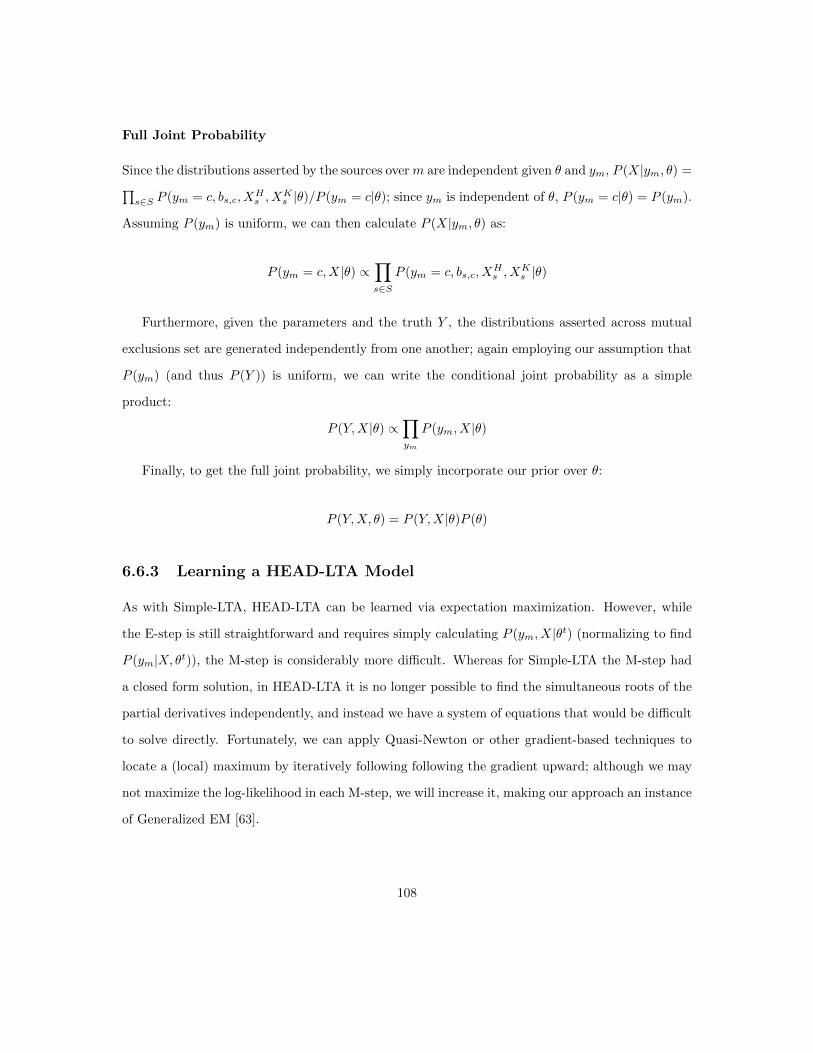
Full Joint Probability

Since the distributions asserted by the sources overm are independent given θ and ym, P (X|ym, θ) =∏s∈S P (ym = c, bs,c, X

Hs , X

Ks |θ)/P (ym = c|θ); since ym is independent of θ, P (ym = c|θ) = P (ym).

Assuming P (ym) is uniform, we can then calculate P (X|ym, θ) as:

P (ym = c,X|θ) ∝∏s∈S

P (ym = c, bs,c, XHs , X

Ks |θ)

Furthermore, given the parameters and the truth Y , the distributions asserted across mutual

exclusions set are generated independently from one another; again employing our assumption that

P (ym) (and thus P (Y )) is uniform, we can write the conditional joint probability as a simple

product:

P (Y,X|θ) ∝∏ym

P (ym, X|θ)

Finally, to get the full joint probability, we simply incorporate our prior over θ:

P (Y,X, θ) = P (Y,X|θ)P (θ)

6.6.3 Learning a HEAD-LTA Model

As with Simple-LTA, HEAD-LTA can be learned via expectation maximization. However, while

the E-step is still straightforward and requires simply calculating P (ym, X|θt) (normalizing to find

P (ym|X, θt)), the M-step is considerably more difficult. Whereas for Simple-LTA the M-step had

a closed form solution, in HEAD-LTA it is no longer possible to find the simultaneous roots of the

partial derivatives independently, and instead we have a system of equations that would be difficult

to solve directly. Fortunately, we can apply Quasi-Newton or other gradient-based techniques to

locate a (local) maximum by iteratively following following the gradient upward; although we may

not maximize the log-likelihood in each M-step, we will increase it, making our approach an instance

of Generalized EM [63].

108

Simplifying Terms

To begin, we will simplify the P (Ks,m|...) and P (Hs|...) probabilities to convert them to logistic

functions more amenable to analysis.

P (Ks,m|X, θ) =(1 + eθ

Dm−θ

Es )−1

∏x∈XKs

P (x|K, θ)(1 + eθ

Dm−θEs )−1

∏x∈XKs

P (x|K, θ) + (1− (1 + eθDm−θEs )−1)

∏x∈XKs

P (x|¬K, θ)

=

∏x∈XKs

P (x|K, θ)∏x∈XKs

P (x|K, θ) + (1 + eθDm−θEs )(1− (1 + eθ

Dm−θEs )−1)

∏x∈XKs

P (x|¬K, θ)

=

∏x∈XKs

P (x|K, θ)∏x∈XKs

P (x|K, θ) + eθDm−θEs

∏x∈XKs

P (x|¬K, θ)

=1

1 + eθDm−θEs

∏x∈XKs

P (x|¬K,θ)∏x∈XKs

P (x|K,θ)

=1

1 + eθDm−θEs +

∑x∈XKs

logP (x|¬K,θ)−logP (x|K,θ)

P (Hs|X, θ) can be similarly converted to:

P (Hs|X, θ) =1

1 + elog( 1

θHs−1)+

∑x∈XHs

logP (x|¬H,θ)−logP (x|H,θ)

Gradients

Recall that we assume binary XKs and XH

s features, giving us conditional probabilities of the form:

P (x|K, θ) = xθP (x|K) + (1− x)(1− θP (x|K)) = 1− θP (x|K) − x+ 2xθP (x|K)

When computing the gradients, there are a number of repeated subexpressions whose values

should be cached to improve performance. Consequently, for the sake of both computational effi-

109

ciency and notational convenience, we will refer to these subexpressions using symbols:

α = θDm − θEs +∑x∈XKs

log(1− θP (x|¬K) − x+ 2xθP (x|¬K))− log(1− θP (x|K) − x+ 2xθP (x|K))

β = log(1

θHs− 1)

+∑x∈XHs

log(1− θP (x|¬H) − x+ 2xθP (x|¬H))− log(1− θP (x|H) − x+ 2xθP (x|H))

K = P (Ks,m|XKs , θ) =

1

1 + eα

H = P (Hs|XHs , θ) =

1

1 + eβ

R = KH

L = log(Rbs,c + |Cm|−1 −R|Cm|−1)

Recall that we seek to maximize the expected log-likelihood of P (X,Y, θ):

EY |X,θt [log(P (X,Y |θ)P (θ))]

After some algebraic manipulation, we can rewrite this as:

Q = log(P (θ)) +∑m

∑ym

P (ym|X, θt)∑s

ws,mL

We will use a Beta distribution for P (θHs ):

P (θHs ) ∝ (θHs )a−1(1− θHs )b−1

P (θ) ∝∏θHs

(θHs )a−1(1− θHs )b−1

110

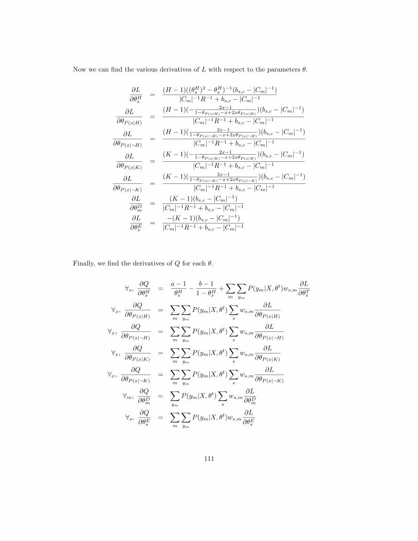
Now we can find the various derivatives of L with respect to the parameters θ.

∂L

∂θHs=

(H − 1)((θHs )2 − θHs )−1(bs,c − |Cm|−1)

|Cm|−1R−1 + bs,c − |Cm|−1

∂L

∂θP (x|H)=

(H − 1)(− 2x−11−θP (x|H)−x+2xθP (x|H)

)(bs,c − |Cm|−1)

|Cm|−1R−1 + bs,c − |Cm|−1

∂L

∂θP (x|¬H)=

(H − 1)( 2x−11−θP (x|¬H)−x+2xθP (x|¬H)

)(bs,c − |Cm|−1)

|Cm|−1R−1 + bs,c − |Cm|−1

∂L

∂θP (x|K)=

(K − 1)(− 2x−11−θP (x|K)−x+2xθP (x|K)

)(bs,c − |Cm|−1)

|Cm|−1R−1 + bs,c − |Cm|−1

∂L

∂θP (x|¬K)=

(K − 1)( 2x−11−θP (x|¬K)−x+2xθP (x|¬K)

)(bs,c − |Cm|−1)

|Cm|−1R−1 + bs,c − |Cm|−1

∂L

∂θDm=

(K − 1)(bs,c − |Cm|−1)

|Cm|−1R−1 + bs,c − |Cm|−1

∂L

∂θEs=

−(K − 1)(bs,c − |Cm|−1)

|Cm|−1R−1 + bs,c − |Cm|−1

Finally, we find the derivatives of Q for each θ.

∀s,∂Q

∂θHs=

a− 1

θHs− b− 1

1− θHs+∑m

∑ym

P (ym|X, θt)ws,m∂L

∂θTs

∀x,∂Q

∂θP (x|H)=

∑m

∑ym

P (ym|X, θt)∑s

ws,m∂L

∂θP (x|H)

∀x,∂Q

∂θP (x|¬H)=

∑m

∑ym

P (ym|X, θt)∑s

ws,m∂L

∂θP (x|¬H)

∀x,∂Q

∂θP (x|K)=

∑m

∑ym

P (ym|X, θt)∑s

ws,m∂L

∂θP (x|K)

∀x,∂Q

∂θP (x|¬K)=

∑m

∑ym

P (ym|X, θt)∑s

ws,m∂L

∂θP (x|¬K)

∀m,∂Q

∂θDm=

∑ym

P (ym|X, θt)∑s

ws,m∂L

∂θDm

∀s,∂Q

∂θEs=

∑m

∑ym

P (ym|X, θt)ws,m∂L

∂θEs

111

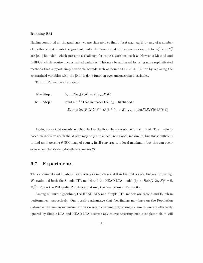
Running EM

Having computed all the gradients, we are then able to find a local argmaxθ Q by any of a number

of methods that climb the gradient, with the caveat that all parameters except for θDm and θEs

are [0, 1] bounded, which presents a challenge for some algorithms such as Newton’s Method and

L-BFGS which require unconstrained variables. This may be addressed by using more sophisticated

methods that support simple variable bounds such as bounded L-BFGS [14], or by replacing the

constrained variables with the [0, 1] logistic function over unconstrained variables.

To run EM we have two steps:

E− Step : ∀m, P (ym|X, θt) ∝ P (ym, X|θt)

M− Step : Find a θt+1 that increases the log − likelihood :

EY |X,θt [log(P (X,Y |θt+1)P (θt+1))] > EY |X,θt−1 [log(P (X,Y |θt)P (θt))]

Again, notice that we only ask that the log-likelihood be increased, not maximized. The gradient-

based methods we use in the M-step may only find a local, not global, maximum, but this is sufficient

to find an increasing θ (EM may, of course, itself converge to a local maximum, but this can occur

even when the M-step globally maximizes θ).

6.7 Experiments

The experiments with Latent Trust Analysis models are still in the first stages, but are promising.

We evaluated both the Simple-LTA model and the HEAD-LTA model (θHs ∼ Beta(2, 2), XHs = ∅,

XKs = ∅) on the Wikipedia Population dataset; the results are in Figure 6.2.

Among all trust algorithms, the HEAD-LTA and Simple-LTA models are second and fourth in

performance, respectively. One possible advantage that fact-finders may have on the Population

dataset is the numerous mutual exclusion sets containing only a single claim: these are effectively

ignored by Simple-LTA and HEAD-LTA because any source asserting such a singleton claim will

112

Figure 6.2: Accuracy of fact-finders, Simple-LTA and HEAD-LTA on the Population dataset.

always be right regardless of trustworthiness. In many situations, this is a good thing—asserting

trivial claims should not make a source more trusted; however, in Wikipedia, the singleton claims

tend to be about more esoteric topics that only dedicated (and trustworthy) users bother with.

While a sizable number of people may dispute the population of, say, Los Angeles, and vandals may

target such popular topics, pages about small towns may see only a few edits, often by proficient,

“expert” users. Fact-finders give sources “credit” for singleton claims, and so those trustworthy

sources who happen to be proficient asserters of singleton claims are (correctly) assigned more trust

by the algorithm.

One of the benefits of LTA models is that they have well-defined semantics; consequently, we

can readily adapt them to our domain knowledge, which, in this case, is that sources asserting

singletons tend to be more trustworthy, and this is what our next set of experiments will explore.

For example, in HEAD-LTA, we can use honesty or knowledge features to capture the number of

singleton assertions a source makes directly. Alternatively, we could add “unknown” claims as we

did with fact-finders, but with the ability to provide a precise prior P (ym = unknown), or simply

113

provide priors over our θ parameters corresponding to the tendency of sources with more assertions

to be more trustworthy in this domain.

6.8 Conclusion

Even without these enhancements, the Latent Trust Analysis models do remarkably well, and have

numerous other advantages over fact-finders. As principled, generative models, they tell a coherent

story of why and how sources make assertions, which, especially in the case of Simple-LTA, can be

readily explained to the user to justify a trust decision. Furthermore, the models’ crisp probabilistic

semantics grant tremendous flexibility in adapting to new domains in ways that are not possible

for fact-finders, in addition to being able to capture the same knowledge permitted by Generalized

Fact-Finding (e.g. via the honesty and expertise observed attributes [which, unlike attributes in

Generalized Fact-Finders, can be real-valued] and the ws,m certainty weights) and Constrained

Fact-Finding (via Generalized Constrained Models). Finally, as probabilistic models, there are

numerous avenues for learning; we have used expectation-maximization for unsupervised learning

analogous to that performed by fact-finders, but both semi-supervised and supervised learning are

also available to us, and potentially invaluable when the trust of some sources or the truth of some

claims is already known.

114

Chapter 7

Conclusion

Throughout this dissertation, we have explored a number of aspects of the information trust problem

in our pursuit of a computational trust system capable of substituting for the user’s own informed

and subjective judgement. We began by first examining how to express the trustworthiness of

an information source, document, publisher or other entity beyond assigning a simple, and often

misleading, accuracy score based on the percent of claims they made that were true. By introducing

a new, more comprehensive set of metrics corresponding to the truthfulness, completeness, and bias

of a source, we can guide the user to the resource best suited to her and relate our trust judgements

in an actionable, accessible manner that allows her to better leverage those sources she does select

(for example, by moderating her reading to account for incompleteness or bias).

Once we established a means of expressing trustworthiness, we studied progressively more so-

phisticated ways of determining trustworthiness, incorporating increasing amounts of knowledge

into our trust decisions, allowing us to escape the erroneous notion of universal “ground truth” and

instead find the subjective truth for the user given her prior knowledge and beliefs: experimentally,

we saw that this was essential even for relatively simple tasks, such as determining the true spelling

of a word. We started with the initial baseline of voting, simply choosing the claim asserted by the

most sources, with the implicit assumption that all sources are equally trustworthy. Next, we saw

that fact-finders remove this (grossly unrealistic) assumption and estimate the trustworthiness of

the source in addition to finding the true claims, but still restrict us to considering only “who said

what”. Generalized Fact-Finding, however, allows us to take advantage of the frequently highly

available and very useful additional information that is available to us, in the form of the source’s

or information extractor’s certainty in a claim (e.g. “I’m 80% sure that John said he was 60%

115

sure that...”), the similarity between claims (“Hawaii is more similar to Alaska than to Kenya”),

and the attributes and membership of sources (“John has a Ph.D.”, “Sarah is a Republican”, etc.).

Constrained Fact-Finding then complimentarily introduces declarative prior knowledge, allowing us

to provide both specific facts (“Los Angeles is larger than Wichita”) and general, axiomatic rules

the world obeys (“Cities usually grow over time”). Moreover, Generalized and Constrained Fact-

Finding combine to create a joint framework which in our experiments provided an almost additive

benefit from the two orthogonal techniques, yielding performance significantly beyond what was

possible with standard fact-finders.

The idea behind Constrained Fact-Finding can also be abstracted to structured learning in

general, in the form of Generalized Constrained Models (GCMs). After the underlying “local”

model makes a prediction, the GCM corrects this prediction to be the most likely label (or label

distribution) that satisfies the the declarative prior knowledge constraints, which is the satisfying

label closest to the original according to the distance metric particular to the problem. This is

in marked contrast to Constrained Conditional Models, Posterior Regularization, and Constraint

Driven Learning, all of which arbitrarily commit to a single metric which does not typically find

the most likely satisfying label distribution. Additionally, GCMs introduce the concept of com-

pact, convex metrics, which allow a GCM to treat the underlying model as a black box (unlike

Posterior Regularization) and simultaneously achieve polynomial running time (unlike Constrained

Conditional Models and Constraint Driven Learning). From a trust perspective, though, GCMs

are important because they allow us to apply declarative prior knowledge to a new type of trust

model, Latent Trust Analysis.

Latent Trust Analysis models the generative process by which sources assert claims, with the

likelihood that a source will assert a claim essentially dependent upon whether the claim is true

and how trustworthy the source is. This provides a principled, probabilistic generative story with

a number of important advantages over fact-finders, most immediately the ability to justify the

trust decision to the user, and Simple-LTA in particular has an extraordinarily natural, intuitive

explanation that other trust algorithms lack. Even more useful is the flexibility this engenders:

the well-defined semantics permit, for example, the ready application of Bayesian priors, and the

116

mechanics of the model are transparent (as opposed to the more nebulous operation of the iterative

transitive voting of fact-finders). Furthermore, unlike fact-finders, LTA models naturally support

semi-supervised and supervised learning, which can be a powerful advantage when the truth of

some claims or trustworthiness of some sources is already known.

Of course, this comes at a tradeoff: though Simple-LTA is quite elegant, the HEAD-LTA model

is the most sophisticated trust algorithm we have encountered, and, while tractable even on large

datasets, is certainly the most computationally demanding. Indeed, as we have moved up the

ladder from basic voting to LTA, we have progressively incorporated more information into our trust

decision, gaining expressiveness and predictive power at the cost of complexity and computation.

As a result, even with the development of Latent Trust Analysis models, Generalized, Constrained

and even standard fact-finding algorithms still have applications in extremely large datasets where

more sophisticated methods would be intractable, or where speed is a primary concern (e.g. making

trust judgements online, in real-time).

Perhaps most exciting, though, is that while we have studied novel algorithms and found new

ways to incorporate the plethora of data available to us and build upon the user’s prior knowledge,

there is still so much potential for further advancement. Latent Trust Analysis is the first strongly

principled approach to the information trust problem and is still largely unexplored. Conversely,

real-world applications of trust algorithms are only beginning to be realized, despite their wide

applicability to many pressing challenges, new and longstanding, in dealing with the curse (and

blessing) of overwhelming amounts of data, and this is yet another frontier upon which large gains

are still to be made. In either case, it is clear that information trust has a future that is both rich

and unmapped.

117

References

[1] B T Adler and L de Alfaro. A content-driven reputation system for the Wikipedia. WWW’07, 7:261–270, 2007.

[2] B Thomas Adler, Krishnendu Chatterjee, Luca De Alfaro, Marco Faella, Ian Pye, and Vish-wanath Raman. Assigning Trust to Wikipedia Content . Computer Engineering, 2008.

[3] G Adomavicius and A Tuzhilin. Toward the Next Generation of Recommender Systems: ASurvey of the State-of-the-Art and Possible Extensions. 2005.

[4] I A Al Mamunur Rashid, D Cosley, S K Lam, S M McNee, J A Konstan, and J Riedl. Gettingto know you: learning new user preferences in recommender systems. Proceedings of the 7thinternational conference on Intelligent user interfaces, January, pages 13–16, 2002.

[5] D Artz and Y Gil. A survey of trust in computer science and the Semantic Web. WebSemantics: Science, Services and Agents on the World Wide Web, 5(2):58–71, June 2007.

[6] R Axelrod. On Six Advances in Cooperation Theory. Analyse & Kritik, 22(1):130–151, 2000.

[7] R Axelrod and W D Hamilton. The evolution of cooperation. Science, 211(4489):1390, 1981.

[8] B P Bailey, L J Gurak, and J A Konstan. An examination of trust production in computer-mediated exchange. Proceedings of the 7th Conference on Human Factors and the Web, 2001.

[9] G H BakIr, T Hofmann, B Scholkopf, A J Smola, B Taskar, and S V N Vishwanathan. Pre-dicting Structured Data. MIT Press, 2007.

[10] Yoshua Bengio and Universite De Montreal. Markovian Models for Sequential Data. ComputingSurveys, 1999.

[11] Elisa Bertino, Chenyun Dai, Hyo-sang Lim, and Dan Lin. High-Assurance Integrity Techniquesfor Databases. Event (London), pages 244–256, 2008.

[12] J S Breese, D Heckerman, and C Kadie. Empirical Analysis of Predictive Algorithms forCollaborative Filtering. Microsoft Research Technical Report, 1998.

[13] S Brin and L Page. The anatomy of a large-scale hypertextual Web search engine. ComputerNetworks and ISDN Systems, 30(1-7):107–117, 1998.

[14] R.H. Byrd, P. Lu, J. Nocedal, and C. Zhu. A Limited Memory Algorithm for Bound Con-strained Optimization. SIAM Journal on Scientific Computing, 16(5):1190–1208, 1995.

118

[15] M Chang, L Ratinov, and D Roth. Guiding semi-supervision with constraint-driven learning.In Proc. ACL, 2007.

[16] M.W. Chang, Lev Ratinov, Nicholas Rizzolo, and Dan Roth. Learning and inference withconstraints. In AAAI, 2008.

[17] A Cheng and E Friedman. Sybilproof reputation mechanisms. Applications, Technologies,Architectures, and Protocols for Computer Communication, pages 128–132, 2005.

[18] Chenyun Dai, D. Lin, E. Bertino, and M. Kantarcioglu. An approach to evaluate data trust-worthiness based on data provenance. SDM, 2008.

[19] Chenyun Dai, D. Lin, E. Bertino, and M. Kantarcioglu. Trust evaluation of data provenance.Technical report, CERIAS Technical Report, 2008.

[20] A S Das, M Datar, A Garg, and S Rajaram. Google news personalization: scalable onlinecollaborative filtering. Proceedings of the 16th international conference on World Wide Web,pages 271–280, 2007.

[21] Hal Daum, John Langford, and Daniel Marcu. Search-based Structured Prediction. Informa-tion Sciences, pages 1–32.

[22] Chrysanthos Dellarocas. The Digitization of Word of Mouth: Promise and Challenges of OnlineFeedback Mechanisms. Management Science, 49(10):1407–1424, October 2003.

[23] A.P. Dempster, N.M. Laird, and D.B. Rubin. Maximum likelihood from incomplete data viathe EM algorithm. Journal of the Royal Statistical Society. Series B (Methodological), 39(1):1–38, 1977.

[24] X Dong, L Berti-equille, and D Srivastava. Integrating conflicting data: the role of sourcedependence. Technical report, AT&T Labs-Research, Florham Park, NJ, 2009.

[25] X.L. Dong, L. Berti-Equille, and Divesh Srivastava. Truth discovery and copying detection ina dynamic world. VLDB, 2009.

[26] J R Douceur. The Sybil Attack. Peer-To-Peer Systems: First International Workshop, IPTPS2002, Cambridge, MA, USA, March 7-8, 2002: Revised Papers, 2002.

[27] Gregory Druck, Gideon Mann, and Andrew Mccallum. Learning from Labeled Features usingGeneralized Expectation Criteria Categories and Subject Descriptors. SIGIR, 2008.

[28] B J Fogg, J Marshall, T Kameda, J Solomon, A Rangnekar, J Boyd, and B Brown. Webcredibility research: a method for online experiments and early study results. Conference onHuman Factors in Computing Systems, pages 295–296, 2001.

[29] B J Fogg, P Swani, M Treinen, J Marshall, O Laraki, A Osipovich, C Varma, N Fang, J Paul,A Rangnekar, and Others. What makes Web sites credible?: a report on a large quantitativestudy. Proceedings of the SIGCHI conference on Human factors in computing systems, pages61–68, 2001.

[30] B J Fogg and H Tseng. The elements of computer credibility. CHI, pages 80–87, 1999.

119

[31] Y Freund and Robert Schapire. A Decision-Theoretic Generalization of On-Line Learning andan Application to Boosting. Computational learning theory, August 1995.

[32] Alban Galland, Serge Abiteboul, A. Marian, and Pierre Senellart. Corroborating informationfrom disagreeing views. In WSDM, 2010.

[33] K. Ganchev, J. Graca, J. Gillenwater, and B. Taskar. Posterior Regularization for StructuredLatent Variable Models. Journal of Machine Learning Research, 2010.

[34] Y Gil and D Artz. Towards content trust of web resources. Web Semantics: Science, Servicesand Agents on the World Wide Web, 5(4):227–239, December 2007.

[35] Y. Gil, J. Cheney, P. Groth, O. Hartig, S. Miles, L. Moreau, and P.P. Da Silva. ProvenanceXG Final Report, 2010.

[36] Yolanda Gil and Varun Ratnakar. TRELLIS: An interactive tool for capturing informationanalysis and decision making. Knowledge Engineering and Knowledge Management: Ontologiesand the Semantic Web, (October):37–42, 2002.

[37] Yolanda Gil and Varun Ratnakar. Trusting information sources one citizen at a time. ISWC,pages 162–176, 2002.

[38] Trond Grenager, Dan Klein, and Christopher D Manning. Unsupervised Learning of FieldSegmentation Models for Information Extraction. Computational Linguistics, (June):371–378,2005.

[39] R Guha, R Kumar, P Raghavan, and A Tomkins. Propagation of Trust and Distrust. Proc.13th Intl Conf. World Wide Web (WWW, 2004.

[40] Z. Gyongyi, H. Garcia-Molina, and J. Pedersen. Combating Web Spam with Trustrank. InProceedings of the Thirtieth international conference on Very large data bases-Volume 30, page587. VLDB Endowment, 2004.

[41] J L Herlocker, J A Konstan, L G Terveen, and J T Riedl. Evaluating collaborative filteringrecommender systems. ACM Transactions on Information Systems (TOIS), 22(1):5–53, 2004.

[42] P Hirsch, S Michaels, and R Friedman. Dirty hands versus clean models. Theory and Society,16(3):317–336, 1987.

[43] A Josang. Artificial reasoning with subjective logic. 2nd Australian Workshop on Common-sense Reasoning, 1997.

[44] A. Josang, S. Marsh, and S. Pope. Exploring different types of trust propagation. LectureNotes in Computer Science, 3986:179, 2006.

[45] L Kagal, T Finin, and A Joshi. Developing secure agent systems using delegation based trustmanagement. In Workshop on Security of Mobile MultiAgent Systems held at AutonomousAgents and MultiAgent Systems. 2002.

[46] S Kamvar, M Schlosser, and H Garcia-molina. The Eigentrust algorithm for reputation man-agement in P2P networks. WWW ’03, 2003.

120

[47] N. Karmarkar. A new polynomial-time algorithm for linear programming. Combinatorica,4(4):373–395, 1984.

[48] Jihie Kim, Ewa Deelman, Yolanda Gil, Gaurang Mehta, Varun Ratnakar, and Marina Rey.Provenance Trails in the Wings / Pegasus System Wings / Pegasus : Creating and ExecutingLarge Workflows. Journal of Concurrency And Computation: Practice And Experience, pages1–11, 2007.

[49] J M Kleinberg. Authoritative sources in a hyperlinked environment. Journal of the ACM,46(5):604–632, 1999.

[50] A Klementiev, D Roth, and K Small. An Unsupervised Learning Algorithm for Rank Aggre-gation. LECTURE NOTES IN COMPUTER SCIENCE, 4701:616, 2007.

[51] J Kohl and B C Neuman. The kerberos network authentication service. IETF RFC 1510,1993.

[52] R. Layfield, M. Kantarcioglu, and B. Thuraisingham. Incentive and Trust Issues in AssuredInformation Sharing. In Collaborative Computing: Networking, Applications and Worksharing:4th International Conference, page 113. Springer, 2008.

[53] R. Levien. Attack-resistant trust metrics. Computing with Social Trust, pages 121–132, 2008.

[54] B.N. Levine, C. Shields, and N.B. Margolin. A survey of solutions to the sybil attack. Universityof Massachusetts Amherst, Amherst, MA, 2006.

[55] Percy Liang, Michael I. Jordan, and Dan Klein. Learning from measurements in exponentialfamilies. ICML, pages 1–8, 2009.

[56] Dong C. Liu and Jorge Nocedal. On the limited memory BFGS method for large scale opti-mization. Mathematical Programming, 45(1-3):503–528, August 1989.

[57] D.W. Manchala. Trust metrics, models and protocols for electronic commerce transac-tions. Proceedings. 18th International Conference on Distributed Computing Systems (Cat.No.98CB36183), pages 312–321, 1998.

[58] G. Mann and A. McCallum. Generalized expectation criteria for semi-supervised learning ofconditional random fields. In ACL, 2008.

[59] S Marsh. Formalising Trust as a Computational Concept. PhD thesis, University of Stirling,1994.

[60] Bhaskar Mehta, Thomas Hofmann, and Wolfgang Nejdl. Robust collaborative filtering. InRecSys ’07: Proceedings of the 2007 ACM conference on Recommender systems, pages 49–56,New York, NY, USA, 2007. ACM.

[61] Luc Moreau, Ben Clifford, Juliana Freire, and Yolanda Gil. The Open Provenance Model CoreSpecification. Future Generation Computer Systems, pages 1–30, 2010.

[62] L. Mui, M. Mohtashemi, and a. Halberstadt. A computational model of trust and reputa-tion. Proceedings of the 35th Annual Hawaii International Conference on System Sciences,00(c):2431–2439, 2002.

121

[63] R.M. Neal and G.E. Hinton. A new view of the EM algorithm that justifies incremental andother variants. Learning in graphical models, pages 355–368, 1998.

[64] M Nielsen and K Krukow. Towards a formal notion of trust. In PPDP 03: Proceedings ofthe 5th ACM SIGPLAN international conference on Principles and practice of declaritiveprogramming. pages:4–7, 2003.

[65] V Novak, I Perfilieva, and J Mockof. Mathematical principles of fuzzy logic. Kluwer AcademicPublishers, 1999.

[66] M Pazzani and D Billsus. Learning and Revising User Profiles: The Identification of InterestingWeb Sites. Machine Learning, 27(3):313–331, 1997.

[67] V. Punyakanok, D. Roth, W. Yih, and D. Zimak. Learning and inference over constrainedoutput. In International Joint Conference on Artificial Intelligence, volume 19, 2005.

[68] Nicholas Rizzolo and Dan Roth. Modeling Discriminative Global Inference. C, pages 597–604,September 2007.

[69] D Roth and W Yih. Global Inference for Entity and Relation Identification via a LinearProgramming Formulation. In Lise Getoor and Ben Taskar, editors, Introduction to StatisticalRelational Learning. MIT Press, 2007.

[70] Dan Roth and Wentau Yih. A linear programming formulation for global inference in naturallanguage tasks. In CoNLL, pages 1–8, 2004.

[71] H Rue and L Held. Gaussian Markov random fields: theory and applications. Chapman &Hall, 2005.

[72] Stuart Russell and Peter Norvig. Artificial Intelligence: A Modern Approach. Prentice Hall,second edition, 2003.

[73] Jordi Sabater and Carles Sierra. Review on Computational Trust and Reputation Models.Artificial Intelligence Review, 24(1):33–60, September 2005.

[74] S Scarr and P Salapatek. Patterns of fear development during infancy. Merrill-Palmer Quar-terly, 16(1):53–90, 1970.

[75] G Shafer. A mathematical theory of evidence. Princeton University Press Princeton, NJ, 1976.

[76] W. Shen, X. Li, and A. Doan. Constraint-Based Entity Matching. In AAAI, pages 862–867,2004.

[77] J A Snyman. Practical mathematical optimization: an introduction to basic optimization theoryand classical and new gradient-based algorithms, volume 97. Springer Verlag, 2005.

[78] V.I. Spitkovsky, H. Alshawi, Daniel Jurafsky, and C.D. Manning. Viterbi training improvesunsupervised dependency parsing. In CoNLL, 2010.

[79] Bryan Taylor. Advogato Has Failed, 2007.

[80] S Tseng and B J Fogg. Credibility and computing technology. Communications of the ACM,42(5):39–44, 1999.

122

[81] Ioannis Tsochantaridis and Thomas Hofmann. Large Margin Methods for Structured andInterdependent Output Variables. JMLR, 6:1453–1484, 2005.

[82] Dong Wang, Tarek Abdelzaher, Hossein Ahmadi, Jeff Pasternack, Dan Roth, Manish Gupta,Jiawei Han, Omid Fatemieh, Hieu Le, and Charu Aggarwal. On Bayesian Interpretation ofFact-finding in Information Networks. Source.

[83] Fei Wu and Daniel S. Weld. Autonomously semantifying wikipedia. CIKM, 2007.

[84] M Wu and A Marian. Corroborating answers from multiple Web sources. In Proc. WebDB,Beijing, China, June, 2007.

[85] X Yin, J Han, and P S Yu. Truth discovery with multiple conflicting information providers onthe web. In Proc. of SIGKDD, 2007.

[86] Xiaoxin Yin, Philip S. Yu, and Jiawei Han. Truth Discovery with Multiple Conflicting In-formation Providers on the Web. IEEE Transactions on Knowledge and Data Engineering,20(6):796–808, 2008.

[87] Bin Yu and Munindar P. Singh. Detecting deception in reputation management. Proceedingsof the second international joint conference on Autonomous agents and multiagent systems -AAMAS ’03, page 73, 2003.

[88] T Yu, M Winslett, and K E Seamons. Interoperable strategies in automated trust negotiation.In CCS 01: Proceedings of the 8th. ACM conference on Computer and CommunicationsSecurity, pages:146–155, 2001.

[89] H Zeng, M Alhossaini, L Ding, R Fikes, and D L McGuinness. Computing trust from revisionhistory. Intl. Conf. on Privacy, Security and Trust, 2006.

[90] Y Zhang, J Callan, and T Minka. Novelty and redundancy detection in adaptive filtering.Annual ACM Conference on Research and Development in Information Retrieval: Proceedingsof the 25 th annual international ACM SIGIR conference on Research and development ininformation retrieval, 11(15):81–88, 2002.

123