Kinship Roles and Women's Time Use in India Tanu Gupta ...

Daughter vs. Daughter-in-Law: Kinship Roles and Women's Time Use in India

Tanu Gupta, Doctoral Student, Indira Gandhi Institute of Development Research, Mumbai, 400065 and [email protected]

Digvijay Singh Negi, Assistant Professor, Indira Gandhi Institute of Development Research, Mumbai,

400065 and [email protected]

Selected Paper prepared for presentation at the 2021 Agricultural & Applied Economics Association

Annual Meeting, Austin, TX, August 1 – August 3

Copyright 2021 by [Tanu Gupta and Digvijay Singh Negi]. All rights reserved. Readers may make verbatim copies of this document for non-commercial purposes by any means, provided that this copyright notice appears on all such copies.

mailto:[email protected]


Daughter vs. Daughter-in-Law: Kinship Roles

and Women’s Time Use in India

Tanu Gupta∗and Digvijay S. Negi†

Abstract

The custom of patrilocal marriage shifts a woman from her natal family to be-

ing part of her husband’s household. This shift and the associated change in the

kinship role has implications for her participation and time use in paid and unpaid

work. In this paper, we compare the participation decision and time use in differ-

ent activities of married and unmarried women in India. Our comparison group

for married women or the daughters-in-law within the household is the unmar-

ried daughters of comparable age and educational qualification. We hypothesize

that conditional on age, educational attainment and other observable characteris-

tics, the differences in time devoted to domestic activities and caregiving of these

women are due to differences in their status and hierarchy in the household. We

find that compared to daughters, daughters-in-law spend more time in home pro-

duction and less time in paid employment, learning, socializing, leisure and self-

care. Moreover, they spend more time on religious activities, which suggests that∗Doctoral Student, Indira Gandhi Institute of Development Research, Mumbai, 400065, India. Email:

[email protected]†Assistant Professor, Indira Gandhi Institute of Development Research, Mumbai, 400065, India.

Email: [email protected]

1



not all women may bear equal responsibility for producing status goods for the

household and that this responsibility may invariably fall on the daughters-in-law.

Keywords: Marriage, Kinship roles, Daughter-in-law, Time use, Division of la-

bor, India

JEL Classification: D13, J12, J22, O15, Z13

2

“Kinship relations-particularly those of sister and wife-are relations of production,

hence, relations of power."

—- Sacks and Brodkin (1979)

1 Introduction

A well-known feature of the Indian labor market is the low participation of women

in the labor force. Globally, one out of every two working-age females participates

in the labor market. However, in India, only 23.8 % or one just out of four women of

working age report being part of the labor force (WorldBank, 2018). Despitewitnessing

rapid economic growth, increasing income levels, declining fertility rates and a rise in

women’s education and age at marriage, India remains a country with a large gender

gap in labor force participation.

The phenomenon of low participation of women in the labor force is not new

to India or South Asia. Cross-country studies show that the female labor force par-

ticipation rate exhibits a U-shaped relation with economic development (Çağatay and

Özler, 1995; Goldin, 1995; Pampel and Tanaka, 1986; Tam, 2011). Goldin (1995), in

her seminal work, finds a U-shaped relation between the labor force participation of

married women and economic development in advanced economies. She argues that

at low levels of economic development, women go out for paid work out of necessity

and for subsistence. But with economic growth, womenwithdraw from the labor force

partly due to strong income effect owing to an increase in household income and partly

due to a decrease in the demand for female labor. This is further reinforced by the so-

3

cial stigma attached to married women working in blue-collar jobs with men in the

manufacturing sector. This pattern reverses only with a reduction in fertility, increase

in women’s educational attainment, and the availability of socially acceptable white-

collar jobs.

In this paper, we use nationally representative employment and unemploy-

ment and time use surveys of individuals to study the time allocation of women in

India. We particularly focus on women’s time use in home production as it is not clear

whether their decision to not participate in the labor force necessarily translates into

more time for learning and leisure (Eswaran et al., 2013). Some indications that Indian

women may be devoting greater time to domestic activities are found in the literature.

Eswaran et al. (2013) find that married women’s market labour supply relative to men

is lower in higher castes households or households with higher educational status and

wealth. They find that women allocate more time to status production activities at the

expense of participating in the labour market. Rangarajan et al. (2011); Kannan and

Raveendran (2012) and Neff et al. (2012) find that rural women are devoting less time

in formal employment and greater time in domestic duties on account of increase in

household income.

Indian families, especially in rural areas, generally comprise of all the house-

hold members living together under one roof. Even if they don’t live under one roof,

family ties are strong and relational hierarchy plays a major role in determining the

time use of men and women in the family (Srinivas, 1977; Dyson and Moore, 1983).

The responsibility of home production may not be equally shared by all the female

members of the household. This is because the intrahousehold status of women may

4

be defined by the rank and status attached to their kinship role (Cain et al., 1979; Khalil

and Mookerjee, 2019; Fafchamps and Quisumbing, 2003). This paper builds on this

idea. We acknowledge that the women in our dataset are part of households with a

strong relational hierarchy and that marriage shifts a woman from her natal family to

being part of her husband’s household. This implies that, in terms of the family rela-

tional structure, a woman’s status changes from the daughter of the household to the

daughter-in-law of another household. We posit that this change in social role and the

norms attached to these roles itself has consequences for the time use of the married

women in comparison to the unmarried women of the household.

There are at least two channels via which the unmarried daughter may have

greater leverage than the daughter-in-law. The first is due to the nature of marriage in

patriarchy under which girls are married off at a younger age into households headed

by their husband’s father. A married woman, therefore, has an indirect link with her

husband’s household and may enjoy less privilege and power in comparison to the

unmarried daughters or sisters who are directly related to the head and the husband

(Dyson and Moore, 1983; Hendrix and Hossain, 1988). The second channel which

reinforces the first is that the daughter-in-law would be subordinate to more senior

women of the household, especially their mother-in-law (Kandiyoti, 1988). Evidence

from anthropological and sociological studies shows that in South Asian countries,

older women are responsible for assigning tasks to younger women of the household

(Cain et al., 1979). They may give greater independence to unmarried daughters as

“there is a strong awareness that the daughter’s stay in the maita1 is transient and

that their existence is peripheral to that of their natal patriline” (Bennett, 1983). The1Means natal home of the married women in the local language.

5

daughter-in-law’s position ismore of an outsider (Dyson andMoore, 1983). As Bennett

(1983) states “the daughter-in-law is an affine who is somehow dangerous to the cen-

tral patrifocal value of agnatic solidarity”. Bennett (1983) in her study of rural Nepali

households documents that this results in the daughters-in-law doing much harder

work than the unmarried daughters of the family. A similar observation is made by

Fafchamps and Quisumbing (2003) in the context of rural Pakistani households.

The discussion in the previous paragraphs not only provides the conceptual

motivation for this paper but also outlines our empirical strategy. Using a household

fixed effects strategy, we compare the participation and time use of married and un-

married women between the ages of 15 to 60 years within a given household. In terms

of the family structure, the women in our sample can be categorized into unmarried

daughters, daughters-in-law andmother-in-law (head’s wife) of the household.2 Since

the mother-in-law is generally much older than other female members, we limit our

comparison to the unmarried daughters and the daughters-in-law. Therefore our com-

parison group for married women within the household is the unmarried daughter of

comparable age and educational qualifications. In the presence of other females of

similar age and education level in the household who can take care of the children and

other domestic chores, it’s not obvious why themarriedwoman or the daughter-in-law

would not participate in the labor market. Our hypothesis is that conditional on age,

educational attainment and other observable characteristics, the differences in time de-

voted to domestic activities and caregiving of these women are due to the difference in

their status and hierarchy in the household.2Most of the female members in our sample can be categorized into these three relations i.e., the

daughters, daughters-in-law and mother-in-law (head’s wife). Only very few household have otherfemale members residing like female cousin, married daughter visiting and sister of the head of thehousehold. We ignore these in our analysis.

6

To test this hypothesis, we specifically select joint families where the house-

hold head, head’s wife, unmarried and married sons, and both the unmarried daugh-

ters and the daughters-in-law are staying together. We first show that the probability

of daughters-in-law engaging in paid employment is lower, while the probability of

being involved in domestic work is much higher, compared to the unmarried daugh-

ters of the same household. Next, we use the time use survey to investigate how the

daughters-in-law are allocating their time in different home production activities. We

find that compared to daughters, daughters-in-law spend 245 minutes per daymore in

home production activities, which includes domestic chores and caregiving to children

and other familymembers. Moreover, they also spendmore time in religious activities,

which suggests that daughters-in-law are more involved in status production activities

(Papanek, 1979; Eswaran et al., 2013). However, compared to daughters-in-law, un-

married daughters spendmore time in paid employment, learning, socializing, leisure

and self-care activities. In addition to this, we also explore the heterogeneity in these

differences across rural, low-caste and poor households. We also conduct a placebo

check where we exploit the fact that some households in our sample have multiple un-

married daughters. If our results are truly driven by differences in kinship role among

these women then we should not observe any differences in time use within multiple

unmarried daughters. We indeed find this to be true in our sample.

We next rule out some alternative explanations for these results. The first pos-

sibility is that any difference in time allocation that we observe among these women is

due to the differences in individual characteristics like age and education qualifications.

To investigate this, we allow the differences in time use between the daughter and the

daughter-in-law to vary by age groups and education levels. We find that the burden

7

of domestic chores invariably falls on the daughter-in-law of the household across all

age groups and education levels. In comparison to the daughters-in-law, highly edu-

cated daughters devote less time to domestic work, socializing and leisure and spend

significantly more time in learning. Unmarried daughters in higher age groups, closer

tomarriageable age, devote less time to learning andmore time to self-care and leisure.

This pattern is rather consistentwith the story that as unmarried daughters come closer

to the marriageable age they are given greater independence and more free time.

The second concern is that these differences in time allocation could be driven

by ‘positive assortative matching’ in the marriage market (Anukriti and Dasgupta,

2017; Ray et al., 2020). In Indian families, most marriages are arranged based on ob-

served characteristics like caste, wealth, education, assets of the household, and most

households prefer to marry their daughters up in the wealth and status ladder (Dyson

and Moore, 1983; Fafchamps and Quisumbing, 2005; Huang et al., 2012; Anukriti and

Dasgupta, 2017; Borker et al., 2017). If this is true for households in our sample, then

any difference in time allocation between daughters and daughters-in-law can be due

to the selection in themarriagemarket. To rule this out, wematch households with un-

married daughters (andnodaughter-in-law) to householdswith daughter-in-law (and

no unmarried daughter) on individual- and household-level observables and then re-

estimate the difference in time use between these matched women. We find that the

differences between the matched women remain statistically significant and are in line

with the baseline findings. Finally, we also test for the robustness of our results to the

influence of unobservables using the procedure proposed by Oster (2019).

The third concern is that, given that almost all fertility in India is within-

8

marriage, the daughters-in-law are more likely to have biological children than un-

married daughters. Therefore, more time spent on home production can just be a con-

sequence of having biological children, either due to a comparative advantage in caring

for one’s own children or a preference for spending time with them.3 These differences

would appear independent of the status considerations that we want to highlight in

this paper. To address this concern, we re-estimate our benchmark specification sep-

arately for the sample of households with and without children.4 We find that even

in households without children, daughters-in-law spends significantly more time in

domestic chores and religious practices and less time in employment, learning, leisure

and self-care.

This paper contributes to at least three related strands of pre-existing litera-

ture. The first strand studies the factors influencing the participation of women in paid

labor (Kapsos et al., 2014; Klasen and Pieters, 2015; Mehrotra and Parida, 2017). We

add to this literature by demonstrating that social norms attached to the status and hi-

erarchies of the household members also contribute to married women’s withdrawal

from the labor force. A parallel strand of literature studies the influence of patrilocal

exogamy onwomen’s economic outcomes (Kambhampati, 2009; Landmann et al., 2017;

Rammohan andVu, 2018). In similar spirit, we study howpatrilocal exogamy impinges

on a woman’s participation in paid work and time devoted to leisure and learning. Fi-

nally, a few studies have emphasized women’s role in status goods production5 as an3We thank Laura Schechter for pointing this out to us.4Or individuals below the age of 15 years. The dataset identifies all children within the households

separately.5Status production activities include preparing meals and feasts; childcare; providing support to

earning household members like upkeep of their work clothes and providing food at the workplace;performing rituals and attending religious ceremonies; building networks to facilitate marital arrange-ments (Papanek, 1979). Eswaran et al. (2013) use involvement in socializing and cultural activities asstatus production activities.

9

important determinant of their time use (Bardhan, 1985; Eswaran et al., 2013). We add

to this literature by highlighting that the responsibility of status production may itself

be based on a woman’s kinship role.

The paper is organized as follows. The next section elaborates on the related

literature and our contribution. Section 3 describes the data used in the analysis and

descriptive statistics. Section 4 lays out our empirical strategy and some robustness

checks. Section 5 presents the results. In the last section, we conclude.

2 Related Literature

Economic theory itself argues for a strong division of labor by gender and age within

the household based on differences in investment in human capital and comparative

advantage in different activities (Becker, 1981). If women have a comparative advan-

tage in domestic activity and men in market activity, then women would specialize in

home production and men would specialize in market production (Becker, 1981). Dif-

ferences in labor market participation and time use may still exist between members of

the same gender with comparable age profiles and educational attainment. This leads

to alternative explanations that emphasize the role of customs and social norms and

propose that an individual’s activities are allocated following a social structure based

on sex and status (Castle, 1993; Fafchamps and Quisumbing, 2003). Fafchamps and

Quisumbing (2003) find that in rural Pakistani households, the gender-based division

of labor cannot be completely explained by systematic differences in comparative ad-

vantage or preferences and that social and kinship roles play an important role in de-

10

termining who does what. Fafchamps and Quisumbing (2003) go on to observe that

these households follow strict hierarchies in the division of work among the members

and that the “daughter-in-lawworks systematically harder compared to the daughters

of comparable age, height and education”.

This paper relates to the literature examining the factors influencing the la-

bor force participation of women. The literature presents many explanations for why

Indian women have been withdrawing from the labor force (Rangarajan et al., 2011;

Chowdhury, 2011; Himanshu, 2011; Kannan and Raveendran, 2012; Neff et al., 2012;

Kapsos et al., 2014; Chatterjee et al., 2015; Klasen and Pieters, 2015; Sorsa et al., 2015;

Andrés et al., 2017; Fletcher et al., 2017; Mehrotra and Parida, 2017; Afridi et al., 2018).

Is this withdrawal explained by specialization? Becker (1981) argues for welfare gains

from the sexual division of labor based on comparative advantage within the house-

hold. However, the reason for this advantage can be biological or just discrimination in

the labor market. Deshpande et al. (2018) show that over the ten year period between

1999-2000 to 2009-10, the wage gap purely accountable to gender based discrimina-

tion has increased in India. Wage rates offered to women in the labor market may be

lower because women spend more time in the household sector and invest more in

human capital relevant to performing domestic chores and caregiving. Hence, special-

ized investment and time allocation could partly explain why the gender gap persists

inmarketwages (Becker, 1981). In the context of India, the declining female labor force

participation is primarily driven bymarried women in rural areas probably on account

of rising returns to education in the marriage market (Behrman et al., 1999) and home

production activities (Afridi et al., 2018). We offer an additional explanation that social

norms attached to the status and hierarchies governing the members of the household

11

also contribute to married women’s withdrawal from the labor force. Our emphasis is

on the role of the household as an institution, which in the Indian context, is rooted its

own political system, social economy and hierarchy.

In the context of India, kinship norms pertaining to patrilocal exogamy have

been shown to play a major role in explaining regional differences in women’s educa-

tion (Sundaram andVanneman, 2008; Kambhampati, 2009; Rammohan andRobertson,

2012; Rammohan and Vu, 2018) and other gendered outcomes like sex ratios, fertility

and infantmortality (Chakraborty andKim, 2010; Krishnan, 2001; Kishor, 1993;Malho-

tra et al., 1995). The influence of kinship norms extends to more subjective outcomes

like freedom and autonomy. Khalil and Mookerjee (2019) find that women belong-

ing to patrilocal households face restrictions on their freedom of movement and have

lesser say in household decision-making in South Asia. Debnath (2015) in the context

of rural India finds that married women in patrilocal households have less bargaining

power, lower autonomy and lower participation in paid work compared to those who

live in nuclear families.

In South Asia, just the act of getting married itself may become a restriction

onwomen’smobility and participation in theworkforce (Sudarshan and Bhattacharya,

2009). Evidence from the literature points to the role of practices and social restrictions

that amarriedwomanmayhave to follow (Bernhardt et al., 2018; Khalil andMookerjee,

2019; Dhanaraj and Mahambare, 2019; Jayachandran, 2020; Anukriti et al., 2020) and

domestic abuse she may bear if she goes against the wishes of her husband and his

family (Bloch and Rao, 2002; Chowdhury, 2011; Jayachandran, 2015). Therefore, in

addition to the childcare responsibilities that a married womanmay have to undertake

12

(Rao, 2014), she may withdraw purely based on the change in her social role.

Another important factor contributing to the withdrawal of married women

from the labor market relates to their family’s desire to gain a better status in society

(Rao, 2014; Eswaran et al., 2013). Married women as members of households pro-

duce many unpaid goods and services (Papanek, 1979). This work, apart from di-

rectly contributing to other members’ well-being also contributes to the family’s social

standing in society (Papanek, 1979). India has a long history of patrilocality as the

dominant social structure (Srinivas, 1977; Khalil and Mookerjee, 2019). In patrilocal

societies, high value is placed on a woman’s purity and hence her activity and mo-

bility are highly restricted (Srinivas, 1977; Cain et al., 1979; Papanek, 1979; Kandiyoti,

1988). In such societies, the notion of ’family reputation and status’ is closely tied to

the behavior of women within the family (Srinivas, 1977; Kandiyoti, 1988). Abraham

(2013), for example, regards the decline in women’s labor force participation in India

as ’de-feminization’ of the labor force. He attributes it to the existence of caste-based

stigma associated with women’s participation in public spaces. Eswaran et al. (2013)

use caste, wealth and education as an indicator of status and demonstrate that desire

for higher family status leads to a shift in women’s time from market work to status

production activities in rural India. But all women may not be alike in terms of their

status and hierarchy within the household and the responsibility of status production

may itself be based on their kinship role. Our empirical strategy tries to capture this

heterogeneity.

13

3 Data and Descriptive Statistics

3.1 Data

We use two different nationally representative cross-sectional surveys for the analysis.

In what follows we describe these datasets.

3.1.1 Periodic Labor Force Survey

Our first source of data is the Periodic Labor Force Survey (PLFS) conducted from July

2017 to June 2018 by theNational Sample SurveyOrganization of theGovernment of In-

dia. It is a nationally representative and covers 102,113 households across the country.

The survey is primarily conducted in each quarter of the year to capture the short-run

dynamics in labor force participation in the country and provides information on in-

dividuals’ employment status in formal and informal employment and involvement in

other non-paid activities. Along with this, the survey also collects information on indi-

vidual characteristics like age, education, marital status, as well as household charac-

teristics like social group, religion, monthly consumption expenditure and household

composition.

We measure a person’s participation in any activity using the “Usual Princi-

pal Activity Status”which records information on themajor activity the individual was

involved in during the reference period of 365 days preceding the date of the survey.

These categories are as follows: (1) worked in own household enterprise; (2) worked

as a regular salaried employee; (3) worked as casual labor; (4) engaged in domestic

14

chores; and (5) attended educational institution; during the reference period. ’Worked

in own household enterprise’ includes all those individuals who were working in their

own household enterprise as an own-account worker, employer or helper during the

reference period. We consider them as ‘self-employed’ individuals. Individuals be-

longing to the category ‘engaged in domestic chores’ include those who attended do-

mestic duties as well as those who were engaged in free collection of goods, tailoring,

sewing, etc. for household use, during the reference period.

We consider the sample of women belonging to the age group of 15-60 years.

Tomeasure a woman’s participation in any particular activity, we create a dummy vari-

able that takes the value one if a woman participates in that particular activity and zero

otherwise.

3.1.2 Time Use Survey

Apart from looking at the participation in market and non-market activities from the

PLFS, we also examine how women allocate their time between different paid and

unpaid activities and leisure. For this, we supplement our analysis with the Time

Use Survey (TUS), conducted by the National Statistical Office (NSO) during Jan-

uary–December 2019. Like the PLFS, the TUS is also canvassed on the entire country

and is nationally representative. It collects information on the time use of individu-

als of at least 6 years of age, covering 138,799 households across India. It records time

spent in different activities by an individual carried out during a reference period of

24 hours, starting 4:00 AM on the day before the survey to 4:00 AM on the day of the

survey. These 24 hours have been divided into 48 slots of 30 minutes each.

15

In the TUS, the activities reported by individuals have been classified, fol-

lowing the International Classification of Activities for Time Use Statistics, 2016. We

consider some of these activities and classify them as follows: paid employment, do-

mestic chores, childcare, care to others, learning, socializing, religious practices, leisure

and self-care. The detailed composition of these activities is provided in Appendix ta-

ble A1. We measure the average time spent by an individual in a day in each activity

by calculating the number of minutes per day spent in that activity. However, if an in-

dividual is not participating in any specific activity during the day, then the time spent

in that activity is coded as zero. If an individual reports a single activity in a time slot,

then the entire time of that slot is assigned to that activity. However, if an individual

reports multiple activities in a time slot, then the entire time of that slot is assigned

equally among all those activities.

3.2 Descriptive Statistics

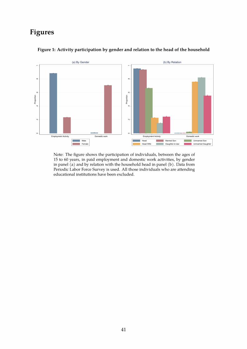
Figure 1 (a) shows the participation of men and women between the ages of 15 to 60

years in paid employment and domestic work. Figure 1 (a) highlights the well-known

fact about the Indian labormarket, that the labor force participation rate is significantly

higher for men than for women. Women on the other hand report far greater partici-

pation in domestic activities than men. These differences, however, are only restricted

to the gender of the individual.

Figure 1 (b) presents the same information as figure 1 (a) but by the rela-

tion of the family members to the head of the household. Comparing the participation

rates of women of the household in paid employment and domestic work, we observe

16

that differences are also visible across the relationship hierarchy within the household.

Figure 1 (b) shows that daughters-in-law report greater participation in domestic ac-

tivities, compared to other females like the head’s wife and the unmarried daughters.

These figures indicate that although there is a sexual division of labor within these

households, differences also exist within individuals of the same gender.

The PLFS is limited in the sense that it only provides reliable information on

participation in an activity but does not informus about how thesewomen allocate time

across different domestic activities and leisure. To investigate time allocation across

different activities, we utilize the TUS. Since we are interested in exploring women’s

time use in home-based activities, we broadly categorize them into three categories:

(1) domestic chores which includes preparing meals, washing clothes, home manage-

ment etc.; (2) child care; and (3) others’ care (which includes care provided to non-

dependent and the elderlymembers). We club these three and call it home production.

We will use home production as the main dependent variable in the analysis.

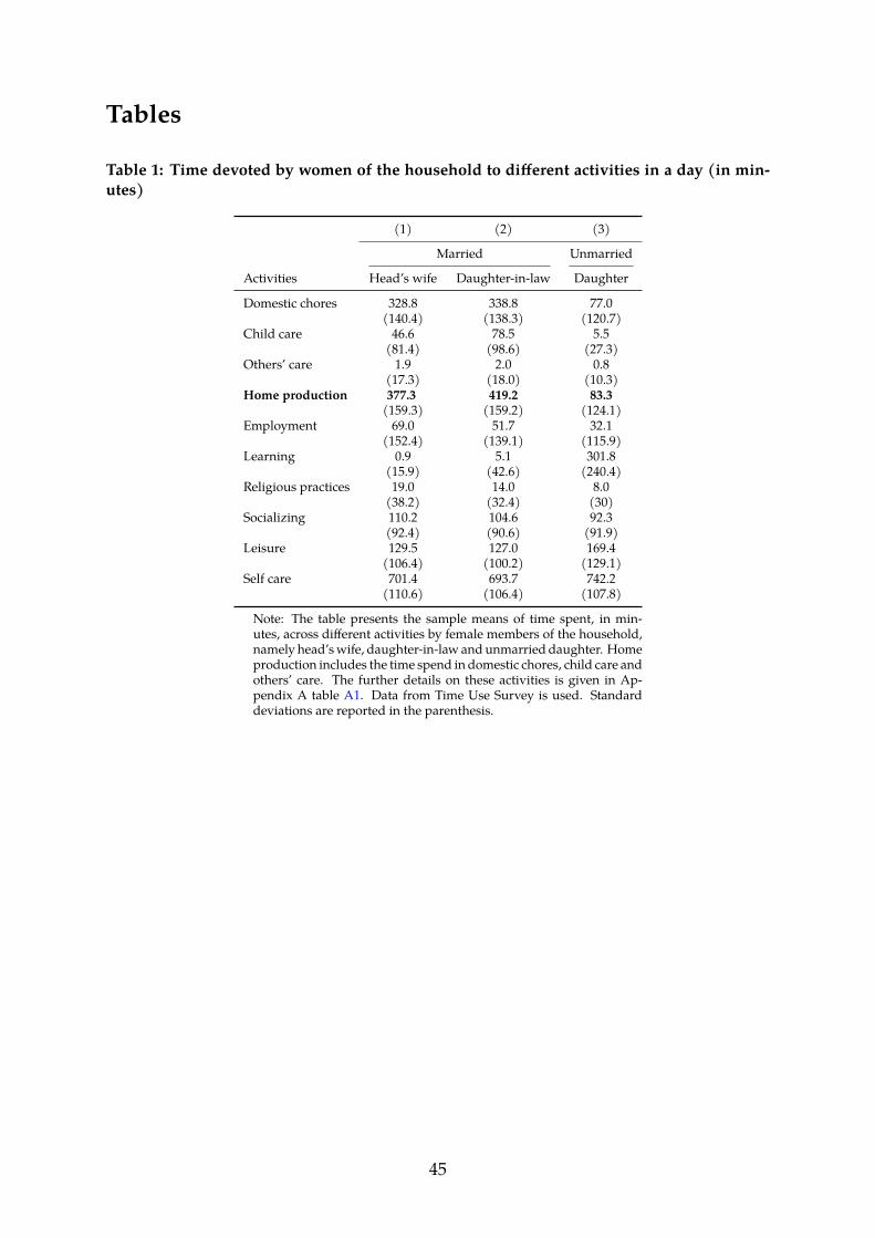
Table 1 presents the average time in minutes in a day that the women of the

household spend in homeproduction andother activities. On average,marriedwomen,

i.e., the head’swife and the daughters-in-law spend significantly higher time in domes-

tic chores and child care compared to unmarried daughters but spend far less time in

learning. Interestingly, married women spend more time in religious activities and

socializing and communicating.

The statistics in table 1 are interesting and indicative but we suspect that the

differences observed in the time use of married and unmarried women across differ-

ent activities would be driven partially by the differences in their age and education

17

level. Figure 2 gives some idea of the differences in the age distribution of these three

categories of women in our sample. Here we would like to point out that although we

have been talking about these women as head’s wife, daughter and daughter-in-law as

if thesewomen are in the same household, that is not the case. In the PLFS and the TUS,

we can categorize households broadly into four types: one, households where there is

no daughter-in-law; two, households where there is no daughter; three, households

where both daughter and daughter-in-law are present, and four, households where

there is neither a daughter nor a daughter-in-law present.

Figure 2 presents the age distribution of head’s wife, daughter and daughter-

in-law for the entire sample in panel (a) and the same for the subsample of households

where both the daughter and the daughter-in-law are present in panel (b). Note that

the average age gap between the daughter and the daughter-in-law for the entire sam-

ple in panel (a) is larger than their average age gap for the subsample in panel (b)

of the figure. This could be because households with a married son may on average

have older unmarried daughters than households where no son is married. The av-

erage age of the unmarried daughter is 15 years in the overall sample but is 19 years

in the subsample of households where both the daughter and the daughter-in-law are

present.

Figure 2 rationalizes our empirical strategy in the sense that married women

in our sample are either the head’s wife or the daughter-in-law but since the head’s

wife belongs to an older cohort, it does not make empirical sense to compare her with

the unmarried woman or the daughter of the household. This is because women’s

time in home production is less valuable at older ages, and more valuable at younger

18

ages, especially during child-rearing age which in turn will influence their decision of

participating in the labor market (Becker, 1981). Although the daughter-in-law is also,

on average, older than the daughter, the difference is just 7 years and there is significant

overlap in their age density (figure 2b).

4 Empirical Strategy

Ideally, to estimate the effect of a shift in the status of a woman due to marriage, we

should observe the time use of thewoman both before and aftermarriage. Such data, to

the best of our knowledge, is not available for India. What we have, however, are large

cross-sectional labor force participation and time use surveys of individuals spread

across the country. Our empirical strategy exploits the fact that all adult members of

the selected householdswere surveyed and hencewe look for the next best comparison

group for married women within the household.

To begin with, we first identify large joint family households in these surveys.

By large joint family, wemean households with older male heads and their wives, their

married and unmarried sons, and unmarried daughters and the wives of married sons

or the daughters-in-law. Since it’s common for married sons to live with their parents

in India, such households are available in the data. We use the rest of the households

in our data, where either there is no unmarried daughter or no daughter-in-law to test

the robustness of the main results of this paper.

Females within a household include the wife of the head, the head’s unmar-

ried daughter and the daughter-in-law. Both the head’s wife and the daughter-in-law

19

are married but the head’s wife belongs to a much senior cohort. We propose that a

reasonable comparison group for the married women or the daughters-in-law are the

unmarried daughters of the household.

Consider the following specification to estimate the differences in participa-

tion rates and time use in different activities of married and unmarried women in the

household

Yih = αh + δDILih +Xihβ + εih (1)

where Yih is either a dummy variable which equals 1 if the woman i in house-

hold h participates in a particular activity and 0 otherwise or is time use in a particular

activity. DILih is a dummy variable which is 1 if the woman is the daughter-in-law of

the household and 0 if she is the unmarried daughter. VectorXih has dummies for the

age and the education levels of these women. With household fixed effects denoted

by αh and dummies for age and education levels inXih, the coefficient δ gives us the

average difference in the time use of the daughter-in-law and the unmarried daughter

of comparable age and education levels, within the same household.

The difference in time use between the daughter-in-law and the unmarried

daughter can be heterogeneous based on their age and education levels. To estimate

this heterogeneity, we use the following specifications:

Yih = αh +J∑j=1

δjAGEjih ×DILih +Xihβ + εih (2)

20

Yih = αh +E∑e=1

δeEDU eih ×DILih +Xihβ + εih (3)

where AGEjih is a categorical variable for different age groups and EDU e

ih is

a categorical variable for different levels of education of the women. The estimated

coefficients δj and δe give the average difference in time use of the daughter-in-law

and the unmarried daughter for different age groups and different education levels

respectively.

Although all our comparisons are between women within the same house-

hold, it is still possible that they may be driven by households with more educated un-

married daughters being matched with less educated daughters-in-law. This may be

an outcome of arranged marriages within the patrilocal setup where the parents of the

prospective groom and the bride may decide the union based entirely on the observ-

able characteristics of each other’s family (Fafchamps and Quisumbing, 2008; Anukriti

and Dasgupta, 2017; Ray et al., 2020). Onemajor factor determiningmarital matches in

arranged marriages is the insurance gains from extending risk-sharing and consump-

tion smoothing links (Rosenzweig and Stark, 1989;Munshi and Rosenzweig, 2009). On

the girl’s side, the family may want to marry their daughter up in the wealth and sta-

tus ladder, hence they prefer a family with relatively higher wealth, status, caste and

educational affiliations (Fafchamps and Quisumbing, 2005; Huang et al., 2012; Baner-

jee et al., 2013; Anukriti and Dasgupta, 2017; Borker et al., 2017). The parents of the

prospective groommay prefer a daughter-in-law that does not contest their position of

power and control over household resources and hencemaymarry their sons towomen

who belong to households with lower socioeconomic status and educational qualifica-

21

tions (Mathur, 2007). This implies that there will be ‘positive assortative matching’ in

the marriage market and the observed differences in time use between the daughters

and the daughters-in-law could be driven by this matching process.

We test the robustness of our results to assortative matching in the marriage

market by explicitly matching the daughter-in-law from the set of households without

any unmarried daughter to the daughter from one of the households where there is

no daughter-in-law present. This matching is done on propensity scores based on the

observables of the two types of households. The idea is that if we match households

with unmarried daughters (no daughter-in-law) to households with daughters-in-law

(no unmarried daughter) on observables and then estimate the difference in time use

between these matchedwomen, we rule out the possibility of wealth and other observ-

ables based assortative matching driving our estimates.

5 Results

5.1 Baseline Results

We begin by discussing the results from the PLFS. Table 3 reports the estimated dif-

ferences in participation in paid employment, learning and domestic work activities of

unmarried daughters and daughters-in-law of the same household. The results show

that on average the daughters-in-law are 6.8 percentage points less likely to work in

paid employment activities which include own enterprise, salaried employment and

casual labor. This effect is stronger for urban and low caste (scheduled and scheduled

tribes) households. In addition, the daughters-in-law are 17.2 percentage points less

22

likely to be involved in educational activities and 37.4 percentage points more likely

to participate in domestic chores, with these magnitudes being somewhat higher for

urban households.

Table 3 reports the difference in time allocation in paid employment, unpaid

domestic work, caregiving, leisure and self-care activities of daughters and daughters-

in-law of the same household. These comparisons are within the households, as all

regressions include household fixed effects. Consistent with the results from the PLFS,

we find that the daughters-in-law allocate significantly less time in paid employment

and more time in domestic work and caregiving activities compared to the unmar-

ried daughters of the household. More specifically, the daughters-in-law on average

allocate 58 minutes per day less than the unmarried daughters in paid employment-

related activities, which amounts to around 7 hours per week. However, they spend

193 and 51 minutes per day more than daughters in domestic chores and caregiving

activities, which is equivalent to 70 hours per week. These results suggest that even in

the presence of daughters of comparable age group in the household, the responsibil-

ity of domestic chores and caregiving disproportionately falls on the daughters-in-law

of the household.

The advantage of using time-use data is that it provides additional informa-

tion on the time allocated to socializing, religious, leisure and self-care (including

sleep) activities. We find that daughters-in-law spend less time in socializing, leisure

and self-care activities than the daughters with the estimates varying between 11 and

47minutes per day. If we compare the differences in educational activities; we find that

daughters spend 89 minutes per day more than daughters-in-law in learning. This is

23

consistent with the fact that in Indian households, women generally stop educational

activities after their marriage. Another interesting observation is that married women

spend more time in religious practices. This, we believe, is a clear indication that these

differences are driven by the differences in the status of these women in the household.

Married women in India are supposed to perform various religious customs and prac-

tices. Strict adherence to these rituals by the married women reflects their devotion

to their husbands and the household, and contributes to the production of status for

the household (Srinivas, 1977; Papanek, 1979). That the daughters-in-law are devot-

ing more time to religious activities also indicates that not all women may bear equal

responsibility of producing status goods for the household and that this responsibility

may invariably fall on the daughter-in-law.

In table 4, we present the estimates of equation (1) for rural, low caste and

poor households and find that in all these subsamples the daughter-in-law devotes

significantly higher time to home production activities. These differences are some-

what smaller in rural areas and for poor households (poor households are defined as

the lowest 20% of the households in the per capita consumption expenditure distri-

bution), suggesting that the effect of hierarchy is less noticeable in rural areas and in

poorer households.

5.2 Heterogeneity by Age and Education

To rule out the possibility that the differences in time use between these womenmay be

driven by the age gap between them, we trim the sample based on the age distribution

and re-estimate equation (1). If these differences in time use between these women are

24

driven by the age gap between them, then these differences should reduce as we nar-

row the age band of the women in our sample. In columns 5 and 6 of table 4, we restrict

the sample to women aged 20 to 45 years and 25 to 40 years respectively and find that

the differences in time use in home production of the daughters and the daughters-in-

law show an increase rather than a decline. Similarly, to rule out the possibility that

these differences may be driven by systematic differences in the education levels of the

daughters and the daughters-in-law, we restrict the sample to women with at least a

higher secondary level of schooling (table 4 column 7). Here again, we find the differ-

ence in time use in homeproduction increaseswith the daughter-in-law spendingmore

than double the amount of time in home production than the unmarried daughter.

Age and education are two important determinants of returns in the labor

market and the type of activity an individual specializes in. Although we get some in-

dication that our results are robust to the age and education gap between thesewomen,

we explore this further in figure 3 and figure 4. Figure 3 plots the predicted marginal

effects from equation (2) for different time use activities for the daughters and the

daughters-in-law by different age groups. For domestic work, we find a consistent gap

in the time use of thesewomen across all age groups. Across all age groups, daughters-

in-law spend more time in domestic work than the daughters of the household.

One concern may be that daughters devote more time to learning and less

time in domestic work because of higher returns to education in the marriage mar-

ket (Behrman et al., 1999; Chiappori et al., 2009; Lafortune, 2013; Klasen and Pieters,

2015; Attanasio and Kaufmann, 2017). If this is true in our case, then the differences

we observe in figure 3 (a) are driven by the households’ expectation of better out-

25

comes for unmarried girls in the marriage market rather than the difference in status

and relational hierarchy between the unmarried daughters and the daughters-in-law.

This argument however is not consistent with what we observe in figure 3. Unmarried

daughters in higher age groups, closer to marriageable age, devote less time to learn-

ing and more time to self-care and leisure. A similar decrease in learning and increase

in leisure is observed for the daughters-in-law of higher age groups but this change is

far less prominent in comparison to the daughters of the household. The difference is

stark for self-care activity, where the daughters-in-law of all age groups devote almost

the same time to self-care but for daughters, it increases with age. This pattern is rather

consistent with the story that as unmarried daughters come closer to the marriageable

age, they are given greater independence and more free time.

Figure 4 shows the predicted time use allocation for daughters and daughters-

in-law across different education categories. There is evidence that education raises the

relative returns to home production, especially in the case of child care (Behrman et al.,

1999; LamandDuryea, 1999;Gobbi, 2018), and therefore the increase in the educational

levels of married women in India has contributed to their withdrawal from the labor

market (Afridi et al., 2018). Figure 4 (a) and (b) show that the time use in domestic

work and child care does not vary much with the education level of the daughters-in-

law in our sample of households. In fact, for all the activities that we consider in fig-

ure 4, the daughter-in-law’s time use doesn’t change much with her level of education.

In contrast, highly educated daughters devote less time to domestic work, socializing

and leisure and spend significantly more time in learning.

26

5.3 Matching on Observables

Table 5 presents some evidence of positive assortativematching on educational qualifi-

cation. Table 5 column (1) shows that the daughters-in-law are 11 percentage point less

likely to have higher secondary education or above than their husbands. This indicates

that women with lower educational qualifications are matched with men of higher ed-

ucational qualifications in our sample of households. Moreover, table 5 column (2)

shows that the daughters-in-law are 8 percentage point less likely to be educated till

the higher secondary level or above than the unmarried daughters of the household.

We match the daughter-in-law from the set of households without an unmar-

ried daughter to a daughter from the households without a daughter-in-law, using

propensity score matching. The propensity scores are predicted from a host of observ-

able individual- and household-level characteristics like woman’s age, her education,

caste, religion, place of residence, the household’s income quintiles based on consump-

tion expenditure, the structure of the dwelling unit, the primary source of energy for

cooking, household head’s education and the number of dependents in the household

(see Appendix table A2). Evidence on common support and balancing is presented in

the Appendix (refer figures A1 and A2).

Table 6 presents the ATT estimates from nearest neighbor matching with 1, 3

and 5 neighbors. The results are qualitatively similar to our earlier findings. For in-

stance, we find that the daughter-in-law invests 238 minutes per day more in home

production activities compared to the matched unmarried daughter (row 3 of table 6).

However, the daughter-in-law allocates less time to paid employment, learning, so-

cializing and self-care activities. Matching based estimates of differences in time use

27

between these women by age groups are presented in Appendix table A3.

5.4 Influence of Unobservables

In the previous section, we show that our results are robust to selection in the marriage

market as long as this selection is driven by observable characteristics of the individuals

and the households. But that still leaves the possibility that unobservables may be

driving this selection.

If we are willing to make the assumption that the selection on observables is

informative about the selection on unobservables, then the influence of unobservables

can simply be gauged by comparing estimates of coefficients with and without con-

trols (Altonji et al., 2005). Oster (2019) develops this idea further by linking coefficient

movements, R2 movements and the omitted variable bias. Oster (2019) proposes a

procedure to bound the true estimate using uncontrolled and controlled estimate of

the treatment effect, the R2 and the proportional selection assumption. We use this

procedure to test the sensitivity of our estimates to unobservables. To generate the es-

timates of δ net of the bias, we assume that the maximum R2 value of the regression is

0.9 and that the coefficient of proportionality between the bias due to observables and

the unobservables is 1.

Table 7 presents the estimates of the difference in time use for the daughters-

in-law and unmarried daughters from the uncontrolled and controlled regressions in

columns (1) and (2). The last column presents the estimates of δ net of the bias compo-

nent. It can be seen that all the estimates of δ in table 7 are still quite large in magnitude

and economically relevant. In some cases, accounting for the bias actually increases the

28

magnitude, however we don’t take that as an indication of the direction of the bias. The

key insight from this section is that the influence of omitted variables in probably not

enough to change the narrative of this paper.

5.5 Additional Robustness Tests

We exploit the fact that households in our data havemultiple unmarried daughters and

daughters-in-law within a household, to test whether differences in time use also exist

between members for the same relation. If our results are truly driven by differences

in hierarchy and status of the unmarried daughters and daughters-in-law then, condi-

tional on age and education levels, we should not observe differences in time usewithin

unmarried daughters. Table 8 presents the results of the placebo test where the depen-

dent variables are the time use (in minutes) in different activities which we regress

on indicators for the middle daughter, the youngest daughter, the youngest daughter-

in-law and the eldest daughter-in-law. The omitted category is the eldest unmarried

daughter of the household.

In activities like paid employment, childcare, learning and leisure; the differ-

ences between the eldest daughter and the younger daughters are statistically insignif-

icant implying that the time use by elder and younger daughters in these activities is

comparable. For domestic work, although the differences among the eldest daughter

and the younger daughters are positive and statistically significant, the magnitudes

are more than four times less than the difference between the eldest daughter and the

youngest daughter-in-law. For self-care activity, we observe that the younger daughters

on average spend 20 to 30 minutes less than their eldest unmarried sister (or daugh-

29

ter); but this is still lower in comparison to the daughters-in-law who spend around 80

minutes less than the eldest unmarried daughter.

Panel (a) and (b) of table 9 present the result of equation (1) estimated sepa-

rately on the subsample of households with andwithout any children respectively. For

households with no children, the time devoted to childcare will be zero therefore the

table omits the child care category. These estimates are comparable to the estimates

from table 3. We find that even in households without any children the daughter-in-

law spends significantly more time in domestic chores and religious practices and less

time in employment, learning, leisure and self-care.

6 Conclusion

In Indian joint families, power relations and status vary among the family members

and play an important role in the division of labor within the household. In this paper,

we show that for a woman, just the act of getting married and joining her husband’s

household has implications for her participation and time allocation in paid andunpaid

work. We exploit the fact that our data reports the relation of eachmemberwith respect

to the head of the household and devise a strategy which compares the participation

and time use in different activities for unmarried daughters and daughters-in-law, of

comparable age and education levels.

We find that, compared to daughters, daughters-in-law aremore likely to par-

ticipate in non-paid home production activities and less likely to engage in paid em-

ployment. We believe that this result is due to the shift in kinship role of a woman after

30

marriage. We use the time use data to further investigate the kind of unpaid activities

the daughters-in-law are engaged in at home. We find that the daughters-in-law al-

locate more time in domestic chores and care giving activities. However, they spend

less time in leisure and self-care activities compared to unmarried daughters. In addi-

tion, we find that they spend more time in religious activities. These results survive a

variety of robustness tests.

The following observations from the literature support these findings. First,

the daughter-in-law’s position in the household is more of an outsider. She may be a

subordinate to the senior women in the household and her household work is more

likely to be seen as ’a source of private welfare and comfort’ by other household mem-

bers (Papanek, 1979). Many studies like Anderson and Baland (2002), Kantor (2003)

and Anderson and Eswaran (2009) find that working outside in paid employment ac-

tivities increases married women’s autonomy within the family. Moreover, they find

that women who are involved in household chores are submissive and have no auton-

omy since household work is deemed as less worthy.

Second, the family’s status concerns may also be at play here. The withdrawal

of a married woman from market work may be a marker of status for their spouse

and family (Kandiyoti, 1988). Daughter-in-law’s involvement in domestic chores and

religious activities is taken as a reflection of their devotion towards their family and

therefore, it increases the family’s status in their social circles. Status concerns together

with subordination may force the married woman to invest more time in unpaid home

production activities.

Our analysis highlights the importance of kinship roles in determining the

31

labor market decisions for married women. In light of these findings, it is important

to emphasize that the influence of kinship roles on women’s work cannot be ignored

while devising policies that aim to empower women and increase female labor force

participation.

32

References

Abadie, A. and Imbens, G. (2006). Large sample properties of matching estimators for

average treatment effects. Econometrica, 74(1):235–267.

Abraham, V. (2013). Missing labour or consistent "De-feminisation"? Economic and

Political Weekly, 48(31):99–108.

Afridi, F., Dinkelman, T., and Mahajan, K. (2018). Why are fewer married women

joining the work force in India? A decomposition analysis over two decades. Journal

of Population Economics, 31(3):783–818.

Altonji, J. G., Elder, T. E., and Taber, C. R. (2005). Selection on observed andunobserved

variables: Assessing the effectiveness of catholic schools. Journal of Political Economy,

113(1):151–184.

Anderson, S. and Baland, J.-M. (2002). The economics of roscas and intrahousehold

resource allocation. The Quarterly Journal of Economics, 117(3):963–995.

Anderson, S. and Eswaran, M. (2009). What determines female autonomy? Evidence

from Bangladesh. Journal of Development Economics, 90(2):179–191.

Andrés, L., Dasgupta, B., Joseph, G., Abraham, V., and Correia, M. C. (2017). Precari-

ous drop: Reassessing patterns of female labor force participation in India. Develop-

ment Economics: Women.

Anukriti, S. and Dasgupta, S. (2017). Marriage markets in developing countries. The

Oxford Handbook of Women and the Economy, pages 97–120.

Anukriti, S., Herrera-Almanza, C., Karra, M., and Pathak, P. K. (2020). Curse of the

33

Mummy-ji: The influence of mothers-in-law on women in India. American Journal of

Agricultural Economics, 102(4):1328–1351.

Attanasio, O. P. and Kaufmann, K. M. (2017). Education choices and returns on the

labor and marriage markets: Evidence from data on subjective expectations. Journal

of Economic Behavior & Organization, 140:35–55.

Banerjee, A., Duflo, E., Ghatak,M., and Lafortune, J. (2013). Marry forwhat? Caste and

mate selection in modern India. American Economic Journal: Microeconomics, 5(2):33–

72.

Bardhan, K. (1985). Women’s work, welfare and status: Forces of tradition and change

in India. Economic and Political Weekly, pages 2207–2220.

Becker, G. S. (1981). A Treatise on the Family. Harvard University Press, Cambridge,

MA.

Behrman, J. R., Foster, A. D., Rosenweig, M. R., and Vashishtha, P. (1999). Women’s

schooling, home teaching, and economic growth. Journal of Political Economy,

107(4):682–714.

Bennett, L. (1983). Dangerous Wives and Sacred Sisters: Social and Symbolic Roles of High-

Caste Women in Nepal. Columbia University Press, New York.

Bernhardt, A., Field, E., Pande, R., Rigol, N., Schaner, S., and Troyer-Moore, C. (2018).

Male social status and women’s work. In AEA Papers and Proceedings, volume 108,

pages 363–67.

Bloch, F. and Rao, V. (2002). Terror as a bargaining instrument: A case study of dowry

violence in rural India. American Economic Review, 92(4):1029–1043.

34

Borker, G., Eeckhout, J., Luke, N., Minz, S., Munshi, K., and Swaminathan, S. (2017).

Wealth, marriage, and sex selection. Cambridge University.

Çağatay, N. and Özler, Ş. (1995). Feminization of the labor force: The effects of long-

term development and structural adjustment. World Development, 23(11):1883–1894.

Cain, M., Khanam, S. R., and Nahar, S. (1979). Class, patriarchy, and women’s work in

Bangladesh. Population and Development Review, 5(3):405–438.

Castle, S. E. (1993). Intra-household differentials in women’s status: Household func-

tion and focus as determinants of children’s illness management and care in rural

Mali. Health Transition Review, 3(2):137–157.

Chakraborty, T. and Kim, S. (2010). Kinship institutions and sex ratios in India. De-

mography, 47(4):989–1012.

Chatterjee, U., Murgai, R., and Rama, M. (2015). Job opportunities along the rural-

urban gradation and female labor force participation in India. Policy Research work-

ing paper No. WPS 7412, The World Bank Group.

Chiappori, P. A., Iyigun, M., and Weiss, Y. (2009). Investment in schooling and the

marriage market. American Economic Review, 99(5):1689–1713.

Chowdhury, S. (2011). Employment in India: What does the latest data show? Eco-

nomic and Political Weekly, 46(32):23–26.

Debnath, S. (2015). The impact of household structure on female autonomy in devel-

oping countries. The Journal of Development Studies, 51(5):485–502.

Deshpande, A., Goel, D., and Khanna, S. (2018). Bad karma or discrimination? Male–

female wage gaps among salaried workers in India. World Development, 102:331–344.

35

Dhanaraj, S. and Mahambare, V. (2019). Family structure, education and women’s

employment in rural India. World Development, 115:17–29.

Dyson, T. and Moore, M. (1983). On kinship structure, female autonomy, and demo-

graphic behavior in India. Population and Development Review, pages 35–60.

Eswaran, M., Ramaswami, B., andWadhwa, W. (2013). Status, caste, and the time allo-

cation ofwomen in rural India. Economic Development and Cultural Change, 61(2):311–

333.

Fafchamps, M. and Quisumbing, A. R. (2003). Social roles, human capital, and the

intrahousehold division of labor: Evidence from Pakistan. Oxford Economic Papers,

55(1):36–80.

Fafchamps, M. and Quisumbing, A. R. (2005). Marriage, bequest, and assortative

matching in rural Ethiopia. Economic Development and Cultural Change, 53(2):347–

380.

Fafchamps, M. and Quisumbing, A. R. (2008). Household formation and marriage

markets in rural areas. Handbook of Development Economics, 4:3187–3247.

Fletcher, E., Pande, R., andMoore, C. M. T. (2017). Women andwork in India: Descrip-

tive evidence and a review of potential policies. HKSWorking PaperNo. RWP18-004.

Gobbi, P. E. (2018). Childcare and commitment within households. Journal of Economic

Theory, 176:503–551.

Goldin, C. (1995). The U-shaped female labor force function in economic development

and economic history. In Schultz, T., editor, Investment in Women’s Human Capital and

Economic Development. University of Chicago Press, Chicago.

36

Hendrix, L. and Hossain, Z. (1988). Women’s status andmode of production: A cross-

cultural test. Signs: Journal of Women in Culture and Society, 13(3):437–453.

Himanshu (2011). Employment trends in India: A re-examination. Economic and Polit-

ical Weekly, 46(37):43–59.

Huang, F., Jin, G. Z., and Xu, L. C. (2012). Love and money by parental matchmaking:

Evidence from urban couples in China. American Economic Review, 102(3):555–60.

Jayachandran, S. (2015). The roots of gender inequality in developing countries.Annual

Review of Economics, 7(1):63–88.

Jayachandran, S. (2020). Social norms as a barrier to women’s employment in devel-

oping countries. Working Paper No. 27449, National Bureau of Economic Research.

Kambhampati, U. S. (2009). Child schooling and work decisions in India: The role of

household and regional gender equity. Feminist Economics, 15(4):77–112.

Kandiyoti, D. (1988). Bargaining with patriarchy. Gender & society, 2(3):274–290.

Kannan, K. and Raveendran, G. (2012). Counting and profiling the missing labour

force. Economic and Political Weekly, 47(6):77–80.

Kantor, P. (2003). Women’s empowerment through home–based work: Evidence from

India. Development and Change, 34(3):425–445.

Kapsos, S., Bourmpoula, E., and Silberman, A. (2014). Why is female labour force

participation declining so sharply in India? ILO Working Papers 994949190702676,

International Labour Organization.

37

Khalil, U. and Mookerjee, S. (2019). Patrilocal residence and women’s social status:

Evidence from South Asia. Economic Development and Cultural Change, 67(2):401–

438.

Kishor, S. (1993). May god give sons to all: Gender and child mortality in India. Amer-

ican Sociological Review, pages 247–265.

Klasen, S. and Pieters, J. (2015). What explains the stagnation of female labor force

participation in urban India? World Bank Economic Review, 29(3):449–478.

Krishnan, P. (2001). Cultural norms, social interactions and the fertility transition in

India. University of Cambridge, Faculty of Economics, Cambridge, UK Processed.

Lafortune, J. (2013). Making yourself attractive: Pre-marital investments and the re-

turns to education in the marriage market. American Economic Journal: Applied Eco-

nomics, 5(2):151–78.

Lam, D. andDuryea, S. (1999). Effects of schooling on fertility, labor supply, and invest-

ments in children: Evidence from Brazil. The Journal of Human Resources, 34(1):160–

192.

Landmann, A., Seitz, H., and Steiner, S. (2017). Patrilocal residence and female labour

supply (no. 10890). Institute for the Study of Labor (IZA).

Malhotra, A., Vanneman, R., and Kishor, S. (1995). Fertility, dimensions of patriarchy,

and development in India. Population and Development Review, 21(2):281–305.

Mathur, D. (2007). What’s love got to do with it? Parental involvement and spouse

choice in urban India.

38

Mehrotra, S. and Parida, J. K. (2017). Why is the labour force participation of women

declining in India? World Development, 98:360–380.

Munshi, K. and Rosenzweig, M. (2009). Why is mobility in India so low? Social in-

surance, inequality, and growth. Working Paper No. w14850, National Bureau of

Economic Research.

Neff, D. F., Sen, K., and Kling, V. (2012). The puzzling decline in rural women’s labor

force participation in India: A reexamination. GIGA working paper no. 196.

Oster, E. (2019). Unobservable selection and coefficient stability: Theory and evidence.

Journal of Business & Economic Statistics, 37(2):187–204.

Pampel, F. C. and Tanaka, K. (1986). Economic development and female labor force

participation: A reconsideration. Social Forces, 64(3):599–619.

Papanek, H. (1979). Family status production: The" work" and" non-work" of women.

Signs: Journal of Women in Culture and Society, 4(4):775–781.

Rammohan, A. and Robertson, P. E. (2012). Human capital, kinship, and gender in-

equality. Oxford Economic Papers, 64(3):417–438.

Rammohan, A. and Vu, P. (2018). Gender inequality in education and kinship norms

in India. Feminist Economics, 24(1):142–167.

Rangarajan, C., Kaul, P. I., and Seema (2011). Where is the missing labour force? Eco-

nomic and Political Weekly, 46(39):68–72.

Rao, N. (2014). Caste, kinship, and life course: Rethinking women’s work and agency

in rural South India. Feminist Economics, 20(3):78–102.

39

Ray, T., Chaudhuri, A. R., and Sahai, K. (2020). Whose education matters? An analysis

of inter caste marriages in India. Journal of Economic Behavior &Organization, 176:619–

633.

Rosenzweig, M. R. and Stark, O. (1989). Consumption smoothing, migration, andmar-

riage: Evidence from rural India. Journal of Political Economy, 97(4):905–926.

Sacks, K. and Brodkin, K. (1979). Sisters and wives: The past and future of sexual equality.

Number 10. University of Illinois Press, Chicago.

Sorsa, P., Mares, J., Didier, M., Guimaraes, C., Rabate, M., Tang, G., and Tuske, A.

(2015). Determinants of the low female labour force participation in India. OECD

Economics Department Working Papers, No. 1207, OECD Publishing, Paris.

Srinivas, M. N. (1977). The changing position of Indian women. Man, 12(2):221–238.

Sudarshan, R.M. andBhattacharya, S. (2009). Through themagnifying glass: Women’s

work and labour force participation in urban Delhi. Economic and Political Weekly,

44(48):59–66.

Sundaram, A. and Vanneman, R. (2008). Gender differentials in literacy in India: The

intriguing relationship with women’s labor force participation. World Development,

36(1):128–143.

Tam, H. (2011). U-shaped female labor participation with economic development:

Some panel data evidence. Economics Letters, 110(2):140–142.

WorldBank, W. (2018). World development report 2019: The changing nature of work.

40

Figures

Figure 1: Activity participation by gender and relation to the head of the household

0.2

.4.6

.81

Pro

porti

on

Employment Activity Domestic work

Male

Female

(a) By Gender

0.2

.4.6

.81

Pro

porti

on

Employment Activity Domestic work

Head Married Son Unmarried Son

Head Wife Daughter-in-law Unmarried Daughter

(b) By Relation

Note: The figure shows the participation of individuals, between the ages of15 to 60 years, in paid employment and domestic work activities, by genderin panel (a) and by relation with the household head in panel (b). Data fromPeriodic Labor Force Survey is used. All those individuals who are attendingeducational institutions have been excluded.

41

Figure 2: Age density of the women of the household0

.02

.04

.06

.08

Den

sity

0 20 40 60 80Age

Head's WifeUnmarried DaughterDaughter in Law

(a) All households

0.0

2.0

4.0

6.0

8D

ensi

ty0 20 40 60 80

Age

Head's WifeUnmarried DaughterDaughter in Law

(b) Households with both daughter and daughter-in-law

Note: The figure shows the kernel density plots for age for the femalemembersbelonging to (a) all the households in the sample; and (b) households withboth daughter and daughter-in-law. Data from Time Use Survey is used. Theaverage ages of household head’s wife (or mother-in-law), unmarried daugh-ter and daughter-in-law in panel (a) are 41, 15 and 29 and in panel (b) are 51,19 and 26 years.

42

Figure 3: Time allocation by the daughter and the daughter-in-law by age groups-1

000

100

200

300

400

15-20 20-30 30-40 40-50 50-60

Unmarried daughterDaughter in law

(a) Domestic work

-50

050

100

15-20 20-30 30-40 40-50 50-60


(b) Child care

-50

050

100

150

15-20 20-30 30-40 40-50 50-60


(c) Others' care

-200

-100

010

020

0

15-20 20-30 30-40 40-50 50-60


(d) Learning

1020

3040

5060

15-20 20-30 30-40 40-50 50-60


(e) Religious practices

5010

015

020

0

15-20 20-30 30-40 40-50 50-60


(f) Socializing

100

150

200

250

300

15-20 20-30 30-40 40-50 50-60


(g) Leisure

650

700

750

800

850

15-20 20-30 30-40 40-50 50-60


(h) Self care

Note: The figure shows the time spent, in minutes in a day, in different activ-ities by the daughter and the daughter-in-law on the vertical axis and the agegroups on the horizontal axis. Predicted from equation (2) with householdfixed effects and education level dummies. The figure also show 95% confi-dence intervals estimated with standard errors clustered at the district level.Data from Time Use Survey is used.

43

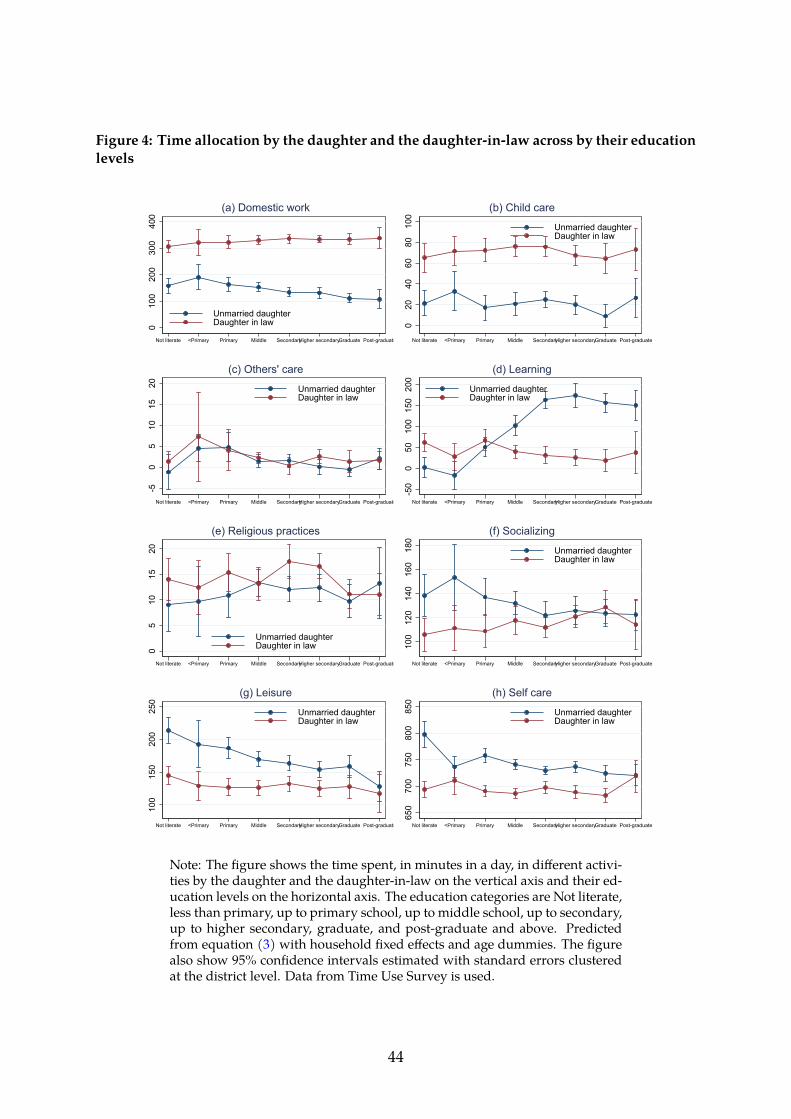
Figure 4: Time allocation by the daughter and the daughter-in-law across by their educationlevels

010

020

030

040

0

Not literate <Primary Primary Middle SecondaryHigher secondaryGraduate Post-graduate


(a) Domestic work

020

4060

8010

0



(b) Child care

-50

510

1520



(c) Others' care

-50

050

100

150

200



(d) Learning

05

1015

20



(e) Religious practices

100

120

140

160

180



(f) Socializing

100

150

200

250



(g) Leisure

650

700

750

800

850



(h) Self care

Note: The figure shows the time spent, in minutes in a day, in different activi-ties by the daughter and the daughter-in-law on the vertical axis and their ed-ucation levels on the horizontal axis. The education categories are Not literate,less than primary, up to primary school, up to middle school, up to secondary,up to higher secondary, graduate, and post-graduate and above. Predictedfrom equation (3) with household fixed effects and age dummies. The figurealso show 95% confidence intervals estimated with standard errors clusteredat the district level. Data from Time Use Survey is used.

44

Tables

Table 1: Time devoted by women of the household to different activities in a day (in min-utes)

(1) (2) (3)Married Unmarried

Activities Head’s wife Daughter-in-law DaughterDomestic chores 328.8 338.8 77.0

(140.4) (138.3) (120.7)Child care 46.6 78.5 5.5

(81.4) (98.6) (27.3)Others’ care 1.9 2.0 0.8

(17.3) (18.0) (10.3)Home production 377.3 419.2 83.3

(159.3) (159.2) (124.1)Employment 69.0 51.7 32.1

(152.4) (139.1) (115.9)Learning 0.9 5.1 301.8

(15.9) (42.6) (240.4)Religious practices 19.0 14.0 8.0

(38.2) (32.4) (30)Socializing 110.2 104.6 92.3

(92.4) (90.6) (91.9)Leisure 129.5 127.0 169.4

(106.4) (100.2) (129.1)Self care 701.4 693.7 742.2

(110.6) (106.4) (107.8)Note: The table presents the sample means of time spent, in min-utes, across different activities by female members of the household,namely head’swife, daughter-in-law andunmarried daughter. Homeproduction includes the time spend in domestic chores, child care andothers’ care. The further details on these activities is given in Ap-pendix A table A1. Data from Time Use Survey is used. Standarddeviations are reported in the parenthesis.

45

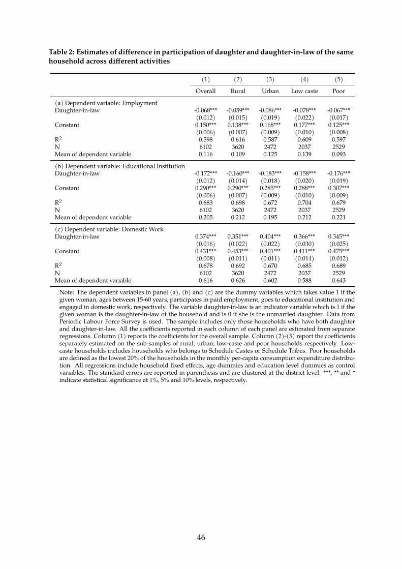
Table 2: Estimates of difference in participation of daughter anddaughter-in-lawof the samehousehold across different activities

(1) (2) (3) (4) (5)Overall Rural Urban Low caste Poor

(a) Dependent variable: EmploymentDaughter-in-law -0.068*** -0.059*** -0.086*** -0.078*** -0.067***

(0.012) (0.015) (0.019) (0.022) (0.017)Constant 0.150*** 0.138*** 0.168*** 0.177*** 0.125***

(0.006) (0.007) (0.009) (0.010) (0.008)R2 0.598 0.616 0.587 0.609 0.597N 6102 3620 2472 2037 2529Mean of dependent variable 0.116 0.109 0.125 0.139 0.093(b) Dependent variable: Educational InstitutionDaughter-in-law -0.172*** -0.160*** -0.183*** -0.158*** -0.176***

(0.012) (0.014) (0.018) (0.020) (0.019)Constant 0.290*** 0.290*** 0.285*** 0.288*** 0.307***

(0.006) (0.007) (0.009) (0.010) (0.009)R2 0.683 0.698 0.672 0.704 0.679N 6102 3620 2472 2037 2529Mean of dependent variable 0.205 0.212 0.195 0.212 0.221(c) Dependent variable: Domestic WorkDaughter-in-law 0.374*** 0.351*** 0.404*** 0.366*** 0.345***

(0.016) (0.022) (0.022) (0.030) (0.025)Constant 0.431*** 0.453*** 0.401*** 0.411*** 0.475***

(0.008) (0.011) (0.011) (0.014) (0.012)R2 0.678 0.692 0.670 0.685 0.689N 6102 3620 2472 2037 2529Mean of dependent variable 0.616 0.626 0.602 0.588 0.643Note: The dependent variables in panel (a), (b) and (c) are the dummy variables which takes value 1 if thegiven woman, ages between 15-60 years, participates in paid employment, goes to educational institution andengaged in domestic work, respectively. The variable daughter-in-law is an indicator variable which is 1 if thegiven woman is the daughter-in-law of the household and is 0 if she is the unmarried daughter. Data fromPeriodic Labour Force Survey is used. The sample includes only those households who have both daughterand daughter-in-law. All the coefficients reported in each column of each panel are estimated from separateregressions. Column (1) reports the coefficients for the overall sample. Column (2)-(5) report the coefficientsseparately estimated on the sub-samples of rural, urban, low-caste and poor households respectively. Low-caste households includes households who belongs to Schedule Castes or Schedule Tribes. Poor householdsare defined as the lowest 20% of the households in the monthly per-capita consumption expenditure distribu-tion. All regressions include household fixed effects, age dummies and education level dummies as controlvariables. The standard errors are reported in parenthesis and are clustered at the district level. ***, ** and *indicate statistical significance at 1%, 5% and 10% levels, respectively.

46

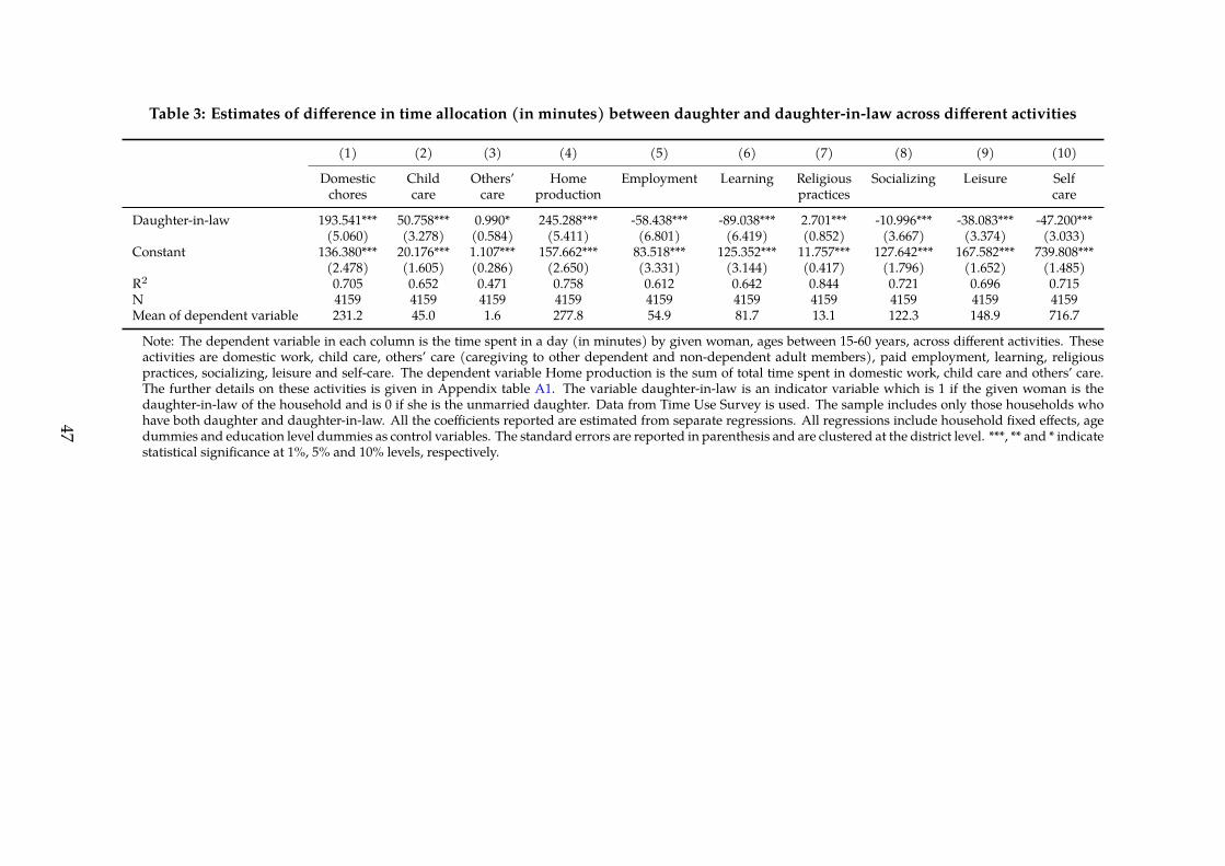
Table 3: Estimates of difference in time allocation (in minutes) between daughter and daughter-in-law across different activities

(1) (2) (3) (4) (5) (6) (7) (8) (9) (10)Domestic Child Others’ Home Employment Learning Religious Socializing Leisure Selfchores care care production practices care

Daughter-in-law 193.541*** 50.758*** 0.990* 245.288*** -58.438*** -89.038*** 2.701*** -10.996*** -38.083*** -47.200***(5.060) (3.278) (0.584) (5.411) (6.801) (6.419) (0.852) (3.667) (3.374) (3.033)

Constant 136.380*** 20.176*** 1.107*** 157.662*** 83.518*** 125.352*** 11.757*** 127.642*** 167.582*** 739.808***(2.478) (1.605) (0.286) (2.650) (3.331) (3.144) (0.417) (1.796) (1.652) (1.485)

R2 0.705 0.652 0.471 0.758 0.612 0.642 0.844 0.721 0.696 0.715N 4159 4159 4159 4159 4159 4159 4159 4159 4159 4159Mean of dependent variable 231.2 45.0 1.6 277.8 54.9 81.7 13.1 122.3 148.9 716.7Note: The dependent variable in each column is the time spent in a day (in minutes) by given woman, ages between 15-60 years, across different activities. Theseactivities are domestic work, child care, others’ care (caregiving to other dependent and non-dependent adult members), paid employment, learning, religiouspractices, socializing, leisure and self-care. The dependent variable Home production is the sum of total time spent in domestic work, child care and others’ care.The further details on these activities is given in Appendix table A1. The variable daughter-in-law is an indicator variable which is 1 if the given woman is thedaughter-in-law of the household and is 0 if she is the unmarried daughter. Data from Time Use Survey is used. The sample includes only those households whohave both daughter and daughter-in-law. All the coefficients reported are estimated from separate regressions. All regressions include household fixed effects, agedummies and education level dummies as control variables. The standard errors are reported in parenthesis and are clustered at the district level. ***, ** and * indicatestatistical significance at 1%, 5% and 10% levels, respectively.

47

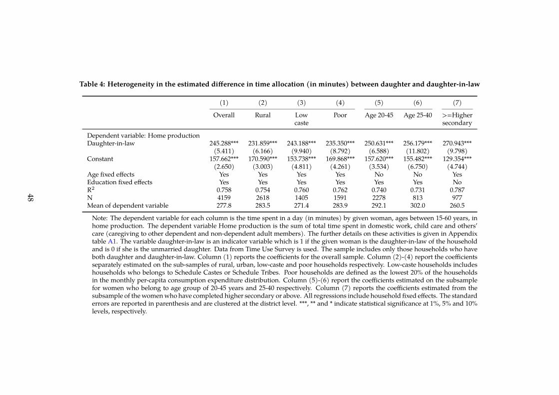
Table 4: Heterogeneity in the estimated difference in time allocation (in minutes) between daughter and daughter-in-law

(1) (2) (3) (4) (5) (6) (7)Overall Rural Low Poor Age 20-45 Age 25-40 >=Higher

caste secondaryDependent variable: Home productionDaughter-in-law 245.288*** 231.859*** 243.188*** 235.350*** 250.631*** 256.179*** 270.943***

(5.411) (6.166) (9.940) (8.792) (6.588) (11.802) (9.798)Constant 157.662*** 170.590*** 153.738*** 169.868*** 157.620*** 155.482*** 129.354***

(2.650) (3.003) (4.811) (4.261) (3.534) (6.750) (4.744)Age fixed effects Yes Yes Yes Yes No No YesEducation fixed effects Yes Yes Yes Yes Yes Yes NoR2 0.758 0.754 0.760 0.762 0.740 0.731 0.787N 4159 2618 1405 1591 2278 813 977Mean of dependent variable 277.8 283.5 271.4 283.9 292.1 302.0 260.5Note: The dependent variable for each column is the time spent in a day (in minutes) by given woman, ages between 15-60 years, inhome production. The dependent variable Home production is the sum of total time spent in domestic work, child care and others’care (caregiving to other dependent and non-dependent adult members). The further details on these activities is given in Appendixtable A1. The variable daughter-in-law is an indicator variable which is 1 if the given woman is the daughter-in-law of the householdand is 0 if she is the unmarried daughter. Data from Time Use Survey is used. The sample includes only those households who haveboth daughter and daughter-in-law. Column (1) reports the coefficients for the overall sample. Column (2)-(4) report the coefficientsseparately estimated on the sub-samples of rural, urban, low-caste and poor households respectively. Low-caste households includeshouseholds who belongs to Schedule Castes or Schedule Tribes. Poor households are defined as the lowest 20% of the householdsin the monthly per-capita consumption expenditure distribution. Column (5)-(6) report the coefficients estimated on the subsamplefor women who belong to age group of 20-45 years and 25-40 respectively. Column (7) reports the coefficients estimated from thesubsample of thewomenwho have completed higher secondary or above. All regressions include household fixed effects. The standarderrors are reported in parenthesis and are clustered at the district level. ***, ** and * indicate statistical significance at 1%, 5% and 10%levels, respectively.

48

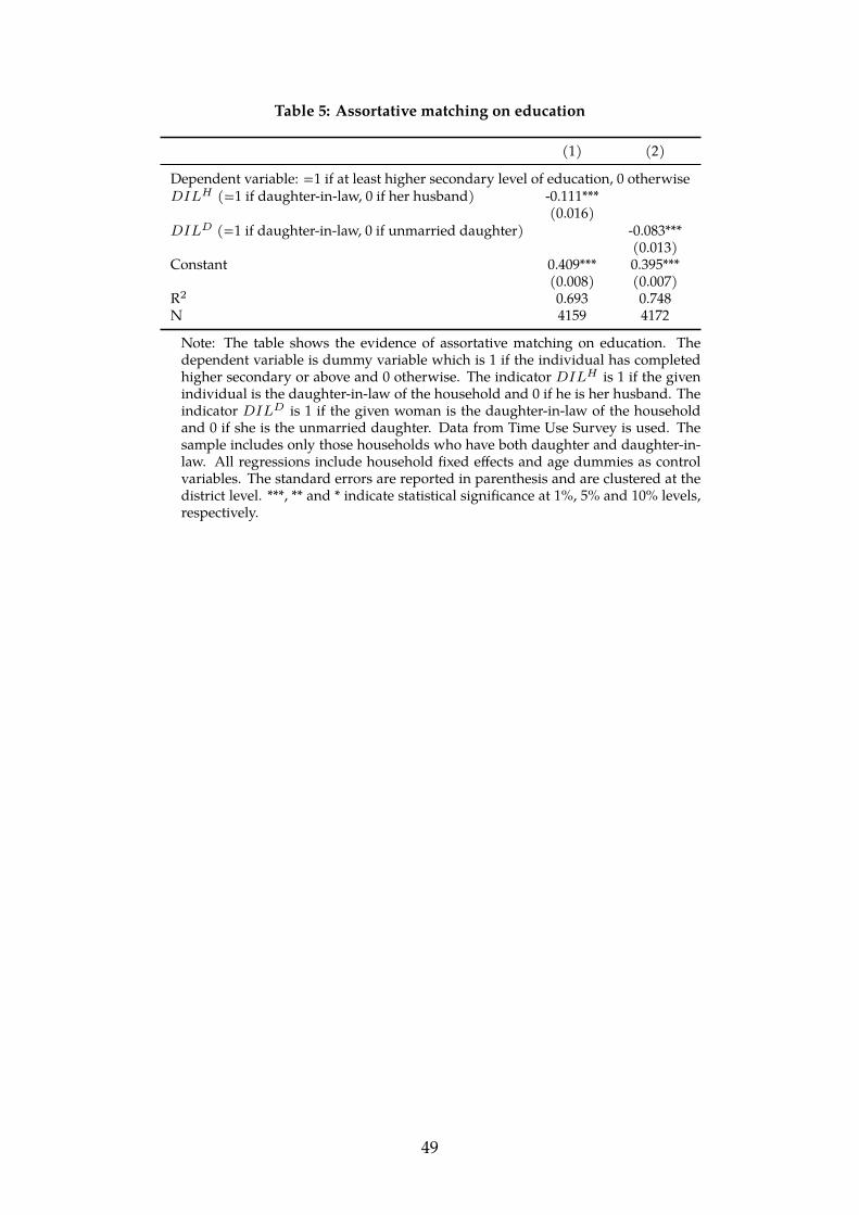
Table 5: Assortative matching on education

(1) (2)Dependent variable: =1 if at least higher secondary level of education, 0 otherwiseDILH (=1 if daughter-in-law, 0 if her husband) -0.111***

(0.016)DILD (=1 if daughter-in-law, 0 if unmarried daughter) -0.083***

(0.013)Constant 0.409*** 0.395***

(0.008) (0.007)R2 0.693 0.748N 4159 4172Note: The table shows the evidence of assortative matching on education. Thedependent variable is dummy variable which is 1 if the individual has completedhigher secondary or above and 0 otherwise. The indicator DILH is 1 if the givenindividual is the daughter-in-law of the household and 0 if he is her husband. Theindicator DILD is 1 if the given woman is the daughter-in-law of the householdand 0 if she is the unmarried daughter. Data from Time Use Survey is used. Thesample includes only those households who have both daughter and daughter-in-law. All regressions include household fixed effects and age dummies as controlvariables. The standard errors are reported in parenthesis and are clustered at thedistrict level. ***, ** and * indicate statistical significance at 1%, 5% and 10% levels,respectively.

49

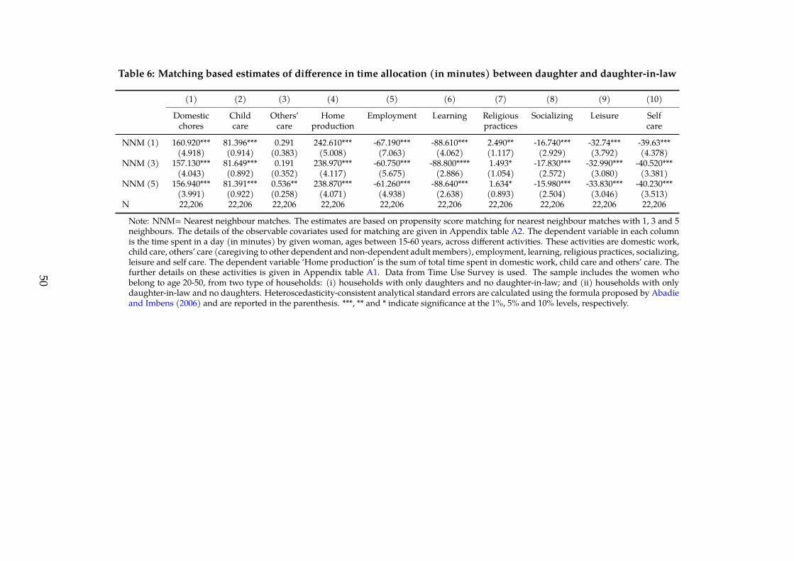
Table 6: Matching based estimates of difference in time allocation (in minutes) between daughter and daughter-in-law

(1) (2) (3) (4) (5) (6) (7) (8) (9) (10)Domestic Child Others’ Home Employment Learning Religious Socializing Leisure Selfchores care care production practices care

NNM (1) 160.920*** 81.396*** 0.291 242.610*** -67.190*** -88.610*** 2.490** -16.740*** -32.74*** -39.63***(4.918) (0.914) (0.383) (5.008) (7.063) (4.062) (1.117) (2.929) (3.792) (4.378)

NNM (3) 157.130*** 81.649*** 0.191 238.970*** -60.750*** -88.800**** 1.493* -17.830*** -32.990*** -40.520***(4.043) (0.892) (0.352) (4.117) (5.675) (2.886) (1.054) (2.572) (3.080) (3.381)

NNM (5) 156.940*** 81.391*** 0.536** 238.870*** -61.260*** -88.640*** 1.634* -15.980*** -33.830*** -40.230***(3.991) (0.922) (0.258) (4.071) (4.938) (2.638) (0.893) (2.504) (3.046) (3.513)

N 22,206 22,206 22,206 22,206 22,206 22,206 22,206 22,206 22,206 22,206Note: NNM= Nearest neighbour matches. The estimates are based on propensity score matching for nearest neighbour matches with 1, 3 and 5neighbours. The details of the observable covariates used for matching are given in Appendix table A2. The dependent variable in each columnis the time spent in a day (in minutes) by given woman, ages between 15-60 years, across different activities. These activities are domestic work,child care, others’ care (caregiving to other dependent and non-dependent adult members), employment, learning, religious practices, socializing,leisure and self care. The dependent variable ‘Home production’ is the sum of total time spent in domestic work, child care and others’ care. Thefurther details on these activities is given in Appendix table A1. Data from Time Use Survey is used. The sample includes the women whobelong to age 20-50, from two type of households: (i) households with only daughters and no daughter-in-law; and (ii) households with onlydaughter-in-law and no daughters. Heteroscedasticity-consistent analytical standard errors are calculated using the formula proposed by Abadieand Imbens (2006) and are reported in the parenthesis. ***, ** and * indicate significance at the 1%, 5% and 10% levels, respectively.

50

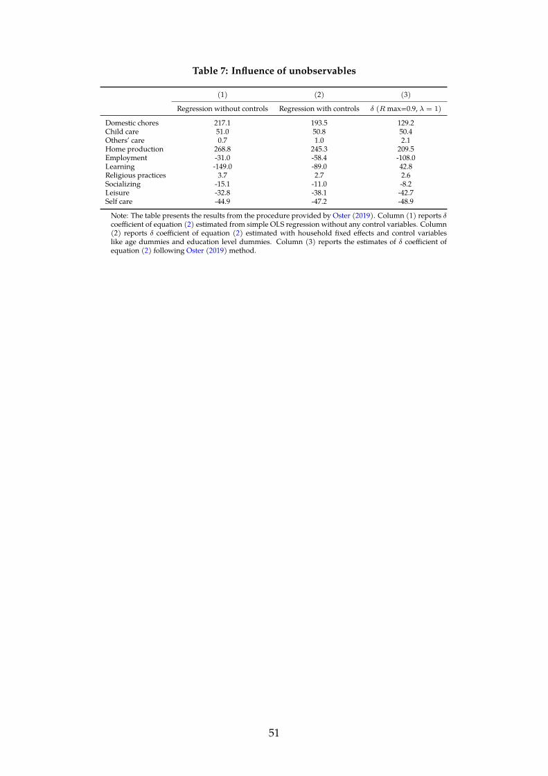
Table 7: Influence of unobservables

(1) (2) (3)Regression without controls Regression with controls δ (Rmax=0.9, λ = 1)

Domestic chores 217.1 193.5 129.2Child care 51.0 50.8 50.4Others’ care 0.7 1.0 2.1Home production 268.8 245.3 209.5Employment -31.0 -58.4 -108.0Learning -149.0 -89.0 42.8Religious practices 3.7 2.7 2.6Socializing -15.1 -11.0 -8.2Leisure -32.8 -38.1 -42.7Self care -44.9 -47.2 -48.9Note: The table presents the results from the procedure provided by Oster (2019). Column (1) reports δcoefficient of equation (2) estimated from simple OLS regression without any control variables. Column(2) reports δ coefficient of equation (2) estimated with household fixed effects and control variableslike age dummies and education level dummies. Column (3) reports the estimates of δ coefficient ofequation (2) following Oster (2019) method.

51

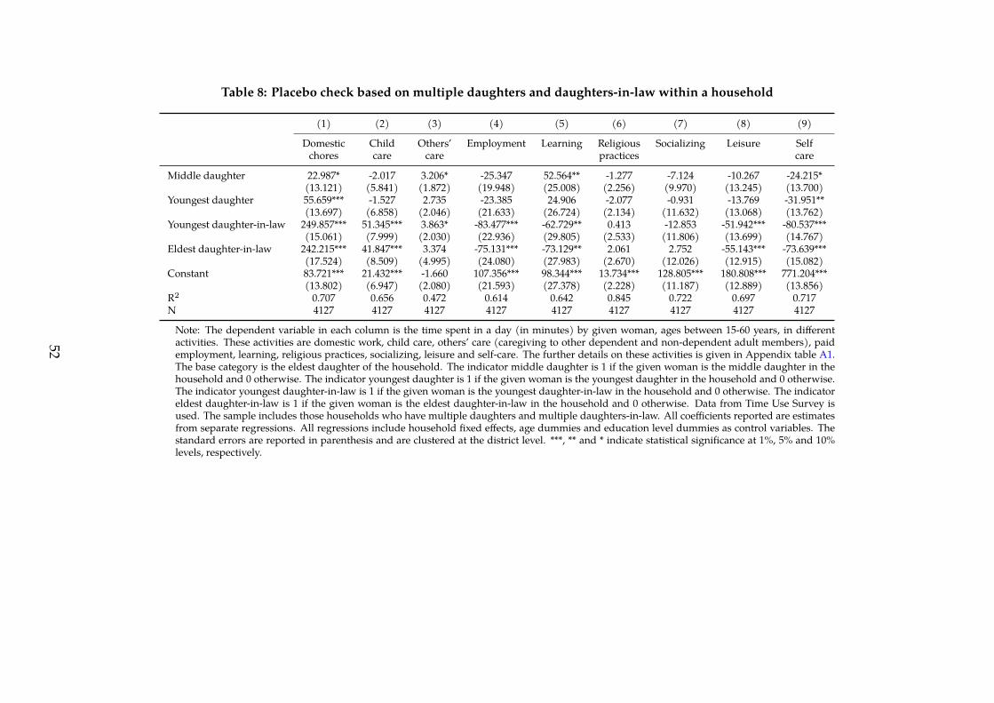
Table 8: Placebo check based on multiple daughters and daughters-in-law within a household

(1) (2) (3) (4) (5) (6) (7) (8) (9)Domestic Child Others’ Employment Learning Religious Socializing Leisure Selfchores care care practices care

Middle daughter 22.987* -2.017 3.206* -25.347 52.564** -1.277 -7.124 -10.267 -24.215*(13.121) (5.841) (1.872) (19.948) (25.008) (2.256) (9.970) (13.245) (13.700)

Youngest daughter 55.659*** -1.527 2.735 -23.385 24.906 -2.077 -0.931 -13.769 -31.951**(13.697) (6.858) (2.046) (21.633) (26.724) (2.134) (11.632) (13.068) (13.762)

Youngest daughter-in-law 249.857*** 51.345*** 3.863* -83.477*** -62.729** 0.413 -12.853 -51.942*** -80.537***(15.061) (7.999) (2.030) (22.936) (29.805) (2.533) (11.806) (13.699) (14.767)

Eldest daughter-in-law 242.215*** 41.847*** 3.374 -75.131*** -73.129** 2.061 2.752 -55.143*** -73.639***(17.524) (8.509) (4.995) (24.080) (27.983) (2.670) (12.026) (12.915) (15.082)

Constant 83.721*** 21.432*** -1.660 107.356*** 98.344*** 13.734*** 128.805*** 180.808*** 771.204***(13.802) (6.947) (2.080) (21.593) (27.378) (2.228) (11.187) (12.889) (13.856)

R2 0.707 0.656 0.472 0.614 0.642 0.845 0.722 0.697 0.717N 4127 4127 4127 4127 4127 4127 4127 4127 4127Note: The dependent variable in each column is the time spent in a day (in minutes) by given woman, ages between 15-60 years, in differentactivities. These activities are domestic work, child care, others’ care (caregiving to other dependent and non-dependent adult members), paidemployment, learning, religious practices, socializing, leisure and self-care. The further details on these activities is given in Appendix table A1.The base category is the eldest daughter of the household. The indicator middle daughter is 1 if the given woman is the middle daughter in thehousehold and 0 otherwise. The indicator youngest daughter is 1 if the given woman is the youngest daughter in the household and 0 otherwise.The indicator youngest daughter-in-law is 1 if the given woman is the youngest daughter-in-law in the household and 0 otherwise. The indicatoreldest daughter-in-law is 1 if the given woman is the eldest daughter-in-law in the household and 0 otherwise. Data from Time Use Survey isused. The sample includes those households who have multiple daughters and multiple daughters-in-law. All coefficients reported are estimatesfrom separate regressions. All regressions include household fixed effects, age dummies and education level dummies as control variables. Thestandard errors are reported in parenthesis and are clustered at the district level. ***, ** and * indicate statistical significance at 1%, 5% and 10%levels, respectively.

52

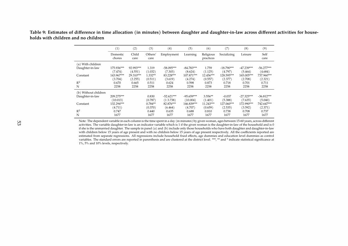
Table 9: Estimates of difference in time allocation (in minutes) between daughter and daughter-in-law across different activities for house-holds with children and no children

(1) (2) (3) (4) (5) (6) (7) (8) (9)Domestic Child Others’ Employment Learning Religious Socializing Leisure Selfchores care care practices care

(a) With childrenDaughter-in-law 175.936*** 92.993*** 1.319 -58.095*** -84.783*** 1.759 -18.790*** -47.239*** -56.277***

(7.474) (4.551) (1.032) (7.303) (8.624) (1.125) (4.797) (5.464) (4.684)Constant 143.967*** 29.310*** 1.332** 83.228*** 107.871*** 12.456*** 128.595*** 165.005*** 737.960***

(3.704) (2.255) (0.511) (3.619) (4.274) (0.557) (2.377) (2.708) (2.321)R2 0.670 0.665 0.511 0.624 0.598 0.873 0.718 0.701 0.711N 2258 2258 2258 2258 2258 2258 2258 2258 2258(b) Without childrenDaughter-in-law 209.275*** 0.830 -52.621*** -95.659*** 3.556** -0.037 -27.325*** -36.812***

(10.013) (0.787) (1 3.738) (10.004) (1.401) (5.388) (7.635) (5.040)Constant 132.294*** 0.784** 82.876*** 146.839*** 11.243*** 127.060*** 172.990*** 742.647***

(4.711) (0.370) (6.464) (4.707) (0.659) (2.535) (3.592) (2.371)R2 0.747 0.440 0.635 0.688 0.810 0.738 0.708 0.737N 1677 1677 1677 1677 1677 1677 1677 1677Note: The dependent variable in each column is the time spent in a day (inminutes) by givenwoman, ages between 15-60 years, across differentactivities. The variable daughter-in-law is an indicator variable which is 1 if the given woman is the daughter-in-law of the household and is 0if she is the unmarried daughter. The sample in panel (a) and (b) include only those households who have both daughter and daughter-in-lawwith children below 15 years of age present and with no children below 15 years of age present respectively. All the coefficients reported areestimated from separate regressions. All regressions include household fixed effects, age dummies and education level dummies as controlvariables. The standard errors are reported in parenthesis and are clustered at the district level. ***, ** and * indicate statistical significance at1%, 5% and 10% levels, respectively.

53

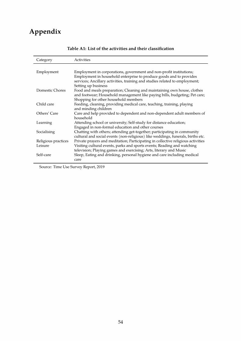
Appendix

Table A1: List of the activities and their classification

Category Activities

Employment Employment in corporations, government and non-profit institutions;Employment in household enterprise to produce goods and to providesservices; Ancillary activities, training and studies related to employment;Setting up business

Domestic Chores Food and meals preparation; Cleaning and maintaining own house, clothesand footwear; Household management like paying bills, budgeting; Pet care;Shopping for other household members

Child care Feeding, cleaning, providing medical care, teaching, training, playingand minding children

Others’ Care Care and help provided to dependent and non-dependent adult members ofhousehold

Learning Attending school or university; Self-study for distance education;Engaged in non-formal education and other courses

Socialising Chatting with others; attending get-together; participating in communitycultural and social events (non-religious) like weddings, funerals, births etc.

Religious practices Private prayers and meditation; Participating in collective religious activitiesLeisure Visiting cultural events, parks and sports events; Reading and watching

television; Playing games and exercising; Arts, literary and MusicSelf-care Sleep, Eating and drinking, personal hygiene and care including medical

careSource: Time Use Survey Report, 2019

54

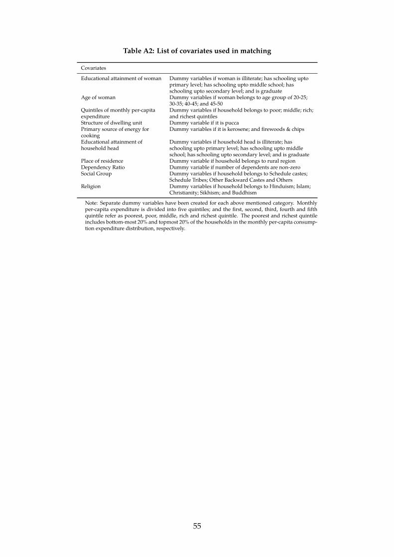
Table A2: List of covariates used in matching

CovariatesEducational attainment of woman Dummy variables if woman is illiterate; has schooling upto

primary level; has schooling upto middle school; hasschooling upto secondary level; and is graduate

Age of woman Dummy variables if woman belongs to age group of 20-25;30-35; 40-45; and 45-50

Quintiles of monthly per-capita Dummy variables if household belongs to poor; middle; rich;expenditure and richest quintilesStructure of dwelling unit Dummy variable if it is puccaPrimary source of energy for Dummy variables if it is kerosene; and firewoods & chipscookingEducational attainment of Dummy variables if household head is illiterate; hashousehold head schooling upto primary level; has schooling upto middle

school; has schooling upto secondary level; and is graduatePlace of residence Dummy variable if household belongs to rural regionDependency Ratio Dummy variable if number of dependents are non-zeroSocial Group Dummy variables if household belongs to Schedule castes;

Schedule Tribes; Other Backward Castes and OthersReligion Dummy variables if household belongs to Hinduism; Islam;

Christianity; Sikhism; and BuddhismNote: Separate dummy variables have been created for each above mentioned category. Monthlyper-capita expenditure is divided into five quintiles; and the first, second, third, fourth and fifthquintile refer as poorest, poor, middle, rich and richest quintile. The poorest and richest quintileincludes bottom-most 20% and topmost 20% of the households in the monthly per-capita consump-tion expenditure distribution, respectively.

55

Figure A1: Common support

Note: The figure plots the condition of common support region for matcheddaughters and daughters-in-law.

56

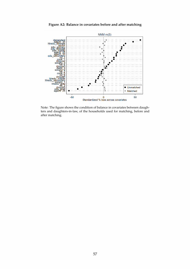
Figure A2: Balance in covariates before and after matching

Note: The figure shows the condition of balance in covariates between daugh-ters and daughters-in-law, of the households used for matching, before andafter matching.

57

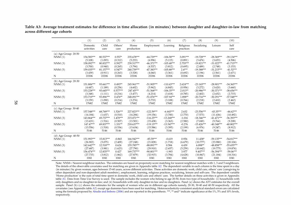
Table A3: Average treatment estimates for difference in time allocation (in minutes) between daughter and daughter-in-law from matchingacross different age cohorts

(1) (2) (3) (4) (5) (6) (7) (8) (9) (10)Domestic Child Others’ Home Employment Learning Religious Socializing Leisure Selfactivities care care production practices care

(a) Age Group: 20-50NNM (1) 154.583*** 80.537*** 0.557* 235.678*** -44.729*** -106.58*** 3.091*** -19.728*** -28.369*** -39.134***

(5.108) (1.093) (0.312) (5.233) (6.996) (5.115) (0.891) (3.476) (3.653) (4.506)NNM (3) 158.092*** 80.832*** 0.592** 239.517*** -46.371*** -105.48*** 2.755*** -19.821*** -31.022*** -41.715***

(3.700) (0.940) (0.265) (3.794) (4.537) (3.812) (0.695) (2.489) (2.748) (3.153)NNM (5) 159.035*** 81.157*** 0.547** 240.739*** -47.383*** -105.88*** 2.4*** -19.388*** -31.215*** -41.52***

(3.439) (0.911) (0.263) (3.528) (4.060) (3.361) (0.692) (2.196) (2.561) (2.671)N 22206 22206 22206 22206 22206 22206 22206 22206 22206 22206(b) Age Group: 20-30NNM (1) 151.806*** 93.661*** 0.493** 245.961*** -51.905*** -110.43*** 2.624*** -23.165*** -28.901*** -34.365***

(4.447) (1.189) (0.256) (4.602) (5.962) (4.845) (0.956) (3.272) (3.620) (3.660)NNM (3) 153.228*** 93.645*** 0.577*** 247.45*** -51.568*** -106.35*** 2.013** -20.986*** -30.371*** -38.656***

(3.348) (1.111) (0.216) (3.477) (4.214) (3.418) (0.785) (2.402) (2.652) (2.715)NNM (5) 153.719*** 93.896*** 0.476** 248.091*** -51.076*** -107.94*** 1.898** -20.716*** -30.291*** -37.548***

(3.159) (1.090) (0.214) (3.274) (3.733) (3.108) (0.766) (2.218) (2.410) (2.462)N 17682 17682 17682 17682 17682 17682 17682 17682 17682 17682(c) Age Group: 30-40NNM (1) 157.548*** 68.749*** 1.526*** 227.823*** -122.59*** -6.443*** 2.632 -23.556*** -43.35*** -44.62***

(14.184) (1.637) (0.510) (14.284) (19.156) (3.700) (2.770) (7.573) (11.436) (10.492)NNM (3) 143.864*** 69.737*** 1.470*** 215.071*** -116.25*** -13.268*** -1.016 -18.346*** -41.471*** -36.393***

(13.431) (1.516) (0.507) (13.501) (15.438) (3.363) (2.580) (7.049) (9.764) (9.208)NNM (5) 147.47*** 69.837*** 1.331** 218.637*** -119.15*** -13.547*** -0.276 -15.426*** -40.348*** -40.802***

(13.556) (1.518) (0.536) (13.634) (15.586) (3.395) (2.199) (6.976) (9.247) (8.912)N 5146 5146 5146 5146 5146 5146 5146 5146 5146 5146(d) Age Group: 40-50NNM (1) 151.993*** 15.813*** -0.865 166.942*** -85.59*** -0.619 0.956 11.438* -59.135*** -54.817***

(26.902) (5.075) (2.409) (27.248) (21.828) (1.718) (6.679) (10.777) (23.980) (20.104)NNM (3) 142.642*** 12.518*** 0.624 155.785*** -88.891*** 0.584 4.439 6.898** -48.858*** -55.655***

(27.687) (3.981) (1.623) (27.790) (29.910) (2.657) (5.259) (10.642) (19.775) (19.874)NNM (5) 156.474*** 12.835*** 0.427 169.737*** -90.801*** -1.993 3.977 9.407*** -56.394*** -59.06***

(27.733) (3.812) (1.862) (27.879) (32.915) (3.784) (4.628) (10.867) (21.184) (18.316)N 1041 1041 1041 1041 1041 1041 1041 1041 1041 1041Note: NNM=Nearest neighbour matches. The estimates are based on propensity-score matching for nearest neighbour matches with 1, 3 and 5 neighbours.The details of the observable covariates used for matching are given in Appendix table A2. The dependent variable in each column is the time spent in a day(in minutes) by given woman, ages between 15-60 years, across different activities. These activities are domestic work, child care, others’ care (caregiving toother dependent and non-dependent adult members), employment, learning, religious practices, socializing, leisure and self-care. The dependent variable’Home production’ is the sum of total time spent in domestic work, child care and others’ care. The further details on these activities is given in Appendixtable A1. Data from Time Use Survey is used. The sample includes the women who belong to age 20-50, from two type of households: (i) households withonly daughters and no daughter-in-law; and (ii) households with only daughter-in-law and no daughters. Panel (a) shows the ATT estimates for the overallsample. Panel (b)-(c) shows the estimates for the sample of women who are in different age cohorts namely, 20-30, 30-40 and 40-50 respectively. All thecovariates (see Appendix table A2) except age dummies have been used for matching. Heteroscedasticity-consistent analytical standard errors are calculatedusing the formula proposed by Abadie and Imbens (2006) and are reported in the parenthesis. ***, ** and * indicate significance at the 1%, 5% and 10% levels,respectively.

58

Kinship Roles and Women's Time Use in India Tanu Gupta ...

Documents

Transcript of Kinship Roles and Women's Time Use in India Tanu Gupta ...