Killing Epsilons with a Dagger: A Coalgebraic Study of

Systems with Algebraic Label Structure

Filippo Bonchia, Stefan Miliusb,1, Alexandra Silvac,d,e, Fabio Zanasia

aENS Lyon, U. de Lyon, CNRS, INRIA, UCBL, FrancebLehrstuhl fur Theoretische Informatik, FAU Erlangen-Nurnberg

cInstitute for Computing and Information Sciences, Radboud University NijmegendCentrum Wiskunde & Informatica (Amsterdam, The Netherlands)eHASLab / INESC TEC, Universidade do Minho (Braga, Portugal)

Abstract

We propose an abstract framework for modeling state-based systems withinternal behaviour as e.g. given by silent or ε-transitions. Our approachemploys monads with a parametrized fixpoint operator † to give a semanticsto those systems and implement a sound procedure of abstraction of theinternal transitions, whose labels are seen as the unit of a free monoid. Morebroadly, our approach extends the standard coalgebraic framework for state-based systems by taking into account the algebraic structure of the labelsof their transitions. This allows to consider a wide range of other examples,including Mazurkiewicz traces for concurrent systems and non-deterministictransducers.

Keywords: coalgebras on Kleisli categories, parametrized fixpointoperator, trace semantics, epsilon transitions, Mazurkiewicz traces,non-deterministic transducers

1. Introduction

The theory of coalgebras provides an elegant mathematical framework toexpress the semantics of computing devices: the operational semantics, which

Email addresses: filippo.bonchi@ens-lyon.fr (Filippo Bonchi),mail@stefan-milius.eu (Stefan Milius), alexandra@cs.ru.nl (Alexandra Silva),fabio.zanasi@ens-lyon.fr (Fabio Zanasi)

1Stefan Milius acknowledges support by the Deutsche Forschungsgemeinschaft (DFG)under project MI 717/5-1

Preprint submitted to Theoretical Computer Science March 7, 2015

is usually given as a state machine, is modeled as a coalgebra for a functor;the denotational semantics as the unique map into the final coalgebra ofthat functor. While the denotational semantics is often compositional (as,for instance, ensured by the bialgebraic approach of [34]), it is sometimesnot fully-abstract, i.e., it discriminates systems that are equal from the pointof view of an external observer. This is due to the presence of internaltransitions (also called ε-transitions) that are not observable but that arenot abstracted away by the usual coalgebraic semantics using the uniquehomomorphism into the final coalgebra.

In this paper, we focus on the problem of giving trace semantics to systemswith internal transitions. Our approach stems from an elementary observa-tion (pointed out in previous work, e.g. [39]): the labels of transitions forma monoid and the internal transitions are those labeled by the unit of themonoid. Thus, there is an algebraic structure on the labels that needs to betaken into account when modeling the denotational semantics of those sys-tems. To illustrate this point, consider the following two non-deterministicautomata (NDA).

// q0

b

a++ q2

b

kk

b

33

a,c

q3

b

css

OO

ε

// q0

a+b∗c++

b

q2

b

kk

bb∗c+a+c

The one on the left (that we call A) is an NDA with ε-transitions: its tran-sitions are labeled either by the symbols of the alphabet A = {a, b, c} or bythe empty word ε ∈ A∗. The one on the right (that we call B) has transitionslabeled by languages in P(A∗), here represented as regular expressions. Themonoid structure on the labels is explicit on B, while it is less evident inA since the set of labels A ∪ {ε} does not form a monoid. However, thisset can be trivially embedded into P(A∗) by looking at each symbols as thecorresponding singleton language. For this reason each automaton with ε-transitions, like A, can be regarded as an automaton with transitions labeledby languages, like B. Furthermore, we can define the semantics of NDA withε-transitions by defining the semantics of NDA with transitions labeled by

languages: a word w is accepted by a state q if there is a path qL1−→ · · · Ln−→ p

where p is a final state, and there exist a decomposition w = w1 · · ·wn suchthat wi ∈ Li. Observe that, with this definition, A and B accept the samelanguage: all words over A that end with a or c. In fact, B was obtained

2

from A in a well-known process to compute the regular expression denotingthe language accepted by a given automaton [25].

We propose to define the semantics of systems with internal transitionsfollowing the same idea as in the above example. Given some transitiontype (i.e. an endofunctor) F , one first defines an embedding of F -systemswith internal transitions into F ∗-system, where F ∗ has been derived from Fby making explicit the algebraic structure on the labels. Next one modelsthe semantics of an F -system as the one of the corresponding F ∗-system e.Naively, one could think of defining the semantics of e as the unique map !einto the final coalgebra for F ∗. However, this approach turns out to be toofine grained, essentially because it ignores the underlying algebraic structureon the labels of e. The same problem can be observed in the example above:B and the representation of A as an automaton with languages as labelshave different final semantics—they accept the same language only modulothe equations of monoids.

Thus we need to extend the standard coalgebraic framework by takinginto account the algebraic structure on labels. To this end, we develop ourtheory for systems whose transition type F ∗ has a canonical fixpoint, i.e.its initial algebra and final coalgebra coincide. This is the case for manyrelevant examples, as observed in [23]. Our canonical fixpoint semantics willbe given as the composite ¡ ◦ !e, where !e is a coalgebra morphism given byfinality and ¡ is an algebra morphism given by initiality. The target of ¡will be an algebra for F ∗ encoding the equational theory associated withthe labels of F ∗-systems. Intuitively, ¡ being an algebra morphism, will takethe quotient of the semantics given by !e modulo those equations. Thereforethe extension provided by ¡ is the technical feature allowing us to take intoaccount the algebraic structure on labels.

It were Simpson and Plotkin [38, Section 6] who realized that the abovecomposites ¡ ◦ !e yield a parametrized fixpoint operator e 7→ e†. This operatorcan be understood as assigning to systems of mutally recursive equations acertain solution, and the properties of e 7→ e† will be crucial for our canonicalfixpoint semantics.

Within the same perspective we also consider a different fixpoint operatore 7→ e‡ turning any system e with internal transitions into one e‡ where thosehave been abstracted away. By comparing the operators e 7→ e† and e 7→ e‡,we are then able to show that such a procedure (also called ε-elimination) issound with respect to the canonical fixpoint semantics.

We further explore the flexibility of our framework by modelling the case

3

in which the algebraic structure of the labels is quotiented under some equa-tions, resulting in a coarser equivalence than the one given by the canonicalfixpoint semantics. As a relevant example of this phenomenon, we give thefirst coalgebraic account of Mazurkiewicz traces.

As our last application, we model non-deterministic transducers (with andwithout ε-transitions). This is a pleasing case study: on the one hand, it wasknown to be a hard problem to solve in the coalgebraic framework [21]; onthe other hand, it follows as a simple application of our approach, thereby il-lustrating its power. In fact, as we observe, the only difference between trans-ducers and non-deterministic automata is a change in the monad capturingthe branching structure. In the NDA case, this is just non-determinism (P,the powerset monad) whereas in the transducer case the monad needs to alsocapture the fact that transitions can output words (P(B∗× Id), compositionof the powerset and monoid action monads).

This paper is an extended and improved version of our CMCS’14 pa-per [10]. We have included all the proofs and the new example of non-deterministic transducers. We were also able to weaken the assumptions ofour framework. In the conference version, Assumption 5.1 required the basecategory C to be Cppo-enriched and the monad T to be locally continuous.These assumptions ensure (a) initial algebra-final coalgebra coincidence forthe functors T (Id + Y ) and (b) that the canonical fixpoint operator e 7→ e†

satisfies the so-called double dagger law. The latter is instrumental in ourframework to correctly capture the semantics of systems with internal be-haviour. Fortunately, it follows from the results of Simpson and Plotkin [38]that (a) and (b) hold whenever T has enough canonical fixpoints, in partic-ular, no Cppo-enrichment and local continuity of T is needed.

Synopsis. After recalling the necessary background in Section 2, we dis-cuss our motivating examples—automata with ε-transitions and automataon words—in Section 3. Section 4 and 5 are devoted to present the canonicalfixpoint semantics and the sound procedure of ε-elimination. This frameworkis then instantiated to the examples of Section 3. In Section 6 we show how aquotient of the algebra on labels induces a coarser canonical fixpoint seman-tics. We propose Mazurkiewicz traces as a motivating example for such aconstruction. Finally, in Section 7 we apply our theory to give a coalgebraicmodeling of non-deterministic transducers.

4

2. Preliminaries

In this section we introduce the basic notions we need for our abstractframework. We assume some familiarity with category theory. We will useboldface capitals C to denote categories, X, Y, . . . for objects and f, g, . . . formorphisms. We use Greek letters and double arrows, e.g. η : F ⇒ G, fornatural transformations and monad morphisms. If C has coproducts we willdenote them by X + Y and use inl, inr for the coproduct injections.

2.1. Monads

We recall the basics of the theory of monads, as needed here. For moreinformation, see e.g. [30]. A monad is a functor T : C→ C together with twonatural transformations, a unit η : idC ⇒ T and a multiplication µ : T 2 ⇒ T ,which are required to satisfy the following equations, for every X ∈ C:µX ◦ ηTX = µX ◦ TηX = idTX and µX ◦ µTX = µX ◦ TµX .

A morphism of monads from (T, ηT , µT ) to (S, ηS, µS) is a natural trans-formation γ : T ⇒ S that preserves unit and multiplication: γX ◦ ηTX = ηSXand γX ◦ µTX = µSX ◦ γSX ◦ TγX . A quotient of monads is a morphism ofmonads with epimorphic components.

Example 2.1. We briefly describe the examples of monads that we use inthis paper.

1. Let C = Sets. The powerset monad P maps a set X to the set PX ofsubsets of X, and a function f : X → Y to Pf : PX → PY given bydirect image. The unit is given by the singleton set map ηX(x) = {x}and multiplication by union µX(U) =

⋃S∈U S.

2. For later reference we introduce another monad on Sets, namely B∗×Id. Its value on a set X is B∗ × X, where B∗ is the set of words ona fixed B. The unit ηX maps x ∈ X into (ε, x) ∈ B∗ × X and themultiplication µX maps (w, v, x) ∈ B∗ ×B∗ ×X to (wv, x) ∈ B∗ ×X.

3. Let C be a category with coproducts and E an object of C. Theexception monad E is defined on objects as EX = E+X and on arrowsf : X → Y as Ef = idE + f . Its unit and multiplication are given onX ∈ C respectively as inrX : X → E+X and ∇E + idX : E+E+X →E + X, where ∇E = [idE, idE] is the codiagonal. When C = Sets,E can be thought as a set of exceptions and this monad is often used

5

to encode computations that might fail throwing an exception chosenfrom the set E.

4. Let H be an endofunctor on a category C such that for every objectX there exists a free H-algebra H∗X on X (equivalently, an initialH(−) + X-algebra) with the structure τX : HH∗X → H∗X and uni-versal morphism ηX : X → H∗X. Then as proved by Barr [8] (seealso Kelly [28]) H∗ is the object mapping of a free monad on H withthe unit given by the above ηX and the multiplication given by thefreeness of H∗H∗X: µX is the unique H-algebra homomorphism from(H∗H∗X, τH∗X) to (H∗X, τX) such that µX ◦ ηH∗X = idH∗X . Also no-tice that for a cocomplete category every free monad arises in this way.Finally, for later use we fix the notation κ = τ ◦ Hη : H ⇒ H∗ for theuniversal natural transformation of the free monad.

Given a monad M : C → C, its Kleisli category K`(M) has the sameobjects as C, but morphisms X → Y in K`(M) are morphisms X → MYin C. The identity map X → X in K`(M) is M ’s unit ηX : X → MX; andcomposition g ◦ f in K`(M) uses M ’s multiplication: g ◦ f = µ ◦ Mg ◦ f .There is a forgetful functor U : K`(T ) → C, sending X to TX and f toµ ◦ Tf . This functor has a left adjoint J, given by JX = X and Jf = η ◦ f .The Kleisli category K`(M) inherits coproducts from the underlying categoryC. More precisely, for every objects X and Y their coproduct X + Y in Cis also a coproduct in K`(M) with the injections Jinl and Jinr.

2.2. Distributive Laws and Liftings

The most interesting examples of the theory that we will present in Sec-tion 4 concern coalgebras for functors H : K`(M)→ K`(M) that are obtainedas liftings of endofunctors H on Sets. Formally, given a monad M : C→ C,a lifting of H : C → C to K`(M) is an endofunctor H : K`(M) → K`(M)such that J◦H = H ◦J. The lifting of a monad (T, η, µ) is a monad (T , η, µ)such that T is a lifting of T and η, µ are given on X ∈ K`(M) (i.e. X ∈ Sets)respectively as J(ηX) and J(µX).

A natural way of lifting functors and monads is by means of a distributivelaw. A distributive law of a monad (T, ηT , µT ) over a monad (M, ηM , µM) isa natural transformation λ : TM ⇒MT , that commutes appropriately withthe unit and multiplication of both monads; more precisely, the diagrams

6

below commute:

TX

TηMX��

TX

ηMTX��

TM2X

TµMX��

λMX //MTMXMλX //M2TX

µMTX��

TMXλX//MTX TMX

λX//MTX

MX

ηTMX

OO

MX

MηTX

OO

T 2MX

µTMX

OO

TλMX

// TMTXλTX

// T 2MX

MµTX

OO

A distributive law of a functor T over a monad (M, ηM , µM) is a naturaltransformation λ : TM ⇒MT such that only the two topmost squares abovecommute.

The following “folklore” result gives an alternative description of distribu-tive laws in terms of liftings to Kleisli categories, see also [26], [33] or [7].

Proposition 2.2 ([33]). Let (M, ηM , µM) be a monad on a category C. Thenthe following holds:

1. For every endofunctor T on C, there is a bijective correspondence be-tween liftings of T to K`(M) and distributive laws of T over M .

2. For every monad (T, ηT , µT ) on C, there is a bijective correspondencebetween liftings of (T, ηT , µT ) to K`(M) and distributive laws of T overM .

In what follows we shall simply write H : K`(M)→ K`(M) for the liftingof an endofunctor H for some distributive law λ : HM ⇒MH. This can beexplicitly given as H(X) = HX for an object X and H(f : X → MY ) =λ ◦Hf : HX →MHX for a morphism f : X → Y in K`(M).

Example 2.3. Consider the powerset monad P (see Example 2.1.1) and thefunctor HX = A × X + 1 on Sets (with 1 = {X}). We can lift H toH : K`(P)→ K`(P) via the distributive law ϕ : HP⇒ PH defined as

ϕX : A× PX + 1→ P(A×X + 1)

X 7→ {X}(a, Y ) 7→ {(a, y) | y ∈ Y }

More explicitly, the functor H lifts to H on K`(P) as follows: for any f : X →Y in K`(P) (that is f : X → P(Y ) in Sets), Hf : A×X + 1→ A× Y + 1 isgiven by Hf(X) = {X} and Hf(〈a, x〉) = {〈a, y〉 | y ∈ f(x)}.

7

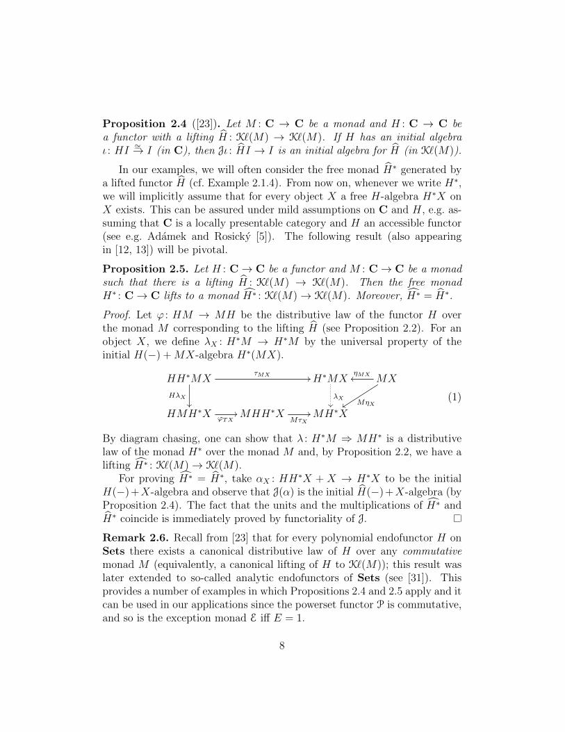
Proposition 2.4 ([23]). Let M : C → C be a monad and H : C → C bea functor with a lifting H : K`(M) → K`(M). If H has an initial algebraι : HI

∼=→ I (in C), then Jι : HI → I is an initial algebra for H (in K`(M)).

In our examples, we will often consider the free monad H∗ generated bya lifted functor H (cf. Example 2.1.4). From now on, whenever we write H∗,we will implicitly assume that for every object X a free H-algebra H∗X onX exists. This can be assured under mild assumptions on C and H, e.g. as-suming that C is a locally presentable category and H an accessible functor(see e.g. Adamek and Rosicky [5]). The following result (also appearingin [12, 13]) will be pivotal.

Proposition 2.5. Let H : C→ C be a functor and M : C→ C be a monadsuch that there is a lifting H : K`(M) → K`(M). Then the free monadH∗ : C→ C lifts to a monad H∗ : K`(M)→ K`(M). Moreover, H∗ = H∗.

Proof. Let ϕ : HM → MH be the distributive law of the functor H overthe monad M corresponding to the lifting H (see Proposition 2.2). For anobject X, we define λX : H∗M → H∗M by the universal property of theinitial H(−) +MX-algebra H∗(MX).

HH∗MXτMX //

HλX��

H∗MX

λX��

MXηMXoo

MηXyy

HMH∗X ϕTX

//MHH∗XMτX

//MH∗X

(1)

By diagram chasing, one can show that λ : H∗M ⇒ MH∗ is a distributivelaw of the monad H∗ over the monad M and, by Proposition 2.2, we have alifting H∗ : K`(M)→ K`(M).

For proving H∗ = H∗, take αX : HH∗X + X → H∗X to be the initialH(−) +X-algebra and observe that J(α) is the initial H(−) +X-algebra (byProposition 2.4). The fact that the units and the multiplications of H∗ andH∗ coincide is immediately proved by functoriality of J.

Remark 2.6. Recall from [23] that for every polynomial endofunctor H onSets there exists a canonical distributive law of H over any commutativemonad M (equivalently, a canonical lifting of H to K`(M)); this result waslater extended to so-called analytic endofunctors of Sets (see [31]). Thisprovides a number of examples in which Propositions 2.4 and 2.5 apply and itcan be used in our applications since the powerset functor P is commutative,and so is the exception monad E iff E = 1.

8

Example 2.7. Continuing Example 2.3 we see that the free monad on HX =A×X + 1 is given by H∗X = A∗ ×X +A∗. It is not difficult to verify thatthe distributive law λ : H∗P⇒ PH∗ acts as follows

λX : A∗ × PX + A∗ → P(A∗ ×X + A∗)

w 7→ {w}(w, Y ) 7→ {(w, y) | y ∈ Y }

for any w ∈ A∗ and Y ∈ PX. Indeed, one readily verifies that this morphismλX makes diagram (1) commutative. Note that both H and H∗ are poly-nomial functors; both ϕ and λ are the canonical distributive laws obtainedfrom the results in [23] (see Remark 2.6).

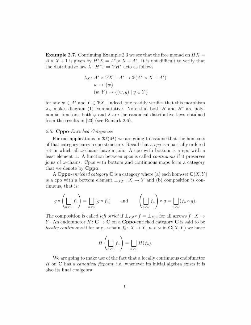
2.3. Cppo-Enriched Categories

For our applications in K`(M) we are going to assume that the hom-setsof that category carry a cpo structure. Recall that a cpo is a partially orderedset in which all ω-chains have a join. A cpo with bottom is a cpo with aleast element ⊥. A function between cpos is called continuous if it preservesjoins of ω-chains. Cpos with bottom and continuous maps form a categorythat we denote by Cppo.

A Cppo-enriched category C is a category where (a) each hom-set C(X, Y )is a cpo with a bottom element ⊥X,Y : X → Y and (b) composition is con-tinuous, that is:

g ◦

(⊔n<ω

fn

)=⊔n<ω

(g ◦ fn) and

(⊔n<ω

fn

)◦ g =

⊔n<ω

(fn ◦ g).

The composition is called left strict if ⊥Y,Z ◦f = ⊥X,Z for all arrows f : X →Y . An endofunctor H : C→ C on a Cppo-enriched category C is said to belocally continuous if for any ω-chain fn : X → Y , n < ω in C(X, Y ) we have:

H

(⊔n<ω

fn

)=⊔n<ω

H(fn).

We are going to make use of the fact that a locally continuous endofunctorH on C has a canonical fixpoint, i.e. whenever its initial algebra exists it isalso its final coalgebra:

9

Theorem 2.8 ([18]). Let H : C→ C be a locally continuous endofunctor onthe Cppo-enriched category C whose composition is left-strict. If an initialH-algebra ι : HI

∼=→ I exists, then ι−1 : I∼=→ HI is a final H-coalgebra.

In the sequel, we will be interested in free algebras for a functor H on Cand the free monad H∗ (cf. Example 2.1.4). For this observe that coproductsin C are always Cppo-enriched, i.e. all copairing maps [−,−] : C(X, Y ) ×C(X ′, Y ) → C(X + X ′, Y ) are continuous; in fact, it is easy to show thatthis map is continuous in both of its arguments using that composition withthe coproduct injections is continuous.

Proposition 2.9. Let C be Cppo-enriched with composition left-strict. Fur-thermore, let H : C → C be locally continuous and assume that all freeH-algebras exist. Then the free monad H∗ is locally continuous.

Proof. First recall that H∗X is a free H-algebra with the structure τX andthe universal morphism ηX (cf. Example 2.1.4). Equivalently, αX = [τX , ηX ] :H(H∗X)+X → H∗X is an initial algebra for H(−)+X. Given a morphismf : X → Y , H∗f is defined by initiality; more precisely, H∗f is the uniquemorphism such that the following diagram commutes:

H(H∗X) +XαX //

H(H∗f)+id

��

H∗X

H∗f

��

H(H∗Y ) +Xid+f

// H(H∗Y ) + Y αY

// H∗Y

Now recall that αX is an isomorphism by Lambek’s lemma and consider thefollowing function

Φ : C(X, Y )×C(H∗X,H∗Y )→ C(H∗X,H∗Y )

withΦ(f, h) = αY · (Hh+ f) · α−1

X .

Since H is locally continuous, we see that Φ is continuous (in both argu-ments). Clearly, H∗f is the unique fixpoint of Φ(f,−). To see that H∗f islocally continuous let fn : X → Y be an ω-chain in C(X, Y ). It is easy tosee that

⊔n<ωH

∗fn is a fixpoint of Φ(⊔

n<ω fn,−); indeed we have (using

10

continuity of Φ): ⊔n<ω

H∗fn =⊔n<ω

Φ(fn, H∗fn)

= Φ

(⊔n<ω

fn,⊔n<ω

H∗fn

).

Thus, by the uniqueness of the fixpoint H∗(⊔

n<ω fn)

we have

H∗

(⊔n<ω

fn

)=⊔n<ω

H∗fn

as desired.

2.4. Final Coalgebras in Kleisli categories

As we mentioned already, in our applications the Cppo-enriched categorywill be the Kleisli category C = K`(M) of a monad on Sets and the endo-functors of interest are liftings H of endofunctors H on Sets. It is knownthat in this setting a final coalgebra for the lifting H can be obtained as alifting of an initial H-algebra (see Hasuo et al. [23]). Recall e.g. from [5]that an endofunctor H on Sets is accessible if it preserves λ-filtered colimitsfor some cardinal λ; equivalently, H is bounded, i.e. there exists a cardinal λsuch that for every x ∈ HX there exists a subset m : Y ↪→ X and y ∈ Ywith |Y | < λ and such that x = Hm(y) (see Adamek and Porst [4]). Manyendofunctors of interest are accessible: basic examples are constant functors,the identity functor and the finite power-set functor; moreover, accessiblefunctors are closed under coproducts, finite products and composition. The(full) power-set functor is a notable example of an endofunctor that is notaccessible.

The following result is a variation of Theorem 3.3 in [23]:

Theorem 2.10. Let M : Sets→ Sets be a monad and H : Sets→ Sets bea functor such that

(a) K`(M) is Cppo-enriched with composition left strict;

(b) H is accessible and has a lifting H : K`(M) → K`(M) which is locallycontinuous.

11

If ι : HI∼=→ I is the initial algebra for the functor H, then

1. Jι : HI → I is the initial algebra for the functor H;

2. Jι−1 : I → HI is the final coalgebra for the functor H.

The first item follows from Proposition 2.4 and the second one followsfrom Theorem 2.8. There are two differences with Theorem 3.3 in [23]:

(1) There the functor H : Sets→ Sets is supposed to preserve ω-colimitsrather than being accessible. We use the assumption of accessibilitybecause it guarantees the existence of all free algebras for H and forH, which implies also that for all Y ∈ K`(M) an initial H∗(Id + Y )-algebra exists. This property of H∗ will be needed for applying ourframework of Section 4.

(2) We assume that the lifting H : K`(M) → K`(M) is locally continuousrather than locally monotone. This assumption is not really restrictivesince, as explained in Section 3.3.1 of [23], in all the meaningful exam-ples where H is locally monotone, it is also locally continuous. On theother hand this stronger assumption allows us to replace preservationof ω-colimits by accessibility of H.

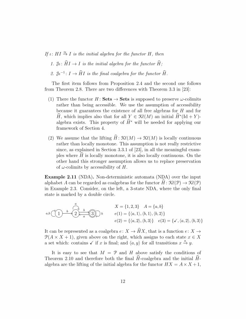
Example 2.11 (NDA). Non-deterministic automata (NDA) over the inputalphabet A can be regarded as coalgebras for the functor H : K`(P)→ K`(P)in Example 2.3. Consider, on the left, a 3-state NDA, where the only finalstate is marked by a double circle.

1a,b)) b // 2

b //

a

3aoo b

ii

X = {1, 2, 3} A = {a, b}e(1) = {〈a, 1〉, 〈b, 1〉, 〈b, 2〉}e(2) = {〈a, 2〉, 〈b, 3〉} e(3) = {X, 〈a, 2〉, 〈b, 3〉}

It can be represented as a coalgebra e : X → HX, that is a function e : X →P(A ×X + 1), given above on the right, which assigns to each state x ∈ Xa set which: contains X if x is final; and 〈a, y〉 for all transitions x

a−→ y.

It is easy to see that M = P and H above satisfy the conditions ofTheorem 2.10 and therefore both the final H-coalgebra and the initial H-algebra are the lifting of the initial algebra for the functor HX = A×X + 1,

12

given by A∗ with structure ι : A×A∗+ 1→ A∗ which maps 〈a, w〉 to aw andX to ε.

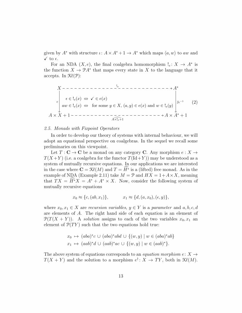
For an NDA (X, e), the final coalgebra homomorphism !e : X → A∗ isthe function X → PA∗ that maps every state in X to the language that itaccepts. In K`(P):

X

e

��

ε ∈ !e(x) ⇔ X ∈ e(x)

aw ∈ !e(x) ⇔ for some y ∈ X, (a, y) ∈ e(x) and w ∈ !e(y)

!e // A∗

Jι−1

��

A×X + 1A×!e+1

// A× A∗ + 1

(2)

2.5. Monads with Fixpoint Operators

In order to develop our theory of systems with internal behaviour, we willadopt an equational perspective on coalgebras. In the sequel we recall somepreliminaries on this viewpoint.

Let T : C→ C be a monad on any category C. Any morphism e : X →T (X+Y ) (i.e. a coalgebra for the functor T (Id+Y )) may be understood as asystem of mutually recursive equations. In our applications we are interestedin the case where C = K`(M) and T = H∗ is a (lifted) free monad. As in theexample of NDA (Example 2.11) take M = P and HX = 1+A×X, meaningthat TX = H∗X = A∗ + A∗ × X. Now, consider the following system ofmutually recursive equations

x0 ≈ {c, (ab, x1)}, x1 ≈ {d, (a, x0), (ε, y)},

where x0, x1 ∈ X are recursion variables, y ∈ Y is a parameter and a, b, c, dare elements of A. The right hand side of each equation is an element ofP(T (X + Y )). A solution assigns to each of the two variables x0, x1 anelement of P(TY ) such that the two equations hold true:

x0 7→ (aba)∗c ∪ (aba)∗abd ∪ {(w, y) | w ∈ (aba)∗ab}x1 7→ (aab)∗d ∪ (aab)∗ac ∪ {(w, y) | w ∈ (aab)∗}.

The above system of equations corresponds to an equation morphism e : X →T (X + Y ) and the solution to a morphism e† : X → TY , both in K`(M).

13

The property that e† is a solution for e is expressed by the following equalityin K`(M):

e† = (X e //T (X + Y )T [e†,ηTY ]

//TTYµTY //TY ). (3)

Definition 2.12 (Following Simpson and Plotkin [38]). Given any monad Ton C a parametrized fixpoint operator is a family of maps C(X,T (X+Y ))→C(X,TY ), e 7→ e†, indexed by parameter objects Y such that for everye : X → T (X + Y ), (3) hold.

Remark 2.13. In our applications we shall need a certain equational prop-erty of the operator e 7→ e† called double dagger law : for all Y ∈ C andequation morphism e : X → T (X +X + Y ),

e†† = (X e //T (X +X + Y )T (∇X+Y )

//T (X + Y ))†.

This and other laws of parametrized fixpoint operators have been studied byBloom and Esik in the context of iteration theories [9].A closely related notionis that of Elgot monads [2, 3]. The parametrized fixpoint operators that weintroduce in Section 4 will satisfy the double dagger law by construction(Theorem 4.3).

Example 2.14 (Least fixpoint solutions). Observe that in the above exampleof NDA every equation morphism e has a least solution e†. More generally, letT : C→ C be a locally continuous monad on the Cppo-enriched category C.Then T is equipped with a parametrized fixpoint operator obtained by takingleast fixpoints: given a morphism e : X → T (X+Y ) consider the function Φe

on C(X,TY ) given by Φe(s) = µTY ◦T [s, ηTY ]◦e. Then Φe is continuous and wetake e† to be the least fixpoint of Φe. Since e† = Φe(e

†), equation (3) holds,and hence we have a parametrized fixpoint operator. Moreover it followsfrom the argument in Theorem 8.2.15 and Exercise 8.2.17 in [9] that theoperator e 7→ e† satisfies the axioms of iteration theories (or Elgot monads,respectively). In particular the double dagger law holds for the least fixpointoperator e 7→ e†.

3. Motivating examples

The work of [23] bridged a gap in the theory of coalgebras: for certainfunctors, taking the final coalgebra directly in Sets does not give the right

14

notion of equivalence on states of coalgebras. For instance, for NDA, onewould obtain bisimilarity instead of language equivalence. The change toKleisli categories allowed the recovery of the usual language semantics forNDA and, more generally, led to the development of coalgebraic trace se-mantics.

In the Introduction we argued that there are relevant examples for whichthis approach still does not yield the right notion of equivalence, the problembeing that it does not consider the extra algebraic structure on the label set.In the sequel, we motivate the reader for the generic theory we will develop bydetailing two case studies in which this phenomenon can be observed: NDAwith ε-transitions and NDA with word transitions. Later on, in Example 6.7,we will also consider Mazurkiewicz traces [29].

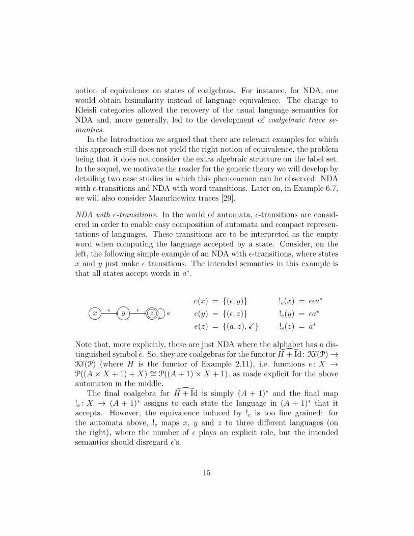
NDA with ε-transitions. In the world of automata, ε-transitions are consid-ered in order to enable easy composition of automata and compact represen-tations of languages. These transitions are to be interpreted as the emptyword when computing the language accepted by a state. Consider, on theleft, the following simple example of an NDA with ε-transitions, where statesx and y just make ε transitions. The intended semantics in this example isthat all states accept words in a∗.

x ε // y ε // z aii

e(x) = {(ε, y)}e(y) = {(ε, z)}e(z) = {(a, z),X}

!e(x) = εεa∗

!e(y) = εa∗

!e(z) = a∗

Note that, more explicitly, these are just NDA where the alphabet has a dis-tinguished symbol ε. So, they are coalgebras for the functor H + Id: K`(P)→K`(P) (where H is the functor of Example 2.11), i.e. functions e : X →P((A ×X + 1) + X) ∼= P((A + 1) ×X + 1), as made explicit for the aboveautomaton in the middle.

The final coalgebra for H + Id is simply (A + 1)∗ and the final map!e : X → (A + 1)∗ assigns to each state the language in (A + 1)∗ that itaccepts. However, the equivalence induced by !e is too fine grained: forthe automata above, !e maps x, y and z to three different languages (onthe right), where the number of ε plays an explicit role, but the intendedsemantics should disregard ε’s.

15

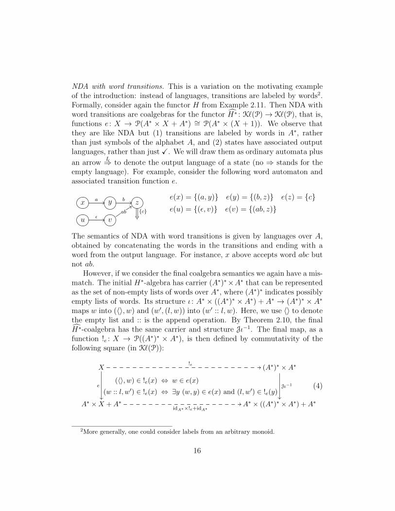
NDA with word transitions. This is a variation on the motivating exampleof the introduction: instead of languages, transitions are labeled by words2.Formally, consider again the functor H from Example 2.11. Then NDA withword transitions are coalgebras for the functor H∗ : K`(P)→ K`(P), that is,functions e : X → P(A∗ × X + A∗) ∼= P(A∗ × (X + 1)). We observe thatthey are like NDA but (1) transitions are labeled by words in A∗, ratherthan just symbols of the alphabet A, and (2) states have associated outputlanguages, rather than just X. We will draw them as ordinary automata plus

an arrowL⇒ to denote the output language of a state (no ⇒ stands for the

empty language). For example, consider the following word automaton andassociated transition function e.

x a // y b // z{c}��u ε // v

ab

99

e(x) = {(a, y)} e(y) = {(b, z)} e(z) = {c}e(u) = {(ε, v)} e(v) = {(ab, z)}

The semantics of NDA with word transitions is given by languages over A,obtained by concatenating the words in the transitions and ending with aword from the output language. For instance, x above accepts word abc butnot ab.

However, if we consider the final coalgebra semantics we again have a mis-match. The initial H∗-algebra has carrier (A∗)∗×A∗ that can be representedas the set of non-empty lists of words over A∗, where (A∗)∗ indicates possiblyempty lists of words. Its structure ι : A∗ × ((A∗)∗ × A∗) + A∗ → (A∗)∗ × A∗maps w into (〈〉, w) and (w′, (l, w)) into (w′ :: l, w). Here, we use 〈〉 to denotethe empty list and :: is the append operation. By Theorem 2.10, the finalH∗-coalgebra has the same carrier and structure Jι−1. The final map, as afunction !e : X → P((A∗)∗ × A∗), is then defined by commutativity of thefollowing square (in K`(P)):

X!e //

e

��

(〈〉, w) ∈ !e(x) ⇔ w ∈ e(x)

(w :: l, w′) ∈ !e(x) ⇔ ∃y (w, y) ∈ e(x) and (l, w′) ∈ !e(y)

(A∗)∗ ×A∗

Jι−1

��

A∗ ×X +A∗idA∗×!e+idA∗

// A∗ × ((A∗)∗ ×A∗) +A∗

(4)

2More generally, one could consider labels from an arbitrary monoid.

16

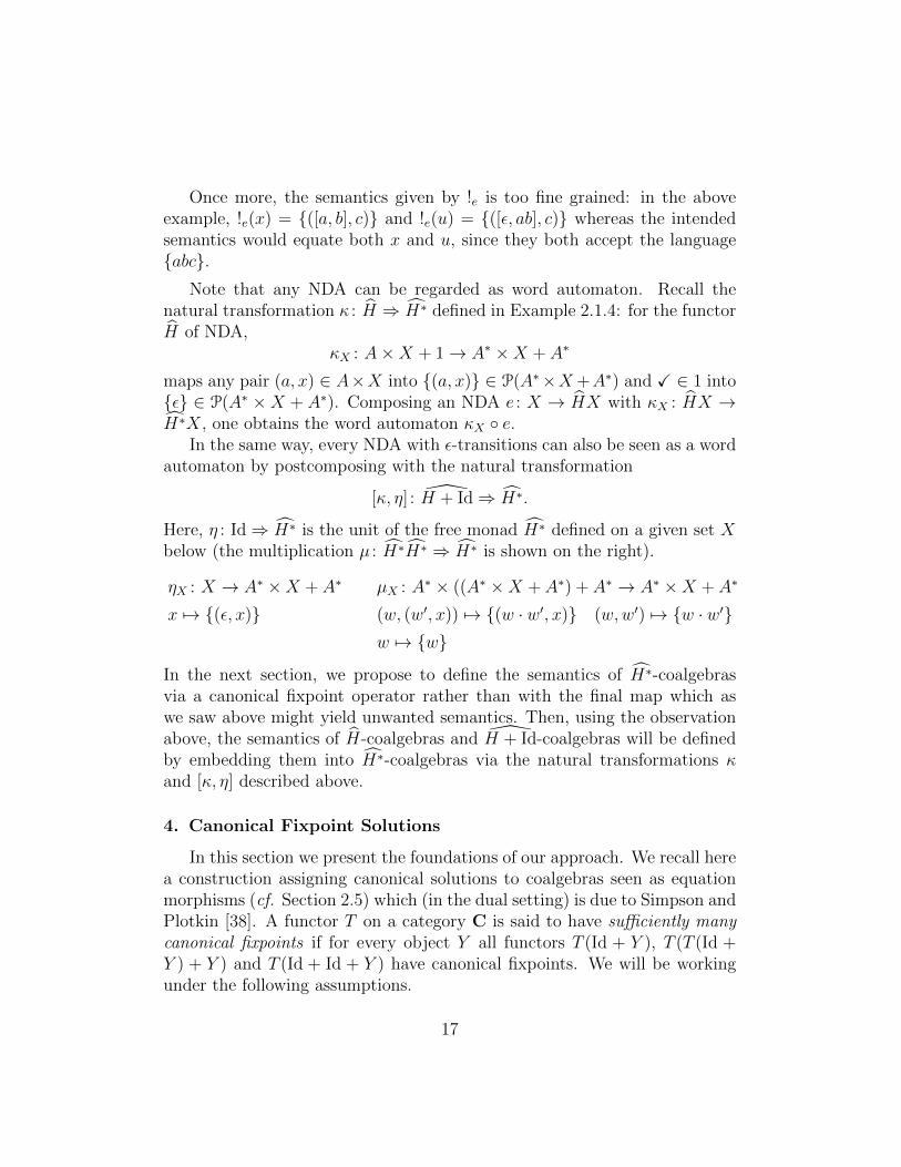
Once more, the semantics given by !e is too fine grained: in the aboveexample, !e(x) = {([a, b], c)} and !e(u) = {([ε, ab], c)} whereas the intendedsemantics would equate both x and u, since they both accept the language{abc}.

Note that any NDA can be regarded as word automaton. Recall thenatural transformation κ : H ⇒ H∗ defined in Example 2.1.4: for the functorH of NDA,

κX : A×X + 1→ A∗ ×X + A∗

maps any pair (a, x) ∈ A×X into {(a, x)} ∈ P(A∗×X+A∗) and X ∈ 1 into{ε} ∈ P(A∗ ×X + A∗). Composing an NDA e : X → HX with κX : HX →H∗X, one obtains the word automaton κX ◦ e.

In the same way, every NDA with ε-transitions can also be seen as a wordautomaton by postcomposing with the natural transformation

[κ, η] : H + Id⇒ H∗.

Here, η : Id⇒ H∗ is the unit of the free monad H∗ defined on a given set Xbelow (the multiplication µ : H∗H∗ ⇒ H∗ is shown on the right).

ηX : X → A∗ ×X + A∗ µX : A∗ × ((A∗ ×X + A∗) + A∗ → A∗ ×X + A∗

x 7→ {(ε, x)} (w, (w′, x)) 7→ {(w · w′, x)} (w,w′) 7→ {w · w′}w 7→ {w}

In the next section, we propose to define the semantics of H∗-coalgebrasvia a canonical fixpoint operator rather than with the final map which aswe saw above might yield unwanted semantics. Then, using the observationabove, the semantics of H-coalgebras and H + Id-coalgebras will be definedby embedding them into H∗-coalgebras via the natural transformations κand [κ, η] described above.

4. Canonical Fixpoint Solutions

In this section we present the foundations of our approach. We recall herea construction assigning canonical solutions to coalgebras seen as equationmorphisms (cf. Section 2.5) which (in the dual setting) is due to Simpson andPlotkin [38]. A functor T on a category C is said to have sufficiently manycanonical fixpoints if for every object Y all functors T (Id + Y ), T (T (Id +Y ) + Y ) and T (Id + Id + Y ) have canonical fixpoints. We will be workingunder the following assumptions.

17

Assumption 4.1. Let C be a category with coproducts and let T be amonad on C having sufficiently many canonical fixpoints.

In Section 5 we will see that these assumptions are satisfied for certainmonads arising from the lifted functor H in Theorem 2.10. This will allowus to apply the theory developed in this section to the motivating examplesof Section 3 and the non-deterministic transducer in Section 7.

Remark 4.2. Recall that, by Freyd’s iterated square theorem [17], for anendofunctor H : C → C an initial algebra for HH yields one for H. Con-versely, one can show that if C has binary products then an initial algebrafor H yields one for HH. Thus, assuming the existence of binary productsand coproducts in C, we see that canonical fixpoints for T (Id + X) exist iffthey exist for T (T (Id + X) + X) (and moreover, these canonical fixpointsare carried by the same object). However, to our knowledge it is not knownwhether existence of canonical fixpoints for T (Id + Id +X) can be obtainedfrom their existence for T (Id +X) (under some reasonable assumptions).

For every parameter object Y ∈ C, denote the initial algebra and finalcoalgebra for T (Id + Y )-algebra by

ιY : T (IY + Y )∼=−→ IY and ι−1

Y : IY∼=−→ T (IY + Y ).

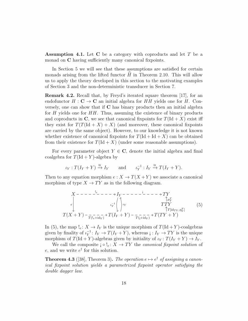
Then to any equation morphism e : X → T (X +Y ) we associate a canonicalmorphism of type X → TY as in the following diagram.

X!e //

e

��

IY

ι−1Y

��

¡// TY

TTYµTY

OO

T (X + Y )T (!e+idY )

// T (IY + Y )

ιY

TT

T (¡+idY )// T (TY + Y )

T [idTY ,ηTY ]

OO (5)

In (5), the map !e : X → IY is the unique morphism of T (Id + Y )-coalgebrasgiven by finality of ι−1

Y : IY → T (IY + Y ), whereas ¡ : IY → TY is the uniquemorphism of T (Id + Y )-algebras given by initiality of ιY : T (IY + Y )→ IY .

We call the composite ¡ ◦ !e : X → TY the canonical fixpoint solution ofe, and we write e† for this solution.

Theorem 4.3 ([38], Theorem 3). The operation e 7→ e† of assigning a canon-ical fixpoint solution yields a parametrized fixpoint operator satisfying thedouble dagger law.

18

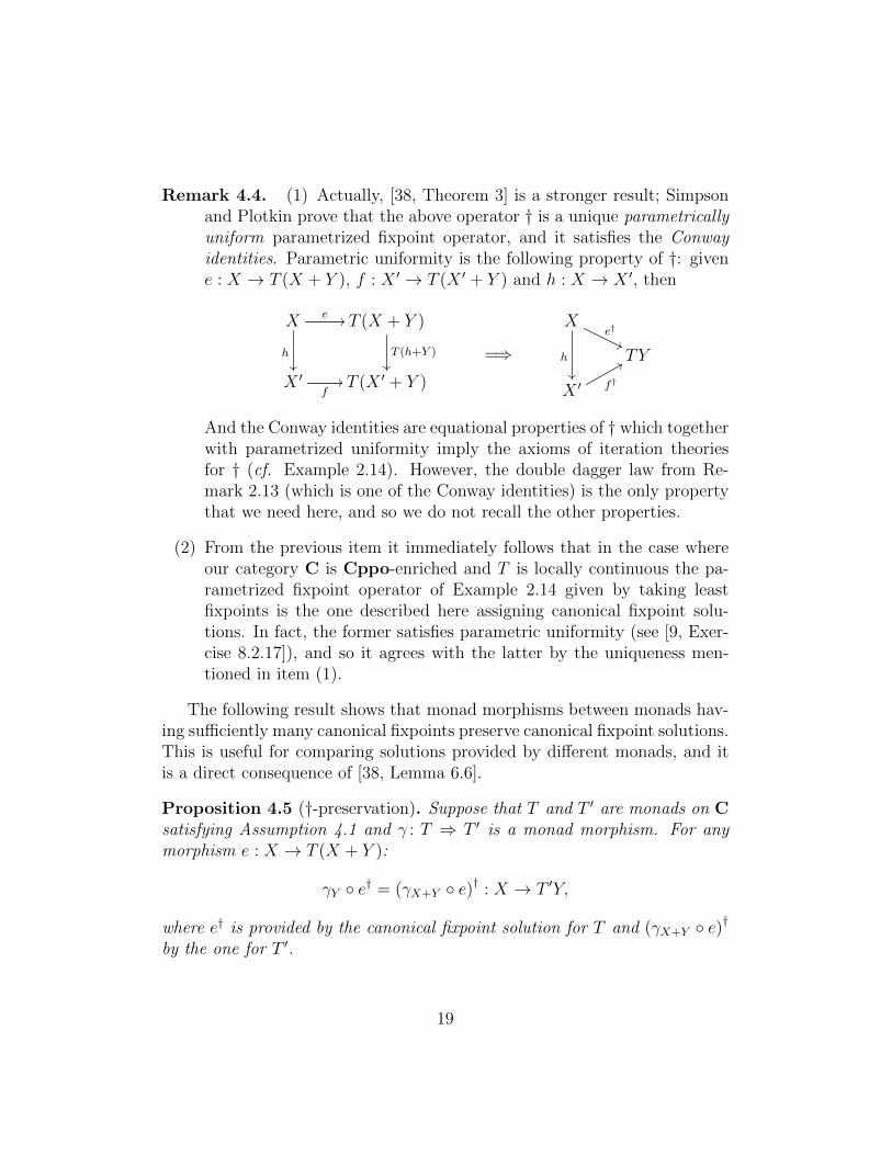
Remark 4.4. (1) Actually, [38, Theorem 3] is a stronger result; Simpsonand Plotkin prove that the above operator † is a unique parametricallyuniform parametrized fixpoint operator, and it satisfies the Conwayidentities. Parametric uniformity is the following property of †: givene : X → T (X + Y ), f : X ′ → T (X ′ + Y ) and h : X → X ′, then

Xe //

h��

T (X + Y )

T (h+Y )

��

X ′f// T (X ′ + Y )

=⇒

Xe†

''

h

��

TY

X ′ f†

77

And the Conway identities are equational properties of † which togetherwith parametrized uniformity imply the axioms of iteration theoriesfor † (cf. Example 2.14). However, the double dagger law from Re-mark 2.13 (which is one of the Conway identities) is the only propertythat we need here, and so we do not recall the other properties.

(2) From the previous item it immediately follows that in the case whereour category C is Cppo-enriched and T is locally continuous the pa-rametrized fixpoint operator of Example 2.14 given by taking leastfixpoints is the one described here assigning canonical fixpoint solu-tions. In fact, the former satisfies parametric uniformity (see [9, Exer-cise 8.2.17]), and so it agrees with the latter by the uniqueness men-tioned in item (1).

The following result shows that monad morphisms between monads hav-ing sufficiently many canonical fixpoints preserve canonical fixpoint solutions.This is useful for comparing solutions provided by different monads, and itis a direct consequence of [38, Lemma 6.6].

Proposition 4.5 (†-preservation). Suppose that T and T ′ are monads on Csatisfying Assumption 4.1 and γ : T ⇒ T ′ is a monad morphism. For anymorphism e : X → T (X + Y ):

γY ◦ e† = (γX+Y ◦ e)† : X → T ′Y,

where e† is provided by the canonical fixpoint solution for T and (γX+Y ◦ e)†by the one for T ′.

19

5. A Theory of Systems with Internal Behaviour

We now use canonical fixpoint solutions to provide an abstract theory ofsystems with internal behaviour, that we will later instantiate to the moti-vating examples of Section 3. Throughout this section, we will develop ourframework for the following ingredients.

Assumption 5.1. Let C be a category with coproducts and let F : C→ Cbe an endofunctor for which all free F -algebras exist. The following monadsderived from F are assumed to have sufficiently many canonical fixpoints:

• the free monad F ∗ : C→ C (cf. Example 2.1.4);

• for every fixed X ∈ C, the exception monad FX + Id: C → C (cf.Example 2.1.3).

In other words the monads F ∗ and FX + Id satisfy Assumption 4.1; thusthey have canonical fixpoint solutions (which satisfy the double dagger law byTheorem 4.3). We shall see in Theorem 5.5 that Assumption 5.1 is satisfiedfor F being the lifted functor H of Theorem 2.10.

To avoid ambiguity, we denote with e 7→ e† the canonical fixpoint operatorassociated with F ∗ and with e 7→ e‡ the one associated with FX + Id.

We will employ the additional structure of those two monads for theanalysis of F -systems with internal transitions. An F -system is simply anF -coalgebra e : X → FX, where we take the operational point of view ofseeing X as a space of states and F as the transition type of e. An F -systemwith internal transitions is an (F +Id)-coalgebra e : X → FX+X, where thecomponent X of the codomain is targeted by those transitions representingthe internal (non-interacting) behaviour of system e.

A key observation for our analysis is that F -systems—with or withoutinternal transitions—enjoy a standard representation as F ∗-systems, that is,coalgebras of the form e : X → F ∗X.

Definition 5.2 (F -systems as F ∗-systems). Let κ : F ⇒ F ∗ be as in Ex-ample 2.1.4. We introduce the following encoding e 7→ e of F -systems andF -systems with internal transitions as F ∗-systems.

• Given an F -system e : X → FX, define e : X → F ∗X as

e : X e //FXκX //F ∗X.

20

• Given an F -system with internal transitions e : X → FX + X, definee : X → F ∗X as

e : X e //FX +X[κX ,η

F∗X ]

//F ∗X.

Thus F -systems (with or without internal transitions) may be seen asequation morphisms X → F ∗(X + 0) for the monad F ∗ (with the initialobject Y = 0 as parameter), with canonical fixpoint solutions (cf. Section 4).This will allow us to achieve the following.

§1 We supply a uniform trace semantics for F -systems, possibly with in-ternal transitions, and F ∗-systems, based on the canonical fixpoint so-lution operator of F ∗.

§2 We use the canonical fixpoint solution operator of FX+Id to transformany F -system e : X → FX + X with internal transitions into an F -system e\ε : X → FX without internal transitions.

§3 We prove that the transformation of §2 is sound with respect to thesemantics of §1.

5.1. Uniform Trace Semantics

The canonical fixpoint semantics of F -systems, with or without internaltransitions, and F ∗-systems is defined as follows.

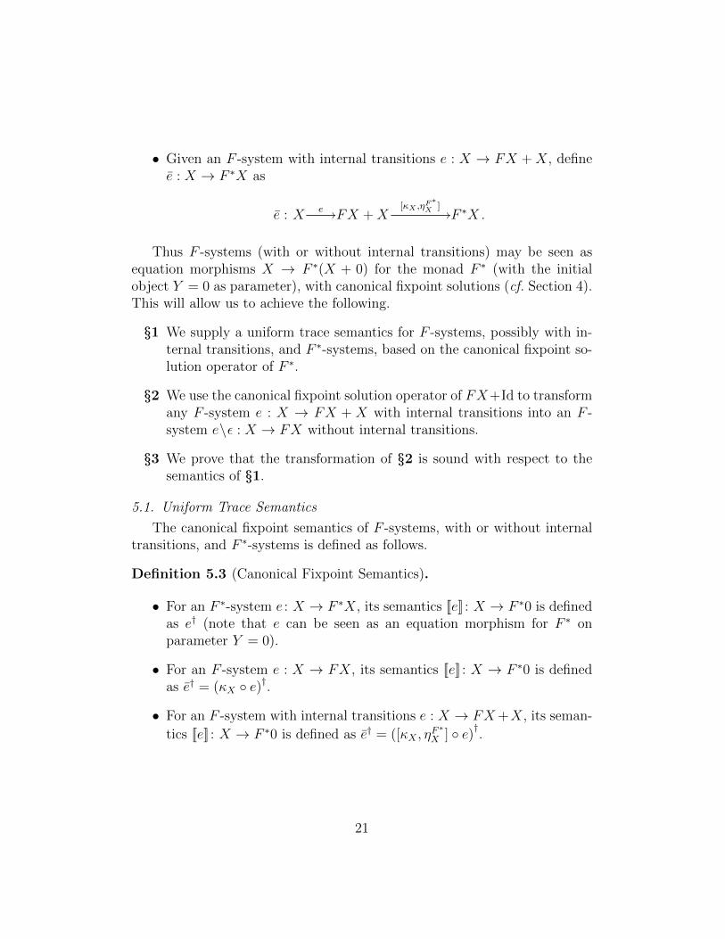
Definition 5.3 (Canonical Fixpoint Semantics).

• For an F ∗-system e : X → F ∗X, its semantics [[e]] : X → F ∗0 is definedas e† (note that e can be seen as an equation morphism for F ∗ onparameter Y = 0).

• For an F -system e : X → FX, its semantics [[e]] : X → F ∗0 is definedas e† = (κX ◦ e)†.

• For an F -system with internal transitions e : X → FX+X, its seman-

tics [[e]] : X → F ∗0 is defined as e† = ([κX , ηF ∗X ] ◦ e)†.

21

The underlying intuition of Definition 5.3 is that canonical fixpoint so-lutions may be given an operational understanding. Given an F ∗-systeme : X → F ∗X, its solution e† : X → F ∗0 is formally defined as the composite¡ ◦ !e (cf. (5)): we can see the coalgebra morphism !e as a map that gives thebehaviour of system e without taking into account the structure of labels andthe algebra morphism ¡ as evaluating this structure, e.g. flattening words ofwords, using the initial algebra µF

∗0 : F ∗F ∗0 → F ∗0 for the monad F ∗. In

particular, the action of ¡ is what makes our semantics suitable for modeling“algebraic” operations on internal transitions such as ε-elimination, as wewill see in concrete instances of our framework.

Remark 5.4. The canonical fixpoint semantics of Definition 5.3 encompassesthe framework for traces in [23], where the semantics of an F -system e :X → FX—without internal transitions—is defined as the unique morphism!e from X into the final F -coalgebra F ∗0. Indeed, using finality of F ∗0, it canbe shown that !e = [[e]]. Theorem 5.5 below guarantees compatibility withAssumption 5.1.

The following result is instrumental in our examples and in comparing ourtheory with the one developed in [23] for trace semantics in Kleisli categories.

Theorem 5.5. Let M : Sets→ Sets be a monad and H : Sets→ Sets be afunctor satisfying the assumptions of Theorem 2.10, that is:

(a) K`(M) is Cppo-enriched and composition is left strict;

(b) H is accessible and has a locally continuous lifting H : K`(M)→ K`(M).

Then K`(M), H, H∗ and HJX + Id (for a given set X) satisfy Assumption5.1.

Before we proceed to prove the above theorem, we first show its relevancefor the motivating examples of Section 3.

Example 5.6 (Semantics of NDA with word transitions). In Section 3, wehave modeled NDA with word transitions as H∗-coalgebras on K`(M), whereH and M are defined as for NDA (see Example 2.11). By Proposition 2.5,H∗ = H∗ and thus, by virtue of Theorem 5.5, H∗ satisfies Assumption 5.1.Therefore we can define the semantics of NDA with word transitions e : X →

22

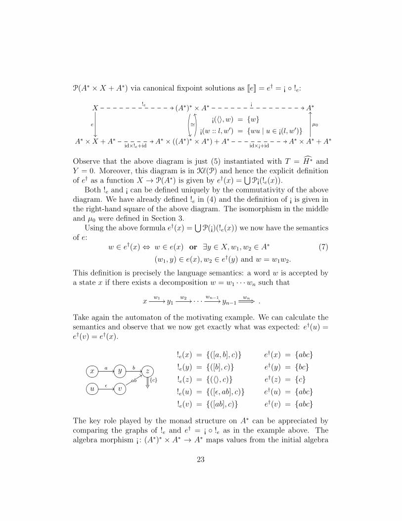
P(A∗ ×X + A∗) via canonical fixpoint solutions as [[e]] = e† = ¡ ◦ !e:

X!e //

e

��

(A∗)∗ ×A∗

∼=

��

¡//

¡(〈〉, w) = {w}¡(w :: l, w′) = {wu | u ∈ ¡(l, w′)}

A∗

A∗ ×X +A∗id×!e+id

// A∗ × ((A∗)∗ ×A∗) +A∗

TT

idס+id// A∗ ×A∗ +A∗

µ0

OO

(6)

Observe that the above diagram is just (5) instantiated with T = H∗ andY = 0. Moreover, this diagram is in K`(P) and hence the explicit definitionof e† as a function X → P(A∗) is given by e†(x) =

⋃P¡(!e(x)).

Both !e and ¡ can be defined uniquely by the commutativity of the abovediagram. We have already defined !e in (4) and the definition of ¡ is given inthe right-hand square of the above diagram. The isomorphism in the middleand µ0 were defined in Section 3.

Using the above formula e†(x) =⋃

P(¡)(!e(x)) we now have the semanticsof e:

w ∈ e†(x)⇔ w ∈ e(x) or ∃y ∈ X,w1, w2 ∈ A∗

(w1, y) ∈ e(x), w2 ∈ e†(y) and w = w1w2.

(7)

This definition is precisely the language semantics: a word w is accepted bya state x if there exists a decomposition w = w1 · · ·wn such that

xw1 // y1

w2 // · · · wn−1// yn−1

wn +3 .

Take again the automaton of the motivating example. We can calculate thesemantics and observe that we now get exactly what was expected: e†(u) =e†(v) = e†(x).

x a // y b // z{c}��u ε // v

ab

99

!e(x) = {([a, b], c)}!e(y) = {([b], c)}!e(z) = {(〈〉, c)}!e(u) = {([ε, ab], c)}!e(v) = {([ab], c)}

e†(x) = {abc}e†(y) = {bc}e†(z) = {c}e†(u) = {abc}e†(v) = {abc}

The key role played by the monad structure on A∗ can be appreciated bycomparing the graphs of !e and e† = ¡ ◦ !e as in the example above. Thealgebra morphism ¡ : (A∗)∗ × A∗ → A∗ maps values from the initial algebra

23

(A∗)∗ ×A∗ for the endofunctor H∗ into the initial algebra A∗ for the monadH∗: its action is precisely to take into account the additional equationsencoded by the algebraic theory of the monad H∗. For instance, we cansee the mapping of !e(u) = {([ε, ab], c)} into the word abc as the result ofconcatenating the words ε, ab, c and then quotienting out of the equationεabc = abc in the monoid A∗.

Remark 5.7 (Multiple Solutions). The canonical solution e† is not theunique solution. Indeed, the uniqueness of !e in the left-hand square and of ¡in the right-hand square of the diagram above does not imply the uniquenessof e†. To see this, take for instance the automaton

x εii

Both s(x) = ∅ and s′(x) = A∗ are solutions. The canonical one is the leastone, i.e., e†(x) = s(x) = ∅. Indeed, as discussed in Remark 4.4(2), wheneverthe underlying category is Cppo-enriched and the monad locally continuous,the canonical solution coincides with the least fixpoint solution introducedin Example 2.14

Example 5.8 (Semantics of NDA with ε-transitions). NDA with ε-tran-sitions are modeled as H + Id-coalgebras on K`(M), where H and M aredefined as for NDA (see Example 2.11). We can define the semantics of NDAwith ε-transitions via canonical fixpoint solutions as [[e]] = e†, where e is theautomaton with word transitions corresponding to e (see Definition 5.2). Thefirst example in Section 3 would be represented as follows,

x ε // y ε // z aii

e(x) = [κX , ηX ] ◦ e(x) = {(ε, y)}e(y) = [κX , ηX ] ◦ e(y) = {(ε, z)}e(z) = [κX , ηX ] ◦ e(z) = {(a, z), ε}

where η and κ are defined as at the end of Section 3. By using (7), it can beeasily checked that the semantics [[e]] = e† : X → PA∗ maps x, y and z intoa∗.

We now proceed to prove Theorem 5.5. First, we give more details onaccessible endofunctors and how they yield a canonical free algebra construc-tion.

24

Remark 5.9. (1) Adamek and Porst [4] showed that an endofunctor Hon Sets is accessible if and only if it is bounded in the following sense:there exists a cardinal λ such that for every set A, every element of HAlies in the image of Hb for some b : B ↪→ A of less than λ elements.

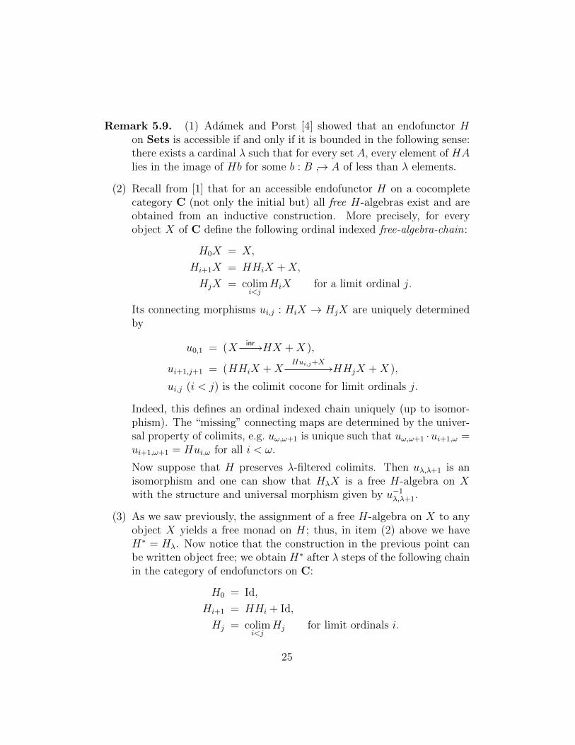
(2) Recall from [1] that for an accessible endofunctor H on a cocompletecategory C (not only the initial but) all free H-algebras exist and areobtained from an inductive construction. More precisely, for everyobject X of C define the following ordinal indexed free-algebra-chain:

H0X = X,

Hi+1X = HHiX +X,

HjX = colimi<j

HiX for a limit ordinal j.

Its connecting morphisms ui,j : HiX → HjX are uniquely determinedby

u0,1 = (X inr //HX +X ),

ui+1,j+1 = (HHiX +XHui,j+X

//HHjX +X ),

ui,j (i < j) is the colimit cocone for limit ordinals j.

Indeed, this defines an ordinal indexed chain uniquely (up to isomor-phism). The “missing” connecting maps are determined by the univer-sal property of colimits, e.g. uω,ω+1 is unique such that uω,ω+1 ·ui+1,ω =ui+1,ω+1 = Hui,ω for all i < ω.

Now suppose that H preserves λ-filtered colimits. Then uλ,λ+1 is anisomorphism and one can show that HλX is a free H-algebra on Xwith the structure and universal morphism given by u−1

λ,λ+1.

(3) As we saw previously, the assignment of a free H-algebra on X to anyobject X yields a free monad on H; thus, in item (2) above we haveH∗ = Hλ. Now notice that the construction in the previous point canbe written object free; we obtain H∗ after λ steps of the following chainin the category of endofunctors on C:

H0 = Id,

Hi+1 = HHi + Id,

Hj = colimi<j

Hj for limit ordinals i.

25

The connecting natural transformations Hi ⇒ Hj have the componentsdescribed as connecting morphisms in item (2).

As a consequence we see that if H is accessible then so is H∗; indeed,all Hi preserve λ-filtered colimits if H does.

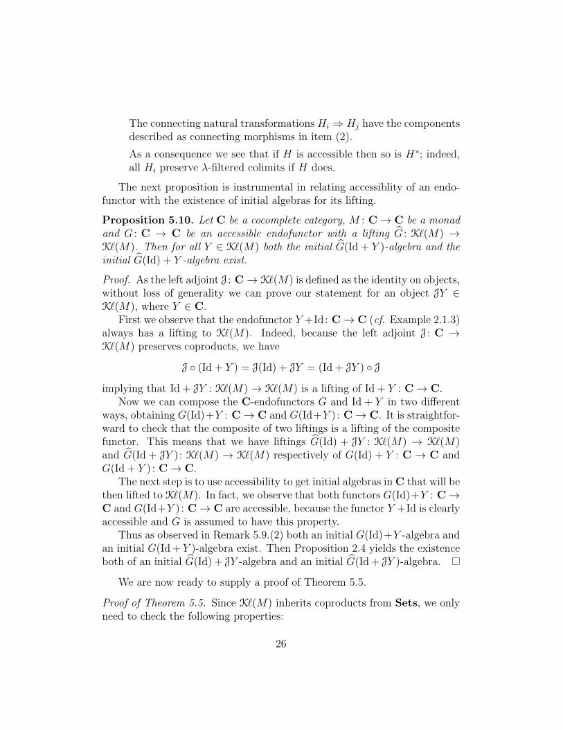
The next proposition is instrumental in relating accessiblity of an endo-functor with the existence of initial algebras for its lifting.

Proposition 5.10. Let C be a cocomplete category, M : C→ C be a monadand G : C → C be an accessible endofunctor with a lifting G : K`(M) →K`(M). Then for all Y ∈ K`(M) both the initial G(Id + Y )-algebra and theinitial G(Id) + Y -algebra exist.

Proof. As the left adjoint J : C→ K`(M) is defined as the identity on objects,without loss of generality we can prove our statement for an object JY ∈K`(M), where Y ∈ C.

First we observe that the endofunctor Y +Id: C→ C (cf. Example 2.1.3)always has a lifting to K`(M). Indeed, because the left adjoint J : C →K`(M) preserves coproducts, we have

J ◦ (Id + Y ) = J(Id) + JY = (Id + JY ) ◦ J

implying that Id + JY : K`(M)→ K`(M) is a lifting of Id + Y : C→ C.Now we can compose the C-endofunctors G and Id + Y in two different

ways, obtaining G(Id)+Y : C→ C and G(Id+Y ) : C→ C. It is straightfor-ward to check that the composite of two liftings is a lifting of the compositefunctor. This means that we have liftings G(Id) + JY : K`(M) → K`(M)and G(Id + JY ) : K`(M) → K`(M) respectively of G(Id) + Y : C → C andG(Id + Y ) : C→ C.

The next step is to use accessibility to get initial algebras in C that will bethen lifted to K`(M). In fact, we observe that both functors G(Id)+Y : C→C and G(Id+Y ) : C→ C are accessible, because the functor Y +Id is clearlyaccessible and G is assumed to have this property.

Thus as observed in Remark 5.9.(2) both an initial G(Id)+Y -algebra andan initial G(Id + Y )-algebra exist. Then Proposition 2.4 yields the existenceboth of an initial G(Id) + JY -algebra and an initial G(Id + JY )-algebra.

We are now ready to supply a proof of Theorem 5.5.

Proof of Theorem 5.5. Since K`(M) inherits coproducts from Sets, we onlyneed to check the following properties:

26

1. all free H-algebras exist;

2. for all Y ∈ K`(M), the initial algebras for H∗(Id + Y ), H∗(H∗(Id +Y ) + Y ) and H∗(Id + Id + Y ) exist;

3. for all Y ∈ K`(M), the initial algebras for HJX + Id + Y , HJX +HJX + Id + Y + Y and HJX + Id + Id + Y exist.

Then it follows from Proposition 2.9, Theorem 2.8 and the fact the coproductsin K`(M) are Cppo-enriched that H∗ and HJX + Id have sufficiently manycanonical fixpoints.

By virtue of Proposition 5.10, the three properties above are impliedrespectively by the following statements:

1. the functor H : Sets→ Sets is accessible;

2. the functor H∗ : K`(M) → K`(M) is the lifting of H∗ : Sets → Setsand H∗ is accessible;

3. the functor HJX+Id: K`(M)→ K`(M) is the lifting ofHX+Id: Sets→Sets and HX + Id is accessible.

The first point is given by assumption. For the second point, H∗ is accessibleby Remark 5.9.(3) and H∗ : K`(M)→ K`(M) is its lifting by Proposition 2.5.For the third point, since the identity Id : Sets → Sets and the constantfunctor HX : Sets → Sets are clearly accessible and coproducts preservethis property, then HX + Id: Sets → Sets is also accessible. As the leftadjoint J : Sets → K`(M) preserves coproducts, it is immediate to checkthat HJX + Id: K`(M) → K`(M) is the lifting of HX + Id: Sets → Sets.Indeed:

J ◦ (HX + Id) = JHX + J(Id) = HJX + J(Id) = (HJX + Id) ◦ J.

This concludes the proof of the three properties above.

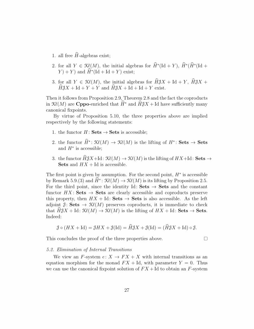
5.2. Elimination of Internal Transitions

We view an F -system e : X → FX + X with internal transitions as anequation morphism for the monad FX + Id, with parameter Y = 0. Thuswe can use the canonical fixpoint solution of FX + Id to obtain an F -system

27

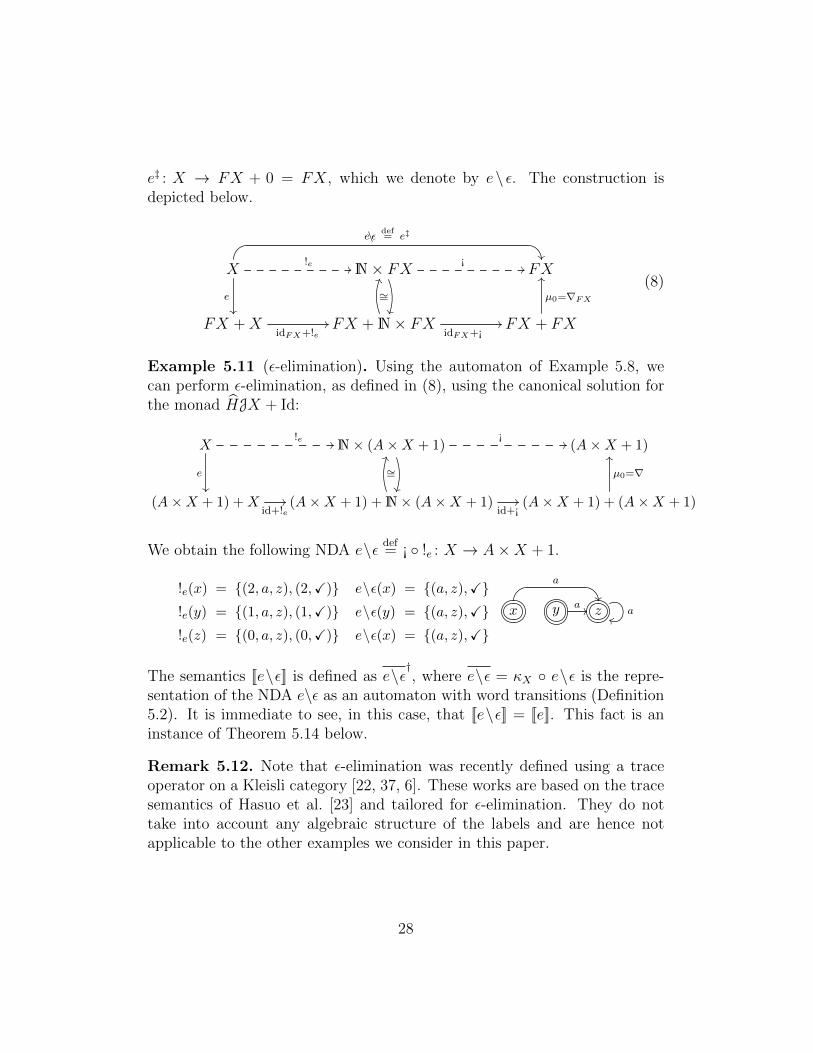
e‡ : X → FX + 0 = FX, which we denote by e\ ε. The construction isdepicted below.

X!e //

e

��

N× FX∼=

¡// FX��

e\ε def= e‡

FX +XidFX+!e

// FX +N× FX

II

idFX+¡// FX + FX

µ0=∇FX

OO(8)

Example 5.11 (ε-elimination). Using the automaton of Example 5.8, wecan perform ε-elimination, as defined in (8), using the canonical solution forthe monad HJX + Id:

X!e //

e

��

N× (A×X + 1)

∼=

¡// (A×X + 1)

(A×X + 1) +Xid+!e// (A×X + 1) +N× (A×X + 1)

JJ

id+¡// (A×X + 1) + (A×X + 1)

µ0=∇

OO

We obtain the following NDA e\ε def= ¡ ◦ !e : X → A×X + 1.

!e(x) = {(2, a, z), (2,X)}!e(y) = {(1, a, z), (1,X)}!e(z) = {(0, a, z), (0,X)}

e\ε(x) = {(a, z),X}e\ε(y) = {(a, z),X}e\ε(x) = {(a, z),X}

x y a // z ahh

��

a

The semantics [[e\ε]] is defined as e\ε†, where e\ε = κX ◦ e\ε is the repre-

sentation of the NDA e\ε as an automaton with word transitions (Definition5.2). It is immediate to see, in this case, that [[e\ε]] = [[e]]. This fact is aninstance of Theorem 5.14 below.

Remark 5.12. Note that ε-elimination was recently defined using a traceoperator on a Kleisli category [22, 37, 6]. These works are based on the tracesemantics of Hasuo et al. [23] and tailored for ε-elimination. They do nottake into account any algebraic structure of the labels and are hence notapplicable to the other examples we consider in this paper.

28

5.3. Soundness of ε-Elimination

We now formally prove that the canonical fixpoint semantics of e and e\εcoincide. To this end, we first show how the construction e 7→ e\ε can beexpressed in terms of the canonical fixpoint solution of F ∗. This turns out tobe an application of †-preservation (Proposition 4.5), for which we introducethe natural transformation π : FX + Id⇒ F ∗(X + Id) defined at Y ∈ C by

πY : FX + Y[κX , η

F∗Y ]

// F ∗X + F ∗Y[F ∗inl,F ∗inr]

// F ∗(X + Y ) .

Since F ∗ is a monad with sufficiently many canonical fixpoints, it followsthat so is F ∗(X + Id). Moreover, π is a monad morphism between FX + Idand F ∗(X + Id). These observations allow us to prove the following.

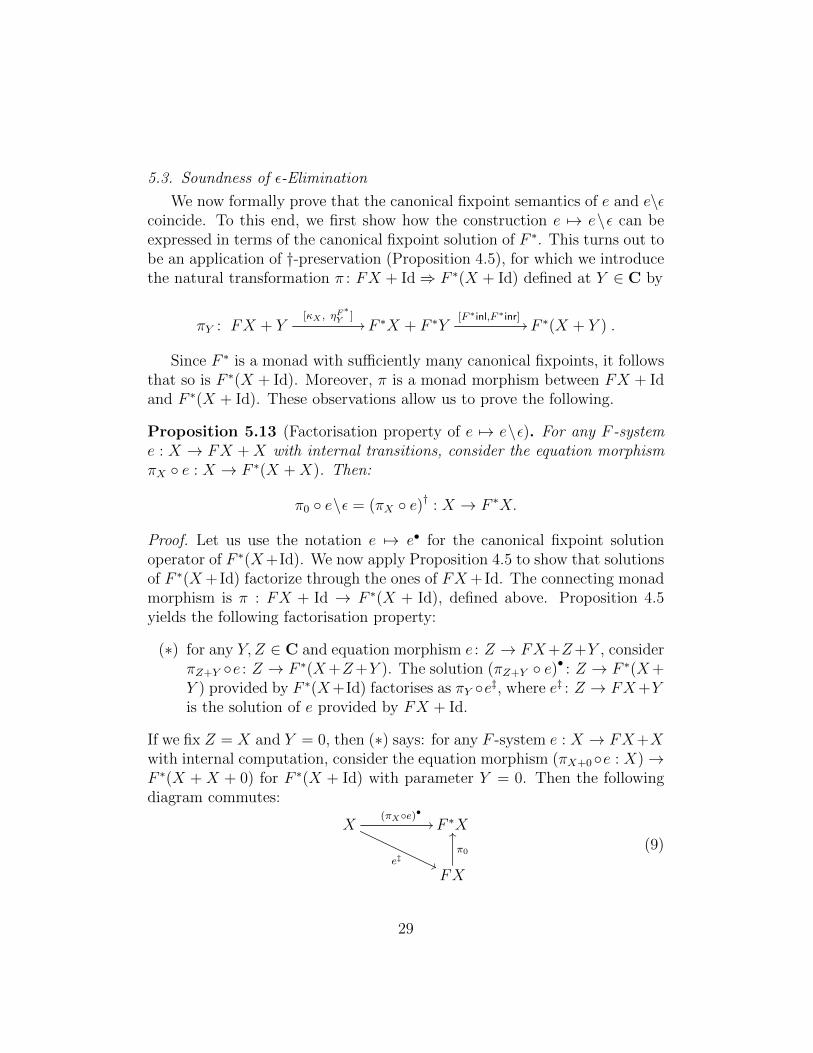
Proposition 5.13 (Factorisation property of e 7→ e\ε). For any F -systeme : X → FX +X with internal transitions, consider the equation morphismπX ◦ e : X → F ∗(X +X). Then:

π0 ◦ e\ε = (πX ◦ e)† : X → F ∗X.

Proof. Let us use the notation e 7→ e• for the canonical fixpoint solutionoperator of F ∗(X+Id). We now apply Proposition 4.5 to show that solutionsof F ∗(X+Id) factorize through the ones of FX+Id. The connecting monadmorphism is π : FX + Id → F ∗(X + Id), defined above. Proposition 4.5yields the following factorisation property:

(∗) for any Y, Z ∈ C and equation morphism e : Z → FX+Z+Y , considerπZ+Y ◦e : Z → F ∗(X+Z+Y ). The solution (πZ+Y ◦ e)• : Z → F ∗(X+Y ) provided by F ∗(X+Id) factorises as πY ◦e‡, where e‡ : Z → FX+Yis the solution of e provided by FX + Id.

If we fix Z = X and Y = 0, then (∗) says: for any F -system e : X → FX+Xwith internal computation, consider the equation morphism (πX+0◦e : X)→F ∗(X + X + 0) for F ∗(X + Id) with parameter Y = 0. Then the followingdiagram commutes:

X(πX◦e)•

//

e‡ ''

F ∗X

FX

π0

OO

(9)

29

To conclude our argument, we observe that the system πX+0◦e : X → F ∗(X+X+0) can be also seen as an equation for F ∗ with parameter Y = X+0. Thismeans that also F ∗ provides a solution to such equation, which can be checkedto coincide with the one given by F ∗(X + Id), that is, (πX ◦ e)• = (πX ◦ e)†.Then the main statement is proven by the following derivation:

π0 ◦ e\ε = π0 ◦ e‡ (Definition of e\ε)= (πX ◦ e)• (commutativity of (9))

= (πX ◦ e)†. (observation above)

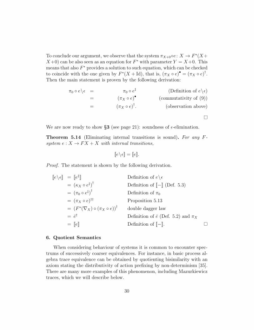
We are now ready to show §3 (see page 21): soundness of ε-elimination.

Theorem 5.14 (Eliminating internal transitions is sound). For any F -system e : X → FX +X with internal transitions,

[[e\ε]] = [[e]].

Proof. The statement is shown by the following derivation.

[[e\ε]] = [[e‡]] Definition of e\ε= (κX ◦ e‡)

†Definition of [[−]] (Def. 5.3)

= (π0 ◦ e‡)†

Definition of π0

= (πX ◦ e)†† Proposition 5.13

= (F ∗(∇X) ◦ (πX ◦ e))† double dagger law

= e† Definition of e (Def. 5.2) and πX

= [[e]] Definition of [[−]].

6. Quotient Semantics

When considering behaviour of systems it is common to encounter spec-trums of successively coarser equivalences. For instance, in basic process al-gebra trace equivalence can be obtained by quotienting bisimilarity with anaxiom stating the distributivity of action prefixing by non-determinism [35].There are many more examples of this phenomenon, including Mazurkiewicztraces, which we will describe below.

30

In this section we develop a variant of the canonical fixpoint semantics,where we can encompass in a uniform manner behaviours which are quotientsof the canonical behaviours of the previous section (that is, the object F ∗0).

Assumption 6.1. Let C, F , F ∗ and FX + Id be as in Assumption 5.1and γ : F ∗ ⇒ Q a monad quotient for some monad Q, i.e., the naturaltransformation γ has epimorphic components. Moreover, suppose that Qhas sufficiently many canonical fixpoints.

Observe that, as Assumption 6.1 subsumes Assumption 5.1, we are withinthe framework of the previous section, with the canonical fixpoint solutionof F ∗ providing semantics for F ∗- and F -systems. For our extension, oneis interested in Q0 as a semantic domain coarser than F ∗0 and we aim atdefining an interpretation for F -systems in Q0. We first note that accordingto Theorem 4.3, Q is a monad with canonical fixpoint solutions, which sat-isfy the double dagger law. We use the notation e 7→ e∼ for the canonicalfixpoint operator of Q. This allows us to define the semantics of Q-systems,analogously to what we did for F ∗-systems in Definition 5.3. Moreover, theconnecting monad morphism γ : F ∗ ⇒ Q yields an extension of this semanticsto include also systems of transition type F ∗ and F .

Definition 6.2 (Quotient Semantics). The quotient semantics of F -systems,with or without internal transitions, F ∗-systems and Q-systems is defined asfollows.

• For a Q-system e : X → QX, its semantics [[e]]∼ : X → Q0 is defined ase∼ (note that e can be regarded as an equation morphism for Q withY = 0).

• For an F ∗-system e : X → F ∗X, its semantics [[e]]∼ : X → Q0 is definedas (γX ◦ e)∼.

• For an F -system e—with or without internal transitions—its semantics[[e]]∼ : X → Q0 is defined as (γX ◦ e)∼, where e is as in Definition 5.2.

Proposition 4.5 allows us to establish a link between the canonical fixpointsemantics [[−]] and the quotient semantics [[−]]∼.

Proposition 6.3 (Factorisation for the quotient semantics). Let e be eitheran F ∗-system or an F -system (with or without internal transitions). Then:

[[e]]∼ = γ0 ◦ [[e]]. (10)

31

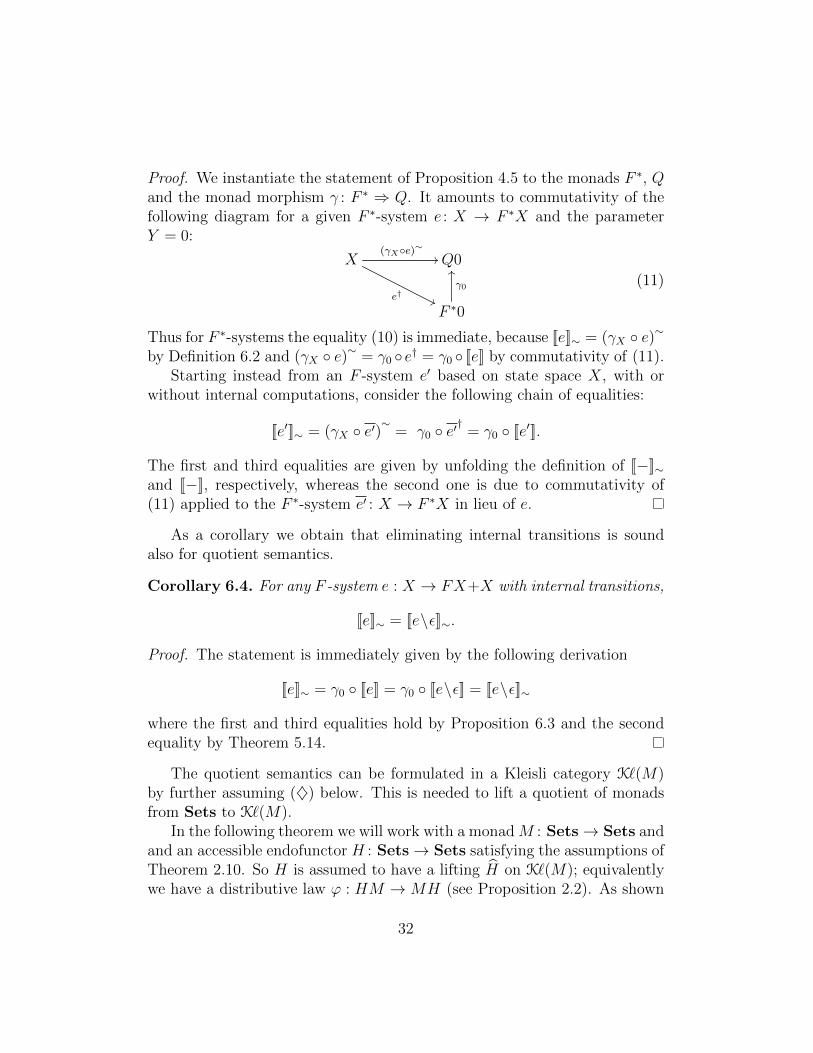
Proof. We instantiate the statement of Proposition 4.5 to the monads F ∗, Qand the monad morphism γ : F ∗ ⇒ Q. It amounts to commutativity of thefollowing diagram for a given F ∗-system e : X → F ∗X and the parameterY = 0:

X(γX◦e)∼

//

e† ''

Q0

F ∗0

γ0

OO

(11)

Thus for F ∗-systems the equality (10) is immediate, because [[e]]∼ = (γX ◦ e)∼by Definition 6.2 and (γX ◦ e)∼ = γ0 ◦ e† = γ0 ◦ [[e]] by commutativity of (11).

Starting instead from an F -system e′ based on state space X, with orwithout internal computations, consider the following chain of equalities:

[[e′]]∼ = (γX ◦ e′)∼

= γ0 ◦ e′†

= γ0 ◦ [[e′]].

The first and third equalities are given by unfolding the definition of [[−]]∼and [[−]], respectively, whereas the second one is due to commutativity of(11) applied to the F ∗-system e′ : X → F ∗X in lieu of e.

As a corollary we obtain that eliminating internal transitions is soundalso for quotient semantics.

Corollary 6.4. For any F -system e : X → FX+X with internal transitions,

[[e]]∼ = [[e\ε]]∼.

Proof. The statement is immediately given by the following derivation

[[e]]∼ = γ0 ◦ [[e]] = γ0 ◦ [[e\ε]] = [[e\ε]]∼

where the first and third equalities hold by Proposition 6.3 and the secondequality by Theorem 5.14.

The quotient semantics can be formulated in a Kleisli category K`(M)by further assuming (♦) below. This is needed to lift a quotient of monadsfrom Sets to K`(M).

In the following theorem we will work with a monad M : Sets→ Sets andand an accessible endofunctor H : Sets→ Sets satisfying the assumptions ofTheorem 2.10. So H is assumed to have a lifting H on K`(M); equivalentlywe have a distributive law ϕ : HM → MH (see Proposition 2.2). As shown

32

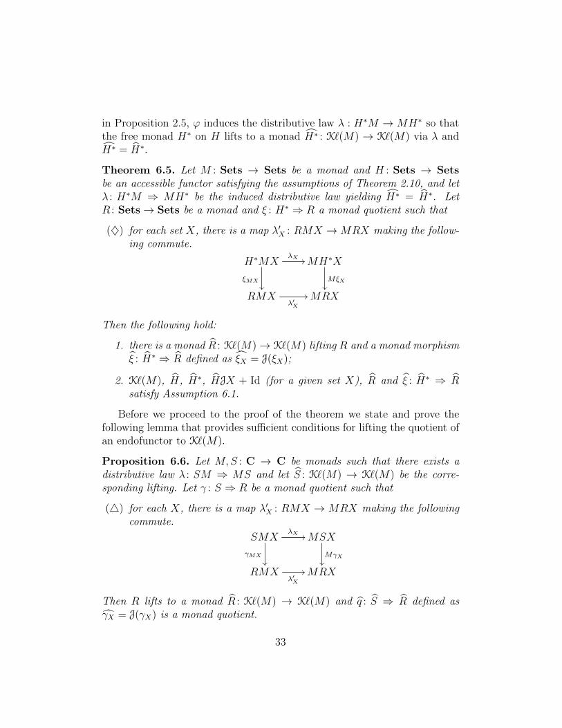
in Proposition 2.5, ϕ induces the distributive law λ : H∗M → MH∗ so thatthe free monad H∗ on H lifts to a monad H∗ : K`(M) → K`(M) via λ andH∗ = H∗.

Theorem 6.5. Let M : Sets → Sets be a monad and H : Sets → Setsbe an accessible functor satisfying the assumptions of Theorem 2.10, and letλ : H∗M ⇒ MH∗ be the induced distributive law yielding H∗ = H∗. LetR : Sets→ Sets be a monad and ξ : H∗ ⇒ R a monad quotient such that

(♦) for each set X, there is a map λ′X : RMX →MRX making the follow-ing commute.

H∗MX

ξMX

��

λX //MH∗X

MξX��

RMXλ′X

//MRX

Then the following hold:

1. there is a monad R : K`(M)→ K`(M) lifting R and a monad morphismξ : H∗ ⇒ R defined as ξX = J(ξX);

2. K`(M), H, H∗, HJX + Id (for a given set X), R and ξ : H∗ ⇒ Rsatisfy Assumption 6.1.

Before we proceed to the proof of the theorem we state and prove thefollowing lemma that provides sufficient conditions for lifting the quotient ofan endofunctor to K`(M).

Proposition 6.6. Let M,S : C → C be monads such that there exists adistributive law λ : SM ⇒ MS and let S : K`(M) → K`(M) be the corre-sponding lifting. Let γ : S ⇒ R be a monad quotient such that

(4) for each X, there is a map λ′X : RMX → MRX making the followingcommute.

SMX

γMX

��

λX //MSX

MγX��

RMXλ′X

//MRX

Then R lifts to a monad R : K`(M) → K`(M) and q : S ⇒ R defined asγX = J(γX) is a monad quotient.

33

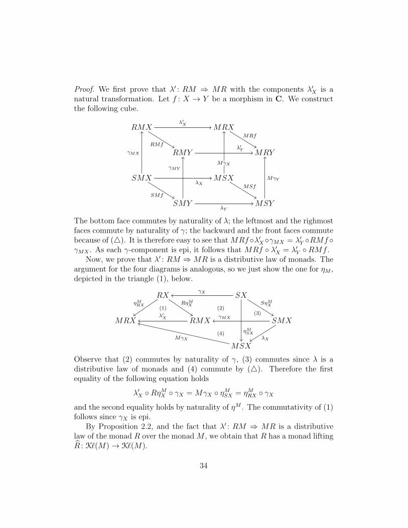
Proof. We first prove that λ′ : RM ⇒ MR with the components λ′X is anatural transformation. Let f : X → Y be a morphism in C. We constructthe following cube.

RMX

RMf %%

λ′X //MRXMRf

%%

RMYλ′Y //MRY

SMX

SMf %%

γMX

OO

λX//MSX

MSf

%%

MγX

OO

SMY

γMY

OO

λY//MSY

MγY

OO

The bottom face commutes by naturality of λ; the leftmost and the righmostfaces commute by naturality of γ; the backward and the front faces commutebecause of (4). It is therefore easy to see that MRf ◦λ′X ◦γMX = λ′Y ◦RMf ◦γMX . As each γ-component is epi, it follows that MRf ◦ λ′X = λ′Y ◦RMf .

Now, we prove that λ′ : RM ⇒MR is a distributive law of monads. Theargument for the four diagrams is analogous, so we just show the one for ηM ,depicted in the triangle (1), below.

RX

(1)RηMX

$$

ηMRX

zz

SX

(2)

ηMSX

��

γXoo

SηMX

%%

MRX RMXλ′Xoo SMX

(3)

λXyy

γMXoo

MSX

(4)MγX

kk

Observe that (2) commutes by naturality of γ, (3) commutes since λ is adistributive law of monads and (4) commute by (4). Therefore the firstequality of the following equation holds

λ′X ◦RηMX ◦ γX = MγX ◦ ηMSX = ηMRX ◦ γXand the second equality holds by naturality of ηM . The commutativity of (1)follows since γX is epi.

By Proposition 2.2, and the fact that λ′ : RM ⇒ MR is a distributivelaw of the monad R over the monad M , we obtain that R has a monad liftingR : K`(M)→ K`(M).

34

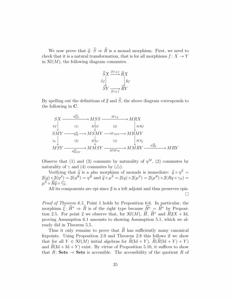
We now prove that q : S ⇒ R is a monad morphism. First, we need tocheck that it is a natural transformation, that is for all morphisms f : X → Yin K`(M), the following diagram commutes.

SXJ(γX)

//

Sf��

RX

Rf��

SYJ(γY )

// RY

By spelling out the definitions of J and S, the above diagram corresponds tothe following in C.

SX

(1)

ηMSX //

Sf��

MSS

(2)

MγX //

MSf��

MRX

MRf��

SMY

(3)

ηMSY//

λY��

MSMY

(4)

MγMY//

MλY��

MRMY

Mλ′Y��

MSYηMMSY

//MMSYMMγY

//MMRYµMRY //MRY

Observe that (1) and (3) commute by naturality of ηM , (2) commutes bynaturality of γ and (4) commutes by (4).

Verifying that q is a also morphism of monads is immediate: q ◦ ηS =J(q) ◦ J(ηS) = J(ηR) = ηR and q ◦ µS = J(q) ◦ J(µS) = J(µR) ◦ J(Rq ◦ γS) =µS ◦ Rq ◦ γS.

All its components are epi since J is a left adjoint and thus preserves epis.

Proof of Theorem 6.5. Point 1 holds by Proposition 6.6. In particular, themorphism ξ : H∗ ⇒ R is of the right type because H∗ = H∗ by Proposi-tion 2.5. For point 2 we observe that, for K`(M), H, H∗ and HJX + Id,proving Assumption 6.1 amounts to showing Assumption 5.1, which we al-ready did in Theorem 5.5.

Thus it only remains to prove that R has sufficiently many canonicalfixpoints. Using Proposition 2.9 and Theorem 2.8 this follows if we showthat for all Y ∈ K`(M) initial algebras for R(Id + Y ), R(R(Id + Y ) + Y )and R(Id + Id + Y ) exist. By virtue of Proposition 5.10, it suffices to showthat R : Sets → Sets is accessible. The accessibility of the quotient R of

35

H∗ : Sets → Sets is guaranteed from the fact that H∗ : Sets → Sets isaccessible (Remark 5.9(3)) and thus bounded (Remark 5.9(1)) and that thequotients of bounded functors are also bounded.

Notice that condition (4) and the first part of Statement 1 are relatedto [11, Theorem 1]; however, that paper treats distributive laws of monadsover endofunctors. Observe also, that [11, Example 3] gives a counterexampleof a monad quotient and distributive law involving the functor FX = R×Xthat does not satisfy (4). This distributive law is easily seen to be a dis-tributive law between monads, if we regard F as a monad (with the monadstructure arising from the monoid (R,+, 0)). Thus, this yields a counterex-ample to Proposition 6.6.

Example 6.7 (Mazurkiewicz traces). This example, using a known equiv-alence in concurrency theory, illustrates the use of the quotient semanticsdeveloped in this section.

The trace semantics proposed by Mazurkiewicz [29] accounts for concur-rent actions. Intuitively, let A be the action alphabet and a, b ∈ A. We willcall a and b concurrent, and write a ≡ b, if the order in which these actionsoccur is not relevant. This means that we equate words that only differ in theorder of these two actions, e.g. uabv and ubav denote the same Mazurkiewicztrace.

To obtain the intended semantics of Mazurkiewicz traces we use the quo-tient semantics defined above3. In particular, for Mazurkiewisz traces oneconsiders a symmetric and irreflexive “independence” relation I on the labelset A. Let ≡ be the least congruence relation on the free monoid A∗ suchthat

(a, b) ∈ I ⇒ ab ≡ ba.

We now have two monads on Sets, namely H∗X = A∗ × X + A∗ andRX = A∗/≡×X+A∗/≡. There is the canonical quotient of monads ξ : H∗ ⇒R given by identifying words of the same ≡-equivalence class. We now verifythat those data satisfy the assumptions of Theorem 6.5.

Proposition 6.8. The monads P : Sets → Sets and R : Sets → Sets, the

3Mazurkiewicz traces were defined over labelled transition systems which are similarto NDA but where every state is final. For simplicity, we consider LTS here immediatelyas NDA.

36

functor H : Sets→ Sets and the quotient of monads ξ : H∗ ⇒ R satisfy theassumptions of Theorem 6.5.

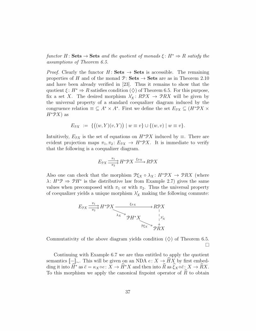
Proof. Clearly the functor H : Sets → Sets is accessible. The remainingproperties of H and of the monad P : Sets → Sets are as in Theorem 2.10and have been already verified in [23]. Thus it remains to show that thequotient ξ : H∗ ⇒ R satisfies condition (♦) of Theorem 6.5. For this purpose,fix a set X. The desired morphism λ′X : RPX → PRX will be given bythe universal property of a standard coequalizer diagram induced by thecongruence relation ≡ ⊆ A∗ × A∗. First we define the set EPX ⊆ (H∗PX ×H∗PX) as

EPX := {((w, Y )(v, Y )

)| w ≡ v} ∪ {(w, v) | w ≡ v}.

Intuitively, EPX is the set of equations on H∗PX induced by ≡. There areevident projection maps π1, π2 : EPX → H∗PX. It is immediate to verifythat the following is a coequalizer diagram.

EPX

π1 //

π2// H∗PX

ξPX // RPX

Also one can check that the morphism PξX ◦ λX : H∗PX → PRX (whereλ : H∗P ⇒ PH∗ is the distributive law from Example 2.7) gives the samevalues when precomposed with π1 or with π2. Thus the universal propertyof coequalizer yields a unique morphism λ′X making the following commute:

EPX

π1 //

π2// H∗PX

ξPX //

λX((

RPX

λ′X

��

PH∗X

PξX((

PRX

Commutativity of the above diagram yields condition (♦) of Theorem 6.5.

Continuing with Example 6.7 we are thus entitled to apply the quotientsemantics [[−]]∼. This will be given on an NDA e : X → HX by first embed-ding it into H∗ as e = κX◦e : X → H∗X and then into R as ξX◦e : X → RX.To this morphism we apply the canonical fixpoint operator of R to obtain

37

(ξX ◦ e)∼, that is, the semantics [[e]]∼ : X → R0 = A∗/≡. It is easy to seethat this definition captures the intended semantics: for all states x ∈ X

[[e]]∼(x) = {[w]≡ | w ∈ [[e]](x)}.

Indeed, by Proposition 6.3, [[e]]∼ = ξ0 ◦ [[e]] and ξ0 : H∗0 → R0 is just Jξ0

where ξ0 : A∗ → A∗/≡ maps every word w into its equivalence class [w]≡.

7. Non-Deterministic Transducers

We now consider another application of our theory, namely to non-deterministictransducers. Introduced by Schutzenberger [36], these systems are a gener-alisation of classical automata by allowing each transition to produce anoutput word. They have been employed in various areas of computationallinguistics [27, 32]. The question of whether transducers could be modelledcoalgebraically was tackled by Hansen [21], though her results were onlyabout deterministic transducers and did not capture the semantics in a fullysatisfactory way.

In this section, we consider the more general case of non-deterministictransducers and show how their semantics can be correctly modeled in aKleisli category. Later, we shall also extend our approach to transducerswith internal behaviour.

Formally, a non-deterministic transducer with inputs in A and outputsin B is a tuple (X, δ, o) where X is a set of states, δ ⊆ X × A × B∗ × Xis a transition relation and o : X → P(B∗) is a terminal output functionassociating to each state a language over B. To avoid confusion amongstthe words in A∗ and those in B∗, we use w,w1, w2, . . . for the former and

v, v1, v2, . . . for the latter. Moreover, we write xa/v−−→ y for (x, a, v, y) ∈ δ

and x⇓v for v ∈ o(x). We shall simply speak of transducers dropping “non-deterministic” whenever we feel like it.

Every state x ∈ X induces a function ‖x‖ : A∗ → P(B∗) mapping a wordw ∈ A∗ into the set

‖x‖(w) = {v | ∃xi ∈ X, ai ∈ A, vi ∈ B∗ s.t. w = a1 · · · an,

v = v1 · · · vn+1 and xa1/v1−−−→ x1 · · ·

an/vn−−−→ xn⇓vn+1}.

For example consider the transducer A (below on the left) with input alpha-bet A = {a} and output alphabet B = {0, 1}. The function o has value {1}

38

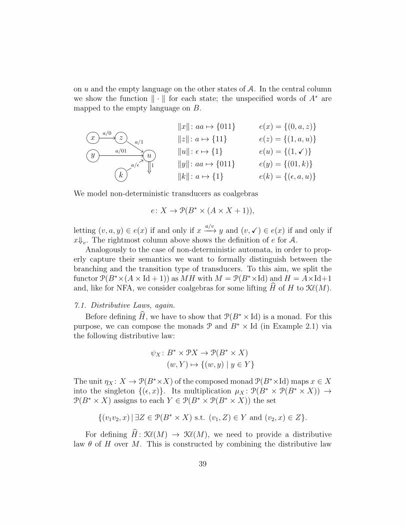
on u and the empty language on the other states of A. In the central columnwe show the function ‖ · ‖ for each state; the unspecified words of A∗ aremapped to the empty language on B.

xa/0// z

a/1

%%y

a/01// u

1

��k

a/ε::

‖x‖ : aa 7→ {011}‖z‖ : a 7→ {11}‖u‖ : ε 7→ {1}‖y‖ : aa 7→ {011}‖k‖ : a 7→ {1}

e(x) = {(0, a, z)}e(z) = {(1, a, u)}e(u) = {(1,X)}e(y) = {(01, k)}e(k) = {(ε, a, u)}

We model non-deterministic transducers as coalgebras

e : X → P(B∗ × (A×X + 1)),

letting (v, a, y) ∈ e(x) if and only if xa/v−−→ y and (v,X) ∈ e(x) if and only if

x⇓v. The rightmost column above shows the definition of e for A.Analogously to the case of non-deterministic automata, in order to prop-

erly capture their semantics we want to formally distinguish between thebranching and the transition type of transducers. To this aim, we split thefunctor P(B∗×(A× Id + 1)) as MH with M = P(B∗×Id) and H = A×Id+1and, like for NFA, we consider coalgebras for some lifting H of H to K`(M).

7.1. Distributive Laws, again.

Before defining H, we have to show that P(B∗× Id) is a monad. For thispurpose, we can compose the monads P and B∗ × Id (in Example 2.1) viathe following distributive law:

ψX : B∗ × PX → P(B∗ ×X)

(w, Y ) 7→ {(w, y) | y ∈ Y }

The unit ηX : X → P(B∗×X) of the composed monad P(B∗×Id) maps x ∈ Xinto the singleton {(ε, x)}. Its multiplication µX : P(B∗ × P(B∗ ×X)) →P(B∗ ×X) assigns to each Y ∈ P(B∗ × P(B∗ ×X)) the set

{(v1v2, x) | ∃Z ∈ P(B∗ ×X) s.t. (v1, Z) ∈ Y and (v2, x) ∈ Z}.

For defining H : K`(M) → K`(M), we need to provide a distributivelaw θ of H over M . This is constructed by combining the distributive law

39

ϕ : HP ⇒ PH (given in Example 2.3) and χ : H(B∗ × Id) ⇒ B∗ × H(Id)with the following components:

χX : A× (B∗ ×X) + 1→ B∗ × (A×X + 1)

X 7→ (ε,X)

(a, (w, x)) 7→ (w, (a, x))

Then, we can give θ : HP(B∗ × Id)⇒ P(B∗ ×H(Id)) as:

θX : HP(B∗ ×X)ϕB∗×X

// PH(B∗ ×X)PχX // P(B∗ ×HX).

By unfolding the definitions of ϕ and χ, this just means:

θX : A× P(B∗ ×X) + 1→ P(B∗ × (A×X + 1))

X 7→ {(ε,X)}(a, Y ) 7→ {(w, (a, x)) | (w, x) ∈ Y }

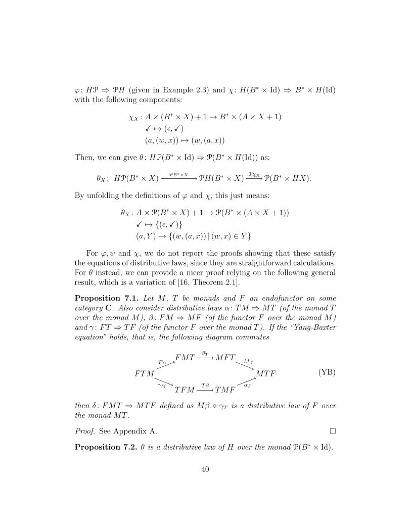
For ϕ, ψ and χ, we do not report the proofs showing that these satisfythe equations of distributive laws, since they are straightforward calculations.For θ instead, we can provide a nicer proof relying on the following generalresult, which is a variation of [16, Theorem 2.1].

Proposition 7.1. Let M , T be monads and F an endofunctor on somecategory C. Also consider distributive laws α : TM ⇒MT (of the monad Tover the monad M), β : FM ⇒ MF (of the functor F over the monad M)and γ : FT ⇒ TF (of the functor F over the monad T ). If the “Yang-Baxterequation” holds, that is, the following diagram commutes

FMTβT //MFT

Mγ))

FTM

Fα 55

γM ))

MTF

TFMTβ// TMF

αF

55(YB)

then δ : FMT ⇒ MTF defined as Mβ ◦ γT is a distributive law of F overthe monad MT .

Proof. See Appendix A.

Proposition 7.2. θ is a distributive law of H over the monad P(B∗ × Id).

40

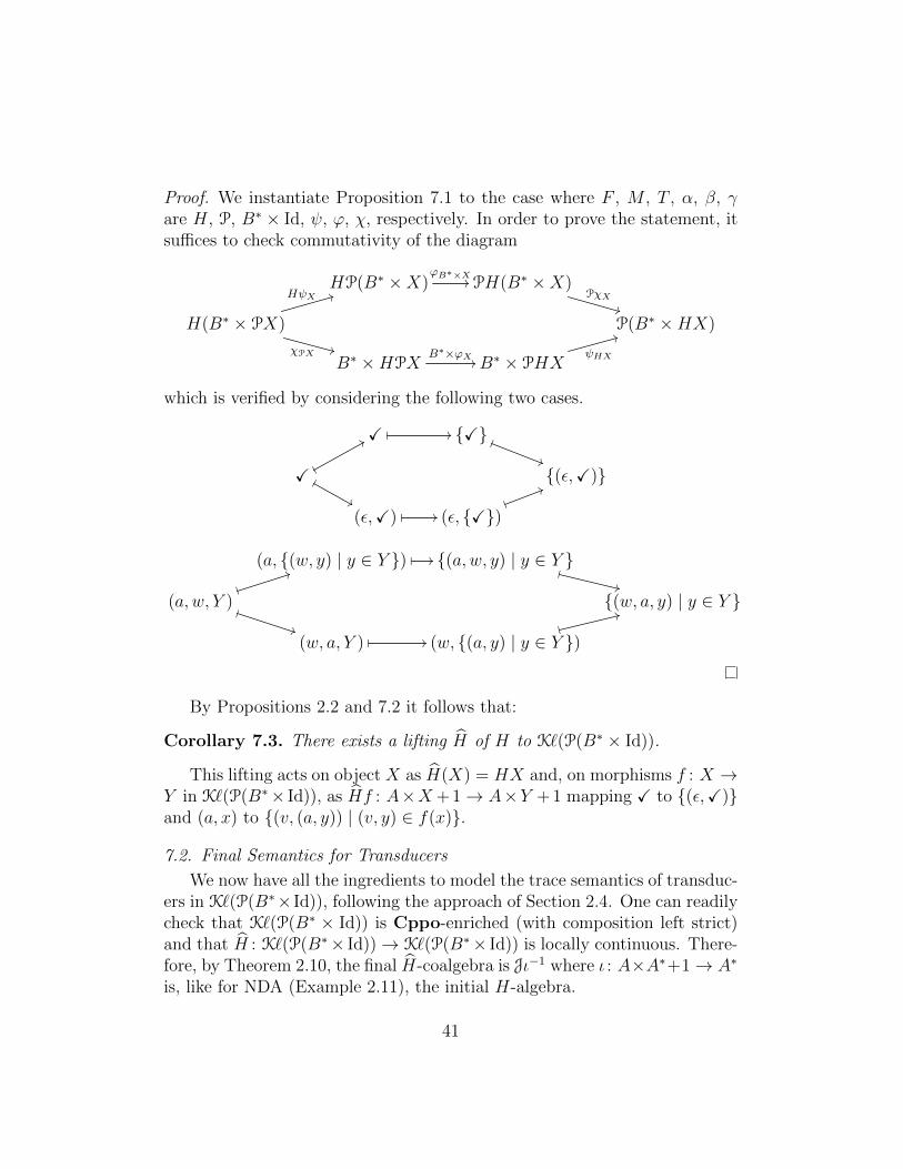
Proof. We instantiate Proposition 7.1 to the case where F , M , T , α, β, γare H, P, B∗ × Id, ψ, ϕ, χ, respectively. In order to prove the statement, itsuffices to check commutativity of the diagram

HP(B∗ ×X)ϕB∗×X

// PH(B∗ ×X)PχX

**

H(B∗ × PX)

HψX 44

χPX ++

P(B∗ ×HX)

B∗ ×HPXB∗×ϕX // B∗ × PHX

ψHX

33

which is verified by considering the following two cases.

X � // {X} �))

X1

88

&&

{(ε,X)}

(ε,X) � // (ε, {X}),

55

(a, {(w, y) | y ∈ Y }) � // {(a, w, y) | y ∈ Y }�

++

(a, w, Y ))

44

�**

{(w, a, y) | y ∈ Y }

(w, a, Y ) � // (w, {(a, y) | y ∈ Y })'

33

By Propositions 2.2 and 7.2 it follows that:

Corollary 7.3. There exists a lifting H of H to K`(P(B∗ × Id)).

This lifting acts on object X as H(X) = HX and, on morphisms f : X →Y in K`(P(B∗× Id)), as Hf : A×X+ 1→ A×Y + 1 mapping X to {(ε,X)}and (a, x) to {(v, (a, y)) | (v, y) ∈ f(x)}.

7.2. Final Semantics for Transducers

We now have all the ingredients to model the trace semantics of transduc-ers in K`(P(B∗× Id)), following the approach of Section 2.4. One can readilycheck that K`(P(B∗ × Id)) is Cppo-enriched (with composition left strict)and that H : K`(P(B∗× Id))→ K`(P(B∗× Id)) is locally continuous. There-fore, by Theorem 2.10, the final H-coalgebra is Jι−1 where ι : A×A∗+1→ A∗

is, like for NDA (Example 2.11), the initial H-algebra.

41

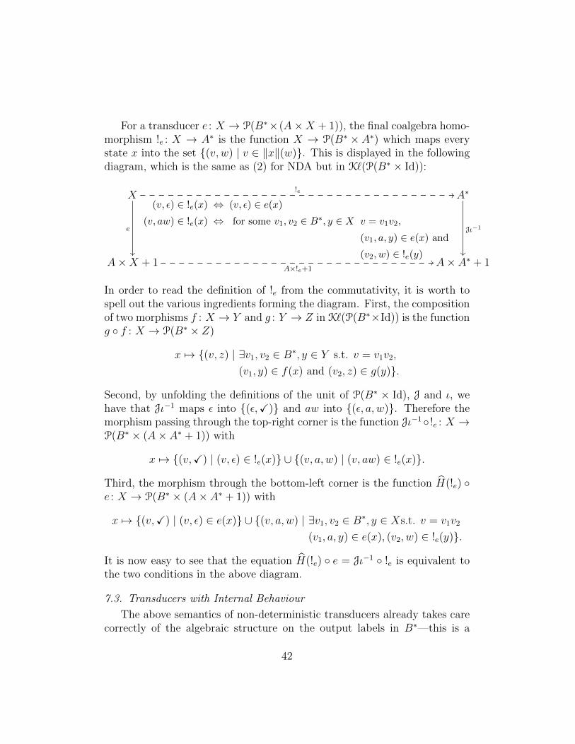
For a transducer e : X → P(B∗×(A×X + 1)), the final coalgebra homo-morphism !e : X → A∗ is the function X → P(B∗ × A∗) which maps everystate x into the set {(v, w) | v ∈ ‖x‖(w)}. This is displayed in the followingdiagram, which is the same as (2) for NDA but in K`(P(B∗ × Id)):

X

e

��

(v, ε) ∈ !e(x) ⇔ (v, ε) ∈ e(x)

(v, aw) ∈ !e(x) ⇔ for some v1, v2 ∈ B∗, y ∈ X v = v1v2,

(v1, a, y) ∈ e(x) and

(v2, w) ∈ !e(y)

!e // A∗

Jι−1

��

A×X + 1A×!e+1

// A× A∗ + 1

In order to read the definition of !e from the commutativity, it is worth tospell out the various ingredients forming the diagram. First, the compositionof two morphisms f : X → Y and g : Y → Z in K`(P(B∗×Id)) is the functiong ◦ f : X → P(B∗ × Z)

x 7→ {(v, z) | ∃v1, v2 ∈ B∗, y ∈ Y s.t. v = v1v2,

(v1, y) ∈ f(x) and (v2, z) ∈ g(y)}.

Second, by unfolding the definitions of the unit of P(B∗ × Id), J and ι, wehave that Jι−1 maps ε into {(ε,X)} and aw into {(ε, a, w)}. Therefore themorphism passing through the top-right corner is the function Jι−1◦ !e : X →P(B∗ × (A× A∗ + 1)) with

x 7→ {(v,X) | (v, ε) ∈ !e(x)} ∪ {(v, a, w) | (v, aw) ∈ !e(x)}.

Third, the morphism through the bottom-left corner is the function H(!e) ◦e : X → P(B∗ × (A× A∗ + 1)) with

x 7→ {(v,X) | (v, ε) ∈ e(x)} ∪ {(v, a, w) | ∃v1, v2 ∈ B∗, y ∈ Xs.t. v = v1v2

(v1, a, y) ∈ e(x), (v2, w) ∈ !e(y)}.

It is now easy to see that the equation H(!e) ◦ e = Jι−1 ◦ !e is equivalent tothe two conditions in the above diagram.

7.3. Transducers with Internal Behaviour

The above semantics of non-deterministic transducers already takes carecorrectly of the algebraic structure on the output labels in B∗—this is a

42

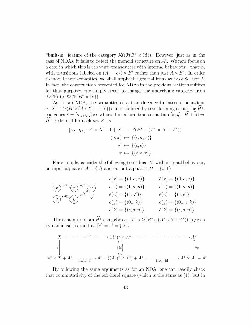
“built-in” feature of the category K`(P(B∗ × Id)). However, just as in thecase of NDAs, it fails to detect the monoid structure on A∗. We now focus ona case in which this is relevant: transducers with internal behaviour—that is,with transitions labeled on (A+ {ε})×B∗ rather than just A×B∗. In orderto model their semantics, we shall apply the general framework of Section 5.In fact, the construction presented for NDAs in the previous sections sufficesfor that purpose: one simply needs to change the underlying category fromK`(P) to K`(P(B∗ × Id)).

As for an NDA, the semantics of a transducer with internal behavioure : X → P(B∗×(A×X+1+X)) can be defined by transforming it into the H∗-coalgebra e = [κX , ηX ]◦ e where the natural transformation [κ, η] : H + Id⇒H∗ is defined for each set X as

[κX , ηX ] : A×X + 1 +X → P(B∗ × (A∗ ×X + A∗))

(a, x) 7→ {(ε, a, x)}X 7→ {(ε, ε)}x 7→ {(ε, ε, x)}

For example, consider the following transducer B with internal behaviour,on input alphabet A = {a} and output alphabet B = {0, 1}.

xa/0// z

a/1// u

1��y

ε/01// k

a/ε99

e(x) = {(0, a, z)}e(z) = {(1, a, u)}e(u) = {(1,X)}e(y) = {(01, k)}e(k) = {(ε, a, u)}

e(x) = {(0, a, z)}e(z) = {(1, a, u)}e(u) = {(1, ε)}e(y) = {(01, ε, k)}e(k) = {(ε, a, u)}.

The semantics of an H∗-coalgebra e : X → P(B∗×(A∗×X+A∗)) is givenby canonical fixpoint as [[e]] = e† = ¡ ◦ !e:

X!e //

e

��

(A∗)∗ ×A∗

∼=

��

¡// A∗

A∗ ×X +A∗id×!e+id

// A∗ × ((A∗)∗ ×A∗) +A∗

TT

idס+id// A∗ ×A∗ +A∗

µ0

OO

(12)

By following the same arguments as for an NDA, one can readily checkthat commutativity of the left-hand square (which is the same as (4), but in

43

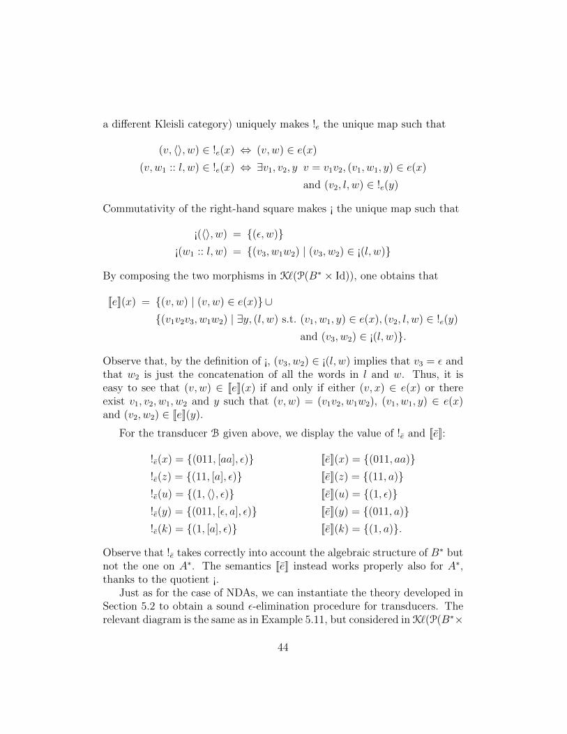
a different Kleisli category) uniquely makes !e the unique map such that

(v, 〈〉, w) ∈ !e(x) ⇔ (v, w) ∈ e(x)

(v, w1 :: l, w) ∈ !e(x) ⇔ ∃v1, v2, y v = v1v2, (v1, w1, y) ∈ e(x)

and (v2, l, w) ∈ !e(y)

Commutativity of the right-hand square makes ¡ the unique map such that

¡(〈〉, w) = {(ε, w)}¡(w1 :: l, w) = {(v3, w1w2) | (v3, w2) ∈ ¡(l, w)}

By composing the two morphisms in K`(P(B∗ × Id)), one obtains that

[[e]](x) = {(v, w) | (v, w) ∈ e(x)}∪{(v1v2v3, w1w2) | ∃y, (l, w) s.t. (v1, w1, y) ∈ e(x), (v2, l, w) ∈ !e(y)

and (v3, w2) ∈ ¡(l, w)}.

Observe that, by the definition of ¡, (v3, w2) ∈ ¡(l, w) implies that v3 = ε andthat w2 is just the concatenation of all the words in l and w. Thus, it iseasy to see that (v, w) ∈ [[e]](x) if and only if either (v, x) ∈ e(x) or thereexist v1, v2, w1, w2 and y such that (v, w) = (v1v2, w1w2), (v1, w1, y) ∈ e(x)and (v2, w2) ∈ [[e]](y).

For the transducer B given above, we display the value of !e and [[e]]:

!e(x) = {(011, [aa], ε)}!e(z) = {(11, [a], ε)}!e(u) = {(1, 〈〉, ε)}!e(y) = {(011, [ε, a], ε)}!e(k) = {(1, [a], ε)}

[[e]](x) = {(011, aa)}[[e]](z) = {(11, a)}[[e]](u) = {(1, ε)}[[e]](y) = {(011, a)}[[e]](k) = {(1, a)}.

Observe that !e takes correctly into account the algebraic structure of B∗ butnot the one on A∗. The semantics [[e]] instead works properly also for A∗,thanks to the quotient ¡.

Just as for the case of NDAs, we can instantiate the theory developed inSection 5.2 to obtain a sound ε-elimination procedure for transducers. Therelevant diagram is the same as in Example 5.11, but considered in K`(P(B∗×

44

Id)) in lieu of K`(P). Concretely, the procedure follows the same rules as theone for NDAs, provided that words of B∗ are composed appropriately whencreating new transitions. For instance, in transforming the transducer B of

the example above, one just needs to replace the transition yε/01−−→ k with

ya/01−−→ u—observe that output ε’s are not eliminated since they belong to

B∗. As a result, one obtains the transducer A introduced at the beginningof this section.

8. Discussion

The framework introduced in this paper provides a uniform way to ex-press the semantics of systems with internal behaviour via canonical fixpointsolutions. Moreover, these solutions are exploited to eliminate internal tran-sitions in a sound way, i.e., preserving the semantics. We have shown ourapproach at work on NDA with ε-transitions but, by virtue of Theorem 5.5,it also covers all the examples in [23] (like probabilistic systems) and more(like the weighted automata on positive reals of [37]).

It is worth noticing that, in principle, our framework is applicable alsoto examples that do not arise from Kleisli categories. Indeed the theoryof Section 4 is formulated for a general category C: Assumption 5.1 onlyrequires C to have coproducts and the monads F ∗ and FX + Id to havesufficiently many canonical fixpoints.

As a further remark, let us recall that our original question concerned theproblem of modeling the semantics of systems where labels carry an algebraicstructure. In this paper we have mostly been focusing on automata theory,but there are many other examples in which the information carried by thelabels has relevance for the semantics of the systems under consideration:in logic programming labels are substitutions of terms; in (concurrent) con-straint programming they are elements of a lattice; in process calculi theyare actions representing syntactical contexts and in tile systems [19] theyare morphisms in a category. We believe that our approach provides variousinsights towards a coalgebraic semantics for these computational models.

The case of process calculi is particularly challenging: internal transitionsare typically abstracted away by a notion of observational equivalence calledweak bisimilarity. Being particularly hard to model by coalgebras, weakbisimilarity has recently captured a renewed interest by the community [12,13, 20, 14]. Some of these works adopt techniques that are also part of

45

our methodology: for instance, the idea of using systems over a free monadalso appeared in [12, 13]. However, the approach is substantially different:rather than eliminating ε-transitions, in weak bisimilarity one has to saturate,namely to add more transitions to the systems.

Acknowledgments. In between the CMCS’14 paper and this journal ver-sion we had the chance to discuss with Alex Simpson at the Bellair Work-shops on Duality and Probabilistic Systems. Alex provided us importantinsights which eventually lead to weaken our assumptions by dropping Cppo-enrichement and local continuity. We would like also to thank Tomasz Bren-gos for the interesting discussion at ETAPS 2014. The work of Alexan-dra Silva is partially funded by the ERDF through the Programme COM-PETE and by the Portuguese Foundation for Science and Technology, projectref. FCOMP-01-0124-FEDER-020537 and SFRH/BPD/71956/2010. The firstand the fourth author acknowledge support by project ANR 12IS0 2001 PACE.

References

[1] Adamek, J., 1974. Free algebras and automata realizations in the lan-guage of categories. Comment. Math. Univ. Carolin. 15, 589–602.

[2] Adamek, J., Milius, S., Velebil, J., 2010. Equational proper-ties of iterative monads. Inform. and Comput. 208, 1306–1348,doi:10.1016/j.ic.2009.10.006.

[3] Adamek, J., Milius, S., Velebil, J., 2011. Elgot theories: a new perspec-tive of the equational properties of iteration. Math. Structures Com-put. Sci. 21 (2), 417–480.

[4] Adamek, J., Porst, H.-E., 2004. On tree coalgebras and coalgebra pre-sentations. Theoret. Comput. Sci. 311, 257–283.

[5] Adamek, J., Rosicky, J., 1994. Locally presentable and accessible cate-gories. Cambridge University Press.

[6] Asada, K., Hidaka, S., Kato, H., Hu, Z., Nakano, K., 2013. A param-eterized graph transformation calculus for finite graphs with monadicbranches. In: Pena, R., Schrijvers, T. (Eds.), PPDP. ACM, pp. 73–84.

[7] Balan, A., Kurz, A., 2011. On coalgebras over algebras. TheoreticalComput. Sci. 412(38), 4989–5005.

46

[8] Barr, M., 1970. Coequalizers and free triples. Math. Z. 116, 307–322.

[9] Bloom, S. L., Esik, Z., 1993. Iteration Theories: the equational logicof iterative processes. EATCS Monographs on Theoretical ComputerScience. Springer.

[10] Bonchi, F., Milius, S., Silva, A., Zanasi, F., 2014. How to kill epsilonswith a dagger - A coalgebraic take on systems with algebraic label struc-ture. In: Coalgebraic Methods in Computer Science - 12th IFIP WG1.3 International Workshop, CMCS 2014, Colocated with ETAPS 2014,Grenoble, France, April 5-6, 2014, Revised Selected Papers. pp. 53–74.

[11] Bonsangue, M. M., Hansen, H. H., Kurz, A., Rot, J., 2013. Presentingdistributive laws. In: [24], pp. 95–109.

[12] Brengos, T., 2013. Weak bisimulation for coalgebras over order enrichedmonads. CoRR abs/1310.3656.URL http://arxiv.org/abs/1310.3656

[13] Brengos, T., 2014. On coalgebras with internal moves. In: Bonsangue,M. M. (Ed.), Coalgebraic Methods in Computer Science - 12th IFIPWG 1.3 International Workshop, CMCS 2014, Colocated with ETAPS2014, Grenoble, France, April 5-6, 2014, Revised Selected Papers. Vol.8446 of Lecture Notes in Computer Science. Springer, pp. 75–97.

[14] Brengos, T., Miculan, M., Peressotti, M., 2014. Behavioural equivalencesfor coalgebras with unobservable moves. CoRR abs/1411.0090.URL http://arxiv.org/abs/1411.0090

[15] Brookes, S. D., Main, M. G., Melton, A., Mislove, M. W., Schmidt, D. A.(Eds.), 1994. Mathematical Foundations of Programming Semantics, 9thInternational Conference, New Orleans, LA, USA, April 7-10, 1993, Pro-ceedings. Vol. 802 of Lecture Notes in Computer Science. Springer.

[16] Cheng, E., 2011. Iterated distributive laws. Math. Proc. Camb. Philos.Soc. 150 (3), 459–487.

[17] Freyd, P., 1991. Algebraically complete categories. In: Carboni, A.,Pedicchio, M. C., Rosolini, G. (Eds.), Category Theory: Proceedings ofthe International Conference held in Como. Vol. 1488 of Lecture Notesin Math. Springer, pp. 95–104.

47

[18] Freyd, P. J., 1992. Remarks on algebraically compact categories. In:Applications of Categories in Computer Science: Proceedings of theLondon Mathematical Society Symposium, Durham 1991. Vol. 177 ofLondon Mathematical Society Lecture Notes Series. Cambridge Univer-sity Press, pp. 95–106.

[19] Gadducci, F., Montanari, U., 2000. The tile model. In: Plotkin, G. D.,Stirling, C., Tofte, M. (Eds.), Proof, Language, and Interaction. TheMIT Press, pp. 133–166.

[20] Goncharov, S., Pattinson, D., 2014. Coalgebraic weak bisimulation fromrecursive equations over monads. In: Esparza, J., Fraigniaud, P., Hus-feldt, T., Koutsoupias, E. (Eds.), Automata, Languages, and Program-ming - 41st International Colloquium, ICALP 2014, Copenhagen, Den-mark, July 8-11, 2014, Proceedings, Part II. Vol. 8573 of Lecture Notesin Computer Science. Springer, pp. 196–207.URL http://dx.doi.org/10.1007/978-3-662-43951-7_17

[21] Hansen, H. H., Dec. 2010. Subsequential transducers: A coalgebraicperspective. Inf. Comput. 208 (12), 1368–1397.

[22] Hasuo, I., 2006. Generic forward and backward simulations. In: Baier,C., Hermanns, H. (Eds.), Proc. International Conference on Concur-rency Theory (CONCUR’06). Vol. 4137 of Lecture Notes in Comput.Sci. Springer, pp. 406–420.

[23] Hasuo, I., Jacobs, B., Sokolova, A., 2007. Generic trace semantics viacoinduction. Log. Methods Comput. Sci. 3 (4:11), 1–36.

[24] Heckel, R., Milius, S. (Eds.), 2013. Algebra and Coalgebra in ComputerScience - 5th International Conference, CALCO 2013, Warsaw, Poland,September 3-6, 2013. Proceedings. Vol. 8089 of Lecture Notes in Com-puter Science. Springer.

[25] Hopcroft, J., Motwani, R., Ullman, J., 2006. Introduction to AutomataTheory, Languages, and Computation (3rd Edition). Wesley.

[26] Johnstone, P., 1975. Adjoint lifting theorems for categories of algebras.Bull. London Math. Soc. 7, 294–297.

48

[27] Jurafsky, D., Martin, J. H., 2009. Speech and Language Processing (2NdEdition). Prentice-Hall, Inc., Upper Saddle River, NJ, USA.

[28] Kelly, G. M., 1980. A unified treatment of transfinite constructions forfree algebras, free monoids, colimits, associated sheaves, and so on.Bull. Austral. Math. Soc. 22, 1–83.

[29] Mazurkiewicz, A., July 1977. Concurrent Program Schemes and TheirInterpretation. Aarhus University, Comp. Sci. Depart., DAIMI PB-78.

[30] Mac Lane, S., 1971. Categories for the Working Mathematician.Springer, Berlin.

[31] Milius, S., Palm, T., Schwencke, D., 2009. Complete iterativityfor algebras with effects. In: Kurz, A., Lenisa, M., Tarlecki, A.(Eds.), Proc. Coalgebraic and Algebraic Methods in Computer Science(CALCO’09). Vol. 5728 of LNCS. Springer, pp. 34–48.

[32] Mohri, M., Jun. 1997. Finite-state transducers in language and speechprocessing. Comput. Linguist. 23 (2), 269–311.

[33] Mulry, P. S., 1993. Lifting theorems for kleisli categories. In: [15], pp.304–319.

[34] Plotkin, G. D., Turi, D., 1997. Towards a mathematical operationalsemantics. In: Proc. Logic in Computer Science (LICS’97). pp. 280–291.

[35] Rabinovich, A. M., 1993. A complete axiomatisation for trace congru-ence of finite state behaviors. In: [15], pp. 530–543.

[36] Schutzenberger, M. P., 1977. Sur une variante des fonctions sequentielles.Theor. Comput. Sci. 4 (1), 47–57.

[37] Silva, A., Westerbaan, B., 2013. A coalgebraic view of -transitions. In:[24], pp. 267–281.

[38] Simpson, A., Plotkin, G. D., 2000. Complete axioms for categoricalfixed-point operators. In: Proc. 15th Symposium on Logic in ComputerScience (LICS’00). IEEE Computer Society, pp. 30–41.

[39] Sobocinski, P., 2012. Relational presheaves as labelled transition sys-tems. In: Coalgebraic Methods in Computer Science (CMCS ‘12). Vol.7399 of LNCS. Springer, pp. 40–50.

49

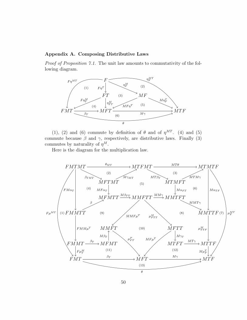
Appendix A. Composing Distributive Laws

Proof of Proposition 7.1. The unit law amounts to commutativity of the fol-lowing diagram.

F

(1)

FηMT

��

FηT

��

ηMF

((

ηMTF

��

FTFηMT

uu

ηMFT��

(3) MF

MFηTvv(5)

(2)

MηTF

((

FMTβT

//

θ

44MFT(6)

(4)

Mγ//MTF

(1), (2) and (6) commute by definition of θ and of ηMT . (4) and (5)commute because β and γ, respectively, are distributive laws. Finally (3)commutes by naturality of ηM .

Here is the diagram for the multiplication law.

FMTMT

FµMT

��

FMαT

��

βTMT ((

θMT //MTFMT

MTβT ((

MTθ //MTMTF

MαTF

��

µMTF

��

MFTMT

(2)

MγMT

66

MFαT��

MTMFT

(3)

MTMγ

66

MαFT��

MFMTT

(4)

MβTT //MMFTT

(5)

MMFµT

~~

µMFTT

MMγ//MMTFT

(6)

MMTγ

((

FMMTT(1) (9)

β66

FMMµT

��

MMTTF (7)(8)

µMTTF

��

MMFT (10)

µPFT

��

MFTT

MFµT

��

MγT��

FMMTβT //

FµMT��

MFMT(11)

MβT

OO

MTFT(12)

MTγ//MTTF

MµTF��

FMTβT //

θ

33MFT(13)

Mγ//MTF

50

Diagrams (1) and (7) commute by definition of µMT and (2), (3) and (13)by definition of θ. (4) and (9) commute by naturality of β, (10) and (8) bynaturality of µM and (6) by naturality of α. Commutativity of diagrams (11)and (12) is because of β and γ being distributive laws. Finally, (5) is justthe application of M to diagram (YB), which commutes by assumption.

51