
JOURNAL OF BUSINESS AND ACCOUNTING Corporate Crisis: An Examination of Merck's Communication...
150
JOURNAL OF BUSINESS AND ACCOUNTING Volume 5, Number 1 ISSN 2153-6252 Fall 2012 Corporate Crisis: An Examination of Merck’s Communication Strategies in the Vioxx Case .................................................................................. Mary Stone, Sheri L. Erickson, Marsha Weber Conflict Minerals Disclosures: A Mandate of the Dodd-Frank Act ............................................................................................ Deborah L. Lindbert and Khalid Razaki Hedging With Currency ETFS: The Implications of Return Dynamics ................................................................................................................................ Robert B. Burney Financial Statement Presentation: A Sneak Peak at the Proposed Format ........................................................................... Suzanne P. Ward, Dan R. Ward, and Alan B. Deck The Comparative Reporting Impact of the FASB and IASB Treatments of Research and Development Expenditures .................................................................................... Patricia G. Mynatt and Richard G. Schroeder IFRS Adoption in Japan: Road Map and Challenges ............................................................. Noriaki Yamaji, Joshua Hudson, and Douglas K. Schneider Issues With Mandatory Audit Firm Rotation ......................................... Homer L. Bates, Bobby E. Waldrup, David G. Jaeger, and Vincent Shea The Impact of Tax Incentives on the Location of Manufacturing Facilities ............................................................ Juan Luis Jay Ramirez, Anwar Y. Salimi, and Hassan Hefzi Tax Practitioners and Ordering Effects of Information in an Ethical Decision ........................................................... Scott Andrew Yetmar, Peter Poznanski, and Elizabeth Koran Anomalies of Tax Legislation: The First Time Homebuyer Credit ................................................................................................... Sheldon Smith and Amourae Riggs Accounting for Sustainability ............................................................................................................................... Mehenna Yakhou A Factor Analysis of the Skills Necessary In Accounting Graduates ......................................................................................... Suzanne N. Cory and Kimberly A. Pruske The Effect of Timing on Student Satisfaction Surveys ................................................................. Pierre L. Titard, James E. DeFranceschi, and Eric Knight Student Plagiarism and Economic Versus Moral Based Pedagogy .................................................................................................Tackett, Shaffer, Wolf and Claypool A REFEREED PUBLICATION OF THE AMERICAN SOCIETY OF BUSINESS AND BEHAVIORAL SCIENCES
-
Upload
independent -
Category
Documents
-
view
4 -
download
0
Transcript of JOURNAL OF BUSINESS AND ACCOUNTING Corporate Crisis: An Examination of Merck's Communication...

JOURNAL OF BUSINESS
AND ACCOUNTING Volume 5, Number 1 ISSN 2153-6252 Fall 2012
Corporate Crisis: An Examination of Merck’s Communication Strategies in the Vioxx Case .................................................................................. Mary Stone, Sheri L. Erickson, Marsha Weber
Conflict Minerals Disclosures: A Mandate of the Dodd-Frank Act ............................................................................................ Deborah L. Lindbert and Khalid Razaki
Hedging With Currency ETFS: The Implications of Return Dynamics ................................................................................................................................ Robert B. Burney
Financial Statement Presentation: A Sneak Peak at the Proposed Format ........................................................................... Suzanne P. Ward, Dan R. Ward, and Alan B. Deck
The Comparative Reporting Impact of the FASB and IASB Treatments of Research and
Development Expenditures .................................................................................... Patricia G. Mynatt and Richard G. Schroeder
IFRS Adoption in Japan: Road Map and Challenges ............................................................. Noriaki Yamaji, Joshua Hudson, and Douglas K. Schneider
Issues With Mandatory Audit Firm Rotation ......................................... Homer L. Bates, Bobby E. Waldrup, David G. Jaeger, and Vincent Shea
The Impact of Tax Incentives on the Location of Manufacturing Facilities ............................................................ Juan Luis Jay Ramirez, Anwar Y. Salimi, and Hassan Hefzi
Tax Practitioners and Ordering Effects of Information in an Ethical Decision ........................................................... Scott Andrew Yetmar, Peter Poznanski, and Elizabeth Koran
Anomalies of Tax Legislation: The First Time Homebuyer Credit ................................................................................................... Sheldon Smith and Amourae Riggs
Accounting for Sustainability ............................................................................................................................... Mehenna Yakhou
A Factor Analysis of the Skills Necessary In Accounting Graduates ......................................................................................... Suzanne N. Cory and Kimberly A. Pruske
The Effect of Timing on Student Satisfaction Surveys ................................................................. Pierre L. Titard, James E. DeFranceschi, and Eric Knight
Student Plagiarism and Economic Versus Moral Based Pedagogy
.................................................................................................Tackett, Shaffer, Wolf and Claypool
A REFEREED PUBLICATION OF THE AMERICAN SOCIETY
OF BUSINESS AND BEHAVIORAL SCIENCES

1
JOURNAL OF BUSINESS AND ACCOUNTING P.O. Box 502147, San Diego, CA 92150-2147: Tel 909-648-2120
Email: [email protected] http://www.asbbs.org
____________________ISSN 2153-6252_______________________
Editor-in-Chief
Wali I. Mondal
Managing Editors: Cheryl Prachyl, University of North Texas at Dallas
Carol Sullivan, University of St. Thomas
Editorial Board
Mark Aquilio
St. John’s University
MaryAnne Atkinson
Central Washington University
Douglas M. McCabe
Georgetown University
Michelle McEacharn
University of Louisiana-Monroe
Shamsul Chowdhury
Roosevelt University
Steve Dunphy
Indiana University – Northwest
Kingsley Olibe
Kansas State University
Darshan Sachdeva
California State University, Long Beach
Ramon Fernandez
University of St. Thomas
Saiful Huq
University of New Brunswick
William J. Kehoe
University of Virginia
Allen Schaeffer
Missouri State University
David Smith
National University
Sheldon Smith
Utah Valley State University
Robyn Lawrence
University of Scranton
Linda Whitten
Skyline College
The Journal of Business and Accounting is a publication of the American Society of
Business and Behavioral Sciences (ASBBS). Papers published in the Journal went through
a blind-refereed review process prior to acceptance for publication. The editors wish to
thank anonymous referees for their contributions.
The national annual meeting of ASBBS is held in Las Vegas in February of each year and
the international meeting is held in September of each year. Visit www.asbbs.org for
information regarding ASBBS.

2
JOURNAL OF BUSINESS AND ACCOUNTING
ISSN ISSN 2153-6252
Volume 5, Number 1 Fall 2012
TABLE OF CONTENTS
CORPORATE CRISIS: AN EXAMINATION OF MERCK’S COMMUNICATION
STRATEGIES IN THE VIOXX CASE
Mary Stone, Sheri L. Erickson, and Marsha Weber .................................................................. 3 CONFLICT MINERALS DISCLOSURES: A MANDATE OF THE DODD-FRANK ACT
Deborah L. Lindbert and Khalid Razaki ................................................................................. 15
HEDGING WITH CURRENCY ETFS: THE IMPLICATIONS OF RETURN DYNAMICS
Robert B. Burney ........................................................................................................................... 25 FINANCIAL STATEMENT PRESENTATION: A SNEAK PEAK AT THE PROPOSED
FORMAT
Suzanne P. Ward, Dan R. Ward, and Alan B. Deck ................................................................ 36 THE COMPARATIVE REPORTING IMPACT OF THE FASB AND IASB
TREATMENTS OF RESEARCH AND DEVELOPMENT EXPENDITURES
Patricia G. Mynatt and Richard G. Schroeder ......................................................................... 50 IFRS ADOPTION IN JAPAN: ROAD MAP AND CHALLENGES
Noriaki Yamaji, Joshua Hudson, and Douglas K. Schneider .................................................. 59 ISSUES WITH MANDATORY AUDIT FIRM ROTATION
Homer L. Bates, Bobby E. Waldrup, David G. Jaeger, and Vincent Shea .............................. 70 THE IMPACT OF TAX INCENTIVES ON THE LOCATION OF MANUFACTURING
FACILITIES
Juan Luis Jay Ramirez, Anwar Y. Salimi, and Hassan Hefzi ................................................. 76 TAX PRACTITIONERS AND ORDERING EFFECTS OF INFORMATION IN AN
ETHICAL DECISION
Scott Andrew Yetmar, Peter Poznanski, and Elizabeth Koran ................................................ 90 ANOMALIES OF TAX LEGISLATION: THE FIRST-TIME HOMEBUYER CREDIT
Sheldon Smith and Amourae Riggs ...................................................................................... 103 ACCOUNTING FOR SUSTAINABILITY
Mehenna Yakhou .................................................................................................................. 112 A FACTOR ANALYSIS OF THE SKILLS NECESSARY IN ACCOUNTING
GRADUATES
Suzanne N. Cory and Kimberly A. Pruske ............................................................................ 121 THE EFFECT OF TIMING ON STUDENT SATISFACTION SURVEYS
Pierre L. Titard, James E. DeFranceschi, and Eric Knight .................................................... 129
STUDENT PLAGIARISM AND ECONOMIC VERSUS MORAL BASED PEDAGOGY
James Tackett, Raymond Shaffer, Fran Wolf and Greg Claypool..........................................136

Journal of Business and Accounting
Vol. 5, No. 1; Fall 2012
3
CORPORATE CRISIS: AN EXAMINATION OF MERCK’S
COMMUNICATION STRATEGIES IN THE VIOXX CASE
Mary Stone
Sheri L. Erickson
Marsha Weber
Minnesota State University Moorhead
ABSTRACT
Image management is essential in crisis situations. This study uses critical analysis to
examine Merck’s communication strategies in the press when the drug Vioxx was removed
from the market. Benoit (1995) and Marcus and Goodman (1991) communication typologies
are used as a framework to determine whether Merck communicated in a way that enhanced
shareholder value. Marcus and Goodman find that when crises are classified as a scandal,
accommodating strategies provided more shareholder value, whereas in product recall type
crises, the results were unclear. Our research indicates that initial negative stock price
reaction could be the result of using defensive rather than accommodating strategies. In
addition, subsequent communication strategies result in mixed market reaction to
shareholders, which is in line with findings of Marcus and Goodman for product recall crises.
INTRODUCTION
Image management is essential to corporations and other organizations, particularly
in crisis situations. Numerous pharmaceutical drugs have been pulled from the market in
recent years, after information concerning product safety has come into question. A crisis of
this nature can deeply hurt an organization and affects many stakeholders. Seeger, Sellnow
and Ulmer (1998) define crisis as, “a specific, unexpected and non-routine organizationally-
based event or series of events which creates high levels of uncertainty and threat or
perceived threat to an organization’s high priority goals” (p. 233). One such crisis involved
Merck’s arthritis drug Vioxx, which was pulled from the market in September 2004 due to
evidence that the drug increased the risk of heart attack and stroke.
The purpose of this paper is to examine the image repair communication strategies
that Merck utilized in press releases during the Vioxx recall. We use Benoit’s (1995) Image
Restoration Typology to analyze Merck’s responses to the media following allegations that
Vioxx posed a health threat. We then compare the analysis using Benoit’s framework to the
framework used by Marcus and Goodman (1991) who found that different types of
communication strategies had varying levels of success in providing value to shareholders,
depending on the type of organizational crisis. As Rotthoff (2010) found, Merck lost $26.8
billion in stock value when Vioxx was pulled from the market.
Our motivation for this study stems from several prior studies. First, while Lyon and
Mirivel (2011) examined the communication strategies of Merck pharmaceutical
representatives with physicians, we examine communication strategies of Merck
representatives in the media. Lyon and Mirivel looked at the purpose and consequences of
communications. With the purpose of boosting sales of Vioxx, Merck’s sales representatives’
communications approach had the logical consequence of obscuring physicians’ ability to
Stone, Erickson, and Weber
4
make a significant choice and resulting in more patients’ lives being put at risk (Lyon &
Mirivel 2011). Our current study examines Merck’s communication strategies with the
overall market of consumers, physicians, and investors after the company pulled Vioxx off
the market. While the intended purpose of these communications is to repair Merck’s image
and maintain stock price for shareholders, our study will show that not all communication
strategies are beneficial.
Second, Chen, Ganesan, and Liu (2009) found that a firm’s strategy for dealing with a
product recall case has an effect on stock market reaction. They found that a proactive
communication strategy, as opposed to a reactive strategy, had a negative effect on firm
value. Marcus and Goodman (1991) discovered that the stock market reacts differently to
corporate communications that are accommodating compared to those that are defensive
during times of accident, scandal, and product safety crisis. Their study was conducted before
Benoit’s (1995) framework was developed, therefore a fresh look into this area, using
Benoit’s framework to categorize communication strategies, is warranted. Marcus and
Goodman (1991) conclude that their ambiguous results in the product safety crisis may be the
result of the latent nature of the effects of corporate communications, therefore suggesting a
replication with a different group of observations.
Our current research study will examine Merck’s corporate communications around
the time of their Vioxx product recall using Benoit’s (1995) framework. We will also
compare our findings to Marcus and Goodman (1991) to determine if their findings are
supported by our study.
MERCK AND COMPANY
Merck and Company, the world’s second largest pharmaceutical company, introduced
Vioxx in May 1999. Along with its competitor Celebrex, Vioxx was a pain relief medicine
used to treat arthritic inflammatory pain. These two medicines, categorized as Cox-2
inhibitors, were scientific breakthrough drugs because while their pain relieving attributes
were similar to aspirin and ibuprofen, they showed a lower risk of causing gastrointestinal
troubles, including ulcers. These drugs were hugely successful, earning more money in their
first year on the market than any other medicine before them (Petersen, 2000).
Research studies, which continued after Vioxx was on the market, revealed an
alarming result; Vioxx increased the risk of heart attacks and strokes by up to two to three
times (Weitz & Luxenberg, 2010). As a result, Merck & Co. voluntarily recalled Vioxx on
September 30, 2004. At the time of the recall, Vioxx was used by approximately 2 million
people and was the source of 11 percent of Merck’s revenue. Merck’s stock price plunged
and they quickly lost $26.8 billion in market capitalization (Rotthoff, 2010). Thousands of
lawsuits, brought by patients, their survivors, and shareholders have been filed against
Merck. In 2010, Merck agreed to a settlement which requires $4.85 billion in payments to
patients who were harmed or killed, $12.15 million payment for plaintiff’s attorney fees, and
many organizational restructuring activities which monitor product safety (The Associated
Press, 2010).

Journal of Business and Accounting
5
CORPORATE CRISIS AND REPUTATION MANAGEMENT
Corporate communication during a crisis reflects the firm’s strategic management of
the situation and is critical in determining how much, if any, damage is done to the firm’s
image. Because stakeholders attribute some responsibility to the organization or industry in
which the crisis exists, communications must explain the facts of the crisis and provide the
feeling that steps are being taken to ensure that the crisis won’t happen again (Fortunato,
2008). By strategically managing the crisis situation through reliable, credible, and
transparent communication, a corporation addresses stakeholders’ anxieties, manages its
corporate image, and restores its reputation (Geppert & Lawrence, 2008).
Communication is a goal-directed activity that involves a purpose. One of the central
goals of communication for the corporation is to maintain a positive public image (Benoit,
1995). A reputation may be damaged intentionally or unintentionally through word or deed.
When this happens the communicator is faced with the problem of negative public image.
According to Valentine (2007, p. 38), a damaged reputation can “translate into decreased
brand value; lowered share price; lost customers, partners, and strategic relationships; and
difficulty in recruiting and keeping top employees.”
Benoit creates his theory based on the assumption that, due to this potential negative
image resulting from a damaged reputation, the communicator is motivated to restore its
image as one of the central goals of its communication to the public.
IMAGE RESTORATION THEORY
Researchers have developed several image restoration strategies based on social
legitimacy theory, which argues that an organization’s continued existence is contingent on
its ability to receive support or approval from stakeholder audiences. In addition to Benoit’s
theory, other image restoration typologies include Allen and Caillouet (1994); Hearit (1995),
Ware and Linkugel (1973), Scott and Lyman (1968), and Suchman (1995) ; however,
Benoit’s (1995, 1997) typology is used most often by communication researchers to analyze
strategic responses to legitimacy issues.
Benoit’s typology identifies five image restoration strategies: 1) denial, or refuting
that the company had any part in the crisis, 2) evasion of responsibility, where the firm
attributes the crisis to actions of another party, 3) reducing the offensiveness of the act, in
which the firm tries to make the crisis seem less threatening, 4) corrective action occurs when
the firm implements steps to solve the problem and prevent a repeat of the crisis, and
5) mortification, where the firm takes responsibility for the crisis and apologizes. The
communication classification categories are somewhat hierarchical in that denial is the best
strategy, if a company is truly blameless. Evasion of responsibility, blaming the crisis on the
provocation of another, claiming defeasibility or the accidental nature or good intentions of
the company becomes a good choice if the company is not able to convince the public that it
had no responsibility for the crisis. If it becomes clear that this strategy will not suffice, most
companies resort to attempting to reduce the offensiveness of the crisis. Very few companies
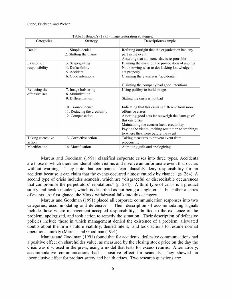
take immediate corrective action and even fewer use mortification by apologizing. Table 1
below provides a detailed summary of Benoit’s five categories which include 14 unique
communication strategies.
Stone, Erickson, and Weber
6
Table 1. Benoit’s (1995) image restoration strategies.
Marcus and Goodman (1991) classified corporate crises into three types. Accidents
are those in which there are identifiable victims and involve an unfortunate event that occurs
without warning. They note that companies “can plausibly deny responsibility for an
accident because it can claim that the events occurred almost entirely by chance” (p. 284). A
second type of crisis includes scandals, which are “disgraceful or discreditable occurrences
that compromise the perpetrators’ reputations” (p. 284). A third type of crisis is a product
safety and health incident, which is described as not being a single crisis, but rather a series
of events. At first glance, the Vioxx withdrawal falls into this category.
Marcus and Goodman (1991) placed all corporate communication responses into two
categories, accommodating and defensive. Their description of accommodating signals
include those where management accepted responsibility, admitted to the existence of the
problem, apologized, and took action to remedy the situation. Their description of defensive
policies include those in which management denied the existence of a problem, alleviated
doubts about the firm’s future viability, denied intent, and took actions to resume normal
operations quickly (Marcus and Goodman (1991).
Marcus and Goodman (1991) found that for accidents, defensive communications had
a positive effect on shareholder value, as measured by the closing stock price on the day the
crisis was disclosed in the press, using a model that tests for excess returns. Alternatively,
accommodative communications had a positive effect for scandals. They showed an
inconclusive effect for product safety and health crises. Two research questions are:
Categories
Strategy Description/example
Denial 1. Simple denial
2. Shifting the blame
Refuting outright that the organization had any
part in the event
Asserting that someone else is responsible
Evasion of
responsibility
3. Scapegoating
4. Defeasibility
5. Accident
6. Good intentions
Blaming the event on the provocation of another
Not knowing what to do; lacking knowledge to
act properly
Claiming the event was “accidental”
Claiming the company had good intentions
Reducing the
offensive act
7. Image bolstering
8. Minimization
9. Differentiation
10. Transcendence
11. Reducing the credibility
12. Compensation
Using puffery to build image
Stating the crisis is not bad
Indicating that this crisis is different from more
offensive crises
Asserting good acts far outweigh the damage of
this one crisis
Maintaining the accuser lacks credibility
Paying the victim; making restitution to set things
to where they were before the event
Taking corrective
action
13. Corrective action Taking measures to prevent event from
reoccurring
Mortification 14. Mortification Admitting guilt and apologizing

Journal of Business and Accounting
7
RQ1: What are the communication strategies, classified according to Benoit (1995), used by
Merck when Vioxx was pulled from the market?
RQ2: Do the strategies Merck used support the findings of Marcus and Goodman (1991)?
DATA AND METHODOLOGY
In the following section we analyze Merck’s responses to media questions on
September 30, 2004, when Vioxx was pulled from the market. We use a critical analysis
method to study communication strategies employed by Merck spokespeople to attempt to
repair its tarnished image. Critical analysis of strategic communication has been used by
many scholars, including Benoit (2006); Benoit and Czerwinski (1997); Benoit and Henson
(2009); Blaney, Benoit, and Brazeal (2002); Coombs (1995); Hearit (1995); Huang and Su
(2009); Erickson, Weber, Segovia, and Dudney (2010); Erickson, Weber, and Stone (2011);
and, Seeger, Sellnow, and Ulmer, (2003). A variety of texts have been evaluated using
critical analysis, including speeches, advertising, newspaper articles, and public relations
announcements.
Wall Street Journal, New York Times, and CNN Money excerpts from 2004, which
exemplify Merck’s responses to the crisis, were analyzed using Benoit (1995). Proquest was
used to find all articles regarding Vioxx and quotes from company employees and
spokespeople were used for analysis. Two researchers independently categorized the
excerpts and all categorizations were mutually agreed upon. Merck used a wide variety of
communication strategies to address questions that arose concerning this crisis. The
following section provides a summary of Merck’s responses and a brief analysis of
responses.
ANALYSIS OF COMMUNICATIONS
On September 30, 2004, Merck announced a worldwide withdrawal of Vioxx based
on results of trials indicating that individuals taking Vioxx were more likely to experience
cardiovascular problems than those not taking the medication. We analyzed 21 excerpts that
included 27 responses from October 1, 2004-December 21, 2004 and analyzed these
responses using Benoit’s (1995) Image Restoration Typology.
Merck used strategies intended to reduce the offensiveness of the crisis in 21 of its
responses. The most commonly used strategy was that of image bolstering (12 instances),
where Merck used phrases such as “serving the best interest of patients” (Merck yanks
arthritis drug Vioxx, 2004) and “putting patient safety first” (Mathews & Martinez, 2004) to
try to rebuild its reputation. Other examples of image bolstering included, “We were
financially strong before this and we will be financially strong after” (Martinez, et al, 2004)
and that Merck remains “very strong financially, with very strong cash flow” (Merck yanks
arthritis drug Vioxx, 2004). Another excerpt states, “…we concluded that a voluntary
withdrawal is the responsible course to take” (A Vioxx elegy, 2004, p. A.14). Perhaps the
most amusing example of bolstering was made by legal counsel for Merck: “Merck wasn’t
dragging its feet” and “It’s pretty hard for me to imagine that you could have done this more
quickly than we did” (Berenson, et al., 2004. p. 1.1).
Some of the above examples that mentioned that Merck was financially strong could
also be categorized as examples of minimization because Merck was attempting to show that

Stone, Erickson, and Weber
8
lost sales of Vioxx would not significantly harm the company financially. Another example
of the use of minimization included “we believe it would have been possible to continue to
market Vioxx with labeling that would incorporate these new data…” (A Vioxx elegy, 2004,
p. A.14). This example is an attempt by Merck to indicate that the only problem was
improper labeling, not the product itself.
Another way to reduce the offensiveness of the crisis is to reduce the credibility of the
accuser. Merck used this tactic three times after Vioxx was pulled off the market. One
comment, in response to an editorial, states that the editorial “is flawed in many important
respects” (Martinez & Hensley, 2004, p. B.8.) and “that the information was ‘taken out of
context’” (Mathews & Martinez, 2004). In response to a Congressional investigation, Merck
stated that documents “will be deliberately presented out of context to advance the interest”
of plaintiffs (Martinez, 2004).
Merck used evasion of responsibility strategies in 5 responses. Defeasibility was used
3 times, primarily when Vioxx was first pulled from the market and the company indicated
that, “What we saw was stunning. We certainly don’t understand the cause of this effect, but
it is statistically significant and it indicated there was an issue” (Berenson et al., 2004). Not
only does this imply that the company lacked the knowledge or ability to understand, but the
use of the word “issue” is an attempt to minimize the crisis. Another example of
defeasibility is, “I’m sorry that I didn’t know four years ago what I know now, but the data
didn’t lead us there four years ago” (Berensen, et al, 2004).
The company also used good intentions, another evasion strategy, twice when it
talked about the study of the effects of Vioxx and stated “we did our best to think of the most
comprehensive study we could have done” (Berenson et al., 2004). Finally, Merck stated that
it “acted responsibly and appropriately as it developed and marketed Vioxx” (E-mails
suggest Merck knew Vioxx’s dangers at early stages, 2004), an example of simple denial.
This strategy is only appropriate if the firm is truly blameless. If the firm uses a denial
strategy and later is found to have blame in the crisis, its reputation can be irreparably
damaged.

Journal of Business and Accounting
9
Table 2 provides a summary of our analysis of the responses made by Merck after
pulling Vioxx off the market.
Table 2. Categories of communication responses after pulling Vioxx.
Typology Number of
Times Used
Total for
Category
Denial:
Denial 1
Shifting the Blame
Total for Denial 1
Evasion of Responsibility
Scapegoating
Defeasibility 3
Accident
Good Intentions 2
Total for Evasion of Responsibility 5
Reducing the Offensiveness
Bolstering Image 12
Minimization 6
Differentiation
Transcendence
Reducing the Credibility 3
Compensation
Total for Reducing the Offensiveness 21
Taking Corrective Action
0
Mortification
0
TOTAL
27
In their research, Marcus and Goodman (1991) compared the stock market reaction of
accommodating communications to the reaction of defensive communications. Their
description of accommodating signals include those where management accepted
responsibility, admitted to the existence of the problem, apologized, and took action to
remedy the situation. Their description of defensive policies include those in which
management denied the existence of a problem, alleviated doubts about the firm’s future
viability, denied intent, and took actions to resume normal operations quickly. Mapping
Marcus and Goodman’s descriptions onto Benoit’s framework produces the following
comparison, as shown in Table 3. Accommodative communications are those which Benoit
titles Corrective Action, and Mortification; while Defensive policies are those categorized as
Denial, Evasion of Responsibility, and Reducing the Offensiveness.

Stone, Erickson, and Weber
10
Table 3. Comparison of Marcus and Goodman to Benoit.
Marcus and Goodman (1991) Corporate Policy signals Benoit’s Crisis Communication Framework
Accommodating Corrective Action
Mortification
Defensive Denial
Evasion of Responsibility
Reducing the Offensiveness
In effect, Merck used only defensive communication strategies for the crisis.
According to Marcus and Goodman’s (1991) study, this type of strategy only serves
shareholder interests effectively by providing significantly better returns to shareholders
when the cause of the crisis is an accident.
The crisis in this study involves a safety and product recall crisis, which, according to
Marcus and Goodman (1991), indicated no significant differences between accommodative
and defensive communication strategies. Although this crisis was that of the product recall
variety, it could be argued that because management had knowledge of the medical risks for
months, yet continued to market Vioxx, it could be considered a scandal. Prior knowledge of
the dangers of Vioxx was indicated on May 18, 2004 when the Wall Street Journal reported
that Merck had requested that their employee, Dr. Cannuscio, be removed from a study
which found harmful side effects for patients who used Vioxx. Merck, claimed, “Merck
disagreed with the conclusions and didn’t think it was appropriate to have a Merck author”
(Burton, 2004, p. B.1). Merck also stated, “You’re not able to control completely for the
differences between groups. There were serious limitations to the analysis” (Burton, 2004, p.
B.1). Also, on November 1, 2001, the Wall Street Journal reported that Merck executives
had been worried in the 1990s that Vioxx would show greater heart risk than cheaper pain
killers (Rotthoff 2010). Both of these communications with the public gave hints that the
product recall crisis was more of a scandal than an accident.
Regardless of whether this crisis is a scandal or a product recall, according to Marcus
and Goodman (1991), shareholders would have been better served by accommodating
strategies. Because Merck utilized defensive strategies, we would expect to see negative
stock market reactions, which is clearly the case on September 30, 2004. Merck withdrew
Vioxx after the market closed on 9/29/2004 and the stock price fell from $45.07 that day to
$33.00 at the close of the market on 9/30/2004, a loss of $26.8 billion in market value
(Rotthoff, 2010). Rotthoff shows the market acted quickly and efficiently to the news.
Marcus and Goodman suggest that Merck needed to handle the crisis, if classified as a
scandal, by using more accommodative strategies, such as corrective action and
mortification.
Corrective action could have included the offer to pay for medical exams for patients
taking Vioxx in order to access possible heart damage. Mortification requires an apology,
which legal counsel generally discourages. Merck researcher Dr. Reicin was the only
individual to say that she was “…sorry that I didn’t know four years ago what I know
now…” (Berenson, et al., 2004), but it isn’t clear what she was actually sorry about: Death
of patients who used Vioxx? Perhaps she was sorry about not withdrawing the drug sooner,
which Rotthoff (2010) contends would have resulted in a smaller total financial loss for
Journal of Business and Accounting
11
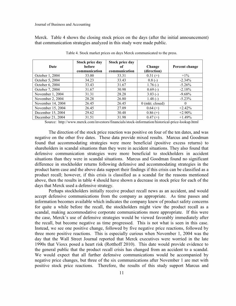
Merck. Table 4 shows the closing stock prices on the days (after the initial announcement)
that communication strategies analyzed in this study were made public.
Table 4. Stock market prices on days Merck communicated to the press.
Date
Stock price day
before
communication
Stock price day
of
communication
Change
(direction)
Percent change
October 1, 2004 33.00 33.31 0.31 (+) +1%
October 5, 2004 34.23 33.43 0.8 (-) -2.34%
October 6, 2004 33.43 31.67 1.76 (-) -5.26%
October 7, 2004 31.67 30.98 0.69 (-) -2.18%
November 1, 2004 31.31 28.28 3.03 (-) -9.68%
November 2, 2004 28.28 26.80 1.48 (-) -5.23%
November 14, 2004 26.45 26.45 0 (mkt. closed) 0
November 15, 2004 26.45 27.09 0.64 (+) +2.42%
December 15, 2004 29.62 30.48 0.86 (+) +2.90%
December 21, 2004 31.51 31.98 0.47 (+) +1.49%
Source: http://www.merck.com/investors/financials/stock-information/historical-price-lookup.html
The direction of the stock price reaction was positive on four of the ten dates, and was
negative on the other five dates. These data provide mixed results. Marcus and Goodman
found that accommodating strategies were more beneficial (positive excess returns) to
shareholders in scandal situations than they were in accident situations. They also found that
defensive communication strategies were more beneficial to stockholders in accident
situations than they were in scandal situations. Marcus and Goodman found no significant
difference in stockholder returns following defensive and accommodating strategies in the
product harm case and the above data support their findings if this crisis can be classified as a
product recall; however, if this crisis is classified as a scandal for the reasons mentioned
above, then the results in table 4 should have shown a decrease in stock price for each of the
days that Merck used a defensive strategy.
Perhaps stockholders initially receive product recall news as an accident, and would
accept defensive communications from the company as appropriate. As time passes and
information becomes available which indicates the company knew of product safety concerns
for quite a while before the recall, the stockholders might view the product recall as a
scandal, making accommodative corporate communications more appropriate. If this were
the case, Merck’s use of defensive strategies would be viewed favorably immediately after
the recall, but become negative as time progressed. This is not what is seen in this case.
Instead, we see one positive change, followed by five negative price reactions, followed by
three more positive reactions. This is especially curious when November 1, 2004 was the
day that the Wall Street Journal reported that Merck executives were worried in the late
1990s that Vioxx posed a heart risk (Rotthoff 2010). This date would provide evidence to
the general public that the product recall crisis has changed from an accident to a scandal.
We would expect that all further defensive communications would be accompanied by
negative price changes, but three of the six communications after November 1 are met with
positive stock price reactions. Therefore, the results of this study support Marcus and

Stone, Erickson, and Weber
12
Goodman if the crisis is classified as a product recall, but do not support their study if the
crisis is classified as a scandal.
CONCLUSION
The current study examined stock price reaction to corporate communications
following crisis. Using Benoit (1995) and Marcus and Goodman (1991) as a framework,
authors mapped Merck Pharmaceutical’s image restoration communications around the time
of the Vioxx recall onto the former scholar’s outcomes. The communications were
categorized as “denial”, “evasion of responsibility”, and “reducing the offensiveness of the
act”, as per Benoit’s framework. These would all map to defensive strategies under Marcus
and Goodman’s typology.
Our results mirror Marcus and Goodman’s (1991) results if the Vioxx crisis can be
labeled as a product recall. However, if viewed as a scandal, our results do not support the
Marcus and Goodman study. We examined the direction of stock price change at the time of
corporate communication. All of the communications we analyzed were defensive, yet the
direction of stock price change was negative in over half of the observations, and was
positive in the remainder of the communications.
If corporate management believes that stockholders will view the product safety
crises more like an accident, management should use defensive strategies. If management
believes stockholders will view the crisis more like a scandal, accommodating strategies
should be used. In the early phases of a product recall crisis, management may want to make
stakeholders believe that this is an accident, not a scandal; therefore utilizing defensive
communication strategies. As the reality of the slow evolution of product recall cases
becomes known by the external stakeholders, the crisis begins to look more like a scandal
than an accident, making defensive communication strategies less appropriate. The mixed
pattern of results in the current study does not support this temporal view of product recall
crisis. Instead of the ambiguous results being a result of stakeholder attitudes differing over
time, perhaps attitudes differ between individual stakeholders. Some might view a product
recall crisis as an accident, while others view it as a scandal; leading to inconclusive results.
Crisis communication is important and management should be cautious when
selecting the proper communication strategy. More studies need to be conducted on product
recall crises in order to better understand which type of communication strategies provide
increased shareholder value. In addition, organizations need to determine if product recall
crises may actually fall into the accident category, like the Tylenol crisis, or into the scandal
category, which appears to be the case for the Vioxx crisis. When faced with a scandal,
companies should use accommodating communication strategies to provide increased
shareholder value.
REFERENCES
A Vioxx Elegy (2004, October 1). The Wall Street Journal. Retrieved March 4, 2010 from
http://proquest.umi.com
Allen, M. W., & Caillouet, R. H. (1994). Legitimation endeavors: Impression management
strategies used by an organization in crisis. Communication Monographs, 61(1), 44-62.
Journal of Business and Accounting
13
Benoit, W. (1995). Accounts, Excuses, and Apologies: A Theory of Image Restoration Strategies.
Albany, NY: State University of New York Press.
Benoit, W. (1997). Image repair discourse and crisis communication. Public Relations Review,
23(2), 177-186.
Benoit, W. (2006). President Bush’s image repair effort on Meet the Press: The complexities of
defeasibility. Journal of Applied Communication Research, 34(3), 285-306.
Benoit, W. & Czerwinski, A. (1997). A critical analysis of USAir’s image repair discourse. Business
Communication Quarterly, 60(3) 38-57.
Benoit, W. & Henson, J. (2009). President Bush’s image repair discourse on Hurricane Katrina.
Public Relations Review, 35, 40-46.
Berenson, A., Harris, G., Meier, B. & Pollack, A. (2004, November 14). Despite warnings, drug
giant took long path to Vioxx recall. The New York Times. Retrieved April 7, 2010 from
http://proquest.umi.com
Blaney, J., Benoit, W., & Brazeal, L. (2002). Blowout!: Firestone’s image restoration campaign.
Public Relations Review, 28, 379-392.
Burton, T.M. (2004, May 18). Merck takes authors name off Vioxx study. The Wall Street Journal.
Retrieved July 15, 2010 from http://proquest.umi.com
Chen, Y, Ganesan, S., & Liu, Y. (2009). Does a firm’s product-recall strategy affect its financial
value? An examination of strategic alternatives during product harm crises. Journal of
Marketing, 73, 214-226.
Coombs, W. (1995). Choosing the right words: The development of guidelines for the selection of
the “appropriate” crisis response strategies, Management Communication Quarterly, 8, 447-
476.
E-mails suggest Merck knew Vioxx’s dangers at early stage. (2004, November 1). WSJ.com.
http://online.wsj.com/articls/SB109926864290160719.html
Erickson, S., Weber, M., Segovia, J. & Dudney, D. (2010). Management use of image restoration
strategies to address SOX 404 material weaknesses. Academy of Accounting and Financial
Studies Journal, 14(2), 59-82.
Erickson, S., Weber, M., & Stone, M. (2011). Corporate reputation management: Citibank’s use of
image restoration strategies during the U.S. banking crisis. Journal of Organizational
Culture, Communications & Conflict, 15(2), 35-56.
Fortunato, J. (2008). Restoring a reputation: The Duke University lacrosse scandal, Public Relations
Review, 34, 116-123.
Hearit, K. M. (1995). From “we didn’t do it” to “it’s not our fault”: The use of apologia in public
relations crises. In W. N. Elwood (Ed.), Public Relations Inquiry as Rhetorical Criticism:
Case Studies of Corporate Discourse and Social Influence (p. 117-131). Praeger Series in
Political Communication. Westport, CT: Praeger.
Geppert, J. & Lawrence, J. (2008). Predicting firm reputation through content analysis of
shareholders’ letter. Corporate Reputation Review, 11(4), 285-307.
Huang, Y. & Su, S. (2009). Determinants of consistent, timely, and active responses in corporate
crises. Public Relations Review, 35(1), 7-17.
Lyon, A., & Mirivel J.C. (2011). Reconstruction Merck’s practical theory of communication: The
ethics of pharmaceutical sales representative-physician encounters. Communication
Monographs, 78(1), 53-72.
Marcus, A., & Goodman, R. (1991). Victims and Shareholders: The dilemmas of presenting
corporate policy during a crisis. Academy of Management Journal, 34(2), 281-305.
Martinez, B. (2004). Merck’s woes grow as credit rating is put on watch. The Wall Street Journal.
November 2. Retrieved from Proquest databases March 4, 2010.

Stone, Erickson, and Weber
14
Martinez, B., & Hensley, S. (2004). Cardiologist calls for inquiry into FDA’s Handling of Vioxx.
The Wall Street Journal. October 7, p. B.8. Retrieved from Proquest databases March 4,
2010.
Martinez, B., Mathews, A., Lubline, J. & Winslow, R. (2004). Expiration date: Merck pulls Vioxx
from market after link to heart problems. The Wall Street Journal. October 1, p. A1.
Retrieved from Proquest databases March 4, 2010.
Mathews, A.W. & Martinez, B. (2004). E-mails suggest Merck knew Vioxx’s dangers at early
Stage. Retrieved from WSJ.com on March 5, 2010.
Merck yanks arthritis drug Vioxx (2004). CNNMoney.com, October 6, 2004. Retrieved March 4,
2010 from http://money.cnn/com/2004/09/30/news/fortune500/merck/
Petersen, M. (2000). Pushing pills with piles of money; Merck and Pharmacia in arthritis-drug
battle, The New York Times. October 5, 2000.
http://www.nytimes.com/2000/10/05/business/pushing-pills-with-piles-of-money-merck-
and-pharmacia-in-arthritis-drug-battle.html
Rotthoff, K.W. (2010). Product liability litigation: An issue of Merck and lawsuits over Vioxx.
Applied Financial Economics, 20(24), 1867-1878.
Scott, M. H., & Lyman, S. M. (1968). Accounts. American Sociological Review, 33(1), 46-62.
Seeger, M., Sellnow, T., & Ulmer, R. (2003). Communication and Organizational Crisis. Westport,
CT: Praeger.
Seeger, M. W., Sellnow, T. L., & Ulmer, R. R. (1998). Communication , organization and crisis. In
M. E. Roloff (Ed.), Communication Yearbook, (Vol. 21, pp. 231-275). Thousand Oaks,
CA: Sage.
Suchman, M. C. (1995). Managing legitimacy: Strategic and institutional approaches. The
Academy of Management Review, 20(3), 571-610.
Table 4, http://www.merck.com/investors/financials/stock-information/historical-price-lookup.html
The Associated Press (2010). Merck’s Vioxx settlement requires committee, medical officer to
monitor drug development. February 10, 2010.
http://www.nj.com/business/index.ssf/2010/02/mercks_vioxx_settlement_requir.html
Valentine, L. (2007) Talk is not cheap. ABA Banking Journal December, 38-41.
Ware, B. L., & Linkugel, W. A. (1973). They spoke in defense of themselves: On the generic
criticism of apologia. Quarterly Journal of Speech, 59(3), 273-283.
Weitz & Luxenberg, P.C. (2010) Vioxx – get the history of the major drug recall.
http://www.weitzlux.com/vioxx/recallhistory_94.html

Journal of Business and Accounting
Vol. 5, No. 1; Fall 2012
15
CONFLICT MINERALS DISCLOSURES:
A MANDATE OF THE DODD-FRANK ACT
Deborah L. Lindberg
Illinois State University
Khalid Razaki
Dominican University
ABSTRACT
For certain humanitarian reasons, such as deprivation of financial resources to
militant groups that seek arms for nefarious purposes, the civilized world is seeking to
eliminate or significantly diminish the trade in “conflict minerals”. The United States is
trying help in this effort by various means, including (a) forcing the publicly traded user
companies of these minerals to establish their supply sources, and (b) after a proper audit,
reporting the results in annual financial statements and official websites.
Section 1502 of the Dodd-Frank Wall Street Reform and Consumer Protection Act of
2010 (Dodd-Frank Act) requires a new reporting requirement for publicly traded companies
that manufacture products for which “conflict minerals” are necessary for their functionality
or production. The conflict minerals included in this provision of are cassiterite, columbite-
tantalite, gold, wolframite, or their derivatives. The supply source of concern is the
Democratic Republic of the Congo or countries adjoining the Congo. The requirements apply
to both domestic and foreign issuers of publicly traded equities (issuers), including smaller
companies that must report to the Securities and Exchange Commission.
Industries that may be subject to these new reporting requirements include aerospace,
automotive, electronics, communication, jewelry, and manufacturers of healthcare machines.
However, while it could be argued that the U.S. Congress' attempts to curb violence in the
Congo and adjoining countries is commendable, there are several issues regarding the
disclosure requirements for conflict minerals.
INTRODUCTION
For certain humanitarian reasons, such as deprivation of financial resources to
illegitimate groups that seek arms for nefarious purposes, the civilized world is seeking to
eliminate or significantly diminish the trade in “conflict minerals”. The United States is
trying help in this effort by various means, including (a) forcing the publicly traded user
companies of these minerals to establish their supply sources, and (b) after a proper audit,
reporting the results in annual financial statements and official websites.
Though there are no specified penalties for the use of conflict minerals (McDermott
Will & Emery, 2010), the U.S. Congress hoped that mandating public disclosure might
shame [the “name and shame” incentive, according to Ayogu and Lewis, 2011] user
companies to curb or eliminate such trade, resulting in the denial of funds to abusers of
human rights (Zweig, 2011).
Section 1502 of the Dodd-Frank Wall Street Reform and Consumer Protection Act of
2010 (Dodd-Frank Act) requires a new reporting requirement for publicly traded companies
that manufacture products for which “conflict minerals” are necessary for their functionality

Lindberg and Razaki
16
or production (McDermott Will & Emery, 2010). The conflict minerals included in this
provision of the Dodd-Frank Act are cassiterite, columbite-tantalite, gold, wolframite, or
their derivatives (SEC, 2010). By passing this section of the Dodd-Frank Act, Congress in
effect ordered the U.S. Securities and Exchange Commission (SEC) to require publicly
traded companies to disclose whether raw materials essential to their products originated
from the Democratic Republic of the Congo or countries adjoining the Congo (DRC
countries) (SEC, 2010; Zweig, 2011). Countries contiguous to the Democratic Republic of
the Congo included in this legislation are South Sudan, Uganda, Rwanda, Burundi, Tanzania,
Malawi, Zambia, Angola, Congo, and the Central African Republic (Ayogu and Lewis,
2011).
The disclosure requirements apply to both domestic and foreign issuers of publicly
traded equities (issuers), including smaller companies that must report to the Securities and
Exchange Commission (SEC, 2010). Industries that may be subject to these new reporting
requirements include aerospace, automotive, electronics, communication, jewelry, and
manufacturers of healthcare machines (Ayogu and Lewis, 2011).
BACKGROUND
Warring factions in the Democratic (sic) Republic of Congo have financed the acts of
murder, mutilation, kidnapping, rape, child labor, pillaging by mining and selling “conflict”
minerals (described below). The Congolese supply amounts to about 20% of the total global
supply (Zweig, 2011).
Congress adopted Section 1502 of the Dodd-Frank Act in the hopes that reporting
requirements about conflict minerals will help curb the violence in the Congo (SEC, 2010).
Disclosures related to the so-called “conflict” minerals are aimed at stemming the brutal
militia groups that often take over the mining and sale of these minerals to finance their
military actions (Wyatt, 2012). While the conflict mineral disclosures mandated by the Dodd-
Frank Act do not impose any penalties on companies that are using such minerals in their
products, the intention of the disclosures is to allow the investing public the opportunity to
judge such companies (McDermott Will & Emery, 2010).
Zweig (2011) expected that about 1200 companies would eventually fall under this
reporting provision. The number of companies meeting this reporting requirement is
increasing (from 2 companies in 2010 to over 40 in 2011 (Ibid). There are significant
monetary and non-monetary costs of adopting this requirement. Zweig (2011) cites the case
of a small company with a market value of $11 million and net income of $228,000 that
estimated its cost of compliance to be around $1 million. Such costs are obviously
prohibitive and untenable for smaller companies.
CONFLICT MINERALS
The conflict minerals specified in the Dodd-Frank Act, for which disclosure by
publicly traded companies will be required, are cassiterite, columbite-tantalite, gold, and
wolframite, or their derivatives (SEC, 2010). Each mineral will be discussed in the following
sections.
Cassiterite: Cassiterite is an important source of the type of tin used in coffee cans
and circuit boards (Wyatt, 2012). It is also used in cell phones, DVD players, and computers.

Journal of Business and Accounting
17
Columbite-tantalite: “Coltan” is short for columbite-tantalite (Epstein & Yuthas,
2011). In industrial uses this mineral is known as “tantalite” or “tantalum.” After columbite-
tantalite is refined it is used in products ranging from small cell phones to giant turbines
(Wyatt, 2012). It is also used in such consumer electronic products as DVD players, video
games, and computers. In Intel’s 2011 annual report, the corporation notes that its goal for
2012 is to verify that the tantalum used in it microprocessors is conflict free (Intel
Corporation, 2012).
Gold: Gold is of course extensively used in jewelry. In addition, gold is often used in
electronic products as a conductor (Wyatt, 2012). This precious metal also has a myriad of
other uses, ranging from dentistry to coins to electric wiring.
Wolframite: Wolframite is used to produce the tungsten that is used in such products
as light bulbs and machine tools (Wyatt, 2012). It is also used in armor-piercing ammunition.
These conflict minerals are sometimes referred to as “3TG” minerals (tin, tantalum,
tungsten, and gold (Ayogu and Lewis, 2011). Refer to Table 1 for a summary of conflict
minerals and their uses in products.
Table 1: Conflict Minerals and Their Use in Products
Conflict Mineral Other Names for
These Minerals Consumer Products
Cassiterite Tin
Coffee cans;
Computers;
Cell phones;
DVD players
Columbite-tantalite
Coltan;
Tantalite;
Tantalum
Cell phones;
DVD players;
Video games:
Computers;
Turbines
Gold Gold Jewelry;
Electronic products
Wolframite Tungsten
Light Bulbs;
Machine Tools;
Armor-piercing ammunition
CONFLICT MINERALS DISCLOSURES
The rules issued by the SEC require a reporting issuer (publicly traded company) to
disclose whether its conflict minerals originated in one of the DRC countries after conducting
a reasonable country of origin inquiry process. Thus, the burden of proof shifts from
corporations relying on their suppliers’ assurances that they don’t have conflict minerals to
the publicly traded company determining the source of the minerals. If the company
concludes its conflict minerals did not originate in any of the DRC countries, it would
describe this determination and the reasonable country of origin process it used to make it. If

Lindberg and Razaki
18
the reporting company concludes that its conflict minerals did originate in one or more of the
DRC countries, it would disclose this conclusion and be required to provide a “Conflict
Minerals Report” and a certified private sector audit of the Conflict Minerals Report (SEC,
2010). Each of these requirements will be discussed in the following sections.
REQUIRED DISCLOSURES - NO CONFLICT MINERALS FROM DRC
COUNTRIES
If after a reasonable country of origin inquiry process a reporting company concludes
its conflict minerals did not originate in any of the DRC countries, it would describe this
determination and the inquiry process it used to make it. Similarly, if after a reasonable
inquiry of the country of origin a company is unable to determine the origin of its minerals, it
must disclose that fact (Ayogu and Lewis, 2011). More specifically, the issuer will be
required to:
Make the disclosure available on its Internet website
Provide the Internet address of this website
Maintain records demonstrating that its conflict minerals did not originate in any
of the DRC countries (SEC, 2010).
CONFLICT MINERALS REPORT - REQUIRED FOR CONFLICT MINERALS
FROM DRC COUNTRIES
If the reporting company concludes that its conflict minerals did originate in one or
more of the DRC countries, the company must disclose this conclusion and issue a Conflict
Minerals Report as an exhibit to the annual report. Specific disclosures would require the
issuer to:
Describe its products manufactured or contracted to be manufactured containing
conflict minerals originating in any of the DRC countries
Disclose the facilities used to process such conflict minerals
Disclose conflict minerals’ country of origin
Describe the efforts used to determine the mine or location of origin with the
“greatest possible specificity”
Note that the Conflict Minerals Report is included as an exhibit to the annual
report
Furnish the Conflict Minerals Report
Make the Conflict Minerals Report available on its Internet website
Disclose that the Conflict Minerals Report is posted on its Internet website
Provide the Internet address of this website (SEC, 2010).
Reporting companies would describe the measures taken by the company to exercise
due diligence regarding the source and chain of custody of conflict minerals that are
necessary to the functionality or production of its products (SEC, 2010).
CERTIFIED INDEPENDENT PRIVATE SECTOR AUDIT
There must be a certified private sector audit of the Conflict Minerals Report (SEC,
2010). However, many constituencies expressed significant reservations regarding several

Journal of Business and Accounting
19
aspects of the audit requirement. For example, in a letter to the SEC sent by Grant Thornton
LLP during the comment period, the CPA firm expressed the following concerns:
It appears that either an attestation engagement or a performance audit would
meet the audit requirement. However the two engagements differ significantly in
nature, scope, and reporting requirements, potentially causing confusion and
misunderstanding among users of the audit report.
The objective of the audit, including the opinion or conclusion to be expressed on
the issuer's Conflict Minerals Report is not described.
The criteria to be used to evaluate the subject matter in the Conflict Minerals
Report are not described (Grant Thornton LLP, 2011).
The American Institute of Certified Public Accountants (AICPA) expressed similar
reservations and concerns in a letter that the organization sent to the SEC (Coffee, 2011).
Moreover, both Grant Thornton and the AICPA expressed concerns regarding
independence issues surrounding the private sector audit of the Conflict Minerals Report.
Grant Thornton noted that the SEC proposal, while consistent with terminology used in the
Dodd-Frank Act, indicates that the independent audit is a “critical component of due
diligence” on the part of the reporting company (Grant Thornton LLP, 2011). However, this
statement is contrary to the concept of an independent audit opinion (Grant Thornton LLP,
2011), since the auditor should not be part of the process regarding the assertion by
management that the audit firm is attesting to. The AICPA noted that since the rules
regarding private sector audit is silent as to independence issues, the SEC needed to clarify
which independence standards apply to the audits of Conflict Mineral Reports. Independence
requirements under Attestation Engagements issued by the AICPA, Performance Audits
within Government Auditing Standards (GAGAS), and audits following SEC independence
standards have differing requirements regarding the independence of the audit firm from its
client (Coffee, 2011).
Several of these concerns were addressed in the final rules issued by the SEC on
August 22, 2012 (Ernst & Young, 2012). For example, regarding auditor independence, the
final rules indicate that the independent private sector audit of the Conflict Minerals Report
must comply with independence standards issued by the Governmental Accounting Office
(GAO). Further, the SEC stated that an audit firm could perform both the audit of the
Conflict Minerals Report and the audit of the financial statements of the issuer and still be
considered independent (SEC, 2012). In the final rules the SEC also indicated what the
objective of an audit of a Conflict Minerals Report it, noting that “the audit’s objective is to
express an opinion or conclusion as to whether the design of the issuer’s due diligence
framework as set forth in the Conflict Minerals Report, with respect to the period covered by the
report, is in conformity with, in all material respects, the criteria set forth in the nationally or
internationally recognized due diligence framework used by the issuer, and whether the issuer’s
description of the due diligence measures it performed as set forth in the Conflict Minerals
Report, with respect to the period covered by the report, is consistent with the due diligence
process that the issuer undertook” (SEC, 2012, p. 217). However, there is still ambiguity in terms of the auditing standards to employ for an
audit of a Conflict Minerals Report. In its final report, the SEC notes that either the standards

Lindberg and Razaki
20
for Attestation Engagements or the standards for Performance Audits will be applicable
(SEC, 2012).
EFFECT OF THE DISCLOSURES ON CORPORATE BEHAVIOR
Even though the disclosure requirements for conflict minerals are not yet in place,
companies such as Intel, Motorola and Hewlett-Packard have already taken significant steps
to inspect and adjust their supply lines to avoid obtaining conflict minerals from DRC
countries (e.g., Wyatt, 2012). For example, in its 2011 annual report disclosures, Intel noted
that it has developed programs to allow for tracking of its source materials, in particular those
sourced from the Democratic Republic of the Congo. Further, Intel states that it will continue
to work to establish a conflict-free supply chain for the company and its industry (Intel
Corporation, 2012).
Several other corporations have already expressed concern about the “reputational
effect” their association with conflict minerals may have. To illustrate, in its 2011 annual
report disclosures, Sprint notes that because their supply chain is complex, the company may
face reputational challenges with its customers and other stakeholders if they are unable to
verify the origins of all the metals used in its products (Sprint Nextel Corporation, 2012).
Dell, Inc. makes a similar statement in its annual report for the fiscal year ended February 3,
2012, noting that the corporation may face reputational harm if its customers or other
stakeholders conclude that Dell is unable to verify sufficiently the origin of the minerals used
in its products (Dell, Inc., 2012). These and other examples of corporate disclosures
associated with the SEC’s disclosure requirements for conflict minerals are provided in Table
2.
Table 2: Conflict Minerals Disclosure Examples
Company FY Ended p. # Excerpts of Disclosures Related to “Conflict Minerals”
Advanced
Micro Devices,
Inc.
12/31/11
26,27
These new requirements could affect the sourcing and availability of
minerals used in the manufacture of semiconductor devices. Also, there
will be additional costs of compliance such as costs related to determining
the source of any conflicting minerals used in our products.
Cabot
Corporation
9/30/11
5
“An independent audit conducted by a third party auditor assigned by the
Electronics Industry Citizenship Coalition and Global e-Sustainability
Initiative (as part of the Conflict-Free Smelter Validation Program)
confirmed that our tantalum supply chain is free of conflict minerals.”
Dell, Inc.
2/3/12
35
“We will incur costs to comply with the new disclosure requirements of
this law and may realize other costs relating to the sourcing an availability
of minerals used in our products. Further, since our supply chain is
complex, we may face reputational harm if our customers or other
stakeholders conclude that we are unable to verify sufficiently the origins
of the minerals used in the products we sell.”
Helen of Troy
Limited
2/29/12
25 If rules are not modified before becoming effective, they will increase the
cost of our sourcing compliance operations.

Journal of Business and Accounting
21
Intel
Corporation
12/31/11
19 “In 2012, Intel will continue to work to establish a conflict-free supply
chain … Intel’s goal for 2012 is to verify that the tantalum we use in our
microprocessors is conflict free, and our goal for 2013 is to manufacture
the world’s first verified, conflict-free microprocessor.”
Motorola
Solutions, Inc.
12/31/11
27
The implementation may limit the pool of suppliers who can provide us
verifiable DRC Conflict Free components and parts, and we are not certain
that we will be able to obtain products in sufficient quantities that meet the
requirements.
RF
Monolithics
Inc.
8/31/11
15 It is unclear whether we will be affected materially.
Sprint Nextel
Corporation
12/31/11
23
The proposed regulation may leave only a limited pool of suppliers who
provide conflict free metals, and we not be able to obtain products in
sufficient quantities or at competitive prices. Also, because our supply
chain is complex, we may face reputational if we are unable to sufficiently
verify the origins for all metals used in the products we sell.
Tiffany & Co.
1/31/12
13
Once polished, it is not considered possible to distinguish conflict
diamonds from diamonds produced in other regions. Tiffany seek(s) to
exclude such diamonds, which represent a small fraction of the world’s
supply, from legitimate trade using an international system of certification
and legislation known as the Kimberley Process Certification Scheme.
*A Supermetals Business listed under Discontinued Operations in Cabot’s 10-K for the fiscal year
ended September 30, 2011 (Cabot Corporation, 2012).
Source: Recent 10-K reports of the corporations listed in this table were the source of the conflict
minerals disclosures included above (Advanced Micro Devices, Inc., 2012; Cabot Corporation, 2012; Dell Inc.,
2012; Helen of Troy Limited, 2012; Intel Corporation, 2012; Motorola Solutions, Inc., 2012; RF Monolithics,
Inc., 2012; Sprint Nextel Corporation, 2012; Tiffany & Co., 2012). The page numbers indicated are from the
SEC’s “Edgar” database of Form 10-K’s for each respective company.
ANTICIPATED COSTS
There are significant costs associated with the compliance by SEC reporting
companies regarding the conflict minerals disclosure mandate in the Dodd-Frank Act of
2009. The National Association of Manufactures has estimated national compliance costs
between $9 billion and $16 billion, whereas the SEC estimate is $71 million (Ayogu and
Lewis, 2011). The extreme variation between the two estimates results from the speculative
nature of the estimation process, the verification process, and the underlying assumptions.
Plausible cost estimates will be available only after the SEC has finalized all the requisite
rules for verification and reporting. An enumeration of possible costs to companies using
conflict minerals is presented below:
Verification Cost: This cost component may be the most significant monetary
cost. Under the new requirements, the cost of establishing source of supply is
shifted from supplier to user (reporting issuer). It should be noted that there is
an “escape clause” for companies experiencing problems with verification. If
a company cannot determine the origins of its conflict minerals, it can just
disclose that fact without any further consequences (Ayogu and Lewis, 2011).
Increased audit costs due to greater testing by auditors. The SEC can help
significantly reduce the overall cost of compliance by providing specific
definitions and audit standards (Ayogu and Lewis, 2011).

Lindberg and Razaki
22
Cost of recording and reporting: A company must file three different forms of
paperwork and publish a “Conflict Minerals Report” in both its audited annual
financial statements and website (Ayogu and Lewis 2011).
If current supply of conflict minerals is tainted, its replacement from
legitimate sources might constrict the remaining global supply, resulting in
higher raw materials cost (Zweig, 2011).
Reputational Cost (Zweig 2011, Ayogu and Lewis 2011): cost of potential
harmful public aversion and bad publicity if a legitimate source of supply
cannot be found. This cost may be difficult to measure or estimate.
Opportunity costs of lost business if customers avoid or boycott products
containing conflict minerals (Zweig, 2011).
Opportunity cost related to increased cost of capital if major investors
(pension plans, religious and other human rights activist investors, social
values investment funds, etc.) disinvest or refuse to invest in involved
companies. On the other hand, there seems to be no effect on the stock prices
of companies that did report using conflict minerals (Zweig, 2010).
FILING REQUIREMENTS
Issuers are required to file a newly created specialized disclosure report (Form SD)
annually by May 31 for the prior calendar year (Ernst & Young, 2012.) The first required
filings of form SD will be on May 31, 2014 for calendar year 2013 (SEC, 2012). The SEC
finalized rules allow issuers to describe their products as “DRC conflict undeterminable” for
the first two years if the issuers cannot determine the source and/or chain of custody of the
minerals they use; during this “transition” period, any such issuers must file the Form SDs,
but they don’t have to have them audited (Ernst & Young, 2012.)
CONCLUSION
While it could be argued that the U.S. Congress' attempts to curb violence in the
Congo and adjoining countries is commendable, there are still several unresolved issues
regarding the disclosure requirements for conflict minerals. For instance, since disclosures
are based on a “reasonable” country of origin inquiry process, the term reasonable is subject
to interpretation by companies, and likely will not be interpreted in a consistent manner
among companies. The “due diligence” required regarding the source and chain of custody of
conflict minerals is also subject to wide interpretation. In addition, the specific requirements
of the certified independent private sector audit that is to be furnished as part of the Conflict
Minerals Report has many unanswered questions (Ayogu and Lewis, 2011; Coffee, 2011;
Grant Thornton LLP, 2011).
The costs of compliance with this mandate are expected to be very significant. In the
case of smaller companies, they may be prohibitive. At present, these costs cannot be fairly
estimated due to the non-specificity by the SEC regarding definitions and standards. Without
making any value judgments, this is another case of increased regulation for the
accomplishment of the government’s socio-political goals that places a financial burden on
businesses. Perhaps most importantly, however, the only consequences of a publicly traded
company continuing to use conflict minerals are the reputational effects of using these
Journal of Business and Accounting
23
minerals. However, if nothing else, disclosures regarding conflict minerals will heighten
awareness of the humanitarian issues in the DRC and their relationship to U.S. trade (Ayogu
and Lewis, 2011).
REFERENCES
Advanced Micro Devices, Inc. (2012). Form 10-K (Annual Report Pursuant to Section 13 or 15(d)
of the Securities Exchange Act of 1934). For the fiscal year ended December 31, 2011,
www.sec.gov/Archives/edgar/data/2488/000119312512075837/d257108d10k.htm.
Ayogu, M. and Lewis, Z. (2011). “Conflict Minerals: An Assessment of the Dodd-Frank Act.” The
Brookings Institute, October 3, http://www.brookings.edu/research/opinions/ 2011/10/03-
conflict-minerals-ayogu.
Cabot Corporation (2012). Form 10-K (Annual Report Pursuant to Section 13 or 15(d) of the
Securities Exchange Act of 1934). For the fiscal year ended September 30, 2011,
www.sec.gov/Archives/edgar/data/16040/000119312511324512/d230919d10k.htm.
Coffee, S.S. (2011). Letter to U.S. Securities and Exchange Commission. (American Institute of
Certified Public Accountants, New York, NY), March 1, http://www.sec.gov/comments/s7-
40-10/s74010-123.pdf.
Dell, Inc. (2012). Form 10-K (Annual Report Pursuant to Section 13 or 15(d) of the Securities
Exchange Act of 1934). For the fiscal year ended February 3, 2012,
www.sec.gov/Archives/edgar/data/826083/000082608312000006/dell10k020312.htm.
Epstein, M.J. and Yuthas, K. (2011). “Conflict Minerals: Managing an Emerging Supply-Chain
Problem.” Environmental Quality Management, Volume 21, Issue 2, 13-25.
Ernst & Young (2012). “Final Conflict Minerals Rule Addresses Many Stakeholder Concerns.”
August 24. http://www.ey.com/UL/en/AccountingLink/Current-topics-SEC-Other-
regulators.
Grant Thornton LLP. (2011). Letter to U.S. Securities and Exchange Commission. (Grant Thornton
LLP, Chicago, IL). March 2, http://www.sec.gov/comments/s7-40-10/s74010-127.pdf.
Helen of Troy Limited (2012). Form 10-K (Annual Report Pursuant to Section 13 or 15(d) of the
Securities Exchange Act of 1934). For the fiscal year ended February 29, 2012.
www.sec.gov/Archives/edgar/data/916789/000110465912030645/a12-2513110k.htm.
Intel Corporation (2012). Form 10-K (Annual Report Pursuant to Section 13 or 15(d) of the
Securities Exchange Act of 1934). For the fiscal year ended December 31, 2011,
www.sec.gov/Archives/edgar/data/50863/ 000119312512075534/d302695d10k.htm.
McDermott Will & Emery (2010). “The ‘Conflict Minerals’ Provision in the Dodd-Frank Act
Imposes New Disclosure Requirements on Manufacturers.” July 22,
http://www.mwe.com/publications/uniEntity.aspx?xpST=PublicationDetail&pub= 5870.
Motorola Solutions, Inc. (2012). Form 10-K (Annual Report Pursuant to Section 13 or 15(d) of the
Securities Exchange Act of 1934). For the fiscal year ended December 31, 2011.
www.sec.gov/Archives/edgar/data/68505/000119312512063569/d280303d10k.htm.
RF Monolithics (2012). Form 10-K (Annual Report Pursuant to Section 13 or 15(d) of the Securities
Exchange Act of 1934). For the fiscal year ended August 31, 2011.
www.sec.gov/Archives/edgar/data/922204/000119312511318374/d257460d10k.htm.
Securities and Exchange Commission (SEC) (2010). “SEC Proposes Specialized Disclosure of Use
of Conflict Minerals under Dodd-Frank Act.” December 15.
http://www.sec.gov/news/press/2010/2010-245.htm.
Securities and Exchange Commission (SEC) (2012). “Conflict Minerals.” August 22.
http://www.sec.gov/rules/final/2012/34-67716.htm.
Lindberg and Razaki
24
Sprint Nextel Corporation (2012). Form 10-K (Annual Report Pursuant to Section 13 or 15(d) of the
Securities Exchange Act of 1934). For the fiscal year ended December 31, 2011.
www.sec.gov/Archives/edgar/data/101830/000010183012000015/sprint201110-k.htm.
Tiffany & Co. (2012). Form 10-K (Annual Report Pursuant to Section 13 or 15(d) of the Securities
Exchange Act of 1934). For the fiscal year ended January 31, 2012.
www.sec.gov/Archives/edgar/data/98246/000119312512136912/d285717d10k.htm.
Wyatt, E. (2012). “Use of ‘Conflict Minerals’ Gets More Scrutiny from U.S.” New York Times,
March 19, http://www.nytimes.com/2012/03/20/business/use-of-conflict-minerals-gets-
more-scrutiny.html?pagewanted=1&_r=1.
Zweig, J. (2011). “The Intelligent Investor: Can Annual Reports Save Lives?” The Wall Street
Journal , December 17, B1.

Journal of Business and Accounting
Vol. 5, No. 1; Fall 2012
25
HEDGING WITH CURRENCY ETFS:
THE IMPLICATIONS OF RETURN DYNAMICS
Robert B. Burney
Coastal Carolina University
ABSTRACT
The emergence of currency exchange traded funds (ETFs) has provided an alternative
vehicle for both speculation and hedging in the currency markets. Because currency ETFs
typically have small minimum transaction sizes and trade like equities, they represent an
easily accessible alternative for the small investor or small business operator. The ease of
access relative to other markets providing foreign exchange exposure makes currency ETFs
of particular interest to those market participants who only occasionally have currency
components to their strategies.
This paper begins with a description of foreign currency transaction options available
for smaller transaction sizes, contrasting the ease of access of the alternatives. Then an
overview of currency ETFs is provided with an emphasis on investment objectives and the
resultant fund return dynamics. Next various hedging scenarios are examined showing
possible outcomes and the potential divergence from initial intended results. These scenarios
are constructed demonstrating both extreme market conditions and typical market conditions.
Finally, recommendations are made concerning how market participants might assess the
utility of currency ETFs in their specific foreign currency risk hedging applications.
OVERVIEW
The trade press has presented various practitioner oriented articles concerning the
usefulness of currency ETFs in hedging foreign currency risk. However, such discussions
typically do not approach the topic systematically. Generally, such treatments fail to
recognize the similarities and differences between ETF based hedges and other hedging
techniques using futures contracts, options contracts, or money market transactions. Most
notably, many of the practitioner oriented articles discount the use of currency ETFs in
hedging applications because of the necessity of tying up capital during the hedge. This
criticism lacks merit since other well established techniques for dealing with foreign
exchange risk also tie up capital during the hedging period. In the following sections this
paper reviews the issues which arise in using currency ETFs in managing foreign exchange
risk. Transaction details specific to currency ETFs are then discussed. Examples are given
contrasting various hedging techniques, with special emphasis on how currency ETF
investment objectives can impact the effectiveness of a hedge.
MANAGEMENT ISSUE
The basic issue at hand is the management of foreign currency risk for those market
participants who face only very small or occasional foreign currency exposures. For such
market participants, existing liquid market derivative securities simply do not match the
transaction scale. Table One summarizes this situation for the dominant U.S. market
derivatives for the euro. In this case, the smallest notional principal amount involves 10,000

Burney
26
euros. A smaller size transaction would force the market participant to, in effect, take on a
residual exposure of opposite nature to the initial exposure.
While services for small scale market participants do exist among the retail foreign
exchange dealers, these arrangements have a reputation of being of a disadvantageous cost
structure with account details which may create more difficulties for the potential hedger
(full margin calls, etc.). Also, the smaller FX dealer based derivative contracts or minor
electronic exchanges suffer from illiquidity which may negatively impact pricing.
Table One: Example Derivative Contract Sizes
PHLX:
Euro Options 10,000 euros
CME:
Euro Futures* 125,000 euros
E-mini Futures 62,5000 euros
E-micro Futures 12,5000 euros
*CME Options are limited to larger contracts.
CURRENCY ETFS
In recent years numerous currency ETFs (CETFs) have been introduced. These
include ETFs which cover most of the major currencies and an increasing number of second
tier currencies. Variations include both long and short position ETFs, and more recently,
double and triple long and short varieties. Table Two presents a sample listing of available
CETFs as presented on the Artremis.com website.
CETF managers strive to match the change of the target currency in the specified
proportion on a day-to-day basis. Essentially, the CETF substitutes for a long or short
position in the target currency. Because the CETFs are traded on a share basis, an investor
can take any conceivable position depending on the number of shares purchased. Based on
varying notional amounts, most attempt to capture the daily percentage change of the target
currency. While most applications of both speculation and hedging in foreign currencies can
be accomplished with outright currency trades and traditional derivatives, the ease of trading
CETFs is attractive to the new or occasionally foreign currency impacted investor. Also,
there is no set denomination per share of such CETFs. Some CETFs are quoted in multiples
of the underlying currency, while others are based on an arbitrary notional principal. Recent
per share values range from $15.87 to $132.72 for the CETFs presented in Table One.
The minimum number of shares which an individual investor could trade depends on
the individual brokerage housing the account. This conceivably could be a few as one share,
and should not be confused with the inter-institutional “creation units” of much larger
magnitude (Abner, 2010). Commissions on CETF trades are also subject to wide variation,
with typical commissions at discount brokerages below $10 per trade. Some brokerages also
offer commission-free trading on select ETFs. The basic CETFs involve foreign currency
denominated bank accounts. The inverse or leveraged CETFs also use derivatives to attempt
to meet their objectives. (Lachini, 2011)

Journal of Business and Accounting
27
Table Two: Examples of Currency ETFs*
Symbol Name Fund Family Currency
FXE CurrencyShares Euro Trust Rydex Euro
EU WisdomTree Dreyfus Euro WisdomTree Euro
ERO iPath EUR/USD Exchange Rate ETN iPath Euro/U.S. dollar exchange rate
ULE Ultra Euro ProShares ProShares 2x EUR/USD daily price change
EUO UltraShort Euro ProShares ProShares 2x inverse EUR/USD daily price
change
URR Market Vectors Double Long Euro Market Vectors 2x long euro
DRR Market Vectors Double Short Euro Market Vectors 2x short euro
UUP PowerShares DB US Dollar Index Bullish PowerShares US Dollar
UDN PowerShares DB US Dollar Index Bearish PowerShares short US Dollar
FXY CurrencyShares Japanese Yen Trust Rydex Japanese Yen
JYF WisdomTree Dreyfus Japanese Yen WisdomTree Japanese Yen
JYN iPath JPY/USD Exchange Rate ETN iPath Japanese Yen/U.S. dollar exchange
rate
YCL Ultra Yen ProShares ProShares 2x JPY/USD daily price change
YCS UltraShort Yen ProShares 2x short , JPY/USD daily price
change
FXC CurrencyShares Canadian Dollar Trust Rydex Canadian Dollar
* Source: Artimis.com
CETF INVESTMENT OBJECTIVES AND RESULTING RETURN DYNAMICS
CETFs are available in both long and short varieties, and in leveraged long and short
varieties. Naturally, the capability to easily take either short or long positions using these
financial instruments would be of interest to those engaged in hedging applications. The
potential utility of using CETFs in hedging foreign exchange risk would appear at first glance
be highest for those who only occasionally face foreign exchange risk or those who face
foreign exchange risk in magnitudes smaller than the sizes of the existing exchange traded
currency derivatives. While foreign currency dealers have in recent years introduced smaller
trading lots, the trading startup learning curve for trading forward currency contracts
probably serves as a deterrent for the market participants in question.
However, existing CETFs operate under investment objectives which are defined
relative to the daily returns on the underlying currency. The nature of the fund’s investment
objective is crucially important to the potential use of CETFs in constructing hedging
portfolios. The essence of any hedging approach is to create an offsetting position which is
negatively correlated to the position originally at risk. However, this inverse relationship
must be defined relative to the entire holding period. It is here that the CETF investment
objective is crucial. While the typical CETF does a good job of tracking the daily changes in
the reference currency, the effect is to create a compound return which can differ
significantly from a continuous holding period return (Cheng and Madhavan, 2009). Thus,
constructing hedge portfolios using CETFs can be problematic.

Burney
28
Given the existing CETFs one day return defined investment objective, the value of
the CETF is driven by its own value change during the previous trading day. This differs
significantly from other hedging instruments such as futures and forward contracts in which
the value of the contract is always defined relative to the current value of the underlying.
The overall effect is that CETF based hedges will drift away from the “perfect hedge” over
time while derivatives based hedges will not deviate from the perfect hedge state during the
contract period.
The drift effect is more pronounced for larger daily changes in the price of the
underlying currency, and for longer periods of time. For lower volatility markets and for
shorter periods of time, the drift effect is negligible. However, for longer periods of time or
high volatility markets, the effect can be substantial. Thus, to ensure a CETF based hedge
remains effective, ongoing rebalancing of the CETF position is required. This rebalancing,
though relatively easy to accomplish due to the CETF trading format, significantly offsets the
apparent appeal of CETFs as a hedging instrument for the occasional or small scale foreign
currency market participant. Table 3 gives a numerical example of the potential divergence
between the returns on a hypothetical underlying currency and a related inverse CETF. The
example is built around a starting point of parity (i.e. 1.00 to 1.00) stated in home currency direct
terms. This data is presented graphically in Figure 1.
Table 3: Hedge Results under Negative and Positive Trends
ETF
Net ETF (Net)
Hedge Hedge Futures
Day Return S Long -1xETF X-S Portfolio Position Hedge
-20 -0.05 0.36 0.36 2.65 0.64 3.01 2.01 1.00 -19 -0.05 0.38 0.38 2.53 0.62 2.90 1.90 1.00 -18 -0.05 0.40 0.40 2.41 0.60 2.80 1.80 1.00 -17 -0.05 0.42 0.42 2.29 0.58 2.71 1.71 1.00 -16 -0.05 0.44 0.44 2.18 0.56 2.62 1.62 1.00 -15 -0.05 0.46 0.46 2.08 0.54 2.54 1.54 1.00 -14 -0.05 0.49 0.49 1.98 0.51 2.47 1.47 1.00 -13 -0.05 0.51 0.51 1.89 0.49 2.40 1.40 1.00 -12 -0.05 0.54 0.54 1.80 0.46 2.34 1.34 1.00 -11 -0.05 0.57 0.57 1.71 0.43 2.28 1.28 1.00 -10 -0.05 0.60 0.60 1.63 0.40 2.23 1.23 1.00 -9 -0.05 0.63 0.63 1.55 0.37 2.18 1.18 1.00 -8 -0.05 0.66 0.66 1.48 0.34 2.14 1.14 1.00 -7 -0.05 0.70 0.70 1.41 0.30 2.11 1.11 1.00 -6 -0.05 0.74 0.74 1.34 0.26 2.08 1.08 1.00 -5 -0.05 0.77 0.77 1.28 0.23 2.05 1.05 1.00 -4 -0.05 0.81 0.81 1.22 0.19 2.03 1.03 1.00 -3 -0.05 0.86 0.86 1.16 0.14 2.02 1.02 1.00 -2 -0.05 0.90 0.90 1.10 0.10 2.01 1.01 1.00 -1 -0.05 0.95 0.95 1.05 0.05 2.00 1.00 1.00 0 1.00 1.00 1.00 0.00 2.00 1.00 1.00
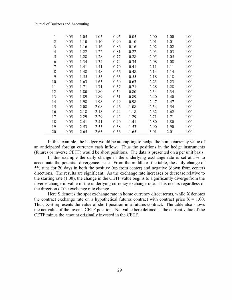
Journal of Business and Accounting
29
1 0.05 1.05 1.05 0.95 -0.05 2.00 1.00 1.00 2 0.05 1.10 1.10 0.90 -0.10 2.01 1.01 1.00 3 0.05 1.16 1.16 0.86 -0.16 2.02 1.02 1.00 4 0.05 1.22 1.22 0.81 -0.22 2.03 1.03 1.00 5 0.05 1.28 1.28 0.77 -0.28 2.05 1.05 1.00 6 0.05 1.34 1.34 0.74 -0.34 2.08 1.08 1.00 7 0.05 1.41 1.41 0.70 -0.41 2.11 1.11 1.00 8 0.05 1.48 1.48 0.66 -0.48 2.14 1.14 1.00 9 0.05 1.55 1.55 0.63 -0.55 2.18 1.18 1.00
10 0.05 1.63 1.63 0.60 -0.63 2.23 1.23 1.00 11 0.05 1.71 1.71 0.57 -0.71 2.28 1.28 1.00 12 0.05 1.80 1.80 0.54 -0.80 2.34 1.34 1.00 13 0.05 1.89 1.89 0.51 -0.89 2.40 1.40 1.00 14 0.05 1.98 1.98 0.49 -0.98 2.47 1.47 1.00 15 0.05 2.08 2.08 0.46 -1.08 2.54 1.54 1.00 16 0.05 2.18 2.18 0.44 -1.18 2.62 1.62 1.00 17 0.05 2.29 2.29 0.42 -1.29 2.71 1.71 1.00 18 0.05 2.41 2.41 0.40 -1.41 2.80 1.80 1.00 19 0.05 2.53 2.53 0.38 -1.53 2.90 1.90 1.00 20 0.05 2.65 2.65 0.36 -1.65 3.01 2.01 1.00
In this example, the hedger would be attempting to hedge the home currency value of
an anticipated foreign currency cash inflow. Thus the positions in the hedge instruments
(futures or inverse CETF) would be short positions. The data is presented on a per unit basis.
In this example the daily change in the underlying exchange rate is set at 5% to
accentuate the potential divergence issue. From the middle of the table, the daily change of
5% runs for 20 days in both the positive (up from center) and negative (down from center)
directions. The results are significant. As the exchange rate increases or decrease relative to
the starting rate (1.00), the change in the CETF value begins to significantly diverge from the
inverse change in value of the underlying currency exchange rate. This occurs regardless of
the direction of the exchange rate change.
Here S denotes the spot exchange rate in home currency direct terms, while X denotes
the contract exchange rate on a hypothetical futures contract with contract price X = 1.00.
Thus, X-S represents the value of short position in a futures contract. The table also shows
the net value of the inverse CETF position. Net value here defined as the current value of the
CETF minus the amount originally invested in the CETF.

Burney
30
In this case, the hedge would be ineffective in the sense that the hedged value was not
maintained regardless of whether the exchange rates were to rise or fall. However, in this
circumstance, the deviation from the “pure hedge” would be to the hedger’s benefit since
there would be a net “gain” on the hedge. This pattern results regardless of the size of the
daily returns, although the divergence increases with both time and the magnitude of the
daily returns.
In the second case, the assumption is made of complete volatility in the daily returns.
Here we use perfect negative correlation between subsequent daily returns. Again we use a
daily return of absolute magnitude of 5% to accentuate the result. In Table Four, the returns
for a perfectly reversing pattern of daily returns beginning with a positive return are shown.
These data are presented graphically in Figure Two.
Table Four shows a pattern which begins with a positive return on the first day,
followed by sequentially reversing returns thereafter. The volatility leads to a constant
deterioration in the CETF hedge. In this stylized case, the hedged position underperforms the
futures hedge noticeably with the long position in the foreign currency remaining above the
ETF hedged value. The CETF hedge would dampen volatility, but would be seen to be
inferior to hedging with forward contracts or not hedging at all.
That is, the volatility leads to a constant deterioration in the ETF hedge. In this
stylized case, the hedged position underperforms the futures hedge noticeably with the long
position in the foreign currency remaining above the ETF hedged value.
Figure One: ETF vs. Futures Hedges Under No Volatility
0.00
0.50
1.00
1.50
2.00
2.50
3.00
0.36 0.42 0.49 0.57 0.66 0.77 0.90 1.05 1.22 1.41 1.63 1.89 2.18 2.53
Spot Exchange Rate
Hed
ged
Posi
tion
Net ETF Hedge
Futures Hedge
Long
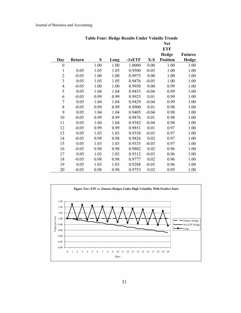
Journal of Business and Accounting
31
Table Four: Hedge Results Under Volatile Trends
Net
ETF
Hedge Futures Day Return S Long -1xETF X-S Position Hedge
0 1.00 1.00 1.0000 0.00 1.00 1.00 1 0.05 1.05 1.05 0.9500 -0.05 1.00 1.00 2 -0.05 1.00 1.00 0.9975 0.00 1.00 1.00 3 0.05 1.05 1.05 0.9476 -0.05 1.00 1.00 4 -0.05 1.00 1.00 0.9950 0.00 0.99 1.00 5 0.05 1.04 1.04 0.9453 -0.04 0.99 1.00 6 -0.05 0.99 0.99 0.9925 0.01 0.99 1.00 7 0.05 1.04 1.04 0.9429 -0.04 0.99 1.00 8 -0.05 0.99 0.99 0.9900 0.01 0.98 1.00 9 0.05 1.04 1.04 0.9405 -0.04 0.98 1.00
10 -0.05 0.99 0.99 0.9876 0.01 0.98 1.00 11 0.05 1.04 1.04 0.9382 -0.04 0.98 1.00 12 -0.05 0.99 0.99 0.9851 0.01 0.97 1.00 13 0.05 1.03 1.03 0.9358 -0.03 0.97 1.00 14 -0.05 0.98 0.98 0.9826 0.02 0.97 1.00 15 0.05 1.03 1.03 0.9335 -0.03 0.97 1.00 16 -0.05 0.98 0.98 0.9802 0.02 0.96 1.00 17 0.05 1.03 1.03 0.9312 -0.03 0.96 1.00 18 -0.05 0.98 0.98 0.9777 0.02 0.96 1.00 19 0.05 1.03 1.03 0.9288 -0.03 0.96 1.00 20 -0.05 0.98 0.98 0.9753 0.02 0.95 1.00
Figure Two: ETF vs. Futures Hedges Under High Volatility With Positive Start
0.90
0.92
0.94
0.96
0.98
1.00
1.02
1.04
1.06
0 1 2 3 4 5 6 7 8 9 10 11 12 13 14 15 16 17 18 19 20
Days
Valu
e p
er
Un
it
Futures Hedge
Net ETF Hedge
Long

Burney
32
In our final case, volatility is again systematic, but with the first of the daily returns
being negative. Each subsequent daily return is of the same absolute magnitude, but of
opposite sign. The resulting values are presented in Table Five. These data are presented
graphically in Figure Three.
Table Five: Hedge Results Under Volatile Trends
Net
ETF
Hedge Futures Day Return S Long -1xETF X-S Position Hedge
0 1.00 1.00 1.00 0.00 1.00 1.00 1 -0.05 0.95 0.95 1.05 0.05 1.00 1.00 2 0.05 1.00 1.00 1.00 0.00 1.00 1.00 3 -0.05 0.95 0.95 1.05 0.05 1.00 1.00 4 0.05 1.00 1.00 1.00 0.00 0.99 1.00 5 -0.05 0.95 0.95 1.04 0.05 0.99 1.00 6 0.05 0.99 0.99 0.99 0.01 0.99 1.00 7 -0.05 0.94 0.94 1.04 0.06 0.99 1.00 8 0.05 0.99 0.99 0.99 0.01 0.98 1.00 9 -0.05 0.94 0.94 1.04 0.06 0.98 1.00
10 0.05 0.99 0.99 0.99 0.01 0.98 1.00 11 -0.05 0.94 0.94 1.04 0.06 0.98 1.00 12 0.05 0.99 0.99 0.99 0.01 0.97 1.00 13 -0.05 0.94 0.94 1.03 0.06 0.97 1.00 14 0.05 0.98 0.98 0.98 0.02 0.97 1.00 15 -0.05 0.93 0.93 1.03 0.07 0.97 1.00 16 0.05 0.98 0.98 0.98 0.02 0.96 1.00 17 -0.05 0.93 0.93 1.03 0.07 0.96 1.00 18 0.05 0.98 0.98 0.98 0.02 0.96 1.00 19 -0.05 0.93 0.93 1.03 0.07 0.96 1.00 20 0.05 0.98 0.98 0.98 0.02 0.95 1.00
From Figure Three it can be seen that the pattern of sequentially reversing returns
which starts with a negative of the first day of the hedge results again in a deteriorating ETF
hedge relative to the benchmark futures hedge. However, in this case the ETF hedged
position value is bracketed by the value of the underlying long position in the foreign
currency. Thus the hedge is reducing volatility, but is not eliminating volatility as would
occur under the futures hedge.
REAL WORLD RELEVANCE OF CETF HEDGE DIVERGENCE
From the examples presented, it is clear that the divergence of a CETF based foreign
currency hedge arises from the shape of the functions. Because the CETF has a return
dependent on is own past return, its relationship to the underlying currency can be curvilinear
(Schubert, 2011). Meanwhile, the futures contract value remains in a linear relationship to

Journal of Business and Accounting
33
the underlying currency since its value is always X-S, which is the contract price minus the
spot price on the value date.
The issue of CETF hedge divergence is thus dependent on the size of the daily returns
in the underlying currency and the length of time over which the hedge position is held. In
our examples, the absolute magnitude of the daily return (i.e. change in price) of the
underlying currency was set at 5%. Clearly this is an unusually high level of change being
only matched occasionally for any currency in the historical record. As a benchmark, from
its high of around $1.45/€1.00 in June 2011, to its current level at the time of this writing
(June 2012) of $1.25/€1.00, the euro has experienced only an aggregate percentage return
(price change) of negative 13.79%. This one year change implies daily average price
changes of .04% over the period. If this period is seen as a relatively volatile period against
the backdrop of the ongoing Eurozone financial crisis, the example volatilities from our
hypothetical cases are clearly extraordinarily large.
For smaller daily returns in the currency whose value is to be hedged, the divergence
of the CETF based currency hedge can be negligible. Table Six presents hedging errors for a
CETF based hedge like those of our first example for various levels of daily currency returns
over representative time periods. As can be seen from the data, for smaller daily returns of a
more typical real world magnitude, the potential divergence of a CETF based hedge can be
quite small.
SUMMARY
The examples above have demonstrated the potential problem of divergence of CETF
based hedges of foreign currency cash flows. The examples show that the divergence can be
extreme under certain daily return scenarios involving exceptional levels of volatility or
exceptional levels of daily returns. However, under assumptions more in keeping with the
historical record, it is seen that the divergence of the CETF based hedge from the benchmark
futures based hedge is rather small.
Figure Two: ETF vs. Futures Hedges Under High Volatility With Positive Start
0.90
0.92
0.94
0.96
0.98
1.00
1.02
1.04
1.06
0 1 2 3 4 5 6 7 8 9 10 11 12 13 14 15 16 17 18 19 20
Days
Valu
e p
er
Un
it
Futures Hedge
Net ETF Hedge
Long

Burney
34
Table Six: Percentage Hedging Errors
Daily Return
Day 0.001 0.01 0.05 0.10
-20.00 0.95% 3.81% 101.18% 484.91%
-15.00 0.53% 2.10% 54.22% 238.31%
-10.00 0.23% 0.90% 22.76% 94.24%
-5.00 0.05% 0.20% 5.01% 20.10%
0.00 0.00% 0.00% 0.00% 0.00%
5.00 0.05% 0.20% 5.01% 20.10%
10.00 0.23% 0.90% 22.76% 94.24%
15.00 0.53% 2.10% 54.22% 238.31%
20.00 0.95% 3.81% 101.18% 484.91%
It has been noted in the literature that the divergence of an ETF hedge can be
eliminated by periodic rebalancing of the hedge (Hill and Teller, 2010). In essence, this
requires selling or purchasing the “excess” or “deficit” amount in the ETF resulting from the
divergent returns on the ETF relative to the underlying asset. However, since our initial
objective in this study was to access the suitability of hedging currency risk by less
sophisticated market participants, we have not included an assessment of the impact of a
rebalancing strategy on the effectiveness of a CETF hedge. That is, to address the
divergence issue through rebalancing can be seen to complicate the situation as much or
more than the introduction of alternative hedging instruments (i.e. futures and forwards).
While CETFs appear to be useful to market participants of this category, more precise
development of implementation criteria is needed.
Bearing in mind the nature of the market participant in question, the result from
consistent directional returns from our first example should be further considered.
Specifically, in that case the returns assumptions modeled a situation in which the currency
being hedged began a persistent, non-reversing, and significant price change. In both the
positive and negative direction, the CETF based hedge diverged from the benchmark futures
hedge in a way that would benefit the hedger. Thus, in situations in which the risk is defined
as plummeting foreign currency value, the simple CETF based hedge should result in an
outcome similar in general effect to an option based straddle position.
ISSUES FOR FURTHER RESEARCH
While the basic construct seems robust, justification for use of CETFs for small scale
foreign exchange risk hedging depends on some operational details. First, while the CETF
management objectives are clearly stated (ex. track double the inverse of the change in the
underlying currency), the effectiveness of the CETF managers should be tested. For example,
a double long CETF should correlate highly to 200% of the underlying currency’s value
change. If not, the utility of using double or triple long or short CETFs to reduce the amount
of capital that is tied up is diminished.
Second, while many widely used currency risk hedging techniques (money market
hedges, back-to-back loans) do tie up capital during the duration of the hedge, the proper

Journal of Business and Accounting
35
opportunity cost treatment for CETF based hedging must be more completely developed.
Surely, those who dismiss CETF based hedging due to this factor overstate the severity of the
issue. Nonetheless, a systematic incorporation of capital availability and costs must be
established.
Finally, it is clear that a CETF hedge would require monitoring and potentially
rebalancing to ensure the hedge objectives were met. However, the required rebalancing must
be assessed relative to the potential adjustments necessary for other types of hedges (ex.
rolling between futures contracts) for longer hedging periods. That is, through ongoing
rebalancing, a CETF hedge could be held open indefinitely. While studies of the
effectiveness of such rebalancing approaches have been conducted for index and commodity
ETFs, the author is unaware of similar studies specifically addressing CETFs (Fill and
Foster, 2009).
REFERENCES
Abner, David (2010). The ETF Handbook, John Wiley & Sons, Hoboken, New Jersey.
Cain, Alexandra (2011). ASmall Exporters Getting Savvy About Currency Risk.@ Sydney Morning
News, July 27.
Cheng, Minder and Ananth Madhaven (2009). “Dynamics of Leveraged and Inverse ETFs.”
Barclays Global Investors, October.
(2011). ACurrency Exchange Traded Funds (ETFs)@. Artremis.com, September 14.
Hill, Joanne and George Foster (2009). “Understanding Returns of Leveraged and Inverse Funds.”
Jounal of Indexes, September/October.
Hill, Joanne and Solomon Teller (2010). “Hedging with Inverse ETFs: A Primer.” Journal of
Indexes, November/December, 18-24.
Goodboy, David (2008). AFOREX spot trades vs. Currency Futures.” TradingMarkets.com, May
21.
(2009). A Hedge Against Exchange Rate Risk With Currency ETFs.” Investopedia, August 12.
Hudacheck, Dennis (2011). ACurrency-Hedged ETFs Lower Volatility.” Index Universe, November
16.
Lachini, Michael (2011). “Leveraged and Inverse ETFs: Not Right for Everyone.” Schwab.com,
October 20.
Lachini, Michael and Tatjana Michel (2011). “Currency ETFs: The Facts and Current Dollar
Outlook.” Schwab.com, October 31.
Schubert, Leo (2011). “Hedge Ratios for Short and Leveraged ETFs.” Revista Atlántica de
Economia, Volumen 1, 1-33.
Yates, Tristan (2007). “The Case Against Leveraged ETFs.” Seeking Alpha.com, May 17.
Zweig, Jason (2009). “How Managing Risk with EFTs Can Backfire.” Wall Street Journal, February
26.

Journal of Business and Accounting
Vol. 5, No. 1; Fall 2012
36
FINANCIAL STATEMENT PRESENTATION:
A SNEAK PEAK AT THE PROPOSED FORMAT
Suzanne P. Ward
Dan R. Ward
The University of Louisiana at Lafayette
Alan B. Deck
Bellarmine University
ABSTRACT
Under current US GAAP and iGAAP (i.e., IFRSs), alternative formats for statement
presentation are allowed with transactions/events not necessarily being reported or classified
consistently from one statement to another. The FASB and the IASB have both recognized
the potential problems in this area with each independently adding a financial reporting
project to their agendas in 2001. In 2004, the two rule-making bodies joined forces to
conduct a joint project on financial reporting to establish a common international standard to
improve how information is organized and presented in financial statements as part of the
overall international convergence movement. This paper overviews the results to date of this
joint FASB-IASB project on financial statement presentation.
INTRODUCTION
A company’s financial statements are central to financial reporting. Investors,
creditors, and other external users look to these statements for information regarding the
financial position, cash flows, and operations of an entity and frequently consider them key
resources for decision making. However, under current US GAAP and iGAAP (i.e., IFRSs),
alternative formats for statement presentation are allowed with transactions/events not
necessarily being reported or classified consistently from one statement to another. Thus, the
linkage among the financial statements as well as the relationships among the items being
reported is frequently difficult for users to understand.
The ever-increasing internationalization of business has only exacerbated this
situation. As businesses expand globally, so does the need for consistent financial reporting
of events and transactions in the financial statements. While the FASB and the IASB have
committed to a program of harmonization of US GAAP and iGAAP and have taken many
steps toward such a convergence, the presentation of information in the financial statements
is governed by two separate and divergent sets of rules. International accounting standards,
or IFRS, provide minimum presentation requirements and US GAAP provides only
fragmented guidance presented in a piecemeal fashion throughout a variety of reporting
standards. This situation simply enhances opportunities for companies to apply their own
unique interpretation of the requirements while still complying with those requirements.
Thus, comparability between different entities’ financial statements and the usefulness of
such statements for users is lessened. This is particularly true for those companies who must
comply with both US GAAP and IFRSs – whose rules must be followed?

Journal of Business and Accounting
37
The FASB and the IASB have both recognized the potential problems in this area
with each independently adding a financial reporting project to their agendas in 2001. In
2004, the two rule-making bodies joined forces to conduct a joint project on financial
reporting to establish a common international standard to improve how information is
organized and presented in financial statements as part of the overall international
convergence movement. This paper overviews the results to date of this joint FASB-IASB
project on financial statement presentation. The first section provides a time line of project
activities with the second section summarizing the proposed guidelines for the financial
statements as a whole. The third section compares financial statements prepared under the
current format with those prepared under the proposed format. The fourth section discusses
the results from selected FASB-IASB outreach activities and the final section presents the
current status of the project and looks toward the future of financial statement presentation.
TIME LINE OF THE JOINT PROJECT
The revision of the basic financial statements was originally initiated to address
several long-standing user concerns: the lack of a common approach for presenting
information in financial statements particularly on a global basis, the lack of linkage and
consistency in reporting information in the financial statements, and the lack of
disaggregation of information in the financial reports themselves. Phase A of the joint
FASB-IASB project, begun in 2004 and completed in 2005, resulted in several amendments
to iGAAP, primarily to bring IFRSs more closely into alignment with how US GAAP reports
comprehensive income. FASB, however, elected not to amend US GAAP until completion
of subsequent phases of the project. After over two years of deliberations with parties
interested in the fundamental issues of financial statements, a joint discussion paper
“Preliminary Views on Financial Statement Presentation” was issued in 2008. Based on
five years of comments from interested parties, results of outreach activities, and academic
research, the IASB and the FASB staffs each individually issued a Staff Draft in July 2010.
These documents, which are essentially the same with slight differences in detail designed to
address specific issues relevant to each Board, reflect the tentative joint decisions by the two
Boards up to that time as well as amendments to the proposals put forth in the discussion
paper. In the United States, the Staff Draft excludes proposals to change the presentation of
Other Comprehensive Income as well as Discontinued Operations; both of which are the
subject of separate FASB projects. This paper focuses on the FASB Staff Draft which differs
from the Discussion Paper in several areas: the format of the statement of cash flows,
application of cohesiveness principle, disaggregation of by-nature information by segments,
and analysis of changes in asset and liability line items.
Both the FASB and the IASB determined, in July 2010, that this ongoing project
required additional outreach activities focusing on what users and preparers perceive as the
benefits and costs of the project as well as what implications the project may have for
financial reporting by financial services entities. Outreach activities related to users focus
primarily on how statements prepared under the proposed guidelines would enhance
statement analysis and resource allocation decisions. Preparer-oriented outreach activities
relate to costs and efforts involved in the adoption of the proposed guidelines. The Boards
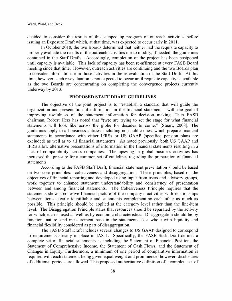
Ward, Ward, and Deck
38
decided to consider the results of this stepped up program of outreach activities before
issuing an Exposure Draft which, at that time, was expected to occur early in 2011.
In October 2010, the two Boards determined that neither had the requisite capacity to
properly evaluate the results of the outreach activities nor to modify, if needed, the guidelines
contained in the Staff Drafts. Accordingly, completion of the project has been postponed
until capacity is available. This lack of capacity has been re-affirmed at every FASB Board
meeting since that time. However, outreach activities are continuing and the two Boards plan
to consider information from those activities in the re-evaluation of the Staff Draft. At this
time, however, such re-evaluation is not expected to occur until requisite capacity is available
as the two Boards are concentrating on completing the convergence projects currently
underway by 2013.
PROPOSED STAFF DRAFT GUIDELINES
The objective of the joint project is to “establish a standard that will guide the
organization and presentation of information in the financial statements” with the goal of
improving usefulness of the statement information for decision making. Then FASB
chairman, Robert Herz has noted that “(w)e are trying to set the stage for what financial
statements will look like across the globe for decades to come.” [Stuart, 2008]. The
guidelines apply to all business entities, including non-public ones, which prepare financial
statements in accordance with either IFRSs or US GAAP (specified pension plans are
excluded) as well as to all financial statements. As noted previously, both US GAAP and
IFRS allow alternative presentations of information in the financial statements resulting in a
lack of comparability across companies. The upswing in global business activities has
increased the pressure for a common set of guidelines regarding the preparation of financial
statements.
According to the FASB Staff Draft, financial statement presentation should be based
on two core principles: cohesiveness and disaggregation. These principles, based on the
objectives of financial reporting and developed using input from users and advisory groups,
work together to enhance statement understandability and consistency of presentation
between and among financial statements. The Cohesiveness Principle requires that the
statements show a cohesive financial picture of the company’s activities with relationships
between items clearly identifiable and statements complementing each other as much as
possible. This principle should be applied at the category level rather than the line-item
level. The Disaggregation Principle states that resources should be separated by the activity
for which each is used as well as by economic characteristics. Disaggregation should be by
function, nature, and measurement base in the statements as a whole with liquidity and
financial flexibility considered as part of disaggregation.
The FASB Staff Draft includes several changes to US GAAP designed to correspond
to requirements already in place in IAS 1. Specifically, the FASB Staff Draft defines a
complete set of financial statements as including the Statement of Financial Position, the
Statement of Comprehensive Income, the Statement of Cash Flows, and the Statement of
Changes in Equity. Furthermore, a minimum of one period of comparative information is
required with each statement being given equal weight and prominence; however, disclosures
of additional periods are allowed. This proposed authoritative definition of a complete set of

Journal of Business and Accounting
39
financial statements converges U.S. GAAP with the iGAAP definition contained in IAS 1.
Table 1 presents the current names for specified U.S. financial statements with the names
proposed in the Staff Draft for a complete set of statements.
Table 1
Proposed Names for Complete Set of Financial Statements
Current
Proposed Balance Sheet
Statement of Financial Position
Income Statement
Statement of Comprehensive Income Comprehensive Income Statement
Statement of Cash Flows
Statement of Cash Flows
Retained Earnings Statement
Statement of Changes in Equity
As can be seen in the following table from the Introduction and Summary of July 1,
2010, Staff Draft, a standardized structure for the three basic statements (Statement of
Comprehensive Income, Statement of Financial Position, and Statement of Cash Flows) with
the same required sections, categories, and subcategories on all three has been identified.
However, the order of presentation of categories and subcategories within the sections, while
the same on all statements, is to be determined by the entity. Totals/subtotals and headings
are required for sections, categories, and subcategories and related information must be
classified in the same section on each statement. A single measurement base should be used
for each line item.
The Business Section reports items that are used by the entity to create value in its
day to day business activities (i.e., to produce goods or provide services which generate
revenue) as well as other income producing activities. Items in the Business Section should
be divided into the Operating Category and the Investing Category. The Operating Category
contains items related to transactions with customers, suppliers, and employees with select
liabilities directly related to operating activities classified in a separate subcategory.
Examples of items, which according to the Staff Draft should be included in this section, are
Cash, Accounts Receivable, Plant Assets, Accounts Payable, Cost of Goods Sold, and
Postemployment Benefit Service Cost. Generally, the sub-category, Operating Finance,
includes all liabilities and related assets that do not meet the definition of financing, are
initially long term, and have a time value of money. Examples of items the Staff Draft
classifies here include Net Pension Liability, Lease Liability, Expected Return on Plan
Assets, and Postemployment Benefit Interest Costs. Cash flows associated with this category
and sub-category are considered Operating. The Investing Category reports those items that
produce non-revenue income and are unrelated to the entity’s day to day activities. Items

Ward, Ward, and Deck
40
classified in this category include Short Term Investments, Investments in Securities, Equity
Method Investments, Interest Income, Equity Income, and Gains/Losses.
Table 2 – Standardized Structure
Source: Introduction to and Summary of July 1, 2010. Staff Draft
The Financing Section reports how the entity finances its business activities; e.g.,
what the entity does to obtain capital and repay capital. This Section is divided into two
categories on the Statement of Financial Position: Debt Category and Equity Category.
Neither the Statement of Comprehensive Income nor the Statement of Cash Flows subdivides
this section. The Debt Category includes obligations involving a borrowing arrangement
designed to raise/repay capital and the related revenues/expenses/cash flows. Examples from
the Staff Draft are Short Term Debt, Long Term Debt, Interest Payable, and Interest Expense.
The Equity Category contains assets/liabilities resulting from transactions with the owners of
the entity with Common Stock being the primary example from the Staff Draft. The
Financing Section does not include a “Treasury Category”; these assets/liabilities being used
as a substitute for cash should be classified in the Business Section.
COMPARISON OF STATEMENTS USING CURRENT AND PROPOSED
FORMATS
This section compares and contrasts financial statements prepared under the current
U.S. GAAP guidelines with those prepared under the proposed format. Proposed guidelines
for each statement are briefly discussed and example statements are presented.

Journal of Business and Accounting
41
STATEMENT OF FINANCIAL POSITION
The Statement of Financial Position is presently known as the Balance Sheet. Under
current U.S. GAAP, this statement is a formal presentation of the accounting equation with
assets, liabilities, and equity divided into subcategories. Assets are generally presented in
order of liquidity, liabilities by due date, and equities in order of permanence. Under the
current format, the balancing of total assets with total liabilities and equity is both readily
apparent and familiar to users. The proposed guidelines change this approach and no longer
allow the presentation of assets, liabilities, and equity in those specific groups, but rather
report items together which are related by major activity (i.e., assets and liabilities netted by
activity). How an item is classified should be determined by the function of that item (i.e.,
how management uses the item) and, thus, is a way of disaggregating the information in the
statements. Explanations of these classifications by management should be included in the
notes. The specific sub-categories are determined by the entity itself and should be the ones
that, in its opinion, provide the most relevant information to users. Sub-category choices
include short term vs. long term (determined using a fixed period of one year) or in order of
liquidity. Assets and liabilities for each category and for each sub-category (if presented)
must be totaled on the face of the statement. Classifications on the other financial statements
are determined by classifications in the Statement of Financial Position. Cash equivalents
would no longer be part of cash but would be classified as a short term investment.
Exhibit 1 presents a statement of financial position prepared under the proposed
guidelines. At first, glance, the proposed statement does not appear to balance; however, all
of the assets, liabilities, and equities currently reported on the Balance Sheet are still being
reported on this proposed statement. The difference is the classifications and arrangements of
the items. As previously noted, the Business section is presented first broken into the
Operating Category and the Investing Category. In the Operating Category, those assets that
contribute to the production of revenue are listed with no distinction between those now
classed as current and those now classed as non-current although the assets are generally
shown in order of liquidity. Operating liabilities, in a separate subcategory within the
operating category (aka Operating Finance Subcategory), generally reflects short term
obligations that are associated with the production of revenue. The second category in the
Business Section, the Investing Category presents the assets that produce non-revenue
income and which are not related to the day to day activities of the entity. These are
primarily the assets that are presently classified in the long term investment section of the
balance sheet. As can be seen, all categories and subcategories must be totaled.
In this example, the income tax section is presented next, but the order is determined
by the individual entity. Since income taxes are primarily a result of revenue or income
producing activities, placement of the income tax section here presents these liabilities in
close proximity to the related assets and liabilities.
The final section on the Statement of Financial Position, the Financing Section, is
subdivided into the Debt Category and the Equity Category and explains how an entity
obtained its capital. All debts not classified in the Operating Finance Subcategory are
presented in the Debt Category and, in this example, are shown in order of due date. The
Equity Category is essentially unchanged from the presentation in current statements. Under
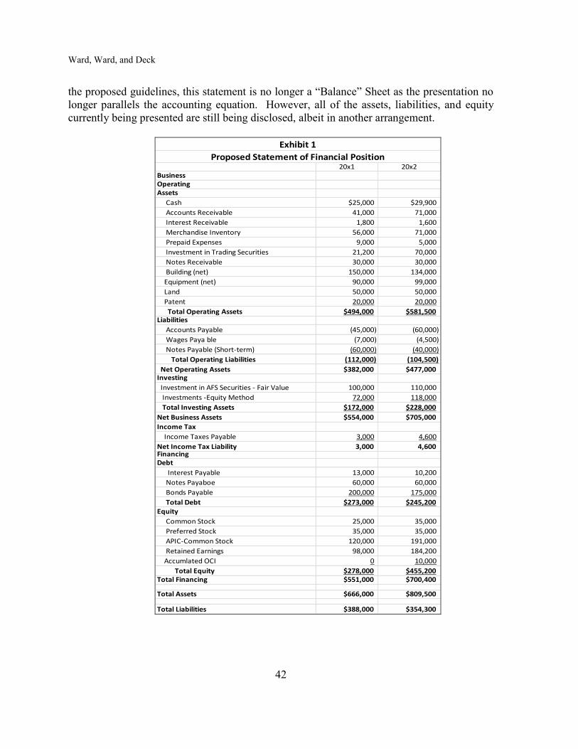
Ward, Ward, and Deck
42
the proposed guidelines, this statement is no longer a “Balance” Sheet as the presentation no
longer parallels the accounting equation. However, all of the assets, liabilities, and equity
currently being presented are still being disclosed, albeit in another arrangement.
20x1 20x2BusinessOperatingAssets
Cash $25,000 $29,900
Accounts Receivable 41,000 71,000
Interest Receivable 1,800 1,600
Merchandise Inventory 56,000 71,000
Prepaid Expenses 9,000 5,000
Investment in Trading Securities 21,200 70,000
Notes Receivable 30,000 30,000
Building (net) 150,000 134,000
Equipment (net) 90,000 99,000
Land 50,000 50,000
Patent 20,000 20,000
Total Operating Assets $494,000 $581,500Liabilities
Accounts Payable (45,000) (60,000)
Wages Paya ble (7,000) (4,500)
Notes Payable (Short-term) (60,000) (40,000)
Total Operating Liabilities (112,000) (104,500)
Net Operating Assets $382,000 $477,000Investing
Investment in AFS Securities - Fair Value 100,000 110,000
Investments -Equity Method 72,000 118,000
Total Investing Assets $172,000 $228,000
Net Business Assets $554,000 $705,000
Income Tax
Income Taxes Payable 3,000 4,600
Net Income Tax Liability 3,000 4,600FinancingDebt
Interest Payable 13,000 10,200
Notes Payaboe 60,000 60,000
Bonds Payable 200,000 175,000
Total Debt $273,000 $245,200Equity
Common Stock 25,000 35,000
Preferred Stock 35,000 35,000
APIC-Common Stock 120,000 191,000
Retained Earnings 98,000 184,200
Accumlated OCI 0 10,000
Total Equity $278,000 $455,200Total Financing $551,000 $700,400
Total Assets $666,000 $809,500
Total Liabilities $388,000 $354,300
Exhibit 1
Proposed Statement of Financial Position

Journal of Business and Accounting
43
STATEMENT OF COMPREHENSIVE INCOME
The Statement of Comprehensive Income is the subject of a separate joint project of
FASB and IASB. Accordingly, the Staff Draft only provides general guidance regarding this
statement which presents information regarding changes in the entity’s net assets during a
period from transactions other than those with owners. This proposed format of this
statement in the Staff Draft combines the current Income Statement with the current
Statement of Comprehensive Income, thus utilizing the single statement approach to the
reporting of comprehensive income. The current format of the Income Statement divides
revenues and expenses into Operating and Non-Operating categories with Extraordinary
Items and Discontinued Operations presented separately. Revenues and expenses are
currently separately reported on the Income Statement with relevant subtotals (e.g., gross
profit) also presented. The current format of the Statement of Comprehensive Income
separates the non-owner changes to equity into Net Income and Other Comprehensive
Income Items.
The proposed Statement of Comprehensive Income, as shown in Exhibit 2, is divided
into two sections, Net Income and Other Comprehensive Income. A subtotal for Net Income
must be presented on the face of the statement. Classification of revenues and expenses
should follow the same categories in the same order as those on the Statement of Financial
Position with related items on both statements classified in the same manner on both. Within
each category, revenue and expense items should be disaggregated by function first (e.g.,
selling goods, providing services) and then those functional amounts should be disaggregated
by nature (e.g., salaries, rent, depreciation) either in the statement itself or in the notes. Each
item reported on the Statement of Comprehensive Income, whether part of net income or as
an other comprehensive income item, must be clearly identified as to whether it relates to an
operating, an investing, or a financing activity. This approach still reports revenues and
expenses in a manner similar to the current format as the operating sections retains the
majority of revenues and expenses currently classed as operating while the non-operating
items will be divided between the investing and financing sections. However, interest
expense will now be classed as a financing expense rather than as an operating one.
Allocation of income taxes continues as in the past and no extraordinary items are
allowed (a change for US GAAP and a convergence with IFRSs). Other Comprehensive
Income Items will be reported in the last section on this statement in a manner similar to
current presentation guidelines. Key subtotals must be presented for each section with the
final figure on the statement being Comprehensive Income. There will no longer be an option
to present a Statement of Comprehensive Income separate from the Income Statement.
Those two current statements will be combined under the proposed guidelines. The IASB
refers to this statement as the “Statement of Profit or Loss and Other Comprehensive
Income”; however, this is a suggested title not a required one. The FASB Staff Draft uses the
name “Statement of Comprehensive Income.”
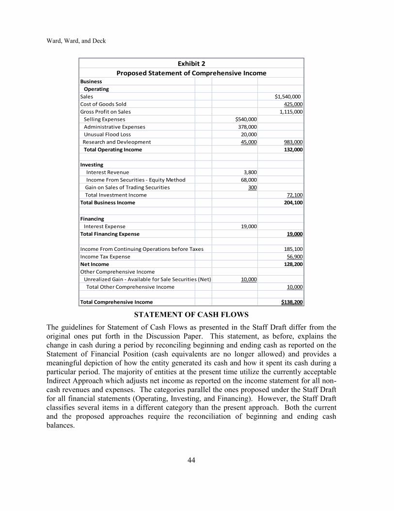
Ward, Ward, and Deck
44
Business
Operating
Sales $1,540,000
Cost of Goods Sold 425,000
Gross Profit on Sales 1,115,000
Selling Expenses $540,000
Administrative Expenses 378,000
Unusual Flood Loss 20,000
Research and Devleopment 45,000 983,000
Total Operating Income 132,000
Investing
Interest Revenue 3,800
Income From Securities - Equity Method 68,000
Gain on Sales of Trading Securities 300
Total Investment Income 72,100
Total Business Income 204,100
Financing
Interest Expense 19,000
Total Financing Expense 19,000
Income From Continuing Operations before Taxes 185,100
Income Tax Expense 56,900
Net Income 128,200
Other Comprehensive Income
Unrealized Gain - Available for Sale Securities (Net) 10,000
Total Other Comprehensive Income 10,000
Total Comprehensive Income $138,200
Exhibit 2
Proposed Statement of Comprehensive Income
STATEMENT OF CASH FLOWS
The guidelines for Statement of Cash Flows as presented in the Staff Draft differ from the
original ones put forth in the Discussion Paper. This statement, as before, explains the
change in cash during a period by reconciling beginning and ending cash as reported on the
Statement of Financial Position (cash equivalents are no longer allowed) and provides a
meaningful depiction of how the entity generated its cash and how it spent its cash during a
particular period. The majority of entities at the present time utilize the currently acceptable
Indirect Approach which adjusts net income as reported on the income statement for all non-
cash revenues and expenses. The categories parallel the ones proposed under the Staff Draft
for all financial statements (Operating, Investing, and Financing). However, the Staff Draft
classifies several items in a different category than the present approach. Both the current
and the proposed approaches require the reconciliation of beginning and ending cash
balances.

Journal of Business and Accounting
45
Business
Operating
Cash Collected from Customers $1,510,000
Cash paid for Merchandise Inventory (425,000)
Cash Paid for Wages (80,500)
Cash Paid for Operating Expenses (785,000)
Cash Paid for Research and Development (45,000)
Purchase of Building (39,000)
Purchase of Equipment (25,000)
Cash Paid on ST- Note (20,000)
Net Cash Flows from Operating Activities 90,500
Investing
Cash Received for Interest 4,000
Sale of Trading Securities 21,500
Purchase of Trading Securities (70,000)
Cash Received for Dividends 22,000
Net Cash Flows from Investing Activities (22,500)
Financing
Cash paid for dividends (42,000)
Cash Paid for Interest (21,800)
Cash Paid for Bonds (25,000)
Cash received from Sale of Common Stock 81,000
Net Cash Flows from Financing Activities (7,800)
Income Tax
Cash paid for Income Taxes (55,300)
Increase in Cash 4,900
Beginning Cash 25,000
Ending Cash $29,900
Proposed Statement of Cash Flows
Exhibit 3
The Staff Draft requires the use of the direct method for preparing the Statement of
Cash Flows (see Exhibit 3) as well as the presentation of the reconciliation of operating
income to operating cash flows. Classifications of cash flows on this statement must be
consistent with how the related items/transactions are classified on the other financial
statements, particularly the Statement of Financial Position. Furthermore, information
regarding significant non-cash activities is required to be presented in the body of the
Statement of Cash Flows rather than the notes. As can be seen in Exhibit 3, cash flows
associated with plant assets which are currently classified as Investing Activities would,
under the proposed guidelines, be presented in the Operating Category in the Business
Section. In addition, several cash flows currently reported in the operating activity category
such as cash inflows for interest and dividends and inflows/outflows related to trading
securities, would be reported in the investing category with cash outflows for interest in the
financing section and income taxes in its own separate section.
STATEMENT OF CHANGES IN EQUITY AND NOTES TO FINANCIAL
STATEMENTS
The footnotes, as always, are required for full disclosure purposes and, under the Staff
Draft, new as well as expanded disclosures must be provided in addition to those currently

Ward, Ward, and Deck
46
required. For example, companies will be required to analyze changes in all asset and
liabilities which are important in understanding changes in the company’s financial position.
However, descriptions of the basis for classifying assets and liabilities into categories will no
longer necessary. Companies must explain each individual change relating to cash
transactions, non-cash transactions, accounting allocations, write downs/impairment losses,
acquisitions/ dispositions, and other remeasurements. Disclosures must include a note
identifying remeasurement amounts recognized on the Statement of Comprehensive Income
as well as a narrative putting each of those amounts into context.
Current U.S. GAAP requires that an entity explain all changes in equity items during
a period; however, these disclosures are generally provided in the footnotes or as a
supporting schedule in those footnotes. Under the proposed guidelines, these disclosures
would be presented in a separate Statement of Changes in Equity which would have equal
prominence with the other three financial statements Exhibit 4 illustrates this new financial
statement.
Common
Stock
Preferred
Stock
APIC
Common
Stock
Accum.
Other Comp
Income
Items
Retained
Earnings Total Equity
Balance as of 1/1/20x2 $25,000 $35,000 $120,000 $0 $98,000 $278,000
Comprehensive Income
Net Income 128,200 128,200
Other Comprehensive Income 10,000 10,000
Total Comprehensive Income 10,000 226,200 416,200
Transactions with Owners
Issuance of Common Stock 10,000 0 71,000 81,000
Dividends Paid (42,000) (42,000)
Balance as of 12/31/20x2 $35,000 $35,000 $191,000 $10,000 $184,200 $455,200
Proposed Statement of Changes in Equity
Exhibit 4
OUTREACH ACTIVITIES
The FASB and the IASB have been conducting a variety of outreach activities to
obtain feedback regarding the proposed revamping of the financial statements. A summary
of selected activities is presented in the next paragraphs.
An example of an outreach activity conducted involved a field test utilizing preparers
of financial statements. This field test was designed to evaluate if the proposed presentation
in the Discussion Paper improved the usefulness of the statements to users, to gain an
understanding of implementation costs, and to identify any unintended consequences of the
proposal. In this field test, thirty companies recast the financial statements for any two
consecutive years using the guidelines from the Discussion Paper. These companies also
completed a 32 question survey about their experience, documenting all time and cost
constraints each encountered. Participating companies represented seven different countries,
with the majority from the U.S. and Europe, as well as seventeen different industries
including banking, insurance, entertainment, and steel works.
The findings from this field test indicated that the majority of participants believe that
the recast statements communicate their company’s results much the same as those prepared

Journal of Business and Accounting
47
using the current guidelines or, in some cases, worse than those utilizing the current
guidelines. Disaggregation of information in the reports, one of the objectives of this project,
increased as an approximately 50 percent increase in line items was indicated. However, the
participants did not feel that this increased disaggregation necessarily translated into an
increase in usefulness. Furthermore, the participants did not perceive that categorizing
information by nature on the face of the statements provided any benefits and they
questioned the effectiveness of the proposed definitions as well as the disaggregation
guidance.
Another outreach activity involved interviews with users of the financial statements
in order to obtain input and feedback regarding the proposed guidelines. Fifty six individuals
from seven different countries with broad, extensive experience in using the financial
statements were interviewed. These users, including analysts, fund managers, and lenders,
expressed no widespread dissatisfaction with financial statements prepared using the current
guidelines nor did they demand any drastic modifications to the current financial statement
presentation. While net income was the normal starting point for analysis, that figure was
not necessarily one of the three most important measures to the participants as users of
financial reports. Furthermore, these users were indifferent concerning the reporting of
comprehensive income in a separate statement as long as the other comprehensive income
items were readily apparent and separately reported. The majority, however, did prefer
utilization of the direct method over the indirect method for preparing the Statement of Cash
Flows.
An additional outreach activity was an academic study conducted under the auspices
of the Financial Accounting Standards Research Initiative. This study focused on the
classification of items in the financial statements into categories as well as on the
disaggregation of expenses by function and nature. Sixty credit analysts were randomly
assigned a complete set of financial statements with different versions varying in category
classification and disaggregation of expenses. Findings indicated that forecasts and
judgments improved when related information associated with classification and
disaggregation were placed together. Furthermore, the disaggregation of information on the
face of the statements while reporting classifications in the notes was somewhat effective.
Interestingly, the reverse situation (classification on the face of the statements with
disaggregation in the notes) was actually counterproductive.
As can be seen from this discussion of selected outreach activities, the results of the
proposed guidelines appear to be mixed with neither users nor preparers endorsing all of the
changes. As previously noted, the findings from outreach activities conducted prior to
Summer 2010 were considered in preparing the Staff Drafts issued by the FASB and by the
IASB in July 2010 resulting in several modifications of the proposals contained in the
discussion paper. Given these results, both Boards wisely elected to continue conducting
outreach activities to gather additional data concerning the amended proposed guidelines
contained in the Staff Drafts.
Plans for future outreach activities include meeting with constituents, both users and
prepares, to discuss details of the FASB Staff Draft as well as the costs/benefits of the
proposed guidelines. Investors and other users will be asked for input regarding the
limitations of current financial reports as well as any benefits they foresee from the proposed

Ward, Ward, and Deck
48
format. Preparers will be asked to evaluate costs involved in adopting the proposal with
additional companies, including financial services and non-public entities, asked to recast
two years of statements using the proposed guidelines. These activities continue to provide
valuable feedback to both Boards.
CURRENT STATUS/UNKNOWN FUTURE
The format for financial statements proposed in the Staff Draft significantly changes
the presentation of financial position, results of operations, and cash flows by all entities –
both in the U.S. and globally – in an attempt to develop a common presentation approach.
Furthermore, the proposal provides for an increased amount of disaggregation in the financial
statements as well as for standardization in presentation to augment the articulation and flow
among the financial statements.
Both the FASB and the IASB have engaged in a series of focused and targeted
outreach activities designed to elicit feedback regarding this project with additional such
activities continuing to be conducted. Findings from these activities have been mixed; some
have reported improvements in financial reporting while others report little or even declines
in usefulness. Users and preparers welcome some of the proposed changes, but do not
appear to appreciate others. Results from these activities have been and continue to be
provided to the Boards; however, both the FASB and the IASB acknowledge that a lack of
capacity exists to properly evaluate these results at this time. Accordingly, the project’s time
line has been modified and the project postponed until the requisite capacity is available.
This decision, originally made in October 2010, has been reaffirmed at each subsequent
Board meeting and no further action on the project by either Board is expected until requisite
capacity is achieved.
A project of this magnitude must be taken slowly and implemented with extreme
caution. As both the FASB and the IASB have discovered, such a massive change, even one
undertaken in answer to user requests, is not always welcomed with open arms by those
requesting the change. Costs and benefits of such a change for both users and preparers must
be collected and assessed; a process which both Boards are painstakingly undertaking. This
collection and analysis takes time and requires that everyone involved, both users and
preparers, be receptive to the changes being proposed. The FASB and the IASB appear to
recognize this and have shown admirable restraint regarding a rush to revamping of the
financial statements. However, little by little, both appear to be taking baby steps toward the
goal of international harmonization of financial statement presentation.
REFERENCES
Ernst & Young (2010, July 7). FASB Staff Draft of New Presentation Model for Financial
Statements. Hot Topic No. 2010-34.
Ernst & Young, (2011, May). Joint Project Watch: FASB/IASB joint projects from a US GAAP
Perspective.
FASB/IASB Joint Project Financial Statement Presentation. Retrieved from www.fasb.org/project/financial_statement_presentation.shtml
FASB (2010, July 1). Staff Draft of an Exposure Draft on Financial Statement Presentation.

Journal of Business and Accounting
49
FEI Financial Reporting Blog: Financial Statement Presentation Project ‘Pauses;’ Removed From
FASB, IASB June, 2011 Priorities, Retrieved from http://financialexecutives.blogspot.com/2010/10/financial-statement-presentation-pauses.html
IFRS Foundation: Introduction to and Summary of July 2010 Staff Draft. Retrieved from www.fasb.org/project/financial_statement_presentation.shtml
KPMG International Financial Reporting Standards (2010, August). New on the Horizon: Financial
Statement Presentation. (Principal authors: S. McGregor, M. Oki, J. Sage, and D. Ward)
McClain, G., and A. McLelland (2008, November). “Shaking Up Financial Statement Presentation”,
Journal of Accountancy. Retrieved from
(http://www.journalofaccountancy.com/Issues/2008/Nov/ShakingUpFinancialStatementPres
entation.com)
Stuart, A. (2008, February), “A New Vision for Accounting”. CFO Magazine. Retrieved from
(http://www.cfo.com/printable/article.cfm/10597001)

Journal of Business and Accounting
Vol. 5, No. 1; Fall 2012
50
THE COMPARATIVE REPORTING IMPACT OF THE FASB AND
IASB TREATMENTS OF RESEARCH AND DEVELOPMENT
EXPENDITURES
Patricia G. Mynatt
Richard G. Schroeder
University of North Carolina at Charlotte
ABSTRACT
In 2002 The Financial Accounting Standards Board and the International Accounting
Standards Board announced their intention to develop high-quality, compatible accounting
standards that could be used for both domestic and cross-border financial reporting (the
Norwalk Agreement). The two bodies are currently working to harmonize differences
between their respective standards. One such difference is in the treatment of research and
development costs (R&D). This paper analyzes the reporting consequences of this difference
to determine if the failure to harmonize this disparity might be a major impediment to the
goals of the Norwalk Agreement. Our study found that the majority of firms reporting in the
U. S. under IASB standards were large firms. Consequently, a company’s decision to
capitalize or expense R&D costs may be influenced by the political visibility theory of
accounting choice because the impact of capitalization is an increase in earnings. This
conclusion is further evidenced by the large difference in average reported earnings between
companies reporting under U. S. generally accepted accounting principles and the companies
reporting under IASB standards. Further support for this conclusion is found in a study of
French firms reported by Cazavan-Jeny, et al, 2007, which indicated that firms capitalizing
R& D expenditures are smaller and are poorer performers than firms expensing R&D
expenditures.
INTRODUCTION
The purpose of accounting is to provide the information for sound economic decision
making. This purpose is attempted to be accomplished by preparing financial reports that
provide information to external parties, such as investors, creditors and tax authorities, about
a firm’s financial performance. In efficient capital markets, investors incorporate public
information into security prices swiftly and accurately. In contrast, in capital markets in
which there is incomplete public information, prices reflect that information slowly,
incompletely or not at all (Stout, 2003).
In order for firms to report financial information fairly and consistently, a set of
accounting standards needs to be developed. There are currently two major standard setting
bodies, The Financial Accounting Standards Board (FASB) and the International Accounting
Standards Board (IASB). The FASB is currently the organization designated by the
Securities and Exchange Commission (SEC) as the authoritative standard setting body in the
United States; whereas, the IASB is recognized as the organization responsible for
promulgating accounting standards by approximately 120 foreign countries.
At a joint meeting in Norwalk, Connecticut, on September 18, 2002, the FASB and
the IASB both acknowledged their commitment to the development of high-quality,

Journal of Business and Accounting
51
compatible accounting standards that could be used for both domestic and cross-border
financial reporting (the Norwalk Agreement). The two boards pledged to use their best
efforts to (1) make their existing financial reporting standards fully compatible as soon as is
practicable; and (2) coordinate their future work programs to ensure that once achieved,
compatibility is maintained. The boards’ goal is to improve the usefulness of the information
provided in an entity’s financial statements to help users make decisions in their capacity as
capital providers (FASB, 2002).
One major area of difference between the two bodies’ standards is in the treatment of
research and development (R&D) costs. The FASB’s Statement of Financial Accounting
Standards (SFAS) No. 2 provides the following definitions of research and development:
Research is planned search or critical investigation aimed at discovery
of new knowledge with the hope that such knowledge will be useful in
developing a new product or service or new process or technique or in
bringing about a significant improvement to an existing product or process.
Development is the translation of research findings or other knowledge
into a plan or design for a new product or process or for a significant
improvement to an existing product or process whether intended for sale or
use. It includes the conceptual formulation, design and testing of product
alternatives, construction of prototypes, and operation of pilot plants. It does
not include routine or periodic alterations to existing products, production
lines, manufacturing processes, and other ongoing operations even though
these alterations may represent improvements and it does not include market
research or market testing activities (FASB, 1974).
The FASB standard requires all R&D costs to be charged to expense as incurred
(FASB, 1974). However, the IASB standard allows development costs to be capitalized
(recorded as assets) if they are found to have future economic benefit. The IASB discussed
this issue in International Accounting Standard (IAS) No. 38 as follows:
Development costs are capitalised only after technical and commercial
feasibility of the asset for sale or use have been established. This means that
the entity must intend and be able to complete the intangible asset and either
use it or sell it and be able to demonstrate how the asset will generate future
economic benefits (IAS No. 38, 2004)
Discussions on the accounting treatment for R&D expenditures are important because
R&D investments in the U.S. and other developed economies have witnessed unprecedented
growth in the last two decades. The U.S. currently leads the global market in corporate R&D
expenditures with 2005 R&D expenditures of $226 billion in current-year dollars, increasing
by $10.3 billion from the 2004 level (National Science Foundation, 2007). R&D investment
is used as one of the critical strategies to maintain and/or enlarge market share. Prior studies
demonstrate that companies with a higher level of R&D investment show far better earnings
and stock performance than companies with a lower level of spending in R&D (Daum,
2001).
All corporate investments, including R&D expenditure, create information
asymmetries between management and investors (Aboody & Lev, 2000), because
management can continually observe changes in investment productivity on an individual

Mynatt and Schroeder
52
asset basis. As a result, managers have superior information about the future cash flows and
earnings of the firm. However, R&D has been identified as a specific source of information
asymmetry (Aboody & Lev, 2000; Givoly & Shi, 2007).
Proponents of capitalization maintain that this treatment allows managers to signal
private information about future performance of the firm through the decision to capitalize or
expense R&D expenditures. That is, signalling theory1
explains how information asymmetry
can be reduced when the more informed party communicates their private knowledge to the
less informed party (Morris, 1987). Opponents of R&D capitalization argue that it creates
opportunities for managers to manipulate earnings by accelerating or delaying impairments
of R&D expenditures of projects with a low probability of success (Cazavan-Jeny et al,
2007). The two standard setting bodies’ differing treatments have reporting consequences in
that net income and assets could be materially different for companies having large amounts
of R&D expenses depending on which treatment standard is adopted.
Prior to 2007 foreign companies wishing to list their securities in United States
capital markets were required to recast their financial statements into U. S. generally
accepted accounting principles (GAAP) by using the Securities and Exchange Commission’s
(SEC) Form 20-F reconciliation. However, for years ending after November 15, 2007, the
SEC has allowed foreign private issuers to present IFRS based financial statements in their
SEC filings, without reconciliation to U.S. GAAP. The SEC’s rationale for this action was to
foster the adoption of a set of globally accepted accounting standards (SEC, 2007). Earlier, in
2005, the chief accountant of the SEC described a roadmap for arriving at a common set of
high-quality global standards and the removal of the need for the reconciliation requirement
for non-U.S. companies that use IFRSs and are registered in the United States (Nicolaisen,
2005).
The SEC also took another step in the direction of convergence in 2007 when it
decided to explore the possibility of allowing U.S. companies to adopt International Financial
Reporting Standards (IFRS) (SEC, 2007). In explaining its rationale for this decision, the
SEC noted that the movement to IFRS has begun to affect U.S. companies, in particular those
with a significant global foot- print. That is, under the new rule amending Form 20-F adopted
by the SEC, foreign registrants can use either U.S. GAAP or IFRS without reconciling their
earnings and shareholders’ equity to U.S. GAAP; consequently, it would seem more
equitable for U.S. companies, which compete for capital in the same securities market, to
also be able to use either U.S. GAAP or IFRS (SEC, 2007). In 2008, the SEC voted to
publish for public comment a proposed roadmap that could lead to the use of IFRS by U.S.
issuers beginning in 2014 (SEC, 2008).
A recent SEC staff paper summarized an analysis of the financial reports of 183
companies, both SEC registrants and other companies, which were prepared under IFRS.
With respect to the reporting of intangible assets, they wrote “For many companies, it was
unclear what costs were being capitalized; thus, comparability was difficult to assess.” (SEC,
2011). The objective of this study is to determine whether there are observable differences
for U.S. listed firms that report under the FASB’s and the IASB’s prescribed accounting
treatments for R&D costs.
The underlying research hypothesis is that there is a material difference on reported
R&D costs, income and assets that is attributable to the alternative treatments for companies

Journal of Business and Accounting
53
with large R&D expenditures. Companies reporting under IFRS may capitalize development
costs as an intangible asset after technical and commercial feasibility has been established.
Companies reporting under FASB standards must expense such costs. We expect, therefore,
that intangible assets, specifically the number reported by firms for intangible assets other
than goodwill, will be larger on average for firms reporting under IFRS as opposed to under
U.S. GAAP. We also expect that R&D expenditures will be smaller on average for firms
reporting under IFRS as opposed to under U.S. GAAP. To control for the overall difference
in firm size, we investigate reported other intangible assets, scaled by firm total assets and
reported R&D costs, scaled by firm total assets. Because IFRS reporting firms may
capitalize some development costs, we also look for an income difference between
companies reporting under IFRS and U.S. GAAP. We expect that net income may be higher
for IFRS reporting firms. We again control for firm size using total assets. Our sample
includes all firms listed in the Compustat North America Annual Database for fiscal year end
2010, in the following five, two-digit sic codes:
28 - Chemical and Allied Products
35 - Industrial Machinery and Equipment
36 - Electrical Equipment
37 - Transportation Equipment
38 - Measuring Instruments
These industries were selected because of historically high research and development
expenditures. (Chan et al, 2001). Wharton Research Data Services (WRDS) was used in
compiling the data for this project.2 We require data on total assets, other intangible assets
and net income. Removal of observations with missing data results in our sample of 1,939
firm observations (73 reporting under IFRS, 1866 reporting under U.S. GAAP).
BACKGROUND AND SIGNIFICANCE
The proper treatment of R&D expenditures has been an important issue for over four
decades and the events that originally led to the adoption of SFAS No. 2, are chronicled by
Selling (2010). At the time that SFAS No. 2 was promulgated, four varieties of R&D-
intensive companies were in evidence: (1 and 2) IBM and AT&T, by dominating the
computer hardware and telecommunications industries respectively, were in classes by
themselves; (3) a group of large pharmaceutical companies whose patented drugs made them
extremely profitable; and (4) numerous smaller technology-driven companies attempting to
gain capital and market acceptance.
In regards to accounting standards, prior to SFAS No. 2, accounting for R&D was
"principles-based." This meant that R&D costs were supposed to be deferred (and matched
with future revenue from a project) if the expenditure created a probable future benefit. The
costs of unsuccessful projects would have been immediately charged to expense. However,
then current market conditions also played a role in the decision to capitalize or expense
R&D expenditures as the conventional wisdom held that only those smaller companies
capable of reporting positive net income in an initial public offering (IPO) prospectus would
have any chance for a successful stock offering.
The result was that actual practice turned out to be the polar opposite of theory; in
that virtually every company did it incorrectly. Smaller companies seeking a successful IPO
Mynatt and Schroeder
54
would capitalize all R&D expenditures, because that was the only way to report positive net
income. For those other R&D intensive companies—like IBM, AT&T and the large
pharmaceutical companies being too profitable was generally not in their best interests, in
part because increased profitability would attract the attention of regulators (the political
visibility theory of accounting choice).3
As a consequence, the large companies expensed
their entire R&D expenditures, even though, because of their market power and
concentration of intellectual capital, they had many successful projects. Consequently, the
situation that the FASB had to confront was one where the R&D projects with the highest
likelihood of success were being expensed, while the smaller companies would defer their
R&D expenditures as long as possible. The FASB attempted to develop a set of subjective
criteria that would permit deferral of some R&D costs, but it ultimately concluded that no set
of qualitative or quantitative criteria would result in comparability across companies.
Consequently, the FASB ruled that all R&D expenditures must be expensed in the period
they were incurred.
There have been a number of empirical studies examining the value relevance of the
treatment of R&D expenditures. Relevance is a quality that makes accounting information
useful for decision making. It generally refers to the impact of accounting information on
decision makers. Relevant accounting information makes a difference to decisions by
improving decision makers’ capacities to predict or by providing feedback on earlier
expectations (FASB, 1980).These empirical studies have generally reported that capitalized
R&D expenditures are value relevant and that their association with the firm’s value exceeds
that of expensed R&D expenditures (See for example, Lev and Sougiannis, 1996; Abrahams
and Sidhu, 1998). Additionally, allowing managers to credibly signal their superior
information by either capitalizing successful R&D investment or expensing unsuccessful
R&D investment is seen as reducing information asymmetry between managers and the
firm’s external users of accounting information, and is likely to enhance firms’ financial
statements relevance, capital markets’ efficiency and resource allocation (Oswalt & Zarowin,
2007). These conclusions tend to favor the IASB’s standard.
On the other hand, it has been argued that mandatory expensing of R&D costs is the
preferred treatment because of earnings concerns. That is, management may manipulate or
misrepresent capitalized R&D accounting data to satisfy earnings forecasts (Davies and
Wallington, 1999; Healy and Wahlen, 1999). By mandating expensing of R&D expenditures,
standard setters imply that they believe the cost of possible earnings misstatement exceeds
the benefits of signaling.
To date, the IASB has sided with the value relevance argument; whereas, the FASB
supports the earning management argument. The two bodies’ positions are apparently firmly
entrenched because there is currently no ongoing project to reconcile this disagreement. Our
study does not address either the value relevance or earnings management arguments, rather
we examine the reporting consequences of adopting one or the other of the two possible
treatments in an attempt to determine if the adoption of one or the other of the methods might
have a material effect on reported financial performance. This information is important for
both academics and policymakers, because it addresses the fundamental issues of whether
and how accounting matters. Additionally, it is important to know the potential balance sheet
and income statement effects if U. S. companies are allowed to report using IFRSs in the

Journal of Business and Accounting
55
future. Finally, no current research studies have focused on the alternative treatments of
R&D expenditures for U.S. listed firms.
RESULTS
The number of reports gathered from each of the selected industries is summarized in
Table 1. Summary data for all observations is presented in Table 2. After controlling for
overall firm size by scaling by total assets, differences between groups were analyzed by
using a T-test for the difference between proportions. Two of the measures expected to differ
between the reporting groups, other intangible assets and net income, are not found to differ
significantly. Other intangible assets relative to total assets for IFRS firms are 8.79%;
whereas, other intangible assets relative to total assets for firms reporting under FASB
standards are 6.86%. Other intangible assets were expected to be higher for IFRS reporting
firms because of the opportunity to capitalize development costs; however, the difference
between the groups was not found to be statistically significant. Average net income relative
to total assets is 8.24% for firms reporting under IFRS standards, and 11.01% for firms
reporting under U.S. GAAP. Net income was expected to be higher, not lower, for firms
reporting under international standards, but again, the difference between the two groups was
not found to be statistically significant. There is a mildly significant difference in reported
R&D costs (p < .05). Average R&D costs relative to total assets are lower, as expected, for
IFRS reporting firms. Average R&D costs were 10.98% for IFRS firms as compared to
20.45% for firms reporting under U.S. GAAP.
Table 1
Industry Representation
Industry
Industry Code
Companies
reporting
under IASB
Standards
Companies
reporting
under FASB
Standards
All
Chemical and Allied
Products
SIC 28
34
617
651
Industrial Machinery
and Equipment
SIC 35
9
279
288
Electrical Equipment
SIC 36
13
515
528
Transportation
Equipment
SIC 37
11
123
134
Measuring
Instruments
SIC 38
6
332
338
All Industries 73 1866 1939
The data in Table 2 indicates, based on both assets and revenues, that foreign issuers
reporting under IASB standards are much larger than the average firm reporting under FASB
standards. That is, the average assets for foreign firms were $23,237,876, while the average
assets for firms reporting under FASB standards were $2,861,026. Similarly, the average
revenue for foreign firms was $16,640,792; whereas, the average revenue for firms reporting
under FASB standards was $2,179,109. This finding is, at least, partially attributable to the
fact that larger firms are more likely to be attempting to find additional sources of capital
than are smaller firms. Additionally, finding mild results for lower R&D costs relative to

Mynatt and Schroeder
56
assets for IFRS firms, but not finding results for higher intangible assets relative to total
assets for the same group, may be explained by this size difference between the groups since
IFRS firms are larger on average and it may be that larger firms are less R&D intensive.
Table 2
Summary Data by Reporting Standard
(000 omitted for dollar amounts)
Variable/Reporting Group
Companies
reporting under
IASB Standards
(n=73)
Companies
reporting under
FASB Standards
(n=1866)
All Companies
(n=1939)
Average Total Assets (TA) $23,237,876 $2,861,026 $3,628,179
Average Other Intangibles (OI) $2,097,832 $235,196 $305,321
Average OI/TA 8.79% 6.86% 6.93%
Average Revenues $16,640,792 $2,179,109 $2,723,566
Average R&D Expense $1,259,829 $128,526 $171,117
Average Net Income (NI) $1,236,532 $150,125 $191,027
Average NI/TA 8.24% 11.01% 10.87%
Average R&D Expense/TA* 10.98% 20.45% 20.07%
*p<.05
CONCLUSIONS
Although IASB standards allow development costs to be capitalized if certain criteria
are met, this study shows only mild support for lower R&D costs for IFRS reporting firms
and does not support higher levels of other intangible assets or higher net income for firms
reporting under international rules. Companies routinely reported, as the following quote
from AIXTRON SE illustrates, that given the regulatory, technical and market uncertainties
inherent in their respective industries, development costs are generally expensed as incurred.
Expenditure on development comprises costs incurred with the purpose of using
scientific knowledge technically and commercially. As not all criteria of IAS 38 are met or
are only met at a very late point within the development process, for reasons of materiality
AIXTRON did not capitalize such costs. [Quote from AIXTRON SE 2010 Form 20F, filed
with SEC on March 1, 2011 (accessed through Morningstar Document Research)]
AIXTRON manufactures semiconductors in the industrial machinery and equipment
industry. Similar comments are noted in the filings of other companies, including those in the
chemical and allied products and in the measuring instruments industries. The current
reporting standards for R&D expenditures do not appear to create significant differences
across firms due to the minimal application of capitalization, even when permitted.
The information perspective holds that managers would signal their private
information to the market, including for example, progress on various R&D projects at
different stages of completion and with varying degrees of uncertainty. Those R&D projects
whose benefits are highly probable would be capitalized, and those whose benefits are less
probable would be expensed. In this way, the quality of financial reports would be
Journal of Business and Accounting
57
maintained and information asymmetry between investors and managers would be reduced.4
However, our finding may be explained by factors similar to those that led to the
development of SFAS No. 2, as detailed earlier. Our study found that the majority of the
firms reporting in the U. S. under IASB standards were large firms. Consequently, a
company’s decision to capitalize or expense R&D costs may be influenced by the political
visibility theory of accounting choice because the impact of capitalization is an increase in
earnings. This conclusion is further evidenced by the large difference in average reported
earning between companies reporting under U. S. GAAP and the companies reporting under
IASB standards. Finally, further support for this conclusion is found in a study of French
firms reported by (Cazavan-Jeny et al, 2007) which indicated that firms capitalizing R&D
expenditures are smaller and are poorer performers than firms expensing R&D expenditures.
Additional research is needed to determine the factors that influence firms’ decisions to
expense or capitalize R&D costs.
ENDNOTES
1Signalling refers to any activity by a party whose purpose is to influence the perception and thereby
the actions of other parties. 2This service and the data available thereon constitute valuable intellectual property and trade secrets
of WRDS and/or its third-party suppliers. 3The political visibility theory of accounting choice suggests that larger firms are less likely to make
income increasing choices (Hand and Skantz, 1998; Holthausen and Leftwich 1983). 4Under the information perspective on accounting, investors seek information (from whatever source)
that will allow them to make investment decisions. Accounting’s role is not to measure firm value
(the measurement perspective on accounting), but to provide information useful to investors in
developing their own assessment of firm value.
REFERENCES
Aboody, D. & Lev, B. (2000). Information asymmetry, R&D, and insider gains.
Journal of Finance. vol. 55, no. 6, pp. 2747-66.
Abraham, T., & Sidhu, B. (1998). The role of R&D capitalizations in firm valuation and
performance measurement. Australian Journal of Management. 23:169-183.
Cazavan-Jeny, A., Joos, P. & Jeanjean, P. (2007). Signaling Future Performance through
Accounting Choice: The Case of R&D Accounting in France. Unpublished Working Paper,
Cedex, France .
Chan, L. K., Lakonishok, J. & Sougiannis, T. (2001). The Stock Market Valuation of Research and
Development Expenditures. The Journal of Finance, vol. LVI, No. 6, December.
Davies, J., Wallington, A. (1999). The R&D paradox. Accountancy (April), 86.
Daum, J. 2001. The New Economy Analyst Report.
http://www.juergendaum.com/jd.htm.
Financial Accounting Standards Board. (1974). Statement of Financial Accounting Standards No. 2:
Accounting for Research and Development Costs. Norwalk, CT.
Financial Accounting Standards Board. (1980). Statement of Financial Accounting Concepts No. 2:
Qualitative Characteristics of Accounting Information, Norwalk, CT.
Financial Accounting Standard Board. (2002). Convergence with the International Accounting
Standards Board (IASB). Press release. http://www.fasb.org/intl/convergence_iasb.shtml.
Givoly, D. & Shi, C. (2007). Accounting for Software Development Costs and the Cost of Capital:
Evidence from IPO Underpricing in the Software Industry. http://ssrn.com/paper=999263.

Mynatt and Schroeder
58
Hand, J. R. M., & T. R. Skantz. (1998). The economic determinants of accounting choices: The
unique case of equity carve-outs under SAB No. 51. Journal of Accounting and Economics
24 _2_: 175–203.
Healy, P.M. & Wahlen, J.M. (1999). A review of the earnings management literature and its
implications for standard setting. Accounting Horizons (December), 365–383.
Holthausen, R. W., & R. W. Leftwich. (1983). The economic consequences of accounting choice
implications of costly contracting and monitoring. Journal of Accounting and Economics 5
_: 77–117
International Accounting Standards Board. (2004). International Accounting Standard 38:
Intangible Assets. IASB: London, UK.
Lev, B., & Sougiannis, T. (1996). The capitalization, amortization, & value relevance of R&D.
Journal of Accounting & Economics 21:107-138.
Morris, R. D. (1987). Signalling, Agency Theory and Accounting Policy Choice. Accounting &
Business Research, vol. 18, no. 69, pp. 47-56.
National Science Foundation. (2007). Expenditures for U.S. Industrial R&D Continue to Increase in
2005: R&D Performance Geographically Concentrated. Arlington, VA.
Nicolaisen, D. T. (2005). SEC Statement: A Securities Regulator Looks at Convergence U.S.
Securities and Exchange Commission, Washington, D.C. available
at/http://www.sec.gov/news/speech/spch040605dtn. htm (3 of 25)6/17/2005 .
Oswalt, D. R. & Zarowin, P. (2007). Capitalization of R&D and the Informativeness of Stock
Prices. European Accounting Review Vol. 16, No. 4, 703–726.
SEC. (2007). SEC Spotlight On: International Financial Reporting Standards "Roadmap," U.S.
Securities and Exchange Commission, Washington, D.C available at
http://www.sec.gov/spotlight/ifrsroadmap.htm.
SEC. (2008). Roadmap for the Potential Use of Financial Statements Prepared In Accordance With
International Financial Reporting Standards by U.S. Issuers. U.S. Securities and Exchange
Commission, Washington, D.C.
SEC. (2011). Work Plan for the Consideration of Incorporating International Financial Reporting
Standards into the Financial Reporting System for U.S. Issuers: An Analysis of IFRS in
Practice. http://sec.gov/spotlight/globalaccountingstandards/ifrs-work-plan-paper-111611-
practice.pdf.
Selling, T. (2010). Failed Convergence of R&D Accounting: Only Politicians and Opportunists
Would Have Downplayed the Implications. The Accounting Onion
http://accountingonion.typepad.com/theaccountingonion/rd/
Stout, L. A. (2003). The Mechanisms of Market Inefficiency: An Introduction to the New Finance.
Journal of Corporation Law, vol. 28, no. 4, pp. 635-69.

Journal of Business and Accounting
Vol. 5, No. 1; Fall 2012
59
IFRS ADOPTION IN JAPAN: ROAD MAP AND CHALLENGES
Noriaki Yamaji
Kwansei Gakuin University
Joshua Hudson
Altia Central
Douglas K. Schneider
East Carolina University
ABSTRACT
The Japanese government announced the delay of a road map for IFRS adoption for
publicly traded companies due to potential costs to Japanese companies already hard hit from
the 2011 earthquake and tsunami (The Accountant 2011). Previously, the Japanese Financial
Services Agency (FSA) had stated that it would make it mandatory for Japanese companies
to report under IFRS in 2015 or 2016, a time frame that has now been abandoned. In
addition, Japan is waiting to see how IFRS adoption plays out in the U.S. and determine if it
should take a similar path. However, when adoption of IFRS is reconsidered, Japan’s
Business Accounting Council (BAC) and Accounting Standards Board of Japan (ASBJ)
should consider an adoption of IFRS that is right for Japan. The majority of Japanese
companies do not issue consolidated financial statements to the investing public.
Accordingly, the optimal application of IFRS in Japan would be to limit IFRS to those
companies that publicly issue consolidated financial statements. Those companies that do
not issue consolidated financial statements to the public should be excluded from the
requirement to report under IFRS.
IFRS ROADMAP IN JAPAN DELAYED
In June, 2009 the International Accounting Standards Board (IASB) announced that
Japan’s Business Accounting Council (BAC) approved a roadmap for Japan’s adoption of
International Financial Reporting Standards (IFRS). The BAC in Japan serves as an advisory
body to the Commissioner of the Financial Services Agency (FSA), which is ultimately
responsible for approving the adoption of IFRS (IASB 2009). Previously, the Japanese
Financial Services Agency (FSA) had stated that it would make it mandatory for Japanese
companies to report under IFRS in 2015 or 2016.
Soon after, the IASB and the Accounting Standards Board of Japan (ASBJ)
reaffirmed their commitment to converging Japanese accounting standards with IFRS: “The
boards [IASB and ASBJ], meeting in Tokyo on 6 and 7 June 2011, also announced their
intention to deepen their co-operation in preparation for a decision around 2012 on the
mandatory application of IFRSs in Japan. Some Japanese domestic companies are already
permitted to prepare financial statements in accordance with IFRSs” (ASBJ 2009; IASB
2011).
However, later in 2011 the Japanese government announced, through the FSA, that it
was delaying the road map for IFRS adoption for publicly traded companies due to concern
over the potential costs to Japanese companies already struggling from the lasting effects of
the earthquake and tsunami that occurred in March, 2011 (The Accountant 2011). If and

Yamaji, Hudson, and Schneider
60
when the adoption of IFRS in Japan will occur is uncertain. The Minister of Financial
Services in Japan (i.e., the FSA), Shozaburo Jimi, announced that mandatory adoption of
IFRS for “listed companies” will likely be delayed for 2 to 4 years. Thus, a decision on
adoption is projected to take place sometime between 2013 and 2015. In addition, even
when IFRS is adopted a grace period of five to seven years will be allowed for individual
companies to actually adopt IFRS (HLB International Limited 2011). The Japan Business
Federation (Keidanren) has called for the FSA to postpone adoption of IFRS for another one
to three years (The Nikkei 2011). Mandatory adoption by 2015 has now been abandoned by
the Japanese government and a final decision has not yet been made as to whether or even
when IFRS will be adopted. However, the FSA did say that if IFRS is adopted at some point
in the future there will be a five to seven year transition period.
Three factors influenced the decision to postpone adoption (HLB International
Limited 2011). First, in the aftermath of the March, 2011 earthquake and tsunami a higher
priority is understandably placed on the economic recovery of Japanese industry as opposed
to the adoption of IFRS. A second reason is that independent of disaster recovery there is
separate opposition by some sectors of Japanese industry regarding the mandatory
application of IFRS. Finally, there is the affect foreign influence has on IFRS adoption in
Japan, particularly U.S. plans for adoption. Japan would like to wait and see what other
countries do in regard to IFRS before committing to a course of action. Japanese news
reports indicate that the Japanese government is keeping a close eye on the pending U.S.
decision on whether to adopt IFRS. If the U.S. does adopt IFRS, Japan will consider the path
the U.S. takes in determining its own the course of action (The Accountant 2011).
The last two reasons above, resistance from some industrial sectors in Japan and the
U.S. policy on IFRS adoption are discussed at greater length in this paper. Then, an
approach to IFRS adoption that would be the right fit for Japan.
JAPANESE BUSINESS CONCERNS ABOUT IFRS ADOPTION
Japan is the world’s third largest economy. The establishment of a roadmap for IFRS
adoption by Japan, along with adoption by the European Union and the pending adoption by
the United States, signifies the global relevance of IFRS and the belief in the universal
benefit of a single set of accounting standards.
Though the BAC approved a roadmap, the convergence of Japanese standards with
IFRS will also be developed by the ASBJ. Several entities have a hand in accounting
standards and financial reporting in Japan. “Business Accounting Principles issued by the
Business Accounting Council (BAC), Accounting Standards issued by the Accounting
Standards Board of Japan (ASBJ), and Practical Guidelines issued by the Japanese Institute
of Certified Public Accountants (JICPA) are deemed to be the generally accepted accounting
principles (GAAP) in Japan” (JICPA 2009).
The roadmap is an agreed upon timetable which outlines the steps for IFRS adoption.
According to the original roadmap, mandatory adoption of IFRS in Japan should have
occurred in 2016, with early adoption available to Japanese firms as early as April 1, 2009
fiscal year. In actuality, Nihon Nihon Dempa Kogo voluntarily adopted IFRS for the first
time in 2010. But only a few companies (HOYA and Sumitomo Corporation) followed it.

Journal of Business and Accounting
61
The final decision to commit to IFRS adoption was supposed to be made by 2012. Instead,
no final decision has been made in regard to IFRS as of 2012.
The BAC has expressed concern about several issues. It called for proactive efforts in
Japan and at the IASB as prerequisites for the successful adoption of IFRS. The steps along
the road to IFRS include the education and training of Japanese investors, preparers, auditors
and regulators (Financial Services Agency 2009). In addition, it will be essential for IFRS,
which are promulgated in English, to be converted into an “authentic” Japanese translation.
The BAC also stressed the need for greater involvement by Japan in the development of
IFRS at the IASB and the IASB’s assurance of due process on issues concerning Japan in the
promulgation of IFRS.
However, the BAC also expressed concern about issues that could constitute
obstacles to the actual, as opposed to official, acceptance and application of IFRS in Japan:
“For IFRS to function well at each stage of the financial reporting process, it is important to
ensure that IFRS appropriately reflect business practices in Japan and fairly represent the
economic reality of Japanese businesses (emphasis added)“ (FSA 2009).
These concerns reveal that IFRS might not be applicable or necessary for most of
Japan’s corporations and businesses. This article will explore why the application of IFRS
should be targeted to the type of organization where it would provide a benefit and why IFRS
should not be imposed on those corporations where the cost would exceed the benefit.
COMPANIES ACT AND FINANCIAL INSTRUMENTS AND EXCHANGE ACT
In Japan business is subject to the Companies Act, which prior to May, 2006 was
referred to as the Commercial Code. The Companies Act (CA) prescribes that all businesses
must be categorized into the following four types of companies, described in their Japanese
name and in their English equivalent; the kabushiki kaisha (stock company), the gomei
kaisha (general partnership company), the goshi kaisha (limited partnership company) and
the godo kaisha (limited liability company). This summarized in the Table 1 below.
Table 1 Categorization of Businesses in Japan
Companies Act in Japan requires all businesses be categorized
into four types, in Japanese and (English):
1) the kabushiki kaisha (stock company [emphasis added])
Potentially subject to IFRS.
2) the gomei kaisha (general partnership company)
3) the goshi kaisha (limited partnership company)
4) the godo kaisha (limited liability company).
In Japan it is “stock” companies that are potentially subject to IFRS because, as their
name suggests, their ownership structure consists of shares of stock. Stock companies are
further identified as either “large” companies or “small’ companies. Large companies are

Yamaji, Hudson, and Schneider
62
then defined as “listed” large companies, and “other” large companies which are defined as
“unlisted” companies.
Stock companies are categorized by type according to the size of their assets and
whether or not their shares are transferable. Article 2(vi) of the CA provides that a company
that has stated capital of at least 500,000,000 yen or liabilities of at least 20,000,000,000 yen
is a "large company." All other stock companies are not considered large, for purposes of
this article, and are henceforth referred to as “small and medium” stock companies. Table 2
summarizes the types of stock companies.
Table 2 Type of Stock Companies in Japan
Type of stock company
Size
Category
Approximate
Number of
Companies
Primary
Financial
Statements
“Listed” large stock companies
subject to FIEA
Large 3,600 Consolidated
“Other’ large stock companies
subject to FIEA
Large 1,000 Consolidated
“All other” large companies
not subject to FIEA
Large 10,000
Parent-only
Stock companies not
considered large (i.e., small
and medium) not subject to
FIEA
Small
and
Medium 2,500,000 Parent-only
In addition to the Companies Act, stock companies in Japan are subject to financial
reporting requirements. Since October, 2007 the Securities and Exchange Act (SEA) has
been referred to as the Financial Instruments and Exchange Act (FIEA). FIEA now requires
that companies file annual and quarterly consolidated financial statements. Also, CA
requires parent-only financial statements as their primary financial statements and
consolidated financial statements as their secondary financial statements for listed large
companies, etc.
Companies traded on exchanges, “listed” large companies, are subject to FIEA,
formerly SEA. They report using consolidated financial statements as their primary financial
statements and parent-only financial statements as the secondary financial statement.
Companies such as Toyota, Nissan, and Sony are classified as this type of company. The
“listed” large companies comprise less than 1% of Japanese companies and yet have the most
significant impact on the Japanese economy. These are the companies often traded on the
stock exchanges (i.e., “listed” companies). The total number of “listed” large companies and
“other” large companies under FIEA is approximately 4,600.

Journal of Business and Accounting
63
Exhibit 1 Transformation of Japanese Triangle Legal System
Japanese Triangle Legal System pre-2000
Commercial Code (CC)
Securities and
Exchange Act (SEA)
Corporation
Tax Act (CTA)
Japanese Triangle Legal System post-2000
Companies Act (CA)
Financial Instruments and
Exchange Act (FIEA)
Corporation
Tax Act (CTA)
TRANSFORMATION OF JAPAN’S TRIANGULAR LEGAL SYSTEM
One of the relatively recent developments in Japan that will make conversion to IFRS
more feasible is the weakening of the links in the financial reporting related to the Triangular
Legal System of Japan. For many years there were three sets of closely intertwined laws that
established accounting objectives in Japan: Securities and Exchange Act (SEA), Commercial
Code (CC) and Corporation Tax Act (CTA) (JICPA 2009). This is referred to as the
Triangular Legal System of Japan (see Exhibit 1). FIEA and CTA now have no relation to
one another. Also of significance is that, unlike in past years, tax-effect accounting is no
longer concerned with potential differences between taxable income and net income.
Financial accounting now tends to be separate from Corporation Tax Accounting (CTA).
The loosening of the Triangular Legal System has implications for the convergences
of IFRS with Japanese accounting standards because Japanese companies can now utilize
IFRS where in the past the legal requirements may have been a barrier to the implementation
of IFRS.
Both CA and FIEA are two parts of what is known as the Triangle Legal System. For
many years prior to the year 2000, the CA, then known as CC, FIEA, formerly SEA, and the
Corporation Tax Act (CTA) formed an interdependent system where ownership, financing,
clients and the tax and legal system were self-sufficient and operated in a closed system, as
shown in the upper half of Exhibit 1. There was little need for financial reporting by any
Japanese company or to issue general purpose financial statements to provide useful
Yamaji, Hudson, and Schneider
64
information for investors for purposes of evaluating a company’s stock. However, a positive
development is that financial accounting based on the CA and FIEA is now considered to be
similar to one another.
Prior to 2000, banks provided most of the financial capital for Japanese corporations.
Therefore, there was little need for financial statements that met the requirements of typical
stock investors. However, the Triangular Legal System has been transformed over the last
decade. The three laws which used to be linked so closely now have a much looser
relationship. Under the Triangular Legal System, as it existed prior to 2000, there would have
been little justification or purpose in Japanese companies reporting under IFRS or even
bothering to merge Japanese GAAP with IFRS for that matter. The loosening of the
Triangular Legal System has facilitated the convergence of IFRS and Japanese GAAP.
IFRS ADOPTION IN THE U.S.
In the U.S., as of early 2012, a decision will not be made for a “few” more months by
the Securities and Exchange Commission in regard to the adoption of IFRS (Tysiac 2012;
Journal of Accountancy. 2011d). The issue of adopting IFRS in the U.S. has been no less
controversial or unsettled than in Japan. The adoption of IFRS has been an exercise in
“delays and more delays” (PwC 2011). For a number of years the U.S. accounting standard
setting agency, the Financial Accounting Standards Board (FASB), has been engaged in a
convergence effort with the International Accounting Standards Board (IASB) where several
major differences between U.S. GAAP and IFRS have been eliminated through a series of
individual projects, formally known as the Memorandum of Understanding (MoU),
informally the “convergence project” (Journal of Accountancy. 2011d).
Significant progress has been made under the convergence project and many of the
major differences between U.S. GAAP and IFRS have been eliminated. Several major
differences still exist, but there is a commitment to complete outstanding projects by the time
IFRS is ultimately adopted by the U.S. Nonetheless, the FASB and IASB chiefs agree that a
new long-term convergence model is needed (Journal of Accountancy 2011e).
In December 2011 the FASB’s Chair, Leslie Seidman, and Hans Hoogervorst, Chair
of the International Accounting Standards Board (IASB), agreed that the FASB and the IASB
should complete the current priority convergence projects on revenue recognition, leasing
and financial instruments and insurance. However, due to both political and practical reasons
convergence projects cannot continue indefinitely (Journal of Accountancy 2011e).
The IASB chair also stated that while the convergence projects have narrowed the
differences between U.S. GAAP and IFRS, in some instances this will lead the two
independent boards (the FASB and the IASB) to “diverged solutions” and “suboptimal
outcomes.” The project on financial instruments is cited as an example where both boards
arrived at different conclusions, but might try to bridge the gap by requiring disclosures.
Also stressed by the IASB chair is the need for the U.S. to set a date where IFRS
would be used by public companies and accept a model where the FASB would endorse
IFRS for use in the U.S. This is similar to the process in most other parts of the world, such
as Australia, Brazil, Canada, Europe and Korea. Frequent non-endorsements of new IFRS
standards and “carve outs” for exceptions in the U.S. should be avoided. In addition, a high
Journal of Business and Accounting
65
threshold for endorsement in the U.S. should exist so that exceptions or deviations from IFRS
in the U.S. rarely occur.
In May, 2011 an SEC staff paper proposed the concept of “condorsement” which
redefines convergence and transforms the role of the FASB as an endorsement body for
international accounting standards, IFRS (Journal of Accountancy 2011a). Under
convergence, individual countries, and more broad jurisdictions, do not automatically adopt
and incorporate accounting standards into their respective countries precisely “as issued” by
the IASB. Instead, jurisdictions maintain their own local standards but attempt over time to
converge those local standards with IFRS. Under endorsement, jurisdictions incorporate
specific IFRS “as issued.” However, local languages do not always have exact equivalent
words to those used in English IFRS. Thus, IFRS translated into local languages may be
interpreted and applied differently from IFRS as intended in the English language.
The May 2011 SEC staff paper would combine convergence and endorsement into a
hybrid of the two approaches. The FASB would be retained as the U.S. standard setter and
would over a defined time horizon incorporate current IFRS as U.S. GAAP. The first phase
would complete the joint projects the FASB and IASB are currently engaged in. The second
phase would require the FASB to merge active IFRS projects into U.S. GAAP using the
FASB’s traditional due process. The third phase would then require that all remaining IFRS
be incorporated into U.S. GAAP. Moving forward after the third phase, the FASB would
continue as the U.S. standard setter and would ensure that new IFRS and amendments to
existing IFRS would meet the needs of U.S. stakeholders. A goal of this process would be
that any firm in compliance with U.S. GAAP would also be in compliance with IFRS. A five
to seven year time frame is envisioned starting with 2011 as a base line (Journal of
Accountancy 2011a).
Under the condorsement approach the FASB would still have the authority to carve
out differences from any new IFRS before they are incorporated into U.S. GAAP. However,
it is presumed that an exception to IFRS would have to meet an established protocol and
would only occur in unusual circumstances which would be rare and generally avoided.
Condorsement would facilitate the conversion to IFRS, but by the FASB’s role as
endorsement of IFRS would retain jurisdiction over U.S. GAAP and would not entirely
surrender sovereignty over U.S. accounting standards (see Exhibit 2).
The parent organization of the FASB, the Financial Accounting Foundation (FAF),
expressed concern about the “condorsement” approach put forth by the SEC in its May 2011
report (Journal of Accountancy 2011c). The FAF holds the position that the FASB would
still set U.S. standards for topics of considerable importance that are not on the IASB’s
agenda and for topics where the IASB doesn’t provide timely or adequate implementation
guidance (Journal of Accountancy 2011e).

Yamaji, Hudson, and Schneider
66
Exhibit 2. Comparison of Status of IFRS in the United States and Japan
I N T E R N A T I O N A L U N I T E D S T A T E S
International Accounting
Standards Board (IASB)
Securities Exchange
Commission (SEC)
Financial Accounting
Foundation (FAF) & Financial
Accounting Standards Board
(FASB)
American Institute of
Certified Public Accountants
(AICPA)
The IASB recommends that
individual jurisdictions and countries, including the U.S.
and Japan, transition into
adoption of IFRS.
In May 2011 an SEC staff
report proposes an approach called “condorsement” of
IFRS by the FASB.
In December 2011 SEC
announces a final report on
IFRS adoption will be made in 2012.
FAF, parent board of the FASB,
agree with the IASB that convergence projects should not
be indefinite. However, both
agree current projects should be completed.
AICPA recommends that U.S.
companies be allowed to adopt IFRS immediately.
J A P A N
Minister of Financial
Services Agency Japan
Accounting Standards
Board of Japan (ASBJ)
Japanese Institute of
Certified Public Accountants
(JICPA)
Financial Services Agency (FSA) has abandoned a
decision for Japanese companies to report under
IFRS in 2015 or 2016.
Instead, no decision has been made to adopt IFRS.
Japan is waiting to see whether and how IFRS is adopted in the
U.S. before deciding on adopting IFRS in Japan.
JICPA suggests that Japan should seriously consider the
adoption of IFRS.
Instead, FAF favors a “U.S. Incorporation Commitment” that would provide the
FASB along with other national standard setting agencies two important considerations: 1)
non-voting observer rights on the IASB with the power to participate in deliberations of the
IASB, and 2) the FASB hold due process and post implementation reviews in the U.S. of
IASB-issued standards and agenda items (Journal of Accountancy 2011e).
The FAF does operate on the premise that international accounting standards will
become the foundation of U.S. GAAP. The FAF does not express opposition to the adoption
of IFRS, but more the process by which adoption of IFRS should occur. Under the FAF
position, the FASB would still have the final authority or veto power over the adoption of an
IASB-issued standard before it becomes U.S. GAAP. The FAF position can be summarized
as any new major IFRS rule should be incorporated into U.S. GAAP only if it improves
existing U.S. GAAP. Other less major IFRS would be incorporated that maintain the
existing quality of U.S. financial reporting and also improve global financial reporting
comparability.
The American Institute of Certified Public Accountants (AICPA) has also expressed
its views on adopting IFRS in the U.S. AICPA President and CEO Barry Melancon called
upon the SEC to allow U.S. Companies the option to adopt IFRS as a way for U.S.
companies to more effectively compete with competitors from other countries who are
permitted to use IFRS for listing in the U.S. or overseas (Journal of Accountancy 2011b). A
“tremendous disparity” exists between multinational firms based in the U.S. versus those
based in other countries in terms of freedom to use IFRS.
Journal of Business and Accounting
67
Also indicated by the AICPA is that only a few U.S. firms would initially exercise the
option to adopt IFRS, so it would not initially create a major impact across the U.S. financial
reporting system. However, the small number of firms likely to exercise the IFRS option
would act as a pilot project and provide insights into IFRS adoption in the U.S.
The AICPA accepts an “endorsement approach” for incorporating IFRS into U.S.
GAAP and support keeping the FASB as the standard setter that will facilitate the
incorporation of IFRS into U.S. GAAP. The endorsement approach would give the FASB
and SEC the ability to modify or supplement IFRS, but would not result in dual IFRS and
U.S. GAAP. However, it could result in significant differences in IFRS in the U.S. from
IFRS in other developed countries. As such, the AIPCA hopes the modification of IFRS in
the U.S. is a rare occurrence.
The AICPA recommends that after the completion of the current Memorandum of
Understanding convergence projects an endorsement process should incorporate specific
IFRS, not currently promulgated in the standard setting process, into U.S. GAAP all at once,
instead of a long, drawn out, one-IFRS-at-a-time process. U.S. auditing and regulatory
environments must change to accommodate the principles-based nature of IFRS such that
under IFRS “second-guessing” the professional judgment of auditors and preparers would be
minimized. For private entities the AICPA supports an independent board under the
Financial Accounting Foundation (FAF) to develop exceptions and modifications of IFRS
incorporated into U.S. GAAP. However, the FAF has not proposed such an independent
board. The AICPA calls upon the SEC to declare “dates certain” for adoption of IFRS in the
U.S. to allow preparers and auditors time to plan for the transition.
So, the issue of IFRS adoption in the U.S. is unsettled and divergent points of view,
related to how IFRS should be applied in the U.S., exist.
JAPAN GAAP VERSUS IFRS – A SOLUTION FOR JAPAN
In all likelihood the decision to adopt IFRS in Japan will not be made until after the
effects of the earthquake and the tsunami are more fully assessed. However, IFRS adoption
in Japan can be examined separate from the affect of the terrible natural disaster of 2011.
In theory, the loosening of the Triangular Legal System may facilitate the
convergence of IFRS and Japanese GAAP. However, the mandatory adoption of IFRS as the
accounting standard for all Japanese accounting would not be optimal. Instead of imposing
the burden of IFRS on all Japanese business, a better approach in terms of cost-benefit would
be to impose the full extent of IFRS on only those the 1% of (large) Japanese companies
which raise capital from stock markets. It is among those companies that seek to raise capital
from foreign markets that the greatest need for transparency exists and that the greatest
benefit would be provided by the standardization of accounting methods under IFRS.
The majority of IFRS policies have already been merged into Japanese accounting
with the exception of about five main features (amortization of goodwill, accounting for
actuarial gains and losses, accounting for research and development costs, fair value
measurement of investment property and measurement of fixed assets accounting for
minority interests) which are seen as important for listed companies, but not beneficial to the
other 2,500,000, or so, small and medium companies which raise capital only in Japan and do
not have a corporate form of ownership that involves outstanding shares issued to the public.

Yamaji, Hudson, and Schneider
68
Table 3 Proposed Japanese Financial Statements under IFRS
Unlisted
companies
Listed
companies
Consolidated financial statements N/A IFRS
Parent-only financial statements J-GAAP J-GAAP
A more optimal cost-benefit application of IFRS is to have two separate sections of
companies in regards to listed and unlisted companies (Table 3). Listed companies should
use IFRS since they raise capital from the stock market, while unlisted companies which
raise capital only in Japan should continue to use Japanese GAAP, which has already
adopted most features of IFRS any way. There is no benefit for unlisted companies incurring
the cost of using IFRS.
If implemented, this suggested policy for listed companies using IFRS, while small
and medium companies of Japan maintain their use of Japanese GAAP, would likely be
effective. Japan would undoubtedly receive criticism for such a policy. However, there is
simply no purpose in requiring small and medium Japanese companies to use IFRS when
they do not seek capital from the international markets. Making a distinction for the
application of IFRS between large listed companies and the small and medium Japanese
companies would constitute an optimal policy for Japan.
SUMMARY
Due to a concern over adding additional costs to Japanese companies already
burdened by the affects of the 2011 earthquake and tsunami, the government of Japan has
decided to proposed a decision on a roadmap to the adoption of IFRS as Japanese accounting
standards. Prior to the natural disaster, Japan had made a commitment to proceed with the
convergence of Japan’s accounting standards with IFRS and to tentatively require IFRS by
2016. Japan has already made some progress in narrowing the differences in Japanese
accounting standards with IFRS and U.S. standards.
At some point in the future Japan will reconsider the adoption of IFRS. When a
decision is made and an adoption date is selected there is expected to be a five to seven year
grace period. Some sectors of Japanese industry are resistant to the mandatory
implementation of IFRS. Japan is also waiting to see how the adoption of IFRS is applied in
other countries, particularly the U.S. However, the decision to convert to IFRS, an adoption
date and time and the role the FASB will play in the adoption of IFRS in the U.S. is still
unsettled as of this writing.
Even if the U.S. arrives at a decision before Japan does, it is in the best interests of
Japan to pursue a path to the adoption of IFRS that is right for Japan. Since the primary
purpose of IFRS is to provide a single set of accounting standards which provide useful
information to investors, IFRS is appropriately applied to those firms that issue publicly
available financial statements. The majority of the firms in Japan do not issue consolidated
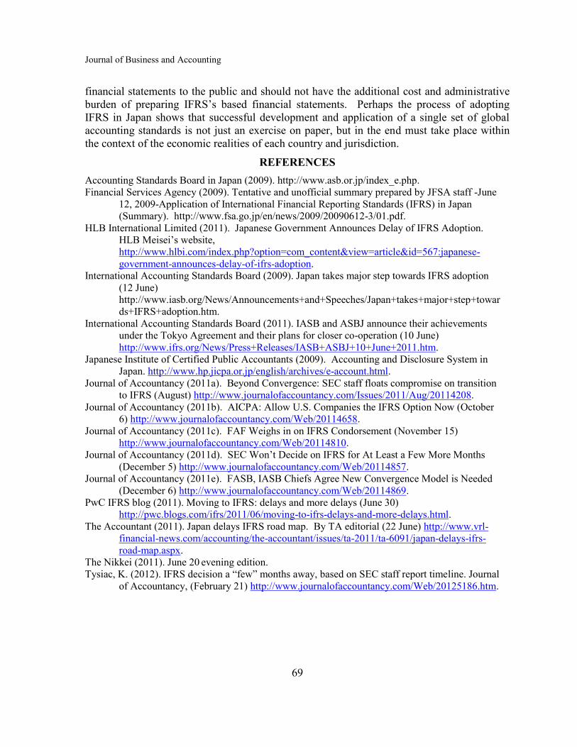
Journal of Business and Accounting
69
financial statements to the public and should not have the additional cost and administrative
burden of preparing IFRS’s based financial statements. Perhaps the process of adopting
IFRS in Japan shows that successful development and application of a single set of global
accounting standards is not just an exercise on paper, but in the end must take place within
the context of the economic realities of each country and jurisdiction.
REFERENCES
Accounting Standards Board in Japan (2009). http://www.asb.or.jp/index_e.php.
Financial Services Agency (2009). Tentative and unofficial summary prepared by JFSA staff -June
12, 2009-Application of International Financial Reporting Standards (IFRS) in Japan
(Summary). http://www.fsa.go.jp/en/news/2009/20090612-3/01.pdf.
HLB International Limited (2011). Japanese Government Announces Delay of IFRS Adoption.
HLB Meisei’s website,
http://www.hlbi.com/index.php?option=com_content&view=article&id=567:japanese-
government-announces-delay-of-ifrs-adoption.
International Accounting Standards Board (2009). Japan takes major step towards IFRS adoption
(12 June)
http://www.iasb.org/News/Announcements+and+Speeches/Japan+takes+major+step+towar
ds+IFRS+adoption.htm.
International Accounting Standards Board (2011). IASB and ASBJ announce their achievements
under the Tokyo Agreement and their plans for closer co-operation (10 June)
http://www.ifrs.org/News/Press+Releases/IASB+ASBJ+10+June+2011.htm.
Japanese Institute of Certified Public Accountants (2009). Accounting and Disclosure System in
Japan. http://www.hp.jicpa.or.jp/english/archives/e-account.html.
Journal of Accountancy (2011a). Beyond Convergence: SEC staff floats compromise on transition
to IFRS (August) http://www.journalofaccountancy.com/Issues/2011/Aug/20114208.
Journal of Accountancy (2011b). AICPA: Allow U.S. Companies the IFRS Option Now (October
6) http://www.journalofaccountancy.com/Web/20114658.
Journal of Accountancy (2011c). FAF Weighs in on IFRS Condorsement (November 15)
http://www.journalofaccountancy.com/Web/20114810.
Journal of Accountancy (2011d). SEC Won’t Decide on IFRS for At Least a Few More Months
(December 5) http://www.journalofaccountancy.com/Web/20114857.
Journal of Accountancy (2011e). FASB, IASB Chiefs Agree New Convergence Model is Needed
(December 6) http://www.journalofaccountancy.com/Web/20114869.
PwC IFRS blog (2011). Moving to IFRS: delays and more delays (June 30)
http://pwc.blogs.com/ifrs/2011/06/moving-to-ifrs-delays-and-more-delays.html.
The Accountant (2011). Japan delays IFRS road map. By TA editorial (22 June) http://www.vrl-
financial-news.com/accounting/the-accountant/issues/ta-2011/ta-6091/japan-delays-ifrs-
road-map.aspx.
The Nikkei (2011). June 20 evening edition.
Tysiac, K. (2012). IFRS decision a “few” months away, based on SEC staff report timeline. Journal
of Accountancy, (February 21) http://www.journalofaccountancy.com/Web/20125186.htm.

Journal of Business and Accounting
Vol. 5, No. 1; Fall 2012
70
ISSUES WITH MANDATORY AUDIT FIRM ROTATION
Homer L. Bates
Bobby E. Waldrup
David G. Jaeger
University of North Florida
Vincent Shea
St. Johns University
ABSTRACT
Mandatory audit firm rotation has been discussed by accounting academics,
regulators and practitioners for decades. Recently, the Chairman of the PCAOB and the
former head of the SEC have stated support for the concept because of the perception that
long-term auditor/client tenure may signify decreased objectivity. This paper examines the
rotation issue from a historical and international perspective. The background of the rotation
issue is discussed along with a brief sample of the mixed prior research findings. Auditor
rotation rules and laws in countries with the largest GDP are also examined and discussed.
Finally, as a result of this examination, the authors recommend a very long mandatory
auditor rotation period of 12 to 20 years in order to increase the perception of objectivity
without significantly increasing long-term costs. A potential future research topic would be
to examine the present status of the mandatory audit firm rotation issue by accounting rule
makers in other large industrialized countries.
INTRODUCTION
Mandatory auditor rotation has been discussed by members of the accounting
profession and by the various users of accounting information for decades. Congress
considered including mandatory audit firm rotation in the Sarbanes-Oxley legislation, but
instead opted for partner-in-charge rotation. In the United States, Sarbanes-Oxley requires
that the in-charge partner be rotated every five years but does not require the audit firm to be
changed. Last August, James R. Doty, the Chairman of the five-member Public Company
Accounting Oversight Board (PCAOB), proposed mandatory auditor rotation as a means of
enhancing “… auditor independence, objectivity and professional skepticism.” Arthur
Levitt, former SEC head, in a recent Wall Street Journal interview (2011) expressed his view
that audit firms should be rotated every ten years. Michel Barnier, the European Union’s
commissioner for the internal market, has also raised the issue of requiring mandatory audit
firm rotation among European Union member countries, along with splitting up the top four
international audit firms (Huw Jones, Reuters, 2011).
The rotation issue has also received considerable recent attention in the financial
media. In the September 3, 2011 issue of The Economist (author unknown), the reporter
showed ambivalence by stating: “Mandatory rotation would probably not do much harm;
but it might well not do much good either.” (2011). The issue was also discussed by a
columnist for The New York Times in the August 17, 2011 issue (author unknown) in an
article with the headline “Accounting Board to Seek Comments on Rotating Auditors.”
(2011).

Journal of Business and Accounting
71
Elected politicians have also got involved in the mandatory auditor issue.
Representative Michael Fitzpatrick (R, Pa.) introduced legislation in March 2012 that would
prohibit the PCAOB from requiring the use of different auditors on a rotating basis.
Representative Fitzpatrick’s argument is that rotation would increase audit costs and would
deprive the company of the auditor’s company-based knowledge that comes from a long-
term audit-client relationship.
One of the primary rationales for the increased interest in mandatory rotation is the
perception that a long, close relationship between the audit firm and the company being
audited may lead to significantly decreased objectivity. In the United States, for example,
GE, Proctor and Gamble, Dow Chemical and four other corporations in the Standard and
Poor’s 500 index have used the same audit firm for over 100 years. Nearly 175 companies in
the index have had the same audit firm for 25 years or more. For companies included in the
Russell 1000, over 36 percent have retained the same external auditors for 21 years or more
(Brookings Institute, 2012). On the international front, the average tenure for an audit firm of
a company in the British FTSE 100 is 48 years. In Germany, over 60% of the companies in
the DAX 30 index have used the same audit firm for over 20 years.
Ghosh and Moon (Ghosh and Moon, 2005) examined the perception of audit tenure
by investors and financial analysts. Their results show that investors and analysts view long
audit tenure as favorably impacting earnings quality. They argue that since stock market
participants view long tenure as a positive that mandatory audit firm rotation might result in
unnecessary additional costs without any substantial additional benefits.
The primary argument against mandatory auditor rotation is the cost of a new auditor.
CFO.com (Johnson, 2012) reported that in 2003 it was estimated that a change in auditors
can add 20% to the initial cost of an audit. Another argument against rotation is that a
company’s auditor choice would be decreased. Most large corporations prefer to be audited
by one of the Big Four audit firms. Sarbanes-Oxley requires that the company select another
accounting firm for nonaccounting consulting services. If a company is being audited by one
of the Big Four and another Big Four firm is providing consulting services, then the choice
when changing auditors would be between only two audit firms.
The first section of this paper will examine the historical perspective of the audit firm
rotation issue. The second section will view audit firm rotation from an international
perspective. The third section will examine a small sample of the empirical research
regarding audit firm rotation. The two major issues are: whether rotation decreases audit
failure and whether the benefits of rotation are greater than the incremental costs. The final
section will be conclusions, recommendations and suggestions for future research.
BACKGROUND
The auditor rotation issue has been examined by accountants and accounting
researchers for decades. In 1961, Mautz and Sharaf suggested that a long association with
the same client may lead to problems with auditor independence. The U.S. Senate examined
the issue in 1976 and proposed a mandatory change of auditors after a period of time. No
actions were taken by Congress. In the mid-1990’s, the SEC examined the adverse effects of
long term auditor tenure but, again, took no action.

Bates, Waldrup, Jaeger, and Shea
72
During the Sarbanes-Oxley (SOX) discussions of 2002, mandatory auditor rotation
was considered, but it was ultimately decided that mandatory audit partner rotation was
sufficient. The Act requires that the chief decision maker on an audit engagement of a public
company rotate off of the audit every five years and remain off the audit for a five year
“cooling-off” period. The Congress did direct the General Accounting Office (GAO) to
prepare a report on mandatory audit firm rotation, and the 2003 report noted that the SEC
would need several years of SOX reforms data to determine if further actions were necessary.
As of June, 2011, the PCAOB created by SOX had conducted annual inspections of
the largest audit firms for eight years, reviewing over 2,800 engagements. They also
conducted over 1,500 inspections of smaller domestic and non-U.S. firms. Jim Doty, the
PCAOB Chair, stated that “Based on this work… it is incumbent on the PCAOB to take up
the debate about firm tenure and examine it with rigorous analysis…” (2011). Other
members of the Board had doubts about the concept because of the additional costs of getting
new auditors up to speed. Member Daniel L. Goelzer stated, “I have serious doubts that
across-the-board mandatory rotation is a practical or cost-effective way of strengthening
independence.” (2011) He argued instead for a more tailored approach, perhaps requiring
rotation when a PCAOB inspection finds a lack of auditor skepticism.
INTERNATIONAL PERSPECTIVE
Audit firm rotation has been examined by the accounting regulatory agencies in most
large industrialized countries and has been rejected. As shown in Table 1, only four of the
largest fifteen countries ranked by GDP have a requirement that audit firms be rotated.
Brazil, Italy, India and South Korea require audit firm rotation; the other eleven countries
including the U.S. and the United Kingdom do not. It is interesting to note that Canada and
Spain required mandatory audit firm rotation at one time, but subsequently repealed the
requirement.
One factor in Spain’s decision was the lack of evidence of the benefits of rotation.
Ruiz-Barbadillo, Gomez-Aquilar, and Carrera (2009) examined Spain’s mandatory audit firm
rotation policy from 1988 to 1995. They found no evidence in favor of mandatory audit
rotation and concluded that, “… our results provide empirical support for the arguments put
forward by opponents of mandatory rotation.”
Kwon, Lim and Simnett (2010) examined the results of the mandatory audit firm
rotation policy in South Korea. They looked at over twelve thousand firm-years of
observations between 2000 and 2007. Since mandatory audit firm rotation began in 2006,
they found that audit hours have increased, audit fees have increased, and audit quality has
remained unchanged or decreased slightly. They concluded that “… mandatory audit firm
rotation … (has) no discernible positive effect on audit quality.”
AUDIT ROTATION RESEARCH FINDINGS
Research into the effects of auditor rotation has had contradictory results. In 1982,
Bates, Ingram and Reckers (1982) conducted a behavioral study using sixty-seven practicing
CPA’s operating in the U.S. and found that “… the rotation of audit firm employees was
found as effective … as audit firm rotation. This study showed the need for auditor rotation
to offset the psychological effect resulting from a long-term auditor-client relationship.

Journal of Business and Accounting
73
However, partner rotation was found to be as effective as audit firm rotation. Those findings
support the accounting profession’s position against mandatory audit firm rotation.” In a
2006 study, Gates, Lowe and Reckers found opposite results and reported “… audit firm
rotation incrementally influenced individuals’ confidence in financial statements. However,
audit partner rotation did not have a similar effect” (2006).
Table 1
Auditor Rotation Rules1 for Largest Countries by GDP
2
Country Ranked by GDP Audit Firm Rotation Rule
1. United States No Mandatory Audit Firm Rotation
2. China No Mandatory Audit Firm Rotation
3. Japan No Mandatory Audit Firm Rotation
4. Germany No Mandatory Audit Firm Rotation
5. France No Mandatory Audit Firm Rotation
6. United Kingdom No Mandatory Audit Firm Rotation
7. Brazil Yes, Banks and Listed Companies every 5 years
8. Italy Yes, Listed Companies and Other Firms Identified
by Law every 9 Years
9. India Yes, Banks, Privatized Insurance Companies and
Government Companies every 4 Years
10. Canada No Mandatory Audit Firm Rotation, Until 1991,
Banks were required to Rotate Audit Firms
11. Russia No Mandatory Audit Firm Rotation
12. Spain No Mandatory Audit Firm Rotation, From 1988 –
1995, Listed Companies were Required to Rotate
Audit Firms every 9 Years
13. Australia No Mandatory Audit Firm Rotation
14. Mexico No Mandatory Audit Firm Rotation
15. South Korea Yes, Listed Companies are Required to Rotate Audit
Firms every 6 Years
1 Wikipedia, List of Countries by GDP (PPP), accessed February 5, 2012.
2 Deloitte LLP, Letter to PCAOB 12/8/11 regarding Public Comment on Concept
Release on Auditor Independence and Audit Firm Rotation. Appendix 2, pages 1-4.
Audit quality may be indirectly measured by the number of audit restatements. If
auditor rotation brings new eyes to the audited company, one would anticipate new findings
and therefore increased restatements. In a 2003 study (Myers, et al, 2003), the authors
examined 562 companies that announced restatements between January 1997 and October
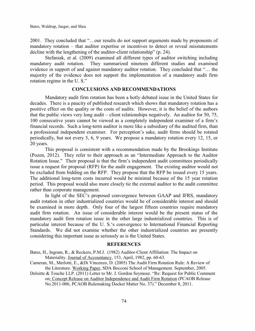
Bates, Waldrup, Jaeger, and Shea
74
2001. They concluded that “…our results do not support arguments made by proponents of
mandatory rotation – that auditor expertise or incentives to detect or reveal misstatements
decline with the lengthening of the auditor-client relationship” (p. 24).
Stefaniak, et al. (2009) examined all different types of auditor switching including
mandatory audit rotation. They summarized nineteen different studies and examined
evidence in support of and against mandatory auditor rotation. They concluded that “… the
majority of the evidence does not support the implementation of a mandatory audit firm
rotation regime in the U. S.”
CONCLUSIONS AND RECOMMENDATIONS
Mandatory audit firm rotation has been a hotly debated issue in the United States for
decades. There is a paucity of published research which shows that mandatory rotation has a
positive effect on the quality or the costs of audits. However, it is the belief of the authors
that the public views very long audit – client relationships negatively. An auditor for 50, 75,
100 consecutive years cannot be viewed as a completely independent examiner of a firm’s
financial records. Such a long-term auditor is more like a subsidiary of the audited firm, than
a professional independent examiner. For perception’s sake, audit firms should be rotated
periodically, but not every 5, 6, 9 years. We propose a mandatory rotation every 12, 15, or
20 years.
This proposal is consistent with a recommendation made by the Brookings Institute
(Pozen, 2012). They refer to their approach as an “Intermediate Approach to the Auditor
Rotation Issue.” Their proposal is that the firm’s independent audit committees periodically
issue a request for proposal (RFP) for the audit engagement. The existing auditor would not
be excluded from bidding on the RFP. They propose that the RFP be issued every 15 years.
The additional long-term costs incurred would be minimal because of the 15 year rotation
period. This proposal would also more closely tie the external auditor to the audit committee
rather than corporate management.
In light of the SEC’s proposed convergence between GAAP and IFRS, mandatory
audit rotation in other industrialized countries would be of considerable interest and should
be examined in more depth. Only four of the largest fifteen countries require mandatory
audit firm rotation. An issue of considerable interest would be the present status of the
mandatory audit firm rotation issue in the other large industrialized countries. This is of
particular interest because of the U. S.‘s convergence to International Financial Reporting
Standards. We did not examine whether the other industrialized countries are presently
considering this important issue as seriously as is the United States.
REFERENCES
Bates, H., Ingram, R., & Reckers, P.M.J. (1982) Auditor-Client Affiliation: The Impact on
Materiality. Journal of Accountancy, 153, April, 1982, pp. 60-63.
Cameran, M., Merlotti, E., &Di Vincenzo, D. (2005) The Audit Firm Rotation Rule: A Review of
the Literature. Working Paper, SDA Bocconi School of Management. September, 2005.
Deloitte & Touche LLP. (2011) Letter to Mr. J. Gordon Seymour. “Re: Request for Public Comment
on: Concept Release on Auditor Independence and Audit Firm Rotation (PCAOB Release
No.2011-006, PCAOB Rulemaking Docket Matter No. 37).” December 8, 2011.
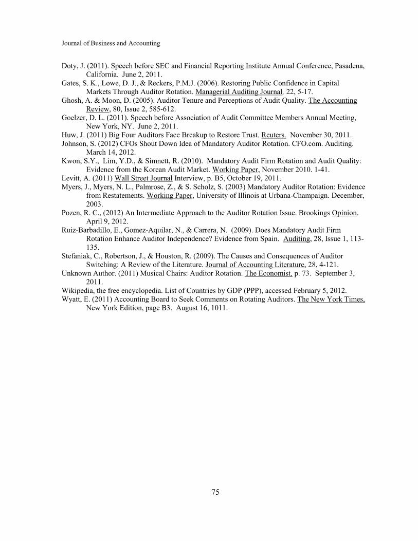
Journal of Business and Accounting
75
Doty, J. (2011). Speech before SEC and Financial Reporting Institute Annual Conference, Pasadena,
California. June 2, 2011.
Gates, S. K., Lowe, D. J., & Reckers, P.M.J. (2006). Restoring Public Confidence in Capital
Markets Through Auditor Rotation. Managerial Auditing Journal, 22, 5-17.
Ghosh, A. & Moon, D. (2005). Auditor Tenure and Perceptions of Audit Quality. The Accounting
Review, 80, Issue 2, 585-612.
Goelzer, D. L. (2011). Speech before Association of Audit Committee Members Annual Meeting,
New York, NY. June 2, 2011.
Huw, J. (2011) Big Four Auditors Face Breakup to Restore Trust. Reuters. November 30, 2011.
Johnson, S. (2012) CFOs Shout Down Idea of Mandatory Auditor Rotation. CFO.com. Auditing.
March 14, 2012.
Kwon, S.Y., Lim, Y.D., & Simnett, R. (2010). Mandatory Audit Firm Rotation and Audit Quality:
Evidence from the Korean Audit Market. Working Paper, November 2010. 1-41.
Levitt, A. (2011) Wall Street Journal Interview, p. B5, October 19, 2011.
Myers, J., Myers, N. L., Palmrose, Z., & S. Scholz, S. (2003) Mandatory Auditor Rotation: Evidence
from Restatements. Working Paper, University of Illinois at Urbana-Champaign. December,
2003.
Pozen, R. C., (2012) An Intermediate Approach to the Auditor Rotation Issue. Brookings Opinion.
April 9, 2012.
Ruiz-Barbadillo, E., Gomez-Aquilar, N., & Carrera, N. (2009). Does Mandatory Audit Firm
Rotation Enhance Auditor Independence? Evidence from Spain. Auditing, 28, Issue 1, 113-
135.
Stefaniak, C., Robertson, J., & Houston, R. (2009). The Causes and Consequences of Auditor
Switching: A Review of the Literature. Journal of Accounting Literature, 28, 4-121.
Unknown Author. (2011) Musical Chairs: Auditor Rotation. The Economist, p. 73. September 3,
2011.
Wikipedia, the free encyclopedia. List of Countries by GDP (PPP), accessed February 5, 2012.
Wyatt, E. (2011) Accounting Board to Seek Comments on Rotating Auditors. The New York Times,
New York Edition, page B3. August 16, 1011.

Journal of Business and Accounting
Vol. 5, No. 1; Fall 2012
76
THE IMPACT OF TAX INCENTIVES ON THE LOCATION OF
MANUFACTURING FACILITIES
Juan Luis Jay Ramirez
CPA, Master of Business Taxation from University of Southern California
Anwar Y. Salimi
Hassan Hefzi
California State Polytechnic University, Pomona
ABSTRACT
This paper illustrates the factors considered by U.S. manufacturing corporations in
determining where to locate a new manufacturing facility. The U.S. government, state
government, local governing bodies, and foreign governments offer a variety of incentives to
persuade companies to locate manufacturing facilities within their borders. The American
Jobs Creation Act is an example of an incentive at the federal level that was put in place to
trigger investment within the U.S. Many states have their own incentives, such as
California’s Manufacturer’s Investment Credit (MIC), which offers a credit against
California income tax based on the purchase and use of property in a manufacturing process
in California. Foreign countries are also involved in similar practices. They negotiate
specific incentive packages in the form of tax breaks or government grants in order to attract
multinational manufacturers and the multitude of jobs that a manufacturing facility can bring.
Contrary to the expectations, this paper shows that taxes and government incentives appear to
be only one of the factors considered by U.S. manufacturers in deciding where they will
locate their manufacturing operations. The choice of location appears to be driven by a
variety of business factors, and taxes are only one such factor. Taxes and incentives
definitely appear to be contributing factors but they are not the most important factors in the
decision making process.
INTRODUCTION
Many governing jurisdictions including the U.S. federal government, state
governments, and foreign governments have recognized the benefits of having manufacturing
facilities within their borders. Manufacturing facilities offer a variety of benefits to the
government and its constituents. These benefits include additional income tax revenue,
property tax revenue, sales tax revenue, jobs for a wide range of constituents from the highly
educated to the unskilled or semi-skilled, and personal income tax revenue for the additional
jobs created within the government’s borders. Governments have been faced with the tax
version of the chicken or egg question. In order to increase tax revenue, more businesses
need to be attracted into the area. However, in order to attract new businesses, the
government needs to reduce taxes. Different governments have chosen to answer this
question in very different ways. The U.S. has a different situation compared to other
countries because only in the last few decades has the U.S. chosen to consider that its
constituents may choose to invest outside its borders. This is due to the fact that U.S. has the
benefit of owning the single largest industrial capital base along with the world’s largest
single consumer market. As a result, the tax history of the U.S. has been based on internal
Journal of Business and Accounting
77
politics rather than reacting to or anticipating external forces. Current U.S. tax legislation
still mirrors this focus on internal politics and the use of incentives to deliver on the wants
and desires of certain interests.
In a global economy that is shrinking on a daily basis, manufacturers have a wide
array of factors to consider in determining where to locate a manufacturing facility. Some
factors will definitely be more important than others depending on industry. For instance, a
steel manufacturer will need to be closer to customers than a semiconductor manufacturer.
Another factor to be considered is the cost of labor. Though low labor rates are considered
universally important, they are much more important in low technology industries which rely
on manual labor than they are to high technology industries which rely on automated labor
(robot assembly lines).
Given the wide variety of factors which impact a corporation’s manufacturing costs,
taxes and government incentives may or may not be an important enough factor to alter a
company’s decision making in determining where to put a manufacturing facility.
Manufacturers may consider more direct costs such as labor rates or availability of labor to
be more important in considering where to make the large investment of building a factory.
The global economy has set governments to compete against each other for
investment dollars. There are various factors at work which will impact a manufacturer’s
decision on where to locate its next plant.
By having a better understanding of what motivates manufacturers, a government
(federal, state, or foreign) can focus the actual incentive dollars that it gives out or it can
better focus the time spent on pursuing potential investors. A better focus of actual incentive
dollars is important to avoid programs that do not actually generate additional investment. A
better understanding of the manufacturers’ motivations can allow governing bodies to focus
their efforts on industries in which they can be competitive. This means that the state seeks
out companies in industries that might find them as an attractive location even if there were
no incentive.
Results of this study may be important to governments as they try to tailor their
incentives. What is important to one type of manufacturer may not be important to another
type of manufacturer.
The remainder of the paper is organized as follows: Section 2 provides review of
existing literature addressing incentives to manufacturing facilities and develops the
hypothesis. Section 3 presents the methodology of the study. The results are presented in
section 4 and a summary, conclusion, and recommendations are included in section 5.
LITERATURE REVIEW AND HYPOTHESIS
Manufacturing Incentives: Few existing studies have investigated the decision-
making process for locating manufacturing facilities. Ondrich and Wasylenko (1993)
reviewed actual foreign direct investment (FDI) activity in the U.S. from 1978 to 1987 and
drew conclusions from that activity. They investigated the factors that are important to
foreign companies when determining where to build a factory in the U.S. They concluded
that foreign investors located new factories in places where a similar factory (though owned
by the competition) already existed. The reason for this appeared to be that foreign investors
chose to take advantage of existing infrastructure and a workforce which was already

Ramirez, Salimi, and Hefzi
78
experienced in their particular industry. Also, foreign investors favored lower tax
jurisdictions over higher tax jurisdictions. However, they did not favor lower labor rates over
higher labor rates. In our study, all participants had chosen to manufacture in the U.S. and
the labor rates within the U.S. vary only to a small degree from one state to the next. When
comparing the labor rates of the U.S. to those of other countries, there is a great deal of
variety. Therefore, we expect that labor rates should prove to be an important criterion in
determining where to build a manufacturing facility for the participants in the proposed
study.
MacCarthy and Atthirawong (2003) asked participants about the main motivation for
seeking to manufacture internationally. The results were to have access to low cost labor and
specific labor skills; to have access to foreign markets; to get tax incentives and benefits; to
have access to host raw materials and technology; and to counterattack against competitors
Two key differences exist between this study and our study. The first difference is
that the initial question made in this study presupposes a desire to manufacture abroad. In
our research, we ask about the factors that are important in determining where to build a new
facility. Though the results listed above may be important to the participants in our study, all
factors may be outweighed by some other factor that necessitates manufacturing within the
U.S. The survey conducted above would have missed this other possibility completely
because it never considered the possibility of manufacturing in the U. S. instead of abroad.
The second difference is that this study limited itself to participants that are doing
business or considering doing business in Asia (may or may not have been U.S.
corporations). In our study, this is not the case. The participants are U.S. corporations that
may or may not ever choose to manufacture in Asia.
State Incentives: The literature has a multitude of examples of state incentives. One
of the most newsworthy incentives was the one given by the state of Alabama to Mercedes
Benz in order to host the first Mercedes plant outside of Germany (Myerson, 1996). This
incentive was newsworthy because it was very large. The total incentive including land,
worker training, site improvement, purchase of Mercedes Benz vehicles and other incentives
was over $500 million.
Foreign Strategies: Dorgan (2006) outlined Ireland’s rise from “one of the poorest
countries in Western Europe to one of the most successful.” The study credits sensible and
pragmatic policies for Ireland’s rise with three key factors at the heart of these policies.
These policies were belief in economic openness to global markets, low tax rates, and
investment in education. Ireland’s historic policy of low taxes was a key in its economic
climb. Currently, Ireland has one of the lowest corporate standard tax rates in Europe. Its
corporate tax rate is a maximum of 12.5%.
Teoh and Seah (2009) provided substantial background on Singapore’s business
climate and its use of tax incentives to drive the Singapore economy in specific directions.
“Foreign direct investment in Singapore was valued at S$363.9 Billion [approximately U.S.
$260B] as of the end of 2006, with the bulk of the direct investment being in financial
services and manufacturing.” Singapore has focused tax incentive program, which negotiates
tax incentives for favorable industries or activities. These tax incentives are generally in the
form of exemption from income tax and reducing tax rates to between 5 percent and 10
Journal of Business and Accounting
79
percent. Singapore not only drives foreign investment through specific tax incentives, it also
drives foreign investment through its development of Singapore’s infrastructure.
Greider (1997) discussed globalization and the way that states and countries have
dealt with that globalization. He specifically discussed the Malaysian semiconductor
industry as an example of both the benefits and detriments of globalization. In the early
1970’s American semiconductor companies made the decision to move to Malaysia as a new
low wage locale for final assembly of products. Japanese firms followed as they were
seeking to move manufacturing costs offshore to offset the rising yen. Malaysia established
“Pioneer” status for the semiconductor industry in order to secure its status as a major export
platform. This status meant no income tax for 5 to 10 years, exemption from import duties,
and other forms of state subsidies. The benefits would expire but could be renegotiated and
extended if the company promised to make new investments such as plant expansions and
new jobs within Malaysia.
Another key attraction of Malaysia, though a controversial one, was the government’s
guarantee that electronics workers would be prohibited from unionizing.
Hypothesis: Based on the previous discussion, this paper states its hypothesis in the
null format:
“Tax and other government incentives are not the first factor considered when
corporations decide where to locate a manufacturing facility.”
METHODOLOGY
Sample and Procedure: This study focuses on large manufacturers headquartered
within the U.S. Publication and library research was conducted from September 2008 to
January 2010. Data research is the primary method used for this study.
Research Design: Data analysis is the primary method of strategy used for this study.
The main research data consists of primary data. The purpose of the study is to gather
feedback from U.S. headquartered manufacturers on what they consider to be the most
important factors in determining where to locate a manufacturing facility.
Research Method: A survey was administered to large U.S. manufacturers. The
survey consists of a list of 14 factors considered to be common factors in determining where
to locate a new manufacturing facility. In addition to the factors included in the survey, an
additional blank is added labeled “Other” which gives the participant the ability to add any
other factors that they think are relevant. The participants are asked to rank each criterion in
order of importance in determining where to locate a manufacturing facility. The survey
included the following criteria for the consideration of the participants:
1. Customer demands Proximity to customer facilities
Proximity to customer’s 3rd party logistics service
Proximity to customer designated suppliers
2. Supply Inputs Cost of local workforce
Proximity to raw materials
Ramirez, Salimi, and Hefzi
80
Proximity to supplier
Cost of local raw materials
Quality of local infrastructure (i.e., dependable energy supply)
3. Facility requirements Cost of land
Cost of building a facility (local construction costs)
Cost of available facility (purchase or rent from third party)
Proximity to transportation services (shipping, air or train)
4. Government and Regulatory Issues Favorable government regulations or requirements
Tax rates, credits or negotiated tax holidays
Population: The survey questionnaire was sent to 99 corporations identified as the
largest manufacturers in the U.S. For purposes of this study, a list of “large” U.S.
manufacturers was generated using the list of the 500 largest manufacturers in the U.S., as
determined by Industry Week magazine. The list used for this study was for the year 2003 to
2004. The corporations on the list from the states of California, Texas, and Washington
were originally used for this study. The original mailing took place on September 15th 2009.
The survey was sent soliciting anonymous responses in order to increase the response rate
and allow for more candid responses from participants. The original 99 mailings resulted in
only 19 responses.
A second set of mailings was sent to 54 more corporations. Fifty-one of these
corporations were selected at random from Industry Week’s top 500 manufacturers list. The
population for random selection excluded manufacturers in California, Washington and
Texas because corporations from these states were already captured in the first mailing. An
additional three were sent to manufacturing corporations in which the researcher has personal
contacts. An additional 13 responses were received from this second set of mailings.
RESULTS
Descriptive information: Results of this study show that although tax is one of the
factors that is considered by decision makers, it is not the most important factor considered in
determining where to locate a new facility. Table 1 lists the factors used in the survey along
with their Average Importance Score, Highest Score on any Survey, Lowest Score on any
Survey, Geometric Mean and Standard Deviation.
Order of Results: Each criterion shows a separate theme in the decision making of
the participants in the survey. The fact that the cost of labor and infrastructure are ranked
first and second is important to analyze because in some ways these two criteria can be
considered inversely related. The cost of labor seems like a likely choice for the most
important criteria as most corporations seek to cut costs, cost of labor is likely to be a very
large component of overall costs. The requirement for infrastructure seems to go hand in
hand with higher labor costs, not lower labor costs.
Labor tends to be less expensive where populations are higher. Two examples are
China and India. An abundance of available labor keeps labor rates low under the simple

Journal of Business and Accounting
81
rule of supply and demand. Higher populations have a supply of labor that outweighs
demand. This tends to push labor costs down.
Table 1: Table of Findings Rank Factor Category Average
Importance
Score
Highest
Score
on any
Survey
Lowest
Score on
any Survey
Geometric
Mean
Standard
Deviation
1 Cost of local
workforce
Supply Inputs 3.17 1 7 2.5276 2.0372
2 Quality of local
infrastructure (ie
dependable
energy supply)
Supply Inputs 4.74 1 10 3.8871
2.7172
3 Favorable
government
regulations or
requirements
Government
and
Regulatory
Issues
5.35
1 13 4.2319
3.4851
4 Tax rates, credits
or negotiated tax
holidays
Government
and
Regulatory
Issues
6.13
1 14 4.5435
4.1812
5 Proximity to
transportation
services (shipping,
air or train)
Facility
requirements
6.78 2 15 6.2676
3.5444
6 Cost of available
facility (purchase
or rent from third
party)
Facility
requirements
7.00 1 13 5.9879
3.8593
7 Proximity to raw
materials
Supply Inputs 7.22 1 15 6.1443
3.6799
8 Cost of local raw
materials
Supply Inputs 7.96 1 15 6.4260
4.5774
9 Proximity to
supplier
Supply Inputs 8.61 2 15 7.6499
3.7506
10 Cost of land Facility
requirements
8.65
1 15 7.5283
3.7125
11 Cost of building a
facility (local
construction
costs)
Facility
requirements
8.74 2 15 7.7105
3.7805
12 Proximity to
customer facilities
Customer
demands
9.09 1 15 7.2393
4.2844
13 Proximity to
customer’s 3rd
party logistics
service
Customer
demands
10.83 3 15 9.8148
3.8097
14 Proximity to
customer
designated
supplier
Customer
demands
11.26 3 15 10.2597
4.0589
Table 1 above shows multiple points that need to be identified and explored.

Ramirez, Salimi, and Hefzi
82
Low labor rates tend to lead to less investment in fixed assets such as machinery.
Less investment in machinery over time leaves a country behind in terms of infrastructure.
Therefore, the lowest labor rates usually come in areas with substantially less infrastructure.
Since labor and infrastructure are required for successful manufacturing activities, a
manufacturer must choose the correct mix between the two inversely related criteria. The
lower the labor rates, the lower the level of infrastructure. Low labor rates may be enticing
to a manufacturer but only if there is sufficient infrastructure to guarantee a consistent flow
of products. For example, regular power shortages and lack of maintained roads for
transporting goods will sway corporations away from a location regardless of how low the
labor rates may be.
Even for low technology manufacturers, the push for lower labor rates can have
catastrophic results if it is pursued without concern for the product consistency generated in
countries that have a proven infrastructure. Manufacturers that require higher technology
will tend to limit their search for lower labor rates in order to maintain high levels of
infrastructure. The fact that cost of labor and infrastructure ranked first and second shows
that manufacturers are searching for the proper mix between the two factors.
Favorable government regulations or requirements took the third rank in the list, and
it is exemplified in the Malaysia example discussed in the Literature Review. One of the
reasons the semiconductor industry flocked to Malaysia was the Malaysian government’s
guarantee that unions would not be allowed to enter the semiconductor industry. This was a
big concern for the industry because their experience was that unions negatively impacted
profits by increasing wages. Another favorable regulation could be the lack of fixed pension
laws in Malaysia which could make the cost of labor much higher. Favorable government
regulations also applied in the case of the auto industry in the South. Manufacturing in
Germany is very expensive not only because of the wages earned by German workers but
also because of the mandatory pension funding requirement for German workers. These
requirements make German manufacturing much more expensive and are likely a big reason
that Mercedes and BMW chose to build plants outside of Germany. Taxes and incentives
took the fourth spot and are discussed at length in a later section.
Proximity to transportation services was ranked fifth and it is a factor that is likely to
have high importance to some industries while having a much lower importance to others.
There is a cost to moving manufactured goods however for some products which are heavy,
perishable or dangerous to move, transportation is a much higher cost of delivering the
products to customers.
The cost of an available facility took the sixth rank. The cost of a facility can be very
important especially in cases in which a facility has strict requirements. One case is the
manufacture of power management chips (example International Rectifier). These chips are
manufactured with clean rooms in ways that are very similar to memory chips manufactured
by companies like Intel but they require a lower level of precision. This industry uses
technology that is behind that used in memory chips. The result is that this industry tends to
move into former memory chip facilities as these facilities become obsolete for the
manufacture of memory chips. The power management chip manufacturers buy these
facilities for a dramatically lower cost than the cost of building a brand new factory. The
availability of these facilities dictates where they will manufacture.
Journal of Business and Accounting
83
Proximity to raw materials came in at rank seven. This could be very important in an
industry where the goods manufactured are much cheaper and easier to transport than the raw
materials. In this case, the manufacturer will locate its facility near the raw materials in order
minimize the cost of moving the raw materials. One example could be the timber industry
which cuts trees then cuts them into usable planks. Uniform planks are the product that will
be delivered to the customer. It is much easier, and therefore cheaper, to create the product
near the source of the raw material (trees) than to move large logs to a factory that is closer to
the customers.
Cost of local raw materials came in eighth place. It is very important to industries in
which the fluctuations in one cost can make or break the manufacturer’s profitability. This is
the case with the aluminum smelting industry, which tends to locate itself in areas in which
the main input is inexpensive.
Proximity to supplier was ranked nine. This is likely important to companies in
which the supply of inputs is scarce or the inputs are more expensive to move than the
finished products. The manufacturer will choose to locate itself near its suppliers in order to
reduce costs. A manufacturer could also get a competitive advantage by being close to many
suppliers. In some cases this is very similar to being close to raw materials. One example
could be paper mills which tend to be located in areas where the timber industry is prevalent.
In some cases, they may be linked directly to a logging company as a separate division or a
company with joint ownership.
The cost of land ranked tenth, and although it is not the main motivation for most
manufacturers, it can be a factor. Manufacturers tend to never be located where land is
expensive because of the large amount of land they usually require in order to run their
operations. Manufacturers tend to located in more rural areas. Note that all of the foreign
auto industry plants that have arisen in the U.S. have been built in the South where land is
relatively inexpensive. In addition, most of these manufacturers were able to get local
governments to acquire the land for them.
The cost of building a facility ranked eleventh among the factors. This factor can be
linked with the cost of buying a facility. In cases in which a facility has expensive
requirements, the manufacturer will consider the cost of building very important if there is no
readymade facility available to purchase. This is the case for most specialized high
technology industries
Proximity to customer facilities ranked twelfth. This factor is considered important
for manufacturers that are required to deliver their product under time constraints as part of
the customer’s manufacturing process. An example might be a company that manufacturers
sterilized bottles for a pharmaceutical company. The sterilized bottles need to arrive at a key
point in the customer’s manufacturing process. As a result, proximity would be a coveted
attribute of any location for a new manufacturing facility. Greater distances lead to larger
risks of late deliveries or contamination of the product. This could also be the case for
manufacturers of automobile inputs.
Proximity to a customer’s third party logistics service ranked thirteenth. It could be
important to a customer that is manufacturing perishable goods for a large customer that uses
those goods throughout the world. For example, a company that manufactures products for a
customer that uses FedEx as its logistics service provider might want to locate its

Ramirez, Salimi, and Hefzi
84
manufacturing location near FedEx’s Tennessee hub regardless of the cost of manufacturing
there. It may well be that the customer demands that manufacturing be conducted in
Tennessee and is willing to pay a premium to make sure that it is properly supplied.
Proximity to a third party supplier ranked last and it is conceptually similar to the
requirement to be close to the customer. In the case of the auto industry and its movements
to just-in-time, many auto manufacturers such as Ford have chosen to have their vendors
move into tiers in order to streamline their procurement process. A first tier provider may
manufacture a whole steering housing which may require inputs from a second tier provider.
The first tier provider becomes the customer of the second tier provider in place of Ford. In
this case, a second tier provider that manufactures a part of the steering housing may need to
locate its facilities near the first tier provider.
Distribution of Results: Among a wide variety of manufacturers, a wide variety of
criteria are the most important in the decision making process. Note that among the 14
criteria for decision-making, nine of the criteria were ranked first for at least one company.
Even the criteria that ranked fourteenth, the proximity to customer designated supplier,
ranked as high as third for at least one company. This shows that different industries have
very different decision making criteria. This fact may be important to governments as they
try to tailor their incentives. What is important to one type of manufacturer may not be
important to another type of manufacturer.
The means and the standard deviations offer some additional insight into the
consistency among the respondents. The lower the standard deviation of the factor, the
greater the consistency among respondents for this factor. The first criteria considered for
locating a manufacturing facility - the cost of the local workforce - had the lowest standard
deviation of 2.0372. This means that it was consistently ranked as important by responders.
The same is true for the criteria which ranked second, quality of local infrastructure. It had
the second lowest standard deviation of 2.7172. These two factors were the clear leaders in
consistency as well as ranking.
The highest standard deviation was generated by the eighth ranked criteria, cost of
local raw materials. This criteria ranked anywhere between 1 and 15 by the responders and
its standard deviation of 4.5774 indicated that it had much less consistency in its rank among
the respondents than any other criteria. This may be linked to the wide array of
manufacturers used in the survey. As explained above, the value of this criterion can be
industry specific.
Tax rates, credits, or negotiated tax holidays had a surprisingly high standard
deviation considering that it placed fourth in importance among all criteria. Its standard
deviation was 4.1812, which means that it was valued very differently by most respondents.
This standard deviation was third highest of all criteria behind cost of local raw materials and
proximity to customer facilities. This may be due to the varying tax positions of the
responders. Corporations with high net operating losses or large amounts of tax credit carry-
forwards may not value tax benefits as highly as those that are currently paying taxes.
Lack of Importance of Customer Demands: Among the 14 criteria offered to
survey participants, it is important to note that the three criteria categorized as Customer
Demands resulted as the least important factors in the survey. This may be the case for
various reasons. The first possibility is that large manufacturers tend not to be tied to one

Journal of Business and Accounting
85
customer. If any of the manufacturers were tied to a limited number of customers, then we
would expect that the proximity to the customer, its logistics service, or its suppliers would
be much more important on this list.
The second possibility is that in tougher economic times, all parties are seeking lower
costs. Customers are likely to accept less convenience in return for lower prices. The
manufacturer is given the task of pushing down costs through greater efficiencies in order to
reduce prices to customers. It is also likely that the customers will make fewer demands with
regard to their overall convenience when they are much more concerned with lower costs. In
selecting a site for a manufacturing facility, the manufacturer might not choose to reduce the
convenience that has been provided to its customers in the past but it probably will not
choose to increase conveniences either. This will definitely be the case when the
manufacturer feels that any additional conveniences it provides will not be coveted enough
by the customer sufficiently to generate higher prices from the customer. Higher prices for
more convenience may not be well received by customers in tough economic times.
The Importance of Tax: The above results show that, among a wide variety of
manufacturers, tax is important as a criteria but it is not the most important criteria
considered when choosing a manufacturing facility. Government investment in tax credits,
deductions, grants and tax holidays are well founded because they are attempting to influence
a key factor for manufacturers. Each government knows that if all else is equal, tax
incentives may tip the decision scale in its favor. Governments can identify the above factors
that would describe their jurisdiction and focus their incentives to work in conjunction with
those factors. As an example, a state within the U.S. may have substantial infrastructure but
also have high wages when compared to locations outside of the U.S.. It might consider
offering a wage credit to manufacturers for wages above a certain level. This would help
offset its high labor costs and also promote the hiring of college graduates within its
jurisdiction.
When considering the above results in conjunction with the growth strategy employed
by Ireland, one can derive a better focus for tax incentives. Ireland is not a country that can
compete with Asia on labor rates. It did not try to attract low technology manufacturers
because this fact was apparent. Ireland was the poorest country in Western Europe and its
strategy focused on differentiating itself from its Western European neighbors. It focused on
attracting high technology investment by using a highly educated and youthful population
(providing more young technical professionals than its neighbors) in conjunction with a tax
rate that is dramatically lower than its competition. Ireland’s focus was on taking
manufacturers from its neighbors rather than taking manufacturers away from global
competitors.
A similar analogy can be drawn with Singapore’s economic strategy. Singapore has
not and will not compete for low tech manufacturing with its Asian neighbors. It does not
have the resources to compete in this environment. It has instead focused on its highly
educated population and its historic role as a logistics hub to build additional foreign
investment. Today, Singapore focuses on being a treasury hub in order to supplement its
central role in logistics.
The same is not the case with Malaysia which has competed for low labor cost jobs.
Malaysia did not have the highly educated population that is available in Singapore and

Ramirez, Salimi, and Hefzi
86
Ireland. It marketed its low labor rates and the result was investment from companies that
coveted low labor rates. Although the standard of living has improved dramatically in
Malaysia though foreign investment, additional prosperity can only be generated through
higher wages for the general population. However, higher wages will only drive away the
foreign investment that Malaysia requires to fuel its economy.
The strategies of Ireland and Singapore can provide a substantial amount of input to
an overall strategy for developing manufacturing in the U.S.
Competition at the Federal Level: For the U.S., competition for manufacturers
through tax legislation and other factors must take place at a federal level, not a state level.
The main reason is that the federal government controls the major part of the tax base. It is
an unreal expectation for the state of Utah, for example, to compete with Malaysia or China
for investment dollars when the state of Utah controls a relatively small portion of the tax
burden that a manufacturer would face for locating in Utah. The federal government controls
most of the tax burden so it is the federal government’s job to compete for manufacturers at a
global level.
Focused Incentives: Specific types of manufacturers must be targeted similar to the
Irish example. Based on labor rates, a tax rate of zero would not be sufficiently low to attract
certain types of manufacturers. The U.S. must purge itself of concerns over low wage rate
jobs leaving the country and going offshore. These jobs pay low wages and they should be
allowed to leave or even promoted to leave. A move must be made to focus on attracting or
maintaining high technology manufacturers which rely on an education level in the local
population and infrastructure that the U.S. can already provide.
The next key step for the U.S. is to incentivize manufacturing in which the U.S. can
be competitive. One major change would be a §199 type incentive with dramatically higher
benefits. As stated earlier, the §199 incentive provides a deduction equal to 9% of income
derived on U.S. production activities. As an example, if a taxpayer only manufactures in the
U.S. and earns $100 from those activities, its incentive benefit is as shown in Table 2. The
entire benefit derived from §199 is only 3.15 percent of taxable income before taking other
limitations into account. §199 is a very meager incentive for purposes of competing with
countries like Ireland or Singapore. An increased incentive would be one that offers a tax
rate of 12.5% to all qualifying manufacturers on manufacturing activity. This would produce
a benefit to manufacturers of 22.5% (35% less 12.5%) of taxable income. This is a benefit
worth around six times that of §199. This type of incentive would make the U.S. highly
attractive to high technology investors. As in the case of Ireland, the U.S. needs to compete
with other countries with similar living standards and infrastructure (mainly Europe). It
should focus on taking manufacturers away from this peer group rather than worrying about
countries with labor rates so low that employment in these industries in the U.S. would result
in a large class of “working poor.”
State Competition: Once the U.S. is established as a more dominant site for
manufacturing, the states can compete with each other on a much more level playing field.
States would be allowed to focus on the attributes that they bring to the table when compared
to other states. This competition would be for higher technology jobs which would mean that
states with weak education systems would be at a severe disadvantage. These states would
be forced to make dramatic improvements in their education systems in order to generate
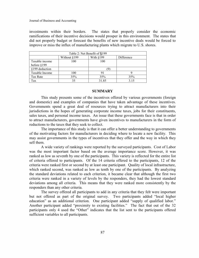
Journal of Business and Accounting
87
investments within their borders. The states that properly consider the economic
ramifications of their incentive decisions would prosper in this environment. The states that
did not properly budget or forecast the benefits of new incentive deals would be forced to
improve or miss the influx of manufacturing plants which migrate to U.S. shores.
Table 2: Net Benefit of §199
Without §199 With §199 Difference
Taxable income
before §199
100 100
§199 deduction (9)
Taxable Income 100 91 9
Tax Rate 35% 35% 35%
Tax 35 31.85 3.15
SUMMARY
This study presents some of the incentives offered by various governments (foreign
and domestic) and examples of companies that have taken advantage of these incentives.
Governments spend a great deal of resources trying to attract manufacturers into their
jurisdictions in the hopes of generating corporate income taxes, jobs for their constituents,
sales taxes, and personal income taxes. An issue that these governments face is that in order
to attract manufacturers, governments have given incentives to manufacturers in the form of
reductions to the taxes that they seek to collect.
The importance of this study is that it can offer a better understanding to governments
of the motivating factors for manufacturers in deciding where to locate a new facility. This
may assist governments in the types of incentives that they offer and the way in which they
sell them.
A wide variety of rankings were reported by the surveyed participants. Cost of Labor
was the most important factor based on the average importance score. However, it was
ranked as low as seventh by one of the participants. This variety is reflected for the entire list
of criteria offered to participants. Of the 14 criteria offered to the participants, 12 of the
criteria were ranked first or second by at least one participant. Quality of local infrastructure,
which ranked second, was ranked as low as tenth by one of the participants. By analyzing
the standard deviations related to each criterion, it became clear that although the first two
criteria were ranked in a variety of levels by the responders, they had the lowest standard
deviations among all criteria. This means that they were ranked more consistently by the
responders than any other criteria.
The survey offered all participants to add in any criteria that they felt were important
but not offered as part of the original survey. Two participants added “local higher
education” as an additional criterion. One participant added “supply of qualified labor.”
Another participant added “proximity to existing facilities.” The fact that out of the 32
participants only 4 used the “Other” indicates that the list sent to the participants offered
sufficient variables to all participants.

Ramirez, Salimi, and Hefzi
88
CONCLUSIONS
In reviewing the results of the survey and the supporting research, the following
observations and conclusions may be made:
The U.S. has a very weak track record in offering incentives that are actually geared
toward changing behavior. Of all the major incentives outlined in this body of research, only
one, the research and development credit, actually required a change in behavior in order to
obtain a tax benefit. The rest of the incentives offered benefits which were available to
companies which continued to conduct activities that they were already conducting. In
addition, the incentives offered only provided minor benefits to constituents which were
unlikely to generate an influx of investment from U.S. multinationals or foreign
multinationals. An example is the Section 199 manufacturing benefit offered by the U.S.
This benefit offers a benefit of 3.15 percent of taxable income. The same activity conducted
in Ireland is taxed at a rate so much lower than the U.S. that when measured in the same
terms as the Section 199 benefit, it provides a tax benefit that is equal to 22.5 percent of the
U.S. taxable income.
Part of the reason for this shortfall in U.S. incentives is the U.S. political system. In
various cases, including the Investment Tax Credit under the Kennedy Administration, the
political system in the U.S. does not allow for meaningful bills to pass. Tax benefits are
usually “watered down” and expanded to benefit more of the existing population and in
effect lose their effectiveness in generating their desired results. Another result of the U.S.
political process is that the U.S. federal government has never offered negotiated tax benefits
in return for specified foreign investment. This is something that the U.S. political landscape
would likely never allow because of its focus on fairness and equality.
The result of the lack of flexibility in the federal government is a “bend over
backward” approach by states. States only control a small portion of the tax burden carried
by a manufacturer and since there is no flexibility on the federal side, the states find
themselves competing vigorously in an attempt to get companies to invest within their
borders. As was the case when Alabama landed Mercedes, this competition can have
negative consequences and result in substantial criticism for state officials.
The survey results show that although governments spend a great deal of money in
attracting manufacturers into their jurisdictions, they are focusing on something that is,
according to this study, the fourth most important factor. Manufacturers appear focused on
two factors which can have an inverse relationship with each other. The first is the drive to
reduce costs, which caused “cost of labor” to be the first criterion in considering where to
locate a factory. The second is the drive to maintain quality which caused “quality of local
infrastructure” to be ranked second in the survey. Countries with the lowest labor rates tend
to be countries with low rates of fixed asset investment and therefore the countries with the
lowest infrastructure. The manufacturer needs to consider infrastructure in order to gain
some assurance on product quality along with timely production through dependable access
to resources such as energy. In order to assure that these concerns are met, the manufacturer
may not go to the very lowest wage area available.

Journal of Business and Accounting
89
RECOMMENDATION
Given that the U.S. political process would never allow federal negotiated incentives,
the U.S. should drop its tax rate for all manufacturers to 12.5 percent following the Irish
example. This incentive would combine a favorable federal tax policy with factors that the
U.S. already has which are coveted by multinationals. These factors include a strong and
politically stable infrastructure, which facilitates the movement of goods within and outside
the country, one of the largest consumer markets in the world, and a strong education system.
The political challenge in the U.S. is that the tax rate would apply to manufacturers only.
This would generate substantial opposition from the large service sector in the U.S.
A reduced federal tax rate for manufacturers would serve to compete with developed
countries for high paying jobs, while shunning away the manufacture of low cost labor
intensive products. Companies that covet low cost labor would continue to manufacture in
Asia rather than bring their manufacturing operations to the U.S. Products manufactured
with low cost labor would stay in Asia no matter how low the U.S. drops its tax rate. Labor
rates are too high a factor in their decision making criteria.
States could continue their negotiated incentive programs in this new environment. If
the U.S. is considered the manufacturing destination of choice, the states would only be in
competition with each other. All states would be forced to improve their education systems
because the types of jobs attracted into the U.S. under this new federal policy would require a
well-educated workforce. States that failed to improve their education systems would likely
miss the industry boom triggered by the federal governments new tax policy. The benefit to
the states is that they would no longer be competing for jobs against other countries;
however, they would only be competing against each other.
REFERENCES
Dorgan, S. (2006), How Ireland became the Celtic Tiger, Backgrounder - The Heritage Foundation,
(June 23), 1–15.
Greider, W. (1997), One World, Ready or Not. New York, New York: Simon & Schuster.
MacCarthy, B.L. & Atthirawong, W. (2003), Factors affecting location decisions in international
operations – A Delphi study, International Journal of Operations and Product Management,
23 (7), 794 – 818.
Myerson, A. R. (1996), O governor, won’t you buy me a Mercedes plant? The New York Times, 3
(September 1,).
Ondrich, J. & Wasylenko, M. (1993), Foreign direct investment in the United States: Issues,
magnitudes, and location choice of new manufacturing plants, Kalamazoo, Michigan: W.E.
Upjohn Institute.
Teoh, L. & Seah C. (2009), Business operation of Singapore, Washington, D.C., Tax Management,
Inc. a subsidiary of Bureau of National Affairs, Inc.

Journal of Business and Accounting
Vol. 5, No. 1; Fall 2012
90
TAX PRACTITIONERS AND ORDERING EFFECTS OF
INFORMATION IN AN ETHICAL DECISION
Scott Andrew Yetmar
Cleveland State University
Peter Poznanski
Cleveland State University
Elizabeth Koran
Meaden & Moore
ABSTRACT
This study investigates the ordering of information (pro-client or pro-IRS) and its
effect on the tax professional’s belief of whether to disclose the tax position taken on behalf
of the client to the IRS. Tax professionals were assigned to one of two groups. Each group
was given the same initial scenario which took a neutral position. Then, Group 1 first
received information that is classified as pro-client while Group 2 first received information
that is classified as pro-IRS. The information order was then reversed with Group 1
receiving the pro-IRS information and Group 2 receiving the pro-client information. The
results indicate that there is an information ordering effect for both groups. The tax
professionals’ decision to disclose or not disclose to the IRS significantly changed as each
piece of information was given to them. The mean score for both groups converged after
being given the first piece of information contrary to the information previously received.
INTRODUCTION
There are times when tax professionals are faced with having to take a position on a
“grey” tax area. They can take a position of client advocacy which may subject the client to
an IRS challenge (pro-client), or one in which leans towards an IRS challenge less likely
(pro-IRS). The tax professional has to work within the bounds of the tax code, but the client
may (or may not) be willing to play the “audit lottery” that is, take a position which is
financially in their interest but may lead to an audit or judicial proceeding. Will the tax
professional’s judgment be influenced by the order of the information presented, if their
client is willing to play the “audit lottery?”
The belief-adjustment model was proposed to explain “a theory of belief updating
that explicitly accounts for order-effect phenomena as arising from the interaction of
information-processing strategies and task characteristics” (Hogarth and Einhorn, 1992, p. 1).
Ordering-effects can influence decisions based on the sequence in which the information is
presented. By changing the order of the information presented, will an individual process the
information differently and make a different decision? Does the order the information is
presented make a difference in the decision? Does presenting information early on result in a
primary effect, or does presenting it later result in a recency effect? Are there instances when
the ordering of information becomes irrelevant? Hogarth and Einhorn (1992) showed that
the sequencing of events and the magnitude of currently held beliefs can ultimately impact
the decision.

Journal of Business and Accounting
91
In accounting, research studies have investigated the belief-adjustment model (belief-
revision model) and its impact on decision making by professional accountants in the fields
of auditing, tax, and managerial accounting. The way in which accountants synthesize
evidence and integrate it with their prior beliefs can impact their ultimate decision. Using
Hogarth and Einhorn’s (1992) belief adjustment model, studies have presented a scenario to
subjects and then provided additional evidence to confirm or disconfirm their initial beliefs.
The general model developed by Hogarth and Einhorn (1992) proposed an anchoring of
beliefs followed by an adjustment process which leads to belief revision.
The general model is presented as:
Sk = Sk-1 + wk[s(xk) – R]
where
Sk = revised belief after evaluating k pieces of evidence (0 < Sk < 1).
Sk-1 = anchor or prior opinion; the initial strength of belief is denoted S0.
Wk = adjustment weight for the kth piece of evidence (0 < wk < 1).
s(xk) = subjective evaluation of the kth piece of evidence.
R = the reference point which the impact of the kth piece of evidence is evaluated.
There are three subprocesses that are within the model. The first deals with how the
evidence is encoded relative to a reference point. The encoding process can either be an
evaluation or an estimation task. If it is an evaluation process, the encoding can be measured
along a scale of “0” (false) to 1 (true). For estimation processes Hogarth and Einhorn (1992)
define those as a process which involves assessing a type of moving average based on prior
beliefs. In this case the scale will be a continuum, for example on a scale of 0 to 1, rather
than a value as in the estimation scale, for example 0 or 1. The second subprocess within the
general model is how evidence is processed. Does belief revision occur after each new piece
of evidence is given, the Step-by-Step (SbS) process, or does it occur after all evidence is
given, the End of Sequence (EoS) process? The SbS process is used when the response
mode is SbS. However, when the response mode is EoS, the SbS process may be used when
the amount of evidence is too demanding to use the EoS mode. The third subprocess
considers how the adjustment is accomplished. The first consideration is the strength of the
anchoring belief. Given a significant positive (negative) piece of additional information, the
belief revision will be greater if the anchor is currently at a “strong” level than if the anchor
is at a “weaker” level. The more sensitive an individual is to positive and negative
information the greater will be the belief adjustment. The second consideration is based on
both individual and situational variables. Some individuals may be more sensitive to positive
(negative) information than others. However, once a belief becomes more firmly rooted, the
value of positive and negative evidence would decline given significant amounts of
additional evidence.
In this study we use a sample of tax professionals to investigate belief-adjustments in
a situation which initially does not take a client advocacy position and then considers
additional information classified as pro-IRS, more pro-IRS, or pro-client situations. We use
an evaluation-type scenario where the evidence to be processed is sequential so that the
ultimate decision should be made on a SbS basis. After each piece of additional information
the tax professional has to make a decision on which position s/he should take, a pro-client or
Yetmar, Poznanski, and Koran
92
pro-IRS position. The subjects in the study are employed at “Big 4” (the four largest public
accounting firms) and non-“Big 4” public accounting firms.
This study will not use a specific tax situation to investigate the role of the belief-
adjustment, but rather general statements which require no specific knowledge of particular
items in the tax code. There are countless tax scenarios that can be developed for use in a
study but we are interested in the tax professionals overall belief-adjustments given pro-client
or pro-IRS evidence. We believe that this will avoid any confounding effects that may occur
given a subject’s level of expertise with any particular area of the tax code, and make the
results more generalizable.
LITERATURE, MOTIVATION, AND HYPOTHESIS DEVELOPMENT
The belief-adjustment model has been used in accounting research to evaluate
decision making influenced by ordering effects in financial and managerial accounting, taxes
and auditing. Kahle, Pinsker, and Pennington (2005) presented a literature review of 25
studies in accounting which used the belief-adjustment model, and since their review there
have been other studies published using the belief-adjustment model. The authors present a
general framework based on Robert’s (1998) categorization from which to view the belief
revision process. Robert’s (1998) organized the factors into (1) individual psychological
factors, (2) environmental factors, (3) input task factors, (4) processing factors, and (5)
output task factors. They posit that “the factor categories be thought of as an overall
framework where each category influences other categories within the model” (p. 35).
Dillard, Kaufmann, and Spires (1991) tested order effect using consistent information
(all negative or all positive) and the recency effect for mixed information (both negative and
positive), using generic and accounting scenarios. The accounting scenarios involved
managerial accounting situations. There were no order effects for consistent information in
the generic scenarios and minor effects in the accounting scenarios. Recency effects were
reported in both the generic and accounting scenarios that used mixed information. When
the negative evidence was presented last the “mean belief change is more negative than when
positive evidence processed last, indicating recency effects” (p. 627).
Pinsker (2011) studied the order effects of a long series of information (cues) is
presented to subjects regarding a (fictitious) semi-conductor company. The disclosure
information was presented either sequentially or simultaneously, in a positive-negative, or
negative-positive pattern. He reports that prior accounting studies which used four to eight
cues led to recency effects; to see at what point a long series of cues can lead to primacy
effects, cues of 20 and 40 items were presented to different groups of subjects. Recency
effects were reported for both groups of subjects in both the sequential and simultaneous
pattern, but in both groups (20 and 40 cues) there were no primacy effects noted. However,
exacerbated recency effects were reported in the 40 cue sequential ordering versus the
simultaneous ordering. .
Kerr and Ward (1994) tested the manner in which auditors integrate information and
the manner it can affect subsequent belief revision. They hypothesized that in audit
judgments tasks, auditors would use averaging models for tasks requiring estimations and
summation models for audit tasks requiring evaluations. Hogarth and Einhorn (1992)
describe evaluation tasks where evaluative evidence will be encoded as positive or negative

Journal of Business and Accounting
93
to the original belief. Supporting evidence will increase belief whereas nonsupporting
evidence will decrease belief. Estimation tasks differ in that the evidence will be considered
based on the current level of belief, with an overall weighting affect based on the prior belief
and additional information. For example, under the averaging model the introduction of new
moderately favorable information when a highly favorable situation is already present will,
overall, make the situation less highly favorable. Under the summation model given the
same highly favorable situation the addition of moderately favorable information will,
overall, make the situation even more highly favorable. The results supported the hypotheses
in which they proposed the manner information would be integrated. When planning the
extent-of-testing of account balances, subjects used a non-additive, differential–weighting
averaging procedure and summated rule when given an evaluation task.
Krishnamoorthy, Mock, and Washington (1999) used auditors as subjects to test four
different model approaches (Cascade Inference Theory Model, Dempster-Shafer Belief
Function Model, and two versions of the Hogarth-Einhorn Belief Adjustment Model) on the
direction and magnitude of belief revision. One version of the Hogarth-Einhorn Belief
Adjustment Model was used to provide information as negative evidence while the other
provided information as positive evidence. A scenario was provided which gave background
information and required the auditors to assess the probability of no material error in pricing
the inventory. Then additional information was provided requiring the auditors to reassess
the probability of no material error in pricing the inventory. While all four models correctly
predicted the direction of the auditor belief revision, only the ordering effect on the direction
and magnitude was only present in the Hogarth-Einhorn Belief Adjustment Model which
provided negative evidence. This was attributed to the way the subjects interpreted a cue as
providing negative evidence.
The belief revision model has been used to investigate tax professionals’ belief
revisions in client preference scenarios. Pei, Reckers, and Wyndelts (1990) based their study
on the Contrast-Inertia model proposed by Einhorn and Hogarth (1987), a descriptive model
of belief revision. The model posits that three principles predict that belief revision will be
influenced by the order of information presented (Pei, et al., 1990). These principles are (1) a
sequential process of anchoring and adjustment, (2) the evaluation of information as either
positive or negative evidence relative to the belief, and (3) conflict (reconciliation) between
forces of adaption and inertia (Pei et al., 1990, p. 122). They hypothesized that (1) Under
conditions of mixed evidence regarding a tax treatment, the judgments of professional
taxpayers will exhibit recency effect. These effects will be depend on the order of the
information presented; negative information preceded by positive information will yield
negative effects; positive information preceded by negative information will yield more
positive effects. They also hypothesized that (2) Tax professionals judgments (and
recommendations) will be reflective (statistically and positively associated with) clients’
stated preferences, and (3) Tax professionals judgments (and recommendations) will be
reflective (statistically associated with) selected individual differences among tax
professionals.
Subjects were given a scenario in which their client preferred to be treated as either a
real estate investor or a real estate dealer, an area where the “tax law where unambiguous
guidance is lacking” (p. 134). Subjects were asked to recommend the tax treatment for their
Yetmar, Poznanski, and Koran
94
client. The ordering of the information within each group was either positive evidence
(supporting the dealer treatment), or negative evidence (supporting the investor treatment).
The results showed that the ordering effect was significant supporting hypothesis 1.
Hypotheses 2 and 3 were not supported indicating that client’s preference and tax
professionals’ judgments did not influence the tax preparer’s decision. As the authors point
out, the decision processes of the professional needs to be given greater consideration.
Pei, Reckers, and Wyndelts (1992) considered not only the decision maker’s leaning
towards client preference but also the decision maker’s level of experience in tax. They
hypothesized that (1) the tax preparer decision will be influenced by the order the
information is presented and (2) that there will be a larger order effects for experienced
versus inexperienced tax preparers. The dependent variable was the tax preparer’s decision
after seeing the information related to the scenario. Six factors were selected for tax
preparers to analyze in order to classify their client as a real estate investor or a real estate
dealer. The choice of classification would impact the client’s tax position. One-half of the
tax preparers were told their client preferred the real estate investor classification, while the
other half preferred the real estate dealer classification.
Order effect was significant for experienced tax preparers but the client preference
was not, nor was the interaction between client preference and the order the information was
presented. The insignificant client preference could have occurred because experienced tax
preparers weighed the information in a client-neutral manner. The recency effect was a
result of “(1) an anchoring and adjustment strategy used by the decision maker and, (2) the
contrast implications from processing a mixed series of positive and negative evidence” (p.
190). For inexperienced tax preparers order effect was not significant but client preference
was significant. As with the experienced tax preparers there was no significant interaction
between client preference and the order the information was presented.
Interestingly, prior studies using auditors as subjects reported significant recency
effects contrary to this study. In their study inexperienced tax preparers final decision was
based more on the negative evidence that opposed their client’s preference. The authors
explain this as a perception held by inexperienced tax preparers for the potential for legal
liability against the tax preparer, and therefore were overly conservative toward the client’s
preference (p. 191). It is also noted that the “subject’s attitude towards the evidence is
inferred rather than directly measured” (p. 194) which can contribute to the results. Also, tax
preparers differ from auditors in that tax preparers are much more an advocate of the client
than auditors whereas auditors maintain a level of professional skepticism.
Kahle and White (2004) used tax professionals to investigate their belief revisions on
the combined effects of evidence direction and client preference. Evidence presented was
either confirming or disconfirming to the tax professional’s initial beliefs. Their first
hypothesis was that magnitude of the belief revision will be evidenced by the confirming or
disconfirming evidence. The second hypothesis proposed was that since tax preparers are
client advocates (compared to auditors used in similar studies) belief revisions will be greater
when the client preference effect is positive rather than negative.
If the tax professional has an initial belief towards the client preference, it is difficult
to determine if the tax preparer exhibits confirmation bias or if the bias is due to their bias
towards the preference of the client. Kahle and White then hypothesized (in null form as the

Journal of Business and Accounting
95
client preference cannot be stated a priori) that there will be no interaction between evidence
direction and client preference effect on the magnitude of the tax professionals’ belief
revisions.
The first two hypotheses were supported. The effect of evidence direction on the
magnitude of belief revisions was significant supporting the first hypothesis. For the second
hypothesis the tax professionals had a greater belief revision when the evidence presented
was confirming rather than disconfirming. The third hypothesis was not supported as there
was no significant level of interaction effects between client preference and the magnitude of
the tax professional’s belief revision. However, effects were found that showed tax
professionals were influenced by client preference when the information presented opposed
their initial beliefs but supported their client’s preference. When the information presented
confirmed their initial belief but opposed their client preference there were only minor belief
revisions. This supports the premise that tax professionals tend to be client advocates and
exhibit client preference.
Our study compares the belief-adjustment of tax professionals given an initial opinion
of the work situation followed by four additional pieces of information regarding the work
situation. The initial opinion is a neutral statement stating that the client has an IRS issue
that is considered a “grey” area. The additional information is categorized as pro-IRS or pro-
client. Pro-IRS information makes it more likely that the tax professional will not advocate
the position of the client and consider disclosure, whereas pro-client information makes it
more likely the tax professional will be an advocate of the client and less likely to disclose
the information to the IRS. Table 1 presents the initial information classification and the
ordering and type of additional pieces of information given to each group. Table 1
Ordering of the additional information
Group 1 Group 2
Initial Information Neutral Neutral
Situation (Additional information)
One Pro-Client1 Pro-IRS
2
Two Pro-Client Pro-IRS
Three Pro-IRS Pro-Client
Four Pro-IRS Pro-Client 1 A Pro-Client position is not disclosing information to the IRS
2 A Pro-IRS position is disclosing information to the IRS
The pro-client and pro-IRS additional information are identical in all of the
questionnaires. The client preference in both questionnaires is that the client is willing to
take the risk of having the tax professional reduce their tax liability, thereby increasing the
possibility of their client’s tax return being audited by the IRS. The pro-IRS information
informs the practitioner that there are disclosure requirements that should be considered
when the tax situation is considered a “grey” area.

Yetmar, Poznanski, and Koran
96
The ordering of the information should lead to effects within groups. As each
additional piece of information is provided it should lead the tax preparers to become more of
a client advocate (less of a client advocate) and less likely to disclose the information to the
IRS (more likely to disclose the information to the IRS) compared to their prior attitude.
Since the ordering of the information between the groups is reversed, we are not doing a
between-group comparison. Rather, we are seeing if the ordering effects of the additional
information (more/less of a client advocate) will make a significant difference. Based on the
Contrast-Inertia model proposed by Einhorn and Hogarth (1987) we propose the following
hypotheses:
H1 – Tax professionals in Group 1 will take more of a client advocacy position (less
pro-IRS) after given the first piece of additional information compared to their initial
assessment, while tax professionals in Group 2 will take less of a client advocacy position
(more pro-IRS) after given the first piece of additional information compared to their initial
assessment.
H2 – Tax professionals in Group 1 will take more of a client advocacy position (less
pro-IRS) after given the second piece of additional information compared to their assessment
after the first piece of additional information, while tax professionals in Group 2 will take
less of a client (more pro-IRS) advocacy position after given the second piece of additional
information compared to their assessment after the first piece of additional information.
H3 – Tax professionals in Group 1 will take less of a client advocacy position (more
pro-IRS) after given the third piece of additional information compared to their assessment
after the second piece of additional information, while tax professionals in Group 2 will take
more of a client advocacy position (less pro-IRS) after given the third piece of additional
information compared to their assessment after the second piece of additional information.
H4 – Tax professionals in Group 1 will take less of a client advocacy position (more
pro-IRS) after given the fourth piece of additional information compared to their assessment
after the third piece of additional information, while tax professionals in Group 2 will take
more of a client advocacy position (less pro-IRS) after given the fourth piece of additional
information compared to their assessment after the third piece of additional information.
In many cases, tax preparers are given an inordinate amount of information to make a
decision for the tax treatment for their client. The decision should be based on all available
information. The tax preparer considers information in the U.S. tax code, the information
presented by their client, and their own level of expertise based on their training and
experience. We negated the effects of the tax law by referring to the situation as being a
“gray area,” rather than a specific aspect of the tax code.
RESEARCH DESIGN
Subjects. Subjects were chosen using a random sample of Certified Public
Accountants (CPA) that belong to the American Institute of CPAs’ Tax Division. The
questionnaire was mailed to 1,200 CPA tax practitioners. The response rate was 35.08%.
Nonresponse bias was tested by comparing the standard deviations of the responses from the
first and last 41 questionnaires received. A one-tailed F-test was used comparing the Fcalc to
the Ftab. The results indicate that there is no statistically significant difference between the
early and late respondents (F40,40 = 1.242, p < .01; Ftab = 2.114).

Journal of Business and Accounting
97
Methodology. Subjects were randomly assigned one of two questionnaires. (See
Appendix A for the research instruments). The initial work situation for each of the four
questionnaires was identical: “A CPA (Certified Public Accountant) tax practitioner has a
client with a gray tax area. The position may not have a realistic possibility of being upheld
if challenged. Should the CPA tax practitioner require disclosure to the IRS before signing
the return?” The work situation poses an issue with the tax practitioner because of the
potential for the tax position not being upheld if challenged by the IRS. The subjects were to
assign a ranking of 0, the pro-client position (absolutely do not require disclosure before
signing the return) to 100, the pro-IRS position (absolutely require disclosure before signing
the return). Situations (additional information) 1 and 2 for Group 1 are presented as
situations (additional information) 3 and 4 for Group 2. Situations (additional information) 3
and 4 for Group 1 are presented as situations (additional information) 1 and 2 for Group 2.
Subjects were required to indicate on the scale of 0 to 100 what they would do after being
given the initial scenario and each additional piece of information.
RESULTS
The mean score for the initial information for each of the groups is presented in Table
2. Table 2
Mean scores for the initial work situation
Group 1 Group 2 Total
Number of respondents 203 218 421
Mean score 65.41 60.16
The mean scores between the two groups were insignificant, t (419) = 1.71, p >.05.
This indicates that the subjects’ opinion with the initial information between the groups were
not significantly different. A mean score of 50.00 would indicate indifference to the initial
information. The respondents leaned slightly towards a conservative, Pro-IRS position
which would require disclosure. Given that conservatism is an acceptable constraint in
accounting practice, it is not surprising that their initial assessment leans towards the pro-IRS
position. However, we are interested in the extent and direction of the deviation from the
initial position (mean score) based on the initial information for the two groups.
Pearson correlations among the initial information and additional information for both
groups are presented in Table 3. All items are significantly correlated (p < .01). Given that
the study is using the same initial information for both groups, and the same questions it
would be assumed that the items would correlate significantly.
Following the initial work situation subjects were asked to respond to four pieces of
additional information which is classified as pro-client or pro-IRS (see Table 1). For all four
pieces of the additional information the subjects were again asked to respond on a ranking of
0 (absolutely do not require disclosure before signing the return) to 100 (absolutely require
disclosure before signing the return). The mean scores for paired samples for each of the
four pieces of additional information for Group 1 are presented in Table 4.
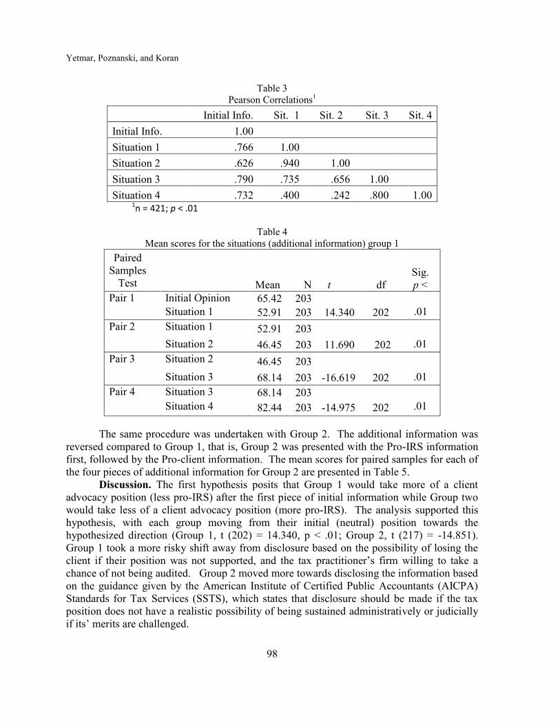
Yetmar, Poznanski, and Koran
98
Table 3
Pearson Correlations1
Initial Info. Sit. 1 Sit. 2 Sit. 3 Sit. 4
Initial Info. 1.00
Situation 1 .766 1.00
Situation 2 .626 .940 1.00
Situation 3 .790 .735 .656 1.00
Situation 4 .732 .400 .242 .800 1.00 1n = 421; p < .01
Table 4
Mean scores for the situations (additional information) group 1
Paired
Samples
Test
Mean N t df
Sig.
p <
Pair 1 Initial Opinion 65.42 203
Situation 1 52.91 203 14.340 202 .01
Pair 2 Situation 1 52.91 203
Situation 2 46.45 203 11.690 202 .01
Pair 3 Situation 2 46.45 203
Situation 3 68.14 203 -16.619 202 .01
Pair 4 Situation 3 68.14 203
Situation 4 82.44 203 -14.975 202 .01
The same procedure was undertaken with Group 2. The additional information was
reversed compared to Group 1, that is, Group 2 was presented with the Pro-IRS information
first, followed by the Pro-client information. The mean scores for paired samples for each of
the four pieces of additional information for Group 2 are presented in Table 5.
Discussion. The first hypothesis posits that Group 1 would take more of a client
advocacy position (less pro-IRS) after the first piece of initial information while Group two
would take less of a client advocacy position (more pro-IRS). The analysis supported this
hypothesis, with each group moving from their initial (neutral) position towards the
hypothesized direction (Group 1, t (202) = 14.340, p < .01; Group 2, t (217) = -14.851).
Group 1 took a more risky shift away from disclosure based on the possibility of losing the
client if their position was not supported, and the tax practitioner’s firm willing to take a
chance of not being audited. Group 2 moved more towards disclosing the information based
on the guidance given by the American Institute of Certified Public Accountants (AICPA)
Standards for Tax Services (SSTS), which states that disclosure should be made if the tax
position does not have a realistic possibility of being sustained administratively or judicially
if its’ merits are challenged.

Journal of Business and Accounting
99
Table 5
Mean scores for the situations (additional information) group 2 Paired
Samples
Test
Mean
N t df
Sig.
p <
Pair 1 Initial Opinion 60.16 218
Situation 1 77.72 218 -14.851 217 .01
Pair 2 Situation 1 77.72 218
Situation 2 82.71 218 -6.833 217 .01
Pair 3 Situation 2 82.71 218
Situation 3 66.12 218 17.309 217 .01
Pair 4 Situation 3 66.12 218
Situation 4 52.91 218 15.786 217 .01
Hypothesis 2 put forth that both Groups positions would become even more polarized
after the second piece of additional information compared to their position after the first
piece of additional information. That is, Group 1 would take more of a client advocacy
position and recommend not disclosing, while Group 2 would take more of an IRS position
and recommend disclosure of the tax position. Hypothesis 2 was also supported (Group 1, t
(202) = 11.690, p < .01; Group 2, t (217) = -6.833). Group 1 took even more of a client
advocacy position after being told that the client is willing to take on risk in order to reduce
their tax liability. Group 2 took even more of an IRS advocacy position to disclose the
information after being informed that penalties could be imposed on their firm if they failed
to disclose a position that does not have a realistic possibility of being upheld.
After the first two additional pieces of information, the third and fourth pieces
changed for each Group. Group 1 was given the same information that Group 2 had already
received, and vice- versa. Hypothesis 3 states that Group 1 will take less of a pro-client
advocacy position (move towards a more pro-IRS position), while Group 2 will take less of a
pro-IRS position (move towards a more pro-client position). Hypothesis 3 was supported for
each group (Group 1, t (202) = -16.619, p < .01; Group 2, t (217) = 17.309), indicating a
change in beliefs on whether or not to disclose (not disclose) the client’s tax position.
Hypothesis 4 posited Group 1 to move towards more a pro-IRS position and Group 2 to
move towards a more pro-client position after the fourth piece of information was presented.
The hypothesis was supported (Group 1, t (202) = -14.975, p < .01; Group 2, t (217) =
15.786) with both groups shifting their prior level of belief to disclose or not disclose the tax
position based on the additional piece of information.
At this point it is interesting to note the degree of percent change in mean scores of
the subjects. After the subjects were given the first piece of additional information, Group 1
changed their initial position to a more client advocacy position by approximately 20%.
After the second question their position changed even more to a client advocacy position but
this time by only approximately 10% of their initial position. Group 2 experienced similar
changes from their initial position. After being given the first piece of additional information
their position changed by approximately 28% of their initial opinion to one favoring the IRS.

Yetmar, Poznanski, and Koran
100
After the second piece of information they became more inclined to disclose the tax position
(more pro-IRS) but by only approximately 8%.
The same occurred after the third and fourth pieces of information were presented.
Group 1 shifted to a more pro-IRS position by approximately 47% after the third piece of
information, and approximately 21% after the fourth piece of information. Group 2 shifted to
a more pro-client position by approximately 21% after the third piece of information and
approximately 20% after the fourth piece of information.
It appears that for both groups, after being given the first piece of additional
information, the subjects were inclined to take a “larger” shift towards a greater advocacy
position for the client (Group 1) or IRS (Group 2) compared to their initial opinion. But after
the second piece of information was given, the shift occurred to a lesser extent than after the
first piece of additional information. As each group approached their limit (0 for a complete
client advocacy position or 100 for a complete IRS position) the magnitude of the increase
diminished, indicating a possible trend towards a more conservative client or IRS advocacy
position. Also, given the subjective nature of whether or not to disclose (the scenario is a
“grey” area), tax professionals may be unwilling to take a stand which places them in a
position completing advocating the client or the IRS. At some future point in time they may
have justify their decision to their client or the IRS.
To determine if there is a significant effects between the groups’ mean scores on the
initial scenario and each additional piece of information, we calculated Cohen’s d to
determine the effect size in a two-group experimental design. We used an average of the
standard deviations of the two groups given the similarity of the groups, and the random
assignment to each group. Since there is no restriction on the sign of the deviation we used a
two-tailed test (µ1 - µ2/σ). Small effects are designated by a result of d = 0.2; medium effects
by d = 0.5; and large effects by d = 0.8.
Table 6
Cohen’s d scores
Average σ Cohen's d
Initial scenario 31.5135 .873
Situation 1 28.3945 1.360
Situation 2 26.7320 .073
Situation 3 27.6595 1.090
Situation 4 27.0650 .167
The effects are significant for situations one, two, and four. There is strength in the
relationship between the responses of the two groups for these situations. There is no
significant effect between the groups in the initial scenario, signifying no difference in their
risk beliefs after given the neutral scenario. What is interesting is the similar risk-belief
position between the groups after responding to situation three.
The mean score for Group 1 after the initial scenario is 65.42. Given the first two
situations Group 1 moves towards the hypothesized direction (pro-client). Situation three,
the first of two pro-IRS situations, moves them towards a pro-IRS position and their mean

Journal of Business and Accounting
101
score shifts to 68.14. The same occurs with Group 2. Their mean score after the initial
scenario is 60.16. After their pro-IRS shift given the first two situations, their mean score is
66.12 after the first pro-client situation. Both groups have near identical mean scores (68.14
and 66.12) after each group was given one piece of information contrary to the two pieces of
information previously given.
CONCLUSION
The ordering effects of the situations based on the initial information and subsequent
information given, moved the subjects’ initial belief towards a more pro-client (do not
disclose) or pro-IRS (disclose) position in the hypothesized direction. Their final position
was based on the last two pieces of information given. The final mean scores, compared to
their initial mean score after being given a neutral scenario, indicated to disclose the
information to the IRS if the last two situations were pro-IRS, or to not disclose the
information if the last two situations were pro-client.
After being given the third situation which was contrary to the situations the subjects
already received, both groups converged to an almost identical position, close to their initial
opinion. It took only one piece of contrary information for the subjects’ to shift to their
initial position, one that is neutral, and a near-identical position for the groups, regardless of
whether they were previously in a pro-client or pro-IRS position.
Tax professionals have to make decisions where the tax laws are considered “grey,”
or information from their clients is subject to interpretation. If a client is attempting to sway
a tax professional to take a specific position (client advocacy) the results indicate that
information contrary to that position be given first, followed by information to support the
clients position. Tax professionals should also be aware that the ordering of the information
can lead them to make decisions based on the effects of ordering, rather than the information
itself. The accounting firm, if risk-averse, may want to remind the tax practitioner of his or
her professional ethics responsibilities at the end of each tax engagement (i.e., prior to
making a decision on the tax position the firm will take).
Financial Accounting Standards Board (FASB) Interpretation 48 (FIN 48, effective
2007) requires the tax preparer to analyze and disclose income tax risks. An entity can only
recognize an income tax benefit if it is more likely than not (defined as a probability of
greater than 50%) that the tax position chosen will be sustained upon an audit by taxing
authorities. This rule applies to all entities that are required to adhere to US GAAP
(generally accepted accounting principles). This rule makes it more important for tax
preparers to understand that the ordering effects, especially when favoring a client advocacy
position, be considered when making their decision on the tax position they will take for their
client. If a tax preparer is aware of the potential impact of the ordering effects on their
decision, they may consider an additional review by another firm member with the
information presented different order. While there is no guarantee that the ordering effect
impact on the tax position decision can be eliminated, every attempt should be made to
minimize them.
Future research should consider differing quantities of additional information
(situations) both pro-client and pro-IRS. For example, would three pieces of pro-client
information followed by one piece of pro-IRS information result in a significant shift towards

Yetmar, Poznanski, and Koran
102
a pro-IRS position (or vice versa)? When difficult tax decisions have to be made it is often
done by more than one person. Would the ordering of the information have any effect on
group dynamics, such as groupthink or a risky shift?
REFERENCES
Dillard, J. F., N. L. Kauffman, & E. E. Spires (1991). ‘Evidence Order and Belief Revision in
Management Accounting Decisions’, Accounting, Organizations and Society, 16(7), 619-
633.
Einhorn, H.J. & R.M. Hogarth (1987). ‘Adaption and Inertia in Belief Updating: The Contra-Inertia
Model’, Working Paper, University of Chicago, IL.
Hogarth, R. M. & H.J. Einhorn (1992), ‘Order Effects in Belief Updating: The Belief Adjustment
Model’, Cognitive Psychology, 24, 1-55.
Kahle, J., R. Pinsker & R. Pennington (2005). ‘Belief Revision in Accounting: A Literature Review
of the Belief-Adjustment Model’, Advances in Accounting Behavioral Research, 8, 1-40.
Kahle, J. B. & R. A. White (2004). ‘Tax Professional Decision Biases: The Effects of Initial Beliefs
and Client Preference’, Journal of the American Taxation Association, 26, 1-29.
Kerr, D. S. & D. D. Ward (1994). ‘The Effects of Audit Task on Evidence Integration and Belief
Revision’, Behavioral Research in Accounting, 6, 21-42.
Krishnamoorthy, G., T. J. Mock, & M. T. Washington (1999). ‘A Comparative Evaluation of Belief
Revision Models in Auditing’, Auditing: A Journal of Practice & Theory, 18(2), 105-127.
Pei, B. K. W., P. M. J. Reckers, & R. W. Wyndelts (1990) ‘The Influence of Information
Presentation Order on Professional Tax Judgment’, Journal of Economic Psychology, 11,
119-146.
Pei, B. K. W., P. M. J. Reckers, & R. W. Wyndelts (1992). ‘Tax Professionals Belief Revision: The
Effects of Information Presentation Sequence, Client Preference, and Domain Experience’,
Decision Sciences, 23(1), 175-199.
Piinsker, R (2011). ‘Primacy or Recency: A Study of Order Effects When Nonprofessional
Investors are Provided a Long Series of Disclosures’, Behavioral Research in Accounting,
23(1), 161-183.
Roberts, M. (1998). ‘Tax Accountants’ Judgment-Decision Making Research: A Review and
Synthesis’, Journal of the American Taxation Association, 20, 78-121.

Journal of Business and Accounting
Vol. 5, No. 1; Fall 2012
103
ANOMALIES OF TAX LEGISLATION: THE FIRST-TIME
HOMEBUYER CREDIT
Sheldon R. Smith
Amourae Riggs
Utah Valley University
ABSTRACT
The first-time homebuyer tax credit was first legislated in 2008. It was amended in
early 2009 and again in November 2009. Previous papers have explained the limitations of
and qualifications for the credit, both as originally legislated and as amended in 2009. This
paper extends the prior research by detailing the amendments and then describing several
situations in which the credit can create anomalies where taxpayers in almost identical
situations are treated very differently because of the rules for this particular credit. Some of
these situations are full of irony, as there is no way taxpayers could have known in advance
that this credit would be created or amended. Therefore, there is no way that appropriate tax
planning could have taken place to take advantage of this tax credit. Whether or not the tax
credit stimulated the economy as intended, the possible anomalies and ironies that have been
created can be seen as unfair. These situations are the result of hurried legislation attempting
to resolve an economic recession rather than the result of good, long-term tax policy.
INTRODUCTION
The first-time homebuyer tax credit was originally created by the Housing and
Economic Recovery Act of 2008, signed by President Bush on July 30, 2008 (P.L 110-289).
This law created a refundable tax credit of up to $7,500 for first-time homebuyers in the U.S.,
but it also included a recapture provision which required the taxpayers to repay the credit
over 15 years as an addition to those years’ taxes. Curatola (2009) described the provisions
of this credit. Smith (2009a) also described the provisions of the credit and included a
discussion of some ambiguities in the credit limitations based on the wording of the original
law.
This credit was amended early in 2009 when President Obama signed the American
Recovery and Reinvestment Act of 2009 on February 17 (P.L. 111-5). This law increased
the possible amount of the credit up to $8,000, extended the timeframe when the home could
be purchased to qualify, and removed the recapture provision. Smith (2009b) discusses the
original provisions as well as the new provisions provided by the amendments.
A law signed by President Obama on November 6, 2009, the Worker,
Homeownership, and Business Assistance Act of 2009 (P.L 111-92), further amended this
credit. It extended the deadline for home purchases which can qualify for the credit and
made several other changes.
The qualifications and limitations on this credit with its amendments have led to
many possible anomalies—situations in which taxpayers in almost identical circumstances
are treated differently because of the timing of the original legislation and its amendments.
Some of these situations are full of irony, as there is no way taxpayers could have known in
advance that this credit would be created or amended. Therefore, there is no way that

Smith and Riggs
104
appropriate tax planning could have taken place to take advantage of this credit. In fact,
some may have relied on the original credit to make tax planning decisions, only to find out
later that the amendments would have given them better tax benefits had they made different
decisions.
This paper reviews some of the qualifications and limitations for the original first-
time homebuyer credit and how those qualifications and limitations changed with the
amendments. Some of the possible anomalies and ironies will then be illustrated.
Implications will be included in the conclusion.
FIRST-TIME HOMEBUYER TAX CREDIT
When created on July 30, 2008, the first-time homebuyer tax credit was a refundable
credit for 10 percent of the purchase price of a principal residence purchased by a first-time
homebuyer in the U.S. (P.L. 110-289). The credit was limited to $7,500 ($3,750 for someone
married filing separately). It also had a phaseout provision such that it phased out over a
$20,000 range for taxpayers with modified AGI above $75,000 ($150,000 for a joint return).
The credit was only available for the purchase of a principal residence on or after April 9,
2008 and before July 1, 2009.
A first-time homebuyer was defined as someone who had not had an ownership
interest in a principal residence during the three-year period prior to the date of purchase of
the principal residence for which the credit would apply. The credit was not available if (1)
the property was acquired from a related person, (2) the taxpayer (or spouse) was eligible for
the first-time homebuyer credit in the District of Columbia for that year or any prior tax year,
(3) the residence was financed by tax-exempt mortgage interest bonds, (4) the taxpayer was a
nonresident alien, (5) the taxpayer disposed of the property before the close of the year of
purchase, or (6) the home ceased to be the principal residence of the taxpayer (and, if the
taxpayer was married, the taxpayer’s spouse) before the close of the year of purchase.
The credit was required to be recaptured—repaid as an additional tax of 6⅔ percent
of the credit amount each year for 15 years starting in the second year after the year in which
the principal residence was purchased. In essence, this made the credit an interest-free loan
from the government rather than a traditional credit which permanently reduces a taxpayer’s
tax liability. An accelerated recapture provision applied if the principal residence was sold or
ceased to be the principal residence before the end of the 15-year recapture period. In these
cases, the remainder of the credit had to be repaid in the year of the sale or cessation of use.
However, the accelerated recapture was limited to the gain on the sale of the residence and
applied differently if the taxpayer died, if there was an involuntary conversion, or if there
was a transfer between spouses or incident to a divorce. For a principal residence purchased
in 2009 (before the July 1 deadline), the taxpayer could elect to take the credit in 2008, either
on the original return or on an amended return if the original return had already been filed.
The credit was amended on February 17, 2009, with the amendments applicable to
homes purchased after December 31, 2008 (P.L. 111-5). The amendments increased the
dollar limit on the credit to $8,000 ($4,000 for someone married filing separately). The
deadline was extended such that homes purchased before December 1, 2009 could qualify for
the credit. The credit was allowed on homes purchased with tax-exempt mortgage interest
bonds. A change was enacted making the first-time homebuyer credit take priority over the
Journal of Business and Accounting
105
first-time homebuyer credit in the District of Columbia. Some of these amendments may
seem relatively minor. However, one amendment fundamentally changed the nature of the
credit. For homes purchased on or after January 1, 2009 and before the extended deadline of
December 1, 2009, the recapture provision was waived such that the credit does not have to
be repaid over 15 years. The only time it has to be repaid under the new rules is if the home
is sold or ceases to be the principal residence within 36 months of the date of the purchase.
Further amendments were made in November 2009 (P.L. 111-92). One amendment
was to extend the credit to first-time homebuyers who purchased a new principal residence
prior to May 1, 2010. However, if a taxpayer entered into a written binding contract by May
1 to close on the purchase of a principal residence before July 1, 2010, the deadline for that
taxpayer moved to July 1, 2010 (the purchase deadline was extended through September 30,
2010 by P.L. 111-198, signed by President Obama on July 2, 2010). The ability to take the
credit in the year prior to the purchase was also extended such that a first-time homebuyer
who purchased a qualifying home in 2010 could claim the credit on a 2009 tax return. A new
requirement was added such that a copy of the settlement statement for the purchase of the
residence must be attached to the tax return.
Additional taxpayers qualified for the credit under the November 2009 amendments if
the new residence was purchased after November 6, 2009. A taxpayer (and spouse, when
applicable) who has owned and used the same principal residence for any 5-consecutive-year
period out of the last 8 years can sell the house and qualify as a first-time homebuyer on the
purchase of a new principal residence. However, the maximum credit for these long-time
owners of a prior residence is only $6,500 ($3,250 for married filing jointly).
The credit still has a modified AGI phaseout range of $20,000, but the range now
starts at $125,000 ($225,000 for married filing jointly). A new limit on the purchase price of
the home was created. The credit is not available if the purchase price of the home exceeds
$800,000. Additionally, the taxpayer (or taxpayer’s spouse, if married) must be at least 18
years old and must not be a dependent of another taxpayer to claim the credit. Previously,
the qualifying home could not be purchased from a relative. Under the amendments, it also
cannot be purchased from a spouse’s relative. These amendments were all effective for
homes purchased after November 6, 2009, the date of enactment.
Some special rules were added for those who are on or ordered to qualified official
extended duty as members of the uniformed services, members of the U.S. Foreign Service,
or employees of the intelligence community. If a residence purchased in 2009 or 2010 which
otherwise qualifies for the credit is sold or ceases to be the principal residence in connection
with Government orders for the taxpayer or the taxpayer’s spouse for qualified official
extended duty service, the credit can still be taken even if the sale or cessation is in the year
of the purchase; also the credit does not have to be recaptured if the sale or cessation occurs
within 36 months of the purchase in these cases. If a residence purchased in 2008 which
qualified for the credit is sold or ceases to be the principal residence in connection with
Government orders as mentioned above, the taxpayer does not have to recapture any
remaining credit.
Taxpayers who are on qualified official extended duty service outside of the United
States for at least 90 days between January 1, 2009 and May 1, 2010 get an extension on the
deadline to purchase the qualified residence. They qualify for the credit if they purchased a

Smith and Riggs
106
principal residence as a first-time homebuyer before May 1, 2011 (or entered into a written
binding contract before May 1, 2011 to close the purchase before July 1, 2011).
ANOMALIES AND IRONIES
Because of the creation of and amendments to this first-time homebuyer tax credit,
many anomalies or ironies can occur due to specific timing or other differences in taxpayers’
situations. Some of these anomalies and ironies will be illustrated in this section.
Situation 1: Mr. and Mrs. A had never owned a home. Mr. and Mrs. B had never
owned a home. Both couples had modified AGI of $120,000. Both couples started looking
near the end of 2008 at homes they could purchase. Mr. and Mrs. A found a home, made an
offer, and purchased the home, closing the purchase on December 27, 2008. Mr. and Mrs. B
found a home, made an offer, and purchased the home, but because of some escrow delays,
they were unable to close on the purchase until January 3, 2009. Although both couples may
qualify for the first-time homebuyer credit, Mr. and Mrs. A can only get a $7,500 credit and
have to repay this amount over 15 years. In addition, if they sell the home within that 15-
year period or cease to use it as their principal residence, they have to repay the remaining
credit in the year of the sale or cessation. Mr. and Mrs. B can get an $8,000 credit which
does not have to be repaid as long as they own the home as their principal residence for at
least 36 months. Mr. and Mrs. A had no notice that they could have improved their credit
immensely by waiting to close until after January 1, 2009, as the amendments increasing the
credit to $8,000 and eliminating the recapture provision were not legislated until February
17, 2009.
Situation 2: Mr. and Mrs. C had never owned a home. Mr. and Mrs. D had never
owned a home. Both couples had modified AGI of $120,000. Both couples were looking to
buy homes in the early months of 2008. Mr. and Mrs. C purchased a home, closing the
transaction on April 1, 2008. Mr. and Mrs. D purchased a home but closed the transaction on
April 20, 2008. While Mr. and Mrs. D will qualify for a $7,500 credit (as an interest-free
loan) because they happened to close the purchased after April 9 (the effective date for the
credit), Mr. and Mrs. C will get no credit. Neither couple knew anything about the
possibility of a credit until after their purchase because the credit was not initially legislated
until July 30, 2008.
Situation 3: Mrs. E, a widow with five children, has never owned a home. She has a
pretty good job and has a modified AGI of $100,000. Mr. and Mrs. F, a couple with four
children, have never owned a home. They have modified AGI of $145,000. Both families
buy essentially identical homes next door to each other in the same neighborhood. Both
transactions were closed on July 8, 2009. Mrs. E gets no credit because the credit phased out
completely when her modified AGI exceeded $95,000. However, Mr. and Mrs. F will get an
$8,000 credit (because the credit phaseout for their joint return would have started at
$150,000) even though their modified AGI is much higher than Mrs. E’s modified AGI and
both families have the same number of members to support.
Situation 4: Mr. and Mrs. G have never owned a home and have a modified AGI of
$175,000. Mr. and Mrs. H have never owned a home and have a modified AGI of $175,000.
Knowing they cannot qualify for the first-time homebuyer credit because it was completely
phased out at $170,000 for joint returns under the original provisions, Mr. and Mrs. G buy a

Journal of Business and Accounting
107
home in August 2009. Mr. and Mrs. H started looking for a home at the same time but took
longer to agree on a home and close on the purchase transaction. Because Mr. and Mrs. H
closed on November 10, 2009 after the credit was amended, they qualify for the $8,000 credit
even though Mr. and Mrs. G do not because their modified AGI was too large based on when
they purchased their home.
Situation 5: Mr. I and Ms. J are both single and each has a modified AGI of $72,000.
They work for the same company and are frequently transferred from one city to another
because of the nature of their jobs. Therefore, they have both owned multiple homes in the
past eight years. Early in 2007, they are both promoted and transferred to Dallas, each of
them selling their prior home as part of the transfer. Thinking they may be transferred again
within a year or two, they both decide to rent for a while instead of buying other homes.
However, by early 2009, the home office is moved to Dallas, and they feel they will not be
moving again. Knowing that he will not qualify for the first-time homebuyer credit because
it expires before he could qualify as a first-time homebuyer, Mr. I goes ahead and purchases
a home in August 2009. Ms. J was a little slower in finding what she wanted, and by the
time she was ready to buy, the first-time homebuyer credit had been extended into 2010.
Therefore, Ms. J postponed the purchase of her home until early 2010 after she had been out
of her prior home for three years. Thus, she qualified for the first-time homebuyer credit
when Mr. I did not.
Situation 6: Mr. and Mrs. K have never owned a home. They have modified AGI of
$145,000 and have saved toward a down payment on their dream home for many years. Mr.
and Mrs. L also have never owned a home. They also have modified AGI of $145,000 and
have saved toward a down payment on their dream home for many years. Mr. and Mrs. K
buy their dream home on October 23, 2009, paying $850,000, most of it in cash. They
qualify for an $8,000 first-time homebuyer credit. Mr. and Mrs. L also buy their dream
home, paying $850,000, most of it in cash. However, Mr. and Mrs. L do not close on the
home purchase until November 9, 2009. Because they were unable to close before
November 6 when the $800,000 purchase price limitation was enacted, they will get no first-
time homebuyer credit even though Mr. and Mrs. K did.
Situation 7: Mr. and Mrs. M have never owned a home. Their modified AGI is
$145,000, and they have saved for a down payment on their dream home for several years.
Mr. and Mrs. N also have never owned a home. Their modified AGI is $145,000, and they
have saved for a down payment on their dream home for several years. These two couples
buy essentially equivalent homes, closing on November 15, 2009. However, because they
are living in different areas of the country, Mr. and Mrs. M are able to buy their home for
$550,000 while Mr. and Mrs. N have to pay $850,000 for theirs. Mr. and Mrs. N do not
qualify for a first-time homebuyer credit because their home price was over $800,000, but
Mr. and Mrs. M qualify for an $8,000 credit simply because they live in an area where homes
do not cost as much.
Situation 8: Ms. O has never owned a home. Her modified AGI is $70,000. Mr. P
has never owned a home, and his modified AGI is $70,000. Each party contracts for
construction of a new home, each signing a purchase contract designating that the
construction is to be completed by June 20, allowing each home to be occupied prior to the
July 1, 2010 credit deadline. Ms. O is able to move into her home on June 28, 2010, so she

Smith and Riggs
108
qualifies for the $8,000 credit. However, due to construction and inspection delays outside
of his control, Mr. P is unable to occupy his house until October 6, 2010. He is not eligible
for the credit since he did not move in by the credit deadline.
Situation 9: Mr. and Mrs. Q have owned a home for the last eight years. They have
modified AGI of $140,000. They have lived in their home for most of the eight years, but
they were living overseas on a work assignment during the fifth year of their ownership.
While they were overseas, they rented their house to another family. Mr. and Mrs. R have
also owned a home for the last eight years and have modified AGI of $140,000. The home
has been their principal residence for the last seven years. They rented the home out the first
year they after they bought it because they were assigned overseas by Mrs. R’s employer for
one year right after they purchased the home. If both couples sell their homes and buy other
houses on November 15, 2009, Mr. and Mrs. R will qualify for the $6,500 first-time
homebuyer credit since they owned a home and used it as a principal residence for a 5-
consecutive-year period during the last eight years. However, Mr. and Mrs. Q will not
qualify for any credit, as they did not occupy their home as their principal residence for any
5-consecutive-year period in the last eight years.
Situation 10: At the beginning of November 2009, Mr. and Mrs. S have owned a
home for the last eight years. They first rented it out for almost three years. But they have
now lived in their home as their principal residence for slightly longer than the last five
consecutive years. Their modified AGI is $145,000. Mr. and Mrs. T have also owned a
home for the last eight years. They have modified AGI of $145,000. They lived in their
home for the first five consecutive years and one month, but then they rented it out. On
November 15, 2009, Mr. and Mrs. S sell their house and buy another. They qualify for the
first-time homebuyer credit of $6,500 for long-time residents. Mr. and Mrs. T could also sell
their home and buy another on November 15, 2009 and qualify for the $6,500 credit for long-
time residents. However, if they wait until December 15, 2009 to sell the home and buy
another principal residence, they will now qualify as first-time homebuyers because they
have not had an ownership interest in a principal residence for three years rather than because
they qualify as first-time homebuyers as long-time residents. Thus, they could qualify for the
$8,000 credit in December 2009 whereas they would only qualify for the $6,500 credit in
November.
Situation 11: Mr. and Mrs. U had owned their principal residence for one month
short of five years when they sold it and bought a new home in mid-November 2009. Their
modified AGI is $200,000. Mr. and Mrs. V have owned their principal residence for slightly
over five years when they sold it and bought a new home in mid-November 2009. Mr. and
Mrs. V also have modified AGI of $200,000. Because Mr. and Mrs. V owned and occupied
their home for at least five consecutive years out of the last eight, they will qualify for the
$6,500 credit. However, Mr. and Mrs. U will not qualify for any credit, as they sold their
home before they had been in it for five consecutive years. Had they known the law changed
on November 6, they could have postponed the sale and purchase to December, thus
qualifying them for the $6,500 credit.
Situation 12: Mr. and Mrs. W have owned and lived in their house for the last thirty
years. Their modified AGI is $140,000. Mr. and Mrs. X have also owned and lived in their
house for the last thirty years. Their modified AGI is also $140,000. Mr. W and Mrs. X had

Journal of Business and Accounting
109
worked for the same company, but they both retired in July 2009. Both couples are also
empty nesters, so they have decided to move to smaller homes in warmer areas of the
country. Mr. and Mrs. W were able to sell their home and purchase a new one in October
2009, but Mr. and Mrs. X closed later in November 2009. Mr. and Mrs. W will not qualify
for any first-time homebuyer credit since they sold their home and purchased a new one in
October. However, Mr. and Mrs. X will qualify for a $6,500 credit as first-time homebuyers.
The difference in this situation comes simply because of the small timing difference between
each couple’s sale/purchase. Mr. and Mrs. W could not have known in October that they
would be better off if they would have closed after the amended legislation on November 6,
2009.
Situation 13: Col. and Mrs. Y qualified for the $8,000 first-time homebuyer credit in
2009 by buying their first home. Mr. and Mrs. Z also qualified for the $8,000 first-time
homebuyer credit in 2009 by buying their first home. Col. Y was called to qualified official
extended duty in 2010, so Col. and Mrs. Y ceased to use their home as their principal
residence. Even though their home is no longer their principal residence and they have not
used it as such for 36 months, they do not have to recapture the credit because of the waiver
due to the qualified official extended duty. Mrs. Z was employed by a defense contractor and
was required by her employer to move in 2010 to directly support the maneuvers of Col. Y’s
military unit. Thus, Mr. and Mrs. Z ceased to use their home as their principal residence.
Although Mrs. Z’s move tied directly to a military mission, Mr. and Mrs. Z will have to pay
back the $8,000 credit since they did not own the home as their principal residence for at
least 36 months after its purchase.
Situation 14: Lt. AA is single and has never owned a home because of extended and
geographically varied service assignments in the military. His last assignment was a
qualified official extended duty assignment outside of the U.S. which lasted from April 25,
2009 to April 25, 2010. Lt. BB is single and has never owned a home because of extended
and geographically varied service assignments in the military. Her last assignment was an
official extended duty assignment in the U.S. which lasted from April 25, 2009 to April 25,
2010. Lt. AA and Lt. BB both retired at the end of their extended duty on April 25, 2010.
Both have modified AGI less than $125,000. Each buys a principal residence for retirement
in the same neighborhood in the summer of 2010. Lt. AA can claim an $8,000 first-time
homebuyer tax credit, but Lt. BB cannot because her extended duty assignment was in the
U.S. which does not allow her an extension to the deadline for the credit.
Situation 15: Mr. and Mrs. CC bought their first home in July 2009 and qualified for
an $8,000 first-time homebuyer credit. Mr. and Mrs. DD also bought their first home in July
2009 and qualified for an $8,000 first-time homebuyer credit. Mr. and Mrs. CC had a job
transfer in June 2012, so they ceased to use their home as their principal residence at that
time. Thus, they have to pay back the entire $8,000 credit under the accelerated recapture
provision because they did not use the home as their principal residence for at least 36
months. Mr. and Mrs. DD also had a job transfer, but they did not have to move until August
2012. Although they only lived in their home for two months longer than Mr. and Mrs. CC,
since Mr. and Mrs. DD have used their home as their principal residence for at least 36
months, they do not have to pay back any of the credit under the accelerated recapture
provision.

Smith and Riggs
110
Situation 16: Mr. and Mrs. EE claimed a $7,500 first-time homebuyer credit in 2008.
Mr. and Mrs. FF also claimed a $7,500 first-time homebuyer credit in 2008. Both couples
resold their homes in 2010 because of job transfers. Although the home market had softened
between 2008 and 2010, because of the location of their home, Mr. and Mrs. EE were able to
sell their home for a $7,500 gain, but they had to immediately recapture the entire $7,500
credit in 2010 because they sold their home before the end of the 15-year recapture period.
However, Mr. and Mrs. FF did not have to recapture any of their credit because they sold
their home for no gain or loss, even though they also sold their home before the end of the
15-year recapture period.
In addition to the specific situations detailed above, other hypothetical situations
could be created that would lead to inequities. Some of these might involve the requirements
that the first-time homebuyer not be a dependent on another taxpayer’s return or that the
homebuyer must be at least 18 by the date of the home purchase. It might be more
acceptable to think that taxpayers who are first-time homebuyers of their own principal
residence should be at least age 18 and not dependent on someone else. These changes in the
limitations for the credit were likely made more to close unanticipated loopholes in the
original law rather than just to arbitrarily change the timing or general limitations and
qualifications on claiming the credit.
Other examples could relate to the changing limitations relating to homes financed by
tax-exempt mortgage interest bonds or the new rule that a home cannot be purchased from a
spouse’s relative (in addition to the existing rule that a home cannot be purchased from a
taxpayer’s relative). These situations are not detailed because they are probably not as ironic
according to public policy, although they could still result in similar cases being treated
differently.
CONCLUSION
As can be seen by the many situations illustrated above, the first-time homebuyer
credit can create situations that seem ironic or inequitable. These anomalies can arise
because of the timing requirements of the original law and the amendments or because of
other qualifications and limitations legislated in this credit. Other hypothetical situations
resulting in ironies could be created. While the first-time homebuyer credit may have
stimulated the economy, specifically the housing sector, it may be seen in many cases as
unfair. The anomalies and ironies are the result of hurried legislation attempting to resolve
an economic recession rather than the result of good, long-term tax policy. Congress should
reconsider the implications of this credit with respect to the situations mentioned before
creating other, similar tax credits.
REFERENCES
Curatola, A.P. (2009). Housing Assistance Tax Act of 2008. Strategic Finance, 90(7), January, 10-
12.
Public Law 110-289. (2008). Housing and Economic Recovery Act of 2008, July 30.
Public Law 111-5. (2009). American Recovery and Reinvestment Act of 2009, February 17.
Public Law 111-92. (2009). Worker, Homeownership, and Business Assistance Act of 2009,
November 6.
Public Law 111-198. (2010). Homebuyer Assistance and Improvement Act of 2010, July 2.

Journal of Business and Accounting
111
Smith, S.R. (2009a). The First-Time Home Buyer Credit: Technical Correction Needed. Tax Notes,
122(3), January 19, 405-409.
Smith, S.R. (2009b). The First-Time Homebuyer Tax Credit. Journal of Business and Accounting,
2(1), Fall, 171-178.

Journal of Business and Accounting
Vol. 5, No. 1; Fall 2012
112
ACCOUNTING FOR SUSTAINABILITY
Mehenna Yakhou
Georgia College & State University
ABSTRACT
Environmental sustainability has gained importance across the globe due to the
increased concern for externalities that companies’ activities place on society. Government
and other stakeholders are putting pressure on businesses for greater transparency regarding
social and external performance and impacts. Accountants have an important role to play in
identifying, measuring and allocating sustainability-related costs, developing and reporting
sustainability performance metrics and helping corporations formulate and implement
environmental strategies. The purpose of this paper is to provide insight into contemporary
understanding of the new dimension of accounting for sustainability.
CORPORATE SUSTAINANBILTY
In recent years, sustainable development has become a significant part of the
objectives of many organizations. In general, corporate sustainability can be considered as a
broad approach, integrating financial, economic, environmental, and social aspects that can
assist firms achieve a more holistic level of accountability (Schaltegger and Burritt 2005).
The United Nations (UN) World Commission on Environment and Development gave the
initial definition of the term, “the ability to meet the needs of the present without
compromising the ability of future generations to meet their own needs,” (Bruntland, 1987).
Dixon and Fallon (1999) describe the development of sustainability concept, from single
resource, to the multiple resource ecosystems, and expanded to integrated social-physical-
economic systems. They provide an operational definition of sustainability as six socio-
economic questions:
How should equity, both intergeneration and intergenerational, be handled with respect
to resource management decisions?
What do we leave to future generations to ensure that they are not worse off?
Will there be enough to go around?
How far into the future do we worry about (next week, next year, next century)?
Are there some patterns of resource use that should be accepted irrespective of losing
or saving the resource?
To what extent can market forces (and technology) intervene in the process of
development vis-a-vis resource use (the conservationist versus possibilist debate?
CORPORATE SUSTAINABILITY AND ACCOUNTING
Gray (1992) provides a structured view of sustainability, as a theoretical foundation
to “sustainability accounting” based on a systems view of the environment. Initially, the
relationship between management accounting and economics fails to notice the environment
and biosphere as relevant to costing. Birkin and Woodward (1997) define essentials to move
management accounting from its economic basis and internal focus, to sustainable
development. Two steps are identified, one from economic efficiency, to environmental
Journal of Business and Accounting
113
efficiency; the other from environmental efficiency to ecological efficiency. To make the
first step, environmental issues must overcome environmental biases and shift to a prime
emphasis. A basic need is to introduce environmental statutory language and concepts into
the language and expertise of management accounting. That shift of focus assures non-
marginal consideration of environmental impacts of corporate activities. Step two is sizable,
to consider the ecosystem in an interconnected, interdependent manner. A basic need here is
to adopt total cost assessment in management accounting. That approach requires measures
of cost of processes, products, and services reflected in managerial decisions and corporate
behavior. Milne (1996) suggests that techniques and tools from other disciplines, such natural
and social sciences, should be integrated into management accounting systems. Bartolomeo
et al. (2000) define environmental management accounting as: “The generation and use of
financial and related non-financial information, in order to support management within a
company or business, in integrating corporate environmental and economic policies and
building sustainable business)”. Main features of environmental management accounting are
described (Birkin, 1996):
setting boundaries for an eco-balance, including life-cycle accounting of product and
process;
appraising performance of technologies and technological change;
recording corporate environmental liabilities;
appraising environmental performance from long-term perspective on environmental
indicators; and
establishing budget planning and control at the detail level of management accounting
The range of extension is described as four levels:
exploitationist, not accounting for nature with economic goals including efficiency;
conservationist, accounting for externalities with goals reflecting values for
recreation, future use and preservation implemented for operational and financial
feasibility;
naturalist-preservationist, recognizing impacts on the ecosystem with
intergenerational issues and technological substitutions considered and constraints on
local projects integrating social/economic/ecological impacts, specifically resource
use and environmental degradation;
extremist-preservationist, on a non-anthropocentric basis with ecological priorities
superior to social, and focusing on the intrinsic value of nature
This overall movement is said to expand the organization’s obligation, to
environmental accountability (Birkin and Woodward, 1997). Effects of expansion are to
improve environmental performance, specifically environmental aspects of industrial
performance and to involve all aspects of the accounting discipline.
Environmental management accounting relates to social accounting and “green”
accounting as well. “Green” accounting is described (Atkinson and Hamilton, 1996) as a
level of accounting based on environmental indicators namely, pressure on companies, state
of the environment and companies’ response. Pressure is both direct and proximate causing
change; state of the environment includes loss from pollution and waste, due to human
activity; and response is from government policies, individual and business practice and

Yakhou
114
environmental activism. From this paradigm, “green” accounting appears to become an
essential adjunct to management accounting. Social accounting includes, among other areas,
reporting data related to effects of global warming, raw material use, solid waste and water
pollution, human toxicity, and ecosystem degradation. As described by Pestoff cited in Gray
(2010), social accounting is concerned with:
the social and environmental (including sustainability) impacts and effects arising
from conventional accounting practice;
ameliorating the social and environmental impacts arising from conventional
accounting practice (including seeking ways to reduce the negative impacts and
looking for ways to encourage positive social and environmental effects;
deriving and developing new methods of accounting that might be implicated in more
benign social and environmental effects and which, typically would advance the case
of accountability
Lamberton (2005) notes: “The provision of sustainability accounting information to
internal users would focus on the provision of relevant and decision useful information to
management. For example, an array of performance indicators and lifecycle data compared to
relevant sustainability targets would assist the internal management of the organization
toward the multidimensional sustainability objective.”
Hence at the business level, long-term effects are focused among others on costs and
revenues, assets and liabilities of the firm. The difficult extension of firm-level accounts is in
introducing the additional performance indicators and lifecycle data, including costs,
revenues, assets, and liabilities. Accounting for effects of environmental compliance must
recognize the regulatory boundaries which represent a variety of costs and expenses and
potential penalties and liabilities. Environmental regulations pose a range of costs and
liabilities, including normative conditions and fees (start-up under environmental regulation,
such as permit fees, and on-going such as permit renewal); incidents of environmental
violations and on-going violations; economic loss due to interference with business activities,
both limitations and cessation; penalties (civil type fines and administrative orders to “cease
and desist” and criminal type fines); costs of complying with environmental regulations in
future; cost of cleaning contaminated sites; revaluation of assets depreciation; potential
liabilities from safety hazards to workers and the community at large, health and ecological
risks arising from operational emissions of pollutants and hazardous materials, and product
safely related issues; and other contingent liabilities arising from environmental exposures.
While environmental accountability is broadly considered as imposing burdens of
compliance, the activities associated with environmental protection also generate assets of
value. For example, under the Clean Air Act, an under-discharge provides salable emissions
rights transferrable to others which are discharge-limited. These rights are viewed as
“intangible operating assets” (Ewer et al., 1992). Cleanup expenditures of joint-hazardous
waste are recovered under the right of contribution. Estimates of these expenditures along
with the contributions of other firms are also recognized as assets in the firm’s balance sheet.
Other recognized assets are premiums paid on liability policies that safe guard business from
environmental claims (Surma, 1992). Also, compliance with environmental regulations

Journal of Business and Accounting
115
requires internal expertise in applying environmental standards and control technologies to
the local emission sources. Such expertise can result in “intellectual property”, as patents for
unique control/removal processes, and as “know how” on applying control to a local or
general situation. An environmentally managed company, and a system to assure
environmental compliance, can add value and hence generate goodwill of being “green”
(Willits and Giuntini (1994)).
Obviously an expanded conventional balance sheet does not fully capture all
environmental impacts. Hawken, et al., (1999) highlight the limitations of the conventional
balance sheet, arguing that current accounting systems do not include environmental and
social impact of corporate activities. Gray (2010) suggests a “system theory” approach, to
provide a rational for subdividing without introducing gross distortions. Systems theory
provides tools in the subdividing (boundary setting, problem definition and analytical
formulae) that form a body of principles. Gray states “At the heart of much of what
comprises social accounting currently is a concern over the impacts and development of
sustainability, accountability and large organizations, a matter within which social
accounting has a considerable potential. If sustainability is the “elephant in the bedroom” (the
issue which so dominates all other issues but still too rarely spoken of analytically) then
social accounting is one- but only one- of the means by which the serious exigencies of
sustainability might be addressed and ameliorated”.
The result is a structured approach to extending the boundaries of accounting and
reporting for determining the environmental, ecological, and social effects, or as Eccles et al.,
(2010) put it:
“The result is improved information provided to stakeholders about the company’s
performance and how it is being achieved – including its costs and benefits – that can
ultimately lead to ..“ the creation of an internal discipline necessary for embedding
sustainability into a company’s strategy and operations; better company understanding that
governance, strategy, and sustainability are inseparable; acknowledgement that a company is
responsive to the risks and opportunities created by the need to ensure a sustainable society;
and enhanced corporate disclosure and transparency.”
Milne (1996) suggests that this extreme extension of management accounting is not
favored by the accounting profession. Indeed, current accounting practice does not
require/allow business to record the consequences of its operations on factors that are
external to it. However, Gray (1992) argues and establishes such extension as certain
information requirements, namely accountability and transparency. Environmental
accountability is based on the social relationship of firm to community. To represent that
relationship, the structure of environmental accounting systems should incorporate a
specified identification of environmental impacts, and the content of environmental law and
quasi-law (regulation). Transparency of the environmental accounting system should be
based on a stewardship notion of providing information on compliance, along with
communication of the information, as a duty of the firm. Gray recognizes that availability
and duty to inform is not necessarily self-imposed, but may be responsive to pressure groups
(as the community), to influence the business firm in its decision-making and financial
assessment processes.

Yakhou
116
TOOLS FOR SUSTAINABILITY ACCOUNTING
Sustainability Reporting: Corporate social disclosure, also called social accounting,
responds to influences by “external pressure groups” (Tilt, 1994). Social disclosure centers
on environmental protection, product quality, and product safety. “Community interest
groups” are the main source of influence on initiating and maintaining social disclosure.
Environmental groups are the most active, and environmental data are the most commonly
demanded (Birkin and Woodword, 1997). A paradigm of community interest groups is
proposed as “pressure groups” (Tilt, 1994). That is the group must be an involved group, able
to exert influence directly or by indirect action, and impose disclosure, at least, at minimum
levels for evaluation as understanding, sufficiency, and credibility. The group has a stake in
making information public, and so takes a penetrating approach (negotiation, analysis,
lobbying) on the disclosing company.
A central issue then for the business firm is how to integrate the range of
stakeholders. A four-step stakeholder management process has been suggested (Freeman,
1984):
identify the relevant stakeholder groups in relation to the issue being addressed;
determine the stake and importance to each stakeholder group (stake is diffuse but is
specific for each group, here considered as “needs” and “expectations);
determine how effectively the “needs” or “expectations” of each group are presently
being met (how a stake is met is diffuse but again specific to a group);
modify corporate policies and priorities to take into consideration stakeholder
interests
The stakeholder management process allows the firm to examine all strategic issues
facing it: economic, direct and secondary stakes, and to develop one or more strategies to
meet issues (stakes) in total and within priorities as set by resource limitation (amount and
return). Perrini and Tencati (2006) believe that “A sustainability-oriented company is fully
aware of its responsibility towards the different stakeholders and adopts methods and tools
that allow it to improve its social and ecological performance”.
So far the most common organizational response to reporting on sustainability
performance has been to publish corporate stand-alone-reports (KPMG, 2008). Examples of
proposed frameworks that have been developed to embed sustainability measurement and
reporting within the organizational structures include:
the Global Reporting Initiative, (GRI), developed by a United Nations affiliate
organization;
the SustainAbility framework developed by an international accounting firm;
the Environment Sustainability Index, developed by the World Economic forum;
the performance criteria framework developed by Figge et al. (2002)
All these frameworks take a multi-disciplinary and stakeholders perspective and show
that the range of issues that can be addressed is extremely broad. The primary goal of these
reports is to communicate the overall ecological, social, financial, and economic impacts of
the corporation; and business risk factors arising from environmental and social issues (Joshi
Journal of Business and Accounting
117
and Krishnan, 2010). However, there is a general consensus that the frameworks do not fully
integrate sustainability considerations in decision-making, accounting, and reporting
processes. Some critics indicate that disclosures of social accounting related information is
motivated by the desire to legitimize organizational actions (legitimacy theory, Deegan,
2002). Hubbard (2009) raises several concerns about these frameworks:
lack integration with conventional economic reports;
focus mostly on positive image of corporate performance;
focus on description outcomes, with no or little benchmarking;
do not involve the users (management and other stakeholders) in the collection,
analysis, reporting and audit of the information provided;
do not provide details as to what is reported, how, and why; and focus on
environmental issues, excluding social sustainability
Milne et al. (2008) have also been critical of these frameworks, arguing they
[frameworks] are “insufficient conditions for organizations contributing to the sustaining or
the Earth ecology. Paradox ally, they may reinforce business-as-usual and greater levels of
un-sustainability”. Ehrenfeld (2005), Bebbington et al., (2007) also note that current
corporate sustainability reports do not in any way come close to representing the
requirements of true social sustainability. Most sustainability accounting systems, as Joshi
and Krishnan (2010) put it “do not provide comprehensive, decision-relevant information to
meet the goal of becoming an environmentally sustainable and socially responsive
organization”. To remediate these shortcomings, new sustainability accounting tools, and full
business attitudes (and or organization culture) will need a “quantum jump” adjustment
[Mathews 2009), Hubbard (2009), and Bennett et al. (2011)].
Sustainability Management Accounting: A number of sustainability management
accounting tools can be used to integrate sustainability measures in traditional accounting
systems in order to influence strategic and operational decisions, improve the environmental
and economic performance of a company, and contribute towards a sustainable business
(Bennett et al., 2011). Modern accounting tools provide the necessary links between business
activities and reducing products and distribution costs, and enhancing revenue through
environmental quality appeal. Extending the intended effect of the environmental product is
to consider the full life of the product. Life-Cycle Costing approximates the expanded
product distribution chain, identifying all cost-bearing activities throughout the product life
cycle (Zach, 1992). That analysis incorporates the “cradle-to-grave” environmental
responsibility. The related benefits are product price reduction, reduction/elimination of
defects, by non use of hazardous materials and environmentally unsafe processes and more
use of recycled materials and/or recycling of materials (Strachan 1999).
Activity-Based-Costing has integrated cost-design drivers to product features
(function, reliability, quality, environmental features and its success in the market (price)
(Navinchandra, 1991). From Activity-Based-Costing, environmental activities can be related
to product/distribution channel/consumer over the business chain (Brooks, 1993).
The balanced score card (BSC) was introduced by Kaplan and Norton in the 1990’s to
improve traditional performance measurement system, a response to a reaction against

Yakhou
118
business’s strict reliance on financial performance and physical asset for measuring success.
Kaplan and Norton (2004) base their framework on stakeholder theory. The BSC identifies
four perspectives (customer, process, organizational learning, as well as financial
perspective), which are broken down into goals, indicators, targets and tasks. The authors
propose strategy maps as a way of visualizing causal links, via cause and effect, of the
performance measures in each of the four perspectives. A modification of the BSC
framework is the S-BSC (Moller and Shaltegger, 2005; Figge et al., 2002). The original BSC
has been extended to include sustainability objectives (such as the environmental or social
impacts of a firm’s operations) in order to influence management’s decision making. As
Joshi and Krishnan (2010) put it “Developing sustainability maps is an essential first step in
visualizing and clarifying the causal links as to how external natural and social capital
resources together with an organization’s internal resources and processes help drive
organizational value creation and performance. These exercises will also help communicate
how various decisions and organizational processes can affect the flow of these ecosystem
and social services and thereby impact long-term performance of the firm. S-BSC can also
help develop strategically important sustainability performance indicators.”
CONCLUSION
The accounting profession’s increasing responsibility is in meeting requirements for
reporting and disclosure of environmental activities. Applicability of present accounting
standards, and the coming direction of environmentally-specific standards, represents a
formidable challenge. Mathews (2009) poses a pertinent question related to the standards
issue: “How should reports be constructed? If the expanded reports are to earn any credibility
amongst users…..there must be a degree of standardization and uniformity, which is also
required if the reports are to be audited”. Mathews (2009) points out that “there are several
issues that must be addressed before more far-reaching changes can be achieved. These
include the development of conceptual frameworks, standards and independent audits to
improve current disclosures. These areas indicate a research agenda for the next period of
development of social and environmental accounting”. There is also a need for discipline-
based environmental sustainability accounting models to develop standards in less developed
areas, value of “being green”, value of management time, and value of lost business
opportunity. The standards menu needs to be extended into these value areas of
environmental management – particularly as specific obligations under sustainable
development actuate in decisions of the firm.
REFERENCES
Bartolomeo, M. Bennett, M., Bouma, J.J., Heykamp, P., and Wolters, T. (2000), Environmental
Management Accounting in Europe: Current Practice and Future Potential. European
Accounting Review, 9(1), 31-52.
Atkinson, G., & Hamilton, K. (1996). Accounting for Progress: Indicators for Sustainable
Development. Environment , 38 (7), 16-20.
Bennett, M., Schaltegger, S., & Zvesdov, D. (2011). The Practice of Corporate Sustainanbility.
London: ICAEW.
Birkin, F. (1996). Environmental Management Accounting. Management Accounting , 7(2), 34-37.

Journal of Business and Accounting
119
Birkin, F., & Woodward, D. (1997). Management Accounting for Sustainable Development: Part 2:
From Economic to Ecological Efficiency. Management Accounting , 75 (7).
Brooks, P. L., Davidson, L., & Palamides, J. (1993, February). Environmental compliance: You
Better Know Your ABCs. Occupational Hazards , 41-46.
Bruntland, G. (1987). Report of the World Commission on Environment and Development. New
York, N.Y: United Nations Publications.
Deegan, C. (2002). The Legitimising Effect of Social and Environmental Disclosures- A Theoretical
Foundataion. Accounting, Auditing & Accountability Journal, 14 (3), 282-311.
Dixon, J. A., & Fallon, L. A. (1989). The Concept of Sustainability: Origins, Extensions, and
Usefulness for Policy. Society and Natural Resources ,(2), 73-84.
Eccles, R. G., & Krzus, M. P. (2010). Integrated Reporting for a Sustainable Strategy. Financial
Executive , 26 (2), 28-32.
Ehrenfeld, J. (2005, Winter). The Roots of Sustainability. Sloan Management Review , 23-35.
Ewer, S. R., Nance, J. R., & Hamlin, S. (1992). Accounting for Tomorrow's Pollution Control.
Journal of Accountancy , 174 (1), 69-74.
Figge, F., Hahn, T., Schaltegger, S., & Wagner, M. (2002). The Sustainability Balanced Scorecard -
Linking Sustainability Management to Business Strategy. Business strategy and the
Environment , 11, 269-284.
Freeman, A. B. (1984). Strategic Management: A Stakholder Approach. Boston, MA: Pitman
Publishers.
Gray, R. (2010). A Re-evaluation of Social, Environmental and Sustainability Accounting, An
Exploratory of an Emerging Trans-disciplinary Field. Sustainability Accounting,
Management and Policy Journal , 1 (1), 11-32.
Gray, R. (1992). Accounting and Envirnmentalism: An Exploration for the Challenge of Gently
Accounting for Accountability, Transparency and Sustainability. Accounting, Organizations
and Society , 17 (5), 399-425.
Hawken, P., Lovins, A., & Lovins, L. H. (1999). Natural Capitalism: Creating the Next Industrial
Revolution. Boston, Little, Brown.
Hubbard, G. (2009). Measuring Organizational Performance: Beyond the Triple Bottom Line.
Business Strategy and the Environment , 199, 177-191.
Joshi, S., & Krishnan, R. (2010). Sustainability Accounting Systems with a Managerial Decision
Focus. Cost Management , 24 (6), 20-30.
Kaplan, R., & Norton, D. (2004). Strategy Maps. Converting Intangible Assets into Tangible
Outcomes. Boston: Harvard business School Press.
Lamberton, G. (2005). Sustainability Accounting- A Brief History and Conceptual Framework.
Accounting Forum, (29), 7-26.
Mathews, M. R. (2009). Mega-Accounting and Reporting; A Proposal for Further Dvelopment.
International Review of Business Research papers , 5 (2), 329-339.
Milne, M. J. (1996). On Sustainability, the Environment and Management Accounting. Management
Accounting Research (7), 135-161.
Milne, M., Ball, A., & Gray, R. H. (2008, July). Wither Ecology? The Triple Bottom Line, the
Global Reporting Initiative, and the Institutionalization of Corporate Sustainability
Reporting. Annual Conference of the AFAANZ .
Navindchandra, D. (1991). Design for Environment Ability. Design Theory and Methodoldy , 119-
125.
Perrini, F., and& Tencati, A. (2006). Sustainability and Stakeholder Management: The Need for
New Corporate Performance Evaluation and Reporting Systems. Business Strategy and the
Environment , 15, 296-308.

Yakhou
120
Pestoff, V. (Forthcomng). Social Accounting and Public Management Accountabililty for the Public
Good, Conclusion. (S. osborn, & A. Ball, Eds.) Routeledge.
Schaltegger, S., & Burrit, R. (2005). Corporate Sustainability. (H. Folmer, & T. Tietengerg, Eds.) in
The International Yearbook of Environental and Resource Economics , 185-222.
Strachan, P. A. (1999). Is the Eco-Management and Audit (EMAS) Regulationtion an Effective
Srategic Marketing Tool for Implementing Industrial Organizations? Eco-Management and
Auditing , 6, 42-51.
Surma, J. P. (1992). Tackling Corporate America's Environmental Challenge. Review , 36 (2), 10-
23.
Tilt, C. A. (1994). The Influence of External Presure Groups on Corporate Social Disclosure: Some
Empirical Evidence. Accounting, Auditing and Accountability Journal , 4, 47-72.
Willits, S. D., & Giuntini, R. (1994, February). Helping Your Company "Go Green'. Management
Accounting , 43-47.
Zach, P. A. (1992). Life Cycle Inventory Analysis as Applied to Recycling System Economic Costs.
Journal of Resource Management and Technology , 20 (4), 181-189.

Journal of Business and Accounting
Vol. 5, No. 1; Fall 2012
121
A FACTOR ANALYSIS OF THE SKILLS NECESSARY IN
ACCOUNTING GRADUATES
Suzanne N. Cory
Kimberly A. Pruske
St. Mary’s University
ABSTRACT
This study obtains the opinions of two important constituent groups for higher
education accounting programs: (1) public accountants and (2) non-public accountants,
regarding the importance of accounting-related skills and topics to be covered in
undergraduate curricula. Factor analysis was used to determine common factors for each
group. The level of importance of factors was then compared within each group.
INTRODUCTION
Dissatisfaction with the level of accounting knowledge and skills exhibited by new
hires has been of concern by employers for a number of years. According to Nelson (1995)
impassioned cries for changes in accounting education have come from the accounting
profession since the “inception of university programs.” As accounting has moved beyond
the use of pencils, erasers, and 12-column worksheet paper toward embracing today’s
technology, these concerns have become more apparent. In short, accounting graduates need
to understand and master accounting-related skills and topics associated with technological
innovations including hardware and software in order to be productive starting with their first
day on the job. Further, in order to function in today’s diverse business environment, other
accounting-related skills and topics may be essential, such as proficiency in a second
language, creativity in problem solving and internet research.
In order to address these issues, accounting curricula may now incorporate business
classes that help students obtain skills in software such as Excel, Word, and Access, and
learn about technology such as telecommunication software, intranets, and client/server
management. Other business courses help students become aware of the impact of diverse
workplaces, as well as global, ethical, and environmental issues. Even so, accounting
programs have been especially inundated in the past two and a half decades with studies and
position papers addressing the quality of education available for accounting students and
recommending changes in educators’ approach to providing a more comprehensive
knowledge of accounting. As recently as 1998 the AICPA issued their top five issues for the
public accounting profession in their Vision Project, also offering guidance for changes in
higher education for aspiring CPAs.
Some practitioners and academicians seem to feel that academic accountants have
addressed only some of the issues raised with only a limited amount of success. The 2000
Albrecht and Sack (A&S) seminal study reporting that, in general, accounting education had
not changed substantively in response to the demands of accounting practitioners which
expresses concern about the future of accounting programs provided further food for
discussion. Albrecht (2002) also took his concerns to the American Association of
Collegiate Schools of Business (AACSB), causing substantial upheaval in accredited

Cory and Pruske
122
institutions. To illustrate the impact of Albrecht and Sack’s research, Johnson and Halabi
(2009) determined that A&S was cited in over 29% of published research papers during the
seven-year period between the beginning of 2001 and the end of 2007, which is certainly
evidence of a strong reaction to their concerns on the part of the professoriate.
Others have expressed concern that accounting programs in general have geared their
accounting curricula solely for students interested in public accounting, excluding students
who are more interested in the non-public accounting arena (Ahadiat, 2008). However, there
does not seem to be a consensus about the courses that should be completed in order to
ensure success in the non-public accounting arena (see, for example, Hurt, 2007). The
purpose of this paper is to report the findings of a study examining the viewpoints of public
accounting and non-public accounting professionals regarding accounting-related skills and
topics they feel students should have prior to employment. Perspectives of practicing
accountants, both in public accounting and in other areas of accounting, were gathered in
order to gain insight into this question.
METHOD
Currently practicing accountants should be well-informed about the skills that are
critical for new hires to possess in order to ensure success in their respective fields and topics
that should be part of an accounting program. Lending further support to this methodology,
A&S indicate that each accounting program has the responsibility of determining the needs
of its own key stakeholders, incorporating internal and external environments that are unique
to each. Finally, AACSB accreditation standards reinforce the concept that curricula must
consider constraints and opportunities that may be specific to a particular business program
based on its mission.
Surveying local accounting professionals regarding perceptions as to the importance
of accounting-related skills and topics needed by their new-hires should provide valuable
insight into the curriculum required of accounting programs in the local area. Cory (2009)
reported results of her study about course topics and degree preference but limited the
analysis of responses from her survey participants to only those currently practicing public
accounting. Similarly, Cory and Huttenhoff (2011) based their analysis solely on responses
from non-public accountants. This study compares perspectives of both groups of external
stakeholders and focuses on accounting-related skills and topics which may also lend support
to a successful accounting career.
The survey was distributed to 2,300 individuals who were either members of a large,
regional CPA society in south Texas, members of the Institute of Management Accountants
in the same area, or employers who had interviewed on a South Texas university campus
during the previous three years. A total of 464 usable surveys were returned which is a
response rate of approximately 19%. This rate is comparable to that reported in similar
studies. Approximately 46% of the surveys were completed by individuals currently
practicing public accounting and 54% by individuals who were employed in the non-public
accounting arena.
Respondents were asked to indicate, from the standpoint of their organization’s
business, how important it was for accounting students to have obtained certain accounting-
related skills prior to graduation. Respondents were provided with a list of 34 skills and

Journal of Business and Accounting
123
asked to rank each one on a three-point scale, with one indicating “not important,” two
indicating “important, but not critical” and three indicating “critical.” If the respondent did
not know how critical a skill was, they chose “4” as the answer. The responses were coded
according to the number chosen for each skill and any response in the “Do Not Know”
column was eliminated from analysis.
RESULTS
Given the amount of information collected (34 skills), principal components factor
analysis was used to determine common factors for each group. This made the analysis more
manageable (Pedhazur and Schmelkin, 1991) and resulted in ten factors for each group. For
the CPAs, six factors consisted of multiple skills, each loading at .45 or above. For the Non-
CPAs, eight factors consisted of multiple skills, each loading at .45 or above. No skills cross
loaded for either group. The next step in the analysis was to compute the average for each
factor. The factors for each group were then compared from one to the next, starting with the
most important factor (e.g. the factor with the highest average). Keeping in mind that a
rating of “2” indicates that the skill is “important, but not critical,” four factors for CPAs
averaged in excess of 2 and four factors for the non-CPAs averaged more than 2. The lowest
mean for CPAs was 1.45883 and the lowest mean for non-CPAs was 1.36618.
The 34 skills are listed in Table 1 and the factor on which each skill loaded is
indicated for each group of respondents. Four skills (Operating Systems other than
Windows, Collaboration Software (e.g. Lotus notes), Process/Operational Improvement and
Sales/Marketing) did not load on any factor for the CPAs. Two skills (Telecommunication
software and Programming Languages) did not load on any factor for the non-CPAs.
As indicated in Table 1, means were then computed for each factor and are shown in
Table 2 for CPAs and in Table 3 for non-CPAs. Finally, t-tests were computed to determine
significant differences between factors, from highest to lowest ranked from one to the next
for each group. The results are shown for the factors for CPAs and for non-CPAs in Tables 4
and 5, respectively.
As Table 2 indicates, CPAs ranked Factor 9 (Problem Solving), as the highest,
followed by Factor 10 (Ethics), Factor 6 (Software), Factor 7 (Technology), Factor 5 (Audit),
Factor 3 (Computers), Factor 2 (Softer Skills), Factor 8 (Language), Factor 4 (Nets) and
finally Factor 1 (Information Systems). Non-CPAs, as shown in Table 3, listed Factor 6
(Software 1) as having the highest importance, followed by Factor 5 (Software 2), then
Factor 8 (Technology), Factor 7 (Projects/Problem Solving), Factor 2 (Softer Skills), Factor 3
(Computer/Nets), Factor 9 (Audit/Language/Sales), Factor 1 (Systems), Factor 10
(Collaboration), and finally, Factor 4 (Web).

Cory and Pruske
124
TABLE 1
Skills and Factor Loadings
Skill/Topic
Factor,
CPAs
Factor,
Non-CPAs
Auditing through the computer 5 9
Telecommunication software 3
Computer hardware 3 3
Database software (e.g. Access) 3 5
Data analysis/use of Audit Command Language 3 5
Web design 1 4
Graphics software (e.g. Adobe) 3 4
Intranets 4 3
Extranets 4 3
Windows 6 6
Presentation Software (e.g. PowerPoint) 6 5
Programming languages 1
Spreadsheet software (e.g. Excel) 6 6
Technology security and controls 7 8
Technology terminology 7 8
Operating systems other than Windows. 1 1
Word processing software (e.g. Word) 6 6
Internet research 6 8
Client/Server management 1 1
Information systems planning 1 1
Information systems auditing 5 1
Project management 1 7
Systems analysis 1 1
Technology management and budgeting 1 1
Collaboration software (e.g. Lotus notes) 10
Process/Operational Improvement 1
Foreign language 8 9
Awareness of global issues 2 2
Sensitivity to cultural diversity 2 2
Awareness of changing demographics 2 2
Awareness of ethical issues 10 7
Sensitivity to environmental issues 2 2
Creativity in problem solving 9 7
Sales/Marketing 9
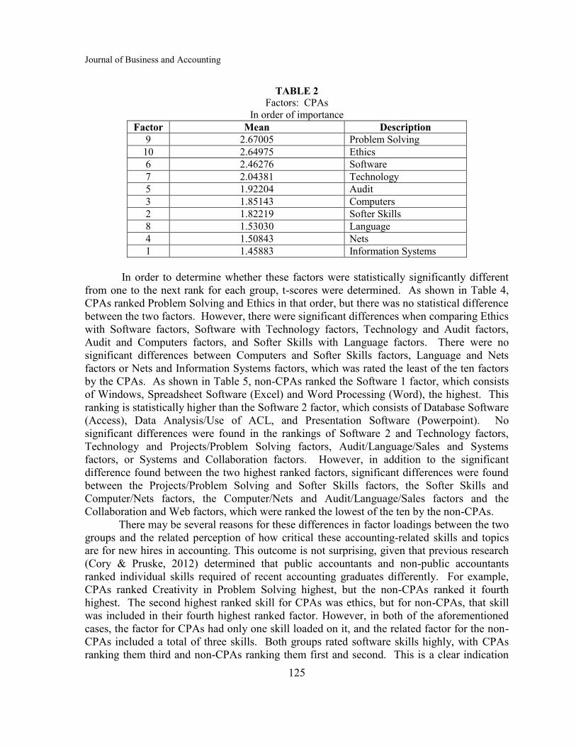
Journal of Business and Accounting
125
TABLE 2
Factors: CPAs
In order of importance
Factor Mean Description
9 2.67005 Problem Solving
10 2.64975 Ethics
6 2.46276 Software
7 2.04381 Technology
5 1.92204 Audit
3 1.85143 Computers
2 1.82219 Softer Skills
8 1.53030 Language
4 1.50843 Nets
1 1.45883 Information Systems
In order to determine whether these factors were statistically significantly different
from one to the next rank for each group, t-scores were determined. As shown in Table 4,
CPAs ranked Problem Solving and Ethics in that order, but there was no statistical difference
between the two factors. However, there were significant differences when comparing Ethics
with Software factors, Software with Technology factors, Technology and Audit factors,
Audit and Computers factors, and Softer Skills with Language factors. There were no
significant differences between Computers and Softer Skills factors, Language and Nets
factors or Nets and Information Systems factors, which was rated the least of the ten factors
by the CPAs. As shown in Table 5, non-CPAs ranked the Software 1 factor, which consists
of Windows, Spreadsheet Software (Excel) and Word Processing (Word), the highest. This
ranking is statistically higher than the Software 2 factor, which consists of Database Software
(Access), Data Analysis/Use of ACL, and Presentation Software (Powerpoint). No
significant differences were found in the rankings of Software 2 and Technology factors,
Technology and Projects/Problem Solving factors, Audit/Language/Sales and Systems
factors, or Systems and Collaboration factors. However, in addition to the significant
difference found between the two highest ranked factors, significant differences were found
between the Projects/Problem Solving and Softer Skills factors, the Softer Skills and
Computer/Nets factors, the Computer/Nets and Audit/Language/Sales factors and the
Collaboration and Web factors, which were ranked the lowest of the ten by the non-CPAs.
There may be several reasons for these differences in factor loadings between the two
groups and the related perception of how critical these accounting-related skills and topics
are for new hires in accounting. This outcome is not surprising, given that previous research
(Cory & Pruske, 2012) determined that public accountants and non-public accountants
ranked individual skills required of recent accounting graduates differently. For example,
CPAs ranked Creativity in Problem Solving highest, but the non-CPAs ranked it fourth
highest. The second highest ranked skill for CPAs was ethics, but for non-CPAs, that skill
was included in their fourth highest ranked factor. However, in both of the aforementioned
cases, the factor for CPAs had only one skill loaded on it, and the related factor for the non-
CPAs included a total of three skills. Both groups rated software skills highly, with CPAs
ranking them third and non-CPAs ranking them first and second. This is a clear indication

Cory and Pruske
126
that both groups perceive the need for new accounting graduates to have mastered certain
software packages. The technology factor and the computer factors are ranked in similar
positions in the two groups, although certain skills associated with factor 1 (ranked tenth) for
the CPAs are ranked lower than for the non-CPAs’ factor 1 (ranked eighth). It is logical that
CPAs would value their Factor 5, Audit, ranked fifth, more than the non-CPAs. The non-
CPAs included auditing skills in their Factor 9, ranked seventh. The factor associated with
Softer Skills is ranked lower for CPAs (seventh) than non-CPAs (fifth).
TABLE 3
Factors: Non-CPAs
In Order of Importance
Factor Mean Description
6 2.79549 Software 1
5 2.26876 Software 2
8 2.18611 Technology
7
2.17969
Projects/Problem Solving
2 1.92946 Softer Skills
3 1.77976 Computer/Nets
9 1.69198 Audit/Language/Sales
1 1.69089 Systems
10 1.65702 Collaboration
4 1.36618 Web
TABLE 4
Differences in Factors
CPAs
Factors T-Test Significance
Factors 9 and 10 0.35 n/a
Factors 10 and 6 4.49 <.0001
Factors 6 and 7 12.93 <.0001
Factors 7 and 5 2.31 .0221
Factors 5 and 3 2.18 .0308
Factors 3 and 2 0.90 n/a
Factors 2 and 8 6.96 <.0001
Factors 8 and 4 0.15 n/a
Factors 4 and 1 -0.14 n/a

Journal of Business and Accounting
127
TABLE 5
Differences in Factors
Non-CPAs
Factors T-Test Significance
Factors 6 and 5 16.60 <.0001
Factors 5 and 8 1.86 n/a
Factors 8 and 7 0.21 n/a
Factors 7 and 2 10.35 <.0001
Factors 2 and 3 3.50 .0006
Factors 3 and 9 2.04 .0430
Factors 9 and 1 -0.14 n/a
Factors 1 and 10 0.54 n/a
Factors 10 and 4 5.93 <.0001
CONCLUSION
Implications for accounting educators are interesting. The statistical differences
between factors also provide interesting results. CPAs basically ranked Creativity in
Problem Solving and Awareness of Ethical Issues equally (first and second, respectively, no
statistical difference between them). Therefore, these would seem to be the top two skills on
which accounting educators should focus when working with students headed for a career in
public accounting. Yet these two are probably the most difficult to convey to students and
also the learning outcomes related to each the most difficult to measure. The non-CPAs’ top
two ranked skills are associated with software, which do not have the same difficulties of
conveyance and learning outcome measurement. Further, CPA candidates are expected to
pass the CPA exam, and creativity in problem solving is not tested on it. Should educators
focus on teaching software aspects, to the exclusion of creativity in problem solving or ethics
when working with students destined for a non-public accounting career? Most would reply
in the negative.
Finally, this study has some limitations that should be addressed. Responses were
obtained from individuals in only one geographical area, which may make findings difficult
to generalize to a wider population. Only 34 skills were listed on the survey, but additional
information could have been gathered with the research instrument. Further, information
about the viewpoints of recently hired accounting graduates regarding the skills they feel are
necessary for a successful career in accounting and whether they had those skills upon arrival
to their first accounting position could be gathered. These can certainly be the seeds for
future research.
REFERENCES
Ahadiat, N. (2008). In Search of Practice-Based Topics for Management Accounting Education.
Management Accounting, 9 (4), 42-53.
Albrecht, W.S. (2002). Accounting Education on the Edge. BizEd, March/April,
41-45.
Albrecht, W.S. & Sack, R.J. (2000). Accounting Education: Charting the Course through a Perilous
Future. Accounting Education Series, 16. Sarasota, FL: American Accounting Association.

Cory and Pruske
128
American Institute of Certified Public Accountants (AICPA) (1998). CPA Vision Project Identifies
Top Five Issues for Profession. The CPA Letter, 1 (12), 1.
Cory, S.N. (2009). What Do Public Accounting Practitioners Really Want? An Exploratory
Investigation. Journal of Business Issues, 1, 47-56.
Cory, S.N. and Huttenhoff, T.F. (2011). Perspectives of Non-Public Accountants about Accounting
Education and Certifications: An Exploratory Investigation. Journal of Finance and
Accountancy 6, 77-89.
Cory, S.N. and Pruske, K.A. (2012). Necessary Skills for Accounting Graduates: An
Exploratory Study to Determine What the Profession Wants. Proceedings of the American
Society of Business and Behavioral Sciences, 19 (1), 208-218.
Hurt, B. (2007). Teaching What Matters: A New Conception of Accounting Education. Journal of
Education for Business, 82 (5), 295-299.
Johnson, G.F. & Halabi, A.K. (2009). A Citation Analysis Measuring the Impact of Albrecht &
Sack (2000). Journal of Modern Accounting and Auditing, 5 (9), 21-29.
Nelson, I.T. (1995). What’s New about Accounting Education Change? An Historical Perspective
on the Change Movement. Accounting Horizons, 9 (4), 62-75.
Pedhazur, E.J. and Schmelkin, L.P. (1991). Measuring, Design and Analysis. Lawrence Erlbaum
Publishers, Hillsdale, N.J.

Journal of Business and Accounting
Vol. 5, No. 1; Fall 2012
129
THE EFFECT OF TIMING ON STUDENT SATISFACTION SURVEYS
Pierre L. Titard
James E. DeFranceschi
Eric Knight
Southeastern Louisiana University
ABSTRACT
This study is based on surveys of student satisfaction of a management accounting
simulation, used in a sophomore/junior-level managerial accounting course, required for all
non-accounting business students. The simulation requires that students, in teams of three,
make decisions to earn a profit for a hypothetical manufacturing firm over a simulated year.
Students’ simulation grades are based on the amount of net income earned by the team.
Students can earn a maximum of 50 points out of 500 course points, plus possible bonus
points. Instructors administer a survey each semester to determine student satisfaction with
the simulation, as well as to determine whether students believe that they have a better
understanding of the subject matter that had been discussed in class.
In previous semesters, some instructors administered surveys on the last day of class,
and some on the day of the final exam. This study was conducted to determine whether there
is a difference in student satisfaction, depending on when the survey is administered. Results
of a t-test show that for most items on the survey, there is a statistical difference.
Specifically, students who completed the survey on the day of the final exam indicated more
satisfaction with the simulation than those who completed it on the last day of class.
INTRODUCTION
At a regional university in the southeastern United States, a management accounting
simulation is used in a sophomore/junior-level managerial accounting course, required for all
non-accounting business students. The simulation (also referred to in this paper as the
“game”) requires that students work in three-person teams to make decisions with the goal to
earn as much profit as possible over a simulated year for a hypothetical manufacturing firm.
The year is divided into four quarters for decision-making purposes. The game is not
interactive; one team’s decisions do not affect the results of any other team. However, the
students do compete to earn a higher net income than their classmates. Simulation grades are
assigned on the basis of cumulative four-quarter net income. The higher the net income, the
more points the team earns, and vice-versa. In addition there are bonus points for the two
highest ranking teams each quarter and at the end of the game.
Not considering bonus points, students can earn a maximum of 50 points out of 500
course points, based on their cumulative net income for the four quarters. In previous
semesters, students were required to submit decisions for each of the four quarters in order to
earn any points. In other words, if a team did not submit decisions for each of the four
quarters, it received a grade of 0 out of 50.
Instructors administer a survey (described below) at the end of the semester to
determine student satisfaction with the simulation. The instructors also want to know whether

Titard, DeFranceschi, and Knight
130
students believe that the simulation has helped in their understanding of managerial
accounting, as discussed in class, and whether it helped in understanding other business
courses and “real world” problems.
PURPOSE OF STUDY
Recently, the authors changed the requirements by making submission of fourth
quarter decisions optional. Since there is a pre-determined grade scale based on cumulative
net income, students who decide to stop after three quarters of play know exactly what grade
they will receive. For example, if a team had a cumulative net income at the end of three
quarters that provided a grade of 40 points, the team could accept those points and not submit
another decision which would earn additional points. Students who elect to play a fourth
quarter know the minimum grade they will receive by using that same scale. Students were
told that in the past, playing the fourth quarter had always increased a team’s game points
and had never decreased the number of points from what the team had earned after three
quarters.
The purpose of the study was to determine whether student satisfaction differs
depending on the timing of the survey. That is, are students who complete the survey later
more satisfied with the simulation than those who complete it earlier? Intuitively, the authors
believed that there should be no significant difference. Students know their grades at the end
of three quarters, and can only increase their grades if they continue. Therefore, the authors
believed that students would have already been satisfied (or not) by the end of three quarters
and that whether the survey were administered earlier or later would make no difference in
the results. Regardless of whether or not students played the fourth quarter, all students in a
specific section completed the survey at the same time–either on the last day of class, or on
the day of the final exam.
PREVIOUS STUDIES
There is a dearth of literature on this topic. In fact, the authors’ literature review
found no previous studies directly related to their study. Previous research on surveys and
timing relate primarily to consumer research. Faught, et al (2004) determined the best time
for Internet surveys was Wednesday mornings. Bassili and Fletcher (1991) researched
methodology for measuring accurately the timing of respondents answers to questions in
computer-assisted telephone surveys. Severson (2002) states that timing is everything in
surveys and the worst timing is after a bad ice storm, weeks of major holidays, county fairs,
or a big local rodeo.
Interestingly, the one study that may have some relevance to our findings is one
related to the timing of paying physicians for their response to a mail survey (Berry and
Kanouse, 1987). This relevance is described in the Conclusions section of this paper.
METHODOLOGY
The population for the study consisted of 140 students in nine sections. Instructor 1
had two sections with 34 students; Instructor 2, four sections with 54 students; and Instructor
3, three sections with 52 students. A fourteen-item survey was administered to each student
at the end of the course to determine their satisfaction with the simulation. The instrument

Journal of Business and Accounting
131
used a five-point Likert scale, with possible responses from Strongly Disagree (1) to Strongly
Agree (5). The survey instrument also provided a space for students to write additional
comments if they desire. A copy of the survey instrument is included as Appendix A to this
paper. The survey was voluntary and anonymous. Instructors 1 and 2 administered the
survey to one and two of their sections, respectively, on the last day of class and to their
remaining three sections on the day of the final exam. Instructor 3 conducted the survey for
all three sections on the day of the final exam. Sections that completed the survey on the last
day of class are referred to as “early” sections; those who completed it on the day of the final
exam are referred to as “late” sections. Note that the difference in timing between early and
late is just one class day, that is, from the last day of class until the day of the final exam,
although it does range from four to seven calendar days.
The methodology used to conduct the research was as follows:
1. The mean for each survey item was calculated for the early sections.
2. The mean for each survey item was calculated for the late sections.
3. A t-test was used to determine whether any differences in means between the early
and late sections were statistically significant.
RESULTS
The results are shown in Table 1.
Table 1
T-Test of Means between Early and Late
Early Late
Item (N = 40) (N = 100) T-Test
1. Understand text 2.85 3.73 .01
2. Understand Managerial Accounting 2.88 3.70 .01
3. Understand other business courses 2.85 3.64 .01
4. Understand “real world” problems 3.60 4.00 .05
5. Liked the game 2.78 3.50 .01
6. Enjoyable experience 2.73 3.36 .01
7. Appropriate weight 3.10 3.54 .05
8. Prefer relative ranking for grade 2.87 2.56 N/S
9. Prefer predetermined grade scale 3.34 3.88 .01
10. Too time-consuming 3.16 2.87 N/S
11. Team did equal work 3.71 3.72 N/S
12. My contribution was greater 2.55 2.05 N/S
14. Include game in the future 3.03 3.80 .01
As shown above, the differences were significant at the .01 level for seven items and
at the .05 level for two items. There were no significant differences for five of the items.
Items 11, 12, and 13 are not totally relevant to the study because those items relate more to
satisfaction with the other team members than with the game itself.
Approximately 24% of the students also wrote comments regarding the simulation.
Although the comments cannot be measured statistically, more positive comments came from

Titard, DeFranceschi, and Knight
132
those who took the survey on the day of the final exam; and more negative comments came
from those who took the survey on the last day of class. A summary of the comments are
shown in Table 2. Table 2
Summary of Comments
Early Late
(N= 11) Percent (N= 23) Percent
Positive 2 18% 10 43%
Negative 7 64% 2 9%
Neutral 2 18% 11 48%
11 23
Sample comments are included as Appendix B.
CONCLUSIONS
As indicated earlier, at the outset of the research the authors would not have expected
to see significant differences between “early” and “late.” They have no explanation for the
reasons for these differences. One possible explanation (untested) is that many of the “late”
students improved their grades by playing the fourth quarter of the game. They knew
precisely how much their grade had improved from the third quarter. Consequently, they
may have been more satisfied than they might have otherwise been. The “early” students
who planned to continue knew that their grade would improve, but did not know exactly by
how much it would improve. Perhaps they ended up more satisfied at the end of the fourth
quarter than they were at the end of the third quarter, but they had already completed the
survey.
This possible explanation relates somewhat to the physician research ( Berry and
Kanouse, 1987). In that study, one-half of the physicians were given $20 along with a
survey. The other half were sent the survey and were promised $20 upon completion of the
survey. The physicians receiving payment up-front had a higher response rate than the other
group. That study parallels to some extent the fact that at the time of the final exam, all
students knew exactly what grade they would receive for the simulation. However, on the
last day of class, students planning to continue knew approximately, but not exactly. Perhaps
this makes a difference.
Students who stopped at the end of three quarters knew their grade regardless of
when the survey was taken. At that point, they were either already satisfied or not, but
nothing else was going to change their opinion. Because the surveys are anonymous, we are
unable to separate the opinions of those who completed three quarters from those who
completed four quarters.
The authors recognize that this survey was specific to the management accounting
simulation used in their class. However, based on the results, they have arrived at the
following two conclusions.
1. More meaningful data may be obtained from administering student surveys as late
as feasibly possible.

Journal of Business and Accounting
133
2. More meaningful data may be obtained for evaluations, such as student
evaluations of teaching, when administered as late as feasibly possible.
Regarding the second conclusion, the authors note that in their experience, some
schools have gone to earlier requirements for student teaching evaluations from times when
they could be administered on the last day of class. While this is probably done for certain
administrative reasons within the university, it may, in some cases, be detrimental to the
instructor’s evaluation.
The authors believe that this study could serve as a basis for additional research in
this area.
REFERENCES
Bassili, J., & Fletcher, J. (1991). Response-Time Measurement in Survey Research. Public Opinion
Quarterly, 55 (3), 331-346.
Berry, S., & Kanouse, D. (1987). Physician Response to a Mailed Survey: An Experiment in Timing
of Payment. Public Opinion Quarterly, 51 (1), 102-114.
Faught, K., Whitten, D. &. Green, Jr., K. (2004). Doing Survey Research on the
Internet: Yes, Timing Does Matter. Journal of Computer Information
Systems, 44 (3), 26-34.
Serverson, J. (2002). What Every Manager Needs to Know About Consumer Research.
Management Quarterly, 43(2), 17-35.
APPENDIX A
MAS SURVEY
Circle the letter than best describes your attitude about each of the statements
regarding the Management Accounting Simulation (MAS game) used in ACCT 225 this
semester. Your responses should be anonymous, so do not write your name on the response
sheet.
1. The game helped me to understand better some of the concepts described in the text.
1 2 3 4 5
Strongly Disagree Neutral Agree Strongly
Disagree Agree
2. I have a better understanding of Managerial Accounting as a result of playing the game.
1 2 3 4 5
Strongly Disagree Neutral Agree Strongly
Disagree Agree
3. I have a better understanding of concepts learned in other business courses as a result of playing
the game.
1 2 3 4 5
Strongly Disagree Neutral Agree Strongly
Disagree Agree

Titard, DeFranceschi, and Knight
134
4. The game gave me a better understanding of “real world” problems faced by business firms in
trying to make a profit.
1 2 3 4 5
Strongly Disagree Neutral Agree Strongly
Disagree Agree
5. I like the fact that the game was a required element of this course.
1 2 3 4 5
Strongly Disagree Neutral Agree Strongly
Disagree Agree
6. Playing the game was an enjoyable experience.
1 2 3 4 5
Strongly Disagree Neutral Agree Strongly
Disagree Agree
7. The weight of the game as a percentage of the total course, 10 % (50 points out of a total of 500
points) is the appropriate weight to assign to the game.
1 2 3 4 5
Strongly Disagree Neutral Agree Strongly
Disagree Agree
8. Points should be awarded based on relative competitive ranking of teams without a predetermined
scale. (For example, the highest team gets 50 points regardless of cumulative net income; the 2nd
highest gets 49 points, etc.)
1 2 3 4 5
Strongly Disagree Neutral Agree Strongly
Disagree Agree
9. Points should be awarded based on a predetermined scale. (For example, $15,000,000 or greater
cumulative net income is 50 points; $14,000,000--$14,999,999 is 49 points, etc.)
1 2 3 4 5
Strongly Disagree Neutral Agree Strongly
Disagree Agree
10. Considering what I learned from the game, it was too time-consuming.
1 2 3 4 5
Strongly Disagree Neutral Agree Strongly
Disagree Agree
11. All members of my team did approximately the same amount of work.
1 2 3 4 5
Strongly Disagree Neutral Agree Strongly
Disagree Agree

Journal of Business and Accounting
135
12. My contribution to the team was significantly more than that of any other team member.
1 2 3 4 5
Strongly Disagree Neutral Agree Strongly
Disagree Agree
13. My contribution to the team was significantly less than that of any other team member.
1 2 3 4 5
Strongly Disagree Neutral Agree Strongly
Disagree Agree
14. The game should be included when the course is offered again.
1 2 3 4 5
Strongly Disagree Neutral Agree Strongly
Disagree Agree
In the space below, please provide any additional comments, recommendations, or criticisms you may
have about the game.
APPENDIX B
Sample Students Comments–Early
• Good times!
• As a sophomore, I would have hated the game. But as a senior, I realize how important
the concepts that it teaches are.
• This “game” was EXTREMELY difficult and time consuming. I have missed work and
spent countless hours at home dealing with it. My other grades in my other classes
suffered. Not beneficial for learning at all in my opinion,! Nothing but STRESS over
something I will NEVER use!!!!
• Not worth it. NOT a game! Does not relate to anything I know. It’s retarded!
• The game was OK.
Sample Student Comments–Late
• The game was challenging but fun at the same time and it really helped me understand
the material better.
• It was a good learning experience.
• It got stressful and time consuming.
• A little too time consuming.
• Extend the game and make it worth more.
Authors’ Note: The third and fourth Late comments were the only two negative comments
from the Late students. Compare the difference in tone to the negative comments by the
Early students. We cannot make any statement that the differences resulted from
administering the survey earlier or later, but it is an interesting observation.

Journal of Business and Accounting
Vol. 5, No. 1; Fall 2012
136
STUDENT PLAGIARISM AND
ECONOMIC VERSUS MORAL BASED
PEDAGOGY
James Tackett
Raymond Shaffer
Fran Wolf
Gregory Claypool
Youngstown State University
ABSTRACT This study examines the relationship between incidents of
plagiarism and ethics pedagogy in a 2x2 full factorial, between subjects, quasi-
experimental design using the General Linear Model. An objective surrogate is
used to approximate the level of plagiarism in student writing assignments and
then compared between classes which emphasized an altruistic approach to ethics
versus a purely pragmatic view of ethical behavior (ethical egoism). The results
show that ethical egoism may be a more effective pedagogy for teaching college
ethics than pure altruism in terms of reducing the incidence of student plagiarism.
INTRODUCTION
Every college professor knows of the Internet's positive impact
on the learning environment in higher education. Powerful search engines enable
students to find large amounts of relevant material for their assignments in a
manner of seconds. Faculty are, however, also painfully aware of the stunning
rise in cut-and-paste plagiarism that is a direct result of these Internet search
engines. This plague of student plagiarism has been documented as a widespread
problem from high school all the way through graduate studies at both public and
private institutions across the globe (Blum, 2009; Comas and Sureda 2010;
Harding et al., 2004; Sunderland-Smith 2008). This creates a paradox because
extensive ethical preparation is required by virtually all business and most other
college curriculums.
The chasm between ethical education and student behavior is
troubling. Some studies have demonstrated that academic dishonesty in college
is a precursor to deceit in the workplace (Harding et al., 2004; Nonis & Swift,
2001). If such is the case, then the widespread prevalence of plagiarism is even
more disturbing because there will be costly consequences to society as students
graduate and enter the workforce.
Unfortunately, it is difficult to measure the impact of ethical
education on student behavior. Ethics questions and examinations can test a
factual knowledge of ethical rules and how a student would respond to a
hypothetical ethical dilemma; but, such artificial measurements will not

Journal of Business and Accounting
137
necessarily be representative of student behavior when they confront real choices
that pit honest scholarship against shady shortcuts. Some studies have directly
queried students about the prevalence and methods of plagiarism (Antenucci et
al. 2009). Such investigations provide useful insights into the problem of
plagiarism, but they fail to adequately measure the real cause-effect relationships
because of potential bias in student perceptions of the problem. Students may
also use the survey as a means to further their own agenda by providing
responses that would cultivate instructor approval. Accordingly, there is a
genuine need for going beyond traditional ethics examinations, case studies, and
honesty surveys; higher education needs to assess the true impact of ethical
preparation on student behavior.
This study examines the relationship between incidents of
plagiarism and ethics pedagogy in a 2x2 full factorial, between subjects, quasi-
experimental design using the General Linear Model. An objective surrogate is
used to approximate the level of plagiarism in student writing assignments and
then compared between classes which emphasized an altruistic approach to ethics
versus a purely pragmatic view of ethical behavior (ethical egoism). The results
show that ethical egoism may be a more effective pedagogy for teaching college
ethics than pure altruism in terms of reducing the incidence of student plagiarism.
THE NATURE OF PLAGIARISM There has been considerable discussion and research into the
various types of student plagiarism as well as the factors that are purported to
cause this form of academic dishonesty (Comas and Sureda 2010; Stevenson,
2001). Overall, the literature is not concerned with plagiarism which is caused
by student ignorance of academic referencing requirements; and, it focuses on the
deliberate submission of written or oral assignments that contain the words or
ideas of other people without proper acknowledgment. There is, however,
another form of unintentional plagiarism whereby writers subconsciously use the
ideas of others. This is known as cryptomnesia and is a relatively unexplored
area of plagiarism (Roig, 2001).
Harding et al. (2004) contends that plagiarism skills are first
developed in high school and then further honed when students enter the writing
intensive environment of college. This argument is supported by studies that
show most high school students have at some point plagiarized their writing
assignments (Bushway and Nash, 1977; Decoo, 2002). A study conducted by
Stevenson (2001) found that 40% of college undergraduates admitted to
plagiarizing material from the Internet. Another study pointed out that most
students do not view this form of cut-and-paste plagiarism as a serious violation
of academic honesty (Yeo, 2007).
The literature yields conflicting results about the prevalence of
plagiarism by academic ability. Smith et al. (2007) and Newstead et al. (1996)
found that plagiarism is more prevalent among weaker students as measured by
grade point average. This result was confirmed by a study which measured the
relationship between grade point average and college plagiarism (Tackett et al.

Tackett,,Shaffer, Wolf and Claypool
138
2010). Conversely, studies by Roberts et al. (1997) and Franklin-Stokes and
Newstead (1995) did not find a statistically significant relationship between
plagiarism and grade point average. Similarly, the relationship between gender
and plagiarism is open to question. Studies by Roberts et al. (1997) and Smith et
al. (2007) found that males are more likely to plagiarize than females. On the
other hand, Franklin-Stokes and Newstead (1995) and Granitz and Loewy (2007)
did not find a significant relationship between gender and plagiarism.
Prior research has demonstrated that such electronic
countermeasures can reduce the incidence of blatant plagiarism by as much as
77% (Tackett et al. 2010). Regrettably, students have adapted to these plagiarism
search engines by avoiding verbatim quotations and choosing to paraphrase the
plagiarized material to make detection more difficult. Paraphrasing can be
effective because it masks the exact source of the plagiarized material, thereby
making formal charges of college cheating difficult to prove beyond reasonable
doubt. This form of "gray plagiarism" has now become the norm for students
seeking dishonest shortcuts to completing college writing assignments.
Paraphrasing can be identified by commercial plagiarism detection engines (e.g.,
similarity indices), but formal prosecution via academic dishonesty committees is
rare because intent cannot be adequately established. This is known as the
cryptomnesia defense, and many students are willing to take full advantage of
this loophole.
THE ETHICAL DILEMMA OF PLAGIARISM Extensive ethical preparation is mandated by most college
accrediting agencies (e.g., AACSB for baccalaureate business accreditation). If
students overwhelmingly choose to plagiarize college assignments, then the
effectiveness of the ethics pedagogy administered to those students must be
questioned.
The traditional underlying theme of all business and professional
ethical codes is altruism, which expresses a sincere concern for the welfare of
others (Cheffers and Pakaluk, 2005). Students who engage in college cheating
are obviously placing self-interest above altruism to achieve economy in
preparing college assignments. The philosophy of acting in one's own self-
interest is called ethical egoism or simply egoism (Sanders, 1988). On the
surface, egoism appears to be the exact opposite of altruism; yet, this is not
necessarily correct. The short-term advantages of unethical behavior can be
more than offset by the long-term consequences. Accordingly, a rational person
pursuing egoism would need to balance the short and long-term consequences of
unethical behavior (Rachels, 2008). It is possible that a rational egoist would
view traditional altruistic behavior as something that would be in their own long-
term best interest. There are of course idealistic issues with egoism because it
advocates selfishness. Nevertheless, when viewed from a long-term perspective,
egoism and altruism can be seen as philosophies that could yield the same
behavior from individuals practicing those ideals.

Journal of Business and Accounting
139
The ethics literature provides mixed results on the impact of
ethical codes on behavior. Some studies show that ethical decision-making is not
affected by having a factual knowledge of ethical codes (Laczniak and
Inderrieden, 1987; White and Dooley, 1993; and Cleek and Leonard 1998). On
the other hand, other studies have suggested that knowledge of ethical codes
provides positive benefits to decision-makers (Barnett and Vaicys, 2000; and
Pflugrath et al. 2007). Tackett et al. (2010) examined the impact of teaching
accounting ethics from an altruistic approach versus ethical egoism and found
that student performance on ethics examination questions was unchanged.
However, students who were exposed to the ideas of egoism evaluated the ethical
conduct of accounting professionals in several classic auditing failures more
harshly than students who were exposed to traditional altruistic ethics. This
result provides evidence that egoism is worthy of further exploration in terms of
altering student beliefs about ethical behavior.
HYPOTHESIS DEVELOPMENT As discussed previously, there is a troubling inconsistency
between the behavior of plagiarizing students and the ethical education imparted
to them in the classroom. This raises the question of whether altering ethics
pedagogy would reduce the magnitude of student plagiarism. If the answer is
yes, then which ethics pedagogy is more effective in promoting student honesty.
In the current study, the AICPA Code of Professional Conduct is
used as an ethical benchmark because it is a structured set of ethical rules that is
taught by every accounting program. The AICPA Code can be supplemented
with either altruistic philosophy, ethical egoism, or both. If both altruism and
egoism are taught together, then one must argue that behaving in a manner that
considers the legitimate interests of others is in our own long-term economic
interest. The following hypotheses are developed:
H1: Presenting the AICPA Code of Professional Conduct combined with
ethical altruism does not alter the incidence of student plagiarism
compared to presenting the Code alone.
H2: Presenting the AICPA Code of Professional Conduct combined with
ethical egoism does not alter the incidence of student plagiarism
compared to presenting the Code alone.
H3: Presenting the AICPA Code of Professional Conduct combined with
ethical altruism and egoism does not alter the incidence of student
plagiarism compared to presenting the Code alone.
METHODOLOGY The above hypotheses are tested using a 2x2 full factorial,
between subjects design with 136 accounting seniors from a Midwestern,
AACSB accredited college of business. Separate sections of the same upper
division accounting class were selected to participate in the study. Students were
unaware that the lectures and presentation of material would be slightly different
between these sections, and they registered according to their own needs in

Tackett,,Shaffer, Wolf and Claypool
140
scheduling. Any students who had previously taken the course were removed
from the study so each participant was viewing the lecture and presentation for
the first time. Demographic information was collected from the students via
academic transcripts and included age, gender, and grade point average. The
dichotomous grouping variable for age was under 25 years old. Random
assignment was used to determine which sections received which set of lectures.
The random assignment of students would have been desirable to create a true
experimental design, but student scheduling needs made this impossible.
Accordingly, a quasi-experimental design by means of the General Linear Model
was used with grade point average as a covariate. The experiment was conducted
as part of the college’s educational assessment program and the results are being
used to evaluate the professional ethics learning goal for accounting majors.
Each student in the study prepared a research assignment
requiring a series of written papers analyzing a major auditing failure. Detailed
instructions for preparing the paper were described in the course syllabus and
discussed in class. These instructions included the need for proper academic
referencing of the sources used; and, specific examples were given of appropriate
referencing procedures. Students were required to submit their papers
electronically as attached files in Microsoft Word, and were warned that they
would be held accountable for proper referencing procedures. The course
syllabus also stipulated that any academic misconduct by students would result in
a failing grade for the course.
All of the student papers were analyzed by a commercial
plagiarism detection service. The output from this service showed a "similarity
index" for each student. This index represented the proportion of the paper that
was taken from the Internet or contained in a publication from their proprietary
database (e.g., published articles, books, manuscripts, etc.). The service also
provided an HTML copy of the student’s paper with highlighted sections and
notes to show exactly where the writing material was taken from. The papers
were reviewed, and any direct quotations or paraphrased statements with proper
references were noted and removed from the calculated similarity index.
Otherwise, the index would be including properly referenced material. This
adjusted similarity index would thus measure quotations and paraphrasing that
was not referenced by the student.
The 136 students in the study were partitioned into four groups.
Each experimental group received the same factual presentation of the AICPA
Code of Professional Conduct as part of the normal course requirement. Three of
the four groups, however, had the following supplemental discussions seamlessly
incorporated into the lecture: Group 2: Ethical Altruism; Group 3: Ethical
Egoism; Group 4: Ethical Altruism and Egoism. There was no discussion of
altruism or egoism in Group 1.
Altruism was discussed as a moral duty to behave in a manner
that benefits the common good of everyone (Cheffers and Pakaluc, 2005).
Specific examples of altruistic thinking included the need for accountants to
protect society from misrepresented financial statements as well as the need for
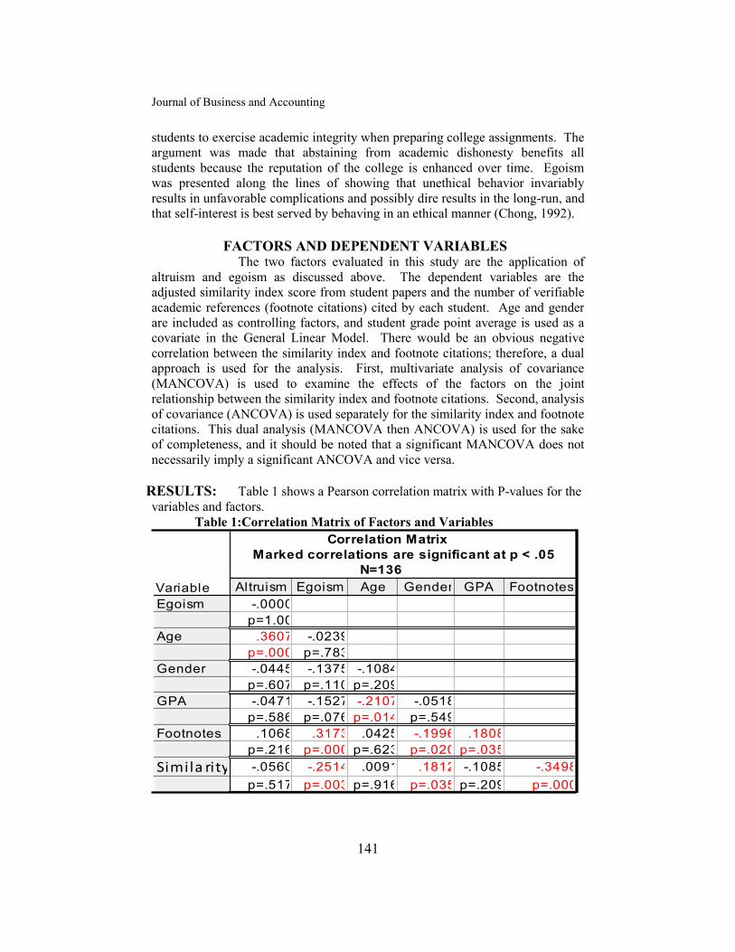
Journal of Business and Accounting
141
students to exercise academic integrity when preparing college assignments. The
argument was made that abstaining from academic dishonesty benefits all
students because the reputation of the college is enhanced over time. Egoism
was presented along the lines of showing that unethical behavior invariably
results in unfavorable complications and possibly dire results in the long-run, and
that self-interest is best served by behaving in an ethical manner (Chong, 1992).
FACTORS AND DEPENDENT VARIABLES The two factors evaluated in this study are the application of
altruism and egoism as discussed above. The dependent variables are the
adjusted similarity index score from student papers and the number of verifiable
academic references (footnote citations) cited by each student. Age and gender
are included as controlling factors, and student grade point average is used as a
covariate in the General Linear Model. There would be an obvious negative
correlation between the similarity index and footnote citations; therefore, a dual
approach is used for the analysis. First, multivariate analysis of covariance
(MANCOVA) is used to examine the effects of the factors on the joint
relationship between the similarity index and footnote citations. Second, analysis
of covariance (ANCOVA) is used separately for the similarity index and footnote
citations. This dual analysis (MANCOVA then ANCOVA) is used for the sake
of completeness, and it should be noted that a significant MANCOVA does not
necessarily imply a significant ANCOVA and vice versa.
RESULTS: Table 1 shows a Pearson correlation matrix with P-values for the
variables and factors.
Table 1:Correlation Matrix of Factors and Variables
Correlation Matrix
Marked correlations are significant at p < .05
N=136
Variable Altruism Egoism Age Gender GPA Footnotes
Egoism
Age
Gender
GPA
Footnotes
Simila rity
-.0000
p=1.00
.3607 -.0239
p=.000 p=.783
-.0445 -.1375 -.1084
p=.607 p=.110 p=.209
-.0471 -.1527 -.2107 -.0518
p=.586 p=.076 p=.014 p=.549
.1068 .3173 .0425 -.1996 .1808
p=.216 p=.000 p=.623 p=.020 p=.035
-.0560 -.2514 .0091 .1812 -.1085 -.3498
p=.517 p=.003 p=.916 p=.035 p=.209 p=.000

Tackett,,Shaffer, Wolf and Claypool
142
The correlation between altruism and age is coincidental, indicating a
disproportionately large group of students who were over age 25 in the altruism
group. This confirms the need for age as a controlling factor. Additionally, older
students had a lower cumulative grade point average. Males provided fewer
footnote citations than females, and had significantly higher similarity index
scores. There is no significant correlation between footnotes or the similarity
index for the altruism group; however, both of these correlations are significant
for egoism. Based on this simple correlation matrix, students in the egoism
group had a lower similarity index and provided more footnotes than the altruism
group.
Table 2: Multivariate Analysis of Covariance
MANCOVA ~ Footnotes and Similarity versus
Altruism, Egoism, Age, Gender, (GPA as Covariate)
Variable W
ilks' F Degrees of Freedom
P
Value
S
tatistic
N
um
Denom
inator
GPA
0
.95351
3
.12 2 128
0
.048
Altruism
0
.99576
0
.272 2 128
0
.762
Egoism
0
.87791
8
.901 2 128
0
.001
Age
0
.99906
0
.06 2 128
0
.941
Gender
0
.96977
1
.995 2 128
0
.141
Altruism*E
goism
0
.99809
0
.122 2 128
0
.885
Table 2 shows the MANCOVA results for how the factors and
GPA covariate influenced the combined effect of similarity and footnote
citations. GPA is significant at the 5% level, suggesting that stronger students
had lower similarity indices and/or higher footnote citations. This result is
consistent with the previously discussed findings of Smith et al. (2007) and
Newstead et al. (1996). Altruism is not significant, but egoism is highly
significant (P-value < 0.001). Gender was the next most significant factor (P-
value 0.141). There was no significant interaction between altruism and egoism.

Journal of Business and Accounting
143
Figure 1: Surface Plot of Similarity and Footnotes
A linear surface plot of the data is shown in Figure 1, and it
provides a visual representation of the MANCOVA results. Each graph shows a
three-dimensional regression model of the similarity (top) and footnote (bottom)
components of the data.
The surface plot of similarity has some significant outliers
(altruism with no egoism), but the overall center mass of the observations seems
to suggest higher levels of plagiarism (similarity index > 12) for the students who
received neither the altruistic or egoistic presentations. The footnote surface plot
is clearly more pronounced and appears to show greater footnote presentation for
students who received both altruistic and egoistic lectures.

Tackett,,Shaffer, Wolf and Claypool
144
Figure 2 shows an ANCOVA graph of the four experimental
groups by similarity index (top) and footnotes (bottom) with grade point average
as a covariate.
Figure 2: Analysis of Covariance ANCOVA Graph on Similarity Index
Current effect: F(3, 131)=3.8000, p=.01188
Vertical bars denote 0.95 confidence intervals
AICPA Only Altruism Egoism Altruism+Egoism
Treatment
-2
0
2
4
6
8
10
12
14
16
18
20
Sim
ila
rity
In
de
x
Covariate means:
GPA: 3.282059
ANCOVA Graph on Footnotes
Current effect: F(3, 131)=5.4094, p=.00154
Vertical bars denote 0.95 confidence intervals
AICPA Only Altruism Egoism Altruism+Egoism
Treatment
0.0
0.5
1.0
1.5
2.0
2.5
3.0
Fo
otn
ote
s
Covariate means:
GPA: 3.282059
The ANCOVA on similarity index is significant at the 1% level.
However, an ex-post multiple comparisons procedure demonstrates that only the
altruism plus egoism group is significantly different from the AICPA group at the
5% significance level (note vertical bars for Tukey’s HSD test). Similarly, the
ANCOVA on footnotes is significant (P-value 0.00154), and only the altruism
plus egoism combination produced a significant difference from the AICPA
group based on Tukey’s HSD test. The graphs in Figure 2 seem to indicate that
altruism alone provides little if any benefit beyond the AICPA Code; egoism
alone produces a stronger (but not statistically significant) response; and, the
combination of altruism plus egoism is more effective in reducing plagiarism
than the AICPA Code alone or the Code plus altruism.

Journal of Business and Accounting
145
Table 3
Factorial ACOVA: Altruism x Egoism x Age x Gender Test of SS Whole Model vs. SS Residual
Dependent
Variable
Multiple
R
Multiple
R²
Adjusted
R²
SS
Model
df
Model
MS
Model
SS
Resid
df
Resid
MS
Resid
F p
Simila rity 0.4318840.186524 0.0771494464.33 16 279.02 19470.01 119 163.61 1.71 0.05
Fisher's LSD Test on Similarity Index
Probabil i ties for Post Hoc Tests
Error: Between MSE = 163.61, df = 119.00
Cell
Alt Ego Age Gen 1 2 3 4 5 6 7 8 9 10 11 12 13 14 15
1
2
3
4
5
6
7
8
9
10
11
12
13
14
15
16
0 0 0 0
0 0 0 1 0.18
0 0 1 0 0.65 0.24
0 0 1 1 0.29 0.78 0.25
0 1 0 0 0.36 0.80 0.32 0.68
0 1 0 1 0.55 0.03 0.88 0.14 0.11
0 1 1 0 0.34 0.03 0.88 0.09 0.08 0.61
0 1 1 1 0.81 0.27 0.83 0.29 0.38 0.90 0.65
1 0 0 0 0.67 0.16 0.91 0.21 0.26 0.98 0.73 0.90
1 0 0 1 0.86 0.17 0.74 0.25 0.31 0.74 0.48 0.92 0.79
1 0 1 0 0.87 0.29 0.59 0.36 0.48 0.46 0.29 0.73 0.59 0.75
1 0 1 1 0.06 0.48 0.14 0.90 0.41 0.01 0.01 0.14 0.07 0.06 0.12
1 1 0 0 0.38 0.02 0.94 0.10 0.08 0.69 0.90 0.71 0.80 0.53 0.32 0.01
1 1 0 1 0.82 0.12 0.75 0.23 0.26 0.75 0.47 0.94 0.80 0.98 0.71 0.04 0.52
1 1 1 0 0.21 0.01 0.79 0.06 0.03 0.42 0.85 0.54 0.60 0.34 0.18 0.00 0.74 0.32
1 1 1 1 0.91 0.19 0.71 0.27 0.34 0.69 0.44 0.88 0.75 0.95 0.80 0.07 0.49 0.92 0.31 Test of SS Whole Model vs. SS Residual
Dependent
Variable
Multiple
R
Multiple
R²
Adjusted
R²
SS
Model
df
Model
MS
Model
SS
Resid
df
Resid
MS
Resid
F p
Footnotes 0.4383 0.1921 0.0835 55.8549605 16 3.49 234.90 119 1.97 1.77 0.04
Fisher's LSD Test on Footnotes
Probabil i ties for Post Hoc Tests
Error: Between MSE = 1.9740, df = 119.00
Cell
Alt Ego Age Gen 1 2 3 4 5 6 7 8 9 10 11 12 13 14 15
1
2
3
4
5
6
7
8
9
10
11
12
13
14
15
16
0 0 0 0
0 0 0 1 0.03
0 0 1 0 0.93 0.21
0 0 1 1 0.18 1.00 0.30
0 1 0 0 0.88 0.02 1.00 0.16
0 1 0 1 0.77 0.00 0.95 0.12 0.92
0 1 1 0 0.79 0.10 0.80 0.28 0.69 0.59
0 1 1 1 0.33 0.70 0.44 0.77 0.29 0.23 0.46
1 0 0 0 0.90 0.09 1.00 0.22 1.00 0.94 0.75 0.35
1 0 0 1 0.06 0.88 0.21 0.92 0.05 0.02 0.13 0.66 0.11
1 0 1 0 0.25 0.44 0.43 0.63 0.20 0.13 0.42 0.90 0.31 0.45
1 0 1 1 0.29 0.22 0.50 0.49 0.24 0.13 0.51 0.75 0.37 0.27 0.80
1 1 0 0 0.74 0.01 0.92 0.13 0.87 0.93 0.58 0.24 0.90 0.03 0.15 0.17
1 1 0 1 0.99 0.04 0.92 0.19 0.87 0.77 0.81 0.34 0.90 0.07 0.27 0.32 0.74
1 1 1 0 0.43 0.00 0.71 0.06 0.54 0.55 0.32 0.13 0.63 0.01 0.06 0.06 0.66 0.43
1 1 1 1 0.73 0.02 0.90 0.13 0.84 0.90 0.57 0.24 0.87 0.04 0.16 0.19 0.96 0.72 0.71
Table 3 shows the results of full factorial ANCOVA on the
similarity index (top) and footnote (bottom) factors with Fisher's LSD multiple
comparisons test. The overall significance of the ANCOVA is 5% for the
similarity index and 4% for footnotes. Yet, as discussed above in the surface
plots, the similarity index contained skewed data that was not normally
distributed. A Box-Cox logarithmic transformation was performed on the
similarity index, and this reduced the ANCOVA significance level from 5% to
1%. Accordingly, a multiple comparisons procedure can be used to search for
significant differences between the factors. Fisher's LSD test is shown because

Tackett,,Shaffer, Wolf and Claypool
146
there were no statistically significant differences between any of the factors using
Tukey’s HSD test. Tukey’s HSD uses a pooled variance to establish confidence
intervals; therefore, each confidence interval will be the same length. Fisher's
LSD calculates individual variances and thereby provides confidence intervals of
different sizes for each variable. Fisher's test is considered more precise, but it is
less conservative than Tukey’s if one is searching for large differences between
the independent variables.
Fisher's LSD multiple comparisons procedure shows that gender
(male = 1, female = 0) is an issue for both the similarity index and footnote
dependent variables. For the similarity index, males in the egoism group
plagiarized less than males in the other groups (column 2, P = 3%). The sharpest
similarity index gender difference occurs between males from the AICPA group
versus females over age 25 from the altruism plus egoism group (P = 1%). This
same gender effect is noted for footnotes and is even stronger (P < 1%). In fact,
males from the AICPA group footnoted significantly less than males or females
from the altruism plus egoism group. This result is consistent with the findings
of Roberts et al. (1997) and Smith et al. (2007) which observed higher plagiarism
rates by males. It also implies that egoism may have its greatest behavioral
impact on males.
Another interesting result from Table 3 concerns the fact that the
altruism group is not significantly different from any combination of egoism,
age, and gender (column 9). Moreover, most of the results for altruism are not
even close to being significant for both the similarity index and footnotes. On
the other hand, the altruism plus egoism group has a significantly lower
similarity index when compared to the altruism group (column 12 of similarity
index). This implies that altruism combined with egoism may be the most
effective pedagogical combination.
DISCUSSION AND CONCLUSIONS Seven of the 136 students received failing grades in the course
for plagiarism (outliers in the similarity index of Figure 1). Another 16 students
had significant grade reductions for negligence in failing to provide acceptable
citations. At least 31 additional students fell into the "gray plagiarism" area of
successful paraphrasing without crossing the line into academic misconduct. All
the reprimanded students alleged human error or fatigue for "forgetting" to add
proper references for their research.
The results from the MANCOVA and ANCOVA analysis
suggest that ethical egoism seems to be more effective than traditional altruism in
reducing the incidence of plagiarism in the selected sample. The most effective
combination appears to be combining altruistic philosophy with egoism by
explaining that ethical behavior is, in the long run, in our own best economic
interest. Egoism appears to have a greater impact on males than females.
The counterargument to this study would advocate the position
that greater discussions with students about the negative consequences of
plagiarism results in less plagiarism. This is, however, overly simplistic. The

Journal of Business and Accounting
147
contribution of this study rests in comparing traditional ethical arguments based
on altruism with those of ethical egoism, and then measuring the impact of these
different philosophies on the ethical behavior of students. Further research on
the advantages and disadvantages of incorporating ethical egoism into traditional
ethics courses seems warranted.
REFERENCES
Antenucci, J., Tackett, J., Wolf, F., & Claypool, G. (2009). The Rationalization
of Academic Dishonesty. Journal of Business and Accounting. 2(1).
Barnett, T. & Vaicys, C. (2000). The Moderating Effect of Individuals’
Perceptions of Ethical Work Climate on Ethical Judgments and
Behavioral Intentions. Journal of Business Ethics. 27(4), 351-362.
Blum, Susan D. (2009). My Word! Plagiarism and College Culture. Ithaca,
Cornell UP.
Bushway, A. & Nash, W. R. (1977). School Cheating Behavior. Review of
Educational Research. 47(4), 623.
Cheffers, M. & Pakaluc, M. (2005). Understanding Accounting Ethics.
Manchaug: David Allen Press, 49-65.
Chong, C. (1992). Ehtical Egoism and the Moral Point of View. The Journal of
Value Inquiry, (26), 23-36.
Cleek, M. & Leonard, S. (1998). Can Corporate Codes of Ethics Influence
Behavior? Journal of Business Ethics. 17(6), 619-630.
Comas, R. & Sureda, J. (2010). Academic Plagiarism: Explanatory Factors from
Student’s Perspective. Journal of Academic Ethics. 8(3), 217-232.
Decoo, W. (2002). Crisis on Campus: Confronting Academic Misconduct. MIT
Press, Cambridge, Mass.
Franklin-Stokes, A. & Newstead, S.E. (1995). Undergraduate Cheating: Who
Does What and Why? Studies In Higher Education. 20(2), 159-172.
Granitz, N. & Loewy, D. (2007). Applying Ethical Theories: Interpreting &
Responding to Student Plagiarism. Journal of Business Ethics. 72(3),
293-306.
Harding, T. S., Carpenter, D. D., Finelli, C. J., & Passow, H. J. (2004). Does

Tackett,,Shaffer, Wolf and Claypool
148
Academic Dishonesty Relate to Unethical Behavior in
Professional Practice? An Exploratory Study. Science &
Engineering Ethics. 10, 311- 324.
Laczniak, G. & Inderrieden, E. (1987). The Influence of Stated Organizational
Concern Upon Ethical Decision Making. Journal of Business
Ethics. 6(4), 297-307.
Newstead, S.E., Franklin-Stokes, A. & Armstead, P. (1996). Individual
Differences in Student Cheating. Journal of Educational
Psychology. 88(2), 229-241.
Nonis, S. & Swift, C.O. (2001). An Examination of the Relationship Between
Academic Dishonesty and Workplace Dishonesty: A
Multicampus Investigation. Journal of Education for Business.
76, 69-77.
Pflugrath, G., Martinov, B. & Chen, L. (2007). The Impact of Codes of Ethics
and Experience on Auditor Judgments. Managerial Auditing
Journal. 22(6), 566-589.
Rachels, J. (2008) Ethical Egoism. Reason and Responsibility: Readings in Some
Basic Problems of Philosophy. California: Thomson Wadsworth.
532-540.
Roberts, P., Anderson, J., & Yanish, P. (1997). Academic Misconduct: Where Do
We Start? Northern Rocky Research Association. Jackson, WY.
Roig, M. (2001). Plagiarism and Paraphrasing Criteria of
College and University Professors. Ethics & Behavior. 11, 307-
24.
Sanders, S. (1988). Is Egoism Morally Defensible? Philosophia. Springer
Netherlands. (18)2.
Smith, M., Ghazali, N., & Minhad, S. (2007). Attitudes Towards Plagiarism
Among Undergraduate Accounting Students: Malaysian
Evidence. Asian Review of Accounting. (15)2, 122-146.
Stevenson, Seth. (2001). Adventures in Cheating: A Guide to Buying Term
Papers Online. Slate Magazine. December 11, 2001.
Sutherland-Smith, W. (2008). Plagiarism, the Internet and Student Learning:
Improving Academic Integrity. London: Routledge.

Journal of Business and Accounting
149
Tackett, J., Wolf, F., Claypool, G. & Antenucci, J. (2010). The Impact of
Plagiarism Detection Software on College Plagiarism. Journal of
Business and Accounting. (3)1.
Tackett, J., Wolf, F., Claypool, G. (2011). Economic vs Moral Based Pedagogies
for Business Ethics. Journal of Business and Educational
Leadership. (3)1.
White, C. & Dooley, R. (1993). Ethical or Practical: An Empirical Study of
Students’ Choices in Simulated Business Scenarios. Journal of
Business Ethics. 12, 643–651.
Yeo, S. (2007). First-Year University Science & Engineering Students’
Understanding of Plagiarism. Higher Education Research &
Development. 26(2), 199-216.