Jason Hoffman, Ecoult Energy Storage Solutions
89
-
Upload
khangminh22 -
Category
Documents
-
view
0 -
download
0
Transcript of Jason Hoffman, Ecoult Energy Storage Solutions


INTERNATIONAL JOURNAL OF MODERN ENGINEERING
THE LEADING JOURNAL OF ENGINEERING, APPLIED SCIENCE, AND TECHNOLOGY
Mark Rajai, Ph.D.
Editor-in-Chief California State University-Northridge College of Engineering and Computer Science Room: JD 4510 Northridge, CA 91330 Office: (818) 677-5003 Email: [email protected]
Contact us:
www.iajc.org www.ijme.us
www.tiij.org
www.ijeri.org
Print ISSN: 2157-8052 Online ISSN: 1930-6628
TO JOIN THE REVIEW BOARD:
• The International Journal of Engineering Research and Innovation (IJERI) For more information visit www.ijeri.org
• The Technology Interface International Journal (TIIJ).
For more information visit www.tiij.org
OTHER IAJC JOURNALS:
• Manuscripts should be sent electronically to the manuscript editor, Dr. Philip Weinsier, at [email protected].
For submission guidelines visit www.ijme.us/submissions
IJME SUBMISSIONS:
• Contact the chair of the International Review Board, Dr. Philip Weinsier, at [email protected]. For more information visit www.ijme.us/ijme_editorial.htm
• IJME was established in 2000 and is the first and official flagship journal of the International Association of Journal and Conferences (IAJC).
• IJME is a high-quality, independent journal steered by a distinguished board of directors and supported by an international review board representing many well-known universities, colleges and corporations in the U.S. and abroad.
• IJME has an impact factor of 3.00, placing it among
the top 100 engineering journals worldwide, and is the #1 visited engineering journal website (according to the National Science Digital Library).
ABOUT IJME:
INDEXING ORGANIZATIONS:
• IJME is currently indexed by 22 agencies. For a complete listing, please visit us at www.ijme.us.

——————————————————————————————————————————————————-
——————————————————————————————————————————————————–
INTERNATIONAL JOURNAL OF MODERN ENGINEERING
INTERNATIONAL JOURNAL OF MODERN ENGINEERING
The INTERNATIONAL JOURNAL OF MODERN ENGINEERING (IJME) is
an independent, not-for-profit publication, which aims to provide the engineering
community with a resource and forum for scholarly expression and reflection.
IJME is published twice annually (fall and spring issues) and includes peer-
reviewed research articles, editorials, and commentary that contribute to our un-
derstanding of the issues, problems, and research associated with engineering and
related fields. The journal encourages the submission of manuscripts from private,
public, and academic sectors. The views expressed are those of the authors and do
not necessarily reflect the opinions of the IJME editors.
EDITORIAL OFFICE:
Mark Rajai, Ph.D.
Editor-in-Chief
Office: (818) 677-2167
Email: [email protected]
Dept. of Manufacturing Systems
Engineering & Management
California State University-
Northridge
18111Nordhoff Street
Northridge, CA 91330-8332
THE INTERNATIONAL JOURNAL OF MODERN ENGINEERING EDITORS
Editor-in-Chief:
Mark Rajai
California State University-Northridge
Associate Editors:
Alok Verma
Old Dominion University
Li Tan
Purdue University North Central
Production Editor:
Philip Weinsier
Bowling Green State University-Firelands
Subscription Editor:
Morteza Sadat-Hossieny
Northern Kentucky University
Web Administrator:
Saeed Namyar
Advanced Information Systems
Executive Editor:
Paul Wilder
Vincennes University
Manuscript Editor:
Philip Weinsier
Bowling Green State University-Firelands
Copy Editor:
Li Tan
Purdue University North Central
Technical Editors:
Michelle Brodke
Bowling Green State University-Firelands
Marilyn Dyrud
Oregon Institute of Technology
Publisher:
Bowling Green State University Firelands

Editor's Note (In This Issue): Measured and Simulated Performance of a Grid-Connected PV System
in a Humid Subtropical Climate .................................................................................................................................................. 3
Philip Weinsier, IJME Manuscript Editor
High-Speed Permanent-Magnet Generator with Optimized Sizing Based on Particle Swarms for Smart Grids ........................ 5
Adel El Shahat, Georgia Southern University; Rami J. Haddad, Georgia Southern University;
Youakim Kalaani, Georgia Southern University
A Simple Block Coding Scheme for Peak-to-Average Power Ratio Reduction in Multi-Carrier Systems ................................. 19
Yoonill Lee, Purdue University Northwest
Battery Energy Storage for a Low-Voltage DC Microgrid System ............................................................................................ 26
Dale H. Litwhiler, Penn State University; Nicholas Batt, Ecoult Energy Storage Solutions;
Jason Hoffman, Ecoult Energy Storage Solutions
Measured and Simulated Performance of a Grid-Connected PV System in a Humid Subtropical Climate .............................. 31
Fredericka Brown, The University of Texas at Tyler; Racquel Lovelace, The University of Texas at Tyler
The Effects of Anchor Rod Failure on the Performance of the New Bay Bridge Tower ............................................................ 37
Abolhassan Astaneh-Asl, University of California, Berkeley; Maryam Tabbakhha, University of California, Berkeley;
Xin Qian, University of California, Berkeley
Geometrical Determination of Maximum Power Point of a Photovoltaic Cell ......................................................................... 45
Mehmet Goksu, Millersville University of Pennsylvania; Faruk Yildiz, Sam Houston State University
Serviceability Performance of Concrete Beams Reinforced with MMFX Steel ......................................................................... 50
Faris Malhas, Central Connecticut State University; Mustafa Mahamid, University of Illinois at Chicago;
Adeeb Rahman, University of Wisconsin-Milwaukee
A General Method for Failure Analysis and Re-Design of a Mechanical Diode ...................................................................... 60
Kevin M. Hubbard, Missouri State University; Martin P. Jones, Missouri State University;
Nebil Buyurgan, Missouri State University
Latency and Phase Transitions in Interconnection Networks with Unlimited Buffers .............................................................. 70
Lev B. Levitin, Boston University; Yelena Rykalova, UMass Lowell
The Role of Adhesive Forces during Separation of Liquid-Mediated Contacts ........................................................................ 78
Prabin Dhital, Minnesota State University, Mankato; Shaobiao Cai, Minnesota State University, Mankato
Instructions for Authors: Manuscript Submission Guidelines and Requirements ..................................................................... 85
——————————————————————————————————————————————–————
——————————————————————————————————————————————–————
INTERNATIONAL JOURNAL OF MODERN ENGINEERING | VOLUME 17, NUMBER 1, FALL/WINTER 2016
TABLE OF CONTENTS

——————————————————————————————————————————————————–
EDITOR’S NOTE (IN THIS ISSUE): MEASURED AND SIMULATED PERFORMANCE OF A GRID-CONNECTED PV SYSTEM 3
IN A HUMID SUBTROPICAL CLIMATE
IN THIS ISSUE (P.31)
CONNECTING A PHOTOVOLTAIC SYSTEM TO
THE ELECTRICAL GRID IN A HUMID
SUBTROPICAL CLIMATE
Philip Weinsier, IJME Manuscript Editor
———————————————————————————————————————————————————–————
Not that long ago, when asking the average homeowner
about photovoltaic (PV) systems, your reply could be ex-
pected to range from a blank stare to a confident, “Sure, I’ve
heard about them!” At that time, perhaps only two decades
ago or so, PV systems represented an expense that, again,
the average homeowner could only gawk at. But there were
plenty of well-to-do individuals, who could afford such sys-
tems. So why weren’t more systems dotting the U.S. land-
scape? That likely was due to the fact that the older systems
were inefficient and either could not connect to the distribu-
tion grid or the additional costs to do so were such that the
return on investment just didn’t compute. Nor were regula-
tory agencies and government giving the industry much
consideration or respect by way of safety regulations.
As if those weren’t reasons enough for avoiding involve-
ment with PVs, homeowners also had to take into account
their environment—where they lived, average temperature,
irradiation levels, amount of sunlight available throughout
the year, effects of snow and clouds, type of PV system to
buy and its efficiency and $/watt costs. Should I buy mono-
crystalline, polycrystalline, amorphous, CdTe (cadmium
telluride), or CIS/CIGS (coper indium gallium selenide)?
Today, though, is quite another matter. State-of-the-art
systems are worth considering; you no longer have to be
quite so well-to-do as before, especially if you are willing to
invest the time to apply for state/federal rebates. There are
also more safety regulations covering installation of PV
systems, plus there’s no shortage of companies ready to
install one for you. For the most part, they are also now ra-
ther well-versed on what type of system you should buy,
given all of the factors that I noted above. But at the end of
the proverbial day, what does a system save you? After all,
if there are no savings down the road, why bother? Looking
at some of the advertising from PV companies, you can
expect to pay (2016) between $3 and $4 per watt to install
your system, with the average system in the U.S. weighing
in at about 5kW (5000 watts). So, you can expect to lay out
$10,000 to $20,000; not exactly chump change.
And what does such an outlay get you? Start by focusing
on the long-term; you likely will have to wait a good seven
years before you start recognizing some savings. But, over
the next 13 years (assuming a 20-year lifespan of your sys-
tem), you can likely double or triple your investment in sav-
ings. That does, of course, depend on where you live: The
west coast and upper east coast will generally return your
money faster and save you more in the long-run.
But there’s more to the story than just how good such a
system might be on your pocketbook. We also need to take
into account the limited resources available in the way of
fossil fuels that the world is burning through—literally and
figuratively. At some point, we just have to get on one
bandwagon or another and help move the world towards
renewable energy resources. For more on this topic, I direct
your attention to the article on p.31 in which the authors
describe their research aimed at determining the measured
and predicted performance of a photovoltaic grid-connected
system. By predicted system performance, I mean the au-
thors also developed a computer model of their system and
compared the results to experimentally collected data. Final-
ly, the research allowed for long-term simulation analysis of
the system under varying conditions that would assist de-
signers with the optimization of the PV system.

Editorial Review Board Members
——————————————————————————————————————————————–————
——————————————————————————————————————————————–————
4 INTERNATIONAL JOURNAL OF MODERN ENGINEERING | VOLUME 17, NUMBER 1, FALL/WINTER 2016
State University of New York (NY) Michigan Tech (MI)
Louisiana State University (LA)
Virginia State University (VA) Ohio University (OH)
Wentworth Institute of Technology (MA)
Guru Nanak Dev Engineering (INDIA) Texas A&M University (TX)
Jackson State University (MS)
Clayton State University (GA) Penn State University (PA)
Eastern Kentucky University (KY)
Cal Poly State University SLO (CA) Purdue University Calumet (IN)
University of Mississippi (MS)
Morehead State University (KY)
Eastern Illinois University (IL)
Indiana State University (IN)
Southern Illinois University-Carbondale (IL) Southern Wesleyen University (SC)
Southeast Missouri State University (MO)
Alabama A&M University (AL) Ferris State University (MI)
Appalachian State University (NC)
Utah State University (UT) Oregon Institute of Technology (OR)
Elizabeth City State University (NC) Tennessee Technological University (TN)
DeVry University (OH)
Sam Houston State University (TX) University of Nebraska-Kearney (NE)
University of Tennessee Chattanooga (TN)
Zagazig University EGYPT) University of North Dakota (ND)
Eastern Kentucky University (KY)
Utah Valley University (UT) Abu Dhabi University (UAE)
Safety Engineer in Sonelgaz (ALGERIA)
Central Connecticut State University (CT) University of Louisiana Lafayette (LA)
St. Leo University (VA)
North Dakota State University (ND) Norfolk State University (VA)
Western Illinois University (IL)
North Carolina A&T University (NC) Indiana University Purdue (IN)
Bloomsburg University (PA)
Michigan Tech (MI) Bowling Green State University (OH)
Ball State University (IN)
North Dakota State University (ND) Central Michigan University (MI)
Wayne State University (MI)
Abu Dhabi University (UAE) Purdue University Calumet (IN)
Southeast Missouri State University (MO)
Daytona State College (FL) Brodarski Institute (CROATIA)
Uttar Pradesh Tech University (INDIA)
Ohio University (OH) Johns Hopkins Medical Institute
Penn State University (PA)
Excelsior College (NY) Penn State University Berks (PA)
Mohammed Abdallah Nasser Alaraje
Aly Mousaad Aly
Jahangir Ansari Kevin Berisso
Salah Badjou
Pankaj Bhambri Water Buchanan
Jessica Buck Murphy
John Burningham Shaobiao Cai
Vigyan Chandra
Isaac Chang Bin Chen
Wei-Yin Chen
Hans Chapman
Rigoberto Chinchilla
Phil Cochrane
Michael Coffman Emily Crawford
Brad Deken
Z.T. Deng Sagar Deshpande
David Domermuth
Ryan Dupont Marilyn Dyrud
Mehran Elahi Ahmed Elsawy
Rasoul Esfahani
Dominick Fazarro Rod Flanigan
Ignatius Fomunung
Ahmed Gawad Daba Gedafa
Ralph Gibbs
Mohsen Hamidi Mamoon Hammad
Youcef Himri
Xiaobing Hou Shelton Houston
Barry Hoy
Ying Huang Charles Hunt
Dave Hunter
Christian Hyeng Pete Hylton
Ghassan Ibrahim
John Irwin Sudershan Jetley
Rex Kanu
Reza Karim Tolga Kaya
Satish Ketkar
Manish Kewalramani Tae-Hoon Kim
Doug Koch
Sally Krijestorac Ognjen Kuljaca
Chakresh Kumar
Zaki Kuruppalil Edward Land
Ronald Land
Jane LeClair Shiyoung Lee
Central Michigan University (MI) Florida A&M University (FL)
Eastern Carolina University (NC)
Penn State University (PA) University of North Dakota (ND)
University of New Orleans (LA)
ARUP Corporation University of Louisiana (LA)
University of Southern Indiana (IN)
Eastern Illinois University (IL) Cal State Poly Pomona (CA)
University of Memphis (TN)
Excelsior College (NY) University of Hyderabad (INDIA)
California State University Fresno (CA)
Indiana University-Purdue University (IN)
Institute Management and Tech (INDIA)
Cal State LA (CA)
Universiti Teknologi (MALAYSIA) Michigan Tech (MI)
University of Central Missouri (MO)
Indiana University-Purdue University (IN) Community College of Rhode Island (RI)
Sardar Patel University (INDIA)
Purdue University Calumet (IN) Purdue University (IN)
Virginia State University (VA) Honeywell Corporation
Arizona State University (AZ)
Warsaw University of Tech (POLAND) Wayne State University (MI)
New York City College of Tech (NY)
Arizona State University-Poly (AZ) University of Arkansas Fort Smith (AR)
Wireless Systems Engineer
Brigham Young University (UT) Baker College (MI)
Zagros Oil & Gas Company (IRAN)
Virginia State University (VA) North Carolina State University (NC)
St. Joseph University Tanzania (AFRICA)
University of North Carolina Charlotte (NC) Wentworth Institute of Technology (MA)
Toyota Corporation
Southern Illinois University (IL) Ohio University (OH)
University of Houston Downtown (TX)
University of Central Missouri (MO) Purdue University (IN)
Georgia Southern University (GA)
Purdue University (IN) Nanjing University of Science/Tech (CHINA)
Lake Erie College (OH)
Thammasat University (THAILAND) Digilent Inc.
Central Connecticut State University (CT)
Ball State University (IN) North Dakota State University (ND)
Sam Houston State University (TX)
Morehead State University (KY) Missouri Western State University (MO)
Soo-Yen Lee Chao Li
Jimmy Linn
Dale Litwhiler Guoxiang Liu
Louis Liu
Mani Manivannan G.H. Massiha
Thomas McDonald
David Melton Shokoufeh Mirzaei
Bashir Morshed
Sam Mryyan Wilson Naik
Arun Nambiar
Ramesh Narang
Anand Nayyar
Stephanie Nelson
Hamed Niroumand Aurenice Oliveira
Troy Ollison
Reynaldo Pablo Basile Panoutsopoulos
Shahera Patel
Jose Pena Karl Perusich
Thongchai Phairoh Huyu Qu
John Rajadas
Desire Rasolomampionona Mulchand Rathod
Mohammad Razani
Sangram Redkar Michael Reynolds
Marla Rogers
Dale Rowe Anca Sala
Mehdi Shabaninejad
Ehsan Sheybani Musibau Shofoluwe
Siles Singh
Ahmad Sleiti Jiahui Song
Yuyang Song
Carl Spezia Michelle Surerus
Vassilios Tzouanas
Jeff Ulmer Mihaela Vorvoreanu
Phillip Waldrop
Abraham Walton Liangmo Wang
Jonathan Williams
Boonsap Witchayangkoon Alex Wong
Shuju Wu
Baijian Yang Mijia Yang
Faruk Yildiz
Yuqiu You Jinwen Zhu

HIGH-SPEED PERMANENT-MAGNET GENERATOR
WITH OPTIMIZED SIZING BASED ON PARTICLE
SWARMS FOR SMART GRIDS ——————————————————————————————————————————————–———–
Adel El Shahat, Georgia Southern University; Rami J. Haddad, Georgia Southern University;
Youakim Kalaani, Georgia Southern University
——————————————————————————————————————————————————–
HIGH-SPEED PERMANENT-MAGNET GENERATOR WITH OPTIMIZED SIZING BASED ON 5
PARTICLE SWARMS FOR SMART GRIDS
motor, temperature sensitivity of the magnetic materials is
an additional, critical factor; therefore, a Samarium Cobalt
(SmCo) magnet is often used to realize higher temperature
designs [1-5]. In fact, there have been extensive studies
dealing with HSPM design and applications [5-22].
In this current study, an optimized design process was
developed and compared to the classical approach that uses
a typical 500 kW output power generator at a tip speed of
250 m/s. These design methods take into consideration mul-
tiple factors, including classical sizing and problem formu-
lation with the objective of optimizing efficiency with
bounded constraints. The optimized set of variables used in
this study were rotor-length-to-diameter ratio, rotor radius,
and stack length. It was observed that this design approach
had the potential to limit losses at high frequencies and low
weight/volume, resulting in higher overall system efficien-
cy. Other parameters like power factor and maximum am-
pere-torque ratio were also shown to improve. Finally, ana-
lytical design examples with waveform variations, harmonic
distortion, rotor losses, and effects of changing poles were
also provided to show the merit of the proposed optimiza-
tion technique.
Classical Sizing
The overall power requirement for HSPM generators is
usually within the range of 5-500 kW. The structural and
thermal design of a permanent-magnet machine is highly
affected by the selections of magnet, stator, and rotor mate-
rials. The sizing and performance of HSPM machines de-
pend on the material properties of the permanent magnet
[23]. The magnets should be selected in order to provide the
required air gap magnetic field and ample coercive force
[24].
Additional information regarding the characteristics of
typical B-H curves can be found in the study by Hansel-
mann [25]. Rare earth magnets such as SmCo and NdFeB
provide high performance when used in HSPM machines,
due to greater power density, high coercivity, high flux den-
sities, and linearity of the demagnetization curves [26].
NdFeB is preferred because it is cheaper and more readily
available [27].
Abstract
High-speed, permanent-magnet (HSPM) types of micro-
generators play an important role in power generation in-
volving smart grid applications. In this study, the authors
developed an optimized analytical design and compared it
with an original machine design with a typical 500 kW tip-
speed of 250 m/s. The two designs take into consideration
multiple factors including classical sizing and problem for-
mulation for optimizing efficiency with bounded con-
straints. A particle swarm optimization (PSO) algorithm
was used to maximize efficiency as an objective or fitness
function and to minimize machine size as a non-linear func-
tion with bounded parameter constraints. Particle swarm
algorithms use population-based on flocks of birds or in-
sects swarming. The parameter variables used for this type
of optimization consist of rotor-length-to-diameter ratio,
rotor radius, and stack length. Test results including simula-
tions using PSO Tool in Matlab showed significant im-
provement in machine design and performance. Further-
more, it was observed that the proposed technique has the
advantage of limiting losses at higher frequencies with low
weight/volume applications, thereby improving overall effi-
ciency. Other system parameters such as power factor were
also improved. Finally, several analytical design problems
with waveform variations, harmonics distortion, rotor loss-
es, and effects of changing poles are provided to show the
merit of the proposed optimization technique.
Introduction
There has been increased interest in smart grid and micro-
grid connected systems, especially those dealing with onsite
generation [1]. This is mainly due to the limitations in the
use of traditional power plants heavily constrained by eco-
nomic and environmental regulations [2]. Therefore, high-
speed permanent-magnet (HSPM) micro-generators repre-
sent a viable and compact solution for onsite generation in
smart grids and micro-grids. Length-to-diameter is the most
important factor, defined as the rotor aspect ratio in high-
speed applications [3]. Classical and optimum designs of
HSPM generators have been studied for distributed power
generation purposes [4]. In the case of a high-speed PM

——————————————————————————————————————————————–————
——————————————————————————————————————————————–————
6 INTERNATIONAL JOURNAL OF MODERN ENGINEERING | VOLUME 17, NUMBER 1, FALL/WINTER 2016
Usually, the rotor is built from the same material as the
stator to simplify the manufacturing process. However, it is
not uncommon to have stators made of economically viable
materials such as steel [28]. Some of the most common ma-
terials used in the design of stators are low-carbon steels,
silicon (Si) steels, nickel (Ni) alloy steels, and cobalt (Co)
alloy steels [29]. The M19 is a 29-gauge electrical silicon
steel used for its economic viability, thin laminations, and
high saturation flux density, which is about 1.8 T [28].
Machine Design Parameters
The main aspect considered in this process is the stator
mechanical design, which can be either a slotted or slotless
design. Figure 1 shows the slotless stator, which has arma-
ture windings located in the air gap of the machine. Figure 2
shows the slotted stator, which has armature windings
wound around the slots or teeth.
Figure 1. Slotless Stator Design
Figure 2. Slotted Stator Design
The overall performance of a slotless stator is always in-
ferior to equivalent slotted stator designs; thus, the slotless
stator design is not usually used in high-power applications.
On the other hand, the slot openings in the slotted stator
design provide a sturdy housing for the windings and their
insulation. Figure 3 illustrates the stator slot geometry. A
key design factor in the slotted stator is to minimize the
difference between the slot depression width and the slot top
width. In power applications requiring a high number of
phases, 36-slot configurations are typically chosen for the
initial machine design.
Figure 3. Stator Slot Geometry
Rotor aspect ratio, defined as length-to-diameter (L/D)
ratio, is an important factor in high-speed applications. A
typical L/D ratio for a wound rotor machine is around 0.5-
1.0 compared to around 1-3 for a PM machine [30]. The
machine tip speed, which is the surface velocity of the rotor,
is governed by the rotational speed and rotor radius, as de-
fined by Equation (1):
(1)
where, r is the rotor radius (m) and ωm is the rotational an-
gular speed (rad/sec).
The tip speed upper bound for most rotating machines is
between 100 and 250 m/s, depending on its application and
design [31]. In a balanced rotational design, the number of
poles is determined by Equation (2):
(2)
where, N is speed (rpm); p is the number of pole pairs; and,
f is the electrical-frequency (Hz).
For a given rotational speed, an efficient solution is to
have a large number of poles and higher frequencies [26].
However, this might induce cogging torque and variations
in the air gap reluctance, flux, and voltage waveforms. To
resolve this issue, magnet poles are skewed to smooth out
these variation. Skew-factor is defined by Equation (3):
Stator Winding
Stator Core
Rotor Core
(Shaft)
Rotor Magnets
Teeth
Slots
Back Iron
Slot
Depression
Wsb
hs
Wst
Wdhd
Air Gap
Wsb : Slot Bottom Width
Wst: Slot Top Width
hs : Slot Height
Wd : Depression Width
hd : Depression Height
mtip rv
fpN 1202

——————————————————————————————————————————————–————
(3)
where, s is the skew angle (rad) and n is the-harmonic
number.
Using a first-order approximation, the air gap flux densi-
ty, Bg, can be represented by Equation (4) [32]:
(4)
where, hm is the magnet height (mm); g is the air-gap (mm);
and, Br is the magnet remnant flux density (T).
In order to get uniform magnetic fields, the magnet height
is usually larger than the air-gap by a factor of 5 to 10.
Power, current, and voltage ratings in an electric machine
are determined by the number of phases, given by Equation
(5):
(5)
where, P is the real power (W); Q is the reactive power
(VAR); q is the number of phases; V is the RMS phase volt-
age (V); and, I is the RMS current (A).
The number of slots per pole per phase, m, is an important
parameter when considering generator design and can be
calculated using Equation (6):
(6)
where, Ns is the number of slots; p is the pole pairs; and q is
the number of phases.
A slot fill factor, λs, [26] is used to determine the extent to
which the slot cross-sectional area is occupied by winding
material, as defined by Equation (7):
(7)
Overall, slot fill factors vary in value from 0.3-0.7 [26],
depending on the number and size of the conductors in the
slots. A slot fill factor of 0.5 was assumed for this current
design.
Machine Calculated Parameters
Assuming the machine is balanced, parameters are deter-
mined on a per-phase basis and can be applied to all phases,
as shown in Figure 4.
Figure 4. Per-Phase Model
The resistance of the copper phase windings, Ra, can be
calculated using Equation (8):
(8)
where, l is the conductor length; is the winding conductiv-
ity; and, A is the winding cross-sectional area.
The conductor cross-sectional area, A ac, can be obtained
using the slot area and slot fill factor, as shown in Equation
(9):
(9)
where, A s is the slot area and Nc is the number of turns per
coil.
Figure 5 illustrated the power loss resulting from eddy
currents in the slot conductors, which increases the re-
sistance in the winding [33], and which can be determined
by Equation (10):
Figure 5. Rectangular Conductor Geometry
(10)
where, Hm is the turn field intensity value and μ0 is the free-
space permeability.
2
sin
s
s
sn
nk
r
m
mg B
gh
hB
IVqjQP
qp
Nm s
2
AreaSlotTotal
AreaWindings
ACEa
Ra Ls
+
Va
_
A
lRa
c
ss
acN
AA
2
22
0
23
12
1mcec HhLP
L
Ih
c
y
z
x
——————————————————————————————————————————————————–
HIGH-SPEED PERMANENT-MAGNET GENERATOR WITH OPTIMIZED SIZING BASED ON 7
PARTICLE SWARMS FOR SMART GRIDS

——————————————————————————————————————————————–————
——————————————————————————————————————————————–————
8 INTERNATIONAL JOURNAL OF MODERN ENGINEERING | VOLUME 17, NUMBER 1, FALL/WINTER 2016
Skin depth is defined by Equation (11):
(11)
And, Equation (10) can be rewritten as shown in Equation
(12):
(12)
Assuming that the slot conductors are distributed uni-
formly in the slot, the total slot eddy current loss can be
calculated by substituting field intensity into Equation (12)
and summing over all ns conductors, as defined by Equation
(13):
(13)
where, I is the RMS conductor current; s is the slot width
(m); and, ds is the slot depth (m).
The single-slot resistance, Rsl, assuming ns conductors
connected in series, is given by Equation (14):
(14)
where, L is the slot length; kcp is the conductor packing fac-
tor, which is the ratio of cross-sectional area occupied by
conductors to the entire slot area; and, is the electrical
resistivity (.m).
Using Equation (14), the total slot resistance, Rst, can be
rewritten as Equation (15):
(15)
In Equation (15), e = Rec/Rsl is a frequency-dependent
term. Using Equations (13) and (14), this term can be sim-
plified and rewritten as Equation (16):
(16)
Winding factor, kw, is the ratio of flux linked by an actual
winding to the flux linked by a full-pitch concentrated-
factor, kp, and a breadth/distribution factor, kb, as shown in
Equation (17):
(17)
The pitch-factor can then be derived, with the final result
shown in Equation (18):
(18)
where, n is the harmonic number and α is the short pitch
coil, as illustrated in Figure 6.
A phase winding normally consists of a large number of
coils linking flux slightly out of phase with each other, as
shown in Figure 7.
Figure 6. Short-Pitch Coil
Figure 7. Winding Breadth
Equation (19) can be used to derive the breadth factor
either magnetically or geometrically:
(19)
where, m is the number of slots per pole per phase and γ is
the electrical angle of the coil.
Equation (20) is the equation for a slotted stator, surface
magnet configuration:
0
2s
2
4
3
6m
cec H
hLP
2
4
22
9I
nLhd
s
sseP
sscp
s
sldk
LnR
2
eslecslst RRRR 1
22
9
1
hd
R
R s
sl
ec
e
bnpnwn kkk
x
x
µ
x
x
x
x
ɤ
2sin
2sin
nnk pn
2sin
2sin
nm
mn
kbn

——————————————————————————————————————————————–————
where, Rs is the outer magnetic boundary; R2 is the outer
boundary of the magnet; R i is the inner magnetic boundary;
and, R1 is the inner boundary of the magnet.
Rs = R + hm + g
Ri = R1 = R
R2 = R + hm
The air gap flux density is also affected by the magnet
geometry in the air gap, as depicted by Equation (20). Since
the magnet poles rotate north/south, the air gap flux density
shape can be approximated using Equations (21)-(25) and is
illustrated in Figure 8.
Figure 8. Air Flux Density
(21)
where, ws is the average slot width; wt is the tooth width;
τs = ws + wt ; and, ws = ( wst + wsb ) / 2;
(22)
where, ge is the effective air gap;
(23)
where, PC is the permeance coefficient and Cφ is the flux
concentration factor (Am/Ag)= ;
(24)
where, μrec is the recoil permeability; Br is the remnant flux
density (T); and, kr is the reluctance factor;
(25)
and where, m is the magnet physical angle.
Assuming the radial flux through coil, B flux, is sinusoidal-
ly distributed—Equation (26)—the peak flux, φpk, for this
ideal coil is given by Equation (27):
(26)
(27)
Through Faraday’s Law, the back EMF, Ea, for the ma-
chine is given by Equation (29):
(28)
where,
(29)
and where,
The fundamental components are used to determine the
internal voltage of the generator, as depicted in Equations
(30) and (31) [4, 33, 34]:
(30)
ppppp
pp
p
nnn
s
p
pnn
p
p
n
i
n
s
n
i
gn RRRn
nRR
n
n
RR
Rk
1
2
1
1
21
1
1
222
1
11(20)
1
15
11
st
s
c
w
g
w
k
gkg ce
Cg
hPC
e
m
180
mp
r
rec
r
r
g B
PCk
CkB
1
B(
Bg
P2
P
P2
3
P
2
noddn
n npBB1
sin
2sin
2sin
4
nnpkB
nB m
gngn
P
stsflux dLRB
0
p
BLR fluxtss
pk
2
noddn
n np1
sin
p
kkBNLR snnwnasts
n
2
noddn
na npVE1
sin
nnndt
dV 0
2sin
41
m
gg
pkBB
——————————————————————————————————————————————————–
HIGH-SPEED PERMANENT-MAGNET GENERATOR WITH OPTIMIZED SIZING BASED ON 9
PARTICLE SWARMS FOR SMART GRIDS

——————————————————————————————————————————————–————
——————————————————————————————————————————————–————
10 INTERNATIONAL JOURNAL OF MODERN ENGINEERING | VOLUME 17, NUMBER 1, FALL/WINTER 2016
(31)
The number of armature turns, Na, can be found using
Equation (32), assuming that each slot has two half coils.
(32)
where, Nc is the number of turns per coil.
The vector relationship, illustrated in Figure 9, between
the terminal voltage, V a, internal voltage, Ea, and the syn-
chronous reactance voltage drop is utilized to obtain Equa-
tion (33) [35]:
Figure 9. Phasor Relationship
(33)
where,
(34)
By substituting Equation (34) into Equation (33), assum-
ing cos = 0.99999 1, and performing some mathematical
simplification, the terminal voltage, V a, can be derived from
the resulting quadratic equation, as shown in Equation (35):
with,
where,
(35)
and where, the air gap power can be calculated using Equa-
tion (36):
(36)
To calculate the air gap inductance, a full-pitch, concen-
trated winding carrying a current, I, is initially examined,
which leads to an air gap flux density determined by Equa-
tion (37) [33]:
(37)
The air gap flux density becomes
The flux can be found using Equation (26) and the total
flux linkage is λ = Na ϕ. With all real winding effects in-
cluded, the air gap inductance is then given by Equation
(38):
(38)
Assuming that the slot is rectangular with slot depressions
as illustrated, in Figure 4, this results in a slot permeance
per unit length given by Equation (39) [25, 34]:
(39)
Equations (40)-(42), assuming m slots per pole per phase
and a standard double-layer winding, show the slot leakage
inductance for self, mutual, and 3-phase windings, respect-
fully:
(40)
Ea
jXs Ia
Va
X
Y
p
BkkNLR swasts 12
0aE
ca NpN 2
sin)cos( 22 asasaa IXIXEV
cos
a
input
aVq
PI
2
2
222222
9 a
input
saasaaV
PXEIXEV
09
2
2224
input
saaa
PXVEV
2
aEBB
922
inputs PXCC
024
CCBBVV aa
2
42 CCBBBBVa
windagecorewrseaagapair PPPTIEP 3
oddisnn
nflux npBB1
sin
p
IN
hgnB a
m
n2
4 0
04
2 2
an
m
q N IB
n g h p
m
wnastsag
hgpn
kNLR
n
q
iL
22
22
04
2
d
d
st
s
w
h
w
hPerm
3
1
]24[222
cpspscstas NNNmNPermLpL

——————————————————————————————————————————————–————
(41)
(42)
(higher-odd-phases)
From the work by Hanselmann [33], the total end-turn
inductance per phase can be defined by Equation (43):
(43)
The total inductance for the phase is the sum of the three
inductances and is given by Equation (44):
(44)
Basic Losses
Empirical data for M-19 (29-gauge material) were ob-
tained. An exponential curve fit was then applied to the data
in order to obtain an equation for estimating the core losses,
as defined by Equations (45)-(47) [26]:
(45)
(46)
(47)
where, Rc is the core resistance; cFe is the correction factor
for the iron-loss calculation; bst is the stator tooth width; kFe
is the specific iron loss; mst is the stator teeth-mass; slot is
the slot angle; and, hsy is stator yoke height.
Conductor losses are then evaluated using Equation (48),
the power equation, for a resistance defined:
(48)
For rotors operating at high speeds, friction and windage
can cause losses, which result in inefficiency and heat pro-
duction. Friction/windage-losses [35] are given by Equation
(49):
(49)
where, Cf is the friction coefficient and ρair is the density of
air.
The coefficient of friction can then be approximated using
Equation (50):
(50)
where, Rey is the Reynold’s number.
Initial Machine Sizing
Air gap magnetic shear stress, τ, is the magnetic shear
force developed per unit gap area and is constrained by
magnetic design and thermal management [36], as shown in
Equation (51):
(51)
where, τ is the shear stress (psi); Kz is the surface current
density; and, Bg is the air gap flux density.
Pepi and Mongeau [36] provide a list of typical values of
air gap shear stress for different types of motors. The air gap
shear stress of 10 psi was assumed for carrying out basic
sizing calculations, assuming the generator were air-cooled.
The fundamental output machine power formula was uti-
lized to derive the rotor radius and stack length of the ma-
chine, as defined by Equation (52):
(52)
where, r is the rotor radius and Lst is the stack length.
The electrical frequency and rotor surface speed were
determined by Equation (53):
(53)
where, ω is the electrical frequency (rad/sec); ωm is the me-
chanical frequency (rad/sec); and, N is the speed (rpm).
22 cpsstam NNPermLpL
qLLL amasslot
2cos2
amasslot LLL
s
ssace
A
NNL
2ln
2
2
0
sseslotags LXLLLL 0,
fB
Cf
f
B
BPP
00
0
c
a
RR
VP
c
2
222
0
5.1
0
222
1118
3
sy
sy
st
slotstFeFe
astc
hm
b
pm
Bkc
NLR
aacu RIqP 2
stairfwind LrCP 43
2.00725.0 eyf RC
gz BKµ
tipstwr vrLP 2
60pN
f
f 2
mp
——————————————————————————————————————————————————–
HIGH-SPEED PERMANENT-MAGNET GENERATOR WITH OPTIMIZED SIZING BASED ON 11
PARTICLE SWARMS FOR SMART GRIDS

——————————————————————————————————————————————–————
——————————————————————————————————————————————–————
12 INTERNATIONAL JOURNAL OF MODERN ENGINEERING | VOLUME 17, NUMBER 1, FALL/WINTER 2016
Machine Detailed Sizing
Once basic sizing was complete, an in-depth analysis was
conducted in order to ascertain the overall performance of
the machine with a 500 kW power rating. The detailed siz-
ing method was developed using MATLAB. Using this
model, all of the desired machine parameters were calculat-
ed. The machine sizing parameters such as length, volume,
and generator mass were calculated using the basic geomet-
ric equations of Equations (54)-(69):
Rotor variables:
hm = 0.02 [Magnet thickness (m)]
Br = 1.2 [Magnet remnant flux density]
m = 50° [Magnet physical angle (deg)]
Magnet skew angle (actual deg) = 10°
Stator variables:
q = 3 (number of phases)
Ns = 36 (number of slots)
Nsp = 1 (number of slots short pitched)
g = 0.002 [air gap (m)]
tfrac = 0.5 (peripheral tooth fraction)
hs = 0.010 [slot depth (m)]
hd = 0.0004 [slot depression depth (m)]
wd = 10-6 [slot depression width (m)]
syrat = 0.7 stator back iron ratio (yoke thick/rotor radius)
Nc = 1 (turns per coil)
s = 0.5 (slot fill fraction)
st = 6.0×10⁷ (stator winding conductivity)
rms = root-mean-square
Densities:
s = 7700 [steel density (kg/m3)]
m = 7400 (Magnet density)
c = 8900 (conductor density)
Constants:
µ0 = 4 × π × 10-7 (free-space permeability)
air = 1.205 (air density at 20 °C [kg/m3])
Magnet Mass:
(54)
Tooth width:
(55)
Slot top width (at air gap):
(56)
Slot bottom width:
(57)
Stator core back iron depth (as p increases, dc decreases):
(58)
Full pitch coil throw:
(59)
Actual coil throw:
(60)
End turn travel (one end):
(61)
End length (half coil):
(62)
End length (axial direction):
(63)
Overall machine length:
(64)
Core inside radius:
(65)
Core outside radius:
(66)
Overall diameter:
(67)
Tooth flux density:
(68)
Back iron flux density:
(69)
mstmmm LrhrpM 225.0
sfracdmt NthhgRw 2
sfracdmt NthhgRw 12
dmdsstsb hhgRhhgRww
pRsd yratc
pNN ssfp 2
spsfpsct NNN
ssctsdmaz NNhhhgRl 5.0
aze ll 2
21 ee ll
12 estmach lLL
sdmci hhghRR
ccico dRR
comach RD 2
fracgt tBB
cgb dpRBB

——————————————————————————————————————————————–————
Equations (54)-(69) were mainly extracted from the work
by Hanselmann [25] and Hendershot and Miller [31].
Particle Swarm Optimization
The particle swarm optimization (PSO) algorithm was
used in this current study and formulated to optimize effi-
ciency as an objective function with bounded parameter
constraints. Particle swarm is a population-based algorithm
based on flocks of birds or insects swarming. The optimiz-
ing variables were rotor-length-to-diameter ratio, rotor radi-
us, and stack length. Simulations were performed using
PSO toolbox in Matlab. The PSO algorithm is well-suited
for solving optimization problems that are too complicated
to be solved using conventional optimization methods, such
as problems in which the objective function is discontinu-
ous, stochastic, or highly nonlinear.
HSPM Generator Optimum Efficiency
Using PSO Sizing
The particle swarm optimization (PSO) algorithm has
been used to optimize generator efficiency [37-39]. The
optimization variables x1, x2, and x3 are L/D ratio, rotor ra-
dius, and rotor stack length, respectively. The efficiency
function was implemented in the form of an m-file. The
PSO algorithm was then used to maximize the efficiency
function and obtain the required variables using [1 0 0] con-
straints as the lower limit, and [3 1 1] as the upper limit. All
of the detailed variables were evaluated for a high-speed
permanent-magnet synchronous generator [25, 31] using
Equations (70)-(80):
(70)
(71)
(72)
where, Mcb is the back iron mass (kg); s is the steel density
(kg/m3); Rco is the core outside radius; and, Rci is the core
inside radius;
(73)
where, hm is the magnet thickness (m); g is the air gap (m);
hd is the slot depression depth (m); and, hs is the slot depth
(m);
(74)
where, dc is the stator core back iron depth (m);
(75)
where, Mct is the teeth mass; Ns is the number of slots; wt is
the tooth width; and, wd is the slot depression width (m);
(76)
where, m is the magnet physical angle; m is the magnet
density; and, p is the pole pairs number;
(77)
(78)
where, Lac is the armature conductor length; A ac is the arma-
ture conductor area (assumes form wound); and, c is the
conductor density;
(79)
(80)
where, Na is the number of armature turns; le2 is the end
length (half coil); A s is the slot area; s is the slot fill frac-
tion; and, Nc is the turns per coil.
To account for the additional services associated with
machine cooling, a 15% service mass fraction was added to
the total mass [36], as defined by Equations (81)-(84):
(81)
(82)
(83)
(84)
Based on the application, the same techniques could be
used to optimize (minimize) the different loss types, mass
part of the machine, or any geometric sizing parameter.
Design Comparisons
In order to make a comparison between the classical and
the optimum design methods, both design methods were
compared using a tip speed of 250 m/s and an output power
of 500 kW. Figures 10-12 show the waveforms of flux den-
sity, EMF, and harmonic content, respectively, for the clas-
sical design. Figures 13-15 show the same for the optimum
ServiceConductorShaftMagnetCoreTotal MMMMMM
ctcbCore MMM
stRRcb LM cicos
22
sdmci hhghRR
ccico dRR
ddsdstssstct whNRhhwNLM 2
mstmmMagnet LrhrpM 225.0
sstShaft LRM 2
cacacConductor ALM 3
222 leLNL staac
cssac NAA 2
CoreMagnetShaftConductorService MMMMM 15.0
WindConductorCoreLossesTotal PPPP _
outLossesTotalinput PPP _
inputout PP
——————————————————————————————————————————————————–
HIGH-SPEED PERMANENT-MAGNET GENERATOR WITH OPTIMIZED SIZING BASED ON 13
PARTICLE SWARMS FOR SMART GRIDS

——————————————————————————————————————————————–————
——————————————————————————————————————————————–————
14 INTERNATIONAL JOURNAL OF MODERN ENGINEERING | VOLUME 17, NUMBER 1, FALL/WINTER 2016
design. Tables 1 and 2 show the complete detailed generator
parameters for the original and optimized designs, respec-
tively.
Figure 10. Initial Flux Density Waveform for the Original
Design
Figure 11. Initial EMF Waveform for the Original Design
Figure 12. Initial Harmonic Content (12.2077 %) for the
Original Design
Figure 13. Initial Flux Density Waveform
Machine Size
Dmach = 0.1397 m D = 0.0608 m ws = 0.0042 m dc = 0.0071 m wst = 0.0046 m wt = 0.0046 m
Lmach = 0.2023 m Lst = 0.1519 m laz = 0.0252 m le1 = 0.0252 m le2 = 0.0792 m wsb = 0.0037 m
Lac = 7.4476 m Aac = 1.0424e-5 m2 As = 4.1697e-5 m2 Rco = 0.0699 m Rci = 0.0628 m
Machine Ratings
Speed = 78,579 rpm Va = 1,225.8 V Ea = 1,284.4 V Pin = 507.42 kW Ia = 135.9692 A
Ra = 0.0119 Ω Pair Gap = 660.4237 Watt Xs = 0.4216 Ω eff = 0.97 pf = 0.964
Stator Parameters
Ls = 1.7077e-2 mH Lslot = 5.0754e-3 mH Bb = 1.2262 mH Bt = 1.7166 mH λ = 0.0736 T
Rotor Parameters
kg = 1.1871 ge = 0.0023 m Bg = 0.8583 T Lag = 1.209e-2 mH τs = 0.0088
Machine Losses
Pc = 4,289.6 Watt Pwind = 2,465.5 Watt Total Rotor Losses = 2,544 Watt Pcb = 1,951.4 Watt
Pct = 2,338.2 Watt THD = 12.2077 % Ptlosses = 7,415.5 Watt
Time Harmonic Losses = 239.9 Watt Space Harmonic Losses = 14.6 Watt
Machine Weights
Mcb = 3.4555 kg Mct = 2.0288 kg Mcore = 5.4843 kg Mm = 2.3768 kg Mservice = 1.9989 kg
Mshaft = 3.3918 kg Mconductor = 2.0729 kg Mtot = 15.3247 kg
Table 1. Complete Classical Design Parameters

——————————————————————————————————————————————–————
Figure 14. Initial EMF Waveform
Figure 15. Initial Harmonic Content (11.6276 %)
From these waveform comparisons, it can be seen that
THD was improved as a result of reduced losses and en-
hanced machine performance.
Original Design Results
Efficiency-Optimized Design Results
Optimizing variables: x1 = 1.3943; x2 = 0.0407; x3 = 0.1134.
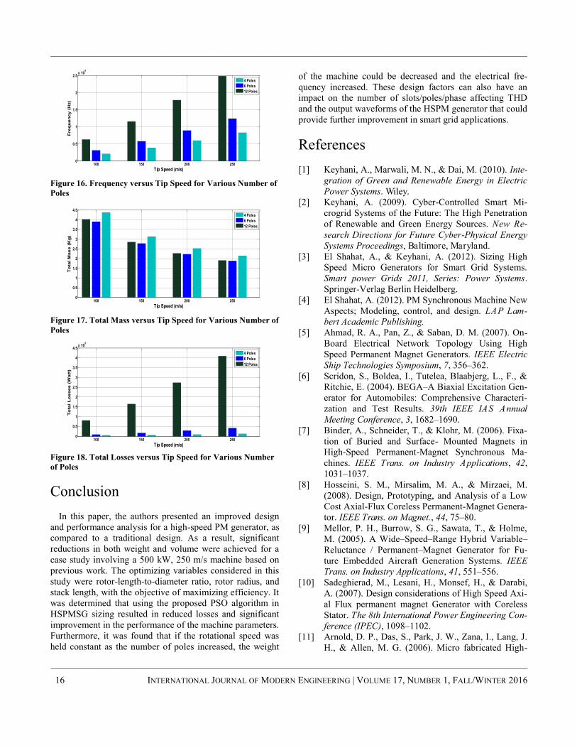
Effect of Number of Poles on Sizing
Parameters and M/C Characteristics
Consider the case of 50 kW of output power with differ-
ent tip speeds of 250, 200, 150, and 100 m/s for different
numbers of poles (4, 6, and 12). The results confirmed that
the number of poles affects the electrical, magnetic, and
structural performance, which have an impact on machine
frequency, voltage waveforms, magnetic flux, magnetic
volume, air gap, and the stator-back iron thickness. Figures
16-18 depict these various effects at 50 kW.
Figures 16-18 show that 1) rpm speed was constant at
each tip speed because the frequency changed with chang-
ing pole numbers; 2) frequency was directly proportional to
the number of poles at each tip speed; and, 3) magnet mass
increased with the number of poles for a specific tip speed
and total losses.
Table 2. Complete Optimized Design Parameters
Machine Size
Dmach = 0.1651 m D = 0. 0814 m ws = 0.0051 m dc = 0.0095 m wst = 0.0055 m wt = 0.0055 m
Lmach = 0.1729 m Lst = 0.1134 m laz = 0.0297 m le1 = 0.0297 m le2 = 0.0933 m wsb = 0.0046 m
Lac = 7.2023 m Aac = 1.2671e-5 m2 As = 5.0686e-5 m2 Rco = 0.0826 m Rci = 0.0731 m
Machine Ratings
Speed = 58,683 rpm Va = 756.8998 V Ea = 815.273 V Pin = 506.52 kW Ia = 220.1965 A
Ra = 0.0095 Ω Pair Gap = 1,378 Watt Xs = 0.2562 Ω eff = 0.992 pf = 0.99
Stator Parameters
Ls =1.3898e-2 mH Lslot = 3.1234e-3 mH Bb = 1.2232 mH Bt = 1.7124 mH λ = 0.0625 T
Rotor Parameters
kg = 1.1319 ge = 0.0024 m Bg = 0.8562 T Lag = 1.0805e-2 mH τs = 0.0106
Machine Losses
Pc = 2,672.9 Watt Pwind = 2,465.5 Watt Total Rotor Losses = 177.6 Watt Pcb = 1,394.9 Watt
Pct = 1,278 Watt THD = 11.6276% Ptlosses = 6,516.3 Watt
Time Harmonic Losses = 167.5 Watt Space Harmonic Losses = 10.2 Watt
Machine Weights
Mcb = 4.0548 kg Mct = 1.8204 kg Mcore = 5.8752 kg Mm = 2.2277 kg Mservice = 2.2622 kg
Mshaft = 4.5417 kg Mconductor = 2.4367 kg Mtot = 17.3436 kg
——————————————————————————————————————————————————–
HIGH-SPEED PERMANENT-MAGNET GENERATOR WITH OPTIMIZED SIZING BASED ON 15
PARTICLE SWARMS FOR SMART GRIDS
——————————————————————————————————————————————–————
——————————————————————————————————————————————–————
16 INTERNATIONAL JOURNAL OF MODERN ENGINEERING | VOLUME 17, NUMBER 1, FALL/WINTER 2016
Figure 16. Frequency versus Tip Speed for Various Number of
Poles
Figure 17. Total Mass versus Tip Speed for Various Number of
Poles
Figure 18. Total Losses versus Tip Speed for Various Number
of Poles
Conclusion
In this paper, the authors presented an improved design
and performance analysis for a high-speed PM generator, as
compared to a traditional design. As a result, significant
reductions in both weight and volume were achieved for a
case study involving a 500 kW, 250 m/s machine based on
previous work. The optimizing variables considered in this
study were rotor-length-to-diameter ratio, rotor radius, and
stack length, with the objective of maximizing efficiency. It
was determined that using the proposed PSO algorithm in
HSPMSG sizing resulted in reduced losses and significant
improvement in the performance of the machine parameters.
Furthermore, it was found that if the rotational speed was
held constant as the number of poles increased, the weight
of the machine could be decreased and the electrical fre-
quency increased. These design factors can also have an
impact on the number of slots/poles/phase affecting THD
and the output waveforms of the HSPM generator that could
provide further improvement in smart grid applications.
References
[1] Keyhani, A., Marwali, M. N., & Dai, M. (2010). Inte-
gration of Green and Renewable Energy in Electric
Power Systems. Wiley.
[2] Keyhani, A. (2009). Cyber-Controlled Smart Mi-
crogrid Systems of the Future: The High Penetration
of Renewable and Green Energy Sources. New Re-
search Directions for Future Cyber-Physical Energy
Systems Proceedings, Baltimore, Maryland.
[3] El Shahat, A., & Keyhani, A. (2012). Sizing High
Speed Micro Generators for Smart Grid Systems.
Smart power Grids 2011, Series: Power Systems.
Springer-Verlag Berlin Heidelberg.
[4] El Shahat, A. (2012). PM Synchronous Machine New
Aspects; Modeling, control, and design. LAP Lam-
bert Academic Publishing.
[5] Ahmad, R. A., Pan, Z., & Saban, D. M. (2007). On-
Board Electrical Network Topology Using High
Speed Permanent Magnet Generators. IEEE Electric
Ship Technologies Symposium, 7, 356–362.
[6] Scridon, S., Boldea, I., Tutelea, Blaabjerg, L., F., &
Ritchie, E. (2004). BEGA–A Biaxial Excitation Gen-
erator for Automobiles: Comprehensive Characteri-
zation and Test Results. 39th IEEE IAS Annual
Meeting Conference, 3, 1682–1690.
[7] Binder, A., Schneider, T., & Klohr, M. (2006). Fixa-
tion of Buried and Surface- Mounted Magnets in
High-Speed Permanent-Magnet Synchronous Ma-
chines. IEEE Trans. on Industry Applications, 42,
1031–1037.
[8] Hosseini, S. M., Mirsalim, M. A., & Mirzaei, M.
(2008). Design, Prototyping, and Analysis of a Low
Cost Axial-Flux Coreless Permanent-Magnet Genera-
tor. IEEE Trans. on Magnet., 44, 75–80.
[9] Mellor, P. H., Burrow, S. G., Sawata, T., & Holme,
M. (2005). A Wide–Speed–Range Hybrid Variable–
Reluctance / Permanent–Magnet Generator for Fu-
ture Embedded Aircraft Generation Systems. IEEE
Trans. on Industry Applications, 41, 551–556.
[10] Sadeghierad, M., Lesani, H., Monsef, H., & Darabi,
A. (2007). Design considerations of High Speed Axi-
al Flux permanent magnet Generator with Coreless
Stator. The 8th International Power Engineering Con-
ference (IPEC), 1098–1102.
[11] Arnold, D. P., Das, S., Park, J. W., Zana, I., Lang, J.
H., & Allen, M. G. (2006). Micro fabricated High-
100 150 200 2500
0.5
1
1.5
2
2.5
3
3.5
4
4.5
Tip Speed (m/s)
To
tal M
ass (
Kg
)
4 Poles
6 Poles
12 Poles
100 150 200 2500
0.5
1
1.5
2
2.5
3
3.5
4
4.5x 10
4
Tip Speed (m/s)
To
tal L
osses (
Watt
)
4 Poles
6 Poles
12 Poles
100 150 200 2500
0.5
1
1.5
2
2.5x 10
4
Tip Speed (m/s)
Freq
uen
cy (
Hz)
4 Poles
6 Poles
12 Poles

——————————————————————————————————————————————–————
Speed Axial-Flux Multi watt Permanent- Magnet
Generators—Part II: Design, Fabrication, and Test-
ing. Journal of Micro Electromechanical Systems, 5,
1351–1363.
[12] Binder, A., Schneider, T., & Klohr, M. (2006). Fixa-
tion of Buried and Surface-Mounted Magnets in High
-Speed Permanent - Magnet Synchronous Machines.
IEEE Trans. on Industry Applications, 42, 1031–
1037.
[13] Paulides, J. J. H., Jewell, G., Howe, W. (2004). An
Evaluation of Alternative Stator Lamination Materi-
als for a High – Speed, 1.5 MW, Permanent Magnet
Generator. IEEE Trans. on Magnetics, 40, 2041-
2043.
[14] El–Hasan, T. S., Luk, P. C. K., Bhinder, F. S., &
Ebaid, M. S. (2000). Modular Design of High–Speed
Permanent–Magnet Axial–Flux Generators. IEEE
Trans. on Magnetics, 36, 3558–3561
[15] Jang, S. M., Cho, H. W., & Jeong, Y. H. (2006). In-
fluence on the rectifiers of rotor losses in high–speed
permanent magnet synchronous alternator. Journal of
Applied Physics, American Institute of Physics,
08R315-3.
[16] Hwang, C. C., Tien, C. L., & Chang, H. C. (2007).
Performance and applications of a small PM genera-
tor. phys. stat. sol., 4, 4635–4638.
[17] Kolondzovski, Z. (2008). Determination of critical
thermal operations for High–speed permanent mag-
net electrical machines. The International Journal for
Computation and Mathematics in Electrical and
Electronic Engineering, 27, 720-727.
[18] Sahin, F., & Vandenput, A. J. A. (2003). Thermal
modeling and testing of a High–speed axial–flux per-
manent–magnet machine. The International Journal
for Computation and Mathematics in Electrical and
Electronic Eng., 22, 982–997.
[19] Vandenput, A. J. A., & Sahin, F. (2008). Design con-
siderations of the flywheel-mounted axial-flux per-
manent-magnet machine for a hybrid electric vehicle.
8th European Conference on Power Electronics and
Applications.
[20] Nagorny, A. S., Dravid, N. V., Dravid, R. H., & Ken-
ny, B. H. (2005). Design Aspects of a High Speed
Permanent Magnet Synchronous Motor/Generator for
Flywheel Applications. International Electric Ma-
chines and Drives Conference, San Antonio, Texas.
[21] Caricchi, F., Crescimbini, F., Mezzetti, F., & Santini,
E., (1996). Multistage axial flux PM machine for
wheel direct drive. IEEE Trans. on Industry Applica-
tions, 32, 882-887.
[22] Binns K. J., & Shimmin, D. W. (1996). Relationship
between rated torque and size of permanent magnet
machines. IEE Proc. Electr. Power Appl., 143, 417-
422.
[23] Fengxiang, W., Wenpeng, Z., Ming, Z., & Baoguo,
W. (2002). Design considerations of high speed PM
generators for micro turbines. IEEE trans. energy
conversion.
[24] Pavlik, D., Garg, V., Repp, J., & Weiss, J. (1988). A
finite element technique for calculating the magnet
sizes and inductances of permanent magnet ma-
chines. IEEE trans. of energy conversion, 3.
[25] Hanselmann, D. C. (1994). Brushless Permanent
Magnet Motor Design. New York: McGraw-Hill.
[26] Kang, D., Curiac, P., Jung, Y., & Jung, S. (2003).
Prospects for magnetization of large PM rotors: con-
clusions from a development case study. IEEE trans.
on Energy Conversion, 18(3).
[27] Website for Magnetic Component Engineering. Inc.,
2004.
[28] Polinder, H., & Hoeijmakers, M. J. (1999). Eddy –
Current Losses in the Segmented Surface Mounted
Magnets of a PM Machine. IEE Proceedings, Electri-
cal Power Applications, 146(3).
[29] Rippy, M. (2004). An overview guide for the selec-
tion of lamination materials. Porto Laminations, Inc.
[30] Bianchi, N., & Lorenzoni, A. (1996). Permanent
magnet generators for wind power industry: an over-
all comparison with traditional generators. Opportu-
nities and advances in international power genera-
tion conference, 419.
[31] Hendershot J. R., & Miller, T. J. E. (1994). Design of
Brushless Permanent Magnet Motors. Oxford, U.K.:
Magna Physics Publishing and Clarendon Press.
[32] Rahman, M. A., & Slemon, G. R. (1985). Promising
Applications of Neodymium Iron Boron Iron Mag-
nets in Electrical Machines. IEEE Trans. On Magnet-
ics, 5.
[33] Hanselmann, D. C. (1994). Brushless Permanent
Magnet Motor Design. New York: McGraw-Hill.
[34] Hendershot J. R., & Miller, T. J. E. (1994). Design of
Brushless Permanent Magnet Motors. Oxford, U.K.:
Magna Physics Publishing and Clarendon Press.
[35] Rucker, J. E., Kirtley, J. L., & McCoy, Jr. T. J.
(2005). Design and Analysis of a Permanent Magnet
Generator for Naval Applications. IEEE Electric Ship
Technologies Symposium, 451–458.
[36] Pepi, J., & Mongeau, P. (2004). High power density
permanent magnet generators. DRS Electric power
technologies, Inc.
[37] Kennedy, J., & Eberhart, R. (1995). Particle swarm
optimization. Proc. IEEE International Conf. on Neu-
ral Networks, Perth, Australia.
[38] Clerc, M. (2004). Discrete Particle Swarm Optimiza-
tion. New Optimization Techniques in Engineering
Springer-Verlag.
——————————————————————————————————————————————————–
HIGH-SPEED PERMANENT-MAGNET GENERATOR WITH OPTIMIZED SIZING BASED ON 17
PARTICLE SWARMS FOR SMART GRIDS

——————————————————————————————————————————————–————
——————————————————————————————————————————————–————
18 INTERNATIONAL JOURNAL OF MODERN ENGINEERING | VOLUME 17, NUMBER 1, FALL/WINTER 2016
[39] Yasuda, K., Ide, A., & Iwasaki, N. (2003). Adaptive
particle swarm optimization. Proceedings of IEEE
International Conference on Systems, Man and Cy-
bernetics, 1554-1559.
Biographies
ADEL EL SHAHAT is an assistant professor of Elec-
trical Engineering in the Department of Electrical Engineer-
ing at Georgia Southern University. He received his BSc
degree and MSc degree (Power and Machines) in Electrical
Engineering from Zagazig University, Egypt, in 1999 and
2004, respectively. He received his PhD (Joint Supervision)
from Zagazig University, Egypt, and The Ohio State Uni-
versity in 2011. His research focuses on various aspects of
power systems, smart grid systems, power electronics, elec-
tric machines, renewable energy systems, energy storage,
and engineering education. Dr. El Shahat may be reached at
RAMI J. HADDAD is an assistant professor in the
Department of Electrical Engineering at Georgia Southern
University. He received his BS degree in Electronics and
Telecommunication Engineering from the Applied Sciences
University, Jordan; his MS degree in Electrical and Com-
puter Engineering from the University of Minnesota; and
his PhD from the University of Akron. He is an IEEE senior
member. His research focuses on various aspects of optical
fiber communication/networks, broadband networks, multi-
media communications, multimedia bandwidth forecasting,
and engineering education. Dr. Haddad may be reached at
YOUAKIM KALAANI is an associate professor and
Chair of the Electrical Engineering Department at Georgia
Southern University. Dr. Kalaani received his BS degree in
Electrical Engineering from Cleveland State University. He
graduated from CSU with masters and doctoral degrees in
Electrical Engineering with a concentration in power sys-
tems. Dr. Kalaani is a licensed professional engineer (PE)
and served as ABET Program Evaluator. He is a senior
member of IEEE and has research interests in distributed
power generation, optimization, and engineering education.
Dr. Kalaani may be reached at yalka-

Abstract
Orthogonal frequency-division multiplexing (OFDM) is
an attractive modulation technique for mitigating effects of
delay spread in a multipath channel. However, the main
disadvantage of OFDM is that it has a large peak-to-average
power ratio (PAPR). One technique for PAPR reduction is
Scheme I, introduced by Jones et al. [1], which is a block
coding scheme using an odd parity check bit and mapping a
3-bit data word onto a 4-bit code word. One disadvantage of
Scheme I is that it can only reduce PAPR when the length
of the code word is an integer multiple of four. Another
technique is Scheme II, introduced by Fragiacomo et al. [2],
for longer code words. In Scheme II, where M and N are
defined as the length of a code word and the length of a data
word, respectively, one additional bit representative of the
complement of the (N-1)th bit of the data word is upended
as the (N+1)th bit of the data word such that M becomes
N+1. Effectively, PAPR can be reduced even though M is
not an integer multiple of four, allowing for a less-limiting
selection of M. However, gains in PAPR reduction are mar-
ginal as M increases. In this paper, the author proposes a
new approach called Scheme III to obtain more PAPR re-
duction, by adding two additional bits to Scheme I. Accord-
ingly, M becomes N+2 rather than N+1, as in Scheme II.
Scheme III is suited for large numbers of sub-carriers at the
expense of two additional bits.
Introduction
A multi-carrier transmission scheme such as orthogonal
frequency-division multiplexing (OFDM) has been pro-
posed for many wireless applications because it is an attrac-
tive modulation technique for mitigating effects of delay
spread in a multi-path channel. However, the main disad-
vantage of OFDM is that it has a large peak-to-average
power ratio (PAPR), which can result in significant distor-
tion when OFDM signals are passed through a nonlinear
device such as a transmitter power amplifier. OFDM can be
combined with multiple-input multiple-output (MIMO)
technology (e.g., multiple antennas at the transmitter and
receiver) to increase the diversity gain to enhance the capac-
ity of the system. Such a MIMO-OFDM system is a key
technology for next generation mobile communications as
well as wireless local area network (WLAN) [3-5]. The
large PAPR problem in OFDM carries over to a MIMO-
OFDM system because it is based on OFDM.
A number of approaches have been proposed to reduce
PAPR for multi-carrier transmission. In general, the PAPR
reduction techniques can be classified into the following
categories: clipping and filtering, coding, selective mapping,
partial transmit sequence, nonlinear companding transforms,
tone reservation, tone injection, and scrambling [6-11]. In
this study, however, the focus was on the coding technique
category.
Block Coding Scheme with an Odd Parity
Check Bit (Scheme I)
The complex envelope of the transmitted OFDM signal
can be written as shown in Equation (1):
(1)
where, dn,m is the data symbol for the m-th sub-carrier of the
n-th OFDM symbol; M is the number of sub-carriers (or
length of the code word); fm is the m-th sub-carrier; T is an
OFDM symbol duration; and, g(t) is a rectangular pulse
shape of duration T.
With no loss in generality, index n can be omitted for
simplicity. Then Equation (1) can be simply expressed as
Equation (2):
(2)
Let p(t) be the envelope power of the OFDM signal. Since
s(t) is a complex number, p(t) is s(t)s*(t), where * denotes a
conjugate of a complex number. If the power in each sub-
carrier is normalized to 1 watt, then the average power is
M watts. The PAPR Γ (in dB) is defined in Equation (3).
First, the uncoded data words will be discussed. Subse-
quently, how the block coding scheme using an odd parity
check bit works for four sub-carriers (M = 4) will be ex-
plained. Table 1 shows the peak envelope powers for all
A SIMPLE BLOCK CODING SCHEME FOR
PEAK-TO-AVERAGE POWER RATIO REDUCTION
IN MULTI-CARRIER SYSTEMS ——————————————————————————————————————————————–———–
Yoonill Lee, Purdue University Northwest
——————————————————————————————————————————————————–
A SIMPLE BLOCK CODING SCHEME FOR PEAK-TO-AVERAGE POWER RATIO REDUCTION IN MULTI-CARRIER SYSTEMS 19
)()(2
,
1
0
nTtgedtstfj
mn
M
mn
m
tfj
m
M
m
medts2
1
0
)(

——————————————————————————————————————————————–————
——————————————————————————————————————————————–————
20 INTERNATIONAL JOURNAL OF MODERN ENGINEERING | VOLUME 17, NUMBER 1, FALL/WINTER 2016
possible uncoded data words. Let us define PEP as the peak
envelope power of p(t). The first PEP was 16.00 watts when
the data words were 0000, 0101, 1010, and 1111. The sec-
ond PEP was 9.44 watts when the data words were 0011,
0110, 1001, and 1100. All other PEPs were the same values
of 7.07 watts. Thus, if data words that generate large PEPs
such as 16.00 watts and 9.44 watts can be removed, the
PAPR can be reduced. This is the main motivation behind
block coding.
(3)
Table 1. PEP for All Possible Uncoded Data Words (N = 4)
The block coding scheme using an odd parity check bit
was introduced by Jones et al. [1]. The basic idea is that a 3-
bit data word is mapped onto a 4-bit code word using an
odd parity check bit. The first three bits c1, c2, and c3 in the
code word are the same as d1, d2, and d3 in the data word.
However, the fourth bit, c4, in the code word is an odd pari-
ty check bit. For example, if a 3-bit data word is d1 = 0,
d2 = 1, and d3 = 0, then the 4-bit code word using an odd
parity check bit is c1 = 0, c2 = 1, c3 = 0, and c4 = 0. The peak
envelope powers for all possible code words using an odd
parity check bit are shown in Table 2. Table 2 shows that
the peak envelope powers have the same value, 7.07 watts,
because the first and second PEPs are removed.
Table 2. PEP for All Possible Code Words Using Scheme I
(M = 4)
Table 3 show the results of PAPR with different lengths
of the code word for uncoded data words and Scheme I for
comparison. Table 3 further shows that Scheme I works
well when the length of the code word was an integer multi-
ple of four. The PAPR value was 2.48 dB in the case of
M = 4. Thus, the amount of PAPR reduction (dBI) relative
to the uncoded data words was as much as 3.54 dB. Howev-
er, it has the same PAPR as the uncoded data words if the
length of the code word is not an integer multiple of four.
This is the main drawback of Scheme I. Block coding
Scheme II, explained in the next section, addresses how to
solve this problem.
Block Coding Scheme with One
Additional Bit (Scheme II)
As shown in the previous section, the disadvantage of
block coding using an odd parity check (Scheme I) is that it
M
tppeak
poweraverage
powerenvelopepeak
)(log10
log10
10
10
Data
Words d1 d2 d3 d4
PEP
(watt)
0 0 0 0 0 16.00
1 0 0 0 1 7.07
2 0 0 1 0 7.07
3 0 0 1 1 9.44
4 0 1 0 0 7.07
5 0 1 0 1 16.00
6 0 1 1 0 9.44
7 0 1 1 1 7.07
8 1 0 0 0 7.07
9 1 0 0 1 9.44
10 1 0 1 0 16.00
11 1 0 1 1 7.07
12 1 1 0 0 9.44
13 1 1 0 1 7.07
14 1 1 1 0 7.07
15 1 1 1 1 16.00
Code
Words c1 c2 c3 c4
PEP
(watt)
0 0 0 0 1 7.07
1 0 0 0 1 7.07
2 0 0 1 0 7.07
3 0 0 1 0 7.07
4 0 1 0 0 7.07
5 0 1 0 0 7.07
6 0 1 1 1 7.07
7 0 1 1 1 7.07
8 1 0 0 0 7.07
9 1 0 0 0 7.07
10 1 0 1 1 7.07
11 1 0 1 1 7.07
12 1 1 0 1 7.07
13 1 1 0 1 7.07
14 1 1 1 0 7.07
15 1 1 1 0 7.07

——————————————————————————————————————————————–————
can only reduce PAPR when the length of the code word is
an integer multiple of four. To be specific, it has the small-
est PAPR value with M = 4. When the length of the code
word is not an integer multiple of four, it does not eliminate
the code word that generate large powers.
Table 3. PAPR (in dB) Comparisons for Uncoded Data Words
and Scheme I
Another approach was introduced by Fragiacomo et al.
[2] for longer code words. Let M and N be defined as the
length of a code word and the length of a data word, respec-
tively. Instead of using an odd parity check bit, one addi-
tional bit, representative of the complement of the (N-1)th
bit of the data word, is upended as the (N+1)th bit of the
data word such that M becomes N+1. Table 4 show the PEP
for all possible code words using one additional bit with
M = 5. The first PEP was 13.33 watts and the second PEP
was 13.00 watts.
Table 5 shows the PAPR for different lengths of code
words for uncoded data words using Scheme II for compari-
son. The PAPR values were reduced even though the length
of the code word was not an integer multiple of four. Thus,
Scheme II has a more general way to select the length of the
code word compared to Scheme I. However, the amount of
PAPR reduction (dBII) does not improve much when the
length of the code word increases. To obtain better PAPR
reduction for large code words, a new approach is proposed
by adding two additional bits to Scheme I.
Table 4. PEP for All Possible Code Words Using Scheme II
(M = 5)
Table 5. PAPR (in dB) Comparisons for Uncoded Data Words
and Scheme II
Length of Code
Words (M) Uncoded Scheme I DdBI
4 6.02 2.48 3.54
5 6.99 6.99 0
6 7.78 7.78 0
7 8.45 8.45 0
8 9.03 6.53 2.50
9 9.54 9.54 0
10 10.00 10.00 0
11 10.41 10.41 0
12 10.79 9.21 1.58
13 11.14 11.14 0
14 11.46 11.46 0
15 11.76 11.76 0
16 12.04 10.88 1.16
Code
Words c1 c2 c3 c4 c5
PEP
(watt)
0 0 0 0 0 1 10.51
1 0 0 0 1 1 13.33
2 0 0 1 0 0 10.48
3 0 0 1 1 0 13.00
4 0 1 0 0 1 13.33
5 0 1 0 1 1 10.51
6 0 1 1 0 0 13.00
7 0 1 1 1 0 10.48
8 1 0 0 0 1 10.48
9 1 0 0 1 1 13.00
10 1 0 1 0 0 10.51
11 1 0 1 1 0 13.33
12 1 1 0 0 1 13.00
13 1 1 0 1 1 10.48
14 1 1 1 0 0 13.33
15 1 1 1 1 0 10.51
Length of Code
Words (M) Uncoded Scheme II DdBII
4 6.02 3.73 2.29
5 6.99 4.26 2.73
6 7.78 5.09 2.69
7 8.45 5.58 2.87
8 9.03 6.53 2.50
9 9.54 7.36 2.18
10 10.00 8.06 1.94
11 10.41 8.67 1.74
12 10.79 9.21 1.58
13 11.14 9.69 1.45
14 11.46 10.12 1.34
15 11.76 10.52 1.24
16 12.04 10.88 1.16
——————————————————————————————————————————————————–
A SIMPLE BLOCK CODING SCHEME FOR PEAK-TO-AVERAGE POWER RATIO REDUCTION IN MULTI-CARRIER SYSTEMS 21

——————————————————————————————————————————————–————
——————————————————————————————————————————————–————
22 INTERNATIONAL JOURNAL OF MODERN ENGINEERING | VOLUME 17, NUMBER 1, FALL/WINTER 2016
Proposed Coding Scheme Adding Two
Additional Bits to Scheme I (Scheme III)
The proposed block coding algorithm is as follows:
Step 1: Apply Scheme I to the data words.
Step 2: Upend the complement of the (N-1)th bit of the
code word as the (N+1)th bit of the code word.
Step 3: Upend the complement of the odd parity check bit
as the (N+2)th bit of the code word.
Accordingly, M becomes N+2 rather than N+1, as in
Scheme II. Table 6 shows the peak envelope power with M
= 6 for the proposed Scheme III. The first PEP was 16.98
watts and the second PEP was 13.29 watts. Although these
values are larger than those in Scheme I and II, the PAPR
values are smaller compared to the two previous schemes.
Moreover, the amount of PAPR reduction (dBIII) is much
larger than the two previous schemes, when the length of
the code word increases. Thus, Scheme III is suited for large
numbers of sub-carriers at the expense of two additional
bits. Table 7 shows a comparison for all schemes with dif-
ferent lengths of code words.
Table 6. PEP for All Possible Code Words Using Scheme III
(M = 6)
Simulation Results
Figures 1 and 2 show the envelope powers for uncoded
data words and under Scheme I, respectively. Figures 3 and
4 show the PAPR values for uncoded data words and under
Scheme II, respectively. Similarly, Figures 5 and 6 show the
PAPR values for uncoded data words and under Scheme III,
respectively. Finally, Figures 7 and 8 show the PAPR com-
parison and reduction for all of the schemes, respectively.
As can be seen, the proposed Scheme III shows improved
performance compared to those of the two previous
schemes, when the length of the code word increases.
Figure 1. Envelope Power for Uncoded Data Words (N = 4)
Figure 2. Envelope Power Using Scheme I (M = 4)
Code
Words c1 c2 c3 c4 c5 c6
PEP
(watt)
0 0 0 0 1 1 0 13.29
1 0 0 0 1 1 0 13.29
2 0 0 1 0 0 1 16.98
3 0 0 1 0 0 1 16.98
4 0 1 0 0 1 1 13.29
5 0 1 0 0 1 1 13.29
6 0 1 1 1 0 0 16.98
7 0 1 1 1 0 0 16.98
8 1 0 0 0 1 1 16.98
9 1 0 0 0 1 1 16.98
10 1 0 1 1 0 0 13.29
11 1 0 1 1 0 0 13.29
12 1 1 0 1 1 0 16.98
13 1 1 0 1 1 0 16.98
14 1 1 1 0 0 1 13.29
15 1 1 1 0 0 1 13.29

——————————————————————————————————————————————–————
Figure 3. PAPR (in dB) for Uncoded Data Words (N = 5)
Figure 4. PAPR (in dB) Using Scheme II (M = 5)
Figure 5. PAPR (in dB) for Uncoded Data Words (N = 6)
Figure 6. PAPR (in dB) Using Scheme III (M = 6)
Table 7. PAPR (in dB) Comparisons for All Schemes
Length of Code Words (M)
Uncoded Scheme I DdBI Scheme II DdBII Scheme III DdBIII
4 6.02 2.48 3.54 3.73 2.29 3.73 2.29
5 6.99 6.99 0 4.26 2.73 4.26 2.73
6 7.78 7.78 0 5.09 2.69 4.52 3.26
7 8.45 8.45 0 5.58 2.87 5.58 2.87
8 9.03 6.53 2.50 6.53 2.50 6.02 3.01
9 9.54 9.54 0 7.36 2.18 6.59 2.95
10 10.00 10.00 0 8.06 1.94 6.64 3.36
11 10.41 10.41 0 8.67 1.74 7.44 2.97
12 10.79 9.21 1.58 9.21 1.58 7.78 3.01
13 11.14 11.14 0 9.69 1.45 8.15 2.99
14 11.46 11.46 0 10.12 1.34 8.54 2.92
15 11.76 11.76 0 10.52 1.24 9.07 2.69
16 12.04 10.88 1.16 10.88 1.16 9.54 2.50
——————————————————————————————————————————————————–
A SIMPLE BLOCK CODING SCHEME FOR PEAK-TO-AVERAGE POWER RATIO REDUCTION IN MULTI-CARRIER SYSTEMS 23

——————————————————————————————————————————————–————
——————————————————————————————————————————————–————
24 INTERNATIONAL JOURNAL OF MODERN ENGINEERING | VOLUME 17, NUMBER 1, FALL/WINTER 2016
Figure 7. PAPR (in dB) Comparison for All Schemes
Figure 8. PAPR Reduction (in dB) for All Schemes
Conclusion
As a PAPR reduction scheme, a new block coding
scheme, referred to as Scheme III, was created by adding
two additional bits to Scheme I. Scheme I only reduces
PAPR when the length of the code word is an integer multi-
ple of four. This is the main drawback of Scheme I. Scheme
II reduces PAPR even though the length of the code word is
not an integer multiple of four. However, the PAPR reduc-
tion gains are marginal when the length of the code word
increases. Scheme III shows improved performance com-
pared to those of the two previous schemes, when the length
of the code word increases. For example, the amount of
PAPR reduction with M = 8 for Scheme I, Scheme II, and
Scheme III are 2.50 dB, 2.50 dB, and 3.01 dB, respectively.
For M = 16, they are 1.16 dB, 1.16 dB, and 2.50 dB, respec-
tively. As a result, Scheme III is suited to large numbers of
sub-carriers, though at the expense of two additional bits.
References
[1] Jones, A. E., Wilkinson, T. A., & Barton, S. K.
(1994). Block Coding Scheme for Reduction of Peak
to Mean Envelope Power Ratio of Multi-Carrier
Transmission Schemes. Electronics Letters, 2098-
2099.
[2] Fragiacomo, S., Matrakidis, C., & O’Reilly, J. J.
(1998). Multi-Carrier Transmission Peak to Average
Power Reduction Using Simple Block Code. Elec-
tronics Letters, 953-954.
[3] Stuber, G. L., Barry, J. R., Mclaughlin, S. W., Li, Y.,
Ingram, M. A., & Pratt, T. G. (2004). Broadband
MIMO-OFDM Wireless Communications. Proceed-
ings of the IEEE, 92(2), 271-294.
[4] Iqbal, Z., Nooshabadi, S., & Lee, H. N. (2012). Anal-
ysis and Design of Coding and Interleaving in a
MIMO-OFDM Communication System. IEEE Trans-
actions on Consumer Electronics, 58(3), 758-766.
[5] Cho, Y. S., Kim, J. W., Yang, W. Y., & Kang, C. G.
(2013). MIMO-OFDM Wireless Communications
with MATLAB. John Wiley & Sons (Asia) Pte Ltd.
[6] Han, S. H., & Lee, J. H. (2005). An Overview of
Peak-to-Average-Power Ratio Reduction Techniques
for Multicarrier Transmission. IEEE Wireless Com-
munications, 12(2), 56-65.
[7] Jiang, T., & Wu, Y. (2008). An Overview: Peak-to-
Average Power Ratio Reduction Techniques for
OFDM Signals. IEEE Transactions on broadcasting,
54(2), 257-268.
[8] Nee, R. V. (1996). OFDM Codes for Peak-to-
Average-Power Reduction and Error Correction.
IEEE GLOBECOM, 740-744.
[9] Tellambura, C. (1997). Use of M-Sequences for
OFDM Peak-to-Average-Power Ratio Reduction.
Electronics Letters, 1300-1301.
[10] Davis, J. A., & Jedwab, J. (1999). Peak to Mean
Power Control in OFDM, Golay Complementary
Sequences, and Reed-Muller Codes. IEEE Transac-
tions Information Theory, 45(7), 2397-2417.
[11] Zhang, Y., Yongacoglu, A., Chouinard, J. Y., &
Zhang, L. (1999). OFDM Peak Power Reduction by
Sub-Block Coding and Its Extended Versions. IEEE
Vehicular Technology Conference, 695-699.

——————————————————————————————————————————————–————
Biography
YOONILL LEE is cur rently an assistant professor of
Electrical Engineering Technology at Purdue University
Northwest. He earned his BS and MS degrees in Electrical
Engineering from Yonsei University in Seoul, South Korea,
in 1984, 1986, respectively; MS in Electrical Engineering
from Oklahoma State University in 1992; and, PhD in Elec-
trical Engineering from the University of South Florida in
2001. He also worked at Cisco Systems as a communica-
tions engineer. His research interests include CDMA, multi-
carrier systems, and MIMO technology. Dr. Lee may be
reached at [email protected]
——————————————————————————————————————————————————–
A SIMPLE BLOCK CODING SCHEME FOR PEAK-TO-AVERAGE POWER RATIO REDUCTION IN MULTI-CARRIER SYSTEMS 25

Abstract
As part of an ongoing collaborative project with local
industry, an advanced lead-acid battery energy storage sys-
tem was designed and installed into an existing 24 VDC
microgrid power system. A small rooftop solar array was
used to provide energy for the lighting load in a laboratory
and classroom space. A building grid-powered AC-DC
power supply provided supplemental energy when the solar
array could not meet the demand of the load. The energy
was distributed throughout the space to the load via a two-
conductor microgrid network embedded in the ceiling tile
support framework. This ceiling grid energy distribution
technology is available as a commercial product and was
installed as part of an earlier collaboration with the manu-
facturer. In this latest phase of the project, advanced lead-
acid batteries were added to the system to store surplus solar
energy for later use. A PLC-based control system provided
supervisory monitoring and control of the charging and dis-
charging of the batteries. The installed energy storage sys-
tem served as a testbed for similar projects under develop-
ment by the industry partner. In this paper, the authors pro-
vide a brief overview of the 24 VDC microgrid system. The
battery energy storage system motivation, design goals, and
tradeoffs are also described. System hardware and software
are presented and discussed. A simple system model devel-
oped to predict performance is also presented. Preliminary
energy storage system performance data is discussed. Ongo-
ing system improvements and lessons learned are also pre-
sented.
Introduction
An emerging technology in building power distribution
involved the use of a room ceiling tile support grid to create
a low-voltage microgrid network. With this network,
24 VDC power was routed throughout the room via conduc-
tors embedded in the drop-ceiling support structure. Users
could then tap into the low-voltage supply from any location
in the room. The microgrid effort was organized by a con-
sortium of industry and university partners called the
Emerge Alliance [1]. The Emerge Alliance promotes the use
of low-voltage DC indoor power distribution for a variety of
commercial, industrial, and residential applications. An ex-
ample of applications on the load side includes lighting and
ventilation devices. Input power for the microgrid can be
derived from many sources including standard building AC
power and alternative sources such as solar. A 24 VDC ceil-
ing system was installed in one room of the engineering
building at Penn State Berks. The room serves as both la-
boratory and classroom space. Students in the engineering
technology programs have been involved with designing
and fabricating devices to use and/or control power derived
from the 24 VDC microgrid system. Devices include room
lighting control and portable device charging stations. The
low-voltage microgrid provides a relatively safe environ-
ment in which to experiment with new devices for occupied
space environmental control [2].
The 24 VDC microgrid receives its energy from multiple
sources. During periods of sunshine, the microgrid load
energy is supplied primarily by a rooftop-mounted solar
array. The system also contains an AC-DC power supply to
maintain the 24 VDC bus voltage regulation during times
when no other sources are available. The utility of the
24 VDC microgrid was further enhanced by incorporating
battery energy storage into the system. Figure 1 shows a
simplified system diagram.
Figure 1. Simplified 24 VDC Microgrid System Diagram
Due to the intermittent occupancy of the room during
daylight hours, there is significant opportunity to store oth-
erwise unused energy collected by the solar array. The
stored energy can then be used by the microgrid to supply
the room load as needed. Together with industry partner
Ecoult, an advanced lead-acid battery technology, UltraBat-
tery®, energy storage system was developed and installed
BATTERY ENERGY STORAGE FOR A
LOW-VOLTAGE DC MICROGRID SYSTEM ——————————————————————————————————————————————–————
Dale H. Litwhiler, Penn State University; Nicholas Batt, Ecoult Energy Storage Solutions;
Jason Hoffman, Ecoult Energy Storage Solutions
——————————————————————————————————————————————–————
26 INTERNATIONAL JOURNAL OF MODERN ENGINEERING | VOLUME 17, NUMBER 1, FALL/WINTER 2016

——————————————————————————————————————————————–————
Figure 2. UltraBattery Construction Diagram
Figure 3 shows that each of the four batteries in the ener-
gy storage system was equipped with battery-monitoring
electronics mounted directly on the positive and negative
terminals. The monitoring hardware and software continu-
ously measured key parameters of voltage, current, and cell
temperature and could also be configured to monitor ambi-
ent temperature and gas concentrations for enhanced safety
and performance.
Figure 3. Battery Monitor Mounted on an UltraBattery
Figure 4 shows the batteries housed in an industrial bat-
tery cabinet. Each battery monitor was connected to the
main monitoring and control electronics via infrared link to
provide galvanic isolation and eliminate grounding issues.
Remote monitoring and control of the entire battery system
was accomplished with a web-enabled PC contained within
the battery cabinet control compartment. This arrangement
also provided a means for remote software updates and sys-
tem troubleshooting. For the system installed on campus, a
wired LAN connection is used, however, a cellular connec-
tion was used for previous similar systems installed in re-
mote locations.
as part of the 24 VDC microgrid. The UltraBattery® oper-
ates very efficiently in continuous Partial State of Charge
(PSoC) use without frequent overcharge maintenance cy-
cles. It can be utilized to continually manage energy inter-
mittencies, smooth power, and shift energy, using a band of
charge that is neither totally full nor totally empty [3]. The
UltraBattery was developed by the CSIRO in Australia and
taken to market by Ecoult [4]. The installed system is very
similar to that already commissioned in Australia to power
remotely located cellular telephone tower equipment [5].
Figure 1 shows how energy from the solar array (five
Canadian Solar 235W panels) is processed by the maximum
power point tracker (MPPT) unit (MidNite Solar Classic
250). The DC-DC converter (Vicor MegaPAC, 1600 watts)
provides a regulated 24.5 VDC output voltage, while the
battery voltage varies depending on its State of Charge
(SoC). The control algorithm of the battery controller pro-
vides control signals to the MPPT and DC-DC converter,
based on the SoC of the battery. When the battery SoC is in
the range where it could accept charge, the MPPT is ena-
bled. Likewise, when the SoC of the battery is in a suitable
range for providing energy (discharging), the DC-DC con-
verter is enabled. When the DC-DC converter is enabled, its
24.5 VDC output voltage overrides the 24 VDC produced
by the AC-DC converter in the Power Server Module. Thus,
no energy is drawn from the AC line to supply the bus
loads, it is all provided by the battery via the DC-DC con-
verter.
Battery Selection and Sizing
The intermittent nature of solar energy and the sporadic
demand profile of the room lighting load align well with the
performance capability of the UltraBattery. As shown in
Figure 2, the UltraBattery’s construction incorporates a tra-
ditional lead-acid battery in parallel with a supercapacitor
structure. This combination produces an energy storage
package that performs very well under partial state-of-
charge conditions, as are typically experienced in this type
of application. The laboratory/classroom space is lit by ceil-
ing fluorescent lighting fixtures. These fixtures were
equipped with electronic dimming ballasts designed for
24 VDC input voltage. The ballasts receive their input volt-
age from the microgrid with a total power of about 850W at
full brightness. The initial design used this load power and a
goal of providing enough energy to sustain this load for two
hours (the typical duration of an evening laboratory class
session). Therefore, the battery was sized at a nominal ener-
gy rating of 2 kWh. The battery arrangement was then four,
12V battery units configured as two parallel strings of two
batteries each.
——————————————————————————————————————————————————–
BATTERY ENERGY STORAGE FOR A LOW-VOLTAGE DC MICROGRID SYSTEM 27

——————————————————————————————————————————————–————
——————————————————————————————————————————————–————
28 INTERNATIONAL JOURNAL OF MODERN ENGINEERING | VOLUME 17, NUMBER 1, FALL/WINTER 2016
Figure 4. Battery Cabinet and Control/Monitoring Electronics
Enclosure
Control System Architecture
The battery controller was implemented using a Program-
mable Logic Controller (PLC). The primary function of the
PLC is to monitor the batteries and protect them from over-
charging or over-discharging. This function is accomplished
by controlling the MPPT (the battery charging component)
and the DC-DC converter (the battery discharging compo-
nent). A simple discrete enable/disable signal is sent from
the PLC to the MPPT and the DC-DC converter based on
the current SoC of the battery. A diagram of these control
signals is shown in Figure 5. A small bit of hysteresis was
added to each signal to minimize excessive system cycling
near the extremes of the SoC.
System Modeling
To get a first-order estimate of expected system perfor-
mance, a simple discretized system model was developed to
describe the battery state-of-charge for various solar array
power and DC bus load power profiles. Equation (1) shows
a simplified linear model (constant) for the battery SoC that
was used:
Figure 5. Battery Charge and Discharge Enable Signal
Hysteresis Curves
(1)
A discrete time step of one minute was used for the simu-
lation. The change in stored energy during each time step
can be calculated using Equation (2), a Coulomb-counting
method [6]:
ΔE = [(PSolar)(EffMPPT) – (PLoad)/EffDC-DC]/60 Wh (2)
where, PSolar is the output power of the solar array; EffMPPT
is the input-output efficiency of the MPPT unit; PLoad is the
power consumed by the room lighting load; and, EffDC-DC is
the input-output efficiency of the DC-DC converter.
The model was implemented in Matlab. Table 1 shows
the generic pseudocode.
Table 1. Listing of System Model Pseudocode
Max MinSoC
SoC SoCK % / Wh
Wh capacity
Loop{
ΔE = ((PSolar)*(EffMPPT) – (PLoad)/(EffDC-DC))/60
if ((ΔE > 0 AND OK2Chrg = True) OR (ΔE < 0 AND
OK2Dischrg = True))
SoC = SoC + KSoC *(ΔE)
if ((SoC < Max AND OK2Chrg = True) OR (SoC < (Max –
Hyst))
OK2Chrg = True
else
OK2Chrg = False
if ((SoC > Min AND OK2Dischrg = True) OR (SoC > Min +
Hyst))
OK2Dischrg = True
VBus = 24.5
else
OK2Dischrg = False
VBus = 24.0
}
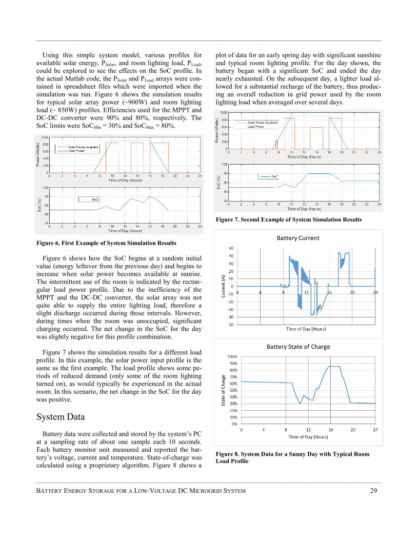
——————————————————————————————————————————————–————
Using this simple system model, various profiles for
available solar energy, PSolar, and room lighting load, PLoad,
could be explored to see the effects on the SoC profile. In
the actual Matlab code, the PSolar and PLoad arrays were con-
tained in spreadsheet files which were imported when the
simulation was run. Figure 6 shows the simulation results
for typical solar array power (~900W) and room lighting
load (~ 850W) profiles. Efficiencies used for the MPPT and
DC-DC converter were 90% and 80%, respectively. The
SoC limits were SoCMin = 30% and SoCMax = 80%.
Figure 6. First Example of System Simulation Results
Figure 6 shows how the SoC begins at a random initial
value (energy leftover from the previous day) and begins to
increase when solar power becomes available at sunrise.
The intermittent use of the room is indicated by the rectan-
gular load power profile. Due to the inefficiency of the
MPPT and the DC-DC converter, the solar array was not
quite able to supply the entire lighting load, therefore a
slight discharge occurred during those intervals. However,
during times when the room was unoccupied, significant
charging occurred. The net change in the SoC for the day
was slightly negative for this profile combination.
Figure 7 shows the simulation results for a different load
profile. In this example, the solar power input profile is the
same as the first example. The load profile shows some pe-
riods of reduced demand (only some of the room lighting
turned on), as would typically be experienced in the actual
room. In this scenario, the net change in the SoC for the day
was positive.
System Data
Battery data were collected and stored by the system’s PC
at a sampling rate of about one sample each 10 seconds.
Each battery monitor unit measured and reported the bat-
tery’s voltage, current and temperature. State-of-charge was
calculated using a proprietary algorithm. Figure 8 shows a
plot of data for an early spring day with significant sunshine
and typical room lighting profile. For the day shown, the
battery began with a significant SoC and ended the day
nearly exhausted. On the subsequent day, a lighter load al-
lowed for a substantial recharge of the battery, thus produc-
ing an overall reduction in grid power used by the room
lighting load when averaged over several days.
Figure 7. Second Example of System Simulation Results
Figure 8. System Data for a Sunny Day with Typical Room
Load Profile
——————————————————————————————————————————————————–
BATTERY ENERGY STORAGE FOR A LOW-VOLTAGE DC MICROGRID SYSTEM 29

——————————————————————————————————————————————–————
——————————————————————————————————————————————–————
30 INTERNATIONAL JOURNAL OF MODERN ENGINEERING | VOLUME 17, NUMBER 1, FALL/WINTER 2016
Ongoing Work
The 24 VDC microgrid installation continues to evolve.
Efficiency improvement changes on both the distribution
and consumption of the microgrid energy were underway at
the time of the writing of this paper. A grant has also been
received to help support research to develop better system
models for this type of application. The DC-DC converter
consumed a large amount of quiescent energy from its input
side just to power the cooling fan and other supervisory
electronics, even when the unit was disabled. This energy
was taken from the batteries and, during periods of sus-
tained cloudiness, can cause the SoC to drop below the de-
sign minimum. A change is being developed to provide a
solid-state switch disconnect between the battery and the
DC-DC converter. A similar switch will also be installed on
the output side of the DC-DC converter to minimize quies-
cent loading on the 24 VDC bus. On the load side, the con-
sumed power can be reduced by managing the light level in
the room, rather than just allowing users to turn the lights on
or off. The installed fluorescent ballasts are dimmable so
this change could be implemented with minimal hardware
changes.
The current model for the battery state of charge as a
function of input/output power is very simplistic. Although
many parameters would be needed to completely model the
energy system behavior, significant improvement can be
achieved by including a few key parameters in a new empir-
ical behavioral model. Performance data will be used to
help develop this model. Also, as more data are obtained on
the UltraBattery, the SoC limits may be able to be widened
to make use of even more stored energy for a given battery
size.
Conclusions
The 24 VDC microgrid is an evolving technology. Low-
voltage DC allows for more experimentation and faster de-
velopment of technology than higher voltages which impose
more safety and regulatory restrictions. Energy storage and
alternative energy sources can easily be added to the
24 VDC microgrid. Although in this study energy storage
was added at the top level (the main 24V bus), energy could
be injected into or stored in any of the 96 watt, class-2 parti-
tions of the microgrid. With proper modeling, the energy
storage system can be appropriately sized to meet the load
requirements. Proper sizing will also help to ensure that the
system uses minimal energy from the AC grid.
References
[1] Merge Alliance. Retrieved from http://
www.emergealliance.org
[2] Litwhiler, D. H., & Wiggins-Lopez, E. (2013). Low
Voltage Power Distribution System Provides Incuba-
tor for Energy-Related Student Projects. ASEE An-
nual Conference, Atlanta, Georgia.
[3] UltraBattery. Ecoult Energy Storage Solutions. Re-
trieved from http://www.ecoult.com/technology/
ultrabattery.
[4] Background—Ecoult Energy Storage Solution. Re-
trieved from http://www.ecoult.com/media/
background.
[5] Batt, N. (n.d.). Ecoult: Hampton Project—Utilising
storage technologies to smooth ramp rates, moderate
peaks and troughs in wind output and variability.
Retrieved from http://www.slideshare.net/
informaoz/7-nicholas-batt-ecoult
[6] Chang, W. Y. (2013). The State of Charge Estimating
Methods for Battery: A Review. ISRN Applied
Mathematics, 2013.
http://dx.doi.org/10.1155/2013/95379
Biographies
DALE H. LITWHILER is an associate professor at
Penn State, Berks Campus. He received his BS from Penn
State University, MS from Syracuse University, and PhD
from Lehigh University, all in electrical engineering. Prior
to beginning his academic career, he worked with IBM Fed-
eral Systems and Lockheed Martin Commercial Space Sys-
tems as a hardware and software design engineer. Dr. Lit-
whiler may be reached at [email protected]
NICHOLAS BATT leads the Application Engineer ing
team at Australian energy storage provider Ecoult. His team
works across kW and MW systems. The team seeks out new
applications that can benefit from the Ecoult UltraBattery,
invented by CSIRO in Melbourne Australia. Nicholas has
over 10 years of experience as a Power and Control engi-
neer, and has focused on renewable energy and smart grids.
Mr. Batt may be reached at [email protected]
JASON HOFFMAN is a senior engineer with Ecoult.
He is focused primarily on managing the design and imple-
mentation of large-scale grid-connected energy storage sys-
tems. He received his BS from Bucknell University and his
MS from Penn State University, both in electrical engineer-
ing. Following his education, he has been working in the
power industry, primarily in the renewable energy and ener-
gy storage areas. Mr. Hoffman may be reached at

Abstract
In this paper, the authors describe research aimed at deter-
mining the measured and predicted performance of a photo-
voltaic grid-connected system in a humid subtropical cli-
mate. The performance was modeled and the predicted per-
formance of the systems was compared to the experimental-
ly collected data for the system. In addition, the research
allowed for long-term simulation analysis of the system
under varying conditions and can assist with the optimiza-
tion of the photovoltaic system.
Introduction
As the global population increases along with the ad-
vancement of human development and technology, so does
the increase in global energy demand. According to the U.S.
Energy Information Administration’s 2013 report, the world
energy consumption was expected to grow by 56% between
2010 and 2040, from 524 quadrillion British thermal units
(Btu) to 820 quadrillion Btu [1]. Through these projections,
it was estimated that fossil fuels will continue to supply
roughly 80% of the world’s energy through 2040 [1]. Fossil
fuels are non-renewable resources with supplies that are
being drastically depleted. It was calculated that the deple-
tion time for oil, gas, and coal was to be about 35, 37, and
107 years, respectively [2]. Though the accurate timing for
fossil fuel depletion is an arguable topic among researchers
and scientists, it is an inarguable fact that fossil fuels cannot
last forever at current usage rates. The increase in demand
for energy coupled with the knowledge of depleting fossil
fuels has led to an increase in demand for research into de-
veloping alternatives to using fossil fuels, the most viable
being solar energy by means of photovoltaic (PV) modules.
PV production has been doubling every two years, in-
creasing by an average of 48% each year since 2002, mak-
ing it the world’s fastest-growing energy technology [3]. PV
systems depend on a variety of factors including weather,
irradiation levels, temperature, and efficiencies in all com-
ponents of the system. Various methods have been devel-
oped to determine the maximum power output of these pho-
tovoltaic systems to improve overall efficiency. In this
study, the authors aimed to determine and analyze the pow-
er output of a photovoltaic grid-connected system using the
TRNSYS simulation program, compared to the recorded
performance of the system.
Description of the System
The University of Texas at Tyler’s Texas Allergy, Indoor
Environment and Energy (TxAIRE) Institute developed
realistic test facilities for the development and demonstra-
tion of new technologies related to energy efficiency. The
photovoltaic system used for this study was the system sup-
plying the energy for TxAIRE House 2, a net-zero energy
house with all the power provided by the PV system. It is
located in Tyler, Texas, which is classified as a humid sub-
tropical climate.
The house has a photovoltaic grid-connected system, con-
sisting of 33 SolarWorld SunModule Plus polycrystalline
225-watt solar panels, rated at 7.4 kW. Tables 1 and 2 show
the performance standards under standard test conditions as
well as the thermal characteristics as supplied by the manu-
facturer on the data sheet, respectively, for the solar mod-
ules. The photovoltaic modules cover an area of 590 ft2 and
are situated 25 ft away from the roofline of the house and
are at a 55.8º angle as shown in Tables 1 and 2.
Table 1. Performance under Standard Test Conditions of 1000
W/m2, 25ºC, AM 1.5
MEASURED AND SIMULATED PERFORMANCE OF A
GRID-CONNECTED PV SYSTEM IN A HUMID
SUBTROPICAL CLIMATE ——————————————————————————————————————————————–————
Fredericka Brown, The University of Texas at Tyler; Racquel Lovelace, The University of Texas at Tyler
——————————————————————————————————————————————————–
MEASURED AND SIMULATED PERFORMANCE OF A GRID-CONNECTED PV SYSTEM IN A HUMID SUBTROPICAL CLIMATE 31
Characteristic Variable SW 225
Maximum power Pmax 225 Wp
Open circuit voltage Voc 36.8 V
Maximum power point voltage Vmpp 29.5 V
Short circuit current Isc 8.17 A
Maximum power point current Impp 7.63 A

——————————————————————————————————————————————–————
——————————————————————————————————————————————–————
32 INTERNATIONAL JOURNAL OF MODERN ENGINEERING | VOLUME 17, NUMBER 1, FALL/WINTER 2016
Table 2. Thermal Characteristics of Solar Panels
The solar panels used for this study were installed in three
circuits of eleven modules per circuit for a total of 33 mod-
ules (see Figures 1 and 2). This array converts the solar ra-
diation into DC electricity, while an inverter unit, SMA
Technology model #SB7000US, converts the DC electricity
to AC so that it can feed into the house’s electrical system.
Figure 1. Back View of Photovoltaic Panels
Figure 2. Front View of Photovoltaic Panels
The archival data used for comparison in this study were
the PV performance and weather data collected from
TxAIRE House 2, from August 17, 2012, to December 31,
2014. The variables of interest in terms of PV performance
included solar panel energy (W) and the total solar radiation
on the tilted surface (W/m2). The radiation data were record-
ed as total radiation. The TRNSYS program requires that
data be input as beam and diffuse radiation; therefore, the
assumption that beam was approximately 85% of the total
and diffuse was 15% the total recorded radiation was split
into the two before being input into the program. Weather
data were also collected throughout the same time period.
The variables of interest in terms of weather data were tem-
perature (°F) and wind speed (mph).
The data for the house were collected using the NI-cRIO-
9074 processor, a 400 MHz industrial real-time processor
for control, data logging, and analysis. PR-T24 thermocou-
ple wires and polyvinyl insulated wires were also used in
retrieving the outside temperature. The data acquisition sys-
tem (DAQ) was connected by USB to a personal software
notebook to retrieve the data. The weather data were col-
lected from a Davis Vantage Pro 2 weather station situated
above the TxAIRE House 2 on the roof as Figure 3 shows.
Data were collected every 30 minutes for the time period
used for this study for weather and PV performance.
Figure 3. Location of the Weather Station on the Roof of the
TxAIRE House 2
System Modeling in TRNSYS
TRNSYS was the software package used to simulate the
PV system. It uses a one-diode, five-parameter model, as
developed by De Soto [4]. The simulation had the basic
outline as shown in Figure 4 and used the following compo-
nents: Type9 (user-entered data labeled as weather data),
Characteristic Parameter
NOCT 45ºC
TC Isc 0.034 %K
TCVoc -0.34 %K
TC Pmpp -0.48 %K
Operating range -40ºC to 90ºC
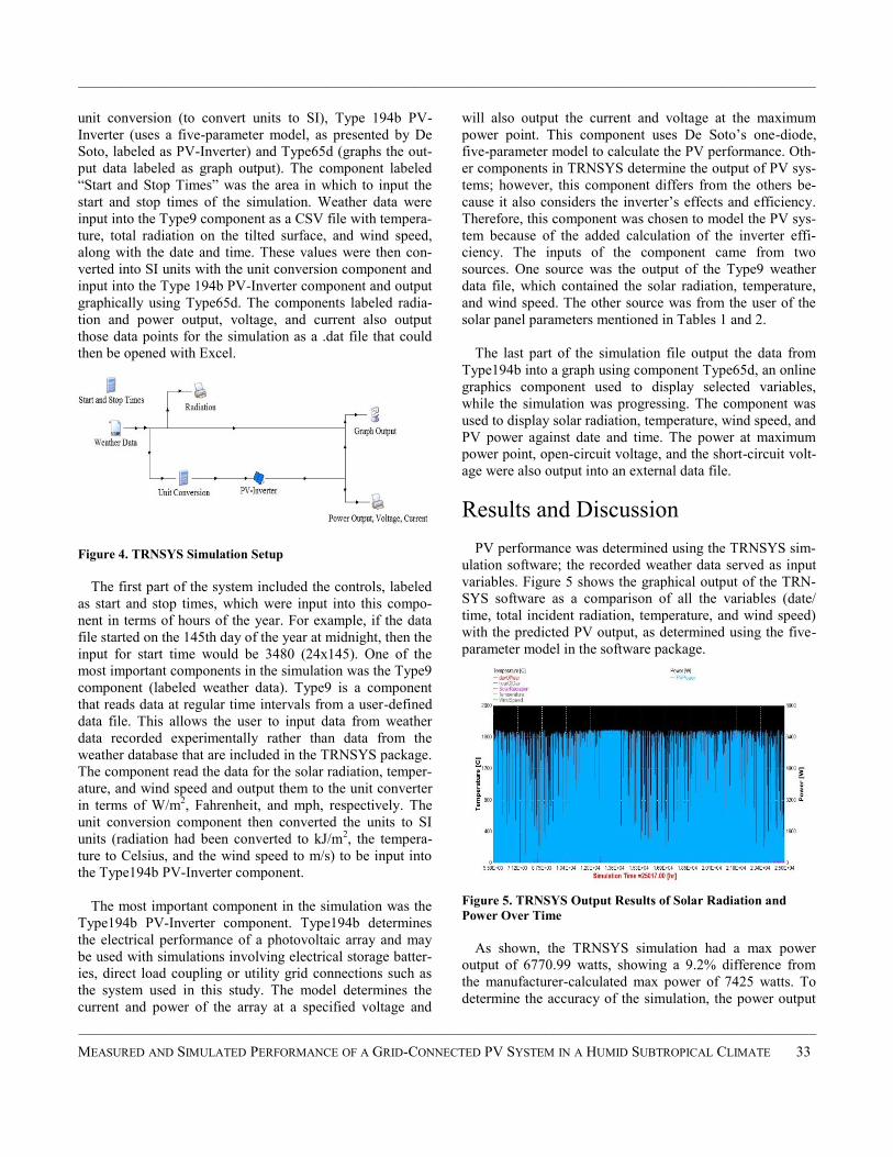
——————————————————————————————————————————————–————
unit conversion (to convert units to SI), Type 194b PV-
Inverter (uses a five-parameter model, as presented by De
Soto, labeled as PV-Inverter) and Type65d (graphs the out-
put data labeled as graph output). The component labeled
“Start and Stop Times” was the area in which to input the
start and stop times of the simulation. Weather data were
input into the Type9 component as a CSV file with tempera-
ture, total radiation on the tilted surface, and wind speed,
along with the date and time. These values were then con-
verted into SI units with the unit conversion component and
input into the Type 194b PV-Inverter component and output
graphically using Type65d. The components labeled radia-
tion and power output, voltage, and current also output
those data points for the simulation as a .dat file that could
then be opened with Excel.
Figure 4. TRNSYS Simulation Setup
The first part of the system included the controls, labeled
as start and stop times, which were input into this compo-
nent in terms of hours of the year. For example, if the data
file started on the 145th day of the year at midnight, then the
input for start time would be 3480 (24x145). One of the
most important components in the simulation was the Type9
component (labeled weather data). Type9 is a component
that reads data at regular time intervals from a user-defined
data file. This allows the user to input data from weather
data recorded experimentally rather than data from the
weather database that are included in the TRNSYS package.
The component read the data for the solar radiation, temper-
ature, and wind speed and output them to the unit converter
in terms of W/m2, Fahrenheit, and mph, respectively. The
unit conversion component then converted the units to SI
units (radiation had been converted to kJ/m2, the tempera-
ture to Celsius, and the wind speed to m/s) to be input into
the Type194b PV-Inverter component.
The most important component in the simulation was the
Type194b PV-Inverter component. Type194b determines
the electrical performance of a photovoltaic array and may
be used with simulations involving electrical storage batter-
ies, direct load coupling or utility grid connections such as
the system used in this study. The model determines the
current and power of the array at a specified voltage and
will also output the current and voltage at the maximum
power point. This component uses De Soto’s one-diode,
five-parameter model to calculate the PV performance. Oth-
er components in TRNSYS determine the output of PV sys-
tems; however, this component differs from the others be-
cause it also considers the inverter’s effects and efficiency.
Therefore, this component was chosen to model the PV sys-
tem because of the added calculation of the inverter effi-
ciency. The inputs of the component came from two
sources. One source was the output of the Type9 weather
data file, which contained the solar radiation, temperature,
and wind speed. The other source was from the user of the
solar panel parameters mentioned in Tables 1 and 2.
The last part of the simulation file output the data from
Type194b into a graph using component Type65d, an online
graphics component used to display selected variables,
while the simulation was progressing. The component was
used to display solar radiation, temperature, wind speed, and
PV power against date and time. The power at maximum
power point, open-circuit voltage, and the short-circuit volt-
age were also output into an external data file.
Results and Discussion
PV performance was determined using the TRNSYS sim-
ulation software; the recorded weather data served as input
variables. Figure 5 shows the graphical output of the TRN-
SYS software as a comparison of all the variables (date/
time, total incident radiation, temperature, and wind speed)
with the predicted PV output, as determined using the five-
parameter model in the software package.
Figure 5. TRNSYS Output Results of Solar Radiation and
Power Over Time
As shown, the TRNSYS simulation had a max power
output of 6770.99 watts, showing a 9.2% difference from
the manufacturer-calculated max power of 7425 watts. To
determine the accuracy of the simulation, the power output
——————————————————————————————————————————————————–
MEASURED AND SIMULATED PERFORMANCE OF A GRID-CONNECTED PV SYSTEM IN A HUMID SUBTROPICAL CLIMATE 33

——————————————————————————————————————————————–————
——————————————————————————————————————————————–————
34 INTERNATIONAL JOURNAL OF MODERN ENGINEERING | VOLUME 17, NUMBER 1, FALL/WINTER 2016
was compared to the power output as recorded by the NI-
cRIO-9074 data logging processor for the years used in this
study. Figure 6 shows the correlation between the predicted
PV output and the recorded output as a function of radia-
tion. The average value for recorded power was calculated
to be 783 watts with a max of 7095 watts. The average val-
ue for predicted power calculated by TRNSYS was 1052
watts with a max of 6771 watts. The percent difference be-
tween the averages was -29% and the maximum was -5%.
Figure 6. Predicted versus Recorded Power Output in Terms
of Radiation
Statistical Analysis
To compare the recorded data to the TRNSYS data, a
statistical analysis was conducted using an analysis of vari-
ance (ANOVA) in Excel. The maximum daily values of
power output of the recorded data were compared to the
maximum daily values of power output supplied by TRN-
SYS. The ANOVA determined whether or not there was a
difference in the data. H0 represented no difference in the
data and H1 represented differences in the data. If the result-
ing P value were less than alpha (alpha, in this case, was
0.05), H0 would be rejected and the H1 condition accepted
as true; if the P value were greater, then the opposite would
be true. Three ANOVA scenarios were run: 1) using the
complete data sets (August 2012-December 2014), 2) using
only the summer months (June-September), and 3) using
only the winter months (December-March).
Figure 7 shows the results of the first analysis. Using the
data set for the complete time, the resulting P value was
6.97E-27, which indicates a difference between the two data
sets. The average of the maximums for the recorded data
was 5157 watts with the average of the maximums for the
TRNSYS data being 6002 watts. The TRNSYS data were
over predicting the power output. As a maximum, TRNSYS
under predicts the data, as shown in Figure 6.
Figure 7. ANOVA Analysis of Statistical Comparison of
TRNSYS Total Power Output and Recorded Power Output
The next analysis was run using only data from the sum-
mer months. Figure 8 shows the results. This resulted in a P
value of 1.65E-74, again showing a difference between the
two data sets and a larger difference than using the entire
data set. The average of the recorded data was 4070 watts
and the average of the TRNSYS output was 6616 watts. The
last analysis used only data from the winter months. The
resulting P value was 0.204, meaning that there was not a
difference in the data (see Figure 9). The average of the
recorded data was 5176 watts and the average of the TRN-
SYS data was 5493 watts.
Figure 8. ANOVA Analysis of Statistical Comparison of
TRNSYS Power Output and Recorded Power Output during
the Summer Months
The analysis showed a difference in the data sets, evident
in the summer months, while the winter months showed no
difference. TRNSYS over predicted during the summer
months but accurately predicted in the winter months. Based
on Figure 6, the hourly data showed that the TRNSYS data
were higher than the recorded data on average but were
lower at the maximum power.
Total
Anova: Single Factor
SUMMARY
Groups Count Sum Average Variance
Column 1 859 4429803.00 5156.93 3260446.02
Column 2 859 5155426.26 6001.66 1880342.94
ANOVA
Source of Variation SS df MS F P-value F crit
Between Groups 306477944.75 1 306477944.75 119.23 6.97E-27 3.85
Within Groups 4410796928.14 1716 2570394.48
Total 4717274872.89 1717
Summer2013
Anova: Single Factor
SUMMARY
Groups Count Sum Average Variance
Column 1 122 496485.00 4069.55 780638.17
Column 2 122 807155.76 6616.03 317253.12
ANOVA
Source of Variation SS df MS F P-value F crit
Between Groups 395558685.26 1 395558685.26 720.58 1.65091E-74 3.88
Within Groups 132844846.16 242 548945.65
Total 528403531.42 243

——————————————————————————————————————————————–————
Figure 9. ANOVA Analysis of Statistical Comparison of
TRNSYS Power Output and Recorded Power Output during
the Winter Months
Root mean square error (RMSE), mean absolute deviation
(MAD), absolute percentage error (MAPE), and model effi-
ciency (EF) were also used to compare the recorded data to
the simulated data. The RMSE is given by Equation (1):
(1)
where, Ht is the recorded value; Ft is the simulated value;
and, n is the number of values in the data set. RMSE was
used to measure the differences between data set values,
with the best results being as close to zero as possible.
The mean absolute deviation was used to calculate the
average distance from each data point to the mean of the
recorded data. MAD is given by Equation (2):
(2)
Absolute percentage error is another measure of accuracy
between the recorded and simulated data points, defined by
Equation (3):
(3)
The last method for determining accuracies between the
data points used Equation (4) for model efficiency:
(4)
where, z is the average value of the recorded data.
Table 3 shows the TRNSYS model accuracy results. The
values for RMSE and MAD were higher than desired,
though they matched the ANOVA analysis, showing differ-
ences in the average data though similar data for the maxi-
mum.
Table 3. Model Accuracy Analysis Results Using RSME, MAD,
MAPE, and EF
Effects of Radiation, Temperature, and
Wind Speed
To further develop the simulation model, radiation, tem-
perature, and wind speed data were purchased for 10 years,
from 2004 to 2014 for the Tyler, Texas, area from Mete-
onorm and used in the TRNSYS simulation model. The
differences in data between the recorded and the purchased
sources showed a 1.3% difference between the temperature
data, 41.5% difference in the wind speed data, and a 30.8%
difference in the radiation data. The wind speed data were
not used in the simulation, and the results ended with an
88% difference of the TRNSYS results with the purchased
data and the recorded data.
Due to the differences in the data results, during the anal-
ysis of the TRNSYS simulation power output compared to
the recorded power output, the effects of the variables of
radiation, temperature, and wind speed were reviewed. The
results showed that radiation was the leading factor in deter-
mining power output, as compared to temperature and wind
speed. According to Khatib et al. [5], the power produced
by PV systems is proportional to the amount of the solar
radiation it collects. Standard test conditions (STC) assume
1000 W/m2; Khatib et al. explained that if only half of the
STC conditions are available then the PV output will also
only produce about half of the power. It was also explained
that temperature negatively affects the power output of PV
systems.
As ambient temperature increases, the cell temperature
also increases. With each 1°C increase of cell temperature,
the PV module’s power decreases by 0.5-0.6%. Bhattachar-
ya et al. [6] showed a correlation coefficient value, R, be-
tween ambient temperature and PV performance to be
0.9642, suggesting a strong positive correlation between the
two. The value of the coefficient of determination, R2, was
determined to be 0.9297, meaning that a 92.97% correlation
between the variables indicating a direct proportionality.
According to Bhattacharya et al., the value of the correlation
Winter2013
Anova: Single Factor
SUMMARY
Groups Count Sum Average Variance
Column 1 121 626343.00 5176.39 4561738.06
Column 2 121 664614.61 5492.68 2905151.97
ANOVA
Source of Variation SS df MS F P-value F crit
Between Groups 6052546.50 1 6052546.50 1.62 0.20 3.88
Within Groups 896026802.66 240 3733445.01
Total 902079349.16 241
2
1
1( )
n
t t
t
RMSE H Fn
1
1(
n
t t
t
MAD H Fn
1
1 ( )100%
n
t t
t t
H FMAPE
n H
2 2
1 1
2
1
n n
t t tt tn
tt
H z F HEF
H z
RMSE MAD MAPE (%) EF (%)
1468 -884 34.88% 33.85%
——————————————————————————————————————————————————–
MEASURED AND SIMULATED PERFORMANCE OF A GRID-CONNECTED PV SYSTEM IN A HUMID SUBTROPICAL CLIMATE 35

——————————————————————————————————————————————–————
——————————————————————————————————————————————–————
36 INTERNATIONAL JOURNAL OF MODERN ENGINEERING | VOLUME 17, NUMBER 1, FALL/WINTER 2016
coefficient between wind speed and PV performance is
0.6857, with a coefficient of determination of 0.4702. This
means that 52.68% of the total variation in the PV perfor-
mance variable is unexplained.
Conclusions
The results of this study showed that in determining the
performance of a PV grid-connected system, the following
should be taken into account:
The weather data have the most significant effect
on prediction performance, with the most effect
coming from the radiation data followed by tem-
perature and lastly wind speed. Therefore, carefully
selecting the correct weather data set is crucial,
particularly for the radiation data.
The TRNSYS simulation was able to accurately
predict the max power output within 5% differ-
ence; however, the average prediction had a 45%
difference with most of the difference coming from
calculations during the summer months.
Though accuracy can be increased with the addition of the
losses due to shading, dirt, differences with the nominal
power, mismatch, and temperature, as well as additional
data for radiation, the model using TRNSYS was deter-
mined to provide an accurate model of power performance.
This model is simple but accurate and can help to design
future PV systems in the East Texas area as well as help to
improve current PV systems.
Acknowledgments
The investigative effort presented in this paper was com-
pleted in the frame of research work in the Department of
Mechanical Engineering, University of Texas at Tyler, Tex-
as, master’s program. The authors gratefully acknowledge
Dr. Fredericka Brown for her support and guidance in the
research work for this paper, and Dr. Harmonie Hawley for
her support in the statistical analysis of this study.
References
[1] US Energy Information Administration. (n.d.). 2013
world energy consumption. Retrieved from http://
www.eia.gov/todayinenergy/detail.cfm?id=12251
[2] Shahriar S., & Topal, E. (2009). When will fossil
fuels reserves be diminished? Energy Policy, 37, 181-
189.
[3] Kropp, R. (2009, March 3). Solar expected to main-
tain its status as the world’s fastest-growing energy
technology. Sustainability Investment News. Re-
trieved from http://www.socialfunds.com/news/
article.cgi/2639.html
[4] De Soto, W., Klein, S. A., & Beckman, W. A. (2006).
Improvement and validation of a model for photovol-
taic array performance. Solar Energy, 80, 78-88.
[5] Khatib, T., Mohamed, A., Mahmoud, M., & Sopian,
K. (2012). A new approach for meteorological varia-
bles prediction at Kuala Lumpur, Malaysia, using
artificial neural networks: Application for sizing and
maintaining photovoltaic systems. Journal of Solar
Energy Engineering, 134(2), 021005-021005-10.
doi:10.1115/1.4005754
[6] Bhattacharya, T., Chakraborty, A. K., & Pal, K.
(2014). Effects of ambient temperature and wind
speed on performance of monocrystalline solar pho-
tovoltaic module in Tripura, India. Journal of Solar
Energy, 2014, id #817078. doi: http://dx.doi.org/
10.1155/2014/817078
Biographies
FREDERICKA BROWN is cur rently an associate
professor of Mechanical Engineering at The University of
Texas at Tyler. She earned her BS degree in Physics from
Xavier University; MS and PhD degrees in Mechanical En-
gineering from The University of Nevada, Las Vegas; and,
an MBA from The University of Texas at Tyler. Dr. Brown
is currently teaching at The University of Texas at Tyler.
Her research interests include renewable energy and thermal
system design. Dr. Brown may be reached at
RACQUEL LOVELACE is an engineer at STEMCO
LP. She earned her BS degree in Mechanical Engineering
from Kettering University and MS in Mechanical Engineer-
ing from The University of Texas at Tyler. Her research
interests include renewable energy and thermal system de-
sign. Ms. Lovelace may be reached at rlove-

Abstract
The single tower of the new Bay Bridge opened in 2013,
and was connected to its footing by 424 high-strength
ASTM A354 BD, hot-dip galvanized anchor rods. The
bridge was expected to experience strong earthquakes from
the nearby Hayward or San Andreas faults. Bridge specifi-
cations did not recommend the use of ASTM A354 BD hot-
dip galvanized anchor rods, due to the high probability of
hydrogen embrittlement in these anchor rods leading to their
fracture. A few months before the bridge opened, 32 A354
BD anchor rods fractured after tightening. In this study, the
authors investigated the pushover behavior of the main tow-
er of the SAS Bay Bridge in the likely event of fracture of
the anchor rods at the base of the tower due to hydrogen
embrittlement. At least two anchor rods have already frac-
tured at this writing.
In this project, the pushover behavior of the main bridge
tower without anchor rods connecting its base to the pile
cap footing was analyzed through numerical simulation. A
realistic non-linear model of the tower was created in AN-
SYS. The bridge tower, base plate, and the concrete-steel
composite pile cap were modeled in detail. No anchor rods
were included in the model to connect the tower to the foot-
ing. After applying the gravity load, the top of the tower
was pushed in the transverse direction until it collapsed. The
results of the realistic pushover analysis indicated that the
lateral strength of the tower drops relatively fast after the
peak, due to local buckling of the legs of the main tower,
yielding of the base plate, and crushing of the concrete un-
der the base plate.
During late stages of the pushover, the partial joint pene-
tration (PJP) welds connecting the tower to the base plate
also fractured. When the anchor rods are in place and tight-
ened, these PJP welds are in compression; however, without
the anchor rods, the welds will be directly subjected to ten-
sion and eventually fracture. The bridge design team indi-
cated that the anchor rods were not needed. The authors of
this current study, however, question the validity of the
statement and suggest the implementation of necessary ret-
rofit measures to restore the strength, stiffness, and ductility
of the tower.
Introduction
The new East Spans of the San Francisco-Oakland Bay
Bridge is a self-anchored suspension (SAS) bridge with a
single tower. The bridge opened to traffic in 2013 and is
located between two active seismic faults, the Hayward and
San Andreas faults. Figure 1 shows the elevation and plan
view of the new self-anchored suspension Bay Bridge. More
information on the properties of the bridge can be found in
studies by Astaneh-Asl and Qian [1] and Caltrans [2].
Figure 1. Elevation and Plan View of the SAS Bay Bridge
Figure 2 shows the pile cap, a concrete-steel composite
box, supporting the tower. The shafts, as well as the base
plate, are made of ASTM A709 Gr. 50 steel with a mini-
mum specified yield stress of 50 ksi (345 MPa) and an ulti-
mate strength of 65 ksi (448 MPa). The shafts are connected
to each other by steel I-shaped shear links along the height
of the tower by a saddle at the top and by steel vertical shear
plates at the base. For more information on the tower, see
Astaneh-Asl and Qian [1]. Figure 3 shows a plan view of a
quarter of the base plate with the locations of 3-in. (75 mm)
and 4-in. (100 mm) diameter ASTM A354 BD hot-dip gal-
vanized anchor rods, 6-in. diameter ASTM A633 shear
dowels, and the anchorage plates. The rods are made of
SAE 4140 steel with a minimum yield strength of 115 ksi
(793 MPa) and a minimum ultimate strength of 140 ksi
(965 MPa) [3]. The base plate of the tower is made of 14
separate plates, as shown in Figure 3(b). Figure 4 shows the
THE EFFECTS OF ANCHOR ROD FAILURE ON
THE PERFORMANCE OF THE NEW
BAY BRIDGE TOWER ——————————————————————————————————————————————–————
Abolhassan Astaneh-Asl, University of California, Berkeley; Maryam Tabbakhha, University of California, Berkeley;
Xin Qian, University of California, Berkeley
——————————————————————————————————————————————————–
THE EFFECTS OF ANCHOR ROD FAILURE ON THE PERFORMANCE OF THE NEW BAY BRIDGE TOWER 37

——————————————————————————————————————————————–————
——————————————————————————————————————————————–————
38 INTERNATIONAL JOURNAL OF MODERN ENGINEERING | VOLUME 17, NUMBER 1, FALL/WINTER 2016
typical details of the connection of the tower shafts to the
base plate and anchorage of the tower base to the pile cap
by anchor rods.
Figure 2. Elevation of the Tower (left) and Plan and Elevation
of the Pile Cap Footing Supporting the Tower
(a) (b)
Figure 3. Plan of the Base Plate and Location of Anchor Rods
Figure 4. Anchor Rods and Details of Tower Anchorage to the
Pile Cap
Investigation of the Fracture of the A354
BD Anchor Rods in the SAS Bay Bridge
The use of A354 BD hot-dip galvanized anchor rods in
this important bridge created a serious, undesirable behav-
ior. In 2013, and a few months before the opening of the
bridge, 32 of the 96 anchor rods connecting the seismic
shear keys to the top of Pier E2 on the east end of the SAS
Bay Bridge fractured when tightened (refer to Figure 1 for
location).
In 2015, Nader (of the TYLI/Moffitt Joint Venture) [4-5],
the Chief Engineer and Engineer of Record for the SAS Bay
Bridge, presented an analysis of the bridge subjected to a
selected number of ground motions. He concluded that even
without any anchor rods, the response of the bridge to six
ground motion records (that the bridge design team had
considered in the design of the bridge) will be almost the
same as the response with all anchor rods present. A critical
review of the validity of this claim as well as the correctness
of the analysis is not possible at this time since Nader did
not provide much information on the analysis itself. Howev-
er, the bridge model that the bridge design team used did
not seem to include local buckling of the tower shaft plates,
and fracture of the partial joint penetration (PJP) welds that
connect the base of the tower to the base plate (see again
Figure 4).
The performance criteria established for this “lifeline”
bridge by Caltrans [6] state that, “The bridge shall have a
clearly defined inelastic mechanism for response to lateral
loads and inelastic behavior shall be restricted to piers, tow-
er shear links, and hinge beam fuses.” According to this
statement in the performance criteria [6] for the bridge and
publications by the bridge design team [7-8], local buck-
ling, yielding, or fracture of any other element of the tower,
including plates, bolts, anchor rods, and welds, is not al-
lowed. To assess whether the performance criteria can be
fulfilled with fractured anchor rods, this paper provides a
summary of the results of a realistic pushover analysis of
the tower of the SAS Bay Bridge without anchor rods con-
necting the tower to the pile cap. Moreover, if the pushover
behavior is not acceptable, a measure of retrofit is suggest-
ed that can prevent premature failure of the tower during
future seismic events.
Objective
The main objective of the research summarized in this
paper was to investigate pushover behavior of the main tow-
er of the new SAS Bay Bridge with no anchor rods connect-
ing the base of the tower to the top of the pile cap.

——————————————————————————————————————————————–————
In 2013, it was discovered that two out of the 424 anchor
rods connecting the tower to the pile cap were fractured.
The cause of fracture was the hydrogen embrittlement of the
A354 BD anchor rods. Since all 424 anchor rods were hy-
drogen embrittled [9-10], it is likely that more anchor rods
would fracture during the service life of the bridge. The
fracture of the remaining anchor rods due to hydrogen em-
brittlement is the reason why this study was undertaken in
order to find out what would happen to the bridge tower
during future major seismic events without any anchor rods.
Realistic Pushover Analysis of the Tower
with No Anchor Rods at the Base
The remainder of the paper focuses on the realistic pusho-
ver analysis of the tower of the SAS Bay Bridge in the
transverse direction (most critical) with no anchor rods con-
necting the tower base plate to the pile cap.
Finite Element Modeling
ANSYS Workbench finite element nonlinear software
was used to simulate the behavior of the main tower, base
plate, and pile cap supporting the tower. All anchor rods
were assumed to have fractured and they were not included
in the model. Proper gap elements were used to allow uplift-
ing of the base plate (see Figure 5).
Figure 5. Finite Element Model of the SAS Bay Bridge Tower,
Base Plate, and Pile Cap
The detailed model of the base plate and pile cap was
added to be able to investigate the effects of failure modes
associated with the connection of the tower to the base
plate, the base plate, and the pile cap, while there were no
anchor rods present. Two types of steel were used in the
modeling of the tower structure. Almost all components of
the main tower and the tower base plate were ASTM A709
Gr. 50 with a minimum specified yield stress of 50 ksi
(345 MPa). The connection plates of the shear links to the
tower shafts were modeled with Gr. 70 steel with a mini-
mum specified yield stress of 70 ksi (485 MPa). A bi-linear
kinematic hardening model was considered for the steel
with an elastic modulus of 29,000 ksi (200 GPa), a Poisson
ratio of 0.3, and a strain hardening ratio of 1%. The concrete
used in this analysis to model the pile cap and the piles had
an elastic modulus of 4350 ksi (30 GPa), a Poisson ratio of
0.18, and a compressive strength of f’c=5.073 ksi (35 MPa),
which was obtained from the construction drawings [2] as
the specified values. The concrete inside the steel box was
modeled as confined concrete. More detailed information on
modeling of the tower itself can be found in the study by
Astaneh-Asl and Qian [1]. After applying the gravity force
to the tower, incremental horizontal displacements were
applied to the cable saddle groove location under the AN-
SYS displacement controlled iteration algorithm [11].
Results of the Pushover Analysis of the
SAS Bay Bridge Tower with No Anchor
Rods
Figure 6 shows the pushover curve of the tower in the
transverse direction regarding horizontal force on the verti-
cal axis versus applied horizontal displacement of the cable
saddle on top of the tower on the horizontal axis. As the
figure shows, the tower does not have a clear yield plateau,
which would be a desirable characteristic of structures in
resisting seismic effects. The tower behaves elastically from
origin to the point of “initial yielding” (see Figure 6) and
continues to yield more elements until it reaches the defined
“yield point” at point Y. In large structures, due to local
yielding of very small areas, the pushover curve starts devi-
ating from the initial elastic stiffness line very early, see
point Y in Figure 6. This point cannot be considered the
yield point, since the structure is essentially elastic. For
these cases, a yield point was defined where the pushover
curve deviates from the initial elastic line, a horizontal dis-
tance equal to 10% of the horizontal elastic deformation [1].
Figure 6. Transverse Pushover Curve When There Are No
Anchor Rods at the Base
——————————————————————————————————————————————————–
THE EFFECTS OF ANCHOR ROD FAILURE ON THE PERFORMANCE OF THE NEW BAY BRIDGE TOWER 39

——————————————————————————————————————————————–————
——————————————————————————————————————————————–————
40 INTERNATIONAL JOURNAL OF MODERN ENGINEERING | VOLUME 17, NUMBER 1, FALL/WINTER 2016
As pushover continued beyond the yield point, point Y in
Figure 6, the tower continued to accept larger forces due to
strain hardening, while the stiffness continued to decrease
due to further yielding. During the pushover, the shear links
yielded first then, as pushover continued, yielding of the
shear links continued, but the base of the tower started up-
lifting on the tension side and yielding on the compression
side of the base plate. As the tower reached its maximum
strength at point U (see Figure 6), significant yielding and
local buckling of the compression side of the base of the
tower had already occurred. Point D on the pushover curve
in Figure 6 is an important point related to the behavior,
since it represents the point where the ductility of the sys-
tem is measured. For a relatively large structural system
such as the SAS Bay Bridge tower, the ductility is defined
as the ratio of the displacement at a point where the strength
is 85% of the maximum strength (in in Figure 6) and the
displacement at the yield point (y in Figure 6). Figure 6
further shows that in and y were 9.8 ft (3.0m) and 4.1ft
(1.25m), respectively. Therefore, the pushover ductility of
the tower was 9.8/4.1 = 2.5.
Performance of the Main Elements of the
Tower during the Pushover
In this section, the authors present the results of the be-
havior of the main elements of the tower during pushover,
when all anchor rods were assumed to have fractured due to
a combination of hydrogen embrittlement and seismic forc-
es.
Tower Behavior under Pushover:
Figure 7 shows the equivalent von Mises stresses in the
tower at points Y, U, and D during the pushover in the
transverse direction. Red represents yielding in the shell
elements, or plates. In this case, yielding is defined as
equivalent von Mises stress reaching the specified minimum
yield stress of the steel plates, 50 ksi (345 MPa), for all steel
plates including the shear links, and 70 ksi (483 MPa) for
the end connection plates of the shear links to the tower
shafts. The points Y, U, and D correspond to the same
points as in Figure 6; that is, yield, maximum strength, and
0.85 maximum strength points on the pushover curve.
At yield point, Figure 7(a) shows two out of seven pairs
of shear links at the top portion of the tower yield, while the
other parts mainly remain elastic. High stresses are generat-
ed on the compression side of the tower in the middle por-
tion and at the base of the tower. At the point of maximum
strength, point U in Figure 6, shear links in the upper part,
as well as in the middle part of the tower have yielded in
shear, as shown in Figure 7(b). There is also yielding and
some local buckling in the compression side of the tower in
the middle portion. However, the compression side of the
tower at the base shows severe yielding and local buckling.
After reaching the maximum strength, pushover strength of
the tower drops relatively quickly, due to local buckling in
several areas of the tower base and corner stiffeners. At the
point where the applied force has dropped to 85% of the
maximum strength, point D in Figure 6, and where ductility
is measured, more yielding of the shear links at the top and
middle portions of the tower occurs, as shown in Figure 7
(c). Moreover, the base of the tower shows widespread
yielding and severe local buckling on the compression side.
Figure 7. Equivalent (von Mises) Stresses at the Yield Point,
Maximum Strength, and 85% Maximum Strength Points for
Transverse Pushover of Tower
The Behavior of PJP Welds Connecting the Tower to the
Base Plate:
Figure 4 shows partial joint penetration welds connect the
tower legs to the base plates. Notice that when anchor rods
are present and tightened to the specified amount of pre-
tensioning (i.e., 70% of their tensile strength), the base of
the tower and the entire area of the base plate are com-
pressed down on top of the pile cap. The tower pressing on
the base plate results in the PJP welds connecting the base
of the tower shafts to the base plate to be in compression.
However, when there are no anchor rods in place, or if the
anchor rods are not tightened to 70% of their tensile
strength, during the pushover, part of the base plate can up-
lift, resulting in subjecting the PJP welds to tension. There-
fore, it is important to determine if the welds connecting the
tower’s vertical plates to the base plate have the strength to
transfer the tensile uplift stresses from the vertical plates of
the tower to the base plate.
The pushover analysis indicated that, when the pushover
horizontal displacement reaches 7.6 ft (2.34m), the PJP
welds at the base of the tower will fracture. Obviously, this

——————————————————————————————————————————————–————
is unacceptable performance for a lifeline bridge in which,
according to its performance criteria, the only damage al-
lowed in the tower is the ductile shear yielding of the shear
links, while no fracture of welds is allowed.
Figure 8(a) shows the equivalent von Mises stresses on
the bottom surface of the tower base plate when the tower
reaches its maximum strength (i.e., point U in Figure 6). At
this point, some areas of the base plate have yielded. Such
yielding of the base plate during the pushover is in violation
of the performance criteria for this bridge, which allow only
yielding of the shear links, while the rest of the tower re-
mains elastic. Figure 8(b) shows the vertical pressures that
the bottom surface of the base plate exert on the top of the
pile cap at point U during the pushover, when the tower,
without anchor rods, reaches its maximum strength during
the pushover. Since the concrete under the base plate is con-
fined, the maximum compression strength on it can reach
1.7f'c, where f’c is the specified compressive strength of the
concrete measured using cylinder specimens. Therefore, in
Figure 8, red corresponds to the locations with pressure on
the concrete exceeding 1.7f'c, which indicates compressive
crushing of concrete under the base plate.
Figure 8. Equivalent (von Mises) Stresses at Two Locations:
(a) the Bottom Surface of the Base Plate and (b) the Top
Surface of the Pile Cap
Comparison of Tower Behavior with and
without Anchor Rods
Figure 9 shows a comparison of the pushover behavior of
the tower with and without anchor rods connecting it to the
pile cap. The curve for the tower pushover with the anchor
rods is extracted from the work done previously by Astaneh
-Asl and Qian [1]. On the curve for the tower with the an-
chor rods, points Y, U, and D correspond to points of yield,
maximum strength, and 85% of maximum strength (i.e., the
point where ductility is measured). Points Y’, U’, and D’ are
similar points on the pushover curve for the tower without
any anchor rods. The initial elastic stiffness for both curves
was almost identical, which means, before significant yield-
ing, under dynamic loading during the earthquakes, the tow-
er with or without anchor rods connecting it to the pile cap
will be subjected to almost the same seismic inertia forces.
However, comparing force at points Y and Y’, the tower
without the anchor rods will yield the shear links at about
70% of the force that will yield the tower with the anchor
rods.
Figure 9. Comparison of Pushover Curves of the Tower with
and without Anchor Rods
As for the maximum strength, comparing points U and
U’, the tower without the anchor rods reaches its maximum
and drops the load at about 63% of what the tower with an-
chor rods could take. To compare ductility of these two cas-
es of the tower with and without anchor rods, the ratio of
displacements at D and Y to the ratio of displacements at D’
and Y’ should be compared. This process indicated that
ductility of the tower without the anchor rods was reduced
to 2.5 compared to 3.2, which is the ductility of the tower
with the anchor rods.
Suggested Retrofit to Mitigate the Hazard
Posed by Brittle Tower Anchor Rods
The problem of SAS Bay Bridge anchor rods is directly
related to the following aspects:
(a) The design decision to use ASTM A354 BD hot-dip
galvanized anchor rods in a very corrosive offshore
environment.
(b) The failure during construction in leaving the anchor
rods in the open environment unprotected for more
than two years.
(c) Embedding the anchor rods in the pile cap concrete
inside sleeves and not filling the sleeves with grout.
The lack of protective grout resulted in the seawater
seeping into the pile cap to collect around the anchor
rods and caused further stress corrosion in them.
——————————————————————————————————————————————————–
THE EFFECTS OF ANCHOR ROD FAILURE ON THE PERFORMANCE OF THE NEW BAY BRIDGE TOWER 41

——————————————————————————————————————————————–————
——————————————————————————————————————————————–————
42 INTERNATIONAL JOURNAL OF MODERN ENGINEERING | VOLUME 17, NUMBER 1, FALL/WINTER 2016
In this paper, the authors show that not having the anchor
rods resulted in the undesirable behavior of the main tower.
To mitigate the problem, the following summary of retrofit
measures is proposed.
1. The tower needed to be retrofitted to prevent yielding
and local buckling of the tower legs. The issue of the
local buckling of the tower legs is also an issue even
when anchor rods have no problem [1]. Hence, the
vertical stiffeners inside the tower legs needed to be
strengthened by adding stiffening material to them
[1]. The satisfactory performance of such stiffeners
was established by Qian and Astaneh-Asl [12].
2. The partial joint penetration (PJP) welds connecting
the tower legs to the base plate needed to be
strengthened to develop the yield strength of the tow-
er leg plates.
3. Many of the 3-in. (7.6 cm) diameter unacceptable
brittle A354 BD anchor rods that were not above the
piles should have been replaced, albeit at a very high
cost, with 3.5-in. (8.9 cm) ductile “upset” A354 BC
anchor rods. To do so would have required boring
through the existing anchor rods through the entire
19.7 ft (6m) depth of the composite pile cap, then
attaching a steel reaction frame to the bottom of the
pile cap, and finally installing the new A354 BC up-
set anchor rods connecting the tower base plate to the
new steel structure at the bottom of the pile cap.
4. Water-sealed caisson around the pile cap needed to
be constructed to prevent seawater from reaching
pile cap. The seawater caused not only corrosion of
the anchor rods but also corrosion of the steel plate
box of the composite pile cap. This latter problem is
not part of this paper but also needs to be solved. So,
this retrofit step could have protected the pile cap as
well.
Summary of the Anchor Rod Issue and
Conclusions of the Pushover Analysis
In 2013, a few months before the SAS Bay Bridge was
opened, 32 3-in. diameter A354 BD hot-dipped galvanized
anchor rods connecting the shear keys on the east end of the
bridge fractured after tightening. The cause of the fracture
was established to be hydrogen embrittlement [9-10].
Bridge specifications did not recommend the use of A354
BD high-strength anchor rods and bolts, and specifically
prohibited hot-dip galvanizing them because of the possibil-
ity of hydrogen embrittlement, as happened in this bridge.
The fracture of the 32 anchor rods in the shear keys after
tightening, and then fracture of at least one anchor rod at the
base of the tower, which was not even fully tightened, creat-
ed a serious concern about the safety of the bridge [13]. In
addition to hydrogen embrittlement of the anchor rods,
when one of the anchor rods at the base of the tower also
failed because of thread stripping, the safety of the entire
bridge came under question. More than 2200 A354 BD hot-
dip galvanized bolts and anchor rods were used in the most
critical connections of the bridge superstructure. In particu-
lar, the single tower of the bridge was anchored to its pile
cap support by 424 A354BD hot-dip galvanized anchor
rods. These are the anchor rods that had the problem of hy-
drogen embrittlement and thread stripping.
After fracture of the first anchor at the base of the tower,
the transportation officials in charge of the bridge initiated
an investigation of the case to establish the cause and to
develop a repair and retrofit strategy. As the investigation
continued, it became apparent that the cause of fracture of
the anchor rod at the base of the tower was hydrogen em-
brittlement, exacerbated by the presence of the salty ocean
water inside the pipe sleeves around the anchor rods, which,
in many cases, were not filled with grout, as specified in the
drawings. The fact that the threads on the anchor rods were
also suspect to stripping made it very likely that, in the long
-term, the anchor rods at the base of the tower would have
been susceptible to fracture during or even before a major
earthquake. Since the bottom ends of the anchor rods were
embedded in the pile cap, removal of the existing brittle
anchor rods and replacing them with sound anchor rods was
almost impossible and cost prohibitive. In 2015, the bridge
design team in a presentation to the Toll Bridge Program
Oversight Committee (TBPOC) provided results of their
analysis. They concluded that the anchor rods at the base of
the tower were not needed, and the seismic performance of
the bridge with or without anchor rods at the base of the
tower would be almost the same during major earthquakes.
They only recommended some limited repair, maintenance,
and monitoring activities for the anchor rods and leaving the
anchor rods in their places.
The main objective of this current investigation was to
establish the pushover behavior of the tower without the
anchor rods connecting it to the pile cap. Also, the two
pushover curves with and without anchor rods were com-
pared. In the model used in this study, and summarized pre-
viously by Astaneh-Asl and Qian [1], all plates in the shafts
were modeled as inelastic shell elements capable of yielding
and buckling.
Based on the results of realistic pushover of the SAS Bay
Bridge tower, using shell elements for the plates, the follow-
ing observation were made and conclusions reached.
1. This study showed that the pushover strength and
ductility of the tower without anchor rods connecting

——————————————————————————————————————————————–————
it to the pile cap was only about 60% and 80% of that
for the case with the anchor rods, respectively.
2. There was a need for seismic retrofit of the tower
itself and its base anchored to the pile cap by remov-
ing the brittle A354 BD hot-dip galvanized anchor
rods. Retrofit plans were proposed, which, if imple-
mented, could mitigate the problems and bring the
performance of this bridge to the level of a lifeline
bridge, and satisfy the corresponding performance
criteria. The lifeline performance is for the bridge to
open to traffic almost immediately after a major
earthquake, with limited damage in specifically des-
ignated areas.
Lessons Learned and How This Problem
Could Have Been Avoided
Following is a list of important lessons learned from this
case study, which also applies to the design and construc-
tion of other structures with similar details.
(a) As many bridge design codes recommend, the A354
BD high-strength anchor rods should not have been
used in this structure in the corrosive environment
over seawater, where the anchor rods are embedded
in the pile cap and the pile cap is submerged in sea-
water.
(b) The A354 BD anchor rods and bolts should not have
been hot-dip galvanized, which is well-known to
cause hydrogen embrittlement in high-strength steel.
Instead, they should have been mechanically galva-
nized with zinc or aluminum, which is a very com-
mon procedure.
(c) The anchor rods should not have been left at the site
in the open environment for more than three years to
be exposed to the rain and seawater environment.
(d) The number of threads per inch and the depth of the
thread should have been specified correctly to avoid
thread stripping under tension.
(e) The anchor rods should not have been embedded in
the concrete of the pile cap. Instead, the following
solutions were recommended in this case. First: the
anchor rods should have been passed through the pile
cap with the bottom nut under the pile cap to ease
replacement. Second: the anchor rods should have
had a small segment at the top, weaker than the main
body of the anchor rods, to ensure that the small por-
tion at the top acts as a fuse and prevents damage to
the main body of the anchor rod embedded in the
concrete. The top segment could be replaced easily in
case of corrosion during the service life or damage
after a seismic event.
(f) Instead of using A354 BD high-strength anchor rods,
not allowed to be hot-dip galvanized, upset A3254
BC anchor rods should have been used. The A354
BC has a specified minimum yield stress of 99 ksi
(683 MPa) [3]. The A354 BC bolts can be galvanized
either by hot-dip galvanizing, without developing
hydrogen embrittlement, or by mechanical galvaniz-
ing.
(g) In regular straight anchor rods and bolts, threads are
cut into the cross section of the shanks, resulting in
the fracture of the under-thread area of the threaded
part to be the tensile failure mode. This failure mode
is quite brittle and is not desirable in high-seismic
applications, where ductile failure modes need to
govern. In upset bolts and anchor rods, the shank
cross-sectional area is smaller than the under-thread
area such that the yielding of the gross area of the
shank is the governing failure mode instead of the
fracture of the under-thread area. If instead of prob-
lematic 3-in. A354 BD bolts, A365 BC upset anchor
rods had been used in this bridge, the diameter of the
anchor rods (outside of the upset portion) would have
been 3.5 inches (8.9 cm) instead of 3 inches (7.6 cm)
for the anchor rods that were used. With this relative-
ly small but very important design decision, there
would have been no problem of hydrogen embrittle-
ment and thread-stripping for bolts and anchor rods,
as occurred in the new $6.5 billion SAS Bay Bridge.
Acknowledgements
This study was part of a larger project on Investigation of
Seismic Performance of the New Self-Anchored Suspension
Bay Bridge East Spans at the University of California
Berkeley, USA, with Professor Abolhassan Astaneh-Asl as
the Principal Investigator. The authors would like to express
their sincere appreciation for the tremendous technical sup-
port provided by Ozen Engineering Inc. (https://
www.ozeninc.com) on the use of the powerful ANSYS non-
linear structural analysis software featured in this project.
The authors would like to acknowledge the input from ma-
terial scientists Yun Chung and Lisa Fulton.
References
[1] Astaneh-Asl, A., & Qian, X. (2016). Pushover Anal-
ysis of the Tower of the New Self-Anchored Suspen-
sion Bay Bridge. Proceedings of the 2016 IAJC-
ISAM Joint International Conference. Nov. 6-8, Or-
lando, Florida.
[2] Caltrans. (1999). Project Plans for Construction on
State Highway in San Francisco County in San Fran-
cisco, Engineering Drawings, The State of California,
Department of Transportation, Sacramento.
——————————————————————————————————————————————————–
THE EFFECTS OF ANCHOR ROD FAILURE ON THE PERFORMANCE OF THE NEW BAY BRIDGE TOWER 43

——————————————————————————————————————————————–————
——————————————————————————————————————————————–————
44 INTERNATIONAL JOURNAL OF MODERN ENGINEERING | VOLUME 17, NUMBER 1, FALL/WINTER 2016
[3] ASTM (2011). Standard Specification for Quenched
and Tempered Alloy Steel Bolts, Studs, and Other
Externally Threaded Fasteners, ASTM Standard
A354-11, American Society for Testing and Material.
[4] Tower Anchor Rod Workshop, Two Day Meeting
Summary, June 16 & 17, 2015. Retrieved from http://
www.baybridgeinfo.org/sites/default/files/pdf/
FinalTBPOCPacket-24Sep15_0.pdf
[5] Nader, M. (2015). Analysis of Self-Anchored Sus-
pension Bridge without Tower Anchor Bolts, Re-
trieved from http://www.baybridgeinfo.org/sites/
default/files/pdf/Analysis-of-SAS-with-No-Tower-
Anchor-Rods.pdf
[6] Caltrans. (2002). Self-Anchored Suspension Bridge-
Design Criteria-100% Submittal, Prepared by T. Y.
Lin International/Moffatt & Nichol Engineers, a Joint
Venture, Retrieved from http://www.dot.ca.gov/
baybridge/a354report/F1_Self-
An-
chored_Suspension_Bridge_Design_Criteria_100_pe
rcent_submittal.pdf
[7] Nader, M., Manzanarez, R., & Maroney, B. (2000).
Seismic Design Strategy of the New East Bay Bridge
Suspension Span. Proceedings of the 12th World
Conference on Earthquake Engineering. Auckland,
New Zealand.
[8] Nader, M., Lopez-Jara, J., & Mibelli, C. (2002). Seis-
mic Design of the New San Francisco-Oakland Bay
Bridge Self-Anchored Suspension Span. Proceedings
of the 3rd Nat. Seismic Conf. and Workshop on Bridg-
es and Highways, Portland, Oregon.
[9] Chung, Y. (2014). Corrosion on the New Eastern
Span of the San Francisco-Oakland Bay Bridge, Ma-
terial Performance. NACE International, P53, 11, 58.
[10] Chung, Y., & Thomas, L. K. (2014). High Strength
Steel Anchor Rod Problems on the New Bay Bridge,
Rev 1. Report to Committee on Transportation and
Housing California State Senate, Sacramento, 105pp.
Retrieved from http://media.sacbee.com/
smedia/2013/12/07/21/47/Djfhs.So.4.pdf
[11] ANSYS, Inc. (2013). ANSY S Mechanical APDL
Theory Reference, Release 15. ANSYS Inc., Can-
onsburg, PA.
[12] Qian, X., & Astaneh-Asl, A. (2016). Behaviour and
Seismic Design of Stiffeners for Steel Bridge Tower
Legs and Piers. Proceedings of the World Congress
on Civil, Structural, and Env. Engineering
(CSEE’16), Prague, Czech Republic.
[13] Martin, G. (2013). Bridge Over Troubled Bolts: Cal
Experts Question Whether New Bridge is Safe. Cali-
fornia Magazine. Retrieved from http://
alumni.berkeley.edu/california-magazine/just-in/2016
-06-20/bridge-over-troubled-bolts-cal-experts-
question-whether-new
Biographies
ABOLHASSAN ASTANEH-ASL is a professor in the
Department of Civil and Environmental Engineering at the
University of California, Berkeley. He has over 48 years of
experience in design, research, and teaching courses in
structural and earthquake engineering and design of build-
ings, bridges, and other structures, as well as blast protec-
tion of structures. He has testified as an expert before the
policy making and judicial bodies, has completed more than
50 major research projects, and has published more than
300 technical papers. Dr. Astaneh-Asl may be reached at
MARYAM TABBAKHHA is cur rently a visiting assis-
tant project scientist in the Department of Civil and Envi-
ronmental Engineering at the University of California,
Berkeley. She earned her BS degree from the University of
Science and Technology (Iran) and two master’s degrees in
Earthquake Engineering and Geotechnical Engineering from
Sharif University (Iran) and Ecole Nationale des Ponts et
Chaussees (France). She earned her PhD from Ecole Centra-
le Paris and worked as a postdoc at Columbia University for
one year. Her research interests include masonry structure,
steel moment frame, the effect of the flood on structures,
earthquake engineering. and probabilistic theory and uncer-
tainty quantification. Ms. Tabbakhha may be reached at
XIN QIAN is cur rently a PhD candidate at the Univer-
sity of California at Berkeley. She earned her BS degree at
the Hong Kong Polytechnic University and MS in Civil
Engineering from the University of California, Berkeley.
Her research interests include steel and composite structures
and earthquake engineering. She is the recipient of the first
Professor T. Y. Lin Fellowship in Structural Engineering at
UC Berkeley, and is active in student activities in earth-
quake engineering as the President of the EERI Berkeley
student chapter. Ms. Qian may be reached at cin-

GEOMETRICAL DETERMINATION OF MAXIMUM
POWER POINT OF A PHOTOVOLTAIC CELL
——————————————————————————————————————————————–———— Mehmet Goksu, Millersville University of Pennsylvania; Faruk Yildiz, Sam Houston State University
Abstract
Renewable energy is one of the most important topics in
energy production today, due to increasing world energy
needs and global warming. An increased use of photovoltaic
(PV) cells is essential for meeting this need, since sunlight
is clean, abundant, and effectively limitless. In this paper,
the authors present a new algorithm for determining the
maximum power point (MPP) of a PV cell, based on the
geometry of a current-voltage (I-V) curve. Even though a
PV cell may be operated at any point on the I-V curve, the
MPP indicates a point where the maximum power output is
obtained from the cell. It is, therefore, necessary to accu-
rately determine the MPP of the cells. This method also
shows that geometrical construction of the MPP is inde-
pendent of the characteristic of PV cells.
Introduction
It is clear that fossil fuel resources are finite, and deple-
tion will happen sooner or later. If the current level of fossil
fuel energy consumption continues, the entire world’s fossil
fuel energy reserve will be depleted in about 100 years [1].
Fossil fuel resources will eventually be replaced by renewa-
ble energy sources, especially by solar energy. Currently,
only a small portion of the world’s energy consumption is
produced by renewable energy. There is an increasing de-
mand for clean, renewable energy as the world’s fossil fuel
reserves continue to diminish. Scientists and engineers are
trying to make renewable energy a more viable and cost-
effective method of generating electricity in an effort to
partially fulfill the world’s energy needs.
I-V and power-versus-voltage (P-V) characteristics of PV
cells have been studied extensively over the last decade.
Some simulations of PV cells have been made primarily to
develop an algorithm to determine precisely the location of
the MPP while it is operating. The location of the MPP con-
tinually changes as the environmental conditions of the PV
cell changes. To extract maximum power from a PV cell in
any weather condition, an MPP controller is used in the
system. An MPP controller is a device that uses either a
logical or mathematical algorithm in order to operate the PV
cell at the maximum efficiency under varying weather con-
dition and loads. There are many MPP controller algorithms
reported in the literature [2-5]. These algorithms vary in
control strategies, variables, and hardware implementation.
Each algorithm has its own unique property, with ad-
vantages and disadvantages with respect to these parameters
[6-10].
The perturb-and-observe (P&O) and incremental conduct-
ance (INC) algorithms are the most widely used methods in
MPP controllers. A P&O algorithm periodically compares
power at different steps by perturbing voltage and current.
This process continues until the MPP is reached. Even
though this algorithm is one of the simplest to implement, a
P&O algorithm suffers from slow dynamic response [11]
and oscillation around the MPP, due to loss in power [12] in
rapidly changing weather conditions. An INC algorithm
uses the conductance of the P-V curve [13]. Similarly, this
algorithm compares the instantaneous conductance and the
perturbed conductance. Comparison between these conduct-
ance values is used to determine the location of the MPP.
To improve the response time reaching the MPP, an INC
algorithm in the perturbation uses variable step size instead
of a fixed step for tracking the MPP [14].
The MPP algorithms used to determine the location of the
MPP require some physical parameters related to the PV
cells. Also, some algorithms use higher levels of computa-
tional analysis. This present study explains a new and sim-
ple method to determine the location of the MPP on the I-V
curve. This method does not require any mathematical com-
putation or knowledge about the PV cell. Kumar and Pachal
[15] presented the geometrical prediction of the MPP by
forming a parallelogram on the I-V characteristic curve. The
method described in their work required different values of
voltage and current on the I-V curve, including short-circuit
current and open-circuit voltage, to construct the parallelo-
gram.
After forming the parallelogram, the Lagrangian interpo-
lation method was used to precisely determine the location
of the MPP. Those authors presented their work in another
study to predict the location of the MPP, based on quadratic
regression analysis of the geometry on the P-V characteris-
tic curve [16]. The new method proposed in this current
study presents the geometrical location of the MPP in a very
straightforward fashion without using any characteristics of
the PV cell. With this method, the location of the MPP is
——————————————————————————————————————————————————–
GEOMETRICAL DETERMINATION OF MAXIMUM POWER POINT OF A PHOTOVOLTAIC CELL 45

——————————————————————————————————————————————–————
——————————————————————————————————————————————–————
46 INTERNATIONAL JOURNAL OF MODERN ENGINEERING | VOLUME 17, NUMBER 1, FALL/WINTER 2016
independent of the PV cell’s characteristics. It is also appli-
cable to any type of PV cells in any environmental condi-
tion.
Theory
In this paper, the authors describe the geometrical loca-
tion of the MPP on the I-V curve using the fact that the
maximum of a function is obtained by setting the differen-
tial of the function to zero. Figure 1 shows the nonlinear I-V
characteristic curve of a PV cell. The I-V curve represents
the possible voltage and current operating points of the PV
cell that depend mainly on solar insolation, temperature of
the cell, and the partial shading condition. A PV cell pro-
duces maximum power only at a single point along the I-V
curve at a specific condition. Also, the maximum power
delivered by a PV cell is given by the largest rectangle fit-
ting under the I-V curve.
Figure 1. I-V Characteristic Curve of the PV Cell
Figure 2 shows a plot of the P-V characteristic of the cell
with the I-V curve. The operating voltage and current at the
MPP are called maximum power point voltage and current,
respectively.
Figure 2. I-V and P-V Characteristic Curves
The MPP of a PV cell is usually located at the knee of the
I-V curve, where the product of current and voltage is maxi-
mum. The condition for the maximum power yields that
derivative of power with respect to voltage is zero, as given
by Equation (1):
(1)
where, power is a function of voltage and current and is
defined by Equation (2):
(2)
Differentiating both sides of the equation yields Equation
(3):
(3)
and rearranging the equation at the MPP yields Equation
(4):
(4)
The right-hand side of the equation represents the tangent
to the MPP on the I-V curve. The left-hand side of the equa-
tion represents the slope of a line that connects the coordi-
nate origin and the MPP. Figure 3 geometrically illustrates
this relationship. From the geometrical construction, Equa-
tion 4 can be viewed in two different ways in order to de-
scribe the location of the MPP in the figure:
1. The MPP occurs on the knee of the I-V curve,
where the I-V line and the I-V tangent both make
the same angle, α, with the horizontal V-axis, as
Figure 3 shows.
2. At the MPP, the tangent to the characteristic curve
makes the same angle, β, with a vertical line to Vmp
as the line connecting the origin and the MPP.
Figure 3. The Geometry of the MPP on the I-V Curve
0dP
dV
,P P I V I V
0dP dV dI dI
I V I VdV dV dV dV
mp mp
I dI
V dV

——————————————————————————————————————————————–————
In this paper, the authors present a new interpretation of
Equation (1) that is different from all of the algorithms re-
ported in the literature. The same mathematical condition
was used in some MPP controller devices, such as INC,
which compared the instantaneous conductance and the per-
turbed conductance. Other MPP controllers were based on
the fact that the sign of derivative of power with respect to
voltage changes from positive to negative when the operat-
ing point of a PV cell changes from the left-hand side of the
MPP to the right-hand side of the MPP.
Analysis
The theory of the algorithm was tested using two different
types of solar panels: a 5-watt multicrystalline solar panel
from Clean Dependable Technology (CDT) and a 255-watt
monocrystalline solar panel from Perlight Solar (PLM-
255M-60). Table 1 shows the parameters of the panels from
the manufacturers’ data sheets. The 5-watt CDT panel was
physically used in the laboratory to obtain the temperature
and light intensity dependence of the I-V curves in order to
test the algorithm described here. On the other hand, the
255-watt panel was tested using the I-V curves provided by
the manufacturer [17].
Table 1. Specifications of the Solar Panels
Figure 4 shows the I-V characteristics of the 5-watt solar
panel. The light intensities used in the experiments were
200.0 W/m2, 400.0 W/m2, 600.0 W/m2, and 800.0 W/m2 at a
temperature of 22.0°C. A light sensor from Vernier Soft-
ware & Technology (LS-BTA) was used to measure the
light intensity in the experiment. Figure 5 represents the
temperature dependence of the I-V curve. The 5-watt solar
panel was tested at a fixed light intensity of 900.0 W/m2 and
temperatures of 14.0°C, 24.0°C, 46.7°C, and 54.0°C. An
infrared thermometer (FLUKE 62-Max) was used to meas-
ure the temperature of the cell. It is important to emphasize
that, as the temperature of the solar panel increased, the size
of the energy gap between the conduction and valance
bands decreased. This decrease in the energy gap allows the
solar panel to absorb photons with longer wavelengths and
lower energy. As a result, the short-circuit current of the
solar panel increased. This is a signature of the semiconduc-
tors used in the PV cells. Due to the scaling of Figure 5, it is
difficult to see the increase in the current.
Figure 4. The Intensity Dependence of I-V the Curves
Figure 5. The Temperature Dependence of the I-V Curves
Tables 2 and 3 illustrate the average of experimental an-
gle measurements, α and β, based on the algorithm. Each
average in the tables represents the average of two angle
measurements at a specified condition. The estimated uncer-
tainty in the measurements is 0.2°. As the tables illustrate,
the average angles are different for the same panel at differ-
ent conditions. It is also true that angles might be different
for different panels at the same condition of radiation inten-
sity or temperature. However, the theoretical sum of angles
α and β should be 90°. The sum is independent of any pa-
rameters, as long as angles are measured as described in the
algorithm. The experimental sum of angles at different light
intensities were (90.3 ± 0.4)° and (90.4 ± 0.5)° for the
5-watt CDT panel and 255-watt PML panel, respectively.
Similar results were obtained at different temperatures:
(89.7 ± 0.6)° for the 5-watt CDT panel and (90.3 ± 0.5)° for
the 255-watt PML panel.
Parameters
5-watt
CDT Panel
(Multicrystalline)
255-watt
Perlight Panel
(Monocrystalline)
Isc (A) 0.32 9.05
Voc (V) 21.01 37.20
Pmp (W) 5.18 255
Imp (A) 0.31 8.17
Vmp (V) 16.68 31.20
——————————————————————————————————————————————————–
GEOMETRICAL DETERMINATION OF MAXIMUM POWER POINT OF A PHOTOVOLTAIC CELL 47

——————————————————————————————————————————————–————
——————————————————————————————————————————————–————
48 INTERNATIONAL JOURNAL OF MODERN ENGINEERING | VOLUME 17, NUMBER 1, FALL/WINTER 2016
The experiment also revealed that the algorithm, de-
scribed for determining the location of the MPP based on
angle measurements, appeared to be independent of the type
of solar panel. It should be valid for any PV cell.
Table 2. Angle Measurements at Different Intensities
Table 3. Angle Measurements at Different Temperatures
Conclusion
In this study, the authors presented a new simple algo-
rithm that explains the geometrical location of the MPP on
the I-V curve. The proposed method was applied to two
different kinds of solar panels under different light intensi-
ties and temperatures. The sum of angles in the algorithm is
90°. The experimental results clearly support the theory that
this algorithm is applicable to any PV cell technology at any
fixed environmental condition. The algorithm described in
the paper could be easily implemented in any MPP control-
ler device to operate the PV cell at the MPP under varying
weather conditions.
Acknowledgments
The authors wish to acknowledge Dr. Michael Nolan for
helpful conversations.
References
[1] US Energy Information Administration. (2015). An-
nual energy outlook with projections to 2040. Re-
trieved from http://www.eia.gov/outlooks/aeo/
pdf/0383(2015).pdf
[2] Eltawil, M. A., & Zhao, A. (2013). MPPT techniques
for photovoltaic applications. Renewable and Sus-
tainable Energy Reviews, 25, 793-813.
[3] Hussain, K. H., Muta, I., Hoshiono, T., & Osakada,
M. (1995). Maximum photovoltaic power tracking:
An algorithm for rapidly changing atmospheric con-
dition. IEEE Proceeding: Generation, Transmission,
and Distribution, 142(1), 59-64.
[4] Casadei, D., Grandi, G., & Rossi, C. (2006). Single-
Phase-stage photovoltaic generation system based on
a ripple correlation control maximum power point
tracking. IEEE Transactions on Energy Conversion,
21(2), 562-568.
[5] Bhatnagar, P., & Nema, R. K. (2013). Maximum
power point tracking control techniques: State-of-the-
art in photovoltaic applications. Renewable and Sus-
tainable Energy Reviews, 22, 224-241.
[6] Esram, T., & Chapman, P. L. (2007). Comparison of
Photovoltaic Array Maximum Power Point Tracking
Techniques. IEEE Transactions on Energy Conver-
sion, 22(2), 439-449.
[7] Dolara, A., Faranda, R., & Leva, S. (2009). Energy
comparison of seven MPPT techniques for PV sys-
tems. Journal of Electromagnetic Analysis and Appli-
cations, 1(3), 152-162.
[8] Tofoli, F. L., Pereira, D. C., & Paula, W. J. (2013).
Comparative study of maximum power point tracking
techniques for photovoltaic systems. International
Journal of Photoenergy, 2015, 1-10.
[9] Bhatnagar, A. P., & Nema, B. R. K. (2013). Conven-
tional and global maximum power point tracking
techniques in photovoltaic application: A review.
Journal of Renewable and Sustainable Energy, 5(3),
p032701-22.
[10] Subudhi, B., & Pradhan R. (2013). A comparative
study of maximum power point tracking techniques
for photovoltaic power systems. IEEE Transactions
on Sustainable Energy, 4(1), 89-98.
[11] Femia, N., Petrone, G., Spagnuolo, G., & Vitelli, M.
(2005). Optimization of perturb and observe maxi-
mum power point tracking method. IEEE Transac-
tions on Power Electronics, 20(4), 963-973.
[12] Chung, H. S-K., Tse, K. K., Hui, S. Y., Mok, C. M.,
& Ho, M. T. (2003). A novel maximum power point
tracking techniques for solar panels using a SEPIC or
Cuk converter. IEEE Transactions on Power Elec-
tronics, 18(3), 717-725.
Intensity
(W/m2)
5-watt Panel Intensity
(W/m2)
255-watt Panel
αave(°) βave(°) αave(°) βave(°)
200 12.2 78.6 200 8.2 82.6
400 21.2 69.2 400 15.8 74.8
600 24.8 65.4 600 23.2 67.6
800 28.2 62.6 800 29.0 61.4
1000 35.2 54.2
Tempera-
ture
(°C)
5-watt
Panel Tempera-
ture
(°C)
255-watt
Panel
αave
(°) βave(°) αave(°) βave(°)
14.0 28.8 60.8 10 32.2 58.4
24.1 31.6 59.0 25 34.6 56.0
46.7 33.4 56.0 40 35.4 54.4
54.0 36.5 52.8 55 38.6 52.2
70 40.0 49.8

——————————————————————————————————————————————–————
[13] Koizumi, H., & Kurokawa, K. (2005). A novel maxi-
mum power point tracking method for PV module
integrated converter. In Proceedings of the IEEE
Power Electronics Specialist Conference (pp. 2081-
2086), Recife, Brazil.
[14] Liu, F., Duan, S., Liu, F., Liu, B., & Kang, Y. (2008).
A variable step size INC MPPT method for PV sys-
tem. IEEE Transactions on Industrial Electronics, 55
(7), 2622-2628.
[15] Kumar, G., & Pachal A. K. (2014). Geometrical pre-
diction of maximum power point for photovoltaics.
Applied Energy, 119, 237-245.
[16] Kumar, G., Trivedi, M. B., & Pachal A. K. (2015).
Innovative and precise estimation using P-V curve
geometry for photovoltaics. Applied Energy, 138,
640-647.
[17] Perlight Solar. (n.d.). Retrieved from http://
www.perlight.com/images/pdf/plm-m-60-series-spec-
sheet.pdf
Biographies
MEHMET I. GOKSU is an associate professor of
Physics at Millersville University of Pennsylvania. He is a
condensed matter experimentalist with extensive experience
in low-temperature physics. His research interests include
quantum computing, physics education, and renewable en-
ergy. He has a strong interest in sustainability and energy-
related issues are his passion. Dr. Goksu may be reached at
FARUK YILDIZ is cur rently an associate professor of
Engineering Technology at Sam Houston State University.
His primary teaching areas are electronics, computer-aided
design, and alternative energy technologies. His research
interests include low-power energy harvesting, conversion,
and storage, renewable energy education and technologies.
Dr. Yildiz may be reached at [email protected]
——————————————————————————————————————————————————–
GEOMETRICAL DETERMINATION OF MAXIMUM POWER POINT OF A PHOTOVOLTAIC CELL 49

——————————————————————————————————————————————–————
Faris Malhas, Central Connecticut State University; Mustafa Mahamid, University of Illinois at Chicago;
Adeeb Rahman, University of Wisconsin-Milwaukee
Abstract
In this paper, the authors report on the serviceability per-
formance of concrete beams reinforced with high-strength
MMFX steel. The measured serviceability parameters were
deflection, elastic stiffness, cracking moment, and crack
width. The experimental program involved testing 22 13-ft
beams with a 12x18-in. cross-section. Two classes of con-
crete strength were used: 6200 psi and 8700 psi. Three rein-
forcement ratios were used for each concrete class. For
comparison purposes, Grade 60 steel was also used in two
beams for each concrete strength. This experimental pro-
gram to investigate MMFX steel was the first of its kind.
The testing of these beams was performed using a monoton-
ic static two-point loading to failure. Strain measurements in
the middle portion of the beam were obtained using LVDTs
with a gage length of about 20 inches. Mid-span deflection
and crack widths were measured at all times and from both
sides of the beam.
The experimental results showed that the beams exhibited
more flexibility under service loads. The general behavior
was similar to regular Grade 60 steel. The presence of half
the steel as regular beams did not yield excessive deflection
under service loads. The stiffness of the beams was signifi-
cantly reduced after cracking and was more pronounced
when compared to computed behavior of regular steel.
However, deflection under service load for all specimens
indicated that live load deflection would most probably sat-
isfy the ACI Code, and at no time was it excessive. Also,
crack widths under service load were reasonable and within
normal ranges typically exhibited by concrete beam with 60
-ksi steel.
Introduction
The number of aging concrete structures has become sig-
nificant. The corroding reinforcement and the durability of
such structures makes it clear that alternative types of steel
should be used to produce much more durable concrete
structures. Much work in recent years has been focused on
the critical issues associated with the durability of concrete.
Reinforcement corrosion has emerged as the single most
important factor impacting the durability of reinforced con-
crete. The corrosion of reinforcing steel leads to severe
cracking of concrete and to serious structural damage. In
many cases, corrosion of the reinforcement is so significant
that the whole structure is rendered unusable and must be
demolished. Normal reinforcing steel, such as ASTM A615,
is protected from corrosion by the surrounding concrete and
the PH level normally created by the concrete. Once the PH
level is altered by the ingress of aggressive salts, such as
chloride, the steel becomes vulnerable to corrosion. Most of
the work in combating this phenomenon has historically
focused on preventing or inhibiting the corrosion activities
of the steel.
Until the advent of MMFX’s steel technology, the corro-
sion problem was addressed by either treating steel materi-
als with coatings, or by substituting standard steel with ex-
pensive alloy steels. Currently, epoxy-coated rebar is the
reinforcing bar for the industry’s primary method of reduc-
ing damage due to corrosion. Material costs for epoxy-
coated rebars are significantly higher than standard black
rebars. MMFX steel addresses the corrosion problem by
essentially engineering the materials at the microstructure
level for the intended performance, by reducing the vulnera-
bility of steel to corrosion. MMFX steel provides high-
strength steel as an effective solution to the corrosion prob-
lem. In this current study, the authors evaluated the experi-
mental results of the overall flexural behavior of full-size
concrete beams reinforced with MMFX steel. A comprehen-
sive research project was conducted at the University of
North Florida, sponsored by MMFX, to evaluate the ductili-
ty, the ultimate strength, and the serviceability of beams
when using MMFX steel [1].
Research Significance
This experimental study was aimed at studying the behav-
ior of concrete beam specimens for two different concrete
strengths and three levels of reinforcement [2-4]. One objec-
tive of this experimental research project was to assess the
flexural behavior of concrete beams reinforced with MMFX
steel at service load, and compare the experimental results
to the ACI requirements and provisions [5, 6]. To evaluate
the performance of the beams at service load, the following
parameters were measured or observed: moment curvature,
stiffness reduction due to cracking, first crack formation,
crack width, and deflection under service load. The second
objective entailed a comparative analysis of experimental
SERVICEABILITY PERFORMANCE OF CONCRETE
BEAMS REINFORCED WITH MMFX STEEL
——————————————————————————————————————————————–————
50 INTERNATIONAL JOURNAL OF MODERN ENGINEERING | VOLUME 17, NUMBER 1, FALL/WINTER 2016

——————————————————————————————————————————————–————
results against analytical moment curvature. Finally, the
investigation examined the validity of ACI provisions in
predicting the service load deflection measured in the exper-
imental results.
Concrete and Steel Mechanical Properties
The experimental program was designed to include two
levels of strength, namely 5000 psi (mix A) and 8000 psi
(mix B). Eight 6-in. diameter by 12-in. high cylinders were
sampled from each concrete mix for a total of 16 cylinders.
The compressive strength was determined at 3 days, 7 days,
14 days, 21 days, and 28 days. These cylinders were left
next to the form during the curing period, and were exposed
to the same identical temperature and humidity as the
beams. For each concrete mix, three cylinders were tested at
28 days. The average 28-day compressive strength was
6200 and 8700 psi. Table 1 shows the results of compres-
sion tests of all 16 specimens. The 28-day strength is an
average value of three cylinders for each mix.
Table 1. Concrete Strength
Figure 1 shows the experimental stress-strain diagram for
the MMFX steel that was used in all of the computations of
this project and which was obtained from the test results
conducted by El-Hacha et al. [7]. Grade 60 steel was used
for beams with regular reinforcement.
Experimental Program
Fabrication and Construction of the Beams
The forms and steel cages were all fabricated at the UNF
campus. The plan was to transport the forms to Gainesville
for concrete pouring and subsequent testing in the structural
laboratory at the University of Florida. To simplify the
transportation process and to save on the cost of materials in
fabricating the forms, ¾-in. plywood was used to make
three-cell boxes for three beams, as shown in Figure 2.
Eight boxes were fabricated, six boxes with three cells and
two boxes with two cells, for a total of 22 beam forms. The
reinforcing steel cages posed a bit of a challenge, especially
when dealing with #8 MMFX bars.
Figure 1. Stress-Strain Behavior of MMFX Steel [7]
Note. From “Fundamental Material Properties of MMFX Steel
Bars,” by El-Hacha, R., and Rizkalla, S. H., 2002, Research
Report RD02/04, North Carolina State University, Constructed
Facilities Laboratory, Raleigh, North Carolina. Reprinted with
permission.
Figure 2. Steel Cages Placed in the Three-Cell Form
Strict quality control was observed during the entire pro-
cess in order to eliminate any sources of error due to work-
manship. The forms were then watered to saturation. The
eleven A beams were first poured with 6200 psi concrete,
followed by the B beams with 8700 psi concrete. The pro-
cess was tremendously simplified because the trucks were
able to come close to the form. Figure 3 shows how the
truck chute was used to directly pour the concrete into the
forms, and how the forms were then covered with burlap
and dripping irrigation hoses were placed on top to allow
for moist curing. The beams were left for 35 days under
moist conditions.
——————————————————————————————————————————————————–
SERVICEABILITY PERFORMANCE OF CONCRETE BEAMS REINFORCED WITH MMFX STEEL 51
Cylinder age (days) A- mix (psi) B-mix (psi)
3 2650 4430
7 3750 6100
10 4460 6430
14 5430 7210
21 6050 8100
28 6200 8700

——————————————————————————————————————————————–————
——————————————————————————————————————————————–————
52 INTERNATIONAL JOURNAL OF MODERN ENGINEERING | VOLUME 17, NUMBER 1, FALL/WINTER 2016
Figure 3. The Finished Beams Covered with Burlap
Figure 4 shows how the beams were then stripped and
transported to the laboratory.
Figure 4. The Cured Beams Stacked in the Laboratory
Test Setup, Instrumentation, and Data
Collection
The testing program was carried out at the University of
Florida’s structural testing facilities. The laboratory has a
strong floor with 50-kip tie-down anchor grid. Theoretical
estimation of the failure load for the B1 beams indicated
that the required maximum load would be about 130 to 150
kips. Therefore, it was decided that four tie-down points
would be utilized to assemble a double frame with a cross
beam, as shown in Figure 5. A 200-kip Enerpac double-
acting actuator with a manual hand pump was used to apply
the load.
Figure 5. Test Setup Showing the Loading Frame and Actuator
Schavetz LVDTs were used to measure the mid-span de-
flection, and to measure the strain at the top of the beam and
at the level of reinforcement. The strain measurement was
performed at both sides of the beam. Each beam had eight
transducers attached to it, four from each side. The applied
force was measured with a load cell below the actuator. The
double readings allowed for verifying the reliability of the
readings and to ensure that the measurements were cap-
tured, in case of transducer failure. The data were collected
using a National Instrument’s data acquisition system. Data
logging was controlled using a LABVIEW module called
Virtual Bench. The strain measurements were taken in the
middle of the beam, where the moment is constant and max-
imum, and where the shear is zero. Figure 6 clearly shows
the instrumentation of the test specimen.
Figure 6. LVDTs Mounted to the Side of the Beam

——————————————————————————————————————————————–————
Test Specimens
The basic experiment involved a 12-ft simple span rectan-
gular beam with two-point loading, to create a pure bending
zone in the middle. All beams were tested to failure. At the
estimated service load, the loading was stopped and crack
width measurements were conducted. Figure 7 shows how
special attention was given to the basic loading arrange-
ment.
Figure 7. Testing Setup
Twenty-two beams were fabricated for the testing pro-
gram. The typical cross-section of the beam was a 12-in.
width and an 18-in. depth. Table 2 shows that two concrete
strengths were used.
Table 2. Concrete Cylinder Strengths
The MMFX steel has a yield strength in the vicinity of
120 ksi, which is twice that of the usual Grade 60 steel. In
principal, the amount of steel required in design would be
cut in half when using MMFX steel instead of Grade 60
steel. However, the minimum ductility is controlled by the
combined effect of the strengths of both concrete and steel.
The ACI maximum reinforcement ratio, based in minimum
ductility [5], was used to select the amount of steel. The
selection of the reinforcement to be used was based on a
target compressive strength of 5000 and 8000 psi. Howev-
er, compressive testing of cylinders taken from both batch-
es yielded a higher compressive strength of 6200 and 8700
psi. These higher compressive strength values altered the
correlation of the level of reinforcement with minimum
ductility, but kept the selected reinforcement levels within
an acceptable ductility range. Based on the two levels of
concrete strength and an assumed yield stress of 120 ksi,
three levels of reinforcement were selected to reflect a var-
iation from high to low reinforcement. Tables 3 and 4
show the calculations that resulted in the following rein-
forcement areas.
BEAM
DESIGNATION ¢fc
A SERIES 6200 PSI
B SERIES 8700 PSI
Target Concrete
Strength (psi)
High Reinforcement Specimen Medium Reinforcement Specimen Low Reinforcement Specimen
ρmax / As (in2)/ Beam 1/2 ρmax / As(in
2)/ Beam 1/4 ρmax / As(in2)/ Beam
5000 0.00893 1.661 A1 .00447 0.831 A2 .00224 0.416 A3
8000 0.0116 2.16 B1 0.00581 1.080 B2 0.00291 0.540 B3
BEAM Bottom Steel
sA Top Steel
s
A Stirrups
cf
A1 2-#8 1.57 2-#4 0.39 #4@ 6 in 6200
A2 4-#4 0.78 2-#4 0.39 #4@ 6 in 6200
A3 2-#4 0.39 2-#4 0.39 #4@ 6 in 6200
B1 2-#8 + 2-#5 2.18 2-#4 0.39 #4@ 6 in 8700
B2 4-#5 1.23 2-#4 0.39 #4@ 6 in 8700
B3 2-#5 0.61 2-#4 0.39 #4@ 6 in 8700
CA2 2-#8+2#5 2.18 2-#4 0.39 #4@ 6 in 6200
CB2 2-#8 1.57 2-#4 0.39 #4@ 6 in 8700
Table 3. High, Medium, and Low Reinforcement Specimens
Table 4. Reinforcement Details for All Concrete Beam Specimens
——————————————————————————————————————————————————–
SERVICEABILITY PERFORMANCE OF CONCRETE BEAMS REINFORCED WITH MMFX STEEL 53
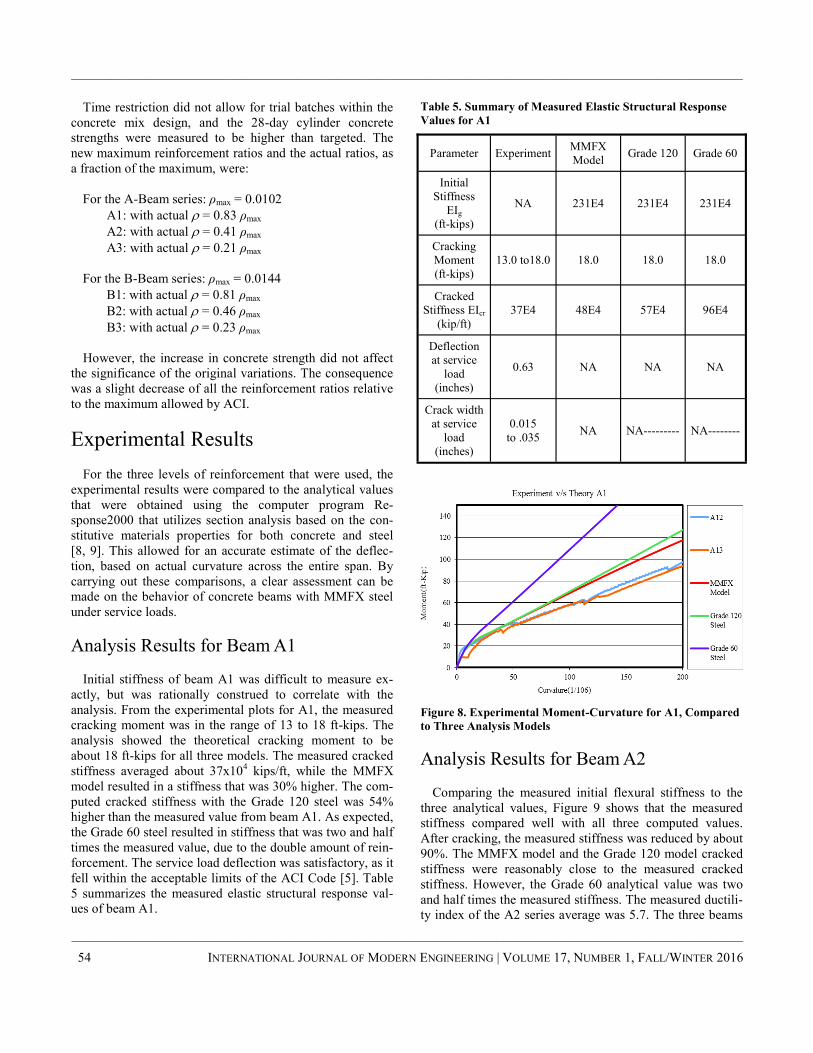
——————————————————————————————————————————————–————
——————————————————————————————————————————————–————
54 INTERNATIONAL JOURNAL OF MODERN ENGINEERING | VOLUME 17, NUMBER 1, FALL/WINTER 2016
Time restriction did not allow for trial batches within the
concrete mix design, and the 28-day cylinder concrete
strengths were measured to be higher than targeted. The
new maximum reinforcement ratios and the actual ratios, as
a fraction of the maximum, were:
For the A-Beam series: ρmax = 0.0102
A1: with actual = 0.83 ρmax
A2: with actual = 0.41 ρmax
A3: with actual = 0.21 ρmax
For the B-Beam series: ρmax = 0.0144
B1: with actual = 0.81 ρmax
B2: with actual = 0.46 ρmax
B3: with actual = 0.23 ρmax
However, the increase in concrete strength did not affect
the significance of the original variations. The consequence
was a slight decrease of all the reinforcement ratios relative
to the maximum allowed by ACI.
Experimental Results
For the three levels of reinforcement that were used, the
experimental results were compared to the analytical values
that were obtained using the computer program Re-
sponse2000 that utilizes section analysis based on the con-
stitutive materials properties for both concrete and steel
[8, 9]. This allowed for an accurate estimate of the deflec-
tion, based on actual curvature across the entire span. By
carrying out these comparisons, a clear assessment can be
made on the behavior of concrete beams with MMFX steel
under service loads.
Analysis Results for Beam A1
Initial stiffness of beam A1 was difficult to measure ex-
actly, but was rationally construed to correlate with the
analysis. From the experimental plots for A1, the measured
cracking moment was in the range of 13 to 18 ft-kips. The
analysis showed the theoretical cracking moment to be
about 18 ft-kips for all three models. The measured cracked
stiffness averaged about 37x104 kips/ft, while the MMFX
model resulted in a stiffness that was 30% higher. The com-
puted cracked stiffness with the Grade 120 steel was 54%
higher than the measured value from beam A1. As expected,
the Grade 60 steel resulted in stiffness that was two and half
times the measured value, due to the double amount of rein-
forcement. The service load deflection was satisfactory, as it
fell within the acceptable limits of the ACI Code [5]. Table
5 summarizes the measured elastic structural response val-
ues of beam A1.
Table 5. Summary of Measured Elastic Structural Response
Values for A1
Figure 8. Experimental Moment-Curvature for A1, Compared
to Three Analysis Models
Analysis Results for Beam A2
Comparing the measured initial flexural stiffness to the
three analytical values, Figure 9 shows that the measured
stiffness compared well with all three computed values.
After cracking, the measured stiffness was reduced by about
90%. The MMFX model and the Grade 120 model cracked
stiffness were reasonably close to the measured cracked
stiffness. However, the Grade 60 analytical value was two
and half times the measured stiffness. The measured ductili-
ty index of the A2 series average was 5.7. The three beams
Parameter Experiment MMFX
Model Grade 120 Grade 60
Initial
Stiffness
EIg
(ft-kips)
NA 231E4 231E4 231E4
Cracking
Moment
(ft-kips)
13.0 to18.0 18.0 18.0 18.0
Cracked
Stiffness EIcr
(kip/ft)
37E4 48E4 57E4 96E4
Deflection
at service
load
(inches)
0.63 NA NA NA
Crack width
at service
load
(inches)
0.015
to .035 NA NA--------- NA--------

——————————————————————————————————————————————–————
exhibited a satisfactory level of ductility. Significant defor-
mation preceded the failure of the beam, which was caused
by concrete crushing. Pronounced yielding of the tension
reinforcement was also observed. The ductility index was
computed with reference to the computed yield moment of
the Grade 120 model. The measured crack width of 0.01
inches at service load was considered within the acceptable
range of values specified by ACI. Grade 60 and Grade 120
models yielded a failure moment within 7% of the measured
value. Table 6 summarizes the measured elastic structural
response values.
Table 6. Summary of Measured Elastic Structural Response
Values for A2
Figure 9. Experimental Moment Curvature for A2, Compared
to Three Analysis models
Analysis Results for Beam A3
As shown in Figure 10, the initial flexural stiffness pre-
dicted by all models correlated to within 8% of recorded
value. The measured cracked flexural stiffness was only 4%
of the initial stiffness, which reflects a 96% loss of stiffness
within the cracked zone. The MMFX model yielded a stiff-
ness that was reasonably close to the measured value. How-
ever, the model with Grade 120 steel resulted in twice the
stiffness. This difference was attributed to the gradual re-
duction in the elastic modulus for the MMFX steel. The
analytical model with an equivalent amount of Grade 60
steel yielded a stiffness value three times the measured stiff-
ness. Even though the amount of steel was only twice that
of A3. The measured crack width under service load was
about 0.025 inches, and exceeded the 0.016 inches specified
in the ACI code, as a limit for normal exposure. Table 7
shows a summary of the measured structural properties for
A3.
Table 7. Summary of Measured Structural Properties for A3
Analysis Results for Beam B1
Figure 11 shows a measured initial stiffness of 287x104
ft-kips, which compared favorably to the computed values
for all three analytical models. The same conclusion was
observed with reference to the cracking moment, where the
computed values overestimated the measured cracking mo-
Property Experiment MMFX
Model Grade 120 Grade 60
Initial
Stiffness
EIg
(ft-kips)
210E4 220E4 220E4 220E4
Cracking
Moment
(ft-kips)
18.0 22.0 22.0 22.0
Cracked
Stiffness
EIcr
(kip/ft)
23E4 31E4 31E4 55E4
Deflection
at service
Load
(inches)
0.77 NA NA NA
Crack
width at
service
load
(inches)
0.01 NA NA NA
Property Experiment MMFX
Model Grade 120 Grade 60
Initial
Stiffness
EIg
(ft-kips)
240E4 220E4 220E4 220E4
Cracking
Moment
(ft-kips)
18.0 22.0 22.0 22.0
Cracked
Stiffness
EIcr
(kip/ft)
8E4 12E4 15E4 25E4
Deflection
at service
Load
(inches)
0.66 NA NA NA
Crack
width at
service
load
(inches)
0.025 -------- --------- --------
——————————————————————————————————————————————————–
SERVICEABILITY PERFORMANCE OF CONCRETE BEAMS REINFORCED WITH MMFX STEEL 55

——————————————————————————————————————————————–————
——————————————————————————————————————————————–————
56 INTERNATIONAL JOURNAL OF MODERN ENGINEERING | VOLUME 17, NUMBER 1, FALL/WINTER 2016
ment by 10%. The measured average flexural stiffness after
cracking correlated perfectly with the MMFX model. How-
ever, the Grade 120 model analysis resulted in a computed
value of 75x104 ft-kips, which was 20% over the measured
value. The Grade 60 model yielded a computed cracked
stiffness of 127x104 ft-kips that was double the measured
value.
Figure 10. Experimental Moment Curvature for A3,
Compared to Three Analysis Models
The deflection of the beam under service load was meas-
ured at 0.72 inches. Assuming 60% was due to a live load,
this yielded a deflection due to a live load of about 0.432
inches, which was less than the maximum deflection al-
lowed by ACI when using the limit L/360. Table 8 summa-
rizes the measured elastic structural properties of beam B1.
Analysis Results for Beam B2
Figure 12 shows that the measured initial stiffness of
beam B2 exhibited some softening that occurred prior to
reaching the theoretical cracking load. This was attributed to
loading and unloading B32 to 13 kips without logging the
data. Therefore, the measured initial stiffness for B2 was not
included in the analysis and, hence, it was not listed in Ta-
ble 9. From the experimental plots for all B2s, the cracking
moment was approximately 25 ft-kips. The analysis of the
three models also indicated that the cracking moment was
about 22 ft-kips. The measured cracked stiffness averaged
about 25 ft-kips, while the MMFX model yielded a stiffness
that was 28% higher. The computed cracked stiffness with
the Grade 120 steel was about twice the measured value and
the Grade 60, which yielded a cracked stiffness three times
the measured value.
The deflection at service load was satisfactory and fell
within the acceptable limits of the ACI Code. Table 8 sum-
marizes the elastic structural response values of beam B2.
Table 8. Summary of Measured Structural Properties for B1
Figure 11. Experimental Moment Curvature for B1,
Compared to Three Analysis Models
Analysis Results for Beam B3
Figure 13 shows that the measured initial stiffness for B3
was 248x104 ft-kips. This value was almost a perfect match
to the computed gross stiffness for all three models. For
beam B3, the cracking moment was around 25 ft-kips. The
analysis for all three models indicated that the cracking mo-
ment was about 22 ft-kips. The measured cracked stiffness
averaged about 16x104 ft-kips, while the MMFX model
yielded a stiffness 18% higher than the measured value. The
Parameter Experiment MMFX
Model Grade 120 Grade 60
Initial
Stiffness
EIg
(ft-kips)
287E4 267E4 267E4 267E4
Cracking
Moment
(ft-kips)
25.0 22.0 22.0 22.0
Cracked
Stiffness
EIcr
(ft-kips)
62E4 61E4 75E4 127E4
Deflection
at service
load
(inches)
0.72 NA NA NA
Crack
width
at service
load
(inches)
.015 to .02 NA NA NA

——————————————————————————————————————————————–————
computed cracked stiffness with the Grade 120 steel was
50% higher than the measured value, and the Grade 60
yielded a stiffness two and half times the measured value.
The deflection at service load was satisfactory and fell
within the acceptable limits of the ACI Code. Table 10 sum-
marizes the measured elastic structural response values of
beam B3.
Table 9. Summary of Measured Structural Properties for B2
Figure 12. Experimental Moment Curvature for B2,
Compared to Three Analysis Models
Table 10. Summary of Measured Structural Response Values
for B3
Figure 13. Experimental Moment Curvature for B3,
Compared to Three Analysis Models
Conclusions
The primary goal of this experimental research project
was aimed at assessing the overall flexural behavior of con-
crete beams reinforced with MMFX steel. The objectives of
this paper were to report the results for the elastic composite
behavior of these beams. The two levels of concrete
strength sheds some light on the impact of the concrete
strength on the beams’ behavior. The reinforcement ratios
Parameter Experiment MMFX
Model Grade 120 Grade 60
Initial
Stiffness
EIg
(ft-kips)
------ 253E4 253E4 253E4
Cracking
Moment
(ft-kips)
25.0 22.0 22.0 22.0
Cracked
Stiffness
EIcr
(ft-kips)
25E4 32E4 48E4 82E4
Deflection
at service
load
(inches)
0.701 NA NA NA
Crack
width
at service
load
(inches)
.015 to .03 NA NA NA
Parameter Experiment MMFX
Model Grade 120 Grade 60
Initial
Stiffness
EIg
(ft-kips)
248E4 243E4 243E4 243E4
Cracking
Moment
(ft-kips)
25.0 22.0 22.0 22.0
Cracked
Stiffness
EIcr
(ft-kips)
16E4 19E4 24E4 43E4
Deflection
at service
load
(inches)
0.54 to 0.82 NA NA NA
Crack
width
at service
load
(inches)
.01 to .03 NA NA NA
——————————————————————————————————————————————————–
SERVICEABILITY PERFORMANCE OF CONCRETE BEAMS REINFORCED WITH MMFX STEEL 57

——————————————————————————————————————————————–————
——————————————————————————————————————————————–————
58 INTERNATIONAL JOURNAL OF MODERN ENGINEERING | VOLUME 17, NUMBER 1, FALL/WINTER 2016
chosen for all MMFX beams were such that steel yielding
was theoretically ensured. The conclusions that can be
drawn from the experimental results are:
1. The stiffness of the MMFX beams was significant-
ly reduced after cracking, and was shown to have a
significant reduction when compared to computed
results of regular steel beams.
2. Deflection under service load for all specimens
indicated that live load deflection would most like-
ly satisfy the ACI Code, and at no time was it ex-
cessive.
3. The measured values of crack width under service
load for all tested beams were within the accepta-
ble range.
4. The cracking moment of the MMFX beams can be
accurately predicted using the ACI procedure.
5. The computer program RESPONSE2000 can be
used with confidence to carry out further paramet-
ric studies.
6. The behavior of the different beam groups con-
firmed the consistency and reliability of the
MMFX steel.
Comparison with control beams showed that, other than
the reduced flexural stiffness, the MMFX beams were com-
parable in behavior to regular steel beams, and the replace-
ment of regular steel with MMFX steel seems to be a viable
alternative that would not compromise the structural ser-
viceability and flexural characteristics of the beams.
Acknowledgement
The authors would like to thank Dr. Salem Faza of
MMFX for the financial support to fund this research pro-
ject, and to Dr. Ronald Cook of the University of Florida for
providing their structural laboratory to carry out the testing.
References
[1] Malhas, F. (2002). Preliminary experimental investi-
gation of the flexural behavior of reinforced concrete
beams using MMFX steel. University of North Flori-
da, report # 904311021.
[2] Hongestad, E. (1951). A Study of Combined Bending
and Axial Load in Reinforced Concrete Members.
Bulletin 399, University of Illinois Engineering Ex-
periment Station, Urbana, Ill.
[3] Rusch, H. (1961). Research toward a General Flexur-
al Theory for Structural Concrete. ACI Journal, 57
(1), 1-28.
[4] Ulfkjaer, J. P. (1998). Experimental Investigation of
Over-Reinforced Concrete Beams of Three Different
Types of Concrete and Two Different Size Scales.
Proceedings FRAMCOS-3, AEDIFICATI Publishers.
[5] ACI Committee 318 (2008). Building Code Require-
ments for Structural Concrete and Commentary (ACI
318 08). American Concrete Institute, Farmington
Hills, MI, 465 pp.
[6] ACI Committee 435 (2003). Control of deflection in
concrete structures (ACI 435R-95). American Con-
crete Institute, Farmington Hills, MI, 89 pp.
[7] El-Hacha, R., & Rizkalla, S. H. (2002). Fundamental
Material Properties of MMFX Steel Bars. Research
Report RD02/04, North Carolina State University,
Constructed Facilities Laboratory, Raleigh, North
Carolina USA, 62 pp.
[8] Bentz, E. C (2002). Sectional Analysis of Reinforced
Concrete. Doctoral Dissertation, Department of Civil
Engineering, University of Toronto, Toronto, Cana-
da.
[9] Bentz, E. C. (2000). Response-2000. Retrieved from
http://www.ecf.utoronto.ca/~bentz/r2k.ht
Biographies
FARIS MALHAS is Dean of the School of Engineer ing
& Technology at Central Connecticut State University. He
earned a BSE and an MSE in Civil Engineering from the
University of Michigan-Ann Arbor, and an MS in Engineer-
ing Mechanics and a PhD in Civil Engineering from the
University of Wisconsin-Madison. His research interests
include the behavior of concrete structures and structural
steel design codes and provisions. Dr. Malhas may be
reached at [email protected]
MUSTAFA MAHAMID is a Clinical Associate Profes-
sor at the University of Illinois at Chicago and an independ-
ent consultant working for several engineering firms. He
earned a BS in Civil Engineering from the Eastern Mediter-
ranean University in Turkey, an MS in Civil Engineering
from Bradley University, and a PhD in Civil Engineering
from the University of Wisconsin–Milwaukee. Dr. Maha-
mid has extensive practical experience in industry and has
worked on projects in the U.S., Europe, the Middle East,
and China. His interests include earthquake engineering,
structural steel building behavior and connection design,
concrete structures, and computational mechanics. Dr. Ma-
hamid may be reached at [email protected]
ADEEB RAHMAN is an associate professor of engi-
neering mechanics in the Department of Civil Engineering
and Mechanics at the University of Wisconsin-Milwaukee.
He received a PhD from the University of Wisconsin-
Madison in the area of solid mechanics. His area of exper-
tise includes computational structural mechanics, the re-

——————————————————————————————————————————————–————
sponse of steel connections to fire loading, and computa-
tional modeling of structural frames in seismic loading. He
has more than fifty journal and conference publications in
highly specialized publications. He is currently active in
research focusing on the performance of steel connections
in elevated temperatures. He was twice the recipient of the
prestigious Fulbright Award for the U.S. Fulbright Scholar-
ship program. Dr. Rahman may be reached at
——————————————————————————————————————————————————–
SERVICEABILITY PERFORMANCE OF CONCRETE BEAMS REINFORCED WITH MMFX STEEL 59

A GENERAL METHOD FOR FAILURE ANALYSIS
AND RE-DESIGN OF A MECHANICAL DIODE ——————————————————————————————————————————————–————
Kevin M. Hubbard, Missouri State University; Martin P. Jones, Missouri State University; Nebil Buyurgan, Missouri State University
Abstract
In this study, the authors performed an extensive investi-
gation on mechanical diode failures and, in this paper offer
recommendations for re-designing elements associated with
the failure of the mechanism. The analysis can be employed
as a case study, which outlines a general method of ap-
proach for solving similar problems. Mechanical diode fail-
ure data were analyzed based on demographics, component
dimensional/geometric and material properties, and me-
chanics of materials. Strut failure and spring weakening
were identified as the two major causes of failure, after a
series of investigations on demographics and component
properties. In-depth mechanics of materials analyses for
struts and springs reveal that weakening and/or failure of the
mechanical diode's springs may lead directly to potential
strut failures and strut failure may lead to major diode fail-
ure. A number of changes in the processing of springs and
struts, the material, and geometry are recommended to yield
additional benefits.
Introduction
Mechanical diodes are unidirectional clutches used to
transmit extremely high torques from the crankshaft of an
engine to the driveshaft of a vehicle [1]. In conventional
unidirectional clutches (sprag- and roller-style clutches), the
torque transmission function takes place as a result of the
frictional contact of several small sprags or rollers between
inner and outer races [2]. The components incorporated in
these types of unidirectional clutches must be machined to
extremely small tolerances [3]. Mechanical diodes incorpo-
rate rectangular struts, which engage between two plates
called a pocket plate and a notch plate, in order to transmit
torque. These types of unidirectional clutches incorporate
fewer components and, therefore, are capable of transmit-
ting larger torques than sprag- or roller-style clutches, and
may be fabricated using less-demanding tolerances.
One manufacturer of agricultural tractors incorporates
mechanical diodes as a torque amplifier option on several
models. Mechanical diodes incorporated into these tractors
experienced high failure rates in service, resulting in signifi-
cant negative financial impact on the company. In this pa-
per, the authors describe the methods employed for per-
forming failure analyses and re-design of the mechanical
diode elements associated with the failure of the mecha-
nism.
The mechanical diode assembly considered in this study
exhibited a relatively high failure rate. Failed units exhibited
lives of approximately 15 months, on average. Figure 1 de-
picts the failed unit of a typical mechanical diode, and Fig-
ure 2 depicts a complete mechanical diode assembly, which
has been cut away to reveal its internal components. Figure
3 shows a schematic diagram of the mechanical diode
mechanism.
Figure 1. Components of a Failed Mechanical Diode
In order to establish possible causes for these failures and
formulate corrective actions, data were collected and ana-
lyzed in the following areas:
1. Demographics: The data collected and analyzed in
this category related to assembly calendar life, geo-
graphic region of service, customer complaint, and
causal/symptomatic diagnosis of the failed unit.
2. Component Dimensional/Geometric and Material
Properties: The data collected and analyzed in this
category related to the conformance of the assem-
bly's component parts with print specifications.
——————————————————————————————————————————————–————
60 INTERNATIONAL JOURNAL OF MODERN ENGINEERING | VOLUME 17, NUMBER 1, FALL/WINTER 2016

——————————————————————————————————————————————–————
3. Mechanics of Materials Analyses: These calcula-
tions related to the strength of the component mate-
rials, and the stresses/strains to which these compo-
nents are subjected in service. Static, dynamic, and
fatigue analyses were performed. These analyses
focused primarily on the mechanical diode's strut
and the double-helical torsion spring components.
Figure 2. Mechanical Diode Assembly
Figure 3. Schematic of a Mechanical Diode Mechanism
Analysis indicated that no correlation existed between
unit failure and demographic data. In addition, no major
problems with dimensional/geometric and material proper-
ties conformance of component parts with print specifica-
tions were identified. Furthermore, the number of stress
cycles experienced by the spring in service quickly exceed-
ed the spring’s fatigue life. It was also noticed that spring
weakening might cause non-full engagement of the strut
with the tooth and pocket plates, leading to strut failure in
compression or buckling.
Materials and Methods
A database containing demographic data was provided by
the manufacturer along with failure cause types and failure
modes. Failure cause types included broken cap on mechan-
ical diode, low lube pressure, strut failure, and no problem
found. Failure modes included freewheel-failure to engage,
lockup, intermittent engagement, and no failure mode iden-
tified. Failure causes and modes were categorized by using
a fishbone diagram, which is a common practice for process
improvement [4]. The most common failure mode was com-
plete lockup (85%), followed by freewheel (15%) and inter-
mittent engagement (5%).
Failures were categorized by the U.S. states in which the
failure occurred. Sales figures for the mechanical diode
were used to determine the approximate percentage of diode
failures rates for each state (i.e., number failed/number
sold). Failures were also categorized by the month of the
year, in an attempt to determine whether extreme tempera-
tures had an effect on mechanical diode life. Table 1 pre-
sents the top ten U.S. states with the highest failure rates,
and Table 2 presents monthly distribution of failures.
Table 1. States with the Highest Failure Rates
Table 2. Failure Rate by Month
Another set of data was collected for inspection and
measurement of the components’ dimensions and material
properties, in comparison to specifications shown in Table
3.
——————————————————————————————————————————————————–
A GENERAL METHOD FOR FAILURE ANALYSIS AND RE-DESIGN OF A MECHANICAL DIODE 61
State % Failure State % Failure
IA 14.68 MI 7.61
MD 10.26 OH 6.94
KS 8.93 MO 6.82
PA 8.33 NE 6.41
WI 7.75 AL 6.25
Month % Failure Month % Failure
February 15.58 December 7.37
August 12.21 April 6.95
November 12.00 May 5.26
July 11.79 October 5.26
September 9.89 January 2.32
June 9.47 March 1.89

——————————————————————————————————————————————–————
——————————————————————————————————————————————–————
62 INTERNATIONAL JOURNAL OF MODERN ENGINEERING | VOLUME 17, NUMBER 1, FALL/WINTER 2016
Table 3. Components and Measured Properties
Based on the collected and analyzed data, no correlation
was found between climatological conditions, such as tem-
perature as a function of region or of month, and mechanical
diode failure rate. The measurements of component proper-
ties were compared to the specifications supplied by the
manufacturer. No significant departures from the specified
dimensional tolerances were found in any of the new or in-
service struts, pocket plates, or notch plates. Visual inspec-
tion of the struts revealed impact marks on the top (notch
plate side) surface of struts, which had seen service and oc-
casional heavy wear and deformation of these struts' contact
edges. Material hardness was found to be within specifica-
tions, and there appeared to be no external or internal cracks
in the struts when inspected using die-penetrant. Fluorescent
magnetic particle inspection of the struts also found no dis-
continuities. A number of struts that had been in service
were bent.
An inspection of springs that had been in service revealed
a significant incidence of heavy wear on the legs and
tongues, and a greatly reduced spring constant (k). Springs
that had not been placed in service exhibited spring con-
stants that were within, or were higher than, specification.
This indicated that the springs weakened in service. It was
concluded that the springs were unlikely to have been sub-
jected to loading in service at or near their natural frequen-
cies, which are a function of spring constant and mass of the
sprung load [5]. Analysis of demographic and geometric
measurement data dismissed a number of possible failure
causes. Two primary failure causes were determined to have
high probabilities: strut failure and spring weakening
(failure in fatigue).
Strut Stress/Strain Analysis
Many of the possible modes of failure arise as a result of
strut column buckling or strut beam bending [6]. It is un-
likely that the strut fails in column buckling, since the force
required to buckle the column (strut) is so great that com-
pressive fracture should occur before buckling. The follow-
ing variables are defined for buckling:
Pcr = force required to buckle the strut
E = Young's modulus of the strut material
I = second moment of inertia of the strut's column
cross-sectional area
L = length of the strut: axial from notch plate to pocket
plate
b = the length of the base of the strut's cross-section
h = the thickness of the strut's cross-section
Then, if the strut is loaded as a column, the buckling force
can be calculated, as given by Equation (1):
(1)
where,
Figure 4 shows the geometry and loading of the strut as a
column. Here, b = 0.450 in., h = 0.090 in./cos(15) = 0.093
in., and I = 3.0210-5 in4. A typical modulus of elasticity for
1075 steel is approximately 30106 psi and a general value
for the modulus of elasticity of 4340 steel is 29106 psi.
With E = 29106 psi and L = 0.440 in., the load necessary to
induce a column buckling-type failure of the strut is about
44,600 lb. If the strut were to experience a 44,600 lb com-
pressive load, then in the small cross-section (where the
cross-sectional area is 0.450 in×0.093 in. = 0.042 in2), the
strut would experience a compressive stress of about
1,061,900 psi.
Figure 4. Strut-Free Body Diagram: Zero Eccentricity Loading
Strut Double-Helical Torsion
Spring
dimensions coil diameter
parallelism of surfaces wire diameter
strut included angle coil axial length
visual surface inspection spring constant (k)
die-penetrant inspection coil leg length
fluor. mag. particle inspection
surface hardness
Pocket Plate Notch Plate
surface parallelism per print visual inspection
pocket dimensions dimensions
2
2
L
EIPcr
12
bhI
3

——————————————————————————————————————————————–————
Figure 5 shows critical buckling load as a function of strut
thickness. If the strut is within dimensional specification,
the compressive strength of the material should always be
exceeded before pure column buckling occurs. A typical
value for compressive strength of this material is 164,500
psi, which is smaller than the stress needed to induce buck-
ling by a factor of approximately six. As a result, strut buck-
ling is an unlikely failure mode.
Figure 5. Critical Column Buckling Load versus Strut
Thickness
A finite element analysis was also conducted on the strut.
If the strut is not misused in service, and assuming that a
minimum of three struts engage during any loading cycle
(per design specifications), each strut would bear 1840 lb of
compressive force with an 800 lb×ft maximum torque car-
ried by the mechanical diode. If only one strut were en-
gaged, that strut would carry 5520 lb of compressive force.
If at least three struts are engaged, the stress induced in the
small cross-section of the strut is approximately 45,400 psi,
which is too small to cause compressive fracture.
However, if only one strut were to be engaged, the stress
induced in the small cross section of the strut would be
about 136,000 psi. Usually, the compressive strength of
4340 steel ranges between about 109,000 psi and 220,000
psi. If only one strut were engaged while the mechanical
diode transmitted a torque of 800 ft×lb, a failure of that strut
by compressive fracture is a real possibility. Note that these
analyses do not take into consideration any surface imper-
fections on the faces of the strut. Wear and other sources of
notching on the strut face can cause local stress concentra-
tions, making failure more likely. Specifically, if the strut is
notched, scratched, or worn, stress concentration factors of
0.5 to 2.0 may apply [7].
The strut experiences complex loading and must be mod-
eled as a beam in compression and bending. Figure 4 also
depicts static loading on one strut when that strut is fully
engaged. The notch plate is at the top of the figure and the
pocket plate is below. The assumption that three struts are
engaged during loading results in a compressive stress of
axial = 45,400 psi, which is significantly below the com-
pressive strength of the material. If the strut is not fully en-
gaged upon loading, however, the forces exerted by the
notch plate/pocket plate combination may be off-axis, re-
sulting in eccentric strut loading. In this case, the two result-
ants form a couple, placing the strut in both bending and
compression, as shown in Figure 6.
Figure 6. Strut-Free Body Diagram: Eccentrically Loaded
The moment, M, generated by this couple is calculated
using Equation (2):
(2)
The normal stress due to bending, b, is then calculated
using Equation (3):
(3)
where, y is the distance from the strut's neutral axis to the
fiber of interest and I is the second moment of inertia of the
beam’s cross-section area.
The neutral axis in this case coincides with the centroidal
axis. Evaluating b at the top and bottom surfaces of the
strut, where sb is maximum, with y = 0.045 in., I = 2.73´10-5
in4, and an eccentricity d = 0.023 in., results in a moment of
42.3 in×lb and a bending stress of 69,725 psi, which is safe-
ly below the tensile and compressive yield strengths of the
strut material. Note that, as designed, the strut would experi-
ence compression on its top surface and tension on its lower
surface. If the strut were subjected only to bending, and if at
least three struts were engaged as the mechanical diode
transmitted 800 lb×ft of torque, the struts would not experi-
ence a significant probability of failure. With only two
struts engaged, b = 139,400 psi leads to a significant possi-
bility of strut bending failure. With a single strut engaged,
b = 209,200 psi and strut bending failure is almost a cer-
tainty.
dR M
I
My = b
——————————————————————————————————————————————————–
A GENERAL METHOD FOR FAILURE ANALYSIS AND RE-DESIGN OF A MECHANICAL DIODE 63

——————————————————————————————————————————————–————
——————————————————————————————————————————————–————
64 INTERNATIONAL JOURNAL OF MODERN ENGINEERING | VOLUME 17, NUMBER 1, FALL/WINTER 2016
If d = 0.030 in. and b = 90,990 psi (with three struts en-
gaged), then this leads to a significant chance of strut bend-
ing, given the range of strengths for 4340 steel due to batch
variation of struts. It is evident that only a small increase in
the eccentricity of the strut loading causes a corresponding-
ly large increase in the normal stress induced in the strut due
to bending moment. If the strut is loaded complexly in com-
pression and bending, the following variables are related in
Equation (4), where c is the compressive normal stress due
to the resultant force, R, in a cross-sectional area, A:
(4)
With three struts engaged and with the mechanical diode
transmitting a torque of 800 lb×ft, c evaluates to 45,432 psi
compressive. The principle of superposition states that the
stresses in the member may be algebraically added at any
given point. Equation (5) shows this force, which defines
tot as the total stress in the strut at a point of interest:
(5)
With three struts engaged and d = 0.023 in., while the
diode transmits a torque of 800 lb×ft, then tot top = -45,432
+ 69,725 = 24,293 psi (tension) and tot bottom = -45,432 +
-69,725 = -115,157 psi (compression). Note: subscript “top”
indicates the stress on the top (notch plate engaging) surface
and the subscript “bottom” denotes the bottom (pocket plate
engaging) surface of the strut. Eccentric loading also pro-
duces a shear stress, , in the strut, as defined by Equation
(6):
= R/AL (6)
where, AL is the transverse cross-sectional area of the strut.
Under the same assumptions (three struts engaged, 800
lb×ft torque) and with L = 0.440 in., AL = 0.440 in×0.450
in. = 0.198 in2, then is evaluated at 9300 psi. The shear
strength of 4340 steel is approximately 124,000 psi. Under
this complex loading situation, the principal stresses (p1,
p2, and max) induced in the strut were evaluated using the
standard Mohr’s Circle plane-stress method. Table 4 enu-
merates these principal stresses. In Cases 1 and 2, the poten-
tial exists for strut failure in compression. Note that if one
strut fails to engage, then the likelihood of failure of the
engaged struts increases dramatically. Also note that these
principal stresses rise dramatically with increases in eccen-
tricity.
Each of the preceding analyses was done under the best-
case assumption that the strut is loaded statically. The fol-
lowing analysis is based on equations developed in mechan-
ical design textbooks. If the strut is loaded dynamically,
impact deformation can be calculated [8] using Equation
(7):
(7)
where,
max = maximum deformation of a mechanical member
under a sudden or impact dynamic load
st = mechanical member deformation under static
load
h = height corresponding to a gravitational potential
energy absorbed by a mechanical member when
a weight is dropped on that member
R = load on the member
L = length of the member along the axis of the load
E = Young's modulus of the member
A = member cross-sectional area perpendicular to
load
Table 4. Principal Stresses at Two Values of Eccentricity
* (T) denotes tension and (C) denotes compression
Note that st is given by Equation (8):
(8)
Since h = 0 for these struts, Equation (7) simplifies to
Equation (9):
(9)
If for a resultant R = 1840 lb (for three struts engaged as
the diode transmits a torque of 800 lb×ft) and assuming
L = 0.440 in, A = 0.090 in×0.450 in. = 0.0405 in2, and
E = 29´106 psi, then st = 6.89´10-4 in. and max = 1.38´10-3
in. As a result, the maximum strain induced in the strut by
A
R = c
bctot σ + σ = σ
d = 0.0225 in., Torque = 800 lb×ft, 3 struts engaged
Top Surface (Case 1)
Principal Stress Values (psi)
Bottom Surface (Case 2)
Principal Stress Values (psi)
sp1 = 26100 (T)* sp1 = 114400 (C)
sp2 = 3300 (C) sp2 = 755 (T)
tmax = 14700 tmax = 57600
d = 0.0300 in., Torque = 800 lb×ft, 3 struts engaged
Top Surface (Case 3)
Principal Stress Values (psi)
Bottom Surface (Case 4)
Principal Stress Values (psi)
sp1 = 47400 (T) sp1 = 137000 (C)
sp2 = 1800 (C) sp2 = 630 (T)
tmax = 24600 tmax = 69000
2
1
st
stmax
h2 + 1 + 1 =
EA
RL = st
stmax 2 =

——————————————————————————————————————————————–————
this sudden load is 0.00313 in/in. Assuming a stress of
164,500 psi, which is the midpoint of the 4340 steel yield
range, the strain at which the strut yields is 0.00567 in/in.
For sudden loading, then, the strut was designed with a fac-
tor of safety of less than two. In the event that a single strut
fails to engage, the likelihood is very high that the remain-
ing two struts will fail. In addition, any eccentricity with
which the load is applied reduces the effective cross-
sectional area of the strut, also making strut failure likely. In
the preceding analysis, a number of problems were shown
to arise if one or more struts (out of three) fail to engage, or
fail to engage fully. The most likely cause of partial- or non-
engagement of the strut is spring weakening or failure,
which will now be discussed.
Spring Life Analysis
When a torque is applied to a torsion spring, the wire in
the spring coil is placed in tension on its outer (farthest from
the coil axis) surface and in compression on its inner sur-
face. The residual stresses left behind in the wire after the
spring winding operation are in the same plane as the work-
ing stress, but of opposite sense. These residual stresses tend
to prolong the life of the spring as long as the load is applied
to the spring in such a way as to cause the spring to wind
up, not un-wind [9]—see Equations (10) and (11):
(10)
where,
M = bending moment to which the spring is subjected
F = external force applied to spring
r = perpendicular distance: force application to coil axis
= normal stress induced in coil wire by applied load F
K = a stress concentration factor
c = distance from spring wire neutral axis to a fiber
I = moment of inertia of wire cross sectional area with
respect to neutral axis
(11)
where,
Ki = stress concentration factor for inner surface of wire
Ko = stress concentration factor for outer surface of wire
C = spring index
D = mean spring diameter
d = spring wire diameter
For this current study, since the spring index C was great-
er than one, the stress concentration factor for the outer sur-
face, Ko, of the wire was less than one, and Ki was greater
than one. For the worst case, Ki would be employed for
stress determination. Substituting M = Fr into the normal
stress Equation (10), Equations (12)-(15) are obtained for
round wire:
results in (12)
where,
= spring angular deflection from its "at-rest" position
(rad)
E = Young's modulus of the spring wire
k = torsion spring constant, aka spring rate (torque/rad)
N = number of coils (turns) in the spring under zero load
(13)
(14)
(15)
where,
Di = inside coil diameter under zero load
Di' = inside coil diameter when loaded
N' = number of spring coil turns when loaded
The ultimate tensile strength of the wires commonly used
in springs depends on the diameter of the spring wire. A
good approximation for this relationship is given by Equa-
tion (16):
(16)
where, A and m are taken from Table 5 [10].
Table 5. Constants and Wire Diameters Used in Sut
Calculation for Spring Types Used by the Manufacturer
Equation (17) was used to determine the maximum oper-
ating torque for "infinite" (106 cycles) spring life, and the
deflection , which corresponds to that torque:
where,
(Fr)a = torque amplitude
(Fr)m = mean torque
I
Mc K= Fr = M and
1C4C
1C4C = K,
1)C4C
1C4C = K,
d
D = C
2
o
2
i
32
πd
c
I 3
3id
32Fr K=
Ed
FrDN67.8 = θ
4
67.8DN
Ed =
Fr =k
4
i'
'i D
N
N = D
S = A
dut m
Type Material ASTM m A (kpsi) d (in)
1 Music Wire A228 0.163 186 0.0140
2 Cr-V A232 0.155 173 0.0136
3 302 Stainless A313 0.146 169 0.0120
——————————————————————————————————————————————————–
A GENERAL METHOD FOR FAILURE ANALYSIS AND RE-DESIGN OF A MECHANICAL DIODE 65

——————————————————————————————————————————————–————
——————————————————————————————————————————————–————
66 INTERNATIONAL JOURNAL OF MODERN ENGINEERING | VOLUME 17, NUMBER 1, FALL/WINTER 2016
(Fr)max = maximum cyclic external torque on the spring
(Fr)min = minimum cyclic torque on the spring
(17)
The current analysis employed the Goodman fatigue
model, since it is among the most conservative [11]. The
mod-Goodman equation is given in Equation (18):
(18)
where, Se is further defined in Equation (19) as the endur-
ance limit of spring wire:
(17)
where,
Using Equation (19) for unpeened springs, the endurance
limits for spring types 1, 2, and 3 were 100 kpsi, 99 kpsi,
and 86 kpsi, respectively. Note the factors for “a” used in
Equation (19) were 0.50, 0.53, and 0.50 for spring types 1,
2, and 3, respectively.
By substitution of Equations (10), (12), and (17) into
Equation (18), Equation (20) shows how infinite life can be
obtained:
(20)
Based on the geometry of the pocket/notch plate, the
spring can "unwind" at most to approximately 35, experi-
encing an angular deflection, , of 25º (0.436 rad) during
over-run. As the strut passes under a tooth on the notch
plate, the spring must deflect to an included angle of ap-
proximately 12, resulting in an angular deflection of 48º
(0.838 rad). For the three types of springs incorporated in
various production runs of the mechanical diode, Table 6
delineates the spring constants and maximum/minimum
torques to which the spring was subjected, corresponding to
these values.
Table 6. Spring Maximum and Minimum Actual Torques at
Low Rotational Speed
The results obtained through the use of Equation (20) are
detailed in Table 7. Tmax N = 106 is the maximum torque al-
lowable, if the strut is to survive for 106 cycles.
Table 7. Maximum Allowable Torques for "Infinite" Life
with Factor of Safety = 1
The (Fr)max torque values in Table 6 should not be al-
lowed to exceed those in Table 7. The torque values in Ta-
ble 7 are based on the following assumptions:
All spring wire diameters are exactly nominal.
All other spring dimensions are exactly nominal.
All spring properties (E, Sut, etc.) are exactly equal to
their theoretical properties.
Considering spring Type 2, listed in Tables 6 and 7, fur-
ther analysis was made considering the following items:
1. If the coil diameter is allowed to go to its lower
limit, then Tmax N=106 remains unchanged.
2. If the wire diameter is as small as d = 0.0136 in (a
± 0.0004-in. tolerance is not unusual for this size
spring wire), then Tmax N=106 = 0.0387 lb×in,, which
is a significant decrease.
3. With a combination of both Items 1 and 2 above,
Tmax N=106 = 0.0389 lb×in.
4. These groups of geometric changes result in the
same sort of corresponding change in Tmax N=106,
regardless of spring type.
5. Changes in the Young's modulus of the spring wire
do not affect Tmax N=106.
6. For all spring types, with a factor of safety of two,
(Fr)max nearly equals or exceeds Tmax N=106, result-
ing in a less than "infinite" life.
Figure 1 show how each of the 21 teeth in the notch plate
travels across each strut of the mechanical diode. Therefore,
at a maximum over-run rotational speed of 5000 rpm, the
2
(Fr) -(Fr) = (Fr) minmax
a
2
(Fr) (Fr) = (Fr) minmax
m
n
1 =
S +
S ut
m
e
a
2
ut
r
re
S
S5.01
0.5S = S
utr aS = S
eut
minutmine
i
3eut
maxS + S
(Fr)S +(Fr)S - nK16
dSS
= (Fr)
Type k (lb×in/rad) (Fr)max (lb×in) (Fr)min (lb×in)
1 0.0283 0.0237 0.0123
2 0.0280 0.0235 0.0122
3 0.0124 0.0104 0.0054
Type Tmax N=106 (lb×in)
1 0.0440
2 0.0389
3 0.0237

——————————————————————————————————————————————–————
strut experiences 6.3106 stress cycles per hour. This indi-
cates that each spring in the mechanical diode, at 5000 rpm
over-run, may be expected to experience 106 cycles in only
9.5 minutes of service. In approximately 16 hours of 5000
rpm over-run service, each spring sees 108 cycles. As the
rotational speed of the mechanical diode decreases, the
number of hours of service that the springs can be expected
to survive in over-run increases, so that at 500 rpm, for ex-
ample, the springs should see 108 cycles of service in 160
hours.
This analysis was performed under the assumption that
the spring deflects as far toward its relaxed position, as is
geometrically permitted when the tip of the strut passes
through the cavity between notch-plate teeth during over-
run. It was also assumed that the tip of the strut would make
physical contact with each tooth as it passes over the strut.
As (Fr)min decreases, the life of the strut also decreases, with
the worst possible case (shortest life) occurring when
(Fr)min = 0. In light of this fact, this analysis covered the
worst-case scenario: rotational speed is low enough to allow
full relaxation of the spring into the notch-plate cavity.
It is possible that, at higher rotational speeds, the spring
does not relax to as great an extent as at low rotational
speeds. Here, the force preventing spring relaxation is the
dynamic pressure caused by the relative velocity of the fluid
with respect to the strut. In order to ascertain the angles to
which the struts and springs were deflected by the fluid's
dynamic pressure, equations were developed that dealt with
the effective area of the strut presented to the fluid stream,
the relative velocity of the fluid with respect to the strut
(using mass continuity), the dynamic pressure caused by
fluid velocity, and the force arising from that dynamic pres-
sure. The torque produced on the strut-spring system by this
force was then balanced against the torque provided by the
spring, since at the top and bottom of the strut's rotation,
angular acceleration was zero and these torques must bal-
ance. These equations were then solved iteratively for .
This analysis was performed at 5000, 2500, and 1000 rpm.
The results are presented in Table 8.
Table 8. qmax as a Function of Rotational Speed Accounting for
Fluid Dynamic Pressure
Even at 5000 rpm, min was calculated to be zero degrees.
Neither the max values in Table 8, nor the min value of zero
is possible, if the geometry of the notch-plate is taken into
account. This analysis did not include the effects of fluid
viscosity and the time response of the strut to moments and
forces acting upon it. However, one conclusion drawn from
these values was that the geometry of the notch-plate (not
the rotational speed of the mechanical diode) is most likely
the controlling factor in determining the maximum and min-
imum values of . Therefore, the maximum and minimum
values of torque experienced by the spring are limited by
the geometry of the notch plate. If this is the case, then the
life values obtained previously are valid, regardless of the
rotational speed at which the mechanical diode is operated.
Results and Discussion
One conclusion arising from this extensive analysis is that
there was no correlation between unit failure and demo-
graphic data. Also, no major problems were identified with
dimensional/geometric and material properties conformance
of the component parts with print specifications. Weakening
and/or failure of the mechanical diode's springs may lead
directly to potential strut failures. The following corrective
measures are indicated:
1. Prevention of Spring Wire Mechanical Stress Re-
lief during Service: It is likely that the residual
stresses left behind by the spring winding operation
are being mechanically relieved. This stress relief
shortens the spring's fatigue life and reduces the
Young's Modulus of the spring wire, leading to
reductions in the spring constant, k. This leads to
eccentric loading of the strut, potentially causing
the strut to fail in compression. One way that this
may be prevented is to subject the spring, after the
winding operation, to a stress relief heat treatment,
thus removing residual stresses before the spring is
placed in service. If this is done, the spring con-
stant should remain constant, or nearly so, through-
out the spring's time in service. Note that if the
spring is subjected to a stress relief heat treatment
before being placed in service, its geometry must
be modified so that the proper spring constant is
obtained after heat treatment [12].
2. Modification of Spring Geometry: The spring's
geometry governs the stress to which the spring
wire is subjected during loading. Increasing the
spring wire diameter, d, and/or decreasing coil di-
ameter, D, reduces stress developed in the wire in
service.
3. Spring Wire Material Substitution: A spring wire
material with a higher ultimate tensile strength
Speed
(rpm)
qmax
(deg.)
Speed
(rpm)
qmax
(deg.)
Speed
(rpm)
qmax
(deg.)
1 5000 25.26 2500 25.28 1000 0
2 5000 25.26 2500 25.28 1000 0
3 5000 25.25 2500 25.26 1000 0
——————————————————————————————————————————————————–
A GENERAL METHOD FOR FAILURE ANALYSIS AND RE-DESIGN OF A MECHANICAL DIODE 67

——————————————————————————————————————————————–————
——————————————————————————————————————————————–————
68 INTERNATIONAL JOURNAL OF MODERN ENGINEERING | VOLUME 17, NUMBER 1, FALL/WINTER 2016
should provide a longer fatigue life [13]. Imple-
mentation of this action alone is not recommended,
however. One or both of the two actions listed pre-
viously should also be employed.
Strut failure may lead to both the lockup-failure mode and
the failure-to-engage mode. Strut failures are likely to occur
primarily as a result of spring weakening and/or failure.
Changes in the processing of the strut, the strut material,
and the strut geometry may, however, yield additional bene-
fits. The following corrective actions are indicated with
respect to the strut components:
1. Elimination of Any Residual Compressive Stress-
es: The strut is subjected to a deburring operation,
which may leave behind residual stresses. These
residual stresses increase the effective stress expe-
rienced by the strut during loading and may lead to
premature strut failure. These residual stresses may
be removed using a stress relief heat treatment,
followed by a strengthening heat treatment to pro-
duce the final desired material properties. In addi-
tion, if decarburization of the strut is a concern, the
strut may be carburized during this heat treatment
cycle.
2. Strut Yield Strength Improvement: A higher yield
and/or ultimate tensile strength may be desirable,
and may be obtained by material substitution or
selection of the proper heat treatment. Care should
be taken, however, when strengthening the materi-
al, to avoid causing susceptibility to failure during
sudden loading or impact.
3. Strut/Pocket Plate/Notch Plate Geometry Modifica-
tion: Sharp corners on the strut act as stress risers.
If a change in geometry becomes necessary, these
corners should be radiused. Also, the triangular
region at each end of the strut has a smaller cross
sectional area than the body of the strut. Thus,
stresses in these regions are higher than those cal-
culated previously, which could be avoided by
providing, if feasible, a generous radius on each
end of the strut. This change, while costly, would
have the additional benefit of making the strut self-
aligning. Actions 1 and 2 should be considered
first, before recommendation 3 is implemented.
Conclusions
Focusing on mechanical diode failures, the authors con-
ducted an extensive study on struts, spring design, and their
properties. Major changes are recommended in the pro-
cessing of springs, the material, and the geometry, including
those of the spring wire and coil diameter. Also recom-
mended are strut material strength improvement (via heat
treatment) and strut geometry modifications. The analysis
presented in this paper represents a thorough approach to
the investigation of the mechanical failure of components
subjected to a wide variety of service conditions, and may
be used as a case study that outlines a general method of
solution for similar problems. Demographic factors based
on geography and seasons were considered. While these
factors were concluded not to have measurable impact on
failure, it is recommended to include these in future failure
investigations.
References
[1] Thorpe, J. F. (1989). Mechanical System Compo-
nents. Prentice Hall.
[2] Budynas, R. G., & Nisbett, J. K. (2015). Shigley's
Mechanical Engineering Design. (10th ed.). McGraw-
Hill Education. New York.
[3] Chesney, D. R., & Kremer, J. M. (1998). Generalized
equations for sprag one-way clutch analysis and de-
sign. (SAE Technical Paper, no. 981092).
[4] Farahmand, K., Grajales, J. V. M., & Hamidi, M.
(2010). Application of Six Sigma to Gear Box Manu-
facturing. International Journal of Modern Engineer-
ing, 11(1), 12-19.
[5] Maier, J. R., Mears, M. L., & Summers, J. D. (2013).
Design of an Apparatus to Detect Small Changes in
the Mass of Rotational Machine Components. Inter-
national Journal of Modern Engineering, 13(2), 5-
16.
[6] Hayduk, R.J., & Wierzbicki, T. (1984). Extensional
Collapse Modes of Structural Members. Computers
& Structures, 18(3), 447-458.
[7] Blandford, G. E. (1997). Review of Progressive Fail-
ure Analyses for Truss Structures. Journal of Struc-
tural Engineering, 123(2), 122-129.
[8] Collins, J. A., Busby, H. R., & Staab, G. H. (2010).
Mechanical Design of Machine Elements and Ma-
chines. (2nd ed.). Wiley.
[9] Akiniwa, Y., Stanzl-Tschegg, S., Mayer, H., Wakita,
M., & Tanaka, K. (2008). Fatigue Strength of Spring
Steel under Axial and Torsional Loading in the Very
High Cycle Regime. International Journal of Fatigue,
30(12), 2057-2063.
[10] Associated Spring-Barnes Group. (1987). Design
handbook: engineering guide to spring design. Bris-
tol, CT.
[11] Osakue, E. E. (2011). A Linearized Gerber Fatigue
Model. International Journal of Modern Engineering,
12(1), 64-72.
[12] Del Llano-Vizcaya, L., Rubio-Gonzalez, C.,
Mesmacque, G., & Banderas-Hernández, A. (2007).

——————————————————————————————————————————————–————
Stress Relief Effect on Fatigue and Relaxation of
Compression Springs. Materials & Design, 28(4),
1130-1134.
[13] Kaiser, B., & Berger, C. (2005). Fatigue Behaviour
of Technical Springs. Material Science and Engineer-
ing Technology, 36(11), 685-696.
Biographies
KEVIN M. HUBBARD is an assistant professor of
Technology and Construction Management at Missouri
State University. He earned his BS degree (Aerospace Engi-
neering, 1991), MS (Engineering Management, 1993), and
PhD (Engineering Management, 1996), all from the Univer-
sity of Missouri–Rolla. Dr. Hubbard is currently teaching at
Missouri State University. His interests include in automa-
tion and device control, manufacturing systems, device de-
sign, and process optimization. Dr. Hubbard may be reached
MARTIN P. JONES is an associate professor of Tech-
nology and Construction Management at Missouri State
University. He earned his BS degree (Physics, 1981) from
University of Maryland Baltimore County, MS (Materials
Science and Engineering, 1984) from the Johns Hopkins
University, and PhD (Materials Science and Engineering,
1987) from the Johns Hopkins University. Dr. Jones is cur-
rently teaching at Missouri State University. His interests
include in scanner technology, nondestructive evaluation,
manufacturing processes, and quality assurance. Dr. Jones
may be reached at [email protected]
NEBIL BUYURGAN is an associate professor of
Technology and Construction Management at Missouri
State University. He earned his BS degree (Industrial Engi-
neering, 1998) from Istanbul Technical University, Turkey,
MS (Engineering Management, 2000) from the University
of Missouri–Rolla, and PhD from the University of Mis-
souri–Rolla (Engineering Management, 2004). Dr. Buyur-
gan is currently teaching at Missouri State University. His
interests include in optimization of logistics operations in
manufacturing, healthcare, military and retail, and supply
chain management. Dr. Buyurgan may be reached at Nebil-
——————————————————————————————————————————————————–
A GENERAL METHOD FOR FAILURE ANALYSIS AND RE-DESIGN OF A MECHANICAL DIODE 69

LATENCY AND PHASE TRANSITIONS
IN INTERCONNECTION NETWORKS
WITH UNLIMITED BUFFERS
Abstract
In this paper, the authors present theoretical and numeri-
cal results for the performance of one-dimensional and a
two-dimensional multiprocessor network models wrapped
around a network of routers with local processors that gen-
erate messages with rate The router models had two and
four output/input ports, respectively. Output ports were as-
sumed to have infinite capacity and are presented here as
M/D/1 queues. Explicit expressions for the distribution of
the number of messages in output port queues, the average
message delivery time (latency), and critical network load
depending on distance between source and destination were
found. Theoretical results were verified with a simulation,
which proved the validity of the mean field theory for these
types of networks, in accordance with the Jackson theorem.
Introduction
Current state-of-the-are computers usually consist of self-
contained processing nodes, with associated memory and
other supporting devices. This type of architecture provides
many advantages, making it possible to perform massively
parallel information processing. However, parallel compu-
ting in such systems requires extensive communications
between processors. These inter-processor communications
are implemented by sending messages from one node to
another via a communication network. This network is im-
plemented as a set of interconnected routers, each connected
to its local processor. Several of the most advanced super-
computers, such as Sequala (BlueGene/Q, IBM), Titan
(Cray XK7), and Trinity (Cray Xc40), have a multi-
dimensional toroidal inter-processor network topology. This
implementation of a network reduces the path length be-
tween nodes and simplifies routing algorithms for static or
dynamic routing.
Many studies [1, 2] have been devoted to analyzing com-
puter communication networks as networks of queues. The
first most important result was obtained by Jackson [3],
where he proved that for an open network of single-server
queues with exponential arrival/departure rates, “the equi-
librium joint probability distribution of queue lengths is
identical with what would be obtained by pretending that
each individual service center is a separate queuing system
independent of the others.” Subsequently, Gordon and New-
ell [4] and Buzen [5] showed that the state distribution for
the M/M/m queuing network has a product form for the first
-come-first-served (FCFS) queuing discipline. (The M/M/m
queuing network consists of nodes that have a Poisson flow
of incoming messages, exponential distribution of service
time, and m servers.) The Baskett, Chandy, Muntz, and Pa-
lacios (BCMP) theorem [6] extends this property of the state
distribution for cases in which the service rate is not neces-
sarily exponential, but has a distribution with a rational La-
place transform, and the queuing discipline is one of the
following four cases: FCFS, processor sharing (PS), infinite
server (IS), or last-come-first-served (LCFS). For FCFS, the
service time distribution must be a negative exponential.
Subsequently, three other classes of networks with exponen-
tial service times have been shown to have product form
distributions [7-9]. Networks with this property have been
analyzed further in [10-14]. Yet other models have been
based on queueing theory [15-20]. Recently, efforts of many
researchers focused on critical phenomena in computer
communication networks [21-33]. Congestion and other
phase transitions were observed and analogies with statisti-
cal mechanics were considered.
One-Dimensional Case: Ring Topology
Each node in the current model consisted of a local pro-
cessor, a router, and buffers of infinite capacity. In this one-
dimensional case, each node was connected to two neigh-
bors, left and right, and had two output ports/buffers. The
following conventions were made in the model.
1. At any clock cycle, a message intended for each of
the output ports could be generated by the local pro-
cessor at every node, independently of others, with a
constant probability .
2. All messages are to be sent to a destination at a dis-
tance exactly l hops from the source. (The distance
between neighbors is equal to one hop.)
3. Any message generated at the node or arriving from a
neighboring node is placed immediately in the output
buffer in the direction of the shortest path to the des-
tination.
——————————————————————————————————————————————–————
Lev B. Levitin, Boston University; Yelena Rykalova, UMass Lowell
——————————————————————————————————————————————–————
70 INTERNATIONAL JOURNAL OF MODERN ENGINEERING | VOLUME 17, NUMBER 1, FALL/WINTER 2016

——————————————————————————————————————————————–————
4. At any clock cycle, if a buffer is not empty, exactly
one message is transferred to the neighboring node,
and it appears at that node at the next clock cycle.
Thus, the service time is equal to one clock cycle.
5. If there is more than one message in the buffer, a
message to be transferred is chosen at random with
equal probabilities, the so-called SIRO (service-in-
random-order) queueing discipline.
6. At the time (clock cycle) when a message reaches its
destination, it is immediately consumed and leaves
the network.
Two-Dimensional Case: Torus
In the two-dimensional case, each node had four neigh-
bors and, correspondingly, four output ports/buffers. In ad-
dition to the conventions listed for the 1-dimentional case,
the following rules were accepted.
1. At any clock cycle, a message intended for each of
the output ports could be generated independently at
every node with probability
2. Each of 4l destinations at distance l from the source
has the same probability of receiving a message.
3. If there is a choice between intermediate nodes on a
shortest path to the destination, each of them is cho-
sen with probability ½.
4. Two different queueing disciplines were considered:
SIRO and the priority discipline in which a newly
generated message is sent first (new-first-order, or
NFO).
It can be seen that this current system differs from net-
works for which the product form of the limiting state prob-
abilities was proved earlier for a number of characteristics.
1. Time is discrete and arrivals occur with specific
probabilities, depending on the distance l (non-
Poisson and non-binomial), as given below by (12).
2. Both SIRO and NFO queueing disciplines were con-
sidered.
3. The service time is deterministic and does not belong
to the class of service time distributions with rational
Laplace transforms.
In general, the choice of models was dictated by two op-
posing considerations. On the one hand, the models were
supposed to reflect some important features of real-life situ-
ations. In particular, the assumption of deterministic service
time is quite natural for homogeneous messages of the same
volume. This case is interesting for researchers, since it does
not satisfy the conditions for which Jackson’s theorem was
proved. On the other hand, the model should be simple
enough to allow a full-fledged theoretical analysis that
would reveal fundamental properties of the communication
process in the network, in the most general closed form as
functions of the parameters of the process. (In particular, it
was important to fix the distance between the source and
destination as one such parameter). Of course, this task can-
not be accomplished by computer simulation.
Theoretical Analysis
The Ring
The time evolution of the queue at each node buffer was
considered as a Markov chain, where the next state depends
on the present state of the buffer, while assuming the steady
- state probability distribution for states of all other buffers.
This approach is similar to the “mean field theory” in statis-
tical physics. The goal of this current project was to obtain
an explicit analytical expression for the distribution of the
number of messages in a buffer at the steady state
(equilibrium) of the network, as it depends on the load
and to determine the critical value of the load that results in
saturation. Let us call the grade of a message the number k
of hops the message has made towards the destination. For
the chosen value of the parameter l, there exist messages of
l different grades in the system: k = 0,1,…, l - 1, since the
messages of grade l disappear from the system. Note that a
message of grade k that leaves a node appears at the next
node as a message of grade k+1. The state of a buffer can be
described as a vector (n0, n1, nl-1), where nk is the number
of messages of grade k. Denote the limiting (steady-state
probabilities) of a state by p(n0, n1, nl-1) in Equation (1):
(1)
According to the SIRO discipline, the probability that a
message of grade k will be transferred is equal to nk/n. Un-
der the steady-state condition, at any clock cycle, the ex-
pected number of messages generated at a node should be
equal to the expected number of messages of grade 0 that
leave the queue. On the other hand, these messages have
grade 1 when they enter the next node, and their expected
number is equal to the expected number of the messages of
grade 1 that leave the next node, and so on, as shown in
Equation (2):
(2)
——————————————————————————————————————————————————–
LATENCY AND PHASE TRANSITIONS IN INTERCONNECTION NETWORKS WITH UNLIMITED BUFFERS 71
1
0
l
k
k
n n
0 1
0 1
0 1
00 1 1
1 0 0
10 1 1
1 0 0
10 1 1
1 0 0
( , , , )
( , , , ) ...
( , , , )
l
l
l
n nl
n n n
n n
l
n n n
n nl
l
n n n
np n n n
n
np n n n
n
np n n n
n

——————————————————————————————————————————————–————
——————————————————————————————————————————————–————
72 INTERNATIONAL JOURNAL OF MODERN ENGINEERING | VOLUME 17, NUMBER 1, FALL/WINTER 2016
Since exactly one message is transferred from any state
except the zero state, Equation (3) follows from Equation
(2),
(3)
and, finally, Equation (4):
p(0,0,…,0) = 1- l (4)
Equation (5) shows how the limiting probabilities of all
states with the same total number n of messages of all
grades are equal:
(5)
where, n is given by (1), is the number of
different states with n messages; and,
P(n) is the total probability of all states with n messages.
After simplification, the balance equations for the limiting
probabilities are given as Equation (6):
(6)
where, P(0) = p(0,0,..,0) is given in Equation (4):
Limiting probabilities are obtained by solving the system
of Equation (6) into Equation (7):
(7)
( 1)!
!( 1)!
m l
m l
Hence, the distribution of the size of the queue is geometric
starting with n =2, and the average number of messages in a
queue is given by Equation (8);
(8)
average latency is given by Equation (9);
(9)
and critical load is given by Equation (10):
(10)
Note that the critical exponent of Equations (8) and (9) is
equal to 1.
The Torus
In the two-dimensional case, similar to the ring case, the
limiting probabilities of all states with the same total num-
ber n of messages of all grades are equal. Therefore, the
equations for limiting probabilities can be written in terms
of P(n), where n is the total numbers of messages in the
buffer. However, an important difference between the
1-dimentional and 2-dimentional cases is that, while in the
Markov chain for the 1-dimentional case there are transi-
tions from a state with n messages only to states with n 1,
n, and n 1 messages n 1), in the 2-dimentional case,
there exist transitions from a state with n messages to the
states with n 1, n, n + 1, n + 2, and n + 3 messages
(n 1). Interestingly, the balance equations for P(n) turn out
to be the same for both SIRO and NFO.
Denoting ai (i = 0,1,2,3) as the probability that exactly i
messages arrive at a particular buffer from neighboring
nodes during one clock cycle, Equation (11) follows from
the description of the model given above:
(11)
0 1
1
0 1 1
0 1 0 0
( , , , )
1 (0,0,..,0)
l
l n nk
l
k n n n
np n n n l
n
p
0 1 1
!( 1)!( , ,.., ) ( )
( 1)!l
m lp n n n P n
m l
( 1) 1 21(0) ( )
1 1 11 (0) ( 1) (1 ) (0) ( 1)
(for )
lP P n
l l
l lP P n P P n
l l l
n 3
( 1) 1 21(0) ( )
1 1 11 (0) ( 1) (1 ) (0) ( 1)
(for )
lP P n
l l
l lP P n P P n
l l l
n 3
2( 1) 1
1(1) (1 ) 1 ,
(1 )(1 )
( 1)( ) (1 ) , for 2
(1 ) (1 )
n n
n n
P ll
lP n l n
l
2
1
( 1)( )
1n
ln nP n l
l
( 1)
1
n ll
l
1crit
l
2
0
1
2 2
2
3 3
3
( 1) ( 1)1 1
2 4
( 1) ( 1) ( 1) ( 1)1 1 1
2 2 2 4
( 1) ( 1) ( 1)1 4 1
16 2 4
( 1)
32
l la
l l l la
l l la
la

——————————————————————————————————————————————–————
Since a message intended for this buffer can also be gen-
erated independently with probability by the local proces-
sor, the probability of the total number of arrivals being
equal to i is given by Equation (12):
(12)
where, a-1 = a4 = 0.
Then, after simplification, the balance equations for each
buffer can be written as Equation (13):
(13)
The characteristic equation is cubic, as shown in Equation
(14):
(14)
The general solution of the system from Equation (13) has
a form given by Equation (15):
(15)
where, A , B, and B* are functions of and l; A is real, while
B and B* are complex conjugates; x1 is the real root of
Equation (14); and, x2 and x3 are two complex conjugate
roots of the characteristic equation. In particular,
Explicit expressions for larger n are too complex to be writ-
ten here. However, with some technical contrivances, rather
simple explicit expressions for the average number of
messages in the buffer, and the average latency can be
obtained, and are described by Equations (16) and (17):
(16)
(17)
Again, the saturation point is given by Equation (18):
(18)
and the critical exponent is equal to 1.
Simulation
The Ring
Simulations were done for rings of length 8 and 16 for
several values of l, starting with l = 2. After achieving the
steady-state regime, the simulation was run for about 50,000
clock cycles at 64 and 256 nodes. Figure 1 shows the proba-
bility distribution of the number of messages (queue length)
n for the ring length of 8 nodes, l = 2, and a near-critical
message generation rate of = 0.45. The solid red line rep-
resents predicted theoretical values, while the green circles
show numerical simulation results.
Probabilities P(n)
Figure 1. Probability Distribution of the Queue Length
n
1 (1 ) ( 0,1,2,3,4)i ia a i
1 0 0
2 1
1 0 0
3 2
2 1 1 0
0
3 3
(0) 1 ,
(1) (1 ) (0) (1) (1 ) (2),
(2) (1 ) (0) (1)
(1 ) (2) (1 ) (3),
(3) (1 ) (0) (1)
(1 ) (2) (1 ) (3)
(1 ) (4),
(4) (0) (1) (1 )
P l
P a a P P a P
P a a P P
a a P a P
P a a P P
a a P a a P
a P
P a P P a a
2
2 1 1 0
0
(2)
(1 ) (3) (1 ) (4)
(1 ) (5),
P
a a P a a P
a P
0
3 2 3
2 3
(1 ) ( 1)
( 2) ( ) ( 1)
( ) ( ),
( 5)
a P n
a P n a a P n
a a a P n
n
3 2
0 1 2 3
2 3 3
(1 ) ( )
( ) 0
a x a a a x
a a x a
*
1 2 3( ) , 5n n nP n Ax Bx B x n
2
32(1) (1 ) 1
(1 )(2 ( 1) )(4 ( 1) )P l
l l
2( 1)(11 5 )
16(1 )
l ln l
l
( 1)(11 5 )
16(1 )
l ll
l
1crit
l
0 20 40 60 80 100 120 140 0
0.01
0.02
0.03
0.04
0.05
0.06
0.07
0.08
——————————————————————————————————————————————————–
LATENCY AND PHASE TRANSITIONS IN INTERCONNECTION NETWORKS WITH UNLIMITED BUFFERS 73

——————————————————————————————————————————————–————
——————————————————————————————————————————————–————
74 INTERNATIONAL JOURNAL OF MODERN ENGINEERING | VOLUME 17, NUMBER 1, FALL/WINTER 2016
Figure 2 shows the inverse value of the average num-
ber of messages as a function of the load for l = 2. The
solid red line represents theoretical values given by Equa-
tion (8). The numerical simulation results for ring lengths 8
and 16 are shown by crosses and circles, respectively.
(probability message generation)
Figure 2. The Inverse Length of the Queue
Figure 3 shows the inverse values of the latency, , as a
function the network load for l = 2. The solid red line repre-
sents theoretical values given by Equation (9). The numeri-
cal simulation results for ring lengths 8 and 16 are shown as
blue crosses and green circles, respectively.
(probability message generation)
Figure 3. The Inverse Latency
1n
1
The Torus
Simulations were done for 16 16 toroidal square lattices
for distances l = 2 and l = 5. The total number of 256´4 buff-
ers were observed at 15,000 points in time with intervals
starting with 10 and going up to 400 clock cycles to guaran-
tee the independence of the samples. Sufficient time was
allowed for the network to come to the steady-state regime
before samples were taken. The probability distribution of
the number of messages in one buffer is given in Figure 4
for a torus size of 256 nodes, l = 5, and = 0.193. The solid
red line represents predicted theoretical values; the blue
dashed line represents numerical simulation results.
Probabilities P(n)
Figure 4. Probability Distribution of the Queue Length
Figure 5 shows the inverse value of the average number
of messages, , as a function of the load . The solid red
line represents theoretical values given by Equation (16);
numerical simulation results for a torus of 256 nodes are
shown as blue dots. The standard deviations of the mean
values were calculated, but because of the large sampling
size, they were too small to be shown in the plot. Figure 6
shows the inverse values of the latency, . The solid red
line represents theoretical values given by Equation (17);
numerical simulation results for a 16 16 torus are shown as
blue crosses.
Discussion of Results
The results showed an excellent agreement between the
theory and numerical experiments. Thus, the presented the-
oretical model of the network as a system of independent
queues provides a very accurate prediction of network be-
n
1n
1
0.1 0.2 0.3 0.4 0.50
1
2
3
4
5
0 0.1 0.2 0.3 0.4 0.5 0
0.1
0.2
0.3
0.4
0.5
0 2 4 6 8 10 12 14 16 18 200.01
0.02
0.03
0.04
0.05
0.06
0.07
0.08

——————————————————————————————————————————————–————
havior. This fact is remarkable, since this system has prop-
erties different from those for which the product form of the
state probability distribution has been proven.
(probability of message generation)
Figure 5. The Inverse Length of the Queue for l = 5
(probability of message generation)
Figure 6. The Inverse Average Latency as a Function of Load
for l = 5
The saturation phenomenon in 1-dimensional and
2-dimensional interconnection networks was shown to be a
phase transition with a critical exponent equal to 1. From
the standpoint of statistical physics, this means that the
mean field theory is exact for the types of networks consid-
ered. In contrast with physical systems, where critical phe-
nomena are observed only in the “thermodynamic limit,”
the saturation in networks occurred for finite systems and,
moreover, the characteristics of network performance seem-
ingly did not depend on the size the system, provided that
the distance l is smaller than the maximum distance between
nodes. It was seen that in both 1-dimensional and
2-dimensional cases, the phase transition was continuous (of
the second order), and the critical load was inversely pro-
portional to the distance between the source and the destina-
tion. This fact is not surprising, since the utilization of every
link in the network (the fraction of time when the link is
busy) is given by Equation (19):
(19)
Also, the analysis showed that the choice of the queueing
discipline had no effect on network behavior.
Conclusions and Future Work
The results of this study demonstrated the existence of a
strong analogy between phenomena in communication net-
works and in systems studied by statistical physics. It opens
a prospect for the development of a consistent physical the-
ory of computer communication systems that would be able
to employ the powerful and well-developed apparatus of
statistical physics for the analysis and control of the pro-
cesses in communication networks. The other possible ex-
tension of this research would be application of a similar
approach to other network topologies, sets of parameters,
queueing disciplines, etc.
References
[1] Kleinrock, L. (1975). Queueing Systems Volume I:
Theory. New York: Wiley.
[2] Kleinrock, L. (1976). Queueing Systems Volume II:
Com. Applications. New York: Wiley,
[3] Jackson, P. (1963). Job shop like queueing systems.
Management Sci., 10(1), 131–142.
[4] Gordon, W. J., & Newell, G. F. (1967). Closed
queueing systems with exponential servers. Oper.
Res., 15, 254-265.
[5] Buzen, J. P. (1973). Computational algorithms for
closed queueing networks with exponential servers.
Commun. ACM., 16(9), 527-531.
[6] Baskett, F., Chandy, K. M., Muntz, R. R., & Pala-
cios, F. G. (1975). Open, closed, and mixed networks
of queues with different classes of customers. J.
ACM, 22(2), 248-260.
[7] Spirn, J. P. (1979). Queueing networks with random
selection for service. IEEE Trans. Software Eng., SE-
5, 287-289.
[8] Noetzel, A. S. (1979). A generalized queueing disci-
pline for product form network solution. J. ACM, 26
(4), 779-793.
0.02 0.04 0.06 0.08 0.1 0.12 0.14 0.16 0.18 0.20
2
4
6
8
10
12
14
16
18
20
Probability of message generation
0 0.02 0.04 0.06 0.08 0.1 0.12 0.14 0.16 0.18 0.20
0.02
0.04
0.06
0.08
0.1
0.12
0.14
0.16
0.18
0.2
1 (0)P l
——————————————————————————————————————————————————–
LATENCY AND PHASE TRANSITIONS IN INTERCONNECTION NETWORKS WITH UNLIMITED BUFFERS 75

——————————————————————————————————————————————–————
——————————————————————————————————————————————–————
76 INTERNATIONAL JOURNAL OF MODERN ENGINEERING | VOLUME 17, NUMBER 1, FALL/WINTER 2016
[9] Chandy, K. M., & Martin, J. (1983). A characteriza-
tion of product form queueing networks. J. ACM, 30
(2), 286-299.
[10] Reiser, M. (1979). Mean Value Analysis of Queueing
Networks—A New Look at an Old Problem. Pro-
ceedings of the Third International Symposium on
Modelling and Performance Evaluation of Computer
Systems: Performance of Computer Systems, M.
Arató, A. Butrimenko, and Erol Gelenbe (Eds.).
North-Holland Publishing Co., Amsterdam, The
Netherlands, The Netherlands, 63-77.
[11] Reiser, M., & Lavenberg, S. S. (1980). Mean value
analysis of closed multichain queueing networks. J.
ACM, 27(2), 313-322.
[12] Reiser, M. (1981). Mean value analysis and convolu-
tion method for queueing dependent servers in closed
queueing networks. Perform. Eval., I(1), 7-18.
[13] Sauer, C. H., & Chandy, K. M. (1981). Computer
Systems Performance Modeling. Englewood Cliffs,
NJ: Prentice-Hall.
[14] Akyildiz, I. F., & Sieber, A. (1988). Approximate
analysis of load dependent general queueing net-
works. IEEE Transactions on Software Engineering,
14(11), 1537-1545.
[15] Nikitin, N., & Cortadella, J. (2009). A performance
analytical model for Network-on-Chip with constant
service time routers. In Proceedings of the 2009 In-
ternational Conference on Computer-Aided De-
sign (ICCAD '09). ACM, New York, NY, USA, 571-
578.DOI=10.1145/1687399.1687506 http://
doi.acm.org/10.1145/1687399.168750
[16] Fischer, E., Fehske, A., & Fettweis, G. P. (2012). A
flexible analytic model for the design space explora-
tion of many-core network-on-chips based on queue-
ing theory. In SIMUL 2012, The Fourth International
Conference on Advances in System Simulation, 119-
124.
[17] Zhang, Y., Xiaoguo, D., Siqing, G., & Weimin, Z.
(2012). A Performance Model for Network-on-Chip
Wormhole Routers. Journal of Computers, 7(1), 76-
84.
[18] Kiasari, A. E., Lu, Z., & Jantsch, A. (2013). An ana-
lytical latency model for networks-on chip. IEEET-
rans. Very Large Scale (VLSI) Syst., 21(1), 113-123.
[19] Qiu, T., Lin, F., Feng, X., Wu, G., & Yu, Z. (2011).
A packet buffer evaluation method exploiting queue-
ing theory for wireless sensor networks. Computer
Science and Information Systems/ComSIS, 8(4), 1027
-1049.
[20] Nagendrappa, T., Muddenahalli, F., Takawira, F.
(2013). Queuing analysis of distributed and receiver-
oriented sensor networks: distributed DS-CDMA-
based medium access control protocol for wireless
sensor networks. IET Wireless Sensor Systems, 3(1),
69-79.
[21] Dabrowski, C. (2015). Catastrophic event phenome-
na in communication networks. Comput. Sci.
Rev. 18, C (November 2015), 10-45. DOI=http://
dx.doi.org/10.1016/j.cosrev.2015.10.001
[22] Sarkar, S., Mukherjee, K., Srivastav, A., & Ray, A.
(2009). Understanding phase transition in
communication networks to enable robust and
resilient control. 2009 American Control Conference,
St. Louis, MO, 1549-1554.
doi: 10.1109/ACC.2009.5159994
[23] Sarkar, S., Mukherjee, K., Srivastav, A., & Ray, A.
(2010). Critical phenomena and finite-size scaling in
communication networks. Proceedings of the 2010
American Control Conference, Baltimore, MD, 271-
276. doi: 10.1109/ACC.2010.5530594
[24] Sarkar, S., Mukherjee, K., Ray, A., Srivastav, A., &
Wettergren, T. A.(2012). Statistical Mechanics-
Inspired Modeling of Heterogeneous Packet
Transmission in Communication Networks. IEEE
Transactions on Systems, Man, and Cybernetics, Part
B (Cybernetics), 42(4), 1083-1094.
doi: 10.1109/TSMCB.2012.2186611
[25] Li, W., Bashan, A., Buldyrev, S. V., Stanley, H. E.,
& Havlin, S. (2012). Cascading failures in
interdependent lattice networks: The critical role of
the length of dependency links. Physical review
letters, 108(22), 228702.
[26] Radicchi, F., & Arenas, A. (2013). Abrupt transition
in the structural formation of interconnected
networks. Nature Physics, 9(11), 717-720.
[27] Lawniczak, A. T., Lio, P. P., Xie, S., & Xu, J. (2007,
April). Study of packet traffic fluctuations near phase
transition point from free flow to congestion in data
network model. In 2007 Canadian Conference on
Electrical and Computer Engineering. IEEE. 360-
363
[28] Dabrowski, C., & Mills, K. (2016). The Influence of
Realism on Congestion in Network
Simulations. NIST Technical Note, 1905, 1-62.
http://dx.doi.org/10.6028/NIST.TN.190
[29] Wang, D., Cai, N., Jing, Y., & Zhang, S. (2009,
June). Phase transition in complex networks. In 2009
American Control Conference. IEEE. 3310-3313
[30] Goltsev, A. V., Dorogovtsev, S. N., & Mendes, J. F.
F. (2003). Critical phenomena in networks. Physical
Review E, 67(2), 026123.
[31] Liu, R. R., Wang, W. X., Lai, Y. C., & Wang, B. H.
(2012). Cascading dynamics on random networks:
Crossover in phase transition. Physical Review E, 85
(2), 026110.

——————————————————————————————————————————————–————
[32] Rykalova, Y., Levitin, L. B., & Brower, R. 2010.
Critical phenomena in discrete-time interconnection
networks. Physica A: Statistical Mechanics and its
Applications, 389(22), 5259-5278
[33] Levitin, L. B., Rykalova, Y. (2015). Analysis and
Simulation of Computer Networks with Unlimited
Buffers. In Al-Sakib Pathan, Muhammad Monowar,
and Shafiullah Khan (Eds.) Simulation Technologies
in Networking and Communications: Selecting the
Best Tool for the Test. CRC Press 2015, 3-30. Print ISBN: 978-1-4822-2549-5 eBook ISBN: 978-1-
4822-2550-1
Biographies
LEV LEVITIN is a Distinguished Professor of Engi-
neering Science in the Department of Electrical and Com-
puter Engineering at Boston University. He has published
over 190 papers, presentations, and patents. His research
areas include information theory, quantum communication
systems, physics of computation, quantum computing,
quantum theory of measurements, mathematical linguistics,
theory of complex systems, coding theory, theory of com-
puter hardware testing, reliable computer networks, and
bioinformatics. He is a Life Fellow of IEEE, a member of
the International Academy of Informatics, and is involved
with other professional societies. Professor Levitin may be
reached at [email protected]
YELENA RYKALOVA is cur rently a visiting re-
searcher with the Department of Electrical and Computer
Engineering at Boston University and teaches at UMass
Lowell. Her research interests include computer networks,
in particular application of concepts and models of statisti-
cal physics to the analysis of network performance. She is a
member of IEEE and the Society for Modeling and Simula-
tion International (SCS). Since 2008, she has been active in
the organization and preparation of the SpringSim Multi-
conference as a technical committee member, reviewer, and
publicity and session chair. Dr. Rykalova may be reached at
——————————————————————————————————————————————————–
LATENCY AND PHASE TRANSITIONS IN INTERCONNECTION NETWORKS WITH UNLIMITED BUFFERS 77

THE ROLE OF ADHESIVE FORCES DURING
SEPARATION OF LIQUID-MEDIATED CONTACTS
Abstract
Menisci may form between two solid surfaces in the pres-
ence of an ultra-thin liquid film. When a separation opera-
tion is needed, meniscus and viscous forces contribute to an
adhesion leading to stiction, high friction, possible high
wear, and potential failure of the contact systems such as
micro-devices, magnetic head disks, and diesel fuel injec-
tors. “The situation may become more pronounced when the
contacting surfaces are ultra-smooth and the normal load is
small [1, 2].” In this study, the authors investigated the ef-
fects of different lubricants on the roles of the meniscus and
viscous forces during the separation process for flat-on-flat
liquid-mediated contact separation. Also evaluated were the
factors that influence any change in role of meniscus and
viscous forces.
Introduction
“Menisci may be formed around the contacting and near
contacting asperities due to surface energy effect of a thin
liquid film, when liquid is present at the contact interface of
two surfaces” [3]. A meniscus is formed wherever an asper-
ity touches the liquid. Small amounts of liquid at the point
of contact between the solid surfaces are called pendular
rings. “During the formation of menisci, pendular rings are
formed on contacting surfaces asperities and liquid bridges
are formed on near-contacting asperities” [3]. “When liquid
mediated contact is considered, the formed menisci are the
center of interest.” “The geometric description of the menis-
cus is the meniscus curve. It is formed between the upper
and lower surfaces of the liquid when the two surfaces are
brought in contact. The shape of the meniscus is determined
by the properties of the liquid and solid” [1-3]. “In some
cases, the liquid spreads evenly on the surface, and some-
times it forms into tiny droplets. Liquid spreading evenly on
the surface with maximizing contact angle is known as hy-
drophilic phenomenon and liquid forming into a droplet is
known as hydrophobic phenomenon.”
“The meniscus is convex for a hydrophobic surface, and it
is concave for a hydrophilic surface. Attractive force
(meniscus force) acts on the interference for hydrophilic
surfaces in contact and repulsive meniscus force for hydro-
phobic surfaces” [1-3]. “The angles formed between the
meniscus curve and the contact surfaces are called contact
angles. The contact angle can be measured through the liq-
uid where a liquid/gas interface meets the solid surface with
sessile drop technique” [2, 4]. The contact angle is an im-
portant indicator of the contacting system. For a multi-phase
solid, such as liquid and gas system under certain conditions
(i.e., different pressures and temperatures), the equilibrium
of the system (represented by the unique contact angles)
reflects the strength or energy level of the materials. “The
formation of the menisci around the contacting and near
contacting surface asperities are due to the effect of the sur-
face energy of the liquid film.”
Figure 1. Schematics of Formation of Menisci between Liquid-
Mediated Contacts [1-3]
“Meniscus and viscous forces are believed to be the major
contributors to adhesion during separation of liquid-
mediated contact” [2]. Many studies have been conducted to
study the separation of liquid-mediated contacts. Cai and
Bushan [5-6] and Cai et al. [7] developed models (CB mod-
el) and studied the separation of two flat-on-flat surfaces
and sphere-on-flat surfaces. In the CB model, various de-
sign parameters, such as contact angle and initial separation
height for specified surface tension and liquid viscosity,
were investigated. More importantly, it was found that the
role of the involved meniscus and viscose forces changes
when the so-called critical meniscus area is reached.
——————————————————————————————————————————————–————
Prabin Dhital, Minnesota State University, Mankato; Shaobiao Cai, Minnesota State University, Mankato
——————————————————————————————————————————————–————
78 INTERNATIONAL JOURNAL OF MODERN ENGINEERING | VOLUME 17, NUMBER 1, FALL/WINTER 2016

——————————————————————————————————————————————–————
The behaviors of a liquid bridge, when compressed and
stretched in a quasi-static fashion between two solid surfac-
es that have contact angle hysteresis (CAH), was studied by
Chen et al. [8]. They developed a theoretical model to ob-
tain the profiles of the liquid bridge, given a specific separa-
tion between the surfaces, where the model is able to cor-
rectly predict the behavior of the liquid bridge during a qua-
si-static compressing/stretching loading cycle in experi-
ments. It was found that the liquid bridge can have two dif-
ferent profiles at the same separation during one loading and
unloading cycle, and more profiles can be obtained during
multiple cycles, where maximum adhesion forces are influ-
enced by contact angle hysteresis (CAH).
When a separation of two liquid-mediated contact surfac-
es is needed, various factors need to be considered in order
to characterize the involved forces. The effects of separation
distance, initial meniscus height, separation time, and
roughness were studied by Cai and Bhushan [1, 3,
5]. Contact angle, as one of the major factors in liquid-
mediated contacts, has been studied intensively. The study
on adhesion contributed by meniscus and viscous forces
during the separation of two hydrophilic smooth surfaces
with symmetric and asymmetric contact angles was studied
by Cai and Bhushan [3, 5]. In these studies, a critical menis-
cus area (at which meniscus force equals the viscous force)
was first identified and defined as the meniscus area at
which meniscus and viscous forces change roles. It was
found that, with the increase in separation distance, menis-
cus forces decrease and the integrative viscous force needed
to overcome increases. The increase in initial meniscus
height for rough surfaces and the increase in surface rough-
ness cause an increase in meniscus force but do not have a
significant effect on the viscous force [5].
A three-dimensional model for liquid-mediated adhesion
between two rough surfaces was developed by Rostami and
Streator [9] by analyzing the effect of liquid surface tension,
nominal contact area, and external load on the stability of
contact interface. They found that an increase in external
load causes more interaction between contact surfaces,
which causes the reduction in the average gap and an in-
crease in separation height and contact area as a result of an
increase in tensile force. Wang et al. [10] investigated the
effect of various parameters such as the mass and radius of
the sphere, viscosity, surface tension, and volume of the
liquid during a dynamic separation process for two different
configurations (sphere from a flat surface and sphere from a
sphere surface). They found that the separation time is long-
er for sphere-on-sphere surfaces for the same limitations.
An increase in mass leads to a decrease in external force, so
that separation time increases. Between two configurations,
they been found that the influence of the mass and radius of
the sphere on separation time are much weaker on sphere-on
-sphere separation. An increase in viscosity and surface ten-
sion leads to an increase in separation time, and it is deter-
mined that the influence of the liquid’s viscosity and surface
tension on separation time are much weaker in sphere-on-
sphere surfaces than that for the sphere-on-flat cases.
For the separation of two surfaces with a formed liquid
bridge, an external force larger than the meniscus force is
required to initiate the separation process, and higher level
forces may be needed to overcome the additional viscous
force contribution thereafter. It was noticed that meniscus
force decreases, whereas the integrated viscous force over
the separation distance from the initial position increases.
This indicates that the role of meniscus and viscous forces
may be changed during the separation process. This has
been numerically verified through the simulation of separa-
tion processes [1]. Further, the effects of separation dis-
tance, initial meniscus height, separation time, contact an-
gle, division of menisci, and roughness on meniscus and
viscous force were analyzed in this current study.
The results showed that the viscous force increases with
an increase in separation distance. Initial meniscus height is
also one of the major factors affecting the magnitude of
viscous forces during the separation process, where the vis-
cous force decreases with an increase in the initial meniscus
height. The time taken to break the meniscus during the
separation process is the separation time. It is common that
the separation time is less than a second, and even at or
about the microsecond scale. The longer the separation
time, the smaller the magnitude of the viscous force, since
the viscous force during the separation process is inversely
proportional to the separation time [1-6].
“During the separation of two flat contact surfaces, the
viscosity of the liquid causes an additional attractive force, a
rate dependent viscous force” [2]. Both the meniscus and
viscous forces cause an adhesive force during the separa-
tion. “When separation operation of two contact surfaces is
needed, adhesion due to the meniscus and viscous force is
one of the major reliability issues leading to failure or
reduction in the consistency of devices such as diesel fuel
injectors in operation.” “The issue becomes more severe
when the applied load is small (which is common) for micro
or nanoparticle devices. The force required to separate two
surfaces is dependent on both meniscus and viscous forc-
es” [1, 3, 5]. It was found that this type of adhesive force is
highly dependent on the formed meniscus area (neck cross-
sectional area at a given meniscus height, which overlaps
the wetted area), separation time, surface tension, and vis-
cosity of the liquid. During the separation process, the me-
niscus force decreases, whereas the integrated viscous force
——————————————————————————————————————————————————–
THE ROLE OF ADHESIVE FORCES DURING SEPARATION OF LIQUID-MEDIATED CONTACTS 79

——————————————————————————————————————————————–————
——————————————————————————————————————————————–————
80 INTERNATIONAL JOURNAL OF MODERN ENGINEERING | VOLUME 17, NUMBER 1, FALL/WINTER 2016
(to be overcome) over the separation distance from the ini-
tial position increases. The roles of the two forces change
before the surfaces are separated.
Although the effects on meniscus and viscous forces con-
tributing to adhesion during separation of liquid-mediated
contacts have been studied, the role of changes of the con-
tributing forces have not been adequately investigated. It is
known that a critical meniscus area determines the role
change of the forces. However, questions such as how the
critical meniscus area changes with a change in the affecting
factors, such as liquid properties, need to be answered in
order to effectively solve issues associated with adhesion. In
this paper, the authors present a comprehensive study of the
roles of meniscus and viscous forces with the critical menis-
cus area (at which meniscus force equals the viscous force)
during liquid-mediated contact separation. The effect on
critical meniscus area with a change in viscosity and surface
tension were studied for flat-on-flat liquid-mediated contact
separation.
Approaches
As part of the data collection procedure, an established
mathematical model was simulated in MATLAB in order to
analyze the roles of the meniscus and viscous forces, con-
sidering the liquid properties as silicon oil. Figure 2 shows
the configuration of the meniscus formed between flat-on-
flat contact surfaces.
Figure 2. Formation of a Liquid Bridge with Hydrophilic Flat-
on-Flat Liquid-Mediated Surface Contact Separation [1, 2]
Meniscus Force
“The meniscus force on flat on flat contact due to the for-
mation of a meniscus is obtained by integrating the Laplace
pressure over the meniscus area and adding the surface ten-
sion effect acting on the circumference of the interface” [5],
which can be represented by Equations (1) and (2):
(1)
(2)
where,
Fs is the external force needed to overcome the intrinsic
forces contributed by the meniscus force.
Fm is the meniscus force.
Fv is the viscous force.
FL is the attractive force due to Laplace.
FT is the attractive force due to surface tension.
h is the separation height.
γ is the liquid surface tension.
r1 is the radii of the meniscus in orthogonal plane.
Xn is the discrete meniscus radius at time step n.
θ is the contact angle.
θ1,2 is the contact angle between solid surface and menis-
cus for the upper and lower surfaces, respectively.
κk is the kelvin radius.
xc,yc are the center coordinates.
The meniscus height WAS calculated using Equation (3):
(3)
The meniscus force, in terms of separation height, can be
calculated by using Equation (4):
(4)
Viscous Force
“Viscous force occurs due to the presence of viscosity
when two surfaces are separated within a short time” [1].
Characterization of the viscous force is important in order to
estimate the total force needed to separate two liquid-
mediated contact surfaces. The equation for viscous force
during the separation of flat-on-flat surfaces was derived by
using the Reynold’s lubrication equation with a cylinder
coordinate system [5], as given by Equation (5):
(5)
where, η is a kinematic viscosity; h is the separation
distance; and, r is an arbitrary distance (the same as Xn, as
shown in Figure 2) in the central plane of the meniscus in
the direction of separation.
m L TF F F
2
1,22 sinm n n
k
F
1 2 cos coskh r
2
1 21,2
(cos cos )2 sinn
m nFh
3 12
p dhrh r
r r dt

——————————————————————————————————————————————–————
For the separation of two smooth, flat surfaces, the vis-
cous force during the separation of two flat-on-flat surfaces
at a given separation height is given by Equation (6) [4]:
(6)
where, ts is the time to separate the two surfaces; hs is the
break point, which is infinite (theoretically) during the sepa-
ration; and, ho is the initial gap between the two flat surfac-
es.
“Both the meniscus and viscous force is operating inside
the meniscus during the separation process in surface con-
tact” [1, 3, 5]. So the condition like the asymmetric angles,
division meniscus, separation time, and height can signifi-
cantly affect the properties of the meniscus and viscous
forces during the separation. An external force is required to
initiate the separation process. “During the break point ex-
ternal force should be larger than total of meniscus and vis-
cous force” [2]. Through the contact of the two liquid-
mediated surfaces, if the meniscus force is larger than the
viscous force, the meniscus will slowly break without the
application of external forces; however, the time to separate
is longer.
Results and Discussion
“It is known that larger meniscus area leads to larger me-
niscus and viscous force.” “Critical meniscus area (at which
meniscus force equals the viscous force) is a function of
surface tension, which increases with increase in surface
tension” [2]. The critical meniscus area and the forces ex-
hibit a nonlinear relationship when the surface tension is
changed. In order to establish the relationship between vis-
cosity and surface tension with the critical meniscus area at
which the forces change the role, an analysis was performed
on silicon oil at room temperature at a viscosity of 0.4860
Ns/m2, a surface tension of 0.0633 N/m, and a separation
time of 1 second, with a contact angle of 60o. Initially, the
preliminary value of the liquid’s viscosity and surface ten-
sion at room temperature were inserted into Equations (4)
and (6), during flat-on-flat contact separation and solved
numerically. The resulting critical meniscus area, and me-
niscus and viscous force values were recorded. The simula-
tion gave the values of critical meniscus area at different
heights (2 nm to 6 nm) for corresponding meniscus and vis-
cous forces for different liquid properties. Each time the
values of the different liquid properties were inserted, the
simulation program gave the corresponding value of the
meniscus and viscous forces, and a critical meniscus area,
which was noted for further analysis.
The symbols ●■▲♦○ represent the critical meniscus area
values for different viscosities and surface tension values
for initial meniscus height, which varied from 2 nm to 6 nm,
respectively, and the highlighted dashed box on left side of
the graph represents the initial critical meniscus area for
different initial meniscus heights for silicon oil (ηo=0.4860
Ns/m2 and γ= 0.0633 N/m) at room temperature during flat-
on-flat liquid-mediated contact separation. In order to study
the effect of viscosity, the initial value of the liquid proper-
ties was taken as silicon oil (ηo=0.4860 Ns/m2 and γ= 0.0633
N/m). The initial value of the surface tension was kept con-
stant at 0.0633N/m, while the viscosity value was increased
at 5% intervals from its initial value. Each time, the constant
surface tension value of 0.0633N/m and the resulting in-
crease in viscosity value were inserted into the simulation
program.
For example, an increase of 5% of the initial viscosity
yielded 0.510 Ns/m2, and 10% of the initial viscosity yield-
ed 0.535 Ns/m2; hence, the new liquid properties of
0.0633N/m and 0.510Ns/m2, 0.0633N/m and 0.535 Ns/m2,
and so on, were inserted into the program. To analyze the
effect of surface tension, the initial value of the liquid prop-
erties was also taken as silicon oil (ηo=0.4860 Ns/m2 and
γ= 0.0633 N/m). The initial value of viscosity was kept con-
stant at 0.4860 Ns/m2; however, the surface tension value
was increased in increments of 5%, starting from its initial
value. Each time, the constant viscosity value of 0.4860 Ns/
m2 and the resulting increase in surface tension value were
inserted into the simulation program. For example, an in-
crease of 5% of the initial surface tension yielded 0.0665
N/m, and 10% of the initial viscosity yielded 0.0696 N/m;
hence, the new liquid properties of 0.0665N/m and
0.4860Ns/m2, 0.0696N/m and 0.4860 Ns/m2, and so on,
were inserted into the program. Table 1 shows the corre-
sponding increase in viscosity and surface tension values
compared to initial values. These different viscosity and
surface tension values were used for meniscus and viscous
force calculations, and the critical meniscus areas were rec-
orded for different initial heights.
To study the effect of liquid properties, the viscosity val-
ue was increased in 5% increments up to 40%, then 50%
and 100% (see Figure 3) from the initial value of the surface
tension constant (0.0633 N/m). Figure 3 shows the effect of
liquid viscosity on the critical meniscus area during flat-on-
flat liquid-mediated contact separation. It also shows the
effect of increasing viscosity of the liquid on constant sur-
face tension. “It is observed that initial meniscus height and
viscosity of the liquid have a significant effect on the criti-
cal meniscus area. The results show that with the contact
angles of ϴ1 and ϴ2 as 60o, any increase in the initial menis-
4
2 2
0
3 1 1
4
niv
s s
Ft h h
——————————————————————————————————————————————————–
THE ROLE OF ADHESIVE FORCES DURING SEPARATION OF LIQUID-MEDIATED CONTACTS 81

——————————————————————————————————————————————–————
——————————————————————————————————————————————–————
82 INTERNATIONAL JOURNAL OF MODERN ENGINEERING | VOLUME 17, NUMBER 1, FALL/WINTER 2016
cus heights leads to a larger critical meniscus area for the
same viscosity.” “This is because a larger initial meniscus
height leads to a much faster decrease in viscous force com-
pared to the meniscus force so a larger meniscus area is
needed for the viscous force to become comparable to the
meniscus force, which explained previously” [2]. The ratio
of the increase of critical meniscus area for increasing vis-
cosity was always same for 2 nm to 3 nm, 3 nm to 4 nm,
4 nm to 5 nm, and 5 nm to 6 nm separation heights. The
results show that changing the critical area from 5 nm to
6 nm had a higher ratio, followed by 4 nm to 5 nm, 3 nm to
4 nm, and 2 nm to 3 nm. It was observed that critical menis-
cus area decreased with an increase in viscosity. The de-
crease in critical meniscus area resulted in a decrease in
meniscus force. From Figure 3, it can also be observed that
the change in the critical meniscus area from 2 nm to 6 nm
initial separation was almost constant as viscosity increased.
Table 1. Viscosity and Surface Tension after Increasing the
Initial Value at Room Temperature
To study the effect of surface tension, the liquid viscosity
value of ηo=0.4860 Ns/m2 at room temperature was kept
constant and the surface tension was increased. The surface
tension value was increased 5% increments up to 40%, then
50% and 100% (see Figure 4). Figure 4 also shows the ef-
fect of liquid surface tension on critical meniscus area dur-
ing flat-on-flat liquid-mediated contact separation. It was
observed that initial meniscus height and surface tension of
the liquid had a significant effect on the critical meniscus
area. The results also showed that with the contact angles of
ϴ1 and ϴ2 at 60o, an increase in the initial meniscus heights
leads to a larger critical meniscus area for same surface ten-
sion. “This is because a larger initial meniscus height leads
to a much faster decrease in viscous force compared to the
meniscus force” [2]. Thus, a larger meniscus area is needed
for the viscous force to be comparable to the meniscus
force. The ratio of the increase of critical meniscus area for
increasing surface tension is also always the same for 2 nm
to 3 nm, 3 nm to 4 nm, 4 nm to 5 nm, and 5 nm to 6 nm
separation heights. The results showed that changing the
critical meniscus area from 5 nm to 6 nm had a higher value
followed by 4 nm to 5 nm, 3 nm to 4 nm, and 2 nm to 3 nm,
the same as the viscosity analysis in Figure 3. It was ob-
served that the critical meniscus area moved to a higher
value with an increase in surface tension. From Figure 4,
one can also conclude that the change in the critical area
from 2 nm to 6 nm initial separation is constant, as surface
tension increases. Figure 3. Dimensional Relationship between Viscosity and
Critical Meniscus Area at Contact Angles ɵ1 = ɵ2 = 60o,
Constant γ with 0.0633 N/m (silicon oil) for Separation
Time = 1s. Note: ηo = 0.4860 Ns/m2. Initial Meniscus
Area = 8.50×10⁻¹⁰m2
Figure 4. Relationship between Surface Tension and Critical
Area with Contact Angles ɵ1 = ɵ2 = 60o, Constant η with 4860
Ns/m2 (silicon oil) for Separation Time = 1s. Note: γo = 0.0633
N/m
Figure 5 shows the relationship between meniscus and
viscous forces with critical meniscus area and the corre-
sponding effects of viscosity and separation height. It was
Initial Viscosity and Surface Ten-
sion at Room Temperature for
Silicon Oil
ηo= 0.4860
Ns/m2 γo = 0.0633 N/
m
Increased percentage with initial
value
Viscosity
( Ns/m2)
Surface tension
( N/m )
5% 0.510 0.0665
10% 0.535 0.0696
15% 0.559 0.0728
20% 0.583 0.0760
25% 0.608 0.0791
30% 0.632 0.0823
35% 0.656 0.0855
40% 0.680 0.0886
50% 0.729 0.0950
100% 0.972 0.1266
γo=0.0633 N/m
Increasing surface tension

——————————————————————————————————————————————–————
observed that critical meniscus area decreased with an in-
crease in liquid viscosity for the cases where the surface
tension was constant with constant initial meniscus height.
This was due to the most rapid increase in viscous force
when the viscosity of the liquid is higher. Thus, viscous
force can dominate at smaller critical meniscus areas. It was
also noticed that the lower initial meniscus height had a
smaller critical meniscus area. In addition, the rate of de-
crease in critical meniscus area was also smaller for a lower
initial meniscus height, when the liquid viscosity was in-
creased.
Figure 5. Relationship between Meniscus Force and Critical
Area with Contact Angles ɵ1 = ɵ2 = 60o, Constant η (0.4860
Ns/m2) for Separation Time = 1s. Note: γo = 0.0633 N/m (silicon
oil) [2]
Figure 6 presents the relationship between meniscus and
viscous forces, as a function of critical meniscus area with
the effect of surface tension and separation height. The fig-
ure also shows the effects of initial meniscus height and
surface tension on the critical meniscus area in a dimension-
al analysis. It was observed that, for a constant initial menis-
cus height, the critical meniscus area (at which meniscus
force equals the viscous force) increased with an increase in
liquid surface tension. The lower initial meniscus height had
a smaller critical meniscus area. In addition, the rate of in-
crease in critical meniscus area was also smaller for a lower
initial meniscus height. This confirmed the observations
made previously. These observations indicated that viscous
force may be likely to take a dominant role, when initial
meniscus height is smaller.
Conclusion
In this paper, the authors present a study of critical menis-
cus area at which meniscus and viscous forces change roles
during flat-on-flat liquid-mediated contact separation. It was
observed that the critical meniscus area depends upon con-
tact configurations such as viscosity, surface tension, and
separation height.
Figure 6. Relationship between Meniscus Force and Critical
Area with Contact Angles ɵ1 = ɵ2 = 60o, Constant η (0.4860
Ns/m2) for Separation Time = 1s. Note: γo=0.0633 N/m (silicon
oil) [2]
For the same separation time, initial meniscus height,
change in viscosity, and surface tension of the liquid had a
significant effect on the critical meniscus area. Critical me-
niscus area decreased at a higher rate for the higher separa-
tion height (i.e., 6 nm) followed by decreasing initial sepa-
ration (5 nm, 4 nm, 3 nm, and 2 nm). Also, it was observed
that critical meniscus area decreased as the viscosity in-
creased. The change in the critical meniscus area from 2 nm
to 6 nm initial separation height was almost constant, as
viscosity increased. With the increase in surface tension,
critical meniscus area increased and the change in critical
meniscus area from 2 nm to 6 nm initial separation was
nearly constant. The critical meniscus area always increased
with an increase in initial separation for a fixed viscosity or
surface tension. For a fixed initial separation, the critical
meniscus area decreased with an increase in viscosity, but
increased with an increase in surface tension.
The increase or decrease in meniscus and viscous forces
during liquid-mediated contact separation were significantly
affected by changes in meniscus area. These two types of
forces were comparable, when the critical meniscus area
was reached. The domination of either meniscus force or
viscous force depends on the size of the critical meniscus
area.
References
[1] Cai, S., & Bhushan, B. (2007). Meniscus and viscous
forces during normal separation of liquid-mediated
contacts. Nanotechnology, 465-704.
[2] Cai, S., Dhital, P., & Zhao, Y. (2015). Interfacial
Adhesion due to Liquid Mediated Contact of Hydro-
philic Solid Surfaces. Proceedings of the 2015 Inter-
ηo =0.4860 Ns/m2
Increasing viscosity
Increasing surface tension
γo=0.0633 N/m
——————————————————————————————————————————————————–
THE ROLE OF ADHESIVE FORCES DURING SEPARATION OF LIQUID-MEDIATED CONTACTS 83

——————————————————————————————————————————————–————
——————————————————————————————————————————————–————
84 INTERNATIONAL JOURNAL OF MODERN ENGINEERING | VOLUME 17, NUMBER 1, FALL/WINTER 2016
national Conference on Structural, Mechanical and
Material Engineering.
[3] Cai, S., & Bhushan, B. (2008). Meniscus and Viscous
Forces during Separation of Hydrophilic and Hydro-
phobic Smooth/rough Surfaces with Symmetric and
Asymmetric Contact Angles. Philos. Trans. A Math.
Phys. Eng. Sci., 366(1870), 1627-1647.
[4] Orr, F. M., Scriven, L. E., & Rivas, A. P. (1975).
Pendular rings between solids: meniscus properties
and capillary force. J. Fluid Mech., 67, 723- 742.
[5] Cai, S., & Bhushan, B. (2008). Viscous force during
tangential separation of meniscus bridges. Philosoph-
ical Magazine, 88(3), 449-461.
[6] Cai, S., & Bhushan, B. (2008). Meniscus and viscous
forces during separation of hydrophilic and hydro-
phobic surfaces with liquid-mediated contacts. Mate-
rial Science and Engineering-R, 61(1-6), 78-106.
[7] Cai, S., Zhao, Y., & Bhushan, B. (2009). Dry and wet
contact analyses for the study of friction and wear
trends. Proceedings of the Society of Tribologists and
Lubrication Engineers Annual Meeting and Exhibi-
tion, 326-328.
[8] Chen, H., Amirfazli, A., & Tang, T. (2013). Model-
ing Liquid Bridge between Surfaces with Contact
Angle Hysteresis. Langmuir, 3310-3319.
[9] Rostami, A., & Streator, J. L. (2015). Study of Liquid
-mediated Adhesion between 3D Rough Surfaces: A
Spectral Approach. Tribology International, 84, 36-
47.
[10] Wang, L., Rong, W., Guo, B., Huang, G., & Sun, L.
(2011). Dynamic Separation of a Sphere from a Flat
or Sphere in the Presence of a Liquid Menis-
cus. Tribology Transactions, 542-547.
Biographies
PRABIN DHITAL is a gr aduate student in the De-
partment of Mechanical and Civil Engineering at Minnesota
State University, Mankato. He is currently pursuing his
master’s degree in Mechanical Engineering. He earned his
bachelor’s degree in Mechanical Engineering from Kath-
mandu University, Nepal. His areas of interest include me-
chanical system design and modeling, application of DFMA
principles for mechanical design, CAD modeling, and man-
ufacturing processes. He is a student member of the Ameri-
can Society of Mechanical Engineers (ASME). Mr. Dhital
may be reached at [email protected]
SHAOBIAO CAI is an assistant professor in the De-
partment of Mechanical and Civil Engineering at Minnesota
State University, Mankato. His areas of interest include ma-
terial design and manufacturing. His areas of expertise and
research interest include interfacial contact mechanics and
tribology, mechanical failure of materials, layered medium
and design, hydrophobic and hydrophilic micro/nano rough-
ness modeling/fabrication and their various multidiscipli-
nary applications, and the application of DFMA principles
in the development of robust design solutions. He is a regis-
tered professional engineer in the state of Minnesota. He is a
member of the American Society of Mechanical Engineers
(ASME) and the Society of Tribologists and Lubrication
Engineers (STLE). Dr. Cai may be reached at sha-

——————————————————————————————————————————————————
INSTRUCTIONS FOR AUTHORS: MANUSCRIPT SUBMISSION GUIDELINES AND REQUIREMENTS 85
INSTRUCTIONS FOR AUTHORS:
MANUSCRIPT REQUIREMENTS The INTERNATIONAL JOURNAL OF MODERN EN-
GINEERING is an online/print publication designed for
Engineering, Engineering Technology, and Industrial Tech-
nology professionals. All submissions to this journal, sub-
mission of manuscripts, peer-reviews of submitted docu-
ments, requested editing changes, notification of acceptance
or rejection, and final publication of accepted manuscripts
will be handled electronically. The only exception is the
submission of separate high-quality image files that are too
large to send electronically.
All manuscript submissions must be prepared in Mi-
crosoft Word (.doc or .docx) and contain all figures, images,
and/or pictures embedded where you want them and appro-
priately captioned. Also, for all accepted manuscripts, each
figure, image, or picture that was imported into your Word
document must be saved individually as a 300dpi or higher
JPEG (.jpg) file and submitted separately; your manu-
script and figure numbers must be used in the title of the file
(e.g., M12-S-18 Figure 4); that means one additional file
for each image imported into your manuscript. These
300dpi images do NOT need to be embedded in your manu-
script. For tables or graphs created directly in Word, you do
not need to submit them as separate files.
Included below is a summary of the formatting instruc-
tions. You should, however, review the sample Word docu-
ment on our website for details on how to correctly format
your manuscript. The editorial staff reserves the right to edit
and reformat any submitted document in order to meet pub-
lication standards of the journal.
The references included in the References section of
your manuscript must follow APA-formatting guidelines. In
order to help you, the sample Word document also includes
numerous examples of how to format a variety of scenarios.
Keep in mind that an incorrectly formatted manuscript will
be returned to you, a delay that may cause it (if accepted) to
be moved to a subsequent issue of the journal.
1. Word Document Page Setup: Two columns with
¼” spacing between columns; Top of page = ¾"; Bot-
tom of page = 1" (from the top of the footer to bottom
of page); Left margin = ¾"; Right margin = ¾".
2. Paper Title: Centered at the top of the fir st page
with a 22-point Times New Roman (Bold), Small-
Caps font.
3. Page Breaks: Do not use page breaks.
4. Body Fonts: Use 10-point Times New Roman (TNR)
for body text throughout (1/8” paragraph indention); 9
-point TNR for author names/affiliations under the
paper title; 16-point TNR for major section titles; 14-
point TNR for minor section titles; 9-point TNR
BOLD for caption titles for tables and figures; other
font sizes as noted in the sample document.
5. In-text Referencing: List and number each refer -
ence when referring to them in the body of your docu-
ment (e.g., [1]). The first entry must be [1] followed
by [2], [3], etc., continuing in numerical order to the
final entry in your References section. Again, see the
sample Word document for specifics. Do not use the
End-Page Reference utility in Microsoft Word. You
must manually place references in the body of the text.
6. Tables and Figures: Center all tables and figures.
Captions for tables must be above the table, while cap-
tions for figures are below; all captions are left-
justified.
7. Page Limit: Manuscr ipts should not be more than
15 pages (single-spaced, 2-column format).
8. Page Numbering: Do not use page numbers.
9. Publication Charges: Manuscr ipts accepted for
publication are subject to mandatory publication
charges.
10. Copyright Agreement: Review the copyright
transfer agreement.
11. Submissions: All manuscr ipts and associated files
must be submitted electronically; the only exception
would be if you wish to submit a CD with the individ-
ual files for your high-quality images, as noted above.
MANUSCRIPTS should be submitted to Dr . Philip
D. Weinsier, manuscript editor, at [email protected]
along with a copy to [email protected].
FILES containing your high-quality images should
ONLY be submitted to [email protected].

INTERNATIONAL JOURNAL OF ENGINEERING RESEARCH AND INNOVATION
CUTTING EDGE JOURNAL OF RESEARCH AND INNOVATION IN ENGINEERING
Mark Rajai, Ph.D.
Editor-in-Chief California State University-Northridge College of Engineering and Computer Science Room: JD 4510 Northridge, CA 91330 Office: (818) 677-5003 Email: [email protected]
Contact us:
www.iajc.org www.ijeri.org
www.ijme.us www.tiij.org
Print ISSN: 2152-4157 Online ISSN: 2152-4165
• Manuscripts should be sent electronically to the manuscript editor, Dr. Philip Weinsier, at [email protected].
For submission guidelines visit www.ijeri.org/submissions
IJERI SUBMISSIONS:
• The International Journal of Modern Engineering (IJME) For more information visit www.ijme.us
• The Technology Interface International Journal (TIIJ)
For more information visit www.tiij.org
OTHER IAJC JOURNALS:
• Contact the chair of the International Review Board, Dr. Philip Weinsier, at [email protected].
For more information visit www.ijeri.org/editorial
a TO JOIN THE REVIEW BOARD:
• IJERI is the second official journal of the International Association of Journals and Conferences (IAJC).
• IJERI is a high-quality, independent journal steered by a distinguished board of directors and supported by an international review board representing many well-known universities, colleges, and corporations in the U.S. and abroad.
• IJERI has an impact factor of 1.58, placing it among
an elite group of most-cited engineering journals worldwide.
ABOUT IJERI:
INDEXING ORGANIZATIONS:
• IJERI is currently indexed by 16 agencies. For a complete listing, please visit us at www.ijeri.org.

THE LEADING JOURNAL OF ENGINEERING, APPLIED
SCIENCE AND TECHNOLOGY
IJME IS THE OFFICAL AND FLAGSHIP JOURNAL OF THE
INTERNATIONAL ASSOCATION OF JOURNALS AND CONFERENCE (IAJC) www.iajc.org
The International Journal of Modern Engineering (IJME) is a highly-selective, peer-reviewed journal covering topics that appeal to a broad readership of various branches of engineering and related technologies.
IJME is steered by the IAJC distinguished board of directors and is supported by an international review board consisting of prominent individuals representing many well-known universities, colleges,
and corporations in the United States and abroad.
IJME Contact Information General questions or inquiries about sponsorship of the journal should be directed to:
Mark Rajai, Ph.D.
Editor-in-Chief
Office: (818) 677-5003
Email: [email protected]
Department of Manufacturing Systems Engineering & Management
California State University-Northridge
18111 Nordhoff St.
Northridge, CA 91330
The latest impact factor (IF) calculation (Google Scholar method) for IJME of 3.0 moves
it even higher in its march towards the top 10 engineering journals.