ITP-07-70 - CORE

Interdisciplinary Transport Phenomena V, Preliminary Proceedings ITP-07-70 1

Proceedings of ITP2007 Interdisciplinary Transport Phenomena V: Fluid, Thermal,

Biological, Materials and Space Sciences October 14-19, 2007, Bansko, Bulgaria

ITP-07-70

EXERGY OPTIMIZATION IN A STEADY MOVING BED HEAT EXCHANGER

A. Soria-Verdugo*, J. A. Almendros-Ibáñez, U. Ruiz-Rivas, D. Santana

ISE Research Group Carlos III University of Madrid

* Corresponding author: [email protected]

ABSTRACT This work provides an exergy analysis of a moving bed heat exchanger to obtain for a range of incoming fluid flow rates the operational optimum and the incidence on it of the relevant parameters such as the dimensions of the exchanger, the particle diameter and the flow rate of the fluid. The MBHE proposed can be analyzed as a cross flow heat exchanger where one of the phases is a moving granular medium. In the present work the exergy analysis of the MBHE is carried out over operation data of the exchanger obtained in two ways: a numerical simulation of the steady state problem and the analytical solution of the simplified (avoiding conduction terms) equations. The numerical simulation is carried over the two steady energy equations (fluid and solid), involving for the solid the convection heat transfer to the fluid and the diffusion term in both directions, and for the fluid only the convection heat transfer to the solid. The analytical solution is the well-known solution of the simplified problem neglecting conduction effects.

NOMENCLATURE

exchangeheat theofLength exchangerheat theofHeigth

tcoefficien Convection termsconduction ldimensiona-Non,tiesconductivi ldirectiona Particle,,

tiesconductivi ldirectiona Fluid,,particle and fluid ofheat Specific,

ndestructioExergy eunit volumper area particle lSuperficia

particles- walland fluid- wallareaContact ,

LHh

KKkkkkkk

CCAa

aa

p

pzpypx

fzfyfx

pppf

d

p

pwfw

ηξ

scoordinate ldimensiona-Non,re temperatuparticlemean Outlet

r temperatuparticleInlet r temperatuParticle

re temperatuparticle ldimensiona-Nondensity particle and Fluid,

tcoefficienheat specific gas IdealPorossity

drop Pressurescoordinate spatial ldimensiona-Non,,

scoordinate Spatial,,exchangerheat theofWidth

particles and fluidfor coeficient lossesheat Global,components velocity Particle,,

components velocity Fluid,,re temperatufluidoutlet Mean

re temperatufluidInlet mperatureAmbient te

re temperatuFuidre temperatufluid ldimensiona-Non

Timetnumber ReynoldsRe

numberPrandlt Prfluid theof PressureInlet

numberNusselt Nuparticles and fluid of ratesflowMass,

*0

*0

ηξθθθθ

ρργε

S

pf

pwfw

ppp

fff

S

A

e

pf

Pzyxzyx

WUU

wvuwvu

TTTTT

P

mm

∆

&&

brought to you by COREView metadata, citation and similar papers at core.ac.uk

provided by Universidad Carlos III de Madrid e-Archivo

https://core.ac.uk/display/29427776?utm_source=pdf&utm_medium=banner&utm_campaign=pdf-decoration-v1


1. INTRODUCTION Moving Bed Heat Exchangers (MBHE, hereafter) are

widely used in industry, on applications involving heat recovery (providing a high volumetric transfer area) and filtering (avoiding common operational problems in fixed bed or ceramic filters like the pressure drop increase during operation).

One of the fundamental problems to be solved for the implementation of biomass gasification processes is the conditioning of the gas yield. When the gas yield is going to be used as syngas or in an integrated gasification and combined cycle (IGCC), a severe gas cleanup (tars, particles and alkalis) is needed. In the pressurized fluidized bed gasification case, filters prevent downstream erosion of the heat exchanger and the turbine whereas in the atmospheric case, filters could fulfill a multipurpose function, removing fine particles and cooling the gas yield.

A thermal and exergy analysis of the heat exchanger have been performed on a Moving Bed Heat Exchanger (MBHE) similar to the one described in [1], to obtain, for a range of incoming fluid flow rates, the operational optimum and the incidence on it of the relevant parameters such as the dimensions of the exchanger, the particle diameter and the gas flow rate. In Figure 1 a schematic illustration of the MBHE is showed.

v

u

L

Ts

T

0

θs

θ

0

x

y

Hf

p

Fig. 1. Schematic of the granular bed heat exchanger

The concept of exergy analysis of fluid flow and heat

transfer is a powerful tool for optimization when analyzing engineering problems. Since entropy generation destroys the exergy of a system, it makes good engineering sense to focus on irreversibility of heat transfer and fluid flow processes to understand the associated exergy destruction mechanisms. The literature on the topic is rich for clear fluids through unobstructed ducts, but modeling entropy generation in a porous media is more complex than the clear fluid case because of the increased number of variables that appear in the governing equations [2]. This is the procedure chosen in this paper to optimize the design of a moving bed heat exchanger.

2. HEAT TRANSFER ANALYSIS We will firstly address the analysis of the heat transfer in

the moving bed and then consider a more general exergy analysis.

Assuming plug flow for both phases, the energy equations can be written as:

( ) ( )

( )

( ) ( )

)1(

1

2

2

2

2

2

2

2

2

2

2

2

2

radApwpwpppzpypx

ppppp

radAfwfwppfzfyfx

fffff

qTaUTahz

ky

kx

k

zw

yv

xu

tC

qTTaUTahzTk

yTk

xTk

zTw

yTv

xTu

tTC

+−−−+∂∂

+∂∂

+∂∂

=

=

∂∂

+∂∂

+∂∂

+∂∂

−

+−−−+∂∂

+∂∂

+∂∂

=

=

∂∂

+∂∂

+∂∂

+∂∂

θθθθθ

θθθθρε

θ

ερ

where the transient and convective terms for each phase balance with heat transferred by conduction through the same phase and convection between phases, heat losses with the surroundings and radiation. These general equations can be simplified for most cases neglecting radiation and heat losses to the surroundings. The present study has been carried out considering a gas (not a liquid) as fluid, so the conductivity in the fluid equation can be neglected [1]. Also, uf » vf , wf and vp » up , wp can be assumed. Considering steady state and neglecting three dimensional effects, the energy equations become:

( )

( ) ( ))2(

1 2

2

2

2

θθθθρε

θερ

−+∂

∂+

∂

∂=

∂∂

−

−=

∂∂

Tahy

kx

ky

vC

TahxTuC

pppypxppp

ppfff

or, in compact form:

( )

( ))3(

1 2

2

2

2

∂∂

−=−=

=∂

∂−

∂

∂−

∂∂

−

xTuCTah

yk

xk

yvC

fpffpp

pypxpppp

ερθ

θθθρε

Equation (3) can be written in non-dimensional form:

( ) )4(2

2

2

2

ξθ

ηθ

ξθ

ηθ

∂∂

−=−=∂∂

−∂∂

−∂∂ TTKK yx

where:

( )

( ) ( )( )

)5(

1,

1,

,

22

00

0

00

0

pppp

pypp

pfff

pxpp

pppp

pp

pfff

pp

Cvkah

KCukah

K

Cvahy

Cuahx

TTT

T

ρεερ

ρεη

ερξ

θθ

θθθθ

ηξ −==

−==

−−

=−−

=

In a moving bed heat exchanger θ and T will have values between 0 and 1, but this may not be the case for the rest of the


non-dimensional coordinates and parameters. Thus, some insight is needed. We will consider as nominal conditions for our study the moving bed heat exchanger defined in [3], which is a representative one. The fluid is air and the particles are spheres of carbon steel with a diameter of 1mm (mono-dispersed). The dimensions are 0.15m in the direction of the air flow and 0.5m in the direction of the particle motion. The inlet fluid and particle velocities are 3m/hr and 1.5m/s respectively.

We should also estimate the conduction and convection coefficients. Following [4], the effective conductivity of the moving bed without flow, kpx, can be obtained from [5] while the conductivity in the transverse direction, kpy, can be obtained using the equation proposed by [6]. The convection coefficient can be estimated using the following expression for the Nusselt number, as obtained by [7]

( )( ) ( )

( )( )

( )

)6(

1PrRe443.21

PrRe037.0

RePr664.0

215.11

321.0

8.0

21

31

2122

−⋅⋅+

⋅⋅=

⋅⋅=

++⋅−⋅+=

−

ε

ε

ε

ε

t

l

tl

Nu

Nu

NuNuNu

For the nominal conditions, the limit values of the non dimensional coordinates ξ and η are:

( )

)7(350

1)(

350)(

≈−

==

≈==

pppp

ppH

pfff

ppL

CvaHh

H

CuaLh

L

ρεηη

ερξξ

and the non-dimensional conductivities (K) will be in the 1-100 domain.

We will first analyze the nominal case, defined by these values of the non-dimensional parameters. However, other cases will be presented along the article, considering variations of the dimensions of the exchanger and several inlet velocities and particle diameters.

Equations (4) can be solved numerically with the proper boundary conditions. Also, an analytical solution can be obtained if the conduction terms are neglected in comparison with convection. For the simplified problem, two boundary conditions are needed and five if conduction effects are considered. Two conditions are straightforward: the inlet temperatures of particles and fluid are known. This is shown in Table 1 a) for the general case, [4] analyzed a similar problem and obtained the optimum boundary conditions presented in Table 1 b).

Note that the inlet temperature condition for the particles is not present in the general case, as conduction effects will transfer heat upstream from the inlet, affecting the temperatures outside the heat exchanger. Thus, the particles temperature will only be θ0 far upstream from the exchanger inlet section.

Particle 0η = 0θ θ= Fluid 0ξ = 0T T=

a) boundary conditions for the simplified case (no conduction effects)

0ξ = 2

2 0θξ∂

=∂

maxξ ξ=

2

2 0θξ∂

=∂

0η = Kηθθη∂

= ⋅∂

Particle

maxη η= 0θη∂

=∂

Fluid 0ξ = 0T T= b) boundary conditions for the general case

Table 1. Boundary conditions

2.1. Analytical Solution The values of the non-dimensional conductivities suggest

that, the conduction terms have a rather small effect in the heat exchanger if the heat exchange region is not restricted to a very narrow zone in the MBHE. Disregarding such effect, equations (4) become:

( ) )8(ξ

θηθ

∂∂

−=−=∂∂ TT

And the two boundary conditions are: ( )( ) )9(

0010

====

ηθξT

With such conditions, fluid and particle temperature have the analytical solution [8]:

)10(

!!1

!!

0 0

0 0

∑ ∑

∑ ∑∞

= =

−−

∞

= =

−−

−=

=

j

j

k

kj

j

j

k

kj

kje

kjeT

ηξθ

ξη

ξη

ηξ

The calculation of these temperatures has the problem of the rather large summation for large values of the coordinates ξ and η. This implies high computational costs. The maximum value of the summation must be larger that 1.5 times the value of ξ and η to ensure a good approximation. Lower values will result in temperature profiles that will not even fulfill the boundary conditions.

The results are shown in figures 2 to 5. Figure 2 shows the isothermal lines for fluid and particles inside the MBHE. In these graphs we are keeping the x-y (ξ-η) axis directions as shown in figure 1 for clarity purposes. Hot inlet fluid, moving from left to right, exchanges heat with the cold inlet particles, which moving from top to bottom. The temperature change is obtained in a narrow zone around the diagonal of the graph and it is odd that, apart from this small zone, both particles and fluid develop isothermally.


Fig. 2. Fluid and particle isotherms

From these two graphs it is difficult to observe the temperature differences between fluid and particles, which define the heat exchange zone. Therefore the temperature differences are plotted in Figure 3. Maximum temperature differences are of order 10-1-10-2 (being the maximum temperature change 1) and are restricted to a ±30 (ξ and η) zone, representing less than 15% of the heat exchanger volume.

Fig. 3. Fluid and particle temperature difference

The two graphs of figure 2 and figure 3 give a lot of information on the thermal behaviour of the heat exchanger. Note that ξ and η are non dimensional spatial coordinates, but vary with design parameters such as dimensions, mass flow or particle diameter. We will now proceed to study this in deep. Figure 4 shows the outlet temperature profiles for four heat exchangers with different dimensions (length and height). It can be seen that a reasonable heat exchanger must have similar values for ξ and η (cases a and d). When values of ξ and η are different (cases b and c), some part of the fluid (zone A in graph b) or particles (zone B in graph c) leave the regenerator with their inlet temperature, without any heat exchange. Their contribution is therefore negligible and the heat exchanger dimensions can be modified becoming ξ = η = min(ξoriginal,ηoriginal) with negligible heat exchanging effects and important economic gains.

a) 300x300 heat exchanger

b) 300x500 heat exchanger

c) 500x300 heat exchanger

d) 500x500 heat exchanger

Fig. 4. Inlet (··) and outlet (-) temperature profiles


Fig. 5. Outlet temperature profiles for ξ = η = 10, 20, 30, 40, 50, 100, 200, 300, 400, 500.

For heat exchangers of aspect ratio ξ=η, figure 5 shows the differences in the outlet temperature profile for different ξ and η pairs. Logically when ξ and η increase there is an improvement in the outlet temperature profile, but this improvement is small and negligible for high values of ξ and η. Thus, heat exchangers of ξ=η larger than 200 results in larger investments with almost equal outlet mean temperature, and therefore negligible efficiency variation. Larger equipments may only be used if larger mass flows are needed. This can also be attained by increasing the exchanger width, but it will proportionally increase both mass flows, while increasing ξ, η may result in a non proportional increase of each mass flow. Using both parameters the two mass flows can be independently tuned.

Going back to the definitions of the non-dimensional parameters in equations (5), it can be shown that equal values for ξ and η means that both flows, fluid and particles, have the same calorific capacity. This also means that for a steady flow there is an optimal length of the regenerator for a given velocity of the particles. This optimal length can be obtained from:

( ) )11(1 pppp

pff

CvCm

Lρε−

=

•

which is basically a reformulation of the ξ(L) = η(H) equation.

Fig. 6. Optimal thermal length Figure 6 shows this optimal thermal length of the heat exchanger as a function of the fluid mass flow and the particle velocity. Note that these two last parameters are also design parameters for the exchanger.

The non-dimensional analysis gives a very compact solution to the problem, but has the drawback that a ξ, η pair represents a variety of heat exchangers which are physically very different. Restore now the problem to the dimensional domain in order to study the influence of the convection coefficient on the heat exchange.

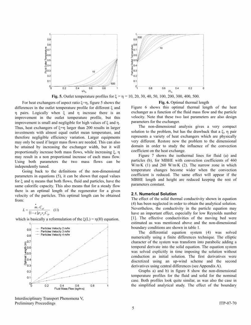
Figure 7 shows the isothermal lines for fluid (a) and particles (b), for MBHE with convection coefficients of 460 W/m·K (1) and 260 W/m·K (2). The narrow zone in which temperature changes become wider when the convection coefficient is reduced. The same effect will appear if the MBHE length and height are reduced keeping the rest of parameters constant.

2.1. Numerical Solution The effect of the solid thermal conductivity shown in equation (4) has been neglected in order to obtain the analytical solution. Nevertheless, the conductivity in the particle equation may have an important effect, especially for low Reynolds number [1]. The effective conductivities of the moving bed were estimated as was mentioned above and the non-dimensional boundary conditions are shown in table 1.

The differential equation system (4) was solved numerically using a finite differences technique. The elliptic character of the system was transform into parabolic adding a temporal derivate into the solid equation. The equation system was solved explicitly in time imposing the solution without conduction as initial solution. The first derivatives were discretized using an up-wind scheme and the second derivatives using central differences (see Appendix A).

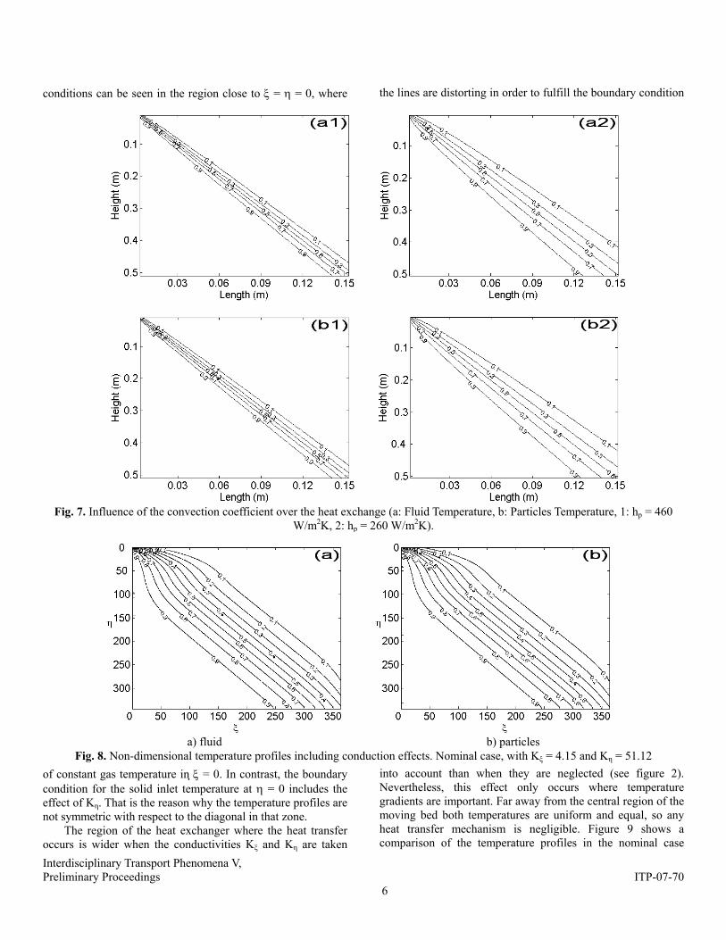
Graphs a) and b) in figure 8 show the non-dimensional temperature profiles for the fluid and solid for the nominal case. Both profiles look quite similar, as was also the case in the simplified analytical study. The effect of the boundary


conditions can be seen in the region close to ξ = η = 0, where the lines are distorting in order to fulfill the boundary condition

Fig. 7. Influence of the convection coefficient over the heat exchange (a: Fluid Temperature, b: Particles Temperature, 1: hp = 460

W/m2K, 2: hp = 260 W/m2K).

a) fluid b) particles

Fig. 8. Non-dimensional temperature profiles including conduction effects. Nominal case, with Kξ = 4.15 and Kη = 51.12 of constant gas temperature in ξ = 0. In contrast, the boundary condition for the solid inlet temperature at η = 0 includes the effect of Kη. That is the reason why the temperature profiles are not symmetric with respect to the diagonal in that zone.

The region of the heat exchanger where the heat transfer occurs is wider when the conductivities Kξ and Kη are taken

into account than when they are neglected (see figure 2). Nevertheless, this effect only occurs where temperature gradients are important. Far away from the central region of the moving bed both temperatures are uniform and equal, so any heat transfer mechanism is negligible. Figure 9 shows a comparison of the temperature profiles in the nominal case


including or neglecting heat conduction (numerical or analytical solution respectively). The temperature profiles are taken in the second diagonal of the exchanger, which goes from (ξ = 0, η = ηmax) to (ξ = ξmax, η = 0). The particle conductivities smooth the slope in the region where heat transfer occurs. When the solid phase conductivity is included in the analysis the heat is transferred, not only from the fluid to the solid, but also by diffusion in the solid phase when solid temperature gradients are important. This effect is particularly important in zones adjacent to the convection heat transfer region.

Fig. 9. Cross section of the non-dimensional solid temperature

obtained from figures 8 (-) and 2 (--) Although the conduction heat exchange has visible effect

on the temperature changes zone, the influence on the outlet temperatures is small for well-designed MBHE. Thus, the general performance of the MBHE can be described in first approximation with the analytical solution.

2. EXERGY ANALYSIS

An exergy optimization analysis was performed in order to get more insight of the optimal design of the MBHE. The exergy balance gives the exergy destruction as:

)12(1 *

0

*

+

∆−−−

=

••

e

Sppp

e

eSpffAd LnCm

PPPLn

TTLnCmTA

θθ

γγ

where and are the mean outlet temperatures of the fluid and the particles, which can either be calculated from the analytical solution or estimated from the numerical solution. The pressure drop was estimated by the Ergun correlation.

)13(75.111501 2

2

⋅⋅+

⋅⋅

−⋅⋅

−⋅=∆

p

ff

p

ff

du

du

LPρρ

εε

εε

The mean outlet temperatures of the fluid and the particles can be calculated from equations (10)

( )

( ))14(

,1

,1

0

*

0

*

∫

∫

==

==

N

N

dT

dTT

NN

S

NN

S

ξ

η

ξηηξξ

θ

ηηξξη

and the following analytical solution can be obtained:

)15(

!1

!1

!1

!

0 00

*

0 00

*

−⋅

−=

−⋅

=

∑ ∑∑

∑ ∑∑∞

= =

−

=

−

∞

= =

−

=

−

j

j

i

ij

k

k

S

j

j

i

ij

k

k

S

ie

ke

ie

keT

ξηξ

θ

ηξη

ξη

ηξ

The dimensional temperatures and can be obtained from these expressions using equations (5).

Computing the mean outlet temperatures has a higher computational cost than computing the temperatures because there are one more summation. Nevertheless, with some refining this calculation can be performed in an average PC in several hours.

We will now study the variations of the exergy destruction with the MBHE length and the particle diameter, for a given fluid mass flow. This will lead to an optimal length and diameter from the exergy point of view. The fluid mass flow can be obtained for different pairs of fluid velocities and MBHE heights (as the mass flow is proportional to the product of fluid velocity and bed height). Thus, we will fix the mass flow and the fluid velocity as parameters in our calculation. This second parameter, obviously, will have an important effect in the pressure drop.

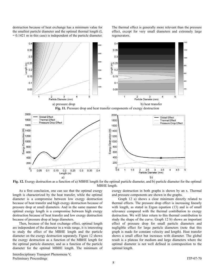
We will first address the nominal case. Figure 10 shows the exergy destruction contour lines for this case, which has a fluid mass flow of 0.3 kg/m·s and a fluid interstitial velocity of 1.5 m/s (this locks the MBHE height to 0.5 m). A minimum exergy destruction of 380.1 W was obtained for a MBHE of 0.139 m length operating with particles of 3.4 mm diameter. Note that the optimal length is almost constant for a wide range of diameters. This length is very similar to the optimal thermal length obtained from equation (11).

Fig. 10. Exergy destruction as a function of exchanger length

and particle diameter for the nominal case From equation (12) the exergy destruction can be divided

into two components, the thermal effect, with contributions of both fluid and particle temperature profiles and the fluid pressure drop effect. Those two components are showed in the two graphs of figure 11 for the same case depicted in figure 10. The exergy destruction because of the pressure drop is higher for larger regenerators and smaller particles, while the exergy

*Sθ

*ST

*Sθ

*ST


destruction because of heat exchange has a minimum value for the smallest particle diameter and the optimal thermal length (L = 0.1421 m in this case) is independent of the particle diameter.

The thermal effect is generally more relevant than the pressure effect, except for very small diameters and extremely large regenerators.

a) pressure drop b) heat transfer

Fig. 11. Pressure drop and heat transfer components of exergy destruction

a) b)

Fig. 12. Exergy destruction as a function of a) MBHE length for the optimal particle diameter, and b) particle diameter for the optimal MBHE length.

As a first conclusion, one can see that the optimal exergy length is characterized by the heat transfer, while the optimal diameter is a compromise between low exergy destruction because of heat transfer and high exergy destruction because of pressure drop at small diameters. And in the same manner the optimal exergy length is a compromise between high exergy destruction because of heat transfer and low exergy destruction because of pressure drop at large diameters.

Then, because of the heat exchange effect, optimal length are independent of the diameter in a wide range, it is interesting to study the effect of the MBHE length and the particle diameter on the exergy destruction separately. Figure 12 shows the exergy destruction as a function of the MBHE length for the optimal particle diameter, and as a function of the particle diameter for the optimal MBHE length. The minimum of

exergy destruction in both graphs is shown by an x. Thermal and pressure components are shown in the graphs.

Graph 12 a) shows a clear minimum directly related to thermal effects. The pressure drop effect is increasing linearly with length, as stated in Ergun equation (13) and is of small relevance compared with the thermal contribution to exergy destruction. We will later return to this thermal contribution to study the shape of the curve. Graph 12 b) shows an important effect of pressure drop for small particle diameters and negligible effect for large particle diameters (note that this graph is made for constant velocity and length). Heat transfer shows a small effect but increases with diameter. The global result is a plateau for medium and large diameters where the optimal diameter is not well defined in contraposition to the optimal length.


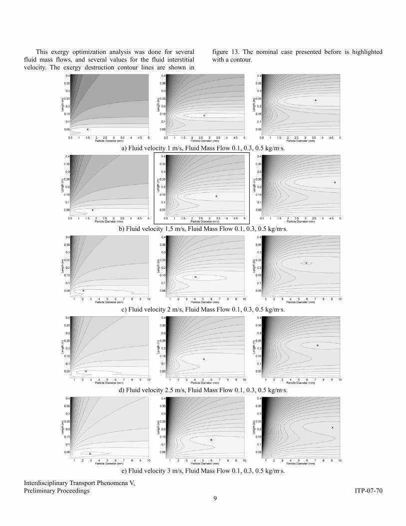
This exergy optimization analysis was done for several fluid mass flows, and several values for the fluid interstitial velocity. The exergy destruction contour lines are shown in

figure 13. The nominal case presented before is highlighted with a contour.

a) Fluid velocity 1 m/s, Fluid Mass Flow 0.1, 0.3, 0.5 kg/m·s.

b) Fluid velocity 1,5 m/s, Fluid Mass Flow 0.1, 0.3, 0.5 kg/m·s.

c) Fluid velocity 2 m/s, Fluid Mass Flow 0.1, 0.3, 0.5 kg/m·s.

d) Fluid velocity 2.5 m/s, Fluid Mass Flow 0.1, 0.3, 0.5 kg/m·s.

e) Fluid velocity 3 m/s, Fluid Mass Flow 0.1, 0.3, 0.5 kg/m·s.


Fig. 13. Exergy destruction contour lines for different values of fluid mass flow and fluid velocity.

a) mass flow effect b) fluid velocity effect Fig. 14. Exergy Optimal Length (for particles velocity of 3 m/hr).

The results presented in figure 13 show that the general behavior presented for the nominal case is global. Optimal lengths depends only on the mass flow and, except for very small particles, are not affected by particle diameters or fluid velocities in the range studied here. The optimal diameter increases both with fluid mass flow and fluid velocity.

Figure 14 shows the exergy optimal length obtained from the data shown in figure 13. In Graph 14 a) a comparison with the thermal optimal length obtained from (11) and presented in figure 6 is done. It shows that the exergy optimal length is mainly defined by thermal effects. The deviation between the optimal lengths obtained by thermal or exergy considerations is shown as a function of the fluid mass flow and velocity. Small deviations appear for large mass flows, mainly because of pressure drop effects, but might be considered negligible in our analysis range. The fluid velocity dependence is more clearly shown in Graph 14 b). A slight non-linear effect of the fluid velocity exists, becoming more important for larger mass flows. This change is again mainly because of pressure drop effects.

Figure 15 shows the optimal particle diameter dependence on fluid mass flow and velocity. The optimal particle diameter increases with fluid mass flow and velocity. The influence of the fluid velocity is more important with high mass flows. When the fluid velocity is high, the optimal particle diameter increases quickly because of the pressure drop. The physical origin of the optimal diameter tendency shown in this figure is probably less clear than that of the optimal length, which could be related directly to thermal effects. For the diameters, both thermal and pressure effects are coupled as was shown in figure 12 b)., The results shown in figure 15 allows us to think that the pressure drop effect dominates, defining the tendency of increasing optimal diameters with mass flow and fluid velocity. Nevertheless, this behavior has to be considered carefully, as the range of diameters with almost equal exergy destructions is

wide, as was seen in figure 12 b) and is probably easy to perceive in the graphs of figure 13.

Fig. 15. Optimal Particle Diameter

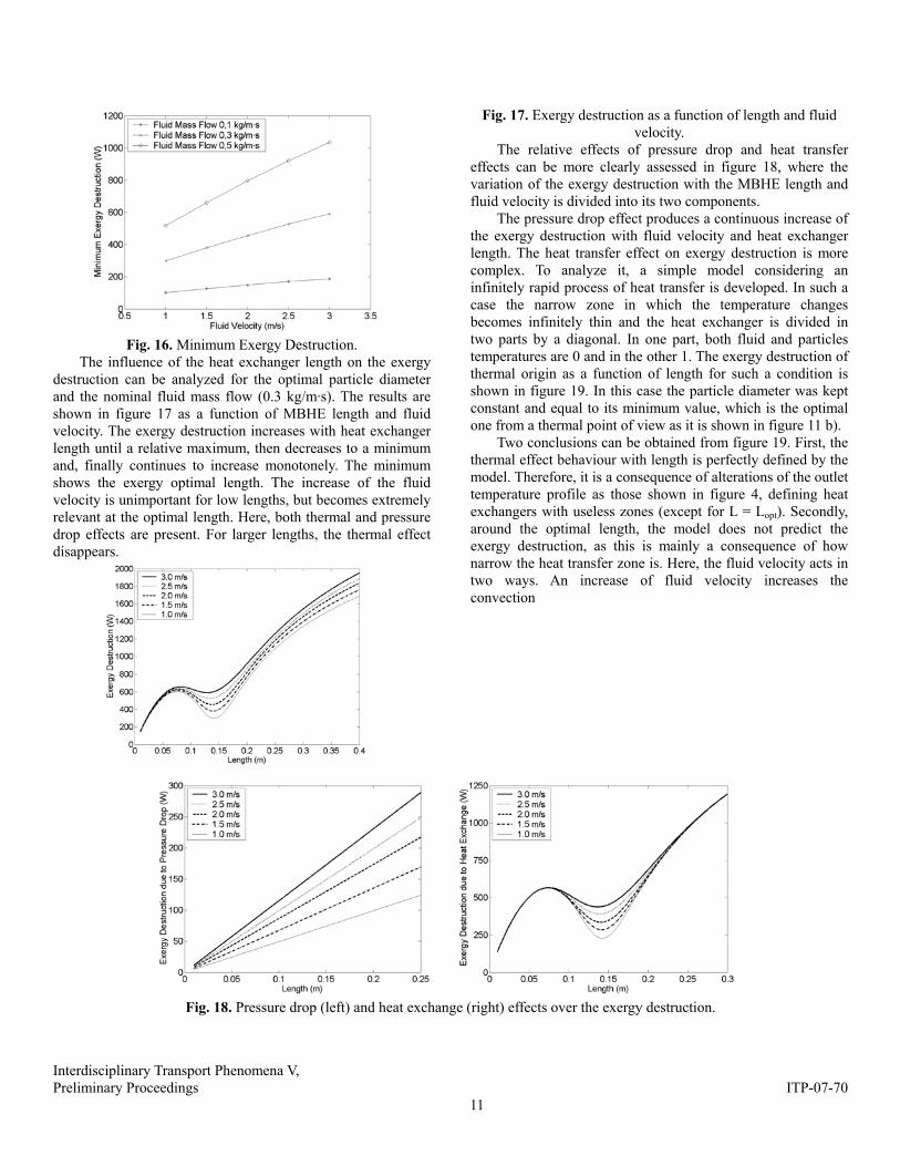
Up to this stage nothing has been said about actual values of the exergy destruction and how it varies for the different minima. This is shown in figure 16. The exergy destruction increases (almost linearly) with fluid mass flow and also with fluid velocity. This last relation seems to saturate for large fluid velocities, implying that the increase of exergy destruction as a consequence of the increase of the pressure drop is compensated with a better heat transfer efficiency.


Fig. 16. Minimum Exergy Destruction.

The influence of the heat exchanger length on the exergy destruction can be analyzed for the optimal particle diameter and the nominal fluid mass flow (0.3 kg/m·s). The results are shown in figure 17 as a function of MBHE length and fluid velocity. The exergy destruction increases with heat exchanger length until a relative maximum, then decreases to a minimum and, finally continues to increase monotonely. The minimum shows the exergy optimal length. The increase of the fluid velocity is unimportant for low lengths, but becomes extremely relevant at the optimal length. Here, both thermal and pressure drop effects are present. For larger lengths, the thermal effect disappears.

Fig. 17. Exergy destruction as a function of length and fluid velocity.

The relative effects of pressure drop and heat transfer effects can be more clearly assessed in figure 18, where the variation of the exergy destruction with the MBHE length and fluid velocity is divided into its two components.

The pressure drop effect produces a continuous increase of the exergy destruction with fluid velocity and heat exchanger length. The heat transfer effect on exergy destruction is more complex. To analyze it, a simple model considering an infinitely rapid process of heat transfer is developed. In such a case the narrow zone in which the temperature changes becomes infinitely thin and the heat exchanger is divided in two parts by a diagonal. In one part, both fluid and particles temperatures are 0 and in the other 1. The exergy destruction of thermal origin as a function of length for such a condition is shown in figure 19. In this case the particle diameter was kept constant and equal to its minimum value, which is the optimal one from a thermal point of view as it is shown in figure 11 b).

Two conclusions can be obtained from figure 19. First, the thermal effect behaviour with length is perfectly defined by the model. Therefore, it is a consequence of alterations of the outlet temperature profile as those shown in figure 4, defining heat exchangers with useless zones (except for L = Lopt). Secondly, around the optimal length, the model does not predict the exergy destruction, as this is mainly a consequence of how narrow the heat transfer zone is. Here, the fluid velocity acts in two ways. An increase of fluid velocity increases the convection

Fig. 18. Pressure drop (left) and heat exchange (right) effects over the exergy destruction.


Fig. 19. Effect of fluid velocity on the destruction of exergy of thermal origin.

coefficient, thus improving the heat transfer mechanism. On the other hand, an increase of the fluid velocity decreases the residence time of the fluid. This second effect is linear, but not the first one. As a result, increasing the fluid velocity will produce a worsening of the heat transfer effect and an increase of the exergy destruction. This effect is clearly shown in the zoom of Graph 19 (right).

Note that the MBHE results of figure 18 b) and 19 are not the same. Both figures show the exergy destruction of thermal origin, but the results in figure 18 b) are for the optimal particle diameter from the exergy point of view, while in figure 19 we have plot the results for the thermal optimal diameter. The thermal optimal diameter is set at the minimum diameter (figure 11 b)) independently of fluid mass flow and velocity, while the exergy optimal diameter increases with both parameters (figure 15). Then, the effect shown in figures 18 b) has the influence of both a higher velocity and a higher diameter, however the results of figure 19 shows only the influence of the fluid velocity around the minimum value of the exergy destruction.

3. CONCLUSIONS

A heat transfer and exergy analysis of a MBHE was

performed, considering variations of the main parameters of the problem, including the MBHE dimensions, the fluid mass flow, and the fluid velocity.

The general problem is addressed and simplified for a gas-solid MBHE. A numerical solution of the problem is given; also an analytical solution is obtained neglecting conduction terms.

The analytical solution of the problem serves as an easy tool for the design of reasonable MBHEs from a thermal point of view. The conduction heat transfer was considered for the numerical solution. The thermal conductivity has an influence on the width of the zone where temperature changes, which becomes wider for both fluid and particles when the conduction effects are considered. This effect of the conduction heat transfer is similar to the one obtained when the convection coefficient increases. Nevertheless, both effects have minor influence on outlet conditions, and the performance of the MBHE for well-designed systems.

The exergy analysis considers the heat transfer, but also the effect of the pressure drop. In this case the optimal length is not only a function of the fluid mass flow like it was in the thermal analysis. From the exergy point of view, the optimal length is obtained by a compromise between the heat transfer (which depends mainly on the fluid mass flow) and the pressure drop (which depends mainly on the fluid velocity and the particle diameter).

The exergy optimal length is always smaller than the thermal one because of the pressure drop, but the differences between both optimal lengths are small for typical values of fluid mass flow and velocity. An increase of the fluid velocity produces a decrease of the exergy optimal length, and the effect is sharper for higher values of the fluid mass flow. Therefore, applications in which both fluid mass flow and velocity are low, could be studied from the thermal point of view with small deviations, but when the fluid mass flow and velocity becomes higher the effect of the pressure drop must be taken into account, and the design must consider the exergy point of view.

The particle diameter is of prior importance for pressure drop, so optimal results are very different considering the thermal or the exergy point of view. In the thermal sense, smaller diameters are optimal while considering an exergy analysis, larger diameters are chosen.

The exergy optimal particle diameter increases with the fluid velocity. This increase is sharper for higher values of the fluid mass flow. Nevertheless, the influence of the optimal length on the exergy destruction is more important than that of the optimal particle diameter.

APENDIX A The governing equations were solved numerically adding a

time derivate to the solid equation and advancing in time explicitly from an initial solution. This initial solution was the temperature maps without conduction. So, the numerical schemes for the time k are:


( )

( )( )

( )

)(2

2

1,

1,

11,

1,

,,2,1,,1

21,,1,,1,,

1,

i

TTT

TK

Kt

kij

kij

kij

kij

kij

kij

kij

kij

kij

kij

kij

kij

kij

kij

kij

kij

+++−

+

+−

+−−+

−=∆−

−+∆

+⋅−+

+∆

+⋅−+

∆

−=

∆

−

θξ

θη

θθθξ

θθθηθθθθ

η

ξ

The non-dimensional solid temperature in time k+1 was obtained from the solution in time k from the following equation:

( ) ( )

( ) ( )

( ) ( )

)(221

,21,21,

22,

2,12,11

,

ii

tTKtKt

tKtKtt

KtKtt

kij

kij

kij

kij

kij

kij

kij

∆⋅+

⋅

∆∆

⋅+

⋅

∆∆

⋅+

∆−⋅

∆∆⋅

−⋅∆∆⋅

−∆∆

−⋅+

+

⋅

∆∆

⋅+

⋅

∆∆

+∆∆

⋅=

+−

+−+

ξξ

ξη

ηη

ξθ

ξθ

ξηηθ

ηθ

ηηθθ

and then, the non-dimensional gas temperature in k+1 was obtained from:

)(1

11,

1,1

, iiiT

Tkij

kijk

ij ξξθ∆+

+∆⋅=

+−

++

ACKNOWLEDGMENTS This work has been partially supported by the National

Energy Program of the Spanish Department of Science and Education and the Madird Community under the project numbers ENE2006-01401 and CCG06-UC3M/ENE-0764 respectively.

REFERENCES [1] D. Vortmeyer, RJ. Schaefer, “Equivalence of one-phase and 2-phase models for heat-transfer processes in packed-beds-one-dimensional theory.” Chemical Engineering Science 29 (2): 485-491 (1974). [2] K. Hooman ,H. Gurgenci , A.A. Merrikh, “Heat transfer and entropy generation optimization of forced convection in porous-saturated ducts of rectangular cross-section.” International Journal of Heat and Mass Transfer 50: 2051–2059 (2007). [3] V. Henriquez, A. Macias-Machin, “Hot gas filtration using a moving bed heat exchanger-filter (MHEF).“ Chemical Engineering And Processing 36 (5): 353-361 (1997) [4] C.M. Marb, D. Vortmeyer, “multiple steady-states of a cross-flow moving bed reactor - theory and experiment.” Chemical Engineering Science 43 (4): 811-819 (1988).

[5] R. Krupiczka, “Analysis of thermal conductivity in granular materials.” International Chemical Engineering 7 (1): 122-& (1967). [6] S. Yagi, D. Kunii, N. Wakao, “Studies on axial effective thermal conductivities in packed beds.” AIChE Journal 6 (4): 543-546 (1960). [7] E. Achenbach, “Heat and flow characteristics of packed beds.” Experimental Thermal And Fluid Science 10 (1): 17-27 (1995). [8] JJ. Saastamoinen, “Heat exchange between two coupled fixed beds by fluid flow.” International Journal Of Heat And Mass Transfer 46 (15): 2727-2735 (2003).

ITP-07-70 - CORE

Documents

Transcript of ITP-07-70 - CORE