MPRAMunich Personal RePEc Archive

Investment, replacement and scrappingin a vintage capital model with embodiedtechnological change

George C. Bitros and Natali Hritonenko and Yuri Yatsenko

Athens University of Economics and Business

June 2007

Online at http://mpra.ub.uni-muenchen.de/3619/MPRA Paper No. 3619, posted 19. June 2007

Investment, replacement and scrapping in a vintage capital model with

embodied technological change

By

George C. Bitros1, Natali Hritonenko2, and Yuri Yatsenko3

Abstract

This paper analyzes and compares two alternative policies of determining the service life and replacement demand for vintage equipment under embodied technological change. The policies are the infinite-horizon replacement and the transitory replacement ending with scrapping. The corresponding vintage capital models are formulated in the dynamic optimization framework. These two approaches lead to different estimates of the duration of replacements and the impact of technological change on the equipment service life.

JEL Classification: E22, O16, O33

Keywords: vintage capital equipment, embodied technological change, service life, replacement,

scrapping

Corresponding Author: Prof. George C. Bitros Athens University of Economics and Business Department of Economics Tel.: +302108223545 Fax: +302108203301 E-mail: bitros@aueb.gr

1 Department of Economics, Athens University of Economics & Business, 76 Patission St, 10434, Athens, Greece. 2 Department of Mathematics, Prairie View A&M University, Prairie View, TX 77446, USA. 3 College of Business and Economics, Houston Baptist University, 7502 Fondren Road, Houston TX 77074, USA.

2

1. Introduction

In order to secure the services of durables at minimum cost, producers and consumers

confront invariably the question: How frequently should a stock of old durables be replaced by a

stock of new ones? Clearly, the old durables should not be replaced too soon because the cost of

acquiring them will occur too frequently and this will raise the unit cost of their services.

However, the durables should not be replaced too late either, because their rising operating costs

and the higher productivity of durables of newer vintages render them economically inferior. So,

to tackle the issues involved in determining the optimal service life of durables, researchers in the

fields of management and economics have adopted over the years various approaches.

Preinreich (1940) was the first to show how the optimal life of durables can be determined.

More specifically, according to his theorem, the optimal economic life of a single machine should

be computed together with the economic life of each machine in the chain of future replacements

extending as far into the future as the owner’s profit horizon1. However, the theorem was

formulated under two crucial assumptions. The first of them abstracted from a technological

progress and postulated that newer machines of identical type replaced older machines (like-for-

like). This assumption contradicted casual observations and was ultimately relaxed by Smith (1961)

who generalized the above result to the case where the older machines were replaced by more

productive machines embodying the most recent advances in science and technology. The second

assumption concerned the horizon of the reinvestment process and required the owner of the

machine to choose its duration on the basis of their perception on how long the investment

opportunity might remain profitable. Later, depending on the specification of the owner’s profit

horizon, different models emerged for the determination of the optimal lifetime of assets.

In particular, by limiting the owner’s profit horizon to a single investment cycle,

researchers in the field of capital budgeting obtained the so-called “abandonment” class of models

and used it to derive strict rules regarding the optimal asset life. Initially, Robichek and Van

Horne (1967) suggested that an asset should be abandoned during any period, in which the present

value of future cash flows did not exceed its abandonment value. Then, based on the possibility

that the function of cash flows might not have a single peak, Dyl and Long (1969) argued that

abandonment should not occur at the earliest possible date that the above abandonment condition

was satisfied, but rather at the date that yielded the highest net present value over all future

1 The terms "capital", "equipment", and "machine" have been employed frequently in the relevant literature to

indicate that the good under consideration has the properties of a producer's durable. In this paper, we use these terms interchangeably. The same comment holds also for “economic life, “service life”, “life”, and “lifetime”.

3

abandonment opportunities. Later, Howe and McCabe (1983) highlighted the patterns of cash

flows and scrap values under which the “abandonment” model led to a unique global optimum of

the abandonment time. They also characterized the complete range of models that could be

obtained by varying the owner’s profit horizon and clarified the practical guidelines for the choice

between “abandonment” and “replacement” models.

Theoretical economists, on the other hand, continued to work in the tradition of Terborgh

(1949) and Smith (1961) by assuming invariably that the owner’s profit horizon is infinite. This in

turn led them to concentrating on a single class of replacement models, all of which presumed that

the infinite reinvestments took place at equal time intervals. This pervasive conceptualization was

adopted in all significant contributions in the area from Brems (1968) to Nickel (1975), Rust (1987)

and to Mauer and Ott (1995) 2. More recently, Van Hilten (1991), Hritonenko and Yatsenko

(1996b, 2004, 2005, 2006), Regnier, Sharp, and Tovey (2004) relaxed these assumptions and

considered both the variable replacement period and the finite profit horizon.

The practical importance of the finite-horizon replacement problem was highlighted by

Hartman and Murphy (2006), who explored the replacement policy which occurs when

companies only require an asset for a specified length of time, usually to fulfill a specific contract

and identify when this policy deviates significantly from optimal. Bitros and Flytzanis (2005)

demonstrated that the policies of infinite-horizon replacements and transitory replacements

ending with scrapping lead to different results regarding the profit horizon, the duration of

replacements, the timing of scrapping, and the impact of output and market structure on service

lives. In doing so, they assumed that the technological progress had the form of random

breakthroughs, which at the time of their occurrence rendered all existing equipment inoperable.

In the real world, there are two fundamentally different modes of technical progress (e.g.,

Simpson, Toman, and Ayres 2005, p.144): a “normal mode”, in which technological

improvements occur incrementally and more or less automatically as a result of accumulated

experience and learning, and the radical innovations (technological breakthroughs). The

normal mode is characterized by a simple positive feedback between increasing consumption,

increasing investment, increasing scale, and learning-by-doing (or experience). The

production technology itself may also gradually become more efficient. It results in gradually

declining costs and prices, stimulating further increases in consumption and, hence, economic

growth. The second mode involves multiple competing and evolving production technologies 2 Probably, the persistence of this approach was encouraged by the proof that Elton and Gruber (1976) provided

regarding the optimality of an equal life policy for a machine subject to technological improvement. However, subsequent research has established that the equal life policy is only a special case of a much more general set of variable life replacement policies. We will say more on this later on in this paper.

4

(plastics and synthetic fibers substituting iron and steel, automobiles replacing horses and

carriages, air transport displacing railways, and so on). The substitution of major general-

purpose technologies can be both very productive and very traumatic.

The goal of this paper is to compare the “abandonment” and “replacement” management

policies when the technological change is in the normal mode and of the embodied type. For this

reason, we adopt the so-called Vintage Capital Model (VCM), in which the units of equipment

brought into operation are more productive than the ones already in place because they

embody the most recent advances in science and technology. We expect to demonstrate that

this setting poses essential challenges because the optimal lifetime of equipment in each

vintage depends on the horizon of the reinvestment opportunity as well as on the date of its

introduction into operations. It requires the solution of a non-linear control problem.

The rest of the paper is organized as follows. In the next section, we set up the model.

Unlike the equipment replacement models considered above, its specification allows for

improvements in the productivity of consecutive vintages of equipment. This, in turn, leads to

a new non-linear optimisation problem that involves the optimal control of the equipment

lifetime in each vintage. Then, in the following two sections, we investigate the implications

of two different approaches to the administration of equipment. Section 3 focuses on the

strategy of infinite-horizon replacements, implying that the equipment is being replaced

indefinitely, whereas Section 4 concentrates on the strategy of transitory replacements, where

the equipment is replaced a finite number of times, ending with abandonment or scrapping.

Lastly, in Section 5, we conclude with a synopsis of main findings.

2. The model and the optimization problem

At the end of the service life of equipment, there are always two options: to replace it

and continue doing so up to some profit horizon, or to abandon or scrap it and terminate

operations. To examine their implications, we assume that during year τ the representative

firm acquires ( )K τ units of new capital, which possess the same efficiency ( )b τ because

they belong to the same vintage and embody the same technology. The output of the new

capital ( )K τ is denoted as ( ) ( ) ( )X b Kτ τ τ= . The units of capital built later in the year

t τ> are more productive because they embody the latest advances of science and

technology. To describe this process, we assume that the capital efficiency (output-capital

ratio) is:

( )( ) ( ) tb t b eμ ττ −= , (1)

5

where 0μ> is a constant and exogenous rate of technological change. Thus, the efficiency of

capital in each vintage depends on the date ν of its construction. Following Malcomson (1975),

van Hilten (1991), Hritonenko and Yatsenko (1996, 199, 2003), Boucekkine et al. (1997, 1998),

Greenwood et al. (2000), and others, we assume that the representative firm acquires only the

newest vintage of equipment and removes from service the oldest equipment that has become

obsolete. Then, the total output produced in year t is described as:

( ) ( )( ) ( ) (0) ( ) , ( ) ,

t t

a t a tX t X d b e K d a t tμττ τ τ τ= = <∫ ∫ (2)

where ( )a t is the purchasing time of the equipment scrapped at time t (known as the capital

scrapping time in Boucekkine et al. (1998)). Namely, the capital bought at time ( )a t is scrapped

at the current time t . Then t - ( )a t is the lifetime of equipment bought at time ( )a t . The integral

over [ ( ), ]a t t in (2) implies that at time t the firm uses only the equipment units placed into

service between ( )a t and t . Introducing the market price ( )p t of output ( )X t , we can represent

the net operating revenue of the firm as:

( )( ) ( ) (0) ( ) ( ) ( )

t

a tQ t p t b e K d w t L tμτ τ τ= −∫ , (3)

where ( )L t is the total labor employed in year t and ( )w t is the wage rate. In this paper, we

restrict ourselves to the labor expenses only, although other operating costs can be also

considered. Assuming that ( )m τ units of labor operate each equipment unit introduced at time

τ, the total labor demand of the firm is described as:

( )( ) ( ) ( ) .

t

a tL t K m dτ τ τ= ∫ (4)

We shall notice that this resource constraint can be imposed on any other critical resource of a

firm such as energy, finances, operating space, or even repair facilities. For example, in energy

production, a crucial restriction is set by the environment contamination limits.

Compared to other models reviewed in the previous section, the VCM (1)-(4) provides

a convenient tool to consider the optimal lifetime of equipment as an unknown (endogenous)

variable. To determine this endogenous variable, we formulate an optimization problem by

assuming that the present value of total profits over the planning horizon 0 max[ , ]t T

6

0

max

[ ( ) ( ) ( )]

Trt

te Q t q t K t dtΠ −= −∫ (5)

is maximized under the given labor resource constraint (4). Here ( )q t is the acquisition price

of the new equipment unit, 0 max[ , ]t T is the planning horizon, and r is the discount rate. We

assume that the residual (salvage) value of the scrapped equipment is negligible compared with

its acquisition price. The dynamics of ( )q t is also determined by technological change and,

together with the output-capital coefficient described in (1), appears to be critical for

determining the optimal service life of equipment. In this paper, we assume dynamics of ( )q t

and ( )p t are different:

( ) (0) tq t q eη= , ( ) (0) tp t p eζ= , (6)

where the constants η and ζ may be positive or negative.

In the formulated optimization problem, the unknown controls are the investment

( )K t and the scrapping time ( )tα . In contrast to the simple model of infinite equal time

replacements employed by Bitros (2005) to compare the two policies, the VCM (1)-(6)

considers the variable equipment lifetime (service life) ( ) ( )T t t a t= − . The output-capital

ratio b(τ), the labor-capital ratio m(τ), the total labor ( )L t , the acquisition price of capital

( )q t , and the product price ( )p t are given on 0 max[ , ]t t T∈ . It is convenient to assume that one

man operates one unit of equipment. Then, m(τ)=1 in (4), ( )b τ in (1) is the output-labor

coefficient, and ( )q t in (5) is the relative price of a labor unit of equipment as in Greenwood

et al. (2000). To simplify the optimization analysis, we also assume that ( )L t =const.

Remark 1. Bitros and Flytzanis (2005) considered a similar problem in a simpler time-invariant framework with an impatience assumption in the absence of embodied technological change.

Let us impose some necessary restrictions on the unknown variables. First of all, we

set max0 ( ) ( )K t K t≤ ≤ . This implies that the maximal possible investment max ( )K t is

determined by certain financial constraints faced by the representative firm. It is also natural

to assume that the scrapped equipment cannot be used again, i.e. ( ) 0a t′ ≥ . Finally, as the

model (1)-(6) is defined on the future interval 0 max[ , ]t T , a specific vintage structure of the

7

equipment should be known at the initial time 0t . This structure is defined by the given

investments 0( ) ( )K Kτ τ= undertaken throughout the pre-history interval [a(t0),t0].

Thus, the optimization problem is to find the functions ( )K t and ( )a t , 0 max[ , ]t t T∈ ),

maxT ≤∞ , which maximize the objective functional (5) under the constraint-equality (4), the

constraint-inequalities:

max0 ( ) ( )K t K t≤ ≤ , (7)

( ) 0, ( )<a t a t t′ ≥ , (8)

and the initial conditions:

0 0 0 0 0( ) , ( ) ( ), , ].a t a t K K a tτ τ τ 0= < = ∈ [ (9)

Malcomson (1975) was first to introduce the VCM (2)-(3) to find the optimal capital

replacement policy of an individual firm with vintage technology under the embodied

technological progress. Silverberg (1988) used the VCM (2)-(3) to describe the rational

equipment replacement of a firm in an evolutionary model of self-regulatory market. In the

same framework, van Hilten (1991) investigated a finite–horizon optimization problem where the

constant lifetime of capital was optimal and showed the importance of the zero-investment period.

Hritonenko and Yatsenko (1996b, 2004) provided a qualitative analysis of the optimization

problem (2)-(9).

Remark 2. It would be interesting to assume that the representative firm faces a demand curve of the constant elasticity type. However, this assumption introduces a scale effect and makes the solution of the problem (1)-(9) considerably more difficult. In particular, the optimal lifetime of equipment would depend on the amount of output produced. So, we leave this specification for future research.

We turn now to the investigation of the possible differences between the two approaches

to the management of capital. In the optimization problem (1)-(9), the policy of infinite-

horizon replacements corresponds to the case maxT =∞ , whereas the policy of transitory

replacements ending with scrapping corresponds to the case maxT <∞ . The structure of the

solutions * *( ( ), ( ))K t a t appears to be quite different under maxT =∞ and maxT <∞ . Section 3

8

below is devoted to the analysis of the infinite horizon replacement policy, whereas the investigation

of the policy of transitory replacements ending with scrapping is relegated to Section 4.

3. Infinite-horizon replacements

The optimization problem (1)-(9) is meaningful at maxT =∞ if the value of the improper

integral in (5) is finite (otherwise, there is no sense to maximize it). Let us assume that

r μ> & .r μ ζ> + (10)

Conditions (10) reflect the natural requirements that the discount factor needs to be greater

than the technological progress rate in order for (5) to yield a finite value of profits in the

infinite horizon.

As shown in Hritonenko and Yatsenko (2004), the optimization problem (1)-(9) at

maxT =∞ has a unique solution * *0( ( ), ( ), [ , )K t a t t t∈ ∞) such that the optimal scrapping time

*( )a t coincides with a special trajectory (turnpike) 0( ), [ , )a t t t∈ ∞∼ on the planning horizon

0[ ,t ∞) except for an initial (transition) period 0[ , ]t μ . The turnpike ( )a t∼ is determined from

the following nonlinear integral equation:

1 ( )

( ) ( ( )) ( )

[1 ] ,

a tr t a r t

te e d Ceζ τ μ τ μ ητ

−− + − − − − +− =∫ 0[ ,t t∈ ∞) , (11)

where 1( )a t− is the inverse function of ( )a t and (0) / (0) (0)C q p b= . The inverse function

1( )a t− exists because ( ) 0a t′ ≥ by (8) and is discontinuous when ( ) 0a t′ = . Equation (11)

demonstrates that the profit from introducing a new equipment unit and using it during its

future lifetime with the simultaneous retirement of an older unit must be equal to the

acquisition price of the new equipment unit.

Proposition 1.

If (10) holds and μ>0, then equation (11) has the unique solution ( )a t∼ at least in the following cases: • If μ = r-ζ and Cμ <1, then 0( ) , [ ,a t t T t t≡ − ∈ ∞)∼ , where the constant T is

determined by the following non-linear equation: ))(1)(()( )( ζμζμζ ζμ −−−−=−− −−− rCreer TrT . (12)

At small μ, the constant T is approximately equal to μ/2C . • If μ≠r-ζ, then ( ) ( ) 0T t t a t= − >∼ ∼ exists only if

9

μζηζ μζη −−<−− −− rerrC t)())(( • If μ > r-ζ, then equation (11) has the unique monotonically increasing solution

( )a t∼ in an interval ( , )crt ∞ , such that ( ) 0 at T t t→ →∞∼ , and ( ) at crT t t t→∞ →∼ . The critical time crt can be estimated as:

)(

ln1ημζ

μζη −−−

−−≈

rCrtcr (13)

• If μ < r-ζ, then equation (11) has the unique solution ( )a t∼ on an interval ( , )crt−∞ , such that the solution ( )a t∼ increases on ( , )crt−∞ , decreases on ( , )c crt t at some c crt t< , and ( ) , ( ) at cra t T t t t→∞ →∞ →∼ ∼ .

The proof of Proposition 1 is provided in the Appendix.

Proposition 1 can be used to estimate the optimal equipment replacement strategies at

the individual plant or firm level. In particular, the following statements about the firm’s

equipment replacement are valid for the problem (1)-(9):

• Except for a possible initial (transitory) period, the optimal lifetime of equipment

( ) ( )T t t a t= −∼ ∼ depends neither on the quantity of produced output nor on the initial

equipment structure and is determined only by the rates of technological change, prices,

and discount rate.

• The optimal lifetime of equipment may be finite only in the presence of the embodied

technological progress, i.e., when the vintage productivity ( )b t increases ( 0μ> in (1)).

• The proportion between the value of productivity ( ) ( )b t p t and the equipment price ( )q t

determines the dynamics of the optimal equipment lifetime. If μ ζ η+ > (i.e., the revenue

( ) ( ) / ( )b t p t q t per unit of new equipment acquisition price increases), then the optimal

lifetime decreases. If μ ζ η+ < (that is, ( ) ( ) / ( )b t p t q t decreases), then the optimal

lifetime increases and becomes infinite at some finite instant crt .

• If the sum of the rates of technological change and output price is equal to the rate of price

change of new equipment, μ+ζ=η, then the ratio ( ) ( ) / ( )b t p t q t is constant and the

optimal equipment lifetime is also constant. This constant depends only on the discount

rate and the ratio between the value of productivity and the acquisition price of equipment.

We shall notice that the last two properties imply that the well-known equidistant equipment

replacement is a sub-case in our more flexible model, which appears to be optimal only in the

case μ+ζ=η .

Bitros and Flytzanis (2005) introduced some special terminology to classify the various

types of equipment on a scale of replaceability. Following them, we say that the equipment is:

10

• Finitely replaceable, if it has a finite number N >0 of profitable replacements;

• Infinitely replaceable, if N =∞;

• Non-replaceable, if no replacement is profitable.

Then, in the setting of the optimization problem (1)-(9), the vintage equipment is:

• Infinitely replaceable, if μ ζ η+ ≥ ,

• Non-replaceable, if μ ζ η+ < and 0crt t< ,

• Finitely replaceable if μ ζ η+ < and 0crt t> . Then, the exact number N of profitable

replacements depends on the proportion between the horizon length 0 0T t− and ( )T t∼ ,

where ( )T t∼ is determined from equation (11).

Now, let us describe the optimal dynamics of the corresponding investment K*(t). During

the initial transitory period 0[ , ]t μ , the investment is maximum possible *max( ) ( )K t K t= if

0 0( )a a t< ∼ or minimum possible *( ) 0K t = if 0 0( )a a t> ∼ . Differentiating (4), we get

( ( )) ( ) ( ) ( )K a t a t K t L t′ ′= − . Hence, under our constant labor condition ( ) constL t = , the

minimum replacement investment regime is *( ) 0K t = , * *( ) 0, ( ) consta t a t′ = = (no working

equipment is scrapped and no new equipment is acquired).

So, in the general case, the optimal investment trajectory *( )K t is boundary (minimum

or maximum) at a beginning part 0[ , ]t μ of the planning horizon. After that, *( )K t is found

from (4) as *( ) ( ( )) ( ) /K t K a t da t dt= ∼ ∼ . The last formula shows that the initial boundary-

valued section of *( )K t is reproduced throughout the whole horizon 0[ , ]t T . In particular, in

the case μ ζ η+ = , the constant lifetime ( )a t t T= −∼ and the strictly periodic investment *( ) ( )K t K t T= − represent the optimal policy. The repetition pattern with bursts and slumps

in *( )K t can be observed in Figure 1. These “spikes” (replacement echoes by Boucekkine et

al. (1997)) were experimentally discovered in recent years by researchers studying investment

at the plant level.

4. Transitory replacements ending with scrapping

Here, we assume that the equipment is managed optimally for a finite number of operating

periods ending with scrapping, i.e., maxT <∞ . Then the structure of the solutions of the

optimization problem is more complicated as compared with the case maxT =∞ .

11

The key new feature is the existence of the ”zero-investment period” max[ , ]TΘ ,

0 maxt TΘ≤ < , at the end of the planning horizon 0 max[ , ]t T (see van Hilten (1991)). During the

max[ , ]TΘ period, the investment is minimum possible since there is no sense in investing in

new capital given that the firm quits production at maxT . This effect is well known in various

economic optimization models. Under our condition of constant labor, ( ) constL t = , the

minimum investment regime is * *( ) 0 and ( ) / 0,K t da t dt= = * *( ) ( consta t a Θ)= = at

max[ , ]t TΘ∈ , i.e., no new investment is made and no equipment is scrapped. The optimal

lifetime * * *max max max( ) ( ) ( )T T T a T T Θ= − = of the oldest equipment at the horizon end

maxt T= is always larger than the optimal lifetime max( )T T∼ in the indefinite-replacement case

from Section 3.

The presence of the zero-investment period causes essential changes in the behavior of

the optimal trajectories *( ) K t and *( )a t on the whole horizon 0 max[ , ]t T . However, the impact

of the zero-investment period weakens when the duration max 0T t− becomes larger. In

particular, the optimal lifetime * *( ) ( )T t t a t= − strives to the “indefinite-replacement”

optimal lifetime ( ) ( )T t t a t= −∼ ∼ as maxT t− →∞ . Mathematically (see Hritonenko and

Yatsenko (2004)), at μ ζ η+ ≥ the finite–horizon of the optimization problem (1)-(9) has the

unique solution * *( ), ( )K t a t ,

0

0 max

1

( ), [ , ],* ( ) ( ), [ , ] 1 2 [ , ],

( ), [ , ]i i i i

i i i

a t t ta t a t i , ,..., t t T

a t t

μ μα α β

β α+

⎧ ∈⎪⎪⎪⎪= ∈ = ∈⎨⎪⎪ ∈⎪⎪⎩

(14)

where the trajectories ..., 1,2,3i =ia are

3 max( )1 0 3

3

1( ) ln 1 ( ) 1 c T tca t t c c ec c

λ − −⎧ ⎫⎪ ⎪⎪ ⎪⎡ ⎤= + − − + −⎨ ⎬⎢ ⎥⎣ ⎦⎪ ⎪⎪ ⎪⎩ ⎭

(15)

1

3 ( ( ) )1 0 3

3

1( ) ln 1 ( ) 1 , 1,2,3,..., ic a t ti

ca t t c c e ic c

λ−− −

+

⎧ ⎫⎪ ⎪⎪ ⎪⎡ ⎤= + − − + − =⎨ ⎬⎢ ⎥⎣ ⎦⎪ ⎪⎪ ⎪⎩ ⎭

and the parameters , , 1, 2,3...,i i iα β = are uniquely determined, 1 max 1, Tβ α Θ,= =

1, i i i iα β β α+< < .

12

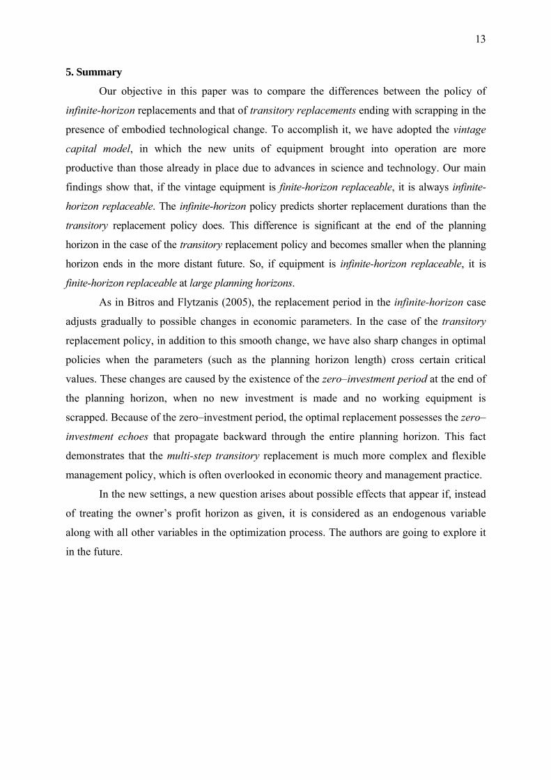
The solution of the optimization problem * *( ), ( )K t a t is shown in Figure 1. The

infinite-horizon replacement solution is indicated with the dotted line (by Section 3,

( ) Ta t t= −∼ is the turnpike in the case 2 1c c= ). The finite-horizon equipment lifetime *( )a t

tends to the infinite-horizon turnpike when the time T-t left to the horizon end T increases.

One can notice that the finite-horizon optimal policy possesses sharper changes at certain

“critical” instants , , 1, 2,3...,i i iα β = , which depend on the length of the planning horizon

0 max[ , ]t T . These changes can be referred to as the zero–investment echoes, because they are

caused by the zero–investment period max[ , ]TΘ and propagate backward through the entire

planning horizon 0 max[ , ]t T .

The beginning moment Θ of the zero-investment period max[ , ]TΘ is found from the

condition:

max

3 3 21 1 1

( )( )

[ ] 0

Tc c cc c ae e e d Ceτ θθ θ

θτ− − +− − =∫ .

Obviously, it is smaller than maxT . If the calculated Θ appears to be less than 0t , then the

equipment is finitely non-replaceable because the planning horizon 0 max[ , ]t T is too small. If

0tΘ> , then the corresponding equipment is finitely replaceable in the interval 0 max[ , ]t T . If

the equipment is finitely replaceable on the interval 0 max[ , ]t T , then it is infinitely replaceable

(see Section 3). Conversely, if the equipment is infinitely replaceable on the interval [t0, ∞)

then it is finitely replaceable on large enough planning horizons 0 max[ , ]t T . Therefore, as in

Bitros (2005), the profitability condition for the infinite-horizon replacement and transitory

replacement on large planning horizons is the same.

Remark 3. As in Bitros (2005), the profit horizon for the transitory replacement ending with

scrapping can be determined endogenously by the equipment parameters and the external market environment (it is obviously infinite in the infinite-horizon case). Namely, taking into account the given initial equipment distribution on the pre-history interval

0 0[ ( ), ]a t t , it may be more profitable to extend (or decrease) slightly the interval

0 max[ , ]t T . For example, in capital budgeting it will allow us to consider the endogenous influence of profit horizon on the selection of projects (and inversely). So, the transitory approach to replacement is more flexible. Mathematically, it requires adding the value

maxT as the additional control variable to the optimization problem. The authors are going to explore this idea in later research.

13

5. Summary

Our objective in this paper was to compare the differences between the policy of

infinite-horizon replacements and that of transitory replacements ending with scrapping in the

presence of embodied technological change. To accomplish it, we have adopted the vintage

capital model, in which the new units of equipment brought into operation are more

productive than those already in place due to advances in science and technology. Our main

findings show that, if the vintage equipment is finite-horizon replaceable, it is always infinite-

horizon replaceable. The infinite-horizon policy predicts shorter replacement durations than the

transitory replacement policy does. This difference is significant at the end of the planning

horizon in the case of the transitory replacement policy and becomes smaller when the planning

horizon ends in the more distant future. So, if equipment is infinite-horizon replaceable, it is

finite-horizon replaceable at large planning horizons.

As in Bitros and Flytzanis (2005), the replacement period in the infinite-horizon case

adjusts gradually to possible changes in economic parameters. In the case of the transitory

replacement policy, in addition to this smooth change, we have also sharp changes in optimal

policies when the parameters (such as the planning horizon length) cross certain critical

values. These changes are caused by the existence of the zero–investment period at the end of

the planning horizon, when no new investment is made and no working equipment is

scrapped. Because of the zero–investment period, the optimal replacement possesses the zero–

investment echoes that propagate backward through the entire planning horizon. This fact

demonstrates that the multi-step transitory replacement is much more complex and flexible

management policy, which is often overlooked in economic theory and management practice.

In the new settings, a new question arises about possible effects that appear if, instead

of treating the owner’s profit horizon as given, it is considered as an endogenous variable

along with all other variables in the optimization process. The authors are going to explore it

in the future.

14

Appendix

Proof of Proposition 1

The proof uses the technique developed in Yatsenko and Hritonenko (2005) for

similar integral equations. Let us adopt the following symbol simplifications:

1 2 3, and .c c c rμ η ζ ζ= = − = −

The differentiation of equation (11) in the text with the respect to the unknown function T(t)

= t - a(t) > 0 leads to

tcctaTctTc eccCcccecec )(23313

))((1

)(3

121

31 )( −−− −−−=−−

. (16)

So, if a solution of (11) exists, it satisfies (16). The case c2 =c1 was analysed in Hritonenko and

Yatsenko (2004) and is easily verified by direct substitution into (16). The proof in the case c2 ≠c1

includes the following steps.

Step 1. Let us show that, if c2 ≠c1, then (16) cannot have a positive solution T(t) on the

infinite interval (-∞,∞). Indeed, we can rewrite (16) as

)()))((),(( 1 tftaTtTG =−

where ycxc ececyxG 3113),( −− −= , tcceccCccctf )(

2331312)()( −−−−=

One can see that -c1 <G(x, y)<c3 for any x, y>0, whereas f(t)→∞ at t→∞ or t→−∞. Hence, for

some values of t, there exist no positive T(t) and T-1(t), that satisfy (16).

For certainty, let us consider the case c2 >c1. Then f(t)<-c1, hence, (16) has no solution at t ≥

)(ln1

233

3

12 ccCcc

cct f −−

= .

Step 2. Let us analyse the possibility of a solution a(t) on an interval (-∞,tcr), tcr<tf. If such

solution a(t) exists, it satisfies a(t)<t-d<tcr-d, d=const>0, at t close to tcr. It means that the

replacement will never happen for the equipment purchased after tcr-d. Hence, a-1(t)=∞ in the

upper limit of (11) at tcr-d≤t<tcr. Then, differentiating (11) gives

tcctTc eccCcccec )(23313

)(3

121 )( −− −−−= . (17)

Equation (17) has the unique solution T(t) on [tcr-d, tcr) such that T(t)→∞ and a(t)→∞ at t→tcr.

Differentiating (17) gives

tcctTc eccccCcetxc )(23123

)(1

121 ))(())('1( −− −−−=−−

The substitution of )(1 tTce− from (16) into the last formula shows that the function a(t)=t-T(t)

15

is such that a’(t)=0 at t=td, a’ (t)>0 at t<td, and a’ (t)<0 at td<t<tcr, where

)()(ln1

2332

131

12 ccCccccc

cctd −

−−

=

Step 3. In continuous time t, the delay equation (16) connects T(t)=t-a(t) and T(a-1(t)). It can

be iteratively solved forward or backward. By analogy with the previous step, we consider the

backward solution. Choosing any fixed instant u, a-1(u)<tcr, and a continuous initial function

T(t)=T0(t) at t∈[u, a-1(u)], which satisfies (11) at t=u, we obtain from (16) the continuous solution

of (11)

⎭⎬⎫

⎩⎨⎧

−+−−−=−−− ]1[)(1ln1)( ))((

3

1)(23

1

1312 taTctcc e

cceccC

ctT (18)

for t∈[a(u), u]. To continue this process to [a(a(u)), a(u)] and further up to -∞, we need to prove

that the backward iterative formula (18) is convergent. To do that, let us give a small variation

δa(t) to the (16) solution a(t). By (16) and c3>c1, we obtain that

|))((||))((||)(| 11))(()( 131 taatxaeta taTctTc −−− <=

−

δδδ for small values of δa(t). Hence, the iterations

converge. If we choose the solution T(t) of (17) from Step 2 as the initial function T(t)=T0(t) at

t∈[td, tcr), then the recurrent formula (19) produces the unique solution T(t) at t∈(-∞, tcr).

Step 4. Finally, let us analyse the behaviour of the solution T(t), when t tends to -∞. Starting

with any u<tcr, we introduce the monotonically decreasing sequence {tk}, tk=ak(u), k=1,2,3,..., and

the sequence zk=T(tk)=tk-a(tk)>0, k=1,2,3,.... By (16), the sequence {zk} satisfies the following

non-linear difference equation

kkk tcczczc eccCcccecec )(2331313

12131 )( −−− −−−−=− − , or

⎭⎬⎫

⎩⎨⎧

−+−−−== −−−− ]1[)(1ln1),( 1312

3

1)(23

11

kk zctcckkk e

cceccC

ctzz ϕ (19)

Calculating and estimating the derivative of ),( 1 kk tz −ϕ , we obtain

0< 1),(131

1

1 <=∂

∂−−

−

− kk zczc

k

kk ez

tzϕ

Then, as follows from the theory of difference equations, the (19) solution zk strives to 0 at k→-∞.

Therefore, T(t)→0 as t→−∞.

The case c1 >c2 is treated similarly.

16

Bibliography

Bitros, G. C. (2005), “Some Novel Implications of Replacement and Scrapping,” Athens University of Economic and Business, Department of Economics, Discussion paper No. 171.

Bitros, G. C. and Flytzanis, E. (2005), “On the Optimal Lifetime of Assets”, Athens University of Economic and Business, Department of Economics, Discussion paper No. 170.

Boucekkine, R., Germain, M., and Licandro, O. (1997), “Replacement Echoes in the Vintage Capital Growth Model”, Journal of Economic Theory, 74, 333-348.

Boucekkine, R., Germain, M., Licandro, O., and Magnus, A. (1998), “Creative Destruction, Investment Volatility and the Average Age of Capital”, Journal of Economic Growth, 3, 361-384.

Brems, H. (1968), Quantitative Economic Theory: A Synthetic Approach (New York: John Wiley & Sons Inc.).

Dyl, E. A. and Long, H. W. (1969), “Abandonment Value and Capital Budgeting”, Journal of Finance, Vol. 24, 88-95.

Elton, E. J. and Gruber, M. J. (1976), “On the Optimality of an Equal Life Policy for Equipment Subject to Technological Improvement”, Operational Research Quarterly, 27, 1, 93-99.

Greenwood, J., Herkowitz, Z., and Krusell, P. (2000), “The Role of Investment Specific Technological Change in the Business Cycle”, European Economic Review, 44, 91-115.

Haavelmo, T. (1960), A Study in the Theory of Investment (Chicago: The Chicago University Press).

Hartman, J. C. and Murphy, A. (2006), “Finite-horizon equipment replacement analysis”, IIE Transactions, 38, 409-419

Howe, K. M. and McCabe, G. M. (1983), “On Optimal Asset Abandonment and Replacement”, Journal of Financial and Quantitative Analysis, 18, 3, 295-305.

Hritonenko, N., and Yatsenko, Y. (1996), “Integral-functional Equations for Optimal Renovation Problems”, Optimization, 36, 249-261.

------------------------------------------ (1996), Modeling and Optimization of the Lifetime of Technologies (Dordrecht: Kluwer Academic Publishers).

------------------------------------------ (1999), Mathematical Modeling in Economics, Ecology, and the Environment, (Dordrecht: Kluwer Academic Publishers).

------------------------------------------ (2003), Applied Mathematical Modeling of Engineering Problems, (Massachusetts: Kluwer Academic Publishers).

------------------------------------------ (2004), “Structure of Optimal Trajectories in a Nonlinear Dynamic Model with Endogenous Delay”, Journal of Applied Mathematics, 5, 433-445.

------------------------------------------ (2005), “Turnpike and Optimal Trajectories in Integral Dynamic Models with Endogenous Delay”, Journal of Optimization Theory and Applications, 127, 109-127.

------------------------------------------ (2006), “Optimization of Financial and Energy Structure of Productive Capital”, IMA Journal of Management Mathematics, Oxford University Press, 17, 245-255.

Malcomson, J. M. (1975), “Replacement and the Rental Value of Capital Equipment Subject to Obsolescence”, Journal of Economic Theory, 10, 24-41.

Mauer, C. D., and Ott, S. H. (1995), “Investment under Uncertainty: The Case of Replacement Investment decisions”, Journal of Financial and Quantitative Analysis, 30, 581-605.

Nickell, S. (1975) “A Closer Look at Replacement Investment”, Journal of Economic Theory, 10, 54-88.

17

Preinreich, G. A. D. (1940), “The Economic Life of Industrial Equipment”, Econometrica, 8, 12-44.

Regnier, E., Sharp, G., and Tovey, C. (2004) “Replacement under Ongoing Technological Progress”, IIE Transactions, 36, 497-508.

Robichek, A. A. and Van Horne, J. V. (1967), “Abandonment Value and Capital Budgeting”, Journal of Finance, 22, 577-589.

Rust, J. (1987), “Optimal Replacement of GMC Bus Engines: An Empirical Model of Harold Zurcher”, Econometrica, 55, 5, 999-1033.

Silverberg, G. (1988), “Modelling Economic Dynamics and Technical Change: Mathematical Approaches to Self-Organization and Evolution”, in: Dosi, G., Freeman, C., Nelson, R., Silverberg, G., and Soete, L. (eds.), Technical Change and Economic Theory, (London: Pinter), 531-559.

Simpson D., Toman M.A., Ayres R.U., Eds. (2005). Scarcity and Growth Revisited: Natural Resources and the Environment in the New Millennium, 292 pp. Washington, DC: Resources for the Future.

Smith, V. L. (1961), Investment and Production: A Study in the Theory of the Capital-Using Enterprise, (Cambridge, Mass.: Harvard University Press).

Terborgh, G., (1949), Dynamic Equipment Policy, (New York: McGraw-Hill). Van Hilten, O. (1991), “The Optimal Lifetime of Capital Equipment”, Journal of Economic

Theory, 55, 449-454. Yatsenko, Y. and Hritonenko, N. (2005), “Optimization of the Lifetime of Capital

Equipment Using Integral Models”, Journal of Industrial and Management Optimization, 1, 415-432.

18

a0 t 0 μ Θ T

a*(t) y=a-1(t)

K*(t)

y=a(t)

t

t