Introducing prerequisite relations in a multi-layered Bayesian student model

C. Carmona, E. Millán, J.L. Pérez-de-la-Cruz, M. Trella and R. Conejo

Departamento de Lenguajes y Ciencias de la Computación ETSI Informática. Campus de Teatinos 29071, Málaga

{cristina, eva, perez, conejo, trella}@lcc.uma.es

Abstract. In this paper we present an extension of a previously developed generic student model based on Bayesian Networks. A new layer has been added to the model to include prerequisite relationships. The need of this new layer is motivated from different points of view: in practice, this kind of relationships are very common in any educational setting, but also their use allows for improving efficiency of both adaptation mechanisms and the inference process. The new prerequisite layer has been evaluated using two different experiments: the first experiment uses a small toy example to show how the BN can emulate human reasoning in this context, while the second experiment with simulated students suggests that prerequisite relationships can improve the efficiency of the diagnosis process by allowing increased accuracy or reductions in the test length.

1. Introduction

In last years, much interest has been devoted to the development and use of user models based on Bayesian Networks (BNs). Successful examples can easily be found in research literature: in student modeling [4,7,9]; in user profiling for information retrieval [14], for inferring user goals and needs [8], etc. All this research has shown that this probabilistic framework offers a theoretically sound methodology for accurate diagnosis in such contexts.

The main goal of our previous work on this field was the development of a generic Bayesian student knowledge model that a) could be used for any domain and b) included proposals to simplify the knowledge engineering effort required (parameters of the Bayesian network). First results in this field were described in [10]: an integrated approach for Bayesian student modeling. Later on, in this model was evaluated and proposed as the basis of computer adaptive testing based in Bayesian networks [11]. To this end, several adaptive criteria for item selection were defined and tested using simulated students. In this way, the integration of a probabilistic user model with adaptive item selection criteria was used to improve the accuracy and efficiency of the diagnosis process.

In parallel to this work, our research group was also working in the MEDEA project. MEDEA is a component-based architecture that allows the integration of different learning systems to be used intelligently for instruction. To achieve this task,

2 C. Carmona, E. Millán, J.L. Pérez-de-la-Cruz, M. Trella and R. Conejo

MEDEA provides a built-in student model and an instructional planner. Learning components are integrated as web services following high-level pre-established protocols. Courses developed with MEDEA guide students in their learning process, but allow them free navigation to better suit their learning needs. So it was natural to integrate our probabilistic generic student model into the MEDEA architecture.

However, there were several problems for this integration, being the most important that prerequisite relationship had been excluded from our theoretical model. In the next section, we will briefly present MEDEA’s student model with special emphasis in the knowledge model. A short explanation of the reasons why this kind of relations were not considered in the first place will be provided, together with a discussion of why these relationships need to be included in the new model and how this can be achieved. The third section presents some preliminary evaluation results of the new prerequisite layer: a first qualitative experiment uses a small toy example to show how the BN prerequisite model can emulate human reasoning in this context, while a second experiment with simulated students is used to evaluate how the efficiency of the diagnosis process can be improved in accuracy and/or reductions of test lengths by using the new prerequisite layer. The paper concludes with some conclusions and future lines of research.

2. Building a generic student model for MEDEA

As described in [2], MEDEA’s student model is divided in two main sub-models: the attitude model and the knowledge model. The attitude model contains information such as preferred learning styles, motivation, learning goals, preferences and technical experience. This information is provided by the student when registering for a course, and can be updated by user demand. Course designers use the student attitude model to establish relations between the student profile and some parameters relative to instructional settings (information that is managed by the instructional planner). For example, when a new course is developed in MEDEA, a course designer can specify that for students with low motivation, the way of teaching should be more interactive (multimedia tests with feedback instead of just showing contents).

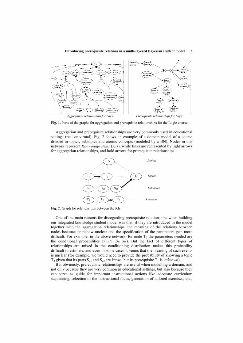
But the focus of this paper is the knowledge model. As aforementioned, one of the main problems that needed to be solved before the integrated student model developed in our previous research [9] could be integrated into the MEDEA architecture was that prerequisite relationships had not been considered. But the need for introducing prerequisite relationships in the model was evident in the very first effort to validate the MEDEA architecture, which was the development of a web-based course of Logic. One of the teachers of this subject at our university started to collaborate with our research group. When building the domain model, he only used two kinds of relationships: aggregation (is_a, is_part_of) and prerequisite, which he represented in separate graphs for better legibility. Fig 1. shows parts of such graphs:

Introducing prerequisite relations in a multi-layered Bayesian student model 3

Aggregation relationships for Logic

Prerequisite relationships for Logic

Fig. 1. Parts of the graphs for aggregation and prerequisite relationships for the Logic course

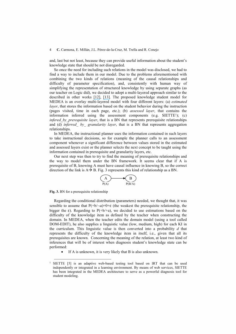
Aggregation and prerequisite relationships are very commonly used in educational settings (real or virtual). Fig. 2 shows an example of a domain model of a course divided in topics, subtopics and atomic concepts (modeled by a BN). Nodes in this network represent Knowledge items (KIs), while links are represented by light arrows for aggregation relationships, and bold arrows for prerequisite relationships.

A

T1 T2 Tn

S11 S21

C1 C2

Subject

Topics

Subtopics

ConceptsC3

S22

Fig. 2. Graph for relationships between the KIs

One of the main reasons for disregarding prerequisite relationships when building our integrated knowledge student model was that, if they are introduced in the model together with the aggregation relationships, the meaning of the relations between nodes becomes somehow unclear and the specification of the parameters gets more difficult. For example, in the above network, for node T2 the parameters needed are the conditional probabilities P(T2/T1,S21,S22). But the fact of different types of relationships are mixed in the conditioning distribution makes this probability difficult to estimate, and even in some cases it seems that the meaning of such events is unclear (for example, we would need to provide the probability of knowing a topic T2 given that its parts S21 and S22 are known but its prerequisite T1 is unknown).

But obviously, prerequisite relationships are useful when modelling a domain, and not only because they are very common in educational settings, but also because they can serve as guide for important instructional actions like adequate curriculum sequencing, selection of the instructional focus, generation of tailored exercises, etc.,

4 C. Carmona, E. Millán, J.L. Pérez-de-la-Cruz, M. Trella and R. Conejo

and, last but not least, because they can provide useful information about the student’s knowledge state that should be not disregarded.

So once the need for including such relations in the model was disclosed, we had to find a way to include them in our model. Due to the problems aforementioned with combining the two kinds of relations (meaning of the causal relationships and difficulty of parameter specification), and, consistently with human way of simplifying the representation of structured knowledge by using separate graphs (as our teacher on Logic did), we decided to adopt a multi-layered approach similar to the described in other works [12], [13]. The proposed knowledge student model for MEDEA is an overlay multi-layered model with four different layers: (a) estimated layer, that stores the information based on the student behavior during the instruction (pages visited, time in each page, etc.); (b) assessed layer, that contains the information inferred using the assessment components (e.g. SIETTE1); (c) infered_by_prerequisite layer, that is a BN that represents prerequisite relationships and (d) inferred_ by_ granularity layer, that is a BN that represents aggregation relationships.

In MEDEA, the instructional planner uses the information contained in such layers to take instructional decisions, so for example the planner calls to an assessment component whenever a significant difference between values stored in the estimated and assessed layers exist or the planner selects the next concept to be taught using the information contained in prerequisite and granularity layers, etc.

Our next step was then to try to find the meaning of prerequisite relationships and the way to model them under the BN framework. It seems clear that if A is prerequisite of B, knowing A must have causal influence in knowing B, so the correct direction of the link is A B. Fig. 3 represents this kind of relationship as a BN.

A B P(A) P(B/A)

Fig. 3. BN for a prerequisite relationship

Regarding the conditional distribution (parameters) needed, we thought that, it was sensible to assume that P(+b/¬a)=0+ε (the weakest the prerequisite relationship, the bigger the ε). Regarding to P(+b/+a), we decided to use estimations based on the difficulty of the knowledge item as defined by the teacher when constructing the domain. In MEDEA, when the teacher edits the domain model (using a tool called DOM-EDIT), he also supplies a linguistic value (low, medium, high) for each KI in the curriculum. This linguistic value is then converted into a probability d that represents the difficulty of the knowledge item in itself, i.e., given that all its prerequisites are known. Concerning the meaning of the relation, at least two kind of inferences that will be of interest when diagnosis student’s knowledge state can be performed:

• If A is unknown, it is very likely that B is also unknown.

1 SIETTE [5] is an adaptive web-based testing tool based on IRT that can be used

independently or integrated in a learning environment. By means of web services, SIETTE has been integrated in the MEDEA architecture to serve as a powerful diagnosis tool for student modeling.

Introducing prerequisite relations in a multi-layered Bayesian student model 5

• If B is known, it is very likely that A is also known. This model can be easily extended for the case of a set of two or more prerequisite

nodes for a KI, by modifying the traditional noisy AND/OR gates (depending on whether all the prerequisites of the KI are needed or there are alternative ways of getting to know it), in which instead of using 1-ε we use the probability value d associated to the KI to represent its intrinsic difficulty.

Let us then describe how the BNs for the aggregation and prerequisite layers have been defined: each elementary concept node Ci can take two values: known (represented by 1) and not_known (represented by 0), while for aggregated nodes (subtopics, topics, subject, etc), we use discrete random variables whose behavior will be emulated by binary nodes (known, not_known)2. The conditional probabilities for the aggregation and prerequisite BNs parameters are estimated in our model by pre-defined functions that use some features specified by the course designer, which namely are: difficulty degrees for each KI (that, as explained before, will be converted into probabilities d that represent their intrinsic difficulty, i.e, the probability of knowing the KI given that all its prerequisites are known) and normalized weights wij for aggregation relationships between two knowledge items Ki and Kj. From this information, an estimation of the parameters needed for the BNs of each layer is done as follows:

• For granularity relationships, the following formula is used:

++=====

otherwise0xw...xwyif1)xK,...,xy/KP(K kk11

kk11i ii

• For prerequisite relationships, the following formulas are used:

ε+======= therwiseo 0

1xxif xKxK1KP k1kk11i

...d),...,/( (Modified noisy AND-gate)

===ε+==== therwiseo

0xxif 0xKxK1KP k1kk11i d

...),...,/((Modified noisy OR-gate)

3. Evaluation of the prerequisite model

When evaluating adaptive systems, it is important to separate the evaluation of the accuracy of the user model from the evaluation of the efficacy of the adaptations based on such user models [3], [1]. If the accuracy of the user model is tested in advance, possible inefficiencies of the mechanisms for adaptation will be more easily isolated and identified and the weakest points can be improved. This section presents a preliminary evaluation of the performance of the new prerequisite layer (the aggregation layer had previously been evaluated with satisfactory results [11]). This evaluation should be considered then as an evaluation of the accuracy of the knowledge student model and not as an evaluation of MEDEA. To this end, two experiments have been performed: the first one is based on the use of a small toy example to study from a qualitative point of view the reasoning process in the

2 This emulation is possible because, as explained in [11], the probability of knowing a KI can

be interpreted as the degree of knowledge reached in such KI

6 C. Carmona, E. Millán, J.L. Pérez-de-la-Cruz, M. Trella and R. Conejo

prerequisite BN, while the second one aims to explore how the use of the prerequisite layer can improve the efficiency of the diagnosis process.

3.2. Experiment 1: a small toy example

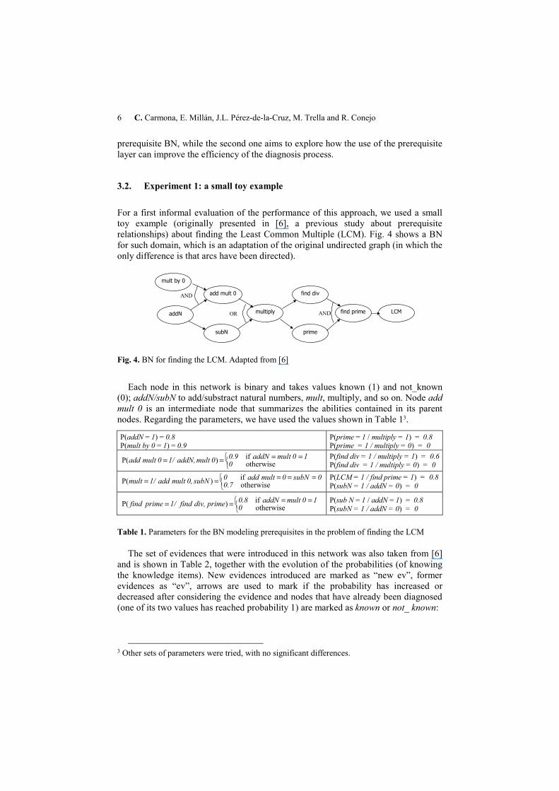
For a first informal evaluation of the performance of this approach, we used a small toy example (originally presented in [6], a previous study about prerequisite relationships) about finding the Least Common Multiple (LCM). Fig. 4 shows a BN for such domain, which is an adaptation of the original undirected graph (in which the only difference is that arcs have been directed).

addN

mult by 0

add mult 0

subN

find div

multiply LCM find prime

prime

OR

AND

AND

Fig. 4. BN for finding the LCM. Adapted from [6]

Each node in this network is binary and takes values known (1) and not_known (0); addN/subN to add/substract natural numbers, mult, multiply, and so on. Node add mult 0 is an intermediate node that summarizes the abilities contained in its parent nodes. Regarding the parameters, we have used the values shown in Table 13.

P(addN = 1) = 0.8 P(mult by 0 = 1) = 0.9

P(prime = 1 / multiply = 1) = 0.8 P(prime = 1 / multiply = 0) = 0

==== otherwise

if )P( 01 0 mult addN 0.90 mult addN, 1/ 0 mult add P(find div = 1 / multiply = 1) = 0.6

P(find div = 1 / multiply = 0) = 0

===== otherwise

if )P( 0.70 subN 0 mult add 0 subN0, mult add 1/ mult P(LCM = 1 / find prime = 1) = 0.8

P(subN = 1 / addN = 0) = 0

==== otherwise

if )P( 01 0 mult addN 0.8prime div, find 1/ prime find P(sub N = 1 / addN = 1) = 0.8

P(subN = 1 / addN = 0) = 0

Table 1. Parameters for the BN modeling prerequisites in the problem of finding the LCM

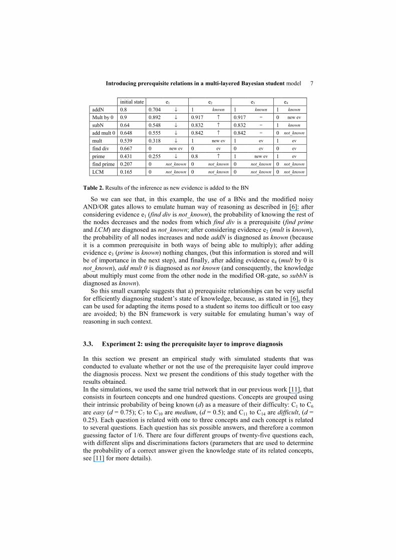
The set of evidences that were introduced in this network was also taken from [6] and is shown in Table 2, together with the evolution of the probabilities (of knowing the knowledge items). New evidences introduced are marked as “new ev”, former evidences as “ev”, arrows are used to mark if the probability has increased or decreased after considering the evidence and nodes that have already been diagnosed (one of its two values has reached probability 1) are marked as known or not_ known:

3 Other sets of parameters were tried, with no significant differences.

Introducing prerequisite relations in a multi-layered Bayesian student model 7

initial state e1 e2 e3 e4

addN 0.8 0.704 ↓ 1 known 1 known 1 known

Mult by 0 0.9 0.892 ↓ 0.917 ↑ 0.917 = 0 new ev

subN 0.64 0.548 ↓ 0.832 ↑ 0.832 = 1 known

add mult 0 0.648 0.555 ↓ 0.842 ↑ 0.842 = 0 not_known

mult 0.539 0.318 ↓ 1 new ev 1 ev 1 ev

find div 0.667 0 new ev 0 ev 0 ev 0 ev

prime 0.431 0.255 ↓ 0.8 ↑ 1 new ev 1 ev

find prime 0.207 0 not_known 0 not_known 0 not_known 0 not_known

LCM 0.165 0 not_known 0 not_known 0 not_known 0 not_known

Table 2. Results of the inference as new evidence is added to the BN

So we can see that, in this example, the use of a BNs and the modified noisy AND/OR gates allows to emulate human way of reasoning as described in [6]: after considering evidence e1 (find div is not_known), the probability of knowing the rest of the nodes decreases and the nodes from which find div is a prerequisite (find prime and LCM) are diagnosed as not_known; after considering evidence e2 (mult is known), the probability of all nodes increases and node addN is diagnosed as known (because it is a common prerequisite in both ways of being able to multiply); after adding evidence e3 (prime is known) nothing changes, (but this information is stored and will be of importance in the next step), and finally, after adding evidence e4 (mult by 0 is not_known), add mult 0 is diagnosed as not known (and consequently, the knowledge about multiply must come from the other node in the modified OR-gate, so subbN is diagnosed as known).

So this small example suggests that a) prerequisite relationships can be very useful for efficiently diagnosing student’s state of knowledge, because, as stated in [6], they can be used for adapting the items posed to a student so items too difficult or too easy are avoided; b) the BN framework is very suitable for emulating human’s way of reasoning in such context.

3.3. Experiment 2: using the prerequisite layer to improve diagnosis

In this section we present an empirical study with simulated students that was conducted to evaluate whether or not the use of the prerequisite layer could improve the diagnosis process. Next we present the conditions of this study together with the results obtained. In the simulations, we used the same trial network that in our previous work [11], that consists in fourteen concepts and one hundred questions. Concepts are grouped using their intrinsic probability of being known (d) as a measure of their difficulty: C1 to C6 are easy (d = 0.75); C7 to C10 are medium, (d = 0.5); and C11 to C14 are difficult, (d = 0.25). Each question is related with one to three concepts and each concept is related to several questions. Each question has six possible answers, and therefore a common guessing factor of 1/6. There are four different groups of twenty-five questions each, with different slips and discriminations factors (parameters that are used to determine the probability of a correct answer given the knowledge state of its related concepts, see [11] for more details).

8 C. Carmona, E. Millán, J.L. Pérez-de-la-Cruz, M. Trella and R. Conejo

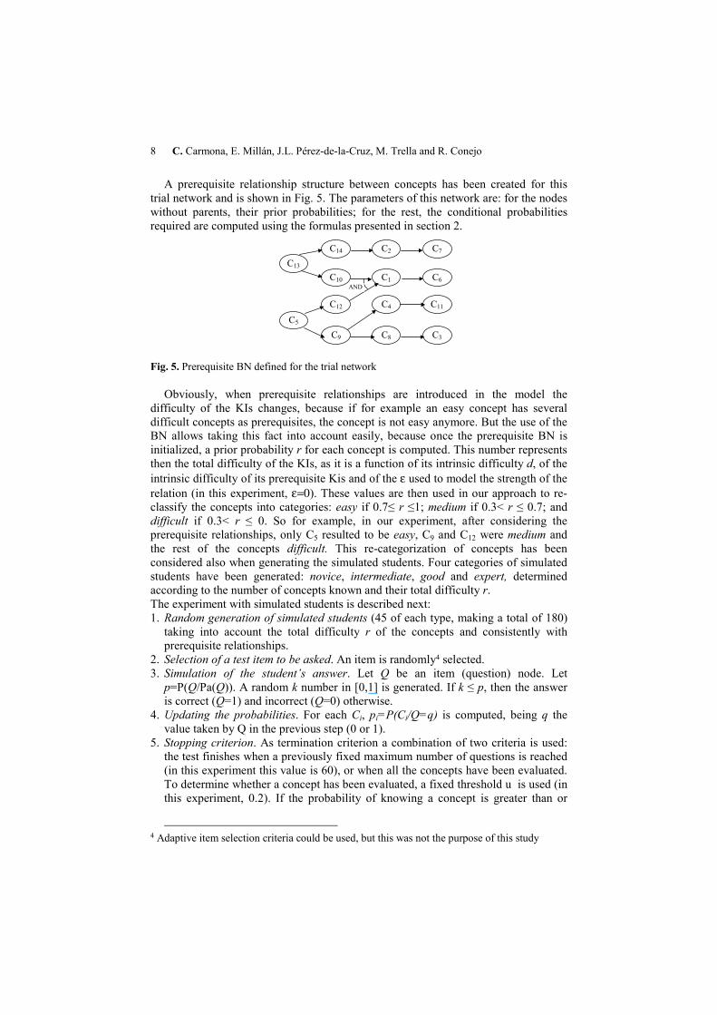
A prerequisite relationship structure between concepts has been created for this trial network and is shown in Fig. 5. The parameters of this network are: for the nodes without parents, their prior probabilities; for the rest, the conditional probabilities required are computed using the formulas presented in section 2.

C13 C14 C2 C7

C10 C1 C6

C5

C12 C4 C11

C9 C8 C3

AND

Fig. 5. Prerequisite BN defined for the trial network

Obviously, when prerequisite relationships are introduced in the model the difficulty of the KIs changes, because if for example an easy concept has several difficult concepts as prerequisites, the concept is not easy anymore. But the use of the BN allows taking this fact into account easily, because once the prerequisite BN is initialized, a prior probability r for each concept is computed. This number represents then the total difficulty of the KIs, as it is a function of its intrinsic difficulty d, of the intrinsic difficulty of its prerequisite Kis and of the ε used to model the strength of the relation (in this experiment, ε=0). These values are then used in our approach to re-classify the concepts into categories: easy if 0.7≤ r ≤1; medium if 0.3< r ≤ 0.7; and difficult if 0.3< r ≤ 0. So for example, in our experiment, after considering the prerequisite relationships, only C5 resulted to be easy, C9 and C12 were medium and the rest of the concepts difficult. This re-categorization of concepts has been considered also when generating the simulated students. Four categories of simulated students have been generated: novice, intermediate, good and expert, determined according to the number of concepts known and their total difficulty r. The experiment with simulated students is described next: 1. Random generation of simulated students (45 of each type, making a total of 180)

taking into account the total difficulty r of the concepts and consistently with prerequisite relationships.

2. Selection of a test item to be asked. An item is randomly4 selected. 3. Simulation of the student’s answer. Let Q be an item (question) node. Let

p=P(Q/Pa(Q)). A random k number in [0,1] is generated. If k ≤ p, then the answer is correct (Q=1) and incorrect (Q=0) otherwise.

4. Updating the probabilities. For each Ci, pi=P(Ci/Q=q) is computed, being q the value taken by Q in the previous step (0 or 1).

5. Stopping criterion. As termination criterion a combination of two criteria is used: the test finishes when a previously fixed maximum number of questions is reached (in this experiment this value is 60), or when all the concepts have been evaluated. To determine whether a concept has been evaluated, a fixed threshold u is used (in this experiment, 0.2). If the probability of knowing a concept is greater than or

4 Adaptive item selection criteria could be used, but this was not the purpose of this study

Introducing prerequisite relations in a multi-layered Bayesian student model 9

equal to 1-u, then the concept is diagnosed as known, whereas if it is smaller than u, the concept is diagnosed as not_known. The rest are considered not-diagnosed.

6. Test results. The cognitive state generated in the previous step is compared to the true cognitive state. The number of correctly/incorrectly/not-diagnosed concepts is computed.

7. Adding evidences. The concepts evaluated as known or not_known in the test are introduced as evidences in the prerequisite BN. The idea is to propagate this information in the network, so we concepts that have not been diagnosed yet can be correctly classified as known or not_known.

8. Prerequisite results. As in step 6, the cognitive state generated in the previous step is compared to the true cognitive state. The number of correctly/incorrectly/not-diagnosed concepts is computed.

9. Final results. The results obtained in steps 6 and 9 are compared to see how the prerequisite relationship improves the results obtained by the test.

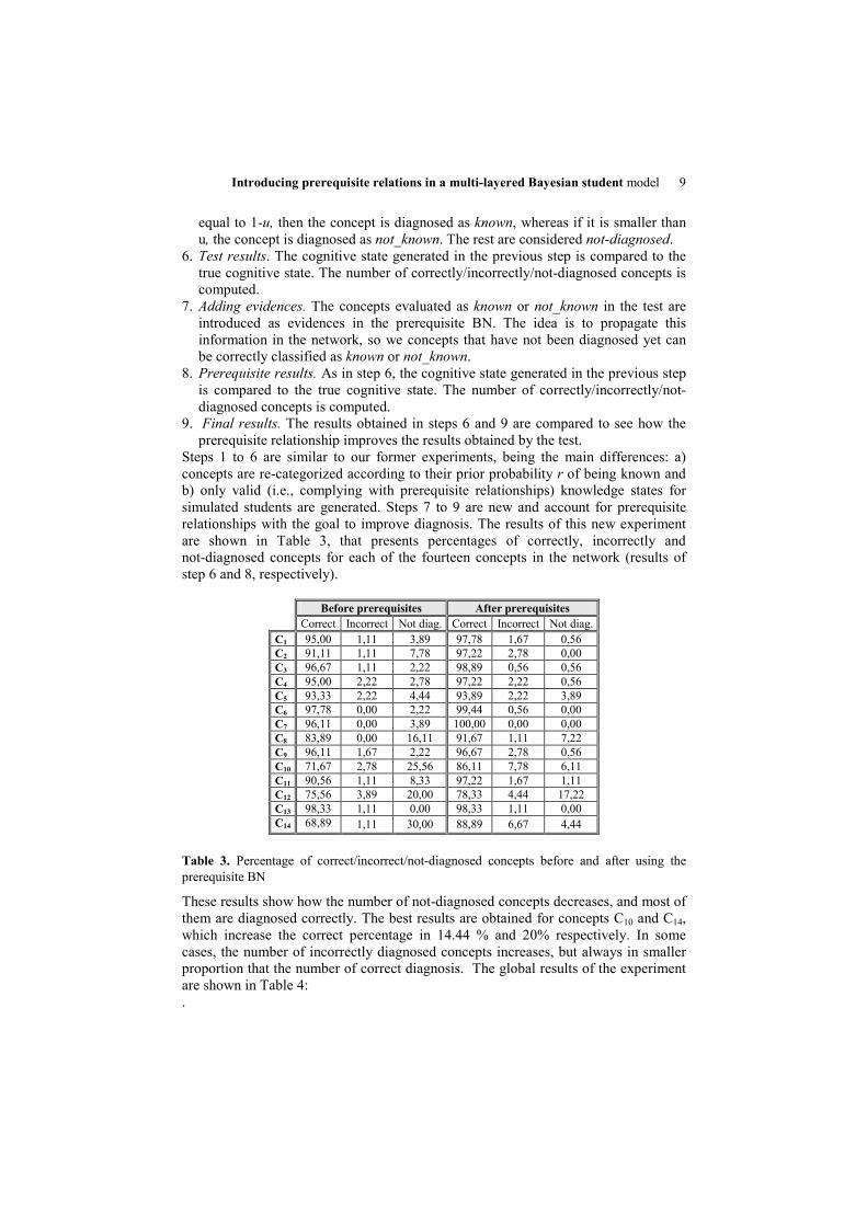
Steps 1 to 6 are similar to our former experiments, being the main differences: a) concepts are re-categorized according to their prior probability r of being known and b) only valid (i.e., complying with prerequisite relationships) knowledge states for simulated students are generated. Steps 7 to 9 are new and account for prerequisite relationships with the goal to improve diagnosis. The results of this new experiment are shown in Table 3, that presents percentages of correctly, incorrectly and not-diagnosed concepts for each of the fourteen concepts in the network (results of step 6 and 8, respectively).

Before prerequisites After prerequisites Correct Incorrect Not diag. Correct Incorrect Not diag.C1 95,00 1,11 3,89 97,78 1,67 0,56 C2 91,11 1,11 7,78 97,22 2,78 0,00 C3 96,67 1,11 2,22 98,89 0,56 0,56 C4 95,00 2,22 2,78 97,22 2,22 0,56 C5 93,33 2,22 4,44 93,89 2,22 3,89 C6 97,78 0,00 2,22 99,44 0,56 0,00 C7 96,11 0,00 3,89 100,00 0,00 0,00 C8 83,89 0,00 16,11 91,67 1,11 7,22 C9 96,11 1,67 2,22 96,67 2,78 0,56 C10 71,67 2,78 25,56 86,11 7,78 6,11 C11 90,56 1,11 8,33 97,22 1,67 1,11 C12 75,56 3,89 20,00 78,33 4,44 17,22 C13 98,33 1,11 0,00 98,33 1,11 0,00 C14 68,89 1,11 30,00 88,89 6,67 4,44

Table 3. Percentage of correct/incorrect/not-diagnosed concepts before and after using the prerequisite BN

These results show how the number of not-diagnosed concepts decreases, and most of them are diagnosed correctly. The best results are obtained for concepts C10 and C14, which increase the correct percentage in 14.44 % and 20% respectively. In some cases, the number of incorrectly diagnosed concepts increases, but always in smaller proportion that the number of correct diagnosis. The global results of the experiment are shown in Table 4: .

10 C. Carmona, E. Millán, J.L. Pérez-de-la-Cruz, M. Trella and R. Conejo

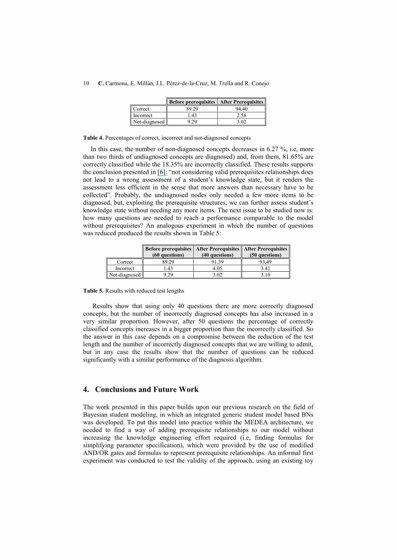
Before prerequisites After PrerequisitesCorrect 89.29 94.40 Incorrect 1.43 2.58 Not-diagnosed 9.29 3.02

Table 4. Percentages of correct, incorrect and not-diagnosed concepts

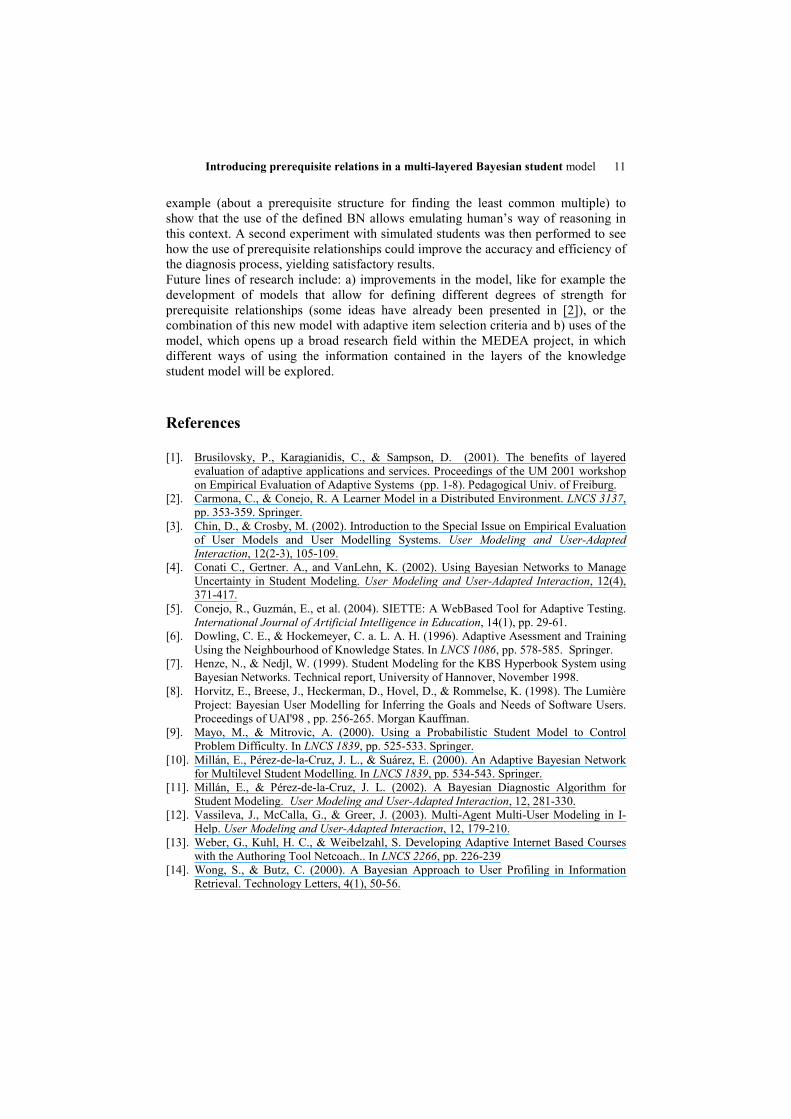
In this case, the number of non-diagnosed concepts decreases in 6.27 %, i.e, more than two thirds of undiagnosed concepts are diagnosed) and, from them, 81.65% are correctly classified while the 18.35% are incorrectly classified. These results supports the conclusion presented in [6]: “not considering valid prerequisites relationships does not lead to a wrong assessment of a student’s knowledge state, but it renders the assessment less efficient in the sense that more answers than necessary have to be collected”. Probably, the undiagnosed nodes only needed a few more items to be diagnosed, but, exploiting the prerequisite structures, we can further assess student’s knowledge state without needing any more items. The next issue to be studied now is: how many questions are needed to reach a performance comparable to the model without prerequisites? An analogous experiment in which the number of questions was reduced produced the results shown in Table 5:

Before prerequisites

(60 questions) After Prerequisites

(40 questions) After Prerequisites

(50 questions) Correct 89.29 91.39 93.49

Incorrect 1.43 4.05 3.41 Not-diagnosed 9.29 3.02 3.10

Table 5. Results with reduced test lengths

Results show that using only 40 questions there are more correctly diagnosed concepts, but the number of incorrectly diagnosed concepts has also increased in a very similar proportion. However, after 50 questions the percentage of correctly classified concepts increases in a bigger proportion than the incorrectly classified. So the answer in this case depends on a compromise between the reduction of the test length and the number of incorrectly diagnosed concepts that we are willing to admit, but in any case the results show that the number of questions can be reduced significantly with a similar performance of the diagnosis algorithm.

4. Conclusions and Future Work

The work presented in this paper builds upon our previous research on the field of Bayesian student modeling, in which an integrated generic student model based BNs was developed. To put this model into practice within the MEDEA architecture, we needed to find a way of adding prerequisite relationships to our model without increasing the knowledge engineering effort required (i.e, finding formulas for simplifying parameter specification), which were provided by the use of modified AND/OR gates and formulas to represent prerequisite relationships. An informal first experiment was conducted to test the validity of the approach, using an existing toy

Introducing prerequisite relations in a multi-layered Bayesian student model 11

example (about a prerequisite structure for finding the least common multiple) to show that the use of the defined BN allows emulating human’s way of reasoning in this context. A second experiment with simulated students was then performed to see how the use of prerequisite relationships could improve the accuracy and efficiency of the diagnosis process, yielding satisfactory results. Future lines of research include: a) improvements in the model, like for example the development of models that allow for defining different degrees of strength for prerequisite relationships (some ideas have already been presented in [2]), or the combination of this new model with adaptive item selection criteria and b) uses of the model, which opens up a broad research field within the MEDEA project, in which different ways of using the information contained in the layers of the knowledge student model will be explored.

References

[1]. Brusilovsky, P., Karagianidis, C., & Sampson, D. (2001). The benefits of layered evaluation of adaptive applications and services. Proceedings of the UM 2001 workshop on Empirical Evaluation of Adaptive Systems (pp. 1-8). Pedagogical Univ. of Freiburg.

[2]. Carmona, C., & Conejo, R. A Learner Model in a Distributed Environment. LNCS 3137, pp. 353-359. Springer.

[3]. Chin, D., & Crosby, M. (2002). Introduction to the Special Issue on Empirical Evaluation of User Models and User Modelling Systems. User Modeling and User-Adapted Interaction, 12(2-3), 105-109.

[4]. Conati C., Gertner. A., and VanLehn, K. (2002). Using Bayesian Networks to Manage Uncertainty in Student Modeling. User Modeling and User-Adapted Interaction, 12(4), 371-417.

[5]. Conejo, R., Guzmán, E., et al. (2004). SIETTE: A WebBased Tool for Adaptive Testing. International Journal of Artificial Intelligence in Education, 14(1), pp. 29-61.

[6]. Dowling, C. E., & Hockemeyer, C. a. L. A. H. (1996). Adaptive Asessment and Training Using the Neighbourhood of Knowledge States. In LNCS 1086, pp. 578-585. Springer.

[7]. Henze, N., & Nedjl, W. (1999). Student Modeling for the KBS Hyperbook System using Bayesian Networks. Technical report, University of Hannover, November 1998.

[8]. Horvitz, E., Breese, J., Heckerman, D., Hovel, D., & Rommelse, K. (1998). The Lumière Project: Bayesian User Modelling for Inferring the Goals and Needs of Software Users. Proceedings of UAI'98 , pp. 256-265. Morgan Kauffman.

[9]. Mayo, M., & Mitrovic, A. (2000). Using a Probabilistic Student Model to Control Problem Difficulty. In LNCS 1839, pp. 525-533. Springer.

[10]. Millán, E., Pérez-de-la-Cruz, J. L., & Suárez, E. (2000). An Adaptive Bayesian Network for Multilevel Student Modelling. In LNCS 1839, pp. 534-543. Springer.

[11]. Millán, E., & Pérez-de-la-Cruz, J. L. (2002). A Bayesian Diagnostic Algorithm for Student Modeling. User Modeling and User-Adapted Interaction, 12, 281-330.

[12]. Vassileva, J., McCalla, G., & Greer, J. (2003). Multi-Agent Multi-User Modeling in I-Help. User Modeling and User-Adapted Interaction, 12, 179-210.

[13]. Weber, G., Kuhl, H. C., & Weibelzahl, S. Developing Adaptive Internet Based Courses with the Authoring Tool Netcoach.. In LNCS 2266, pp. 226-239

[14]. Wong, S., & Butz, C. (2000). A Bayesian Approach to User Profiling in Information Retrieval. Technology Letters, 4(1), 50-56.