Interpreting the spatial distribution of lithic artifacts from the ...

Lakehead University

Knowledge Commons,http://knowledgecommons.lakeheadu.ca

Electronic Theses and Dissertations Electronic Theses and Dissertations from 2009

2015-06-15

Interpreting the spatial distribution of

lithic artifacts from the RLF Paleoindian

site (DdJf-13), Thunder Bay Region,

Northwestern Ontario

Langford, Dale G.

http://knowledgecommons.lakeheadu.ca/handle/2453/630

Downloaded from Lakehead University, KnowledgeCommons

Interpreting the Spatial Distribution of Lithic Artifacts from

the RLF Paleoindian Site (DdJf-13), Thunder Bay Region,


Dale G. Langford

Master of Environmental Studies (NECU)

Lakehead University Thunder Bay, Ontario

Submitted to the Faculty of Graduate Studies in Partial Fulfillment of the Requirements

for the Degree of Masters of Environmental Studies in Northern Environments and Cultures

© Dale G. Langford 2015

PERMISSION TO USE

In presenting this thesis in partial fulfillment of the requirements for a Masters of

Environmental Science in Northern Environments and Cultures from Lakehead

University, I agree that copies of this thesis shall be deposited in the Institute Library and

the department of Northern Environments and Cultures to be freely available for public

use. I further agree that permission for copying of this thesis in any manner, in whole or

in part, for scholarly purposes may be granted by my supervisor and graduate coordinator

Dr. Scott Hamilton, or in their absence, the chair of the Department of Northern

Environments and Cultures or the Dean of the Faculty of Science and Environmental

Studies. It is understood that any copying or publication of this thesis, or parts thereof for

financial gain shall not be allowed without my written permission. Also it is understood

that due recognition will be given to me and Lakehead University in any scholarly use

which may be made of any material in this thesis.

ii

ABSTRACT

This thesis explores the intra-site organization of Late Paleoindian, Lakehead

Complex populations at the RLF site (DdJf-13), located east of Thunder Bay, Ontario.

Situated upon a relic Lake Minong beach ridge, the RLF site�s modest lithic composition

and simple depositional context offered an ideal scenario for interpreting the organization

of activities during a relatively brief occupational event.

The analysis and interpretation of the RLF site was conducted using a

combination of spatial analytical techniques and ethnoarchaeological/archaeological case

studies. This resulted in the identification and interpretation of eight distinct cluster sub-

zones situated within two larger zone areas.

The results of this thesis suggest that the RLF site represents a brief Late

Paleoindian occupation during which early stage biface production was conducted. Lithic

reduction took place in distinct flint knapping areas and was oriented towards the

production of transportable biface blanks. Additionally, the southern portion of the site

exhibited evidence of cutting/scraping activities, likely associated with either food

preparation or hide working. Further spatial patterning, in correlation with the results

from near surface geophysics (NSG), provided evidence for the possible presence of a

built structure and hearth focused lithic distribution in the northern portion of the site.

The RLF site analysis is a valuable case study for the application of intra-site

spatial analysis on Boreal forest sites, as well as those utilizing CRM derived data sets.

Furthermore, it provides a starting point from which future studies of Lakehead Complex

site organization and use can be compared.

iii

ACKNOWLEDGEMENTS

I would first like to thank my advisor Dr. Scott Hamilton (Department of

Anthropology, Lakehead University) for the countless hours he spent helping me

throughout the process of this thesis. Thank you to Dr. Matt Boyd (Department of

Anthropology, Lakehead University) and Dr. Terry Gibson (Senior Manager and

Founding Partner of Western Heritage - Adjunct Professor, Department of Anthropology,

Lakehead University) for their valuable feedback throughout the review process. I want

to thank Dr. David F. Overstreet (College of Menominee Nation) for the insight he

provided as external examiner for this thesis.

I would like to thank Western Heritage and all of the people involved with this

project, from initial excavation to the final analysis. Without the dedication of everyone

involved with the RLF site project this thesis would not have been possible.

Lastly, I would like to thank my family, friends, and colleagues (you know who you

are). I could not have completed this project without your support. I owe all of you a

drink. Cheers.

iv

TABLE OF CONTENTS

PERMISSION TO USE.............................................................................................. ii

ABSTRACT................................................................................................................ iii

ACKNOWLEDGEMENTS ...................................................................................... iv

LIST OF FIGURES ................................................................................................... ix

LIST OF TABLES ................................................................................................... xix

1. INTRODUCTION....................................................................................................1

1.1 Site Summary..................................................................................................2 1.2 Study Objectives .............................................................................................3 1.3 Thesis Outline .................................................................................................4

2. DEGLACIATION AND ENVIRONMENTAL DEVELOPMENT ....................6

2.1 Introduction .....................................................................................................6 2.2 Glacial History of Northwestern Ontario........................................................6

2.2.1 Pre-Marquette Glacial Retreat .........................................................7 2.2.1 The Marquette Advance...................................................................8

2.3 Glacial Lake Development .............................................................................9 2.3.1 Glacial Lake Agassiz and Lake-Level Fluctuations in the

Superior Basin................................................................................10 2.4 Vegetation Change within Northwestern Ontario.........................................14 2.5 Summary .......................................................................................................14

3. PALEOINDIAN OCCUPATION IN NORTHWESTERN ONTARIO............16

3.1 Introduction ...................................................................................................16 3.2 The Lakehead Complex ................................................................................16 3.3 The Interlakes Composite .............................................................................21 3.4 Spatial Investigations of Lakehead Complex Sites.......................................22

3.4.1 The Naomi Site (DcJh-42) .............................................................23 3.4.2 The Crane Cache (DcJj-14) ...........................................................26

3.5 Summary .......................................................................................................27

4. THE RLF SITE ......................................................................................................29

4.1 Introduction ...................................................................................................29 4.2 Site Location and Environment ....................................................................29

4.2.1 Site Stratigraphy.............................................................................30 4.3 Proposed Site Environment during Site Occupation ....................................32 4.4 Excavation Methods......................................................................................36

4.4.1 Field Methodologies: Lakehead University...................................36 4.4.2 Field Methodologies: Western Heritage ........................................37

4.5 Near Surface Geophysics ..............................................................................38 4.6 Artifact Analysis and Cataloging: ADEMAR ..............................................39 4.7 Artifact Recoveries: Overview .....................................................................40 4.8 Lithic Artifacts ..............................................................................................42

4.8.1 Lithic Artifacts: FCR .......................................................................43

4.8.2 Lithic Artifacts: Non-Debitage........................................................43

v

4.8.3 Lithic Artifacts: Debitage ................................................................54 4.9 Summary and Preliminary Site Interpretation ..............................................58

5. SPATIAL ANALYSIS IN ARCHAEOLOGY ....................................................60

5.1 Introduction ...................................................................................................60 5.2 Current Approaches to the Archaeology of Northwestern Ontario ..............60 5.3 Spatial Analysis in Archaeology...................................................................61 5.4 Lithic Recoveries as an Indicator of Activity Location ................................65

5.4.1 Lithic Reduction and Maintenance Loci ........................................66 5.4.2 Bone Tool Production ....................................................................67 5.4.3 Hide Preparation and Working ......................................................68 5.4.4 Butchering and Cooking Activities................................................68

5.5 Identifying Hearth Centred Activities...........................................................69 5.6 Structure vs. Non-Structure Related Deposits ..............................................70 5.7 Cultural Transformation Processes Affecting Spatial Investigations ...........72 5.8 Non- Cultural Transformation Processes Affecting Spatial

Investigations ................................................................................................74 5.9 Summary .......................................................................................................75

6. METHODS.............................................................................................................77

6.1 Introduction ...................................................................................................77 6.2 Data Access...................................................................................................77 6.3 Geographic Information Systems (GIS) .......................................................77 6.4 K-Means and Kernel Density Cluster Analysis ............................................78 6.5 Nearest Neighbour Analysis and Ripley�✁ ✂ Function .................................80

6.6 Getis-Ord General Gi Clustering Analysis....................................................81 6.7 Refitting Analysis .........................................................................................82 6.8 Interpreting Activity Areas ...........................................................................82 6.9 Summary .......................................................................................................83

7. RESULTS ...............................................................................................................85

7.1 Introduction ...................................................................................................85 7.2 Sub-Zone Identification ................................................................................85

7.2.1 Initial Clustering Results................................................................85 7.2.2 Identified Mechanical Disturbance ................................................89 7.2.3 Sub-Zones ......................................................................................92

7.3 Sub-Zone A1 .................................................................................................98 7.3.1 A1: Artifact Recoveries .................................................................98 7.3.2 A1: Vertical Distribution .............................................................100 7.3.3 A1: Horizontal Distributions: General .........................................101 7.3.4 A1: Horizontal Distributions: Recoveries by Level.....................103 7.3.5 A1: Horizontal Distributions: Recoveries by Material Type .......108 7.3.6 A1: Horizontal Distributions: Debitage .......................................111 7.3.7 A1: Horizontal Distributions: Tools ............................................117 7.3.8 A1: NSG Results..........................................................................120

7.4 Sub-Zone A2 ...............................................................................................121

vi

7.4.1 7.4.2 7.4.3

7.4.4

A2: Artifact Recoveries ...............................................................122 A2: Vertical Distribution .............................................................124 A2: Horizontal Distributions: General .........................................125

A2: Horizontal Distributions: Recoveries by Level.....................127

7.4.5 A2: Horizontal Distributions: Recoveries by Material Type .......128 7.4.6 A2: Horizontal Distributions: Debitage .......................................138 7.4.7 A2: Horizontal Distributions: Tools ............................................148 7.4.8 A2: NSG Results..........................................................................152

7.5 Sub-Zone B1 ...............................................................................................153 7.5.1 B1: Artifact Recoveries................................................................153 7.5.2 B1: Vertical Distribution..............................................................154 7.5.3 B1: Horizontal Distributions: General .........................................156 7.5.4 B1: Horizontal Distributions: Recoveries by Level .....................158 7.5.5 B1: Horizontal Distributions: Recoveries by Material Type .......158 7.5.6 B1: Horizontal Distributions: Debitage .......................................158 7.5.7 B1: Horizontal Distributions: Tools ............................................158 7.5.8 B1: NSG Results ..........................................................................172

7.6 Sub-Zone B2 ...............................................................................................173 7.6.1 B2: Artifact Recoveries................................................................173 7.6.2 B2: Vertical Distribution..............................................................175 7.6.3 B2: Horizontal Distributions: General .........................................177 7.6.4 B2: Horizontal Distributions: Recoveries by Level.....................178 7.6.5 B2: Horizontal Distributions: Recoveries by Material Type .......182 7.6.6 B2: Horizontal Distributions: Debitage .......................................185 7.6.7 B2: Horizontal Distributions: Tools ............................................191 7.6.8 B2: NSG Results ..........................................................................196

7.7 Sub-Zone B3 ...............................................................................................197 7.7.1 B3: Artifact Recoveries................................................................198 7.7.2 B3: Vertical Distribution..............................................................199 7.7.3 B3: Horizontal Distributions: General .........................................200 7.7.4 B3: Horizontal Distributions: Recoveries by Level .....................202 7.7.5 B3: Horizontal Distributions: Recoveries by Material Type .......204 7.7.6 B3: Horizontal Distributions: Debitage .......................................205 7.7.7 B3: Horizontal Distributions: Tools ............................................210 7.7.8 B3: NSG Results ..........................................................................211

7.8 Sub-Zone B4 ...............................................................................................211 7.8.1 B4: Artifact Recoveries................................................................212 7.8.2 B4: Vertical Distribution..............................................................214 7.8.3 B4: Horizontal Distributions: General .........................................215 7.8.4 B4: Horizontal Distributions: Recoveries by Level .....................217 7.8.5 B4: Horizontal Distributions: Recoveries by Material Type .......217 7.8.6 B4: Horizontal Distributions: Debitage .......................................217 7.8.7 B4: Horizontal Distributions: Tools ............................................217

7.8.8 B4: NSG Results ..........................................................................221

vii

8. SITE INTERPRETATIONS...............................................................................222 8.1 8.2

8.3

Introduction .................................................................................................222 Disturbance Processes at the RLF Site .......................................................222

RLF Site: Sub-Zone Interpretations ............................................................223

8.3.1 Sub-Zone A1 ................................................................................223 8.3.2 Sub-Zone A2 ................................................................................225 8.3.3 Sub-Zone B1 ................................................................................231 8.3.4 Sub-Zone B2 ................................................................................231 8.3.5 Sub-Zone B3 ................................................................................234 8.3.6 Sub-Zone B4 ................................................................................234

8.4 Overall Site Function and Organization .....................................................235

9. DISCUSSION .......................................................................................................238

9.1 Introduction .................................................................................................238 9.2 The RLF Site and the Lakehead Complex ..................................................238 9.3 Implications for the Study of Small Scale Sites in Northwestern

Ontario ........................................................................................................241 9.4 Study Limitations, Concerns, and Future Directions ..................................243

9.4.1 Spatial Analysis and CRM Derived Samples ..............................243 9.4.2 Comments on Spatial Analysis in Archaeology ..........................246 9.4.3 Improving Activity Area Interpretability.....................................248

9.5 Summary .....................................................................................................248

10. CONCLUSION ..................................................................................................250

11. REFERENCES...................................................................................................254

viii

LIST OF FIGURES

Figure 1.1.1 Location of RLF site along the north shore of Lake Superior .....................3

Figure 2.1.1 Approximate locations of end moraines within Northwestern

Ontario with relative depositional chronology. Where Vm) vermillion, E-F) Eagle-Finlayson, BC) Brule Creek, Ma) Marks, Ha) Hartman, DL) Dog Lake, LS) Lac Seul, SL) Sioux Lookout, Ka) Kaiashk, WH) Whitewater, Ag) Agutua, Ni) Nipigon, and Nk) Nakina (After Björck 1985, Kingsmill 2011, and Lowell et al. 2010) ................................................................................7

Figure 2.1.2 Approximate locations of the Laurentide Ice Sheet margin

during the Marquette advance ~10.4 to 9.5 kaBP (After Phillips 1993) ............................................................................................................9

Figure 2.2.1 Various drainage outlets of glacial Lake Agassiz over the

course of its existence. NW) Northwestern, S) Southern, K) Eastern outlets through Thunder Bay, E) Eastern outlets through Nipigon Basin, KIN) Kinojevis outlet, HB) Hudson Bay final drainage route (From Shultis 2013 after Teller et al. 2005) ..........................................................................................................11

Figure 3.1.1 Examples of Late Paleoindian projectile points of the Lakehead

Complex. A) Various Lakehead Complex sites, B) Mackenzie 1 site (From Bennett 2015, images by Markham 2013) ............................20

Figure 3.3.1 The Interlakes composite, including 1) Lake of the

Woods/Rainey River, 2) Quetico/Superior, 3) Lakehead, and 4) Reservoir Lakes (After Ross 1995)............................................................22

Figure 3.4.1 Lithic distributions from the Naomi site (DcJh-42). A) Cluster

�A✁✂ B) Cluster �B✁✂ and C✄ ☎✆✝✞✟✠✡ �☎✁ (From Adam 1995) .....................24

Figure 4.2.1 Location of RLF site at the time of excavation..........................................30

Figure 4.2.2 Vertical distribution of artifacts by level at the RLF site.

Recovery levels 2 and 3 indicated by red star............................................32

Figure 4.3.1 Topography of the RLF site area: A) Plan map, B) Plan map

with artifact clusters, and C) Side relief of site topography with general artifact cluster areas illustrated. Note: Elevation by

metres. ........................................................................................................34

ix

Figure 4.3.2 Conceptual placement of the RLF site within the local environment based of topography and stratigraphic sequences. This is highly speculative...........................................................................35

Figure 4.8.1 Adze recovered from the RLF site .............................................................48

Figure 4.8.2 Taconite artifact catalogued as being a wedge. This piece may

represent an early stage failed biface End exhibiting battering indicated by red stars .................................................................................49

Figure 4.8.3 Possible failed projectile point or drill.......................................................50

Figure 4.8.4 Core 2820 with blade flake removal. Note: blade flake is

missing striking platform (indicated by red star) .......................................54

Figure 4.8.5 Example of RLF size grade sorting during artifact cataloging ..................57

Figure 5.3.1 Stylized example of the drop/toss/displacement model with

various cluster discard models indicated. (After Binford 1983; Gibson 2001; and Stevenson 1986, 1991) .................................................64

Figure 7.2.1 Results of RLF catalog trimming prior to application of k-

means, kernel density, and Getis-Ord Gi. Trimmed artifacts were generally the result of surface collection or excavation outliers........................................................................................................86

Figure 7.2.2 Line graph of plotted Log10%SSE for k-means tests 2 through

10. Inflection at k=8 clusters indicated by red circle .................................87

Figure 7.2.3 Maps illustrating the resulting cluster designations (A), kernel density results (B), and map comparing the two results (C). It can be seen here that cluster 4 (orange) was not identified during kernel density analysis. Due to identification within k- means analysis this cluster area will still be explored ...............................88

Figure 7.2.4 Results of Getis-Ord Gi represented visually by plotting resulting z-scores. This illustrates the two areas of highest recovery, of �hot-✁✂✄☎✁✆✝ within the RLF site. ............................................89

Figure 7.2.5 Areas of site disturbance. Note: the boundaries of this site

disturbance are not well defined and represent the proposed impacted area from field excavation notes. Yellow square indicates area of greatest disturbance as indicated by field notes..............90

Figure 7.2.6 Units discussed in text in relation to site disturbance ................................91

x

Figure 7.2.7 Mapped artifact distributions by level. This map series illustrates that as recoveries are removed down to identified undisturbed sediments, little to no artifacts remain within the

area .............................................................................................................93

Figure 7.2.8 Map of k-means cluster results for k=8 (A) with trimmed map

of defined clusters with cluster two removed (B) ......................................94

Figure 7.2.9 Defined sub-zone with comparison to cluster designations. It

can be seen here that cluster 3 and 8 were combined to form one cluster. This was due to the observed disturbance discussed in section 7.2.2 ...........................................................................................96

Figure 7.2.10 Defined sub-zones compared with topographic relief map

(Represented by black lines) (A) and resulting zone designations (B) .........................................................................................97

Figure 7.3.1 Sub-zone in relation to topography with close up of sub-zone

A1 illustrating all tool recoveries with total debitage by quad ..................98

Figure 7.3.2 Total artifact recoveries by level indicating high recovery

frequency within upper levels; likely the result of disturbance activities previously discussed .................................................................100

Figure 7.3.3 Total artifact distribution by level and size showing that

debitage in the size ranges of 2-12mm are recovered in highest frequencies around level 1, while larger size grades are

recovered near level 3 ..............................................................................101

Figure 7.3.4 Results of nearest neighbour analysis indicating that at a z-

score of -8.929599 there is a less than 1% chance that the observed distribution is the result of random chance...............................102

Figure 7.3.5 Graph of Ripley�✁ ✂ function analysis illustrating that the

observed distribution if likely the result of a clustered distribution ...............................................................................................102

Figure 7.3.6 Results of Getis-Ord Gi analysis indicating that at a z-score of

6.093171 there is a less than 1% chance that the observed distribution is the result of random chance ..............................................103

Figure 7.3.7 Sub-zone A1 recoveries by level ✄ Frequency and Getis-Ord

Gi. While levels yielding few artifact recoveries are generally not useful for the application of spatial statistics, Getis-Ord Gi

results are illustrated for all levels in order to maintain

consistency ...............................................................................................107

xi

Figure 7.3.8 Sub-zone A1 artifact distributions by material type � Frequency and Getis-Ord Gi. A) Taconite, B) Gunflint Silica, C) Siltstone, D) Chert, and E) Quartz ......................................................110

Figure 7.3.9 Artifact cluster identified through the mapping of taconite

artifacts. Yellow represents clustering likely related to disturbed artifacts while blue represents clustering observed throughout vertical analysis. Clusters discussed in text as A) Western, B) Northeastern, C) South-central, and D) South- eastern ......................................................................................................111

Figure 7.3.10 Debitage distributions by size grade � Frequency and Getis-

Ord Gi .......................................................................................................114

Figure 7.3.11 Debitage distributions by type � Frequency and Getis-Ord Gi ................116

Figure 7.3.12 Distribution of all tool recoveries from sub-zone A1 with total debitage by quadrat ..................................................................................117

Figure 7.3.13 Distribution of sub-zone A1 cores by cortex type and level....................118

Figure 7.3.14 Distribution of sub-zone A1 bifaces by level (indicated within

yellow circle) ...........................................................................................119

Figure 7.3.15 Distribution of sub-zone A1 bifaces by production stage

(indicated within yellow circle) ...............................................................119

Figure 7.3.16 NSG results in relation to sub-zone A1 ...................................................121

Figure 7.4.1 Sub-zone in relation to topography with a close up of sub-zone

A2 illustrating all tool recoveries with total debitage by quad ................122

Figure 7.4.2 Total artifact recoveries by level indicating highest artifact

clustering around level 3 ..........................................................................124

Figure 7.4.3 Total artifact recoveries by size and level................................................125





xii

Figure 7.4.6 Graph of Ripley�✁ ✂ function analysis illustrating that the observed distribution is likely the result of a clustered distribution ...............................................................................................127

Figure 7.4.7 Sub-zone A2 artifacts by level ✄ Frequency and Getis-Ord Gi................134

Figure 7.4.8 Sub-zone A2 artifact distributions by material type. A)

Taconite, B) Gunflint Silica, C) Siltstone, D) Chert, E) Quartz, F) Mudstone, and G) Amethyst ...............................................................138

Figure 7.4.9 Distribution of all debitage by quadrat illustrating a circular

distribution of materials. Segmenting discussed in figure 7.4.10 indicated by dashed lines .........................................................................139

Figure 7.4.10 Results of sub-zone cross-section. A) North/South artifact

frequencies, B) West/East artifact frequencies ........................................139

Figure 7.4.11 Kernel density of sub-zone A2 artifact distributions ...............................140

Figure 7.4.12 Distributions of sub-zone A2 debitage by size ........................................143

Figure 7.4.13 Distribution of sub-zone A2 debitage by type .........................................146

Figure 7.4.14 Distribution of sub-zone A2 debitage vs. microdebitage.........................147

Figure 7.4.15 Distribution of all sub-zone A2 tools with total debitage by

quadrat. Field photos of anvil stones inset (Photos by S. Hamilton and C. Surette) .........................................................................148

Figure 7.4.16 Distribution of sub-zone A2 cores by cortex type ...................................149

Figure 7.4.17 Distribution of sub-zone A2 bifaces by level (A) and stage (B).

Level and stage indicated by numbers within yellow circles ..................150

Figure 7.4.18 Distribution of sub-zone A2 re-touched flakes by intentional or

incidental flaking .....................................................................................151

Figure 7.4.19 NSG results for sub-zone A2. High magnetic anomalies can be

seen in correlation with voids in artifact concentrations and high recovery frequencies ........................................................................152


B1 illustrating all tool recoveries with total debitage by quad ................153

Figure 7.5.2 Total artifact recoveries by level for sub-zone B1 ...................................155

xiii

Figure 7.5.3 Total artifact recoveries by size and level................................................155






observed distribution is likely the result of a clustered distribution ...............................................................................................157

Figure 7.5.7 Distribution of sub-zone B1 artifacts by level. This shows that

locations of high frequency artifact recoveries remains constant ............164

Figure 7.5.8 Distribution of sub-zone B1 artifacts by material. A) Taconite,

B) Gunflint Silica .....................................................................................165

Figure 7.5.9 Distribution of sub-zone B1 debitage by size ..........................................168

Figure 7.5.10 Distribution of sub-zone B1 debitage by type .........................................170

Figure 7.5.11 Distribution of sub-zone B1 tools with total debitage by quad ...............171

Figure 7.5.12 Sub-zone B1 biface distributions by stage ...............................................171

Figure 7.5.13 NSG results for sub-zone B1 ...................................................................172



Figure 7.6.2 Total recoveries by level for sub-zone B2 ...............................................176

Figure 7.6.3 Sub-zone B2 total recoveries by size and level .......................................176





xiv

Figure 7.6.6 Graph of Ripley�✁ ✂ function analysis illustrating that the observed distribution is likely the result of a clustered distribution ...............................................................................................178

Figure 7.6.7 Distribution of sub-zone B2 artifacts by level indicating two

primary clustering areas ...........................................................................182

Figure 7.6.8 Distribution of sub-zone B2 artifacts by materials type: A)

Taconite, B) Gunflint silica, C) Siltstone, D) Chert, E) ✄Other�☎ F) Quartz, and G) Amethyst.....................................................................185

Figure 7.6.9 Distribution of all sub-zone B2 debitage by quadrat showing

two primary cluster locations with lesser debitage frequencies occurring in between ................................................................................186

Figure 7.6.10 Sub-zone B2 debitage distributions by size .............................................188

Figure 7.6.11 Sub-Zone B2 debitage distribution by type .............................................190

Figure 7.6.12 Distribution of all tools in sub-zone B2 with total debitage

recoveries by quadrat ...............................................................................192

Figure 7.6.13 Distribution of sub-zone B2 cores by cortex type and level ....................193

Figure 7.6.14 Distribution of sub-zone B2 bifaces by recovery level............................193

Figure 7.6.15 Distribution of sub-zone B2 bifaces by stage ..........................................194

Figure 7.6.16 Distribution of re-touched flakes by intention vs. incidental

flaking ......................................................................................................194

Figure 7.6.17 Distribution of FCR and charcoal recoveries from sub-zone B2.............196

Figure 7.6.18 Results of NSG for sub-zone B2..............................................................197



Figure 7.7.2 Sub-zone B3 total artifact recoveries by level .........................................199

Figure 7.7.3 Sub-zone B3 artifact recoveries by size and level ...................................199


score of -0.399164 the observed pattern varies little from that

of a random distribution ...........................................................................200

xv

Figure 7.7.5 Results of Getis-Ord Gi analysis indicating that at a z-score of 3.825710 there is a less than 1% chance that the observed distribution is the result of random chance ..............................................201



Figure 7.7.7 Sub-zone B3 artifact recoveries by level .................................................204

Figure 7.7.8 Sub-zone B3 artifact distributions by material: A) Taconite,

and B) Gunflint silica...............................................................................205

Figure 7.7.9 Sub-zone B3 debitage distribution by size...............................................207

Figure 7.7.10 Sub-zone B3 debitage distribution by type ..............................................209

Figure 7.7.11 Sub-zone B3 tool recoveries with total debitage by quadrat ...................210

Figure 7.7.12 Results of NSG survey for sub-zone B3 ..................................................211



Figure 7.8.2 Siltstone artifact recoveries from the Mackenzie 1 (A) and RLF

(B and C) sites. Flake refits from items B and C do not appear to exhibit cultural modification, but rather natural fracturing .................213

Figure 7.8.3 Sub-zone B4 artifact frequencies by level ...............................................214

Figure 7.8.4 Sub-zone B4 artifact frequencies by size and level .................................215


score of 1.146096 the observed pattern varies little from that of a random distribution ...............................................................................215

Figure 7.8.6 Results of Getis-Ord Gi analysis indicating that at a z-score of -

0.094854 the observed pattern varies little from that of a random distribution ..................................................................................216



Figure 7.8.8 Distribution of sub-zone B4 recoveries by level......................................219

xvi

Figure 7.8.9 Distribution of sub-zone B4 recoveries by material type: A) Taconite, B) Gunflint silica, and C) Siltstone ..........................................220

Figure 7.8.10 Sub-zone B4 tool distributions with total debitage by quadrat ................221

Figure 7.8.11 Results of NSG survey for sub-zone B4. The presence of

magnetic anomalies can be seen spreading into the sub-zone from the west............................................................................................221

Figure 8.2.1 Vertical distribution of all artifact recoveries by level ............................223

Figure 8.3.1 Artifact distributions for sub-zone A1 indicating presence of three distinct

cluster areas. Note: Surface and level 1 recoveries removed....................................................................................................224

Figure 8.3.2 Artifact distributions for sub-zone A2 with two primary cluster

areas indicated..........................................................................................226

Figure 8.3.3 Proposed hearth location with A) artifact distributions, and B)

Magnetic results from NSG .....................................................................227

Figure 8.3.4 Distribution of potlidded artifacts with results of near surface

magnetometry. Proposed hearth location indicated by black circle.........................................................................................................228

Figure 8.3.5 Debitage distributions for sub-zone A2 with proposed

structural elements indicated based on the confined distribution of lithic artifacts .......................................................................................230

Figure 8.3.6 Artifact distributions for sub-zone B2 with areas of proposed

lithic reduction (B2-A and B2-B) and secondary cutting/scrapping activities (B2-C) ..........................................................233

Figure 8.3.7 Location of sub-zone B2 artifacts in relation to magnetic

anomalies .................................................................................................233

Figure 8.4.1 Distribution of activities within the RLF site in zone� ✁A✂ (red)

a✄☎ ✁✆✂ (yellow) with topographic contours represented by black lines ................................................................................................236

Figure 9.2.1 Percent total bifaces by stage for the RLF (DdJf-13), Naomi

(DcJh-42), and Biloski (DcJh-9) sites......................................................239

Figure 9.4.1 Idealized diagram illustrating the effects of batch cataloguing

of artifact resulting in the blurring of fine scale debitage

patterning in a 1x1 m unit ........................................................................244

xvii

Figure 9.4.2 Diagram illustrating the effects of quadrat size on the spatial interpretability of artifact distributions. While reducing quadrat size further to 25x25 cm would improve the spatial resolution of patterning, the time required would double. This would limit the ability to excavate large areas of a site, reducing the overall

site picture ................................................................................................245

xviii

LIST OF TABLES

Table 3.1.1 Frequency of Late Paleoindian material recoveries illustrating preference for the exploitation of Gunflint materials ................................19

Table 4.7.1 Total recoveries from the RLF site for the four basic catalog

categories. Note: Bone is likely modern intrusion, item #3391 removed as fragments ................................................................................41

Table 4.7.2 Faunal recoveries from the RLF site..........................................................41

Table 4.7.3 Charcoal recoveries from the RLF site ......................................................42

Table 4.8.1 Breakdown of lithic recoveries from the RLF site by basic type ..............42

Table 4.8.2 Breakdown of non-debitage lithic recoveries from the RLF site...............44

Table 4.8.3 Results of Biface staging for RLF site recoveries. Staging

conducted following the non-metric descriptions by Bennett (2015) .........................................................................................................46

Table 4.8.4 RLF lithic waste recovery frequencies by four base categories ................55

Table 4.8.5 RLF lithic waste recoveries by material type ............................................56

Table 4.8.6 RLF lithic recovery frequencies by size ....................................................57

Table 4.8.7 Description of methods used to classify RLF debitage by type

with total recovery frequencies ..................................................................58

Table 7.3.1 All tool recoveries from sub-zone A1........................................................99

Table 7.3.2 Results of biface staging for sub-zone A1 following Bennett

(2015) .........................................................................................................99

Table 7.3.3 Results of cortex identification for sub-zone A1 .......................................99

Table 7.3.4 Debitage frequencies by type .....................................................................99

Table 7.3.5 Debitage frequencies by material...............................................................99

Table 7.3.6 Debitage frequencies by size grades ..........................................................99

Table 7.4.1 All tool recoveries from sub-zone A2......................................................123

xix

Table 7.4.2 Results of biface staging for sub-zone A2 following Bennett (2015) .......................................................................................................123

Table 7.4.3 Results of cortex identification for sub-zone A2 .....................................123

Table 7.4.4 Debitage frequencies by type ...................................................................123

Table 7.4.5 Debitage frequencies by material.............................................................124

Table 7.4.6 Debitage frequencies by size grades ........................................................124

Table 7.5.1 Sub-zone B1 tool recoveries ....................................................................154

Table 7.5.2 Debitage frequencies by size ...................................................................154

Table 7.5.3 Debitage frequencies by type ...................................................................154

Table 7.5.4 Debitage frequencies by material.............................................................154

Table 7.6.1 Sub-zone B2 tool recoveries by type. Note: Bracketed number

represents total without refitted artifacts..................................................174

Table 7.6.2 Sub-zone B2 core frequencies by cortex type..........................................174

Table 7.6.3 Sub-zone B2 biface frequencies by stage following Bennett

(2015) .......................................................................................................174

Table 7.6.4 Breakdown of sub-zone B2 re-touched flakes by either

incidental or intentional flaking ...............................................................175

Table 7.6.5 Sub-zone B2 debitage by material ...........................................................175

Table 7.6.6 Sub-zone B2 debitage by type .................................................................175

Table 7.6.7 Sub-zone B2 debitage by size grade ........................................................175

Table 7.7.1 Sub-zone B3 tool recoveries ....................................................................198

Table 7.7.2 Sub-zone B3 debitage frequencies by size...............................................198

Table 7.7.3 Sub-zone B3 debitage frequencies by type ..............................................198

Table 7.7.4 Sub-zone B3 debitage frequencies by material........................................198

Table 7.8.1 Sub-zone B4 debitage frequency by size .................................................213

xx

Table 7.8.2 Sub-zone B4 debitage frequency by type ................................................214

Table 7.8.3 Sub-zone B4 debitage frequency by material ..........................................214

Table 9.2.1 Comparison of biface recoveries by stage for the RLF (DdJf-

13), Naomi (DcJh-42), and Biloski (DcJh-9) sites ..................................239

xxi

Chapter 1

Introduction

1.0 Introduction

This thesis presents research conducted to assess the spatial organization of

artifacts in order to interpret activities that occurred at the RLF site (DdJf-13), located

east of Thunder Bay, Ontario. Excavated during the summer of 2011, this Late

Paleoindian, Lakehead Complex (Fox 1975, 1980), site yielded modest lithic remains,

exhibiting distinct and localized clustering. The site�s small size and relatively simple

depositional context suggests a brief occupation, offering an opportunity to address long-

standing questions regarding the spatial organization of Late Paleoindian sites in the

Thunder Bay region.

While research regarding the Lakehead Complex has contributed to the

understanding of the lithic industry, tool use, site selection, and regional trade employed

by past populations, it has been unable to address site organization at the intra-site level

(exception see Adams 1995). This limited spatial research has not been without effort

(e.g. Hinshelwood and Weber 1987), but rather, a consequence of poor taphonomic and

recovery conditions resulting in reduced spatial integrity. Compounding these issues is

the tendency for previous excavations to focus on large, complex, and repeatedly

occupied sites with severe bioturbation of shallow artifact deposits. While similar

taphonomic issues are expected at the RLF site, the comparatively brief and simple

occupation profile improves its interpretive resolution.

1

2

The discovery and excavation of the RLF site provides the opportunity to study the

intra-site organization of Lakehead Complex people, and increase the understanding of

how these past populations utilized their site environments.

1.1 Site Summary

The RLF site is located in the Thunder Bay region of Northwestern Ontario. For the

purpose of this thesis, the Thunder Bay region is used to refer to an area spreading east to

include the Sibley Peninsula, west to the Canada/United States border, and approximately

50km inland from the shores of Lake Superior. The RLF site was first discovered in 2010

during an archaeological survey, prior to the twinning of Highway 11/17 east of Thunder

Bay, Ontario. The site is located approximately 20km east of Thunder Bay, and 1.2 km

inland from the current Lake Superior Shoreline (Figure 1.1.1). There are five other

archaeological sites of proposed Late Paleoindian association in close proximity to the

RLF site. These include the Mackenzie I site (DdJf-9), the Mackenzie II site (DdJf-10),

and the Electric Woodpecker Sites I, II, and III (DdJf-11, DdJf-12, DdJf-14).

Archaeological excavations were conducted on these sites in order to collect cultural

information prior to highway construction.

The RLF site excavations consisted of approximately 206m2 units yielding 14,790

artifacts. While the recovered material remains consisted of few finished formal tools

warranting in-depth analysis, the relatively discrete clustering of material suggested that

the lithic recoveries may represent interpretable primary deposits of past human activity.

3

Figure 1.1.1: Location of the RLF site along the north shore of Lake Superior.

1.2 Study Objectives

The primary objective of this thesis is to explore how the Late Paleoindian

occupants of the RLF site organized themselves within their living space. More

specifically, it explores whether the spatial distribution of artifacts at the RLF site enables

interpretation of site use and activity distribution. To accomplish this, a series of primary

objectives are proposed:

I. Determine if artifact clustering is present at the RLF site;

II. Assess the nature of artifact clustering as deriving from either natural or

cultural processes;

III. Determine the function of culturally produced artifact clusters; and,

IV. Interpret site function and organization based on the distribution of

clusters/activity areas

4

The results of these objectives will help to expand current interpretations regarding

Late Paleoindian life within the Thunder Bay region. This research will also serve as a

case study through which further investigations can be conducted both regionally and

beyond.

1.3 Thesis Outline

The following chapters are organized to introduce the current archaeological

research within the study region, review the theory and methods involved in intra-site

spatial research, and to present and discuss the spatial analysis of the RLF site as a case

study.

The initial Chapters offer a conceptual framework of Paleoindian studies within

Northwestern Ontario. Chapter 2 describes conditions prior to initial occupation of the

region, and discusses the various aspects of deglaciation, glacial lake development, and

floral recovery within the study region. This provides an understanding of site

environment and conditions that may have been present during the occupation of the RLF

site.

Chapter 3 introduces the Late Paleoindian period human populations who spread

northward into this recently deglaciated land. Cultural characteristics are presented as a

background regarding the people who occupied the RLF site. The current state of

regional Paleoindian studies as they pertain to intra-site studies is also discussed.

Chapter 4 introduces the RLF site assemblage. This chapter discusses aspects of

site location and stratigraphy, excavation methods, and artifact recoveries. This provides

a base from which spatial interpretations can be made.

5

Chapters 5 and 6 introduce the key concepts and methods of spatial analysis.

Chapter 5 explores the current theories associated with intrasite spatial analysis including

the development of spatial theory, key concepts for identifying various activity types, and

the concerns and limitations associated with spatial research. Results of the RLF analysis

are addressed within this framework in order to identify culturally related activity

patterns. Chapter 6 outlines the methodologies used to apply these concepts to the

analysis of the RLF site.

The results of the RLF spatial analysis are presented in Chapter 7. How these

results fit within the understanding of site function and organization will be presented in

Chapter 8. This chapter will expand upon how the observed patterns identified in Chapter

7 can be used to infer Late Paleoindian organization at the RLF site.

Chapter 9 discusses how the RLF site fits within the current understanding of Late

Paleoindian site organization in the Thunder Bay Region and discusses the implications

of this thesis regarding the study of small scale lithic sites in general. Concluding remarks

and observations will be presented in Chapter 10.

Chapter 2

Deglaciation and Paleoenvironmental Context

2.1 Introduction

The events following the Last Glacial Maximum (LGM) in North America played

an important role in the spread of Paleoindian populations, often influencing site location

selection, subsistence economy, and technological development (see Chapter 3).

Understanding these processes, however, is complex. The development and fluctuations

of Lake Minong throughout its history affected how and where Late Paleoindian people

would move and interact on the land. Understanding relative chronologies for this

development and fluctuation can allow for relative date ranges to be applied to

archaeological deposits. This can provide researchers with important information

regarding possible site environment and use during occupation. This chapter briefly

reviews the processes of deglaciation, lake evolution, and vegetative development as the

Laurentide Ice Sheet (LIS) retreated from northwestern Ontario. Through this, an

understanding of the environmental conditions faced by early Paleoindian populations

inhabiting the RLF site can be established, aiding in the overall interpretations of site

organization.

2.2 Glacial History of Northwestern Ontario

The LGM occurred ~21,700 cal (18,00014C) yrBP during a period of relative

climatic stability and low global sea levels, at which point the Laurentide and Cordilleran

ice sheets had coalesced (Dyke 2004, Dyke et al. 2002). Following a period of relative

6

7

stability in ice limits, the Laurentide Ice Sheet (LIS) began to retreat northwards towards

the Great Lakes Watershed (Larson and Schaetzl 2001).

2.2.1 Pre-Marquette Glacial Retreat ~13,500-11,500 cal (11,700-10,00014C) yrBP

Mapping the northward retreat of the LIS is accomplished through the study of

glacial end moraines. End moraines represent the approximate locations of glacial

deposits from retreating ice fronts throughout time. Dating the deposition of these

moraines is difficult due to the lack of organic materials, however, relative ages of end

moraines have been estimated through radiocarbon dating of associated basal organic

materials (Björck 1985; Dyke 2004; Teller et al. 2005; Loope 2006; Lowell et al. 2009).

Figure 2.1.1: Approximate locations of end moraines within Northwestern Ontario with relative depositional chronology. Where Vm) Vermillion, E-F) Eagle-Finlayson, BC) Brule Creek, Ma) Marks, Ha) Hartman, DL) Dog Lake, LS) Lac Seul, SL) Sioux Lookout, Ka) Kaiashk, WH) Whitewater, Ag) Agutua, Ni) Nipigon, and Nk) Nakina (After Björck 1985, Kingsmill 2011, and Lowell et al 2009).

In Northwestern Ontario, extensive mapping of end moraines was combined with

dated organic materials in order to provide a relative chronology for regional deglaciation

8

(Lowell et al. 2009; Zoltai 1965, Figure 2.1.1). The general sequence of moraine

deposition begins with the Vermillion Moraine, dating to ~13,900 cal yrBP (Lowell et al.

2009). By ~12,300-12,100 cal yrBP ice had retreated to the Eagle-Finlayson/Brule Creek

Moraines (Lowell et al. 2009). Although not directly connected, these two moraines are

thought to be contemporaneous (Zoltai 1965). The formation of the Hartman/Dog lake

Moraines occurred either during or near the end of the Younger Dryas ~12,900-11,700

cal yrBP (Lowell et al. 2009). The final moraines that formed prior to the re-advance of

glacial ice were the Lac Seul/Kaiashk Moraines ~11,300-11,150 cal yrBP (Lowell et al.

2009).

These early stages of glacial retreat may have provided an opportunity for human

migrations northward into the region. Unfortunately, the subsequent southward readvance

of glacial ice during the Marquette advance likely destroyed any evidence of this

occupation.

2.2.2 The Marquette Advance ~11,500 cal (10,00014C) yrBP

The retreat of the LIS was interrupted during the Marquette advance when glacial

ice spread south across the Superior basin. The advance of ice covered an area reaching

1000km from Duluth, Minnesota to North Bay, Ontario, and to the southern portions of

Lake Superior where it deposited the Grand Marais I moraine and buried a portion of

forest near Lake Gribben, Michigan (Lowell et al. 1999).

By dating nine wood samples recovered from the buried Lake Gribben forest,

Lowell et al. (1999) estimate the timing of the Marquette advance to ~11,500 cal

(10,00014C) yrBP. The recovery of the buried forest from within lacustrine and outwash

9

deposits indicates that the forest was buried by sediments from ice marginal melt-water

associated with the Marquette advance (Lowell et al. 1999). The locations of the ice sheet

during this time are recorded by the Grand Marais I Moraine sequence in Marquette,

Michigan, while the Marks Moraine indicates the extent of Marquette related ice in

Northwestern Ontario (Farrand and Drexler 1985).

Following the Marquette advance, the LIS once again began to retreat and by

~10,000 cal (9,00014C) yrBP glacial ice had retreated from the Great Lakes Watershed

(Breckenridge 2007; Larson and Schaetzl 2001; Loope 2006).

Figure 2.1.2: Approximate locations of the Laurentide Ice Sheet margin during the Marquette advance, ~10.4 to 9.5 kaBP. (After Phillips 1993)

2.3 Glacial Lake Development

The processes of ice retreat and advance during the de-glaciation of North

America resulted in the formation and evolution of numerous water bodies. Glacial lakes

10

first occupied the Superior Basin ~12,900 cal (11,00014C) yrBP (Saarnisto 1974). Along

the western front of the LIS, Glacial Lakes Ontonagon, Ashland, and Nemadji coalesced

to form Glacial Lake Duluth (Saarnisto 1974). Between ~12,900 and 11,700 cal (11,000-

10,10014C) yrBP, various Post-Duluth lakes occupied the western Lake Superior Basin

(Saarnisto 1974). At the same time, post-Main Algonquin lakes occupied the southern

Superior Basin (Farrand and Drexler 1985; Saarnisto 1974). With the southward push of

ice associated with the Marquette readvance, post-Main Algonquin water was expelled

from the Superior Basin, leaving only Post-Duluth lake waters to the southwest and early

Minong waters to the southeast (Farrand and Drexler 1985). As Marquette ice retreated,

early Lake Minong rapidly expanded to fill the Superior Basin, reaching its maximum by

~10,800 cal (9,50014C) yrBP (Farrand and Drexler 1985). The development of Lake

Minong was heavily influenced by the alternating drainage of Glacial Lake Agassiz

(Boyd et al. 2012; Breckenridge 2007; Breckenridge et al. 2010; Farrand and Drexler

1985; Leverington and Teller 2003; Saarnisto 1974; Teller and Thorleifson 1983). As

such, an understanding the drainage history of Glacial Lake Agassiz is needed in order to

properly understand the lake-level fluctuations in the Superior Basin during the Late

Paleoindian period.

2.3.1 Glacial Lake Agassiz and Lake-Level Fluctuations in the Superior Basin

~13,500-8,800 cal (11,700-800014C) yrBP

Forming between the ice of the LIS and recently deglaciated land, Glacial Lake

Agassiz was the largest proglacial lake to occupy North America, with a drainage basin

covering at least 1.5 million km2 (Teller and Clayton 1983; Leverington and Teller 2003).

11

Over the course of its roughly 5,000 year existence, the size and extent of Lake Agassiz

was controlled by factors such as glacial ice advance and retreat, spillway elevations, and

the transformation of terrain morphology through differential isostatic rebound and

erosion (Teller 1985; Teller and Leverington 2004; Leverington and Teller 2003). These

various influences had the effect of alternating the drainage of Lake Agassiz through five

main outlets, with a sixth outlet carrying the final drainage north (Teller et al. 2005,

Figure 2.2.1). The transition of Lake Agassiz drainage both towards and away from the

eastern outlets had profound effects on lake levels within the Superior Basin (Farrand and

Drexler 1985).

Figure 2.2.1: Various drainage outlets of glacial Lake Agassiz over the course of its existence. NW) Northwestern outlet, S) Southern Outlet, K) Eastern outlets through Thunder Bay area, E) Eastern outlets through Nipigon basin, KIN) Kinojevis outlet, HB) Hudson Bay final drainage route. (From Shultis 2013 after Teller et al. 2005)

12

The initial drainage of Lake Agassiz occurred during the Lockhart Phase ~13,500

cal (11,70014C) yrBP. During this period, Lake Agassiz drained south through the

Minnesota River and Mesabi Range outlets (Teller 1985, Figure 2.2.1-S) These outlets,

however, were abandoned by ~12,700 cal (10,80014C) yrBP when glacial outlets to the

east (Breckenridge 2007; Teller 1985; Teller and Thorleifson 1983, Figure 2.2.1-E) or

northwest (Lowell et al. 2009; Teller et al. 2005, Figure 2.2.1-NW) were free from

retreating glacial ice. This change in drainage initiated the start of the Moorhead Phase.

The Moorhead Phase lasted until ~11,500 cal (10,00014C) yrBP and resulted in a

drop of Lake Agassiz water levels to below the Campbell beach level (Teller 1985; Teller

et al. 2005; Teller and Thorleifson 1983). During this time the Superior Basin was

occupied in the east by a series of Post-Duluth lakes and to the west by Post-Algonquian

waters (Farrand and Drexler 1985)

By the end of the Moorhead Phase, ice from the Marquette re-advance cut off

access to both the eastern and northwestern outlets, returning drainage to the south

(Fisher 2003; Teller 1985; Teller and Thorleifson 1983). While Lake Agassiz rose to

approximately the Campbell levels, establishing the Emerson Phase, the Lake Superior

Basin was separated into a Post-Duluth lake in the west and Early Minong to the east

(Farrand and Drexler 1985; Fisher 2003; Teller 1985; Teller and Thorleifson 1983)

The final retreat of glacial ice following the Marquette re-advance allowed the

merging of Post-Duluth and early Minong lakes to form Lake Minong (Farrand and

Drexler 1985). At this time the eastern outlets from Lake Agassiz to the Lake Superior

Basin were once again opened initiating the Nipigon Phase of Lake Agassiz by ~10,600

cal (9,40014C) yrBP (Fisher 2003; Teller and Thorleifson 1983). While ice continued to

13

retreat further north, a series of five progressively lower drainage outlets were opened.

This allowed melt water from Lake Agassiz to flow into Lake Kelvin (modern Lake

Nipigon) and through the Nipigon Basin into the Superior Basin (Leverington and Teller

2003). It has been speculated that flow through the Nipigon Basin into Lake Superior

occurred in catastrophic surges, exceeding 100,000 m3s-1 in volume (Teller and

Thorleifson 1983). The result of these outbursts was the eventual erosion of a sill at

Nadoway Point and the rapid decline of Lake Superior water levels (Farrand and Drexler

1985). This rapid drainage and the introduction of high levels of freshwater to the North

Atlantic Ocean has been interpreted as the cause for the global cooling event of ~9,300

cal yrBP (Yu et al. 2010).

The flow of water into the Superior Basin ended by ~8,800 cal (8,00014C) yrBP

during the Ojibway Phase. As the LIS retreated beyond the Nakina moraines, drainage

from the amalgamated Lake Agassiz-Ojibway bypassed the Superior Basin. This resulted

in water flowing through the Ottawa River Valley to the St. Lawrence and into the North

Atlantic Ocean before transitioning and discharging for the last time north through

Hudson Bay by ~8,500 cal (7,70014C) yrBP (Leverington and Teller 2003; Teller 1985;

Teller et al. 2005; Teller and Thorleifson 1983, Figure 2.2.1-KIN/HB).Due to the lack of

Lake Agassiz discharge into the Superior Basin, and the erosion of the Nadoway sill,

water levels in the Superior Basin dropped resulting in the Houghton Low phase of Lake

Superior by ~8,800 cal (8,00014C) yrBP (Boyd et al. 2012; Breckenridge et al. 2004;

Farrand and Drexler 1985; Saarnisto 1974; Yu et al. 2010).

14

2.4 Vegetation Change within Northwestern Ontario after ~11,500 cal (10,000 14C)

yrBP

Following the retreat of the LIS, the biotic capacity of the Thunder Bay region

began to develop. Vegetation initially consisted of park-tundra adapted plants but this

transitioned quickly (within 50-100 year period) into a tundra/sparse forest, and then to

closed forest environment (Björck 1985). Cores from Oliver Pond and Cummins Pond

near Thunder Bay suggest that by ~11,500 cal (10,000 14C) yrBP the region was

comprised mostly of a closed spruce (Picea) dominated forest (Julig et al. 1990). As

Hypsithermal warming increased, jack pine (Pinus) and birch (Betula) became

increasingly present (Björck 1985; Julig et al. 1990). Julig et al. (1990) suggest that by

~8,800 cal (8,000 14C) yrBP pine, birch, and alder became the dominant tree species

within the Thunder Bay area. Organics associated with a buried forest component along

the Kaministiqua River Valley suggest that Boreal forest cover was established by at least

9,100 cal (8140 14C) yrBP (Boyd et al. 2012). Areas with wetter conditions (e.g. along

water-ways) may have continued to maintain a spruce-dominated environment. This

results in variable interpretations of local forest landscapes based on geographic location,

while maintaining a general Boreal forest composition (Boyd et al. 2012; Julig et al.

1990).

2.5 Summary

The deglaciation of northwestern Ontario began ~13,900 cal yrBP (Lowell et al.

2009). The retreat of glacial ice was interrupted during the Marquette re-advance at

~11,500 cal (10,00014C) yrBP when glacial ice covered the Superior Basin. Following the

15

final retreat of ice, a series of post-glacial Lakes formed. The first of these Post-Glacial

lakes to occupy the whole of the Superior Basin was Lake Minong (Farrand and Drexler

1985). Water levels of this pro-glacial lake were heavily influenced by the influx of water

from Glacial Lake Agassiz (Boyd et al. 2012; Breckenridge 2007; Breckenridge et al.

2004; Farrand and Drexler 1985; Saarnisto 1974).

While glacial ice retreated and the Lakes of the Superior Basin evolved, vegetation

developed in newly exposed lands. The development of vegetation within northwestern

Ontario transitioned quickly through park-tundra and forest-tundra environments (Björck

1985), to establish a general Boreal Forest assemblage within the Thunder Bay region by

at least 9,100 cal (8140 14C) yrBP (Boyd et al. 2012).

The evolution of lakes and their water levels within the Superior Basin, and the

development and spread of flora, provide the broad environmental context of the RLF site

at the time of occupation. This provides an understanding of possible occupation date

ranges and the local environment in which these people lived.

Chapter 3

History of Paleoindian occupation in the Thunder Bay Region,


3.1 Introduction

The initial peopling of the Americas is believed to have occurred between 16,500-

12,700 cal (13,500-10,80014C) yrBP (Fiedel 1999; Waters and Stafford 2007). As glacial

ice began to retreat, some Paleoindian populations migrated to inhabit the newly opened

land. When the last glacial ice had finally receded from the Thunder Bay area ~10,200 cal

(9,000 14C) yrBP, populations of Late Paleoindian (Plano) people entered the region (Fox

1975; Ross 1995). The term Plano is used to describe Paleoindian groups who

manufacture un-fluted, lanceolate style projectile points (Fiedel 1987) and includes

complexes such as Agate Basin, Hell Gap, Cody, Lusk, Plainview/Goshen, and

Angostura (Julig 1994). Within the Thunder Bay region, this Late Paleoindian tradition is

termed the Lakehead Complex (Fox 1975, 1980).

3.2 The Lakehead Complex

There have been numerous sites of Late Paleoindian affiliation recorded in the

Thunder Bay region since the initial excavations of the Brohm site by MacNeish in 1950

(MacNeish 1952). However, the study of these sites is limited as few have been

extensively excavated (Julig 1994). Despite this, Fox (1975, 1980) provided the first

cultural synthesis for the region, introducing the Lakehead Complex as a means of

describing these sites.

16

17

Dating the Lakehead Complex occupation of Northwestern Ontario is difficult due to

poor organic preservation. Instead, the timing for site occupation is often indirectly

inferred based upon their spatial association with post-glacial landscape features,

especially relict beaches. For example, the frequent recovery of Paleoindian materials

from proglacial beach formations associated with the Minong Phase of Lake Superior

suggests that the earliest possible occupation likely occurred between ~10,700-10,500 cal

(9,500-9,30014C) yrBP (Fox 1975, 1980; Julig 1994).

A few radiocarbon dates have been recovered from Lakehead Complex sites,

although the security of these dates remains open to debate. A date of 9503 ±509 cal

(8,480±39014C) yrBP (CRNL-1216) was obtained from a disturbed cremation burial at

the Cummins site and represents one of the few recovered dates (Dawson 1983). Due to

the disturbed nature of the recovery, its direct association with the site occupation

remains open to debate. Charcoal recovered from artifact bearing levels at the Electric

Woodpecker II site yielded dates of 9,760-9,540 cal (8,680 ±5014C) yrBP (Beta-323410).

While this date is consistent with a late Paleoindian affiliation, the charcoal and artifacts

are not directly associated within an anthropogenic feature such as a hearth. Furthermore,

sediment dating of other artifact bearing locations using Optically Stimulated

Luminescence (OSL) have yielded conflicting dates of a much more recent age, at 6,090

± 41 cal yrBP (SUTL-2458). Some of these deposits are interpreted as relating to the

Minong phase of the Superior Basin (Shultis 2012) suggesting that these OSL dates may

not be dating the occupation, but rather the most recent exposure of sediments to sunlight.

Conversely, these more recent dates may be dating a subsequent Archaic period

occupation that cannot clearly be differentiated from the earliest late Paleoindian period

18

deposits. What appears consistent within the dating of Lakehead Complex, and other

Northern sites, is the relative inconsistency between absolute dates (Mulholland et al.

1997).

While site location on pro-glacial Lake Minong shorelines provides an approximate

date range (~10,800-10,000 cal yrBP), it also allows researchers to interpret preferred site

locations. Along with an association to proglacial beach formations, Lakehead Complex

sites exhibit a strong correlation with Gunflint Formation bedrock outcrops, river

crossings, and permanent water sources (Fox 1975; Julig 1994). As no systematic survey

has been conducted on a full range of landforms (due to the difficulties associated with

boreal forest survey) these observed trends may represent a sample bias (Julig 1994). It is

likely that sites representing inland or winter habitation sites may be underrepresented

within the current site database (exception see Ross 2011).

Site locations have heavily influenced early interpretations of Late Paleoindian

subsistence for the Lakehead Complex. The location of sites near river crossings would

have been strategic in exploiting migrating animals, suggesting a subsistence pattern

involving the primary exploitation of caribou, with a lesser focus on the exploitation of

fish and various water fowl (Dawson 1983; Fox 1975). A caribou-focused subsistence

orientation was further supported by the recovery of calcined faunal remains from the

Cummins site, and a caribou antler recovered from Steep Rock Lake near Atikokan,

Ontario (antler dated to 11,400 cal (9,940 ±120 14C) yrBP) (Jackson and McKillop 1989;

Julig 1984). While the latter of these two recoveries was not recovered in association

with cultural artifacts, they both indicate that caribou was present within the region

during the late Paleoindian period. Blood residue analysis conducted on tools from within

19

the region (Newman and Julig 1989, see critique by Fiedel 1996) and the faunal analysis

of Paleoindian sites in adjacent regions (Kuehn 1998) suggests that Late Paleoindian

populations also employed a broad based subsistence strategy consisting of large and

small game animals and collected organics (see also Adams 1995:8).

The close association between site location and Gunflint Formation outcrops is

directly related to lithic raw material use by Paleoindian populations. Among Lakehead

Complex sites, there is a strong preference for the use of Gunflint Formation materials

(e.g. Taconite, Gunflint Silica, Kakabeka Chert) as a primary raw material for tool

manufacture (Fox 1975, see frequency example in Table 3.1.1). Though there is a strong

tendency for the use of bedrock sources, the use of cobbles collected from outwash till

and gravels has also been observed (Halverson 1992; Julig 1994).

Table 3.1.1: Frequency of Late Paleoindian material recoveries illustrating preference for the exploitation of Gunflint Formation materials (After Fox 1975; Halverson 1992; Hinshelwood 1990).

DEBITAGE MATERIAL FREQUENCIES FOR VARIOUS LAKEHEAD COMPLEX SITES

MATERIAL

Simmonds

(DcJh-4)

Naomi

(DcJh-42)

Cummins

(DcJi-1)

Brohm

(DdJe-1)

Biloski

(DcJh-9)

% Total % Total % Total % Total % Total

TACONITE 90.18 100 98.6 94.4 100

GUNFLINT SILICA 3.03 0 0 1.8 0

CHERT 6.3 0 0 0.4 0

SILTSTONE 0.3 0 0 0.4 0

HIXTON

SILICIFIED

SANDSTONE

0

0

0

0.3

0

QUARTZ 0.15 0 0 2.0 0

OTHER 0.15 0 1.4 0.7 0

TOTAL 100 100 100 100 100

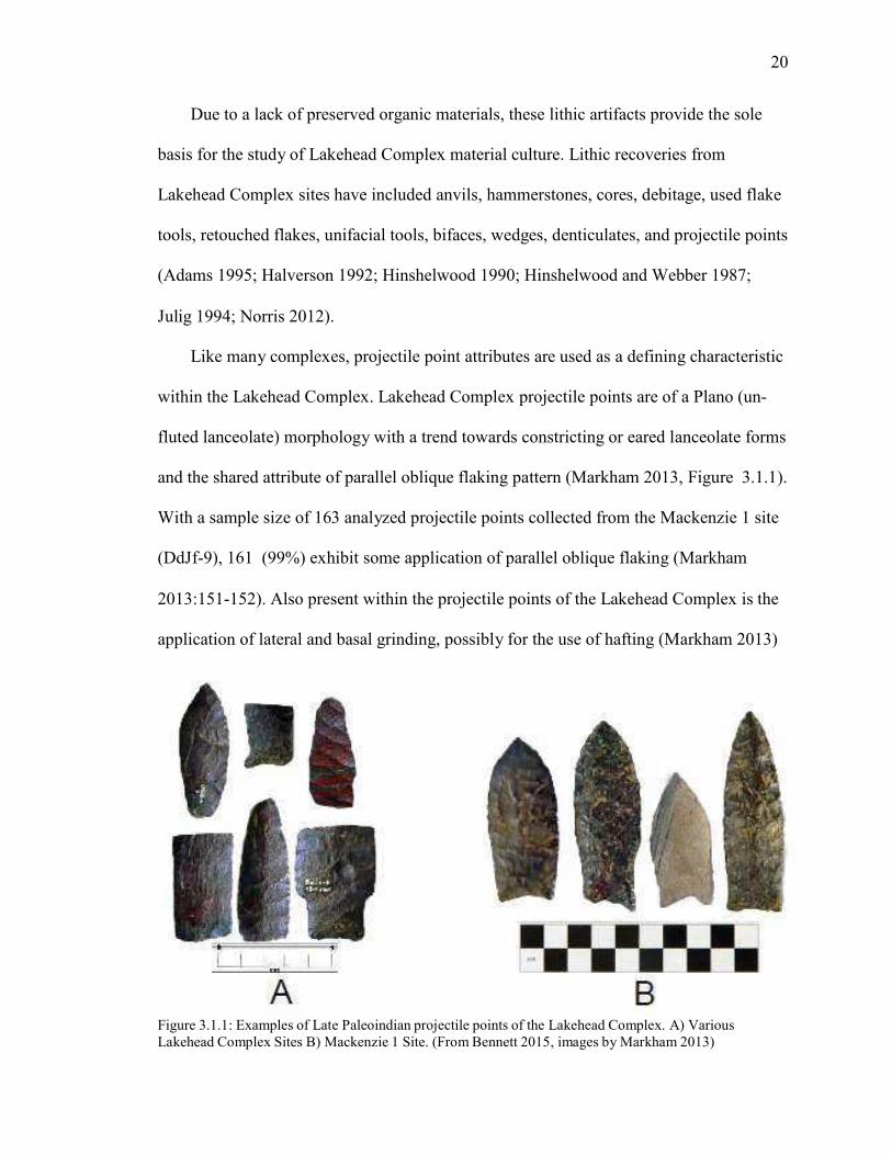
20

Due to a lack of preserved organic materials, these lithic artifacts provide the sole

basis for the study of Lakehead Complex material culture. Lithic recoveries from

Lakehead Complex sites have included anvils, hammerstones, cores, debitage, used flake

tools, retouched flakes, unifacial tools, bifaces, wedges, denticulates, and projectile points

(Adams 1995; Halverson 1992; Hinshelwood 1990; Hinshelwood and Webber 1987;

Julig 1994; Norris 2012).

Like many complexes, projectile point attributes are used as a defining characteristic

within the Lakehead Complex. Lakehead Complex projectile points are of a Plano (un-

fluted lanceolate) morphology with a trend towards constricting or eared lanceolate forms

and the shared attribute of parallel oblique flaking pattern (Markham 2013, Figure 3.1.1).

With a sample size of 163 analyzed projectile points collected from the Mackenzie 1 site

(DdJf-9), 161 (99%) exhibit some application of parallel oblique flaking (Markham

2013:151-152). Also present within the projectile points of the Lakehead Complex is the

application of lateral and basal grinding, possibly for the use of hafting (Markham 2013)

Figure 3.1.1: Examples of Late Paleoindian projectile points of the Lakehead Complex. A) Various Lakehead Complex Sites B) Mackenzie 1 Site. (From Bennett 2015, images by Markham 2013)

21

Many of these projectile point attributes occur within surrounding regions such as

Northern Minnesota and Northern Wisconsin (Ross 1995). This resulted in the

development of the Interlakes Composite as a way of interpreting this collection of

similar, yet regionally distinct, cultural complexes (Ross 1995).

3.3 The Interlakes Composite

The Interlakes Composite was defined by Ross (1995) as a way of describing the

observed shared characteristics between the Lake of the Woods/Rainy River, Quetico

Superior, Lakehead, and Reservoir Lakes complexes (Figure 3.3.1). Differentiated from

one another on the basis of geographic location and preferred raw tool material,

complexes of the Interlakes Composite exhibit a number of shared morphological traits in

projectile point manufacture. These include the presence of parallel oblique flaking, the

application of basal and lateral grinding, and the general lanceolate morphological shape

of the projectile points (Ross 1995).

The use of exotic materials, such as Hixton Silicified Sandstone, in the Interlakes

Composite further suggests that these regions were connected. Bedrock exposures of

Hixton Silicified Sandstone are known from only one quarry in south-central Wisconsin

(Ross 1995). Despite this, formal tools manufactured from this raw material are found

(though in limited numbers) in all complexes of the Interlakes Composite (Ross 1995).

While a few formal tools manufactured from Hixton Silicified Sandstone are reported in

complexes far removed from the source, the very limited recovery of debitage suggests

that these tools were manufactured near the lithic source and transported as completed

tools (Ross 1995).

22

Figure 3.3.1: The Interlakes composite, including 1) Lake of the Woods/Rainey River, 2) Quetico/Superior, 3) Lakehead, and 4) Reservoir Lakes (After Ross 1995).

3.4 Spatial Investigations of Lakehead Complex Sites

Though archaeological survey has resulted in the documentation of numerous Late

Paleoindian sites within the boundaries of the Lakehead Complex, few have been

excavated and studied to address the intra-site spatial and structural distribution of

artifacts. As such, there is currently little data pertaining to the intrasite organization of

Lakehead Complex sites. Many interpretations regarding site activity do not go beyond

describing the general site functions. The following discussion will summarize the

available material for two Lakehead Complex sites that provide the best spatial

interpretations from which to compare the results of the RLF study.

23

3.4.1 The Naomi Site (DcJh-42)

The Naomi site was excavated during the summer of 1994 as part of a cultural

resource management investigation by Adams Heritage Consultants on behalf of the

Ministry of Transportation Ontario (MTO) (Adams 1995). On the basis of projectile point

morphology and the use of Hixton Silicified Sandstone, Adams concluded that the site

was most likely of Paleoindian age.

Excavations of the Naomi site included the collection of fine-resolution spatial data,

enabling the study of intra-site artifact patterning. As a result, Adams (1995) was able to

identify three distinct lithic clusters which he referred to as areas �A✁, �B✁✂ a✄☎ �✆✁

(Figure 3.4.1).

Area �A✁ was excavated from an area covering 5x5 m. This cluster yielded a large

lithic spread, sloping downwards to form a lithic debris midden. These distributions were

found in association with a group of large rocks. Although the rocks did not readily

exhibit any signs of pecking, Adams (1995:18) suggested that they were likely used as

anvils for lithic production. Reduced lithic recoveries within the centre of the cluster was

believed to be the result of a tree throw event (Adams 1995:18).

The recovery of formal tools from within lithic debitage distribution suggested that

the tools were discarded during production (Adams 1995:18). Tools of note consisted of a

finely flaked drill made of a fine-grained blue-grey silicified siltstone (possibly from the

Wabigoon Greenstone Belt), and a finely made projectile point base made of taconite

(Adams 1995:18). The drill recovered represented the only non-taconite formal tool

within Area �A✁✝

24

Area �✁✂

N

Area �A✂

Area �✄✂

Figure 3.4.1: Lithic distributions from the Naomi site (DcJh-42). A) Cluster ☎A✆, B) Cluster ☎B✆, and C) Cluster ☎✝✆ (From Adams 1995).

Area ✞✟✠ was excavated in an irregular shape covering an area of 15 m2. Similar to

Area ✞A✠✡ ☛☞✌ location of lithic debitage was located in relation to a group of large

boulders derived from till (Adams 1995:20). One of the boulders located within this area

displayed clear evidence of use wear, likely due to its use as an anvil.

25

Formal artifacts were once again recovered in close proximity to the concentration of

lithic debitage, suggesting discard during manufacture (Adams 1995:20). Located within

Area �✁✂ was an extensively re-worked projectile point made of Hixton Silicified

Sandstone. A small collection of fire cracked rocks (FCR) in Area �B✂ ✄ay suggest the

presence of a small hearth near the eastern edge of the boulder group associated with

lithic manufacture.

Area �☎✂ differed from Areas �✆✂ and �✁✂ ✝✞ ✟✠✡✟ ✟✠☛ ☞✌cation of lithic debitage was

not in association with any large glacial boulders. However, formal tools were once again

recovered from either within or directly adjacent to a large cluster of taconite flakes. This

excavation area covered 19m2 and included two lithic clusters. It was noted that the

eastern cluster was less concentrated and relatively smaller than the other.

Through the analysis of lithic reduction loci, debitage, and a detailed biface staging,

Adams (1995:29) concluded that the Naomi site likely functioned as a small biface

reduction station. Due to the relatively high proportion of failed bifaces produced and

discarded during early stage reduction, and limited tertiary debitage recovery, Adams

suggested that reduction was focused primarily on the production of biface blanks that

were suitable for transportation and finishing at a later time.

Although relevant data was not recovered to enable the interpretation of site function

on the basis of floral and faunal resources, it was suggested that the observed biface

reduction may have served as a secondary site activity (Adams 1995:29). Adams

(1995:29) proposes that the Naomi site was located near a shallow bay or swamp that was

present during site occupation. The decision to perform lithic reduction activities near

this shallow bay/swamp, rather than near lithic resources, suggests that subsistence was a

26

primary consideration for the selection of site location. This would support Fox�✁

(1975:42) interpretation of Lakehead Complex sites as subsistence focused, with lithic

production representing a secondary objective. However, the lack of supporting evidence

left Adams (1995) to conclude that this was largely speculative.

The intra-site analysis of the Naomi site provides a good example of what a

relatively undisturbed lithic reduction loci may look like for Lakehead Complex sites.

This can be applied to the analysis of the RLF site in regards to lithic clustering, and

provides a possible analog for biface production and caching methods among Lakehead

Complex groups.

3.4.2 The Crane Cache (DcJj-14)

The Crane Cache (DcJj-14) was discovered in 1982, when Mr. Alex Crane recovered

a number of taconite bifaces while working in his potato garden (Ross 2011). The

discovery was brought to the attention of the regional archaeologist, Bill Ross, who upon

further investigation discovered two in-situ biface caches beneath Mr. Crane�✁ garden. In

total, 153 different bifaces were recovered, with 126 recovered from in-situ cache

deposits and 27 from outside of the cache area (Ross 2011:10).

Within the excavation of four 1x1m units, Ross (2011) recovered not only two biface

caches (Cache ✂A� n=20, Cache ✂B� n=106), but also a number of post-molds of varying

sizes. Two large post-molds were observed within the first two excavated units, while a

number of smaller post-molds formed a slight arc throughout the other units. The lack of

immediately available water sources, distance from bedrock lithic sources, and no

27

obvious game lookouts, led Ross (2011:10-11) to propose that the Crane site likely

represented a winter structure and camp.

The lack of diagnostic Lakehead Complex projectile points does not directly

associate the Crane Cache with Paleoindian populations. However, the nature of biface

reduction, and the exclusive use taconite for tool production strongly suggests Lakehead

Complex affiliation (Ross 2011). This makes the recovery and excavation of the Crane

Cache extremely important in the understanding of Paleoindian site use. Not only does

the site represent the first professionally excavated biface cache of Late Paleoindian age

within the region (Ross 2011), it also has some of the only evidence of structural remains.

While the Crane Cache site likely represented a winter encampment, it does provide

a glimpse into the possible site structure employed by Lakehead Complex populations

within their domestic areas. However, the limited data currently available regarding the

spatial structuring of the Crane Cache hinders its application within overall site structure

analysis.

3.5 Summary

As glacial ice retreated from the Thunder Bay region, Late Paleoindian populations

of the Lakehead Complex occupied the region (Fox 1975). These groups primarily

utilized taconite available from local Gunflint Formation outcrops to make Plano-style

projectile points with unique parallel oblique flaking patterns (Fox 1975, 1980; Markham

2013). The presence of Hixton Silicified Sandstone as well as similarities in projectile

point morphology suggests that the populations of the Lakehead Complex were part of

28

the larger Interlakes Composite, which also included the Lake of the Woods/ Rainy

River, Quetico/Superior, and Reservoir Lakes complexes (Ross 1995).

Sites of the Lakehead Complex exhibit a strong correlation with pro-glacial beaches,

Gunflint Formation outcrops, river and stream crossings, and permanent water bodies

(Julig 1994). The lack of site survey conducted within the region, however, likely under-

represents interior and/or winter encampments (Julig 1994).

While a number of Lakehead Complex sites have been excavated, few provide any

substantial data from which intra-site structure or pattern can be interpreted. The Naomi

site (DcJh-42) (Adams 1995) and the Crane Cache (DcJj-14) (Ross 2011) present the best

contexts through which spatial investigations of the RLF site can be compared.

Chapter 4

The RLF Site

4.1 Introduction

The excavation of the RLF site was conducted during the summer of 2011 and

resulted in the recovery of 14,790 artifacts from an excavation area of 206m2. This

chapter reviews the nature of site excavation and the laboratory analysis of recovered

artifacts. Primary interpretations of the RLF site are proposed on the basis of recovered

materials and location within its physical environment. These interpretations serve as a

basis from which the intra-site analysis of artifact distribution is conducted.

4.2 Site Location and Environment

The RLF site is located ~ 20km east of Thunder Bay, Ontario and ~ 800m from

the west bank of the Mackenzie River (Figure 4.2.1). Approximately 100m to the east of

the site there is a small stream that drains into a standing beaver pond. Modern vegetation

at the site is typical of boreal forest cover for the region, consisting dominantly of birch,

spruce, and pine trees.

The site was discovered during archaeological inspection of the centre line of the

north highway lane. Trees were uprooted and pushed over with a bulldozer, and then

pushed into windrows. Lithic debitage was encountered in sediment disturbed by tree

roots pulled out of the ground. Prior to site excavation the balance of the tree cover along

the road right of way was removed through the use of mechanical harvesting equipment.

Tree removal was carried out during the late winter and early spring in order to minimize

29

30

the impact on archaeological materials. The north-western section of the excavated block

exhibited some disturbance resulting from the piling and/or pushing of tree trunks during

the initial bulldozing operations. The effects of this disturbance on artifact distributions

will be discussed further during spatial inquiry.

Figure 4.2.1: Location of RLF site at the time of excavation.

While understanding that site environment upon recovery is important for

addressing questions of post-depositional effects on artifacts distributions, it does not

provide answers for why Late Paleoindian populations would have selected this location

for their camp site. To address this, hypotheses are proposed using site stratigraphy and

location in relation to key geographic and topographic features.

4.2.1 Site Stratigraphy

Interpretations of site deposition and stratigraphy at the RLF site are addressed by

Shultis (2012). In her analysis, Shultis (2012:216-217) identifies three lithofacies within

the stratigraphic profiles of RLF; 1K, 2K, and 3K.

31

Lithofacies 1K consists of parallel-stratified low angle fine-grained sand with

pebble layers in the northern portions of the site, and medium-grained sand with pebble

layers in the southern units (Shultis 2012:216). Shultis identifies this layer as being

consistent with a beach environment.

Lithofacies 2K is seen throughout the southern portions of the RLF site and is

represented by fine-grained to medium-grained sand with pebble layers. Magnetite-rich

layers are interbedded with non-magnetite layers, likely as a result of wave action and

sorting (Shultis 2012:216-217). This is interpreted as representing a beach front

environment, with massive layers present within the lithofacies indicative of storm events

during which higher energy waves deposited larger particles (Shultis 2012:217).

The final lithofacies, 3K, is interpreted as the result of bioturbation consistent

with boreal forest tree root patterns (Shultis 2012:217). This lithofacies consists of a

30cm wide by 40cm deep tapered concave feature with a diffuse contact and consistent

root evidence throughout.

The elevation of these interpreted beach formations, at 243m above sea level

(ASL), are consistent with those of Glacial Lake Minong levels (Shultis 2012:217).

Lithic artifacts from the RLF site are recovered primarily from levels 2 (5-10cm,

n=3253 22.07%) and 3 (10-15cm, n=4175 28.32%) (See Figure 4.2.2). In the northern

portions of the site this correlates with the bioturbated portions of lithofacies 1K, which

consisted of very fine-grained to fine-grained sand with pebble layers. Artifact recoveries

from the southern portion of the site were associated with the bioturbated portions of

lithofacies 2K (fine-grained sand with pebble layers) and 3K (silty medium-grained sand

with pebbles). From this, Shultis (2012:217) suggests that occupation at the RLF site may

32

To

tal R

eco

ve

red

Lit

hic

s

have been contemporaneous with active Minong beaches. However, with the absence of

identifiable stratigraphic sequences associated directly with artifact bearing levels, this

interpretation cannot be confirmed. To help address this, the location of the RLF site

recoveries in relation to topographic features can be explored.

4500

Total Lithics by Level (5cm)

4000

3500

3000

2500

2000

1500

1000

500

0

Recovery Level

Figure 4.2.2: Vertical distribution of artifacts by level at the RLF site. Recovery levels 2 and 3 indicated by red star.

4.3 Proposed Site Environment during Site Occupation

At the time of excavations, the RLF site was located ~ 1.2km inland from the

modern Lake Superior shoreline. However, with stratigraphic analysis suggesting that site

occupation may have occurred during active Lake Minong levels it is likely that local

resources would have been different during site occupation.

By considering the RLF site in its topographic context, artifact clustering occurs

on what appear to be dune-like formations. This clustering is situated back from an

33

abrupt slope which grades down towards current lake levels (Figure 4.3.1). These dune

formations are interpreted as representing back beach deposits. Occupation on this may

have provided a better drained area upon which to locate a camp. While stratigraphic

analysis places artifacts within active beach sediments, a lack of water-rolling on lithic

recoveries suggests that the deposition of these materials occurred back from the active

beach front.

With very-fine sediments occurring within the northern occupation levels

(lithofacies 1K) and fine to medium sediments in the southern occupation levels

(lithofacies 2K and 3K), it can be proposed that occupation may have occurred shortly

after active water levels had receded, and prior to finer sediment build-up within the

south portion of the site. This would place occupation close to the active beach, but far

enough back so as to not be effected by fluctuating water levels resulting it water-rolled

cultural materials. It can be speculated that the northern clusters of the occupation may

have been placed within the scrub brush/tree line of the beach, with the southern clusters

located on the open beach (Figure 4.3.2).

What can be proposed from these interpretations is that the RLF site location was

chosen based on its slight, well-drained, rise along the Lake Minong shoreline. Located

within a short distance of multiple water sources, this site may have provided an ideal

location at which lithic reduction could take place, while allowing occupants to watch up

and down the beach for possible game. Unfortunately, geoarchaeological investigations

conducted at the RLF site do not allow for the confirmation of this proposal, and as such

it remains speculative.

34

A

B

C

Figure 4.3.1: Topography of the RLF site area: A) Plan Map, B) Plan map with artifact clusters, and C) Side relief of site topography with general artifact cluster areas illustrated. Note: Elevation by metres.

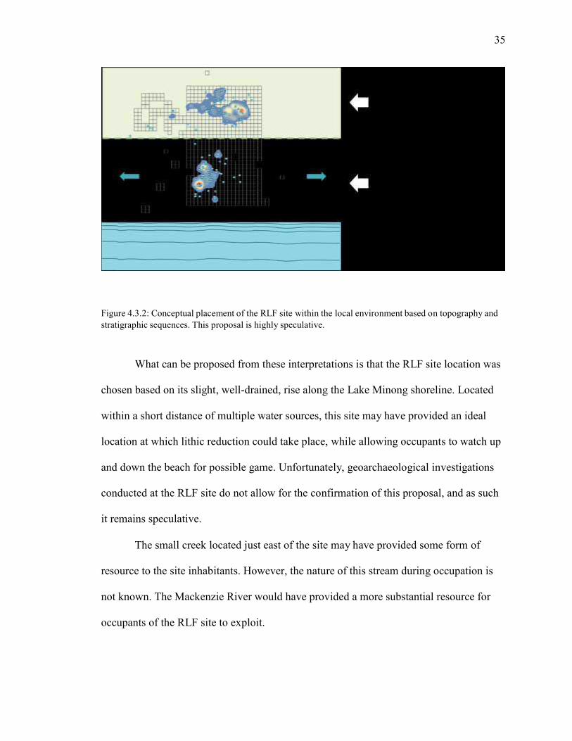
35

Figure 4.3.2: Conceptual placement of the RLF site within the local environment based on topography and

stratigraphic sequences. This proposal is highly speculative.

What can be proposed from these interpretations is that the RLF site location was

chosen based on its slight, well-drained, rise along the Lake Minong shoreline. Located

within a short distance of multiple water sources, this site may have provided an ideal

location at which lithic reduction could take place, while allowing occupants to watch up

and down the beach for possible game. Unfortunately, geoarchaeological investigations

conducted at the RLF site do not allow for the confirmation of this proposal, and as such

it remains speculative.

The small creek located just east of the site may have provided some form of

resource to the site inhabitants. However, the nature of this stream during occupation is

not known. The Mackenzie River would have provided a more substantial resource for

occupants of the RLF site to exploit.

36

4.4 Excavation Methods

While the initial Stage 2 archaeological assessment of the RLF site yielded

limited cultural material, the recovery of a large number of taconite flakes from a tree

push following initial tree removal prompted further excavations. The subsequent

investigations were conducted through the joint operations of Lakehead University and

Western Heritage, with both parties completing different phases of research. Despite all

excavations being conducted following the Standards and Guidelines for Consulting

Archaeologists (Ministry of Tourism, Culture, and Sport (MTCS) 2011), some variation

in excavation methodologies was observed. As such, general excavation methodologies

will be outlined separately for both Lakehead University and Western Heritage.

4.4.1 Field Methodologies: Lakehead University

The excavation by Lakehead University was conducted as part of an

archaeological field school offered through the Department of Anthropology. In order to

provide a variety of experience to field school students, excavations involved both a 5 x 5

m gridded test pit survey and 1 x 1 m unit excavations. Both of these were conducted

following Stage 2 and 3 archaeological assessment guidelines (Scott Hamilton personal

communication).

The 1x1 m excavation units were further subdivided into 50x50 cm quadrants

(quads) and dug following 5cm arbitrary levels. All sediment was sifted through both

6mm and 3mm mesh screens. S�✁✂✄☎�✆✝ ✞☎✞tial training involved the excavation of units

using hand trowels, while later units were excavated using shovel shaving techniques as

students became more confident in their skills. During trowel excavations, all artifacts

were mapped in situ (using X, Y, and Z co-ordinates) if possible. Later shovel

37

excavations focused on only mapping the in situ locations of formal tools, with lithic

debitage being collected in bulk by quad and level. Throughout the excavation all

significant changes in soil colour or staining were to be mapped and described.

The excavations conducted by Lakehead University are comparable in both

quality and speed to those completed by Western Heritage during Stage 4 investigations.

This serves to limit variations within the quality of catalog data, with any significant

differences reflecting the academic nature of the Lakehead University field school. This

results in field school excavations generally yielding better composed maps, notes, and

field photography.

4.4.2 Field Methodologies: Western Heritage

Western Heritage excavations at the RLF site included the initial Stage 2 test

pitting survey, as well as the final stage 4 block excavations. Stage 4 block excavations

were conducted in order to document, remove, and preserve all available site information

since site avoidance or protection was not possible (MTCS 2010:74). This required that

Western Heritage employees expand upon the excavations conducted by Lakehead

University until all cultural material was deemed to have been collected. This involved

excavating all units to a depth that yielded at least 1-2 sterile levels (devoid of cultural

material), with a buffer of one sterile excavation unit around the periphery of the site

area. In some areas of the site this general guideline was deviated from based on the

professional judgement of the supervising archaeologist.

Similar to Lakehead University investigations, excavation units were 1x1 m in

size, segmented into 50x50 cm quads. These were dug using shovel shaving techniques

38

following 5cm arbitrary levels. All dirt was screened through both 3mm and 6mm screen

mesh with lithic debitage collected in bulk by quad and level while lithic tools were

mapped in situ. All changes in soil colour were to be mapped whenever possible;

however due to the time-restricted nature of CRM archaeology this level of detail was not

always maintained. This resulted in some field notes yielding limited excavation data

beyond the collected materials.

4.5 Near Surface Geophysics

Prior to initial excavations, Western Heritage conducted a gradiometer survey in

order to provide value added research that would otherwise have not been part of CRM

oriented investigations. Near surface geophysics (NSG) is a form of passive subsurface

remote sensing, reading changes in subsurface magnetic fields rather than producing its

own (Gaffney 2008; Kvamme 2005, 2006). Features of anthropogenic origin exhibit

magnetic fields that differ from the surrounding sedimentary matrix. These can include

buried walls, foundations, rock formations, filled pits, metallic objects, or heated surfaces

such as hearths or ovens (Kvamme 2006).

The significance of utilizing NSG on the RLF site is the ability to identify hearth

features that, through the natural acidity and intense leaching of boreal forest soils, may

not yield any preserved organic features or staining. When soils in a hearth are repeatedly

heated, a build-up of magnetic soils occurs (Gibson 1986). This accumulation of

magnetically susceptible soils allows for the detection of hearth features, as they will

produce a secondary magnetic field different from their surroundings (Gibson 1986). This

magnetic build-up can also occur as a result of long-term organic decay.

39

NSG can also detect the presence of fired artifacts such as fire cracked rock,

ceramics, or bricks as a result of thermoremanent magnetization (Gibson 1986; Kvamme

2005). At temperatures beyond the Curie point (approximately 600o C) the magnetic

properties of an object (including magnetic minerals in sediments) re-align to the earth�s

magnetic field, where they remain situated upon cooling (Kvamme 2006). Artifacts

heated beyond the Curie point can intensify the magnetism observed in localized areas,

making them detectable using NSG. This can be used to detect hearth related FCR

fragments and lithics in the absence of defined hearth features.

It is important when interpreting NSG results to keep in mind that both

anthropogenic and natural fires may produce magnetic signatures. Therefore, determining

the nature of the magnetic anomaly depends on the strength and isolation of the anomaly

and it✁ ✂✄round truthing� to document artifact densities (Kvamme 2006). Other factors

that can affect the validity of NSG results are the presence of metallic objects, processes

of natural decay and weathering, and natural concentrations of magnetically rich soils

(Kvamme 2006). In order to confirm the anthropogenic nature of magnetic anomalies

within site areas, it is therefore important to assess whether the presence of such events

may be the result of the observed magnetic anomalies. It should be noted that all figures

used within this thesis illustrating NSG results were produced using the original maps

provided by Western Heritage.

4.6 Artifact Analysis and Cataloging: ADEMAR

The cataloging of all recovered artifacts was conducted by Western Heritage with

the use of the Archaeological Data Entry, Management, and Reporting program

40

(ADEMAR v 7.0). ADEMAR represents the latest version of cataloging software

developed by Western Heritage to aid in the management and analysis of site recovery

data.

Using ADEMAR while conducting a spatial analysis of the RLF site permitted

both the manipulation and export of tabular data suitable for use within computer

mapping software as well as the compilation and analysis of relative artifact frequencies

and attributes (e.g. artifact size, material, recovery level, etc.).

Furthermore, the use of ADEMAR allowed for the randomization of data point

locations (X and Y) for artifacts collected in bulk (e.g. debitage by quad/level). This

randomization allows for the visual interpretation of artifact distributions despite a lack of

formal provenienced location. This randomization of recovery location is limited to

within the excavation quad. While ADEMAR produces new randomized co-ordinates

(termed Xrand and Yrand) for all tabular exports, only one master export file was used

throughout this thesis to maintain consistency. While the use of randomized co-ordinates

within excavation quads limits the application of fine scale spatial interpretation, they

allowed for statistical analysis across the larger site area (see Chapter 6).

4.7 Artifact Recoveries: Overview

In total, 14,790 artifacts were cataloged from the RLF site during both field

school and CRM excavations. These recoveries fall within four basic categories: bone

(n=2), charcoal (n=21), lithic items (n=14,744), and miscellaneous (including ochre,

wood fragments, etc. n=23) (See Table 4.7.1). With the exception of lithic materials (see

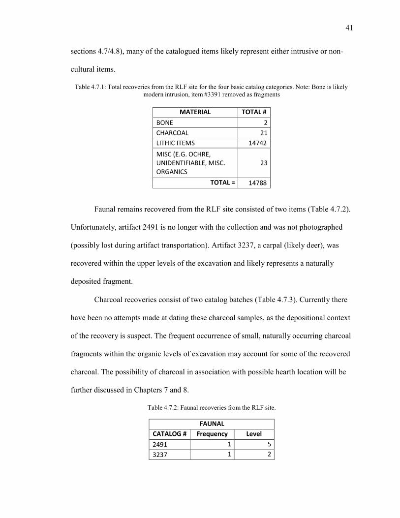
41

sections 4.7/4.8), many of the catalogued items likely represent either intrusive or non-

cultural items.

Table 4.7.1: Total recoveries from the RLF site for the four basic catalog categories. Note: Bone is likely modern intrusion, item #3391 removed as fragments

MATERIAL TOTAL #

BONE 2

CHARCOAL 21

LITHIC ITEMS 14742

MISC (E.G. OCHRE,

UNIDENTIFIABLE, MISC.

ORGANICS

23

TOTAL = 14788

Faunal remains recovered from the RLF site consisted of two items (Table 4.7.2).

Unfortunately, artifact 2491 is no longer with the collection and was not photographed

(possibly lost during artifact transportation). Artifact 3237, a carpal (likely deer), was

recovered within the upper levels of the excavation and likely represents a naturally

deposited fragment.

Charcoal recoveries consist of two catalog batches (Table 4.7.3). Currently there

have been no attempts made at dating these charcoal samples, as the depositional context

of the recovery is suspect. The frequent occurrence of small, naturally occurring charcoal

fragments within the organic levels of excavation may account for some of the recovered

charcoal. The possibility of charcoal in association with possible hearth location will be

further discussed in Chapters 7 and 8.

Table 4.7.2: Faunal recoveries from the RLF site.

FAUNAL

CATALOG # Frequency Level

2491 1 5

3237 1 2

42

Table 4.7.3: Charcoal recoveries from the RLF site.

FAUNAL

CATALOG # Frequency Level

2491 1 5

3237 1 2

During the RLF site excavations there was no clear association observed for the

presence of ochre fragments and archaeological material. The recovered ochre may

represent a natural occurrence.

4.8 Lithic Artifacts

A total of 14,727 lithic artifacts were cataloged during the analysis of the RLF site

materials. These include tools, cores, debitage, microdebitage, fire cracked rock, and

other materials (e.g. amethyst, quartz, and unidentifiable lithics) (Table 4.8.1). Materials

collected and catalogued as �✁✂✄e☎✆ were kept based on material type, but are represented

primarily by water-rolled pebbles. Based on appearance, these artifacts likely represent

naturally occurring materials.

Table 4.8.1: Breakdown of lithic recoveries from the RLF site by basic type.

LITHIC*

ARTIFACT TYPE Total #

TOOL (INCL. PREFORM) 107

CORE 43

DEBITAGE (INC. SHATTER) 11451

MICRODEBITAGE 3041

FIRE CRACKED ROCK (FCR) 67

OTHER LITHIC 18

TOTAL = 14727

* REFIT ITEMS UNDER ONE

CATALOG NUMBER ARE COUNTED

AS A FREQUENCY OF '1'

43

4.8.1 Lithic Artifacts: FCR

Fire cracked rock (FCR) occurs primarily as the result of human activity. It is

identified by the degradation or fracturing of rocks as a result of the application of

concentrated heat from cooking activities (Quigg 1978; Quigg 1986). At the RLF site,

this degradation resulted in a crumbled/cracked appearance. A total of 67 FCR pieces

were collected from the RLF site, weighing over 6,600g.

While Thoms (2008:130) observes a �virtual absence✁ of FCR recoveries from

Paleoindian sites within the United States, this was offered in comparison to the use of

rock-filled earth ovens among subsequent cultures. The recovery of FCR in limited

quantities has been recorded for Paleoindian sites within Northwestern Ontario that bear

diagnostic cultural materials (Adams 1995:29). Similar to the recoveries from the RLF

site these FCR pieces are present, but extremely limited, especially when compared with

frequencies one might expect from Archaic period sites (Thoms 2008). This suggests that

while the use of heated stones for cooking is unlikely, stones were being used within

hearths; either for holding heat or some other alternative function.

4.8.2 Lithic Artifacts: Non-Debitage

In total, 152 non-debitage lithics were recovered during excavations (Table 4.8.2),

and include formal flaked tools, expedient flake tools, cores, and knapping tools (such as

anvils and hammerstones).

The identification and cataloging of flaked stone tools was conducted following

basic morphological trait analysis. In order to maintain inter-assemblage consistency,

tools were typed following methods and descriptions used within the current Lakehead

44

Complex literature (e.g. Julig 1994). It is important to keep in mind that many stone

artifacts likely functioned as multi-use tools (Andrefsky 1998). However, without proper

multi analytical residue and use-wear studies, this multi-use must remain speculative.

Consequently, this thesis will utilize the generic use as the primary classification method.

A breakdown of flaked stone tools and their description is offered below.

Table 4.8.2: Breakdown of non-debitage lithic recoveries from the RLF site.

LITHIC TOOLS*

TOOL TYPE Material Number Total # % Total

BIFACE**

Taconite 42

50

32.9

GFS 3

Chert 2

Mudstone 1

Siltstone 2

FAILED PROJECTILE/DRILL Taconite 1 1 0.7

ADZE Siltstone 1 1 0.7

SPOKESHAVE Taconite 1 1 0.7

CORE Taconite 39

42

27.6 GFS 3

WEDGE Taconite 1 1 0.7

PERFORATOR Taconite 2 2 1.3

GRAVER/ PERFORATOR Taconite 2 2 1.3

RE-TOUCHED FLAKE Taconite 27

28

18.4 Chert 1

RACLETTE/BLADE FLAKE Taconite 4 4 2.6

SCRAPER Taconite 6 6 3.9

UNIFACE Taconite 4 4 2.6

UNDETERMINED TOOL Taconite 1 1 0.7

GRINDING STONE***

Other

Material

1

2

1.3

Siltstone 1

POSSIBLE ABRADING STONE Other

Material

1

1

0.7

HAMMER-STONE Other

Material

2

2

1.3

OTHER TOOL (ANVILS) Other

Material

4

4

2.6

Total = 152 100

* REFIT ITEMS UNDER ONE CATALOG NUMBER ARE COUNTED AS '1'

** REFIT ITEMS UNDER ONE CATALOG #: 1613, 3126, 3148

*** ITEM 3391 NOT COUNTED AS THEY ARE BROKEN PORTIONS FROM ITEM

3390

45

Raw material use for the production of flaked non-debitage lithics exhibits a

strong preference for the exploitation of Gunflint Formation materials. Taconite is the

most common material recovered at 90.9% (n=130) with gunflint silica at 4.2% (n=6).

Other materials recovered include siltstone (2.1%, n=3), chert (2.1%, n=3), and mudstone

(0.7%, n=1).

While flaked tools can be identified by the presence of reduction related processes

(discussed below), hammer stones and anvils were identified by the presence of pecking

as well as depositional placement relative to high concentrations of lithic materials.

While it is possible that some of these anvils may have functioned as grinding stones, a

lack of preserved organics and micro-botanical research did not currently allow

exploration of this proposal.

Bifaces

Of the 50 bifaces recovered from the RLF site, 42 were made of taconite, three

were made of gunflint silica, two were made of chert, two were made of siltstone, and

one was made of mudstone. In order to provide a more in-depth analysis of lithic tool

production at the RLF site, the reduction stage represented by each biface was

determined.

The use of bifacial reduction stages as a method of inferring general production

activities has frequently been employed at Lakehead Complex sites (see Halverson 1992;

Hinshelwood and Weber 1987; Adams 1995). This bifacial staging allows for the

organization of bifacial production into separate categories based on level of

completeness, as well as shifting reduction objectives and tool functionality. These stages

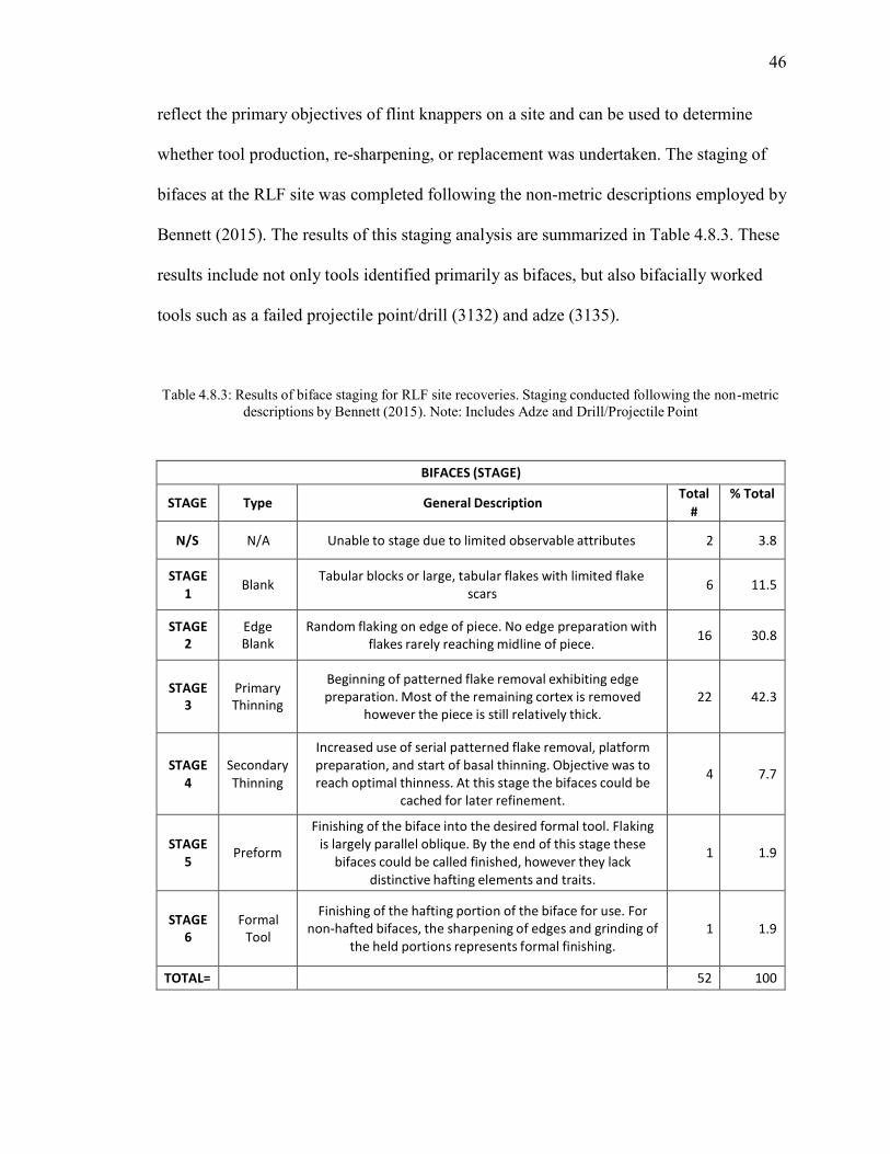
46

reflect the primary objectives of flint knappers on a site and can be used to determine

whether tool production, re-sharpening, or replacement was undertaken. The staging of

bifaces at the RLF site was completed following the non-metric descriptions employed by

Bennett (2015). The results of this staging analysis are summarized in Table 4.8.3. These

results include not only tools identified primarily as bifaces, but also bifacially worked

tools such as a failed projectile point/drill (3132) and adze (3135).

Table 4.8.3: Results of biface staging for RLF site recoveries. Staging conducted following the non-metric descriptions by Bennett (2015). Note: Includes Adze and Drill/Projectile Point

BIFACES (STAGE)

STAGE

Type

General Description Total

#

% Total

N/S

N/A

Unable to stage due to limited observable attributes

2

3.8

STAGE

1

Blank

Tabular blocks or large, tabular flakes with limited flake

scars

6

11.5

STAGE

2

Edge

Blank

Random flaking on edge of piece. No edge preparation with

flakes rarely reaching midline of piece.

16

30.8

STAGE

3

Primary

Thinning

Beginning of patterned flake removal exhibiting edge

preparation. Most of the remaining cortex is removed

however the piece is still relatively thick.

22

42.3

STAGE

4

Secondary

Thinning

Increased use of serial patterned flake removal, platform

preparation, and start of basal thinning. Objective was to

reach optimal thinness. At this stage the bifaces could be

cached for later refinement.

4

7.7

STAGE

5

Preform

Finishing of the biface into the desired formal tool. Flaking

is largely parallel oblique. By the end of this stage these

bifaces could be called finished, however they lack

distinctive hafting elements and traits.

1

1.9

STAGE

6

Formal

Tool

Finishing of the hafting portion of the biface for use. For

non-hafted bifaces, the sharpening of edges and grinding of

the held portions represents formal finishing.

1

1.9

TOTAL= 52 100

47

What these results suggest is that the primary lithic production objective at the

RLF site was the manufacture of bifacial blanks that could later be turned into a finished

tool. The discard of early stage bifaces (stages 1-3) appears to be deliberate and due to

inherent flaws in the raw material causing breakage during manufacture, and account for

84.6% of the total biface recoveries from the site. This is significant not only for the

characterization of a possible site use or objective, but also as a site-specific snapshot of

the general reduction sequence observed by Bennett (2015) within the Mackenzie 1 site

assemblage.

The comparative manufacture similarities between the bifaces recovered from the

RLF site and those from the Mackenzie 1 site help to place the RLF site within the

Lakehead Complex. Bifaces from the RLF site exhibit edge grinding as preparation for

flake removal, another characteristic observed within Lakehead Complex manufacturing

techniques (Hinshelwood and Webber 1987; Julig 1994)

Adzes

One siltstone adze was recovered during the RLF site excavations (Figure 4.8.1).

It is roughly flaked on all sides and lacks a distinctive fault plane that often characterize

the trihedral adzes of the Thunder Bay region.

The use and cultural affiliation of various adze forms within Northwestern

Ontario is heavily debated as none have been recovered from secure site contexts. Some

adze morphologies, such as the trihedral adze, have been placed within the temporal

periods of the Paleoindian and/or Shield Archaic cultures (Fox 1977; Julig 1994;

Steinbring and Buchner 1980). Residue work by Cook (n.d.) will begin to address these

48

issues, but until a developmental sequence can be recovered from secure datable contexts

this cannot be verified. It is possible that these various adze morphologies could have

functioned as wood working tools. However, without the application of use-wear or

residue analysis this cannot be confirmed.

Figure 4.8.1: Adze recovered from the RLF site.

Wedges

One taconite wedge was identified during artifact cataloging (Figure 4.8.2). It

exhibits crude bifacial flaking with possible battering/crushing on the distal end of the

artifact. Further analysis however suggest that this battering/crushing may be the cobbled

cortex of the initial piece that was not yet removed. Flakes removed from the tool exhibit

a number of faults that may have resulted in the discard of the item.

49

Figure 4.8.2: Taconite artifact catalogued as being a wedge with scale in centimetres. This piece may represent an early stage failed biface. End exhibiting possible battering indicated by red stars.

Drill/Failed Projectile Point

Artifact 3132 has been identified as a possible failed taconite projectile point that

was later re-purposed as a perforator/drill, or, discarded due to flaws (Figure 4.8.3). This

artifact exhibits a mix of crude parallel oblique and co-lateral flaking with a prominent

dorsal ridge. Multiple attempts appear to have been made by the flint knapper to remove

this ridge resulting in compounding hinge fractures. With limited evidence of further

reduction occurring on the face opposite this ridge, it is likely that the inability to remove

it resulted in tool discard. A fracture on the tools tip may suggest later use as a

perforator/drill however without the application of residue or use-wear analysis this

cannot be confirmed.

50

Figure 4.8.3: Possible failed projectile point or drill.

With no hafting element present on the tool, assigning cultural affiliation is not

possible. The thick cross section resulting from the dorsal ridge and un-finished nature of

the point also limit metric analyses that may help to culturally associate the tool. While

speculative, the presence of extremely crude parallel oblique flaking may suggest a

connection with Lakehead Complex manufacturing techniques.

Spokeshaves, Perforators, and Gravers

One spokeshave, two perforators, and two perforators/gravers were identified

during artifact cataloging. All of these artifacts were identified based on morphological

traits.

51

The spokeshave (artifact 3186) exhibits a concavity on its proximal end that may

have functioned as an expedient tool. There does not appear to be any distinctive

retouching within this area suggesting that it may also represent a conveniently shaped

flake. The artifact was recovered in two pieces, having broken along an oxidized fault

running through the item.

The proposed perforating tools also do not exhibit clear indications of intentional

retouching or use-wear. It is possible that these artifacts (2105 and 3125) may only

represent fragments of shatter.

This interpretation is similar for the two identified gravers/perforators. While these

items are similar in morphology to gravers identified by Julig (1994:138) from the

Cummins site, a lack of observable retouch or use-wear could suggest that these represent

convenient fragments of shatter. Until a proper residue/use-wear study can be conducted

these artifact interpretations must remain speculative.

Unifaces and Retouched Flakes

A total of 39 artifacts were identified as unifacially flaked or retouched. Of these.

11 are classified as formal unifacial tools and 28 as expedient flake tools.

Unifacial tools have been divided into two classes: those that can be clearly

identified as scraping tools (n=7), and those that are unifacially worked to a greater

degree than retouched flakes but are not yet scrapers (n=4). The latter of these two classes

appear to represent scraper preforms that failed part way through production.

52

The classification as a scraper requires the presence of flaking greater than 1.5

mm in length (Julig 1994:102). Of the seven identified scrapers, there are five end

scrapers, one side/end scraper, and one side scraper.

Initial cataloging identified 28 retouched flake tools. A re-examination of these

items resulted in the separation of the cataloged tools into two groups based on

intentional and un-intentional retouch. While intentional retouch represents flakes that

exhibit a clear, use-oriented flake removal, un-intentional retouched flakes exhibited

random, non-functional flakes that were likely removed either during artifact transport, or

through depositional trauma such as trampling. A lack of in-depth use-wear studies meant

that unworked utilized flakes were not identified prior to this thesis.

There were four expedient blade flakes recovered from the RLF site similar to

those described by Julig (1994). These thin flake tools appear to have minimal retouching

along their edges. Based on their unique morphological shape, these artifacts are

cataloged separate from other retouched flake tools.

Cores

There were 43 cores recovered during the RLF site excavations. All of these were

made from Gunflint Formation materials with 39 (92.9% made of taconite and three

(7.1%) of gunflint silica.

Of these, 17 (39.5%) exhibited some form of cortex. In this study, cortex refers to

the rough, weathered outer portion of the lithic material as the result of either chemical

(exposure to heat or water altering the composition of the material) or mechanical

(changes in material texture as a result of events such as water-rolling or abrasion)

53

processes (Andrefsky 1998). To describe these different cortex types, the term �tabula✁✂

cortex refers to removal from a bedrock source, while �c✄☎☎✆✝✂ refers to cortex produced

trough water rolling.

Both tabular and cobble derived cores were observed at the RLF site. Of the 17

cores exhibiting cortex, six (35.3%) were tabular and 11 (64.7%) were cobble derived.

While Lakehead Complex sites generally exhibit the use of bedrock materials, the use of

cobble derived cores has been observed at the Simmonds site (Halverson 1992). This

mixed exploitation with a greater reliance on cobble material would be understandable

given that the RLF site is not located within the immediate vicinity of any documented

Gunflint bedrock exposures.

The tabular cores at the RLF site likely represent materials that were transported

to the site by its occupants; similar to observations at the Naomi site (Adams 1995).

Cobble derived cores may have been collected locally from either rivers such as the

Mackenzie River, or from shore deposits.

Two core recoveries from the RLF site were unique from the others. These cores

(2820 and 3208) appear to have been used for the removal of blade flakes (Figure 4.8.4).

One of these cores refits with a recovered blade flake (2299) and exhibits evidence of

multiple flake blade removals. Similar cores have been recorded from the Cummins site

(Julig 1994:98-99). These likely do not represent prepared blade cores, but rather cores

that provided convenient opportunities to strike off multiple blades.

54

Figure 4.8.4: Core 2820 with blade flake removal. Note: blade flake is missing striking platform (indicated by red star).

4.8.3 Lithic Artifacts: Debitage

A total of 14,492 pieces of lithic waste material was collected during the

RLF excavations. Initial cataloging of these materials involved sorting the artifacts into

four basic categories: debitage flake, debitage shatter, microdebitage flake, and

microdebitage shatter (Table 4.8.4).

Differentiating debitage from microdebitage was based on size, with debitage

referring to artifacts larger than 6mm and microdebitage being smaller than 6mm.

Identifying debitage and microdebitage as being flake or shatter was based on the

presence of identifiable flake features. Flakes exhibit attributes such as a bulb of

percussion or striking platform, while shatter is generally amorphous and blocky in

nature with no discernible characteristics

55

Table 4.8.4: RLF lithic waste recovery frequencies by four base categories.

DEBITAGE

TYPE

Material Sub-

Total

Total

DEBITAGE-FLAKE

Taconite 9610

10437

GFS 685

Chert 6

Siltstone 110

Quartz 1

Other

Material

25

MICRODEBITAGE-FLAKE

Taconite 2673

2946

GFS 249

Chert 9

Siltstone 13

Quartz 2

DEBITAGE-SHATTER

Taconite 929

1014

GFS 50

Chert 11

Siltstone 12

Quartz 4

Amethyst 3

Other

Material

5

MICRODEBITAGE-

SHATTER

Taconite 81

95

GFS 3

Chert 4

Quartz 6

Amethyst 1

Total = 14492

Key attributes collected during cataloging were lithic material, size, and flake

type. These descriptors help to further classify and group various forms of debitage

during spatial analyses.

Debitage: Material Types

Debitage material type is dominated by Gunflint Formation materials, with

taconite representing the primary material type at 91.7% (13,293). Gunflint silica was

second most frequent at 6.8% (987). Other materials recovered in lesser amounts include

56

siltstone, chert, quartz, amethyst, and �other✁; where �✂✄he☎✁ materials includes

unidentifiable materials (Table 4.8.5).

Table 4.8.5: RLF lithic waste recovery frequencies by material type.

MATERIAL TOTAL % TOTAL

TACONITE 13293 91.73

GFS 987 6.81

CHERT 30 0.21

SILTSTONE 135 0.93

QUARTZ 13 0.09

OTHER 30 0.21

AMETHYST 4 0.03

TOTAL= 14492 100

Debitage: Size

Lithic production represents a reductive process, and as such, it is generally

understood that as a stone tool nears completion, the size of debitage produced will

become progressively smaller (Andrefsky 2001). Knowing this information allows for

more complex interpretations regarding lithic debitage when lithic sizes are included

within site analysis. During the cataloging of the RLF site, basic measurements were

collected for all debitage and microdebitage.

Understanding the time sensitive nature of CRM excavation and cataloging, the

collection of individual measurements for all debitage was not feasible. As an alternative,

the collected materials were divided into size grades using graduated squares. To do this,

debitage was placed face up on a series of squares that decreased in size until the artifact

no-longer fit within the borders of the square. The smallest square that the artifact could

fit in without going over would represent the artifacts size grade (Figure 4.8.5). The sizes

used during RLF site analysis were 0-2mm, 2-6mm, 6-12mm, 12-25mm, 25-50mm, and

50+mm. The results of this size grading can be seen in Table 4.8.6.

57

Figure 4.8.5: Example of RLF size grade sorting during artifact cataloging.

At the RLF site, size recoveries tend to be centred on debitage 6-12mm is size.

There is a notable absence of debitage in the size grade of 0-2mm. This low

representation could be the result of excavation methods, as 6mm and 3mm nested

screens would not have allowed for the recovery of these artifacts.

Table 4.8.6: RLF lithic waste recovery frequencies by size.

SIZE TOTAL % TOTAL

0-2MM 17 0.12

2-6MM 3026 20.88

6-12MM 6392 44.11

12-25MM 3928 27.10

25-50MM 1058 7.30

50+MM 71 0.49

TOTAL 14492 100

Debitage: Type

Further debitage attributes also allowed lithic flakes to be classified by type. A

breakdown of these flake types and the total identified pieces can be seen in Table 4.8.7.

58

Table 4.8.7: Description of methods used to classify RLF debitage by type with total recovery frequencies.

DEBITAGE BY TYPE

TYPE Description Total %

PRIMARY Flakes exhibiting some form or cortex or fault plane with

limited flake scars on the dorsal surface

257

1.9

SECONDARY Any flakes greater than 12mm exhibiting flake scars on the

dorsal surface

10167

76.0

TERTIARY Flakes smaller than 12mm exhibiting flake scares on the

dorsal surface

1413

10.6

UNKNOWN Undetermined flake type 1544 11.5

TOTAL 13381 100

Similar to debitage size, information on flake types allow for further

interpretations of lithic reduction to be developed. Primary flakes exhibiting large

amounts of cortex are produced during the earliest stages of lithic manufacture

(Andrefsky 2001). Therefore, if primary flakes are present at a site, then it can be

proposed that some form of early stage lithic reduction was occurring.

4.9 Summary and Preliminary Site Interpretation

Prior to the application of spatial analysis on the RLF site, an understanding of

possible site function should be explored. Based on the analysis of site location,

stratigraphy, and artifact recoveries, preliminary interpretations for the RLF site can be

developed.

While no datable materials were recovered from the RLF site, its location along a

pro-glacial beach ridge in sediments suggesting a near beach environment suggest that

site occupation occurred during the Minong phase of the Lake Superior Basin (~10,800-

8,800 cal, 9,500-8,000 14C yrBP). This, combined with the almost exclusive use of

taconite and bifacial reduction techniques supports the initial proposal that the RLF site

59

belongs to the Lakehead Complex. This is further supported the close proximity of other

Late Paleoindian period sites such as Mackenzie I to the RLF site. While the re-

occupation of Late Paleoindian sites by Shield Archaic groups has been observed within

the region (Hinshelwood 2004), there is little material evidence to suggest this occurred

at the RLF site.

The materials recovered from the RLF site consist primarily of early stage bifaces

and cores, suggesting that the site occupants were participating in the reduction of lithic

materials in order to produce cache stage bifaces. These bifaces would have likely been

further reduced elsewhere when needed. The acquisition of raw materials appears to have

been a combination of tabular lithic blocks transported to the site from elsewhere, and

locally collected river cobbles of Gunflint Formation materials.

What these interpretations suggest is that the RLF site represents a small scale

lithic reduction camp along the shores of Lake Minong. Occupants of the site spent their

time reducing cobbles of knappable material, as well as some quarried materials brought

with them to site. These were then made into cache stage bifaces that would have been

more easily transported. These finished cache bifaces were then transported away from

the RLF site where they could later be turned into finished tools.

Chapter 5

Spatial Analysis in Archaeology

5.1 Introduction

The analytic importance of artifact patterning within archaeological sites has long

been known as a key component of interpretation. However, it wa�✁✂✄ ☎✁✄il the 1970s that

archaeologists began to implement the systematic study of the spatial relations between

artifacts. With the help of archaeological and ethnoarchaeological observations, spatial

statistical inquiry, and experimental replication, spatial analyses have become critical for

inferring site function, organization, and structure. This chapter provides a summary of

the development of spatial analysis in archaeology. It will also explore how these studies

have provided an understanding of the formation processes of different archaeological

activity assemblages, as well as how natural processes can serve to disrupt and blur these

patterns.

5.2 Current Approaches to the Archaeology of Northwestern Ontario

While spatial patterning of material on Lakehead Complex sites has been

examined (see Adams 1995), these studies have focused largely on point plotted artifact

locations to aid interpretation of site function. While this is one of the most common

methods for inferring site use/organization it requires meticulously plotted artifact

locations, relatively discrete clustering of artifacts, and areas of minimal disturbance or

reoccupation - characteristics frequently lacking on boreal forest sites. This has resulted

in regional research that is more focused on the artifacts themselves rather than their

60

61

intra-site spatial relationships (see Bennett 2015; Bouchard n.d.; Hodgson n.d.; Markham

2013). While these studies have been able to provide insight into the methods of tool

production, use, and broader cultural relations, they have not been able to address how

these populations utilized their site environments.

Limited investigation of spatially interpretable sites has constrained spatially

based statistical studies of Lakehead Complex materials. This thesis provides the first

step in introducing current spatial-analytical techniques within the research of Lakehead

Complex materials (see also McCulloch n.d.).

5.3 Spatial Analysis in Archaeology

The archaeological application of intra-site spatial analysis developed out of a

desire to understand how past populations organized themselves within their site

environments, and how the relationships between observable spatial clusters can be used

to infer past human behaviour (Carr 1984). Initial spatial studies were met with criticism

regarding the underlying assumptions that clearly visi�✁✂ ✄activity areas☎✆ defined by

Binford (1983:148) as ✝places, facilities, or surfaces where technological, social, or ritual

activities occur✞, were a natural aspect of site formation (Gibson 2001; Kroll and Price

1991). Today, spatial analysts have become concerned with determining whether or not

discernible activity areas can be observed within the distributions of archaeological

debris, and if so, what can the composition of such areas tell us about the human use of

space (Kroll and Price 1991).

Attempts by archaeologists to identify functional or activity areas within sites has

resulted in the development of a wide array of analytical methods. The earliest spatial

62

studies relied heavily on the visual interpretation of artifact distribution maps (Kroll and

Price 1991). However, as spatial archaeology evolved, numerous techniques were

developed in order to address more complex questions of spatial relations and site

development, including: the visual interpretation of artifact distribution maps (e.g.

Lavachery and Cornelissen 2000; Rigaud and Simek 1991), aggregate analysis of

materials (e.g. Kroll and Isaac 1984; Healan 1995), the application of spatial statistical

tests (e.g. Gregg et al. 1991; Lavachery and Cornelissen 2000; Rigaud and Simek 1991),

and the analysis of refitted artifacts both horizontally and vertically within a site (e.g.

Bamforth et al 2005; Kroll and Isaac 1984; Lavachery and Cornelissen 2000; Rigaud and

Simek 1991).

Simply identifying areas within a site where artifact clustering occurs does not

fulfill the primary goals of spatial archaeology. Once identified, these clusters need to be

interpreted, and the statistical strength and validity of spatial patterns need to be critically

assessed. Lavachery and Cornelissen (2000:156) describe artifact clustering as the result

of either an in-situ activity zone, an accumulated refuse zone, or a natural accumulation

of artifacts caused by natural or post-depositional processes. Determining which of these

clustering processes is responsible for the observed site patterns relies heavily on the use

of ethnoarchaeological, archaeological, and experimental data (Binford 1978, 1983;

Schiffer 1975, 1987).

Ethnoarchaeology developed as a result of the understanding that introduction of

artifacts into the archaeological record was not as simple as previously thought.

Ethnoarchaeology in itself is the study of existing populations and how their

manipulation of material culture, and their use of space within a site results in the

63

disposal of materials as an archaeological deposit (David and Kramer 2001). These

studies have resulted in the development of numerous site formation models and

hypotheses (e.g. Binford 1978, 1983; Kent 1984; Yellen 1977, compiled works in Kroll

and Price 1991).

It is important to stress though that no ethnographic study of modern hunter-

gatherer groups can be applied directly to past cultures as no two populations can be

assumed to act in an identical manner. While cultural variability limits the direct

application of site formation models towards the interpretation of past populations,

valuable examples of behavioural modelling regarding hunter gatherer campsites have

been developed on the basis of analogy (Binford 1978, 1983; Gibson 2001; Stevenson

1986, 1991). Traditionally, these models have been concerned primarily with the mode or

method of refuse discard within a site context and include: drop zone discard (Binford

1978, 1983), toss zone discard (Binford 1978, 1983), displacement zone discard

(Stevenson 1986, 1991), and cluster discard (Gibson 2001:74, Figure. 5.3.1).

The drop and toss zone discard model was developed by Binford (1978) during

ethnoarchaeological work with the Nunamiut Eskimo at the Mask site in North Central

Alaska. While watching the hunters perform activities around a hearth, Binford noted that

smaller fragmentary objects would fall within the direct vicinity of the individual. This

area he termed the drop zone. Meanwhile larger items that would have created an

inconvenience if left within the drop zone would be picked up and tossed backwards from

the hearth (or occasionally into the hearth) into what Binford termed the toss zone.

64

Figure 5.3.1: Stylized example of the drop/toss/displacement model with various cluster discard models indicated. (After Binford 1983; Gibson 2001; and Stevenson 1986, 1991)

The introduction of the idea of displacement zone discard was developed as an

extension to Binfor�✁✂ �rop/toss model (Stevenson 1986, 1991). The displacement

discard zone represents an intermediate area between the drop and toss zones where

larger items would be placed away from the individual rather than tossed (Gibson 2001).

A drawback of the Binford-Stevenson model is that both were developed

regarding activity around open-air hearths (Gibson 2001). This did not take into account

the depositional variation that may occur within the constraints of a structure, where

limited space would not allow for such an accumulation of debris. Binford (1978:350)

does note that within a structure the toss zone pattern would be unlikely, instead larger

65

objects would be placed near hearths for easy clean up. Gibson (2001) goes beyond this

to classify a fourth discard method: cluster discard. This cluster discard is described as

the purposeful collection of materials, presumably on skins, during an activity and

dumping away from the use areas. Gibson (2001) classifies three basic types of cluster

discard within his analysis of the Bushfield West site structures: Type 1) where the

heterogeneous collection of materials are discarded expediently to the side of the

individual into the drop/toss zones, Type 2) where materials are collected and dumped

within the hearth centre, and Type 3) where materials are gathered and removed from the

structure entirely and discarded in a peripheral dump pile.

Based on the nature of discard and the composition of the collected materials, the

characterization and interpretation of artifact clusters can be developed. It is from these

ethnoarchaeological and archaeological models and the work conducted through previous

spatial investigations that the interpretations of the RLF site distributions will be

compared.

5.4 Lithic Recoveries as an Indicator of Activity Location

Poor organic preservation severely impedes identification of activities that

involved the use of organic materials. However, the patterned distribution and co-

occurrence of lithic recoveries still enables interpretation of site use. Understanding that

individual tools may have served multiple functions, it is important to develop

interpretations using populations of artifacts, rather than the presence of single tool items

(Andrefsky 1998).

66

5.4.1 Lithic Reduction and Maintenance Loci

Of primary importance to the study of intra-site organization at the RLF site is the

identification and characterization of lithic reduction events. This is due to the fact that

the primary recoveries are waste flakes produced during tool production, and tool forms

that failed at an early production stage. Lithic reduction has been the primary focus of the

limited number of spatial studies performed on Lakehead Complex Sites, but few have

moved beyond the visual interpretation of cluster plots (e.g. Adams 1995; Halverson

1992; Hinshelwood and Weber 1987). Studying the placement and characteristics of

lithic debitage within a site context allows for interpretations regarding reduction

objectives to be inferred.

Identifying lithic reduction loci relies primarily on the interpretation of debitage

distributions based on their relative size. Stone tool production is a reductive process and

as such it is generally understood that as a tool nears completion the maximum size of

waste flakes produced will also decrease (Andrefsky 1998:126-127, 2001:3).

Additionally, smaller waste flakes will be produced throughout the reduction process

(Andrefsky 2001), likely as a result of platform preparation and unintentional fracturing

of the stone. It is these smaller flakes that allow researchers to interpret the location of

reduction events.

In areas where lithic reduction is occurring, a great deal of waste will be

produced. If this accumulation of debris becomes too great, the site occupants may decide

to clear it away into discard piles (e.g. Gibson 2001). While larger debris will be

collected, smaller objects are more likely to be overlooked and remains in-situ

(Stevenson 1991). While the identification of primary reduction loci generally depends of

67

the collection and study of microscopic debitage, Healan (1995) suggests that

macroscopic debitage can also be used. Using macroscopic waste flakes, Healan (1995)

identifies lithic clusters with a high frequency of flake recoveries within the 2-4mm range

as most likely to represent primary deposits.

Understanding this, it can be proposed that homogenous deposits of lithic flakes

with few to no small flake recoveries are more likely to represent lithic discard piles.

These conclusions however rely heavily on the ability for excavators to effectively

identify and collect these smaller flake classes, an issue when working within the

constraints of CRM archaeology. As well, if the collection of lithic materials was done

with the use of animal skins as suggested by Gibson (2001), then the displacement of

smaller grade debitage could also occur. It is therefore important to assess the horizontal

distribution along with the composition of lithic clusters in order to provide the best

suggestions for in situ lithic production loci versus lithic dump areas. Assessing the

horizontal distribution of lithic debitage can allow for the characterization of debris zones

following the drop, toss, and displacement model (Binford 1978, 1983; Stevenson 1986,

1991).

5.4.2 Bone Tool Production

Traditionally, the identification of bone tool production areas involves the

recovery of bone splinters and fragments resulting from tool manufacture. With no

organic recoveries from the RLF site this is not possible. As such, the frequent recovery

of lithic tools associated with this activity can be used to propose the possible presence of

this activity.

68

The lithic artifacts associated with bone tool production include various forms of

scrapers and knives as well as awls and drilling tools (Gibson 2001). The multi-purpose

use of many of these artifacts for activities such as wood working mean that without any

comprehensive use-wear analysis, confidently identifying the presence of bone tool

production is highly unlikely for the RLF site.

5.4.3 Hide Preparation and Working

Hide preparation and working would have involved any of the processes related to

the removal, treatment, and manufacture of hide items. Similar to bone tool production,

identifying the presence of hide working at the RLF site proves difficult. Material

recoveries often associated with this activity are generally organic, and can also include

various hearth forms and stretching posts. Lithics involved may have included end

scrapers, retouched flakes, awls, or knives (Gibson 2001). Again, use-wear analysis

would be required for determining this at the RLF site.

5.4.4 Butchering and Cooking Activities

The identification of butchering and cooking activities at hunter-gatherer

campsites relies heavily on the presence of animal remains exhibiting evidence of human

modification through butchery, food processing, and consumption. With no faunal

remains, lithic tools such as choppers, bifacial knives, retouched flakes, hammerstones,

and anvils can be used to infer butchering activities (Gibson 2001). While edged tools

would have been used for dismemberment and cutting, hammerstones and anvils may

have been used to break open bones for the marrow (Binford 1983).

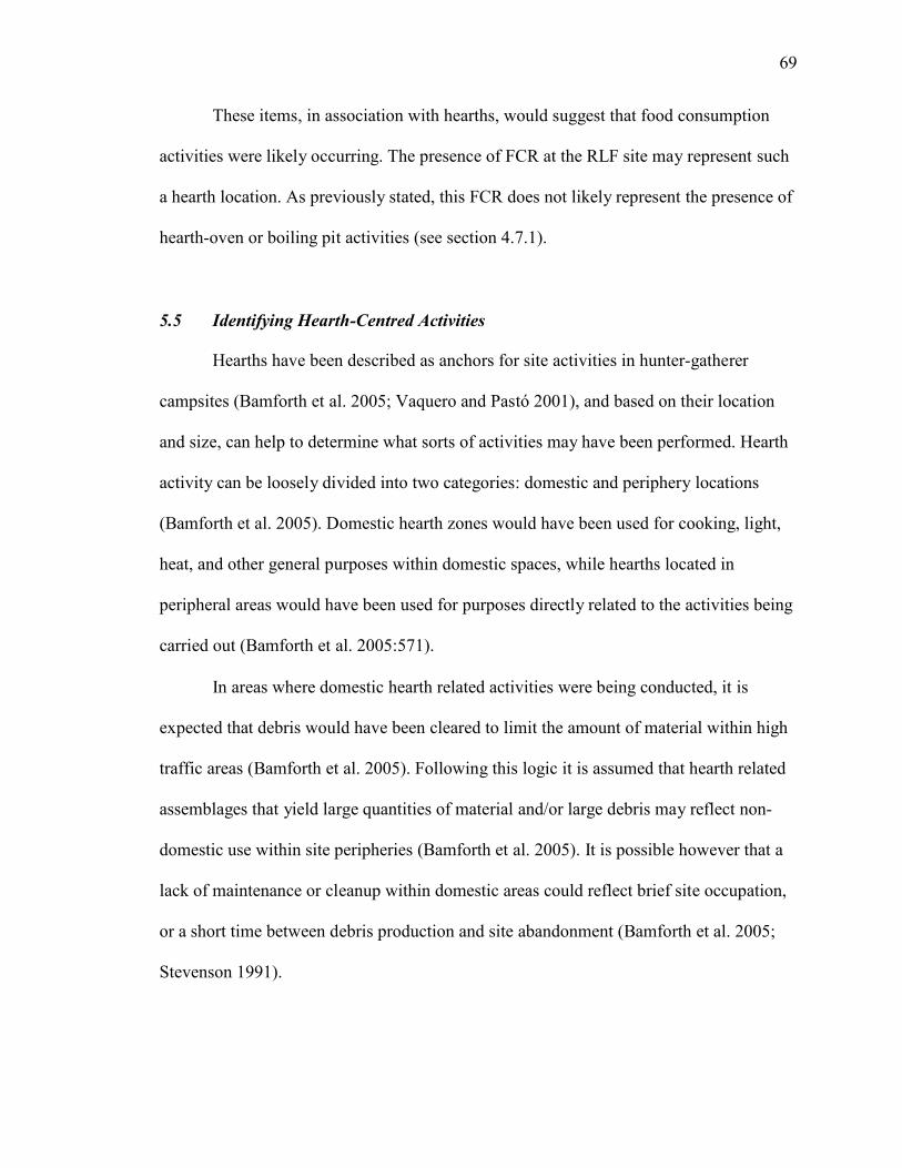
69

These items, in association with hearths, would suggest that food consumption

activities were likely occurring. The presence of FCR at the RLF site may represent such

a hearth location. As previously stated, this FCR does not likely represent the presence of

hearth-oven or boiling pit activities (see section 4.7.1).

5.5 Identifying Hearth-Centred Activities

Hearths have been described as anchors for site activities in hunter-gatherer

campsites (Bamforth et al. 2005; Vaquero and Pastó 2001), and based on their location

and size, can help to determine what sorts of activities may have been performed. Hearth

activity can be loosely divided into two categories: domestic and periphery locations

(Bamforth et al. 2005). Domestic hearth zones would have been used for cooking, light,

heat, and other general purposes within domestic spaces, while hearths located in

peripheral areas would have been used for purposes directly related to the activities being

carried out (Bamforth et al. 2005:571).

In areas where domestic hearth related activities were being conducted, it is

expected that debris would have been cleared to limit the amount of material within high

traffic areas (Bamforth et al. 2005). Following this logic it is assumed that hearth related

assemblages that yield large quantities of material and/or large debris may reflect non-

domestic use within site peripheries (Bamforth et al. 2005). It is possible however that a

lack of maintenance or cleanup within domestic areas could reflect brief site occupation,

or a short time between debris production and site abandonment (Bamforth et al. 2005;

Stevenson 1991).

70

Both ethnographic and archaeological consideration of hearth related assemblages

reveal a variation of the distribution patterns described in the drop, toss, and displacement

models (Binford 1983; Gibson 2001; and Stevenson 1986, 1991, see Figure 5.3.1). The

results of hearth use, especially when more than one individual is present, produces either

a crescent or circular shaped distribution of debris around a central location (e.g. Binford

1978, 1983; Carr 1991; Stevenson 1991). In many of these circumstances, the hearth

location will exhibit a relatively low concentration of debris compared to the identified

discard zone areas. However, the use of type 2 cluster discard as defined by Gibson

(2001) could result in the dumping of materials into hearth centres. Using the observed

distributions of artifacts, it may be possible to propose where hearth locations may have

been, even without preserved organics or staining.

5.6 Structure vs. Non-Structure Related Deposits

The distribution of artifacts around hearths plays a crucial role in interpreting

whether or not the observed activities took place within a covered shelter. While most

studies of site activity in relation to structures are aided by the presence of organic or

sedimentary indicators (e.g. post-molds, tent rocks, or occupation floor compaction), this

is not possible for the RLF site. This means that interpretations of lithic dispersal are the

only method of identifying built structures.

Non-structure related, or open-air, assemblages contain remnants of activities that

would have produced considerable debris or mess (Binford 1983). These open-air hearth

distributions would exhibit a distinctive drop-toss-displacement distribution and a lack of

artifact confinement (Binford 1978, 1983; Stevenson 1986, 1991). Binford (1983) states

71

that these �doughnut-shape✁✂ distributions did not occur inside structures, as people

would have likely avoided throwing materials against tent walls.

Where activities occurred within structures, one would expect to see a significant

degree of maintenance and removal of debris rather than the tossing of items (Binford

1983). Although this could refer to the removal of debris from the structure entirely

(Binford 1983), the cluster discard model could result in discard within structures (e.g.

type 1 and 2 discard - Gibson 2001). As such, the interpretation of structure related

assemblages relies on the identification of relatively contained artifact distributions with

a lack of a distinctive toss-zone and evidence of activity area cleaning or maintenance.

Given the significant amount of waste produced during full lithic reduction

activities, it is reasonable to assume that it occurred in association with open-air hearths.

However, the results of intra-site spatial patterning by Gibson (2001) at the Bushfield

West site suggests otherwise. Spatial interpretations at Bushfield West reveal that the

reduction of lithic materials was being conducted within tent structures. While lithic

debris would have posed a hazard within the structure, cluster discard activities

demonstrate that waste was being collected and discarded elsewhere (Gibson 2001). It is

suggested that performing these lithic reduction tasks in-doors would have provided a

warmer, more productive environment for tasks requiring considerable manual dexterity.

While it is evident that the interpretation of structure related assemblages using

only lithic recoveries is fraught with concerns and issues regarding the interpretability of

distributions, the general models presented provide a good reference. Using these general

models, interpretations for either open-air or structured related deposits can be compared

72

in order to provide balanced interpretations. Without clear structural evidence however,

these interpretations remain speculative.

5.7 Cultural Transformation Processes Affecting Spatial Interpretation

As discussed in section 5.3.1, the maintenance of site activity areas can affect

archaeological interpretations. These cultural transformation processes are not limited to

the clean-up of lithic reduction areas during site use. The curation of lithic materials, re-

use/movement of refuse piles, and use of the site by modern, contemporary, and

subsequent occupational groups can have the effect of further blurring interpretable site

distributions.

The curation of artifacts by hunter-gatherer groups can result in the limited

recovery of a number of materials that may have been deemed highly desirable by past

populations (e.g. exotic materials). It has already been proposed that the production of

cache stage bifaces for later use and refinement elsewhere was occurring at the RLF site.

This represents only one form of potential curation behaviour from lithic sites. The

collection of larger, usable flakes for the production of flake based tools can also affect

sites recoveries. In this scenario, site occupants would collect and store flakes produced

during lithic reduction for later use as expedient tool blanks. These curated tools may be

limited to smaller, more easily transported items, while larger cumbersome object were

either left behind or reduced further for transit (Schiffer 1987)

If sites are re-occupied by subsequent groups, the use of materials or features left

behind may occur. Cached materials such as anvil stones or lithic materials could be used

by different populations resulting in alternative depositional patterns. Bamforth et al.

73

(2005) observed the re-use of lithic waste piles by subsequent populations at the Allen

site. Rather than re-using the materials left behind, new site occupants may have

continued to dispose of refuse into the still visible middens of previous occupations

(Bamforth et al. 2005). This re-use of visible site features affects the abilities of

researchers to interpret distinct occupation activities based on the composition of artifact

clusters.

While not a culturally related transformation process in the sense of site

occupation by past hunter-gatherer groups, the disturbance of sites through modern

human processes must also be taken into consideration. It has been observed that the

trampling of artifacts by people, animals, and machines can result in the reduction of

overall artifact size, as well as the sorting and vertical movement of artifacts (Schiffer

1987:268). The results of surface scarring from the removal and stacking of trees, similar

to a ploughing effect, results in an upward and lateral movement of artifacts (Schiffer

1987). Properly documenting these disturbances throughout the excavation process will

aid in the spatial interpretation of the site.

While these cultural formation processes do pose serious problems regarding the

ability for researchers to interpret the spatial distribution of artifacts in relation to cultural

behaviour, their effects can be mitigated. The use of vertical and horizontal artifact

distribution, when combined with artifact attribute analysis, can be used to determine

variations in occupation, presence of site disturbance, and even the general reduction

processes undertaken on a site.

74

5.8 Non-Cultural Transformation Processes Affecting Spatial Interpretation

Along with the number of anthropogenic factors that can affect the deposition of

material, numerous non-cultural formation processes must also be considered when

interpreting site patterns. Of primary concern within the study of the RLF site are the

effects of non-cultural soil disturbance, termed pedoturbation (Schiffer 1987; Wood and

Johnson 1978), caused by bioturbation, cryoturbation, hydrological, Aeolian, or other

events.

Bioturbation is used to describe soil disturbance caused by organic mechanisms

including burrowing animals (faunalturbation) and vegetation (floralturbation) (Schiffer

1987; Wood and Johnson 1978). While evidence for animal burrowing was not noted

within stratigraphic profiles, there was significant evidence of floralturbation.

Disturbance through floralturbation results in the upwards and downwards movement of

artifacts through the push and pull of roots (Schiffer 1987). Tree falls were not clearly

identified during the RLF excavation, however these events could have resulted in the

mixing and upward displacement of artifacts trapped within the root systems of fallen

trees, with subsequent re-deposition during decomposition (Schiffer 1987).

Similarly, cryoturbation activities can result in the vertical displacement of

artifacts following deposition. The effects of frost heaving can serve to displace lithic

artifacts, with this effect compounding during the duration of time that the item is buried.

This will blur the vertical distribution of artifacts within a site. Frost action however, does

not only displace artifacts vertically, but also horizontally. Experiments by Bowers et al.

(1983) have observed the horizontal displacement of exposed lithic artifacts by as much

as 10cm in only a few years.

75

Hydrological and aeolian activities can further displace artifacts horizontally if

exposed to various factors. Schiffer (1987) discusses the effects of water and wind on

artifact distributions as following the same basic rules that apply to sedimentology

studies. During relatively high energy events, such as a beach face storm event, smaller

artifacts will be transported away along with small sediment particles leaving only the

larger and heavier objects. This has been observed as a form of site disturbance on

archaeological sites elsewhere, resulting in the size sorting and displacement of artifacts

(e.g. Lavachery and Cornelissen 2000).

5.9 Summary

With the development of ethnoarchaeological behaviour models, archaeologists

have been able to better understand how artifact distributions may have entered the

archaeological record. The most significant of these involves the discard of materials

through drop-zone, toss-zone, displacement, and cluster discard (Binford 1978, 1983;

Gibson 2001; Stevenson 1986, 1991). These models of artifact disposal have allowed for

the interpretations of hearth related assemblages, linking them to both open-air and

structure related activities.

While the RLF site recoveries limit the direct association of artifacts with these

features, their patterned distributions are able to provide some insight into possible

scenarios. These interpretations translate into the ability to identify site activities that

would have relied heavily on preserved organic remains such as bone and hide working.

Despite these limitations, there is significant evidence to suggest the ability to identify

both lithic reduction events and associated activities through artifact co-occurrence.

76

Before these interpretations can be made though, an assessment of the post-

depositional transformation processes acting upon the RLF site must be considered.

These can include the alteration of site deposits through both anthropogenic and natural

agencies such as: artifact curation, site re-occupation, trampling and scarring during the

past and present, bioturbation, cryoturbation, and hydrological and aeolian activities

(Bowers et al. 1983; Schiffer 1987; Wood and Johnson 1978). Understanding processes

of depositional alteration allows researchers to better understand and interpret

archaeological site patterning.

Chapter 6

Methods

6.1 Introduction

This chapter outlines the methodological approaches taken during the intra-site

analysis of the RLF site from initial data acquisition to the development of final

interpretations. The methodologies outlined below were selected for both their frequent

use within the current literature, as well as their ability to address some of the limitations

of CRM derived data.

6.2 Data Access

The data used within this thesis were obtained from CRM excavation projects

jointly conducted by Lakehead University and Western Heritage. This co-operation

allowed for the storage of archaeological materials and catalogs at Lakehead University

for the purpose of research and analysis by graduate and undergraduate students, thereby

furthering the research and understanding of Lakehead Complex sites.

6.3 Geographic Information Systems (GIS)

Since their introduction into archaeology in the 1970s and 1980s, geographic

information systems, or GIS, have allowed archaeologists to explore the spatial relations

of archaeological sites and materials in more depth and with increased efficiency

(Gillings and Wheatley 2005; Mills 2009; Wheatley and Gillings 2002). Various GIS

programs exist with which archaeologists can work (e.g. SURFER, QGIS, ArcGIS, etc.),

77

78

and their use as a tool within intra-site spatial analyses has been explored (Mills 2009;

Moyes 2002).

Differing primarily in user interfaces, these programs allow for manipulation,

analysis, and presentation of spatially registered data (including archaeological data)

(Gillings and Wheatley 2005). For the spatial analysis of the RLF site, ArcGIS was

chosen as the preferred platform due to its availability and ease of use. Spatial data were

created using artifact catalog outputs generated within the ADEMAR cataloging program

and was displayed using randomized Xrand and Yrand co-ordinates for un-provenienced

items (see Chapter 4). Various shape files for different catalog categories were developed

in order to provide multiple analytical approaches.

Along with the use of GIS as a spatial display tool, it also provided numerous

statistical capabilities that helped with the identification of artifact clusters. Tests run

within the ArcGIS program included kernel density, nearest neighbour, and Ripley�s K.

6.4 K-Means and Kernel Density Cluster Analysis

K-means analysis was chosen as the primary method of cluster exploration based

upon its ease of use with the available spatial data sets from the RLF site, as well as its

extensive use within the current literature (Koetje 1994; Enloe et al. 1994; Gregg et al.

1991; Rigaud and Simek 1991). K-means analysis provides an exploratory tool, through

which researchers can assess the nature of artifact clustering through a predetermined set

of artifact clusters.

In order to conduct a K-means analysis, a number of different tests were run for

various values of K; where K represents the number of clusters allotted within the test

79

run. For each test, K seed points would be placed within the study area at random. Each

data point is then related to the nearest of these seed points. These distances are then used

to place a new seed point within the centre of the observed distances, where data points

will again be assigned to the nearest seed point. This re-evaluation and placement of seed

points is run continuously until no new seed point can be placed that will reduce the

distance values between the data points and seed points. These final data/seed point

assignments result in the assigned cluster number (de Smith et al. 2007).

For the RLF site analysis, K-means tests were run for values of K from 2-10 in

order to explore a wide range of possible outputs. These tests were run within SPSS

(Statistical Package for the Social Sciences), and then later translated into shape files for

the visual representation of cluster membership within ArcGIS.

In order to determine which K value provided the most appropriate fit, the

Log10%SSE (sum of squared errors) for all K values was calculated. When plotted, values

of appropriate fit will exhibit an inverse inflection (Gregg et al. 1991). Clusters at this

point represent the ideal number through which further analysis of site activity can be

based.

While this analysis provided an excellent starting point for analysis, there are

some limitations regarding the initial catalog methodology. The use of bulk catalog

numbering for similar artifacts from within levels resulted in the frequent occurrence of

single data point entries representing multiple cataloged items. To reaffirm the result of

the K-means tests, further exploratory tests that could take this frequency into account

were required. As such, the results of the best fit K-means tests were mapped against

kernel density mapping outputs to assess appropriate cluster membership. This

80

combination of techniques was employed by Enloe et al. (1994) in order to visually test

the validity/selection of K-means results.

Kernel density uses a magnitude per unit area in order to apply a smooth surface

contour. Similar to K-means, the kernel density tests provide an exploratory tool for the

identification of clustering hot spots (de Smith et al. 2007; Mills 2009). This test is easily

run within the ArcGIS program using the point data for all artifacts recovered from the

RLF site, and utilizes artifact frequency counts to address some of the catalog limitations.

The combination of both K-means and kernel density provide an excellent

exploratory tool to determine artifact clustering that may have been the result of human

activity. These clusters are then used to develop sub-zones. These sub-zones provide the

basic investigative units through which further analysis is conducted.

6.5 Nearest Neighbour Analysis and Ripl�✁✂s K Function

Since K-means and kernel density function primarily as exploratory tools, it was

important to perform follow-up statistical analysis to ensure that the identified clustering

was in fact the product of a non-random, clustered distribution. To test this, nearest

neighbour analysis and Ripley✄s K function were run on the distribution of all artifacts

from all subzones.

The nearest neighbour statistical test compares the mean observed distances

between artifact point data and their nearest neighbour with that of the mean expected

distance values of a random distribution (de Smith et al. 2007; Mills 2009). The variance

of these mean distances can be explored using a z-test, in order to assess the likelihood

81

that the observed clusters are the result of a random, normal, or clustered distribution

(Mills 2009).

While the nearest neighbour test allows for the testing of cluster strength, it only

compares point distances to the nearest single point. Therefore using Ripley�s K function

in conjunction with nearest neighbour allows for a greater confidence in cluster strength

results.

Ripley�s K function goes beyond the single nearest neighbour, utilizing all point

to point relationships (de Smith et al. 2007). Rather than comparing the observed and

expected distances between points, Ripley�s K function utilizes circles of defined

diameters over artifact point data in order to compare the number of observed points

within a circle circumference to the expected number of points if the pattern were

random.

Both of these tests were run within the ArcGIS software using point data files for

the various defined sub-zones. The use of ArcGIS as a statistical tool provided not only a

user friendly interface, but also allowed for the export of cluster data information in the

form of charts and graphs that provided a secondary visualization of cluster strength.

This combination approach allows for the further interpretation of the distribution

of the archaeological remains. If the artifacts do in fact exhibit significant clustering then

further exploration can be undertaken in order to determine the nature of this clustering.

6.6 Getis-Ord General Gi Clustering Analysis

Throughout the analysis of the RLF site, the Getis-Ord General Gi statistic (Getis-

Ord Gi) was used in order to determine areas of lithic debitage clustering. The Getis-Ord

82

method is a spatial auto-correlation statistic that utilizes artifact frequencies in relation to

neighbouring clusters in order to determine intense clustering �hot-✁✂✄☎✁✆ (Mills 2001).

The results of the Getis-Ord Gi test can be displayed directly in ArcGIS using the

resulting z-scores.

As with most spatial statistical test, the Getis-Ord Gi method does not in itself

provide definitive clustering results. As such, the Getis-Ord Gi test within this study is

compared directly with observed artifact frequencies.

6.7 Refitting Analysis

While the use of artifact refitting provides a valuable tool within the intra-site

analysis of archaeological sites (e.g. Bamforth et al. 2005), it was not extensively

employed during RLF site analysis and was limited to formal tool items. The exclusion of

debitage within the refit analysis was due to the use of a CRM derived artifact

assemblage catalog, and the inability to conduct a refit analysis prior to spatial analysis

due to time restraints. While this is not ideal, the use of refit tools still provides valuable

information regarding post-depositional artifact movement as well as artifact movement

related to use. Refitted artifacts were analysed by associated clustered sub-zones

identified during K-means analysis.

6.8 Interpreting Activity Areas

While the use of statistical and mathematical approaches to the intrasite study of

artifact distributions are useful tools for establishing and displaying artifact clustering,

they do not in themselves explain how these clusters were produced (Enloe et al. 1994).

83

In order to develop these interpretations, the observed location, frequency, and

morphology of artifacts are compared to ethnoarchaeological and archaeological

literature (see Chapter. 5). Hypotheses regarding the use and distribution of artifacts,

when combined with cluster locations within the site environment (see Chapter. 4) are

then used to build a proposed model for site use and occupancy at the RLF site.

Following the development of interpretations regarding sub-zone activity, the

results of the near surface gradiometer (NSG) survey were plotted in order to address the

presence or absence of features no longer visible within the archaeological record (e.g.

hearths). The decision to explore the results of the NSG following interpretations was

made so as to limit biases that may have been introduced within the study prior to initial

analysis.

6.9 Summary

The intra-site spatial analysis performed for the RLF site required the use of

multiple exploratory and clustering spatial statistical tests in order to identify areas of

distinct artifact clustering. These tests, including K-means, kernel density, nearest

neighbour, Ripley�s K, and Getis-Ord Gi were chosen based on their ability to function

within a CRM derived data set. The results of these tests are then used to determine ✁sub-

zone� areas, where unit areas that contain identified clusters are selected for further

analysis.

Once artifact clustering is determined and sub-zone areas defined,

ethnoarchaeological and archaeological examples for activity area patterns and use are

compared to the observed patterns for the RLF site. This will include artifact patterning

84

that is both cultural and natural in nature. These comparisons, when combined with the

results from near surface gradiometer survey, formed the basis through which

interpretations of the RLF site were developed.

Chapter 7

Results of Spatial Analysis

7.1 Introduction

The intra-site analysis of the RLF site involved the manipulation and query of

artifact spatial data. This chapter outlines the results of the spatial analysis through

observed and tested artifact patterning. While the results outlined below follow a linear

order of development, spatial inquiry often involves the frequent back-checking and re-

analysis of observed patterns in light of varying artifact attributes. It is through this

analysis/re-analysis that a critical assessment of observed patterns can be made prior to

interpretation.

7.2 Sub-Zone Identification

Prior to the analysis of artifact patterning, K-means and kernel density clustering

analyses were performed in order to: A) identify distinct areas of artifact clustering, and

B) segment the RLF site into manageable sections through which a more in-depth

analysis was applied. The exploratory nature of these tests allow for the selection and

modification of clustering results by the researcher where necessary. This resulted in the

designation of what are defined here as cluster �sub-zone✁✂✄

7.2.1 Initial Clustering Results

To properly apply K-means, kernel density, and Getis-Ord Gi analyses, recovery

outliers within the RLF catalog had to be removed (e.g. surface recoveries from outside

85

86

the excavation areas or distant excavation units). When included, these outliers resulted

in a disproportionate skewing in the placement of clustering points. The results of this

catalog trimming can be seen in Figure 7.2.1.

Figure 7.2.1: Results of RLF catalog trimming prior to application of k-means, kernel density, and Getis-

Ord Gi. Trimmed artifacts were generally the result of surface collection or excavation outliers.

Once the artifact catalog had been trimmed, K-means analysis was run for 2-10

total clusters and the resulting Log10%SSE of each was plotted in order to determine the

most appropriate cluster number (K). A line graph of the plotted Log10%SSE exhibited a

sharp inverse bend where K=8, suggesting that eight clusters represented the most

appropriate fit (Figure 7.2.2, see also Section 6.4).

87

LOG

10%

SS

E

4.6

Results of log10(SSE)

4.4

4.2

4

3.8

3.6

3.4

3.2 K2 K3 K4 K5 K6 K7 K8 K9 K10

CLUSTER NUMBERS

Figure 7.2.2: Line graph of plotted Log10%SSE for k-means tests 2 through 10. Inflection at k=8 clusters

indicated by red circle.

The results for K-means clustering at K=8, or eight clusters, was then mapped

against the results of kernel density analysis for all artifacts (Figure 7.2.3). With the

exception of one K-means cluster (Cluster 4 in Figure 7.2.3), the resulting density zones

identified within the kernel density analysis match closely with K-means results. From

this outcome it was determined that the clusters for K=8 should be used to base cluster

sub-zone identification.

Additionally, the use of Getis-Ord Gi within this early stage of sub-zone

identification allowed for the determination of primary clustering areas, or �✁✂t-✄☎✂✆✄✝✞

These �✁✂✆-✄☎✂✆✄✝ ✟✠entify areas of greatest artifact concentration relative to their

surroundings (see Section 6.6). As can be seen in Figure 7.2.4, there are two primary

clustering zones, with comparatively low clustering in surrounding areas.

88

Results of K-Means Cluster Analysis, Kernel Density Analysis,

and Comparative Overlay

1m

5m

Figure 7.2.3: Maps illustrating the resulting cluster designations (A), kernel density results (B), and map

comparing the two results (C). It can be seen here that cluster 4 (orange) was not identified during kernel

density analysis. Due to identification within k-means analysis this cluster area will still be explored.

89

Results of Getis-Ord Gi for All Debitage by Quadrat

1m

5m

Figure 7.2.4: Results of Getis-Ord Gi represented visually by plotting resulting z-scores. This illustrates the two areas of highest recovery, or �hot-spots✁, within the RLF site.

7.2.2 Identification of Modern Mechanical Disturbance

Surface disturbance was identified during the initial excavations of the RLF site.

Tree felling and stacking activities with a bulldozer resulted in the disturbance of

sediments within the northwestern portion of the excavated area (Figure 7.2.5). Field

notes for units in the affected area indicate that undisturbed sediments were not

encountered within the far west of this area until levels 4-5, or 20-25 cm below surface

(see discussed units Figure 7.2.6).

This was a significant factor in the identification of sub-zones within this analysis.

As seen in Figure 7.2.7, when artifact recoveries were removed by level the northwest

90

(area indicated by the yellow square in Figure 7.2.5) becomes devoid of recoveries at the

levels of non-disturbance. As almost all recoveries within this area appear to be the result

of disturbed push activity, they yield little spatially significant information.

Figure 7.2.5: Areas of site disturbance. Note: the boundaries of this site disturbance area are not well

defined and represent the proposed impacted area from field excavation notes. Yellow square indicates the

area of greatest disturbance as indicated by field notes.

91

1m

5m

Figure 7.2.6: Units discussed in text in relation to site disturbance.

92

7.2.3 Sub-Zones

Units with evidence of artifact clustering, as identified during K-means and kernel

density analyses, were used to determine sub-zones. Due to the disturbance activities

discussed in section 7.2.2, not all clusters were given their own sub-zones.

Cluster 2 (teal) consisted primarily of artifacts displaced through disturbance (see

Figure 7.2.7) and as such, were removed from sub-zone determination. Removing

artifacts from Cluster 2 enabled the trimming of the RLF site map into a more

manageable shape and size (Figure 7.2.8). This trimmed map was utilized throughout the

remainder of the RLF site analysis.

While the disturbance that impacted Cluster 2 was observed to extend into the

primary excavation area, it did not appear to have affected artifact deposition as severely.

However, due to their proximity to the disturbance activities, it was determined that

Clusters 3 (blue) and 8 (pink) could be combined within one sub-zone in order to further

assess artifact displacement. In total this resulted in the designation of six site sub-zones

(Figure 7.2.9).

These subzones were differentiated into larger zone� ✁A✂ and ✁B✂ ✄ased on the

observed separation of artifact clusters by a slight rise within topography (Figure 7.2.10

A), see also Section 4.2). As such, sub-zones were given the titles A1, A2, B1, B2, B3,

and B4 (Figure 7.2.10 B). In areas where sub-zones bordered one another, overlap was

provided. It should be noted that this resulted in the occurrence of some artifacts within

multiple sub-zones.

93

Figure 7.2.7: Mapped artifact distributions by level. This map series illustrates that as level recoveries are

removed down to identified undisturbed sediments, little to no artifacts remain within the area.

94

RLF Site Map Before and After Removing Disturbed Cluster Two

1m

5m

Figure 7.2.8: Map of k-means cluster results for k=8 (A) with trimmed map of defined clusters with cluster

two removed (B).

95

Additionally, not all artifact recoveries were included within these subzones. This

did not mean that these artifacts were excluded from the final spatial interpretations, but

only excluded from sub-zone analysis in order to focus on primary clustering areas.

Furthermore, some K-means clusters were split within sub-zones (e.g. cluster 7). This

was due to the observed separation when cluster results were compared with map outputs

for kernel density and Getis-Ord Gi analyses.

RLF Site Sub-Zone Designations based on K-Means

1m

5m

96

1m

5m

Figure 7.2.9: Defined sub-zone with comparison to cluster designations. It can be seen here that cluster 3 and 8 were combined to form one cluster. This was due to the observed disturbance discussed in section 7.2.2.

97

Sub-Zone Location and Topography Resulting in the

Des ig na tio n o f Zo nes �A✁

✂✄☎ �✆✁

A

1m

5m

B

Figure 7.2.10: Defined sub-zone compared with topographic relief map (Represented by black lines) (A) and resulting zone designations (B).

98

7.3 Sub-Zone: A1

Sub-zone A1 consisted of 99, 50 x 50cm quadrats in the northwest corner of the

RLF site (Figure 7.3.1). This sub-zone contained Clusters 3 and 8, and was subject to

surface disturbance prior to excavation.

Figure 7.3.1: Sub-zone in relation to topography with a close up of sub-zone A1 illustrating all tool recoveries with total debitage by quad.

7.3.1 A1: Artifact Recoveries

Sub-zone A1 consisted of 1,950 artifact recoveries. Of this, 31 were tools (33

excluding tool refits). Tools included nine cores, 16 bifaces, one graver/perforator, one

perforator, one retouched flake, one scraper, one anvil stone, and one wedge (Table 7.3.1,

biface staging Table 7.3.2). Of the recovered cores, four exhibited a cobble cortex while

five did not have any identifiable cortex (Table 7.3.3).

A total of 1,909 lithic waste fragments were located within sub-zone A1, of which

1,599 were classified as debitage and 310 as microdebitage. Waste flakes were further

subdivided by type (Table 7.3.4), material (Table 7.3.5), and size (Table 7.3.6). The

remainder of artifacts consisted of three pieces of FCR, and five fragments of unknown

or non-cultural lithic items.

99

A1: BIFACES

BIFACES

STAGE

Frequency

N/S 1

1 2

2 2

3 8 (9)

4 3

5 0

6 0

A1: DEBITAGE

TYPE Frequency

PRIMARY 53

SECONDARY 1296

TERTIARY 198

UNDETERMINED 101

SHATTER 261

A1: DEBITAGE

SIZE Frequency

0-2MM 0

2-6MM 313

6-12MM 728

12-25MM 627

25-50MM 222

50+MM 19

Table 7.3.1: All tool recoveries from sub-zone A1 Table 7.3.2: Result of biface staging for sub-zone A1 following Bennett (2015)

A1: TOOLS

TOOL TYPE Frequency

CORE 9 (10)

BIFACE 16 (17)

GRAVER/PERFORATOR 1

PERFORATOR 1

RETOUCHED FLAKE 1

SCRAPER 1

WEDGE 1

ANVIL 1

Table 7.3.3: Results of cortex identification for sub- zone A1.

Table 7.3.4: Debitage frequencies by type

A1: CORES

CORTEX

TYPE

Frequency

N/A 5 (6)

COBBLE 4

TABULAR 0

Table 7.3.5: Debitage frequencies by material Table 7.3.6: Debitage frequencies by size grades

A1: DEBITAGE

MATERIAL Frequency

TACONITE 1685

GFS 137

CHERT 9

SILTSTONE 71

QUARTZ 4

OTHER 3

100

To

tal R

eco

ve

red

Art

ifa

cts

7.3.2 A1: Vertical Distribution

The effects of site disturbance is clearly evident within the vertical distribution of

artifacts in sub-zone A1. Artifacts were concentrated highest around level one, and

maintained a high frequency until level 3 before declining with increased depth (Figure

7.3.2)

In order to explore this distribution further, vertical distributions were plotted for

all artifacts by size class (Figure 7.3.3). It can be seen from these results that the high

frequency of artifacts in level one is attributed largely to artifacts within the 2-6mm and

6-12mm size range. All other size grades in turn cluster around level three, yielding the

greatest recovery frequencies.

600

Sub-Zone 'A1' - Vertical Distribution of All Artifacts

500

400

300

200

100

0

Surface Level 1 Level 2 Level 3 Level 4 Level 5 Level 6 Level 7 Level 8 Level 9 Level 10

Excavation Level

Figure 7.3.2: Total artifact recoveries by level indicating a high recovery frequency within the upper levels;

likely the result of disturbance activities previously discussed.

101

To

tal R

eco

ve

red

Art

ifa

cts

250

Sub-Zone 'A1' - Vertical Distribution by Artifact Size

200

150

100

50

0

Surface Level 1 Level 2 Level 3 Level 4 Level 5 Level 6 Level 7 Level 8 Level 9 Level 10

Excavation Level

2-6mm 6-12mm 12-25mm 25-50mm 50+mm

Figure 7.3.3: Total artifact distribution by level and size showing that debitage in the size ranges of 2-

12mm are recovered in highest frequencies around level 1, while larger size grades are recovered near level

3.

7.3.3 A1: Horizontal Distributions: General

Prior to artifact distribution analysis, nearest neighbour, Ripley�✁ ✂ function, and

Getis-Ord General were conducted in order to determine if artifact clustering within the

sub-zone was significant. The results of these tests can be seen in Figures 7.3.4, 7.3.5,

and 7.3.6, respectively. These tests indicate that the clustering of artifacts is significant,

with nearest neighbour and Getis-Ord Gi results suggesting that there is less than 1%

chance that the observed artifact distribution is the result of random chance.

102

Figure 7.3.4: Results of nearest neighbour analysis indicating that at a z-score of -8.929599 there is a less

than 1% chance that the observed distribution is the result of random chance.

Figure 7.3.5: Graph of Ripley�s K function analysis illustrating that the observed distribution is likely the

result of a clustered distribution.

103

Figure 7.3.6: Results of Getis-Ord Gi analysis indicating that at a z-score of 6.093171 there is a less than 1% chance that the observed distribution is the result of random chance.

7.3.4 A1: Horizontal Distributions: Recoveries by Level

The recovery of tools by level with corresponding debitage frequencies is shown

in Figure 7.3.7. It is apparent that Level 1 exhibits a unique distribution with the highest

concentrations of artifacts coming from the western portion of the sub-zone. As recovery

levels progress, artifact distributions become concentrated within two cluster areas in the

south-central and northeastern areas of the sub-zone; with a possible third area of high

concentrations near the shared boundary with sub-zone A2. It should be noted that while

limited recoveries exhibited by some distribution maps are not overly useful for the

application of spatial statistics, Getis-Ord Gi results are illustrated regardless in order to

maintain consistency throughout.

104

-J- G- 10

Do

-.-,- ·

Al: Horizontal Distribution of Artifacts by Level

sub-zone Al i·i0r1'zontuIDI'St r'1but'mns - Su rfal ce Recove r1es

Sub-Zon e A I Getis-OI'd Gi Res ults - Suo· face Recovel'ies

I

I

- 1-

1 - -

� I

TotalDebitge

Surface

CJ o 1-5

CJ ow 11-20

- 21-)

N

A '-----1---J.--1-

lli.!.!!.!!

Surfac e

GiZSwe

- <2MS:t<l0e

- ..2 :ili --196Stcl(le<t

- -1116- -I GSSMoe.'

=::J -t-165Sid Oe¥

- 165-11l6Std.✁✂✄ - 1116 - Z SidDe

- >256Sk10eof

N

1-1--+----1- A

sub-zone Al H. OI"IZOHt UI DI'St r1'bUt'lOPS - Leve11 Rt'Covedes

Legend

0 111!-.:e

☎ F1'39Mfll'll

£ M<!Aak

Total Oebitge

Level t

I" c::

Sub-Zone A I Getis-OI'd Gi Results - Level I Recovel'ies

.b!a!..!!!! Leve l1

GiZS we

- ..2 :ili - U Sti:I De¥

- -196 --1G5Sid 0e¥

-165 -165Sid0e¥

- 165- IIISStd.Oe.

- 196 - 2 5eSid De

,_ .....

[Jl✆ D,, zo 1::]21-50

1 -100

- \0\\0i

N

- >2 58SICI. Oe.

N

c

A

Suh-zom.✝ A l Horizontal Distributions- Lcvel 2 Recoveries

Legend

0 Bi!Oict

e COreFr*'O)!litf"'t

¢ ...,✞✟✞, Total Oebitge

CJo CJ"

0 &-10

l::]lt -20

- 21-51

A Sub-Zone A I Getis-Or·d Gi Results - Level 2 Recovel'ies

ill!..!!!! Level2

-CilS<.:o,re ., · - ..2 5e --196Stl:l (le<t

- -l ll6 --1{>5std0e¥

==:J -\ S6 -166Sid De¥

- L65-1Std.De .

- ··25eStdDe

- 2-6Ski. Oe.

105

p

�✁ ✂ 1 =::::

-., ·· ·

·-= 1-

c

t-

sub-zone A l I I.O.I IZOnt aI D"tstrt"bu f 10ns - Level 3 Recovedes

Legend

0 Bo!&ee

t e COreF mel'll

0 GranriP<"rtor✄ or

A_ Scraper

Total Debitge

Levell

c:::::J o

Q "

b!9!.!!.!!

Levell

- <2MS!<I0e

- :ii!I--196Stcl !;le\'

- -196- -165Siol oe.'

=::J - -165Sid Oe¥

- t 65-196Std.De☎ - 1 96 - Z stdCle

- 2 56Sk10e.

- c:.

f---'

N

V' A

C]&-10

c ::::J 11 20

N

A j- 1--

IU c

+.AA"

suh-zone Al i i O.ZOntaID"IS trt"hU fIOnS - Leve14RCCOVCJ"ICS

Legend

"' ✆ 'o'kdgc

TotalDebitge

L..,el 4

c:::::J o 1::!1-S 06-10

.c: 011-20

1- - 21-33

1- N

A

Suh-zone At I IOI"✝IZOnt aIn St r"th UfIOns:- LeveI 5 Rccovc✝·ies

Legend ✞ Corrc>lete Core ✞ Core hlllmenl

Total Oebitge 1-

Level s

c:::::Jo 1::::11-

1 96

11- \

-0

20 - ZI-4\1

Sub-Zone A I Getis-Ord Gi Results - Level 4 Recoveries

ill!M Levtl4

--2:ill- -196Sto De¥

- -196 - -165Sid oe.

=:::J -!65 -165Sid0e¥

- t 65- t96Std.Oe.

- 1 96 - 2 5eSidDe

- >258SICI. Oe.

N

A

- -196 - -165SW Oe¥

=:::J -165-165Sid0e¥

- L65- t 96Std.Oe.

- t 96 - 25estdoe

- >BISI<I. Oe.

- r--

1- N N

1- A A

106

- ......

lt c

-"

sub-zone A l I I.O.I IZOnt aI D"tstrt"buf 10ns - Level 6 Recovedes

Legend

f-- � Bt!IICe

To tal Oebitge

CJo I::J1-S

0 &-tO

1'::]11-20

- 21-35

- <2 M S!<I 0e

-:ii!I--196Stcl !;le\'

- -196- -165Siol oe.'

=::J -t -165Sid Oe¥

- t65-196Std.De✁

- 1 96 - Z stdCle

1- t- ,_ 1- N

1- A

suh-zone Al iiOI.'ZOnta IDI"S trt"hUfIOnS - Leve17 RCCOVCJ"ICS

Legend

- 0 KO

- 2 56Sk10e.

N

A

ill!M

Levtl7

r-- Total Debitge

Level7

CJ o -., ·· · [:l t-5

06-10

t:::l t\20

- 21..(0

1- 1 t- t -

- -2:ill - -196Sto De¥

- -196 --165Sid oe.

=:::J -t65 -165Sid 0e¥

- t 65- t 96Std.Oe.

- 196 - 2 5e Sid De

- >258SICI. Oe.

N N

A A

Su h-zone At IIOI"✂IZOntaI n·IStr"t hufwn:s- LeveI 8 Rccovc✂·ies

lt Legend

r-- Tota l Oebitge L11Vel8

r-- Do -

Levt

.l8

,-·- - 1$- 12

t-

N

A

-5e --196Stc! Oe¥

- -196 --165SW Oe¥

=:::J -t 65 -165Sid 0e¥

- L65- t96 Std.Oe.

- t 96 - 25estdoe

- > BISI<I. Oe.

N

A

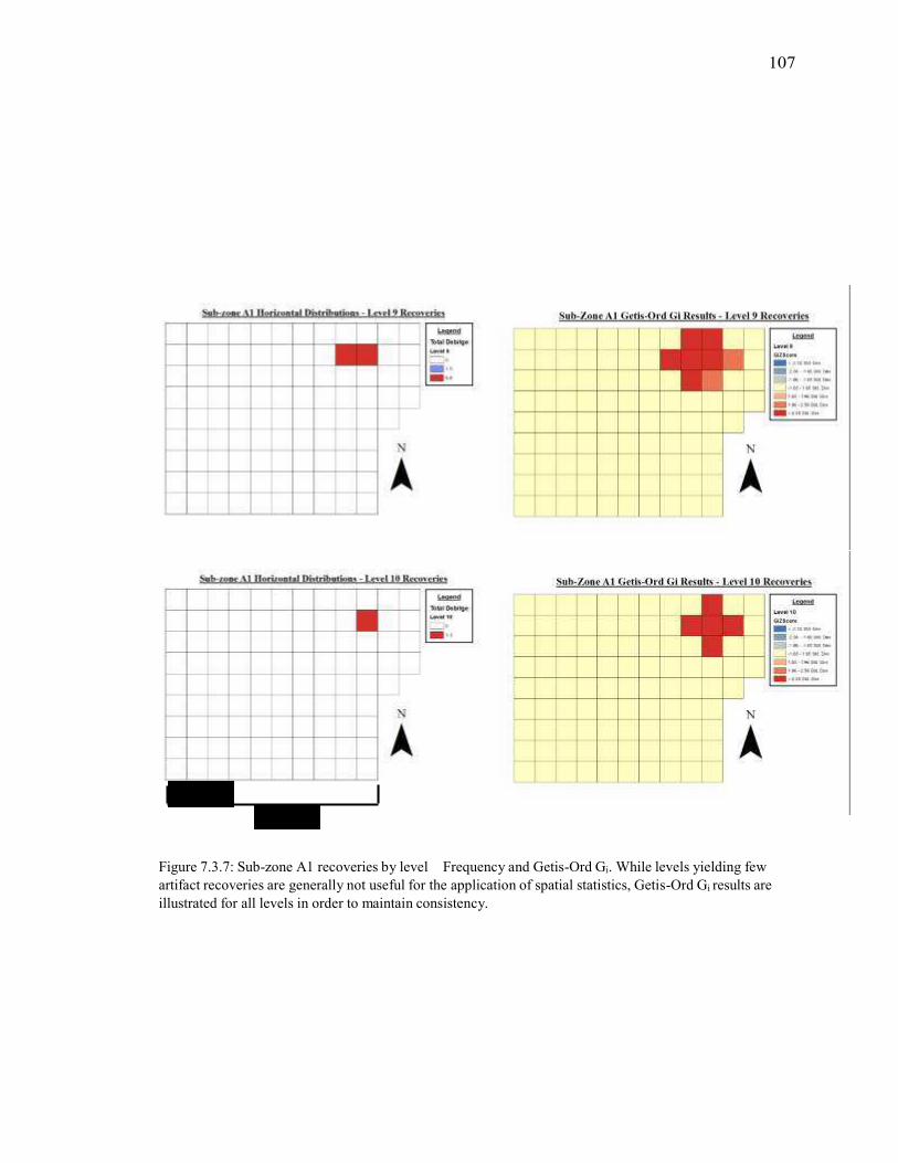
107

1m

5m

Figure 7.3.7: Sub-zone A1 recoveries by level � Frequency and Getis-Ord Gi. While levels yielding few

artifact recoveries are generally not useful for the application of spatial statistics, Getis-Ord Gi results are

illustrated for all levels in order to maintain consistency.

108

7.3.5 A1: Horizontal Distributions: Recoveries by Material Type

Material recoveries from sub-zone A1 consisted of taconite (Figure 7.3.8 A),

gunflint silica (GFS - Figure 7.3.8 B), siltstone (Figure 7.3.8 C), chert (Figure 7.3.8 D),

and quartz (Figure 7.3.8 E). While quartz and chert were the least frequently represented,

their distribution appears to loosely coincide with high density recovery zones identified

in Section 7.3.4. However, the low frequency of recovery limits the strength of this

interpretation.

Siltstone recoveries, while also limited, were concentrated within the northern

area of the sub-zone. Similarly, concentrations of gunflint silica were greatest near high

density zones in the northern section of the sub-zone, with a secondary cluster to the

south. Mapping taconite recoveries revealed clustering similar to those observed within

level-by-level distributions, with a small cluster of artifacts near the southwestern edge of

the sub-zone (likely correlating with Level 1 recoveries, Figure 7.3.9-A), and three

clusters coinciding with high recovery rates in the northeast and central areas (Figure

7.3.9-B,C, and D).

109

lrJA ��

.. A or -SO

--

h

A

✁ B

,.

c

Al: Artifact Distributions bv Material

sub-zone Al iion.zontaIDI'S tr'lbutrons- T.acon'ate RCCOVCri CS

Legend

0 Botue

Sub-Zone Al Getis-OI'd Gi Resul ts - Taconite Recovel'ies

✂c 4

✄ Co"'9re Core

Coie Frag'""nt

¢ G<n.,rr'Peri<l rot<><

0 Perfar☎lor

Taconite

GjlSeOfe

- 2!>4S!dl»v

- -2!>4 - -tWiS"'O.:.

- -\ !16- -tt5SDf:o<

- ·165Sid0e¥

A tJl]

�

c "t

c C)

c

1&- .6. ReW<Khed flal<e

A &r:op<!!r ✆ Weoge

Total Debitge

Taconite

N CJ o

- 165- tiiSStci.O..✝ - 1116 - 2:i8SIClew

-25t Sk10e.

N

t::]s.to

-u 011-20 ✞ - 51-100

- 101-1!>0

sub-zone Al IIor✟. zontaI n· IS t 1'

'' 1 ut1'0ns ✠ - GFS Rec0\✡eries

Legend

Botace

Total Oebitg e

OF$

CJo

Os..to 0 11-20

- 21-24

N

A

0 "'"'

l ge

- <2MS!d0ev

- -2:ill - -1G6Sto0e¥

- -196 --1{.5Skl 0e¥

=:::J -t65 -165Sid0e¥

- 165- tiiSStd.Oev. ☛ ☞>·25eSIoe· - 2 51SICI. Oe.

N

A

sub_ -zon e Al H. O I'IZORtaI DI'St rl'b ut'wns - Siltsto"'✌ Rcc·ovcrics

Legend Tota Oebit

Siltstone

CJo D t- 0 6- tO

- 11-21

1 -

N

A

SlitStOM

CilS<:ore

- <>M.O ✍ - -2 58 - -IIISSta oe-'

- -19& --165std0e¥

=:::J -t 65 -165Sid0e¥

- L65-tii6 Std_ ()e .

- I W-25estdDe

- 2-tSI<I. Oe.

N

A

110

D

E

1m

5m

Figure 7.3.8: Sub-zone A1 artifact distributions by material type � Frequency and Getis-Ord Gi. A)

Taconite, B) Gunflint Silica, C) Siltstone, D) Chert, and E) Quartz.

111

B

A C

D

1m

5m

Figure 7.3.9: Artifact cluster identified through the mapping of taconite artifacts. Yellow represents

clustering likely related to disturbed artifacts while blue represents clustering observed throughout vertical

analysis. Clusters discussed in text as A) Western, B) Northeastern, C) South-central, and D) South-eastern.

7.3.6 A1: Horizontal Distributions: Debitage

Debitage distributions were mapped by both size grade and type in order to test if

horizontal distributions were affected by different artifact characteristics.

Debitage Size

Debitage mapped by size exhibits concentrations forming discrete northern and

southern clusters (Figure 7.3.10). In the northern cluster (Figure 7.3.9-B), debitage of all

sizes appear to concentrate within the same area. Of note within these distributions is the

112

difference in the location of hot-spots within the southern concentrations between varying

size grades. In smaller size grades (2-6mm and 6-12mm) concentrations occur near the

shared A2 border (Figure 7.3.9-D), while larger size grades (12-25mm, 25-50mm, and

50+mm) and concentrated slightly to the left of this.

Distributions within the western portion of the sub-zone (Figure 7.3.9-A) appear

to focus primarily around flakes within the smaller size range (2-6mm and 6-12mm),

though some larger sized debitage does occur.

Debitage Type

The debitage types that were mapped included primary, secondary, tertiary, and

undetermined flakes as well as shatter (Figure 7.3.11). Limited primary debitage was

collected from sub-zone A1, although recovery concentrations appear to correspond

loosely with northern and southern clusters (Figure 7.3.9-B, C, and D).

The recovery of secondary debitage best illustrates this distinction between the

northern and southern clusters as two distinct clustering areas can be seen. The mapping

results for secondary debitage also exhibit a split within the southern cluster recoveries,

further suggesting that two clusters may be present (Figure 7.3.11).

To a lesser extent tertiary and undetermined debitage exhibit this similar pattern

between northern and southern clustering. Highest concentrations for tertiary debitage,

however, occur along the western edge of the sub-zone. Meanwhile, the strongest

concentrations of lithic shatter occur within the northern area of the sub-zone with lesser

amounts in the southern clusters.

113

:.0

lC -

Al: Horizontal Distribution of Debitage by Size

Sub-zone AI Horizontal Debitage Distributions: 2-6mm Recoveries

Legend

TotalDebitge

CJ o

1::1" 06-\0

CJ 11-20

- 21 38

sub-zone AlIIor1.zont aI Deh"1tage nL·r1t "bufu> ns:6-12mm ReCOvC� l" CS

Legend

- TotalDebitge

11·12mm

c:::J o

Sub-Zone A l Get is-Ord Gi Results- 2-6mm Recoveries

GIZSeore

- 2 M S!<IOev

- -2:ill - -1G6Sid De¥

- -196 - -165Sid oe.

=:::J -\66 -165Sid0e¥

- t 65- t 96 Std.Oe.

- 196 - 2 5e SI Dev

- >258SICI. Oe.

N

A

11-12flYil

Gil leon

,....._

.---. t::l 1-5

C]&-10

1 5)

!1

z1

✁-

-2

o0

- S! ..SS

f-

N N

A A

sub-zone AI HOI"IZOD taI D✂b"1tage n·ISt1""bU fIO n S: 12 25mm Re✄coven"es

Legend

- TotalDebitge

12·2mm

CJ o Cl☎ -5 C]&-10

C]11-20

D z1-

1- - SI .GCI

Sub-Zone Al Getis-Ord Gi Results- 12-25mm Recove1·ies

12-25mm

GilSCOfe

-2MS!d 0ev

- -.2 M- 1WiSid O.:.

- -\ 96 - -16.5Sid0f:¥

=:::J -160 -16-$ $1(1 oev - 1.65-196 SIOev

- \96 -2.5t1 Sid0ev

- > 2.56 Sid. Oe.

N N

t--- A

114

1m

5m

Figure 7.3.10: Debitage distributions by size grade � Frequency and Getis-Ord Gi.

115

Legend

Total Debitge

Shatter

CJo O t -s c:=J 6-10

c:::::J ll-20

- 21-25

N

A

-., ·· ·

.... -.,···

Al: Horizontal Distribution of Debitage by Type

sub-z:one AlBor1'zontnIDeba'tu :,e DI'S t'lbutw' ns: ShaIter

�

sub-zone AlB· on'zontuIDcbJ'tUK,C DI'Str'ibU tI'OnS: p·r lffiU!J:' Dcb1'ta ::e

Legend

Total De bitge

PriiT'Illry Debbg✁CJ o D"

ill!M

Shltta r

Gli l e

- -2:ill - -1G6 Sto De¥

- -196 --166Sidoe.

=:::J -t66 -165Sid0e¥

- t 65- t96Std.Oe .

-96 - 2 5e SI oe

- >256SICI. Oe.

N

A

Sub-Zone A1 Getis-OI'd Gi Resu lts: Pl'imal'v Debitage

Primary Deblt.tge

- -2 5e--HI6Sid 0e¥

- -11l6 --1&5 Sid0e¥

-\G6 - t65Sid0e¥

.! 65· !96Sid DI:Y

- !96 - 2_58Sid[)ey

- >2.58SICI. Oe.

+ -

N N

A

Sub-zone Al Horizontal Debitage Distributions:Secondan·Debitage

Legend

Total Oebitge

secondary Debltage

CJo r:::] t -5

CJ6-t0

O n-20

CJ 21.&1

51-100

- 101-116

N

A

Sub-Zone Al Getis-Ot·d Gi Results: Secondal'v Debitage

Seconeklry O ebltege

- <2!1& S!d0eY

- ..2 :ili - 1116 Stcl0e¥

- -196- -165Sid 0e¥

=::J -t 65 -165Sid Oe¥

- t 65- t96Std.De✂ - 1 96 - 2 5(1Sid[)eY

- >2 58Sid0e.

N

A

116

1m

5m

Figure 7.3.11: Debitage distributions by type � Frequency and Getis-Ord Gi.

117

7.3.7 A1: Horizontal Distributions: Tools

The distribution of all tool recoveries for sub-zone A1 is shown in Figure 7.3.12.

While a variety of tools were recovered, cores and bifaces were the most abundant.

1m

5m

Figure 7.3.12: Distribution of all tool recoveries from sub-zone A1 with total debitage by quadrat.

Cores

Cores recovered from sub-zone A1 can be seen in Figure 7.3.13. While affected

by small recovery numbers, the distribution of cores appears to correlate with both the

northern and southern cluster areas. Core recoveries by level indicate that one outlier,

located within the southwestern corner of the sub-zone, was recovered from the site

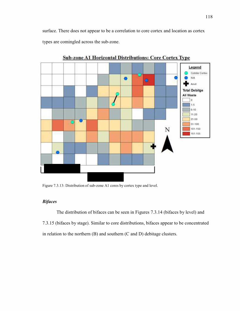
118

surface. There does not appear to be a correlation to core cortex and location as cortex

types are comingled across the sub-zone.

1m 5m

Figure 7.3.13: Distribution of sub-zone A1 cores by cortex type and level.

Bifaces

The distribution of bifaces can be seen in Figures 7.3.14 (bifaces by level) and

7.3.15 (bifaces by stage). Similar to core distributions, bifaces appear to be concentrated

in relation to the northern (B) and southern (C and D) debitage clusters.

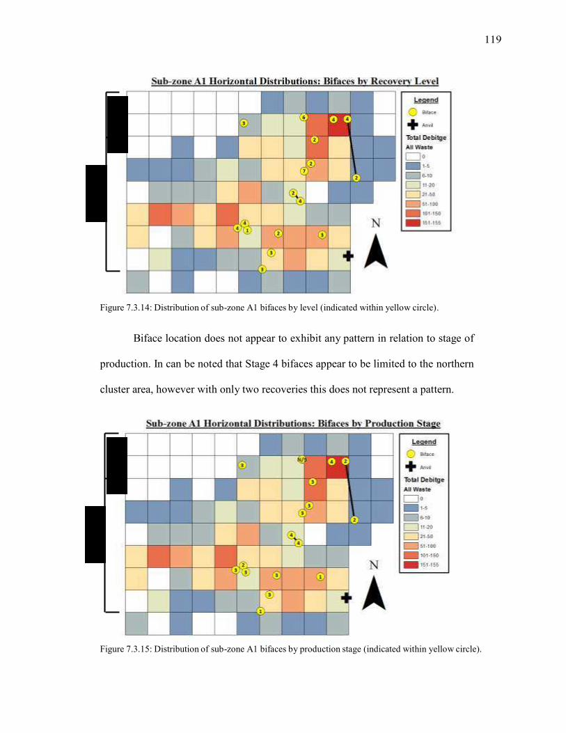
119

1m

1

m

4m

4

m

Figure 7.3.14: Distribution of sub-zone A1 bifaces by level (indicated within yellow circle).

Biface location does not appear to exhibit any pattern in relation to stage of

production. In can be noted that Stage 4 bifaces appear to be limited to the northern

cluster area, however with only two recoveries this does not represent a pattern.

Figure 7.3.15: Distribution of sub-zone A1 bifaces by production stage (indicated within yellow circle).

120

Tool Refits

Three tool fragments refit within sub-zone A1. These included one core and two

bifaces (see Figure 7.3.12). Two of these refits occur within a relatively short distance

from one another, either in the same or adjacent quadrat. The third refit occurs over a

slightly greater distance, but remains within the debitage cluster area.

Vertical separation between refitted artifacts varied. The refit core pieces were

recovered from one level apart (0-10cm vertically), while biface refits were recovered

from three levels apart (10-15cm vertically).

General Tool Distributions

Other tool recoveries from within sub-zone A1 appear to occur at random (see

Figure 7.3.12). This is due largely to the limited number of tools recovered. The anvil

stone located within the southeastern corner of the sub-zone is shared with sub-zone A2

and will be further discussed in section 7.4.7. While the anvil stone from sub-zone A1 is

located near high debitage recoveries within the southern clusters, it does not occur in

direct proximity limiting interpretations of direct association.

7.3.8 A1: NSG Results

The results from NSG do not appear to indicate that any substantial magnetic

anomalies are present within the A1 sub-zone. However, a slightly higher magnetic

reading does occur within the upper northeast corner of the sub-zone, in the general

vicinity of highest artifact clustering (Figure 7.3.16).

121

1m

5m

Figure 7.3.16: NSG results in relation to sub-zone A1.

7.4 Sub-Zone: A2

Sub-zone A2 consisted of a tightly clustered concentration of lithic debris in the

northeastern portion of the site (Figure 7.4.1). This sub-zones contained cluster 4 and

covered 94 50 x 50cm quadrats, overlapping along its western side with sub-zone A1.

122

1m

4m

Figure 7.4.1: Sub-zone in relation to topography with a close up of sub-zone A2 illustrating all tool

recoveries with total debitage by quad.

7.4.1 A2: Artifact Recoveries

A total of 6,446 artifacts were recovered from sub-zone A2. This included 30

tools (frequency = 33) consisting of ten cores, seven bifaces, six retouched flakes, two

blade flakes, one spokeshave, one uniface, and one undetermined tool (possible biface

fragment)(Table 7.4.1).

Many of the recovered tools did not exhibit a clear function. Retouched flakes

within sub-zone A2 consisted of three incidental retouched tools and three intentionally

retouched tools. As previously discussed, the artifact identified as a �✁✂✄☎esha✆✝✞ may

123

A2: DEBITAGE TYPE

PRIMARY 58

SECONDARY 4337

TERTIARY 1023

UNDETERMINED 553

SHATTER 407

have also taken this form unintentionally. Meanwhile, cores and bifaces were further

broken down into core cortex type (Table 7.4.2) and biface stage (Table 7.4.3).

A total of 6,378 lithic waste pieces were recorded for sub-zone A2. A breakdown

of their type, size, and material type can be seen in Tables 7.4.4, 7.4.5, and 7.4.6,

respectively.

Table 7.4.1: All tool recoveries from sub-

zone A2

A2: TOOLS

TYPE Frequency

ANVIL 2

CORES 10 (11)

BIFACE 7

RETOUCHED

FLAKES

6 (7)

BLADE FLAKES 2

SPOKESHAVE 1 (2)

UNIFACE 1

UNDETERMINED 1

Table 7.4.3: Result of biface staging for sub-

zone A2 following Bennett (2015)

Table 7.4.2: Results of cortex identification

for sub-zone A2.

A2: CORES

CORTEX Frequency

N/A 7 (8)

COBBLE 2

TABULAR 1

Table 7.4.4: Debitage frequencies by type

A2: BIFACES

STAGE Frequency

N/S 0

1 1

2 1

3 4

4 1

5 0

6 0

124

A2: DEBITAGE MATERIAL

TACONITE 6237

GFS 98

CHERT 13

SILTSTONE 10

QUARTZ 4

OTHER 16

To

tal R

eco

ve

red

Art

ifa

cts

Table 7.4.5: Debitage frequencies by material Table 7.4.6: Debitage frequencies by size grades

A2: DEBITAGE

SIZE Frequency

0-2MM 17

2-6MM 1605

6-12MM 2881

12-25MM 1571

25-50MM 290

50+MM 14

7.4.2 A2: Vertical Distribution

The vertical distribution of artifacts in sub-zone A2 peak in level 3, with the

balance of recoveries being from level 2 to 5 (Figure 7.4.2). This general trend is

observed for all artifact size grades (Figure 7.4.3)

2000

1800

1600

1400

1200

1000

800

600

400

200

0

Sub-Zone 'A2' - Vertical Distribution of All Artifacts

Excavation Level

Figure 7.4.2: Total artifact recoveries by level indicating highest artifact clustering around level 3.

125

To

tal R

eco

ve

red

Art

ifa

cts

900

800

700

600

500

400

300

200

100

0

Sub-Zone 'A2' - Vertical Distribution by Artifact Size

Excavation Level

0-2mm 2-6mm 6-12mm 12-25mm 25-50mm 50+mm

Figure 7.4.3: Total artifact recoveries by size and level.

7.4.3 A2: Horizontal Distribution: General

The results of statistical analysis indicate that there is significant artifact

clustering within sub-zone A2. Both nearest neighbour (conducted on all artifacts) and

Getis-Ord Gi (conducted on debitage) indicate that there is a less than 1% chance that the

observed artifact distribution is the result of random chance (Figures 7.4.4 and 7.4.5).

This is supported by the results from Ripley�✁ ✂ function (Figure 7.4.6).

126




127



7.4.4 A2: Horizontal Distribution: Recoveries by Level

Artifact distributions by level indicate a high degree of clustering located within

the central area of the sub-zone (Figure 7.4.7). As excavation levels progress, the densest

artifact concentrations transition from the upper right of the cluster area, towards the

bottom left. Re-assessing original field excavation notes suggest that some differences in

the amount of organic overburden may be responsible for changes in level designation of

artifacts, as different excavators/ excavation floors resulted in varying placements of

datum strings. This could result in some variations as to when artifacts would have been

encountered. Overall, greatest artifact concentrations occur within levels 2-4.

128

7.4.5 A2: Horizontal Distribution: Recoveries by Material Type

Materials recovered from sub-zone A2 included taconite, gunflint silica, siltstone,

chert, quartz, mudstone, and amethyst (Figure 7.4.8 A-G). In sub-zone A2, the use of

siltstone, chert, quartz, and amethyst appears to have been extremely limited. While most

of these recoveries appear to come from within the area of artifact clustering, chert

debitage generally occurred towards the north of the sub-zone.

Taconite recoveries were the most prominent within sub-zone A2, and cluster

strongly within the centre. The highest proportion of taconite artifacts were recovered in

the northeast of this central cluster. Meanwhile, gunflint silica recoveries occur along the

northern portion of the high density cluster zone.

A2: Horizontal Distribution of Artifacts by Level

129

Legend

0

� B1face

Retouched Flake

leve l1

C

gJo

\-5 06-tO

011-20

[:=J 2 \ -50

DS\-too

g101·200

- 20\ -205

_(j

1 .&

A U

..

Sub-zone A2 Horizontal Distributions- Levell

N

A ... Core Fragment

Sub-zone A2 Horizontal Distributions- Level 3

N Legend

0 B1face

.A RetouChed Flake

A mface

Sub-zoneA2 Getis-Ord Gi - Levell Recoveries

N

Leve t 1

GiZScore

- < -258StdDev

- -258 ...t 96 -- t65StdDev

c=J -1.66 - t 65Std.OeY

. 1 65 - 196Std Oev

..196 - 258Std 0ev

->258Std Dev

Sub-zone A2 Getis-Ord Gi -Level 2 Recoveries

N

Level 2

GiZScore

Level 2

CJo

\-5

c:J6-t0

C]11-20

C]2 t -5<J

DS\ -too

Ot ot -200

- 201-500

- 50\ -639

130

A -- � 0

,_,

Sub-zone A2 Horizontal Distributions- Leve1 3

N Legend

Core Fragment

A Retouched Fl ake

Undetermined Tool

level 3

Sub-zoneA2 Getis-Ord Gi - Leve1 3 Recoveries

N

Level 3

OiZScore

- -258

-=c.o C

gJo

\-5 c=J -1.66- 1 65Std.OeY

06-tO

011-20

[:=J 2 \ -50

DS\-t oo

g101-200

- 20\ -354

. 165 - 196Std Oev

..0.

Sub-Zone A2 Horizontal Distributions - Leve14

legend

Q lace

✁ COre Fragment

A RetoocnedRake

A BladeFiake

+ An" level 4

CJo


N

Level4

GIZScore

- < -258StdDev

. .2.58 - -1 96Std0ev

. . t 96 --1 65StdDev

c=J -Ul5- 1 65 Stcl_ OeY

165 - 196Std Dev

. 196 - 258Std Dev

- >258Std Dev

0 6-

10

0 11-20 c:J zt.al

- 51-100

- 101-193

131

Legend

0� Biface

Level 5

D o

r:::J 1-5

Ds-1o

D 11-20

D 21-50

051-100

- 101-200

- 201-372

0

Legend

Leve16

Do

u 1-5

Ds-10

D 11-20

c::J 21-50

- 51-77

A ...


N

Core Fragment

Retouched Flake

Sub-zoneA2 Getis-Ord Gi - LevelS Recoveries

N

Level 5

OiZScore

- < -258StdDev

- -258 . .1 96- -165StdDev

c=J -1.66-165Std.OeY

. 165 - 196Std Oev

. 196 - 258Std 0ev

- >258Std Dev


N

A

✁


N

Level 6

GIZScore

- < -258StdDev

. .2.58 - -1 96Std0ev

. . 1 96 --1 65StdDev

c=J -Ul5- 1 65 Stcl_ OeY

165 - 196Std Dev

. 196 - 258Std Dev

- >258Std Dev

132

N

A

£;,.

Legend

Level9

C_]o

01-5

- 6-8

011·20

Sub-Zone A2 Hol"izon tal Distributions - Level 7

Legend

A Bladeflake

level 7

CJo o,.. 06-10

1 21-50 - 01-72

Sub-zoneA2 Getis-Ord Gi - Leve1 7 Recoveries

N

Level7

OiZScore

- < -258StdDev

- -258 - -196 - -165StdDev

c=J -1.66 - 1 65Std.OeY

. 165 - 196Std Oev

. 196 - 258Std0ev

- >258Std Dev


N

A


N

Level9

GiZScore

- < -2.58Std0ev

- -2.58 --196Std 0ev

-- 196 --1 65Std

Dev [=:J -L65 � 1 65

Std.Oev. c::J 1 65 - I

96Std Oev

- 1 96 - 2 58Sid Oev

- > 2.58Std 0ev

133

A -1

Sub-zoneA2 Horizontal Distributions- LevellO

N Legend

.A, Spokeshave

Level 10

Do - 1-2

Sub-zone A2 Horizon tal Distributions - Level 11

N Legend

Level11

Do

=-=El

Sub-zone A2 Getis-Ord Gi - LevellO Recoveries

N Legend

Level 10

GiZScore

- < -2_58Std Dev

- -258 - -196Std v

-- 1 96 --1 65Std Dev

c=J -1.65 - 1 65 Std.Dev.

. 165 - 196Sid Dev

- 1 96 - 258Sid Dev

- :. 2.58 StdDev

Sub-zoneA2 Getis-Ord Gi - Levelll Recoveries

Legend

Level 11

GiZScore

- < -2.58Std Dev

- -2.58 --196Std Dev

-- 1 96 --1 65Std

Dev [=:J -L65 � 1 65

Std.Dev. c::J 1 65 - I

96Std Oev

- 1 96 - 2 58Sid Dev

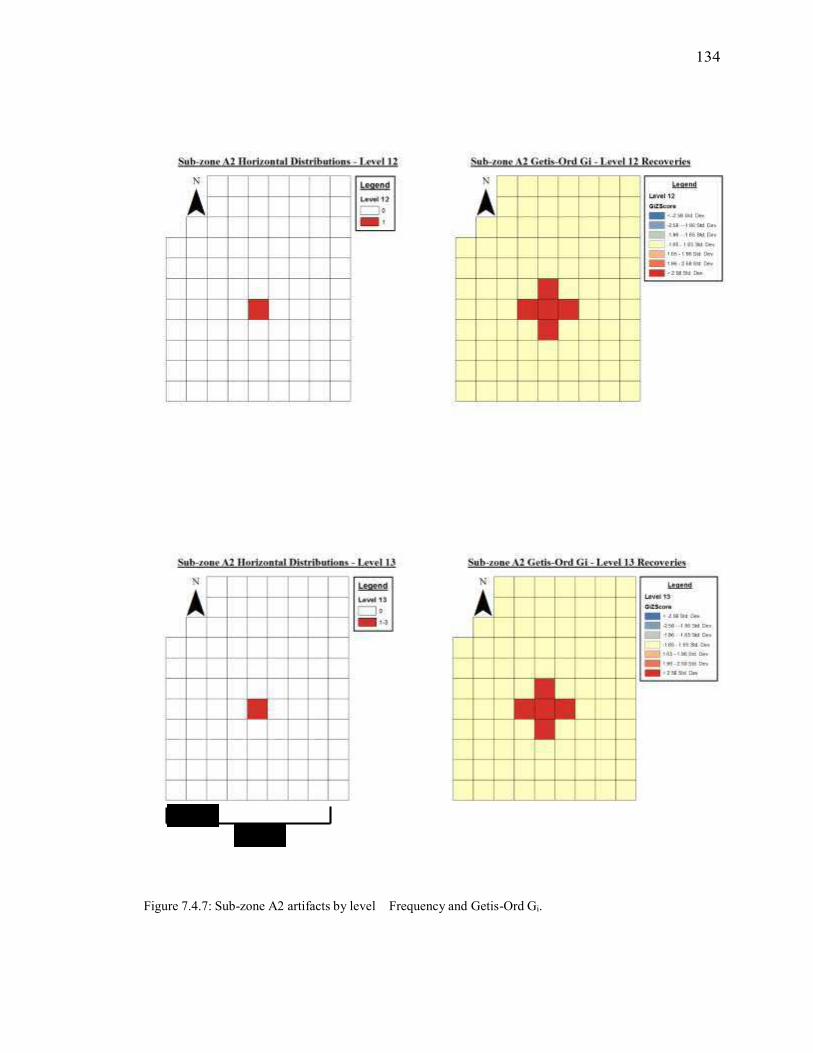
134

1m

4m

Figure 7.4.7: Sub-zone A2 artifacts by level � Frequency and Getis-Ord Gi.

135

A2: Artifact Distributions by Material

A

B

136

C

D

137

E

F

138

G

1m

4m

Figure 7.4.8: Sub-zone A2 artifact distributions by material type. A) Taconite, B) Gunflint Silica, C)

Siltstone, D) Chert, E) Quartz, F) Mudstone, and G) Amethyst.

7.4.6 A2: Horizontal Distribution: Debitage

Initial observations of all mapped debitage by quadrat frequency reveals a circular

shaped lithic distribution with a relatively low frequency zone in the centre (Figure

7.4.9). This observed patterning was further explored by segmenting the sub-zone and

plotting the concentrations of artifacts per quadrat (Figures 7.4.10). This cross section

analysis further supported the observed ring-shaped distribution. It should be noted,

however, that high artifact frequencies do not form a full circle, as the lower right side

appears to exhibit a lower recovery frequency. In order to better illustrate this, a kernel

density contour map was generated using artifact frequencies (Figure 7.4.11). This shows

areas of highest recovery (e.g. hot-spots identified through Getis-Ord Gi), with the

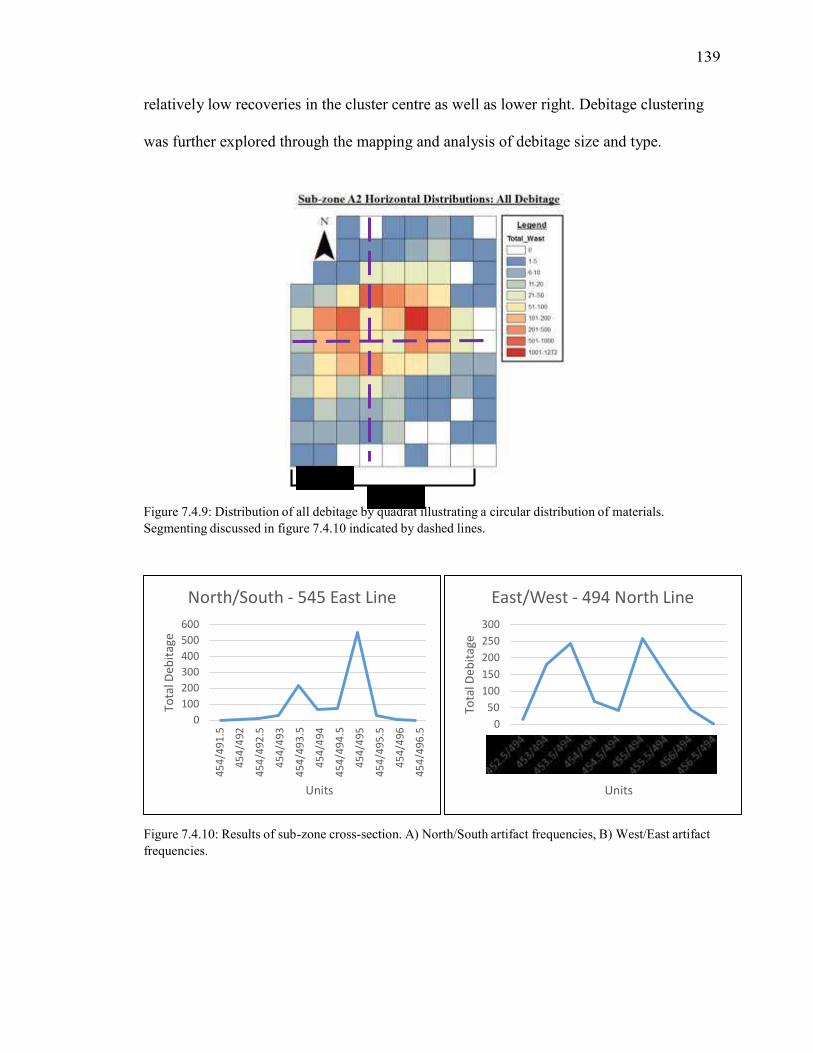
139

To

tal D

eb

ita

ge

45

4/4

91

.5

45

4/4

92

45

4/4

92

.5

45

4/4

93

45

4/4

93

.5

45

4/4

94

45

4/4

94

.5

45

4/4

95

45

4/4

95

.5

45

4/4

96

45

4/4

96

.5

To

tal D

eb

ita

ge

relatively low recoveries in the cluster centre as well as lower right. Debitage clustering

was further explored through the mapping and analysis of debitage size and type.

1m

4m Figure 7.4.9: Distribution of all debitage by quadrat illustrating a circular distribution of materials.

Segmenting discussed in figure 7.4.10 indicated by dashed lines.

North/South - 545 East Line

600

500

400

300

200

100

0

East/West - 494 North Line

300

250

200

150

100

50

0

Units Units

Figure 7.4.10: Results of sub-zone cross-section. A) North/South artifact frequencies, B) West/East artifact

frequencies.

140

1m

4m

Figure 7.4.11: Kernel density of sub-zone A2 artifact distributions.

Debitage Size

The distribution of debitage by size can be seen in Figure 7.4.12. Overall,

debitage distributions by size cluster within the high recovery zones previously identified.

There is some distinction between primary clustering within this zone, as there appears to

be a split between the west and east cluster areas. In the left side of the cluster, there is a

tendency for higher clustering of very small debitage (0-2mm and 2-6mm) and very large

debitage (50+mm). Meanwhile, mid-range debitage size categories (6-12mm, 12-25mm,

and 25-50mm) appear to occur in higher frequencies towards the eastern cluster area. It

can also be observed that debitage clustering in the west is closely related to the location

of recovered anvil stones.

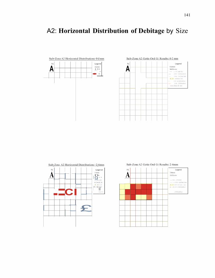
141

N

A Legend

0-2mm

GI Z Se:ore

- c-2 std 0ev

- -258··1G6StoDe'4

- -106··165Std Dell

D -- t60std DeY

- 1 65 -t Q6StdOev

- 1 06 - 258Std0ev

-zse sw oev

A ....

A

l tot-200

A

A2: Horizontal Distribution of Debitage by Size

Su b-Zone A2 Horizontal Distri butions·0 -2 mm

N Legend

0-2mm

�✁ ✂·✂

-

Su b-Zone A2 Getis-Ord Gi Results: 0-2 mm

Sub- Zone A2 Horizon tal Distributions·2-6mm Sub-Zone A2 Getis-Ord Gi Results: 2-6mm

N Legend N

2-8mm

D✄ l g·· 1::)6-tO

Otl -20

Legend

2-6mm

GIZScore

-58--196$10

--Ul6--1.65Std De¥

-=CI

021-¢0

l::]st-too

D -t65-16:isto oev

[:l t 65 - 106Std0ev

- 201-270 ,.258SidDev

£

142

N

A

-

-

N

·C-J o

Ost -too - 101-200

- 201-309

A

f--

,

..... 01

-· A

Sub-Zone A 2 Horizontal Distributions· 6-12mm Su b-Zone A2 Getis-Ord Gi Results:6-12mm

Legend N

6-12mm

CJ o

C]&-10

CJ t t-20

021-60

CJ st -too C) tot-200

201-&10

501--6611

Legend

6 12mm

GZI Score

- < -2.58std_De'l

- -258 --19&510 DeY

- -1.96 - -165Std0ell

D - -16:isto oev

- 1 65 - 106Std0ev

- 11Mi- 258Stdoev

..258SIOC>ev

Sub-Zone A2 Horizon tal Distributions: 1 2-25mm Sub-Zone A2 Getis-01·d Gi Results: 12-25mm

Legend N

12-25mm

A 06-10

Ott-20

021-60

Legend

12-25mm

GIZScore

- < -2.58StODev

- -2 58- -196510 Dell

- -106 - -165Std0eY

o --- Sid[)ey - 1 65 - 106SUI0ev

- 11Mi - 258Sid0ev

- ,2sesrooev

143

1m

4m

Figure 7.4.12: Distributions of sub-zone A2 debitage by size.

144

Debitage Type

Similar to debitage size, the distribution of debitage by type exhibits a split

distribution within the primary cluster area. Primary, secondary, and undetermined flakes

exhibit a stronger distribution within the eastern portion of the cluster, while tertiary

flakes and shatter are predominantly located within the west (Figure 7.4.13). This pattern

is also observed when comparing concentrations of debitage vs. microdebitage (Figure

7.4.14). Again, the location of anvil stones appears to occur in relation to western

debitage clustering.

A2: Horizontal Distribution of Debitage by Type

145

N

A

N

A Legend

Secondary

GZI Score

- < -2.58StdDev

- -2 58- -196510 Dell

- -106 - -165Std0eY

o --- Sid[)ey - 1 65 - 106 SUI0ev

- 11Mi - 258Sid0ev

- ,2se srooev

C

-J

·o

·-

A

Sub-Zone A2 Hor· izontal Distributions· Prima rv Debita!!e

,.----

Sub-Zone A2 Getis-Ord Gi Results: Pr·imarv Debitage

legend N

Prtmary

Do D�-�

- 6-10

'-------

Legend

Prmi ary

GZI Score

- < -2.58std_ De'l

- -258 - -19&510 DeY

- -1.96 - -165Std0ell

D - -16:isto oev

- 1 65 - 106Std0ev

- 11Mi- 258Stdoev

..258SIOC>ev

Sub-Zone A2 Horizontal Distributions·Secondarv DebI" t✁a!!e Sub-Zone A2 Getis-Or·d Gi Results: Secondary Debitage

N Legend

A Secondary

j=:JG-10

011-20

021-tiO

051-100

r::J101-200

- 201-500

- 501-047

146

1m

4m

Figure 7.4.13: Distribution of sub-zone A2 debitage by type.

147

A2: Horizontal Distribution of Debitage vs.

Microdebitage

1m

4m

Figure 7.4.14: Distribution of sub-zone A2 debitage vs. microdebitage.

148

7.4.7 A2: Horizontal Distribution: Tools

A variety of tools were collected from within sub-zone A2 (Figure 7.4.15). Of the

recovered tools, three main classes stand out: cores, bifaces, and retouched flakes.

1m

4m

Figure 7.4.15: Distribution of all sub-zone A2 tools with total debitage by quadrat. Field photos of anvil stones inset (Photos by S. Hamilton and C. Surette).

Cores

The distribution of cores by cortex type is illustrated in Figure 7.4.16. The

distribution by cortex type does not suggest any specific pattern (due to low recovery

numbers), however, general distribution patterns exhibit a correlation between core

149

location and debitage hot-spots. This is particularly apparent near the highest lithic

recovery zone in the eastern portion of the cluster. It can also be observed that core

recoveries are limited to the periphery of these lithic recovery zones.

1m

4m

Figure 7.4.16: Distribution of sub-zone A2 cores by cortex type.

Bifaces

Biface distributions in sub-zone A2 follow a similar pattern to cores, being

limited to areas outside high debitage concentrations (Figure 7.4.17). Bifaces located

closer towards the centres of these high debitage areas are also of earlier production

stages, representing either blanks or roughly edged pieces.

150

A

B

1m

4m

Figure 7.4.17: Distribution of sub-zone A2 bifaces by level (A) and stage (B) � Level and stage indicated

by numbers within yellow circles.

151

Retouched Flakes

Retouched flakes were mapped by their designation of either intentional or

incidental in order to see if there was a patterned distribution (Figure 7.4.18). No clear

pattern could be detected, however, and the overall distribution of artifacts followed a

similar pattern to that observed for cores and bifaces. The distribution of retouched flakes

appears to be limited to the periphery of the debitage cluster.

1m

4m

Figure 7.4.18: Distribution of sub-zone A2 retouched flakes by intentional or incidental flaking.

Tool Refits

One artifact refit was recovered from sub-zone A2 (see Figure 7.4.15). This

consisted of a blade flake that refit to its original core. As this refit represents a tool item

detached from a core, the observed distance (~2m) could be the result of transport for use

during site occupation.

152

1m

4m

General Tool Distribution

The distribution of all recovered tools can be seen in Figure 7.4.15. In general,

tool clustering appears to occur in correlation with observed debitage distributions. Of

interest in this distribution is the continued pattern of limited tool recoveries from within

the centre of debitage clustering. As well, there is a strong association with recovered

anvil stones and high density debitage recoveries.

7.4.8 A2: NSG Results

The results of the NSG survey indicate an area of high magnetic anomalies within

the centre of artifact clustering (Figure 7.4.19). When compared with kernel density

results, the areas of highest readings occurs roughly within the central cluster area of low

artifact recovery, while the lowest readings are associated with high artifact concentration

zones (see Figure 7.4.11). The implications of this association will be discussed further in

Chapter 8.

Figure 7.4.19: NSG results for sub-zone A2. High magnetic anomalies can be seen in correlation with voids in artifact concentrations and high recovery frequencies.

153

7.5 Sub-Zone: B1

Sub-zone B1 consisted of a relatively small lithic cluster within 36 50 x 50cm

quadrats (Figure 7.5.1). It is located near the centre of the site excavation area, just below

the 238 metres above sea level (masl) topographic line. The southern portion of this area

overlaps with sub-zone B2. It was noted within excavation notes that the quadrat of

highest artifact recoveries within this sub-zone (452N/488E NW) was between two units

with tree stumps.

Figure 7.5.1: Sub-zone in relation to topography with a close up of sub-zone B1 illustrating all tool


7.5.1 B1: Artifact Recoveries

Sub-zone B1 yielded 251 artifacts, including eight tools. Tool recoveries included

one core, five bifaces, one retouched flake, and one scraper (Table 7.5.1). Debitage

recoveries consisted of 222 pieces, which were further analyzed by size, type, and

material (Figures 7.5.2-7.2.4). Other artifact recoveries included 20 fragments of charcoal

154

B1: DEBITAGE

SIZE Frequency

0-2MM 0

2-6MM 12

6-12MM 64

12-25MM 100

25-50MM 43

50+MM 3

B1: DEBITAGE

MATERIAL

TYPE Frequency

TACONITE 217

GFS 5

(shared with sub-zone B2), and one faunal item recovered from level 2 (5-10cm below

surface).

Table 7.5.1: Sub-zone B1 tool recoveries Table 7.5.2: Debitage frequencies by size.

B1: TOOLS

TYPE Frequency

CORE 1

BIFACE 5

RETOUCHED

FLAKE

1

SCRAPER 1

Table 7.5.3: Debitage frequencies by type. Table 7.5.4: Debitage frequencies by material.

B1: DEBITAGE

TYPE Frequency

PRIMARY 5

SECONDARY 195

TERTIARY 0

UNDETERMINED 11

SHATTER 11

7.5.2 B1: Vertical Distribution

Vertical artifact distributions illustrate that artifact recoveries occur primarily in

Level 4, with few recoveries occurring above and below this depth (Figure 7.5.2).

Assessing this distribution by artifact size reveals a similar pattern (Figure 7.5.3). This

distribution differs from other sub-zones where primary recovery zones occur within the

Level 3 range. Excavation notes for units 489N/452E and 488N452E indicate the

155

To

tal R

eco

ve

red

Art

ifa

cts

To

tal R

eco

ve

red

Art

ifa

cts

presence of tree stumps along either side of the high artifact recovery zones. These tree

stumps could explain the differences observed in average artifact recovery levels.

120

Sub-Zone 'B1' - Vertical Distribution of All Artifacts

100

80

60

40

20

0

Surface Level 1 Level 2 Level 3 Level 4 Level 5 Level 6 Level 7 Level 8 Level 9 Level 10Level 11

Excavation Level

Figure 7.5.2: Total artifact recoveries by level for sub-zone B1.

Sub-Zone 'B1' - Vertical Distribution by Artifact Size

40

35

30

25

20

15

10

5

0

Surface Level 1 Level 2 Level 3 Level 4 Level 5 Level 6 Level 7 Level 8 Level 9 Level 10 Level 11

Excavation Level

0-2mm 2-6mm 6-12mm 12-25mm 25-50mm 50+mm

Figure 7.5.3: Total artifact recoveries by size and level.

156

7.5.3 B1: Horizontal Distribution: General

The results of statistical analysis for artifact clustering indicate that the

distribution in sub-zone B1 is not the result of random chance (Figures 7.5.4-7.5.6). Both

nearest neighbour and Getis-Ord Gi indicate that there is a less than 1% likelihood that

the observed artifact distribution is random.



157




158

7.5.4 B1: Horizontal Distribution: Recoveries by Level

The distribution of artifacts by level indicate that artifact recoveries occur

primarily in one central location with little variation (Figure 7.5.7).

7.5.5 B1: Horizontal Distribution: Recoveries by Material Type

Only two different material types were collected from sub-zone B1: taconite and

gunflint silica. Taconite was the most common, being concentrated within the middle of

the sub-zone (Figure 7.5.8 A). Lesser amounts were recovered along the southern

portions of the sub-zone where it borders with sub-zone B2. Gunflint silica recoveries

were extremely limited, and appear to be distributed randomly (Figure 7.5.8 B).

7.5.6 B1: Horizontal Distribution: Debitage

The distributions of debitage by both size (Figure 7.5.9) and type (Figure 7.5.10)

follow a similar pattern of distribution concentrated within the centre of the sub-zone. All

recoveries are highly clustered within the northwest quadrant of unit 488N/452E.

7.5.7 B1: Horizontal Distribution: Tools

Tools recoveries from sub-zone B1 occur generally within the area of high

debitage recovery in the sub-zone centre (Figure 7.5.11). However, two bifaces and one

scraper occur along the periphery of this cluster in areas of little to no debitage recovery.

It is not possible to make inferences regarding biface distributions by stage due to limited

recoveries (Figure 7.5.12).

15

9

B1: Horizontal Distribution of Artifacts by Level

-

-

-

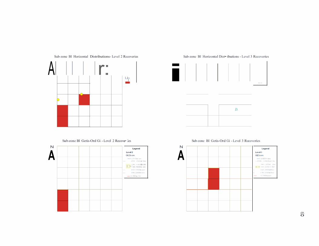
A A

Sub-zone Bl Horizontal Distributions- Level 2 Recoveries Sub-zone Bl Horizontal Dist�·ibutions - Level 3 Recoveries

AI I I I l r:.

L-J·o

il l l l l l l 11-21

D.

Sub-zone Bl Getis-Ord Gi - Level 2 Recov✁✂✄☎es

N

Legend

Sub-zone Bl Getis-Ord Gi - Level 3 Recoveries

N

Legend

Level 2

GIZScore

-< -2.58 Sta oev

- -258··196Std Dev

-1 96 --1 65 sta oev

D-1 65-165Sta oev

- 1 65-196Sta.oev

- 1 96·258SICIOev

-> 2.58Sta Oev

Level 3

GIZScore

-< -2-58 51<1 Dev

--258··196Std Dev

·196 ✆·165 Sid Dev

D·165-165St<l De\'

- 1 65·196StdDev

- 1 96-258St(l0ev

- >2.58Staoev

0\ 0

A �

A

Sub-zone Bl Ho1·izontal DistJ·ibutions - Level 4 Recoveries

AI I I I I I I - !51-87

Sub-zone Bl Horizon tal Distributions - Level 5 Recovel'ies

N Legend

* cnarcoat

_ Bltace

✁ COI'e Fragment

Level 5

LJ o LJ 1-5 06-tO

c::J tt -20

- 21-24

0

Sub-zone Bl Getis-01·d Gi - Level 4 Recoveries

N

legend

Su b-zone Bl Getis-Ord Gi - Level 5 Recoveries

N

Legend

GIZScore

- < -2-58 Std Dev

--258--196510 Dev

- -196·-165510 DeY

D ·165-165 Sta Dev

t:::] t 65- t96Sto oev

- 196·258Sta oev

- > 2_58 Sta

Dev

Level5

GIZScore

- "-2-58 Sid oev --258··t 96sta oev

- -t9 6 1 65Sta oev

D·t65- t 65Sta oev

- 165·t96Sto Dev

- 1 96·258Std.Oev

-> 2.58StO Oev

0--\

-

Sub-zone Bl Ho1·izontal DistJ·ibutions - Level 6 Recoveries

N

A

Su b-zone Bl Horizontal Distributions- Level 7 Recovel'ies

AI I I I I I I t[

Sub-zone Bl Getis-Ord Gi- Level 6 Recoveries

N

Legend

Sub-zone Bl Getis-01·d Gi- Level 7 Recoveries

N

Legend

Level6

GIZScore

- --258 --1 96510 Dev

- ·1 96 � 1 65 Sid DeY

D ·165· 1 65Sta oev

96 -2 58Sta_ oev

- > 2.58 Sta Oev

Level7

GIZScore

f-1-f-1-f----t------1 - "2·.58 Sid Dell

- -2 58··196 Sta oev

- -1 96· 165Sta oev

D·165·1 65 Sta oev

- 1 65·1 96 Sto Dev

- 1 96·258 Std.Dev

-> 2.58StO Oev

0\ N

AI I I I I I I AI I I I I I -·-·

A A

Sub-zone Bl Horizontal Distributions - Level 8 Recoveries Su b-zone Bl Horizon tal Distributions - Level 9 Recovel'ies

Legend

Q Stlace

LevelS

CJo FI ·-

Sub-zone Bl Getis-Ord Gi- Level 8 Recoveries

N

Legend

Sub-zone Bl Getis-O�·d Gi- Level 9 Recoveries

N

Legend

Level8

GIZScore

-< -2.58 Sta Dev.

- -258 --196Stcl Dev

--1 96 -·165510 Dev

0-1 65 - 165 Sid Oev

E:] 165 - 196St<l Oev

- 196·2 58StCIOeY

- > 2.58 Sta Oev

Level9

GIZScore

- "-2.58 Sid oev - -258--1 96810 Dev

--1 96 - -1 65810 Dev

D -165-1 65 Sia oev

- 1 65-1 96 Sto Dev

- 1 96-258 Std.Oev

-> 2.58StO Oev

0-w

\

-

A A

Sub-zone Bl Hol'izontal Distributions - Levelll Recoveries Sub-zone Bl Horizontal Distributions- LevellO Recoveries

N N

A A

Sub-zone Bl Getis-Ord Gi - Levelll �✁✂✄☎✁✆✝✞✁✟

N

Legend

Sub-zone Bl Getis-Ord Gi- LevellO Recoveries

N

Legend

Level11

GIZScore

-< -2-58 Sid Dell_

- -258 --19651<1 DeY

-196--165 Sid DeY

D -165·1 65Std Dev

- 165 -196Sta Dev

- 196-258Stcl Oev

-> 2.58Sto Dev

I tm I I 3m

Figure 7.5.7: Distribution of sub-zone Bl artifacts by level. This shows that locations of high frequency artifact

recoveries remains constant.

Level10

GiZScore

- < -2.58Std 0ell

- -258--196Sta oev

-t96--165Std Oev

D -165- 1 65SUI Dell

- 165-196Std Oev

- 196-258Std Oev

-> 2.58 Sid Dev

165

B1: Horizontal Distribution of Artifacts by Material

A B

1m

3m

Figure 7.5.8: Distribution of sub-zone B1 artifacts by material. A) Taconite, and B) Gunflint silica.

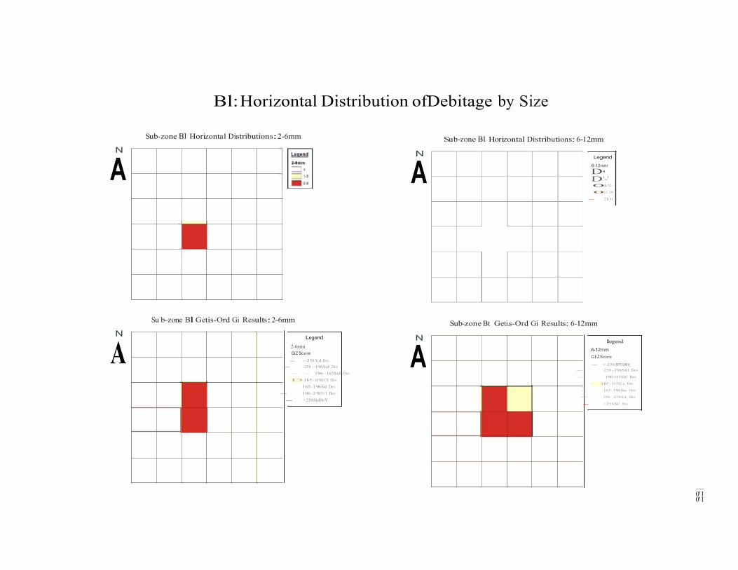
A A

A

Bl: Horizontal Distribution ofDebitage by Size

Sub-zone Bl Horizontal Distributions:2-6mm

N

Sub-zone Bl Horizontal Distributions: 6-12mm

N Legend

6-12mm

D�

D'-' 0&-10

011·20

- 21-51

Su b-zone Bl Getis-Ord Gi Results:2-6mm

N

A 2-6mm

Legend

Sub-zone Bt Geti.s-Ord Gi Results: 6-12mm

N

legend

GiZ Score

- < -2 58 S.d.Oev.

- -258 --196Sid Dev

- - 196 --165Sid Dev

D-165 - 165SI:CS Dev

- 165-196 Sid Dev

- 196- 25851<1 Dev

- >258Std0eY

6-12mm

GI Z Score

- < -2 58 sm.oev_ - -258--196Sl(l Dev

- -196·165Sl(l Dev

· 165-165SI:a Dev

- 165 - 196Sto Oev

- 196 - 258Sto Oev

- >258Sk1 Dev

......... 0'1 0'1

-51

-

A A

Sub-zone Bl Horizontal Distl'ibutions: 12-25mm

N legend

12-25mm

D�,_, 06-10

O tt-:zo

21

Su b-zone Bl Ho1·izontal Distl'ibutions: 25-50mm

N Legend

25-SOmm

D✁ 01-5 06-tO

O t t-20

- 21-26

Sub-zone Bl Getis-01·d Gi Results:12-25mm

N

Legend

-2 Std. Dev.

Sub-zone Bl Getis-Ord Gi Results: 25-50mm

N

A

Legend

GIZ Score

-<

-58--1 96Std DeY

-- 1 96 --1 65Std Oe'l

CJ -t 65 - 165StCI Dev

- 165- 1 96Std0ev

- 1 96-2.56 Std Dev

- >258SI00eY

25-50mm

GIZScore

- <-258StCI.Dev.

- -258--196Std DeY

--196--165Std DeY

CJ -t65-165 StCI Dev

- 165-1 96Std Oev

- t96-2.56Std Oev

- >258Sto oev

0\ ---l

A

Sub-zone Bl Horizontal Distributions: SO+mm

N

A

Sub-zone Bl Getis-01·d Gi Results: SO+mm

N

Legend

50+mm

GIZ Score

-2.58 Sill- Oev_

-<

- .,258 - -196Sfd Oev

- -1 96 - -165Std Dev

D-1 65 - 165Std Dev

1.65 - 1 9651<! Oev

- 1 96 - 2.58St<l Oev

-> 2 58 Sid. Dev

I lm I I 3m

Figure 7.5.9: Distribution of subzone Bl debitage by size grade.

........ 0\ 00

A A

Bl: Horizontal Distribution ofDebitage by Size

Sub-zone Bl Getis-Or·d Gi Results: Shatter·

N

Leaend

Sub-zone Bl Getis-Ord Gi Results: Pr·ima ry Debitage

N Leaend

Sha tter

GiZScore

- < -2 58 Stet Dev_

Pr mary

GIZ Score

- < -258StllDeV

- -258--196Sl<J Oev - .,258--196Std Oev

- -1 96 --165Std Oev - -196--165 Sl<J Dev

0-1 65 - 16551:0 Dev

165 - 19651<1 Dev

- 196- 25851<1 Dev

- >256Std0eY

Sub-zone Bl Hor izon tal Distr·ibu tions: Sha tter

N

O-t65-165Sla Dev

- 165 - 19681<1 Dev

- 196-2_58 81<1 Dev

- >258SI00ev

Sub-zone Bl Ho·r izon tal Distributions: Primary Debitage

N

A f-t- A f----+---f----+---f--------+-----

......... 0'1 \0

-

-

-

I I I I I I

--1 A

N

A

Sub-zone B1 Getis-01·d Gi Results: Seconda1y Debitage

N Legend

Secondary

GI Z Score

- < 2585t<IDeY

- 58-·1G6Sid Oev

165-196810 Oev

Sub-zone Bl Getis-0 1·d Gi Results:Secondan' Debitage

Leaend

Undetermined

GIZSeore

- <-258sta oev

--2SB··196Std

oev

-- 1Q6 --166Sid Oev

D-165-165Sia Oev

·1 Q6-·165Sid DeY

0·1 65·16551:!1 oev

G6-258SICI 0ev

- >258Sid0e'l

Sub-zone Bl Hol"izontal Dish·ibutions: SecondaJ"V Debitage

165·196510 ()ell

19G 258Skl Oev

- >2511Sta De¥

Sub-zone Bl H01·izontal Distl"ibutions: U ndete� mined Debitage

AI I r l I I I i" AI I§?._.·

I lm I I 3m

Figure 7.5.10: Distribution sub-zone Bl debitage by type.

......... -..)

0

171

1m

3m

Figure 7.5.11: Distribution of sub-zone B1 tools with total debitage by quad.

1m

3m

Figure 7.5.12: Sub-zone B1 biface distributions by stage.

172

7.5.8 B1: NSG Results

NSG results do not appear to indicate any substantial anomalies within sub-Zone

B1 (Figure 7.5.13). However, a slightly higher reading does occur within the lower mid-

section of the sub-zone.

1m

3m

Figure 7.5.13: NSG results for sub-zone B1.

173

7.6 Sub-Zone: B2

Sub-Zone B2 covered the largest lithic cluster within the southern portion of the

RLF site. This sub-zone consisted of 96 50 x 50cm quadrats within a crescent shaped

distribution (Figure 7.6.1).

1m

3m




A total of 5,461 artifacts were recovered from sub-zone B2. This included 63

tools (frequency = 67). A breakdown of tools by type can be seen in Table 7.6.1. Tool

recoveries were further analysed by core cortex type (Table 7.6.2), biface stage (Table

7.6.3), and retouched flake type (Table 7.6.4).

Debitage recoveries consist of 5,315 total pieces. These were further broken down

by material, type, and size (Tables 7.6.5 � 7.6.7 respectively). Other recoveries included

FCR (n = 52), charcoal (n = 20), and miscellaneous items (n = 7).

174

B2: BIFACE

STAGE Frequency

N/S 0

1 1 (2)

2 8

3 5

4 0

5 1

6 1

Table 7.6.1: Sub-zone B2 tool recoveries by type.

Note: Bracketed number represents total without refitted artifacts

B2: TOOLS

TYPE Frequency

CORE 17

BIFACE 14 (15)

ADZE 1

DRILL 1

ANVIL 2

GRAVER/PERFORATOR 1

GRINDING STONE 1

HAMMERSTONE 2

RETOUCHED FLAKE 16 (17)

BLADE FLAKE 2

SCRAPER 4 (5)

UNIFACE 2 (3)

Table 7.6.2: Sub-zone B2 core frequencies

by cortex type.

Table 7.6.3: Sub-zone B2 biface frequencies by

stage following Bennett (2015). Note: this includes

adze and drill recoveries.

B2: CORES

CORTEX Frequency

N/A 10

COBBLE 4

TABULAR 3

175

B2: DEBITAGE

MATERIAL Frequency

TACONITE 4583

GFS 701

SILTSTONE 9

CHERT 4

QUARTZ 5

AMETHYST 2

OTHER 11

B2: DEBITAGE

SIZE Frequency

0-2MM 0

2-6MM 1026

6-12MM 2452

12-25MM 1384

25-50MM 427

50+MM 26

Table 7.6.4: Breakdown of sub-zone B2 retouched flakes

by either incidental or intentional flaking.

Table 7.6.5: Sub-zone B2 debitage by

material.

B2: RETOUCHED FLAKES

INTENTIONAL 10 (11)

INCIDENTAL 6

Table 7.6.6: Sub-zone B2 debitage by

type.

Table 7.6.7: Sub-zone B2 debitage by size

grade.

B2: DEBITAGE

TYPE Frequency

PRIMARY 112

SECONDARY 3829

TERTIARY 165

UNDETERMINED 835

SHATTER 374


The vertical distribution of artifacts from sub-zone B2 exhibit highest recovery

frequencies in levels 2, 3, and 4, with peak densities in level 3 (Figure 7.6.2). Exploring

artifact distributions by size produces a similar distribution with the exception of 2-6mm

debitage, which occurs in greatest frequencies around level 2 (Figure 7.6.3).

It was noted that recovery outliers existed within sub-zone data. A single flake

was recovered from excavation level 16 in the Southwest quad of unit 485N/451E.

Further inquiry determined that the flake likely fell into the unit during profile trenching,

176

To

tal R

eco

ve

red

Art

ifa

cts

To

tal R

eco

ve

red

Art

ifa

cts

as there were no other artifact recoveries above or below. As such, this level was

removed from the study of this sub-zone.

2000

1800

1600

1400

1200

1000

800

600

400

200

0

Sub-Zone ' B2' - Vertical Distribution of All Artifacts

(Outlier Removed)

Surface Level 1 Level 2 Level 3 Level 4 Level 5 Level 6 Level 7 Level 8 Level 9

Excavation Level

Figure 7.6.2: Total recoveries by level for sub-zone B2.

900

Sub-Zone ' B2' - Vertical Distribution of Artifacts by Size

800

700

600

500

400

300

200

100

0

Surface Level 1 Level 2 Level 3 Level 4 Level 5 Level 6 Level 7 Level 8 Level 9

Excavation Level

0-2mm 2-6mm 6-12mm 12-25mm 25-50mm 50+mm

Figure 7.6.3: Sub-zone B2 total recoveries by size and level.

177


Statistical clustering tests indicate that the observed artifact distributions are

highly clustered (Figures 7.6.4 - 7.6.6). The results of both nearest neighbour and Getis-

Ord Gi indicate that there is a less than 1% chance that the observed artifact distribution

could be the result of random chance.




178




Artifact recoveries by level in sub-zone B2 indicate that highest artifact recoveries

remain constant over two cluster areas; one in the north and one in the south (Figure

7.6.7). Clustering remains concentrated within these areas until Level 6, where

concentration then tend towards areas of FCR recovery. Recoveries of FCR in sub-zone

B2 come from between Levels 2 and 6, while tool recoveries range from surface

collected materials to Level 8.

179

Legend

Surface

OIZScore

-2SI 186SidO.V

-- 1t0--\66 Sid

llev lliiiiiiiilo -185- I&SS!d

Oh

- 166- IINISIIIO.. ...

- 1116-2S8Sid0n

- "'2S8Sid0ev

N

A

.l.!sJ.!n2

Level1

OIZScore

- <SIStdOev

- -2SI1li8SidO.V

- 1M 165SW 0...

.iliiiiiiiiiiii -t 8S-105Sid lev

- 185 - 1 11111$1110...

- 1118-2S8Sid0n

.. 2S8Sid0ev

A

- 101-200

- 201-600

t

-


.,._l.!ll!!!ll

Sub-zone 82 Horizontal Distributions- Surface Recoveries

e co.�F, D-Sur

·l✁c

·✁

Sub-zone B2 Getis-Ord Gi Results- Surface Recoveries

N

A

=-=-

0&.10

11-20

- 21-27

""' "- .

✂.. Sub-zone B2 Getis-Ord Gi Results- Level I Reco,✄eries

b!ll!!!l! A RlttouthN flike Level1

-8-10

c:::J 11 20

021-50

Os,.,oo

- 501-614

180

Legend

0 .. Level2

.'*' "- - &.10

e c-F,.gme:nt Do

- 101-200

- 201-600

- 501-769

N

A

K

'\. c

�

I>

✁

r:li

..

level2

GIZScore

..-2 !>1Std 0e¥

- 251 186Sid

0.'1

-- 1t8--1 65 5&d

l>e'l

:::::::::::::: -185-18SS1d Oev

- t 86 - 1 11111SII:ICn.

- 1 116 - 258 SII:ICn

N

A

A

Sub-zone 82 Horizontal Distl"ibu tions - Level 2 Recoveries Sub-zone B2 Getis-Ord Gi Results - Level 2 Recoveries

.A, ReiOutllfllf ..e 1-5

'"" D1t -2o

021-$0

5.1.1()0

Sub-zone B2 Horizontal Distributions - Level3 Recoveries

Legend

✂ Adze L.evel3

+ ... D✄ . St.ce

D

Sub-zone B2 Getis-Ord Gi Results - Level 3 Reco,☎eries

Legend

GIZScore

..-2 !>1Slc:!Oev

,.. 1 86 Sid0....

"'' c::J 2t-50 -18S- 18SS1d Oev

- 1 86 - IIMI SII:I C.v

- 1 116 -258SII:ICn

- >-2 !>1Std 0ev

I✆ A ._- .A. Re">uthedFiekeO Ielle

f::J. UnfKt

yo_

- .....

'

✝ FCR

Sub-zone B2 Horizontal Distributions - Level 4 Recoveries Sub-zone B2 Getis-Ord Gi Results- Level 4 Reco,☎eries

.. l.a.

L.evel 4

e c-Fgment Do

l::J. c:J t1-20

Sc 021-50

Legend

Level4

GIZScore

--l t8--186Sid0ev

- 1 86- l iMI SkiCn

- 101-200

.,. o.l

- IIMI - 2 51SII:I On

✞ ✟

·-

v

'41

181

N

A ...

�

+-

✁

4

N N

Sub-zone 82 Horizontal Distl"ibu tions - Level 5 Recoveries

0 .._ Legend

Leve( 5

LevelS

e ecre:Fragment CJo

,A. RetovchedFa.ke-15

_6 Ul'llke CJ $.10 D 11-20

- 21-30 ✂ J:CR

A ✄ A

GIZScore

..-2f>IStdDe¥

- 2 1

186Sid0.'1

--t M--1655&dl>t'l

-18S-18SS!d Oev

- 1t!6- 1 11111SII:ICn.

- >2S8 Stc1Cev

u 41

·:x

"

Sub-zone B2 Horizontal Distributions - Level 6 Recoveries

Legend

☎81aa level S

,A. RetovchedflakeB ..$

✂ FCR ..

Sub-zone B2 Horizontal Distributions - Level 7 Recoveries

- Legend

Level 7

Do D✆✆ - 6.10

-

Sub-zone B2 Getis-Ord Gi Results - Level 6 Recoveries

Legend

Level6

GIZScore

..-2f>IStciOev

- 2SI1li6SidO.V

- 191 165Sid0....

-1eS- 18SS!d Oev

Sub-zone B2 Getis-Ord G i Resu lts - Level 7 Recoveries

Legend

Level7

GIZScore

..-2f>ISld0ev

- 2SI1li6Sldl>e'l

--t M--Ie6SidDev

A -= - -

182

1m

5m

Figure 7.6.7: Distribution of sub-zone B2 artifacts by level indicating two primary clustering areas.


The material types recovered from sub-zone B2 included taconite, gunflint silica,

siltstone, chert, �other✁✂ quartz, and amethyst (Figure 7.6.8 A-G). Recovered in extremely

low frequencies, the distribution of chert, quartz, and amethyst loosely coincide with high

artifact recovery zones previously identified. Siltstone a✄☎ �othe✆✁ material recoveries

however were more closely distributed near FCR recoveries.

183

Taconite and gunflint silica represented the highest frequency of recoveries by

material. The distribution of taconite within sub-zone B2 occurred in highest amounts

within the two previously identified cluster locations, with lower recovery rates

distributed in-between. Meanwhile, the distribution of gunflint silica cores and debitage

were highly clustered within the south. There are limited distributions of this material in

other areas of the subzone.


A

B

184

N

A

D

A

.

c

D

-""

·"'

A

E A

Sub-zone B2 Getis-Ord Gi Resu lts - Siltstone

� Mu Siltstone

✁✂ ✄ ☎☎

N

A

Sub-zone B2 Horizon tal Distribu tions - Chert

,--- Legend

Chert

b!Mmt

Siltstone

GIZScore

✆ ...2SIS1dee..

-251 llil6s.r:IO.v

--I P8··166s.d0w

-115-I&SSlldOw

N - 166-1118Std0tv

- llii6·258Sid0tv

-2 SidOev

Su b-zone B2 Getis-Ord Gi Results - Chert

Legend

GIZScore

D AN -==t

'---- .. 2SIS1dQe...

-251 11i16s.r:IO.v

-185 - 1&55!1:! Ow

- t66.1118Std0tv

- tlii6-2 58Sid0tv

-2 Sid0ev

Su b-zone B2 Hol'izontal Distri butions - Ot her

- .ldR!ru1

✝ ✞✟

-

Su b-zon e B2 Getis-Ord G i Resu lts - Othe✠·

Other

GIZScore

- «-251S1dQe...

-258 11i16s.r:IO.v

-- 1 P8--166s.d0ev

L ] -115 - 1&5Stcl On

N - 1 85·1118Std0tv

- llii6.2SIStd0ev

.. 2 S1d0ev

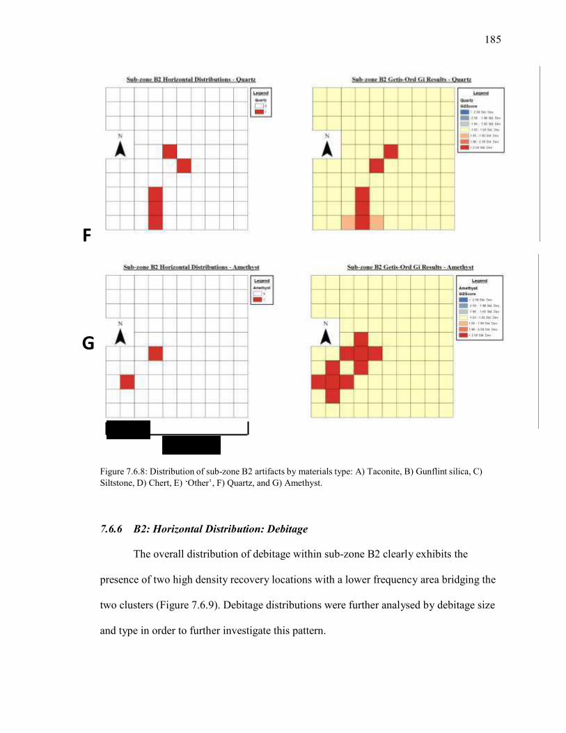
185

F

G

1m

5m

Figure 7.6.8: Distribution of sub-zone B2 artifacts by materials type: A) Taconite, B) Gunflint silica, C)

Siltstone, D) Chert, E) �Other✁, F) Quartz, and G) Amethyst.


The overall distribution of debitage within sub-zone B2 clearly exhibits the

presence of two high density recovery locations with a lower frequency area bridging the

two clusters (Figure 7.6.9). Debitage distributions were further analysed by debitage size

and type in order to further investigate this pattern.

186

1m

5m

Figure 7.6.9: Distribution of all sub-zone B2 debitage by quadrat showing two primary cluster locations

with lesser debitage frequencies occurring in between.

Debitage Size

Artifact distributions by size are shown in Figure 7.6.10. The distribution of

various debitage size grades maintains significant clustering in the same relative

locations. However, there is an observed difference between the size compositions of

those clusters. In the southern cluster zone, there appears to be a higher recovery of

debitage within the 2-25mm size range, while the northern cluster yielded a greater

number of large debitage between 25-50mm.

187

D12-

o.. 25mm

0 11-

20

021-!0

- 61-HlO

- 101-200

- 201-387

N

A

-·

·-

A

A

A

B2: Horizontal Distribution of Debitage by Size

Sub-zone 82 Hori zontal Distributions: 2-6mm

ill!.illl

2-0mm

CJo

c:J G-10

0 11-20

021-!0

- 61-100

- 101-200

201..478

Sub-zone 82 Horizontal Distributions: 6-J2mm

Legend

S 12mm

CJo

-6-10

c::J H-20 021-!oO

c:J 61-100

c::J !OI -200

- 201-600

- 501-1000

- 1001 1062

Sub-zone 82 Horizon tal Distributions: J2-25mm

Legend

L:]G-10

Sub-zone B2 Horizontal Distributions: 2-6mm

2 mm GIZScore

- <261Std0...

- -2.58--UeStd

- -1 98..1115SUI

N 166-1M Std Oev

- 186 - 258SI:d0ev

..2 Std 0ev

Sub-zone B2 Horizontal Distributions: 6-12mm

5--12mm

G1ZScore

- c 251Std0...

- -.B8--1 M$td0...

- -198--lti5SUI

-1 156-185Std0oe\l

N - 1661· MStd0ev

- 188-258Std0ev

..258StdDev

Sub-zone B2 Hol'izontal Distributions:12-25mm

Loaend

122·5mm

G1ZScore

- c 251Sid0...

- -2!i8--19eSUIO...

- -198 - -1&55-. 0ev

N - 166 - 1MStdo-

- 188 - 258Std0ev

..258StdDev

188

1m

5m

Figure 7.6.10: Sub-zone B2 debitage distributions by size.

189

Debitage Type

Similar to debitage size distributions, the location of debitage by type coincides

directly with high recovery locations (Figure 7.6.11). Highest concentrations for all

debitage types occurs within the southern cluster location, while there is a slight split

between northern and southern clusters regarding primary debitage hot-spots.

B2: Horizontal Distribution of Debitage by Type

190

c-::·J o

- 51-100

N

A

- 101-101

-

N

A

-

-

-

.

-

A

-

-

-

·- A A

·- A

Sub-zone B2 Horizontal Distributions: Secondar-y Debitage

l:!R!rul secondary secondary

o GIZScore

... 251Sid0e¥

-&-10 - -258--t iiO SidO...

D n-.20 - -1 9S --155Sid0eY

021..50 -IM- 1t59td Oev

N c::Jst-t oo N 166- t 81J StdDev

c::J tOt-200 - 186-25HU OIN'

- 201.500 ,.2SISU Dev

- $01-1000

- 1001 1) 44

Sub-zone 82 Horizontal Distri butions· Tert ian� Debital!o Sub-zone B2 Horizontal DistJ·ibutions·Tet·tian Debih!!e

Tenlary

0&.10

01120

021-60

Sub-zone 82 Boo·izontal Dist ributions·Undetermined Debital!c

lli!.!!!l

Und tm'llnd

c::Jo

810

c::J 11-20

21.5Q

Leg end

Tenlary

GIZScore

c 251Sid0...

--B8 --ti10Sid0...

- - I'M -- .&'i'ildO...

-IM-IHiSlld Oev

166 - t 81J SI:d0ev

1116 -HlSidO....

"268SU Dev

Su b-zone B2 Horizontal DistJ·ibutions: U ndeterm ined Debitage

Leg end

Undetermined

GIZScOfe

.. H8Sid0...

- -2.58 --tile$140...

- - t9S --t .S5Sid0ev

-tM-HSSlld Oev

51-100 N - IOt -200

201-3511

- 166·1 8'3St<I DeY

- 186-25-JSidDe¥

..2$8SU Dev

lm

Sm

Figure 7.6.11: Sub-Zone B2 debitage distribution by type.

191


The distribution of all tool recoveries from sub-zone B2 can be seen in Figure

7.6.12. These recoveries were further analyzed by cores, bifaces, retouched flakes, FCR

and charcoal distributions, and general tool distributions.

Cores

Similar to other sub-zones, the mapping of cores by cortex type does not appear to

reveal any form of significant clustering. It can be noted though that the general

distribution of cores occurs between the areas of highest debitage recoveries (Figure

7.6.13), with the highest concentration of cores occurring near the recovered

grinding/anvil stone.

Bifaces

Bifaces from sub-zone B2 are located primarily within the areas between high

debitage recoveries, similar to the distribution of cores. Assessing the distribution by

stage and level does not appear to exhibit any distinct pattern (Figure 7.6.14 and Figure

7.6.15). While there may be a tendency for later stage bifaces to occur closer to the

northern cluster area, this is not a direct association.

Retouched Flakes

Distributions of retouched flakes by either intentional or incidental flaking does

suggest that there is a stronger distribution of intentionally retouched items within the

192

vicinity of FCR clustering (Figure 7.6.16). The distribution of incidental retouched items

in contrast does not appear to exhibit any patterning.

Tool Refits

There are two tool refits within sub-zone B2. One consists of a broken core

fragment made of gunflint silica while the other is a broken taconite core fragment. There

is little separation between the two taconite pieces both vertically and horizontally. The

gunflint silica cores are also within close proximity, being separated by only one vertical

level and less than 50cm horizontally.

1m

5m

Figure 7.6.12: Distribution of all tools in sub-zone B2 with total debitage recoveries by quadrat.

193

1m

5m

Figure 7.6.13: Distribution of sub-zone B2 cores by cortex type and level.

1m

5m

Figure 7.6.14: Distribution of sub-zone B2 bifaces by recovery level.

194

1m

5m

Figure 7.6.15: Distribution of sub-zone B2 bifaces by stage.

1m

5m

Figure 7.6.16: Distribution of retouched flakes by intention vs. incidental flaking.

195

FCR and Charcoal Distributions

There are two clusters of FCR within subzone B2. Cluster 1 consists of a

dispersed grouping of FCR fragments towards the middle of the sub-zone, while cluster 2

is a dense cluster of fragments contained within one quadrat (Figure 7.6.17).

Cluster 1 contains primarily small sized FCR fragments (25-50mm), with two

larger FCR pieces in the 50+mm size range (combined mass of 261.2g). Cluster 2

consists of one large FCR piece (over 50+mm, 5000+ g), with a number of smaller FCR

fragments that likely broke off of this larger item during transportation.

Charcoal recoveries from sub-zone B2 were recovered from level 5 in the upper

northeast area. Artifact recoveries from within this area are minimal, and no FCR was

noted for this portion of the sub-zone.

General Tool Distribution

Other tool recoveries from sub-zone B2 included scrapers, unifaces, blade flakes,

a graver/perforator, hammerstones, and three anvil stones. The distribution of all

recovered tools occurs in close association with high concentrations of debitage. Many

tools were recovered from between the two primary cluster zones.

The location of anvil stones in sub-zone B2 vary in their relation to debitage and

artifact frequencies (see Figure 7.6.12). The southernmost anvil stone is located within

the centre of highest debitage recovery, while the northern most anvil stone does not

appear to have any direct relation to reduction activities. The central grinding stone/ anvil

is located where debitage recoveries are lower, however, there are a number of tool

recoveries within the immediate area.

196

Distributions of scrapers and unifaces in sub-zone B2 appear to be relatively

dispersed, while still occurring within general artifact cluster areas.

1m

5m

Figure 7.6.17: Distribution of FCR and charcoal recoveries from sub-zone B2.


There are no significant magnetic anomalies contained within sub-zone B2

(Figure 7.6.18). Along the eastern border there is a strong magnetic anomaly that extends

east towards sub-zone B4. This will be discussed further in section 7.8.

197

1m

5m

Figure 7.6.18: Results of NSG for sub-zone B2.

7.7 Sub-Zone: B3

Sub-zone B3 consists of a relatively small cluster within the southern extent of the

RLF site (Figure 7.7.1). In total, this sub-zone contains 30 50 x 50cm quadrats. There is

some overlap along the northern edge of this area with sub-zone B2.

1m

3m

Figure 7.7.1: Sub-zone in relation to topography with a close up of sub-zone B3 illustrating all tool recoveries with total debitage by quad.

198

B3: DEBITAGE

SIZE Frequency

0-2MM 0

2-6MM 23

6-12MM 60

12-25MM 48

25-50MM 12

50+MM 2

B3: DEBITAGE

MATERIAL Frequency

TACONITE 138

GFS 7


A total of 171 artifacts were recovered from sub-zone B3, including three cores

(frequency = 6), one biface, one retouched flake, one abrading stone, and 17 pieces of

FCR (Table 7.7.1). Debitage recoveries for this sub-zone include 145 pieces, which were

further divided by size, type, and material (Tables 7.7.2-7.7.4).

Table 7.7.1: Sub-zone B3 tool recoveries. Table 7.7.2: Sub-zone B3 debitage

frequencies by size.

B3: TOOLS

TYPE Frequency

CORE 3 (6)

BIFACE 1

RETOUCHED

FLAKE

1

ABRADING

STONE

1

Table 7.7.3: Sub-zone B3 debitage

frequencies by type.

Table 7.7.4: Sub-zone B3 debitage

frequencies by material.

B3: DEBITAGE

TYPE Frequency

PRIMARY 2

SECONDARY 103

TERTIARY 13

UNDETERMINED 11

SHATTER 16

199


The vertical distribution of artifacts in sub-zone B3 centre around Level 3 (Figure

7.7.2). This distribution is mirrored by all artifact size ranges (Figure 7.7.3). Second

highest frequencies occur in Levels 4 and 2 respectively.

Sub-Zone ' B2' - Vertical Distribution of Artifacts by Level

80

70

60

50

40

30

20

10

0

Surface Level 1 Level 2 Level 3 Level 4 Level 5 Level 6 Level 7

Figure 7.7.2: Sub-zone B3 total artifact recoveries by level.

Sub-Zone ' B2' - Vertical Distribution of Artifacts by Size and Level

35

30

25

20

15

10

5

0

Surface Level 1 Level 2 Level 3 Level 4 Level 5 Level 6 Level 7

2-6mm 6-12mm 12-25mm 25-50mm 50+mm

Figure 7.7.3: Sub-zone B3 artifact recoveries by size and level.

200


The results of statistical clustering analysis for sub-zone B3 yielded conflicting

results. While both Getis-Ord Gi and Ripley�✁ ✂ suggest that the placement of artifacts

exhibits a clustered distribution, nearest neighbour analysis suggests that the observed

artifact locations are random in nature (Figures 7.7.4-7.7.6). Differences between these

tests may be the result of differing methods, as nearest neighbour utilizes location but not

frequency, whereas Getis-Ord Gi utilizes cell frequencies. Furthermore, nearest

neighbour assesses the distance between the nearest single point rather than multiple

point locations.

Figure 7.7.4: Results of nearest neighbour analysis indicating that at a z-score of -0.399164 the observed

pattern varies little from that of a random distribution.

201




202


Artifact recoveries by level generally exhibit clustering towards the centre of the

sub-zone (Figure 7.7.7). It should be noted though, that through all levels there is a

consistent horizontal dispersal of debitage in low frequencies.


203

� A

✁

- <·2.SSS!d. O.v

-·

A

A

Sub-Zone B3 Horizontal Distributio ns - Lcl' el 3 Recoveries

N Legend N

Bif✂te

Core Fragn-..nt

Legend

Levell

G ZScore

✄ ✄ FCR

Level3

CJ o L:J 1 5

C]&-10

- 11-20 - 21-27

Sub-Zone R3 Horizontal Distributions - Lc\'cl 4 Recoveries

1.96 ·2.SSSd: .O.....

- >2.SBStd.Oev.

N

A 1---------+---l-----1--------+------+--------1

e Cor. Fragm.r t

☎ FCR

Level4

CJo CJ 1 5

CJ &-10

. 11-13

N

A 1----------+------+---

Legend

Level4

GI ZScore -'-----------'--------i

- -25a - -196Sid0ev.

- -1.96- -1.65 Std.Oev.

·165- t 65Std Oev

- 16S· 1.96 Std.Otv.

- 1 96 - 2. 58 Std.O.v.

- >2.S8Std Oev.

Sub-Zone 83 Horizontal Dist ributions - Level 5 Recoveries

N

A 1---------+-----+---l---------+-------+--------1

✆

Legend N

0 Abfa iding Stone

e Core Fragment

LevelS

CJo CJ 1·5

Legend

Level5

GI ZScore

- c -2.58 Std. Otv

- -2 5a - -t 96Sid0ev.

- -1.96 · 1.65Std.Oev.

-165 - 1 65Sid Oev

- 165 - 1.96Std.O.v.

.1 96·2-SB Std.Oev.

0 - >2.S8Sid Oev.

204

1m

3m

Figure 7.7.7: Sub-zone B3 artifact recoveries by level.


Material types recovered from sub-zone B3 were limited to taconite and gunflint

silica. Gunflint silica artifacts appear to be randomly dispersed (Figure 7.7.8 B) while

taconite, being the primary recovery material within B3, follows the same dispersal

patterns observed in level distributions (Figure 7.7.8 A).

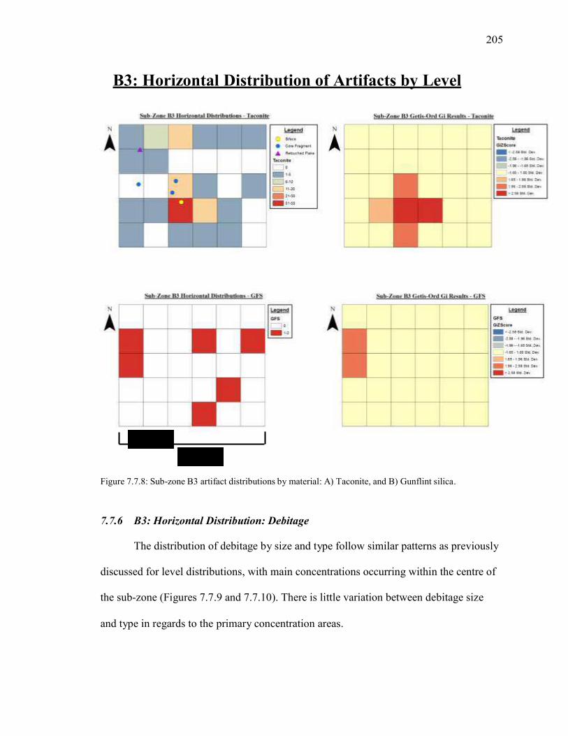
205


1m

3m

Figure 7.7.8: Sub-zone B3 artifact distributions by material: A) Taconite, and B) Gunflint silica.


The distribution of debitage by size and type follow similar patterns as previously

discussed for level distributions, with main concentrations occurring within the centre of

the sub-zone (Figures 7.7.9 and 7.7.10). There is little variation between debitage size

and type in regards to the primary concentration areas.

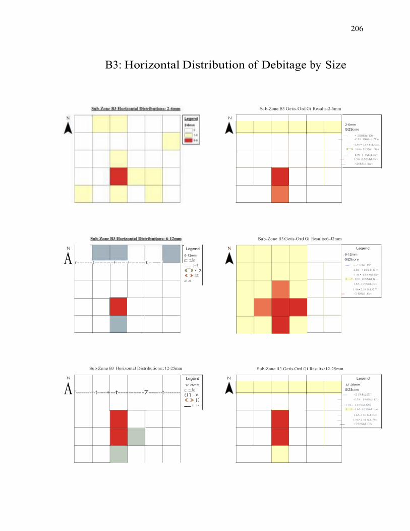
206

Legend

6-12mm

GIZScore

- < -:!.8 Std. DIY

- -2.58- -1 96 Sid O.v.

- ·1.96 �·1.65 Std.Oev.

D-166-165Std o.... - 1.65- 196Std.Dev.

- 1.96✁ 2.58 Std.0.'1.

- >2 S8Std .Oev


Su b-Zone B3 Getis-Ord Gi Results:2-6mm

N

2-6mm

GIZScore

- <-2S8Std Otv

- -2.58 196Sid O.v.

- ·1.96 ✂·1.65 Std.Oev.

D·166- 165Sid Dev

- U5 1 Std.DeY.

- 1.96·2.58Std.Dev.

- >258Sid .Oev

Su b-Zone H3 Getis-Ord Gi Results:6-J2mm

N

A r------t-----+-- +----t--

Sub-Zone B3 Horizontal Distributions:12-25mm

Legend

6-12mm

c::::Jo - 1·5

0 ✄☎✆✝ 0112· 0 21-27

Sub-Zone 113 Getis-Ord Gi Resu l ts:12-25mm

N

A !----------t----+--t----------7-------t---------

Legend N

12-25mm

c::::Jo ✞✟✠✡ 0✄☎✆✝ . 11 1☛

Legend

12-25mm

GIZScore

- <2· 58StdDIY

- -2.58··196Std O.v.

-·1.96 ☞·1.65 Std.O.v.

D-165-165Std D☛v

- 1.65✁ 1 96 Std.DeY.

- 1.96✁ 2.58 Std. Dev.

- >258Std .Oev

207

1m

3m

Figure 7.7.9: Sub-zone B3 debitage distribution by size.

208


Sub-Zono Il3 Getis-Ord Gi Results:Shutter

N

A

Sub-Zone 83 Horizontal Distributions:Sccondnn·Oebitnge

N Legend

Shatter

GIZScore

- <-2S8Std.O.v.

- -2.58 ··196Std Oev.

- -1.96 �·L!5Stet Oev

D· 1 66 - 165Std Dev

- 1.65·1.96510.0.11.

- 1.96✁ 2.58 Std.O.v.

- >258Stci.D...,

Sub-Zone 113 Getis-Ord Gi Resu lts: l'rimur\' J)ebituge N Legend

Primary

GIZScore

- <-258Std.O.v.

- ·2.58··I 96 Std Oev.

- -1.96 ✁ -L65Stet Oev

CJ 1 66 - 165Std Dev

- 1.65·1.96Std.0.11.

- 1.96✁ 2.58 Std.DIY.

- >258Stci.D...,

Sub-Zone 113 Getis-Ord Gi Results: Seconda ry Jlebituge

N

A F-------1-----\-----1----------+----+-----1

N

A f--------'-----+---f---t-------'--------1

Legend

Secondary

GIZScore

- <-258Std.O.v.

- -2.58··196Std Oev.

- -1.96 ✁·L65Stet Oev

D· 1 66 - 165Std Dev

- 1.65·1.96Sid.0.11.

- 1.96✁ 2.58 Std.O.v.

- >258Stci.D...,

209

1m

3m

Figure 7.7.10: Sub-zone B3 debitage distribution by type.

210


There were limited tool recoveries from sub-zone B3. Artifacts that were

recovered exhibit a general association to high artifact frequency areas within the centre

of the sub-zone (Figure 7.7.11). One outlier is the recovered retouched flake, however,

this appears to exhibit incidental retouching. This sub-zone also includes the recovered

FCR cluster discussed in section 7.6. This cluster consists of one large fragment with a

number of smaller secondary pieces that likely broke off from the original item.

One artifact refit was recorded for sub-zone B3. This consisted of a core re-fit

from within the same quadrat and within one level of each other (levels 4 and 5).

1m

3m

Figure 7.7.11: Sub-zone B3 tool recoveries with total debitage by quadrat.

211


Sub-zone B3 does not appear to have any significant magnetic anomalies (Figure

7.7.12). It does occur just south of an extended anomaly that stretches between subzone

B2 and B4.

1m

3m

Figure 7.7.12: Results of NSG survey for sub-zone B3.

7.8 Sub-Zone: B4

Sub-zone B4 covers a relatively small and localized cluster of artifacts within the

southeastern portion of the RLF site (Figure 7.8.1). This is the smallest sub-zone within

this study, consisting of only 20, 50 x 50cm quadrats.

212

1m




A total of 26 artifacts were recovered from sub-zone B4. Of this, 2 bifaces were

recovered (frequency = 3). Biface recoveries consisted of one stage 2 biface made of

taconite recovered from level 8, and one stage 3 biface made of gunflint silica recovered

from the excavation surface. These represent the only tool recoveries from this subzone.

Debitage recovered from sub-zone B4 included 22 artifacts, of which the majority

were siltstone (Tables 7.8.1-7.8.3). Further assessment of the artifact catalog indicated

that these siltstone recoveries may not represent culturally modified materials. As such,

further analysis was conducted. This revealed that, while this material has been used to

produce tools on other sites (e.g. Mackenzie 1, Figure 7.8.2-A), the artifacts from RLF

may not be the result of cultural modification (Figure 7.8.2-B, C). Re-fitting broken

fragments suggests that rather than fracturing through percussion, it is more likely that

these objects broke along natural faults within the material. This leaves six flakes of other

213

materials within the sub-zone, of which three exhibit water rolling that may suggest

natural pebbles. The final artifact recovery consisted of one chert pebble cataloged as

�✁✂✄e☎✆ and is likely natural.

Figure 7.8.2: Siltstone artifact recoveries from the Mackenzie 1 (A) and RLF (B and C) sites. Flake refits

from items B and C do not appear to exhibit cultural modification, but rather natural fracturing.

Table 7.8.1: Sub-zone B4 debitage frequency by size.

B4: DEBITAGE

SIZE Frequency

0-2MM 0

2-6MM 1

6-12MM 4

12-25MM 9

25-50MM 6

50+MM 2

214

B4: DEBITAGE

MATERIAL Frequency

TACONITE 2

GFS 2

SILTSTONE 16

CHERT 2

Table 7.8.2: Sub-zone B4 debitage frequency by

type.

Table 7.8.3: Sub-zone B4 debitage frequency by

material.

B4: DEBITAGE

TYPE Frequency

PRIMARY 6

SECONDARY 11

TERTIARY 1

UNDETERMINED 0

SHATTER 4


The vertical distribution of artifacts within sub-zone B4 does not follow the

pattern exhibited within other sub-zone areas (Figures 7.8.3 and 7.8.4). Artifact clustering

within B4 is spread primarily between levels 2-5, with level 5 yielding the greatest

number of recoveries. Removing siltstone debitage from the vertical distribution of

artifacts does not change this varied distribution, as one taconite biface was recovered

from level 8.

Sub-Zone ' B2' - Vertical Distribution of Artifacts by Level

8

7

6

5

4

3

2

1

0

Surface Level 1 Level 2 Level 3 Level 4 Level 5 Level 6 Level 7 Level 8

Figure 7.8.3: Sub-zone B4 artifact frequencies by level.

215

Sub-Zone ' B2' - Vertical Distribution of Artifacts by Size

and Level

5

4

3

2

1

0

Surface Level 1 Level 2 Level 3 Level 4 Level 5 Level 6 Level 7 Level 8

0-2mm 2-6mm 6-12mm 12-25mm 25-50mm 50+mm

Figure 7.8.4: Sub-zone B4 artifact frequencies by size and level.


The results of both nearest neighbour and Getis-Ord Gi tests indicate that the

observed distribution of artifact in sub-zone B4 is the result of random chance (Figures

7.8.5 and 7.8.6). Conversely, Ripley�✁ ✂ analysis suggests that some clustering is

occurring, likely associated with dense siltstone concentrations (Figure 7.8.7).

Figure 7.8.5: Results of nearest neighbour analysis indicating that at a z-score of 1.146096 the observed

pattern varies little from that of a random distribution.

216

Figure 7.8.6: Results of Getis-Ord Gi analysis indicating that at a z-score of -0.094854 the observed pattern

varies little from that of a random distribution.



217


The distribution of recoveries by level varies greatly. However, all siltstone

artifacts are recovered from within the same quadrat (Figure 7.8.8). As artifact recoveries

were limited within this sub-zone it was determined that the application of Getis-Ord Gi

was not necessary.


The limited artifact recoveries from sub-zone B4 inhibits the application of

material distribution studies, however it can be noted again that all siltstone recoveries

occur within the same quadrat (Figure 7.8.9).


The distribution of debitage follows a similar pattern as illustrated in distributions

by level and material. There does not appear to be any patterned distribution of debitage

by size and type aside from the concentrations of siltstone within a single quadrat.


There does not appear to be any correlation between the two recovered bifaces in

sub-zone B4, as one was recovered from a surface context while the other was recovered

from level 8 (35-40cm below surface) (Figure 7.8.10).

218

l--

l- -

-

-

1-

Legend

0 Blface

Surtace

CJ o

�

I


Sub-Zone B4 Horizontal Distribution - Surf ace Recoveries

N

Sub-Zon e B4 Horizo ntal Distribution - Level I Recoveries

N

A -t-

N

Al-+--1-1--

N

Al-t--1--1--1--

N

AI---+-

N

Al--l-- -t- -f- -

219

1m

Figure 7.8.8: Distribution of sub-zone B4 recoveries by level.

220


1m

Figure 7.8.9: Distribution of sub-zone B4 recoveries by material type: A) Taconite, B) Gunflint silica, and C) Siltstone.

221

1m

Figure 7.8.10: Sub-zone B4 tool distributions with total debitage by quadrat.


There does appear to be a strong NSG anomaly recorded for area B4. This

consists of an elongated high and low reading area that extends into the sub-zone from

the west (Figure 7.8.11). The limited recovery of artifacts however inhibits interpretations

regarding cultural association.

1m

Figure 7.8.11: Results of NSG survey for sub-zone B4. The presence of magnetic anomalies can be seen spreading into the sub-zone from the west.

Chapter 8

Site Interpretations

8.1 Introduction

The results presented in Chapter 7 provide the foundation from which

interpretations of site use and organization are based. This chapter presents

interpretations for individual sub-zones as well as the larger zone �✁✂ and �B✂ ✄☎eas,

leading to hypotheses regarding activity areas and overall site function.

8.2 Disturbance Processes at the RLF Site

Although the effects of mechanical tree removal and stacking have already been

discussed, it is not the only observable disturbance process at the RLF site. The analysis

of artifact distributions by level for all sub-zones indicates that vertical movement of

artifacts has occurred, likely as a result of pedoturbation and cryoturbation (Schiffer

1987; Wood and Johnson 1978).

Despite this, the primary artifact distribution peaks in levels 2-4, with greatest

quantities in level 3 (Figure 8.2.1). The observed unimodal distribution suggests a

comparatively simple depositional sequence, and is consistent with the RLF being a

single component site, or possibly multiple occupations with limited soil accumulation

between occupation events. It is proposed that slight variations observed within some

sub-zones (e.g. sub-zone B1) may be the result of tree stumps offsetting initial excavation

datum placement and providing differing amounts of organic overburden. However,

limitations in vertical recovery control due to 5cm arbitrary level excavations may have

222

223

To

tal A

rtif

act

s

distorted any subtle variations that may have existed within vertical artifact distributions

resulting in an oversimplification of the observed pattern.

4500

4000

3500

3000

2500

2000

1500

1000

500

0

RLF: All Artifact Recoveries by Level

Recovery Level

Figure 8.2.1: Vertical distribution of all artifact recoveries by level.

8.3 RLF Site: Sub-Zone Interpretations

The following sections (8.3.1-8.3.6) explore site use interpretations for each sub-

zone based on observed artifact composition and distributions.

8.3.1 Sub-Zone A1

While surface disturbance has resulted in the horizontal displacement of artifacts

within sub-zone A1, it is still possible to propose sub-zone activity. After removing

surface and level 1 recoveries from the analysis, three lithic clusters are apparent within

the sub-zone (Figure 8.3.1).

224

A1-A

A1-B

A1-C

1m

Figure 8.3.1: Artifact distributions for sub-zone A1 indicating the presence of three distinct cluster areas. Note: Surface and level 1 recoveries removed.

Consideration of debitage by size and type shows very little variation between

clusters A1-A and A1-B. This differs from cluster A1-C. A separation in debitage size is

observed with larger waste occurring to the west and the smaller waste to the east.

However, debitage of all sizes for A1-C overlap within a general cluster zone.

With all flake types and sizes occurring in relatively confined spatial distributions,

it is proposed that these clusters represent in-situ lithic reduction activities. The limited

recovery of small waste flakes (<6mm or tertiary reduction flakes) compared to larger

debris suggests that this reduction activity was focused more towards the early stages of

tool production rather than tool finishing. This interpretation is supported by the recovery

of a larger than expected number of broken early stage biface fragments and cores.

225

An alternate explanation for the clusters in sub-zone A1 is that they represent

periodic cluster discard (Gibson 2001). This alternative hypothesis is based on the

number of broken and fragmentary bifaces and cores relative to the amount of recovered

debitage (~1 biface for every 119 debitage flakes recovered). However, this could be

explained by disturbance removing some flakes from the sub-zone. As well, the initial

stage/size of the lithic piece prior to beginning bifacial reduction would directly affect the

number of recovered flakes, as late stage bifaces (~ stage 3) would require less flake

removal in order to reach a cache stage. Unfortunately the interpretation of sub-zone A1

as representing a lithic dumping area cannot be properly investigated due to a lack of

refitting analysis of recovered debitage (Bamforth et al. 2005).

The presence of the anvil stone within sub-zone A1 does not appear to directly

relate to any of the high density artifact clusters, and is more strongly associated with

artifact clusters in sub-zone A2. Furthermore, the limited variety in recovered tool types

does not allow for interpretations of activity beyond stone tool production.

Based on the observed spatial distribution and composition of clusters in sub-zone

A1, it is proposed that the production of cache/preform stage bifaces accounts for all

three distinct areas. Taconite appears to be the primary material employed, although

modest recoveries of gunflint silica in clusters A1-A and A1-C suggests it was also

utilized for tool production.

8.3.2 Sub-Zone A2

Artifact distributions within sub-zone A2 are concentrated to form a ring-shaped

pattern, with two primary depositional areas in the west and east (Figure 8.3.2). The

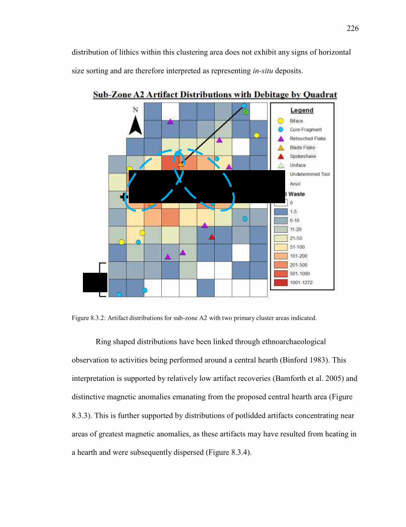
226

distribution of lithics within this clustering area does not exhibit any signs of horizontal

size sorting and are therefore interpreted as representing in-situ deposits.

A2-A A2-B

1m

Figure 8.3.2: Artifact distributions for sub-zone A2 with two primary cluster areas indicated.

Ring shaped distributions have been linked through ethnoarchaeological

observation to activities being performed around a central hearth (Binford 1983). This

interpretation is supported by relatively low artifact recoveries (Bamforth et al. 2005) and

distinctive magnetic anomalies emanating from the proposed central hearth area (Figure

8.3.3). This is further supported by distributions of potlidded artifacts concentrating near

areas of greatest magnetic anomalies, as these artifacts may have resulted from heating in

a hearth and were subsequently dispersed (Figure 8.3.4).

227

A

1m

B

Figure 8.3.3: Proposed hearth location with A) artifact distributions, and B) Magnetic results from NSG.

228

1m

Figure 8.3.4: Distribution of potlidded artifacts with results of NSG. Proposed hearth location indicated by black circle.

While Binford (1983:158) asserted that these ring (or doughnut) shaped

distributions occur almost exclusively with open-air hearths, similar patterns (exhibiting a

confined distribution, expedient maintenance activities, and a lack of distinctive drop-toss

displacement zones) could occur within short-term shelters. As it is not possible to

definitively suggest whether a structure was associated with sub-zone A2, two

interpretations must be considered.

Firstly, it can be proposed that the distribution of lithic debris in sub-zone A2 took

place around a central hearth in an open-air environment, with at least two primary work

zones being represented. The smaller of these two clusters (Figure 8.3.2-A2-A) involved

the primary reduction of materials using the observed anvil stones, with a secondary

focus of biface production. This is indicated by the high frequencies of shatter and small

fragmentary debitage. Meanwhile, the primary cluster (Figure 8.3.2-A2-B) suggests

activities related to the reduction of suitable material into bifaces/preforms. This is

229

indicated by the greater frequency of mid-sized flakes and directly associated biface

fragments. It is proposed that the lack of an identifiable toss-zone is the result of limited

spatial resolution in debitage data, and a limited spacing between the drop and toss zones

areas during site use. The observation that tool recoveries generally occurred back from

primary debitage distributions could represent a possible toss-zone, however this is not

certain.

The second interpretation is similar to the first, however these activities are

interpreted as having occurred within a structure, limiting the spatial distribution of

debris until after the structure had been removed (Figure 8.3.5). In this interpretation,

dense artifact concentration areas are interpreted as representing Type 1 cluster discard

(Gibson 2001:74), in which flint knappers within a confined structure were performing

lithic reduction tasks and periodically collected and dumped large quantities of mixed

debris into a side dump area. This results in areas of extremely high lithic concentration.

The use of type 1 cluster discard could help to explain the lack of toss-zone distributions

as well as areas of highly mixed debitage recoveries in both high density recovery quads.

One might argue that flint knapping within a structure is unlikely given that it

generates a great deal of sharp debris. However, if it can be proposed that some form of

floor covering was being used and preventative maintenance kept harmful debris in a

defined area, then this is not an improbable interpretation. It can also be speculated that if

lithic reduction occurred within a structure just prior to camp abandonment then there

would not be a need to worry about debris build-up. Furthermore, suggesting that debris

from flint knapping would have made the structure uninhabitable assumes that all

structures functioned as living spaces. Given the placement of the RLF site on the

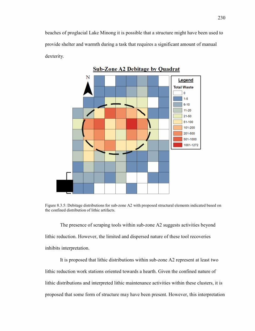
230

beaches of proglacial Lake Minong it is possible that a structure might have been used to

provide shelter and warmth during a task that requires a significant amount of manual

dexterity.

1m

Figure 8.3.5: Debitage distributions for sub-zone A2 with proposed structural elements indicated based on the confined distribution of lithic artifacts.

The presence of scraping tools within sub-zone A2 suggests activities beyond

lithic reduction. However, the limited and dispersed nature of these tool recoveries

inhibits interpretation.

It is proposed that lithic distributions within sub-zone A2 represent at least two

lithic reduction work stations oriented towards a hearth. Given the confined nature of

lithic distributions and interpreted lithic maintenance activities within these clusters, it is

proposed that some form of structure may have been present. However, this interpretation

231

must remain speculative as it is equally possible that the observed distribution is the

result of limited spatial resolution, blurring patterns attributed to open-air activities.

8.3.3 Sub-Zone B1

The vertical and horizontal distribution of debitage recoveries by size and type

indicate that limited post-deposition size sorting has occurred. This suggests that

materials are likely minimally displaced aside from vertical movement.

The tightly clustered nature of debitage, biface, and core recoveries suggests that

sub-zone B1 represents either a very brief lithic reduction event or, more likely, a type 3

lithic dumping area (Gibson 2001). This is based primarily on the highly clustered nature

of debris within a 50x50cm quad, with little to no artifact recoveries from adjacent units.

This interpretation remains tentative in light of the limited spatial resolution of recovered

debitage, tree root activity, and a lack of debitage refit analysis.

8.3.4 Sub-Zone B2

Sub-zone B2 is interpreted as containing two distinct flint knapping areas, with a

central area of undetermined activity (Figure 8.3.6). These flint knapping areas are

interpreted to represent in-situ production activity based on the co-occurrence of all

debitage sizes and types, the dispersal around central �hot-spots✁, and the clustered

distribution of similar raw material types (e.g. Gunflint Silica). This interpretation is also

supported by the presence of extensively used anvil stones near cluster B2-B as well as

hammer stone recoveries near cluster B2-A. The presence of fragmentary early stage

bifaces, and limited recovery of fine scale debitage and finished formal tools suggests

232

that the primary function of these reduction areas was the production of bifaces suitable

for caching.

This sub-zone also yielded a significant variety of lithic tools suggesting that

activity was not limited to bifacial reduction. The high frequency and concentration of re-

touched flakes, scrapers, and unifaces suggest that some form of cutting or scraping

related activities were being performed within the central area of this sub-zone (see

Figure 8.3.6-B2-C). The co-occurrence of re-touched flakes in high concentrations

around FCR fragments further suggests some form of craft activities. If the FCR

distribution derives from a hearth, then the re-touched flakes may represent a range of

domestic activities. Alternatively, if the FCR was relocated to the area, they could have

functioned as weights for activities such as hide working (Gibson 2001).

While no magnetic anomalies similar to sub-zone A2 were recorded in direct

relation to the FCR clusters, there is an observed magnetic anomaly to the east. This

occurs as an elongated magnetic anomaly spreading east-west just beyond sub-zone B2

(Figure 8.3.7). While a direct association cannot be made, it is possible that the readings

are the result of hearth related activities near the sub-zone B2 FCR clusters, and the

elongation of NSG reading a result of data collection.

Overall, sub-zone B2 is interpreted as representing at least two primary lithic

reduction zones, with cutting/scraping activities, possibly related to either butchering or

hide-working, occurring in a central area. Based on artifact dispersion and lack of relative

artifact confinement, activities within sub-zone B2 are interpreted as occurring in an

open-air environment away from built structures.

233

B2-A

B2-B

B2-C

1m

Figure 8.3.6: Artifact distributions for sub-zone B2 with areas of proposed lithic reduction (B2-A and B2- B) and secondary cutting/scrapping activities (B2-C).

1m

Figure 8.3.7: Location of sub-zone B2 artifacts in relation to NSG results.

234

8.3.5 Sub-Zone B3

Similar to sub-zone B1, distributions in B3 consist of a tight cluster of lithic

artifacts. Distributions of debitage types and sizes all concentrate within the one small

cluster area separated from cluster B2 by an area of low recoveries. The presence of core

fragments and a broken early stage biface is suggestive of a brief lithic reduction event

during which the biface broke and the knapper abandoned the area. Due to limited spatial

resolution it cannot be determined if this is the result of in-situ lithic production or type 3

cluster discard.

The cluster of FCR located in sub-zone B3 represents one large fragment with

smaller secondary fragments. This may be the result of either use as a heated stone

removed from fire, or dumping after use within a hearth. It does not appear to be directly

associated with deposition of artifacts in B3, although this cannot be ruled out.

Overall sub-zone B3 is interpreted as representing the remains of a relatively brief

lithic reduction episode during which biface production failed and the knapper moved

away from the area.

8.3.6 Sub-Zone B4

Re-analysis of material recovered from this zone suggests that siltstone objects

are not the result of cultural manipulation, and therefore sub-zone B4 does not appear to

represent an area of cultural activity. While some biface fragments were recovered from

this area, the fact that they were separated by a significant vertical depth suggests that

they are not directly related. The extremely limited and un-patterned debitage

235

distributions rule out the possibility that sub-zone B4 represents lithic production

activities. The presence of an intense magnetic reading during NSG survey may represent

an event no long visible within the archaeological record, however, this cannot be

explored further.

8.4 Overall Site Function and Organization

While lithic reduction activities were conducted in all areas of the RLF site, there

is a distinct difference in the nature of deposits between zones A and B (Figure 8.4.1).

Zone A is interpreted as representing intense lithic reduction activities occurring

around a central hearth (sub-zone A2) with a number of smaller lithic clusters to the west

likely reflecting independent biface production activities. The hearth centred activities of

sub-zone A2 exhibit characteristics that may indicate the presence of a shelter. If this

interpretation is correct, then it can be proposed that zone A may contain a structure

associated with the observed lithic reduction activities. This structure could have

functioned as either a habitation area where flint knapping occurred as a secondary

activity, or as a structure utilized primarily for flint knapping in order to protect the site

occupants from the elements.

The southern section of the site, zone B, contained evidence of both intensive

lithic reduction activities, and butchering/hide working activities suggested by the higher

frequency of retouched flakes, scrapers, and unifaces. The dispersed artifact distribution

suggests that these activities were more likely conducted in an open-air setting.

The observed separation of zones A and B by a slight rise in elevation, as well as

observed differences in artifact distribution patterns, suggests that the separation of these

236

activity areas occurred intentionally. This separation may have functioned to locate the

built structures further back from the beach, possibly within a more wind protected area.

Meanwhile the messier activities associated with tool recoveries from sub-zone B2 could

be conducted in a more open site area towards the active beach front.

1m

Lithic Reduction within Possible Structure

Lithic Reduction

Scraping/Cutting Activities

Figure 8.4.1: Distribution of activities within the RLF site in zones �✁✂ (red) and �B✂ (yellow) with topographic contours represented by black lines.

Despite this separation, it can be proposed that the primary observable function of

the RLF site was the manufacture of cache stage bifaces from both cobble cores collected

locally and bedrock derived cores that may have been transported to the site. The lack of

237

cortical material on most RLF site recoveries indicates that at least some form of primary

testing or reduction was conducted elsewhere. This reduction objective provides a

snapshot of the cognitive reduction techniques employed by Lakehead Complex peoples

(Bennett 2015) wherein site inhabitants are producing Stage 4/5 bifacial blanks for later

finishing elsewhere. The implications of this will be further discussed in Chapter 9.

Chapter 9

Discussion

9.1 Introduction

The interpretation of activities undertaken at the RLF site have important

implications for understanding Lakehead Complex site use and organization, as well the

study of small scale lithic sites within the boreal forest as a whole. This chapter explores

how the results of this spatial analysis affect the current understanding of Lakehead

Complex culture, and provides commentary on how archaeologists could consider

approaching the excavation and analysis of these smaller boreal forest lithic sites.

Furthermore, it will discuss any limitations observed within the presented research and

offer suggestions as to how future studies could best avoid and mitigate the encountered

shortcomings.

9.2 The RLF Site and the Lakehead Complex

As previously discussed, few Lakehead Complex intra-site spatial investigations

have been conducted (See Chapter 3), making it difficult to compare RLF to a wide range

of sites. However, the interpretations proposed for the RLF site are similar to many

regional sites in regards to general site composition and basic function. Of the currently

excavated sites classified under the Lakehead Complex, the RLF site is most similar to

the Naomi site (DcJh-42) and the Biloski site (DcJh-9).

Both the Naomi and Biloski sites are interpreted as being oriented towards the

production of cache stage bifaces for transportation and refinement elsewhere (Adams

238

239

Pe

rce

nt

To

tal B

ifa

ce

1995; Hinshelwood and Webber 1987). These interpretations are based primarily on the

recovery of large quantities of fragmentary and failed early stage bifaces with few other

tool recoveries. Comparing biface recoveries from Naomi and Biloski to those identified

for the RLF site reveals a similar distribution of biface stages, with the exception that

Naomi exhibits a greater abundance of stage 4 bifaces and an under-representation of

stage 2 bifaces (Figure 9.2.1, Table 9.2.1).

Percent Total Bifaces by Stage

50

45

40

35

30

25

20

15

10

5

0

Stage 1 Stage 2 Stage 3 Stage 4 Stage 5 Stage 6

RLF Naomi Biloski

Figure 9.2.1: Percent total bifaces by stage for the RLF (DdJf-13), Naomi (DcJh-42), and Biloski (DcJh-9) sites (Adams 1995; Hinshelwood and Weber 1987).

Table 9.2.1: Comparison of biface recoveries by stage for the RLF (DdJf-13), Naomi (DcJh-42), and Biloski (DcJh-9) sites (Adams 1995; Hinshelwood and Weber 1987).

RLF (DDJF-13) NAOMI (DCJH-42) BILOSKI (DCJH-9)

Total % Total Total % Total Total % Total

STAGE 1 6 12.00 0 0.00 10 5.56

STAGE 2 16 32.00 3 5.77 82 45.56

STAGE 3 22 44.00 17 32.69 67 37.22

STAGE 4 4 8.00 23 44.23 13 7.22

STAGE 5 1 2.00 8 15.38 5 2.78

STAGE 6 1 2.00 1 1.92 3 1.67

TOTAL 50 100 52 100 180 100

240

It was proposed by Fox (1975) that littoral sites, such as Naomi and RLF, were

chosen primarily for resource acquisition, with a secondary focus on lithic reduction

activities. The Naomi site supports this hypothesis, as its location would not have been

directly beneficial for tool production but rather the exploitation of food resources from

adjacent wetlands (Adams 1995). The RLF site supports this hypothesis as well, as its

location does not appear to coincide directly with either bedrock or cobble lithic sources.

Therefore, all materials at the RLF site would have had to be transported to the site. As

such, the RLF site location may have been selected based on its proximity to stream

sources, well drained beach sediments, and placement back from the active beach front

rather than its functionality as a lithic reduction area. However, aside from the

butchering/hide working activities proposed for sub-zone B2, there is little direct

evidence suggesting activities other than lithic tool production. This is similar to the

observations made by Adams (1995) regarding the Naomi site assemblage. It is proposed

that these sites may have functioned primarily as biface production stations, and that site

location was chosen based on the immediate availability of resources during the brief

occupation period.

The RLF site therefore represents a distinct Lakehead Complex site type at which

biface production for transportation and later finishing was conducted as a primary

activity during a relatively brief occupation, similar to the Naomi and Biloski sites. This

differs markedly from quarry sites such as Cummins (DcJi-1) and hunting/occupation

sites like Brohm (DdJe-1) and Mackenzie 1 (DdJf-9) in regards to debitage and tool

composition.

241

Aside from these broad generalizations of site type, it is difficult to compare the

intra-site organization of the RLF site to others within the Lakehead Complex. This is

due to the general lack of detailed intra-site analyses.

The presence of distinctive knapping zones utilizing anvil stones as identified at

the Naomi site (Adams 1995) is also seen in the RLF site. Aside from this however, little

spatial similarities can be discussed beyond the presence and use of distinctive knapping

locations (e.g. Adams 1995; Halverson 1992; Hinshelwood and Webber 1987).

Interpretations derived from the RLF site analysis will help form the basis through which

further intra-site comparison can be established.

9.3 Implications for the Study of Small Scale Sites in Northwestern Ontario

It is common that higher level archaeological research focuses on sites that yield

large quantities of artifacts. This results in smaller lithic sites generally being subjected to

cursory investigation. The interpretive resolution of the RLF site spatial data, coupled

with its apparent brief occupation, was of primary importance for the ability to draw

conclusions regarding site use and activity areas. With relatively modest lithic recoveries,

the effects of post-depositional artifact movement did not heavily impact spatial

resolution allowing for activity area interpretation. This is a unique characteristic of small

scale sites, as spatial resolution on large/multi-component Boreal forest lithic sites are

heavily affected by post-depositional disturbance, blurring distinctions in artifact

distributions between multiple occupations.

242

Furthermore, the study of small scale sites, in regards to their intra-site

organization and function, provide an opportunity to identify under-represented aspects

of settlement systems and clarify the archaeological signatures of activity areas. While

these larger sites are invaluable for the information that can be derived regarding the

material culture and cognitive behaviours of past populations, the repeated nature of

occupation limits their interpretability at an occupational level (see exception McCulloch

n.d.). Smaller, more discrete sites, while yielding limited artifact recoveries, can begin to

answer questions of site organization and occupation.

Unfortunately, the identification and documentation of smaller, more interpretable

sites, is negatively impacted even in the early stages of archaeological investigations as a

result of the methods required during site survey activities (Adams 1995). It is common

for archaeological test-pit surveys during CRM investigations in Ontario to employ a 5m

x 5m transect during initial site investigations. Given the small spatial footprint of the

lithic knapping areas identified within the RLF site, consistently locating these discrete

activity areas during 5m test pit surveys is unlikely. This results in smaller, more

interpretable sites, being missed. However, expanding upon this standard to increase the

number of test-pits within a survey area will directly impact the ability for archaeologists

to effectively survey large areas within the allotted time and budget requirements. This

leaves the difficult question of how one can both effectively locate small scale lithic sites

while maintaining efficiency. Providing a solution to this will take the collective effort of

the archaeological community and is beyond the scope of this paper.

What is clear is that the RLF site illustrates the importance of studying these

smaller lithic sites, as it has yielded an interpretable distribution of lithic artifacts in large

243

part due to its discrete and limited occupation history. Spatial studies utilizing small scale

lithic sites help to form an interpretive base through which large or repeatedly occupied

Lakehead Complex sites can be compared.

9.4 Study Limitations, Concerns, and Future Directions

As with all archaeological research, it is important to acknowledge the limitations

present. Understanding these weaknesses helps to address questions that arise, and

propose ways through which they may be overcome in future research. The primary

limitations encountered during the RLF site analysis were a result of either the nature of

CRM derived data sets, the inherent biases of archaeological spatial analysis, or the

interpretive limitations associated with base level artifact identification and analysis. The

following sub-sections address the concerns associated with these limitations and provide

comments on how to best adapt future spatial studies in order to alleviate any observed

shortcomings.

9.4.1 Spatial Analysis and CRM Derived Samples

The overwhelming majority of archaeological investigations conducted within

Northwestern Ontario today are driven by development rather than academic research. As

such, CRM standards and procedures are directly responsible for the accessibility and

condition of much of the data that is available for research. While many of the

shortcomings observed within this thesis are a direct result of the policies imposed upon

CRM archaeologists, they illustrate the difficulties in finding the balance between

efficiency and data quality within the consulting world.

244

Limitations that result from CRM derived data are primarily associated with the

scale of spatial resolution available. The excavation of units by 50cm quadrats and

arbitrary levels meant that debitage data was batch catalogued by area, rather than by

direct location. This limits the ability to identify fine scale patterning within debitage

distributions that may represent unique or spatially distinct site activities by blurring

together groups of artifacts (Figure 9.4.1).

Figure 9.4.1: Idealized diagram illustrating the effects of batch cataloguing of artifact resulting in the blurring of fine scale debitage patterning in a 1x1 m unit.

While the use of batch cataloguing may limit fine scale interpretability, it does

provide alternative benefits. Given the likelihood that post-deposition movement will

displace artifacts (Bowers et al 1983; Schiffer 1987; Wood and Johnson 1978), the use of

batch cataloguing allows the researcher to look beyond the individual artifacts in order to

see the greater overall pattern. This reduces the possibility of falsely interpreting

displaced artifacts. The use of batch cataloging also allows for a greater site area to be

excavated, yielding a better overall site interpretation. However, the scale of the quadrats

245

used for batch cataloging must be chosen carefully to both maintain efficiency while also

providing an appropriate amount of detail. Utilizing excavation units that are too large

will result in the blurring or blending of artifact distributions, while too fine a scale will

reduce the ability to excavate large site areas within the allotted excavation resources

(Figure 9.4.2).

A

B

Figure 9.4.2: Diagram illustrating the effects of quadrat size on the spatial interpretability of artifact distributions. While reducing quadrat size further to 25x25 cm would improve the spatial resolution of patterning, the time required would double. This would limit the ability to excavate large areas of a site, reducing the overall site picture.

246

Further difficulties in spatial interpretability were encountered while attempting to

determine whether concentrated lithic scatters were the result of in-situ production or

secondary dumping activities. Utilizing sequences of artifact refitting may be able to

distinguish these different depositional processes as an in-situ production event will yield

long sequences of material refits while lithic dumping activities will not (Bamforth et al.

2005). Given the resource sensitive nature of CRM investigations, this form of time-

intensive interpretation could not be employed for this analysis. Although the inability to

perform a debitage refit analysis hindered the current study, it can be applied to future

spatial analyses if conducted prior to initial spatial interpretations.

While many of the shortcomings observed within this thesis occur as both direct

and indirect results of the constraints imposed upon consulting archaeologists, CRM

excavations still prove promising for future spatial distribution studies. The RLF site

analysis has shown promise for the use of NSG in CRM investigations, as it provides a

method for identifying areas of significant archaeological potential in a Boreal forest

setting prior to excavation. While this method is not currently a mandatory practise, it

does prove feasible within the scope of a mitigation project. Furthermore, the use of

properly scaled excavation quadrats (despite a loss of fine scale spatial resolution) allow

for the interpretation of artifact distributions across a larger site area. The capability for

CRM excavations to provide data suitable for higher level analysis is a direct result of the

ability to balance time, scale, and resources. Finding this balance will provide an overall

site impression, while maintaining enough fine scale data to interpret site organization

and activity distribution.

247

9.4.2 Comments on Spatial Analysis in Archaeology

While utilizing spatial statistics aids in limiting researcher bias, they are not able

to provide interpretations regarding the site activities responsible for an observed

distribution. To accomplish this, one must utilize examples from both

ethnoarchaeological and archaeological studies. Although these do provide valuable case

studies through which the observed patterns can be compared, they also expose the

research to the various personal opinions of the one interpreter. This is especially true

when interpreting sites where only lithic artifacts remain.

On sites with poor organic preservation, it is difficult to identify hearths and/or

structures that would have provided anchors for site activity. As such, one must rely on

the various models/hypotheses available for the identification of artifact distributions

resulting from hearth-related activities (Binford 1983; Gibson 2001; Stevenson 1986,

1991). While these models are very useful in providing generalized trends in formation

processes, they do not account for subtle variations in site use that may have occurred

between different populations due to environment, site location, group size/composition,

or other unknown variables. Furthermore, with limited organic preservation even basic

interpretations of site use are based solely on the morphological characteristics of stone

tools. This makes comparisons in site formation different between sites (e.g. hearths used

for food, warmth, light, hafting, and etc. will exhibit different characteristics that may not

survive in the Boreal forest). As such, interpretations cannot be used to provide a direct

series of events for a site, and must instead focus on generalized scenarios of site-use and

organization based on all possible lines of evidence.

248

It is an unfortunate reality of spatial analyses that researchers can never truly

eliminate all elements of research bias. Without a direct understanding of how or why

past populations utilized their site space it is not possible to eliminate any feasible site

scenarios. Therefore, it is important in any spatial interpretation to present all possible

scenarios that could have resulted in the observed artifact distribution. In doing so, one is

able to offer conclusions regarding site formation processes while providing the reader

with alternative scenarios through which they can critically assess the results.

9.4.3 Improving Activity Area Interpretability

As stated previously (section 9.4.2), the application of spatial studies to sites

yielding only lithic artifacts pose difficulties for the accurate interpretation of site

function. Alternative archaeological studies can help to alleviate this issue by providing a

more comprehensive understanding of tool use, and thus site activity distributions.

Incorporating micro-fossil, residue, and use-wear analyses into spatial studies would

allow for a more direct understanding of the organization and distribution of various

activities. When applied to sites yielding little to no organic remains this can serve to

expand and diversify the site catalog by function/use.

9.5 Summary

The limited number of intra-site spatial studies conducted for Lakehead Complex

sites impedes in-depth comparisons regarding site organization and use. However, the

similarities observed between the Naomi (DcJh-42) and the Biloski (DcJh-9) sites

suggest that the RLF site is representative of a short term occupation at which cache stage

249

bifaces were produced for transport and refinement elsewhere. Similar to the Naomi site,

the location of RLF does not appear to have been selected based on lithic reduction

activities, but rather for the exploitation of the surrounding environment.

The similarities between the RLF and Naomi sites suggest a distinct site type

where lithic reduction formed the primary function, despite its littoral setting away from

available lithic sources. This supports the idea that Lakehead Complex littoral site

locations were chosen primarily for resource availability despite primary observable site

function.

The conclusions and spatial interpretations gathered from the RLF site analysis

illustrates the importance of studying these small and seemingly unimportant lithic sites

as they have the ability to provide interpretable patterns of activity. However, as is

evident within this thesis, the proper documentation and analysis of these sites is needed

in order to interpret lithic distributions. While data derived from CRM excavation does

allow for interpretations of site use and organization, the spatial resolution and laboratory

procedures do not permit in-depth interpretations regarding the nature of observed

activity clusters. Future studies should strive to improve both the quality of spatial data

collected in the field, as well as apply multiple forms of artifact analyses such as debitage

refitting, micro-fossil analysis, residue analysis, and use-wear studies in order to better

interpret activity area functions.

Chapter 10

Conclusion

It is common in archaeology to focus research on sites that yield either unique or

significant recoveries. This is especially true in regards to the Late Paleoindian sites of

Northwestern Ontario. The multi-occupational, sometimes multi-component, nature of

these larger sites means that they often yield a variety of tool forms from which

morphological and technological studies can be based. However, these frequently

occupied sites are often subjected to poor taphonomic conditions (such as slow soil

accumulation, highly acidic soils, and heavy pedoturbation), making it nearly impossible

to distinguish distinct signatures of site use and organization at a settlement level. The

inability to address long-standing questions of site-use and settlement patterns, has

resulted in a gap in the current understanding of how Lakehead Complex populations

organized themselves within their lived space. In order to fill this void, research

regarding site-use could greatly benefit from a focus on small scale lithic sites such as

RLF. These smaller sites, while generally unassuming in nature, provide the best

opportunities to answer questions of intra-site organization. Their single-component, and

sometimes single-occupation, history means that issues of taphonomy and preservation

will be less detrimental towards archaeological signatures of activity areas.

While past studies have sought to address the nature of artifact distributions on

Lakehead Complex sites (e.g. Adams 1995), they relied primarily on visual

interpretations of piece plotted artifact maps. This thesis moves beyond visual inspection,

addressing the intra-site organization of activities at the RLF site through the application

of spatial analytical techniques and ethnoarchaeological and archaeological comparison.

250

251

The use of both spatial statistics and case study comparisons has enabled the critical

assessment of observed artifact distributions in light of site disturbance and formation

processes. This methodology aided in the identification and interpretation of six distinct

lithic activity clusters within the RLF site (see Figure 8.4.1).

These cluster areas suggest that the primary function of the RLF site was the

production of cache stage bifaces that would have been transported away for further

refinement elsewhere. Biface production occurred in distinct flint knapping areas, with

some evidence for hearth centred activity occurring in both the north and south of the

site. There is also some evidence to suggest that a structure may have been associated

with a hearth centred artifact distribution in the northern area of the site. Meanwhile, the

southern portions of the site exhibited evidence of possible secondary activities oriented

towards tasks that involved cutting and scraping, possibly hide working or butchering.

The distinction between different areas of site activity allowed for the interpretation of

various site-use zones that appear to have been chosen in order to distribute different

activities within the site as a whole.

While the limited application of intra-site spatial analyses have restricted the

comparative discussion between other Lakehead Complex occupations, similarities in

basic site type and objectives are observed between the RLF and Naomi sites (Adams

1995). Both sites demonstrate that the primary observable activity was the production of

bifaces suitable for caching, which represents a distinct facet within the cognitive

production chain identified by Bennett (2015). Sites such as RLF and Naomi demonstrate

the importance of producing cache stage bifaces that would have provided blanks for a

252

variety of different formal tools; a trait illustrated in the extensive cache recovered from

the Crane site (Ross 2011).

Due to the lack of Lakehead Complex intra-site studies, the RLF site analysis is

an important case study through which future spatial analyses can be compared and

contrasted. It has demonstrated the significance of small scale lithic sites in regards to

their spatial interpretability and ability to address questions that larger, more intensively

occupied sites cannot. With the ability to clearly identify the archaeological signatures of

various site activities on Lakehead Complex sites, we can begin to develop a picture of

how Late Paleoindian populations within the region functioned at the household level.

Furthermore, the RLF site analysis has been able to evaluate the feasibility and

effectiveness of applying intra-site spatial analyses to data sets obtained through CRM

excavations. Despite limitations regarding fine scale interpretability, the ability to

effectively segment excavation units into quadrats of a sufficient size provided enough

spatial resolution to make informed and confident interpretations of debitage distribution

patterns. These compromises in data resolution illustrate the importance of finding a

balanced approach while conducting CRM projects, so as to ensure that excavations are

able to provide both a holistic view of the site itself, as well as sufficient fine scale

resolution to differentiate and interpret site activity areas.

An additional benefit of the RLF site analysis were the results gained from NSG

survey conducted prior to excavation. While NSG survey is not a standard practise in the

CRM community, it enabled the identification of possible hearth features that would have

otherwise gone unnoticed. The identification of hearth features is invaluable when

developing interpretations of site use, especially within Boreal forest sites where most

253

features do not survive in the archaeological record. The success of NSG in regards to the

spatial analysis of the RLF site helps to validate both the use of remote sub-surface

testing in the Boreal forest, and the value it can add to the spatial analysis and study of

sites recovered through salvage excavations.

Overall, the RLF site study represents one of the first true applications of intra-

site spatial analysis on a Lakehead Complex site (see also McCulloch n.d.). Utilizing both

spatial analytical techniques and ethnoarchaeological and archaeological case studies,

multiple distinct flint knapping activity areas were identified. These knapping areas

suggest a site activity focused towards the production of cache stage bifaces. Further

spatial patterning, correlated with NSG results, was able to provide evidence for the

possible presence of a built structure and hearth focused activities. The many similarities

observed with the Naomi site (Adams 1995) suggests a distinct site type where primary

activities are the production of transportable biface blanks (Bennett 2015), despite being

far removed from lithic sources. Additionally, the RLF site provides a case study into the

application of spatial analysis utilizing CRM derived data sets, which represents the

dominant form of archaeological investigation in Northwestern Ontario. Of primary

importance, the intra-site spatial analysis of the RLF site provides a starting point from

which questions of Lakehead Complex site use and organization can begin to be

answered, enhancing our understanding of the people who occupied Northwestern

Ontario over 9,000 years ago.

Chapter 11

References

Adams, N. 1995. A Preliminary Report on an Archaeological Excavation at the Naomi

Site (DcJh-42) Thunder Bay, Ontario. (W.P. 621-89-00, Northwest Region). Report Prepared for the Ontario Ministry of Transportation. P223-026-2009

Andrefsky Jr., W. 1998. Lithics: Macroscopic Approaches to Analysis. Cambridge

University Press. New York, New York

Andrefsky Jr., W. 2001. Lithic Debitage: Context, Form, Meaning. The University of

Utah Press. Salt Lake City, Utah

Bamforth, D.B., Becker, M., and Hudson, J. 2005. Intrasite Spatial Analysis,

Ethnoarchaeology, and Paleoindian Land-Use on the Great Plains: The Allen Site. American Antiquity 70(3):561-580

Bennett, G. 2015. Late Paleoindian Biface Manufacture: A Case Study from the

Mackenzie I Site (DdJf-9) near Thunder Bay, Ontario. Master�✁ ✂hesis. Department of Anthropology. Lakehead University

Binford, L.R. 1978. Dimensional Analysis of Behaviour and Site Structure: Learning

from an Eskimo Hunting Stand. American Antiquity 43(3):330-361

Binford, L.R. 1983. In Pursuit of the Past: Decoding the Archaeological Record. Thames

and Hudson. New York, New York

Bouchard, S. n.d. Unpublished Master�✁ ✂hesis. Department of Anthropology. Lakehead

University

Björck, S. 1985. Deglaciation Chronology and Revegitation in Northwestern Ontario.

Canadian Journal of Earth Sciences 22:850-871

Bowers, P.M., Bonnichsen, R., and Hoch, D.M. 1983. Flake Dispersal Experiments:

Noncultural Transformation of the Archaeological Record. American Antiquity 48(3):553-572

Boyd, M., Teller, J. T., Yang, Z., Kingsmill, L., and Shultis C. 2012. An 8900-Year-Old

Forest Drowned by Lake Superior: Hydrological and Paleoecological Implications. Journal of Paleolimnology 47:339-355

254

255

Breckenridge, A. 2007. The Lake Superior Varve Stratigraphy and Implications for Eastern Lake Agassiz Outflow from 10,700 to 8,900 yBP (9.5-8.0 14C ka). Paleogeography, Paleoclimatology, Paleoecology 246:45-61

Breckenridge A., Lowell, T. V., Fisher, T.G., and Yu, S. 2010. A Late Minong

Transgression in the Lake Superior Basin as Documented by Sediments from Fenton Lake, Ontario. Journal of Paleolimnology 47(3):313-326

Carr, C. 1984. The Nature and Organization of Intrasite Archaeological Records and

Spatial Analytic Approaches to their Investigation. Advances in Archaeological

Method and Theory 7:103-222

Carr, C. 1991. Left in the Dust: Contextual Information in Model-Focused Archaeology.

In The Interpretation of Archaeological Spatial Patterning. Edited by Kroll E.M. and Price, T.D. Pp.221-256. Plenum Press. New York, New York

Cook, R. n.d. Unpublished Master�✁ ✂hesis. Department of Anthropology. Lakehead

University

David, N., and Kramer, C. 2001. Ethnoarchaeology in Action. Cambridge University

Press. New York, New York

Dawson, K.C.A. 1983. Prehistory of Northern Ontario. Thunder Bay Historical Museum.

Guide Publishing and Printing, Thunder Bay, Ontario

De Smith, M.J., Goodchild, M.F., and Longley, P.A. 2007. Geospatial Analysis: A

Comprehensive Guide to Principles, Techniques, and Software Tools. Troubador Publishing. Leicester, UK

Dyke, A.S. 2004. An Outline of North American Deglaciation with Emphasis on Central

and Northern Canada. In Quaternary Glaciations-Extent and Chronology, Part II:

North America. Edited by Ehlers J. and Gibbard, P.L. Vol 2b Pp. 373-424. Elsevier, Amsterdam

Dyke, A.S., Andrews, J.T., Clark, P.U., England, J.H., Miller, G.H., Shaw, J., and

Veillette, J.J. 2002. The Laurentide Innuitian Ice Sheets during the Last Glacial Maximum. Quaternary Science Reviews 21:9-31

Enloe, J.G., David, F., and Hare, T.S. 1994. Patterns of Faunal Processing at Section 27

of Pincevent: The Use of Spatial Analysis and Ethnoarchaeological Data in the Interpretation of Archaeological Site Structure. Journal of Anthropological

Archaeology 13:105-124

Farrand, W.R. and Drexler, C.W. 1985. Late Wisconsinan and Holocene History of the

Lake Superior Basin. In Quaternary Evolution of the Great Lakes, Edited by Karrow, P.F. and Calkin, P.E. Geological Association of Canada Special Paper 30

256

Fiedel, S.J. 1987. Prehistory of the Americas. Cambridge University Press. New York,

New York

Fiedel, S.J. 1996. Blood from Stones? Some Methodological and Interpretive Problem in

Blood Residue Analysis. Journal of Archaeological Science 23:139-147 Fiedel, S.J. 1999. Older Than We Thought: Implications of Corrected Dates for

Paleoindians. American Antiquity 64(1):95-115

Fisher, T. 2003. Chronology of Glacial Lake Agassiz Meltwater Routed to the Gulf of

Mexico. Quaternary Research 59:271-276

Fox, W.A. 1975. The Palaeo-Indian Lakehead Complex. In Canadian Archaeological

Association Collected Papers, Research Report 6 March 1975, Edited by Nunn, P. Pp.29-53. Ontario Ministry of Natural Resources, Historic Sites Branch

Fox, W.A. 1977. The Trihedral Adze in Northwestern Ontario. In Collected

Archaeological Papers. Edited by Melvin, D.S. Pp. 113-126. Ontario Ministry of Culture and Recreation Archaeological Research Report 13

Fox, W.A. 1980. The Lakehead Complex: New Insights. Data Box Research Manuscript

Series. Historical Planning and Research Branch, Ontario Ministry of Culture and Recreation, Pp. 1-22

Gaffney, C. 2008. Detecting Trends in the Prediction of the Buried Past: A Review of

Geophysical Techniques in Archaeology. Archaeometry 50(2):313-336

Gibson, T.H. 1986. Magnetic Prospection on Prehistoric Sites in Western Canada.

Geophysics 51(3):553-560

Gibson, T.H. 2001. Site Structure and Ceramic Behaviour of a Protohistoric Cree

Aggregation Campsite. BAR Archaeopress Series V. 947. British Archaeological Reports

Gillings, M. and Wheatley, D. 2005. Geographic Information Systems. In Handbook of

Archaeological Methods Volume 1. Edited by Maschner, H.D.G. and Chippindale, C. AltaMira Press. Lanham, Maryland

Gregg, S.A., Kintigh, K.W. and Whallon, R. 1991. Linking Ethnoarchaeological

Interpretation and Archaeological Data: The Sensitivity of Spatial Analytical Methods to Postdepositional Disturbance. In The Interpretation of Archaeological

Spatial Patterning. Edited by Kroll E.M. and Price, T.D. Pp. 149-196. Plenum Press. New York, New York

257

Halverson, C. 1992. The 1991 Excavations of the Simmonds Site (DcJh-4): A Late

Palaeo-Indian Site on the Current River. Conservation Archaeology Report. Ontario Ministry of Citizenship and Culture, Northern Region No. 30. Thunder Bay, Ontario

Healan, D.M. 1995. Identifying Lithic Reduction Loci with Size-Graded Macrodebitage:

A Multivariate Approach. American Antiquity 60(4):689-699

Hinshelwood, A. 1990. Brohm Site Archaeological Project: 1987. Conservation

Archaeology Report. Ontario Ministry of Citizenship and Culture, North Central Region No.27. Thunder Bay, Ontario

Hinshelwood, A. 2004. Archaic Reoccupation of Late Palaeo-Indian Sites in

Northwestern Ontario. In The Late Palaeo-Indian Great Lakes. Edited by Jackson L.J. and Hinshelwood, A. Pp. 225-250. Canadian Museum of Civilization, Mercury Series, Archaeology Paper 165.

Hinshelwood, A. and Weber, E.

1987 Testing and Excavation of the Ozbolt Property, Part of the Biloski Site

(DcJh-9), a Late Palaeo-Indian Archaeological Site, Thunder Bay, Ontario. Conservation Archaeology Report. Ontario Ministry of Citizenship and Culture, North Central Region No. 25. Thunder Bay, Ontario

Hodgson, T. n.d. Unpublished Master�✁ ✂hesis. Department of Anthropology. Lakehead

University

Julig, P.J. 1994. The Cummins Site Complex and Paleoindian Occupations in the

Northwestern Lake Superior Region. Ontario Archaeological Reports 2. Ontario Heritage Foundation. Toronto, Ontario

Julig, P.J., McAndrews, J., and Mahaney, W.C.

1990 Geoarchaeology of the Cummins Site on the Beach of Proglacial Lake Minong, Lake Superior Basin, Canada. In Archaeological Geology of North America

Centennial Special Volume 4. Edited by Lasca N.P. and J. Donahue. Geological Society of America. Boulder, Colorado

Kent, S. 1984. Analyzing Activity Areas: An Ethnoarchaeological Study of the Use of

Space. University of New Mexico Press. Albuquerque, New Mexico

Kingsmill, L. 2011. Middle Holocene Archaeology and Paleoenvironments of the

Thunder Bay Region, Lake Superior Basin. Master�s Thesis, Department of Anthropology. Lakehead University

Koetje, T.A. 1994. Intrasite Spatial Structure in the European Upper Paleolithic:

Evidence and Patterning from the SW of France. Journal of Anthropological

Archaeology 13:161-169

258

Kroll, E.M. and Isaac, G.L. 1984. Configurations of Artifacts and Bones at Early Pleistocene Sites in East Africa. In Intrasite Spatial Analysis in Archaeology. Edited by Hietala, H.J. and Larson, P.A. University of Cambridge Press. New York, New York

Kroll, E.M. and Price, T.D. 1991. The Interpretation of Archaeological Spatial

Patterning. Plenum Press. New York, New York

Kuehn, S.R. 1998. New Evidence for Late Paleoindian-Early Archaic Subsistence

Behaviour in the Western Great Lakes. American Antiquity 63(3):457-476

Kvamme, K.L. 2005. Terrestrial Remote Sensing in Archaeology. In Handbook of

Archaeological Methods Volume 1. Edited by Maschner H.D.G. and Chippindale, C. AltaMira Press. Lanham, Maryland

Kvamme, K.L. 2006. Magnetometry: Nature�✁ Gift to Archaeology. In Remote Sensing in

Archaeology: An Explicitly North American Perspective. Edited by Johnson J.K. University of Alabama Press. Tuscaloosa, Alabama

Larson, G. and Schaetzl, R. 2001. Origin and Evolution of the Great Lakes. Journal of

Great Lakes Research 27:518-546

Lavachery, P. and Cornelissen, E. 2000. Natural and Cultural Patterning in the Late

Holocene Deposits of Shum Laka Rock Shelter, Cameroon. Journal of Field

Archaeology 27(2):153-168

Leverington, D.W., and Teller, J.T. 2003. Paleotopographic Reconstructions of the

Eastern Outlets of Lake Agassiz. Canadian Journal of Earth Sciences 40:1259-1278

Loope, H. M. 2006. Deglacial Chronology and Glacial Stratigraphy of the Western

Thunder Bay Lowland, Northwest Ontario, Canada. Master�✁ ✂✄esis, Department of Geology, University of Toledo

Lowell, T. V., Fisher, T. G., Hajdas, I., Glover, K., Loope, H., and Henry, T. 2009.

Radiocarbon Deglaciation Chronology of the Thunder Bay, Ontario Area and Implications for Ice Sheet Retreat Patterns. Quaternary Science Reviews 28:1597- 1607

MacNeish, R.S. 1952. A Possible Early Site in the Thunder Bay District, Ontario.

National Museum of Canada Bulletin 120:23-47

Markham, S. 2012. Projectile Point Assemblage Variability at the Paleoindian

Mackenzie 1 Site, near Thunder Bay, Ontario. Master�✁ ☎hesis, Department of Anthropology. Lakehead University

259

McCulloch, B. n.d. Unpublished Master�✁ ✂✄esis. Department of Anthropology. Lakehead University

Mills, T. 2009. A GIS Based Approach to the Spatial Analysis of the Fincastle Bison Kill

Site (DIOx-5). Master�s Thesis. Department of Geography. University of Lethbridge

Moyes, H. 2002. The Use of GIS in the Spatial Analysis of an Archaeological Cave Site.

Journal of Cave ad Karst Studies 64(1):9-16

Mulholland, S.C., Mulholland S.L., Peters, G.R., Huber, J.K., Mooers, H.D. 1997. Paleo-

Indian Occupation in Northeastern Minnesota: How Early? North American

Archaeologist 18(4):371-400

Newman, M. and Julig, P. 1989. The Identification of Protein Residues on Lithic

Artifacts from a Stratified Boreal Forest Site. Canadian Journal of Archaeology 13:119-132

Norris, D. 2012. Current Archaeological Investigations in Ontario: The Discovery of and

Preliminary Information Regarding Several Paleoindian Sites East of Thunder Bay. Minnesota Archaeologist 71:45-59

Phillips, B.A.M. 1993. A Time-Space Model for the Distribution of Shoreline

Archaeological Sites in the Lake Superior Basin. Geoarchaeology 8:87-107

Quigg, J.M. 1978. Tipi Rings in Southern Alberta: The Lazy Dog Site. Archaeological

Survey of Alberta Occasional Paper No.8. Alberta Culture Historical Resource Division. Edmonton, Alberta

Quigg, J.M. 1986. Ross Glen: A Besant Stone Circle Site in Southeastern Alberta.

Archaeological Survey of Alberta Manuscript Series No.10. Alberta Culture Historical Division. Edmonton, Alberta

Rigaud, J.P. and Simek, J.F. 1991. Interpreting Spatial Patterns at the Grotte XV: A

Multiple Method Approach. In The Interpretation of Archaeological Spatial

Patterning. Edited by Kroll, E.M. and Price, T.D. Pp. 199-220. Plenum Press. New York, New York

Ross, W. 1995. The Interlakes Composite: A Re-Definition of the Initial Settlement of

the Agassiz-Minong Peninsula. The Wisconsin Archaeologist 76:244-268

Ross, W. 2011. The Crane Site: An Example of an Individual (?) from the Prehistoric

Record. In Visual Arts in the North, Lakehead University Centre for Northern

Studies, Occasional Paper #20, Edited by P. Vervoot

Saarnisto, M. 1974. The Deglaciation History of the Lake Superior Region and its

Climatic Implications. Quaternary Research 4:316-339

260

Schiffer, M.B. 1975. Archaeology as Behavioural Science. American Anthropologist.

77(4):836-848

Schiffer, M.B. 1987. Formation Processes of the Archaeological Record. University of

New Mexico Press. Albuquerque, New Mexico

Shultis, C. 2012. Quaternary Sedimentology East of Thunder Bay, Ontario; Implications

for Five Paleoindian Sites. Master�✁ ✂hesis. Department of Geology. Lakehead University

Steinbring, J. and Buchner, A.P. 1980. The Caribou Lakes Complex: A Provisional

Definition. In Directions in Manitoba Prehistory. Edited by Pettipas, L.F. Pp. 25-35. Association of Manitoba Archaeologists and the Manitoba Archaeological Society. Winnipeg, Manitoba

Stevenson, M.G. 1986. Window on the Past: Archaeological Assessment of the Peace

Point Site, Wood Buffalo National Park, Alberta. Studies in Archaeology, Architecture and History. National Historic Parks and Sites Branch, Parks Canada, Environment Canada. Ottawa, Ontario

Stevenson, M.G. 1991. Beyond the Formation of Hearth-Associated Artifact

Assemblages. In The Interpretation of Archaeological Spatial Patterning. Edited by Kroll E.M. and Price T.D. Pp. 269-299. Plenum Press. New York, New York

Teller, J.T. 1985. Glacial Lake Agassiz and its Influences on the Great Lakes. In

Quaternary Evolution of the Great Lakes Special Paper 30, Edited by Karrow, P. and Calkin, P. Geological Association of Canada

Teller, J.T., Boyd, M., Yang, J., Kor, P.S.G., and Fard, A. 2005. The Alternative Routing

of Lake Agassiz Overflow during the Younger Dryas: New Dates and a Re- evaluation. Quaternary Science Reviews 24:1890-1905

Teller, J.T. and Clayton, L. 1983. Glacial Lake Agassiz (Vol. 26). Geological Association

of Canada: St. J✄☎✆�✁✝ Newfoundland

Teller, J.T. and Leverington, D.W. 2004. Glacial Lake Agassiz: A 5000 yr History of

Change and its Relationship to the ✞✟✠✡ ☛☞cord of Greenland. Geological Society of

America Bulletin 116(5-6):729-742

Teller, J.T. and Thorleifson, L.H. 1983. The Lake Agassiz-Lake Superior Connection. In

Glacial Lake Agassiz, Edited by Teller, J.T., and Clayton, L. Pp: 261-290. Geological Association of Canada Special Paper 26

Thoms, A.V. 2008. Ancient Savannah Roots of the Carbohydrate Revolution in South-

Central North America. Plains Anthropologist 53:121-136

261

Vaquero, M. and Pastó, I. 2001. The Definition of Spatial Units in Middle Palaeolithic

Sites: The Hearth Related Assemblages. Journal of Archaeological Science 28:1209- 1220

Waters, M.R., and Stafford, T.W. 2007. Redefining the Age of Clovis: Implications for

the Peopling of the Americas. Science 315:1122-1126

Wheatley, D. and Gillings, M. 2002. Spatial Technology and Archaeology: The

Archaeological Applications of GIS. Taylor & Francis. New York, New York

Wood, W.R. and Johnson, D.L. 1978. A Survey of Disturbance Processes in

Archaeological Site Formation. Advances in Archaeological Method and Theory 1:315-381

Yellen, J.E. 1977. Archaeological Approaches to the Present: Models for Reconstructing

the Past. Academic Press. New York, New York

Yu, S., Colman, S.M., Lowell, T.V., Milne, G.A., Fisher, T.G., Breckenridge, A., Boyd,

M., and Teller, J.T. 2010. Freshwater Outburst from Lake Superior as a Trigger for the Cold Event 9,300 Years Ago. Science 328:1262-1266

Zoltai, S.C. 1965. Glacial Features of the Quetico-Nipigon Area, Ontario. Canadian

Journal of Earth Sciences 2:247-269

Interpreting the spatial distribution of lithic artifacts from the ...

Documents

Transcript of Interpreting the spatial distribution of lithic artifacts from the ...