ESPON 2013 1

INTERCO Indicators of territorial cohesion

Scientific Platform and Tools Project 2013/3/2

Interim Report | Version 31/03/2011

ESPON 2013 2

This report presents a more detailed overview of

the analytical approach to be applied by the

project. This “Scientific Platform and Tools”

Project is conducted within the framework of the

ESPON 2013 Programme, partly financed by

the European Regional Development Fund.

The partnership behind the ESPON Programme

consists of the EU Commission and the Member

States of the EU27, plus Iceland, Liechtenstein,

Norway and Switzerland. Each partner is

represented in the ESPON Monitoring

Committee.

This report does not necessarily reflect the

opinion of the members of the Monitoring

Committee.

Information on the ESPON Programme and

projects can be found on www.espon.eu

The web site provides the possibility to

download and examine the most recent

documents produced by finalised and ongoing

ESPON projects.

This basic report exists only in an electronic

version.

© ESPON & University of Geneva, 2011.

Printing, reproduction or quotation is authorised

provided the source is acknowledged and a

copy is forwarded to the ESPON Coordination

Unit in Luxembourg.

ESPON 2013 3

List of authors

University of Geneva (Lead Partner)

- Hy DAO

- Vanessa ROUSSEAUX

- Pauline PLAGNAT

National Technical University of Athens (Partner)

- Minas ANGELIDIS

- Epameinontas TSIGKAS

- Vivian BAZOULA

- Anastasia FOUNTA

Nordregio - Nordic Centre for Spatial Development (Partner)

- Alexandre DUBOIS

- José STERLING

RRG Spatial Planning and Geoinformation (Expert)

- Carsten SCHÜRMANN

Spatial Foresight GmbH (Expert)

- Kai BÖHME

- Erik GLOERSEN

- Susan BROCKETT

ESPON 2013 4

ESPON 2013 5

Table of contents

Summary........................................................................................................................... 7 1. Territorial cohesion ........................................................................................................ 9

1.1. Multiple viewpoints on territorial cohesion ................................................... 9 1.2. Measuring territorial cohesion with indicators............................................ 13

2. Methodology.................................................................................................................18 2.1. General approach : theory and participation ............................................. 18 2.2. The three definitions of “themes” in the INTERCO project ........................ 19 2.3. Issues : themes at stake ........................................................................... 20 2.4. Storylines.................................................................................................. 21 2.5. The dimensions : toward a synthetic approach to territorial cohesion........ 22 2.6. Selection and calculation of the indicators ................................................ 23

3. Indicators selection.......................................................................................................24 3.1. Results from the workshops...................................................................... 24 3.2. The dimensions ........................................................................................ 26 3.3. The dimensions viewed at global and local scales .................................... 33 3.4. The list of indicators.................................................................................. 36

4. Testing of initial Indicator set ........................................................................................37 4.1. Data situation............................................................................................ 37 4.2. Indicator calculation, evaluation and mapping........................................... 39 4.3. Evaluation of indicators : technical considerations .................................... 42

Concluding remarks..........................................................................................................51 Next steps ........................................................................................................................52

Foreseen activities........................................................................................... 52 Work plan until the Final report ........................................................................ 54

Annex 1. Bibliographic references ....................................................................................57 Annex 2. Themes of the classification scheme .................................................................67 Annex 3. Story lines..........................................................................................................68 Annex 4. Consulted stakeholders .....................................................................................82 Annex 5. White paper .......................................................................................................83 Annex 6. White paper (list of indicators) ...........................................................................84 Annex 7. The ESPON DB 2013 and the INTERCO coding systems .................................85 Annex 8. Structure of the INTERCO database..................................................................88 Annex 9. Inventory of indicators........................................................................................95 Annex 10. Inventory of World indicators .........................................................................115 Annex 11. GIS layers used as input data for indicator calculations .................................122 Annex 12. INTERCO NUTS-3 region layer .....................................................................129 Annex 13. Factsheets.....................................................................................................130 Annex 14. Expected deliveries of the INTERCO project .................................................131

ESPON 2013 6

Figures

Figure 1. Cohesion, well-being and sustainability .................................................................13 Figure 2. How to measure cohesion : the example of GDP per capita ..................................17 Figure 3. Challenges, policies, issues, indicators, data.........................................................18 Figure 4. Inventory, matrices ................................................................................................19 Figure 5. Evolution of disparities in GDP per capita between EU 27 countries .....................50 Figure 6. States and trends of GDP per capita in 2005 (EU 27 countries) ............................50 Figure 7. The project's budget (in Euros)..............................................................................55 Figure 8. Workflow of the INTERCO project .........................................................................56

ESPON 2013 7

Summary This Interim Report covers the work done during the second reporting period of the INTERCO project, i.e. the project Part II, the exploratory phase (1 September 2010 - 31 March 2011).

According to the INTERCO Subsidy Contract (dated 22 July 2010), the Interim Report shall include the following results :

• A complete review of existing territorial indicators and indices referring to the above mentioned thematic scope and general objectives;

• Results of the testing of territorial indicators and indices, including integrated /

composite indicators meeting the best the scope of the project.

• Examples of visualisation of indicators and indices.

• Recommendation, based on the completed review and testing results, of a set of appropriate and operational territorial indicators and indices that would best mirror the European policy aim of territorial cohesion and that could be used to measure, communicate and report this aim to policy makers and other stakeholders.

• Work plan until the Final report.

The document is divided into 4 main sections :

o chapter 1 “Territorial cohesion” reviews the concept of territorial cohesion and the use of indicators for measuring it;

o chapter 2 “Methodology” presents the theoritical and participatory approaches used to identify, select, calculate and assess the test indicators;

o chapter 3 “Indicators selection” presents the results of the indicators selection process;

o chapter 4 “Testing of initial Indicator set” presents empirical results of the calculation of indicators. The data situation is first described, followed by the introduction of the indicators factsheets and conclude with considerations on the evaluation of the indicators.

The annexes provide the main lists of bibliographic references, the white paper prepared for the selection of indicators, lists of indicators, the facsheets (including tables, maps and assessments), as well as more details on some other aspects of the INTERCO activities and results of the second period of the project (the Exploratory phase). It is expected that the Management Committee will select on the basis of this Interim Report indicators and indices to be incorporated in Part III of the project, implementing.

ESPON 2013 8

ESPON 2013 9

1. Territorial cohesion

1.1. Multiple viewpoints on territorial cohesion Knowing the growing interactions within European territory from an economic, social and cultural perspective, the need to integrate various territories is urgent. It mainly asks for policy tools flexible enough to answer the needs and constraints at each level. Indicators and indices shall be combined to help shaping those policy tools, for a better governance of cohesion policy.

Territorial cohesion, which has been a priority in the ESPON research framework since long, is at the centre of the new cohesion policy and the search for indices and indicators that can monitor this evolution is crucial. The European institutions and stakeholders claiming for it or concerned by territorial issues have often their own understanding of territorial cohesion.

The Green Paper The Green Paper (2008) introduced the term in the public sphere and launched the debate, reminding the main issues related to territorial cohesion: harmonious development of all territories and of European territory, competitiveness, territorial diversity and potential, accessibility, inclusion and sustainability. It did not propose any clear definition of territorial cohesion but had a wide and integrated approach, with balanced and sustainable development at its centre. Territorial cohesion is a means of achieving it, by transforming diversity into an asset. Thus, “the key challenge is to ensure a balanced and sustainable territorial development of the EU as whole, strengthening its economic competitiveness and capacity for growth while respecting the need to preserve its natural assets and ensuring social cohesion.” (p. 6). As a policy response, the Green Paper proposed three fronts of action, namely concentration, connection and cooperation, to overcome respectively disparities, distance and division.

This broad vision shows the will to bring together the approaches of the previous key documents, namely the European Spatial Development Perspective (ESDP, 1999), the Territorial States and Perspectives of the European Union (TSP, 2005) and the Territorial Agenda (TA, 2007).

European Spatial Development Perspective More than ten years after its publication, the ESDP is still up-to-date as concerns its objectives (economic and social cohesion; conservation and management of natural resources and the cultural heritage; more balanced competitiveness of the European territory) but did not speak about territorial cohesion. It rather considers the spatial approach as crucial and the “territory” as an essential dimension of European policy. Thus, territorial cohesion is not only a third dimension of cohesion, but a new territorial perspective to adopt, crossing economic and social fields. Likewise, polycentrism, which is the key proposition of ESDP to achieve it, is model as well as a principle.

The Territorial States and Perspectives and the Territorial Agenda TSP and TA continue this approach while being more explicit about territorial cohesion since the concept has been introduced also in the Third Cohesion Report (2004). The additional idea of those two documents is, on one hand, the focus on the “territorial capital”, which is easy to understand in a context of Lisbon Strategy and the publication of the OECD Territorial Outlook1, and, on the other hand, the explanation of the need of territorial governance, “an intensive and continuous dialogue between all stakeholders of territorial development” (TA, art. 5). Considering territorial cohesion more as a “permanent and

1 The OECD Territorial Outlook states that the territorial capital refers “to the stock of assets which form the basis for endogenous development in each city and region, as well as to the institutions, modes of decision-making and professional skills to make best use of those assets”. (p. 13)

ESPON 2013 10

cooperative process”, the Territorial Agenda tries also to integrate the environmental dimension expressed by the Gothenburg Strategy and the following Sustainable Development Strategies (last review in 2009). Two of its six priorities concern climate change, ecological structures and natural resources. But policy context has changed since 2007, especially with the entering into force of the Lisbon Treaty (1st December 2009) and the adoption of the Europe 2020 Strategy in June 2010. Thus, as foreseen by its article 45, TA is currently being revised by Hungarian Presidency and a new “TA 2011” together with “TSP 2011” will be discussed by the director generals in charge of territorial cohesion in Budapest at the end of March, for its adoption during the informal meeting of ministers responsible for territorial cohesion in May.

The Cohesion Reports The Cohesion Reports have followed this evolution and contributed to it. After an introduction of the territorial dimension of imbalances in the Second Report (2001), an ambitious definition2 in the Third one (2004) and its application in the Fourth, the Fifth Cohesion Report is finally the first published under the new Treaties and the Europe 2020 Strategy. In the context of recovery from the crisis, Cohesion Policy and its programmes should put the emphasis on few priorities, such as “the role of cities, functional geographies, areas facing specific geographical or demographic problems and on macro-regional strategies” (Fifth Cohesion Report, p. xxviii). If more attention paid to functional areas is welcomed, there is a strong focus on cities and urban regions, considered as engines for growth, following the new economic geography’s theories. Cities are crucial for innovation, service provision, and connection challenge, among others. Thus, environmental concerns are left on second rank within Cohesion Policy, although the report dedicates few chapters to it. Nevertheless, sustainable development is said to be one of the four key dimensions of territorial cohesion, together with access to services, functional geographies and territorial analysis. Indeed, territorial cohesion has the particularity to be strongly linked with policy-making process, while its own governance is of highest importance. Territorial Impact Assessments (TIA) and territorial governance deserve a great attention. In addition, as it “builds bridges between economic effectiveness, social cohesion and ecological balance” (Green Paper, p.3), it can not be isolated from the search of well-being, through sustainable and coherent development. The Fifth Cohesion Report integrate fully this dimension, by quoting the propositions of the Stiglitz-Sen-Fitoussi report (2009), trying to measure living standard differently. In that context, “cohesion” should take a broader sense including, as a process, sustainability in its traditional meaning. This would make more evident that cohesion is a process which can not be reduced to the policy objectives of “convergence”, “regional competitiveness and employment” and “cooperation”, to which the European Fund for Regional Development, the European Social Fund and the Cohesion Fund (for transport and environment) are contributing.

Europe 2020 Strategy Taking over the previous Lisbon and Gothenburg Strategies, the Europe 2020 Strategy for smart, sustainable and inclusive growth has adopted a limited sense of sustainability, focusing on “more resource efficient, greener and more competitive economy”. Inclusion, reduced to “fostering a high-employment economy delivering economic, social and territorial cohesion”, is addressed apart from sustainability, while smart growth, i.e. “developing an economy based on knowledge and innovation”3 is a mean rather than a goal. The links between the recovery strategy, territorial cohesion and more generally Cohesion Policy are 2 “The concept of territorial cohesion extends beyond the notion of economic and social cohesion by both adding to this and reinforcing it. In policy terms, the objective is to help achieve a more balanced development by reducing existing disparities, avoiding territorial imbalances and by making both sectoral policies which have a spatial impact and regional policy more coherent. The concern is also to improve territorial integration and encourage cooperation between regions”. Access to essential services, basic infrastructure and knowledge is also mentioned as of highest importance (Third Cohesion Report, p. 27). 3 COM (2010) 2020, A European strategy for smart, sustainable and inclusive growth, p. 8.

ESPON 2013 11

complex. The Commission tried to clarify them in two recent publications about the contribution of Cohesion Policy to smart and sustainable growth4. In fact, the real contribution is that of territories, were they cities, regions, macro regions, etc. Diversity is seen as a potential for every territory, which can make a smart use of its assets, through innovation. This will be a way to reach or boost competitiveness at all scales and to face new challenges to which regions are confronted, such as globalisation, demographic change, climate change and energy (as identified in Regions 2020). As this process does not involve only Cohesion Policy, there is a need to coordinate other European policies involved in the achievement of smart, sustainable and inclusive growth of territories, with an integrated approach aware of territorial impacts and trends.

Territorial cohesion and sustainable development Thus, territorial cohesion exceeds the reduction of disparities between regions mentioned in famous article 174 and the service provision of article14 TFEU. As a multi-dimensional and long-term vision, it is strongly linked to sustainable development. From “a territorial perspective on economic and social cohesion” (Green Paper), it has been now recognised by the Commission as the “territorial dimension of sustainable development”5 or its translation in “territorial settings” (TSP, 2005). This vision of territorial cohesion is shared by authors such as Camagni, which considered three dimensions, crossing the sustainability triangle (Camagni, 2006):

- territorial Efficiency: resource-efficiency with respect to energy, land and natural resources; competitiveness and attractiveness; internal and external accessibility; capacity of resistance against de-structuring forces related to the globalisation process; territorial integration and cooperation between regions;

- territorial Quality: the quality of the living and working environment; comparable living standards across territories; fair access to services of general interest and to knowledge;

- territorial Identity: presence of “social capital”; landscape and cultural heritage; creativity; local know-how and specificities; productive “vocations” and “uniqueness” of each territory.

This division deserves credit for integrating economic, social and environmental objectives, but it is more a way to organize its components rather than to define it. Indeed, territorial cohesion has been broadly researched by academics the last decades, with a trend to more focus on territorial capital (Polverari et al., 2005). But a definition is hard to set, because on one hand the concept is to extensive as regards its themes and, on the other hand, it has a temporal dimension (Hamez, 2005), related to the notion of cohesion. It can be a goal and a process (Barca, 2010), but it is first of all a policy aim with a changing content, making more difficult the attempt to measure it (Zillmer, Böhme, 2010).

INTERCO multi-dimensional approach Therefore, INTERCO team has decided to develop a multi-dimensional approach of territorial cohesion, with the following seven dimensions (see below p. 26 for details):

- territorial structure - networking - competitiveness - innovation

4 COM (2010) 553 final, Regional Policy contributing to smart growth in Europe 2020.

COM (2011) 17 final, Regional Policy contributing to sustainable growth in Europe 2020. 5 Already expressed by the Ljubljana Declaration adopted by the Ministers responsible for Regional Planning at the 13th Session of the CEMAT, in Ljubljana, on 17 September 2003.

ESPON 2013 12

- accessibility and inclusion - quality of environment - cooperation

This is not aimed at defining territorial cohesion in absolute, but a way to make the link between territorial challenges, policy orientations and thematic classification of indicators Those challenges and policy orientations, expressed essentially in Territorial Agenda, Cohesion Reports and the Europe 2020 Strategy, are of course of highest importance for the current policy context of territorial cohesion and thus for its understanding. According to the Terms of Reference, they can be summarised as follows:

- Policy orientations o Balanced territorial development; o Strengthening a polycentric development by networking of city regions and

cities; o Urban drivers (large European cities, small and medium sized cities,

suburbanisation, inner city imbalances); o Development of the diversity of rural areas; o Emphasis on ultra-peripheral, northern sparsely populated, mountain areas,

islands; o Creating new forms of partnership and territorial governance between urban

and rural areas; o Promoting competitive and innovative regional clusters; o Strengthening and extending the Trans-European Networks; o Promoting trans-European risk management including impacts of climate

change; o Strengthening ecological structures and cultural resources.

- Challenges o Global economic competition: Increasing global pressure to restructure and

modernise, new emerging markets and technological development; o Climate change: New hazard patterns, new potentials; o Energy supply and efficiency: Increasing energy prices; o Demography: Ageing and migration processes; o Transport and accessibility / mobility: Saturation of euro-corridors, urban

transport; o Geographic structure of Europe: Territorial concentration of economic

activities in the core area of Europe, and in capital cities in Member States of 2004, further EU enlargements.

Beyond these acknowledged challenges and actual policy orientations, this is the overarching question of well-being of people that is at stake, even more the question of progress , i.e. an economic and social well-being that is sustainable (see the work of the Commission on the Measurement of Economic Performance and Social Progress Following (Stiglitz,Sen and Fitoussi 2009)).

There are indeed clear links bewteen territorial cohesion, well-being (economic, social, environmental) and sustainability. Well-being must be sustainable in the long term and shared among people and territories; cohesion is a condition for sustainability; sustainability must be looked after while maintaining the highest possible level of well being (Figure 1).

ESPON 2013 13

Figure 1. Cohesion, well-being and sustainability

Sustainability could be seen as the temporal component of well-being, cohesion being an horizontal component across the various dimensions of well-being (economy, society, environment). In reference to Da Cunha (2003) for his definition of sustainable development, cohesion can be seen as :

- a principle of action (something must be done)

- ethics (a set of values, such as economical, social and territorial equity)

- an integrative concept (multi-dimensional approach)

This is this integrative concept that the INTERCO project is trying to measure by means of indicators that must be usable for action.

1.2. Measuring territorial cohesion with indicators Given the multidimensional and undefined nature of territorial cohesion, indicators are an essential tool for approaching this rather loose, yet demanded, notion. In fact, the main asumption behind the ESPON call for a project on indicators is that territorial cohesion can be measured, eventhough indirectly, through data and statistics, provided these are relevant and available.

Nature and functions of indicators At this stage, it is important to propose working definitions of basic terms that are used troughout the INTERCO project:

- data : they are facts collected by observation (measured) and/or by estimation; data are generally formatted for further processing by machines / analysis by humans (e.g. a land-cover dataset based on remote sensing images and made available in GIS format);

- statistics : an upper level of aggregation, analysis and interpretation of data done in a numerical manner (e.g. the areas for each land-cover types as calculated from land-cover data);

- indicator : an indirect measure of a phenomenon/issue developed for a given purpose (e.g. the use of the land-cover statistics as an indicator of sustainable development);

- composite indicators (indices ) : combination of single indicators into an index by means of a mathematical formula (e.g the Human Development Index).

All indicators should be computable using data / statistics, but not all data / statistics are necessarily indicators. Indicators are always defined in a context, for a given purpose. The same data / statistics can serve different purposes : e.g. a data on population density can be used as an indicator about demography, environmental pressure, economic potential, etc.

In relation with the territorial entities, indicators can have two very different functions:

Well-being

Cohesion Sustainability

ESPON 2013 14

- a descriptive function , i.e. the characterisation of existing territorial entities, e.g. statistics by NUTS;

- a constructive function , i.e. to serve as criteria for the definition of territorial entities, e.g. the delineation of regions such as mountains, islands, sparsely populated areas based on geo-physical, demographic variables.

The mutual influence of these two functions appears clearly in the INTERCO project during the process of indicators selection, through the questions such as “can the same indicators set be applied to all types of territories ?”, “should we first use indicators for identifying types of comparable territories (mountains, urban areas, rural areas, ...) and then apply specific indicators for analysing territories within each type ?”.

Steps for building indicators When building indicators, the following steps must be followed:

- indicators creation

o decomposing the phenomenon/issue at stake, i.e. identify the dimensions/themes to consider and specify these dimensions/themes until they can be measured (e.g. territorial cohesion => population density => number of inhabitants per square kilometer);

o selection of dimensions/indicators and prioritising/weighting (e.g. in case composite indicators are needed). Both operations may produce different results according to viewpoints, types of territories, etc.);

o data acquisition and indicators calculation (including computation of composite indicators).

- indicators interpretation

o making assumptions (e.g. concentration is good for territorial cohesion);

o setting thresholds/critical values/min. levels (targets or reference values) based on scientific and/or political considerations;

o comparing actual figures with thresholds/critical values.

The TEQUILA model (ESPON TIPTAP project), which implements the “Territorial Efficiency Quality Identity” concept of cohesion (Camagni, 2006), is a good example of a structured method for building indicators relevant for the assessment of the territorial impacts of policies.

What to measure In the context of territorial cohesion, indicators can have different focuses:

- indicators can reflect on the territorial situation (including the drivers of this situation), or on the policies that have a territorial impact;

- in a policy evaluation framework, indicators can help to evaluate the various levels of public action : inputs (human and financial resources), outputs (policy measures), outcomes (effects on the target groups), impacts (effects on the problem at stake); this approach assumes a chain of causality that sometimes difficult to identify( EEA 2009);

- indicators can depict states , trends , disparities (differences between territories). If well-being and sustainable clearly refer to states and trends, maybe cohesion can be associated to the the measurement of disparities;

- indicators can reflect on flows (consumption, production) or on stocks (wealth, capital). The Stiglitz/Sen/Fitoussi report argues that the measurement of progress

ESPON 2013 15

should concentrate on flows (income & consumption by households versus production by enterprises/territorial units) rather than on stocks ;

The INTERCO team is considering these different aspects in the selection of indicators for territorial cohesion.

Units of observation The units of observation are of crucial importance when trying to define/evaluate territorial cohesion:

- spatial characteristics

o geographical entities : NUTS, territories with geographical specificities, urban/rural areas, functional areas, ...

o spatial resolution : cell, NUTS0=>5

- temporal characteristics

o timespan : past, present (needed for rapid decisions), future (e.g. 2020)

o time resolution (time between observations)

- thematic characteristics, i.e. the thematic dimensions (e.g. economy, society, environment) and categories considered

Type of knowledge Indicators can convey different types of territorial knowledge:

- quantitative / objective indicators (e.g. based on census data) versus qualitative / subjective (e.g. based on perceptions, such as a corruption index)

considering the levels of analysis :

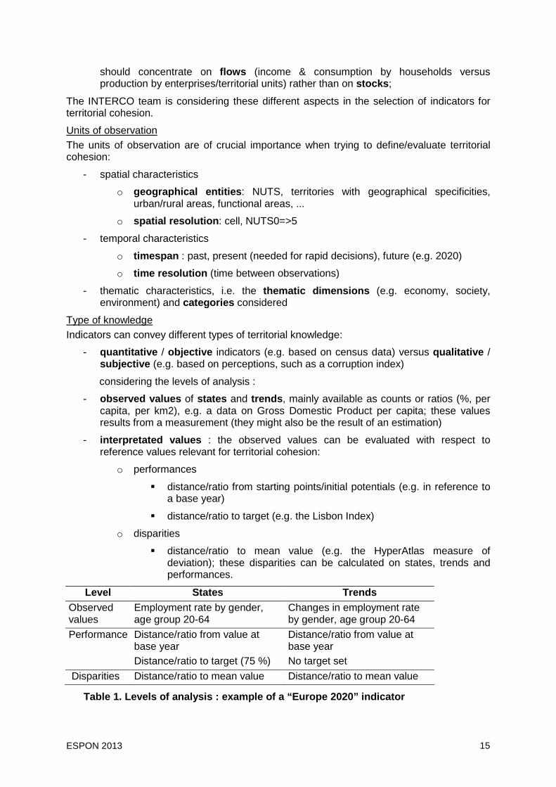
- observed values of states and trends , mainly available as counts or ratios (%, per capita, per km2), e.g. a data on Gross Domestic Product per capita; these values results from a measurement (they might also be the result of an estimation)

- interpretated values : the observed values can be evaluated with respect to reference values relevant for territorial cohesion:

o performances

� distance/ratio from starting points/initial potentials (e.g. in reference to a base year)

� distance/ratio to target (e.g. the Lisbon Index)

o disparities

� distance/ratio to mean value (e.g. the HyperAtlas measure of deviation); these disparities can be calculated on states, trends and performances.

Level States Trends Observed values

Employment rate by gender, age group 20-64

Changes in employment rate by gender, age group 20-64

Performance Distance/ratio from value at base year

Distance/ratio from value at base year

Distance/ratio to target (75 %) No target set

Disparities Distance/ratio to mean value Distance/ratio to mean value

Table 1. Levels of analysis : example of a “E urope 2020” indicator

ESPON 2013 16

The choice of appropriate levels of analysis and metrics is a key challenge of the INTERCO project. For instance, how can one measure territorial cohesion from the data shown on the graph in Figure 2 (page 13) ?

The graph shows that disparities exist between countries, some are showing better trends than other. It is difficult to set an absolute target value for this indicator. Maybe a starting point would be to state that all countries should improve, but countries lagging behind should improve more than other. These aspects will be further discussed once the selected indicators are presented in chapter 4.

Number of indicators The number of indicators to consider is also a difficult question. Given the complex nature of notions such as territorial cohesion or sustainable development, there is a strong tendancy to multiply the number of indicators in order to tackle all dimensions of the phenomenon at stake. As a matter of fact, international and national indicators systems generally include several dozens of variables.

But conversely, humans (in particular decision-makers) need to focus on a limited number of parameters for both cognitive and pragmatic reasons : simple messages are more easy to understand, decisions are more easily taken and communicated on the basis of a limited number of arguments.

That is why the prioritisation of indicators and the construction of synthetic indicators are now also promoted. This quantitive reduction eases the calculation and communication of indicators, while increasing the risk of becoming oversimplistic and to abstract.

A track followed by many institutions is to develop multi-leveled systems of indicators that comprise:

- synthetic/composite indicators , i.e. the simplification of several indicators into one single index summarising all the underlying dimensions of the issue and policy at stake;

- headline/priority indicators , i.e. a limited number (less than 20) of indicators that have the highest explanatory power and the highest relevance for the issue and policy at stake;

- analytical indicators , i.e. a full set of indicators (can be as much as 100) that provide additional insights for the issue and policy at stake;

- other data (that may once become indicators under different circumstances, i.e. if issues of interest or policy objectives are modified).

Given the very high number of potential indicators already identified in the Design phase of the INTERCO project, the TPG has decided to adopt such a 4-level approach (that was also used in the ESPON project 4.1.3 “Monitoring Territorial Development”). All levels have their relevance, specially when specific requirements by regions and local authorities are taken into account in the relation with the EU-wide policies.

The next chapters will develop these conceptual and empirical aspects of territorial cohesion indicators.

ESPON 2013 17

Gross Domestic Product - Purchasing Power Parity - per C apita

0

10'000

20'000

30'000

40'000

50'000

60'000

70'000

80'000

1'980 1'985 1'990 1'995 2'000 2'005

Con

stan

t 200

0 In

tern

atio

nal U

S$

Austria Belgium Bulgaria

Cyprus Czech Republic Denmark

Estonia Finland France

Germany Greece Hungary

Ireland Italy Latvia

Lithuania Luxembourg Malta

Netherlands Poland Portugal

Romania Slovakia Slovenia

Spain Sweden UK

Data source : The World Bank : World Development Indicators 2009

Figure 2. How to measure cohesion : the example of GDP per capita

ESPON 2013 18

2. Methodology The objective of this methodological chapter is to explain how the TPG moved from the results of the Design phase, in particular from the initial inventory of indicators, towards a selection of the indicators that are most relevant to address territorial cohesion, while keeping the links to the challenges, issues and policies expressed in the project call.

2.1. General approach : theory and participation Since the beginning of the projet, from a first broad conceptual point of view, indicators were linked to challenges, issues and policies as follows (Figure 3) :

Policy orientations

Main territorial challengesEconomic competition - Climate change - EnergyDemography – Transport - Geographic structure

DataIndicators/indices• Classical / simple socio-economic indicators• (Composite) indicators on thematic / territorial issues• New composite "territorial cohesion" indicators

Issues (to be measured and communicated)• traditional issues• complex territorial development and structural issues• territorial dimension of main challenges

require

identify

define

evaluate

respond to

realise

Figure 3. Challenges, policies, issues, indicators, data

In the second phase of the project (the Exploratory phase), the TPG developed concrete steps for making these links explicit, in order to be able to further select and calculate relevant indicators.

To this end a combined theoritical and participatory approach was applied :

ESPON 2013 19

Data

Indicators

ChallengesPoliciesIssues

Story linesstakeholders

MatricesTPG

InventoryTPG

CalculationsTPG

DimensionsTPG

Figure 4. Inventory, matrices

- the matrices are tables (in Excel format) in which challenges, policies and issues are listed along with the indicators that were found relevant by the TPG (theoritical approach)

- narratives in the form of story lines were prepared to capture in a more simple manner the complexity caused by the high number of challenges, policies and issues, these story lines were used for the discussions with stakeholders (the participatory approach)

- the results of these two previous works were further reformulated by the TPG into 7 main dimensions of territorial cohesion that served as a basis for the selection of indicators, along with criteria about data

- calculations (and mapping) of a number of selected indicators were then done by the TPG

- during this process, the initial inventory of indicators was continuously updated as new idea and information sources were provided.

2.2. The three definitions of “themes” in the INTER CO project At this stage a clarification must be provided about the various thematic approaches that were applied to classify indicators in the INTERCO project. Three different terms referring to themes are used:

- themes : this term refers to the categories of the classification scheme (nomenclature) in the inventory of indicators (note : all the indicators in the inventory were not necessary designed to measure territorial cohesion); the current themes in the classification scheme are shown in Annex 2.

- issues : they can be seen as themes (in the general sense, not only those themes of the classification scheme) of interest for territorial cohesion, hence to be measured by the INTERCO project; which themes are turned into issues is determined by challenges and policies;

- dimensions : they are the thematic focus of the narratives used to communicate with stakeholders.

The approaches to issues and dimensions are further explained in the next sections.

ESPON 2013 20

2.3. Issues : themes at stake The following figure summarize the different level of comprehension needed to be taken into account: policy orientations, territorial and global complex challenges and issues to be measured.

Summary from ESPON Project Call :

Policy orientations Territorial and global Challenges Issues to measure

- Balanced territorial development; - Strengthening a polycentric development by networking of city regions and cities; - Urban drivers (large European cities, small and medium sized cities, suburbanisation, inner city imbalances); - Development of the diversity of rural areas; - Emphasis on ultra-peripheral, northern sparsely populated, mountain areas, islands; - Creating new forms of partnership and territorial governance between urban and rural areas; - Promoting competitive and innovative regional clusters; - Strengthening and extending the Trans-European Networks; - Promoting trans-European risk management including impacts of climate change; - Strengthening ecological structures and cultural resources

- Global economic competition - Climate change - Energy supply and efficiency - Demography - Transport and accessibility / mobility - Geographic structure of Europe - Climate change impact; - Regional competitiveness; - Territorial opportunities / potentials; - Innovative creativity; - Well-being standards, quality of live, etc.

- Population and migration - Economic development and potentials - Social issues - Environmental issues - Cultural factors - Balance and polycentricity - Urban sprawl - Proximity to services of general interest - Border discontinuities - Geographical specificities - Sub-regional disparities - (Potential) accessibility - Natural assets - Cultural assets - Land (sea) use issues - Territorial cooperation options (urban-urban, rural-urban), etc.

Table 2. Policy orientations, challenges and issues

As we can see, those three levels are not of the same nature, even if there are strongly related. “Policy orientations give the current most reliable indications on the policy maker’s objectives for European territorial development and cohesion” (project specification, p. 6), whereas main territorial challenges could appear less policy-driven. Issues to be measured and communicated are a first guidance in the search for indicators of territorial cohesion. Here, following the project specification, they are divided in two groups: “simple traditional issues” and “more complex territorial development and structural issues” (project specification, p.7). These issues allow a first rough thematic selection of indicators, since the combination of several of them is required to reflect on the main challenges and on the related policy orientations. For example, to translate the “climate change” challenge in territorial cohesion terms, one needs to measure “environmental issues”, “natural assets”, “land (sea) use issues” and “geographical specificities”, in priority. Nevertheless, these issues are very broad categories that would not be useful if they are not clearly linked to the territorial dimension of challenges and policy orientations. Indeed, they are many indicators that can measure e.g. “population and migration”, and many ways to do it, whether we want to focus on states, trends, impacts, etc.

Therefore, the main challenge for INTERCO was to select indicators that have at first a high explanatory power as for specific territorial cohesion challenges and EU policies territorial priorities. In this frame, in a first stage of our work we have examined which groups of themes must be used to study the major relevant themes that are behind each territorial challenge and policy orientation and, therefore,

ESPON 2013 21

determine which indicators are the most appropriate for the analysis of these relevant themes. Thus, policy orientations, challenges and issues are a solid basis for the search of indicators, but as such they cannot deliver full guidance. It is their translation in territorial cohesion terms, by identifying how there are related to territorial cohesion, that is crucial for our work, as well as the attempt to cross them, in order to make the linkages more evident. Storylines (see below, section 2.4) and dimensions (2.5) were developed in this context.

2.4. Storylines To develop indicators to measure territorial cohesion, it was necessary to sharpen the understanding of what territorial cohesion may comprise. Over the last years, debates have shown that a precise definition of territorial cohesion is impossible. Because different groups of stakeholders focus on different dimensions of the territorial cohesion idea, any attempt to define it will exclude certain understandings and thus lead to a poorer result.

Consequently, the ESPON INTERCO project has decided to develop different stories about territorial cohesion. Each of these stories highlights different facets of the territorial cohesion debate as observed during the past decade. These stories are not mutually exclusive. However, there may be contradictions between the different stories. The five stories of territorial cohesion are presented in Annex 3.

The stories have been the organising principles of the stakeholder workshops organised. This facilitated a more thorough discussion on the different facets of territorial cohesion and how a limited number of indicators can be used to illustrate or measure the single facets. After a few overall conclusions from the workshops, the results of the workshop discussions will be presented for each storyline.

The workshops organised were:

• ESPON MC workshop – Key storylines for territorial cohesion 16.11.2010, Liege The workshop discussed the different storylines with regard to their policy relevance. Furthermore, the weighing of the different storylines with regard to their policy relevance was discussed.

• ESPON seminar workshop – Investigating measurable s torylines 17.11.2010, Liege Based on the wide experience within ESPON, the storylines for the operationalisation of territorial cohesion were discussed - incl. the balance between them. Thereafter, for each of the storylines, the themes to be addressed were discussed in smaller groups.

• ESPON seminar workshop – Liking indicators to the s torylines 18.11.2010, Liege The workshop built on and deepened the discussions of the workshop of the previous day with new participants. The focus moved towards concrete indicators fort he single storylines and also the relations between them.

• External workshop – Territorial cohesion indicators 14.01.211, Brussels The workshop addressed policy makers from different sectors and different geographical levels usually not participating in ESPON events. The focus was on their understanding of territorial cohesion and what kind of territorial indicators can support them in their daily work.

The list of consulted stakeholders can be found in Annex 4.

ESPON 2013 22

2.5. The dimensions : toward a synthetic approach t o territorial cohesion The work on the storylines and the results of the workshops enabled a better understanding of the policy demands, the stakeholders’ expectations as well as of the concerns of scales and the specificities of each territory. We synthesised those elements in an internal discussion paper (Annex 5) which enabled us to have a broad overview, so that we make sure to include all challenges, policy orientations and issues. Crossing these challenges, policy orientations, issues between them and with the stakeholders demands, we identified the major territorial cohesion issues to be covered, and searched for indicators closely related (see Annex 5, chapter 4). Through a detailed vision, we tried to establish clear linkages and to find precisely what should be measured.

This work was necessary to identify the themes that would be relevant for every territory. Moreover, thinking about the meaning of “cohesion”, we deemed that measuring disparities could be done after the selection of indicators, during their calculation. Therefore, we decided not to include issues related to scales and geographic characteristics. On the basis of this preliminary work, we retained seven dimensions to explore territorial cohesion:

- territorial structure

- networking

- competitiveness

- innovation

- accessibility and inclusion

- quality of environment

- cooperation

These dimensions will be discussed in more details in the next chapter. Their role is to be the crossing points between the relevant themes defined by the challenges and the policy orientations on one hand, and the issues to be measured and the indicators on the other hand. Their denomination can seem neutral, but it is a way to get closer to the indicators selection after more attention paid on the challenges and the policy demand. Moreover, they integrate fully the stakeholders’ requirements and they review from scratch the different levels of analysis made from the beginning.

Thus, each dimension is related to several challenges and several policy orientations and issues. The indicators chosen to measure them can be sometimes similar, but they will vary according to the scale considered, and the purpose (policy goals, issues at stake). For example, observing roads networks can be meaningful for territorial structure as well as for accessibility, but not in the same way.

More over, these dimensions should not be understood are being from the same nature, and do not follow any hierarchy. Indeed, some of them are “enablers” (innovation, cooperation, networks), whereas other can be seen as outcomes (quality of environment). They are not related in the same way to territorial cohesion, as we can see when detailing them, but they allow a synthetic approach of it that fits better with the search for indicators and the calculation of them. Indeed, by focusing on thematics shared by all territories, they leave room for the role that metrics and scales can play afterwards, when measuring disparities.

ESPON 2013 23

2.6. Selection and calculation of the indicators A first selection of indicators was already made for the storylines by the TPG and it has been updated after the results of the workshops. The seven dimensions allow us to focus on few themes, reducing the criteria for selection since indicators have to cover these dimensions. More over, indicators have to be very close to each element within the dimensions. To that end, detailing them by showing the linkages between each factor was crucial. A second criterion was the will to begin with indicators on impacts (related to well-being and sustainability for example) that territorial cohesion is supposed to improve, and give less importance at this stage to indicators on means put in place to achieve these goals. For instance an indicator on environmental quality is preferred to a one on expenditures for the environment. This criteria is a subject of discussion, since the efforts done also deserve attention. The third criterion was of course the data availability, as explained in next chapter.

Then, calculation of indicators has started. Beginning with the evaluation of the data availability, we have then proceeded, for those available, to their acquisition, documentation (metadata) and structuration in a GIS database (see Annex 7 and Annex 8). Then indicators were calculated, mapped, presented and discussed in factsheets grouped in thematic categories of the classification scheme.

ESPON 2013 24

3. Indicators selection

3.1. Results from the workshops Overall conclusions from the workshops Any attempt to draw overall conclusions will only result in incomplete reflections. However, it appears that there are some issues which were recurrent in the discussions about the various storylines. Among those are:

• The storylines developed for discussing the various facets of territorial cohesion have been confirmed and work for structuring a debate which allows all participants to set their own priorities of what is the most important dimension of territorial cohesion.

• The need for flexible geographies and different levels of detail of geographical information depending on the questions to be assessed. Most prominently was the plea for data at the level of functional regions.

• It has also been debated at several occasions whether the most prominent need is on indicator or on territorial typologies identifying and grouping territories with similar development preconditions for further assessment of performances of comparable territories.

• In many discussions about territorial cohesion, the focus was less on a European-wide picture of a cohesive territory but rather on the different preconditions for development, growth and contribution to the aims of Europe 2020 in the different areas.

• In addition to the rather strong growth emphasis of the European policy debate at present, the discussion stressed the issue of quality. This concerned the quality of infrastructure and services as well as the quality of life and policy making.

• When it comes to indicators allowing for measuring the overall state of play of territorial cohesion at European level, the discussions revealed hesitation as to whether such an indicator is meaningful and possible.

• Last but not least it has been stressed that the policy makers rather demand simple and useful indicators than complex indicators.

Considering alternative territorial entities Concerns over the limited heuristic value of data compiled and mapped at the level of NUTS regions were voiced during the INTERCO workshops. Some participants argued that analyses based on functional regions would provide evidence that would be more useful for the design and implementation of policies promoting territorial cohesion. The ESPON Database project has made considerable progress identifying commuting regions based on LAU2 units around towns and cities of more than 20,000 inhabitants across most countries of the ESPON area. These are first based on the identification of so-called “morphological urban areas” (MUA), i.e. urban core LAU-2 unit with a population density of more than 650 inh./km2 (IGEAT et al., 2007, p. 8). As a second step, LAU2 units with more than 10% in-commuting to these MUA municipalities are identified. These LAU2 units are then associated with the MUA in direction of which the largest commuting flows occur, and identified as forming the corresponding Functional Urban Area. This allows for a distinction between the urban and rural spheres in Europe, and also between in labour basins of cities of different sizes. Notwithstanding these important qualities, FUAs only represent one type of functional areas in Europe, i.e. labour market areas. These can in some respects be considered as a proxy for urban daily mobility areas. However, they do not

ESPON 2013 25

correspond to the functional areas of e.g. higher education or to the areas within which agricultural and manufacturing production systems are organised. Basing territorial analyses on “Functional Areas” would presuppose a delineation of the geographies pertaining to each of the sectors of activity that are considered. Because of the multiplicity of interaction modes and ranges, a synthesis of results would not be trivial.

One may furthermore note that Functional Urban Areas are mutually exclusive: individual LAU2 units area associated to the MUA to which the highest proportion of the economically active population commutes. This implies that contrasts between cities and towns at different levels of the urban hierarchy are amplified, as only a limited proportion of the LAU2 units from which in-commuting to secondary towns in the vicinity of larger cities are actually included in the FUA of these secondary towns.

Finally, FUAs are necessarily based on current commuting patterns. This provides useful information on the ways in which daily mobility patterns are organised around cities. However, it does not necessarily offer an optimal basis for strategic policy-making, insofar as one of the objectives may be precisely to promote alternative, more ecologically and socially sustainable, modes of mobility. Analyses based on current functional areas may therefore be complemented by alternative ones based on politically defined objectives in terms of mobility ranges and choice of transportation modes.

It is also important to note that one can consider functional contexts of territorial development without delineating regions and areas, simply by compiling data that describe the surroundings of each LAU2 unit rather than considering its internal features, as illustrated in Figure 1. The definition of the relevant “surroundings” may either be based on normative considerations on the desirable interaction ranges, or on an empirical observation of the spatial patterns of flows, mobility and exchanges. The GEOSPECS project has demonstrated that it is possible to construct calculations on time-distance based potential across the ESPON space, even if these calculations require considerable computing time. These calculations of so-called “potentials” around each locality, i.e. the sum of all values occurring in the LAU2 units in their vicinity, are particularly relevant to assess the territorial development context of rural and secondary nodes.

Overall, the overlay of current functional areas, identified from different sectoral points of view, to which one may add other functional areas based on strategic objectives regarding mobility ranges, transportation modes and spatial patterns of interaction and exchange, creates a complex system. The challenge for the formulation of territorial cohesion indicators would be to combine the different types of delineations. This would generally imply a greater focus on how the administrative and political regions in interaction with which through territorial policies are designed and through which they are implemented relate to this variety of functional contexts.

ESPON 2013 26

Source: University of Geneva, ESPON GEOSPECS

Figure 1 Calculation of potentials

Data associated to all LAU2 of which the centre point falls within the 50 km circle or area accessible within 45 minutes are summarised; this sum is the “potential”. This means that the same data is taken into account as many times as they are associated to LAU2 units that are part of the potential functional neighbourhoods of the points of measurement.

Another way of defining areas that would share common characteristics is to proceed with typologies such as those developed by the ESPON Database project using clustering techniques based on statistical data at NUTS levels1. This approach might help in the reflection about the need by some stakeholders for specific indicators depending on the type of areas considered.

The next chapter will further expand the results of the workshops as well as of the Inventory of indicators by defining synthetic dimensions of territorial cohesion.

3.2. The dimensions As already said previously, INTERCO has decided to develop a multi-dimensional approach of territorial cohesion, in order to make easier the link between policy demand, territorial challenges and the selection of indicators. Here are the seven dimensions in details.

1. Territorial structure Territorial cohesion is strongly related with the territorial structure of European territory, i.e. how it is spatially organized and shaped, at all scales. The objective of “harmonious and balanced development” (article 174 TFEU) which is assigned to the European Union (EU) from its very beginning has not been reach as regards territorial structure. A “pentagon” has emerged, concentrating population, wealth production and command functions in an area delimited by the metropolitan areas of London, Paris, Milan, Stuttgart and Hamburg. There is a huge challenge of concentration, as expressed by the Green Paper, which concerns on one hand the negative effects of concentration and on the other hand the returns of agglomeration

1 Interactive Workshop – ESPON Database 2, ESPON Seminar Alcala presentation 10 June 2010, http://www.espon.eu/export/sites/default/Documents/Events/OpenSeminars/MadridJune2010/Database2_How-to-use-ESPON-data.ppt

ESPON 2013 27

which benefit to the surrounding areas. Thus, a “cohesive spatial structure”, to quote previous ESPON 4.1.3 project1, means reducing disparities between centre and peripheries, at all scales, connecting cities between them and with other areas, especially rural, and avoiding negative externalities. These challenges where already mentioned in the ESDP, which proposed a bridging concept to address them, namely polycentrism. Polycentric development first concerns urban system and urban-rural relations, which should avoid dualism. A “polycentric settlement structure across the whole territory of the EU with a graduated city-ranking” is seen as “an essential prerequisite for the balanced and sustainable development of local entities and regions” (parag. 71) and for the EU’s advantage at global scale. More gateway and compact cities are thus needed, to help facing the environmental challenge which requires greener infrastructures of transport. The challenge is to strength and extend the Trans-European Networks while strengthening also ecological structures, which are fully part of balanced territorial development. Indeed, polycentricity is not a goal in itself but a mean to achieve economic competitiveness, social equity and sustainable development (ESPON 1.1.1).

As far as indicators are concerned, the degree of polycentricity could be approached through the set of indicators developed in ESPON on MEGAs and FUAs. Further on, for the study of the functional integration around cities, ESPON indicators on the definition of Potential Integration areas (PIAs) through commuting and accessibility as well as new indicators on the labour force attracted by cities are necessary.

Nevertheless, recent studies have questioned this overarching concept and moderate the belief that polycentric development helps fighting against imbalances, particularly at regional and local level. Indeed, urban system at national level can be monocentric without increasing regional disparities (Sandberg, Meijers, 2006). Therefore, it seems important to observe the structure of the European territory without looking a priori for polycentrism. The objective of balanced and harmonious development may endure other structure models.

2. Networking Strongly related to the structure are the networks which allow concentration, connection, access, partnership and cooperation. The emphasis on networks seems to have followed the emergence of polycentrism, since they are central for polycentric development. The Territorial Agenda make it its first priority for territorial development of the EU, stating that city regions and cities should implement “networks in a polycentric European territory in an innovative manner”. This will “create conditions to allow them to benefit global competition in terms of their development.” (art. 14). Networks are also at the centre of the next priorities of TA, namely “promote regional clusters of competition and innovation in Europe” and “strengthening and Extension of Trans-European Networks”. The three domains of the Trans-European Networks (TEN), namely transport, energy and communication, show that networking is not only about inter-modal transports but also about reliable connections to energy networks and information and communication technologies (ICT).

If interconnections of European hubs or MEGAs are crucial for global competitiveness, secondary networks are also of key importance for local and regional development. Their smart extension and modernisation, in order to improve their efficiency and to reduce costs, will also be a way to make them compatible with environmental concerns. As for immaterial networks which allow linkages between, e.g. universities, research centres and businesses, there are central for the

1 The work package “cohesive spatial structure” of ESPON 4.1.3 was significantly named “territorial cohesion” in a first time, but the team decided to change because this concept was too broad.

ESPON 2013 28

emergence of clusters and the connectivity of firms, as well as for the access to knowledge (e.g. e-learning) and to on-line services. There is still a lot to do for broadband coverage: its extension is critical as regards inclusion and accessibility and for “bridging the digital divide”.

Networking has also an international dimension, for example in the energy field, where external networks are crucial for cooperation with producing, transit and consuming countries, as the European Council remind it on February 4th, putting emphasis on the contribution of secure and affordable energy to competitiveness. Finally, (inter)connection and networking are factors of greater and better circulation of people, wealth and knowledge, thus enhancing cohesion among more integrated territories, while allowing them to spread their assets.

Therefore, for this dimension, we need among others indicators on the structure, more precisely on density and capacity of the transport networks per mode: road, rail, air and multimodal transport, per transport category (passengers and freight transport) and per territorial level: local, regional national, international. The use of indicators on the transport costs and employment will allow evaluate the overall territorial structure of transport / communication. We also need specific indicators on the urban transportation or the use of telematics in transport networks which are of priority for EU policies (new indicators).

3. Competitiveness To face the challenges of globalisation and to recover from the crisis, Europe has to be competitive on global scale, but also to boost competitiveness among its territories.

Global competitiveness was already the main goal of the Lisbon Strategy, which aimed making Europe “the most competitive and dynamic knowledge-based economy in the world”, and the current Europe 2020 Strategy follows this direction whilst detailing the ways to “get back on track and to stay on track” (Barroso’s foreword). Europe has to enter in a “new economy”, based on knowledge and innovation as means to face new challenges, and competitiveness is still at the heart of the new strategy, since the focus is on growth, declined in 3 aspects: smart, inclusive and sustainable growth.

In that context, urban areas, from small towns to metropolitan regions, are seen as key elements to wealth (=>urban drivers), and they have to keep being competitive, to be more connected to the global scale. Global cities have to reduce their negative externalities, becoming more sustainable, especially as regards transports and energy. For lagging regions or cities, they should make full use of growth potentials and facilitate knowledge, mobility and innovation, to become more competitive on regional scale. Clusters and innovation are expected to be at the heart of regional competitiveness. At all levels, efforts have to be made on productivity, employment and attractiveness, with the aim to improve business environment, especially for small and medium size enterprises.

The objective of competitiveness could appear rather opposite to that of territorial cohesion (Héraud, 2009), since it can lead for example to polarisations. A certain degree of concentration (of means, of critic mass, etc) is needed to gain in competitiveness. But the rationale is that balanced economic development of the European territory is possible only if global cities remain competitive and if other cities and territories seek to boost their competitiveness, in order to join the regional, national or global network. More over, the means of competitiveness, e.g. knowledge, innovation and ICT networks should be reachable for every territory, in order to allow them turning really their specificities into strength and to face current challenges.

ESPON 2013 29

Therefore, as regards indicators, it is first necessary to examine the regional income, consumption and investments at lower than the NUTS3 level, if this is possible. Specifically, we should use indicators of regional GDP per capita as well as per employee and economic activity; the income of households and the exportations should also be considered (see the list of proposed indicators in Annex 9) The analysis of firms’ division of labour enhances significantly the analysis of the regional economy through GDP. Better indicators for this issue, are those referring to the location of the international headquarters and the change of the location of the business per branch.

It is also necessary to study the regional labour force, employment and unemployment, because it completes the approach of the driving forces of the location of economic activity, but also the analysis of the social impacts of development. To resume, several indicators for this dimension would ideally need low level data, in addition to those that the global competitiveness challenge also requires.

4. Innovation Innovation was already at the centre of Lisbon Strategy but had been identified as not fully exploited (Aho Report, 2006). A “European year for creativity and innovation” (2009) and an Innovation Plan have followed, and now innovation has permeated all fields of European policies, being the first flagship initiative of the Europe 2020 Strategy. The headline target of investing 3% of GDP in R&D of the Strategy reinforces the goals of the decision of 2006, which defined innovation as “comprising the renewal and enlargement of a range of products and services and their associated markets; the establishment of new methods of design, production, supply and distribution; the introduction of changes in management, work organisation, and working conditions and skills of the workforce; and covers technological, non-technological and organisational innovation.”1 The main policy involved in innovation, in accordance with this definition, is Industry. The Innovation Union Scoreboard (IUS 2010) published in 2010, which a “new tool meant to help monitor the implementation of the Europe 2020 Innovation Union flagship”2, has now based innovation on eight dimensions:

- human resources

- research systems

- finance and support

- firm investment

- linkages & entrepreneurship

- intellectual assets

- innovators

- economic effects

Moreover, it has created combined indicators for inputs and outputs at national level. The lack of data at regional level does not reflect the importance of innovation for regional and local development. The Commission is now invited by the European

1 Decision No 1639/2006/EC of the European Parliament and of the Council of 24 October 2006 establishing a Competitiveness and Innovation Framework Programme (2007 to 2013), recital 8. 2 http://www.proinno-europe.eu/inno-metrics/page/innovation-union-scoreboard-2010

ESPON 2013 30

Council, which has recently put the emphasis on innovation, to develop a single integrated indicator1.

Considered as a key element for competitiveness and growth, innovation is seen as central for regions, because it can help creating and distributing wealth. It is the main way for territories to “turn diversity into strength”2 and to face environmental challenges, including energy. “Eco-innovation” is expected to deliver appropriate response to the need of energy efficiency and “environmentally friendly” processes. Thus, research and development should not be only for top class territories and actors. Innovation potential should rather be accessible for every territory. As organisations such as CPMR3 calls for, there is a strong need for more synergy between Cohesion Policy and European programs for R&D, competitiveness and innovation4. Otherwise, bringing together education, research and business could lead to the same concentration that already exists in competitive cities.

This contributes to make even more urgent a broader definition of innovation, which should includes culture and focuses more on creativity. The consultancy KEA denounces that “so far, these strategies [of innovation] have almost exclusively focussed on technological development and research expenditure. On the contrary, “they should embrace the concepts of people-driven innovation and related soft skills, including the notion of creativity. The role that the arts, culture and the creative industries play in fostering a more creative and innovation friendly society as well as a more competitive and sustainable economy should be more strongly reflected by EU innovation policy makers.”5 The innovation theme, in the context of territorial cohesion, should integrate fully this essential dimension, while using at best the existing national and regional indicators of the IUS 2010.

5. Accessibility and inclusion Despite their diversities, territories and people must have the same chances and opportunities. To that end, they should benefit from equal development potentials and from well-being standards. This double demand brings together territorial cohesion with the concept of European Model of Society (EMS), from which Faludi has shown the “common roots”: for him, “the shared concerns are equity, competitiveness, sustainability and good governance and the balancing of these concerns against each other.”6 If EMS is more abstract, territorial cohesion gives it a spatial expression, especially with the concerns of service provision, accessibility and social inclusion. They all contribute to cohesion and territorial integration, reminding that market is not everything. A “spatial justice” is required, putting the focus no more on people (social justice) but on territories (Davoudi, 2005). Accessibility and access to material and immaterial goods are considered as one of the ways to reach it.

1 Conclusions of the European Council of February 4th, 2011, article 17. 2 Green Paper on Territorial Cohesion, 2008. 3 Conference of Peripheral and Maritime Regions, “Putting the regions and the territorial dimension at the heart of synergies between regional policy and the RTD and CIP Framework Programme”, Position Paper, October 2010. 4 Mainly the Framework Programme for Research and Technological Development and the Framework Programme for Competitiveness and Innovation. 5 KEA European Affairs, 2009, “Contribution to the European Commission’s public consultation on Community innovation policy”, p. 1. Available at http://www.keanet.eu/docs/contriinnovationpolicy.pdf 6 A. Faludi, “Territorial Cohesion Policy and the European Model of Society”, Paper for AESOP Conference, Vienna, 2005. See also his collective work on the same topic, Faludi, A. (dir.), Territorial Cohesion and the European Model of Society, 2007.

ESPON 2013 31

The other dimensions of accessibility and access are their role in endogenous development, since they permit to every territory, whatever its territorial capital, to increase its development (particularly thanks to ICT) and to participate to global competitiveness. Emphasis should be put on ultra peripheral regions (UPR), northern sparsely, mountain areas, islands, coastal and river zones, where local accessibility play a key role, but also on areas affected by the “tunnel-effect”. But better accessibility may not be enough, and on the contrary we have famous examples of remote areas which are competitive despite their low accessibility. In any case, accessibility and infrastructures of all types are crucial for cohesion since they should contribute to the reduction of disparities. At the end, inclusion of territories is the spatial dimension of social inclusion, which means essentially reduction of poverty and access to basic services, jobs and market. In a word, accessibility and inclusion is about quality of life and participation of every territory to a balanced and sustainable development.

Hence, for this dimension, we need indicators measuring different aspects of accessibility and connectivity: potential accessibility to regions or to population, accessibility to public services (health, education) or to market, connectivity to airports, motorways, railway stations, health and education facilities as well as ICT connectivity (new indicator). We also need some basic indicators on the population change rate, the population versus the resident population potential as well as the population density. Further on, indicators on population ageing per gender, dependency rates, life expectancy, crude birth and death rates as well as on fertility rate are necessary in order to come to the changes on the population growth rate. It is also necessary to study some crucial characteristics of the households: Lone-person / Lone-parent, including children, living in owned housing or in social housing etc. Also, the analysis of the citizenship allows us to study the regional process towards multi-cultural local communities.

6. Quality of environment The environmental matter is crossing the various dimensions of territorial cohesion but constitutes also a crucial aspect of it. First of all, one has to say that nature, environment and the sustainable concern are not referring to the same thing. Environment is not only nature, and sustainability does not concern only environment. Indeed, following the Brundtland Report (1987), the Commission defined sustainable development as “meeting the needs of current generations without compromising the ability of future generations to meet their own needs” 1. It is more related to quality of life rather to only environment. The EU Sustainable Development Strategy has identified several priority challenges such as public health, social inclusion, demography, migration and poverty, which are also included in the Europe 2020 Strategy (and where already included in the Gothenburg Strategy). The resources and risk aspects are well covered in this strategy, but more quality-oriented questions have been long time avoided by concrete European actions, despite the international engagements of the EU. Biodiversity, for example, declared theme of the year in 2010 by the United Nations, were not a category of spending of the Structural and Cohesion Funds till 2007, whereas it is recognised that Cohesion Policy has a great role to play in that specific field as well as in broader environmental objectives. The latter were rather missing from the Green Paper on Territorial Cohesion (2008), although there is no territorial cohesion apart from environmental concerns.

Speaking of environment quality, in our sense, encompasses three dimensions: risks, resources and quality of life. Climate change is a global challenge which must be tackled at all scales and it represents a multi-dimensional risk for territories, since its 1 COM (2011) 17, “Cohesion Policy contributing to sustainable growth in Europe 2020”, p. 10.

ESPON 2013 32

impacts are numerous and asymetric. A low-carbon economy is required, through environmentally friendly technologies and improved energy efficiency. In particular, urban transportations have a key role to play. But reduction in green gas emission is not the only answer to natural hazards. Environmental policies should also pay attention to their own impact on environment. Thus, environment can be seen itself as a risk (floods, earthquakes, etc) and is at the same time subject to risks (e.g. pollution).

This double environmental challenge can be turn into opportunity for territories, using the new constraints to promote innovative solutions. To that end, renewable energies are essential, especially for local potential. All natural assets can thus be used for development and preserved at the same time, for example through ecological tourism. The geographic specificity of European territories becomes an asset for them, as it enables them to bring appropriate responses, fitting to their characteristics, even if they are all differently affected by environmental challenges.

Smart and sustainable use of natural resources will also help protecting environment as an irreplaceable component of quality of life. Indeed, a healthy environment with preserved landscapes is an asset for Europe as a whole, and this is not possible without improvement of environmental services at local scale, especially in cities. Waste water treatment networks, noise reduction and cleaning up, for example, are part of this process. Finally, better quality of life in a preserved natural patrimony will ensure attractiveness of Europe as a smart and sustainable place.

Thus, indicators on the causal links among the economy and society with the environment in the frame of the sustainable development option are of primary importance for this dimension. It is also essential to provide appropriate indicators that could reflect the current and the potential quality of the environment and of the management regarding natural assets as land, air, water resources. Therefore, respective sets of indicators refer to Ecosystems (biodiversity, biomass, share of sensitive eco-regions etc), Water, Landscape (e.g. visual attractiveness, cultural heritage including agricultural landscapes etc), Food, Agriculture and Seas - fishing (e.g. status of marine fish stocks) (see in the list of indicators) or to protected areas (e.g. coverage of protected areas NATURA 2000) and environmental services.

For the study of the climate change, we should use indicators regarding its impacts on the environment but also on the economy and the society. Both indicators refer to the prevention of the climate change and the mitigation of its impacts on territories, such the indicators on the rise of the sea level, the temperature changes, the impacts on different sectors and the natural risks (e.g. groups of population, regions and activities which are more sensible to climate change). Priority is given to complex indicators such the Tourism Climate Index (5th CR) or the “Climate change index” (“Regions 2020”), which is based on a wide range of simpler indicators crossing environmental and socio-economic parameters.

As for renewable energies, since their exploitation is a priority in EU existing policies and perspectives, we should use appropriate indicators for both the total of renewable energies and per category of sources: photovoltaic, wind power, solar energy potential and production. It is also useful to include the different territorial aspects of energy in a complex territorial index. A first relevant index -“Energy Index”- has been produced by “Regions 2020”. It uses variables on the energy consumption, the national energy import dependency and the national carbon content of gross inland energy consumption.

7. Cooperation Cooperation could be seen as a non territorial theme if it is mixed up with governance or if it is considered only as a way of management. In our sense, cooperation includes territorial governance which is inseparable from territorial cohesion. Indeed,

ESPON 2013 33

the Territorial Agenda states that “territorial cohesion can only be achieved through an intensive and continuous dialogue between all stakeholders of territorial development”, i.e. a process of cooperation called territorial governance. More over, territorial governance is double-face, since on one hand it focus on spatial impacts of policies and on the other hand it is part of the territorial cohesion process (see ESPON 4.1.3 part B p. 65).

The cooperation dimension has this particularity to refer on both policy process and territorial integration itself. Motor of the European construction from the very beginning, cooperation took place between states but also between regions, beyond national borders. The INTERREG program has encouraged this trend, helps regions to work together on common projects, often at a very local scale. If the Cohesion Policy as a whole may present mixed results as regards territorial integration, it had been demonstrated that cross-border and interregional cooperation play a key role for effective territorial integration. The three dimensions of INTERREG are now integrated in the overarching objective of European Territorial Cooperation (ETC), and the Strategic Guidelines for Cohesion for the period 2007-2013 take them up as such, stressing that cooperation expresses the territorial dimension of Cohesion Policy. The Green Paper (2008) make cooperation the third aspect of territorial cohesion, divided in three dimensions: inter-regional, cross-border and trans-national.

The need of cooperation comes from the necessity to bring a common and coordinate answer to challenges which do not know any border, such as climate change. The risks related to it need actually a trans-European management which can be done only through cooperation at al scales. Migration and energy supply and efficiency are also the current main challenges which ask for greater coordination and partnership. More over, partnership must be improved between small cities and between urban and rural areas, to allow the latter to benefit from agglomeration rather than suffering of it. Rural areas surrounding cities have a great role to play and this can not be done with the actual dualism which divide or even oppose them. New forms of partnership will help reducing congestion costs, improving water and waste management and quality of life in both cities and countryside. This can also be a way of diversifying and developing rural areas.

More generally, the possibility to cooperate easily, beyond administrative borders, is a chance for every territory to pool resources, means and outputs and thus to take full advantage of common actions. That is the reason why cooperation is crucial for territorial cohesion. It aims at bringing together territories, at achieving territorial integration. And this will be a way for territories to be more efficient as regards competitiveness, since cooperation can help reducing inutile costs and increasing market size. As such, cooperation can be considered as “a midwife for territorial cohesion and an essential tool for European recovery and resilience”1.

3.3. The dimensions viewed at global and local scal es Almost for each dimension, it is clear that the themes at stake can be considered at various scales. Thus, there is a need to think about how to deal with the different levels, especially as concerns global and local ones.

From the outset, it may seem odd to take a global outlook of territorial cohesion, and there is also a risk of sounding very Euro-centric in attempting to project the European territorial development paradigm outside its borders. In spite of this, we

1 First ESPON 2013 synthesis report, New evidence on smart, sustainable and inclusive territories, p. 29.

ESPON 2013 34

deem that it makes sense to use a global approach for investigating territorial cohesion on at least two accounts.

The first one relates to the acknowledgement that, even if ‘territorial cohesion’ is not mentioned explicitly, other international organizations have taken up similar stands on the future of territorial development policies1. Consequently, not only can the European experiment of territorial cohesion can be useful in feeding in that process, but it also emphasize the need to see the territorial cohesion processes within Europe as a link with other processes that occur in its close vicinity (neighbourhood), but also further away. Moreover, it seems that there is a certain momentum regarding new deals for territorial development policies in many countries outside the EU, for instance in the OECD2.

The second one relates to the nature of globalization itself. The increase in interdependencies between states and regions worldwide implies that achieving territorial cohesion in Europe is only possible if one brings into the picture the necessary ways of mitigating and adapting to global processes connected to trade, demography, migration, climate change or energy consumption/production.

If territorial cohesion can be perceived as a multifaceted notion, Globalisation is as well a term that is used in many ways, but the principal underlying idea is the progressive integration of economies and societies, according to the WCSDG report3. It is driven by new technologies, new economic relationships and the national and international policies of a wide range of different actors. This report identifies also a number of elements of the EU model as having contributed particularly to its success in improving living and working conditions: a strong legal framework; openness to the world economy and an effective market economy; supportive national social protection systems and common minimum standards for employment; involvement of the stakeholders; gender equality; and, more widely, respect for human rights and the rule of law, democracy and the strengthening of democratic supervision.

The problem of Multiscalarity An important aspect to have in mind when approaching territorial cohesion at several scales is the element of ‘multiscalarity’ which refers to the fact that the degree of cohesion can fluctuate according to the scale it’s applied. Thus spatial disparities at, for example the national level may be masked if the analysis is up-scaled to the EU or global level or down-scaled to regional or local levels.4

As an example Davoudi (2007) mentions how the pursuit of polycentricity at the EU level has led to monocentrism at national level, represented by concentration of population and economic activity in capital cities or major urban centres; another example is presented by Schön (2005)5 when referring to socio-economic developments in which cohesion between the EU Member states increases while disparities between regions are constantly growing.

1 See World Development Reports at http://econ.worldbank.org/WBSITE/EXTERNAL/EXTDEC/EXTRESEARCH/EXTWDRS/0,,contentMDK:20227703~pagePK:478093~piPK:477627~theSitePK:477624,00.html 2 Yamazaki-Honda, R. (2005) Territorial Policy in OECD Countries, appears in Planning Theory and Practice, Vol. 6, No. 3, p. 387-413, September 2005 3 Definition used by the World Commission on the Social Dimension of Globalization (WCSDG) prepared by ILO the International Labor Office: http://www.ilo.org/public/english/wcsdg/globali/index.htm 4 Davoudi, S. (2007): Territorial Cohesion, the European Social Model and Spatial Policy Research; appears in Faludi, A. (2007). Territorial Cohesion and the European Model of Society, p. 81-101 5 Schön, P. (2005): Territorial Cohesion in Europe?; appears in Planning Theory and Practice, Vol. 6, No. 3, p. 387-413, September 2005

ESPON 2013 35

These studies have already shown that the multiscalar dimension of territorial cohesion is difficult to handle within Europe, so we can imagine that it is not going to get easier by adding up the global scale. The multiscalar dimension of territorial cohesion is already present when looking at territorial development policies: the quest for territorial cohesion is framed between the inter-national (e.g. with policy initiatives taken by the EU or the World Bank) and the multi-national (e.g. with similar policy initiatives taken within many countries across the world).

One simple conclusion to the above is that the inclusion of the global scale in our work should not be ‘plastered’ over the analysis of the other scales, but should rather feed a specific purpose, i.e. enhancing our understanding of the processes occurring within Europe by framing them in broader perspective.

An important standpoint from the outset is that, according to Taylor1, “geographical scales are social constructs that should not be reified”. Consequently, the global, the one that ‘really matters’2, understood as the territorial representation of the processes of “stretching and deepening of social relations and institutions across space and time”3, cannot be conceived as equivalent to worldwide, which is a static, both in space and time, territorial contour.

Limitations for global and local indicators We have discussed earlier the difficulty to define what the global entails, especially in terms of thematic focus, geographical coverage and territorial level of investigation. The conceptual approach to the global (and the local) needs thus to be pragmatic and tailor-made for each of the dimensions. Yet, beyond the conceptual challenges, the empirical limitations may seem at least as overwhelming. Indeed, the possibility to construct global indicators for territorial cohesion is strongly dependent on the availability of data for territories outside the Europe, which means that such data cannot be derived from the Eurostat office. Furthermore, there is no database that provides access to regional (i.e. NUTS 2 or 3) data on a worldwide basis. When worldwide coverage will be needed, the comparative analysis will be made at the lowest level available, i.e. the NUTS0 (country) level. However, for some specific theme, the comparison can be performed for specific territories, and especially urban areas, for which specific datasets are often available. Other data such as point data (for instance regarding localisation of natural resources) will be sought. When it comes to the local scale, the analytical dimension will be implemented by conducting ‘zoomed-in’ analysis. In concrete terms, this will imply an analysis of disparities within a NUTS 2 or 3 region in a selection of countries. This will require the compilation of LAU1 or 2 data. Consequently, we deem that it would be more practical to compile data for countries covered by TPG partners, i.e. Germany, Greece, Sweden and Switzerland.

Identifying key themes of Territorial Cohesion in a global scale In line with the claims made by many knowledgeable researchers on territorial cohesion, there is not a simple, straight way to develop global indicators for territorial cohesion. Consequently, the ‘multiple dimensions’ approach fits very well to this need for tailor-designed global indicators.

1 Taylor, P.J. (2008) Cities, world Cities, Networks and Globalization, GaWC Research Bulletin 238, http://www.lboro.ac.uk/gawc/rb/rb238.html 2 Taylor, P. (1982) A materialist framework for political geography, Transactions of the Institute of British Geographers NS 7 15-34, cited in Marston, S.A., Jones, J.P. and Woodward, K. (2005) Human geography without scale Transactions of the Institute of British Geographers NS 30 416-432 3 Held, D. (1995) Democracy and the Global order. Cambridge: Polity.

ESPON 2013 36

For each of the dimension developed in the project, the first step of the methodology was to answer the following basic questions:

- What does ‘the global’ mean in this dimension?

- To what global processes does the dimension relate to?

- How can it be operationalised in terms of thematic focus?

- At what territorial level and for what geographical coverage should this phenomenon be measured?

- What currently existing global indicators can fit in this approach?

Another step is identification of key themes of relevance for territorial cohesion in a global scale, in relation to the three central features revealed by Camagni, as already mentioned (page 11): economy, environment (including natural and built environments) and society/socio-cultural system. We also find these three dimensions (plus the governance/institutional dimension) to be pertinent in examining global indicators. Key themes at the global level, including those used in this report and other global indicator sets, often put more focus on measuring levels of ‘development’ or ‘sustainable development’. Territorial cohesion indicators in Europe still consider the economic aspects of ‘smart growth’ to be the defining indicator, even if the social, environmental and governance factors are gaining in importance for achieving territorial cohesion, as we see from the broad storylines depicted in this report.

One of the reasons for this may be that social and environmental disparities are much greater at the global level than at the European level. In this vein, some of the global sustainability indicators include many where there is a degree of similarity among the countries at EU-level. For instance it is less meaningful to discuss indicators measuring infant mortality rates or literacy rates at only European scale, as the intra-European differences in terms of territorial cohesion are relatively small.

With regard to key themes defined for the story-lines and used in the seven dimensions, we have chosen indicators that may be useful to show patterns of territorial cohesion at both the global and intra-European level and potentially the local level (see Annex 10).

3.4. The list of indicators The general list of indicators is provided in Annex 9, in the following order :

a) the tested indicators, which are presented in chapter 4 of this report; b) 57 more indicators selected as relevant to territorial cohesion, based on the

examination of their interest for the thematical dimensions (see in particular Annex 5 and Annex 6);

c) around 500 more indicators listed, but not considered of highest relevance to territorial cohesion.

Within each of these groups, indicators are sorted by category number and indicator name. This list, which still needs some more restructuration (see in chapter “Next steps, p. 52 the request for a next submission early May 2011), will be the base for the selection of the final indicators.

ESPON 2013 37

4. Testing of initial Indicator set

4.1. Data situation 4.1.1 Administrative boundaries From a GIS perspective, the administrative boundaries layer plays the crucial role in all activities. This layer will be used to map all indicators, but the layer will furthermore be input to GIS operations (like intersect, overlay) to calculate or process data and indicators.

Based upon the data assessment results as presented in the ESPON INTERCO Inception Report, the zone system used in INTERCO is characterized by the following features:

- the basic spatial unit for all EU Member States will be NUTS level 3;

- according to the latest NUTS classification (i.e. 2006, as published by Eurostat);

- including equivalent regional units for all countries of the Western Balkan, Turkey, and other candidate countries;

- including equivalent regional units for Norway, Switzerland, Iceland, Andorra and Liechtenstein;

- sufficient spatial resolution of the layer allowing GIS operations.

Even though the ESPON Databank project already developed a seamless NUTS-3 layer including corresponding regional subdivisions for candidate countries and countries of the Western Balkan, this layer entails some drawbacks from the INTERCO perspective:

- the ESPON Databank NUTS-3 region layer did not include latest changes to the NUTS classification in Eastern Germany, Poland, Denmark or Finland, as introduced by Eurostat;

- the ESPON Databank NUTS-3 region layer is a highly generalized layer, i.e. the spatial resolution is too coarse to do spatial analyses, especially for some overlay analyses;

- for mapping purposes the ESPON Databank layer virtually ‘moved’ the French overseas territories and also the Spanish and Portuguese islands to Russia, which may be fine for mapping purposes in the ESPON standard map layout, but which is not useful to conduct spatial analyses.

For these reasons it was decided to generate a new integrated and seamless polygon NUTS-3 region layer with higher spatial resolution based upon the following inputs (Annex 12):

- for EU Member States, Norway, Iceland, Switzerland, Andorra and Liechtenstein an existing NUTS-3 region layer from the RRG GIS Database, which provides higher spatial resolution, and which already incorporated all latest amendments to the NUTS classification, was selected as the base input;

- regional subdivisions corresponding to NUTS-3 level for countries of the Western Balkan and for Candidate Countries are taken from the ESPON Databank project layer, even though this layer has a coarser spatial resolution. Common country boundaries between this layer and the RRG layer have manually been adjusted.

ESPON 2013 38

This new NUTS-3 region layer will be used in INTERCO for all indicator generation and indicator mappings. The name of the layer is ZONES_INTERCO.

Based upon this NUTS-3 region layer, corresponding aggregates for NUTS-2, NUTS-1 and NUTS-0 levels were generated, which are named accordingly (ZONES_INTERCO_NUTS2, ZONES_INTERCO_NUTS1, and ZONES_INTERCO_NUTS0).

4.1.2 Database for Statistical Data As already outlined in the INTERCO Inception Report, there are a number of data sources on statistical data that were reviewed. Particular attention was given to three of them, which are (i) the overall ESPON Database of the ESPON 2006 and ESPON 2013 programmes, (ii) ongoing ESPON projects, and the (iii) Eurostat Regio Database.

In addition, statistical data from the European Environment Agency (EEA), nef, RRG Spatial Planning and Geoinformation (RRG), SILC, and the UNDEP have been used.

Statistical data basically have been collected at regional level, as far as possible at NUTS-3 level, unless any indicator required higher spatial resolutions or unless a lack of data at NUTS-3 level. Some statistical data have also been calculated by using GIS simple to complex methods and tools, for instance concerning land use indicators. Other indicators have also been generated with the help of complex simulation models, first of all to mention the different accessibility indicators, combining different GIS and statistical data into one model.

The advantage of the indicators derived through GIS or modeling approaches is that basically they can be calculated for any spatial level, ranging from raster level to NUTS-0 level; the disadvantage of these indicators, however, is that they are only hardly available as time series data since their computation requires a lot of input data that are only available for few points in time.

Detailed information on the used input data are given in the indicator fact sheets in Annex 11.

4.1.3 Other GIS layers In order to compute some of the indicators, additional GIS layers were needed as input to the GIS tools and models. Besides the administrative boundary layers as described above, such additional GIS layers include :

- Corine land use layer (EEA, 2011a) (Figure 2)

- NATURA 2000 layer (EEA, 2011b) (Figure 3)

- Pan-European population grid layer (EEA, 2011c) (Figure 4)

- Pan-European road network layer (RRG, 2011) (Figure 5)

- Pan-European rail network layer (RRG, 2011) (Figure 6)

- Urban-rural typology of NUTS-3 regions (DG REGIO, DG AGRI) (Figure 7)

- Metropolitan European Growth Areas (MEGAs) (ESPON 1.1.1) (Figure 8)

Subject to the individual copyright and licensing conditions of these layers, they could be used in INTERCO to calculate certain indicators, but they cannot be included as layers in the INTERCO geodatabase.

The figures in Annex 11 present the original GIS layers as a map series, which were used as input data for indicator calculations.

ESPON 2013 39

4.2. Indicator calculation, evaluation and mapping A tentative list of proposed cohesion indicators (see below) have been calculated, assessed and mapped. The calculation and illustration of indicators help to choose among the vast number of possible indicators those indicators that are most suitable and those for which the required input data are available.

The indicators are presented in a standardized way by fact sheets, one fact sheet per indicator. The indicator fact sheets provide the following information:

- Indicator code

- Indicator name

- Type of issue

- Category / theme

- Reference project / reference publication

- Data source(s)

- Available year(s)

- Spatial level(s)

- Spatial coverage

- Gaps

- General availability / intervals / update policy

- Indicator definition, indicator calculation (including methodological remarks)

- Description / comments

- Indicator map

Besides the standardized fact sheets, the indicators have also been tested by calculating initial statistics on coefficients of variations and on time series developments, which are accompanied by short descriptions. For some indicators different input data from different data providers (e.g., data on land use), or different input data for different spatial levels (e.g., population density at different levels) are tested, to see to what extend different results are to be expected. In this sense some maps deal only with selected countries or selected groups of countries to highlight national, conceptual or geographical specifics.

Sometimes the detailed indicator definition is not yet fixed, so that different versions are tested as well, depending on data availability or on theoretical considerations. For instance, per-capita water consumption of public water supply of households was tested again the indicator per-capita water consumption of total public water supply (including industries and agriculture). Results may yield that a certain indicator definition will not work as cohesion indicator, while another definition may work well, or results may be that two indicators more or less measure the same phenomena, so that one of it might be skipped (for instance, residence density vs. population density).

The following indicator discussions will also be used to test different mathematical cohesion measures, such as min/max, coefficient of variations, dispersion measures, standardized time series graphs, GINI coefficients etc., some of which are already provided by Eurostat or other data providers, some of them which are calculated by the INTERCO project team. Usually one of these cohesion measures is presented for each indicator tested. A side objective of these tests in the INTERO project context is to see how cohesion measures can be best presented to the reader in the final report.

ESPON 2013 40

The initial statistics only shed first insights into cohesion issues. The aim in the INTERCO Interim Report being only to assess whether the proposed indicator is a promising candidate to be included in the final selection set. A thorough analysis and discussion of cohesion issues, however, will be prepared for the Final Report upon definition of the final selection set.

Altogether, for every indicator tested, the following information are reported in the Interim Report:

- States : map, table and/or chart based upon the finest spatial level and for the most recent year available.

- Trends : map or chart, usually shown from the year 2000 to the most recent year; if data situation allows at sub-national level, otherwise at country level. For some indicators where data are only available for one point in time, trends cannot be discussed in this Interim Report.

- Measures of variation : charts and tables at country level, measured over indicator performance at subnational level (NUTS-2 or NuTS-3, whatever is available); different measures are tested (coefficient of variation, Gini coefficient, dispersion measure, min/max). It is also looked at how these measures of variation develop over time.

Since the INTERCO Interim Report is dedicated to test potential indicators, so far no efforts were made to fill data gaps for individual countries, since the final selection set of indicators have not been defined. Therefore, some maps may entail gaps for individual regions or countries. Upon definition of the final selection set of indicators, efforts will be made to close data gaps as far as possible, with acceptable efforts.

The tested indicators are the folowing (grouped by categories of the classification scheme) :

2 DEMOGRAPHY

o Population density

o Life expectancy

o Population average annual growth

o Urban-rural population

3 TRANSPORT, ACCESSIBILITY, COMMUNICATION

o Share of tertiary educated people

o Potential accessibility by road to population

o Potential accessibility by road to GDP

o Households with broadband access

o Access to nearest national road

o Access to nearest railway station

4 ENERGY o Greenhouse gas emissions

6 SOCIAL AND CULTURAL AFFAIRS o At-persistant-risk-of poverty rate

o Happiness index

7 ECONOMY

ESPON 2013 41

o GDP per capita (in pps and euros) and its development over time

o Employment rate and its development over time

o Unemployment rate and its development over time

o Median disposable household income

o Employment in transport sector

o Research and development expenditures

8 ENVIRONMENT, HAZARDS

o Summer smog: ozone concentration o Summer smog: particular matter (PM10) o Renewable energy consumption o Per-capita consumption of water (public supply to households) o Per-capita consumption of water (total public water supply) o Residents connected to potable water systems o Residence density o Ares with high ecological value

9 GOVERNANCE

o Electoral participation

10 TERRITORIAL COHESION

o Human Development Index (HDI)

11 BALANCE AND POLYCENTRICITY

o Dependency ratio

o Ageing index

o Population potential within 50 km

o Life expectancy at birth

o High education of population

o Distance to MEGAs

14 NATURAL ASSETS, NATURAL & TECHNOLOGICAL HAZARDS

o Natura 2000 area

15 LAND USE ISSUES

o Share of open or green space on the overall NUTS-3 region territory

o Open space or green space provision per capita.

These tested indicators are presented in Annex 13 of the report.

The next chapter provides an evaluation of the tested indicators, in terms of their suitability as cohesion indicator from the point of view of input data availability both in spatial and temporal dimension. Based upon the indicator evaluation, proposals are made for a selection set of national cohesion indicators, and for subnational cohesion indicators. Furthermore, detailed indicator definitions will be proposed, and also methodological recommendations will be given how to present the selected cohesion indicators in a standardized way in the final report.

ESPON 2013 42

4.3. Evaluation of indicators : technical considera tions In order to select any of the proposed indicators as cohesion indicators, the indicators need to fulfill certain important criteria. Indicators need to be available at national and at sub-national level (NUTS-1, NUTS-2, NUTS-3 or finer), and for different points in time to look at the state and at the trend (development) of each indicator.

The spatial dimension, first of all, is important to analyse disparities between countries and regional disparities between regions within a country (regional variations), i.e. to analyse the state of an indicator.

Second, the indicators need to be available for different points in time to analyse cohesion as a process. At minimum for two different years, but the more years are available, the better actual trends and developments can be analysed.

Table 3 (page 46) evaluates the tentative set of cohesion indicators against these criteria individually for both national and subnational levels. Sub-national level may be any level below the national level, whether it is NUTS-1, NUTS-2, NUTS-3, NUTY-5 or raster level. National and subnational levels are separated since both spatial levels are often treated separately in policy debates. Also, if an interesting indicator may be useful at national level, but is not available at subnational level, he may nonetheless be used to compare country performance.

The evaluation in Table 3, however, does not account for data gaps for individual regions or countries.

4.3.1. Data availability All proposed cohesion indicators have been calculated, tested and mapped in the previous sections. Unfortunately, not all indicators are available at the same spatial level nor are all of them available as time series data (Table 3). The tests have shown that the selection of the appropriate spatial level is a matter of concern when analyzing cohesion.

The lower the NUTS level used is, the more spatial detail any indicator reveal, but also the higher the regional variations are usually. More aggregated NUTS levels like NUTS-2, NUTS-1 or NUTS-0 tend to equalize and thus tend to blur regional variations, so that cohesion measurements will reveal smaller disparities compared to more disaggregated NUTS level. On the other hand, the lower the NUTS levels (NUTS-3, NUTS-5, raster), the lower data availability is, thus preventing a comprehensive analysis framework. Despite the very interesting raster results for selected indicators, which were presented in the previous sections, NUTS-3 is proposed as a good compromise between a sufficiently disaggregated spatial level to reveal spatial disparities, and data availability. If data are not available at NUTS-3 level, the next higher NUTS level should be used instead.

When analyzing (cohesion) trends over time, the choice of the starting and ending year is also a matter that strongly influences analysis results. Trends, or tendencies, may change if different years or different time intervals are considered. Unfortunately, not all data are available for all years. The main problem is not general unavailability of data for a specific point in time. The main problem instead being that even if time series data are generally available, often there are gaps in the sense that data for certain countries or certain regions may be missing for a certain year. If this particular year now is chosen as the reference year to calculate growth rates, or changes, or to identify trends, the analysis will be biased. There is no general solution to this problem. For INTERCO it is proposed to try to analyse the indicator development over the last decade, starting in the year 2000, and ranging until the most recent year

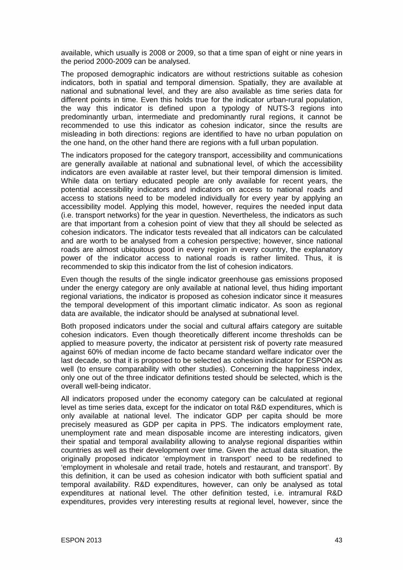
ESPON 2013 43

available, which usually is 2008 or 2009, so that a time span of eight or nine years in the period 2000-2009 can be analysed.

The proposed demographic indicators are without restrictions suitable as cohesion indicators, both in spatial and temporal dimension. Spatially, they are available at national and subnational level, and they are also available as time series data for different points in time. Even this holds true for the indicator urban-rural population, the way this indicator is defined upon a typology of NUTS-3 regions into predominantly urban, intermediate and predominantly rural regions, it cannot be recommended to use this indicator as cohesion indicator, since the results are misleading in both directions: regions are identified to have no urban population on the one hand, on the other hand there are regions with a full urban population.

The indicators proposed for the category transport, accessibility and communications are generally available at national and subnational level, of which the accessibility indicators are even available at raster level, but their temporal dimension is limited. While data on tertiary educated people are only available for recent years, the potential accessibility indicators and indicators on access to national roads and access to stations need to be modeled individually for every year by applying an accessibility model. Applying this model, however, requires the needed input data (i.e. transport networks) for the year in question. Nevertheless, the indicators as such are that important from a cohesion point of view that they all should be selected as cohesion indicators. The indicator tests revealed that all indicators can be calculated and are worth to be analysed from a cohesion perspective; however, since national roads are almost ubiquitous good in every region in every country, the explanatory power of the indicator access to national roads is rather limited. Thus, it is recommended to skip this indicator from the list of cohesion indicators.

Even though the results of the single indicator greenhouse gas emissions proposed under the energy category are only available at national level, thus hiding important regional variations, the indicator is proposed as cohesion indicator since it measures the temporal development of this important climatic indicator. As soon as regional data are available, the indicator should be analysed at subnational level.

Both proposed indicators under the social and cultural affairs category are suitable cohesion indicators. Even though theoretically different income thresholds can be applied to measure poverty, the indicator at persistent risk of poverty rate measured against 60% of median income de facto became standard welfare indicator over the last decade, so that it is proposed to be selected as cohesion indicator for ESPON as well (to ensure comparability with other studies). Concerning the happiness index, only one out of the three indicator definitions tested should be selected, which is the overall well-being indicator.

All indicators proposed under the economy category can be calculated at regional level as time series data, except for the indicator on total R&D expenditures, which is only available at national level. The indicator GDP per capita should be more precisely measured as GDP per capita in PPS. The indicators employment rate, unemployment rate and mean disposable income are interesting indicators, given their spatial and temporal availability allowing to analyse regional disparities within countries as well as their development over time. Given the actual data situation, the originally proposed indicator ‘employment in transport’ need to be redefined to ‘employment in wholesale and retail trade, hotels and restaurant, and transport’. By this definition, it can be used as cohesion indicator with both sufficient spatial and temporal availability. R&D expenditures, however, can only be analysed as total expenditures at national level. The other definition tested, i.e. intramural R&D expenditures, provides very interesting results at regional level, however, since the

ESPON 2013 44

limited spatial coverage of the available data, including severe data gaps, prevents it from being proposed as cohesion indicator at the moment.

Eight indicators have been proposed under the environments and hazards category. Data for all of them are available at national level only, except for the indicator residence/settlement density, which was calculated by GIS techniques based on Corine land use data at subnational level. While from the data availability perspective all indicators represent feasible cohesion indicators, not all of them are useful as they are defined right now:

- two indicators on water consumption have been tested. Both are measuring more or less the same spatial phenomena, so it is proposed to select only one indicator as cohesion indicator. Per-capita consumption of water of total public water supply should be selected since this indicator covers all water consumption, including industries and agriculture, and not just household consumption as the other indicator;

- even though the indicator residence/settlement density yields interesting results including detailed spatial patterns, it highly correlates with the indicator on population density of the demography category. In order to keep the number of cohesion indicator small, it is proposed to skip the residence/settlement density indicator;

- the present definition of the indicator “areas with high ecological value” is not optimal. It is associated with the share of protected areas for biodiversity according to the habitat´s directive. Since this is a political document, the protected areas were defined in a political process, and, moreover, once defined they will not change over time, thus shares remain unchanged. Unless there is no better indicator definition, it is recommended to skip this indicator.

Eventually, from the eight indicators tested under the environments and hazards category the following five are proposed as cohesion indicators: (i) renewable energy consumption, (ii) summer smog: ozone, (iii) summer smog: PM10, (iv) per-capita water consumption of total public water supply, and (v) residents connected to potable water systems. All these indicators are available at national level only, but as time series.

Under governance category only one indicator was proposed, which is electoral participation at national elections. Even though the indicator is only available at national level, and with certain restrictions concerning time series analyses, the indicator is proposed as cohesion indicator since it measures the degree to which people in the countries participate at election, thus expressing their political will.

There was only one indicator proposed under territorial cohesion category, which is the human development index developed by UNDP. Even though it is only available at national level, it provides a very good composite indicator assessing the general development level of nations. Therefore it is proposed as a cohesion indicator.

Several indicator candidates have been proposed for the balance and polycentricity category. Two of them, i.e. life expectancy and higher education, were already included in other two categories. Both the dependency ration and the ageing index are suitable candicates as cohesion indicators, however, since both indicators correlate to a high degree with each other, only one indicator should be selected. It is proposed to use the dependency ratio. Even though the indicator population potential within 50 km requires complex GIS analysis, it is proposed as cohesion indicator since it measures the potential of any point in space for further economic, social and demographic development. The two indicators on distances to MEGAs are excluding as cohesion indicators as well. The indicator distance to next MEGA since it highly

ESPON 2013 45

correlates with the indicator population potential within 50 km, and the indicator average distance to all MEGAs because it eventually just represents a geographical distance to the geographical centre of Europe. Eventually, only two of the tested balance and polycentricity indicators passed indicator assessment successfully.

Only one indicator of the natural assets, natural and technological hazards category could be tested so far, subject to data availability, which is the share of NATURA2000 areas on total region area. Even though the indicator is available for just one year, it is proposed to use this as cohesion indicator at regional level, representing the degree of nature protection.

Under the category land use issues the indicator share of green space per capita was tested both at raster level and at NUTS-2/3 region levels. Despite the technical restrictions of the Corine input data used for indicator calculation, it is recommended to include the indicator share of green space per capita at NUTS-3 as cohesion indicator.

Table 3 summarizes the indicator evaluation, differentiating between national and subnational level, and spatial dimension.

Data availability

NUTS-0 subnational Evaluation

Category Indicator

spatial tempo-ral spatial tempo-

ral NUTS0 subnattional

Population density ���� ���� ���� ���� ���� ���� Life expectancy ���� ���� ���� ���� ���� ���� Population average growth ���� ���� ���� ���� ���� ����

Demography

Urban-rural population ���� ���� ���� ���� ���� ���� Share of tertiary educated people ���� (����) ���� (����) (����) (����)

Potential accessibility by car to population ���� (����)1 ���� (����)1 (����)1 (����)1

Potential accessibility by car to GDP ���� (����)1 ���� (����)1 (����)1 (����)1

Households with broadband access ���� (����) 4 ���� (����) 4 (����) 4 (����) 4

Access to nearest national road ���� ���� ���� ���� ���� ����

Transport, accessibility, communica-tion

Access to nearest railway station ���� ���� ���� ���� ���� ����

Energy Greenhouse gas emission ���� ���� ���� ���� ���� ���� At risk of poverty rate ���� ���� ���� ���� ���� ���� Social and

cultural affairs Happiness index ���� ���� ���� ���� ���� ����

GDP per inhabitant ���� ���� ���� ���� ���� ����

Employment rate ���� ���� ���� ���� ���� ����

Unemployment rate ���� ���� ���� ���� ���� ����

Median disposable annual household income ���� ���� ���� ���� ���� ����

Employment in transport ���� ���� ���� ���� ���� ����

Economy

Total R&D expenditures ���� ���� ���� ���� ���� ����

ESPON 2013 46

Intramural R&D expenditures ���� (����) 4 ���� (����) 4 (����) 4 (����) 4

Renewable energy consumption ���� (����) 4 ���� ���� (����) 4 ����

Summer smog: ozone ���� ���� ���� ���� ���� ���� Summer smog: PM10 concentrations ���� ���� ���� ���� ���� ����

Consumption of water per capita, household water supply

���� ���� ���� ���� ���� ����

Consumption of water per capita, total water supply ���� ���� ���� ���� ���� ����

Residents connected to potable water system ���� ���� ���� ���� ���� ����

Residence density, settlement density ���� ���� ���� ���� ���� ����

Environment, hazards

Share of areas with high ecological value ���� ����

3 ���� ���� ����

3 ����

Governance Electoral participation ���� (����)4 ���� ���� (����)4 ����

Territorial cohesion Human Development Index ���� ���� ���� ���� ���� ����

Dependency ratio ���� ���� ���� ���� ���� ����

Ageing index ���� ���� ���� ���� ���� ����

Life expectancy at birth ���� ���� ���� ���� ���� ���� High education population ���� (����)4 ���� (����)4 (����) (����) Share high educated population in percent ���� (����)4 ���� (����)4 (����) (����)

Population potential 50 km ���� (����)2 ���� (����)2 (����)2 (����)2 Distance to next MEGA ���� ���� ���� ���� ���� ����

Balance and polycentricity

Average distance to all MEGAs ���� ���� ���� ���� ���� ����

Natural assets, natural & technological hazards

NATURA 2000 area ���� ���� ���� ���� ���� ����

Land use issues

% of green space per inhabitant ���� ���� ���� ���� ���� ����

1 Even though currently the indicator is only available for one point in time, it can be modeled for every year, provided that appropriate road network layers for the year are available. 2 As soon updated population grid data are available, the indicator can easily be updated by using GIS techniques. 3 Even though from Eurostat there are time-series data available, starting in 2003, the share of high ecological areas does not change over time, since according to the habitat´s directive no changes are being made so far to the protected areas, so that the shares remain. 4 Principally times series data are available, however, actually data are only available for two points in time, or times series datasets have great gaps for many spatial entities, so that they cannot be analysed in-depth.

Table 3. Evaluation scheme for indicator set ( � = test successfully passed; � = test failed)

ESPON 2013 47

4.3.2. National and subnational cohesion indicators Based upon this indicator assessment, two sets of cohesion indicators are proposed, which are so-called national cohesion indicators and subnational cohesion indicators. These indicators are proposed as INTERCO cohesion indicators to be further analysed for the Final Report.

For both national and subnational indicators, unique 3-digit indicator codes have been assigned, where national indicators start with the letter ‘N’ while subnational indicators start with letter ‘S’, both followed by consecutive numbers. By implementing this coding system, the code already indicates whether any indicator represents a national or subnational cohesion indicator.

The differentiation of the cohesion indicators into national and subnational indicators does not presuppose any preference of subnational over national indicators (or vice versa), or does not imply any weighting according to explanatory power of the indicators, but it gives an indicators to what degree and by what means the indicators can be analyzed for the final report. National indicators, as a fact, cannot be analyzed at subnational level to identify any disparities among NUTS-2 or NUTS-3 regions within countries, since data availability does not allow for this.

In this sense the division into national and subnational indicators already points to the analysis possibilities for the coming project phases, with greater analysis options for the subnational ones.

National cohesion indicators National cohesion indicators are cohesion indicators that can only be calculated and analysed at national level, since required input data at subnational level are not available today. To compensate for the missing spatial disaggregation, usually the national cohesion indicators are available as time series indicators for several years. Thus, cohesion can be analysed as a process over time (trends), and as disparities at European level.

The following eleven national cohesion indicators are proposed (N01 to N11) in Table 4:

Code Indicator Time series ( ���� = available; ���� = not

available). N01 Total R&D expenditures ����

N02 At persistent risk of poverty rate ����

N03 Happiness index, overall well-being ����

N04 Greenhouse gas emissions ����

N05 Summer smog: ozone concentration ����

N06 Summer smog: particular matter (PM10) ����

N07 Per-capita consumption of total public water supply ����

N08 Renewable energy consumption ����

N09 Residents connected to potable water systems ����

N10 Electoral participation rate ���� N11 Human development index ����

Table 4. Proposed national cohesion indicators

Except for the happiness index, for all others time series data are available, allowing analyzing cohesion trends over the last decade. Most of the national cohesion

ESPON 2013 48

indicators are concerned with climatic conditions, consumption and general well-being.

Subnational cohesion indicators Subnational cohesion indicators are cohesion indicators that are available at a subnational level (NUTS-2, NUTS-3, NUTS-5, raster). Sometimes, however, the spatial disaggregation is available only at dispense of temporal availability, i.e. the indicators are available for only one or two points in time. The spatial disaggregation allows analysing cohesion as disparities at regional level within countries, and in aggregated manner at European level between countries.

The following 17 subnational cohesion indicators are proposed (S01 to S16) in Table 5:

Code Indicator Time series ( ���� = available; ���� = not

available). S01 Population density ����

S02 Life expectancy at birth ����

S03 Population average growth ����

S04 Share of tertiary educated people ����

S05 Potential accessibility by road to population ����

S06 Potential accessibility by road to GDP ����

S07 Households with broadband access ����

S08 Access to nearest railway station ���� S09 GDP per capita in PPS ����

S10 Employment rate ����

S11 Unemployment rate ����

S12 Mean disposable household income ����

S13 Employment in wholesale and retail trade, hotels and restaurants, and transport (% of total employment)

����

S14 Dependency ratio ����

S15 Population potential within 50 km ����

S16 Share of NATURA2000 areas ����

S17 Green space per capita ����

Table 5. Proposed subnational cohesion indicators

14 out of these 17 indicators are not only available at subnational level, but also as time series data, allowing to analyse cohesion in both spatial and temporal dimensions. The indicators access to nearest railway station and population potential within 50 km are currently only available for one point in time, theoretically they can however be calculated by GIS techniques for different years. The one indicator left, share of NATURA2000 areas, remains available for one year.

The selected subnational cohesion indicators deal with demographic trends and the economy in general, as well as comprise all accessibility indicators.

4.3.3. Evaluation results with respect to methodology : which metrics ? One further objective of the indicator tests presented in this chapter was to derive methodological hints on how to best present the indicator evaluation. Different means

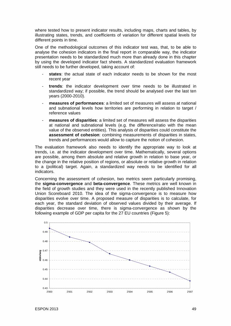
ESPON 2013 49

where tested how to present indicator results, including maps, charts and tables, by illustrating states, trends, and coefficients of variation for different spatial levels for different points in time.

One of the methodological outcomes of this indicator test was, that, to be able to analyse the cohesion indicators in the final report in comparable way, the indicator presentation needs to be standardized much more than already done in this chapter by using the developed indicator fact sheets. A standardized evaluation framework still needs to be further developed, taking account of:

- states : the actual state of each indicator needs to be shown for the most recent year

- trends : the indicator development over time needs to be illustrated in standardized way; if possible, the trend should be analysed over the last ten years (2000-2010).

- measures of performances : a limited set of measures will assess at national and subnational levels how territories are performing in relation to target / reference values

- measures of disparities : a limited set of measures will assess the disparities at national and subnational levels (e.g. the difference/ratio with the mean value of the observed entities). This analysis of disparities could constitute the assessment of cohesion : combining measurements of disparities in states, trends and performances would allow to capture the notion of cohesion.

The evaluation framework also needs to identify the appropriate way to look at trends, i.e. at the indicator development over time. Mathematically, several options are possible, among them absolute and relative growth in relation to base year, or the change in the relative position of regions, or absolute or relative growth in relation to a (political) target. Again, a standardized way needs to be identified for all indicators.

Concerning the assessment of cohesion, two metrics seem particularly promising, the sigma-convergence and beta-convergence . These metrics are well known in the field of growth studies and they were used in the recently published Innovation Union Scoreboard 2010. The idea of the sigma-convergence is to measure how disparities evolve over time. A proposed measure of disparities is to calculate, for each year, the standard deviation of observed values divided by their average. If disparities decrease over time, there is sigma-convergence as shown by the following example of GDP per capita for the 27 EU countries (Figure 5):

0.43

0.44

0.45

0.46

0.47

0.48

0.49

0.5

2'000 2'001 2'002 2'003 2'004 2'005 2'006 2'007

stde

v/av

g

ESPON 2013 50

Figure 5. Evolution of disparities in GDP per capit a between EU 27 countries

This graph can be compared to the one with GDP per capita figures in page 17.

The idea of the second metric, beta-convergence, is to analyse trends or performances in comparison to states : in order to achieve convergence (i.e. reducing disparities), territories with bad states should perform better than others if they want to catch up. Mathematically, beta-convergence can be measured by calculating the correlation between states and trends (Figure 6) :

0.0%

1.0%

2.0%

3.0%

4.0%

5.0%

6.0%

7.0%

8.0%

9.0%

0 10'000 20'000 30'000 40'000 50'000 60'000 70'000 80'000

GDP per capita (PPP, constant 2000 International US $)

GD

P p

er c

apita

gro

wth

(%

per

yea

r)

Luxembourg

CorrelationEU27 : -0.50EU26 (Luxembourg excluded) : -0.71

Figure 6. States and trends of GDP per capita in 20 05 (EU 27 countries)

Like for every calculation of correlation, it is interesting to analyse the residuals, i.e. the observations that do not fit the expected model (e.g. Luxembourg is an interesting case of over-performance in GDP per capita).

Two additional aspects must be considered.

Since the various indicators have different units of measure, they need to be standardized (e.g. using averages), allowing for comparisons between the indicators, for all types of analysis (states, trends, disparities).

Finally, since national cohesion indicators as well as subnational cohesion indicators have now been identified (see previous section), the evaluation framework also needs to develop proposals for a clever combination of indicators calculated at both scales. Disparities might be low between countries, but high within countries : metrics should provide an account of these two levels.

The above mentioned metrics will be analysed and tested more in depth in the next phase of the project.

ESPON 2013 51

Concluding remarks The Interim Report is an important milestone of the INTERCO project on several aspects:

the scientific and policy litterature concerned more or less directly with territorial cohesion has been extensively studied;

• “dimensions” of territorial cohesion have been defined by INTERCO based on the careful examination of the links between challenges, policy orientations and issues (as expressed in the ESPON call), as well as on the story lines used for the communication with stakholders during the workshops. The “dimensions” offer a flexible and understanble way to tackle the concept of territorial cohesion;

• the Inventory of indicators has been expanded and further structured;

• the prioritisation of indicators has been initiated using the lenses provided by the INTERCO “dimensions” as well as criteria related to data (quality, availability, resolution);

• a first set of 38 test indicators have been calculated, mapped and assessed;

• some cohesion metrics have been proposed as paths for further analyses.

The first two phases of the INTERCO project (Design and Exploratory) have confirmed that territorial cohesion is very difficult to be defined in an univocal way. The thematic dimensions covered by this concept are multiple, various stakeholders seem to have their own views on the appropriate thematic focus and territorial scales to consider.

In front of this rather vague concept, there are a myriad of quality data, hence potential indicators, ready to be used as indicators.

The indicators system that INTERCO is aiming at will have have to be based on the good data available and to allow for moving thematic priorities that may arise in the future. In this respect, the focus on the metrics (how to measure cohesion) is probably an interesting path to follow.

Further steps needed for moving forward towards robust and relevant territorial cohesion indicators during the second half of the project are listed in the next chapter.

ESPON 2013 52

Next steps

Foreseen activities Evaluating the indicators (promising/feasible/potential and “wishful” indicators) Given the very high number of identified potential indicators, the inventory of indicators took much more time than expected and still needs to be refined.

First assessments and prioritisations have already been done based on (a) the quality and availability of the data (including the existence of time series data) and (b) the relevance of the indicator for territorial cohesion. A considerable amount of material has been accumulated and synthesised, but further processing of this material is needed. This work will be pursued on the basis of the comments received after the delivery of the Interim Report.

In this respect, the TPG is asking ESPON CU for the possibility to submit a more complete and finalised Inventory of indicator s by 6 May 2011 (after a planned TPG meeting). This inventory will also incl ude a commented list of metrics to be applied for depicting states, trends, disparities of the various dimensions of territorial cohesion.

Terminology In the Inception Report it was previewed that, on the basis of the results from the terminology sub-activity of INTERCO, a terminology spreadsheet, which would explain the indicators and data names as well as the categories used for classifying them, would have been provided for the Interim Report as a first quick solution.

The major part of this spreadsheet - terms for the themes and sub-themes (see Annex 2), content of the sub-themes, terminology for several divisions of indicators (simple / complex / complex territorial, etc.) - has already been advanced and used in the selection of indicators. However, after the first implementation of the division / sub-division of themes, it seemed necessary to revise it. Also, the TPG should also finalise the terminology regarding the division of indicators in categories as for the “priority” and the extent to be studied in the frame of INTERCO. These two tasks are foreseen to be finalised at the end of April 2011, therefore the terminology spreadsheet will be submitted to the ESPON CU on 6th May 2011.

EU candidate countries The TPG did not further assess the availability and quality of the respective data until the submission of the Interim Report because the Inventory of indicators has been finalized at the end of March 2011, the total number of indicators in the Inventory is much higher than expected and the selection of a set of “priority” indicators which will be examined in more depth has not been finalised yet.

After the finalisation of the selection of “priority” indicators foreseen for a short time after the submission of the Interim Report, the TPG will assess the availability and quality of the EU candidate countries’ data for the “priority” indicators.

It should be taken into consideration that the project ESPON 2013 Database has assessed the availability and quality of data for these countries only for a relatively short range of “basic” themes in line with the entire ESPON 2013 Database project’s scope for the collection of data. Therefore, it is necessary to extend this scope in order to meet the demand of INTERCO for an assessment covering a much wider range of themes.

Calulation of the indicators (Activity C) The following tasks of Activity C are already finished with the Interim Report:

ESPON 2013 53

- identification of potential data sources for statistical data, administrative boundaries and other GIS layers (sub-activity C1);

- list of data sources (sub-activity C1);

- gathering of required statistical input data from various data sources (data collection) (sub-activity C1);

- initial setup of INTERCO GIS Database (sub-activity C2);

- filling INTERCO_DB geodatabase by importing layers from ESPON 2013 Database project, as well as generating new layers and tables. Where necessary existing data from ESPON 2013 Database project were amended to meet INTERCO requirements (sub-activity C2);

- implementation of base structure and data format for INTERCO GIS Database and the overall INTERCO folder (sub-activity C2);

- initial development of standardized indicator fact sheets (sub-activity C2);

- initial indicator assessment of proposed indicators, including indicator mapping and calculation of various statistics, charts and tables (indicator assessment and tests) (sub-activity C2);

- proposal for core set of cohesion indicators at national and subnational level (sub-activity C2).

The next steps under Activity C for the following project phase are :

- as far as necessary additional data collection to fill data gaps (sub-activity C1);

- as far as necessary data harmonization (sub-activity C1);

- upon adoption of the proposed core set of cohesion indicators, finalization of INTERCO geodatabase with respect to (sub-activity C2) :

o filling data gaps (as far as possible);

o filling timer series (as far as possible);

o improve/refine existing data (as far as needed);

- development of a standardized evaluation framework for all indicators (sub-activity C2, together with other Activities);

- standardization of time series data: all data series need to be standardized to either a common start year, or end year, to make developments in the different countries comparable. Otherwise indicators can hardly be compared since they all have different units and reference points (sub-activity C2);

- developing GIS scripts and tools for indicator calculations (for the Interim Report so far only test implementations have been developed, while in next phase final implementations are due) (sub-activity C2);

- final indicator mapping according to the developed standardized evaluation framework. Mapping not only include formal cartographic maps, but also a certain fixed set of charts and tables (based upon test presented in Interim Report) (sub-activity C2);

- implementing access to data and finalise data evaluation (phase 3) (sub-activity C1);

- developing metadata description of INTERCO database (phase 3) (sub-activity C1);

ESPON 2013 54

- writing user manual for INTERCO database and scripts and tools (phase 3) (sub-activity C1);

- finalizing and improving GIS scripts and tools, finalization INTERCO Toolbox (Phase 3) (sub-activity C2);

- implementing calculations and mapping of indicators (Phase 3) (sub-activity C2);

- generation of final maps, final Excel files and final layer files of all indicators (Phase 3) (sub-activity C2).

Stakeholder participation The second round of the stakeholder involvement is envisaged for the autumn 2011. This will involve mainly one open workshop and one presentation / workshop at the ESPON seminar:

- Open workshop on territorial indicators (21 October 2011)

This workshop will be organised in cooperation with the ESPON CU and be open to the interested public with particular emphasis on the participants of the INTERCO workshop held in January 2011 in Brussels. The aim is to present first results of the INTERCO work to the participants and discuss how they can be useful in the policy work in different sectors and at different levels of policy making.

- ESPON seminar presentation / workshop (29-30 November 2011)

At this event the final results of the INTERCO project will be presented to the ESPON community. The focus will be on a discussion of how these results can be useful for the future ESPON work.

Work plan until the Final report Reminder of the general workplan The INTERCO project is divided into three main parts, the design, exploratory and implementation phases :

- Start of the project (16 February 2010)

o 5 May 2010 : Kick-off Meeting in Luxembourg

- Part I, the design phase (until 31 August 2010)

o 31 August 2010 : Inception Report

o 27-28 September 2010 First Team Meeting (in Switzerland)

- Part II of, the exploratory phase (until 31 March 2 011)

o January 2011 (to be confirmed) Second Team Meeting

o 31 March 2011 : Interim Report

- Part III, the implementation phase (until 29 Februa ry 2012)

o September 2011 (to be confirmed) Third Team Meeting

o 30 November 2011 : Draft Final Report

o 29 February 2012 : Final report

o 29 February 2012 : Closure of the activities

- Closure of the administrative duties (29 May 2012)

A more detailed description of deadlines and outputs is provided in Annex 14.

ESPON 2013 55

It must be noted that all (sub-)activities A, B, C, and D are conducted in parallel. The advantage of this approach is to keep all the teams involved during the whole lifespan of the project.

On the financial side, the break down of the project's budget is as follows (Figure 7):

Budget line UniGe NTUA NordRegio Total

1. Staff 86'600 104'400 33'000 224'000

2. Administration 7'000 8'300 2'700 18'000

3. Travel and accommodation 18'100 6'600 3'300 28'000

4. Equipment 700 700 1'400

5. External expertise and services * 125'000 125'000

Total 237'400 120'000 39'000 396'400

* Breakdown : RRG 78'000 / Spatial Foresight 42'000 / other 5'000

Figure 7. The project's budget (in Euros)

Work Plan until the Final Report (29 February 2012) With the release of the Interim Report the INTERCO project has reached the step nr 13 of the planned workflow (Figure 8). The next important steps are :

- further assessments of indicators by the TPG, based on the the evaluation scheme and feedbacks from MC and stakeholders (until 6 May 2011);

- a TPG meeting to discuss and finalise the list of indicators, as well as the cohesion metrics to be implemented (foreseen on 2-3 May 2011 in Athens, to be confirmed);

- implementation of the indicators (until 15 August 2011).

Other planned interactions / presentations to stakeholders are as follows:

- participation to the ESPON Seminar (22-23 June 2011 in Hungary, to be confirmed);

- organisation of an Open workshop on territorial indicators (21 October 2011 in Luxembourg or Brussels, place to be confirmed);

- presentation of the final results (29-30 November 2011, place and context to be confirmed).

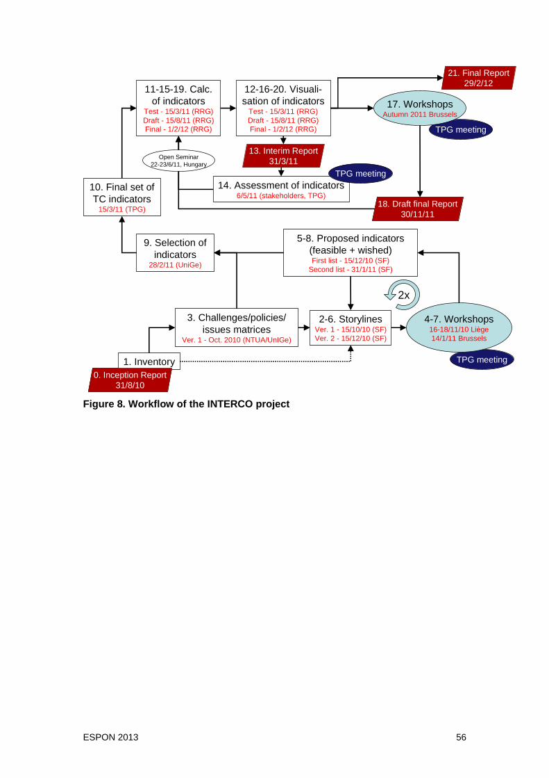
ESPON 2013 56

0. Inception Report31/8/10

TPG meeting

TPG meeting

1. Inventory

2-6. StorylinesVer. 1 - 15/10/10 (SF)Ver. 2 - 15/12/10 (SF)

3. Challenges/policies/ issues matrices

Ver. 1 - Oct. 2010 (NTUA/UnIGe)

5-8. Proposed indicators(feasible + wished)First list - 15/12/10 (SF)

Second list - 31/1/11 (SF)

10. Final set of TC indicators

15/3/11 (TPG)

11-15-19. Calc. of indicators

Test - 15/3/11 (RRG)Draft - 15/8/11 (RRG)Final - 1/2/12 (RRG)

12-16-20. Visuali-sation of indicators

Test - 15/3/11 (RRG)Draft - 15/8/11 (RRG)Final - 1/2/12 (RRG)

17. WorkshopsAutumn 2011 Brussels

4-7. Workshops16-18/11/10 Liège14/1/11 Brussels

14. Assessment of indicators6/5/11 (stakeholders, TPG)

2x

13. Interim Report31/3/11

18. Draft final Report30/11/11

21. Final Report29/2/12

0. Inception Report31/8/10

18. Draft final Report30/11/11

Open Seminar22-23/6/11, Hungary

TPG meeting

9. Selection of indicators

28/2/11 (UniGe)

Figure 8. Workflow of the INTERCO project

ESPON 2013 57

Annex 1. Bibliographic references General Literature

ADAMS, N.; COTELLA, G.; NUNES, R. (eds.) 2010, Territorial Development, Cohesion and Spatial Planning: Knowledge and Policy development in an Enlarged EU, London: Routledge.

AHO, E., 2006, Creating an Innovative Europe, Report of the Independent Expert Group on R&D and Innovation appointed following the Hampton Court Summit.

ALLAIN, R., 2003, Le Polycentrisme, Un Projet Pour l’Europe. Rennes: Presses universitaire de Rennes.

ARNESEN, T.; OVERVÅG, K.; GLØRSEN, E.; SCHÜRMANN, C.; RISE, Ø., 2010, Fjellområder og Fjellkommuner i Sør-Norge. Definisjon, avgrensning of karakterisering. Lillehammer: Østlandsforskning.

BARCA, F., 2009, An agenda for a reformed Cohesion Policy, a place-based approach to meeting European Union Challenges and expectations, Independent Report at the Request of Danuta Hübner, Commissioner for regional Policy.

BARCA, F., 2010, “The Future of Europe’s Regional Policy”, European Regional Association Congress, Jönköping, 19-23 August, 2010. Available at http://www.regional-studies-assoc.ac.uk/

BEGG, I., 2010, “Cohesion or Confusion: A Policy Searching for Objectives”, Journal of European Integration 32 (1), pp. 77-96.

BÖHME, K.; T.W. ESER, 2008, Territorial Impact Analysis of EU Policies, European Spatial Research and Planning, Cambridge, Massachusetts: Lincoln Institute of Land Policy.

BÖHME, K.; ZILLMER, S., 2010, “Die Territoriale Agenda der EU und ihr Aktionsprogramm: zwischen europäischen Obstkörben und Papiertigern”, Informationen zur Raumentwicklung 8/2010, pp.567-576.

CAMAGNI, R., 2006, “The rationale for territorial cohesion: issues and possible policy strategies”, in L. Pedrazzini (ed.), The process of territorial cohesion in Europe, Milano: F. Angeli, pp. 53-67.

CAMBRIDGE ECONOMETRICS, 2010, Pilot study on the estimation of regional capital stocks, Final report for the European Commission (Directorate General Regional Policy).

COLLECTIF, 1993, Europe: Espace Ou Territoire ? Paris: Seuil.

DATAR, 2007, Territoires 2020, Revue Scientifique de la DATAR, n° 7.

DATAR, 2010, La cohésion territoriale en Europe, Paris : La Documentation Française.

DAVOUDI, S., 2005, “Understanding territorial cohesion”, Planning Practice and Research, 20(4), pp. 433-441.

DAVOUDI, S., 2007, “Territorial Cohesion, the European Social Model and Spatial Policy Research”, appears in Faludi, A., 2007, Territorial Cohesion and the European Model of Society, p. 81-101.

DAVOUDI, 2009, “Territorial Cohesion, European Social Model and Transnational Cooperation”, in KNIELING, J.; OTHENGRAFEN, F. (ed.), Planning cultures in Europe : decoding cultural phenomena in urban and regional planning, Burlington

ESPON 2013 58

VT: Ashgate, pp. 269-279.

DE VRIES, A.; VELASCO, X., 2010, Territorial indicator system as a tool for evaluating territorial strategies. Available: http://programm.corp.at

DUBOIS, A.; GLØERSEN, E.; LÄTHEENMÄKI-SMITH, K.; DAMSGAARD, O.; GRASLAND, C.; YSEBAERT, R.; ZANIN, CHR.; LAMBERT, N.; SCHÜRMANN, C.; HANELL, TH.; GENSEL, J.; THOMAS, R., 2007, Regional Disparities and Cohesion: What Strategies for the Future? Report to the Directorate General Internal Policies of the Union of the European Parliament. IP/B/REGI/IC/2006_201 14/05/2007. Brussels: European Parliament.

EDERVEEN S.; GORTER J., 2002, “Does European cohesion policy reduce regional disparities?”, CPB Discussion Paper, The Hague: CPB Netherlands Bureau for Economic Policy Analysis.

EUROSTAT, 2009, Science, technology and Innovation in Europe, European Commission, Pocketbook.

EUROSTAT, 2009, Sustainable development in the European Union, 2009 monitoring report of the EU sustainable development strategy, Eurostat statistical books, European Commission.

EUROSTAT, 2010, Feasibility study for Well-Being Indicators, Brussels.

FALUDI, A., 2002, European spatial planning, Cambridge Mass.: Lincoln Institute of Land Policy.

FALUDI, A., 2005, “Territorial cohesion: an unidentified political objective: Introduction to the special issue”, Town Planning Review, 76(1), pp.1-13.

FALUDI, A., 2005, “Territorial Cohesion Policy and the European Model of Society”, Paper for AESOP Conference, Vienna, 2005.

FALUDI, A., 2006. “From European spatial development to territorial cohesion policy”, Regional Studies 40 (6), pp. 667-678.

FALUDI, A. (ed.), 2007, Territorial Cohesion and the European Model of Society, Cambridge, Massachusetts: Lincoln Institute of Land Policy.

FALUDI, A., 2009, “Territorial cohesion under the looking glass: synthesis paper about the history of the concept and policy background to territorial cohesion”, European Commission, Regional Policy, Inforegio.

FALUDI, A., 2009, “A Turning Point in the Development of European Spatial Planning? - The 'Territorial Agenda of the European Union' and the 'First Action Programme'”, Progress in planning, 71 (1), pp. 1-42.

FARRUGIA N. ; GALLINA A., 2008, Developing Indicators of Territorial Cohesion, Federico Caffè Centre Research Report Nr 1/2008, Department of Society and Globalization, Roskilde University.

GLØERSEN, E.; DUBOIS, A.; COPUS, A.; SCHÜRMANN, C., 2006, Northern Peripheral, Sparsely Populated Regions in the European Union and in Norway. Nordregio Report 2006:2. Stockholm: Nordregio.

HAMEZ, G., 2005, “Territorial Cohesion: How to Operationalize and Measure the Concept?” Planning Theory & Practice, 6 (3), 400-402.

HELD, D., 1995, Democracy and the Global order, Cambridge: Polity.

ESPON 2013 59

HERAUD, J.-A., 2009, “Les objectifs politiques européens de compétitivité et de cohésion territoriale sont-ils compatibles ? ”, Bulletin de l’Observatoire des politiques économiques en Europe, n°20, summer 2009.

HUSSON, C., 2002, L'Europe Sans Territoire: Essai sur le concept de cohésion territoriale, La Tour d'Aigues: Ed. de l'Aube.

JEAN, Y. ; BAUDELLE, G., 2009, L'Europe: Aménager Les Territoires, Paris: A. Colin.

JENSEN, O.; RICHARDSON T., 2004, Making European Space: Mobility, Power and Territorial Identity. London: Routledge.

JOUEN, M., 2008, “La cohésion territoriale, de la théorie à la pratique”, Notre Europe, Available at: http://www.notre-europe.eu/uploads/tx_publication/Policypaper35-FR-MJouen-CohesionTerritoriale.pdf.

JRC - JOINT RESEARCH CENTRE, 2004, Global 2000 Landcover. http://www.gvm.jrc.it/glc2000 /objectivesGLC2000.htm. Ispra: JRC.

MEIJERS, E.J.; WATERHOUT, B.; ZONNEVELD W.A.M., 2007, “Closing the

GAP: Territorial Cohesion through Polycentric Development”, European Journal of Spatial Development, no 24.

MIRWALDT, K., MCMASTER, I., BACHTLER, J., 2008, “Reconsidering Cohesion Policy: The Contested Debate on Territorial Cohesion” (EoRPA Paper 08/5), European Policy Research Paper No 66.

NEF, 2009, National Accounts of Well-being: bringing real wealth onto the balance sheet. London: new economic foundation.

OECD-JRC, 2008. Handbook on Constructing Composite Indicators, Methodology and user guide. OECD Publishing

PAREJO NAVAJAS, T., 2005, “From sustainable territorial development to territorial cohesion: towards an effective European spatial planning in the enlarged European Union” Paper presented at the AESOP Conference in Vienna, 13-17 July 2005.

PEDRAZZINI, L. (ed.), 2006, The process of territorial cohesion in Europe, Milano: F. Angeli.

PELCOM - Pan-European Land Use and Land Cover Monitoring, 2001, Development of a Consistent Methodology to Derive Land Cover Information on a European Scale from Remote Sensing for Environmental Monitoring.

http://www.geo-informatie.nl/projects/pelcom/public/index.htm.

POLITECNICO DI MILANO, Bocconi University Milan, IGEAT-ULB, October 2009, Regions Benefiting from Globalisation and Increased trade, Study for DG region, Final report.

POLVERARI, L., QUIOGUE, N., GROSS, F., and NOVOTNY, V., 2005, “Territorial Cohesion and Structural Funds Programmes: Urban Development and Territorial Cooperation”, IQ-Net Thematic Paper No. 16(2), Newcastle upon Tyne.

SANDBERG, K., MEIJERS, E., 2006, “Polycentric development: a panacea for regional disparities in European countries ?” Response Paper presented at the 10th UNECE Conference on Urban and Regional Research, May 22-23, Bratislava.

ESPON 2013 60

SCHMITT, P.; DUBOIS, A., 2008, Exploring the Baltic Sea Region – On territorial Capital and Spatial Integration. Nordregio Report 2008:3. Stockholm: Nordregio.

SCHOLICH, D. (Ed.), 2007, German Annual of Spatial Research and Policies 2007- Territorial Cohesion, Berlin, Heidelberg : Springer.

SCHÖN, P., 2005, “Territorial Cohesion in Europe?”, Planning Theory and Practice, 6 (3), pp. 387-413.

SCHÖN, P., 2009, “Territorial Cohesion-Current Views of the Commission and the Member States of the European Union”, in KILPER, H. (ed.), German Annual of Spatial Research and Policy 2009, New Disparities in Spatial Development in Europe, pp. 7-17. Berlin, Heidelberg : Springer-Verlag.

SCHOUT J. A.; JORDAN A. J., 2007, “From Cohesion to Territorial Policy Integration (TPI): Exploring the Governance Challenges in the European Union”, European Planning Studies, 15 (6), pp. 835-851.

SERVILLO, L, 2010. “Territorial Cohesion Discourses: Hegemonic Strategic Concepts in European Spatial Planning”, Planning Theory & Practice 11 (3), pp. 397-416.

TAPPEINER, U.; BORSDORF, A.; TASSER, E. (ed.), 2008, Alpenatlas. Atlas des Alpes. Atlante delle Alpi. Atlas Alp. Mapping the Alps. Society – Economy – Environment. Heidelberg: Spektrum Akademischer Verlag.

TAYLOR, P., 2008, Cities, world Cities, Networks and Globalization, GaWC Research Bulletin 238, available at http://www.lboro.ac.uk/gawc/rb/rb238.html

TAYLOR, P., 1982, “A materialist framework for political geography”, Transactions of the Institute of British Geographers NS 7, pp. 15-34, cited in Marston, S.A., Jones, J.P. and Woodward, K., 2005, “Human geography without scale”, Transactions of the Institute of British Geographers NS 30, pp. 416-432.

VANOLO, A., 2010, “European Spatial Planning Between Competitiveness and Territorial Cohesion: Shadows of Neo-liberalism”, European Planning Studies 18 (8), pp. 1301-1315.

WATERHOUT, B., 2008, The Institutionalisation of European Spatial Planning, Amsterdam: IOS Press.

YAMAZAKI-HONDA, R., 2005, “Territorial Policy in OECD Countries”, Planning Theory and Practice, 6 (3), pp. 387-413.

Officials and European sources

COMMITTEE OF THE REGIONS, 2003, Opinion No 2003/C 244/05 of the 10 October 2003, “Territorial Cohesion in Europe”, JO C 244, 10.10.2003, p. 23.

CONFERENCE OF PERIPHERAL AND MARITIME REGIONS, 2010, “Putting the regions and the territorial dimension at the heart of synergies between regional policy and the RTD and CIP Framework Programme”, Position Paper, available at http://www.crpm.org/pub/docs/291_cpmr_ppp_synergies-en.pdf

COUNCIL OF THE EUROPEAN COMMUNITIES, 1992, Directive No 92/43/EEC of 21 May 1992 on the conservation of natural habitats and of wild fauna and flora (Habitats’ Directive), OJ L 206, 22.7.1992, p.7.

COUNCIL OF THE EUROPEAN COMMUNITIES, 2006, Directive No 2006/105/EC of 20 November 2006, L 363/368, 20.12.2006, amending the Council Directive 92/43/EEC on the conservation of natural habitats and of wild fauna and flora of 21 May 1992 (OJ L 206, 22.7.1992, p. 7).

ESPON 2013 61

EEA – EUROPEAN ENVIRONMENTAL AGENCY, 2007, The pan-European environment: glimpses into an uncertain future, EEA report, n° 4/2007

EEA – EUROPEAN ENVIRONMENTAL AGENCY, 2007, State of the environment report, EEA report, n°1/2007

EEA – EUROPEAN ENVIRONMENTAL AGENCY, 2008, Impacts of Europe's changing climate - 2008 indicator-based assessment, EEA Report, n°4/2008 (http://www.eea.europa.eu/publications/eea_report_2008_4)

EEA – EUROPEAN ENVIRONMENTAL AGENCY, 2009, Territorial cohesion — Analysis of environmental aspects of the EU Cohesion Policy in selected countries, EEA Technical report No 10/2009.

EEA – EUROPEAN ENVIRONMENTAL AGENCY, 2010a, Corine Land Cover 2000 by Country. http://www.eea.europa.eu/data-and-maps/figures/corine-land-cover-2000-by-country-1. Copenhagen: EEA.

EEA – EUROPEAN ENVIRONMENTAL AGENCY, 2010b, Population density disaggregated with Corine land cover 2000. http://www.eea.europa.eu/data-and-maps/data/population-density-disaggregated-with-corine-land-cover-2000-2. Copenhagen: EEA.

EEA – EUROPEAN ENVIRONMENTAL AGENCY, 2011a, Corine Land Cover 2006 seamless vector data – version 13 (02/2010). http://www.eea.europa.eu/data-and-maps/data/clc-2006-vector-data-version. Copenhagen: EEA.

EEA – EUROPEAN ENVIRONMENTAL AGENCY, 2011b, NATURA 2000 data – the European network of protected sites. http://www.eea.europa.eu/data-and-maps/data/natura. Copenhagen: EEA.

EEA – EUROPEAN ENVIRONMENTAL AGENCY, 2011c, Population density disaggregated with Corine land cover 2000. http://www.eea.europa.eu/data-and-maps/data/population-density-disaggregated-with-corine-land-cover-2000-2. Copenhagen: EEA.

EUROPEAN COMMISSION, 2001, European Governance – A White Paper, COM (2001) 428 final, Brussels.

EUROPEAN COMMISSION, 2005, Communication from the Commission, Cohesion Policy in Support of Growth and Jobs: Community Strategic Guidelines, 2007-2013, COM (2005) 0299, Brussels.

EUROPEAN COMMISSION, 2005, Communication from the Commission to the Council and the European Parliament, Common Actions for Growth and Employment: The Community Lisbon Programme, COM(2005) 330 final, Brussels.

EUROPEAN COMMISSION, 2006, Communication from the Commission to the Council and Parliament, Cohesion policy and cities: the urban contribution to growth and jobs in the regions, COM (2006) 385 final, Brussels.

EUROPEAN COMMISSION, 2006, Communication from the Commission, The regions for economic change, COM (2006) 675 final, Brussels.

EUROPEAN COMMISSION, 2007, Communication from the Commission to the European Parliament and the Council, Fourth report on economic and social cohesion – Growing regions, growing Europe, May 2007.

EUROPEAN COMMISSION, 2008, Communication from the Commission to the Council, the European parliament, the Committee of the regions and the European

ESPON 2013 62

Economic and Social Committee, Green Paper on Territorial Cohesion, Turning territorial diversity into strength, COM(2008) 616 final, Brussels.

EUROPEAN COMMISSION, 2008, Commission staff working document accompanying the Green Paper on Territorial Cohesion Turning territorial diversity into strength (COM (2008) 616 final, Brussels.

EUROPEAN COMMISSION, 2008, Communication from the Commission to the European Parliament and the Council, Fifth progress report on economic and social cohesion – Growing regions, growing Europe, COM, (2008) 371 final, Brussels.

EUROPEAN COMMISSION, 2008, Fostering the urban dimension: analysis of the operational programmes co-financed by the European Regional Development Fund (2007-2013), Working Document of the Directorate General for Regional Policy, Brussels.

EUROPEAN COMMISSION, 2009, Report from the Commission to the European Parliament and the Council: Sixth progress report on economic and social cohesion, {SEC (2009) 828 final}, Brussels.

EUROPEAN COMMISSION, 2009, Communication from the Commission to the European Parliament and the Council, Sixth progress report on economic and social cohesion - Creative and innovative regions, COM (2009) 295, Brussels.

EUROPEAN COMMISSION, 2009, Communication from the Commission to the European Parliament, the Council, the European Economic and Social Committee and the Committee of the Regions, Mainstreaming sustainable development into EU policies: 2009 Review of the European Union Strategy for Sustainable Development, COM(2009) 400 final, Brussels.

EUROPEAN COMMISSION, 2009, Communication from the Commission to the European Parliament, the Council, the European Economic and Social Committee and the Committee of the Regions, Reviewing Community innovation policy in a changing world, COM(2009) 442 final, Brussels.

EUROPEAN COMMISSION, 2010, Europe 2020 A European strategy for smart, sustainable and inclusive growth, COM (2010) 2020, Brussels.

EUROPEAN COMMISSION, 2010, Regional Policy contributing to smart growth in Europe 2020, COM (2010) 553 final, Brussels.

EUROPEAN COMMISSION, 2011, Regional Policy contributing to sustainable growth in Europe 2020, COM (2011) 17 final, Brussels.

EUROPEAN COMMISSION / REGIONAL POLICY , 2004, Interim Territorial Cohesion Report.

EUROPEAN COMMISSION / REGIONAL POLICY, 2008, Regions 2020 - An Assessment of Futures challenges for EU Regions, Commission Staff Working Document, SEC(2008), Brussels.

EUROPEAN COMMISSION / REGIONAL POLICY, 2009, Regional Challenges in the Perspective of 2020 - Regional disparities and future challenges, Brussels.

EUROPEAN COMMISSION / REGIONAL POLICY (by Philippe Monfort), 2009, Territories with specific geographical features, Working Papers, A series of short paper on regional research and indicators produced by the Directorate-General for Regional Policy, n°2/2009

EUROPEAN COMMISSION / REGIONAL POLICY, 2009, Promoting sustainable urban development in Europe: achievements and opportunities, Brussels.

ESPON 2013 63

EUROPEAN COMMISSION / INTER-SERVICE GROUP ON URBAN DEVELOPMENT, 2010, The urban dimension in European Union policies, Brussels.

EUROPEAN COMMISSION / REGIONAL POLICY (by Marielle Riché), 2010, Regional Innovation Governance, Regional focus n° 2/2010.

EUROPEAN COMMISSION / REGIONAL POLICY, 2010, Fifth Report on Economic, Social and Territorial Cohesion, Investing in Europe’s Future, Brussels.

EUROPEAN COUNCIL, PORTUGUESE PRESIDENCY OF THE EUROPEAN UNION, 2000, Presidency conclusions - Lisbon European Council - 23 and 24 March 2000.

EUROPEAN COUNCIL, SWEDISH PRESIDENCY OF THE EUROPEAN UNION, 2001, Presidency conclusions – Göteborg European Council - 15 and 16 June 2001.

EUROPEAN COUNCIL, 2004, Extracts from presidency conclusions on the Lisbon strategy European councils: Lisbon (March 2000) to Brussels (June 2004).

EUROPEAN COUNCIL, GERMAN PRESIDENCY OF THE EUROPEAN UNION, 2007, Leipzig Charter on Sustainable European Cities - Final Draft, 02 May 2007.

EUROPEAN COUNCIL, HUNGARIAN PRESIDENCY OF THE EUROPEAN UNION, 2011, Presidency conclusions –Brussels European Council – 24 and 25 March 2011.

EUROPEAN PARLIAMENT (ed.), 2007: Regional Disparities and Cohesion: What Strategies for the Future? IP/B/REGI/IC/2006_201. Brussels: European Parliament.

EUROPEAN PARLIAMENT AND COUNCIL, 2002, Decision No 1600/2002/EC of 22 July 2002 laying down the Sixth Community Environment Action Programme, OJ L 242/1 of 10.9.2002.

EUROPEAN PARLIAMENT AND COUNCIL, 2006, Regulation (EC) No 1080/2006 of the European Parliament and of the Council of 5 July 2006 on the European Regional Development Fund and repealing Regulation (EC) No 1783/1999, OJ L 210/1, 31.7.2006 – see the Article 6 on European Territorial Cooperation objective (ETC).

EUROPEAN PARLIAMENT AND COUNCIL, 2006, Decision No 1639/2006/EC of the European Parliament and of the Council of 24 October 2006 establishing a Competitiveness and Innovation Framework Programme (2007 to 2013), OJ L 310/15, 09.11.2006.

EUROPEAN PARLIAMENT AND COUNCIL, 2007, Directive No 2007/2/EC of 14 March 2007 establishing an Infrastructure for Spatial Information in the European Community (INSPIRE), OJ L 108/1, 14.03.2007

EUROPEAN PARLIAMENT AND COUNCIL, 2009, Directive No 2009/147/EC on the conservation of wild birds (codified version of Directive 79/409/EEC as amended), OJ L 20/7, 26.01.2010.

EUROPEAN UNION, 1999, European Spatial Development Perspective: Towards balanced and sustainable development of the territory of the EU, CEC, Luxembourg.

EUROPEAN UNION, 2005, The Territorial State and Perspectives of the European Union, Towards a Stronger European Territorial Cohesion in the Light of the Lisbon and Gothenburg Ambitions, Based on the Scoping Document discussed by Ministers at their Informal Ministerial Meeting in Luxembourg in May 2005, Background Document for the Territorial Agenda of the European Union.

ESPON 2013 64

EUROPEAN UNION, 2007, Territorial Agenda of the European Union, Towards a more competitive and sustainable Europe of diverse regions, Agreed on the occasion of the Informal Ministerial Meeting in Leipzig on 24/25 May 2007.

EUROSTAT, 2011, Eurostat Regio Database. http://epp.eurostat.ec.europa.eu/portal/page/portal/region_cities/regional_statistics/data/database. Luxembourg: Eurostat.

KEA EUROPEAN AFFAIRS, 2009, “Contribution to the European Commission’s public consultation on Community innovation policy”, Brussels.

MERIT-JRC, 2009, Regional Innovation Scoreboard 2009.

MERIT-JRC, 2011, Innovation Union Scoreboard 2010.

ORGANISATION FOR ECONOMIC CO-OPERATION AND DEVELOPMENT, 2001, Territorial Outlook, Paris: OECD.

EU Candidate and Potential Candidate Countries

EUROSTAT, 2010, Pocketbook on candidate and potential candidate countries - 2010 edition, European Union, Brussels.

Websites of the National Statistical Organisations of the EU candidate countries

Albania: Albania Institute of Statistics: http://www.instat.gov.al

Bosnia and Herzegovina: Agency for statistics of Bosnia and Herzegovina: http://www.bhas.ba, Federation of Bosnia and Herzegovina Federal office of Statistics: http://www.fzs.ba and Republika Srpska Institute of Statistics: http://www.rzs.rs.ba

Croatia: CROSTAT, Republic of Croatia – Central Bureau of Statistics: http://www.dzs.hr/

FYROM: Republic of Macedonia State Statistical Office: http://www.stat.gov.mk/

Serbia, Montenegro and Kosovo (Under UN Security Council Resolution 1244): Serbia Republic Statistical office: http://www.statserb.sr.gov.yu/ and Serbia and Montenegro Statistical Office: http://www.szs.sv.gov.yu/

Montenegro: Statistical Office of the Republic of Montenegro – MONSTAT: http://www.monstat.cg.yu/EngPrva.htm

Kosovo (Under UN Security Council Resolution 1244): Statistical office of Kosova: www.ks-gov.net/ESK/

Turkey :Turkey Statistical office: http://www.tuik.gov.tr

Regional and Turkey Urban Audit statistics:

http://www.tuik.gov.tr/BolgeselIstatistik/menuAction.do?dil=en

ESPON reports and drafts reports

ANGELIDIS, M., 2010, Analysis of the Availability and the Quality of Data on Western Balkans and Turkey. ESPON 2010 Database Project. Draft Report.

ESPON 2013 Programme, 2010, First ESPON 2013 Synthesis Report. New Evidence of Smart, Sustainable and Inclusive Territories.

ESPON 2013 Programme, 2010, Project FOCI / Future Orientations for Cities, Int. Rep.

ESPON 2013 65

ESPON 2013 Programme, 2010, Project EDORA / European Development Opportunities for Rural Areas, Int. Rep.

ESPON 2013 Programme, 2010, Project DEMIFER / Demographic and migratory flows affecting European regions and cities, Int. Rep.

ESPON 2013 Programme, 2010, Project TIPTAP / Territorial Impact Package for Transport and Agricultural Policies, Int. Rep.

ESPON 2013 Programme, 2010, Project CLIMATE / Climate Change and Territorial Effects on Regions and Local Economies.

ESPON 2013 Programme, 2010, Project ReRisk / Regions at Risk of Energy Poverty

ESPON 2006 Programme, May 2006, Project 2.4.2, Integrated Analysis of Transnational and National Territories Based on ESPON Results, Final Report

ESPON 2006 Programme, October 2006, Project 3.1, ESPON ATLAS, Mapping the structure of the European territory, Germany.

ESPON 2006 Programme, January 2007, Project 3.2, Spatial scenarios and orientations in relation to the ESDP and Cohesion Policy, Final Report,.

ESPON 2006 programme, June 2007, Project 4.1.3, Feasibility study on monitoring territorial development based on ESPON key indicators, Final Report

ESPON 2006 Programme, May 2005, Project 1.1.1, Potentials for polycentric development in Europe, Final Report,

ESPON 2013 Programme, 2009, ESPON Typology Compilation, Scientific Platform and Tools 2013/3/022, Interim Report, Luxembourg.

ESPON Programme Workshop Report, 2 April 2008, Towards Territorial Indicators and Indices

GROZA, O.; RUSU, A., 2010, Integrating local data. First investigations in Romania, Bulgaria, Czech Republic and Slovakia. ESPON 2013 Database Project.

IGEAT et al., 2007. ESPON Project 1.4.3. Study on Urban Functions, ESPON Project 1.4.3.

MILEGO, R.; RAMOS, M.J., 2010, Disaggregation of Socioeconomic Data into a Regular Grid: Results of the Methodology Testing Phase. ESPON 2013 Database Project. Draft report.

ZANIN, CHR.; LAMBERT, N.; YSEBAERT, R., 2010, Mapping Guide. Cartography for ESPON Projects. ESPON 2013 Database Project. Draft Report as of June 2010.

Online sources and references

EIONET (http://www.eionet.europa.eu/)

European Environmental Agency (EEA) (http://www.eea.europa.eu/)

European Regional Policy / Inforegio: (http://ec.europa.eu/regional_policy/index_en.htm)

EUROSTAT (http://epp.eurostat.ec.europa.eu)

EUROSTAT, 2010, European Regional and Urban Statistics Reference Guide, 2010 Edition

FAO (http://www.fao.org/ )

ESPON 2013 66

INSPIRE GeoPortal: http://www.inspire-geoportal.eu/

JRC (http://www.jrc.ec.europa.eu, in particular the section on composite indicators: http://composite-indicators.jrc.ec.europa.eu/

OECD (http://www.oecd.org)

RRG – RRG Spatial Planning and Geoinformation, 2010, The RRG GIS Database. http://www.brrg.de/database.php?language=en. Oldenburg i.H.: RRG.

RRG Spatial Planning and Geoinformation – RRG, 2011, RRG GIS Database. http://www.brrg.de/database.php?language=en. Oldenburg in Holstein: RRG

UN (http://www.un.org/ )

UNEP (http://www.unep.org/ )

UNDP, 2011, Human Development Reports. http://hdr.undp.org/en/statistics/data/.

URBACT www.urbact.eu

Urban Audit (http://www.urbanaudit.org/index.aspx)

World Bank (http://www.worldbank.org/ )

World Development Reports at

http://econ.worldbank.org/WBSITE/EXTERNAL/EXTDEC/EXTRESEARCH/EXTWDRS/0,,contentMDK:20227703~pagePK:478093~piPK:477627~theSitePK:477624,00.html

World Commission on the Social Dimension of Globalization (WCSDG) prepared by ILO the International Labor Office: http://www.ilo.org/public/english/wcsdg/globali/index.htm

ESPON 2013 67

Annex 2. Themes of the classification scheme Category Sub-category

Classical (sectoral) themes 1.01 Land Use

1.02 Farms Structure

1.03 Employment

1.04 Livestock

1 AGRICULTURE AND FISHERIES

1.05 Production

2.01 Population Structure 2 DEMOGRAPHY

2.02 Population Movement (Migration)

3.01 Transport Infrastructurre

3.02 Passengers and Good Transport

3.03 Accessibility

3.04 Impacts of Transport Policies

3 TRANSPORT, ACCESSIBILITY, COMMUNICATION

3.05 Information & Communication Technologies

4 ENERGY 4.01 Energy

5 LAND USE 5.01 Land Use

6.01 Education

6.02 Poverty 6.03 Other social

6 SOCIAL AND CULTURAL AFFAIRS

6.04 Culture

7.01 Labour force

7.02 Employment, Unemployment

7.03 Income and Consumption

7.04 Finances and Expenditures

7.05 Tourism

7.06 Industry, Services

7.07 Innovation

7 ECONOMY

7.08 Business

8.01 Environment quality (etc)

8.02 Climate change

8 ENVIRONMENT, HAZARDS

8.03 Hazards

9 GOVERNANCE 9.01 Governance Complex territorial themes 10 TERRITORIAL COHESION 10.01 Global synthetic "Territorial cohesion"

indicators

11.01 Cities dynamics,hierarchy and networking 11 BALANCE AND POLYCENTRICITY

11.02 Reg. potential: Human potential

12 GEOGRAPHICAL SPECIFICITIES 12.01 Geographical specificities ("Specific regions")

13 (POTENTIAL) ACCESSIBILITY 13.01 (Potential) accessibility

14 NATURAL ASSETS, NATURAL & TECHNOLOGICAL HAZARDS

14.01 Natural assets, natural & technological hazards

15 LAND USE ISSUES 15.01 Land use issues

16 TERRITORIAL COOPERATION OPTIONS (URBAN-URBAN, RURAL-URBAN)

16.01 Territorial cooperation options

ESPON 2013 68

Annex 3. Story lines

Smart growth in a competitive and polycentric Europ e Point of departure: Territorial cohesion must contribute to economic growth in order to achieve the aims of Europe 2020 and boost European competitiveness. This implies a strong focus in territorial potentials and the support of smart growth and the connectivity of Europe’s economic centres. Only if the economic viable and powerful places in Europe are making full use of their growth potentials and acting as engines for development for larger areas surrounding each of them, will territorial cohesion be possible. These economic centres are at the forefront of development and are important nodes in global economic networks. A key issue is European polycentric development, i.e. the development of a number of interconnected European hubs or Major European Growth Areas (MEGAs) which mutually reinforce each other and lead to the strong growth envisioned for 2020.

Different geographical levels can be in the focus for the debate of territorial cohesion and competitiveness:

• INTERNATIONAL TOP EXCELLENCE Following the original intention of the storyline the focus can be on global competitiveness and the European regions acting as hubs or important nodes for global trade, exchange and competition. In this case mainly a limited number of regions would be in the focus with an underlined need to support and develop international excellence in order to increase attractiveness at the global markets. This could e.g. be linked to support “triple helix” collaboration of international top excellence in leading or promising European regions.

• TERRITORIALLY DIFFERENTIATED POTENTIALS Another line of the competitiveness discussion focused on the territorial diversity in terms of competitiveness and the identification of comparative advantages and specific development potentials in different types of regions. The main reasoning goes that different types of regions can be competitive by different means and in different fields.

During the discussion a number of basic ideas of competition have been highlighted:

• In a network society, links and relations between actors and also between actors in different territories (i.e. between territories) are increasingly important. Competition and cooperation are closely linked, as e.g. expressed in the term “competition”. An example for this is the indicator on co-patenting currently developed by the OECD.

• The importance of European and in particular national contexts and frameworks is important. On the one hand they shape the possibilities for businesses to develop and become competitive. On the other hand, the debate about territorial cohesion should imply a review of these frameworks and how they can be improved.

• Competition is not only about products and services that can be moved, but also about immobile goods or qualities of places etc. The idea of competition needs to be thought widely open to different types of competition.

• In the end the territorial cohesion dimension of competitiveness is about the capacity to grow. This implies different types of support factors and limits in different types of territories.

ESPON 2013 69

During the discussion competition was not only about economic fastest and highest growth but also about qualities which are needed to support long-term development and “sustainable growth”. A key word in this respect is attractiveness.

• Quality of life is an important factor for the development of competitive areas, which can attract the labour force etc. In this respect demographic development and migration might be interesting indicators.

• Individual perceptions are important factors shaping the inhabitants satisfaction in an area. Indeed, there are cases where areas which are not the best performing in GDP display rather high values as regards the inhabitants’ satisfaction, whereas areas with high GDP values display lower values (e.g. because negative agglomeration effects).

Competition needs to be discussed in relation to the assets and development conditions of a territory, therefore it has been stressed that different types of territories must be distinguished as regards

• Different factors for competitiveness and indeed competition regarding different things (types of investments, people etc.)

• This is closely linked to different functionalities of these different types of regions, i.e. various types of regions have different roles to in the overall development picture.

• In conclusions this implies that the competitiveness story is not only about urban areas in global competition but about all types of areas albeit with a different focus and understanding of competitiveness.

Overall, the issue of diversity has been constantly stressed in the debate, this regards the diversity of territories as well as the diversity of factors and indicators for competitiveness.

A general warning concerns the way to construct ideas and indicators which shall enable us to develop policies for the future based on the present situation and past experience. More needs to be done to take into account societal and technical changes as well as wild cards, e.g. what will mean the development of broadband in most parts of Europe for the demand for physical transport etc.

Focus on indicators

Indicator lists to be proposed for policy information should preferably be short and simple.

The geographical level is very important and it seems that indicators at NUTS 3 or below are needed as well as indicators at the level of functional regions.

• Demographic change In the end people’s well-being is the main success factor, and accordingly is the demographic change the most important indicator. Proportionality of costs and imbalances of voices need to be considered in this context, as different types of areas feature differently in the debate. Indicators on migration should be linked to education indicators to see better who is moving.

• Education & languages spoken Education levels have been of interest in general, and with regard to the location of international players, the languages spoken in a region and to which extent (native or at high level) might be interesting.

• Economic indicators GDP smoothing at 40-50 km presented at the workshop was appealing.

ESPON 2013 70

Another indicators of interest with regard to global competition could be international headquarters. Furthermore, the number of start-ups have been discussed as an indicators for entrepreneurship.

• Accessibility global – local Accessibility indicators need to consider also maritime transport, and information on the reliability and costs of accessibility and be checked for statistical artefacts. In this respect also the ICT connectivity should be considered. In addition to the European or global accessibility features, also the interlinkage between international transport infrastructure and local / regional infrastructure and the modal spilt in the regional transport might be of interest.

• Beyond GDP Well-being indicators instead of GDP, or any other attempt to move beyond GDP, e.g. HDI. In this respect also the quality of life indicators or the trust in the future can be mentioned.

• Environmental quality For understanding the competitiveness of an areas in a broader perspective also the environmental quality needs to be considered.

• Services of General Interest Access to basic services (health care, education etc.) incl. Information on the accessibility in time, the quality provide and the minimum level needed (adequate efficiency) would be needed.

• Small markets Possibly indicators on market sizes and the proportionality of rules (e.g. state aid) for specific small markets might be worthwhile investigating. Peripheral areas and islands are of particular interest in this respect.

• Housing prices The costs for housing in relation to purchase power might also be interesting in particular in order to raise interest of policy makers at local and regional level.

Inclusive, balanced development, and fair access to services

Point of departure: Territorial cohesion is about balanced development focusing on European solidarity and stressing inclusive growth, fair access to infrastructure services and the reduction of economic disparities. There is a strong idea of strengthening the use of development potentials outside the main growth poles and ensuring a minimum of welfare in all regions. Every territory has its own distinct set of potentials for further development – its territorial capital or comparative advantage. At the same time, every region and local area also has resources available to make use of assets and balance deficiencies. The difference between the assets and deficiencies on the one side and the resources available to territories to activate potentials and to respond to deficiencies on the other, results in the strength or fragility of a territory. Supporting “equal” or fair development opportunities is a key issue, not least expressed in the debate on fair access to infrastructure and services. People and companies in all parts of a territory need to have access to certain standards of services. The delivery of these can depend on the territorial context, i.e. the same service can be delivered by different means in different areas.

1) The group first discussed the definition of the balanced story line for Territorial Cohesion. The two most important aspects that were related to the balanced story line were identified as: (1) level of dispersion and (2) minimum level.

ESPON 2013 71

Both levels were found equally important and in relation to the level of dispersion it was mentioned that it should be analysed not only at different levels but also among different types of regions. Other aspects that were considered important were:

a. The complementarities between territories and people; when is an aspect social and when is it territorial; are we looking at territories or are we looking at people.

b. The attractiveness of regions is to a certain extent linked to a balanced Europe.

c. Multi-level balance should be considered d. The political debate is important. Who can decide on what, who is

responsible and who will pay?

2) The following areas and indicators should be addressed within our ideal report:

a. Level of education b. Level of unemployment c. Level of employment – number of people and type of work (high- or

low-level) d. Level of income e. Level of access to:

i. Public transport ii. Hospitals iii. Other general services iv. New technologies (such as internet, etc.)

f. Attractiveness of regions for businesses. This is also linked to logistics. g. Environmental aspects h. Level of security i. Demography, and for this the following indicators:

i. Population structure by age ii. In- and out-migration iii. Birth rate iv. Death rate

j. Money flows on various levels, including the global level. It was found important to know where the money is coming from and where it is going to. And this in relation to public and private money.

k. Existing assets of regions; for balance territorial cohesion it is important to support the existing assets of regions and in order to be able to do this, one has to know them. An example is a more natural region that can then be supported developing green energy.

3) Different types of analysis and their results were seen to be valuable in an ideal report on territorial cohesion. These were the following:

a. Analysis and presentation of the current situation of the economy, social situation, population, infrastructure, services, environment, quality of governance, etc.

b. SWOT analysis on in-balances and inequalities for all regions on NUTS3 level, but even on lower level in order to also capture mountain

ESPON 2013 72

areas and small islands. Also the grid level was mentioned here as an option to capture everything.

c. An appraisal of changes and trends d. Analyzing the citizens perspective on their level of poverty, access to

health services and other public services, safety, education, etc. And maybe not only the citizens perspective on their own situation in their own region but also on other regions in order to be able to learn about the attractiveness of other regions and their potential for in-migration.

e. Comparing the current situation to regional objectives including the reasons of the gaps and successes and an analysis of the visions for the future to bridge the gaps.

f. Finding the outliers among the regions for specific aspects. High performers can be examples of good situations and low performers can be analysed and advice can be given on possibilities on how to bridge the gap.

g. Analysis of regional and sectoral policies and the impact of these policies. Are the objectives achieved and to what extent do they contribute to balanced territorial cohesion or to what extent are they a barrier to balanced cohesion.

4) Possible indicators and remarks on indicators mentioned during the last discussion rounds are:

a. Location of services b. Access to services for functional areas for each of the services

identified c. Combining grid data with data on administrative areas for

environmental data and data on the two indicators mentioned above d. Quality of education, health care, etc. e. Quality of governance f. Finding cross-sectoral impacts of policies using the indicators

(grouping, correlation) g. Income instead of GDP to look at inequalities h. Gini coefficient i. Investments in R&D and creative workforce j. International cooperation and its added values, this especially

focussed on border regions k. One composite indicator for territorial cohesion based on various

relevant indicators. This should also include the possibility to go one or more steps lower in order to find the causes of the result, i.e. the underlying indicators

Local development conditions and geographical speci ficities Point of departure: (a) Local development: Territorial cohesion is about place-based policy making, paying particular attention to local development conditions – going below the regional level. Indeed the identification and exploitation / use of tangible and intangible endogenous potentials is the key for development and smart, inclusive and sustainable growth in Europe. Particular attention is given to the specificities of places and their comparative advantages. In many cases the intangible factors of tacit knowledge and local networks (incl. clusters) and the access to the nearest

ESPON 2013 73

economic centres are considered to be of key importance. Thus territorial cohesion is very much about recognising the territorial diversity in Europe and also the importance of the territorial context and its multifaceted dynamics as key to success. This involves endogenous development potentials and fragilities, as well as exogenous factors such as the impact of developments in other territories, and the impacts of different sector policies at various levels of decision making. (b) Geographical specificities : Territorial cohesion is about geographical specificities. There are particular types of regions and the key reference text is art. 174 of the Treaty: “In order to promote its overall harmonious development, the Union shall develop and pursue its actions leading to the strengthening of its economic, social and territorial cohesion. In particular, the Union shall aim at reducing disparities between the levels of development of the various regions and the backwardness of the least favoured regions. Among the regions concerned, particular attention shall be paid to rural areas, areas affected by industrial transition, and regions which suffer from severe and permanent natural or demographic handicaps such as the northernmost regions with very low population density and island, cross-border and mountain regions.”

The discussion started with a debate on the appropriateness of combining the “local development” and “areas with geographic specificities” storylines in a single discussion. Different positions were voiced in this respect, but the workshop participants agreed that data could only be used as guidance for territorial cohesion policies if they were compiled for functional areas. An approach of territorial cohesion focusing on “local development” was criticised, as the “local” scale was considered to be more narrow than the “functional” one and therefore not necessarily relevant. A flexible scale approach was advocated, in which the interactions between different levels and scales would be incorporated in the model (“Chinese boxes” metaphor).

A diversity of measures for diverse territories?

In terms of indicators, the participants insisted on the relativity of observed figures, and pointed out the meaninglessness of comparing e.g. European northernmost sparsely populated regions to metropolitan regions of the so-called Pentagon. Arguments were made in favouring of constructing flexible typologies of Europe, in which for example metropolitan, urban, mountainous, insular, sparsely populated and outermost territories would be approached separately.

The flexibility of these categories entails that they may overlap and, in some cases, evolved over time. Depending on the territorial issue considered, one would then extract a relevant type or sub-type of territories. However, the question was asked how this approach would interact with European macro-regions such as the Baltic Sea. There is a risk of subdividing the European territory so much that one ends up confirming that every region and locality is unique; such a typology would not be of much help for European policy-making.

The participants considered that each type should be characterised by different sets of indicators, reflecting their respective development challenges and opportunities. Groups of similar regions should in other terms be described on their own terms. One should avoid using measures corresponding to a “mainstream development model”, generally implicitly reflecting issues encountered in areas that are relatively urban, densely populated and central, to all types of territories. Such measures create a bias in the perception of their social and economic performance and fail to reveal their particular development potentials.

They furthermore do not reflect some of the value added of developing or maintaining the human presence in these areas. The participants for example mentioned that one should take better account of the public goods and environmental services produced in regions with geographic specificities. One also needs to incorporate the cost of

ESPON 2013 74

closing down local communities and of adapting infrastructures to the concentration of population in major agglomerations in the models. Finally, one has to take into account the fact that some of these areas export their problems. Youth unemployment may for example be low because unemployed youth migrates out, but without necessarily finding jobs in the agglomerations to which they move.

By assessing similar types of regions, one should also be able to assess territorial performance comparative to potentials. The participants insisted that this potential not only includes physical aspects such as natural resources or a favourable geographic position, but also the human capital of each area.

The specific challenges of geographically specific areas

The development perspectives of geographically specific areas such as islands, mountains and sparsely populated areas were said to be different primarily because of the limited population and economic mass within their functional areas. This first creates size limitations, reducing the scope of available transport infrastructure and limits the level of service for e.g. trains, ferries and air transport. Secondly, the local markets are limited and the production of public and private services is more expensive; trade-offs are therefore needed between ensuring sufficient levels of service provision and covering the corresponding extra costs. The key issues for development in these areas were therefore said to be:

• Creating mechanisms that make it possible to handle the extra costs (some referred to a need for compensation, while other insisted that the notion of “proportionality of costs” should rather be used);

• Ensuring that the potentials are fully exploited, that entrepreneurs in these areas are given every opportunity to take advantage of possibilities of creating sustainable economic activities. This was described as a “liberation” of these areas’ potential.

The underlying rationale is that the added value of such policies would be obvious if one incorporates the positive externalities of small, peripheral economies and negative externalities of major agglomerations and metropolitan regions in the models. Indicators to be used for debates on territorial cohesion should help unravelling the biased perception of economic performance created by the excessive focus on GDP. By doing so, they would contribute to “balance the voices” in European debates, by giving small and peripheral communities and regions greater weight.

As an alternative to GDP, it was proposed to identify measures of territorial attractiveness. These could for example be based on demographic trends, focusing particularly on migrations among different social groups, age groups, genders etc. The participants emphasised that one should consider flows rather than net migration, as this makes it possible to identify the relative attractiveness of areas with negative net migration. It is important to identify the different types of attractiveness in European regions. Demographic data should also to a greater extent be analysed in combination with survey data. Finally, quality of life indicators could be developed. The usefulness of attempts at quantifying subjective perceptions, such as measures of happiness, was however challenged. There were also debates as to whether different indicators of territorial cohesion should be constructed for different social groups.

Is the notion of “TC indicator” a contradiction in terms?

Irrespective of the thematic focus of the indicators, there was as previously noted a consensus on the fact that data should be compiled for functional areas. However, further discussions led to a consensus on the fact that functional areas cannot be

ESPON 2013 75

identified independently from the issues that are being considered. This implies that there is a multiplicity of functional areas to be considered; these functional areas may be overlapping, of different scales, and change over time. It can also be an objective of territorial policies to modify the spatial extent and nature of functional areas, e.g. through investments in transport infrastructure or through measures modifying the daily mobility of individuals or the geographic scope of interaction between companies.

This leads to the conclusion that there are methodological obstacles to the construction of synthetic indicators of territorial cohesion. These difficulties are not, as is often the case, due to insufficient data availability or to the lack of adequate analytical tools. The problem is rather that the construction of territorial cohesion is about the territorially balanced functioning of a variety of social, economic, ecological and political processes. Each of these processes have a specific spatial and territorial dimension, as they operate on the basis of particular set of relevant territorial or spatial units, proximities, boundaries, obstacles, networks, flows, perceptions, solidarities etc. The ambition of constructing territorial cohesion indicators is therefore confronted to the wide and diverse range of “territorialities” that makes it extremely difficult to construct synthetic indicators.

One can argue that administrative units such as NUTS regions are of particular importance among this diversity of territories insofar as they are used for design and implementation of territorial policies. One could therefore think that territorial structures and trends observed at the level of such NUTS regions would provide the type of synthesis that is most needed by policy-makers. This position is rejected by the workshop participants, who consider that the purpose of such indicators is to understand the ways in which the territory functions, its challenges and potentials. If one were to measure only the overall performance of administrative regions, there would be no need to change the focus from “convergence” to “cohesion”.

Rather than considering Territorial Cohesion as an objective that could be measured, the workshop group therefore came to the conclusion that Territorial Cohesion is achieved by applying a “territorial method” in the understanding of social, economic and ecological phenomena as well as in the design and implementation of corresponding policies. “Territorial cohesion Indicators” may not support such a process. Instead, policy makers need quantitative evidence on the territorial dimension of the phenomena on which they would like to exert an influence. In other words, the focus should not be on isolating territorial cohesion as a separate concern; one should on the contrary emphasize the territorial dimension of sectoral issues, and the possibility of designing more coherent overall policy responses with the help of a Territorial strategy.

This would for example imply that one should construct a pan-European delineation of labour market areas across in view of creating a better understanding of the territorial dimension of employment dynamics and policies, and analysing their interactions with e.g. transport or education policies.

Conclusion

On a principle level, the workshop group considered that the achievement of territorial cohesion as an objective of the European Union cannot be translated into quantified objectives. Instead, Territorial Cohesion is about applying a territorial method in the understanding of the challenges and opportunities for the balanced social and economic development of the European Union.

The group therefore did not produce a list of territorial cohesion indicators, but insisted on the necessity of using relevant functional areas for the quantitative assessment of each type of issues. They also emphasised that functional areas

ESPON 2013 76

themselves can be changed, e.g. through transport infrastructure investments and the use of information and communication technology (ICT).

Finally, the institutional and governance dimensions of the construction of territorial cohesion were highlighted. Success stories in the vertical and horizontal integration of actors could provide a useful source of inspiration for the identification of indicators on the territorial dimension of development processes.

Environmental dimension and sustainable development Point of departure: To contribute to the sustainable growth aim of the Europe 2020 strategy, and with regard to need to consider the environment and climate change, territorial cohesion also has an environmental dimension stressing sustainable development. The richness of Europe's natural heritage and landscapes is an expression of its identity and is of general importance. To reverse any process of abandonment and decline and to hand this heritage on to future generations in the best possible conditions requires a creative approach. Territorial cohesion requires a more resource efficient and greener economy. Initiatives tackling climate change or to make more efficient use of resources should no longer be seen only as concerns of environmentalists: rather territorial development at all scales from the EU to the local need to include such measures. In that respect clean and efficient energy are preconditions for the future development that also help the economy to cope with increasing energy prices. Furthermore, this storyline has a clear global dimension, as the EU has 7.7% of the world’s population and contains 9.5% of the world’s biocapacity, but accounts for 16% of the world’s ecological footprint.

The discussion in this group started with a general discussion on the links between :

- environment and sustainable development (SD) : environment as the missing component of SD;

- environment and territorial cohesion (TC) : of course environment is important, in particular in an SD approach, but what are the links with territorial cohesion ?

The lack of a single, global environmental index was noted (nothing such as the Human Development Index exists for environment).

In relation with territorial cohesion, broad notions were introduced, such as :

- distribution (of activities, persons, assets, ...)

- distance

- access

- equal opportunities

- These dimensions relate to :

- impacts on the environment (e.g. because of transport) and ultimately on health;

- the right for citizen to benefit from environmental assets (good quality environment).

Themes/indicators proposed

• water o clean drinking water o transboundary water management

• policy

ESPON 2013 77

o environmental politico-administrative instruments o application of environmental norms/standards o integration of environment in policies

• ecosystems (biological dimensions) o biomass (change) o biodiversity

• food o distance to food production (food-miles)

• agriculture o type o peri-urban agriculture (incl. changes) o use of good agricultural soils for urban development o bio-fuels (in particular area occupied)

• risk (natural) o prevention o frequency of hazards/disasters o protection against floods + unusual risks (not covered by present

infrastructure)

• noise disturbance o noise levels o exposure to excessive noise (nb of people exposed)

• energy o price o source o consumption o green infrastructures o renewable energies (wind, solar, ...)

� investments (shares of European, national, local investments) � share of total energy produced/consumed � impacts (on agriculture, landscapes)

• landscape o area for housing o visual attractiveness o cultural heritage (incl. agricultural landscapes)

• wastes o management type (public, private, ...) o local services o transboudary managment

• seas o fishing o industry (aquaculture)

General considerations on data/indicators

• need for a bottom-up approach (collect data from local sources)

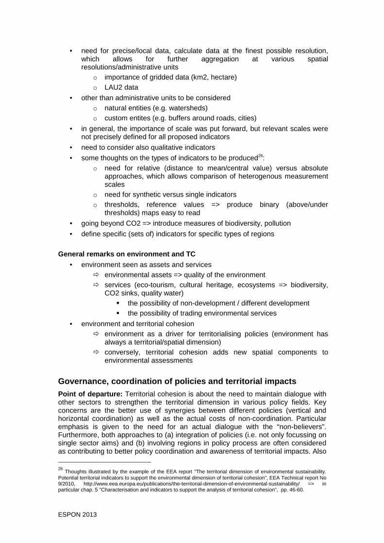
ESPON 2013 78

• need for precise/local data, calculate data at the finest possible resolution, which allows for further aggregation at various spatial resolutions/administrative units

o importance of gridded data (km2, hectare) o LAU2 data

• other than administrative units to be considered o natural entities (e.g. watersheds) o custom entites (e.g. buffers around roads, cities)

• in general, the importance of scale was put forward, but relevant scales were not precisely defined for all proposed indicators

• need to consider also qualitative indicators

• some thoughts on the types of indicators to be produced26: o need for relative (distance to mean/central value) versus absolute

approaches, which allows comparison of heterogenous measurement scales

o need for synthetic versus single indicators o thresholds, reference values => produce binary (above/under

thresholds) maps easy to read

• going beyond CO2 => introduce measures of biodiversity, pollution

• define specific (sets of) indicators for specific types of regions

General remarks on environment and TC

• environment seen as assets and services � environmental assets => quality of the environment � services (eco-tourism, cultural heritage, ecosystems => biodiversity,

CO2 sinks, quality water) � the possibility of non-development / different development � the possibility of trading environmental services

• environment and territorial cohesion � environment as a driver for territorialising policies (environment has

always a territorial/spatial dimension) � conversely, territorial cohesion adds new spatial components to

environmental assessments

Governance, coordination of policies and territoria l impacts Point of departure: Territorial cohesion is about the need to maintain dialogue with other sectors to strengthen the territorial dimension in various policy fields. Key concerns are the better use of synergies between different policies (vertical and horizontal coordination) as well as the actual costs of non-coordination. Particular emphasis is given to the need for an actual dialogue with the “non-believers”. Furthermore, both approaches to (a) integration of policies (i.e. not only focussing on single sector aims) and (b) involving regions in policy process are often considered as contributing to better policy coordination and awareness of territorial impacts. Also

26 Thoughts illustrated by the example of the EEA report "The territorial dimension of environmental sustainability. Potential territorial indicators to support the environmental dimension of territorial cohesion", EEA Technical report No 9/2010, http://www.eea.europa.eu/publications/the-territorial-dimension-of-environmental-sustainability/ => in particular chap. 5 "Characterisation and indicators to support the analysis of territorial cohesion", pp. 46-60.

ESPON 2013 79

various approaches to territorial impact assessments play an important role in the discussion. Largely, the storylines focus on governance and cooperation processes – as a key aspect of territorial cohesion – rather than actual territorial development features. Therefore this storyline clearly differs from the others as it is in its nature non-territorial. The basic idea is that better vertical and horizontal coordination of policies will lead to more balanced development as they are better territorial targeted and thus support territorial cohesion.

As pointed out from the beginning, the governance storyline is different from the other, since it concerns the how, opposed to the what, the latter being the aim of the other. The relation to territorial cohesion is not the same and it seems more difficult to find what kind of indicators could for example render account of policy coordination or cooperation. Without defining governance, one should nevertheless identify what are its components, and more specifically what should be in place or should be done, from a –territorial– cohesion point of view, to achieve “good” governance in this policy field. The White Paper on European Governance (2001) identifies 5 principles of a “good” governance: openness, participation, accountability, effectiveness and coherence, which all must reinforce the principles of proportionality and subsidiarity. Despite none of the speakers mentioned the two first principles, they were mostly present in the discourse of the participants, who insisted more on coordination.

First of all, the perfect policy report should have a good structure, which follows the main aspects of governance: (1) horizontal and (2) vertical coordination, and (3) cooperation.

The most obvious need of coordination is the one between sectoral policies, moreover between those which have a territorial impact. Sectoral policies can easily be in contradiction (e.g. transport and environment), but trade-offs can also appear in one policy: the cohesion policy, with its multiple goals, is a good example. One of the solutions proposed is to better link the policies with the objective of sustainable development, which should be superior and included in each sector, like the territorial approach. But policy makers have to understand why their sector will be better if they adopt such an approach.

Coordination between sectors is not easy at all levels, especially at a national scale, though it would be very helpful to know about coordination at that level.

Vertical coordination must concern all levels, from the European to the local one. The main information to have is “who does what” and what are the agreements in place. The decision making process and the actors should be very well identified, in order to show the relationships to legal institutions, the overlapping cases of government and the alternative governance institutions. Responsibility and accountability are the key issues of the decision making process within the administrative areas, which are democratically elected. On the contrary, in the functional areas, this process is more difficult to identify, though it will be very useful to identify who the stakeholders are in those areas.

A typology of agreements would also be helpful, including the nature, the means and the quality of the cooperation, whether this latter is effective, feasible or desired. Non coordination is important as well: in such a case, we should know about the barriers and the reasons why this doesn’t work.

Cooperation between territories is the third important dimension of governance. It can be cross border, inter regional or transnational, but the most relevant seems to be cooperation between neighbouring entities, which are the key actors of territorial integration. To evaluate this territorial integration, data about flows, connections and functional areas (new or in place) are central.

ESPON 2013 80

At macro regional level, new institutions are needed and more data must be collected, in order to improve the analysis and the policies of cooperation. As for urban rural cooperation, there is a strong call for binding systems, to simplify the functioning of the cooperation.

In any case, rhetoric and good intentions are far from being sufficient. There must be a real territorial strategy with concrete territorial objectives, which the dreamed report must show through tangible examples. What works concretely is as much important to know as what –and why– is inefficient. This could be done by comparative analysis of different areas on the same policy implementation (benchmarking).

The participants insisted on the need of concrete and specific discourse, moreover in the context of a general Territorial Impact Assessment. Indeed, to be able to evaluate sectoral policies from the cohesion point of view, particular examples of “good” and “bad” governance, of what improves the implementation, are necessary. This general TIA (see figure 1) would concern each level of policy production, including functional areas (?), and would show the linkages between the policies (agriculture, transport, etc), which would be evaluated with respect to the storylines.

Figure 1. General Territorial Impact Assessment of policies at each level.

If a TIA is not very original as such, the participants specified several key informations that must be included, such as the costs and opportunity costs and more generally the good use of the amounts allocated for each policy. Suggestion has been done to evaluate the “multiplier effect” (direct and indirect) of policies, because opportunity cost for not doing something could be seen as a negative way to analyze political collaboration. They also asked for an evaluation of the territorial distortion created by the policies, to illustrate to the people in charge of the territorial cohesion policy how their action could be considered as a compensation for bad cohesion effect of other policies.

For the first time, the language and the subjectivity were mentioned as something to be cautious of. Indeed, one should not forget that analysis is a political and cultural activity which can not be fully objective. To avoid being only academic, analysis should be built on interactive cooperation with users. The dreamed report should be understandable for all and take a critical view on the “eurospeak”, trying not to reproduce it and showing how the different policies are shaped by cultural misunderstanding on what do really mean European texts. The different “philosophies” of the countries and their different approach are also to take into account. As one speaker said, the question is: “how do I have to think when I talk to this country?”, or “to this territory”, could we add. Territories can also be subjective

Level of policy production Policy field

ESPON 2013 81

and be considered as “communities” (e.g. Sicily), and those “ideas of territories” are to often forgotten.

The issue of bringing different policies for different territories was also addressed, especially from the point of view of the indicators. The general agreement was about the need of thresholds and rates, rather than different indicators for each specific territory (assuming that one could differentiate each territory with relevant criteria –aside from administrative, economic or geographic ones). Once again, pragmatism was said to be the right approach, including for the scale of policy. As already said, and not only for our storyline, functional areas are central. But borders of all levels should also be more analysed, because they are the place were the gradients appear. There is no doubt that the reduction of discontinuities is a key issue for territorial cohesion. For that issue in particular, data at grid level are required, in addition to NUTS 3 and other scales. It could seem unrealistic, but in fact the lack of data in general should not be a problem. Indeed, we could give a proxy indicator or use sample surveys, and indicate 1) which indicator or index would be the best and 2) what kind of data are missing for it. This could create a virtuous circle and encourage data collection. Thus, indicators and policies are linked in two ways: of course, we need indicators to measure policy issues already known, but thanks to what indicators show, new anomalies or issues can emerge, then leading to a more appropriate political answer (new policy).

Aside from the indicators already mentioned, here are those proposed by the participants during the last discussion. Generally speaking, they said that there is a need for a synthetic indicator on governance, which will be able to show territorially the quality of governance. They didn’t focus only on our storyline but proposed various ways to measure what they thought important for territorial cohesion:

• Good use of money.

• Corruption.

• Logistic efficiency.

• Relative GDP.

• Flows and kind of flows within functional areas.

• Emigration (they said it is good to have such indicators that can say a lot)

• Life expectancy (at birth ?)

• Statistics about VAT (in particular concerning exportation).

• Location of the business (where do they move from, where do they locate, which branch is where ?)

• Location of China’s investment.

• Educational level (need new, reliable ways to measure it).

• Access to services.

• Implementation of EU 2020 strategy at different levels and in different territories.

• Happiness.

• Regional comparisons of GINI coefficient.

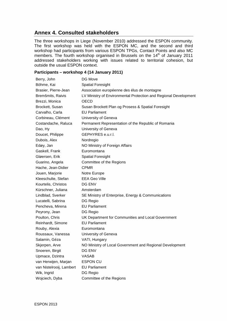
ESPON 2013 82

Annex 4. Consulted stakeholders The three workshops in Liege (November 2010) addressed the ESPON community. The first workshop was held with the ESPON MC, and the second and third workshop had participants from various ESPON TPGs, Contact Points and also MC members. The fourth workshop organised in Brussels on the 14th of January 2011 addressed stakeholders working with issues related to territorial cohesion, but outside the usual ESPON context.

Participants – workshop 4 (14 January 2011)

Berry, John DG Move

Böhme, Kai Spatial Foresight

Brasier, Pierre-Jean Association européenne des élus de montagne

Bremšmits, Raivis LV Ministry of Environmental Protection and Regional Development

Brezzi, Monica OECD

Brockett, Susan Susan Brockett Plan og Prosess & Spatial Foresight

Carvalho, Carla EU Parliament

Corbineau, Clément University of Geneva

Costandache, Raluca Permanent Representation of the Republic of Romania

Dao, Hy University of Geneva

Doucet, Philippe GEPHYRES e.u.r.l.

Dubois, Alex Nordregio

Edøy, Jan NO Ministry of Foreign Affairs

Gaskell, Frank Euromontana

Gløersen, Erik Spatial Foresight

Guarino, Angela Committee of the Regions

Hache, Jean-Didier CPMR

Jouen, Marjorie Notre Europe

Kleeschulte, Stefan EEA Geo Ville

Kourtelis, Christos DG ENV

Kürschner, Juliana Amsterdam

Lindblad, Sverker SE Ministry of Enterprise, Energy & Communications

Lucatelli, Sabrina DG Regio

Pencheva, Mirena EU Parliament

Peyrony, Jean DG Regio

Poulton, Chris UK Department for Communities and Local Government

Reinhardt, Simone EU Parliament

Rouby, Alexia Euromontana

Roussaux, Vanessa University of Geneva

Salamin, Géza VATI, Hungary

Skjerpen, Arve NO Ministry of Local Government and Regional Development

Snoeren, Birgit DG ENV

Upmace, Dzintra VASAB

van Herwijen, Marjan ESPON CU

van Nistelrooij, Lambert EU Parliament

Wik, Ingrid DG Regio

Wojciech, Dyba Committee of the Regions

Annex 5. Selection of indicators on the basis of the territo rial chal-lenges, the EU policies priorities, the “storylines ” and the proposals of stakeholders NTUA team 1

TABLE OF CONTENTS Introduction....................................... .......................................................................... 3

1. Territorial cohesion and territorial challenges. ..................................................... 3

1.1. The Territorial cohesion dimensions .................................................................3

1.2. Territorial challenges in the EU policy documents.............................................4

2. The evolution of the territorial priorities of t he EU policies................................. 6

3. The “storylines” and the opinion of stakeholders .............................................. 12

3.1. The “storylines................................................................................................ 12 Introduction ...................................................................................................................... 12 3.1 Smart growth in a competitive and polycentric Europe.............................................. 12 3.2 Inclusive, balanced development, and fair access to services .................................. 12 3.3 Local development conditions and geographical specificities ................................... 13 3.4 Environmental dimension and sustainable development........................................... 13 3.5 Governance, coordination of policies and territorial impacts ..................................... 13

3.2. New insights and specific indicators of territorial cohesion proposed by stakeholders ..................................................................................................... 14

4. The major territorial cohesion Issues and the pr oposed indicators ................. 15

4.1 Competitive and polycentric Europe ................................................................ 15 (4.1.1) Smart, competitive development .......................................................................... 15 Rationale: Smart, competitive development .................................................................... 17 (4.1.2) Cities and polycentric development...................................................................... 18 Rationale: Cities and polycentric development................................................................ 19

4.2 Inclusive development and fair access to services .......................................... 20 Rationale: Inclusive development and fair access to services......................................... 21 See for the Proposed indicators in Annex 2..................................................................... 23

4.3 Environmental dimension, climate change and risk management.................... 23 Rationale: Environmental dimension, hazards and climate change ................................ 24 See for the Proposed indicators in Annex 2..................................................................... 26

4.4 Sustainable energy.......................................................................................... 26 Rationale: Energy............................................................................................................. 27 See for the Proposed indicators in Annex 2..................................................................... 28

4.5 Specific regions, local development and rural areas........................................ 28 (4.5.1) Specific regions and local development ............................................................... 28 Rationale: specific regions and local development.......................................................... 29 See for the Proposed indicators in Annex 2..................................................................... 30 (4.5.2) The rural areas ..................................................................................................... 30 Rationale: rural areas....................................................................................................... 31 See for the Proposed indicators in Annex 2..................................................................... 31

4.6 Sustainable mobility and connectivity .............................................................. 32 Rationale: Sustainable mobility and connectivity............................................................. 33 See for the Proposed indicators in Annex 2..................................................................... 34

4.7 Territorial governance, coordination of policies and territorial impacts ............. 34 Rationale: Territorial governance, coordination of policies and territorial impacts .......... 35 See for the Proposed indicators in Annex 2..................................................................... 35

1 Minas Angelidis, contributions: Epameinontas Tsigkas, Vivian Bazoula, Anastasia Founta. We have included in the paper texts from the “storylines” (Spatial Foresight) and the Territorial Cohesion approach (UniGe). See references in the respective sections

2

4.8 Global indicators of territorial cohesion............................................................ 36 The Overall (Global) Territorial cohesion challenge ........................................................ 36

References ......................................... ....................................................................... 36

Annex 1.1: Extracts from the “Regions 2020” ........ ................................................ 38

A. The approach of new global challenges ............................................................ 38

B. Indicators used for assessing sensitivity to combined challenges: range and weights ............................................................................................................. 39

Annex 1.2: All challenges and themes ............... ..................................................... 40

Annex 1.3: All EU policies territorial priorities a nd themes................................... 41

Abbreviations FUA: Functional Urban Area GDP: Gross Domestic Product CEMAT: Council of Europe Conference of Ministers Responsible for Spatial/Regional Planning

(Conférence du Conseil de l’Europe des Ministres responsables de l’Aménagement du Territoire)

List of Tables and Figures Figure 1: Links among territorial challenges, driving forces of territorial development and themes

.............................................................................................................................................. 4

Figure 2: From three narratives to one single narrative on the links of challenges, policies and storylines to themes and indicators....................................................................................... 5

Figure 3: The seven major Issues links to challenges, policy orientations and storylines. ........... 5

Table 4.1.1: Smart, competitive development............................................................................. 16

Table 4.1.2: Cities and polycentric development ........................................................................ 19

Table 4.2: Inclusive development and fair access to services .................................................... 21

Table 4.3. Environmental dimension, climate change and risk management............................. 24

Table 4.4: Sustainable energy..................................................................................................... 27

Table 4.5.1: Specific regions, local development........................................................................ 29

Table 4.5.2: Rural areas.............................................................................................................. 31

Table 4.6: Sustainable mobility and connectivity ........................................................................ 33

Table 4.7: Territorial governance, coordination of policies and territorial impacts...................... 35

3

Introduction In this working paper (in Annex of the Interim Report), the NTUA team explains the methodology and the results of the definition / selection of indicators in the frame of INTERCO on the basis of the territorial challenges, the EU policies territorial priorities, the “storylines” developed by the project2 and the proposals of stakeholders.

A summary of this working paper is included in the Interim Report. However, we con-sidered necessary to present here in more extent the several steps implied in this work in order to better justify the selection of the indicators in INTERCO. In general, the se-lection of territorial indicators should be primarily based on the explanatory power of the indicators in relation to the territorial issue at stake; in our case, Territorial cohe-sion. This is not the case in several other attempts to create territorial indicators. Fur-thermore, this paper discusses in more extent the correlation of the issues raised by the EU policies territorial priorities with selected indicators, this correlation being of pri-mary importance for INTERCO. Finally, the presentation of Rationales of selection of indicators which refer directly to the indicators themselves allow stakeholders and the supervisors of this work propose modifications or additions to the list of indicators in respect to structured Rationales.

Specifically, we repeat in this Annex 1, in almost all the sections on Issues, the ration-ales which have been included in the respective short text of the Interim Report. In the following Annex 2, which follows immediately the Annex 1, are included, per major Is-sues, the proposed indicators grouped per themes. Annex 2 is also useful for those who read only the respective short text of the Interim Report.

In its response to the project Inception Report, ESPON CU has mentioned, concerning this matter, that “agrees with revised approach (of TPG) to develop a list of feasible and meaningful territorial indicators and indices in continuous interaction with the stakeholders during the project” and this progress of this list will be reported in the In-terim Report. We believe more specifically it is essential (as it is also stressed in the Inception Report Annex) that the determination of indicators should advance as a com-bination of the conclusions of stakeholders meetings and of the thorough examination: (a) of the territorial challenges and the EU policies territorial objectives and the relationships of these last with appropriate groups of themes (issues) (b) of appropri-ate territorial storylines (prospective policy options).

In next we will define /select a set of feasible indicators based on a review of the above (a) challenges, policies and themes (b) territorial storylines (c) opinions of stakeholders.

Essentially, challenges, policies, storylines, stakeholders’ proposals and themes are parts of a multi-dimensional matrix which contains matrices of challenges / themes, challenges / policies, policies / themes , challenges / storylines and so on . How-ever, in order to produce a narrative understandable by stakeholders we applied the following steps:

We started from the review of the main territorial challenges that European space faces -section 1 - and we then examine the evolution of the territorial priorities of the EU policies -section 2 . Next -section 3 -, we present shortly the “storylines” which served as the basis for the discussion of the territorial cohesion indicators by the selected stakeholders. Then, we cross-check the challenges, the existing EU policies, the “storylines” and the proposals of stakeholders with appropriate groups of themes and indicators (simple or “territorial”) order to define a set of indicators feasible as for their explanatory power. We firstly took into account the indicators which have already been defined in

2 By Spatial Forth-sight

4

the Inception Report and its Annex and we then proposed additional appropriate indica-tors.

We followed the next methodological steps: In a first stage of our work we have exam-ined which groups of themes are necessary to use in order to study the major driving forces that are behind each territorial challenge and, therefore, determine which indicators are the most appropriate for the analysi s of these driving forces –see Figure 1. A similar cross-check of the territorial objectives of the EU policies with rele-vant policy driven forces and respective groups of themes and specific indicators has also been made. Finally, the storylines and the comments and proposals of the se-lected stakeholders on the base of the storylines have been used to further discuss the relevant driving forces and policy driven forces.

Figure 1: Links among territorial challenges, drivi ng forces of territorial development and themes

Therefore, we have initially produced three distinct narratives on the causal links among territorial challenges and indicators, existing territorial policy objectives and in-dicators and, finally, prospective policy options (storylines) and indicators3. In order to make this work more understandable from the interested stakeholders and the ESPON community, it is worthwhile to make a single holistic narrative relating challenges, existing policy objectives and storylines with indicators and respective themes that are included in the INTERCO Inventory of indicators – Figure 2.

This single narrative is based on seven Rationales corresponding to respective major Territorial Cohesion Issues -section 4 . This structuring will also enable us to more clearly relate the seven Rationales with the respective matrices of indicators (challenges / themes, policy objectives / themes etc). The correspondence of the seven Issues to challenges / policy orientations and storylines is presented in the Figure 3.

3 See for the correspondence of the challenges, policy priorities and storylines to indicators in respective Annexes.

5

Figure 2: From three narratives to one single narra tive on the links of challenges, policies and storylines to themes and indicators

Figure 3: The seven major Issues links to challenge s, policy orientations and storylines.

As we have stressed, we will emphasise on the causal links among challenges, policies and storylines with the proposed indicator s on the basis of an in depth analysis of the relevant literature on the EU policies territorial priorities. Evidently, we focused on the “Europe 2020” documents and the 5 th Cohesion Report as both ex-plore better the territorial cohesion policy perspectives.

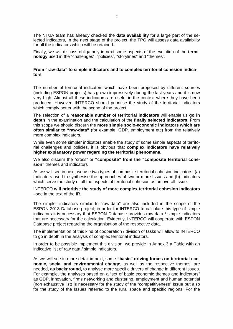
2

The NTUA team has already checked the data availability for a large part of the se-lected indicators, In the next stage of the project, the TPG will assess data availability for all the indicators which will be retained..

Finally, we will discuss obligatorily in next some aspects of the evolution of the termi-nology used in the “challenges”, “policies”, “storylines” and “themes”.

From “raw-data” to simple indicators and to complex territorial cohesion indica-tors

The number of territorial indicators which have been proposed by different sources (including ESPON projects) has grown impressively during the last years and it is now very high. Almost all these indicators are useful in the context where they have been produced. However, INTERCO should prioritise the study of the territorial indicators which comply better with the scope of the project.

The selection of a reasonable number of territorial indicators will enable us go in depth in the examination and the calculation of the finally selected indicators . From this scope we should discern the more simple socio-economic indicators which are often similar to “raw-data” (for example: GDP, employment etc) from the relatively more complex indicators.

While even some simpler indicators enable the study of some simple aspects of territo-rial challenges and policies, it is obvious that complex indicators have relatively higher explanatory power regarding the territorial phenomena .

We also discern the “cross” or “composite” from the “composite territorial cohe-sion” themes and indicators

As we will see in next, we use two types of composite territorial cohesion indicators: (a) Indicators used to synthesise the approaches of two or more Issues and (b) indicators which serve the study of all the aspects of territorial cohesion as an overall Issue.

INTERCO will prioritise the study of more complex territor ial cohesion indicators –see in the text of the IR.

The simpler indicators similar to “raw-data” are also included in the scope of the ESPON 2013 Database project; in order for INTERCO to calculate this type of simple indicators it is necessary that ESPON Database provides raw data / simple indicators that are necessary for the calculation. Evidently, INTERCO will cooperate with ESPON Database project regarding the organisation of the respective data.

The implementation of this kind of cooperation / division of tasks will allow to INTERCO to go in depth in the analysis of complex territorial indicators.

In order to be possible implement this division, we provide in Annex 3 a Table with an indicative list of raw data / simple indicators.

As we will see in more detail in next, some “basic” driving forces on territorial eco-nomic, social and environmental change , as well as the respective themes, are needed, as background, to analyse more specific drivers of change in different Issues. For example, the analyses based on a “set of basic economic themes and indicators” as GDP, innovation, firms networking and clustering, employment and human potential (non exhaustive list) is necessary for the study of the “competitiveness” Issue but also for the study of the Issues referred to the rural space and specific regions. For the

3

study of these last we should use the “set of basic economic themes and indicators” as background in order to build analyses of the specific features of the rural space and the specific regions. Also, even the analysis of the “climate change” Issue should use the same “set of basic economic themes and indicators” in order to study the economic development aspects of the climate change.

Thus at least three “basic sets of themes and indicators” : economic, demographic / social and environmental, are commonly needed for the study of several Issues; in other words, the respective indicators are overlapping among different Issues. As the discussion of these obvious “overlapping” is useful, we will specify more, during the project, the above “basic sets of themes and indicators” as well as their affiliation with specific Issues. 1. Territorial cohesion and territorial challenges 1.1. The Territorial cohesion dimensions

As it was stressed in the Inception Report4, defining territorial cohesion is far from be-ing easy, and perhaps not even wanted by part of stakeholders. However, we can try to draw few essential guidelines of what those terms may signify. The use of the adjective "territorial" allows many interpretations. Several interdependent aspects are to be taken into consideration: the territorial cohesion as a spatial dimension of a cohesion policy more attentive to territorial impacts of sectoral policies, as promotion of equality and equity, as a kind of territorial development policy at European level, and as principle of governance. Indeed, what emerges of various communications of institutions, lobbies or experts is first a fresh look on cohesion -or regional- policy. The cohesion between regions of EU must be not only economic and a bit social, but also territorial, meaning that small towns, cities, rural areas, islands, etc. must be taken into account as well, either to catch up or to remain competitive.

See for an in depth analysis of the several dimensions of Territorial cohesion in the respective section of the Interim Report.

4 This paragraph, is extracted from the respective section of the Inception Report, produced by UniGe

4

1.2. Territorial challenges in the EU policy docume nts The Project’s specifications (2009) refer to the main territorial challenges in rela-tion to Cohesion Policy considerations and the Territorial Agenda of the EU, including:

We will report them, concisely, in next, where it needs, as: (1) «Global economic com-petition”, (2) Climate change”, (3) “energy”, (4) “demography”, (5) “transport” and (6) “geographic structure of Europe”.

For the further analysis of these challenges (in order to, later on, examine which are the most relevant themes and indicators for the challenges) we will first discuss: (a) the Territorial Agenda of the EU (2007), (b) the EU Cohesion Policy documents , mainly the 4th Report on economic and social Cohesion (2008), the Sixth progress re-port on economic and social cohesion (2009) and the recently published (on November 2010) 5th Cohesion Report (c) the “Europe 2020” documents and the EC document “Regions 2020” (2008).

All these documents refer with the one or the other way to the above six challenges. Certain documents subdivide one or more from the above challenges in other “chal-lenges” or group two or more of the initial challenges to one. We are not interested so much in the precise number of challenges but to the driving forces that are behind the challenges and, afterwards, in the themes and indicators which are most suit-able to analyse these challenges.

A first set of territorial challenges was discussed in the ESDP dated on 1999. A new approach of these challenges is presented in The Territorial Agenda of the EU (2007). This approach has taken into account the changes in the EU territorial devel-opment occurred in the first half of the 2000’ decade. The most important changes as for the understanding of the territorial challenges is that Territorial Agenda put more emphasis on the territorial impacts of globalisation and climate change.

Territorial Agenda refers, specifically, to the following “new territorial challenges” that EU space faces (Territorial Agenda of the EU pages 2 and 3):

1. Accelerating integration of our regions, including cross-border areas, in global economic competition, and at the same time increasing dependencies of states and regions in the world,

2. Impacts of EU enlargement on economic, social and t erritorial cohesion, par-ticularly with regard to the transport and energy infrastructure related integration of Eastern Europe and the new EU Member States as well as their regions,

(1) Global economic competition : Increasing global pressure to restructure and modernise, new emerging markets and technological development;

(2) Climate change : New hazard patterns, new potentials; (3) Energy supply and efficiency : Increasing energy prices; (4) Demography : Ageing and migration processes; (5) Transport and accessibility / mobility : Saturation of euro-corridors, urban trans-

port; (6) Geographic structure of Europe : Territorial concentration of economic activities in

the core area of Europe, and in capital cities in Member States of 2004, further EU enlargements.

5

3. Regionally diverse impacts of climate change on the EU territory and its neighbours, particularly with regard to sustainable development

4. Rising energy prices, energy insufficiency and different opportunities for new forms of energy supply

5. Overexploitation of the ecological and cultural res ources and loss of biodiver-sity, particularly through increasing development sprawl whilst remote areas are facing depopulation,

6. Territorial effects of demographic change (especial ly ageing) as well as in and out migration and internal migration on labour markets, on the supply of public services of general interest as well as the housing market, the development of the settlement structure and how people live together in our cities and regions.

(We have changed the order with which challenges are reported and we numbered them)

The above challenge (1) refers to “Global economic competition”, challenge (2) refers also to Global economic competition regarding by priority the new EU Member States, but also to social cohesion, transport and energy issues as for the same states. Chal-lenges (3) on climate change, (4) on energy issues and (6) on demographic change correspond more or less to the project specifications’ challenges (2), (3) and (4). Chal-lenge (5) that refers to “Overexploitation of the ecological and cultural resources” was not included in the project specifications’ territorial challenges; it is related to a great extent with challenge on climate change.

The 4th EC Report on economic and social cohesion dated on 2007 emphasized on the same more or less global and territorial challenges; there are some slight changes on priority themes inside each challenge.

The “Green paper on territorial cohesion : Turning territorial diversity into strength” (2008) launched a first debate on the concept of territorial cohesion and its specific objectives. We will discuss in next section the Territorial cohesion objectives while we will be limited here to refer to the approach of the territorial challenges by this docu-ment.

The “Green paper” refers also, more or less, to the same, territorial challenges already reported: global economic competition, climate change, energy issues, demographic and social challenges (including migration and social exclusion etc). Specifically, it gives more emphasis to the challenge of best using the territorial assets in an in-creasingly globalising and competitive economy. It also points out the growing impor-tance of strong links / flows of technology and ideas, goods, servi ces and capital among territories through cooperation in order to use the common assets in a coor-dinated and sustainable way.

A relatively new understanding of the territorial challenges is presented in 2009 and 2010 in the EC documents on “Europe 2020” strategy which is related to the EU de-velopment during the last years of the 2000’ decade including the effects of the 2008 economic crisis and the discussion inside the EU on how to face the weak points of the EU economic structure that are revealed by the crisis.

Specifically, these documents preparing the Europe 2020 strategy as well as the new Cohesion Policy 2014 – 2020, acknowledge the territorial challenges identified above and put more emphasis on their aspects more closely related to the recent fast moving

6

of the globalisation: “the world is moving fast and long-term challenges –globalisation, pressure on resources, ageing – intensify” (“Europe 2020” Communication from the Commission (2010)). However, in line with the respective policy developments (see next in section 3), emphasis is given to the innovation aspect of the globalisation and even more to the “creativity” component of innovation as well as to the “social exclu-sion” and the “pressure on resources”.

The “Europe 2020” documents refer mainly to the “global” challenges and say little about the territorial aspects of these challenges. Such a “territorial specification” is pre-sented in the 5th Cohesion Report which is published in November 20105. It is also useful to see how the EC “Regions 2020” (2008) document (which has adopted more or less the same scope with the Europe 2020 strategy) analyses the “regional” aspects of the challenges that EU faces.

In general terms, “Regions 2020” states that: “the following four (challenges) may be of particular relevance for European regions: Globalisation, Demographic change, the impact of climate change and “Secure, sustainable a nd competitive energy” 6. The document produced respective “vulnerability” indexes (composite territorial in-dexes) for these challenges.

The 5th Cohesion Report (2010) explains what territorial cohesion adds to Cohesion Policy, following the debate launched by the Green Paper on territorial cohesion and presents new indicators that reveal the territorial dimension of issues like poverty and access to services – see in more detail in next.

2. The evolution of the territorial priorities of t he EU policies The different aspects of “Territorial cohesion” have been discussed in section 1. In next we will further discuss these different aspects in more close relation with the definition of the territorial objectives of the EU policies.

According to the “Green Paper on Territorial Cohesion (2008): “Territorial cohesion is about ensuring the harmonious development of all these places and about making sure that their citizens are able to make the most of inherent features of these territories. As such, it is a means of transforming diversity into an asset that contributes to sustain-able development of the entire EU”.

As we have already pointed out, this definition is obviously very general; large debates on the concept of territorial cohesion took place during the last years. While there is not a unanimous acceptable definition of territorial cohesion, in all the different approaches of the concept is accepted that economic, social and environmental aspects are crucial for the territorial cohesion. Some approaches stress the importance of the eco-nomic (competitiveness) dimension while other, on the contrary, emphasise the social and / or environmental approach. Also, other aspects as governance or some specific territorial aspects have seen as of crucial importance for territorial cohesion.

5 In preliminary version – see in References 6 «This document seeks to explore the regional effects of these challenges in the medium - term perspective of 2020. It seeks to illustrate which regions are most vulnerable to these challenges, as a step towards a better understanding of the potential pattern of regional disparities that these challenges will generate” (Regions 2020, 2008)

7

Since the Lisbon Treaty (2007) has added territorial cohesion to the goals of economic and social cohesion, all European policies which impact on territorial development and even more the Cohesion policy should address the objective of territorial cohesion in their implementation.

In next we will try to discuss in more depth both the content and the term inology of the EU policies territorial objectives ; we will present first the project’ specifica-tions general classification and terminology of the “policies” and we then will try to fur-ther develop their territorial objectives.

• Balanced territorial development;

• Strengthening a polycentric development by networking of city regions and cities;

• Urban drivers (large European cities, small and medium sized cities, suburbanisation, inner city imbalances);

• Development of the diversity of rural areas;

• Emphasis on ultra-peripheral, northern sparsely populated, mountain areas, islands;

• Creating new forms of partnership and territorial governance between urban and rural ar-eas;

• Promoting competitive and innovative regional clusters;

• Strengthening and extending the Trans-European Networks;

• Promoting trans- European risk management including impacts of climate change

• Strengthening ecological structures and cultural resources

We will make necessary changes according to the recent development of the thinking on the territorial objectives of the EU policies. Territorial objectives of the EU policies have been integrated in texts of broader territo-rial orientations, starting from the ESDP (European Spatial Development Perspective, 1999) and the Territorial agenda of the European Union (2007). However, other texts of orientations for the EU Cohesion Policy as the Cohesion Reports and specific guidelines on the implementation of the Cohesion Policy or even more general texts for the entire development of the EU as the former Lisbon strategy , the more recent Lis-bon treaty (2009) and the actually in discussion documents on “Europe 2020” define respective priorities for the territorial development of the European space. Finally, a series of texts supporting with one or another way the definition of the territorial priori-ties of the EU policies or discussing and further developing these priorities should also taken into account.

We will examine in next the evolution of the entire “territorial priorities ” thinking in order to better precise the actual territorial priorities and objectives of EU policies as well as the priorities more oriented towards the future of the EU policies.

Undoubtedly, the initially defined (see in the ESDP) territorial economic, social and environmental objectives which all together formed the overall territorial vision of the

8

EU policies tend to be integrated in the overarching concept of “territorial cohe-sion” which is included in the Lisbon Treaty (2007).

During the ‘90s were adopted (worded more or less clearly) and included in texts of European Council resolutions, in guidelines of Cohesion Policy, in guidance documents for spatial development etc as three key strategic territorial orientations, the c om-petitiveness, the cohesion and the sustainability.

This vision was mainly reflected in the ESDP (1999) which defined as main priorities: (a) Polycentric Spatial Development and a New Urban-Rural Relationship (b) Parity of Access to Infrastructure and Knowledge (c) Wise Management of the Natural and Cul-tural Heritage.

Next, the Lisbon Strategy emphasized the importance of competitiveness and in par-ticular the Knowledge and Innovation for the development of Europe. Specifically, the Lisbon Strategy highlighted the need to make the EU economy the most competitive and dynamic economy in the world with the "knowledge" as the driving force, so as to obtain sustainable economic development with more and better jobs and social cohe-sion (Presidency Conclusions, Lisbon European Council, 23-24 March 2000). Cohesion Policy is acknowledged as a key tool in this effort (Presidency Conclusions, Brussels European Council, 22-23 March 2005).

Towards the 4th programming period of the Cohesion Policy (2007 - 2013) the key strategic orientations were further specified, giving priority to the development of en-trepreneurship and innovation. The strategic priority of cohesion maintains its impor-tance, while the priority of sustainable development of the Community area was further emphasized -see especially the final conclusions of the Gothenburg Council (2001). Critical factors in this "Knowledge society" are innovation, research, technology devel-opment, learning and sharing experiences, which require a dense network of cooperat-ing "actors".

According to the European Commission strategic guidelines for cohesi on for the period 2007-2013 (2005), the programmes co-financed by cohesion policy should tar-get their resources according to the following three priorities: - Improving the attractive-ness of Member States, regions and cities (...)

- Encouraging innovation, entrepreneurship and development of the knowledge econ-omy through research and innovation, including new information and communication technologies.

- Creating more and better jobs by attracting more people into employment or entre-preneurial activity (...).

More specifically, the territorial dimension of cohesion policy in this document had been taken into account through the following guidelines:

(a) The contribution of cities to growth and jobs (b) Supporting the economic diversification of rural areas (c) Cooperation

- Cross-border cooperation - Transnational cooperation - Interregional cooperation

9

Next, the Territorial Agenda of the EU (2007) reviewed the territorial vision and objec-tives of the EU policies. The Agenda attempted first to make the territorial policy priori-ties clearer as well as more understandable by stakeholders using for this purpose a shorter and simpler text compared to the text of the ESDP. Without diverging to a con-siderable degree from the objectives of the ESDP, it integrated EU territorial policy de-velopments occurred during the first half of the 2000’ decade, mainly the new policy priorities related to new economic competition and climate change challenges.

The 4th Cohesion report , published in 2007 titled “Growing Regions, growing Europe”, stress that Europe should place the main emphasis on knowledge, innovation and optimisation of human capital by mobilizing to best way its resources (national and Community) in order to achieve its objectives (of increasing its competitiveness, poten-tial and productivity).

It specifically underlines that: “Leading edge economic activities and talent tend to be geographically highly concentrated in a few urban centres that are global players”.

The report also introduces the concept of climate change and its impact on cohesion, economical, social and territorial7.

It is specifically mentioned that: “Agriculture, fisheries and tourism are most directly influenced from climate change and require significant investment to face drought, fires, coastal erosion and flooding . It’s obvious that the most vulnerable groups of this situation are the disadvantaged or low income groups which might lack the means to adapt to them”. Thus, as it is stressed, the optimistic perspective of this new design parameter is that provides regional economies with new economic incentives and op-portunities through eco-innovation , the growth of environmentally friendly indus-tries and employment in this area.

Thus, composite indicators that measure this type of entrepreneurship and its influence in improvement of environmental conditions are of high interest for INTERCO.

An also important issue of this report was the increased energy prices that will affect EU regions in different ways depending on their energy mix, economic structure and the energy efficiency of their firms. Geographically peripheral and touristic regions are more vulnerable due to transport costs. Although, high prices could be the driving force for the development or expansion of renewable energies, the investments in energy efficiency, the growth strategies on less energy-intensive methods of production, pro-viding major opportunities for most regions.

For this issue, apart from the respective composite indicators, several new indicators relating aspects of energy efficiency, renewable energies etc could be created.

The Green paper on Territorial Cohesion (2008) capitalised the first results of the debate on the concept and objectives of “Territorial cohesion”. As it points out (in gen-

It specifically stresses that “Asymmetric impact of climate change … depends on geographical character-istics, existing infrastructure and other factors”.

10

eral terms) : Main target of “Territorial Cohesion” is to achieve a “more balanced and harmonious development ” throughout Europe…”.

“Green paper” does not differ essentially from the ESDP (1999) as for the three general policy priorities; strengthening economic competitiveness / capacity of growth , en-suring social cohesion and preserving natural assets . However, it gives more em-phasis in three territorial cohesion orientations: overcoming differences in concen-tration, overcoming distance among territories (“connecting territories”) and over-coming division through cooperation. We will specify more the territorial objectives of these major “territorial cohesion” orientations in next section8. The “Europe 2020” EC document9 (2010), compared to the older ones, has taken into account the recent economic crisis and reformed the essential challenges that EU faces, acknowledging as an immediate challenge its “recovery”. The lessons from the crisis are on the one hand the growing role of the interdependence of economies10 and on the other hand the important role of transport and energy in the internal market and of coordination, that stabilize banking system.

Specifically, the document of the conclusions of European Council (25/26 March 2010) on the “Europe 2020” strategy emphasizes that «the EU needs a new strategy, based on an enhanced coordination of economic policies , in order to deliver more growth and jobs ” (General Secretariat of the Council 2010 page 2).

“Europe 2020” puts forward three mutually reinforcing priorities: – Smart growth : developing an economy based on knowledge and innovation. – Sustainable growth : promoting a more resource efficient, greener and more com-petitive economy. – Inclusive growth : fostering a high-employment economy delivering social and terri-torial cohesion”

According to the document (2010, page 7), the strengths of Europe that are needed to be measured and integrated in the approach of territorial cohesion, are:

(a) Human resources (talent, creativity) (b) Industrial base (strong) (c) Service sector (d) Agricultural sector (e) Maritime tradition (f) Cultural diversity, gender equality (g) Environment respect (h) Territorial cohesion solidarity

We should note that other political approaches of territorial cohesion, as for example that of CEMAT (Council of Europe Conference of ministers responsible for spatial / regional planning) Moscow declaration 2010 11, bring some new aspects of Territorial cohesion. CEMAT 2010 conceives Territorial cohesion as a basic territorial dimension

8 We should also note that “Green paper” stresses the necessity to improve the flexibility of policies and actions by referring to smaller or bigger region levels and not NUTS 2. 9 Europe 2020, Strategies for smart, sustainable and inclusive growth, 2010. 10 “The one country affect the performance of all others” (EUROPE 2020, 2010,page 4) 11 CEMAT / Council of Europe, 2010, 15th Council of Europe Conference of ministers responsible for Spa-tial / regional planning, Moscow Declaration on “Future challenges: sustainable territorial development of the European continent in a changing world.

11

of human rights”12 without diverging considerably as for the specific targets of Territorial cohesion from the EC “Green paper” and “Europe 2020” approach.

The CEMAT 2010 declaration underlines a number of “new challenges” that are in general the same with those referred in “Europe 2020” and older documents (4rth Co-hesion Report, etc).These are: climate change, population ageing (demographic) and social polarization (social-cultural), under the umbrella of the latest economic crisis. All of them call for appropriate and efficient territorial policy responses and territorial de-velopment initiatives. The contribution of cities in economic recovery , because of their considerable added value for innovation, is highlighted as very important13 (CEMAT, 2010). Finally, CEMAT proposes policy priorities on numerous areas of terri-torial development: energy, transport, construction and renovation of buildings, agricul-ture and forestry, tourism and so on 14 (CEMAT, 2010). Finally, the 5th Report on cohesion (2010), regarding specifically territorial cohesion, analyses the role of urban areas, based on their advantages and disadvantages as well as their strengths and weaknesses; it also put emphasis on the role of functional geog-raphies and of the areas facing specific geographical and demographic problems. Its main objectives (in parentheses: similar objectives of “Europe 2020”) are oriented to15:

• Supporting active inclusion (inclusive growth-Europe 2020) • Fostering social innovation • Developing innovation strategies (smart growth) • Designing schemes for regeneration of deprived areas • Rural development • Maritime policies16

Some territorial challenges identified by this Report should be further analysed through innovative indicators; for example, how cohesion policy could take better into account

12 “The overarching objective of territorial cohesion, as promoted by the [CEMAT} Guiding Principles, should be interpreted primarily as a basic territorial dimension of human rights. It represents a fundamental value of European society that can reconcile European citizens and their daily aspirations in terms of hu-man dignity, equity and security, and good living, working and cultural environments, with the unavoidable transformations in production systems and in the international and interregional division of labour, with changes in natural conditions such as climate change, and with the move towards a more multicultural society”. 13 See in CEMAT 2010, page 7: “European continent is more and more determined by the skills of people and the strengths of our cities in which knowledge, education, innovation and research find a powerful base…Innovative, sustainable and cohesive territorial development contributing to overcoming the conse-quences of the economic crisis. Furthermore, the crisis and its consequences should also be considered and used as an opportunity for boosting territorial cohesion, especially in promoting place-based strategies which permit more rational and economical use of public resources. It is therefore of primary importance that the capabilities of territorial development policies be fully utilised and this requires a number of signifi-cant adjustments. Territorial development policies should be helpful in reconciling the short-term, often sectoral measures adopted by governments to overcome the crisis with long-term values and principles, such as territorial cohesion and sustainable territorial development.” 14 See in CEMAT declaration 2010, page 8: “The adoption of new adaptation generates a great many new activities and significant numbers of new jobs, while contributing to improved quality of life and reduced risks related to climate change. Responding successfully to new challenges requires (in the territorial devin the context of cross-border co-operation, enabling territorial development policies to be efficiently com-bined with efforts to regenerate the European economy in a sustainable way and to provide efficient and adequate mitigation and adaptation solutions to the issues related to climate change”. 15 5th Cohesion Report, Conclusions: the future of cohesion policy. 16 The approach of maritime policies requires the formulation of appropriate indicators. The 5th Report does not have any specific reference to such indicators in a figure, map or table.

12

the key role of urban areas and territories (geographical features, macro – regional strategies etc) and how improve partnership.

3. The “storylines” and the opinion of stakeholders

3.1. The “storylines 17

Introduction INTERCO project has decided to develop different stories about territorial cohesion in order to sharpen the understanding of what territorial cohesion actually may comprise. The stories aim to facilitate a more thorough discussion on the different facets of territorial cohesion and how a limited number of indicators can be used to illustrate or measure the single facets. Each of these stories highlights different facets of the territorial cohesion debate as observed during the past decade. These stories are not mutually exclusive. The five stories- or dimensions of territorial cohesion highlighted – are: • Smart growth in a competitive and polycentric Europe • Inclusive, balanced development, and fair access to services • Local development conditions and geographical specificities • Environmental dimension and sustainable development Environmental dimension • Governance, coordination of policies and territorial impacts

3.1 Smart growth in a competitive and polycentric E urope Point of departure:

Territorial cohesion must contribute to economic growth in order to achieve the aims of Europe 2020 and boost European competitiveness. This implies a strong focus in territorial potentials and the support of smart growth and the connectivity of Europe’s economic centres . Only if the economic viable and powerful places in Europe are making full use of their growth potentials and acting as engines for development for larger areas surroundin g each of them, will territorial cohesion be possible. These economic centres are at the forefront of development and are important nodes in global economic networks. A key issue is European polycentric de-velopment, i.e. the development of a number of interconnected European hubs or Major Euro-pean Growth Areas (MEGAs) which mutually reinforce each other and lead to the strong growth envisioned for 2020.

3.2 Inclusive, balanced development, and fair acces s to services Point of departure:

Territorial cohesion is about balanced development focusing on European solidarity and stress-ing inclusive growth, fair access to infrastructure ser vices and the reduction of economic disparities. There is a strong idea of strengthening the use of development potentials outside the main growth poles and ensuring a minimum of welfare in all regions. Every territory has its own distinct set of potentials for further development – its territorial capital or comparative ad-vantage. At the same time, every region and local area also has resources available to make use of assets and balance deficiencies. The difference between the assets and deficiencies on the one side and the resources available to territories to activate potentials and to respond to deficiencies on the other, results in the strength or fragility of a territory. Supporting “equal” or fair development opportunities is a key issue, not least expressed in the debate on fair access

17 They are developed by Spatial Foreshight

13

to infrastructure and services . People and companies in all parts of a territory need to have access to certain standards of services. The delivery of these can depend on the territorial con-text, i.e. the same service can be delivered by different means in different areas.

3.3 Local development conditions and geographical s pecificities Point of departure:

(a) Local development: Territorial cohesion is about place-based policy making, paying par-ticular attention to local development conditions – going below the regional level. Indeed the identification and exploitation / use of tangible and intangible endogenous potentials is the key for development and smart, inclusive and sustainable growth in Europe. Particular attention is given to the specificities of places and their comparative advan tages. In many cases the intangible factors of tacit knowledge and local networks (incl. clusters) and the access to the nearest economic centres are considered to be of key importance. Thus territorial cohesion is very much about recognising the territorial diversity in Europe and also the importance of the territorial context and its multifaceted dynamics as key to success. This involves endogenous development potentials and fragilities, as well as exogenous factors such as the impact of de-velopments in other territories, and the impacts of different sector policies at various levels of decision making.

(b) Geographical specificities : Territorial cohesion is about geographical specificities. There are particular types of regions and the key reference text is art. 174 of the Treaty: “… In particu-lar, the Union shall aim at reducing disparities between the levels of development of the various regions and the backwardness of the least favoured regions. Among the regions concerned, particular attention shall be paid to rural areas, areas affected by industrial transition, and regions which suffer from severe and permanent natural or demographic handicaps such as the northernmost regions with very low popu lation density and island, cross-border and mountain regions .”

3.4 Environmental dimension and sustainable develop ment Point of departure:

To contribute to the sustainable growth aim of the Europe 2020 strategy, and with regard to need to consider the environment and climate change , territorial cohesion also has an envi-ronmental dimension stressing sustainable development. The richness of Europe's natural heritage and landscapes is an expression of its identity and is of general importance. To re-verse any process of abandonment and decline and to hand this heritage on to future genera-tions in the best possible conditions requires a creative approach. Territorial cohesion requires a more resource efficient and greener economy. Initiatives tackling climate change or to make more efficient use of resources should no longer be seen only as concerns of environmentalists: rather territorial development at all scales from the EU to the local need to include such meas-ures. In that respect clean and efficient energy are preconditions for the future development that also help the economy to cope with increasing energy prices. Furthermore, this storyline has a clear global dimension...

3.5 Governance, coordination of policies and territ orial impacts Point of departure:

Territorial cohesion is about the need to maintain dialogue with other sectors to strengthen the territorial dimension in various policy fields. Key concerns are the better use of synergies be-tween different policies (vertical and horizontal coordination) as well as the actual costs of non-coordination. Particular emphasis is given to the need for an actual dialogue with the “non-believers”. Furthermore, both approaches to (a) integration of policies (i.e. not only focussing on

14

single sector aims) and (b) involving regions in policy process are often considered as contribut-ing to better policy coordination and awareness of territorial impacts. Also various approaches to territorial impact assessments play an important role in the dis-cussion. Largely, the storylines focus on governance and cooperation processes – as a key aspect of territorial cohesion – rather than actual territorial development features. Therefore this storyline clearly differs from the others as it is in its nature non-territorial. The basic idea is that better vertical and horizontal coordination of poli cies will lead to more balanced develop-ment as they are better territorial targeted and thus support territorial cohesion.

3.2. New insights and specific indicators of territ orial cohesion pro-

posed by stakeholders Stakeholders which have participated in the Brussels workshop have proposed new insights of territorial cohesion per storyline as well as new themes and specific indica-tors which better reflect different aspects of territorial cohesion. In the following, we refer to some of the proposals of the stakeholders. We will inte-grate the more appropriate proposals for the territorial cohesion approach through indi-cators in the next section on a “single narrative for the selection of indicators”. - Several aspects of “sustainable growth” were highlighted: “Competition is not only about economic fastest and highest growth but also about qualities which are needed to support long-term development and “sustainable growth”. A key word in this respect is “attractiveness” of places: quality of life, Individual perceptions, the inhabitants’ satis-faction …». - In a network society, links and relations between actors and also betwee n actors in different territories (i.e. between territories) are increasingly important. Competi-tion and cooperation are closely linked, as e.g. expressed in the term “competition”. - The importance of the “accessibility global – local” was stressed: among others, the importance of “the inter-linkage between international transport infrastructure and local / regional infrastructure and the modal spilt in the regional transport”. - The approach of competitiveness at different territorial levels should not be only about urban areas in global competition but about all types of areas albeit with a different focus and understanding of competitiveness. - It is needed to take further into account the educational level of the human potential at different types of territories linked, among others, to the kind of migration flows. - Regarding “specific regions”, “the participants considered that each type (of specific regions) should be characterised by different sets of indicators, reflecting their respec-tive development challenges and opportunities. Groups of similar regions should in other terms be described on their own terms….”. For these cases, we should “par ex-cellence” avoid the excessive focus on GDP, giving, this way, small and peripheral communities and regions greater weight. - Regarding territorial governance and coordination of policies, the need to go further the general need for horizontal and vertical coordination was stressed. For example, “Vertical coordination must concern all levels, from the European to the local one. The main information to have is “who does what” and what are the agreements in place…”. “The most obvious need of coordination is the one between sectoral policies, moreover between those which have a territorial impact. From the same scope, “a typology of agreements would also be helpful, including the nature, the means and the quality of the cooperatio n, whether this latter is effective, feasible or desired”. Cooperation between territories should be seen in close relation with territorial in-tegration. “To evaluate territorial integration, data about flows, connections and func-

15

tional areas (new or in place) are central”. In more general, the need to use indicators corresponding to appropriate functional areas or functional regions was highlighted. The need to implement a “general Territorial Impact Assessment ” is also pointed out. “Indeed, to be able to evaluate sectoral policies from the cohesion point of view, par-ticular examples of “good” and “bad” governance, of what improves the implementa-tion, are necessary”. Regarding the environmental dimension of territorial cohesion, it was proposed to cre-ate appropriate synthetic indicators actually missing –on the overall environmental di-mension of TC. But, it is also needed to introduce synthetic measures on important environmental issues as biodiversity or pollution.

4. The major territorial cohesion Issues and the pr oposed indi-

cators

4.1 Competitive and polycentric Europe

This Issue refers to challenges related to the “New economic competition”, to EU poli-cies priorities on “balanced polycentric development” and to the storyline “Smart growth in a competitive and polycentric Europe”

This section is divided into two sub-sections, on “Smart, competitive development” and “Cities and polycentric development” which are closely related to each other.

(4.1.1) Smart, competitive development

Starting with the “Global economic competition” challenge, emphasis is given by the 4th Cohesion report on the need “to restructure, modernise and facilitate continu-ous knowledge-based innovation, in products, management and processes as well as human capital, to face the challenge of globalization”. “Regions 2020” also emphasizes on the role of the globalisation as driving scientific and technological progress , making the European dimension ever more important in boosting knowl-edge, mobility, competitiveness and innovation 18.

As it is pointed out in almost all the documents examined, there is a more important pressure from the globalisation scope to the regions of the New Member states.

The same report stresses also the role of the urban centres as drivers of the devel-opment, specifically that of a few urban centres are “global players” , however, it re-marks that “after a certain size, negative externalities linked to the concentration of population such as pollution, urban sprawl, and congestion start to emerge”. Similar aspects of this challenge have been analysed in other EU documents and in relevant academic papers.

18 “Globalisation is driving scientific and technological progress, making the European dimen-sion ever more important in boosting knowledge, mobility, competitiveness and innovation” (“Regions 2020”) – see in more detail in Annex 2.

16

- The “balanced polycentric development” in the EU policies

Territorial Agenda of the EU dated on 2007 builds upon the three main aims of the ESDP19.

More in detail, per major territorial policy priorities as they are formulated in the project’ specifications (see in section 3): - “Balanced territorial development” and “Promoting competitive and innovative regional

clusters”

These two territorial priorities of the project’ specifications are (more or less) ap-proached together by Territorial Agenda and other EU policy documents.

Territorial Agenda refers to the “balanced territorial development in relation to the re-gional clusters: “The creation of clusters where business community, scientific and administration work together is an action that provides the competition and innova-tio n in regional terms and contribute to their balanced development20.

We present in Table 4.1.1 the themes necessary for the study of the driving forces for all the above mentioned aspects of the “Global economic competition” challenge as well as with the EU policy priorities on “Balanced polycentric development”. We also present the correspondence of the latter themes with the territorial themes classified according to the INTERCO classification of themes (see in the project’ Inventory of indicators).

We note that the themes used are both “simple ” and “complex territorial cohesion”. In the “simple” themes is included the economic performance of the regions as it is measured with simple indicators (or even “variables”) while economic performance is also approached through more complex territorial cohesion indicators.

Table 4.1.1: Smart, competitive development

Challenge / policy priority / storyline: New economic competition / Balanced polycentric development / Smart growth in a

competitive and polycentric Europe

Challenge / pol-

icy priority /

storyline

Themes corresponding to driving forces

for the challenge

Correspondence to the

classification of themes in

the Inventory

New economic

competition /

Balanced poly-

centric devel-

opment / Smart

growth in a

competitive and

polycentric

Europe

• Economic performance: GDP Growth, In-

come, Trade, Investment, Inflation and In-

terest rates, Labour productivity, Mobility,

Employment, Wages, firms networking and

clustering

• R&D and innovation performance

• Human capital

• EU enlargement (it could be studied using

the rest of themes and indicators)

• Cities as territorial development drivers

• Classical (sectoral) themes

(issues)

07.03 Income and Consump-

tion

07.07 Innovation

07.01 Labour force

07.02 Employment, Unem-

ployment

• Complex territorial themes

(issues)

19 Development of a balanced and polycentric urban system and a new urban-rural partnership, securing parity of access to infrastructure and knowledge, sustainable development, prudent management and protection of nature and cultural heritage (Territorial Agenda, 2007 p.4). 20 Territorial Agenda, 2007 p.6, §3

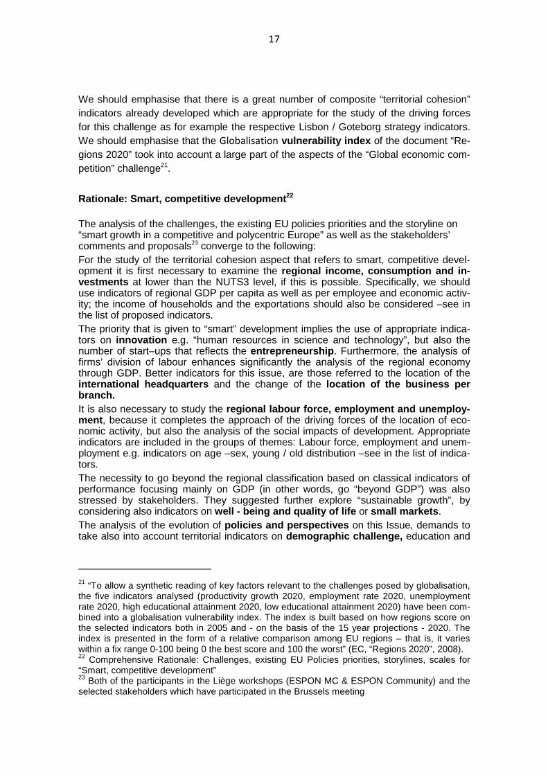
17

We should emphasise that there is a great number of composite “territorial cohesion” indicators already developed which are appropriate for the study of the driving forces for this challenge as for example the respective Lisbon / Goteborg strategy indicators. We should emphasise that the Globalisation vulnerability index of the document “Re-gions 2020” took into account a large part of the aspects of the “Global economic com-petition” challenge21.

Rationale: Smart, competitive development 22 The analysis of the challenges, the existing EU policies priorities and the storyline on “smart growth in a competitive and polycentric Europe” as well as the stakeholders’ comments and proposals23 converge to the following: For the study of the territorial cohesion aspect that refers to smart, competitive devel-opment it is first necessary to examine the regional income, consumption and in-vestments at lower than the NUTS3 level, if this is possible. Specifically, we should use indicators of regional GDP per capita as well as per employee and economic activ-ity; the income of households and the exportations should also be considered –see in the list of proposed indicators. The priority that is given to “smart” development implies the use of appropriate indica-tors on innovation e.g. “human resources in science and technology”, but also the number of start–ups that reflects the entrepreneurship . Furthermore, the analysis of firms’ division of labour enhances significantly the analysis of the regional economy through GDP. Better indicators for this issue, are those referred to the location of the international headquarters and the change of the location of the business per branch. It is also necessary to study the regional labour force, employment and unemploy-ment , because it completes the approach of the driving forces of the location of eco-nomic activity, but also the analysis of the social impacts of development. Appropriate indicators are included in the groups of themes: Labour force, employment and unem-ployment e.g. indicators on age –sex, young / old distribution –see in the list of indica-tors. The necessity to go beyond the regional classification based on classical indicators of performance focusing mainly on GDP (in other words, go “beyond GDP”) was also stressed by stakeholders. They suggested further explore “sustainable growth”, by considering also indicators on well - being and quality of life or small markets . The analysis of the evolution of policies and perspectives on this Issue, demands to take also into account territorial indicators on demographic challenge, education and

21 “To allow a synthetic reading of key factors relevant to the challenges posed by globalisation, the five indicators analysed (productivity growth 2020, employment rate 2020, unemployment rate 2020, high educational attainment 2020, low educational attainment 2020) have been com-bined into a globalisation vulnerability index. The index is built based on how regions score on the selected indicators both in 2005 and - on the basis of the 15 year projections - 2020. The index is presented in the form of a relative comparison among EU regions – that is, it varies within a fix range 0-100 being 0 the best score and 100 the worst” (EC, “Regions 2020”, 2008). 22 Comprehensive Rationale: Challenges, existing EU Policies priorities, storylines, scales for “Smart, competitive development” 23 Both of the participants in the Liège workshops (ESPON MC & ESPON Community) and the selected stakeholders which have participated in the Brussels meeting

18

other services of general interest -which are discussed in Issue 2- as well as on envi-ronmental quality and accessibility -discussed in Issues 3 and 4.

From the challenges / policies / storylines analysis, is revealed that we should prioritise complex indicators on the different aspects of regional potentials as the Income and production aspect, the Human potential aspect and the Innovation aspect –see for the appropriate indicators in the list. Stakeholders also stressed the necessity to use a single comprehensive indicator for regional economi c performance (on “Regional Competitiveness” or “Globalisation”). Relevant indicators have also been produced (see the list). All they are useful. Their content and then the feasibility of their use re-garding the availability of data will be further analysed in the next stage of the project. See in the following list for the proposed sets of indicators. Among others are included: Sets of indicators on: Income, Consumption and Investments, Innovation, firms division of labour and small markets, Labour force, Employment, and Unemployment 1st priority Complex territorial indicators (non exhaustive list): Regional potentials (Income & production, Human potential, Innovation), Globalisation, Regional Competi-tiveness on the basis of Lisbon strategy, Globalisation index of "Regions 2020" (EC 2008), Regional Competitiveness Index of the 5th Cohesion Report (CR).

Territorial levels / scales: For several indicators of this Issue we would ideally need data at LAU1 and LAU2 lev-els. However, most of the respective Eurostat data are at NUTS3 or even at NUTS2 levels –see indicatively the data used for the indicators of the 5th CR. Therefore, we will be limited to the NUTS2 / NUTS3 levels. Under this condition, the respective indicators are feasible. This issue will be further examined in the frame of the “local data” activity of the project. This evaluation apply also foe all the other Issue except from the Issue 3 on Environ-ment.

(4.1.2) Cities and polycentric development The issue of polycentric development through networking of cities is included in several parts of the analyses of territorial challenges as well as in the documents on the EU policies territorial priorities. Specifically, the following two territorial priorities of the project’ specifications: “Strengthening a polycentric development by networking of city regions and cities” and “Urban drivers” are approached together by Territorial Agenda and other EU policy documents.

Specifically: Territorial Agenda (2007) aims to “Strengthen Polycentric Development and Innovation through Networking of City Regions a nd Cities”.

We present the respective parts of the Agenda with emphasis (marked in Bold) on some specific objectives and respective issues:

“(14). City regions and cities of varying size are best able to build upon their own strengths in the context of a Europe-wide cooperation with entrepreneurs as well as societal and political stakeholders. If they succeed in implementing networks in a polycentric European ter ri-tory in an innovative manner , they will create conditions to allow them to benefit global competition in terms of their development

(15). Cities which function as regional centres should co operate as parts of a polycen-tric pattern to ensure their added value for other cities in rural and peripheral areas as well as for areas with specific geographic challenges and needs (e.g. structurally weak parts of islands, coastal zones and mountainous areas). To facilitate this process, infrastructure

19

networks within and between regions in Europe need to be extended and updated on a continuous basis”24.

In this context, Territorial Agenda emphasises the role of the cooperation between cities 25 –see also in the Issue 7 on Governance.

CEMAT 2010 approaches the networking of city regions and cities as an appropri-ate response to the growing social polarization in European society 26 both in mainly remote rural and low density population areas and in old industrial districts.

It emphasises the need to ensure the provision of essential services and promote economic development and social cohesion in order to maintain the vitality of settle-ments and prevent further deprivation.

Especially for cities, it stresses that, In order to counterbalance the effects of growing social polarisation , which often result in social segregation, growing intolerance, insecurity and even violence , territorial development and urban planning measures, in combination with other public policies … have to prevent such tensions, ensure so-cial inclusion and alleviate social segregation by rehabilitating and regenerating problem neighbourhoods .

The respective themes are presented in the Table 4.1.2.

Table 4.1.2: Cities and polycentric development

Challenge / policy priority:

Cities and polycentric development

Challenge / policy prior-

ity / storyline Themes corresponding to driv-

ing forces for the challenge /

policy priority

Correspondence to the classifi-

cation of themes in the Inven-

tory

Cities networking / "Strengthening a polycen-tric development by net-working of city regions and cities" and "Urban drivers" (large European cities, small and medium sized cities, sub-urbanisation, inner city imbalances)"

• Networking of firms • Networking of city regions and cities • Cities development • Growing concentration in urban areas: Diseconomies of agglomera-tion, congestion, pollution, social segregation, urban sprawl • Increased regional disparities due to different effects of urban drivers

Complex territorial indicators 1.1 Cities hierarchy and networking

Rationale: Cities and polycentric development We should start on this issue with the challenge and policy option of: “Strengthening a polycentric development by networking of city regions and cities”. Polycentric development should be approached at different territorial levels. For the competitiveness of cities at global but as well as to lower levels through networking , location of international headquarters and location of the business per branch as well

24 Territorial Agenda, 2007, p. 4-5 25 “We therefore support European cooperation between city regions as well as with small and medium-sized towns at the internal borders and also beyond the external borders of the EU”. (Territorial Agenda, 2007, p. 5). 26 CEMAT 2010 Moscow Declaration, p. 6

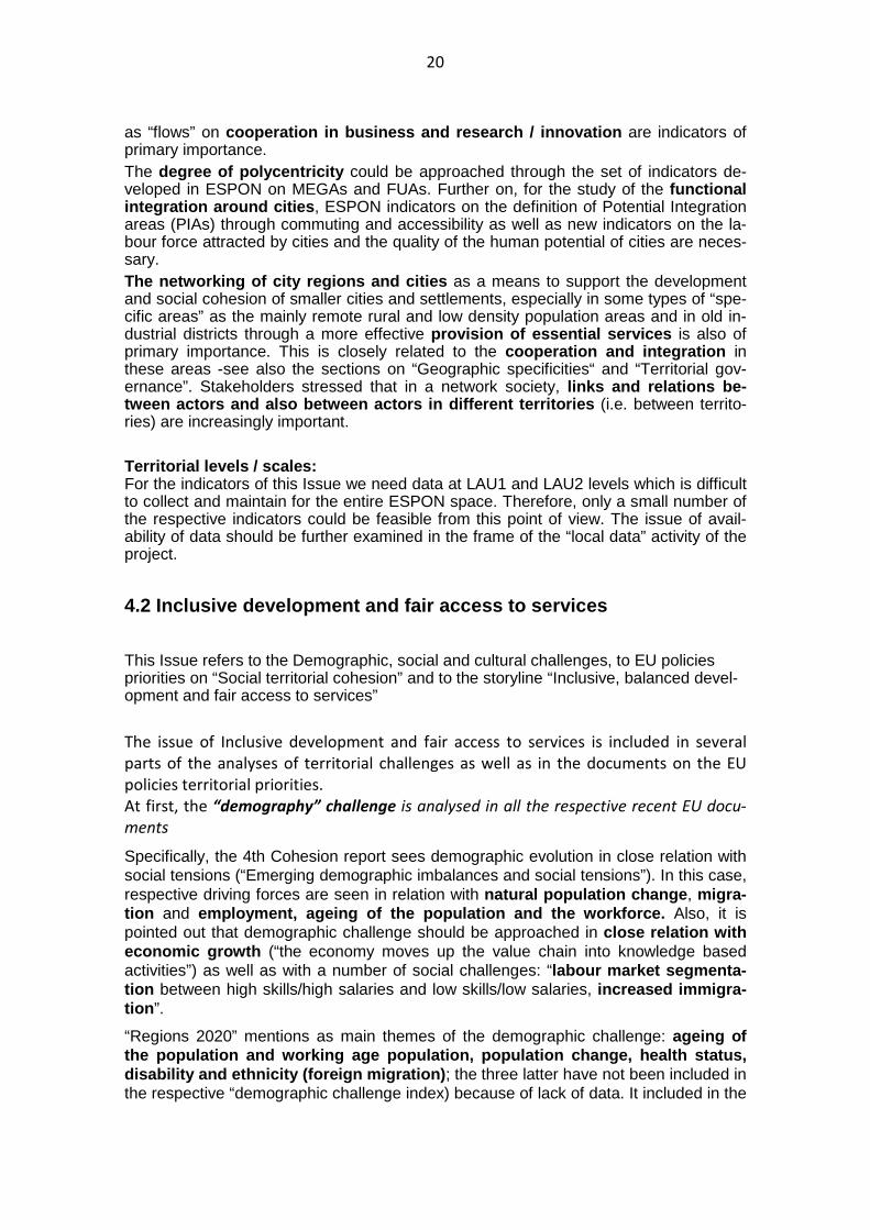
20

as “flows” on cooperation in business and research / innovation are indicators of primary importance. The degree of polycentricity could be approached through the set of indicators de-veloped in ESPON on MEGAs and FUAs. Further on, for the study of the functional integration around cities , ESPON indicators on the definition of Potential Integration areas (PIAs) through commuting and accessibility as well as new indicators on the la-bour force attracted by cities and the quality of the human potential of cities are neces-sary. The networking of city regions and cities as a means to support the development and social cohesion of smaller cities and settlements, especially in some types of “spe-cific areas” as the mainly remote rural and low density population areas and in old in-dustrial districts through a more effective provision of essential services is also of primary importance. This is closely related to the cooperation and integration in these areas -see also the sections on “Geographic specificities“ and “Territorial gov-ernance”. Stakeholders stressed that in a network society, links and relations be-tween actors and also between actors in different t erritories (i.e. between territo-ries) are increasingly important. Territorial levels / scales: For the indicators of this Issue we need data at LAU1 and LAU2 levels which is difficult to collect and maintain for the entire ESPON space. Therefore, only a small number of the respective indicators could be feasible from this point of view. The issue of avail-ability of data should be further examined in the frame of the “local data” activity of the project.

4.2 Inclusive development and fair access to servic es

This Issue refers to the Demographic, social and cultural challenges, to EU policies priorities on “Social territorial cohesion” and to the storyline “Inclusive, balanced devel-opment and fair access to services”

The issue of Inclusive development and fair access to services is included in several

parts of the analyses of territorial challenges as well as in the documents on the EU

policies territorial priorities.

At first, the “demography” challenge is analysed in all the respective recent EU docu-

ments

Specifically, the 4th Cohesion report sees demographic evolution in close relation with social tensions (“Emerging demographic imbalances and social tensions”). In this case, respective driving forces are seen in relation with natural population change , migra-tion and employment, ageing of the population and the workfo rce. Also, it is pointed out that demographic challenge should be approached in close relation with economic growth (“the economy moves up the value chain into knowledge based activities”) as well as with a number of social challenges: “labour market segmenta-tion between high skills/high salaries and low skills/low salaries, increased immigra-tion ”.

“Regions 2020” mentions as main themes of the demographic challenge: ageing of the population and working age population, populati on change, health status, disability and ethnicity (foreign migration) ; the three latter have not been included in the respective “demographic challenge index) because of lack of data. It included in the

21

“indicators used to assess overall sensitivity” indicators related to poverty, employ-ment rate, educational attainment and welfare syste ms 27. Also, in numerous other EU documents and academic papers the above aspects of this challenge have been referred.

In several relevant documents, the “demography” challenge is approached in close relation with the social and cultural challenges as well as with policy priorities on social territorial cohesion and the use of territor ial assets for development.

See for the themes corresponding to these aspects in Table 4.2.

Table 4.2: Inclusive development and fair access to services

Challenge / policy priorities / storyline:

Demographic, social and cultural challenge / Social territorial cohesion / Inclusive, bal-anced development and fair access to services

Challenge /

policy prior-

ity / story-

line

Themes corresponding to driving

forces for the challenge

Correspondence to the classification

of themes in the Inventory

Demographic

challenge

(including

social and

cultural chal-

lenges)

• Demographic changes and imbal-

ances: population and workforce

ageing, in-out migration, labour

market segmentation

• Social tensions and disparities

• Downgrading and insufficient use of

cultural assets for development

• Classical (sectoral) themes (issues)

02.01 Population Structure

02.02 Population Movement (Migration)

06.01 Education

06.02 Poverty

06.03 Other social

06.04 Culture

• Complex territorial themes (issues)

Rationale: Inclusive development and fair access to services

A first aspect of this Issue refers to the territorial challenges, existing EU policy priori-ties and policy perspectives on demographic change and migration.

Here, a first component is the population structure: potential, age, gender, natur al growth – see in the list of proposed indicators as well as in the Issue 1.

We need at first some basic indicators on the population change rate, the population versus the resident population potential as well as the population density. the ageing of the population, based, in more general, in the overall population change.

Second, indicators on population ageing per gender, dependency rates, Life expec-tancy, crude birth and death rates as well as to the fertility rate are necessary in order to come to the changes on the population National Growth rate

It is also necessary to study some crucial characteristics of households : the rate of Lone-person and Lone-parent households as well as of those including children; the rates of households living in owned housing, in social housing etc.

The analysis of the citizenship through appropriate indicators is also needed as it al-lows us to study the regional process towards multi-cultural local communities. 27 See in Annex 1: “Indicators used for assessing sensitivity to combined challenges: range and weights”.

22

Migration (population movement) is a second crucial point of interest for the overall population change. In order to study its evolution as well as its impacts on the popula-tion change, we should specifically use territorial indicators on in and out migration, net migration rate, migratory balance and internal mobility by region. Finally, indicators on migration by country of origin and destination allow the analysis of the highly important migratory flows from country to country or from / to lower level functional regions of Europe.

Further on (as it is also proposed by some stakeholders) Indicators on migration should be linked to education indicators to see better who is moving.

The study of natural growth and migration allow us to produce regional population pro-jections which are of highly importance for the evaluation of the regional dynamics.

As we saw, the education level of the population is very important for the approach of “smart growth” –see Issue 1- but also of social disparities. From this scope, appropriate indicators are at first those on the accessibility to High Secondary School, to Techno-logical Education and to training structures. For the challenges analysis it is worthwhile to use simple indicators on the population with a tertiary education per age group and on the rate of school leavers. For the policy approach we propose to use the complex indicators proposed by the 5th Cohesion report on (a) the Population of certain age group with a tertiary education and distance to Europe 2020 target (b) the rate of the Early school leavers and distance to Europe 2020 target. Indicators about spoken lan-guages are also included in this Issue, as stakeholders have proposed for Issue 1. However, this information is also important, regarding the degree of integration of the foreign migrants in local communities.

The social disparities challenge closely related to the “inclusive development” policy objective could be analysed through indicators on poverty, quality of dwellings, Homeless people, Social security and Crime –see in the list of proposed indicators. Especially for the poverty which has a primary importance from this scope, we have included in the list the 5th Cohesion report indicators. In the same frame we should use, in addition, indicators on the level of health services used, on the share of public healthcare services etc.

The citizens’ point of view on these themes could be analysed through indicators such as the Level of satisfaction of residents with aspects of quality of life in selected cities (5th C.R.) -see in the list.

Some stakeholders stressed, regarding the demographic change that people’s well-being is the main success factor, and accordingly is the demographic change the most important indicator. Proportionality of costs and imbalances of voices need to be con-sidered in this context, as different types of areas feature differently in the debate.

Also, stakeholders stressed the need to take into account the citizens’ perspective on their level of poverty, access to health services and other public services, safety, edu-cation, etc. These proposals have been included on the Rationale –see previously.

As we have already stressed, complex territorial indicators are of first priority for INTERCO, as they combine two or more simple themes and thus they allow better ana-lyse the driving forces of territorial change. In this issue are included several such indi-cators produced by DG Regio in the frame of the 5th Cohesion Report. These specific DG Regio indicators are of first priority for INTERCO. In the next stage of the project, we will comment these indicators and we will propose possible improvements of their content.

23

Territorial levels / scales:

For several indicators of this Issue we would ideally need data at LAU1 and LAU2 lev-els. However, most of the respective Eurostat data are at NUTS3 or even at NUTS2 levels –see for example the data used for the respective complex territorial indicators of the 5th Cohesion Report. Therefore, we will be limited to the NUTS2 / NUTS3 levels. Under this condition, the respective indicators are feasible.

The availability of respective data at LAU1 and LAU2 levels for a limited number of indicators should be further in the frame of the “local data” activity of the project.

See for the Proposed indicators in Annex 2.

4.3 Environmental dimension, climate change and ris k management

This Issue refers to the Environment, climate change and hazards challenges, to EU policies priorities on Strengthening risk management including impacts of climate change, ecological structures and cultural resources and to the storyline: Environ-mental dimension and sustainable development.

The issue of Environmental sustainability, climate change and risk management is in-

cluded in several parts of the analyses of territorial challenges as well as in the docu-

ments on the EU policies territorial priorities.

The challenges regarding specifically the changes in the ecological structures and cul-

tural resources will be discussed in next in the frame of the analysis of the respective

EU policies territorial priorities.

Specifically for the “Climate change” challenge, the 4th Cohesion Report noted that it has an asymmetrical impact: “This will pose serious challenges to agriculture, fisher-ies and the tourism industry in certain areas, and will require significant investment to face drought, fires, coastal erosion and flooding ”. In addition, this challenge is seen as closely related to the social situation of some reg ions: “These changes may have disproportionate effects on disadvantaged or low income groups which might lack the means to adapt to them”.

Therefore it is needed to analyse these interactions through appropriate synthetic indicators, as for example: climate change – social development.

“Regions 2020” includes in its synthetic index of the impacts of climate change on European regions the vulnerability to drought , population affected by river floods and exposed to coastal erosion , exposure to climate change of the agriculture, fisheries and tourism sector.

Similar aspects of this challenge have been analysed in other EU documents and in relevant academic papers.

EU policies territorial priorities emphasize two objectives: “Promoting trans-European

risk management including impacts of climate change” and “Strengthening ecologi-

cal structures and cultural resources”. We examine these two priorities together because an important number of the issues to which they refer are common.

24

These territorial policy priorities are also included mot-à-mot in the Territorial Agenda 28

- “We Promote Trans-European Risk Management including the Impacts of Cli-mate Change”:

“Joint trans-regional and integrated approaches and strategies should be further developed in order to face natural hazards, reduce and mitigate greenhouse gas emissions and adapt to climate change […]”

= “We Require the Strengthening of Ecological Struc tures and Cultural Re-sources as the Added Value for Development:

The irreplaceable values of European ecological structures and cultural and natural heritage, especially cultural landscapes and the quality of design and process on architecture as well as the built environment, should constitute, against the background of the respective regional circumstances and potentials, the foundation for environmentally and culturally oriented de-velopment […]”.

All other EU policy documents’ (the cohesion policy documents, “Green paper”, “Europe 2020” etc) territorial objectives refer to several climate change issues and natural hazards issues and they give emphasis to the need to define appropriately the respective vulnerable regions as well as to prevent climate change and mitigate its im-pacts

See for the themes corresponding to these aspects in Table 4.3.

Table 4.3. Environmental dimension, climate change and risk management

Challenge / policy priorities / storyline:

Environment, climate change and hazards challenges/ Strengthening risk management including impacts of climate change, ecological structures and cultural resources / En-

vironmental dimension and sustainable development.

Challenge / policy

priority / storyline

Themes corresponding to driving

forces for the challenge

Correspondence to the

classification of themes in

the Inventory

Environment , Climate

change and risk man-

agement challenges,

policy priorities: "Pro-

moting risk manage-

ment including impacts

of climate change",

"Strengthening ecologi-

cal structures and cul-

tural resources"

• Environment quality,

• Exposure to climate change (including

exposure of the agriculture, fisheries

and tourism sector)

• Natural hazards (droughts, fires,

coastal erosion, flooding)

• Vulnerable regions

• Vulnerable groups of people (disad-

vantaged-low income)

• Classical (sectoral) themes (issues) 08.01 Environment quality (etc) (Physical environment) 08.02 Climate change 08.03 Hazards • Complex territorial themes (issues)

Rationale: Environmental dimension, hazards and cli mate change

28 Both are described in the page 7 of the Agenda

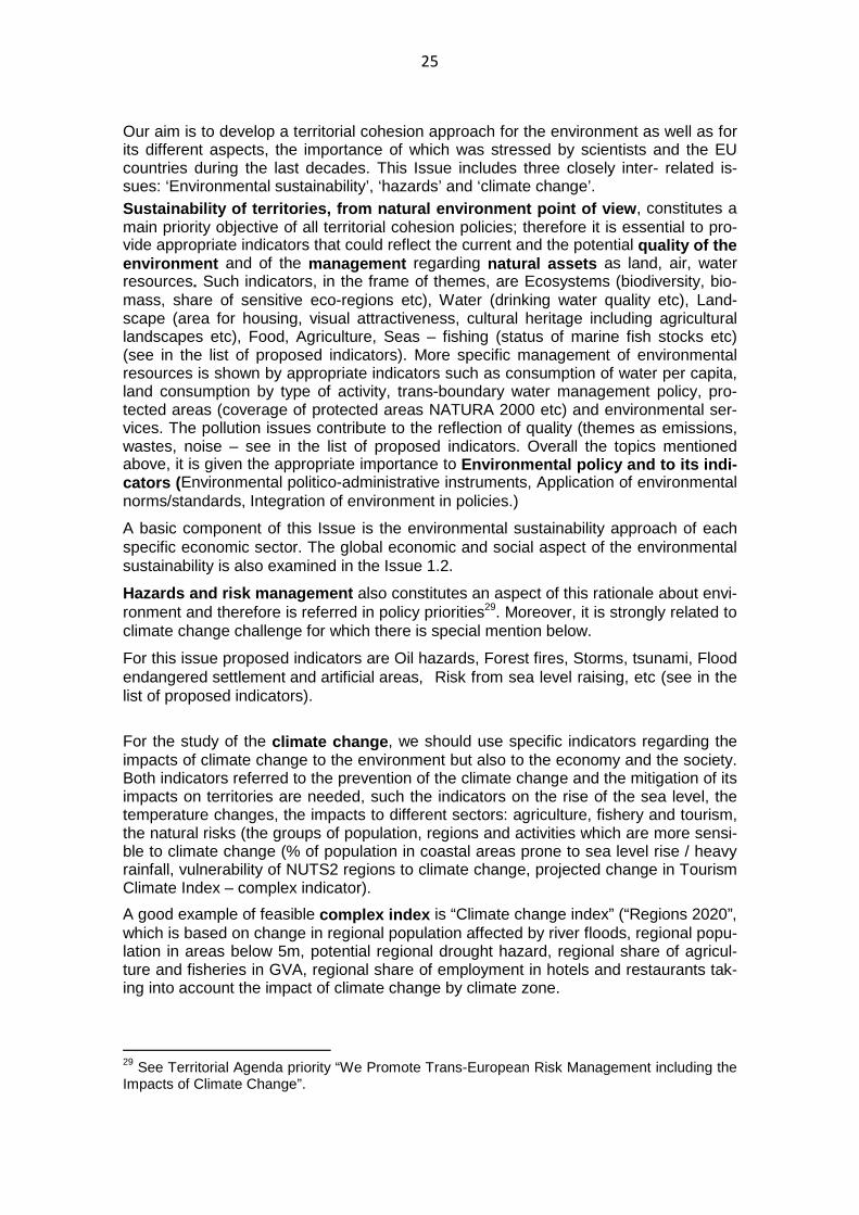
25

Our aim is to develop a territorial cohesion approach for the environment as well as for its different aspects, the importance of which was stressed by scientists and the EU countries during the last decades. This Issue includes three closely inter- related is-sues: ‘Environmental sustainability’, ‘hazards’ and ‘climate change’. Sustainability of territories, from natural environ ment point of view , constitutes a main priority objective of all territorial cohesion policies; therefore it is essential to pro-vide appropriate indicators that could reflect the current and the potential quality of the environment and of the management regarding natural assets as land, air, water resources. Such indicators, in the frame of themes, are Ecosystems (biodiversity, bio-mass, share of sensitive eco-regions etc), Water (drinking water quality etc), Land-scape (area for housing, visual attractiveness, cultural heritage including agricultural landscapes etc), Food, Agriculture, Seas – fishing (status of marine fish stocks etc) (see in the list of proposed indicators). More specific management of environmental resources is shown by appropriate indicators such as consumption of water per capita, land consumption by type of activity, trans-boundary water management policy, pro-tected areas (coverage of protected areas NATURA 2000 etc) and environmental ser-vices. The pollution issues contribute to the reflection of quality (themes as emissions, wastes, noise – see in the list of proposed indicators. Overall the topics mentioned above, it is given the appropriate importance to Environmental policy and to its indi-cators ( Environmental politico-administrative instruments, Application of environmental norms/standards, Integration of environment in policies.)

A basic component of this Issue is the environmental sustainability approach of each specific economic sector. The global economic and social aspect of the environmental sustainability is also examined in the Issue 1.2.

Hazards and risk management also constitutes an aspect of this rationale about envi-ronment and therefore is referred in policy priorities29. Moreover, it is strongly related to climate change challenge for which there is special mention below.

For this issue proposed indicators are Oil hazards, Forest fires, Storms, tsunami, Flood endangered settlement and artificial areas, Risk from sea level raising, etc (see in the list of proposed indicators).

For the study of the climate change , we should use specific indicators regarding the impacts of climate change to the environment but also to the economy and the society. Both indicators referred to the prevention of the climate change and the mitigation of its impacts on territories are needed, such the indicators on the rise of the sea level, the temperature changes, the impacts to different sectors: agriculture, fishery and tourism, the natural risks (the groups of population, regions and activities which are more sensi-ble to climate change (% of population in coastal areas prone to sea level rise / heavy rainfall, vulnerability of NUTS2 regions to climate change, projected change in Tourism Climate Index – complex indicator).

A good example of feasible complex index is “Climate change index” (“Regions 2020”, which is based on change in regional population affected by river floods, regional popu-lation in areas below 5m, potential regional drought hazard, regional share of agricul-ture and fisheries in GVA, regional share of employment in hotels and restaurants tak-ing into account the impact of climate change by climate zone.

29 See Territorial Agenda priority “We Promote Trans-European Risk Management including the Impacts of Climate Change”.

26

Territorial levels / scales: The territorial cohesion aspects of the environment should be theoretically studied at the lowest level e.g. LAU2 as they have an explicit territorial dimension. This was stressed by stakeholders. However, for the majority of the respective issues there are data only for the NUTS2 or the NUTS3 level. Thus an important number of the respec-tive indicators are not actually feasible as for the existence of data. See for the Proposed indicators in Annex 2. 4.4 Sustainable energy

This Issue refers to the energy challenge and policy priorities The “energy” challenge

It is reported in the 4th Cohesion report as “Increased energy prices”. Here are in-cluded issues that concern the production of energy as the need to expand renew-able energies but also the issue of energy efficiency in relation to the productive system and the consumption: energy efficiency of the firms, transport costs etc.

Similar aspects of this challenge have been analysed in the EC “Green paper on terri-torial cohesion” document (2008), in “Europe 2020” and “Regions 2020” documents, in the EC 6th progress report on economic and social cohesion (2009) as well as in rele-vant academic literature.

The EU policies territorial priorities on Energy are included in the general objective on “Strengthening and extending the Trans-European Net works ” (TNTs) –as, specifi-cally, for the Energy TNT. However, priorities on Energy refer not only to the trans-European level but also to the national, regional and local levels.

We refer here to the Energy priorities -see for the discussion on the entire TNTs in Is-sue 6 – Transport etc.

This policy priority on TNTs is included mot-à-mot in the Territorial Agenda 30:

“We Support the Strengthening and Extension of Trans -European Networks:

[…] Rising energy demand in the face of limited reserves of non-renewable energy sources, and a growing dependence of the EU on imported energy as well the chal-lenge of climate change, means that we should further explore and develop opportuni-ties for decentralized, efficient, safe and environmentally friendly production of renew-able energy , which is as yet underutilised.[...]” Green Paper on Territorial Cohesion (2008, p.6): “Connecting territories today requires adequate access to services such as health care, education and sustainable energy , [….] , reliable connections to energy networks […] . This is also essential to address the special needs of disadvantaged groups.[...]”

In other words, in the objective to improve the Trans-European Network (TN) of Energy is associated to other priorities as the use of renewable energy etc –see in Table 4.6.

See for the themes corresponding to these aspects in Table 4.4.

30 2007, p.5

27

Table 4.4: Sustainable energy Challenge / policy priorities: Energy

Challenge / policy

priority

Themes corresponding to driving

forces for the challenge

Correspondence to the

classification of themes in

the Inventory

Energy supply and

efficiency challenge,

Policy priorities:

Strengthening and

extending the Trans-

European Network of

Energy etc

• Energy prices

• Energy production

• Renewable energies

• Energy consumption,

• Energy sufficiency

• Energy efficiency (including energy

efficiency of firms)

• Secure, sustainable and competitive

energy

• Classical (sectoral) themes

(issues)

04 Energy

• Complex territorial themes

(issues)

Rationale: Energy

This Issue refers to the energy challenge and policy priorities The role of energy in the territorial challenges regarding the economy, the society and the environment becomes much more important during the last decades. Energy sav-ings and prevention of the negative impacts of the energy consumption have a growing priority in the existing EU policies. In this frame, the different aspects of the energy balance: Energy demand, consump-tion, production and economy should be investigated at regional level, through ap-propriate indicators; among others, the share of total energy produced/consumed, the energy intensity of the economy, the private energy use, the investments, the energy prices. The employment rate in energy production should also be examined – see the list of proposed indicators. As the exploitation of renewable energies has a priority in EU existing policies and perspectives we should use appropriate indicators for both the total of Renewable en-ergies and per category of sources: photovoltaic, wind power, solar energy potential and production. The study of the energy impacts (on agriculture and landscapes) has also a high pri-ority.

It is useful to include the different territorial aspects of energy in a complex territorial index . A first relevant index -“Energy Index”- has been produced by “Regions 2020”. It uses variables on the regional energy consumption of households, activities (industry, agri-culture, services) and freight transport, the national energy import dependency, the national carbon content of gross inland energy consumption. This index reflects the major territorial cohesion aspects of energy except from the En-ergy impacts on territories, as the impacts on agriculture and landscapes. In next stage of the project, we could propose the completion of the index with the latter aspect. Territorial levels / scales: The territorial cohesion aspects of the energy issues should be theoretically studied at a low territorial level e.g. NUTS3 or lower, as they have an explicit territorial dimension. However, for the majority of the respective issues there are data only for the NUTS2 or

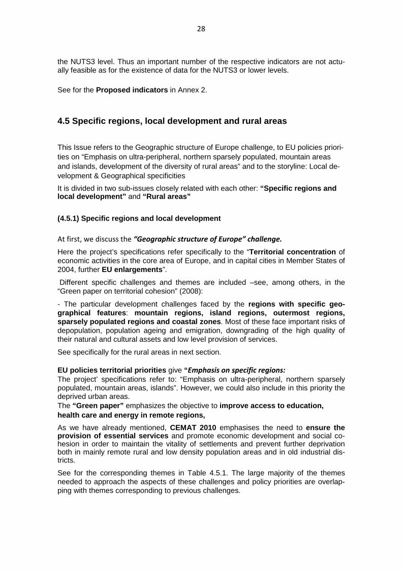
28

the NUTS3 level. Thus an important number of the respective indicators are not actu-ally feasible as for the existence of data for the NUTS3 or lower levels.

See for the Proposed indicators in Annex 2.

4.5 Specific regions, local development and rural a reas

This Issue refers to the Geographic structure of Europe challenge, to EU policies priori-ties on “Emphasis on ultra-peripheral, northern sparsely populated, mountain areas and islands, development of the diversity of rural areas” and to the storyline: Local de-velopment & Geographical specificities

It is divided in two sub-issues closely related with each other: “Specific regions and local development” and “Rural areas”

(4.5.1) Specific regions and local development

At first, we discuss the “Geographic structure of Europe” challenge.

Here the project’s specifications refer specifically to the “Territorial concentration of economic activities in the core area of Europe, and in capital cities in Member States of 2004, further EU enlargements ”.

Different specific challenges and themes are included –see, among others, in the “Green paper on territorial cohesion” (2008):

- The particular development challenges faced by the regions with specific geo-graphical features : mountain regions, island regions, outermost regions , sparsely populated regions and coastal zones . Most of these face important risks of depopulation, population ageing and emigration, downgrading of the high quality of their natural and cultural assets and low level provision of services.

See specifically for the rural areas in next section. EU policies territorial priorities give “ Emphasis on specific regions:

The project’ specifications refer to: “Emphasis on ultra-peripheral, northern sparsely populated, mountain areas, islands”. However, we could also include in this priority the deprived urban areas. The “Green paper” emphasizes the objective to improve access to education, health care and energy in remote regions,

As we have already mentioned, CEMAT 2010 emphasises the need to ensure the provision of essential services and promote economic development and social co-hesion in order to maintain the vitality of settlements and prevent further deprivation both in mainly remote rural and low density population areas and in old industrial dis-tricts.

See for the corresponding themes in Table 4.5.1. The large majority of the themes needed to approach the aspects of these challenges and policy priorities are overlap-ping with themes corresponding to previous challenges.

29

Table 4.5.1: Specific regions, local development

Challenge / policy priorities / storyline:

Geographic structure of Europe challenge / Emphasis on ultra-peripheral, northern sparsely populated, mountain areas and islands / Local development & Geographical specificities

Challenge, policy pri-

orities

Themes corresponding to driving

forces for the challenge

Correspondence to the

classification of themes in

the Inventory

Challenge:

Geographic structure

of Europe,

Policy priority:

Emphasis on ultra-

peripheral, northern

sparsely populated,

mountain areas, is-

lands

• Growing de-concentration (dispersal) in

specific regions: insufficient agglomera-

tion effects, uneven exploitation of as-

sets and endogenous development,

• Difficulties in service provision

• Growing concentration in urban areas:

Diseconomies of agglomeration, con-

gestion, pollution, social segregation,

urban sprawl

• Increased regional disparities due to

different effects of urban drivers

Themes and Indicators over-

lapping with those of the

other challenges and policy priorities Complex territorial indicators 1.4 Regional potential: GDP, Income & production 8. Natural assets, natural & technological hazards 1.1 Cities / settlements hier-archy and networking

The respective group of stakeholders (who have participated in the Brussels work-shop) did not produce a list of territorial cohesion indicators, but insisted on the neces-sity of using relevant functional areas for the quantitative assessment of each type of issues. They also emphasised that functional areas themselves can be changed, e.g. through transport infrastructure investments and the use of information and communi-cation technology (ICT). Finally, the institutional and governance dimensions of the construction of territorial cohesion were highlighted. Success stories in the vertical and horizontal integration of actors could provide a useful source of inspiration for the iden-tification of indicators on the territorial dimension of development processes.

Rationale: specific regions and local development

Geographic structure is a crucial component of territorial cohesion. It is mainly re-ferred to several specificities of the European territories defining respective “spe-cific regions ” as the mountain regions, island regions, northern sparsely populated areas and coastal zones. The second dimension of the Issue, closely related to the first, is the local development .

In this frame, we need at first appropriate indicators for the delimitation of the area of each type of specific regions : the northern sparsely populated areas, the mountain areas, the “islands”.

Through EU policies, priority has been given to issues (and indicators) relating to the specific characteristics of these regions, as the geographical and environmental fea-tures, the human potential and the services availability. From the same scope, stake-holders underlined that: “Groups of similar regions should be described on their own terms….For these cases, we should “par excellence” avoid the excessive focus on GDP, giving, this way, small and peripheral communities and regions greater weight”. In this line, we have included indicators on the particular weaknesses and opportunities

30

of these areas regarding specifically the natural and cultural assets , the accessibil-ity with focus on the accessibility to services of general interest , the human po-tential e.g. employment in selected economic activities such as fishing, mining, for-estry, tourism and age dependency ratios. Indicators on the small and medium sized cities’ networking in relation to the provision of services and territorial governance are also of priority in this case. The majority of the previous options for the selection of in-dicators apply also for the issues of local development. On the basis of these indica-tors we will explore, in the next stage of the project the possibility to produce relevant synthetic indicators per type of specific regions .

See for the Proposed indicators in Annex 2. (4.5.2) The rural areas

The rural areas in the “Geographic structure of Europe” challenge:

The rural areas challenges are related to the pressure of globalization to the rural ac-tivities development, demography change as well as pressures on their natural and cultural assets of high quality and, finally, ineffective provision of services Regarding the challenge on “Development of the diversity of rural areas” , Territorial Agenda emphasises the need to strengthen the relationships of rural areas with the closest important cities in “intermediate regions” or to facilitate the integration of rural areas with the networks of small and medium sized cities in more remote from impor-tant cities regions. The “Green paper” develops a similar approach.

In both cases a first important territorial sub-priority (or sub-objective) is facilitate the reach of activities and inhabitants to services of general interest as well as to RD centres .

A second sub-objective is the combination of the rural development with the preserva-tion of their environment together with the diversi ty of these areas. Here important are the preservation of the natural resources and n atural areas : lakes, forests, Natura 2000 sites etc (see in the “Green paper”) as well as the preservation of the cultural assets .

The need to combine these objectives with the mitigation of the climate change im-pacts is also emphasized. An also important sub-priority is to preserve social cohe-sion and mitigate the negative demographic evolutio n in these areas .

Finally, it is stressed that EU policies should support the restructuring of rural areas prioritising environmentally friendly agricultural activities.

See for the respective themes in Table 4.5.2.

31

Table 4.5.2: Rural areas

Challenge / policy priorities / storyline: Rural areas

Challenges,

policy priorities Themes corresponding to driving forces for the

challenges and territorial priorities Correspondence to the classification of

themes in the In-ventory

Challenge: uneven development, de-concentration, Policy priority: Development of the diversity of rural areas

• Demographic evolution: negative actually / to mitigate • Social cohesion: to preserve • De-concentration (dispersal) in rural areas: agglomera-

tion effects: insufficient actually / to improve • Preservation together with exploitation of natural assets

and endogenous development: insufficient today / to improve in relation with the mitiga-

tion of the impacts of climate change • Provision of services of general interest from the small

and medium sized town in remote rural areas and from the close cities in intermediate regions:

insufficient actually / to improve

01. Agriculture and fisheries 01.01 Land Use 01.02 Farms Structure 01.03 Employment 01.04 Livestock 01.05Production Complex territorial indicators

Rationale: rural areas

The process of development of rural areas presents considerable similarities with those of specific regions; however, the development processes in certain types of rural areas (e.g. those which are close to cities) present important differences.

EU policy priorities in rural areas address at first the negative demographic evolution challenge and prioritise the preservation of the social cohesion . They also address the de-concentration (dispersal) in relation with insufficient agglomeration effects and prioritise the preservation together with exploitation of natural assets and endoge-nous development in relation with the mitigation of the impacts of climate change . Finally, they promote the provision of services of general interest from the small and medium sized town in remote rural areas and fro m the close cities in inter-mediate regions .

Therefore, apart from the indicators that are common with those for the specific re-gions, we have included here indicators on specific rural activities (e.g. on farms structure: holdings and holders, livestock, fisheries). In the next stage of the project we will produce complex synthetic (crossing issues) indicators on rural area.

See for the Proposed indicators in Annex 2.

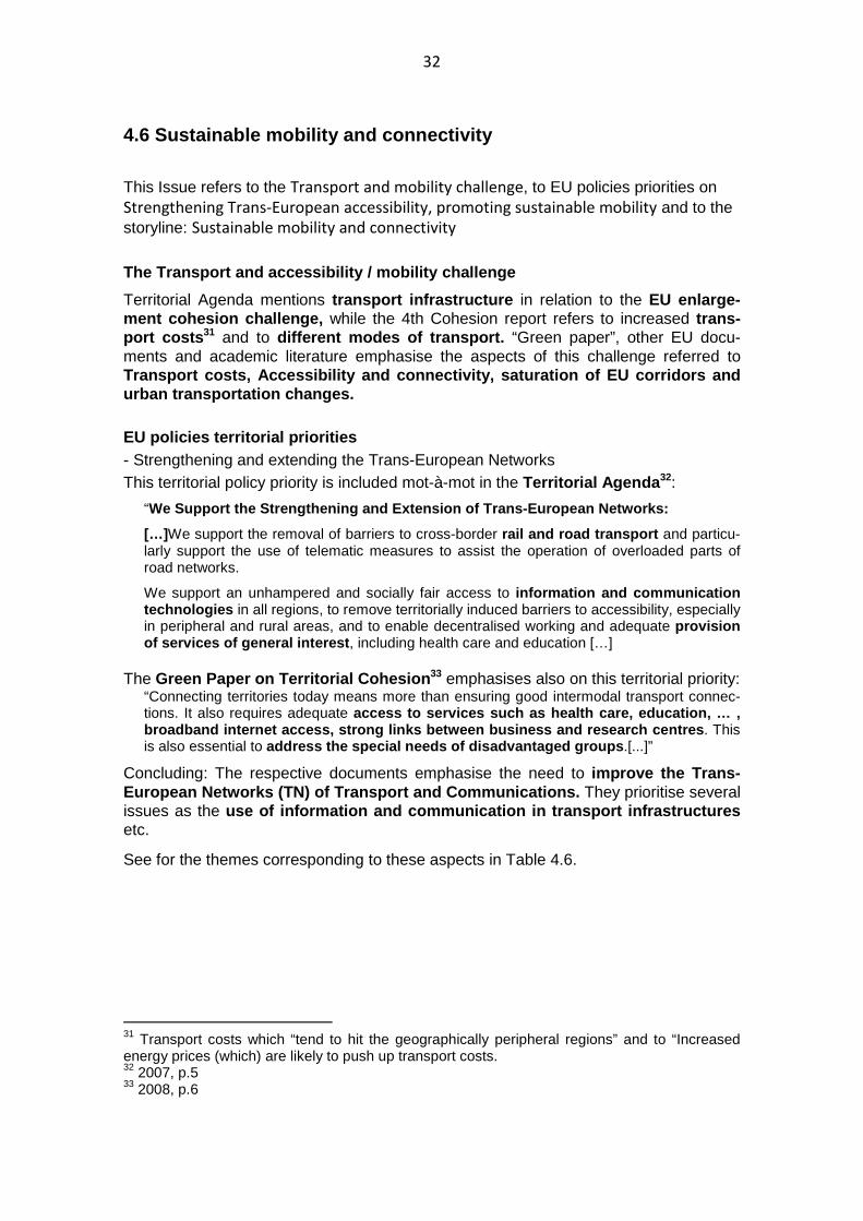
32

4.6 Sustainable mobility and connectivity

This Issue refers to the Transport and mobility challenge, to EU policies priorities on Strengthening Trans-European accessibility, promoting sustainable mobility and to the storyline: Sustainable mobility and connectivity

The Transport and accessibility / mobility challeng e

Territorial Agenda mentions transport infrastructure in relation to the EU enlarge-ment cohesion challenge, while the 4th Cohesion report refers to increased trans-port costs 31 and to different modes of transport. “Green paper”, other EU docu-ments and academic literature emphasise the aspects of this challenge referred to Transport costs, Accessibility and connectivity, sa turation of EU corridors and urban transportation changes.

EU policies territorial priorities - Strengthening and extending the Trans-European Networks This territorial policy priority is included mot-à-mot in the Territorial Agenda 32:

“We Support the Strengthening and Extension of Trans -European Networks:

[…]We support the removal of barriers to cross-border rail and road transport and particu-larly support the use of telematic measures to assist the operation of overloaded parts of road networks.

We support an unhampered and socially fair access to information and communication technologies in all regions, to remove territorially induced barriers to accessibility, especially in peripheral and rural areas, and to enable decentralised working and adequate provision of services of general interest , including health care and education […]

The Green Paper on Territorial Cohesion 33 emphasises also on this territorial priority: “Connecting territories today means more than ensuring good intermodal transport connec-tions. It also requires adequate access to services such as health care, education, … , broadband internet access, strong links between bus iness and research centres . This is also essential to address the special needs of disadvantaged groups .[...]”

Concluding: The respective documents emphasise the need to improve the Trans-European Networks (TN) of Transport and Communicati ons. They prioritise several issues as the use of information and communication in transport i nfrastructures etc.

See for the themes corresponding to these aspects in Table 4.6.

31 Transport costs which “tend to hit the geographically peripheral regions” and to “Increased energy prices (which) are likely to push up transport costs. 32 2007, p.5 33 2008, p.6

33

Table 4.6: Sustainable mobility and connectivity

Challenge / policy priorities / storyline:

Transport and mobility challenge / Strengthening Trans-European accessibility, pro-

moting sustainable mobility / Sustainable mobility and connectivity

Challenge / policy pri-

ority / storyline

Themes corresponding to driving

forces for the challenges/ policy pri-

orities

Correspondence to the

classification of themes in

the Inventory

Transport and accessi-

bility / mobility chal-

lenge,

Policy priorities:

the Trans-European

Networks of Transport

and Communications

• Transport and communications net-

works’ density, capacity, costs per mode

and category

• Accessibility, connectivity

• Impacts of Transport Policies

• Urban transportation

• Classical (sectoral) themes (issues) 03.01 Transport Infrastructure 03.02 Passengers and Good Transport 03.04 Impacts of Transport Policies • Complex territorial themes (issues)

Rationale: Sustainable mobility and connectivity In summary, this Issue refers to the Transport and mobility challenge, to EU policies priorities on Strengthening Trans-European accessibility, promoting sustainable mobil-ity and to the storyline: Sustainable mobility and connectivity.

Transport and communication are at first economic activities and infrastructures . Therefore, we need indicators on the structure, density and capacity of the transport networks per mode: road, rail, air and multimodal transport, per transport category (passengers and freight transport) and per territorial level: local, regional national, in-ternational: the use of indicators on the transport costs and employment will allow evaluate the overall territorial structure of transport / communication –see the list of indicators.

On the other hand, as transport / communication connect places it plays a very impor-tant role in many different aspects of territorial cohesion. Mobility, accessibility and connectivity in territorial challenges and EU policies’ priorities (e.g. strengthening and extending the Trans-European Networks of Transport and Communication) should be approached from this scope. For example strengthening of the transport network at different territorial levels impacts not only to the competitiveness of regions and cities but also to polycentric potentials, social territorial cohesion, environment and cli-mate change, specific regions and territorial cooperation (therefore, respective indicators are also included in the Issues 1, 2, 3, 5 and 7). In this frame, we need indi-cators measuring different aspects of accessibility and connectivity : potential ac-cessibility to regions or to population, accessibility to public services (health, edu-cation) or to market, connectivity to airports, motorways, railway stations, health and education facilities as well as ICT connectivity (new indicator). We also need specific indicators on the urban transportation or the use of telematics in transport networks which are of priority for EU policies (new indicators). Indicators on the territorial im-pacts of transport structure and policies are included in the Issues on competitive-ness and polycentricity, social territorial cohesion, environment, specific regions and territorial cooperation –see in the respective lists of proposed indicators. We have in-

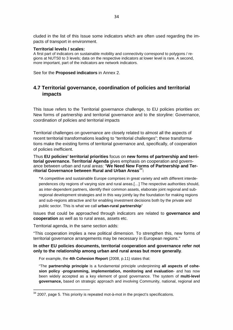
34

cluded in the list of this Issue some indicators which are often used regarding the im-pacts of transport in environment.

Territorial levels / scales: A first part of indicators on sustainable mobility and connectivity correspond to polygons / re-gions at NUTS0 to 3 levels; data on the respective indicators at lower level is rare. A second, more important, part of the indicators are network indicators. See for the Proposed indicators in Annex 2.

4.7 Territorial governance, coordination of policie s and territorial impacts

This Issue refers to the Territorial governance challenge, to EU policies priorities on: New forms of partnership and territorial governance and to the storyline: Governance, coordination of policies and territorial impacts

Territorial challenges on governance are closely related to almost all the aspects of recent territorial transformations leading to “territorial challenges”; these transforma-tions make the existing forms of territorial governance and, specifically, of cooperation of policies inefficient.

Thus EU policies’ territorial priorities focus on new forms of partnership and terri-torial governance. Territorial Agenda gives emphasis on cooperation and govern-ance between urban and rural areas: “We Need New Forms of Partnership and Ter-ritorial Governance between Rural and Urban Areas 34:

“ A competitive and sustainable Europe comprises in great variety and with different interde-pendences city regions of varying size and rural areas.[…] The respective authorities should, as inter-dependent partners, identify their common assets, elaborate joint regional and sub-regional development strategies and in this way jointly lay the foundation for making regions and sub-regions attractive and for enabling investment decisions both by the private and public sector. This is what we call urban-rural partnership ”

Issues that could be approached through indicators are related to governance and cooperation as well as to rural areas, assets etc.

Territorial agenda, in the same section adds:

“This cooperation implies a new political dimension. To strengthen this, new forms of territorial governance arrangements may be necessary in European regions.”

In other EU policies documents, territorial coopera tion and governance refer not only to the relationship among urban and rural area s but more generally .

For example, the 4th Cohesion Report (2008, p.11) states that:

“The partnership principle is a fundamental principle underpinning all aspects of cohe-sion policy -programming, implementation, monitorin g and evaluation - and has now been widely accepted as a key element of good governance. The system of multi-level governance, based on strategic approach and involving Community, national, regional and

34 2007, page 5. This priority is repeated mot-à-mot in the project’s specifications.

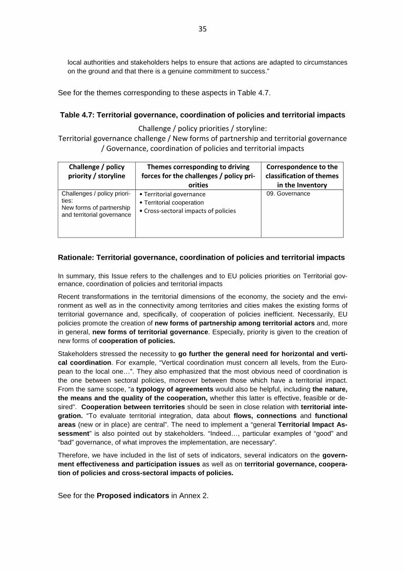
35

local authorities and stakeholders helps to ensure that actions are adapted to circumstances on the ground and that there is a genuine commitment to success.”

See for the themes corresponding to these aspects in Table 4.7.

Table 4.7: Territorial governance, coordination of policies and territorial impacts

Challenge / policy priorities / storyline:

Territorial governance challenge / New forms of partnership and territorial governance

/ Governance, coordination of policies and territorial impacts

Challenge / policy

priority / storyline Themes corresponding to driving

forces for the challenges / policy pri-

orities

Correspondence to the

classification of themes

in the Inventory Challenges / policy priori-ties: New forms of partnership and territorial governance

• Territorial governance

• Territorial cooperation • Cross-sectoral impacts of policies

09. Governance

Rationale: Territorial governance, coordination of policies and territorial impacts In summary, this Issue refers to the challenges and to EU policies priorities on Territorial gov-ernance, coordination of policies and territorial impacts

Recent transformations in the territorial dimensions of the economy, the society and the envi-ronment as well as in the connectivity among territories and cities makes the existing forms of territorial governance and, specifically, of cooperation of policies inefficient. Necessarily, EU policies promote the creation of new forms of partnership among territorial actors and, more in general, new forms of territorial governance . Especially, priority is given to the creation of new forms of cooperation of policies.

Stakeholders stressed the necessity to go further the general need for horizontal and vert i-cal coordination . For example, “Vertical coordination must concern all levels, from the Euro-pean to the local one…”. They also emphasized that the most obvious need of coordination is the one between sectoral policies, moreover between those which have a territorial impact. From the same scope, “a typology of agreements would also be helpful, including the nature, the means and the quality of the cooperation, whether this latter is effective, feasible or de-sired”. Cooperation between territories should be seen in close relation with territorial inte-gration. “To evaluate territorial integration, data about flows, connections and functional areas (new or in place) are central”. The need to implement a “general Territorial Impact As-sessment ” is also pointed out by stakeholders. “Indeed…, particular examples of “good” and “bad” governance, of what improves the implementation, are necessary”.

Therefore, we have included in the list of sets of indicators, several indicators on the govern-ment effectiveness and participation issues as well as on territorial governance, coopera-tion of policies and cross-sectoral impacts of poli cies.

See for the Proposed indicators in Annex 2.

36

4.8 Global indicators of territorial cohesion The Overall (Global) Territorial cohesion challeng e

Starting from the previously discussed 7 territorial Issues, we conclude to an Overall (global) approach of Territorial cohesion challenges and policies, based on specific complex - global indicators. Their functionality lies in synthesising wide ranges of as-pects of territorial cohesion, been analysed extensively before.

Such indicators are:

- Those of “Regions 2020”: the Globalisation index (based on labour productivity, employment rate and low and high educational attainment, the Climate change index (based on 5 indicators crossing climate change with economic and social aspects35) and the Demography index

- Those of the 5th Cohesion Report: the Lisbon index (2008), Change in Lisbon in-dex (2000–2008), Competitiveness index, Vulnerability to climate cha nge (NUTS2 regions), Happiness and life satisfaction indices in 5 less developed Member States, Happiness and GDP per head , etc.

Furthermore, we should define in the next stage of the project, even more complex territorial cohesion indicators including almost all the aspects of Territorial cohesion and better contribute. We should mention here the index of synthesis of territorial cohesion challenges produced by "Regions 2020" , showing the Intensity of multiple risks (challenges) for European Regions. Also the ONU Human Development Index (HDI) is useful for the study of several aspects of the Overall Territorial cohesion chal-lenge.

References CEMAT / Council of Europe (CoE), 2010, 15th Council of Europe Conference of minis-

ters responsible for spatial / regional planning, Moscow Declaration on “Future challenges: sustainable territorial development of the European continent in a changing world”, Moscow, Russian Federation 8-9 July 2010

CEMAT / CoE 2000, Guiding Principles for Sustainable Spatial Development of the European Continent, adopted at the 12th Session of the European Conference of Ministers responsible for Regional planning on 7-8 September 2000 in Hannover

Council of European Union, 2006, Council Decision on Community strategic guidelines on cohesion (2006/702/EC), 6 October 2006

Council of European Union, Presidency Conclusions, Brussels European Council, 22-23 March 2005.

Council of European Union, Presidency Conclusions, Gothenburg Council, 15 and 16 June 2001

Council of European Union, Presidency Conclusions, Lisbon European Council, 23-24 March 2000

35 Change in regional population affected by river floods, regional population in areas below 5m, potential regional drought hazard, regional share of agriculture and fisheries in GVA, regional share of employment in hotels and restaurants taking into account the impact of climate change by climate zone

37

ESDP, 1999, European Spatial Development Perspective: Towards balanced and sus-tainable development of the territory of the EU, CEC, Luxembourg.

ESPON 2013 Program, 2009, Specification ESPON Project 2013 Territorial Indicators and Indices (2010-2012)

European Commission, 2010, Fifth report on economic, social and territorial cohesion; Investing in Europe’s future (preliminary version), Report from the Commission, November 2010.

European Commission, 2010, Communication from the Commission, EUROPE 2020: A strategy for smart, sustainable and inclusive growth, March 2010

European Commission, 2009, Report from the Commission to the European Parliament and the Council, Sixth progress report on economic and social cohesion

European Commission, 2008, Communication from the Commission to the European Parliament and the Council, Fifth progress report on economic and social cohesion

European Commission, 2008, Communication from the Commission to the European Parliament and the Council, Green Paper on Territorial Cohesion: Turning territo-rial diversity into strength, Brussels 6.10.2008 {SEC(2008) 2550}

European Commission, 2007, Communication from the Commission to the European Parliament and the Council, Fourth report on economic and social cohesion – Growing regions, growing Europe, May 2007

European Union / Regional Policy, 2008, Regions 2020: An Assessment of Futures challenges for EU Regions, Commission Staff Working Document.

European Union, 2007, Territorial Agenda of the European Union, Towards a more competitive and sustainable Europe of diverse regions, Agreed on the occasion of the Informal Ministerial Meeting in Leipzig on 24/25 May 2007

General Secretariat of the Council, Subject: EUROPEAN COUNCIL, CONCLUSIONS, Brussels, 25/26 March 2010.

Spatial Foresight, 2001, Report on the Workshop on Territorial Cohesion Indicators organised by the ESPON INTERCO project 14.01.2011

38

Annex 1.1: Extracts from the “Regions 2020”

A. The approach of new global challenges - Globalisation is driving scientific and technological progress, making the European dimension

ever more important in boosting knowledge, mobility, competitiveness and innovation. The

opening up of huge new markets creates vast new opportunities for Europeans, but it will at the

same time test Europe's capacity to further adjust to structural change and manage the social

consequences of that change. The transformation to a knowledge and service economy is as

profound as the earlier changeover from agriculture to industry.

- Demographic change will transform the age and employment structure of our societies, rais-

ing important issues of both economic efficiency and intergenerational equity. Migratory pres-

sure will have a particularly strong effect on Europe, due to its proximity to some of the world's

poorest regions and those likely to be worst affected by climate change and natural resource

constraints.

- The impact of climate change on Europe's environment and its society has become central

to the European agenda, challenging policymakers to reflect on how best to respond with the

policy instruments at the EU's disposal. This applies both to efforts to mitigate climate change

by tackling the growth in greenhouse gas emissions and the need for measures to adapt to the

consequences of climate change.

- Secure, sustainable and competitive energy represents one of society's main challenges.

Limited supply, increased global demand and the imperative to cut emissions have led to a new

realisation of the need to move towards a low-carbon economy in Europe.

Together these challenges will impact on the development of Europe's economies and societies

over the coming years.

39

B. Indicators used for assessing sensitivity to com bined challenges: range and weights

The following table summarises the challenge indicators used to assess overall sen-sitivity, their normalised range and weights.

Exhibit 30 – indicators used to assess overall sensitivity Indicator

Change in population exposed to floods Population in low-lying coastal areas Vulnerability to drought Risk of heat islands'

Climate change

Agriculture and tourism Above or below average share of population of work-ing age (15-65)

Prospective increase or decrease in population of work-ing age

Share of the very old (80+)

Natural demographic change

Prospective increase in the very old Migration Net in or out migration

Revealed comparative advantage -business services

Revealed comparative advantage -medium-high tech manufacturing

Revealed comparative advantage -other services

People with tertiary education Share of employment in hotels and restaurants

Per capita GDP growth

Globalisation

Employment growth Dependence on imported energy Energy consumption by households

Energy risks

Energy intensity (low efficiency) Population at risk of poverty Traditional social risks Low employment rate Low educational attainment of working people New social risks Ineffective or less sustainable welfare systems

40

Annex 1.2: All challenges and themes

Table Annex 1.2: All challenges and themes

Challenge Themes corresponding to driving forces for the challenge

Correspondence to the classi-fication of themes in the In-

ventory

Global economic competition chal-lenge

• Economic performance: GDP Growth, In-come, Trade, Investment, Inflation and Interest rates, Labour productivity, Mobility, Employ-ment, Wages, firms networking and clustering • R&D and innovation performance • Human capital • EU enlargement (it could be studied using the rest of themes and indicators) • Cities as territorial development drivers

• Classical (sectoral) themes (is-sues) 07.03 Income and Consumption 07.07 Innovation 07.01 Labour force 07.02 Employment, Unemployment • Complex territorial themes (issues)

Environment and Climate change challenge (includ-ing hazards)

• Environment quality, • Exposure to climate change (including expo-sure of the agriculture, fisheries and tourism sector) • Natural hazards (droughts, fires, coastal ero-sion, flooding) • Vulnerable regions • Vulnerable groups of people (disadvantaged-low income)

• Classical (sectoral) themes (is-sues) 08.01 Environment quality (etc) (Physical environment) 08.02 Climate change 08.03 Hazards • Complex territorial themes (issues)

Energy supply and efficiency challenge

• Energy prices • Energy production • Renewable energies • Energy consumption, • Energy sufficiency • Energy efficiency (including energy efficiency of firms) • Secure, sustainable and competitive energy

• Classical (sectoral) themes (is-sues) 04 Energy • Complex territorial themes (issues)

Demographic challenge (includ-ing social and cultural chal-lenges)

• Demographic changes and imbalances: population and workforce ageing, in-out migra-tion, labour market segmentation • Social tensions and disparities • Downgrading and insufficient use of cultural assets for development

• Classical (sectoral) themes (is-sues) 02.01 Population Structure 02.02 Population Movement (Migra-tion) 06.01 Education 06.02 Poverty 06.03 Other social 06.04 Culture • Complex territorial themes (issues)

Transport and accessibility / mobility challenge

• Transport costs • Accessibility, connectivity • Saturation of EU corridors • Urban transportation

• Classical (sectoral) themes (is-sues) 03.01 Transport Infrastructure 03.02 Passengers and Good Transport 03.04 Impacts of Transport Policies • Complex territorial themes (issues)

Geographic struc-ture of Europe challenge

• Growing concentration in urban areas: Dis-economies of agglomeration, congestion, pollu-tion, social segregation, urban sprawl • Growing de-concentration (dispersal) in rural areas and specific regions: insufficient agglom-eration effects, uneven exploitation of assets and endogenous development, difficulties in service provision • Increased regional disparities due to different effects of urban drivers

Themes and Indicators overlapping with those of the other challenges

41

Annex 1.3: All EU policies territorial priorities a nd themes

Table Annex 1.3: EU policies territorial priorities and themes

EU policies territorial priorities

Themes corresponding to driving forces for the challenge

Correspondence to the classification of themes in

the Inventory

"Balanced territorial development" and "Promoting competitive and innovative regional clusters"

• Economic performance: GDP Growth, In-come, Trade, Investment, Inflation and Interest rates, Labour productivity, Mobility, Employment, Wages, firms networking • R&D and innovation performance • Regional clusters (firms clustering) • Human capital • EU enlargement (it could be studied using the rest of themes and indicators) • Demographic changes and imbalances: population and workforce ageing, in-out migration, labour market segmentation

• Classical (sectoral) themes (issues) 07.03 Income and Consumption 07.07 Innovation 07.01 Labour force 07.02 Employment, Unemploy-ment • Complex territorial themes (issues)

"Strengthening a poly-centric development by networking of city re-gions and cities" and "Urban drivers" (large European cities, small and medium sized cities, suburbanisation, inner city imbalances)"

• Networking of firms • Networking of city regions and cities • Cities development

Complex territorial indicators 1.1 Cities hierarchy and network-ing

"Development of the diversity of rural areas"

• Growing de-concentration (dispersal): insufficient agglomeration effects • Uneven exploitation of assets and en-dogenous development, • Difficulties in service provision

"Emphasis on ultra-peripheral, northern sparsely populated, mountain areas, is-lands"

• Growing de-concentration (dispersal): insufficient agglomeration effects • Uneven exploitation of assets and en-dogenous development, • Difficulties in service provision

"Creating new forms of partnership and territo-rial governance "

Governance

42

"Strengthening and extending the Trans-European Networks (TN)" (TN Transport, Communications, En-ergy)

Transport • Transport costs • Accessibility, connectivity • Saturation of EU corridors • Urban transportation Communications •Capacity of communication networks Energy • Energy prices • Energy production • Renewable energies • Energy consumption, • Energy sufficiency • Energy efficiency (including energy effi-ciency of firms) • Secure, sustainable and competitive energy

• Classical (sectoral) themes (issues) 03.01 Transport Infrastructure 03.02 Passengers and Good Transport 03.04 Impacts of Transport Poli-cies 04 Energy • Complex territorial themes (issues)

"Promoting trans- European risk man-agement including impacts of climate change" and "Strengthening eco-logical structures and cultural resources"

• Environment quality, • Exposure to climate change (including exposure of the agriculture, fisheries and tourism sector) • Natural hazards (droughts, fires, coastal erosion, flooding) • Vulnerable regions • Vulnerable groups of people (disadvan-taged-low income)

• Classical (sectoral) themes (issues) 08.01 Environment quality (etc) (Physical environment) 08.02 Climate change 08.03 Hazards • Complex territorial themes (issues)

Overall Territorial co-hesion policy

Specific themes corresponding to chal-lenges

Complex territorial indicators

Annex 6. Proposed indicators per seven Territorial Cohe-sion Issues NTUA team

TABLE OF CONTENTS

Issue 1.1: Smart, competitive development ....................................................................... 2

Proposed indicators ........................................................................................................... 2

Issue 1.2: Cities and polycentric development .................................................................. 3

Proposed indicators ........................................................................................................... 3

Issue 2: Inclusive development and fair access to services .............................................. 4

Proposed indicators ........................................................................................................... 4

Issue 3: Environmental dimension, hazards and climate change...................................... 6

Proposed indicators ........................................................................................................... 6

Issue 4: Energy .................................................................................................................. 8

Proposed indicators ........................................................................................................... 8

Issue 5.1: Specific regions and local development............................................................ 8

Proposed indicators ........................................................................................................... 8

Issue 5.2: Rural areas ........................................................................................................ 9

Proposed indicators: rural areas ........................................................................................ 9

Issue 6: Sustainable mobility and connectivity .................................................................. 9

Proposed indicators ........................................................................................................... 9

Issue 7: Territorial governance, coordination of policies and territorial impacts .............. 10

Proposed indicators ......................................................................................................... 10

2

Issue 1.1: Smart, competitive development Proposed indicators Income, Consumption, Investments Regional GDP per inhabitant, GDP change per capita in pps or euros GDP per employee, GDP per economic activity Median disposable annual household income Intra-regional income dispersion GDP smoothing at 40-50 km presented Innovation, firms division of labour, small markets Human resources in science and technology Number of start-ups (entrepreneurship). Location of the business per branch (where do they move from, where do they locate) International headquarters. Small markets: Market sizes, proportion of rules (e.g. state aid) for specific small markets (Peripheral areas and islands are of particular interest in this respect.) Labour force, Employment, Unemployment Economic activity rate change Employment rate change (growth), Employment rate change %, 20–64 years, in certain

time period and distance to Europe 2020 target Employment in primary, secondary and tertiary sector, Employment in the NACE groups of

activities, Employment in public and private sector Unemployment rate, over/under 25 years, Development of unemployment rate (male, fe-

male, young, total) Beyond GDP Well-being indicators, HDI, Quality of life indicators, Trust Housing prices Crossing with indicators of other Issues Demographic change, education, services of General Interest – see Issue 2 Environmental quality (needs to be considered) – see Issue 3 Accessibility global / local – see Issue 6

Complex territorial indicators Regional potential Regional potential: GDP, Income & production Classified Lisbon performance per region Productivity - GDP per person employed Income distribution in quintiles Labour costs % Number of firms by sector of operation Cluster size, Cluster specialization, Cluster focus Regional potential: Human potential: Ageing index, Population between 15 and 64 years Population with 65 and more years Life expectancy at birth High educated population Labour Force Replacement Regional potential: Innovation Percentage of employment in high and medium tech manufacturing activities Percentage of employment in knowledge intensive high technology services

3

Patent applications to the EPO by priority year at the regional level. Regional economic performance, Globalisation, Regional Competitiveness Regional performance based on economic indicators (Lisbon strategy) (Including: labour productivity, expenditure on research and development, youth education

attainment level, consumption by private households, business investment) Globalisation index ["Regions 2020", EC 2008] Globalisation index

(Based on labour productivity, employment rate and low and high educational attainment) Regional Competitiveness Index [5th Cohesion Report, NUTS 2 regions] – 1st priority indicator

It consists of eleven pillars based on a total of 69 indicators organised into three groups. Include many indicators relating to economy, quality of life, life expectancy adjusted by perception of health and trust.

Issue 1.2: Cities and polycentric development Proposed indicators

International headquarters Location of the business per branch Flows and kind of flows between and within functional areas Flows on cooperation in business and research / innovation FUA primacy rate Share of FUA-Population in NUTS 2, NUTS3 MEGA population change PIA / Potential Integration Areas population change PUSH areas population change Settlement area in PUSH Gini coefficient / Concentration Index (measurement for inequality of income or wealth) Employment commuting among NUTS3 regions Employment commuting from / to FUAs Provision of services by urban networks in “specific areas” – see also in Issue 2.

4

Issue 2: Inclusive development and fair access to s ervices Proposed indicators

Population: Structure (age, gender, natural growth)

Population change, Population average annual growth Population projections Population density Urban - rural population Population and Resident population: total, gender proportion Ageing, Dependency rates - Overlapping with Issue 1 Life expectancy - Overlapping with Issue 1 Crude birth rate / Crude death rate, Changes in Natural Growth Potential, Total fertility rate Residents’ citizenship, Nationals, EU nationals, Non-EU nationals (numbers, proportion of

the total population) Ageing "Labour Force"

Households Lone - person, Lone – parent, Households with children aged to under 18 Households living in owned housing, in social housing, in private rented housing, in apart-ments, in house

Population: Movement (Migration) Emigration & Immigration, In migration & Out migration per territorial level (NUTS2, NUTS3), Net migration rate, Absolute migratory balance Migration by country of origin and destination Internal mobility by region Migration indicators linked to education indicators (complex indicators)

Education Population with a tertiary education per age group (5th CR) – 1st priority indicator

5th Cohesion Report: Population of certain age group (e.g. 30-34) with a tertiary educa-tion in 2008 and distance to Europe 2020 target

Accessibility to High Secondary School, to Technological Education, to training structures (3 indicators) Early school leavers (5th CR)

5th Cohesion Report: Early school leavers and distance to Europe 2020 target / in cer-tain time period, distance to the Europe 2020 target (thousands of persons), % of popu-lation of certain age group, e.g. 20-24) - 1st priority indicator

Education & languages spoken in a region – see also in Issue 1. Poverty

Population at risk of poverty Population share with 60 % of the national equivalent median income Share of population at risk of poverty by degree of urbanisation (5th CR) - 1st priority indicator Population suffering from severe material deprivation (% of total population) (5th CR) – 1st priority indicator

Share of population materially deprived and severely deprived by degree of urbanisation (5th CR) - 1st priority indicator Share of population unable to face unexpected financial expenses by degree or urbanisa-tion (5th CR) - 1st priority indicator Share of population living in households at risk of poverty severely materially deprived with low work intensity (5th CR) - 1st priority indicator Human Poverty Index (5th CR) - 1st priority indicator

This indicator is based on share of population aged 25-64 with a low education attain-ment, long-term unemployed as share of the labour force, probability of not living to 65 at birth, % population with an at-risk-of-poverty income relative to the national median.

Dwellings: average occupancy, basic amenities Average occupancy per occupied dwelling Proportion of dwellings lacking basic amenities

Homeless people, Social security

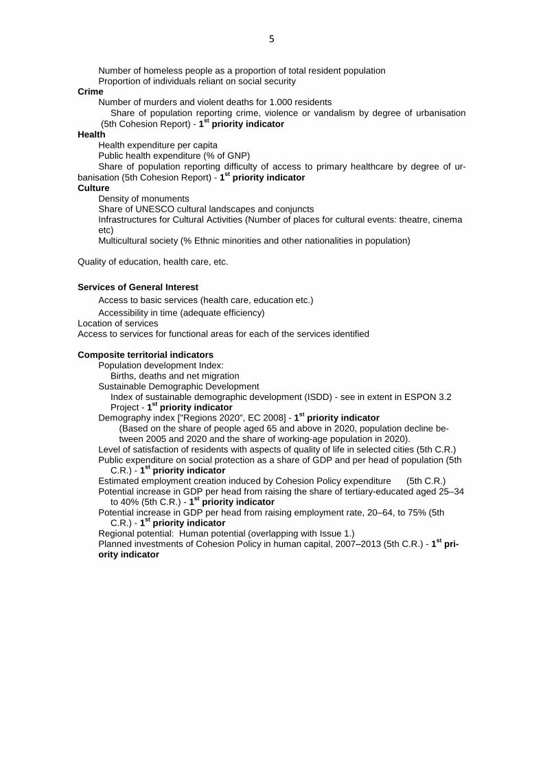
5

Number of homeless people as a proportion of total resident population Proportion of individuals reliant on social security

Crime Number of murders and violent deaths for 1.000 residents

Share of population reporting crime, violence or vandalism by degree of urbanisation (5th Cohesion Report) - 1st priority indicator Health

Health expenditure per capita Public health expenditure (% of GNP) Share of population reporting difficulty of access to primary healthcare by degree of ur-banisation (5th Cohesion Report) - 1st priority indicator Culture

Density of monuments Share of UNESCO cultural landscapes and conjuncts

Infrastructures for Cultural Activities (Number of places for cultural events: theatre, cinema etc)

Multicultural society (% Ethnic minorities and other nationalities in population) Quality of education, health care, etc. Services of General Interest

Access to basic services (health care, education etc.) Accessibility in time (adequate efficiency) Location of services Access to services for functional areas for each of the services identified Composite territorial indicators

Population development Index: Births, deaths and net migration

Sustainable Demographic Development Index of sustainable demographic development (ISDD) - see in extent in ESPON 3.2 Project - 1st priority indicator

Demography index ["Regions 2020", EC 2008] - 1st priority indicator (Based on the share of people aged 65 and above in 2020, population decline be-tween 2005 and 2020 and the share of working-age population in 2020).

Level of satisfaction of residents with aspects of quality of life in selected cities (5th C.R.) Public expenditure on social protection as a share of GDP and per head of population (5th C.R.) - 1st priority indicator Estimated employment creation induced by Cohesion Policy expenditure (5th C.R.) Potential increase in GDP per head from raising the share of tertiary-educated aged 25–34 to 40% (5th C.R.) - 1st priority indicator Potential increase in GDP per head from raising employment rate, 20–64, to 75% (5th C.R.) - 1st priority indicator Regional potential: Human potential (overlapping with Issue 1.) Planned investments of Cohesion Policy in human capital, 2007–2013 (5th C.R.) - 1st pri-ority indicator

6

Issue 3: Environmental dimension, hazards and clima te change Proposed indicators

(1) Sustainable environment Physical environment quality

Land consumption by type of activity Land cover/land use in selected cities (5th C.R.) - 1st priority indicator Ecosystems (biological dimensions), biodiversity

Biodiversity Biomass (change)

Fragmentation by urbanisation, infrastructure and agriculture Species diversity

Share of fragmented natural areas Share of sensitive eco-regions

Share of areas with high ecological value Ecosystems biodiversity, CO2 sinks, quality water

Water Consumption of water per capita, Drinking water quality Trans-boundary water management policy

Soil Soil sealed area, 2006 (5th CR) - 1st priority indicator Soil sealing per inhabitant, 2006 (5th CR) - 1st priority indicator

Food: Distance to food production (food-miles) Agriculture

Type Peri-urban agriculture (incl. changes) Use of good agricultural soils for urban development Bio-fuels (in particular area occupied)

Landscape Visual attractiveness Cultural heritage including agricultural landscapes Area for housing Management

Management type (public, private), Local services, Trans-boundary management Protected areas

Coverage of protected areas NATURA 2000 area (Share of Natura 2000 area in %) (5th C.R.) - 1st priority ind. Seas, fishing Sea surface temperature changes Changes in sea level rise Status of marine fish stocks

Fishing, Industry (aquaculture) Coastal areas

Coastal erosion Environment assets (quality of the environment) Cultural heritage (overlapping with Issue 2) Congestion, Emissions, Wastes, Noise

Congestion index on the main road network (5th C.R.) - 1st priority indicator Emissions

CO2 Emissions, intensity, per capita Greenhouse gas emissions Emissions of Acidifying Substances Acidifying Potential

Passenger flights of less than 500 km (5th C.R.) - 1st priority indicator Concentration of particulate matter (PM10) at surface level (5th C.R.) - 1st priority indic.

7

Wastes Urban waste water treatment capacity (5th C.R.) - 1st priority indicator Noise

Noise disturbance, Noise levels Share of residents exposed to excessive noise (by various source of noises)

Environment services Eco-tourism Possibility of trading environmental services

Environmental policy

Environmental politico-administrative instruments Application of environmental norms/standards Integration of environment in policies

Complex indicators on environment Regional performance based on environmental indicat ors (Percentage change in emissions of 6 main greenhouse gasses (in CO2 equivalents) be-

tween base year and year x) Possibility of non-development / different development (2) Hazards, Risks

Oil hazards, Forest fires, Storms, tsunami Flood endangered settlement and artificial areas Risk from sea level raising Exposure of ecosystems to acidification, eutrophication and ozone

Ozone concentration exceedances in NUTS 3 regions (5th C. R.) - 1st priority indic. Temperature, precipitation, snow cover Projected change of temperature and precipitation (5th C. R.) - 1st priority indic. Observed climatological average of total annual precipitation

Projected change in number of tropical nights (5th C. R.) - 1st priority indic. Projected change in annual number of days with snow cover (5th C. R.) - 1st priority indic.

Sum of all weighted hazard values classified in 5 categories Risk (natural) prevention, Frequency of hazards/disasters, Protection against floods + un-usual risks (not covered by present infrastructure)

(3) Climate change

Avalanches, Droughts, Earthquakes, Floods Mean max, min annual temperature Change of the average precipitation

Change of the average annual number (amount) of days with heavy rainfall / water evapo-ration / snow covering

Settlement prone to heavy rainfall / sea level rise Exposure to climate change of the agriculture, fisheries and tourism sector % of population in coastal areas prone to sea level rise / heavy rainfall Vulnerability of NUTS2 regions to climate change (5th C. R.) - 1st priority indicator Projected change in Tourism Climate Index (5th C. R.) - 1st priority indicator Climate change index (“Regions 2020”, EC 2008) - 1st priority indicator

(Based on change in regional population affected by river floods, regional population in ar-eas below 5m, potential regional drought hazard, regional share of agriculture and fisheries in GVA, regional share of employment in hotels and restaurants taking into account the impact of climate change by climate zone)

8

Issue 4: Energy Proposed indicators Energy demand, consumption, production, economy

Energy consumption (Inland, other), Final Energy Demand, Energy Production, Energy Net Imports Share of total energy produced/consumed Energy intensity of the economy (Gross inland consumption of energy divided by GDP) Private energy use Energy Prices: Electricity / Gas Prices Investments (shares of European, national, local investments)

Employment rate in industries with high energy purchases Energy source: renewable, other

Renewable energies PV (photovoltaic), Wind Power, Solar Energy Potential and production Wind energy potential: onshore full load hours (5th CR) - 1st priority indicator Solar energy resources per NUTS 3 regions hours (5th CR) - 1st priority indicator

Electricity Generation Green infrastructures

Energy Impacts on agriculture, landscapes Energy index ["Regions 2020", EC 2008] - 1st priority indicator

(Based on four variables, regional energy consumption of households regional energy consumption of industry, agriculture, services and freight transport, national energy import dependency, national carbon content of gross inland energy consumption)

Issue 5.1: Specific regions and local development Proposed indicators

Indicators (thresholds, rates) for the delimitation of the areas of the specific regions (5th C.R.) – 1st priority indicators / typologies

Mountain regions NUTS 3 regions where 50% of the population lives in a mountainous area or 50% of the land area is considered mountainous.

Island regions NUTS 3 regions where the majority of the population live on one or more islands without fixed connections to the mainland, such as a bridge or a tunnel.

Sparsely populated regions NUTS 3 regions with a population density of less than 12.5 inhabitants per km².

Particular characteristics of specific areas Population density, Age dependency ratios Income and wealth measurement

Gini coefficient / Concentration Index (Standard measurement for inequality of income or wealth)

Local specialization potentials Employment by primary, secondary and tertiary sector Employment in selected economic activities such as fishing, mining, forestry, tourism Physical environment assets Cultural heritage assets Connectivity: transport, ICT, energy Accessibility to the nearest economic centre Accessibility Access to services of general interest (education, healthcare etc) Cities / other local centres’ hierarchy and network ing - See also in Issue 1.2.

Cities and other local centres’ hierarchy Flows among cities / other local centres

9

Indicators for the definition of functional areas in specific regions Territorial governance in specific regions - See in the list of indicators for Governance Issue 5.2: Rural areas Proposed indicators: rural areas Land use: rural areas and fisheries

Land Use Utilised agricultural areas

Production Share (%) of added value in agriculture, forestry and fishery in the regional added value

Agriculture turnover Livestock Farms Structure (Holdings)

% (change in number) of holdings > x ESU (European Size Unit) % of holdings with an OGA (Other Gainful Activity) Number of farm holdings Farms Structure (Holders)

% (change of) holders who are full time Total number of holders

% of forestry and logging holders in the total number of holders % of Fishing and agriculture holders in the total number of holders Age of farm holders, 55yrs < change in holders < 35yrs Employment

Annual work unit (AWU) per European Size Unit (ESU) Number of persons working in agriculture, forestry and fishing (3 indicators) Particular characteristics of rural areas – See in the list of indicators for specific regions Cities / other local centres’ hierarchy and network ing - See in the list of indicators for spe-

cific regions Territorial governance in rural areas - See in the list of indicators for Governance. Issue 6: Sustainable mobility and connectivity Proposed indicators Transport and communication activity and infrastruc ture

Density of motorways, trunk roads, railways , capacity of maritime transport Traffic separation in different infrastructure levels / International transport infrastructure and

local / regional infrastructure Urban transportation infrastructure (new indicator)

Productivity of inland infrastructure Employment in the transport sector as % of total employment Use of telematics in transport networks (new indicator) See also in Issue 1

Passengers and Goods Transport Number of passengers travelling by air, maritime transport Road freight crossing the region borders Modal spilt in the regional transport Population commuting to other regions / working in the same region

External passengers (outside the region) at more than 3h Spending on transport fuel for freight as % of GDP Accessibility

Multimodal/road/rail potential accessibility Potential accessibility to population/GDP (road network/airline distance)

Proportion of regional population within 1 hour car travel time to next airport/ university / hospital

10

Accessibility time to market Access to high-speed train services Peripherality indicator by car with respect to population Daily market accessible by car in terms of GDP Reliability and costs of accessibility (statistical artefacts) See also in Issue 1 Accessibility to Public Services

Average travel time to three higher hierarchical cities Accessibility to the nearest/ most frequently used hospital See also in Issue 2 Connectivity

Connectivity to commercial airports Time to the nearest facility or motorway or railway station Car driving time to the nearest (x) facility (Included in accessibility indicators)

Time to the nearest motorway access Travel time to railway stations Car travel time to commercial airports Car travel time to universities/ polytechnics /hospitals ICT connectivity (new indicator) Impacts of Transport structure and policies

Impacts on the environment Age of car park CO2 emissions per usable land Congestion cost See also in other Issues Issue 7: Territorial governance, coordination of po licies and territorial im-

pacts Proposed indicators

Territorial governance Government effectiveness, participation issues

Electoral participation Government effectiveness index Public attitudes towards the political-administrative system

Trust in the legal system (Share of persons having complete trust/ no trust at all in the legal system of a

counrty) Share of persons working in an organisation or association (other than a political party) within the last x months

Quality of governance Corruption

Existence of a national adaptation strategy Decentralisation Effectiveness of public administration (4th C.R) Territorial cooperation Number of project co-operations

Way in which roles and responsibilities are distributed among local government and other involved actors

Cross-sectoral impacts of policies Finding cross-sectoral impacts of policies using the indicators (grouping, correlation)

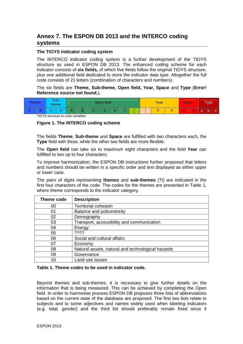
ESPON 2013 85

Annex 7. The ESPON DB 2013 and the INTERCO coding systems The TtOYS indicator coding system

The INTERCO indicator coding system is a further development of the TtOYS structure as used in ESPON DB 2013. The enhanced coding scheme for each indicator consists of six fields, of which five fields follow the original TtOYS structure, plus one additional field dedicated to store the indicator data type. Altogether the full code consists of 21 letters (combination of characters and numbers).

The six fields are Theme, Sub-theme, Open field, Year, Space and Type (Error! Reference source not found. ).

Theme Sub-theme Open field Year Space Type

# # # # A B C d e f # # X X X X X TtOYS structure to code variables

Figure 1. The INTERCO coding scheme

The fields Theme , Sub-theme and Space are fulfilled with two characters each, the Type field with three, while the other two fields are more flexible.

The Open field can take six to maximum eight characters and the field Year can fulfilled to two up to four characters.

To improve harmonization, the ESPON DB instructions further proposed that letters and numbers should be written in a specific order and text displayed as either upper or lower case.

The pairs of digits representing themes and sub-themes (Tt) are indicated in the first four characters of the code. The codes for the themes are presented in Table 1, where theme corresponds to the indicator category.

Theme code Description 00 Territorial cohesion 01 Balance and policentricity 02 Demography 03 Transport, accessibility and communication 04 Energy 05 ???? 06 Social and cultural affairs 07 Economy 08 Natural assets, natural and technological hazards 09 Governance 10 Land use issues

Table 1. Theme codes to be used in indicator code.

Beyond themes and sub-themes, it is necessary to give further details on the information that is being measured. This can be achieved by completing the Open field. In order to harmonise process ESPON DB proposes three lists of abbreviations based on the current state of the database are proposed. The first two lists relate to subjects and to some adjectives and names widely used when labeling indicators (e.g. total, gender) and the third list should preferably remain fixed since it

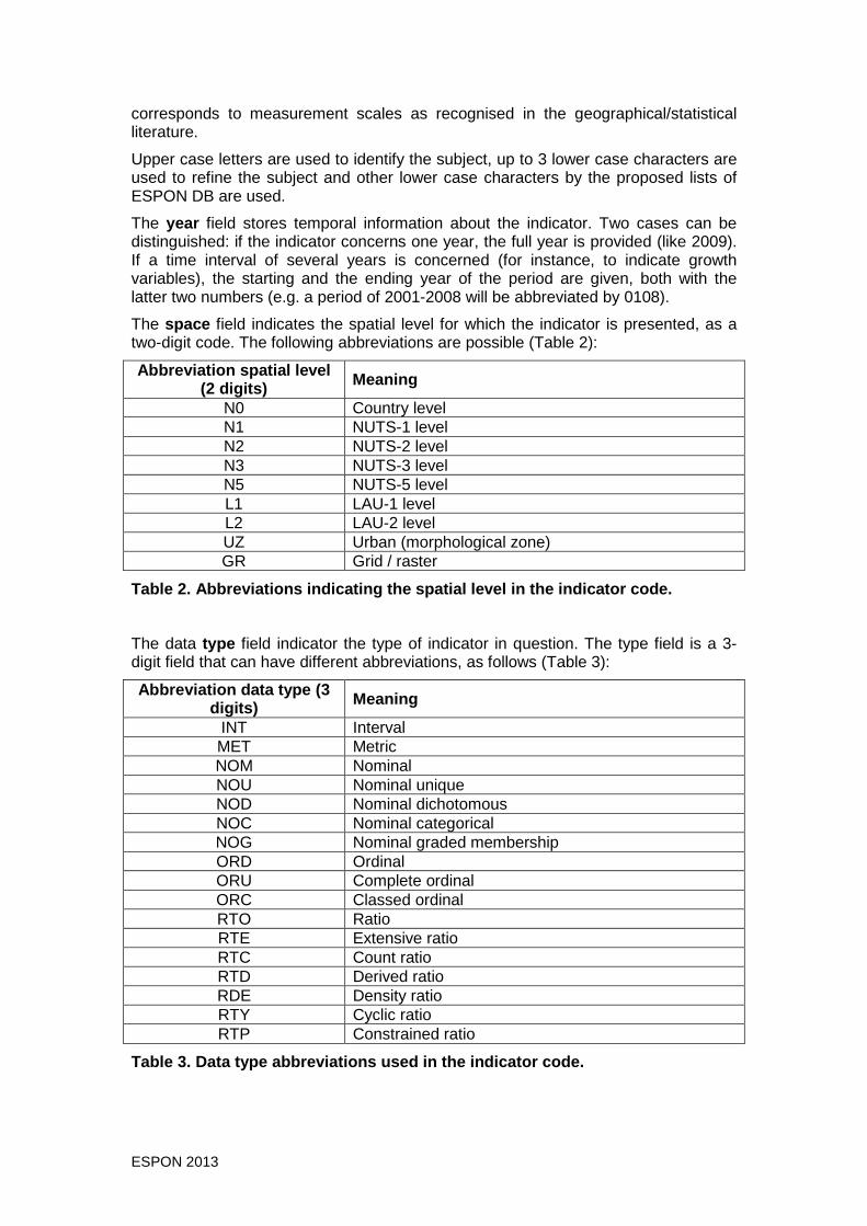
ESPON 2013 86

corresponds to measurement scales as recognised in the geographical/statistical literature.

Upper case letters are used to identify the subject, up to 3 lower case characters are used to refine the subject and other lower case characters by the proposed lists of ESPON DB are used.

The year field stores temporal information about the indicator. Two cases can be distinguished: if the indicator concerns one year, the full year is provided (like 2009). If a time interval of several years is concerned (for instance, to indicate growth variables), the starting and the ending year of the period are given, both with the latter two numbers (e.g. a period of 2001-2008 will be abbreviated by 0108).

The space field indicates the spatial level for which the indicator is presented, as a two-digit code. The following abbreviations are possible (Table 2):

Abbreviation spatial level (2 digits) Meaning

N0 Country level N1 NUTS-1 level N2 NUTS-2 level N3 NUTS-3 level N5 NUTS-5 level L1 LAU-1 level L2 LAU-2 level UZ Urban (morphological zone) GR Grid / raster

Table 2. Abbreviations indicating the spatial level in the indicator code.

The data type field indicator the type of indicator in question. The type field is a 3-digit field that can have different abbreviations, as follows (Table 3):

Abbreviation data type (3 digits) Meaning

INT Interval MET Metric NOM Nominal NOU Nominal unique NOD Nominal dichotomous NOC Nominal categorical NOG Nominal graded membership ORD Ordinal ORU Complete ordinal ORC Classed ordinal RTO Ratio RTE Extensive ratio RTC Count ratio RTD Derived ratio RDE Density ratio RTY Cyclic ratio RTP Constrained ratio

Table 3. Data type abbreviations used in the indica tor code.

ESPON 2013 87

The indicator codes need to be unique for each indicator. If there are two or more indicators with similar characteristics, the OpenField can be used to differentiate the indicator codes from each other.

Coding system implemented in INTERCO geodatabase

The indicator coding system described above is not only used in the fact sheets for indicator identification, but the codes are also used in the INTERCO_DB geodatabase as column header (i.e. field names) in the data tables (Figure 2). Since the indicator codes are unique, by that the column headers in the tables are also distinctive. The benefit of using these codes in the database over using other names is their compactness and uniqueness.

Figure 2. Indicator codes as field names in data ta bles of INTERCO_DB geodatabase

Indicator codes

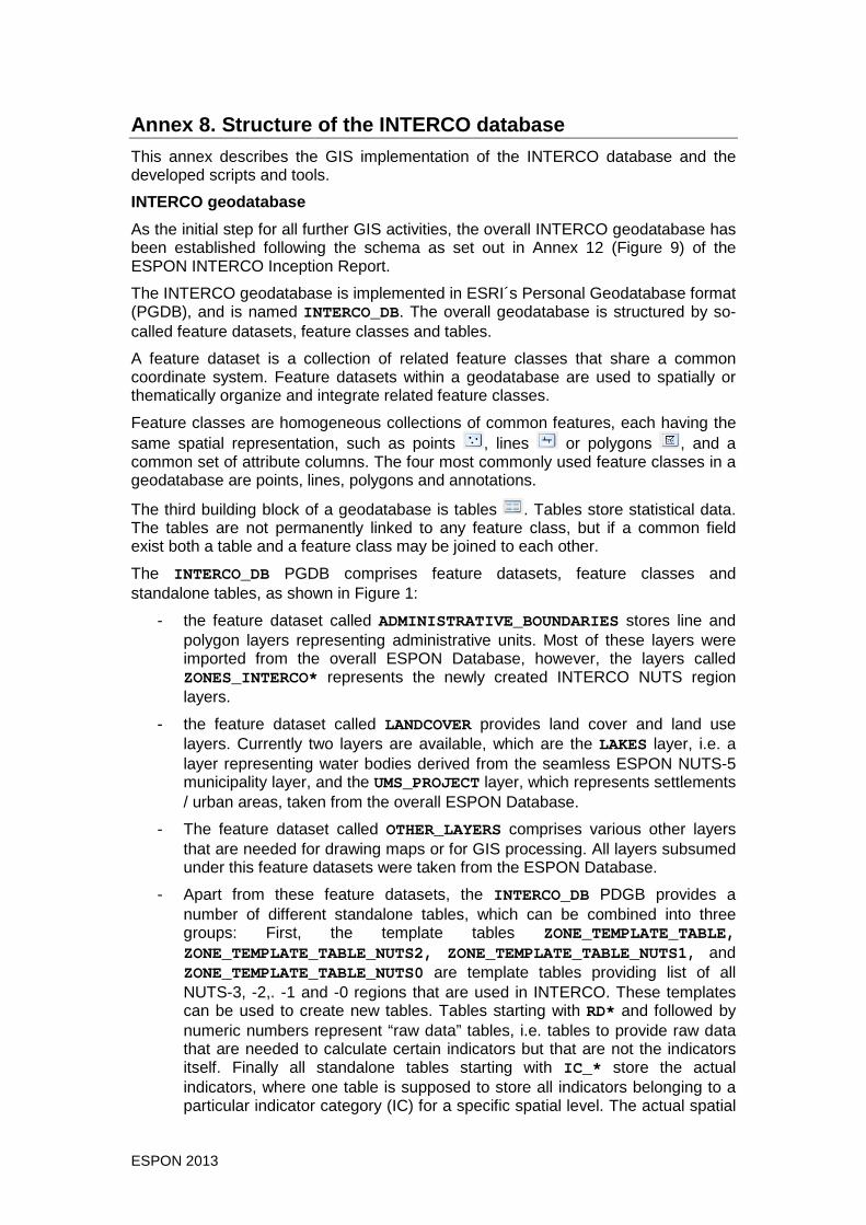
ESPON 2013 88

Annex 8. Structure of the INTERCO database This annex describes the GIS implementation of the INTERCO database and the developed scripts and tools.

INTERCO geodatabase

As the initial step for all further GIS activities, the overall INTERCO geodatabase has been established following the schema as set out in Annex 12 (Figure 9) of the ESPON INTERCO Inception Report.

The INTERCO geodatabase is implemented in ESRI´s Personal Geodatabase format (PGDB), and is named INTERCO_DB. The overall geodatabase is structured by so-called feature datasets, feature classes and tables.

A feature dataset is a collection of related feature classes that share a common coordinate system. Feature datasets within a geodatabase are used to spatially or thematically organize and integrate related feature classes.

Feature classes are homogeneous collections of common features, each having the same spatial representation, such as points , lines or polygons , and a common set of attribute columns. The four most commonly used feature classes in a geodatabase are points, lines, polygons and annotations.

The third building block of a geodatabase is tables . Tables store statistical data. The tables are not permanently linked to any feature class, but if a common field exist both a table and a feature class may be joined to each other.

The INTERCO_DB PGDB comprises feature datasets, feature classes and standalone tables, as shown in Figure 1:

- the feature dataset called ADMINISTRATIVE_BOUNDARIES stores line and polygon layers representing administrative units. Most of these layers were imported from the overall ESPON Database, however, the layers called ZONES_INTERCO* represents the newly created INTERCO NUTS region layers.

- the feature dataset called LANDCOVER provides land cover and land use layers. Currently two layers are available, which are the LAKES layer, i.e. a layer representing water bodies derived from the seamless ESPON NUTS-5 municipality layer, and the UMS_PROJECT layer, which represents settlements / urban areas, taken from the overall ESPON Database.

- The feature dataset called OTHER_LAYERS comprises various other layers that are needed for drawing maps or for GIS processing. All layers subsumed under this feature datasets were taken from the ESPON Database.

- Apart from these feature datasets, the INTERCO_DB PDGB provides a number of different standalone tables, which can be combined into three groups: First, the template tables ZONE_TEMPLATE_TABLE, ZONE_TEMPLATE_TABLE_NUTS2, ZONE_TEMPLATE_TABLE_NUTS1, and ZONE_TEMPLATE_TABLE_NUTS0 are template tables providing list of all NUTS-3, -2,. -1 and -0 regions that are used in INTERCO. These templates can be used to create new tables. Tables starting with RD* and followed by numeric numbers represent “raw data” tables, i.e. tables to provide raw data that are needed to calculate certain indicators but that are not the indicators itself. Finally all standalone tables starting with IC_* store the actual indicators, where one table is supposed to store all indicators belonging to a particular indicator category (IC) for a specific spatial level. The actual spatial

ESPON 2013 89

level is provided as suffix to the table name (*_NUTS0, *_NUTS1, or *_NUTS2). If no suffix is provided, the table stores indicators at NUTS-3 level. The following indicator categories were identified:

o Cohesion

o Demography

o Economy

o Energy

o Environment

o Governance

o Landuse

o Natural assets

o Polycentricity

o Social

o transport

Eventually the number and names of the IC_* tables in the geodatabase will correspond to the classification schema as developed for the overall indicator toolset. Subject to any modifications of the cohesion indicators, the indicator categories may vary until project end.

There will be one column per indicator in the IC_* tables. The column header corresponds to the unique TtOYS indicator code (see Annex 7).

If necessary additional feature datasets, feature classes or standalone tables may be added to the INTERCO_DB at later stages of the project.

The metadata describing the INTERCO_DB PGDB will also be stored as part of the geodatabase. From there they can be accessed, or exported to text formats like DOC or PDF. The exported metadata in PDF format can be accessed from outside ArcGIS via the DOC sub-directory (see folder description below). Metadata will be stored in one of the following three standards:

- INSPIRE metadata directive

- ISO 19139 metadata implementation specification

- North American profile of ISO 19115 2003

A full description of this geodatabase, including detailed descriptions of database structures, fields and formats, will be given in the metadata document that will be developed towards the end of this project.

ESPON 2013 90

Figure 1. INTERCO_DB PGDB structure and contents.

ESPON 2013 91

Scripts and tools

The generation of the indicators usually requires a sequence of mathematical, statistical or GIS operations, or even the development of dedicated GIS models, depending on the indicator complexity and the required input data. All needed operations will be implemented by scripts, with one script per indicator or per indicator group. The scripts will be subsumed in a new INTERCO toolbox for ArcGIS, called INTERCOtools. The tools can then be launched from ArcGIS to re-calculate any of the indicators easily without the need to redevelop the methodological basis again. Upon successful processing of a script, the script will update all relevant GIS layers and/or tables.

Figure 2 illustrates how the scripts can be accessed from ArcGIS Toolbox, as a collection of INTERCOtools, subdivided by themes. The theme names correspond to the classification schema (Cohesion, Demography, Economy, Energy, … ,Transport), so as the script names correspond to the indicator names. The illustration in Figure 2 is based upon the tentative set of indicators as descripted in Chapter XX, so the final available tools may vary subject to the final selection set of cohesion indicators.

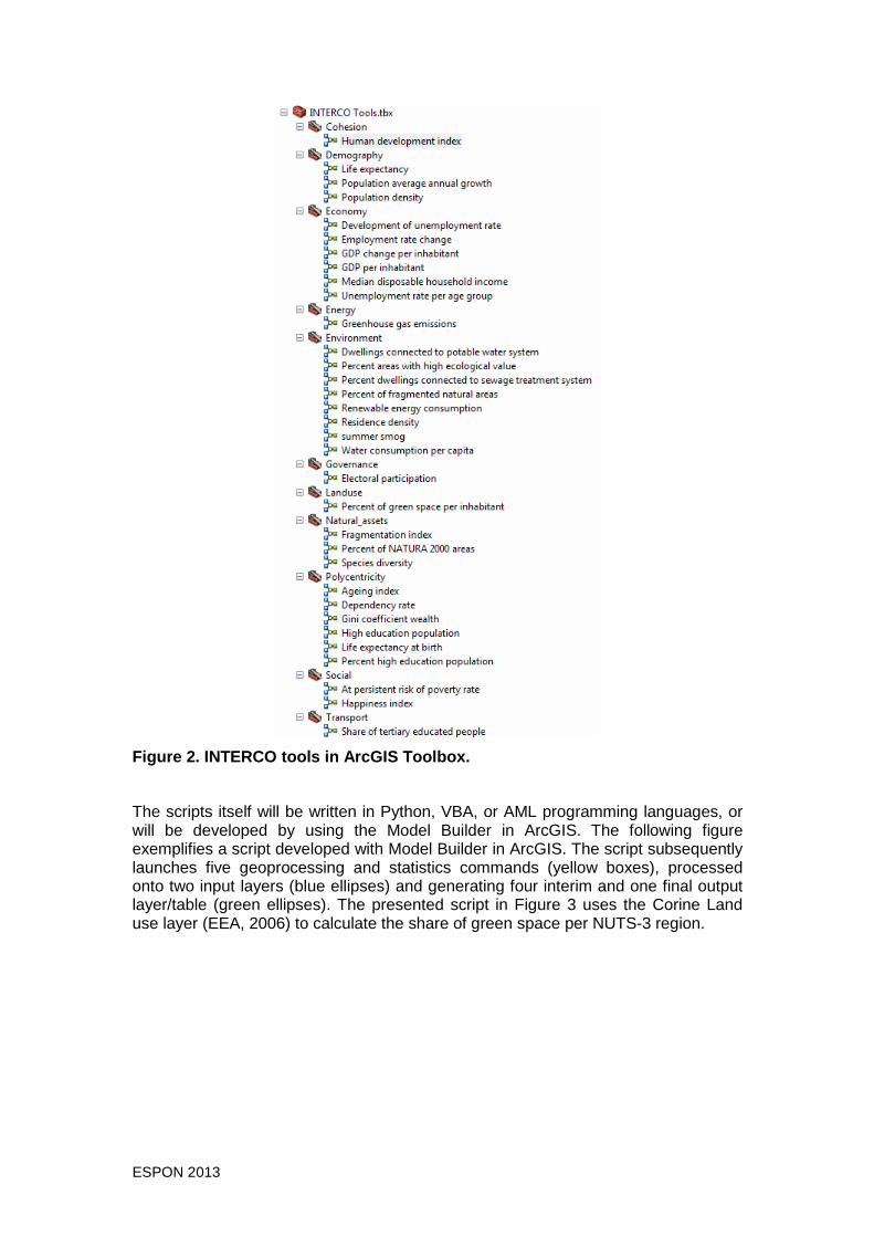
ESPON 2013 92

Figure 2. INTERCO tools in ArcGIS Toolbox.

The scripts itself will be written in Python, VBA, or AML programming languages, or will be developed by using the Model Builder in ArcGIS. The following figure exemplifies a script developed with Model Builder in ArcGIS. The script subsequently launches five geoprocessing and statistics commands (yellow boxes), processed onto two input layers (blue ellipses) and generating four interim and one final output layer/table (green ellipses). The presented script in Figure 3 uses the Corine Land use layer (EEA, 2006) to calculate the share of green space per NUTS-3 region.

ESPON 2013 93

Figure 3. Custom script developed with Model Builde r in ArcGIS.

All scripts, however, will eventually be implemented after the final definition and selection of the cohesion indicators.

Mapping and cartography

The mapping of the indicators and the cartographic layout will be based upon the mapkits developed by the ESPON 2013 Database project (Zanin et al., 2010). Among the four available mapkits, the ESPON Space mapkit was selected as the most suitable one for INTERCO. Even though, unlike the ESPON Space and Candidate Countries mapkit, the territory of Turkey is not fully covered by it, it was selected since it provides the most detailed insight (=highest resolution) for Europe as a whole.

All European-wide maps will be produced by using this template. The template is stored as template file for ArcGIS (i.e. MXT and MXD files) in a specific folder (see below). The original MXD file of the ESPON 2013 Database project has been amended to some extent, to meet the INTERCO requirements. Additional zoom-in maps for specific regions or territories may use alternative map layouts.

The layers used in the maps will also be provided as so-called LYR files, i.e. specific files that store the layer symbology (colors, symbols, line width, line and polygon patters, markers etc.) for later uses in other maps, without the need to re-establish the overall symbology again. Figure 4 illustrates the LYR files that constitute the basic map layout, which are stored in the LYRS subdirectory (see below).

Summary statistics

Adding field

Projecting layer Calculating field

Overlay with zone layer

ESPON 2013 94

Figure 4. LYR files constituting the base map in th umbnails view.

Folder structure

The overall output of the GIS works in INTERCO will be stored and will be made available in a comprehensive folder structure, including the GIS database, the documentation, the cartography, Excel tables as well as layer files.

The following folder structure has already been implemented to store the results of all INTERCO works:

CARTO comprises all generated MXD files for indicator mapping

DOC metadata documentation and user manual for the INTERCO database

EXCEL collection of Excel files (input and output of indicator calculation)

LYRS collection of layer files for mapping (referenced in MXD files)

MAPS collection of maps in PNG file format, exported from ArcGIS

TOOLS sub-directory storing the INTERCO toolbox and the developed scripts

The actual INTERCO_DB PGDB is stored in parallel to these sub-directories. The mentioned folders may also comprise one or several sub-directories, as appropriate.

ESPON 2013 95

Annex 9. Inventory of indicators Cat. nr Category name Indicator name status

2 DEMOGRAPHY Life expectancy tested

2 DEMOGRAPHY Population average annual growth tested

2 DEMOGRAPHY Population density tested

2 DEMOGRAPHY Population potential within 50 km tested

2 DEMOGRAPHY Urban - rural population in Europe based on national classification

tested

3 TRANSPORT, ACCESSIBILITY, COMMUNICATION

Employment in the transport sector as % of total employment

tested

3 TRANSPORT, ACCESSIBILITY, COMMUNICATION

Share of tertiary educated people in % tested

3 TRANSPORT, ACCESSIBILITY, COMMUNICATION

travel time to railway stations tested

4 ENERGY Greenhouse gas emission tested

4 ENERGY Renewable energy consumption tested

6 SOCIAL AND CULTURAL AFFAIRS

At persistent risk of poverty rate (Population share with 60 % of the national equivalent median income)

tested

6 SOCIAL AND CULTURAL AFFAIRS

happiness tested

7 ECONOMY % of households having broadband access tested

7 ECONOMY development of unemployment rate (male, female, young, total, 99-04)

tested

7 ECONOMY employment rate change (growth) tested

7 ECONOMY GDP change per inhabitant (capita) in pps or euros tested

7 ECONOMY GDP per inhabitant (capita) in pps or euros, per year tested

7 ECONOMY median disposable annual household income tested

7 ECONOMY Unemployment rate per age: classes of 5 years tested

8 ENVIRONMENT, HAZARDS Consumption of water per capita tested

8 ENVIRONMENT, HAZARDS Dwellings connected to potable water system tested

8 ENVIRONMENT, HAZARDS ozone concentrations tested

8 ENVIRONMENT, HAZARDS PM10 concentrations tested

8 ENVIRONMENT, HAZARDS Residence density tested

8 ENVIRONMENT, HAZARDS Share of areas with high ecological value tested

9 GOVERNANCE Electoral participation tested

10 TERRITORIAL COHESION GERD (Gross domestic expenditure on research and development)

tested

10 TERRITORIAL COHESION Human Development Index tested

11 BALANCE AND POLYCENTRICITY

Ageing index (persons 65+ / persons 0-14) tested

11 BALANCE AND POLYCENTRICITY

Dependency rate tested

11 BALANCE AND POLYCENTRICITY

High education population tested

11 BALANCE AND POLYCENTRICITY

Life expectancy at birth tested

11 BALANCE AND POLYCENTRICITY

MEGA / Metropolitan European Growth Areas tested

11 BALANCE AND POLYCENTRICITY

Share high educated population in percent tested

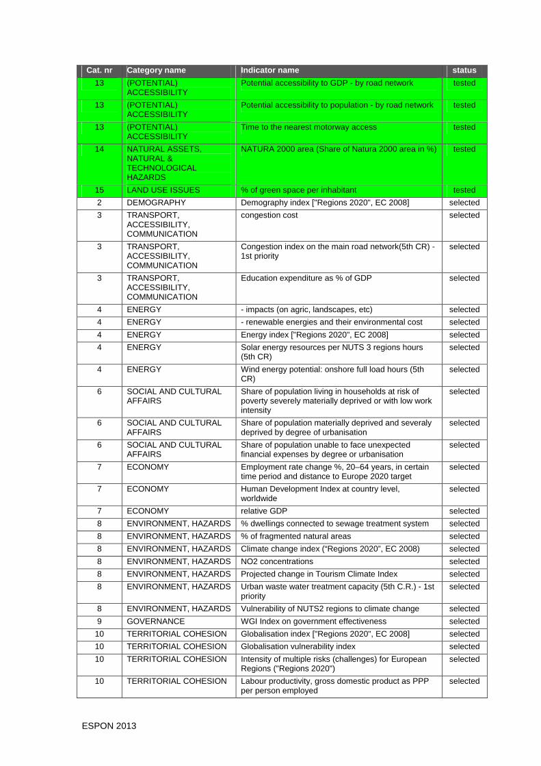
ESPON 2013 96

Cat. nr Category name Indicator name status

13 (POTENTIAL) ACCESSIBILITY

Potential accessibility to GDP - by road network tested

13 (POTENTIAL) ACCESSIBILITY

Potential accessibility to population - by road network tested

13 (POTENTIAL) ACCESSIBILITY

Time to the nearest motorway access tested

14 NATURAL ASSETS, NATURAL & TECHNOLOGICAL HAZARDS

NATURA 2000 area (Share of Natura 2000 area in %) tested

15 LAND USE ISSUES % of green space per inhabitant tested

2 DEMOGRAPHY Demography index ["Regions 2020", EC 2008] selected

3 TRANSPORT, ACCESSIBILITY, COMMUNICATION

congestion cost selected

3 TRANSPORT, ACCESSIBILITY, COMMUNICATION

Congestion index on the main road network(5th CR) - 1st priority

selected

3 TRANSPORT, ACCESSIBILITY, COMMUNICATION

Education expenditure as % of GDP selected

4 ENERGY - impacts (on agric, landscapes, etc) selected

4 ENERGY - renewable energies and their environmental cost selected

4 ENERGY Energy index ["Regions 2020", EC 2008] selected

4 ENERGY Solar energy resources per NUTS 3 regions hours (5th CR)

selected

4 ENERGY Wind energy potential: onshore full load hours (5th CR)

selected

6 SOCIAL AND CULTURAL AFFAIRS

Share of population living in households at risk of poverty severely materially deprived or with low work intensity

selected

6 SOCIAL AND CULTURAL AFFAIRS

Share of population materially deprived and severaly deprived by degree of urbanisation

selected

6 SOCIAL AND CULTURAL AFFAIRS

Share of population unable to face unexpected financial expenses by degree or urbanisation

selected

7 ECONOMY Employment rate change %, 20–64 years, in certain time period and distance to Europe 2020 target

selected

7 ECONOMY Human Development Index at country level, worldwide

selected

7 ECONOMY relative GDP selected

8 ENVIRONMENT, HAZARDS % dwellings connected to sewage treatment system selected

8 ENVIRONMENT, HAZARDS % of fragmented natural areas selected

8 ENVIRONMENT, HAZARDS Climate change index (“Regions 2020”, EC 2008) selected

8 ENVIRONMENT, HAZARDS NO2 concentrations selected

8 ENVIRONMENT, HAZARDS Projected change in Tourism Climate Index selected

8 ENVIRONMENT, HAZARDS Urban waste water treatment capacity (5th C.R.) - 1st priority

selected

8 ENVIRONMENT, HAZARDS Vulnerability of NUTS2 regions to climate change selected

9 GOVERNANCE WGI Index on government effectiveness selected

10 TERRITORIAL COHESION Globalisation index ["Regions 2020", EC 2008] selected

10 TERRITORIAL COHESION Globalisation vulnerability index selected

10 TERRITORIAL COHESION Intensity of multiple risks (challenges) for European Regions ("Regions 2020")

selected

10 TERRITORIAL COHESION Labour productivity, gross domestic product as PPP per person employed

selected

ESPON 2013 97

Cat. nr Category name Indicator name status

10 TERRITORIAL COHESION Regional competitiveness index selected

11 BALANCE AND POLYCENTRICITY

Cluster focus selected

11 BALANCE AND POLYCENTRICITY

Early school leavers and distance to Europe 2020 target - 5th CR

selected

11 BALANCE AND POLYCENTRICITY

Estimated employment creation induced by Cohesion Policy expenditure (5th CR)

selected

11 BALANCE AND POLYCENTRICITY

Human Poverty Index (5th CR) selected

11 BALANCE AND POLYCENTRICITY

Level of satisfaction of residents with aspects of quality of life in selected cities (5th C.R.)

selected

11 BALANCE AND POLYCENTRICITY

Planned investments of Cohesion Policy in human capital, 2007–2013 (5th C.R.)

selected

11 BALANCE AND POLYCENTRICITY

Population suffering from severe material deprivation (% of total population) (5th CR)

selected

11 BALANCE AND POLYCENTRICITY

Population with a tertiary education per age group (5th CR)

selected

11 BALANCE AND POLYCENTRICITY

Potential increase in GDP per head from raising employment rate, 20–64, to 75% (5th CR)

selected

11 BALANCE AND POLYCENTRICITY

Potential increase in GDP per head from raising the share of tertiary-educated aged 25–34 to 40% (5th C.R.)

selected

11 BALANCE AND POLYCENTRICITY

Production of renewable energy per country ? selected

11 BALANCE AND POLYCENTRICITY

Public expenditure on social protection as a share of GDP and per head of population (5th CR)

selected

11 BALANCE AND POLYCENTRICITY

Share of population at risk of poverty by degree of urbanisation (5th CR)

selected

11 BALANCE AND POLYCENTRICITY

Share of population reporting crime, violence or vandalism by degree of urbanisation (5th CR) - 1st priority indicator

selected

11 BALANCE AND POLYCENTRICITY

Share of population reporting difficulty of access to primary healthcare by degree of urbanisation (5th Cohesion Report)

selected

13 (POTENTIAL) ACCESSIBILITY

logistic efficiency selected

13 (POTENTIAL) ACCESSIBILITY

Multimodal/road/rail potential accessibility selected

13 (POTENTIAL) ACCESSIBILITY

Potential accessibility to GDP - by airline selected

13 (POTENTIAL) ACCESSIBILITY

Potential accessibility to population - by airline selected

13 (POTENTIAL) ACCESSIBILITY

Secondary networks selected

14 NATURAL ASSETS, NATURAL & TECHNOLOGICAL HAZARDS

Fragmentation index selected

14 NATURAL ASSETS, NATURAL & TECHNOLOGICAL HAZARDS

Intensity of multiple risks (challenges) for European Regions ("Regions 2020")

selected

14 NATURAL ASSETS, NATURAL & TECHNOLOGICAL HAZARDS

Island Vulnerabilitry index selected

14 NATURAL ASSETS, Ozone concentration exceedances in NUTS 3 regions selected

ESPON 2013 98

Cat. nr Category name Indicator name status

NATURAL & TECHNOLOGICAL HAZARDS

(5th C. R.) -

14 NATURAL ASSETS, NATURAL & TECHNOLOGICAL HAZARDS

Projected change in number of tropical nights (5th C. R.)

selected

14 NATURAL ASSETS, NATURAL & TECHNOLOGICAL HAZARDS

Projected change of temperature and precipitation between 1961–1990 and 2071–2100

selected

14 NATURAL ASSETS, NATURAL & TECHNOLOGICAL HAZARDS

Soil sealing per inhabitant, 2006 (5th CR) - 1st priority selected

14 NATURAL ASSETS, NATURAL & TECHNOLOGICAL HAZARDS

Species diversity selected

15 LAND USE ISSUES Land cover/land use in selected cities (5th C.R.) selected

1 AGRICULTURE AND FISHERIES

% (change in number) of holdings > x ESU (European Size Unit)

1 AGRICULTURE AND FISHERIES

% (change of) holders who are full time

1 AGRICULTURE AND FISHERIES

% of holdings with an OGA (Other Gainful Activity)

1 AGRICULTURE AND FISHERIES

55yrs < change in holders < 35yrs

1 AGRICULTURE AND FISHERIES

"Added value in Agriculture, Forestry and Fisheries"

1 AGRICULTURE AND FISHERIES

Age of farm holders

1 AGRICULTURE AND FISHERIES

agriculture - bio-fuels (areas occupied)

1 AGRICULTURE AND FISHERIES

agriculture - peri-urban agriculture (incl. changes)

1 AGRICULTURE AND FISHERIES

agriculture - type

1 AGRICULTURE AND FISHERIES

agriculture - use of good agric soils for urban development

1 AGRICULTURE AND FISHERIES

Agriculture turnover

1 AGRICULTURE AND FISHERIES

Annual work unit (AWU) per European Size Unit( ESU)[Standard Gross Margin (SGM)

1 AGRICULTURE AND FISHERIES

aquaculture

1 AGRICULTURE AND FISHERIES

fishing

1 AGRICULTURE AND FISHERIES

Livestock

1 AGRICULTURE AND FISHERIES

Number of farm holdings

1 AGRICULTURE AND FISHERIES

Number of Holders in Fishing and agriculture

1 AGRICULTURE AND FISHERIES

Number of Holders in Forestry and logging

1 AGRICULTURE AND Output-Input ratio agriculture

ESPON 2013 99

Cat. nr Category name Indicator name status

FISHERIES

1 AGRICULTURE AND FISHERIES

persons working in agriculture

1 AGRICULTURE AND FISHERIES

persons working in fishing

1 AGRICULTURE AND FISHERIES

persons working in forestry

1 AGRICULTURE AND FISHERIES

Total number of Holders

1 AGRICULTURE AND FISHERIES

Utilised agricultural areas

2 DEMOGRAPHY - in migration (related to educ. level)

2 DEMOGRAPHY % of the total country population living in top-largest city (and or cities)

2 DEMOGRAPHY % of women by level, worldwide of education at country level, worldwide

2 DEMOGRAPHY Ageing "Labour Force"

2 DEMOGRAPHY Ageing of population

2 DEMOGRAPHY Changes in Natural Growth Potential

2 DEMOGRAPHY Components of population development

2 DEMOGRAPHY Crude birth rate / Crude death rate

2 DEMOGRAPHY Dependency rate

2 DEMOGRAPHY emigration & immigration per country, in migration & out migration per territorial level (NUTS 2, NUTS 3)

2 DEMOGRAPHY Employment ratio of female to male rates at country level, worldwide

2 DEMOGRAPHY Households with children aged to under 18

2 DEMOGRAPHY In migration, Out migration, Emigration , Immigration

2 DEMOGRAPHY index of demographic sustainability (ESPON 3.2)

2 DEMOGRAPHY Infant mortality

2 DEMOGRAPHY Internal / External / Total / Absolute migratory balance

2 DEMOGRAPHY Internal mobility by region

2 DEMOGRAPHY Lone - parent

2 DEMOGRAPHY Lone - person

2 DEMOGRAPHY migration by country of origin and destination

2 DEMOGRAPHY Migratory balance by regions

2 DEMOGRAPHY Nationals as a proportion of the total population

2 DEMOGRAPHY Nationals, EU nationals, Non-EU nationals that have moved into the city

2 DEMOGRAPHY Net migration rate

2 DEMOGRAPHY Number, Avg size

2 DEMOGRAPHY Population by sex and age

2 DEMOGRAPHY Population change

2 DEMOGRAPHY Population projections

2 DEMOGRAPHY Population pyramid

2 DEMOGRAPHY population size

2 DEMOGRAPHY PSR in 2050

2 DEMOGRAPHY Relative rurality based on national classifications

2 DEMOGRAPHY Resident population (total, gender proportion)

2 DEMOGRAPHY Residents’ citizenship

2 DEMOGRAPHY Rural population per NUTS

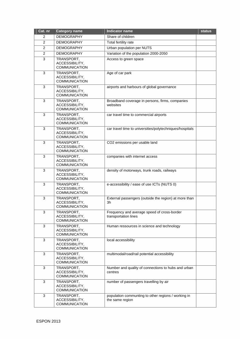
ESPON 2013 100

Cat. nr Category name Indicator name status

2 DEMOGRAPHY Share of children

2 DEMOGRAPHY Total fertility rate

2 DEMOGRAPHY Urban population per NUTS

2 DEMOGRAPHY Variation of the population 2000-2050

3 TRANSPORT, ACCESSIBILITY, COMMUNICATION

Access to green space

3 TRANSPORT, ACCESSIBILITY, COMMUNICATION

Age of car park

3 TRANSPORT, ACCESSIBILITY, COMMUNICATION

airports and harbours of global governance

3 TRANSPORT, ACCESSIBILITY, COMMUNICATION

Broadband coverage in persons, firms, companies websites

3 TRANSPORT, ACCESSIBILITY, COMMUNICATION

car travel time to commercial airports

3 TRANSPORT, ACCESSIBILITY, COMMUNICATION

car travel time to universities/polytechniques/hospitals

3 TRANSPORT, ACCESSIBILITY, COMMUNICATION

CO2 emissions per usable land

3 TRANSPORT, ACCESSIBILITY, COMMUNICATION

companies with internet access

3 TRANSPORT, ACCESSIBILITY, COMMUNICATION

density of motorways, trunk roads, railways

3 TRANSPORT, ACCESSIBILITY, COMMUNICATION

e-accessibility / ease of use ICTs (NUTS 0)

3 TRANSPORT, ACCESSIBILITY, COMMUNICATION

External passengers (outside the region) at more than 3h

3 TRANSPORT, ACCESSIBILITY, COMMUNICATION

Frequency and average speed of cross-border transportation lines

3 TRANSPORT, ACCESSIBILITY, COMMUNICATION

Human ressources in science and technology

3 TRANSPORT, ACCESSIBILITY, COMMUNICATION

local accessibility

3 TRANSPORT, ACCESSIBILITY, COMMUNICATION

multimodal/road/rail potential accessibility

3 TRANSPORT, ACCESSIBILITY, COMMUNICATION

Number and quality of connections to hubs and urban centres

3 TRANSPORT, ACCESSIBILITY, COMMUNICATION

number of passengers travelling by air

3 TRANSPORT, ACCESSIBILITY, COMMUNICATION

population communting to other regions / working in the same region

ESPON 2013 101

Cat. nr Category name Indicator name status

3 TRANSPORT, ACCESSIBILITY, COMMUNICATION

Productivity of inland infrastructure

3 TRANSPORT, ACCESSIBILITY, COMMUNICATION

Productivy of airports

3 TRANSPORT, ACCESSIBILITY, COMMUNICATION

Proportion of firms with own website

3 TRANSPORT, ACCESSIBILITY, COMMUNICATION

Road freight crossing the region borders

3 TRANSPORT, ACCESSIBILITY, COMMUNICATION

roads (km) and railways

3 TRANSPORT, ACCESSIBILITY, COMMUNICATION

Share of business internet users

3 TRANSPORT, ACCESSIBILITY, COMMUNICATION

Share of private internet users

3 TRANSPORT, ACCESSIBILITY, COMMUNICATION

Spending on transport fuel for freight as % of GDP

3 TRANSPORT, ACCESSIBILITY, COMMUNICATION

Traffic separation in different infrastructure levels

3 TRANSPORT, ACCESSIBILITY, COMMUNICATION

Urban transportations / public transportations

3 TRANSPORT, ACCESSIBILITY, COMMUNICATION

Water access

4 ENERGY - green infrastructure

4 ENERGY - investments (share of european, national, local)

4 ENERGY - share of total energy produced/consumed

4 ENERGY - source

4 ENERGY % employment in industries with high energy purchases

4 ENERGY % of GVA in industries with high energy purchases

4 ENERGY CO2 Emissions, intensity, per capita

4 ENERGY Electricity / Gas Prices

4 ENERGY Electricity Generation

4 ENERGY Emissions of Acidifying Substances Acidifying Potential

4 ENERGY Energy Inland consumption

4 ENERGY Energy Net Imports

4 ENERGY Energy Production

4 ENERGY Final Energy Demand

4 ENERGY Local potential in renewable energies

4 ENERGY Photovoltaic potential

4 ENERGY Private energy use

4 ENERGY Renewable electricity production at country level, worldwide

4 ENERGY Share of renewable generation in respect to total

ESPON 2013 102

Cat. nr Category name Indicator name status

electricity generation at country level, worldwide

4 ENERGY Total energy consumption

4 ENERGY Wind Power Energy Potential 2005

6 SOCIAL AND CULTURAL AFFAIRS

% households living in social housing

6 SOCIAL AND CULTURAL AFFAIRS

Access to cultural services

6 SOCIAL AND CULTURAL AFFAIRS

Accessibility to High Secondary School

6 SOCIAL AND CULTURAL AFFAIRS

Accessibility to Technological Education

6 SOCIAL AND CULTURAL AFFAIRS

Accessibility to training structures

6 SOCIAL AND CULTURAL AFFAIRS

Attitudes / public info on climate change

6 SOCIAL AND CULTURAL AFFAIRS

Average area of living accommodation (m2 per person)

6 SOCIAL AND CULTURAL AFFAIRS

Average occupancy per occupied dwelling

6 SOCIAL AND CULTURAL AFFAIRS

Average price of dwelling

6 SOCIAL AND CULTURAL AFFAIRS

cost of housing (in relation to purchase power)

6 SOCIAL AND CULTURAL AFFAIRS

Density of monuments

6 SOCIAL AND CULTURAL AFFAIRS

Early school leavers

6 SOCIAL AND CULTURAL AFFAIRS

Empty conventional dwellings

6 SOCIAL AND CULTURAL AFFAIRS

Enrollment ratios in secondary and tertiary education at country level, worldwide

6 SOCIAL AND CULTURAL AFFAIRS

Expenditure on health as part of GDP (national level)

6 SOCIAL AND CULTURAL AFFAIRS

Expenditure on health per capita at country level, worldwide

6 SOCIAL AND CULTURAL AFFAIRS

Health expenditure per capita

6 SOCIAL AND CULTURAL AFFAIRS

healthy life expectancy (ESPON 3.2)

6 SOCIAL AND CULTURAL AFFAIRS

Highest education attainment

6 SOCIAL AND CULTURAL AFFAIRS

Households living in owned housing, in social housing, in private rented housing, in apartments, in houses

6 SOCIAL AND CULTURAL AFFAIRS

Infrastructures for Cultural Activities (Number of places for cultural events (theatre, cinema, ….)

6 SOCIAL AND CULTURAL AFFAIRS

inhabitants satisfaction ( // GDP, neg. Agglomaration effects)

6 SOCIAL AND CULTURAL AFFAIRS

languages spoken (native / at high level / etc)

6 SOCIAL AND CULTURAL AFFAIRS

level of security

6 SOCIAL AND CULTURAL AFFAIRS

Levels of education attained by population (NUTS 0)

6 SOCIAL AND CULTURAL AFFAIRS

Multicultural society

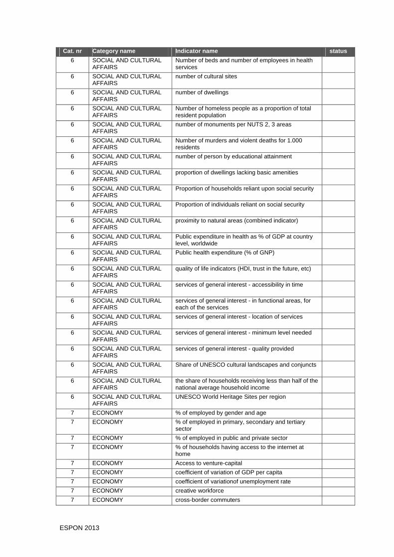
ESPON 2013 103

Cat. nr Category name Indicator name status

6 SOCIAL AND CULTURAL AFFAIRS

Number of beds and number of employees in health services

6 SOCIAL AND CULTURAL AFFAIRS

number of cultural sites

6 SOCIAL AND CULTURAL AFFAIRS

number of dwellings

6 SOCIAL AND CULTURAL AFFAIRS

Number of homeless people as a proportion of total resident population

6 SOCIAL AND CULTURAL AFFAIRS

number of monuments per NUTS 2, 3 areas

6 SOCIAL AND CULTURAL AFFAIRS

Number of murders and violent deaths for 1.000 residents

6 SOCIAL AND CULTURAL AFFAIRS

number of person by educational attainment

6 SOCIAL AND CULTURAL AFFAIRS

proportion of dwellings lacking basic amenities

6 SOCIAL AND CULTURAL AFFAIRS

Proportion of households reliant upon social security

6 SOCIAL AND CULTURAL AFFAIRS

Proportion of individuals reliant on social security

6 SOCIAL AND CULTURAL AFFAIRS

proximity to natural areas (combined indicator)

6 SOCIAL AND CULTURAL AFFAIRS

Public expenditure in health as % of GDP at country level, worldwide

6 SOCIAL AND CULTURAL AFFAIRS

Public health expenditure (% of GNP)

6 SOCIAL AND CULTURAL AFFAIRS

quality of life indicators (HDI, trust in the future, etc)

6 SOCIAL AND CULTURAL AFFAIRS

services of general interest - accessibility in time

6 SOCIAL AND CULTURAL AFFAIRS

services of general interest - in functional areas, for each of the services

6 SOCIAL AND CULTURAL AFFAIRS

services of general interest - location of services

6 SOCIAL AND CULTURAL AFFAIRS

services of general interest - minimum level needed

6 SOCIAL AND CULTURAL AFFAIRS

services of general interest - quality provided

6 SOCIAL AND CULTURAL AFFAIRS

Share of UNESCO cultural landscapes and conjuncts

6 SOCIAL AND CULTURAL AFFAIRS

the share of households receiving less than half of the national average household income

6 SOCIAL AND CULTURAL AFFAIRS

UNESCO World Heritage Sites per region

7 ECONOMY % of employed by gender and age

7 ECONOMY % of employed in primary, secondary and tertiary sector

7 ECONOMY % of employed in public and private sector

7 ECONOMY % of households having access to the internet at home

7 ECONOMY Access to venture-capital

7 ECONOMY coefficient of variation of GDP per capita

7 ECONOMY coefficient of variationof unemployment rate

7 ECONOMY creative workforce

7 ECONOMY cross-border commuters

ESPON 2013 104

Cat. nr Category name Indicator name status

7 ECONOMY Economic activity rate per year and change

7 ECONOMY Economic diversification of rural areas

7 ECONOMY Economic specialisation (in advanced service activities, R&D, high education, etc)

7 ECONOMY employment - number of people and type of work

7 ECONOMY employment (levels -000s)

7 ECONOMY employment by sector at local level

7 ECONOMY employment communting from / to FUAs

7 ECONOMY employment density

7 ECONOMY Employment in ICT/science and technology

7 ECONOMY Employment in technology and knowledge intensive sectors by gender

7 ECONOMY employment in the NACE groups of activities

7 ECONOMY Employment per economic activity

7 ECONOMY employment rate per year

7 ECONOMY Expenditures in RDI as total of GDP

7 ECONOMY female activity rate

7 ECONOMY flows and kind of flows within functional areas

7 ECONOMY Foreign Direct Investments

7 ECONOMY Foreign Direct Investments in reporting economies (inward and outward) at country level, worldwide

7 ECONOMY GDP Growth at country level, worldwide

7 ECONOMY GDP per economic activity

7 ECONOMY GDP per economic sector

7 ECONOMY GDP per employee

7 ECONOMY GDP per person employed at country level, worldwide

7 ECONOMY GDP smoothing at 40-50 km

7 ECONOMY GERD as % of GDP at country level, worldwide

7 ECONOMY GINI coefficient at country level, worldwide

7 ECONOMY GNI per capita based on purchasing power parity (PPP) at country level, worldwide

7 ECONOMY GNP per inhabitant

7 ECONOMY Green investments

7 ECONOMY Gross capital formation (% of GDP) at country level, worldwide

7 ECONOMY growth rate of GDP in PPS per capita

7 ECONOMY Human resources in science and technology

7 ECONOMY Innovation and eco-innovation pilot and market replication projects

7 ECONOMY international headquarters

7 ECONOMY Intra-regional income dispersion

7 ECONOMY investment in ICT (especially for SME)

7 ECONOMY Labour Productivity

7 ECONOMY Labour productivity growth at country level (only OECD countries)

7 ECONOMY level of income

7 ECONOMY local economic activities (fishing, tourism, etc)

7 ECONOMY location of business

7 ECONOMY location of China's investments

7 ECONOMY long term unemployment rate

7 ECONOMY male activity rate

ESPON 2013 105

Cat. nr Category name Indicator name status

7 ECONOMY market sizes

7 ECONOMY money flows on various levels

7 ECONOMY No. of hospital days

7 ECONOMY No. of nights spent

7 ECONOMY No. of tourist bed places

7 ECONOMY Number of companies created

7 ECONOMY Number of Creation and transfer of enterprises

7 ECONOMY Number of Small and Medium size Enterprises

7 ECONOMY number of start-ups

7 ECONOMY old active unemployment rate

7 ECONOMY part-time employment by gender

7 ECONOMY Public expenditure as % of GDP in R&D at country level, worldwide

7 ECONOMY Regional GDP

7 ECONOMY Regional GDP per inhabitant

7 ECONOMY Regional GVA (billions of euros, 2000 base year)

7 ECONOMY Research & Development Expenditures

7 ECONOMY self - employment rate (residents)

7 ECONOMY Share of administration, education, health and social services in the regional added value

7 ECONOMY Share of financial and business services in the regional added value

7 ECONOMY Share of technological manufacturing industries in the regional added value

7 ECONOMY Share of total trade in GDP at country level, worldwide

7 ECONOMY Specialisation of region’s economy

7 ECONOMY Taxation

7 ECONOMY Telecommunication uptake

7 ECONOMY Theil index

7 ECONOMY total active population

7 ECONOMY Total household income

7 ECONOMY Total labour force at country level, worldwide

7 ECONOMY total number of employees by sector

7 ECONOMY total number of unemployed by sector

7 ECONOMY Total trade in merchandise and services (imports and exports) at country level, worldwide

7 ECONOMY Turnover in tourism sector

7 ECONOMY Unemployment rate at country level, worldwide

7 ECONOMY Unemployment rate by level, worldwide of education at country level, worldwide

7 ECONOMY unemployment rate per age : class of 5 years

7 ECONOMY unemployment rate, over/under 25 years

8 ENVIRONMENT, HAZARDS % of residents exposed to various source of noises

8 ENVIRONMENT, HAZARDS Avalance data

8 ENVIRONMENT, HAZARDS Average precipitation per year in kg/sqm

8 ENVIRONMENT, HAZARDS Basins

8 ENVIRONMENT, HAZARDS Biogeographic regions

8 ENVIRONMENT, HAZARDS Change of the average precipitation

8 ENVIRONMENT, HAZARDS Changes in sea level rise

8 ENVIRONMENT, HAZARDS Chemical plants

ESPON 2013 106

Cat. nr Category name Indicator name status

8 ENVIRONMENT, HAZARDS Coastal erosion

8 ENVIRONMENT, HAZARDS Coastal zone with Natura 2000

8 ENVIRONMENT, HAZARDS Drinking water quality

8 ENVIRONMENT, HAZARDS Droughts

8 ENVIRONMENT, HAZARDS Dry spell

8 ENVIRONMENT, HAZARDS Earthquakes

8 ENVIRONMENT, HAZARDS Environmental services

8 ENVIRONMENT, HAZARDS Evolution of natural surfaces

8 ENVIRONMENT, HAZARDS Extreme temperature

8 ENVIRONMENT, HAZARDS Flood endangered settlement and artifical areas

8 ENVIRONMENT, HAZARDS Floods

8 ENVIRONMENT, HAZARDS Floods in urban areas

8 ENVIRONMENT, HAZARDS Forest fires

8 ENVIRONMENT, HAZARDS GHG emissions (total) and per capita at country level, worldwide

8 ENVIRONMENT, HAZARDS Global CO2 emissions (metric tons per capita) at country level, worldwide

8 ENVIRONMENT, HAZARDS Land consumption by transport infrastructure

8 ENVIRONMENT, HAZARDS Land consumption by type of activity

8 ENVIRONMENT, HAZARDS Landslides

8 ENVIRONMENT, HAZARDS Mean max, min annual temperature

8 ENVIRONMENT, HAZARDS Municipal waste production

8 ENVIRONMENT, HAZARDS Municipal waste treatment

8 ENVIRONMENT, HAZARDS noise disturbance - exposure to excessive noise (nb of people exposed)

8 ENVIRONMENT, HAZARDS noise disturbance - noise level

8 ENVIRONMENT, HAZARDS Number of days of rain per year

8 ENVIRONMENT, HAZARDS Number of frost days per year

8 ENVIRONMENT, HAZARDS Nutrients in coastal water

8 ENVIRONMENT, HAZARDS Oil hazards

8 ENVIRONMENT, HAZARDS Percentage of artificial area - Corine

8 ENVIRONMENT, HAZARDS Proportion of protected areas at country level, worldwide

8 ENVIRONMENT, HAZARDS Renewable freshwater resources per capita at country level, worldwide

8 ENVIRONMENT, HAZARDS Risk from sea level rising

8 ENVIRONMENT, HAZARDS Sea surface temperature per year

8 ENVIRONMENT, HAZARDS Share of different types of forest

8 ENVIRONMENT, HAZARDS Share of sensitive ecoregions

8 ENVIRONMENT, HAZARDS Statuts of marine fish stocks

8 ENVIRONMENT, HAZARDS Storms,tsunami

8 ENVIRONMENT, HAZARDS UNESCO world heritage areas prone to heavy rainfall / sea level

8 ENVIRONMENT, HAZARDS Vehicle emissions

9 GOVERNANCE control of corruption

9 GOVERNANCE corruption

9 GOVERNANCE decentralisation

9 GOVERNANCE describes the related processes of negotiation and consensus building within the territorially oriented political fields

9 GOVERNANCE Effectiveness of public administration (4th C.R)

ESPON 2013 107

Cat. nr Category name Indicator name status

9 GOVERNANCE existence of a national adaptation strategy

9 GOVERNANCE good use of money

9 GOVERNANCE government effectiveness

9 GOVERNANCE Government effectiveness index

9 GOVERNANCE international cooperation and its added value (esp. for border areas)

9 GOVERNANCE Number of project co-operations

9 GOVERNANCE political stability and absence of violence

9 GOVERNANCE public attitudes towards the political-administrative system

9 GOVERNANCE Public Private Partnership

9 GOVERNANCE regulatory quality

9 GOVERNANCE rule of law

9 GOVERNANCE Share of persons working in an organisation or association (other than a political party) within the last x months

9 GOVERNANCE shift from government to governance

9 GOVERNANCE Trust in the legal system (Share of persons having complete trust/ no trust at all in the legal system of a counrty)

9 GOVERNANCE voice and accountability

9 GOVERNANCE way in which roles and responsabilities are distributed among local government and other involved actors

9 GOVERNANCE way in which roles and responsabilities are distributed among the different government levels

9 GOVERNANCE WGI Index on control of corruption

9 GOVERNANCE WGI Index on political stability and absence of violence

9 GOVERNANCE WGI Index on regulatory quality

9 GOVERNANCE WGI Index on rule of law

9 GOVERNANCE WGI Index on voice and accountability

10 TERRITORIAL COHESION Business investment: gross fixed capital formation by private sector as a share of GDP (%)

10 TERRITORIAL COHESION Business investment: gross fixed capital formation by private sector as a share of GDP (%) in 2000

10 TERRITORIAL COHESION Comparative price levels of final consumption by private households (including indirect taxes) in 2000

10 TERRITORIAL COHESION Dispersion of regional unemployment rates

10 TERRITORIAL COHESION Employment rate

10 TERRITORIAL COHESION Employment rate of older workers

10 TERRITORIAL COHESION energy intensity of the economy

10 TERRITORIAL COHESION Greenhouse gas emissions change

10 TERRITORIAL COHESION Gross Domestic Product

10 TERRITORIAL COHESION volume of freight transport relative to GDP

10 TERRITORIAL COHESION Youth education attainment level

11 BALANCE AND POLYCENTRICITY

1.5 Regional potential: Human potential - Overlapping with "Comprtitiveness"

11 BALANCE AND POLYCENTRICITY

Additive combination of classified demography indicators divided by # of indicators

11 BALANCE AND POLYCENTRICITY

Additive combination of classified economy indicators divided by # of indicators

11 BALANCE AND POLYCENTRICITY

Additive combination of classified labour market indicators divided by # of indicators

ESPON 2013 108

Cat. nr Category name Indicator name status

11 BALANCE AND POLYCENTRICITY

Age dependency ratio

11 BALANCE AND POLYCENTRICITY

Aged People vs. Youth

11 BALANCE AND POLYCENTRICITY

Area assigned to the PUSH using the % criterion

11 BALANCE AND POLYCENTRICITY

attractiveness (to be detailed) - citizen's perspective on other regions

11 BALANCE AND POLYCENTRICITY

Classified demography

11 BALANCE AND POLYCENTRICITY

Classified economy

11 BALANCE AND POLYCENTRICITY

Classified labour market

11 BALANCE AND POLYCENTRICITY

Classified Lisbon performance

11 BALANCE AND POLYCENTRICITY

Cluster size

11 BALANCE AND POLYCENTRICITY

Cluster specialization

11 BALANCE AND POLYCENTRICITY

co-patenting (OCDE)

11 BALANCE AND POLYCENTRICITY

dispersion of GDP

11 BALANCE AND POLYCENTRICITY

Distance to settlement areas

11 BALANCE AND POLYCENTRICITY

Employment and commuting among NUTS level 2 regions

11 BALANCE AND POLYCENTRICITY

Employment by professional status

11 BALANCE AND POLYCENTRICITY

Employment by sector of operation (2 digits)

11 BALANCE AND POLYCENTRICITY

Employment commuting among NUTS3 regions

11 BALANCE AND POLYCENTRICITY

Employment commuting from / to FUAs

11 BALANCE AND POLYCENTRICITY

Employment in innovation / RDI / high tech activities

11 BALANCE AND POLYCENTRICITY

Energy intensity of the economy (Gross inland consumption of energy divided by GDP (kilogram of oil equivalent per 1000 Euro at const. prices) in 2000, indexed on 1996=100

11 BALANCE AND POLYCENTRICITY

Expenditures, R&D, all institutional sectors, in %

11 BALANCE AND POLYCENTRICITY

Extent of 45 min isochrones

11 BALANCE AND POLYCENTRICITY

FUA / Functional Urban Areas

11 BALANCE AND POLYCENTRICITY

FUA primacy rate

11 BALANCE AND POLYCENTRICITY

Generation of PIAs- x iteration

11 BALANCE AND POLYCENTRICITY

Greenhouse gas emissions (Percentage change in emissions of 6 main greenhouse gasses (in CO2 equivalents) between base year and year x)

11 BALANCE AND Human capital intensity ?

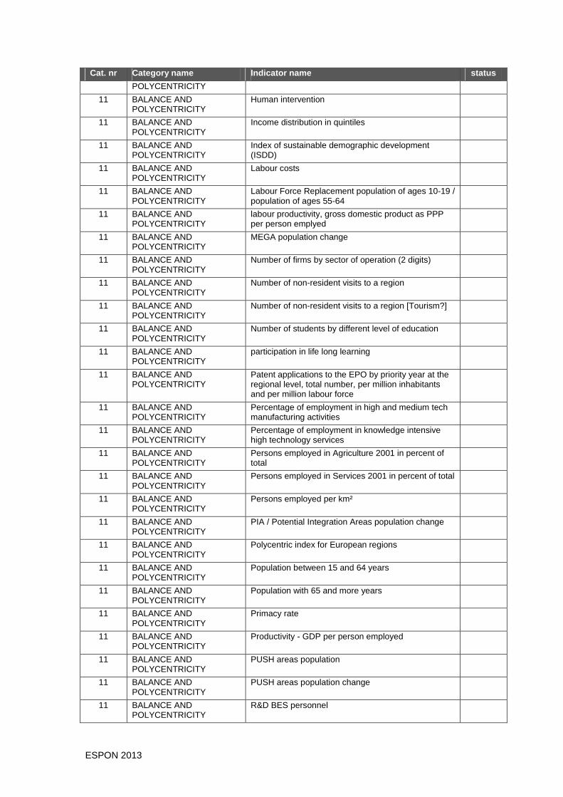
ESPON 2013 109

Cat. nr Category name Indicator name status

POLYCENTRICITY

11 BALANCE AND POLYCENTRICITY

Human intervention

11 BALANCE AND POLYCENTRICITY

Income distribution in quintiles

11 BALANCE AND POLYCENTRICITY

Index of sustainable demographic development (ISDD)

11 BALANCE AND POLYCENTRICITY

Labour costs

11 BALANCE AND POLYCENTRICITY

Labour Force Replacement population of ages 10-19 / population of ages 55-64

11 BALANCE AND POLYCENTRICITY

labour productivity, gross domestic product as PPP per person emplyed

11 BALANCE AND POLYCENTRICITY

MEGA population change

11 BALANCE AND POLYCENTRICITY

Number of firms by sector of operation (2 digits)

11 BALANCE AND POLYCENTRICITY

Number of non-resident visits to a region

11 BALANCE AND POLYCENTRICITY

Number of non-resident visits to a region [Tourism?]

11 BALANCE AND POLYCENTRICITY

Number of students by different level of education

11 BALANCE AND POLYCENTRICITY

participation in life long learning

11 BALANCE AND POLYCENTRICITY

Patent applications to the EPO by priority year at the regional level, total number, per million inhabitants and per million labour force

11 BALANCE AND POLYCENTRICITY

Percentage of employment in high and medium tech manufacturing activities

11 BALANCE AND POLYCENTRICITY

Percentage of employment in knowledge intensive high technology services

11 BALANCE AND POLYCENTRICITY

Persons employed in Agriculture 2001 in percent of total

11 BALANCE AND POLYCENTRICITY

Persons employed in Services 2001 in percent of total

11 BALANCE AND POLYCENTRICITY

Persons employed per km²

11 BALANCE AND POLYCENTRICITY

PIA / Potential Integration Areas population change

11 BALANCE AND POLYCENTRICITY

Polycentric index for European regions

11 BALANCE AND POLYCENTRICITY

Population between 15 and 64 years

11 BALANCE AND POLYCENTRICITY

Population with 65 and more years

11 BALANCE AND POLYCENTRICITY

Primacy rate

11 BALANCE AND POLYCENTRICITY

Productivity - GDP per person employed

11 BALANCE AND POLYCENTRICITY

PUSH areas population

11 BALANCE AND POLYCENTRICITY

PUSH areas population change

11 BALANCE AND POLYCENTRICITY

R&D BES personnel

ESPON 2013 110

Cat. nr Category name Indicator name status

11 BALANCE AND POLYCENTRICITY

R&D BES personnel (in fte) per 1000 active person 2002 rsp. last year available

11 BALANCE AND POLYCENTRICITY

R&D BES, Total personnel (in fte) per 1000 active person

11 BALANCE AND POLYCENTRICITY

Rank of PIAs

11 BALANCE AND POLYCENTRICITY

Region´s share of EU 27+2 GDP in PPS, Change in percent

11 BALANCE AND POLYCENTRICITY

Region´s share of EU 27+2 population, Change in percent

11 BALANCE AND POLYCENTRICITY

regional innovation performance index, from European Regional Innovation Scoreboard - 16 indicators of the 29 used in the EIS

11 BALANCE AND POLYCENTRICITY

see also indicators in ESPON 1.1.1

11 BALANCE AND POLYCENTRICITY

Settlement area in PUSH

11 BALANCE AND POLYCENTRICITY

Settlement structure assignment

11 BALANCE AND POLYCENTRICITY

Settlement units within the PUSH

11 BALANCE AND POLYCENTRICITY

Share of children 0-2 years old in childcare

11 BALANCE AND POLYCENTRICITY

Share of FUA-Population in NUTS 2, NUTS3

11 BALANCE AND POLYCENTRICITY

Share of Internet users to100 inhabs regression

11 BALANCE AND POLYCENTRICITY

Share of population in cities below 50.000 inhabitants

11 BALANCE AND POLYCENTRICITY

Share of population in the ages over 65 in percent

11 BALANCE AND POLYCENTRICITY

Size and spacing of cities or of FUA

11 BALANCE AND POLYCENTRICITY

Urban influence

11 BALANCE AND POLYCENTRICITY

Urban sprawl

11 BALANCE AND POLYCENTRICITY

Wages and salary

12 GEOGRAPHICAL SPECIFICITIES

environmental quality

12 GEOGRAPHICAL SPECIFICITIES

landscape - area of housing

12 GEOGRAPHICAL SPECIFICITIES

landscape - cultural heritage (agric landscapes)

12 GEOGRAPHICAL SPECIFICITIES

landscape - visual attractiveness

12 GEOGRAPHICAL SPECIFICITIES

Several indicators included in "Economy"

13 (POTENTIAL) ACCESSIBILITY

Access to high-speed train services

13 (POTENTIAL) ACCESSIBILITY

Accessibility

13 (POTENTIAL) ACCESSIBILITY

accessibility (incl. Maritime transport) - costs of accessibility

13 (POTENTIAL) accessibility (incl. Maritime transport) - interlinkage

ESPON 2013 111

Cat. nr Category name Indicator name status

ACCESSIBILITY between international transp. Infrastr. and local /regional

13 (POTENTIAL) ACCESSIBILITY

accessibility (incl. Maritime transport) - modal split in the regional transport

13 (POTENTIAL) ACCESSIBILITY

accessibility (incl. Maritime transport) - new technologies

13 (POTENTIAL) ACCESSIBILITY

accessibility (incl. Maritime transport) - reliability

13 (POTENTIAL) ACCESSIBILITY

Accessibility time to market

13 (POTENTIAL) ACCESSIBILITY

Accessibility to the nearest/ most frequently used hospital

13 (POTENTIAL) ACCESSIBILITY

Additive combination of classified accessibility indicators divided by # of indicators

13 (POTENTIAL) ACCESSIBILITY

Average travel time to three higher hierarchical cities

13 (POTENTIAL) ACCESSIBILITY

Car driving time to the nearest (x) facility

13 (POTENTIAL) ACCESSIBILITY

classified accessibility

13 (POTENTIAL) ACCESSIBILITY

Connectivity to commercial airports

13 (POTENTIAL) ACCESSIBILITY

Daily market accessible by car in terms of GDP

13 (POTENTIAL) ACCESSIBILITY

Peripherality indicator by car with respect to population

13 (POTENTIAL) ACCESSIBILITY

Potential accessibility

13 (POTENTIAL) ACCESSIBILITY

Potential accessibility, multimodal, to population

13 (POTENTIAL) ACCESSIBILITY

Proportion of regional population within 1 hour car travel time to next airport/ university / hospital

13 (POTENTIAL) ACCESSIBILITY

Regional road connectivity

13 (POTENTIAL) ACCESSIBILITY

Stock of vehicles by category at regional level

14 NATURAL ASSETS, NATURAL & TECHNOLOGICAL HAZARDS

% of population in coastal areas prone to sea level rise / heavy rainfall

14 NATURAL ASSETS, NATURAL & TECHNOLOGICAL HAZARDS

(Total agricultural area entered into agri-environment schemes under Pillar2 of Cap)/Total agricultural area)*100

14 NATURAL ASSETS, NATURAL & TECHNOLOGICAL HAZARDS

Additive combination of classified environment indicators divided by # of indicators

14 NATURAL ASSETS, NATURAL & TECHNOLOGICAL HAZARDS

Additive combination of classified hazard indicators divided by # of indicators

14 NATURAL ASSETS, NATURAL & TECHNOLOGICAL HAZARDS

application of environmentas norms/standards

14 NATURAL ASSETS, NATURAL &

Areas at risk of soil erosion (ton/ha/year)*(5% of

ESPON 2013 112

Cat. nr Category name Indicator name status

TECHNOLOGICAL HAZARDS

areas with farms <10ha / total agricultural areas)*100

14 NATURAL ASSETS, NATURAL & TECHNOLOGICAL HAZARDS

Artificialisation of coast

14 NATURAL ASSETS, NATURAL & TECHNOLOGICAL HAZARDS

change of bio mass

14 NATURAL ASSETS, NATURAL & TECHNOLOGICAL HAZARDS

Change of dry spell combination with drought

14 NATURAL ASSETS, NATURAL & TECHNOLOGICAL HAZARDS

Change of the average annual number (amount) of days with heavyn rainfall / water evaporation / snow covering

14 NATURAL ASSETS, NATURAL & TECHNOLOGICAL HAZARDS

Classified natural hazards

14 NATURAL ASSETS, NATURAL & TECHNOLOGICAL HAZARDS

Classified naturalness

14 NATURAL ASSETS, NATURAL & TECHNOLOGICAL HAZARDS

Classified technological hazards

14 NATURAL ASSETS, NATURAL & TECHNOLOGICAL HAZARDS

Coverage of protected areas

14 NATURAL ASSETS, NATURAL & TECHNOLOGICAL HAZARDS

Exposure of ecosystems to acidification, eutrophication and ozone

14 NATURAL ASSETS, NATURAL & TECHNOLOGICAL HAZARDS

Exposure to climate change of the agriculture, fisheries and tourism sector

14 NATURAL ASSETS, NATURAL & TECHNOLOGICAL HAZARDS

Flood endangered settlement and artifical areas

14 NATURAL ASSETS, NATURAL & TECHNOLOGICAL HAZARDS

food-miles

14 NATURAL ASSETS, NATURAL & TECHNOLOGICAL HAZARDS

Fragmentation by urbanisation, infrastructure and agriculture

14 NATURAL ASSETS, NATURAL & TECHNOLOGICAL HAZARDS

frequency of hazards/disasters

14 NATURAL ASSETS, NATURAL &

Number of all volcanoes in NUTS2 area

ESPON 2013 113

Cat. nr Category name Indicator name status

TECHNOLOGICAL HAZARDS

14 NATURAL ASSETS, NATURAL & TECHNOLOGICAL HAZARDS

Oil Hazards - average of 3 standardized hazard indicators (harbours, pipeline, refinieries)

14 NATURAL ASSETS, NATURAL & TECHNOLOGICAL HAZARDS

prevention of natural risks

14 NATURAL ASSETS, NATURAL & TECHNOLOGICAL HAZARDS

protection against floods & unusual risks

14 NATURAL ASSETS, NATURAL & TECHNOLOGICAL HAZARDS

Risk from sea level rising

14 NATURAL ASSETS, NATURAL & TECHNOLOGICAL HAZARDS

Settlement prone to heavy rainfall / sea level rise

14 NATURAL ASSETS, NATURAL & TECHNOLOGICAL HAZARDS

Share of Agricultural Land under Organic Farming

14 NATURAL ASSETS, NATURAL & TECHNOLOGICAL HAZARDS

Soil Erosion

14 NATURAL ASSETS, NATURAL & TECHNOLOGICAL HAZARDS

Sum of all weighted hazard values classicied in 5 categories

14 NATURAL ASSETS, NATURAL & TECHNOLOGICAL HAZARDS

Sum of the vulnerability indicators

14 NATURAL ASSETS, NATURAL & TECHNOLOGICAL HAZARDS

transboundary water management

14 NATURAL ASSETS, NATURAL & TECHNOLOGICAL HAZARDS

wastes management (private, public, transboundary, etc)

14 NATURAL ASSETS, NATURAL & TECHNOLOGICAL HAZARDS

Water Exploitation Index

15 LAND USE ISSUES % of the area in green space/ sports/commercial activities/transports

15 LAND USE ISSUES Agricultural intensity

15 LAND USE ISSUES Artificial surfaces / territories

15 LAND USE ISSUES CORINE land use

15 LAND USE ISSUES Corine LC Artificial surface

15 LAND USE ISSUES Corine LC Natural surface

15 LAND USE ISSUES Land use changes

ESPON 2013 114

Cat. nr Category name Indicator name status

15 LAND USE ISSUES Loss of land from agriculture to artificial surfaces

15 LAND USE ISSUES Proportion morphological city area outside administrative limits

15 LAND USE ISSUES total area of the regions (land use total) in km2

16 TERRITORIAL COOPERATION OPTIONS (URBAN-URBAN, RURAL-URBAN)

Capacity to conclude agreements (interregional, transnational, cross-border)

16 TERRITORIAL COOPERATION OPTIONS (URBAN-URBAN, RURAL-URBAN)

Cooperation between cities of small/medium size at internal and external borders of EU

16 TERRITORIAL COOPERATION OPTIONS (URBAN-URBAN, RURAL-URBAN)

Inter municipal cooperation

16 TERRITORIAL COOPERATION OPTIONS (URBAN-URBAN, RURAL-URBAN)

Number of local units

16 TERRITORIAL COOPERATION OPTIONS (URBAN-URBAN, RURAL-URBAN)

Relative rurality

16 TERRITORIAL COOPERATION OPTIONS (URBAN-URBAN, RURAL-URBAN)

Trans-national and interregional cooperation

16 TERRITORIAL COOPERATION OPTIONS (URBAN-URBAN, RURAL-URBAN)

Twinning

ESPON 2013 115

Annex 10. Inventory of World indicators 1 Smart growth in a competitive Europe

Key themes of relevance for territorial cohesion in a global scale

Indicator Unit Year or period covered

Source

NU

TS

Other: Data Description / Gaps

Pot

entia

l

Wis

hful

(w

ith g

aps)

Story-line Smart growth in a competitive and polyce ntric Europe

Foreign Direct Investments

Foreign Direct investment in reporting economy (FDI Inward) and/or direct investment abroad (FDI Outward)

US Dollars at current prices and current exchange rates in millions

2000-2009 UNCTAD, Division on Investment and Enterprise

0 Foreign direct investment (FDI) is defined as an investment involving a long-term relationship and reflecting a lasting interest in and control by a resident entity in one economy (foreign direct investor or parent enterprise) of an enterprise resident in a different economy (FDI enterprise or affiliate enterprise or foreign affiliate). (UNCTAD definition)

GDP growth Real GDP growth (Annual percent change)

% growth/ change

1980-2015 IMF or World Bank 0 GDP is the most commonly used single measure of a country's overall economic activity representing total value, constant prices of final goods and services produced within a year. (IMF definition)

Share of total trade in GDP per cent 2000-2009 World Bank national accounts data, and OECD National Accounts data files

0 Trade is the sum of exports and imports of goods and services measured as a share of gross domestic product. One direct expressions of globalisation is the increase in the share of trade value in GDP.

International trade

Total trade in merchandise and services (imports and exports)

US Dollars at current prices and current exchange rates in

1980-2009 UNCTAD secretariat calculations

0 Compilation of trade statistics, reported by countries in accordance with the recommendations of the UN International Merchandise Trade Statistics: concepts and definitions,

1 Indicators are defined following the story-lines defined for the Interco Interim Report and classified according to criteria of (a) quality & availability and (b) relevance defined in the Interco Inception Report (p. 29); indicators are then classified as Potential when fulfilling criteria (a) and (b) and Wishful that do not fulfill one or all the criteria but could probably be improved to meet the criteria (due to lack of data for a considerable number of countries, one-year-only data or lack of time-series or as indicated in the tables).

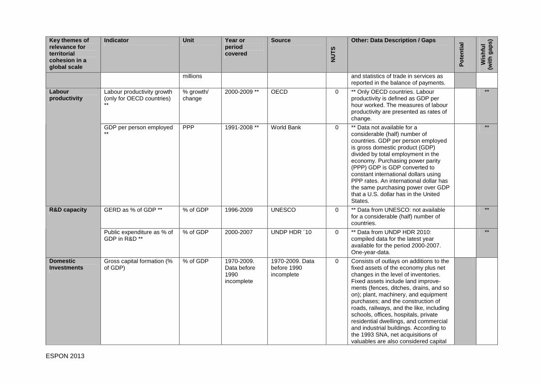
ESPON 2013 116

Key themes of relevance for territorial cohesion in a global scale

Indicator Unit Year or period covered

Source

NU

TS

Other: Data Description / Gaps

Pot

entia

l

Wis

hful

(w

ith g

aps)

millions and statistics of trade in services as reported in the balance of payments.

Labour productivity growth (only for OECD countries) **

% growth/ change

2000-2009 ** OECD 0 ** Only OECD countries. Labour productivity is defined as GDP per hour worked. The measures of labour productivity are presented as rates of change.

** Labour productivity

GDP per person employed **

PPP 1991-2008 ** World Bank 0 ** Data not available for a considerable (half) number of countries. GDP per person employed is gross domestic product (GDP) divided by total employment in the economy. Purchasing power parity (PPP) GDP is GDP converted to constant international dollars using PPP rates. An international dollar has the same purchasing power over GDP that a U.S. dollar has in the United States.

**

GERD as % of GDP ** % of GDP 1996-2009 UNESCO 0 ** Data from UNESCO: not available for a considerable (half) number of countries.

** R&D capacity

Public expenditure as % of GDP in R&D **

% of GDP 2000-2007 UNDP HDR ´10 0 ** Data from UNDP HDR 2010: compiled data for the latest year available for the period 2000-2007. One-year-data.

**

Domestic Investments

Gross capital formation (% of GDP)

% of GDP 1970-2009. Data before 1990 incomplete

1970-2009. Data before 1990 incomplete

0 Consists of outlays on additions to the fixed assets of the economy plus net changes in the level of inventories. Fixed assets include land improve-ments (fences, ditches, drains, and so on); plant, machinery, and equipment purchases; and the construction of roads, railways, and the like, including schools, offices, hospitals, private residential dwellings, and commercial and industrial buildings. According to the 1993 SNA, net acquisitions of valuables are also considered capital

ESPON 2013 117

Key themes of relevance for territorial cohesion in a global scale

Indicator Unit Year or period covered

Source

NU

TS

Other: Data Description / Gaps

Pot

entia

l

Wis

hful

(w

ith g

aps)

formation. (World Bank definition)

ESPON 2013 118

Inclusive, balanced development, and fair access to services Key themes of relevance for territorial cohesion in a global scale

Indicator Unit Year or period covered

Source

NU

TS

Other: Data Description / Gaps

Pot

entia

l

Wis

hful

(w

ith g

aps)

Story-line Inclusive, balanced development, and fai r access to services

GINI coefficient of income disparities **

GINI coefficient

2009, 2010 **

World Bank / UNDP - HDR 2010

0 ** Incomplete data for time series but harmonised figures for the period 2000-2010 compiled by the United Nations HDR Report corresponding to the latest available figure during this period. The Gini index lies between 0 and 100. A value of 0 represents absolute equality and 100 absolute inequality and measures the degree of inequality in the distribution of income in a given society.

** Income imbalances

GNI per capita based on purchasing power parity (PPP)

PPP GNI US dollars

1980-2009 World Bank International Comparison Program database or alternative HDR 2010

0 GNI is the sum of value added by all resident producers plus any product taxes (less subsidies) not included in the valuation of output plus net receipts of primary income (compensation of employees and property income) from abroad. Data are in current international dollars.

Global human development

Human Development Index of development

HDR 2010 Index

2009, 2010 UNDP - HDR 2010

0 Composite statistic used to rank countries by level of "human development" and separate developed (high development), developing (middle development), and underdeveloped (low development) countries. The statistic is composed from data on life expectancy education and per-capita GNI (as an indicator of standard of living) collected at the national level The HDI rankings featured above were published in the HDR 2010.

Total labour force thousands 1980-2020 ILO collected from UNCTAD database

0 Total labour force expressed in thousands.

Unemployment Rate ** per cent 2009 0 **

Access to work, employment

Unemployment rate by level of education **

per cent 2009-2010

UNDP - HDR 2009, 2010 based on ILO

0

** Incomplete data from ILO in time series. Calculations for 2009 and harmonised figures for this year only

**

ESPON 2013 119

Key themes of relevance for territorial cohesion in a global scale

Indicator Unit Year or period covered

Source

NU

TS

Other: Data Description / Gaps

Pot

entia

l

Wis

hful

(w

ith g

aps)

and OECD compiled by the United Nations HDR Report 2009.

Enrollment ratios in secondary and tertiary education **

gross ratio 2001-2009 UNESCO and UNDP – HDR 2010

0 ** Data refer to the most recent year available during the period specified; compiled by UN HDR Report.

** Access to education

Public expenditure in education as % of GDP **

% of GDP 2000-2007 UNDP HDR ´10 0 ** Data from UNDP HDR 2010: compiled data for the latest year available for the period 2000-2007

**

Expenditure on health per capita **

PPP int US$ 2008 ** World Health Organisation

0 ** One-year-only data.. Data from WHO World Health Organisation, the directing and coordinating authority for health within the United Nations system

** Health

Public expenditure in health as % of GDP **

% of GDP 2000-2007 UNDP HDR ´10 0 ** Data from UNDP HDR 2010: compiled data for the latest year available for the period 2000-2007

**

Share of urban population % of total * 1950-2050 UN-DESA collected from UNCTAD database

0 Because data are based on national definitions of what constitutes a city or metropolitan area, cross-country comparisons should be made with caution.

Old age dependency ratio old age ratio 1990 & 2009

UNDP - HDR 2009

0 Data on old age dependecy helps identifying increases or decreases in labour force

Demographic conditions

Crude birth rate births per 1000 people

1960-2008 World Bank from different sources

0 Crude birth rate indicates the number of live births occurring during the year, per 1,000 population estimated at mid-year

% of women by level of education

per cent 1999-2010 UNESCO 0 School age population in primary, secondary and tertiary level

Gender balance

Employment: ratio of female to male rates **

ratio 2000-2008 UNDP - HDR 2010 based on ILO data

0 ** Data refer to the most recent year available during the period specified. Compilation of figures by the United Nations HDR Report 2010. Data not available for alll countries

**

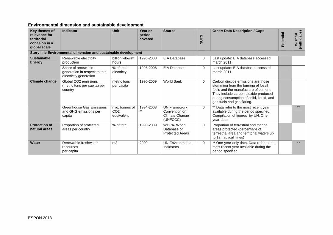
ESPON 2013 120

Environmental dimension and sustainable development Key themes of relevance for territorial cohesion in a global scale

Indicator Unit Year or period covered

Source

NU

TS

Other: Data Description / Gaps

Pot

entia

l

Wis

hful

(w

ith g

aps)

Story-line Environmental dimension and sustainable development

Renewable electricity production

billion kilowatt hours

1998-2008 EIA Database 0 Last update: EIA database accessed march 2011

Sustainable Energy

Share of renewable generation in respect to total electricity generation

% of total electricty

1998-2008 EIA Database 0 Last update: EIA database accessed march 2011

Global CO2 emissions (metric tons per capita) per country

metric tons per capita

1990-2009 World Bank 0 Carbon dioxide emissions are those stemming from the burning of fossil fuels and the manufacture of cement. They include carbon dioxide produced during consumption of solid, liquid, and gas fuels and gas flaring.

Climate change

Greenhouse Gas Emissions and GHG emissions per capita

mio. tonnes of CO2 equivalent

1994-2008 **

UN Framework Convention on Climate Change (UNFCCC)

0 ** Data refer to the most recent year available during the period specified. Compilation of figures by UN. One year-data

**

Protection of natural areas

Proportion of protected areas per country

% of total 1990-2009 WDPA- World Database on Protected Areas

0 Proportion of terrestrial and marine areas protected (percentage of terrestrial area and territorial waters up to 12 nautical miles)

Water Renewable freshwater resources per capita

m3 2009 UN Environmental Indicators

0 ** One-year-only data. Data refer to the most recent year available during the period specified.

**

ESPON 2013 121

Governance, coordination of policies and territoria l impacts Key themes of relevance for territorial cohesion in a global scale

Indicator Unit Year or period covered

Source

NU

TS

Other: Data Description / Gaps

Pot

entia

l

Wis

hful

(w

ith g

aps)

Story-line Governance, coordination of policies and territorial impacts

WGI Index on Voice and Accountability

WGI Index on Political stability and Absence of Violence

WGI Index on Government Effectiveness

WGI Index on Regulatory Quality

WGI Index on Rule of Law

Governance

WGI Index on Control of Corruption

The six governance indicators are measured in units ranging from about -2.5 to 2.5, with higher values corresponding to better governance outcomes

1996-2009 World Bank, WGI Project database

0 The Worldwide Governance Indicators (WGI) project reports aggregate and individual governance indicators for 213 economies over the period 1996–2009, for six dimensions of governance: Voice and Accountability, Political Stability and Absence of Violence, Government Effectiveness, Regulatory Quality, Rule of Law, Control of Corruption. The aggregate indicators combine the views of a large number of enterprise, citizen and expert survey respondents in industrial and developing countries. The individual data sources underlying the aggregate indicators are drawn from a diverse variety of survey institutes, think tanks, non-governmental organizations, and international organizations. The six aggregate indicators and the underlying data sources can be viewed interactively on the "Access Governance Indicators" page.

ESPON 2013 122

Annex 11. GIS layers used as input data for indicat or calculations

Figure 2. Corine land use cover (EEA, 2011a).

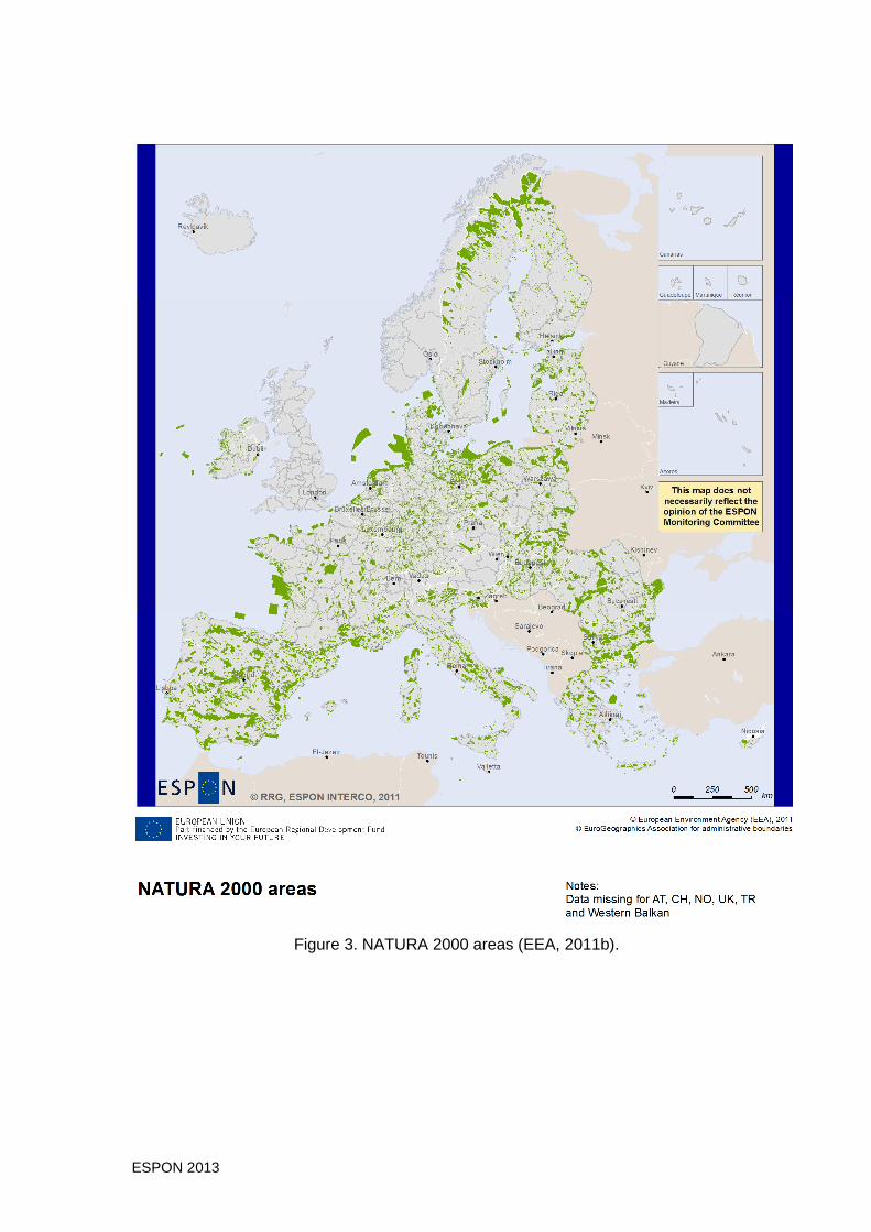
ESPON 2013 123

Figure 3. NATURA 2000 areas (EEA, 2011b).

ESPON 2013 124

Figure 4. European population grid 2000 (EEA, 2011c).

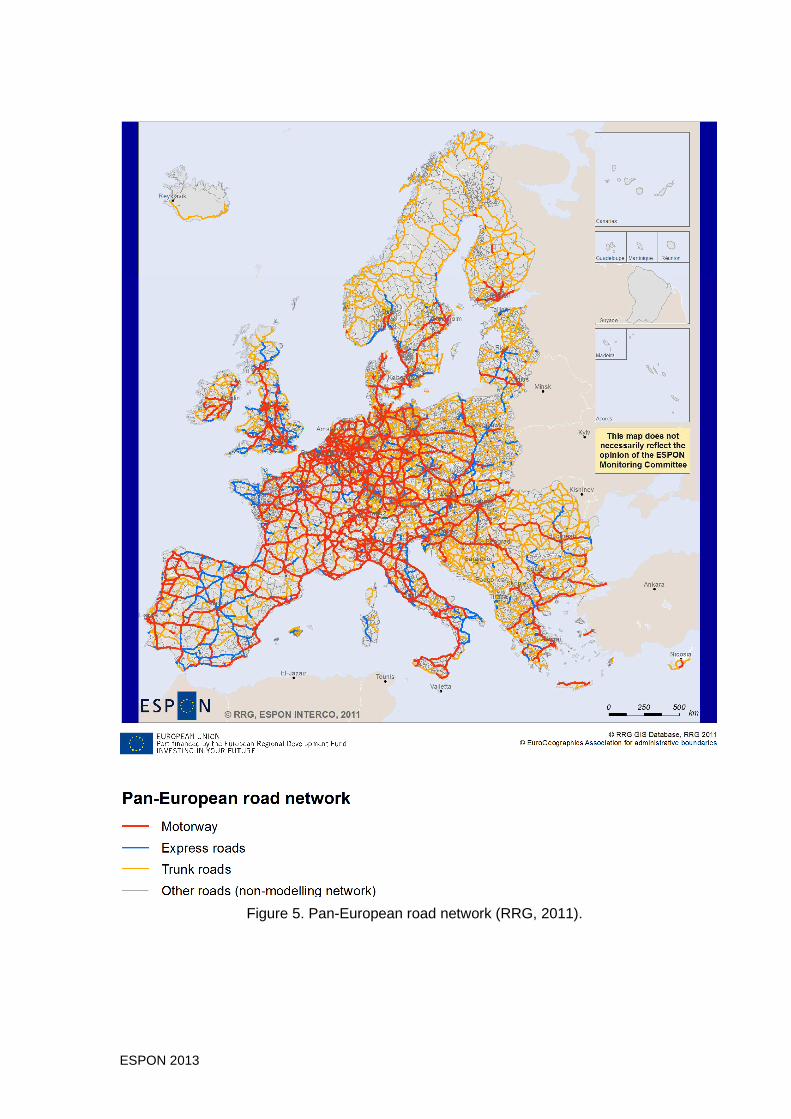
ESPON 2013 125

Figure 5. Pan-European road network (RRG, 2011).

ESPON 2013 126

Figure 6. Pan-European railway network (RRG, 2011).

ESPON 2013 127

Figure 7. Urban-rural typology of NUTS-3 regions (DG REGIO, DG AGRI 2011)

ESPON 2013 128

Figure 8. Metropolitan European Growth Areas (MEGAs) (ESPON 1.1.1)

ESPON 2013 129

Annex 12. INTERCO NUTS-3 region layer

ESPON 2013 6

Annex 13. Factsheets

Draft indicators category demography There are three indicators proposed under demography category, which are population density, life expectancy, population average annual growth and relation between urban and rural population. All three indicators are tested in various directions:

Population density: It makes significant differences at which spatial levels the indicator is calculated, and how the indicator is presented. Following sample maps include densities for NUTS-3, NUTS-5/LAU-2 and 100x100 m raster levels. Another map shows NUTS-5 population densities with class breaks adjusted to national situations rather than European-wide conditions.

Table 1 illustrates that the question of the appropriate spatial level is not only a scientific debate: The minimum and maximum and also the average population densities differ significantly, subject to the level. Following these statistics, also spatial patterns of regional disparities, and in consequence the trends towards convergence, differ greatly. Table 1. Statistical measures on population density for different spatial levels.

NUTS-3 NUTS-5 Raster

Maximum 21,022 37,824 82,225

Mean 424 209 120

Std. deviation 1,014 831 698

Minimum 1 0.02 0

The higher the spatial level used is, the more the disparities will be leveled out, with closer value ranges between minima and maxima, higher means but also higher standard deviations. At raster level, extreme outliers are pronounced: on the one hand there are extremely high maxima (approx. 4 times the maxima of NUTS-3 regions), but also extremely low mean, indicating that most areas are uninhabited or have only very low population density.

Figure 1 shows the range of values for overall population at national level. Most of the countries are dominated by few agglomerations (usually capital cities), which have significant higher population figures and thus population densities compared to the rest of the country. France is an extreme example, but also the UK; Romania, Spain or Belgium are prominent examples. For the other countries, the range of values are rather modest.

ESPON 2013 7

Figure 1. Population (in 1,000): variations within countries at NUTS-3 level.

Following this finding, Figure 2 presents the coefficients of variation of population density for each country, measured at NUTS-3 level.

Figure 2. Population density (2009): coefficients of variation measured over NUTS-3 regions. The differences in these measures are striking. Romania and France by far show the greatest national disparities, followed by Austria and Norway. These countries are dominated by one big agglomeration. On the other end of the spectrum are Lithuania, Slovenia and Slovakia, i.e. small countries with homogeneous population distributions.

ESPON 2013 8

For reasons of practicability, the raster level cannot be used as the standard spatial level since EEA provides the data only for two points in time, i.e. 1990 and 2000, with probably long future update intervals. Data at NUTS-3 level are provided by Eurostat at annual basis for all ESPON countries, but they appear to be already too aggregated to reflect the real dichotomy between settlement areas and rural areas. Thus, conceptually NUTS-5 level appears to be the most suitable spatial level to analyse population densities; however, efforts for compiling a NUTS-5 population layer are higher than the NUTS-3 data, since they are not regularly provided by Eurostat.

Life expectance The indicator life expectancy at birth for both women and men is presented; however, from literature it is know that in reality it makes a difference to look at female or male life expectancy. Even though the general range of values at European level between 72 years and 84 years is rather small, the variations between the countries are totally different (Figure 3). There are countries with very small ranges, smaller than two or one years (Austria, Ireland, Netherlands, Norway, but there are also countries with rather great disparities with four or even more years (for instance, Hungary, Portugal, UK); in the latter case obviously it very much depend where people are living.

Figure 3. Life expectancy at birth (2008): variations within countries measured over NUTS-2 regions.

ESPON 2013 9

This observation is also reflected in the coefficients of variation (Figure 4): Portugal, Slovenia, Croatia and the UK are those countries experiences greatest disparities, while on the other end Ireland, Netherlands, Sweden and Norway show the least disparities at regional level.

Figure 4. Life expectancy at birth (2008): coefficients of variation measured over NUTS-2 regions.

Population average annual growth Even though the general regional trends persist, in detail it will make a difference which years or which time intervals will be looked at to calculate the growth rates; sometimes even the trend (increasing population vs. decreasing population) may change (Figure 1). Thus, the reference time need to be selected with great care.

ESPON 2013 10

Figure 1. Comparison of growth rates 2006 vs. 2008 (NUTS-3 regions): similar trends (red dots), diverging trends (blue dots)

Urban-rural population The relation of urban to rural population at country level is analysed. The indicator is based upon a classification of NUTS-3 regions into the following three categories: o PU = predominantly urban o IN = intermediate o PR = predominantly rural jointly developed by DG Regio and DG AGRI of the European Commission. The indicator then is defined as the population sum of all PU NUTS-3 regions in a country in relation to the population sum of all PR NUTS-3 regions in the country. Population of intermediate regions are excluded. This indicator illustrates the relationship between urban and rural population at NUTS-2 level, calculated based upon the urban-rural typology of NUTS-3 regions. Most of the NUTS-2 regions do not have urban population at all, for some NUTS-2 regions the rural population exceeds the urban population. On the other hand, agglomerations stand out where urban population exceeds significantly the rural population, for instance in many regions in the UK, Benelux, Germany, Italy or Poland. Nevertheless, depending on the indicator definition based on a typology of NUTS-3 regions, some strange results can be observed, for instance the significant overrepresentation of urban population for Latvia, Iceland, or Northern Ireland. On the other hand, an indication of no urban population in Southern Sweden, East Germany, or many regions in France is also blurring reality.

ESPON 2013 11

The reasons for this indicator behavior is that at the level of NUTS-3 regions a region is either designated as predominantly urban or rural – it would be better if even at NUTS-3 level a detailed counting of people living in cities and people living in rural communities would be available.

ESPON 2013 12

02 2 0 1 P O P 2 0 0 8 N 3 R T O

Indicator name

Population density

Type of issue

Classical (sectoral) issues

Category

Demography

Reference

METRODORDER

Data source(s)

Eurostat Regio Database (table demo_r_d3dens)

Year(s)

2008, except BE, CY, IE, IT, LU (200), AL, BA, HR, RS, UK (2007)

Spatial level

NUTS-3

(except Poland partly for NUTS-2)

Spatial coverage

ESPON Space, Candidate countries, countries of Western Balkan

Gaps

Data missing for some NUTS-3 regions in Poland; in this case NUTS-2 region density used.

General availability

Available on annual basis for 2000-2009.

Indicator definition, indicator calculation (methodological remarks)

Number of inhabitants per sqkm.

Description / comment

Map at NUTS-3 level mainly shows disparities between agglomerations and non-urban region, with the latter regions appear to have similar population densities. In many countries only capital city regions stand out with higher densities.

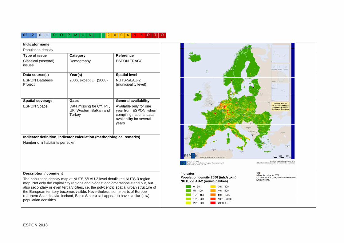
ESPON 2013 13

02 2 0 1 P O P M U N 2 0 0 6 N 5 R T O

Indicator name

Population density

Type of issue

Classical (sectoral) issues

Category

Demography

Reference

ESPON TRACC

Data source(s)

ESPON Database Project

Year(s)

2006, except LT (2008)

Spatial level

NUTS-5/LAU-2 (municipality level)

Spatial coverage

ESPON Space

Gaps

Data missing for CY, PT, UK, Western Balkan and Turkey

General availability

Available only for one year from ESPON; when compiling national data availability for several years

Indicator definition, indicator calculation (methodological remarks)

Number of inhabitants per sqkm.

Description / comment

The population density map at NUTS-5/LAU-2 level details the NUTS-3 region map. Not only the capital city regions and biggest agglomerations stand out, but also secondary or even tertiary cities, i.e. the polycentric spatial urban structure of the European territory becomes visible. Nevertheless, some parts of Europe (northern Scandinavia, Iceland, Baltic States) still appear to have similar (low) population densities.

ESPON 2013 14

02 2 0 1 P O P G R I D 2 0 0 0 G R R T O

Indicator name

Population density

Type of issue

Classical (sectoral) issues

Category

Demography

Reference

European Parliament Cohesion Study

Data source(s)

European Environment Agency (EEA)

Year(s)

2000 (AT, DK, FI, NL, SE 2001)

Spatial level

100x100 meters raster level

Spatial coverage

ESPON Space

Gaps

Data missing for AL, BA, CH, ME, MK, NO, RS, TR, and XK.

General availability

1990, 2000

Indicator definition, indicator calculation (methodological remarks)

Units: number of inhabitants per sqkm. Values estimated based upon NUTS-5 population figures and CORINE land use layer; population disaggregated/allocated to inhabited land use cells. For Austria, Denmark, Finland, the Netherlands and Sweden existing population grids at 1x1 km have been used for disaggregation.

Description / comment

The population density map at raster level even more details the NUTS-5/LAU-2 map. Uninhabited regions are clearly separated from settlement areas, where the population is concentrated. Population concentrations appear very punctual and very concentrated, with sparsely populated areas even in West European countries like Spain or France, but of course also in Scandinavia or in parts of the Alps.

ESPON 2013 15

02 2 0 1 P O P M U N B S 2 0 0 6 N 5 R T O

Indicator name

Population density

Type of issue

Classical (sectoral) issues

Category

Demography

Reference

ESPON TRACC

Data source(s)

ESPON Database Project

Year(s)

2006, except LT (2008)

Spatial level

NUTS-5/LAU-2 (municipality level)

Spatial coverage

ESPON Space

Gaps

Data missing for CY, PT, UK, Western Balkan and Turkey

General availability

Available only for one year from ESPON; when compiling national data availability for several years

Indicator definition, indicator calculation (methodological remarks)

Number of inhabitants per sqkm.

Description / comment

If class breaks are used that correspond to regional or local conditions, a population density map at NUTS-5/LAU-2 levels reveals higher spatial detail even in countries which in the other maps appear to have no spatial disparities. The map exemplifies the Baltic States, highlighting not only the capital cities with higher population densities, but also suburban developments around Riga or Kaunas, or local concentrations in other rural parts of all three countries.

ESPON 2013 16

02 2 0 1 L I F t r t c _ 9 0 0 8 N 2 M E T

Indicator name

Life expectancy

Type of issue

Classical (sectoral) issues

Category

Demography

Reference

EUROISLANDS

Data source(s)

Eurostat Regio Database (table demo_r_mlifeexp)

Year(s)

2008, except BE, NO and UK 2007

Spatial level

NUTS-2, except DE4, ES64 and FR91 NUTS-1

Spatial coverage

ESPON Space, Candidate countries and Western Balkan

Gaps

AL, BA, RS, TR and XK.

General availability

Data available at Eurostat for several years (1997-2008).

Indicator definition, indicator calculation (methodological remarks)

Life expectancy at birth in years for both men and women.

Description / comment

The map basically illustrates three findings: First, the general life expectancy in Europe lies between 72 and 84 years, i.e. within a time span of 12 years. Second, life expectancy is generally higher in EU15 compared to EU27, since all new EU Member States have significantly lower expectancy compared to Western Europe. Third, even in West European countries a distinction between Northern regions (lower expectancy) and southern regions (high expectancy) can be found, for nstance in the UK and Germany and, to a lesser degree, in France or Greece.

ESPON 2013 17

02 2 0 1 P O P [ 2 ] _ _ 2 0 0 8 N 3 R T O

Indicator name

Population average annual growth

Type of issue

Classical (sectoral) issues

Category

Demography

Reference

Data source(s)

Eurostat Regio Database (table demo_r_gind3)

Year(s)

2007-2008

Spatial level

NUTS-3

Spatial coverage

ESPON Space, Candidate countries, Western Balkans

Gaps

AL, BA, RS, XK

General availability

Data available for different points in time (2000-2008), but with gaps for individual countries

Indicator definition, indicator calculation (methodological remarks)

Annual growth rate of total population in percent of previous year.

Description / comment

The map shows different developments (increases/decreases) not only between countries, but moreover within countries between growth poles and rural countries with declining population trends. More or less all countries are concerned by these diverging trends. Differences within a country often bigger than between different countries.

ESPON 2013 18

02 2 0 1 P O P [ 2 ] _ _ 2 0 0 6 N 3 R T O

Indicator name

Population average annual growth

Type of issue

Classical (sectoral) issues

Category

Demography

Reference

Data source(s)

Eurostat Regio Database (table demo_r_gind3)

Year(s)

2005-2006

Spatial level

NUTS-3

Spatial coverage

ESPON Space, Candidate countries, Western Balkans

Gaps

AL, BA, RS, XK

General availability

Data available for different points in time (2000-2008), but with gaps for individual countries

Indicator definition, indicator calculation (methodological remarks)

Annual growth rate of total population in percent of previous year.

Description / comment

Even though the general patters shown in this map are similar to those for 2007-2008, the actual rates for individual regions differ to a large degree. For some regions even the trend changed (for instance for some regions in Eastern Germany or in Rumania). The conclusion from this is that it is a matter of concern which year or which time interval is selected as reference year. The situation may significantly change from one year to the other.

ESPON 2013 19

02 2 0 1 P O P U R R R 2 0 0 8 N 2 R T O

Indicator name

Urban-rural population

Type of issue

Classical (sectoral) issues

Category

Demography

Reference

Data source(s)

Eurostat Regio Database, DG Regio, DG AGRI

Year(s)

2008

Spatial level

NUTS-0, -1, and -2

Spatial coverage

ESPON Space, Candidate countries, Western Balkans

Gaps

Data missing for non-EU countries.

General availability

Data available for different points in time (2000-2008), but with gaps for individual countries

Indicator definition, indicator calculation (methodological remarks)

Indicator defined as the ratio between urban population and rural population. Urban population is the total population of all NUTS-3 regions in a country classified as predominantly urban (PU), while rural population is the total population of all NUTS-3 regions in the country classified as predominantly rural (PR) region. The typology of urban and rural NUTS-3 regions relies upon work of DG Regio and DG Agri of the European Commission.

Description / comment

This indicator illustrates the relationship between urban and rural population at NUTS-2 level, calculated based upon the urban-rural typology of NUTS-3 regions. Most of the NUTS-2 regions do not have urban population at all, for some NUTS-2 regions the rural population exceeds the urban population. On the other hand, agglomerations stand out where urban population exceeds significantly the rural population, for instance in many regions in the UK, Benelux, Germany, Italy or Poland.

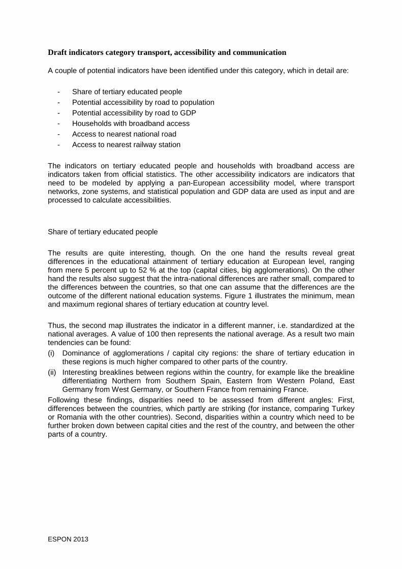
ESPON 2013 20

Draft indicators category transport, accessibility and communication A couple of potential indicators have been identified under this category, which in detail are:

- Share of tertiary educated people - Potential accessibility by road to population - Potential accessibility by road to GDP - Households with broadband access - Access to nearest national road - Access to nearest railway station

The indicators on tertiary educated people and households with broadband access are indicators taken from official statistics. The other accessibility indicators are indicators that need to be modeled by applying a pan-European accessibility model, where transport networks, zone systems, and statistical population and GDP data are used as input and are processed to calculate accessibilities.

Share of tertiary educated people The results are quite interesting, though. On the one hand the results reveal great differences in the educational attainment of tertiary education at European level, ranging from mere 5 percent up to 52 % at the top (capital cities, big agglomerations). On the other hand the results also suggest that the intra-national differences are rather small, compared to the differences between the countries, so that one can assume that the differences are the outcome of the different national education systems. Figure 1 illustrates the minimum, mean and maximum regional shares of tertiary education at country level.

Thus, the second map illustrates the indicator in a different manner, i.e. standardized at the national averages. A value of 100 then represents the national average. As a result two main tendencies can be found: (i) Dominance of agglomerations / capital city regions: the share of tertiary education in

these regions is much higher compared to other parts of the country. (ii) Interesting breaklines between regions within the country, for example like the breakline

differentiating Northern from Southern Spain, Eastern from Western Poland, East Germany from West Germany, or Southern France from remaining France.

Following these findings, disparities need to be assessed from different angles: First, differences between the countries, which partly are striking (for instance, comparing Turkey or Romania with the other countries). Second, disparities within a country which need to be further broken down between capital cities and the rest of the country, and between the other parts of a country.

ESPON 2013 21

Figure 1. National differences in tertiary education in Europe.

Potential accessibility by road to population

This indicator measures the number of people within reach from each origin, weighted by a distance decay function. The indicator was first calculated for a raster grid of 2.5 x 2.5 km grid cells for the whole of Europe, and was then aggregated to combined system of NUTS-2/3 regions (Dubois et al., 2007) as weighted averages with raster population being the weight. With this the selected approach is different to other potential accessibility calculations in other ESPON projects, where usually each NUTS region is represented by only one centroid. This continuous surface map for the whole of Europe clearly shows the European core area with Benelux countries, Western Germany, Southern England and Northern Italy as those areas with highest accessibilities. But the map also shows regional centers with accessibility gradients (for instance, for Stockholm Toulouse, or Thessalonica), which are not visible if the indicator is illustrated at regional level. While the raster map shows smooth accessibility gradients, the NUTS-2/3 region map shows sharp differences between neighboring regions. The overall spatial pattern, with the European triangle between London-Milano-Hamburg (the so-called ‘blue banana’) representing the core area with highest accessibilities, is still visible. The variations within a country are significant (Figure 2). For many countries the minimum is close to 10,000 people, while the maximum is as high as 12 Mio people that can be reached. Greatest disparities are found in the UK, France and Germany, smallest disparities in the Baltic States, Luxembourg and Slovenia and Slovakia. The range of values for each country measured at raster level is, not surprisingly, greater compared as to measured over NUTS2/3 regions.

ESPON 2013 22

Figure 2. Potential accessibility to population (in 1,000 people): Min, mean and max, calculated over raster level (top) and over NUTS2/3 regions (bottom).

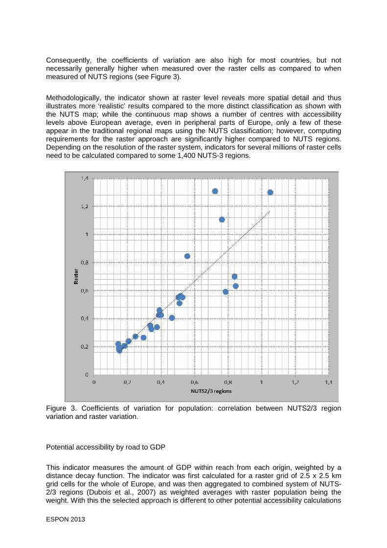
ESPON 2013 23

Consequently, the coefficients of variation are also high for most countries, but not necessarily generally higher when measured over the raster cells as compared to when measured of NUTS regions (see Figure 3).

Methodologically, the indicator shown at raster level reveals more spatial detail and thus illustrates more ‘realistic’ results compared to the more distinct classification as shown with the NUTS map; while the continuous map shows a number of centres with accessibility levels above European average, even in peripheral parts of Europe, only a few of these appear in the traditional regional maps using the NUTS classification; however, computing requirements for the raster approach are significantly higher compared to NUTS regions. Depending on the resolution of the raster system, indicators for several millions of raster cells need to be calculated compared to some 1,400 NUTS-3 regions.

Figure 3. Coefficients of variation for population: correlation between NUTS2/3 region variation and raster variation.

Potential accessibility by road to GDP This indicator measures the amount of GDP within reach from each origin, weighted by a distance decay function. The indicator was first calculated for a raster grid of 2.5 x 2.5 km grid cells for the whole of Europe, and was then aggregated to combined system of NUTS-2/3 regions (Dubois et al., 2007) as weighted averages with raster population being the weight. With this the selected approach is different to other potential accessibility calculations

ESPON 2013 24

in other ESPON projects, where usually each NUTS region is represented by only one centroid. The general spatial pattern generated by this indicator is similar to the potential accessibility to population indicator, first of all highlighting the European core area of high accessibilities in the ‘blue banana’. The main difference to the previous indicator, however, is the sharp fall in accessibility from the old to the new EU Member States: in the latter one only the greater city areas of Warsaw and Budapest yield accessibilities above the average, while all other parts are well or even far below the European average, like areas in Baltic States, Romania or Bulgaria. This finding is confirmed by Figure 5, showing the minimum, mean and maximum values by country: None of the new EU Member States yield maximum values of more than 50,000 GDP within reach, whereas most of the old member states do significantly better than this threshold. Nevertheless, while variations among the new member states are quite low, variations within the old member states are extreme, in particular for Italy, Germany, France and the UK, for both types of measurement (raster as well as NUTS2/3). Similar as for population, variations measured at raster level are bigger than those at NUTS2/3 level. The two types of measurements (raster level vs. NUTS2/3 level) highly correlate with each other (Figure 4), even though generally the coefficients of variation are somewhat smaller for NUTS2/3. The higher the variations as such are the bigger are the differences between the two coefficients. This means that for these countries the highest accessible areas perform much better compared to the average or to the least areas.

Figure 4. Coefficients of variation for GDP: correlation between NUTS2/3 region variation and raster variation.

ESPON 2013 25

Figure 5. Potential accessibility to GDP: Min, mean and max, calculated over raster level (top) and over NUTS2/3 regions (bottom).

ESPON 2013 26

Households with broadband access

This indicator is defined as the share of households with broadband access at home on all households. Even though the variation in household broadband access in Europe is significant, ranging from 45 % in Romania towards 100 % in Benelux, Spain or Iceland, the distribution is rather region-specific: for instance, the share in East Germany is significantly lower compared to West Germany; similarly, regions in Southern Italy have lower access compared to Northern Italy. In France, in contrary, shares are higher in southern parts of the country compared to the northern regions. Nevertheless, the overall variations within a country are rather small (Figure 6), with 5 to 10 percentage points. Only Bulgaria, Italy, UK ad Romania yield differences of more than 20 percentage points between the maximum and the minimum, with Romania clearly being the (negative) outlier.

Figure 6. Households with broadband access (2010): variations within countries. While generally the coefficients of variation are rather low for most countries, the variation for Slovakia, Bulgaria and Romania are the highest in 2010 (Figure 7). For the old EU Member States, Italy and the Netherlands have the greatest variations, Belgium, Spain and Denmark the lowest. Even though the dataset comprises the time period 2006-2010, a formal plotting of the growth rate is difficult since data for 2006 and 2007 are available for only very few regions, and, moreover, sometimes only at NUTS-1 or national level. Nevertheless the indicator is concerned with modern IT technologies, and should therefore be included as cohesion indicator. One can assume that technological mid-term developments will lead to an access

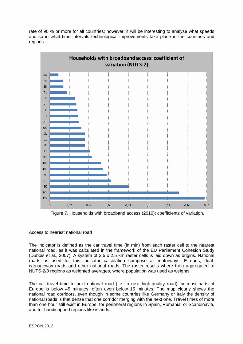
ESPON 2013 27

rate of 90 % or more for all countries; however, it will be interesting to analyse what speeds and so in what time intervals technological improvements take place in the countries and regions.

Figure 7. Households with broadband access (2010): coefficients of variation.

Access to nearest national road The indicator is defined as the car travel time (in min) from each raster cell to the nearest national road, as it was calculated in the framework of the EU Parliament Cohesion Study (Dubois et al., 2007). A system of 2.5 x 2.5 km raster cells is laid down as origins. National roads as used for this indicator calculation comprise all motorways, E-roads, dual-carriageway roads and other national roads. The raster results where then aggregated to NUTS-2/3 regions as weighted averages, where population was used as weights. The car travel time to next national road (i.e. to next high-quality road) for most parts of Europe is below 45 minutes, often even below 15 minutes. The map clearly shows the national road corridors, even though in some countries like Germany or Italy the density of national roads is that dense that one corridor merging with the next one. Travel times of more than one hour still exist in Europe, for peripheral regions in Spain, Romania, or Scandinavia, and for handicapped regions like islands.

ESPON 2013 28

While the classification in the first map aimed to show the full range of travel times in regular intervals, the alternative version focuses on those areas with travel times less than 45 minutes to next national road. Now the road corridors become even more visible. Still, there are parts in Europe (Benelux, Germany, England, and Italy) with extremely dense national road networks, compared to other parts where networks are extremely low. The raster approach chosen for this indicator, however, allows great flexibility in the indicator presentation and adjustment even after the figures have been calculated. At aggregated NUTS-2/3 level, to which the raster results were aggregated, regions in Benelux countries, Germany, Italy and England appear to be those regions with on average shortest car travel times to nearest national roads, with less than 10 minutes. In the other countries there are regions with fairly short access times between 10 and 20 minutes, but there are also regions in contrary with 20, 30 or even more than 45 minutes travel times. For those regions a lack of national road infrastructure can be observed. Figure 8 illustrates interesting variations within countries at raster level. The minimum values for all countries is one minute (i.e. if there is any national road in a country, there will in any case be raster cells that are only one minute (actually even less than one minute) travel time away. Also the mean travel times are rather short, but the maximum travel times for several countries is very extreme. First of all to mention is Portugal, follows by Italy, Greece and Spain, i.e. countries with several islands that lack high-quality road infrastructures, thus have long access time to it.

Figure 8. Access times to national roads (min): variations within countries at raster level.

ESPON 2013 29

For the same reason the maximum travel times in countries like Germany, Denmark or France is rather long, which is due to the long access time from islands to the usually very dense national road network in these countries. In contrast, continental countries without islands, like Czech Republic, Hungary, Luxembourg, Slovenia or Slovakia have a comparable small range of values, despite the fact that often the density of national roads is lower compared to Germany or France. While the coefficients of variation gradually increase from Malta to Italy, the three countries of Greece, UK and Portugal, comprising a number of islands, can be considered as clear outliers in this respect, yielding the greatest variations in access times (Figure 9). Apart from these three countries, the other countries have similar variations between the most accessible and least accessible parts of their territory.

Figure 9. Access times to national roads (min): coefficients of variation (raster level).

Access to nearest railway station The indicator is defined as the car travel time (in min) from each raster cell to the nearest railway station, as it was calculated in the framework of the EU Parliament Cohesion Study (Dubois et al., 2007). A system of 2.5 x 2.5 km raster cells is laid down as origins. All railway stations under operation in 2007 were used as destinations, regardless what type of train services operate. The raster results where then aggregated to NUTS-2/3 regions as weighted averages, where population was used as weights. Due to the rather dense railway network in many countries, the car travel times to the next station are rather short with often less than 45 or 30 minutes. Only in some countries/areas

ESPON 2013 30

with lower railway densities (Alps, Scandinavia, Spain, Scotland, Romania, islands) travel times of more than 60 or more than 120 minutes can be observed. The least accessible area is of course Northern Scandinavia. On-average access time to rail stations at aggregated NUTS-2/3 take 20-40 minutes for most regions; only few regions yield less than 20 minutes on average. The other regions in central Europe take 40 to 60 minutes on average; regions in Spain, Scotland, Romania and the islands require even longer access times of 120 minutes and more. Since the aggregated indicators were derived through averaging over the raster cells, the results at NUTS-2/3 level provide more realistic pictures as if only one centroid for each region, which usually is the main regional city, would be selected. Variations within countries are great for some countries (Greece, Norway, Italy, Finland, Spain, UK) (Figure 10), for other countries they are surprisingly low (e.g. France, Germany). The indicator ranges, however, are always dominated by the maxima; the average travel times, however, remain modest in all countries, except for the three countries of Finland, Norway and Sweden.

Figure 10. Access to stations (min): variations within countries, measured at raster level.

The coefficients of variation are between 0.4 and 0.6 for the majority of countries (from Lithuania to Portugal), which means rather modest disparities at raster level within the countries (Figure 11). The remaining countries experience greater disparities, with Estonia, Norway, Italy, UK and Greece showing coefficients of more than 1.0.

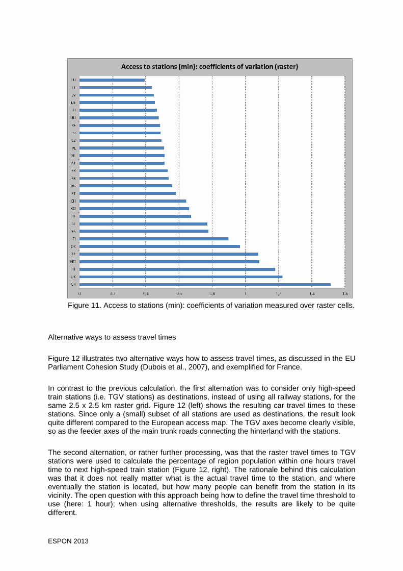
ESPON 2013 31

Figure 11. Access to stations (min): coefficients of variation measured over raster cells.

Alternative ways to assess travel times Figure 12 illustrates two alternative ways how to assess travel times, as discussed in the EU Parliament Cohesion Study (Dubois et al., 2007), and exemplified for France. In contrast to the previous calculation, the first alternation was to consider only high-speed train stations (i.e. TGV stations) as destinations, instead of using all railway stations, for the same 2.5 x 2.5 km raster grid. Figure 12 (left) shows the resulting car travel times to these stations. Since only a (small) subset of all stations are used as destinations, the result look quite different compared to the European access map. The TGV axes become clearly visible, so as the feeder axes of the main trunk roads connecting the hinterland with the stations. The second alternation, or rather further processing, was that the raster travel times to TGV stations were used to calculate the percentage of region population within one hours travel time to next high-speed train station (Figure 12, right). The rationale behind this calculation was that it does not really matter what is the actual travel time to the station, and where eventually the station is located, but how many people can benefit from the station in its vicinity. The open question with this approach being how to define the travel time threshold to use (here: 1 hour); when using alternative thresholds, the results are likely to be quite different.

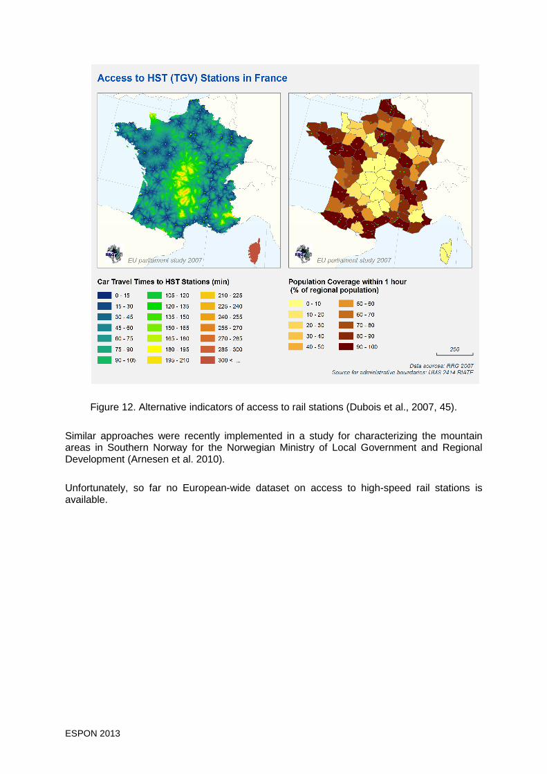
ESPON 2013 32

Figure 12. Alternative indicators of access to rail stations (Dubois et al., 2007, 45).

Similar approaches were recently implemented in a study for characterizing the mountain areas in Southern Norway for the Norwegian Ministry of Local Government and Regional Development (Arnesen et al. 2010). Unfortunately, so far no European-wide dataset on access to high-speed rail stations is available.

ESPON 2013 33

0 3 0 4 T R P [ 5 ] 2 0 0 9 N 2 R T O

Indicator name

Share of tertiary educated people in %

Type of issue

Classical (sectoral) issues

Category

Transport, Accessibility, Communication

Reference

CLIMATE

Data source(s)

Eurostat Regio Database (table edat_lfse_11)

Year(s)

2009

Spatial level

NUTS-2

Spatial coverage

ESPON Space, Candidate Countries, Western Balkan

Gaps

Missing data for AD, AL, BA, LI, ME, RS and XK.

General availability

2008 and 2009

Indicator definition, indicator calculation (methodological remarks)

Share of tertiary educated people in percent of total population. Tertiary education is defined as a university degree qualifying people to study at a technical university or at a university of applied science.

Description / comment

The map reveals significant differences in the qualification levels, ranging from small 5 percent tertiary education level up to 52 percent (agglomerations, capital city regions). Some East European countries such as Romania, Bulgaria, Turkey or Czech Republic appear to have general lower tertiary education levels, compared to the other countries. Nevertheless, the map also hints that generally the differences within a country are rather small compared to international differences, i.e. illustrating that the education system plays a dominant role in the level of educational attainment.

ESPON 2013 34

0 3 0 4 T R P [ 5 ] S T 2 0 0 9 N 2 R T O

Indicator name

Share of tertiary educated people in %

Type of issue

Classical (sectoral) issues

Category

Transport, Accessibility, Communication

Reference

CLIMATE

Data source(s)

Eurostat Regio Database (table edat_lfse_11)

Year(s)

2009

Spatial level

NUTS-2

Spatial coverage

ESPON Space, Candidate Countries, Western Balkan

Gaps

Missing data for AD, AL, BA, LI, ME, RS and XK.

General availability

2008 and 2009

Indicator definition, indicator calculation (methodological remarks)

Share of tertiary educated people in percent of total population standardized at the national averages (100 = national average). Tertiary education is defined as a university degree qualifying people to study at a technical university or at a university of applied science.

Description / comment

This indicator classification even more illustrates intra-national disparities in educational attainment, as it shows underperforming regions (blue colors; often rural and peripheral areas) differentiated from regions with percent of tertiary education above the national average. The latter ones are most often the big agglomerations, but in some countries also other interesting breaklines can be seen (like Spain or France, Poland, East Germany, Finland).

ESPON 2013 35

0 3 0 4 P O T A C C P O 2 0 0 4 G R M E T

Indicator name

Potential accessibility to population by car

Type of issue

Classical (sectoral) issues

Category

Transport, Accessibility, Communication

Reference

EU Parliament Cohesion Study

Data source(s)

RRG

Year(s)

2004

Spatial level

Raster system (2.5 x 2.5 km grid cells)

Spatial coverage

ESPON Space, Candidate Countries, Western Balkan

Gaps

Missing data for TR and Western Balkans

General availability

2004

Indicator definition, indicator calculation (methodological remarks)

The indicator measures the number of people that can be reached by car from each origin (i.e. each raster cell), weighted by a function of distance and travel time. Results are standardized at the European average.

Description / comment

This continuous surface map for the whole of Europe clearly shows the European core area with Benelux countries, Western Germany, Southern England and Northern Italy as those areas with highest accessibilities. But the map also shows regional centers with accessibility gradients (for instance, for Stockholm Toulouse, or Thessalonica), which are not visible if the indicator is illustrated at regional level.

ESPON 2013 36

0 3 0 4 P O T A C C P O 2 0 0 4 N 2 M E T

Indicator name

Potential accessibility to population by car

Type of issue

Classical (sectoral) issues

Category

Transport, Accessibility, Communication

Reference

EU Parliament Cohesion Study

Data source(s)

RRG

Year(s)

2004

Spatial level

Combined NUTS-2/3 region system

Spatial coverage

ESPON Space, Candidate Countries, Western Balkan

Gaps

Missing data for TR and Western Balkans

General availability

2004

Indicator definition, indicator calculation (methodological remarks)

The indicator measures the number of people that can be reached by car from each origin, weighted by a function of distance and travel time. The figures at regional level (NUTS-2/3 regions) were derived as the weighted average over all raster cells of that region. Weighting was done by using raster population. Results are again standardized at the European average. The approach chosen here is different to other potential accessibility calculations in ESPON where each NUTS region usually is only represented by one centroid.

Description / comment

The results of this indicator representation are similar to the continuous surface map, however, they are even more pronounced. While the raster map shows smooth accessibility gradients, the NUTS-2/3 region map shows sharp differences between neighboring regions. The overall spatial pattern, with the European triangle between London-Milano-Hamburg (the so-called ‘blue banana’) representing the core area with highest accessibilities, is still visible.

0 3 0 4 P O T A C C G D 2 0 0 4 G R M E T

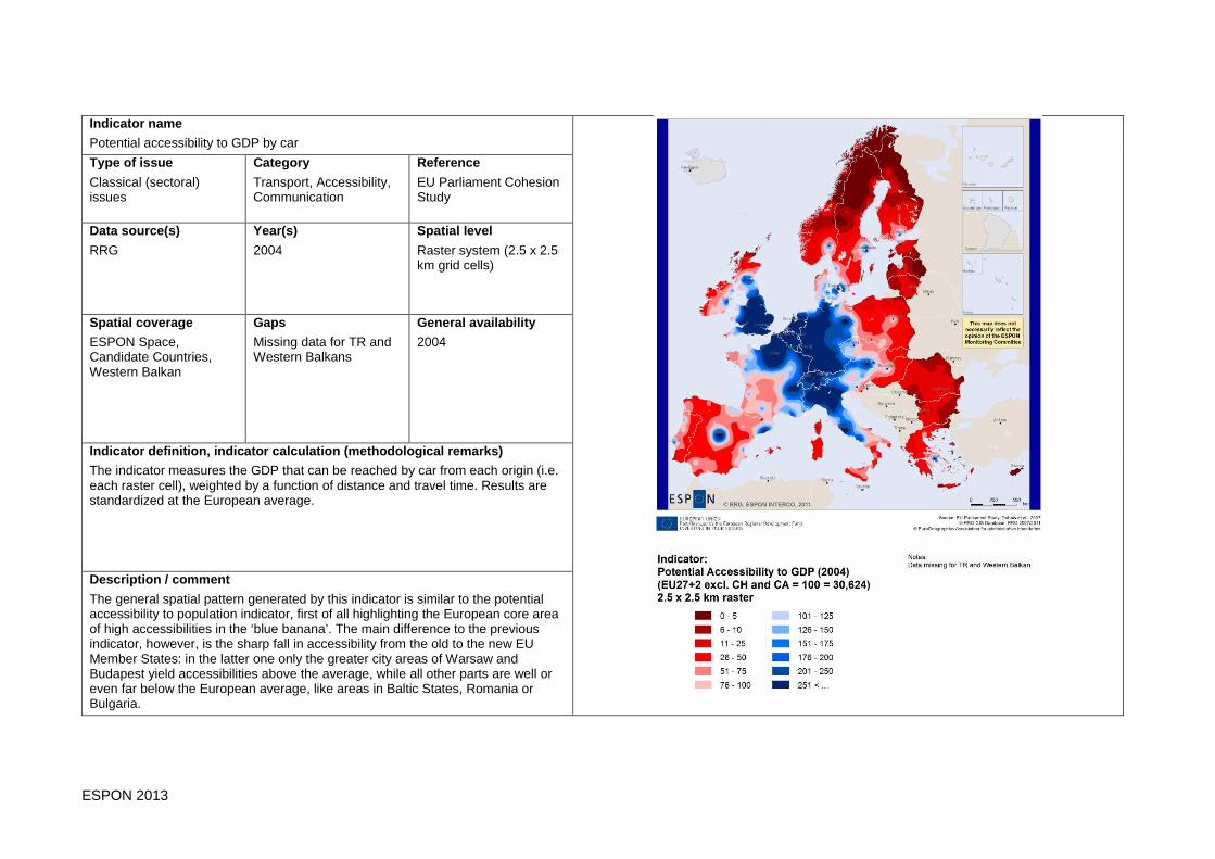
ESPON 2013 37

Indicator name

Potential accessibility to GDP by car

Type of issue

Classical (sectoral) issues

Category

Transport, Accessibility, Communication

Reference

EU Parliament Cohesion Study

Data source(s)

RRG

Year(s)

2004

Spatial level

Raster system (2.5 x 2.5 km grid cells)

Spatial coverage

ESPON Space, Candidate Countries, Western Balkan

Gaps

Missing data for TR and Western Balkans

General availability

2004

Indicator definition, indicator calculation (methodological remarks)

The indicator measures the GDP that can be reached by car from each origin (i.e. each raster cell), weighted by a function of distance and travel time. Results are standardized at the European average.

Description / comment

The general spatial pattern generated by this indicator is similar to the potential accessibility to population indicator, first of all highlighting the European core area of high accessibilities in the ‘blue banana’. The main difference to the previous indicator, however, is the sharp fall in accessibility from the old to the new EU Member States: in the latter one only the greater city areas of Warsaw and Budapest yield accessibilities above the average, while all other parts are well or even far below the European average, like areas in Baltic States, Romania or Bulgaria.

ESPON 2013 38

0 3 0 4 P O T A C C G D 2 0 0 4 N 2 M E T

Indicator name

Potential accessibility to GDP by car

Type of issue

Classical (sectoral) issues

Category

Transport, Accessibility, Communication

Reference

EU Parliament Cohesion Study

Data source(s)

RRG

Year(s)

2004

Spatial level

Combined NUTS-2/3 region system

Spatial coverage

ESPON Space, Candidate Countries, Western Balkan

Gaps

Missing data for TR and Western Balkans

General availability

2004

Indicator definition, indicator calculation (methodological remarks)

The indicator measures the GDP that can be reached by car from each origin, weighted by a function of distance and travel time. The figures at regional level (NUTS-2/3 regions) were derived as the weighted average over all raster cells of that region. Weighting was done by using raster population. Results are again standardized at the European average.

Description / comment

The indicator map at NUTS2/3 level even more pronounces the sharp fall in accessibility between the European core area (from London via Benelux and Germany towards Northern Italy) and the new EU Member States, but also to Scandinavian countries or countries in Southern Europe. Apart from the core area, only regions around Madrid, Barcelona, Roma, Copenhagen and Vienna experience accessibilities above the European average. Another observation worth to mention are the extremely low accessibilities in Rumania and Bulgaria, which are as low as in Northern Scandinavia.

ESPON 2013 39

0 3 0 4 B R O A D A H H 2 0 1 0 N 2 R T O

Indicator name

Households with broadband access (%)

Type of issue

Classical (sectoral) issues

Category

Transport, Accessibility, Communication

Reference

Data source(s)

Eurostat Regio Database (table isoc_r_broad_h)

Year(s)

2010, BG and FI 2007, NL, IS and UK 2009

Spatial level

NUTS-2 (DE, GR, FR, and PL NUTS-1)

Spatial coverage

ESPON Space, Candidate Countries, Western Balkan

Gaps

Missing data for CH, TR and Western Balkan

General availability

2006-2010

Indicator definition, indicator calculation (methodological remarks)

Share of households with broadband internet access at home on all households (%)

Description / comment

Even though the variation in household broadband access in Europe is significant, ranging from 45 % in Romania towards 100 % in Benelux, Spain or Iceland, the distribution is rather region-specific: for instance, the share in East Germany is significantly lower compared to West Germany; similarly, regions in Southern Italy have lower access compared to Northern Italy. In France, in contrary, shares are higher in southern parts of the country compared to the northern regions.

ESPON 2013 40

0 3 0 4 A C C N A T R A 2 0 0 7 G R M E T

Indicator name

Access to national roads (min)

Type of issue

Classical (sectoral) issues

Category

Transport, Accessibility, Communication

Reference

EU Parliament Cohesion Study

Data source(s)

RRG

Year(s)

2007

Spatial level

Raster (2.5 x 2.5 km grid cells)

Spatial coverage

ESPON Space, Candidate Countries, Western Balkan

Gaps

Missing data for IS, TR and Western Balkan

General availability

2007

Indicator definition, indicator calculation (methodological remarks)

The indicator is defined as the car travel time (in min) from each raster cell to the nearest national road, as it was calculated in the framework of the EU Parliament Cohesion Study (Dubois et al., 2007). A system of 2.5 x 2.5 km raster cells is laid down as origins. National roads as used for this indicator calculation comprise all motorways, E-roads, dual-carriageway roads and other national roads.

Description / comment

The car travel time to next national road (i.e. to next high-quality road) for most parts of Europe is below 45 minutes, often even below 15 minutes. The map clearly shows the national road corridors, even though in some countries like Germany or Italy the density of national roads is that dense that one corridor merging with the next one. Travel times of more than one hour still exist in Europe, for peripheral regions in Spain, Romania, or Scandinavia, and for handicapped regions like islands.

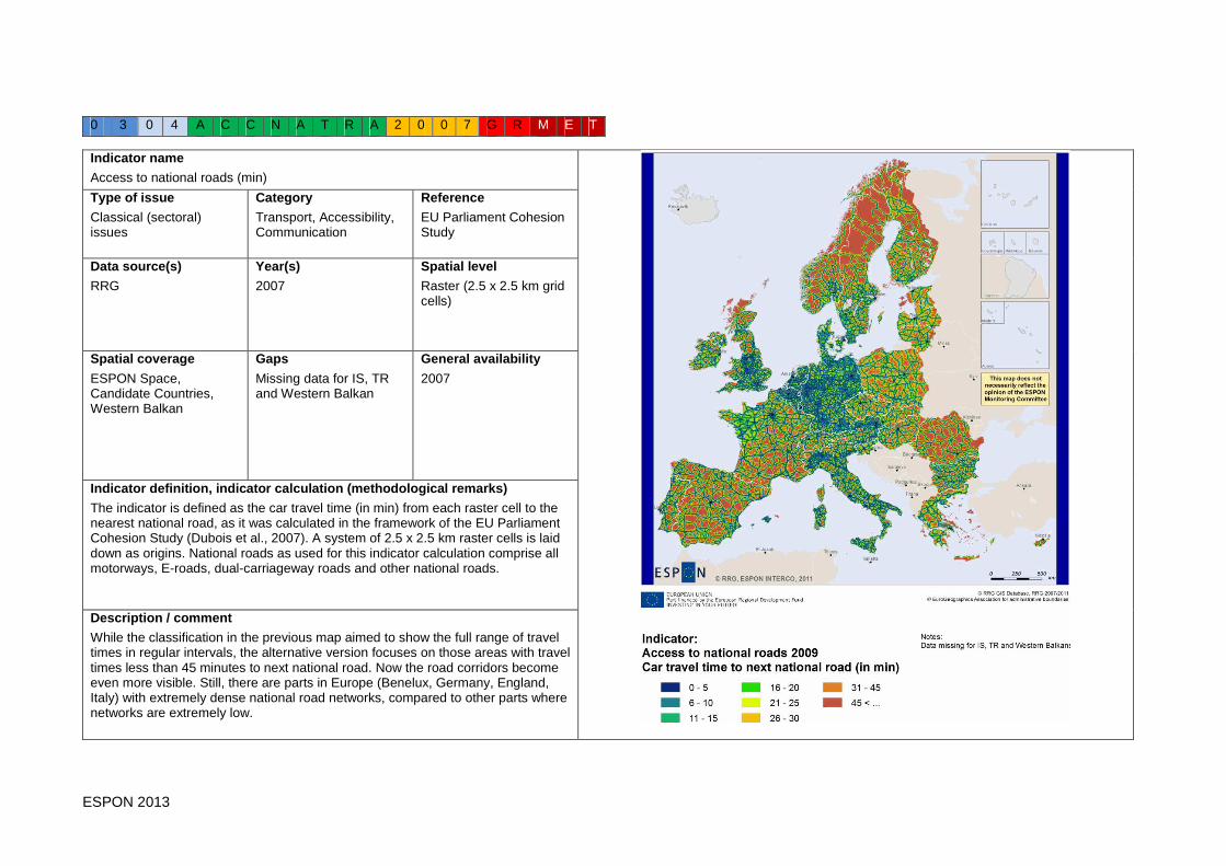
ESPON 2013 41

0 3 0 4 A C C N A T R A 2 0 0 7 G R M E T

Indicator name

Access to national roads (min)

Type of issue

Classical (sectoral) issues

Category

Transport, Accessibility, Communication

Reference

EU Parliament Cohesion Study

Data source(s)

RRG

Year(s)

2007

Spatial level

Raster (2.5 x 2.5 km grid cells)

Spatial coverage

ESPON Space, Candidate Countries, Western Balkan

Gaps

Missing data for IS, TR and Western Balkan

General availability

2007

Indicator definition, indicator calculation (methodological remarks)

The indicator is defined as the car travel time (in min) from each raster cell to the nearest national road, as it was calculated in the framework of the EU Parliament Cohesion Study (Dubois et al., 2007). A system of 2.5 x 2.5 km raster cells is laid down as origins. National roads as used for this indicator calculation comprise all motorways, E-roads, dual-carriageway roads and other national roads.

Description / comment

While the classification in the previous map aimed to show the full range of travel times in regular intervals, the alternative version focuses on those areas with travel times less than 45 minutes to next national road. Now the road corridors become even more visible. Still, there are parts in Europe (Benelux, Germany, England, Italy) with extremely dense national road networks, compared to other parts where networks are extremely low.

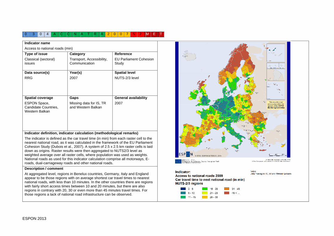
ESPON 2013 42

0 3 0 4 A C C N A T R A 2 0 0 7 N 2 M E T

Indicator name

Access to national roads (min)

Type of issue

Classical (sectoral) issues

Category

Transport, Accessibility, Communication

Reference

EU Parliament Cohesion Study

Data source(s)

RRG

Year(s)

2007

Spatial level

NUTS-2/3 level

Spatial coverage

ESPON Space, Candidate Countries, Western Balkan

Gaps

Missing data for IS, TR and Western Balkan

General availability

2007

Indicator definition, indicator calculation (methodological remarks)

The indicator is defined as the car travel time (in min) from each raster cell to the nearest national road, as it was calculated in the framework of the EU Parliament Cohesion Study (Dubois et al., 2007). A system of 2.5 x 2.5 km raster cells is laid down as origins. Raster results were then aggregated to NUTS2/3 level as weighted average over all raster cells, where population was used as weights. National roads as used for this indicator calculation comprise all motorways, E-roads, dual-carriageway roads and other national roads.

Description / comment

At aggregated level, regions in Benelux countries, Germany, Italy and England appear to be those regions with on average shortest car travel times to nearest national roads, with less than 10 minutes. In the other countries there are regions with fairly short access times between 10 and 20 minutes, but there are also regions in contrary with 20, 30 or even more than 45 minutes travel times. For those regions a lack of national road infrastructure can be observed.

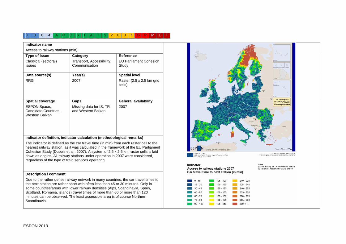
ESPON 2013 43

0 3 0 4 A C C S T A T S 2 0 0 7 G R M E T

Indicator name

Access to railway stations (min)

Type of issue

Classical (sectoral) issues

Category

Transport, Accessibility, Communication

Reference

EU Parliament Cohesion Study

Data source(s)

RRG

Year(s)

2007

Spatial level

Raster (2.5 x 2.5 km grid cells)

Spatial coverage

ESPON Space, Candidate Countries, Western Balkan

Gaps

Missing data for IS, TR and Western Balkan

General availability

2007

Indicator definition, indicator calculation (methodological remarks)

The indicator is defined as the car travel time (in min) from each raster cell to the nearest railway station, as it was calculated in the framework of the EU Parliament Cohesion Study (Dubois et al., 2007). A system of 2.5 x 2.5 km raster cells is laid down as origins. All railway stations under operation in 2007 were considered, regardless of the type of train services operating.

Description / comment

Due to the rather dense railway network in many countries, the car travel times to the next station are rather short with often less than 45 or 30 minutes. Only in some countries/areas with lower railway densities (Alps, Scandinavia, Spain, Scotland, Romania, islands) travel times of more than 60 or more than 120 minutes can be observed. The least accessible area is of course Northern Scandinavia.

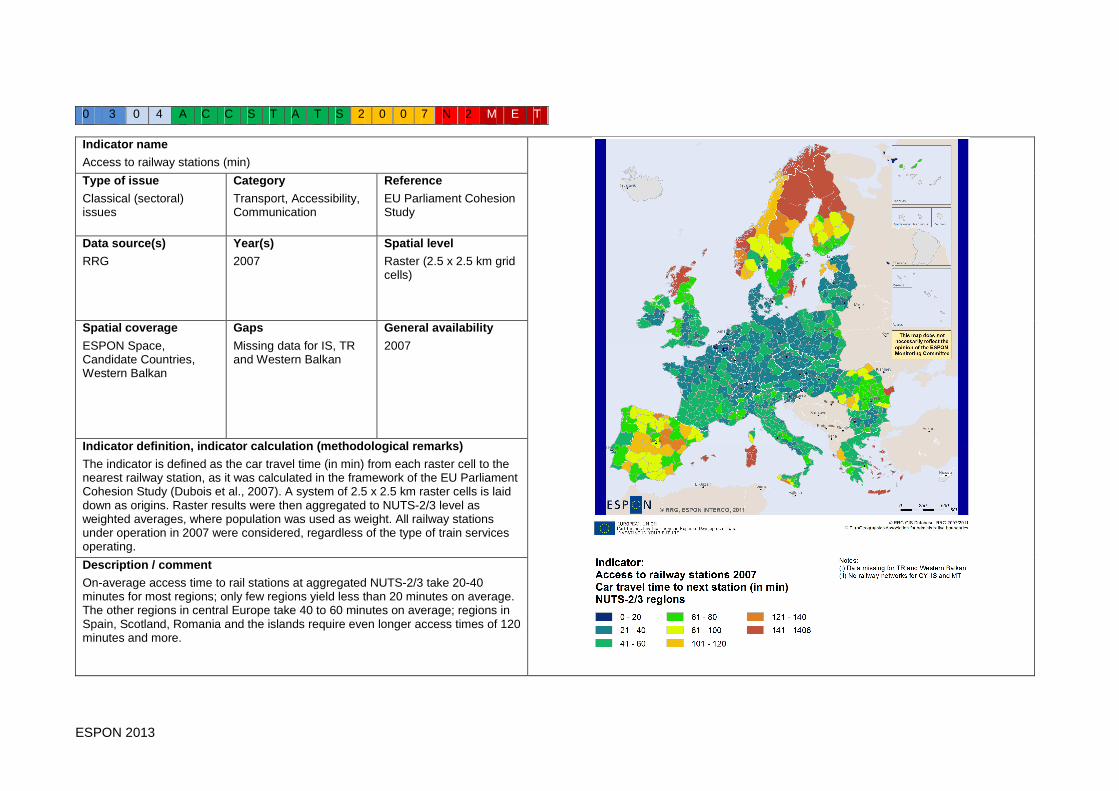
ESPON 2013 44

0 3 0 4 A C C S T A T S 2 0 0 7 N 2 M E T

Indicator name

Access to railway stations (min)

Type of issue

Classical (sectoral) issues

Category

Transport, Accessibility, Communication

Reference

EU Parliament Cohesion Study

Data source(s)

RRG

Year(s)

2007

Spatial level

Raster (2.5 x 2.5 km grid cells)

Spatial coverage

ESPON Space, Candidate Countries, Western Balkan

Gaps

Missing data for IS, TR and Western Balkan

General availability

2007

Indicator definition, indicator calculation (methodological remarks)

The indicator is defined as the car travel time (in min) from each raster cell to the nearest railway station, as it was calculated in the framework of the EU Parliament Cohesion Study (Dubois et al., 2007). A system of 2.5 x 2.5 km raster cells is laid down as origins. Raster results were then aggregated to NUTS-2/3 level as weighted averages, where population was used as weight. All railway stations under operation in 2007 were considered, regardless of the type of train services operating.

Description / comment

On-average access time to rail stations at aggregated NUTS-2/3 take 20-40 minutes for most regions; only few regions yield less than 20 minutes on average. The other regions in central Europe take 40 to 60 minutes on average; regions in Spain, Scotland, Romania and the islands require even longer access times of 120 minutes and more.

ESPON 2013 45

Draft indicators category energy So far there is one indicator subsumed under the energy category, which is the indicator on greenhouse gas emissions. The selection of appropriate reference year is difficult, because the level of greenhouse gas emission as well as the development since 2000 is quite different in the ESPON countries, as Figure 1 shows. Some countries have rather high emission levels (Austria, Spain, Greece, Ireland, Portugal) while others have extremely low levels (Bulgaria, Czech Republic, Germany, Estonia, Latvia, Romania, UK). In some countries a clear negative trend towards reduced emissions can be observed (Belgium, Germany, Netherlands, Sweden, UK), others remain more or less stable in emission levels (Finland, Ireland, Norway, Poland), while others experienced clear, constant increases in greenhouse gas emissions over the last decade (Austria, Iceland, Lithuania, Latvia, Slovenia). Even though the map of Greenhouse gas emissions at country levels shows some interesting results, with low emission levels in East European countries (after the closure of their industrial basis) and rather high levels in Mediterranean countries, this map is rather weak due to its incondusiveness from a regional cohesion point of view. Looking at the trends of the emissions over the last decade (Figure 1) adds some value to the analysis since it provides interesting information how policies succeeded in the reduction of the emissions, even though the pure numbers give no hint on the reason for the reduction. Possible reasons may include: - Closure of pollutants / closure of heavy industries - Substitution of old, energy-intensive technologies by new, energy-saving technologies

and products - Implementation of higher, environment-friendly standards and regulations (thresholds),

along with appropriate filter technologies - Generally reduction in per-capita energy consumption of households and industries - General decline in population and economy resulting in overall reduction of energy

consumption. What national data still hide is the question whether there are different trends at regional level. Even in countries experience overall trends towards a reduction of greenhouse gas emissions it may well be that in certain areas (for instance, agglomerations, industrial parks etc.) emissions increase, while in other parts of the country emission dropped. Also, it may well be that in certain economic sectors emissions increased, while at the same time emissions in other sectors fell. The map for Germany proofs that there are significant differences between the regions in the country, with North-Rhine-Westfalia as the negative outlier, and Hamburg as the county with the least emissions. Standardizing the NUTS-1 values on a per capita basis (notwithstanding that Greenhouse gas emission are also a function of production and not only consumption) provides even more insights into the spatial distribution of the Greenhouse gas emissions. Now it appears that per capita Brandenburg, Bremen and the Saarland are the worst counties in Germany, polluting the highest level of Greenhouse gases in Germany.

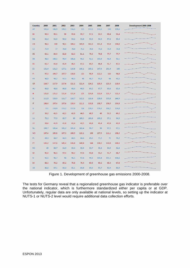
ESPON 2013 46

Figure 1. Development of greenhouse gas emissions 2000-2008.

The tests for Germany reveal that a regionalized greenhouse gas indicator is preferable over the national indicator, which is furthermore standardized either per capita or at GDP. Unfortunately, regular data are only available at national levels, so setting up the indicator at NUTS-1 or NUTS-2 level would require additional data collection efforts.

ESPON 2013 47

0 3 0 4 E N R 2 0 0 8 N 0 M E T

Indicator name

Greenhous gas emissions

Type of issue

Classical (sectoral) issues

Category

Energy

Reference

ESPON 3.3

Data source(s)

Eurostat Regio Database (table env_air_ind); European Environment Agency

Year(s)

2008

Spatial level

NUTS-0

Spatial coverage

ESPON Space

Gaps

Missing data for CY, HR, MT, TR, Western Balkan

General availability

1998-2008

Indicator definition, indicator calculation (methodological remarks)

Total Greenhouse Gas Emissions in CO2 equivalent indexed to Kyoto base year (1990).

Description / comment

The map shows that the level of Greenhouse gas emissions in East European countries is rather low, probably due to the closure and breakdown of the industrial basis over the last 20 years. In contrast, all Mediterranian countries (Portugal, Spain, Italy, Greece) show high levels of Greenhouse gas emissions.

ESPON 2013 48

0 3 0 4 E N R D E 2 0 0 3 N 1 M E T

Indicator name

Greenhous gas emissions

Type of issue

Classical (sectoral) issues

Category

Energy

Reference

Umweltbundesamt

Data source(s)

Landesamt f. Datenverarbeitung u. Statistik NRW

Year(s)

2003

Spatial level

NUTS-1

Spatial coverage

Germany

Gaps

---

General availability

Only 2003

Indicator definition, indicator calculation (methodological remarks)

Total Greenhouse Gas Emissions in CO2 equivalents

Description / comment

The map for Germany clearly shows great differences in the Greenhouse gas emissions between the German Länder for the year 2003. While North-Rhine-Westfalia clearly stands out negatively with more than 320,000 CO2 equivalents, Hamburg experiences the least emissions with only 12,000 CO2 equivalents.

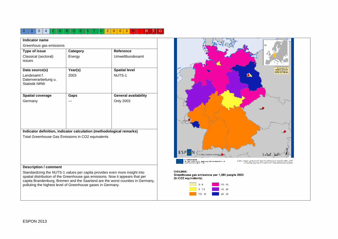
ESPON 2013 49

0 3 0 4 E N R D E S T D 2 0 0 3 N 1 R T O

Indicator name

Greenhous gas emissions

Type of issue

Classical (sectoral) issues

Category

Energy

Reference

Umweltbundesamt

Data source(s)

Landesamt f. Datenverarbeitung u. Statistik NRW

Year(s)

2003

Spatial level

NUTS-1

Spatial coverage

Germany

Gaps

---

General availability

Only 2003

Indicator definition, indicator calculation (methodological remarks)

Total Greenhouse Gas Emissions in CO2 equivalents

Description / comment

Standardizing the NUTS-1 values per capita provides even more insight into spatial distribution of the Greenhouse gas emissions. Now it appears that per capita Brandenburg, Bremen and the Saarland are the worst counties in Germany, polluting the highest level of Greenhouse gases in Germany.

ESPON 2013 50

Draft indicators category social and cultural affairs There are two indicators identified under the social and cultural affairs category in the draft selection set. The two indicators are - At-persistant-risk-of poverty rate - Happiness index Concerning the at-persistant-risk of poverty indicator, the literature mentions the threshold of 60 % of national equivalent income (see map). As a result, the percent of population at risk of poverty is highest in East European countries, with Latvia, Romania and Bulgaria being in the worst situation. On the other end of the spectrum, Czech Republic, Slovakia and Norway are those countries with the least population share. Nevertheless, Figure 1 illustrates what would happen if other thresholds, such as 50 % or 70 % of national equivalent income would be applied. Even though the ranking of countries will only change marginal when other thresholds are used, the share of population at risk will change drastically; for instance, if 70 % income threshold would be applied, more than 30% of the population of Latvia are at risk of poverty, and still more than 15 % of the Czech population. If the threshold would be changed to 50% of the equivalent national income, some 18 % of the population in Latvia and still almost 5 % of the Czech population, just to mention the two extreme countries, are at risk of poverty.

ESPON 2013 51

Figure 1. Share of population at risk of poverty according to different thresholds: 70 %, 60% and 50%. The happiness index was developed by nef (2009) based upon evaluations of questionnaires concerning the quality of life of people in Europe, where questions concerning quality-of-life went far beyond the traditional economic wealth fare approach by including questions on emotions/feelings, general satisfaction, resilience and self-esteem, supportive personal or social relationships, vitality, social networks etc. Results were first aggregated to two individual happiness indicators, which are the personal and the social happiness. Both indicators were standardized at a scale from 0 (no happiness) to 10 (absolute happiness), with 5 representing the European average among all countries. In a second stage, these two synthetic indicators were further aggregated to the overall well-being indicator, again based upon the same scale.

ESPON 2013 52

The overall well-being indicator and also the personal well-being indicator show clear spatial patterns: - Well-being in Scandinavian and Alpine countries seems to be much higher compared to

the other European countries, in particular to East European countries, with a lot of extreme votes.

- Furthermore, bigger countries (in terms of population) such as France, Germany or the UK seem to be more indifferent compares to smaller countries.

In contrast, the social well-being indicator levels out the extreme results of the other two indicators to some extent, however, the general spatial patterns remain the same as for the other two indicators. Altogether, despite the small differences with the social well-being indicator, all three happiness indicators point into the same direction, so that only one indicator would be sufficient to consider. This should be the overall well-being indicators, as the combination of the other two indicators.

ESPON 2013 53

0 6 0 2 P O V 2 0 0 9 N0 R T O

Indicator name

At persistent risk of poverty rate

Type of issue

Classical (sectoral) issues

Category

Social and cultural affairs

Reference

Euroislands

Data source(s)

Eurostat Regio Database (table ilc_li03)

Year(s)

2009

Spatial level

NUTS-0

Spatial coverage

ESPON Space, plus HR

Gaps

Western Balkan, Turkey

General availability

1998-2009

Indicator definition, indicator calculation (methodological remarks)

Population share with 60 % of the national equivalent median income.

Description / comment

The share of population at-persistent-risk of poverty is highest in East European countries (Bulgaria, Romania, Latvia), followed by Estonia and Lithuania and the Mediterranean countries of Greece and Spain. On the other end, lowest shares can be found in Czech Republic, Norway, Netherlands, France and Iceland, as well as Austria, Slovakia, Slovenia and Hungary.

ESPON 2013 54

0 6 0 2 H I O W B 2 0 0 7 N 0 O R D

Indicator name

Happiness index, overall well-being

Type of issue

Classical (sectoral) issues

Category

Social and cultural affairs

Reference

Report by the Commission on the Measurement of Economic Performance and Social Progress

Data source(s)

nef

Year(s)

2007

Spatial level

NUTS-0

Spatial coverage

ESPON Space

Gaps

Data missing for CZ, IS, IT, LT, LU, LV, RO, TR and Western Balkan

General availability

2007

Indicator definition, indicator calculation (methodological remarks)

Happiness index overall well-being. Synthetic indicator with the following scale:

0 = worst, 5 = European average, 10 = best

Indicator based upon evaluation results of questionnaires. Replies standardised at a scale from 0 to 10, where 5 is always representing the European average. Results for personal well-being and social well-being were combined to derive this overall well-being indicator.

Description / comment

The overall well-being in Scandinavian and Alpine countries seems to be much higher compared to new EU Member States in Eastern Europe (Bulgaria, Hungary, Slovakia, Poland or Estonia). Bigger countries (in terms of population) seem to be more indifferent than smaller countries, holding more extreme views.

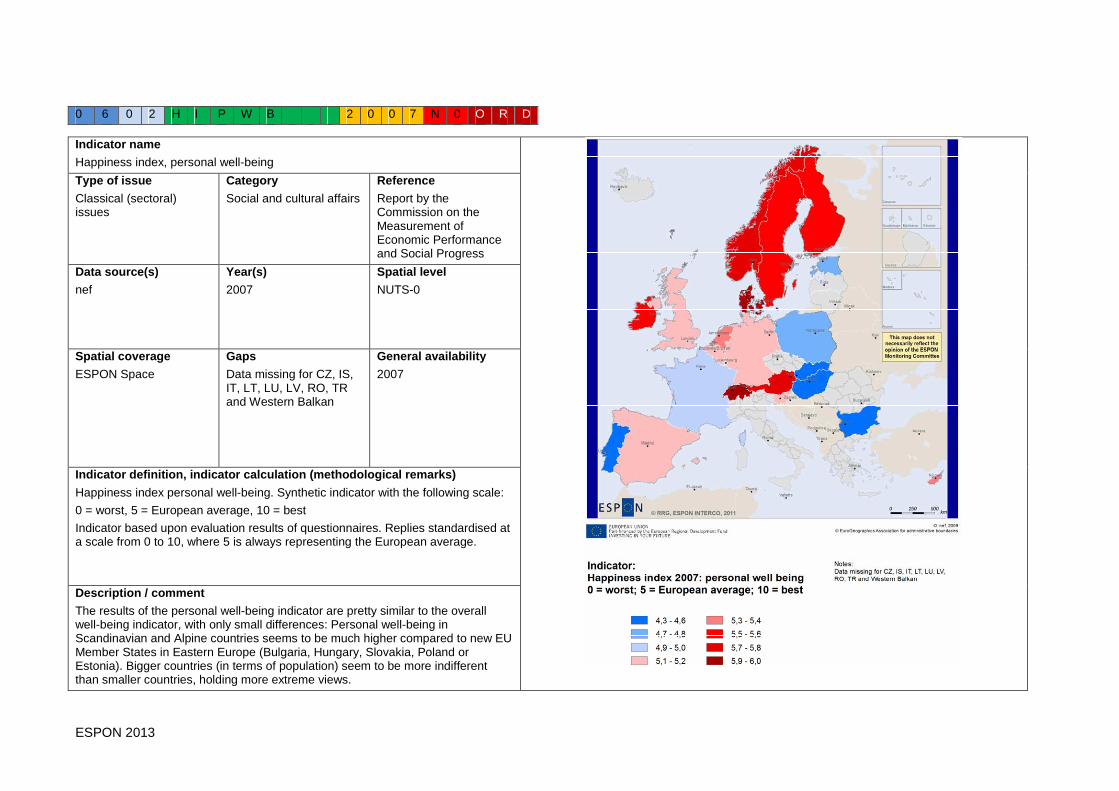
ESPON 2013 55

0 6 0 2 H I P W B 2 0 0 7 N 0 O R D

Indicator name

Happiness index, personal well-being

Type of issue

Classical (sectoral) issues

Category

Social and cultural affairs

Reference

Report by the Commission on the Measurement of Economic Performance and Social Progress

Data source(s)

nef

Year(s)

2007

Spatial level

NUTS-0

Spatial coverage

ESPON Space

Gaps

Data missing for CZ, IS, IT, LT, LU, LV, RO, TR and Western Balkan

General availability

2007

Indicator definition, indicator calculation (methodological remarks)

Happiness index personal well-being. Synthetic indicator with the following scale:

0 = worst, 5 = European average, 10 = best

Indicator based upon evaluation results of questionnaires. Replies standardised at a scale from 0 to 10, where 5 is always representing the European average.

Description / comment

The results of the personal well-being indicator are pretty similar to the overall well-being indicator, with only small differences: Personal well-being in Scandinavian and Alpine countries seems to be much higher compared to new EU Member States in Eastern Europe (Bulgaria, Hungary, Slovakia, Poland or Estonia). Bigger countries (in terms of population) seem to be more indifferent than smaller countries, holding more extreme views.

ESPON 2013 56

0 6 0 2 H I S W B 2 0 0 7 N 0 O R D

Indicator name

Happiness index, social well-being

Type of issue

Classical (sectoral) issues

Category

Social and cultural affairs

Reference

Report by the Commission on the Measurement of Economic Performance and Social Progress

Data source(s)

nef

Year(s)

2007

Spatial level

NUTS-0

Spatial coverage

ESPON Space

Gaps

Data missing for CZ, IS, IT, LT, LU, LV, RO, TR and Western Balkan

General availability

2007

Indicator definition, indicator calculation (methodological remarks)

Happiness index social well-being. Synthetic indicator with the following scale:

0 = worst, 5 = European average, 10 = best

Indicator based upon evaluation results of questionnaires. Replies standardised at a scale from 0 to 10, where 5 is always representing the European average.

Description / comment

Even though the results of the social well-being indicator generally show similar spatial patterns compared to the overall and the personal well-being indicators, the social well-being indicator to some extent levels out the extreme votes. In particular results for the East European countries are not that bad compared to the other two synthetic indicators.

ESPON 2013 57

Draft indicators category land use issues Land use issues and the conversion of open space into settlement areas is one of the major concerns in environmental and social debates. Green space, or open space, is not only the considered as key variable from environmental perspective, but also crucial for social contacts, recreation and even for holidays and tourism industries. What is the degree of open space / green space left in Europe? To answer this question, the seamless pan-European Corine land use layer (EEA, 2006) has been overlaid with the NUTS-3 region boundaries to calculate two types of indicators:

- The share of open or green space on the overall NUTS-3 region territory - The open space or green space provision per capita.

The following Corine land use classes have been considered as built-up areas: continuous urban fabric, discontinuous urban fabric, industrial or commercial units, road and rail networks and associated land, port areas, airports, mineral extraction sites, dump sites, construction sites. All other land use classes are considered as open space or green space. Looking at the results one has to remember the technical limitations of the Corine dataset in order to understand the spatial patterns. Since the dataset was generated by satellite images analysis, the following restrictions are immanent: - The general scale of the dataset is 1:100,000 - The minimum size of individual patches to be recognized is 25 ha for areal objects

and a minimum width of 100 m for linear objects - Following this not all built-up areas are included in the dataset, in particular transport

infrastructures such as motorways are only rarely included, so as small settlement or housing units outside villages and towns.

In consequence it is not surprising that the share of green space on the overall NUTS-3 territory is rather high. Given the above restrictions, the calculated shares overestimate the share of open space. Only the agglomerations experiences shares of open space of less than 70 or 60 percent, while all other regions show very high shares of more than 90 %. Standardising the open space at the region population, the resulting map favors regions in the European periphery. Regions in Scandinavia, Spain, Turkey, Western Balkan and the Baltic countries show the highest amount of open space per capita – both because these areas still own large unfragmented open areas and due to their extremely low population density. On the other hand, Central European countries (Benelux, Germany) show only very low figures of open space, with less than 50 sqkm per capita, often even less than 20 or 10 sqkm. The variations in the green space per capita within the countries are extremely different (Figure 1 and Table 1). While there are extreme differences in the Scandinavian countries (Finland, Iceland, Norway, Sweden), Spain, Latvia or Turkey, there are only very small differences in other countries such as Albania, Germany, Netherlands, or Slovenia.

ESPON 2013 58

Figure 1. Greenspace per capita (2006): variations within countries (Scandinavian countries excluded).

Table 1. Greenspace per capita (2006): Statistical measures (ranked by coefficient of variation).

Country Minimum Mean Std.

deviation Maximum Coefficient of variation

FI 21,00 3424,84 10812,97 48920,25 3,16

SE 19,66 3602,17 8434,88 34858,50 2,34

NO 0,41 2785,78 5310,82 23467,39 1,91

HR 0,37 63,33 110,49 529,58 1,74

BE 0,01 4,21 6,85 29,38 1,62

PT 0,26 92,77 135,29 549,81 1,46

DE 0,00 6,85 9,79 63,65 1,43

IS 4,48 49151,05 69503,74 98297,62 1,41

BA 4,11 96,51 135,49 393,81 1,40

ES 0,00 269,92 366,16 1458,99 1,36

DK 0,02 42,20 46,63 119,35 1,10

IT 0,18 23,92 25,55 109,89 1,07

TR 1,86 181,57 187,17 1182,21 1,03

PL 0,07 52,01 48,36 193,42 0,93

AT 0,04 43,16 37,09 129,56 0,86

NL 0,04 2,43 2,08 7,55 0,86

EE 30,95 440,32 363,44 770,37 0,83

FR 0,00 90,95 73,84 341,35 0,81

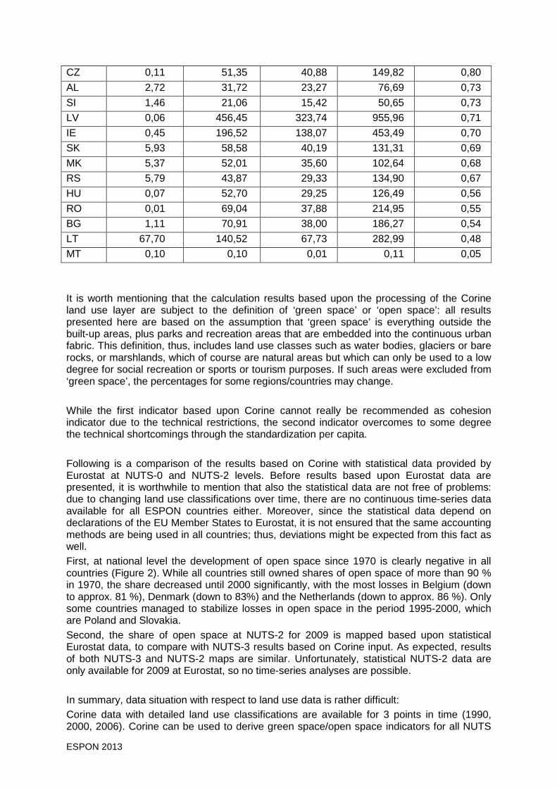
ESPON 2013 59

CZ 0,11 51,35 40,88 149,82 0,80

AL 2,72 31,72 23,27 76,69 0,73

SI 1,46 21,06 15,42 50,65 0,73

LV 0,06 456,45 323,74 955,96 0,71

IE 0,45 196,52 138,07 453,49 0,70

SK 5,93 58,58 40,19 131,31 0,69

MK 5,37 52,01 35,60 102,64 0,68

RS 5,79 43,87 29,33 134,90 0,67

HU 0,07 52,70 29,25 126,49 0,56

RO 0,01 69,04 37,88 214,95 0,55

BG 1,11 70,91 38,00 186,27 0,54

LT 67,70 140,52 67,73 282,99 0,48

MT 0,10 0,10 0,01 0,11 0,05

It is worth mentioning that the calculation results based upon the processing of the Corine land use layer are subject to the definition of ‘green space’ or ‘open space’: all results presented here are based on the assumption that ‘green space’ is everything outside the built-up areas, plus parks and recreation areas that are embedded into the continuous urban fabric. This definition, thus, includes land use classes such as water bodies, glaciers or bare rocks, or marshlands, which of course are natural areas but which can only be used to a low degree for social recreation or sports or tourism purposes. If such areas were excluded from ‘green space’, the percentages for some regions/countries may change. While the first indicator based upon Corine cannot really be recommended as cohesion indicator due to the technical restrictions, the second indicator overcomes to some degree the technical shortcomings through the standardization per capita. Following is a comparison of the results based on Corine with statistical data provided by Eurostat at NUTS-0 and NUTS-2 levels. Before results based upon Eurostat data are presented, it is worthwhile to mention that also the statistical data are not free of problems: due to changing land use classifications over time, there are no continuous time-series data available for all ESPON countries either. Moreover, since the statistical data depend on declarations of the EU Member States to Eurostat, it is not ensured that the same accounting methods are being used in all countries; thus, deviations might be expected from this fact as well. First, at national level the development of open space since 1970 is clearly negative in all countries (Figure 2). While all countries still owned shares of open space of more than 90 % in 1970, the share decreased until 2000 significantly, with the most losses in Belgium (down to approx. 81 %), Denmark (down to 83%) and the Netherlands (down to approx. 86 %). Only some countries managed to stabilize losses in open space in the period 1995-2000, which are Poland and Slovakia. Second, the share of open space at NUTS-2 for 2009 is mapped based upon statistical Eurostat data, to compare with NUTS-3 results based on Corine input. As expected, results of both NUTS-3 and NUTS-2 maps are similar. Unfortunately, statistical NUTS-2 data are only available for 2009 at Eurostat, so no time-series analyses are possible.

In summary, data situation with respect to land use data is rather difficult: Corine data with detailed land use classifications are available for 3 points in time (1990, 2000, 2006). Corine can be used to derive green space/open space indicators for all NUTS

ESPON 2013 60

levels; however, results may overestimate the share of green space due to the technical limitation of the Corine approach. Statistical data on land use are available at Eurostat for both NUTS-0 and NUTS-2. For NUTS-0 time series data are available, but due to changing definitions of land use classes not continuously for all years. At NUTS-2, only recent data for 2009 are available.

Figure 2. Development of open space at national level 1970-2000.

ESPON 2013 61

1 0 0 1 L U O S P E R 2 0 0 6 N 3 R T O

Indicator name

Green space: open space

Type of issue

Complex territorial issues

Category

Land use issues

Reference

Data source(s)

European Environment Agency (EEA)

Year(s)

2006

Spatial level

NUTS-3

Spatial coverage

ESPON Space

Gaps

Missing data for CH, GR, and UK.

General availability

1990, 2000 and 2006

Indicator definition, indicator calculation (methodological remarks)

Open space in percent of overall NUTS-3 region area. Indicator calculated through overlay of Corine landuse layer with NUTS-3 region boundaries. From Corine layer, all land use classes with grid codes < 10 were considered as settlement areas, the remaining classes were considered as open space (including parks, forests, agricultural areas, water bodies, other open land).

Description / comment

The map shows that according to the Corine landuse layer the majority of European NUTS-3 regions still own a lot of open space, accumulating to more than 90 % of the NUTS-3 region territory. Only regions in Germany, Benelux, parts of France and Italy, and the agglomerations in the other countries have share of open space of lass then 70 percent.

ESPON 2013 62

1 0 0 1 L U O S P I N H 2 0 0 6 N 3 R T O

Indicator name

Green space: open space per capita

Type of issue

Complex territorial issues

Category

Land use issues

Reference

Data source(s)

European Environment Agency (EEA)

Year(s)

2006

Spatial level

NUTS-3

Spatial coverage

ESPON Space

Gaps

Missing data for CH, GR, and UK.

General availability

1990, 2000 and 2006

Indicator definition, indicator calculation (methodological remarks)

Open space per capita of NUTS-3 resident population (in sqkm/capita). Indicator calculated through overlay of Corine Landuse layer with NUTS-3 region boundaries; ratio calculated between open space and NUTS-3 region population.. From Corine layer, all land use classes with grid codes < 10 were considered as settlement areas, the remaining classes were considered as open space (including parks, forests, agricultural areas, water bodies, other open land).

Description / comment

As expected this indicator highlights the European peripheries: regions in Scandinavia, Spain, Turkey, Western Balkan and the Baltic countries show the highest amount of open space per capita – both because these areas still own large unfragmented open areas and due to their extremely low population density. On the other hand, Central European countries (Benelux, Germany) show only very low figures of open space, with less than 50 sqkm per capita, often even less than 20 or 10 sqkm.

ESPON 2013 63

1 0 0 1 L U O S P E R 2 0 0 9 N 2 R T O

Indicator name

Green space: open space

Type of issue

Complex territorial issues

Category

Land use issues

Reference

Data source(s)

Eurostat Regional Database (table lan_lu_ovw)

Year(s)

2009

Spatial level

NUTS-2

Spatial coverage

ESPON Space

Gaps

Missing data for BG, CH, CY, NO, RO, TR and Western Balkans.

General availability

only 2009

Indicator definition, indicator calculation (methodological remarks)

Open space in percent of overall NUTS-2 region area. Indicator calculated through combination of different open-space land use classes (agriculture, forestry, fischery, other unused land) in relation to total region area.

Description / comment

The general patterns of the NUTS-2 map are similar to those of the corresponding NUTS-3 map, even though in an aggregated manner. Regions in Benelux, Germany, southern UK, Northern Italy as well as the capital city regions in France, Greece, Spain, Austria and Slovakia are those regions with the lowest share of open space in 2009. On the other hand, regions in Scandinavia, in the Baltic States, Spain, Greece and Poland are those with the highest shares.

ESPON 2013 64

Draft indicators category economy From a cohesion perspective, the development of the economy of European regions is crucial. This is reflected in a number of indicators that are subsumed under this category: - GDP per capita (in pps and euros) and its development over time - Employment rate and its development over time - Unemployment rate and its development over time - Mean disposable household income - Employment in transport sector - Research and development expenditures

Required input data for all these indicators will be taken from Eurostat Regio Database. GDP per capita There are four maps illustrating the indicator GDP per capita, expressed in different manners (in Euro, in PPS, in Euro as percent of EU average, in PPS as percent of EU average). All four indicators highlight two main spatial patterns: First, an extreme concentration of GDP per capita in the capital city areas and in agglomerations. Second, a clear East-West divide between the old and the new EU Member States, which still exist even in 2009. The map also shows the dichotomy of economically successful regions next to poorly developed regions in all parts of Europe. The four different ways of indicator presentation all have their particular foci: generally GDP indicators expressed in PPS reduce spatial disparities to some extent; in particular they reduce the extreme outliers. GDP indicators expressed as percent of EU average are in turn most suitable to follow the indicator over time (time-series observations), since they are already standardized. It is suggested that when looking at states, GDP per capita in PPS is selected as indicator, and when looking at trends correspondingly GDP per capita in PPS expressed as percentage of EU average is being used. What are changes of GDP per capita over time? Again there are several options how to measure the changes of GDP per capita. Three options were tested, with remarkably results: First, the GDP growth 2000-2008 expressed in percent of 2000 is calculated. Then, the absolute GDP growth for the said period is illustrated, followed by the relative change of percentage points in relation to the EU averages of 2000 and 2008 is analysed, with the following outcomes: The indicator relative change of GDP per capita in relation to 2000 state illustrates that many regions in Eastern Europe, but also in Spain, in the Baltic States or in Eastern Germany experienced real gains in GDP per capita (in Euro) in the period of 2000-2008. Standardized at 2000 GDP level, the gains partly account for more than 200% in these regions; however,

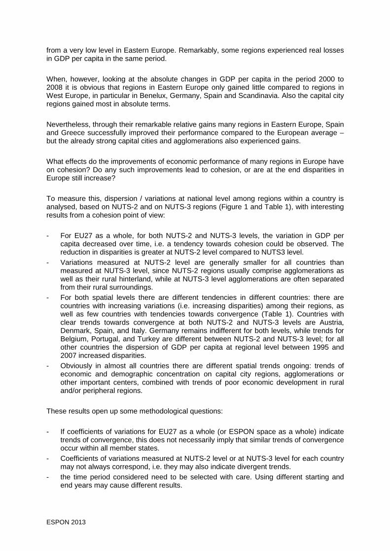
ESPON 2013 65

from a very low level in Eastern Europe. Remarkably, some regions experienced real losses in GDP per capita in the same period. When, however, looking at the absolute changes in GDP per capita in the period 2000 to 2008 it is obvious that regions in Eastern Europe only gained little compared to regions in West Europe, in particular in Benelux, Germany, Spain and Scandinavia. Also the capital city regions gained most in absolute terms. Nevertheless, through their remarkable relative gains many regions in Eastern Europe, Spain and Greece successfully improved their performance compared to the European average – but the already strong capital cities and agglomerations also experienced gains. What effects do the improvements of economic performance of many regions in Europe have on cohesion? Do any such improvements lead to cohesion, or are at the end disparities in Europe still increase? To measure this, dispersion / variations at national level among regions within a country is analysed, based on NUTS-2 and on NUTS-3 regions (Figure 1 and Table 1), with interesting results from a cohesion point of view: - For EU27 as a whole, for both NUTS-2 and NUTS-3 levels, the variation in GDP per

capita decreased over time, i.e. a tendency towards cohesion could be observed. The reduction in disparities is greater at NUTS-2 level compared to NUTS3 level.

- Variations measured at NUTS-2 level are generally smaller for all countries than measured at NUTS-3 level, since NUTS-2 regions usually comprise agglomerations as well as their rural hinterland, while at NUTS-3 level agglomerations are often separated from their rural surroundings.

- For both spatial levels there are different tendencies in different countries: there are countries with increasing variations (i.e. increasing disparities) among their regions, as well as few countries with tendencies towards convergence (Table 1). Countries with clear trends towards convergence at both NUTS-2 and NUTS-3 levels are Austria, Denmark, Spain, and Italy. Germany remains indifferent for both levels, while trends for Belgium, Portugal, and Turkey are different between NUTS-2 and NUTS-3 level; for all other countries the dispersion of GDP per capita at regional level between 1995 and 2007 increased disparities.

- Obviously in almost all countries there are different spatial trends ongoing: trends of economic and demographic concentration on capital city regions, agglomerations or other important centers, combined with trends of poor economic development in rural and/or peripheral regions.

These results open up some methodological questions: - If coefficients of variations for EU27 as a whole (or ESPON space as a whole) indicate

trends of convergence, this does not necessarily imply that similar trends of convergence occur within all member states.

- Coefficients of variations measured at NUTS-2 level or at NUTS-3 level for each country may not always correspond, i.e. they may also indicate divergent trends.

- the time period considered need to be selected with care. Using different starting and end years may cause different results.

ESPON 2013 66

ESPON 2013 67

Figure 1. Dispersion of GDP per capita for ESPON countries (in %, 1995-2007): NUTS-3 level (top), NUTS-2 level (bottom) (Eurostat Regio Database, 2011, table nama_r_e0digdp).

Table 1. Dispersion of GDP at regional level 1995-2007: trends at NUTS3 and NUTS2 level.

Country Trend NUTS-3 Trend NUTS-2 CommentEU27 convergence (cohesion)

AT convergence (cohesion)

BE trend indifferent

BG increasing disparities

CZ increasing disparities

DE stagnant

DK convergence (cohesion)

EE n.a. increasing disparities

ES convergence (cohesion)

FI increasing disparities

FR increasing disparities

GR increasing disparities

HR increasing disparities

HU increasing disparities

IE n.a. increasing disparities

IT convergence (cohesion)

LT n.a. increasing disparities

LV n.a. increasing disparities

MK n.a. increasing disparities

NL increasing disparities

PL increasing disparities

PT trend indifferent

RO increasing disparities

SE increasing disparities

SI n.a. increasing disparities

SK increasing disparities

TR trend indifferent

UK increasing disparities n.a. = NUTS-2 level = country level, i.e. measures of variations cannot be calculated

Employment rate and development of employment rate Employment rates significantly differ across Europe. As tendencies the rates are lower the farther south and the farther east a region is located, i.e. resulting in lowest employment rates in southern Spain, southern Italy and Turkey. In contrast, highest employment rates are found in Scandinavia, Benelux, UK, Germany and Switzerland. The map also suggest visually that there are great disparities within the countries itself (for instance, Italy, France, Spain). This is confirmed by Figure 2, which shows that variations among NUTS-2 regions are highest in Turkey, Italy and Spain, and are smallest in Denmark, Ireland and Slovenia.

ESPON 2013 68

Figure 2. Employment rate variations in 2009 per country for NUTS-2 regions.

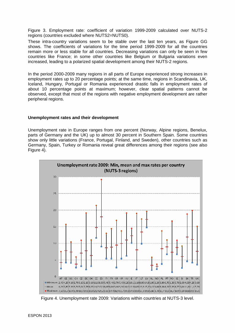
ESPON 2013 69

Figure 3. Employment rate: coefficient of variation 1999-2009 calculated over NUTS-2 regions (countries excluded where NUTS2=NUTS0). These intra-country variations seem to be stable over the last ten years, as Figure GG shows. The coefficients of variations for the time period 1999-2009 for all the countries remain more or less stable for all countries. Decreasing variations can only be seen in few countries like France; in some other countries like Belgium or Bulgaria variations even increased, leading to a polarized spatial development among their NUTS-2 regions. In the period 2000-2009 many regions in all parts of Europe experienced strong increases in employment rates up to 20 percentage points; at the same time, regions in Scandinavia, UK, Iceland, Hungary, Portugal or Romania experienced drastic falls in employment rates of about 10 percentage points at maximum; however, clear spatial patterns cannot be observed, except that most of the regions with negative employment development are rather peripheral regions. Unemployment rates and their development Unemployment rate in Europe ranges from one percent (Norway, Alpine regions, Benelux, parts of Germany and the UK) up to almost 30 percent in Southern Spain. Some countries show only little variations (France, Portugal, Finland, and Sweden), other countries such as Germany, Spain, Turkey or Romania reveal great differences among their regions (see also Figure 4).

Figure 4. Unemployment rate 2009: Variations within countries at NUTS-3 level.

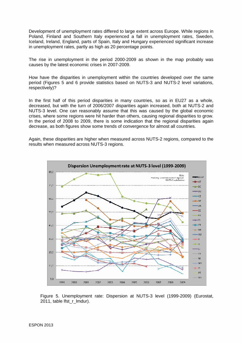
ESPON 2013 70

Development of unemployment rates differed to large extent across Europe. While regions in Poland, Finland and Southern Italy experienced a fall in unemployment rates, Sweden, Iceland, Ireland, England, parts of Spain, Italy and Hungary experienced significant increase in unemployment rates, partly as high as 20 percentage points. The rise in unemployment in the period 2000-2009 as shown in the map probably was causes by the latest economic crises in 2007-2009. How have the disparities in unemployment within the countries developed over the same period (Figures 5 and 6 provide statistics based on NUTS-3 and NUTS-2 level variations, respectively)? In the first half of this period disparities in many countries, so as in EU27 as a whole, decreased, but with the turn of 2006/2007 disparities again increased, both at NUTS-2 and NUTS-3 level. One can reasonably assume that this was caused by the global economic crises, where some regions were hit harder than others, causing regional disparities to grow. In the period of 2008 to 2009, there is some indication that the regional disparities again decrease, as both figures show some trends of convergence for almost all countries. Again, these disparities are higher when measured across NUTS-2 regions, compared to the results when measured across NUTS-3 regions.

Figure 5. Unemployment rate: Dispersion at NUTS-3 level (1999-2009) (Eurostat, 2011, table lfst_r_lmdur).

ESPON 2013 71

Figure 6. Unemployment rate: Dispersion at NUTS-2 level (1999-2009) (Eurostat, 2011, table

lfst_r_lmdur). Median disposable household income Apart from the capital cities and the big agglomerations, the disposable household income in 2007 is highest in Southern Germany, Austria, England (Greater London region), France (Paris) and Northern Italy. There is furthermore a clear divide between the old and new EU Member States, with Bulgaria and Romania yielding the lowest household incomes (< 5,000 EUR). Countries with the highest disposable household income are also those countries with the highest disparities among their regions, as Figure 7 shows: the UK; Germany, Italy, but also Greece experience extreme divide between their richest and poorest regions.

ESPON 2013 72

Figure 7. Household income: disparities within the countries measured across NUTS-2 regions. Almost all regions in Europe gained increases in disposable household income between 2000 and 2007, except for some few ones. Highest relative gains allocated in East European countries, i.e. Baltic States and Bulgaria and Romania, but starting from a rather low level; in contrast, gains in Germany, Benelux, or Italy are smaller in relative terms, but starting from a much higher level. What impact do these growths rates of disposable household income have on the reduction of disparities between and within the countries? A Gini coefficient on income distribution was calculated (SILC, 2011) that helps to answer the question (Figure 8). This Gini coefficient is defined as the relationship of cumulative shares of the population arranged according to the level of equivalised disposable income, to the cumulative share of the equivalised total disposable income received by them. Gini coefficients have values between 0 (=equal distribution) and 1 (=all income concentrated at one person).

The least variations of household income in the period concerned have Slovenia, Denmark and Sweden, highest variations can be observed for Turkey, Portugal and Latvia (even though all three countries with small trends towards convergence). There is no overall general trend to observe in the reduction or in increase of income variations across the countries. Some countries like Bulgaria, France or Romania experienced significant increase in household disparities, while in the same period income variations in countries like Greece or Spain reduced. The general impression from Figure DD, however, is, that income variations are rather stable over time within countries, and also across countries, as the graphs for EU27 and EU15 show.

ESPON 2013 73

Figure 8. Household income: Development of Gini coefficients 1998-2009 (SILC, 2011, downloaded via Eurostat, table tessi190). Employment in transport sector The initial idea was to define an indicator describing the employment in the transport sector in Europe; unfortunately, pan-European statistical employment data provided by Eurostat at regional level only use sectoral disaggregation according to the NACE_R1 classification, i.e. the corresponding sector class for transport is defined as “Wholesale and retail trade; hotels and restaurant; transport”. The indicator thus was redefined as “Employment in wholesale and retail trade; hotels and restaurants; transport” and was expressed in percent on total employment (%). The percentages were calculated by dividing employment in wholesale and retail trade, hotels and restaurants and transport by total employment, multiplied by 100. High proportions of employment in wholesale and retail trade, hotels and restaurant, and transport can first of all be found in coastal regions all over Europe, in particular at Mediterranean Sea, but also in other touristic destinations like the Alps. Significant lower shares are found in Eastern Europe, mainly Bulgaria, Poland and Romania, and in Northern Scandinavia. In Germany, Spain and Italy the situation is very mixed with regions yielding high shares next to regions with rather low percentages. Variations between regions with the lowest and highest proportions are remarkable for all countries; often, a range of values of more than ten percentage points can be observed (Figure 9). Highest value ranges are detected for Greece, Spain, Germany and Romania; lowest ranges for Malta, Ireland and Slovakia.

ESPON 2013 74

Figure 9. Employment in transport (%, 2007): variations within countries at NUTS-3 level. Following this diverse picture, the coefficients of variation for the countries measured over NUTS-3 regions differ significantly. Malta, Ireland and Slovakia, again, show up as those countries with the smallest variations, while Romania, Portugal, Macedonia and Greece represent those countries with by far the highest disparities in the share of transport employment (Figure 10). Even though the shares in Eastern Europe are still quite low in 2007, many of these regions increased shares significantly, when looking at the development of employment in transport in the period 2000-2007, though from a very low level, so that in comparison to regions in Western Europe they still yield small shares.

ESPON 2013 75

Figure 10. Employment in transport (%) (2007): Coefficients of variations measured over NUTS-3 regions.

Otherwise, regions in Spain, Italy, Greece, France and Ireland also increased employment in wholesale and retail, hotels and restaurants, and in transport. Since this NACE classification does not allow to differentiate between tourism industries and transport, increasing shares for some regions may be due to tourism sector, while in other regions it may be due to logistics and forwarders activities. On the other hand, there are also regions scattered across Europe who experienced absolute reduction in employment in these sectors since the year 2000. Despite this heterogeneous development at regional level, the coefficients of variation for twenty out of 28 countries decreased for the time period (Figure 11), i.e. indicating overall reductions in disparities at regional level. Only for Bulgaria, Germany, Estonia, Hungary, Italy, Macedonia, Netherlands and the UK increased in disparities since 2000 can be observed.

ESPON 2013 76

Figure 11. Employment in transport: Development of coefficients of variation 2000-2007.

Research and development expenditures

R&D expenditures in a country are a measure of the degree of innovations in a society, and for future prospects of the society as a whole, and the national economy in particular.

Data availability at Eurostat allows testing of two different indicator definitions, which are:

- total R&D expenditures at national level

- total intramural R&D expenditures by NUTS-2 regions

While the first definition captures all R&D expenditures in a country, but is only available at country level, the second indicator captures only a certain part of all R&D expenditures, but input data are available at subnational level.

The R&D intensity at national level is highest in Denmark, Finland and Sweden with more than 3 % of GDP, followed by Austria, France and Germany. Latvia, Romania and Slovakia, on the other hand, spent only less than 0.5 % of its GDP for R&D, which represents the lowest R&D intensity in Europe. Generally, East European countries show smaller shares compared to the old EU Member States. The R&D intensity stabilized over the last decade (Figure 12); slight tendencies towards increasing R&D intensities can be observed for almost all countries, except for Sweden (stable) and Croatia (slight decrease). In the first half of the period, the coefficient of variation for EU27 stabilized after an increase from 0.66 to 0.69, while in the second half the coefficient decreased again steadily to 0.6, which indicates a small reduction in variations (Table 2).

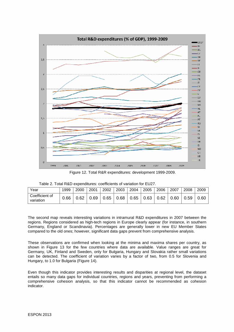
ESPON 2013 77

Figure 12. Total R&R expenditures: development 1999-2009.

Table 2. Total R&D expenditures: coefficients of variation for EU27.

Year 1999 2000 2001 2002 2003 2004 2005 2006 2007 2008 2009

Coefficient of variation 0.66 0.62 0.69 0.65 0.68 0.65 0.63 0.62 0.60 0.59 0.60

The second map reveals interesting variations in intramural R&D expenditures in 2007 between the regions. Regions considered as high-tech regions in Europe clearly appear (for instance, in southern Germany, England or Scandinavia). Percentages are generally lower in new EU Member States compared to the old ones; however, significant data gaps prevent from comprehensive analysis.

These observations are confirmed when looking at the minima and maxima shares per country, as shown in Figure 13 for the few countries where data are available. Value ranges are great for Germany, UK, Finland and Sweden, only for Bulgaria, Hungary and Slovakia rather small variations can be detected. The coefficient of variation varies by a factor of two, from 0.5 for Slovenia and Hungary, to 1.0 for Bulgaria (Figure 14).

Even though this indicator provides interesting results and disparities at regional level, the dataset entails so many data gaps for individual countries, regions and years, preventing from performing a comprehensive cohesion analysis, so that this indicator cannot be recommended as cohesion indicator.

ESPON 2013 78

Figure 13. Intramural R&D expenditures (2007): variations within countries.

Figure 14. Intramural R&D expenditures 2007: coefficients of variation.

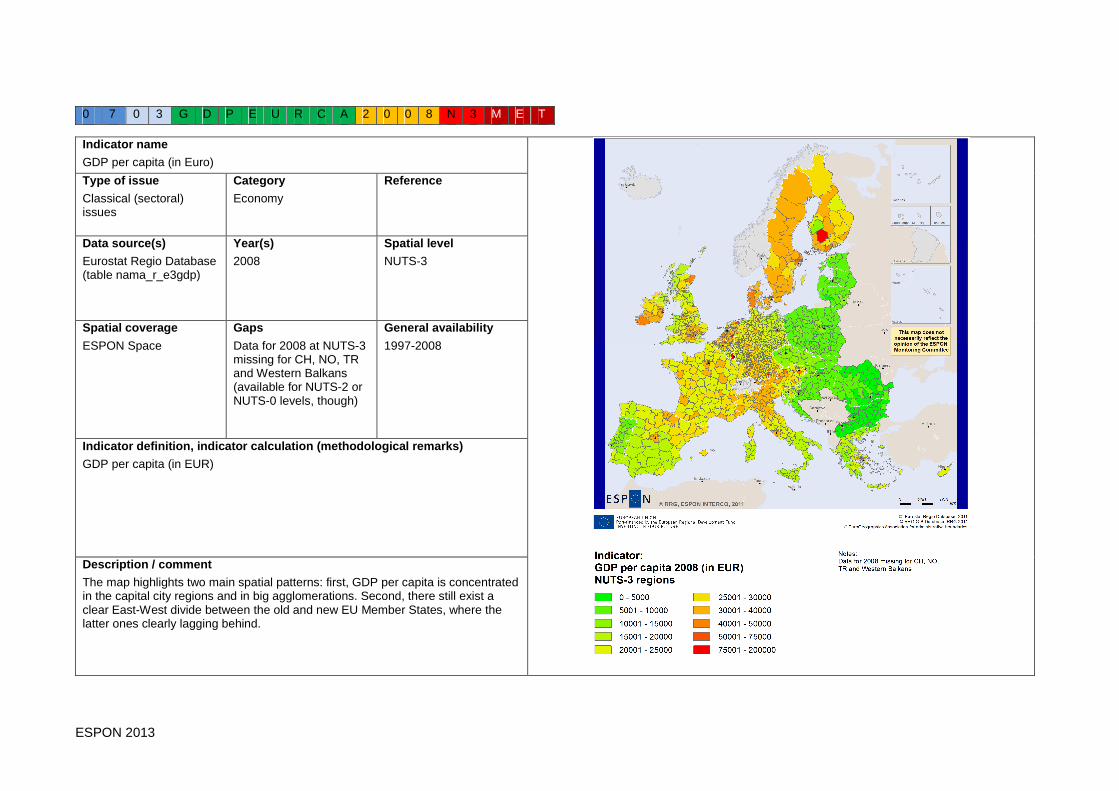
ESPON 2013 79

0 7 0 3 G D P E U R C A 2 0 0 8 N 3 M E T

Indicator name

GDP per capita (in Euro)

Type of issue

Classical (sectoral) issues

Category

Economy

Reference

Data source(s)

Eurostat Regio Database (table nama_r_e3gdp)

Year(s)

2008

Spatial level

NUTS-3

Spatial coverage

ESPON Space

Gaps

Data for 2008 at NUTS-3 missing for CH, NO, TR and Western Balkans (available for NUTS-2 or NUTS-0 levels, though)

General availability

1997-2008

Indicator definition, indicator calculation (methodological remarks)

GDP per capita (in EUR)

Description / comment

The map highlights two main spatial patterns: first, GDP per capita is concentrated in the capital city regions and in big agglomerations. Second, there still exist a clear East-West divide between the old and new EU Member States, where the latter ones clearly lagging behind.

ESPON 2013 80

0 7 0 3 G D P P P S C A 2 0 0 8 N 3 M E T

Indicator name

GDP per capita (in PPS)

Type of issue

Classical (sectoral) issues

Category

Economy

Reference

Data source(s)

Eurostat Regio Database (table nama_r_e3gdp)

Year(s)

2008

Spatial level

NUTS-3

Spatial coverage

ESPON Space

Gaps

Data for 2008 at NUTS-3 missing for CH, NO, TR and Western Balkans (available for NUTS-2 or NUTS-0 levels, though)

General availability

1997-2008

Indicator definition, indicator calculation (methodological remarks)

GDP per capita (in PPS)

Description / comment

The basic spatial patterns of the indicator GDP per capita in PPS are similar to the indicator GDP per capita in Euro, i.e. concentration on agglomerations and capital cities, East-West divide, but altogether the range of values is slightly smaller, and the new EU Member States slightly perform better. All in all, the differences here are smaller compared to the previous map.

ESPON 2013 81

0 7 0 3 G D P E U R E A 2 0 0 8 N 3 R T O

Indicator name

GDP per capita (in Euro expressed in % of EU average)

Type of issue

Classical (sectoral) issues

Category

Economy

Reference

Data source(s)

Eurostat Regio Database (table nama_r_e3gdp)

Year(s)

2008

Spatial level

NUTS-3

Spatial coverage

ESPON Space

Gaps

Data for 2008 at NUTS-3 missing for CH, NO, TR and Western Balkans (available for NUTS-2 or NUTS-0 levels, though)

General availability

1997-2008

Indicator definition, indicator calculation (methodological remarks)

GDP per capita (in EUR expressed in % of EU average). 100 = EU average

Description / comment

While the map highlights again the two main spatial patterns (concentration on capital cities and agglomerations, East-West divide), this map even more illustrates the extremely poor economic performance of regions in East Europe, which are below 50% of the EU average. It also becomes obvious that regions performing extremely good and those who are lagging behind are often next to each other (for instance, Finland), resulting in very distinct patterns.

ESPON 2013 82

0 7 0 3 G D P P P S E A 2 0 0 8 N 3 R T O

Indicator name

GDP per capita (in PPS expressed in % of EU average)

Type of issue

Classical (sectoral) issues

Category

Economy

Reference

Data source(s)

Eurostat Regio Database (table nama_r_e3gdp)

Year(s)

2008

Spatial level

NUTS-3

Spatial coverage

ESPON Space

Gaps

Data for 2008 at NUTS-3 missing for CH, NO, TR and Western Balkans (available for NUTS-2 or NUTS-0 levels, though)

General availability

1997-2008

Indicator definition, indicator calculation (methodological remarks)

GDP per capita (in PPS expressed in % of EU average). 100 = EU average

Description / comment

The fourth map illustrating the GDP per capita indicator again shows the same spatial patterns, in relation to the EU average (100). The differences are not as extreme as in the previous map, since in a number of countries in Eastern Europe catch up to the European average to some degree.

ESPON 2013 83

0 7 0 3 I N C O 0 0 0 8 N 3 R T O

Indicator name

GDP change per capita in PPS 2000-2008 (relative change)

Type of issue

Classical (sectoral) issues

Category

Economy

Reference

DEMIFER

Data source(s)

Eurostat Regio Database (table nama_r_e3gdp)

Year(s)

2008

Spatial level

NUTS-3

Spatial coverage

ESPON Space

Gaps

Data for 2008 at NUTS-3 missing for CH, NO, TR and Western Balkans (available for NUTS-2 or NUTS-0 levels, though)

General availability

1997-2008

Indicator definition, indicator calculation (methodological remarks)

GDP change per capita in PPS 2000-2008, expressed in % of 2000.

Description / comment

The indicator illustrates that many regions in Eastern Europe, but also in Spain, in the Baltic States or in Eastern Germany experienced real gains in GDP per capita (in Euro) in the period of 2000-2008. Standardized at 2000 GDP level, the gains partly account for more than 200% in these regions; however, from a very low level in Eastern Europe. Remarkably, some regions experienced real losses in GDP per capita in the same period.

ESPON 2013 84

0 7 0 3 I N C O A B S 0 0 0 8 N 3 M E T

Indicator name

GDP change per capita in PPS 2000-2008 (absolute change)

Type of issue

Classical (sectoral) issues

Category

Economy

Reference

DEMIFER

Data source(s)

Eurostat Regio Database (table nama_r_e3gdp)

Year(s)

2008

Spatial level

NUTS-3

Spatial coverage

ESPON Space

Gaps

Data for 2008 at NUTS-3 missing for CH, NO, TR and Western Balkans (available for NUTS-2 or NUTS-0 levels, though)

General availability

1997-2008

Indicator definition, indicator calculation (methodological remarks)

GDP change per capita in PPS 2000-2008, absolute difference between 2000 and 2008

Description / comment

When looking at the absolute changes in GDP per capita in the period 2000 to 2008 it is obvious that regions in Eastern Europe only gained little compared to regions in West Europe, in particular in Benelux, Germany, Spain and Scandinavia. Also the capital city regions gained most in absolute terms.

ESPON 2013 85

0 7 0 3 I N C O P P S 0 0 0 8 N 3 M E T

Indicator name

GDP change per capita in PPS 2000-2008 (relative change in rank in relation to EU average)

Type of issue

Classical (sectoral) issues

Category

Economy

Reference

DEMIFER

Data source(s)

Eurostat Regio Database (table nama_r_e3gdp)

Year(s)

2008

Spatial level

NUTS-3

Spatial coverage

ESPON Space

Gaps

Data for 2008 at NUTS-3 missing for CH, NO, TR and Western Balkans (available for NUTS-2 or NUTS-0 levels, though)

General availability

1997-2008

Indicator definition, indicator calculation (methodological remarks)

GDP change per capita in PPS 2000-2008, expressed in percentage points.

Description / comment

Nevertheless, through their remarkable relative gains many regions in Eastern Europe, Spain and Greece successfully improved their performance compared to the European average – but the already strong capital cities and agglomerations also experienced gains.

ESPON 2013 86

0 7 0 2 E M P 2 0 0 9 N 2 R T O

Indicator name

Employment rate

Type of issue

Classical (sectoral) issues

Category

Economy

Reference

Data source(s)

Eurostat Regio Database (table lfst_r_lfe2emprt)

Year(s)

Spatial level

NUTS-2

Spatial coverage

ESPON Space

Gaps

Missing data for Western Balkans.

General availability

1993-2009

Indicator definition, indicator calculation (methodological remarks)

Total employment rate (aged 15 to 64 years)

Description / comment

Employment rates significantly differ across Europe. As tendencies the rates are lower the farther south and the farther east a region is located, i.e. resulting in lowest employment rates in southern Spain, southern Italy and Turkey. In contrast, highest employment rates are found in Scandinavia, Benelux, UK, Germany and Switzerland. The map also suggest that there are great disparities within the countries itself (for instance, Italy, France, Spain).

ESPON 2013 87

0 7 0 2 E M P C H G 0 0 0 9 N 2 R T O

Indicator name

Employment rate, change in percentage points 2000-2009

Type of issue

Classical (sectoral) issues

Category

Economy

Reference

Data source(s)

Eurostat Regio Database (table lfst_r_lfe2emprt)

Year(s)

Spatial level

NUTS-2

Spatial coverage

ESPON Space

Gaps

Missing data for 2000 for BG, CH, DK, SI, TR, Western Balkans, and parts of Germany and Scotland.

General availability

1993-2009

Indicator definition, indicator calculation (methodological remarks)

Total employment rate (aged 15 to 64 years), change in percentage points 2000-2009.

Description / comment

Since 2000 many regions in all parts of Europe experienced strong increases in employment rates up to 20 percentage points; at the same time, regions in Scandinavia, UK, Iceland, Hungary, Portugal or Romania experienced drastic falls in employment rates of about 10 percentage points at maximum; however, clear spatial patterns cannot be observed, except that most of the regions with negative employment development are rather peripheral regions.

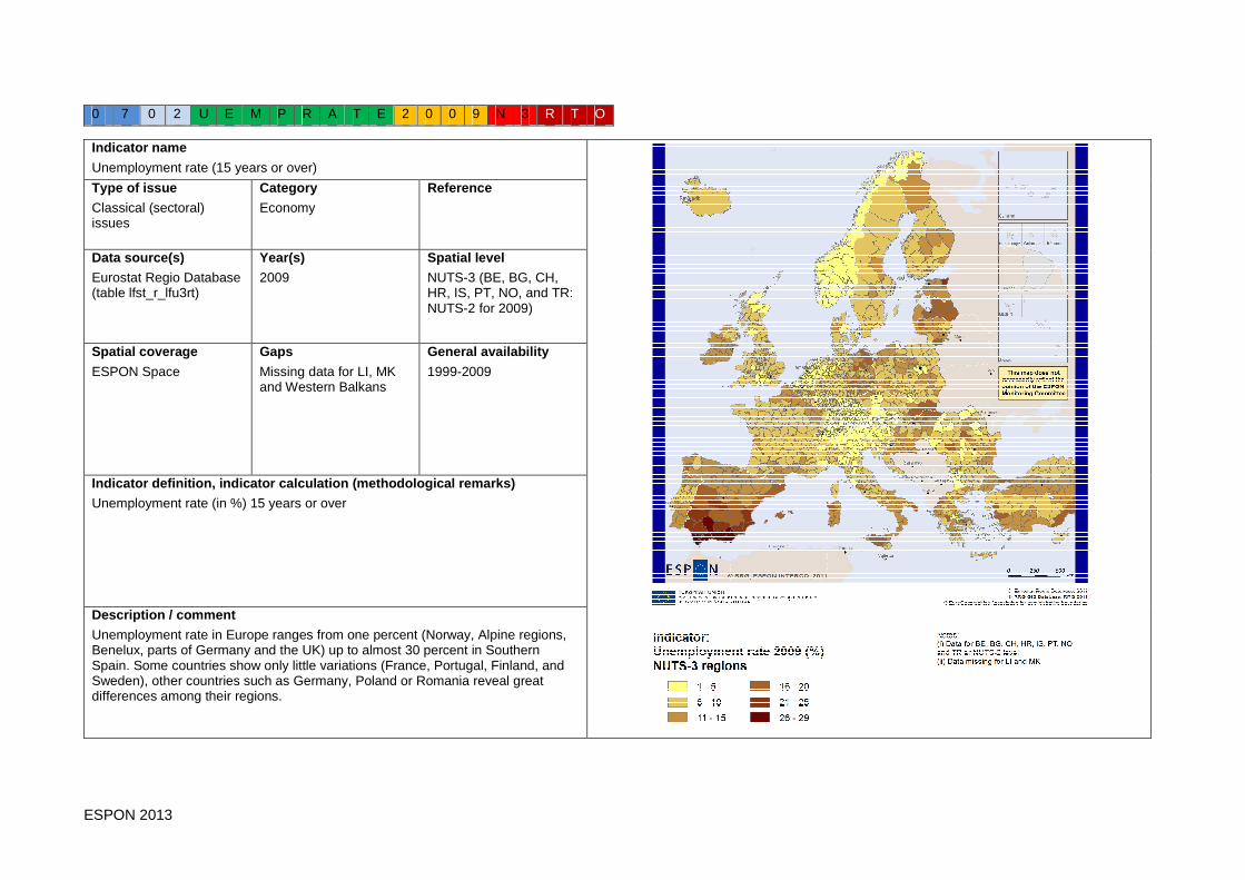
ESPON 2013 88

0 7 0 2 U E M P R A T E 2 0 0 9 N 3 R T O

Indicator name

Unemployment rate (15 years or over)

Type of issue

Classical (sectoral) issues

Category

Economy

Reference

Data source(s)

Eurostat Regio Database (table lfst_r_lfu3rt)

Year(s)

2009

Spatial level

NUTS-3 (BE, BG, CH, HR, IS, PT, NO, and TR: NUTS-2 for 2009)

Spatial coverage

ESPON Space

Gaps

Missing data for LI, MK and Western Balkans

General availability

1999-2009

Indicator definition, indicator calculation (methodological remarks)

Unemployment rate (in %) 15 years or over

Description / comment

Unemployment rate in Europe ranges from one percent (Norway, Alpine regions, Benelux, parts of Germany and the UK) up to almost 30 percent in Southern Spain. Some countries show only little variations (France, Portugal, Finland, and Sweden), other countries such as Germany, Poland or Romania reveal great differences among their regions.

ESPON 2013 89

0 7 0 2 U E M P D E V 0 0 0 9 N 3 R T O

Indicator name

Development of unemployment rate (15 years or over)

Type of issue

Classical (sectoral) issues

Category

Economy

Reference

Data source(s)

Eurostat Regio Database (table lfst_r_lfu3rt)

Year(s)

2009

Spatial level

NUTS-3 (BE, BG, CH, HR, IS, PT, NO, and TR: NUTS-2 for 2009)

Spatial coverage

ESPON Space

Gaps

Missing data for BG, CH, DE, DK, SI, TR, Western Balkans and Scotland (due to lack of data for 2000)

General availability

1999-2009

Indicator definition, indicator calculation (methodological remarks)

Unemployment rate (15 years or over), change 2000-2009 in percentage points. Increasing percentage points represent increasing unemployment rates, while decreasing percentage points represent lower unemployment rates in 2009, compared to 2000.

Description / comment

Development of unemployment rates differed to large extent across Europe. While regions in Poland, Finland and Southern Italy experienced a fall in unemployment rates, Sweden, Iceland, Ireland, England, parts of Spain, Italy and Hungary experienced significant increase in unemployment rates, partly as high as 20 percentage points.

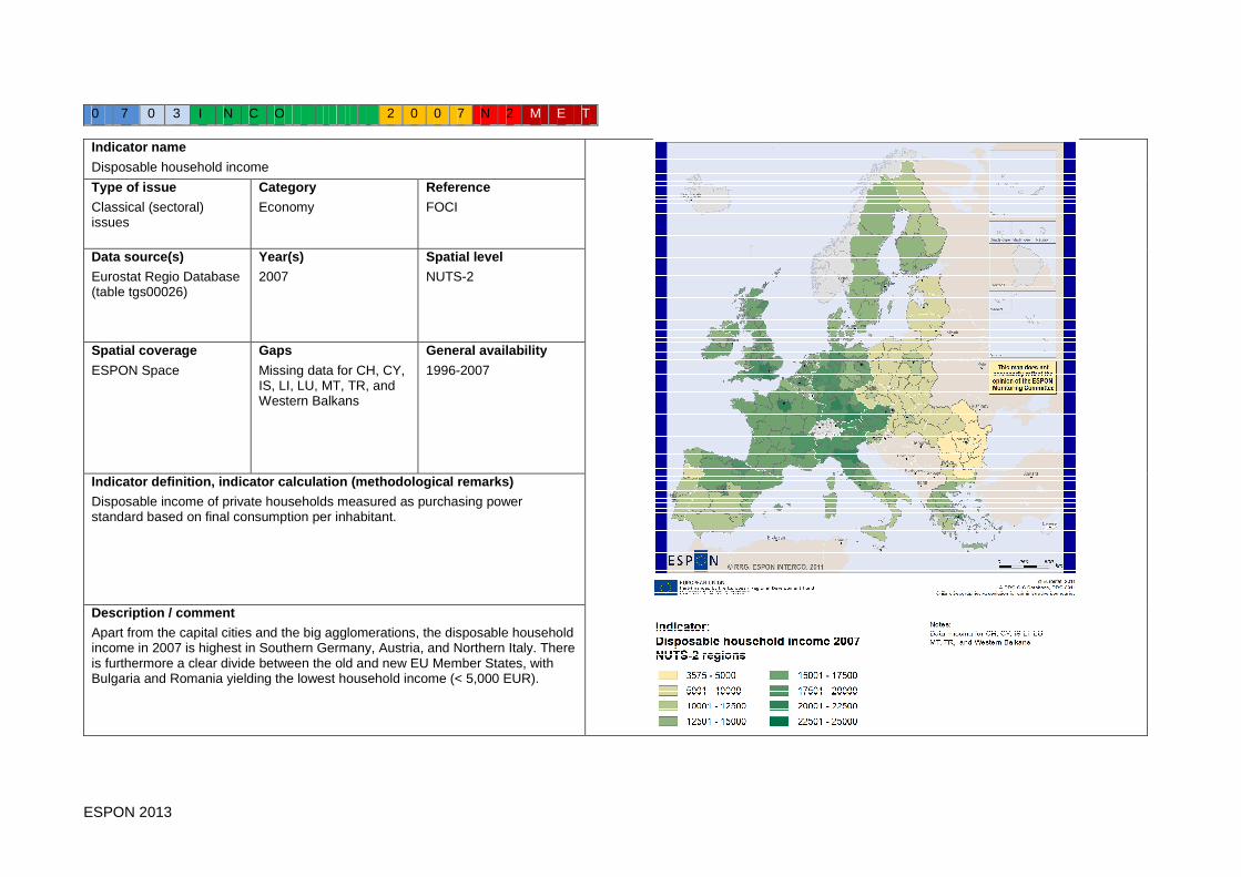
ESPON 2013 90

0 7 0 3 I N C O 2 0 0 7 N 2 M E T

Indicator name

Disposable household income

Type of issue

Classical (sectoral) issues

Category

Economy

Reference

FOCI

Data source(s)

Eurostat Regio Database (table tgs00026)

Year(s)

2007

Spatial level

NUTS-2

Spatial coverage

ESPON Space

Gaps

Missing data for CH, CY, IS, LI, LU, MT, TR, and Western Balkans

General availability

1996-2007

Indicator definition, indicator calculation (methodological remarks)

Disposable income of private households measured as purchasing power standard based on final consumption per inhabitant.

Description / comment

Apart from the capital cities and the big agglomerations, the disposable household income in 2007 is highest in Southern Germany, Austria, and Northern Italy. There is furthermore a clear divide between the old and new EU Member States, with Bulgaria and Romania yielding the lowest household income (< 5,000 EUR).

ESPON 2013 91

0 7 0 3 I N C O G R W 0 0 0 7 N 2 R T T

Indicator name

Disposable household income, growth 2000-2007 (% of 2000)

Type of issue

Classical (sectoral) issues

Category

Economy

Reference

FOCI

Data source(s)

Eurostat Regio Database (table tgs00026)

Year(s)

2007

Spatial level

NUTS-2

Spatial coverage

ESPON Space

Gaps

Missing data for CH, CY, IS, LI, LU, MT, TR, Western Balkans, Scotland

General availability

1996-2007

Indicator definition, indicator calculation (methodological remarks)

Disposable income of private households measured as purchasing power standard based on final consumption per inhabitant. Growth rate defined as income growth expressed in percent of 2000 income.

Description / comment

Almost all regions in Europe gained increases in disposable household income between 2000 and 2007, except for some few ones. Highest relative gains allocated in East European countries, i.e. Baltic States and Bulgaria and Romania, but starting from extremely low levels; in contrast, gains in Germany, Benelux, or Italy are smaller in relative terms, but starting from a much higher level.

ESPON 2013 92

0 7 0 2 E M P T R A N S 2 0 0 7 N 3 R T O

Indicator name

Employment in wholesale and retail trade; hotels and restaurants; transport (%)

Type of issue

Classical (sectoral) issues

Category

Economy

Reference

Data source(s)

Eurostat Regio Database (table nama_r_e3empl95)

Year(s)

2007

Spatial level

NUTS-2

Spatial coverage

ESPON Space

Gaps

Data missing for CH, IS, TR, Northern Ireland and Western Balkan

General availability

2000-2007

Indicator definition, indicator calculation (methodological remarks)

The indicator is redefined as “Employment in wholesale and retail trade; hotels and restaurants; transport” and was expressed in percent on total employment (%).

Description / comment

High proportions of employment in wholesale and retail trade, hotels and restaurant, and transport can first of all be found in coastal regions all over Europe, in particular at Mediterranean Sea, but also in other touristic destinations like the Alps. Significant lower shares are found in Eastern Europe, mainly Bulgaria, Poland and Romania, and in Northern Scandinavia. In Germany, Spain and Italy the situation is very mixed with regions yielding high shares next to regions with rather low percentages.

ESPON 2013 93

0 7 0 2 E M P T R A N D 0 0 0 7 N 3 R T O

Indicator name

Employment in wholesale and retail trade; hotels and restaurants; transport, growth 2000-2007 (in % of 2000 employment)

Type of issue

Classical (sectoral) issues

Category

Economy

Reference

Data source(s)

Eurostat Regio Database (table nama_r_e3empl95)

Year(s)

2000-2007

Spatial level

NUTS-2

Spatial coverage

ESPON Space

Gaps

Data missing for CH, IS, TR, Northern Ireland and Western Balkan; data for NL & UK missing for 2000

General availability

2000-2007

Indicator definition, indicator calculation (methodological remarks)

The indicator is redefined as “Employment in wholesale and retail trade; hotels and restaurants; transport” and was expressed in percent on total employment (%). Growth rate 2000-2007 was calculated as change in employment expressed in percent of 2000 level.

Description / comment

Even though shares in Eastern Europe are still quite low in 2007, many of these regions increased shares significantly in the period 2000-2007, though from a very low level. Otherwise, regions in Spain, Italy, Greece, France and Ireland also increased employment in these sectors. Since this NACE classification does not allow to differentiate between tourism industries and transport, increasing shares for some regions may be due to tourism sector, while in other regions it may be due to logistics and forwarders activities. On the other hand, there are also regions scattered across Europe who experienced absolute reduction in employment in these sectors since the year 2000.

ESPON 2013 94

0 7 0 2 R D E X P 2 0 0 9 N 0 R T O

Indicator name

Total R&D expenditures

Type of issue

Classical (sectoral) issues

Category

Economy

Reference

Data source(s)

Eurostat Regio Database (table tsc00001)

Year(s)

2009

Spatial level

NUTS-0

Spatial coverage

ESPON Space

Gaps

Data missing for CH, GR, IS and Western Balkan

General availability

1999-2010

Indicator definition, indicator calculation (methodological remarks)

Total R&D expenditures as percentage of GDP (=R&D intensity)

Description / comment

The R&D intensity is highest in Denmark, Finland and Sweden with more than 3 % of GDP, followed by Austria, France and Germany. Latvia, Romania and Slovakia, on the other hand, spent only less than 0.5 % of its GDP for R&D, which represents the lowest R&D intensity in Europe. Generally, East European countries show smaller shares compared to the old EU Member States.

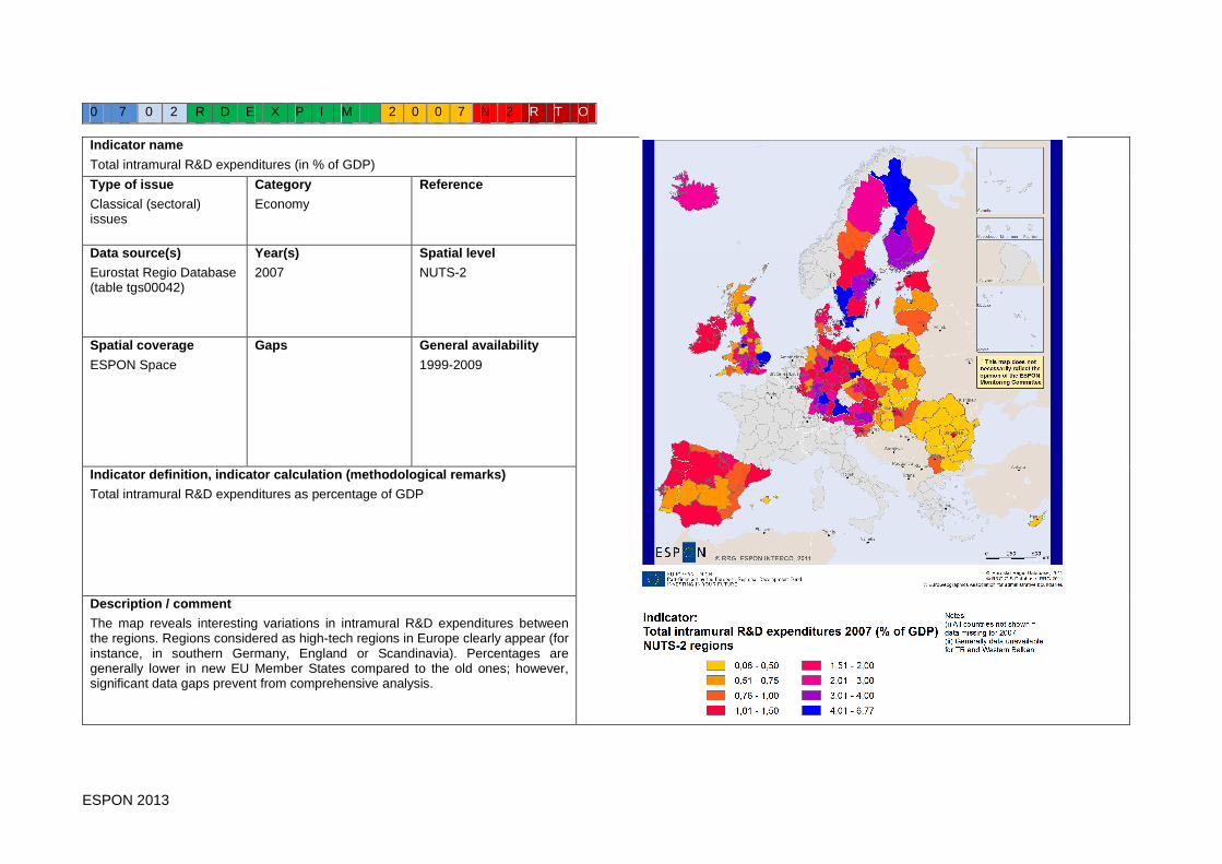
ESPON 2013 95

0 7 0 2 R D E X P I M 2 0 0 7 N 2 R T O

Indicator name

Total intramural R&D expenditures (in % of GDP)

Type of issue

Classical (sectoral) issues

Category

Economy

Reference

Data source(s)

Eurostat Regio Database (table tgs00042)

Year(s)

2007

Spatial level

NUTS-2

Spatial coverage

ESPON Space

Gaps

General availability

1999-2009

Indicator definition, indicator calculation (methodological remarks)

Total intramural R&D expenditures as percentage of GDP

Description / comment

The map reveals interesting variations in intramural R&D expenditures between the regions. Regions considered as high-tech regions in Europe clearly appear (for instance, in southern Germany, England or Scandinavia). Percentages are generally lower in new EU Member States compared to the old ones; however, significant data gaps prevent from comprehensive analysis.

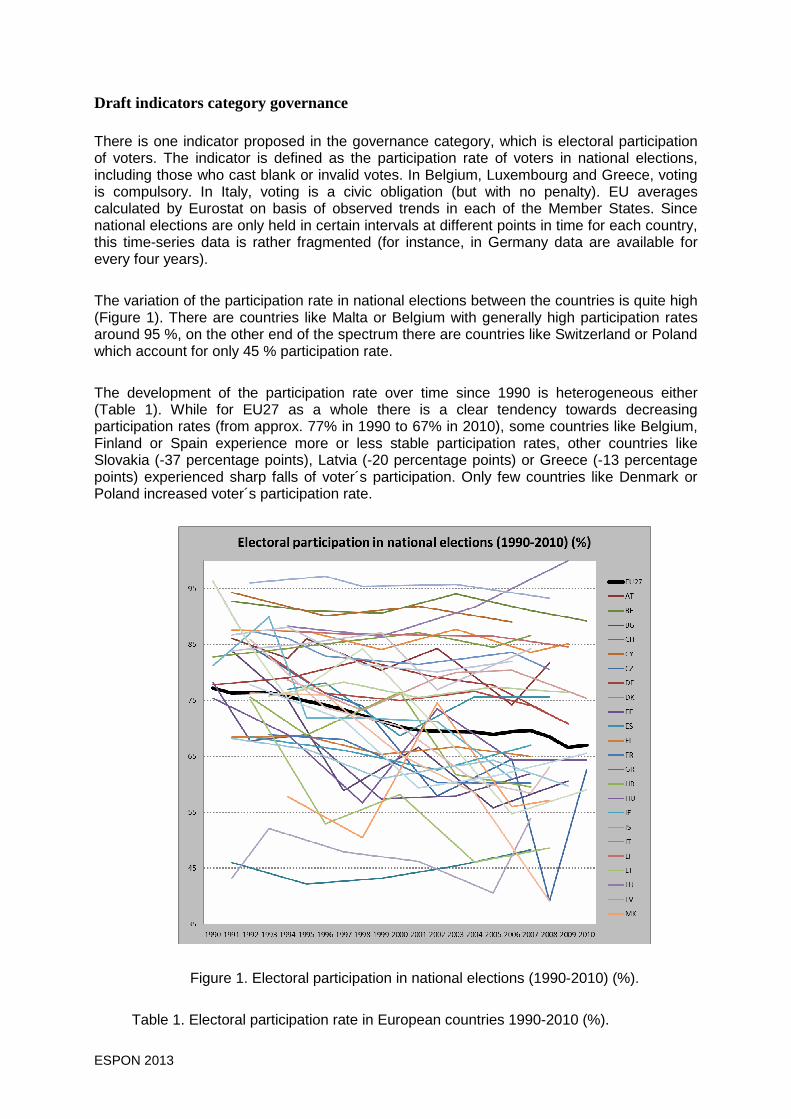
ESPON 2013 96

Draft indicators category governance There is one indicator proposed in the governance category, which is electoral participation of voters. The indicator is defined as the participation rate of voters in national elections, including those who cast blank or invalid votes. In Belgium, Luxembourg and Greece, voting is compulsory. In Italy, voting is a civic obligation (but with no penalty). EU averages calculated by Eurostat on basis of observed trends in each of the Member States. Since national elections are only held in certain intervals at different points in time for each country, this time-series data is rather fragmented (for instance, in Germany data are available for every four years). The variation of the participation rate in national elections between the countries is quite high (Figure 1). There are countries like Malta or Belgium with generally high participation rates around 95 %, on the other end of the spectrum there are countries like Switzerland or Poland which account for only 45 % participation rate. The development of the participation rate over time since 1990 is heterogeneous either (Table 1). While for EU27 as a whole there is a clear tendency towards decreasing participation rates (from approx. 77% in 1990 to 67% in 2010), some countries like Belgium, Finland or Spain experience more or less stable participation rates, other countries like Slovakia (-37 percentage points), Latvia (-20 percentage points) or Greece (-13 percentage points) experienced sharp falls of voter´s participation. Only few countries like Denmark or Poland increased voter´s participation rate.

Figure 1. Electoral participation in national elections (1990-2010) (%).

Table 1. Electoral participation rate in European countries 1990-2010 (%).

ESPON 2013 97

CC 90 91 92 93 94 95 96 97 98 99 00 01 02 03 04 05 06 07 08 09 10

EU27 77 76 76 76 76 75 74 73 72 71 70 70 70 69 69 69 69 70 69 67 67

AT 86 83 86 80 84 74 82

BE 93 91 91 94 91 89

BG 84 75 59 67 56 61

CH 46 42 43 45 48

CY 94 90 92 89

CZ 96 85 76 74 58 65 39 63

DE 78 79 82 79 78 71

DK 83 84 86 87 85 87

EE 78 68 69 57 58 62

ES 77 78 69 76 76

FI 68 69 65 67 65

FR 69 68 60 60

GR 83 76 75 77 74 71

HR 76 69 77 62 60

HU 75 69 57 74 64 64

IE 69 66 63 67

IS 88 87 84 88 84 85

IT 87 86 83 81 84 81

LI 88 87 87 87 85

LT 75 53 58 46 49

LU 88 87 92 100

LV 81 90 72 72 71 61

MK 58 51 75 56 57

MT 96 97 95 96 93

NL 79 73 79 80 80 75

NO 76 78 76 77 76

PL 43 52 48 46 41 54

PT 68 66 61 63 64 60

RO 76 76 65 59 39

SE 87 88 81 80 82

SI 86 74 70 61 58 63

SK 96 85 75 84 70 55 59

TR 84 85 87 77 84

UK 78 72 59 61 66

ESPON 2013 98

0 9 0 1 G O V R 2 0 0 9 N 0 R T O

Indicator name

Electoral participation in national election (in %)

Type of issue

Classical (sectoral) issues

Category

Governance

Reference

Data source(s)

Eurostat Regio Database (code tsdgo310)

Year(s)

Most recent year of nat. election (period 2007-2010)

Spatial level

NUTS-0

Spatial coverage

ESPON Space

Gaps

Missing data for Western Balkan.

General availability

1990-2010

Indicator definition, indicator calculation (methodological remarks)

Percent of voters who cast a vote or “turn out” at an election, including those who cast blank or invalid votes. In Belgium, Luxembourg and Greece, voting is compulsory. In Italy, voting is a civic obligation (but with no penalty). EU averages calculated by Eurostat on basis of observed trends in each of the Member States. Since national elections are only held in certain intervals at different points in time for each country, this time-series data is rather fragmented (for instance, in Germany data are available for every four years).

Description / comment

The variation of the participation rate in national elections between the countries is quite high. There are countries like Malta or Belgium with generally high participation rates around 95 %, on the other end of the spectrum there are countries like Switzerland, Lithuania, Romania or Poland which account for less than 50% participation rate.

ESPON 2013 99

Draft indicators category territorial cohesion The Human Development Index (HDI) as promoted and regularly calculated by the UNDP is selected as the only indicator under the territorial cohesion category. The HDI is a composite indicator at national level used to rank countries by level of “human development”. It is composed from data on life expectancy, education and per-capita GNI, collected at national level. An indicator value of 1 is best (optimum development index), while a value of 0 is the worst situation. The HDI for Europe clearly shows five groups of countries: best performers which are Norway, Sweden, Ireland, Netherlands and Germany (with Norway being the best-performing country world-wide in 2010). Following is a second group of countries with Belgium, Switzerland, France, Spain, Iceland and Finland, as well as a third group consisting of Austria, Italy, Czech Republic, Greece and the UK. Then two groups of countries follow which perform rather badly (Baltic States, Poland, Slovakia, Slovenia, Hungary, Portugal, Croatia), followed by the rest. All European countries improved their HDI since 1980, in particular Spain, Turkey and also Norway. However, Turkey is still the worst-performing country in Europe, ranking only 83 position world-wide (Table 1). Since an indicator value of 1 is considered the optimum, to which all countries strive, following Figure 1 a trend towards cohesion / convergence of human development in Europe at national level can be observed. Though, eleven countries in Europe are still considered by UNDP ‘only’ of high human development, starting with Lithuania.

Figure 1. Human development index, 1980-2010, European countries (UNDP, 2011).

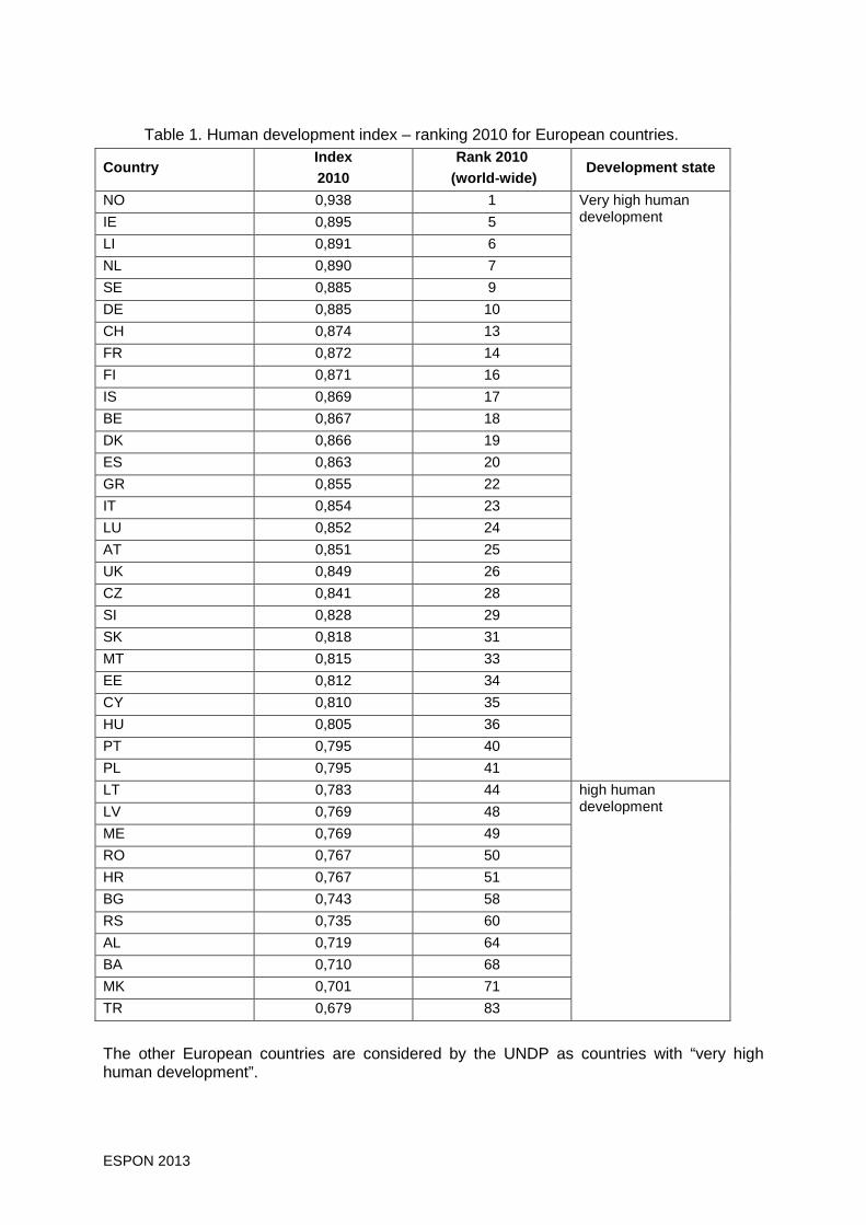
ESPON 2013 100

Table 1. Human development index – ranking 2010 for European countries.

Country Index 2010

Rank 2010 (world-wide)

Development state

NO 0,938 1

IE 0,895 5

LI 0,891 6

NL 0,890 7

SE 0,885 9

DE 0,885 10

CH 0,874 13

FR 0,872 14

FI 0,871 16

IS 0,869 17

BE 0,867 18

DK 0,866 19

ES 0,863 20

GR 0,855 22

IT 0,854 23

LU 0,852 24

AT 0,851 25

UK 0,849 26

CZ 0,841 28

SI 0,828 29

SK 0,818 31

MT 0,815 33

EE 0,812 34

CY 0,810 35

HU 0,805 36

PT 0,795 40

PL 0,795 41

Very high human development

LT 0,783 44

LV 0,769 48

ME 0,769 49

RO 0,767 50

HR 0,767 51

BG 0,743 58

RS 0,735 60

AL 0,719 64

BA 0,710 68

MK 0,701 71

TR 0,679 83

high human development

The other European countries are considered by the UNDP as countries with “very high human development”.

ESPON 2013 101

1 0 0 1 H D I R T S T 2 0 1 0 N 0 O R D

Indicator name

Human development index (HDI)

Type of issue

Complex territorial issues

Category

Territorial cohesion

Reference

Human Development Report

Data source(s)

UNDP

Year(s)

2010

Spatial level

NUTS-0

Spatial coverage

ESPON Space

Gaps

n.a.

General availability

1980-2010 in 5-year intervals

Indicator definition, indicator calculation (methodological remarks)

The HDI is a composite indicator used to rank countries by level of “human development”. It is composed from data on life expectancy, education and per-capita GNI, collected at national level. A value of 1 is best (optimum development index), while a value of 0 is the worst situation.

Description / comment

The HDI for Europe clearly shows five groups of countries: best performers which are Norway, Sweden, Ireland, Netherlands and Germany (with Norway being the best-performing country world-wide in 2010). Following is a second group of countries with Belgium, Switzerland, France, Spain, Iceland and Finland, as well as a third group consisting of Austria, Italy, Czech Republic, Greece and the UK. Then two groups of countries follow which perform rather badly (Baltic States, Poland, Slovakia, Slovenia, Hungary, Portugal, Croatia), followed by the rest.

ESPON 2013 102

Draft indicators category balance and polycentricity Several indicators have been identified under this category, which are: - dependency ratio - ageing index - population potential within 50 km - life expectancy at birth - high education of population - distance to MEGAs

Since two of the indicators were also assigned under demography category (life expectancy) and category transport, accessibility and communication (high education), they are not presented here again. So the following discussion only concerns the dependency rate, ageing index, population potential within 50 km and the distance to MEGAs. Dependency ratio (old-age dependency ratio) This indicator is defined as the number of persons aged 65 and over expressed as a percentage of the number of persons aged between 15 and 64. It measures the relation between the elderly (retired) population and the working-age population. The issue here is that the higher the ratio (share) is the fewer workers need to obtain pension of the increasing number of retired pensioners. In this sense the old-age dependency ratio becomes a social concern in countries experiencing a significant shift in the age pyramid towards overaging. Generally the indicator illustrates that the size of the working-class population in East European countries is higher compared to West European or Scandinavian countries, as more people in working-age exist compared to elderly people. But even in Western Europe there are distinct areas with extremely high dependency ratios, such as in South of France, East Germany, border area between Spain and Portugal or Greece, leading to high variations in indicator performance at NUTS-3 level within the countries (see Figure 1). Even though variations for all countries are quite high with often 10-15 percentage points difference between the worst and best performing region, the Spain, Germany, Portugal, Greece and France are remarkable since they yield extremely big variations up to 30 percentage points. Variations over time remain stable for most countries, as the development of the coefficients of variation in Figure 2 show. The coefficient decreased only for few countries (Austria, Bulgaria, Portugal), indicating convergence in indicator performance over time; for Belgium and Turkey the coefficient even increased (polarization trend). Interestingly, for Malta the disparities reduced until 2006, but since 2008 an opposite trend with increasing disparities can be observed again. The remaining countries experienced only very small changes in the coefficient of variation in the ten years 2000-2010.

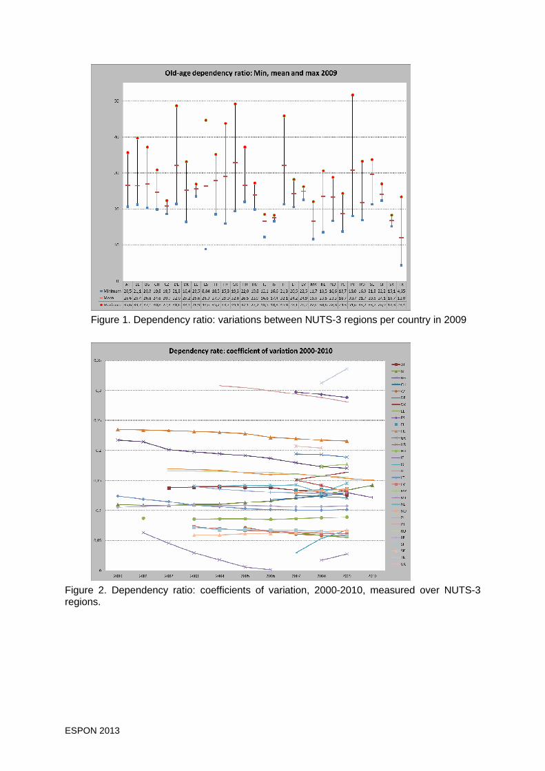
ESPON 2013 103

Figure 1. Dependency ratio: variations between NUTS-3 regions per country in 2009

Figure 2. Dependency ratio: coefficients of variation, 2000-2010, measured over NUTS-3 regions.

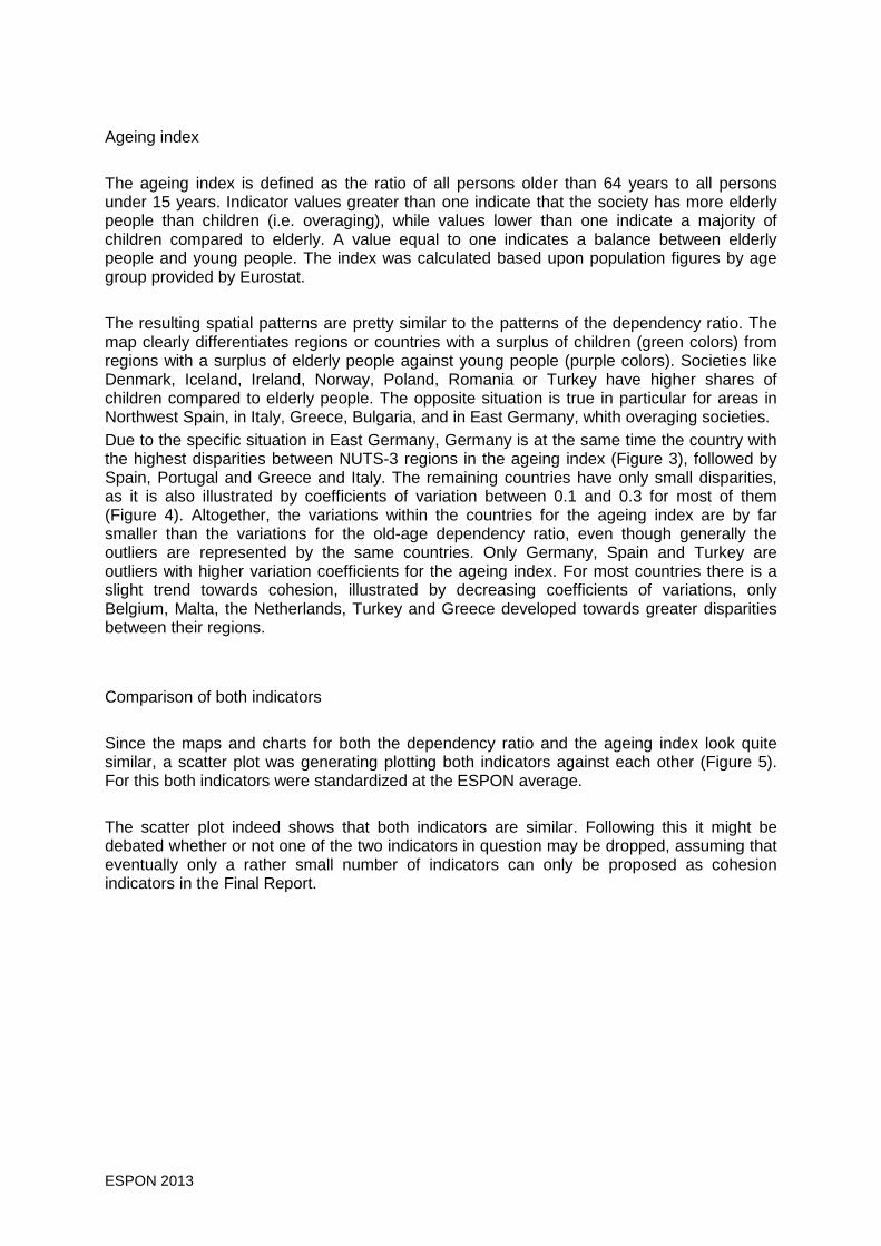
ESPON 2013 104

Ageing index

The ageing index is defined as the ratio of all persons older than 64 years to all persons under 15 years. Indicator values greater than one indicate that the society has more elderly people than children (i.e. overaging), while values lower than one indicate a majority of children compared to elderly. A value equal to one indicates a balance between elderly people and young people. The index was calculated based upon population figures by age group provided by Eurostat. The resulting spatial patterns are pretty similar to the patterns of the dependency ratio. The map clearly differentiates regions or countries with a surplus of children (green colors) from regions with a surplus of elderly people against young people (purple colors). Societies like Denmark, Iceland, Ireland, Norway, Poland, Romania or Turkey have higher shares of children compared to elderly people. The opposite situation is true in particular for areas in Northwest Spain, in Italy, Greece, Bulgaria, and in East Germany, whith overaging societies. Due to the specific situation in East Germany, Germany is at the same time the country with the highest disparities between NUTS-3 regions in the ageing index (Figure 3), followed by Spain, Portugal and Greece and Italy. The remaining countries have only small disparities, as it is also illustrated by coefficients of variation between 0.1 and 0.3 for most of them (Figure 4). Altogether, the variations within the countries for the ageing index are by far smaller than the variations for the old-age dependency ratio, even though generally the outliers are represented by the same countries. Only Germany, Spain and Turkey are outliers with higher variation coefficients for the ageing index. For most countries there is a slight trend towards cohesion, illustrated by decreasing coefficients of variations, only Belgium, Malta, the Netherlands, Turkey and Greece developed towards greater disparities between their regions. Comparison of both indicators Since the maps and charts for both the dependency ratio and the ageing index look quite similar, a scatter plot was generating plotting both indicators against each other (Figure 5). For this both indicators were standardized at the ESPON average. The scatter plot indeed shows that both indicators are similar. Following this it might be debated whether or not one of the two indicators in question may be dropped, assuming that eventually only a rather small number of indicators can only be proposed as cohesion indicators in the Final Report.

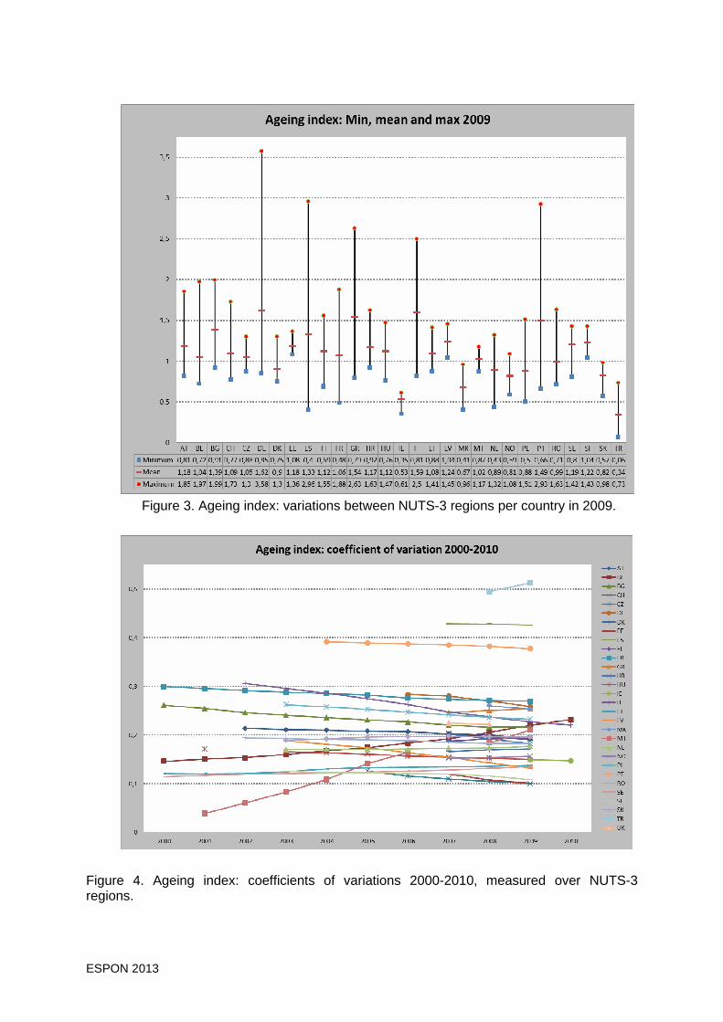
ESPON 2013 105

Figure 3. Ageing index: variations between NUTS-3 regions per country in 2009.

Figure 4. Ageing index: coefficients of variations 2000-2010, measured over NUTS-3 regions.

ESPON 2013 106

Figure 5. Comparison of dependency ration with ageing index for 2009.

Population potential within 50 km The indicator is defined as the number of people within reach of 50 km airline distance for each 2.5 x 2.5 km raster cell. This potential indicates the “daily life” type of service provision that requires certain minimum potential within reasonable distance or travel time, if the origin becomes a center for private or public service provision. In order to highlight regions that are above or below the European average, the indicator has been standardized at this average. This indicator was first developed in the EU Parliament Cohesion Study (Dubois, 2007) at raster level. Within INTERCO, the results were also aggregated to NUTS2/3 level. The map highlights the stronger population potential that lies in the most urbanized parts of Europe: the Benelux countries, Western Germany, Southern England and Northern Italy. But more importantly, the map also highlights that territories in the New Member States, but also in other ‘peripheral’ parts Iberian Peninsula, or even Scandinavia, often enjoy a rather high population potential. By this the importance of regional centers in Poland, Czech Republic, Hungary, Rumania or Spain becomes apparent. On the other hand, the map also shows large areas with below-average potentials in France, Spain, Austria and other parts of Europe.

ESPON 2013 107

The aggregated indicator map at NUTS2/3 level basically shows the same picture as the corresponding raster map, with Benelux, West Germany, South England and North Italy being the regions with the highest population potential within 50 km airline distance; however, the aggregated maps hides many of the regional city hubs that are visible in the continuous map, such as those in Scandinavia, in the Baltic States, in East Europe but also in Spain, Portugal or Greece. The variation in terms of range of values at raster level within the countries are significant, not only for usual subjects like Germany, France, Italy or UK, but also for countries like Netherlands, Spain, Belgium, or Poland (Figure 6). However, these results are not subject to the overall size of the country territory, as the small variations for Sweden or Finland show, just to mention two countries with rather great territories in the ESPON space.

Figure 6. Population potential (50 km): Variations within the countries (raster level).

Variations within countries measured over raster level expressed as coefficient of variation are shown in Figure 7. The ranking of countries from this with smallest variations (Liechtenstein, top) to those with greatest variation (Norway, bottom) is clearly a function of the potential and size of the territory. As expected, those countries with a great range of indicator values and a great overall territory experience the greatest variations.

ESPON 2013 108

Figure 7. Population potential (50 km): Coefficients of variation measured at raster level. Distance to MEGAs Metropolitan European Growth Areas (MEGAs) first have been identified in ESPON 1.1.1 project, and since then have been analysed in various other projects. They are considered as the key driving engines for European economic, social and spatial development. In order to analyse to what extend surrounding regions may benefit from positive developments within the MEGAs, the indicator distance to MEGAs was proposed as a potential candidate as cohesion indicator. Actually, two different distance indicates are tested:

- distance to next MEGA - average distance to all MEGAs

As points of origin, a system of 2.5 x 2.5 raster cells has been used, similar to the one used in the EU Parliament Cohesion Study (Dubois et al., 2007). Raster results are then aggregated to NUTS2/3 level as weighted averages. As destinations, a layer of 76 MEGA centroids defined in ESPON 1.1.1 was used. The distances between the raster cells and MEGAs were then calculated by means of GIS techniques. The first map illustrates distances to next MEGA at raster level. Concentric rings around the MEGA centres are shown. Only in some countries the rings overlap, forming continuous surfaces of uniform distances (Benelux, West Germany, Northern Italy, Poland, and England). Most parts of Europe are located between 100 and 500 km distance away from the next MEGA, areas in Romania, Greece, Scandinavia, Southern Italy, Scotland, France and Spain are even farther away, implying extremely long travel distances/times to reach the MEGA centre.

ESPON 2013 109

The results aggregated to NUTS2/3 level show continuous regions with on average short distances to the next MEGA, with a seamless coverage ranging from Northern France via Benelux and Northern Germany towards Poland; similarly another set of regions ranges from Valencia in Spain along the Mediterranean Sea via France and Northern Italy towards Naples. Regions in central parts of France, in Spain, most regions in Romania, Bulgaria, Greece and Northern Scandinavia, however, experience mean distances of more than 250 km. For most countries, the maximum distance to next MEGA is less than 200 km (Austria, Belgium, Switzerland etc.) (Figure 8). Some East European countries experience maximum distances between 200 and 400 km due to the low density of MEGAs, while in extreme cases (country with islands, big countries), the maximum distance exceeds 900 km (Sweden) or 1,000 km (Finland, Norway, Spain, Portugal). Spain and Portugal are exceptional (Figure 9), since the value range is dominated from the islands (Madeira, Baleares, and Azores). The average distance for most countries, except for the three Nordic countries Finland, Norway and Sweden, lies between 100 and 200 km.

Figure 8. Distance to next MEGA: variations within countries at raster level. Since most of the MEGAs are located more or less in the geographical centre of Europe, the map at raster level illustrating the average airline distance to all MEGAs shows concentric rings around the geographical centre of Europe, with the centre being located somewhere in the middle of Germany. The picture at NUTS2/3 level follows the one at raster level: Regions in the heart of Europe reveal shortest average distances to all MEGAs, with increasing distances the farther away they are located from the geographical centre. These, eventually, very simple results for the average distance to all MEGAs indicator disqualify the indicator from being a cohesion indicator. The indicator distance to next MEGA, however, has some potentials as a cohesion indicator, however, there are great similarities in the output with the indicator population potential within 50 km. The advantage of the latter indicator being that it is a dynamic indicator which changes as soon as new population figures are available, while the distance to next MEGA indicator remains the same over time

ESPON 2013 110

as the distance will not change. In this sense the indicator on population potential within 50 km is preferable over the distance to MEGA indicator.

Figure 9. Distance to next MEGA: coefficients of variation.

Thus, both MEGA indicators will not be recommended as cohesion indicators. This assessment will not change even if the definition of the indicator will be changed. For instance, instead of distance to next MEGA or average distance to all MEGAs the indicator could be defined as average distance to next X MEGA, where X could be any number between 1 and 76. Another modification could be to use all FUA centroids as defined in ESPON 1.1.1 as destinations, and not only the MEGA as being most prominent examples of a FUA. In any case, it is not to expect that results will change significantly; the results of any such indicator will always be similar to the indicator population potential within 50 km.

ESPON 2013 111

1 0 0 2 O A D E P R A T 2 0 0 9 N 3 R T O

Indicator name

Dependency ratio (old-age dependency ratio)

Type of issue

Complex territorial issues

Category

Balance and policentricity

Reference

Euroislands

Data source(s)

Eurostat Regio Database (table demo_r_pjanaggr3)

Year(s)

2009

Spatial level

NUTS-3

Spatial coverage

ESPON Space

Gaps

Data missing for 2009 for UK and Western Balkan

General availability

2000-2010

Indicator definition, indicator calculation (methodological remarks)

This indicator is defined as the number of persons aged 65 and over expressed as a percentage of the number of persons aged between 15 and 64. It measures the relation between the elderly (retired) population and the working-age population. The issue here is that the higher the ratio (share) is the fewer workers need to obtain pension of the increasing number of retired pensioners.

Description / comment

Generally the map illustrates that the size of the working-class population in East European countries is higher compared to West European or Scandinavian countries, as more people in working-age exist compared to elderly people. But even in Western Europe there are distinct areas with extremely high dependency ratios, for instance in South of France, East Germany, border area between Spain and Portugal or Greece.

ESPON 2013 112

1 0 0 2 A G E I 2 0 0 9 N 3 R T O

Indicator name

Ageing index

Type of issue

Complex territorial issues

Category

Balance and policentricity

Reference

Data source(s)

Eurostat Regio Database (table demo_r_pjanaggr3)

Year(s)

2009

Spatial level

NUTS-3

Spatial coverage

ESPON Space

Gaps

Data missing for 2009 for UK and Western Balkan

General availability

2000-2010

Indicator definition, indicator calculation (methodological remarks)

The ageing index is defined as the ratio of all persons older than 64 years to all persons under 15 years. Indicator values > 1 indicate that the society has more elderly people than children (i.e. overaging), while values < 1 indicate a majority of children compared to elderly. A value of 1 indicates a balance between elderly people and young people.

Description / comment

The map clearly differentiates regions or countries with a surplus of children (green colors) from regions with a surplus of elderly people against young people (purple colors). Societies like Denmark, Iceland, Ireland, Norway, Poland, Romania or Turkey have higher shares of children compared to elderly people. The opposite situation is true in particular for areas in Northwest Spain, in Italy, Greece, Bulgaria, and in East Germany, with overaging societies.

ESPON 2013 113

1 0 0 2 P O P P O T 2 0 0 7 G R M E T

Indicator name

Population potential within 50 km

Type of issue

Complex territorial issues

Category

Balance and policentricity

Reference

European Parliament Cohesion Study

Data source(s)

RRG, based upon EEA population grid

Year(s)

2007

Spatial level

2.5 x 2.5 km raster grid

Spatial coverage

ESPON Space

Gaps

Data missing for CH, IS, TR, and Western Balkans

General availability

2007

Indicator definition, indicator calculation (methodological remarks)

The indicator is defined as the number of people within reach of 50 km airline distance for each 2.5 x 2.5 km raster cell. This potential indicates the “daily life” type of service provision that requires certain minimum potential within reasonable distance or travel time, if the origin becomes a center for private or public service provision. In order to highlight regions that are above or below the European average, the indicator has been standardized at this average.

Description / comment

The map highlights the stronger population potential that lies in the most urbanized parts of Europe: the Benelux countries, Western Germany, Southern England and Northern Italy. But more importantly, the map also highlights that territories in the New Member States, but also in other ‘peripheral’ parts Iberian Peninsula, or even Scandinavia, often enjoy a rather high population potential. By this the importance of regional centers in Poland, Czech Republic, Hungary, Rumania or Spain becomes apparent. On the other hand, the map also shows large areas with below-average potentials in France, Spain, Austria and other parts of Europe.

ESPON 2013 114

1 0 0 2 P O P P O T 2 0 0 7 N 2 M E T

Indicator name

Population potential within 50 km

Type of issue

Complex territorial issues

Category

Balance and policentricity

Reference

European Parliament Cohesion Study

Data source(s)

RRG, based upon EEA population grid

Year(s)

2007

Spatial level

NUTS-2/3

Spatial coverage

ESPON Space

Gaps

Data missing for CH, IS, TR, and Western Balkans

General availability

2007

Indicator definition, indicator calculation (methodological remarks)

The indicator is defined as the number of people within reach of 50 km airline distance. First, the indicator was calculated for 2.5 x 2.5 km raster cells, and then aggregated to NUTS2/3 level. This population potential indicates the “daily life” type of service provision that requires certain minimum potential within reasonable distance or travel time, if the origin becomes a center for private or public service provision. In order to highlight regions that are above or below the European average, the indicator has been standardized at this average.

Description / comment

The aggregated indicator map at NUTS2/3 level basically shows the same picture as the corresponding raster map, with Benelux, West Germany, South England and North Italy being the regions with the highest population potential within 50 km airline distance; however, the aggregated maps hides many of the regional city hubs that are visible in the continuous map, such as those in Scandinavia, in the Baltic States, in East Europe but also in Spain, Portugal or Greece.

ESPON 2013 115

1 0 0 2 M E G A O N E 2 0 1 1 G R M E T

Indicator name

Distance to next MEGA

Type of issue

Complex territorial issues

Category

Balance and policentricity

Reference

ESPON 1.1.1

Data source(s)

RRG, based upon ESPON 1.1.1 input

Year(s)

2011

Spatial level

Raster (2.5x2.5 km grid cells)

Spatial coverage

ESPON Space

Gaps

Data missing for CY, IS, TR, and Western Balkans

General availability

2011

Indicator definition, indicator calculation (methodological remarks)

Airline distance to next MEGA (in km). Non-EU countries excluded from processing since no MEGAs were defined.

Description / comment

The map illustrates concentric rings around the MEGA centres. Only in some countries the rings overlap, forming continuous surfaces of uniform distances (Benelux, West Germany, Northern Italy, Poland, and England). Most parts of Europe are located between 100 and 500 km distance away from the next MEGA, areas in Romania, Greece, Scandinavia, Southern Italy, Scotland, France and Spain are even farther away, implying extremely long travel distances/times to reach the MEGA centre.

ESPON 2013 116

1 0 0 2 M E G A O N E 2 0 1 1 N 2 M E T

Indicator name

Distance to next MEGA

Type of issue

Complex territorial issues

Category

Balance and policentricity

Reference

ESPON 1.1.1

Data source(s)

RRG, based upon ESPON 1.1.1 input

Year(s)

2011

Spatial level

NUTS2/3

Spatial coverage

ESPON Space

Gaps

Data missing for CY, IS, TR, and Western Balkans

General availability

2011

Indicator definition, indicator calculation (methodological remarks)

Airline distance to next MEGA (in km). Distances are first calculated at 2.5 x 2.5 km raster level, between each raster cell and the MEGA centroids. Results are then aggregated to NUTS2/3 level as weighted averages. Non-EU countries excluded from processing since no MEGAs were defined.

Description / comment

The results aggregated to NUTS2/3 level show continuous regions with on average short distances to the next MEGA, with a seamless coverage ranging from Northern France via Benelux and Northern Germany towards Poland; similarly another set of regions ranges from Valencia in Spain along the Mediterranean Sea via France and Northern Italy towards Naples. Regions in central parts of France, in Spain, most regions in Romania, Bulgaria, Greece and Northern Scandinavia, however, experience mean distances of more than 250 km.

ESPON 2013 117

1 0 0 2 M E G A A L L 2 0 1 1 G R M E T

Indicator name

Average distance to all MEGAs

Type of issue

Complex territorial issues

Category

Balance and policentricity

Reference

ESPON 1.1.1

Data source(s)

RRG, based upon ESPON 1.1.1 input

Year(s)

2011

Spatial level

Raster (2.5x2.5 km grid cells)

Spatial coverage

ESPON Space

Gaps

Data missing for CY, IS, TR, and Western Balkans

General availability

2011

Indicator definition, indicator calculation (methodological remarks)

Average airline distance to all MEGAs (in km). Non-EU countries excluded from processing since no MEGAs were defined.

Description / comment

Since most of the MEGAs are located more or less in the geographical centre of Europe, the map at raster level illustrating the average airline distance to all MEGAs shows concentric rings around the geographical centre of Europe, with the centre being located somewhere in the middle of Germany.

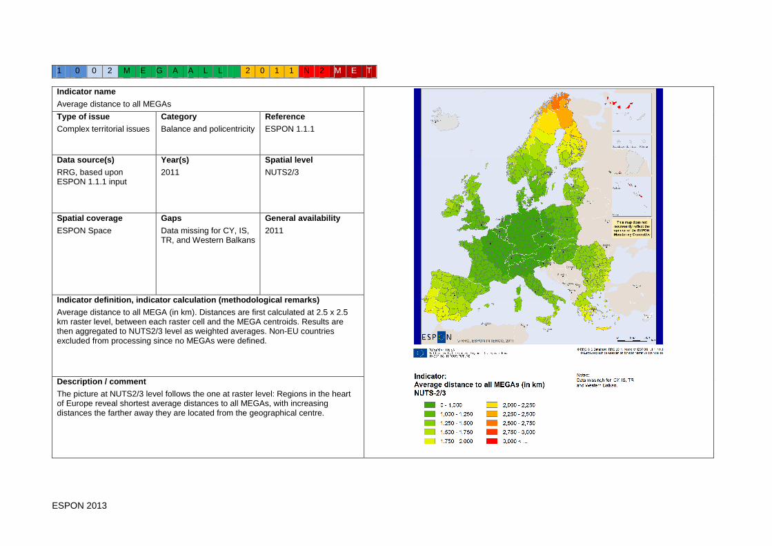
ESPON 2013 118

1 0 0 2 M E G A A L L 2 0 1 1 N 2 M E T

Indicator name

Average distance to all MEGAs

Type of issue

Complex territorial issues

Category

Balance and policentricity

Reference

ESPON 1.1.1

Data source(s)

RRG, based upon ESPON 1.1.1 input

Year(s)

2011

Spatial level

NUTS2/3

Spatial coverage

ESPON Space

Gaps

Data missing for CY, IS, TR, and Western Balkans

General availability

2011

Indicator definition, indicator calculation (methodological remarks)

Average distance to all MEGA (in km). Distances are first calculated at 2.5 x 2.5 km raster level, between each raster cell and the MEGA centroids. Results are then aggregated to NUTS2/3 level as weighted averages. Non-EU countries excluded from processing since no MEGAs were defined.

Description / comment

The picture at NUTS2/3 level follows the one at raster level: Regions in the heart of Europe reveal shortest average distances to all MEGAs, with increasing distances the farther away they are located from the geographical centre.

ESPON 2013 119

Indicator category environment and hazards There are several indicator candidates identified under this category, among them - Summer smog: ozone concentration - Summer smog: particular matter (PM10) - Renewable energy consumption - Per-capita consumption of water (public supply to households) - Per-capita consumption of water (total public water supply) - Residents connected to potable water systems - Residence density - Ares with high ecological value These indicators will be discussed in the following sections. Apart from the residence density indicator, which is a GIS indicator derived from the Corine land use layer that can be calculated for any spatial level, all other indicators under this category are only available with pan-European datasets at national level. While their spatial resolution is aggregated, all indicators are available as time series datasets, covering a period of time of at least the last ten years so that trends of cohesion can be analysed over time. Summer smog: ozone concentration This indicator is defined as the urban population exposure to air pollution by ozone. The indicator shows the population weighted yearly sum of maximum daily 8-hour mean ozone concentrations above a threshold (70 microgram Ozone per m3) at the urban background stations in agglomerations. Ozone is a strong photochemical oxidant, which causes serious health problems and damage to the ecosystem, agricultural crops and materials. Statistical data for ESPON space, are, however, only available at national level. Indicator results show that the ‚cleanest‘countries in terms of urban population exposed to ozone Ireland, Estonia and Latvia, followed by the Netherlands and the UK. On the other side of the spectrum Italy, Austria, Slovakia, Hungary and Slovenia are those countries with the highest exposure. The differences between the lowest (956) and highest exposure are remarkable (11,973). Given the huge political debate about air pollutants during the last decade, one could assume that the political measures taken to reduce ozone concentration resulted in a corresponding reduction in exposure figures. For EU27 as all (Figures 1 and 2) there is an overall tendency towards reduced ozone concentration observed between 1999 and 2008, however, reductions are very small (-3%). At national level, the development since 1999 is very different. The majority of countries yield a reduction in ozone concentration, but at very different rates. Belgium, Estonia, Italy, Latvia, Romania and also Iceland experienced major significant reduction of ozone concentrations of more than 30%, while other countries like Denmark (+5 %), Ireland (+45%), Greece (+67%), Hungary (+100%) or Portugal (+98%) saw strong increases in ozone concentration. Thus, there is no clear tendency towards cohesion or increasing disparities of the coefficient of variation over time (Table 1).

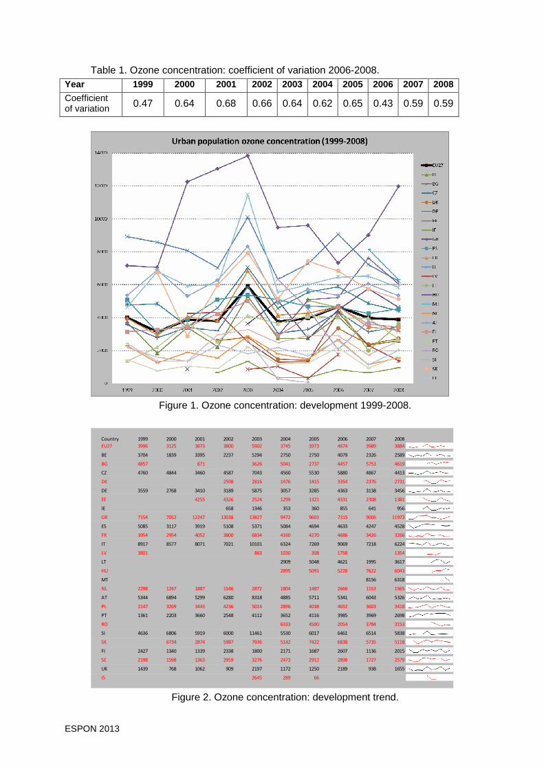
ESPON 2013 120

Table 1. Ozone concentration: coefficient of variation 2006-2008. Year 1999 2000 2001 2002 2003 2004 2005 2006 2007 2008

Coefficient of variation 0.47 0.64 0.68 0.66 0.64 0.62 0.65 0.43 0.59 0.59

Figure 1. Ozone concentration: development 1999-2008.

Country 1999 2000 2001 2002 2003 2004 2005 2006 2007 2008

EU27 3996 3125 3873 3800 5902 3745 3973 4674 3989 3884

BE 3704 1839 3395 2237 5294 2750 2750 4079 2326 2589

BG 4857 871 3626 5041 2737 4457 5753 4619

CZ 4760 4844 3460 4587 7043 4560 5530 5880 4867 4413

DK 2598 2816 1476 1415 3354 2376 2731

DE 3559 2768 3410 3189 5875 3057 3285 4363 3138 3456

EE 4255 4326 2524 1299 1321 4331 2308 1381

IE 658 1346 353 360 855 641 956

GR 7154 7052 12247 13038 13827 9472 9601 7315 9006 11973

ES 5085 3117 3919 5108 5371 5084 4694 4633 4247 4528

FR 3954 2954 4052 3800 6834 4160 4270 4686 3426 3266

IT 8917 8577 8071 7021 10101 6324 7269 9069 7218 6224

LV 3801 863 1030 308 1758 1354

LT 2909 5048 4621 1995 3617

HU 2895 5091 5228 7622 6043

MT 8156 6318

NL 2298 1247 1887 1546 2872 1804 1487 2666 1153 1565

AT 5344 6894 5299 6280 8318 4885 5711 5341 6043 5326

PL 3147 3269 3443 4236 5014 2896 4038 4652 3603 3418

PT 1361 2203 3660 2548 4112 3652 4116 3985 3969 2698

RO 6333 4500 2054 3784 3153

SI 4636 6806 5919 6000 11461 5530 6017 6461 6514 5838

SK 6734 2874 5987 7936 5142 7422 6838 5735 5118

FI 2427 1340 1339 2338 1800 2171 1687 2607 1136 2015

SE 2198 1598 1363 2959 3276 2473 2912 2898 1727 2579

UK 1439 768 1062 909 2197 1172 1250 2189 938 1655

IS 2645 289 66

Figure 2. Ozone concentration: development trend.

ESPON 2013 121

Particular matter (PM10) The indicator is defined as the urban population exposure to air pollution by particular matter. The indicator shows the population weighted annual mean concentration of particulate matter at urban background stations in agglomerations. Fine particulates (PM10), i.e. particulates whose diameter is less than 10 micrometers, can be carried deep into the lungs where they can cause inflammation and a worsening of the condition of people with heart and lung diseases. In 1996, the Environment Council adopted Framework Directive 96/62/EC on ambient air quality assessment and management. The first Daughter Directive (1999/30/EC) relating to limit values for PM10 and other pollutants in ambient air fixed an annual limit value of 40 microgram of PM10 per m3. Annual reporting must follow Commission Decision 2004/224/EC of 20 February 2004 laying down arrangements for the submission of information under Council Directive 96/62/EC in relation to limit values for certain pollutants in ambient air. The indicator is only available at national level. Highest exposures of urban population to PM10 can be observed for Romania and Bulgaria, Greece and Italy, followed by Poland. Lowest PM10 concentrations are in Finland, Iceland and Estonia. Since 1999 there has been no substantial reduction in the urban population exposed to PM10 at European level, as Figure 3 shows. Fourteen out of 27 countries even experienced an increase, for only nine countries substantial reductions could be observed, with Slovakia being the country with the highest reduction rate (-11.5 %). On the other hand, in Bulgaria (+53%), Romania (+41%), Greece (+37%) or Italy (+34%) a number of countries saw strong increases of PM10 in urban areas, presumably because of increases in road transport. Consequently, there is no clear tendency of the corresponding PM10 coefficients of variation (Table 2) over the last decade.

Figure 3. Particular matter (PM10): Urban population exposure development 1999-2008.

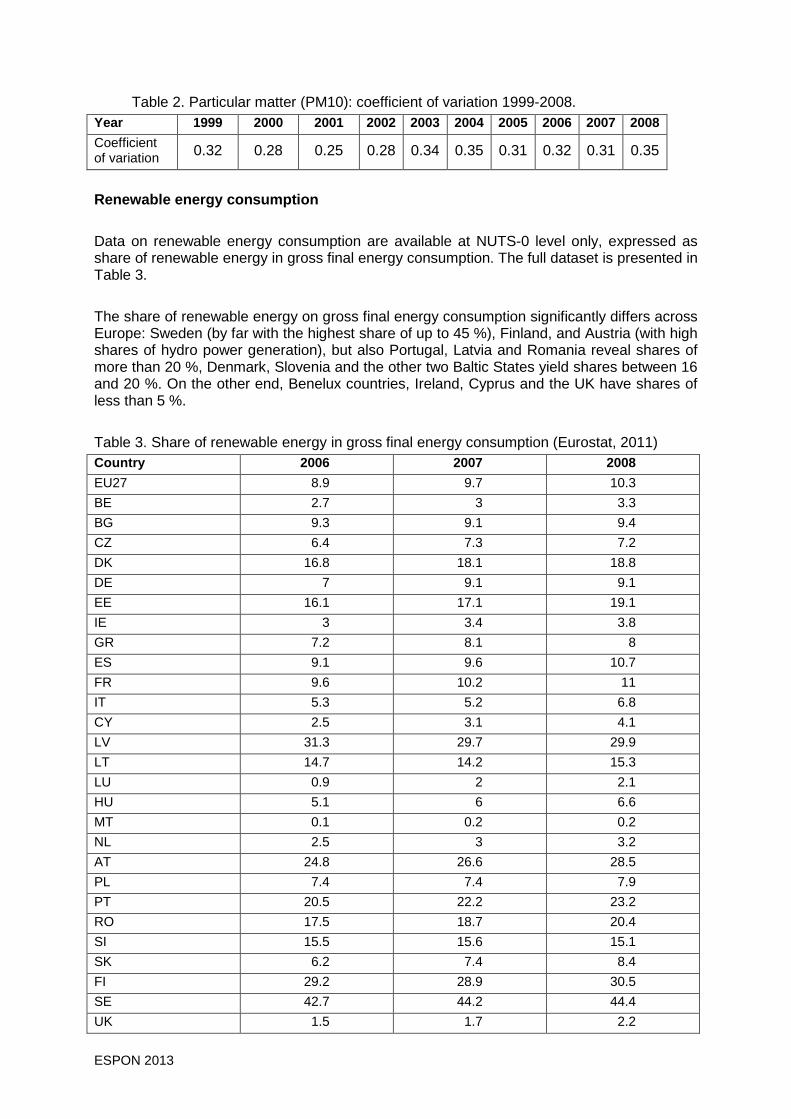
ESPON 2013 122

Table 2. Particular matter (PM10): coefficient of variation 1999-2008. Year 1999 2000 2001 2002 2003 2004 2005 2006 2007 2008

Coefficient of variation 0.32 0.28 0.25 0.28 0.34 0.35 0.31 0.32 0.31 0.35

Renewable energy consumption Data on renewable energy consumption are available at NUTS-0 level only, expressed as share of renewable energy in gross final energy consumption. The full dataset is presented in Table 3. The share of renewable energy on gross final energy consumption significantly differs across Europe: Sweden (by far with the highest share of up to 45 %), Finland, and Austria (with high shares of hydro power generation), but also Portugal, Latvia and Romania reveal shares of more than 20 %, Denmark, Slovenia and the other two Baltic States yield shares between 16 and 20 %. On the other end, Benelux countries, Ireland, Cyprus and the UK have shares of less than 5 %. Table 3. Share of renewable energy in gross final energy consumption (Eurostat, 2011) Country 2006 2007 2008

EU27 8.9 9.7 10.3

BE 2.7 3 3.3

BG 9.3 9.1 9.4

CZ 6.4 7.3 7.2

DK 16.8 18.1 18.8

DE 7 9.1 9.1

EE 16.1 17.1 19.1

IE 3 3.4 3.8

GR 7.2 8.1 8

ES 9.1 9.6 10.7

FR 9.6 10.2 11

IT 5.3 5.2 6.8

CY 2.5 3.1 4.1

LV 31.3 29.7 29.9

LT 14.7 14.2 15.3

LU 0.9 2 2.1

HU 5.1 6 6.6

MT 0.1 0.2 0.2

NL 2.5 3 3.2

AT 24.8 26.6 28.5

PL 7.4 7.4 7.9

PT 20.5 22.2 23.2

RO 17.5 18.7 20.4

SI 15.5 15.6 15.1

SK 6.2 7.4 8.4

FI 29.2 28.9 30.5

SE 42.7 44.2 44.4

UK 1.5 1.7 2.2

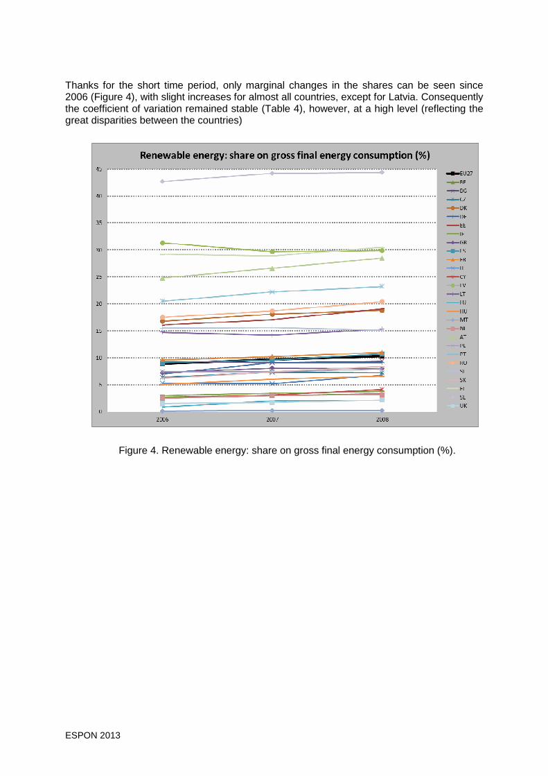
ESPON 2013 123

Thanks for the short time period, only marginal changes in the shares can be seen since 2006 (Figure 4), with slight increases for almost all countries, except for Latvia. Consequently the coefficient of variation remained stable (Table 4), however, at a high level (reflecting the great disparities between the countries)

Figure 4. Renewable energy: share on gross final energy consumption (%).

ESPON 2013 124

Table 4. Renewable energy consumption: coefficient of variation 2006-2008.

Year 2006 2007 2008 Coefficient of variation 0.889 0.849 0.819

Per-capita consumption of water (public supply to households) This indicator is defined as the consumption of water per capita, measured in cubic metres, based upon the public supply to households. The water consumption per capita across Europe differs significantly between European countries, ranging from 19 cubic metres per capita in Lithuania to more than 100 cubic metres in Iceland (Figure 5). Norway, Finland, Switzerland and Italy also show very high consumption figures, while Western Balkan countries and Romania only have consumption between 20 and 30 cubic metres per capita. From the view of environmental protection, and reduction of freshwater consumption, almost all countries experienced a reduction in per-capita consumption of household water between 1 and 55 % (Romania), except for Cyprus (+28%), Norway (+12%) and Macedonia (+10%), whose per-capita consumption rate rose in the period 1998-2009. The coefficient of variations calculated over all countries thus increased more or less steadily in the period from 0.38 to 0.47, indicating increasing disparities rather than cohesion in water consumption (Table 5).

Figure 5. Per-capita consumption of water, 1998-2009 (public water supply).

ESPON 2013 125

Table 5. Per-capita household water consumption: coefficient of variation 1999-2009. Year 1998 1999 2000 2001 2002 2003 2004 2005 2006 2007 2008 2009

Coefficient of variation 0.38 0.38 0.40 0.41 0.41 0.43 0.42 0.46 0.42 0.39 0.37 0.47

Per-capita consumption of public water supplied to households however concern only a small portion of all freshwater used in a country, since it excludes industrial water consumption, or water consumption for services, leisure facilities etc. Thus, a second per-capita water consumption indicator was tested which takes account of the total water supply and consumption in a country. Per-capita consumption of water (total public water supply) This indicator extends the previous indicator in that now the overall public freshwater supply is considered, whether supply goes to households, industries, services, leisure facilities or other types of usages. Again, the per-capita consumption is mapped. Generally the per-capita rates of freshwater consumption are higher compared to the previous indicator. Countries like Sweden, Iceland, Ireland, UK, Switzerland, Croatia or Latvia now have the highest consumption with more than 80 cubic metres per capita. Estonia and Lithuania are, on the other end of the spectrum, those countries with the lowest per-capita consumption in between 30 and 35 cubic metres. Generally, new EU Member States have a lower per-capita consumption compared to the old member states. The general trend since 1998 is a reduction in the overall per-capita freshwater consumption (Figure 6). Countries like Romania (-65%), Estonia (-33%), Latvia (-31%), or Cyprus (-25%) are those countries with highest reductions, even though probably due to the closure of industries. But there are also countries like Belgium (+59%) or Lithuania (+76%) who significantly increased their consumption. Despite these diverging trends at national level, the coefficients of variations slightly decreased since 1998, indicating a slight reduction of overall disparities (Table 6). Table 6. Per-capita total water consumption: coefficient of variation 1999-2009. Year 1998 1999 2000 2001 2002 2003 2004 2005 2006 2007 2008 2009

Coefficient of variation 0.46 0.47 0.47 0.48 0.53 0.52 0.54 0.53 0.44 0.42 0.36 0.40

Comparison of both water consumption indicators

Figure 7 compares the two water consumption indicators in a standardized way with each other, and reveals that both are more or less similar. Consequently, for the final selection set of cohesion indicators it would be sufficient to select only one of the two. In order to capture the overall water consumption, including industries and agriculture, it is suggested to use the per-capita water consumption based on total public water supply.

ESPON 2013 126

Figure 6. Per-capita consumption of water, 1998-2009 (total public water supply).

Figure 7. Per-capita water consumption: comparison of indicators.

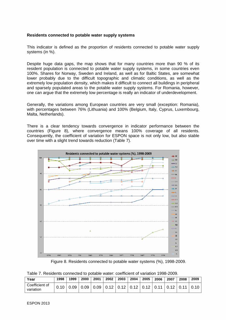
ESPON 2013 127

Residents connected to potable water supply systems This indicator is defined as the proportion of residents connected to potable water supply systems (in %). Despite huge data gaps, the map shows that for many countries more than 90 % of its resident population is connected to potable water supply systems, in some countries even 100%. Shares for Norway, Sweden and Ireland, as well as for Baltic States, are somewhat lower probably due to the difficult topographic and climatic conditions, as well as the extremely low population density, which makes it difficult to connect all buildings in peripheral and sparsely populated areas to the potable water supply systems. For Romania, however, one can argue that the extremely low percentage is really an indicator of underdevelopment. Generally, the variations among European countries are very small (exception: Romania), with percentages between 76% (Lithuania) and 100% (Belgium, Italy, Cyprus, Luxembourg, Malta, Netherlands). There is a clear tendency towards convergence in indicator performance between the countries (Figure 8), where convergence means 100% coverage of all residents. Consequently, the coefficient of variation for ESPON space is not only low, but also stable over time with a slight trend towards reduction (Table 7).

Figure 8. Residents connected to potable water systems (%), 1998-2009.

Table 7. Residents connected to potable water: coefficient of variation 1998-2009. Year 1998 1999 2000 2001 2002 2003 2004 2005 2006 2007 2008 2009

Coefficient of variation 0.10 0.09 0.09 0.09 0.12 0.12 0.12 0.12 0.11 0.12 0.11 0.10

ESPON 2013 128

Residence density The indicator is defined as the share of settlement areas on regional area (in %). Settlement areas are taken from Corine land use layer. Settlements are defined as continuous and discontinuous urban fabric (=Corine grid codes 1 & 2). This indicator definition was selected since no other statistical data are available European-wide that can measure residence densities. With this definition the indicator inherits all advantages and disadvantages of the Corine layer. Since the dataset was generated by satellite images analysis, the following restrictions are immanent:

- The general scale of the dataset is 1:100,000 - The minimum size of individual patches to be recognized is 25 ha for areal objects and a

minimum width of 100 m for linear objects - Following this not all built-up areas are included in the dataset, in particular transport

infrastructures such as motorways are only rarely included, so as small settlement or housing units outside villages and towns.

The variation of settlement density across Europe is very high, ranging from close to zero percent in Scandinavia, Spain, Portugal or in the Alps, towards 80 % for the main cities in Benelux or Germany. Regional cities in other countries such as Poland, Portugal, or Italy are also highlighted. Eventually the indicator is a function of the size and delimitation of the NUTS-3 regions: small NUTS-3 regions like in Benelux countries or in Germany are likely to have higher indicator values compared to great regions in Scandinavia or other parts of Europe, which tend to have lower shares (Figure 9). The highest range of values reveals France, followed by Belgium, Germany, Austria and Romania. Malta, Lithuania and Estonia have the smallest range.

Figure 9. Settlement density (%): variations within countries 2006.

ESPON 2013 129

In terms of coefficient of variation, Norway, Latvia, and Ireland indicate greatest disparities within their countries (Figure 10), illustrating the great dichotomy between the highly urbanized capital city regions, and the extremely low settlement densities in the rural parts of the countries. In this ranking, the Benelux countries and Germany show rather modest variations, since they have a balanced polycentric city system, combined with extensive rural parts.

Figure 10. Settlement density (%): coefficient of variations measured over NUTS-3 regions. The indicator furthermore correlates very high with the population density indicator, as shown in Figure 11. Even though the higher the population density, the lower this correlation is, one can constitute that both indicators measure similar development trends: usually, resident population is located within the settlement areas, and the higher the population figures are for any statistical unit, the greater usually the settlement areas are. Of course, this relationship is restricted by the overall available land, so at a certain point (i.e. a certain population density) the correlation becomes weak. Mathematically this point seems to be approx. 200 % of the ESPON average of the standardized population density. Following this observation one may conclude that an individual indicator on settlement density is not needed as cohesion indicator when the corresponding population density indicator is already selected. Since population density is also available as time series, this indicator should be chosen.

ESPON 2013 130

Figure 11. Correlation population density vs. settlement density (100=ESPON average).

Ares with high ecological value This indicator is defined as the percent of protected areas for biodiversity on total country territory, according to the habitats directive. In this sense it is assumed that areas with high ecological value correspond to these protected areas. The indicator is available at national level from Eurostat statistics. There are great disparities in the share of areas of high ecological value within the EU. The majority of the West European countries, including Germany, France, UK, Benelux, and Czech Republic, have shares of less than 10%. Slovenia, Bulgaria, and Spain, on the other hand, have the highest share of more than 20% of their territories designated as areas of high biodiversity. Even though there are times series data available at Eurostat, starting in 2003, the shares are not changing since the Habitat´s directive is a political initiative, i.e. those areas that are designated and reported to the Commission as highly sensitive areas for biodiversity, their status maintain and thus nothing changed over time. Another drawback from the Eurostat data is that they are only available at national level, even though one can assume that these protected areas are not distributed equally across the countries, but that they will concentrate in certain parts – depending on the natural conditions. An analysis at sub-national level is, however, not possible with the present data source.

ESPON 2013 131

Taking both drawbacks together, i.e. the missing temporal dimension and the missing subnational dimension, the indicator in its present form cannot be used as cohesion indicator.

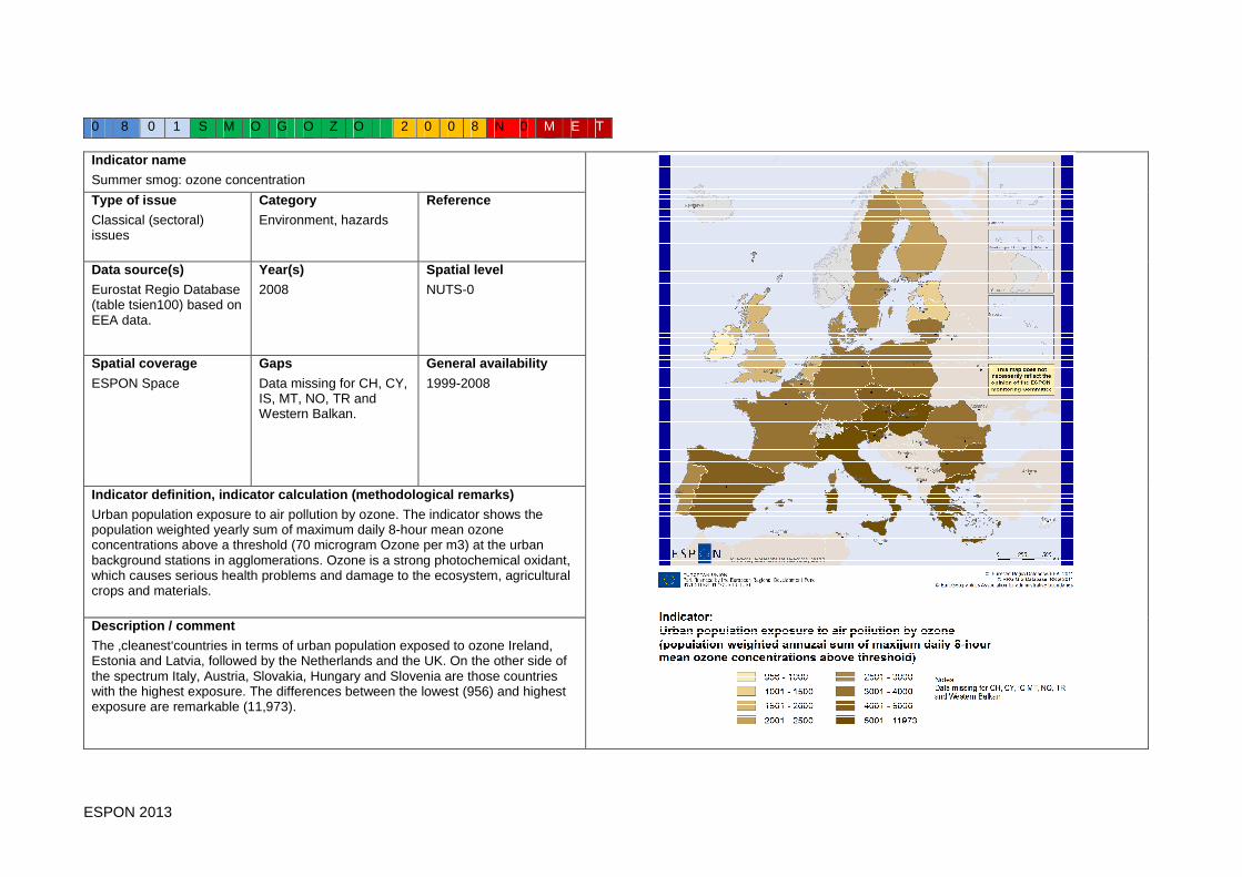
ESPON 2013 132

0 8 0 1 S M O G O Z O 2 0 0 8 N 0 M E T

Indicator name

Summer smog: ozone concentration

Type of issue

Classical (sectoral) issues

Category

Environment, hazards

Reference

Data source(s)

Eurostat Regio Database (table tsien100) based on EEA data.

Year(s)

2008

Spatial level

NUTS-0

Spatial coverage

ESPON Space

Gaps

Data missing for CH, CY, IS, MT, NO, TR and Western Balkan.

General availability

1999-2008

Indicator definition, indicator calculation (methodological remarks)

Urban population exposure to air pollution by ozone. The indicator shows the population weighted yearly sum of maximum daily 8-hour mean ozone concentrations above a threshold (70 microgram Ozone per m3) at the urban background stations in agglomerations. Ozone is a strong photochemical oxidant, which causes serious health problems and damage to the ecosystem, agricultural crops and materials.

Description / comment

The ‚cleanest‘countries in terms of urban population exposed to ozone Ireland, Estonia and Latvia, followed by the Netherlands and the UK. On the other side of the spectrum Italy, Austria, Slovakia, Hungary and Slovenia are those countries with the highest exposure. The differences between the lowest (956) and highest exposure are remarkable (11,973).

ESPON 2013 133

0 8 0 1 S M O G P M 1 0 2 0 0 8 N 0 M E T

Indicator name

Summer smog: particular matter (PM10)

Type of issue

Classical (sectoral) issues

Category

Environment, hazards

Reference

Data source(s)

Eurostat Regio Database (table tsien110) based on EEA data.

Year(s)

2008

Spatial level

NUTS-0

Spatial coverage

ESPON Space

Gaps

n.a.

General availability

1999-2008

Indicator definition, indicator calculation (methodological remarks)

Urban population exposure to air pollution by particular matter. The indicator shows the population weighted annual mean concentration of particulate matter at urban background stations in agglomerations. Fine particulates (PM10), i.e. particulates whose diameter is less than 10 micrometers, can be carried deep into the lungs where they can cause inflammation and a worsening of the condition of people with heart and lung diseases. In 1996, the Environment Council adopted Framework Directive 96/62/EC on ambient air quality assessment and management. The first Daughter Directive (1999/30/EC) relating to limit values for PM10 and other pollutants in ambient air fixed an annual limit value of 40 microgram of PM10 per m3. Annual reporting must follow Commission Decision 2004/224/EC of 20 February 2004 laying down arrangements for the submission of information under Council Directive 96/62/EC in relation to limit values for certain pollutants in ambient air.

Description / comment

Highest exposures of urban population to PM10 can be observed for Romania and Bulgaria, Greece and Italy, followed by Poland. Lowest PM10 concentrations are in Finland, Iceland and Estonia.

ESPON 2013 134

0 8 0 1 E N Q 2 0 0 8 N 0 R T O

Indicator name

Renewable energy consumption

Type of issue

Classical (sectoral) issues

Category

Environment, hazards

Reference

Data source(s)

Eurostat Regio Database

(code tsdcc11)

Year(s)

2008

Spatial level

NUTS-0

Spatial coverage

ESPON Space

Gaps

Missing data for CH, IS, NO, TR and Western Balkan

General availability

2006-2008

Indicator definition, indicator calculation (methodological remarks)

Share of renewable energy in gross final energy consumption (%). Indicator estimated on the basis of energy statistics covered by the Energy Statistics Regulation

Description / comment

The share of renewable energy on gross final energy consumption significantly differs across Europe: Finland, Sweden, Austria (with high shares of hydro power generation), but also Portugal, Latvia and Romania reveal shares of more than 20 %, Denmark, Slovenia and the other two Baltic States yield shares between 16 and 20 %. On the other end, Benelux countries, Ireland, Cyprus and the UK have shares of less than 5 %.

ESPON 2013 135

0 8 0 1 W A T C O N H H 2 0 0 9 N 0 R T O

Indicator name

Consumption of water per capita, water supply to households (in cubic metres per inhabitant)

Type of issue

Classical (sectoral) issues

Category

Environment, hazards

Reference

Data source(s)

Eurostat Regio Database (table env_watq3)

Year(s)

2009

Spatial level

NUTS-0

Spatial coverage

ESPON Space

Gaps

General availability

1998-2009

Indicator definition, indicator calculation (methodological remarks)

Consumption of water per capita in cubic metres per inhabitant, including public water supply to households only.

Description / comment

The water consumption per capita across Europe differs significantly between European countries, ranging from 19 cubic metres per capita in Lithuania to more than 100 cubic metres in Iceland. Norway, Finland, Switzerland and Italy also show very high consumption figures, while Western Balkan countries, and Romania only have consumption between 20 and 30 cubic metres per capita.

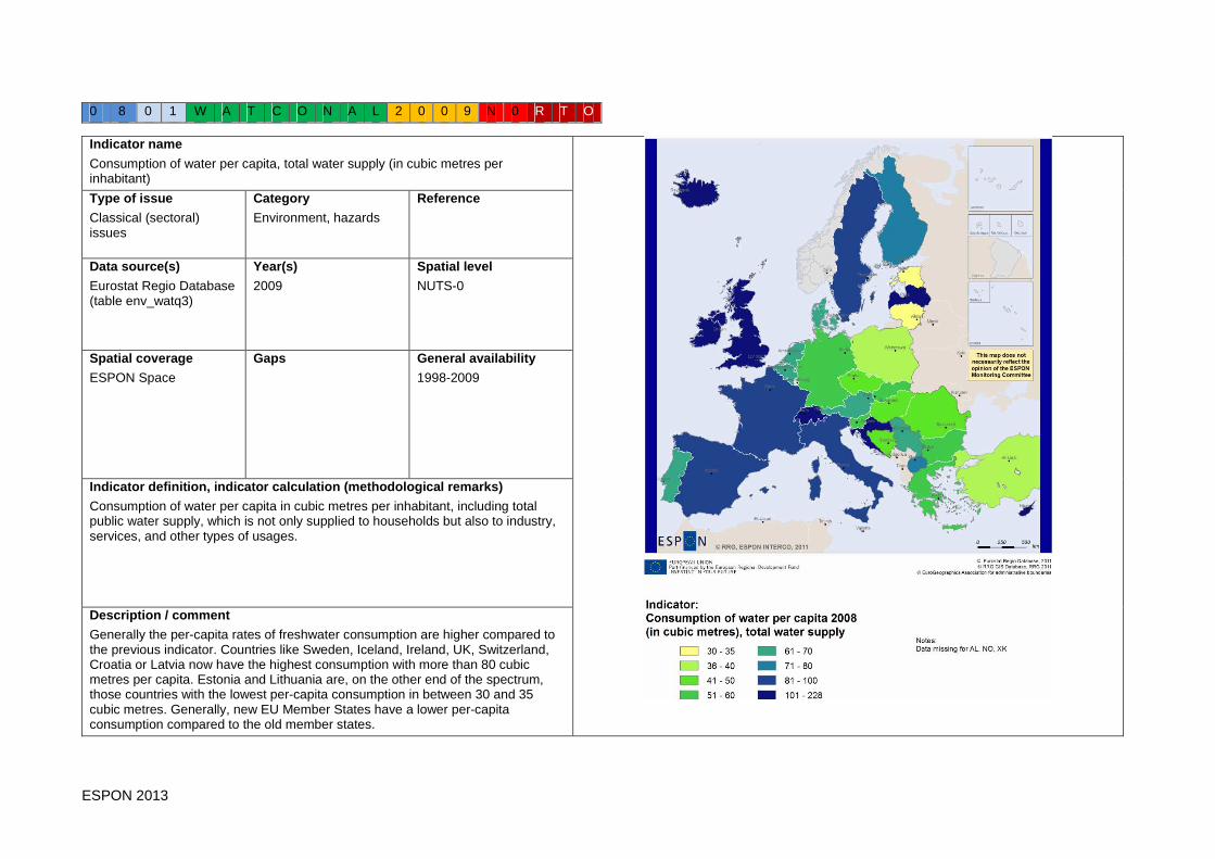
ESPON 2013 136

0 8 0 1 W A T C O N A L 2 0 0 9 N 0 R T O

Indicator name

Consumption of water per capita, total water supply (in cubic metres per inhabitant)

Type of issue

Classical (sectoral) issues

Category

Environment, hazards

Reference

Data source(s)

Eurostat Regio Database (table env_watq3)

Year(s)

2009

Spatial level

NUTS-0

Spatial coverage

ESPON Space

Gaps

General availability

1998-2009

Indicator definition, indicator calculation (methodological remarks)

Consumption of water per capita in cubic metres per inhabitant, including total public water supply, which is not only supplied to households but also to industry, services, and other types of usages.

Description / comment

Generally the per-capita rates of freshwater consumption are higher compared to the previous indicator. Countries like Sweden, Iceland, Ireland, UK, Switzerland, Croatia or Latvia now have the highest consumption with more than 80 cubic metres per capita. Estonia and Lithuania are, on the other end of the spectrum, those countries with the lowest per-capita consumption in between 30 and 35 cubic metres. Generally, new EU Member States have a lower per-capita consumption compared to the old member states.

ESPON 2013 137

0 8 0 1 R E S P O T W A N 0 R T O

Indicator name

Residents connected to potable water supply systems (%)

Type of issue

Classical (sectoral) issues

Category

Environment, hazards

Reference

Data source(s)

Europstat Regio Database (table env_wat_pop)

Year(s)

2009 (latest available year)

Spatial level

NUTS-0

Spatial coverage

ESPON Space

Gaps

Data missing for CH, ES, FI, LV, SI and Western Balkan.

General availability

1998-2009

Indicator definition, indicator calculation (methodological remarks)

Resident population connected to public potable water supply systems (in %).

Description / comment

Despite the huge data gaps, the map shows that for many countries more than 90 % of resident population is connected to potable water supply system, in some countries even 100%. Shares for Norway, Sweden and Ireland, as well as for Baltic States, are somewhat lower probably due to the difficult topographic and climatic conditions, as well as the extremely low population density, which makes it difficult to connect all buildings in peripheral and sparsely populated areas to the potable water supply systems. For Romania, however, one can argue that the extremely low percentage is really an indicator of underdevelopment.

ESPON 2013 138

0 8 0 1 R E S D E N S 2 0 0 6 N 3 R T O

Indicator name

Residence density

Type of issue

Classical (sectoral) issues

Category

Environment, hazards

Reference

Data source(s)

Own calculation based on European Environment Agency (EEA)

Year(s)

2006

Spatial level

NUTS-3

Spatial coverage

ESPON Space

Gaps

n.a.

General availability

1990, 2000, 2006

Indicator definition, indicator calculation (methodological remarks)

The indicator is defined as the share of settlement areas on regional area (in %). Settlement areas are taken from Corine land use layer. Settlements are defined as continuous and discontinuous urban fabric (=Corine grid codes 1 & 2).

Description / comment

The variation of settlement density across Europe is very high, ranging from close to zero percent in Scandinavia, Spain, Portugal or in the Alps, towards 80 % for the main cities in Benelux or Germany. Regional cities in other countries such as Poland, Portugal, or Italy are also highlighted.

ESPON 2013 139

0 8 0 2 C L C H 2 0 1 0 N 0 R T O

Indicator name

Areas with high ecological value (%)

Type of issue

Classical (sectoral) issues

Category

Environment, hazards

Reference

Data source(s)

Eurostat Regio Database (tabke env_bio1)

Year(s)

2010

Spatial level

NUTS-0

Spatial coverage

ESPON Space

Gaps

Data are missing for non-EU countries.

General availability

2003-2010

Indicator definition, indicator calculation (methodological remarks)

The indicator is defined as the share of protected areas for biodiversity on the overall national territories in percent, according to the biodiversity directive.

Description / comment

There are great disparities in the share of areas of high ecological value within the EU. The majority of the West European countries, including Germany, France, UK, Benelux, and Czech Republic, have shares of less than 10%. Slovenia, Bulgaria, and Spain, on the other hand, have the highest share of more than 20% of their territories designated as areas of high biodiversity.

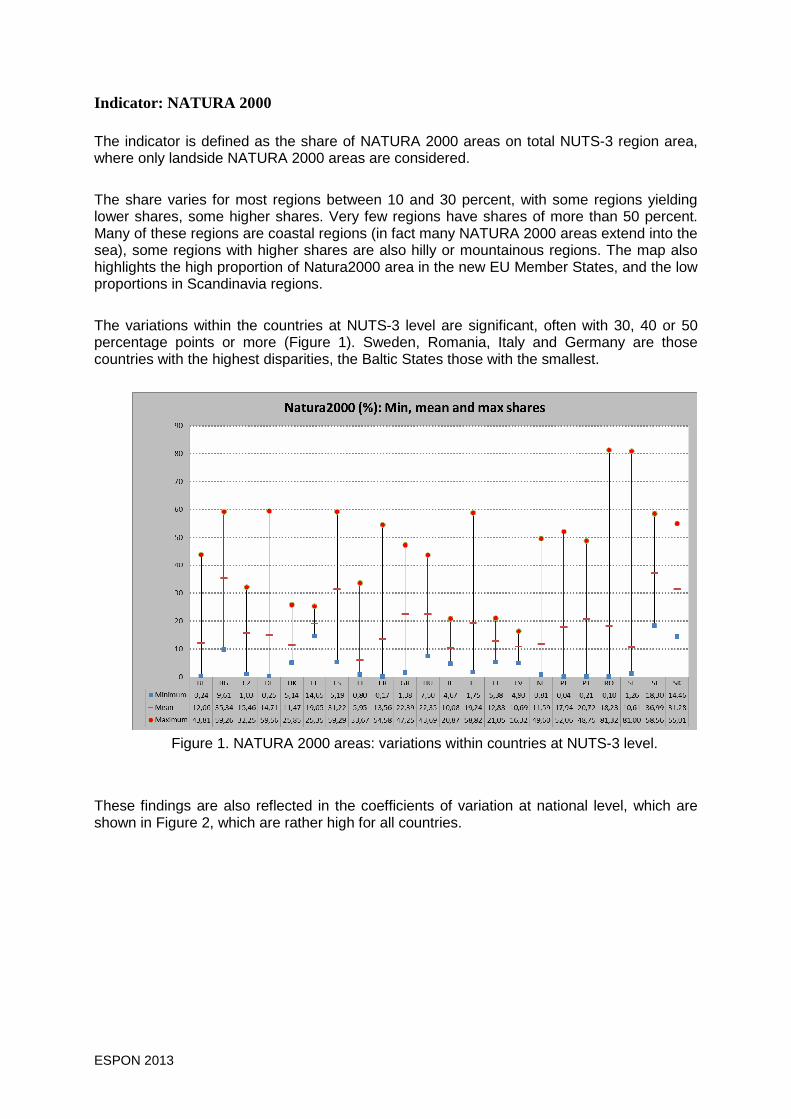
ESPON 2013 140

Indicator: NATURA 2000 The indicator is defined as the share of NATURA 2000 areas on total NUTS-3 region area, where only landside NATURA 2000 areas are considered. The share varies for most regions between 10 and 30 percent, with some regions yielding lower shares, some higher shares. Very few regions have shares of more than 50 percent. Many of these regions are coastal regions (in fact many NATURA 2000 areas extend into the sea), some regions with higher shares are also hilly or mountainous regions. The map also highlights the high proportion of Natura2000 area in the new EU Member States, and the low proportions in Scandinavia regions. The variations within the countries at NUTS-3 level are significant, often with 30, 40 or 50 percentage points or more (Figure 1). Sweden, Romania, Italy and Germany are those countries with the highest disparities, the Baltic States those with the smallest.

Figure 1. NATURA 2000 areas: variations within countries at NUTS-3 level.

These findings are also reflected in the coefficients of variation at national level, which are shown in Figure 2, which are rather high for all countries.

ESPON 2013 141

Figure 2. NATURA 2000 – Coefficients of variation at national level.

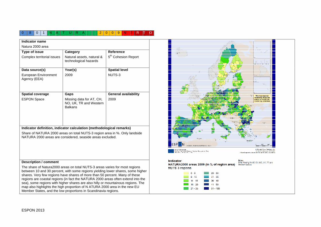
ESPON 2013 142

0 8 0 1 N A T U R A 2 0 0 9 N 3 R T O

Indicator name

Natura 2000 area

Type of issue

Complex territorial issues

Category

Natural assets, natural & technological hazards

Reference

5th Cohesion Report

Data source(s)

European Environment Agency (EEA)

Year(s)

2009

Spatial level

NUTS-3

Spatial coverage

ESPON Space

Gaps

Missing data for AT, CH, NO, UK, TR and Western Balkans

General availability

2009

Indicator definition, indicator calculation (methodological remarks)

Share of NATURA 2000 areas on total NUTS-3 region area in %. Only landside NATURA 2000 areas are considered, seaside areas excluded.

Description / comment

The share of Natura2000 areas on total NUTS-3 areas varies for most regions between 10 and 30 percent, with some regions yielding lower shares, some higher shares. Very few regions have shares of more than 50 percent. Many of these regions are coastal regions (in fact the NATURA 2000 areas often extend into the sea), some regions with higher shares are also hilly or mountainous regions. The map also highlights the high proportion of N ATURA 2000 area in the new EU Member States, and the low proportions in Scandinavia regions.

ESPON 2013 131

Annex 14. Expected deliveries of the INTERCO projec t Excerpt from the Annex III of the INTERCO Subsidy Contract :

31 August 2010 (Inception Report):

Twelve weeks after the Kick-off Meeting the Inception Report shall be delivered covering the results of Part I, the design phase, which is the following:

- A proposal on a clear and consistent terminology in relation to territorial indicators and indices.

- An overview and a first review of existing territorial indicators and indices, including integrated / composite indicators referring to the above mentioned thematic scope and general objectives;

- A well-founded proposal of feasible territorial indicators and indices, including integrated / composite indicators that should be further considered to meet the scope of the project.

- A plan to involve stakeholders in the search for and the testing and implementing of indicators and indices.

- A detailed work plan until the Interim report, a more global work plan until the final report, description of the project, and a timing of the necessary dialogue with policy makers from the MC;

On the basis of this Inception report the MC will select indicators and indices to be incorporated in Part II of the project, exploring.

31 March 2011 (Interim Report):

The Interim report shall cover the results of Part II, the exploratory phase, which is the following:

- A complete review of existing territorial indicators and indices referring to the above mentioned thematic scope and general objectives;

- Results of the testing of territorial indicators and indices, including integrated / composite indicators meeting the best the scope of the project.

- Examples of visualisation of indicators and indices.

- Recommendation, based on the completed review and testing results, of a set of appropriate and operational territorial indicators and indices that would best mirror the European policy aim of territorial cohesion and that could be used to measure, communicate and report this aim to policy makers and other stakeholders.

- Work plan until the Final report.

On the basis of this Interim report the MC will make the final selection of the indicators and indices to be incorporated in Part III of the project, implementing.

30 November 2011 (Draft Final Report):

- The Draft Final report will take into account feed-back on the Interim report from an ESPON seminar and ESPON CU. The report is supposed to cover the following:

- Report (max. 50 pages) on the main results of implementing the selected territorial indicators and indices including the results of analyses, tests, data considerations, reporting, communication aspects, etc. Particularly important are findings for policy makers, which could provide the basis for interventions

ESPON 2013 132

related to opportunities for improving European competitiveness and cohesion.

- An executive summary (max. 10 pages) summarising the main results of the project that can be communicated to a wider audience of stakeholders. This summary should be based on the report mentioned above.

- Scientific report documenting the scientific work undertaken in the project including elements such as:

o Literature, definitions and methodology/theory used.

o Methodologies and concepts developed and used.

o Tools and models used or developed.

o An overview of all indicators and indices selected, each described in a structured way including the aspects given in the Annex, its way to visualise, communicate and report, its test results, etc.

o Maps produced in support of the results, covering the territory of EU 27, Iceland, Liechtenstein, Norway and Switzerland.

o Future research avenues to consider, including further data requirements, filling of possible data gaps, building time series, improving weak aspects in the selected set of indicators and indices and further developments linked to the database and monitoring.

Once the Draft Final Report is delivered to the ESPON Coordination Unit, the report will be presented for the ESPON MC for discussion.

29 February 2012 (Final report):

The Final Report will be a revision of the Draft Final report on the basis of comments received.

The ESPON 2013 Programme foresees in Priority 4 also capitalisation of project results including events, printed reports, website facility, etc. The Programme includes, in other words, substantial dissemination activities at Programme level which all projects should make use of and support. This means that the project’s dissemination activities shall ensure consistency and avoid overlaps with and repetition of respective activities organised at Programme level. The project team shall refer to the objectives of Priority 4 of the ESPON 2013 Programme “Capitalisation, ownership and participation: Capacity building, dialogue and networking” when considering dissemination activities and closely coordinate these with the ESPON CU.

ESPON 2013 133

ESPON 2013 134

The ESPON 2013 Programme is part-financed by the European Regional Development Fund, the EU Member States and the Partner States Iceland, Liechtenstein, Norway and Switzerland. It shall support policy development in relation to the aim of territorial cohesion and a harmonious development of the European territory.

ISBN