Integrative Bayesian Network Analysis of Genomic Data

39CanCer InformatICs 2014:13(s2)

Open Access: Full open access to this and thousands of other papers at http://www.la-press.com.

Cancer Informatics

IntroductionCancer is a disease caused by multiple genetic mutations. To explore the underlying biological system, numerous methods based on genomic data from single platforms have been proposed. For example, methods for reverse engineering gene regulatory networks from mRNA gene expression data can successfully describe complex biological systems1–3 but are applicable to just one platform. However, cancer arises from a series of genome-wide genetic mutations (eg, DNA copy number alterations) and epigenetic mutations (eg, DNA methylation) rather than a small number of platform-specific mutations.4 Given this complexity, recovering a regulatory network from a single platform can only provide a partial view of the cancer genome. Therefore, the focus should shift from single-platform analysis to integrative analysis of data arising from multiple genomic platforms. This is feasible, in

part, because of the rapid development of high-throughput genome-wide profiling technologies such as microarrays5 and array comparative genomic hybridization, aCGH.6 Thus, multi-platform data of matched tumor/patient samples are now widely available, which motivates integrative network analy-sis to elucidate mechanisms of cancer development and pro-gression. Specifically, since 2006, the Cancer Genome Atlas (TCGA) research network1 has made a great effort to col-lect and make publicly available such data (including mRNA gene expression, DNA methylation) for over 30 types of can-cer, including glioblastoma multiforme (GBM), squamous cell lung carcinoma, and ovarian serous cystadenocarcinoma, among others.

In this study, we are particularly interested in GBM as it is the most common and most lethal malignant primary brain tumor in human adults.7 Due to its aggressiveness, GBM

Integrative Bayesian Network Analysis of Genomic Data

Yang ni1, francesco C. stingo2 and Veerabhadran Baladandayuthapani21Department of Statistics, Rice University, Houston, Texas, USA. 2Department of Biostatistics, The University of Texas MD Anderson Cancer Center, Houston, Texas, USA.

AbstrAct: Rapid development of genome-wide profiling technologies has made it possible to conduct integrative analysis on genomic data from multiple platforms. In this study, we develop a novel integrative Bayesian network approach to investigate the relationships between genetic and epigenetic alterations as well as how these mutations affect a patient’s clinical outcome. We take a Bayesian network approach that admits a convenient decomposition of the joint distribution into local distributions. Exploiting the prior biological knowledge about regulatory mechanisms, we model each local distribution as linear regressions. This allows us to analyze multi-platform genome-wide data in a computationally efficient manner. We illustrate the performance of our approach through simulation studies. Our methods are motivated by and applied to a multi-platform glioblastoma dataset, from which we reveal sev-eral biologically relevant relationships that have been validated in the literature as well as new genes that could potentially be novel biomarkers for cancer progression.

Keywords: glioblastoma multiforme, integrative analysis, Bayesian network, multiple platforms

the Cancer Center Support Grant (CCSG) (P30 CA016672). The content is solely the responsibility of the authors and does not necessarily represent the official views of the National Cancer Institute or the National Institutes of Health.

CoMPETING INTERESTS: Authors disclose no potential conflicts of interest.

CoPYRIGhT: © the authors, publisher and licensee Libertas Academica Limited. This is an open-access article distributed under the terms of the Creative Commons CC-BY-NC 3.0 License.

CoRRESPoNDENCE: [email protected]

This paper was subject to independent, expert peer review by a minimum of two blind peer reviewers. All editorial decisions were made by the independent academic editor. All authors have provided signed confirmation of their compliance with ethical and legal obligations including (but not limited to) use of any copyrighted material, compliance with ICMJE authorship and competing interests disclosure guidelines and, where applicable, compliance with legal and ethical guidelines on human and animal research participants. Provenance: the authors were invited to submit this paper.

Supplementary Issue: Classification, Predictive Modelling, and Statistical Analysis of Cancer Data (A)

SUPPLEMENT: Classification, Predictive Modelling, and Statistical Analysis of Cancer Data (A)

CITATIoN: Ni et al. Integrative Bayesian Network Analysis of Genomic Data. Cancer Informatics 2014:13(s2) 39–48 doi: 10.4137/CIn.s13786.

RECEIvED: march 6, 2014. RESUBMITTED: may 4, 2014. ACCEPTED foR PUBLICATIoN: may 5, 2014.

ACADEMIC EDIToR: JT Efird, Editor in Chief

TYPE: original research

fUNDING: FS’s research is partially supported by the NIH Cancer Center Support Grant (CCSG) (P30 CA016672). VB’s research is partially supported by NIH Grant R01 CA160736 and

http://www.la-press.com


http://cancergenome.nih.gov/

http://dx.doi.org/10.4137/CIN.S13786

mailto:[email protected]

Ni et al

40 CanCer InformatICs 2014:13(s2)

was the first cancer profiled by TCGA. Multiple-platform genomic data were collected by TCGA, which included DNA copy number, DNA methylation, and mRNA gene expres-sion for the same set of samples. Associated with each sample, the clinical outcome (eg, the patient’s survival time) was also recorded.

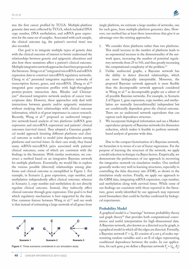
Our goal is to integrate multiple types of genetic data with the clinical outcome of interest to better understand the relationships between genetic and epigenetic alterations and also how these mutations affect a patient’s clinical outcome. Multiple integrative network approaches have been proposed in the literature. Stingo et al.8 integrated microRNA and mRNA expression data to construct microRNA regulatory networks. Cheng et al.9 presented integrative regulatory networks of transcription factors, genes, and microRNA. Zhang et al.10 integrated gene expression profiles with high-throughput protein–protein interaction data. Rhodes and Chinnai-yan11 discussed integrative network analysis of cancer tran-scriptome data. However, these approaches only deal with interactions between genetic and/or epigenetic mutations without studying their relationships with clinical outcome information, which is of great importance in cancer research. Recently, Wang et al.12 proposed an undirected integra-tive network-based analysis of two platforms (mRNA gene expression and microRNA expression) and patients’ clinical outcomes (survival times). They adopted a Gaussian graphi-cal model approach (treating different platforms and clini-cal outcome as nodes) to model joint dependencies among platforms and survival times. In their case study, they found many mRNA–microRNA pairs associated with patients’ clinical outcomes, some of which are consistent with the findings in the literature. With similar motivation, we con-struct a method based on an integrative Bayesian network for multiple platforms. Essentially, we would like to explore the various possible (directed) relationships among plat-forms and clinical outcome as exemplified in Figure 1. For example, in Scenario 2, gene expression, copy number, and methylation independently affect clinical outcome; whereas in Scenario 3, copy number and methylation do not directly regulate clinical outcome. Instead, they indirectly affect clinical outcome through gene expression. Our goal is to find which regulatory mechanism is best supported by the data. One common feature between Wang et al.12 and our work is that instead of estimating a large network of all genes from

single platform, we estimate a large number of networks, one for each gene, from multiple-platform genomics data. How-ever, our method has at least three innovations that give it an advantage over the existing approaches.

1. We consider three platforms rather than two platforms. This small increase in the number of platforms leads to an exponential increase in the dimensionality of the net-work space, increasing the number of potential regula-tory networks from 25 to 543, and thus greatly increasing the computational complexity of the problem.13

2. Unlike undirected graphs, a Bayesian network has the ability to detect directed relationships, which are more biologically interpretable. Moreover, the proposed Bayesian network approach is more flexible than the decomposable network approach considered in Wang et al.12 as decomposable graphs are a subset of all possible Bayesian networks. For example, in Scenario 2 of Figure 1, gene expression, copy number, and methy-lation are mutually (unconditionally) independent but are conditionally dependent given the clinical outcome. There are no undirected network equivalents that can capture such dependence structure.

3. We incorporate biological information and use a Markov equivalence property of Bayesian networks for dimension reduction, which makes it feasible to perform network-based analysis of genome-wide data.

Due to the compact factorization of a Bayesian network, we formulate it in terms of a set of linear regressions. For the purpose of learning the structure of the network, we apply a model selection technique via Bayes factors. Empirically, we demonstrate the performance of our approach in recovering the integrative network via simulation studies. Our method generally works very well in learning structures, especially in controlling the false discovery rate (FDR), as shown in the simulation study section. Finally, we apply our approach to the GBM data, integrating mRNA expression, copy number, and methylation along with survival times. While some of our findings are consistent with those reported in the litera-ture, genes newly-identified by our approach may represent novel biomarkers that could be further confirmed by biologi-cal experiments.

Probability ModelA graphical model is a “marriage” between probability theory and graph theory14 that provides both computational conve-nience and useful interpretation for high-dimensional data. A Bayesian network, also known as a directed acyclic graph, is a graphical model in which all the edges are directed. Formally, a Bayesian network Γ = (ς, Ε) consists of a set ς of nodes rep-resenting random variables and a set Ε of edges representing conditional dependence between the nodes. In our applica-tion, for each gene g we define a Bayesian network Γg = (ςg, Εg)

C C C

G

YScenario 1 Scenario 2 Scenario 3

Y Y

M M MG G

figure 1. Three scenarios considered in our simulation study.


Integrative Bayesian network analysis of genomic data


with ςg = {Y, Gg, Cg, Mg}, where Y is the clinical outcome, Gg is the mRNA gene expression, Cg is the DNA copy number, Mg is the DNA methylation status, and Εg ⊂ ςg × ςg contains the interactions between the platforms and the patients’ clini-cal outcomes. Given a priori ordering, say, {Mg, Cg, Gg, Y} (ie, the node present earlier in the ordering can affect those that appear later, but not vice versa; the next paragraph describes how we obtain the ordering), we can factorize the joint distri-bution into local (conditional) distributions as

( , , , ) ( ) ( | ( )) ( |

( )) ( | ( ))g g g g g g g

g

p M C G Y p M p C pa C p G

pa G p Y pa Y

=

(1)

where pa(⋅) denotes the parent set, ie, the set of nodes pointing at the given node. For example, in Scenario 1 of Figure 1, pa(G) = {C}, pa(Y) = {C, M}.

We are interested in exploring the biological relationships among these four variables using Bayesian networks on a gene-by-gene basis. There are 543 possible Bayesian networks for dif-ferent edge combinations for the four nodes.13 However, from a priori biological knowledge, we exclude the possibilities that Y → Gg, Y → Cg, Y → Mg, Gg → Cg, and Gg → Mg; that is, clin-ical outcome cannot affect mRNA expression, copy number, or methylation as genomic variables are measured at baseline and the clinical outcome is measured at follow-up times; and mRNA expression cannot affect copy number and methyla-tion since according to the central dogma of molecular biology, mRNA is produced by transcription from segments of DNA on which the copy number and methylation are measured, but the reverse processes are rare and biologically uninterpretable. As a consequence, the number of possible graphical models is reduced to 96. We notice that the direction of the edge between Mg and Cg does not affect the conditional independence asser-tion of the Bayesian network due to Markov equivalence. In other words, we cannot discriminate between two graphs that only differ in the direction of the edge between Mg and Cg, as the likelihood of these two graphs is identical.13 In summary, we define the following edges of interest:

Platform-outcome edges:

γ γ γg g g g gI G Y I C Y( ) ( ) ( )( ), ( ),1 2 3= → = → = II M Yg( ),→

Between platform edges:

φ φ δg g g g g ggI M G I C G( ) ( ) ( )( ), ( ),1 2= → = → == →I M Cg g( ),

where I(⋅) is the indicator function that shows whether the given relationship is present or not. Then the model space can be repre-sented by binary parameters Gg g g g g g g= ( , , , , , ).( ) ( ) ( ) ( ) ( )γ γ γ φ φ δ1 2 3 1 2 Therefore, the number of possible models is further reduced to 26 = 64, and, as a consequence, the ordering is naturally defined as {M, C, G, Y}.

Suppose we have n samples of gene expression G g g g

nG G= ′( , , ) ,( ) ( )1 … copy number Cg g gnC C= ′( , , ) ,( ) ( )1 … and

methylation status M g g gnM M= ′( , , )( ) ( )1 … matched to a cer-

tain gene g. We also have clinical outcome y = (Y1, … , Yn)’ associated with each sample. Each conditional distribution in (1) is then modeled as a set of conditional normal distributions (linear models):

| , , , , , ~ ( | , )

| , , , , ~ ( | , )

| , , , ~ ( | , )

| ~ ( | , ),

g g n

g g n

g g n

g g n

N H I

N R I

N M I

N I

γ γ

φ φ

δ δ

γ β σ β σ

φ α τ α τ

δ ω λ ω λ

η η

2 2

2 2

2 2

2 20

Y G C M Y

G M C G

C M C

M M

g g

g g

g g

g g g g g

g g g g g g

g g g g g

g g

(2)

with binary vectors γ γ γ γ φ φ φg g= ′ = ′( , , ) , ( , ) ,( ) ( ) ( ) ( ) ( )g g g g g1 2 3 1 2

design matrices Hg = (Gg, Cg, Mg), Rg = (Mg, Cg), and regres-

sion coefficients β β β β α α αg g= ′ = ′( , , ) , ( , ) .( ) ( ) ( ) ( ) ( )g g g g g1 2 3 1 2

We use a binary vector as the subscript of the matrix (vector) to denote the submatrix (subvector) with columns (rows) for which the corresponding binary variable is 1. Inference on the binary vectors γg, φg leads to the identification of the edges of the Bayesian network for each gene and consequently to the understanding of the regulatory mechanisms related to the disease of interest.

bayesian InferencePrior distribution. We treat parameters β α ω σg g g, , , ,g

2 τ λ ηg g g

2 2 2, , as random, and place conjugate priors on all parame ters for computational ease. In particular,

| ~ ( , ) ~ ( , )

| ~ ( , ) ~ ( , )

| ~ ( , ) ~ ( , )

~ ( , )

g g g

g g g

g g g

g

N V IG a b

N V IG a b

N V IG a b

IG a b

β β σ σ

α α τ τ

ω ω λ λ

η η

β σ µ σ σ

α τ µ τ τ

ω λ µ λ λ

η

2 2 2

2 2 2

2 2 2

2

g

g

g

where IG(⋅, ) is the inverse-Gamma distribution. And a priori we assume each model Gg

i is equally likely, p gi( ) ,G = 1

64 for i = 1, … ,64. These prior distributions fall in the invariant class characterized by Geiger and Heckerman,15 implying that two independence-equivalent graphs, ie, two graphs that dif-fer only by the direction of the edge between Mg and Cg, are assigned the same marginal likelihood.

Marginal likelihood and posterior distribution of regression coefficients. Next, we provide the marginal likeli-hood and marginal posterior distribution of the regression coef-ficients. For ease of notation, we rewrite the model generically,

2 2| , , ~ ( , ),nW N W Iθ κ θ κZ

with design matrix W, regression coefficients θ, and residual vari-ance κ2. The parameters follow normal-inverse-Gamma priors,


Ni et al


( )2 2 2| ~ ( , ), ~ IG , .N µ V a bθ κ κ κ

Due to conjugacy, we can analytically integrate out parameters θ, κ2 and obtain the marginal likelihood of Z, which is given by

| ~ ( , ( )),a n

bW MVT W I WVWa

µ + ′2Z (3)

where In is the identity matrix with dimension n and MVT2a (⋅, ) stands for a multivariate Student’s t distribution with degrees of freedom 2a. Likewise, we can obtain the marginal posterior distribution of θ in closed form, which is also a multivariate Student’s t distribution,

* * *| , ~ ( , ),W MVTνθ µ ∑Z

where ν* = 2a*, µ* = V*(V–1µ + W′ Z) and ∑ =* ***

ba V with

V V W W a a b b V Vn* * * * * *( ) , , ( ).= + ′ = + = + ′ + ′ − ′− − − −1 1

212

1 1µ µ µ µZ Z Under a squared error loss, the Bayes estimator of θ is *

ˆ .θ µ=Model selections via bayes factors. Our goal is to select

the best Bayesian network supported by the data for each gene. To this end, we rank the 64 models according to their marginal likelihood and denote the best and the second best models by Gg

( )1 and Gg( ) ,2 respectively. For model comparison,

we calculate the Bayes factor for these two models

( )

( )

( , , , | )( , , , | )

g g g g

g g g g

p M C G YBF

p M C G Y=

1

12 2

GG

by equations (1–3). Since the distribution in (3) is in closed form, no stochastic algorithm such as a Markov chain Monte Carlo algorithm is needed in our calculation of Bayes factors. According to Jeffrey’s scale,16 if BF12 . 3, we conclude that there is substantial evidence supporting the best model, ie, Gg

( )1 is significant. Notice that since the prior distribution of the model is uniform, the posterior distribution of model Gg

i( ) is simply proportional to the marginal likelihood and is given by

( )( )

( )

( , , , | )( | , , , ) .

( , , , | )

ig g g gi

g g g g ig g g gj

p M C G Yp M C G Y

p M C G Y=

=∑ 64

1

GG

G (4)

We use this posterior probability to rank genes in our analysis of GBM data. Essentially, a gene ranks higher when the associated gene network has greater posterior probability. This approach yields a list of genes with regulatory networks that are clearly supported by the data. Such a list could guide biologists in screening out a large number of genes that are irrelevant to clinical outcome and allow them to focus their experiments solely on this small set of genes.

Moreover, given the posterior probability of each Bayesian network, we can easily calculate the posterior probability of

edge selection. For example, the posterior probability of edge (Mg, Y) is given by

( ) ( )

( edge ( , ) is present | , , , )

( , , , | ) {( , ) }.

g g g g

j jg g g g g g

j

p M Y M C G Y

p M C G Y I M Y=

=

∈∑64

1

G G

simulation studyIn this section, we evaluate the performance of our proposed method with simulated examples. To mimic the GBM data analysis, which we describe in the next section, we set the sample size at n = 233 and set the regression coefficients at around the values estimated from the GBM data. We consider three scenarios (given in Figure 1). For each edge, we vary the regression coefficient in the range {–0.4, –0.2, –0.1, 0.1, 0.2, 0.4} (totaling 63 = 216 combinations), and for each combina-tion of regression coefficients, we generate 1000 datasets.

The residual variances are set at 0.25. For the hyperparam-eters specification, our goal is to be objective/non-informative. Using the generic notation in computing the marginal likeli-hood, the hyperparameters (a, b) of inverse-Gamma are set at (0.5, 10); we adopt a standard g-prior setting for the hyper-covariance V of regression coefficient: V = g(W′W)–1 with g = n. To evaluate the performance of our model selection, we calculate the percentage of correctly selected models (PCM), the percentage of incorrectly selected models (PIM), and the percentage of non-significant models (PNM), ie, BF12 , 3. We also compute the true positive rate (TPR) and FDR, which are defined as the proportion of edges correctly selected and the proportion of incorrectly selected edges among all selected edges, respectively, ignoring whether the best model is significant or not. An edge included in the best Bayesian network is correctly selected if it is part of the true Bayesian network. The TPR and FDR show the edge-wise performance of our method without formal hypothesis testing. The TPR and FDR then quantify how much the best model deviates from the truth under very noisy data for which the best model would never pass the significance test. In addition, we define two complexity measures for illustration purposes.

• Median correlation complexity measure (MCC): ˆmedian(| | )u− ∑1 where | ⋅ | is the element-wise absolute

value and ˆ u∑ is the upper triangular part of the sample correlation. The intuition behind this is that higher cor-relation renders easier detection, hence it is assigned a lower level of complexity.

• Frobenius norm complexity measure (FNC): ˆ|| | |||u

FA− ∑ where A is the adjacency matrix of {M, C, G, Y} (eg, A12 = 1 if and only if M → C) and || ⋅ ||F is the Frobenius norm. We center it only for plotting ease. The intuition is that the most complex (the simplest) case is having perfect correlation between disconnected




(connected) nodes while having zero correlation between connected (disconnected) nodes. Hence, the closer the correlation to the adjacency matrix, the less complex the case. Also, we use the Frobenius norm to quantify the closeness.

In Figure 2, we plot PCM, PIM, and TPR against the MCC for the three scenarios. In order to better understand the performance of the method under different levels of com-plexity, we use a black-and-white gradient to reflect the FNC level, with black indicating high complexity and white indicat-ing low complexity. We do not show PNM and FDR because PNM is determined by PCM and PIM as they must sum up to one, and FDR is uniformly very close to zero, which implies that our method performs uniformly well in controlling the FDR (ie, our method does not select any spurious edges). In Table 1, we list eight combinations for different magnitude of regression coefficients in Scenario 3 (namely, all possible com-binations that each regression coefficient has either small (0.1) or large (0.4) magnitude; the sign is chosen randomly). This provides a connection between the complexity measures and the regression coefficients. We refer readers who would like to explore more on the connections to full tabulated results for all scenarios in supplementary material (Tables 1–12).

As expected, the performance of our approach improves as the complexity decreases for all the scenarios. Generally, the performances of Scenarios 1 and 2 are similar; whereas the performance of Scenario 3 is a bit worse than those of the other two, especially in the extreme case where the PCM of Scenario 3 goes to zero while the PCMs of Scenarios 1 and 2 are always well above zero. Although the PCM drops very

low when the complexity increases, the edge-wise TPR is still quite satisfactory. For example, for Scenario 2, even in the extremely complex cases, the TPR is still around 0.75 (or equivalently, the false negative rate = 1−TPR = 0.25), despite the PCM dropping down to around 0.15.

Generally, our approach shows good performance in recovering networks between platforms and patients’ out-comes. Particularly, we have very good control of the FDR throughout the scenarios. Although in the situation where the signal is very weak (ie, the magnitude of the coefficient is very small) the graph-wise performance is not ideal, the edge-wise performance is still quite reasonable. We also show a three-dimensional plot for Scenario 1 with each coordinate being one regression coefficient in Figure 3. Large dot size indicates lower PCM and darker color shows lower TPR. As the regres-sion coefficients get farther away from zero, the performance gets better.

To test the robustness of our approach, we conduct a sen-sitivity analysis on the hyperparameters (a, b) of the inverse-Gamma prior and the hyperparameter g of the g-prior. We summarize the results for Scenario 1 in Table 2. The edge-wise performance is very robust to different hyperparameter settings while the graph-wise performance shows a reasonable trade-off between PCM and PIM as the hyperparameters vary. That is, higher PCM usually associates with higher PIM. In general, we would not recommend setting b higher than 50 and g too away from sample size n.

We develop a frequentist analog of our Bayesian method for comparison. Specifically, while keeping the model formu-lation unchanged, we rank models by Bayesian information criterion (BIC) instead of marginal likelihood and test the

1.00Scenario 1 Scenario 2 Scenario 3

PC

MP

IMT

PR

0.75

0.50

0.50

0.25

0.25

0.00

1.00

0.00

1.00

0.50

0.25

0.000.00 0.25 0.50 0.75 1.000.00 0.25 0.50

Median correlation complexity

0.75 1.000.00 0.25 0.50 0.75 1.00

1.00

Frobenius normcomplexity

0.750.500.250.00

0.75

0.75

figure 2. Bayesian approach. The percentage of correctly selected models (PCM), the percentage of incorrectly selected models (PIM), and the true positive rate (TPR) are plotted against the median correlation complexity measure (MCC) for each scenario. The gradient reflects the Frobenius norm complexity measure (FNC) level.


Ni et al


significance of the best model via a non-nested frequentist hypothesis testing procedure instead of Bayes factor. How-ever, this approach is “ad-hoc”: when the best model is nested in the second best model, since the smaller model has to be always on the null hypothesis, we claim that the best model is significant if we fail to reject the alternative. In other words, we “accept the null hypothesis”. Bayes factor, on the contrary, naturally evaluates evidence in favor of the null hypothesis. While in general the frequentist analog produces results com-parable to our Bayesian approach (as shown in Figure 4): the frequentist approach generally has slightly higher error rate (PIM) along with higher PCM. This shows that our Bayesian methods strike the right balance between model selection and error rates, in fully probabilistic modeling framework. Besides, the performance of the frequentist analog also depends on the criterion (AIC, BIC, R2, and so on) that we choose to rank the model.

GbM data AnalysisFrom the TCGA GBM dataset, we extract 233 samples of mRNA gene expression G, copy number C, and methylation M. Originally, there were 12,042 genes for mRNA expression data. After removing duplicate genes and matching them with copy number and methylation data, we analyze the data from three platforms on the same set of 9,412 genes. Many genes have duplicates within the copy number and methylation data. We perform principal component analysis (PCA) on duplicate genes and project them onto the leading eigen vectors, which explains most of the variability. We also have a matched sur-vival time (T, ∆) for each tumor sample, where T denotes the observed survival time and binary variable ∆ denotes the censoring indicator. For a censored survival time, we impute the survival time by calculating the mean residual life using a Kaplan–Meier estimate

if

( | ) ifi i

ii i

TY

E T T T

∆ = > ∆ =

1

0

for i = 1,2, … , 233 with

ˆ( )( | ) ,ˆ( )ii i T

i

S uE T T T T duS T

∞> + ∫

where ˆ( )S ⋅ is the Kaplan–Meier estimate of the survival function. Then we perform log-transformation on both the observed and imputed survival times. All the data are scaled to have mean 0 and standard deviation 1. We apply model (2) to each gene. To summarize the results, we focus on networks for which the corresponding genes are relevant to the clinical

Table 1. Simulation study. Results for eight regression coefficients settings in scenario 3.

REGRESSIoN CoEffICIENTS

MCC fNC PCM PIM TPR

(−0.1,−0.1,−0.1) 0.93 1 0.02 0.27 0.54

(−0.4,−0.1,−0.1) 0.85 0.75 0.26 0.12 0.82

(0.1,0.4,0.1) 0.89 0.7 0.06 0.28 0.67

(0.1,0.1,0.4) 0.98 0.74 0.08 0.3 0.66

(0.4,0.4,−0.1) 0.56 0.32 0.44 0.12 0.9

(−0.4,−0.1,−0.4) 0.84 0.47 0.44 0.1 0.91

(−0.1,0.4,−0.4) 0.96 0.37 0.19 0.3 0.8

(0.4,0.4,−0.4) 0 0.02 0.83 0.01 1

−0.4−0.4

−0.2

0.0

0.2

0.4

−0.2 0.0

Coefficient 1

Co

effi

cien

t 2

Co

effi

cien

t 3

0.2 0.4−0.4

−0.2

0.0

0.2

0.4

figure 3. Simulation study. 3D plot for Scenario 1 with each coordinate being one regression coefficient in Figure 3. Large dot size indicates lower percentage of correctly selected models (PCM) and darker color shows lower true positive rate (TPR).




outcome, ie, having at least one edge between {M, C, G} and Y. Moreover, we further divide the networks into four categories that have different biological interpretations:

1. Epigenomic networks: methylation directly affects the clinical outcome, but copy number does not directly affect the clinical outcome;

2. Genomic (copy number) networks: the copy number directly affects the clinical outcome, but methylation does not directly affect the clinical outcome;

3. Transcriptomic networks: only gene expression directly affects the clinical outcome;

4. multi-platform networks: both methylation and copy number directly affect the clinical outcome.

We rank networks by their posterior probability (4) for each category. In Figure 5, we show the top four significant models for epigenomic, genomic, and transcriptomic net-works. Blue arrows represent positive relationships, while red arrows represent negative ones. Since the direction of the edge between Mg and Cg cannot be determined, we use a bi-directed edge to represent this connection. Bi-directed edges can be interpreted in either direction. The posterior probability of each network is given at the top of each network, along with the corresponding gene/probe symbol. In addition, next to each arrow present in the network, we also provide its posterior probability. We do not have a plot for the complex networks because we found only two models, neither of which was significant, and their posterior probabilities were very low. Complementary to Figure 5, we list all the genes with significant epigenomic, genomic, or transcriptomic networks in Table 3. We use boldface to indicate positive regulations between corresponding platforms and clinical outcome, and present the posterior probability of the network within paren-theses. There are 23 genes with epigenomic networks, 31 genes with genomic networks, and 7 genes with transcriptomic net-works, totaling 61 genes.

Some of our findings are consistent with the exist-ing literature. For example, in our study, we find that gene CDKN2C (shown in Figure 5), also known as p18 or INK4C, is directly related to the survival time of a patient with GBM. In particular, the copy number of CDKN2C is positively correlated with the patient’s survival time,

1.00Scenario 1 Scenario 2 Scenario 3

PC

MP

IMT

PR

0.75

0.50

0.50

0.25

0.25

0.001.00

0.001.00

0.50

0.25

0.000.00 0.25 0.50 0.75 1.00 0.00 0.25 0.50

Median correlation complexity

0.75 1.00 0.00 0.25 0.50 0.75 1.00

1.00

Frobenius normcomplexity

0.750.500.250.00

0.75

0.75

figure 4. Frequentist approach. The percentage of correctly selected models (PCM), the percentage of incorrectly selected models (PIM), and the true positive rate (TPR) are plotted against the median correlation complexity measure (MCC) for each scenario. The gradient reflects the Frobenius norm complexity measure (FNC) level.

Table 2. Sensitivity analysis (Scenario 1).

hYPERPARAMETERS PCM PIM TPR fDR

a = 0.5 b = 10 g = n 0.73 0.27 0.92 0.01

a = 0.5 b = 1 g = n 0.50 0.09 0.92 0.01

a = 0.5 b = 5 g = n 0.49 0.10 0.91 0.01

a = 0.5 b = 20 g = n 0.46 0.12 0.90 0.01

a = 0.5 b = 50 g = n 0.34 0.19 0.86 0.01

a = 0.5 b = 10 g = 50 0.40 0.03 0.94 0.02

a = 0.5 b = 10 g = n/2 0.46 0.07 0.92 0.01

a = 0.5 b = 10 g = 2n 0.48 0.15 0.89 0.01

a = 0.1 b = 10 g = n 0.48 0.10 0.91 0.01

a = 0.25 b = 10 g = n 0.48 0.10 0.91 0.01

a = 1 b = 10 g = n 0.50 0.10 0.91 0.01

a = 5 b = 10 g = n 0.49 0.10 0.91 0.01


Ni et al


which implies that a deletion of CDKN2 A may drive the pathogenesis of GBM and hence may be a tumor suppres-sor gene, which was experimentally confirmed by the copy number analysis of CDKN2A in GBM.17,18 Furthermore, the methylation of SPON2 and down-regulation of TSPYL4 and RPL13 identified by our study were also found in pre-vious work.19–21 Genes that have not been validated in the current biomedical literature may represent novel biomark-ers for GBM and may require further functional validation eg, via knockout experiments. Moreover, several studies have identified frequent chromosomal copy number aberrations

in GBM such as chromosome 6 deletion, chromosome 7 amplification, and chromosome 10 deletions.22–24 Our study confirms that chromosome 6 has significantly large number of copy number aberrations (as compared to random chance) as shown in Figure 6 (P-value 1.95 × 10−10, binomial test with H0: P = 1/32 vs Ha: P . 1/32). In addition, we also observe a statistically significant number (P-value 1.13 × 10−11) of copy number aberrations in chromosome 16, which have not been reported previously in the GBM literature. Given the extremely unlikely event of such occurrences (as evidenced by the P-values), we feel chromosome 16 could be an important

Epigenomic

GRM6, P = 0.71

G G G G

GGGG

G G G G

1

0.9

0.9

0.90.90.80.9

0.9 0.8

0.9

0.9

0.8

1

1

1

11111

1

1 1 1

1

1

1

1

C C C C

CCCC

C C C C

M M M M

MMMM

M M M M

Y Y Y Y

YYYY

Y Y Y Y

MAP3K7, P = 0.74

MAN2A2, P = 0.73 ZNF80, P = 0.65 ZDHHC11, P = 0.6 RPL13, P = 0.53

TSPYL4, P = 0.68 HMGN3, P = 0.68 CDKN2C, P = 0.67

ELF4, P = 0.7 SPON2, P = 0.65 CUTL2, P = 0.59

Genomic

Transcriptomic

figure 5. Glioblastoma multiforme (GBM) data analysis. Top four networks for epigenomic, genomic, and transcriptomic networks. They are ranked based on the posterior probability which is shown at the top of each network, along with the corresponding gene/probe symbol. Notes: Blue arrows are activations. Red arrows are inhibitions. Bi-directed edges can be interpreted in either direction. Next to each arrow is the posterior probability of the corresponding arrow.

10

5

Nu

mb

er o

f b

iom

arke

rs

0

Chr1 Chr2 Chr3 Chr4 Chr5 Chr6 Chr7 Chr8

ChromosomeChr9 Chr11 Chr12 Chr15 Chr16 Chr17 Chr22 ChrX

Network

EpigenomicGenomicTranscriptomic

figure 6. Glioblastoma multiforme (GBM) data analysis. The number of biomarkers vs the chromosome number. Colors correspond to different networks.




chromosome in the GBM context that can be used for future functional validation studies.

conclusionIn this study, we proposed an integrative Bayesian network approach to jointly analyze multiple-platform genomic data and patients’ clinical outcomes. We used a known biological mechanism and Markov equivalence to reduce the network space, and conducted model selection via Bayes factor to recover the network structure. We exploited the conjugacy of the priors for exact computation, which makes genome-wide network analysis feasible. Our simulation studies demon-strated that our approach is capable of detecting significant networks. Applying our method to the whole GBM genome identified several genes consistent with the existing litera-ture, as well as novel genes that need to be experimentally validated. Although a benchmark dataset would be helpful to evaluate the performance of our approach, to the best of our knowledge, we are not aware of any genome-wide dynamic CRN dataset, as large scale of knockout experiments would be required to create such dataset. In fact, if some dependencies

are a priori suspected to be more relevant, they can be easily incorporated into our prior distributions as previously done by Peterson et al.25 and Baladandayuthapani et al.26

We have seen that an increase in the number of platforms from two to three leads to a great increase in the dimension of the model space, from 25 to 543. Indeed, the dimension of the model space increases super-exponentially with increases in the number of platforms. Manually ruling out models that are inconsistent with known biological mechanisms or are Markov equivalent to each other requires much more infor-mation and effort. Therefore, as constructed, our method of integrative analysis will become prohibitive beyond the analy-sis of three platforms. In some situations, it might be inter-esting to consider interactions among genes as well as other molecular features. Our models can be generalized in prin-ciple to accommodate these dependencies. Specifically, the second conditional distribution in model (2) can be modified as

[ ] [ ]| , , , , , ~ ( | , )g g g g nN R G Iφ φφ α ψ τ α ψ τ− −+2 2g g

G G M C Gg g g g g g g g to account for gene–gene interactions in the level of mRNA gene expression where G[–g] is the gene expression levels of genes other than gene g and ψg is the corresponding regres-sion coefficients. However, this approach may result in a more computationally demanding procedure, given the very large number of the combinatorial pairs of genes. We plan to address these issues in future work. The software used to per-form the analyses has been posted on the authors’ webpage (http://odin.mdacc.tmc.edu/∼vbaladan/Veera_Home_Page/Software_files/code-zip).

Author contributionsFCS and VB conceived the idea and developed the statistical model. YN, FCS, and VB designed the study and analysis. YN conducted simulations and analyzed the data. YN, FCS, and VB wrote the first draft of the manuscript. YN, FCS, and VB contributed to the writing of the manuscript. YN, FCS, and VB agree with manuscript results and conclusions. YN, FCS, and VB jointly developed the structure and argu-ments for the paper. FCS and VB made critical revisions and approved final version. All authors reviewed and approved the final manuscript.

supplementary datasupplementary tables 1–12. In this supplementary

file, we tabulate the simulation results for all combinations of regression coefficients in Tables 1–12.

references 1. Friedman N, Linial M, Nachman I, Pe’er D. Using Bayesian networks to analyze

expression data. J Comput Biol. 2000;7:601–20. 2. Dobra A, Hans C, Jones B, Nevins JR, Yao G, West M. Sparse graphical models

for exploring gene expression data. J Multivar Anal. 2004;90:196–212. 3. Ni Y, Stingo FC, Baladandayuthapani V. Bayesian non-linear model selection

for gene regulatory networks. Submitted to Biometrics. 2013. 4. Jones PA, Baylin SB. The epigenomics of cancer. Cell. 2007;128:683–92. 5. Schena M, Shalon D, Davis RW, Brown PO. Quantitative monitoring of

gene expression patterns with a complementary DNA microarray. Science. 1995;270:467–70.

Table 3. Glioblastoma multiforme (GBM) data analysis. A list of genes that have epigenomic, genomic, and transcriptomic regulatory effects on clinical outcome. Bold genes positively affect clinical outcome, while the rest negatively affect clinical outcome. The gene names appear in the order of posterior probability (from high to low), with the posterior probability of the network in parentheses. Only genes whose network is significant are shown.

GENES/PRoBES

Epigenomic GRM6(0.71), ELf4(0.70), SPoN2(0.65), CUTL2(0.59), NUP155(0.59), STEAP1(0.58),

POLR3C(0.57), BBS5(0.56), RGN(0.55), KCNA2(0.55), WNT2(0.54), AGPAT2(0.52),BGN(0.52),

ADCY8(0.51), sLC2 a2(0.50), Sv2B(0.50), C11orf2(0.50), RARRES2(0.49), sorBs3(0.48),

fMNL1(0.47), EIf5A2(0.47), UPK3 A(0.44), PDE1B(0.44)

Genomic MAP3K7(0.74), TSPYL4(0.68), HMGN3(0.68), CDKN2C(0.67), CASP8AP2(0.65), orC3 L(0.65),

CFDP1(0.64), CCL22(0.62), DOPEY1(0.62), OGFOD1(0.60), ZCCHC14(0.59), foLR1(0.58),

GNS(0.56), CGA(0.56), RBM35B(0.56), CNGB1(0.55), ME1(0.54), UBE2 J1(0.53), NUDT21(0.52),

WBSCR16(0.52), CTCF(0.51), PIGL(0.50), DST(0.50), sLC12 a3(0.50), CCL17(0.50),

PLCG2(0.49), CDH11(0.48), EPHA7(0.43), GNAO1(0.42), EIf4A1(0.39), Lama4(0.35)

Transcriptomic MAN2 A2(0.73), ZNF80(0.65), ZDHHC11(0.60), RPL13(0.53), hPGD(0.53), CLDN5(0.52), sfI1(0.51)


Ni et al


6. Oostlander AE, Meijer GA, Ylstra B. Microarray-based comparative genomic hybridization and its applications in human genetics. Clin Genet. 2004;66:488–95.

7. Holland EC. Glioblastoma multiforme: the terminator. Proc Natl Acad Sci U S A. 2000;97:6242–4.

8. Stingo FC, Chen YA, Vannucci M, Barrier M, Mirkes PE. A Bayesian graphical modeling approach to microRNA regulatory network inference. Ann Appl Stat. 2010;4:2024–48.

9. Cheng C, Yan KK, Hwang W, et al. Construction and analysis of an integrated regulatory network derived from high-throughput sequencing data. PLoS Comput Biol. 2011;7:el002190.

10. Zheng S, Tansey WP, Hiebert SW, Zhao Z. Integrative network analysis identifies key genes and pathways in the progression of hepatitis C virus induced hepatocellular carcinoma. BMC Med Genomics. 2011;4:62.

11. Rhodes DR, Chinnaiyan AM. Integrative analysis of the cancer transcriptome. Nat Genet. 2005;37:S31–7.

12. Wang W, Baladandayuthapani V, Holmes CC, Do K-A. Integrative network-based Bayesian analysis of diverse genomics data. BMC Bioinformatics. 2013;14:S8.

13. Andersson SA, Madigan D, Perlman MD. A characterization of Markov equiv-alence classes for acyclic digraphs. Ann Stat. 1997;25:505–41.

14. Jordan MI, Ghahramani Z, Jaakkola TS, Saul LK. An Introduction to Variational Methods for Graphical Models. Springer; 1998. Netherlands.

15. Geiger D, Heckerman D. Parameter priors for directed acyclic graphical models and the characterization of several probability distributions. Ann Stat. 2002;30:1412–40.

16. Jeffrey H. Theory of Probability. Oxford: Clarendon Press; 1961:72. 17. Solomon DA, Kim JS, Jenkins S, et al. Identification of pl8INK4c as a tumor

suppressor gene in glioblastoma multiforme. Cancer Res. 2008;68:2564–9. 18. TCGA. Comprehensive genomic characterization defines human glioblastoma

genes and core pathways. Nature. 2008;455:1061–8. 19. Noushmehr H, Weisenberger DJ, Diefes K, et al. Identification of a CpG island

methylator phenotype that defines a distinct subgroup of glioma. Cancer Cell. 2010;17:510–22.

20. Mangiola A, Saulnier N, De Bonis P, et al. Gene expression profile of glioblas-toma peritumoral tissue: an ex vivo study. PLoS One. 2013;8:e57145.

21. Zeng Y, Yang Z, Xu J-G, Yang M-S, Zeng Z-X, You C. Differentially expressed genes from the glioblastoma cell line SHG-44 treated with all-trans retinoic acid in vitro. J Clin Neurosci. 2009;16:285–94.

22. Brennan CW, Verhaak RG, McKenna A, et al. The somatic genomic landscape of glioblastoma. Cell. 2013;155:462–77.

23. Sintupisut N, Liu P-L, Yeang C-H. An integrative characterization of recur-rent molecular aberrations in glioblastoma genomes. Nucleic Acids Res. 2013;41:8803–21.

24. Sturm D, Bender S, Jones DT, et al. Paediatric and adult glioblastoma: multi-form (epi) genomic culprits emerge. Nat Rev Cancer. 2014;14:92–107.

25. Peterson C, Stingo F, Vannucci M. Bayesian inference of multiple Gaussian graphical models. J Am Stat Assoc. In press. 2014.

26. Baladandayuthapani V, Talluri R, Ji Y, et al. Bayesian sparse graphical models for classification with application to protein expression data. Ann Appl Stat. In press.


Integrative Bayesian Network Analysis of Genomic Data

Documents

Transcript of Integrative Bayesian Network Analysis of Genomic Data