Colby College Colby College

Digital Commons @ Colby Digital Commons @ Colby

Honors Theses Student Research

2002

Integrated test for exploitation and discrimination in the National Integrated test for exploitation and discrimination in the National

Basketball Association Basketball Association

Kathleen Carney Colby College

Follow this and additional works at: https://digitalcommons.colby.edu/honorstheses

Part of the Economics Commons

Colby College theses are protected by copyright. They may be viewed or downloaded from this

site for the purposes of research and scholarship. Reproduction or distribution for commercial

purposes is prohibited without written permission of the author.

Recommended Citation Recommended Citation

Carney, Kathleen, "Integrated test for exploitation and discrimination in the National Basketball

Association" (2002). Honors Theses. Paper 46.

https://digitalcommons.colby.edu/honorstheses/46

This Honors Thesis (Open Access) is brought to you for free and open access by the Student Research at Digital Commons @ Colby. It has been accepted for inclusion in Honors Theses by an authorized administrator of Digital Commons @ Colby.

An Integrated Test For Exploitation and Discrimination in the National Basketball Association

Kathleen Carney Colby College '02

Abstract

Over the past thirty years, economists have become increasingly interested in the labor market for professional sports. These studies have focused primarily on exploitation, the difference between marginal revenue product and salary, or discrimination, salary differentials based on race, or ethnic background. This paper attempts to combine both areas of research. that is, to explain the systematic deviation of marginal revenue product from salary as a function of race, or ethnic background. Using NBA data collected over three seasons 1995-98, we specify a three-equation model. an enhancement of the Scully two-step method presented in 1976. We then ask if players are paid a salary equal to the revenue they generate. and if not. can the resulting differential be explained using a dummy variable for race and ethnic background.

INTRODUCTION

Previous studies on the labor market for professional sports have focused on

exploitation and/or discrimination separately. Few efforts have been made to test for both

simultaneously. This paper does just that. The model presented here attempts to explain

the systematic deviation of NBA players' salaries from their marginal revenue products

as a function of race or ethnic background.

Who cares? Economists have become increasingly interested in the labor market

for professional sports. This arena provides an advantage over traditional labor studies,

since more extensive, publicly kept measures of productivity are available. Even more

enticing perhaps is the chance to shed light on a topic surrounded by misconceptions and

controversy. The public as a whole tends to think that professional sports are perhaps the

perfect equal economic employer, rewarding players on merit alone. This misconception

is logical since the ratio of minority players to white players is greater than that same

ratio for the labor force as a whole. Second, many of the.highest paid athletes are black.

For example in 1995, eighty percent of NBA players and thirteen of the highest paid

players where black.

In general, the salaryof athletes has been a controversial topic. For example, in

the mid to late 90s, journalists and sports writers questioned whether college athletes

should be compensated for the revenue they generated. The underlying theory behind the

model estimated is if the NBA is a perfectly competitive market, players should be paid a

salaryequal to their productivity. This implies that athletes should be paid a salary equal

to their marginal revenue product, a salary equal to the amount of revenue they generate.

If they are not paid as much, are they being exploited? In the NBA however it is

1

important to note, the salary cap restricts the amount of revenue that can be paid out to

the players. For example in 1995, players should have received about 39.26 percent of

their MRPs.

Previous research has provided us with substantial evidence of exploitation in the

four major sports leagues. This paper takes the difference between marginal revenue

product and salary and attempts to explain the discrepancy as a function of race or ethnic

background using the 1995-98 NBA seasons. The paper proceeds as such: first a look at

previous literature written on the major professional sports and then specifically

basketball, next I will take you through the model specification and provide details of the

data, we will analyze the results, and finally I will offer some brief conclusions and

possible extensions of the model.

LITERATURE REVIEW

Beginning in the early 1970s, labor economists became increasingly interested in

studying exploitation and discrimination in the professional sports industry. As a labor

market, professional sports provide elaborate, publicly available measures of

performance and compensation. With such accurate measures of productivity and the

nature of sports, researchers have been able to measure whether discrimination exists and

in what forms. They have studied wage discrimination, hiring discrimination, exit

discrimination or retention barriers, and positional segregation. As an extension, some

economists have focused their efforts solely on identifying which of the three forms of

discrimination present in the labor market, - employer discrimination, co-worker

discrimination, and customer discrimination affect the professional sports industry (Gary

Becker 1957).

2

Within the sports arena, economists cite the owners, the fans and occasionally

teammates as the possible roots of discrimination. The fact that blacks were excluded

from all major sports until after World War I, for example Jackie Robinson became the

first black major league baseball player in 1947, is often used as the starting point for the

owner discrimination argument (Okrent & Wulf 1989) . Furthermore, sports leagues are

virtually monopolies that do not have to contend with free entry, a market force that

reduces employer discrimination. Several studies have been conducted on monopsony in

professional sports, few by looking at the rise and fall of rival leagues, most recently by

examining changes in free agency policy, and traditionally comparing marginal revenue

with salary to test whether employer monopsony lowers worker's pay. The latter is the

model typically used in tests for general exploitation, for example in the often-cited

works, Pay and Performance in Major League Baseball be Gerald Scully or On

Monopsonistic Exploiuuion in Professional Baseball by Marshall Medoff.

The second type of discrimination listed above receives less attention, - few

studies have researched whether white players demand a premium for playing with

blacks. This has become rather a moot point since the majority of players in the NBA

(74.3% in the 1985-86 season) and NFL (56% in 1988) today are black, as well as a

significant percent of MBL players (27.8% in 1987).

The third and final source is customer discrimination, which has proved to be a

major source of discrimination in MLB and the NBA, where the majority of players are

black and the majority of fans are white. Customer discrimination is of particular interest

to economists since perfect competition will not eliminate this form. If it truly exists, then

traditional market forces will not necessarily eliminate unequal treatment of equally

3

productive players. The sports industry is a customer-based service sector; a team,

specifically the owners are rewarded tbrough.revenue for acquiring players that the fans

are willing to pay to watch. In this section, I will use two papers written by Lawrence

Kahn, Monopsony and Player Salaries and Discrimination in Professional Sports: A

Survey of the Literature to present the general history of economic research on

exploitation and discrimination in the four major sports leagues, the NBA, NFL. MLB

and the NfU.. through the 1980s. I will then provide you with a closer look into the world

of basketball, and the research previously done that served as the basis for this paper.

Traditionally, economists have defined discrimination as unequal treatment of

equally productive workers (Becker 1971), measuring discrimination and productivity

through wage regressions. The first models used in sports economics regress salary (or its

log) on a host of productivity measures and on a dummy variable for race. The coefficient

on this dummy is translated as an estimate of market discrimination. This method

assumes that both white and black players receive the same returns to changes in

performance level variables that influence salary. In 1974, Scully introduced a two-stage

process that first estimated how players' performance statistics affected their team's

winning percentage and second how winning percentage and other demand side variables

affect team revenue. He then calculated a marginal revenue product by multiplying a

player's contribution to win percentage by the contribution of win percentage on team

revenue. From there economist can test for exploitation or the degree of exploitation in

various ways. Scully (1974), Medoff (1976) and Hill (1983) measured exploitation as

(MRP-SalarylMRP), Zirnbalist (1992) as MRP/Salary, Sommers and Quinton (1982) as

MRP-Salary.

4

Either approach explained above also allows an economist to test for salary

discrimination. Beginning in 1972, economists found little evidence of wage

discrimination in baseball (pascal and Rapping). Based on data from 1968-71, calculated

discrimination coefficients for blacks were not statistically significantly negative. rather

some economists found a white shortfall in salary (pascal and Rapping 1972;

Christiano1986, 1988). This suggested the possibility of omitted. variables, which results

in biased estimates of the parameters. Others economists found insignificant results in

white-nonwhite wage equation differences (Medoff 1975; Mogull 1981; Cymrot 1983;

Kahn 1989). Funhermore, Scully (1974) and Mogull (1975) found that black players

recei ved a higher return for experience, a finding that supports the theory that blacks

faced retention barriers.

Unlike the results from baseball, research on professional basketball players'

salaries in the 19805 found clearly significant discrimination coefficients. " ...several

studies found statistically significant black salary shortfalls of 11-25 percent." (Kahn

2000, p. 84) Based on data from the 1984-85 and/or 1985-86 season (usually excluding

rookies), the discrimination coefficients calculated were found to be positive and

significant for white players and negative and significant for blacks. This was surprising

to some since free agency had existed in basketball since 1970, not to mention that

seventy-four percent of NBA player's were black in the 85-86 season, and just two years

later four out of the five players making at least three million dollars were black. Recent

studies, however, by Dey (1997) and Bodvarsson and Brastow (1998) do not find

significant racial salary differences ceteris paribus; however, Hamilton (1997) gives us a

~-

5

possible explanation for their results coupled with a way to improve the model. We will

take a closer look a bit later in the paper at their work and its implications for this paper.

Finally, two other sports have received some attention in this area The first being

football which at the time of Kahn's literature survey 1991 had only been investigated

twice, both over the 1970-71 season. In these two cases, discrimination coefficients were

not calculated rather mean salaries by race were compared and the results did not indicate

discrimination was an issue in the NFL The problem economists faced in trying to

specify early models of football or defense in the NHL was a lack of performance

variables. Early work in hockey focused on discrimination against French-Canadians who

faced generally negative stereotypes. To test for discrimination one had to look at

individual performance numbers, which are more easily recorded for a goaltender or

forward. Hence statistically significant discrimination against defensemen makes sense if

owners/coaches determine pay according to both prior and predicted performance

statistics and their own stereotypes. Recently more 'in -depth work has been possible on

exploitation in the NHL (Nelson and Pearl 2001) that is an extension of the Scully model

1974. Nelson and Pearl find about thirty-five percent of their sample gets paid a salary

equal to their marginal revenue product, thirty-seven percent are paid salaries above their

MRP and twenty-eight percent are exploited. Unfortunately, lime progress has been made

in football since measuring a player's individual contribution to team level defense

measures is still difficult based on the nature of defense in football.

Economists have spent considerable time testing for a second type of

discrimination, hiring discrimination, to find out whether nonwhites face tougher

admissions standards. Prior to World War L there is no question racial barriers were in

6

place; rather, the question for economists in the 19805 was do they still exist? To

understand these studies, I present you with a generally accepted definition of hiring

discrimination: unequal job offer probabilities facing different applicants with the same

ability. The majority of studies conducted on the NBA in the 19805, did not find any such

hiring barriers (Kahn, Sherer 1988, Brown, Spiro & Keenan 1988). They looked for

racial differences in the order that players were drafted and at the performances of

benchwarmers to bone in on differences among the marginal players accepted or rejected.

In general, hiring discrimination studies compare the performances of whites and

nonwhites, which may indirectly signal hiring discrimination at the margin. In general.

research done on the National League (Medoff 1975) and the NBA (Brown. Spiro, &

Keenan 1988) suggests only that black players outperform whites. As such, the fact that

there are more white players on a NBA bench than nonwhites is a hot topic under the

heading of customer discrimination!

Similarly studies on the NHL suggest hiring discrimination against French­

Canadians. The methods employed in these studies follow those done on the NBA. For

example, Lavoie, Grenier, and Coulombe (1987) found that French-Canadians bad to be

even more qualified than English-Canadians to go as early in the draft. To further support

their conclusions they examined the correlation of performance advantage and position

with French-Canadian representation in that position.

As a third possibility, economists look at positional segregation on two levels.

The first is that whites tend to occupy certain positions such as quarterback or pitcher,

while fewer nonwhites hold or have held that position. This fact may be used as a defense

for salary discrimination. Due to the importance and profile of these positions, the players

7

that hold them should be thus rewarded and so one may find white players tend to get

paid a salarycloser premium due to the nature of the position held. If so, then why are

whites more likely to hold these positions? One explanation is owners wish to keep

nonwhites out of positions that typically lead to managerial or executive positions. The

second is that some owners make decisions based on negative stereotypes about

nonwhites' intellectual or leadership abilities. A third possibility is that whites are less

willing to take orders or directions from nonwhite leaders. Finally, there are researchers

who look at the early years, as far back as little league, high school teams and even

trai.ning in college as the point of discrimination conception. The evidence concludes that

few blacks baseball players are pitchers, catchers or hold positions in the infield. Fewer

black football players are quarterbacks, linebackers or kickers. Fewer French-Canadians

are defenseman. The evidence on basketball varies and is inconsistent. First, Kahn and

Sherer (1988), contrary to theory, suggest that more blacks have played guard, a

leadership position. On the flip side of the coin, Dey -(1997) criticizes the work of Brown,

Spiro, and Keenan for omitting a variable for the center position, which he concludes is

key to a great team and crucial to measuring a white salary advantage since a significant

number of whites pay center.

Finally, retention andior exit discrimination receives much less attention overall;

yet, I will mention briefly a recent study on exit discrimination in the NBA because it

lends itself as evidence of customer discrimination the next topic explored. The article

entitled, The NBA, Exit Discrimination and Career Earnings, asserts that exit

discrimination exists, - "involuntary dismissal of workers based on the preferences of

employers, coworkers, or customers." (Ha Hoang and Dan Rascher 1999, p. 69) Based on

8

data from eleven NBA seasons throughout the 19805, the two men found first, that black

players are cut more often than whites, whites have a thirty-six percent lower risk of

being cut, which results, controlling for performance variables, in an average career

length for whites of 7.5 years and 5.5 for blacks and second that the resulting career

earnings decrease was greater than earning differentials due to wage discrimination. Most

notably, they name customer discrimination as the fundamental cause by examining fan

attendance and racial composition. Their data exhibits a positive relationship between the

percentage of the population that is white and the number of white players on the home

team.

The above fore mentioned leads to our review of possible forms of discrimination

in professional sports, a topic I propose is a logical follow-up to this paper. Already

touched upon, discrimination may stem from the owners, teammates or fans. In terms of

testing for owner discrimination specifically, my understanding is that economists look at

salary and MRP differences before and after free agency. The reserve clause in most

early professional sports contracts has often been given as a plausible explanation for

salary discrimination before free agency gave a player greater mobility. The argument

says that if some employers discriminated and others did not then the induction of free

agency in 1976 (for both basketball and baseball) would reduce discrimination (Kahn

1991). In other words, there would be more salarydiscrimination for those not eligible

for free agency than those with unlimited mobility.

Having said that, we move onto customer discrimination, which seems to be of

particular interest to economists since market forces, increased competition, free agency,

and free entry may not eliminate fan discrimination. Studies have found traces of

9

customer discrimination in basketball and baseball. Scully (1974a. 1974b) found that in

the 1960s blacks players significantly lowered team revenue all else equal. However, by

1976-77, Sommers and Quinton (1982) found no evidence that the racial makeup of a

team affects team revenue. On the other band, evidence of customer discrimination in

basketball appears in the 19805. Kahn and Sherer (1988) found based on 1980-86 team

data that white players raise attendance, - replacing a black player with white player

raises attendance by 5,700 to 13,000 fans per year. Brown, Spiro and Keenan (1988)

found that replacing a fulltime white player with a black player leads to 8400 fewer fans

attending. By the 199Os, conclusions are less striking, In 1997 Matthew Dey "found all

else equal, white players added a statistically insignificant 60 fans apiece per season

during the 1987-93 period (Kahn, 2000, p .85). In addition, research reveals a positive link

between team racial composition and a similar racial composition in that team's home

city population. As previously mentioned, the fact that the NBA is predominantly black

and the fans are predominantly white may serve as a plausible cause for discrimination.

That is, as teams carried inore nonwhite players, white fans put more and more value on

an additional. white player, even as a benchwarmer. "If NBA fans do have preferences for

white players, having white benchwarmers may be a cheap way to satisfy such demands"

(Kahn, 2000, p.8S).

Whether or not white fans are appeased by white benchwarmers is up for grabs at

this point in the game, as is whether salary differentials still exists. The most recent work

on the NBA conducted by Barton H. Hamilton over the 1994-95season used a new

approach that looked at discrimination by salary percentiles. His theory stems from

Becker's hypothesis that consumer discrimination increases with the degree of contact

10

with the customer (Hamilton 1997). Meaning, players with the greatest visibility are

subject to greater discrimination and as the number of white stars decrease the premiums

paid for white stars will increase if demand remains constant,

First, be tested to see if population, percent of the population that is black,

average income, or the number of white players affected borne attendance; His results

claim that white players increased home attendance by 3.9 percent. This led him to

believe that customer discrimination existed. To discredit the possibility of employer

discrimination he compared hiring and salary profiles of teams with black general

managers with those of teams with white general managers and found the white-nonwhite

salary gap the same in both cases. Next, be measures the mean difference in salaries of

whites and nonwhites. To do so, he regresses. using OLS, a player's salary on MRP

controlling for games played,scoring averages, rebounds, assists per game and a dununy

variable equal to one if the payer is white. His results imply that whites earn an

insignificant 1 percent more than their black counterparts; if he takes out any team and

city characteristics, he finds that whites earn 1.3 percent less.

Fearing that this approach hides substantial differences and that superstars'

salaries skew the means. he takes his work one step further. Dividing his dataset by salary

percentiles, he compares the earnings of both groups at the .10, .25, .50, .75, and .90

quantiles of salary distribution. This eliminates the effect of outliers on the mean, a

worthwhile exercise since by 1995 the thirteen highest paid ball players were black. His

results find that whites get paid less than equally talented blacks at the lower end (though

the coefficient on this is not significant), yet receive a twenty percent premium over

blacks at the upper end of the distribution. The first result mentioned supports the idea

11

above that whites benchwarmers are a cheap way to increase the number of white players

on a given team; yet, this study suggests that this alone is not sufficient to reduce

customer discrimination.

Finally, I feel it is necessary to touch upon the most recent article that stands in

opposition to all the evidence presented above. In an article entitled, Racial Differences

in National Basketball Association Players ' Salaries: A New Look, Matthew Dey says

that changes in the structure of the league, specifically the addition of new franchises,

increases in the amount of mobility a player has, and the institution of the salary cap have

eliminated racial wage differences. Manipulating data collected over 5 seasons beginning

in 1987 and omitting 1989, they find first that blacks outperform whites across the board.

a finding that is consistent with previous studies, and second that mean real earnings of

black players in this period is $110,000 greater than the mean for white players. This may

be accurate to the extent that Dey allows superstars' salaries to skew his results. Next.

Dey attempts to squash any lingering notions of consumer discrimination. He regresses

home attendance on team and franchises variables paying particular attention to the sign

and significance of the estimated coefficient on number of white players. He finds that

not only is the coefficient insignificant, but that replacing an all-black team with an all

white team increases attendance by 694 people. Compared with the results offered by

Kahn and Sherer, Dey claims that customers no longer discriminate and therefore profit­

maximizing entities, such as an NBA team, have no incentive to award unequal pay for

equal productivity.

The discussion above has provided a general look at studies done on

discrimination and/or ex.ploitation. Few economists have successfully combined these

12

two hot areas of research. Based on the evidence I have presented thus far, one could

connect persistent salary discrimination and customer discrimination in the NBA.

Meaning, if fans are willing to pay more to see white players, white players may increase

a team's revenue and thus will be given a bigger piece of the action for equal

performances.

BASKETBALL UTERATURE

The model I present in the next section is modeled after the work found in two

different articles specifically addressing the marginal revenue product and salary of

basketball players in the NBA. The first entitled, Salary Vs. Marginal Revenue Product

Under Monopsony and Competition: The Case ofProfessional Basketball, uses the

salary-marginal revenue framework to look at racial discrimination. Scon, Long and

Somppi test whether African American and/or European players receive a lower salary

than whites for equal performance. The theory presented focuses on the elimination of the

reserve clause, which prior to 1976 bound an athlete to his employer for his career and

created owner monopsony power. They believed that if the NBA was a competitive

market then any given player should receive a salary equal to his marginal revenue

product (MRP). In other words, only if owners had monopsony power could salary be

below MRP, and likewise only if the worker had monopoly power over the labor supply

should salary be above MRP.

The framework of their model relies on the work of Scully (1974) previously

mentioned. Scully says a player's MRP is ..the ability or performance that he contributes

to the team and the effect of that performance on gate receipts" (Scott, Long & Sompii

1985, p.52). This ability to generate revenues can be direct through outstanding play or

13

indirect, - a result of popularity, hype etc . One can measure the direct effect by relating

individual performance statistics to ream statistics and relating that to revenue. Inherent

in this type of model is the assumption that an overall team's performance is simply the

summation of individual player performances. In specifying their actual model, Scott,

Long and Sompii use a variation on the work done by Zak, Huang, and Siegfried (1979)

with the Cobb-Douglas production function. First, they estimated winning percentage as

a-function of the field goal percentage and free throw percentage for both teams, and total

rebounds, assists, and fouls for each team. They expected the winning percentage of a

given team to be a positively affected an increase in its own field goal and free throw

percentage, its total rebounds and assists, and the total number of fouls by their opponent.

They expected the estimated coefficients on the opponents' field goal and free throw

percentages, the opponents' total number of assists and rebounds, and its own level of

fouls.

Next, they regressed team revenue, measured as gate receipts plus local and

national broadcast revenue, on winning percentage, hometown population, stadium

capacity, hometown population that was black, per capita income in hometown, number

of years the team had been in the city, the number of players that made All-Pro team at

least five times, a dummy variable for whether the team was a playoff contender and

finally the percentage of players on that team that were black. They were interested in the

sign of the coefficients on hometown black population and percentage of black players on

the team as measures of racial preference for watching basketball and white fan

discrimination against black player. They used data collected from 10 seasons, 1970­

1980 for the winning percentage equation and data from the 1978-81 seasons in the

14

revenue equation. Next, they reasoned that the coefficients on the winning percentage

equation variables were essentially elasticities, so if one multiplied them by the mean

ratio of mean winning percentage to mean of the appropriate independent variable you

have marginal physical product and if you then multiply that number by the coefficient

on winning percentage in the revenue equation you would get marginal revenue product.

They then converted this number to an individual marginal revenue product. In doing so

they assumed that an individual's total contribution was equal to the linear summation of

his separate performance statistics. To account for a player's responsibility for points

give up to the other team, they divided up points scored by the number of minutes an

individual played during the season. This adjustment will underestimate the MRP of a

good defenseman and overestimate the MRP of a lousy defenseman.

Scott, Long and Sompii offer two conclusions or results. First, they reject the null

hypothesis of no difference between salary as a percentage of MRP for free agents and

non free agents. Put differently, free agents are paid relatively higher percentages of their

MRPs. SecondJy, having regressed salary on.MRP and a dummy for white/black they

accepted the null hypothesis that the coefficient on the dummy was equal to zero. These

results are consistent with those found in other studies previously mentioned; yet, these

results were not included in Kahn's work as significant since the sample size was too

small. I simply present the model employed in this study as the starting point for the one

in this paper.

The second article by David Berri, Who is 'Most Valuable'? Measuring the

Player's Production ofWins in the National Basketball Association, also looks at player

productivity and salary to test for racial discrimination. Specifically Berri wanted to

15

answer one question: Who is more valuable to his team Michael Jordan or Karl Malone?

To do this, Berri uses aggregate team data collected over four seasons1994-1998, both

regular and post-season play, to calculate per-game averages that will be used in his

regressions. The model he uses is also based largely on Zak, Huang, and Siegried. (1979)

ZHS proposed that the relationship between wins and the ratio of a team's accumulation

of specified statistics relative to its opponent follow the Cobb Douglas functional form.

However, Bern argues 'with their choice of the Cobb-Douglas functional form, the

utilization of the opponent's statistics, and raises the issue of team tempo as a significant

factor. First, his argument against the Cobb-Douglas is for a linear form, that a player's

statistical value is independent of his teammates. Second. he disagrees with the

adjustment made by Scott, Long. and Sompii to account for defensive play . He argues

that such an approach implies that a point guard is equally responsibly for an opponent's

power forward as is his own forward or center.

Bern attempts to make some corrections for this in his estimation of winning

percentage. Based on the issues just mentioned, Bern estimates wins as a function of

points scored and points allowed which explains ninety-five percent of variation in team

winning percentage. Points scored and points allowed are then defined as a function of

how the team acquires the ball, efficiency in ball handling, and its ability to convert

possession into points (Berti, 1999). A team's points are a positive function of a team's

points per shot, free throw percentage, free throw anempts, offensive rebounds, defensive

rebounds, assist to turnover ratio and its opponents turnovers. The opponent's points are

then assumed to be a positive function of the their free throw percentage and free throws

anempted, their defensive and offensive rebounds, their field goals attempted, assist to

16

turnover ratio, and finally their opponent's personal fouls, and a negative function of their

own turnover ratio . Berri runs these two equations separately and simultaneously using

three stage least squares an estimation method that I will get into in more detail in the

next section. He fmds each statistic to be significant at the 99% confidence interval and

of the correct sign. From there he calculates the marginal value of each statistic; that is.

he moves from two equations to one equation that relates the statistics to winning

percentage.

Knowing the impact of each statistic on winning percentage allows him to

calculate the number of wins a player produces individually. He does this in three steps.

The first involves multiplying player's accumulation of each statistic by the

corresponding marginal value divided by the number of minutes played for a per-minute

production measure. Next Berri attempts to construct some measure of a team's tempo,

which plays a role in the opponent's ability to score as a team and the number of

opportunities the players have to shot the ball. His theory is based on the idea that the

number a shots a given team takes is equal to the number of opportunities the other team

has to score ceteris paribus. To measure team tempo, Berri multiplies the values of the

team tempo statistics by the total accumulation of these and then divides by the total

minutes a team played that season. This per-minute tempo factor is added to the

individual players per-minute production. To incorporate team defense, Berri decides that

each player's contribution to defense will be a function of minutes played; this is

consistent with Scott, Long and Sompii. Finally, a player's marginal value is calculated

with two final tweaks; one for position played, the average production at each position is

subtracted out from the player's per minute production, and second values are adjusted to

17

reflect just regular season production. This last issue is not relevant in my study as all

data is regular season figures. Bern goes on in his article to discuss whether Michael

Jordan or Karl Malone is most valuable in the league; however, our discussion of the

paper will end here.

DATA

Data for this paper is collected over three consecutive NBA seasons stating with

the 1995·96 season and covers only the regular seasons. Salary figures for a particular

year are regressed against team and player statistics from that same year. In other words,

Michael Jordan's salary from the 1995-96 season is regressed against a MRP constructed

from his performance measures and statistics for the Chicago Bulls from 1995-96season.

Some economists prefer to regress salary against productivity measures from the previous

season arguing that salary is based on last season's performance. However, based on

varying lengths of contracts and a belief that salaries are indeed based on predicted

MRPs, this paper uses team statistics and player performance and compensation all from

the same season.

Team and individual performance measures and financials were gathered from

three main sources: www .basketball.coffi, Rodney Fort's Sport's Business Pages, and

Slats Pro Basketball Handbooks 1996-97, 1997-98, 1998-99. www.dfw.netl-patricial was

used in cases were additional salary figures were needed. Population figures for each

metropolitan area corresponding with a team's home city came from table K.1 of the

Survey of Current Business, September 2000. Per capita income figures were collected

from the Bureau of Economic Analysis, Regional Accounts Data- Local Area Personal

Income by Metropolitan Statistical Areas. Stadium capacity was found on

18

www.ballparks.com . Finally, race or ethnic background was ascertained from players'

profiles and pictures found in the NBA registers for 1996-97,97-98, and 98-99 housed in

the NBA Hall of Fame. Note that information was collected for all eligible players,

including rookies, who played for one team during a given season. Players who played

for more than one team during a season were not included. as was not, injured players or

players for whom data was missing. Given these limitations, this paper proceeds with a

rather large sample, approximately 900 players and 29 teams/season. The racial and

ethnic composition of the sample reflects the NBA as a whole, twenty percent of the

players from the sample period are white, and eighty percent are black, and about five

percent of the entire sample are of European or other backgrounds. Furtbennore, the

dataset shows that eight out of ten of the highest paid players are black, one is white and

one is European or other,

THE MODEL

To test for both exploitation and discrimination. we have specified a unique three­

equation model that follows the early work of Sully (1974), and, in terms of manipulating

basketball statistics. the two papers presented above. The first two specifications are the

Scully two-equation model. First, we regress revenue on winning percentage and a host

of demand-side variables, such as population or per-capita income, that affect a team's

revenue.

REV :: CX() + (1,WINNPCT + L O;Xi + EI

where the Xi are the demand-side variables and e, is the random error term. Next we set

winning percentage equal to several team level performance statistics:

WINPCf = ~o + L ~iZI + E2

19

where the Zi are the team level performance measures that influence points scored and

points surrendered, which explains ninety five percent of the winning percentage (Berri

1999). The third and unique step that sets this paper apart from previous work is to

regress salary as a function of these estimated parameters and other explanatory

variables, for example, race or ethnic background. The equation takes this form:

SALARY= ('Yo + "Ii Di) [0:] *a:~iVj)J + E3

where D, are the possible explanations for salarylMRP differences not explained by the

salary cap. Ifplayers are paid their estimated MRPs we would expect 'Yo to equal one and

the D, to equal zero. Because of the salary cap, however. which limits the total salaries

paid to a team's players to a fixed amount, we expect 'Yo to equal the fraction of a team's

revenue allocated to the salary cap. During the 1995-96, 1996-97, and 1997-98 seasons

the salary cap averaged forty percent of a team's revenues, implying 'Yo equal forty

percent T-tests are performed on the estimated parameters to determine if we can reject

the null hypothesis that Dj=O. 0:\ as you recall is the percent change in revenue for a one

percent change in a team's winning percentage. 13i are the percent changes in winning

percent given a one percent increase in any given team level performance measure.

Finally, the Vi are the individual contributions a player makes to the team level

performance. Therefore 0:1 * :L13iVi is equal to a player's marginal revenue product.

The theory of perfect markets dictates MRP must equal salary. If MRP differs

from salary then that group is treated unfavorably. This paper tests to see if systematic

departures of salary from MRP are a function of race, ethnic background, number of

years in the NBA, minutes played. or a rookie year. In our analysis of the results, we

recall that the salarycap limits the amount of revenue appropriated for players. This

20

particular model is unique in that we use an integrated system of equations, rather than a

two-step process and as a result our estimates are more efficient Previous studies, using

the two-equation model, take the estimated parameters from the revenue and winning

percentage equations and calculate MRP, which, in tum, is compared to salary. This is

the test for exploitation and if found. dummy variables are then added to explain the

difference. Since MRP, a right-hand side variable is the product of estimated parameters,

it is not exogenous and as a result the estimates are inefficient Our model avoids this

problem by estimating MRP and tests for discrimination in one equation.

Before we discuss the exact specifications of revenue and winning percent, one

more issue needs to be addressed. That is, estimated coefficients obtained using OLS,

ordinary least squares regression method, will be both biased and inefficient for two

reasons. First off, the winning percent variable appears a dependent variable in the

revenue equation and as the dependant variable in the second equation. Therefore,

winning percent is not an exogenous variable and is correlated with the disturbance term

in the revenue equation. Since these two are simultaneous equations, that is. there is

feedback between the equations; OLS will generate biased. inefficient estimated

coefficients. If this was the end of the story one could use two stage least squares to get

biased but consistent estimates. However, it has been suggested by Medoff that the

disturbance terms are correlated if we allow for the possibility of omined variables "if

any of the excluded variables from equation (1) [the winning percent equation for our

purposes] also influence equation (2) [the revenue equation], then Ul [E21 and U2 [Ed are

not serially independent Yet it seems extremely plausible that some of the omitted

variables from equation (1) [winning percent], such as managerial, quality, fan

21

enthusiasm, entrepreneurial ability in player acquisitions and commercial promotions to

attract fans, and stadium constraints such as playing field configuration and capacity do

in fact influence team revenue." (Medoff, 1976, p.114) If this is indeed true and e l, e2* o then we have violated one of the five classical assumptions. In this case, we must

employ three stage least squares. 'The 3SLS estimator is consistent and in general is

asymptotically more efficient than the 2SLS estimator"(Kennedy, p.167)

Three stage least squares as the name suggests involves three steps. The first two

are the same as using two stage least squares. Since l-iel:O and X iC2:O, that is, each of the

other variables are exogenous and are not correlated with the error term of their given

equation, we can estimate winning percentage using OLS. Next we take our estimated

values of the endogenous variable, winning percentage, and plug them into the right hand

side of the revenue equation. The estimated coefficients are now biased and consistent.

The third step involved calculating the variance and covariance of the estimated error

terms to transform the original variables to which we apply generalized least squares. In

our case we allow the computer to estimate the parameters using three stage least squares.

These parameters are biased but consistent and more efficient than two stage least

squares.

AN APPLICAnON TO THE NBA

Based on the theory presented above, we now turn to the actual specifications of

the model. First, the variable team revenue measured in millions of dollars is the

summation of gate, media and venue revenue plus other revenue such as licensing and

merchandise for both the regular season and postseason play . Although not every team

plays in the post season, or in the same number of rounds, we proceed with the

22

assumption that winning percentage is indicative of postseason play. Team revenue is

then assumed to be positively related to the population (POP) and per capita income

(INC) of the SMSA in which the team is located, and the capacity of the home stadium

(CAP). Two dummy variables are included Y96 which is equal to one for the 1996­

97season and zero otherwise, and Y97 equal to one for the 1997-98season and zero

otherwise. In addition, a dummy variable for competition was considered, the theory

being that competition for revenue may exist if a NBA team is located in a city with an

NHLteam. However, the inclusion of this variable did Dot increase the explanatory

power of our equation. Hence we estimate revenue (0 be:

(1) REV =no + a1WINPCT + a2CAP + a:JNC + a.J>OP + Y96 + Y97 + £1

I have not included variables for percent of the population that is nonwhite, or the number

of white players as this is not a test specifically for customer discrimination. Also, I did

not include a measure for the increase in revenue due to the number of superstars a team

has .

The second equation specified looks like this:

(2) WINPCf= ~o + ~IOEFGPCT + ~DEFGPcr + ~~GA + ~41)1FfTREB + ~sFTPCf

+ ~~IFFfO + £2

The dependant variable winning percentage is the number of games won in a given

season divided by the number of games played; teams in the NBA play 82 games a year

in the regular season. OEFGPCf is the offensive effective field goal percentage. This is

calculated as 2PFGM + 1.5(3PFGM)/FGA * 100 where 2PFGM is two point field goals

made, 3PFGM is threepoint field goals made, and FGA is total free throws attempted.

This variable allows us to minimize the number of variables used. DEFGPCf is

23

calculated the same way for the opponent. FGA is field goals anempted; DIFFTREB is

the total rebounds for offensive team less total rebounds for the opponent; FfPCf is free

throw percentage; and DlFFTO is the difference between a team's total number of

turnovers and his opponent's total number of turnovers. We expect OEFGPCf, FGA,

DIFFfREB, FTPCTto have a positive influence on a team's winning percentage and

DEFGPCf and DlFFTO to have negative signs.

Finally, equation three is specified below:

(1) (3) SALARY::; (10 + 'YlRACE +)'zOTHER + 13YEARS +rMIN + 'YsROOKIE)*

[a, (I3,V1 + f32V2 + IhV3 + ~4V4 + ~5V5 + ~6V6)J + £3

Salary is measured in millions of dollars and in some cases is taken as an average salary

for a year of a given contract, the figure listed on the cap for that season, not necessarily

what the player made since bonuses are for accounting purposes spread over the ife of the

contract. The dummy variable RACE is equal to one if black, and 0 otherwise. OTIIER is

equal to one if player is European or other. Rookie equals one for a player's rookie

season, 0 otherwise. Negative and significant values for 1h 12, and 15 would indicate that

black players, non-US players, and rookies are discriminated against in the sense that

their MRPs are less than their MRPS. YEARS and MIN are continuous variables; their

estimated coefficients may be interpreted as indicating the change in the percent of a

player' 5 MRP he receives as the number of years of NBA experience or minutes played

changes. If13 and "(4 are positive, more experienced players with greater playing time

receive a larger fraction of their MR.P in the form of salary than less experienced players

who sit on the bench.

24

player's marginal revenue product. In the table below you will find the formulas for

calculating each player's contribution. Notice that defensive contributions are assumed to

be a function of the number of minutes played divided by the total number of minutes

played by the team. So, if a player plays 100percent of the

Vi Formula VI =FGA (player) ·OEFGPCf

FGA (team) V2 =Player minutes played * DEFGPCT

Team minutes played Vl =FGA for the player V4 = Total Rebounds (player)- minutes played (player) * total defensive rebounds

minutes played (team) Vs =Free throw percentage (player) * Free throws atremnted (player)

Free throws attempted (team) V6 =Turnovers (player)- minutes played (player) • total defensive turnovers

minutes played (team)

time, he is

responsible for

one-fifth of the

points given up

and the

consequent

revenue lost. In a world of perfect knowledge, you would be able to deduct from an

individual's MRP each rebound given up, or every shot taken by the opposing player he

was guarding, but these statistics are not available. As a result the lvIRPs will understate

the value of good defensi ve players and overestimate the value of poor defensive players.

(Scott. Long, Somppi) MRP is thus equal to a player's contribution to team level

performance offensively and defensively, multiplied by that performance measure's

connibution to team winning percentage, which is then multiplied by the percent change

in revenue from a one percent change in winning percentage, the estimated coefficient a. ,

RESULTS

Having applied threestage least squares to the model explained in detail in the

above section, we find that no significant racial wage difference exists in the 1990s.

Rather, we find that black players may be paid more than equally productive white

25

players, and that being European/Other is insignificant as a plausible explanation. In

equation one, the estimated parameters on population, capacity and winning percentage

are of the correct sign and are significant at the 5 percent confidence level. Specifically,

we find that one unit increases in population and stadium capacity increase team revenue

by $1,778.33 and $1,187.76 respectively. More importantly, we find that a one

percentage point increase in winning percentage increases revenue by approximately

$490,678.~. The estimated parameter on per capita income is positive, but insignificant

at the ten percent confidence level. The dummy variables for the seasons 1996 and 1997

are significant and of the correct sign, reflecting increases in revenue based on other

economic factors such as inflation. The R squared for the revenue equation is .4666, a

reasonable fit if one takes into account the omission of a variable for number of

superstars, and proxies for customer discrimination. All the results and implications of

the revenue equation along t-stats are summarized in Table 1.

The second equation is also consistent with theory. We find that increases in

offensive effective field goal percentage and free throw percentage increases winning

percentage while increases in the opponents' effective field goal percentages decreases

winning percentage. In numeric terms, a one percentage point increase in a tearn's

effective field goal percentage, free throw percentage increases win percentage 4.78 and

.478 percentage points respectively. Likewise a one percentage point increase in your

opponents effective field goal percentage decreases your win percent by 2.74 percentage

points. Furthermore, getting more rebounds than your opponents increases the number of

chances you have to shoot and therefore increases your winning percentage, while

turning over the ball more times than your opponents deceases winning percentage . The

26

results imply a one-unit increase in net rebounds (team-opponent rebounds) increases win

percent by .027 percentage points. In the opposite direction, a one-unit increase in a

team's turnovers less his opponents' turnovers decreases win percent by .038 percentage

points. The estimated coefficients on each of these variables are significant at the one

percent confidence interval and the R-squared is .8746, suggesting a reasonably good fit.

All the estimated coefficients and asymptotic t-statistics for equation 2 can be found in

Tablel.

We now take a look at the third equation, which tells a rather interesting story. I

recall for you the integrated equation used to estimated exploitation and discrimination.

(3) SALARY = ('Yo + 'YtRA CE +Y20THER + 13YEARS + 'Y~ + 'YsROOKIE)* [<XI

(~IVI + ~2V2 + ~3V3 + ~4V4 + ~5VS + !36V6)] + E3

In the absence of the salary cap and discrimination a player should receive a salary equal

to his marginal revenue product, implying that Yo =1 and YI ... Ys =O.

Because of the salary cap, however, players will receive a salary less than their estimated

MRP, implying that Yo < 1. During the 1995-96, 1996-97, and 1997-98 seasons the salary

cap was set at $23 million, $24.4 million, and $26.9 million, respectively; the

corresponding average team revenues were $58.59 million, $58 million, and $64.6

million, respectively. The salary cap was thus equal to 39.26%,42.07%, and 41.64% of

average team revenues during the 1995-96, 1996-97, and 1997-98 seasons, respectively,

with an average of 40.00% over the 3 seasons. As a result of th~ salary cap, we thus

expect players to receive a salary roughly equal to 40% of their estimated MRPs.

The estimate of Y3 is positive and significant, implying that more experienced

players receive a larger percentage of the estimated MRPs in salary than less experienced

27

players, while the estimate of Y4 is negative and significant, implying that players who

receive little playing time receive a higher fraction of their estimated MRP than players

who log a lot of minutes. One possible explanation is that the NBA and the players'

union have established minimum and maximum salary levels that vary by experience.

During the 1989-90 season rookies had a minimum salary of $287,500 and a maximum

of $9 million, while players with ten or more years of experience had minimums and

maximums of $1 million and $14 million, respectively. More experienced players may

receive a larger percentage of their estimated MRP because their minimum and maximum

salaries are higher than less experienced players. Alternatively, older players may have

established a proven track record over a Dumber of years, making it possible for teams to

more accurately assess their contribution to the team and their MRPs. Teams may be

willing to pay a higher percentage of this estimated MRP in salary because they are more

confident of their prediction of the player's MRP.

The minimum salary scale may also explain why players who play very linle

receive a higher percentage of their estimated MRP in salaries than players who playa

lot. Approximately 9% of the players of the players in our sample played fewer than 100

minutes in a season, which over an eighty-two game season means that they played Jess

than 1.22 minutes per game. Presumably their MRPs are very low, but teams may be

prevented from paying them a salary commensurate with their MRP because of the

minimum salary requirement. On the other hand, players who log a lot of minutes may

have very high MRPs, but teams may be prevented from paying them a commensurately

high salary because of the salary maximums.

28

The estimated coefficient for EURO is positive or negative. but insignificant,

implying no discrimination against non-U.S. players. The estimated coefficient for

ROOKlE is negative and significant at the 10% level. implying that rookies receive a

smaller percentage of their estimated MRPs than more experienced players with similar

playing time and productivity. Finally, the coefficient of RACE is positive and

significant at the 10% level, implying that Black players receive a larger share of their

estimated MRPs than white players with similar tenure and productivity. This finding is

consistent with Matthew Dey's findings of a one percent bonus for blacks in his recent

regressions over the early 199Os. The above findings are summarized in Table 1.

We employ two different definitions of exploitation in our attempts to test

whether or not NBA players are exploited. First, if one adopts a Marxian, labor theory of

value interpretation. workers are the ultimate source of all wealth and thus are responsible

for all of the revenues generated by the NBA. Under this theory a player's salary should

be equal to his estimated MRP, implying that

(Yo + y1RACE +Y20THER + "(3YEARS + Y~ + YsROOKlE): 1.

Bowing to the realities of the NBA salary cap, however, we recognize that teams are

limited in the salaries that they can pay. As a result, players will receive only a fraction

of a team's total revenues in the form of compensation. Under this more realistic

interpretation, we argue that players are exploited if the fraction of their estimated MRP

that they receive in salaries is less than the fraction of the salary cap as a proportion of a

team' s revenues. During the 1995-96 through 1m-98 seasons the ratio of the salary cap

to average team revenues was ..4, implying that

(Yo + )'1RACE +Y20THER + 'Y3YEARS + y.MIN + )'sROOKIE)= .4

29

We test these hypotheses by computing the asymptotic t-statistics for the

expressions with the parentheses, and then testing to see if the differences between the

estimated and hypothesized values (l and .4) are statistically different. We test the

hypotheses for four different groups of players, White, Black, European, and rookies

while holding the variables YEARS and MIN at the average values.

The test statistics and corresponding significance levels for the tests are presented

in Table 2. If we take the Marxian point of view, we find that black players are getting

46.17 % of their MRP, whites get just over 40%, Europeans and other non-US players

41 %, and rookie31 % of their MRP. In every case we can reject the null hypothesis that

they are getting their full MRP at the 1% level. If we are testing for exploitation while

acknowledging that a salary cap does exist, the estimates for blacks, whites and

Europeans are positive implying they get more than 40%, but the results are insignificant

at the 10% level. The estimate for rookies is negative, implying they get less than 40%,

but once again it is not significant at the 10% confidence level.

CONCLUSIONS

Based on NBA player and team data collected over the 1995-96, 1996-97, 1997­

98 seasons, regression analysis, using three stage least squares on simultaneous

equations, suggests that racial wage differences no longer exist. Gone are the white salary

advantages in the area of twenty percent found in the 19805. Rather, our enhanced model,

which produces more efficient estimates than those of the 19805, finds that players are

not exploited by team owners. However, if one proposes that the salary cap was

established to make the league more competitive and inherently exploit players by

keeping their salaries below their MRP, one can look at the first chart in Table 2 and say

30

that players of any race or nationality are paid a salary less than their MRP, and are thus

by definition exploited. In addition, we find that more experienced players gel a higher

percentage of their MRPs in salary, while rookies receive a smaller percentage of their

estimated MRPs than those more experienced players with similar playing time and

productivity. Also, players who play fewer minutes receive a greater portion of their

MRP. Finally, our evidence reveals that non-U.S. players are not discriminated against;

however, black players receive a larger share of their estimated MRPs than white players

with similar tenure and productivity.

31

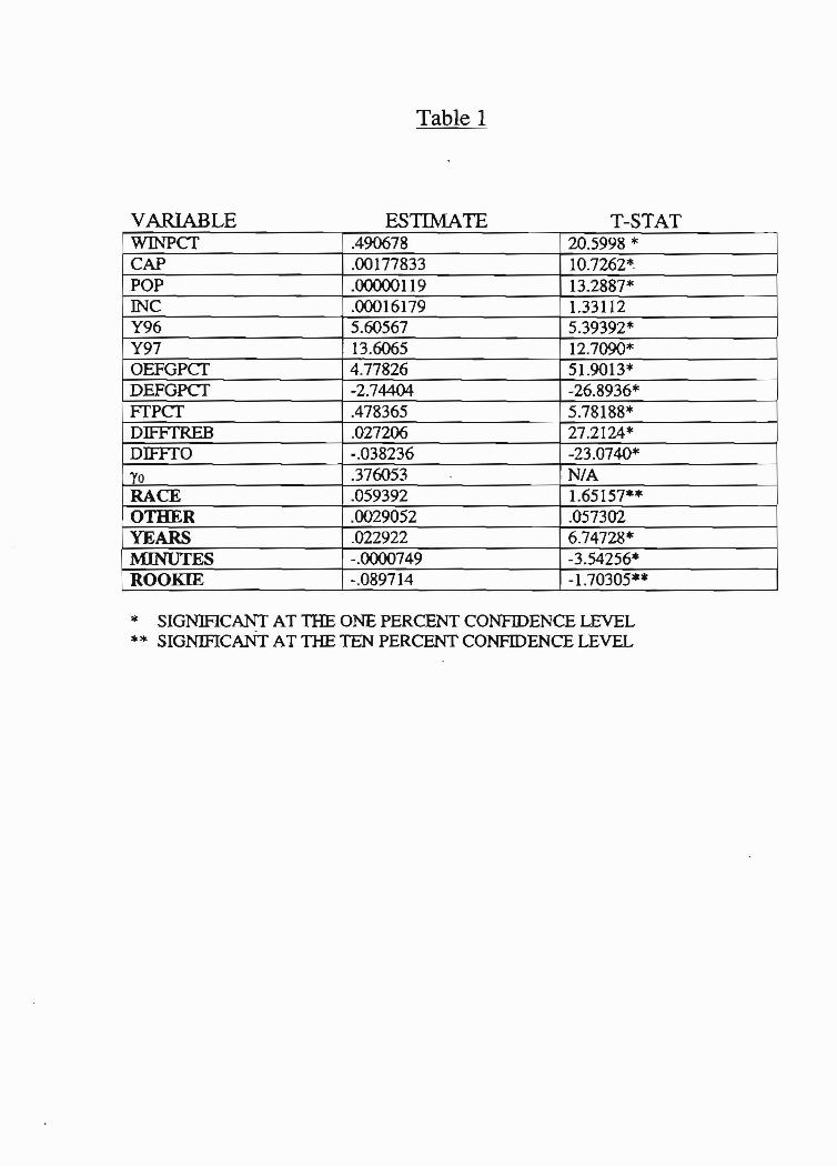
Table 1

VARIABLE ESTIMATE T-STAT WINPCf .490678 20.5998 * CAP .00177833 10.7262*­POP .00000119 13.2887* INC .00016179 1.33112 Y96 5.60567 5.39392* Y97 13.6065 12.7090* OEFGPCf 4.77826 51.9013* DEFGPCT -2.74404 -26.8936* FfPCT .478365 5.78188* DIFFfREB .027206 27.2124* DIFFTO -.038236 -23.0740*

"Yo .376053 N/A RACE .059392 1.65157** OTHER .0029052 .057302 YEARS .022922 6.74728* MINUTES -.(X)OO749 -3.54256* ROOKIE -.089714 -1.70305**

* SIGNIFICANT AT TIiE ONE PERCENT CONFIDENCE LEVEL ** SIGNlFICANT AT THE TEN PERCENf CONFIDENCE LEVEL

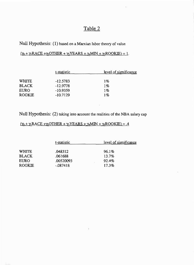
Table 2

Null Hypothesis: (1) based on a Marxian labor theory of value

112 + ylRACE +"U0 THER + "QYEARS + yMIN + Y2ROOKIE) =1.

t-statistic level of significance

WIDTE -12.5783 BLACK -12.9778 EURO -10.9359 ROOKIE -10.7129

1% 1% 1% 1%

Null Hypothesis: (2) taking into account the realities of the NBA salary cap

!Yo + rlRACE ±"bOTHER + 11YEARS + y.MIN + YsROOKIE) =.4

WIDTE BLACK EURO ROOlUE

t -statistic level of significance

.04&312

.061688

.00520093 -.087418

96.1% 13.7% 92.4% 17.3%

Data Appendix

Data for WlNPCT, OEFGPCT, DEFGPCT, ,FGA, FTPCT, DIFFTO, and DIFFTREB for each player were taken from Slats Inc. NBA Handbook, 1996-97, 1997-98,1998-99.

Team data for the WINPCT equation were taken from www .basketball.com basketball database.

Data for POP appears in The Survey ofCurrent Business, September 2000 table K.l

Data for per capita income was found on the Bureau of Economic Analysis website, Local Area Personal Income by Metropolitan Statistical Areas.

Data on stadium capacity were taken from Ballparks by Munsey & Suppes at www.ballparks.com .

Revenue data were found on Rodney Fort's Sport's Business Pages on the web.

Salary data were found on Rodney Fort's Business Pages and www.dfw.netl-patricial. The figures from the latter were taken from the Dallas Morning News.

References

Berri, David. "Who is 'Most Valuable'? Measuring the Player's Production of Wins in the National Basketball Association." Managerial andDecision Economics. Vol. 20 (1999), pp. 411-427.

Dey, Matthew. "Racial Differences in National Basketball Association Players' Salaries: Another Look." The American Economist. VoI.41, No.2 (1997), pp. 84-90.

Hamilton, Barton Hughes. "Racial Discrimination and Professional Basketball Salaries in the 1990s." Applied Economics. Vo1.29, No.3 (1997), pp. 287-96.

Hoang, Ha, & Rasher, Dan. "The NBA, Exit Discrimination and Career Earnings." Industrial Relations, Vol. 38, No.1 (January 1999), pp. 69-91.

Kahn, Lawrence. "Discrimination in Professional Sports: A Survey of the Literature," Industrial and Labor Relations Review. Vol. 44, No.3 (April 1991), pp. 395 - 418.

Kahn, Lawrence. "The Sports Business as a Labor Market Laboratory." Journal of Economic Perspectives. Vol. 14, No.3 (Summer 2000), pp.75-94.

Kennedy, Peter. "A Guide to Econometrics." Fourth Edition, MIT Press, p. 167.

Medoff, M.H. "On Monopsonistic Exploitation in Professional Baseball." Quarterly Review ofEconomics and Business. Vol. 16, No.3 (Summer 1976), pp.113-21.

Nelson, R. & Pearl, M. "Testing For Exploitation in the Labor Market for Professional Athletes." Department of Economics, Colby College, pp. 1-18.

Scott, E, Long, J. & Sompii, K. "Salary Vs. Marginal Revenue Product Under Monopsony and Competition: The Case of Professional Basketball!' Atlantic Economic Journal. VoU3, No.3 (September 1985), pp. 50-59.

STATS Inc, NBA Handbook, 1996-97, 1997-98, 1999-98, Stokie, m.. STATS Publishing.

Acknowledgements

A special thanks to Professor Randy Nelson for his all his help and support. This paper was possible because of his generous efforts and guidance throughout the process.

Thank you to Professor Reid for providing me with the literature and the explanations for most of the econometrics in this paper and for all his support over the last four years .

Thank. you Professor Donihue for many kind words and encouragements along the way.

Finally thank you to my friends and family who encouraged and supported me for the duration of this project and the years leading up to this final work . A special thanks to Michael for his patience and his help organizing. collecting, and creating the dataset.