INSTITUTO NACIONAL DE PESQUISAS DA AMAZÔNIA
93
INSTITUTO NACIONAL DE PESQUISAS DA AMAZÔNIA – INPA UNIVERSIDADE DO ESTADO DO AMAZONAS - UEA Programa Integrado de Pós-Graduação - Clima e Ambiente – PPG-CLIAMB Estudo da advecção horizontal de CO 2 em florestas na Amazônia e sua influência no balanço de Carbono JULIO TÓTA Manaus, Amazonas Outubro 2009 .
-
Upload
khangminh22 -
Category
Documents
-
view
0 -
download
0
Transcript of INSTITUTO NACIONAL DE PESQUISAS DA AMAZÔNIA
INSTITUTO NACIONAL DE PESQUISAS DA AMAZÔNIA – INPA
UNIVERSIDADE DO ESTADO DO AMAZONAS - UEA
Programa Integrado de Pós-Graduação - Clima e Ambiente – PPG-CLIAMB
Estudo da advecção horizontal de CO2 em florestas na Amazônia e sua
influência no balanço de Carbono
JULIO TÓTA
Manaus, Amazonas
Outubro 2009
.
INSTITUTO NACIONAL DE PESQUISAS DA AMAZÔNIA – INPA
UNIVERSIDADE DO ESTADO DO AMAZONAS - UEA
Programa Integrado de Pós-Graduação - Clima e Ambiente – PPG-CLIAMB
Estudo da advecção horizontal de CO2 em florestas na Amazônia e sua
influência no balanço de Carbono
JULIO TÓTA
Orientador: Dra. MARIA ASSUNÇÃO FAUS DA SILVA DIAS
Co-Orientador: Dr. DAVID ROY FITZJARRALD
Tese de doutorado apresentada ao PPG-
CLIAMB como parte dos requisitos
para obtenção do título de Doutor em
Clima e Ambiente, área de
concentração: Geociências.
Manaus, Amazonas
Outubro 2009.
ii
Sinopse:
Este estudo apresenta observações da dinâmica do escoamento do vento dentro e
acima em área de Floresta Tropical na Amazônia, verificando sua relação
com o transporte horizontal de CO2 sobre terrenos de topografia complexa e
avaliando seu impacto no balanço de carbono com o uso do sistema de
correlações de vórtices turbulentos (Eddy Correlation System).
Palavras-chaves: Advecção Horizontal de CO2, Floresta Tropical, Amazônia,
Escoamento de drenagem; Sistema de Correlações de Vórtices Turbulentos,
CO2.
C586e Silva, Julio Tóta da
Estudo da advecção horizontal de CO2 em florestas na Amazônia e
sua influência no balanço de carbono / Julio Tóta da Silva. -- Manaus :
[s.n.], 2009.
xviii, 93 f. : il. (algumas color.)
Tese (doutorado em Clima e Ambiente)--INPA/UEA, Manaus, 2009.
Orientadora: Maria Assunção Faus da Silva Dias
Co-orientador: David Roy Fitzjarrald
Área de concentração: Interações Clima-Biosfera na Amazônia
1.Advecção-Carbono 2.Florestas tropicais-Amazônia 3.Vórtices
turbulentos I.Título
CDD 19ª ed. 551.5112

iii
Dedico
Aos meus pais Antonio Tota e Severina
Soares, e aos meus filhos Luny Tota e Luan Tota
iv
Agradecimentos
A Deus,
Ao Instituto Nacional de Pesquisas da Amazônia (INPA), pela oportunidade de formação,
À Fundação de Amparo a Pesquisa do Estado do Amazonas (FAPEAM) pela bolsa de
estudos,
Agradeço ao Conselho Nacional de Desenvolvimento Científico e Tecnológico – CNPq,
Eu sou especialmente grato aos meus orientadores Dra. Maria Assunção e Dr. David
Fitzjarrald, pela paciência, orientação e apoio constante e pela amizade,
Agradeço aos membros da banca pelas sugestões e revisão do texto da tese,
Expresso minha gratidão ao Dr. Manzi, Coordenador do Programa de Pós-Graduação em
Clima e Ambiente (CLIAMB-INPA/UEA), pelo constante encorajamento, a atenção e pela
amizade desses muito anos,
Agradeço a todos os amigos que me ajudaram nesse caminho: Hermes, Amaury, Juliana,
Julio, Galúcio, Madruga, Alessandro, Celso, Betânia, Veber, e muitos... Todos os
funcionários do LBA Manaus, eu sou grato por todo o apoio logístico,
Especial obrigado para Claudia Vitel e Edwin Keiser pela amizade e apoio,
Aos professores do Programa CLIAMB-INPA/UEA e aos colegas de classe,
v
RESUMO
Fluxos horizontais e verticais de CO2 foram feitos na floresta tropical na Amazônia dentro da
Reserva de Floresta Nacional do Tapajós (FLONA-Tapajós - 54˚58‟W, 2˚51‟S). Duas
campanhas de medidas observacionais foram conduzidas em 2003 e 2004 para descrever o
escoamento abaixo do dossel, determinar sua relação com o vento acima da floresta, e estimar
como este escoamento transporta CO2 horizontalmente. Atualmente já está reconhecido que o
transporte horizontal de CO2 respirado abaixo da floresta não está representado pelo balanço
obtido somente em um ponto de medida nas torres de fluxos (Eddy Covariance - EC), com
erros mais significativos sob condições de noites calmas. Neste trabalho testamos a hipótese
de que o transporte horizontal médio, anteriormente não medido em florestas tropicais, possa
representar a quantidade de CO2 respirado destas condições. Foi instalada uma rede de
sensores de vento e CO2 abaixo da vegetação. Um significante transporte horizontal de CO2
foi observado nos primeiros 10 metros da floresta. Os resultados indicaram que a advecção de
CO2, para todas as noites calmas estudadas, representou 73 e 71% do déficit noturno, definido
pela diferença entre a respiração total do ecossistema (medida ecológica) e o fluxo medido
pelo sistema EC na torre de fluxo, durante as estações seca e chuvosa, respectivamente. Foi
também encontrado que a advecção horizontal de CO2 noturna é igualmente importante, tanto
para condições de baixos níveis de turbulência como para aquelas com altos valores de
velocidade de fricção (nível de turbulência), sendo estes limiares comumente usados para
correções dos fluxos noturnos (correção por u*). Sobre uma área de terreno complexa coberta
por floresta tropical densa (Reserva Biológica do Cuieiras – ZF2 - 02◦36′17.1′′S,
60◦12′24.5′′W) foram medidos gradientes horizontais e verticais de temperatura do ar,
concentrações de CO2 e o campo de vento durante as estações seca e chuvosa de 2006. Foi
testada a hipótese de que escoamento de drenagem horizontal sobre a área de estudo é
significativa e pode afetar a interpretação das altas taxas de absorção de carbono reportadas
por trabalhos anteriores. Um experimento de campo similar ao desenvolvido por Tóta et al.
(2008) foi usado, incluindo uma rede de sensores de vento, temperatura do ar e concentração
de CO2, acima e abaixo da floresta. Foi observado um padrão de escoamento abaixo da
floresta, persistente e sistemático, sobre uma área de encosta de moderada inclinação (~12%),
subindo durante a noite (associada com flutuabilidade positiva) e descendo durante o dia
(flutuabilidade negativa). Acima da floresta (38m) sobre a mesma área de encosta foi também
observado um movimento vertical descendente indicando convergência vertical e
correspondente divergência horizontal em direção ao centro do vale próximo a torre de

vi
medida. Foi observado que as micro-circulações acima da floresta foram dirigidas pelo
balanço entre as forças gradiente de pressão e de flutuabilidade (buoyancy), e abaixo da
floresta também foram dirigidas pelo mesmo mecanismo físico. Os resultados também
indicaram que os gradientes horizontais e verticais de CO2 foram modulados pelas micro-
circulações acima e abaixo da vegetação, sugerindo que as estimativas da advecção usando a
estratégia experimental anterior não são apropriadas devido a natureza tri-dimensional do
transporte horizontal e vertical do local.
vii
SUMMARY
Horizontal and vertical CO2 fluxes and gradients were obtained in an Amazon tropical rain
forest, the Tapajós National Forest Reserve (FLONA-Tapajós - 54o58‟W, 2
o51‟S). Two
observational campaigns in 2003 and 2004 were conducted to describe subcanopy flows,
clarify their relationship to winds above the forest, and estimate how they may transport CO2
horizontally. It is now recognized that subcanopy transport of respired CO2 is missed by
budgets that rely only on single point Eddy Covariance measurements, with the error being
most important under nocturnal calm conditions. We tested the hypothesis that horizontal
mean transport, not previously measured in tropical forests, may account for the missing CO2
in such conditions. A subcanopy network of wind and CO2 sensors was installed. Significant
horizontal transport of CO2 was observed in the lowest 10m of the canopy. Results indicate
that CO2 advection accounted for 73% and 71%, respectively of the carbon budget deficit
(difference between total ecosystem respiration and respective eddy flux tower measured) for
all calm nights evaluated during dry and wet periods. We found that horizontal advection was
significant to the canopy CO2 budget even for conditions with the above-canopy friction
velocity higher than commonly used thresholds (u* correction). On the moderate complex
terrain cover by dense tropical Amazon rainforest (Reserva Biológica do Cuieiras – ZF2 -
02◦36′17.1′′S, 60◦12′24.5′′W) subcanopy horizontal and vertical gradients of the air
temperature, CO2 concentration and wind field were measured for dry and wet periods in
2006. We tested the hypothesis that horizontal drainage flow over this study area is significant
and it can affect the interpretation of the high carbon uptake reported by previous works. A
similar experimental design to the one by Tota et al. (2008) was used with subcanopy network
of wind, air temperature and CO2 sensors above and below the forest canopy. It was observed
a persistent and systematic subcanopy nighttime upsloping (positive buoyancy) and daytime
downsloping (negative buoyancy) flow pattern on the moderate slope (~12%) area. Above
canopy (38 m) on the slope area was also observed a downward motion indicating vertical
convergence and correspondent horizontal divergence into the valley area direction. It was
observed that the micro-circulations above canopy were driven mainly by the balancing
pressure and buoyancy forces and that in subcanopy was driven similar physical mechanisms.
The results also indicated that the horizontal and vertical scalar gradients (e.g. CO2) were
modulated by these micro-circulations above and below canopy, suggesting that advection
estimates using the previous experimental approach is not appropriate due to the tri-
dimensional nature of the vertical and horizontal transport locally.
viii
LISTA DE FIGURAS
Capítulo I: Amazon rain Forest subcanopy flow and the carbon budget: Santarém LBA-ECO
Site.
Figura 1. Site Location in the vegetation cover image and high resolution (30m grid space)
tower-base local topography as determined by the Shuttle Radar Topography Mission
(SRTM). The arrows shows the modal wind direction at 57.8 m (red, from East) and in the
subcanopy (magenta, from southeast)…………………………………………………….. 22
Figure 2. Main tower and Draino deployed instruments systems……………………………23
Figure 3. The autocorrelation coefficient for total wind speed (left panel) and CO2
concentration (center panel) as a function of distance between sampling points 1.8m above
ground in the subcanopy. (3-minute averages data from “Draino” Phase 1 (DOY 198-
238/2003). “C” represents the calibration period. The right panel shows the temporal
autocorrelation, the solid line represents the median, and the thinner lines the upper and
lower quartiles. Mean wind speed in the subcanopy was 0.13 m/s. …………………...…27
Figure 4. Typical nighttime normalized median profiles of CO2, wind speed and their product
(uc) horizontal transport (left panel); and the diurnal cycle of the shape factor for horizontal
advection (right panel). ……………………………………………………………………30
Figure 5. Night time composite of averaged subcanopy CO2 concentration field and wind
vectors for Phase 1 and Phase 2 campaigns. The units are in ppm and ms-1, respectively.
(Largest arrow is 0.15 m s-1).……………………………………………………………...32
Figure 6. Vertical profiles of concentration of CO2, wind speed, temperature, and water
vapor, for both Phases (dry and wet) .……………………………………………………..33
Figure 7. Frequency distribution histogram of friction velocity (u*) at 57.8 m, for Phase 1 and
Phase 2 measurements, separate day and night periods. .………………………………….34
Figure 8. Nighttime distribution of the wind rose and its magnitude (m s-1) for the Draino
sonic anemometer network and at top of main tower (57.8 m), including its localization see
Figure 2). .……………………………………………………………………………….....37
Figure 9. Diurnal cycle of buoyancy term forcing fractions relative to stress divergence term
for Phase 1 (top panel) and Phase 2 (middle panel) observations, and (bottom panel) the
buoyancy forcing term vs. subcanopy wind direction. .…………………………………..38
ix
Figure 10a. Hourly-averaged summary of results for the Phase 1 and all the terms except
eddy flux are average values for 0 to 57.8 m control volume. Top panel: vertical eddy flux
at 57.8 m; 2nd panel: storage; 3th panel: east-west advection; and 4th panel: south-north
advection, terms. .……………………………………………………………………….....39
Figure 10b. Hourly-averaged summary of results for the Phase 2 and all the terms except
eddy flux are average values for 0 to 57.8 m control volume. Top panel: vertical eddy flux
at 57.8 m; 2nd panel: storage; 3rd panel: vertical advection; 4th panel: east-west advection;
and 5th panel: and south-north advection, terms. .………………………………………...40
Figure 11a. Top panel: Hourly-averaged vertical eddy flux at 57.8 m; 2nd panel: storage
term; 3rd panel: east-west advection term; and 4th panel: and south-north advection, terms.
Note the change in vertical scale between the phases. .…………………………………....41
Figure 11b. Top panel: Hourly-averaged vertical eddy flux at 57.8 m; 2nd panel: storage
term; 3rd panel: vertical advection term; 4th panel: east-west advection term; and 5th panel:
and south-north advection terms. Note the change in vertical scale between the phases….42
Figure 12a. Mean nocturnal variation of the NEE (Eddy covariance flux + storage),
ecosystem respiration, horizontal advection and NEE plus advection, for Phase 1 (Dry
period). .…………………………………………………………………………………....43
Figure 12b. Same Figure 12a, for Phase 2 (Wet period). .…………………………………..44
Figure 13. Mean nocturnal variation of the advection term as a function of the friction
velocity rank, for Phase 1 (left panel) and Phase 2 (right panel) datasets. Solid line with
dots indicates binned average values (0.1 intervals)). Error-bar also is plot with standard
deviation, respectively. .…………………………………………………………………...45
Capítulo II: Amazon rain Forest subcanopy flow and the carbon budget: Manaus LBA Site -
a complex terrain condition.
Figure 1. Detailed measurements towers‟s view in the ZF-2 Açu catchment (East-West valley
orientation) from SRTM-DEM datasets. Large view in the above panel and below panel the
points of measurements (B34 – Valley, K34 – Plateau, and subcanopy Draino system
measurements over slopes in south and north faces (red square points).…………………..51
Figure 2. (a) Açu Cachment with level terrain cotes and vegetation cover from IKONOS‟s
image and (b) vegetation structure measured from Lidar sensor over yellow transect (a).
From (a) the blue color is valley and vegetation transition to plateau areas (red colors)….52
x
Figure 3. Draino measurement system used in Manaus LBA (South Face, see also Figure
4)…………………………………………………………………………………………...54
Figure 4. Draino measurement system (South and North Slope face) implemented at Manaus
LBA Site, including topographic view and instrumentation deployed…………………….55
Figure 5. 10 days time series of the CO2 concentration, air temperature (DRAINO System)
and total precipitation (plateau tower)……………………………………………………..57
Figure 6. Boxplot of the virtual potential temperature vertical profile for dry (a, b) and wet
periods (c,d) of the 2006 during night (b,d) and daytime (a,c), on the plateau K34 tower..59
Figure 7. Daily course of the vertical deviation of the virtual potential temperature for dry (a)
and wet (b) periods of the 2006, on the plateau K34 tower…………………………..……60
Figure 8. Boxplot of the virtual potential temperature vertical profile for dry (a, b) and wet
periods (c, d) of the 2006 during night (b, d) and daytime (a, c), on the slope area DRAINO
System tower (south face, see Figure 2)…………………………………………………...61
Figure 9. Daily course of the vertical deviation of the virtual potential temperature for dry (a)
and wet (b) periods of the 2006, and virtual potential temperature vertical gradient (c), on
the slope area DRAINO System tower…………………………………………………….62
Figure 10. Frequency distribution of the wind speed and direction. For dry (a, b) and wet (c,
d) periods from 2006 during day (a, c) and nighttime (b, d), on the plateau K34 tower…..64
Figure 11. Frequency distribution of the wind speed and direction above canopy (38 m above
ground level – a.g.l). For dry (a, b) and wet (c, d) periods from 2006 during day (a, c) and
nighttime (b, d), on the slope area at DRAINO system tower……………………………..65
Figure 12. Frequency distribution of the wind speed and direction in the subcanopy array (2
m above ground level – a.g.l) on the microbasin south face slope area at DRAINO
horizontal array system (see Figure 4). For dry (a-f) and wet (g-l) periods from 2006,
during day (a, b, c, g, h, i) and nighttime (d, e, f, j, k, l)…………………………………...67
Figure 13. Frequency distribution of the subcanopy wind direction (a) upsloping (from north
quadrant) and (b) downsloping (from south quadrant) on the south face slope area at
DRAINO horizontal array system (see Figure 4)……………………………………….....69
Figure 14. Mean vertical velocity raw and correct vertical velocity (a) for DRAINO system
slope tower (38 m), and hourly mean vertical velocity (b) for: plateau K34 tower (55 m),
DRAINO system slope tower (above canopy - 38 m and subcanopy - 3 m) and for valley
B34 (43 m) towers (see Figure 4, for details)……………………………………………...70
Figure 15. Schematic local circulations in the site studied, valley and slopes flow (a), 2D
view from suggested below and above canopy airflow (b)……………………………..….72
xi
Figure 16. Example at midnight (local time) of the horizontal CO2 concentration over the
DRAINO System south face domain including an interpolated horizontal wind field (10 m
grid), note the geographic orientation and the red arrow indicating slope inclination (see
Figure 4)……………………………………………………………………………...…….74
Figure 17. Hourly average of the subcanopy (2 m) CO2 concentration and horizontal wind
speed over DRAINO System south face area during dry period of the 2006, note the
geographic orientation and the red arrow indicating slope inclination (see Figure 4). The
axis represents distances from center of the main tower……………………………...……75
Figure 18. Hourly average of the subcanopy (2 m) CO2 concentration on the DRAINO
System north face area during dry period of the 2006, note the geographic orientation (see
Figure 4). The axis represents distances from center of the main tower…………………...76
xii
SUMÁRIO
INTRODUÇÃO GERAL………………………………………………………..........………14
OBJETIVO GERAL……………………………………………………………...........……..16
OBJETIVOS ESPECÍFICOS……………………………………………………...………….16
Capítulo I: Amazon rain forest subcanopy flow and the carbon budget: Santarém LBA-ECO
…………………....…….......................................................................................................18
Abstract …………………………………………………………………………..........……..18
1. Introduction ….….................................................................................................................19
2. Material and Methods ….…….............................................................................................21
2.1 Site description ….……......................................................................................................21
2.2. Instrumentation and observation ……..…….....................................................................23
2.3. Preinstallation intercomparison ……..…….......................................................................26
2.4. CO2 conservation equations ……..……............................................................................28
2.5. Vertical integration of the horizontal advection terms ……..……....................................30
3 – Results and Discussion ……..…….....................................................................................32
3.1. CO2 concentration field ……..…….................................................................................32
3.2. Subcanopy horizontal wind field ……..……....................................................................36
3.3. Subcanopy flow forcing terms ……..……........................................................................37
3.4. Estimates of Advection Terms ……..……........................................................................39
3.5. CO2 budget ……..……......................................................................................................43
3.6. Correlation between advection components and friction velocity ……..……..................44
4. Summary and Conclusions ……..…….................................................................................45
Capítulo II: Amazon rain Forest subcanopy flow and the carbon budget: Manaus LBA Site -
a complex terrain condition …..……....................................................................................48
Abstract …………………………………………………………………………..........……..48
1. Introduction ….….................................................................................................................49
2. Material and Methods ….…….............................................................................................50
2.1 Site description ….……......................................................................................................50
2.2. Measurements and instrumentation ….…….....................................................................53
xiii
3 – Results and Discussion ….……..........................................................................................57
3.1. Air Temperature field ........................................................................................................58
3.1.1 - Plateau K34 tower .........................................................................................................58
3.1.2 – DRAINO System Slope tower .....................................................................................60
3.2. Wind field .........................................................................................................................63
3.2.1 – Horizontal wind regime - above canopy.......................................................................63
3.2.1.1 - Plateau K34 tower …………………..........................................................................63
3.2.1.2 - DRAINO System slope tower ...................................................................................64
3.2.2 – Horizontal wind regime – Subcanopy array measurements (2 m a.g.l) …...................65
3.2.3 – Mean Vertical wind velocity – subcanopy and above canopy …….............................69
3.3. Phenomenology of the local circulations: Summary ........................................................72
3.4. CO2 concentration and subcanopy horizontal wind field .…............................................73
4. Summary and Conclusions ...................................................................................................77
CONCLUSÃO GERAL....……………………………………….....….………..……………79
REFERÊNCIAS…………………………………………………………………..….……….82

14
INTRODUÇÃO GERAL
Nas últimas décadas há um crescente interesse da comunidade cientifica em
quantificar as trocas liquidas de dióxido de carbono (CO2) entre ecossistemas florestais e a
atmosfera, devido ao nível de incerteza das estimativas das fontes e sumidouros desses
ecossistemas no balanço global de carbono. Enquanto as estimativas do crescente nível de
aumento de CO2 atmosférico e os sumidouros de CO2 pelos oceanos são bem conhecidas,
as fontes e sumidouros da biosfera ainda não são estimados precisamente (IPCC 2007).
Reduzir as incertezas das fontes e sumidouros de dióxido de carbono da biosfera tem sido
um grande desafio da comunidade cientifica atualmente visando melhor entender o balanço
global de carbono e o papel dos biomas terrestres no assim chamado “aquecimento global”.
Os biomas florestais exercem um papel importante no balanço global de carbono,
pois representam 80% de biomassa aérea e 40% de biomassa de raízes e serrapilheira do
carbono orgânico global (Dixon et al., 1994). Dentre estes ecossistemas, as florestas
tropicais da Amazônia são uma importante componente para o balanço global de carbono,
em função da sua grande quantidade de biomassa armazenada e de seu rápido ciclo de
carbono através dos processos de fotossíntese e respiração. As florestas da Amazônia
representam 10% da produtividade primária terrestre e do carbono armazenado nos
ecossistemas terrestres (Melillo et al., 1993; Malhi et al., 1998). Portanto, para melhor
quantificar o balanço global de carbono é preciso também determinar o balanço regional de
carbono na Amazônia e sua variabilidade em resposta as mudanças do meio ambiente. Para
isso, torna-se crítico entender os processos de respiração e fotossíntese do ecossistema
Amazônico detalhadamente.
Atualmente não há um consenso da comunidade científica se as florestas tropicais
na Amazônia atuam como fontes ou sumidouros de CO2 atmosférico. Estimativas com base
em medidas biométricas, sugerem tanto um papel de sumidouro (Phillips et al., 1998; Baker
et al., 2004), como uma fonte de CO2 atmosférico (Rice et al., 1998; Miller et al., 2004).
Por outro lado, estimativas com base em medidas pelo método das covariâncias de vórtices
turbulentos (EC – “Eddy covariance System”), sugerem que o ecossistema de floresta
tropical na Amazônia atua como sumidouro (Grace et al., 1995; Malhi et al., 1998; Araújo
et al., 2002), uma pequena fonte (Saleska et al., 2003; Hutyra et al., 2007), ou em equilíbrio
(Miller et al., 2004), com relação às trocas líquidas de CO2 atmosférico.
15
Portanto, existe uma urgente necessidade em melhor entender e quantificar as
incertezas dessas estimativas em ecossistemas terrestres, em especial na Amazônia.
As estimativas realizadas por EC na escala espacial das torres micrometeorológicas,
são uma importante ferramenta para quantificar as trocas líquidas entre a superfície e a
atmosfera e amplamente utilizada desde seu desenvolvimento (Montgomery, 1948;
Swinbank, 1951) para estimativas das trocas de energia (Antonia et al., 1979; Fitzjarrald et
al., 1988; Bergstrom and Hogstrom, 1989; Gao et al., 1989; Shuttleworth, 1989) e gases
traços, como CO2 (Fan et al., 1990; Lee et al., 1992; Wofsy et al., 1993; Grace et al., 1995;
Black et al., 1996; Moncrieff et al., 1997; Malhi et al., 1998; Baldocchi et al., 2001; Araújo
et al., 2002). A metodologia de EC tem a vantagem de obter medidas diretas e de longo
prazo dos fluxos de CO2 na interface floresta-atmosfera (Wofsy et al., 1993, Goulden et al.,
1996; Urbanski et al., 2007).
Entretanto, teoricamente este método assume que as áreas representativas das
medidas sejam horizontalmente homogêneas e planas para uma melhor estimativa dos
fluxos turbulentos obtidos pelas torres. Dessa forma, considera que a mistura turbulenta
atmosférica seja suficientemente efetiva para eliminar o efeito da variabilidade da cobertura
da superfície em pequena escala (tipo de vegetação e terreno) e represente o fluxo
turbulento médio da área obtido nas torres de fluxos.
Em termos de balanço de energia ou de gases, isto significa que os termos de
transportes horizontais (advecção) são desprezados ou não significativos, predominando
apenas os fluxos verticais turbulentos. Isto tem um efeito significativo nas trocas liquidas
entre o ecossistema e a atmosfera (NEE – “Net Ecosystem Exchange”), a qual é obtida,
neste caso, somente pela soma dos fluxos verticais turbulentos e o termo de armazenamento
(Storage) abaixo do nível da medida (NEE = Eddy Flux + Storage). O termo de
armazenamento, por exemplo, na Amazônia, tem sido obtido raramente de maneira
contínua, dada as dificuldades específicas de cada sitio e das condições ambientais
adversas, gerando uma barreira para as estimativas de NEE (Iwata et al., 2005).
Sob certas condições de baixo nível de turbulência atmosférica (geralmente nos
períodos noturnos) e certo grau de complexidade topográfica, circulações secundárias e
escoamento horizontal sobre as encostas do terreno, o chamado escoamento de drenagem
(“Drainage Flow”), podem se desenvolver (Yoshino et al., 1984). Isto tem sido evidenciado
por vários estudos em diversas localidades, os quais indicam a importância da advecção de
CO2 no balanço de carbono (Aubinet et al., 2003; Staebler and Fitzjarrald, 2004, 2005;
Marcolla et al., 2005; Feigenwinter et al., 2008; Leuning et al., 2008). Porém, os estudos de
16
advecção de CO2 foram realizados sobre regiões montanhosas de latitude média e não em
regiões de florestas tropicais, passando a ser uma motivação e um desafio, investigar a
existência e quantificar a importância da advecção de CO2 no balanço de carbono das áreas
de floresta tropicais na Amazônia.
Com o objetivo de quantificar e melhor entender as fontes e sumidouros de CO2 na
região de floresta tropical na Amazônia, o Projeto de Grande Escala da Biosfera-Atmosfera
na Amazônia (LBA - “Large Scale Biosphere-Atmosphere experiment in Amazonia”)
estabeleceu uma rede de torres micrometeorológicas com o sistema EC em vários pontos na
região (Keller et al., 2004).
Esta tese visa investigar os processos de transporte não turbulentos, os quais são os
termos advectivos componentes da equação de balanço de carbono, e os mecanismos
físicos que os dirigem, nos sítios experimentais do Projeto LBA de Santarém (PA) e de
Manaus (AM). Para isso, foi concebido um sistema de medida direta e detalhada das
principais variáveis (velocidade do vento, temperatura do ar e concentração de CO2) usadas
para caracterizar a dinâmica do escoamento acima e abaixo da floresta, e calcular os termos
advectivos de transporte de CO2 sobre as áreas representativas das torres
micrometeorológicas do projeto LBA.
OBJETIVO GERAL
Esta tese tem como objetivo geral investigar e quantificar através de medidas
observacionais os mecanismos físicos que dirigem os termos não turbulentos das equações
de balanço de carbono associados com o transporte lateral de CO2 em dois sítios de floresta
tropical do projeto LBA na Amazônia.
OBJETIVOS ESPECÍFICOS
1) Implementar um sistema de medidas observacional para investigar a dinâmica do
escoamento acima e abaixo da floresta tropical na Amazônia sobre terrenos complexos,
capaz de medir baixos limiares de velocidade do vento e gradientes horizontais de CO2
abaixo da copa da floresta;
17
2) Determinar e quantificar os gradientes horizontais e verticais de concentrações de CO2
importantes para os transportes horizontais de CO2, (advecção horizontal – Capitulo I –
Sitio do LBA em Santarém - PA);
3) Avaliar e/ou determinar a existência do escoamento horizontal abaixo da copa da floresta,
bem como, sua persistência e sistemática em produzir transporte horizontal de CO2 para
fora da área de representatividade do sistema EC das torres micrometeorológicas do projeto
LBA e determinar sua validade;
4) Determinar os mecanismos físicos da dinâmica do escoamento responsáveis pela advecção
horizontal de CO2;
5) Quantificar os termos de transportes horizontais e/ou advecção horizontal de CO2, que
contribuem para o balanço de carbono na escala das torres micrometeorológicas do LBA;
18
Capítulo I - Amazon rain forest subcanopy flow and the carbon budget:
Part I – Santarém LBA-ECO 1
Abstract
Horizontal and vertical CO2 fluxes and gradients were obtained in an Amazon tropical rain
forest, the Tapajós National Forest Reserve (FLONA-Tapajós - 54o58‟W, 2
o51‟S). Two
observational campaigns in 2003 and 2004 were conducted to describe subcanopy flows,
clarify their relationship to winds above the forest, and estimate how they may transport CO2
horizontally. It is now recognized that subcanopy transport of respired CO2 is missed by
budgets that rely only on single point Eddy Covariance measurements, with the error being
most important under nocturnal calm conditions. We tested the hypothesis that horizontal
mean transport, not previously measured in tropical forests, may account for the missing CO2
in such conditions. A subcanopy network of wind and CO2 sensors was installed. Significant
horizontal transport of CO2 was observed in the lowest 10 m of the canopy. Results indicate
that CO2 advection accounted for 73% and 71%, respectively of the carbon budget deficits for
all calm nights evaluated during dry and wet periods. We found that horizontal advection was
significant and important to the canopy CO2 budget, during environmental conditions with
lower above-canopy friction velocity values and also during higher values commonly used
thresholds to the u* corrections approach.
Key words: Amazon Rainforest; Advection, Drainage Flow, Eddy Covariance, Subcanopy.
1 Tóta, J., Fitzjarrald, D.R., Staebler, R.M., Sakai, R.K., Moraes, O.M.M., Acevedo, O.C., Wofsy, S.C., Manzi,
A.O., 2008. Amazon rain forest subcanopy flow and the carbon budget: Part I – Santarem LBA-ECO Site.
Journal of Geophysical Research – Biogeosciences, 113, 1-15.
19
1. Introduction
In the last decade tower-based eddy-covariance (EC) observations have been
established worldwide to monitor net ecosystem exchange (NEE) of carbon dioxide [Goulden
et al., 1996; Black et al., 1996; Baldocchi et al., 2001]. This micrometeorological method is
considered the most accurate when applied at nearly flat sites that have long homogeneous
upwind fetches. Its application has spawned global scale flux-measuring networks [Baldocchi
et al., 1988; Aubinet et al., 2000] whose justification has been to estimate long-term carbon
exchange. Two related issues complicate this ambition. First, proper estimates of nocturnal
respiratory fluxes are essential, but weak turbulent mixing at night is common. This issue of
underreporting of nocturnal CO2 fluxes has been addressed using the approach advocated by
Goulden et al [1996], formalized by the FLUXNET committee [Baldocchi et al., 2001]. Data
on very calm nights (often an appreciable fraction of all nights) is simply discarded and
replaced with the result of an ecosystem respiration rate found on windy nights that are
otherwise similar [Miller et al., 2004; Gu et al., 2005]. A second issue is that many flux-
observing sites lie in complex terrain [Lee, 1998; Paw U et al., 2000; Aubinet et al., 2003;
Feigenwinter et al., 2004; Staebler and Fitzjarrald, 2004, 2005]. On the very calm nights for
which flux underestimates occur, subcanopy drainage flows are most common [Yoshino et al.,
1984; Sun et al., 2007]. Whether or not subcanopy drainage flows also advect sufficient CO2
laterally out of the budget “box” to account for the „missing flux‟ on calm nights is site
specific, and must be determined observationally [Lee, 1998; Feigenwinter et al., 2004;
Staebler and Fitzjarrald, 2004; Aubinet et al., 2005]. Previous studies show that, under light
wind and very stable conditions over the canopy, the importance of advection on the carbon
balance can be as large as, or even larger than, the magnitude of NEE, observed by the EC
approach when there are drainage flows [Staebler, 2003; Staebler and Fitzjarrald, 2004,
20
2005; Sun et al., 2007]. To assess the importance of subcanopy flows one must present a
plausible physical mechanism to account for this underestimation as past studies asserted
[Kruijt et al., 2004; Araújo et al., 2002]. Even on gentle slopes, it is risky to assume that there
is no lateral motion or divergence that can advect CO2 (e.g., Acevedo and Fitzjarrald, 2003)
and applying the ideal site criteria to more typical situations is questionable [Baldocchi et al.,
2000; Staebler and Fitzjarrald, 2004, 2005].
Most studies of subcanopy advection to date have been done at midlatitude sites. We
are not aware of similar studies in the tropical rain forest. The forests in the Amazon region
account for 10% of the world‟s terrestrial primary productivity and about the same fraction of
carbon stored in land ecosystems [Malhi et al., 1998]. In the last decade reports have
suggested that this region has such a positive sink of CO2, which, when scaled for the entire
Amazon region, could account for a significant fraction of the carbon budget, the so called
residual terrestrials sink (IPCC, 2007). Since results from the Large Scale Biosphere-
Atmosphere experiment in Amazonia (LBA, Keller et al., 2004) will likely be used to
represent the Amazon in its entirety in global change models, it is important to identify
systematic observation problems. In this paper we describe a detailed subcanopy CO2 and
wind system sensors deployed for the first time in the Amazon tropical rainforest combined
with EC tower flux and respiration measurements and analyze the results with the aim to
better understand the local carbon budget. Formally, we test the hypotheses that EC
measurements underestimate the CO2 flux on calm nights because of lateral air flow out of the
control volume at the km67 Santarém LBA site. We seek to demonstrate that observed
subcanopy horizontal CO2 gradients and wind transport processes yield significant mean net
transport of CO2 into or out of the control volume. Following Staebler and Fitzjarrald [2004,
2005], we examine the importance of subcanopy advection in the following steps:
(1) We must show that systematic subcanopy flows exist and are measurable; and
21
(2) Observed subcanopy flows must be related to a physical driving mechanism (e.g.
drainage forcing) that ensures that they are sufficiently systematic so that long-term
budgets are affected.
2. Material and Methods
2.1. Site description
The study site (54° 58‟W, 2° 51‟S) is part of the ecological component of the Large
Scale Biosphere-Atmosphere experiment in Amazonia (LBA-ECO), which aims to achieve
better understanding of the regional carbon balance. It is located in the Tapajós National
Forest reserve (FLONA Tapajós), near km 67 of the Santarém-Cuiabá highway (BR-163).
The average temperature, humidity, and rainfall are 25.8°C, 85%, and about 1800 mm per
year, respectively [Parotta et al., 1995]. This area contains predominantly nutrient-poor clay
oxisols with some sandy utisols [Silver et al., 2000], each of which has low organic content
and cation exchange capacity.
Vegetation consists of occasional 55 m height emergent trees with a closed canopy at
40m and below [Parker et al., 2004]. Trees include Manilkara huberi (Ducke) Chev.,
Hymenaea courbaril L., Betholletia excelsa Humb. and Bonpl., and Tachigalia spp species,
and epiphytes. There is overall an uneven age distribution, but the forest can be considered to
be primary or old growth [Clark, 1996; Goulden et al., 2004].
Local topographic features include a steep nearby river escarpment sloping to the
Tapajós River to the west, but with a weak eastward-facing slope into the basin of the Curua-
Una watershed. Except near the escarpment, drainage flows would be expected to move
opposing the easterly prevailing wind field (red arrow in the Figure 1).
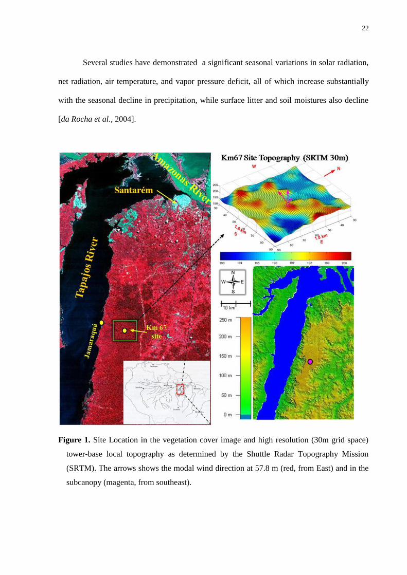
22
Several studies have demonstrated a significant seasonal variations in solar radiation,
net radiation, air temperature, and vapor pressure deficit, all of which increase substantially
with the seasonal decline in precipitation, while surface litter and soil moistures also decline
[da Rocha et al., 2004].
Figure 1. Site Location in the vegetation cover image and high resolution (30m grid space)
tower-base local topography as determined by the Shuttle Radar Topography Mission
(SRTM). The arrows shows the modal wind direction at 57.8 m (red, from East) and in the
subcanopy (magenta, from southeast).
23
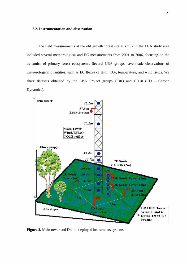
2.2. Instrumentation and observation
The field measurements at the old growth forest site at km67 in the LBA study area
included several meteorological and EC measurements from 2001 to 2006, focusing on the
dynamics of primary forest ecosystems. Several LBA groups have made observations of
meteorological quantities, such as EC fluxes of H2O, CO2, temperature, and wind fields. We
share datasets obtained by the LBA Project groups CD03 and CD10 (CD – Carbon
Dynamics).
Figure 2. Main tower and Draino deployed instruments systems.
24
The CD10 tower systems include EC and meteorological wind, CO2, temperature and
water vapor profiles collected between 2001 and 2006 (Table 1 and Figure 2). The
instrumentation descriptions and quality control procedures for the basic datasets obtained at
the main km67 tower site are given in Saleska et al. [2003] or at the online web page
http://www-as.harvard.edu/data/lbadata.html. A weather station was deployed in Jamaraquá at
the base of the Tapajós escarpment to help in identifying topographical effects. A high
resolution STRM map was made, based on a 90m grid, interpolated to 30 meters, to describe
the gentle topography around the tower site (Figure 1).
Table 1. LBA – Old Growth (KM67) Site Sensors
Level (m) Parameter Instrument
64.1,52,38.2,30.7 Wind speed Cup anemometers
57.8
u‟ v‟ w‟ T‟,CO2, H20 CSAT 3D sonic anemometers
LI-7000 CO2/H20 analyzers
5 U‟ v‟ w‟ T‟ ATI 3D sonic anemometer
1.8 CO2, U, V, T
(horizontal array)
CATI/2 2D sonic anemometers,
LI-7000
62.2,50.1,39.4,28.7
19.6,10.4,3.1,0.9
CO2, H20 Profile LI-7000 CO2/H20 analyzer
61.9,49.8,39.1,28.4
18.3,10.1,2.8,0.6
Temperature Aspirated thermocouples
Subcanopy network observations are available for two campaigns in 2003 (Phase 1,
DOY 198-238) and 2004/2005 (Phase 2, DOY 250-366 and 01-32). The subcanopy data
complement observations that were made around the central 65-meter tower. The observation
and acquisition approach was developed at Atmospheric Sciences Research Center, ASRC
(Staebler and Fitzjarrald, 2005) and includes a PC operating in Linux, an outboard Cyclades
multiple serial port (CYCLOM-16YeP/DB25) collecting and merging serial data streams
from all instruments in real time, with the data archived into 12-hour ASCII files.
Observations include CO2, temperature, H2O and wind field measurements at 1 Hz
(Figure 2), this sufficient to cover advection and storage fluxes (non turbulent fluxes). The
25
system included a LI-7000 Infrared Gas Analyzer (LI-COR inc., Lincoln, Nebraska, USA), a
multi-position valve (Vici Valco Instrument Co., Inc.) controlled by a CR23x Micrologger
(Campbell Scientific, Inc., Logan, Utah, USA), which also monitored flow rates. The
instrument network array (Figure 2 and Table 1) consisted of 6 subcanopy sonic
anemometers: a Gill HS (Gill Instruments Ltd., Lymington, UK) 3-component sonic
anemometer at 5 m elevation in the center of the grid and 5 SPAS/2Y (Applied Technologies
Inc., CO, USA) 2-component anemometers (1 sonic at center and 4 sonic along the
periphery), with a resolution of 0.01 m s-1
. The horizontal gradients of CO2/H2O were
measured in the array at 2 m above ground, by sampling sequentially from 4 horizontal points
surrounding the main tower location at distances of 70-80m, and from points at 6 levels on the
small Draino tower, performing a 3 minute cycle. Air was pumped continuously through 0.9
mm Dekoron tube (Synflex 1300, Saint-Gobain Performance Plastics, Wayne, NJ, USA)
tubes from meshed inlets to a manifold in a centralized box.
A baseline air flow of 4 LPM from the inlets to a central manifold was maintained in
all lines at all times to ensure relatively “fresh” air was being sampled. The air was pumped
for 20 seconds from each inlet, across filters to limit moisture effects. The delay time for
sampling was five seconds and the first ten seconds of data were discarded. At the manifold,
one line at a time was then sampled using an infrared gas analyzer (LI-7000, Licor, Inc.). The
6-level CO2 profile on the 5 m tower was determined in a similar, sequential manner, using a
LI-7000 gas analyzer sampling pumped air from all 10 points (6 vertical, 4 horizontal) in the
measurement array. Flow rates at the inlets were checked regularly to ensure proper flow and
to detect potential leaks.
26
2.3. Preinstallation intercomparison
Following Staebler and Fitzjarrald [2004] an initial instrument intercomparison was
made to identify the performance of the integrated subcanopy observation system. The CO2
sensor (Licor 7000 sensor) and the sonic anemometers (CATI/2 and SPAS/2Y, Applied
Technologies, Inc. sensors) were co-located on the small tower for a calibration period (5
days) before being deployed at 1.8 meters above the ground (Figure 2). We anticipated that
the horizontal transport product uc would be near its largest value at this height, a finding later
confirmed at this site (see Figure 4 below). We had insufficient instrumentation to construct a
network of towers to measure the CO2 concentration up to canopy top, and this led us to
continue our earlier practice of asserting a profile similarity hypothesis, where one
hypothesizes spatial similarity between vertical CO2 and wind profiles and their product (the
horizontal transport). Using a single gas analyzer with a common path multi-position valve
for the horizontal and vertical profiles minimizes the potential for systematic concentration
errors. A field calibration was performed by co-locating sensors and gas inlets at the same
point of measurement. The comparisons indicate scatter in [CO2] because samples were
sequential, not synchronous. The mean standard error was < 0.05 ppm. The wind comparisons
were made using a 3D sonic as the standard for the 2D sonic anemometers, resulting in a
mean standard error of about 0.005 ms-1
. Ambient subcanopy wind speed was on the order of
a few cm s-1
and can be reliably measured in the subcanopy space by the system. After
intercomparison, the sonic anemometers and the CO2 inlet tubes were moved from the small
tower center point and deployed about 2 meters above ground as indicated in Figure 2.
We examined to what extent the subcanopy sensor geometry of CO2 allows the system
to function as a “network”, where each point of the measurements are correlated and the space
27
between them is on the order of the relevant scales of transport or smaller. We test whether
the network can be used to capture the relevant gradients and transport processes in very low
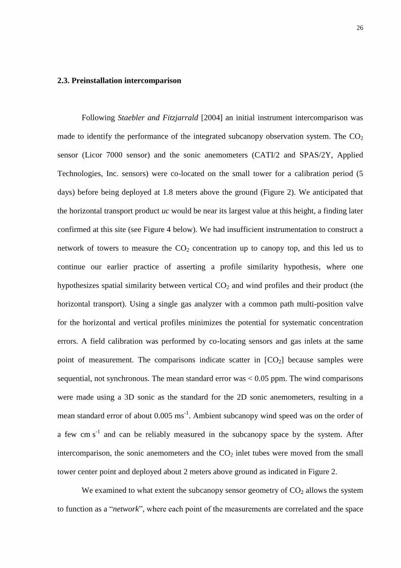
wind conditions [Staebler and Fitzjarrald, 2004]. Figure 3 (left panel) shows the 3-min data
autocorrelation of CO2 and wind fields determined from continuous measurements.
Figure 3. The autocorrelation coefficient for total wind speed (left panel) and CO2
concentration (center panel) as a function of distance between sampling points 1.8m above
ground in the subcanopy. (3-minute averages data from “Draino” Phase 1 (DOY 198-
238/2003). “C” represents the calibration period. The right panel shows the temporal
autocorrelation for wind, the solid line represents the median, and the thinner lines the
upper and lower quartiles. Mean wind speed in the subcanopy was 0.13 m.s-1
.
The relevant spatial scale X is approximately 70-150 m. We assessed our choice of
network size by examining observed spatial and temporal autocorrelations of the wind
measurements. The spatial autocorrelation of horizontal wind speed (Figure 3 - center panel)
drops rapidly to 0.2 in 60 m, but fluctuations in CO2 (Figure 3 - left panel) exhibit a larger
integral scale 100-200 m, while the temporal integral is approximately 100-300s (Figure 3,
right panel). This is consistent with results obtained by Staebler and Fitzjarrald [2004] in a
very different forest, except that the characteristic horizontal CO2 scale is larger than that at

28
Harvard Forest, consistent with the thicker canopy at the Tapajós National Forest. We do not
understand why the spatial correlations do not decrease with increasing distance, as was
observed in Staebler and Fitzjarrald [2004]. This could be a consequence of the temporal
scale variations being larger than are the spatial ones.
2.4. CO2 conservation equations
The net ecosystem exchange (NEE) for a horizontal plane at height h, which
represents the exchange rate between forest and atmosphere, is given by,
NEEh F
0 s
_
dz0
h
(1),
where F0 is the soil flux entering (or leaving) the control volume at the bottom and the _
s
integral describes the sum of all sources and sinks in the canopy space. The Reynolds average
conservation equation of a scalar “c”, ignoring molecular diffusion process, can be expressed
by,
_''s
x
cu
x
uc
xcu
tc
i
i
i
i
ii
(2),
with ),,( wvuui . Considering using equations 1 and 2, and considering incompressibility,
after integrating vertically, it can be written in the form,
h
h
hhhhhh
dzscwdzzcvdz
zcudz
zcwdz
ycvdz
xcudz
tc
0
_
000000
'''''' (3),
[1] [2] [3] [4] [5] [6] [7] [8]
where u, v, and w, are wind components and “c” a scalar, such as CO2. The term [4] is the
vertical advection term and term [8] the sum of all sinks and sources between z=0 and z=h,
including everything crossing the lower boundary at z=0.
29
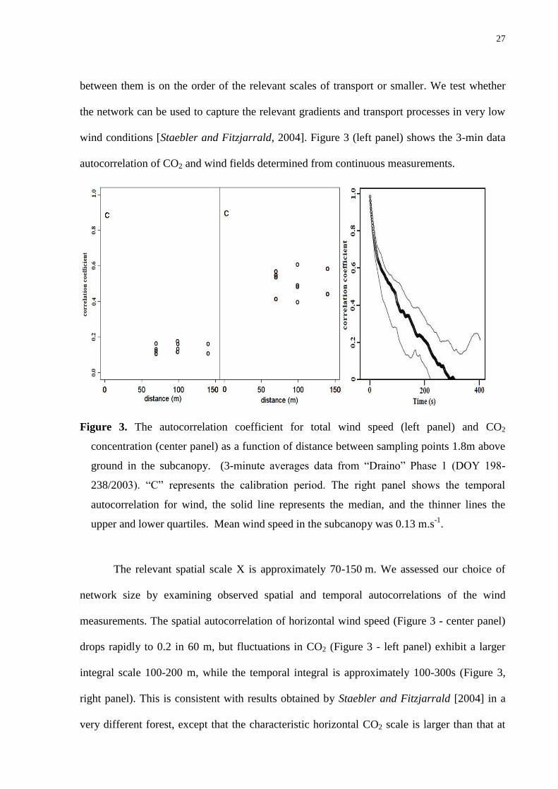
In the case of horizontal homogeneity, terms [1], storage in the canopy space, and [7],
vertical eddy flux at z=h (57.8 m for the site studied), are obtained from standard EC and
profile sensors at the flux site. Terms [5] and [6] are the horizontal turbulent flux divergence
and negligible when compared with other terms [Yi et al., 2000; Turnipseed et al., 2003]. The
terms [2], [3] and [4] respectively are horizontal and vertical advection. The vertical mean
advection was integrated using the method of Lee [1998]:
h
h
h
hh dzzch
hcwdzzch
wcw
00
0 )(1
)()(][ (4),
where hw and )(hc are the residual vertical velocity and the mean concentration at the top of
the layer (57 m), respectively [see in Staebler and Fitzjarrald, 2004]. Staebler and Fitzjarrald
[2004] argued that Lee‟s approach is an overestimate, noting that the assumption of a linear
increase of hw with height is often violated. Comparisons of the divergence measurements at
1.8 m height with measured vertical velocities at 46 m and 57.8 m were made for a few days
of wind data and the results show no correlation indicating that Lee‟s approach is also
violated for the site studied here. However, Lee‟s formulation will be used to provide an
upper estimate of the vertical advection term in order to compare its potential significance
relative to the other terms. The calculation of mean vertical advection was made only during
phase 2 (DOY 250-366/2004 and 01-32/2005) when sufficient data for the calculation was
available. We recognize that obtaining credible mean vertical velocity from sonic
anemometers is still a challenge (e.g., Vickers and Mahrt, [2006]). However, the difficulties in
assessing one term in the continuity equation should not preclude efforts to obtain the others.
30
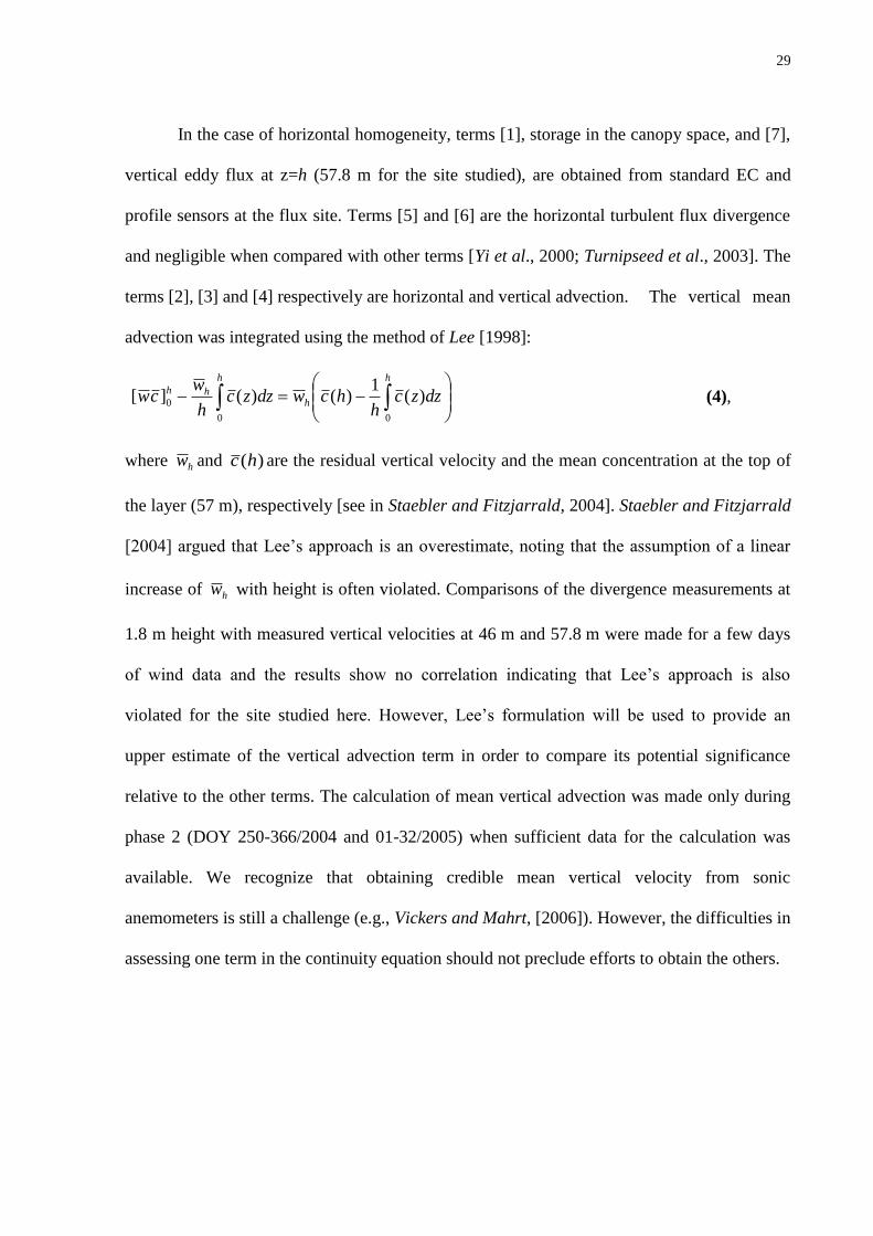
2.5. Vertical integration of the horizontal advection terms
To perform a complete three-dimensional forest CO2 box budget it is necessary to
obtain vertical profiles of the horizontal gradient measurements for the entire control volume,
and this is generally not feasible. We lacked resources to install a network of towers to
measure the CO2 profile at a number of locations in the canopy. Noting, as in Staebler and
Fitzjarrald [2004], that the product uc is largest near the forest floor, we relied on subcanopy
measurements made 1.8 m above the ground. To compensate for the missing network of
vertical profiles, we approximate the vertical integration through the canopy of the horizontal
advective terms [2] and [3] following methods developed by Staebler and Fitzjarrald [2004].
One hypothesizes spatial similarity between vertical CO2 and wind profiles and their product
(horizontal transport) uc, where u is the average wind and c the average CO2 concentration. In
this assumption, the shapes of the profiles throughout the canopy space are considered similar
to the central point where the profiles are measured (Figure 2).
Figure 4. Typical nighttime normalized median profiles of CO2, wind speed and their product
(uc) horizontal transport (left panel); and the diurnal cycle of the shape factor for horizontal
advection (right panel).
31
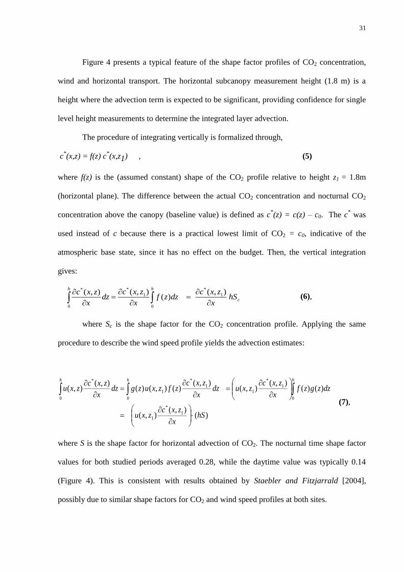
Figure 4 presents a typical feature of the shape factor profiles of CO2 concentration,
wind and horizontal transport. The horizontal subcanopy measurement height (1.8 m) is a
height where the advection term is expected to be significant, providing confidence for single
level height measurements to determine the integrated layer advection.
The procedure of integrating vertically is formalized through,
c*(x,z) = f(z) c
*(x,z1) , (5)
where f(z) is the (assumed constant) shape of the CO2 profile relative to height z1 = 1.8m
(horizontal plane). The difference between the actual CO2 concentration and nocturnal CO2
concentration above the canopy (baseline value) is defined as c*(z) = c(z) – c0. The c
* was
used instead of c because there is a practical lowest limit of CO2 = c0, indicative of the
atmospheric base state, since it has no effect on the budget. Then, the vertical integration
gives:
c
hh
hSx
zxcdzzf
x
zxcdz
x
zxc
),()(
),(),( 1
*
0
1
*
0
*
(6),
where Sc is the shape factor for the CO2 concentration profile. Applying the same
procedure to describe the wind speed profile yields the advection estimates:
)(),(
),(
)()(),(
),(),(
)(),()(),(
),(
1
*
1
0
1
*
1
0
1
*
1
0
*
hSx
zxczxu
dzzgzfx
zxczxudz
x
zxczfzxuzgdz
x
zxczxu
hhh
(7),
where S is the shape factor for horizontal advection of CO2. The nocturnal time shape factor
values for both studied periods averaged 0.28, while the daytime value was typically 0.14
(Figure 4). This is consistent with results obtained by Staebler and Fitzjarrald [2004],
possibly due to similar shape factors for CO2 and wind speed profiles at both sites.
32
3 – Results and Discussion
3.1. CO2 concentration field
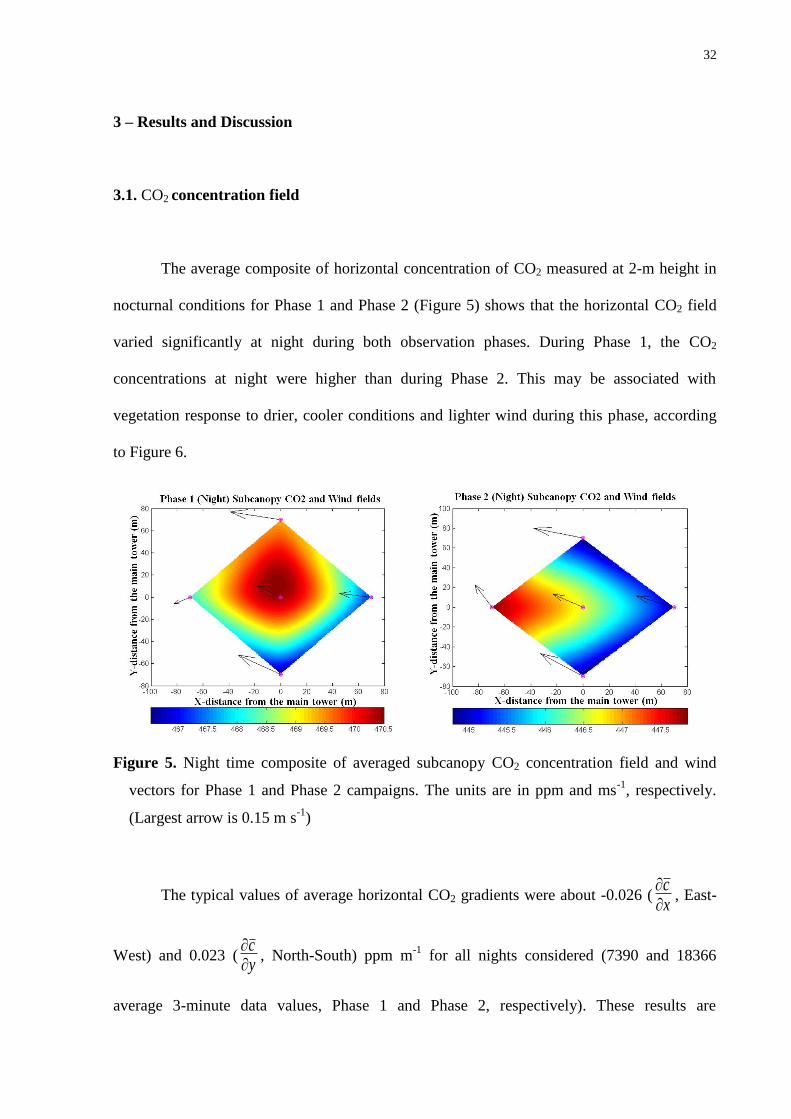
The average composite of horizontal concentration of CO2 measured at 2-m height in
nocturnal conditions for Phase 1 and Phase 2 (Figure 5) shows that the horizontal CO2 field
varied significantly at night during both observation phases. During Phase 1, the CO2
concentrations at night were higher than during Phase 2. This may be associated with
vegetation response to drier, cooler conditions and lighter wind during this phase, according
to Figure 6.
Figure 5. Night time composite of averaged subcanopy CO2 concentration field and wind
vectors for Phase 1 and Phase 2 campaigns. The units are in ppm and ms-1
, respectively.
(Largest arrow is 0.15 m s-1
)
The typical values of average horizontal CO2 gradients were about -0.026 (xc
, East-
West) and 0.023 (yc
, North-South) ppm m-1
for all nights considered (7390 and 18366
average 3-minute data values, Phase 1 and Phase 2, respectively). These results are
33
comparable to the range of horizontal CO2 gradients that have been reported in the literature,
0.025 to 0.079 ppm m-1
[Feigenwinter et al., 2004; Staebler and Fitzjarrald, 2004; Aubinet et
al., 2005]. One expects CO2 concentrations and gradients near the ground to be site-specific
under calm night wind speed conditions, due to varying soil respiration rates that depend on
soil and litter layer composition, temperature and moisture.
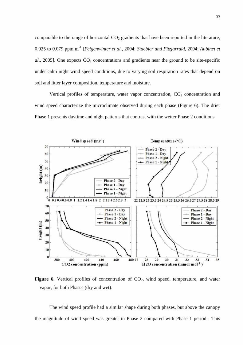
Vertical profiles of temperature, water vapor concentration, CO2 concentration and
wind speed characterize the microclimate observed during each phase (Figure 6). The drier
Phase 1 presents daytime and night patterns that contrast with the wetter Phase 2 conditions.
Figure 6. Vertical profiles of concentration of CO2, wind speed, temperature, and water
vapor, for both Phases (dry and wet).
The wind speed profile had a similar shape during both phases, but above the canopy
the magnitude of wind speed was greater in Phase 2 compared with Phase 1 period. This
34
suggests a reduction on turbulence level or vertical mixing during the nighttime, as shown in
Figure 7. The temperature profiles show the same pattern for the two phases, however, the dry
phase was about 2˚C warmer. During the daytime, for both dry and wet periods, a maximum
air temperature was observed at 30 m associate with the absorption of sunlight by vegetation,
generating a light unstable condition between 30 and 50 m, and stable condition below 30 m.
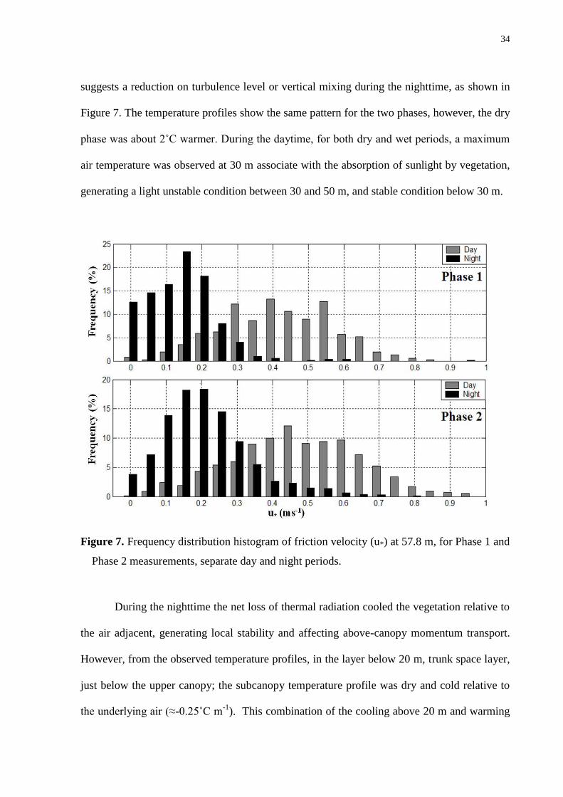
Figure 7. Frequency distribution histogram of friction velocity (u*) at 57.8 m, for Phase 1 and
Phase 2 measurements, separate day and night periods.
During the nighttime the net loss of thermal radiation cooled the vegetation relative to
the air adjacent, generating local stability and affecting above-canopy momentum transport.
However, from the observed temperature profiles, in the layer below 20 m, trunk space layer,
just below the upper canopy; the subcanopy temperature profile was dry and cold relative to
the underlying air (≈-0.25˚C m-1
). This combination of the cooling above 20 m and warming
35
below generates instability associated with negative buoyancy [see also Fitzjarrald et al.,
1990; Fitzjarrald and Moore, 1990]. This process may be contributing or creating horizontal
flow gravitationally such as suggested by Lee [1998]. Similar temperature profiles were
reported by Goulden et al., [2006] for km83 LBA site 16 km away to the south.
As expected, the vertical concentration of CO2 reflects both atmospheric transport and
forest physiological processes, in which during the daytime photosynthesis removes CO2 from
the air depleting concentration levels, and during the nighttime the concentration builds up
due to respiration, the reduction of turbulence, and absence of photosynthesis.
The frequency distribution of the friction velocity above the canopy for the both dry
(Phase 1) and wet (Phase 2) periods (Figure 7) shows very small values at nighttime.
Nocturnal values of friction velocity smaller than 0.2 ms-1
accounted for more than 85% and
65% for dry and wet periods, respectively. Therefore, we define deficit nights, using the
procedure outlined by Staebler and Fitzjarrald [2004], when NEE (CO2 eddy flux plus
storage term) was less than total ecosystem respiration (see Saleska et al. [2003] and Hutyra
et al. [2007], for details of these datasets). About 130 selected nights in each period, Phase 1
and Phase 2 match these criteria and were considered calm nighttime conditions.
Recently, Saleska et al. [2003] and Miller et al. [2004] have used a cutoff value of
0.3 ms-1
for u* correction to NEE estimates for the site studied. As show in Figure 7, much of
the observed data must be discarded using this criterion, possibly altering the results. As
reported by Miller et al. [2004], the tropical forest in Amazonia becomes a source than sink of
atmospheric CO2 depending of the cutoff value u* used.
36
3.2. Subcanopy horizontal wind field
To calculate horizontal advection (terms [3] and [4] Equation 3), we estimated the
horizontal wind field on the subcanopy space using the measurement subcanopy network
described above. Though the site was considered flat in earlier reports [Saleska et al., 2003;
Miller et al., 2004], a high resolution image shows that the forest floor gently slopes in a
west-northwest direction from the main tower, according to Figure 2. Goulden et al. [2006]
inferred the presence of drainage flows toward the SE at the km83 site to the south of the
present study site, but they did not demonstrate subcanopy motion forced by density
anomalies. Figure 8 shows statistics of the subcanopy wind field at night. There is a persistent
wind direction that follows the local topographic gradient (see also Figure 1).
These nocturnal horizontal wind directions are in accord with nocturnal wind
directions observed at the Jamaraquá station (Figure 1) close to the river Tapajós [Fitzjarrald
et al., 2004]. The statistics indicate that the nocturnal horizontal wind magnitude, varies
among the subcanopy measurement points, probably due to the large heterogeneity of
vegetation structure obstructions [see also Staebler and Fitzjarrald, 2004]. The average
magnitude of the horizontal wind field in the subcanopy varied from 0.1 to 0.45 m s-1
.
The observed subcanopy wind direction was prevailing from the southeast, with an
interesting shift compared to the top of the main tower (57.8 m) wind direction, indicating a
clearly uncoupled situation (Figure 8). Apparently, it seems that the subcanopy flow responds
primarily to the local terrain gradients. Goulden et al. [2006] have reported a similar shift of
the wind direction following the terrain gradient, even at 20 m when compared against the 64
m wind direction (see Figure 6, pg. 8 there in). Sun et al., [2007] have also indicated that this
shift happen at large spatial scales using short term datasets.
37
Figure 8. Nighttime distribution of the wind rose and its magnitude (m s-1
) for the Draino
sonic anemometer network and at top of main tower (57.8 m), including its localization
(see Figure 2).
3.3. Subcanopy flow forcing terms
We follow the analysis presented by Staebler and Fitzjarrald [2004]. Subcanopy
flows are generated by the balance of three driving forces; the pressure gradient perturbations,
the buoyancy and the stress divergence, according to the momentum equation. The
momentum equation is given by,
u
t u
u
xw
u
z
1
p'
x g
v'
v
h
x
z, where is the
38
density, p‟ the pressure perturbation , v the virtual temperature, 'v the local departure of v
from the mean, x
h
the topographic slope, and is the vertical stress, and drag effects are
ignored We do not believe that the terrain at the site studied is not so steep as to produce
pressure perturbations strong enough to affect subcanopy flow locally, and it is ignored in the
subsequent analysis. Thereby, the relative importance of buoyancy (x
hgb
v
vterm
') and
stress divergence (z
tterm
) terms will be considered. Observed fractions of the buoyancy
term (bterm/(bterm+tterm) and stress divergence term (tterm/(tterm+bterm) indicate that the buoyancy
term was more important during the nighttime than was the stress divergence term (Figure 9).
The stress divergence term was more significant during the daytime associated with a higher
degree of turbulent mixing as expected (Figure 9).
Figure 9. Diurnal cycle of buoyancy term forcing fractions relative to stress divergence term
for Phase 1 (top panel) and Phase 2 (middle panel) observations, and (bottom panel) the
buoyancy forcing term vs. subcanopy wind direction for both Phases.

39
Flows generated by the buoyancy term force the flow down the dominant terrain
slope. Nocturnal wind directions were predominantly from the southeast toward northwest, as
would be expected given the local topographic gradient (Figure 1). Our observations strongly
indicate that the negative buoyancy term is the physical mechanism that explains the
nocturnal drainage flow at this relatively flat study site.
3.4. Estimates of Advection Terms
The horizontal advection terms ([2] and [3] in Equation 3) were estimated using
subcanopy wind speed components and CO2 observation datasets from Phase 1 and Phase 2
(14350 and 36459 3-min valid observations, respectively). The horizontal CO2 gradients
were calculated using a linear least-square planar fit (Figure 5). (Note that the interpolated
fields shown in Figure 5 were not used in the calculation).
Figure 10a. Hourly-averaged summary of results for the Phase 1 and all the terms except
eddy flux are average values for 0 to 57.8 m control volume. Top panel: vertical eddy flux
at 57.8 m; 2nd
panel: storage; 3th
panel: east-west advection; and 4th
panel: south-north
advection, terms.
40
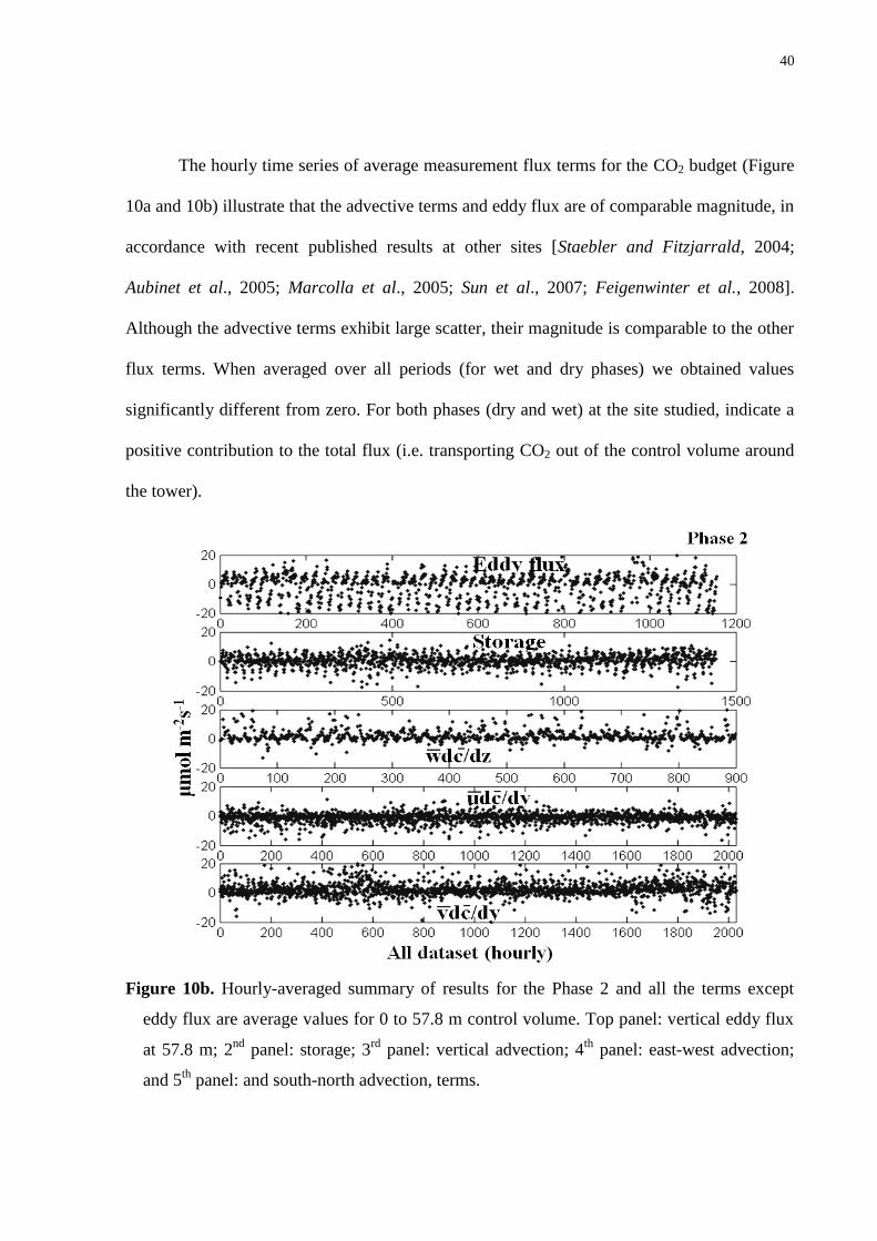
The hourly time series of average measurement flux terms for the CO2 budget (Figure
10a and 10b) illustrate that the advective terms and eddy flux are of comparable magnitude, in
accordance with recent published results at other sites [Staebler and Fitzjarrald, 2004;
Aubinet et al., 2005; Marcolla et al., 2005; Sun et al., 2007; Feigenwinter et al., 2008].
Although the advective terms exhibit large scatter, their magnitude is comparable to the other
flux terms. When averaged over all periods (for wet and dry phases) we obtained values
significantly different from zero. For both phases (dry and wet) at the site studied, indicate a
positive contribution to the total flux (i.e. transporting CO2 out of the control volume around
the tower).
Figure 10b. Hourly-averaged summary of results for the Phase 2 and all the terms except
eddy flux are average values for 0 to 57.8 m control volume. Top panel: vertical eddy flux
at 57.8 m; 2nd
panel: storage; 3rd
panel: vertical advection; 4th
panel: east-west advection;
and 5th
panel: and south-north advection, terms.
41
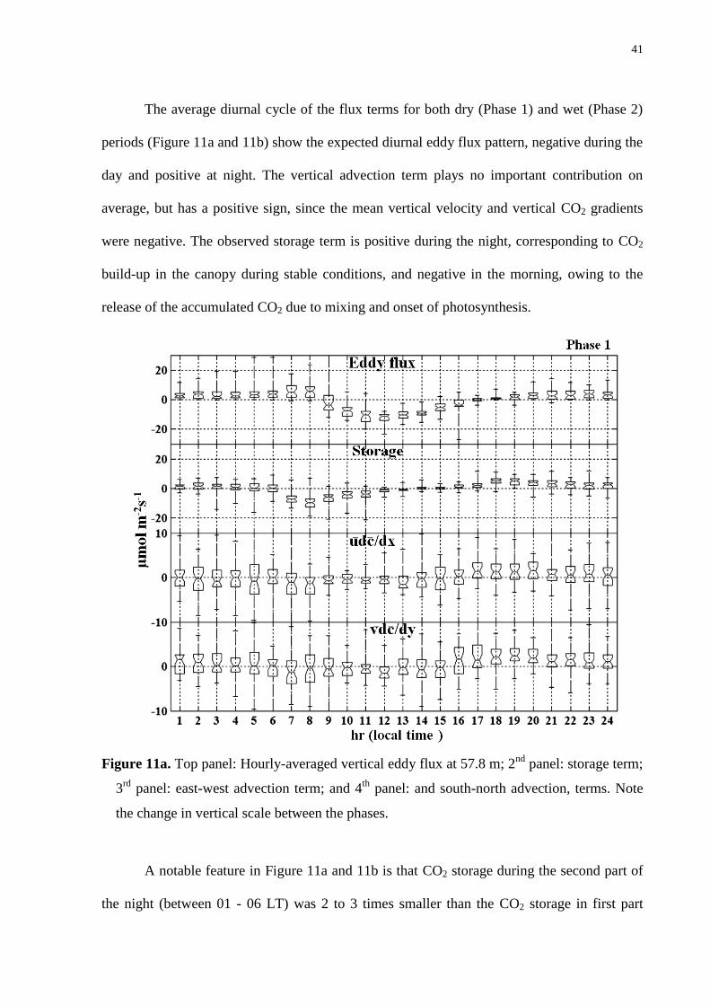
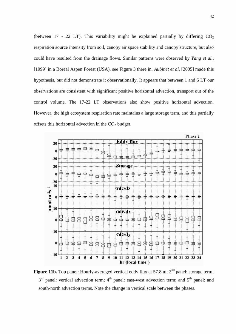
The average diurnal cycle of the flux terms for both dry (Phase 1) and wet (Phase 2)
periods (Figure 11a and 11b) show the expected diurnal eddy flux pattern, negative during the
day and positive at night. The vertical advection term plays no important contribution on
average, but has a positive sign, since the mean vertical velocity and vertical CO2 gradients
were negative. The observed storage term is positive during the night, corresponding to CO2
build-up in the canopy during stable conditions, and negative in the morning, owing to the
release of the accumulated CO2 due to mixing and onset of photosynthesis.
Figure 11a. Top panel: Hourly-averaged vertical eddy flux at 57.8 m; 2nd
panel: storage term;
3rd
panel: east-west advection term; and 4th
panel: and south-north advection, terms. Note
the change in vertical scale between the phases.
A notable feature in Figure 11a and 11b is that CO2 storage during the second part of
the night (between 01 - 06 LT) was 2 to 3 times smaller than the CO2 storage in first part
42
(between 17 - 22 LT). This variability might be explained partially by differing CO2
respiration source intensity from soil, canopy air space stability and canopy structure, but also
could have resulted from the drainage flows. Similar patterns were observed by Yang et al.,
[1999] in a Boreal Aspen Forest (USA), see Figure 3 there in. Aubinet et al. [2005] made this
hypothesis, but did not demonstrate it observationally. It appears that between 1 and 6 LT our
observations are consistent with significant positive horizontal advection, transport out of the
control volume. The 17-22 LT observations also show positive horizontal advection.
However, the high ecosystem respiration rate maintains a large storage term, and this partially
offsets this horizontal advection in the CO2 budget.
Figure 11b. Top panel: Hourly-averaged vertical eddy flux at 57.8 m; 2nd
panel: storage term;
3rd
panel: vertical advection term; 4th
panel: east-west advection term; and 5th
panel: and
south-north advection terms. Note the change in vertical scale between the phases.
43
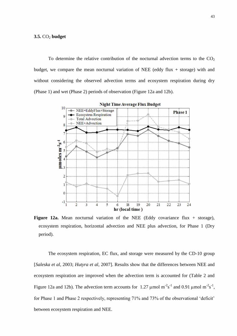
3.5. CO2 budget
To determine the relative contribution of the nocturnal advection terms to the CO2
budget, we compare the mean nocturnal variation of NEE (eddy flux + storage) with and
without considering the observed advection terms and ecosystem respiration during dry
(Phase 1) and wet (Phase 2) periods of observation (Figure 12a and 12b).
Figure 12a. Mean nocturnal variation of the NEE (Eddy covariance flux + storage),
ecosystem respiration, horizontal advection and NEE plus advection, for Phase 1 (Dry
period).
The ecosystem respiration, EC flux, and storage were measured by the CD-10 group
[Saleska et al, 2003; Hutyra et al, 2007]. Results show that the differences between NEE and
ecosystem respiration are improved when the advection term is accounted for (Table 2 and
Figure 12a and 12b). The advection term accounts for 1.27 mol m-2
s-1
and 0.91 mol m-2
s-1
,
for Phase 1 and Phase 2 respectively, representing 71% and 73% of the observational „deficit‟
between ecosystem respiration and NEE.
44
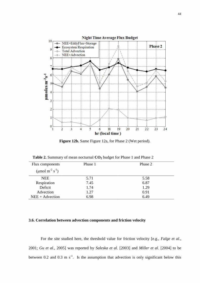
Figure 12b. Same Figure 12a, for Phase 2 (Wet period).
Table 2. Summary of mean nocturnal CO2 budget for Phase 1 and Phase 2
Flux components
(μmol m-2
s-1
)
Phase 1 Phase 2
NEE 5.71 5.58
Respiration 7.45 6.87
Deficit 1.74 1.29
Advection 1.27 0.91
NEE + Advection 6.98 6.49
3.6. Correlation between advection components and friction velocity
For the site studied here, the threshold value for friction velocity [e.g., Falge et al.,
2001; Gu et al., 2005] was reported by Saleska et al. [2003] and Miller et al. [2004] to be
between 0.2 and 0.3 m s-1
. Is the assumption that advection is only significant below this

45
threshold valid? Our results show a clear dependence of the advection term on friction
velocity for both observation periods (Figure 13). There is a significant positive advection
contribution to the CO2 budget that should be included in the NEE calculation, even when the
friction velocity is higher than the threshold values commonly used. Our results in the Tapajós
forest indicate that this interval lies between 0.3 and 0.6 m s-1
.
Figure 13. Mean nocturnal variation of the advection term as a function of the friction
velocity rank, for Phase 1 (left panel) and Phase 2 (right panel) datasets. Solid line with
dots indicates binned average values (0.1 intervals)). Error-bar also is plot with standard
deviation, respectively.
4. Summary and Conclusions
We present results of the first effort to determine observationally the importance of the
nocturnal advection processes on the CO2 budget in the Amazon tropical rain forest. We
tested the hypothesis that persistent nocturnal subcanopy horizontal advection exists and
transports an important amount of CO2 out of the control volume at one old-growth tropical

46
rain forest site. We determined the magnitude of the horizontal subcanopy gradients of CO2
and of the wind field and found sufficient net horizontal advection to affect the CO2 budget.
The methodology established by Staebler and Fitzjarrald [2004, 2005] was applied
and tested to measure the subcanopy scalar gradients and wind field. These data were
complemented by eddy flux and mean profile observations made at the same site on a 65-m
tower (section 2). The measurements were performed in the dry season (DOY 198-238 2003 -
Phase 1) and in the wet season (DOY 278-366 2004 and 1-32 2005 - Phase 2). The horizontal
gradient of the CO2 concentration and average wind speed, were on the order of 0.02 ppm m-1
and 0.12 m s-1
, respectively (section 3.1).
Prevailing subcanopy wind directions were from the southeast and were well
correlated with gentle undulations of the landscape near the tower. The tropical forest
subcanopy near the forest floor was stable at all times of day, but it was more pronounced
during all 130 selected nights analyzed (section 3.2). That there was little coupling with the
flow aloft indicates that there is potential for lateral export of subcanopy CO2 even during the
daytime, when this effect is often ignored. The negative buoyancy term was the principal
physical mechanism responsible for generating the nocturnal subcanopy flow. During the
daytime the stress divergence term was dominant, suppressing the dominance of the buoyancy
effect (Section 3.3).
The results from direct measurements of the horizontal gradients of CO2 and wind
speed components measured in the subcanopy indicated that their magnitudes were
sufficiently significant to produce a net nocturnal horizontal advection average between 0.91
and 1.27 mol m-2
s-1
for dry and wet observation periods, respectively. Nocturnal horizontal
advection was of the same order as the vertical EC and storage flux components. Depletion of
the storage component was due in large part to net positive horizontal advection, primarily
during the second part of the night (01 – 06 LT; section 3.4).
47
Comparison of the nocturnal deficit from ecosystem respiration and NEE measured on
the eddy flux tower demonstrated the important contribution of the mean nocturnal horizontal
advection on the atmospheric CO2 budget. The mean nocturnal advection component
represented 73% and 71% of this deficit for dry and wet periods analyzed (130 nights),
respectively.
This suggests an important role of the nocturnal advection for the total CO2 budget at
this site. It was also verified that for nighttime intervals, with friction velocity between 0.3
and 0.6 m s-1
(commonly accepted as sufficient to provide correct nighttime eddy fluxes),
there was a positive net horizontal transport of CO2 by the advection component. Therefore,
even under considerable high turbulence levels at night, horizontal advection transport in the
total CO2 budget is significant.
These results confirm that few sites are flat enough that horizontal advective effects
can be ignored a priori. In future work the validity of the CO2 profile similarity hypothesis
we invoked to introduce shape factors in (4) should be linked explicitly to the observed mean
vegetation profile. Observational estimates of the effect of mean vertical velocity on scalar
budgets may be the major source of uncertainty in the budget. Continuous, long-term
observations with redundant instrumentation are needed to clarify this issue.
48
Capítulo II - Amazon rain forest subcanopy flow and the carbon budget:
Manaus LBA Site - a complex terrain condition 2
Abstract
On the moderately complex terrain covered by dense tropical Amazon rainforest (Reserva
Biologica do Cuieiras – ZF2 - 02◦36′17.1′′S, 60◦12′24.5′′W) subcanopy horizontal and
vertical gradients of the air temperature, CO2 concentration and wind field were measured for
dry and wet periods in 2006. We tested the hypothesis that horizontal drainage flow over this
study area is significant and can affect the interpretation of the high carbon uptake rates
reported by previous works. A similar experimental design as the one by Tóta et al. [2008]
was used with a network of wind, air temperature and CO2 sensors above and below the forest
canopy. A persistent and systematic subcanopy nighttime upslope (positive buoyancy) and
daytime downslope (negative buoyancy) flow pattern on a moderately inclined slope (12%)
was observed. The micro-circulations observed above the canopy (38 m) over the sloping area
during nighttime presents a downward motion indicating vertical convergence and
correspondent horizontal divergence toward the valley area. During the daytime an inverse
pattern was observed. The micro-circulations above the canopy were driven mainly by
buoyancy balancing the pressure gradient forces. In the subcanopy space the micro-
circulations were also driven by the same physical mechanisms but probably with the stress
forcing contribution. The results also indicated that the horizontal and vertical scalar gradients
(e.g., CO2) were modulated by these micro-circulations above and below canopy, then
suggesting that estimates of advection using previous experimental approaches are not
appropriate due to the tri-dimensional nature of the vertical and horizontal transport locally.
Key words: Amazon Rainforest; Advection, Drainage Flow, Eddy Covariance, Subcanopy.
2 Tóta, J., Fitzjarrald, D.R., Parker, G., Sakai, R.K., Silva Dias, M.A.F., Manzi, A.O., 2009. Amazon rain forest
subcanopy flow and the carbon budget: Manaus LBA Site - a complex terrain condition (to be submitted).
49
1. Introduction
The terrestrial biosphere is an important component of the global carbon system. The
uncertainty level of its long term exchanges estimates is a challenge and has resulted in
ongoing debate [Baldocchi et al., 2008; Aubinet et al., 2008]. For monitoring long-term net
ecosystem exchange (NEE) of carbon dioxide, energy and water in terrestrial ecosystems,
tower-based eddy-covariance (EC) techniques have been established worldwide [Baldocchi et
al., 2008].
It is now recognized that the EC technique has serious restrictions for application over
complex terrain and under calm and stable nighttime conditions with low turbulence or
limited turbulent mixing of air [e.g., Goulden et al., 1996; Black et al., 1996; Baldocchi et al.,
2001; Massman and Lee, 2002; Loescher et al., 2006; Aubinet et al., 2008]. To overcome this
problem, the friction velocity (u*)-filtering approach has been formalized by the FLUXNET
committee for the estimation of annual carbon balances [Baldocchi et al., 2001; Gu et al.,
2005]. This approach simply discarded calm nights flux data (often an appreciable fraction of
all nights) and replaced them with ecosystem respiration rates found on windy nights [Miller
et al., 2004]. Papale et al., [2006] pointed out that this approach itself must be applied with
caution and the friction velocity (u*) corrections threshold is subject to considerable concerns
and is very site specific. Miller et al., [2004] reported that depending of the u* threshold value
used to correct the flux tower data at Santarem LBA site the area can change from carbon sink
to neutral or carbon source to the atmosphere.
The transport of CO2 by advection process has been suggested by several studies as the
principle reason for the „„missing‟‟ CO2 at night [Lee, 1998; Finnigan, 1999; Paw U et al.,
2000; Aubinet et al., 2003; Feigenwinter et al., 2004; Staebler and Fitzjarrald, 2004]. The
search for this missing CO2 has spurred a great deal of research with the goal of explicitly
estimating advective fluxes in field experiments during the last decade, in order to correct the
NEE bias over single tower eddy covariance measurements (Aubinet et al., 2003, 2005;
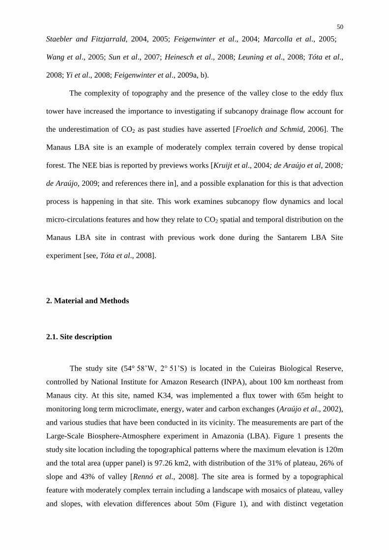
50
Staebler and Fitzjarrald, 2004, 2005; Feigenwinter et al., 2004; Marcolla et al., 2005;
Wang et al., 2005; Sun et al., 2007; Heinesch et al., 2008; Leuning et al., 2008; Tóta et al.,
2008; Yi et al., 2008; Feigenwinter et al., 2009a, b).
The complexity of topography and the presence of the valley close to the eddy flux
tower have increased the importance to investigating if subcanopy drainage flow account for
the underestimation of CO2 as past studies have asserted [Froelich and Schmid, 2006]. The
Manaus LBA site is an example of moderately complex terrain covered by dense tropical
forest. The NEE bias is reported by previews works [Kruijt et al., 2004; de Araújo et al, 2008;
de Araújo, 2009; and references there in], and a possible explanation for this is that advection
process is happening in that site. This work examines subcanopy flow dynamics and local
micro-circulations features and how they relate to CO2 spatial and temporal distribution on the
Manaus LBA site in contrast with previous work done during the Santarem LBA Site
experiment [see, Tóta et al., 2008].
2. Material and Methods
2.1. Site description
The study site (54° 58‟W, 2° 51‟S) is located in the Cuieiras Biological Reserve,
controlled by National Institute for Amazon Research (INPA), about 100 km northeast from
Manaus city. At this site, named K34, was implemented a flux tower with 65m height to
monitoring long term microclimate, energy, water and carbon exchanges (Araújo et al., 2002),
and various studies that have been conducted in its vicinity. The measurements are part of the
Large-Scale Biosphere-Atmosphere experiment in Amazonia (LBA). Figure 1 presents the
study site location including the topographical patterns where the maximum elevation is 120m
and the total area (upper panel) is 97.26 km2, with distribution of the 31% of plateau, 26% of
slope and 43% of valley [Rennó et al., 2008]. The site area is formed by a topographical
feature with moderately complex terrain including a landscape with mosaics of plateau, valley
and slopes, with elevation differences about 50m (Figure 1), and with distinct vegetation
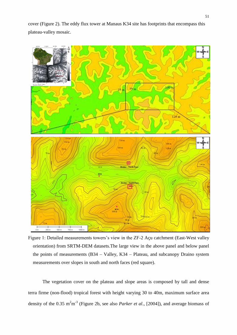
51
cover (Figure 2). The eddy flux tower at Manaus K34 site has footprints that encompass this
plateau-valley mosaic.
Figure 1: Detailed measurements towers‟s view in the ZF-2 Açu catchment (East-West valley
orientation) from SRTM-DEM datasets.The large view in the above panel and below panel
the points of measurements (B34 – Valley, K34 – Plateau, and subcanopy Draino system
measurements over slopes in south and north faces (red square).
The vegetation cover on the plateau and slope areas is composed by tall and dense
terra firme (non-flood) tropical forest with height varying 30 to 40m, maximum surface area
density of the 0.35 m2m
-3 (Figure 2b, see also Parker et al., [2004]), and average biomass of
52
the 215 to 492 ton.ha-1
[Laurance et al., 1999; Castilho, 2004]. On the valley area the
vegetation is open and smaller with heights from 15 to 25 m, but with significant surface area
density more than the 0.35 m2m
-3 (Figure 2b). The soil type on the plateau and slopes area is
mainly formed by Oxisols (USDA taxonomy) or clay-rich ferrasols ultisols (FAO soil
taxonomy), while on the valley area, waterlogged podzols (FAO)/spodosols (USDA) with
sand soil low drained predominates. Also, in the valley area the presence of small patchy of
Campinarana typical open vegetation with low biomass is also common [Luizão et al., 2004].
Figure 2: (a) IKONOS‟s image of the site at Açu Cachment with level terrain cotes and
vegetation cover and (b) vegetation structure measured from LIDAR sensor over yellow
transect in (a). From (a) the valley vegetation (blue color) and vegetation transition to
plateau areas (red colors).
a)
b)
53
The precipitation regime on the site show wet (December to April) and dry (June to
September – less than 100 mm.month-1
) periods. The total annual rainfall is about 2400 mm
and the average daily temperature is from 26 (April) to 28˚C (September). For more
detailed information about the meteorology and hydrology of this site see Waterloo et al.
[2006], Cuartas et al. [2007], Hodnett et al. [2008], Tomasella et al. [2008], Malhi et al.
[2008] and de Araújo [2009].
2.2. Measurements and intrumentation
The datasets used in this study include a measurement system to monitor airflow
above and below the forest, horizontal gradients of CO2, and the thermal structure of the air
below the canopy, named “DRAINO System” [see, Tóta et al., 2008]. The data used in this
study were collected during the wet season (DOY 1-151) and the dry season (DOY 152-
250) of the year 2006. Complementary information was used from flux tower K34 (LBA
tower) on the plateau, and sonic anemometer data collected in the valley flux tower (B34,
see de Araújo [2009] for details).
The flux tower K34 includes turbulent EC flux and meteorological observations of
the vertical profiles of the air temperature, humidity and CO2/H2O concentrations, and
vertical profile of wind speed, as well as radiation measurements. The fast response eddy
flux data were sampled at 10 Hz and slow response (air temperature and wind profiles) at
30 min average [see Araújo et. al., [2002] for details information].
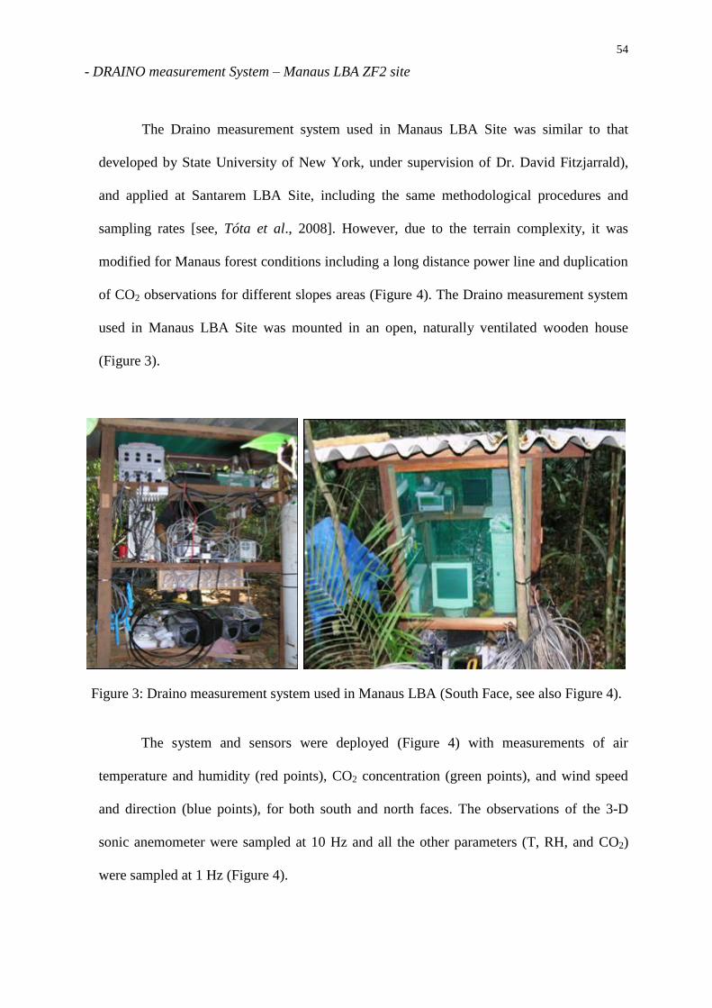
54
- DRAINO measurement System – Manaus LBA ZF2 site
The Draino measurement system used in Manaus LBA Site was similar to that
developed by State University of New York, under supervision of Dr. David Fitzjarrald),
and applied at Santarem LBA Site, including the same methodological procedures and
sampling rates [see, Tóta et al., 2008]. However, due to the terrain complexity, it was
modified for Manaus forest conditions including a long distance power line and duplication
of CO2 observations for different slopes areas (Figure 4). The Draino measurement system
used in Manaus LBA Site was mounted in an open, naturally ventilated wooden house
(Figure 3).
Figure 3: Draino measurement system used in Manaus LBA (South Face, see also Figure 4).
The system and sensors were deployed (Figure 4) with measurements of air
temperature and humidity (red points), CO2 concentration (green points), and wind speed
and direction (blue points), for both south and north faces. The observations of the 3-D
sonic anemometer were sampled at 10 Hz and all the other parameters (T, RH, and CO2)
were sampled at 1 Hz (Figure 4).
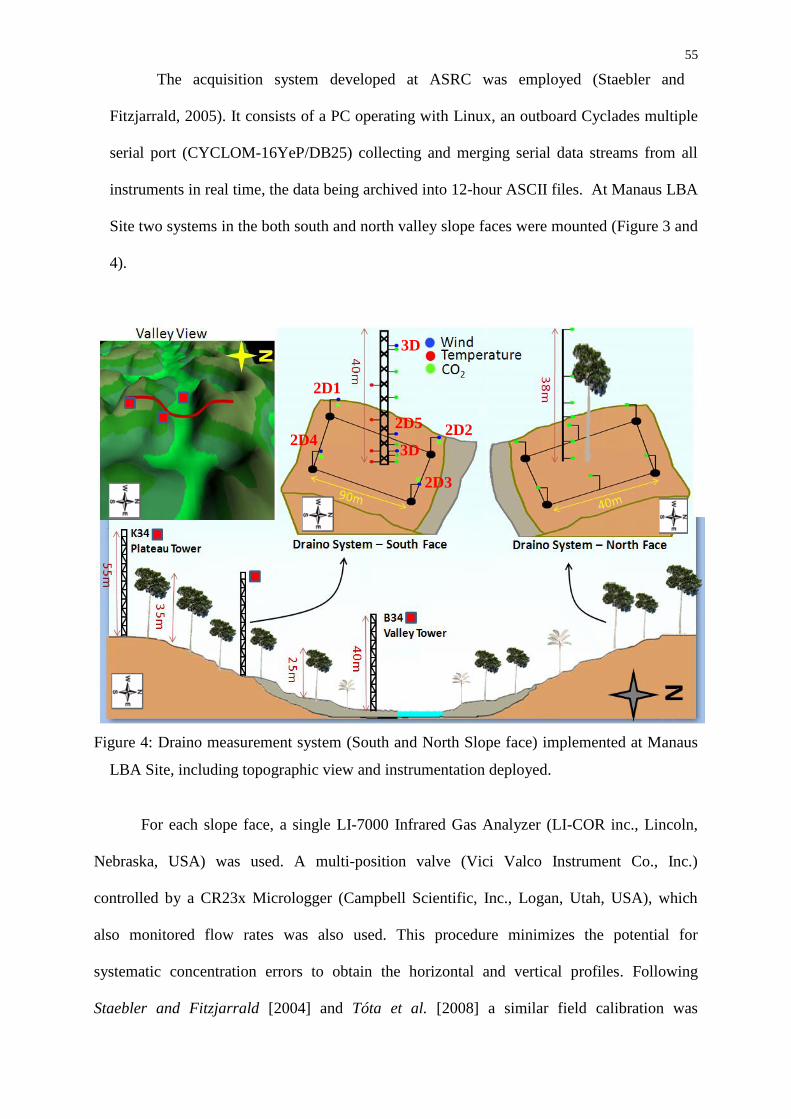
55
The acquisition system developed at ASRC was employed (Staebler and
Fitzjarrald, 2005). It consists of a PC operating with Linux, an outboard Cyclades multiple
serial port (CYCLOM-16YeP/DB25) collecting and merging serial data streams from all
instruments in real time, the data being archived into 12-hour ASCII files. At Manaus LBA
Site two systems in the both south and north valley slope faces were mounted (Figure 3 and
4).
Figure 4: Draino measurement system (South and North Slope face) implemented at Manaus
LBA Site, including topographic view and instrumentation deployed.
For each slope face, a single LI-7000 Infrared Gas Analyzer (LI-COR inc., Lincoln,
Nebraska, USA) was used. A multi-position valve (Vici Valco Instrument Co., Inc.)
controlled by a CR23x Micrologger (Campbell Scientific, Inc., Logan, Utah, USA), which
also monitored flow rates was also used. This procedure minimizes the potential for
systematic concentration errors to obtain the horizontal and vertical profiles. Following
Staebler and Fitzjarrald [2004] and Tóta et al. [2008] a similar field calibration was
2D4 3D
2D2
2D3
3D
2D5
2D1
56
performed during the observations at Manaus LBA Site, including initial instrument
intercomparison. The result was similar that obtained by Tóta et al. [2008], with CO2 mean
standard error was < 0.05 ppm and mean standard error of about 0.005 ms-1 for wind speed
measurements. After intercomparison, the sonic anemometers and the CO2 inlet tubes were
deployed as shown in Figure 4.
On the south face, the instrument network array (Figure 4 and Table 1) consisted of 6
subcanopy sonic anemometers, one 3-D ATI (Applied Technologies Inc., CO, USA) at 2m
elevation in the center of the grid (named 3-D ATI), and 5 SPAS/2Y (Applied Technologies
Inc., CO, USA), 2-component anemometers (1 sonic at 6m in the grid center and 4 sonic
along the periphery at 2m, see Figure 4), with a resolution of 0.01 m s-1. Also, a Gill HS (Gill
Instruments Ltd., Lymington, UK) 3-component sonic anemometer was installed above the
canopy (38 m). The horizontal gradients of CO2/H2O were measured in the array at 2 m
above ground, by sampling sequentially from 4 horizontal points surrounding the main tower
location at distances of 70-90m, and from points at 6 levels on the main Draino south face
tower, performing a 3 minute cycle. On the north face, similar CO2 measurements were
mounted including a 6 level vertical profile and 6 points in the array at 2 m above ground,
performing a 3 minute cycle.
On both slope faces the air was pumped continuously through 0.9 mm Dekoron tube
(Synflex 1300, Saint-Gobain Performance Plastics, Wayne, NJ, USA) tubes from meshed
inlets to a manifold in a centralized box. A baseline air flow of 4 LPM from the inlets to a
central manifold was maintained in all lines at all times to ensure relatively “fresh” air was
being sampled. The air was pumped for 20 seconds from each inlet, across filters to limit
moisture effects. The delay time for sampling was five seconds and the first ten seconds of
data were discarded. At the manifold, one line at a time was then sampled using an infrared
gas analyzer (LI-7000, Licor, Inc.). To minimize instrument problems, only one LI-7000 gas
analyzer sensor, for each slope face, was used to perform vertical and horizontal gradients of
the CO2.
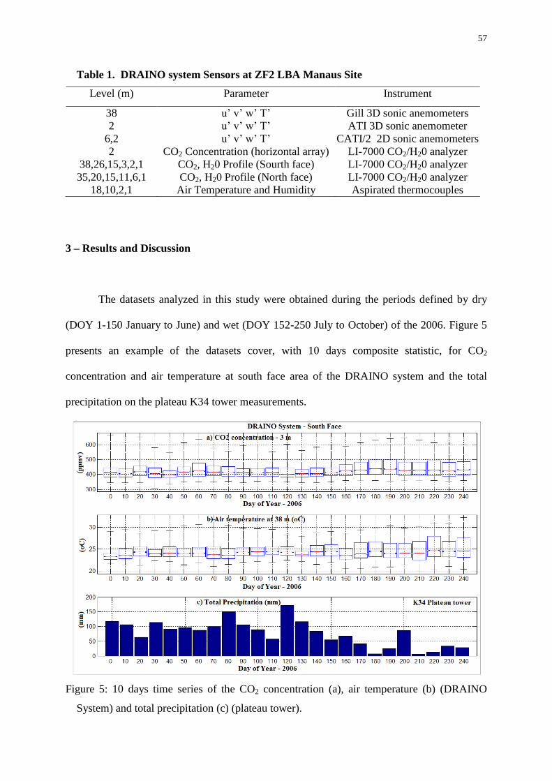
57
Table 1. DRAINO system Sensors at ZF2 LBA Manaus Site
Level (m) Parameter Instrument
38 u‟ v‟ w‟ T‟ Gill 3D sonic anemometers
2 u‟ v‟ w‟ T‟ ATI 3D sonic anemometer
6,2 u‟ v‟ w‟ T‟ CATI/2 2D sonic anemometers
2 CO2 Concentration (horizontal array) LI-7000 CO2/H20 analyzer
38,26,15,3,2,1 CO2, H20 Profile (Sourth face) LI-7000 CO2/H20 analyzer
35,20,15,11,6,1 CO2, H20 Profile (North face) LI-7000 CO2/H20 analyzer
18,10,2,1 Air Temperature and Humidity Aspirated thermocouples
3 – Results and Discussion
The datasets analyzed in this study were obtained during the periods defined by dry
(DOY 1-150 January to June) and wet (DOY 152-250 July to October) of the 2006. Figure 5
presents an example of the datasets cover, with 10 days composite statistic, for CO2
concentration and air temperature at south face area of the DRAINO system and the total
precipitation on the plateau K34 tower measurements.
Figure 5: 10 days time series of the CO2 concentration (a), air temperature (b) (DRAINO
System) and total precipitation (c) (plateau tower).
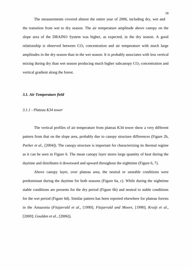
58
The measurements covered almost the entire year of 2006, including dry, wet and
the transition from wet to dry season. The air temperature amplitude above canopy on the
slope area of the DRAINO System was higher, as expected, in the dry season. A good
relationship is observed between CO2 concentration and air temperature with much large
amplitudes in the dry season than in the wet season. It is probably associates with less vertical
mixing during dry than wet season producing much higher subcanopy CO2 concentration and
vertical gradient along the forest.
3.1. Air Temperature field
3.1.1 - Plateau K34 tower
The vertical profiles of air temperature from plateau K34 tower show a very different
pattern from that on the slope area, probably due to canopy structure differences (Figure 2b,
Parker et al., [2004]). The canopy structure is important for characterizing its thermal regime
as it can be seen in Figure 6. The mean canopy layer stores large quantity of heat during the
daytime and distributes it downward and upward throughout the nighttime (Figure 6, 7).
Above canopy layer, over plateau area, the neutral or unstable conditions were
predominant during the daytime for both seasons (Figure 6a, c). While during the nighttime
stable conditions are presents for the dry period (Figure 6b) and neutral to stable conditions
for the wet period (Figure 6d). Similar pattern has been reported elsewhere for plateau forests
in the Amazonia (Fitzjarrald et al., [1990]; Fitzjarrald and Moore, [1990]; Kruijt et al.,
[2000]; Goulden et al., [2006]).
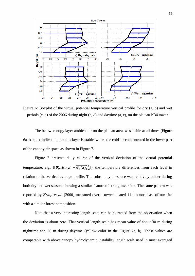
59
Figure 6: Boxplot of the virtual potential temperature vertical profile for dry (a, b) and wet
periods (c, d) of the 2006 during night (b, d) and daytime (a, c), on the plateau K34 tower.
The below-canopy layer ambient air on the plateau area was stable at all times (Figure
6a, b, c, d), indicating that this layer is stable where the cold air concentrated in the lower part
of the canopy air space as shown in Figure 7.
Figure 7 presents daily course of the vertical deviation of the virtual potential
temperature, e.g., ([
]), the temperature differences from each level in
relation to the vertical average profile. The subcanopy air space was relatively colder during
both dry and wet season, showing a similar feature of strong inversion. The same pattern was
reported by Kruijt et al. [2000] measured over a tower located 11 km northeast of our site
with a similar forest composition.
Note that a very interesting length scale can be extracted from the observation when
the deviation is about zero. That vertical length scale has mean value of about 30 m during
nighttime and 20 m during daytime (yellow color in the Figure 7a, b). Those values are
comparable with above canopy hydrodynamic instability length scale used in most averaged
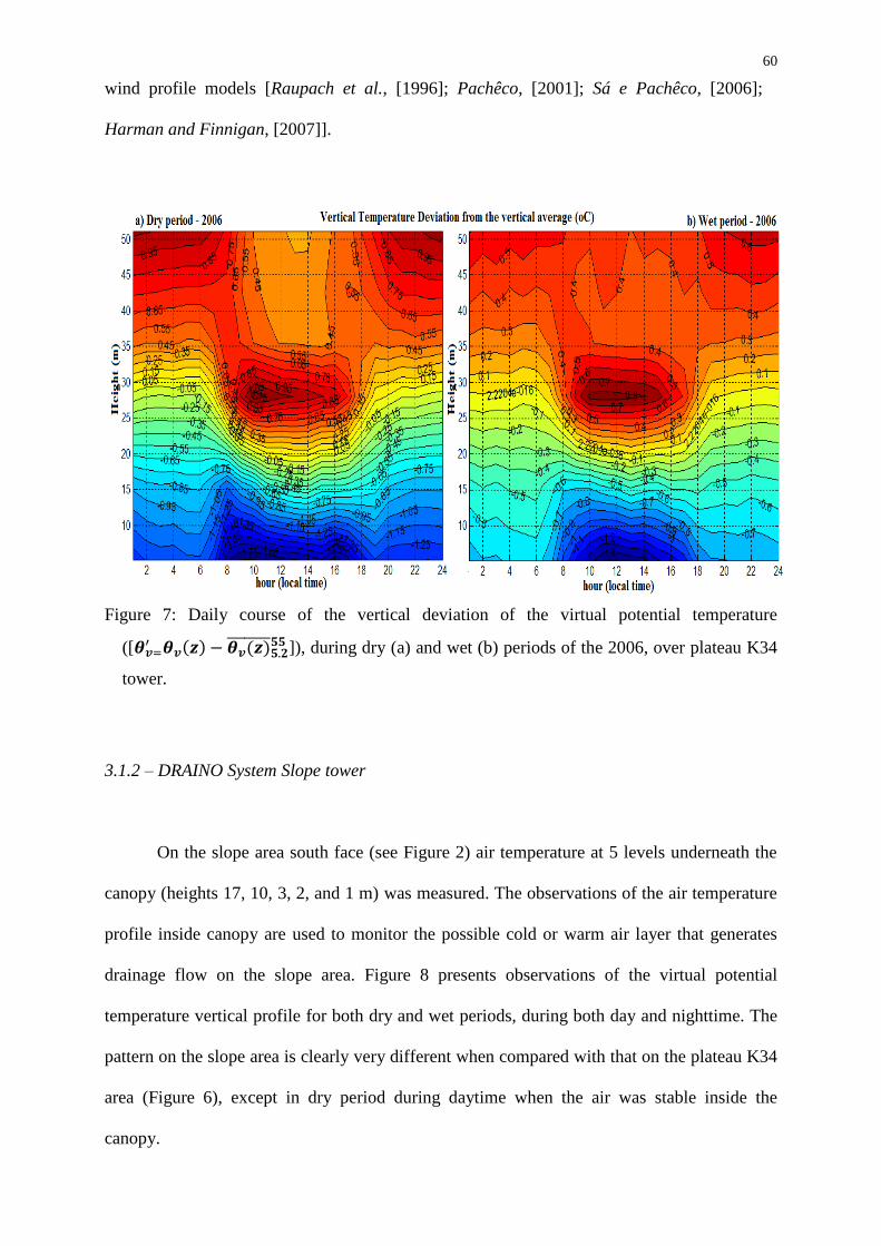
60
wind profile models [Raupach et al., [1996]; Pachêco, [2001]; Sá e Pachêco, [2006];
Harman and Finnigan, [2007]].
Figure 7: Daily course of the vertical deviation of the virtual potential temperature
([
]), during dry (a) and wet (b) periods of the 2006, over plateau K34
tower.
3.1.2 – DRAINO System Slope tower
On the slope area south face (see Figure 2) air temperature at 5 levels underneath the
canopy (heights 17, 10, 3, 2, and 1 m) was measured. The observations of the air temperature
profile inside canopy are used to monitor the possible cold or warm air layer that generates
drainage flow on the slope area. Figure 8 presents observations of the virtual potential
temperature vertical profile for both dry and wet periods, during both day and nighttime. The
pattern on the slope area is clearly very different when compared with that on the plateau K34
area (Figure 6), except in dry period during daytime when the air was stable inside the
canopy.
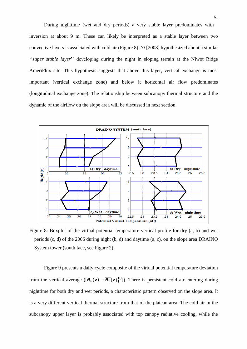
61
During nighttime (wet and dry periods) a very stable layer predominates with
inversion at about 9 m. These can likely be interpreted as a stable layer between two
convective layers is associated with cold air (Figure 8). Yi [2008] hypothesized about a similar
„„super stable layer‟‟ developing during the night in sloping terrain at the Niwot Ridge
AmeriFlux site. This hypothesis suggests that above this layer, vertical exchange is most
important (vertical exchange zone) and below it horizontal air flow predominates
(longitudinal exchange zone). The relationship between subcanopy thermal structure and the
dynamic of the airflow on the slope area will be discussed in next section.
Figure 8: Boxplot of the virtual potential temperature vertical profile for dry (a, b) and wet
periods (c, d) of the 2006 during night (b, d) and daytime (a, c), on the slope area DRAINO
System tower (south face, see Figure 2).
Figure 9 presents a daily cycle composite of the virtual potential temperature deviation
from the vertical average ([
]). There is persistent cold air entering during
nighttime for both dry and wet periods, a characteristic pattern observed on the slope area. It
is a very different vertical thermal structure from that of the plateau area. The cold air in the
subcanopy upper layer is probably associated with top canopy radiative cooling, while the
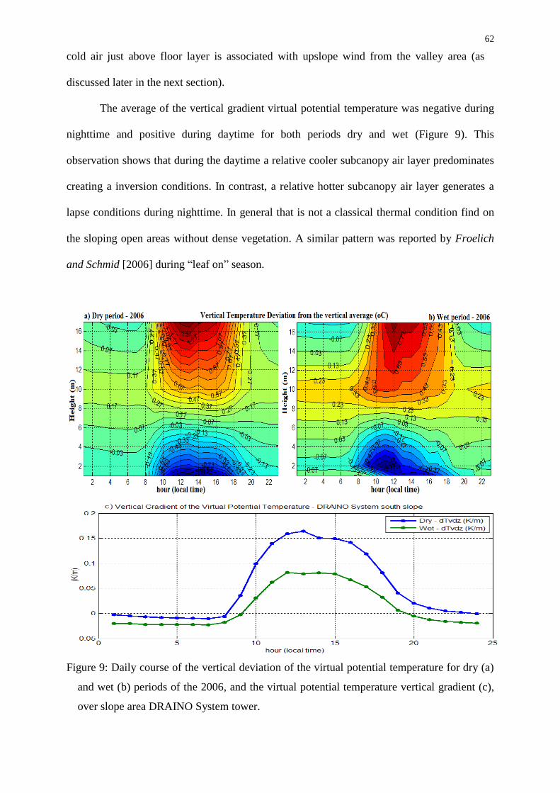
62
cold air just above floor layer is associated with upslope wind from the valley area (as
discussed later in the next section).
The average of the vertical gradient virtual potential temperature was negative during
nighttime and positive during daytime for both periods dry and wet (Figure 9). This
observation shows that during the daytime a relative cooler subcanopy air layer predominates
creating a inversion conditions. In contrast, a relative hotter subcanopy air layer generates a
lapse conditions during nighttime. In general that is not a classical thermal condition find on
the sloping open areas without dense vegetation. A similar pattern was reported by Froelich
and Schmid [2006] during “leaf on” season.
Figure 9: Daily course of the vertical deviation of the virtual potential temperature for dry (a)
and wet (b) periods of the 2006, and the virtual potential temperature vertical gradient (c),
over slope area DRAINO System tower.
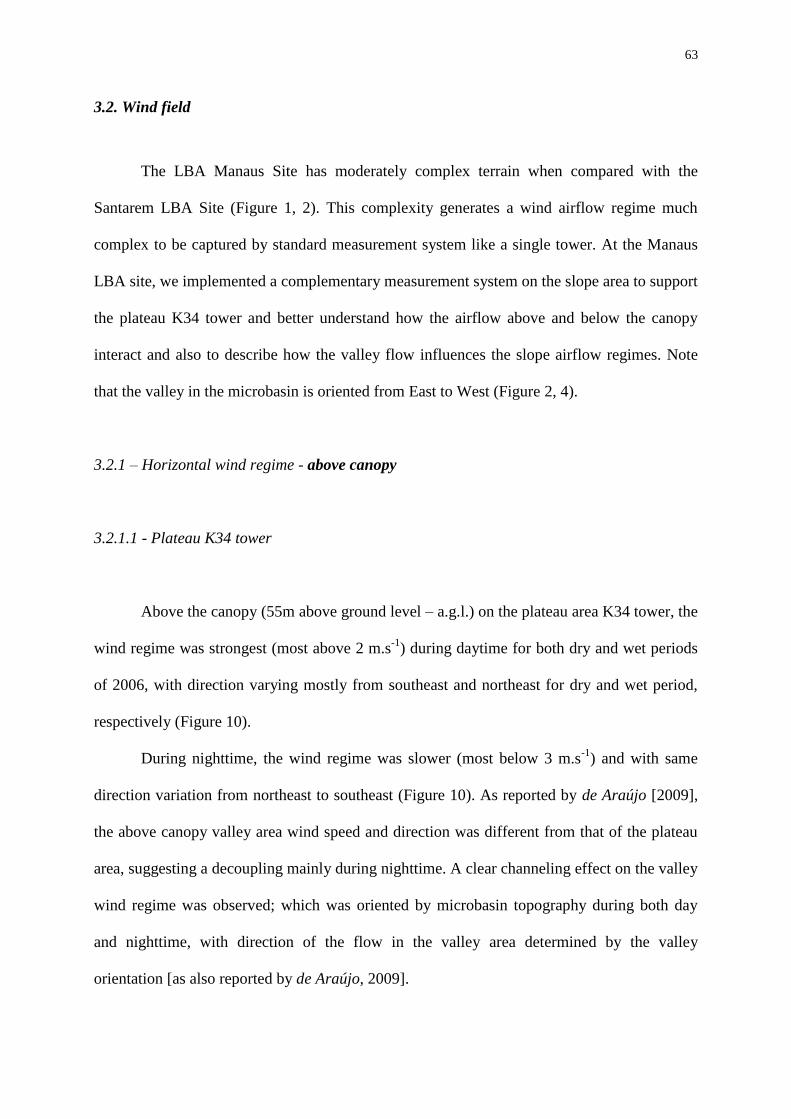
63
3.2. Wind field
The LBA Manaus Site has moderately complex terrain when compared with the
Santarem LBA Site (Figure 1, 2). This complexity generates a wind airflow regime much
complex to be captured by standard measurement system like a single tower. At the Manaus
LBA site, we implemented a complementary measurement system on the slope area to support
the plateau K34 tower and better understand how the airflow above and below the canopy
interact and also to describe how the valley flow influences the slope airflow regimes. Note
that the valley in the microbasin is oriented from East to West (Figure 2, 4).
3.2.1 – Horizontal wind regime - above canopy
3.2.1.1 - Plateau K34 tower
Above the canopy (55m above ground level – a.g.l.) on the plateau area K34 tower, the
wind regime was strongest (most above 2 m.s-1
) during daytime for both dry and wet periods
of 2006, with direction varying mostly from southeast and northeast for dry and wet period,
respectively (Figure 10).
During nighttime, the wind regime was slower (most below 3 m.s-1
) and with same
direction variation from northeast to southeast (Figure 10). As reported by de Araújo [2009],
the above canopy valley area wind speed and direction was different from that of the plateau
area, suggesting a decoupling mainly during nighttime. A clear channeling effect on the valley
wind regime was observed; which was oriented by microbasin topography during both day
and nighttime, with direction of the flow in the valley area determined by the valley
orientation [as also reported by de Araújo, 2009].
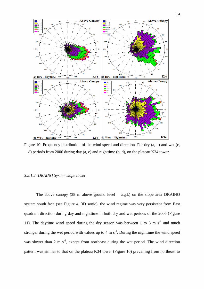
64
Figure 10: Frequency distribution of the wind speed and direction. For dry (a, b) and wet (c,
d) periods from 2006 during day (a, c) and nighttime (b, d), on the plateau K34 tower.
3.2.1.2 -DRAINO System slope tower
The above canopy (38 m above ground level – a.g.l.) on the slope area DRAINO
system south face (see Figure 4, 3D sonic), the wind regime was very persistent from East
quadrant direction during day and nighttime in both dry and wet periods of the 2006 (Figure
11). The daytime wind speed during the dry season was between 1 to 3 m s-1
and much
stronger during the wet period with values up to 4 m s-1
. During the nighttime the wind speed
was slower than 2 m s-1
, except from northeast during the wet period. The wind direction
pattern was similar to that on the plateau K34 tower (Figure 10) prevailing from northeast to
65
southeast. This observation indicates that the airflow above the canopy on the slope area is
related to how the synoptic flow enters in the eastern part of the microbasin (see Figure 2, 4).
Figure 11: Frequency distribution of the wind speed and direction above canopy (38 m above
ground level – a.g.l). For dry (a, b) and wet (c, d) periods from 2006 during day (a, c) and
nighttime (b, d), on the slope area at DRAINO system tower.
3.2.2 – Horizontal wind regime – Subcanopy array measurements (2 m a.g.l)
In Figure 12 the subcanopy array frequency distribution of the wind speed and
directions is shown for both dry and wet periods of the 2006, during both day and nighttime.
The observations show that the airflow in the subcanopy is very persistent and with similar
pattern during both dry and wet periods of 2006. Note that the south slope area in the
DRAINO System (see Figure 4) is downslope from south and upslope from north quadrants.
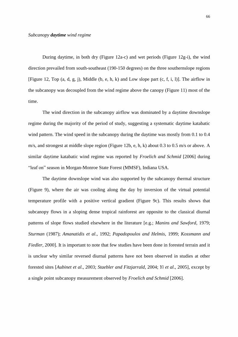
66
Subcanopy daytime wind regime
During daytime, in both dry (Figure 12a-c) and wet periods (Figure 12g-i), the wind
direction prevailed from south-southeast (190-150 degrees) on the three southernslope regions
[Figure 12, Top (a, d, g, j), Middle (b, e, h, k) and Low slope part (c, f, i, l)]. The airflow in
the subcanopy was decoupled from the wind regime above the canopy (Figure 11) most of the
time.
The wind direction in the subcanopy airflow was dominated by a daytime downslope
regime during the majority of the period of study, suggesting a systematic daytime katabatic
wind pattern. The wind speed in the subcanopy during the daytime was mostly from 0.1 to 0.4
m/s, and strongest at middle slope region (Figure 12b, e, h, k) about 0.3 to 0.5 m/s or above. A
similar daytime katabatic wind regime was reported by Froelich and Schmid [2006] during
“leaf on” season in Morgan-Monroe State Forest (MMSF), Indiana USA.
The daytime downslope wind was also supported by the subcanopy thermal structure
(Figure 9), where the air was cooling along the day by inversion of the virtual potential
temperature profile with a positive vertical gradient (Figure 9c). This results shows that
subcanopy flows in a sloping dense tropical rainforest are opposite to the classical diurnal
patterns of slope flows studied elsewhere in the literature [e.g.; Manins and Sawford, 1979;
Sturman (1987); Amanatidis et al., 1992; Papadopoulos and Helmis, 1999; Kossmann and
Fiedler, 2000]. It is important to note that few studies have been done in forested terrain and it
is unclear why similar reversed diurnal patterns have not been observed in studies at other
forested sites [Aubinet et al., 2003; Staebler and Fitzjarrald, 2004; Yi et al., 2005], except by
a single point subcanopy measurement observed by Froelich and Schmid [2006].

67
Figure 12: Frequency distribution of the wind speed and direction in the subcanopy array (2 m
above ground level – a.g.l) on the microbasin south face slope area at DRAINO horizontal
array system (see Figure 4). For dry (a-f) and wet (g-l) periods from 2006, during day (a, b,
c, g, h, i) and nighttime (d, e, f, j, k, l).
a) b) c)
d) e) f)
g) h) i)
j) k) l)
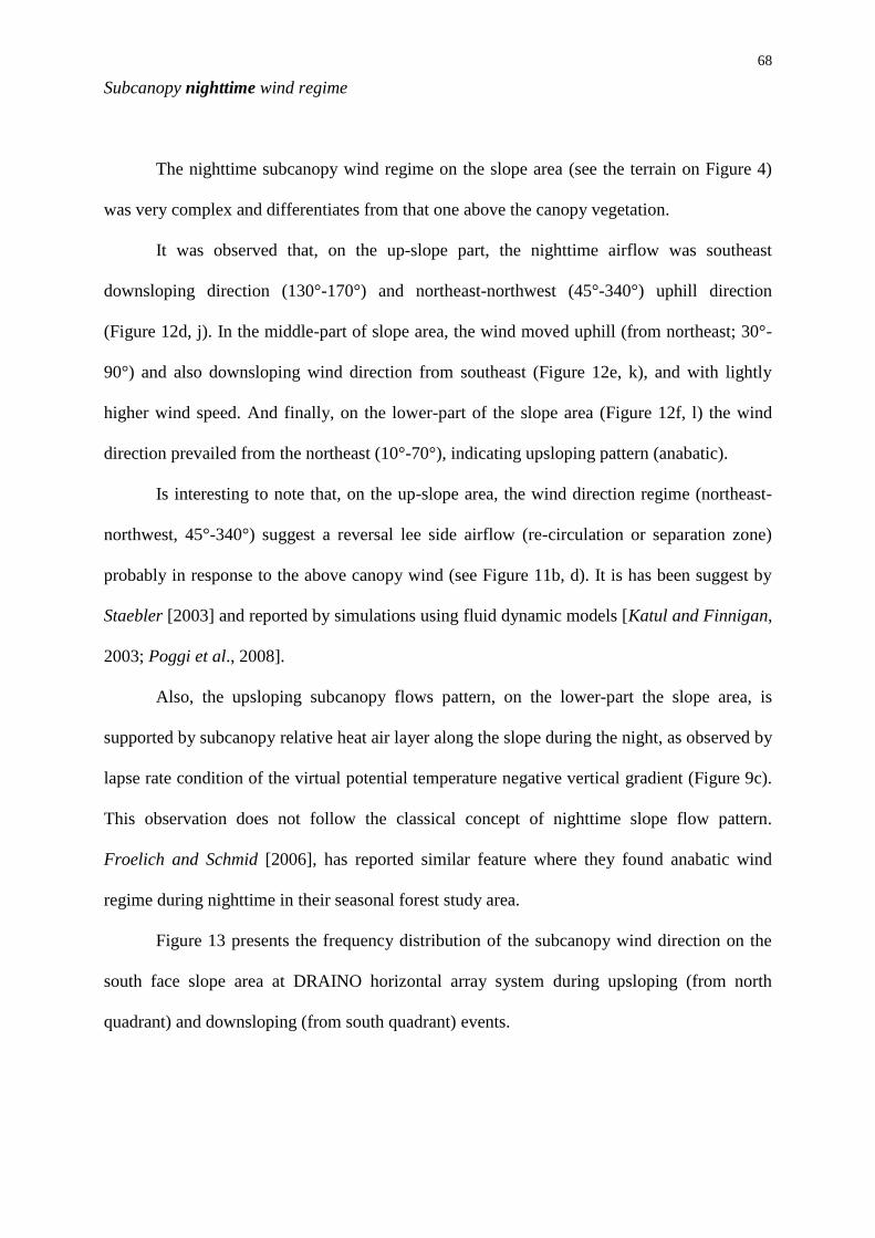
68
Subcanopy nighttime wind regime
The nighttime subcanopy wind regime on the slope area (see the terrain on Figure 4)
was very complex and differentiates from that one above the canopy vegetation.
It was observed that, on the up-slope part, the nighttime airflow was southeast
downsloping direction (130°-170°) and northeast-northwest (45°-340°) uphill direction
(Figure 12d, j). In the middle-part of slope area, the wind moved uphill (from northeast; 30°-
90°) and also downsloping wind direction from southeast (Figure 12e, k), and with lightly
higher wind speed. And finally, on the lower-part of the slope area (Figure 12f, l) the wind
direction prevailed from the northeast (10°-70°), indicating upsloping pattern (anabatic).
Is interesting to note that, on the up-slope area, the wind direction regime (northeast-
northwest, 45°-340°) suggest a reversal lee side airflow (re-circulation or separation zone)
probably in response to the above canopy wind (see Figure 11b, d). It is has been suggest by
Staebler [2003] and reported by simulations using fluid dynamic models [Katul and Finnigan,
2003; Poggi et al., 2008].
Also, the upsloping subcanopy flows pattern, on the lower-part the slope area, is
supported by subcanopy relative heat air layer along the slope during the night, as observed by
lapse rate condition of the virtual potential temperature negative vertical gradient (Figure 9c).
This observation does not follow the classical concept of nighttime slope flow pattern.
Froelich and Schmid [2006], has reported similar feature where they found anabatic wind
regime during nighttime in their seasonal forest study area.
Figure 13 presents the frequency distribution of the subcanopy wind direction on the
south face slope area at DRAINO horizontal array system during upsloping (from north
quadrant) and downsloping (from south quadrant) events.
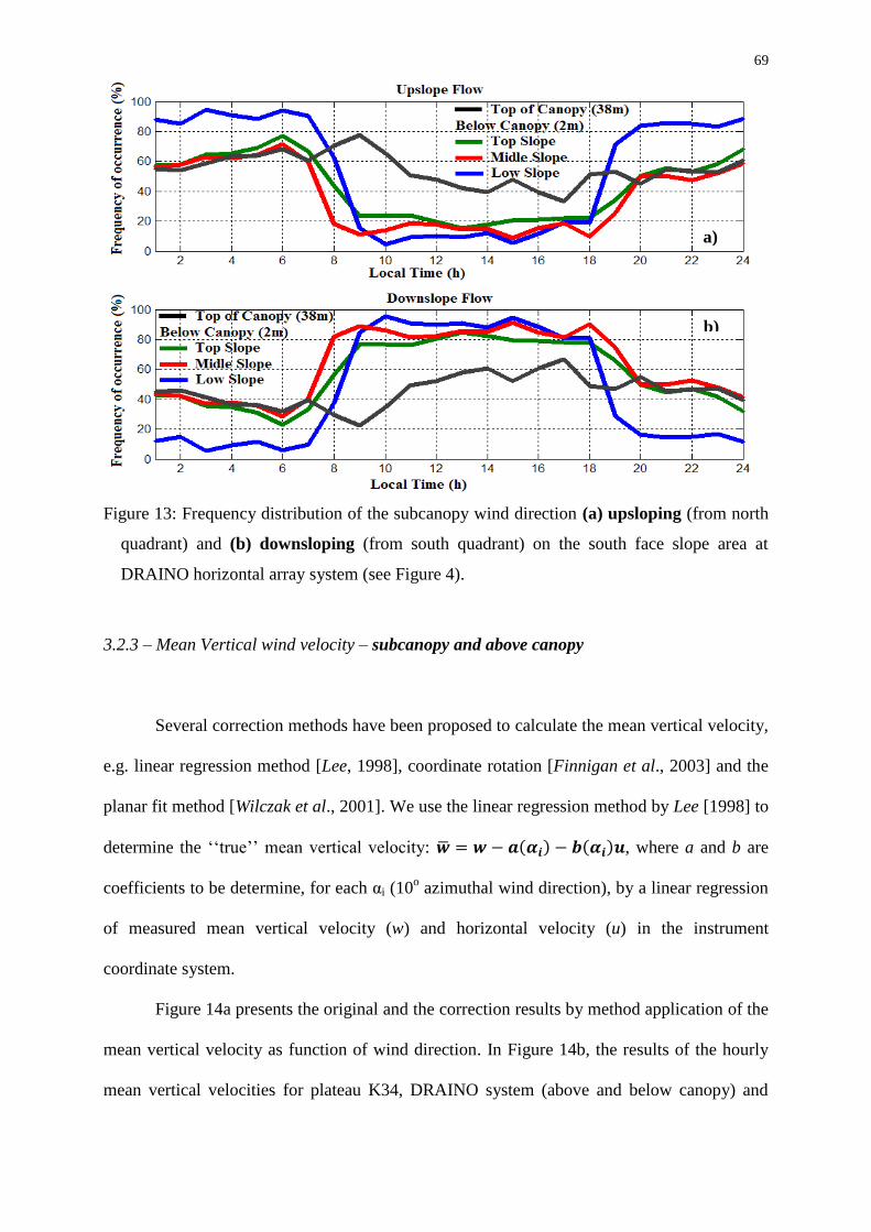
69
Figure 13: Frequency distribution of the subcanopy wind direction (a) upsloping (from north
quadrant) and (b) downsloping (from south quadrant) on the south face slope area at
DRAINO horizontal array system (see Figure 4).
3.2.3 – Mean Vertical wind velocity – subcanopy and above canopy
Several correction methods have been proposed to calculate the mean vertical velocity,
e.g. linear regression method [Lee, 1998], coordinate rotation [Finnigan et al., 2003] and the
planar fit method [Wilczak et al., 2001]. We use the linear regression method by Lee [1998] to
determine the „„true‟‟ mean vertical velocity: , where a and b are
coefficients to be determine, for each αi (10o azimuthal wind direction), by a linear regression
of measured mean vertical velocity (w) and horizontal velocity (u) in the instrument
coordinate system.
Figure 14a presents the original and the correction results by method application of the
mean vertical velocity as function of wind direction. In Figure 14b, the results of the hourly
mean vertical velocities for plateau K34, DRAINO system (above and below canopy) and
a)
b)
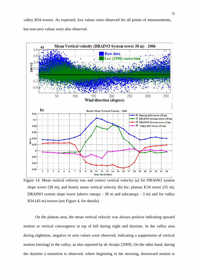
70
valley B34 towers. As expected, low values were observed for all points of measurements,
but non-zero values were also observed.
Figure 14: Mean vertical velocity raw and correct vertical velocity (a) for DRAINO system
slope tower (38 m), and hourly mean vertical velocity (b) for: plateau K34 tower (55 m),
DRAINO system slope tower (above canopy - 38 m and subcanopy - 3 m) and for valley
B34 (43 m) towers (see Figure 4, for details).
On the plateau area, the mean vertical velocity was always positive indicating upward
motion or vertical convergence at top of hill during night and daytime. In the valley area
during nighttime, negative or zero values were observed, indicating a suppression of vertical
motion (mixing) in the valley, as also reported by de Araújo [2009]. On the other hand, during
the daytime a transition is observed, where beginning in the morning, downward motion is
a)
b)
71
observed, changing after mid-morning to upward motion (Figure 14b). This suggests that
probably the cold air pooled during night moved downslope and started to warm, resulting in
a breakdown the inversion over the valley (see de Araújo [2009], for detailed description and
references there in for this process). The mechanism of the breakdown the inversion process
over the valley is consistent with positive vertical velocity observed above canopy at slope
area observed by the DRAINO system tower during daytime (Figure 14b).
The subcanopy diurnal pattern of the mean vertical velocity observed shows positive
values during nighttime and negative during daytime, consistent with observed up and
downsloping flow regime, respectively (Figure 13 a, b). Also this is consistent with thermal
vertical virtual potential temperature gradient on the slope (see Figure 9c), where during
nighttime (daytime) an unstable (inversion) condition is associated with upward (downward)
mean vertical velocity (see Figure 9c).

72
3.3. Phenomenology of the local circulations: Summary
The Figure 15 shows a schematic cartoon of local flow circulation from the previews
sections observations.
Figure 15: Schematic local circulations in the site studied, valley and slopes flow (a), 2D view
from suggested below and above canopy airflow (b).
The above canopy airflow (red arrow Figure 15a) and forcing mechanisms associate.
The observations result from previews sessions suggests that the balance of the buoyancy and
a)
b)
73
pressure gradient forces generates the airflow or microcirculations patterns in the site
studied. During nighttime (Figure 15b), in the subcanopy there is an upslope flow reaching
about 10 m height above ground, associate with positive mean vertical velocity (indicating
upward movement). Also, above canopy there is a downslope flow associate with negative
mean vertical velocity, downward convergence above the canopy. The microcirculation along
the plateau-slope-valley is promotes by an feedback mechanism of accumulation of cold air
drainage above canopy into the valley center (Figure 15b), creating the forcing need to sustain
nighttime pattern. The air temperature structure above canopy in the valley (see Araújo, 2009)
is a good indication of cold air pool in the center of the valley. Maybe, also, the local pressure
gradient force due the cold air accumulation promoting the upward airflow in the both slopes
of the valley. During daytime periods an inverse pattern is found (not show), indicating that
this microcirculation is a systematic pattern in the site.
3.4. CO2 concentration and subcanopy horizontal wind field
The CO2 concentration was measured by DRAINO system on the south face slope area
for dry and wet periods of the 2006, and on the north face slope during dry period (Figure 4).
The Figure 16 presents an example, for midnight (local time), of the horizontal wind field and
spatial CO2 concentration over the DRAINO System south face domain. The wind field was
interpolated from the blue points onto a 10 m grid. Similar procedures have been reported in
the literature (Sun et al., 2007; Feigenwinter et al., 2008). The horizontal wind regime plays
important role in modulating the horizontal spatial distribution of CO2 concentration (Figure
16).
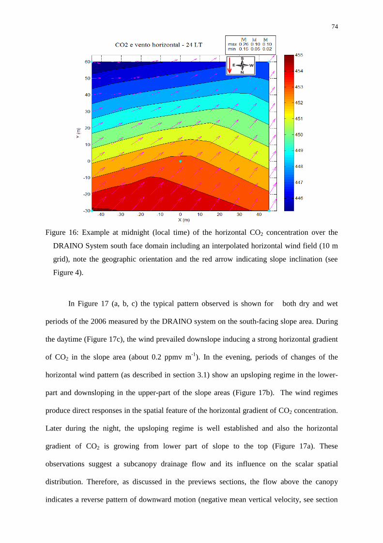
74
Figure 16: Example at midnight (local time) of the horizontal CO2 concentration over the
DRAINO System south face domain including an interpolated horizontal wind field (10 m
grid), note the geographic orientation and the red arrow indicating slope inclination (see
Figure 4).
In Figure 17 (a, b, c) the typical pattern observed is shown for both dry and wet
periods of the 2006 measured by the DRAINO system on the south-facing slope area. During
the daytime (Figure 17c), the wind prevailed downslope inducing a strong horizontal gradient
of CO2 in the slope area (about 0.2 ppmv m-1
). In the evening, periods of changes of the
horizontal wind pattern (as described in section 3.1) show an upsloping regime in the lower-
part and downsloping in the upper-part of the slope areas (Figure 17b). The wind regimes
produce direct responses in the spatial feature of the horizontal gradient of CO2 concentration.
Later during the night, the upsloping regime is well established and also the horizontal
gradient of CO2 is growing from lower part of slope to the top (Figure 17a). These
observations suggest a subcanopy drainage flow and its influence on the scalar spatial
distribution. Therefore, as discussed in the previews sections, the flow above the canopy
indicates a reverse pattern of downward motion (negative mean vertical velocity, see section
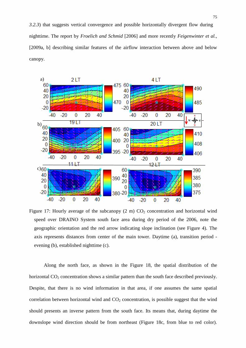
75
3.2.3) that suggests vertical convergence and possible horizontally divergent flow during
nighttime. The report by Froelich and Schmid [2006] and more recently Feigenwinter et al.,
[2009a, b] describing similar features of the airflow interaction between above and below
canopy.
Figure 17: Hourly average of the subcanopy (2 m) CO2 concentration and horizontal wind
speed over DRAINO System south face area during dry period of the 2006, note the
geographic orientation and the red arrow indicating slope inclination (see Figure 4). The
axis represents distances from center of the main tower. Daytime (a), transition period -
evening (b), established nighttime (c).
Along the north face, as shown in the Figure 18, the spatial distribution of the
horizontal CO2 concentration shows a similar pattern than the south face described previously.
Despite, that there is no wind information in that area, if one assumes the same spatial
correlation between horizontal wind and CO2 concentration, is possible suggest that the wind
should presents an inverse pattern from the south face. Its means that, during daytime the
downslope wind direction should be from northeast (Figure 18c, from blue to red color).
c)
b)
a)
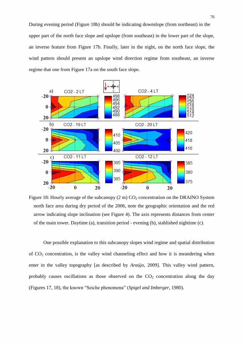
76
During evening period (Figure 18b) should be indicating downslope (from northeast) in the
upper part of the north face slope and upslope (from southeast) in the lower part of the slope,
an inverse feature from Figure 17b. Finally, later in the night, on the north face slope, the
wind pattern should present an upslope wind direction regime from southeast, an inverse
regime that one from Figure 17a on the south face slope.
Figure 18: Hourly average of the subcanopy (2 m) CO2 concentration on the DRAINO System
north face area during dry period of the 2006, note the geographic orientation and the red
arrow indicating slope inclination (see Figure 4). The axis represents distances from center
of the main tower. Daytime (a), transition period - evening (b), stablished nightime (c).
One possible explanation to this subcanopy slopes wind regime and spatial distribution
of CO2 concentration, is the valley wind channeling effect and how it is meandering when
enter in the valley topography [as described by Araújo, 2009]. This valley wind pattern,
probably causes oscillations as those observed on the CO2 concentration along the day
(Figures 17, 18), the known “Seiche phenomena” (Spigel and Imberger, 1980).
c)
b)
a)
77
4. Summary and Conclusions
The main objective of this study was to measure and understand the local circulation
over a dense forest site in Manaus with moderately complex terrain and to verify the existence
of the drainage flow regimes on slope and valley areas.
The main pattern of the airflow above and below the canopy in dense tropical forest in
Amazonia was captured by a relative simple measure system, as also has been done by more
sophisticated measurements system as those described recently by Feigenwinter et al., [2009a,
b].
As described and discuss in previews sections it was identified drainage flow in both
day and nighttime periods in the site studied. Evidence of the drainage current above canopy
was suggested by Goulden et al, (2006) similar to that one observed here.
It was identified that the local micro-circulation was complicate and presented tri-
dimensional nature where to estimate the advection flux at this site seems uncertain and not
possible with the limited measurement system employed.
As reported recently by Feigenwinter et al., [2009a, b], even using a more
sophisticated measurement design, the level of uncertainties is still high and some processes
are not yet known and need more exploration perhaps using a more complete spatial
observation network or even applying model resources (Foken, 2008; Aubinet, 2008, Belcher
et al., 2008).
In summary, the drainage flow exists and is observed at K34 LBA site area and the
high carbon uptake reported by previews work may be called into doubt and requires more
research.
Also, the use of nighttime correction in order to save the urge necessity to estimate
long term Net Ecosystem exchange is inappropriate by the using only turbulence information
from above canopy, as has been pointed out here The interactions above and below canopy

78
breakdown the footprint principle and the representativeness of the eddy flux tower in most
difficult conditions (complex terrain and calm nights).
In summary, the drainage flow exists and is observed at K34 LBA site. Very large
carbon uptake estimates reported previously should be questioned [Kruijt et al., 2004; Araújo
et al., 2002]. More research is needed. The use of nighttime u* correction to avoid estimating
canopy storage is inappropriate. One cannot get by using only above canopy turbulence
information. The interactions between motions above and below canopy question the
foundations of the footprint analysis [Schuepp et al., 1990; Schimid, 2006]. The
representativeness of the eddy flux tower is most in question for complex terrain, especially
on calm nights).
79
CONCLUSÃO GERAL
No Capítulo I foi apresentado que:
- Foi realizado o primeiro esforço em determinar observacionalmente a importância dos
processos de advecção noturna no balanço de CO2 em uma densa floresta tropical na
Amazônia.
- Foi testada a hipótese de que uma persistente advecção horizontal abaixo da floresta existe e
transporta uma importante quantidade de CO2 para fora do volume de controle representado
pelas medidas da torre de fluxo do LBA em Santarém.
- Foi determinada a magnitude dos gradientes horizontais de CO2 e do campo do vento abaixo
da floresta e encontrado um saldo suficiente de advecção para afetar o balanço de CO2.
- A metodologia estabelecida foi aplicada e testada para medir os gradientes horizontais de
CO2 e do vento horizontal dentro da floresta. Esses dados foram complementados pelos
fluxos turbulentos e observações dos perfis médios obtidos em uma torre de 65 metros de
altura no mesmo sítio experimental (sessão 2). As medidas foram realizadas durante o
período das estações seca (DOY 198-238 2003 – Fase 1) e úmida (DOY 278-366 2004 e 1-
32 2005 – Fase 2).
- Os gradientes horizontais médio de CO2 e do vento horizontal foram da ordem de
0.02 ppm m-1
e 0.12 m s-1
, respectivamente (seção 3.1).
- Abaixo da floresta a direção do vento horizontal foi bem correlacionada com a inclinação
suave do terreno próxima a torre de medida dos fluxos. Foi observado que a direção do
escoamento abaixo da floresta foi desacoplada do escoamento acima, o que sugere um
potencial para transporte lateral de CO2 mesmo durante o período diurno (sessão 3.2).
- O principal mecanismo físico responsável pela geração do escoamento noturno abaixo da
floresta foi o termo de flutuabilidade negativa (seção 3.3).
80
- A comparação do déficit noturno entre a respiração total do ecossistema e NEE medida no
sistema de fluxo da torre foi associado à advecção noturna média de CO2, a qual
representou 73% e 71% do mesmo, para 130 noites analisados durante os períodos seco e
chuvoso estudados. Isto indica um importante papel da advecção noturna no balanço total
de CO2.
- Foi observado também que, durante períodos noturnos com níveis de turbulência
significativos (u* entre 0.3 a 0.6 m s-1
, limiares considerados suficiente para fornecer
corretas medidas pelos fluxos turbulentos), o transporte de CO2 pela advecção horizontal
foi significativo.
- Esses resultados confirmam que poucos sítios de medidas de fluxos são suficientemente
planos e homogêneos para ignorar a priori os efeitos da advecção horizontal. Estimativa
observacional do efeito da velocidade vertical média no balanço de escalares aparece como
a maior fonte de incertezas, e medidas continua e de longo prazo com instrumentação mais
adequada são necessárias para esclarecer este tema.
No Capítulo II foi apresentado que:
- Seguindo a metodologia e design experimental desenvolvido no Capitulo I, foi possível ser
aplicada também para um sitio experimental com topografia de maior complexidade.
- Foi observado que existem escoamentos de drenagem horizontal abaixo e acima da floresta,
e que esses estão fortemente influenciados pela canalização do vento horizontal ao longo do
vale da microbacia Asu próximo da torre de fluxo (K34) e das medidas nas encostas abaixo
da floresta (Sistema DRAINO).
- Especialmente no sítio do LBA em Manaus, não foi possível estimar quantitativamente a
magnitude da advecção horizontal de CO2, em função da complexa heterogeneidade
topográfica da área produzindo uma complicada natureza tridimensional do escoamento
81
abaixo e acima da floresta, que se interagem e criando uma barreira para medir em detalhe
todas as informações com a metodologia e instrumentação disponível neste estudo.
- As sub-estimativas noturnas das taxas de respiração através de medidas aplicando a técnica
de “Eddy Covariance” sobre vários tipos de ecossistemas e terrenos já é bem reconhecida
pela comunidade científica mundialmente. Os estudos observacionais aqui apresentados
suportam esta hipótese demonstrando a importância do transporte horizontal que ocorre
abaixo do nível de medida das torres de fluxo de ambos os sítios de medidas do LBA. E
finalmente adverte que correções dos fluxos turbulentos noturnos com base em condições
acima da vegetação somente podem ser inapropriadas e com significante incerteza.
- Como sugestões os estudos de modelagem do tipo LES, já que foi identificado um padrão de
micro circulações locais de natureza tridimencional, seriam de fundamental importância
para avaliar e ajudar a entender melhor as observações aqui obtidas.
82
REFERÊNCIAS
Acevedo, O. C. and Fitzjarrald, D.R. (2003), In the Core of the Night - Effects of Intermittent
Mixing on a Horizontally Heterogeneous Surface. Boundary-Layer Meteorology, Dordrecht,
v. 106, n. 1, p. 1-33.
Antonia, R.A., Chambers, A.J., Frieh, C.A.E. and van Atta, C.W., (1979), Temperature ramps
in the atmospheric surface layer. J. Atmos. Sci. 36, pp. 99–108.
Araújo, A. C., et al., (2002), Comparative measurements of carbon dioxide fluxes from two
nearby towers in a central Amazonian rainforest: The Manaus LBA site, Journal of
Geophysical Research, 107(D20), 8090, doi:10.1029/2001JD000676.
Araújo, A. C., et al., (2008), Interaction of micrometeorology and surface fluxes confounding
the interpretation of CO2 fluxes in Central Amazonia. Submited to Agricultural and Forest
Meteorology.
Araújo, A. C., (2009), Spatial variaton of CO2 fluxes and lateral transport in an area of terra
firme forest in central Amazonia. PhD Thesis, Vrije Universiteit Amsterdam, VU, Holanda.
Aubinet M, P. Berbigier, C. H. Bernhofer, A. Cescatti, C. Feigenwinter, A. Granier, T. H.
Grunwald, K. Havrankova, B. Heinesch, B. Longdoz, B. Marcolla, L. Montagnani, P.
Sedlak (2005), Comparing CO2 storage and advection conditions at night at different
Carboeuroflux sites. Boundary Layer Meteorol., 116: 63-94.
Aubinet, M., B. Heinesch, and M. Yernaux (2003), Horizontal and vertical CO2 advection in a
sloping forest, Boundary Layer Meteorol., 108(3), 397–417.
Aubinet, M., et al., (2000), Estimates of the annual net carbon and water exchange of forests:
the EUROFLUX methodology. Adv. Ecol. Res., 30, 113–175.
Baker I. T., Prihodko, L., Denning, A.S., Goulden, M., Miller, S., da Rocha, H.R., (2008),
Seasonal drought stress in the Amazon: Reconciling models and observations, J. Geophys.
Res., 113, G00B01, doi:10.1029/2007JG000644
Baker, T.R. et al., (2004), Increasing biomass in Amazonian forest plots. Philosophical
Transactions of the Royal Society of London. Series B-Biological Sciences, 359(1443): 353-
365.
Baldocchi, D. D., B. B. Hicks, and T. P. Meyers (1988), Measuring biosphere-atmosphere
exchanges of biologically related gases with micrometeorological methods, Ecology, 69(5),
1331– 1340.
Baldocchi, D., et al. (2001), FLUXNET: A new tool to study the temporal and spatial
variability of ecosystem-scale carbon dioxide, water vapor, and energy flux densities, Bull.
Am. Meteorol. Soc., 82(11), 2415 – 2434.
83
Baldocchi, D., J. Finnigan, K. Wilson, T. Paw U, and E. Falge (2000), On measuring net
ecosystem carbon exchange over tall vegetation on complex terrain, Boundary Layer
Meteorol., 96(1–2), 257–291.
Barr, S., (1971), A modeling study of several aspects of canopy flow. Monthly Weather
Review, vol. 99, No. 6: 485-493.
Baynton, H. W., Biggs, W. G., Hamilton, H. L., Jr., Sherr, P. E., and Worth, J. J. B., (1965),
Wind Structure in and Above a Tropical Forest. Journal of Applied Meteorology, Vol. 4,
No. 6: 670-675.
Bergstrom, H., Hogstrom, U., (1989), Turbulent exchange above apine forest II. Organized
structures. Bound.-Layer Meteorol.49: 231-263.
Bitencourt, D.P. and Acevedo, O. C., (2008), Modelling the Interaction Between a River
Surface and the Atmosphere at the Bottom of a Valley. Boundary-Layer Meteorology, v.
129, p. 309-321.
Black, T. A., et al. (1996), Annual cycles of water vapour and carbon dioxide fluxes in and
above a boreal aspen forest, Global Change Biol., 2(3), 219–229.
Bohrer, Gil, (2007), Large Eddy Simulations of Forest Canopies for Determination of
Biological Dispersal by Wind. PhD Thesis. Department of Civil and Environmental
Engineering, Duke University, 2007.
Castilho, C., (2004), Variação espacial e temporal da biomassa arbórea viva em64 km2 de
floresta de terra-firme na Amazônia Central. 87p. Doctoral Thesis, ecology, Instituto
Nacional de Pesquisa da Amazônia, Manaus-AM.
Chambers, J.Q. et al., (2004), Respiration from a tropical forest ecosystem: Partitioning of
sources and low carbon use efficiency. Ecological Applications, 14(4): S72-S88.
Cionco, R. M., 1965: A mathematical model for air flow in a vegetation canopy. J. Appl.
Meteor., 4, 517–522.
Clark D. B. (1996), Abolishing virginity. Journal of Tropical Ecology, 12, 735–739.
Cohen, J. C. P., Sá, L.D.A., Nogueira, D. S., Gandu, A.W., (2006), Jatos de baixos níveis
acima da floresta amazônica em Caxiuanã. Revista Brasileira de Meteorologia, São Paulo,
v.21, n.3b, p. 271-282.
Cuartas, L.A. et al., (2007), Interception water-partitioning dynamics for a pristine rainforest
in Central Amazonia: Marked differences between normal and dry years. Agricultural and
Forest Meteorology, 145(1-2): 69-83.
da Rocha, H. R., M. L. Goulden, S. D. Miller, M. C. Menton, L. D. V. O. Pinto, H. C. de
Freitas, and A. M. E. S. Figueira (2004), Seasonality of water and heat fluxes over a tropical
forest in eastern Amazonia, Ecol. Appl., 14(4), suppl. S, S22– S32.
84
Denmead, O.T. and Bradley, E.F., (1985), Flux-gradient relationships in a forest canopy. In:
B.A. Hutchison and B.B. Hicks (Editors). The forest-atmosphere interaction. D. Reidel
Publishing Company, Dordrecht, Holland, pp. 421-442.
Dias, M. A. F. S. and P. Regnier., (1996), Simulation of mesoscale circulations in a deforested
area of rondônia in the dry season. In Amazonian deforestation and climate, ed. J. H. C.
Gash, C. A. Nobre, J. M. Roberts and R. L. Victoria:531-547. Chichester: J Weily.
Dixon, R.K., S.Brown, R.A. Houghton, A.M. Solomon, M.C. Trexler and J. Wisniewski,
(1994), Carbon pools and flux of global forest ecosystems. Science, 263, 185-190.
Falge, E., et al. (2001), Gap filling strategies for defensible annual sums of net ecosystem
exchange. Agric. For. Meteorol. 107, 43-69.
Fan, S.M., Wofsy, S.C., Bakwin, P.S., Jacob, D.J. and Fitzjarrald, D.R., (1990), Atmosphere-
biosphere exchange of CO2 and O3 in the Central-Amazon-forest. Journal of Geophysical
Research-Atmospheres, 95(D10): 16851-16864.
Feigenwinter, C., C. Bernhofer, and R. Vogt, (2004), The influence of advection on the short
term CO2-budget in and above a forest canopy, Boundary Layer Meteorol., 113(2), 201–
224.
Feigenwinter, C., C. et al., (2008), Comparison of horizontal and vertical advective CO2
fluxes at three forest sites, Agric. Forest. Meteorol., 145,1–21.
Feigenwinter, C., et al. (2009a), Spatiotemporal evolution of CO2 concentration, temperature,
and wind field during stable nights at the Norunda forest site. Agric. Forest Meteorol.,
doi:10.1016/j.agrformet.2009.08.005
Feigenwinter, C., Montagnani, L., Aubinet, M. (2009b), Plot-scale vertical and horizontal
transport of CO2 modified by a persistent slope wind system in and above an alpine forest.
Agric. Forest Meteorol., doi:10.1016/j.agrformet. 2009.05.009.
Ferraz, J., Ohta, S. and Sales, S., 1988. Distribuição dos solos ao longo de dois transectos em
floresta primária ao norte de Manaus. In: N. Higuchi, M.A.A. Campos, P.T.B. Sampaio and
J. dos Santos (Editors), Análise estrutural da floresta primária da bacia do rio Cuieiras,
ZF-2, Manaus-AM, Brasil. MCT/INPA/JICA, Manaus, pp. 109-144.
Finnigan, J.J., R. Clement, Y. Malhi, R. Leuning and H.A. Cleugh, (2003), A reevaluation of
long-term flux measurement techniques. Part I: Averaging and coordinate rotation. Bound.-
Layer Meteorol., 107, 1-48.
Fitzjarrald, D. R., and K. E. Moore, (1990), Mechanisms of nocturnal exchange between the
rain-forest and the atmosphere, Journal of Geophysical Research, 95(D10), 16,839–16,850.
Fitzjarrald, D. R., K. E. Moore, O. M. R. Cabral, J. Scolar, A. O. Manzi, and L. D. D. Sa
(1990), Daytime turbulent exchange between the Amazon Forest and the atmosphere,
Journal of Geophysical Research, 95(D10), 16,825 – 16,838.
85
Fitzjarrald, D. R., R. K. Sakai, O. L. L. Moraes, M. J. Czikowsky, O. C. Acevedo, R. C.
Oliveira, (2004), Mesoclimate of the LBA-ECO Santarém Study Area, paper presented at III
LBA Scientific Conference, Braz. Minist. of Sci. and Technol., Brasilia, Brazil, July.
Fitzjarrald, D. R., Stormwind, B.L., Fisch, G., Cabral, O. M. R. (1988), Turbulent Transport
Observed Just Above the Amazon Forest, Journal of Geophysical Research, 93(D2), 1,551–
1,563.
Fitzjarrald, D.R., and K.M. Moore, (1995), Physical mechanisms of heat and mass exchange
between forests and the atmosphere. In: M. Lowman and N. Nadkarni, eds., Forest
Canopies: A Review of Research on This Biological Frontier, Academic Press, 45–72.
Foken, T. (2008), The energy balance closure problem: An overview. Ecological
Applications: Vol. 18, No. 6, pp. 1351-1367.
Freitas, S. R., Longo, K.M., Silva Dias, M.A. F., Silva Dias, P.L., Chatfield, R., Prins, E.,
Artaxo, P., Grell, G., Recuero, F.S., (2005), Monitoring the transport of biomass burning
emissions in South America, Environ. Fluid Mech., 5(1–2), doi:10.1007/s10652-0050243-7.
Freitas, S. R., M. A. F. Silva Dias, P. L. Siva Dias, K. M. Longo, P. Artaxo, M. O. Andreae,
and H. Fischer (2000), A convective kinematic trajectory technique for low-resolution
atmospheric models, J. Geophys. Res., 105(D19), 24,375–24,386.
Froelich, N.J. and Schmid, H.P., (2006), Flow divergence and density flows above and below
a deciduous forest Part II. Below-canopy thermotopographic flows. Agricultural and Forest
Meteorology, Volume 138, Issues 1-4.
Gandu, A. W., Cohen, J.C.P., Souza, J. R. S., (2004), Simulation of deforestation in eastern
Amazonia using a high-resolution model. Theoretical and Applied Climatology, Austria, v.
78, n. 1-3, p. 123-135.
Gao, W., Shaw, R.H., Paw U, K.T., (1989), Observation of organized structure in turbulent
flow within and above a forest canopy. Bound.-Layer Meteorol. 47: 349-377.
Garratt, J. R., (1980), Surface Influnce upon Vertical Profiles in the Atmospheric near-surface
layer. Quart. J. Roy. Meteorol. Soc., v.106, n.450, p. 803-819.
Goulden, M. L., J. W. Munger, S. M. Fan, B. C. Daube, and S. C. Wofsy (1996),
Measurements of carbon sequestration by long-term eddy covariance: Methods and a critical
evaluation of accuracy, Global Change Biol., 2(3), 169– 182.
Goulden, M. L., S. D. Miller, H. R. da Rocha, M. C. Menton, H. C. de Freitas, A. M. E. S.
Figueira, and C. A. D. de Sousa (2004), Diel and seasonal patterns of tropical forest CO2
exchange, Ecol. Appl., 14(4), suppl. S, S42–S54.
Goulden, M.L., Miller, S.D. and da Rocha, H.R., (2006), Nocturnal cold air drainage and
pooling in a tropical forest. Journal of Geophysical Research-Atmospheres, 111(D8),
10.1029/2005JD006037.
86
Grace, J. et al., (1995a), Carbon-Dioxide Uptake by an Undisturbed Tropical Rain-Forest in
Southwest Amazonia, 1992 to 1993. Science, 270(5237): 778-780.
Grace, J., et al. (1995b), Carbon dioxide uptake by an undisturbed tropical rain forest in
southwest Amazonia, Science, 270, 778–780.
Grace, J., Y. Malhi, J. Lloyd, J. McIntyre, A. C. Miranda, P. Meir, and H. S. Miranda (1996),
The use of eddy covariance to infer the net carbon dioxide uptake of Brazilian rain forest,
Global Change Biol., 2, 208– 217.
Gu L., E. Falge, T. Boden, D. D. Baldocchi, T. A. Black, S. R. Saleska, T. Suni, T. Vesala, S.
Wofsy, L. Xu (2005), Observing threshold determination for nighttime eddy flux filtering,
Agric. For. Meteorol., 128:179–197.
Harman, I.N. and Finnigan, J.J., (2007), A simple unified theory for flow in the canopy and
roughness sublayer. Boundary-Layer Meteorology, 123, 339-363.
Hodnett, M.G., Tomasella, J., Cuartas, L.A., Waterloo, M.J., and Nobre, A.D., (2007),
Subsurface hydrological flow paths in a Ferralsol (Oxisol) landscape in central Amazonia.
Hydrological Sciences Journal (in press).
Hutyra, L. R., J. W. Munger, S. R. Saleska, E. Gottlieb, B. C. Daube, A. L. Dunn, D. F.
Amaral, P. B. de Camargo, and S. C. Wofsy (2007), Seasonal controls on the exchange of
carbon and water in an Amazonian rain forest, Journal of Geophysical Research, 112,
G03008, doi:10.1029/2006JG000365.
Inoue, E., (1963), On the turbulent structure of air flow within crop canopies. J. Meteor. Soc.
Japan, 41, 317–326.
IPCC 2007. Climate Change 2007: The physical science basis. Contribution of Working
Group I to the Fourth Assessment Report of the Intergovernmental Panel on Climate
Change. WMO/UNEP, 18 pp.
Iwata, H., Y. Malhi, and C. Von Randow, (2005), Gap-filling measurements of carbon
dioxide storage in tropical rainforest canopy airspace. Agricultural and Forest Meteorology.
132, 3-4: 305–314.
Kanda, M., R. Moriwaki, and F. Kasamatsu., (2004), Large-eddy simulation of turbulent
organized structures within and above explicitly resolved cube arrays. Boundary-Layer
Meteorology 112: 343-368.
Katul, G.G., J.J. Finnigan and R. Leuning, (2003), The influence of hilly terrain o canopy-
atmosphere carbon dioxide exchange. Boundary Layer Meteorology.
Keller, M., et al. (2004), Ecological research in the large-scale biosphere atmosphere
experiment in Amazonia: Early results, Ecol. Appl., 14(4), suppl. S, S3– S16.
Kruijt, B. et al., (2000), Turbulence statistics above and within two Amazon rain forest
canopies. Boundary-Layer Meteorology, 94(2): 297-331.
87
Kruijt, B. J., A. Elbers, C. von Randow, A. C. Arau‟jo, P. J. Oliveira,A. Culf, A. O. Manzi,
A. D. Nobre, P. Kabat, and E. J. Moors (2004), The robustness of eddy correlation fluxes
for Amazon rain forest conditions, Ecol. Appl., 14, suppl. S, S101–S113.
Kruijt, B., et al., (2000), Turbulence Statistics Above and Within Two Amazon Rain Forest
Canopies. Boundary-Layer Meteorology, v. 94, n. 2, p. 297-331.
Laurance, et al., (1999), Relationship between soils and Amazon Forest biomass: a landscape-
scale study. Forest Ecology Management, 118:127-138.
Lee, X. H. (1998), On micrometeorological observations of surface-air exchange over tall
vegetation, Agric. For. Meteorol., 91(1– 2), 39–49.
Lee, X. and Hu, X., (2002), Forest-air fluxes of carbon and energy over non-flat terrain,
Boundary-Layer Meteorology, 103: 277-301.
Lee, X., Neumann, H.H., den Hartog, G., Fuentes, J.D., Black, T.A., Mickle, R.E., Yang, P.C.
and Blanken, P.D., (1992), Observation of gravity waves in a boreal forest. Bound.-Layer
Meteorol. 84, pp. 383–398.
Leuning, R., Zegelin, S. J., Jones, K., Keith, H., Hughes, D., (2008), Measurement of
horizontal and vertical advection of CO2 within a forest canopy. Agricultural and Forest
Meteorology, Volume 148, Issue 11, Pages 1777-1797.
Li, B. and R. Avissar. 1994. The impact of spatial variability of land-surface characteristics on
land-surface heat fluxes. Journal of Climate 7: 527-537.
Lu, C.-H., and D.R. Fitzjarrald, (1994), Seasonal and diurnal variations of coherent structures
over a deciduous forest. Boundary-Layer Met., 69, 43-69.
Lu, L., Denning, A S.; Silva Dias, M.A.F., Ssilva Dias, P. L., Longo, M., Freitas, S. R.,
Saatchi, S., (2005), Mesoscale circulations and atmospheric CO2 variations in the Tapajós
region, Pará, Brazil. Journal of Geophysical Research, doi 10.1029/2004JD005757, v. 110,
n. D21102.
Luizão, R.C.C., Luizão, F.J., Paiva, R.Q., Monteiro, T.F., Sousa, L.S., Kruijt, B., (2004),
Variation of carbon and nitrogen cycling processes along a topographic gradient in a central
Amazonian forest. Global Change Biology, 10: 592-600.
Mahrt, L., (1982), Momentum balance of gravity flows. J. Atmos. Sc., 39, 2701-2711.
Malhi, Y., A. D. Nobre, J. Grace, B. Kruijt, M. G. P. Pereira, A. Culf, and S. Scott, (1998),
Carbon dioxide transfer over a central Amazonian rain forest. Journal of Geophysical
Research, 103, 31,593–31,612.
Malhi, Y., et. al. (2009), Comprehensive assessment of carbon productivity, allocation and
storage in three Amazonian forests. Global Change Biology, Volume 15, Issue 5, 1255-
1274.
88
Marcolla, B, A. Cescatti, L. Montagnani, G. Manca, G. Kerschbaumer and S. Minerbi,
(2005), Importance of advection in the atmospheric CO2 exchanges of an alpine forest.
Agric. For. Meteorol., 130, 193-206.
Melillo, J.M. et al.,(1993), Global climate change and terrestrial net primary production.
Nature 363, 234-240.
Meroney, Robert N., (1968), Characteristics of Wind and Turbulence in and Above Model
Forests. Journal of Applied Meteorology, Vol. 7, NO. 5: 780-788.
Miller, S. D., M. L. Goulden, M. C. Menton, H. R. da Rocha, H. C. de Freitas, A. M. E. S.
Figueira, and C. A. D. de Sousa (2004), Biometric and micrometeorological measurements
of tropical forest carbon balance, Ecol. Appl., 14(4), suppl. S, S114– S126.
Moncrieff, J. B., J. M. Massheder, H. deBruin, J. Elbers, T. Friborg, B. Heusinkveld, P.
Kabat, S. Scott, H. Soegaard, and A. Verhoef. “A system to measure surface fluxes of
momentum, sensible heat, water vapour and carbon dioxide.” Journal of Hydrology 189, 1-
4: (1997) 589–611.
Montgomery, R.B., (1948), Vertical flux of heat in the atmosphere. Journal of Meteorology,
5, 265–274.
Nogueira, D. S., Sá, L.D.A., Cohen, J. C. P., (2006), Rajadas Noturnas e Trocas de CO2
Acima da Floresta de Caxiuanã, PA, Durante a Estação Seca. Revista Brasileira de
Meteorologia, São Paulo, v.21, n.3b, p. 212-223.
Pachêco , V. B., (2001), Algumas Características do Acoplamento entre o Escoamento Acima
e Abaixo da Copa da Floresta Amazônica em Rondônia. 2001 109f. Dissertação (Mestrado
em Meteorologia) - Instituto Nacional de Pesquisas Espaciais, São José dos Campos.
Parker, G., and D. R. Fitzjarrald (2004), Canopy structure and radiation environment metrics
indicate forest developmental stage, disturbance, and certain ecosystem functions, paper
presented at III LBA Scientific Conference, Braz. Minist. of Sci. and Technol., Brasilia,
Brazil, July.
Parotta J.A., J. K. Franci, R. R. de Almeida (1995), Trees of the Tapajos: a photographic field
guide. General Technical Report IITF-1. United States Department of Agriculture, Rio
Piedras, Puerto Rico, 371 pp.
Patton, E. G., (1997), Large-eddy simulation of turbulent flow above and within a plant
canopy. Ph.D. Thesis, University of California Davis.
Patton, Edward (2008), Large-eddy simulation (LES); Momentum and scalar transport in
canopy-covered terrain. ADVEX Workshop.
Paw U. K. T., D. D. Baldocchi, T. P. Meyers, and K. B. Wilson (2000), Correction of eddy
covariance measurements incorporating both advective effects and density fluxes. Boundary
Layer Meteorol., 97, 487-511.
89
Phillips, O.L. et al., (1998), Changes in the carbon balance of tropical forests: Evidence
from long-term plots. Science, 282(5388): 439-442.
Poggi, D., Katul, G., Finnigan,J. J., Belcher,S. E., (2008) Analytical models for the mean flow
inside dense canopies on gentle hilly terrain Q. J. R. Meteorol. Soc. 134: 1095–1112 (2008).
Prandtl, L., (1925), Uber die ausgebildete turbulenz. Z. Angew. Math. Mech., 5, 136–139.
Ramos da Silva, R., Avissar, R., (2000), A Large Eddy Simulation (LES) of the Boundary
Layer Evolution Over a Deforested Region of Rondonia (Brazil). In: American Geophysical
Union - Fall Meeting, 2002, San Francisco. EOS Trans., San Francisco: American
Geophysical Union, 2002. v. 83.
Raupach, M. R., and J. J. Finnigan., (1997), The influence of topography on meteorological
variables and surface-atmosphere interactions. Journal of Hydrology 190, 3-4: 182–213.
Raupach, M. R., J. J. Finnigan, and Y. Brunet., (1996), Coherent eddies and turbulence in
vegetation canopies: The mixing-layer analogy. Boundary-Layer Meteorology 78: 351-382.
Raupach, M. R., Thom, A. S., (1981), Turbulence in and above Plant Canopies. Annual
Review of Fluid Mechanics, v. 13, p. 97-129.
Raupach, M.R., Finnigan, J.J. and Brunet, Y., (1996), Coherent eddies and turbulence in
vegetation canopies: The mixing layer analogy. Boundary-Layer Meteorology, 78, 351-382.
Rennó, C. D., et al., (2008), HAND, a new terrain descriptor using SRTM-DEM: Mapping
terra-firme rainforest environments in Amazonia. Remote Sensing of Environment,
doi:10.1016/j.rse.2008.03.018
Sá, L. D. A., Pachêco, V. B., (2001), Relação de Similaridade para os Perfis de Velocidade do
Vento dentro da Copa da Floresta Amazônica em Rondônia. Revista Brasileira de
Meteorologia, v.16, n. 1, p. 81-89, 2001.
Sá, L. D. A., Pachêco, V.B., (2006), Wind velocity above and inside Amazonian Rain Forest
in Rondônia. Revista Brasileira de Meteorologia, v.21, n.3a, 50-58, 2006.
Sakai, R., D. Fitzjarrald, and K. E. Moore., (2001), Importance of low-frequency
contributions to eddy fluxes observed over rough surfaces. Journal Applied Meteorology,
40: 2178–2192.
Saleska, S. R., et al. (2003), Carbon in Amazon forests: Unexpected seasonal fluxes and
disturbance-induced losses, Science, 302(5650), 1554– 1557.
Shaw, R. H., 1977: Secondary wind speed maxima inside plant canopies. J. Appl. Meteor., 16,
514–521.
Shuttleworth, W.J., (1989), Micrometeorology of temperate and tropical forest. Philosophical
Transactions of the Royal Society of London, series B, 324, 1223: 299-334.
90
Silva Dias, M.A.F, (2006), Meteorologia , desmatamento e queimadas na Amazônia: uma
síntese de resultados do LBA. Revista Brasileira de Meteorologia, v.21, n.3a, 190-199,
2006.
Silva Dias, M.A.F., Silva Dias, P. L., Longo, M., Fitzjarrald, D. R., Denning, A S., (2004),
River breeze circulation in eastern Amazon: observations and modeling results. Theoretical
and Applied Climatology, DOI 10.1007/s00704-004-0047-6, v. 78, n. 1-3, p. 111-121.
Silver W. L., et al., (2000), Effects of soil texture on belowground carbon and nutrient storage
in a lowland Amazonian forest ecosystem. Ecosystems, 3, 193–209.
Sousa, A.M.L. (2005), Estudo Observacional de Jatos de Baixos Níveis no Litoral Norte e
Nordeste do Pará Durante o Período Chuvoso e Seco. 140 f. Dissertação Mestrado em
Meteorologia, UFPel, Pelotas, RS.
Souza, J.S.D., (2004), Dinâmica espacial e temporal do fluxo de CO2 do solo em floresta de
terra firme na Amazônia central. MSc Thesis, Universidade Federal do Amazonas, Manaus,
Brazil, 62 pp.
Staebler R.M., and Fitzjarrald D.R. (2005), Measuring canopy structure and kinematics of
subcanopy flows in two forests. J. Appl. Meteor., 44, 1161-1179.
Staebler, R. M., and D. R. Fitzjarrald (2004), Observing subcanopy CO2 advection, Agric.
For. Meteorol., 122(3– 4), 139– 156.
Staebler, R.M., 2003. Forest subcanopy flows and micro-scale advection of carbon dioxide.
Ph.D. Dissertation, SUNY Albany.
Sun J., S. P. Burns, A. C. Delany, S. P. Oncley, A. A. Turnipseed, B.B. Stephens, D. H.
Lenschow, M. A. LeMone, R. K. Monson, D. E Anderson (2007), CO2 transport over
complex terrain. Agric. Forest. Meteorol., 145,1–21.
Swinbank, W.C., (1951), The measurements of vertical transfer of heat and water vapor by
eddies in the lower atmosphere. Journal of Meteorology, 8, 135–145.
Tomasella, J. et al., (2008), The water balance of an Amazonian micro-catchment: the effect
of interannual variability of rainfall on hydrological behaviour. Hydrological Processes,
22(13): 2133-2147.
Tóta J., Fitzjarrald, D.R., Staebler, R.M., Sakai, R.K., Moraes, O.M.M., Acevedo, O. C.,
Wofsy, S.C., Manzi, A.O., (2008), Amazon rain Forest subcanopy flow and the carbon
budget: Santarém LBA-ECO site, Journal Geophysical Research - Biogeosciences, 113,
G00B02, doi:10.1029/2007JG000597.
Tóta, J., Santos, R., Fisch, G., Querino, C., Silva Dias, M.A.F., Artaxo, P., Guenther, A.,
Martin, S., Manzi, A.O., (2008b), Nocturnal Boundary Layer measurements during the
Amzonian Aeorosol Characterization Experiment - AMAZE. In: 2008 AGU Fall Meeting,
A11C-0125, Dec-08, San Francisco-CA.
91
Turnipseed A. A., D. E. Anderson, S. Burns, P. D. Blanken, and R. K. Monson (2004),
Airflows and turbulent flux measurements in mountainous terrain. Part 2. Mesoscale effects.
Agricultural and Forest Meteorology, 125, 187-205.
Turnipseed, A. A., D. E. Anderson, P. D. Blanken, W. M. Baugh, and R. K. Monson., (2003),
Airflows and turbulent flux measurements in mountainous terrain: Part 1 - Canopy and local
effects. Agricultural and Forest Meteorology, 119:1–21.
Urbanski, S., Barford, C., Wofsy, S., Kucharik, C., Pyle, E., Budney, J., McKain, K.,
Fitzjarrald, D.R., Czikowsky, M., Munger, J.W. (2007), Factors controlling CO2 exchange
on timescales from hourly to decadal at Harvard Forest, Journal Geophysical Research -
Biogeosciences. 112.
van Diepen, R., (2006), Spatial variability of soil respiration in a micro-scale rain forest
catchment in Central Amazonia, Brazil. MSc Thesis, Vrije Universiteit Amsterdam,
Amsterdam, the Netherlands, 68 pp.
Vickers, D., L. Mahrt, (2006), Contrasting mean vertical motion from tilt correction methods
and mass continuity, Agric. For. Meteorol., 138, 93 –103.
Von Randow, C., (2007), On turbulent exchange processes over Amazonian Forest. Tese de
Doutorado em Ciências Ambientais. Wageningen University and Research Centre, WUR,
Holanda.
Waterloo, M.J. et al., (2006), Export of organic carbon in run-off from an Amazonian
rainforest blackwater catchment. Hydrological Processes, 20(12): 2581-2597.
Wilczak, J.M., S.P. Oncley, and S.A. Stage (2001), Sonic anemometer tilt correction
algorithms. Bound.-Layer Meteorol.,99, 127-150.
Wilson, N. R., and R. H. Shaw, (1977), Higher-order closure model for canopy flow. J. Appl.
Meteor., 16, 1197–1205.
Wofsy, S. C., Goulden, M.L., Munger, J.W., Fan, S.M., Bakwin, P.S., Daube, B.C., Bassow,
S.L., Bazzaz, F.A., (1993), Net ecosystem exchange of CO2 in a midlattitude forest, Science
260, pp. 1314–1317.
Yang, P.C., T. A. Black, H. H. Neumann, M. D. Novak, and P. D. Blanken, (1999), Spatial
and temporal variability of CO2 concentration and flux in a boreal aspen forest. Journal of
Geophysical Research, 104 (D22), 27653-27661.
Yi C, K. J. Davis, P. S. Bakwin, B. W. Berger, and L. Marr (2000), The influence of
advection on measurements of the net ecosystem-atmosphere exchange of CO2 from a very
tall tower. Journal of Geophysical Research, 105, 9991-9999.
Yi, C., (2008), Momentum transfer within canopies. Journal of Applied Meteorology and
Climatology, 47, 262-275, doi:10.1175/2007JAMC1667.1.
92
Yi, C., R. K. Monson, Z. Zhai, D. E. Anderson, B. Lamb, G. Allwine, A. A. Turnipseed,
and S. P. Burns (2005), Modeling and measuring the nocturnal drainage flow in a high-
elevation, subalpine forest with complex terrain, Journal of Geophysical Research, 110,
(D22)303, doi:10.1029/2005JD006282.
Yoshino, M.M. (1984), Thermal belt and cold air drainage on the mountain slope and cold air
lake in the basin at quiet, clear night. GeoJournal, 8 (3), 235–250.