Institutional Repository - Research PortalDépôt Institutionnel - Portail de la Recherche

THESIS / THÈSE

Author(s) - Auteur(s) :

Supervisor - Co-Supervisor / Promoteur - Co-Promoteur :

Publication date - Date de publication :

Permanent link - Permalien :

Rights / License - Licence de droit d’auteur :

Bibliothèque Universitaire Moretus Plantin

researchportal.unamur.beUniversity of Namur

MASTER IN COMPUTER SCIENCE PROFESSIONAL FOCUS IN SOFTWAREENGINEERING

Short-term time series forecasting of the electricity consumption in Spain using anEvolutionary Algorithm and an Ensemble Method

Gilson, Aude

Award date:2018

Awarding institution:University of Namur

Link to publication

General rightsCopyright and moral rights for the publications made accessible in the public portal are retained by the authors and/or other copyright ownersand it is a condition of accessing publications that users recognise and abide by the legal requirements associated with these rights.

• Users may download and print one copy of any publication from the public portal for the purpose of private study or research. • You may not further distribute the material or use it for any profit-making activity or commercial gain • You may freely distribute the URL identifying the publication in the public portal ?

Take down policyIf you believe that this document breaches copyright please contact us providing details, and we will remove access to the work immediatelyand investigate your claim.

Download date: 28. Dec. 2021

Universite de NamurFaculty of Computer Science

Academic Year 2017–2018

Short-term time series forecasting of the

electricity consumption in Spain using an

Evolutionary Algorithm and an Ensemble

Method

Aude Gilson

Internship mentor: Professor Federico Divina

Supervisor: (Signed for Release Approval - Study Rules art. 40)

Professor Wim Vanhoof

A thesis submitted in the partial fulfillment of the requirementsfor the degree of Master of Computer Science at the Universite of Namur

Acknowledgements

This thesis is submitted for the Master’s Degree in Computer Sciences at the Universityof Namur. The research described here was conducted under the supervision of ProfessorWim Vanhoof from the University of Namur and Professor Federico Divina from theUniversity Pablo de Olavide in Spain between September 2017 and June 2018.

I am very grateful to my Professor and supervisor Wim Vanhoof for making thisincredible experience possible as well as for his help, advice, correction and guidance inwriting this thesis.

I would also thank my internship mentor, Professor Federico Divina, for his hospitalityand his advice during the internship.

A big thank you to the member of the Data Science & Big Data research lab: RicardoTalavera-Llames, David Gutiérrez-Avilés, Antonio Galicia, Rubén Pérez-Chacón, JoséFrancisco Torres, Antonio Fernández and Francisco Martínez-Álvarez for welcoming mewith open arms in their lab for the duration of the internship. This allowed me to live avery beautiful experience at the university Pablo de Olavide and in Sevilla.

I

II

Abstract

The ability to predict short-term electricity consumption provides several benefits, bothat the economic and environmental level. Indeed, it would allow for an efficient use ofresources in order to face the actual demand, reducing the costs associated with theproduction as well as the emission of CO2.

The aim of this thesis is to propose two methodologies based on an EvolutionaryAlgorithm for regression trees and an Ensemble Method by Stacking strategy in order totackle the short-term consumption forecasting problem.

The Ensemble Method uses a Stacking ensemble learning method, where the pre-dictions produced by three bases learning methods (Random forest, Artificial NeuralNetworkand Evolutionary Algorithm for regression trees) are combined in a generalizer(Gradient Boosted Method) in order to produce final predictions.

The two methods are applied on a dataset reporting the electric consumption in Spainover more than nine years.

Résumé

La capacité de prédire la consommation d’électricité à court terme présente plusieursavantages, tant sur le plan économique qu’environnemental. En effet, elle permettraitune utilisation efficace des ressources pour faire face à la demande réelle, en réduisant lescoûts associés à la production ainsi que l’émission de CO2.

L’objectif de cette thèse est de proposer deux méthodologies basées sur un algo-rithme évolutif pour les arbres de régression et une méthode ensembliste par stratégied’empilement afin d’aborder le problème de la prévision de consommation à court terme.

La méthode d’ensemble utilise une méthode d’apprentissage d’ensemble par empile-ment, où les prédictions produites par trois méthodes d’apprentissage de base (forêtaléatoire, réseau neuronal artificiel et algorithme évolutif pour les arbres de régression)sont combinées dans un généralisateur (méthode du gradient boosté) afin de produiredes prédictions finales.

Les deux méthodes sont appliquées sur un ensemble de données rapportant la con-sommation électrique en Espagne sur plus de neuf ans.

III

IV

Contents

Acknowledgements I

Abstract III

Résumé III

Introduction 1a Background and motivation . . . . . . . . . . . . . . . . . . . . . . . . . . 1b Time series and time series forecasting . . . . . . . . . . . . . . . . . . . . 1c What is electric energy consumption forecasting? . . . . . . . . . . . . . . 2d Thesis definition . . . . . . . . . . . . . . . . . . . . . . . . . . . . . . . . 3e Thesis contribution . . . . . . . . . . . . . . . . . . . . . . . . . . . . . . . 3f Thesis organization . . . . . . . . . . . . . . . . . . . . . . . . . . . . . . . 4

1 State of the art 51.1 Technology . . . . . . . . . . . . . . . . . . . . . . . . . . . . . . . . . . . 5

1.1.1 Time series . . . . . . . . . . . . . . . . . . . . . . . . . . . . . . . 51.1.2 Evolutionary Algorithms . . . . . . . . . . . . . . . . . . . . . . . . 61.1.3 Decision tree . . . . . . . . . . . . . . . . . . . . . . . . . . . . . . 71.1.4 Ensemble Method . . . . . . . . . . . . . . . . . . . . . . . . . . . 9

1.2 Related work . . . . . . . . . . . . . . . . . . . . . . . . . . . . . . . . . . 111.2.1 Electricity consumption forecasting with conventional approach . . 111.2.2 Electricity consumption forecasting with Machine Learning . . . . 121.2.3 Electricity consumption forecasting with Evolutionary Algorithms . 131.2.4 Electricity consumption forecasting with Ensemble Methods . . . . 13

2 Methodology 152.1 Material . . . . . . . . . . . . . . . . . . . . . . . . . . . . . . . . . . . . . 15

2.1.1 Dataset . . . . . . . . . . . . . . . . . . . . . . . . . . . . . . . . . 152.1.2 R software and language . . . . . . . . . . . . . . . . . . . . . . . . 16

2.2 Methods . . . . . . . . . . . . . . . . . . . . . . . . . . . . . . . . . . . . . 172.2.1 EAs for regression trees . . . . . . . . . . . . . . . . . . . . . . . . 172.2.2 Ensemble Method by Stacking strategy . . . . . . . . . . . . . . . . 21

3 Results 273.1 Notations . . . . . . . . . . . . . . . . . . . . . . . . . . . . . . . . . . . . 273.2 Result of the method Evolutionary Algorithm for regression trees . . . . . 27

V

3.3 Result of the method Ensemble Method by Stacking strategy . . . . . . . 293.4 Comparison . . . . . . . . . . . . . . . . . . . . . . . . . . . . . . . . . . . 36

3.4.1 Comparison of the two methods with each other . . . . . . . . . . 363.4.2 Comparison with other method . . . . . . . . . . . . . . . . . . . . 38

3.5 Conclusion . . . . . . . . . . . . . . . . . . . . . . . . . . . . . . . . . . . . 40

Conclusion 41

Bibliography 43

A Code source of the EA method i

B Code source of the ensemble method v

VI

Introduction

With the apparition of technologies for extracting information from large databases suchas Big Data - Data Mining or data analyses, a large number of specialists have taken aninterest in their usefulness for predicting the evolution of this data. Indeed, in certainfields such as economy, finance or, in the case of this thesis, electricity consumption,having access to a prediction of the evolution of data can make it possible to avoidoverproduction, the loss of money and unnecessary pollution.

a Background and motivation

Electricity has become the motor of human development. It makes it possible to feed alarge part of the everyday objects (cooker, heater, light bulb, etc.) that meets the mostessential needs of man.

The world’s energy demand is increasing day by day. The reasons are various, forexample the rapid development of the human population, or the increase of the en-ergy required by buildings and technology applications. It follows that efficient energymanagement and forecasting energy consumption are important in decision-making foreffective energy saving and development in particular places, in order to decrease boththe costs associated with the consumption and the environmental impact it has. Infact, energy consumption is important not only at the economic level, but also for therepercussions that it has on the environment. For example, the European Union hasrecently issued a directive (European Directive 2009/28/EC [1]) that requires that allEU countries will have to adopt a set of minimum energy efficiency requirements. Morespecifically, it stipulates a 20% reduction in energy consumption by 2020 relative to 1990levels along with a 20% reduction in CO2 emissions and 20% of all energy produced byrenewable technologies.

b Time series and time series forecasting

In their book, Introduction to Time Series and Forecasting [2], P. Brickwell and R. Davisdefine time series as :"a set of observations xt, each observation being recorded at aspecific time t". In other words, a time series is a sequence of time-ordered observationsmeasured at equal intervals of time. A time series can be discrete (measurements aretaken at fixed intervals) or continuous (measurements are recorded continuously over aperiod of time).

Time series forecasting is the use of a model or a method to predict from the mea-surements already known the continuation of the time series.

1

A section of the chapter 1 : State of the art explains these two elements in detail.

c What is electric energy consumption forecasting?

Electric energy consumption forecasting algorithms can provide several improvementsto the issues outlined in the section background and motivation. For example, in [3, 4]forecasting is used to assess what fraction of the generated power should be stored locallyfor later use and what fraction of it can instead be fed to the loads or injected into thenetwork. Generally, forecasting can be divided into three categories, depending on theprediction horizon, i.e., the time scale of the predictions. Short-term load forecasting,characterised by prediction horizons going from one hour up to a week, medium-term loadforecasting, with prediction from one month up to a year, and long-term load forecasting,for prediction involving a prediction horizon of more than one year [5]. Predictions aremore accurate for short-term load forecasting, and so most of the recent work in thisfield focus on this kind of prediction horizon [5].

In fact, with reliable and precise prediction of short-term load, schedules can be gener-ated in order to determine the allocation of generation resources, operational limitations,environmental and equipment usage constraints. Knowing the short-term energy demandcan also help in ensuring the power system security since accurate load prediction canbe used to determine the optimal operational state of power systems. Moreover, thepredictions can be of help in preparing the power systems according to the future pre-dicted load state. Precise predictions also have an economic impact, and may improvethe reliability of power systems. The reliability of a power system is affected by abruptvariations of the energy demand. Shortage of power supply can be experienced if thedemand is underestimated, while resources may be wasted in producing energy if suchenergy demand is overestimated. From the above observations, we can understand whyshort-term load forecasting has gained popularity. This thesis focuses on short-term loadforecasting.

Basically, there are two main approaches to forecasting energy consumption, conven-tional methods, such as [6, 7] and, more recently, a method based on Machine Learning.Conventional methods, including statistical analysis [8], smoothing techniques [9] such asthe autoregressive integrated moving average (ARIMA) [10] and exponential smoothing[11] and regression-based approaches [12], can achieve satisfactory results when solvinglinear problems. Machine Learning strategies, in contrast to traditional methods, arealso suitable for non-linear cases (like in [13, 14, 15, 16]). Among the Machine Learningstrategy approaches, strategies such as Artificial Neural Networks (NN) [17] or SupportVector Machines (SVM) [18] have been successfully exploited to forecast power consump-tion data, for example, [19, 20, 21].

2

d Thesis definition

The aim of this thesis is to design, using Machine Learning methods, an algorithm toobtain the best predictions of Spanish electricity consumption based on a large quantityof data. The core of the thesis is the design of a technique to explore trends in electricityconsumption using Evolutionary Algorithms and Ensemble Methods to obtain accuratepredictions in the short-term.

e Thesis contribution

This thesis proposes a methodology for forecasting electricity consumption. To achievethis goal, two Machine Learning (ML) techniques are used. One is the EvolutionaryAlgorithms (EAs) [22] for Regression Trees and the other is the ensemble learning [23,24, 25].

EAs are population-based strategies which are mainly inspired by evolutionary bi-ology in an attempt to use techniques such as inheritance, mutation, selection, andcrossover. The goal behind all these techniques is to put enough "pressure" on the pop-ulation to make it evolve towards a solution, like natural selection. Each individual ofthe population represents a candidate solution to a given problem.

Regression trees [26] are commonly used in regression-type problems, where we at-tempt to predict the values of a continuous variable from one or more continuous and/orcategorical predictor variables. An advantage of using regression trees is that results canbe easier to interpret.

Ensemble learning [27] is a ML paradigm where multiple learners are trained to solvethe same problem. In contrast to ordinary ML approaches, which try to learn one hy-pothesis from training data, Ensemble Methods try to construct a set of hypothesesand combine them. This approach usually yields better results than the use of a singlestrategy, since it provides better generalizations, i.e. adaptation to unseen cases, bet-ter capabilities of escaping from local optima and superior search capabilities. ArticleStacking Ensemble Learning for Short-Term Electricity Consumption Forecasting [28] isrelated to the research that led to this thesis and focuses on the Ensemble Method.

These three technologies are explained in more detail in chapter 1 : State of the art.In order to assess the correctness of our proposal,a dataset regarding the electricity

consumption in Spain registered over a period of more than nine years has been used.We use a fixed prediction horizon of four hours while we vary the historical window sizei.e, the amount of historical data used in order to make predictions.Results show that anensemble scheme can achieve better results than single methods, obtaining more precisepredictions.

3

f Thesis organization

This thesis is organised as follows.The first part presents the technologies used for this thesis as well as a state of the

art of what has already been done in terms of electricity consumption prediction as wellas the use of Evolutionary Algorithm or Ensemble Method for electricity consumptionforecasting.

The second part presents the material (dataset and programming language) used forthe thesis and the two prediction methods as well as how they work.

The third part presents the results obtained by the methods and a comparison be-tween them and with other methods.

A conclusion followed by future improvements will then be proposed to the reader.The code implementing the two methods is present in the appendix.

4

1 | State of the art

This chapter gives the reader the basics of the main technologies used to realize thethesis. Once these technologies have been introduced, examples of their use in case ofenergy consumption forecasting will be provided.

1.1 Technology

1.1.1 Time series

Most of this section is based on the book Introduction to Time Series and Forecasting[2].

As said in the introduction, a time series is a sequence of time-ordered observationsmeasured at equal intervals of time. In a time series consisting of T real value sam-ples x1, . . . xT , xi (1 ≤ i ≤ T ) represents the recorded value at time i. We can thendefine the problem of time series forecasting as the problem of predicting the values ofxw+1, . . . , xw+h, given the previous x1, . . . xw (w + h ≤ T ) samples, with the objectiveof minimizing the error between the predicted value xw+i and the actual value xw+i

(1 ≤ i ≤ h). Here, we refer to w as the historical window (how many values we considerin order to produce the predictions) and to h as the prediction horizon (how far in thefuture one aims to predict).

R. Weber, professor at the University of Cambridge, explains in his course on timeseries [29], that they can be decomposed into 4 elements:

1. Trend - This term refers to the general tendency exhibited by the time series. A timeseries can present different types of trends, such as linear, logarithmic, exponentialpower, polynomial, etc.

2. Seasonal effects - This is a pattern of changes that represents periodic fluctuationsof constant length. These variations are originated by effects that are stable alongwith time, magnitude and direction.

3. Cycles[30] - When data show increases and decreases that are not fixed time periodsit is a cyclical pattern. These cycles can be observed when the time series has avery large number of measurements (more than two years of measurement).

4. Residual - This component represents the remaining, mostly unexplainable, partsof the time series. It also describes random and irregular influences that, in case ofbeing high enough, can mask the trend and seasonality.

5

Although the components cycle and seasonal seem quite similar, there is a notice-able difference: the fluctuations are cycle if they do not appear at fixed periods. Thefluctuations are seasonal if the period is immutable and associated with an aspect of thecalendar [30].

According to the number of variables involved, time series analysis can be dividedinto univariate and multivariate analysis. In the univariate case, a time series consistsof a single observation recorded sequentially. In contrast, in multivariate time series thevalue of more than one variable is recorded at each time stamp. The interaction amongsuch variables should be taken into account.

There are different techniques that can be applied to the problem of time seriesforecasting. Such approaches can be roughly divided into two categories, linear andnon-linear methods [31, 32].

Linear methods try to model the time series using a linear function. the basic ideais that although the random component of a time series may prevent accurate predic-tions, the strong correlation between the data suggests that the next observation canbe determined by a linear combination of the previous observations. The basic idea isthat even if the random component of a time series may prevent one from making anyprecise predictions, the strong correlation among the data makes it possible to assumethat the next observation can be determined by a linear combination of the precedingobservations, except for additive noise i.e. noise introduced into a time series to imitatethe effect of many random processes that happen in nature and are added to the noisealready present.[33].

Non-linear methods are currently in use in the Machine Learning domain. Thesemethods try to extract a model, that can be non-linear, which describes the observeddata, and then uses the so obtained model in order to forecast future values of the timeseries. Machine Learning techniques have gained popularity in the forecasting field, dueto the fact that while conventional methods can achieve satisfactory results in linearproblems, Machine Learning methods are suitable also for non-linear modelling [34].

Such approaches can be roughly divided into conventional methods and data-drivenapproaches [35]. Among the conventional methods, two widely used approaches arestochastic [36] and regression-based methods [12], which were very popular before theemergence of Machine Learning methods.

Data-driven approaches, on the other hand, are based on analysing the data withoutan explicit knowledge of the physical behaviour of the system.

1.1.2 Evolutionary Algorithms

Much of this section is based on the book Introduction to Evolutionary Computing [22].As said earlier, Evolutionary Algorithms (EAs) are population-based strategies that

use techniques inspired by evolutionary biology such as inheritance, mutation, selectionand crossover. Each individual i of the population represents a candidate solution toa given problem and is assigned a fitness value, which is a measure of the quality ofthe solution represented by i. Typically EAs start from an initial population consistingof randomly initialised individuals. Each individual is evaluated in order to determine

6

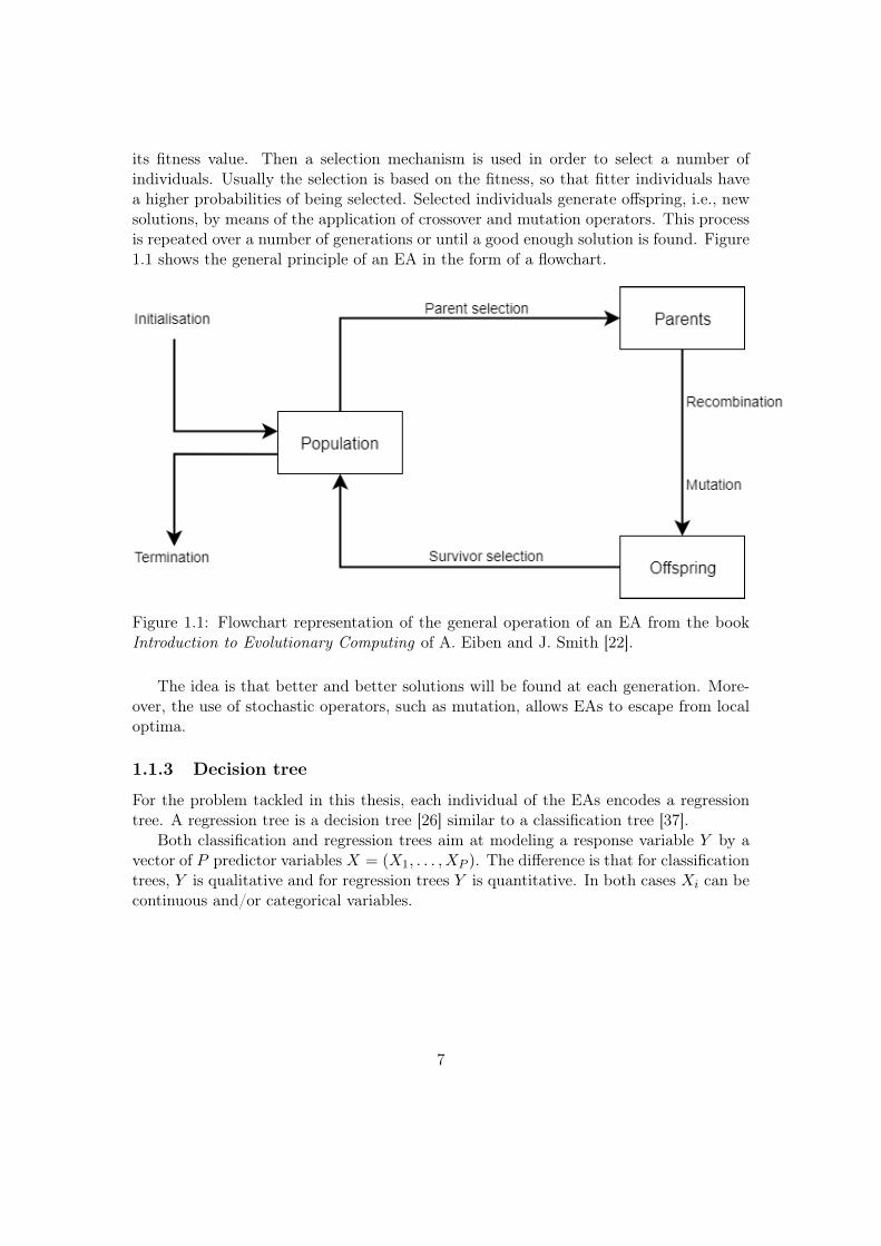
its fitness value. Then a selection mechanism is used in order to select a number ofindividuals. Usually the selection is based on the fitness, so that fitter individuals havea higher probabilities of being selected. Selected individuals generate offspring, i.e., newsolutions, by means of the application of crossover and mutation operators. This processis repeated over a number of generations or until a good enough solution is found. Figure1.1 shows the general principle of an EA in the form of a flowchart.

Figure 1.1: Flowchart representation of the general operation of an EA from the bookIntroduction to Evolutionary Computing of A. Eiben and J. Smith [22].

The idea is that better and better solutions will be found at each generation. More-over, the use of stochastic operators, such as mutation, allows EAs to escape from localoptima.

1.1.3 Decision tree

For the problem tackled in this thesis, each individual of the EAs encodes a regressiontree. A regression tree is a decision tree [26] similar to a classification tree [37].

Both classification and regression trees aim at modeling a response variable Y by avector of P predictor variables X = (X1, . . . , XP ). The difference is that for classificationtrees, Y is qualitative and for regression trees Y is quantitative. In both cases Xi can becontinuous and/or categorical variables.

7

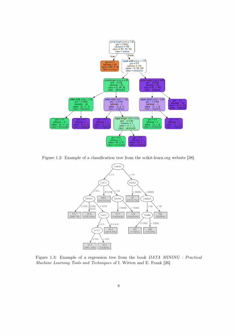
Figure 1.2: Example of a classification tree from the scikit-learn.org website [38].

Figure 1.3: Example of a regression tree from the book DATA MINING : PracticalMachine Learning Tools and Techniques of I. Witten and E. Frank [26].

8

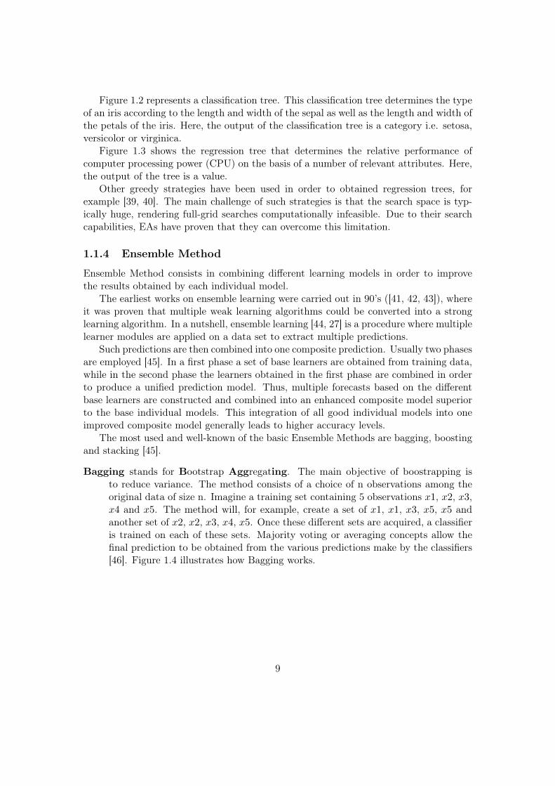
Figure 1.2 represents a classification tree. This classification tree determines the typeof an iris according to the length and width of the sepal as well as the length and width ofthe petals of the iris. Here, the output of the classification tree is a category i.e. setosa,versicolor or virginica.

Figure 1.3 shows the regression tree that determines the relative performance ofcomputer processing power (CPU) on the basis of a number of relevant attributes. Here,the output of the tree is a value.

Other greedy strategies have been used in order to obtained regression trees, forexample [39, 40]. The main challenge of such strategies is that the search space is typ-ically huge, rendering full-grid searches computationally infeasible. Due to their searchcapabilities, EAs have proven that they can overcome this limitation.

1.1.4 Ensemble Method

Ensemble Method consists in combining different learning models in order to improvethe results obtained by each individual model.

The earliest works on ensemble learning were carried out in 90’s ([41, 42, 43]), whereit was proven that multiple weak learning algorithms could be converted into a stronglearning algorithm. In a nutshell, ensemble learning [44, 27] is a procedure where multiplelearner modules are applied on a data set to extract multiple predictions.

Such predictions are then combined into one composite prediction. Usually two phasesare employed [45]. In a first phase a set of base learners are obtained from training data,while in the second phase the learners obtained in the first phase are combined in orderto produce a unified prediction model. Thus, multiple forecasts based on the differentbase learners are constructed and combined into an enhanced composite model superiorto the base individual models. This integration of all good individual models into oneimproved composite model generally leads to higher accuracy levels.

The most used and well-known of the basic Ensemble Methods are bagging, boostingand stacking [45].

Bagging stands for Bootstrap Aggregating. The main objective of boostrapping isto reduce variance. The method consists of a choice of n observations among theoriginal data of size n. Imagine a training set containing 5 observations x1, x2, x3,x4 and x5. The method will, for example, create a set of x1, x1, x3, x5, x5 andanother set of x2, x2, x3, x4, x5. Once these different sets are acquired, a classifieris trained on each of these sets. Majority voting or averaging concepts allow thefinal prediction to be obtained from the various predictions make by the classifiers[46]. Figure 1.4 illustrates how Bagging works.

9

Figure 1.4: illustration of the mechanism of Bagging from the Machine Learning : fromNeurals Networks to Big Data course given by B. Frénay at the University of Namur[47].

Boosting is similar to bagging, but with one conceptual modification. Instead of as-signing equal weighting to models, boosting assigns different weights to classifiers,and derives its ultimate result based on weighted voting. In case of regression aweighted average is usually the final output.

Stacking This method works on two layers. In the first layer, we put as many learningalgorithms as we need. Each of these algorithms will work on the data and produceresults. These results are then transmitted to the second layer, which contains acombiner algorithm that combines the results to get better results. In summary,this method will build models using different learning algorithms, then a combineralgorithm is formed to make the ultimate predictions using the predictions gen-erated by the basic algorithms. Figure 1.5 shows an abstract view of a stakingmethod.

10

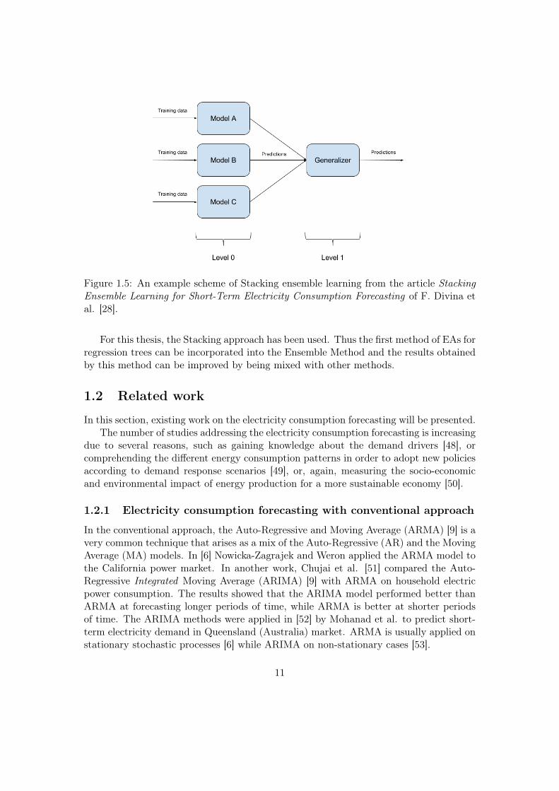
Figure 1.5: An example scheme of Stacking ensemble learning from the article StackingEnsemble Learning for Short-Term Electricity Consumption Forecasting of F. Divina etal. [28].

For this thesis, the Stacking approach has been used. Thus the first method of EAs forregression trees can be incorporated into the Ensemble Method and the results obtainedby this method can be improved by being mixed with other methods.

1.2 Related work

In this section, existing work on the electricity consumption forecasting will be presented.The number of studies addressing the electricity consumption forecasting is increasing

due to several reasons, such as gaining knowledge about the demand drivers [48], orcomprehending the different energy consumption patterns in order to adopt new policiesaccording to demand response scenarios [49], or, again, measuring the socio-economicand environmental impact of energy production for a more sustainable economy [50].

1.2.1 Electricity consumption forecasting with conventional approach

In the conventional approach, the Auto-Regressive and Moving Average (ARMA) [9] is avery common technique that arises as a mix of the Auto-Regressive (AR) and the MovingAverage (MA) models. In [6] Nowicka-Zagrajek and Weron applied the ARMA model tothe California power market. In another work, Chujai et al. [51] compared the Auto-Regressive Integrated Moving Average (ARIMA) [9] with ARMA on household electricpower consumption. The results showed that the ARIMA model performed better thanARMA at forecasting longer periods of time, while ARMA is better at shorter periodsof time. The ARIMA methods were applied in [52] by Mohanad et al. to predict short-term electricity demand in Queensland (Australia) market. ARMA is usually applied onstationary stochastic processes [6] while ARIMA on non-stationary cases [53].

11

Regression based methods are also popular in energy consumption studies. The useof the simple regression model of the ambient temperature was proposed by Schrockand Claridge [54], where the authors investigated a supermarket’s electricity use. Inlater studies, however, the use of multiple regression analysis is preferred, due to thecapability to handle more complex models. Lam et al. [55] used such an approach toanalyse office buildings in different climates in China. In another work, Braun et al. [56]performed multiple regression analysis on gas and electricity usage in order to study howthe change in the climate affects the energy consumption in buildings. In a more recentwork Mottahedia et al [57] investigated the suitability of the multiple-linear regression tomodel the effect of building shape on total energy consumption in two different climateregions.

1.2.2 Electricity consumption forecasting with Machine Learning

A significant part of recent studies in the literature is focussed on time series forecastingusing Machine Learning techniques. Among these techniques, Artificial Neural Networks(ANN) have been extensively applied. In an early work presented by Nizami and Ai-Garni [58], the authors developed a two-layered fed-forward ANN to analyse the relationbetween electric energy consumption and weather-related variables. In another work,Kelo and Dudul [59] proposed to use a wavelet Elman neural network to forecast short-term electrical load prediction under the influence of ambient air temperature. In [60]Chitsaz et al. combined the wavelet and ANN for short-term electricity load forecastingin micro-grids. In a more recent work, Zheng et al. [61] developed a hybrid algorithmthat combines similar days selection, empirical mode decomposition, and long short-termmemory neural networks to construct a prediction model for short-term load forecasting.

Despite the popularity of ANN, other novel-techniques are lately gaining attention.For instance, Talavera-Llames et al. [62] adapted a Nearest Neighbours-based strategy toaddress the energy consumption forecasting problem in a Big Data environment. Torreset al. [63] developed a novel strategy based on Deep Learning to predict times seriesand tested such strategy on electricity consumption data recorded in Spain from 2007 to2016. Zheng et al. [64] also presents a Deep Learning approach to deal with forecastingshort-term electric load time series. Galicia et al. [65] compared Random Forest withDecision Trees, Linear Regression and the gradient-boosted trees on Spanish electricityload data with a ten-minute frequency. Furthermore, Evolutionary Algorithms havebeen applied to short-term forecasting energy demand by Castelli et al. in [66, 67].Burger and Moura [68] tackled the forecasting of electricity demand by applying anensemble learning approach that uses Ordinary Least Squares and k-Nearest Neighbors.In [69], Papadopoulos and Karakatsanis explore the ensemble learning approach andcompare four different methods: seasonal autoregressive moving average (SARIMA),seasonal autoregressive moving average with exogenous variable (SARIMAX), randomforests (RF) and Gradient Boosting regression trees (GBRT). Finally, Li et al. [70]proposed a novel Ensemble Method for loads forecasting based on wavelet transform,extreme learning machine (ELM) and partial least squares regression.

The reader can find a more exhaustive review about time series forecasting in the

12

articles of Martínez-Álvarez et al. [71] (about Machine Learning methods) and Daut etal. [72] and Deb et al. [34] (about conventional and artificial intelligence methods).

1.2.3 Electricity consumption forecasting with Evolutionary Algorithms

In electricity consumption forecasting, Evolutionary Algorithms are often coupled withother methods [73, 74]. We use them especially when we are dealing with a non-lineartime series. In their article [75], Y. Lee and L. Tong proposes a hybrid forecasting modelmixing ARIMA and genetic programming i.e. a type of algorithm used in EAs. Thishybrid model achieves very good results, whether the databases were large or small. Itwas tested on energy consumption data of China. The hybrid model obtained a lowererror rate than those of the other models with which it was comparing. In this casethe authors used genetic programming to improve forecasting of non-linear time series.C. Unsihuay-Vila et al. [76] prefer to use a genetic algorithm to determine the optimalparameters for the nonlinear chaotic dynamic based predictor that is charged to forecastelectricity loads and prices of the New England data set consists of hourly electricityloads and Alberta data set consists of hourly electricity loads.

Although Evolutionary Algorithms are most often used in combination with otheralgorithms, studies using directly Evolutionary Algorithms for electricity consumptionprediction were also conducted. In their article [77], A. Azadeh and S. Tarverdian seeksto predict a month of energy consumption in Iran through three methods : a geneticalgorithm, the ARIMA approach for time series and simulated-data i.e. simulation ofone month of consumption data based on the stochastic behaviour of the raw data. Thegenetic algorithms stand out from the three as the one with the smallest relative error.

Harun Kemal Ozturka et al. [78] and H. Ceylan and H. Ozturk [79] use EvolutionaryAlgorithms to predict electricity consumption in Turkey. In article [78] the objective istwofold, on the one hand the authors seek estimated the Turkish electricity demand andon the other hand, show that genetic algorithms are a very good way of doing so.

Article [79] seeks to prove the effectiveness of two forms of equations, one linear andthe other exponential through genetic algorithms.

1.2.4 Electricity consumption forecasting with Ensemble Methods

Ensemble Methods have been successfully applied for solving pattern classification, re-gression and forecasting in time series problems [80, 81]. For example, Adhikari [82]proposed a linear combination method for time series forecasting that determines thecombining weights through a novel neural network structure. Bagnal et al. [83] proposeda method using an ensemble of classifiers on different data transformations in order toimprove the accuracy of time-series classification. Authors demonstrated that the sim-ple combination of all classifiers in one ensemble obtained better performance than anyof its components. Jin and Dong [81] proposed a deep neural network-based EnsembleMethod that integrates filtering views, local views, distorted views, explicit and implicittraining, subview prediction, and Simple Average for classification of biomedical data. Inparticular, they used the Chinese Cardiovascular Disease cardiogram database.

13

Chatterjee et al. [84] developed an ensemble support vector machine algorithm forreliability forecasting of a mining machine. This method is based on least square sup-port vector machine (LS-SVM) with hyper parameters optimized by a Genetic Algorithm(GA). The output of this model was generalized from a combination of multiple SVMpredicted results in time series dataset. Additionally, the advantages of Ensemble Meth-ods for regression from different viewpoints such as strength-correlation or biasvariancewas also demonstrate in the literature [85].

Ensemble learning based methods have been also applied in energy time series fore-casting context. For example, Zang et al. [86] proposed a method, called extreme learningmachine (ELM), which was successfully applied on the Australian National ElectricityMarket data.

Another example was presented by Tan et al. in [87] where the authors proposeda price forecasting method based on wavelet transform combined with ARIMA andGARCH models. The method was applied on Spanish and PJM electricity markets.Fan et al. [88] proposed a ensemble Machine Learning model based on Bayesian Cluster-ing by Dynamics (BCD) and SVM. The proposed model was trained and tested on thedata of the historical load from New York City in order to forecasts the hourly electricityconsumption. Tasnim et al. [89] proposed a cluster-based ensemble framework to predictwind power by using an ensemble of regression models on natural clusters within winddata. The method was tested on a large number of wind datasets of locations acrossspread Australia.

Ensembles of ANNs have been recently applied in the literature with the aim of energyconsumption or price forecasting. For instance, the authors in [90] presented a building-level neural network-based ensemble model for day-ahead electricity load forecasting.The method showed that it outperforms the previously established best performing modelby up to 50%, in the context of load data from operational commercial and industrialsites. Jovanovic et al. [91] used three artificial neural networks for prediction of heatingenergy consumption of a university campus. The authors tested the neural networks withdifferent parameter combinations, which, when used in an ensemble scheme, achievedbetter results.

14

2 | Methodology

The main objective of this chapter is to present the functioning of the two predictionmethodologies : an Evolutionary Algorithm for regression trees and an Ensemble Methodby Stacking strategy. Firstly, a section is dedicated to present to the reader the dataon which the methods have been applied and the language chooses to implement themethods. The reader will then have an explanation of how these two methods work.

2.1 Material

2.1.1 Dataset

The dataset used in this thesis records the general electricity consumption in Spain(expressed in megawatts) over a period of 9 years and 6 months, with a 10 min periodbetween each measurement. Thus, what is measured is the electricity consumption takenas a whole, not relative to a specific sector. In total, the dataset is composed of 497.832measurements, which go from 1 January 2007 at midnight till 21 June 2016 at 11:40 p.m.

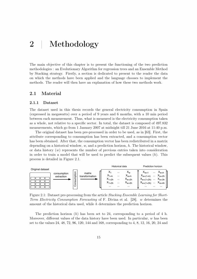
The original dataset has been pre-processed in order to be used, as in [63]. First, theattribute corresponding to consumption has been extracted, and a consumption vectorhas been obtained. After that, the consumption vector has been redistributed in a matrixdepending on a historical window, w, and a prediction horizon, h. The historical window,or data history (w) represents the number of previous entries taken into considerationin order to train a model that will be used to predict the subsequent values (h). Thisprocess is detailed in Figure 2.1.

Figure 2.1: Dataset pre-processing from the article Stacking Ensemble Learning for Short-Term Electricity Consumption Forecasting of F. Divina et al. [28]. w determines theamount of the historical data used, while h determines the prediction horizon.

The prediction horizon (h) has been set to 24, corresponding to a period of 4 h.Moreover, different values of the data history have been used. In particular, w has beenset to the values 24, 48, 72, 96, 120, 144 and 168, corresponding to 4, 8, 12, 16, 20, 24 and

15

28 h, respectively. The resulting datasets have been divided into 70% for the training setand 30% for the test set.

Table 2.1 provides the details of each dataset. Notice that for all the obtaineddatasets, the last 24 columns represent the values to be predicted, and thus are notconsidered for training purposes.

w #Rows #Columns (w+h)

24 20,742 4848 20,741 7272 20,740 9696 20,739 120120 20,738 144144 20,737 168168 20,736 192

Table 2.1: Dataset information depending on the value of w.

2.1.2 R software and language

Figure 2.2: R logo from the website R [92]

This part is based on the book Introduction à la programmation en R 1 by V. Goulet [93].R is an integrated data manipulation, calculation and graphing environment created byRobert Gentleman and Ross Ihaka[94]. It is also a complete and autonomous program-ming language. It is free, open source and multi-platform i.e it can be installed on Linux,Window or Mac. It is a very powerful and complete tool, well adapted for the computerimplementation of statistical methods. One of the most practical features of this softwareis the integrated documentation system that allows direct access to the documentationof the functions it offers. It also has efficient procedures and data storage capabilities.It offers some treatment for tables and matrices, which is ideal for our data presentedabove. The R language also provides tools for the learning machine [95]. R’s internalfunction library is divided into sets of functions and related data sets called packages.Some are present by default, but it is easy to add packages for very specific treatments.

R has been chosen to implement both methods as it offers a large number of packagesfor both evolutionary and learning algorithms. In the next section, the two methods willbe presented and the R packages will be quoted, as well as the parameters used in them.

1Introduction to R programming

16

2.2 Methods

This section details how work the methods and which R package have been used toimplement them.

2.2.1 EAs for regression trees

The approach for the EAs prediction method is as follows: the population consists ofregression trees. Each individual, i.e. a tree, is trained on the training set accordingto certain parameter e.g. the maximum depth of the tree. At each iteration of theEvolutionary Algorithm, individuals will be selected according to the error between theprediction and the real value and the complexity of the tree. These individuals will thenbe modified. For example, we will mix parameters from two regression trees to producea third. Individuals are trained on the data and so on.

To train the method means that the method will run with certain parameters and itsoutputs will be compared to the real values. The model will then adjust these parametersto a better approximation of its predictions compared to the actual values. The methodwith the best parameters become the output model that will produce predictions on datawhose real value is unknown [96].

For the implementation, the R package Evtree [97] has been used with the followingparameters:

• minbucket : 8 (minimum number of observations in each terminal node)

• minsplit : 100 (minimum number of observations in each internal node)

• maxdepth: 15 (maximum tree depth)

• ntrees: 300 (number of trees in the population)

• niterations: 1000 (maximum number of generations)

• alpha: 0.25 (complexity part of the cost function)

• operatorprob: with this parameter, we can specify, in list or vector form, the prob-abilities for the following variation operators:

– pmutatemajor : 0.2 (Major split rule mutation, selects a random internal noder and changes the split rule, defined by the corresponding split variable vr,and the split point sr [97])

– pmutateminor : 0.2 (Minor split rule mutation is similar to the major split rulemutation operator. However, it does not alter vr and only changes the splitpoint sr by a minor degree, which is defined by four cases describes in [97])

– pcrossover : 0.8 (Crossover probability)

17

– psplit : 0.2 (Split selects a random terminal-node and assigns a valid, ran-domly generated, split rule to it. As a consequence, the selected terminalnode becomes an internal node r and two new terminal nodes are generated)

– pprune: 0.4 (Prune chooses a random internal node r, where r > 1, which hastwo terminal nodes as successors and prunes it into a terminal node [97])

For more information on how Evtree works, the reader is invited to consult evtree:Evolutionary Learning of Globally Optimal Classification and Regression Trees in R writ-ten by T. Grubinger, A. Zeileis and K. Pfeiffer [97]. In this document, the creators ofEvtree explain the mechanics behind their algorithm.

Functioning

Before using the Evtree method, processing is carried out on the input data.

Data preparationFor reasons of calculation time, it was decided to predict the columns separately from

each other to be able to run the code in parallel. This choice requires data preparation.Once the data in matrix form has been obtained as shown in Figure 2.1 page 15 (it

can be of different sizes depending on the historical window: 24, 48, 72, 96, 120, 144or 168 values representing 4, 8, 12, 16, 20, 24 or 28 hours respectively), the matrix isdivided into two sets: the training set and the test set. Once it is done, the column Ito be predicted, divided in the same way into training and test set, is added to them.The column I is one of the 24 columns of the horizon prediction representing the 4 hoursfollowing the historical data.

18

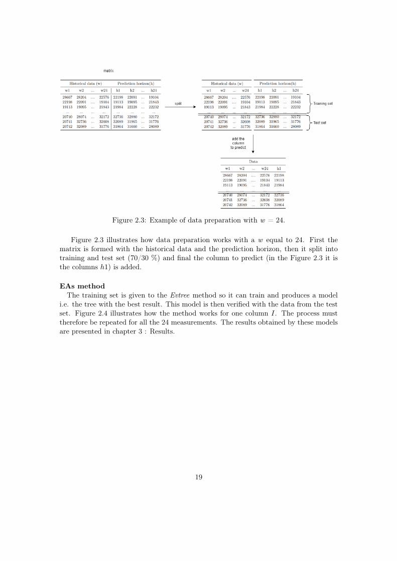
Figure 2.3: Example of data preparation with w = 24.

Figure 2.3 illustrates how data preparation works with a w equal to 24. First thematrix is formed with the historical data and the prediction horizon, then it split intotraining and test set (70/30 %) and final the column to predict (in the Figure 2.3 it isthe columns h1) is added.

EAs methodThe training set is given to the Evtree method so it can train and produces a model

i.e. the tree with the best result. This model is then verified with the data from the testset. Figure 2.4 illustrates how the method works for one column I. The process musttherefore be repeated for all the 24 measurements. The results obtained by these modelsare presented in chapter 3 : Results.

19

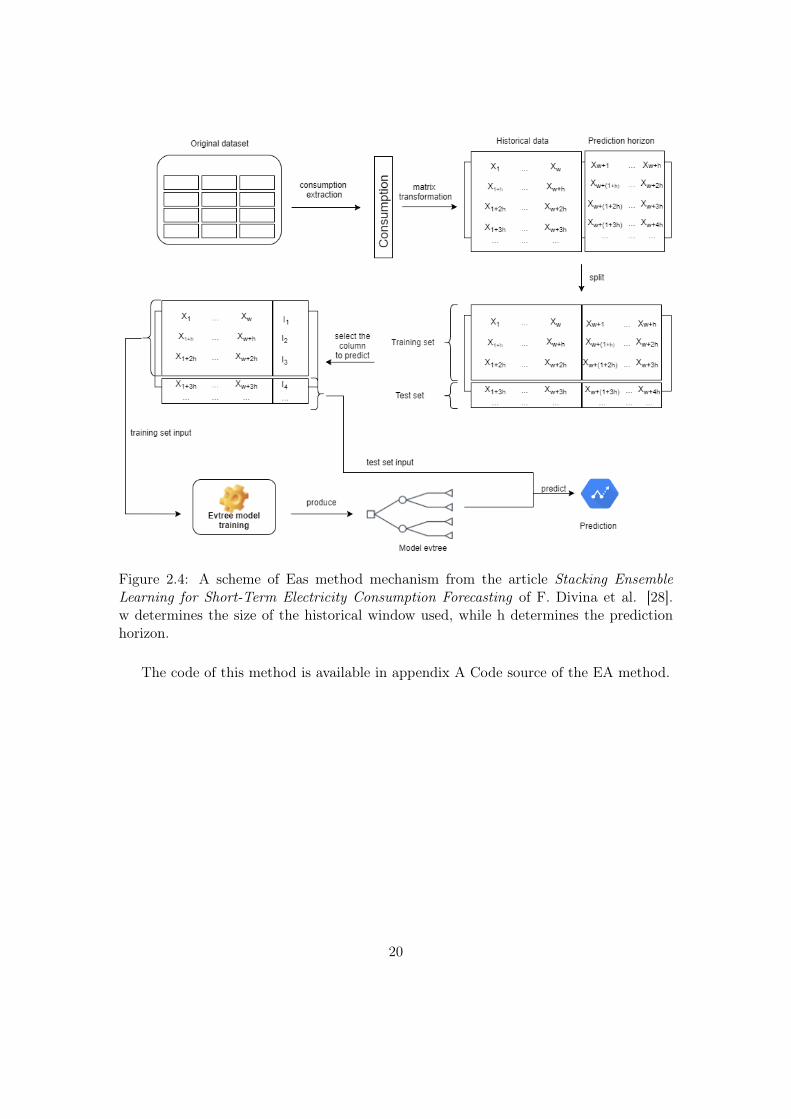
Figure 2.4: A scheme of Eas method mechanism from the article Stacking EnsembleLearning for Short-Term Electricity Consumption Forecasting of F. Divina et al. [28].w determines the size of the historical window used, while h determines the predictionhorizon.

The code of this method is available in appendix A Code source of the EA method.

20

2.2.2 Ensemble Method by Stacking strategy

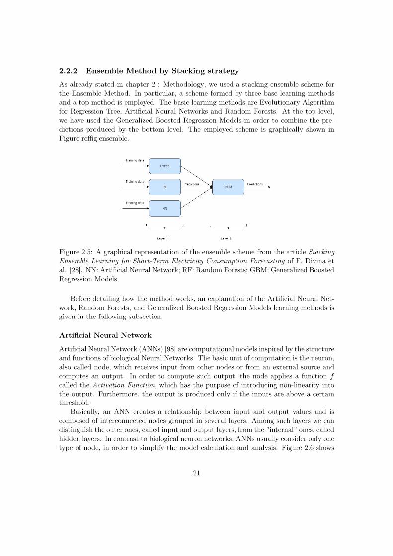
As already stated in chapter 2 : Methodology, we used a stacking ensemble scheme forthe Ensemble Method. In particular, a scheme formed by three base learning methodsand a top method is employed. The basic learning methods are Evolutionary Algorithmfor Regression Tree, Artificial Neural Networks and Random Forests. At the top level,we have used the Generalized Boosted Regression Models in order to combine the pre-dictions produced by the bottom level. The employed scheme is graphically shown inFigure reffig:ensemble.

Figure 2.5: A graphical representation of the ensemble scheme from the article StackingEnsemble Learning for Short-Term Electricity Consumption Forecasting of F. Divina etal. [28]. NN: Artificial Neural Network; RF: Random Forests; GBM: Generalized BoostedRegression Models.

Before detailing how the method works, an explanation of the Artificial Neural Net-work, Random Forests, and Generalized Boosted Regression Models learning methods isgiven in the following subsection.

Artificial Neural Network

Artificial Neural Network (ANNs) [98] are computational models inspired by the structureand functions of biological Neural Networks. The basic unit of computation is the neuron,also called node, which receives input from other nodes or from an external source andcomputes an output. In order to compute such output, the node applies a function fcalled the Activation Function, which has the purpose of introducing non-linearity intothe output. Furthermore, the output is produced only if the inputs are above a certainthreshold.

Basically, an ANN creates a relationship between input and output values and iscomposed of interconnected nodes grouped in several layers. Among such layers we candistinguish the outer ones, called input and output layers, from the "internal" ones, calledhidden layers. In contrast to biological neuron networks, ANNs usually consider only onetype of node, in order to simplify the model calculation and analysis. Figure 2.6 shows

21

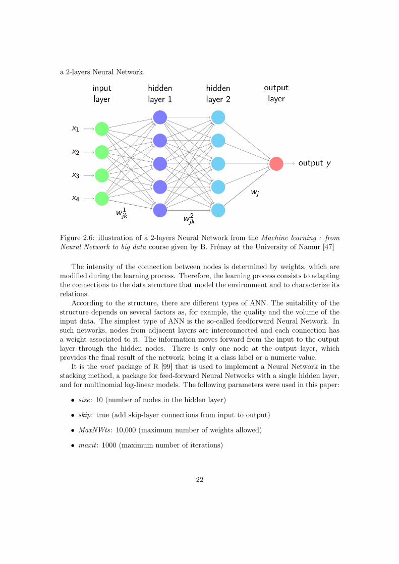
a 2-layers Neural Network.

Figure 2.6: illustration of a 2-layers Neural Network from the Machine learning : fromNeural Network to big data course given by B. Frénay at the University of Namur [47]

The intensity of the connection between nodes is determined by weights, which aremodified during the learning process. Therefore, the learning process consists to adaptingthe connections to the data structure that model the environment and to characterize itsrelations.

According to the structure, there are different types of ANN. The suitability of thestructure depends on several factors as, for example, the quality and the volume of theinput data. The simplest type of ANN is the so-called feedforward Neural Network. Insuch networks, nodes from adjacent layers are interconnected and each connection hasa weight associated to it. The information moves forward from the input to the outputlayer through the hidden nodes. There is only one node at the output layer, whichprovides the final result of the network, being it a class label or a numeric value.

It is the nnet package of R [99] that is used to implement a Neural Network in thestacking method, a package for feed-forward Neural Networks with a single hidden layer,and for multinomial log-linear models. The following parameters were used in this paper:

• size: 10 (number of nodes in the hidden layer)

• skip: true (add skip-layer connections from input to output)

• MaxNWts: 10,000 (maximum number of weights allowed)

• maxit : 1000 (maximum number of iterations)

22

Random Forest

The term Random Forest (RF) was introduced by Breinman and Cutle in [100], andrefers to a set of decision trees which form an ensemble of predictors.

Thus, RF is basically an ensemble of decision trees, where each tree is trained sepa-rately on an independent randomly selected training set. It follows that each tree dependson the values of an input dataset sampled independently, with the same distribution forall trees.

In other words, the trees generated are different since they are obtained from differenttraining sets from a bootstrap subsampling and different random subsets of features tosplit on at each tree node. Each tree is fully grown, in order to obtain low-bias trees.Moreover, at the same time, the random subsets of features result in low correlationbetween the individual trees, so the algorithm yields an ensemble that can achieve both,low bias and low variance [101]. For classification, each tree in the RF casts a unit votefor the most popular class at the input. The final result of the classifier is determinedby a majority vote of the trees. For regression, the final prediction is the average of thepredictions from the set of decision trees.

The method is less computationally expensive than other tree-based classifiers thatadopt bagging strategies, since each tree is generated by taking into account only aportion of the input features [102].

the randomForest package of R [103] have used for the implementation, which providesan R interface to the original implementation by Breiman and Cutle [100]. In the code,the algorithm is used with the following parameters:

• ntree : 100 (number of trees to be built by the algorithm).

• maxnodes: 100 (maximum number of terminal nodes trees in the forest can have).

Generalized Boosted Regression Models

The following part is based on Greedy Function Approximation: A Gradient BoostingMachine and Stochastic Gradient Boosting from J. Friedman [104, 105].

This method iteratively trains a set of decision trees. The current ensemble of treesis used in order to predict the value of each training example. The prediction errorsare then estimated, and poor predictions are adjusted, so that in the next iterations theprevious mistakes are corrected.

Gradient Boosting involves three elements:

• A loss function to be optimized. Such function is problem dependent. For instance,for regression a squared error [106] can be used and for classification we could usea logarithmic loss [107].

• A weak learner to make predictions. Regression trees are used to this aim, and agreedy strategy is used in order to build such trees. This strategy is based on usinga scoring function used each time a split point has to be added to the tree. Other

23

strategies are commonly adopted in order to constrain the trees. For example, onemay limit the depth of the tree, the number of splits or the number of nodes.

• An additive model to add trees to minimise the loss function. This is done ina sequential way, and the trees already contained in the model built so far arenot changed. In order to minimise the loss during this phase, a gradient descendprocedure is used. The procedure stops when a maximum number of trees has beenadded to the model or once there is no improvement in the model.

Overfitting is common in Gradient Boosting, and usually, some regularization meth-ods are used in order to reduce it. These methods basically penalize various parts ofthe algorithm. A model is overfitting when it sticks so much to the training data thatit learns the details and the noise present in it. This has a negative impact on modelperformance when it faces new data [108].

Usually some mechanisms are used in order to impose constraints on the constructionof decision trees. For example : limit the depth of the trees, the number of nodes or leafsor the number of observations per split.

Another mechanism is shrinkage, which is basically weighting the contribution of eachtree to the sequential sum of the predictions of the trees. This is done with the aim ofslowing down the learning rate of the algorithm.

As a consequence the training takes longer, since more trees are added to the model.In this way a trade-off between the learning rate and the number of trees can be reached.

The GBM package of R [109] is used in the stacking method with the followingparameters:

• distribution: Gaussian (function of the distribution to use)

• n.trees: 3000 (total number of trees, i.e., the number of Gradient Boosting iteration)

• interaction.depth: 40 (maximum depth of variable interactions)

• shrinkage: 0.9 (learning rate)

• n.minobsinnode: 3 (minimum number of observations in the trees terminal nodes)

Functioning of the Ensemble Method

The choice of predicting the 24 measurements separately was also made for this method.The data goes through the same preparation that was described in paragraph data prepa-ration on page 18.

Once the preparation is complete, the training set is given to these three methods(NN, RF and Evtree) constituting level 0 of the Ensemble Method. Each of these threemethods train a model on these data and produce predictions. These predictions aregiven to the GBM method (the level 1 of the Ensemble Method) which uses them totrain its own model. Once the GBM model is obtained, the test set is given an inputand it produces the predictions. Figure 2.7 shows the mechanism of the method. Theresults obtained by these models are presented in chapter 3 : Results.

24

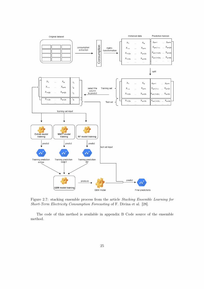
Figure 2.7: stacking ensemble process from the article Stacking Ensemble Learning forShort-Term Electricity Consumption Forecasting of F. Divina et al. [28].

The code of this method is available in appendix B Code source of the ensemblemethod.

25

26

3 | Results

This chapter provides the results obtained by the two prediction methodologies, an Evo-lutionary Algorithm for regression trees and an Ensemble Method by Stacking strategy,on the dataset described in chapter 2 as well as some observations about them.

In order to assess the performances of both the Evolutionary Algorithm and theEnsemble Method (for the different methods it uses), the mean relative error (MRE) wasused. The formula of the MRE is :

MRE =1

n

n∑i=1

|Yi − Yi|Yi

(3.1)

Where, Yi is the predicted value, Yi the real value and n the number of lines in the testset.

3.1 Notations

The following notations are used throughout this chapter:

• w corresponds to the historical window and has as value 168, 144, 120, 96, 72, 48and 24.

• h corresponds to the prediction horizon i.e. the 24 columns that contain the valuesto forecast.

• i is one of the 24 columns of h and the column with the values that the method(the Eas or the Ensemble Method) has to predict. It has as values 1 to 24.

3.2 Result of the method Evolutionary Algorithm for re-gression trees

In this section, the results obtained by the EAs method are exposed.Figure 3.1 and Table 3.1 show the MRE obtained by the Evtree method for the

different value of i and historical window (w). We can see that the longer the historicalwindow, the smaller the error. Indeed, when w is equal to 168 the corresponding averageMRE is 3.09 %. In comparison when w is equal to 24 the corresponding average MRE is4.49 %. It can also be seen that the further away the column to be predicted is from theprediction window (the higher the i), the greater the MRE. For example, when w equalto 168 and i equal to 1 the MRE is 1.15 % but when the i equal to 24 the MRE is of4.13 %.

27

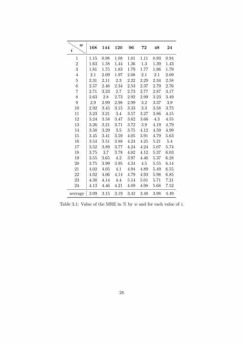
iw 168 144 120 96 72 48 24

1 1.15 0.98 1.08 1.01 1.11 0.93 0.942 1.63 1.58 1.44 1.36 1.3 1.39 1.433 1.81 1.75 1.83 1.79 1.77 1.86 1.794 2.1 2.09 1.97 2.08 2.1 2.1 2.095 2.31 2.11 2.3 2.22 2.29 2.34 2.586 2.57 2.46 2.34 2.53 2.37 2.79 2.767 2.71 3.23 2.7 2.73 2.77 2.87 3.178 2.63 2.8 2.73 2.92 2.99 3.23 3.499 2.9 2.99 2.98 2.99 3.2 3.37 3.910 2.92 3.45 3.15 3.33 3.3 3.58 3.7511 3.23 3.21 3.4 3.57 3.27 3.86 4.1512 3.24 3.58 3.47 3.62 3.66 4.3 4.5513 3.26 3.21 3.71 3.72 3.9 4.19 4.7914 3.58 3.29 3.5 3.75 4.12 4.59 4.9915 3.45 3.41 3.59 4.05 3.91 4.79 5.6316 3.54 3.51 3.88 4.24 4.25 5.21 5.417 3.52 3.89 3.77 4.24 4.24 5.07 5.7418 3.75 3.7 3.78 4.02 4.12 5.37 6.0319 3.55 3.65 4.2 3.97 4.46 5.37 6.2820 3.75 3.99 3.95 4.24 4.5 5.55 6.1421 4.02 4.05 4.1 4.94 4.89 5.49 6.5522 4.02 4.06 4.14 4.79 4.93 5.98 6.8523 4.38 4.14 4.4 5.14 5.01 5.71 7.2124 4.13 4.46 4.21 4.89 4.98 5.68 7.52

average 3.09 3.15 3.19 3.42 3.48 3.98 4.49

Table 3.1: Value of the MRE in % by w and for each value of i.

28

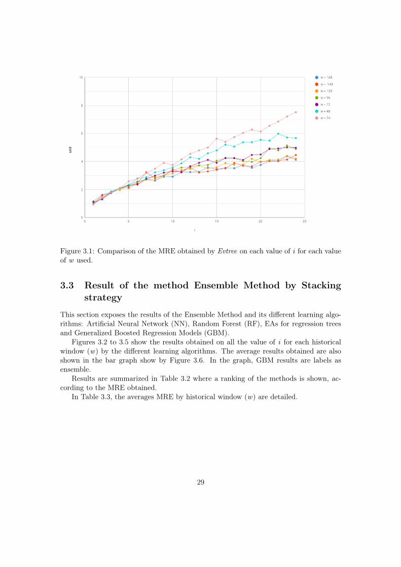
Figure 3.1: Comparison of the MRE obtained by Evtree on each value of i for each valueof w used.

3.3 Result of the method Ensemble Method by Stackingstrategy

This section exposes the results of the Ensemble Method and its different learning algo-rithms: Artificial Neural Network (NN), Random Forest (RF), EAs for regression treesand Generalized Boosted Regression Models (GBM).

Figures 3.2 to 3.5 show the results obtained on all the value of i for each historicalwindow (w) by the different learning algorithms. The average results obtained are alsoshown in the bar graph show by Figure 3.6. In the graph, GBM results are labels asensemble.

Results are summarized in Table 3.2 where a ranking of the methods is shown, ac-cording to the MRE obtained.

In Table 3.3, the averages MRE by historical window (w) are detailed.

29

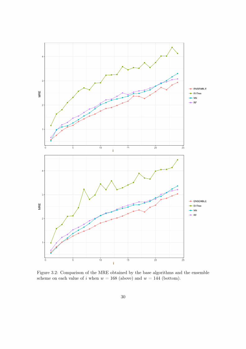
Figure 3.2: Comparison of the MRE obtained by the base algorithms and the ensemblescheme on each value of i when w = 168 (above) and w = 144 (bottom).

30

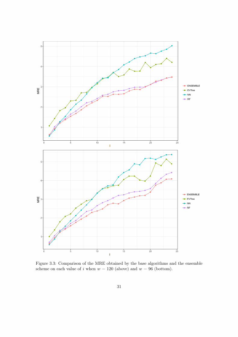
Figure 3.3: Comparison of the MRE obtained by the base algorithms and the ensemblescheme on each value of i when w = 120 (above) and w = 96 (bottom).

31

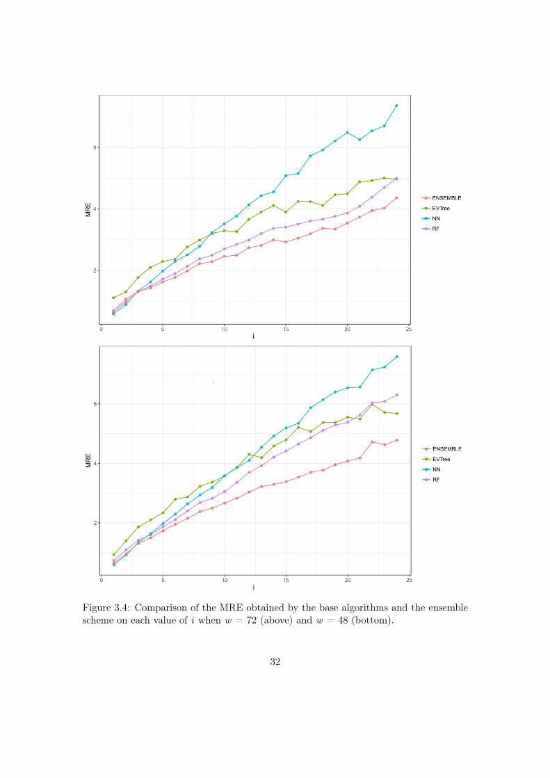
Figure 3.4: Comparison of the MRE obtained by the base algorithms and the ensemblescheme on each value of i when w = 72 (above) and w = 48 (bottom).

32

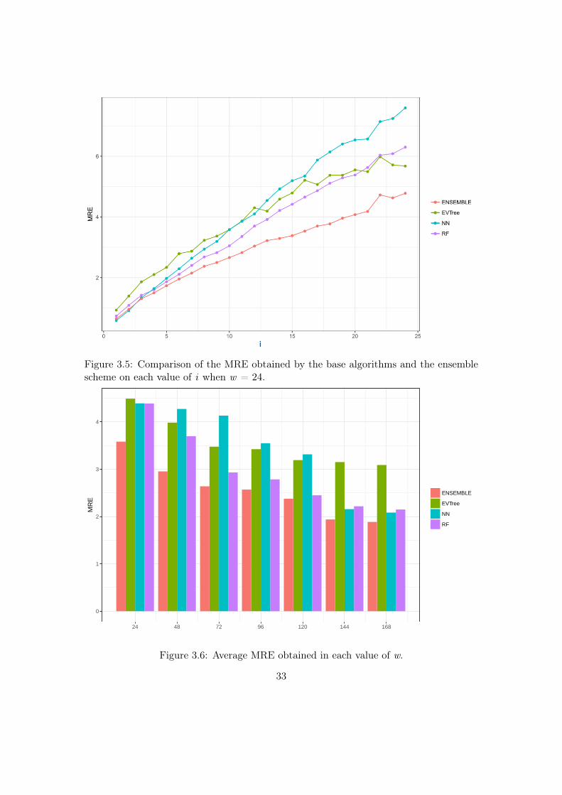
Figure 3.5: Comparison of the MRE obtained by the base algorithms and the ensemblescheme on each value of i when w = 24.

0

1

2

3

4

16814412096724824

MR

E

ENSEMBLE

EVTree

NN

RF

Figure 3.6: Average MRE obtained in each value of w.

33

168 144 120 96 72 48 24

GBM GBM GBM GBM GBM GBM GBMNN NN RF RF RF RF RF,NN,EVRF RF NN,EV NN,EV EV NN,EVEV EV NN

Table 3.2: Ranking of the methods according to their performances obtained on differentvalues of w, according.

w Evtree RF NNET GBM - ENSEMBLE

168 3.09 2.15 2.08 1.88144 3.15 2.22 2.16 1.94120 3.19 2.45 3.31 2.3896 3.42 2.78 3.55 2.5772 3.48 2.93 4.13 2.6448 3.98 3.7 4.27 2.9524 4.49 4.39 4.39 3.58

average 3.62 3.08 3.64 2.68

Table 3.3: Average value of the MRE in % by w and method.

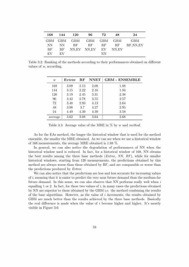
As for the EAs method, the longer the historical window that is used for the methodensemble, the smaller the MRE obtained. As we can see when we use a historical windowof 168 measurements, the average MRE obtained is 1.88 %.

In general, we can also notice the degradation of performances of NN when thehistorical window used is reduced. In fact, for a historical window of 168, NN obtainsthe best results among the three base methods (Evtree, NN, RF ), while for smallerhistorical windows, starting from 120 measurements, the predictions obtained by thismethod are always worse than those obtained by RF, and are comparable or worse thanthe predictions produced by Evtree.

We can also notice that the predictions are less and less accurate for increasing valuesof i, meaning that it is easier to predict the very near future demand than the medium-farfuture demand. In this sense, we can also observe that NN performs really well when iequalling 1 or 2. In fact, for these two values of i, in many cases the predictions obtainedby NN are superior to those obtained by the GBM i.e. the method combining the resultsof the base algorithms. However, as the value of i increments, the results obtained byGBM are much better than the results achieved by the three base methods. Basicallythe real difference is made when the value of i become higher and higher. It’s mostlyvisible in Figure 3.6

34

0 50 100 150 200 250

2000

025

000

3000

035

000

KW

h

Ensemble Prediction

Actual values

(a)

0 200 400 600 800 1000

2000

025

000

3000

035

000

4000

0

KW

h

Ensemble Prediction

Actual values

(b)

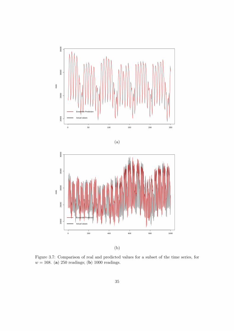
Figure 3.7: Comparison of real and predicted values for a subset of the time series, forw = 168. (a) 250 readings; (b) 1000 readings.

35

Finally, Figure 3.7 presents a comparison of the real and predicted values for a subsetof the time series when a historical window of 168 was used.

For readability reasons (it was not possible to graphically represent the comparisonof all data given the number of observations present in the time series), the selectionof two subsets of 250 and 1000 readings, respectively shown in Figure 3.7 a,b has beenmade. We can notice that the predictions are very accurate, and that they can describein a very precise way the original time series.

3.4 Comparison

3.4.1 Comparison of the two methods with each other

The EAs method for regression trees has an acceptable MRE. Without being very close to0, it is not more than 5 %. However Table 3.3 shows that the EAs method is less efficientthan RF or NN. On the contrary, the Ensemble Method with GBM (that combines theresults of the other three bases methods) shows excellent results.

Figure 3.8 shows the MRE for each method according to different values of i and thehistorical window (w).

36

Figure 3.8: Results of each learning method for each historical window considered andeach value of i. In the table EV stands for Evtree, RF for Random Forest, NN for NeuralNetwork and GBM stand for the Gradient Boost Models and it is used on the results ofthe other three bases methods [28].

37

3.4.2 Comparison with other method

In this subsection, the two forecasting methods are compared with four methods citedin the state of the art: linear regression (LR), ARMA and ARIMA, Deep Learning (DL)and a decision tree algorithm (DT). More details on how these methods were used in thecontext of the problematic of this thesis are given in the section Results of the articleStacking Ensemble Learning for Short-Term Electricity Consumption Forecasting [28].

Table 3.4 shows the average MRE obtains by the methods for each value of w. TheGBM column corresponds to the use of the GBM method on the time series data whilethe ENSEMBLE column corresponds to the GBM method used on the results of thebasic algorithms.

As see in Table 3.4, the Ensemble Method by Stacking strategy has much betterresults than all the other methods. It also obtained the best results in all the historicalwindow values considered. Another observation can be made on this table: LR and NNobtain good results which are also quite similar.

The RF method obtains good results, especially for smaller values of historical win-dow. In comparison with NN and LR method, RF produces better results except whenw has as values 144 or 168. But in every case it outperforms DL and EV.

The EV method gets fairly good results for the different values of w without reallystanding out. In general, the classical strategies ARMA and ARIMA and DT methoddo not perform well on this problem.

In conclusion, the results obtained on this problem by the ensemble scheme are sat-isfactory, as they achieve more accurate predictions for this short-term electricity con-sumption forecast problem than all the other methods considered.

38

wLR

ARMA

ARIM

ADL

DT

GBM

RF

EV

NN

ENSEMBLE

168

2.07

(0.77)

2.43

(0.97)

6.92

(2.97)

2.46

(0.29)

8.79

(0.96)

4.45

(1.56)

2.15

(0.69)

3.09

(0.84)

2.08

(0.74)

1.88

(0.67)

144

2.15

(0.77)

2.57

(0.91)

7.63

(2.54)

2.32

(0.29)

8.86

(1.01)

4.49

(1.54)

2.22

(0.71)

3.15

(0.90)

2.16

(0.78)

1.94

(0.69)

120

3.33

(1.37)

5.21

(1.87)

6.79

(2.53)

2.98

(0.28)

9.08

(1.12)

5.02

(1.81)

2.45

(0.79)

3.19

(0.95)

3.15

(1.41)

2.38

(0.81)

963.57

(1.57)

4.66

(1.81)

14.03(13.00)

3.12

(0.42)

9.40

(1.45)

5.33

(2.08)

2.78

(1.04)

3.42

(1.15)

3.55

(1.56)

2.57

(0.97)

724.20

(2.11)

8.08

(4.54)

11.37(10.43)

3.39

(0.30)

9.33

(1.39)

5.73

(2.23)

2.93

(1.16)

3.48

(1.18)

4.13

(2.05)

2.64

(0.99)

484.28

(2.15)

8.67

(4.71)

8.26

(4.73)

3.46

(0.33)

9.45

(1.48)

6.59

(2.71)

3.69

(1.71)

3.98

(1.52)

4.27

(2.16)

2.95

(1.19)

244.44

(2.27)

7.67

(5.37)

8.82

(5.31)

4.51

(0.52)

9.52

(1.55)

8.07

(3.82)

4.39

(2.13)

4.49

(1.91)

4.39

(2.23)

3.58

(1.65)

Table 3.4: Average results for different historical window values. Standard deviationbetween brackets [28].

39

3.5 Conclusion

Of the two forecasting methods, it is the Ensemble Method by Stacking strategy thatobtains the best results. The fact that the Ensemble Method has really good result isconfirmed by the comparison with the four methods of the state of the art. Therefore, tohave the best results, it is recommended to use the Ensemble Method. The computationtime is also a crucial factor: where the Evolutionary Algorithm method trains only onemodel, the Ensemble Method trains four. In both cases, the electricity consumption ofthe previous 24 hours at least is required to have good results.

40

Conclusion

The ability to predict electricity consumption in a short-term is a real financial andenvironmental benefit. From a financial point of view, companies supplying electricitycan predict with good accuracy future consumption and thus avoid losses by not pro-ducing too much. The fact that these companies produce only what is necessary allowsunnecessary pollution avoidance.

Through this thesis, two forecasting methods were offered and analysed as a responsefor short-term electricity consumption forecasting problem. Both methods and theiroperation were explained. Finally, the results they obtain was presented and a comparisonbetween each other and with other methods was offered.

The first method proposed is an Evolutionary Algorithm for regression trees. Thesecond is an Ensemble Method by Stacking strategy using three base algorithms: RandomForest, Artificial Neural Networks and Evolutionary Algorithm for regression trees anda generalize method: Gradient Boost Model.

The purpose of this thesis was to design a methodology to obtain the best predictionof Spanish electricity consumption. Of the two proposed methods, the Ensemble Methodof Stacking strategy is closer to this goal. The Evolutionary Algorithm for regressiontrees provided good result too, but compared to the Ensemble Method by Stacking orthe four methods presented in the state of the art it is the Ensemble Method that is themost accurate.

The Ensemble Method could be improved by adding or replacing some method in thebase algorithms. For example, replace the Evolutionary Algorithm for regression treesby a method based on the deep learning method [110] or support vector machines. Orkeep the Evolutionary Algorithm and add one of these methods or both of them.

Using other datasets/time series of electricity consumption would also be a good wayto ensure that this methodology can be generalized to this type of problem.

41

42

Bibliography

[1] Directive 2009/28/EC of the European parliament and of the council of 23 April2009 on the promotion of the use of energy from renewable sources and amendingand subsequently repealing directives 2001/77/EC and 2003/30/ECOff. J. Eur.Union, L140. 2009.

[2] P. J. Brockwell and R. A. Davis. Introduction to Time Series and Forecasting.Heidelberg, Germany: Springer, 2002.

[3] Balakrishnan Narayanaswamy, T. S. Jayram, and Voo Nyuk Yoong. “Hedgingstrategies for renewable resource integration and uncertainty management in thesmart grid”. In: 3rd IEEE PES Innovative Smart Grid Technologies Europe, ISGT.2012, pp. 1–8. doi: 10.1109/ISGTEurope.2012.6465718. url: https://doi.org/10.1109/ISGTEurope.2012.6465718.

[4] R. Haque et al. “Smart management of PHEV and renewable energy sources forgrid peak demand energy supply”. In: 2015 International Conference on Electri-cal Engineering and Information Communication Technology (ICEEICT). 2015,pp. 1–6. doi: 10.1109/ICEEICT.2015.7307497.

[5] Muhammad Qamar Raza and Abbas Khosravi. “A review on artificial intelli-gence based load demand forecasting techniques for smart grid and buildings”.In: Renewable and Sustainable Energy Reviews 50 (2015), pp. 1352 –1372. issn:1364-0321. doi: https : / / doi . org / 10 . 1016 / j . rser . 2015 . 04 . 065. url:http://www.sciencedirect.com/science/article/pii/S1364032115003354.

[6] J. Nowicka-Zagrajek and R. Weron. “Modeling electricity loads in California:ARMA models with hyperbolic noise”. In: Signal Processing 82.12 (2002), pp. 1903–1915. issn: 0165-1684. doi: https://doi.org/10.1016/S0165- 1684(02)00318 - 3. url: http : / / www . sciencedirect . com / science / article / pii /S0165168402003183.

[7] Shyh Jier Huang and Kuang Rong Shih. “Short-term load forecasting via ARMAmodel identification including non-Gaussian process considerations”. In: IEEETransactions on Power Systems 18.2 (May 2003), pp. 673–679. issn: 0885-8950.doi: 10.1109/TPWRS.2003.811010.

[8] Rafal Weron. Modeling and Forecasting Electricity Loads and Prices: A StatisticalApproach. John Wiley & Sons, 2007.

[9] James Durbin and Siem Jan Koopman. Time Series Analysis by State Space Meth-ods. Clarendon Press, 2001.

43

[10] D.C. Montgomery, C.L. Jennings, and M. Kulahci. A regression-based approachto short-term system load forecasting. Wiley Series in Probability and Statistics.Wiley, 2015. isbn: 9781118745229. url: https://books.google.be/books?id=pwzQBwAAQBAJ.

[11] R. Weron. Modeling and Forecasting Electricity Loads and Prices: A StatisticalApproach. The Wiley Finance Series. Wiley, 2007. isbn: 9780470059999. url:https://books.google.be/books?id=cXcWdMgovvoC.

[12] Alex D. Papalexopoulos and Timothy C. Hesterberg. Introduction to Time SeriesAnalysis and Forecasting. IEEE, 1989. url: https://ieeexplore.ieee.org/document/39025/.

[13] Kelly Kissock and John Seryak. “Understanding manufacturing energy use throughstatistical analysis”. In: Mechanical and Aerospace Engineering Faculty Publica-tions ().

[14] Anzar Mahmood Anila Kousar Muhammad Yamin Younis Bilal Akbar GhulamQadar Chaudhary Khuram Pervez Amber Muhammad Waqar Aslam and SyedKashif Hussain. “Energy Consumption Forecasting for University Sector Build-ings”. In: Energies (2017). url: http://www.mdpi.com/1996-1073/10/10/1579.

[15] Junwei Miao. “The Energy Consumption Forecasting in China Based on ARIMAModel”. In: (). url: https://www.researchgate.net/publication/301369875_The_Energy_Consumption_Forecasting_in_China_Based_on_ARIMA_Model.

[16] R.C. Souza P.M. Maçaira and F.L. Cyrino Oliveira. “Modelling and Forecast-ing the Residential Electricity Consumption in Brazil with Pegels ExponentialSmoothing Techniques”. In: Procedia Computer Science ().

[17] Kevin L. Priddy and Paul E. Keller. Artificial Neural Networks: An Introduction.SPIE Press, 2005.

[18] Ingo Steinwart and Andreas Christmann. Support Vector Machines. Springer Sci-ence & Business Media, 2008.

[19] Riccardo Bonetto and Michele Rossi. “Machine Learning Approaches to EnergyConsumption Forecasting in Households”. In: CoRR abs/1706.09648 (2017). url:http://arxiv.org/abs/1706.09648.

[20] Krzysztof Gajowniczek and Tomasz Ząbkowski. “Short Term Electricity Forecast-ing Using Individual Smart Meter Data”. In: Procedia Computer Science 35 (2014).Knowledge-Based and Intelligent Information & Engineering Systems 18th An-nual Conference, KES-2014 Gdynia, Poland, September 2014 Proceedings, pp. 589–597. issn: 1877-0509. doi: https : / / doi . org / 10 . 1016 / j . procs . 2014 .08 . 140. url: http : / / www . sciencedirect . com / science / article / pii /S1877050914011053.

44

[21] Z. Min and P. Qingle. “Very Short-Term Load Forecasting Based on Neural Net-work and Rough Set”. In: Intelligent Computation Technology and Automation,International Conference on(ICICTA). Vol. 03. May 2010, pp. 1132–1135. doi:10.1109/ICICTA.2010.38. url: doi.ieeecomputersociety.org/10.1109/ICICTA.2010.38.

[22] Agoston E. Eiben and J. E. Smith. Introduction to Evolutionary Computing.SpringerVerlag, 2003. isbn: 3540401849.

[23] Martin Sewell. Ensemble Learning. Tech. rep. 2008.

[24] Zhi-Hua Zhou. Ensemble Methods: Foundations and Algorithms. 1st. Chapman &Hall CRC, 2012. isbn: 1439830037, 9781439830031.

[25] Cha Zhang and Yunqian Ma. Ensemble Machine Learning: Methods and Ap-plications. Springer Publishing Company, Incorporated, 2012. isbn: 1441993258,9781441993250.

[26] Ian H. Witten and Eibe Frank. DATA MINING, Practical Machine Learning Toolsand Techniques. Morgan Kaufmann, 2005.

[27] João Mendes-Moreira et al. “Ensemble Approaches for Regression: A Survey”. In:ACM Comput. Surv. 45.1 (Dec. 2012), 10:1–10:40. issn: 0360-0300. doi: 10.1145/2379776.2379786. url: http://doi.acm.org/10.1145/2379776.2379786.

[28] Goméz-Vela Francisco García Torres Miguel Divina Federico Gilson Aude and Tor-res José F. “Stacking Ensemble Learning for Short-Term Electricity ConsumptionForecasting”. In: Energies 11.4 (2018).

[29] Richard Weber. Time series. Faculty of Mathematics. Last modified: 17 January2007, Accessed: 2018-04-07. url: http://www.statslab.cam.ac.uk/~rrw1/timeseries/t.pdf.

[30] Rob J Hyndman. Cyclic and seasonal time series. Accessed: 2018-04-07. url:https://robjhyndman.com/hyndsight/cyclicts/.

[31] Francisco Martínez-Álvarez et al. “A Survey on Data Mining Techniques Ap-plied to Electricity-Related Time Series Forecasting”. In: Energies 8.11 (2015),pp. 13162–13193. issn: 1996-1073. doi: 10.3390/en81112361. url: http://www.mdpi.com/1996-1073/8/11/12361.

[32] Serkan Usanmaz Janset Kuvulmaz and Seref Naci Engin. “Time-Series Forecastingby Means of Linear and Nonlinear Models”. In:MICAI 2005: Advances in ArtificialIntelligence (2005), pp. 504–513.

[33] A. Galka. Topics in Nonlinear Time Series Analysis: With Implications for EEGAnalysis. Advanced series in nonlinear dynamics. World Scientific, 2000. isbn:9789810241483. url: https://books.google.be/books?id=JSfqwnIFXOEC.

[34] Junjing Yang Siew Eang Lee Chirag Deb Fan Zhang and Kwok Wei Shah. “Areview on time series forecasting techniques for building energy consumption”. In:Renewable and Sustainable Energy Reviews 74 (2017), pp. 902–924.

45

[35] Mohammad Azhar Mat Dauta et al. “Building electrical energy consumption fore-casting analysis using conventional and artificial intelligence methods: A review”.In: Renewable and Sustainable Energy Reviews 70 (2017), pp. 1108–1118.

[36] Peter J. Brockwell and Richard A. Davis. Time Series: Theory and Methods.Springer Science & Business Media, 2013.

[37] Wei-Yin Loh. “Classification and regression trees”. In: Wiley Interdisciplinary Re-views: Data Mining and Knowledge Discovery 1.1 (2011), pp. 14–23. issn: 1942-4795. doi: 10.1002/widm.8. url: http://dx.doi.org/10.1002/widm.8.

[38] scikit-learn - 1.10. Decision Trees. http://scikit-learn.org/stable/modules/tree.html. Accessed: 2018-04-11.

[39] L. Breiman et al. Classification and Regression Trees. Monterey, CA: Wadsworthand Brooks, 1984.

[40] J. Ross Quinlan. C4.5: Programs for Machine Learning. San Francisco, CA, USA:Morgan Kaufmann Publishers Inc., 1993. isbn: 1-55860-238-0.

[41] Lars Kai Hansen and Peter Salamon. “Neural network ensembles”. In: IEEE trans-actions on pattern analysis and machine intelligence 12.10 (1990), pp. 993–1001.

[42] Iris Ginzburg and David Horn. “Combined neural networks for time series analy-sis”. In: Advances in Neural Information Processing Systems. 1994, pp. 224–231.

[43] Michael P Perrone and Leon N Cooper. “When networks disagree: Ensemblemethods for hybrid neural networks”. In: How We Learn; How We Remember:Toward An Understanding Of Brain And Neural Systems: Selected Papers of LeonN Cooper. World Scientific, 1995, pp. 342–358.

[44] Thomas G. Dietterich. “Ensemble Methods in Machine Learning”. In: Proceed-ings of the First International Workshop on Multiple Classifier Systems. MCS’00. London, UK, UK: Springer-Verlag, 2000, pp. 1–15. isbn: 3-540-67704-6. url:http://dl.acm.org/citation.cfm?id=648054.743935.

[45] Zhi-Hua Zhou. Ensemble Methods: Foundations and Algorithms. CRC Press, 2012.

[46] Saurav Kaushik. How to build Ensemble Models in machine learning? (with codein R). Accessed: 2018-04-20. url: https://www.analyticsvidhya.com/blog/2017/02/introduction-to-ensembling-along-with-implementation-in-r/.

[47] Benoît Frénay. Machine Learning: Lesson 9 - Ensemble Methods: from SingleModels to Ensemble of Models. Faculty of Computer Science.

[48] M. Ranjan and V. K. Jain. “Modelling of electrical energy consumption in Delhi”.In: Energy 24.4 (1999), pp. 351–361.

[49] Javier Campillo et al. “Energy Demand Model Design For Forecasting Electric-ity Consumption And Simulating Demand Response Scenarios In Sweden”. In:International Conference on Applied Energy. 2012.

46

[50] Ana Medina, Ángeles Cámara, and José-Ramón Monrobel. “Measuring the So-cioeconomic and Environmental Effects of Energy Efficiency Investments for aMore Sustainable Spanish Economy”. In: Sustainability 8.10 (2016), pp. 1–21.

[51] Pasapitch Chujai, Nittaya Kerdprasop, and Kittisak Kerdprasop. “Time SeriesAnalysis of Household Electric Consumption with ARIMA and ARMA Models”.In: International MultiConference of Engineers and Computer Scientists. Vol. 1.2013.

[52] Mohanad S.Al-Musaylhab et al. “Short-term electricity demand forecasting withMARS, SVR and ARIMA models using aggregated demand data in Queensland,Australia”. In: Advanced Engineering Informatics 35 (2018), pp. 1–16.

[53] G. P Zhang. “Time series forecasting using a hybrid ARIMA and neural networkmodel”. In: Neurocomputing 50 (2003), pp. 159–175.

[54] D. W. Schrock and D. E. Claridge. “Predicting Energy Usage in a Supermarket”.In: 6th Symposium on Improving Building Systems in Hot and Humid Climates.Dalas, USA, 1989.

[55] J. C. Lam et al. “Multiple regression models for energy use in air-conditionedoffice buildings in different climates”. In: Energy Conversion and Management51.12 (2010), pp. 2692–2697.

[56] M. R. Braun, H. Altan, and S. B. M. Beck. “Using regression analysis to predictthe future energy consumption of a supermarket in the UK”. In: Applied Energy130 (2014), pp. 305–313.

[57] Mohammad Mottahedia et al. “Multi-linear Regression Models to Predict theAnnual Energy Consumption of an Office Building with Different Shapes”. In:Procedia Engineering 118 (2015), pp. 622–629.

[58] J. Nizami and A. Z. Ai-Garni. “Forecasting electric energy consumption usingneural networks”. In: Energy Policy 23 (1995), pp. 1097–1104.

[59] S. Kelo and S. Dudul. “A wavelet Elman neural network for short-term electricalload prediction under the influence of temperature”. In: International Journal ofElectrical Power & Energy Systems 43 (2012), pp. 1063–1071.

[60] H. Chitsaz et al. “Short-term electricity load forecasting of buildings in micro-grids”. In: Energy Build 99 (2015), pp. 50–60.

[61] Huiting Zheng, Jiabin Yuan, and Long Chen. “Short-Term Load Forecasting UsingEMD-LSTM Neural Networks with a Xgboost Algorithm for Feature ImportanceEvaluation”. In: Energies 10.8 (2017), pp. 1168–1188.

[62] Ricardo L. Talavera-Llames et al. “A Nearest Neighbours-Based Algorithm forBig Time Series Data Forecasting”. In: Hybrid Artificial Intelligent Systems: 11thInternational Conference, HAIS 2016, Seville, Spain, April 18-20, 2016, Proceed-ings. Ed. by Francisco Martínez-Álvarez et al. Cham: Springer International Pub-lishing, 2016, pp. 174–185. isbn: 978-3-319-32034-2. doi: 10.1007/978-3-319-32034-2_15. url: https://doi.org/10.1007/978-3-319-32034-2_15.

47

[63] J. F. Torres et al. “Deep Learning-Based Approach for Time Series Forecastingwith Application to Electricity Load”. In: Biomedical Applications Based on Nat-ural and Artificial Computing: International Work-Conference on the InterplayBetween Natural and Artificial Computation, IWINAC 2017, Corunna, Spain,June 19-23, 2017, Proceedings, Part II. Ed. by José Manuel Ferrández Vicenteet al. Cham: Springer International Publishing, 2017, pp. 203–212. isbn: 978-3-319-59773-7. doi: 10.1007/978-3-319-59773-7_21. url: https://doi.org/10.1007/978-3-319-59773-7_21.

[64] Jian Zheng et al. “Electric load forecasting in smart grids using Long-Short-Term-Memory based Recurrent Neural Network”. In: 51st Annual Conference on Infor-mation Sciences and Systems (CISS). 2017.

[65] Antonio Galicia et al. “Scalable Forecasting Techniques Applied to Big Electric-ity Time Series”. In: Advances in Computational Intelligence: 14th InternationalWork-Conference on Artificial Neural Networks, IWANN 2017, Cadiz, Spain, June14-16, 2017, Proceedings, Part II. Ed. by Ignacio Rojas, Gonzalo Joya, and An-dreu Catala. Cham: Springer International Publishing, 2017, pp. 165–175. isbn:978-3-319-59147-6. doi: 10.1007/978-3-319-59147-6_15. url: https://doi.org/10.1007/978-3-319-59147-6_15.

[66] Mauro Castelli, Leonardo Vanneschi, and Matteo De Felice. “Forecasting short-term electricity consumption using a semantics-based genetic programming frame-work: The South Italy case”. In: Energy Economics 47.C (2015), pp. 37–41. url:https://EconPapers.repec.org/RePEc:eee:eneeco:v:47:y:2015:i:c:p:37-41.

[67] Mauro Castelli, Leonardo Trujillo, and Leonardo Vanneschi. “Energy Consump-tion Forecasting Using Semantic-based Genetic Programming with Local SearchOptimizer”. In: Intell. Neuroscience 2015 (Jan. 2015), 57:57–57:57. issn: 1687-5265. doi: 10.1155/2015/971908. url: https://doi.org/10.1155/2015/971908.

[68] E. M. Burger and S. J. Moura. “Gated ensemble learning method for demand-sideelectricity load forecasting”. In: Energy and Buildings 109 (2016), pp. 23–34.

[69] S. Papadopoulos and I. Karakatsanis. “Short-term electricity load forecasting us-ing time series and ensemble learning methods”. In: 2015 IEEE Power and EnergyConference at Illinois (PECI). 2015, pp. 1–6.

[70] S. Li, L. Goel, and P. Wang. “An ensemble approach for short-term load forecastingby extreme learning machine”. In: Applied Energy 170 (2016), pp. 22–29.

[71] Francisco Martínez-Álvarez et al. “A Survey on Data Mining Techniques Appliedto Electricity-Related Time Series Forecasting”. In: Energies 8 (2015), pp. 13162–13193.

[72] Mohammad Azhar Mat Daut et al. “Building electrical energy consumption fore-casting analysis using conventional and artificial intelligence methods: A review”.In: Renewable and Sustainable Energy Reviews 70 (2017), pp. 1108–1118.

48

[73] Heiko Hahn, Silja Meyer-Nieberg, and Stefan Pickl. “Electric load forecastingmethods: Tools for decision making”. In: European Journal of Operational Re-search 199.3 (2009), pp. 902 –907. issn: 0377-2217. doi: https://doi.org/10.1016/j.ejor.2009.01.062. url: http://www.sciencedirect.com/science/article/pii/S0377221709002094.

[74] Hesham K. Alfares and Mohammad Nazeeruddin. “Electric load forecasting: liter-ature survey and classification of methods”. In: International Journal of SystemsScience 33 (2002), pp. 23–34.

[75] Yi-Shian Lee and Lee-Ing Tong. “Forecasting time series using a methodologybased on autoregressive integrated moving average and genetic programming”. In:Knowledge-Based Systems 24.1 (2011), pp. 66 –72. issn: 0950-7051. doi: https://doi.org/10.1016/j.knosys.2010.07.006. url: http://www.sciencedirect.com/science/article/pii/S0950705110001127.

[76] J.W. Marangon-Lima C. Unsihuay-Vila A.C. Zambroni de Souza and P.P. Balestrassi.“Electricity demand and spot price forecasting using evolutionary computationcombined with chaotic nonlinear dynamic model”. In: International Journal ofElectrical Power & Energy Systems 32 (2010), pp. 108–116.

[77] A. Azadeh and S. Tarverdian. “Integration of genetic algorithm, computer simu-lation and design of experiments for forecasting electrical energy consumption”.In: Energy Policy 35.10 (2007), pp. 5229 –5241. issn: 0301-4215. doi: https://doi.org/10.1016/j.enpol.2007.04.020. url: http://www.sciencedirect.com/science/article/pii/S0301421507001668.

[78] Harun Kemal Ozturk et al. “Electricity estimation using genetic algorithm ap-proach: a case study of Turkey”. In: Energy 30.7 (2005), pp. 1003 –1012. issn:0360-5442. doi: https://doi.org/10.1016/j.energy.2004.08.008. url:http://www.sciencedirect.com/science/article/pii/S0360544204003391.

[79] Halim Ceylan and Harun Kemal Ozturk. “Estimating energy demand of Turkeybased on economic indicators using genetic algorithm approach”. In: Energy Con-version and Management 45.15 (2004), pp. 2525 –2537. issn: 0196-8904. doi:https://doi.org/10.1016/j.enconman.2003.11.010. url: http://www.sciencedirect.com/science/article/pii/S0196890403003479.

[80] Xueheng Qiu et al. “Ensemble deep learning for regression and time series fore-casting”. In: Computational Intelligence in Ensemble Learning (CIEL), 2014 IEEESymposium on. IEEE. 2014, pp. 1–6.

[81] Lin-peng Jin and Jun Dong. “Ensemble deep learning for biomedical time seriesclassification”. In: Computational intelligence and neuroscience 2016 (2016).

[82] Ratnadip Adhikari. “A neural network based linear ensemble framework for timeseries forecasting”. In: Neurocomputing 157 (2015), pp. 231–242.

[83] Anthony Bagnall et al. “Time-series classification with COTE: the collective oftransformation-based ensembles”. In: IEEE Transactions on Knowledge and DataEngineering 27.9 (2015), pp. 2522–2535.

49

[84] Snehamoy Chatterjee, Ansuman Dash, and Sukumar Bandopadhyay. “Ensemblesupport vector machine algorithm for reliability estimation of a mining machine”.In: Quality and Reliability Engineering International 31.8 (2015), pp. 1503–1516.

[85] Zhi-Hua Zhou. “Ensemble learning”. In: Encyclopedia of biometrics (2015), pp. 411–416.

[86] Rui Zhang et al. “Short-term load forecasting of Australian National ElectricityMarket by an ensemble model of extreme learning machine”. In: IET Generation,Transmission & Distribution 7.4 (2013), pp. 391–397.

[87] Zhongfu Tan et al. “Day-ahead electricity price forecasting using wavelet transformcombined with ARIMA and GARCH models”. In: Applied Energy 87.11 (2010),pp. 3606–3610.

[88] Shu Fan et al. “Forecasting electricity demand by hybrid machine learning model”.In: Neural Information Processing. Springer. 2006, pp. 952–963.

[89] Sumaira Tasnim et al. “Wind power prediction using cluster based ensemble re-gression”. In: International Journal of Computational Intelligence and Applica-tions (2017), p. 1750026.

[90] Jorjeta G Jetcheva, Mostafa Majidpour, and Wei-Peng Chen. “Neural networkmodel ensembles for building-level electricity load forecasts”. In: Energy and Build-ings 84 (2014), pp. 214–223.

[91] Radiša Ž Jovanović, Aleksandra A Sretenović, and Branislav D Živković. “Ensem-ble of various neural networks for prediction of heating energy consumption”. In:Energy and Buildings 94 (2015), pp. 189–199.

[92] The R Project for Statistical Computing. https://www.r-project.org/. Ac-cessed: 2018-04-24.

[93] Vincent Goulet. Introduction à la programmation en R. École d’actuariat. Ac-cessed: 2018-04-23. url: https://cran.r-project.org/doc/contrib/Goulet_introduction_programmation_R.pdf.

[94] Ross Ihaka and Robert Gentleman. “R: A Language for Data Analysis and Graph-ics”. In: Journal of Computational and Graphical Statistics 5.3 (1996), pp. 299–314.doi: 10.1080/10618600.1996.10474713. url: https://www.stat.auckland.ac.nz/~ihaka/downloads/R-paper.pdf.

[95] B. Lantz.Machine Learning with R. Packt Publishing, 2015. isbn: 9781784394523.url: https://books.google.be/books?id=ZaJNCgAAQBAJ.

[96] S.V. Burger. Introduction to Machine Learning with R: Rigorous MathematicalAnalysis. O’Reilly Media, 2018. isbn: 9781491976395. url: https : / / books .google.be/books?id=buhPDwAAQBAJ.

[97] Thomas Grubinger, Achim Zeileis, and Karl-Peter Pfeiffer. “evtree: EvolutionaryLearning of Globally Optimal Classification and Regression Trees in R”. In: Jour-nal of Statistical Software 61.1 (2014), pp. 1–29. url: http://www.jstatsoft.org/v61/i01/.

50

[98] R. E. Uhrig. “Introduction to artificial neural networks”. In: Industrial Electronics,Control, and Instrumentation, 1995., Proceedings of the 1995 IEEE IECON 21stInternational Conference on. Vol. 1. 1995, 33–37 vol.1. doi: 10.1109/IECON.1995.483329.

[99] W. N. Venables and B. D. Ripley. Modern Applied Statistics with S. Fourth. NewYork: Springer, 2002.

[100] Leo Breiman. “Random Forests”. In: Machine Learning 45.1 (Oct. 2001), pp. 5–32.issn: 0885-6125. doi: 10.1023/A:1010933404324. url: https://doi.org/10.1023/A:1010933404324.

[101] Ramón Díaz-Uriarte and Sara Alvarez de Andrés. “Gene selection and classifica-tion of microarray data using random forest”. In: BMC Bioinformatics 7.1 (2006),p. 3.

[102] Pall Oskar Gislason, Jon Atli Benediktsson, and Johannes R Sveinsson. “Randomforests for land cover classification”. In: Pattern Recognition Letters 27.4 (2006),pp. 294–300.

[103] Andy Liaw and Matthew Wiener. “Classification and Regression by randomFor-est”. In: R News 2.3 (2002), pp. 18–22. url: http://CRAN.R-project.org/doc/Rnews/.

[104] Jerome H. Friedman. “Greedy Function Approximation: A Gradient Boosting Ma-chine”. In: Annals of Statistics 29 (2000), pp. 1189–1232.

[105] Jerome H. Friedman. “Stochastic gradient boosting”. In: Computational Statistics& Data Analysis 38.4 (2002), pp. 367–378.

[106] C. Sammut and G.I. Webb. Encyclopedia of Machine Learning. Encyclopediaof Machine Learning. page 331. Springer US, 2011. isbn: 9780387307688. url:https://books.google.be/books?id=i8hQhp1a62UC.

[107] R.F. Schaefer et al. Information Theoretic Security and Privacy of InformationSystems. Definition page 87. Cambridge University Press, 2017. isbn: 9781107132269.url: https://books.google.be/books?id=t5okDwAAQBAJ.

[108] Jason Brownlee. Overfitting and Underfitting With Machine Learning Algorithms.Accessed: 2018-04-24. url: https://machinelearningmastery.com/overfitting-and-underfitting-with-machine-learning-algorithms/.

[109] Greg Ridgeway. Generalized boosted models: A guide to the gbm package. 2005.

[110] Ian Goodfellow et al. Deep learning. Vol. 1. MIT press Cambridge, 2016.

51

52

A | Code source of the EA method

The function takes two parameters: the problem number corresponding to the columnto be predicted and w i.e. the history window

#l i b r a r y usel ibrary ( ev t r e e )l ibrary ( rpar t . plot )require ( reshape )

#Ret r i e v ing arguments t ha t i s the problem number and theh i s t o r i c a l window

args = commandArgs( t r a i l i n gOn l y=TRUE)

i f ( length ( args )==0) {msg <− "At l e a s t two argument must be supp l i ed : the f i r s t i s

the number o f the problem the second the h i s t o r i c a l window.\ n"

stop (msg , ca l l .=FALSE)}

numProb = as . integer ( args [ 1 ] )print (numProb)

w = as . integer ( args [ 2 ] )h = 24print (w)

#ge t the matrix corresponding to the h i s t o r i c a l windownameData <− paste ( " . /dataHW" ,w, "PW" ,h , " . csv " , sep = "" )matrix <− read . csv ( f i l e=nameData , head=TRUE, sep=" , " ,

s t r i ng sAsFac to r s=F)matrix$X<− NULL

#Sp l i t the matrix to data_t r a i n i n g and data_t e s tsp l i t = 0.7co r t e = f loor ( sp l i t∗nrow(matrix ) )data_ev t r e e_t r a i n i n g = matrix [ 1 : corte , ]data_ev t r e e_t e s t = matrix [ ( c o r t e+1) :nrow(matrix ) , ]

i

data_ev t r e e_t r a i n i n g <− as . data . frame (data_ev t r e e_t r a i n i n g )data_ev t r e e_t e s t <− as . data . frame (data_ev t r e e_t e s t )

#Make sure we on ly use the h i s t o r i c a l windowdata_p_t r a i n i n g <− data_ev t r e e_t r a i n i n g [ , 1 :w]data_p_t e s t <− data_ev t r e e_t e s t [ , 1 :w]

####de f i n e the column to p r e d i c t####

numPredic <− w+numProbco lP r ed i c <− paste ( "X" , numPredic , sep ="" )data_p_t r a i n i n g$X169 <− data_ev t r e e_t r a i n i n g [ [ c o lP r ed i c ] ]data_p_t e s t$X169 <− data_ev t r e e_t e s t [ [ c o lP r ed i c ] ]

####Evtree treatment#####Define the parameter f o r e v t r e e

minbucket = 8Lminsp l i t = 100Lmaxdepth = 15Lnt r e e s = 300Lcontro lEv <− ev t r e e . control ( minbucket = minbucket , m in sp l i t =

minsp l i t , maxdepth = maxdepth , n i t e r a t i o n s = 1000L , n t r e e s =ntrees , alpha =0.25 , operatorprob = l i s t ( pmutatemajor = 0 . 2 ,pmutateminor = 0 . 2 , pc ro s sove r = 0 . 8 , p s p l i t= 0 . 2 , pprune =0 . 4 ) , seed = NULL)

r e s <− c ( )r e s <− c ( format ( Sys . time ( ) , "%d−%b−%Y %H.%M") )

#crea t e the model on the t r a i n i n g data ( p r e d i c t X169 in func t i ono f the h i s t o r i c a l window )

Evtree_model_p <− ev t r e e (X169 ~ . , data = data_p_t r a in ing , control= contro lEv )

r e s <− c ( res , ( format ( Sys . time ( ) , "%d−%b−%Y %H.%M") ) )

#use the model to p r e d i c t X169 on the t e s t dataEvtree_p r ed i c t i o n_p <− predict ( Evtree_model_p , data_p_t e s t )nbRow <− nrow(data_p_t e s t )

ii

#Compute the mean r e l a t i v e er ror (mre)mreEVTREE_p <− (sum(abs (data_p_t e s t$X169 − Evtree_p r ed i c t i o n_p)

/ data_p_t e s t$X169) ) / nrow(data_p_t e s t )∗100

#save the e v t r e e model , the p r e d i c t i on and the mre in a R o b j e c tnameModel <− paste ( " . /modelEvtree_HW" ,w, "PW" ,h , "_p" ,numProb , " .

rda" , sep ="" )save ( Evtree_model_p , Evtree_p r ed i c t i o n_p ,mreEVTREE_p , f i l e=

nameModel )

#pr in t the time o f s t a r t and end o f the c r ea t i on o f e v t r e e modeland the mre

r e s <− c ( res ,mreEVTREE_p)nameResult <− paste ( " . / r e s u l t_HW" ,w, "PW" ,h , "_p" ,numProb , " . txt " ,

sep = "" )write . table ( res , sep =" " , e o l="\n" , nameResult )

#Do the p l o t r e a l and p r e d i c t datarequire ( ggp lot2 )x_evtreeV3<−c ( 1 : nbRow)y1_evtreeV3 <− data_p_t e s t$X169y2_evtreeV3 <− Evtree_p r ed i c t i on_p

dfV3<−data . frame ( x_evtreeV3 , y1_evtreeV3 , y2_evtreeV3 )

g_evtreeV3 <− ggp lot ( dfV3 , aes ( x_evtreeV3 ) )g_evtreeV3 <− g_evtreeV3 + geom_l i n e ( aes ( y=y1_evtreeV3 ) ,

co l ou r="blue " )g_evtreeV3 <− g_evtreeV3 + geom_l i n e ( aes ( y=y2_evtreeV3 ) ,

co l ou r=" green " , alpha =0.8)

#Save the p l o tnameplot <− paste ( " . / ev t r e eP lo t_HW" ,w, "PW" ,h , "_p" ,numProb , " . pdf "

, sep = "" )pdf ( nameplot )plot ( g_evtreeV3 )dev . of f ( )

iii

iv

B | Code source of the ensemble method

l ibrary ( readr )l ibrary ( ev t r e e )l ibrary ( rpar t )l ibrary ( ggp lot2 )l ibrary ( "mlbench" )l ibrary ( " randomForest" )l ibrary ( "nnet " )l ibrary ( ’ c a r e t ’ )l ibrary ( "gbm" )

#Ret r i e v ing arguments t ha t i s the problem number and theh i s t o r i c a l window

args = commandArgs( t r a i l i n gOn l y=TRUE)i f ( length ( args )==0) {

msg <− "At l e a s t two argument must be supp l i ed : the f i r s t i sthe number o f the problem the second the h i s t o r i c a l window.\ n"

stop (msg , ca l l .=FALSE)}

numProb = as . integer ( args [ 1 ] )print (numProb)

w = as . integer ( args [ 2 ] )h = 24print (w)

#ge t the matrix corresponding to the h i s t o r i c a l windownameData <− paste ( " . /dataHW" ,w, "PW" ,h , " . csv " , sep = "" )matrix <− read . csv ( f i l e=nameData , head=TRUE, sep=" , " ,

s t r i ng sAsFac to r s=F)matrix$X<− NULL#Sp l i t the matrix to data_t r a i n i n g and data_t e s tsp l i t = 0.7

v

co r t e = f loor ( sp l i t∗nrow(matrix ) )data_ev t r e e_t r a i n i n g = matrix [ 1 : corte , ]data_ev t r e e_t e s t = matrix [ ( c o r t e+1) :nrow(matrix ) , ]

data_ev t r e e_t r a i n i n g <− as . data . frame (data_ev t r e e_t r a i n i n g )data_ev t r e e_t e s t <− as . data . frame (data_ev t r e e_t e s t )

#Make sure we on ly use the h i s t o r i c a l windowdata_p_t r a i n i n g <− data_ev t r e e_t r a i n i n g [ , 1 :w]data_p_t e s t <− data_ev t r e e_t e s t [ , 1 :w]

#sav ing the p r e d i c t o r s to be used ( needed f o r NN)p r ed i c t o r s = names(data_p_t r a i n i n g )####de f i n e the column to p r e d i c t####

numPredic <− w+numProbco lP r ed i c <− paste ( "X" , numPredic , sep ="" )data_p_t r a i n i n g$X169 <− data_ev t r e e_t r a i n i n g [ [ c o lP r ed i c ] ]data_p_t e s t$X169 <− data_ev t r e e_t e s t [ [ c o lP r ed i c ] ]

####load EVtree model#####format i s l i k e t h i s : modelEvtree_HW24PW24_p5EVTreeModelName = paste ( "modelEvtree_HW" ,w, "PW24_p" ,numProb , " .

rda" , sep = "" )print (EVTreeModelName)objectsEVTree=load (EVTreeModelName)modelEvTree = Evtree_model_p

r e s <− c ( )r e s <− c ( format ( Sys . time ( ) , "%d−%b−%Y %H.%M") )#pred i c t on the t r a i n i n g and t e s t s e t snbRowTest <− nrow(data_p_t e s t )nbRowTrain = nrow(data_p_t r a i n i n g )#use the model to p r e d i c t X169 on the t e s t data#Evtree_p r e d i c t i on_p <− p r e d i c t ( Evtree_model_p , data_p_t e s t )nbRow <− nrow(data_p_t e s t )p red i c tTra in_ev t r e e = predict (modelEvTree , data_p_t r a i n i n g )p red i c tTes t_ev t r e e <− predict (modelEvTree , data_p_t e s t )MRE_EvTree <− mreEVTREE_p

####RANDOM FOREST PART ####

vi

#save the RF model , the p r e d i c t i on and the mre in a R o b j e c tmodelRF = randomForest (X169 ~ . , data = data_p_t r a in ing , n t r ee

=100 ,maxnodes = 100 , prox=TRUE)pred i c tTes t_RF <− predict (modelRF , data_p_t e s t )mreRF_p <− (sum(abs (data_p_t e s t$X169 − pred i c tTes t_RF) / data_p_

t e s t$X169) ) / nrow(data_p_t e s t )∗100

#pred i c t i on on t r a i n i n gpredictTrainRF = predict (modelRF , data_p_t r a i n i n g )

nameModel <− paste ( " . /modelRF_HW" ,w, "PW" ,h , "_p" ,numProb , " . rda" ,sep ="" )

save (modelRF , pred i c tTes t_RF, mreRF_p , f i l e=nameModel )

####NN par t####f <− as . formula (paste ( "X169 ~" , paste ( p r ed i c t o r s , c o l l a p s e = " +

" ) ) )

modelNN <− nnet ( f , data_p_t r a in ing , s i z e =10, l i n ou t=TRUE, sk ip=TRUE, MaxNWts=10000 , trace=FALSE, maxit=1000)

predictTestNN = predict (modelNN , data_p_t e s t )mreNN_p <− (sum(abs (data_p_t e s t$X169 − predictTestNN ) / data_p_

t e s t$X169) ) / nrow(data_p_t e s t )∗100

#pred i c t i on on t r a i n i n gpredictTrainNN = predict (modelNN , data_p_t r a i n i n g )

nameModel <− paste ( " . /modelNN_HW" ,w, "PW" ,h , "_p" ,numProb , " . rda" ,sep ="" )

save (modelNN , predictTestNN , mreNN_p , f i l e=nameModel )####ADD PREDICTION TO TEST AND TRAINING#####add p r e d i c t i on to t e s t datadata_p_t e s t$Pred_EV = pred i c tTes t_ev t r e edata_p_t e s t$Pred_RF = pred i c tTes t_RFdata_p_t e s t$Pred_NN = predictTestNN

#add p r e d i c t i on to t r a i n i n g and t e s t s e t s f o r l a t e r s t e p sdata_p_t r a i n i n g$Pred_EV = pred i c tTra in_ev t r e edata_p_t r a i n i n g$Pred_RF = predictTrainRFdata_p_t r a i n i n g$Pred_NN = predictTrainNN

vii

####TOP LAYER OF ENSEMBLE#####use lm to b u i l d emsamble , check i t out , i t ’ s too s imple now#model_lm = lm(X169 ~ Pred_EV + Pred_RF + Pred_NN, data=data_p_

t r a in ing , na . ac t i on = NULL)model_gbm = gbm(X169 ~ Pred_EV + Pred_RF + Pred_NN, data = data_

p_t r a in ing , d i s t r i b u t i o n = " gauss ian " , n . t r e e s = 5 ,interaction . depth = 8 , shr inkage = 1 , n . minobsinnode = 1)

#pred i c tpred i c tTes t_gbm <− predict (model_gbm, data_p_t e s t , n . t r e e s = 5)mreGBM_p <− (sum(abs (data_p_t e s t$X169 − pred i c tTes t_gbm) / data_

p_t e s t$X169) ) / nrow(data_p_t e s t )∗100

nameModel <− paste ( " . /modelGBM_HW" ,w, "PW" ,h , "_p" ,numProb , " . rda" ,sep ="" )

save (model_gbm, pred i c tTes t_gbm, mreGBM_p , f i l e=nameModel )

#sav ing timer e s <− c ( res , ( format ( Sys . time ( ) , "%d−%b−%Y %H.%M") ) )

name <− c ( " ev t r e e " , " r f " , "GBM" , "nnet" )MRE <− c (MRE_EvTree ,mreRF_p ,mreGBM_p ,mreNN_p)ch <− paste (name , " : " , MRE, sep ="" )r e s <− c ( res , ch )

nameResult <− paste ( " . / r e s u l t_HW" ,w, "PW" ,h , "_p" ,numProb , " . txt " ,sep = "" )

write . table ( res , sep =" " , e o l="\n" , nameResult )print (mreGBM_p)print (mreNN_p)print (mreRF_p)

<fe

viii