Innovation Fund (InnovFund) Call for proposals Annex B

Innovation Fund (InnovFund)

Call for proposals

Annex B: Methodology for Relevant Costs calculation

Innovation Fund Large-scale Projects InnovFund-LSC-2021

Version 2

21 January 2022

EU Grants: InnovFund-LSC-2021 Call document Annex B: V2.0 – 21.01.2022

2

HISTORY OF CHANGES

Version Publication date Change

1.0 26.10.2021 Initial version.

2.0 21.01.2022 Deletion of reference prices descriptions from section

3.2.1 as the reference prices are now fully discussed in

section 4.1.2.5.; highlight that fixed operating costs

must be included in the LCOE and LCOP formula;

clarification on the required approach applicants must

follow when determining the reference price in the

levelised cost methodology and when the product has a

forecast green price premium; deletion of point viii in

the definition of Construction Costs to align with

4.1.3.2; alignment of the formulas with the text in 4.3.1

and 4.4.1; small text edits whose only purpose is to

emphasize certain points.


3

Annex B: Methodology for Relevant Costs calculation

Contents

Annex B: Methodology for Relevant Costs calculation ......................................................................... 3

Foreword .............................................................................................................................. 4

1. Introduction ......................................................................................................................... 4

2. Calculation of relevant costs compared to reference scenario ...................................................... 5

3. Choice of the cost methodology .............................................................................................. 5

3.1. Decision tree .............................................................................................................. 5

3.2. Introduction to the cost methodologies .......................................................................... 7

3.2.1. Option 1 – The levelised cost methodology ...................................................... 7

3.2.2. Option 2 – The reference plant methodology .................................................... 7

3.2.3. Option 3 – The ‘no reference scenario’ methodology ......................................... 7

3.3. Key parameters and data inputs ................................................................................... 8

3.3.1. Key parameters that will impact the selection of the cost methodology ............... 8

3.3.2. Key data inputs across the methodologies ....................................................... 9

3.3.3. How to account for possible differences in regulatory regimes and public support

which affect relevant costs across all methodologies ......................................... 9

3.3.4. Determining the Weighted Average Cost of Capital (WACC) – the discount rate -

across different project types ........................................................................ 10

4. Methodologies for calculating relevant costs ............................................................................ 16

4.1. Levelised Cost methodology ........................................................................................ 16

4.1.1. Principles ................................................................................................... 16

4.1.2. Detailed approach ....................................................................................... 17

4.1.3. Costs which must be excluded from relevant costs calculations ......................... 23

4.2. Electricity storage methodology ................................................................................... 23

4.2.1. Principles ................................................................................................... 23


4.3. Reference plant methodology ...................................................................................... 27

4.3.1. Principles ................................................................................................... 27


4.4. Calculations in the absence of a reference product or conventional technology .................. 29

4.4.1. Principles ................................................................................................... 29


Appendix 1– Glossary .................................................................................................................... 31

Appendix 2 – Support with WACC calculations .................................................................................. 35


4

Foreword

This methodology introduces minor updates to the previous Relevant Costs

methodology published for the 2020 Innovation Fund calls for proposals for large-scale and small-scale projects. The text has been clarified in order to help applicants prepare

more easily their submissions.

Applicants that have used the previous texts should take into consideration that the following changes have been made:

• A new section on the Weighted Average Cost of Capital (WACC) consolidates and

makes consistent all references as applied to each relevant cost methodology. This

includes further guidance on how to calculate key elements of the WACC as well as

guidance on when to use an Innovation Premium;

• The marginal tax rate should be used, not the effective tax rate, in the country of

project demonstration;

• Applicant contribution, Maintenance CAPEX (formerly known as Occasional Lifecycle

Costs), Contingencies, Fixed OPEX and Variable OPEX are all now defined (see

Glossary in Appendix 1);

• Confirmation of a new average carbon price for the past two years.

1. Introduction

The Innovation Fund (IF) supports the additional costs that are borne by the applicant

as a result of the application of the innovative technology related to GHG emission avoidance. According to Article 5(1) of the IF Delegated Regulation:

“The relevant costs shall be the additional costs that are borne by the project

applicant as a result of the application of the innovative technology related to the reduction or avoidance of the greenhouse gas emissions.

The relevant costs shall be calculated as the difference between the best estimate of the total capital expenditure, the net present value of operating

costs and benefits arising during 10 years after the entry into operation of the project compared to the result of the same calculation for a conventional

production with the same capacity in terms of effective production of the respective final product.”

Where conventional production … does not exist, the relevant costs shall be the

best estimate of the total capital expenditure and the net present value of

operating costs and benefits arising during 10 years after the entry into operation of the project.”

The relevant cost is not to be confused with the maximum grant award that is

equivalent to 60% of the relevant costs.

Since the IF is a competitive scheme, and cost-efficiency is one of the five award criteria, once relevant costs have been determined, applicants are free to request less

than 60% of the relevant costs to improve their scoring under the award criterion

related to cost-efficiency.


5

2. Calculation of relevant costs compared to reference scenario

The calculations of GHG emission avoidance as well as of relevant costs rely on a comparison with reference scenarios that should reflect the current state-of-the-art in

the different sectors:

Table 2.1 Reference Scenarios

Sector Reference scenarios for GHG emission

avoidance

Energy-intensive industries (EIIs) EU ETS benchmark(s)

Carbon Capture and Storage (CCS) CO2 releases that would occur in the

absence of the project

Renewable electricity Expected 2030 electricity mix

Renewable heat Natural gas (NG) boiler

Energy storage Single-cycle NG turbine (peaking power)

To be consistent with the calculations of GHG emission avoidance (see Annex C for the

full methodology, including a complete list of sectors covered under EIIs), the calculation of the relevant costs should build on the same reference scenarios and their

respective costs.

However, applicants should be aware that in some cases the reference product or

process (and therefore methodology) used for relevant costs calculations may differ from the methodology used for the reference GHG emissions avoidance calculations.

For example, for manufacturing of components, such as a manufacturing plant for

innovative solar PVs, the reference for relevant costs for such a manufacturing plant should be based on the market price for standard solar PV (or the costs for such a

manufacturing plant), while the reference for GHG avoidance is determined by emissions that will be displaced from the grid by the innovative PV panels, when

implemented.

Consequently, the project applicant needs to work with the relevant costs methodology

that is best suited to a specific innovative project.

3. Choice of the cost methodology

3.1. Decision tree

The Decision tree presented in Figure 3.1 below directs applicants to the most

appropriate reference scenario for the calculation of their relevant costs. The Decision tree follows the requirements of the IF Delegated Regulation and is based on the key

characteristics of the project. By working down the left side of the diagram, and based on the characteristics of their projects, applicants will arrive at the appropriate relevant

cost methodology.

The default methodology is Option 1, based on a Levelised Cost methodology that

should be suitable for a wide variety of projects covering:

• Option 1a – Energy/electricity generation;


6

• Option 1b – Product manufacture from energy-intensive industries (as well as

the manufacture of innovative renewable or storage technology components from a

new production facility1);

• Option 1c –Electricity storage.

The current market prices of products (“Reference price”) reflect the cost of the conventional technologies (including financing cost), as used in a given Reference

scenario, and are therefore used in the calculation steps below as the Reference price

(see the detailed approach to calculate the levelised cost in section 4.1.2).

In some, limited, situations, where a Reference price is not available, applicants will find that the Decision tree takes them to the reference plant methodology (Option 2).

The project costs are then compared to the best estimate of the CAPEX and OPEX of a plant with conventional technology (e.g. ETS benchmark installation in the case of

industrial products).

Finally, Option 3 is the “last-resort” methodology for cases where neither Option 1 nor

Option 2 are applicable and relies on a methodology without a Reference scenario.

Applicants will need to decide whether or not to deviate from the default methodology in Option 1. Applicants will however have to justify their choice based on the principles

outlined below and ensure the traceability and transparency of the calculations.

For the purposes of ensuring a fair and transparent evaluation process, any applicant

deviating from the methodology on specific parameters will have to justify this, based on considerations such as accuracy and availability of data, and comparability of the

final product, or process. The evaluators should be able to understand the quantitative

impact from any deviation from specific or default parameters.

Figure 3.1 The Decision tree to help applicants select the correct calculation

methodology

1 Applicants with projects falling under this category should already have demonstrated through the GHG

emission avoidance methodology the existence of a buyer of the components (i.e. a company that will run

the innovative technology to generate renewable electrical or thermal energy) to ensure that the intended

GHG avoidance will be delivered. Therefore, it is assumed in the first instance that the product replaces an

existing product in the market where there is a comparable product price.


7

3.2. Introduction to the cost methodologies

3.2.1. Option 1 – The levelised cost methodology

This methodology calculates the relevant costs based on the difference between the

levelised cost of producing an output unit computed over the full project lifetime using

the project’s innovative technology, and the Reference price expected to be received in

the market for the quantity to be produced (be it electricity or an industrial product for

example).

The levelised cost can be computed using the following models:

• Energy model (Levelised Cost of Energy - LCOE): This model can be used

for power or heat generation and equates to the well-known LCOE calculation which is

a standard when comparing technologies’ cost of producing a MWh or equivalent of

energy;

• Industrial Product model (Levelised Cost of Product - LCOP): This model

computes a levelised cost of production per unit for the new technology and compares

this cost to the market price of the industrial product.

• Electricity Storage model (Levelised Cost of Storage - LCOS): This model

computes a blended cost per discharge for several and specific use cases of a storage

technology in a particular country, focusing only on those services offered and

remunerated in that country. It then compares that blended cost to the income that

would be received by those services at the levels of remuneration unique to that setting.

This second calculation is the assumed market price for that use case. As per the other

Levelised Cost methodologies, the difference in these two calculations per unit provides

the basis for the calculation of relevant costs.

3.2.2. Option 2 – The reference plant methodology

This methodology uses the project’s capital expenditure (CAPEX) and the Net Present

Value (NPV)2 of the Revenues, Operational Benefits and Operational Costs (OPEX) and

compares them to those of a Reference Plant with conventional technology but of the

same size and output, over the first ten years of operation. This is the “fall-back”

methodology to be used when a product Reference price is not available.

The Reference Plant should be based on a plant that achieves the EU ETS benchmarks

for industrial products3.

3.2.3. Option 3 – The ‘no reference scenario’ methodology

2 Net Present Value (NPV) is the difference between the present value of cash inflows and the present value

of cash outflows. In contrast, Present Value (PV) is the present value of future cash inflows given a

specific rate of return.

3 A product benchmark is based on the average GHG emissions of the best performing 10% of the installations

producing that product in the EU and EEA-EFTA states. Revised ETS benchmarks have now been

published, so applicants should refer to: Commission Implementing Regulation (EU) 2021/447 of 12

March 2021 determining revised benchmark values for free allocation of emission allowances for the

period from 2021 to 2025 pursuant to Article 10a(2) of Directive 2003/87/EC of the European Parliament

and of the Council. Available at: https://eur-lex.europa.eu/eli/reg_impl/2021/447.

https://eur-lex.europa.eu/eli/reg_impl/2021/447


8

This methodology derives the relevant costs based on the best estimate of the total

CAPEX and the NPV of the Revenues, Operational Benefits, and OPEX arising over the

first ten years of operation. This is the “last-resort” methodology that can only be

applied in case no reference product or conventional technology is available as

reference.

3.3. Key parameters and data inputs

3.3.1. Key parameters that will impact the selection of the cost methodology

Applicants need to consider various parameters to determine whether deviating from the default cost methodology under option 1 is justified:

Option 1 – The levelised-cost methodology

• Existence of a product Reference price - In the vast majority of cases there

will be some form of reference product4 and therefore a Reference price. For substitute

products, the same approach will be used.

• Project boundaries - A general principle is to establish an identifiable final

product in most cases. When a project is only focused on part of an installation, then

the contribution of this partial process to the overall cost of the full process must be

assessed. Where a project combines industrial production with electricity storage, and

if the storage is integrated into an industrial process then only the LCOP model is used,

with the benefit (i.e. electricity cost saving) taken into account. The LCOS model is only

for electricity storage as a standalone service.

If a project:

- is focused only on producing an intermediate product (e.g. liquid steel) or

- concerns a well-defined innovation in a certain process step,

and there exists no reliable market price or substitute product, or this product is traded below its face value or with an uncertain price, and internal cost data is more

reliable for the calculation of the costs in the reference scenario, then option 2 based on a Reference Plant scenario should be followed.

Option 2 – The reference plant methodology

• Existence of a Reference Plant - which should be a conventional plant (e.g.

EU ETS benchmark installation for industrial products or a fossil fuel-equivalent for

renewable electricity or heat).

• Reliable Reference Plant cost data – required to ensure that the relevant

costs calculation can be robustly calculated.

In some cases, neither a substitute product nor a conventional technology will exist

(e.g. when a new and additional production step is added to the process or a new service is offered – such as standalone CO2 storage and transport project). Only in

these cases and if the costs related to and necessary for the innovation itself have been

well documented, can option 3 be chosen.

Option 3 – No reference plant methodology

4 Note, this does not refer to ETS product benchmarks which are sometimes wrongly termed ‘Reference

products’ (see https://ec.europa.eu/clima/policies/ets/allowances/industrial_en for more details)

https://ec.europa.eu/clima/policies/ets/allowances/industrial_en


9

• No comparable conventional production plant exists – either in the EU

(i.e. an EU ETS benchmark installation for industrial products or a fossil fuel-equivalent

for renewable electricity or heat) or globally.

• No reference product exists – this is the case where relevant costs are

derived from cost data, Revenues and any Operational Benefits from the planned

project.

3.3.2. Key data inputs across the cost methodologies

The key data inputs are based on standard financial indicators that would typically form

the basis of a project financing model. These include:

■ Capacity of the project

■ Project lifetime

■ CAPEX

■ Variable annual OPEX

■ Fixed annual OPEX

■ Maintenance CAPEX

■ Decommissioning costs

■ Timing inputs (for example, construction start/end date, commercial operational

date, financial close)

■ Expected Annual production (tpa, MWh/annum, tCO2 stored/annum, etc.)

■ Operational Benefits

The calculation of relevant cost for each innovative project should ideally be based on a relevant cost Excel file template (mandatory) available to download from the Tenders

and Funding Portal5.

In parallel, applicants are required to (1) fill a Financial Model Summary Sheet (mandatory) including a summary overview of the financial model projections from

revenues and costs, down to free cash flows, as well as key elements of the P&L and balance sheet; and (2) provide a detailed financial model (mandatory) with detailed

information on model assumptions and calculations to derive the financial projections

(see section 8 of Application Form Part B for more details). The projections should be consistent with those used in the calculation of relevant costs.

For guidance on modelling practice, applicants can download from the Portal a fully

developed financial model example (optional, for information only).

3.3.3. How to account for possible differences in regulatory regimes and public

support which affect relevant costs across all methodologies

There could be differences in electricity prices, indirect cost compensation or other

Operational Costs (OPEX) and Operational Benefits (i.e. income from electricity tariffs) due to differences in regulatory regimes. If applicants are aware of particular regulatory

features in their Member State in which their project is situated that could have a positive or negative impact on their relevant costs calculation, they should explain

carefully how these will be taken into account in the proposal.

For example, when calculating OPEX in the Levelised Cost methodology and the

Operational benefits in the reference plant model, it is important to include public support related to the price or quantity sold of the final product, such as a feed-in tariff

or feed-in premium.

5 https://ec.europa.eu/info/funding-tenders/opportunities/portal/screen/programmes/innovfund


10

As a guiding principle, applicants must include any such public support to which a

project has a right and that is equally applicable and accessible to all market

participants on a common basis (market wide). It must be included either as a reduction of OPEX in the Levelised Cost methodology or as an Operational Benefit in the reference

plant model.

On the contrary, any public support that is project-specific - and derived either from a competitive tendering process and/or as notified State Aid - must not be incorporated

into the calculation of the relevant costs.

3.3.4. Determining the Weighted Average Cost of Capital (WACC) – the discount rate

- across different project types

The discount rate used for the NPV calculations in the relevant cost methodologies is the Weighted Average Cost of Capital (WACC) of the project. This is the blended cost

of capital of the project depending on the ratio of equity and debt in the project. It is

calculated using the formula below:

WACC = E/V * Re + D/V*Rd * (1-Td)6

• Re = cost of equity

• Rd = cost of debt

• E/V = equity portion of total capital (Equity over total Value), as expected at

financial close7, and which must exclude public funding sources

• D/V = debt portion of total capital (Debt over total Value), as expected at

financial close

• Td = marginal tax rate

The WACC is applied to discount future income and cost streams over the project lifetime to make them comparable. The WACC forms an intrinsic aspect of all

methodologies and is an important mechanism to help reflect overall “project risk”. The WACC level also underpins the assessment of projects by independent evaluators and

it must therefore be deemed to be realistic. For example, taking a very low WACC level - that is more in keeping with a company WACC - for a high-risk project is likely to be

challenged by evaluators.

Many applicants will be experienced and familiar with the cost of equity and debt - and

therefore the WACC to be used for their project. For some applicants, however, this

could pose a challenge. The following sections help applicants to understand what the

appropriate WACC should be for different types of project.

Applicants should use the indicated default values for the WACC, including cost of equity and cost of debt. Applicants should justify any higher value due to increased risks and

quantify its impact on the relevant costs.

3.3.4.1. Establishing the WACC for a renewable energy project (Option 1a)

Applicants are requested to follow the methodology provided in this section to derive

the project WACC for their renewable energy project.

6 This is a nominal discount rate calculation (the debt and equity funding cost already take into account

inflation).

7 Applicants need to present the projected capital structure at financial close (i.e. as agreed by the project

funders) and which should be in line with the financial information provided in the Financial Model Summary

Sheet.


11

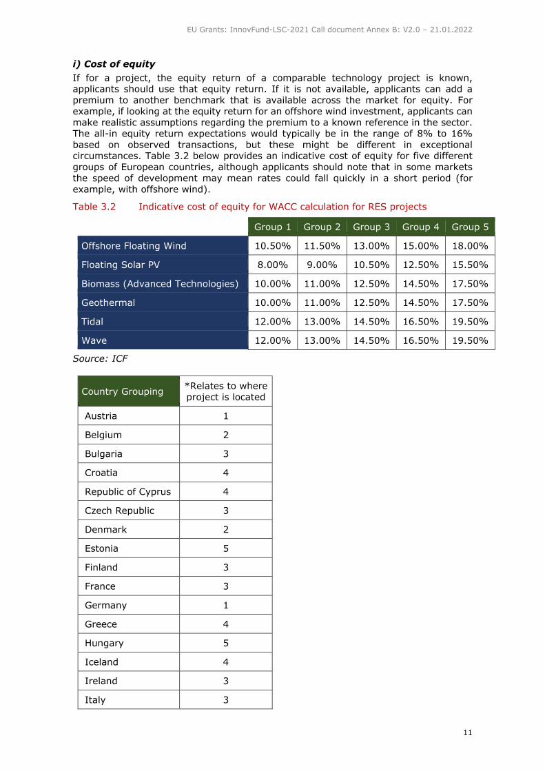
i) Cost of equity

If for a project, the equity return of a comparable technology project is known, applicants should use that equity return. If it is not available, applicants can add a

premium to another benchmark that is available across the market for equity. For example, if looking at the equity return for an offshore wind investment, applicants can

make realistic assumptions regarding the premium to a known reference in the sector. The all-in equity return expectations would typically be in the range of 8% to 16%

based on observed transactions, but these might be different in exceptional circumstances. Table 3.2 below provides an indicative cost of equity for five different

groups of European countries, although applicants should note that in some markets

the speed of development may mean rates could fall quickly in a short period (for

example, with offshore wind).

Table 3.2 Indicative cost of equity for WACC calculation for RES projects

Group 1 Group 2 Group 3 Group 4 Group 5

Offshore Floating Wind 10.50% 11.50% 13.00% 15.00% 18.00%

Floating Solar PV 8.00% 9.00% 10.50% 12.50% 15.50%

Biomass (Advanced Technologies) 10.00% 11.00% 12.50% 14.50% 17.50%

Geothermal 10.00% 11.00% 12.50% 14.50% 17.50%

Tidal 12.00% 13.00% 14.50% 16.50% 19.50%

Wave 12.00% 13.00% 14.50% 16.50% 19.50%

Source: ICF

Country Grouping *Relates to where project is located

Austria 1

Belgium 2

Bulgaria 3

Croatia 4

Republic of Cyprus 4

Czech Republic 3

Denmark 2

Estonia 5

Finland 3

France 3

Germany 1

Greece 4

Hungary 5

Iceland 4

Ireland 3

Italy 3


12

Country Grouping *Relates to where project is located

Latvia 5

Lithuania 5

Luxembourg 1

Malta 5

Netherlands 3

Norway 2

Poland 5

Portugal 2

Romania 5

Slovakia 3

Slovenia 3

Spain 3

Sweden 3

Source: ICF

ii) Cost of debt

Applicants can assume a margin for risk above the base bank lending rate8 as they

would be quoted for project finance by a commercial lender. If a reference is not available for the particular technology, a premium over an established technology debt

margin can be used.

Unlike the cost of equity, it is not possible to provide applicants with market assumptions about the cost of debt, since this requires knowledge of the base rate in

each country (and currency) and then the margin for debt in each country and for each technology. It will also have a different base rate depending on the tenor of the debt

for each specific project. However, Applicants should consider a default range of 150 to 650 basis points9 over the base rate, or alternatively use the credit spread of BBB- to

C10. Applicants should provide appropriate documentation for their chosen cost of debt.

iii) Leverage

Applicants should use the gearing ratio (i.e. proportion of debt relative to the sum of

equity and debt injected to finance the project) they contemplate and expect to be achievable for the project as implied by their projected financing plan and reflected in

the financial model. In some cases, this might be 100% equity.

8 Even if government yields are negative, banks will not lend money at negative rates

9 One basis point is one hundredth of one percentage point

10 As per S&P’s credit rating score. Anything above this is considered not risky enough and anything below

this is considered too risky


13

3.3.4.2. Establishing the WACC for an energy-intensive industrial project or for an

innovative manufacturing facility (Option 1b)

Applicants are requested to follow the methodology provided in this section to derive

the project WACC for their energy-intensive industrial project or for an innovative

manufacturing facility project.

For innovative manufacturing facilities (for example, of renewables components), the new products will inevitably fall into a specific market sector. In this case applicants

should use the WACC calculations for industry, not a renewables project.

WACC rates for energy-intensive industrial projects should be calculated according to the country in which the projects will be executed as well as the sector. Levered

reference market betas for industrial projects, as well as the equity risk premium by country, are provided to applicants in order to perform this calculation and are included

in Appendix 1 at the end of this document.

The calculation will follow the following steps for a notional project, as shown in Figure

4.1:

Figure 4.1 Calculation of the Cost of Equity for a notional innovative project in the

Chemicals sector

Reference

Risk-Free Rate (a) 0.65% EOIPA11 example figure

Market Risk Premium (b) 5.20% Damodaran b = c-a

Equity Return (Market) (c) 5.85%

Chemical Sector levered

Beta (d) 1.79

Damodaran (for a sector standard levered Beta based on conventional

market technologies)

Equity Return (e) 9.96% e = a+b*d

Innovation Premium (f) 3.00% Based on company assessment of risks

Equity Return with Innovation Premium (g) 12.96% g = e+f

The Risk-Free Rate is the theoretical interest rate that a zero-risk investment will

achieve. Applicants should use the average over the last ten years of the twenty-year Government bond rate or swap rate and not, for example, the Euribor 6-month rate.

Applicants may add a further premium in case the high degree of innovation leads to

risks that go beyond the conventional sector WACC. To the extent possible, the applicant should quantify the perceived risks and use this to justify the “Innovation

Premium”. Furthermore, the applicant should calculate and transparently show the impact of the “Innovation Premium” on the relevant costs. For transparency across

applicants, a notional “Innovation Premium” of 3% should be applied for higher risk projects. Applicants are free to increase this level, with justification, however the upper

bound on such an “Innovation Premium” is 4%.12

11 European Insurance and Occupational Pensions Authority (EIOPA): EU financial regulatory institution

12 This percentage has been calculated as a blended market observed equity risk premium based on research

from Ibbotson Associates, Duff and Phelps and KPMG (see Appendix for further details on premia by

company size)


14

If there is no comparable levered reference market beta for an industry (e.g. for renewable hydrogen production), a cost of equity and debt must be justified by

reference to similar technologies' WACC in Appendix 1. For this particular example,

depending on the predominant capital expenditure, this might be either the chemical sector beta plus an “Innovation Premium” or based on a higher risk renewable

technology.

3.3.4.3. Establishing the WACC for an energy storage project (Option 1c)

The WACC is an important component of calculation when determining the LCOS. The WACC for the reference price and for the LCOS should be the same.

i) Cost of equity

Equity cost of capital will vary from technology to technology, country to country, and by currency and therefore must be justified by the applicant based on a relevant

reference, publicly-available date or recent funding round. It is expected that the equity cost of capital for electricity storage projects will be in the range of 8-15%, although it

could fall out of this range in unique circumstances and Member States. Applicants have to justify any deviation from the default values and to calculate the impact on the

relevant costs.

ii) Cost of debt

Applicants should use a debt interest rate comprising the swap rate (in line with the

debt lifetime) plus a margin and ensure that the key terms expected are justified by the project risks, projected cash flows and in line with loan/debt market standards.

iii) Leverage

The leverage or gearing should be that implied for the project by their projected financial model. The same gearing should be used for the LCOS and reference price

calculation.

iv) Marginal tax rate

The marginal tax rate will be that prevailing in the country of project demonstration.

3.3.4.4. Establishing the WACC for the reference plant methodology (Option 2)

The discount rate to be used for the calculation of the Net Present Value (NPV) in the

reference plant methodology (see specific formula to be followed in section 4.3.1) must follow the WACC approach. However, there are key differences in the WACC for the

Reference Plant and the project plant.

i) WACC for project plant

The WACC calculation for the project plant shall follow the guidelines set out in the

sections above.

ii) WACC for Reference Plant

The Reference Plant WACC will follow the guidelines set out in section 3.3.4.1 with the

following differences:

• For leverage, applicants must use the same gearing ratio as for the project;

• For cost of debt, applicants should use levels generally assumed for the sector;

and,


15

• For cost of equity, applicants must remove any “Innovation Premium”

assumed for the cost of equity of the project.

3.3.4.5. Establishing the WACC for the ‘no reference scenario’ methodology (Option 3)

The discount rate to be used for the calculation of the Net Present Value (NPV) in the ‘no reference scenario’ methodology (see specific formula to be followed in section

4.4.1) must follow the WACC approach, set out more fully in Option 1 (see section

3.3.4).


16

4. Methodologies for calculating relevant costs

4.1. Levelised Cost methodology

4.1.1. Principles

In many industries there are accepted methodologies for the calculation of levelised

unit costs. The levelised unit cost is the cost of one unit of production, including the financing costs (i.e. the return expected from debt and equity investors), over the

lifetime of a project. This is akin to an estimated fair price of the unit produced based on the costs of production and the costs of finance.

Levelised Cost of Energy (LCOE) formula

LCOE means the present value of the costs divided by the discounted sum of energy units produced (MWh) over the project lifetime:

𝐿𝐶𝑂𝐸 [€

𝑀𝑊ℎ] =

𝐶𝐴𝑃𝐸𝑋 + ∑𝑂&𝑀𝑐𝑜𝑠𝑡(1 + 𝑟)𝑛 + ∑

𝐹𝑢𝑒𝑙 𝑐𝑜𝑠𝑡(1 + 𝑟)𝑛

𝑁𝑛

𝑁𝑛

∑𝐸𝑙𝑒𝑐𝑃𝑟𝑜𝑑𝑢𝑐𝑒𝑑

(1 + 𝑟)𝑛𝑁𝑛

Where:

▪ CAPEX = capital expenditure

▪ O&M cost = Operations & Maintenance cost (Fixed and Variable, net of

Operational Benefits)

▪ r = discount rate (WACC)

▪ n = the year

▪ N = project lifetime

▪ Fuel Cost = feedstock cost (for example Biomass or Waste streams)

▪ MWh = Megawatt Hour

Note that there is no fuel cost in most renewables projects.

Levelised Cost of Product (LCOP) formula The product price methodology uses the same approach as LCOE to calculate the fixed

nominal unit price (over the project lifetime) that would need to be paid for the innovative product in order to justify the investment to build the project (Levelised Cost

of Product, or LCOP) including its cost of funding:

𝐿𝐶𝑂𝑃 [€

𝑃𝑟𝑜𝑑𝑢𝑐𝑡] =


𝐹𝑢𝑒𝑙 𝑐𝑜𝑠𝑡, 𝑀𝑎𝑡𝑒𝑟𝑖𝑎𝑙𝑠 𝑐𝑜𝑠𝑡 𝑒𝑡𝑐.(1 + 𝑟)𝑛

𝑁𝑛

𝑁𝑛

∑𝑈𝑛𝑖𝑡𝑠𝑃𝑟𝑜𝑑𝑢𝑐𝑒𝑑


Where:


▪ O&M cost = Operations & Maintenance cost (Fixed and Variable, net of



▪ n = the year



17

The levelised cost is calculated by building financial projections of the costs for the

innovative project. Key components of the relevant cost calculation are to estimate the

present value of the Operational Costs of the project (OPEX) using the WACC as the discount rate over the lifetime of the project and using the reference product

(benchmark) price as the unit sales price assumption.

Note that the CAPEX (even if disbursed over a period longer than one year), are committed at financial close and are not discounted. Further, O&M costs exclude

depreciation/amortization.

As part of O&M costs, applicants are allowed to incorporate Maintenance CAPEX, which

should only be used to address cases where there is a clear need to replace capital items or implement periodic system updates, which are essential for projects to

continue operating in their current state. Such CAPEX could include the replacement of key equipment, or other significant one-off purchases that are likely to occur

periodically throughout the project lifetime. Applicants must separate out Maintenance CAPEX from other CAPEX in their financial model. For the purposes of the relevant cost

calculation, which is a discounted cash flow model, the Maintenance CAPEX is treated alongside OPEX.

Contingencies refer to additional CAPEX and OPEX that may arise from unforeseen risks and issues occurring during project construction (e.g. increased cost of equipment) and

operation (e.g. feedstock price rises), thereby impacting on original project financing projections. They may be included in the relevant cost but however, robust justification

will be required from applicants as to why these contingencies are required, why they are at the level proposed, and how they will be allocated – and therefore taken into

account in the calculation of relevant costs. This justification can be presented in the form of a deterministic calculation supported by a benchmark or previous experience

which must be referenced or probabilistic, in which case the calculation must be backed

up by a summary of the calculation method. This insight will also form an integral part of the evaluation of the project’s financial maturity.

The resulting LCOE or LCOP is the price at which the product would have to be sold on

average to reach a market-related return for investors (i.e. the theoretical product market price using the new process).The LCOE or LCOP for the innovative product will

be compared to the reference price (see section 4.1.2.5). The difference per unit between the levelised cost and reference price is the basis of the estimated relevant

costs in the IF Delegated Regulation. As a final step, and to ensure consistency with

article 5 (1) of the Innovation Fund Delegated Regulation, an adjustment is made to exclude the post 10-year OPEX in the final calculation of relevant costs using this

methodology (see below).

4.1.2. Detailed approach

4.1.2.1. Summary of the steps for calculating the relevant costs using the Levelised

cost methodology

Step 1: Establish the CAPEX and OPEX Upfront costs of construction and ongoing Operational Costs (OPEX) for the full project

lifetime must be established.

Step 2: Reduce the OPEX by any Operational Benefits (such as EU ETS

Allowance sales or preferential electricity tariffs)

See section 4.1.2.6 below on Carbon price assumptions.


18

Step 3: Determine the number of units forecast to be produced by the project over the full lifetime of the project

Step 4: Discount the OPEX and units forecast to be produced over the full project lifetime using the WACC as discount factor

See section 4.1.2.3 below on determining the WACC.

Step 5: Divide CAPEX plus NPV of the OPEX (the “total discounted costs”) by the total discounted units produced over the full project lifetime (the

“Levelised cost”)

Step 6: Establish the difference between the Levelised Cost and the Reference

price. If relevant, adjust if the innovative energy or product is expected to be sold at a premium price (see section 4.1.2.5).

See section 4.1.2.5 below on determining a comparable Reference price.

Step 7: Multiply this difference by the total discounted units produced over the full project lifetime

Step 8: Calculate the percentage of Discounted Costs that the discounted OPEX

after 10 years of operation represents

This will be the total OPEX after 10 years until the end of the project's operational lifetime. See section 4.1.2.10 below on OPEX adjustment.

Step 9: Subtract this percentage from 100% and multiply this difference by

the total in Step 7 This will be the relevant cost.

4.1.2.2. Rules regarding input parameters

In the two models (Option 1a and 1b) under this relevant costs methodology (and other methodologies to varying degrees – see Figure 3.1), applicants need to make

assumptions in order to enable a robust calculation of relevant costs across the

following areas:

• WACC (discount rate);

• marginal tax rate;

• determining a comparable Reference product price (reference scenario);13

• carbon price and carbon allowances;

• project lifetime;

• indexation/inflation;

• decommissioning; and,

• OPEX adjustments.

Each of these aspects is briefly described in the following sections, along with exclusion rules which applicants must follow relating to (i) terminal value and (ii) the write down

of existing (old) technologies (see section 4.1.3.).

4.1.2.3. Determining the WACC (discount rate) across different project types

Applicants should follow the guidance in section 3.3.4.1 for renewables projects and

section 3.3.4.2 for an energy-intensive industrial project or for an innovative manufacturing facility.

13 Product price will be assumed to include Carbon Costs


19

4.1.2.4. Marginal tax rate assumptions

As shown above (section 4.1.1), an important aspect of the WACC formula is the determination of the marginal tax rate prevailing in the country of project

demonstration.

4.1.2.5. Determining a comparable reference price

i) Assumptions about the price of the product from the project and implications for the Reference price

Achieving some comparability between product prices in relevant costs calculations is

important, both for ensuring fairness and for determining the project’s revenue line.

As the levelised cost of the innovative product includes a cost of capital, it should be

compared to a market price, or production cost plus an appropriate profit margin in the

reference scenario.

ii) General rules for establishing Reference prices

Unless specified otherwise, applicants need to provide Reference price data.

For energy (power/heat) projects using the LCOE approach: The project LCOE should be compared against the achievable long-term market prices,

where these exist, for either power or heat. Otherwise, the fall back choice should be

the average market price of the last two years.

For industrial projects using the LCOP approach:

The levelised cost of the innovative product should be compared with the market price of its reference product. Where the project involves the manufacture of innovative

renewable or storage technology components from a new production facility, the same procedure will apply.

iii) Consideration of EU ETS costs in Reference prices

For the LCOP and LCOE methodologies, the market price (i.e. the comparable

reference) should already include the EU ETS costs (of the marginal installation) that

are passed on to consumers.

If unit costs (that do not include EU ETS costs of the marginal installation) are used, the EU ETS costs of the marginal installation need to be added to the unit cost as per

the product emissions calculation, if that particular unit cost benchmark does not include Carbon costs. This might vary from cost benchmark to cost benchmark and will

have to be verified by the applicants.

iv) Obtaining Reference price data

It is assumed that applicants considering introducing an innovative product to an existing market will know what the reference price is for the product they are seeking

to compete with or displace. Indeed, in many cases, applicants will be seeking to enhance their own existing production facilities and will therefore already be well versed

in reference costs and prices.

Reference price data is available for most sectors. For products that have a clear

reference price that applies across Member States (for instance, London Metal Exchange prices for certain metals), applicants may choose to specify a fixed source

for the reference price. The price of most products will vary by country and therefore

applicants will need to propose the most appropriate reference in each case.

In general, historic information is often available, as well as limited spot and futures

traded prices. Prices are however volatile and widely different results are typical,

depending on the timeframe you calculate any average for.

Pricing for specialty chemicals is more opaque, but it is likely that most applicants will already have activities in the relevant sector and will therefore be able to provide EU

evaluators with pricing information and supporting evidence.

v) Determining an appropriate Reference price for new or multiple products


20

Whilst, in many cases, perfect substitute products will be generated by an innovative project, and hence the price should be the same irrespective of the production

technology, there are likely to be exceptions.

For example:

• If a product can be obtained by several processes (i.e. hydrogen from steam

reforming or hydrolysis), the process with the largest current market share

should be used.

• For CCU projects, the reference should be guided by what it will replace (the

reference is a proxy for the price that the innovative product will sell for).

• Projects in some sectors might not have comparable prices that are easy to

establish and therefore a comparable product is required. For example,

alternative fuels / oil-based products are two such identified sectors, where

mineral oil could be a comparable product.

• If a project is focused only on producing an intermediate product (e.g. liquid

steel) or on well-defined innovation in a certain process step, with no reliable

market price or substitute product, and internal cost data more reliable for the

calculation of the costs in the reference scenario, then option 2 based on a

Reference plant model should be followed.

vi) Approach to follow where the innovative product is expected to be sold at

a premium price or is different in quality relative to its reference Where a product will substitute another one of different composition (for example,

ethanol to substitute gasoline in transport, rather than ethanol as a fine chemical), the relevant EU ETS sector of the substituted product may be chosen (the refinery sector

in this case).

A new product that is not identical to the reference product may attract different prices in the market. Applicants applying into the IF will most likely have already

demonstrated the production process at small scale. Sample production from a pilot

plant is then used to obtain a purchase (off-take) contract for the proposed larger plant (often required before the plant can be financed). It should therefore be clear in most

cases whether there will be a product price difference.

The achievable market sale price for the new product produced by the applicant is the reference price.

If the price of the new product and reference is expected to be different, either due to

a premium for ‘being Green’ or a better product, adjustments need to be made. The

premium can differ markedly within and across sectors (for example, for green hydrogen compared to some energy storage components). In the LCOP methodology,

if a qualitatively different or ‘green’ product is sold with a price premium, the reference price should be increased by this premium. The relevant cost Excel file template

(mandatory), which is available to download from the Tenders and Funding Portal14, has a specific line in the Inputs table where a unit sale premium must be added.

Applying a price premium has the general effect of reducing the total relevant costs and hence the maximum IF support that can been applied for. It is essential that

applicants not only clearly explain the rationale for the price premium and provide

evidence that such a premium is possible (for example, by supplying details of an offtake agreement or some other verifiable means). There must also be consistency

between the product price forecast in an applicant’s financial model and the project product price used to determine relevant costs.

14 https://ec.europa.eu/info/funding-tenders/opportunities/portal/screen/home


21

There may also be situations where the new product will be sold into more than one market (i.e. supply of hydrogen for transport and heating), with different prices

achievable in each market. In these situations, the weighted average reference price

should be used.

4.1.2.6. Carbon price and carbon allowance assumptions

The expected revenues from the sale of the free allocation of EU ETS allowances during operation will need to be taken into account in the relevant costs calculation.

Furthermore, if the reference price does not include the carbon costs, the applicant needs to include them in the reference price.

Applicants are advised to use at least a carbon price estimate based on an averaged EU ETS price over the last two years before application (the average price from 1

October 2019 to 30 September 2021 was 34 EUR/t). However, applicants are free to use higher carbon prices if they consider this appropriate, explaining why they have

chosen to follow this approach in the application form. The carbon price must be consistently applied in both the calculation of relevant costs and in the applicant’s

financial model.

Projects that reduce the GHG emissions compared to the reference scenario will benefit

from the revenues from the sale of the free allocation of EU ETS allowances that they have received and do not need to surrender because of the reduced process emissions

below the applicable benchmark(s). These additional revenues from the sale of the excess allowances need to be included in the calculation of Operational Benefits. While

installations could theoretically hold onto the excess allowances for sale later, for the purposes of the relevant costs calculation, the excess allowances are assumed to be

sold in the year received.

4.1.2.7. Project lifetime assumptions

For the purposes of the calculation of the relevant costs using the Levelised Cost

methodology, the full project lifetime should be taken into account. Applicants will be required to use a market standard asset lifetime with no terminal value (as stated in

section 4.1.3.1 below). This will normally be the same for all the projects in a sector (generally associated with the depreciation period of the assets financed or asset

lifetime which is typically 20 – 25 years for renewables but in some cases may extend to 25 or 30 years or longer). For some industrial projects the asset lifetimes might be

shorter.

The 10-year horizon forms the basis of the relevant costs calculations, as set out in

Article 5 of the IF Delegated Regulation, since this covers the “additional operating costs and benefits arising during 10 years after the entry into operation of the project

compared to the result of the same calculation for a conventional production with the same capacity in terms of effective production of the respective final product”.

This period then links to the amount of the IF support which can be disbursed (in

accordance with paragraph 5 of Article 6) after the financial close, which “shall be

dependent on the avoidance of greenhouse gas emissions verified on the basis of annual reports submitted by the applicant for a period between 3 to 10 years following the

entry into operation.”

This means that once the Levelised Cost per unit has been established, the difference between this figure and the reference price (including the potential green price

premium) is calculated and subsequently multiplied by the discounted number of units produced over the project lifetime. This is then adjusted for the contribution of that

percentage of OPEX which occurs after 10 years of operations in order to make it

consistent with the IF Delegated Regulation.


22

4.1.2.8. Indexation/inflation assumptions

Indexation refers to the adjustment of OPEX by inflation over the period of the action. Applicants are allowed to provide their own inflation rate linked to the Member State

where the project is planned to operate. Table 4.2 below provides Harmonised Indices of Consumer Prices (HICP) which are designed for international comparisons of

consumer price inflation. Due to the variation evident between years, applicants are advised to use an inflation rate averaged over the last two years (i.e. 2019/20).

Table 4.2 Harmonised Indices of Consumer Prices (HICP), Inflation rate -

Annual average rate of change for EU27 (%)

2015 2016 2017 2018 2019 2020

EU (27 countries - from 2020) 0.1 0.2 1.6 1.8 1.4 0.7

Euro area - 19 countries (from 2015) 0.2 0.2 1.5 1.8 1.2 0.3

Belgium 0.6 1.8 2.2 2.3 1.2 0.4

Bulgaria -1.1 -1.3 1.2 2.6 2.5 1.2

Czechia 0.3 0.6 2.4 2.0 2.6 3.3

Denmark 0.2 0.0 1.1 0.7 0.7 0.3

Germany 0.7 0.4 1.7 1.9 1.4 0.4

Estonia 0.1 0.8 3.7 3.4 2.3 -0.6

Ireland 0.0 -0.2 0.3 0.7 0.9 -0.5

Greece -1.1 0.0 1.1 0.8 0.5 -1.3

Spain -0.6 -0.3 2.0 1.7 0.8 -0.3

France 0.1 0.3 1.2 2.1 1.3 0.5

Croatia -0.3 -0.6 1.3 1.6 0.8 0.0

Italy 0.1 -0.1 1.3 1.2 0.6 -0.1

Cyprus -1.5 -1.2 0.7 0.8 0.5 -1.1

Latvia 0.2 0.1 2.9 2.6 2.7 0.1

Lithuania -0.7 0.7 3.7 2.5 2.2 1.1

Luxembourg 0.1 0.0 2.1 2.0 1.6 0.0

Hungary 0.1 0.4 2.4 2.9 3.4 3.4

Malta 1.2 0.9 1.3 1.7 1.5 0.8

Netherlands 0.2 0.1 1.3 1.6 2.7 1.1

Austria 0.8 1.0 2.2 2.1 1.5 1.4

Poland -0.7 -0.2 1.6 1.2 2.1 3.7

Portugal 0.5 0.6 1.6 1.2 0.3 -0.1

Romania -0.4 -1.1 1.1 4.1 3.9 2.3

Slovenia -0.8 -0.2 1.6 1.9 1.7 -0.3

Slovakia -0.3 -0.5 1.4 2.5 2.8 2.0

Finland -0.2 0.4 0.8 1.2 1.1 0.4

Sweden 0.7 1.1 1.9 2.0 1.7 0.7

Source: Eurostat15

4.1.2.9. Decommissioning assumptions

Where decommissioning costs arise during the first 10-year period, they may be taken into account as part of the relevant costs calculation. Cost estimates will vary by project

and therefore need to be accurately accounted for in the calculation.

15 https://ec.europa.eu/eurostat/databrowser/bookmark/f4a84965-5cdb-4242-9b29-ee2599c57995?lang=en


23

4.1.2.10. OPEX adjustment

The default adjustment assumes that the relative share of OPEX in total costs is the same in the project and conventional technologies. While this will be a good

approximation, the relative share of OPEX may in some cases significantly differ between the project and conventional technologies and introduce an inconsistency in

the calculation. In such cases, the applicant should verify the effect of the Present Value of the difference between the total OPEX of the project and the pre-dominant

conventional technology for the remaining lifetime after 10 years of operation. In case of a significant impact on the relevant costs, given a reliable estimate of the OPEX for

the pre-dominant conventional technology, a more detailed calculation should be

applied for the OPEX adjustment.16

4.1.3. Costs which must be excluded from relevant costs calculations

4.1.3.1. Terminal value assumptions

Applicants are advised that terminal value beyond the asset lifetime is not to be taken

into account in the relevant costs calculations. The exclusion of terminal value is

consistent with project finance practice for calculation of IRR (which is usually done on the useful life of the assets).

4.1.3.2. Write down of existing (old) technologies

It is recognised that some large company applicants may have to replace old technology

that is not fully depreciated. The costs associated with any stranded assets that might arise as a result of a project being supported are not allowable under the relevant costs

calculations. Therefore, for the purposes of calculating the relevant costs for any

calculation methodology, costs associated with the replacement of existing technologies should be excluded.

This approach is necessary not only because it is difficult to incorporate this aspect into

the relevant costs methodology, but because it ensures a level playing field with new market players. These would be disadvantaged by not having made previous

investments in technology and not being able to claim such a benefit.

4.2. Electricity storage methodology

4.2.1. Principles

Electricity storage technologies can be used in numerous applications or ‘use cases’

offering different services to different components of the electricity system. Different regulatory treatments, the availability of commercial service requests and technical

requirements across Member States determine the applicability of use cases. For

example:

• Pumped hydro and underground compressed air energy storage are

characterised by relatively slow response times (>10 seconds) and large

minimum system sizes (>5 MW). Therefore, they are ill suited to fast-response

applications such as primary response and power quality and small-scale

consumption applications.

16 This effect will be amplified where the project has a very different cash flow profile to that of the comparable

technology (i.e. a very high CAPEX, low OPEX compared to Very low CAPEX and High OPEX and the

reverse), and the project carries a far higher WACC than the conventional technology would bear.


24

• Flywheels and supercapacitors are characterised by short discharge durations

(<1 hour) and are not suitable for applications requiring longer-term power

provision.

• Seasonal storage requires power provision for months. This can only be met by

technologies where energy storage capacity can be designed to be fully

independent of power capacity.

An electricity storage project proposed for support under the IF will envisage a specific ‘use case’17 within the country in which it is implemented. This will in turn determine

the nature of the services to be provided and the extent to which these services can be

rewarded in that market; it will also affect the reference price of the ‘use case’. Therefore, comparison of LCOS with the Reference price will be based on each specific

application (use case).

Lazard publishes a LCOS survey each year which examines the different use cases for each type of existing storage application and offers a number of examples for markets

around the world18. The universe of use cases proposed by Lazard is presented in Figure 4.2:19

Figure 4.2 Summary of Energy Storage Use Cases

Source: Lazard (2020)

The LCOS electricity storage methodology has been specifically developed for

standalone storage facilities providing specialist services of storage only. It can take

account of the different types of business cases for electricity storage: multiple services can be entered, based on revenue ‘stackability’, thereby avoiding any limitations in the

relevant costs calculations and creating a more realistic assessment.

17 A use case refers to the group of services that the particular energy storage installation in a particular country

sets out to fund in their IF application.

18 Most recently, Lazard’s Levelised Cost of Storage Analysis – Version 6.0 (2020). Available at:

https://www.lazard.com/media/451566/lazards-levelized-cost-of-storage-version-60-vf2.pdf [Accessed 18

March 2021]

19 Note that these use cases are specific to the Lazard LCOS analysis. The use case of the applicant will be

specific to its installation.

https://www.lazard.com/media/451566/lazards-levelized-cost-of-storage-version-60-vf2.pdf


25

If an energy-intensive industry project incorporates storage technology which provides,

for example, some heat and electricity to the project, it will represent an increased

CAPEX but will reduce the OPEX (energy costs) of that project calculation. Consequently, applicants for such a project should use the LCOP approach and should

deduct from OPEX any savings caused by the storage device. If the project is designed to also operate electricity services then it should be regarded as a discrete project and

will follow the LCOS methodology.


4.2.2.1. LCOS Methodology

The LCOS methodology is unique to electricity storage and follows a similar methodology to that applied in the product based LCOE/LCOP approaches. However,

because electricity storage technologies can be used in numerous applications covering the entire electricity supply chain, it is applied differently and therefore forms a unique

relevant costs approach in its own right.

Revenue streams from different technologies and applications vary enormously

according to the following factors:

1. Time to dispatch (which will determine the service it can provide);

2. Where the storage is located (i.e. front-of-meter (FTM) or behind-the-

meter (BTM)20;

3. Whether (in the case of FTM) it is serving the wholesale market, it is

embedded in the transmission operations addressing local network constraints

or a combination of the two which may allow revenue stacking; and,

4. The extent to which the jurisdiction in which it is implemented rewards

(or has a market to reward) the specific service that it provides.

The LCOS methodology computes the discounted cost per unit of discharged electricity

for a specific storage technology application over the lifetime of the project. It includes

all capital and ongoing costs affecting the lifetime cost of discharging stored electricity in order to derive the LCOS of the project.

For calculation purposes, the LCOS can be described as the total discounted lifetime

cost of the investment net of potential Operational Benefits in an electricity storage technology divided by the total discounted volume of electricity expected to be

delivered, including financing costs (as per the LCOE/LCOP approach)..

Figure 4.3 IF Relevant Cost LCOS equation

𝐿𝐶𝑂𝑆 [€

𝑀𝑊ℎ] =


𝐶ℎ𝑎𝑟𝑔𝑖𝑛𝑔𝑐𝑜𝑠𝑡(1 + 𝑟)𝑛

𝑁𝑛

𝑁𝑛

∑𝐸𝑙𝑒𝑐𝐷𝑖𝑠𝑐ℎ𝑎𝑟𝑔𝑒𝑑


Where:

20 BTM storage installation typically refers to storage connected behind the meter of commercial, industrial

or residential consumers, whereas FTM storage is connected to the distribution or transmission network or

in conjunction with generation. For the avoidance of doubt, FTM are also metered for utilisation and

settlement purposes. However, there are some network specific services (not provided by storage) that are

truly not metered (for example, tap stagger).


26


▪ O&M cost= Operations & Maintenance cost (Fixed and Variable, net of



▪ n = the year


It is important for applicants to note that the calculation is different both for each use

case and for each market. The revenues for each use case differ from country to

country, as do the O&M costs for each use case. In calculating their relevant costs, applicants should reflect these differences for their specific installation in their specific

regulatory environment.

4.2.2.2. Determining the Reference price

Applicants should also be aware that unlike, for example, the LCOE model for renewable power, the reference price in this electricity storage model is not a single external

market price. The ‘market price’ is derived by using the prices for each service

achievable in the particular market to determine a price for the unique set of services offered, and calculating a per discharged MWh reference price This includes both

utilization and availability income. This derived reference price is compared to the LCOS of the innovative technology. The actual or expected market price for specific services

related to storage is used (either as published by the Regulator or as realised auction prices).

4.2.2.3. Determination of the WACC

Applicants should follow the guidance in section 3.3.4.3 for energy storage projects.

4.2.2.4. Calculating the relevant costs

Step 1: Definition of use case The use case should be justified based on the best estimated revenue streams for the

project, i.e. should be based on their best forecast of achievable revenues for each service (based on bid pricing, observed pricing, or regulatory pricing and for both

utilization and availability revenue streams). Where a specific use case is envisaged,

but the associated revenue stream is uncertain and there is no market data whatsoever, this service may be excluded from the inputs.

Step 2: Calculate LCOS for that specific use case

As per the LCOE calculation, and following the formula shown in Figure 4.3 above, the LCOS calculation will include:

• CAPEX (the same rules in options 1a and 1b apply);

• OPEX net of Operational Benefits (the same rules in options 1a and 1b apply

with O&M costs and fixed charging costs as main parameters);

• the LCOS calculation would also contain certain storage specific elements in the

calculations:

– discharges per annum

– depth of discharge

– storage efficiency

– project lifetime


27

Step 3: Determine reference price based on best estimate of projected market revenues

The reference price will only assume revenue derived from the use cases (revenue

streams / sales per service or ‘product’ in the revenue stack). This reference price is calculated by dividing the current annual aggregate sales (e.g. for services such as

flexibility, voltage optimization, arbitrage etc.) by the energy discharged in one year to get current per MWH discharged price.

Step 4: Calculate the difference between the LCOS and reference price

This will be the difference between the LCOS and the reference price based on the services provided by this specific installation in its specific market (applicants should

refer to the worked example in the Guidance for further information).

Step 5: Multiply this by the discounted MWh discharged over the project

lifetime

Step 6: Calculate the percentage of the Discounted Costs that the discounted OPEX after 10 years of operation represents

Step 7: Subtract this percentage from 100% and multiply with the total in

Step 5

This will be the Relevant Cost.

4.3. Reference plant methodology

4.3.1. Principles

The reference plant methodology – designed to be used only when a reference unit cost

or product price is not available – will not apply in many cases. It therefore represents a fall-back option when the Levelised cost methodology (Option 1) does not work.

Examples of situations where the reference plant methodology may be preferable to a

product-based approach include processes that either generate intermediate or multiple products, whose market prices cannot be easily established, or are limited to trade/are

traded below their face value, or prices are uncertain, or where neither market prices nor substitute products exist and internal cost data deliver more reliable results.

The Reference Plant model assumes an installation that emits the emissions at exactly the level of the applicable benchmark value (the ‘benchmark setter’). This installation

will therefore have zero costs under the EU ETS, because the emissions for which it has to surrender the corresponding allowances are equal to the amount of free allowances

it receives under the EU ETS.

Further rules that applicants should adhere to in their choice of Reference plant are shown in the box below.

Applicants should follow the following rules when considering Reference Plants:

1/ Establish the type of Reference Plant to be used for industrial products

The Reference Plant should be defined by the product produced, not the sector.

2/ Choose the type and location of the Reference Plant

The Reference Plant should be the most widely deployed process in the EU or, if required, globally for producing a given product, i.e. that is the best in class for each

sector and sets the standard. In the first instance it shall always be the benchmark


28

plant under the EU ETS if such a plant exists. This means that applicants should choose their Reference Plant in the first instance from the Member State where the project is

to be located, or else a European installation or, if that does not exist, then

internationally. A strong justification will be required for the use of a different plant.

The methodology is based on a formula that examines the difference in CAPEX and the

difference in the Net Present Value (NPV) of the Operational Costs (OPEX) net of Revenues and Operational Benefits over a 10-year period for both the project and the

Reference Plant:

𝑅𝑒𝑙𝑒𝑣𝑎𝑛𝑡𝑐𝑜𝑠𝑡𝑠 = ( 𝐼𝐹 𝑝𝑟𝑜𝑗𝑒𝑐𝑡 𝐶𝐴𝑃𝐸𝑋 – 𝑅𝑒𝑓𝑒𝑟𝑒𝑛𝑐𝑒 𝑃𝑙𝑎𝑛𝑡 𝐶𝐴𝑃𝐸𝑋)+ (𝑃𝑉 𝑜𝑓 𝐼𝐹 𝑝𝑟𝑜𝑗𝑒𝑐𝑡 𝑂𝑃𝐸𝑋 – 𝑃𝑉 𝑜𝑓 𝑅𝑒𝑓𝑒𝑟𝑒𝑛𝑐𝑒 𝑃𝑙𝑎𝑛𝑡 𝑂𝑃𝐸𝑋)

−(𝑃𝑉 𝑜𝑓 𝐼𝐹 𝑝𝑟𝑜𝑗𝑒𝑐𝑡 𝑂𝑝𝑒𝑟𝑎𝑡𝑖𝑜𝑛𝑎𝑙 𝐵𝑒𝑛𝑒𝑓𝑖𝑡𝑠– 𝑃𝑉 𝑜𝑓 𝑅𝑒𝑓𝑒𝑟𝑒𝑛𝑐𝑒 𝑃𝑙𝑎𝑛𝑡 𝑂𝑝𝑒𝑟𝑎𝑡𝑖𝑜𝑛𝑎𝑙 𝐵𝑒𝑛𝑒𝑓𝑖𝑡𝑠)− (𝑃𝑉 𝑝𝑟𝑜𝑗𝑒𝑐𝑡 𝑅𝑒𝑣𝑒𝑛𝑢𝑒𝑠 − 𝑃𝑉 𝑅𝑒𝑓𝑒𝑟𝑒𝑛𝑐𝑒 𝑃𝑙𝑎𝑛𝑡 𝑅𝑒𝑣𝑒𝑛𝑢𝑒𝑠)

See Glossary in Appendix 1 for a definition of Operational Benefits and Revenues.

In the calculation of the NPV, the level of the applied WACC will be different for the

project and for the Reference Plant (see section 3.3.4.4 for more details).21


In the reference plant model, applicants need to be fully aware of the following key

assumptions both for the project and the Reference Plant in order to enable a robust

calculation of relevant costs for their project:

• WACC (discount rate);

• Marginal tax rate;

• Revenues22;

• Operational Costs (OPEX);

• Operational Benefits (such as carbon price and carbon allowances); and,

• Indexation/inflation.

4.3.2.1. Marginal tax rate

As shown in section 4.1.1, an important aspect of the WACC formula is the determination of the marginal tax rate prevailing in the country of project

demonstration.

4.3.2.2. Revenues

This covers all sources of revenue (with the exception of Operational Benefits below) of

the project plant and Reference Plant.

4.3.2.3. Operational Costs (OPEX)

This covers all Operational Costs (both fixed and variable) over the first ten years of

the project and the Reference Plant.

4.3.2.4. Operational Benefits

Sales of excess EU ETS allowances are to be considered as an Operational Benefit, leading to a reduction in relevant costs. The treatment of the EU ETS allowances income

21 Subject to the maximum differences between project and reference scenario, as explained further below.

22 Product price will be assumed to include Carbon Costs


29

calculation will be the same as for the LCOP methodology, and applicants should refer to section 4.1.2.6 above for the correct approach.

Applicants should also review the rules on how to account for public support – see

section 3.3.3.

4.3.2.5. Indexation/inflation

Applicants should follow section 4.1.2.8.

4.4. Calculations in the absence of a reference product or conventional

technology

4.4.1. Principles

As noted in Section 1, the IF Delegated Regulation creates an exception to the use of

a reference scenario where conventional production does not exist. This “last-resort” option will apply to very few projects because in most cases it will be possible to identify

a reference product or plant based on a conventional technology. In such circumstances, Article 5(1) states that:

“the relevant costs shall be the best estimate of the total capital expenditure and the net present value of operating costs and benefits arising during 10

years after the entry into operation of the project.”

Such projects can therefore use a much simpler relevant cost calculation methodology: Relevant cost = CAPEX + PV of OPEX – PV of Operational Benefits – PV of

Revenues

The applicant must justify in detail why it was not possible to apply another

methodology.


This methodology derives the relevant costs based on the best estimate of the total capital expenditure and the NPV of Revenues, Operational Costs (OPEX) and

Operational Benefits arising over the first ten years of operation.

It mimics the reference plant model approach (Option 2), however applicants do not

include the Reference plant data.

Under this methodology, the following rules need to be adhered to:

1. The discount rate to be used for the calculation of the NPV will follow the WACC

approach, set out more fully in Option 1 (see section 3.3.4.1).

2. The approach taken for CAPEX is that it is committed (price wise) in its entirety

on day one and therefore does not need to be discounted.

3. Any CAPEX and OPEX must be strictly related to and necessary for the innovative

aspects as identified in the award criterion on degree of innovation. CAPEX and OPEX

should not be included if they were related to other activities based on conventional

technology and unnecessary for carrying out the identified innovative aspects.

4. Any additional revenues due to the project, are to be included in the calculation.

Any applicant needs to justify in detail the scope of the included revenues and costs.


30

5. As with other methodologies, close attention is required for the treatment of

carbon costs and benefits. These must be included as per the rules referred to earlier

in this document (see section 4.1.2.6). Specifically, any revenues from the sale of

excess allowances must be included in the calculation.

6. Finally, regarding the write down of existing (old) technologies, as with other

methodologies, the costs associated with any stranded assets that might arise as a

result of a project being supported are not allowable under the relevant costs

calculations.


31

Appendix 1– Glossary

Terms specific to Annex B are included in the present Glossary.

Term Meaning

Applicant contribution Financing sources provided by (i) the shareholders

(including equity and shareholder loans), (ii) the debt providers (including senior and junior lenders) and (iii)

market wide public support. For avoidance of doubt, it does not include any Innovation Fund grant amount or

project-specific public support (derived either from a competitive tendering process and/or as notified State

Aid funding to the project).

Capital Expenditure (CAPEX)

The following costs incurred or to be incurred in connection with the development and construction of

the project (without double counting): (a) Construction costs

(b) Site infrastructure costs

(c) Development costs (d) Intangible assets

(For each area of capital expenditure, please see

individual term definitions for their full meanings)

Construction costs All costs and expenses incurred in connection with

design, engineering, procurement, construction, commissioning and testing of the project:

(i) costs of employee benefits arising directly

from the construction or the acquisition of

the item of property, plant and equipment; (ii) costs of site preparation;

(iii) initial delivery and handling costs; (iv) installation and assembly costs;

(v) costs of testing whether the asset is functioning properly, after deducting the net

proceeds from selling any items produced while bringing the asset to that location and

condition;

(vi) professional fees and fees for environmental permits;

(vii) certifications expenses for necessary repairs during the construction phase;

Contingencies Contingencies refer to additional CAPEX and OPEX that may arise from unforeseen risks and issues occurring

during project construction (e.g. increased cost of equipment) and operation (e.g. feedstock price rises),

thereby impacting on original project financing projections. The contingency is typically held in

reserve.

Applicants are allowed to include contingencies in their

CAPEX and OPEX. However, robust justification will be required from applicants as to why these contingencies

are required, why they are at the level proposed, and how they will be allocated. This justification can be

presented in the form of a deterministic calculation


32

supported by a benchmark or previous experience

which must be referenced or probabilistic, in which case the calculation must be backed up by a summary

of the calculation method. This insight will also form an integral part of the evaluation of the project’s financial

maturity.

Development costs All costs and expenditures incurred that are specifically

required for the development activities of the project:

(i) permitting and environmental assessment;

(ii) planning, design, engineering, start-up and testing;

(iii) legal, insurance and other advisors; (iv) personnel costs.

However, applicants should exclude from the cost

above any costs or expenses incurred, including

personnel costs, which do not demonstrate a direct link with the project’s development, training expenses,

VAT, advertising and marketing expenses (e.g. for introduction of new product or service).

Discounted Costs The sum of CAPEX (undiscounted) and the Net Present Value (“NPV”) of the future stream of OPEX (net of any

Operational Benefits) discounted over full the project lifetime using the WACC as discount factor.

Financial Close The moment in the project development cycle where all the project and financing agreements have been

signed and all the required conditions contained in them have been met.

Financial Model

Summary Sheet

As part of Application Form B, applicants must

complete a standardized financial information sheet, available to download from the Funding and Tenders

Portal23, with the output of their own financial model

including a summary overview of the cash flow projections from revenues and costs, down to free

cash flows, as well as key elements of the P&L and balance sheet. The projections should be consistent

with ones those used in the calculation of relevant costs. For guidance on modelling practice, applicants

can download from the Portal a fully developed financial model example (optional, for information

only).

Fixed Operational Costs

(Fixed OPEX)

These would typically include direct site costs and

overheads, such as salaries, insurance, rental lease,

property taxes, and potentially some utilities.

Selling, General and Administrative (SG&A) expenditure, which covers all non-production costs and

includes items such as accounting and legal expenses, can be included in the Fixed OPEX.

23 https://ec.europa.eu/info/funding-tenders/opportunities/portal/screen/home


33

For full transparency, applicants must provide a

detailed breakdown of their Fixed OPEX.

Intangible assets These include licensing of patents and intellectual

property (IP) from a third party by the project developer in order to introduce innovation into Member

State for demonstration.

The acquisition of IP for the purposes of use can be

capitalized and is allowable under the following conditions:

(i) the transaction must be justified (it must be

necessary to purchase it outright and licensing must not be an option). The price

of acquisition must be justified given the level of development of the IP and both the

reason for acquisition and the price should

be verified by an independent expert.

(ii) under no conditions can a sale of IP be executed to a project entity supported by IF

in order for one of the project sponsors to make a profit.

Levelised Costs The project’s Discounted Costs divided by the total discounted units produced over the full project lifetime

using the WACC as discount factor.

Maintenance CAPEX Maintenance CAPEX should be considered where there

is a need to replace capital items which are essential

for projects to continue operating in their current state. Such CAPEX could include the replacement of

key equipment, implementation of periodic system updates, or other significant one-off purchases that are

likely to occur periodically throughout the project lifetime. Applicants must separate out Maintenance

CAPEX from other CAPEX in their financial model. For the purposes of the relevant cost calculation

Maintenance CAPEX is discounted alongside OPEX.

Operational Benefits Any revenue received by the project from the sale of

EU ETS allowances for reductions in CO2 emissions,

preferential tariffs or feed-in premia, or other regulatory support programmes if equally applicable

and accessible to all market participants on a common basis (market wide).

Operational Costs (OPEX)

Should include all Operations and Maintenance (O&M), and include any feedstock costs such as fuel usage,

where applicable. Replacement costs are also considered in the relevant costs methodologies and are

eligible O&M costs (see Maintenance CAPEX definition above). O&M costs are the best estimate of operational

costs arising due to the application of the project

during the first ten years of operation.


34

Note that O&M costs exclude depreciation and

amortization.

Decommissioning costs for demonstration projects, including electricity storage, will be acceptable if they

occur in the first ten years.

Project The project means all activities and costs incurred by

the applicant (and potential beneficiaries) which are

eligible to be funded by the Innovation Fund.

Revenues All sources of revenues generated by the project,

excluding operational benefits and external benefits outside the project boundary.

Reference Plant An installation which reflects the current state-of-the-art in the sector of the project and for industrial

products the plant which achieves the EU ETS benchmarks.

Reference scenario One of the scenarios referred to in the Decision tree in Figure 3.1.

Site infrastructure costs

The following can be included:

(i) the purchase of land; and (ii) expenses incurred to maintain authorisation

(e.g. licence, filing, notarisation or registration).

However, land lease costs should be excluded.

Variable OPEX All operational expenditure associated with the

project’s process and dependent on the volume of production, such as the use of energy, water,

chemicals, materials, etc.


35

Appendix 2 – Support with WACC calculations

1. Reference market betas (levered) for cost of equity calculation

European Market Sector Betas

(levered)

Industry Name

Number of

firms Beta

Beverage (Alcoholic) 51 0,60

Beverage (Soft) 16 0,61

Building Materials 86 1,01

Chemical (Basic) 53 0,92

Chemical (Diversified) 7 1,79

Chemical (Specialty) 95 1,22

Coal & Related Energy 16 1,10

Construction Supplies 111 1,20

Diversified 65 1,28

Drugs (Biotechnology) 202 1,46

Drugs (Pharmaceutical) 116 1,15

Electrical Equipment 131 1,34

Electronics (Consumer & Office) 17 1,36

Electronics (General) 160 1,29

Engineering/Construction 139 1,13

Environmental & Waste Services 49 0,97

Food Processing 144 0,71

Green & Renewable Energy 48 0,92

Healthcare Products 183 1,23

Household Products 72 0,86

Machinery 214 1,31

Metals & Mining 101 1,28

Oil/Gas (Integrated) 14 1,27

Oil/Gas (Production and Exploration) 110 1,55

Oil/Gas Distribution 27 1,28

Packaging & Container 51 1,11

Paper/Forest Products 36 1,07

Power 71 0,86

Precious Metals 59 1,13


36

Publishing & Newspapers 89 0,81

Rubber & Tyres 8 1,26

Semiconductor 34 1,87

Semiconductor Equipment 19 2,08

Shoe 8 2,01

Steel 55 1,39

Utility (General) 21 0,68

Utility (Water) 10 0,49

Source: Damadoran Columbia University 2020

2. Equity risk premium by country

Equity Risk premium by country

Country

Total Equity Risk

Premium

Croatia 8,16%

Czech Republic 5,80%

Estonia 5,89%

Hungary 7,37%

Latvia 6,38%

Lithuania 6,38%

Poland 6,04%

Romania 7,37%

Serbia 8,75%

Slovakia 6,04%

Slovenia 6,77%

Austria 5,59%

Belgium 5,80%

Cyprus 8,16%

Denmark 5,20%

Finland 5,59%

France 5,69%

Germany 5,20%

Greece 9,64%

Iceland 6,04%

Ireland 6,04%


37

Italy 7,37%

Luxembourg 5,20%

Malta 6,04%

Netherlands 5,20%

Norway 5,20%

Portugal 7,37%

Spain 6,77%

Sweden 5,20%

Switzerland 5,20%

Source: Damadoran 2020

3. Innovation premium benchmarks for cost of equity calculations

The Innovation Premium is based on observed Small Cap equity risk premia observed in three studies:

1. Small Cap Equity premia across three studies

Company size Premium

Large companies USD 3,322m < 0.00%

Mid-cap companies USD 774m-USD 3,321m +1.04%

Low-cap companies USD 202m-USD 773m +1.75%

Micro-cap USD 201m < +3.47%

Source: Ibbotson Associates 2015


Market cap USD 1,400m < 0.00%

Market cap USD 845m-USD 1,400m +1.6%

Market cap USD 449m-USD 844m +2.0%



Source: Duff & Phelps 2016 Valuation Handbook


Market cap USD 1,001m < 0.0%

Market cap USD 501m-USD 1,000m 0.0%

Market cap USD 251m-USD 500m 0.9%


38



Market cap USD 51m-USD 100m +3%

Market cap USD 50m < +5%

Source: KPMG (Australia) study 2017 on Small Cap premia

Innovation Fund (InnovFund) Call for proposals Annex B

Documents

Transcript of Innovation Fund (InnovFund) Call for proposals Annex B