Information shares in the US Treasury market

Research Division Federal Reserve Bank of St. Louis Working Paper Series

Information Shares in the U.S. Treasury Market

Bruce Mizrach and

Christopher J. Neely

Working Paper 2005-070E http://research.stlouisfed.org/wp/2005/2005-070.pdf

November 2005 Revised October 2007

FEDERAL RESERVE BANK OF ST. LOUIS Research Division

P.O. Box 442 St. Louis, MO 63166

______________________________________________________________________________________

The views expressed are those of the individual authors and do not necessarily reflect official positions of the Federal Reserve Bank of St. Louis, the Federal Reserve System, or the Board of Governors.

Federal Reserve Bank of St. Louis Working Papers are preliminary materials circulated to stimulate discussion and critical comment. References in publications to Federal Reserve Bank of St. Louis Working Papers (other than an acknowledgment that the writer has had access to unpublished material) should be cleared with the author or authors.

Information Shares in the U.S. Treasury Market

Bruce MizrachDepartment of Economics

Rutgers University

Christopher J. Neely∗

Research DepartmentFederal Reserve Bank of Saint Louis

This Draft: September 30, 2007

Abstract:

This paper characterizes the tatonnement of high-frequency returns from U.S. Treasury spotand futures markets. In particular, we highlight the previously neglected role of the futures marketsin price discovery. The highest futures market shares are in the longest maturities. The estimatesof 5-year and 10-year GovPX spot market information shares typically fail to reach 50% from 1999on. The GovPX information shares for the 2-year contract are higher than those of the 5- and10-year maturities but also decline after 1998. Standard liquidity measures, including the relativebid-ask spreads, number of trades, and realized volatility are statistically significant and explainup to 21% of daily information shares. The futures market gains information share in about 1/4 ofthe events where public information is released, but days of macroeconomic announcements rarelyexplain information shares independently of their effects on liquidity.

Keywords: information shares; Treasury market; microstructure; GovPX; futures; price dis-covery.

JEL Codes: G14; G12; D4; C32;

∗ Address for editorial correspondence: Chris Neely, Research Division, Federal Reserve Bank of St. Louis,P.O. Box 442, St. Louis, MO 63166-0442. Voice (314) 444-8568, Fax: (314) 444-8731, [email protected] would like to thank Justin Hauke for outstanding research assistance. The paper has benefited fromcomments by an anonymous referee and seminar participants at the 2006 SNDE conference,Queen’s-Belfast, Cambridge, Federal Reserve Bank of Boston, the Federal Reserve Bank of New York andthe Federal Reserve Bank of Atlanta. The views expressed are those of the authors and not necessarilythose of the Federal Reserve Bank of Saint Louis or the Federal Reserve System.

1. Introduction

The market for U.S. Treasury securities provides an excellent context in which to study price

discovery–the process by which information is incorporated into prices. The Treasury market is

highly liquid and receives a steady flow of public information, such as scheduled macroeconomic

announcements. Throughout the 1990s, GovPX consolidated tick-by-tick transactions data from a

high proportion of the spot market, enabling econometricians to study the price discovery process.

These characteristics of the Treasury market make it a natural place to study how heterogeneous

traders impound new information into prices.

There have been two major lines of research on Treasury market microstructure. The first of

these has focused on the impact of public information around macroeconomic announcements. The

second strand of research has studied how quotes and trading activity reveal private information.

Fleming and Remolona (1997, 1999a) did the seminal work on how Treasury prices respond to

economic news, examining how GovPX trading activity and prices react to the surprise components

of macroeconomic releases. Following this line of research, Fleming and Piazzesi (2005) looked at

the high-frequency behavior of Treasury note yields around FOMC announcements from 1994 to

the end of 2004. They reconcile the high volatility of such yields with modest average effects of

announcements by showing that the reaction of Treasury yields depends on the shape of the yield

curve at the time of announcement. They found that the market reaction to FOMC inter-meeting

moves is sluggish.

Additional research has investigated how prices react to order flow. Green (2004) looks at

the informational role of trading around announcements. Using the Madhavan, Richardson and

Roomans (MRR, 1997) model and GovPX data on the most recently issued 5-year Treasury note,

from July 1, 1991, through September 29, 1995, Green finds that trades have a greater informational

role in the 15 minutes after macroeconomic announcements and that order flow reveals information

about the riskless rate. With a vector autoregressive (VAR) model and GovPX data from January

1992 through December 1999, Brandt and Kavajecz (2004) find that order flow imbalances (excess

buying or selling pressure) account for up to 26% of the day-to-day variation in U.S. Treasury yields

on non-announcement days. The paper also finds that price discovery is important to understanding

the yield curve. Cohen and Shin (2003) estimate a VAR on quotes and signed trades of 2-year,

5-year and 10-year on-the-run U.S. Treasury notes. They confirm the results of Hasbrouck (1991)–

order flow causes prices–but found that there is often a curious positive feedback effect: price

1

increases seem to generate buying pressure during periods of market stress and volatility.

Not all Treasury market microstructure research investigates the reactions to announcements

or order flow. Boni and Leach (2004) also use the GovPX data from October 1997 to investigate

depth discovery–the process by which traders determine the quantity that can be traded at a

particular price–in Treasury markets.

The bond market microstructure literature, with a few exceptions, has largely ignored the

important futures market in Treasury instruments, however, leaving the findings incomplete. Tse

(1999) finds that the Tokyo market reveals more information about Japanese government bond

futures than does the London market. Upper and Werner (2002) examine how Bund price discovery

shifts from spot to futures markets at times of crises. Brandt, Kavajecz, and Underwood (2006)

show that futures and spot market order flow are useful in predicting daily returns in each market

and that the type of trader influences the effect of order flow. Campbell and Hendry (2006) look

at the 10-year bond and futures contracts in both the United States and Canada.

The goal of this paper is to model interaction between the GovPX spot markets and the

Chicago Board of Trade (CBOT) futures market. Our paper extends the price discovery literature

in several ways. This paper is the first to estimate the Hasbrouck (1995) and Harris, McInish

and Wood (2002) price discovery measures for several maturities of U.S. Treasury instrument spot

and futures markets. We establish that the futures and the basis adjusted on-the-run Treasury

securities are cointegrated. This enables us to compare the price discovery from liquid spot with

futures instruments and to compute the speed of adjustment to equilibrium. The futures data

contribute substantially to price discovery, often dominating the GovPX market. Studies that

exclude futures data might be misleading or incomplete.

After characterizing the information share measures, we document and explain the cross-

sectional and intertemporal variation in those measures. While information shares vary sub-

stantially day-to-day, a given market’s relative share of trades, spread size and realized volatility

strongly explain its contribution to price discovery. This enables us to estimate information shares

out-of-sample or when there is missing data.

We find that days of macroeconomic announcements modestly raise futures market information

shares, particularly in a one-hour window after the announcement. Macro announcements appear

to have their effects on information shares through liquidity/volatility variables, however. The

latter variables subsume the effects of news releases. In contrast, FOMC-related events have

2

essentially no effect on information shares.

2. A Model with Multiple Markets

Price discovery seeks to identify which of several markets tend to incorporate permanent changes

in asset prices first. That is, to what extent does a market “discover” the price to which all markets

for the security are tending in the long run.

There are two standard methods by which one can apportion weights to markets in the process

of price discovery: The Hasbrouck (1995) information share (H) and the Harris, McInish and Wood

(2002) measure (HMW ) which utilizes the Gonzalo and Granger (1995) permanent-transitory

decomposition. The Hasbrouck share H is the contribution of shocks to market i on the total

variance of the permanent component of prices. The HMW weights can be interpreted as the

limits of the changes in the price with respect to the elements of the shock vector, as the time

horizon goes to infinity.

Both of these methods start with the observation that asset prices appear to be very persistent,

and one is generally unable to reject that such prices are I(1). Arbitrage prevents prices of the

same security from diverging in different markets, however. I(1) behavior in individual prices,

combined with stationary linear combinations of those prices, implies that prices of similar assets

in different markets can be considered a cointegrated process.

2.1 Error-correction model

Hasbrouck (1995) developed the standard measure of price discovery for multiple markets. He

argued that prices pi,t in market i should deviate from some some unobservable fundamental price,

p∗t , only by some transient noise:

pi,t = βi,tp∗

t + ξi,t. (1)

In the case of the Treasury market, a range of maturities can be delivered at expiry, so our model

extends Hasbrouck to allow for basis adjustments between similar but not identical instruments.1

1 It is quite common with derivative securities to have multiple assets which can be delivered at expiry, andneither the Hasbrouck model nor the price discovery framework requires the securities to be identical. For thedecomposition we propose in Section 2.4, we only need the prices to be cointegrated. This relationship existstheoretically because of arbitrage between highly correlated substitutes, and we confirm the cointegrationlink empirically.

3

The fundamental price itself is assumed, like before, to be a random walk:

p∗t = p∗t−1 + ηt. (2)

The error terms may be contemporaneously and serially correlated,

cov(ξi,t, ξj,t−k) = ωi,j,t−k, (3)

with V ar(ηt) = σ2η.

If the price series are I(1), cointegrated, and have an rth order VAR representation,

pt = Φ1pt−1 +Φ2pt−2 + · · ·+Φrpt−r + εt,

it follows that returns,

rt =

p1,t − p1,t−1...

pN,t − pN,t−1

= ∆pt, (4)

which share a common random walk fundamental, have the convenient Engle-Granger (1987) error-

correction representation,

∆pt = αzt−1 +A1∆pt−1 + · · ·+Ar∆pt−r−1 + εt, (5)

where zt is the error-correction term of rank N − 1.

In most price discovery applications, zt is a vector of differences in prices between markets.

Because futures prices are not directly comparable to spot bond prices, zt includes coefficients βi,t

that adjust for daily changes in basis,

zt−1(N−1×1)

=

p1,t−1 − β2p2,t−1...

p1,t−1 − βNpN,t−1

. (6)

The coefficients, α (α > 0), reveal the speed with which deviations between the prices in market 1

and the other markets are corrected. Other things equal, a larger αj indicates a greater speed of

correction to the price in market 1 and less price discovery in market j.

2.2 Futures basis adjustment

A bond is a security that pays a known income (the coupon yield). If one is trading at time t, (t <

T < N), there are two ways to obtain an n-year bond, maturing at N , to hold in one’s portfolio at

time T : (1) buy the asset in the spot market, at price pt,N , and hold the bond until T ; or (2) buy

4

the n-year bond through a futures contract for delivery at T , at price f casht,T,N .2 Buying the bond

in the spot market requires an immediate outlay of cash but garners the purchaser the accrued

interest on the bond from purchase to delivery. The absence of arbitrage ensures the following

relation between the cash futures price and the cash spot price,

f casht,T,N

(1 + rt,T )T−t= pcasht,N − It,T,N , (7)

where It,T,N is the (time t) value of accrued interest on the bond from the trading day (t) to the

contract delivery date (T ). The “cash” superscripts denote cash prices, not quoted prices. The

cash price of a bond is the quoted price plus accrued interest since the last coupon payment.

pcasht,N = pqt,N +AIt,N , (8)

where the superscript q denotes quoted prices, and AIt,N is the accrued interest, since the last

coupon payment, on the given n-period bond. Note that the interest accrued between the trading

day and the expiration day, It,T,N , is distinct from the interest accrued from the last coupon

payment to the trading day, AIt,N .

In addition to distinguishing between cash and quoted prices, the CBOT allows the party with

a short position to pick which bond it will deliver. The cash received for futures settlement depends

on which bond is delivered through a conversion factor and the accrued interest on the particular

bond at the time of settlement. For a given deliverable bond, maturing at N , the cash received by

the party with the short position is as follows:

fcasht,T,N = fqt,T,NCFN +AIt,N , (9)

where CFN is the CBOT’s conversion factor that depends on which bond is actually delivered.

Parties with the short position will pick the cheapest-to-deliver bond by minimizing the net

cost of delivery (purchasing the bond in the spot market less cash received) over all eligible bonds,

minN

(pcasht,N

− fcasht,T,N

)= min

N

[pqt,N+AIt,N −

(fqt,T,N

CFN +AIt,N

)](10)

= minN

[pqt,N− fq

t,T,NCFN

],

where N indexes the eligible bonds. The bond that minimizes this quantity is known as the

cheapest-to-deliver (CTD).

Assuming that the CTD bond is known and matures at N , (7) implies the following relation

2 Here we assume away any difference between forward and futures prices by assuming that the futures priceis paid at delivery rather than being marked to market.

5

for quoted spot and futures prices:

f qt,T,NCFN +AIT,N

(1 + rt,T )T−t= pqt,N +AIt,N −

It,T,N(1 + rt,T )T−t

(11)

Therefore, the relation between quoted spot and futures prices (11) for the conversion-factor

adjusted n-period bond is approximately linear, within a day,

f qt,T,NCFN

(1 + rt,T )T−t= pqt,N+AIt,N−

AIT,N(1 + rt,T )T−t

−It,T,N

(1 + rt,T )T−t. (12)

The only quantity in (12)–besides the quoted spot and futures prices–that varies within the

day is the discount rate, (1+rt,T )T−t. If this quantity is not too variable within the day, compared

to spot and future prices, then intraday spot and futures prices are effectively cointegrated.3 This

discount rate assumption seems reasonable for our relatively close-to-maturity futures contracts

compared with the prices of the much longer time-to-expiry of the 2-, 5- and 10-year bonds.

A difficulty with directly using the relation in (12) is that the CTD bond is almost always

an off-the-run bond, but these bonds are too illiquid to contribute much to price discovery. The

most liquid spot market instruments (by far) are on-the-run bonds. We would like to compare

price discovery in the futures market to the most liquid, but still closely related, on-the-run spot

market instruments. To compare on-the-run bond prices to futures prices, we need to assume that

the on-the-run and the CTD off-the-run bond prices are cointegrated.4 We assume that a linear

relation links the prices of these bonds of similar maturity,

pt,N∗/CFN∗ = βnpt,N/CFN . (13)

where N∗ denotes quantities pertaining to the CTD bond, N pertains to the on-the-run bond

and βn is adjusted each day in our estimation. The conversion factors are constant within our

daily estimation period. Later, we will show that the use of daily betas is innocuous. There is

no evidence of intraday variation in the βns and that the qualitative inference is very robust to

further restricting variation in βn, including setting it equal to one.

In the case of the 2-year, the interpolation range is only 3 months. 5-year bond delivery range

is also quite narrow, between 4 years and 2 months and 5 years and 3 months. In the case of the

3 In addition to the cointegration of the spot and futures prices, the daily return series are highly correlated.Daily spot and futures returns have a correlation of 76.2% for the 2-year note, 93.0% for the 5-year, and 96.2%for the 10-year. Given that the spot and futures prices are noisy estimates of the unobserved equilibriumprice at any given time, these are very high correlations.4 The existence of the off-the-run puzzle indicates that one would expect the on- and off-the-run prices tomove together, for the bonds to be close substitutes. Note that our cointegration requirement does notpreclude a level difference between on- and off-the-run bonds.

6

10-year, it is between 6.5 years and 10 years. In any case, the assumption of a linear, cointegrating

relation is ultimately an empirical one which we will test.

2.3 Cointegration between the on-the-run spot and adjusted futures prices

Our analysis of the information shares requires the spot and futures prices to be cointegrated.

Arbitrage between spot and futures markets will ensure cointegration between the cheapest-to-

deliver (CTD) bond and the futures contract. Arbitrage will also closely link prices of the cheapest-

to-deliver (CTD) bond and the close-in-maturity on-the-run instrument. Therefore the futures

price and the on-the-run prices should be closely linked. We next show that the on-the-run bonds

and the conversion-factor adjusted futures prices are, in fact, cointegrated.

Denote by ut the estimated difference between on-the-run Treasury price pt,N and the basis

adjusted futures price, CFNfqt,N ,

ut = pqt,N − βnCFNfqt,N . (14)

Note that the conversion factor pertains to the on-the-run instrument.

We need to show that ut is a stationary process. We follow the suggestion of Engle and Granger

(1987) to use the augmented Dickey-Fuller (ADF) test on the residuals,

∆ut = φ0ut−1 +∑ki=1 φi∆ut−i + εt. (15)

Pesavento (2004) shows that the ADF test has good size and reasonable power properties for our

sample size, 400 daily 1-minute returns, and R2 of around 0.20. A rejection of the unit root, using

the t-ratio on φ0, indicates that the spot and futures markets are cointegrated. Even with our daily

sample, we can reject the null of no cointegration, in 98.7% of the cases for the 2-year, 98.5% for

the 5-year, and 94.2% for the 10-year. We find this evidence very persuasive, given the well known

difficulty of rejecting the unit root hypothesis for alternative hypotheses that imply persistent data.

Establishing that the basis adjusted futures price and the on-the-run spot market bond appear

to be cointegrated is, to our knowledge, a new result.

2.4 Information shares

2.4.1 Hasbrouck measure

Hasbrouck (1995) introduced the notion of information share, which is derived from the Stock-

Watson (1988) permanent/transitory decomposition. The vector moving average (VMA) represen-

7

tation for returns provides the elements necessary to calculate the information share,

∆pt = Ψ(L)εt. (16)

Hasbrouck notes that the sum of the N ×N moving average matrices, Ψ(1) =∑∞

j=0Ψ(Lj), rep-

resents the long-run multipliers, the permanent effect of the shock vector on all the cointegrated

security prices.

Fortunately, the error-correction framework provides the long-run multipliers, Ψ(1), far more

compactly than summing the VMA coefficients. Baillie et al. (2002) show that

Ψ(1) = β⊥πα′

⊥= π

γ1 · · · γN...

...γ1 · · · γN

, (17)

where π is a scalar factor under our assumption of a single common factor. β⊥ and α⊥ are the

orthogonal complements5 of the original parameter vectors in (6) and (5). Because the prices are

cointegrated, each error term must have the same long-run impact on prices. This means that all

the rows in (17) are identical.

To obtain the contributions of shocks to market i on the permanent component of prices, we

follow Hasbrouck and perform a Choleski decomposition on Ω = E [εtε′t], the N × N covariance

matrix, to find a lower triangular matrix M , whose i, jth element we denote mij , such that

MM ′ = Ω. We now define, in the same manner as Baillie et al. (2002), the Hasbrouck information

share for market j,

Hj =

[∑ni=j γimij

]2

[∑ni=1 γimi1]

2 + [∑ni=2 γimi2]

2 + · · ·+ (γnmnn)2. (18)

where the γi are the elements of row i of the long-run multipliers in (17).

The denominator is the total variance of the permanent component of the one-step price change;

it can equivalently be written as γ′Ωγ, where γ is the N × 1 vector consisting of the γi’s. The

numerator is the jth shock’s contribution to the variance of the permanent component of prices,

including the covariance of the jth shock with shocks j + 1, j + 2, . . . , N. That is, market j’s

information share is the proportion of variance in the common factor that is attributable to shocks

in market j.

The Hasbrouck information share is closely related to the forecast error decomposition in con-

ventional VAR modeling. Like that decomposition, it may be sensitive to the ordering of the

5 The orthogonal complement of a vector α is denoted α⊥ and solves the linear equation α′α⊥ = 0.

8

variables in the VAR — which is an implicit identification scheme — if the errors εt are contempo-

raneously correlated. That is, the Hasbrouck share of the jth market will generally include the

variance of the jth shock plus the contribution of the covariance of the jth shock with later shocks.

Putting a variable earlier in the ordering will increase its information share. In a two-variable

system, the two possible orderings will provide upper and lower bounds on the information shares

of the variables. In larger systems, the first and last orderings will give the greatest/least possible

information share for a given variable.

Systems with correlated errors create inherent uncertainty about information shares. This

uncertainty reflects the fact that one simply cannot identify price leadership between two markets

when the prices in those markets move together during the sampling interval. Longer sampling

intervals create higher correlations between markets, increasing the ambiguity about information

shares. Hasbrouck’s (1995) study used a one-second sampling interval and found that the lower

and upper bounds were very close. Most studies use longer sampling intervals and find that the

lower/upper bounds are much wider and that inference depends to some degree on the ordering

of the variables. This paper reports both the Hasbrouck lower- and upper-bound (HL and HU)

estimates for the GovPX market share.

2.4.2 Harris-McInish-Wood measure

The literature contains an active and ongoing discussion of the interpretation of the information

share. Harris, McInish, and Wood (2002) have argued for the use of an alternative decomposition

based on the Gonzalo and Granger (1995) common-factor approach.

Gonzalo and Granger decompose the price vector into permanent, gt, and transitory, ht, com-

ponents,

pt = θ1gt + θ2ht, (19)

where the permanent component is a linear combination of current prices, gt = Γpt. The ad-

ditional identifying assumption that ht does not Granger-cause gt implies that θ1 = β⊥α′

⊥=

(γ1, γ2, . . . , γN)′, where the γi are defined in (17). The weights given to price discovery are defined

as the partial derivative of the permanent component with respect to shocks. In our notation, we

define them as

HMW =γj∑Ni=1 γi

. (20)

What is the relation between the Hasbrouck information share and the HMW permanent-

9

transitory price weights? Both measures are defined in terms of the orthogonal complement α⊥to

the cointegrating vector, but they differ in how this information is used. De Jong (2002) points

out that the Hasbrouck information share vector includes the γ’s , but they are normalized by

the total variance of the common trends innovations. The HMW weights can be interpreted

as the limit of the change in the price with respect to the shock vector, as the time horizon

goes to infinity. H measures each shock’s share of the variance of the one-step-ahead permanent

component. Uncorrelated shocks and similarly sized shocks (across markets) will equalize the

measures. De Jong (2002) compares the relation between the two measures to the relation between

a regression coefficient (HMW ) and a partial R2 (H).

Which measure is better? De Jong says that both measures have their merits. The HMW

measure permits one to reconstruct the efficient price history from the full innovation vector while

Hasbrouck’s information share describes how much price variation that the shocks to each market

explain. De Jong believes H to be a more useful definition of price discovery. Baillie et al. (2002)

believe that Hasbrouck’s method has more general appeal and interpretation. But Harris, McInish,

and Wood (2002) argue that the HMW measure recovers the true microstructure in a wide range

of financial market models. As Lehmann (2002) argues, the VECM is a reduced form, so examples

can be constructed in which either measure is arbitrarily good or bad. Lehmann concludes that it

is sensible to report both estimates.

2.5 Bivariate case

The general model simplifies quite a bit in the caseN = 2, as in our study of the relative information

shares of the GovPX screen-based market and the futures market. We can write the error-correction

representation as follows:[∆p1,t∆p2,t

]=

[c1 − α1(p1,t−1 − βtp2,t−1)c2 + α2(p1,t−1 − βtp2,t−1)

]+

[ ∑rj=1−A11,j∆p1,t−j +A21,j∆p2,t−j∑rj=1−A12,j∆p1,t−j +A22,j∆p2,t−j

]+

[ε1,tε2,t

].

(21)

We follow Baillie, et al. (2002) by constructing information shares from the error-correction

coefficients α and the elements of the covariance matrix,

Ω =

[σ21,ε ρσ1,εσ2,ε

ρσ1,εσ2,ε σ22,ε

]. (22)

After taking the Choleski decomposition, they obtain

M =

[σ1,ε 0

ρσ2,ε σ2,ε(1− ρ2)1/2

], (23)

10

where MM ′ = Ω.

The Hasbrouck upper-bound information share of the first asset in the VAR is

H1 =(α2σ1,ε + α1ρσ2,ε)

2

(α2σ1,ε + α1ρσ2,ε)2 + (α1σ2,ε(1− ρ2)1/2)2. (24)

The Harris-McInish-Wood information share of the first asset in the VAR is

HMW1 =α2

α1 + α2. (25)

Note that if variances are equal (σ1,ε = σ2,ε) and the covariance matrix is diagonal (ρ = 0), the

measures should be quite close.

3. Data

3.1 GovPX

A growing literature explores the screen-based electronic trading markets in U.S. Treasuries. The

GovPX trading platform consolidated quotes and trades from nearly all the major inter-dealer

brokers.6 Fleming (2003) describes the characteristics of liquidity in this market in the period

from 1997 to 2000. Mizrach and Neely (2006) characterize the shift of the interdealer market to

electronic trading.

Three types of Treasury securities are traded on GovPX. The on-the-run Treasury is the most

recently auctioned security of a particular maturity. Previous issues are considered off-the-run.

The when-issued market consists of trading in securities that are about to be auctioned or are still

to be delivered.

We will look at the on-the-run 2-year, 5-year, and 10-year notes, the most active securities in

the GovPX data set, over the period October 1, 1995, to March 30, 2001. These instruments are

liquid and we can reliably identify7 trades in GovPX in this period.

[INSERT Figure 1 HERE]

Figure 1 shows that most trades are in on-the-run securities. In the 2-year note, for example,

there were an average of 348 on-the-run, 203 off-the-run, and 29 when-issued trades per day in 1997.

6 The contributing brokers during 1995-2001 included Garban-Intercapital, Garvin Guy Butler, HilliardFarber, RMJ, and Tullett & Tokyo Liberty.7 After March 30, 2001, GovPX no longer reports aggregate trading volume. It is difficult after this pointto identify trades uniquely.

11

The volume of on-the-run trading shows no strong trends from 1995 to 1998 but falls substantially

after 1998 for the 5- and 10-year notes. Trading volume in the 2-year note similarly falls after 1999.

There is trading in nearly 22 distinct off-the-run issues per day, making each individual security

rather illiquid. The off-the-run Treasuries typically trade at a discount to the on-the-run security

of similar maturity. The academic and practitioner communities debate whether one can exploit

these differences through arbitrage. The off-the-run puzzle has been explored most recently in a

theoretical paper by Vayanos and Weill (2005) and in empirical papers by Krishnamurthy (2002)

and Barclay, Hendershott, and Kotz (2006). GovPX trading in off-the-run securities tends to

decline throughout the sample.

When-issued trading is the smallest portion of the GovPX market. The overall number of

trades can mislead, though. When-issued trading is intense primarily in short periods prior to

auctions. For example, on October 25, 1995, there were 511 trades and a total volume of 5, 207

bonds in the when-issued 5-year note. When-issued trading in GovPX declines substantially over

the sample and is negligible by 2001.

The reasons for the decline in GovPX trading over the sample are not entirely clear. The

reduction in federal deficits from 1992 to 2000 reduced the size of the bond market pie, but

Mizrach and Neely (2006) note that primary dealer transactions increased from 1995 to 2001. It

seems more likely that the introduction of electronic communications networks (ECNs), such as

eSpeed in 1999 and Brokertec in 2000, contributed to the decline in GovPX trading.

3.2 Futures

We incorporate futures prices into our study to investigate the relative information content of the

spot and futures markets. Futures markets permit small trades of standardized assets at relatively

low cost or settlement risk. The information content of spot and futures trades differs from market

to market. In stock markets, for example, futures prices generally incorporate information about

market trends more rapidly than those of individual stocks (e.g., de Jong and Nijman (1997)). In

foreign exchange, the evidence is mixed. Hutcheson (2003) finds that the highly liquid spot market

leads the futures prices. Martens and Kofman (1998) find that indicative Reuter’s FXFX spot

market quotes do not subsume the futures market quotes and Rosenberg and Traub (2005) report

that futures order flow seems to dominate in price discovery. Ex ante, it is not obvious whether

spot or derivatives markets should dominate in bond price discovery. Failing to account for futures

prices in a study of Treasury market price discovery could lead to mistaken inference.

12

We use 2-, 5- and 10-year historical futures transactions prices, time-stamped to the second.8

These notes trade on the CBOT in an open outcry auction from 8:20 AM to 3:00 PM Eastern

time. We have floor session data from all three instruments.

This paper follows the usual practice of splicing futures data at the beginning of contract expiry

months: March, June, September and December. For example, settlement prices for the futures

contract expiring in March 1996 are collected for all trading days in December 1995 and January

and February 1996. Then data pertaining to June 1996 contracts are collected from March, April

and May 1996 trading dates. We follow a similar procedure for the September and December

contracts. This method avoids pricing problems near final settlement that result from illiquidity

(Johnston, Kracaw and McConnell (1991)).

Figure 2 shows that, in this time period, the most liquid futures market is the 10-year bond

with an average of 560 trades per day over the whole sample. The 5-year is second with an average

of 280 trades per day. The 2-year is a distant third with 47 trades per day.


There are increasing numbers of trades in all futures contracts during the 1995-2001 sample.

We will see that this trend is mirrored in increasing futures market information shares.

4. Estimates of the Information Shares

We report the HMW and both the Hasbrouck lower- and upper-bound estimates of the GovPX

market information share. To compute the Hasbrouck upper (lower) bound, we place the spot

market first (second) in the bivariate VAR. We examine the three most liquid spot market securities,

the 2-year, 5-year and 10-year on-the-run spot bonds, and their maturity matched futures contracts.

Figure 3 shows the annual averages from 1995 to 2001 of daily information shares.


Table 1 shows the annual averages for the information shares, illustrated in Figure 3, and the

α and β coefficients from the VARs. We report bootstrap standard errors for each.

We explored two ways in which the β′smight vary during the day. The first model we considered

was where β changed between the morning, 08:20 to 12:00 and then from 12:00 to 15:00. The

8 Contract details on the Treasury futures may be found at http://www.cbot.com/cbot/pub/page/ 0,3181,830,00.html.

13

second model permitted each β to be a function of a constant and a time trend. Statistical tests

failed to reject a constant β against these alternatives only about as often as one would expect

under the null.

The Hasbrouck and HMW estimates of the GovPX information shares display common patterns

across instruments and over time. First, the GovPX information share measures are negatively

related to the maturity of the instruments and the trading activity in the futures market. That

is, the GovPX share is highest for 2-year notes, where it ranges from 42 to 86 percent, depending

on the measure and the time period. The GovPX share for 5-year notes is lower, varying from 21

to 72 percent. Finally, the GovPX shares are lowest for the 10-year bonds; the Hasbrouck upper

bound never exceeds 50%.

The second common pattern is that all the GovPX information shares rise from 1995, peaking

in 1998. The Hasbrouck estimates for the 2-year and 5-year notes indicate that most price discovery

occurs in the spot market in 1998. The HU estimate of the GovPX share for the 10-year bond

hovers just below 50 percent in that year.

[INSERT Table 1 HERE]

After 1999, GovPX trading volume and information shares decline for all three markets. For

example, by 2001, GovPX performs only 27% of the price discovery in the 5-year market, according

to the HU measure. Likewise, the HU estimate of the GovPX share of the 10-year market declines

very rapidly after 1998, falling to only 17% in 2001.9 The Hasbrouck estimates of the GovPX share

of the 2-year market also declines but GovPX retains the majority share of the shortest maturity

market, for both Hasbrouck measures. The HMW estimate of the GovPX share of the 2-year

market is somewhat lower in 2001, at 42%.

To assess the robustness of our results to the specification of β, we reestimated information

shares under two alternative assumptions: 1) β equal to its annual mean value from Table 3 for

each day of the year; 2) β = 1, removing it from the analysis. These changes produce very modest

(0 to 10 percent) level shifts in the average 2-year information shares but very similar information

shares for the 5- and 10-year cases. Neither choice for β affected the qualitative pattern of a

gradual rise and then decline of the GovPX market.

Both GovPX and futures markets influence tatonnement in the U.S. Treasury market, but the

9 Campbell and Hendry (2006) report a 23.3% average spot market information share across four months in2000 for the 10-year/ 10-year combination.

14

growth of ECNs like eSpeed and BrokerTec, which debuted in 1999 and 2000, respectively, lead to

a growing dominance of the futures market in price discovery.10


The parameters used to construct the price discovery measures also imply estimates of the

half-lives of the deviations from equilibrium. For example, in 1995, the average partial adjustment

coefficient for the 10-year spot market is 0.0424. This value implies a half-life of noisy shocks in

the spot market of 16 minutes.11 The average partial adjustment coefficient falls to 0.0139 in 2001,

raising the half life to 49 minutes. Table 2 reports similar estimates for the 2-year and 5-year

notes. For the 5- and 10-year notes, the difference between maximum and minimum half-lives is

substantial. The maximum half life for the 5- and 10-year notes are more than two and three times

the level of the minimum half lives.

Adjustment in the futures market is quicker, never taking more than 15 minutes. For the

actively traded 5- and 10-year contracts, adjustment occurs in 7 minutes or less. These estimates

provide an intuitive measure of the time necessary to correct disequilibria.

5. Predictability of Information Share

What observable characteristics of market structure explain information shares? Yan and Zivot

(2004) address this question in a structural VAR. We consider the question using the time series

of daily estimates of the spot market’s information share, ISt, for both the HMW and the upper

bound12 HU measures. To determine whether liquidity measures explain information shares, we

estimate the regression,

ln(IS1,t/(1− IS1,t)) = c+ b1 ln(S1,t/(S1,t + S2,t)) + b2 ln(N1,t/(N1,t +N2,t)) (26)

+b3 ln(RV1,t/(RV1,t +RV2,t)) + b4 × Trend+ εt,

where IS1,t, represents the spot market’s daily HMW or H share and N1,t and N2,t are the daily

number of trades in the cash and futures market.13 S1,t and S2,t are the Thompson and Waller

10 Mizrach and Neely (2006) discuss the rise of Treasury ECNs.11 That is, 16 is the smallest integer, i, such that 0.5 > (1− 0.0424)i.12 Liquidity measures also explain lower bound estimates; results omitted for brevity.13 We have volume data for the spot market only; but, in any case, we found trades dominated volume inevery specification.

15

(1988) daily average spreads, for the spot and futures markets, respectively,

STWt =∑Ti=1 |pi − pi−1|

+ /T+. (27)

T+is the number of non-zero changes in the transactions prices on day t.14 We transform the depen-

dent variable to alleviate the distributional problems associated with limited dependent variables.

RV is the annualized daily realized volatility based on 5-minute, linearly interpolated returns. The

time trend is a simple linear trend.

We hypothesize that a smaller bid-ask spread expedites the tatonnement, b1 < 0. We further

consider whether greater liquidity (trades) should also contribute to a larger information share,

b2 > 0. Finally, noisy trades should diminish the information share, so we anticipate that b3 < 0.

We filter out 1% of the days where trading activity is skewed heavily toward either the spot or

futures markets. The days of disproportionate activity in futures markets are usually associated

with holidays or the very end of the sample. The spot market tends to have disproportionate

activity near the futures contract rollover points, when volume is shifting between futures contracts.

Eliminating these outliers allows us to more precisely estimate the impact of trading activity on

information shares.


Table 3 illustrates that microstructure variables strongly explain the GovPX information share

estimates. For both the Hasbrouck upper-bound and HMW shares, an increase in relative spread in

the spot market decreases the spot-market information share in all 6 combinations. An increase in

the realized volatility of the spot market also lowers information significantly across all maturities.

The spot market’s information share rises with its proportion of trades in the cash market, but the

results are significant only for the 2- and 10-year.

The R2s from equation (26) range from just 5% for the 2-year Hasbrouck estimates to 21% for

the 5-year. We conclude that standard liquidity measures strongly capture daily fluctuations in

the information share.

We think the ability to quickly compute a back-of-the-envelope estimate of information share

will be of great practical value. For example, we are missing the data for 1999 from the CBOT

for the 2-year note futures, but we can calculate an estimate of the GovPX information share for

14 We have only transactions prices for the futures market, so we are unable to compute quoted spreads. Inthe GovPX data, the correlation between quoted spreads and the Thompson and Waller spreads is 0.99.

16

1998. Interpolating average spreads and trades between 1998 and 2000, we obtain the following

estimate for the 1999 HMW information share

ln(IS1/(1− IS1)) = −3.150− 2.601×−0.9351 + 0.882×−0.1696

−1.206×−0.6722 + 0.107× 4.5

= 0.4249

which implies an HMW share of 60.46%. Averaging the 1998 and 2000 shares would produce a

lower estimate of 50.11%.

The model can also be applied out-of-sample. Using actual futures trading activity and spreads

in the 10-year note for 2002, and (optimistically) assuming that GovPX measures stay at 2001

levels, we compute a Hasbrouck upper bound of

ln(IS1/(1− IS1)) = −6.612− 2.553×−0.3148 + 1.263×−3.0921

−4.463×−0.8045 + 0.666× 7.5

= −4.7186.

which translates into an information share of less than 1%.

We next turn to how the release of public information affects information shares.

6. Macro and FOMC Announcements

The literature on Treasury microstructure has focused on the release of public information. These

event studies provide an opportunity to assess the possible changes in liquidity and information

shares. As Fleming and Remolona (1999b) note: “In contrast to stock prices, U.S. Treasury security

prices largely react to the arrival of public information on the economy.” Brandt and Kavajecz

(2004) draw a more cautious conclusion, finding that order flow imbalances can explain up to 26%

of the day-to-day variation in yields on non-announcement days. Our focus here is on information

shares and if they change substantially during macroeconomic and/or FOMC announcements.

Why do we control for these announcements? Because the timing of such announcements is

predictable, individuals can anticipate that prices might change quickly and might choose to trade

in one of the markets based on an ability to observe prices and trade rapidly. The average level of

activity in the spot versus futures markets might not be informative about the market’s contribution

to price discovery around the times of macro announcements. Therefore it is important to control

17

for such announcements in assessing the influence of trading activity and spreads on price discovery

measures.

6.1 Data

We have data on the dates and times of 8 important U.S. macroeconomic announcements and

3 types of FOMC related events. One group of macro announcements is related to the labor

market: (1) initial jobless claims; (2) employees on nonfarm payrolls. The second group provides

information about prices: (3) consumer price index; (4) producer price index. The remaining four

provide information about business cycle conditions: (5) durable goods; (6) housing starts; (7)

trade balance of goods and services; and (8) leading indicators. These are the same announcements

used in Green (2004), except for retail sales. We also look at (9) the FOMC announcements, (10)

releases of minutes, and (11) unexpected FOMC events. All of these are predictable except the

unexpected FOMC events.

Several studies, including: Fleming and Remolona (1997, 1999a), Balduzzi, Elton and Green

(2001), Huang, Cai and Wang (2002), Green (2004), and Brandt, Kavacejz, and Underwood (2006),

have looked at the impact of macroeconomic announcements on the spot bond market. Fleming

and Remolona (1997, 1999a) find that the surprise components of macroeconomic announcements

are associated with the largest increases in trading volume and the largest price shocks in the

GovPX bond market (all instruments) from August 23, 1993, to August 19, 1994. Balduzzi, Elton

and Green (2001) find that 17 news releases influence bonds of various maturities in different

ways. The adjustment to news occurs within one minute and bid-ask spreads return to normal

values after five to 15 minutes, but increases in volatility and trading volume persist. Huang, Cai

and Wang (2002) study trading patterns, announcement effects and volatility—volume relations in

the trading behavior of primary dealers in the 5-year Treasury note inter-dealer broker market.

Brandt, Kavacejz, and Underwood (2006) control for macroeconomic announcements in estimating

the impact of bond market order flow on prices. Boukus and Rosenberg (2006) examine the effect

of FOMC minutes releases on the Treasury yield curve.

Ederington and Lee (1993) examine the impact of monthly economic announcements on Trea-

sury bond futures prices. The employment, PPI, CPI and durable goods orders releases produce

the greatest impact of the 9 significant announcements, out of 16 studied. Andersen, Bollerslev,

Diebold and Vega (2007) study the reaction of international equity, bond and foreign exchange

markets to U.S. macroeconomic announcements.

18

The only paper to look directly at bond market information shares during times of stress is

Upper and Werner (2002). Comparing relatively illiquid cheapest-to-deliver German Bund spot

market prices to the futures market, their paper finds that the spot market contribution to price

discovery during the 1998 Long Term Capital Management crisis is essentially zero.

6.2 Information share on announcement days

To investigate whether information shares differ from normal on the days of macroeconomic an-

nouncements, we regress the Hasbrouck upper bound and HMW information shares on a constant,

the time trend, and a dummy variable,

ln(IS1,t/(1− IS1,t)) = c+ b4 × Trend+ b5Di,t + εt. (28)

Di,t = 1 for days of the 11 announcements and zero otherwise. We use information shares computed

earlier for the entire trading day, 8:20 to 15:00. Results for all three maturities are in Table 4.

We also test whether the announcements influence information shares through spreads and

trades–or whether their effects are independent of those liquidity variables–by adding an an-

nouncement indicator to the model (26),

ln(IS1,t/(1− IS1,t)) = c+ b1 ln(S1,t/(S1,t + S2,t)) + b2 ln(N1,t/(N1,t +N2,t)) + (29)

b3 ln(RV1,t/(RV1,t +RV2,t)) + b4 × Trend+ b′5Di,t + εt.


Table 4 displays the results of (28) and (29). The odd numbered columns of Table 4 show the

coefficients, b5, on the 8 macro and 3 FOMC announcements, obtained by estimating (28). The

dependent variables were the transformations of the HU measure (upper panel) and HMW shares

(lower panel). The boldfaced coefficients are statistically significant at the 5% level. The top panel

of Table 4 reveals that jobless claims, CPI, durables, PPI and non-farm payrolls are significant

announcements. The CPI, PPI and payrolls are all significantly negative for the 5- and 10-year

Hasbrouck shares. Jobless claims and PPI are significantly negative for the HMW shares for the 5-

and 10-year markets. Nonfarm payrolls and the unscheduled FOMC announcements for the 2-year

HMW share are the only coefficients which are significantly positive.

In summary, in 15 of 48 cases, macro announcements significantly lower the relative GovPX

share of price discovery during the business day of the macro announcement. This shift in price

19

discovery is especially likely to happen for the 5- and 10-year instruments. The declines are modest

though. Over all announcements, the declines average 3.76% for theHU and 0.70% for theHMW .15

This does not indicate a dramatic preference for the futures market. Nevertheless, the statistically

significant variables are associated with average declines of 3 to 16% in the GovPX information

shares.

The even numbered columns of Table 4 show the coefficients b′5 on the macro and FOMC

announcements in (29). There are only 4 of 66 statistically significant regression coefficients after

the inclusion of spreads, trades and realized volatility. The positive coefficients on non-farm payrolls

and the unscheduled FOMC announcements for the 2-year note are no longer significant. For

the HU measure of price discovery, the only significant impact remaining is durables for the 2-

year note. The decline in statistical significance for macro announcements in (29) indicates that

relative liquidity and volatility subsume the explanatory impact. Of course, the news releases can

be predicted in advance, while the changes in relative liquidity/volatiltiy are much less predictable.

To check the robustness of these results, we recomputed information shares for the 1-hour in-

terval after typical macro announcement times, 8:30 - 9:30 a.m.. That is, we computed information

shares, spreads, trade volume and volatility in a one-hour window and recomputed the regression

results from (28) and (29) to see if announcements and liquidity measures explain information

shares within this narrow window. While we omit the full results for the sake of brevity, we find

that as one might expect, news releases have a greater impact on information shares in a narrow

window after announcements. Information shares for the spot market are significantly lower in the

morning window for 20 of 48 macro announcements. The average impact on price shares over the

20 significant announcements range from 4 to 18 percent. After controlling for spreads, trades and

volatility, however, only 7 announcements are significant. Again, the relative liquidity/volatility

variables subsume the information about releases. The most pertinent event is again the CPI with

3 significant negative coefficients, even after the inclusion of liquidity variables.

We think this provides some perspective on the results in this paper compared to the prior

literature. Information shares of the more highly leveraged futures markets do often rise modestly

but in a predictable way, consistent,with changes in relative liquidity and volatility.

15 We computed the average declines directly; they are not shown in the tables for the sake of brevity.

20

7. Conclusion

This paper has examined three very active spot and futures markets: the 2- and 5-year spot notes

and 10-year spot bonds, and the corresponding futures markets. We analyzed high-frequency tick

data from the GovPX trading platform and the Chicago Board of Trade over the period 1995-2001.

This paper is the first to investigate information shares in the price discovery process in the

U.S. bond market across a range of maturities, in both spot and futures markets. We employed

bivariate VECM systems to estimate information shares for the common component of bond prices

of similar maturities. GovPX information shares are highest in the 2-year note where futures market

trading is the least active. The GovPX market’s information shares rise from 1995 to 1998 for all

instruments, but then decline significantly. By 2001, the Hasbrouck information share lower bound,

HL, for GovPX is only 22% in the 5-year and 14.5% in the 10-year. Only in the 2-year note does

the GovPX spot market maintain the bulk of price discovery. The HL for the GovPX 2-year note

declines from 72% in 1998 to only 55% in 2001. The importance of the futures market in all periods

suggests that bond-market studies that exclude this market might be misleading or incomplete.

We also provide a new result that standard liquidity measures, including the number of trades,

relative bid-ask spreads, and realized volatility strongly explain daily bond-market information

shares in an economically sensible way. The GovPX information shares decline in a statistically

significant fashion during days of a number of macroeconomic news releases. This effect is even

stronger in a one-hour window after the times of macroeconomic news releases. Days of macroeco-

nomic announcements rarely predict information shares independently of their effects through the

liquidity and volatility measures, however.

Our results illustrate that both transitory factors, such as daily variation in liquidity, volatility

and macroeconomic announcements, and long-term trends, such as the movement to electronic

markets, influence price discovery.

21

References

Andersen, T. G., T. Bollerslev, F. X. Diebold and C. Vega (2007). “Real-Time Price Discovery in Stock,

Bond and Foreign Exchange Markets,” Journal of International Economics, forthcoming.

Baillie, R., G. Booth, Y. Tse, and T. Zabotina (2002). “Price Discovery and Common Factor Models,”

Journal of Financial Markets 5, 309-21.

Balduzzi, P., E.J. Elton, and T.C. Green (2001). “Economic News And Bond Prices: Evidence From

The US Treasury Market,” Journal Of Financial And Quantitative Analysis 36, 523-543.

Barclay, M. J., T. Hendershott, and K. Kotz (2006). “Automation Versus Intermediation: Evidence

from Treasuries Going Off the Run,” Journal of Finance 61, 2395-2414.

Boni, L., and J. Leach (2004). “Expandable Limit Order Markets,” Journal of Financial Markets 7,

145-185.

Boukus, E. and J. V. Rosenberg (2006). “The Information Content of FOMC Minutes,” Available at

SSRN: http://ssrn.com/abstract=922312.

Brandt, M., and K. Kavajecz (2004). “Price Discovery in the U.S. Treasury Market: The Impact of

Orderflow and Liquidity on the Yield Curve,” Journal of Finance 59, 2623-2654.

Brandt, M., K. Kavajecz, and S. Underwood (2006). “Price Discovery in the Treasury Futures Market,”

Journal of Futures Markets, forthcoming.

Campbell, B. and S. Hendry (2006), “A Comparative Study of Canadian and U.S. Price Discovery in

the Ten Year Government Bond Marke,” in Fixed Income Markets. Proceedings of a Conference Held by the

Bank of Canada.

Cohen, B., and H. Shin (2003). “Positive Feedback Trading Under Stress: Evidence from the U.S.

Treasury Securities Market,” LSE Working Paper, London, U.K.

de Jong, F. (2002). “Measures of the Contribution to Price Discovery: A Comparison,” Journal of

Financial Markets 5, 323-28.

de Jong, F., and T. Nijman (1997). “High Frequency Analysis of Lead-lag Relationships between Fi-

nancial Markets,” Journal of Empirical Finance 4, 259-77.

Ederington, L., and J. Lee (1993). “How Markets Process Information: News Releases and Volatility,”

Journal of Finance 48, 1161-1191.

Engle, R., and C. Granger (1987). “Co-integration and Error Correction Representation, Estimation

and Testing,” Econometrica 55, 251—276.

22

Fleming, M. (2003). “Measuring Treasury Market Liquidity,” FRBNY Economic Policy Review 9, 83-

108.

Fleming, M., and M. Piazzesi (2005). “Monetary Policy Tick-by-Tick,” Working Paper, Federal Reserve

Bank of New York, New York, NY.

Fleming, M., and E. Remolona (1997). “What Moves The Bond Market?” FRBNY Economic Policy

Review 3, 31-50.

Fleming, M., and E. Remolona (1999a). “Price Formation and Liquidity in the U.S. Treasury Market:

The Response to Public Information” Journal of Finance 54, 1901-15.

Fleming, M., and E. Remolona (1999b). “What Moves Bond Prices?” Journal of Portfolio Management

25, 28-38.

Green, T., (2004). “Economic News and the Impact of Trading on Bond Prices,” Journal of Finance

59, 1201-33.

Gonzalo, J., and C. Granger (1995). “Estimation of Common Long-memory Components in Cointegrated

Systems,” Journal of Business and Economic Statistics 13, 27-35.

Harris, F., T. McInish, and R. Wood (2002). “Security Price Adjustment Across Exchanges: An Inves-

tigation of Common Factor Components for Dow Stocks,” Journal of Financial Markets 5, 277-308.

Hasbrouck, J. (1991). “Measuring the Information Content of Stock Trades,” Journal of Finance 46,

179-207.

Hasbrouck, J. (1995). “One Security, Many Markets: Determining the Contribution to Price Discovery,”

Journal of Finance 50, 1175-99.

Huang, R., J. Cai, and X. Wang (2002). “Information Based Trading in the Treasury Note Interdealer

Broker Market,” Journal of Financial Intermediation 11, 269-296.

Hutcheson, T. (2003). “Lead-lag Relationship in Currency Markets,” Working Paper, University of

Technology, Sydney, Australia.

Johnston, E., W. Kracaw, and J. McConnell (1991). “Day-of-the-week Effects in Financial Futures: An

Analysis of GNMA, T-bond, T-note, and T-bill Contracts,” Journal of Financial and Quantitative Analysis

26, 23-44.

Krishnamurthy, A. (2002) “The Bond/Old-Bond Spread,” Journal of Financial Economics 66, 463—506.

Lehmann, B. (2002). “Some Desiderata for the Measurement of Price Discovery Across Markets,”

Journal of Financial Markets 5, 259—276.

23

Madhavan, A., M. Richardson, and M. Roomans (1997). “Why Do Security Prices Change? A

Transaction-Level Analysis of NYSE Stocks,” Review of Financial Studies 10, 1035-64.

Martens, M. and P. Kofman (1998), “The Inefficiency of Reuters Foreign Exchange Quotes,” Journal of

Banking and Finance 22, 347-66.

Mizrach, B. and C. Neely (2006). “The Transition to Electronic Trading in the Second Treasury Market,”

Federal Reserve Bank of St. Louis Review, November/December 88, 527-41.

Pesavento, E. (2004). “Analytical Evaluation of the Power of Tests for the Absence of Cointegration,”

Journal of Econometrics 122, 349-84.

Rosenberg, J., and L. Traub (2005). “The Information Content of Foreign Currency Futures Versus Spot

Order Flow,” Working Paper, Federal Reserve Bank of New York.

Stock, J., and M. Watson (1988). “Testing for Common Trends,” Journal of the American Statistical

Association 83, 1097—1107.

Thompson, S., and M. Waller (1988). “The Intraday Variability Of Soybean Futures Prices: Information

and Trading Effects,” Review of Futures Markets 7, 110-126.

Tse, Y. (1999). “Round-the-Clock Market Efficiency and Home Bias: Evidence from the International

Japanese Government Bonds Futures Markets,” Journal of Banking and Finance 23 (1999) 1831-60.

Upper, C., and T. Werner (2002). “Tail Wags Dog? Time-Varying Information Shares in the Bund

Market,” Bundesbank Working Paper 24/02, Frankfurt, Germany.

Vayanos, D., and P. Weill (2005). “A Search-Based Theory of the On-the-Run Phenomenon,” Working

Paper, NYU Stern, New York, NY.

Yan, B., and E. Zivot (2004). “The Dynamics of Price Discovery,” Working Paper, U. of Washington,

Seattle, WA.

24

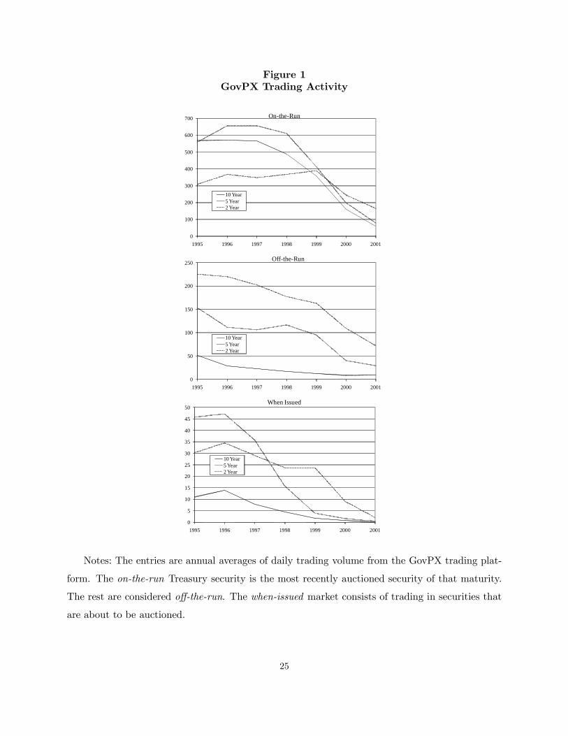
Figure 1

GovPX Trading Activity

0

100

200

300

400

500

600

700

1995 1996 1997 1998 1999 2000 2001

On-the-Run

10 Year5 Year2 Year

0

50

100

150

200

250

1995 1996 1997 1998 1999 2000 2001

Off-the-Run

10 Year5 Year2 Year

0

5

10

15

20

25

30

35

40

45

50

1995 1996 1997 1998 1999 2000 2001

When Issued

10 Year5 Year2 Year

Notes: The entries are annual averages of daily trading volume from the GovPX trading plat-

form. The on-the-run Treasury security is the most recently auctioned security of that maturity.

The rest are considered off-the-run. The when-issued market consists of trading in securities that

are about to be auctioned.

25

Figure 2

Futures Market Trading Activity

0

200

400

600

800

1,000

1,200

1995 1996 1997 1998 1999 2000 2001

10 Year5 Year2 Year

Notes: We report annual average trading activity in the 2-, 5-, and 10-year CBOT futures

contracts. The calculations are based on a continuous futures contract, assuming that contracts

rollover on the first day of the expiration month. The CBOT 2-year futures data for 1999 are

incomplete, so we do not report an average for that year.

26

Figure 3

Spot Market Information Shares, 1995-2001

0%

25%

50%

75%

100%

1995 1996 1997 1998 1999 2000 2001

2-Year Note

Hasbrouck Upper

Harris-McInish-Wood

Hasbrouck Lower

0%

25%

50%

75%

100%

1995 1996 1997 1998 1999 2000 2001

5-Year Note

Hasbrouck Upper

Harris-McInish-Wood

Hasbrouck Lower

0%

25%

50%

75%

100%

1995 1996 1997 1998 1999 2000 2001

10-Year Bond

Hasbrouck Upper

Harris-McInish-Wood

Hasbrouck Lower

Notes: The figures show the annual averages of the daily information share estimates for the

spot market. We use 1-minute returns. The upper-bound Hasbrouck information share (18),

places the spot market first in a bivariate system, and the lower-bound places it second. The

Harris-McInish-Wood information share is given by (20).

27

Table 1

VAR Estimates

2 -year HU HMW HL β α1 α2

1995 0.678(0.032)

0.460(0.020)

0.585(0.028)

0.906(0.010)

0.065(0.007)

0.041(0.003)

1996 0.785(0.018)

0.533(0.010)

0.661(0.017)

0.908(0.008)

0.060(0.003)

0.046(0.002)

1997 0.853(0.013)

0.546(0.008)

0.718(0.013)

0.923(0.007)

0.046(0.003)

0.044(0.002)

1998 0.857(0.018)

0.579(0.016)

0.716(0.015)

0.911(0.030)

0.056(0.192)

0.043(0.006)

2000 0.833(0.014)

0.570(0.009)

0.703(0.013)

0.903(0.004)

0.051(0.003)

0.047(0.002)

2001 0.642(0.045)

0.419(0.015)

0.546(0.041)

0.931(0.004)

0.101(0.008)

0.050(0.005)


1995 0.415(0.029)

0.249(0.015)

0.358(0.000)

0.983(0.006)

0.192(0.008)

0.052(0.005)

1996 0.425(0.012)

0.226(0.007)

0.365(0.013)

0.985(0.002)

0.220(0.006)

0.051(0.003)

1997 0.493(0.014)

0.253(0.008)

0.444(0.014)

0.989(0.004)

0.227(0.003)

0.060(0.003)

1998 0.716(0.011)

0.374(0.010)

0.585(0.011)

0.985(0.003)

0.129(0.006)

0.054(0.004)

1999 0.606(0.017)

0.333(0.009)

0.488(0.015)

0.961(0.002)

0.133(0.005)

0.060(0.005)

2000 0.494(0.017)

0.300(0.010)

0.418(0.019)

0.959(0.005)

0.173(0.008)

0.068(0.002)

2001 0.269(0.028)

0.213(0.018)

0.221(0.034)

0.959(0.005)

0.124(0.003)

0.031(0.004)


1995 0.284(0.024)

0.204(0.013)

0.261(0.029)

0.993(0.004)

0.184(0.007)

0.042(0.004)

1996 0.282(0.014)

0.196(0.008)

0.246(0.013)

0.994(0.002)

0.166(0.003)

0.037(0.002)

1997 0.302(0.010)

0.221(0.007)

0.264(0.009)

0.999(0.003)

0.157(0.003)

0.0360(0.003)

1998 0.496(0.016)

0.266(0.014)

0.400(0.021)

0.993(0.015)

0.119(0.059)

0.032(0.004)

1999 0.388(0.009)

0.221(0.010)

0.318(0.013)

0.987(0.002)

0.101(0.004)

0.021(0.004)

2000 0.290(0.013)

0.183(0.009)

0.244(0.013)

0.972(0.003)

0.137(0.004)

0.024(0.002)

2001 0.172(0.026)

0.148(0.015)

0.145(0.016)

0.975(0.009)

0.108(0.006)

0.014(0.001)

Notes: The table shows the annual averages of the daily information share estimates for the

GovPX spot market. We use 1-minute returns. HU is the Hasbrouck information share (18), with

the spot market first in a bivariate system, and HL places it second. HMW is the Harris-McInish-

Wood information share (20). β, α1 and α2 are the parameters from the VAR system (5) and(6).

Bootstrap standard errors are in parentheses.

28

Table 2

Speeds of Adjustment

GovPX Spot Market

2-year 5-year 10-yearMin Max Min Max Min Max

Year 2001 1995 2000 2001 1995 2001α2 0.0496 0.0409 0.0680 0.0314 0.0424 0.0139

Half-Life (mins.) 14 17 10 22 16 49

CBOT Futures Market2-year 5-year 10-yearMin Max Min Max Min Max

Year 2001 1997 1997 1998 1995 2001α1 0.1006 0.0458 0.2269 0.1287 0.1838 0.1083

Half-Life (mins.) 7 15 3 6 4 7

Notes: The table reports maximum and minimum half lives implied by the daily average partial

adjustment coefficients in the GovPX spot market, α2 and the CBOT futures market, α1. Half-lives

are the expected number of minutes for 50% of a shock to the spot market to dissipate.

29

Table 3

Models for the Information Share

Hasbrouck HMWMat. Const. Spreads Trades RV Trend R2 Const. Spreads Trades RV Trend R2

2-year -0.18 -1.14 3.08 -3.02 0.18 0.05 -3.15 -2.60 0.88 -1.21 0.11 0.13(0.61) (0.57) (0.66) (0.60) (0.07) (0.30) (0.28) (0.33) (0.30) (0.03)

5-year -11.39 -9.63 0.34 -3.11 0.54 0.21 -6.37 -3.16 0.49 -2.44 0.28 0.13(0.97) (0.97) (0.52) (0.96) (0.06) (0.55) (0.54) (0.29) (0.54) (0.04)

10-year -6.61 -2.55 1.26 -4.46 0.67 0.15 -5.20 -1.58 0.36 -2.63 0.26 0.09(0.61) (0.49) (0.21) (0.63) (0.06) (0.38) (0.31) (0.13) (0.40) (0.04)

Notes: The table reports estimates of (26). The dependent variable is a transformation (ln(IS/(1− IS))) of the Hasbrouck

upper bound or Harris-McInish-Wood (right panel) information share for the spot market in a bivariate system with the maturity

matched futures market. Regressions use daily data from October 1, 1995, to March 30, 2001. Standard errors are in parentheses.

Bold type indicates coefficients that are statistically significant at the 5 percent level.

30

Table 4

Impact on Information Share of Macro Announcements

Hasbrouck

2-year 5-year 10-yearMacro b5 b′5 b5 b′5 b5 b′5Jobless -0.042 -0.071 -0.340 -0.127 -0.289 -0.151CPI 0.379 0.346 -0.753 -0.137 -0.564 -0.163Durables -1.224 -1.275 -0.440 -0.251 -0.206 0.004Housing -0.230 -0.267 -0.280 -0.158 -0.393 -0.349Leading Ind. 0.061 0.000 0.111 0.249 0.295 0.369Trade -0.086 -0.008 -0.031 -0.134 0.045 0.005Payrolls 0.313 -0.052 -1.423 -0.020 -0.655 0.167PPI 0.607 0.416 -1.301 -0.556 -0.866 -0.392

FOMC

Announcement 0.202 0.241 -0.762 -0.430 -0.483 -0.505Minutes 0.375 0.512 -0.021 0.245 -0.463 -0.338Unscheduled -0.300 -0.379 -1.223 -0.244 -0.538 -0.057

HMW

2-year 5-year 10-yearMacro b5 b′5 b5 b′5 b5 b′5Jobless -0.137 -0.218 -0.237 -0.138 -0.243 -0.178

CPI 0.199 0.136 -0.564 -0.326 -0.311 -0.106Durables -0.950 -0.992 -0.262 -0.190 -0.084 0.031Housing -0.070 -0.028 -0.182 -0.115 -0.255 -0.221Leading Ind. 0.145 0.081 0.190 0.257 0.216 0.258Trade 0.102 0.141 0.094 0.054 0.047 0.033Payrolls 0.378 -0.002 -0.306 0.247 -0.377 0.030PPI 0.258 0.119 -0.389 -0.095 -0.450 -0.211

FOMC

Announcement 0.085 0.035 -0.148 -0.028 0.168 0.142Minutes 0.252 0.371 -0.259 -0.158 -0.249 -0.205Unscheduled 2.332 2.080 0.134 0.548 -0.235 -0.088

Notes: The table reports estimates of (28) in the first, third and fifth columns and thosefrom (29) in the second, fourth and sixth columns. The dependent variable is a transformation(ln(IS/(1 − IS))) of the Hasbrouck upper bound (first panel) or Harris-McInish-Wood (secondpanel) information share for the GovPX market. The odd columns (labeled b5) report resultsfrom estimates that do not control for daily liquidity (28), and the even columns (labeled b5’) addrelative spreads, trades and volatility (29). Regressions use daily data from October 1, 1995, toMarch 30, 2001. Bold type indicates coefficients that are statistically significant at the two-sided5 percent level.

31

Information shares in the US Treasury market

Documents

Transcript of Information shares in the US Treasury market