Inference with the lognormal distribution

Nicholas T. Longford

SNTL and UPF, Barcelona, Spain∗

Abstract

Several estimators of the expectation, median and mode of the lognormal distribution are

derived. They aim to be approximately unbiased, efficient, or have a minimax property in the

class of estimators we introduce. The small-sample properties of these estimators are assessed by

simulations and, when possible, analytically. Some of these estimators of the expectation are far

more efficient than the maximum likelihood or the minimum-variance unbiased estimator, even

for substantial sample sizes.

Keywords: χ2 distribution, efficiency, lognormal distribution, minimax estimator, Taylor expansion.

JEL classification: C13 — Estimation (Economic and Statistical Methods); C42 — Specific Distri-

butions (Special Topics).

∗Departament d’Economia i Empresa, Universitat Pompeu Fabra, Ramon Trias Fargas 25–27, 08005 Barcelona,

Spain; NTL@sntl.co.uk

1

Introduction

The lognormal distribution is used in a wide range of applications, when the multiplicative scale

is appropriate and the log-transformation removes the skew and brings about symmetry of the data

distribution (Limpert, Stahel and Abbt, 2001). Normality is the preferred distributional assumption in

many contexts, and logarithm is often the first transformation that an analyst considers to promote it.

Linear models are convenient to specify and all the relevant moments are easy to calculate and operate

with on the log-scale. However, there are instances when moments, and the expectation in particular,

are of interest on the original (exponential) scale. For example, the lognormal distribution is frequently

applied to variables in monetary units, such as companies’ assets, liabilities and profits, residential

property prices (Zabel, 1999) and household income (Longford and Pittau, 2006). The population

mean of such a variable may be a much more relevant target for inference than the population mean of

its logarithm. The sample mean is a suitable estimator for large samples, when asymptotics provide

a good approximation. In samples that are not large enough, and especially when the underlying

(normal-scale) variance is large, the sample mean is very inefficient. We explore several alternatives

and study their small-sample properties.

Finney (1941) derived the minimum-variance unbiased estimator of the expectation and variance

of the lognormal distribution, but it involves the evaluation of an infinite series; see Thoni (1969) for

an application. Aitchison and Brown (1957) is a comprehensive reference for the lognormal distribu-

tion; see also Crow and Shimizu (1988). Royston (2001) considers the lognormal distribution as an

alternative basis for survival analysis, claiming robustness and convenience. He fits a linear model on

the log scale, but implies that the prediction obtained on the log scale can be transformed back to the

original scale straightforwardly. The confidence intervals can be, but the prediction as such cannot,

because the transformation is highly nonlinear. Toma (2003) derives estimators for the multivariate

lognormal distribution, but her focus is on large-sample properties. Zhou, Gao and Hui (1997) study

tests for comparing two lognormal samples, but consider only test statistics that resemble the t, which

include the likelihood ratio. We derive a closed-form estimator that is biased but is more efficient

than Finney’s estimator. With our approach, we also study estimation of the median and mode of

the lognormal distribution.

The remainder of this section introduces the notation and reviews the basic results. The next

section derives estimators of the quantities exp(µ + aσ2), which include the expectation, median and

mode of the lognormal distribution related to the normal distribution with mean µ and variance

σ2. The following sections describe simulations of these estimators. The paper is concluded by a

discussion.

Let X = (X1 , . . . , Xn)⊤ be a random sample from a lognormal distribution, generated by ex-

2

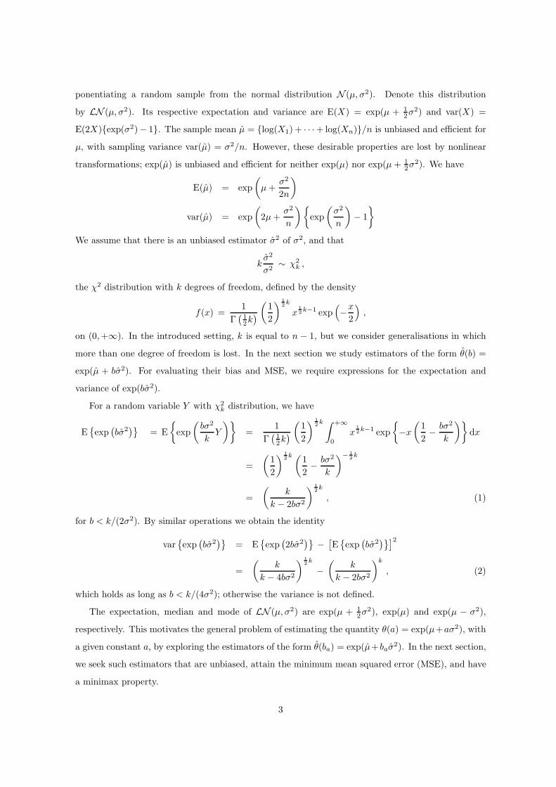
ponentiating a random sample from the normal distribution N (µ, σ2). Denote this distribution

by LN (µ, σ2). Its respective expectation and variance are E(X) = exp(µ + 1

2σ2) and var(X) =

E(2X){exp(σ2)− 1}. The sample mean µ = {log(X1) + · · ·+ log(Xn)}/n is unbiased and efficient for

µ, with sampling variance var(µ) = σ2/n. However, these desirable properties are lost by nonlinear

transformations; exp(µ) is unbiased and efficient for neither exp(µ) nor exp(µ + 1

2σ2). We have

E(µ) = exp

(

µ +σ2

2n

)

var(µ) = exp

(

2µ +σ2

n

){

exp

(

σ2

n

)

− 1

}

We assume that there is an unbiased estimator σ2 of σ2, and that

kσ2

σ2∼ χ2

k ,

the χ2 distribution with k degrees of freedom, defined by the density

f(x) =1

Γ(

1

2k)

(

1

2

)1

2k

x1

2k−1 exp

(

−x

2

)

,

on (0, +∞). In the introduced setting, k is equal to n − 1, but we consider generalisations in which

more than one degree of freedom is lost. In the next section we study estimators of the form θ(b) =

exp(µ + bσ2). For evaluating their bias and MSE, we require expressions for the expectation and

variance of exp(bσ2).

For a random variable Y with χ2k distribution, we have

E{

exp(

bσ2)}

= E

{

exp

(

bσ2

kY

)}

=1

Γ(

1

2k)

(

1

2

)1

2k ∫ +∞

0

x1

2k−1 exp

{

−x

(

1

2− bσ2

k

)}

dx

=

(

1

2

)1

2k (

1

2− bσ2

k

)− 1

2k

=

(

k

k − 2bσ2

)1

2k

, (1)

for b < k/(2σ2). By similar operations we obtain the identity

var{

exp(

bσ2)}

= E{

exp(

2bσ2)}

−[

E{

exp(

bσ2)}]2

=

(

k

k − 4bσ2

)1

2k

−(

k

k − 2bσ2

)k

, (2)

which holds as long as b < k/(4σ2); otherwise the variance is not defined.

The expectation, median and mode of LN (µ, σ2) are exp(µ + 1

2σ2), exp(µ) and exp(µ − σ2),

respectively. This motivates the general problem of estimating the quantity θ(a) = exp(µ+aσ2), with

a given constant a, by exploring the estimators of the form θ(ba) = exp(µ+baσ2). In the next section,

we seek such estimators that are unbiased, attain the minimum mean squared error (MSE), and have

a minimax property.

3

Estimation

We seek first the constant b for which θ(b) = exp(µ + bσ2) is unbiased for θ(a) = exp(µ + aσ2). As µ

and σ2 are independent,

E{

θ(b)}

= exp

(

µ +σ2

2n

) (

k

k − 2bσ2

)1

2k

. (3)

Therefore θ(b) is unbiased for θ(a) when

k − 2bσ2

k= exp

{

−2σ2

k

(

a − 1

2n

)}

,

that is, for

b∗a,ub =k

2σ2

[

1 − exp

{

−σ2

k

(

a − 1

2n

)}]

. (4)

As b∗a,ub depends on σ2, we have to estimate it. Its naive estimator is denoted by b∗a,ub . Its dependence

on σ2 is avoided by the Taylor expansion, which yields the approximation

b†a,ub= a − 1

2n.

It can be interpreted as a multiplicative bias correction of the naive estimator exp(µ) which has the

expectation exp{µ + σ2/(2n)}. For a = 1

2it agrees with the linear term of the expansion of the

function g(t) in the minimum-variance unbiased estimator exp(µ) g(1

2σ2), derived by Finney (1941);

g (t) = 1 +

∞∑

h=1

(n − 1)2h−1th

h! nh

h−1∏

m=1

1

n + 2m − 1,

with the convention that the product of no terms (for h = 1) is equal to unity. Unlike Finney’s

estimator, neither θ(b∗a,ub) nor θ(b†a,ub

) are unbiased because the estimators b are not linear in σ2.

Both estimators θ turn out to be very inefficient for all three values of a.

The sampling variance of θ(b) is

var(

µ + bσ2)

= E {exp (2µ)}E{

exp(

2bσ2)}

−[

E (µ) E{

exp(

bσ2)}]2

= exp

(

2µ +2σ2

n

) (

k

k − 4bσ2

)k

2

− exp

(

2µ +σ2

n

) (

k

k − 2bσ2

)k

, (5)

and its bias for θ(a) is

exp(µ)

{

exp

(

σ2

2n

) (

k

k − 2bσ2

)k

2

− exp(

aσ2)

}

.

Hence the MSE of θ(b) in estimating θ(a) is

m(b; a) = exp (2µ)

{

exp(

2aσ2)

− 2 exp

(

σ2

2n+ aσ2

) (

k

k − 2bσ2

)k

2

+ exp

(

2σ2

n

) (

k

k − 4bσ2

)k

2

}

.

(6)

4

The minimum of this function of b is found as the root of its derivative

∂m

∂b= 2σ2 exp(2µ)

{

exp

(

σ2

2n

) (

k

k − 4bσ2

)k

2+1

− exp

(

aσ2 +σ2

2n

) (

k

k − 2bσ2

)k

2+1

}

.

The solution is

b∗a,ms =k

2σ2

Da − 1

2Da − 1, (7)

where

Da = exp

{

2σ2

k + 2

(

a − 3

2n

)}

.

Finiteness of the MSE (b < 1

4k/σ2) implies the condition Da > 1

2. The (linear) Taylor expansion of

Da ,

Da.= 1 +

2σ2

k + 2

(

a − 3

2n

)

,

yields the approximation to b∗a,ms

b†a,ms =k(2an − 3)

4kσ2(2an − 3) + 2(k + 2)n. (8)

Assuming that a is not very large (values of particular interest are 1

2, 1 and −1), and k < n not

extremely small, this approximation is good for small values of σ2/(k +2) and when the denominator

in b†a,ms is distant from zero. Singularity occurs for σ2 = − 1

2(k + 2)n/(2an − 3)/k, which raises a

concern for a = 0 only for small n and large σ2 (when σ2 .= n/6), and for a = −1 when σ2 .

= 0.25.

Beyond these points of singularity (σ2 > n/6 for a = 0 and σ2 > 0.25 for a = −1), the MSE is infinite

(not defined). As σ2 is estimated, the problem with evaluating θ(b†−1,ms) arises whenever 0.25 is a

plausible (unexceptional) value of the estimator σ2.

If we managed to obtain b∗a,ms , we would attain with θ(b∗a,ms) the so called ideal MSE

m(

b∗a,ms; a)

= exp(2µ)

{

exp

(

2σ2

n

)

(2Da − 1)k

2 − 2 exp

(

σ2

2n+ aσ2

) (

2Da − 1

Da

)k

2

+ exp(

2aσ2)

}

.

(9)

It is the lower bound for the MSE in the class of estimators θ(b) in which b is a constant. We regard

m(b∗a,ms ; a) as a reference against which we compare the MSEs of other (realisable) estimators of θ(a).

Minimax estimation

In the range in which it is well defined, the variance var{θ(b)} is an increasing function of σ2. To see

this, we differentiate the expression in (5).

∂var{θ(b)}∂σ2

=1

nexp(2µ)

{

2 exp

(

2σ2

n

) (

k

k − 4bσ2

)k

2

− exp

(

σ2

n

) (

k

k − 2bσ2

)k

2

}

+ σ2 exp(2µ)

{

2 exp

(

2σ2

n

) (

k

k − 4bσ2

)k

2+1

− exp

(

σ2

n

) (

k

k − 2bσ2

)k

2+1

}

.

5

The expression in the braces in the first line is positive, because by dropping the leading factor 2 we

obtain the variance var(µ + bσ2) when µ = 0; see (2). The expression in the braces in the second

line can also be related to this variance. Since k/(k − 4bσ2) > k/(k − 2bσ2) > 1, it is also positive.

Therefore var{θ(b)} is an increasing function of σ2 throughout the interval 0 < σ2 < k/(4b), where it

is well defined.

One can expect that the MSE m(b, a) is an increasing function of σ2 for any reasonable choice

of b. If we cannot find an estimator that is (uniformly) efficient for all σ2 > 0, we might pay more

attention to efficiency for greater values of σ2, for which more is at stake. This motivates the following

approach to estimating θ(a). Suppose we are certain (or very confident) that σ2 does not exceed a

specified value σ2mx . Then we use the coefficient ba,mx for which the estimator θ(ba,mx) is efficient

when σ2 = σ2mx ,

ba,mx =k

2σ2mx

Da,mx − 1

2Da,mx − 1, (10)

as in (7), with implicitly defined Da,mx , and apply the estimator θ(ba,mx). Rigour would be enhanced

by writing ba,mx = ba,mx(σ2mx), but that would make the notation cumbersome. We rule out the

setting with 0 < a < 3/(2n), so that Da is an increasing function of σ2 and Da > 1 when a > 3/(2n).

When a ≤ 0, Da decreases with σ2 and the condition that Da,mx > 1

2imposes an upper bound on the

values of σ2mx that can be declared.

One might reasonably expect that the estimator θ(ba,mx) based on a value σ2mx = σ2

1 is more

efficient for all σ2 ∈ (0, σ21 ] than θ(ba,mx) based on a value σ2

2 > σ21 . That is, for a sharper (smaller)

upper bound σ2mx we should be rewarded by uniformly more efficient estimation, so long as this bound

is justified. This conjecture is proved by differentiating the function var{θ(ba,mx)} with respect to

σ2mx .

The MSE of the estimator θ(ba,mx) based on a given value of σ2mx is obtained directly from (6):

m(ba,mx ; a) = exp(2µ)

[

exp

(

2σ2

n

) {

1 − 2 (Da,mx − 1)

2Da,mx − 1

σ2

σ2mx

}− k

2

− 2 exp

(

σ2

2n+ aσ2

) (

1 − Da,mx − 1

2Da,mx − 1

σ2

σ2mx

)− k

2

+ exp(

2aσ2)

]

. (11)

Let Ca = log(Da,mx)/σ2mx , so that ∂Da,mx/∂σ2

mx = CaDa,mx . Then

∂m(ba,mx ; a)

∂σ2mx

= exp

(

2µ +2σ2

n

)

kσ2

σ4mx

{

(2Da,mx − 1) (Da,mx − 1) − CaDa,mx σ2mx

}

(2Da,mx − 1)2

×[

exp

{

σ2

(

a − 3

2n

)}{

(2Da,mx − 1)σ2mx

(2Da,mx − 1)σ2mx − (Da,mx − 1)σ2

}k

2+1

−{

(2Da,mx − 1)σ2mx

(2Da,mx − 1)σ2mx − 2 (Da,mx − 1)σ2

}k

2+1

]

. (12)

6

The long fraction in the first row is positive because the inequality Da,mx − 1 > Caσ2mx > 0, obtained

from the Taylor expansion of Da,mx around σ2mx = 0, implies that

(2Da,mx − 1) (Da,mx − 1) − CaDa,mx σ2mx > (Da,mx − 1)2 . (13)

The exponential in the second row is equal to Dk/2+1a , and so the sign of the expression in (12) is the

same as the sign of

Da

{

(2Da,mx − 1)σ2mx − 2 (Da,mx − 1)σ2

}

− (2Da,mx − 1)σ2mx − (Da,mx − 1)σ2

= (Da − 1) (2Da,mx − 1)σ2mx − (2Da − 1) (Da,mx − 1)σ2

={

F (σ2) − F (σ2mx)

}

(2Da − 1) (2Da,mx − 1)σ2

σ2mx

,

where F (σ2) = σ−2(Da − 1)/(2Da − 1). The function F is decreasing, since

∂F

∂σ2=

DaCa

(2Da − 1)2

1

σ2− Da − 1

2Da − 1

1

σ4

= − (Da − 1) (2Da − 1) − CaDaσ2

(2Da − 1)2 σ4< 0 ,

using the same argument as in (13). Therefore F (σ2) < F (σ2mx) and (12) is positive, whenever

σ2 < σ2mx . This concludes the proof that a smaller upper bound σ2

mx results in a uniformly more

efficient estimator θ(ba,mx ), so long as the bound is justified, that is, σ2 < σ2mx .

The simulations described in the following sections are conducted for σ2 ∈ (0, 10). For orientation,

a typical draw from LN (µ, 10) is about exp(√

10).= 24 times greater or smaller than the median

exp(µ). The expectations and biases of all estimators have the multiplicative factor exp(µ), and the

variances and MSEs the factor exp(2µ). Therefore we can reduce our attention to the targets θ(a)

with µ = 0, so that σ2 is the sole parameter of interest. Nevertheless, µ is estimated throughout. We

study the relative biases and relative root-MSEs, defined as

Brel

(

θ)

=E

(

θ)

θ(a)− 1

rMSErel

(

θ)

=

√

√

√

√

MSE(

θ)

m(

b∗a,ms , a) .

They reduce the strong association of the biases and MSEs with σ2.

Estimating the mean

Table 1 lists the estimators of the expectation θ(1

2) = exp(µ + 1

2σ2). The relative biases and MSEs

of these estimators with sample size n = 50 are plotted as functions of σ2 in Figure 1. They are

7

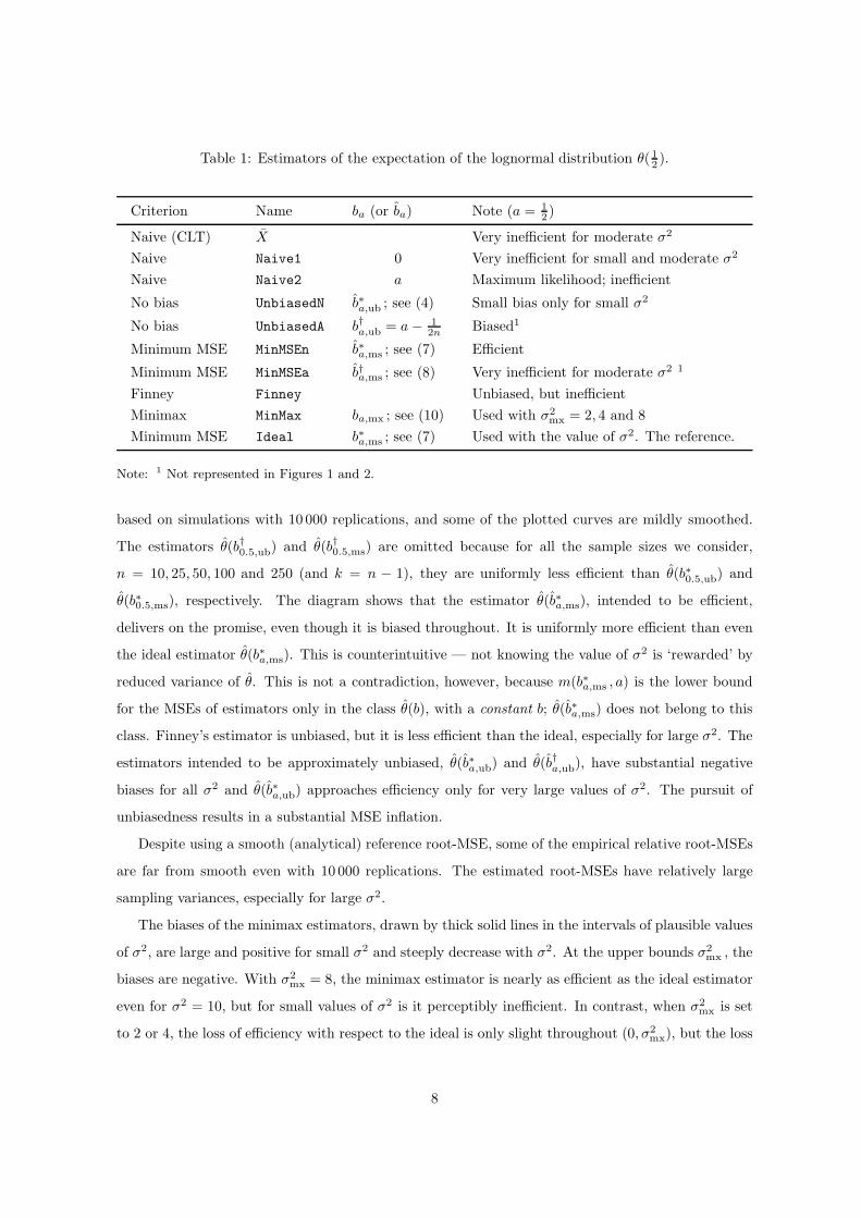
Table 1: Estimators of the expectation of the lognormal distribution θ(1

2).

Criterion Name ba (or ba) Note (a = 1

2)

Naive (CLT) X Very inefficient for moderate σ2

Naive Naive1 0 Very inefficient for small and moderate σ2

Naive Naive2 a Maximum likelihood; inefficient

No bias UnbiasedN b∗a,ub; see (4) Small bias only for small σ2

No bias UnbiasedA b†a,ub= a − 1

2n Biased1

Minimum MSE MinMSEn b∗a,ms ; see (7) Efficient

Minimum MSE MinMSEa b†a,ms ; see (8) Very inefficient for moderate σ2 1

Finney Finney Unbiased, but inefficient

Minimax MinMax ba,mx ; see (10) Used with σ2mx = 2, 4 and 8

Minimum MSE Ideal b∗a,ms ; see (7) Used with the value of σ2. The reference.

Note: 1 Not represented in Figures 1 and 2.

based on simulations with 10 000 replications, and some of the plotted curves are mildly smoothed.

The estimators θ(b†0.5,ub

) and θ(b†0.5,ms) are omitted because for all the sample sizes we consider,

n = 10, 25, 50, 100 and 250 (and k = n − 1), they are uniformly less efficient than θ(b∗0.5,ub

) and

θ(b∗0.5,ms), respectively. The diagram shows that the estimator θ(b∗a,ms), intended to be efficient,

delivers on the promise, even though it is biased throughout. It is uniformly more efficient than even

the ideal estimator θ(b∗a,ms). This is counterintuitive — not knowing the value of σ2 is ‘rewarded’ by

reduced variance of θ. This is not a contradiction, however, because m(b∗a,ms , a) is the lower bound

for the MSEs of estimators only in the class θ(b), with a constant b; θ(b∗a,ms) does not belong to this

class. Finney’s estimator is unbiased, but it is less efficient than the ideal, especially for large σ2. The

estimators intended to be approximately unbiased, θ(b∗a,ub) and θ(b†a,ub), have substantial negative

biases for all σ2 and θ(b∗a,ub) approaches efficiency only for very large values of σ2. The pursuit of

unbiasedness results in a substantial MSE inflation.

Despite using a smooth (analytical) reference root-MSE, some of the empirical relative root-MSEs

are far from smooth even with 10 000 replications. The estimated root-MSEs have relatively large

sampling variances, especially for large σ2.

The biases of the minimax estimators, drawn by thick solid lines in the intervals of plausible values

of σ2, are large and positive for small σ2 and steeply decrease with σ2. At the upper bounds σ2mx , the

biases are negative. With σ2mx = 8, the minimax estimator is nearly as efficient as the ideal estimator

even for σ2 = 10, but for small values of σ2 is it perceptibly inefficient. In contrast, when σ2mx is set

to 2 or 4, the loss of efficiency with respect to the ideal is only slight throughout (0, σ2mx), but the loss

8

0 5 10

−1

01

2Sample size 50

Variance

Rel

ativ

e bi

as

Sample meanNaive1Naive2(ML)UnbiasedNMinMSEnFinneyMinimax

0 5 10

1.0

1.5

2.0

2.5

VarianceR

elat

ive

root

−M

SE

Figure 1: The relative biases and relative root-MSEs of estimators of the expectation of the lognormaldistribution, as functions of the variance σ2. Sample size n = 50, with k = 49 degrees of freedom forestimating σ2.

is substantial for large values of σ2. The minimax estimators have relatively small variances, and the

biases are substantial contributors to the MSE for most values of σ2. With increasing σ2, the relative

biases converge to −1, the lower bound for any nonnegative estimator.

Figure 2 summarises the biases and MSEs of the discussed estimators for a selection of other

sample sizes, using the same layout as Figure 1. Estimator θ(b∗a,ms) is slightly more efficient than

the ideal, but uniformly so, for all sample sizes. Finney’s estimator is uniformly less efficient than

the ideal, but its inefficiency decreases with sample size. The inefficiency of the ML estimator also

decreases with sample size, but at n = 250 it is still not competitive, except when σ2 is very small.

With increasing sample size, the root-MSE inflation when σ2mx is understated becomes less severe.

Efficiency is associated with substantial negative bias even for n = 250. We conclude that θ(b∗0.5,ms)

is uniformly most efficient for θ(1

2) among the estimators we explored for sample sizes in the range

10 – 250.

Estimating the median

The median corresponds to the setting a = 0. The two naive estimators coincide for a = 0, so we

use the label Naive for the common estimator. We also exclude estimator θ(b†a,ms) because for larger

values of σ2 (e.g., for σ2 > 5 when n = 50) it attains very large values with nontrivial probabilities.

9

0 5 10

02

Sample size 10

Variance

Rel

ativ

e bi

as

0 5 10

12

Variance

Rel

ativ

e ro

ot−

MS

E

0 5 10

02

Sample size 25

Variance

Rel

ativ

e bi

as

0 5 10

12

Variance

Rel

ativ

e ro

ot−

MS

E

0 5 10

02

Sample size 100

Variance

Rel

ativ

e bi

as

0 5 10

12

Variance

Rel

ativ

e ro

ot−

MS

E

0 5 10

02

Sample size 250

Variance

Rel

ativ

e bi

as

0 5 10

12

Variance

Rel

ativ

e ro

ot−

MS

E

Figure 2: The relative biases and relative root-MSEs of estimators of the expectation of the lognormaldistribution, as functions of the variance σ2. See the legend in Figure 1 to identify the estimators.

10

0 5 10

−0.

2−

0.1

0.0

0.1

0.2

Sample size 50

Variance

Rel

ativ

e bi

as

0 5 10

1.0

1.5

2.0

VarianceR

elat

ive

root

−M

SE

SampleNaiveUnbiasedNUnbiasedAMinMSEnMinimax

Figure 3: The relative biases and relative root-MSEs of estimators of the median of the lognormaldistribution, as functions of the variance σ2. Sample size n = 50.

The results for sample size n = 50 are presented in Figure 3. The biases of the estimators are

much more moderate than for estimating the expectation θ(1

2). The sample median is uniformly less

efficient than any other estimator. The minimax estimator and the estimator θ(b∗0,ms) are about as

efficient as the ideal estimator θ(b∗0,ms), and they are uniformly more efficient than the sample and

naive estimators, as well as the estimators intented to be unbiased.

Some properties of θ(b∗0,ms) and θ(b0,mx) can be inferred from the expression

D0 = exp

{

− 3σ2

(k + 2)n

}

.

The dependence of D0 on σ2, or of θ(b0) on σ2, is very weak for all but very small k and n. Of course,

the sample median does not depend on σ2 at all, but the weak influence of σ2 on θ(b0) is sufficient to

make it an efficient estimator. For small bσ2 (or bσ2), exp(bσ2).= 1+bσ2 and var{exp(bσ2)} .

= 2b2σ4/k.

That is why the root-MSEs of the estimators θ(b) are approximately proportional to σ2.

Figure 4 summarises the results for the other sample sizes. The sample median is uniformly the

least efficient of the estimators we study, except for n = 10 and σ2 > 6, because estimator θ(b∗0,ms)

has a breakdown at around σ2 = 6, indicated by the vertical dashes. With increasing sample size,

the relative biases of all the estimators converge to zero. The minimax estimators are very forgiving;

their inefficiency when σ2 > σ2mx is appreciable only for n = 10. We conclude by recommending the

estimator θ(b∗0,ms) when n > 20, although it is indistinguishable from θ(b0,mx) based on a liberally

11

05

10

−0.2 −0.1 0.0 0.1 0.2

Sam

ple size 10

Variance

Relative bias

05

10

1.0 1.5 2.0

Variance

Relative root−MSE

05

10

−0.2 −0.1 0.0 0.1 0.2

Sam

ple size 25

Variance

Relative bias

05

10

1.0 1.5 2.0

Variance

Relative root−MSE

05

10

−0.2 −0.1 0.0 0.1 0.2

Sam

ple size 100

Variance

Relative bias

05

10

1.0 1.5 2.0

Variance

Relative root−MSE

05

10

−0.2 −0.1 0.0 0.1 0.2

Sam

ple size 250

Variance

Relative bias

05

10

1.0 1.5 2.0

Variance

Relative root−MSE

Fig

ure

4:

The

relativ

ebia

sesand

relativ

ero

ot-M

SE

sof

estimato

rsof

the

med

ian

of

the

lognorm

al

distrib

utio

n,as

functio

ns

ofth

eva

riance

σ2.

12

0 5 10

−1.

0−

0.5

0.0

0.5

1.0

Sample size 50

Variance

Rel

ativ

e bi

as

UnbiasedNMinMSEnMinimax

0 5 10

24

68

VarianceR

elat

ive

root

−M

SE

Figure 5: The relative biases and relative root-MSEs of estimators of the mode of the lognormaldistribution, as functions of the variance σ2. Sample size n = 50.

chosen value of σ2mx . For smaller sample sizes, θ(b0,mx) does not have the drawback of a sudden MSE

inflation.

Estimating the mode

The mode of a continuous distribution does not have a natural sample or naive estimator. We could

select a ‘window’ width w and define the estimator of the mode as the center of the interval of width

w (or the mean of such centres), which contains the largest number of observations. However, such

an estimator is bound to be very inefficient.

The relative biases and root-MSEs of the estimators intended to be unbiased and efficient for θ(−1)

with sample size n = 50 are plotted in Figure 5. Both estimators are severely biased, except when σ2 is

very small. The biases and MSEs of θ(b†−1,ms) and θ(b†−1,ub) are extremely large; they are off the scale

in both panels of the diagram for most values of σ2, and are therefore not plotted at all. Estimator

θ(b∗−1,ms) is inefficient only slightly for σ2 < 5 but breaks down at about σ2 = 7.9; the graphs of

its relative bias and root-MSE are discontinued in the diagram at that value. With a well informed

setting of σ2mx , the minimax estimator is quite efficient. For example, θ(b−1,mx) with σ2

mx = 8 is only

slightly less efficient than the ideal even for σ2 = 10, and is more efficient than θ(b∗−1,ms) for σ2 > 4.1.

It is relatively very inefficient only when σ2 is very small. The estimators θ(b−1,mx) with σ2mx = 2 and

4 are quite efficient for very small values of σ2, but for large values of σ2 they are very inefficient.

13

Some insight into the breakdown of the estimators θ(b∗−1,ms) and θ(b†−1,ms) can be gained directly

from the expressions for the respective coefficients b. The singularity of the coefficient b−1 caused by

the value D−1 = 1

2corresponds to σ2 = log(2)(k + 2)n/(2n + 3), that is, for n = 50 and k = 49,

to σ2† = 17.16. In b−1,ms , we substitute σ2 for σ2 in D−1 , so very large or very small values of b1

are obtained whenever values around 17 are plausible for σ2. For n = 50 this occurs for σ2 > 7.9.

With the approximation to D−1 by the Taylor expansion, the denominator of b†−1,ms vanishes when

σ2 = (k +2)n/{k(2n+3)}, which is close to 0.25 for all but very small k and n. Hence the breakdown

of θ(b†a,ms) for σ2 around 0.25; it occurs also for other sample sizes.

The relative biases and root-MSEs are plotted in Figure 6 for sample sizes n = 10, 25, 100 and 250.

Some of the curves are discontinued at breakdowns, where they suddenly diverge. For n = 10, D−1 <

0.5 for σ2 > 3.3, and the variance of the reference estimator θ(b−1,ms) is not defined. Breakdown

occurs even for the minimax estimators for σ2mx = 4 and 8. For sample sizes n = 100 and 250, only

the estimator θ(b∗−1,ub) performs well throughout the range of values of σ2. The minimax estimators

are useful with small samples only when we can narrow down the range of plausible values of σ2 and

σ2 is not very large. The penalty for understating σ2mx is quite harsh, except when n ≥ 250.

We conclude by suggesting that estimation of the mode be based on at least n = 50 observations.

Estimator θ(b∗−1,ms) is nearly efficient for small values of σ2, and is a relatively safe choice otherwise.

It breaks down for large values of σ2, but these breakdown values increase with σ2. If the values of

σ2 can be narrowed down, say, to an interval of length 2.0 or shorter, then the minimax estimator is

quite efficient.

MSE estimation

In this section we consider estimation of the MSE of θ(ba), with a focus on a = 1

2and b0.5 = b∗0.5,ms ,

for which the estimator is more efficient than the ideal. We estimate MSE{θ(b∗0.5,ms ); θ(1

2)} by the

MSE of the ideal evaluated at σ2 = σ2, that is,

m

(

b∗0.5,ms ;1

2

)

= MSE

{

θ(

b∗0.5,ms

)

; θ

(

1

2

)∣

∣

∣

∣

σ2 = σ2

}

.

We have to consider estimation of MSE and root-MSE separately because these targets are related

nonlinearly. For example, if an estimator m is unbiased for m, then√

m need not be unbiased for√

m.

The relative biases, defined as ¯m/m − 1 and√

¯m/√

m − 1, where the bar ¯ indicates averaging over

the replications, are plotted for n = 50, 100 and 250 in Figure 7. Both m and√

m overestimate their

respective targets, the MSE and root-MSE, except for very small values of σ2. On the multiplicative

scale, the extent of overestimation is smaller for root-MSE than for MSE, and is smaller for larger

sample sizes. For n = 10 and n = 25, the estimators are useful only for very small σ2; for n > 250 the

bias of the root-MSE estimator is very small even for σ2 = 10.

14

05

10

−1.0 −0.5 0.0 0.5 1.0

Sam

ple size 10

Variance

Relative bias

05

10

1.0 1.5 2.0 2.5 3.0

Variance

Relative root−MSE

05

10

−1.0 −0.5 0.0 0.5 1.0

Sam

ple size 25

Variance

Relative bias

05

10

1.0 1.5 2.0 2.5 3.0

Variance

Relative root−MSE

05

10

−1.0 −0.5 0.0 0.5 1.0

Sam

ple size 100

Variance

Relative bias

05

10

1.0 1.5 2.0 2.5 3.0

Variance

Relative root−MSE

05

10

−1.0 −0.5 0.0 0.5 1.0

Sam

ple size 250

Variance

Relative bias

05

10

1.0 1.5 2.0 2.5 3.0

Variance

Relative root−MSE

Fig

ure

6:

The

relativ

ebia

sesand

relativ

ero

ot-M

SE

sof

estimato

rsof

the

mode

of

the

lognorm

al

distrib

utio

n,as

functio

ns

ofth

eva

riance

σ2.

15

0 5 10

1.0

1.1

1.2

Variance

Rel

ativ

e M

SE

n=50 n=100

n=250

0 5 10

1.0

1.1

1.2

Variance

Rel

ativ

e ro

ot−

MS

E

n=50

n=100

n=250

Figure 7: The biases of the estimators of the MSE and root-MSE of the estimator θ(b∗0.5,ms) of theexpectation of the lognormal distribution.

The substantial bias of these estimators for small sample sizes should be judged in the context

of large variance of the data as well as of the distribution of the MSE and rMSE estimators. For

example, the relative biases of the MSE and root-MSE for σ2 = 5 and n = 10 are 3.45 and 0.32,

respectively, but these figures are associated with standard deviations (over the replications) of 35.6

and 1.11, respectively. We smoothed the empirical values of the biases only slightly, to indicate the

uncertainty about them that is present in 10 000 replications. The same set of random numbers was

used for each sample size n.

Conclusion

Estimating the expectation, median and mode of the lognormal distribution are examples of failure

of the maximum likelihood and of inapplicability of the asymptotic theory for sample sizes that for

many other commonly encountered distributions would be sufficiently large. We derived estimators

that are much more efficient than their naive alternatives, and explored how information about σ2

can be incorporated in (minimax) estimation. Although biased, our estimator of the expectation is

much more efficient than Finney’s estimator, especially for large variances σ2. Finney’s estimator is

minimum-variance unbiased, a clearly formulated optimality property, whereas our estimator has no

(universal) optimality properties. Our results indicate that unbiasedness and efficiency (small MSE)

are conflicting inferential goals when estimating the location of a lognormal distribution. Insisting

on unbiasedness when pursuing efficiency is an unaffordable luxury. Instead of MSE, the criterion to

16

minimise var(θ) + ρ{E(θ) − θ}2 could be adopted for a specified constant ρ, but a rationale for any

particular value of ρ > 1 is difficult to formulate.

The counterintuitive result that θ(b∗0.5,ms) is (slightly) more efficient than θ(b∗0.5,ms) for estimating

the expectation exp(µ + 1

2σ2) can be exploited for estimating the MSE of θ(b∗0.5,ms) by substituting

σ2 in the expression (9) for MSE{θ(b∗0.5,ms); θ(1

2)}. The resulting MSE (and root-MSE) estimator has

a positive bias which for a given σ2 declines with sample size, and for a given sample size increases

with σ2.

Our estimators rely on the functional form of the target, exp(µ+aσ2), and so their robustness might

be questioned. Robustness can be assessed by simulations, for instance, using the exponential of a

distribution that differs slightly from the normal. The t-distributions with few degrees of freedom (and

some noncentrality) are not suitable for this purpose because their exponentials (log-t distributions)

do not have expectations for any number of degrees of freedom. In any sensitivity study, the naive

estimators start with a considerable handicap which is unlikely to be overcome for moderate departures

from lognormality.

Acknowledgements

Research for this manuscript was supported by the Grant SEJ2006–13537 from the Spanish Ministry

of Science and Technology. Suggestions made by Omiros Papaspiliopoulos are acknowledged.

References

Aitchison, J., and Brown, I. A. C. (1957). The Lognormal Distribution. Cambridge University Press,

Cambridge, UK.

Crow, E. L., and Shimizu, K. (Eds.) (1998). Lognormal Distributions. Theory and Applications. M.

Dekker, New York.

Finney, D. J. (1941). On the distribution of a variate whose logarithm is normally distributed. Journal

of the Royal Statistical Society, Supplement 7, 155–161.

Limpert, E., Stahel, W. A., and Abbt, M. (2001). Log-normal distributions across the sciences: keys

and clues. Biosciences 51, 341–352.

Longford, N. T., and Pittau, M. G. (2006). Stability of household income in European countries in

the 1990’s. Computational Statistics and Data Analysis 51, 1364–1383.

Royston, P. (2001). The lognormal distribution as a model for survival time in cancer, with an

emphasis on prognostic factors. Statistica Neerlandica 55, 89–104.

17

Thoni, H. (1969). A table for estimating the mean of a lognormal distribution. Journal of the

American Statistical Association 64, 632–636.

Toma, A. (2003). Robust estimators of the parameters of multivariate lognormal distribution. Com-

munications in Statistics. Theory and Methods 32, 1405–1417.

Zabel, J. (1999). Controlling for quality in house price indices. Journal of Real Estate Finance and

Economics 13, 223–241.

Zhou, X.-H., Gao, S., and Hui, S. L. (1997). Methods for comparing the means of two independent

log-normal samples. Biometrics 53, 1129–1135.

18