Individual notions of distributive justice and relative economic status

ISSN 1988-088X

Department of Foundations of Economic Analysis II University of the Basque Country Avda. Lehendakari Aguirre 83 48015 Bilbao (SPAIN) http://www.dfaeii.ehu.es

DFAE-II WP Series

Abigail Barr, Justine Burns, Luis Miller, and Ingrid Shaw

Individual notions of distributive justice and

relative economic status

2011-03

1

Individual notions of distributive justice and relative economic

status

by

Abigail Barr1, Justine Burns2, Luis Miller3, and Ingrid Shaw4

24 September 2011

Abstract: We present two experiments designed to investigate whether

individuals’ notions of distributive justice are associated with their relative

(within-society) economic status. Each participant played a specially designed

four-person dictator game under one of two treatments, under one initial

endowments were earned, under the other they were randomly assigned. The first

experiment was conducted in Oxford, United Kingdom, the second in Cape Town,

South Africa. In both locations we found that relatively well-off individuals make

allocations to others that reflect those others’ initial endowments more when those

endowments were earned rather than random; among relatively poor individuals

this was not the case.

Keywords: Distributive Justice, Inequality, Laboratory Experiments.

JEL classification: D63, C91, C93.

1-University of Nottingham, [email protected]; 2- University of the Basque Country,[email protected]; 3- University of Cape Town, [email protected]; [email protected]. Acknowledgements: We owe a considerable debt of thanks to SimonHeadford, our script reader and long suffering recruiter of the unemployed participants in the UKexperiment. We are also grateful to our other research assistants, Aran Sezekely, MeenakshiParameshwaran, Silvana Cimpoca and Ece Yagman. The research was funded by The John Fell Fund,University of Oxford.

2

Individual notions of distributive justice and relative economic

status

Not long ago, climate-related catastrophes were viewed principally, if not solely, as

emergencies and the causes of immediate human suffering. Now, they are also viewed as

profound reminders of the finiteness of our global physical resource pool. Against this

backdrop, the banking crisis underscored the sense that, as a species, as members of societies

and as individuals, we cannot continue to live beyond our means. As this growing awareness

of constraints on consumption takes over from a prior sense of ever-expanding prosperity,

issues of inequality, distribution and redistribution are commanding progressively more

attention in the minds not only of world leaders, politicians, and academics but also of

ordinary people. And where injustice is perceived, there is protest, unrest, and considerable

cost in the form of damage to property, human death and injury, and the time and effort of all

concerned.

So, what constitutes distributive justice in the minds of ordinary people? The philosophical

literature offers several alternative principles of distributive justice. John Rawls proposed that

“undeserved inequalities call for redress; and since inequalities of birth and natural

endowment are undeserved, these inequalities are to be somehow compensated for” (Rawls,

1971 p. 100). In contrast, Robert Nozick argued that “The complete principle of distributive

justice would say simply that a distribution is just if everyone is entitled to the holdings they

possess under the distribution” (Nozick, 1974 p.151). In fact, some sense of entitlement is

central to most normative theories of distributive justice. According to some, people should

be rewarded according to their contribution to the social product (Miller, 1976), while others

propose that people should be rewarded according to the effort they put into productive work

(Milne, 1986).

But which of these, if any, do ordinary people adopt as the principle against which to judge

their own and other people’s and entities’ outcomes and actions? Does the principle or notion

they apply vary systematically with their context? Are the poor more inclined towards the

egalitarian principle of Rawls and the relatively well-off towards the entitlement theories of

Miller and Milne? In this paper, we investigate whether individuals’ notions of distributive

justice are associated with their economic status relative to others within their own society

and whether this association is stable across societies.

3

Early theoretical models of the political economy assumed that people cared only about their

own consumption and that, as a consequence, poorer people preferred redistribution, while

the rich did not.1 Some theories gave credence to the idea that people take account of the fact

that the redistribution of unequal earnings discourages effort and may be disadvantageous to

society as a whole and so, indirectly, to themselves (Meltzer and Richards, 1981; Alesina and

Rodrik, 1994; Persson and Tabellini, 1995). Others explored the idea that an association

between inequality and crime or positive externalities to education may enhance preferences

for redistribution (Perotti, 1993; Galor and Zeira, 1993). More recent theories account for

individuals’ actual and perceived prospects for upward mobility showing that they may

suppress preferences for redistribution (Benabou and Ok, 2001; Alesina and Glaeser, 2004;

Benabou and Tirole, 2006). However, what we are interested in are individual notions of

distributive justice, i.e., individual preferences relating directly to the level of inequality

conditioned on the way that inequality came into being.

When thinking about how these direct preferences might vary systematically across

individuals, economists are increasingly referring to Babcock and Lowenstein’s (1997)

proposition that “people tend to arrive at judgments of what is fair or right that are biased in

the direction of their own self-interests” (Babcock and Loewenstein, 1997: 111). In this vein,

Alesina and Giuliano (2011) write “Rich people […] are likely to believe strongly in the

beneficial incentive effects of inequality so as to justify in terms of efficiency their

preferences for less equality. The opposite applies for those less wealthy and/or left leaning

individuals. They tend to disregard the incentive effects of inequality to justify their

ideological preferences for equality” (Alesina and Giuliano, 2011:101).

Empirical evidence derived from attitudinal surveys such as the World Values Survey and the

US General Social Survey supports the hypothesis that the poor are more in favour of

redistribution than the rich. However, such data does not allow us to isolate the effect of

direct preferences relating to inequality on redistributional attitudes from the effect of the

simple preference for higher own current and future consumption. Alesina and Giuliano

(2011) found in the existing literature and from their own empirical analysis that being more

left wing, having a religious upbringing, being a member of a racial minority that is relatively

poor, being from a country in which preferences for redistribution are commonplace, being

exposed to macro-economic volatility in youth, and believing that prosperity had more to do

1Persson and Tabellini (2002) and Drazen (2002) provide extensive reviews of political economy models.

4

with luck than hard work were all associated with a more positive attitude towards

redistribution and took this as evidence of the role of such direct preferences in determining

such attitudes.2 However, none of these findings tell us whether and how direct preferences

for redistribution vary with relative economic status. The problem is that, to the extent that

current and future economic status determines how much a person cares about inequality, the

effect of that person’s caring is captured in the coefficients on income and education and is,

thus, indistinguishable from a preference for more own consumption. The ideal way to

overcome this problem is to generate direct measures of individuals’ preferences for

redistribution and investigate how these measures vary with relative economic status.

A considerable number of experimental social scientists have measured and investigated

individual notions of distributive justice in the lab. However, whether and how these notions

vary across individuals has not been the focus. Instead, they have focused on how the relative

importance of luck and effort in determining the level of inequality affects what people

perceive as a fair final distribution. Using a variety of experimental designs they have found

evidence of an earned endowment effect (hereafter EEE) that is consistent with the luck

versus effort findings of Alesina and co-authors cited above and is often described as being

consistent with liberal egalitarianism. Specifically, in sharing and bargaining games, the

allocations that participants make to themselves and others reflect initial endowments

considerably more when those endowments are earned rather than when they are pure

windfall gains (Hoffman et al 1994; Ruffle 1998; Konow 2000; Rutstrom and Williams 2000;

Cherry 2001; Gantner et al, 2001; Cherry et al 2002; Frohlich et al 2004; Cappelen et al 2007;

Oxoby and Spraggon 2008; List and Cherry 2008). However, most of these studies involved

student participants, i.e., participants who are investing in their future earning capacity. So, if

peoples’ preferences are biased in the direction of their own self-interests, this evidence

pertains only to a type of individual that, by virtue of the economic status they are aiming to

attain, is highly likely to be attracted to the idea of deserved inequalities.

To date, to our knowledge, there have been only two experimental studies involving

participants who, according to the reasoning set out above, would be less inclined to

acknowledge entitlement to earnings derived from effort. Jakiela (2011) involved poor

2 The existing literature to which Alesina and Giuliano (2011) refer includes Alesina and Glaeser (2004),Alesina and Angeletos (2005), Luttmer and Singhal (2008), Giuliano and Spilimbergo (2009), Alesina andLaFerrara (2002) and Fong (2001). Other studies exist that corroborate this body of evidence. For example, arecent report by the Fabian Society points out that most people in Britain believe that effort should be rewardedand luck redressed (Hampson and Olchawski, 2009).

5

Kenyan villagers in a sharing game experiment and found no EEE, while Jakiela, Miguel and

Te Velde (2010) found no EEE among Kenyan girls with low academic achievements and a

significant EEE among similar girls who, owing to a scholarship programme, had higher

academic achievements and, hence, higher potential economic status. These studies provide

valuable insights into the origins of individual notions of distributive justice. However, the

experimental designs render it impossible to tell whether we are looking at an African effect

in the first case and an Africa-specific effect in the second.

In this paper, we present the findings from two experiments designed to test the conjecture

that individuals’ notions of distributive justice are associated with their economic status

relative to others within their own society. Specifically, we conjecture that the tendency to

respect the earnings of others and feel entitled to one’s own increases with relative (within

society) economic status. If this conjecture is well founded, we should not have to go to

Africa to find experimental participants that exhibit no EEE. We should be able to find them

within any society. With this in mind, we conducted our first experiment in the UK, a

relatively affluent society with relatively well functioning institutions. We selected

unemployed residents of one city to represent low economic status individuals and students

and employed individuals residing in the same city as bases for comparison.3 The students

allowed us to demonstrate that, when applied to the standard participant pool, our experiment

yields the usual result, i.e., an EEE. However, the employed are the better basis for

comparison as they, rather than investing in their future economic status, are realizing their

current actual economic status. In addition, they are likely to be more comparable to the

unemployed in terms of age, marital status and familial responsibilities. We found a

statistically significant EEE among the students and employed and no EEE among the

unemployed and a statistically significant difference between the unemployed and the others.

Our second experiment was designed to test the external validity of our first and to build a

bridge back to the work of Jakiela and co-authors (op. cit.). It was conducted in Cape Town, a

South African city containing one of the continent’s best universities. Thus, we were able to

build a participant sample that was highly comparable to the UK sample in many regards,

3While there is an extensive literature on the psychological effects of unemployment (Clark, 2003; Paul and

Moser, 2009; Winefield et al 1991), there has been very little quantitative behavioural and experimental work onwhether and how experiences of unemployment affect individual behavioural tendencies, values and attitudes.This is both a surprise and a concern as such values may, in turn, affect future labour market participationdecisions and outcomes (Bowles et al. 2001).

6

while varying in terms of its wider societal context. There, we found a statistically significant

EEE among the relatively well-off, but not among the poor.

Armed with the findings from the Cape Town experiment, we returned to the UK data and

sought to reorganize our participant sample there into the relatively well-off and the relatively

poor and found that, in-so-doing, we could improve upon our earlier analytical results. And

finally, when pooling the data from the two experiments, we found that the relationships

between individual notions of distributive justice and relative economic status in the two

societies were indistinguishable.

The remainder of the paper is organized as follows: section I, directly below, presents our

experimental design, analytical framework and hypotheses; section II presents the results; and

section III concludes.

I. EMPIRICAL STRATEGY

A. Experimental Design

At the core of the experimental design is a four person dictator game (4PDG). In this game,

each participant is initially endowed with a positive sum of money, ,ݕ each knows his or

her own initial endowment and the initial endowments of the three other participants, and

each is free to make final allocations to him or herself and to the others subject to the

constraint that the sum of the four allocations must equal the sum of the four initial

endowments. Once all the participants have made their allocation decisions, the decisions of

one are randomly selected to determine the final payoffs of all four participants.

Play is one shot and anonymous. The participants know the initial endowments of their three

co-participants and, in the event that their own allocation decisions are not randomly selected

to determine the final payoffs, the final allocations chosen by one of their co-participants.

However, they never know the precise identities of their three co-participants.

Prior to the 4PDG, the participants engaged in a real effort task and, in more than half of the

experimental sessions, their performance ranking in that task determined their initial

endowments. However, in order to control for the possible conditioning of final allocations

on initial endowments even when they are not earned, in some experimental sessions the

7

participants’ initial endowments were randomly assigned. These participants were also

engaged in the real effort task, but their performance in that task did not determine their

initial endowment in the 4PDG. Below, we use the term “earned treatment” when referring to

the sessions in which the participants’ performance in the real effort task determined their

initial endowments and “random treatment” when referring to the sessions in which the

participants’ initial endowments were randomly assigned.

The specific design and presentation of both the 4PDG and the real effort task reflected our

intention to involve people from all walks of life in the experiment. Both were manual, highly

visual, and required neither literacy nor much in the way of numeracy or analytical ability.

The real effort task involved sorting yellow and blue gravel into various containers for seven

minutes. There were two versions of the task. In one (referred to below as the “filling task”),

participants were given a box of mixed yellow and blue gravel and a tray full of small plastic

pots (see Photo 1 in the supplementary materials). They had to put seven pieces of blue

gravel and seven pieces of yellow gravel in each small pot. In the other (referred to below as

the “emptying task”), participants received a tray full of small plastic pots each containing a

mixture of blue and yellow gravel and two larger containers and were asked to empty the

small pots and sort the gravel by colour, putting the blue gravel in one of the larger containers

and the yellow gravel in the other (see Photo 2 in the supplementary materials). Note that the

filling task can be viewed as preparation for the emptying task and vice-versa. This enabled

us to tell the participants in each session that they were helping us sort out some materials

that would be used in subsequent sessions. Thus, we encouraged the participants to view their

efforts as genuinely productive.

In the earned treatment, the number of small pots either filled or emptied and their contents

sorted determined a participant’s performance rank and, hence, his or her initial endowment

in the 4PDG. We chose to use rank instead of absolute numbers of pots to determine initial

endowments in the 4PDG for four reasons. First, we conjectured that participant types might

vary with respect to either their ability or their willingness to exert effort in the gravel sorting

task. In this case, had we used absolute numbers of pots to determine initial endowments,

those initial endowments would have varied systematically across types and we would have

been unable to distinguish between type and initial endowment effects. Second, participants’

willingness to exert effort in the gravel sorting task might vary depending on whether they

were assigned to the earned or random treatment. In this case, had we used absolute numbers

of pots to determine initial endowments, those initial endowments would have varied

8

systematically across the two treatments and we would have been unable to distinguish

between treatment and initial endowment effects. Third, had we used absolute numbers of

pots to determine initial endowments we would have had to wait until the gravel sorting task

was finished before setting up for the 4PDG. Relying on rank allowed us to have the 4PDG

already set up, thereby saving time. Finally, we were keen to have the two real effort tasks,

pot filling and pot emptying, each one setting up for the other. However, we expected that pot

filling would take longer than pot emptying and did not want initial endowments to depend

on the task undertaken.

The 4PDG was undertaken using specially designed and manufactured trays (see Photo 3 in

the supplementary materials). Each participant received a tray. Each tray was divided into

four quadrants, each quadrant relating to a participant. The tray-receiving participant’s own

quadrant was blue and located at the side of the tray closest to the participant when the tray

was placed on a desk in front of him or her. Each quadrant contained a number of counters

indicating the initial endowment of the corresponding participant. Each counter was worth £1

(1.64USD at the time of the experiments). The participants were invited to rearrange the

counters across the quadrants as they saw fit, while being instructed not to remove any of the

counters from the tray.

The distribution of initial endowments across participants within sessions did not vary

depending on the treatment (earned or random). In a session involving 16 participants (so

four game sets of four participants), two received initial endowments of £20, four initial

endowments of £14, two initial endowments of £12, two initial endowments of £10, four

initial endowments of £8, and two initial endowments of £2. This enabled us to arrange the

16 participants into four game sets, with each set’s initial endowments summing to £44.4 In

sessions where initial 4PDG endowments were earned, all 16 participants were ranked

according to performance in the real effort task, their initial endowments were then assigned

accordingly and then they were assigned to game sets. In sessions where initial 4PDG

endowments were random, all 16 participants were simultaneously and randomly assigned

their initial endowments and to their game sets.

4It also enabled us to present two game sets of participants with highly unequal initial endowments (£20, £14,

£8, £2) and two with relatively equal initial endowments (£14, £12, £10, £8) and thereby observe the effects ofwithin experiment endowment inequality on allocation decisions. However, in the interests of brevity, while wecontrol for this feature of the experimental design in our analysis, we do not present the findings in detail.

9

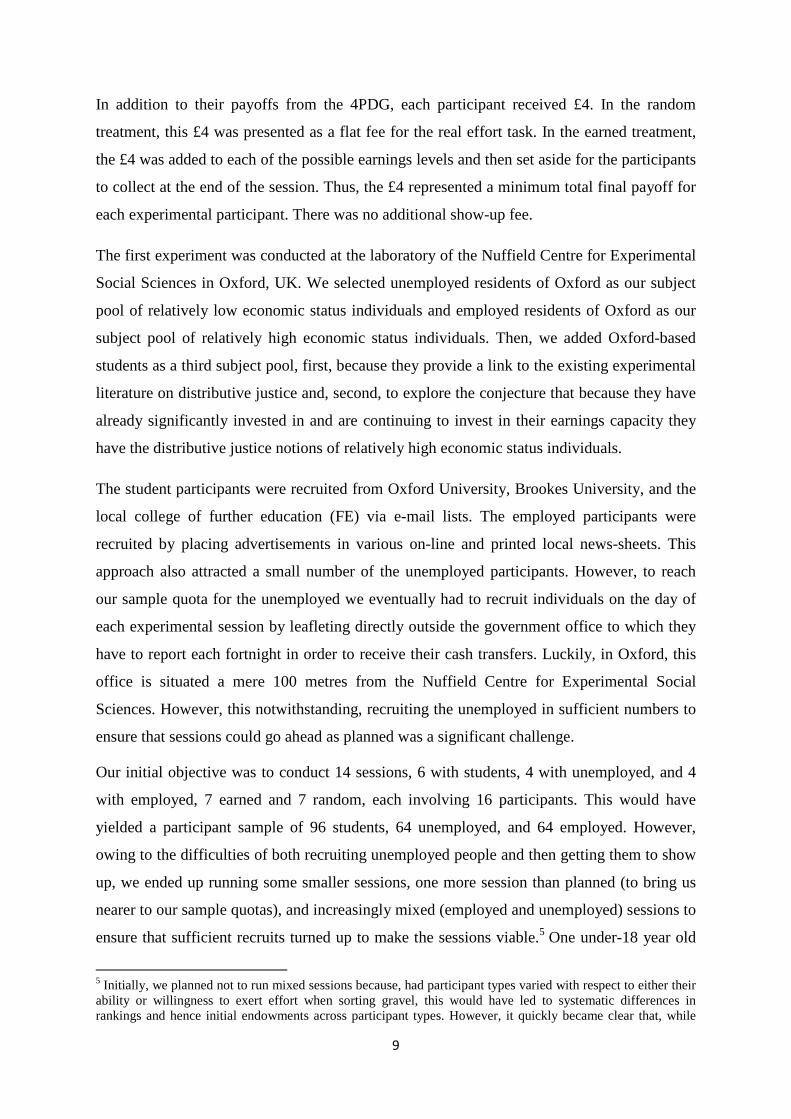
In addition to their payoffs from the 4PDG, each participant received £4. In the random

treatment, this £4 was presented as a flat fee for the real effort task. In the earned treatment,

the £4 was added to each of the possible earnings levels and then set aside for the participants

to collect at the end of the session. Thus, the £4 represented a minimum total final payoff for

each experimental participant. There was no additional show-up fee.

The first experiment was conducted at the laboratory of the Nuffield Centre for Experimental

Social Sciences in Oxford, UK. We selected unemployed residents of Oxford as our subject

pool of relatively low economic status individuals and employed residents of Oxford as our

subject pool of relatively high economic status individuals. Then, we added Oxford-based

students as a third subject pool, first, because they provide a link to the existing experimental

literature on distributive justice and, second, to explore the conjecture that because they have

already significantly invested in and are continuing to invest in their earnings capacity they

have the distributive justice notions of relatively high economic status individuals.

The student participants were recruited from Oxford University, Brookes University, and the

local college of further education (FE) via e-mail lists. The employed participants were

recruited by placing advertisements in various on-line and printed local news-sheets. This

approach also attracted a small number of the unemployed participants. However, to reach

our sample quota for the unemployed we eventually had to recruit individuals on the day of

each experimental session by leafleting directly outside the government office to which they

have to report each fortnight in order to receive their cash transfers. Luckily, in Oxford, this

office is situated a mere 100 metres from the Nuffield Centre for Experimental Social

Sciences. However, this notwithstanding, recruiting the unemployed in sufficient numbers to

ensure that sessions could go ahead as planned was a significant challenge.

Our initial objective was to conduct 14 sessions, 6 with students, 4 with unemployed, and 4

with employed, 7 earned and 7 random, each involving 16 participants. This would have

yielded a participant sample of 96 students, 64 unemployed, and 64 employed. However,

owing to the difficulties of both recruiting unemployed people and then getting them to show

up, we ended up running some smaller sessions, one more session than planned (to bring us

nearer to our sample quotas), and increasingly mixed (employed and unemployed) sessions to

ensure that sufficient recruits turned up to make the sessions viable.5 One under-18 year old

5 Initially, we planned not to run mixed sessions because, had participant types varied with respect to either theirability or willingness to exert effort when sorting gravel, this would have led to systematic differences inrankings and hence initial endowments across participant types. However, it quickly became clear that, while

10

and several retired people participated and had to be dropped from the sample prior to

analysis. Thus, we ended up with an analyzable sample containing 204 participants; 80

students (61 in universities, 19 in FE), 62 unemployed, and 62 employed. The main

characteristics of this sample and their assignment to treatments are presented in Table 1.

Despite the mixed sessions, Table 1 indicates that we managed to balance the sample by

participant type across the earned and random treatments. However, the individual

characteristics of our three sub-samples vary markedly. The students were significantly

younger, the employed had completed significantly more education, and women were

overrepresented in the employed sample and very much underrepresented in the unemployed

sample, probably owing child care arrangements or a lack thereof.

B. Analytical Framework

Consider a participant i with the following utility function:

(1) = −ݔߛ ∑ߚ ൫ݔ− ൯

ଶସୀଵ

where ݔ is participant i’s allocation to him or herself in the 4PDG expressed as a proportion

of the maximum amount that i could allocate to him or herself (£44), ݔ is participant i’s

allocation to participant j also expressed as a proportion of the maximum amount that i could

allocate j (also £44), is the proportional allocation to j that participant i perceives as fair

in context k, and andߛ areߚ the preference parameters associated with own final allocation

and adherence to own notions of distributive justice. 6 Assuming an interior solution,

maximizing subject to the constraint ∑ ݔସୀଵ = 1 yields the optimal allocations, ݔ

∗ and

ஷݔ∗ :

(2) ݔ∗ =

+ଷఊ

ଶఉஷݔ∗ =

−ఊ

ଶఉ

students tended to process more pots especially in the earned treatment, there was no significant differencebetween the employed and unemployed.6 Cappelen et al. (2007) used a similar utility function, the key differences being that they focused on absoluteallocations and initial earned endowments and on only one context. We focus on proportional allocations andinitial endowments because, in our game, the sums of the initial endowments and the final allocations are fixedand held constant across all game sets of four players. We condition on context because, unlike Capellen et al.(2007), we conducted both earned and random initial endowment versions of the game.

11

Thus, i’s optimal allocations are directly related to the allocations that i perceives as fair and

that, as long as <ߛ 0 and <ߚ 0, the allocation to self is greater than the fair allocation to

self and the allocation to each of the others is less than the fair allocation to each of those

others.

The two most likely determining factors of are participant j’s initial endowment

expressed as a proportion of the sum of all initial endowments (£44), ,ݕ and the equal

division, =)തݕ ¼), and given the model thus far, it is natural to express as the weighted

average of these two, = ߙ

ݕ+ ൫1 − ߙ൯ݕത.

Two decision-making contexts were created, in one the initial endowments, ,ݕ were earned

(indicated below by = ), in the other they were random (indicated below by = .(ݎ The

weights assigned by different types of i to their co-participants’ initial endowments in these

two contexts depend on their notions of distributive justice. Rawlsian egalitarians would have

both ߙ and ߙ

equal to zero and so their allocations to themselves and others would never be

related to initial endowments. Liberal egalitarians would have ߙ equal a value greater than

zero and, as long as no other preferences come into play, ߙ equal to zero. However, a

preference for not taking from others in any context would manifest as a greater than zero ߙ

and a liberal egalitarian with such a preference would then have ߙ ߙ�<

> 0.

So, the earned endowment effect (EEE) associated with liberal egalitarianism corresponds to

the difference ߙ−ߙ�

and we can investigate whether any given type of experimental

participant is subject to an EEE by estimating linear regression Model 1:

ஷݔ∗ = � + � ଵܧ+ ଶݕ+ ଷ൫ܧ∗ +൯ݕ ߝ

where ܧ takes the value 1 if played under the earned treatment and zero if played under

the random treatment, , ଵ, ଶ, and ଷ are the coefficients to be estimated, and ߝ is the

error term which is non-independent within and will be adjusted accordingly by clustering.7

The coefficient in this empirical specification corresponds to (1 − ߙ)ݕത− ߛ ⁄ߚ2 in the

theoretical model,8 the coefficient ଵ corresponds to ߙ)−ߙ�

)ݕത, ଶ simply corresponds to

7 The error terms may also be non-independent within sessions. We will return to this issue below.8 Note that, owing to ,ߚ varies across individuals. So, to be strictly consistent with the theoretical framework,we should include individual fixed effects in the model. However, if we do this, the coefficient ଵ would not beidentified. For this reason, we present estimations that do not include individual fixed effects. Including fixedeffects does not substantively change any of the findings reported below.

12

ߙ and ଷ corresponds to ߙ)

−ߙ�). So, an EEE manifests in two ways: a negative ଵ and a

positive ଷ.

Initially, we estimate this model for each of our participant sub-samples in turn. Below, we

refer to these models as Model 1s, based only on the student sample, Model 1e, based only on

the employed sample, and Model 1u, based only on the unemployed sample. Then we pool

across pairs of sub-samples and introduce one sub-sample identifier and three more

interaction terms. So, when comparing the unemployed to the employed, for example, we

pool the allocations to others made by each of those sub-samples and estimate Model 2:

ஷݔ��∗ =�� + � ଵܧ+ ଶݕ+ ଷ൫ܧ∗ +൯ݕ

+ ସ+ ହ(ܧ∗ ) + ൫ݕ ∗ ൯+ ൫ܧ∗ ݕ ∗ ൯+ ߝ

where equals 1 if the decision-making participant is unemployed and zero if is

employed. Now, the coefficients , �ଵ, ଶ, and ଷ pertain to the employed participants’

behavioural tendencies and the coefficients ସ, ହ, , and identify any differences in

behavioural tendencies between the unemployed and the employed. Most importantly, ହ and

identify differences in the EEE.

In all estimations we exclude those participants who made the maximal allocation to

themselves as, owing to their low ,ߚ their ߙ are not manifest in our data.

With these models fully specified, we can set out our hypotheses in precise terms.

Hypothesis 1: For high economic status individuals, i.e., students and employed people, the

EEE is positive, so the coefficient ଷ in Models 1s, 1e and 2 is positive and the coefficient ଵ

in Models 1s, 1e and 2 is negative.

Hypothesis 2: For low economic status individuals, i.e., unemployed people, the EEE is zero,

so the coefficients ଵ and ଷ in Model 1e are zero; the coefficients ହ and in Model 2 are

positive and negative respectively; and the sum of coefficients ଵ and ହ and the sum of

coefficients ଷ and in Model 2 are zero.

13

II. RESULTS

A. Experiment 1: Oxford, UK

Before turning to the regression analyses and the formal tests of the hypotheses stated above,

it is useful to take a look at the experimental data. In Table 2, we present a brief summary of

behaviour for the sub-samples of participants that played under the random and earned

treatments. In the first column, we pool across participant types. In the second, third, and

fourth columns we present the same statistics for students, the employed, and the unemployed

participants separately. Table 2 reveals that only 12 and 5 percent of the participants in the

random and earned treatments respectively acted in accordance with pure selfishness by

allocating all of the counters to themselves. These proportions are very low compared to

other studies. We think that this is owing to the experiment not being computerized. Given

our objectives, this feature of the data is useful as purely selfish participants reveal nothing

about their ߙ. The table also reveals that 38 and 29 percent of the participants made equal

allocations to themselves and others under the random and earned treatments respectively and

that, while only 1 percent left the initial endowments untouched in the random treatment, 13

percent did so in the earned treatment.

Just over and just under one quarter of the students made equal allocations in the random and

earned treatments respectively, while the proportions leaving the initial endowments

untouched were zero and just over ten percent respectively. More than half of the employed

made equal allocations in the random treatment, while less than a third did so in the earned

treatment. The proportion leaving the initial endowments untouched moved in the opposite

direction, from less than 5 and over 15 percent. Just over one third of the unemployed made

equal allocations under both treatments (marginally more under the earned treatment).

However, while none left the initial endowments untouched under the random treatment, just

under 10 percent did so under the earned treatment.

Under both treatments all participant types allocated more to themselves as compared to

others, with students allocating the most to themselves on average. The table suggests that

employed and unemployed participants allocated somewhat less on average to themselves in

the earned treatment. However, the difference is only statistically significant in the case of the

employed.

14

The differences in mean allocations to self and others are consistent with the theoretical

model presented above. The proportions of participants choosing equal allocations and not to

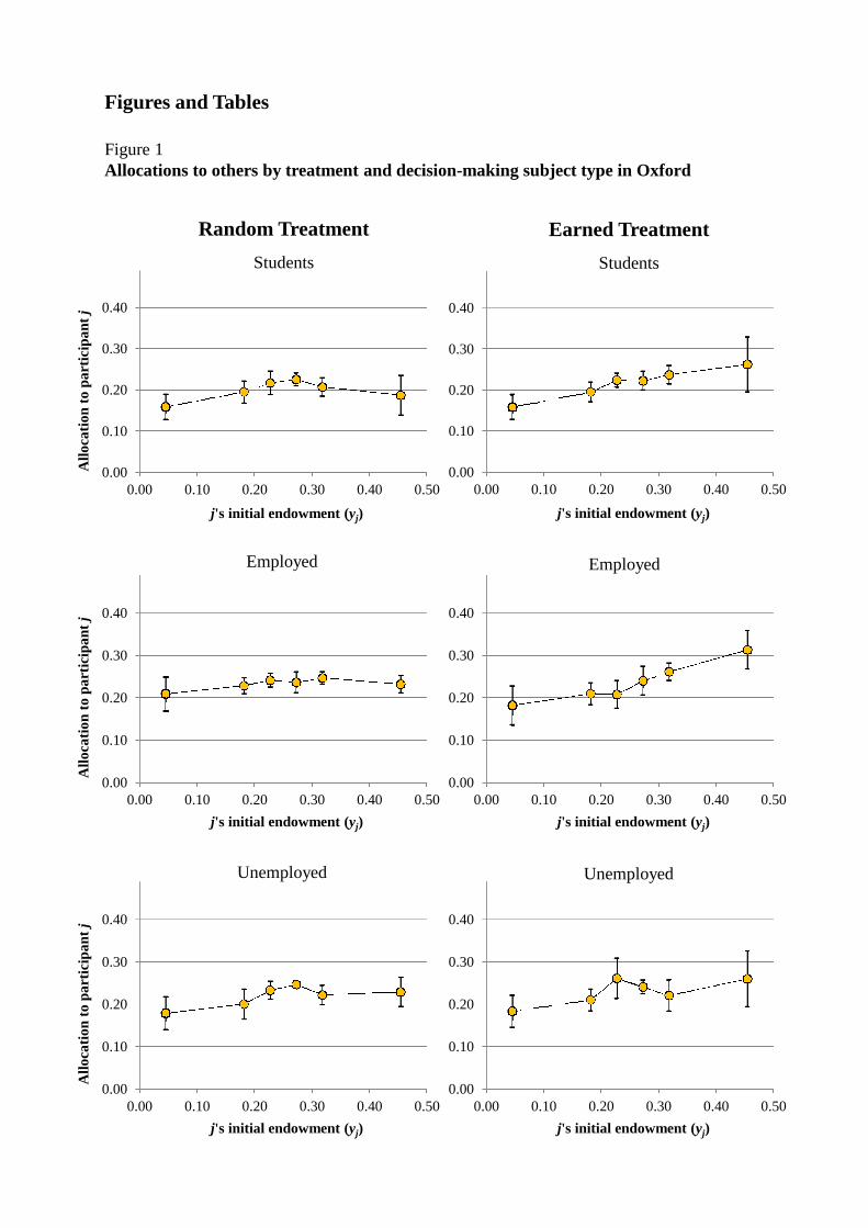
redistribute at all are broadly in line with our hypotheses. However, Figure 1, in which mean

allocations to others are plotted against those others’ initial endowments for each participant

type under each treatment, offers greater insight. Participants allocating nothing to others are

excluded.

The upper and middle panels in Figure 1 show that students and the employed conditioned

final allocations to others on those others’ initial endowments in the earned treatment, but not

in the random treatment. In the case of the students the EEE is concentrated at the upper end

of the domain. In the case of the employed it manifests as a swivel about a midpoint, which is

entirely consistent with the theory. The lower panel reveals a less clear pattern for the

unemployed. There may be a positive relationship between final allocations and initial

endowments under the earned treatment. However, note how similar the graphs relating to the

two treatments are; there is no evidence of an EEE here. Figure 1 provides further but still

preliminary support for our hypotheses.

In Table 3 we present a series of linear regressions conforming to either Model 1 or Model 2

above. The first, second, and third columns contain estimations of Model 1 for students, the

employed, and the unemployed respectively. The estimations for students and the employed

reveal the expected EEE: the coefficient ଵ, on the earned treatment identifier, E, is negative

and significant; the coefficient, ଷ, on j’s initial endowment, yj, interacted with the earned

treatment identifier, E, is positive and significant. Finally, the coefficient, ଶ, on j’s initial

endowment, yj, uninteracted is insignificant. Together, these results indicate that the swivels

in the relationships between final allocations and initial endowments from flat in the random

treatment to upward-sloping in the earned treatment that we observed in Figure 1 are

statistically significant. In the earned treatment, a one percentage point increase in initial

endowment leads to a 0.3 percentage point increase in final allocations made by students and

a 0.27 percentage point increase in final allocations made by employed participants.

The estimation for the unemployed tells a different story. Here the significant positive

coefficient, ଶ, on j’s initial endowment, yj, uninteracted indicates a positive relationship

between those initial endowments and final allocations, while the insignificant coefficients

ଵ, on E, and ଷ, on the interaction between yj and the earned treatment identifier, E, indicate

no EEE. Finally, it is worth noting that the slope of the relationship between initial

15

endowments and final allocations is considerably smaller in magnitude than the slope in the

earned treatment for students and the employed. Here, a one percentage point increase in

initial endowment leads to a 0.13 percentage point increase in final allocations.

When we pool the student and employed samples and estimate an appropriately adjusted

version of Model 2, we find no significant differences in behaviour between the two

participant types.9 However, when we pool across all three participant types and estimate

Model 2, distinguishing between the unemployed and the other two types, the coefficients

and standard errors reported in the fourth column of Table 3 are returned.

The significant positive coefficient, ହ, on the interaction between the unemployed identifier

and the earned treatment identifier, E, and the significant negative coefficient, , on the

three way interaction between the unemployed identifier, Ui, yj and E indicate that the

unemployed are significantly different in terms of the treatment effect. In addition, linear

restriction tests do not allow us to reject the hypotheses that ଵ + ହ = 0 and ଷ + = 0

indicating, once again, that the unemployed are not subject to an EEE.

To test the robustness of these findings we extended Model 2 to include several control

variables and their interactions with yj, E and yj x E. To minimize the problem of

multicollinearity that tends to arise when multiple interactions involving the same variables

are introduced into a regression model, we investigated one control variable at a time. The

control variables investigated in this way were: the high inequality treatment identifier; the

real effort task undertaken (filling or emptying); and the decision-making participant’s own

initial endowment, age, sex, education. None of the additional controls or interactions bore a

significant coefficient. Owing to Jakiela et al’s (2011) reporting of an effect of education on

sharing rules, in the fifth column of Table 3 we present the regression containing the

education controls. Then, in column 6, we present a regression containing the education

controls but not the unemployed identifier and its interactions with yj, E and yj x E. Thus, we

see that when we do not factor in the effects of unemployment, education is associated with

an EEE.

9 The estimations are not tabulated but are available from the authors on request.

16

B. Experiment 2: Cape Town, South Africa

The objective of the second experiment was to test the external validity of our findings by

rerunning the experiment in a different society. Given the prior interest in this literature on

the continent of Africa, we chose to take the experiment to Africa. However, to enhance

comparability, we chose to take it to a city containing an elite university as well as many

employed and unemployed people. Thus, we took it to Cape Town, South Africa. The Cape

Town experiment was identical to the Oxford experiment except that: the value of one

counter was set to 7 Rand (just over 1 USD), the flat earnings rate in the random treatment

and the put-aside minimum earnings in the earned treatment were set to 28 Rand (just over 4

USD); and the language used in the session script was simplified.10 We ran 15 sessions in

Cape Town, three involving only students and 11 involving a mix of principally employed

and unemployed people.11 We conducted the student sessions on campus in a room within the

main library and the other sessions in a municipal library, a school that runs courses for

adults, and a non-governmental organization that works with homeless and unemployed

people.

At first glance, the participant sample for the Cape Town experiment appeared very similar to

the Oxford sample; it included 101 students, 72 employed and 63 unemployed people.

However, while setting up for the recruitment it became clear that our assumptions about how

participant types map onto economic status would not apply as well in Cape Town as in

Oxford. First, the majority (75 percent) of the unemployed in our Oxford sample were

receiving means-tested government cash transfers at the time of the experiment indicating

that they were indeed of relatively low economic status, while in Cape Town there were no

equivalently indicative government cash transfers. Second, owing to the existence of the

government cash transfers in the UK, unemployment in the UK is clearly defined whereas in

South Africa it is not. Given this ambiguity combined with there being no safety-net and

unemployment being high (around 25 percent as compared with just under 8 percent in the

UK at the end of 2010) we conjectured that there may be many Cape Town residents who

work part time, casually or rarely and who variably refer to themselves as employed and

unemployed. Third, in comparison to Brooks and Oxford University, the University of Cape

10 Originally, we planned to translate the script. However, talking to prospective Cape Town participantsindicated that simplifying the language used would be sufficient. This meant that the script could be read by thesame person in both Oxford and Cape Town.11

Three students found their way into the mixed sessions.

17

Town, in partnership with various non-governmental organizations and the government, is far

more actively seeking to include individuals from low income households among its enrolled

students.

So, in Cape Town we asked the experimental participants to complete a more comprehensive

post-experimental questionnaire designed to explore this mapping of types onto relative

economic status and to give us an alternative measure by which to distinguish between

individuals of low and high economic status. The resulting data supported our conjectures

about type and economic status being only weakly associated in Cape Town. While the

average self-proclaimed employed person in our sample earned just below 6,000 Rand (just

over 880 USD) per calendar month, 30 percent earned less than the highest earner among the

unemployed.12 In addition, a question inviting the participants to categorize their households

as either rich, upper income, middle income, low income, or poor revealed that there was

considerable overlap not only between the employed and unemployed, but also between the

students and the other two groups.

Table 4 shows that, while the unemployed in our sample were far more likely than the

employed and the students to perceive their households as low income or poor, there was

greater variation in perceptions among the employed and students. So, 87 percent of the

unemployed indicated that they were from low income or poor households and 51 and 30

percent of the employed and the students respectively did likewise.13 Table 4 also shows that,

as in Oxford, individual characteristics varied markedly across the students, employed and

unemployed sub-samples. However, here the relative characteristics of the sample seem to

correspond more closely with data from large-scale surveys. Specifically, relative to the

employed, the unemployed are younger, more likely to be male and more likely to be of

African origin as compared to the employed (Bhorat, 2005).

In Table 5, we present a brief summary of behaviour for the Cape Town participants that

played under the random and earned treatments. In the first column, we pool across all

participants. In the second, third, and fourth columns we present the same statistics for

students, the employed, and the unemployed participants separately. Then, in the fifth and

12 The highest earner among the unemployed reported earnings of 2,000 Rand (approximately 300 USD) percalendar month. Ten out of the 63 unemployed people reported positive monthly earnings, with the averageacross those ten being 960 Rand (142 USD). Fields (2000) refers to this as South Africa's “employmentproblem” as opposed to its unemployment problem and characterizes the problem as encompassing not onlyunemployment but also the low hourly wages and low work hours of the employed.13

Of course, we know that individuals’ subjective evaluations of where they fall in an income distribution areoften incorrect. However, the greatest discrepancies tend to appear between the middle and upper income levels.

18

sixth columns we present the same statistics for high and low status participants. We define

high status participants as those who reported that their households were rich or high or

middle income and low status participants as those who reported that their households were

poor or low income.14

Table 5 reveals that only 1 and 3 percent of the participants in the random and earned

treatments respectively acted in accordance with pure selfishness. These proportions are even

smaller than those observed in Oxford. The table also reveals that 40 and 26 percent of the

participants made equal allocations to themselves and others under the random and earned

treatments respectively and that, while only 3 percent left the initial endowments untouched

in the random treatment, 10 percent did so in the earned treatment.

Almost one quarter of the students made equal allocations in the random treatment, while

only just over ten percent did likewise in the earned treatment. The proportion leaving the

initial endowments untouched moved in the opposite direction, from zero to over ten percent.

Two thirds of the employed made equal allocations in the random treatment, while less than

forty percent did so in the earned treatment. Again, the proportion leaving the initial

endowments untouched moved in the opposite direction, from zero to just under ten percent.

As in Oxford, the unemployed were distinct. Just under one third made equal allocations

under the random treatment, while over forty percent did so in the earned treatment. And the

proportion leaving the initial endowments untouched moved in the opposite direction, from

over ten percent in the random treatment to just over five percent in the earned treatment.

Dividing the sample according to economic status reveals that just over forty percent of the

high status participants made equal allocations under the random treatment, while only just

over fifteen percent did so in the earned treatment. And, once again, the proportion leaving

the initial endowments untouched moved in the opposite direction, from zero in the random

treatment to almost fifteen percent in the earned treatment. In contrast, the low status

participants were barely affected by the treatment: in each treatment, just under forty percent

made equal allocations (marginally fewer in the earned treatment) and just over five percent

left the initial endowments unaltered.

14 This approach yields two similarly sized sub-samples and obviates the problem that individuals from highincome and rich households tend to understate their economic status when asked this subjective question.

19

As in Oxford, under both treatments all participant types allocated more to themselves as

compared to others, with students allocating most to themselves on average. Average

allocations to self and others are almost indistinguishable across treatments.

The differences in mean allocations to self and others are consistent with the theoretical

model presented above. The proportions of participants choosing equal allocations and

electing not to redistribute at all are broadly in line with our hypotheses. However, Figures 2

and 3 in which mean allocations to others are plotted against those others’ initial endowments

for the various participant types under each treatment, offer greater insight. In Figure 2 the

sample is divided into students, the employed, and the unemployed. In Figure 3 the sample is

divided into participants with high and low economic status. Participants allocating nothing

to others are excluded.

The middle panel of Figure 2 reveals an EEE for the employed; they conditioned final

allocations to others on those others’ initial endowments in the earned treatment, but not in

the random treatment. The upper and lower panels reveal no sign of an EEE for the students

and the unemployed, although the lower panel suggests that the unemployed conditioned

their final allocations to others on those others’ initial endowments irrespective of treatment.

In Figure 3 the upper panel very clearly reveals an EEE for the high economic status

participants. In contrast, the lower panel reveals no evidence of an EEE for the low status

individuals, but clearly indicates that they conditioned final allocations to others on those

others’ initial endowments in both the random and the earned treatments.

The regressions in the first three columns of Table 6 confirm that the employed were subject

to an EEE, while the students and the unemployed were not. They also reveal that not only

the unemployed but also, to a lesser extent, the employed conditioned final allocations to

others on those others’ initial endowments in the random treatment. The regressions in the

fourth and fifth columns confirm that the high economic status participants were subject to an

EEE, while the low economic status participants were not. They also reveal that low and, to a

lesser degree, high economic status participants conditioned final allocations to others on

those others’ initial endowments in the random treatment.

Despite the apparent differences between the regressions in the first and second columns of

Table 6, when we pool the student and employed samples and estimate an appropriately

adjusted version of Model 2, we find no significant difference in behaviour between the two

types. Using a similar approach, we find no significant difference in behaviour between

20

students and the unemployed, and the employed and the unemployed. However, when we

work with the full sample and estimate an appropriately adjusted version of Model 2 that

includes an identifier for the participants with low economic status and interacts this variable

with yj, E and yj x E, the estimates presented in the sixth and final column of Table 6 are

returned. These reveal that the differences in treatment effects between the high and low

status participants are statistically significant. It seems that, in Cape Town, individual notions

of distributive justice are associated with participants’ relative economic status rather than

their type or labour market status.

When we add controls to the analysis of the Cape Town data the problem of multicollinearity

looms large. When we add the decision-making participant’s own initial endowment it bears

an insignificant coefficient and leaves the results reported above unchanged. Adding the

binary variable that identifies participants of African ethnic origins and its interactions with

yj, E and yj x E yields similar results. However, when we add the decision-making

participant’s own initial endowment and this variable’s interactions with yj, E and yj x E,

while they all bear insignificant coefficients and are jointly insignificant, the coefficients on E

and yj are rendered insignificant. Adding the binary variable that identifies female

participants and its interactions with yj, E and yj x E yields similar results. Adding the

participants’ age and this variable’s interactions with yj, E and yj x E yields similar results

again, except that age and its interactions are jointly significant. Further investigation

indicates that when only age uninteracted is added it bears a significant positive coefficient

while leaving the results pertaining directly to our hypotheses unchanged and that, when

added to this model, the interactions with age are jointly insignificant. Finally, adding the

natural log of the participants’ years of education and its interactions with yj, E and yj x E

renders the coefficients on E, yj, and yj x L x E insignificant, while the four new variables are

singly insignificant but jointly significant. However, when only the natural log of years

education variable uninteracted is added, while it bears a significant negative coefficient, the

results pertaining directly to our hypotheses are left unchanged and when the three

interactions with the education variable are added to this model they are jointly insignificant.

Further, when the education variable and its interactions are included but the low economic

status identifier and its interactions are not, neither education nor any of its interactions bear

significant coefficients and they are jointly insignificant.15


21

We draw the following conclusions from this investigation: older participants allocate more

to others on average; more educated participants allocate less to others on average; there is no

evidence that the EEE varies depending on the allocators’ initial endowments or their sex,

age, ethnicity, or education in the same manner as their economic status; however, our

findings relating directly to our hypotheses are not as robust as we would like owing to

multicollinearity.

C. Further exploratory analysis of the Oxford data and the two datasets pooled

The findings from the Cape Town experiment indicated that individual notions of distributive

justice are associated with participants’ relative economic status rather than their type or

labour market status. This caused us to wonder whether we could improve our analysis of the

Oxford data by accounting for differences in economic status within types. In Oxford we did

not ask participants whether their households were rich, upper income, middle income, low

income, or poor. However, we knew that our unemployed sample included some who were

not receiving cash transfers from the government and judged it reasonable to assume that they

would be of higher economic status. Similarly, we knew that our student sample included

both university and FE students and judged it reasonable to assume that the FE students

would originate from households with relatively lower economic status. 16 Among the

employed, 44 of the 62 answered a question about which income bracket their household fell

into potentially allowing us to distinguish between high and low economic status individuals

in that sub-sample also.

The outcome of this exploratory investigation is presented in Table 7. The first and second

columns of Table 7 contain estimations of Model 1 for unemployed participants who are not

and who are receiving government transfers respectively. For the unemployed not receiving a

transfer, the coefficient on the interaction between initial endowments and the earned

treatment identifier, yj x E, is positive and significant. This is consistent with an EEE and so

too is the negative coefficient on the earned treatment identifier uninteracted, although the

latter is insignificant. For the unemployed receiving a transfer, there is no evidence of an EEE

and, once again, we see evidence of the conditioning of allocations on initial endowments

even when those initial endowments are randomly assigned.

16 Further, Mchintosh (2006) shows that UK FE graduates earn less, on average, than UK university graduates inlater life, i.e., the FE graduates can expect less upward mobility.

22

The third and fourth columns of Table 7 contain estimations of Model 1 for university and FE

students respectively. The estimation for the university students reveals an EEE, the

coefficient on yj x E is positive and significant, while the coefficient on E uninteracted is

negative and significant. However, for the FE students there is no evidence of an EEE. In the

fifth column the two types of student are pooled and an appropriately adjusted version of

Model 2 is estimated to reveal that the university and FE students are distinct with regard to

their notions of distributive justice. However, a similar analysis of the unemployed revealed

that those receiving and not receiving transfers were not statistically distinguishable in the

same way (estimation not tabulated). None of our analyses of the employed sub-sample

yielded significant findings.

Using an adjusted version of Model 2 to compare, first, FE students and the unemployed and,

second, the unemployed not receiving benefits and the employed revealed no statistically

significant behavioural differences.17 So, in the final column of Table 7 we estimate another

appropriately adjusted version of Model 2 in which university students, the employed, and

the unemployed not receiving transfers are treated as a single sub-sample of relatively high

economic status individuals, FE students and the unemployed who are receiving transfers are

treated as a separate sub-sample of relatively low economic status individuals and the two

sub-samples are compared. Thus, we see that the two sub-samples are different, the high

status sample is subject to an EEE, and according to linear restriction tests (Ho: ଵ + ହ = 0

and Ho: ଷ + = 0) the low status sub-sample is not. However, dividing the sample with

reference to assumed economic status rather than known employment status only marginally

improved the fit of the model.

Before concluding, and with a considerable degree of circumspection, we could not resist

pooling the Oxford and Cape Town samples in order to test for cross-context differences. The

first column in Table 8 presents a version of Model 2 that distinguishes between high and low

status participants in Oxford (previously presented in the final column of Table 7). The

second column of Table 8 presents the same model for participants in Cape Town (previously

presented in the final column of Table 6). The third and final column in Table 8 presents an

extended version of Model 2 based on the data from both cities. This model contains all of

the regressors used in the preceding two models, a binary variable indicating that a data point

was generated in Cape Town and the interactions between that indicator variable and all of


23

the other regressors. Neither the Cape Town indicator variable nor any of the new interaction

terms bears a significant coefficient and they are also jointly insignificant. So, despite the

minor differences in the experiment between the two contexts (stakes and scripts) and the

major differences in the way that high and low economic status participants are identified in

the datasets, we cannot reject the hypothesis that the relationship between notions of

distributive justice and relative economic status is common across these two very distinct

contexts.

Finally, pooling offers one further advantage; it allows us to control for the possible non-

independence of errors across participants within sessions.18 Clustering by session yields

lower standard errors on the variables of principle interest, while leaving the coefficient on

Cape Town and all of its interactions insignificant both individually and jointly.19

III. SUMMARY, DISCUSSION AND CONCLUSION

This paper presented the findings from two experiments designed to investigate whether

individuals’ notions of distributive justice are associated with their economic status relative to

others within their societies. Specifically, the experiments allowed us to establish whether the

earned endowment effect (EEE) varied with the relative (within society) economic status of

the experimental participants. We hypothesised that, while the EEE would be significant

among high economic status individuals, i.e, that high economic status individuals would

make allocations to others that reflect those others’ initial endowments considerably more

when those endowments were earned rather than pure windfall gains, among low status

individuals the EEE would be less pronounced or absent.

The findings from the first experiment, conducted in Oxford, United Kingdom, supported this

hypothesis; among students and the employed there was a statistically significant EEE,

among the unemployed there was not and the difference between the two participant pools

was significant. The findings from the second experiment, conducted in Cape Town, South

Africa, also supported the hypothesis; among individuals who classified their own households

as rich or high income there was a statistically significant EEE, among individuals who

18 We could not do this when working on each dataset separately because, with only 15 sessions-worth of data,the clustered standard errors would have been biased.19 The estimations are not tabulated but are available from the authors on request.

24

classified their own households as poor or low or middle income there was not and the

difference between the two participant pools was significant.

Additional analysis of the Oxford data revealed that we could marginally improve on our

earlier results by accounting for differences in economic status within the student and

unemployed participant samples. And finally, while there were many reasons why we should

not expect the Oxford and Cape Town data to pool, when doing so we found no evidence of a

difference in the relationship between individual notions of distributive justice and relative

economic status. This null finding supports the conclusion that it is relative economic status

within a society that is associated with an individual’s notions of distributive justice and that

this is a generalizable result even though definitions of relative economic status may vary

across societies.

One of our findings was unexpected. For the low status participants in Cape Town and the

unemployed receiving government transfers in Oxford the absence of an EEE was owing, in

part, to such participants conditioning their allocations to others on those others’ initial

endowments even when those endowments were windfalls rather than earnings. This is

consistent with the lower status individuals being less willing to take from others under any

conditions. Our efforts to find a theoretical explanation for this finding in the literature have

been unsuccessful. However, conversations with colleagues and other social scientists

interested in distributive justice have raised a few interesting suggestions. Here are two that

we think can be disregarded given our data and one that we think is worthy of study.

First, there is the possibility that the lower status participants were more stressed by the

unusual context in which they were placed during the experiment and became more passive

as a consequence. However, note from Table 2 that in Oxford the unemployed were the least

likely to leave the initial endowment unchanged. And in Cape Town, Table 5 shows that,

while the low status participants were more inclined than the high status participants to leave

the initial endowments unchanged, in the random treatment they were less inclined to do so.

Second, it may be that lower status individuals are lazier and so stopped reallocating counters

before reaching their otherwise preferred distribution. If this were the case, we would expect

this laziness also to manifest in the number of pots participants processed in the first stage of

the experiment. However, in Oxford there was no difference in the number of pots processed

by the relatively high and low status participants and in Cape Town the relatively low status

participants process marginally fewer pots only in the earned treatment.

25

Third, there is one striking similarity between the low status participants in the Cape Town

sample and the unemployed receiving government transfers in the Oxford sample; on average

they had 11.2 and 11.5 years of education respectively compared to 13.3 years of education

for the rest of the participants in each city. In our regressions controlling for years of

education presented or described above we found no effect of education on the conditioning

of allocations on initial endowments in the random treatment. However, we treated education

as a continuous variable. Perhaps there is a critical change in the way individuals are taught if

they remain in school beyond their first public exams (taken at the age of 16 in both

countries). Perhaps the education systems in both countries are devised to ensure that those

who leave education prior to or at this point have been inculcated into believing that taking

anything from other people is bad, while those who continue in education beyond this point

are encouraged to think more freely. This would be worthy of further investigation.

Finally, there are certain aspects of our study that could be improved upon in future work.

First and most importantly, our participant samples are not representative of the populations

from which they were drawn. Second, our survey data covered only a few variables of

interest and did not go into as much depth concerning income and wealth as would have been

ideal. Both of these concerns could be addressed by embedding the experiment within

existing household or individual surveys covering random samples of respondents. Third, we

conducted our experiment in only two societies. Ideally, one would conduct it in a larger

number of societies that vary along different dimensions of interest. Fourth, it is important to

bear in mind that we have not identified a causal relationship. And finally, our findings tell us

nothing about the preferences of the very rich.

REFERENCES

Alesina, A. and George Marios Angeletos. “Fairness and Redistribution: US vs. Europe.”

American Economic Review, 2005, 95, pp. 913-35.

Alesina, Alberto, and Paola Giuliano. “Preferences for Redistribution.” In Jess Benhabib,

Alberto Bisin, and Matthew Jackson (eds), Handbook of Social Economics, 2011, Elsevier.

Alesina, Alberto F., and Edward Glaeser. Fighting Poverty in the US and Europe: A World

of Difference. 2004, Oxford, UK, Oxford University Press.

26

Alesina, Alberto F., and Eliana la Ferrara. “Preferences for Redistribution in the Land of

Opportunities.” Journal of Public Economics, 2005, 89, pp. 897-931.

Alesina Alberto F. and Dani Rodrik. “Distributive Policies and Economic Growth.”

Quarterly Journal of Economics, 1994, 109, pp. 465–490.

Babcock, Linda, and George Loewenstein. “Explaining bargaining impasse: the role of

self-serving biases.” Journal of Economic Perspectives. 1997, 11, pp. 109-126.

Benabou, Roland, and Efe A. Ok. “Social Mobility and the Demand for Redistribution: the

POUM Hypothesis.” Quarterly Journal of Economics, 2001, 116, pp. 447-487.

Benabou, Roland, and Jean Tirole. “Beliefs in a Just World and Redistributive Politics.”

Quarterly Journal of Economics, 2006, 121(2), pp. 699-746.

Bhorat, Haroon. “Poverty, Inequality and Labour Markets in Africa: A Descriptive

Overview.” Working Papers 9631, University of Cape Town, Development Policy Research

Unit.

Bowles, Samuel, Herbert Gintis, and Melissa Osborne. “The Determinants of Earnings: A

Behavioral Approach.” Journal of Economic Literature, 2001, 39(4), pp. 1137-1176.

Cappelen, Alexander W., Astri Drange Hole, Erik O. Sorensen, and Bertil Tungodden.

“The pluralism of fairness ideals: An experimental approach." American Economic Review,

2007, 97 (3), pp. 818-827.

Cherry, Todd L. “Mental Accounting and Other-regarding Behavior: Evidence from the

Lab.” Journal of Economic Psychology, 2001, 22 (5), 605-615.

Cherry, Todd L., Peter Frykblom, and Jason F. Shogren. “Hardnose the Dictator.”

American Economic Review, 2002, 92 (4), pp. 1218-1221.

Clark, Andrew E. “Unemployment as a Social Norm: Psychological Evidence from Panel

Data.” Journal of Labor Economics, 2001, 21(2), pp. 323-351.

Drazen, Allan. Political Economy in Macroeconomics, Princeton, Princeton University

Press.

Fields, Gary S. “The Employment Problem in South Africa.” 2000, Trade and Industry

Monitor.

27

Fong, Christina. “Social Preferences, Self-Interest, and the Demand for Redistribution.”

Journal of Public Economics, 2001, 82, pp. 225-246.

Frohlich, Norman, Joe Oppenheimer, and Anja Kurki. “Modeling other-regarding

preferences and an experimental test.” Public Choice, 2004 119, pp. 91–117.

Galor, Oded and Josepth Zeira. “Income Distribution and Macroeconomics.” Review of

Economic Studies, 1993, 60, pp. 35-52.

Gantner, Anita, Werner Güth, and Manfred Königstein. “Equitable choices in bargaining

games with joint production.” Journal of Economic Behavior and Organization, 2001, 46, pp.

209–225.

Giuliano, Paola, and Antonio Spilimbergo. “Growing Up in Bad Times: Macroeconomic

Volatility and the Formation of Beliefs.” UCLA mimeo, 2008.

Hampson, Tom., Jemima Olchawski, and Fabian Society. Is Equality Fair?: What the

Public Really Think About Equality - and What We Should Do About It. 2009, London:

Fabian Society.

Hoffman, Elizabeth, Kevin A. McCabe, Keith Shachat, and Vernon L. Smith.

“Preferences, Property Rights, and Anonymity in Bargaining Games.” Games and Economic

Behavior, 1994, 7 (3), pp. 346-380.

Jakiela, Pamela. “Social Preferences and Fairness Norms as Informal Institutions:

Experimental Evidence.” American Economic Review. Papers and Proceedings, 2011.

Jakiela, Pamela, Edward Miguel, and Vera L. te Velde. “You've Earned It: Combining

Field and Lab Experiments to Estimate the Impact of Human Capital on Social Preferences.”

Mimeo.

Konow, James. “Fair shares: Accountability and cognitive dissonance in allocation

decisions.”American Economic Review, 2000, 90 (4), pp. 1072-1091.

List, John, and Todd L. Cherry. “Examining the Role of Fairness in High Stakes

Allocation Decisions” Journal of Economic Behavior and Organization, 65, 1-8.

Luttmer, Erzo F.P. and Monica Singhal. “Culture, Context and the Taste for

Redistribution.” American Economic Journal: Economic Policy, 2011, 3(1), pp. 157-79.

28

Mcintosh, Steven. “Further Analysis of the Returns to Academic and Vocational

Qualifications.” Oxford Bulletin of Economics and Statistics. 2006, 68(2), 225-251.

Meltzer, Allan H and Scott F. Richards. “A Rational Theory of the Size of Government.”

Journal of Political Economy. 1981, 89, pp. 914–927.

Miller, David. Social Justice, 1976, Oxford, Clarendon Press.

Milne, Heather. “Desert, effort and equality”, Journal of Applied Philosophy, 1986, 3, pp.

235-243.

Nozick, Robert. Anarchy, State and Utopia, 1974, New York, Basic Books.

Oxoby, Roberts, and John Spraggon. “Mine and yours: Property rights in dictator games.”

Journal of Economic Behavior and Organization, 2008, 65, pp. 703-713.

Paul, Karsten I., and Klaus Moser. “Unemployment impairs mental health: Meta-

analyses.” Journal of Vocational Behavior, 2009, 74 (3), pp. 264-282.

Perotti Roberto. “Political Equilibrium, Income Distribution and Growth.” Review of

Economic Studies, 1993, 60(4), pp. 755-776.

Personn, Torsten, and Guido Tabellini. Political Economics: Explaining Economics

Policy, 2002, Cambridge, Massachusetts, MIT Press.

Rawls, John. A Theory of Justice. 1971, Harvard, MA, Harvard University Press.

Ruffle, Bradley J. “More is better, but fair is fair: Tipping in dictator and ultimatum games.”

Games and Economic Behavior, 1998, 23 (2), pp. 247-265.

Rutström, E. Elisabet, and Melonie B. Williams. “Entitlements and fairness: an

experimental study of distributive preferences.” Journal of Economic Behavior and

Organization, 2000, 43(1), 75–89.

Winefield, Anthony H., Helen R. Winefield, Marika Tiggemann and Robert D. Goldney.

“A Longitudinal Study of the Psychological Effects of Unemployment and Unsatisfactory

Employment on Young Adults.” Journal of Applied Psychology, 1991, 76 (3), pp. 424-431.

0.00

0.10

0.20

0.30

0.40

0.00 0.10 0.20 0.30 0.40 0.50

j's initial endowment (yj)

Earned Treatment

Students

0.00

0.10

0.20

0.30

0.40

0.00 0.10 0.20 0.30 0.40 0.50

All

oca

tio

nto

pa

rtic

ipa

nt

j


Random Treatment

Students

0.00

0.10

0.20

0.30

0.40

0.00 0.10 0.20 0.30 0.40 0.50


Employed

0.00

0.10

0.20

0.30

0.40

0.00 0.10 0.20 0.30 0.40 0.50

All

oca

tio

nto

pa

rtic

ipa

nt

j


Employed

0.00

0.10

0.20

0.30

0.40

0.00 0.10 0.20 0.30 0.40 0.50


Unemployed

0.00

0.10

0.20

0.30

0.40

0.00 0.10 0.20 0.30 0.40 0.50

All

oca

tio

nto

pa

rtic

ipa

nt

j


Unemployed

Figures and Tables

Figure 1Allocations to others by treatment and decision-making subject type in Oxford

0.00

0.10

0.20

0.30

0.40

0.00 0.10 0.20 0.30 0.40 0.50


Earned Treatment

Students

0.00

0.10

0.20

0.30

0.40

0.00 0.10 0.20 0.30 0.40 0.50

All

oca

tio

nto

pa

rtic

ipa

nt

j


Random Treatment

Students

0.00

0.10

0.20

0.30

0.40

0.00 0.10 0.20 0.30 0.40 0.50


Employed

0.00

0.10

0.20

0.30

0.40

0.00 0.10 0.20 0.30 0.40 0.50

All

oca

tio

nto

pa

rtic

ipa

nt

j


Employed

0.00

0.10

0.20

0.30

0.40

0.00 0.10 0.20 0.30 0.40 0.50


Unemployed

0.00

0.10

0.20

0.30

0.40

0.00 0.10 0.20 0.30 0.40 0.50

All

oca

tio

nto

pa

rtic

ipa

nt

j


Unemployed

Figure 2Allocations to others by treatment and decision-making subject type in Cape Town

0.00

0.10

0.20

0.30

0.40

0.00 0.10 0.20 0.30 0.40 0.50


Earned Treatment

High economic status

0.00

0.10

0.20

0.30

0.40

0.00 0.10 0.20 0.30 0.40 0.50

All

oca

tio

nto

pa

rtic

ipa

nt

j


Random Treatment

High economic status

0.00

0.10

0.20

0.30

0.40

0.00 0.10 0.20 0.30 0.40 0.50


Low economic status

0.00

0.10

0.20

0.30

0.40

0.00 0.10 0.20 0.30 0.40 0.50

All

oca

tio

nto

pa

rtic

ipa

nt

j


Low economic status

Figure 3Allocations to others by treatment and decision-making subject's economic status inCape Town

32

Table 1

Participants and treatment assignment in the UK

Participant sample

All Student Employed Unemployed

Sample sizes 204 80 62 62

Characteristics

Female (%) 46% 48% 61% 27%

Age 32.1 22.4 37.7 39.03

Years in education 12.8 12.7 14.0 12.02

Treatments

Random 46.2 43.5 46.7 45.59

Earned 53.7 56.4 53.2 54.41

Table 2

Oxford experimental data summarized

Participant sample


Random treatment

Allocated zero to all others (%) 11.8% 8.1% 18.5% 10.3%

Allocated ¼ to each (%) 37.6% 27.0% 55.6% 34.5%

Left initial endowments unchanged (%) 1.1% 0.0% 3.7% 0.0%

Allocation to self (mean proportion) 0.43 0.44 0.43 0.42

Allocation to others (mean proportion) 0.19 0.19 0.19 0.19

Earned treatment

Allocated zero to all others (%) 5.4% 9.3% 2.9% 3.0%

Allocated ¼ to each (%) 28.8% 23.3% 28.6% 36.4%

Left initial endowments unchanged (%) 12.6% 11.6% 17.1% 9.1%

Allocation to self (mean proportion) 0.37 0.42 0.31 0.35

Allocation to others (mean proportion) 0.21 0.19 0.23 0.22

Notes: Unit of analysis: a participant

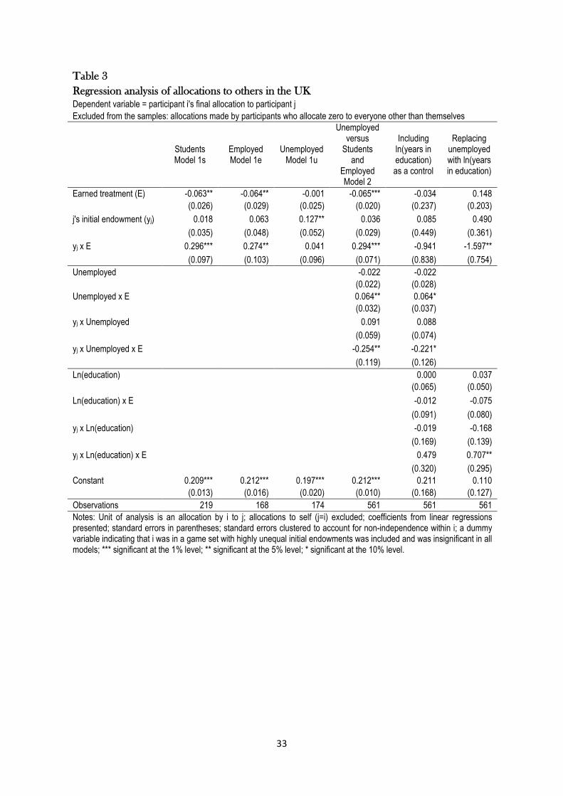
33

Table 3

Regression analysis of allocations to others in the UKDependent variable = participant i's final allocation to participant j

Excluded from the samples: allocations made by participants who allocate zero to everyone other than themselves

StudentsModel 1s

EmployedModel 1e

UnemployedModel 1u

Unemployedversus

Studentsand

EmployedModel 2

Includingln(years ineducation)as a control

Replacingunemployedwith ln(yearsin education)

Earned treatment (E) -0.063** -0.064** -0.001 -0.065*** -0.034 0.148

(0.026) (0.029) (0.025) (0.020) (0.237) (0.203)

j's initial endowment (yj) 0.018 0.063 0.127** 0.036 0.085 0.490

(0.035) (0.048) (0.052) (0.029) (0.449) (0.361)

yj x E 0.296*** 0.274** 0.041 0.294*** -0.941 -1.597**

(0.097) (0.103) (0.096) (0.071) (0.838) (0.754)

Unemployed -0.022 -0.022

(0.022) (0.028)

Unemployed x E 0.064** 0.064*

(0.032) (0.037)

yj x Unemployed 0.091 0.088

(0.059) (0.074)

yj x Unemployed x E -0.254** -0.221*

(0.119) (0.126)

Ln(education) 0.000 0.037

(0.065) (0.050)

Ln(education) x E -0.012 -0.075

(0.091) (0.080)

yj x Ln(education) -0.019 -0.168

(0.169) (0.139)

yj x Ln(education) x E 0.479 0.707**

(0.320) (0.295)

Constant 0.209*** 0.212*** 0.197*** 0.212*** 0.211 0.110

(0.013) (0.016) (0.020) (0.010) (0.168) (0.127)

Observations 219 168 174 561 561 561

Notes: Unit of analysis is an allocation by i to j; allocations to self (j=i) excluded; coefficients from linear regressionspresented; standard errors in parentheses; standard errors clustered to account for non-independence within i; a dummyvariable indicating that i was in a game set with highly unequal initial endowments was included and was insignificant in allmodels; *** significant at the 1% level; ** significant at the 5% level; * significant at the 10% level.

34

Table 4

Participants and treatment assignment in South Africa

Participant sample

All Students Employed Unemployed

Sample sizes 236 101 72 63

Characteristics

Female (%) 53% 46% 68% 49%

Age 30.35 22.05 38.56 34.27

Years in education 12.22 13.27 12.44 10.28

Economic status

Rich 3% 3% 0% 5%

High income 6% 13% 3% 0%

Middle income 39% 54% 46% 7%

Low income 33% 22% 36% 47%

Poor 19% 8% 15% 42%

Population group

African 54% 61% 36% 63%

White 12% 14% 11% 10%

Coloured 23% 9% 44% 22%

Indian 3% 4% 3% 2%

Other 4% 8% 3% 0%

Prefer not to answer 3% 4% 3% 3%

Treatments

Unearned 39% 33% 42% 46%

Earned 61% 67% 58% 54%

35

Table 5

South African experimental data summarized

Participant sample


Higheconomic

status

Loweconomic

status

Random treatment

Allocated zero to all others (%) 1.1% 3.0% 0.0% 0.0% 2.3% 0.0%

Allocated ¼ to each (%) 40.2% 24.2% 66.7% 31.0% 40.9% 39.6%

Left initial endowments unchanged (%) 3.3% 0.0% 0.0% 10.3% 0.0% 6.3%

Allocation to self (mean proportion) 0.34 0.44 0.28 0.29 0.36 0.32

Allocation to others (mean proportion) 0.22 0.19 0.24 0.24 0.21 0.23

Earned treatment

Allocated zero to all others (%) 3.5% 5.9% 2.4% 0.0% 4.4% 2.7%

Allocated ¼ to each (%) 26.4% 11.8% 38.1% 41.2% 15.9% 36.0%

Left initial endowments unchanged (%) 9.7% 11.8% 9.5% 5.9% 13.0% 6.7%

Allocation to self (mean proportion) 0.35 0.44 0.27 0.28 0.38 0.32

Allocation to others (mean proportion) 0.22 0.19 0.24 0.24 0.21 0.23

Notes: Unit of analysis: a participant

36

Table 6

Regression analysis of allocations to others in South AfricaDependent variable = participant i's final allocation to participant j


StudentsModel 1s

EmployedModel 1e

UnemployedModel 1u

Higheconomic

status

Loweconomic

status

High versuslow

economicstatus

Earned treatment (E) -0.015 -0.042* -0.014 -0.056*** -5.7e-5 -0.056***

(0.026) (0.022) (0.028) (0.020) (0.022) (0.020)

j's initial endowment (yj) 0.065 0.075*** 0.189** 0.061* 0.153** 0.061*

(0.049) (0.028) (0.095) (0.032) (0.064) (0.032)

yj x E 0.095 0.210** 0.056 0.217*** 0.014 0.219***

(0.089) (0.082) (0.111) (0.074) (0.084) (0.074)

Low economic status (L) -0.012

(0.020)

L x E 0.056*

(0.030)

yj x L 0.092

(0.072)

yj x L x E -0.203*

(0.112)

Constant 0.179*** 0.220*** 0.196*** 0.201*** 0.196*** 0.204***

(0.020) (0.009) (0.024) (0.014) (0.017) (0.013)

Notes: Unit of analysis is an allocation by i to j; allocations to self (j=i) excluded; coefficients from linear regressionspresented; standard errors in parentheses; standard errors clustered to account for non-independence within i; adummy variable indicating that i was in a game set with highly unequal initial endowments was included and wasinsignificant in all models; *** significant at the 1% level; ** significant at the 5% level; * significant at the 10% level.

37

Table 7

Further regression analysis of allocations to others in Oxford

Dependent variable = participant i's final allocation to participant j

Unemployedno gov'ttransfer

Unemployedwith gov'ttransfer

Universitystudents

FE students

Universityand FE

studentscompared

High and loweconomic

statuscompared#

j's initial endowment (yj) -0.012 0.146** 0.023 0.018 0.023 0.036

(0.012) (0.057) (0.043) (0.027) (0.043) (0.031)

Earned treatment (E) -0.037 -0.003 -0.068** 0.021 -0.068** -0.060***

(0.025) (0.031) (0.028) (0.032) (0.028) (0.018)

yj x E 0.240* -0.010 0.331*** -0.047 0.331*** 0.285***

(0.114) (0.125) (0.103) (0.111) (0.104) (0.066)

Further education (FE) 0.024

(0.026)

FE x E 0.093**

(0.040)

yj x FE -0.009

(0.054)

yj x FE x E -0.403***

(0.143)

Low economic status (L) -0.018

(0.020)

L x E 0.064**

(0.032)

yj x L 0.077

(0.054)

yj x L x E -0.301**

(0.130)

Constant 0.221*** 0.200*** 0.202*** 0.216*** 0.199*** 0.212***

(0.013) (0.022) (0.017) (0.013) (0.017) (0.011)

Observations 48 126 165 54 219 561

Notes: Unit of analysis is an allocation by i to j; allocations to self (j=i) excluded; coefficients from linear regressionspresented; standard errors in parentheses; standard errors clustered to account for non-independence within i; ***significant at the 1% level; ** significant at the 5% level; * significant at the 10% level; # high economic status includesuniversity students, the employed, and the unemployed who do not receive government transfers, low economic statusincludes FE students and the unemployed who are receiving government transfers.

38

Table 8

Regression analysis of Oxford and Cape Town data pooled

Dependent variable = participant i's final allocation to participant j


Oxford Cape Town Oxford and Cape Town

j's initial endowment (yj) 0.036 0.061* 0.036

(0.031) (0.032) (0.032)

Earned treatment (E) -0.060*** -0.056*** -0.059***

(0.018) (0.020) (0.018)

yj x E 0.285*** 0.219*** 0.285***

(0.066) (0.074) (0.066)

Low Economic Status (L) -0.018 -0.012 -0.018

(0.020) (0.020) (0.020)

L x E 0.064** 0.056* 0.064**

(0.032) (0.030) (0.032)

L x yj 0.077 0.092 0.077

(0.054) (0.072) (0.054)

L x yj x E -0.301** -0.203* -0.301**

(0.130) (0.112) (0.129)

Cape Town (CT) -0.004

(0.016)

CT x yj 0.025

(0.045)

CT x E 0.004

(0.028)

CT x yj x E -0.065

(0.100)

CT x L 0.006

(0.028)

CT x L x E -0.009

(0.043)

CT x L x yj 0.015

(0.091)

CT x L x yj x E 0.096

(0.169)

Constant 0.210*** 0.204*** 0.209***

(0.012) (0.013) (0.011)

Observations 561 690 1251

Joint sig. of CT and interactions involving CT (p-value) 0.925

Notes: Unit of analysis is an allocation by i to j; in Oxford, low economic status corresponds to being eitherunemployed or a student at a college of further education, in Cape Town, low economic status corresponds to self-reporting that one's family is low income or poor; allocations to self (j=i) excluded; coefficients from linearregressions presented; standard errors in parentheses; standard errors clustered to account for non-independencewithin i; *** significant at the 1% level; ** significant at the 5% level; * significant at the 10% level.

Individual notions of distributive justice and relative economic status

Documents

Transcript of Individual notions of distributive justice and relative economic status