Increasing Durability of HMA Pavements Designed with the ...
139
STATE HIGHWAY ADMINISTRATION RESEARCH REPORT Increasing Durability of Hot Mix Asphalt Pavements Designed with the Superpave System Dr. Dimitrios Goulias (PI) Dr. Charles Schwartz (Co-PI) Sahand Karimi (Graduate Research Assistant) University Of Maryland Chuck Hughes Consultant Project number SP708B4E FINAL REPORT June 30, 2009 August 25, 2009 (rev) MD-09-SP708B4E Martin O’Malley, Governor Anthony G. Brown, Lt. Governor Beverley K. Swaim-Staley, Secretary Neil J. Pedersen, Administrator
-
Upload
khangminh22 -
Category
Documents
-
view
1 -
download
0
Transcript of Increasing Durability of HMA Pavements Designed with the ...

STATE HIGHWAY ADMINISTRATION
RESEARCH REPORT
Increasing Durability of Hot Mix Asphalt Pavements Designed with the Superpave System
Dr. Dimitrios Goulias (PI)
Dr. Charles Schwartz (Co-PI) Sahand Karimi (Graduate Research Assistant)
University Of Maryland
Chuck Hughes Consultant
Project number SP708B4E
FINAL REPORT
June 30, 2009 August 25, 2009 (rev)
MD-09-SP708B4E
Martin O’Malley, Governor Anthony G. Brown, Lt. Governor
Beverley K. Swaim-Staley, Secretary Neil J. Pedersen, Administrator

The contents of this report reflect the views of the author who is responsible for the facts and the accuracy of the data presented herein. The contents do not necessarily reflect the official views or policies of the Maryland State Highway Administration. This report does not constitute a standard, specification, or regulation.

Form DOT F 1700.7 (8-72) Reproduction of form and completed page is authorized.
Technical Report Documentation Page1. Report No.
MD-09-SP708B4E
2. Government Accession No. 3. Recipient's Catalog No.
4. Title and Subtitle Increasing Durability of Hot Mix Asphalt Pavements Designed with the Superpave System
5. Report Date
August 25, 2009 6. Performing Organization Code
7. Author/s
Dimitrios Goulias, Charles Schwartz, Sahand Karimi, & Chuck Hughes
8. Performing Organization Report No.
9. Performing Organization Name and Address University of Maryland 0147A G.L. Martin Hall College park, MD 20742
10. Work Unit No. (TRAIS) 11. Contract or Grant No.
SP708B4E
12. Sponsoring Organization Name and Address
Maryland State Highway Administration Office of Policy & Research 707 North Calvert Street Baltimore MD 21202
13. Type of Report and Period Covered
Final Report 14. Sponsoring Agency Code 7120) STMD - MDOT/SHA
15. Supplementary Notes 16. Abstract Maryland SHA’s concern with the lower asphalt levels in HMA mixes have lead efforts to explore strategies to increase the asphalt content in Superpave mixes. National studies identified methods for adjusting binder content without compromising rutting performance of asphalt mixtures and remaining loyal to the Superpave philosophy. The applicability of these methods to SHA conditions were addressed based on the findings of recent National Cooperative Highway Research Program projects, ongoing discussions with SHA engineers, and experts’ feedback in this area. Furthermore, this study addressed the differences in HMA properties that have been observed over the years between samples taken at the plant versus behind the paver. A large set of SHA QA and QC data was analyzed statistically in the context of current specifications and pay factors to evaluate potential risks to both SHA and contractors. The research team developed the Operating Characteristic (OC) curves based on the QA data and for estimating the risks to SHA and contractors (Type I and II risks). With the aid of a new simulation tool the associated pay factors were analyzed using the population characteristics and considering potential correlations between the HMA mix parameters. 17. Key Words Quality Assurance, quality control, specifications, Pay Factor, Superpave Mix Design
18. Distribution Statement: No restrictions This document is available from the Research Division upon request.
19. Security Classification (of this report)
None
20. Security Classification (of this page)
None
21. No. Of Pages
128
22. Price

University of Maryland, College Park
Department of Civil and Environmental Engineering
Increasing Durability of Hot Mix Asphalt Pavements Designed with the Superpave System
Final Research Report
Maryland State Highway Administration
Research Project SP708B4E
Prof. Dimitrios Goulias (PI)
Prof. Charles Schwartz (Co-PI)
Sahand Karimi (Graduate Research Assistant)
Chuck Hughes (Consultant)
June 30, 2009 August 25, 2009 (rev)
i
TABLE OF CONTENTS
LIST OF FIGURES ....................................................................................................................... I
LIST OF TABLES ...................................................................................................................... IV
CHAPTER 1 .................................................................................................................................. 1
1.1 Introduction ............................................................................................................................. 1
1.2 Research Approach ................................................................................................................. 2 1.2.1 Increasing the Durability of Superpave Mixes .................................................................. 2 1.2.2 Review of QA/QC Data, Risk and Expected Pay Analysis ............................................... 3
1.3 Organization of the Report .................................................................................................... 4
CHAPTER 2 LITERATURE REVIEW ..................................................................................... 5
2.1 Improving Durability of Superpave HMA Mixtures ........................................................... 5 2.1.1 Durability Basics ................................................................................................................ 5 2.1.2 State of the Literature......................................................................................................... 6 Overall Findings.......................................................................................................................... 7 Binder Content ............................................................................................................................ 8 Design Air Voids ...................................................................................................................... 10 In-Place Air Voids .................................................................................................................... 11 VMA ......................................................................................................................................... 13 Permeability .............................................................................................................................. 13 Age Hardening .......................................................................................................................... 14 Summary ................................................................................................................................... 15 2.1.3 Implications for Maryland SHA Practice ........................................................................ 17
2.2 Quality Measures for HMA Mixtures ................................................................................. 21 2.2.1 Introduction ...................................................................................................................... 21 2.2.2 Comparison of QA and QC data (F and t test)................................................................. 21 2.2.3 Quality Indicators............................................................................................................. 24 2.2.4 Evaluating Specification Limits ....................................................................................... 26 2.2.5 Risk Analysis and Pay Factor Evaluation ........................................................................ 28
CHAPTER 3 COMPARISON OF QA & QC DATA .............................................................. 34
3.1 F and t Tests ........................................................................................................................... 34 3.1.1 Initial Exploratory Assessment Using Random Projects ................................................. 34 3.1.3 Analysis Based on Mixtures Type and Property (Matched Lots and Sublots) ................ 36

ii
3.1.4 Unpaired vs. Paired Analysis based on Mixture Type and Property (Matched Lots and Sublots) ..................................................................................................................................... 37 3.1.5 Analysis based on Mixtures Type, Mix Property, and Mix Band ................................... 38 3.1.6 Analysis based on Deviations from the Target Values .................................................... 39
3.2 Transfer Functions Between QA and QC Data ................................................................. 44
CHAPTER 4 TYPE I AND TYPE II ERROR ANALYSIS & OPERATION CHARACTERISTIC (OC) CURVES ....................................................................................... 45
4.1. Definitions ............................................................................................................................. 45
4.2. Construction of OC Curves and Calculation of Type I and Type II Errors .................. 48 4.2.1 Assessing the Current Conditions .................................................................................... 48 4.2.2 Modifying AQL and RQL to balance the risks (α= 1% and β= 5%) ............................... 51 4.2.3 Revised Specification Tolerances for α= 1% and β= 5% ................................................ 51
CHAPTER 5 SIMULATION ANALYSIS ............................................................................... 53
5.1 Analysis Based on Previous Specifications ......................................................................... 54 5.1.1 Reducing Asphalt Content Variability ............................................................................. 54 5.1.2 Modifying Specification Tolerances ................................................................................ 56 5.1.3 Population Characteristics and Effects on CMPSWL and MF ........................................ 61
5.2 Analysis Based on Current Specification (with Bonus Provision) ................................... 62 5.2.1 Reducing Asphalt Content Variability ............................................................................. 63 5.2.2 Modifying Specification Tolerances ................................................................................ 64 5.2.3 Population Characteristics and Effects on CMPSWL and MF ........................................ 67
5.3 Other Analysis ....................................................................................................................... 68
CHAPTER 6 PAY FACTOR ANALYSIS................................................................................ 70
6.1 Dense Graded HMA ............................................................................................................. 70 6.1.1 Mixture Expected Pay Analysis ....................................................................................... 70 6.1.2 Improving Production Quality & Potential Modifications in Spec Tolerances ............... 81
6.2 Gap Graded HMA ................................................................................................................ 85 6.2.1 Mixtures Expected Pay Analysis ..................................................................................... 85
6.3 Density Analysis .................................................................................................................... 91
CHAPTER 7 SUMMARY, CONCLUSIONS & RECOMMENDATIONS .......................... 97
7.1 Summary ................................................................................................................................ 97
7.2 Conclusions ............................................................................................................................ 99

iii
7.3 Recommendations ............................................................................................................... 101
REFERENCES .......................................................................................................................... 104
APPENDIX ................................................................................................................................ 108
A. Simulation Tool .................................................................................................................... 108 A.1 Description of the Simulation Process ............................................................................. 108 A.2 MATLAB Codes of the Simulation Tool for HMA Mix Properties ............................... 110 A.3 MATLAB Codes of the Simulation Tool for the Density Analysis ................................ 113 A.4 Implications of Correlation Coefficients on PF ............................................................... 118
B. Impact of Reducing Population Variability and/or Modifying Spec Tolerances ........... 119
C. Alternative Approach for Defining HMA Specifications ................................................. 120

i
LIST OF FIGURES
FIGURE 2.1 EFFECT OF DESIGN VBE ON RELATIVE IN-SITU FATIGUE LIFE .............................. 9 FIGURE 2.2 EFFECT OF AGGREGATE FINENESS AND DESIGN VMA ON RUT RESISTANCE OF
SUPERPAVE MIXTURES AT A CONSTANT IN-PLACE AIR VOID CONTENT OF 7% ........... 9 FIGURE 2.3 EFFECT OF DESIGN VMA AND AIR VOIDS ON RUT RESISTANCE OF SUPERPAVE
MIXTURES AT CONSTANT IN-PLACE AIR VOID CONTENT ................................................. 10 FIGURE 2.4. EFFECT OF DESIGN AIR VOIDS AND DESIGN VMA ON RELATIVE IN-SITU
FATIGUE LIFE AT CONSTANT IN-PLACE AIR VOIDS............................................................. 10 FIGURE 2.5 EFFECT OF BINDER GRADE AND NDESIGN ON RUT RESISTANCE AT 4% DESIGN
AIR VOIDS AND 7% IN-PLACE AIR VOIDS ................................................................................ 11 FIGURE 2.6 EFFECT OF VMA AND IN-PLACE AIR VOIDS ON RUT RESISTANCE OF
SUPERPAVE MIXTURES AT CONSTANT DESIGN AIR VOID CONTENT ............................. 12 FIGURE 2.7 EFFECT OF IN-PLACE AIR VOIDS AND DESIGN AIR VOIDS ON RELATIVE IN-
SITU FATIGUE LIFE ....................................................................................................................... 12 FIGURE 2.8 PERMEABILITY OF SPECIMENS AND NCHRP PROJECTS 9-25 AND 9-31 AS A
FUNCTION OF EFFECTIVE AIR VOID CONTENT ..................................................................... 14 FIGURE 2.9 PREDICTED MIXTURE AGE-HARDENING RATIO AT 25OC AND 10 HZ AS A
FUNCTION OF IN-PLACE AIR VOID CONTENT AND FM300 FOR A MAAT OF 15.6OC ........ 15 FIGURE 2.10 CONTACTOR AND OWNER RISK USING UNKNOWN STANDARD DEVIATION . 29 FIGURE 3.1 DEVIATIONS FROM THE TARGET VALUES FOR AC ................................................. 40 FIGURE 3.2 DEVIATIONS FROM THE TARGET VALUES FOR 4.75MM ......................................... 40 FIGURE 3.3 DEVIATIONS FROM THE TARGET VALUES FOR 2.36MM ......................................... 41 FIGURE 3.4 DEVIATIONS FROM THE TARGET VALUES FOR 0.075MM ....................................... 41 FIGURE 3.5 COMPARISON OF QA & QC DATA FOR THE 0.075MM OF THE 12.5 GAP GRADED
MIXTURES ....................................................................................................................................... 45 FIGURE 3.6 COMPARISON OF QA & QC DATA FOR THE 2.36 MM OF THE 12.5 GAP GRADED
MIXTURES ....................................................................................................................................... 45 FIGURE 3.7 COMPARISON OF QA & QC DATA FOR THE 4.75MM OF 12.5 GAP GRADED
MIXTURES ....................................................................................................................................... 45 FIGURE 3.8 COMPARISON OF QA & QC DATA FOR THE AC CONTENT OF 12.5 GAP GRADED
MIXTURES ....................................................................................................................................... 46 FIGURE 4.1 OC CURVE FOR 0.075 MM OF GAP GRADED MIXTURES .......................................... 49 FIGURE 4.2 OC CURVE FOR 2.36 MM OF GAP GRADED MIXTURES ............................................ 49 FIGURE 4.3 OC CURVE FOR 4.75 MM OF GAP GRADED MIXTURES ............................................ 50 FIGURE 4.4 OC CURVE FOR AC CONTENT OF GAP GRADED MIXTURES .................................. 50 FIGURE 5.1 EFFECT OF REDUCTION IN ASPHALT CONTENT VARIABILITY ............................ 55 FIGURE 5.2 EFFECT OF REDUCTION IN ASPHALT CONTENT VARIABILITY ON MF ............... 55 FIGURE 5.3 EFFECT OF REDUCTION IN ASPHALT CONTENT VARIABILITY ON CMPWSL.... 56 FIGURE 5.4 EFFECTS OF CHANGE IN AC SPECIFICATION TOLERANCE ON CMPWSL ........... 57 FIGURE 5.5 EFFECTS OF CHANGE IN AC SPECIFICATION TOLERANCE ON MF ...................... 57 FIGURE 5.6 EFFECTS OF CHANGE IN 0.075 SPECIFICATION TOLERANCE ON CMPWSL ........ 58 FIGURE 5.7 EFFECTS OF CHANGE IN 0.075 SPECIFICATION TOLERANCE ON MF ................... 58 FIGURE 5.8 EFFECTS OF CHANGE IN 2.36 SPECIFICATION TOLERANCE ON CMPWSL .......... 59 FIGURE 5.9 EFFECTS OF CHANGE IN 2.36 SPECIFICATION TOLERANCE ON MF ..................... 59 FIGURE 5.10 EFFECTS OF CHANGE IN 4.75 SPECIFICATION TOLERANCE ON CMPWSL ........ 60 FIGURE 5.11 EFFECTS OF CHANGE IN 4.75 SPECIFICATION TOLERANCE ON MF ................... 61 FIGURE 5.12 CMPSWL AND MF FOR DIFFERENT MIXTURES USING PAY EQUATION 5.1...... 62 FIGURE 5.13 EFFECT OF REDUCTION IN AC CONTENT VARIABILITY ON MF ......................... 63 FIGURE 5.14 EFFECTS OF CHANGE IN AC SPECIFICATION TOLERANCE ON MF .................... 64 FIGURE 5.15 EFFECTS OF CHANGE IN 0.075 SPECIFICATION TOLERANCE ON MF ................. 65

ii
FIGURE 5.16 EFFECTS OF CHANGE IN 2.36 SPECIFICATION TOLERANCE ON MF ................... 66 FIGURE 5.17 EFFECTS OF CHANGE IN 4.75 SPECIFICATION TOLERANCE ON MF ................... 67 FIGURE 5.18 CMPSWL AND MF FOR DIFFERENT MIXTURES USING BONUS PROVISION ..... 68 FIGURE 5.19 VARIABILITY IN ASPHALT CONTENT BY VARIOUS PLANTS IN MARYLAND . 69 FIGURE 6.1 DISTRIBUTION OF ASPHALT CONTENT POPULATION AND THE TOLERANCES 70 FIGURE 6.2 DISTRIBUTION OF PASSING 0.075MM POPULATION AND THE TOLERANCES ... 71 FIGURE 6.3 DISTRIBUTION OF PASSING 2.36MM POPULATION AND THE TOLERANCES ..... 71 FIGURE 6.4 DISTRIBUTION OF PASSING 4.75MM POPULATION AND THE TOLERANCES ..... 72 FIGURE 6.5 DISTRIBUTION OF ASPHALT CONTENT AT AQL ....................................................... 72 FIGURE 6.6 DISTRIBUTION OF ASPHALT CONTENT AT RQL ....................................................... 73 FIGURE 6.7 DISTRIBUTION OF PASSING 0.075MM AT AQL ........................................................... 73 FIGURE 6.8 DISTRIBUTION OF PASSING 0.075MM AT RQL ........................................................... 74 FIGURE 6.9 DISTRIBUTION OF PASSING 2.36MM AT AQL ............................................................. 74 FIGURE 6.10 DISTRIBUTION OF PASSING 2.36MM AT RQL ........................................................... 75 FIGURE 6.11 DISTRIBUTION OF PASSING 4.75MM AT AQL ........................................................... 75 FIGURE 6.12 DISTRIBUTION OF PASSING 4.75MM AT RQL ........................................................... 76 FIGURE 6.13 EP CURVES WITH EXPECTED PF USING POPULATION CHARACTERISTICS ..... 77 FIGURE 6.14 CMPWL AND PAY FACTOR DISTRIBUTION FOR PRODUCTION “CLOSE TO”
AQL (MAX CMPWL = 88.7 USING POPULATION STANDARD DEVIATION) ....................... 79 FIGURE 6.15 CMPWL AND PAY FACTOR DISTRIBUTION FOR RQL (WITH POPULATION
STANDARD DEVIATION) .............................................................................................................. 80 FIGURE 6.16 EP CURVES WITH EXPECTED PF USING REDUCED POPULATION VARIABILITY
............................................................................................................................................................ 82 FIGURE 6.17 CMPWL AND PAY FACTOR DISTRIBUTION FOR AQL PRODUCTION WITH
REDUCED POPULATION VARIABILITY .................................................................................... 83 FIGURE 6.18 CMPWL AND PAY FACTOR DISTRIBUTION FOR RQL PRODUCTION WITH
REDUCED POPULATION VARIABILITY .................................................................................... 84 FIGURE 6.19 DISTRIBUTION OF PASSING AC POPULATION AND THE TOLERANCES ............ 85 FIGURE 6.20 DISTRIBUTION OF PASSING 0.075MM POPULATION AND THE TOLERANCES . 85 FIGURE 6.21 DISTRIBUTION OF PASSING 2.36MM POPULATION AND THE TOLERANCES ... 86 FIGURE 6.22 DISTRIBUTION OF PASSING 4.75MM POPULATION AND THE TOLERANCES ... 86 FIGURE 6.23 EP CURVES WITH EXPECTED PF USING POPULATION CHARACTERISTICS
(GAP GRADED)................................................................................................................................ 87 FIGURE 6.24 GAP GRADED CMPWL AND PAY FACTOR DISTRIBUTION FOR PRODUCTION
AT AQL ............................................................................................................................................. 89 FIGURE 6.25 GAP GRADED CMPWL AND PAY FACTOR DISTRIBUTION FOR RQL .................. 90 FIGURE 6.26 DISTRIBUTION OF INDIVIDUAL GAP GRADED DENSITY VALUES ..................... 91 FIGURE 6.27 DISTRIBUTION OF INDIVIDUAL DENSE GRADED DENSITY VALUES ................ 92 FIGURE 6.28 DISTRIBUTION OF LOT AVERAGES OF GAP GRADED DENSITY VALUES ......... 92 FIGURE 6.29 DISTRIBUTION OF LOT AVERAGES OF DENSE GRADED DENSITY VALUES .... 93 FIGURE 6.30 DISTRIBUTION OF SIMULATED DENSITY DATA OF GAP GRADED MIXES ....... 94 FIGURE 6.31 DISTRIBUTION OF SIMULATED DENSITY DATA OF DENSE GRADED MIXES .. 94 FIGURE 6.32 PAY FACTOR DISTRIBUTION OF DENSITY DATA OF GAP GRADED MIXES ..... 95 FIGURE 6.33 PAY FACTOR DISTRIBUTION OF DENSITY OF DATA OF DENSE GRADED
MIXES ............................................................................................................................................... 95 FIGURE A1 FLOW CHART OF SIMULATION ANALYSIS ............................................................... 109 FIGURE C1 EP CURVES WITH EXPECTED PF USING POPULATION STANDARD DEVIATION
AND C = 73 CMPWL (Α=5%)........................................................................................................ 123 FIGURE C2 EP CURVES WITH EXPECTED PF USING POPULATION VARIABILITY STANDARD
DEVIATION AND C = 63 CMPWL (Α=1%) ................................................................................. 124

iii
FIGURE C3 EP CURVES WITH EXPECTED PF USING REDUCED POPULATION VARIABILITY AND C VALUE OF C= 73 CMPWL .............................................................................................. 125
FIGURE C4 EP CURVES WITH EXPECTED PF USING REDUCED POPULATION VARIABILITY AND C VALUE OF C= 63 CMPWL .............................................................................................. 126

iv
LIST OF TABLES
TABLE 2.1 NDESJGN VALUES FOR SUPERPAVE MIX DESIGN ........................................................... 17 TABLE 2.2 MARYLAND IN-PLACE DENSITY PAY FACTORS ........................................................ 20 TABLE 2.3 COMPARISONS OF GDOT AND CONTRACTOR QC TEST RESULTS USING MEANS
............................................................................................................................................................ 23 TABLE 2.4 COMPARISONS OF GDOT AND CONTRACTOR QC TEST RESULT USING
VARIANCES ..................................................................................................................................... 23 TABLE 2.5 COMPARISONS OF GDOT AND CONTRACTOR QC TEST RESULT USING PROJECT
MEANS AND VARIANCES ............................................................................................................ 24 TABLE 2.6 VARIABILITY VALUES USED IN INITIAL SCDOT HMA QA SPECIFICATION-
REVISED SPEC ................................................................................................................................ 27 TABLE 2.7 SPECIFICATION LIMITS IN INITIAL AND REVISED SCDOT HMA QA
SPECIFICATION .............................................................................................................................. 28 TABLE 2.8 CALCULATED AQL AND RQL BASED ON DIFFERENT SAMPLE SIZES ................... 30 TABLE 2.9 PROBABILITIES THAT POPULATIONS WITH VARIOUS QUALITY LEVELS
WOULD REQUIRE REMOVAL AND REPLACEMENT FOR ONE VERSUS FOUR INDEPENDENT QUALITY CHARACTERISTICS ........................................................................ 32
TABLE 2.10 CORRELATION COEFFICIENTS FOR ALL PAIRS OF PLANT QUALITY CHARACTERISTICS ....................................................................................................................... 32
TABLE 2.11 EFFECTS OF CORRELATIONS BETWEEN VARIABLES USING SIMULATION ANALYSIS ........................................................................................................................................ 33
TABLE 3.1 F AND T TEST ON RANDOM PROJECTS.......................................................................... 35 TABLE 3.2 EXAMPLE OF F AND T TESTS BY MIX TYPE ................................................................. 36 TABLE 3.3 UNPAIRED ANALYSIS ........................................................................................................ 37 TABLE 3.4 PAIRED ANALYSIS.............................................................................................................. 38 TABLE 3.5 UNPAIRED ANALYSIS FOR HIGH POLISHED MIXTURES .......................................... 39 TABLE 3.6 PAIRED ANALYSIS FOR HIGH POLISHED MIXTURES ................................................ 39 TABLE 3.7 F AND T ANALYSIS ON DELTA FOR PROJECTS WITH UNIQUE TARGET VALUES –
MIX HIGH POLISHED ..................................................................................................................... 42 TABLE 3.8 F AND T ANALYSIS ON DELTA FOR PROJECTS WITH UNIQUE TARGET VALUES –
MIX GAP GRADE ............................................................................................................................ 42 TABLE 3.9 F AND T ANALYSIS ON DELTA FOR PROJECTS WITH UNIQUE TARGET VALUES –
MIX S ................................................................................................................................................. 42 TABLE 3.10 F AND T ANALYSIS ON DELTA FOR PROJECTS WITH UNIQUE TARGET VALUES
– MIX RAP ........................................................................................................................................ 43 TABLE 3.11 F AND T ANALYSIS ON DELTA FOR PROJECTS WITH UNIQUE TARGET VALUES
– MIX VIRGIN .................................................................................................................................. 43 TABLE 4. 1 REPRESENTATIVE LOTS FOR THE 0.075, 2.36, 4.75, AND AC CONTENT OF GAP
GRADED MIXTURES ...................................................................................................................... 48 TABLE 4.2 RISKS BASED ON AQL= 90% AND RQL = 40% FOR N=6. ............................................. 51 TABLE 4.3 AQL AND RQL FOR Α= 1% AND Β= 5% (N=6). ............................................................... 51 TABLE 4.4 REVISED SPECIFICATION TOLERANCES FOR Α= 1% AND Β= 5%. .......................... 52 TABLE 5.1 CORRELATIONS BETWEEN MIX PARAMETERS FOR DENSE GRADED MIXTURES
............................................................................................................................................................ 53 TABLE 5.2 POPULATION CHARACTERISTICS .................................................................................. 54 TABLE 5.3 EFFECTS OF CHANGE IN AC SPECIFICATION TOLERANCE ..................................... 56 TABLE 5.4 EFFECTS OF CHANGE IN 0.075 SPECIFICATION TOLERANCE ON MF .................... 58 TABLE 5.5 EFFECTS OF CHANGE IN 2.36 SPECIFICATION TOLERANCE ON MF ...................... 59 TABLE 5.6 EFFECTS OF CHANGE IN 4.75 SPECIFICATION TOLERANCE ON MF ...................... 60

v
TABLE 5.7 EFFECTS OF CHANGE IN AC SPECIFICATION TOLERANCE AND IMPACT ON MF ............................................................................................................................................................ 64
TABLE 5.8 EFFECTS OF CHANGE IN 0.075 SPECIFICATION TOLERANCE AND IMPACT ON MF ...................................................................................................................................................... 65
TABLE 5.9 EFFECTS OF CHANGE IN 2.36 SPECIFICATION TOLERANCE ON MF ...................... 66 TABLE 5.10 EFFECTS OF CHANGE IN 4.75 SPECIFICATION TOLERANCE ON MF .................... 66 TABLE 6.1 STANDARD DEVIATION OF DIFFERENT PROPERTIES ............................................... 77 TABLE 6.2 PROBABILITY OF RECEIVING ≥PF AT DIFFERENT CMPWL WITH POPULATION
CHARACTERISTICS ....................................................................................................................... 77 TABLE 6.3 EXPECTED PAYMENT IN RELATION TO CMPWL WITH POPULATION
CHARACTERISTICS* ..................................................................................................................... 78 TABLE 6.4 PROBABILITY OF RECEIVING ≥PF AT DIFFERENT PWL BY REDUCING
POPULATION VARIABILITY ........................................................................................................ 82 TABLE 6.5 STANDARD DEVIATION OF DIFFERENT PROPERTIES (GAP GRADED) .................. 87 TABLE 6.6 PROB. OF RECEIVING ≥PF AT DIFFERENT CMPWL WITH POPULATION
CHARACTERISTICS (GAP GRADED) .......................................................................................... 87 TABLE 6.7 AVERAGE PF IN RELATION TO CMPWL WITH POPULATION CHARACTERISTICS*
(GAP GRADED)................................................................................................................................ 88 TABLE 6.8 A AND B PARAMETERS FOR WEIBULL DISTRIBUTION OF HMA MIXTURES ....... 93 TABLE 6.9 MODIFIED DENSE GRADED HMA MIXES PERCENT OF MAXIMUM DENSITY ...... 96 TABLE A1 EXAMPLE OF EFFECT OF CORRELATION VALUE ON THE AVERAGE PF ............ 118 TABLE B1 EFFECTS OF REDUCING POPULATION STANDARD DEVIATION ........................... 119 TABLE B2 EFFECTS OF INCREASING SPEC TOLERANCES .......................................................... 119 TABLE C1 WSDOT PAY FACTORS ..................................................................................................... 121 TABLE C2 PROBABILITY OF RECEIVING ≥PF AT DIFFERENT CMPWL USING POPULATION
CHARACTERISTICS & C = 73CMPWL (Α=5%) ......................................................................... 122 TABLE C3 PROBABILITY OF RECEIVING ≥PF AT DIFFERENT CMPWL USING POPULATION
CHARACTERISTICS AND C = 63CMPWL (Α=1%) ................................................................... 123 TABLE C4 PROBABILITY OF RECEIVING ≥PF AT DIFFERENT CMPWL BY REDUCING
POPULATION VARIABILITY AND WITH C = 73CMPWL...................................................... 125 TABLE C5 PROBABILITY OF RECEIVING ≥PF AT DIFFERENT CMPWL BY REDUCING
POPULATION VARIABILITY AND WITH C = 63CMPWL...................................................... 126

1
CHAPTER 1
1.1 Introduction
The Maryland State Highway Administration (MSHA) has implemented the Superpave
mix design method since 1998. While the adoption of this mix design method has provided
significant benefits to the state by improving rutting resistance of pavements, a reduction in
asphalt cement content of the asphalt mixtures has been observed. These drier mixtures are more
difficult to compact to target field density, especially in thin lifts. Lower density eventually leads
to potholes, premature fatigue cracking and durability problems. The lower asphalt content of
these mixtures reduces the asphalt film thickness, which accelerates oxidation and stripping
effects. Other related problems include premature raveling at joints, increased segregation, and
higher permeability.
Maryland SHA’s concern with the lower asphalt levels in Superpave mixes have lead
efforts through the HMA Pay Factor Team to explore strategies to increase the asphalt content in
Superpave mixes. As a starting point, a national survey with other states was conducted. This
initial survey and follow up national studies identified methods for adjusting binder content
without compromising rutting performance of asphalt mixtures and remaining loyal to the
Superpave philosophy. The applicability of these methods to MSHA conditions are addressed
based on the findings of recent National Cooperative Highway Research Program projects,
ongoing discussions with SHA engineers, and experts’ feedback in this area (Objective I).
Another issue addressed in this study is the differences in HMA properties that have been
observed over the years between samples taken at the plant versus behind the paver. A large set
of SHA QA and QC data was analyzed statistically in the context of current specifications and
pay factors to evaluate potential risks to both SHA and contractors (Objective II).

2
1.2 Research Approach
To address these objectives the following tasks and analysis were undertaken.
1.2.1 Increasing the Durability of Superpave Mixes
Maryland SHA has already explored strategies to increase the percentage asphalt in
Superpave mixes1
• NCHRP Project 9-09: Refinement of the Superpave Gyratory Compaction Procedure
(Contractor: Auburn University/NCAT; completed)
via a national survey with other states. In addition, there have been several
major recent/ongoing national research projects related to the durability of Superpave mixes:
• NCHRP Project 9-25: Requirements for Voids in Mineral Aggregate for Superpave Mixtures
(Contractor: Applied Asphalt Technologies LLC; completed)
• NCHRP Project 9-31: Air Void Requirements for Superpave Mix Design (Contractor:
Applied Asphalt Technologies LLC; competed)
• NCHRP Project 9-33: A Mix Design Manual for Hot Mix Asphalt (Contractor: Advanced
Asphalt Technologies LLC; ongoing—mix design manual not yet published)
These national studies identified methods for adjusting binder content without compromising
rutting performance of asphalt mixtures and without moving too far from the Superpave
philosophy. In particular, the results from NCHRP Projects 9-25 and 9-31 as documented in
NCHRP Report 567 Volumetric Requirements for Superpave Mix Design (2006) represent the
best current thinking on enhancing durability of Superpave mixes.2
1 Only Superpave dense-graded mixtures are considered here. Although Maryland places large quantities of SMA materials each year, these gap-graded mixtures do not conform to Superpave HMA mixture design criteria. 2 R. Bonaquist, Advanced Asphalt Technologies LLC – personal communication

3
1.2.2 Review of QA/QC Data, Risk and Expected Pay Analysis
The research team first reviewed the state-of-practice in QA/ QC analysis by other states.
An extensive literature review was conducted on HMA pay factors. The AASHTO and FHWA
recommendations were examined as well. Specifically issues related to the following areas were
examined:
• contractor vs. agency data,
• impact of sample size,
• evaluation and assessment of agency and contractor risks and use of OC curves, and,
• definition/evaluation of individual and composite pay factors.
A synthesis of key literature findings is provided in Chapter 2.
The analysis then proceeded with a review of the quality control (contractor) and quality
acceptance (agency) data for HMA materials and an assessment of the risks and pay factor
implications using the SHA data from 2002 to 2007. The effort of the HMA Pay Factor team in
evaluating and assessing the existing method of acceptance and the pay factors for HMA
materials described in SPS 504 and MSMT 735 was reviewed as well. Then an extensive
analysis was performed to compare contractor and agency data at the plant and from the roadway
(“behind the paver”). A series of statistical analyses (F and t tests) were conducted to assess and
quantify the differences between these data sets. The research team then developed the Operating
Characteristic (OC) curves based on the QA data and for estimating the risks to SHA and
contractors (Type I and II risks). With the aid of a new simulation tool the associated pay factors

4
were analyzed using the population characteristics and considering potential correlations
between the HMA mix parameters.
A series of meetings were scheduled with SHA engineers, the industry, and when
appropriate with the HMA Pay Factor Team, to discuss the preliminary findings from the
analyses and to formulate possible recommendations.
1.3 Organization of the Report
The first chapter presents the introduction, research objectives, the analysis approach and
the organization of this report. Chapter 2 presents an extensive literature review on the durability
of HMA mixtures and QA/QC and acceptance testing. Chapter 3 includes the results of the F and
t test analyses comparing the Quality Assurance (QA) and Quality Control (QC) data. Chapter 4
presents the analyses related to the type I & II errors using the Operation Characteristic (OC)
curves. Chapter 5 describes the simulation analysis used in this research for examining the
percent within limits and mixture pay factor effects. Chapter 6 presents the pay factor analysis
results for the HMA mix properties in-place density. Finally, chapter 7 includes the summary,
conclusions, and recommendations.

5
CHAPTER 2 LITERATURE REVIEW
2.1 Improving Durability of Superpave HMA Mixtures
2.1.1 Durability Basics
The design of HMA mixtures requires balancing permanent deformation resistance,
fatigue cracking resistance, strength, modulus, and other properties. The goal is to optimize the
aggregate, asphalt, and mixture properties to produce the maximum pavement service life.
The durability of an HMA mixture is a measure of its resistance to disintegration-type
distresses (e.g., raveling), moisture damage (e.g., stripping), and hardening over time (e.g.,
aging) with associated distresses (e.g., block cracking, top-down fatigue cracking). Such property
can have a significant impact on asphalt concrete mixture performance and significantly change
the other properties (e.g., permanent deformation and fatigue resistance) over time and thus it is
normally considered in the mix design process by the control of asphalt content and air voids.
High mixture permeability is often associated with poor durability. Permeability is related
to density, which in turn is related to the air voids in the compacted mix. A high air voids
percentage allows water and air to penetrate the asphalt concrete mixture, causing stripping,
moisture damage, and oxidation. These will eventually result in accelerated raveling and/or
cracking. In addition, stripping and moisture damage significantly reduce the strength of the mix.
The sizes of the voids, their interconnection, and the access of the voids to the surface of the
pavement all have an influence on the permeability of the compacted HMA mixture. Asphalt
film thickness, which is a function of asphalt content and aggregate gradation (particularly the
fine portion), also has a major influence on potential moisture damage and durability.

6
Although increasing the effective asphalt binder content is the most direct method for
increasing durability, other approaches that have been pursued either individually or in
combination in recent years include:
− Changes to the design air voids (total voids in mix, VTM)
− Increasing minimum voids in mineral aggregate (VMA) requirements
− Imposing a maximum VMA cap
− Increasing the design voids filled with asphalt (VFA)
− Lower design compaction levels (Ndesign), including the “locking point” concept
− Increasing required field compaction levels (% density)
Many of these factors are interrelated, therefore their modification must be done with some care
to avoid unintended consequences with regard to resistance to permanent deformations, fatigue
cracking, and other structural distresses.
2.1.2 State of the Literature
NCHRP Project 9-25 “Requirements for Voids in Mineral Aggregate for Superpave
Mixtures” and the closely related Project 9-35 “Air Void Requirements for Superpave Mix
Design” examined the impacts of potential changes in the current criteria for design VTM,
VMA, and VFA on the performance and durability of HMA. The research team for these studies
conducted a thorough and critical literature review of the impact of variations in HMA
volumetric properties on mixture performance and durability as the starting point for their
studies. They then evaluated the effect of changes in VTM, VMA, VFA, aggregate specific
surface, and other factors on the several performance measures of HMA.

7
These laboratory results, along with other data sets from the literature, were used to
develop and validate a set of semi-empirical models for estimating quantitatively the structural
performance (permanent deformation and fatigue cracking) and durability (via permeability and
age hardening) of HMA mixtures as functions of HMA volumetric parameters. These
comprehensive studies as summarized in NCHRP Report 567 (Christensen and Bonaquist, 2006)
represent the best snapshot of the current state of the literature and the most rational
interpretation of the state of practice on this subject.
The overall conclusion from these studies was that the current Superpave volumetric mix
design criteria do not need major revision. However, the studies found that broadening the design
air voids requirement to 3-5% is reasonable as long as the potential consequences on HMA
performance are understood. In addition, while the study found it reasonable to consider changes
in the minimum VMA or the addition of a maximum VMA limit, the effect of such changes,
particularly if implemented in tandem with changes in design volumetrics requirements, must be
carefully evaluated to avoid reducing resistance to permanent deformation and fatigue of the
mix.
The following sections summarize the key findings from NCHRP Report 567 as related
to mix durability. The material is reorganized here in order to focus more tightly on each of the
major parameters available for improving durability.
Overall Findings
Superpave mixtures tend to be coarser, have lower binder contents, and be more difficult
to compact in the field than earlier Marshall-based designs. The relatively few fines in
combination with relatively high in-place air voids of Superpave mixtures can result in higher

8
permeability and more age hardening—i.e., less durability. Consequently, many state highway
agencies have modified the requirements for VMA, VTM, and related factors for Superpave
mixtures. The three most common Superpave modifications included: (1) an expansion of the
design air voids from a target 4% to a range of 3% to 5% (i.e., matching the older Marshall mix
design system); (2) addition of a maximum VMA limit at 1.5% to 2.0% above the minimum
value; and (3) a slight increase in the minimum VMA values, typically by about 0.5%.
These modifications have been suggested individually, in combinations, or in addition to
other changes (e.g., Ndesign). However, some care must be exercised. First, volumetric factors
such as VBE, VTM, VMA, and VFA are all interrelated, making it difficult if not impossible to
change only one volumetric parameter at a time. Second, changes in volumetric requirements,
compaction levels, materials specifications, and other mixture characteristics are additive, and
often in a nonlinear way. Unless these multiple types of interactions are carefully evaluated, they
can cause significant and unanticipated reductions in pavement performance.
Binder Content
Fatigue resistance, which can be taken as a proxy for durability, is influenced by effective
asphalt content (VBE) as well as design air voids, lab compaction (Ndesign), field compaction, and
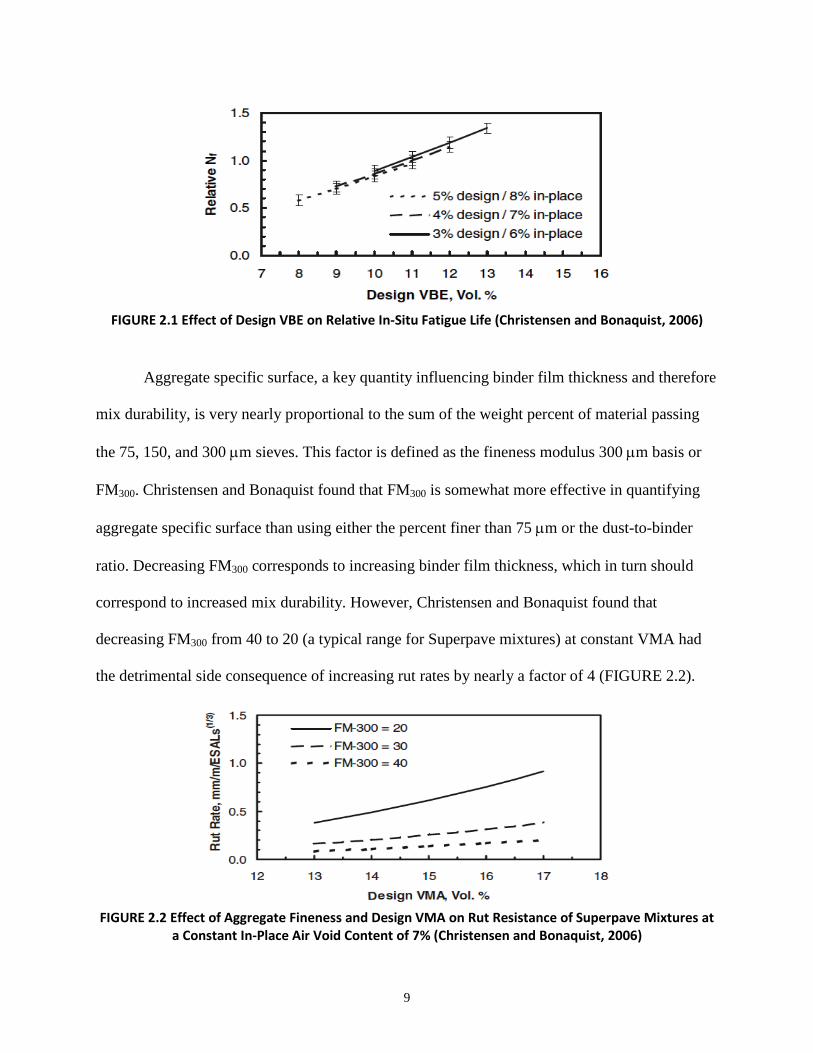
other factors. Christensen and Bonaquist found that each 1% increase in VBE corresponds to an
increase in fatigue life of 13% to 15% (FIGURE 2.1).
9
FIGURE 2.1 Effect of Design VBE on Relative In-Situ Fatigue Life (Christensen and Bonaquist, 2006)
Aggregate specific surface, a key quantity influencing binder film thickness and therefore
mix durability, is very nearly proportional to the sum of the weight percent of material passing
the 75, 150, and 300 µm sieves. This factor is defined as the fineness modulus 300 µm basis or
FM300. Christensen and Bonaquist found that FM300 is somewhat more effective in quantifying
aggregate specific surface than using either the percent finer than 75 µm or the dust-to-binder
ratio. Decreasing FM300 corresponds to increasing binder film thickness, which in turn should
correspond to increased mix durability. However, Christensen and Bonaquist found that
decreasing FM300 from 40 to 20 (a typical range for Superpave mixtures) at constant VMA had
the detrimental side consequence of increasing rut rates by nearly a factor of 4 (FIGURE 2.2).
FIGURE 2.2 Effect of Aggregate Fineness and Design VMA on Rut Resistance of Superpave Mixtures at
a Constant In-Place Air Void Content of 7% (Christensen and Bonaquist, 2006)

10
Design Air Voids
Decreasing design air voids while holding VMA constant increases VBE, which should
result in increased fatigue resistance and durability. However, reducing VTM also reduces the
field compaction effort required to achieve a given in-place air voids target; this would be
expected to degrade both rutting resistance and fatigue resistance. As shown in FIGURE 2.3 and
FIGURE 2.4, the latter effect dominates the response; decreasing design air voids while holding
VMA and in-place air voids constant increases the rut rate and decreases the expected fatigue
life.
FIGURE 2.3 Effect of Design VMA and Air Voids on Rut Resistance of Superpave Mixtures at Constant
In-Place Air Void Content (Christensen and Bonaquist, 2006)
FIGURE 2.4. Effect of Design Air Voids and Design VMA on Relative In-Situ Fatigue Life at Constant In-
Place Air Voids (Christensen and Bonaquist, 2006).

11
Note that decreasing the design air voids for a given aggregate structure at constant VMA
has essentially the same effect as reducing the design compaction effort Ndesign (FIGURE 2.5;
compare with FIGURE 2.3). Reducing design air voids or Ndesign at constant VMA
simultaneously increases VBE (good for durability) and reduces the required field compaction
effort for fixed target density (bad for durability). The latter effect generally dominates and will
tend to decrease permanent deformation resistance, fatigue resistance, and durability.
Conversely, increasing design air voids (or Ndesign) will increase the difficulty of field
compaction. This may increase in-place air voids which in turn may counteract any benefits from
increased design air voids as well as result in a more permeable mix that is more susceptible to
age hardening and moisture damage.
FIGURE 2.5 Effect of Binder Grade and Ndesign on Rut Resistance at 4% Design Air Voids and 7% In-Place
Air Voids (Christensen and Bonaquist , 2006)
In-Place Air Voids
Christensen and Bonaquist found from their empirical performance models that a 1%
decrease in in-place air void content at constant design air voids increases both rut resistance and

12
fatigue resistance by about 20% (FIGURE 2.6 and FIGURE 2.7). Decreasing design air voids
while simultaneously decreasing in-place air voids provides even greater benefits in terms of rut
and fatigue resistance and mix durability (e.g., FIGURE 2.7). This is consistent with the very
rough “rule of thumb” by Linden et al. (1988) that every 1% increase in in-place air voids results
in about a 10% reduction in performance. Achieving adequate compaction in the field is clearly
the best thing to do for pavement performance, including durability.
FIGURE 2.6 Effect of VMA and In-Place Air Voids on Rut Resistance of Superpave Mixtures at Constant
Design Air Void Content (Christensen and Bonaquist, 2006)
FIGURE 2.7 Effect of In-Place Air Voids and Design Air Voids on Relative In-Situ Fatigue Life
(Christensen and Bonaquist, 2006)

13
Before modifying Superpave mix design specifications, the level of in-place density
being achieved in projects should be critically examined. Inadequate field compaction will have
a broad and significant negative impact on pavement performance that can only be partially
offset by altered mix design. Simultaneously decreasing design air voids and in-place air voids
by a similar amount will increase rut resistance and fatigue and decrease permeability —
therefore provide a more durable and better performing pavement.
VMA
Increasing VMA, while maintaining constant design air voids increases VBE and
therefore improves fatigue resistance and, by implication, durability (FIGURE 2.4). However,
Christensen and Bonaquist found that a 1% increase in VMA at constant design air voids
decreases rutting resistance by about 20% (FIGURE 2.6) unless care is taken to ensure that
adequate aggregate specific surface is maintained.
Permeability
Permeability is an inverse indicator for durability--i.e., durability tends to decrease with
increasing permeability. Permeability increases with increasing air voids (FIGURE 2.8) and
decreasing aggregate specific surface (i.e., increasing aggregate size). Permeability can be
modeled effectively using the concept of effective air voids, defined as the total air voids minus
the air void content at zero permeability. At constant total air voids effective air voids decrease
with increasing aggregate fineness. Based on permeability study data by Choubane et al. (1998)
and others, permeability increases by about 10-3 cm/s for every 1% increase in air voids or 3%
decrease in FM300 (FIGURE 2.8).

14
FIGURE 2.8 Permeability of Specimens from Choubane et al. (1998) and NCHRP Projects 9-25 and 9-31
as a Function of Effective Air Void Content (Christensen and Bonaquist, 2006)
Permeability of HMA measured from laboratory-prepared specimens tends to be
significantly lower than permeability values measured on field cores of the same mixture.
Consequently, laboratory measurement of mixture permeability has little utility for use in routine
mix designs.
Age Hardening
Age hardening of HMA is a key factor in durability; increased hardening tends to
produce durability problems associated with raveling, block cracking, and top-down fatigue
cracking. Christensen and Bonquist found that hardening depended not only on air void content
but also on the specific combination of aggregate and binder in the mixture. Applying a modified
version of the Mirza and Witczak (1995) global aging system at a mean annual air temperature of
15.6oC, Christensen and Bonaquist found that the age hardening ratio for the mixture decreased
about 2% to 7% for every 1% increase in FM300 (i.e., decreasing aggregate size) and increased
about 5% to 14% for every 1% increase in in-place air voids (FIGURE 2.9). In general, the effect
of increasing air voids by 2% on age hardening is comparable to the effect of decreasing FM300

15
by 5%. Careful control of aggregate specific surface can therefore help maintain good resistance
to age hardening.
FIGURE 2.9 Predicted Mixture Age-Hardening Ratio at 25oC and 10 Hz as a Function of In-Place Air Void
Content and FM300 for a MAAT of 15.6oC (Christensen and Bonaquist, 2006)
Summary
The very extensive analyses summarized by Christensen and Bonaquist in NCHRP
Report 567 show that optimal performance for HMA mixtures can be ensured by: (1) including
enough asphalt binder to ensure good fatigue resistance (and, by implication, durability); (2)
assuring adequate mineral filler and fine aggregate to keep permeability low (good for
durability) and rut resistance high; and (3) obtaining proper compaction in the field (also good
for durability). The results also clearly demonstrate the interdependence of many of the
volumetric variables in a mix design. It is difficult if not impossible to change one volumetric
parameter (e.g., design air voids) without simultaneously changing several others (e.g., VBE,
VMA, or in-place air voids at a given compaction effort). The effects of these factors are
additive, and often in a nonlinear way. Individual factors that may not produce any serious
decrease in performance may in combination with other simultaneous changes cause premature

16
failure. This must be kept in mind during any attempts to modify current requirements for
volumetric composition of HMA mixtures.
With specific regard to durability, Christensen and Bonaquist cite four critical factors for
improvement while simultaneously maintaining good rut resistance:
1. Effective binder content should be increased to provide better fatigue resistance.
2. Aggregate fineness should be increased to decrease mixture permeability.
3. Design air voids can be decreased to improve compaction, but only if in-place air void
targets are also significantly decreased.
4. Targets for in-place air voids can be decreased.

17
2.1.3 Implications for Maryland SHA Practice
In July 2008, while the present research project was already underway, Maryland SHA
adopted a new volumetric mix design specification (Section 904) in an effort to improve
durability.3
TABLE 2.1
The sole change in the specification was a reduction in the Ndesign values. The new
Maryland SHA values are summarized in , along with the national standards as
specified in AASHTO M323. The new Maryland specification reduces Ndesign by 10 gyrations for
design level 2, 20 gyrations for design levels 3 and and 4, and 25 gyrations for design level 5
relative to the AASHTO national specification values.
TABLE 2.1 Ndesjgn Values for Superpave Mix Design Design
Level
20-Year Design Traffic
(Million ESALs)
AASHTO M323
Ndesign
MD SHA 904
Ndesign
1 <0.3 50 50
2 0.3 to <3 75 65
3 3 to <10 100 (75)* 80
4 10 to <30 100 80
5 >30 125 100
*When the estimated 20-year design traffic loading is between 3 and < 10 million ESALs, the agency may, at its discretion, specify Ndesign = 75
The expected ramifications of this specification change can be best summarized by quoting
directly from NCHRP Report 567:
3 This new specification had been publicized in draft form before it was formally implemented in July 2008.

18
“Some engineers may suggest that simply lowering Ndesign will provide significant
improvement in durability, believing that this will increase design binder content and
improve field compaction, resulting in improved fatigue resistance and lowered
permeability. However, lowering Ndesign will not necessarily increase design binder
content—in this situation, many producers will adjust their aggregate gradation so that
the design binder content remains as low as possible since this will minimize the cost of
the HMA and maximize profits. Paying for asphalt binder as a separate item removes the
incentive to minimize binder content, but in no way guarantees that binder contents will
be sufficient for good fatigue resistance. If an agency believes that current minimum
binder contents are too low for adequate fatigue resistance and/or durability, the most
effective and efficient remedy is simply to increase these minimum values. A similar
situation exists for field compaction. Lowering Ndesign values will tend to make HMA
mixtures easier to compact, but will not guarantee that in-place air voids will decrease.
Assuming most successful contractors are motivated not by maximizing losses but by
maximizing profits (and therefore staying in business), the competitive marketplace
demands that they adjust their compaction methods to optimize their profits, based on the
cost of performing compaction and the penalties and/or bonuses that results from
different levels of compaction. Lowering Ndesign will help improve field compaction, but
unless this is combined with a payment schedule adjusted to produce additional incentive
for thorough field compaction, in the long run it will not likely result in significant
lowering of in-place air voids.” (Christensen and Bonaquist, 2006).

19
In other words, a simple reduction in Ndesign is not necessarily the most effective way of
achieving increased mix durability as producers can “game” the system to keep binder contents
low. Nonetheless, the new specification has been in place for nearly a year. Although the true
measure of its effectiveness will be mixture durability, rutting, and fatigue performance over a
period of many years, there are some actions that Maryland SHA can implement now to
determine whether the specification change is having the intended effects. These include:
1. Comparison of QA binder content data for mixtures designed before and after the
specification change to see whether the asphalt percentage has increased on average as
intended.
2. Comparison of QA in-place density data for mixtures designed before and after the
specification change to see whether lower in-place air voids are now being achieved.
3. Review density pay factor schedules to ensure that there is sufficient incentive for
contractors to achieve lower in-place air voids.
With regard to point 3 above, Maryland SHA also revised its in-place density pay factor
specification (Section 504) in July 2008. The old and new pay factor schedules are compared.
The new in-place density pay factors are slightly higher than the old and should provide some
incentive for contractors to reduce in-place air voids.

20
TABLE 2.2 Maryland In-Place Density Pay Factors
Lot Average %
Minimum
No Individual Sublot Below
%
Old Pay Factor %
(Pre-July 2008)
New Pay Factor %
(Post-July 2008) 94.0 94.0 105 105.0 93.8 93.7 103 104.5 93.6 93.4 103 104.0 93.4 93.1 103 103.5 93.2 92.8 102 103.0 93.0 92.5 102 102.5 92.8 92.2 101 102.0 92.6 91.9 100 101.5 92.4 91.6 100 101.0 92.2 91.3 100 100.5 92.0 91.0 100 100.0 91.8 90.8 95 99.0 91.6 90.6 95 98.0 91.4 90.4 95 97.0 91.2 90.2 95 96.0 91.0 90.0 95 95.0 90.8 89.8 85 94.0 90.6 89.6 85 93.0 90.4 89.4 85 92.0 90.2 89.2 85 91.0 90.0 89.0 85 90.0 89.8 88.8 75 89.0 89.6 88.6 75 88.0 89.4 88.4 75 87.0 89.2 88.2 75 86.0 89.0 88.0 75 85.0 88.8 87.8 -- 84.0 88.6 87.6 -- 83.0 88.4 87.4 -- 82.0 88.2 87.2 -- 81.0 88.0 87.0 -- 80.0
Less than 88.0 87.0 -- 75.0 or rejected by Engineer
21
2.2 Quality Measures for HMA Mixtures
2.2.1 Introduction
Over the years different agencies have implemented different quality measures in
order to increase the quality of hot-mix asphalt (Parker and Turochy 2007). Thus, several
methods have been developed for measuring the level of quality (Burati and Weed 2006).
After determining the quality indicator and the quality characteristics that need to be
measured, a tolerance is specified for each measured characteristic (Sholar et al. 2005). In
this process it is also important to evaluate the risks involved with the specifications to
make sure that the specs provide acceptable levels of risks for the agency and contractor
(Mahoney and Muench 2001).
The objective of the literature review was to review these past experiences on the
development of specifications by different state DOTs and focus on the following
important aspects: comparison of QA and QC data; definition of quality indicators;
establishment of specification tolerances; and risk analysis.
2.2.2 Comparison of QA and QC data (F and t test)
Many projects have investigated the null hypothesis - that the contractor-performed tests
(plant QC data) provide the same results as state DOT test (behind the paver QA data in the case
of MSHA) - for use in the acceptance decisions (Parker and Turochy 2007). Some examples of
the most relevant studies are reported next.
Parker and Turochy (2007) investigated whether or not the contractor and state DOT
results are from the sample populations. The studied states included: Georgia, Florida, North
Carolina, Kansas, California, and New Mexico. The study found that the differences in means
22
and variances between the contractor and state DOT are often significant. Generally, the DOT
data had more variability in comparison to contractor’s data. The conclusion is that the
contractor and the agency’s data are not from the same population.
Turochy et al. (2006) investigated the comparison of contractor quality control and
Georgia DOT data. The analyzed data were from the 2003 construction season. The target value
of each job-mix formula (JMF) was used to calculate the difference between an observed test
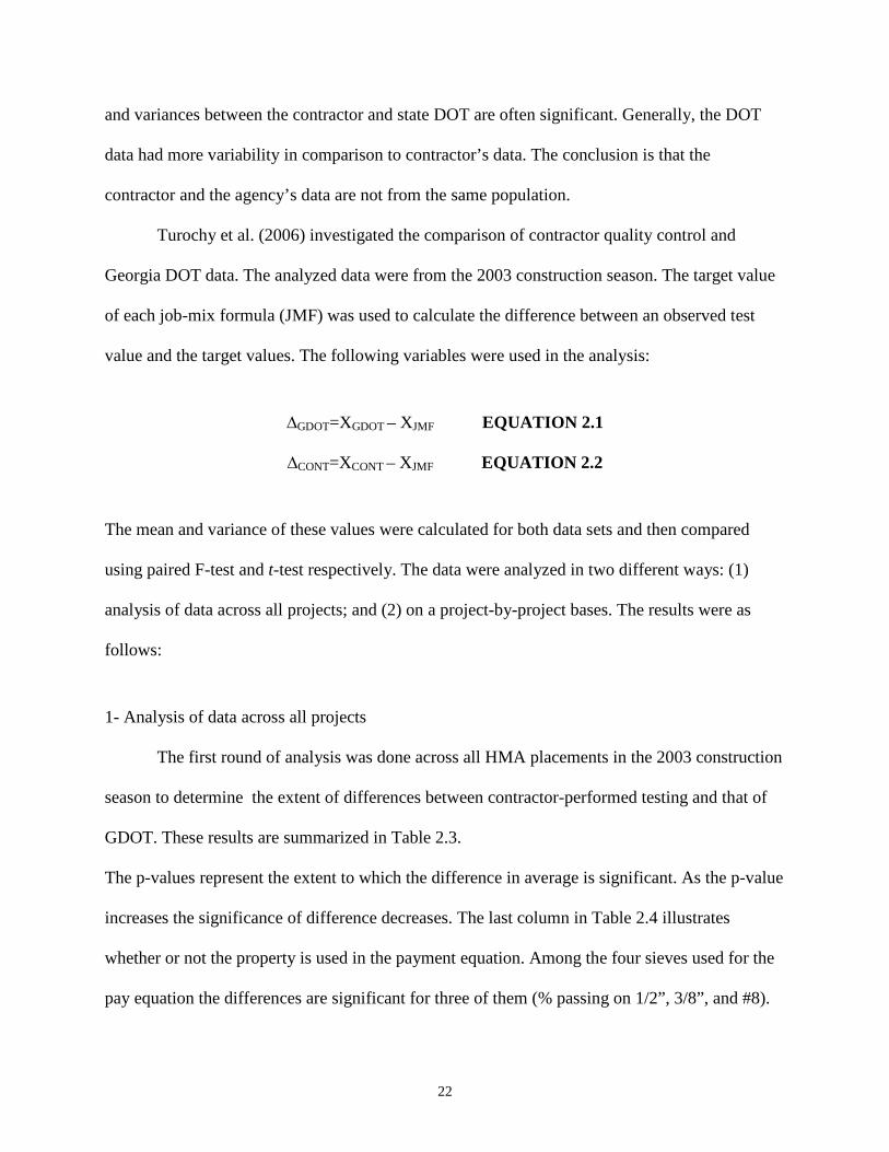
value and the target values. The following variables were used in the analysis:
∆GDOT=XGDOT – XJMF EQUATION 2.1
∆CONT=XCONT – XJMF EQUATION 2.2
The mean and variance of these values were calculated for both data sets and then compared
using paired F-test and t-test respectively. The data were analyzed in two different ways: (1)
analysis of data across all projects; and (2) on a project-by-project bases. The results were as
follows:
1- Analysis of data across all projects
The first round of analysis was done across all HMA placements in the 2003 construction
season to determine the extent of differences between contractor-performed testing and that of
GDOT. These results are summarized in Table 2.3.
The p-values represent the extent to which the difference in average is significant. As the p-value
increases the significance of difference decreases. The last column in Table 2.4 illustrates
whether or not the property is used in the payment equation. Among the four sieves used for the
pay equation the differences are significant for three of them (% passing on 1/2”, 3/8”, and #8).

23
The same comparison was done on the variances of GDOT and the contractor data using the F-
test. The results are summarized in Table 2.4.
TABLE 2.3 Comparisons of GDOT and Contractor QC Test Results Using Means (Turochy et al. 2006)
TABLE 2.4 Comparisons of GDOT and Contractor QC Test Result Using Variances (Turochy et al. 2006)

24
2- Analysis of data on project-by-project bases.
In this set of analysis were included only projects for which at least six GDOT
comparison tests were recorded. These analyses were performed on the asphalt content, percent
passing the ½ in sieve, and percent passing the No. 200 sieve. The results on both means and
variances are summarized in Table 2.5. As a general trend, the differences in variances tend to
be higher than the difference in the means. In conclusion, the analysis of GDOT QA and QC data
for HMA shows that differences in results of tests conducted by GDOT and the contractors differ
often significantly
TABLE 2.5 Comparisons of GDOT and Contractor QC Test Result Using Project Means and Variances (Turochy et al. 2006)
2.2.3 Quality Indicators
Several studies have examined the use of alternative quality indicators for HMA mixtures
(Burati and Weed 2006). Some examples of the most relevant studies are reported next.
Burati and Weed (2006) investigated the accuracy and precision of typical quality
measures (PWL, AAD and CI). From the statistical point of view an accurate measure is a
measure that provides an unbiased estimate for the corresponding population parameter. A
precise estimator is an estimator with low variability. The suggested quality measures are
summarized below:

25
a) Percent Within Limits (PWL)
In order to estimate the percent within limit (PWL) the Q-value is used with a PWL table.
QL = 𝑋𝑋−𝐿𝐿𝐿𝐿𝐿𝐿s
EQUATION 2.3
and
QU= 𝑈𝑈𝐿𝐿𝐿𝐿−𝑋𝑋s
EQUATION 2.4
Where:
QL = quality index for the lower spec limit
QU= quality index for the upper spec limit
X= sample mean for the lot
s= sample standard deviation for the lot
LSL= lower spec limit
USL=upper spec limit
Then using a PWL table, the total PWL is estimated (PWLT = PWLU + PWLL – 100).
Where:
PWLu =percent below the upper specification limit (based on Qu)
PWLL=percent above the lower specification limit (based on QL)
PWLT=percent within the upper and lower specification limits
As seen in the equations, this process takes both the mean and standard deviation into account.
b) Average Absolute Deviation (AAD)
The average absolute deviation from the target is calculated using the following equation
AAD= ∑ |𝑋𝑋𝑖𝑖−𝑇𝑇|𝑛𝑛
EQUATION 2.5
Where:

26
Xi = individual test results
T = target value
n = number of tests per lot
c) Conformal Index (CI)
The concept of CI is very similar to AAD. The AAD uses the average of the absolute
values of the deviations from the target value, but CI uses the squares of the deviations from
the target values. Both CI and AAD do not allow the contractor to adjust the process at the
middle of a lot production. This occurs by not allowing the negative and positive deviations
to cancel out.
CI=�∑(𝑋𝑋𝑖𝑖−𝑇𝑇)2
𝑛𝑛 EQUATION 2.6
For each of the three measures, 10,000 lots were generated. The results illustrated that as the
number of samples increases (3 to 5 to 10) the variability between the generated lot and actual
population decreases. The study also showed that for PWL, the variability increased as the actual
population PWL moves from 0 or 100 PWL and peaked at 50 for both the CI and AAD the
variability increased as the actual population vales moved from 0. The average differences of
simulated lots and actual population values indicated that both the AAD and PWL are unbiased
whereas CI is a biased estimator.
2.2.4 Evaluating Specification Limits
Several studies have investigated the definition and adequacy of specification limits
(Burati 2006, Sholar et al. 2005). Burati (2006) investigated the accuracy of assumed standard
deviations by South Carolina Department of Transportation (SCDOT) when developing their

27
initial QA specifications. The SCDOT QA specification is based on lot-by-lot acceptance,
therefore it is appropriate to use a variability of a typical lot. In order to achieve this, the standard
deviation values for each lot must be calculated and then be pooled to get a typical within-lot
standard deviation. In addition to the within-lot variability, the agency should also consider the
typical process variability. Based on multiple reports and specially the Optimal Procedures for
Quality Assurance Specifications (FHWA-RD-02-095) there is no single correct way to decide
the typical variability. Burati suggested to add both variances (within-lot and process variability),
and take the square root of that value to obtain the typical standard deviation. Table 2.6
summarizes the assumed standard deviations for the current spec and the standard deviations
found by Burati.
TABLE 2.6 Variability Values Used in Initial SCDOT HMA QA Specification-Revised Spec (Burati 2006)
After defining the typical variability, the number of standard deviations that the
population should fall within the population mean is calculated. Since the AQL is 90% for
SCDOT this value comes out to be 1.645. The following table summarizes the current
specification and the suggested specification limits.

28
TABLE 2.7 Specification Limits in Initial and Revised SCDOT HMA QA Specification (Burati 2006)
For all four parameters (Asphalt Content, Air Voids, Voids in Mineral Aggregate, and
Density) the suggested limits are narrower. The results of this study confirm the importance of
the continuous monitoring of the specifications adequacy and the need for adjustments based on
the test results obtained from actual projects.
2.2.5 Risk Analysis and Pay Factor Evaluation
There are generally two types of acceptance plans: 1) The accept/reject acceptance plans
and 2) Acceptance plans that include pay adjustment provisions (FHWA-RD-02-095). These
methods are presented next using specific studies from the literature.
2.2.5.1 Accept/Reject Acceptance Plans
Villiers et al. (2003) evaluated the PWL specification parameters. The study illustrated how
to balance the seller and buyer’s risk by adjusting certain specification parameters. In this
process the following parameters are defined:
a) Buyer’s risk (β): The probability that the buyer would accept poor quality material
b) Rejectable Quality Level (RQL): The maximum level of quality that the material is fully
unacceptable

29
c) Seller’s risk (α): The probability that seller’s good quality material would be rejected
d) Acceptable Quality Level (AQL): The minimum level of quality that the material is fully
acceptable
The AQL and RQL are the parameters that agency can utilize to determine incentives and
penalties. Each state sets its own AQL and RQL and for the state of Florida these values are set
at 90% and 50% respectively.
Using the Operation Characteristic Curve (OC Curve), the study illustrated that with the
current spec limits and sampling size of 4 or 5 per lot the buyer’s risk was equal to 33 and 24%
respectively, figure 2.1. In order to achieve the AASHTO recommended risk level of 5%, ten
samples per lot were required. Since this number of sampling is not practical, it was required to
adjust the AQL and RQL in order to achieve the 1% and 5% seller and buyer’s risk. After
constructing the OC curves and setting the risks at the suggested levels, it was concluded that the
agency need to change their AQL and RQL. Table 2.8 summarizes these values.
FIGURE 2.10 Contactor and Owner Risk using Unknown Standard Deviation (Villiers et al. 2003)

30
TABLE 2.8 Calculated AQL and RQL Based on Different Sample Sizes (Villiers et al. 2003) Sample Size AQL RQL
3 91 17 4 87 20 5 85 23
6 83 25 10 71 28
Therefore, the agency needs to either increase sampling size or adjust the AQL and RQL
values to achieve the recommended risk levels.
2.2.5.2 Acceptance Plans that Include Pay Adjustment Provisions
In order to consider the impact of specification on provisions, simulation analysis has
been used to generate alternative scenarios based on the population characteristics observed from
the HMA production (Burati 2005, Mahoney and Muench 2001). For example, a study by Burati
(2005) used computer simulation to illustrate how the removal and replacement provisions place
much greater risk on the contractor. In addition, 1742 sets of test results were analyzed for
correlations.
Many state highway agencies (SHAs) use the recommended pay factor relationship
recommended by the AASHTO Quality Assurance Guide Specification (1996) which is:
PF = 55 + (0.5 * PWL) EQUATION 2.7
From this equation it can be seen that the maximum pay factor is 105% when PWL = 100
and the minimum pay factor is 55% when PWL = 0. However, almost all states reject any lot that
has a PWL smaller than RQL and some states have some form of remove and replace provisions

31
(Burati 2005). Some agencies use as many as four or more quality characteristics to determine
the final pay factor for the lot. The study by Burati used the common method of weighted
average of the individual pay factors to determine the composite pay factor. In this study the
specifications of SCDOT were investigated. SCDOT uses four parameters; AC, AV, VMA and
in-place density from cores to determine payment for HMA.
One problem that is caused by the remove and replace provision is how often the lot is
actually an acceptable one but it gets rejected. Table 2.9 clearly illustrates how going from one
quality characteristic pay factor to four HMA mix characteristics increases the probability of
rejecting a good quality material. For example, at 90 PWL and three samples per lot (n=3) the
probability of rejecting a lot is 6% for a one mix characteristic; the probability rises to 22% for a
four mix property pay factor. This table clearly illustrates that the remove and replace provision
is problematic.
The composite pay factor that SCDOT uses to calculate the composite pay factor is:
LPF = 0.25(PFAC) + 0.30(PFAV) + 0.10(PFVMA) + 0.35(PFDEN) EQUATION 2.8
This equation assumes that the four parameters are statistically independent. To
investigate any possible correlations between the mixture parameters project test results were
analyzed. Only the correlations of the following pairs were analyzed: AC-AV, AC-VMA, and
AV-VMA.

32
TABLE 2.9 Probabilities that Populations with Various Quality Levels Would Require Removal and Replacement for One Versus Four Independent Quality Characteristics (Burati 2005)
The correlation values are summarized in Table 2.10.
TABLE 2.10 Correlation Coefficients for all Pairs of Plant Quality Characteristics (Burati 2005)
A computer simulation program (PAYSIM2) was used to compare the effect of these
correlations on the average payments. The results showed that on average the payments tend to
be the same in both cases (with and without the correlations). Table 2.11 illustrates these effects.

33
TABLE 2.11 Effects of Correlations between Variables Using Simulation Analysis (Burati 2005)

34
CHAPTER 3 COMPARISON OF MARYLAND QA & QC DATA
Several state specifications have used QA (Quality Assurance- behind the paver) and QC
(Quality Control- at the plant) data in their acceptance plans. The Maryland HMA Pay Factor
Team has been discussing such option as related to the past and current SHA specifications for
the acceptance of the Superpave HMA mixtures. This comparison involves the use of F and t
tests to determine whether QA and QC data can be considered as statistically representing the
same population, in statistical terms. Standard statistical analyses (F and t test) were conducted
comparing the QA and QC data for all the HMA mixtures (aggregate level), as well as for
specific mixtures (disaggregating the data into subsets representing common mixture types and
characteristics). The steps of the analysis are described in the following sections along with the
results. All the analyses followed the steps indentified in the SHA MSMT 733 report of the State
Highway Administration.
3.1 F and t Tests
3.1.1 Initial Exploratory Assessment Using Random Projects
An initial comparison between the QA and QC data was conducted using 15 randomly
selected projects: 5 large, 5 medium, and 5 small size projects. To assess the null hypothesis (i.e.,
equal mean and the standard deviation for the two populations, QA and QC), the F and t tests
were performed on all mix properties together and at 5% level of significance. The results,
shown in Table 3.1, indicated that as the number of observations (n) increased, the rejection rate
increased. Thus, the data and comparison had to be analyzed further.

35
TABLE 3.1 F and t Test on Random Projects Small Sample Size Medium Sample Size Large Sample Size t Tests F Test t Tests F Test t Tests F Test
Accepted 100% 83% 88% 75% 50% 45% Rejected 0% 17% 13% 25% 50% 55%
3.1.2 Analysis Based on Mixture Type and Property (Unmatched Lots and Sublots)
Each project is identified with a series of numbers and letters which is called the Job Mix
Formula ID (JMFID). The JMFID of each project describes the following characteristics of that
project:
i) Region
ii) Plant Number (The number identification of the plant)
iii) Nominal Maximum Aggregate Size (4.75mm, 9.5mm, 12.5mm, 19mm, 25mm, and
37.5mm)
iv) Mix Type (Virgin (V), Rap (R), Trinidad Lake Asphalt (TLA), Glass (GL), Gap
Grade (G), and High Polish (H))
v) ESAL Level
vi) Binder Type (A, B, C, D, E, and F)
vii) Mix Number (01 to 99)
viii) Status (Tentative and Final)
For example a JMFID of N12312V2A01T means that the job is in the North region (N), the plant
number is 123, the mix band is 12.5 mm, mix type is Virgin, ESAL level is 2, binder type is 58-
22 (A), mix number is 01, and the status is tentative (T).
Four QA properties are used by Maryland SHA (2008 specification) for determining mixture
pay factors:

36
i) Aggregate Passing 0.075mm /No. 200 sieve
ii) Aggregate Passing 2.36mm / No. 8 sieve
iii) Aggregate Passing 4.75mm / No. 4 sieve
iv) Asphalt Content (AC)
In order to sort the QA and QC data conveniently by mix type and mix characteristics it was
necessary to break the JMFIDs into their components (Mix Type, Max Aggregate Size (Mix
band), mix property, etc.). After parsing the JMFIDs, the F and t analyses were conducted by
mix type and property (e.g. G-12-AC, H-12- AC, etc.) at the 5% level of significance. An
example of these analyses is shown in Table 3.2. In many cases the Ho hypothesis was rejected.
Overall, only 53% of the t tests and 21% of the F tests were “Accepted”. This comparison dealt
with unpaired observations (i.e., different number of observations for QA and QC data). Due to
the low level of acceptance, it was necessary to disaggregate the data into more details.
TABLE 3.2 Example of F and t Tests by Mix Type MixSize MixType Property t Test F Test # of Observations Mean Variance QA QC QA QC QA QC
12 G AC Rejected Rejected 636 870 6.4074 6.5140 0.0881 0.0261 12 H AC Rejected Rejected 311 429 4.9040 4.8390 0.0941 0.0486
3.1.3 Analysis Based on Mixtures Type and Property (Matched Lots and Sublots)
Since for the 12-G-AC and 12-H-AC mixtures, shown in Table 3.2, both the F and t tests
were rejected, these data were further examined. In the next step the F and t analysis were run by
matching the lots and sub-lots of the QA and QC data for each project. Very often such task has
been shown to be challenging since there is not a unique reciprocity between the numbering of
lots and sublots between the QA and QC data, and the recoding dates did not match. Thus, while
such analysis has shown to increase the acceptance rate, it was felt that the analysis were
unreliable.

37
3.1.4 Unpaired vs. Paired Analysis based on Mixture Type and Property (Matched
Lots and Sublots)
The next step was to conduct unpaired and paired analysis with the data. In the first case
the lots were matched but eventually the sublot number between the QA and QC may have been
different. The latter case required selecting projects that had the same number of sublot
observations for the QA and QC data. The results are shown in tables 3.3 and 3.4. The paired
analyses produced a significant improvement in the statistical agreement between the QA and
QC data.
TABLE 3.3 Unpaired Analysis
** Table includes all the data.

38
TABLE 3.4 Paired Analysis
3.1.5 Analysis based on Mixtures Type, Mix Property, and Mix Band
For the High Polished mixtures, a relatively high rate of acceptance was observed, Tables
3.3 and 3.4. Thus it was decided to particularly focus on this group of data and further
subcategorize the projects with respect to nominal maximum aggregate size (9.5, 12.5 and 19
mm). Tables 3.5 and 3.6 summarize the results for both unpaired and paired analyses. It can be
seen that the acceptance rate increases with pairing, however the number of projects (# of
performed tests) decreases significantly. As tabulated in Table 3.6, none of the 19 mm mixtures
had projects with equal number of observations.

39
TABLE 3.5 Unpaired Analysis for High Polished Mixtures
TABLE 3.6 Paired Analysis for High Polished Mixtures
3.1.6 Analysis based on Deviations from the Target Values
In the next step of the analysis, the deviations from the target values were considered for
all mixtures together. One of the benefits of such approach is that the distribution of the
deviations is immediately evident for both QA and QC data. Also the variability of such data sets
in relation to the tolerances identified for every mix property can be immediately assessed. Such
analyses also allow for the different target values from one project to the next, especially for
asphalt content. As shown in Figures 3.1 to 3.4 (representing the AC content, and percent
passing 4.75mm, 2.36mm, and the 0.075mm) the dispersion of the QA data is larger than that for

40
the QC data. The QC data are clearly more concentrated towards the central tendency (in this
case higher frequency around the zero deviation from the target values).
FIGURE 3.1 Deviations from the Target Values for AC
FIGURE 3.2 Deviations from the Target Values for 4.75mm
0%
10%
20%
30%
40%
50%
-1 -0.8 -0.6 -0.4 -0.2 0 0.2 0.4 0.6 0.8 1
Delta AC
Freq
uenc
y
QAQC
0%
5%
10%
15%
20%
25%
30%
35%
-12 -10 -8 -6 -4 -2 0 2 4 6 8 10 12
Delta p4.75
Freq
uenc
y
QAQC

41
FIGURE 3.3 Deviations from the Target Values for 2.36mm
FIGURE 3.4 Deviations from the Target Values for 0.075mm
Further review of the QA and QC databases revealed that for certain projects and
mixtures there was more than one target for the same project. These projects, totaling about 138
0%
5%
10%
15%
20%
25%
30%
35%
40%
-12 -10 -8 -6 -4 -2 0 2 4 6 8 10 12
Freq
uenc
y
Delta p2.36
QAQC
0%
10%
20%
30%
40%
50%
60%
-6 -5 -4 -3 -2 -1 0 1 2 3 4 5 6
Freq
uenc
y
Delta p0.075
QAQC
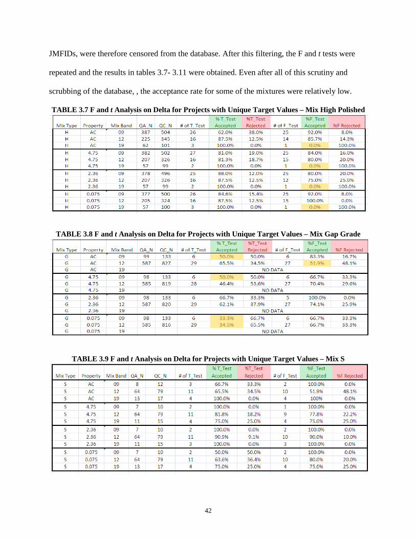
42
JMFIDs, were therefore censored from the database. After this filtering, the F and t tests were
repeated and the results in tables 3.7- 3.11 were obtained. Even after all of this scrutiny and
scrubbing of the database, , the acceptance rate for some of the mixtures were relatively low.
TABLE 3.7 F and t Analysis on Delta for Projects with Unique Target Values – Mix High Polished
TABLE 3.8 F and t Analysis on Delta for Projects with Unique Target Values – Mix Gap Grade
TABLE 3.9 F and t Analysis on Delta for Projects with Unique Target Values – Mix S

43
TABLE 3.10 F and t Analysis on Delta for Projects with Unique Target Values – Mix Rap
TABLE 3.11 F and t Analysis on Delta for Projects with Unique Target Values – Mix Virgin
In all analyses, regardless of whether the entire QA and QC datasets or just subsets
representing specific mixture types were considered, a significant number of F and t tests were
rejected. The inescapable conclusion is that the QA and QC data cannot be considered as
representative of the same population, and thus the null hypothesis (Ho) must be rejected.
Furthermore, the analyses indicated that
i) differences in variability are greater than differences in mean and
ii) The QA data show higher variability than the QC data.

44
Some of these differences are certainly due to different sampling locations. Although
Paired-t results compare more often than unpaired, there are still several significant differences
between paired results (15-20% overall). Some of these differences may have to do with the
difficulty in matching the lots and sublots between QA and QC data, primarily due to:
i) Discrepancies in the database, and
ii) Lack of using a common and unique identification for the material departing the plant
and the one behind the paver.
In other words a better tracking technique is needed in this area.
3.2 Transfer Functions Between QA and QC Data
The results of the F and t analysis on the QA and QC data indicated that these two data
sets represent statistically different populations. Based on the interaction and feedback of the
MSHA research project engineer, it was decided to examine whether it was possible to define
transfer functions between the material properties of the QA and QC data.
In order to examine whether such relationships were possible, the research team directed the
effort of the analysis towards the premium SHA asphalt mixture where better quality control is
expected. Thus, the analyses were oriented towards the gap graded 12.5mm mixture. The QA
and QC data from the gap-graded projects were matched on a lot-by-lot basis and the average
value of each lot was calculated and plotted in Figures 3.5 through 3.8. As it can be seen from
these figures there is a significance scatter between these two data sets providing very poor
correlations between the QA and QC data for any mixture property.

45
FIGURE 3.5 Comparison of QA & QC Data for the 0.075mm of the 12.5 Gap Graded Mixtures
FIGURE 3.6 Comparison of QA & QC Data for the 2.36 mm of the 12.5 Gap Graded Mixtures
FIGURE 3.7 Comparison of QA & QC Data for the 4.75mm of 12.5 Gap Graded Mixtures
y = 0.620x + 3.785R² = 0.269
6
7
8
9
10
11
12
6 7 8 9 10 11 12
QA
QC
0.075 x=y Linear (0.075) Linear (x=y)
y = 0.707x + 6.064R² = 0.502
151617181920212223242526
15 16 17 18 19 20 21 22 23 24 25 26
QA
QC
2.36 x=y Linear (2.36) Linear (x=y)
y = 0.721x + 10.54R² = 0.507
20
25
30
35
40
45
20 25 30 35 40 45
QA
QC
4.75 x=y Linear (4.75) Linear (x=y)

46
FIGURE 3.8 Comparison of QA & QC Data for the AC Content of 12.5 Gap Graded Mixtures
y = 0.832x + 0.961R² = 0.247
5.6
5.8
6
6.2
6.4
6.6
6.8
7
5.6 5.8 6 6.2 6.4 6.6 6.8 7
QA
QC
AC x=y Linear (AC) Linear (x=y)

46
CHAPTER 4 TYPE I AND TYPE II ERROR ANALYSIS & OPERATION CHARACTERISTIC (OC) CURVES
4.1. Definitions
The “FHWA Optimal Procedures for Quality Assurance Specifications” report (Burati et.
al. 2003) provides the following definitions for the OC curves, type I and type II errors:
OC Curve: A graphic representation of an acceptance plan that shows the relationship
between the actual quality of a lot and either (1) the probability of its acceptance (for
accept/reject acceptance plans) or (2) the probability of its acceptance at various payment
levels (for acceptance plans that include pay adjustment provisions)
Seller’s risk (α): also called risk of a type I error. The probability that an acceptance plan
will erroneously reject acceptable quality level (AQL) material or construction with respect
to a single acceptance quality characteristic. It is the risk the contractor or producer takes in
having AQL material or construction rejected.
Buyer’s risk (β): also called risk of a type II error. The probability that an acceptance plan
will erroneously fully accept (100 percent or greater) rejectable quality level (RQL) material
or construction with respect to a single acceptance quality characteristic. It is the risk the
highway agency takes in having RQL material or construction fully accepted. [The
probability of having RQL material or construction accepted (at any pay) may be
considerably greater than the buyer’s risk.
The TRB glossary (Transportation Research Circular No. E-C037) offers the following
definitions for AQL and RQL
AQL: That minimum level of actual quality at which the material or construction can be
considered fully acceptable (for that quality characteristic). For example, when quality is

47
based on PWL, the AQL is that actual (not estimated) PWL at which the quality
characteristic can just be considered fully acceptable. [Acceptance plans should be designed
so that AQL material will receive an EP of 100 percent.]
RQL: That maximum level of actual quality at which the material or construction can
be considered unacceptable (rejectable). For example, when quality is based on PD, the
RQL is that actual (not estimated) PD at which the quality characteristic can just be
considered fully rejectable. [It is desired to require removal and replacement, corrective
action, or the assignment of a relatively low pay factor when RQL work is detected.
Based on these terms the seller’s risk (α) and the buyer’s risk (β) are calculated at AQL and RQL
respectively.
As mentioned previously there are generally two types of acceptance plans: 1) the
accept/reject acceptance plans and 2) acceptance plans that include pay adjustment provisions.
The development of traditional OC curves and the definitions of α and β risks are more
appropriate for the first case and less relevant to the current SHA specification that include pay
adjustment provisions. Nevertheless, the examination of these parameters was included in this
study as an exercise of probability analysis involved if a pay provision is not considered, and
thus, it was limited to only the premium (gap graded) SHA mixtures. The analysis and results are
reported in this chapter.
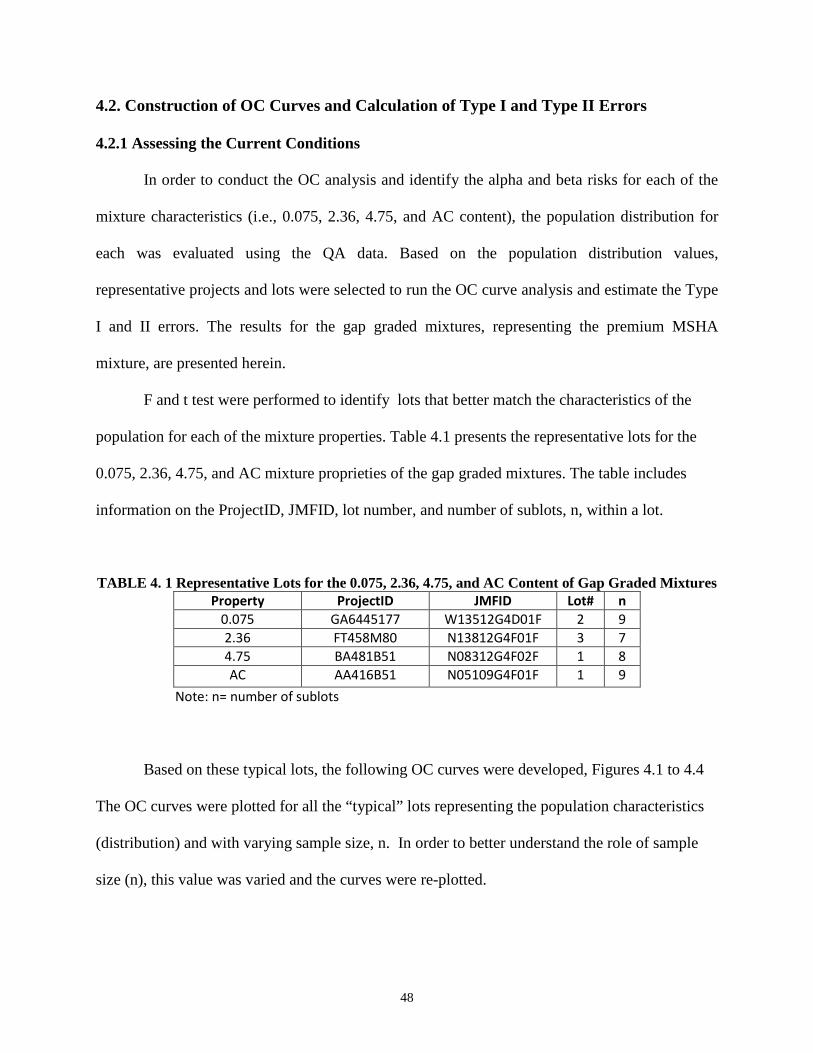
48
4.2. Construction of OC Curves and Calculation of Type I and Type II Errors
4.2.1 Assessing the Current Conditions
In order to conduct the OC analysis and identify the alpha and beta risks for each of the
mixture characteristics (i.e., 0.075, 2.36, 4.75, and AC content), the population distribution for
each was evaluated using the QA data. Based on the population distribution values,
representative projects and lots were selected to run the OC curve analysis and estimate the Type
I and II errors. The results for the gap graded mixtures, representing the premium MSHA
mixture, are presented herein.
F and t test were performed to identify lots that better match the characteristics of the
population for each of the mixture properties. Table 4.1 presents the representative lots for the
0.075, 2.36, 4.75, and AC mixture proprieties of the gap graded mixtures. The table includes
information on the ProjectID, JMFID, lot number, and number of sublots, n, within a lot.
TABLE 4. 1 Representative Lots for the 0.075, 2.36, 4.75, and AC Content of Gap Graded Mixtures Property ProjectID JMFID Lot# n
0.075 GA6445177 W13512G4D01F 2 9 2.36 FT458M80 N13812G4F01F 3 7 4.75 BA481B51 N08312G4F02F 1 8 AC AA416B51 N05109G4F01F 1 9
Note: n= number of sublots
Based on these typical lots, the following OC curves were developed, Figures 4.1 to 4.4
The OC curves were plotted for all the “typical” lots representing the population characteristics
(distribution) and with varying sample size, n. In order to better understand the role of sample
size (n), this value was varied and the curves were re-plotted.

49
The OC curves were developed using the procedure followed by Villiers et al. (2003) and
using the standard error of the population in order to relate PWL and probability of acceptance.
FIGURE 4.1 OC Curve for 0.075 mm of Gap Graded Mixtures
FIGURE 4.2 OC Curve for 2.36 mm of Gap Graded Mixtures
0%10%20%30%40%50%60%70%80%90%
100%
0%10%20%30%40%50%60%70%80%90%100%
Prob
abili
ty o
f Acc
epta
nce
PWL
Gap Graded 0.075
n=9
n=8
n=7
n=6
0%10%20%30%40%50%60%70%80%90%
100%
0%10%20%30%40%50%60%70%80%90%100%
Prob
abili
ty o
f Acc
epta
nce
PWL
Gap Graded 2.36
n=7
n=6
n=5
n=4

50
FIGURE 4.3 OC Curve for 4.75 mm of Gap Graded Mixtures
FIGURE 4.4 OC Curve for AC content of Gap Graded Mixtures
As illustrated in figures 4.1through 4.4, for a sample size n=6 , the α and β risks
corresponding to an AQL of 90% and RQL of 40 % (back calculated from equation 3) are equal
to about 0% and 26.5% respectively, Table 4.2. The effects of changing the sample size n can be
also assessed from the OC Figures.
0%10%20%30%40%50%60%70%80%90%
100%
0%20%40%60%80%100%
Prob
abili
ty o
f Acc
epta
nce
PWL
Gap Graded 4.75
n=8
n=7
n=6
n=5
0%10%20%30%40%50%60%70%80%90%
100%
0%20%40%60%80%100%
Prob
abili
ty o
f Acc
epta
nce
PWL
Gap Graded AC
n=9
n=8
n=7
n=6

51
TABLE 4.2 Risks Based on AQL= 90% and RQL = 40% for n=6. Property Tolerance α @ AQL=90% β @ RQL=40%
0.075 ± 2 0.0% 26.5% 2.36 ± 5 0.1% 26.8% 4.75 ± 5 0.0% 27.6% AC ± 0.5 0.1% 26.3%
4.2.2 Modifying AQL and RQL to balance the risks (α= 1% and β= 5%)
Since the α and β risks are far from the typical values of 1% and 5% respectively used in
practice (ASSHTO R-9), new values of AQL and RQL may be identifying for balancing these
risks. Table 4.3 provides the values of AQL and RQL that result in α and β risks of 1% and 5%
respectively.
TABLE 4.3 AQL and RQL for α= 1% and β= 5% (n=6).
Property Tolerance AQL @ α=1% RQL @ β=5% 0.075 ± 2 82.9% 25.0% 2.36 ± 5 82.9% 25.1% 4.75 ± 5 75.6% 25.0% AC ± 0.5 83.4% 25.9%
4.2.3 Revised Specification Tolerances for α= 1% and β= 5%
Based on the revised values of AQL and RQL providing α= 1% and β= 5% risks, Table
4.3, new tolerance may be defined for the specification. Based on the recommendations of the
FHWA Optimal Procedures for QA Specifications study (Burati et. al. 2003), these new
tolerances can be determined by first calculating the standard normal Z-values corresponding to
each AQL value and then multiplying it by the standard deviation of the representative lot. The
new set of specification tolerances (shown in Table 4.4) were obtained by following this

52
procedure. The important question is whether such tolerances represent realistic achievable
levels of production by the paving industry.
TABLE 4.4 Revised Specification tolerances for α= 1% and β= 5%.
Property Tolerance
0.075 0.9 2.36 1.2 4.75 2.9 AC 0.15
The α and β risk analysis and OC calculations provided an initial assessment of the risks
involved with the current specifications. However, these analyses were not expanded to the
remaining MSHA mixtures since such risks are assessed for each individual mixture property
rather than providing an assessment of a combined risk associated with all mixture properties, as
it is the case of the combined MSHA specification. Also, as indicated previously the above
approach is primarily used for accept/ reject plans. Since the SHA specs include pavement
adjustment provisions, the focus of the research was directed toward the expected pay (EP)
calculations approach using simulation analysis.

53
CHAPTER 5 SIMULATION ANALYSIS
The purpose of the simulation analysis was to examine the impact of the current Hot Mix
Asphalt (HMA) production quality on the composite PWL and pay factor, and assess the impact
of alternative scenarios in terms of specification tolerances or pay equations. In these analyses
the revised 2008 HMA specs were used. Only dense graded HMA mixtures were considered in
the simulation because of the comparatively large amount of data available for these mixtures in
the SHA database. The simulation tool developed under this study considers the four HMA
mixture parameters (AC content and percent passing the 0.075, 2.36, 4.75 mm sieves) and their
correlations for calculating the composite pay factor CMPWSL and the expected mix pay factor
(MF). An example of the correlations between the four mix properties for dense graded mixtures
is shown in Table 5.1. Preliminary analyses have shown that the correlation effects of the four
HMA mix properties have little impact on the pay factor analysis. Example calculations are
shown in appendix section A.4. Details on the Monte Carlo simulation algorithms and associate
program code can be found in the appendix. Once the simulation code was verified to make sure
that the algorithms were working properly and providing reasonable and rational responses,
several alternative scenarios were investigated. Mean values and standard deviations for the
specification variables were based on all dense graded QA data, excluding JMFIDs with multiple
target values. The statistical results for this data population are tabulated in the Table 5.2.
TABLE 5.1 Correlations Between Mix Parameters for Dense Graded Mixtures Property 0.075 2.36 4.75 AC
0.075 1 0.338 0.208 0.242 2.36 0.338 1 0.562 0.261 4.75 0.208 0.562 1 0.305 AC 0.242 0.261 0.305 1

54
TABLE 5.2 Population Characteristics Property Delta Mean* Std. Dev.
0.075 0.992 1.20 2.36 -0.192 3.88 4.75 0.066 5.60 AC -0.002 0.31
*Deviations from the target values 5.1 Analysis Based on Previous Specifications
The first set of analyses were based on the following pay equation and the population
characteristics shown in Table 5.2.
�𝑀𝑀𝑀𝑀 = 0.55 + 0.5𝐶𝐶𝑀𝑀𝐶𝐶𝐶𝐶𝐿𝐿𝐿𝐿𝑖𝑖𝑖𝑖 𝐶𝐶𝑀𝑀𝐶𝐶𝐶𝐶𝐿𝐿𝐿𝐿 ≥ 90% 𝑀𝑀𝑀𝑀 = 1𝑖𝑖𝑖𝑖 𝐶𝐶𝑀𝑀𝐶𝐶𝐶𝐶𝐿𝐿𝐿𝐿 < 40% 𝑀𝑀𝑀𝑀 = 0
� EQUATION 5.1
5.1.1 Reducing Asphalt Content Variability
The goal of this analysis was to examine how much a producer might be able to reduce
the asphalt content and still have an acceptable product, assuming that he/she can improve
production control and thus reduce production variability (standard deviation). All the gradations
(0.075, 2.36 and 4.75) were kept at the population characteristics values. The standard deviation
of AC content was progressively reduced to 75%, 50% and 25% of the population value. The
results were plotted in Figure 5.1, for a constant MF of 97.5% representing the value obtained
based on the current population characteristics at the long run. As shown in Figure 5.1, a
contractor that is able to produce a HMA mixture with 75% lower variability (0.25 SD/SDpop)
than the current QA population variability can reduce the AC content by 0.4% from the target
and receive the same MF. Considering that the current tolerance for AC content is ±0.5%, this
change in AC content is significant.
Next the effect of reducing production variability of AC content on CMPWSL and MF
was examined, all remaining parameters (including population means for all mixture parameters

55
and variances for the three gradation percent passing) were at the population values. As shown in
Figures 5.2 and 5.3, if a contractor reduces production variability by 75% (0.25 SD/SDpop)while
aiming for the target AC content, it can increase its CMPWSL from 86% to about 93% and
receive an MF of about 99.7% instead of 97.5% (corresponding at SD/SDpop=1).
FIGURE 5.1 Effect of Reduction in Asphalt Content Variability
FIGURE 5.2 Effect of Reduction in Asphalt Content Variability on MF
-0.45-0.4-0.35-0.3-0.25-0.2-0.15-0.1-0.050
0 0.25 0.5 0.75 1
Delta
_AC
SD/SDpop
97
97.5
98
98.5
99
99.5
100
0 0.25 0.5 0.75 1
Mea
n_M
F
SD/SDpop

56
FIGURE 5.3 Effect of reduction in asphalt content variability on CMPWSL
5.1.2 Modifying Specification Tolerances
The next set of analysis examined the effects of specification limit (tolerance) changes on
the average MF and CMPWSL. Based on the current specifications, the tolerance for AC is
±0.5%. All other tolerances were kept constant and only the AC tolerance was varied. The results
are shown in Table 5.3 and Figures 5.4 and 5.5. A change in the tolerance of AC content of about
20% will result in a change of 4% CMPWSL and 1.4% in MF.
TABLE 5.3 Effects of Change in AC Specification Tolerance AC_Tol %Change Mean_CM Mean_MF % Change CM % Change MF
1 100% 92.4 99.7 7% 2.4% 0.75 50% 91.6 99.5 6% 2.1% 0.6 20% 89.4 98.7 4% 1.4%
0.55 10% 88.0 98.2 2% 0.8% 0.5 0% 86.0 97.4 0% 0.0%
0.45 -10% 83.6 96.3 -3% -1.1% 0.4 -20% 80.7 95.0 -6% -2.4%
0.25 -50% 66.9 88.4 -22% -9.3%

57
FIGURE 5.4 Effects of Change in AC Specification Tolerance on CMPWSL
FIGURE 5.5 Effects of Change in AC Specification Tolerance on MF
Similarly, the effects of changing the 0.075mm percent passing specification tolerance
was also examined. The current specification has a tolerance of ±2%. The results of varying the
0.075 mm percent passing tolerance while holding all other constant are shown in Table 5.4 and
Figures 5.6 and 5.7.
-25%-20%-15%-10%
-5%0%5%
10%
-50% -40% -30% -20% -10% 0% 10% 20% 30% 40% 50% 60% 70% 80% 90% 100%Chan
ge in
Mea
n_CM
PWSL
Change in Tolerance
AC
-10.0%-8.0%-6.0%-4.0%-2.0%0.0%2.0%4.0%
-50% -40% -30% -20% -10% 0% 10% 20% 30% 40% 50% 60% 70% 80% 90% 100%
Chan
ge in
Mea
n_M
F
Change in Tolerance
AC

58
TABLE 5.4 Effects of Change in 0.075 Specification Tolerance on MF 0.075_Tol %Change Mean_CM Mean_MF % Change CM % Change MF
4 100% 90.9 98.8 5.6% 1.5% 3 50% 89.8 98.5 4.4% 1.2%
2.4 20% 88.0 98.1 2.3% 0.7% 2.2 10% 87.3 97.8 1.5% 0.5% 2 0% 86.0 97.4 0.0% 0.0%
1.8 -10% 84.8 96.9 -1.5% -0.5% 1.6 -20% 83.4 96.4 -3.1% -1.0% 1 -50% 78.0 94.0 -9.3% -3.5%
FIGURE 5.6 Effects of Change in 0.075 Specification Tolerance on CMPWSL
FIGURE 5.7 Effects of Change in 0.075 Specification Tolerance on MF
The effects of changing the 2.36 percent passing specification tolerance was then
examined. The current specifications have a tolerance of ±5%. The results of varying the
-15.0%
-10.0%
-5.0%
0.0%
5.0%
10.0%
-50%-40%-30%-20%-10% 0% 10% 20% 30% 40% 50% 60% 70% 80% 90% 100%Chan
ge in
Mea
n_CM
PWSL
Change in Tolerance
0.075
-4.0%
-3.0%
-2.0%
-1.0%
0.0%
1.0%
2.0%
-50% -40% -30% -20% -10% 0% 10% 20% 30% 40% 50% 60% 70% 80% 90% 100%
Chan
ge in
Mea
n_M
F
Change in Tolerance
0.075

59
2.36mm percent passing tolerance while holding all other tolerances constant are shown in Table
5.5 and Figures 5.8 and 5.9.
TABLE 5.5 Effects of Change in 2.36 Specification Tolerance on MF 2.36_Tol %Change Mean_CM Mean_MF % Change CM % Change MF
10 100% 87.5 97.9 1.76% 0.40% 7.5 50% 87.0 97.7 1.13% 0.20% 6 20% 86.6 97.6 0.71% 0.07%
5.5 10% 86.4 97.5 0.49% 0.02% 5 0% 86.0 97.4 0.00% -0.12%
4.5 -10% 85.7 97.3 -0.28% -0.21% 4 -20% 85.4 97.2 -0.65% -0.32%
2.5 -50% 83.9 96.6 -2.45% -0.90%
FIGURE 5.8 Effects of Change in 2.36 Specification Tolerance on CMPWSL
FIGURE 5.9 Effects of Change in 2.36 Specification Tolerance on MF
-3%
-2%
-1%
0%
1%
2%
-50% -40% -30% -20% -10% 0% 10% 20% 30% 40% 50% 60% 70% 80% 90% 100%Chan
ge in
Mea
n_CM
PWSL
Change in Tolerance
2.36
-1.0%-0.8%-0.6%-0.4%-0.2%0.0%0.2%0.4%0.6%
-50% -40% -30% -20% -10% 0% 10% 20% 30% 40% 50% 60% 70% 80% 90% 100%
Chan
ge in
Mea
n_M
F
Change in Tolerance
2.36

60
Finally, the effects of changing the 4.75 percent passing specification tolerance was
examined. The current specifications has a tolerance of ±7%. The results from varying the
4.75mm percent passing tolerance while holding all others tolerances constant are shown in
Table 5.6 and Figures 5.10 and 5.11.
TABLE 5.6 Effects of Change in 4.75 Specification Tolerance on MF
4.75_Tol %Change Mean_CM Mean_MF % Change
CM % Change
MF 14 100% 87.5 97.9 1.7% 0%
10.5 50% 87.1 97.8 1.3% 0.3% 8.4 20% 86.6 97.6 0.8% 0.1% 7.7 10% 86.4 97.5 0.4% 0.0% 7 0% 86.0 97.4 0.0% -0.1%
6.3 -10% 85.8 97.3 -0.3% -0.2% 5.6 -20% 85.4 97.2 -0.6% -0.3% 3.5 -50% 83.9 96.6 -2.5% -1%
FIGURE 5.10 Effects of Change in 4.75 Specification Tolerance on CMPWSL
-3.0%
-2.0%
-1.0%
0.0%
1.0%
2.0%
-50% -40% -30% -20% -10% 0% 10% 20% 30% 40% 50% 60% 70% 80% 90% 100%Chan
ge in
Mea
n_CM
PWSL
Change in Tolerance
4.75
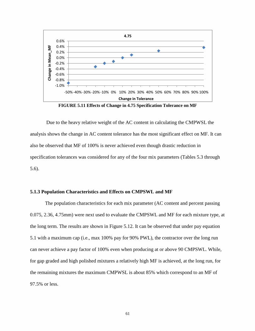
61
FIGURE 5.11 Effects of Change in 4.75 Specification Tolerance on MF
Due to the heavy relative weight of the AC content in calculating the CMPWSL the
analysis shows the change in AC content tolerance has the most significant effect on MF. It can
also be observed that MF of 100% is never achieved even though drastic reduction in
specification tolerances was considered for any of the four mix parameters (Tables 5.3 through
5.6).
5.1.3 Population Characteristics and Effects on CMPSWL and MF
The population characteristics for each mix parameter (AC content and percent passing
0.075, 2.36, 4.75mm) were next used to evaluate the CMPSWL and MF for each mixture type, at
the long term. The results are shown in Figure 5.12. It can be observed that under pay equation
5.1 with a maximum cap (i.e., max 100% pay for 90% PWL), the contractor over the long run
can never achieve a pay factor of 100% even when producing at or above 90 CMPSWL. While,
for gap graded and high polished mixtures a relatively high MF is achieved, at the long run, for
the remaining mixtures the maximum CMPWSL is about 85% which correspond to an MF of
97.5% or less.
-1.0%-0.8%-0.6%-0.4%-0.2%0.0%0.2%0.4%0.6%
-50% -40% -30% -20% -10% 0% 10% 20% 30% 40% 50% 60% 70% 80% 90% 100%
Chan
ge in
Mea
n_M
F
Change in Tolerance
4.75
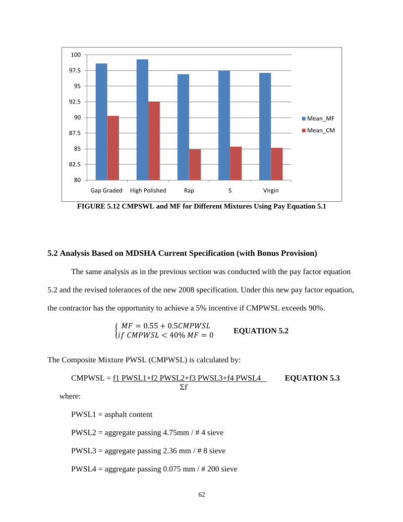
62
FIGURE 5.12 CMPSWL and MF for Different Mixtures Using Pay Equation 5.1
5.2 Analysis Based on MDSHA Current Specification (with Bonus Provision)
The same analysis as in the previous section was conducted with the pay factor equation
5.2 and the revised tolerances of the new 2008 specification. Under this new pay factor equation,
the contractor has the opportunity to achieve a 5% incentive if CMPWSL exceeds 90%.
� 𝑀𝑀𝑀𝑀 = 0.55 + 0.5𝐶𝐶𝑀𝑀𝐶𝐶𝐶𝐶𝐿𝐿𝐿𝐿𝑖𝑖𝑖𝑖 𝐶𝐶𝑀𝑀𝐶𝐶𝐶𝐶𝐿𝐿𝐿𝐿 < 40% 𝑀𝑀𝑀𝑀 = 0
� EQUATION 5.2
The Composite Mixture PWSL (CMPWSL) is calculated by:
CMPWSL = f1 PWSL1+f2 PWSL2+f3 PWSL3+f4 PWSL4 Σf
EQUATION 5.3
where: PWSL1 = asphalt content PWSL2 = aggregate passing 4.75mm / # 4 sieve PWSL3 = aggregate passing 2.36 mm / # 8 sieve
PWSL4 = aggregate passing 0.075 mm / # 200 sieve
80
82.5
85
87.5
90
92.5
95
97.5
100
Gap Graded High Polished Rap S Virgin
Mean_MF
Mean_CM

63
f1 = asphalt content = 62 f2 = aggregate passing 4.75mm / # 4 sieve=7 f3= aggregate passing 2.36 mm / # 8 sieve =7 f4= aggregate passing 0.075 mm / # 200 sieve=24
5.2.1 Reducing Asphalt Content Variability
As in the previous analysis, the goal was to examine how a reduction in AC variability
will affect the average MF while holding the variability of all other parameters (percent passing
0.075, 2.36 and 4.75mm) constant at the population characteristics. The standard deviation of AC
was set at 75%, 50% and 25% of the population; the results are shown in Figure 5.13. As it can
be seen from this figure, a contractor that is able to produce an HMA mixture with 75% lower
variability (0.25 SD/SDpop) than the current QA population variability can increase MF from 98%
to about 101% .
FIGURE 5.13 Effect of Reduction in AC Content Variability on MF
97.598
98.599
99.5100
100.5101
101.5
0 0.25 0.5 0.75 1
Mea
n_M
F
SD/SDpop

64
5.2.2 Modifying Specification Tolerances
The effects of changing specification limits (tolerances) on the average MF were
examined by using the revised pay equation with the bonus provision. Based on the current
specifications, the tolerance for AC is ±0.5%. All other tolerances were kept constant and the AC
tolerance was changed for the spec in question. The results are shown in Table 5.7 and Figures
5.14. A change in the tolerance of AC content of about 20% will result in a change of 4%
CMPWSL and 1.6% in MF.
TABLE 5.7 Effects of Change in AC Specification Tolerance and Impact on MF AC_Tol %Change Mean_CM Mean_MF % Change CM % Change MF
1 100% 92.4 101.2 7% 3.1% 0.75 50% 91.5 100.8 6% 2.7% 0.6 20% 89.3 99.7 4% 1.6%
0.55 10% 88.0 99.0 2% 0.9% 0.5 0% 86.2 98.1 0% 0.0%
0.45 -10% 83.6 96.8 -3% -1.3% 0.4 -20% 80.7 95.4 -6% -2.8%
0.25 -50% 66.8 88.4 -23% -10.0%
FIGURE 5.14 Effects of Change in AC Specification Tolerance on MF
-10.0%
-8.0%
-6.0%
-4.0%
-2.0%
0.0%
2.0%
4.0%
-50% -40% -30% -20% -10% 0% 10% 20% 30% 40% 50% 60% 70% 80% 90% 100%
Chan
ge in
Mea
n_M
F
Change in Tolerance
AC

65
Similarly, the effect of changing the 0.075 percent passing specification tolerance was
also examined. The current specification has a tolerance of ±2%. The results are shown in Table
5.8 and Figure 5.15.
TABLE 5.8 Effects of Change in 0.075 Specification Tolerance and Impact on MF 0.075_Tol %Change Mean_CM Mean_MF % Change CM % Change MF
4 100% 90.8 100.4 5.5% 2.4% 3 50% 89.8 99.9 4.3% 1.9%
2.4 20% 88.1 99.1 2.4% 1.0% 2.2 10% 87.2 98.6 1.3% 0.5% 2 0% 86.1 98.0 0.0% 0.0%
1.8 -10% 84.9 97.5 -1.3% -0.6% 1.6 -20% 83.4 96.7 -3.1% -1.4% 1 -50% 78.0 94.0 -9.4% -4.1%
FIGURE 5.15 Effects of Change in 0.075 Specification Tolerance on MF
The effect of changing the 2.36 percent passing specification tolerance was also
examined with the bonus provision. The current specifications has a tolerance of ±5%. The
results are shown in Table 5.9 and Figure 5.16.
-5.0%-4.0%-3.0%-2.0%-1.0%0.0%1.0%2.0%3.0%
-50% -40% -30% -20% -10% 0% 10% 20% 30% 40% 50% 60% 70% 80% 90% 100%
Chan
ge in
Mea
n_M
F
Change in Tolerance
0.075

66
TABLE 5.9 Effects of Change in 2.36 Specification Tolerance on MF 2.36_Tol %Change Mean_CM Mean_MF % Change CM % Change MF
10 100% 87.4 98.7 1.48% 0.57% 7.5 50% 87.1 98.5 1.13% 0.41% 6 20% 86.7 98.3 0.69% 0.22%
5.5 10% 86.3 98.2 0.26% 0.03% 5 0% 86.1 98.0 -0.01% -0.09%
4.5 -10% 85.7 97.8 -0.48% -0.29% 4 -20% 85.3 97.6 -0.92% -0.49%
2.5 -50% 83.9 96.9 -2.57% -1.21%
FIGURE 5.16 Effects of Change in 2.36 Specification Tolerance on MF
Finally, the effect of changing the 4.75 percent passing specification tolerance was
examined. The current specifications has a tolerance of ±7%. The results are shown in Table 5.10
and Figure 5.17.
TABLE 5.10 Effects of Change in 4.75 Specification Tolerance on MF 4.75_Tol %Change Mean_CM Mean_MF % Change CM % Change MF
14 100% 87.5 98.8 1.7% 1% 10.5 50% 87.2 98.6 1.3% 0.5% 8.4 20% 86.6 98.3 0.7% 0.2% 7.7 10% 86.2 98.1 0.2% 0.0% 7 0% 86.1 98.0 0.0% -0.1%
6.3 -10% 85.8 97.9 -0.3% -0.2% 5.6 -20% 85.2 97.6 -1.0% -0.5% 3.5 -50% 83.9 97.0 -2.5% -1%
-1.5%
-1.0%
-0.5%
0.0%
0.5%
1.0%
-50% -40% -30% -20% -10% 0% 10% 20% 30% 40% 50% 60% 70% 80% 90% 100%
Chan
ge in
Mea
n_M
F
Change in Tolerance
2.36

67
FIGURE 5.17 Effects of Change in 4.75 Specification Tolerance on MF
Due to the heavy relative weight of the AC content in calculating the CMPWSL the
analysis shows the change in AC content tolerance has the most significant effect on MF. It can
also be observed that with the bonus provision of the new specification an MF above 100% is
achievable for certain conditions.
5.2.3 Population Characteristics and Effects on CMPSWL and MF
The population characteristics for each mix parameter (AC content and percent passing
0.075, 2.36, 4.75mm sieves) were used next to evaluate the CMPSWL and MF for each mixture
type at the long term using equation 5.2 with bonus pay provision. The results are shown in
Figure 5.18. It can be observed that using the bonus provision the contractor can achieve on the
average a pay factor of 100% when producing at 90 CMPWSL. While for gap graded and high
polished mixtures an MF above 100% is achieved for the remaining mixtures an MF of 97.5% is
achieved.
-1.5%
-1.0%
-0.5%
0.0%
0.5%
1.0%
-50% -40% -30% -20% -10% 0% 10% 20% 30% 40% 50% 60% 70% 80% 90% 100%
Chan
ge in
Mea
n_M
F
Change in Tolerance
4.75

68
5.3 Other Analysis
The variability in the population characteristics was then compared to the variability of the
various plants producing HMA mixtures in MD. The results of this analysis for the asphalt
content of the virgin mixtures are shown in Figure 5.19. Both median and mean values are shown
as well. While the majority of the plants produce below the average value, the plants with higher
variability affect the overall variability since they represent high production HMA plants.
FIGURE 5.18 CMPSWL and MF for Different Mixtures Using Bonus Provision
80
82.5
85
87.5
90
92.5
95
97.5
100
102.5
Gap Graded High Polished Rap S Virgin
Mean_MF
Mean_CM
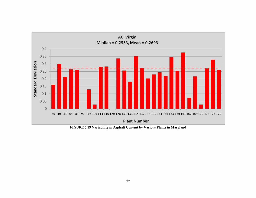
69
FIGURE 5.19 Variability in Asphalt Content by Various Plants in Maryland

70
CHAPTER 6 PAY FACTOR ANALYSIS
6.1 Dense Graded HMA
6.1.1 Mixture Expected Pay Analysis
In order to develop the EP Curves for the acceptance plan with payment adjustments the
population characteristics were used for the four mix parameters, Table 6.1. The population
distributions were then shifted at levels producing different PWL values. Figures 6.1 through 6.4
show the current location of the populations for each one of the four mix parameters in relation
to the specification tolerances (USL, LSL).
Schematically, the populations of the four mix parameters are then shifted at AQL and
RQL so that 90% and 40% of the population is within tolerances (Figures 6.5 through 6.14). To
notice that in some of the cases (0.075, 2.36, and 4.75) 90PWL cannot be achieved due to the
distribution variability and width of the tolerances. The EP Curves were thus generated for
different pay factor levels (0.075, 0.80, 0.90, 1.00 and 1.04).
FIGURE 6.1 Distribution of Asphalt Content Population and the Tolerances
0
200
400
600
800
1000
1200
1400
-1.1
8-1
.1 -1-0
.9-0
.8-0
.7-0
.6-0
.5-0
.4-0
.3-0
.2-0
.1 00.
10.
20.
30.
40.
50.
60.
70.
80.
9 11.
11.
16
Freq
uenc
y
Delta
AC Distribution (Delta_Average=0.00 & Standard Dev. = 0.31)
LSL (-0.5) USL (+0.5)
90 PWL

71
FIGURE 6.2 Distribution of Passing 0.075mm Population and the Tolerances
FIGURE 6.3 Distribution of Passing 2.36mm Population and the Tolerances
0
100
200
300
400
500
600
700
800
-3.6 -3.2 -2.8 -2.4 -2 -1.6 -1.2 -0.8 -0.4 0 0.4 0.8 1.2 1.6 2 2.4 2.8 3.2 3.6 4 4.4 4.8 5.2 5.6
Freq
uenc
y
Delta
0.075 Distribution (Delta_Average=0.99 & Standard Dev. =1.2 )LSL (-2.0) USL (+2.0)
81 PWL
0
200
400
600
800
1000
1200
-15
-14
-13
-12
-11
-10 -9 -8 -7 -6 -5 -4 -3 -2 -1 0 1 2 3 4 5 6 7 8 9 10 11 12 13 14 15
Freq
uenc
y
Delta
2.36 Distribution (Delta_Average= -0.19 & Standard Dev. = 3.88)
LSL (-5.0) USL (+5.0)
80 PWL

72
FIGURE 6.4 Distribution of Passing 4.75mm Population and the Tolerances
FIGURE 6.5 Distribution of Asphalt Content at AQL
0
200
400
600
800
1000
1200
1400
1600
-24 -22 -20 -18 -16 -14 -12 -10 -8 -6 -4 -2 0 2 4 6 8 10 12 14 16 18 20 22
Freq
uenc
y
Delta
4.75 Distribution (Delta_Average=0.07 & Standard Dev. = 5.6)
USL (+7.0)LSL (-7.0)
80 PWL
0
200
400
600
800
1000
1200
1400
1600
-1.2
-1.1 -1
-0.9
-0.8
-0.7
-0.6
-0.5
-0.4
-0.3
-0.2
-0.1 0
0.1
0.2
0.3
0.4
0.5
0.6
0.7
0.8
0.9 1
1.1
1.2
1.3
Freq
uenc
y
Delta
AC Distribution at AQL (Delta_Aveage=0.00 & Standard Dev. = 0.31)
LSL (-0.5) USL (+0.5)
90 PWL

73
FIGURE 6.6 Distribution of Asphalt Content at RQL
FIGURE 6.7 Distribution of Passing 0.075mm at AQL
*Note: In order to achieve 90PWL the standard deviation was reduced by 33%
0
200
400
600
800
1000
1200
1400
-2-1
.9-1
.8-1
.7-1
.6-1
.5-1
.4-1
.3-1
.2-1
.1 -1-0
.9-0
.8-0
.7-0
.6-0
.5-0
.4-0
.3-0
.2-0
.1 00.
10.
20.
30.
40.
5
Freq
uenc
y
Delta
AC Distribution at RQL (Delta_Aveage=-0.002 & Standard Dev. = 0.31)USL (+0.5)LSL (-0.5)
40 PWL
0
200
400
600
800
1000
1200
1400
1600
-4.8
-4.4 -4
-3.6
-3.2
-2.8
-2.4 -2
-1.6
-1.2
-0.8
-0.4 0
0.4
0.8
1.2
1.6 2
2.4
2.8
3.2
3.6 4
4.4
4.8
Freq
uenc
y
Delta
0.075 Distribution at AQL (Delta_Average=0.99 & Standard Dev. = 0.80*)
USL (+2.0)LSL (-2.0)
90 PWL

74
FIGURE 6.8 Distribution of Passing 0.075mm at RQL
FIGURE 6.9 Distribution of Passing 2.36mm at AQL
*Note: In order to achieve 90PWL the standard deviation was reduced by 21%
0
200
400
600
800
1000
1200
1400
1600
1800
-7 -6.5 -6 -5.5 -5 -4.5 -4 -3.5 -3 -2.5 -2 -1.5 -1 -0.5 0 0.5 1 1.5 2
Freq
uenc
y
Delta
0.075 Distribution at RQL (Delta_Average=0.99 & Standard Dev. = 1.20)
USL (+2.0)LSL (-2.0)
40 PWL
0
200
400
600
800
1000
1200
1400
1600
-11 -10 -9 -8 -7 -6 -5 -4 -3 -2 -1 0 1 2 3 4 5 6 7 8 9 10 11
Freq
uenc
y
Delta
2.36 Distribution at AQL (Delta_Average= -0.19 & Standard Dev. =3.07*)
LSL (-5.0) USL (+5.0)
90 PWL

75
FIGURE 6.10 Distribution of Passing 2.36mm at RQL
FIGURE 6.11 Distribution of Passing 4.75mm at AQL
*Note: In order to achieve 90PWL the standard deviation was reduced by 23%
0
200
400
600
800
1000
1200
-22 -20 -18 -16 -14 -12 -10 -8 -6 -4 -2 0 2 4 6 8
Freq
uenc
y
Delta
2.36 Distribution at RQL (Delta_Average= -0.19 & Standard Dev. = 3.88)LSL (-5.0) USL (+5.0)
40 PWL
0
500
1000
1500
2000
2500
-15 -13 -11 -9 -7 -5 -3 -1 1 3 5 7 9 11 13 15 17
Freq
uenc
y
Delta
4.75 Distribution at AQL (Delta_Average=0.07 & Standard Dev. = 4.31*)
LSL (-7.0) USL (+7.0)
90 PWL

76
FIGURE 6.12 Distribution of Passing 4.75mm at RQL
Figure 6.13 shows the probability of receiving ≥PF (y-axis) in relation to the quality level
CMPWL (x-axis), while Table 6.2 summarizes the values obtained at each CMPWSL from the
simulation analysis.
As it can be seen from Table 6.2, when the population standard deviations for the four
mixture parameters are used the highest achievable CMPWSL is 88.7. Thus, for values above
this level the probability values were interpolated. Furthermore, the simulation analysis have
shown that the probability of receiving a PF< 1 when producing at AQL (90CMPWL) is about
40%, while the probability of receiving a PF≥ 1 when producing at RQL (40CMPWL) is 0%.
Similarly the expected pay at any other level of CMPWSL, or the probability of receiving
different levels of PF at AQL and RQL can be estimated from these results.
0
200
400
600
800
1000
1200
1400
1600
1800
-29 -27 -25 -23 -21 -19 -17 -15 -13 -11 -9 -7 -5 -3 -1 1 3 5 7 9 11 13 15
Freq
uenc
y
Delta
4.75 Distribution at RQL (Delta_Average=0.07 & Standard Dev. = 5.6)
USL (+7.0)LSL (-7.0)
40 PWL

77
FIGURE 6.13 EP Curves with Expected PF Using Population Characteristics
TABLE 6.1 Standard Deviation of Different Properties
Property 0.075 2.36 4.75 AC Std. Dev. 1.2 3.88 5.6 0.31
TABLE 6.2 Probability of Receiving ≥PF at Different CMPWL with Population Characteristics
CMPWL Prob of Receiving ≥PF
0.75 0.8 0.9 1 1.04 0 0 0 0 0 0
10 0.1 0 0 0 0 20 3.81 0.55 0.01 0 0 30 21.47 5.72 0.17 0 0 40 51.11 22.9 1.57 0.01 0 50 79.19 51.82 7.3 0.13 0 60 94.14 79.86 23.57 1 0.02 70 99.04 95.08 52.71 4.76 0.14 80 99.98 99.78 84.15 19.43 1.25 86 100 100 96.02 39.82 3.77
88.7 100 100 98.95 52.41 6.88 100 100 100 100 100 100
Note1: simulation at 10000 iterations for each CMPWL Note2: assumed values at 100PWL since only 88.7% of the data fits within spec tolerances
Figures 6.14 and 6.15 show the CMPWL and pay factor distribution. At the long run the
average pay factor for a 88.7CMPWL is equal to 0.99, while for RQL the average pay factor is
0.40. Table 6.3 includes the expected pay - EP ( PF at the long run) calculations when the
population is shifted within the specification tolerances to produce different levels of CMPWSL.
0102030405060708090
100
0 10 20 30 40 50 60 70 80 90 100
Prob
. of R
ecei
ving
≥PF
Composite PWL
0.75
0.8
0.9
1
1.04

78
TABLE 6.3 Expected Payment in relation to CMPWL with Population Characteristics* CMPWL EP
100.0 1.05 90.0 1.00 88.7 0.99 80.0 0.95 70.0 0.89 60.0 0.81 50.0 0.65 40.0 0.41
Note: * The maximum achievable CMPWL with population standard deviation is 88.7; 90CMPWL obtained with population standard deviation reduced by 3.6%;
100CPWL obtained by reducing population standard deviation by 55%.
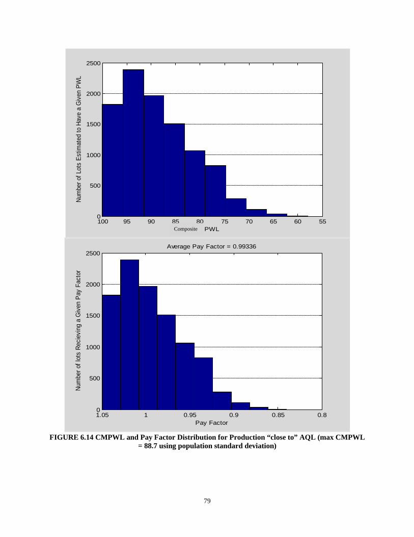
79
FIGURE 6.14 CMPWL and Pay Factor Distribution for Production “close to” AQL (max CMPWL
= 88.7 using population standard deviation)
5560657075808590951000
500
1000
1500
2000
2500
PWL
Num
ber o
f Lot
s Es
timat
ed to
Hav
e a
Giv
en P
WL
0.80.850.90.9511.050
500
1000
1500
2000
2500
Pay Factor
Num
ber o
f lot
s Re
ciev
ing
a G
iven
Pay
Fac
tor
Average Pay Factor = 0.99336
Composite

80
FIGURE 6.15 CMPWL and Pay Factor Distribution for RQL (with population standard deviation)
01020304050607080901000
500
1000
1500
2000
2500
3000
PWL
Num
ber o
f Lot
s Es
timat
ed to
Hav
e a
Give
n PW
L
00.20.40.60.810
500
1000
1500
2000
2500
3000
3500
4000
4500
5000
Pay Factor
Num
ber o
f Lot
s Re
ceiv
ing
a G
iven
Pay
Fac
tor
Average Pay Factor = 0.40578
Composite

81
6.1.2 Improving Production Quality & Potential Modifications in Spec Tolerances
As indicated previously, based on the population characteristics of the four HMA mixture
parameters only 88.7% of the data are within the specification tolerances. Thus, in order to
achieve, at the long run, a 90CMPWSL (AQL value for MSHA spec) either the mixture
production variability has to be reduced (higher homogeneity during production, reducing
variability and consequently the population standard deviation), or the specification limits have
to be widen (if it is concluded that the existing variability represents the best achievable levels of
production). As an example, in the first case reducing the population standard deviations for all
four properties by 3.6% (i.e., improving production uniformity) will provide a 90CMPWSL with
the current tolerances. The results of the simulation analysis are summarized in Table 6.4 and
plotted in Figure 6.16.
As shown from these analyses the probability of receiving a PF< 100% when producing
at AQL (90CMPWL) and the probability of receiving a PF≥ 1 when producing at RQL
(40CMPWL) remain at the same levels of 40% and 0% respectively.
Figures 6.17 and 6.18 show the CMPWSL and pay factor distribution for these analyses.
Similarly to the previous analysis, the average pay factor, at the long run, remains the same (for a
90CMPWL is equal to 1.0, while for RQL the average pay factor is 0.4.
Further analyses have shown that reducing the variance of the population, and/or
modifying the specification tolerances, wouldn’t affect the above PF parameters at AQL and
RQL (these results are reported in the Appendix). Thus, an alternative approach may be required
if the agency is interested in modifying the mix property pay factor specifications. In such an
approach either the AQL has to be modified and/or the associated PWL - pay schedule equation.

82
A method was proposed by WSDOT and is reported in the Appendix along with some example
analysis.
TABLE 6.4 Probability of Receiving ≥PF at Different PWL by Reducing Population Variability
PWL Prob of Receiving >=PF
0.75 0.8 0.9 1 1.04 0 0 0 0 0 0
10 0.09 0.01 0 0 0 20 3.47 0.53 0 0 0 30 21.9 5.96 0.14 0 0 40 50.22 22.99 1.44 0 0 50 78.78 51.69 7.22 0.14 0 60 94.19 80.05 24.03 0.91 0.03 70 98.96 94.72 52.13 4.74 0.23 80 99.96 99.7 84.53 20.01 1.38 90 100 100 99.43 59.66 10.16
100 100 100 100 100 100 Note1: 10000 iterations at each PWL Note2: The values at 100PWL are interpolated
FIGURE 6.16 EP Curves with expected PF Using Reduced Population Variability
0102030405060708090
100
0 10 20 30 40 50 60 70 80 90 100
Prob
of R
ecei
ving
≥PF
Composite PWL
0.75
0.8
0.9
1
1.04

83
FIGURE 6.17 CMPWL and Pay Factor Distribution for AQL Production with Reduced Population
Variability
60657075808590951000
500
1000
1500
2000
2500
3000
PWL
Num
ber o
f Lot
s Es
timat
ed to
Hav
e a
Giv
en P
WL
0.850.90.9511.050
500
1000
1500
2000
2500
3000
Pay Factor
Num
ber o
f Lot
s R
ecei
ving
a G
iven
Pay
Fac
tor
Average Pay Factor = 1.0001

84
FIGURE 6.18 CMPWL and Pay Factor Distribution for RQL Production with Reduced Population
Variability
01020304050607080900
500
1000
1500
2000
2500
3000
Composite PWL
Num
ber o
f Lot
s E
stim
ated
to H
ave
a G
iven
PW
L
00.10.20.30.40.50.60.70.80.910
500
1000
1500
2000
2500
3000
3500
4000
4500
5000
Pay Factor
Num
ber o
f lot
s R
ecei
ving
a G
iven
Pay
Fac
tor
Avarage Pay Factor = 0.40913

85
6.2 Gap Graded HMA
6.2.1 Mixtures Expected Pay Analysis
The same analysis was carried out for the gap graded HMA mixtures. The population
characteristics are shown in Table 6.5. Similarly, the population distributions were then shifted at
levels producing different PWL values and The OC Curves were thus generated for different pay
factor levels (0.75, 0.80, 0.90, 1.00 and 1.04).
FIGURE 6.19 Distribution of Passing AC Population and the Tolerances
FIGURE 6.20 Distribution of Passing 0.075mm Population and the Tolerances
0200400600800
1000120014001600
-1.2
6-1
.2-1
.1 -1-0
.9-0
.8-0
.7-0
.6-0
.5-0
.4-0
.3-0
.2-0
.1 00.
10.
20.
30.
40.
50.
60.
70.
80.
9 11.
1
Freq
uenc
y
Delta
AC Distribution (Delta_Aveage=-0.12 & Standard Dev. = 0.30)
88.5 PWL
LSL (-0.5) USL (+0.5)
0
500
1000
1500
2000
2500
-3.5 -3 -2.5 -2 -1.5 -1 -0.5 0 0.5 1 1.5 2 2.5 3 3.5 4 4.5
Freq
uenc
y
Delta
0.075 Distribution (Delta_Aveage=0.27 & Standard Dev. = 0.91)
97 PWL
USL (+2.0)LSL (-2.0)
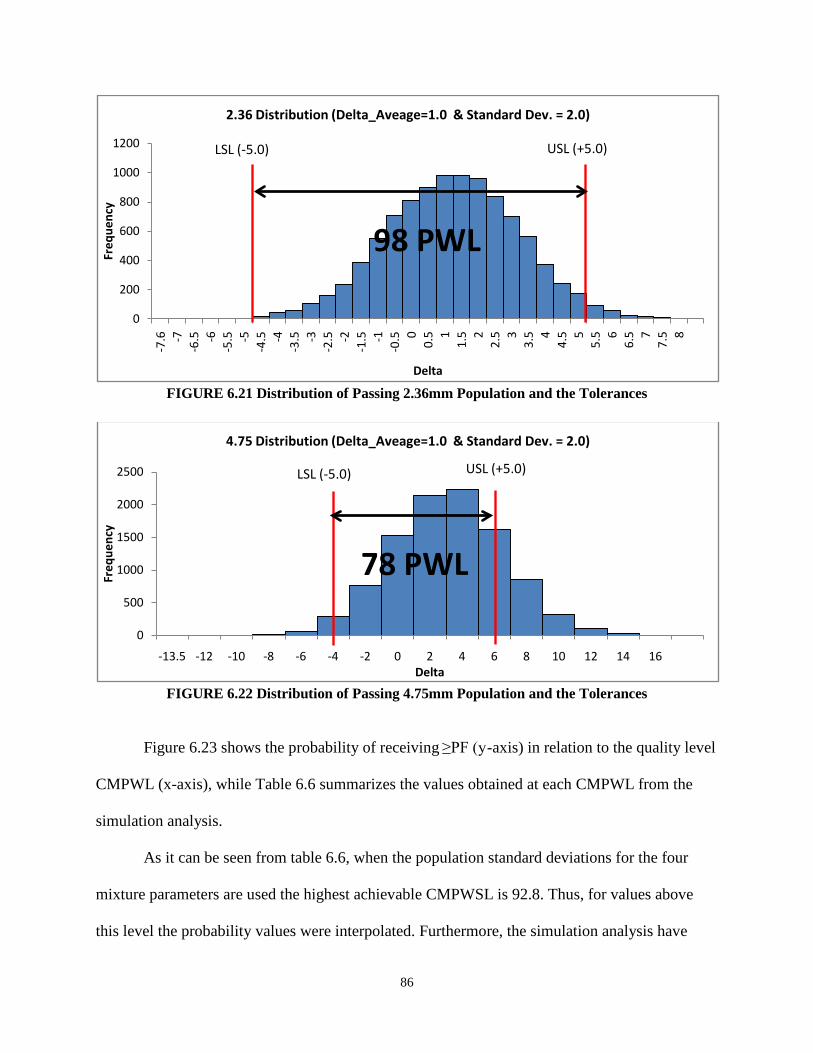
86
FIGURE 6.21 Distribution of Passing 2.36mm Population and the Tolerances
FIGURE 6.22 Distribution of Passing 4.75mm Population and the Tolerances
Figure 6.23 shows the probability of receiving ≥PF (y-axis) in relation to the quality level
CMPWL (x-axis), while Table 6.6 summarizes the values obtained at each CMPWL from the
simulation analysis.
As it can be seen from table 6.6, when the population standard deviations for the four
mixture parameters are used the highest achievable CMPWSL is 92.8. Thus, for values above
this level the probability values were interpolated. Furthermore, the simulation analysis have
0
200
400
600
800
1000
1200-7
.6 -7-6
.5 -6-5
.5 -5-4
.5 -4-3
.5 -3-2
.5 -2-1
.5 -1-0
.5 00.
5 11.
5 22.
5 33.
5 44.
5 55.
5 66.
5 77.
5 8
Freq
uenc
y
Delta
2.36 Distribution (Delta_Aveage=1.0 & Standard Dev. = 2.0)
98 PWL
USL (+5.0)LSL (-5.0)
0
500
1000
1500
2000
2500
-13.5 -12 -10 -8 -6 -4 -2 0 2 4 6 8 10 12 14 16
Freq
uenc
y
Delta
4.75 Distribution (Delta_Aveage=1.0 & Standard Dev. = 2.0)
USL (+5.0)LSL (-5.0)
78 PWL

87
shown that the probability of receiving a PF< 1 when producing at AQL (90CMPWL) is about
40%, while the probability of receiving a PF≥ 1 when producing at RQL (40CMPWL) is 0%.
Similarly the expected pay at any other level of CMPWL, or the probability of receiving
different levels of PF at AQL and RQL can be estimated from these results.
FIGURE 6.23 EP Curves with expected PF Using Population Characteristics (Gap Graded)
TABLE 6.5 Standard Deviation of Different Properties (Gap Graded)
Property 0.075 2.36 4.75 AC Std. Dev. 0.912 1.969 3.507 0.299
TABLE 6.6 Prob. of Receiving ≥PF at Different CMPWL with Population Characteristics (Gap
Graded)
PWL Prob of Receiving >=PF
0.75 0.8 0.9 1 1.04 0 0 0 0 0 0
10 0.15 0.01 0 0 0 20 4.06 0.62 0.01 0 0 30 21.66 5.47 0.22 0 0 40 51.25 22.98 1.56 0 0 50 78.08 52.21 7.31 0.13 0 60 94.75 79.73 22.91 0.85 0.01 70 99.31 95.36 51.91 5.05 0.25 80 100 99.63 83.82 20.39 2.17 90 100 99.99 99.04 57.53 17.25
100 100 100 100 100 100 Note1: simulation at 10000 iterations for each CMPWL
Note2: assumed values at 100PWL since only 92.8% of the data fits within spec tolerances
0102030405060708090
100
0 20 40 60 80 100
Prob
of R
ecei
ving
≥PF
Composite PWL
0.75
0.8
0.9
1
1.04
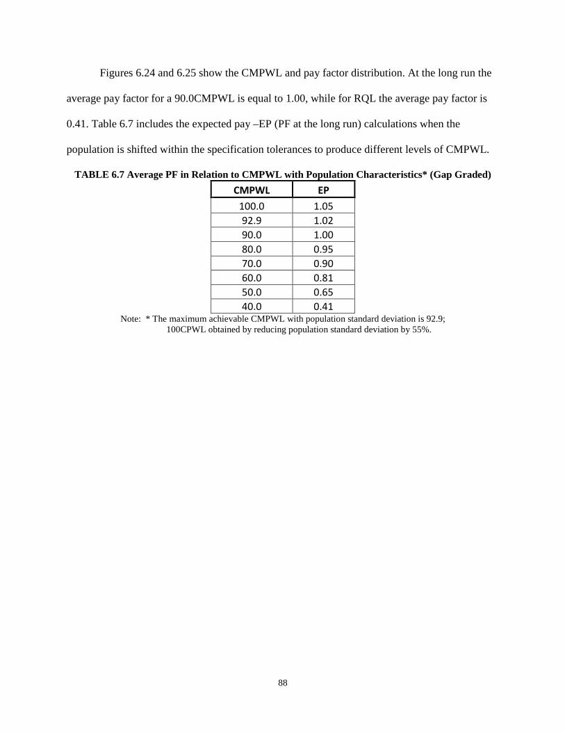
88
Figures 6.24 and 6.25 show the CMPWL and pay factor distribution. At the long run the
average pay factor for a 90.0CMPWL is equal to 1.00, while for RQL the average pay factor is
0.41. Table 6.7 includes the expected pay –EP (PF at the long run) calculations when the
population is shifted within the specification tolerances to produce different levels of CMPWL.
TABLE 6.7 Average PF in Relation to CMPWL with Population Characteristics* (Gap Graded) CMPWL EP
100.0 1.05 92.9 1.02 90.0 1.00 80.0 0.95 70.0 0.90 60.0 0.81 50.0 0.65 40.0 0.41
Note: * The maximum achievable CMPWL with population standard deviation is 92.9; 100CPWL obtained by reducing population standard deviation by 55%.

89
Figure 6.24 Gap Graded CMPWL and Pay Factor Distribution for Production at AQL
505560657075808590951000
500
1000
1500
2000
2500
3000
Composite PWL
Num
ber o
f Lot
s Es
timat
ed to
Hav
e a
Giv
en P
WL
0.80.850.90.9511.050
500
1000
1500
2000
2500
3000
Pay Factor
Num
ber o
f Lot
s R
ecei
ving
a G
iven
Pay
Fac
tor
Average Pay Factor = 1.000
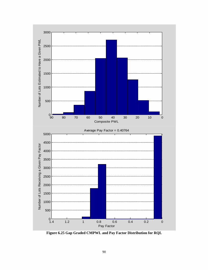
90
Figure 6.25 Gap Graded CMPWL and Pay Factor Distribution for RQL
01020304050607080900
500
1000
1500
2000
2500
3000
Composite PWL
Num
ber o
f Lot
s Es
timat
ed to
Hav
e a
Giv
en P
WL
00.20.40.60.811.21.40
500
1000
1500
2000
2500
3000
3500
4000
4500
5000
Pay Factor
Num
ber o
f Lot
s R
ecei
ving
a G
iven
Pay
Fac
tor
Average Pay Factor = 0.40764

91
6.3 Density Analysis
The density data were divided into two categories: Gap Graded and Dense Graded. This
is due to different specifications for each mix type. The original QA and QC data were compared
according to the specification with the F & t tests on a lot by lot case. The combined QA and QC
data provided 1502 recorded data points for gap graded mixes (297 lots) and 4865 for dense
graded (972 lots). Out of 297 lots of gap graded mixes, 237 lots passed both tests and the QA and
QC values were averaged. For the remaining 60 lots that didn’t pass either the F or the t test only
the QA value was used. Dense graded mixes had 870 lots passing the tests and 102 lots being
rejected in at least one of the tests. On average both mixes had 5 sublots per lot. The distributions
of all data points and the average of each lot are illustrated below. It should be noted that all the
values above 100% and below 85% were considered not acceptable density values and thus were
excluded from the analysis. Figures 6.26 to 6.29 show the population distributions for the gap
and dense graded mixtures using the sublot (individual values) and the average lot values
FIGURE 6.26 Distribution of Individual Gap Graded Density Values
0
100
200
300
400
500
600
88% 89% 90% 91% 92% 93% 94% 95% 96% 97% 98% 99% 100%
Freq
uenc
y
Density

92
FIGURE 6.27 Distribution of Individual Dense Graded Density Values
FIGURE 6.28 Distribution of Lot Averages of Gap Graded Density Values
0
200
400
600
800
1000
1200
1400
1600
87% 88% 89% 90% 91% 92% 93% 94% 95% 96% 97% 98% 99% 100%
Freq
uenc
y
Density
0
20
40
60
80
100
120
89% 90% 91% 92% 93% 94% 95% 96% 97% 98% 99% 100%
Freq
uenc
y
Density

93
FIGURE 6.29 Distribution of Lot Averages of Dense Graded Density Values
In order to be able to find the best fitting curve for each set of data, different types of
distributions were tested by using the built-in functions of MATLAB. Neither of the mixes
passed the normality test, therefore the Weibull distribution was used. Each Weibull distribution
is defined with two parameters, A and B. A is the scale parameter, so different values stretch or
compress the graph in the x direction and B is the shape parameter. For both of the mixes these
values were calculated and are summarized in Table 6.8.
TABLE 6.8 A and B Parameters for Weibull Distribution of HMA Mixtures Individual Lot Average
Mix A B A B Gap Graded 95.78 83.43 95.67 98.32
Dense Graded 94.14 64.17 94.04 71.66
Since the pay factor is based on both the sublot and lot average values, the “individual”
values were used to in the simulation process where 10000 iterations and 5 samples per iteration
were considered. The simulation results are shown in the following Figures, 6.30 to 6.31.
Each of these mixture distributions has a weighted pay factor associated with it. The pay factors
are shown in Figures 6.32 and 6.33. As it can be seen at the long run the average pay factor for
0
50
100
150
200
250
300
350
400
88% 89% 90% 91% 92% 93% 94% 95% 96% 97% 98% 99% 100%
Freq
uenc
y
Bin

94
density of gap graded is equal to 100% while for dense graded mixtures is 95%. Therefore, the
pay schedule provide reasonable PF and doesn’t need any modifications, unless the agency wants
to promote increased quality in terms of density values, implying adjustments either in the
acceptance density values or the pay schedule associated with each density level. An example of
such case is included next.
FIGURE 6.30 Distribution of Simulated Density Data of Gap Graded Mixes
FIGURE 6.31 Distribution of Simulated Density Data of Dense Graded Mixes
02000400060008000
1000012000140001600018000
85 86 87 88 89 90 91 92 93 94 95 96 97 98 99 100
Freq
uenc
y
Density (%)
0
2000
4000
6000
8000
10000
12000
14000
85 86 87 88 89 90 91 92 93 94 95 96 97 98 99 100
Freq
uenc
y
Density (%)

95
FIGURE 6.32 Pay Factor Distribution of Density Data of Gap Graded Mixes
FIGURE 6.33 Pay Factor Distribution of Density of Data of Dense Graded Mixes
Since the average PF for dense graded material is 95%. There are two possible scenarios:
1) The SHA believes that the current quality level deserves 100% PF, on average, or 2) SHA
may want the contractors to improve their quality to achieve higher PF. In the first case there is a
need to assign a higher PF to the current Lot Average Minimum and Individual minimum. The
following table provides an example on the adjustment necessary on the pay schedule in order to
0
200
400
600
800
1000
1200
1400
00.
730.
740.
750.
840.
850.
860.
870.
880.
89 0.9
0.91
0.92
0.93
0.94
0.95
0.96
0.97
0.98
0.99 1
1.01
1.02
1.03
1.04
1.05
Freq
uenc
y
Pay Facotr
Pay Factor Distribution of Gap Graded Mixes (Average PF = 1.00)
0200400600800
10001200140016001800
00.
780.
79 0.8
0.81
0.82
0.83
0.84
0.85
0.86
0.87
0.88
0.89 0.
90.
910.
920.
930.
940.
950.
960.
970.
980.
99 11.
011.
021.
031.
041.
05
Freq
uenc
y
Pay Factor
Pay Factor Distribution of Dense Grade Mixes (Average PF = 0.95)

96
pass from 95% to 100% PF. This pay schedule has up to 12% bonus where the current SHA spec
includes a bonus of 5%.
TABLE 6.9 Modified Dense Graded HMA Mixes Percent of Maximum Density
Lot Average % Minimum
No Individual Sublot Below %*
Pay Factor %
94.0 94.0 112.0 93.8 93.7 111.0 93.6 93.4 110.0 93.4 93.1 109.0 93.2 92.8 108.0 93.0 92.5 107.0 92.8 92.2 106.0 92.6 91.9 105.0 92.4 91.6 104.0 92.2 91.3 103.0 92.0 91.0 102.0 91.8 90.8 101.0 91.6 90.6 100.0 91.4 90.4 99.0 91.2 90.2 98.0 91.0 90.0 97.0 90.8 89.8 96.0 90.6 89.6 95.0 90.4 89.4 94.0 90.2 89.2 93.0 90.0 89.0 92.0 89.8 88.8 91.0 89.6 88.6 90.0 89.4 88.4 89.0 89.2 88.2 88.0 89.0 88.0 87.0 88.8 87.8 86.0 88.6 87.6 85.0 88.4 87.4 84.0 88.2 87.2 83.0 88.0 87.0 82.0
Less than 88.0 87.0 75.0 or rejected by Engineer
97
CHAPTER 7 SUMMARY, CONCLUSIONS & RECOMMENDATIONS
7.1 Summary
Following the implementation of the Superpave mix design method, the Maryland SHA
experienced a reduction in asphalt binder content of HMA mixtures that led to durability issues
such as premature raveling at joints, increased segregation, and higher permeability.
The review of the past and ongoing NCHRP studies have shown that optimal
performance and durability of HMA mixtures can be ensured by: (1) including enough asphalt
binder to ensure good fatigue resistance (and, by implication, durability); (2) including adequate
mineral filler and fine aggregate to keep permeability low (good for durability) and rut resistance
high; and (3) obtaining proper compaction in the field (also good for durability). Since the
volumetric variables are interrelated it is difficult to change one volumetric parameter (e.g.,
design air voids) without simultaneously changing several others (e.g., VBE, VMA, or in-place
air voids at a given compaction effort). The four principal recommendations from recent studies
for improving the durability of Superpave mixtures while maintaining good rut resistance were:
increase effective binder content to provide better fatigue resistance; increase aggregate fineness
to decrease mixture permeability; decrease design air voids to ease compaction in the field; and
control the in-place air voids effectively. The Maryland SHA introduced a new volumetric mix
design specification (Section 904) in 2008 in an effort to improve durability. This new
specification reduces Ndesign as an indirect way to increase asphalt content.
In terms of the QA and QC data comparisons, a series of F and t tests were performed
with data from SHA projects over the past several years. The initial analyses using randomly
selecting lots and comparing their means and standard deviations indicated that these two data

98
sets cannot be considered from the same population. The QA/QC data were further analyzed
after disaggregating the data by nominal maximum aggregate size, mix type, and property.
Analyses were performed for both paired and unpaired conditions and by matching lots and
sublots from each project.
Operating Characteristic curves were then used to identify the alpha and the beta risks
for each one of the four mixture characteristic (0.075, 2.36, 4.75, and AC content). The AQL,
RQL, and the specification tolerance values were modified to examine their impacts on decision
risks. Based on single-variable OC curves, the AQL, RQL and/or tolerances must be modified to
achieve the AASHTO recommended alpha and beta values. However, this process was primarily
investigative in nature since it does not apply to multi-parameter specifications, and acceptance
plans with pay adjustment provisions similar to those at Maryland SHA. For such conditions
simulations and expected pay analyses are more appropriate since relate probability of
occurrence with expected pay. Thus, a simulation tool was developed to study the effects of
reducing asphalt content variability, modifying specification tolerances, and other scenarios on
the expected pay factor over the long run. This simulation tool considered the statistical
variability of each one of the four HMA mix pay factor parameters as well as their
intercorrelations and enables the user to modify all aspects of the specifications and population
statistical characteristics. The analyses were performed on both the previous HMA specification
without any bonus provisions, and the revised specification which incorporates bonus.
Finally, the simulation analyses were extended to examine the average composite pay
factor at AQL and RQL considering all four mixture parameters. Expected pay (EP) curves, were
generated for different pay factor levels (0.75, 0.80, 0.90, 1.00 and 1.04).

99
7.2 Conclusions
From the analysis of this study the following conclusions were obtained:
1. In regards to Maryland State Highway Administration specifications, as it was concluded
from previous studies, including a recent NCHRP study, a simple reduction in Ndesign is
not necessarily the most effective way of achieving increased mix durability. As
mentioned, the true measure of the effectiveness of this new specification will be mixture
durability, rutting, and fatigue performance over a period of many years. Thus specific
follow up actions are needed to assess the effectiveness of this specification.
2. The F and t analyses have shown consistently that the two data sets (QA and QC)
eventually represent different populations. The possibility of defining transfer function
between mix parameters using the QA and QC data was examined but it proved
impossible to develop acceptable relationships.
3. The simulation analyses have shown that, i) while the four mix properties were
correlated, the correlations among the mix parameters have no effect on the average pay
factor, ii) a contractor with tight control over the variability of mixture production can
significantly reduce the AC content and still receive a reasonable pay factor, iii) due to
the high weight of the AC content in the final composite pay factor equation, the effects
of changing the AC tolerances has a more pronounced impact on the pay factor than any
other mixture property, iv) the revised specifications with the bonus provision have
provided higher pay factor values than previously. The average PF under the new

100
specification is very close to 1.00, over the long run, for material meeting or exceeding
the AQL.
4. Based on the historical variability of HMA production, the maximum achievable
Composite Mix Percent Within Specification Limits (CMPSWL) for dense graded
material is 88.7%. The corresponding average mix pay factor (PF) at this quality level is
equal to 0.99, over the long run. In order to achieve AQL of 90 CMPSWL with the
current population characteristics changes in the specification are needed.
5. The average pay factor at 90 CMPSWL (AQL) is equal to 1.00 for the gap graded
mixtures. Thus, the current specification is appropriate for this mixture.
6. Based on the average pay factors the current pay factor equation fairly awards and
penalizes the good and bad quality material and there is no need to modify the pay
equation. Since the expected pay factor (over the long run) at 40 CMPSWL (RQL) is
0.4 for both dense and gap graded mixtures, the agency bears lower risk for inferior
quality material.
7. The simulations and PF analyses for the density data have shown that over the long run
the average expected pay factors equal to 1.00 and 0.95 for gap and dense graded
mixtures, respectively.

101
7.3 Recommendations
The following recommendations are suggested from the analyses and conclusions of this study:
1. For evaluating the effectiveness of the Maryland HMA specification the following
actions are recommended for determining whether the specification change is having the
intended effects, i) comparison of QA binder content data for mixtures designed before
and after the specification change to see whether the asphalt percentage has increased as
intended, ii) comparison of QA in-place density data for mixtures designed before and
after the specification change to see whether lower in-place air voids are now being
achieved, iii) review density pay factor schedules to ensure that there is sufficient
incentive for contractors to achieve lower in-place air voids.
2. A major difficulty in conducting the QA and QC data analysis was to pair the
observations from material in the plant (QC) and behind the paver (QA). Thus a better
material identification and tracking techniques is recommended if this study is to be
repeated in the future.
3. Even though the revised specification with the bonus provision provided a PF of 1.00, if
SHA decides to modify the specification tolerances of the four HMA mix properties to
achieve a different average pay factor, it is recommended that the AC tolerance should be
addressed first due to its heavy weight in the composite pay factor.

102
4. Since the EP analysis at AQL have shown that the maximum achievable CMPSWL for
dense graded mixtures is 88.7% the specification can be fine tuned to achieve 90
CMPWSL and a PF of 1.00. In order to achieve so, the standard deviation of all four
parameters must be reduced by 3.6 percentage points. If the achievable levels of
variability in HMA production cannot be improved, then adjustments in the specification
tolerances and/or pay factor equation are needed.
5. Since EP at RQL was 0.40 the agency may want to fine tune the specification. As a guide
to potential future fine tuning of the specification and pay factor equation, the impact of
modifying production variability and/or specification limits has been studied and reported
here, along with an alternative method of modifying AQL.
6. For density values whether the agency wants to consider a higher PF at the long run, or
improve quality, either adjustments in the acceptance density values or the associated pay
schedule may be used. As an example a pay schedule with up to 12% incentive was
suggested to increase the current 0.95 PF to 1.00. SHA needs to decide whether this
amount of incentive is desired or not, and assess any potential cost/benefit of such large
incentive.
As shown in this study the current specifications do provide reasonable rewards and penalties
in relation to the HMA production quality. Further monitoring of the specification response
and implications of the pay-schedule and bonus provisions is required as HMA production
goes on year after year in Maryland.

103
It is desirable that the implications on pavement performance and agency cost due to superior
or inferior HMA quality work be assessed through the development and use of performance
based specifications. Under such type of specification the as-built HMA quality is compared
to the design- target quality through performance predictions. The costs associated with the
differences in performance are then used for evaluating the economic implications. For this
purpose performance based specifications should be developed for Maryland. This requires
the development of performance prediction models, agency cost models, and eventually user
cost models.
Another area that SHA needs to address is issues related to QA/QC data quality, as well as
database quality. As it was mentioned, during this study significant effort was needed to pair
the QA/QC data and identify potential data entry errors and outliers. Thus, a process is
needed to improve such aspects. Eventually the database should be coupled with a
verification process of data quality, (perhaps some short of flagging subroutine comparing
expected versus input values), before storing the data into the database. The same could be
applied to the existing data.
104
REFERENCES
Burati J., “Risks with Multiple Pay Factor Acceptance Plans,” Transportation Research Record
No. 1907, pp. 97-42, Transportation Research Board of the National Academies, Washington,
D.C., 2005
Burati J., “Evaluating Specification Limits,” Transportation Research Record No. 1946, pp. 92-
98, Transportation Research Board of the National Academies, Washington, D.C., 2006
Burati J., and R. Weed, “Accuracy and Precision of Typical Quality Measures,” Transportation
Research Record No. 1946, pp. 82-91, Transportation Research Board of the National
Academies, Washington, D.C., 2006
Burati J., R. Weed, C. Hughes, and H. Hill, “Optimal Procedures for Quality Assurance
Specifications” Federal Highway Administration (FHWA), Report FHWA-RD-02-095
“Glossary of Highway Quality Assurance Terms,” Transportation Research Circular
No. E-C037, Transportation Research Board, Washington, DC, April 2002
Mahoney J, and S. Muench “A Quantification and Evaluation of WSDOT’s Hot Mix Asphalt
Concrete Statistical Acceptance Specification” Washington State Transportation Center, Report
T9903.2, 2001

105
Maryland Department of Transportation State Highway Administration Specification “Section
504 – Hot Mix Asphalt Pavement” 2004
Maryland Department of Transportation State Highway Administration Specification “Section
504 – Hot Mix Asphalt Pavement” 2009
Maryland Department of Transportation State Highway Administration Specification “Section
904 – Performance Graded Asphalt Binders and Mix Asphalt” 2004
Maryland Department of Transportation State Highway Administration Specification “Section
904 – Performance Graded Asphalt Binders and Mix Asphalt” 2009
Maryland Department of Transportation State Highway Administration Office of Materials and
Technology Maryland Standard Method of Tests “MSMT 457 – Sampling Hot Mix Asphalt
Prior to Compaction” 2005
Maryland Department of Transportation State Highway Administration Office of Materials and
Technology Maryland Standard Method of Tests “MSMT 733 – Procedure for Evaluating HMA
Lot Compaction for Compliance” 2002
Maryland Department of Transportation State Highway Administration Office of Materials and
Technology Maryland Standard Method of Tests “MSMT 734 – Procedure for Determining
Statistical Outliers” 2004

106
Maryland Department of Transportation State Highway Administration Office of Materials and
Technology Maryland Standard Method of Tests “MSMT 735 – Statistical Analysis of Material
Using Quality Level Analysis for Determination of Pay Factors” 2008
NCHRP Project 9-09: Refinement of the Superpave Gyratory Compaction Procedure
(Contractor: Auburn University/NCAT; completed)
NCHRP Project 9-25: Requirements for Voids in Mineral Aggregate for Superpave Mixtures
(Contractor: Applied Asphalt Technologies LLC; completed)
NCHRP Project 9-31: Air Void Requirements for Superpave Mix Design (Contractor: Applied
Asphalt Technologies LLC; competed)
NCHRP Project 9-33: A Mix Design Manual for Hot Mix Asphalt (Contractor: Advanced
Asphalt Technologies LLC; ongoing—mix design manual not yet published)
Parker F., and R. E. Turochy, “Using the Results of Contractor-Performed Tests in Quality
Assurance,” NCHRP Research Results Digest 323, Transportation Research Board of the
National Academies, 2007
Quality Assurance Guide Specification. AASHTO, Washington, D.C., 1996

107
Sholar G. A., G. C. Page, J. A. Musselman, P. B. Upshaw, and H. L. Moseley, “Development of
the Florida Department of Transportation’s Percent Within Limits Hot-Mix Asphalt
Specification” Transportation Research Board Record No. 1907, pp. 43-51, Transportation
Research Board of the National Academies, Washington, D.C., 2005
Turochy R., R. Willis, and F. Parker,“ Quality Assurance of Hot-Mix Asphalt Comparison of
Contractor Quality Control and Georgia Department of Transportation Data,” Transportation
Research Record No. 1946, pp. 47-54, Transportation Research Board of the National
Academies, Washington, D.C., 2006
Villiers C., Y. Mehta, G. Lopp, M. Tia, and R. Roque, “ Evaluation of Percent-within-limits-
Construction Specification Parameters,” International Journal of Pavement Engineering, pp. 221-
228, London, U.K., 2003
Weed, R.M., “Quality Assurance Software for the Personal Computer,” Publication
No. FHWA–SA–96–026, Federal Highway Administration, Washington, DC, May
1996.

108
APPENDIX
A. Simulation Tool
A.1 Description of the Simulation Process
Objective of the simulation tool was to produce a number of normal random lots, calculate
the PWL for each parameter (0.075, 2.36, 4.75 and AC) with respect to the spec tolerances and
finally provide a histogram of the expected pay and the average pay factor. It should be noted
that every aspect of the specs and populations can be modified in this program since all the
values are set to be a user input.
The structure of the system in MATLAB is as follows:
1- The number of lots, number of sublots, target value of production, standard deviation of all
four properties and the tolerances are given as inputs.
2- Random normal lots are generated based on the correlation matrix of the four properties. The
method used to generate “Random Normal Correlated” numbers is the Cholesky
decomposition. The correlation matrix was found using all the previous data recorded in the
data base, Table A1.
3- The produced lots are then processed in accordance with MSMT 735 to obtain the CMPWSL
of each lot.
4- The CMPWSL is then translated to the Mix Pay Factor of that lot based on section 504.04.02
of State Highway Administration Special Provision Insert Category 500.
5- The histograms of the Mix Pay Factors are generated by MATLAB which were the ultimate
tool for our final conclusions.
The flow chart below summarizes the preceding steps:

109
FIGURE A1 Flow Chart of Simulation Analysis
Pay Factor
CMPWSL

110
A.2 MATLAB Codes of the Simulation Tool for HMA Mix Properties
%SSK close all clear clc PL_PU_Matrix; h=input('delta Value='); u=input('sd value='); m=10000; n=6; if n<3 | n>300 fprintf('Number of Sublots Must be 3<n<300 \n') n=input('Please Enter a Value (3<n<300) for the Number of Sublots='); if n<3 | n>300 button = questdlg('n must be 3<n<300 do you understand?', ... 'Exit Dialog','Yes','No','No'); switch button case 'Yes', n=input('Please Enter a Value (3<n<300) for the Number of Sublots='); if n<3 | n>300 disp('Exiting MATLAB'); exit end case 'No', exit; end end end % delta_ZERO=input('Mean of plant production minus target value for 0.075='); % delta_TWO=input('Mean of plant production minus target value for 2.36='); % delta_FOUR=input('Mean of plant production minus target value for 4.75='); % delta_AC=input('Mean of plant production minus target value for AC='); % delta=[delta_ZERO,delta_TWO,delta_FOUR,delta_AC]; % delta=[0.992,-.192,0.066,-0.002]; delta=[-2+(2*h),-5+(5*h),-5+(5*h),-0.5+(.5*h)]; % std_dev_ZERO=input('std_dev for 0.075='); % std_dev_TWO=input('std_dev for 2.36='); % std_dev_FOUR=input('std_dev for 4.75='); % std_dev_AC=input('std_dev for AC='); % sd = [std_dev_ZERO,std_dev_TWO,std_dev_FOUR,std_dev_AC]; sd = [0.912-(0.912*u),1.969-(1.969*u),3.507-(3.507*u),0.299-(0.299*u)]; SL=[2,5,5,0.5]; f_ZERO_TWO_FOUR_AC=[24,7,7,62]; CORR =[1.0000,0.3377,0.2085,0.2423;0.3377,1.0000,0.5620,0.2607;0.2085,0.5620,1.0000,0.3048;0.2423,0.2607,0.3048,1.0000]; % CORR =[1.0000,h,h,h;h,1.0000,h,h;h,h,1.0000,h;h,h,h,1.0000]; USL=SL; LSL=-SL; for k=1:m T = CORR; for u=1:1:4 T(:,u) = T(:,u) * sd(u); end

111
for r=1:1:4 T(r,:) = T(r,:) * sd(r); end % now T is the covariance matrix B = chol(T); N_ZERO = normrnd(0,1,n,1); N_TWO = normrnd(0,1,n,1); N_FOUR = normrnd(0,1,n,1); N_AC = normrnd(0,1,n,1); N=[N_ZERO,N_TWO,N_FOUR,N_AC]; X = N*B; X=X+repmat(delta,n,1); % B = chol(T); % N_ZERO = normrnd(0,3.57,n,1); % N_TWO = normrnd(0,8.93,n,1); % N_FOUR = normrnd(0,12.50,n,1); % N_AC = normrnd(0,.89,n,1); % N=[N_ZERO,N_TWO,N_FOUR,N_AC]; % X = N; %MSMT 735 MEAN=mean(X); STDEV=std(X); QU=chop((USL-MEAN)./STDEV,3); QL=chop((MEAN-LSL)./STDEV,3); p=n-1; for j=1:4; for i=1:50; if (QU(1,j)==A(i,p)) PU(1,j)=A(i,1); end if (QU(1,j)>A(i+1,p) & QU(1,j)<A(i,p)) PU(1,j)=A(i,1); end if (QU(1,j)>A(1,p)) PU(1,j)=100; end if (-QU(1,j)==A(i,p)) PU(1,j)=100-A(i,1); end if (-QU(1,j)>A(i+1,p) & -QU(1,j)<A(i,p)) PU(1,j)=100-A(i,1); end if (-QU(1,j)>A(1,p)) PU(1,j)=0; end if (QL(1,j)==A(i,p)) PL(1,j)=A(i,1); end if (QL(1,j)>A(i+1,p) & QL(1,j)<A(i,p)) PL(1,j)=A(i,1); end if (QL(1,j)>A(1,p)) PL(1,j)=100; end if (-QL(1,j)==A(i,p)) PL(1,j)=100-A(i,1);

112
end if (-QL(1,j)>A(i+1,p) & -QL(1,j)<A(i,p)) PL(1,j)=100-A(i,1); end if (-QL(1,j)>A(1,p)) PL(1,j)=0; end end PWSL(1,j)=PU(1,j)+PL(1,j)-100; end CMPWSL(1,k)=round([sum(PWSL.*f_ZERO_TWO_FOUR_AC)/sum(f_ZERO_TWO_FOUR_AC)]); if (CMPWSL(1,k)<40) MF(1,k)=0; end % if (CMPWSL(1,k)<90 & CMPWSL(1,k)>=40) % MF(1,k)=0.55+0.5*CMPWSL(1,k)/100; % end % if (CMPWSL(1,k)>=90) % MF(1,k)=1; % end if (CMPWSL(1,k)<=100 & CMPWSL(1,k)>=40) MF(1,k)=0.55+0.5*CMPWSL(1,k)/100; end end hist(CMPWSL); % grid; xlabel('Composite PWL'); ylabel('Number of Lots Estimated to Have a Given PWL'); Mean_CMPWSL=mean(CMPWSL); Std_CMPWSL=std(CMPWSL); Mean_MF=mean(MF); Std_MF=std(MF); Meadian_MF=median(MF); figure; hist(MF); % grid; PF75=sum(histc(MF,.75:.01:1.05))/m*100; PF80=sum(histc(MF,.80:.01:1.05))/m*100; PF90=sum(histc(MF,.90:.01:1.05))/m*100; PF100=sum(histc(MF,1.00:.01:1.05))/m*100; PF104=sum(histc(MF,1.04:.01:1.05))/m*100; PF=[PF75,PF80,PF90,PF100,PF104] RISK=[(100-PF100)/100,PF100]; % Histogram_CountCM=histc(CMPWSL,90:2.5:100); % xlabel('Mixture Pay Factor'); % ylabel('Frequency'); format short g; Delta_MF=MF-Mean_MF; Mean_Delta_MF=mean(Delta_MF); Total_Delta_MF=sum(Delta_MF); Report=[m n delta sd Mean_CMPWSL Std_CMPWSL Mean_MF Std_MF]; Report=[Mean_CMPWSL,Mean_MF] % sum(Histogram_Count)

113
A.3 MATLAB Codes of the Simulation Tool for the Density Analysis
A.3.1 Gap Graded %SSK close all clear clc m=input('Number of Lots='); n=input('Number of Sublots='); G=xlsread('C:\Documents and Settings\Sahand\Desktop\MSHA project\Density_Final.xls','Gap_Graded_Ind','a2:a1503')*100; GW=wblfit(G); for k=1:m XG=wblrnd(GW(1),GW(2),n,1); MEAN=mean(XG); MIN=min(XG); for i=1:n if XG(i)<85 XG(i)=85; end if XG(i)>100 XG(i)=100 end end N(k*n:(k*n+n-1),1)=XG; if (MEAN<91.0) PF(1,k)=0.75; end if (MEAN>=91.0 & MIN>=88.5) PF(1,k)=0.85; end if (MEAN>=91.2 & MIN>=88.8) PF(1,k)=0.86; end if (MEAN>=91.4 & MIN>=89.1) PF(1,k)=0.87; end if (MEAN>=91.6 & MIN>=89.4) PF(1,k)=0.88; end if (MEAN>=91.8 & MIN>=89.7) PF(1,k)=0.89; end if (MEAN>=92.0 & MIN>=90.0) PF(1,k)=0.90; end if (MEAN>=92.2 & MIN>=90.3) PF(1,k)=0.91; end if (MEAN>=92.4 & MIN>=90.6) PF(1,k)=0.92; end if (MEAN>=92.6 & MIN>=90.9) PF(1,k)=0.93;
114
end if (MEAN>=92.8 & MIN>=91.2) PF(1,k)=0.94; end if (MEAN>=93.0 & MIN>=91.5) PF(1,k)=0.95; end if (MEAN>=93.2 & MIN>=91.8) PF(1,k)=0.96; end if (MEAN>=93.4 & MIN>=92.1) PF(1,k)=0.97; end if (MEAN>=93.6 & MIN>=92.4) PF(1,k)=0.98; end if (MEAN>=93.8 & MIN>=92.7) PF(1,k)=0.99; end if (MEAN>=94.0 & MIN>=93.0) PF(1,k)=1.00; end if (MEAN>=94.1 & MIN>=93.2) PF(1,k)=1.005; end if (MEAN>=94.2 & MIN>=93.4) PF(1,k)=1.01; end if (MEAN>=94.3 & MIN>=93.6) PF(1,k)=1.015; end if (MEAN>=94.4 & MIN>=93.8) PF(1,k)=1.02; end if (MEAN>=94.5 & MIN>=94) PF(1,k)=1.025; end if (MEAN>=94.6 & MIN>=94.2) PF(1,k)=1.03; end if (MEAN>=94.7 & MIN>=94.4) PF(1,k)=1.035; end if (MEAN>=94.8 & MIN>=94.6) PF(1,k)=1.04; end if (MEAN>=94.9 & MIN>=94.8) PF(1,k)=1.045; end if (MEAN>=95 & MIN>=95) PF(1,k)=1.05; end if (MEAN>97.5) PF(1,k)=0.75; end if sum(sum(XG>97))==3

115
PF(1,k)=0.75; end if sum(sum(XG>97.5))>=4 PF(1,k)=0.75; end end PF; mean(PF) for i=1:m PFF(i,1)=PF(1,i); end % xlswrite('c:\density.xls',PFF) A.3.2 Dense Graded %SSK close all clear clc m=input('Number of Lots='); n=input('Number of Sublots='); D=xlsread('C:\Documents and Settings\Sahand\Desktop\MSHA project\Density_Final.xls','Dense_Graded_Ind','a2:a4866')*100; DW=wblfit(D) for k=1:m XD=wblrnd(DW(1),DW(2),n,1); MEAN=mean(XD); MIN=min(XD); for i=1:n if XD(i)<85 XD(i)=85; end if XD(i)>100 XD(i)=100 end end N(k*n:(k*n+n-1),1)=XD; if (XD(i)<87.0) PF(1,k)=0; end if (MEAN<88.0 & MIN>=87.0) PF(1,k)=0.75; end if (MEAN>=88.0 & MIN>=87.0) PF(1,k)=0.80; end if (MEAN>=88.2 & MIN>=87.2) PF(1,k)=0.81; end if (MEAN>=88.4 & MIN>=87.4) PF(1,k)=0.82; end if (MEAN>=88.6 & MIN>=87.6) PF(1,k)=0.83;

116
end if (MEAN>=88.8 & MIN>=87.8) PF(1,k)=0.84; end if (MEAN>=89.0 & MIN>=88.0) PF(1,k)=0.85; end if (MEAN>=89.2 & MIN>=88.2) PF(1,k)=0.86; end if (MEAN>=89.4 & MIN>=88.4) PF(1,k)=0.87; end if (MEAN>=89.6 & MIN>=88.6) PF(1,k)=0.88; end if (MEAN>=89.8 & MIN>=88.8) PF(1,k)=0.89; end if (MEAN>=90.0 & MIN>=89.0) PF(1,k)=0.90; end if (MEAN>=90.2 & MIN>=89.2) PF(1,k)=0.91; end if (MEAN>=90.4 & MIN>=89.4) PF(1,k)=0.92; end if (MEAN>=90.6 & MIN>=89.6) PF(1,k)=0.93; end if (MEAN>=90.8 & MIN>=89.8) PF(1,k)=0.94; end if (MEAN>=91.0 & MIN>=90.0) PF(1,k)=0.95; end if (MEAN>=91.2 & MIN>=90.2) PF(1,k)=0.96; end if (MEAN>=91.4 & MIN>=90.4) PF(1,k)=0.97; end if (MEAN>=91.6 & MIN>=90.6) PF(1,k)=0.98; end if (MEAN>=91.8 & MIN>=90.8) PF(1,k)=0.99; end if (MEAN>=92 & MIN>=91) PF(1,k)=1.00; end if (MEAN>=92.2 & MIN>=91.3) PF(1,k)=1.005; end if (MEAN>=92.4 & MIN>=91.6)

117
PF(1,k)=1.01; end if (MEAN>=92.6 & MIN>=91.9) PF(1,k)=1.015; end if (MEAN>=92.8 & MIN>=92.2) PF(1,k)=1.02; end if (MEAN>=93 & MIN>=92.5) PF(1,k)=1.025; end if (MEAN>=93.2 & MIN>=92.8) PF(1,k)=1.03; end if (MEAN>=93.4 & MIN>=93.1) PF(1,k)=1.035; end if (MEAN>=93.6 & MIN>=93.4) PF(1,k)=1.04; end if (MEAN>=93.8 & MIN>=93.7) PF(1,k)=1.045; end if (MEAN>=94 & MIN>=94) PF(1,k)=1.05; end if (MEAN>97.5) PF(1,k)=0.75; end if sum(sum(XD>97))==3 PF(1,k)=0.75; end if sum(sum(XD>97.5))>=4 PF(1,k)=0.75; end end PF; mean(PF) for i=1:m PFF(i,1)=PF(1,i); end xlswrite('c:\density.xls',PFF)

118
A.4 Implications of Correlation Coefficients on PF
Based on the correlation coefficients for dense graded mixtures, several analyses show
that their effects had no impact on the pay factor analysis. In the example of Table A1 the values
of the correlations were changed ranging from 0.001 to 0.999. As it can be seen no effects on PF
were observed. The correlations of four mix parameters for gap graded mixtures were not
established since limited data were available for these mixtures
TABLE A1 Example of Effect of Correlation Value on the Average PF
Average CMPWL Std. Dev. CMPWL Average PF Std. Dev. PF Correlation 86.2 10.3 98.1 5.2 0.999 86.2 8.0 98.1 4.0 0.5 86.0 7.2 98.0 3.6 0.001 86.2 7.5 98.1 3.8 Population

119
B. Impact of Reducing Population Variability and/or Modifying Spec Tolerances
TABLE B1 Effects of Reducing Population Standard Deviation
at AQL (90CMPWL) at RQL (40 CMPWL)
% Reduction in SDpop
Probability of
receiving a PF< 1
Average PF
Probability of
receiving a PF≥ 1
Average PF
0.0% N/A N/A 0.01 0.41 3.6% 0.40 1.00 0.00 0.41 5.0% 0.40 1.00 0.00 0.41
10.0% 0.40 1.00 0.00 0.41 20.0% 0.39 1.00 0.00 0.41 35.0% 0.41 1.00 0.01 0.41 50.0% 0.40 1.00 0.00 0.41
TABLE B2 Effects of Increasing Spec Tolerances
at AQL (90CMPWL) at RQL (40 CMPWL)
% Increase in Tolerance
Probability of
receiving a PF< 1
Average PF
Probability of
receiving a PF≥ 1
Average PF
0.0% N/A N/A 0.01 0.41 3.6% 0.40 1.00 0.00 0.41 5.0% 0.40 1.00 0.00 0.41
10.0% 0.40 1.00 0.00 0.41 20.0% 0.40 1.00 0.00 0.41 35.0% 0.40 1.00 0.00 0.41 50.0% 0.41 1.00 0.01 0.41

120
C. Alternative Approach for Defining HMA Specifications
This section identifies an alternative approach for modifying mix property PF parameters
at AQL and RQL. This method is based on the procedure adopted by WSDOT (Mahoney, and
Muench, 2001) and requires the definition of PF in function of PWL and sample size, similar to
the ones reported in Table B1. To be noticed that the WSDOT procedure, does not address
correlated quality characteristics. This increases the risk to the contractor because if he/she is
penalized on one sieve, the probability certainly increases that he will be penalized on the other.
There has been some debate over the use of the acceptance "c" factor used by WSDOT and
FHWA Western Federal Lands. There are two schools of thought; 1) the adjustment using the
"c' factor is necessary to address small sample sizes; and 2) that the PWL analysis already
incorporates sample size in the estimate of the PWL, so the "c" factor overcompensates. In fact,
whether it is stated or not an acceptance value of 73CMPWL by definition actually sets the AQL
at 73 PWL.
This approach is based on the definition of an acceptance value, c, which is the lot quality
associated with a pay factor of 1.00. The steps for quantifying this parameter include:
1. Determine the acceptable quality limit (AQL) in percent defective (PD).
PD = 100 – PWL
2. Set the primary α risk (the contractor’s risk that material produced at AQL will be either
rejected or subject to reduced pay).
3. Determine the sample size to be used (n).

121
4. Determine the z-statistic associated with the primary α risk, z(αc). This is just the
cumulative normal probability value associated with the primary α risk and can be
obtained with Microsoft Excel (NORMSDIST function) or standard statistical tables.
5. Use the basic equation below to solve for zc.
z(αc)= √n (zAQL-zc)
where: z(αc) = z-statistic associated with the primary α risk
zAQL = z-statistic associated with AQL
zc = z-statistic associated with the acceptance value (c)
n = sample size
6. Determine the acceptance value (c) from zc . This can be done with Microsoft Excel
(NORMSINV function) or standard statistical tables.
TABLE C1 WSDOT Pay Factors

122
Example analysis: Using Population Characteristics
Based on this procedure example analysis were carried out using the population
characteristics for two levels of α risk, 5% and 1%. The c values obtained with the above
procedure provided CMPWL of 73% and 63%, respectively for a sample size of 6, reflecting the
SHA practice. The OC Curves were then generated. The results for an α risk of 5% are shown in
Table B2 and Figure B1. The α (equal to 1-97.88) and (equal to 0.84) risks are calculated
based on the values highlighted in Table B2.
Similarly the results for an α risk of 1% are reported in Table B3 and Figure B2.
TABLE C2 Probability of Receiving ≥PF at Different CMPWL Using Population Characteristics &
C = 73CMPWL (α=5%)
PWL Prob of Receiving >=PF 0.75 0.8 0.9 1
0 0 0 0 0 10 0.14 0.04 0 0 20 4.20 0.48 0.03 0.02 30 22.37 5.77 0.20 0.14 40 51.18 22.59 1.43 0.84 50 78.58 50.91 6.69 4.32 60 94.47 80.79 23.95 17.47 70 99.26 95.66 53.21 43.96 80 99.97 99.69 84.14 76.67
88.95 100 100 99.17 97.88 100 100 100 100 100
Note1: 10000 iterations at each PWL Note2: The values at 100PWL are interpolated

123
FIGURE C1 EP Curves with Expected PF Using Population Standard Deviation and C = 73
CMPWL (α=5%)
TABLE C3 Probability of Receiving ≥PF at Different CMPWL Using Population Characteristics and C = 63CMPWL (α=1%)
CMPWL Prob of Receiving >=PF
0.75 0.8 0.9 1 0 0 0 0 0
10 0.09 0.01 0 0 20 4.33 0.68 0.02 0.02 30 21.45 5.87 0.66 0.66 40 50.64 22.18 4.12 4.12 50 79.08 51.68 17.03 17.03 60 94.38 80.51 43.13 43.13 70 99.29 95.52 74.82 74.82 80 99.96 99.7 95.38 95.38
88.781 100 100 99.91 99.91 100 100 100 100 100
Note1: 10000 iterations at each PWL Note2: The values at 100PWL are interpolated
0
20
40
60
80
100
0 20 40 60 80 100
Prob
. of R
ecei
ving
≥PF
Composite PWL
0.75
0.8
0.9
1

124
FIGURE C2 EP Curves with Expected PF Using Population Variability Standard Deviation and C
= 63 CMPWL (α=1%)
Example analysis: Reducing Population Variability
As indicated previously, based on the population characteristics of the four HMA mixture
parameters only 88.7% of the data are within the specification tolerances. Thus, in order to
achieve, at the long run, a 90CMPWL (AQL) either the mixture production variability has to be
reduced (higher homogeneity during production) reducing thus the population standard
deviation, or the specification limits have to be widen (if it is concluded that the existing
variability represents the best achievable levels of production). As shown in the example before,
a reduction of 3.6% in the population standard deviation is needed in order achieve a 90CMPWL
with the current tolerances. Using this value the simulation analysis were carried out with this
methodology and the results are summarized in Tables B4-B5, and Figures B3-B4. As it can be
seen from the results of the simulation analysis, by setting C equal to 73PWL the α and β are
estimated to be 1.5% and 1% respectively. These values may represent a more balanced set of
agency and contractor risk than when the C is set to be equal to AQL (90%).
When the C value of 63 CMPWL was used the risk to the agency (β) increased to 5%
where the contractor is bearing no risk at all. Therefore, having C = 73PWL results in a more
balanced set of risks.
0
20
40
60
80
100
0 20 40 60 80 100
Prob
. of R
ecei
ving
≥PF
Composite PWL
0.75
0.8
0.9
1

125
TABLE C4 Probability of Receiving ≥PF at Different CMPWL by Reducing Population Variability and with C = 73CMPWL
PWL Prob of Receiving >=PF 0.75 0.8 0.9 1
0 0 0 0 0 10 0.1 0.01 0 0 20 4.11 0.61 0.02 0.01 30 21.23 6.11 0.2 0.11 40 52.01 23.47 1.42 0.89 50 79.16 50.96 6.76 4.3 60 94.35 80.1 23.86 17.05 70 99.23 95.1 51.74 42.51 80 99.92 99.51 84.21 76.54 90 100 100 99.36 98.44
100 100 100 100 100 Note1: 10000 iterations at each PWL
Note2: The values at 100PWL are interpolated
FIGURE C3 EP Curves with Expected PF Using Reduced Population Variability and C Value of c=
73 CMPWL
0102030405060708090
100
0 20 40 60 80 100
Prob
. of R
ecei
ving
≥PF
Composite PWL
0.75
0.8
0.9
1
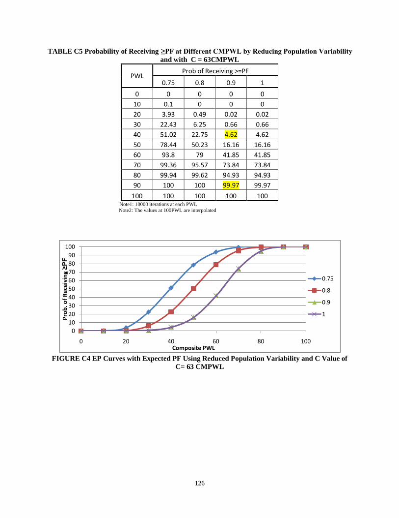
126
TABLE C5 Probability of Receiving ≥PF at Different CMPWL by Reducing Population Variability and with C = 63CMPWL
PWL Prob of Receiving >=PF 0.75 0.8 0.9 1
0 0 0 0 0 10 0.1 0 0 0 20 3.93 0.49 0.02 0.02 30 22.43 6.25 0.66 0.66 40 51.02 22.75 4.62 4.62 50 78.44 50.23 16.16 16.16 60 93.8 79 41.85 41.85 70 99.36 95.57 73.84 73.84 80 99.94 99.62 94.93 94.93 90 100 100 99.97 99.97
100 100 100 100 100 Note1: 10000 iterations at each PWL
Note2: The values at 100PWL are interpolated
FIGURE C4 EP Curves with Expected PF Using Reduced Population Variability and C Value of
C= 63 CMPWL
0102030405060708090
100
0 20 40 60 80 100
Prob
. of R
ecei
ving
≥PF
Composite PWL
0.75
0.8
0.9
1