(In-)Formal Methods: the Lost Art. . . or

Carroll Morgan

(In-)Formal Methods:the Lost Art. . . or

How to write programs that work

Draft of March 13, 2022

Preface

What is this text about, and who is it for?

This text is about how to program more effectively, faster, with better results. . . andhow to enjoy doing so.And it’s intended for two kinds of people: those who have some experience of

programming, but are not yet experts; and those who are experts, but might liketo see a possible explanation of why they are. Thus its purpose is to introduce (tothe first group) and make explicit (to the second group) some coding techniques thatcan be used to organise, check and maintain large programs, especially those whosecorrect functioning is crucial (i.e. must have as few bugs as possible).But –in spite of that emphasis on “large”– the examples used in this text are very

small ones; and many will be programs that readers have written already. In fact themore experienced programmers might have written them dozens of times.Using familiar examples to introduce “(In-)Formal methods” is a deliberate, al-

though possibly unusual choice; and it is quite different from what is usually done.

The usual approach to teaching programming is to introduce a general-purpose, widely used language as a first step, and then to apply it initially to verysimple problems. The idea there is to instil familiarity with some programming lan-guage –it does really not matter so much which one– and then by choosing more andmore ambitious examples to move the students to a level where they realise that whatthey are learning has two main components. One of them is “How to find algorithms.”Algorithms are the steps that a program follows to solve a problem. They are

expressed in a programming language so that a computer can perform them automat-ically, fast and reliably. An algorithm is the “essence” of a program.The other component of this approach to learning to program is of course coding:

it’s putting an idea, the algorithm (the essence) into words: the program code.But when programs are large and complex, it is not easy to be sure they will work.

First, the algorithm itself might be complex, and not well understood. It could evenbe wrong. And second, even if the algorithm is not complex (but especially if itis), translating it into code can be tricky too, and sometimes very error prone. It’sa bit like “typos” in ordinary writing; but actually it’s much worse. A typo (think“misspelling”) in a computer program is usually picked up automatically: the rules forprograms, their “spelling and grammar”, are very exact. Computers detect “syntaxerrors” in programs very easily.

⇑ Table of contents Index ⇓ Copyright © Carroll Morgan 2021 iii

Preface

What computers don’t detect is grammatically correct programs that –actually–don’t do what their programmers think they do. Maybe the algorithm is wrong inthe first place; maybe it was coded up incorrectly; maybe both. But most peoplesimply accept all that as just a “fact of life” when writing computer programs.

But another approach is often taken by people who don’t accept “allthat. . . as a fact of life” : it’s called “Formal Methods”.Formal Methods uses rigorous logic, sometimes in a very sophisticated form, to

prove mathematically that a program does what it should. Obviously, to prove that,it must be known in the first place what “should” means, what the program is actuallysupposed to do — and that knowledge must be exact, at least if the proof is to haveany rigour at all. So to use Formal Methods properly, the program’s specification mustbe written in mathematical language too, not just the proof. And it must be possibleto translate the program’s code into a mathematical form as well; and then after thatmore mathematics must be deployed to connect the (mathematised) program to the(mathematical) specification. So it’s “mathematics all the way down.”Formal Methods is therefore a very specialised part of Computer Science, and how

it works –and especially why it works– are fascinating topics in their own right. This“second, alternative” approach to teaching programming, which we are describingin this paragraph, presents Formal Methods first, though perhaps not at its highestintensity, as a sort of “limbering-up exercise” before the students are even allowed toattempt and submit answers to real programming exercises, to “touch the computerat all” so to speak. After that, they are allowed to use the just-learned formal methodson real programs, first small ones and then steadily larger, and they proceed as in thefirst approach above.

The problem with both of those two approaches. . .is that neither of them gets us where we want to go. Not the programmers, and notthe people who depend on the programs they write. And that’s why we don’t adopteither of those approaches in this text.

The first approach leads to enormous amounts of time wasted as running programsare tested, debugged, tested again, debugged further. . . Nights and weekends are lostdoing that, and –even then– there are further losses when users suffer because theprograms still don’t work, and their unexpected failures prevent ordinary people fromdoing their own jobs.And the second approach simply puts off many people right from the start. You

don’t have to be a mathematician to be a programmer: “everyone knows that” —and actually they are right. Many students therefore reject the Formal-Methods–firstapproach: they develop a skepticism of the whole idea, and we all end up worse offthan we would have been if we just went straight into programming, i.e. without any“method” at all.

What’s left is what you will find in this text: neither of those two approaches.Here, we use simple programs, programs that people can write already and, at thesame time general ideas “lifted” from Formal Methods and made accessible and un-derstandable in an everyday way. This approach really does deserve its title: 1

(In-)Formal Methods.1 “The Lost Art” is explained in the Afterword ⇓.

iv (In-)Formal Methods: the Lost Art ⇑ Table of contents Index ⇓

(In-)Formal Methods shows you how to combine the ideas of Formal Methods, a wayof thinking about programs, and the ideas built into designing algorithms you wantto program, into an approach that

• Reduces the number of mistakes you make when coding.

• Helps you to divide a large programming job into smaller pieces, share themwith colleagues, and then put the results back together again.

• Leaves behind a description of the essential ideas that were used during thecoding (the “documentation”), so that the program can be easily understoodand modified by others, later on.

• Helps to understand where an error occurred in the design process, if after alla bug turns up in the running code, so that the programming process (e.g. inyour organisation, or just your daily life), can be tuned and improved. If aprogram ends up wrong, you need to fix not only the program but also the wayit was made. Sometimes that involves “tweaking” the social processes involved.(In-)Formal Methods helps you find out which ones need attention.

• Helps to produce modular components that can be reused in many programs,not just the ones they were originally written for.

• Suggests ways in which the program (components) can be tested, both duringcoding and after it is complete.

The simple programming examples used in this text –the ones you have probablydone already in a more traditional way– can be found listed under Program Examplesin the index ⇓. The programming language used for the examples is Python, but thecode can easily be adapted to other, similar languages. (See also App. G.1.)

The text includes more than 200 exercises ⇓, cross-referenced to the topics thatgave rise to them, and to each other, and a selection of their answers is given inApp. H. (A complete set of answers is available, but many of them are reserved as ateaching resource.)

The general algorithmic topics covered include sorting, searching, order of growth(complexity), data structures and encapsulation, loop correctness and concurrency.But none of those topics is covered exhaustively: it would be more accurate to say

that in this text they are only “visited”. Our purpose here is to introduce and thenencourage further interest in more specialised programming topics and techniques–which readers will later discover to have their own authoritative texts– and at thesame time to give some idea of how to think effectively about those topics and howto use them. We don’t tell the whole story here; rather we help people to find andbetter understand the more comprehensive stories, told by others, that will deepenand complete their knowledge.Because of the simple examples chosen, the programs we study here are connected to

what people already know: they can concentrate on the new process we are following,without having to wonder how the example program actually works. Introducinga new topic and how to think about it and why it works and the really difficultproblems that it solves, all at the same time. . . for a general audience, that is oftena bad idea. . .. . . because most people learn best in layers, each layer building on the one before,

each one benefiting from the proper assimilation of earlier material.

⇑ Table of contents Index ⇓ Copyright © Carroll Morgan 2021 v

Preface

So what I’m aiming for in this text, in this approach, is that when peopleget a bit further into their programming careers, meet new topics, stretchtheir capabilities, they will say“Oh! Yes — I learned about that in (In-)Formal Methods. . . and how tothink about it.”

And then they will get off to a running start — in the right direction.

vi (In-)Formal Methods: the Lost Art ⇑ Table of contents Index ⇓

Organisation and use

The text is organised into four major parts, and the first is the most important:Everyday Programs. It could be used on its own for an introductory course.

Exercises are given throughout, and those with answers included in the text aremarked ⇓. The remainder can be used in class, for students to solve.

The material is substantially based on the “(In-)Formal Methods” course that isgiven at The University of New South Wales, in Sydney, and elsewhere; and thereare mini-project–sized assignments associated with the course (but not given here)which can take up to a week to complete each. It’s not hard to fit 3 of them into saya 9-week term. They include using the “IFM techiques” explained here to develop,program and test. . .

• An “optimal paragraph formatter”, such as is used by LATEX.

• A Unix “diff” protype.

• A circular-buffer–based copy utility, developed using IFM but “tested” by anautomatic program-checker .

• More. . .

Acknowledgments

I’m grateful for the support of the School of Computer Science and Engineering, whichallowed me the flexibility to try out this approach on undergraduate students at theUniversity of New South Wales (seven times now. . . ) and similarly the TrustworthySystems Group, at the time part of CSIRO’s Data61 but now at UNSW, who allowedme time to teach the course, to write this text and which provided the right intellec-tual environment for an experiment of this kind and –indeed– provided many of thestudents who over several years have attended and helped to improve the course.Improvements and corrections to the text have been suggested by the students of

COMP6721 in 2021, Annabelle McIver and Jack ???.

Dedication

This introduction to reasoning about programs –rather than just writing them– isdedicated to the men and women whose insights into how to employ both simplicityand power, at the most fundamental level, will eventually be recognised by everyoneas the true determinant of how computers should be designed, programmed and de-ployed. Only a small number of them are cited here directly: they are indicated bybold-face entries in the index.

⇑ Table of contents Index ⇓ Copyright © Carroll Morgan 2021 vii

Contents

Preface iiiWhat is this text about, and who is it for? . . . . . . . . . . . . . . . . . . . . iiiOrganisation and use . . . . . . . . . . . . . . . . . . . . . . . . . . . . . . . . vii

List of Figures xvi

I Everyday programs 1

1 Programs that work 31.1 Introduction . . . . . . . . . . . . . . . . . . . . . . . . . . . . . . . . . 31.2 Jack be nimble, Jack be quick. . . . . . . . . . . . . . . . . . . . . . . . 31.3 When does a program “work” ? . . . . . . . . . . . . . . . . . . . . . . 41.4 Requirements and specifications . . . . . . . . . . . . . . . . . . . . . . 51.5 Assertions . . . . . . . . . . . . . . . . . . . . . . . . . . . . . . . . . . 71.6 Making it happen . . . . . . . . . . . . . . . . . . . . . . . . . . . . . . 101.7 Assertions for loops . . . . . . . . . . . . . . . . . . . . . . . . . . . . . 101.8 Avoiding infinite loops . . . . . . . . . . . . . . . . . . . . . . . . . . . 141.9 Summary . . . . . . . . . . . . . . . . . . . . . . . . . . . . . . . . . . 151.10 Exercises . . . . . . . . . . . . . . . . . . . . . . . . . . . . . . . . . . 16

2 Using invariants to design loops 232.1 Introduction . . . . . . . . . . . . . . . . . . . . . . . . . . . . . . . . . 232.2 The longest Good subsegment . . . . . . . . . . . . . . . . . . . . . . . 232.3 First program . . . . . . . . . . . . . . . . . . . . . . . . . . . . . . . . 242.4 Second program . . . . . . . . . . . . . . . . . . . . . . . . . . . . . . . 262.5 Third program . . . . . . . . . . . . . . . . . . . . . . . . . . . . . . . 272.6 Exercises . . . . . . . . . . . . . . . . . . . . . . . . . . . . . . . . . . 29

3 Finding invariants 313.1 Introduction . . . . . . . . . . . . . . . . . . . . . . . . . . . . . . . . . 313.2 Split a conjunct . . . . . . . . . . . . . . . . . . . . . . . . . . . . . . . 313.3 Introduce a new variable . . . . . . . . . . . . . . . . . . . . . . . . . . 333.4 Simplify the postcondition . . . . . . . . . . . . . . . . . . . . . . . . . 383.5 Cascading invariants . . . . . . . . . . . . . . . . . . . . . . . . . . . . 423.6 Exercises . . . . . . . . . . . . . . . . . . . . . . . . . . . . . . . . . . 45

⇑ Table of contents Index ⇓ Copyright © Carroll Morgan 2021 ix

Contents

4 Finding variants 494.1 Introduction . . . . . . . . . . . . . . . . . . . . . . . . . . . . . . . . . 494.2 Simple variants . . . . . . . . . . . . . . . . . . . . . . . . . . . . . . . 494.3 Lexicographic variants . . . . . . . . . . . . . . . . . . . . . . . . . . . 514.4 Structural variants . . . . . . . . . . . . . . . . . . . . . . . . . . . . . 524.5 General variants . . . . . . . . . . . . . . . . . . . . . . . . . . . . . . 524.6 Exercises . . . . . . . . . . . . . . . . . . . . . . . . . . . . . . . . . . 53

5 Assignments and conditionals 575.1 Introduction . . . . . . . . . . . . . . . . . . . . . . . . . . . . . . . . . 575.2 Assignments . . . . . . . . . . . . . . . . . . . . . . . . . . . . . . . . . 575.3 Do nothing . . . . . . . . . . . . . . . . . . . . . . . . . . . . . . . . . 595.4 Conditionals . . . . . . . . . . . . . . . . . . . . . . . . . . . . . . . . . 595.5 Exercises . . . . . . . . . . . . . . . . . . . . . . . . . . . . . . . . . . 61

6 Summary of Part I 656.1 What’s not obvious . . . . . . . . . . . . . . . . . . . . . . . . . . . . . 656.2 What is obvious . . . . . . . . . . . . . . . . . . . . . . . . . . . . . . 67

II Data structures 69

7 Introduction 717.1 Data vs. data structures . . . . . . . . . . . . . . . . . . . . . . . . . . 717.2 Data encapsulation . . . . . . . . . . . . . . . . . . . . . . . . . . . . . 72

8 Coupling invariants 738.1 Introduction . . . . . . . . . . . . . . . . . . . . . . . . . . . . . . . . . 738.2 Implementing sets as sequences . . . . . . . . . . . . . . . . . . . . . . 738.3 Sentinels . . . . . . . . . . . . . . . . . . . . . . . . . . . . . . . . . . . 758.4 Writing abstract data-types . . . . . . . . . . . . . . . . . . . . . . . . 778.5 Coding concrete data-types . . . . . . . . . . . . . . . . . . . . . . . . 798.6 Exercises . . . . . . . . . . . . . . . . . . . . . . . . . . . . . . . . . . 81

9 Fibonacci numbers 839.1 Definition vs. implementation . . . . . . . . . . . . . . . . . . . . . . . 839.2 Linear-time Fibonacci . . . . . . . . . . . . . . . . . . . . . . . . . . . 849.3 Introducing matrices . . . . . . . . . . . . . . . . . . . . . . . . . . . . 849.4 Logarithmic-time Fibonacci . . . . . . . . . . . . . . . . . . . . . . . . 859.5 Remove auxiliary variables . . . . . . . . . . . . . . . . . . . . . . . . . 869.6 Summary . . . . . . . . . . . . . . . . . . . . . . . . . . . . . . . . . . 889.7 Exercises . . . . . . . . . . . . . . . . . . . . . . . . . . . . . . . . . . 88

10 Encapsulated data types 9110.1 Introduction . . . . . . . . . . . . . . . . . . . . . . . . . . . . . . . . . 9110.2 Data-type invariants . . . . . . . . . . . . . . . . . . . . . . . . . . . . 9110.3 Rules for encapsulation . . . . . . . . . . . . . . . . . . . . . . . . . . . 9510.4 Rules justified . . . . . . . . . . . . . . . . . . . . . . . . . . . . . . . . 9810.5 More advanced techniques . . . . . . . . . . . . . . . . . . . . . . . . . 10010.6 Exercises . . . . . . . . . . . . . . . . . . . . . . . . . . . . . . . . . . 101

x (In-)Formal Methods: the Lost Art ⇑ Table of contents Index ⇓

Contents

11 The Mean Calculator 10511.1 Specification . . . . . . . . . . . . . . . . . . . . . . . . . . . . . . . . . 10511.2 Implementation . . . . . . . . . . . . . . . . . . . . . . . . . . . . . . . 10711.3 Exercises . . . . . . . . . . . . . . . . . . . . . . . . . . . . . . . . . . 108

12 Summary of Part II 10912.1 What is obvious . . . . . . . . . . . . . . . . . . . . . . . . . . . . . . 10912.2 Specifications and implementations . . . . . . . . . . . . . . . . . . . . 11012.3 What is not obvious . . . . . . . . . . . . . . . . . . . . . . . . . . . . 11212.4 Exercises . . . . . . . . . . . . . . . . . . . . . . . . . . . . . . . . . . 114

III Concurrency 117

13 What is “concurrency” ? 11913.1 Examples of concurrent programs . . . . . . . . . . . . . . . . . . . . . 11913.2 A minimal concurrent example . . . . . . . . . . . . . . . . . . . . . . 12013.3 What simple locks guarantee . . . . . . . . . . . . . . . . . . . . . . . 12213.4 What simple locks actually do . . . . . . . . . . . . . . . . . . . . . . . 12313.5 Critical sections . . . . . . . . . . . . . . . . . . . . . . . . . . . . . . . 12313.6 Concurrency and interference . . . . . . . . . . . . . . . . . . . . . . . 12413.7 Exercises . . . . . . . . . . . . . . . . . . . . . . . . . . . . . . . . . . 124

14 The Owicki-Gries method 12714.1 Introduction . . . . . . . . . . . . . . . . . . . . . . . . . . . . . . . . . 12714.2 Controlled interleaving . . . . . . . . . . . . . . . . . . . . . . . . . . . 12714.3 Checking local correctness . . . . . . . . . . . . . . . . . . . . . . . . . 12814.4 Checking global invariants . . . . . . . . . . . . . . . . . . . . . . . . . 12814.5 Checking global correctness . . . . . . . . . . . . . . . . . . . . . . . . 12914.6 Exercises . . . . . . . . . . . . . . . . . . . . . . . . . . . . . . . . . . 130

15 Critical sections with Owicki-Gries 13115.1 Introduction . . . . . . . . . . . . . . . . . . . . . . . . . . . . . . . . . 13115.2 Single Boolean . . . . . . . . . . . . . . . . . . . . . . . . . . . . . . . 13115.3 Deadlock. . . . . . . . . . . . . . . . . . . . . . . . . . . . . . . . . . . . 13315.4 Exercises . . . . . . . . . . . . . . . . . . . . . . . . . . . . . . . . . . 135

16 Peterson’s algorithm 13716.1 Introduction . . . . . . . . . . . . . . . . . . . . . . . . . . . . . . . . . 13716.2 Implementation based on a queue . . . . . . . . . . . . . . . . . . . . . 13916.3 Eliminating multiple assignments . . . . . . . . . . . . . . . . . . . . . 14116.4 Liveness of Peterson’s algorithm . . . . . . . . . . . . . . . . . . . . . 14216.5 Peterson’s algorithm without locks . . . . . . . . . . . . . . . . . . . . 14316.6 Exercises . . . . . . . . . . . . . . . . . . . . . . . . . . . . . . . . . . 143

17 Garbage collection on the fly 14517.1 Introduction . . . . . . . . . . . . . . . . . . . . . . . . . . . . . . . . . 14517.2 What “garbage” is . . . . . . . . . . . . . . . . . . . . . . . . . . . . . 14617.3 Why? . . . . . . . . . . . . . . . . . . . . . . . . . . . . . . . . . . . . 14717.4 How? . . . . . . . . . . . . . . . . . . . . . . . . . . . . . . . . . . . . . 14717.5 Origins . . . . . . . . . . . . . . . . . . . . . . . . . . . . . . . . . . . . 14817.6 Boolean flag . . . . . . . . . . . . . . . . . . . . . . . . . . . . . . . . . 151

⇑ Table of contents Index ⇓ Copyright © Carroll Morgan 2021 xi

Contents

17.7 Local correctness . . . . . . . . . . . . . . . . . . . . . . . . . . . . . . 15217.8 Global correctness . . . . . . . . . . . . . . . . . . . . . . . . . . . . . 15317.9 Using a count . . . . . . . . . . . . . . . . . . . . . . . . . . . . . . . . 15517.10Evaluating |blacks| . . . . . . . . . . . . . . . . . . . . . . . . . . . . 15917.11Atomicity of the Mutator, in two steps . . . . . . . . . . . . . . . . . . 16117.12The completed program . . . . . . . . . . . . . . . . . . . . . . . . . . 16517.13Exercises . . . . . . . . . . . . . . . . . . . . . . . . . . . . . . . . . . 166

IV Checking programs automatically 171

18 Machine-assisted program checking 17318.1 Introduction and rationale . . . . . . . . . . . . . . . . . . . . . . . . . 17318.2 Automated checking of assertions . . . . . . . . . . . . . . . . . . . . . 17418.3 Interactive program checking . . . . . . . . . . . . . . . . . . . . . . . 17818.4 Exercises . . . . . . . . . . . . . . . . . . . . . . . . . . . . . . . . . . 178

Afterword 179

Notes for teachers 180

Appendices 181

A Drill exercises 183A.1 Sequences and operators on them . . . . . . . . . . . . . . . . . . . . . 183A.2 Substitution . . . . . . . . . . . . . . . . . . . . . . . . . . . . . . . . . 184A.3 Invariants . . . . . . . . . . . . . . . . . . . . . . . . . . . . . . . . . . 185A.4 Variants . . . . . . . . . . . . . . . . . . . . . . . . . . . . . . . . . . . 185A.5 Propositions, sets and predicates . . . . . . . . . . . . . . . . . . . . . 186A.6 Thinking outside the box . . . . . . . . . . . . . . . . . . . . . . . . . 187A.7 Hoare triples “in the small” . . . . . . . . . . . . . . . . . . . . . . . . 187A.8 Hoare triples in the large(r) . . . . . . . . . . . . . . . . . . . . . . . . 188A.9 Whole-program drills . . . . . . . . . . . . . . . . . . . . . . . . . . . . 189

B Rules for checking programs 191B.1 The basic programs . . . . . . . . . . . . . . . . . . . . . . . . . . . . . 191B.2 Assertions . . . . . . . . . . . . . . . . . . . . . . . . . . . . . . . . . . 192B.3 Rules for checking larger program fragments . . . . . . . . . . . . . . . 193B.4 Rules for checking loops . . . . . . . . . . . . . . . . . . . . . . . . . . 194B.5 Concurrency . . . . . . . . . . . . . . . . . . . . . . . . . . . . . . . . 196B.6 Exotica . . . . . . . . . . . . . . . . . . . . . . . . . . . . . . . . . . . 197B.7 Exercises . . . . . . . . . . . . . . . . . . . . . . . . . . . . . . . . . . 198

C Data refinement 201C.1 Adding auxiliary variables . . . . . . . . . . . . . . . . . . . . . . . . . 201C.2 Imposing a (data type) invariant . . . . . . . . . . . . . . . . . . . . . 201C.3 Removing auxiliary variables . . . . . . . . . . . . . . . . . . . . . . . 202C.4 Other manipulations . . . . . . . . . . . . . . . . . . . . . . . . . . . . 202C.5 An example . . . . . . . . . . . . . . . . . . . . . . . . . . . . . . . . . 202C.6 Getting your improved datatype to compile . . . . . . . . . . . . . . . 204

xii (In-)Formal Methods: the Lost Art ⇑ Table of contents Index ⇓

C.7 Exercises . . . . . . . . . . . . . . . . . . . . . . . . . . . . . . . . . . 205

D The arithmetic of conditions 207D.1 Introduction and rationale . . . . . . . . . . . . . . . . . . . . . . . . . 207D.2 Why is my program correct? . . . . . . . . . . . . . . . . . . . . . . . 207D.3 How do I write my program in the first place? . . . . . . . . . . . . . . 209D.4 Calculating with conditions . . . . . . . . . . . . . . . . . . . . . . . . 210D.5 Simple calculations in logic . . . . . . . . . . . . . . . . . . . . . . . . 212D.6 Terms . . . . . . . . . . . . . . . . . . . . . . . . . . . . . . . . . . . . 213D.7 Simple formulae . . . . . . . . . . . . . . . . . . . . . . . . . . . . . . . 214D.8 Propositions, and propositional formulae . . . . . . . . . . . . . . . . . 215D.9 Operator precedence . . . . . . . . . . . . . . . . . . . . . . . . . . . . 215D.10 Calculation with logical formulae . . . . . . . . . . . . . . . . . . . . . 217D.11 Exercises on propositions . . . . . . . . . . . . . . . . . . . . . . . . . 218D.12 Quantifiers . . . . . . . . . . . . . . . . . . . . . . . . . . . . . . . . . 221D.13 Exercises on quantifiers . . . . . . . . . . . . . . . . . . . . . . . . . 222D.14 (General) formulae . . . . . . . . . . . . . . . . . . . . . . . . . . . . . 223

E Some helpful logical identities 225E.1 Some basic propositional rules . . . . . . . . . . . . . . . . . . . . . . . 225E.2 Some basic predicate rules . . . . . . . . . . . . . . . . . . . . . . . . . 228E.3 Exercises on rules for logic . . . . . . . . . . . . . . . . . . . . . . . . 232E.4 Epilogue on notation and terminology . . . . . . . . . . . . . . . . . . 232

F Illustration of garbage collection 235F.1 Mark-and-sweep . . . . . . . . . . . . . . . . . . . . . . . . . . . . . . 235F.2 Woodger’s scenario . . . . . . . . . . . . . . . . . . . . . . . . . . . . . 235

G Python-specific issues 241G.1 Block structure (and assertions) . . . . . . . . . . . . . . . . . . . . . . 241G.2 for-loops vs. while-loops . . . . . . . . . . . . . . . . . . . . . . . . . 241G.3 Object orientation in Python . . . . . . . . . . . . . . . . . . . . . . . 243G.4 Exercises . . . . . . . . . . . . . . . . . . . . . . . . . . . . . . . . . . 243

H Exercise answers suppressedin this copy 245

I Drill answers suppressedin this copy 247

Index 249

List of Figures

1.1 Flowchart for summing a sequence . . . . . . . . . . . . . . . . . . . . 12

2.1 Finding longest Good subsegment: first attempt . . . . . . . . . . . . . 252.2 Finding longest Good subsegment: second attempt . . . . . . . . . . . 262.3 Finding longest Good subsegment: recommended method . . . . . . . 29

3.1 The conditional strict majority found in linear time . . . . . . . . . . . 413.2 Outer structure of maximum segment sum algorithm . . . . . . . . . . 433.3 The maximum segment sum . . . . . . . . . . . . . . . . . . . . . . . . 44

9.1 Fibonacci as matrix exponential . . . . . . . . . . . . . . . . . . . . . . 85

10.1 An array-based implementation of Set . . . . . . . . . . . . . . . . . . 9410.2 Abstract definition of a more robust class Set . . . . . . . . . . . . . . 9710.3 Concrete version of Set, without assert . . . . . . . . . . . . . . . . . 9810.4 Two versions of class Set . . . . . . . . . . . . . . . . . . . . . . . . . 99

15.1 Mutual exclusion with await and single Boolean . . . . . . . . . . . . 13115.2 Mutual exclusion with await and auxiliary variable t . . . . . . . . . 132

16.1 Framework for critical-section program . . . . . . . . . . . . . . . . . . 13816.2 Peterson’s algorithm implemented with a queue . . . . . . . . . . . . . 13916.3 Encoding queue qs as three Booleans t1,t2 and t. . . . . . . . . . . . 14016.4 Peterson’s algorithm. . . . . . . . . . . . . . . . . . . . . . . . . . . . . 142

17.1 Reference-counting misses some garbage . . . . . . . . . . . . . . . . . 14917.2 Why garbage collection on the fly needs mark-bits . . . . . . . . . . . 15017.3 Interference between Mutator and Scanner . . . . . . . . . . . . . . . . 15417.4 Interference between Mutator and Scanner . . . . . . . . . . . . . . . . 15617.5 Scanner Version 2 . . . . . . . . . . . . . . . . . . . . . . . . . . . . . . 15717.6 “Approximate” black-counting specification . . . . . . . . . . . . . . . 15917.7 Scanner Version 3 . . . . . . . . . . . . . . . . . . . . . . . . . . . . . . 16017.8 Scanner Version 4: final version . . . . . . . . . . . . . . . . . . . . . . 16517.9 Scanner propagation alone, without assertions . . . . . . . . . . . . . . 166

18.1 Binary-search program in Dafny . . . . . . . . . . . . . . . . . . . . . 17518.2 Dafny verifies binary search . . . . . . . . . . . . . . . . . . . . . . . . 175

⇑ Table of contents Index ⇓ Copyright © Carroll Morgan 2021 xv

List of Figures

18.3 Dafny rejects incorrect binary search . . . . . . . . . . . . . . . . . . . 17618.4 Dafny rejects incorrect binary search . . . . . . . . . . . . . . . . . . . 17618.5 Dafny rejects incorrect binary search . . . . . . . . . . . . . . . . . . . 176

D.1 Intersection of sets: a Venn diagram . . . . . . . . . . . . . . . . . . . 211D.2 Intersection of disjoint sets, i.e. with no elements in common . . . . . 211D.3 Some terms . . . . . . . . . . . . . . . . . . . . . . . . . . . . . . . . . 213D.4 Some simple formulae . . . . . . . . . . . . . . . . . . . . . . . . . . . 214D.5 Truth tables for propositional connectives . . . . . . . . . . . . . . . . 216D.6 Some propositional formulae . . . . . . . . . . . . . . . . . . . . . . . . 216D.7 Some general formulae . . . . . . . . . . . . . . . . . . . . . . . . . . . 224

F.1 Illustration of mark-sweep . . . . . . . . . . . . . . . . . . . . . . . . . 236F.2 Woodger’s scenario . . . . . . . . . . . . . . . . . . . . . . . . . . . . . 239

xvi (In-)Formal Methods: the Lost Art ⇑ Table of contents Index ⇓

Part I

Everyday programs

Programs that workChapter

1

1.1 Introduction

This first part of the text deals with “ordinary” programs comprising assignment state-ments, conditionals and loops, and simple data structures (mainly). The language forthe program examples is Python, but the techniques apply to other “conventional”languages that also have those features. Program text will be written in this font. 1

Part of the novelty (perhaps) of what we are doing will be that we use “conditions”,which can be thought of as Boolean-valued expressions, to write down what we expectthe programs to do. What we call “checking” a program is simply making sure thatthe program satisfies those conditions. The conditions’ syntax will be in Python aswell, i.e. just as you would find a condition in an if-statement: thus we’ll write x==2instead of x=2, and x!=2 instead of x 6=2.

Although our aim is to write programs that work, we will in fact begin our studyof “everyday programs” with a famous example of one that didn’t work. It’s not hardof course to find programs that don’t work — we all write them every day, and thewhole point of this text is to help us to do that less often.More unusual, though, is to find a “doesn’t work” program that was in the pockets

of millions of people. So that will be our first example.

1.2 Jack be nimble, Jack be quick. . .

The following program was part of the operating system for a portable music player,of which millions were sold around the world. The variable d (for “day”) was kept upto date by the player’s hardware, giving at all times the number of days elapsed since“epoch” 1 January 1980. When the player was switched on, on of its first tasks wasto convert that day-number d to a date in calendar style: “the Dth day of month M inyear YYYY”.

Here is the code for calculating the YYYY: 2See Ex. 1.16.

1 And comments about Python specifically will be mainly in footnotes, from here on.2 The original program was written in C; aside from that, this version in Python is the exact codeexcept for the added comments.

⇑ Table of contents Index ⇓ Copyright © Carroll Morgan 2021 3

Programs that work

# –- Calculate the year number y for today,# –- where d is the number of days since 1/1/1980.y= 1980while d>365:if leapYear(y):if d>366:d= d-366y= y+1

else:d= d-365y= y+1

# The current year is y.

(1.1)

It was done so that the calendar date could be displayed on the player’s screen.(Subsequent code dealt with month and day-in-month.)Yet on 31 December in the first leap year after the music player was released, every

single one of these players, in the whole world, froze when it was turned on. Can yousee why?There are many posts about this error on the internet, and many blog comments

attached to them where the program is “fixed” by one reader only to have the nextreader find a new mistake in the supposed repair. But the “why” of this error is notthe actual mistake in the program: the real cause of it is that programmers are oftennot given the chance to learn how to avoid simple mistakes like this in the first place.It’s the process that led to this program that needs to be debugged.

This program should never have been installed. And even if the programmer wasnew, and inexperienced (but we do not know), more experienced colleagues shouldhave been able to ask simple questions –as part of the review process– that wouldhave revealed the problem.

The problem is the culture that allowed this program to be written, in-stalled and deployed.Jack should have been encouraged to be less nimble, been shown how to bemore careful.See Ex. 1.16.

See Ex. 3.1.

Can we do better than Jack? Yes. This book shows how.

1.3 When does a program “work” ?

Suppose we have a sequence A[0:N] of numbers, indexed from 0 inclusive to N exclu-sive, and we want to calculate their sum. Does this program work?

s= 0 # Start from zero.for n in range(N):s= s+A[n] # Add the current element.

(1.2)

To answer that question, we check various things.Is s correctly initialised? Yes. Are all the sequence elements considered, once

exactly? And does the indexing remain within the bounds of the sequence? (Weremind ourselves that the elements of A[0:N] are indexed from 0 up to N-1, and thatn in range(N) iterates over 0,1,...,N-1.) So, Yes. Is the correct operator + beingused in the loop body? Yes.

4 (In-)Formal Methods: the Lost Art ⇑ Table of contents Index ⇓

Requirements and specifications

So –overall– Yes. It does work. For a program of this (tiny) size, we can be surewe’ve checked everything.

Or does it work, really. . . What does that mean? It does run without crashing. Butyou can’t say that something works (or does not) unless you know what it’s supposedto do. And there’s nothing “officially” associated with Prog. 1.2 that says what it’sactually for. For that, all we have is the text “. . . we have a sequence A[0:N] ofnumbers, and we want to calculate their sum.” written in a paragraph nearby (here,just above it). When asking whether a program works, we have to point not only tothe program, but also a description of what it’s supposed to do. (See Sec. 18.2.3.)So it’s probably a good idea to make a (rough) description of the program’s purpose

into part of the program itself, say as a comment at its beginning. That would giveus

# –- Sum the elements of sequence A[0:N].s= 0for n in range(N): s= s+A[n] .

(1.3)

(We have removed the two comments already there, which were not really doinganything useful; and so the for-loop can now be all on one line.)Now we can now ask simply “Does Prog. 1.3 work?” and it does make sense, provided

we know we are following the convention that the comment at the front (for now, itsonly comment) is supposed to give the program’s purpose. That is, the first line is“officially” where the purpose is to be stated, the requirements; and we have herethe convention that the “ # –- ” identifies it as such. (Any other similar conventionwould do.)More than that, though, we’ll also write a comment at the end of the program

that states, perhaps in more precise and technical terms, what the final state of theprogram is supposed to be: that gives us the program

# –- Sum the elements of sequence A[0:N].s= 0for n in range(N): s= s+A[n]# s ==

∑A[0:N] ,

(1.4)

where∑

means “the sum of”. The more technical comment is at the end because it See Ex. 1.15.

is telling us what we expect to be true at the end of the program’s execution, and itcan be thought of as a more precise, more detailed version of the # –- comment atthe beginning.In later sections we will see many more reasons that putting a “postcondition”

there, at the end, is a good idea.

1.4 Requirements and specifications,pre- and postconditions

In careful programming, the comment

# –- Sum the elements of sequence A[0:N]. (1.5)

might be called the requirements, and the comment

# s ==∑

A[0:N] (1.6)


Programs that work

would be called a postcondition. The requirements say what the program is supposedto do, and the postcondition states something that is supposed to be true (a condition)at its end (post). That is, the requirements (1.5) express what our customer (or boss)wants the program to do: and “gathering” requirements is an important topic on itsown. The postcondition (1.6) states what the program will have achieved when it hasended.Obviously, requirements and specifications are related; but they do not have exactly

the same purpose. We will explain at the end of this section what the differencebetween those two things is.For now, however, we look at a third feature — preconditions. They go at the front

of the program, and interact with postconditions in the following way. Suppose wehave the slightly different program shown here, for finding the largest element in asequence:

# –- Find the largest element of sequence A[0:N].m= A[0]for n in range(1,N): m= m max A[n]# m == max A[0:N] ,

(1.7)

where in general a max b is the maximum of a and b and maxA is the overall maximumof a sequence A of values. 3

If we check this program, as we checked Prog. 1.2 at the beginning of Sec. 1.3,we would check similar things; but here we have deliberately introduced a slightcomplication. The requirements comment # –- doesn’t make sense if the sequenceis empty, because there can’t be a largest element if there is no element at all. So –ifwe are to meet the requirements– we must somehow make sure that this program isnot run when A is empty, that is when N is zero. That’s what the precondition is for.Just as a postcondition states what must be true at a program’s end, a precondition

states what must be true at its beginning. To make it clear which is which, we will(temporarily) write pre and post within them:

# pre 0<Nm= A[0]for n in range(1,N): m= m max A[n]# post m == max A[0:N] .

(1.8)

You could read the whole thing as

“If 0<N is true at the beginning of program (pre)

m= A[0]for n in range(1,N): m= m max A[n] ,

then m == the largest element in A[0:N] will be true at its end (post).”

Reading it that way, i.e. saying “if” this “then” that, makes it clear who has respon-sibility for making those conditions true: the person who is using the program mustensure that the precondition is met if the program is to operate correctly — that is,after all, exactly what “if” means. And the person who wrote the program must makesure that (if its precondition holds) then its postcondition will hold once the programends. In the case of Prog. 1.8, that means “If 0<N then the program will set m tothe largest element in A[0:N].”3 In Python “max” is written as a function, thus here max(m,A[n]).


Assertions

And if Prog. 1.8 is run when its precondition does not hold, what then? In thatcase, the program (and its programmer) is absolved from any responsibility for whathappens. That takes us back to requirements: does the program meet them? Theywere there in Prog. 1.7, that is

# –- Find the largest element of sequence A[0:N]. ,

and it’s now clear that they are too strong: the requirements should read instead

# –- Find the largest element of non-empty sequence A[0:N]. (1.9)

and our overall program becomes See Ex. 1.14.

# –- Find the largest element of non-empty sequence A[0:N].# pre 0<Nm= A[0]for n in range(1,N): m= m max A[n]# post m == max A[0:N] .

(1.10)

That leaves “specifications” as the last keyword in the title of this section. We’llcall the pre- and postcondition pair together the specification: you could think of itas

precondition =⇒ (program) =⇒ postcondition ,where if a program is sitting between the two conditions then it should “satisfy”the specification that the pre- and postcondition together express. The difference,between the requirements Prog. 1.9 and the specification precondition ⇒ · · · ⇒postcondition , is then that the requirements can be thought of as the purpose ofthe program, and the specification can be thought of as a contract — a contract thatthe programmer has checked the program is guaranteed to meet.It’s crucial that the specification imply that the requirements are met. And of

course it’s just as crucial that the program be guaranteed to satisfy its specification.Those are however two separate things. In the next section, we will look at thesecond one: checking the program meets, “satisfies” its specification. That is whatthe programmer does.

1.5 Satisfying a specification: assertions

We now return to the original Prog. 1.2, but suppose additionally that N is 3 (anarbitrary choice) so that we can “unroll” the program. Because A[0:N] is now A[0:3],that is [ A[0],A[1],A[2] ], we get

# pre Trues= 0s= s+A[0]s= s+A[1]s= s+A[2]# post s ==

∑A[0:3] ,

(1.11)

where we have put a precondition True to indicate unambiguously that the precon-dition hasn’t simply been left off by accident. Does this program (the middle fourlines) satisfy its specification (the first and last lines)?It’s intuitively clear that it does (once we remember –again– that the last element

of A[0:3] is A[2]). But there is a now sense in which we can “prove” that, even


Programs that work

though for such a small program it seems hardly worth it. But we do it anyway, justto show how it is done. We begin by splitting it up into smaller pieces.The program (1.11) is actually four smaller programs one after the other; and we

can give each one a specification of its own. Instead of writing them as conventionalcomments, here we write them between brackets {· · ·} to help separate them textuallyfrom the programs in between. Their meaning is the same:

{pre True} s= 0 {post s ==∑

A[0:0]}

{pre s ==∑

A[0:0]} s= s+A[0] {post s ==∑

A[0:1]}

{pre s ==∑

A[0:1]} s= s+A[1] {post s ==∑

A[0:2]}

{pre s ==∑

A[0:2]} s= s+A[2] {post s ==∑

A[0:3]}

The precondition of the first program is True, meaning that we are assuming nothing(because True is true no matter what the variables’ values are). After that, though,the post-condition of each smaller program is the pre-condition of the next one, until–at the end– the final postcondition, i.e. of the final statement, is the postconditionof the whole original program.Let’s look at the third small program s= s+A[1] now, the one in the middle, all on

its own. If we write it vertically, we can include our conditions as comments again:

# pre s ==∑

A[0:1]s= s+A[1]# post s ==

∑A[0:2] .

(1.12)

Its precondition s ==∑

A[0:1] will be true just before it is executed, because it isexactly the postcondition of the previous program s= s+A[0] . And if this fragment isitself correct, it will establish its postcondition s ==

∑A[0:2], which is then ready

for the s= s+A[2] that follows. So each fragment “does its bit”, and the nextfragment assumes that has been done.But does the small program Prog. 1.12 work? (Yes.) How do we check that?To find out whether Prog. 1.12 works, we take the postcondition s ==

∑A[0:2]

and simply make the textual substitution given by the assignment statement, i.e.replacing s by s+A[1]. It’s as simple as that, just doing it with a text editor: finds, then replace s with s+A[1]. Literally: just find, then replace. The new textSee Drill A.3.

is s+A[1] ==∑

A[0:2] . Once that’s done, we check that the new, edited text isimplied by (V) the precondition; that is we check that

implies—antecedent— —consequent—s ==

∑A[0:1] V s+A[1] ==

∑A[0:2] ,

(1.13)

which is to say that “Whenever (left of V) the antecedent is true, then so is (right ofV) the consequent.” After some simplification, that boils down to just

(∑

A[0:1]) + A[1] ==∑

A[0:2] ,

and of course the checks for the other three small programs (i.e. including the initial-isation s= 0) are just as simple, as you can see in App. B.1.1.But now here is the magic: although we checked those program fragments sepa-

rately, 4 we can be sure they will work when put all together — without checkinganything further.4 They could even have been checked by different people, at different times and in different places.


Assertions

All of that is an example of decomposing one fairly simple problem into four ex-tremely simple ones. Later however we will use the same technique to decomposenot-so-simple problems into a number of simple-but-not-trivial ones; and later still,we will decompose complex problems into a number of less complicated ones, andthose into less complicated ones still. . . until eventually we reach (at last) the ex-tremely trivial again.Overall, we decompose large single complicated problems into a (large) number of

very simple ones: it’s like a tree with a large trunk (a complicated problem) whosebranches split, and split again — getting smaller and smaller until we reach the leaves(many simple problems).

Because we have got used to preconditions and postconditions, and that we canwrite them either as comments # · · · or between braces { · · · } as we like, and thatwe can suppress the pre’s and post’s — we’ll now write just

{ True }s= 0{ s ==

∑A[0:0] }

s= s+A[0]

{ s ==∑

A[0:1] }s= s+A[1]

→ Recall (1.12) above.{ s ==

∑A[0:2] }

s= s+A[2]{ s ==

∑A[0:3] }

(1.14)

for the example above. The {· · ·} are called assertions, and each one is the post-condition {post · · ·} of the program statement before it and the precondition{pre · · ·} of the one after: an example is Lines 5–7 of the above, which togethergive our earlier (1.12) once we re-insert the pre’s and the post’s and use the verticalformat. If we wrote the whole thing out in that style, it would become

# pre Trues= 0# post s ==

∑A[0:0]

# pre s ==∑

A[0:0]s= s+A[0]# post s ==

∑A[0:1]

→ These are the same.# pre s ==

∑A[0:1]

s= s+A[1]# post s ==

∑A[0:2]

# pre s ==∑

A[0:2]s= s+A[2]# post s ==

∑A[0:3] ,

(1.15)

and that is why the whole, single program is correct provided each of its four smallercomponents is correct.


Programs that work

1.6 Making it happen: just “turn the handle”

An easy way to visualise (1.14) is to imagine the program’s execution flowing from onestatement to the next: we just follow the program’s progress, the program counter’sposition, as it moves from the program’s beginning to its end.When the program counter “flows through a statement,” the statement is executed;

and when it flows through an assertion, that assertion must be true. The secondof those –that the assertion must be true– is the key to rigorous reasoning aboutprograms like this. 5

If each statement does its job properly, then the truth of its precondition guaranteesthe truth of its postcondition, which becomes in turn the precondition of the nextstatement. . . and so on. Taken all together, the truth of the very first precondition,i.e. of the first statement in the program and thus the precondition of the wholeprogram, leads inevitably via this “baton passing” of must-be-true assertions to thetruth of the postcondition of the very last statement — which is the postcondition ofthe whole program.It’s like lining up dominoes, checking the adjacent pairs separately to be sure that

each one’s falling is certain to strike the next. If all adjacent pairs have been checked,even if by different people at different times, and no matter how many there are, thenpushing the very first “precondition domino” will –eventually– cause the postconditiondomino to fall.

1.7 Assertions for loops

Our original Prog. 1.2 from Sec. 1.3 was a loop, and to discuss its correctness weadded pre- and postconditions (1.15) and “unrolled” the loop. We now repeat that,but this time we include the variable n that is initialised and then incremented “be-hind the scenes” by the for n in range(N) . The initial (multiple) assignments,n= 0,0 sets both s and n to 0 and establishes the postcondition (of the initialisa-tion), i.e. that s ==

∑A[0:n] which, because n==0 at that point, is the same as

our earlier s ==∑

A[0:0]. And all the subsequent assertions s ==∑

A[0:1] ands ==

∑A[0:2] and s ==

∑A[0:3] are also replaced by the same s ==

∑A[0:n],

and for the same reason:

↓ Now these are all the same.{pre True}s,n= 0,0{post n==0 and s ==

∑A[0:n]} 6

{pre s ==∑

A[0:n]}s,n= s+A[0],n+1{post n==1 and s ==

∑A[0:n]}

{pre s ==∑


∑A[0:n]}

{pre s ==∑


∑A[0:n]} ,

(1.16)

5 That second, complementary point of view was proposed by RWFloyd— and it changed everything.


Assertions for loops

But now we can go even further: we can replace the A[0] and A[1] etc. in theassignments by A[n] in all cases, and we can remove the n==0 and n==1 etc. from theassertions. That gives

{pre True}s,n= 0,0

}→ This is the initialisation, but. . .

{post s ==∑

A[0:n]}

{pre s ==∑

A[0:n]}s,n= s+A[n],n+1

}→ . . . this one, and

{post s ==∑

A[0:n]}

{pre s ==∑

A[0:n]}s,n= s+A[n],n+1

}→ . . . this one and

{post s ==∑

A[0:n]}

{pre s ==∑

A[0:n]}s,n= s+A[n],n+1

}→ . . . this one are all the same.

{post s ==∑

A[0:n]}

# But how do we know that n==3 here?

And so we find that all the component programs except the initialisation –and theirassertions– are the same. If we could somehow add the postcondition { n==3 } atthe very end, we would be able to assert { s ==

∑A[0:3] } there as well.

And so, as a final step, to recover our final # n==3 , we’ll “roll (1.16) up” again,but use a while-loop rather than a for-loop: the advantage of the while-loop is thatit makes the incrementing and testing of the loop index n explicit. With colouredprogram statements, to make them stand out from the assertions, that gives us See Ex. 1.2.

See Ex. 1.8.

See Ex. 1.9.{pre 0<=N}s,n= 0,0{post 0<=n<=N and s==

∑A[0:n]}

{pre 0<=n<=N and s==∑

A[0:n]}while n!=N:{post n!=N and 0<=n<=N and s==

∑A[0:n]}

{pre 0<=n<N and s==∑

A[0:n]}s,n= s+A[n],n+1{post 0<=n<=N and s==

∑A[0:n]}

{post n==N and 0<=n<=N and s==∑

A[0:n]}

{post s==∑

A[0:N]} .

(1.17)

Notice that the while statement itself has two postconditions, because it can send the See Ex. 1.5.

program execution in either of two directions: one of them enters the loop, where thecondition n!=N is added; and the other exits the loop, where the opposite conditionn==N is added. They are underlined for emphasis. (The underlined n==N at theend is supplied by the fact that the loop condition must be False at that point.)6 In Python “and” is used rather than for example “&&” for conjunction, to make a single conditionthat holds just when both of its components (conjuncts) do.


Programs that work

{ sum==P

A[0:N] }

<latexit sha1_base64="9J0tzYE76fLJlqyR6Pq7rigf9ns=">AAADMHicdVJLb9QwEPaGVwmvLRzhYLGt1EtXyWolClKltogKDkVBYvtQHK0cx9u1GtuR7UBXVnrg13ClvwZOiCu/gQNONod2F0ay/Hlmvnl4Ji1ypk0Q/Oh4N27eun1n5a5/7/6Dh4+6q48PtSwVoSMic6mOU6xpzgQdGWZyelwoinma06P07HVtP/pElWZSfDSzgiYcnwo2YQQbpxp3n6HoxKJdra0u+fb2GnLX2m4cvHqfVNW42wv6QSNwGYQt6IFWovFq5w/KJCk5FYbkWOs4DAqTWKwMIzmtfFRqWmByhk9p7KDAnOrENm1UcN1pMjiRyh1hYKO9yrCYaz3jqfPk2Ez1oq1W/ssWl2aylVgmitJQQeaJJmUOjYT1n8CMKUpMPnMAE8VcrZBMscLEuJ/z/XW4rySH7/YP4CAItgZDHwn6mUjOscjQ3l4cJtBa1NRr07ykVS+sqmtOkaIH0CJDz40m1k1o0S61uergngsebkRvmkTINtEueiGqXCvQGaiqh7npwhIpMlY/+ovklutoF0s8l+0/xOhkzuOpPJ9XZ4ytu6sjRDMzlQIysVlvX9/33b6Ei9uxDA4H/XDYf/lh2NvZaDdnBTwFz8EGCMELsAPeggiMAAFfwFfwDVx6l95376f3a+7qdVrOE3BNvN9/AfBeBUw=</latexit>

while n!=N:

<latexit sha1_base64="4izcw1eu1uRDl+9wS0vv8GpmA/Q=">AAADKXicdVJLbxMxEHaWV1keTUGcuBiiSr002o0i0VZCKkVUcChaJNKHslHkdZzGqh8re5Y2srb/hSv9NdyAK3+DA95NDm0CI1n6PN98M+PxZLngFqLoZyO4dfvO3Xsr98MHDx89Xm2uPTm0ujCU9agW2hxnxDLBFesBB8GOc8OIzAQ7ys7eVvzRF2Ys1+ozTHM2kORU8TGnBLxr2HyWJicu3dtz5xMuGFYvXn/cKcthsxW1o9rwMojnoIXmlgzXGn/SkaaFZAqoINb24yiHgSMGOBWsDNPCspzQM3LK+h4qIpkduLr/Eq97zwiPtfFHAa691xWOSGunMvORksDELnKV819cv4Dx1sBxlRfAFJ0VGhcCg8bVMPCIG0ZBTD0g1HDfK6YTYggFP7IwXMf7Rkv8Yf8Ad6Joq9MNU8XOqZaSqJEfWj8eYOfSul+XiYKVrbgsbwQlhh1glwK7AEud/5pFXlu4HuCvCxFvrH1XF0pdne2yFaelfwr2BDPVL276tFSrEa8u7UXxXOtll0s6X+0/wuRkppOZvph1B+Cq11UZkilMtMJcbVZr1w5Dvy/x4nYsg8NOO+62tz91W7sb881ZQc/RS7SBYvQK7aL3KEE9RJFDX9E3dBVcBd+DH8GvWWjQmGueohsW/P4LxyQCdw==</latexit>

sum,n= 0,0

<latexit sha1_base64="zNyPA6+EzK5UpWqLT5cBIHwETys=">AAADKHicdVJLb9QwEPaGVwmvLXDjYrGq1EMbJauVKAekUkQFh0pBYvvQJlo5Xm/XamxH9gS6WOlv4Up/DTfUK7+DA042h3YXRrL0eb75ZsbjyYqcGwjDq4536/adu/fW7vsPHj56/KS7/vTQqFJTNqQqV/o4I4blXLIhcMjZcaEZEVnOjrKzdzV/9IVpw5X8DPOCpYKcSj7llIBzjbvPk/jEJnt71pRiS77B4VZYVeNuLwzCxvAqiFrQQ63F4/XOn2SiaCmYBJoTY0ZRWEBqiQZOc1b5SWlYQegZOWUjByURzKS2ab/CG84zwVOl3ZGAG+91hSXCmLnIXKQgMDPLXO38FzcqYbqTWi6LEpiki0LTMsegcD0LPOGaUcjnDhCquesV0xnRhIKbmO9v4H2tBP64f4D7YbjTH/iJZF+pEoLIiZvZKEqxtUnTr83yklW9qKpuBMWaHWCbADsHQ637mWVeGbge4K5LEW+Ned8USmyT7aIXJZV7CnYE0/Unbru0VMkJry/BsrjVOtnFis5V+48wPlnoRKbOF90B2Pp1dYZ4DjMlMZfb9dYFvu/2JVrejlVw2A+iQfD606C3u9luzhp6gV6iTRShV2gXfUAxGiKKvqHv6Ae69C69n94v72oR6nVazTN0w7zffwGyAwG4</latexit>

{ 0<=n and n<=N and sum==P

A[0:n] }

<latexit sha1_base64="e+3wBirwyP7ve8rMXJ4DwaR28kY=">AAADQnicdVJbb9MwFHbDbYTLOnjkxaKbtJdFSVWJgVZpG2KCh6Eg0V1UR5XjuKu12I5sB1ZZ2a/g1/DK/gR/gTfE6x5w0j5sLRwpyudzznfuaZEzbcLwZ8u7c/fe/QcrD/1Hj588XW2vPTvSslSEDojMpTpJsaY5E3RgmMnpSaEo5mlOj9Pzt7X9+AtVmknx2UwLmnB8JtiYEWycatQOUHxq0Z7WNtzpC4hFBsVO/2MDdMn7/XXkfut7w/CNSKpq1O6EQdgIXAbRHHTAXOLRWusaZZKUnApDcqz1MAoLk1isDCM5rXxUalpgco7P6NBBgTnViW0aq+CG02RwLJX7hIGN9ibDYq71lKfOk2Mz0Yu2Wvkv27A04+3EMlGUhgoySzQuc2gkrKcEM6YoMfnUAUwUc7VCMsEKE+Nm6fsb8EBJDj8cHMJuGG53ez4S9CuRnLu5of39YZRAa1FTr03zkladqKpuOcWKHkKLDL0wmli3s0W71Oamg3sueLilvWsSIdtEu+xEqHKtQGegql7vlgtLpMhY/QgWyXOuo10u8Vy2/xDj0xmPp/JiVp0xtu6ujhBPzUQKyMRWfY+B77t7iRavYxkcdYOoF7z+1Ovsbs4vZwW8AC/BJojAK7AL3oMYDAAB38B38ANceVfeL++392fm6rXmnOfglnjXfwG6BgtS</latexit>

{ 0<=n and n<N and sum==P

A[0:n] }

<latexit sha1_base64="4r7q/k9QH9k+6a2P7AK2woG9Zqk=">AAADQXicdVJLb9MwHHczHiM81o0jF4tu0i6tkqoSA63SNsQEh6Eg0T1UR5XjuKu12I5sB1ZZ2Zfg03Bln4KPwA1xhQNO2sPWwl+y/H/9/u8kz5g2QfC94a3cuXvv/uoD/+Gjx0/Wmusbx1oWitABkZlUpwnWNGOCDgwzGT3NFcU8yehJcvG6sp98okozKT6aaU5jjs8FGzOCjVONmm0UnVm0r7UNdvsCYpFCsfu+/nXB+/1N5L7N/WHwSsRlOWq2gk5QE1xmwjnTAnOKRuuNPyiVpOBUGJJhrYdhkJvYYmUYyWjpo0LTHJMLfE6HjhWYUx3buq8SbjlNCsdSuScMrLU3ERZzrac8cZ4cm4letFXKf9mGhRnvxJaJvDBUkFmicZFBI2E1JJgyRYnJpo7BRDFXKyQTrDAxbpS+vwUPleTw3eER7AbBTrfnI0E/E8m5mxs6OBiGMbQW1fXaJCto2QrL8pZTpOgRtMjQS6OJdStbtEttbjo4ccHD7exNnQjZOtpVK0SlawU6A1XVdtsuLJEiZZXQWQTPsQ52tYRz2f4DjM5mOJ7Iy1l1xtiquypCNDUTKSAT7eocO77v7iVcvI5l5rjbCXudlx96rb3t+eWsgmfgOdgGIXgB9sBbEIEBIOAL+Aq+gWvv2vvh/fR+zVy9xhzzFNwi7/df4xcLCw==</latexit>

{ 0<=n and n<=N and sum==P

A[0:n] }

<latexit sha1_base64="e+3wBirwyP7ve8rMXJ4DwaR28kY=">AAADQnicdVJbb9MwFHbDbYTLOnjkxaKbtJdFSVWJgVZpG2KCh6Eg0V1UR5XjuKu12I5sB1ZZ2a/g1/DK/gR/gTfE6x5w0j5sLRwpyudzznfuaZEzbcLwZ8u7c/fe/QcrD/1Hj588XW2vPTvSslSEDojMpTpJsaY5E3RgmMnpSaEo5mlOj9Pzt7X9+AtVmknx2UwLmnB8JtiYEWycatQOUHxq0Z7WNtzpC4hFBsVO/2MDdMn7/XXkfut7w/CNSKpq1O6EQdgIXAbRHHTAXOLRWusaZZKUnApDcqz1MAoLk1isDCM5rXxUalpgco7P6NBBgTnViW0aq+CG02RwLJX7hIGN9ibDYq71lKfOk2Mz0Yu2Wvkv27A04+3EMlGUhgoySzQuc2gkrKcEM6YoMfnUAUwUc7VCMsEKE+Nm6fsb8EBJDj8cHMJuGG53ez4S9CuRnLu5of39YZRAa1FTr03zkladqKpuOcWKHkKLDL0wmli3s0W71Oamg3sueLilvWsSIdtEu+xEqHKtQGegql7vlgtLpMhY/QgWyXOuo10u8Vy2/xDj0xmPp/JiVp0xtu6ujhBPzUQKyMRWfY+B77t7iRavYxkcdYOoF7z+1Ovsbs4vZwW8AC/BJojAK7AL3oMYDAAB38B38ANceVfeL++392fm6rXmnOfglnjXfwG6BgtS</latexit>

sum,n= sum+A[n],n+1

<latexit sha1_base64="Voq1A+dNzNTcWPOHtxSRs9nqHYs=">AAADMXicdVJLaxsxEJa3r3T7iNMeS0HUBAJJzK4xND0UkpSG9hDYQp0H3sVotXIsspIWabaNEZtLf02vza/JrfTav9BDtWsfErsdEPo0M9+8NGmRcwNBcN3y7ty9d//BykP/0eMnT1fba8+OjCo1ZQOqcqVPUmJYziUbAIecnRSaEZHm7Dg9f1fbj78wbbiSn2FasESQM8nHnBJwqlH7ZRyd2nh/35pSbMm32F2be0OZbMnNsKpG7U7QDRrByyCcgw6aSzRaa/2JM0VLwSTQnBgzDIMCEks0cJqzyo9LwwpCz8kZGzooiWAmsU0fFV53mgyPlXZHAm60NxmWCGOmInWegsDELNpq5b9swxLGO4nlsiiBSTpLNC5zDArXQ8EZ14xCPnWAUM1drZhOiCYU3Oh8fx0faCXwx4ND3AuCnV7fjyX7SpUQRGZueMMwwdbGTb02zUtWddzwbjlFmh1iGwO7AEOt+6JFuzJw08E9Fzz2jHnfJIptE+2yE8aVawU7A9P1b267sFTJjNeP7iJ5znW0yyWey/YfYnQ644lUXcyqA7B1d3WEaAoTJTGX2/X6dX3f7Uu4uB3L4KjXDfvdN5/6nd2N+easoBfoFdpAIXqNdtEHFKEBougb+o5+oCvvyrv2fnq/Zq5ea855jm6J9/svPnYFYw==</latexit>

{ n==N and sum==P

A[0:n] }

<latexit sha1_base64="+BjH9CJVHnsIpjB0BoEQ4/9sAvQ=">AAADOXicdVJNb9MwGHbD1wgf6+DIxSKrtMuqpKrEQKq0DTHBYShIdB+qo8px3dVabEe2A6us7A/wa7iyX8KRG+LKlQNO2sOWwitFefy+7/N+p3nGtAnD7y3v1u07d++t3fcfPHz0eL298eRIy0IROiQyk+okxZpmTNChYSajJ7mimKcZPU7PX1f2409UaSbFRzPPacLxmWBTRrBxqnG7g+JTi/a0tmIweA+xmEBd8MFgE7nf5t4ofCWSshy3g7Ab1gJXQbQEAVhKPN5o/UETSQpOhSEZ1noUhblJLFaGkYyWPio0zTE5x2d05KDAnOrE1v2UsOM0EziVyn3CwFp7nWEx13rOU+fJsZnppq1S/ss2Ksx0J7FM5IWhgiwSTYsMGgmr4cAJU5SYbO4AJoq5WiGZYYWJcSP0/Q48UJLDdweHsBeGO72+jwT9TCTnbm5of38UJdBaVNdr06ygZRCV5Q2nWNFDaJGhF0YT61bVtEttrju4Z8PD7epNnQjZOtplEKHStQKdgapqq9suLJFiwqpHt0lech3tcoXnsv2HGJ8ueDyVF4vqjLFVd1WEeG5mUkAmtqsz7Pq+u5eoeR2r4KjXjfrdlx/6we7W8nLWwDPwHGyBCLwAu+AtiMEQEPAFfAXfwJV35f3wfnq/Fq5ea8l5Cm6I9/svIXIIbw==</latexit>

{ 0<=N }

<latexit sha1_base64="PkSWNY7KiFpBuWdXdruZZETZ6Eg=">AAADI3icdVJLb9QwEPaGVwmPbuHIxSKq1EtXyWqlFgmkUkQFh6IgsX1os1o5Xm/XamxH9gS6stI/wpX+Gm6ICwf+CQecbA5tFkay9Hm++WbGnknzjBsIw18d79btO3fvrd33Hzx89Hi9u/HkyKhCUzakKlP6JCWGZVyyIXDI2EmuGRFpxo7T8zcVf/yZacOV/ASLnI0FOZN8xikB55p015P41CavjbHhy1cfynLSDcJeWBteBVEDAtRYPNno/EmmihaCSaAZMWYUhTmMLdHAacZKPykMywk9J2ds5KAkgpmxrTsv8abzTPFMaXck4Np7XWGJMGYhUhcpCMxNm6uc/+JGBcx2x5bLvAAm6bLQrMgwKFx9A55yzShkCwcI1dz1iumcaELBfZbvb+IDrQR+f3CI+2G42x/4iWRfqBKCyGmyvz+KxtjapO7XplnByiAqyxtBsWaH2CbALsBQ64bS5pWB6wHu2opwU3lbF0psne0yiJLSPQU7gulqftsuLVVyyqtLry1utE52uaJz1f4jjE+XOpGqi2V3ALZ6XZUhXsBcSczldrVwPd93+xK1t2MVHPV70aD34uMg2NtqNmcNPUPP0RaK0A7aQ+9QjIaIogJ9Rd/QlXflffd+eD+XoV6n0TxFN8z7/ReAiABI</latexit>

This is the precondition for the whole program.

This is the postcondition for the whole program.

This weakening of the assertion is allowed: it just discards information about n which we don’t need anymore.

Each assertion is true at the moment that program control passes through it

The overall precondition of the program is 0<=N, at the top; and its overall postcon-dition is s==

∑A[0:N], at the bottom.

If you imagine starting the program in a state where its precondition 0<=N is true,and then travelling through the program as it executes, you’ll notice two things:

(a) Every time you reach an assertion, the program variables make it evaluate toTrue (as a Boolean).

(b) Every time you travel through a statement, it will make its postcondition true(the assertion after it) provided its precondition was true (the assertion beforeit).

As a result, when the program is finished and you have therefore reached the overallpostcondition, i.e. of the whole program, it will be true too.

Figure 1.1 Flowchart for Prog. 1.17


Assertions for loops

Again, the program has been split up into simpler pieces; but this time the num-ber of pieces does not depend on N, as it did before (where for example there werefour pieces when N was 3). Instead of having to write out an instance of the loopbody for every time it’s executed, we can write it just once — because the pre- andpostconditions are the same every time:– Initialisation

{pre 0<=N} s,n= 0,0 {post 0<=n<=N and s==∑

A[0:n]}

If we treat the assignment statement just as we did at (1.13), and make thesubstitution, we see that we just have to check that

0<=N =⇒ 0<=0 and 0<=N and 0==∑

A[0:0] ,

which is indeed easy.– Test for loop entry

{pre · · ·} while

↓n!=N {

↓n!=N and · · · n<=N · · · } (loop body)

The effect of entering the loop is to add the loop-entry condition n!=N to theloop’s precondition (at ↓).

– Loop body

{pre · · · n<N · · ·} s,n= s+A[n],n+1 {post · · ·}

Here the precondition is not textually the same as the postcondition before, butit is equivalent: if n<=N and n!=N then n<N (and vice versa).We must check that

0<=n<N and s==∑

A[0:n]V 0<=(n+1) and (n+1)<=N and s+A[n]==

∑A[0:n+1] .

– Loop exit

{pre · · ·} while n!=N (exit loop) {post n==N and · · ·}

Here the effect of not entering the loop is to add the negation of the loop-entrycondition to the loop’s postcondition, that is n==N to get the postcondition forthe whole loop.

– End of program

{post s==∑

A[0:N]}

This second postcondition is the postcondition for the whole program, and it isstrictly weaker than the postcondition passed to it from the while-loop: we arenot interested in n anymore.It is always allowed to have several assertions in a row, as long as each one isimplied by (V) the one before.

Each of those five parts corresponds to taking one step in the execution of the program,as shown in the flowchart of Fig. 1.1.Even the “weakening of the final postcondition” (the final item above) corresponds

to a step in the flowchart, though it is not a step in the program (because there is noprogram statement there). But it makes sense, because if the first assertion impliesthe second, and the first is true, then you will find that the second is true as well.


Programs that work

1.8 Avoiding infinite loops

Our original summing program (1.3) cannot loop forever, because it’s a “for-loop”,that is a loop where the number of iterations, and the values of the index variable,are fixed in advance. (That is an advantage of for-loops.) As long as the code in theloop body does not assign to the index (and it should not), the loop will eventuallyend. Here it is again, with assertions added:

# –- Sum the elements of sequence A[0:N].s= 0for n in range(N): # s==

∑A[0:n] ← the invariant

s= s+A[n]# s==

∑A[0:N] .

(1.18)

We have split the for-loop into two lines so that there is a convenient place towrite the invariant, the assertion s==

∑A[0:n] . It’s called the invariant of the

loop, because (as we saw above, with the while-loop), it’s true every time the for (orwhile) is reached — and that is precisely what allowed us to “roll up” the separateprogram fragments (for n being 0,1,2 etc.) into a single piece of code.

For “while-loops” on the other hand it is possible that the loop will never end:and usually, at least in simple programs (like Prog. 1.1), that’s a mistake. But luckily–again, for simple programs– there is an easy way to check that an infinite loop cannothappen. We look for an integer expression that can never become negative, and weshow that each execution of the loop body must execute assignment statements thatstrictly decrease that expression. In the while-loop version of the summing program,which was

# –- Sum the elements of sequence A[0:N].# 0<=Ns,n= 0,0while n!=N: # 0<=n<=N and s==

∑A[0:n] ← the invariant

s,n= s+A[n],n+1# s==

∑A[0:N] ,

(1.19)

the variant is the expression is N-n . From the invariant’s n<=N we see that N-n cannever be negative; and from the loop body’s n= n+1 we see that it must decreaseevery time the loop body is executed (since N does not change). With some practice,one simply says that n on its own is an “increasing” variant (which therefore mustbe bounded above).

And now if we go all the way back to (1.1) from Sec. 1, which was

# –- Calculate the year number for today, 7

# –- where y is the number of days since 1/1/1980.y= 1980while d>365:if leapYear(y):if d>366:d= d-366y= y+1

else:d= d-365y= y+1

# The current year is y.


Summary

we can see that it has no variant: it cannot, because when y is a leap year and d==366,the first if-test is True and the second one is False; and in that case the loop bodymakes no assignments at all — it can’t decrease anything, variant or otherwise.

That concludes our introduction to checking programs, making sure that theywork: the ideas are extremely simple, though often overlooked (and –surprisingly–not taught). They become complicated only when they are applied to complicatedprograms. But –as we will see– keeping invariants and variants in mind when writingcomplicated programs can actually help to find the program, and indeed often canresult in programs that are simpler than they might have been otherwise.

1.9 Summary

Here is a summary of what we have covered so far — and you can do a lot with justthis alone.

(a) What are requirements?Requirements state informally, “in English” what the program is for, what it issupposed to do. They should not be too technical.

(b) What are comments good for?Comments help people understand the program: they can state what the pro-gram is supposed to do; they can explain why certain code is the way it is; andthey can give conditions (assertions, pre- and postconditions, invariants) thathelp to check that the program works.

(c) What are assertions? When are they supposed to be true?Assertions are Boolean expressions that should be true whenever the programis executing at that point. Preconditions and postconditions are special casesof assertions.

(d) What are preconditions?Preconditions are assertions written before a program fragment. They statewith reasonable rigour the conditions that the fragment relies on in its initialstate.

(e) What are postconditions? Postconditions are assertions written after a pro-gram fragment. They state with similar rigour the conditions that a the frag-ment must establish when it reaches its final state, provided the precondition(s)were met in its initial state.

(f) What are specifications?Specifications are precondition/postcondition pairs.

(g) What does it mean for a program to satisfy its specification?A program satisfies a specification if it treats the pre- and postcondition asdescribed at (d) and (e) just above, and checking the resulting program succeeds.The rules for checking programs are summarised in App. B.

(h) When can you say a program “works” ?A program works just when it satisfies its specification.


Programs that work

(i) How do you show that an assignment statement satisfies a a specifi-cation?Treat the assignment statement as a textual substitution, replacing in the spec-ification’s postcondition all occurrences of the variables on its left-hand sideby the corresponding expressions on the right-hand side. Then check that thespecification’s precondition implies the result of that substitution.

(j) How do we decompose big complicated programs into smaller, sim-ple ones? We split the program between statements, inserting an assertion inbetween: it becomes the postcondition of the first statement and the precon-dition of the second. Each precondition/statement/postcondition is treated asa small program on its own, and checked with respect to its own preconditionand postcondition. As with the “tree” analogy mentioned earlier, those smallerprograms can themselves be split again.

(k) What’s the connection between specifications and requirements?Requirements are the interface between the programmer and the client, and canbe informal — but they should be clear. Specifications state in more rigorousterms what a program should do, and they should imply the requirements; butthat can only be checked informally.The rigour of specification is what makes them useful for checking reliably thatthe program works. Check carefully that the program satisfies its specification,by splitting the program up into smaller pieces connected by assertions; butcheck also that the specification meets the requirements. Here is a final example:requirements — Find the (integer) quotient // and remainder % of non-negative

num and positive den.specification — {pre den>0} · · · {post q==num//den and r==num%den}

program (that works)See Ex. 1.20.

# –- Find the quotient and remainder of num and den.# pre num>=0 and den>0q,r= 0,numwhile r>=den: # inv q*den+r==num and 0<=r

q,r= q+1,r-den{ q*den+r==num and 0<=r<den }# post q==num//den and r==num%den

(1.20)

We wrote “inv” to remind us that the assertion there is the loop invariant.

1.10 ExercisesExercise 1.1 This program sets m to the maximum value among a,b and c:

if a>=b:if a>=c: m= aelse: m= c

else:if b<=c: m= celse: m= b ,

(1.21)


Exercises

and a conventional approach to checking it would be to examine all four paths itmight follow when run. Write out the four paths, and the checks you would have todo.If you extended this program in the same style, to include a fourth variable d, how

many paths would you have to check then? See Ex. 5.4.

Exercise 1.2 (p. 11) In Prog. 1.17 there was the program fragment See Ex. 1.3.

See Ex. 1.4.

See Ex. 1.6.{pre 0<=n<N and s==∑

A[0:n]}s,n= s+A[n],n+1{post 0<=n<=N and s==

∑A[0:n]} .

If you perform the substitution of s+A[n] for s and n+1 for n, as the assignmentstatement suggests, what exact condition do you get? Just do the substitution: donot simplify it (yet).

Exercise 1.3 (p. 17) Use arithmetic and facts about sequences (and∑

) to simplifyyour answer to Ex. 1.2 as much as you can. See Ex. 1.2.

Exercise 1.4 (p. 17) Split the program of Ex. 1.2 into two assignments, one after theother: See Ex. 1.2.


A[0:n]}s= s+A[n]{ What assertion goes here? }n= n+1{post 0<=n<=N and s==

∑A[0:n]} .

Use the substitution implied by the second assignment n= n+1 to tell you what theassertion that should go between the statements could be: that way, you do not haveto guess. Then simplify it. And only then perform the substitution, on that new See Ex. 1.6.

assertion, that is implied by the first statement s= s+A[n] ; and, finally, check thatit’s implied by the precondition.

Exercise 1.5 (p. 11) In Prog. 1.17, where have we checked that sequence A is alwaysbeing accessed within bounds?

Exercise 1.6 (p. 17) Split the program of Ex. 1.2 into two assignments, one after theother as in Ex. 1.4, but this time the other way around:


A[0:n]}n= n+1{ What assertion goes here? }s= s+A[n]{post 0<=n<=N and s==

∑A[0:n]} .

Use substitution to tell you the assertion that should go between the statements. See Ex. 1.4.

Then perform the substitution implied by the first statement. Is it implied by theprecondition? Does the program check? See Ex. 1.7.


Programs that work

Exercise 1.7 (p. 17) If the program in Ex. 1.6 does not check, i.e. the intermediateSee Ex. 1.6.

assertion you found is not implied by the precondition, can you by some other meansfind an intermediate assertion that does show that the program work? If not, whatdoes that tell you about the assertion that substitution found for you?

Exercise 1.8 (p. 11) The following program is like Prog. 1.17 except that it goes in theopposite direction, from high n to low. The presentation is simplified by removingsome of the assertions, and most of the pre’s and post’s; and some question marks“?” have been introduced for you to fill in:

{pre 0<=N}

s,n= 0,N{ 0<=n<=N and s==

∑A[?:?] } # Start here.

while n!=0:{ 0<n<=N and s==

∑A[?:?] }

n= n-1{ ??? } # And calculate this from the one below.s= s+A[n]{ 0<=n<=N and s==

∑A[?:?] } # Then here.

{ n==0 and s==∑

A[?:?] }

{post s==∑

A[0:N]} .

(1.22)

Fill in the missing pieces indicated by ?’s.Remember that it is easier to calculate assertions backwards, working from post-

conditions to preconditions. For example, the assertion marked Start here. is theloop “invariant”, and you should figure it out first, and check that it is established bythe initial assignment (given the program’s overall precondition 0<=N ). Then theassertion marked Then here. , at the end, should be exactly the same. Only afterall that, use substitution to calculate the intermediate assertion in the middle.

Exercise 1.9 (p. 11) The comments in this version of Prog. 1.17 should be enough forchecking that it works:

# –- Calculate the sum of sequence A[0:N].# 0<=Ns,n= 0,0while n!=N: # s==

∑A[0:n]

s,n= s+A[n],n+1# s==

∑A[0:N] .

(1.23)

The reason is that the requirements comment can be checked against the other two“assertion” comments, to see that the program is doing what the customer wants.Then the assertion comments can be turned into actual assertions, with the obvious“housekeeping” inequalities on n added. Then the intermediate assertions can begenerated by substitution, and the implications checked by arithmetic and sequence-based reasoning. The pre and post labels are not necessary — we use them justto explain how the reasoning works. Any assertion is simply considered to be aprecondition of the statement after it, and a postcondition of the one before it.In the end, the only significant fact turns out to be that

0<=n<N V∑

A[0:(n+1)] ==∑

A[0:n] + A[n] ,


Exercises

which is actually a law of sequences: that for any two sequences A and B we have See Ex. 1.11.∑(A+B) ==

∑A +

∑B , (1.24)

where (+) sticks two sequences together, “concatenates” them.Starting from Prog. 1.23, go through the process of generating all the assertions

needed to check that it works.You should do an exercise like this at least once in your life. Later, you will develop

your own style: you will learn which assertions you should include and which onesyou can safely leave out, which implications you should check carefully and whichones you can just “eyeball”.And indeed there are are program-checking tools that can generate many assertions

for you automatically, at least the simple ones. But before you use those tools, youmust know how to do it yourself! Otherwise you will never understand what is actuallygoing on.

Exercise 1.10 The two programs

# pre N>=0s,n= 0,0while n<=N: # inv s==

∑ni=0 i

2

s,n= s+n*n,n+1# post s==

∑Ni=0 i

2

(1.25)

and

# pre N>=0s= 0for n in range(N+1): # inv s==

∑ni=0 i

2

s= s+n*n# post s==

∑Ni=0 i

2

(1.26)

have the same pre- and postconditions, and the same invariant. The loop body isexecuted the same number of times (N+1) and for the same values of n (from 0 to Ninclusive).And they assign the same final value to s.But what is the final value of n in Prog. 1.25? In Prog. 1.26? Hint: See App. G.2.

Exercise 1.11 (p. 19) In Ex. 1.9 we mentioned a “law” (1.24) that related addition andsequence concatenation. How would you use that law to argue that the sum of theempty sequence must be zero, i.e. that

∑[] == 0 ?

What is the product∏[] of the empty sequence? See Ex. 1.12.

See Ex. 1.13.

Exercise 1.12 (p. 19) Any square matrix (of numbers) has a determinant. For thematrices

|a| and∣∣∣∣ a bc d

∣∣∣∣ and

∣∣∣∣∣∣a b cd e fg h i

∣∣∣∣∣∣the determinants are a and ad− bc and

a

∣∣∣∣ e fh i

∣∣∣∣ + b

∣∣∣∣ f di g

∣∣∣∣ + c

∣∣∣∣ d eg h

∣∣∣∣⇑ Table of contents Index ⇓ Copyright © Carroll Morgan 2021 19

Programs that work

respectively.What is the determinant of the empty matrix?

Exercise 1.13 (p. 19) By analogy with + and∑

, and similarly * and∏, define max to

be the maximum of two numbers, and max to be the maximum of a sequence. Thus1 max 2 == 2 and max[1,3,2] == 3.What is the maximum max[] of the empty sequence?

Exercise 1.14 (p. 7) Program (1.10) finds the largest element of a sequence, and it wasintroduced as an example to motivate preconditions, because it worked only on non-empty sequences: there cannot be a largest element of a sequence if the sequence hasno elements at all. If we re-phrase its requirements slightly, however, we can make theprogram more general — provided we assume for now that the programming languageincludes the value that was the answer to Ex. 1.13. The program becomes

# –- Find the maximum of all elements in A[0:N].# pre 0<=Nm= ?for n in range(N): # m == max A[0:n]

{ What goes here? }m= m max A[n]{ What goes here? }

# m == max A[0:N]

Note that we are alternating freely between writing assertions as { · · · } betweenbrackets and assertions as comments # · · · . They are the same thing: but we arefollowing a convention that the { · · · } for is used for checking that a program works,and the # · · · form is used for conditions that we would like to remain in the pro-gram afterwards, as comments, for documentation. Thus, in the above, the commentthat is the loop invariant, # m == max A[0:n] , should be part of the program’sdocumentation — but also an assertion of course that we actually use when reason-ing about whether the program works. On the other had, the { What goes here? }assertions we can probably remove once we are happy they have done their job.What are those two { What goes here? } assertions? Use them to show that the

program works.

Exercise 1.15 (p. 5) A simple example of a continued fraction is 1 + 12 , which has the

value 3/2 . If we go two more steps we have

1 + 12 + 1

3and 1 + 1

2 + 13+ 1

4

,

which have values 10/7 and 43/30 .Suppose we represent a continued fraction as a (finite) non-empty sequence of inte-

gers A[0:N] where A[0] is the leading term, and elements A[1:N] give the subsequentdenominators. Thus [a] would be a and [a,b] would be a + 1

b and [a,b,c] wouldbe a+ 1

b + 1c

and so on.

Write a program in the style of this chapter that, given a sequence of positiveintegers, calculates the value of the continued fraction it represents.“In the style of this chapter” means


Exercises

(a) Include an initial requirements comment.

(b) Write the precondition of the whole program as a comment at its beginning.

(c) Write the postcondition of the whole program as a comment at its end.

(d) Give an invariant for your loop; write it as a # inv -comment immediatelyafter the colon on the for-loop or while-loop header.

Note that the way you write these assertion/comments does not have to be super-rigorous: it’s the ideas they express that are important.After all, the summation

∑was introduced into as assertion at (1.4) in the running

example for this chapter, wholly without rigour — we never defined it, except infor-mally in words. But we did use a property of it, which turned to be all we needed: itwas the “law” (1.24) (stated without proof) in Ex. 1.9.The whole idea of checking programs this way is to reduce the job systematically to

a number of much smaller and, crucially, separate and independent checks for which“eyeballing” suffices for each one on its own. A good example of that technique wasgiven at (1.17).

Exercise 1.16 (p. 3) Use the invariant “Today is d days from 1/1/y .” to write a version See Ex. 1.19.

of Prog. 1.1 that actually works; assume that the function DiY(y) gives the numberof days in Year y. Be sure to state somewhere whether 1/1/80 is Day 0 or Day 1.(Should that be in the requirements, or in the precondition, or in the postondition?)Do not use break to escape the loop; instead call DiY() twice if necessary. See Ex. 1.17.

What is the variant, and how do you know it decreases? Note that (integer) variantsdo not have to be non-negative: it’s enough to show that they are bounded below.“Non-negative” is just the special case where the below-bound is zero. See Ex. 3.1.

Exercise 1.17 (p. 21) In your answer to Ex. 1.16 you might have called function DiY(y) See Ex. 1.18.

in two places. Figure out how to use assertions to check loops that use break, andthen write a version of Prog. 1.1 that uses break, and so needs only one call of DiY().Introduce an extra variable n if you need it.

Exercise 1.18 (p. 21) Make a flowchart for your answer to Ex. 1.17 in the style ofFig. 1.1. Check that all assertions are true as program control passes through them.

See Ex. 1.16.

Exercise 1.19 Suppose that the date today is 1 January 2021, so that “1 day ago”would be 31 December 2020, and “366 days ago” would be 1 January 2020 (because2020 was a leap year). Assume (as above) that you have a function DiY such thatthat DiY(y) is the number of days in Year y.

Use the invariant

G+DiY(y)>g and “Day 1 in Year y is g days ago.”

to write a program that uses the natural number G (for “aGo”) to set variables d (for“day”) and y (for “year”) so that “G days ago” (from 1 January 2021) is the d-th dayof Year y, where 1 January in any year is Day 1 (in that year). Thus for examplewith input G==365 initially, the program should establish y==2020 and d==2 finally.The following “skeleton” gives a hint for the program structure:


Programs that work

# pre G>=0 and “Today is 1 January 2021.”{ FFF and “Today is 1 January 2021.” }g= EEE{ AAA and “Day 1 in Year 2021 is g days ago.” }y= CCC

{ AAA and BBB }while kkk:{ AAA and BBB and KKK }{ KKK and “Day 1 in Year y-1 is g+DiY(y-1) days ago.” }y= HHH{ KKK and “Day 1 in Year y is g+DiY(y) days ago.” }g= GGG{ AAA and BBB }

{ LLL and AAA and BBB }

{ 1<=g+1-G<=DiY(y) and “Day g+1-G of Year y is G days ago.” }d= JJJ# post III and “Day d of Year y is G days ago.”

(1.27)

Write the program by using the invariant, and various other assertion-manipulationtechniques, to supply the missing pieces XXX.What is the variant?See Ex. 1.21.

Exercise 1.20 (p. 16) What is the variant that makes sure that the loop in Prog. 1.20of Sec. 1.9(k) does not iterate forever?

Exercise 1.21 Look carefully at the precondition of Prog. 1.27 in Ex. 1.19, and use thechecking rules to see if perhaps it could be weaker. In particular, are there situationsin which G<0 but Prog. 1.27 is still guaranteed to establish its postcondition?See Ex. 1.19.

See Ex. 1.16. Now, more generally than in Ex. 1.19, suppose that today is Day D in Year Y (sothat in Ex. 1.19 we would have D==1 and Y==2021). Otherwise, the purpose of theprogram is the same, to find d and y so that “G days ago” (from today) is the d-thday of Year y. How would you approach writing that program? And what is itsprecondition?


Using invariants to design loopsChapter

2

2.1 Introduction

In this chapter, we will go through the program-design process in three different ways,but for the same problem. The first two will use a conventional approach (althoughwe do mention invariants, after the fact, to help check them); but the third uses aninvariant before the fact, to help design the program in the first place. 1

2.2 The longest Good subsegment

Assume we have a Boolean function Bad() whose argument is a sequence of integersof length exactly 3, for some (not yet made precise) property of “badness”. Here aresome examples of what Bad( [a, b, c] ) might be:

• All equal: a = b = c.

• In a run, up or down: either a+ 1 = b and b+ 1 = c, or a− 1 = b and b− 1 = c.

• Able to make a triangle: thus a+ b+ c ≥ 2(amax bmax c).

• The negation of any of the above.

Suppose further we are working (as usual) with a sequence A[0:N] and that wehave a Boolean function Bad(n) that calculates Bad(A[n], A[n+1], A[n+2]). (Notethat Bad itself has just the one argument, but it examines A in three places.) It is aprogramming error –subscript out of range– if n<0 or n+3>N.Now a subsegment of A[0:N] is any consecutive run A[i:j] of elements with

0<=i<=j<=N . We say that such a subsegment of A is Good just when it has nobad subsegments inside it: a Good subsegment of A can potentially be any length upto the length N of A itself. And any subsegment of length 2 or less is Good, since it istoo short to have a Bad subsegment inside it. (Remember that Bad subsegments havelength exactly 3 and, since they can overlap, it’s clear that A can contain anywherefrom 0 up to N-2 of them.)

1 The problem itself is from a first-year university course “Introduction to Programming in C”.


Using invariants to design loops

The requirements for this program might be written

# –- Determine the length of the longest Good subsegment# –- of sequence A[0:N], where a Good subsegment has no# –- subsegment of three (consecutive) elements inside it# –- that are Bad.# –- Assume that Bad(n) determines whether A[n:n+3] is Bad,# –- for 0<=n<=N-3.

Its specification might be

# pre Bad(n) is well defined for 0<=n and n+3<=N.· · ·# post good == largest value such that# .... there is a low with 0<=low<=N and# .... there’s no n with low<=n and n+3<=low+good# .... and Bad(n).

Notice that the requirements state that Bad must actually calculate Bad, but thespecification does not: it makes no demands on the function Bad except that it be welldefined for 0<=n and n+3<=N. This is deliberate: given the many possible definitionsof Bad, it might be a distraction if the programming task were to depend on whatBad() actually calculates.We now design the first of our three programs for this specification.

2.3 First program: locate Bad ’s, then measure Good ’s

A straightforward approach to solving this problem might be along these lines.First go through all of A and store its “bad positions” b in an extra array B. Then

find the largest difference between any two adjacent elements of B. Then –after somecareful thought– set good based on that largest difference.Notice the operational phrasing “go through. . . ” and the slightly fuzzy “based on”

(One more than that? One less? Exactly that?) A typical approach might be to codeup the program at this point, using the guess above, and see whether the answerlooked right. It’s only an assignment statement, after all, and if it contains a one-off error — well, it can be “tweaked”, based on testing runs, without affecting thestructure of the rest of the program. (Really?)With the above intuitions, the program is easy to code: it’s shown in Fig. 2.1. There

are in that program however a number of careful calculations necessary to figure outthe length of Good subsegments as they are discovered, plus the special cases of “noBad subsegments” and “exactly one Bad subsegment” (when the first and the lastBad’s are the same), and finally the Good subsegments that run from the start of A,or right up to the end of A.It’s “easy to code”, this program; but perhaps it’s not so easy to check.


First program

# Sequence B must have length at least N-2.

bads= 0 # Number of Bad subsegments found.for b in range(N-2): # Find starting points of Bad subsegments.

if Bad(b): B[bads],bads= b,bads+1# Now know where the Bad’s are.

if bads==0: good= N # Special case.else:good= B[0]+2 # First Bad subsegment gives first Good subsegment.for n in range(1,bads): # Subsequent Bad subsegments...good= good max (B[n]-B[n-1]+1) # ...give subsequent Good’s.

good= good max (N-B[bads-1]-1) # Very last Bad subsegment.(2.1)

The first part of the program records the starting indices of all Bad triples in A.Its invariant is that B[:bads] records all such indices found so far, i.e. in A[:n].For the second part of the program there are three cases. If there are no Bad’sat all, then the whole of A is Good, and has length N.If not, then the first Good subsegment begins at A[0] and ends at A[B[0]+1](inclusive), and so has length B[0]+2. And the last Good subsegment (which–remember– might be the same as the first one!) begins at A[B[bads-1]+1] andends at A[N-1] (again inclusive), and so has length N-B[bads-1]+1).In between, the invariant is that good is correct for all Bad’s recorded in B[:b]— that is, again “so far”.

Figure 2.1 First program — 9 lines of code, and extra sequence B (Sec. 2.3)



a0,a1,good= -1,-1,0 # Pretend there is a Bad subsegment at -1.while True:a1= a1+1 # Look for the next Bad subsegment.if a1+3>N: # There isn’t one.good= good max (N-a0-1) # Take last a0 into account.break

if Bad(a1): # Found one: update good from a0,a1 and carry on.good,a0= good max (a1-a0+1), a1

(2.2)

This second program improves the first in two major ways: it doesn’tneed an extra sequence B, and there are fewer special cases. A minorimprovement is that it has only two max’es instead of three.

Think of a0 and a1 as being the tail and head resp. of a caterpillar.The tail always rests on a Bad subsegment; and on each iteration thehead advances to the next Bad subsegment further along. Then goodis updated by max’ing it with the current length of the caterpillar; andfinally the caterpillar brings its tail a0 up to its head a1. Then the processrepeats.

At the beginning, the caterpillar is bunched up at −1, in effect pretendingthere’s a Bad subsegment there. At the end, the caterpillar pretendsthere’s a Bad subsegment at N.

Figure 2.2 Second program — 8 lines of code, no extra sequence (Sec. 2.4)

2.4 Second program: using a caterpillar

The second program can be derived from the first. We realise that having the extraarray B is useful for separating the problem into sub-problems, but logically speakingit is a waste of space: a more space-efficient program uses a “conceptual” B whosecurrently interesting element is maintained as you go along. After all, that’s the onlypart of B you need.

It’s a nice idea, and it improves Prog. 2.1 so that it becomes Prog. 2.2 in Fig. 2.1— and so it’s probably worth the effort. And the result, given in Fig. 2.2, might evenbe considered a clearer coding than the first program: the caterpillar analogy reallyhelps to see what’s going on. It’s slightly marred, though, by the mysterious “-1”initialisations.

Its invariant is that as a0 and a1 move through the indices of A, the subsegmentA[a0:a1] is a non-extendable Good subsegment, and the value of good is alwaysup-to-date with respect to A[:a1].


Third program

2.5 Third program: let an invariant design the loop for you

We saw in Chp. 1 that assertions –a special kind of comment– can help to checkthat a program works. (That’s why we gave invariants to help checking the twoearlier version of this program.) Special cases were preconditions, which state what aprogram(mer) can assume about the initial state, and postconditions, state what thefinal state must satisfy and invariants, which state what should be true every time aloop condition is evaluated (to decide whether to (re-)enter the loop or not).The first two are external, because they are directly related to the requirements:

from the programmer’s point of view they are “given”. The invariants, on the otherhand (one per loop) help to see why the loop is doing the right thing.But invariants can do more — they can also be used to design the loop; and the

loop works because the invariant was used to make it, not (just) to check it. We areabout to see how the example of this chapter shows this nicely.Let’s write for brevity lgs(n) for the length of the largest Good subsegment in the

prefix A[:n] of A, so that the program’s specification becomes simply

# pre Bad(n) is well defined for 0<=n and n+3<=N.· · ·# post good == lgs(N) .

For many simple programs (like this one) we can find a candidate invariant immedi-ately by splitting the postcondition: it becomes n==N and good == lgs(n), referringnow to a new variable n that will be the index for the loop we are about to create.(It is the technique “iterate up” from Sec. 3.3.1 to come.) The n==N is the negationof the loop condition (if we use a while-loop) or the actual termination condition (ifwe use a for-loop). Just that small step allows us to begin writing the program —but we write it from the outside in rather than from front to rear, or in one part andthen another. Our first step is

# pre Bad(n) is well defined for 0<=n and n+3<=N.

n,good= 0,0{ good==lgs(n) }

while n!=N: # inv good==lgs(n) ←invariant{pre good==lgs(n) and n<N}· · ·

}← This specifies the loop body.

{post good==lgs(n+1) and n<=N}

n= n+1{post good==lgs(n) and n<=N}

{ n==N and good == lgs(n) }# post good == lgs(N) .

In some places we leave out the 0<=n<=N parts of the invariant to reduce clutter;but we put them in where they’re important.The programming is now reduced to finding the loop body, the “inside”: the rest of

the program, the “outside”, is already there. And the specification of the loop bodytells us what it must do. If good==lgs(n) at this point, and we are consideringA[n], which we know is well defined because of n<N, how do we “update” good sothat it now takes A[n] into account as well?

Updating good means increasing it if a longer Good subsegment is found than theones already considered. All the subsegments of A[:n] were considered (says the



invariant), and so if good must change it must be because of a Good subsegment thatends at the newly considered element A[n]. So we add a new variable low to keeptrack of that, and an second invariant

Inv2: A[low:n] is the longest Good suffix of A[:n] .

(See Sec. 3.5 to come for a more general discussion of this.) We’ll call it Inv2(n), andour earlier invariant we’ll now rename to Inv1(n). Both of them apply. Our programbecomes


good,low= 0,0{ Inv1(0) and Inv2(0) }

n= 0while n!=N: # Inv1(n) and Inv2(n) ← invariants

{pre Inv1(n) and Inv2(n)}· · ·

}← This specifies how low must be updated.

{post Inv1(n) and Inv2(n+1)}Theseare thesame:

l{pre Inv1(n) and Inv2(n+1)}good= good max (n+1-low)

}← This is correct by inspection.

{post Inv1(n+1) and Inv2(n+1)}

{pre Inv1(n+1) and Inv2(n+1)}n= n+1{post Inv1(n) and Inv2(n)} ← invariants re-established

{ n==N and good == lgs(n) } ← loop exit: not (n!=N) and Inv1(n)# post good == lgs(N) .

Notice l how the postcondition of the low-update becomes the precondition of thegood-update, and tells us what that good-update must be even before we have figuredout how to update low itself . . .

. . . which is what we now do: we update low as its specification directs. If the lastthree elements of A[:n+1], that is A[n-2], A[n-1] and A[n] are Bad, then low mustbecome n-1. (Remember that A[n-1:n+1], of length only 2, cannot be Bad.) On theother hand, if they are not Bad then low need not be changed. Bearing in mind thatthe subsegment must be of length 3 –and that there must be room for it– the finaljigsaw piece is

if 2<=n and Bad(n-2): low= n-1 .

If we insert that in the above, and then remove all the “scaffolding” –that is, theassertions we used, along the way, to help us design the program– the result is Fig. 2.3.

See Ex. 2.2.

See Ex. 2.1.


Exercises


# Inv1(n): good is the length of a longest Good subsegment of A[:n].# Inv2(n): A[low:n] is the longest Good suffix of A[:n].

good,low,n= 0,0,0while n!=N: # Inv1(n) and Inv2(n) and 0<=n<=Nif n>=2 and Bad(n-2): low= n-1good,n= good max (n+1-low), n+1

# post Inv1(N).(2.3)

Figure 2.3 Third program — only 4 lines, no array, one max. (Sec. 2.5)

2.6 ExercisesExercise 2.1 (p. 28) Explain why Prog. 2.3 of Fig. 2.3 cannot index A out-of-boundswith its call of Bad. Then write the program as a for-loop.Since a subsegment must have length at least 3 to be Bad, is it true that the program

always sets good to at least 2?

Exercise 2.2 (p. 28) Modify the postcondition for Prog. 2.3 from Sec. 2.5 so that thesubsegment A[start:end], that is A[start], A[start+1],. . . ,A[end-1], is an actualGood subsequence of maximum length. Modify the invariant to take account of that.And write the program that results.(There should not be too much to change.)

Exercise 2.3 (p. 36) For 0<=n<=N let

# pre 0<=N and A[0:N] is sorted in ascending order.· · ·# post A[:n]<x and x<=A[n:]

be the specification of a program that finds value x within A[0:N] if it is there. ReadA[:n]<x as “Every element of A[:n] is less than x.” etc.

(a) Why is A[0:0]<x always true, no matter what the value x is?

(b) If x is strictly less than every element of A, what will the final value of n be?

(c) If x is strictly greater than all of A, what will the final value of n be?

(d) Describe informally what the final value of n will be if neither of the aboveholds, but still x does not occur anywhere in A.

(e) Describe informally what the final value of n will be if x occurs in A exactlyonce.

(f) Describe informally what the final value of n will be if x occurs in A more thanonce.



(g) Write an if-statement that branches after the above program depending onwhether x is in A or not: that is, complete

# pre A[:n]<x and x<=A[n:]if ???: # x is in A.else: # x is not in A.


Finding invariantsChapter

3

3.1 Introduction

Invariants were introduced in Sec. 1.7 as assertions used specifically for designingand checking loops; and indeed we devoted all of the previous chapter (Chp. 2) to asingle extended example of how that is done. Using “conventional” design techniquesgave programs that were twice as long as the one we found, finally, by choosing aninvariant first, before beginning to code.

And so invariants turn out to be one of the major skills that lead to simple, effi-cient and evidently correct programs, easy to check — even when the problems thoseprograms appear at first to be difficult, or at least “fiddly” and “tricky” (as in thelast chapter).

This chapter is more general, giving you some of the techniques used to find in-variants before you write the program, then using them to help design the programso that it is “automatically” easy to check — precisely because it was designed withchecking in mind.

We begin with the most common invariant-finding technique: splitting a conjunct.

3.2 Split a conjunct

This first invariant-finding technique is the simplest, and indeeed the most common.We introduce it by returning to our very first topic — date finding (Sec. 1.2). Butthis time we will concentrate on months rather than years.

Suppose we have a function DiM(m) that gives for any month m from 1 to 12 inclusivethe number of days in that month: thus DiM(1)==31 and DiM(6)==30 etc. We ignoreleap years for now.

Here is a program that converts a day-in-year d, again starting at 1, to a month-


Finding invariants

number m and a day-in-month d:

# –- Given the day-number in a year,# –- find the month-number# –- and the day-number in that month.# –- Ignore leap years.

# pre 1<=d<=365# pre DiM() contains correct values.· · ·# post This month is m and d is the day number in it.

We begin by rewriting the postcondition as

Today is d days from the 1st of m, and 1<=d and d<=DiM(m).

and we see that the postcondition is in three pieces, joined by and’s — they’re called“conjuncts”. We will take the first two of them for the invariant, and establish thethird by making its opposite (i.e. its negation not) the condition of the loop: that is,we “split” the three conjuncts between the second and the third. That gives

# pre 1<=d and Today is d days from the 1st of January.m= 1while d>DiM(m): # inv 1<=d and Today is d days from the 1st of m.· · ·# d<=DiM(m) and 1<=d and Today is d days from the 1st of m.# post Today is day d in month m this year.

Notice that when m==1, as it is initially, the sum DiM(1)+· · ·+DiM(m-1) is zero,because it is the sum of no terms. It is strictly less than d, because we have 1<=dfrom the precondition.See Ex. 1.11.

Now that we’ve found an invariant, our job is to code a loop body that maintainsit. That loop body is d,m= d-DiM(m),m+1, giving the program

m= 1while d>DiM(m): # Inv: 1<=d and Today is d days from the 1st of m.d,m= d-DiM(m),m+1 # Maintain the invariant.

# d>DiM(m) must be False if the loop has finished. And so...# d<=DiM(m) and (still) 1<=d and Today is d days from the 1st of m.# post Today is month m and day d.

(3.1)And that’s our program done.See Ex. 3.1.

Recalling Jack’s difficulties in Sec. 1, however, we will check carefully that thisprogram does not loop forever. The variant for the loop (Sec. 1.8) is d itself, whichthe invariant bounds below by 1. And the subtraction d= d-DiM(m) strictly decreasesd, because from the overall precondition (that DiM() contains correct values), we knowthat DiM(m)>=1; and so that is sufficient for a strict decrease. So this loop cannot goon forever.We must check also, of course, that the invariant really is respected — that is, the

loop must give the right answer when it does terminate. We will do that carefullyusing the rule for checking assignments: so we are therefore checking the programfragment

# pre d>DiY(m) and 1<=d and Today is d days from the 1st of m.d,m= d-DiM(m),m+1# post 1<=d and Today is d days from the 1st of m.


Introduce a new variable

where we note the extra conjunct d>DiY(m) in the precondition: it is the while-condition. If it were not true, we could not be in the loop.As at (1.13) earlier, to check an assignment we make the substitution and then

check an implication. In this case the implication is

d>DiY(m) and 1<=d and Today is d days from the 1st of m.V 1<=d-DiM(m) and Today is d-DiM(m) days from the 1st of m+1 .

Because d>DiY(m) V 1<=d-DiM(m) , we can simplify that implication to

Today is d days from the 1st of m.V Today is d-DiM(m) days from the 1st of m+1 ,

which (again) follows from the precondition that DiM() contains correct values.

3.3 Introduce a new variable

The second common invariant-finding technique is often used together with the first,and the result is a program with a loop that goes up or down in regular steps.

3.3.1 Iterating up, or down

Most of the examples we have done so far use an invariant that could be found byintroducing a new variable. The sum’ing and max’ing programs in Chp. 1 were all ofthe form

# pre A is a sequence of length N.· · ·# post r == Fun(A) ,

in other words “Assign to result-variable r the value of some function Fun applied tothe whole sequence A.” Function Fun might be “the sum of” (

∑) or “the product of”

(∏) or “the maximum of” (max); and in each case the invariant-finding strategy is

(a) Replace (just) A in the postcondition by the more explicit A[0:N].

(b) Introduce a new variable n and rewrite the postcondition as

r == Fun(A[:n]) and n==N ,

which makes not n==N , that is n!=N become the loop condition.

(c) Split the conjunct (Sec. 3.2 just above), and use the invariant

0<=n<=N and r == Fun(A[:n]) .


Finding invariants

The program becomes

# pre A is a sequence of length N.n,r= 0,Fun([])while n!=N: # Inv: 0<=n<=N and r == Fun(A[:n])

{pre 0<=n<N and r == Fun(A[:n])}· · · # Examine A[n]; update r.{post r == Fun(A[:n+1])}n= n+1 # Invariant restored.{ r == Fun(A[:n]) }

{ n==N and r == Fun(A[:n]) }{ r == Fun(A[0:N]) }# post r == Fun(A) ,

(3.2)

which “iterates up” from 0 towards N.

See Ex. 3.2.

For the analogous “iterating down” technique, see Ex. 3.2.

For a not-completely-trivial example of iterating up, let Fun be “the largest absolutedifference between any two adjacent elements” — call it lad. From the above, oncewe have followed the routine steps just above, we are left with the loop body

{pre 0<=n<N and r == lad(A[:n])}· · ·{post r == lad(A[:n+1])}

n= n+1

in which the assignment · · · is clearly r= r max abs(A[n]-A[n-1]) . Or is it?

The value max’ed with r has to be –writing very carefully– the absolute differencebetween two adjacent elements where the second one is A[n]. But unless 0<=n-1,there isn’t such a pair. So we must write if n>=1: r= r max abs(A[n]-A[n-1]).

And we mustn’t forget the initialisation, which should include r= lad([]) . Sinceour program produces only non-negative results, we can take zero –the least non-negative number– for lad([]), and the program becomes

# pre 0<=Nn,r= 0,0while n!=N: # Inv: 0<=n<=N and r == lad(A[:n])if n>=1: r= r max abs(A[n]-A[n-1])n= n+1

# post r == lad(A)

(3.3)

See Ex. 3.2.



3.3.2 A note on efficiency

It’s true that Prog. 3.3 contains the irritating feature that it tests n>=1 again andagain, where we can easily see that only one test is required. That can easily beavoided — just rewrite it as See Ex. 3.3.

# pre 0<=Nr= 0if 0!=N:n= 1 ↓ Note!while n!=N: # Inv: 1<=n<=N and r == lad(A[:n])

r= r max abs(A[n]-A[n-1])n= n+1

# post r == lad(A) ,

(3.4)

but –Note! – this should not be just a “quick fix”. There’s no point in carefullychecking a program and then risking its correctness –all that work– with a casual,off-the-cuff adjustment: so we will do it in stages, and alter the invariant to takeaccount of what we do. Quick fixes should be avoided. . . and we’ll use this programas an example of how to proceed carefully.The first stage is to “unroll” the loop in Prog. 3.3 just once, so that the program

becomes

n,r= 0,0if n!=N: # n==0 here.if n>=1: r= r max abs(A[n]-A[n-1]) # and here.n= n+1while n!=N:if n>=1: r= r max abs(A[n]-A[n-1])n= n+1

and –crucially– it does not have to be checked again: if the loop was correct beforeunrolling, it’s still correct afterwards.The next step is to replace n with 0 in the places where the unrolling has made

n==0 true. (Just replace it: don’t simplify yet. Small, careful steps are the key. . . )That gives

n,r= 0,0if 0!=N: # n==0 here.if 0>=1: r= r max abs(A[0]-A[0-1]) # and here.n= 0+1 # and here.while n!=N:if n>=1: r= r max abs(A[n]-A[n-1])n= n+1 ,

where the illegal sequence-indexing A[0-1] is not a problem: behind an if 0>=1:that is an if False , it is dead code. See Ex. 3.3.

See Ex. 3.4.The third step is to simplify what we now have, trivially and therefore reliably,to Prog. 3.4 above. We removed the redundant initialisation n= 0 and the “dead”if 0>=1: and simplified the 0+1 to just 1 . A final step might be to turn the while-loop into into a for-loop.Just as in loops “with or without early exits” (mentioned elsewhere), it is a a good

strategy to write programs first in a way that makes them easy to check. Only after


Finding invariants

that do you make small changes, if necessary, for efficiency. There’s a good chancethat the extra checking for those changes will be quite small, and the earlier checks“come along for the ride”.

3.3.3 Iterating towards the middle: Binary Search

In this example we look at iterations that go both up and down: it is based on Ex. 2.3.Our program is given a sequence A[0:N] that is sorted in ascending order, and a valueSee Ex. 2.3.

x, and it must find where x occurs in the sequence:

# –- Find the location of a given value in a sorted sequence.# pre Sequence A[0:N] is sorted into ascending order.# post A[:n]<x and x<=A[n:] .

In general A[l:h]<x means that all elements in that subsegment of A are strictlyless than x, and similarly for other comparisons: for example A[l:h]==x means thatall values in A[l:h] are equal to x (and hence also to each other).See Ex. 2.3.

In Ex. 2.3 you can work out the conclusions that can be drawn from the result,i.e. from the postcondition of the above program. Here we will concentrate on howto discover a good invariant for it. We introduce a new variable m, and replace oneof the n’s by that — and then add a conjunct m==n so that the new postconditionimplies the one we really want. The postcondition is now

A[:m]<x and x<=A[n:] and m==n .

Then using “split a conjunct” from Sec. 3.2 above, we can add some more code to ourgrowing program. As usual, we try to work “from the outside in”, and we get

# pre Sequence A[:N] is sorted into ascending order.m,n= 0,Nwhile m!=n: # Inv: 0<=m<=n<=N and A[:m]<x and x<=A[n:]

· · · # Need to look at some A[p] in A[m:n].

# post A[:n]<x and x<=A[n:] .

The “Need to look at. . . ” comment is a temporary note to ourselves, a hint toour own intuition: since the invariant says for example that x is not in A[:m] –it isstrictly greater than all of them– we must have “looked at those elements already”.Similar reasoning suggests that we have looked at A[n:] already, and therefore thatthe only only place left to look is A[m:n] , the “middle” segment

Being precise at this stage is quite helpful, as we are about to see. It is indeed truethat the elements we need still to look at are “the ones in the middle” — but sincewe can say exactly, precisely, which ones those are, we should do it. The earlier thatthe accessible information is brought to light, the easier our later steps will be.And indeed our first payoff is to know how to choose p. If it’s to index into

A[m:n] , it must satisfy m<=p<n : that’s direct and obvious, without any “Is it < or≤ ?” -guesswork involved. All that is taken care of for us. (Remember that subseg-ment indexing is inclusive/exclusive.) Our precise identification of the subsequenceof possible “p targets” is what told us that the inequality must be <= · · · <, that isless-than-or-equal-to on the left, and strict less-than on the right. No head-scratchingis required.Now the one thing that everybody knows about binary search is that somewhere

in the middle there is a statement something like p= (m+n)//2 , where // is integer



division (rounding down). And then A[p] is compared with x. But that “somethinglike”. . . Should we maybe round up? Does it matter? The remainder of our programSee Ex. 3.5.

is now

# pre 0<=m<n<=N and A[:m]<x and x<=A[n:]p= (m+n)//2if A[p]<x: { A[:m]<x and A[p]<x and x<=A[n:] } · · ·else: { A[:m]<x and x<=A[p] and x<=A[n:] } · · ·# n-m has decreased# post 0<=m<n<=N and A[:m]<x and x<=A[n:] ,

where with # n-m has decreased we are stating that the variant is n-m and we areusing it to check that the loop does not continue forever. Notice that the preconditionof this remaining portion has m<n, which comes from the invariant’s m<=n and the loopcondition m!=n. We can’t check { n-m has decreased } yet, because we have not seewhat the if-branches do; but by writing it now, we make sure we won’t miss it.As usual, we try to reason in small pieces: here, that means “one if-branch at a

time.” The first branch (with inessential conjuncts removed) is now

# pre A[:m]<x and m<=p and A[p]<xm= p+1# post A[:m]<x and n-m has decreased ,

(3.5)

where the p+1 comes from our careful observation that we must set m so that p is thelast index included in [:m], and that last index is m-1. That is, to make m-1==p wemust set p= m+1. That being so, we see that n-m has decreased is satisfied because mhas increased and n has not changed.When we move to the second if-branch, i.e. the else part, we can forget about

the then part: it’s already done, and we already know it’s right. So we just look at

# pre x<=A[n:] and p<n and x<=A[p]n= p# post x<=A[n:] and n-m has decreased ,

(3.6)

all on its own, where n= p is justified because A[n] is the first element of A[n:] (notA[n+1] or A[n-1]), and because p<n ensures that the assignment decreases n-m.Once we put the whole thing together, we have See Ex. 8.3.

# –- binary search:# –- Find the location of a given value in a sorted sequence.# pre Sequence A[0:N] is sorted into ascending order.

m,n= 0,Nwhile m!=n: # inv 0<=m<=n<=N and A[:m]<x and x<=A[n:]

p= (m+n)//2if A[p]<x: m= p+1else: n= p# var n-m has decreased.

# post A[:n]<x and x<=A[n:] ,

(3.7)

where as usual most of the assertions we used along the way have been removed —because we can regenerate them, if we need to, from the ones left behind. The varidentifies the variant, which we leave as part of the program’s documentation becauseof its importance for this program and the fact that it’s not completely obvious. See Ex. 3.6.


Finding invariants

3.4 Simplify the postcondition

In this section we will look at two examples. Neither of them is obvious if codedwithout choosing an invariant first, i.e. to begin designing our program before codingbegins. Our first example is finding an exponential in logarithmic time.

3.4.1 The logarithmic-time exponential

A base B is to be raised to the exponent E: the starting point is

# –- Raise a given base to a non-negative integer power.# pre E:int and 0<=E· · ·# post p==B**E ,

where ** means “to the power of”. By introducing new variable e , an invariantp==B**e and the loop postcondition e==E we then have

# pre 0<=Ep,e= 1,0while e!=E: { Inv: p==B**e }p,e= p*B,e+1

{ p==B**e and e==E }# post p==B**E ,

(3.8)

which (in spite of this section’s title) takes time linear (not logarithmic) in E. Wehave used the “iterate up” (Sec. 3.3.1) strategy to design this simple program. Evenin this simple case, however, having an invariant helps: we are more likely to get theinitialisation (p,e= 1,0) and the loop guard (e!=E) right first time. . . if we have aninvariant to refer to.Indeed, the invariant-finding techniques so far have all been of the form “modify

the postcondition” in this or that way (as we did just above). But now we will dothat more generally: we “simplify” the postcondition; but how we do that depends ofcourse on what it is in the first place.And now we design a faster program, taking time only O(log E) — for that we

use instead the invariant B**E == p*b**e in which b,e= B,E have captured theoriginal values, and the goal B**E is simplified to finding b**e for smaller and smallere. The key insight is that when e is even, the calculation can be sped up enormouslyby using b,e= b*b,e//2 instead of the p,e= p*B,e+1 we used in Prog. 3.8 above— the remaining exponent is halved, rather than simply being decreased by 1. Whene is odd, however, we proceed (more or less) as above (which was the point of doingthat one first). That gives the alternative (and much faster) program

# pre 0<=Ep,b,e= 1,B,Ewhile e!=0: { Inv: B**e == p*b**e }if e%2==0: b,e= b*b,e//2else: p,e= p*b,e-1

{ B**E == p*b**e and e==0 }# post p==B**E .

(3.9)

To see just how much faster it is, we note that Prog. 3.8 takes 1,000 iterationsfor 21000 , but the more efficient Prog. 3.9 needs only 10. If print(e) is inserted at


Simplify the postcondition

the beginning of the loop body for Prog. 3.9, and print(p) at the end of the wholeprogram, we see

1000500250125124623130151476321

107150860718626732094842504906000181056140481170553360744375038837 · · ·035105112493612249319837881569585812759467291755314682518714528569 · · ·231404359845775746985748039345677748242309854210746050623711418779 · · ·541821530464749835819412673987675591655439460770629145711964776865 · · ·42167660429831652624386837205668069376 ,

where the last five lines are taken together, one large 306-digit integer. See Ex. 3.7.

3.4.2 The strict majority

Our second example in this section again illustrates simplifying the postcondition;and it’s even more surprising. The obvious algorithm (we will see) is O(N logN); butwith the invariant we will use to design a “non-obvious” version, that can be reducedto linear, that is O(N).A value x is a strict majority in sequence A[0:N] just when it occurs strictly more

than half the time. Thus a is a strict majority in [a,b,a], because 2>3/2 — but it isnot a strict majority in [a,b,a,b] (because 2 6>4/2). As special cases, the empty list[] has no strict majority, because every element occurs 0 times, which is not strictlymore than half its length (also 0); and in the singleton list [a] the element a is astrict majority, because it occurs strictly more than 1/2 times.The obvious approach, mentioned above, is to sort the list –which takes time

O(N logN)— and then look for the longest run of equal elements. The point ofsorting is not in fact to put the elements in order; it is just to make sure that equalelements come together in subsegments, and so can easily be counted. See Ex. 3.17.

But –in spite of all that– we will use quite a different method. We start by writingcsm(x,S), for “conditional strict majority” to mean the value x is a strict majorityin the sequence S if there is one. (If there is no strict majority in S, then csm(x,S)allows x to be anything at all.)


Finding invariants

Our first step in designing the program is then

# –- If there is a value occurring strictly more than half the time# –- in A[0:N] then set x to that value.

# pre 0<=N· · ·# post csm(x,A[0:N]) ,

(3.10)and the straightforward realisation mentioned above could be made by taking a sortingprogram “off the shelf”, and then using the invariant-finding techniques “replace aconstant by a variable” and “split a conjunct” (Secs. 3.2 and 3.3) to code

# pre 0<=N# Put a “sort sequence A” program fragment here. 1

# post A is sorted.

# pre A is sorted.c,e= 0,0# Inv1(0): x occurs c times, and is# a most frequent occurrence in A[0:0];# Inv2(0): and e indexes the start of the longest# all-equal suffix of A[0:0].

for n in range(N): # Inv1(n) and Inv2(n)if n>=1 and A[n]!=A[n-1]: e= nif n+1-e>c: x,c= A[n],n+1-e

# post x is a most frequently occurring value in A.

# post csm(x,A[0:N]) .

(3.11)

If c>N/2 then x is a strict majority; otherwise, there is no strict majority.See Ex. 12.4.

Program3.11 takes time O(N log N) however, because its first part –the sorting–takes that long to sort A. (The second part of the program is only O(N).)

But our second realisation of Prog. 3.10 will take only linear time. The crucialinsight that leads to it is this:

If some sequence has a strict majority, and you remove two unequal ele-ments from it, then what’s left has that same strict majority.

A counting argument suffices for that: since the removed elements are unequal, atmost one of them can be a strict majority — and so its count decreases by at most 1.But the length of the overall sequence decreases by 2 — and so the same strict majoritywill remain in what’s left, because c>N/2 V (c-1)>(N-1)/2. Our sequence S herewill be A[0:N] initially, and then will become smaller and smaller as we simulateremoving elements from it.It is in that sense that we are simplifying the problem — we make the part of A we

are considering shorter and shorter, until it becomes so short that csm is obvious. Toorganise that into a neat program, we take as invariant that for any value x we have

Inv3(n): If A has a strict majority, then[x]*r+A[n:] has the same strict majority , (3.12)

1 Look ahead to Sec. 12.2 and Ex. 12.4 to see how to put a specification here.


Simplify the postcondition

# –- If there is a value occurring strictly more# –- than half the time in A[0:N]# –- then set x to that value.

# pre 0<=N

r= 0for n in range(N): # Inv3(n)if r==0: x,r= A[n],1 # case r==0elif x!=A[n]: r= r-1 # case r>0 and x!=A[n]else: r= r+1 # case r>0 and x==A[n]

{ Inv3(N) }

# post csm(x,A)

(3.13)

Note that x is not explicitly initialised!

Figure 3.1 The conditional strict majority found in linear time

where [x]*r is the sequence in which x is repeated exactly r times. That wholeexpression is our “simulation” of the part of A we are still considering: the entiresuffix A[n:] together with r copies of some x that occurred in A[:n]. The rest ofA[:n] has been removed.The invariant is established by r,n= 0,0 — and when finally we have n==N , the

invariant tells us that if A has a strict majority, then [x]*r+A[N:N], that is [x]*rhas that same strict majority, which has to be x.The body of the loop (omitting the increment of n) will be

# pre Inv3(n)if r==0: x,r= A[n],1 # case r==0elif: x!=A[n]: r= r-1 # case r>0 and x!=A[n]else: r= r+1 # case r>0 and x==A[n]# post Inv3(n+1) ,

and we can see that it maintains the invariant by examining the cases below:

— case r==0 Here we have [x]*r+A[n:] == [A[n]]*1+A[n+1:], because bothare equal to A[n:] itself.

— case r>0 and x!=A[n] Here we remove the two unequal elements x and A[n].

— case r>0 and x==A[n] Here we record one more occurrence of x.

Notice how much simpler it is to examine the cases each one on its own, ratherthan trying to solve the whole construction at once. The overall program is given inFig. 3.1. A slightly shorter version is given in Ex. 3.10. See Ex. 3.8.

See Ex. 3.9.

See Ex. 3.10.


Finding invariants

3.5 Cascading invariants: one leads to another

A “cascade” of invariants occurs when, having found one invariant, we discover thatin order to maintain it we need a second one. (In fact we saw that in the example ofSec. 2.5, where we first suggested Inv but found that we needed another invariant tomaintain it: then Inv became Inv1 and Inv2 was introduced to help maintain Inv1.)The general situation is that when we have found one invariant, say Inv1(n), we

might find that we need another invariant Inv2(n) to take the step from Inv1(n) toInv1(n+1). The typical pattern is in the loop body is

{ Inv1(n) and Inv2(n) }· · · # Update Inv2 to hold for n+1.

{ Inv1(n) and Inv2(n+1) }· · · # Update Inv1 to hold for n+1,

# given that Inv2 already does.

{ Inv1(n+1) and Inv2(n+1) } ,

and indeed we saw this already in Programs 2.3 and 3.11. Invariant Inv1 was foundusing one of the techniques above, and then Inv2 was derived from that. Here isanother example: the maximum segment-sum. It is to. . .

# –- Find the largest sum of any contiguous subsegment of A[0:N].# pre 0<=N· · ·# post m= mss A ,

where mss –the maximum segment sum– of a sequence A is the largest value of∑A[l:h] for any 0<=l<=h<=len(A).Of course there is a straightforward program for this, that isSee Ex. 3.11.

m= 0 # m for “max”for l in range(N+1): # l for “low”for h in range(l,N+1): # h for “high”s= 0 # s for “sum”for n in range(l,h): s= s+A[n]m= m max s ,

(3.14)

which simply sums all subsegments –including the empty ones– and records the largestsum found. Unfortunately however it takes time O(N3) to do so. But we will have acloser look at Prog. 3.14 anyway.Although Prog. 3.14 looks simple enough not to need invariants, it’s still good prac-

tice (in both senses) to put them in: if the program really is simple, its invariants willbe simple too; and even simple invariants help to prevent one-off indexing errors andsimilar.For this program, it’s clear that it checks the subsegment sums in the order A[0:0],

A[0:1], . . . A[0:N], then A[1:1], . . . and finally A[N-1:N], A[N:N], and so for brevitywe’ll write muh(l,h) for

the Maximum segment sum in the above orderUp to just before Here , (3.15)

where “here” is (l,h) – and so, because of “just before”, the sum∑

A[l:h] is itselfSee Ex. 4.6.


Cascading invariants

# pre 0<=Nn,s= 0,0while n!=N: # Inv1(n): 0<=n<=N and s==mss (A[:n])

{ 0<=n<N and m==mss(A[:n]) }· · · } ← Code needed here.{ 0<=n<N and m==mss( A[:n+1]) }n= n+1

# post s= mss A ,

Figure 3.2 Outer structure of maximum segment sum algorithm

not yet included. With its invariants, and one helpful extra assertion, Prog. 3.14becomes

m= 0for l in range(N+1): # Inv1: m==muh(l,0)for h in range(l,N+1): # Inv2: m==muh(l,h)s= 0for n in range(l,h): # Inv3: s==

∑A[l:n]

s= s+A[n]{ s==

∑A[l:h] } ← Put this postcondition in Inv2 ?

m= m max s .

Now Inv3 suggests that the program’s efficiency can be improved to O(N2) by movingits associated assertion s==

∑A[l:h] into Inv2, and that gives

m= 0for l in range(N+1): # Inv1: m==muh(l,N)

s= 0for h in range(l,N+1): # Inv2: m==muh(l,h) and s==

∑A[l:h]

m= m max ss= s+A[h] ← Oops! ,

(3.16)

which is shorter, and faster — except for the fact that the s= s+A[h] would indexA[N] –out of bounds– on the very last iteration of the inner loop. That did not occur See Ex. 3.11.

in Prog. 3.14; why has it occurred here? See Ex. 3.12.

Instead of pursuing that issue now we’ll use a different invariant altogether, basedon iterating up (Sec. 3.3.1). We aim for a linear, that is O(N) program, and begin withthe program of Fig. 3.2, whose the loop body taken alone is this, where for brevitywe now write just mss(n) etc. , that is leaving out the A[0: ]:

{pre 0<=n<N and m==mss(n)}· · ·

}←

This specifiesthe missingloop body.{post 0<=n<N and m==mss(n+1)}

In mss(n) , all the subsegments A[l:h] with 0<=l<=h<=n have been considered;and for mss(n+1) we must therefore take into account all subsegments A[l:n+1]with 0<=l<=n+1, because they are exactly the subsegments of A[:n+1] that are notsubsegments of A[:n]. And that gives us our second invariant.Define mes(n) –the maximum end sum– to be the maximum sum of all suffixes

of A[:n] and define Inv2(n) to be e==mes(n). Our loop body becomes (with some


Finding invariants

# pre 0<=Nn,m,e= 0,0,0while n!=N: # inv 0<=n<=N and m==mss(n) and e==mes(n)e= e+A[n] max 0 # Establish e==mes(n+1) given e==mes(n).m= m max e # Establish m==mes(n+1) given m==mes(n) and e==mes(n+1).n= n+1

# post m= mss A

With the above as a guide, we can write the program as below, a for-loop, slightlymore concisely. However it is usually easier to check a program in its original whileform.

# pre 0<=Nm,e= 0,0for n in range(N): # inv 0<=n<=N and m==mss(n) and e==mes(n)e= e+A[n] max 0m= m max e

# post m= mss A

This version of maximum segment sum runs in linear time, and has no problems withindexing errors.

Figure 3.3 The maximum segment sum

assertions suppressed)

{ e==mes(n) }· · ·{ m==mss(n) and e==mes(n+1) }m= m max e{ m==mss(n+1) } ,

and to “fill in the dots” we realise that there are two possible values for mes(n+1) —either it is e+A[n], since e is the earlier maximum, or it is 0 in the case that e+A[n]is negative. The latter case corresponds to taking the empty suffix A[n+1:n+1].

For example, when A[:n+1] is [3,-4,2,1, 5], thus with A[n]==A[4]==5, themes(n+1) will become (2+1)+5, that is 8 because 2+1 was the mes beforehand, i.e.in A[:n]. But if A[:n+1] was instead [3,-4,2,1, -5], then we would take 0 formes(n+1) — since adding the final -5 to the greatest suffix sum (2+1) of A[0:4] thatwe had before would still be less than we can achieve by just summing the emptysubsegment.

Thus the missing piece of the loop body is e= e+A[n] max 0. Putting it all to-gether gives the program in Fig. 3.3.See Ex. 3.13.

See Ex. 3.15.

See Ex. 3.16.


Exercises

3.6 ExercisesExercise 3.1 (p. 32) Combine Prog. 3.1 with your answer to Ex. 1.16 to write and checkthis program

# –- Given that today is d days from 1 January 1980,# –- determine today’s date in the form d/m/y.# –- Assume correctly operating functions DiY(y) and DiM(m).# pre ???# post ???

Fill in the precondition and postcondition yourself, making sure they agree with therequirements. Take leap years into account, supplying your own functions DiY(y)and DiM(m,y).Use break if you wish; but make sure it does not interfere with your program-

checking. One approach to that is to code first without break’s, because the checkingis easier with “pure” while-loops, and it is more reliable. Once that is done, modifyyour program to use break’s, if it helps to avoid repeated tests or function calls; butcarry over your assertions as much as possible.The DiMY function could easily be implemented based a fixed sequence and using

m-1 as index: [31,28,31,30,31,30,31,31,30,31,30,31] .

Exercise 3.2 (p. 34) Replay the invariant-finding strategy of Sec. 3.3.1 for a programthat “iterates down”.

Exercise 3.3 (p. 35) Rewrite the “tweaked” code of Prog. 3.4 as a for-loop.

Exercise 3.4 (p. 35) Would there be anything gained by unrolling Prog. 3.4 a secondtime?

Exercise 3.5 (p. 37) As we remarked in Sec. 3.3, the integer division p= (m+n)//2rounds down, so that for example 3//2 == 1 — it is the floor of the actual quotient1.5. How would you write an expression that rounds up instead? (Can you do itwithout using the “ceiling” function?)Would our binary search have worked if we had rounded up instead of down? If so,

say why; if not, explain how it might fail and –in particular– state where our processof program-checking would have discovered the error before it was too late.

Exercise 3.6 (p. 37) Where in our development of binary search did we use that A isin ascending order?

Exercise 3.7 (p. 39) The program

B,E= 2,10for e in range(E): { Inv: p==B**e }p= p*B

{ p==B**e and e==E } ← incorrect!print(p,e)

prints 1024 9 — which is the correct answer for 210 but gives a misleading impres-sion. And its assertion is incorrect. Why? Hint: See App. G.2.


Finding invariants

Exercise 3.8 (p. 41) In Prog. 3.13 the result variable x is not assigned-to at all in thecase where N==0. How can the program be considered to be “working” in that case?

Exercise 3.9 (p. 41) In Prog. 3.13 it is possible that the final value of r is 0, even whenN is not zero: in that case, the program has established only that csm(x,[x]*0+[]),that is csm(x,[x]*0+[]), which is trivially True for all possible values of x.That is, in this case the program guarantees nothing at all about x finally, even

though it has been busily assigning to x throughout the run.How can the program be said to be “working” in that case?

Exercise 3.10 (p. 41) Explain why Prog. 3.13 is equivalent to this slightly smallerprogram — only 4 lines:

# –- Find a conditional strict majority in A[0:N]: see Sec. 3.4.2.r= 0for n in range(N): # Inv3(n): see Prog. 3.12.

if r==0 or x==A[n]: x,r= A[n],r+1else: r= r-1

With A,N= [0,1,1,0],4 · · · print(x) placed around this program, it prints 1.With A,N= [0,1,0],3 · · · print(x) it prints 0. And

A= [0,1,0,1,1,0,1,0,1,1,1,0,1,0,1,1,0,0,0,0,1] prints 1, whereasA= [0,1,0,1,1,0,1,0,1,1,1,0,1,0,0,1,0,0,0,0,1] prints 0.

Exercise 3.11 (p. 42) The difficulties with Program3.16 in Sec. 3.5 arise partly from itsexamining every subsegment, including all the empty ones, that is A[n:n] for every nfrom 0 up to N inclusive. If we skipped those (which sum to zero anyway, all of them),we could use range(l,N) for the inner loop and avoid the index-out-of-bounds. Butskipping the empty segments is perhaps a bad idea. Why?Instead, rewrite the inner for-loop as a while True: · · · break · · · loop , and

so avoid the subscript error while continuing to visit every segment, including all theempty ones. Include invariants and helpful assertions.

Exercise 3.12 (p. 43) In Prog. 3.16 a bug was introduced (“Oops!”) by what seemedto be a perfectly reasonable manipulation of the program just before. What is theroot cause of that problem?

Exercise 3.13 (p. 44) Use the strategy of Sec. 3.5 to write programs that consider sumsSee Ex. 3.14.

of non-empty segments only: both the O(N2) and O(N) versions. Use the value -∞ ifnecessary; if you do use it, say why.

Exercise 3.14 (p. 46) If you used -∞’s in your answer to Ex. 3.13, write new versionswithout them in which you assume that A itself is non-empty, i.e. that 0<N.

Do it by modifying your answers to Ex. 3.13 in just one place, and explain why youdo not have to check the program again.What’s the new invariant for m? It can’t be just m == mss(n) anymore, because

mss(0)!=A[0] and so it would not be True initially.


Exercises

Exercise 3.15 (p. 44) Use the strategy of Sec. 3.5 to write an O(N) program for themaximum segment product in A[0:N]: both the O(N2) and O(N) versions. Includeempty segments.Hint: You will have to “cascade” twice.Suggestion: Try figuring out what the invariants will be before writing any code.

Exercise 3.16 (p. 44) Write lr(n) for the length of the longest run (subsegment of See Ex. 3.17.

equal values) in sequence A[0:N]. Make and check a program to find the length ofthe longest run in all of A, that is to establish the postcondition {post l==lr(N)}.Hint: First use Sec. 3.3.1 to suggest an invariant Inv1; then use Sec. 3.5 to suggest

a second invariant Inv2. Only then write the program code: it should practicallycheck itself.

Exercise 3.17 (p. 47)Write sr(n) for the length of the shortest run of equal values in the prefix A[:n]

of A that cannot be extended on either side. Write and check a program to findthe length of the shortest such run in all of A, that is to establish the postcondition{post l==sr(N)}.Hint: First use Sec. 3.3.1 to suggest an invariant Inv1; but then use choose the

same second invariant Inv2 that you used in Ex. 3.16. Then write the program code.Use ∞ in your code (since you’re min’ing) if it’s convenient: don’t try to program

your way around it. .Test your program however by defining INF to be somethingsuitable. What?


Finding variantsChapter

4

4.1 Introduction

We have by now seen that there are two aspects to checking programs: one is tomake sure they have the right answer when they terminate, for which invariants andassertions generally are the main tools; and the other is to make sure they actuallydo terminate. For the latter, we use a different tool: “variants”.Proving termination is usually quite easy — which is precisely why it is sometimes

overlooked. (Remember Jack in Sec. 1.2.) Easy or hard, the accepted technique forchecking program termination is the variant, in its simplest form an integer expressionthat every loop iteration must decrement by at least one, but which can never becomenegative.We will as usual begin with the simple cases.

4.2 Simple variants

“Simple” variants are ones like those we have seen already in our earlier examples,integer expressions that strictly decrease but cannot become negative: they are the“other half” of loop checking. That is, the first half (using an invariant) is being ableto check that a loop produces the right final state — if it produces a final state at all.That is called partial correctness. But how might it not produce a final state? Whenit iterates forever.A variant is how we check that it does terminate — which is of course termination.

And if a loop checks for partial correctness and it checks for termination, then itchecks for what is called total correctness.Unlike an invariant (which is a condition that must be True at the beginning of each

loop iteration), a variant is an integer expression (not a Boolean) that every iterationof the loop is guaranteed to decrease strictly but at the same time is also guaranteednever to make negative. With those two guarantees, the loop cannot iterate forever.A typical example of a variant is is found in Prog. 1.22 from Ex. 1.8, partly repro-


Finding variants

duced here:

# pre 0<=Ns,n= 0,N{ 0<=n<=N } # Start the loop at n==N.while n!=0: # var n{ 0<n==V }n= n-1s= s+A[n]{ 0<=n<V }

# n==0 Finish the loop when n==0.# post s==

∑A

(4.1)

This program obviously terminates: variable n starts at N and goes down in steps of 1until it reaches 0. And in fact the expression n all by itself is the variant in this case:it is an integer; it is decreased strictly on each iteration; and it cannot go below 0.The V is an “auxiliary variable” which we can think of as capturing the value of thevariant n at the beginning of each iteration, allowing us to check at the end of theloop body that it has decreased but not below 0, that is 0<=n<V. The postconditionin this case depends on (the value of) V in the precondition).Another example is in Prog. 1.19, where however the iteration went up instead of

down, from n==0 up to n==N; in that case the “actual” variant was N-n . In general,a variant can be any integer expression expr that either always increases strictly oralways decreases strictly (but not a mixture) and which is bounded by a constant inthe direction that it is moving: if it’s decreasing and bounded below by L, the “actual”variant is expr -L . If it’s increasing and bounded above by H, then the actual variantis H -expr .Even simple variants might not be simple to find, however. For example, in Euclid’s

algorithm for calculating the greatest common divisor, the gcd of two positive integersA and B, the loop body decreases either a or b (but never both). Thus neither a norb can be used as the variant on its own, since on any given iteration it might be theother one that decreases. The algorithm is

# Euclid’s algorithm# pre 0<A and 0<Ba,b= A,Bwhile a!=b: { Invariant: 0<a and 0<b and gcd(a,b)==gcd(A,B) }

if a<b: b= b-aelse: { b<a } a= a-b

# post a == b == gcd(A,B)

(4.2)

The important invariant of this loop for partial correctness is gcd(A,B)==gcd(a,b),See Ex. 4.1.

maintained because

gcd(A,B) == gcd(a-b,b) == gcd(a,b-a) ,

and the loop checks as a whole because gcd(A,B) == gcd(a,b) == a == b whenthe loop terminates with the loop condition negated — that is, when not (a!=b) .But here we will concentrate on the variant. It is not either a or b on its own,

because –as we observed above– sometimes one is decreased and sometimes the other.The variant is in fact the sum a+b , which is decreased whichever branch of the if istaken. It is a strict decrease (i.e. of at least one) because we know from the invariantthat both a and b are strictly positive. And we know also from the invariant of theloop that the variant can never become negative: in fact it is always at least 2.See Ex. 4.1.

See Ex. 4.2.

See Ex. 4.4.


Lexicographic variants

4.3 Lexicographic variants: not so simple

Another kind of variant is called “lexicographic”, because it resembles the order ofwords in a dictionary. Here is an example, where we use the old-style British “impe-rial” currency: twelve pence make a shilling (12d = 1s) and twenty shillings make apound (20s = £1). This program models an ATM that allows withdrawals until theaccount is empty, and then terminates:

# Allow withdrawals from a bank account until it is empty.# pre L>=0 and S>=0 and D>=0

while L>0 or S>0 or D>0:read(l,s,d) # Requested withdrawal.# Assume input validation ensures 0<=l and 0<=s<20 and 0<=d<12,# and 0<l or 0<s or 0<d.

L,S,D= L-l,S-s,D-d # See Ex. 4.7.S= S + D//12 # // is integer division.D= D%12 # % is remainder.L= L + S//20S= S%20if L>=0 write("Please take your cash.")else:write("Insufficient funds.")break # Possible fraud: ATM closed.

(4.3)See Ex. 4.7.

The program is (deliberately) a bit cryptic, because such complications do occur —and we want to be able to check such programs regardless. Here are are concentratingonly on whether the bank account will eventually be empty (and not so much onwhether the debits are being done correctly — but see Prog. 4.5 in Ex. 4.5). See Ex. 4.5.

What is the variant for termination? It cannot be any of L or S or D on its own,because for each variable separately there are situations in which it does not decrease:withdrawing 1d from £1/0s/0d leaves 19s/11p, where the number of shillings and thenumber of pence have both increased. The same example shows that it cannot beL+S+D either, because it increases the sum from 1+0+0 = 1 to 19+11 = 30.

The variant (of course!) is the number of pence in the account altogether, that is(20*L+S)*12+D or, written out as 240*L+12*S+D . And with some calculations thatcan be shown to decrease strictly with each withdrawal.But that is a lot of annoying arithmetic — and an easier approach is to use a

lexicographic variant, in which the three variables are ordered by importance –first Lthen S then D in this case– and less important variables may increase as long as thereis a more important one that decreased at the same time: in the example above bothS and D increased, but that decreased the lexicographic variant (L,S,D) because themore important (in both cases) variable L decreased from 1 to 0. See Ex. 4.6.

In more detail: if l>=L then break terminates the loop immediately; otherwise ifl==0, so that L does not decrease, then S or D decreases; and if S does not, then Dmust. And that is sufficient, without any arithmetic at all. See Ex. 4.8.

Some lexicographic variants are so obvious that we don’t notice they are there: forexample decreasing an integer considered as a string of three digits H,T,U for “hundreds,tens, units” uses as variant the actual integer the digits together represent. We don’tnotice it because, in this case, the multipliers are all the same (10) instead of theunusual 20,12 from the pounds/shillings/pence example. See Ex. 4.10.

See Ex. 4.9.


Finding variants

And as for “dictionary order”: as you move from “banana” to “apple” in the dic-tionary, the second letter has “increased” from “a” to “p”; but the (more important)first letter decreased from “b” to “a”. Here all of the multipliers are all 27 (if youcount blanks). One word is “less than” another if the first letter where they differ isSee Ex. 4.11.

going in the right direction, i.e. towards “a”.See Ex. 4.9.

4.4 Structural variants

In programming languages where structured datatypes can be declared directly, somethinglike

DATA tree: Leaf int | Node tree tree , 1 (4.4)

a variant function can be defined on the new datatype directly (tree in this case):any value in the type is strictly greater than any of its components. For exampleNode (Leaf 9) (Node (Leaf 17) (Leaf 23)) is strictly greater than both Leaf 9and Node (Leaf 17) (Leaf 23), since they are its two direct components; and thesecond of those is in turn greater than both Leaf 17 and Leaf 23. The values Leaf 9and Leaf 27 and Leaf 23 are not greater than anything, and thus play the role ofzero in the simple variant. They are however not minimum elements: rather they are(all three) minimal elements: the difference is that a minimum element is less thanall others, whereas a minimal element has nothing less than it. For example, in afamily tree the “age in seconds” order has a minimum element, the youngest person(barring conincidences); but the “is a descendant of” order usually has only minimalelements, those with no children.See Ex. 4.14.

In languages without declarations like (4.4) directly, but where types like that canstill be represented by other means (for example sequences represented as linked listswith pointers, or classes and their instances), structural variants can still be usedprovided you have as an invariant that the representation is correct.As for lexicographic variants, it is often possible to reduce a structural variant to

a simple one: in (4.4) for example the simple variant would be the number of Node’sin the tree (or equivalently the number of Leaf’s, with minimum 1). But using thestructural variant directly avoids having to go that extra conceptual step.See Ex. 4.16.

See Ex. 4.15.

4.5 General variants

In general a variant’s value can come from any “well founded” set — all the techniquesabove are special cases of that.A well founded set is a partially ordered set without infinitely descending chains;

and a (non-strict) partial order is like a total (i.e. ordinary) order except that therecan be pairs of elements that are neither greater than nor less than each other. A goodexample of a partial order, perhaps the simplest one, is sets with the subset order,where it’s easy to find two sets that are not equal but neither contains the other (like{0, 1} and {1, 2}). An infinitely descending chain is a sequence of elements, each onestrictly less than the one before, that goes on forever: an example of an infinitelydescending chain on the total order of integers is 0>− 1>− 2> · · · .

Both partial- and total orders are reflexive, anti-symmetric and transitive: reflexivemeans that any element is less than or equal to itself; anti-symmetric means that if1 This kind of definition does not seem to be possible in Python, unless you use classes at the sametime.


Exercises

two elements are less than or equal to each other, then they must in fact be equal; andtransitive means that if a is greater than or equal to b, and b to c, then a is greaterthan or equal to c. See Ex. 4.17.

See Ex. 4.18.

See Ex. 4.12.

See Ex. 4.13.

See Ex. 4.19.4.6 ExercisesExercise 4.1 (p. 50) On the else branch of the conditional in Prog. 4.2 there is theassertion { b<a }, a reminder of the fact that the 0<a part of the invariant will bepreserved by the subtraction a= a-b .Why is it { b<a } rather than the exact negation { b<=a } of the if condition?

And why is that important?

Exercise 4.2 (p. 50) You are given a (rectangular) matrix of numbers, positive nega-tive or zero; and you can choose any row or any column and negate all the numbers init. Show that by doing that repeatedly, with rows and/or columns of your choice, youcan eventually bring the matrix into a state where no row or column has a strictlynegative sum.The difficulty of course is that negating a row (or column) might disturb the num-

bers in the other columns (or rows) that it crosses, possibly changing their sum frompositive to negative (just as fixing one face in a Rubik’s Cube can disturb other faces).

This activity can be expressed as a program

while “Some row or column has a negative sum.” :“Choose a row or a column.” # ← What’s your strategy here?“Negate every number in it.”

# post “No row or column has a negative sum.”

Can you find a strategy that works, and a variant that checks it?

Exercise 4.3 For safety during a pandemic, queueing people are required to stand onpainted circles along a line: each circle is 1.5m from the next. But sometimes severalpeople stand together on the same circle, and have to be asked to move apart: one ofthem must move one circle forward, and the other one circle backward.A single police officer does this repeatedly: if two or more people are on the same cir-

cle, one is asked to move one circle forward, and the other one circle backward. 2Thatmight of course create a new multiple occupancy in either direction, and even so theoriginal circle might still be multiply occupied: for example [0,1,2+2,1,1] mightbecome [0,1+1,2,1+1,1], in which case there are now 3 multiple occupancies 1+1,2 and 1+1 instead of the original 1.Show that if there are only finitely many people (and even if there are infinitely

many circles), and the police officer deals with just one pair of multiple-occupyingpeople at a time, eventually the line will have at most one person per circle.

Exercise 4.4 (p. 50) There is a train yard with strings of coupled carriages in it: letthat be represented by a sequence cs of positive integers with each integer being thelength of a string of coupled carriages. Thus there are initially len(cs) strings ofcarriages in the yard, and

∑cs carriages in total. Your aim is to empty the yard.

2 Strictly speaking, moving just one of the people would be enough; but then termination might notbe assured. Why not?


Finding variants

But only single carriages can be removed from the train yard, one at a time; andthe only other move allowed is to separate some string of carriages into two (smaller)strings.This activity can be expressed as a program

while cs!=[]:“Choose any single string c of carriages in cs.”if c==1: “Remove that c from cs (i.e. from the yard).”else: # It’s not a single carriage.

“Choose any positive c1,c2 so that c==c1+c2.”“Replace c in cs with [c1,c2].” # Break c into two pieces.

# post The train yard is empty: cs==[] .

Show that now matter how the two “any” choices are made above, the above programis guaranteed to terminate. (Note: This is not “Find a strategy to empty the yard.”Rather it to show that any strategy will empty the yard.)

Exercise 4.5 (p. 51) Integer quotient (//) and remainder (%) are related by this equal-ity: when d!=0 we have

(q//d)*d + q%d == q . (4.5)

Use that to check this program:

{pre ss == 20*L + S}L= L-l + (S-s)//20S = (S-s)%20{post ss == 20*(L+l) + (S+s)} .

What’s the significance of the program?Hint: Use substitution (Sec. B.1.1) to check the assignments, and work from post-

condition to precondition. Don’t forget (4.5).

Exercise 4.6 (p. 51) In Sec. 3.5 (at 3.15) there was an “up to” (just before here) -orderintroduced, used to express invariants for a program

· · ·for l in range(N+1):for h in range(l,N+1):# Process A[l,h].

· · ·

that examined every subsegment A[0:0],A[0:1],... of a given sequence A. Can yourelate that to the idea of a lexicographic order, such as might be used for a variant?

Exercise 4.7 (p. 51) What happens in Prog. 4.3 if D= D-d makes D negative?


Exercises

Exercise 4.8 (p. 51) Give some other examples of lexicographic variants in everydaylife, and how you could reduce them to a simple variant.

Exercise 4.9 (p. 52) Explain the fact that “dictionary order” does not work as a lexi-cographic variant if the words can be arbitrarily long.If however there is a maximum length (however large), give a simple argument that

dictionary order does work as a (lexicographic) variant. See Ex. 4.10.

Exercise 4.10 (p. 51) We remarked in Sec. 4.3 earlier that three-digit non-negative in-tegers HTU (hundreds, tens, units) give a lexicographic order with each H being “worth”10 T’s and each T being worth 10 U’s. Yet in Ex. 4.9 it’s stated that lexicographicorder does not work for variants if the “words” can be arbitrarily long.But non-negative integer variants do work for checking termination, no matter how

many digits they have. What’s going on?

Exercise 4.11 (p. 52) Suppose in the example of “banana” and “apple” the lexico-graphic variant was over six-letter words, including trailing blanks but no other punc-tuation. Thus “apple” would be “apple␣” — and ‘␣’ would be letter 0, then ‘a’ wouldbe 1 and finally ‘z’ would be 26. If you converted “banana” and “apple␣” to simplenon-negative integer variants, what would they become? See Ex. 4.12.

Does it decrease strictly from “banana” to “apple␣”?

Exercise 4.12 (p. 53) Suppose variables a:A and b:B come from types A,B respectively,and that both of those types have infinitely many values (yet each one separately isstill well founded). Thus the “reduce to an integer variant by multiplying” strategywon’t work. Is the lexicographic variant “a then b” permissible even so? See Ex. 4.11.

See Ex. 4.13.

Exercise 4.13 (p. 53) Does this program terminate? How (if so) can you reduce it toa simple variant in the style of Ex. 4.8? See Ex. 4.8.

# pre All variables read are non-negative integers.

read(a,b,c) # a,b,c can be arbitrarily large.while not (a==b==c==0):if c>0: c= c-1else:read(c) # c can be arbitrarily large.if b>0: b= b-1else:read(b) # b can be arbitrarily large.{ a>0 } a= a-1

# post a==b==c==0

Why does a>0 equal True where indicated?

Exercise 4.14 (p. 52) Give an some examples of genealogical family trees which haveminimum (rather than just minimal) elements in the “is a descendant” order.


Finding variants

Exercise 4.15 (p. 52) A (finite, non-circular) list of characters could be defined as thestructured type

DATA list: Empty | Cons char list ,

and for example Cons ’a’ (Cons ’b’ Empty) would be greater than both Empty andCons ’b’ Empty.

How would you reduce this structural variant to a simple one? Is this equivalentlya lexicographic variant?

Exercise 4.16 (p. 52) If you reduce a structural variant to an integer variant (as sug-gested in Ex. 4.15 or, earlier, by counting the number of Leaf’s in a tree), it’s possiblethat several of the original data-type values could reduce to the same integer. Doesthat matter?

Exercise 4.17 (p. 53) Why is any finite partially ordered set well founded?

Exercise 4.18 (p. 53) Is the set of all sets of integers well founded under subset? Whatabout the set of all finite sets of integers?Hint: Is {0, 1, 2, . . .} a strict superset of {1, 2, 3, . . .} ?

Exercise 4.19 (p. 53) The inhabitants of Flatland are polygons of at least three sides:and the more sides they have, the more their status. The least respected are thereforethe equilateral triangles.When a polygon dies, as they all eventually do, with its last gasp it “spawns”

baby polygons, arbitrarily many but all of strictly lesser status than it had: a dyinghexagon might spawn a million pentagons, a hundred squares and a billion triangles.But lowly triangles do not spawn: since there are no polygons of degree 2,1 or 0, whena triangle dies it leaves no legacy at all.

Suppose the polygon species began with a single ur-polygon, a circle with infinitelymany sides (thus a polygon only on a technicality — but there was no one thereto complain). When it died, it left behind an enormous (but finite) number of realpolygons of arbitrarily large (but finite) status.

In spite of all the polygons that the ur-polygon created, will Flatland’s polygon-species nevertheless eventually die out altogether?


Checking assignments andconditionals

Chapter

5

5.1 Introduction

So far, our checking of assignments and conditionals has been partly (but not wholly)intuitive, because we have been concentrating on the bigger issue: how to design andcheck loops. Here however we will look at these basic building blocks more closely.

5.2 Checking assignments

At (1.13) in Sec. 1.5 we checked an assignment statement s= s+A[1] (Prog. 1.12),repeated here:

# pre s ==∑

A[0:1]s= s+A[1]# post s ==

∑A[0:2] .

(5.1)

By substituting s+A[1] for s in the postcondition s ==∑

A[0:2], just as a texteditor would, we got (s+A[1]) ==

∑A[0:2], and we had to show that the resulting

assertion was implied by the precondition. Again we use that reasoning here: because(∑

A[0:1]) + A[1] ==∑

A[0:2] we have the implication

s ==∑

A[0:1] V s+A[1] ==∑

A[0:2] , (5.2)

and because of that (and we need no other reason), we know that Prog. 5.1 works.Notice the two steps we have done here, however: the first one was substitution,where we did not need to know about sequences at all; and the second one was aboutsequences and addition, and we did not need to know about substitution at all.Here are some further examples:

(a) x= 1 {post x==1} works because True V 1==1. (Remember that the defaultprecondition is True.) Here the 1==1 comes from substitution, but its truthcomes from arithmetic. And because 1==1 is unconditionally True, this programwould work no matter what its precondition was.

(b) {pre x==1} x= x+1 {post x==2} works because x==1 V (x+1)==2. Herethe precondition has to be what it is: the default True would not work.


Assignments and conditionals

(c) {pre x==X} x= x-1 {post x<X} works because x==X V (x-1)<X. The X inthe precondition is also a variable, but one that is not in the program bodyx= x+1: that’s how we write postconditions that depend on the precondition.

(d) {pre 0<n==V} n= n-1 {post 0<=n<V} works because 0<n==V V 0<=(n-1)<V,and is the typical check you might do for the variant in a loop that is iteratingdown. We’re using V for the initial Value of n.

(e) {pre V==n<N} n= n+1 {post V<n<=N} works because V==n<N V V<(n+1)<=N,and is the typical check you might do for a variant in a loop that is iteratingup.See Ex. 5.1.

(f) {pre x==X and y==Y} x,y= y,x {post x==Y and y==X} works because of theimplication (actually equivalence — but implication is enough)

x==X and y==Y V y==Y and x==X .

(g) {pre x==X and y==Y} x= y; y= x {post x==Y and y==X} does not work, how-ever. With two statements one after the other, we pass the assertions along asusual: the program is actually

{ x==X and y==Y }x= y{ ??? }y= x{post x==Y and y==X} ,

and there is no “intermediate” assertion ??? which, placed in the middle, wouldmake both

{pre x==X and y==Y} x= y {post ???}and {pre ???} y= x {post x==Y and y==X}

work. One of them must fail.A good (perhaps desperate?) guess for ??? comes from the substitution we’dcarry out for the second assignment: that would give us { x==Y and x==X } ,which does look unlikely: we are not allowed to assume that X and Y are equal.But if we apply the first assignment’s substitution to that anyway, we get{ y==Y and y==X } , which is not implied by x==X and y==Y unless indeedx==y.So not only do we see that x= y; y= x does not swap x and y in general, wediscover the precise conditions when actually it would: when x and y are equalalready. 1

(h) As our final example, we show that this well-known “swap x and y” programworks:

{pre x==X and y==Y} t= x; x= y; y= t {post x==Y and y==X}

1 In Python, the swap can be done with x,y= y,x, a multiple assignment. But we are pretendingthat multiple assignment is not available here, because not all languages have it. For example Cdoes not.


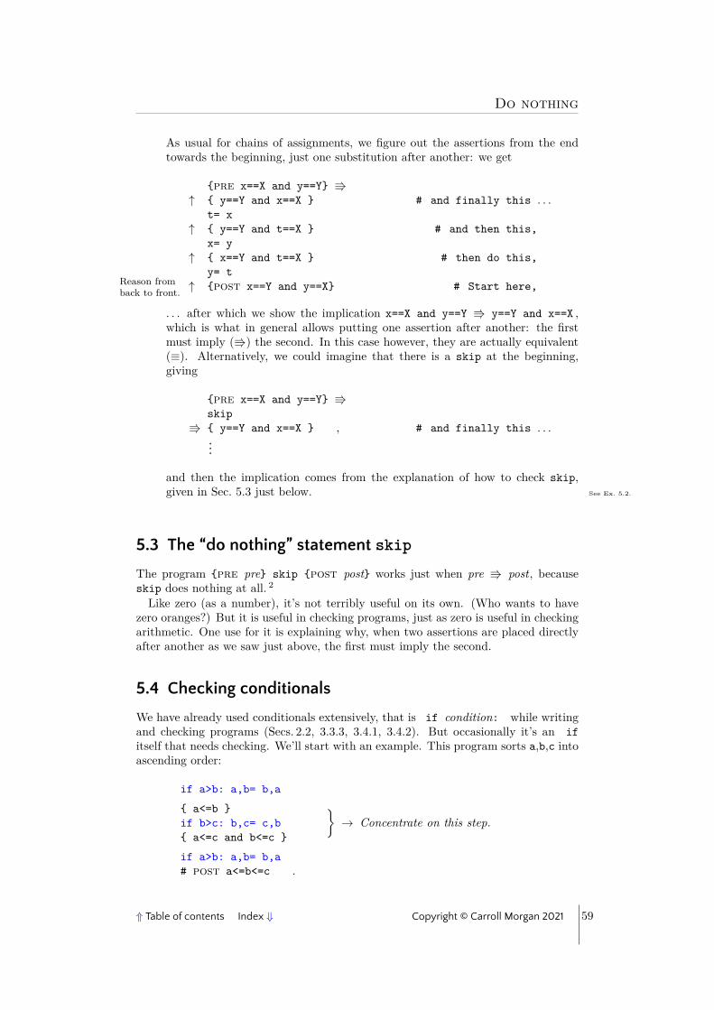
Do nothing

As usual for chains of assignments, we figure out the assertions from the endtowards the beginning, just one substitution after another: we get

{pre x==X and y==Y} V↑ { y==Y and x==X } # and finally this . . .

t= x↑ { y==Y and t==X } # and then this,

x= y↑ { x==Y and t==X } # then do this,

y= tReason fromback to front. ↑ {post x==Y and y==X} # Start here,

. . . after which we show the implication x==X and y==Y V y==Y and x==X ,which is what in general allows putting one assertion after another: the firstmust imply (V) the second. In this case however, they are actually equivalent(≡). Alternatively, we could imagine that there is a skip at the beginning,giving

{pre x==X and y==Y} Vskip

V { y==Y and x==X } , # and finally this . . ....

and then the implication comes from the explanation of how to check skip,given in Sec. 5.3 just below. See Ex. 5.2.

5.3 The “do nothing” statement skip

The program {pre pre} skip {post post} works just when pre V post, becauseskip does nothing at all. 2

Like zero (as a number), it’s not terribly useful on its own. (Who wants to havezero oranges?) But it is useful in checking programs, just as zero is useful in checkingarithmetic. One use for it is explaining why, when two assertions are placed directlyafter another as we saw just above, the first must imply the second.

5.4 Checking conditionals

We have already used conditionals extensively, that is if condition: while writingand checking programs (Secs. 2.2, 3.3.3, 3.4.1, 3.4.2). But occasionally it’s an ifitself that needs checking. We’ll start with an example. This program sorts a,b,c intoascending order:

if a>b: a,b= b,a

{ a<=b }if b>c: b,c= c,b

}→ Concentrate on this step.

{ a<=c and b<=c }

if a>b: a,b= b,a# post a<=b<=c .



Let’s check the second statement more closely: pulled out of context, and presented See Ex. 5.6.

for independent checking, it becomes

# pre a<=bif b>c: b,c= c,b# post a<=c and b<=c .

We see that if the if condition b>c is False, then b<=c holds, and so it can bein the postcondition without action on our part. (You can see it there as the secondconjunct.) But where does the first conjunct a<=c come from? And why don’t wehave the precondition’s a<=b any more? These questions are answered by lookingmore closely at how if’s are checked in detail (when we have to).The first conjunct comes from taking the precondition a<=b and the (failed) if-

condition b<=c together: they give a<=b<=c , and the a<=c in the postcondition isa consequence of that.The reason we must discard the a<=b however –it is not in the postcondition– is

that it does not (necessarily) hold if the if condition is True, because b,c are thenswapped, and b’s value can decrease, potentially invalidating a<=b .Let’s leave that for a moment, though, while we look at the other branch of the if.

The overall precondition, and the truth of the condition b>c , together give the firstextra assertion (1), and applying the assignment b,c= c,b as a substitution to thepostcondition a<=c and b<=c gives the second extra assertion (2):

# pre a<=bif b>c: { a<=b and b>c } # (1){ a<=b and c<=b } # (2)b,c= c,b

# post a<=c and b<=c ,

Since the assertions are next to each other, we must check as usual that the firstimplies the second, that is that a<=b and b>c V a<=b and c<=b ; and it does.And now we can see, by analogy, that what we should be checking in the case that

the if condition is False is the implication a<=b and not b>c V a<=b and b<=c ;and that holds too.The overall pattern of checking an if is easier to see if we include the else part of

the conditional explicitly: to checkSee Ex. 5.3.

# pre preif cond: thenBranchelse: elseBranch# post post

we check each branch separately: we check both

# pre pre and condthenBranch# post post

and# pre pre and not condelseBranch# post post ,

2 In Python skip is called pass.


Exercises

which is precisely what we did in the example above — but because in that casethe second branch was actually skip, we could check it with an implication, becausechecking skip is always done with an implication, as we saw in Sec. 5.3.Most of the time, conditionals don’t need such careful attention; but sometimes

they do. (The small program above is one of them; and what if we had a fourthvariable d as well?) An example is the Binary-Search program from Sec. 3.3.3, inparticular checking that it does not go into an infinite loop. The variant for thatprogram is n-m, and we need to check that it decreases strictly in each iteration.Here is the part of the Binary-Search program where that happens, with assertionsconcentrating on the variant:

# pre 0<=m<n<=N and V==n-mp= (m+n)//2{ m<=p<n }if A[p]<x: m= p+1else: n= p# post 0<=n-m<V

Once we apply the above, and leave out the conjuncts we don’t need, the two checksfor the branches are

# pre 0<V==n-m and m<=p<nm= p+1# post 0<=n-m<V

and# pre 0<V==n-m and m<=p<nn= p# post 0<=n-m<V ,

and the implications that result from them (after carrying out the substitutions) areseparately

0<V==n-m and m<=p<n V 0<=n-(p+1)<Vand 0<V==n-m and m<=p<n V 0<=p-m<V .

Both of those hold.Notice how we introduced the auxiliary variable V so that we could check that it

was decreased by the loop body.

5.5 ExercisesExercise 5.1 (p. 58) Example (e) in Sec. 5.2 can be (re-)written as a decreasing variant,bounded below by 0: it becomes {pre V==(N-n)>0} n= n+1 {post V>(N-n)>=0}—that is, the (decreasing) variant is N-n , not just n on its own. What is the implicationthat you have to check for that?

Exercise 5.2 (p. 59) Show that the program

{pre x==X and y==Y} x= y-x; y= y-x; x= x+y {post x==Y and y==X}

works. Hint: Remember to figure out the assertions from the end of the programtowards the beginning. Simplify the conditions, if you can, as you go along.



Exercise 5.3 (p. 60) Here is how assertions are placed inline when checking conditionalSee Ex. 5.5.

statements:

# pre preif cond:{pre cond and pre}· · ·{post post}

else:{pre not cond and pre}· · ·{post post}

# post post .

Give a similar procedure for if on its own (no else). Hint: Use the above, withskip for the else part. (See also App. B.3.3.)Then show how to check if and elif and else.

See Ex. 1.1.

Exercise 5.4 This program sets m to the largest value among a,b,c and d:

m= aif b>m: m= bif c>m: m= cif d>m: m= d

Add assertions between the statements that will allow the program to be easilychecked. Hint: Write [a,b,c]<=d for a<=d and b<=d and c<=d etc.How many paths need to be checked in this program? If you added an extra variable

e, how much longer would the program have to be?

Exercise 5.5 Use your techniques from Ex. 5.3 to check the program

{pre True} if a>b: a,b= b,a {post a<=b} .

Then check the “sort three variables” program

{pre True} ← True is the default precondition.if a>b: a,b= b,aif b>c: b,c= c,bif a>b: a,b= b,a{post a<=b<=c}

Hint: Use Sec. 5.4 and the substitution technique for assignments, working from theoverall postcondition backwards towards the True precondition (which can be omitted— it’s the default). You will find V-constraints that suggest what the intermediateassertions should be.


Exercises

Exercise 5.6 (p. 60) Add assertions to check the “sort four variables” program

{pre True}if a>b: a,b= b,aif b>c: b,c= c,bif c>d: c,d= d,cif a>b: a,b= b,aif b>c: b,c= c,bif a>b: a,b= b,a{post a<=b<=c<=d} .

Hint: See the hint for Ex. 5.4, which suggests e.g. that the a<=c and b<=c fromthere could be written more concisely as [a,b]<=c. See Ex. 5.7.

Exercise 5.7 (p. 63) The following (incomplete) Bubble Sort program uses the ideasof Ex. 5.6 to sort a whole sequence a[0:N] of N values instead of just four variablesa,b,c,d. Its invariants are suggested by the assertions you would have used in youranswer to Ex. 5.6. See Ex. 5.6.

See Ex. 5.8.

{pre · · ·}for i in range(?1?): # inv Inv1for j in range (?2?): # inv Inv2

if ?3?: ?4?{ ?5? }

# A[0:N] are in their final sorted positions.# post The whole of A is sorted. ,

where Inv1 is “A[i:] are in their final sorted positions.” and Inv2 isA[:j]<=A[j] and

(a) range(?1?) should establish Inv1 initially, and imply that A[0:N] are in theirfinal sorted positions when the outer for-loop has terminated. What should?1? be?

Hint: Use range(high,low,-1) “iterate down” in the for-loop.

(b) range(?2?) should establish Inv2 initially, and imply ?5? when the inner for-loop has terminated. What are ?2? and ?5? and why?

(c) The code of the inner-loop body will be

{pre A[:j]<=A[j]}if ?3?: ?4?{post A[:j+1]<=A[j+1]}

(5.3)

What do ?3? and ?4? have to be so that the code checks?

(d) Explain in words why your completed Prog. 5.3 checks. Note however thatBubble Sort is quite inefficient.

Hint: Do the else part first.



Exercise 5.8 Another elementary (and similarly inefficient) sorting program is Inser-tion Sort:See Ex. 5.7.

{pre · · ·}for i in range(?1?): # inv A[i:] are in order.for j in range(?2): # inv Inv2 ?6?

if ?3?: ?4?{ ?5? }

{ A[0:N] are in order. }{post · · ·} .

Complete the missing assertions and code fragments. (Note the new one, ?6?.) LikeBubble Sort, Insertion Sort is quite inefficient.

Exercise 5.9 This simple program sorts a sequence A[0:N] by continuing to swap untilno more swaps can be done. What’s its invariant ?I? ? What’s its variant ?V? ? Whatshould the assertion ??? be?

Remember that an invariant is a Boolean condition, whereas a variant is a non-negative integer.

# –- Sort sequence A[0:N] into ascending order.# pre 0<=N

while True: # Var: ?V?noSwaps= Truefor n in range(N-1): # Inv(n): ?I?if A[n]>A[n+1]:A[n],A[n+1]= A[n+1],A[n]noSwaps= False

{ Inv(N-1) }if noSwaps: { ??? } break

# post A[0:N] is sorted

Like Bubble Sort and Insertion sort, Exchange Sort is quite inefficient.


Summary of Part IChapter

6

6.1 What’s not obvious

Programming is both a vocational skill 1 and an engineering discipline. As a vocation,people learn to “code” (so-called to make it sound less forbidding?) at school, andpossibly from their parents, siblings and friends too. Coding is not very hard — andso by the time they start university, most whose interests lie there are already quitegood at it; and a substantial subset of those have discovered that –more than that–they have a natural aptitude for programming, and even computer science in general.There is a difference though between a vocation and a discipline: it’s the difference

from being able to build a garden shed yourself (with help perhaps from your family)and organising the construction of an office block or a bridge or an aeroplane (withhelp from perhaps hundreds of people you’ve never met before). In the first case,you have an instinctive understanding of what to do, based on (years of) experience,and you have a built-in rapport with the people who are helping you: you probablyeat breakfast with them every day. In the second case, instinct is only a start, andyou might have never met the team who are working for you. It’s the differencebetween being able to tune your motorcycle yourself, and being able to design onefrom scratch, and then organise its being manufactured and sold.That difference, the small vs. the large, the instinct vs. the science, is why there

are 4-year university courses in Engineering, indeed in various different kinds of en-gineering, and professional bodies that accreditate engineers so that we can trustwhat they build, and what they organise others to build. What is the analogue forprogramming?Unlike engineering in general, the technical gap between vocation and discipline in

programming is actually

astonishingly small,

although the organisational and social gap remains as large as it is for any otherbranch of engineering. And the technical gap is very easily bridged — if only you aregiven the chance. We need accreditation there too.

The techniques explained in our Part I show that –for example– instead of figuring

1 “Vocational” skills pertain to some occupation, trade or business or profession. [Macquarie Dictio-nary]


Summary of Part I

out how to write a loop by following the conventional thought processes

• Imagining what one of its iterations must do (“It must add an-other one of the array elements to the current running total.”)

• Working backwards from the initialisation to determine whatthe first step must be (“After the first addition, the runningtotal must be the first element alone: so we start at zero.”)

• Figuring out what the last iteration must do in order to makethe loop complete (“We mustn’t forget to add the very lastelement, so the index on the last iteration must be N-1. . . Oris it N?”)

• Checking the edge cases (“Does it still work if the sequence isempty?”)

(6.1)

. . . instead you might do better by remembering Program1.18 (for example), and sendthose thought processes in a different, and startlingly more efficient direction once youget the hang of it:

• The invariant is that the running total is the sum of the se-quence prefix so far. And to preserve that invariant you simplyadd the current element to the sum, and lengthen the prefixby 1 position.

• At the beginning, “the prefix so far” is empty, so the runningtotal is 0.

• At the end, “the prefix so far” must be the whole sequence.

• The edge cases are handled automatically.

(6.2)

You might not have heard of a loop invariant before: but you have now. Are invariants“unconventional”? Perhaps. But most of the time they make your programs easier towrite, easier to check and sometimes even more efficient. And soon they will be theconventional process for you.

But the difference between (6.1) and (6.2) above is not necessarily “an amountof work”. Indeed, for small programs the amount of work is about the same. Forlarger programs, however, the second one (6.2) is actually less work in the end, whenyou factor in the debugging and other program maintenance that might have to bedone. Instead of “an amount of work”, the difference is a point of view — plus theastounding advantage that the (6.2)-approach brings, these three extra benefits:

1. Approach (6.2) scales up.Checking a program in terms of “What steps does it carry out in this situa-tion? And this situation? And this situation that my customer mentioned onlyyesterday?” , as in (6.1), becomes harder at a much faster rate than simply thesize of the problem. Remember Exercise 1.1, that showed how in that smallprogram, every new variable doubled the amount of checking needed — if donein the conventional style.

2. Approach (6.2) makes it easier for team members to collaborate.The idea of documenting “What’s true at this point in the program?”, as in(6.2), instead of “What does this bit of code do?”, as in (6.1), is the glue that


What is obvious

binds together large teams of programmers, and that allows large programs tobe divided into pieces that can be handled separately.

3. For very important programming projects, where failure is extremely expensive,even catastrophic, the approach of (6.2) can be to some extent be automated.(See Part IV.) For (6.1), that is much more difficult.

Because the difference in effort required, –i.e. to move from thinking in the (6.1)-style to thinking in the (6.2)-style– is so small but makes so much difference, we havestarted in Part I with programs that you already know and understand — and thatmeans you can concentrate on how you are thinking about them, rather than havingto worry at the same time about what those programs are actually doing.Later, however, we will see the payoff that “What’s true here?” thinking brings.

As just one example, the program in Chp. 16 is just four lines line (plus another fourthat are a symmetric copy of the first four): but it took 15 years to discover thatprogram, and the person who did is still celebrated today. 2 There are more than50 program-execution paths to think about were we to check those four lines of codeconventionally. See Ex. 16.9.

What’s not obvious about these insights into thinking about your programs in adifferent way? The only non-obvious thing (before you read this) was that it’s possibleto do it.You were not told; and nobody showed you how.

6.2 What is obvious

Once you know about this style of thinking about programming, and have had somepractice, it is indeed pretty obvious in most cases how to do it. Figure 1.1 showed aflowchart for summing a sequence (Prog. 1.18 again). And it’s very clear what’s goingon: the operations of the program occur within the boxes –rectangles for assignments,diamonds for tests– and the lines (with arrows where necessary) show how the programmoves from one action to the next.Inside each box is written what it does; and you can simulate the program’s actions,

execute it “in your head” just by following the lines around.But there is more to these flowcharts: on the lines between the boxes is written

“what is true when the program is travelling along this line”. The principal reason itis so much easier to use those for checking –to use what’s between the boxes ratherthan what’s in them– is that if you use the boxes alone, then to check whether aparticular box is doing the right thing, you must look at the box before, to see whatit did; and for that one, you must look at the one before it, and so on.

On the other hand, if you use what’s written on the lines between the boxes, youneed only check whether the box successfully takes you from what was written on itsincoming line to what is written on its outgoing line. If that checks, then this box isworking, and you do not need to check other boxes to see whether this box works.And even more significantly,

If you check all the boxes in that style (“Does it take you from its incomingline to its outgoing line?”) even if you check them all separately, even atdifferent times, even with different people. . . and they all work, then thewhole program works too.

2 Forty years later, at time of writing.


Summary of Part I

That is, those other boxes can be checked by other people, or yourself on other days;and what’s written on the lines, our pre- and postconditions, are the “glue” that putsall the checks together, what reminds you tomorrow what you have to check then(even if by then you have by then forgotten the details of what you checked today).Or it tells your colleagues what they have to check, separately, in order for the wholething to work properly when it’s assembled.

The more you practise checking programs by using the techniques we’ve introducedin this Part I, the more you will appreciate it, in both senses of that word: you willbe glad you were told about it, and you will understand how it works.


Part II

Data structuresand their encapsulation

IntroductionChapter

7

7.1 Data vs. data structures

The data values of a program are stored in its variables: in the simplest cases they arethings like numbers (integers, floating point), characters, Booleans: those are called“basic”, or “primitive” data types. Using those basic types, “building” on them, givesus things like sequences of integers, characters, Booleans, strings, and sets of suchthings, and tuples of them and so on. There you get more than just the basic: youget data structures.As an example, let’s take people’s names and ages, both primitive types, 1 and make

a data structure from them: we can build a directory using a sequence variable diras a sequence of triples. It might be initialised with the assignment

dir= [("Alex", "Smith", 35), ("John", "Jones", 60)] ,

so that it stores that information for just two people: Alex Smith is aged 35; andJohn Jones is aged 60. The data structure here, the type of dir, is a sequence oftriples, with each tuple based on two basic types: two strings and an integer.The family name of the first person in dir is dir[0][1], where dir[0] is the first

person (because we index lists from 0), and · · ·[1] is the second component of thattriple — "Smith".

You can do a lot with that structure. But if your directory dir grows to containthousands of entries, or you want to store middle names as well, then two issues arise:

1. Having a simple sequence of entries might make it quite inefficient to search thewhole directory: using linear search might take too long.

2. Expanding the directory to include middle names (with "" for “none”) wouldgive things like

dir= [("Alex", "", "Smith", 35),("John", "Paul", "Jones", 60)] ,

and the dir[0][1], to access the family name “Smith” of Person 0, would haveto be changed to dir[0][2] –everywhere, throughout your whole program–because all the family names are now in the third position.

1 Strictly speaking, the names’ type is not basic, because it is a sequence of characters. We’ll ignorethat however: where you start is to some extent flexible. Isn’t a character in turn a sequence of bits?


Introduction

The solution to both problems is to use procedures and functions to access andupdate the data structure; and then when you want to have a faster lookup you mightalter the search function to use binary search instead of linear search (Sec. 3.3.3).But you would at the same time have to alter the add procedure to put new entriesin the right place, so that the sequence of triples is always sorted (since binary searchdoesn’t work, otherwise). All the various procedures would have to be modified in aconsistent way.The second problem (a simpler one) is also solved by using procedures and functions:

in that case you would probably have to make only one change: the “getFamilyName”function would have its “· · ·[1]” altered to a “· · ·[2]”.

7.2 Data encapsulation

Data encapsulation is the practice of gathering all the code for the declaration, ini-tialisation, access and updating of a data type, all of it, together in one place for eachconceptual data structure. So for example the declaration and initialisation of dirjust above, and its related functions, would all be grouped together. Data relatedto another concept (say a directed graph) would also be grouped together, but in itsown, separate encapsulation.The advantage of doing all that, and the topic of this Part II, is how that encap-

sulation is organised and how –in particular– changes like the two mentioned above(many entries, middle name), and others, can then be carried out in a way that doesnot undo the checking that might already have been done in the surrounding programthat used the data structure in its original form. And it is as well likely to take lesstime to carry out than it would have without the encapsulation.Very simple examples will be used to illustrate the process, pretending we have dis-

covered the idea of encapsulation, and its advantages, for the first time. See Sec. G.3however for a brief discussion of how encapsulation has evolved into Object-Orientedprogramming, and the extra concerns that apply.As in Part I, the key tool is assertions and invariants.


Coupling invariantsChapter

8

8.1 Introduction

Invariants –we recall– are assertions that are intended to describe things that are“always true”, like the condition that “always holds” every time your program beginsa particular loop’s body. Those are loop invariants, of course.But invariants are used in many places, and for many purposes: here we look at

“coupling” invariants that state the relationship that “always holds” between twodifferent representations of the same data.We’ll use “sets” as a running example of coupling invariants.

8.2 Implementing sets as sequences

Our first illustration of coupling invariants concerns writing code at a “low level” thatexpresses an idea at “higher level”. The low level is sequences; the higher level is sets.Suppose we can write programs that use finite sets directly, with statements like

ss= {} that assigns the empty set to set ss, 1 or like ss= ss∪{s} that adds elements to set ss, or like the conditional s∈ss that determines whether s is in ss.This is the “higher level”.The reality at the “lower level” however might be that actually you can’t use sets

directly in your code, because your programming language doesn’t support them: 2

but you still have to write that program. In that case, you might decide to representthe set ss as a sequence qs, and write your code directly at that lower level, translatingas you go: you’d write

• qs= [] to initialise the “set” to the empty set, and

• qs= qs+[s] to add an element s to the set, using sequence concatenation +,and

1 In Python you must write set() for the empty set: the two-bracket notation is used for empty“dictionary”. We will use {} here, however.2 Python does support sets; but here we are pretending it does not: and the language you are actuallyusing might not. Sets are not build in to C, for example. The techniques we’ll use here apply tomore or less any language.


Coupling invariants

• the small program 3

b= Falsefor q in qs:if q==s: b= True; break

(8.1)

for setting Boolean b depending on whether s is in qs: instead of a singlestatement, we must use a small linear-search loop to search the “set” for theelement. In this case the low level is the code you are writing, and the highlevel is in your head.

See Ex. 8.1.

So now imagine that you wanted to add a new operation, to take an element outof the set, i.e. to remove it: with sets directly, i.e. “in your head”, you are thinkingss= ss-{s}. But that’s not what you write: you are implementing the set in codedirectly, as you go, as a sequence qs. And so you must now decide whether to take“just one” s out of qs, or “all of them”. How do you decide?In the implementation above, you would have to take them all out, and to learn

that you have to do that, you would have to examine the code of add (which mightbe pages away) to see whether it is possible for elements to be repeated in qs. Andindeed we would find that adding s “a second time” will include it twice.And –another variation– what if for efficiency of searching you decided to keep

the sequence qs in ascending order? In that case, you could use binary search formembership checking, but a loop would be necessary for insertion (and deletion).This example simply reminds us that if we are using a collection of procedures and

low-level data to implement a higher-level concept, the collection must be consistent:its members must cooperate with each other. Here we will show that to do that it’sa good idea to group them all together, and to introduce a “coupling invariant” tostate clearly and explicitly what “cooperating” with each other actually means.

In fact most programs (and programmers) carry out “representation” exercises likethe above in almost every program. Often it is trivial, and easy to keep track of. Buta clear advantage of putting all the information in one place, and having a couplinginvariant, is that it makes the consistency checking so much easier. If say there were5 procedures associated with the concrete representation of the data, then checkingeach against all the others would amount to 10 checks. With a coupling invariant,it would be only 5 checks; if there were 10 procedures, it would be 45 checks vs. 10.The more procedures there are, the bigger the difference becomes.As remarked in the Introduction to this chapter (Sec. 8.1), we have seen assertions

already as “What’s true at this point in the program.” comments; and we have seena more specialised use of them as “What’s true every time this loop begins?” Whatwe will now see is how assertions can describe the connection between the variableswe would like to have –like sets– and the variables we actually do have, in this casesequences. Those assertions are called coupling invariants, and the coupling invariantfor our example above is

The elements in the sequence qs, ignoring repeats, are the membersof the set ss that we are actually thinking of as we write the program. (8.2)

It’s a condition on variables’ values, just like the others we have written, in this casecontaining both the variables ss and qs — that is, both the high level and the low3 Python implements in for sequences directly; but many languages do not. We are pretendinghere that Python does not.


Sentinels

level, the “abstract” and the “concrete”. It tells us for example that add(s) canappend s to qs even if s is already there; and it tells us that remove must check thewhole sequence in order to find every occurrence.

8.3 Sentinels as “high level” data

Another use of coupling invariants is to implement “sentinels”.A sentinel is an extra, “special” value added to data in order to simplify program

code. For example, we might want to find program code “· · ·” such that this programwould check:

# –- Find the position of some value in a given sequence, if it’s there.# pre 0<=N· · ·# post A[n]==x if x∈A else n==N

(8.3)Notice that the requirements are (deliberately) a bit loose, but do state the generalpurpose of the program. The postcondition however is more precise: it says whichsequence (A) is to be searched, which variable (n) is to receive the result, and how “xis not there” is to be indicated.We’ll do it with linear search.

Linear search is not a hard program. But it would be slightly easier to code if we See Ex. 2.3.

See Ex. 8.2.

See Ex. 8.3.knew that x was in A somewhere, because the search for x would then be guaranteedto succeed — we would not have to worry about “falling off the end”.To use a sentinel for that, we imagine extending A with an extra element x at

position N, “beyond the end” of A — that is, we would use a sequence B[0:N+1] thatwas equal to A+[x]. We’d therefore have B[n]==A[n] when 0<=n<N but B[N]==x inparticular. Searching for the x that might be in A is then the same as searching forthe x that must be in B. . . somewhere. If x is not in A at all, then it won’t be inB[0:N] either, in which case our program will set n to N — that’s exactly what thesentinel B[N]==x is for.

Here is the program that uses our “imaginary”, high-level B with its sentinel:

# –- Find x in B[0:N+1].# pre 0<=N and x∈B ← Notice the extra precondition.n= 0while x!=B[n]:n= n+1

# post 0<=n<=N and x 6∈B[:n] and B[n]==x

(8.4)

The extra “x 6∈B[:n]” in the postcondition is important: without it we could simplywrite the code n= N ! And as usual the postcondition is just the invariant and thenegated loop condition. See Ex. 8.4.

What we will now look at is how to translate that Prog. 8.4 to a program aboutour “actual”, low-level sequence A instead of the imaginary B . And that is done witha coupling invariant.As we have said, a coupling invariant –like other invariants– states a condition

that the program maintains: it links two or more variables together. In Sec. 8.2 thevariables were ss and qs; here they are B and A.In the earlier example of Sec. 8.2, we wanted to think in terms of sets, but had to

program in terms of sequences. The coupling invariant expressed that the “set we


Coupling invariants

are thinking of” is the set “that the sequence represents”. In addition, the couplinginvariant might express extra constraints like “the set has no more than N elements”,or “the sequence is sorted” or “the sequence does not contain repeated elements”. Wedon’t do that now, but we will return to it in Sec. 10.2.In this example we do something much simpler: we use a coupling invariant to link

our original A to our fictitious B. Indeed we mentioned it above already: it’s just

B == A+[x] . (8.5)

Since neither A nor B is being updated by our linear-search program, we do not have tofigure out corresponding updates to keep the coupling invariant true. We do howeverneed it to convert references to B into corresponding references to A. There are threeplaces that B is referred to in Prog. 8.4:

• in the precondition, with x∈B;

• in the loop condition, with x!=B[n]; and

• in the postcondition, with x6∈B[:n] and B[n]==x .

One of the principal advantages of invariants generally (i.e. loop invariants as well)is that they allow us to deal with things one at a time, knowing that if each thingseparately respects the invariant then all of them together will respect it as well.In the case of a loop invariant, that translates into checking that the invariant isestablished by the loop initialisation (one thing), then checking that the loop bodymaintains it (another thing), and then being able to use the fact that the invariantholds when the loop terminates — in effect the “all of them together” payoff. (InSec. 8.2 it was the point about having to do only 5 checks instead of 10.)The same thing will happen with this small program:

• In the precondition x∈B becomes x∈(A+[x]), which is trivially True. So it canbe deleted altogether from the precondition.

• The loop condition x!=B[n] becomes x!=(A+[x])[n], which we deal with intwo cases: either n==N or n!=N. In the n==N case it’s trivially False ; but in theother case it is just x!=A[n]. Thus the loop condition translates to

n==N and Falseor n!=N and x!=A[n] ,

and that simplifies to just n!=N and x!=A[n] .See Ex. 8.5.

• In the postcondition, the x 6∈B[:n] and B[n]==x becomes

x6∈(A+[x])[:n] and (A+[x])[n]==x ,

and again we can separate it into the two cases. This time we get

n==N and x 6∈A and Trueor n!=N and x 6∈A[:n] and A[n]==x .

If we discard the “and True”, and weaken the postcondition by discarding thex6∈A[:n] because the requirements didn’t ask for the first occurrence of x, thenwe get

# post A[n]==x if n!=N else x6∈A .


Writing abstract data-types

When we make those substitutions, replacing references to B by correspondingreferences to A as figured out just above, we get the linear search program

# –- Find x in A[0:N].# pre 0<=Nn= 0while n!=N and A[n]!=x: n= n+1# post A[n]==x if n!=N else x6∈A .

(8.6)

Curiously however, the postcondition of this program is not the same as the postcon-dition of Prog. 8.3 above. See Ex. 8.6.

See Ex. 8.7.We are not of course saying that Prog. 8.6 is complicated, or that it could not havebeen written in this form directly. What we are saying is that here we have used the(coupling) invariant to construct that program; and if Prog. 8.4 (the “B version”) iscorrect then Prog. 8.6 must be as well — there’s no need here to check it again.

8.4 Writing abstract data-types

We now put the ideas of the two previous sections together: having simultaneouslyan “abstract” and a “concrete” view of our data (sets vs. sequences in Sec. 8.2); andusing a coupling invariant to transform one program into another (usually abstract,using sequence B with its imaginary extra element, transformed into the concrete useof sequence A in Sec. 8.3).

We begin by returning to our set example (Sec. 8.2) and collecting the set-valuedvariable ss, and the functions that use it, all together in one place: 4

class Set: # Pretend that sets cannot be implemented directly:local ss= {} # Start empty, yet

def makeEmpty:ss= {} # we have no “{}” ...

def add(s):ss= ss∪ {s} # ...nor “∪ ”,

def isIn(s):return s∈ss # nor “∈”.

(8.7)

This code does not itself make a set: it is more like declaring a Set type. To make See Ex. 10.2.

a set instead, we write things like ss1= Set() to make a set-valued variable, in thiscase called ss1. With ss2= Set() we could make a second one.

Given that (we are pretending) there are no “real” sets in our programming lan-guage, the code above is fantasy: it won’t compile, and we can’t run it.So it’s tempting to call Prog. 8.7 above “pseudocode” — but it is much more than

that. Here’s why. Suppose we have a program that uses our (more than) “pseudo-

4 We’re using something like the Python syntax for declaring a “class”, and will explain it as wego. Remember though that we are pretending that the statements ss= ss∪{s} and similar are notPython (even though actually they are), because sets might not be in whatever language we areactually using. local is not a keyword of Python, where global/local is determined implicitly. Weuse it here to make reasoning easier.


Coupling invariants

code” like this:

{pre True}ss1= Set()ss1.add(2*2)has4 = ss1.isIn(4){post has4} .

(8.8)

It initialises set ss1 to empty, adds the value 2*2 to the set, and then sets Booleanhas4 to whether the element 4 is in the set. Can we check this program, even thoughwe can’t compile it, can’t run it?Yes. We can check this program with the methods we have already, by inserting

assertions in between the statements. We “inline” the procedure calls, that is wereplace the call to the procedure with the code that’s in the procedure (with theappropriate substitutions done) — and then we check that. As usual, we start fromthe bottom (the postcondition) and work towards the top (the precondition), getting

{pre True} # And see that indeed it checks. ←{ 4∈ {4} } # Simplify. ↑{ 4∈ {}∪{4} } # Inline local, substitute. ↑ss1= Set(){ 4∈ ss1.ss∪{4} } # Arithmetic. ↑{ 4∈ ss1.ss∪{2*2} } # Inline add(2*2), substitute. ↑ss1.add(2*2){ 4∈ ss1.ss } # Inline isIn(4). ↑{ ss1.isIn(4) } # Substitute. ↑has4 = ss1.isIn(4) # Work towards the front. ↑{post has4} , # Start checking here. ↑

(8.9)

and we see that indeed it checks. But in doing that check, we have done somethingthat ordinary pseudocode cannot do, and that is why this is more than pseudocode.You cannot reason rigorously about pseudocode. The best you can do is “execute it inyour head.”

We have reasoned about code (the set operations) that is not onlynot really there, it can never be there in the language we imaginewe are using.

But –in spite of that– we can check our programs anyway.

(8.10)

This is what the abstract/concrete approach allows us to do. If we check the abstract,and construct the concrete using the methods of this Part, we do not need to checkthe concrete: the checking is done during the construction, a beneficial side-effect ofthe methods we are using.The reason we call Prog. 8.7 an “abstract” data type is that it is a data type, and we

can reason about it, but it abstracts from the details of the particular programminglanguage we might be using.


Coding concrete data-types

8.5 Coding concrete data-types

At (8.10) we saw that we were able to check a real program Prog. 8.8 without actuallyhaving real, runnable code for the data it was using. We did it at Prog. 8.9 by usingthe abstract version of the data type as if it had been real code. But in the end dowe need real code, in a real programming language that we can compile and run ona real computer, if ever we are to use our program. And so we now use the ideasof Sec. 8.3 do do the complementary thing: we reason about the abstract data-typeitself without having to worry about the programs (however many and varied theymight be) that might be using it.That’s worth emphasising: on the one hand, we can check programs that use the

data without having the actual code that manipulates the data — we did that inSec. 8.4 above. But we are now about to see that we can implement the actual codethat manipulates the data without having to see the programs that use the data. Thatis, we won’t have to look at “use cases” at all, things like (8.9), while we are figuringout how to implement the encapsulation in Prog. 8.7.It’s coupling invariants that make it possible to separate the two activities: writing

the code without having an implementation of the data type; and implementing thedata type without knowing anything about the code that’s using it. Here the couplinginvariant was given in Sec. 8.2 at (8.2), and we will use it just as we did in Sec. 8.3for sentinels, where B was abstract and A was concrete.Translating an abstract data-type to a concrete data-type is done in three steps,

and we will use both Sec. 8.2 and Sec. 8.3 as examples.

8.5.1 Add concrete (auxiliary) variables

We’ll start with the set data-type, and convert it gradually into one that uses se-quences instead. Our first step is to add the concrete, sequence-valued variables –inthis case just qs, a single sequence– to the abstract data-type, and add statementsthat maintain the coupling invariant; that is, we will temporarily have both ss andqs; but to begin with qs will be only an auxiliary variable, one that has no effect onthe execution of the procedures (methods) of the data type. We have (temporarily)a kind of abstract/concrete hybrid. This first step gives

class Set:local ss= {} # Abstract. }

→ Together.local qs= [] # Concrete

# Coupling invariant is established.

def makeEmpty:# pre If coupling invariant holds here,ss,qs= {},[]# post then it holds here too.

def add(s):# pre If coupling invariant holds here,ss,qs= ss∪ {s},qs+[s]# post then it holds here too.

def isIn(s):# pre Coupling invariant holds here, before.return s∈ss # And ensures the correct value is returned.

(8.11)

See Ex. 8.8.


Coupling invariants

In the code above (8.11), the coupling invariant must hold after any initialisation(local), before any read-only function (isIn), and before and after an updatingprocedure (makeEmpty,add).That was the first step.

8.5.2 Use the coupling invariant

The second step in the translation procedure is to use the coupling invariant to swapthe roles of the abstract- and concrete variables. In Prog. 8.11 just above the abstractvariable ss is “real” and the concrete qs is auxiliary. We want to swap that around,to make qs become real and ss become auxiliary; and so we must remove ss fromthe return of isIn while preserving the meaning of what is returned. For that weintroduce the loop from Prog. 8.1. Provided it terminates, it has no effect on IsIn atall:

class Set:...def isIn(s):# pre Coupling invariant holds here, before.b= Falsefor q in qs:if q==s: b= True; break

{ b == (s∈qs) } ←− Established by the loop.# Coupling invariant holds here, which gives us{ b == (s∈ss) } ⇐= this also.return s∈ss# We can now replace the return s∈ss by return b .

(8.12)

The loop establishes the postcondition←− and the coupling invariant tells us that⇐=holds too. And then the ⇐= allows us to replace the return s∈ss by return b ,which eliminates the reference to ss, making it auxiliary.See Ex. 8.9.

8.5.3 Remove abstract (auxiliary) variables

After our changes in Sec. 8.5.2 just above, we now have that ss is auxiliary and qs is“real”, exactly the opposite of before. And because it’s ss that is now auxiliary, wecan remove it altogether; that gives

class Set: # This is the actual implementation.local qs= []

def makeEmpty: qs= []def add(s): qs= qs+[s]

def isIn(s):b= Falsefor q in qs:if q==s: b= True; break

return b .

(8.13)

The question is now “How do we re-check Prog. 8.8 –that uses the abstract Set– withthis new (concrete) version (8.13) that actually implements Set?”


Exercises

The (surprising) answer is that we don’t have to (re-)check at all! We checked italready, at Prog. 8.9 in its abstract form. That is, we checked our program using theabstract data-type, but when we run it we supply the concrete data-type — and wecan be sure that the check is still valid. . .

. . . provided the abstract- and concrete data-types together respect thecoupling invariant,

and you follow the rules illustrated here, and summarised in Chapter 10below.

The reason for splitting this process into two pieces –write the surrounding programin terms of the abstract data-type; implement the abstract data-type using concretetypes– is that the surrounding program is more easily checked with the abstractdata-type, because we are reasoning at a higher level, as in Prog. 8.9. But for theactual code, we need the concrete data-type, because the abstract code might not besupported by our programming language. See Ex. 8.10.

8.6 ExercisesExercise 8.1 (p. 74) Introduce requirements, pre- and postconditions for Prog. 8.1,and then add a loop invariant so you can check it.

Exercise 8.2 (p. 75) Find the code for Prog. 8.3 directly (i.e. without using a sentinel),using the invariant

0<=n<=N and x 6∈A[:n] .

Exercise 8.3 (p. 37) In Prog. 3.7, binary search, we used the assignment statement See Ex. 8.2.

p= (m+n)//2 to establish the assertion m<=p<n given that m<n held: that is

# pre m<np= (m+n)//2# post m<=p<n

checked. But doesn’t the simpler

# pre m<np= m# post m<=p<n

also check? If so, then the resulting program as a whole also checks, i.e. it searchesfor x in A, just as binary search did. But what kind of search is it really?

Exercise 8.4 (p. 75) What is the invariant for Prog. 8.4? What is the variant? Checkyour program carefully with the invariant and variant you have chosen.Hint: Be especially careful with the upper bound for n in the variant.


Coupling invariants

Exercise 8.5 (p. 76) Explain why

n==N and False or n!=N and x!=A[n]

simplifies to just n!=N and x!=A[n] .

Exercise 8.6 (p. 77) The postcondition of Program8.6 is not the same as the post-condition of Prog. 8.3, which was our original goal. Indeed both of them are missing0<=n<=N, which really should be there. But they are still not the same.

Give an example that shows they are not, explain “methodologically” how it hap-pened and what the consequences might be.

Exercise 8.7 (p. 77) Give the most concise formulation you can of the condition

x6∈A if n==N else x==A[n] and x6∈A[:n] .

Exercise 8.8 (p. 79) What does it mean to be an auxiliary variable? Why is qs anauxiliary variable in Prog. 8.11?

Exercise 8.9 (p. 80) To check Prog. 8.12, in particular the assertion { b == (s∈ss) },we need an invariant for the linear-searching for-loop in isIn. What is it?What checking rule do we use (from App. B.2.2) to move from (←−) to (⇐=) ?And why does it check?

Exercise 8.10 (p. 81) Often the the concrete data-type can be simplified, a sort of“tweaking” process, once the abstract variables are gone — and that is the case withisIn above at (8.13) above. What is the simplified code for inIn? Why is it allright to change it now?


Case study in couplinginvariants:

Fibonacci numbers

Chapter

9

9.1 Definition vs. implementation

The Fibonacci numbers are well known: they start with 1,1, and then carry on with2,3,5,8,13. . . where each new one is the sum of the two just before. Their usualdefinition is that

fib (n+2) = fib (n+1) + fib (n) , with fib (1) = fib (0) = 1 , (9.1)

and that leads directly to an easy (recursive) program to calculate them:

# –- Calculate the n-th Fibonacci number# pre n>=0def fib(n):if n==0: return 1elsif n==1: return 1else: return fib(n-1)+fib(n-2)

# post fib(n) returns fib(n) .

(9.2)

The above function is “recursive” because it can call itself, but it is still meaningful:the reason it is not a circular definition is that it does not always call itself. Eventually,it stops doing that, and starts to construct the answer: the check that it does stop,eventually, is done with a variant; and the check that it returns the right answer,when it stops, is done with an invariant. And it’s an easy check. See Ex. 9.1.

What makes Prog. 9.2 impractical though, as an implementation of (9.1), is thatfor n of any reasonable size it’s simply too inefficient: to calculate fib (0) and fib (1)takes one call of fib (each), but to calculate fib (2) takes three; and fib (3) takesfive. The number of calls is exponential in n. See Ex. 9.2.

The more efficient program that is typically used to calculate Fibonacci numbers isinstead the one given in the next section, and we will explain it in detail, even thoughit’s well known, because it illustrates two of our invariant-finding techniques. And ittakes time linear in n.


Fibonacci numbers

The aim of this chapter however (from Sec. 9.4 on) is to show how, using a couplinginvariant, we can calculate fib (n) in logarithmic time. The final program is given at(9.10).

9.2 Linear-time Fibonacci

The usual program for calculating Fibonacci numbers is this one:

# –- Calculate the N-th Fibonacci number.{pre N>=0}f,g= 1,0for n in range(N): { Inv: f==fib(n) and g==fib(n-1) }f,g= f+g,f

{post f==fib(N)} ,

(9.3)

where we note that in the multiple assignment f,g= f+g,f the initial values of f andg are used on the right hand side.We have introduced the convenient fiction that fib(-1)==0. Checking –indeed

designing– this program is an example of iterate up and cascading invariants fromSecs. 3.5 and 3.3.1 — the first step, iterate up, is to propose the invariant f==fib(n).But then to code the loop body, which must calculate the next value fib(n+1) of ffrom its current value fib(n), you discover that you need fib(n-1) as well, and thatis the second step: the “cascaded invariant” is g==fib(n-1).See Ex. 9.3.

See Ex. 9.4.

9.3 Introducing matrices, but still linear time

If we look at the loop body of Prog. 9.3 just above, that is f,g= f+g,f , we see thatit is equivalently the matrix multiplication(

fg

)=

(1 11 0

) (fg

);

and so we can re-write Prog. 9.3 as shown in Fig. 9.1. It has become a simpleexponential-calculating program (and does not need cascading invariants any more,because the n and n-1 case are combined together in the column vector for f and g).Still Prog. 9.4, like Prog. 9.3, takes linear time.But it is an exponential-calculating program — and our earlier Program3.9 calcu-

lated B**E for scalars in the much more efficient logarithmic time, using a halving-and-squaring strategy. (It was the straightforward, but slower algorithm Prog. 3.8that took time linear in E.) With the cleverer invariant B**E==p*b**e (though itwas not an obvious one) the faster, logarithmic-time program was easy to write andcheck.Using a coupling invariant, we can therefore transform the program Prog. 9.4 of

Fig. 9.1 into a much faster program that calculates the Nth Fibonacci number inlogarithmic time. It uses matrices rather than integers, but is otherwise structurallythe same as Prog. 3.9.That is, the coupling invariant will allow us transform the logarithmic-time expo-

nentiation program on numbers in to one that works the same way on matrices —and then we will then have a logarithmic-time Fibonacci calculator.


Logarithmic-time Fibonacci

{pre N>=0}(fg

)=

(10

)for n in range(N): # inv Inv(

fg

)=

(1 11 0

) (fg

){post f==fib(N)} ,

(9.4)

where Inv is(fg

)==

(1 11 0

)n (10

). (9.5)

This linear-time Fibonacci program, using matrices, is a simple example of iterate upfrom Sec. 3.5.

Figure 9.1 Fibonacci as matrix exponential

9.4 Logarithmic-time Fibonacci

Below is Prog. 3.9, the logarithmic-time exponential calculator from Sec. 3.4.1 forsimple numbers, that is scalars, repeated here for convenience. We have changed itsE to an N:

# pre 0<=Np,b,n= 1,B,Nwhile n!=0: { Inv: B**N == p*b**n }if n%2==0: b,n= b*b,n//2else: p,n= p*b,n-1

{ B**N == p*b**n and n==0 }# post p==B**N .

(9.6)

The checking we did for this program, in Sec. 3.4.1 earlier, relied mainly on asso-ciativity of multiplication for ordinary numbers, i.e. that a(bc) = (ab)c. In particular,checking the assignments in the loop body (with substitution, as usual), that theymaintained the loop invariant, required things like

p*b**n == p*(b*b)**(n//2) when e is evenand p*b**n == p*b*b**(n-1) in any case.

Since matrix multiplication is associative, just as it is for scalars, we should be able touse the same checking strategy. (Matrix multiplication is not commutative, however.)We will replace the “abstract” matrix-typed variables b and p by “concrete” integer

variables, using one concrete variable for each position in a matrix. The concretevariables are b00, b01, b10, b11 and p00, p01, p10 and p11, and the coupling invariant


Fibonacci numbers

will be

b ==(

b00 b01b10 b11

)

and p ==(

p00 p01p10 p11

),

so that the ordinary multiplications in Prog. 9.6 will be replaced by matrix multipli-cations. The result is this program:

# Variable N is given.b00,b01,b10,b11= 1,1,1,0 # from (9.5) abovep00,p01,p10,p11= 1,0,0,1 # the matrix equivalent of 1n= N

while n!=0:if n%2==0:b00,b01,b10,b11= b00*b00+b01*b10, \

b00*b01+b01*b11, \b10*b00+b11*b10, \b10*b01+b11*b11

n= n//2

else:p00,p01,p10,p11= p00*b00+p01*b10, \

p00*b01+p01*b11, \p10*b00+p11*b10, \p10*b01+p11*b11

n= n-1f= p00

(9.7)

where the final assignment f= p00 implements the multiplication of the final matrixby the initial (column) vector (1 0).

And indeed this program Prog. 9.7 calculates fib(N) in logarithmic time. But itcan be simplified. . .

9.5 Remove auxiliary variables

In the final assignment to f in Prog. 9.7 just above, only one of the four p’s appears onthe right-hand side. In fact, in the whole program the variables p10 and p11 appearonly in assignments to themselves, which means they are (jointly) auxiliary. Butp01 is used in an assignment to p00 — so it is not auxiliary, and must remain. If weremove the auxiliaries p10 and p11, however, we get the new, smaller (but equivalent)program


Remove auxiliary variables

b00,b01,b10,b11= 1,1,1,0 # from (9.5) abovep00,p01= 1,0n= N

while n!=0:if n%2==0:b00,b01,b10,b11= b00*b00+b01*b10, \

b00*b01+b01*b11, \b10*b00+b11*b10, \b10*b01+b11*b11

n= n//2else:p00,p01= p00*b00+p01*b10, p00*b01+p01*b11n= n-1

f= p00 .

(9.8)

But there is more. In fact two further variables can be removed, once we noticethat the program satisfies the loop invariant

b00 == b10+b11 and b01==b10 . (9.9)See Ex. 9.5.

So far, that invariant has not been used — we didn’t even know it was there. Butwe will use it now, because it means we can remove b00 and b01, replacing themwith the right-hand sides just above. Doing this is another example of “tweaking” —we have already checked the program, but we are now making it slightly neater (andmore efficient).That gives the program

b10,b11,p00,p01,n= 1,0,1,0,Nwhile n!=0:if n%2==0:b10,b11= b10*(b10+2*b11), b10*b10+b11*b11n= n//2

else:p00,p01= p00*b00+p01*b10, p00*b01+p01*b11n= n-1

f= p00 ,which (still) calculates fib(N) in time logarithmic in N. We can finish off by renamingthe variables to reduce the clutter, a further simplification: say b10 to just b, and b11to c, and similarly for the p’s. Then we get the following compact (and intriguing)program, one that is already checked: it is

# –- Calculate fib(N) in logarithmic time{pre N>=0}b,c,f,g,n= 1,0,1,0,Nwhile n!=0:if n%2==0: b,c,n= b*(b+2*c), b*b+c*c, n//2else: f,g,n= f*b+f*c+b*g, f*b+g*c, n= n-1

{post f==fib(N)} ,

(9.10)

where the renaming of p00 to f allowed us to delete the final assignment f= p00. 1

1 If you transliterate this to C, you will have to convert the multiple assignments into single assign-


Fibonacci numbers

9.6 Summary

What we saw in this chapter was the transformation of a whole “program” (actuallyfunction) from abstract- to concrete form. The abstract form was matrices, and theconcrete form was ordinary numbers, i.e. scalars. (An added point of interest wasthat checking the abstract program, the matrices, had already been done when it wasconstructed in its scalar form, i.e. ordinary exponentiation of scalars. Only because ofthat check –its explicit reliance on associativity of multiplication, for example– couldwe just “carry it over” to matrices, without having to start again from scratch. It’sthe assertions and invariants that made that possible.)Similarly, in Chp. 8.3 we transformed a whole (sequential search) program from

abstract form, using B, to its concrete form using A. In both cases, transformationof the program/procedure/function was transforming “everything” — except thatits inputs and outputs, or initial- and final state, were not transformed. Only the“internal workings” were affected, and they were not visible from the “outside”, whichis one reason that such transformations work.In Chp. 8.2 however, the various procedures of the Set class do input and output

their internal state, in the sense that each one passes its final state onto the next,where it is initial state; and it’s essential for their correct working that those internalsare not exposed to the outside world, that is to the surrounding program. That’sachieved by the “encapsulation” that we will now discuss in more detail in the nextchapter. The internal state that is shared by all those functions and procedures(e.g. clear, add and isIn for the Set’s) is hidden, and can be accessed only by theprocedures and functions supplied. It’s as if the state is put in a box, on exit fromone of the procedures, and the box is locked: only entering another procedure fromthe same encapsulation can unlock it. Users of the encapsulation, the surroundingprogram, cannot get into the box.

9.7 ExercisesExercise 9.1 (p. 83) How would you adapt our invariant/variant techniques so thatyou could check recursive procedures and functions?

Exercise 9.2 (p. 83) How many calls of fib in Prog. 9.2 does it take to calculatefib(10)?Give a simple argument to show that fib (n) itself is exponential in n, and then

express the number of calls needed to calculate fib (n) in terms of fib itself. . . andconclude that the number of calls needed is also exponential.Hint: “Exponential” is this context means “is at least cn for some c> 1.” You don’t

have to give the actual c.

Exercise 9.3 (p. 84) Fill in the detailed assertions for checking Prog. 9.3, but do itSee Ex. 9.4.

without using multiple assignment f,g= · · · (for example because you are program-ming in C, which does not have them). Instead introduce a “temporary” variable tto carry out the update as (three) separate assignments in the loop body.

ments successively.


Exercises

Exercise 9.4 (p. 84) Repeat Ex. 9.3 but this time do not introduce an extra variable See Ex. 9.3.

t. Instead, do something “tricky” with f,g to get the effect of the multiple assignmentbut using only (two) single assignments. (This is how you would have to do it in C.)Fill in the detailed assertions that you need.Hint: This is an excellent small problem for practising how to check assignments.

Do it! You might also need App. B.2.2.

Exercise 9.5 (p. 87) Show that (9.9) is an invariant of the loop in Prog. 9.7.Hint: Do it using substitutions for the assignments, as explained in App. B.1.1.

Although it’s tempting to write down equations based on what you think the loopbody is doing, it’s a bad idea: it is then very easy to become confused between whichvariables are “before” and which are “after”.Much better is to use the substitution approach, which avoids all that, and gives

the same (elementary) algebra anyway. Actually, it organises your work so that inthe end you are doing the right elementary algebra.

Exercise 9.6 The variables of Prog. 9.10 are b,c,p,q and of course n and N. Use acoupling invariant

b’ == b%1000000 and · · · and q’ == q%1000000

to transform Prog. 9.10 into one that that calculates only the last 6 digits of fib (N).

Since keeping only the last 6 digits prevents the numbers from growing arbitrarilylarge, you can run this program for huge values of N .What are the last 6 digits of fib(1000000)?What are the last 6 digits of fib(1000000000)?


Encapsulated data types:how exactly is it done?

Chapter

10

10.1 Introduction

In earlier chapters, we introduced “coupling invariants” as a way of tying the abstract-and concrete versions of a data type together. Like loop invariants (we saw), the keyidea is something that is “always true”. Here we will look a bit behind the scenes,and see that coupling invariants are a special case of something more generally useful,the “data type” invariant. They describe something about a data-type representationthat is. . . always true.

10.2 Data-type invariants 1

Before summarising all the material above, we introduce “data-type invariants”, whichensure that a data type is used consistently in a way that preserves an importantproperty of it. It’s the “consistency” that matters.If you decide to represent a set as a sorted sequence, because you want membership

tests to be efficient (e.g. using binary search) then you must make sure that whenyou add an element to the set, it is put in its proper place in the (sorted) sequencethat represents it. How does that “need” (for being sorted) in find reach an entirelydifferent function add and become a requirement (to maintain “is sorted”) there?In fact, using a sorted-sequence representation for sets could easily be a second

stage of abstract–data-type translation: the first, a “quick and dirty” implementationof ss in terms of a sequence qs with possibly repeated elements, is only a prototype;then the second, implemented when time allows (or the need arises), is a more sophis-ticated sequence version with a sorted sequence sqs, with all the procedures alteredsystematically to be consistent with that. As we will see, the second translation doesnot have to refer to the original ss version: its work was done already when we in-troduced qs. The second translation works directly from qs, imposing the additionalconstraint that the sequence be kept in order.All of that is, admittedly, trivial: but writing code that works is as much an exercise

in care, and good organisation, as it is in brilliant insight. As we’ve already remarked,it’s for that reason that when a data-type representation contributes in many placesto a program, it’s helpful to gather its use all in one place textually, that is within


Encapsulated data types

a class: then it becomes an encapsulation. The advantage of doing that is is simple:it makes it easy to see whether the data type is being used consistently, because allreferences to it are in one place textually. You do not have to search through thesource file to find them. And if the compiler enforces the encapsulation properly, youknow that the data has been gathered in that one place — because you would get acompile-time error otherwise.Not so trivial however, but still very important, is that when the data is gathered,

i.e. encapsulated this way, it is possible to check that an abstract data-type hasbeen correctly implemented by a concrete version of it (as sets were by sequences,above) again without searching through the rest of the program: it’s all done in oneplace, inside the encapsulation. And if, later, you want to change the representation(abstractly still sets, but perhaps now implemented concretely as binary-search trees),that too is done in one place — the same place, inside the encapsulation.

With all that in mind, we now look at data-type invariants specifically, continuingwith the Set example.In Program8.13 we gave an implementation for Set: it had been specified, earlier,See Ex. 8.10.

in Prog. 8.7, where we showed (Prog. 8.9) how in that earlier form it could have beenused to help write a program that used a set, for its own purposes. (It was thediscussion about “more than pseudocode”.) The implementation we provided, in termsof sequences, was guaranteed not to invalidate any of the checks that might have beenperformed on the program using the abstract version. “For its own purposes” meansthat we don’t know how the set was used, and –because we followed the abstract-to-concrete transformation that a coupling invariant enables– we don’t care. That wasthe theme of Sec. 8.5.But we might want to go even further: the implementation we have chosen uses se-

quences, which are possibly expensive to implement (because they are copied around):for efficiency, we might use arrays instead. Arrays are like sequences, but are allo-cated just once and do not move around afterwards; but their disadvantage is thatthey are not easily extended. Can we implement our Set datatype in Prog. 8.7 witha fixed-size array, instead of with sequences as we did in Program8.13? How do wefind out?What we find out is that no, actually, we cannot implement Prog. 8.7 that way. Not

as it currently stands. Whatever the size of the array we used, say some N no matterhow big, if some surrounding program calls procedure add(s) for N+1 times in a rowwith a different, i.e. a new s each time, the N-length array inside the encapsulationwould have to store N+1 values. And that is impossible.Thus we will have to change the abstract Set specification slightly, and we introduce

some new features as we do it. Here is the new version of the abstract data-type, thespecification, written out all together in one place:

class Set(N):# inv |ss|<=N # Data-type invariant.

local { N>=0 } ss= {} # Data-type precondition.

def makeEmpty:ss= {}

def add(s):assert |ss|!=N # This must hold when add() is called.ss= ss∪ {s}

def isIn(s):return s∈ss

(10.1)


Data-type invariants

There are four new features. The first is a parameter N for the whole Set class— it is the size of the set the class must be able to represent. The second is aprecondition N>=0 for the whole class: it refers to the parameter N. Obviously it ispointless asking the set to be able to store at least a negative number of elements.The third new feature is the assertion |ss|!=N placed at the beginning of

add(s), which states that unless that condition holds whenever add(s) is called,the result of the call could be arbitrary. That is, if the calling procedure does not See Ex. 10.5.

See Ex. 10.6.

See Ex. 10.7.respect the assertion, then the Set data type, in particular its add(s) procedure, isallowed to fail.Such assert statements are common in programming languages, 2 and principally

intended as an aid to debugging at runtime: when executed at runtime, they checkthe condition given and, if that condition evaluates to False, the program is haltedat that point — usually with a helpful error message that the programmer attachedto the assert statement (and, at the very least, an indication of which assert itwas, e.g. a line number and a trace-back). They are especially useful for catchingbugs that are caused by coding errors in one place, but would not actually crash theprogram until it had reached some other place, possibly far away.But assert statements can also be used at checking time, i.e. before the program is

ever run: when you check an assert statement, you are making sure that its conditioncan never be False. But you do that while writing the program, not (as above) whilerunning it. And that is how we use it here. (We discuss assertions further in Chp. 12,and give the rule for checking them in App. B.6.1.)By placing assert |ss|!=N at the beginning of add(s) we are forcing anyone

who is checking a program that uses this class to make sure that add(s) is nevercalled when |ss|==N , because otherwise that program would fail. And it’s this new,slightly weaker specification of Set() that can after all be implemented with arrays,provided that the check for duplicates is done: if the encapsulation stores each elementin the array only once, then the Set-user’s checks will make sure that add is nevercalled in a situation where it would cause the array to overfill. That is, the assertionis imposing an obligation on the Set-user, not on the Set-implementer.

The fourth new feature is a data-type invariant: it states a property that

(a) Must be established by the initialisation. (It is, in (10.1), given the preconditionfor the whole class.)

(b) Must be True at the end of any procedure. (It is, in (10.1), provided it. . . )

(c) (. . . ) Can be assumed to hold at the beginning of any procedure. (It is, providedthat only procedures in the class can assign to its variables. Whatever procedureof the class that was called immediately before the current one must by (b) haveleft the coupling invariant True.)

Here the data-type invariant is |ss|<=N.The data-type invariant, if there is one, can be considered a checking obligation on

the whole class: it is an implicit pre- and in the postcondition of every procedure —with the exception that it is not a precondition of the initialisation. The initialisationmust establish the data-type invariant using only the precondition for the initialisationitself. And all three procedures makeEmpty(), add(s) and isIn(s) must be checkedto see that they maintain the data-type invariant:

• The check for the initialisation is {pre N>=0} ss= {} {post |ss|<=N} . Itsprecondition is the precondition for the whole class.

2 Python has them.



class Set(N):# inv Array "ar" contains no repeated values.# inv 0<=n<=N

local { N>=0 } ar= [0]*N # "ar" has constant size N;local n= 0 # but only ar[:n] is in use.

local def find(s): # local procedurefor i in range(n):if ar[i]==s: return i

return n

def makeEmpty: n= 0

def add(s):i= find(s)if i==n: ar[n],n= s,n+1

def isIn(s):return find(s)!=n

(10.2)

Figure 10.1 An array-based implementation of Set

• The check for makeEmpty is {pre |ss|<=N} ss= {} {post |ss|<=N} . Itsprecondition is the data-type invariant, ensuring that N>=0; that ensures thetruth of the postcondition, since |{}|==0.

• The check for isIn is {pre |ss|<=N} return s∈ss {post |ss|<=N} . Herethe check is trivial, because the procedure does not change ss.

• The check for add is

{pre |ss|<=N and |ss|!=N}ss= ss∪ {s}{post |ss|<=N} ,

where the |ss|!=N has been included in the precondition because it is an obli-gation on the caller who is –by the very presence of that extra conjunct– warnedthat only N distinct elements may be added to this set. 3 The precondition canbe simplified to {pre |ss|<N} but it is written out to show where its two com-ponents come from: the first is the data-type invariant, and the second is theinitial assertion in add itself.See Ex. 10.7.

In Fig. 10.1 is a possible concrete implementation of the abstract Set above, nowSee Ex. 10.1.

See Ex. 10.2. using arrays and taking advantage of the assert we have just been discussing: 4

Most of that implementation is straightforward — except perhaps for the behaviourof add() when “too many” elements are added. What does add actually do in thatcase? And where has the assert gone?(The “local” procedure find cannot be accessed from outside the encapsulation,

and has no data-type-invariant restrictions.)3 Actually, what it literally says is that no element may be passed to add when the size of the set isalready N. As we will see later, that condition can be slightly weakened.4 We continue to write in the Python style; but we will use the sequence ar only in “array like” ways.


Rules for encapsulation

If ar is full (that is, if n==N), and a new element is added, one that isn’t theset ss already (the abstract view), then the array update ar[n]= x will actuallybe ar[N]= x, which is a run-time error (the concrete view): index out-of-bounds.But that is acceptable in this situation (though inconvenient) because the assertion

|ss|!=N was in the abstract specification of add(s), at its beginning: it states thatif “too many” elements are added, then the user cannot place any reliance on theoutcome. And it’s the abstract encapsulation that the user is looking at. If that userhas checked the program, the assertion will make sure that the “too many elements”error can never be committed by the user’s program.In practice, however, an instance of “defensive programming”, we would still prob-

ably rewrite procedure add() as

...def add(s):i= find(s)if i==n<N: ar[n],n= s,n+1else: assert False, "Too many elements added."

... ,

(10.3)

where the assert condition, message statement, executed at run-time, evalu-ates the condition and, if it is not True, halts the program at that point and printsthe message. 5 Here, the assert is being used in both ways: at checking time, itshould ensure that the user writes code that calls add(s) properly. But if the userdoes not check that code, and add(s) is –after all– called improperly, at runtime,then the assert will catch the error at that point, and prevent it from propagatingfurther. (And it will place the blame for the error where it belongs: with the caller.)Better late. . . See Ex. 10.3.

See Ex. 10.4.

10.3 Rules for encapsulation: the basics summarised

Now that we have dealt with data-type invariants, we can bring the earlier materialof this Part II together: the principal idea of encapsulation is that data –at least,non-trivial data– should be grouped textually together with the code that accessesand changes it. Aside from the fairly obvious general advantage of having things allin one place, there is the technical advantage that the representation of the data, orthe trade-offs between speed of access and complexity of coding, can be done withoutaffecting other parts of the program. It could be something as simple as decidingnot to keep duplicates in a sequence that’s representing a set (mentioned in Sec. 8.2,this would speed up deletions but slow down insertions), or something as complexas storing the set as a balanced binary tree (which would slow down insertions anddeletions, but speed up searches).As long as the rules below are followed, changes like that can be made behind the

scenes, even when the software is already delivered and running in the field. But whatare the rules, and what precisely do they guarantee?The basic rules are given here; more advanced possibilities are discussed in Sec. 10.5.

Rules for encapsulated data types:

5 This is Python’s version of assert.



(a) The data should be gathered and declared in one place, and enclosedby an explicit indication of where the data-type definition begins andends. 6

This is the “encapsulation”. The compiler should be able to check(with scope rules etc.) that this is done.

(b) Within the encapsulation there are a number of declarations:(i) Declaration of all the “local” variables used to represent the

datatype. These should not be accessible directly from out-side the encapsulation, i.e. not directly from the surroundingprogram. (A program that tries to do that should generate acompile-time error.) The only way local variables can be read orwritten should via procedures and functions declared within theencapsulation. Sometimes these variables are called “attributes”.We are calling them the local variables.

(ii) Declaration of procedures and functions that the surroundingprogram can use to access the local variables. The simplest formof these are sometimes called “get- and set methods”; but ingeneral they may access/update the local variables in any way.Sometimes these procedures/functions are called “methods”.

(iii) Declaration of local procedures and functions that can be usedby the procedures and functions of (ii), but may not themselvesbe called directly from the surrounding program. (Again, a pro-gram that does that should generate a compile-time error.) Anexample was find in Fig. 10.1.

(iv) Declaration of formal parameters (if desired) of the encapsulationas a whole, that will be determined by the surrounding programwhen the data type is initialised.

(c) The encapsulation may have a data-type invariant (which we havelabelled with inv). If several are given, they all apply. Each (non-local) procedure or function may assume the invariant holds whenit is called, and must re-establish it (if necessary) before its returnto the surrounding program; but it does not have to maintain it“in between” call and return (though it often will maintain it) —except that it must not call one of its own non-local procedures (eitherdirectly or indirectly) if the invariant is not true at that point of call.(Why not? See App. G.3.)See Ex. G.1.

The data-type invariant usually refers only to the local variables ofthe encapsulation and possibly the formal parameters of the wholeencapsulation. (See Sec. 10.5.)

(d) The procedures and functions may have assertions (written eitherassert − or { − }), and it is that it is the caller’s obligation tosatisfy them. (An example is the assertion |ss|!=N in the add(s)in Prog. 10.1 for the datatype Set.) They can be written anywherewithin the procedure or function, but are usually put at its beginning.To repeat: it is the user of the encapsulation that must make surethose assertions –the extra ones, not part of the data-type invariant–don’t fail.

6 We have been using Python’s class declaration for that.


Rules for encapsulation

class Set(N):# inv |ss|<=N

local { N>=0 } ss= {}

def makeEmpty():ss= {}

def add(s):assert s 6∈ss ⇒ |ss|!=Nss= ss∪ {s}


(10.4)

Figure 10.2 Abstract definition of a more robust class Set

(e) The local variables may have an initialisation, and an assertion thatrefers to the formal parameters of the class. Again, it is the class-user’s responsibility to ensure that the assertion is True when theclass is initialised. Given the assertion, the initialisation must estab-lish the data-type invariant, if there is one.

Our Set data-type gives us two examples of encapsulation as described above. Onewe have called “abstract”; the other is “concrete”. Figure 10.2 gives the abstractversion (a slight variation on Prog. 10.1).

In Fig. 10.2 the local variable is (simply) the set ss, and it is within theexplicit indication of the data-type scope: beginning immediately afterthe class Set: declaration, and ending when the outer indentation-levelis resumed. The surrounding program cannot refer to ss directly. That is(a).Its declaration is given immediately after the local. That is (i). Often 7

the type of the local variable would be given here.The procedures and functions that access the local variable ss aremakeEmpty, add and isIn. That is (ii). There are no local proceduresor functions (iii).The formal parameter of the size-limited Set class is N, the maximum sizeof the set. That is (iv).The data-type invariant of this class is |ss|<=N, that the size of the setss may not exceed N. That is (c). All the externally accessible functionsmakeEmpty, add and isIn may assume it holds when they are called.Procedure add(s) has an assertion s 6∈ss ⇒ |ss|!=N which it is theobligation of the surrounding program to make True when it calls add(s).(It’s slightly weaker than the assertion in Prog. 10.1.) If it is not True, thesurrounding program will not check. If for some reason the surroundingprogram was not checked, and add(s) was called anyway, then it mightcrash — and it is allowed to do so. (But recall defensive programming asin Prog. 10.3.) That is (d).

7 In Python, this typing is sometimes implicit.



class Set(N):# inv Array ar[:n] contains no repeated values.# inv 0<=n<=N

local { N>=0 } ar= [0]*Nlocal n= 0

local def find(s): # local procedurefor i in range(n):if ar[i]==s: return i

return n

def makeEmpty: n= 0

def add(s): No explicit assumption.i= find(s)if i==n: ar[n],n= s,n+1


(10.5)

Figure 10.3 Concrete version of Set, without assert

The initialisation ss= {} has an assertion N>=0, which it is the surround-ing program’s responsibility to make True when the class is initialised.That is (e).

In Fig. 10.3 –a second example– is the concrete version of the Set class, the arrayimplementation Prog. 10.2 that we have seen before:

The concrete version in Fig. 10.3 has two encapsulation features that theabstract version did not need. It has a local procedure find , that isnot accessible from the surrounding program; and the procedure add(s)has only an “implicit” assumption, which (we will see) turns out to be thesame as the explicit assumption in the abstract version. In concrete terms,though, if it were made explicit it would be n==N ⇒ s∈ar, because onthe concrete level |ss| is n and s∈ss is s∈ar[:n].See Ex. 10.10.

See Ex. 10.11.See Ex. 10.12.

10.4 Rules for encapsulation: their justification

In Sec. 10.3, the rules for encapsulation were simply stated: to motivate them, wenow look at Fig. 10.4. If a program –any program– is successfully checked using theleft-hand class, then replacing the left-hand class by the right-hand class must notinvalidate that check. And it’s precisely the rules for encapsulation that make thatpossible: by following them, we make sure that no user of the right-hand class canever be sure that “There’s not a real set ss in there.”And the process can be repeated: we could at a later stage replace the Set class a

second time, putting in a bit more programming effort to keep the array in ascendingorder, in order to speed up membership tests. And still no surrounding programwould be affected. 8

See Ex. 10.13.

8 We are concentrating only on the values returned by the procedures, not how fast they run or howmuch space they take — and that is called “functional correctness”. The other issues are importanttoo, but are not covered by our encapsulation rules here.


Rules justified

class Set(N):

# inv |ss|<=N

local { N>=0 } ss= {}

def makeEmpty(): ss= {}

def add(s):assert |ss|!=Nss= ss∪ {s}


class Set(N):# inv Array "ar[:n]" has no repeated values.# inv 0<=n<=N

local { N>=0 } ar= [0]*Nlocal n= 0

def makeEmpty: n= 0

def add(s):i= find(s)if i==n: ar[n],n= s,n+1


local def find(s):for i in range(n):

if ar[i]==s: return ireturn n

Replacing the left-hand implementation of a fixed-size set by the right-hand one can-not invalidate the checking of any surrounding program.

(We are using the original, stronger assert on the left.)

Figure 10.4 Two versions of class Set

Indeed, this second step is the motivating example we used in Sec. 8.2 and returnedto in Sec. 8.4. But we can go further: to replace sequence qs by a sorted sequencesqs with no repeating variables, we would use the coupling invariant

Sequences qs and sqs contain the same elements(ignoring repeats in qs), but sqs is sorted intoascending order and does not contain repeats.

The resulting new concrete encapsulation Set of sets would be

class Set:# inv Sequence sqs is sorted, without repeats.

local sqs= [] # Internal variable.

local def binarySearch(x):# pre sqs is sorted (from data-type invariant)· · · ← Fill this in later (Chp. 12.2).# post sqs[:n]<x<=sqs[n:] and 0<=n<=len(sqs)return n

def makeEmpty: sqs= []def add(s):n= binarySearch(s)if n<len(sqs) and s==sqs[n]: returnelse: sqs= sqs[:n]+[s]+sqs[n:]

def isIn(s): return binarySearch(s)!=len(sqs) ,

(10.6)



but functionally speaking it would be indistinguishable from the original qs or ssversion.See Ex. 10.8.

See Ex. 10.9.

See Ex. 10.14.The relation between the left- and the right-hand programs in Fig. 10.4 is called

“refinement”. Saying that once piece of code, whether standing alone or an encapsu-lated data-type, is a refinement of another, means that any check that succeeds onthe first (less refined) one will succeed on the second (more refined) one too. If thetwo pieces of code have exactly the same effect, then that is equality, a trivial kind ofrefinement. 9 An example is that the sorted-sequence sqs class is equal to the original(unordered) sequence sq class which, in turn, is equal to the original set ss version ofthe Set class: the equality is in the sense that no surrounding program can tell thedifference.Adding a data-type invariant to a data type always results in a refinement of it.

(Remember that being equal is a special case of refinement.)But the array-based implementation ar of the class is not equal to the fixed-size

set ss one in Fig. 10.4 — it is actually better, because the ss version can fail if addis called when |ss|==N but the ar version can fail only if n==N and s is not in aralready. A refinement that’s not equality is called a proper refinement.

We can now give a more precise justification for the rules of data-type encapsulation,in terms of refinement: it is that

If you follow the rules in Sec. 8.5 for replacing an abstract data-typedefinition by a concrete one, and the encapsulations themselves follow therules given in Sec. 10.3, then the concrete version will be a refinement ofthe abstract version.The translation of an abstract- to a concrete data-type is called data re-finement.

It is also true that imposing an extra data-type invariant, even if you don’t changethe local variables, produces a refinement of the original data type. That is effectivelywhat we did between the versions of qs and sqs — the extra data-type invariant wasthat the sequence was sorted, and that was the only change. (Indeed, as a final stepwe could rename sqs back to qs.)See Ex. 10.14.

See Ex. 10.16.

10.5 Rules for encapsulation:more advanced techniques

Some of the “basic” rules given in Sec. 10.3 can be relaxed, for more advanced situa-tions. In this section we explain some of those situations.

More advanced rules for encapsulations and their data-refinements

(a) The data type may declare variables that are directly accessible fromthe surrounding program, as long as they cannot be assigned to bythe surrounding program, nor their declarations changed during adata-refinement.

(b) The surrounding program may refer to the formal parameters of theencapsulation; but it may not change them. (For example, the sur-rounding program may read the set-size N in Prog. 10.2; but it maynot assign to it.)

9 In the same way, equality (=) is a trivial form of (≤).


Exercises

(c) The coupling invariant may refer to global variables, i.e. those in thesurrounding program, provided that the surrounding program doesnot assign to those globals. (The best way to ensure this is to usea programming language that allows declarations of constants, saylabelled const, so that an assignment to a const is a syntax error.)The same applies to the special case of imposing a further data-typeinvariant, without changing the variables. It too may refer to globalconstants. See Ex. 10.15.

(d) The precondition(s) for the encapsulation (assertions before the ini-tialising statements) can refer to variables outside the encapsulation,with no restrictions. They do not have to be constants.

(e) The new version may have more procedures/functions than the old;but they must use the same coupling invariant.

See App. C for a concise summary of all the above rules, in their most basic form.

10.6 ExercisesExercise 10.1 (p. 94) In Prog. 10.2 the last statement of find(s) is return n . Wouldit not be clearer to have return i instead, to match the return in the loop body?Hint: See (G.1) and Sec. B.4.4.

Exercise 10.2 (p. 94) Add a remove(s) procedure to the abstract Set type ofProg. 8.7. Then add a corresponding remove(s) procedure to the concrete Set typeof Prog. 10.2. Make sure the data-type invariant is respected.What should the specification of remove(s) do if s is not in ss? See Ex. 10.14.

Exercise 10.3 (p. 95) What does the concrete code (10.3) do when adding s to set ssin the case that s∈ss already?

Exercise 10.4 (p. 95) In Prog. 10.3, it would probably be clearer to put the assertjust before the if , rather than in its else branch. What would that look like?Why however is the “behaviour is unpredictable” still important?

Exercise 10.5 (p. 93) The assertion |ss|!=N at the beginning of the abstract add(s)is stronger than it needs to be. The reason it’s there at all is that add(s) is obligedto preserve the data-type invariant |ss|<=N, and it does preserve it. But let’s lookat it more closely.The place that |ss|<=N must hold is actually at the end of add(s) — so let’s put

the assertion there instead. That gives

def add(s):ss= ss∪ {s}assert |ss|<=N

(10.7)

Then we use the program-equality

x= expr; assert cond = assert cond’; x= expr



where cond’ is cond with x replaced by expr. It’s an example of “program algebra” —an equality is asserted between programs rather than, as in normal algebra, betweennumbers.Use the program equality above to rewrite Prog. 10.7 in the form

def add(s):assert ???ss= ss∪ {s} .

(10.8)

Do it by first using the program algebra to find out what ??? is, and only thensimplifying it. What do you get? Does it make sense?

Exercise 10.6 (p. 93) Use the data-type invariant and your answer to Ex. 10.5 toexplain why the assertion at the beginning of add(s) can be just s6∈ss⇒ |ss|!=N.See Ex. 10.5.

Exercise 10.7 (p. 93) Is add(s) allowed to break the data-type invariant if it is calledwhen n==N, that is when the assert n!=N at its beginning is not True?Discuss both the abstract and concrete cases.Hint: Think carefully about what “allowed to” means.

Exercise 10.8 (p. 100) Exercise 10.2 added an extra procedure remove(s) to the setdata type. Is it all right in general to add new procedures? Is it all right to removethem?

See Ex. 10.9.

Exercise 10.9 (p. 102) Suppose the hidden procedure binarySearch in Prog. 10.6 werechanged to visible. Does that break the rules?No, it does not break the rules, because that procedure was not there before and so

could just be considered to be a new procedure. Or. . .Yes, it does break the rules, because it reveals the inner structure of the represen-

tation: searching for some s could reveal its position in sqs, which a surroundingprogram could then depend on. In fact you could search for all the possible s’s, oneby one, and so deduce the exact value of sqs.Which is correct? Either? Both?

Exercise 10.10 (p. 98) In the discussion of the concrete version (10.5) of the Setdatatype, the explicit version of the assertion of add(s) was said to be n==N ⇒ s∈ar.Why is it that?And why, in the very next sentence, is s∈ar[:n] written, instead of just s∈ar?

Exercise 10.11 (p. 98) In spite of the fact that the concrete version (10.5) of the SetSee Ex. 10.10.

datatype does not need an explicit assert, it still might be a good idea to write theassertion assert n==N ⇒ s∈ar there explicitly .Why?See Ex. 10.12.

See Ex. 10.10.

Exercise 10.12 (p. 102) In spite of Ex. 10.11, it might be that there’s no point inadding the assertion explicitly, as suggested, because no one would ever see it. Is thattrue?See Ex. 10.11.


Exercises

Exercise 10.13 (p. 98) Take any data type, and impose on it an additional data-typeinvariant inv False .If the rules of this section have been followed by the data type, the new version

is at least as good as the old: no surrounding program would be adversely affected.Yet the implementor of that new version now finds an implicit assert False at thebeginning of every procedure, and so can place any code at all inside the procedure:infinite loops, array-accesses out of bounds, divisions by zero. . . or simply skip!What has gone wrong with our method?

Exercise 10.14 (p. 100) Start with the array-based implementation of Set, as in Fig. 10.4,and refine it so that it keeps the array ar in ascending order.Add a procedure remove(s) that removes s from the set, if it is there, and does

nothing otherwise. See Ex. 10.2.

Exercise 10.15 (p. 101) What is the difference between a variable in the encapsulationthat is accessible (by cannot be altered) from outside, as in (a), and a variable outsidethe encapsulation, as in (c), that can be referred to by the coupling invariant butcannot be altered by anything.

Exercise 10.16 (p. 100) The left- and right-hand sides of Fig. 10.4 look wholly unre-lated: the left-hand one is in terms of so-called “sets”, which we are assuming ourprogramming language doesn’t even implement; the right-hand one uses an “array”,and doesn’t have sets –whether implementable or not– anywhere. How can we saythat they might be “equal”?


Case study:the Mean Calculator

Chapter

11

11.1 Specification of the calculator

This case-study in data-type encapsulation models a pocket calculator with a “findthe average” function.

First you clear it, then you enter a collection of numbers, and thenyou press “mean” — the calculation will display the mean (average)of the numbers you entered.After that, you can go further –enter more numbers– or clear andstart again. You can also remove a number if you decide, along theway, that it should not have been included.

(11.1)

The paragraph above is presented as a unit of its own, set off from the surroundingtext, because it serves as the “user manual” for this calculator, and is written inEnglish so that it can be understood by anyone who is likely to want to calculateaverages. It’s the requirements, in our earlier sense.

The program text below is similar, but is written in a Python-like programminglanguage. We say “Python like” because it uses the “multi-set”, or “bag” data type,which we assume our whatever 1 -like programming language does not have or, atleast cannot compile directly to running code. (Multi-sets will be explained below.)But –again– it is not “pseudo-code”; again, it is more than that.

This code agrees with the requirements above –as it is supposed to– but it says quitea bit more, and it is more precise too. Think of requirements as being used to decidewhether to buy a thing, and the more detailed specification as being a description of

1 We could just as well give a C-like or a Java-like specification, and the following comments wouldalso apply.


The Mean Calculator

how it is to be used once you have bought it.

class MeanCalculator: # Using bags.local nb

def clear: nb= *+ # Empty bag.def enter(n): nb= nb+*n+ # Add single element.def del(n): nb= nb-*n+ # Remove single element.

def mean(): # calculate mean.assert nb!=*+return

∑nb / |nb|

(11.2)

If our programming language for specifying has a precise meaning, as this one does,it can –and should– be used for writing specifications in the style above. Because it issimple (no complicated control-structures used) and has powerful and intuitive datatypes (like multi-sets), it can be clear and precise at the same time. As such, it servesa dual rule: it serves the customer, or user, who might have detailed questions about“What happens in this-or-that unusual situation?” And it serves the programmer,who ultimately must create code that behaves as the specification says it should.For example, answering questions like “What happens when I press mean but

haven’t entered any numbers?” should not be part of the requirements (11.1). It’stoo detailed, a distraction, and is dealing with something that might never happenand which –if it does– will probably not cause a disaster. A similar question is “WhatSee Ex. 11.4.

happens if I delete a number that I did not enter?” The same remarks apply as justabove.Both those questions are answered however by the program text at (11.2). In the

first case, there is assert nb!=*+ , a statement which means (as we have seen)“If the condition nb!=*+ is not True, then the calculator (i.e. program) can behavearbitrarily after this point.”To answer the other question, we use the properties of multi-sets. A multi-set, or

bag is like a set except that it can have a given element more than once. (Alternatively,it is like a sequece where you have forgotten the order.) Specific multi-sets, like *n+above, are written with “bag brackets” *−+ rather than set brackets {−}, and forexample *1, 2, 3, 2+ has one 1, two 2’s and one 3 and overall size 4, whereas the set{1, 2, 3, 2} has one each of 1,2 and 3 and has size 3. For bag nb and potential element n,we write n∈nb for the number of times n occurs in nb; if n is not in nb at all, then n∈nbis 0. The sum of two bags takes the sum of the memberships, so that n∈(nb1+nb2)is (n∈nb1)+(n∈nb2), and the difference is similar except that membership cannotbecome negative:

n∈(nb1-nb2)== if (n∈nb1)>=(n∈nb2) then (n∈nb1)-(n∈nb2) else 0 .

A notational convenience is to be able to write n∈nb where a Boolean is expected,in which case we understand it as shorthand for (n∈nb)!=0; and if we write n6∈nb fora bag nb we always mean (n∈nb)==0.With bags now understood, we can see how Prog. 11.2 answers the question “What

happens if I delete a number n that I did not enter?” In that case, the bag nb isunchanged, because n∈nb cannot become negative.


Implementation

11.2 Implementation of the calculator

It is not hard to implement the MeanCalculator using sequences (if the programminglanguage provides them). But actual pocket calculators probably do not do that.Instead they would keep only the sum of the numbers entered, giving the followingas a possible concrete implementation

class MeanCalculator: # Using a running total.local s,c

def clear: s,c= 0,0def enter(n): s,c= s+n,c+1def del(n): s,c= s-n,c-1 # Hmm... See below.

def mean():assert c!=0return s/c ,

(11.3)

which has been designed using the coupling invariant s==∑

nb and c==|nb| . But as See Ex. 11.1.

part of that design process, we would have found ourselves checking the fragment

{pre s==∑

nb and c==|nb|}nb,s,c= nb-*n+,s-n,c-1{post s==

∑nb and c==|nb|} ,

(11.4)

which expresses that the coupling invariant is maintained; and it would not havechecked. It checks only when n∈nb, because only then does the number of n’s inthe abstract nb actually decrease; but the concrete c is decreased unconditionally. Agross failure of the check occurs when some n is removed from the empty bag. Inthe specification, the bag remains empty; but in our “implementation” the count cbecomes −1. A natural question –faced with the check failure– is to try to fix the See Ex. 11.4.

See Ex. 12.2.

See Ex. 12.3.implementation, or the coupling invariant or both, so that the check succeeds. Butin fact that’s not possible: if the implementation is recording only the sum and countof the entered numbers, there is no way it can remove a specific number. Instead, wehave discovered a bug in the specification, and that is what we must fix.One way to repair the specification would be to remove the del button on the

calculator altogether. Another would be to replace it with an undo button thatwould remove the most recently entered number (but could be used only once). Athird way (which we will now do) is to alter the specification so that it requires thedeleted number to be one that was entered: we’d add that as an assertion to theabstract version

def del(n):assert n∈nbnb= nb-*n+ ,

(11.5)

and when the coupling invariant and concrete variables are added we’d then have

def del(n):assert s==

∑nb and c==|nb|

assert n∈nbnb= nb-*n+s,c= s-n,c-1assume s==

∑nb and c==|nb| .

(11.6)


The Mean Calculator

Removing the abstract variables would give us simply See Ex. 11.3.

See Ex. 11.4.

def del(n):s,c= s-n,c-1 (11.7)

for the concrete implementation — which, remarkably, is just what we had before.But it checks now, because what it checks against has been changed.See Ex. 11.2.

11.3 ExercisesExercise 11.1 (p. 107) Is the assert c!=0 necessary in mean() in Prog. 11.3?

Exercise 11.2 (p. 108) In the code of Prog. 11.7 it’s clear that calling del “too often”could make the variable c negative. Yet c is supposed to be the number of elementsin the bag, whose mean will eventually be asked for. How can a bag have a negativenumber of elements? What’s going on? Is the code of Prog. 11.7 correct?

Exercise 11.3 (p. 108) Use the rules in App. C to remove the assert’s and the assumefrom Prog. 11.6.

Exercise 11.4 (p. 108) In the discussion of the failed check at (11.4), it was suggestedthat the del operation be replaced by an undo. Do that, and give both the bag- andthe sum version of the MeanCalculator class.

Then explain what happens (is “allowed” to happen) if undo is (i) pressed twice ina row, or is (ii) pressed when the bag is empty.Hint: You might have to add extra variable(s).Then give the coupling invariant that you’ve used to connect your specification and

implementation.Hint: It might have to refer to the extra variable(s) you might have added.


Summary of Part IIChapter

12

12.1 What is obvious

This Part II has been about organising the data in your programs. (Part I was about“organising” the programs themselves.) The main point is that it is good style togroup conceptually related variables, and their procedures and functions, together inone place: it’s as simple as that, and it is the part of the “why” of Object-OrientedProgramming. (See Sec. G.3.) Further features of object-oriented programming are“inheritance” (where more specific types can be derived from others) and “persistence”(where internal data of a procedure can be retained from one invocation to the next). 1

For example, when the programmer is thinking about a “set” of values that thealgorithm relies on conceptually, the program code that implements that set withinan array can then be considered easily all at once, without having to search througha file or leaf through a printout.It would be silly for example in Prog. 10.5 to put the declaration of our set-

implementing array ar[0:N] in one place, and yet to put the n, that indicates howmany variables are currently in it, in some other place, and then maybe its initialisa-tion ar= [0]*N somewhere else again. It’s common sense not to do that.Much of “common sense” however turns out to have sound engineering principles

behind it. In this case, the grouping together of the related data and proceduresenables systematic and practical techniques that simplify the understanding, checkingand maintenance of large programs, by separating their components into portions thatcan be dealt with one at a time. In particular, one of the main themes of this part is theway in which the implementation of a sophisticated data type can be altered “behindthe scenes” by taking advantage of an absolute guarantee that it won’t invalidate analready-checked program.We will return to that issue of “already checked” in Sec. 12.3 below. In between,

however, we examine some interesting possibilities of abstract vs. concrete and speci-fication vs. implementation that have suggested by the way we have been organisingour data types.

1 We don’t those aspects of object orientation in this text.


Summary of Part II

12.2 Specifications and implementations:how are they connected?

See Ex. 10.14.

In Fig. 10.4 we showed two version of the Set data-type: the left-hand one was interms of size-limited sets directly, using a set-valued variable ss; and the right-handone used two variables: an array ar and a “How full is it?” variable n.The left-hand “abstract” version in Fig. 10.4 made it clear what could be done with

the set, and it could also answer more obscure issues like “What happens if you tryto remove an element that is not there?” (once we add a remove() procedure as well,See Ex. 10.2.

as in Ex. 10.2).The larger issue here is, however, that the abstract version allows a programmer to

check a surrounding program, using that abstract version, even though the set-valuedvariable ss might not be supported directly in the programming language being used.That was the point of our example Prog. 8.9, and it is again an example of “morethan (just) pseudocode”. It’s an astonishing advantage of abstraction, and –at leastat first– it might not be obvious that it’s even possible.The right-hand “concrete” version in Fig. 10.4 shows how to write the Set data type

in the programming language we actually have. That is, the left-hand side “specifies”and the right-hand side “implements”. That they correspond is precisely what theRules for Encapsulation in Sec. 10.3 achieve: the rules were designed to make thatpossible.

Inside the right-hand version, however, we find another opportunity for specificationvs. implementation. The find(s) function is local, not accessible from outside theencapsulation, and we used it in two places to see whether element s was already inthe set. (Remember, the set is ss on the left and ar[:n] on the right.) While codingthat implementation, it was a bit of a nuisance to have to “take time out” to writethe body of find(s), the linear search with its for-loop, where really all we wantedto do was to say what find(s) was for, what it was supposed to do. We had to geteven more concrete there, temporarily, deciding whether to search the array from itsbeginning (range(n)) or its end (range(n-1,-1,-1)) because sought-for elementsare perhaps more likely to have been added recently, or even to implement binarysearch if we had decided to keep the array ar in ascending order.

Having to dive briefly into those details is distracting and, because it is energy-sapping, it is also error prone. Better would be to be able to say what find(s)must do without (at this stage) having to say how it does it. Chapter 10 has a niceexample of that: 2 in Program10.6, rather than write out the code of binarySearch,we wrote just “· · ·” but at the same time gave a pre- and a postcondition that wouldbe checked later, when the · · ·’s were actually filled in. (They could even be suppliedby someone else, say a more junior programmer: we would use the pre and the postto check the code of our class; the junior programmer would use the very same preand the post to check the code replacing the · · · .)

2 There is also a nice example in Sec. 17.10 of Part III to come, where a “count the black-colourednodes” specification is introduced, which we don’t bother to implement until we have checked thatcounting those black nodes actually does the job that the surrounding program requires it to do.


Specifications and implementations

In Fig. 10.4,using the same technique would mean that we would write

local def find(s):# pre 0<=n<=N· · ·# post if s∈ar[:n]# then 0<=i<n and ar[i]==s# else i==nreturn i ,

(12.1)

and we wouldn’t write the actual for-loop until later. The postcondition is all weneed to know in order to use function find correctly within add and isIn.We will now –finally– introduce an abbreviation that makes all that easier. We

have been writing

# pre preprog# post post

(12.2)

for some specific precondition pre, postcondition post and program prog and asserting“This program works.” if whenever prog is started in a state satisfying pre, then it willfinish in a state satisfying post. And we have been saying that “after the fact”, whenwe have our program prog already and we want to check it.But now we are seeing that it would also be useful to be able to write “We must

find a program prog so that (12.2) works.” in a similar way, when we know what preand post are but (of course) not prog: for that, we have been writing

# pre pre· · ·# post post

(12.3)

with the dots indicating where our code must be put in order to check it.The “streamlining” is to introduce an abbreviation for the whole of Prog. 12.3. By

x:[pre,post] we mean “some code that, when replacing · · · just above, will makeProg. 12.3 work while changing only variable(s) x in the process.” Thus x can be alist if we want: it is called the frame, and the whole thing is called a specification —it has a frame, a precondition and a postcondition. Although we don’t know (and atthis stage, don’t care) what that code actually is, because we know what “Prog. 12.3works” means, we do know that the code –whatever it turns out to be– will have theseproperties:

(a) If its initial state does not satisfy pre, then it can do anything at all. Given thatthe specification says clearly what is expected of the initial state, that seemsfair.

(b) If the initial state does satisfy pre, then the code must make sure that its finalstate satisfies post while changing only variable(s) x. The specification says thatclearly too.

As an extra convenience, however, we introduced

(c) The code can change only variables in the list x — and that allows us to intro-duce some useful further abbreviations:


Summary of Part II

(d) The specification [pre,True] (with no x: ) that insists on the initial state’ssatisfying pre, but changes no variables at all, must do nothing if indeed preholds; but if pre does not hold, it can crash. We write that assert pre . See Ex. 12.1.

(e) The specification x:[post], where the precondition is missing, takes a defaultprecondition of True. And furthermore. . .

(f) That specification x:[post], allowing any initial state but establishing post whilechanging only x, we can write assume x:post .If it is allowed to change no variables at all then we leave the x: off, writingjust assume post .

Once we put (c)–(f) all together, we have a nice vocabulary for specifying whatprograms must do, and writing their specifications at the moment we realise we needthem. We do that before we go on to find the code. And so our motivating example(12.1) can be replaced by the simple

local def find(s):i:[ 0<=n<=N ,

(0<=i<N and ar[i]==s) if s∈ar[:n] else i==n ]return i

It could also be writtenSee Ex. 12.2.

See Ex. 12.4.

See Ex. 12.6. local def find(s):assert 0<=n<=Nassume i:(0<=i<N and ar[i]==s if s∈ar[:n] else i==n )return i

See Ex. 12.5.

Now that we have a concise way of writing specifications, we can even give rulesfor using them directly in checking programs (App. B.6.3).

12.3 What is not obvious

It might not be obvious why the rules of Sec. 10.3 work, i.e. why they guaranteethat for all possible surrounding programs a concrete implementation data-type willbe as good as the abstract data-type that it came from. How could we ever check allpossible surrounding programs?The coupling invariant is the key, and it works in a similar way to a loop invariant

which, after all, guarantees that once the loop has finished the invariant will still beTrue — no matter how many iterations have occurred (even none).

For the loop invariant, you reason “If there are no iterations, the invariant is Trueafter the loop because it was True before.” And “If there is just one iteration, thenit’s True after the loop because we have checked that a single iteration preserves theinvariant.”And if there are two iterations, then it’s still True because that’s just one more

iteration than one iteration, and we already know (just above) that the invariant isstill True after just one iteration. So it’s still True now, as well.” And from three on,it’s the same argument again, each time referring to the one before. 3

3 This is a proof by induction, written out in words.


What is not obvious

For the abstract- and concrete data-types, the reasoning is similar. You imagineboth of them executing in parallel, as in Sec. 8.5.1 where we (temporarily) had boththe abstract and the concrete variables together, and then you see that no matterhow many times the operations of the data type are called, and with no matterwhat parameters, the abstract- and the concrete version will give the same answer (ifthey are functions) and will result in final states whose abstract- and concrete partscorrespond according to the coupling invariant. In more detail:

• At the beginning, the abstract initialisation and the concrete initialisation areboth executed (in parallel). If the abstract precondition is True, then the con-crete precondition must be True too. And the rules say that executing the twoof them together must establish the coupling invariant. So the coupling invari-ant is True after initialisation, provided the datatype’s abstract preconditionwas True.

• When for the very first time an operation on the data type is called, the data-type invariant is True (from just above). And so (1) the two operations, theabstract and the concrete, return the same answer (if they are functions), and(2) the coupling invariant is re-established afterwards.

• When for the second time an operation on the data type is called, the data-typeinvariant is still True from the first time, because the scope rules do not allowthe surrounding program to invalidate it between the two calls. 4 And so againthe two operations, the abstract and the concrete, return the same answer (iffunctions) , and the coupling invariant is re-established afterwards, ready forthe third operation. 5

• And so it continues, in a way similar to the description we gave for the loopinvariant.

Some of the rules for encapsulation are necessary to make the argument abovework. The remainder –mainly to do with certain variables not being assigned to– arewhat make sure that the surrounding program cannot falsify the coupling invariant.(Recall our earlier comment in Sec. 9.6 about encapsulation being like “putting theinternal state in a locked box”.) If it could, we would not be able to string theconstructs together as we did, with each operation being able to assume the couplinginvariant at its start, because it was (re-)established by the operation before, at itsend. Specifically

• We don’t allow the surrounding program to assign to the encapsulation’s lo-cal variables, because we have no way of checking that those assignments willpreserve the coupling invariant. (Remember — we don’t even know what thesurrounding program is.)

• And we don’t allow the coupling invariant to refer to non-constant variables inthe surrounding program because, again, that program might change them, andso falsify the coupling invariant.

4 That is, the surrounding program cannot change the encapsulated variariables because it cannoteven refer to them.5 Again. . . This is a proof by induction, written out in words.


Summary of Part II

12.4 ExercisesExercise 12.1 (p. 112) Can the specification [pre,True] change the program variablesif pre is False, i.e. if the program is allowed to crash? There is no x: there. . .

Exercise 12.2 (p. 112) The code below is from add(s) in the right-hand encapsulationin Fig. 10.4, but replacing the code i= find(s) with its actual body, assuming thatbody has been written as a specification, as in

# Code of add(s), with find written as a specification.# pre (s6∈ar[:n]⇒ n!=N) and invi:[ 0<=n<=N , ← specification of find

if s∈ar[:n] then (0<=i<n and ar[i]==s) else i==n ]if i==n: ar[n],n= s,n+1 ← implementation of add(s)# post s∈ar[:n] and inv ,

(12.4)

where inv is the data-type invariant

# inv Array ar[:n] contains no repeated values.# inv 0<=n<=N

of the right-hand encapsulation in Fig. 10.4 that we are starting from.We have surrounded it with pre and post, so that we can check that add(s) really

does add s to the set. Using only the specification of find (i.e. as given above), checkSee Ex. 12.3.

that Prog. 12.4 works.Remember though that this is only an exercise, because add in its concrete version

does not have to be checked: we know already that it works — because it has beenconstructed, using a coupling invariant, from the abstract version while following therules of Sec. 12.3.

Exercise 12.3 (p. 114) In Ex. 12.2, the pre for our proposed check contains the condi-See Ex. 12.2.

tion s 6∈ar[:n]⇒ n!=N . But that happens to be precisely the condition required fortermination of the concrete code for add(s) — if it does not hold, then add(s) willattempt to access ar[N], which gives a subscript-out-of-range error.Doesn’t it seem like cheating, therefore, to include that condition in the pre? It’s

like assuming the very thing you need for the check to go through, which surely defeatsthe whole purpose of the check.Where does the condition really come from, and why isn’t it cheating to include it?

Exercise 12.4 (p. 112) Go all the way back to Prog. 3.11 (length of the longest run)and insert a specification where the comment says “Put a ‘sort sequence A’ programfragment here.” How precise do we need to be?

Exercise 12.5 (p. 112) Explain informally why x:[pre,post] is the same as

assert preassume x:post .


Exercises

Exercise 12.6 (p. 112) What is the difference between writing { cond } and writingassert cond ?


Part III

Concurrency —and how to check it

What is “concurrency” ?Chapter

13

13.1 Examples of concurrent programs

Concurrent programs (or systems) are groups of conventional programs (“conven-tional” as in “like those we have considered up to now”) that execute all at the sametime and interact with each other as they run. (We have so far been consideringeach program executing alone.) The kinds of interaction we will now see are wheretwo or more programs share variables between them, and can read and update thosevariables independently of each other.Here is perhaps the simplest possible example:

# Initially:x==0

# One (conventional) program: call it Thread 1:x= x+1

←concurrentsystem

# Another (conventional) program: call it Thread 2:x= x*2

Programs that run concurrently, also described as “running in parallel”, are some-times called “threads”, which we abbreviate Th1 and Th2 for the two above. A typicalway of indicating that two programs together are running in parallel is to write

Th1 || Th2 , (13.1)

with “||” suggesting “in parallel”; and the effect is to allow each of the two programsto execute as it usually would. . . except that at any moment the variables of oneprogram might be altered “behind its back” by the other program.In the case above, we can ask “What will the final value of x be if the concurrent

system in Prog. 13.1 is run from an initial state x==0 ?” The answer depends on whichof the two threads goes first: if Th1 (Thread 1) goes first, then x will be (0+1)*2 == 2afterwards; but if Th2 goes first, then x will be (0*2)+1 == 1.

This –obviously– can be quite tricky to deal with, especially if the programs arecomplicated even on their own. The “interleaving” style of computation allows thethreads’ individual statements to execute in any order that respects their individualcoding, and there can be many, very many possibilities for that interleaving. Forexample if each of our threads Th1, Th2 had two statements instead of just one,say A then B in the first and C then D in the second, then the possible execution


What is “concurrency” ?

interleavings would be ABCD, ACBD, ACDB, CABD, CADB, CDAB, that is six possibilities inall. (If they were not run in parallel, there would be only two possibilities: first onethen the other, or first the other then the one, that is ABCD or CDAB. But when thereare six possibilities, checking the program would –in principle– require checking allsix of those interleavings.)See Ex. 16.9.

But before going on to show that checking concurrent programs is not (quite) asbad as the above makes it sound, we should at least make it clear why we needconcurrent programs at all. In the next section Sec. 13.2 we give a simple reason forthat: it is that most activities (in the world) go on concurrently, and although manydo not interact with each other very much, in some cases there is intense interaction,as Sec. 13.2 will illustrate: thousands of bank ATM ’s throughout a whole country areactive at the same time, and they interact with each other through the bank accountsthat they access. If they were kept separate, it would be as if every bank transactionhad to be done at head office, where there was exactly one bank teller and a (verylong) single queue.At the other extreme, in Chp. 17 we give an example of concurrent activities within

a single computer, deep in the operating system. Here the activities are not physicallyseparated from each other but, for efficiency, they must both be active most of thetime: it’s not practical (as we explain there) to make one execute separately from theother.So we must live with concurrent programs, and therefore we must check them. This

part of our text shows how that is done, mainly in Chp. 14 and Chp. 15.

13.2 A minimal concurrent example:automatic teller machines

Suppose integer b is your bank balance, and there are two ATM ’s (automated tellermachines) from which you can make withdrawals. We can imagine that their codecould be something like this, where we’re using b to represent your bank balance,stored centrally, and c1 and c2 are variables local to each ATM:

# ATM1if c1<=b: # Check balance.

b= b-c1 # Cash withdrawn.

# ATM2if c2<=b # Check balance.

b= b-c2 # Cash withdrawn. .(13.2)

Each ATM checks that you have sufficient funds and, if you do, delivers your cashinto c1,c2 respectively. If you use one ATM and then the other (and you have atleast c1+c2 in your account), which you could call serial use, then afterwards youwill have b-c1-c2 in your account, and c1+c2 in your pocket. If initially you havenothing in your pocket and B in your bank account, that is c1==c2==0 and b=B, thenB==b+c1+c2 is an invariant of this system, you and the bank considered together,and it is maintained no matter which ATM you visit first. A second invariant is b>=0See Ex. 13.1.

that you cannot withdraw more than you have in your account.Suppose now that you and a friend visit the two ATM ’s at the same time, which

we could call concurrent use, and that each ATM communicates with the bank twice:first it checks your balance, and then it notifies the bank that it dispensed cash to you.Let’s say that your account has $100, i.e. initially B==b==100, and both you and yourfriend ask to withdraw the whole $100 from your account — that is c1==c2==100.Each ATM asks the bank whether you have $100 in your account, and each receivesthe answer “Yes.” Those are the first two actions.


A minimal concurrent example

The third and fourth actions are that both you and your friend withdraw the $100,and your balance is finally minus $100 — so that you are overdrawn. Althoughthe first invariant B==b+c1+c2 is maintained, the second invariant b>=0 has beenbroken.

The simple example, and others like it, above motivates the first three of the severalinteresting issues that concurrency introduces: they are “atomicity”, “locks” and (aswe saw earlier) “threads”.We begin with atomicity. What went wrong in concurrent scenario above was that

the statement-by-statement execution order of the activities of the two ATM ’s wasinterleaved in an unexpected way:

if c1<=b: # ATM1 checks c1<=b.if c2<=b: # ATM2 checks c2<=b.

b= b-c1 # Cash withdrawn at ATM1.b= b-c2 # Cash withdrawn at ATM2.

(13.3)

If the visits had been serial, that is all of one before any of the other, then the orderwould instead have been say

if c1<=b: # ATM1 checks c1<=bb= b-c1 # Cash withdrawn at ATM1.

if c2<=b: # ATM2 checks c2<=bskip # Cash not withdrawn at ATM2.

where we remember that if’s whose conditions are False can be thought of as ex-ecuting else: skip . Each of those smaller pieces is called atomic because it isexecuted by the bank in one piece: it cannot be further subdivided.Fixing the problem illustrated by Prog. 13.3 above brings us to the second issue

introduced by the ATM example: the use of locks. Obviously what real banks mustdo, instead of Prog. 13.2, is this: 1

# ATM1lock b # Lock the account.if c1<=b:

b= b-c1unlock b # Unlock the account.

# ATM2lock b # Lock the account.if c2<=b

b= b-c2unlock b # Unlock the account.

(13.4)

The effect is to convert the whole of the program text shown for ATM1 into a singleatomic action (and the same for ATM2) — thus ATM2 cannot “interrupt ATM1 inthe middle” (or vice versa).The third issue is threads. The two programs ATM1 and ATM2 above are called

threads and, in general, a thread gives a guaranteed execution order for its ownconstituent atomic actions only. Thus the code of Thread ATM1 guarantees thatif c1<=b: will occur before b= b-c1 (or the else); but it has nothing to sayabout if c2<=b: and b= b-c2 . That’s the concern of Thread ATM2.1 In Python there are function calls acquire() and release() corresponding to the (fictitious) com-mands lock and unlock that we’re using here for these examples. There many different schemes forconcurrency and locks: we are concentrating just on the essentials.



13.3 What simple locks guarantee

The lock b / unlock b combination introduced in Prog. 13.4 just above is guaranteedto execute so that there cannot be two lock’s in a row, i.e. without an unlock inbetween. Usually that means that the lock’s and unlock’s occur in alternation,i.e. lock, unlock, lock, unlock. . . although that can be disturbed by two unlock’sin a row. (If that happens, though, it could mean there is a programming errorsomewhere.)The simple scheme above separates the behaviour of the locks themselves from the

goal that using the locks is supposed to achieve: that’s a conceptual advantage; butit means that the programmer does have to put the locks in the right place. We nowlook at how a programmer can check that, with simple locks like these.With each variable that can be locked, say b (which is here an integer, but it doesn’t

matter what it is), we associate a special extra lock variable $b whose possible valuesare thread names (or abbreviations for them) plus a special value ⊥ that means“no thread”. Command lock b executes $b= T where T is the name of the threadexecuting it, but only if $b==⊥ beforehand. (What lock b does in the other case,i.e. when $b!=⊥, we will see in a moment.) Command unlock b executes $b= ⊥unconditionally.With that, we can add assertions to Prog. 13.4 as follows, using abbreviations 1,2

for thread names ATM1 and ATM2 that are assigned to $b. That gives

# ATM1lock b # Lock account b.{ $b==1 }if c1<=b:

{ $b==1 and c1<=b }b= b-c1{ $b==1 and b>=0 }

unlock b # Unlock account b.{ $b==⊥ }

# ATM2lock b # Lock account b.{ $b==2 }if c2<=b

{ $b==2 and c2<=b }b= b-c2{ $b==2 and b>=0 }

unlock b # Unlock account b.{ $b==⊥ }

(13.5)

and we can now see that the invariant b>=0 is maintained, because

{pre $b==1 and c1<=b} b= b-c1 {post $b==1 and b>=0}

works (and similarly for ATM2) — except that we must explain why ATM2 cannotfalsify the precondition { $b==1 and c1<=b } just above. Here are the reasons; wedeal with $b==1 and c1<=b separately.See Ex. 15.1.

See Ex. 15.2. For ATM2 to falsify $b==1 in ATM1 it must execute an assignment to $b, that iseither $b= 2 from lock b in ATM2, or $b= ⊥ from unlock b. But lock can executeonly when $b==⊥ (and, again, here $b is not ⊥ — instead $b==1); and unlock inATM2 has precondition $b==2, so it cannot execute either. So ATM2 cannot falsify$b==1 in ATM1.For ATM2 to falsify c1<=b in ATM1, it must execute an assignment to b or to c1,

and only b= b-c2 assigns to b in ATM2 (and there is no assignment in ATM2 to c1).Like unlock in ATM2, it has precondition $b==2, so it cannot execute. So ATM2cannot falsify c1<=b in ATM1.

That reasoning checks that the problems in Prog. 13.3 cannot occur anymore, if weuse locks in the right way. But what do they actually do?


What simple locks actually do

13.4 What simple locks actually do

Actual implementations of locking depend ultimately on a hardware instruction thatreads and writes as one atomic action: a typical example is “compare and swap”,abbreviated CAS, which assigns a new value to a variable only if its current valueequals one that is given; if the current value does not equal the one given, no assign-ment occurs. It must read the current value and then, if it’s equal to the given value,write the new value without being interrupted in between: it reads, compares, then(possibly) writes — all executed as a single atomic action on the hardware level.

Thus we could implement lock b in some thread T by using a tight loop

while $b!=T:“Compare $b with ⊥ and ← CAS, atomic in hardware.assign T to $b if they are equal.”

(13.6)

This is sometimes called a “spin lock” implementation, because the thread “spins”around the loop until it acquires the lock. The key observation is that even if someother thread U is trying to lock b at the same time, only one of T,U can succeed: ifthe code above sets $b to T, then $b cannot be changed to U by a CAS in Thread Ubecause its comparison of $b with ⊥ in U will fail, and no assignment of U to $b willbe done at that point. See Ex. 13.2.

See Ex. 13.3.

See Ex. 13.4.

13.5 Critical sections and other techniques

Locks are typically used to provide “critical sections” within threads: a critical sectionis usually a small code fragment appearing within each of several threads that mustnever be simultaneously active with any similar fragment in one of the other threads.Critical sections are precisely what the code fragments if c1<=b: b= b-c1 andif c2<=b: b= b-c2 are in threads ATM1 and ATM2. A group of critical sectionsis easily implemented with locks by associating a lock l (for some fresh l) with eachgroup, and enclosing each individual critical section with lock l · · · unlock l .

Introducing a critical section group is similar to making the enclosed fragmentatomic, but it is not quite the same: critical-section fragments from different groups(i.e. different “l” names) can be active simultaneously, and this is important forefficiency. If for example we simply made if c1<=b: b= b-c1 atomic, then everyATM for the bank would have to take turns, even if accessing different accounts: onlyone withdrawal could be taking place at a time among all the bank’s ATM ’s. Toavoid that, a separate lock is associated with each bank account.

Critical sections are therefore an example of a typical approach to concurrencyproblems, and a the above is a “pattern” of solving them with locks. Another exampleof a pattern is “synchronised methods” where data that requires serial access (onethread after another, not interleaved) is collected within a class, and access to it usvia methods that act as critical sections for that a particular instance (object) of theclass.



13.6 Concurrency and interference

The example above, with its final annotations at Prog. 13.5, shows how seriously wemust take into account the extra work that can be involved in checking concurrentprograms, even quite small ones. As well as the usual checks we have already learnedin Part I, we now have an extra set of checks to do: that atomic program fragmentsin one thread do not “interfere” with assertions in another thread. That is preciselywhat we did at the end of Sec. 13.3. In more detail:

(a) To show that invariant b>=0 was maintained by the assignment b= b-c1 inATM1, we needed to refer to the assignment’s precondition c1<=b. This will becalled local checking (or checking for local correctness), and is what we did inPart I.

(b) Even though that precondition was established (as a postcondition) by the con-ditional if c1<=b just before, it might be invalidated by execution of b= b-c2in ATM2. That would be an example of interference, i.e. Thread ATM2 inter-fering with (an assertion in) ATM1. Thus, more precisely,

interference occurs between threads when a statement in one threadinvalidates (changes from True to False) an assertion in anotherthread.

Note in particular that interference is not merely one thread’s changing a vari-able that another thread accesses: indeed that is normal, for without that thethreads could not cooperate at all. To interfere, you must falsify an assertion.

Making sure that interference does not happen is global checking (or checkingfor global correctness), and is the main new feature of this section.

(c) To show that the interference cannot happen, we relied on the fact that all thepotentially interfering statements in ATM2 could execute only when $b==2, andthat as well as c1<=b we had $b==1 (i.e. that $b was not 2) at the point wewere checking for interference.

In the next chapter we draw all that together, discussing how our ordinary checksand our checks for non-interference fit together. The method is called “Owicki-Gries”,named after its inventors.See Ex. 13.5.

13.7 ExercisesExercise 13.1 (p. 120) Alter the code of (13.2) so that it models the total cash youhave, no matter how many times you visit the ATM ’s. What is the new invariant?

Exercise 13.2 (p. 123) The spin lock in Prog. 13.6 is inefficient because in a multi-programming environment (i.e. a single core), where a single CPU is shared betweenthreads, the time the lock spends “spinning” is time that could have been used byother threads for something more important. Even in a multi-core environment, thespinning is still using (extra) electricity and possible contributing to bus contention.What is usually done to prevent that?


Exercises

Exercise 13.3 (p. 123) We have learned that infinite loops are to be avoided, and thatvariants are used to show that a loop terminates. Yet the loop in Prog. 13.6 appearsnot to terminate, and has no evident variant. Does it terminate? Does it have avariant?

Exercise 13.4 (p. 123) Check that

{pre $b==1 and c1<=b} b= b-c1 {post $b==1 and b>=0}

works.

Exercise 13.5 (p. 124) In Prog. 13.5 the extra variable $b had three possible values:⊥, 1 and 2. But the only tests of that variable in the code were whether it was ⊥ ornot: there was no test “Is it 1?” or “Is it 2?” So we could merge those two values intoa single one, having now ⊥ for “unlocked” and > for “‘locked”. The program wouldstill work.What would be a disadvantage of merging 1 and 2 into a single value >? (See also

Sec. 15.2 to come.)


The Owicki-Gries methodChapter

14

14.1 Introduction

In Sec. 13.1 we saw just how difficult it is to check concurrent programs that aresharing variables: the reason was the very large number of “interleavings” in whichtheir statements could execute. And because you cannot predict which interleavingwill happen –it could be different on each run– the techniques of Part I would haveto be used to check every one of them. See Ex. 16.9.

Luckily, the techniques of Part I can be carried over into the concurrent setting,once we concentrate not on “what happens” when the program executes, but rather onwhat is true as it executes. That is the difference we have been emphasising so much,between thinking “What does this statement do?” and “What does this statementmake true?”, between “What did the previous iteration of this loop do?” and “Whatdoes every iteration of this loop make true?”The key is to examine how the activities of other thread affect the checking of this

thread, rather than the execution of it. In this chapter we will see how that is done.The main innovation is explained beginning in Sec. 14.5.

14.2 Controlled interleaving

Assume we have a collection of threads Th1, Th2. . . ThN, like the ATM ’s we looked atabove (but which had only the two threads ATM1 and ATM2). All those programs willrun concurrently, which means that their atomic program fragments will be interleavedarbitrarily except that within each thread individually, the fragments execute in theorder determined by the code of the thread itself.Further, each of the threads has an assertion

(a) At every point within the thread where program control can pass from oneatomic fragment to the next, 1

(b) At the thread’s very beginning and

(c) At the thread’s very end;

and before the whole collection of threads is a single global precondition; and afterthe whole collection of threads is a single global postcondition.1 For us, that is usually between lines of code.


The Owicki-Gries method

As we saw in Part I, each assertion mentioned in (a) is a postcondition for thefragment immediately before, and a precondition for the one immediately after.And finally, there is a single (global) invariant that applies to the whole collection

of threads together. There’s an example of all this in Fig. 15.1 of Sec. 15.2 ahead.(Have a look.)How exactly do we check a system like this? We will discuss that in stages, in the

next three sections 14.3–14.5.

14.3 Checking local correctness: what’s old

For “local correctness” we check each thread separately, entirely on its own — and,while this is being done, we have only “local” concerns. It is exactly what did inPart I for sequential programs (i.e. not concurrent), and that is because an ordinary(sequential) program is a special case of a concurrent system: it is just that it hasonly one thread.Here are the three steps:

(a) We check every program fragment

{pre pre} prog {post post} ,

where we recall that the pre and the post are there just to remind us of therole that those assertions play. In the actual thread code we would possibly findsimply { pre } prog { post } . This is called “local correctness”, abbreviatedLC, and it is done just as we did in Part I.

Assertions within a line are checked for local correctness too.

In particular, we do not need to consider (yet) the “other” threads that mightinterfere.

(b) We also must show that the global precondition (of the whole system) impliesthe very first (local) precondition of each thread.

(c) Finally, we must show that the conjunction of all the local postconditions, i.e.all of them taken together, implies the global postcondition.

If we wish, we can assume as many (or as few) of the global invariant(s) while doingthose checks: i.e. for (a) we could check

{pre pre and gInv1 and gInv2 · · ·} prog {post post}

which, because it has a stronger precondition, might be slightly easier to do.

14.4 Checking global invariants

To check that the global invariants really are invariant, however, we make sure thateach one is established initially, and that it is preserved by every atomic fragmentin the whole system, no matter which thread that fragment is in. That is, for thispart we ignore the thread structure altogether and simply consider the statementsseparately.


Checking global correctness

In more detail: we check that the global precondition implies each global invariant

gPre V gInv1gPre V gInv2

... ,

and we can even use one invariant to help with another, as in

gPre V gInv1gPre and gInv1 V gInv2 (14.1)

provided we don’t do so circularly. For example

gPre and gInv1 V gInv2gPre and gInv2 V gInv1 (14.2)

is obviously not allowed.Then for every atomic fragment prog in the system, whichever thread it might be

in, we check

{pre pre and gInv} prog {post gInv} .

Just as in (14.1), if there are several global invariants then we can use some of themto help check others — and here we can do that even if it looks circular. For example

{pre pre and gInv1} prog {post gInv2}and {pre pre and gInv2} prog {post gInv1}

(14.3)

is allowed. See Ex. 14.2.

See Ex. 14.1.

14.5 Checking global correctness: what’s new

The idea of “global correctness” is the principal innovation of the Owicki-Gries method;it is that –as mentioned in Sec. 14.1– we look at how the checking of a thread is in-terfered with, or not, by the activities of other threads.Global correctness is where it is checked that the activity of those “other threads”

does not interfere “too much” in the local reasoning we have already checked (i.e. inSecs. 14.3 and 14.4). For every assertion { assn } (pre- or postcondition), whereverit might be (but not the global precondition, nor the global postcondition nor theglobal invariants), global correctness checks

{pre assn and pre} prog {post assn} , (14.4)

where {pre pre} prog {post · · ·} is any program fragment in any other thread.(We do not care about prog’s postcondition here.) Obviously we need only considerprog’s that assign to variables that actually in the assn. Also, we can appeal to globalinvariant(s) by checking the easier

{pre assn and pre and gInv} prog {post assn} ,

This is what is called global correctness, abbreviated GC.And that –amazingly– is all that Owicki-Gries entails. In the next chapter, we will

see examples of how it all works. See Ex. 14.3.

See Ex. 14.4.

See Ex. 14.5.


The Owicki-Gries method

14.6 ExercisesExercise 14.1 (p. 129) The situation in (14.3) certainly seems circular: it looks like weare using gInv1 to prove gInv2 and similarly gInv2 to prove gInv1 — as we disallowedin (14.3). But here it is allowed. Why?See Ex. 14.5.

Exercise 14.2 (p. 129) We will follow the convention that statements written all on oneline are atomic, i.e. that stmt1; stmt2 cannot be “interrupted at the semicolon”.Suppose however that there is an assertion there, for example

stmt1; { assn } stmt2 .

Does assn have to be checked for local correctness, i.e. that it is established by stmt1?Does it have to be checked for global correctness, i.e. that it cannot be falsified by astatement in another thread? Do global invariants have to be checked against stmt1on its own (and similarly stmt2 on its own)?

Exercise 14.3 (p. 129) Why do we not have to check (14.4) when assn is the globalpre- or postcondition?

Exercise 14.4 (p. 129) Why do we not have to check (14.4) when assn is a globalinvariant?

Exercise 14.5 (p. 129) In Sec. 14.5 we allow the precondition pre from another threadto be used when we are checking an assertion assn in this thread, which is of coursethe precondition of the fragment following it. But we will also check that that follow-ing fragment in this thread, whose precondition is assn, does not interfere with theassertion assn from the other thread.

Why is that not circular reasoning?See Ex. 14.1.


Critical sections withOwicki-Gries

Chapter

15

15.1 Introduction

We discussed critical sections in Sec. 13.5, and introduced some ad-hoc notation (usingvariables $b) for them. In this chapter, we show how the Owicki-Gries method makesit possible to check that locks are doing what they are supposed to do.

15.2 Using a single Boolean

Consider two threads, each in a never-ending loop, as in Fig. 15.1. “Other business”is arbitrary code; “critical section” must eventually terminate; and neither of thoseaccesses the variable c (nor any other variable that we might later introduce to controlaccess to the critical section). Mutual exclusion is what we say we have achieved ifthe critical sections can never be active simultaneously.The system in Fig. 15.1 uses an abstract version of the “compare and swap” that

we discussed above in Sec. 13.4. Here we have written

await not c: c= True (15.1)

to mean “Wait here until c is False, and then non-interruptably set c to True.” Thevariable c means intuitively to us that “Some thread is in its critical section.” andso the await statement prevents a thread from entering the critical section whenanother thread is already there, just as CAS did in Secs. 13.4 and 13.5. But the codein Fig. 15.1 does not (yet) contain enough information for us to show that it achievesmutual exclusion.

# Th1“other business 1”await not c: c= True

“Critical section 1”c= False

# Th2“other business 2”await not c: c= True

“Critical section 2”c= False

Figure 15.1 Mutual exclusion with await and single Boolean


Critical sections with Owicki-Gries

c= False ← overall precondition

# Th1 repeats this forever.

“other business 1”await not c: c,t= True,1{ c and t==1 }

“Critical section 1”{ t==1 }c= False


“other business 2”await not c: c,t= True,2{ c and t==2 }

“Critical section 2”{ t==2 }c= False

Because we cannot have t==1 and t==2 true at the same time, mutual exclusionis achieved — provided we successfully check local- and global correctness of theassertions.

The variable t is auxiliary, and therefore does not appear in the actual runningprogram.

Figure 15.2 Mutual exclusion with await and auxiliary variable t

The general await causes execution to pause (so that some other thread is sched-uled instead), unless (or until) the condition holds. The condition is evaluated atom-ically and –if it is true– execution proceeds to the await body without any potentialinterruption from other threads and, furthermore, the entire body of the await isexecuted without interruption as well. On the other hand — if execution was paused,then when the thread is rescheduled the condition is evaluated again (and so on. . . )By analogy with conditional statements (as in Sec. 5.4 but without else), to check

the await

{pre pre} await cond: awaitBody {post post}

we check only

{pre pre and cond } awaitBody {post post} , (15.2)

where –crucially– there is no else branch, and no implication to check. That’s thedifference between if and await: if the if-condition is False, then else-branch(default skip) is taken; but if the await-condition is False, the thread simply waitsuntil it becomes True, which (of course) must be done by some other thread. Anawait never “takes else” — because it doesn’t have one.See Ex. 15.1.

See Ex. 15.2. In Fig. 15.2 we’ve extended Fig. 15.1 by adding an auxiliary variable t (for “thread”)and, with that, we can use Owicki-Gries to show that mutual exclusion is achieved.The reason t is auxiliary here is that it is never read and never written at runtime:it participates only in the assertions, i.e. while we are checking. But that is enoughto check mutual exclusion at runtime.Here’s how it works. For local correctness we use the “how to check await” at

(15.2) just above: in Th1 to check

{pre True} await not c: c,t= True,1 {post c and t= 1}

we check only

{pre True and not c} c,t= True,1 {post c and t==1} ,


Deadlock. . .

which is obvious. (In fact it doesn’t need the precondition.) And checking Th2 is thesame. (What’s the precondition for, then? See below.)For global correctness we check two things: the first is the surprising

{ c and t=1 } await not c: c,t= True,2 { c and t=1 } (15.3)

where the statement t= 2 occurs in the await body, but the postcondition containst==1. From (15.2) however, checking requires

{ c and t=1 and not c } c,t= True,2 { c and t=1 } .

And that check succeeds because the precondition c and t=1 and not c is identi-cally False, meaning that the await cannot execute yet: it must. . . wait. (And thereis where we used the await’s precondition: recall above.)

The second is

{ c and t=1 and t=2 } c= False { c and t=1 } ,

which again has precondition False, and so again checks successfully. The aboveProg. 15.3 probably seems quite mysterious: it seems to be saying that we must showthat · · · t= 2 · · · establishes t==1. But actually it does not say that. It says

If c and t==1 holdsand await not c: c,t= True,2 executesthen c and t==1 will still be True.

(15.4)

The key to understanding that is to realise that when c and t==1 holds, theawait not c: c,t= True,2 cannot execute. And so (15.4) is vacuously true: itsantecedent (the “If. . . executes” part) is False.

And now we know we have mutual exclusion because if both Th1 and Th2 were intheir critical sections at the same time, the assertions show us that we would havet==1 and t==2 , which cannot happen.There is a clear conceptual connection between this auxiliary t and the lock values

1,2 assigned to the variable $b used in Prog. 13.5. But the difference is that thosevalues are used in the actual running code of Prog. 13.5, whereas neither t nor itspossible values will appear in the actual running code of Fig. 15.2. (See Ex. 13.5,which suggests that 1,2 might be replaced by a single value > in Prog. 13.5.) See Ex. 13.5.

See Ex. 15.3.

15.3 Deadlock and starvation

It seems obvious that establishing critical sections must rely ultimately on hardwarelocks, at least at some level: as we saw in Sec. 13.4, typically that is a instruction thatboth reads and writes and is guaranteed to be atomic. We mentioned compare andswap as one example, where the “critical section” is between the comparison with theexisting value and its (possible) replacement by a new one.Similarly an await cond: awaitBody can be implemented by (spin) locks in the

style of Prog. 13.6 by

while True:lock c“Set c to cond.” # This might be several statements.if c: breakunlock c

awaitBodyunlock

(15.5)


Critical sections with Owicki-Gries

where locking c must guarantee that the evaluation of cond is atomic, no matter howcomplicated it might be, and that the execution of awaitBody begins while cond istrue and is carried out atomically.

But it is actually not true that critical sections must rely ultimately on hardwarelocks, at least not in the obvious way. The following code implements a critical sectionwithout using locks at all. The await’s have no bodies, and their conditions are singleBoolean variables — there’s no need to lock anything: 1


“other business 1”c1= Trueawait not c2:{ c1 and not c2 }

“Critical section 1”{ c1 and not c2 }c1= False


“other business 2”c2= Trueawait not c1:{ c2 and not c1 }

“Critical section 2”{ c2 and not c1 }c2= False

(15.6)

Indeed await not c2 is easily implemented by while c2: skip.

There is nevertheless a problem with Prog. 15.6 — if both threads set their Booleansto True, and then both await, then they will wait forever. This is called deadlock— the system doesn’t crash; it just. . . stops. If however the await is implementedas suggested just above, with a spin lock, then instead the whole system might loopforever, checking Booleans that will never change: that is called livelock. We mustfigure out how to check that neither deadlock nor livelock occurs.

That the critical sections are indeed mutually exclusive is called safety, meaningthat the dangerous situation, in which both threads are in their critical section at thesame time, cannot occur. But the system (15.6) as a whole does not satisfy liveness— that eventually something useful will be done.

The possibility of deadlock is enough on its own to make Prog. 15.6 unsatisfactory;and so perhaps we do need hardware locks at some level. And yet the simple imple-mentation of critical sections in Fig. 15.1, where implicitly hardware locks are usedto implement await not c: c= True , has its own problems, though they are not soobvious.

1 Actually, it is not quite true that no locking is ultimately required: at a very low level, it is. Here itwould be at the hardware level where a single memory location (e.g. containing c1 is not read-fromand written-to at the same time. The bakery algorithm, however. . .


Exercises

Suppose for example that the two threads were interleaved in this pattern:

c==False # initially

Th1 Th2

OB1 OB2 # other businessesawait not c: c= True # successful

await not c # unsuccessfulCS1 # Critical section 1

c= FalseOB1await not c: c= True # successful

await not c # unsuccessfulCS1 # Critical section 1

c= False

...

(15.7)

This system is safe (as we already know), but it is not live — it is possible for oneof the threads to “starve” the other: it is possible for Th1 to execute CS1 repeatedly,but Th2 never gets to execute CS2 even though it “wants” to (is at its await). Thisis essentially a problem of “fairness”, where the interleaving is unfair in the sense thatTh2 is allowed to execute its await only when the await condition –at that particularmoment– is False. It’s unfair in the same sense as it would be unfair to make anoffer repeatedly to someone, but only when you know they cannot accept it at thatmoment. See Ex. 16.2.

In the next chapter we will see how to avoid all those problems — achieving allthree properties of safety, absence of deadlock and absence of starvation, at least fortwo threads.

15.4 ExercisesExercise 15.1 (p. 132) If the programs of Fig. 15.2 and (13.5) were executed in lockstep, there would be a correspondence between the values of c,t in the first and $b inthe second. What is the strongest condition (over all three variables) that describesthat correspondence?

Exercise 15.2 (p. 132) Explain why simply knowing that the use of a lock in Prog. 13.5has established critical sections in the two threads (in the sense of Fig. 15.2) allowsyou to conclude that the invariant b>=0 is maintained.

Exercise 15.3 (p. 133) Why don’t we need “bottom” ⊥ as a possible value for t in theOwick-Gries version of a critical sections?

Exercise 15.4 Show that Prog. 15.6 implements critical sections.


Peterson’s algorithmfor mutual exclusion

Chapter

16

16.1 Introduction

In Sec. 13.5 we began the discussion of critical sections and mutual exclusion: a criticalsection (recall) is a portion of code that must be allowed to execute without beinginterrupted by other threads’ executing code of the same kind. That is, all those codefragments in the whole system must be mutually excluded from each other, so that notwo can be active at the same time. As we saw in the rest of Chp. 13, that is such animportant programming tool that there are special hardware instructions (like CAS )for doing it, or by controlling interrupts (i.e. turning them on and off).It might be surprising therefore that it is possible to program mutual exclusion

without special instructions, or manipulation of interrupts. Although it isn’t muchdone in practice, the “puzzle” of figuring out how to do it is a very good showcasefor many of the techniques we have spent the earlier part of this book learning andpractising: assertions, invariants, data abstraction, careful checking. As a specialcase, we will set it as an exercise right here. Do try it for yourself before looking atthe (partial) answer!

Exercise 16.1 Using only single-assignment statements to simple variables (i.e. no mul-tiple assignments, no expressions referring to more than one global variable, nosequences or other non-primitive data types) and body-free await-statements (i.e.await cond do skip), program a two-thread mutual-exclusion protocol that is safe(the two threads cannot be in the critical section at the same time), cannot deadlock(the two threads cannot both be “stuck”, trying to enter the critical section), thatdoes not stop one thread from entering the critical section simply because the otherthread is not participating in the protocol at all (i.e. is busy elsewhere), and does notallow one thread to overtake the other indefinitely (i.e. no “queue jumping”).The structure should be as in the code skeleton in Fig. 16.1, and when complete

should not be more than say 8 statements in each thread. And the solution should besymmetric, i.e. the code for Th2 should be the same as for Th1 except for swapping1’s and 2’s in the obvious way.


Peterson’s algorithm

Some initialisation # outside of both threads


“Other business 1”single-assignment statements # ...# ... to shared (or not) variables# ... to indicate that Th1 wants to enter the CS

await cond1 # with no body“Critical section 1”

single-assignment statements # to leave the CS


“Other business 2”single-assignment statements # prepare to enter

await cond2 # enter“Critical section 2”

single-assignment statements # leave

Figure 16.1 Framework for critical-section program


Implementation based on a queue

qs==[] # queue initially empty


“other business 1”qs= qs+[1] # Th1 joins qs at rear.await qs[0]==1: # qs[0] is the head of qs.

“Critical section 1”qs= qs[1:] # qs[1:] is the tail of qs.


“other business 2”qs= qs+[2] # Th2 joins qs at rear,await qs[0]==2: # waits until at front,

“Critical section 2”qs= qs[1:] # and leaves qs.

(16.1)

Figure 16.2 Peterson’s algorithm implemented with a queue

16.2 Implementation based on a queue

Peterson’s algorithm achieves mutual exclusion between two threads (safety), whileavoiding the deadlock and starvation problems mentioned in Sec. 15.3 of the lastchapter (i.e. achieving not only safety, but also liveness). That is (we will see), it is acomplete answer to Ex. 16.1.The key idea is to think abstractly about what you really want, and then to build

that with the tools you have: so we begin by imagining that the two threads cooperateby using a two-place queue to decide which of them enters the critical section, andwhen. 1 The scheme is shown in Fig. 16.2, where it is implemented by a two-placequeue. See Ex. 16.3.

Informal checking for safety relies on qs[0] always being the name of the currentthread in the critical section: i.e. that fact is invariant. Since qs[0] cannot have morethan one value, there cannot be more than one thread there. See Ex. 16.4.

Absence of deadlock relies on the fact that if both threads are at their await’s,then the queue is full and they cannot both be not at the head.And absence of starvation relies on the fact that once (say) Th1 has joined qs

it must eventually reach the front, provided Th2 does not stay in its critical sectionforever (always assumed — otherwise there is no hope of achieving liveness at all). See Ex. 16.4.

The reason however that we don’t immediately take Prog. 16.1 as “the solution”however is precisely because it is abstract: the manipulations of qs itself need pro-tection from interference. To join the queue for example, a thread has to write itsidentity into the queue and increase an index, and it must not be interrupted byanother thread while it is doing that. So the scheme Prog. 16.1 “as is” would justpush the critical-section issue to a lower level.1 This approach is due to Jay Misra. But it is not yet a complete answer to Ex. 16.1, because it usesa sequence variable which itself requires mutual exclusion to be manipulated safely. In Ex. 16.1,only simple variables were allowed.



not t1 and not t2 # initialisation

# Th1

OB1t1,t= True,2 # atomicawait not t2 or t==1CS1t1= False

# Th2

OB2t2,t= True,1 # atomicawait not t1 or t==2CS2t2= False

The two multiple assignments, and the “or” in the await conditions, look like theymight themselves need critical sections. But we will discover that they do not.

Figure 16.3 Encoding queue qs as three Booleans t1,t2 and t.

To get from abstract to concrete, we use the data-abstraction techniques of Part IIto implement the sequence qs in terms of more elementary variables: we will introducea coupling invariant that links the “abstract” qs to a “concrete” representation asthree simple Booleans t1, t2 and t. Our first step for that is to realise that qs canhave only 5 values: either it’s empty, or it has just 1 or 2 in it, or it has both 1 and 2but in either order. (This is a global invariant, and has to be checked.) Our couplinginvariant is then that t1 means that 1 is in qs (somewhere); and similarly t2 meansthat 2 is in qs. And t (an “honorary” Boolean, so-called since it has only two values,which we could call True and False) applies only when both 1 and 2 are in qs — itindicates which of the two is in qs[0], i.e. is at the head of the queue. (If qs is notfull, then t has no significance.) With that coupling invariant we convert Prog. 16.1into the program shown in Fig. 16.3, using the translations that the coupling invariantdetermines, following the techniques of Part II for the qs-manipulations and -tests toexpress them in terms of the three Booleans:

(a) Initially the queue is empty: so we have t1==t2==False.

(b) qs= qs+[1], i.e. Th1 joins the queue, becomes t1,t= True,2.

(c) qs= qs+[2] becomes t2,t= True,1.

(d) await qs[0]==1, i.e. Th1 waits until it is at the head of the queue, becomesawait not t2 or t==1.

(e) await qs[0]==2 becomes await not t1 or t==2.

(f) qs= qs[1:], i.e. leave the queue (either thread), becomes t1= False in Th1and t2= False in Th2.

Using those translations gives us Fig. 16.3, where there is no longer a queue variableqs — but still we have not yet eliminated the possible need for “lower level” criticalsections: there are still multiple assignments, and there are still compound awaitstatements that must be split into smaller pieces. That is the topic of Secs. 16.3 and16.5 to come.See Ex. 16.6.


Eliminating multiple assignments

16.3 Eliminating the multiple assignments

The code in Fig. 16.3 has two multiple assignments: they are t1,t= True,2 andt2,t= True,1. Each is written on a single line, which is how we indicate that it’satomic; and because of that (1) we could check the local correctness with a singlemultiple substitution, and (2) we would not have to check for interference between thetwo assignments — they have no “between”.But to implement that “at run time” where we have only single-assignment atom-

icity, we would have to put the two statements in a critical section of their own: inthe first case for example, we would have to write

lockt1= True }

→ Indentation documents the critical sec-tion that the lock/unlock establishes.t= 2

unlock ,

(16.2)

where the two statements in the critical section –between the lock and the unlock– See Ex. 16.5.

can be in either order precisely because the locking is there. If we remove the lock,however, which is what we want to do, then the order of the two statements becomesvery important — because interference might happen between them. It is even pos-sible that neither order works (but luckily we will discover that one of them does).

Thus when we split those assignments in Fig. 16.3, we have only two possibilities:See Ex. 16.7.

t= 2t1= True

t= 1t2= True

(16.3)

or

t1= Truet= 2

t2= Truet= 1 .

The first of those (16.3) however is no safe: mutual exclusion is no longer guaranteed.See Ex. 16.2.

Informal reasoning to show that the second alternative is safe would be that (onthe left) Thread Th1 is “about to” execute t= 2 and that, if it is, variable t1 cannotbe set to False before it does so — because setting t1 to False can be done only byTh1 itself, and Th1 is “here” (between the assignments) and not “there” (at the endof CS1). And the problem with the first alternative is now clear: it is that t can beset to 1, falsifying t==2, while Th1 is between the assignments, because the t= 1 isdone by Th2.But “informal” is only helpful, not conclusive. To check carefully, we add a label-

likeauxiliary variable. For two program fragments as below, the L: –designed to looklike a label– is shorthand for introducing an auxiliary Boolean variable L that is truein between the two statements, and nowhere else. That is, the left-hand side is anabbreviation for the right:

stmt1L: stmt2

stmt1; L= True # atomicstmt2; L= False # atomic

With that we can be more precise with “about to” and introduce two auxiliaries L1,L2in that style, giving Fig. 16.4 based on Fig. 16.3. In effect the L means that the thread See Ex. 16.8.

is “poised” to execute stmt2 , but has not yet done so.Although the assertions in Fig. 16.4 are long (three conjuncts, one of them a triple

disjunct), they are easy to motivate: on the left, the not L1 is there because control



not t1 and not t2 # initialisation

# Th1

OB1t1= TrueL1: t= 2await not t2 or t==1{ not L1 and t1 and

(not t2 or L2 or t==1) }CS1t1= False

# Th2

OB2t2= TrueL2: t= 1await not t1 or t==2{ not L2 and t2 and

(not t1 or L1 or t==2) }CS2t2= False

The atomic double assignments from Fig. 16.3 have been split into single assignments.

The two assertions before CS1 and CS2 are inconsistent, and so establish mutualexclusion between the critical sections.

Figure 16.4 Peterson’s algorithm.

is not at that “label” (and it is globally correct, since only Th1 can affect L1); thet1 is from the assignment t1= True (and is globally correct, because Th2 does notassign to t1), and the not t2 or L2 or t==1 is implied by the await conditionnot t2 or t==1— but it has been weakened by including the extra (or L2) preciselyin order to make it globally correct:

• if not t2 is falsified by Th2’s assignment t2= True, the disjunct as a whole isstill true, because L2 is now true;

• and if L2 is falsified by Th2’s moving beyond the label L2: , then the disjunctas a whole is still true because t==1 becomes true;

• and t==1 cannot be falsified by Th2, since Th2’s only assignment to t is t= 1.

Figure 16.4 is Peterson’s algorithm; and we have now established that it is safe.See Ex. 16.9.

See Ex. 16.8.

16.4 Liveness of Peterson’s algorithm

It is easy to check that Peterson’s algorithm cannot deadlock: if both await conditionsare False, we have t!=1 and t!=2 which is impossible, because 1 and 2 are the onlyvalues assigned to t. (More precisely, we have that t==1 or t==2 is a globalinvariant.)See Ex. 16.10.

For absence of starvation, we must show that not t2 or t==1 must eventuallybecome –and remain– True if Th2 continues to execute (and vice versa): for that wemust assume that Th2 cannot execute indefinitely in its critical section.Once Th2 leaves its critical section, it must eventually reach OB2; and while it

remains there not t2 is true, so that Th1 can enter the critical section. But if Th2leaves OB2, then eventually t==1 must become true and remain true — and againTh1 can enter the critical section.Thus Th1 cannot be starved by Th2.


Peterson’s algorithm without locks

16.5 Peterson’s algorithm without locks

In Fig. 16.3 it was remarked that there were two places where Peterson’s algorithmmight need locks for its implementation: one was the atomic multiple assignments,dealt with in Sec. 16.3; and the other was the multiple tests in the two await’s, whichwe look at now.For the “multiple tests” we recall from Prog. 15.5 in Sec. 15.3 that an await can be

implemented with a lock, no matter how complicated the condition, because the lockcan be used to make evaluation of the condition atomic. In Prog. 15.6 however it wasshown that if the condition is based on a single variable, a lock is not necessary.The full truth lies between those two extremes: an await can be implemented

without a lock provided its condition refers only to a single variable from anotherthread: that variable is read once, and then the calculation of the condition is basedon the value read. But if two (or more) variables must be read from other threads,there is a risk that the thread performing the two reads could be interrupted betweenone read and the other.Now Peterson’s Th1-await does read two variables, both t2 and t, and both can

be written by Th2. Yet it can be implemented without a lock because the conditiont==1 is stable in Th1, meaning that Th2 cannot falsify it. A lock-free implementationof await not t2 or t==1 in Th1 is therefore possible: it is

while True:if not t2: breakif t==1: break ,

(16.4)

where we have written the two tests sequentially to emphasise that they are evaluatednon-atomically (i.e. instead of writing if not t2 or t==1: ). See Ex. 16.14.

See Ex. 16.11.

See Ex. 16.12.

See Ex. 16.13.

See Ex. 16.15.16.6 ExercisesExercise 16.2 (p. 135) Set out a schedule in the style of Prog. 15.7 that shows the firstalternative at (16.3) above for splitting t1,t= True,2 is not safe.

Exercise 16.3 (p. 139) Add assertions to Prog. 16.1 in Fig. 16.2 that are sufficientlydetailed to check its safety carefully. Remember that manipulations of qs must havepreconditions that ensure absence of “everyday” errors: if the queue is empty, forexample, you can’t check its first element, nor can you take its tail.

Exercise 16.4 (p. 139) Explain in detail why deadlock cannot occur in the Peterson’s-algorithm system of Fig. 16.2, i.e. that qs[0]!=1 and qs[0]!=2 can never both beFalse. How do we know that qs[0] is defined? See Ex. 16.3.

Exercise 16.5 (p. 141) Using Prog. 16.2 as inspiration (or otherwise), suggest a nicesyntax for critical sections. Propose a checking rule (in the style of App. B) thatwould be used for it.

Exercise 16.6 (p. 140) In (b) and (c), where one thread joins the queue qs at its end,the variable t is set to the identity of the other thread — even though that threadmight not be in the queue at all.Why?



Exercise 16.7 (p. 141) Are there really only two possibilities for splitting the doubleassignment in Peterson’s algorithm? Can you think of a third? Does it work?

Exercise 16.8 (p. 141) Check that the two assertions mentioned in Fig. 16.4 are indeedinconsistent, so establishing that Th1 and Th2 cannot simultaneously be in theircritical sections.Hint: See App. D.

Exercise 16.9 (p. 142) Consider just one “run” of each of Th1 and Th2 in Fig. 16.4:ignore theOB and CS, so that each thread is just four lines long. If you checked mutualexclusion for every single possible execution path possibly arising from running thetwo threads in parallel, how many paths would you have to check? Since each path is4 lines long, how many pre-post checks (i.e. Hoare triples) would that checking requirealtogether?Hint: It is more than 500.

Exercise 16.10 (p. 142) Check that the negations of the two await consitions men-tioned in Fig. 16.4 are indeed inconsistent, so establishing that Th1 and Th2 cannotdeadlock.Hint: Remember to consider global invariants; and see App. D.

Exercise 16.11 (p. 143) What is the difference between a condition’s being stable, beingglobally correct and being globally invariant?

Exercise 16.12 (p. 143) Why would

while True:if cond1: breakif cond2: break

(16.5)

not be a correct implementation of await cond1 or cond2 if neither cond1 norcond2 were stable?See Ex. 16.14.

See Ex. 16.15.

Exercise 16.13 (p. 143) Why couldn’t we simply write while t2 and t!=1: skipfor Prog. 16.4?

Exercise 16.14 (p. 143) Why do we know that Program16.4 is a correct implementa-tion of await not t2 or t==1?See Ex. 16.15.

See Ex. 16.12.

Exercise 16.15 (p. 143) Give a lock-free implementation of await cond1 and cond2where cond1 is stable and each of the two conditions refers to at most one sharedvariable (but not necessarily the same one). Be sure to take starvation into account.See Ex. 16.14.

See Ex. 16.12.


Garbage collection on the flyChapter

17

17.1 Introduction

In Sec. 13.1 we mentioned that concurrency occurs both “in the large”, e.g. betweenthousands of ATM’s accessing the same bank account from widely separated locations,but also “in the small”, deep within the operating system of a single isolated computer.The latter is the subject of this chapter: garbage collection “on the fly”.We explain below what “garbage” is (in a computer), and what “on the fly” means

— but in broad terms the problem here is that for efficient execution of some computerprograms it’s convenient not to force them to “clean up after themselves” as theygo. It takes too much time, and it might not be necessary anyway. But sometimesit is necessary, especially if the program runs for a long time. In that case, thestraightforward solution is to pause the program temporarily, and clean up everythingat that point. Then the program is allowed to resume.An alternative solution, but much more complicated, is to have an extra “clean

up” program running separately in parallel, all the time; and then the main programdoes not have to be paused. But if those two things are active at the same time, thenyou are dealing with concurrency; and you must make sure that the extra programdoes not interfere with the main program. Think of leaving empty coffee cups aroundthe house all day, because you (the main program) are too busy to take them to thekitchen yourself; and at the end of the day someone (perhaps you?) collects them allat once. That’s simple and efficient — unless at some point during the day you go tomake your next coffee and find that there are no clean cups at all.The more complicated “on the fly” 1 alternative is to have a separate “parallel”

person whose sole job during the day is to search continually for used empty cups,take them to the kitchen, clean them and return them to the shelves. Interference–which we must prevent– is in this case the situation where you turn away from yournearly-but-not-quite empty cup, just for a moment — and when you turn back totake that very last sip. . . the cup has disappeared.This chapter is about how to implement the on-the-fly, collect-in-parallel algorithm

for computers in a way that allows it to be checked rigorously that only garbage iscollected, and never items that are still in use.

1 “On the fly” is perhaps by analogy with in-flight refueling, i.e. without having to land and wait.


Garbage collection on the fly

17.2 What “garbage” is

Garbage is a feature of programs that use “pointer variables” either explicitly, orimplicitly behind the scenes. Pointer variables refer to other variables indirectly, i.e.to their location and not directly to their value. The simplest example of a pointer(here in C rather than Python) is the variable p that refers indirectly to n below:

int n= 0; // Declare integer n; initialise it to 0.int *p; // Declare pointer-to-integers p.p= &n; // Assign "the address of n" to p.*p= *p+1; // Increment the integer that p points to.// Because p was pointing to n, it is n that was incremented.

{post n==1}

Pointers are however not very often used as above, to access variables (like n)that were available directly by name already (i.e. are “in the stack”). We couldhave achieved the same effect much more simply with n= n+1. Instead pointers arecombined with “dynamic memory allocation” where, rather than declare an integerat compile time (say via int n, so that it can be referred to directly), instead space isallocated for the integer at runtime: the space comes from an area called “the heap”,which is reserved precisely to allow such run-time allocations. The integer has noname, but does have an address; and then the above program becomes

int *p; // Declare pointer-to-integers p.

// Allocate space from the "heap" for an integer;// and make p point to it.p= malloc(sizeof(int));

*p= 1; // Set the integer that p points to to 1.

(17.1)

Typically, the heap (and pointers) are used where the amount of memory a programwill use is not known until it is run (because for example it might depend on howmuch data the program is given). And that is where the “garbage” problem comesfrom: it occurs when a program allocates space (using malloc()) but then loses it by“losing” the value of variables (like p) that point to it. If for example we used p toallocate a second integer in Prog. 17.1 above, getting something like

int *p; // Declare pointer-to-integers p.p= malloc(sizeof(int));*p= 1; // Set the integer that p points to to 1.

p= malloc(sizeof(int)); // Garbage created here.*p= 2; // Set this second integer that p points to to 2. ,

then the first integer is still 1 (somewhere on the heap) but the program cannot find it:its address was in p, but is no longer. The “1” has become garbage, an integer-sizedspace the program has taken from the heap but can no longer use.The garbage problem above is avoided by returning the no-longer-needed space to


Why?

the heap, just before the second assignment to p. The result would be

int *p;p= malloc(sizeof(int));*p= 1;

free(p); // Give the integer-space back to the heap.

p= malloc(sizeof(int)); // No garbage now.*p= 2; .

(17.2)

This is precisely the “clean up your coffee cup as you go” scenario from above.

17.3 Why garbage needs to be collected

If all programs were written as carefully as Prog. 17.2 was, garbage would not needto be collected: in effect, free() is “putting the garbage in the bin” instead of justdropping it onto the floor. But knowing when something is garbage, and when it isnot, can be tricky. For example, although

p= malloc(sizeof(int)); *p= 1; free(p)

is fine (i.e. the garbage is properly “tidied up”, not just thrown away), the related

p= malloc(sizeof(int); *p= 1; q= p; free(p)

is not fine: when p is freed here, it is not garbage — the address formerly in p is stillheld by q, and the integer returned to the heap can be accessed via *q even thoughin the meantime it might have been allocated (malloc()’d) to something else.Because of that (and other complications), the free()’ing of no-longer-needed space

is often not done when it should be. . . the lesser of two evils; and so the garbage buildsup, invisible and unreachable but still taking up space. This is known as a “spaceleak”, and eventually the program might run out of memory — even though thememory it is actually using might be quite small.

17.4 How garbage is collected

There are two main ways garbage is collected.The first way, called mark and sweep, is to pause the execution of the program, and

then let a “Scanner” go through the heap, marking all reachable nodes: if a markednode points to an unmarked node, then the latter becomes marked also; and thenthe check is repeated, propagating the markings. Once there is a check in which nomarks are propagated, a Collector then sweeps through the heap, moving all unmarked(hence unreachable) nodes to a “free chain”, which is where malloc() gets them fromwhen the program needs them (again). That process is illustrated in App. F.1.In more detail: the program is paused, and all nodes are set to unmarked, thus

considered as potential garbage. Then the “root nodes” that are explicit and namedprogram variables (like p in Prog. 17.1 above) are marked as “reachable”; and thatprocess is repeated, marking more and more nodes reachable from other reachablenodes, until no new nodes are marked. Then everything (still) unmarked is consideredgarbage, and the Collector sweeps through the whole heap, moving those unmarkednodes to the free chain. Once that is done, the program is resumed. Since the in-use



markings were propagated from the program variables through the heap until theycould not go any further, all that was left, unreachable, was garbage.The main disadvantage of the mark-sweep method, as described above, is the paus-

ing of the program: anyone (or -thing) using the program –a self-driving car forexample– is likely to be at risk while it is paused for garbage collection.The second main way of collecting garbage is reference counting: a newly allocated

portion is given a reference count of 1; every time its address is copied into anotherpointer the reference count is increased by 1; every time a pointer is reassigned topoint elsewhere, the count of what it used to point to is decreased by 1, and the countof where it now points increased by 1; and when any count reaches 0, the portion isfree()’d automatically. 2

The main disadvantage of reference counting is that circular structures, i.e. thosethat point to themselves although nothing else does, will not be collected. Here is anexample (still in C ), illustrated in Fig. 17.1:

typedef struct node struct node* ptr; Node;Node *p,*q;p= malloc(sizeof(Node)); // *p’s reference count is 1.q= malloc(sizeof(Node)); // *q’s reference count is 1.p->ptr= q; // *q’s reference count is now 2.q->ptr= p; // *p’s reference count is now 2.p= NULL; // *p’s reference count is back to 1.q= NULL; // *q’s reference count is back to 1.// Both *p and *q are garbage, but their reference counts are not 0.

(17.3)

See Ex. 17.1.Garbage collection “on the fly”, this chapter’s topic, is a variation on mark-sweep

method — but (astonishingly) it can be carried out without pausing the program.That is, the marking and propagating –the scanning– occurs concurrently with thecontinuing activity of the program: the program might slow down slightly, but it doesnot at any time stop altogether. The challenge of on-the-fly collection however is tomake sure that the “Mutator” (the program, which changes the pointers) and theScanner (which marks non-garbage) do not interfere with each other. An example ofsuch interference is shown in Fig. 17.2. There is no danger of interference betweenthe Mutator and Collector, however, since the portions freed by the Collector cannot(by definition) be reached by the Mutator.See Ex. 17.2.

See Ex. 17.22.

17.5 Origins of this presentation

Pointer-generated garbage is not itself the problem: in Sec. 17.4 we saw some solutionsto collecting it.The issue here is concurrency. What we present in this chapter concerns finding a

concurrent program that solves an easy to understand but still very difficult problem,and to check that the program works. Ideally, the “finding” and the “checking” gotogether, one supporting the other:

“ One of the problems that have to be dealt with is organizing the coop-eration of . . . concurrent processes so as to keep exclusion and synchroniza-tion constraints extremely weak, in spite of very frequent manipulations(by all processes involved) of a large shared data space. The problem ofgarbage collection was selected as one of the most challenging problems

2 Python uses reference counting.


Origins

P points to Q

and Q points to P

Q

P

Both nodes P, Q above are “pointed to”, and so their reference counts willbe (at least) 1 in each case. But if they are exactly 1, i.e. not pointed-tofrom anywhere else, then they are both garbage.Yet looking for reference-count 0’s won’t find them.

Figure 17.1 Circular structure: garbage, but reference counts not zero

in this respect (and hopefully a very instructive one). Our exercise hasnot only been very instructive, but at times even humiliating, as we havefallen into nearly every logical trap possible. 3 ”

That is, although concurrent garbage collection “on the fly” is a real, practical prob-lem, it was chosen by the authors of the above mainly as an exercise in writing any(complicated) program and being sure that it worked. (That is of course the point ofthis book!) And our first step –following those authors– is to be very clear about thecontext, in this case the behaviour of pointers and what programs do with them. Solet us begin with that.A node is a structure containing pointers (and possibly other data, that we won’t

worry about); if a node is declared directly in a program, it is a root node, becausethe program does not need to follow pointers to find it. But nodes can allocated atruntime as well, and “pointed to”. A node is said to be reachable just when either itis a root, or it can be found by following a chain of pointers from a root. Here’s whatprograms can do with pointers:

(a) A reachable pointer p (see below) can be “swung”, that is changed from pointingto “this” node to pointing instead to “that” reachable node. (Note the “reach-able” — a pointer cannot be swung unless the target of the swing –the node it isabout to point to– is reachable already: see Sec. 17.8 for why that’s important.)

3 This quote comes from the original article by Dijkstra, Lamport, Martin, Scholten and Steffens,later modified by van der Schnepscheut. Our presentation here comes from the latter. None of thoseauthors used Owicki-Gries reasoning, though, because it had only just been invented and was notyet widely known. Later, however, Gries himself did: but still our presentation is based mainly onvan de Schnepscheut’s.



Not linkedhere

Not linkedhere either

root1

notgarbage

Scanner

Scanner

Collector...

Mutator

root2

root1

...believes itis garbage

The Scanner looks on the left (top sketch), and the bottom node seems to be garbage:but in fact it is reachable from the right-hand root. When the Scanner looks on theright (two steps later, third sketch), however, the bottom node still seems to begarbage: but now it is reachable from the left-hand root, because the Mutator swungthe pointer between the Scanner’s two visits (second sketch), “behind the Scanner’sback” so to speak.Then –last sketch, at bottom– the Collector, believing the unfortunate node to begarbage because it found no link on either side, collects it — in error. It is notgarbage.

Figure 17.2 Interference between Mutator and Scanner


Boolean flag

(b) A reachable pointer can be changed from pointing to “this” node to pointinginstead to a new node (malloc()). (Remember that malloc() is the C-namefor the procedure by which new nodes are allocated at runtime.)

(c) A reachable null pointer can be changed to point to a reachable node.

(d) A reachable null pointer can be changed to point to a new node.

(e) A reachable pointer can be set to null.

Cases (a), (b) and (e) can create garbage; Case (c) and (d) “recycle” it.Following the original authors, we now simplify the problem by reducing those five

cases above to just one. Instead of having a “null” pointer, we have a special rootnode called N that points to itself: all other previously-called-null pointers point to Ninstead. And the “free” nodes are themselves in a chain starting from a special rootnode F, whose last element points to N. With those modifications, the only operationon pointers we must consider is (a). That’s how the original five cases are reduced tojust one.The other original Cases (b)–(e) of course sometimes become several instances of

the single remaining Case (a): to implement (b) for example we would replace p withthe pointer within F that points to the head node h say of the free chain (providedit is not N, in which case we are out of memory); then F’s pointer would be updatedto point to the tail t say (found within node h) of the free chain; then the pointerswithin h would be both set to point to N; and finally p would be set to point to h. See Ex. 17.3.

17.6 Use a Boolean “mark-bit” to control scanning

The point of the example in Fig. 17.2 was to show that the Scanner will need to markthe nodes somehow, because otherwise it could not possibly notice the interferenceof the Mutator — that is, we cannot escape marking altogether. But we will needonly 1 extra bit per node. And so we assume every node is marked with a colour,either white w or black b and, during scanning, white will mean “not yet reached”and black will mean “reachable from a root”.The scanning phase goes through all nodes in some sequence (directly in the heap,

not following pointers). Call the nodes pointed to by a given node its “successors”.We begin with a “whitening” phase

(i) Go through the heap, one node at a time (in any order — just make sure thatall of them are examined). Set the colour of every node to white w.

And then we have a “scanning” phase:

(ii) Set the colour of every root node to black b. That includes N and F, but alsoany node that is declared explicitly as a variable in the Mutator program (likep and q in Prog. 17.3).

(iii) Propagate the b colouring by scanning through all the nodes again (and again),and for every b-marked node encountered, set its successors –the nodes it pointsto– to b as well. (Note — after that, however, do not follow the pointer to thesuccessors; instead keep scanning nodes in the original sequence.) When allnodes have been scanned on this pass. . .

(iv) Go back and do it again if necessary: repeat the previous step until an entirescan is completed in which no w nodes were changed to b.



For “until no w nodes were changed to b”, we will use a Boolean flag c to recordwhether any changes were made.Once the whole scanning process is complete, there should be no b-marked nodes

that point to w nodes anymore, anywhere; and, since all roots are b, we know thatall w nodes are not reachable, and the scanning can stop. The Collector phase thenbegins, and goes through all the nodes again in some sequence, transferring all wnodes to the free chain that begins at root F. (And the process begins again, withwhitening at (i) above).But –remember– while all this scanning and collecting is going on, theMutator –our

application program that is possibly creating the garbage– is “out there” potentiallymessing things up by executing pointer-swing operations of type (a) from above. It is(potentially) interfering with the scanning/collecting activity: in Owicki-Gries terms,actually, it is potentially interfering with the assertions that we will be using to checkthe garbage-collection thread.The postcondition that we need for scanning, for collection to be safe, is “White

nodes are garbage.” But “garbage” means “not reachable from a root”, and all theSee Ex. 17.17.

roots are black. So we can take as our postcondition “No black node points to a whiteone.” The variant for the inner loop (iii) will be “number of nodes left to scan”; thevariant for the outer loop we will see below.See Ex. 17.5.

17.7 Checking local correctness

We now look at the scanning phase in more detail. For local correctness, the Scannercode uses a “Boolean” c to note whether any b7→w’s were removed. 4 For now, weimagine that the Scanner is executing on its own, in particular without the Mutatorrunning at the same time. It is 5

See Ex. 17.4.

# Scanner (Version 1): Find and remove all b7→w’s.c= wrepeatc= bfor n in nodes: # In some order: doesn’t matter what.if n.colour==b:if n.left.colour ==w: n.left.colour, c= b,wif n.right.colour==w: n.right.colour,c= b,w

until c==b

(17.4)

The inner loop’s variant is “the number of nodes not yet examined in nodes”. Thevariant for the outer loop is “the number of w’s including c”.See Ex. 17.6.

Now we consider the two invariants. Since for the outer loop we want postcondition“No black node in nodes points to a white node.” we simply take as our invariant

If c==b then no black node in nodes points to a white node. (17.5)

Finding an invariant for the inner loop is in the style of “iterating up” (Sec. 3.3.1)where the iteration is from “no nodes scanned” to “all nodes scanned”. Writing b 7→wfor “black points to white”, it is

If there was a node in the nodes scanned so far with b 7→w, then c==w. (17.6)4 We call it “Boolean” because it is two-valued, and because of what it means. For convenience inchecking, however, we make it a colour, either b or w. It’s an “honorary” Boolean.5 Python does not have a repeat loops; but they are easily implemented with while True: andbreak.


Global correctness

On termination of the for-loop, “nodes scanned so far” will be “all nodes”, and sothe postcondition of the inner loop is simply

If there is any node at all with b7→w, then c==w.

(That is a nice example of the “split a conjunct” style of invariant from Sec. 3.2.)Then the until condition of the outer loop c==b gives the overall postcondition

There is no node with b7→w.

Finally, we return to the inner invariant (17.6) — and here is perhaps the only bitof checking that is not routine. The assignment n.left.colour= b can introduce ab7→w into the “nodes scanned so far” because n.left itself (rather than n) mightalready have been scanned. If it was white and had a white successor, then nothingwould have been changed: but now we have made it black, and so have introduced ab7→w into the already scanned portion of nodes. That is why we must set c to w.The above effect is supported by our intuition that the only reason we must make

multiple scans is that some nodes might “point backwards” into the already scannedportion of nodes; and so we need another scan to go back and repair those, i.e. tochange those b 7→w’s to b7→b’s; but those repairs might introduce b 7→w’s even furtherback, and so on. That’s why the Scanner must keep scanning until c remains b.We have now checked local correctness of the Scanner.

17.8 Checking global correctness

Although we now see (from above) that the Scanner checks-out in isolation, we mustcheck global correctness too: remember that in reality the Mutator is active at thesame time. We must now imagine that pointer swings in the Mutator are occurringas the Scanner (Prog. 17.4) executes. Although we wrote the Scanner’s inner-loopconditionals on single lines (for neatness), we will allow interference between the ifcondition and its then-branch. Multiple assignments however, also on one line, will See Ex. 17.7.

See Ex. 17.8.for now however remain atomic. In Fig. 17.3 we illustrate what might go wrong ifthe Scanner and the Mutator are executing in parallel, i.e. at the same time: it’s acounter-example to our efforts so far.The counter-example (its existence) means that our program Prog. 17.4 is wrong

— but how do we find the error? Just “head-scratching” is not enough, not effective:

instead, we look at each of the assertions we used for local correctness and ask “Isthis the one that is not globally correct?”It’s the inner-loop invariant (17.6) that is not globally correct: the Mutator can

swing a pointer in an already-scanned node and make it point to an arbitrary whitenode somewhere else. (In retrospect, that does seem obvious.)And what about the outer-loop invariant (17.5)? In fact it is globally correct: the

Mutator cannot make its antecedent c==b true, because the Mutator cannot assignto c at all. Can it make its consequent false: that “no black node in nodes pointsto a white node”? It cannot, at least not when c==b — for if c==b then all whitenodes are unreachable, and so the Mutator cannot swing any pointer to one of them.(Remember (a) in Sec. 17.5.)There are two possible ways we might fix the interference with the inner invariant.

One is that the Mutator is allowed access to c and executes c= w every time it See Ex. 17.21.

swings a pointer. But this is terribly inefficient: the Scanner would have to re-scanif even just one pointer had been swung by the Mutator; and in fact the Scanner’s



1 2 3

4 65

Mutator wakes here

Node 2 is collected

Scanner goestop to bottom

First scanSe

cond

sca

n

Here is a counter-example for Prog. 17.4. We concentrate on just one successor foreach node, and the Scanner visits the nodes from top to bottom.

At (1) we see the four nodes: the root, Node 1 at the top, points to Node 4; and eachof the others points to the one before, except for Node 2 which points to N, i.e. is null.(We omit the null pointers from the picture.)In the first inner loop of the Scanner, Node 4 is blackened immediately, giving (2);

and then at the very end Node 3 is blackened too (3), because Node 4 was black.Since some nodes were blackened, a second scan is begun. But just after its first

step (where the Scanner sees that Node 4 is already black), the Mutator interferes byswinging Node 1’s pointer from Node 4 to Node 2, and Node 3’s pointer from Node2 to itself, giving (5).The Scanner then resumes and completes its scan, reaching (6) — and terminating,

because it did not blacken anything. Node 2, though it is reachable from Node 1, isnow up for collection because it is still white.



Using a count

variant might not decrease, which would mean that the scan could go on forever.(Remember Jack, from Sec. 1.2.)The other option is that when the Mutator swings a pointer it atomically colours

the new target black. In Fig. 17.3 that would mean that the Mutator’s action inStage (4) would make Node 2 black in Stage 5, preventing it from being collected inerror. But –for atomicity– every pointer-swing-and-blacken would then have to beput inside a critical section, a lock-then-unlock which, however small in size, is likelyto be too inefficient in general because there are potentially too many executions ofthem.But –surprisingly– even with atomicity here the “solution” so far is not correct: see

Fig. 17.4. The problem is that the target-blackening done by the Mutator might itselfintroduce a b7→w into “nodes scanned so far”, breaking the invariant. (Again thatseems obvious once it’s pointed out: but –ask yourself– what made sure that it waspointed out? It was “checking the invariant”. That’s why we do it.)

Because of those failures, we will have to do something more sophisticated than thestraightforward “Use a ‘Has anything changed?’ flag”.

17.9 Using a count to control scanning

“More sophisticated” is encouraging: it is much better than “start again from scratch”.Although the “changed-flag c” approach of the previous sections did not work,

we have still made progress in our understanding of the problem and its possiblesolution. First, we learned from it that the Mutator must communicate somehowback to the Scanner that a node has been blackened: that suggests our use of b-counting, introduced below. Second –as we will see- the invariants and variants weused in Secs. 17.7 and 17.8 will suggest the invariants and variants we will use for thecounting version: we will not have to discover them from scratch.Thus we rewrite the Scanner so that it controls termination not with a “Boolean”

but rather based on whether the number of black nodes in nodes has increased: weuse two variables nB,oB for “new blacks” and “old blacks” respectively, and assume–temporarily– that the expression |blacks| gives atomically the exact number ofblack nodes in all of nodes. 6

As mentioned above, the intuitive reason for this approach is that part of ourearlier problem (with Scanner Version 1) was that the Mutator could not access theScanner’s “Boolean” variable c in order to indicate that by blackening a node it mighthave introduced a b7→w into the already scanned portion of nodes. Our countingapproach here gets around that because a newly blackened node, whether caused bythe Scanner or by the Mutator, will be detected automatically in the Scanner simplyby an increase of |blacks|. In this way the Mutator is communicating with theScanner implicitly.So we write just |blacks| for “the number of black nodes in nodes”, and –as

stated above– we assume for the moment it is evaluated atomically. (Relaxing thatassumption will be dealt with further below: for now, we just accept it.) We alsocontinue to assume that the Mutator swings-and-blackens atomically. (That too willbe relaxed later.) Our new Scanner (Version 2) is in Fig. 17.5.The assertions we introduce are the invariants Inv1 and Inv2 for the inner loop,

and Inv3 for the outer loop. (As before, for repeat-loops we do not require theinvariant to be true on the very first iteration.)6 The idea of counting rather than “flagging” comes from Ben-Ari, and was also used by van derSnepscheut.



1 3

Mutator wakes here

Node 2 is collected

Scanner goestop to bottom

First scanSe

cond

sca

n

4 5

2

Here is a counter-example for Prog. 17.4 even when the Mutator’s swing-then-blackenis made atomic.

The Mutator wakes up midway through the second scan, and swings Node 1’spointer to Node 3, blackening Node 3 (atomically) at the same time.

When the Scanner resumes it finds Node 4 is black, but the node it points to, Node 3,is already black — so the Scanner simply carries on, doing nothing here. And whenit completes its second scan, no node has been blackened (by it), so the overall scanterminates. Node 2, not garbage, will then be collected.

The problem, now revealed, is that the Scanner does not “notice” node-blackeningdone by the Mutator, and so might terminate early. That’s the motivation for theapproach taken in Sec. 17.9.



Using a count

# Scanner (Version 2): Find and remove all b7→w’s.Atomic → nB= |blacks|

repeatoB= nBfor n in nodes: # In some order: doesn’t matter what.# Inv1: If |blacks|==oB then no b 7→w’s in already-scanned.# Inv2: |blacks|>=oB.if n.colour==b:n.left.colour= bn.right.colour= b

Atomic → nB= |blacks|# Inv3: if nB==oB then no b 7→w’s anywhere.# Inv4: |blacks|>=nB.

until nB==oB# post No b7→w’s anywhere.

(17.7)

Note that the two inner if’s of Prog. 17.4 have been removed in Prog. 17.7: with ablacks-counting scheme they are not necessary.

Figure 17.5 Scanner Version 2

Here is our reasoning for local correctness of those assertions:

(a) Inv1 is true initially because nothing is (yet) scanned: already-scanned is empty.

(b) Inv2 is true initially because of the initial assignment oB= nB= |blacks|, forthe first iteration of the outer loop, and because of Inv4 for subsequent itera-tions.

(c) Inv1 is maintained because, from Inv2, the antecedent |blacks|==oB can neverchange from False to True; and if the consequent is made false by an assignmentn.–-.colour= b, then |blacks| increases and the antecedent becomes false aswell.

(d) Inv3 is true because of Inv1 and the for-loop termination condition that “al-ready scanned” is now “anywhere”, and the assignment nB= |blacks| just be-fore.

(e) Inv4 is true because of the assignment nB= |blacks| just before.

(f) The overall postcondition is true because of Inv3 and the until-condition.

Now we must do global correctness: we must consider the effect of the (still includingsome atomicity) Mutator, which can introduce a b7→w anywhere by swinging a pointerto a new target that it changes (at the same time) from w to b. (The possiblyintroduced b 7→w would be from the newly-b target to some other w node.) If it doesthat, however, it must increase |blacks| at the same time (atomically, for now). Itcan never decrease |blacks|.Here is our reasoning for global correctness:



(a) Inv1 is globally correct for the same reason given at (c) above. There the“interference” was from within the body of the for-loop in the Scanner itself;here it is from the Mutator.

(b) Inv2 and Inv4 are globally correct because the Mutator can only blacken, neverwhiten nodes.

(c) Inv3 and post are globally correct because “No b 7→w’s anywhere.” cannot befalsified by the Mutator: it blackens a node (possibly introducing a new b7→wfrom it to somewhere else, as explained just above) only if the node is currentlywhite but is pointed-to by some other black node. . . in which case there was ab 7→w already.

But –actually– when checking global correctness, strictly speaking we have to checkthe intermediate assertions as well — even the “invisible” ones that we tend to skipover while doing local correctness, because they were so obviously right. In this case,those assertions are

if n.colour==b: { n.colour==b }n.left.colour= bn.right.colour= b

else: { n.colour==w } skip ,

(17.8)

where we have even made explicit the hidden else-part of the one-branch if-statement.And in Prog. 17.8 just above, in fact the assertion n.colour==w is not globally cor-rect, because the Mutator can change a node’s colour from w to b.If it does, though, then |blacks| will increase; and so the solution to this global-

correctness problem is to weaken the else-assertion to

|blacks|==oB ⇒ n.colour==w ,

which is (still) locally correct, because it is weaker than before (but, more explicitly,because the code of Prog. 17.8 makes its consequent True). And it is (now) globallycorrect because if the Mutator falsifies the consequent –changes n.colour from w tob– then the antecedent |blacks|==oB is False.But there is another “invisible” assertion we must check, shown here in Prog. 17.9

if n.colour==b:n.left.colour= b { n is not b7→w }n.right.colour= b { n is not b7→w } ,

(17.9)

because this node n is going to change from unscanned to scanned (at the end of tisiteration of the inner loop), and it (still) must not be b7→w when that happens. Itmight in principle become b7→w if the Mutator swings n.–- after this code but justbefore the end of the inner loop; but the target of the swing must have colour b oncethe swing has been carried out, because the target is blackened atomically (for themoment) as the swing occurs.Thus Scanner Version 2 (with its atomic |blacks|) and the Mutator (still with its

atomic swing-and-blacken) is both locally and globally correct. It works! And yet. . .We still have two things to do to reach a practical and efficient solution: we must

count the blacks non-atomically, and we must allow the Mutator to swing then blackennon-atomically.


Evaluating |blacks|

Auxiliary → cB= |blacks| # The number of blacks when we start.Specification → nB:[ pre cB<=|blacks|, post cB<=nB<=|blacks|]

(17.10)

The point of having a specification here is that we can use it to check carefully that thesurrounding program will work, given this approximate-count program fragment, without(yet) actually having to code it up. If we find out that if fact the approximate count is notsufficient to check the surrounding program, then there is no point in implementing it —and we have saved ourselves some work.

Figure 17.6 “Approximate” black-counting specification

17.10 Evaluating |blacks| non-atomically

In general there is no way to “count the blacks atomically” without actually imposinga critical section around the counting loop, which (as we’ve already mentioned) isexactly what we’re trying to avoid: that would hardly be “on the fly”. But –wenotice– the Mutator’s interference with |blacks| is limited: it can not decrease it.And that turns out to be enough to solve the problem.We introduce an auxilary variable cB (for “current blacks”) to capture the actual

value of |blacks|, and we then count the actual blacks in a non-atomic loop, say into avariable nB (for “new blacks”). The result will be that after the count-loop is completewe’ll have only nB>=cB , more than were there when the count started, because newblacks might have been created “in front of our count” as we were counting. Butalso we’ll have only only nB<=|blacks|, because new blacks might have been created“behind our count”, i.e. that we did not notice.The reason that will still be good enough is that we can use it –before we start the

scan– to capture in say oB (“old blacks”) a black-count that is possibly too low; thenafter the scan we capture in say nB (“new blacks”) a block-count that is possibly toohigh. If “maybe too low” ≤ “just right” ≤ ”maybe too high” and “maybe too low”and “maybe too high” are equal, then all three must be equal. That is, if it turns outafter all that oB==nB , we know that they both equal |blacks| at that moment, andthat the number of blacks did not increase.Rather than write that block-counting code now, however, we will specify it and

then use (only) its properties (i.e. its specification) to make a Scanner Version 3 andcheck that. Only if Version 3 works, we will bother to implement our specification ofblock counting. The “approximate counting” program fragment is shown in Fig. 17.6,where the specification stands for some code, which we will write later, that wouldcheck if placed between that pre- and postcondition pair.Using Prog. 17.10, we write Scanner Version 3 as in Fig. 17.7. Remember that

the rationale is that if approximate black-count before (which was possibly too low)is equal to the approximate black-count after (possibly too high), then in fact theblack-count cannot have changed.Many of our checks for the earlier Version 2 still go through. But we will check

them all again anyway:

Local correctness:

(a) Unchanged — Inv1 is true initially because nothing is (yet) scanned.

(b) Inv2 is true initially because nB<=|blacks| is established before the outer loopand there is an assignment ob= nB. We continue to rely on Inv4 and thatassignment for subsequent iterations.



# Scanner (Version 3): Find and remove all b 7→w’s.nB= 0repeatoB= nBfor n in nodes:# Inv1: If |blacks|==oB then no b7→w’s in already-scanned.# Inv2: |blacks|>=oB.if n.colour==b:

n.left.colour= bn.right.colour= b

Auxiliary → cB= |blacks|New → # oB<=cB and (if cB==oB then no b7→w’s anywhere) # LC and GC.

nB:[ pre cB<=|blacks|, post cB<=nB<=|blacks| ]# Inv3: if nB==oB then no b7→w’s anywhere.# Inv4: |blacks|>=nB.

until nB==oB# post No b 7→w’s anywhere.

(17.11)

Figure 17.7 Scanner Version 3

(c) Unchanged— Inv1 is maintained because, from Inv2, the antecedent |blacks|==oBcan never change from False to True; and if the consequent is made false byan assignment n.–-.colour= b, then |blacks| increases and the antecedentbecomes false as well.

(new) The new assertion’s oB<=cB comes from Inv2 and the assignment cB= |blacks|just before, and the

If cB==oB then no b 7→w’s anywhere.

is true because of Inv1 and the for-loop termination condition that “alreadyscanned” is now “anywhere”, and the assignment cB= |blacks| just before.(Similar reasoning was used for Inv3 at (d) in Version 2.)

(d) Inv3 now depends on oB<=cB from the first half of the new assertion, and cB<=nBfrom the postcondition of the specification, which together give nB==oB => cB==oB.Then the second half of the new assertion can be used.

(e) Inv4 is true because of the specification’s postcondtion.

(f) Unchanged — The overall postcondition is true because of Inv3 and the until-condition.

Global correctness:

The global-correctness arguments are unchanged.

So that establishes that Scanner Version 3 works; and all that’s left is to implementthe specification for approximate counting of blacks, since we have now establishedthat approximate counting is good enough for checking the Scanner. It is the straight-See Ex. 17.9.

See Ex. 17.10.


Atomicity of the Mutator, in two steps

forward

# pre cB<=|blacks| ← precondition of specification abovenB= 0for n in Nodes:if n.colour==black: nB= nB+1

# post cB<=nB<=|blacks| ← postcondition of specification above

(17.12)

All that’s left now is to deal with the (impractical) atomicity of the Mutator.

17.11 Atomicity of the Mutator, in two steps

17.11.1 Step 1: the main part of the scanning loop

The very last issue we must deal with is that currently our Mutator swings one ofthe pointers in some node s (“source”) to a new node t (“target”) and blackens thetarget at the same time. That is, the Mutator’s sole (and atomic) command is “swingand blacken”, as follows:

# s,t are both reachable nodes.s.left,t.colour= t,b # ...or s.right , (17.13)

where the two assignments are done together. The issue is thus that, in order to avoidhaving to put those two assignments in a critical section, we have to break them intotwo separate assignments: either

t.colour= bs.left= t

or s.left= tt.colour= b . (17.14)

The left alternative is “blacken then swing”, and the right is “swing then blacken”.(That is “and” has become “then”.) At first sight, since the motivation for doing themboth at once, i.e. atomically (as at 17.13), was to preserve the Scanner’s inner-loopinvariant

inv1: If |blacks|==oB then no b7→w’s in scanned. , (17.15)

it seems safer to blacken first, so that if indeed t.colour is changed from w to b thenthe antecedent |blacks|==oB of inv1 just above is falsified before the subsequentswing falsifies the consequent.Yet that turns out to be a mistake, as the original designers of this algorithm dis-

covered the hard way and described as follows:

“ To keep invariant that there are no b7→w’s in the scanned nodes,during the marking cycle, we at first made our Mutator atomic.Encouraged by this success, we then tried to keep the invariant with anon-atomic Mutator, that is one in which the Mutator’s action was splitinto two separate atomic operations: one for redirecting the pointer andanother for blackening the new target. To be sure of maintaining thatinvariant, the Mutator had to blacken the target first, and only then swingthe pointer.This non-atomic “finer grained” solution –although presented in a waysufficiently convincing to fool ourselves– contained a bug. . . 7 ” See Ex. 17.11.

7 This quote is freely adapted from the article by Dijkstra et al. (with italics added). The bug wasdiscovered by Stenning and Woodger; an analogue for our current solution is shown in App. F.2.



The bug is essentially that if the target is blackened before the pointer is swung andthen an entire whiten-scan-collect process is carried out. . . when control is returnedfinally to the Mutator and it actually swings the pointer –the second of the twoassignments it must carry out– its target will have been changed to w by the initial“Whiten everything.” phase of the new scan (instead of remaining black as it was inthe previous scan). And so the Mutator might have created a b 7→w in scanned afterall. App. F.2 sets out the sequence in detail.See Ex. 17.12.

The only only alternative remaining is the right-hand, “swing then blacken”. Beforewe reason about it, we make a further restriction, and then an observation:

(a) restriction: We assume there is only one Mutator. (But there are extensionsSee Ex. 17.21.

of this approach that work for multiple Mutators.) The practical implication ofthat is that we can now assume that the Mutator’s interference always alternatesswing, blacken, swing, blacken,. . . In particular, there are never two swing’sin a row.

(b) observation: When the (single) Mutator carries out a swing, the (new) targetmust be reachable. (Remember “reachable” in (a) of Sec. 17.5, and the pre-condition of Prog. 17.13.) That means that if the target t is w (which is the“problem case”), there must be a b 7→w step somewhere on the path to t froma root node. 8

But if the swing occurs during the inner Scanner loop, where Inv1 holds, thatb 7→w cannot be already scanned (when |blacks|==oB): thus it must be un-scanned, and so the Scanner’s completing its inner loop will blacken it even-tually, even if the Mutator doesn’t — forcing a re-scan because |blacks| willhave increased. This observation is what “saves the day”.

We won’t be completely rigorous from this point on, because the detail seems tobe quite intricate and so would require very careful checking indeed (such as anautomated program verifier might help with). 9 However. . .See Ex. 17.13.

For (a) we will introduce a label-like Boolean auxiliary P (for “poised”) that usuallyFalse, but becomes briefly True just (and only) when the Mutator has swung butnot yet marked. That is, the Mutator (17.14, right-hand alternative) becomes

# Atomic multiple assignments, with auxiliary label-Boolean P.

{ not P and s,t both reachable }s.left= t # Swing.

{ P }P: t.colour= b # Blacken.{ not P } .

(17.16)

Our new version of the original inv1 (17.15), taking advantage of P and the obser-vation above, is now this Inv1A:

# This Inv1A replaces Inv1 from (17.15).|blacks|==oB ⇒

no b 7→w in scannedor P and t.colour==w and b7→w in unscanned ,

(17.17)

8 It’s reachability of t that implies the existence of a path from a root node to it. It doesn’t matterwhich root node it is: what matters is that the root node is b yet t is w.9 See van de Snepscheut’s treatment (on which this presentation is based) for complete rigour.


Atomicity of the Mutator, in two steps

and we first look at its local correctness in the Scanner.The first thing we must check is that Inv1A holds at the beginning of the inner

scanning loop: since scanned is empty there, no b7→w in scanned holds trivially.The second thing we check is that it suffices for no b 7→w anywhere when the

inner loop ends with |blacks|==oB. And at that point it’s unscanned that is empty,leaving |blacks|==oB ⇒ no b7→w in scanned — but now scanned is anywhere.It’s not quite trivial in this case, but still convincing.What’s left for local correctness is to check that Inv1A is invariant, i.e. is maintained

by the inner loop. But the only update the inner loop can make is to change somenode’s colour from w to b, which falsifies Inv1A’s antecedent. So the invarianceis pretty clear too — except for the hidden transfer at the very end of the loop ofthe current node n from unscanned to scanned.† We will come back to that trickytransfer in Sec. 17.11.2 below: we leave it for now 10 and turn to global correctness ofInv1A: we must check both statements in the Mutator, and because of the removedatomicity they must be checked separately. For the swing we have as preconditionnot P and t is reachable , and from Inv1A itself (because of not P) we have|blacks|==oB ⇒ no b7→w in scanned . Afterwards, however, we will have P, andso we must show that swing under these circumstances establishes as well

|blacks|==oB ⇒no b 7→w in scanned

or t.colour==w and b7→w in unscanned .

Now if t.colour==b, i.e. the swing is to b, then no b 7→w in scanned is preserved;but if the swing is tow then, because of swing’s precondition that t is reachable, theremust be a b7→w somewhere on the path from a root to t and, from our preconditionfor swing in this context, that b7→w must be in unscanned. (That was not trivial.)

For the other step in the Mutator we again assume Inv1A, but now also blacken’sprecondition P 11 — and then t.colour is set to b and P to False. In the case thatt.colour==b already, the blackening has no effect, preserving Inv1A trivially; if how-ever t.colour==w , then blackening t will falsify Inv1A’s antecedent |blacks|==oB,again preserving it trivially.

17.11.2 Step 2: moving from one node to the next in the scanning loop

This last step (deferred from † in Sec. 17.11.1 above) turns out to be the trickiest one:when the current node n has been dealt with, i.e. at the end of the for-loop body,it is removed from unscanned and added to scanned. How do we know that localcorrectness of Inv1A is preserved by that?

There’s a obvious risk, because although the Scanner sets both n.left.colourand n.colour.right to b, by the time the end of the for-loop is reached a Muta-tor swing could have set (say) n.left.colour==w, i.e. after the Scanner’s assign-ment n.left.colour= b. And although we know from global correctness –in spiteof the Mutator’s interference– that Inv1A still holds before the transfer, the transferitself could invalidate no b7→w in scanned (because n, set to b7→b and aboutto be added to scanned, has been changed to b7→w by a Mutator swing); or the

10 By “hidden” is meant that it happens, but (in Python) there is no source text like“choose the next n for the loop” that can be annotated with assertsions.

11 Recall our comment above about checking the two statements in the Mutator separately: we arenot assuming that this blacken occurs immediately after a swing: in principle, there could be twoblacken’s in a row. To avoid having to consider that here, in practice, is the main reason forintroducing P.



transfer could invalidate b7→w in unscanned (because n, about to be removed fromunscanned, is the very b7→w that Inv1A needs to be there).More precisely, the hidden “transfer n from unscanned to scanned” does not main-

tain Inv1A on its own (a failure of local correctness). We need to add some assertionsto the scanner’s inner-loop body, in effect to “save” Inv1A from falsification causedby the transfer.See Ex. 17.14.

To do that, we formulate and establish that a stronger condition than just the invari-ant Inv1A itself holds just before the transfer: we add assertions { n.-.colour==b }to the loop-body to capture the effect of the node-blackening it performs: referringto Prog. 17.11, we see that it becomes (in part)

{ Inv1A }if n.colour==b:n.left.colour= b{ Inv1A } { n.left.colour==b }n.right.colour= b{ Inv1A } { n.right.colour==b } .

(17.18)

But the problem now is (of course) that those new assertions, while locally correct,are not globally correct: they can be falsified by the Mutator. And so we must weakenthem, to make them globally correct, while nevertheless keeping them strong enoughto establish the condition that Ex. 17.14 established we need just before the transfer.

See Ex. 17.14.

A nice technique of finding how to weaken assertions so that they become globallycorrect is to experiment with how they are weakened by the interference they suffer(in this case, from the Mutator). In Ex. 17.15 we show how to do that rigorously.For now, however, we will justify the transfer of n quite informally, so that we canSee Ex. 17.15.

See Ex. 17.16. concentrate on the principal ideas that help systematically (Ex. 17.15) to find theassertions that a truly careful check requires.We begin our informal discussion by assuming that program control is “positioned”

just before the implicit transfer of n from unscanned to scanned, and we reason asfollows:

(a) If both n.left.colour and n.right.colour are b, then the invariant is clearlyunaffected: a b 7→w is neither added to scanned nor removed from unscannedby the transfer of n: it is b7→b, not b7→w.

(b) If however (say) n.left.colour is w, then it must have been swung there bythe mutator since it was set to b by a scanner swing. When that happened,however, it must have been b7→b and so could not itself have been the b 7→wasserted to be in unscanned — that “justifying” b7→w must be some other.

(c) And that b7→w must be still there (in unscanned) because, if it was changedto b7→b by a colour-assignment, then |blacks| would have increased; but if itwas changed by a second swing (the only other possibility), the Mutator musthave carried out a mark in between and so increased |blacks|.

(d) Because the justifying b 7→w is still there in unscanned, at the end of the loop,and is not n itself, it is therefore safe to transfer n from unscanned to scanned.

See Ex. 17.18.

See Ex. 17.19.


The completed program

# –- Scanner (Version 4): Set all reachable nodes to b# Initialisation.for n in nodes: n.colour= w # Whiten everything.for n in roots: n.colour= b # Blacken roots.

# Propagation.nB= 0repeatoB= nBfor n in nodes:# Inv1 and Inv2if n.colour==b:n.left.colour= bn.right.colour= b

nB= 0for n in Nodes:

}→ count blacks

if n.colour==black: nB= nB+1# Inv3 and Inv4

until nB==oB# post No b7→w’s anywhere.

# Collectionfor all n in nodes:if n.colour= w: # Add n to free list.n.left= FF= n

# Inv1A: See (17.17).# Inv2: |blacks|>=oB# Inv3: if nB==oB then no b7→w’s anywhere# Inv4: |blacks|>=nB

(17.19)

The specification of the count (from Prog. 17.11) has been replaced by its implemen-tation (17.12); and the auxiliary cB has been removed, because it is no longer needed..

Figure 17.8 Scanner Version 4: final version

17.12 The completed program

The final version of the Garbage Collector is given in Fig. 17.8; in Fig. 17.9 thepropagation part of the Scanner is given alone, without assertions, to emphasisehow much careful reasoning is required even for short programs — when they areconcurrent. See Ex. 17.17.

See Ex. 17.22.



# Propagation alone.nB= 0repeatoB= nBfor n in nodes: # Propagate b.if n.colour==b:n.left.colour= bn.right.colour= b

# Propagation complete: did anything change?nB= 0 # Recalculate nB.for n in Nodes:if n.colour==black: nB= nB+1

until nB==oB # ...until nothing changed.

(17.20)

Figure 17.9 Scanner propagation alone, without assertions

17.13 ExercisesExercise 17.1 (p. 148) Give an example of the circular-structure problem of Prog. 17.3in Python.

Exercise 17.2 (p. 148) A garbage-collection method is safe if it never collects nodesthat are still in use, i.e. are not actually garbage. Is mark-sweep safe?Is reference-counting safe? If you believe reference counting is safe, state an invari-

ant that establishes its safety beyond any doubt.See Ex. 17.17.

Similarly, a garbage-collection method is complete if it collects all garbage: noneleft behind. Is reference-counting complete?Is mark-sweep complete when the Mutator is paused? Is it complete “on the fly”?

Hint: See Fig. 17.4.

Exercise 17.3 (p. 151) Why is the problem not made more complex by having tocarry out what was originally one instance of operation (b) by four instances of otheroperations?

Exercise 17.4 (p. 152) The c= w just before the repeat in Prog. 17.4 is clearly notnecessary, because c= b is executed immediately after. So we can (and will) removeit. But why is it useful for now?

Exercise 17.5 (p. 152) Is “All white nodes are garbage.” the same as “All garbage iswhite.” or not? If not, does it matter?

Exercise 17.6 (p. 152) Check carefully that the variant is strictly decreased in theouter loop of Prog. 17.4.


Exercises

Exercise 17.7 (p. 153) In Prog. 17.4 we did not assume that the step from evaluatingthe if-condition to the if-body was atomic (athough we did write it all on the oneline). The assertion { n.left.colour==w } after the if (and similarly for right)must therefore be checked for correctness. It is trivially locally correct; but it isobviously not globally correct, since the mutator might execute n.left.colour= bif n.left.colour were the target of its pointer swing. That being so, we cannot leavethat assertion in our program. But what can replace it?What assertion should be there? Would { True } do? After all, can’t matter that

if n.left.colour is set to b when it’s b already, surely. But if { True } is goodenough, why do we need the if n.left.colour==w: at all? See Ex. 17.8.

Exercise 17.8 (p. 153) Suppose we removed both if’s from the inner-loop code, so that See Ex. 17.7.

the inner loop simply blackens everything. Wouldn’t that be simpler?In fact it’s too simple: then the inner loop would run at most twice, after which

the outer loop would terminate with all nodes black (and, trivially, all white nodeswould be garbage).What essential property would that trivial loop not have, and how do we prove

that the actual loop has it? See Ex. 17.17.

Exercise 17.9 (p. 160) The specification

nB:[ pre cB<=|blacks|, post cB<=nB<=|blacks| ]

is easily implemented by the simple assignment nB= cB . And we have already checkedthat Scanner Version 3 works if that specification is met. Yet it clearly cannot workin that case, because it negligently declines to count anything at all. Or does it workafter all. . .Can you clear that up?

Exercise 17.10 (p. 160) Check Prog. 17.12 for local correctness, and for global correct-ness with respect to the Mutator.

Exercise 17.11 (p. 161) The Owicki-Gries method requires each thread’s assertions tobe checked for global correctness, that is to be checked that they cannot be falsified byassignments in other threads. Most of the concurrency-related reasoning in this chap-ter –at least the subtler parts– has been doing just that, checking that the Mutatordoes not interfere (destructively) with the assertions in the Scanner/Collector.But don’t we have to check also that the Scanner/Collector does not interfere with

the Mutator? Did we do that?

Exercise 17.12 (p. 162) Re-do the explanation of Woodger’s Scenario in App. F.2, butwith the Mutator (now) correctly swinging before blackening. Is the bug avoided?

Exercise 17.13 (p. 162) Give rigorous reasoning for Sec. 17.11. See Ex. 17.15.

Exercise 17.14 (p. 164) What we need is that Inv1A holds at the actual end of thefor-loop, not only just before the transfer of n. Formulate a multiple-assignmentstatement to account for the (implied) transfer, and then use the Assignment Rule(Sec. B.1.1) to figure out what must hold at the apparent end of the for-loop, i.e.immediately before the hidden assignment you have just brought out into the open.That will be needed for the actual rigorous check asked for in Ex. 17.16. See Ex. 17.16.



Exercise 17.15 (p. 164) To weaken the assertion { n.left.colour==b } so that itbecomes globally correct, we imagine the effect that the Mutator might have on it,and disjoin (i.e. or) that to the original assertion because –after all– perhaps theMutator did not interfere, allowing the original assertion to persist. Write a singleassertion ?1? so that both

{pre n.left.colour==b} swing {post ?1?}and {pre n.left.colour==b} blacken {post ?1?}

(17.21)

hold. Make it as strong as you can, without being too complicated. And then checkto see whether

n.left.colour or ?1? (17.22)

is globally correct. If it is, you are done; if not, apply the same procedure to (17.22)as you did to (17.21), this time to discover a ?2?, and check whether

n.left.colour or ?1? or ?2? (17.23)

is globally correct.Hint: Just doing it once might indeed not be enough. But twice, that is (17.18),

should achieve (local and) global correctness. Note also, during the second check, thatif P holds then a swing cannot occur: that simplifies things a lot. (Recall (14.4) fromthe explanation of global correctness in Sec. 14.5, and look carefully at the assertionsin the Mutator at (17.16).)See Ex. 17.14.

Exercise 17.16 (p. 164) Show that the inner-loop assertion you discovered in Ex. 17.15entails your answer to Ex. 17.14.

Exercise 17.17 (p. 165) We have shown that the on-the-fly garbage collector here issafe, since all white nodes are garbage. But is it complete: is all garbage white?If not, figure out whether it is possible for a piece of garbage to remain forever

uncollected. If not, for how long can a piece of garbage escape collection?

Exercise 17.18 (p. 164) Can you find a “hole” in the informal argument given inSee Ex. 17.19.

Sec. 17.11.2?

Exercise 17.19 (p. 168) Can you fix the “hole” you discovered Ex. 17.18 with a morecareful, but still informal argument?See Ex. 17.18.

Exercise 17.20 In Sec. 17.11.2 there were four “Why?” questions. Can you answerthem here? Remember that there is only one Mutator.See Ex. 17.21.

Exercise 17.21 (p. 168) In fact the counter-example in Fig. 17.3 does not apply if thereis only one mutator: it uses two pointer-swings in succession and, between the two,the Mutator must have blackened its target and the Scanner will “notice” it, forcinga re-scan. The counter-example in Fig. 17.4 however still applies.Give the simplest counter-example you can for our program 17.20’s being incorrect

if there are two mutators. Hint: You don’t need many nodes for this.


Exercises

Exercise 17.22 (p. 165) The Collector runs after the Scanner, and moves all w-nodesto the free list, which is a singly linked list starting with root node F (and using onlyone of its pointers). It might be something like this:

for n in nodes:if n.colour==w:n.left= Fn.colour= bF.left= n

(17.24)

But the Mutator is still executing while this collecting going on: might it interferewith the code above?Further, the Mutator might be acquiring a new node from the free list at the very

same time as the Collector is adding a node to the free list: the Mutator’s code(corresponding to “malloc()” in C ) would be something like

newNode= FF= F.left . (17.25)

Discuss (informally, perhaps) how these potential problems might be avoided.


Part IV

Checking programs automatically

Machine-assistedprogram checking

Chapter

18

18.1 Introduction and rationale

Up to this point, we have concentrated exclusively on by-hand checking of fairlysmall programs, though in some cases they are still quite complex — however smallthey might be. We have done that because, generally speaking, most programmershave not been taught the basic insights needed to see how correctness-checking canbe done cheaply and effectively, nor have they been given the opportunity to seethe improvements it brings not only in the quality of their programs, but in thesatisfaction they experience from really, seriously understanding the good job theyhave done.And being unaware of those techniques and insights is not the programmers’ fault.It is the fault of their teachers: remember “The Lost Art”.

One of the reasons that rigorous program checking was lost, became rarely taught,is that it was originally promoted in an all-or-nothing way. And the cost of rigour,the “all” option, in many cases was simply too high, too hard, too complicated; andso we were left with the “nothing”. The art therefore is in knowing how to use a lighttouch, to operate between those two extremes, to concentrate just on the assertionsyou really need: write them informally at least; or even just be aware that they arethere. That is what makes the difference, and that is in a nutshell what this text isintended to demonstrate: how astonishingly effective that can be.Even so, it’s easy to make mistakes in the checking process itself, even for small

programs. (And that’s one of the reasons that program-testing remains so important,whether you checked your program or not.) Who has not occasionally made mistakesin adding up a shopping bill by hand?With larger, or more complex programs, indeed the risk of “checking-time” errors

becomes too large to tolerate for programs whose correct functioning is vital, whosefailure could lead to death or disaster. In those cases, we can use special-purposeprograms to “check our checks”, and in this Part we look at three styles of thosechecking-checkers. An analogy worth remembering is that even when we have learnedthe theory of differential equations, applying it to electrical circuits, or statics anddynamics applied to buildings and and bridges, we still use pocket calculators fordoing the arithmetic.


Machine-assisted program checking

We’ll look at two styles of computer-assisted program-checking tools, picking foreach a typical example of its type. The tools chosen here are not necessarily the best,nor even the most common or famous. The idea is simply to give you an idea ofwhat’s possible. Both are however are in serious use (at time of writing), when theexpense is warranted.

18.2 Automated checking of assertions

18.2.1 Compile-time vs. run-time

The first tool is closest in style to what we have done in this text (but until now byhand). Dafny is a programming language, similar in style to Python or C, but withthe important difference that the assertion statements in Dafny programs are checkedat compile time. We discuss below how that is done — but we stress here that aDafny program with an assertion that could fail at runtime cannot in fact be run atall: the compiler will refuse to produce code for it. Thus for example the Pythonprogram

x= 0print("Hello!!!")assert x==1

would not fail at runtime with an assertion error if it were processed in the Dafnystyle. Instead Dafny would produce a compile-time error, looking roughly like this: 1

Notice that the print statement is not executed, because the program is never run:

File assertionError.dfyLine 3 character 1: assertion violation.Dafny program verifier finished with 0 verified, 1 error.

On the other hand, if the program were processed entirely by Python, instead wewould get something like this:

Hello!!!Traceback (most recent call last):File "assertionError.py", line 3, in <module>assert x==1

AssertionError ,

where we can see that the program is run, the "Hello!!!" is printed, and only thendoes x==1 evaluate to False and give a run-time assertion error.

That’s too late, if you’re on your way to Mars.

1 This output is edited from what Dafny actually produces, in order to make the point with as littlesyntactic distraction as possible. Below we will see actual examples.


Automated checking of assertions

method BinarySearch(A: seq<int>, a: int) returns (n: nat)

precondition → requires forall i,j:: 0<=i<j<|A| ==> A[i]<=A[j];ensures n<=|A|;

postconditions → ensures forall i: 0<=i<n ==> A[i]<a;ensures forall i: n<=i<|A| ==> a<=A[i];

{ var low,high:= 0,|A|;while (low!=high)

invariant 0<=low<=high<=|A|; ←“housekeeping”loop invariants → invariant forall i:: 0<=i<low ==> A[i]<a; ← A[:low]<a

invariant forall i:: high<=i<|A| ==> a<=A[i]; ← a<=A[high:]

loop variant → decreases high-low;{ var mid:= (low+high)/2;

loop body → if (A[mid]<a) { low:= mid+1; }else { high:= mid; }

}n:= low;

}

Figure 18.1 Dafny program

Running dafny BinarySearch.dfyDafny 3.2.0.30713Dafny program verifier finished with 2 verified, 0 errors

Figure 18.2 Dafny checking of Fig. 18.1

18.2.2 Binary search in Dafny

The program text in Fig. 18.1 is “real” Dafny, our binary-search program fromSec. 3.3.3 but re-written using Dafny syntax. It’s a “method” (rather than def),whose precondition (labelled requires) is that the sequence is in order, and whosepostcondition (ensures) is what we discussed in Ex. 2.3. The loop invariant (threeconjuncts) is given just after the while keyword, and the loop variant (decreases)is just after that. See Ex. 2.3.

Binary search is small program, but is not trivial. Yet Dafny checks it automatically,with no further help from the programmer, and says that it verifies (Fig. 18.2). 2

In Fig. 18.3 is Dafny’s output if we introduce a deliberate mistake, replacingA[mid]<a by A[mid]<=a. For Fig. 18.4 we instead replace low:= mid+1 by low:= mid;2 In Programming Pearls (1986, p36), Jon Bentley writes that professional programmers who weregiven a couple of hours to code binary search, in a language of their choice, at the end –in almost allcases– reported that they had found correct code for the task. But once they tested their programs(for about half-an-hour each), apparently some 90% found bugs.Bentley goes on to say that Knuth in his Sorting and Searching (Sec. 6.2.1) writes that the first

binary-search program was published in 1946, but the first published bug-free version did not appearuntil 1962.(And that’s leaving aside the famous overflow bug that was discovered later — see Ex. 18.1.)



Running dafny BinarySearch1.dfyBinarySearch1.dfy(30,12):Error: This loop invariant might not be maintained by the loop.

Related message: loop invariant violation.Dafny program verifier finished with 1 verified, 1 error.

Figure 18.3 Dafny checking of Fig. 18.1 with an incorrect test

Running dafny BinarySearch2.dfyBinarySearch2.dfy(28,1):Error: decreases expression might not decrease.

Dafny program verifier finished with 1 verified, 1 error.

Figure 18.4 Dafny checking of Fig. 18.1 with an incorrect assignment

Running dafny BinarySearch3.dfyBinarySearch3.dfy(30,12):Error: This loop invariant might not be maintained by the loop.

BinarySearch.dfy(31,12):Error: This loop invariant might not be maintained by the loop.

Dafny program verifier finished with 1 verified, 2 errors

Figure 18.5 Dafny checking of Fig. 18.1 with a missing precondition


Automated checking of assertions

and in Fig. 18.5 we leave off the requirement (i.e. precondition) that the sequence besorted.

18.2.3 Limitations

To use Dafny effectively, one obviously must supply pre- and postconditions for thecode that is to be checked — because, otherwise, how do we know what it’s supposedto do? (Recall Sec. 1.3.) One limitation, therefore, is that the “requirements”cannot be written (only) informally, not at least if they are to be checked: Dafny doesnot understand English. The pre- and postconditions must therefore be written inDafny’s language of assertions, which is more or less standard predicate calculus (withsome concessions to the use of a reasonable character set, for example forall ratherthan “∀”). This issue however is common to all computerised program-checking tools.A more interesting question however is “How many of the intermediate assertions

must the programmer supply?” The answer is “It depends.” For anything non-trivial, the programmer is usually responsible for finding at least the loop invariantsand adding them to the program text. In many cases, however, Dafny can find thevariant itself. And assertions that can be hand-generated by working backwardsthrough assignment statements and/or conditionals — they too can often be foundby Dafny itself, so that they need not be written down: it’s just substitution, andeven a text editor can do that.However the assertions are found –automatically or programmer-introduced– there

does remain the problem of showing that one assertion implies another. In otherwords, Dafny transforms your problem of program correctness into its problem ofproving theorems in logic, using essentially the rules of App. B for that transforma-tion. 3

And so a second, and major, limitation is here: Dafny cannot prove alltruths even (for example) about simple arithmetic, no matter how much time yougive it. Remarkably, it has been shown that no computer program (as we currentlyunderstand them) can be sure of finding all such proofs, i.e. neither Dafny nor anythingelse. 4 In spite of that, the scope of things that can be proved automatically isconstantly being extended, and each advance there leads to “spin off” advances in theprogram-checking tools that use them.

18.2.4 The payoff

In spite of the limitations above, the overwhelming payoff of a “machine-checkedcheck” is that you can trust it, provided you are clear about the assumptions youare making: that the requirements (pre- and post) are correctly formulated, that thehardware you are running your program on functions correctly, that the compiler youuse to translate your program to machine code is itself error-free. . . And that mightseem to be quite a few provisos.But the main source of error in computer applications remains the bugs

introduced by the programmer during coding, or inherent in (what turnsout to be) an incorrect algorithm.Those last potential errors are greatly reduced by (In-)Formal Methods, even more

so if backed up by computer-assisted proof-checking. It really is worth it.

3 The technique it uses for that is “satisfaction modulo theories” (SMT), which is an advanced topicworth reading about if you are interested in “under the hood” material.4 This is Gödel’s (first) incompleteness theorem (1931).



18.3 Interactive program checking

Lorem ipsum dolor sit amet, consectetur adipiscing elit, sed do eiusmod tempor in-cididunt ut labore et dolore magna aliqua. Ut enim ad minim veniam, quis nostrudexercitation ullamco laboris nisi ut aliquip ex ea commodo consequat. Duis aute iruredolor in reprehenderit in voluptate velit esse cillum dolore eu fugiat nulla pariatur.Excepteur sint occaecat cupidatat non proident, sunt in culpa qui officia deseruntmollit anim id est laborum.

18.4 Exercises

Exercise 18.1 The binary-search code in Fig. 18.1 contains mid:= (low+high)/2, theinfamous binary-search “overflow bug”, where even if low and high were within rangeof the computer’s representation of integers (say 231−1), the intermediate expressionlow+high might overflow.Why did Dafny not flag that as an error?


Afterword

Most of the program-checking techniques explained here 5 were invented in the late1960’s and the 1970’s by J-R Abrial, EW Dijkstra, RW Floyd, D Gries, CAR Hoareand S Owicki and –for a while– it looked like they would change radically the way inwhich programming was taught.But they did not — and now, in general, these techniques are not taught at all.

Hence “The Lost Art”.

Why are they not taught? What happened is that the sophistication required toapply Formal Methods “properly”, even to small programs, was beyond the reach ofmost people who were still perfectly capable of becoming reasonably good program-mers anyway. And that’s what we’ve got: those are our IT Professionals today.And there is a smaller group of people, those fascinated by the whole idea of Formal

Methods and inclined to study it for its own sake; they became highly sought-afterspecialists and are nowadays the experts who develop, check and implement programsand systems whose failure would be too expensive to tolerate. They work for Apple,Microsoft, Google, Amazon, NASA, Trustworthy Systems. . . and although we mightnever see those people, we do depend on them. They not only check their programs,but they use other programs to “check their checks”, to verify that they haven’t mademathematical mistakes (Part IV). And some of them write those programs that checkthe checks. (And then those programs, that check the programs that check the checks,must themselves be checked: it really is “mathematics all the way down”.)

This text however, the one you are reading, is for the rest of us. It “rescues” themethods lost in the ’70’s, lifts the bar for what “reasonably good” means, and showstoday’s programmers that they can use the experts’ methods in an informal way, andthat the result is not to make their programming harder, but actually easier. Andmore effective.

5 . . . and there are many techniques, more advanced, that we do not mention here.



Notes for teachers

Sketchy — just bullet points for now.

• Examples first — and only then the rules that make them work. The exampleswill build the intuition for “what’s going on”, and that intuition will help thestudents understand the reason the rules make sense.The rules for conditionals, i.e. for if-statements, are particularly sensitive tobeing introduced at the right moment: more sensitive than loops, in my opinion.The rules for conditionals are sometimes more complicated than the increasedconfidence they actually achieve. Until then, let the students think of them asatomic — and entice the clever ones to wonder “If there’s a rule for assignment,and for loops, why isn’t there one for conditionals?” Make them want it beforeyou give it to them.

• Present conventional programs as well as their celebrity-cousins, 6 and use in-variants for both. That diminishes the “novelty” of assertion-based reasoningand so reinforces the idea that it can be used very widely, even for everydayprograms.

• Give examples of actual runs. Python is widespread, and easy to use: temptthe students to try out their own assertion-based ideas by actually programmingthem and running them. Do not however get into input and output (in Python):it’s a distraction. Keen students will do that for themselves anyway — and onemust absolutely avoid any suggestion that we are talking about “Programmingin Python”.

• Try not to talk about “verifying” and “correctness”. Try not to use those wordsat all. Students already know that they must check their programs: it’s justthat they are often doing it in an inefficient way. Pretend you are teaching thema better way to do what they already do, rather than advising them to discardsomething they have learned and replace it with what you claim is better.Early-stage programmers don’t do verifying/proving at all, at least not by thatname. Many of them will be unfamiliar with (and wary of) proofs of anything,of any kind. “Proving a program” doesn’t make sense, not at all, from thatperspective.Instead, they check their programs: stick to that nomenclature. It’s what theydo already, although they haven’t learned yet how to do it in any other waythan “executing the program in their heads”, tearing their hair out becausethey can’t find the bug and then, finally, choosing good test cases.Those are good beginnings. This material is to take them further.

6 The “celebrity cousins” are the programs that you’ve never heard of, very tricky to program eventhough usually quite short, that are used by FM proselytisers to dazzle their audience. It’s a mistake:it gives the impression that FM is just for fancy stuff.


Appendices


Appendix A

Drill exercises

A.1 Sequences and operators on them

A sequence A has some length N>=0 and (in Python) is indexed from A[0] inclusive toA[N] exclusive: thus the elements are A[0], A[1],. . . A[N-1]. Usually all the elementshave the same type. (That’s not always true; but we will assume it here.)Python’s subsequence notation A[l:h] means (again in the in/ex-clusive style)

A[l], A[l+1],. . . A[h-1], and there are various conventions for “default” range values:a missing l is 0; and a missing h is N. Just A on its own is the same as A[0:N], and[] is the empty sequence. All but the first element (the “tail”) is A[1:].

Python allows also negative sequence indices, which “count backwards from theend” so that for example A[-1] is A’s last element and A[:-1] is all but the lastelement. 1

Now speaking mathematically for a moment: for associative binary operators on thesequence’s type, like say (+) for numbers, there are corresponding general operatorsthat act on a whole (sub-sequence) at once, like (

∑). The drill exercises below are

about that. Some of the mathematical operators are implemented directly in Python(like (+) that becomes + of course, and (

∑) becomes sum() .. And some are not: but

that doesn’t stop us from using them in assertions — as long as we know what theymean.Assume in the exercises that all indices have “sensible” values: thus in 1. for example

we assume 0<=l<=h<=N .

Drill A.1 Suppose that A has length N .

1. How long is A[l:h] ?

2. Simplify∑

A[l:m] +∑

A[m:h] .

3. Simplify∑

A[l:m] + A[m] .

4. How many elements does A[n:n] have?

5. What is∑

A[n:n] ?

6. Why is it sensible to write it just [], without mentioning A ?1 Note however that “out of order” indices in Python give the empty sequence, not an error, as dosubsequence selectors that are out of bounds. Since the conventions in other languages might differ,it’s best not to rely on those behaviours.


Drill exercises

7. If for all 0<=n<N we have A[n]==n , what is∑

A ?

8. How many elements does A[:] have?

9. Write∏

for the product of all elements in a sequence. With the same values forA as in 7. , what is

∏A, where by A alone we mean “the whole thing A[0:N]” ?

What is∏A[1:] ?

10. Are [] and A[0:0] and A[1:1] and . . . A[N:N] all equal? What is∏A[n:n] ?

Drill A.2 Continue to assume we are working over sequences of numbers, and thatmathematically we have both positive and negative infinity, i.e. both ∞ and −∞.Write max and min for the whole-sequence generalisations of the binary operatorsmax and min.

1. Simplify max A[l:m] max max A[m:h] .

2. Simplify max A[l:l] max max A[l:h] .

3. Given your two answers just above, what must max A[l:l] be? And thereforemax [] ?

4. Repeat 1.–3. for min.

A.2 Substitution

Substitution is the key operation for checking whether assignments work. But in thesedrills we practise substitutions on their own. (See Sec. E.2.1.) Each of the followingexercises should be done in two stages: first, perform the substitution exactly as it is,putting additionally parentheses (· · ·) around the new text. Second, use “ordinary”reasoning to simplify the result. Here are two examples, written in the ordinarymathematical style:

1. Substitute 1 for x in x+ 1. 2 Answer: First (1) + 1 and then simplify to 2.

2. Substitute y+ 1 for x in 2x. Answer: First 2(y+ 1) and then (if you want to)simplify to 2y+ 2.

Drill A.3 (p. 8) Do these substitutions, using Python syntax, and simplify them if youcan. When simplifying, assume x is an integer.

1. Substitute x+1 for x in x==0.

2. Substitute x//2 for x in x==2.

3. Substitute 2 for x in x==2.

4. Substitute 2 for x in 0==x.

5. Substitute x-y-1 for y in x-y>=3.

6. Substitute x*x-2*x+1 for y in y==0.2 You could also say “Replace x by 1 in x + 1.


Invariants

7. Substitute x*x-3*x+2 for y in y==0.

8. Substitute t for y in x==Y and y==X.

9. Substitute y for x in your answer to 8.

10. Substitute x for t in your answer to 9.

A.3 Invariants

Drill A.4 Suppose that A[0:N] is an array of integers.

1. What would be a good invariant for a loop that summed A from low-to-highindex? (Make up your own variable names, but keep them simple.)

2. What would be a good invariant for loop that summed A from high-to-low index?

3. What would be a good invariant for loop that found the largest element in A,assuming A is not empty?

4. What would be a good invariant for loop that found the smallest element in A,assuming A is not empty?

5. What postcondition should be the last statement in your your program to 1. ,2. ?

6. What precondition should be the first statement in your your program to 3. ,4. ?

7. What would be a good invariant for a loop that set Boolean b to whether integera occurred in A ?

8. What would be a good invariant for a loop that set integer n to the index ofthe first occurrence of a in A , if there is one? (And what would therefore be agood value for n when there is no a in A ?)

9. What would be a good invariant for a loop that found the first element of A thatwas greater than the average of all elements before it? Would that program needa precondition?

A.4 Variants

We will re-use the questions from Sec. A.3, concentrating this time on the variant.

Drill A.5 Suppose again that A[0:N] is an array of integers. Remember that variants(for now) must be integer-valued and either strictly decreasing or strictly increasing(but not a mixture) on each loop iteration — and they must be bounded below orabove in the direction they are moving.

1. What would be a good variant for the loop in Question 1. of Drill A.4 thatsummed A from low-to-high index?

2. What would be a good variant for the loop in Question 2. of Drill A.4 thatsummed A from high-to-low index?


Drill exercises

3. What would be a good variant for loop in Question 3. of Drill A.4 that found thelargest element in A, assuming A is not empty? Do you need the preconditionfor your choice?

4. What would be a good variant for loop in Question 4. of Drill A.4 that foundthe smallest element in A, assuming A is not empty?

5. What would be a good variant for a loop in Question 7. of Drill A.4 that setBoolean b to whether integer a occurred in A ?

6. What would be a good variant for a loop in Question 8. of Drill A.4 that setinteger n to the index of the first occurrence of a in A , if there is one?

7. (Harder) What would be a good variant for a loop that set integer n to theindex of the first occurrence of a in A when it is known that there is one? Theprogram’s precondition would be {pre “Element a occurs in A.”} and the loopentry would probably be while A[n]!=n: · · ·.You must be sure to establish that the variant is bounded (probably above).

A.5 Propositions, sets and predicates

In these drills we will use mainly Python syntax for logic (as elsewhere in the maintext) except for “implies” ⇒.

Drill A.6 State for each of the following implications whether it is True or False:1. True⇒ True

2. True⇒ False

3. False⇒ True

4. False⇒ False

Drill A.7 It’s a simple rule of elementary set theory that for two sets A,B their inter-section A∩B is a subset of each of the two sets A,B separately: that is, we have bothA∩B ⊆ A and A∩B ⊆ B.

But is that still true when A and B have no elements in common: that is whentheir intersection is empty (i.e. they are disjoint)? If yes, say why; if no, give acounter-example.

Drill A.8 Consider the statement (in English) “If A is true then also B is true.” whereA,B stand for any claims at all. In logic (e.g. in an assertion) we would write itA⇒ B. Which of the following are equivalent to it?

1. B ⇒ A

2. not A or B

3. not B ⇒ not A

4. A or B

5. not A⇒ not B

6. A and B

Drill A.9 State for each of the following implications whether it is True for all valuesof integers x,y:

1. x<=y and y<=x ⇒ x==y

2. x<y and y<x ⇒ x==y

3. x<y and y<x ⇒ x!=y

4. x<y or y<x ⇒ x!=y

Note that the first three are and but the last is or .


Thinking outside the box

Drill A.10

Consider the statement “If you can’t see my mirrors, then I can’t see you.”. Which ofthe following are equivalent statements?

1. “If I can’t see you,then you can’t see my mirrors.”

2. “You can see my mirrorsor I can’t see you.”

3. “If I can see you,then you can see my mirrors.”

4. “You can’t see my mirrors,or I can’t see you."

5. “If you can see my mirrors,then I can see you.”

6. “You can’t see my mirrors,and I can’t see you.”

A.6 Thinking outside the box

Drill A.11 When people were figuring out how to reason with negative numbers, aquestion arose about multiplying two negative numbers. If −1×2 = −2, i.e. multipli-cation by −1 takes +2 down to −2, shouldn’t multiplication of an (already) negativenumber by −1 go “even more negative”?Give a rigorous argument that the product of two negative numbers should be

positive. You can use any general algebraic facts about non-negative numbers inorder to do so.

A.7 Hoare triples “in the small”

Drill A.12 Which of the following Hoare triples are correct? For those that aren’t,explain why not.

1. { x==0 } x= x+1 { x==1 }

2. { x==1 } x= x+1 { x==0 }

3. { True } x= x+1 { x==1 }

4. { True } x= x+1 { x==0 }

5. { False } x= x+1 { x==1 }

6. { False } x= x+1 { x==0 }

Drill A.13 Fill-in the missing assertions. Simplify them arithmetically if you can; butdo the substitution first.

1. { ??? } x= x+1 { x==1 }

2. { ??? } x= x//2 { x==4 }

3. { ??? } x= x*x-2*x+1 { y==0 }

4.

{ ??? }y= x*x-3*x+1{ y==0 }

5. { ??? } x= x*x+1 { y==0 }

6.

{ ??? }x= x+y{ ??? }y= x-y{ x==Y and y==X }

7.

{ ??? }x= x+y{ ??? }y= x-y{ ??? }x= x-y{ x==Y and y==X }


Drill exercises

8.

{ ??? }s= x{ ??? }s= s+y{ ??? }s= s+z{ s== x+y+z }

9.

{ ??? }p= 1{ ??? }p= p*x{ ??? }p= p*y{ ??? }p= p*z{ p== x*y*z }

A.8 Hoare triples in the large(r)

Drill A.14

Here is an initialised loop, with some assertions:

{ pre }init{ Inv }while test:

{ test and Inv }body{ Inv }

{ post }

(A.1)

Assume the assertions are correctly placed, which means that if the Prog.A.1 startsin a state where pre is True, then every time the program’s flow of control reachesan annotation, that annotation will be True. What are the implications and Hoaretriples that therefore must be correct?

Drill A.15 Here’s the same loop as in Drill A.6, but with different assertions: 3

{ A }init{ B }while test:

{ C }body{ D }

{ E }

(A.2)

Which of the following Hoare triples and implications must be correct in order forProg.A.2 above to have been correctly annotated?

1. { A } init { B }

2. B and test ⇒ C

3. B and not test ⇒ E

4. { C } body { D }

5. D and test ⇒ C

6. D and not test ⇒ E

3 That is, whatever init, test and body might be, they are the same in both cases: the programs arethe same; the assertions are different.


Whole-program drills

Drill A.16 Give invariants that could be used to annotate the following loops correctlyfor (partial) correctness. You may write the invariants in English if you wish, as longas they are precise and clear. You do not have to write out the loop again: just givethe invariant.Give also for each program a variant that could be used to establish its successful

termination which, together with its partial correctness, establishes total correctness.In each case A is a sequence of length N.

1.

n= 0while n!=N and A[n]!=x:n= n+1

{ “If x is in A at all, then its first occurrence is at A[n].” }

2.

n,c= N,0while n!=0:n= n-1if A[n]==x: c= c+1

{ “c is the number of occurrences of x in A.” }

3.n,l,e= 0,0,0while n!=N:if A[n]!=x: e= 0else: e= e+1n,l= n+1,lmax e

{ “l is the length of a longest run of consecutive x’s in A.” }

(A.3)

A.9 Whole-program drills

Drill A.17 Modify your invariant from Drill A.6(3.) to give an invariant for a programthat establishes “l is the length of a longest run of almost-consecutive x’s in A.” wherea run has “almost-consecutive x’s” just when it never contains two or more consecutivenon-x’s. For example, these are almost-consecutive x runs:

[], x, xx, y, xy, yx, xyx, yxx, xxy, yxyxyxyxyxy . . .

These are examples of runs that are not almost-consecutive x:

yy, xyy, yyx, xxxxxxxxxxxxxxyyxxxxxxxxxxxxxx . . .

Drill A.18 Using your answer to Drill A.17, change only the if-statement in Prog.A.3to make a program that establishes the postcondition of Drill A.17 above.


Drill exercises

Drill A.19 Suppose B gummy bears (gummibären) are to be handed out to C children.If C divides B exactly, then each child should receive B/C (whole!) bears. But if thedivision is not exact, then some children will receive more bears than others; yet notwo children should have bear-numbers more than one apart.

Let bL (for “low”) and bH be bB/Cc and dB/Ce respectively, where b·c and d·e are thefloor- and ceiling functions from arithmetic. If every child receives only bL bears, thenclearly B bears will be enough overall — but some bears might be left over. On theother hand, if every child receives pH bears, then B bears might not be enough. So thesolution is to give each child c some (whole) number bc of bears with bL <= bc <= bH.But how do we decide when to “go low” (with bL) and when to “go high” (with bH)? 4

Below is a program that does that.

b,c= B,C # Number of bears; number of children.while c!=0:

“Set r to some integer such that floor(b/c)<=r<=ceil(b/c) .”“Hand out r bears to the next child.” # (A.6) below.b,c= b-r,c-1

# Each child gets between bL and bH bears; no bears left over.

(A.4)

We want to show that Prog.A.4 checks, that indeed

all the bears are handed out; and (A.5)each child receives between bL and bH bears. (A.6)

(Remember that bL and bH are fixed, and are no more than 1 apart.)

Hint: Consider an invariant resembling 5

bL<=bb/cc and db/ce<=bHand B == b + “the number of bears handed out already” (A.7)

4 Do you suffer from “indexitis”? Did you feel the urge to write “child ci” and “bL <= bci <= bH” here?5 You might have to alter it slightly. . .


Appendix B

Summary of rulesfor checking programs

In this section we gather all the checking rules for programs in one place, for easyreference.

Remember that one strategy for checking an already written program is to applythese checking rules to the smallest pieces of your program (the assignment state-ments, principally), and then use the combining rules –the rules for sequential com-position, conditionals and loops– to work your way outwards.

On the other hand, if you are using these rules to help design programs, then theorder is reversed: you figure out what the pre- and postconditions (and invariants)might be that would make your overall program work, and then you use these rules,working inwards, to fill in the smaller pieces.

If some of the checks are intricate, then it might help to refer to the rules in App. Dfor simplifying conditions.

B.1 The basic programs

B.1.1 Assignment statements

Assignment statements are checked by first doing a substitution (as if with a texteditor), and then checking an implication: the assignment

{pre pre} x= expr {post post}

checks just if pre V post’ , where the post’ is the original post but with all occur-rences of x replaced by expr . For multiple assignments, the replacements are donesimultaneously.

Program1.12 in Sec. 1.5 gives an example.


Rules for checking programs

B.1.2 Do nothing — skip

The skip program literally does nothing, and is not often used in actual code. But –asfor zero in artihmetic– it is helpful to understand how it is checked, and skip helpsto understand other checking rules later on (for example the else-less conditionalApp. B.3.2, and multiple assertions on separate lines App. B.2.2). The rule is that

{pre pre} skip {post post}

checks successfully if pre V post . 1

See p. 59 and p. 61 for examples.

B.2 Assertions

Sometimes its useful to write assertions without program fragments in between. Hereis how they are checked.

B.2.1 Multiple assertions on one line

Two (or more) assertions { assn1 } { assn2 } on the same line are treated assingle assertion { assn1 and assn2 } .

If the assertion is a postcondition, then both assn1 and assn2 must check from thestatement before; If it’s a precondition, then either or both assn1 and assn2 may beused to check the statement after.

B.2.2 Multiple assertions on successive lines

If assertions occur one after the other on separate lines, the it must be checked thateach one implies the one that follows it. The very first one should be checked from thestatement before; and the last one may be used to check the statement after. Thus

{ assn1 } ← Imagine a skip here.{ assn2 }

checks if { assn1 V assn2 } . It is exactly as if there were a skip in between, as in

{pre assn1}skip{post assn2} ,

and you applied the rule from App. B.1.2 above.A common pattern for multiple assertions mixes both arrangements: it is

{ inv } { not cond }{ post } ,

which is often found at the end of a loop. The required check, as explained above, is

inv and not cond V post .

1 In Python skip is called pass.


Rules for checking larger program fragments

B.2.3 Assertions for expressions: are they well defined?

When an expression (say in an assignment statement, or in a condition) could possiblycause an error, it must be checked that the precondition of the statement implies theexpression to be defined. Thus for example use of division n/d requires that d is notzero, that is that d!=0 occurs in (or is implied by) the precondition.

Another example is the use of A[n] indexing into to sequence A[0:N] , which re-quires 0<=n<N in the precondition.

See Ex. 16.3 on p. 143 for examples.

B.3 Rules for checking larger program fragments

B.3.1 Sequential composition

Sequential composition of two programs prog1 and prog2 is the program that firstexecutes prog1 and then executes prog2. 2 That means that the postcondition ofthe first one must imply (or be equal to) the precondition of the second: thus thecomposition

{pre pre}prog1prog2{post post}

checks just if there is an assertion assn “in between” so that

{pre pre} prog1 {post assn}and {pre assn} prog2 {post post}

both check on their own. When used in annotating a program with assertions, insteadof writing { assn } twice, as above, it can be written just once, between the twoprogram fragments, as here:

{pre pre}prog1{ assn }prog2{post post} .

See p. 8 for examples.

B.3.2 Conditional without else

The simple “no-else” conditional requires a separate check of its body, but with theprecondition now including the if’s condition (which makes the check easier). It mustalso be checked that the precondition with the negated condition implies the overallpostcondition directly: so

{pre pre} if cond: prog {post post}

checks just if both

{pre pre and cond } prog {post post}2 In Python, sequential composition is either newline or semicolon, In C it is just writing the twoprograms next to each other, because semicolons in C are mandatory.



checks, and the implication

pre and not cond V post

holds.See p. 59 for examples, and Ex. 5.3.

B.3.3 Conditional with elseSee Ex. 5.3.

The conditional without else (just above) is a special case of the conditional withelse, but where the else-branch is actually skip. (This is an example of where skipis useful understanding other checking rules.) If the else-branch is not skip (or evenif it is skip), then this rule is used:

{pre pre}if cond: prog1else: prog2{post post}

checks if both

{pre pre and cond } prog1 {post post}and {pre pre and not cond } prog2 {post post}

both check.See Ex. 5.3.

See p. 60 for examples.

B.4 Rules for checking loops

In general, loops have two things to check: their partial correctness, that they establishthe postcondition if they terminate; and that they actually do terminate. Partialcorrectness and termination are together called total correctness.

B.4.1 Partial correctness for while-loops

To check

{pre pre}while cond:

body{post post} ,

an invariant must be found, a condition that is true before and after each iteration ofthe body. This was explained in Chp. 2, and finding those invariants was the subjectof Chp. 3.Thus to check the loop above we must find an condition inv and check it in these


Rules for checking loops

three ways:

pre V inv # The invariant is true initially.

and {pre cond and inv}body

}→ # The invariant is maintained.

{post inv}

and inv and not cond V post# The invariant and the negated condition# imply the postcondition.

(B.1)

See Ex. B.1.

B.4.2 Termination for while-loops

To check termination of while cond: body , we find must an integer-valued variantexpression expr so that the loop body is guaranteed to decrease it, but not belowzero. (Variants were the subject of Chp. 4.)We have to show that

{pre inv and cond and expr==V}body{post 0<=expr<V}

checks, where expr is an integer expression and V is an auxiliary variable (not otherwiseused), and invariant inv checks as in Sec. B.4.1 just above.For examples, see Chp. 4.

B.4.3 Total correctness

Checking total correctness of a loop means checking its partial correctness and itstermination. As we saw just above, that is usually done by checking partial correctnessfirst, and then termination separately.

B.4.4 Partial correctness for for-loops

Particularly simple while-loops can be written as for-loops, with the initialisation,incrementing (or decrementing) and exiting the loop all “built in” — and the rules areas a result similar to the while-loop rules: in particular, you will need an invariant.To check a (Python) for-loop of the form 3

{pre inv(“initial iterator”) }for e in “iterator”:

body{post inv(“complete iterator”) }

we must check

{pre inv(“iterator so far”) }body{post inv(“iterator so far and e as well”) }

3 Although while-loops are more or less the same in all languages, the for-loops might differ. SeeApp. G.2.



checks. A common example of an iterator is range(N) for some integer N.Note however that (in Python) it is not true in general that “the iterator is com-

plete” is true after the for-loop has ended. For example, if we are using n to iteratethrough the sequence range(N), then we would have that

initial iterator corresponds to n==0, and

iterator so far to n, and

iterator so far and. . . as well to n+1 and

complete iterator to n==N.

See Sec. 1.7 for some examples of for-loops. More detail about for-loops is given inApp. G.2.

B.4.5 Termination for for-loops

A for-loop usually doesn’t need a variant, because –as mentioned above– the exitingis built in. But we must be careful about the final value returned by the iterator. Atthe end of the (Python) for-loop described just above, we have n == N-1, not n==N asyou might expect.Even worse, if the range happened to be empty then the iterator might even be

undefined once the loop has terminated (which it does immediately). Again, moredetail about for-loops is given in App. G.2.

B.5 Concurrency

Reasoning about concurrency (the subject of Part III) adds two ingredients to whatwe have already seen above: the await syatement, and checking global correctness.

B.5.1 The await statement

The await statement is used to make one thread wait until a condition is made trueby some other thread. (If the condition is already true, then it does not have to wait,a special case.)It is like an else-less if, but one that does not skip over its body if the condition

is False: instead, it waits until the condition becomes True. The rule is that

{pre pre} await cond: prog {post post }

checks if

{pre pre and cond } prog {post post }

Just await cond is treated as await cond: skip.See Ex. B.4.


Exotica

B.5.2 Global correctness and interference

In a concurrent setting, it must be checked that assertions in one thread are notinterfered with by (assignment) statements in other threads. To check that { assn1 }is not interfered with by { assn2 prog } in another thread, we check that the otherthread cannot change assn1 from True to False: we check

{pre assn1 and assn2}prog{post assn1} ,

where the precondition assn2 of the possibly interfering prog can be included in thecheck (if it helps).As a convention, we indicate atomicity by whether several assignment statements

are written on the same line: if they are, then assertions between them do not haveto be checked for global correctness. Assertions between program components onseparate lines do have to be checked.Expressions on the right-hand side of an assignment, however, are usually not as-

sumed to be atomic if they refer to two or more variables that can be changed by otherthreads. In our presentations we have not used special notations for that; rather wehave pointed it out in the surrounding text, and in the final version of the programmade sure that assignments refer to at most one non-local variable. See Ex. B.2.

B.6 Exotica: assertions, assumptions and specifications

There are three elementary programs that are used mainly in checking, but do notusually appear in the final code. They are used “temporarily” to make the programconstruction and its checking easier.

B.6.1 assert

The assert statement is used mainly, at least for us here, to express the connectionbetween abstract and concrete datatypes (the subject of Part II), and to help tospecify not-yet-written code. In particular, an assert is used to state a conditionthat “must be true at this point” if the program is to check (and thus work correctly).The rule is that

{pre pre} assert cond {post post}

checks just when

pre V cond and post .

assert-statements are sometimes available in programming languages, as exe-cutable code, where they are used for debugging and defensive programming. 4 Inthat case, an assert evaluates its condition, and halts the program (usually with amessage) if the condition is not met.

4 Python has assert-statements.



B.6.2 assume

assume-statements are used only in specifying and checking: they are usually consid-ered to be “non-compilable”.The statement assume cond “forces” the program to make cond hold at that point.

If in fact the program does not do that, then it cannot be compiled to code: somehowthe assume must be removed. In spite of that, it has a checking rule:

{pre pre} assume cond {post post}

checks just when

pre and cond V post .

See Ex. B.4.

The only way to remove an assume cond is to make sure (i.e. check carefully) thatthe preceding code makes cond true already.

B.6.3 Specification x:[pre,post]A specification is like an assert followed by an assume, and is used to describe theeffects of “not yet written” code in a way that the surrounding program can be checkednow, rather only after that “not yet written” code has been written. The rule is

{pre pre} x:[pre1,post1] {post post}

checks just when

pre V pre1 and (∀x· post1 ⇒ post) ,

where an “empty ∀”, that is no x given, can simply be removed.See Ex. B.3.

A very common case is when pre and pre1 are the same, and post and post1 ,in which case there is nothing to check. But –like assume statements– in generalspecifications cannot be compiled. The only way to “get rid” of them is to supply themissing code.

B.7 ExercisesExercise B.1 (p. 195) Explain why with Sec. B.2.2 above it’s sufficient to be able tocheck while-loops with just one rule:

{pre inv}while cond:

body{post inv and not cond}

if {pre cond and inv} body {post inv} .For examples, see Chapters 2 and 3.

Exercise B.2 (p. 197) Why is it reasonable to assume that “only one non-local vari-able” on the right-hand side of an assignment allows the statement to be consideredatomic? What if that non-local variable appears more than once on the right-handside? What if it appears on the left- and on the right-hand side?


Exercises

Exercise B.3 (p. 198) What is the difference between x:[pre,post] and

assert preassume post ?

Exercise B.4 (p. 198) What is the difference between assume cond , that is withno variable x, and await cond , that is with no following statement?


Appendix C

Data refinement:the absolutely primitive rulesfor encapsulated data-types

The following collection of steps describes exactly what you can do to an encap-sulated data-type while preserving its correctness. Put together in the right way,they describe replacing abstract- by concrete encapsulations, imposing a data-typeinvariant and transforming a whole program: all of three techniques we illustrated inPart II can be expressed in some combination of these steps.

C.1 Adding auxiliary variables

You can add a (new) variable c, say, and code that manipulates it, in any way youlike — provided the old code’s behaviour is not affected. In particular:

(a) The new code (concrete) terminates whenever the existing code (abstract) would.

(b) The new code does not assign to any already-there variables “a” in a way thatthat would introduce dependencies on c, and there can be no c-controlled con-ditionals or loops that contain assignments to a.

C.2 Imposing a (data type) invariant

You can impose any data-type invariant inv you like, and it may refer to any variablesthat only the encapsulation can alter. 1

Do it by

(a) Adding assume inv to the end of the initialisation.

(b) Adding assert inv at the beginning of every externally accessible procedureor function.

(c) Adding assume inv at the end of every externally accessible procedure or justbefore every return of a function.

1 In fact as a special case you can just add a data-type invariant anytime, without changing anyvariables.


Data refinement

C.3 Removing auxiliary variables

Auxiliary variables can be removed at any time except for assume statements thatcontain auxiliary variables — to remove those, you must show (by other means, usingcontext as in Sec. C.4(e) below) that the assumed condition is identically True. Butthey must actually be auxiliary, occurring only in assignments and conditionals thatdo not affect other variables.

C.4 Other manipulations

In addition, there are other things you can do to your code at any time, i.e. notnecessarily within an encapsulated data-type:

(a) You can weaken any assertion assert.

(b) You can strengthen any assumption assume.

(c) You can reduce nondeterminism, for example replacing m:[l<h,l<=m<h] bym= (l+h)//2 .

(d) You can replace equals by equals (using context provided by assertions).

(e) You can add or remove whole assertions/assumptions provided context makestheir conditions True.

C.5 An example: procedure add from Set

We return to the add example from Fig. 10.4. It is “syntactic sugar” for

class Set(N)local { N>=0 } ss= {}; assume |ss|<=N

def add(s):assert |ss|<=Nss= ss ∪ {s}assert |ss|<=N # ← See Exercise C.1.assume |ss|<=N ,

(C.1)

where the blue statements are the de-sugaring of the data-type invariant # inv |ss|<=Nin Fig. 10.4. The other statements, including the assert |ss|<=N, are explicitly partof the program.See Ex. C.1.

We can immediately simplify the program to

class Set(N)local { N>=0 } ss= {}; assume |{}|<=N

def add(s):assert |ss|<=Nassert |ss ∪ {s}|<=Nss= ss ∪ {s} ,

where we have first used the ←’ed assert to justify removing the assume, and thenmoved the assert before the assignment to ss, using substitution. We can thensimplify it further by removing the assume |{}|<=N, which is where we use the class


An example

precondition N>=0, and the assert |ss|<=N because it is weaker than the assert thatimmediately follows it. That gives

class Set(N)local { N>=0 } ss= {}

def add(s):assert |ss ∪ {s}|<=Nss= ss ∪ {s} .

We now add a auxiliary variables ar and n to get

class Set(N)local { N>=0 } ss= {}local ar,n= [0]*N,0

def add(s):assert |ss ∪ {s}|<=Nss= ss ∪ {s}i= find(s)if i==n<N: ar[n],n= s,n+1

local def find(s): · · · ,

where the <N condition is necessary to make sure that the added code for the newauxiliaries is terminating: without it, there could be an index-out-of-bounds referenceinto ar. Note that the new (auxiliary) code does not affect in any way the “real” codethat manipulates ss.Now however we add a data-type invariant to link them together: it is ss = set(ar[:n])

and, when distributed throughout the code (i.e. again “de-sugaring” the data-type in-variant) we get

class Set(N)local { N>=0 } ss= {}local ar,n= [0]*N,0;assume ss == set(ar[:n])

def add(s):assert ss = set(ar[:n])assert |ss ∪ {s}|<=Nss= ss ∪ {s}i= find(s)if i==n<N: ar[n],n= s,n+1assume ss = set(ar[:n])

local def find(s): · · · .

The first assumption can be removed, because the assignments just before reduce itto assume {} == set(ar[:0]), whose condition is identically True.The extra test n<N can also be removed, because n<N is guaranteed by the postcon-

dition of find (not shown here) and the two assertions at the beginning of add. That


Data refinement

gives

def add(s):assert ss = set(ar[:n])assert |ss ∪ {s}|<=Nss= ss ∪ {s}i= find(s)if i==n: ar[n],n= s,n+1assume ss = set(ar[:n]) ,

in which the final assume can be removed, since its condition is guaranteed to beTrue by the initial assert’s. Once they have allowed us to remove that assume,those assert’s themselves can be removed, because we are always allowed to removeassert’s. We now have

def add(s):ss= ss ∪ {s}i= find(s)if i==n: ar[n],n= s,n+1 ,

in which the variable ss has become auxiliary. So –our final step– it can be removedas well, leaving

def add(s):i= find(s)if i==n: ar[n],n= s,n+1 ,

(C.2)

our concrete code. Notice that this can get a subscript-out-of-bounds error.See Ex. C.2.

C.6 Getting your improved datatype to compile

Call the data-type invariant dti.Recall from Sec. C.2(a) that you can add an assume dti at the end of the initiali-

sation, but that (unlike (b) for procedures) you are not allowed to add a compensatingassert dti at the beginning of the initialisation.

Any assume’s in your code (at the end of the procedures, or anywhere else infact) cannot be compiled, however: the only way to remove them is to show (byreasoning) that their conditions are True whenever they are reached. Usually that isdone by treating the assert · · · assume as a precondition-postcondition pair, i.e. aspecification for the procedure body and checking that the procedure is correct. Analternative (but equivalent) approach is to distribute each assume forwards, throughearlier code step-by-step, until it comes to rest just after some statement(s) thatestablish its condition trivially: and one such statement could be an assert of thevery same condition, as we have seen in examples.For the assume dti at the end of initialisation, the same applies except that there

is (possibly) no helpful assert dti sitting there unless it was there already: inSec. C.2(a) we were forbidden from adding it. And so if we find that that assume(or indeed any other) cannot be removed by reasoning, we have made our code un-compilable (but not incorrect).The only way out of that impasse is that data-type precondition (which is an

assert) might imply the assume’s condition: and then indeed you can remove theassume. But if the precondition needs to be strengthened, then you need to ask


Exercises

permission to do so — it is a social issue, because strengthening the precondition ofany code makes it less applicable than before. Strengthening the precondition of yourdata type might invalidate checks already done of other code that use it.

C.7 ExercisesExercise C.1 (p. 202) What would happen if we left out the marked assert |ss|<=Nin Prog. C.1?

Exercise C.2 (p. 204) The code in Prog. C.2 will get an index-out-of-bounds error ifit is called when n==N and with an s that does not already occur in ar. How can suchcode be correct?


Appendix D

The arithmetic of conditions

D.1 Introduction and rationale

We have so far seen “conditions” in two places mainly: the first is as Boolean-valued,True or False expressions that control whether the then- or the else-branch of anif statement is taken, or whether a while-loop is (re-)entered. Readers who have gotthis far are very familiar with those uses already. Such conditions are executed as theprogram runs, and contribute to the answer the program finally gives.But we have also seen conditions as assertions: preconditions, postconditions, in-

variants, or sometimes just “# —” -labelled comments between statements, or simplybetween braces “{ — }”. Those conditions are not executed as the program runs:their only (but crucially important) role is to help us to understand the answer theprogram finally gives — and to increase our confidence that the answer is correct. See Ex. D.1.

In this appendix we will make the connection between “conditions” in our programsand mathematical logic as it really is, i.e. concentrating on their second use: makingsure that programs are correct; and helping to write them in the first place.Sometimes these conditions –soon to be called called “formulae”– have to be ex-

tracted from the program text and thought about on their own, a bit like grabbing See Ex. 8.5.

See Ex. 8.6.

See Ex. 10.5.

See Ex. 16.8.

See Ex. 17.5.

a bit of scrap paper to do a complicated bit of arithmetic on the side, perhaps arisingout of your tax return. (That has happened in a number of exercises.) Your copied-out calculations are carried out in a different state of mind: you forget temporarilywhy you need to know what 15% of $1234.56 is (but you continue to resent having todo it). Instead you are focussing only on getting the right answer.When you do that with logic, you are in effect using scrap paper for conditions

rather than for numbers, for programs rather than for tax returns. Again, it does notmatter why you need to simplify that condition: what’s important is that you do itright.That is what we are studying here.

D.2 Why is my program correct?

We return to this well-known program fragment for swapping two variables, which wefirst saw at p. 58(h):

t= xx= yy= t .



As we all know, the effect of that program is that x finally will have the value thaty had initially, and similarly for y. But in what sense can we prove that to be true?And why do we bother?To answer the second question first: for a program of this size, and indeed one you

have written many times, we probably wouldn’t bother with a proof. But for biggerprograms, becomes much more valuable to be able to prove that bits of them aredoing what they should; it’s a double-check while coding that might save you hoursof debugging later.Now for the first question: we have seen that we can show that a program “works”

by inserting carefully chosen comments that simply say (with a condition) what issupposed to be true at that point in the program. For the program above, we introduce(auxiliary) variables X,Y to stand for the initial values of x,y, and we add a comment,at the very beginning of the program, that shows clearly what X and Y are for; andthen, at the end of the program, we insert another comment that says that thosevalues have been swapped. Thus the comment at the beginning says “Here, let x,ybe some X,Y respectively.” And the comment at the end says “In that case, here wewill find that they have been swapped, that now x==Y and y==X.”Note that the conditions in the assertions/comments are not “executed”, that there

is no assignment going on there. They merely state “what is true” (or what we hopeis true) at that point in the program. It’s the program’s assignment statements that“do stuff”, and the program’s comments that “assert stuff”. And if those commentsare right (about the program), then indeed the program swaps those two variables.Of course there will be other comments in your program (one hopes); and they

might be of the form “This is why I did it this way.” or “The following steps do moreor less as follows.” They are necessary, but do not contribute directly to proof: onlythe “This is true here.” comments do that.How do we know the comments are right? That’s what we did earlier with the

“how to check parts of your program” techniques we have explained already (Sec. 5.2and Sec. B.1.1). We wroteSee Ex. D.2.

{pre x==X and y==Y}t= x{ t==X and y==Y }x= y{ t==X and x==Y }y= t{post y==X and x=Y}

(D.1)

Each comment-like assertion says what’s true at that point. But how do we knowthe assertion is right? We’ll look at just one step in the program, and apply a bit ofmagic:

...{pre t==X and y==Y}x= y{post t==X and x==Y}...

The “magic” is that you can be sure the comments are right if you get the initialcomment by carrying out the assignment on the final comment: that is the x in x==Y


How do I write my program in the first place?

is replaced by y because of the assignment x= y, giving y==Y. (The other half of thecondition has no x, so it is left alone.) Remember that that you “go backwards”, fromthe after-comment to the before-comment. See Ex. D.3.

It’s as simple as that.

D.3 How do I write my program in the first place?

Remember our exponential-calculating program that sets p to the value B**E, whereB was for “base” and E was for “exponent” ? A straightforward solution was Prog. 3.8,reproduced here:

# pre 0<=Ep,e= 1,0while e!=E: { Inv: p==B**e }p,e= p*B,e+1{ p==B**e and e==E }

# post p==B**E .

(D.2)

But the much faster, logarithmic-time exponential program turned out to be Prog. 3.9,this one:

# pre 0<=Ep,b,e= 1,B,Ewhile e!=0: { Inv: B**E == p*b**e }if e%2==0: b,e= b*b,e//2else: p,e= p*b,e-1

{ B**E == p*b**e and e==0 }# post p==B**E .

(D.3)

Do you remember how logical calculations helped us to write this program?Forget that you have seen the solution Prog.D.3 already (just above). And suppose

you have realised that in the special case where E is a power of 2, say E==2**N forsome N, it would be enough to set p to B initially, and then to square it N times. This isa typical starting point for thinking about this problem (and where we all begin withwriting a program to solve it). But getting the details right is tricky. And gettingthe details wrong consumes nights and weekends as you try to debug what was yourbest guess. Details like these. . .

• What do you do when E==0? There is no 2**N for that. Would your (not yetwritten) program just go into an infinite loop, dividing 0 by 2 again and again,forever?

• What do you do when E!=0 but still is not a power of 2? You’d have to fiddlesomething. . . But what? And how, exactly?

If you brushed those worries aside (temporarily), you might as your first step get asfar as the incomplete program here:

p,e= B,Ewhile e!=1: # But what if E was zero?if e%2 == 0: p,e= p*p,e//2else: # And what do I do here?

(D.4)



Now what? This is where logic, and our “what’s true here” comments, helped us toget our weekends back. Instead of guessing Prog.D.4 as just above, take your firststep instead to a different incomplete program that at least handles E correctly evenwhen it is zero:

# What do I do here, to make B**E = p*b**e true unconditionally?while e!=0:if e%2 == 0:e= e//2# What do I do here, to make B**E = p*b**e true again?

else:e= e-1# What do I do here, to make B**E = p*b**e true again?

else:

In this program it’s already clear that it will terminate (eventually e will reachzero) even if you’re not sure what to do with p and b. So that’s one problem solved:no more worries about E==0 initially.And now. . . we introduce a “what’s true here” comment to identify the so-called

invariant B**E = p*b**e of the loop. Remember that it’s called “an invariant”because it is true just before the loop condition is checked, every single time andwhether or not the loop is entered; and it remains true no matter how many timesthe loop iterates. That means it must be true the first time (which is therefore thejob of the loop initialisation) and it is true the last time (and so describes whetherthe loop has accomplished).So, finally. . . What then is the role of the formulae, and the “magic”? It’s that,

with them, you can use the substitution technique from Sec. 5.2 (or Sec. B.1.1) tocheck that your “what’s true” comments are correct. And you can do it mechanically,almost without thinking. (And there are computer programs that can check them foryou — mostly.)Finding those comments can be hard, however, particularly for a tricky program

(or a sneaky one — not quite the same thing). But if you use logic, it’s much easierto be sure you have the right ones.See Ex. D.2.

D.4 Calculating with conditions: let’s start with sets

We begin our discussion of logic with a discussion of something much simpler: ele-mentary set-theory.Sets contain elements, and x∈S is how we write that element x is contained in set

S. Similarly we write x/∈S for the opposite. Thus “∈” means “is an element of”.That’s all there is to it — for example we have 2∈{1, 2, 3} and 0 /∈{1, 2, 3}.What more could there be?Not too much, actually, at least for our purposes here. But sometimes we have to

“calculate” with sets — usually to figure out when two sets written in different waysare actually the same set. It’s more than just {1, 2, 3} = {3, 2, 1} however; a betterexample is A ∩B = B ∩A, where “∩” is set intersection, and is defined by

x ∈ A ∩B just when x ∈ A and x ∈ B . (D.5)

So we can easily see that A ∩B = B ∩ A holds, because “x∈A and x∈B” means thesame as “x∈B and x∈A” . It’s a “set fact”. We can also see it from Fig. D.1, becauseSee Ex. D.3.


Calculating with conditions

BA A�B

The intersection A ∩ B is the lens-shaped region in the middle above, filled withhorizontal stripes ≡. It is obvious that it lies inside of the circle of set A (andsimilarly B).

Figure D.1 Intersection of sets: a Venn diagram

BA

Where is A ∩B now?

Where do we put the ≡ lines now? Since there is no picture corresponding to theintersection of A and B, we cannot “see” whether it is inside of A (or B).

Figure D.2 Intersection of disjoint sets, i.e. with no elements in common

the drawing is symmetric.

Here are two other common notations used with sets:

(∪) — union x ∈ A ∪B just when x∈A or x∈B(⊆) — containment A ⊆ B just when x∈A implies x∈B

Using those, we can write another “set fact” — it is A ∩ B ⊆ A. But how wouldwe prove this second fact (or indeed prove the first one)? Actually, why do we haveto “prove” it? Isn’t it obvious from the “Venn” diagram in Fig. D.1?



Maybe it isn’t. What about when A and B have no elements in common? Thecorresponding figure (Fig. D.1 becomes Fig. D.2) is not much help now — and that’swhy we need proofs. 1

But in this case the proof is simple: it isx ∈ A ∩B

≡ “by definition of A ∩B”x∈A ∧ x∈B 2

V “since A ∧ B V A for any propositions A,B ”x∈A ,

so that A ∩B ⊆ A by definition of (⊆) from (D.5) above. (For now, think of “≡” as“if and only if (iff)” and “V” as “implies”.)But what are these “propositions” A and B? And what do we mean by A∧B V A ?

And how do we know that the implication is valid?

In general –and that is the point of this introduction– you can usually find a set-like analogue for your reasoning steps in logic (as just above). And it does help withthe intuition. But over time it becomes tiresome and indeed unreliable to think interms of little circles and how they overlap, or don’t: 3 you would rather be writingprograms. And getting them right.That’s what logic is for.

D.5 Simple calculations in logic

Here we will use the usual symbols from logic, rather than their Python equivalents.Thus not is ¬ and and is ∧ and or is ∨.Logic is the arithmetic of Computer Science. In this section we just look at how it

works, and how you can use it. (Later you can study why it works, if you want to.)It’s a bit like differentiation d/dx. You don’t need all those epsilons and deltas to doit: you just follow the rules. Later (and only if your interests incline that way) youcan study why the differential calculus works.Similarly, only if your interests incline that way do you need to know why logic

works. Here we are just looking at what it is and how to “follow its rules”.

Our main aim is to be able to work out whether logical statements are correct orincorrect: 4 it is quite easy (with some practice), and furthermore is fundamental tocomputer programming. This is a “fast forward” introduction help you get started.Indeed you don’t need to learn very much at this point: your skill will increase “by

osmosis”, as you get more and more used to reasoning carefully about your programs.Referring to a more comprehensive list will help; 5 but you don’t have to learn themall by heart right from the start! Just knowing that they are there is enough.

We start with “propositional” logic, and we present it of course in the context ofprogramming — where there is a “program state” containing “variables” that have“values”, and there are “functions” that you can apply to them.1 EW Dijkstra once began a lecture by showing a slide with nothing on it at all. “This is a graph,”he said. “It is the empty graph.”The two sets above have empty intersection: but where is it in the picture?

2 The symbol ∧” means and ; the symbol “∨” (not yet used here) means or .3 Think of an engineer who brings Cuisinaire Rods to work every day, to help him with his arithmetic,or –worse– counts using fingers.4 The technical terms in logic are “valid” and “invalid”. We’ll stick with correct and incorrect.5 There is one in App. E.


Terms

0xx+1log x

sin(π/2)(a+b)× 3!

Figure D.3 Some terms

D.6 Terms in logic are like expressions in programming

Terms in logic are like what you find on the right-hand side of assignment statementsin programs: they are built from variables, constants and functions. Thus x on itsown is a term (it is a variable); and 1 is a term (it is a constant); and x+1 is a term(it is formed by applying the function + to the two terms x and 1). 6

The state, which maps variables to values, is what determines the values of terms:one speaks of a term “having some value” in a state. For example, in a state thatmaps x to three, the term x has the value three (trivially), and 0 has the value zero(in every state, in fact: that is why it is called a constant). And x+1 has the valuefour, because in that state x has value 3 and in every state (by convention) we knowthat “+” means addition and “1” means one.Our variables will have short lower-case italic (maths font) names, drawn from the

Roman alphabet. Our constants will have their usual mathematical symbols, like0 and π. (The real number constants e and i will not cause trouble.) And R is aset-valued constant, meaning “all the real numbers”.Our functions will have their usual mathematical names too, like square root

√,

plus +, and factorial ! . Some of those take one argument (√

and !), some take two(+), and the position of the arguments can vary: sometimes the function is writtenbefore its argument (

√), sometimes between its arguments (+), and sometimes after

its argument (!). The number of arguments a function takes is called its arity. See Ex. D.9.

We often need to introduce new functions, of our own, just for a particular problem.For those, the syntax is more regular: they will have short lower-case sans-serif names,in the Roman alphabet. Their arguments follow them, separated by spaces.With all that, we can show how terms are constructed in general: a term is either

(a) a constant; or

(b) a variable; or

(c) a function applied to the correct number of other terms, depending on its arity.

Figure D.3 lists some terms.

6 In the earlier parts of this twxt we would have used “programming font” here, so that x would bea variable (and a term too) and x+1 a term (but not a variable). Here we will move to the moregeneral mathematical conventions.



false1 < (a÷2)(x+1) = 7

even 6π∈R

Figure D.4 Some simple formulae

D.7 Simple formulae are like (in)equalities in programming

Simple formulae 7 are built from terms and “predicate symbols”. The best-knownpredicate symbols represent 8 the binary comparison relations from arithmetic: (<),(=), (≤) etc. Like functions, predicates have an arity; for binary relations, the arityis two. Again like functions, predicates are applied to terms.

Unlike functions, a predicate applied to (the correct number of) terms is not anotherterm: it is a simple formula. Simple formulae do not have general values like terms;instead, they are either “True” or “False” in a particular state.See Ex. D.8.

But here we must make a careful distinction for these Booleans. In our programs wehave been writing True and False for the values that Booleans (or Boolean-valuedexpressions) can take: they are terms (as we saw in Sec. D.6 above), and we willcontinue to write them that way. But for the predicate versions of “true” and “false”,the first selecting all states and the second selecting none, we will write true and false.That is, True and False are terms (denoting) the Boolean values that terms can take;but true and false are predicate symbols (of arity 0).

For conventional predicates (like binary relations) we use the usual notation. Pred-icate symbols that we introduce ourselves will be short Roman sans-serif and theirarguments will follow them, separated by spaces (as for our introduced functions).Thus for example true and false are predicates of arity 0.See Ex. D.9.

Figure D.4 lists some simple formulae. In any particular state (that assigns valuesto terms), a simple formula is either “True” or “False”. To summarise so far: “True” isa Boolean value that a term can denote in a given state; “true” is a predicate symbolthat holds for all states; and “True” is what a formula can be in a particular state. Ifyou evaluate the formula in that state and get True as your answer, then that formulais True in that state. 9

7 They are called atomic formulae in the logic literature.8 Note the bit of pedantry here: the predicate symbols “represent”, not “are” relations. The sameapplies to constants vs. constant symbols and functions vs. funcgtion symbols.9 An alternative to “yet another version of ‘true’ ” would be to say that the formula “holds” in thatstate, or “does not hold”. Experience shows however that however carefully you try to capture thesenuances in different fonts, different words etc. it always takes a while before the ideas settle down.In the end, though, it all becomes clear anyway, and it doesn’t matter so much what words you

use. Like riding a bicycle, once these distinctions are clear in you mind, you cannot imagine howthey could ever have been confusing. And you never forget.


Propositions, and propositional formulae

D.8 Propositions, and propositional formulae

Propositional formulae are built from simple formulae, using propositional connectives— that is, we regard simple formulae as propositions, and propositional formulae aremade connecting them together. The connectives are ∧ (and), ∨ (or), ¬ (not), ⇒(implies), and ⇔ (if and only if, or iff).The expressions either side of and are called “conjuncts”; those either side of or

are called “disjuncts”.(As nouns, they are conjunction, disjunction, negation, implication and equivalence.

In our programming language they were and, or, not, (nothing) and ==. ) 10

Except for ¬, all have two arguments, written on either side; the single argumentof ¬ is written after it.Like simple formulae, propositional formulae are either True or False, once given

a state. If, for example, A and B are propositional formulae, then the propositionalformula A ∧ B is True in a state exactly when both A and B are True in that samestate. That is summarised in this table:

A B A ∧ BTrue True TrueTrue False FalseFalse True FalseFalse False False

.

A complete set of “truth tables” for the five connectives is given in Figure D.5. In a See Ex. D.12.

See Ex. D.11.formula A ⇒ B, the subformula A is the antecedent, and B is the consequent.Following convention, we allow the abbreviation a< b< c (and similar) for the

propositional formula a < b ∧ b < c.Figure D.6 gives some propositional formulae. See Ex. D.10.

D.9 Operator precedence

Strictly speaking, a term like 2 + 3× 4 is ambiguous: is its value fourteen or twenty?Such questions can be resolved by parentheses, that is 2 + (3× 4) vs. (2 + 3)× 4 , butthey can be resolved also by general precedence rules. The usual rule from arithmeticis that × is done before + and we say that × has higher precedence.We adopt all the usual precedence rules from arithmetic, adding to them that

functions have highest precedence of all: thus√

4 + 5 is seven, not three. Whenseveral functions are used, the rightmost is applied first: thus log sin(π/2) is zero. 11

We do not require parentheses around function arguments; but note that sin π/2 iszero, whereas sin(π/2) is one.In propositional formulae, the precedence is (highest) ¬, ∧, ∨, ⇒, ⇔ (lowest).

10 We explain in Sec. D.10.1 below the difference between the “≡” and “V” that we have been usingearlier, and the “⇔” and “⇒” that we are using now.

11 Without higher-order functions, the reverse does not make sense anyway.



A B A ∧ BTrue True TrueTrue False FalseFalse True FalseFalse False False

A B A ∨ BTrue True TrueTrue False TrueFalse True TrueFalse False False

A B A ⇒ BTrue True TrueTrue False FalseFalse True TrueFalse False True

A B A⇔BTrue True TrueTrue False FalseFalse True FalseFalse False True

A ¬ATrue FalseFalse True

Note the way that “True” and “False” are being used here. For example, the first lineof the top-left truth table says that if some formula A is True in a particular state,and some (other) formula B is True in that same state, then the formula A ∧ B isTrue in that same state.

Figure D.5 Truth tables for propositional connectives

truex2 = −1

(x ≤ y) ∧ (y ≤ x+ 1)(x > 0) ⇒ (x+ y 6= y)(0 ≤ p < q) ⇒ (0 < q)

(n! = n) ⇔ (n=1) ∨ (n=2)

Figure D.6 Some propositional formulae


Calculation with logical formulae

D.10 Calculation with logical formulae

D.10.1 Relations between formulae

The two (simple) formulae x=y ⇒ x 6=z and x=z ⇒ x 6=y are equivalent in this sense:in every state they are both True or both False together. In general, that two formulaeA and B are equivalent is written A ≡ B, and means

In every state, A is True if and only if B is True .

And that is indeed the same as saying “In every state, A⇔B is True.” But there isan important difference between ≡ and ⇔. The first is a relation between formulae:A ≡ B is a statement about the two separate formulae A and B; it is not a formulaitself. The second is a propositional connective: writing A⇔ B says nothing aboutany relationship between A and B; rather it is a formula itself.Here are two other relations between formulae. The statement AV B means

In every state, if A is True then B is True .

That is the same as “In every state A⇒B is True.” And the statement AW B means

In every state A is True if B is True .

It is the same as “In every state B⇒A is True.” Officially, the relation V betweenformulae is known as entailment, although in everyday speech we often say “implies”(and will continue to do so).Those three relations are used to set out chains of reasoning like this one: for any

formulae A, B, and C,

(A ⇒ C) ∨ (B ⇒ C)≡ “writing implication as disjunction”

(¬A ∨ C) ∨ (¬B ∨ C)≡ “associativity,commutativity of ∨”

(¬A ∨ ¬B) ∨ (C ∨ C)≡ “De Morgan, idempotence of ∨”

¬(A ∧ B) ∨ C≡ “writing disjunction as implication”

A ∧ B ⇒ C .

Each formula is related to the one before it by the relation ≡, V, or W. (Abovehowever they are all three ≡.) And each step between formulae carries a decoration,a “hint”, suggesting why it is valid. The quotes “—” separate the hints from the proofitself. They are not part of the proof; they are about the proof. See Ex. D.13.

The relation ≡ between formulae is transitive, which means that whenever bothA ≡ B and B ≡ C, then we have A ≡ C too. That is why the chain of equivalencesabove establishes overall that the first formula is equivalent to the last:

(A ⇒ C) ∨ (B ⇒ C) ≡ A ∧ B ⇒ C .

The other relationsV andW are transitive as well, but not if mixed together. Eithercan be mixed with ≡, however; thus from A ≡ B V C we still have A V C. Finally,writing just V A on its own means that A is True in every state.



D.10.2 Rules for calculation

To reason as above requires some knowledge of the rules to which one can appeal, like“associativity, commutativity of ∨”, that is “disjunction” as described in Sec. E.1.1.Each can be used to justify steps in a calculation, and often there are several thatwill do. One soon acquires favourites.We do not present all those rules here; indeed, it will be some time before we need

many of them. Where helpful, however, we refer to them directly. The reasoningabove proved Rule E.40. 12 Here it is again, by numbers:

(A ⇒ C) ∨ (B ⇒ C)≡ “Rule E.26 connecting ⇒ with ¬ and ∨”

(¬A ∨ C) ∨ (¬B ∨ C)≡ “Rules E.3, E.5”

(¬A ∨ ¬B) ∨ (C ∨ C)≡ “Rules E.22, E.1”

¬(A ∧ B) ∨ C≡ “Rule E.26”

A ∧ B ⇒ C .

Note the use of equivalence to replace a part of a formula, leading to an equivalencefor the whole formula. That is the usual rule in mathematics: we can substituteequals for equals. But some of our rules are entailments V, not equivalences ≡; theirsubstitution within formulae can lead either to overall entailment or to its converseW. But not always: entailment does distribute through quantification, conjunction,disjunction, and the consequent of implication; and it is reversed in negations andantecedents of implications. However it does not distribute at all through equivalence⇔.Here is an example of distribution. Suppose we have AV A′, B W B′, and C ≡ C′.

Then we can proceed as follows:

(A ⇒ B)⇒ CV “since AV A′ ”

(A′ ⇒ B)⇒ CV “since B W B′ ”

(A′ ⇒ B′)⇒ C≡ “since C ≡ C′ ”

(A′ ⇒ B′)⇒ C′ .

D.11 Exercises on propositions

Exercise D.1 (p. 207) What about assert and assume statements? Are they executedor not? Do they contribute to the program’s answer, or instead to our confidence inthe answer?

Exercise D.2 (p. 208) In Sec. D.2 it probably seems more natural that you should goforwards in checking Prog.D.1 — carry out the assignment on the initial comment,work your way through, and hope to end up with the final one.Go on. . . Try it.

12 The “Rule number” refers to the list in App. E; the actual number has no other significance.


Exercises on propositions

Exercise D.3 (p. 210) Why does the set fact A∩B ⊆ A look so much like the propo-sitional fact A ∧ B V A ?

Exercise D.4 We’ve seen that intersection “∩” between sets corresponds to “and” be-tween propositions: you are an element of the intersection of two sets, say the set ofwomen and the set of people taller than 1.75m, just if you are a woman and you aretaller than 1.75m. Similarly “∪” and “or” correspond.In the same vein,

(a) What operator between sets corresponds to “V” between propositions?

(b) What operator on sets corresponds to “¬” on propositions?

(c) What operator between sets corresponds to “⇒” between propositions?

Exercise D.5 Which of these are terms?

(a) True See Ex. D.8.

(b) 17

(c) log2 x

(d) log log x

(e) (log x)2

(f) log x2

(g) 2x

(h) x < x+1

Exercise D.6 Write terms for the following:

(a) The square root of the factorial of n.

(b) The factorial of the square root of n.

Exercise D.7 Which of these are propositional formulae?

(a) true

(b) true

(c) true

(d) True

(e) x<y V z

(f) x<y ⇒ z

(g) x<y V y<z

(h) x<y ⇒ y<z

(i) x<y V y>x



Exercise D.8 (p. 214) Suppose your program contained a variable b of Boolean type,that is having value True or False. It could occur in several contexts:

(a) On the left of an assignment, as in b= True.

(b) On the right of an assignment, as in b= not b.

(c) In a conditional, as in if b==True:.

(d) In a conditional, as in if b:.

(e) In an assertion, as in { b }.

(f) In an assert statement, as in assert b.

In each of those cases, is it a term — or is it a formula? Or something else?

Exercise D.9 (p. 214) What is another name for a term of arity 0?

Exercise D.10 (p. 215) Assuming that all variables denote natural numbers, which ofthese propositional formulae are True in all states?

(a) x ≥ 0

(b) x < y ⇒ x+ 1 ≤ y

(c) x ≤ y ∨ y ≤ x

(d) x ≤ y ∧ y ≤ x⇒ x = y

(e) x < y ∧ y < x⇒ x = y

(f) x < y ∧ y < x⇒ x 6= y

(g) x < y ∨ y < x⇒ x 6= y

Exercise D.11 (p. 215) Use the truth tables of Figure D.5 to show that these formulaeare True in all states:

(a) A ⇒ (B ⇒ A)

(b) (A ⇒ (B ⇒ C))⇒ ((A ⇒ B)⇒ (A ⇒ C))

(c) (¬A ⇒ ¬B)⇒ (B ⇒ A)

Exercise D.12 (p. 215) We remarked that true and false are “0-adic” predicate sym-bols, being True respectively False in all states. How would you define 0-adic propo-sitional connectives? What would their truth-tables be? Do we need them?

Exercise D.13 (p. 217) Show that A V B ⇒ A is correct (valid). Hint: Recall theSee Ex. D.11.

meaning of V.What about A ⇒ B V A ?


Quantifiers

D.12 Quantifiers

“Quantifiers” take us beyond purely propositional logic: they are how we express“for all” and “there exist”. We haven’t used them very much in this text; but forcompleteness we give here a brief description.

D.12.1 Universal quantification

A universally quantified formula is written

(∀x · A) , 13

where x is a variable, called the bound variable, and A is some other formula, calledthe body. It is True in a state exactly when A is True for all values of x, where it isunderstood that we know the set from which those values of x are drawn (for example,the real numbers).For now we assume that the possible values of x come from the state’s entire

collection of possible values; but the state does not map this x to any particular oneof them.We also allow a list of bound variables, as in (∀x, y · A). There, the quantifica-

tion is True exactly when the body is True for all values of those variables chosenindependently. The order in the list does not affect the meaning.Consider this parody of the distributive rule from arithmetic:

a+ (b× c) = (a+ b)× (a+ c) .

Although one would say informally “that is False”, it is in fact True in some states.(Map all three variables to one-third.)But the quantified formula

(∀a, b, c · a+ (b× c) = (a+ b)× (a+ c)) , (D.6)

in which a, b, c are understood to range over the real numbers, is identically False inevery state, because it is not the case that the body is true for all values of a, b, andc.But now consider the similar formula

(∀b, c · a+ (b× c) = (a+ b)× (a+ c)) , (D.7)

in which we have quantified only b and c. Its truth depends on the value the stateassigns to a; and it is True when a is assigned 0, and False otherwise.

13 It’s a good idea to put parentheses around the outside of a quantification: they are like the {· · ·}that indicate scope of local variables in programming languages like C.



D.12.2 Free and bound variables

Formula (D.7) depends on a, but not on b or c. Variable a is a free variable; variablesb and c are not free, because they are bound by the quantifier ∀. In fact, variablesb and c are just place-holders in that formula, indicating the positions at which allpossible values in the state are to be considered. Changing their names does not affectthe formula (provided the new names do not conflict with existing ones). Thus

(∀d, e · a+ (d× e) = (a+ d)× (a+ e))

has the same meaning as (D.7). On the other hand, Formula (D.6) has no freevariables, since a, b, c are bound; it does not depend on the value of any variable.In general, bound variables are those bound by a quantifier, as is x in (∀x · A); all

free occurrences of x in A itself become bound occurrences in the larger (∀x · A).

D.12.3 Existential quantification

Existential quantification is used to express “there exists”. An existentially quantifiedformula is written

(∃x · A) ,

where x and A are as before. It is True exactly when there exists a value for x thatmakes A True. So the existentially quantified formula

(∃a, b, c · a+ (b× c) = (a+ b)× (a+ c))

is True. Free occurrences of x in A are bound in (∃x · A) just as they are in (∀x · A).

D.12.4 Typed quantifications

A typed quantification indicates explicitly the set from which values for the boundvariable are drawn. For example, if Z stands for the set of all integers, and N thefor set of all natural numbers (non-negative integers). Then (∃x:Z · x < 0) is True,but (∃x:N · x < 0) is False (because 0 is the least natural number). In general, typedquantifications are written

(∀x:T · A) and (∃x:T · A) ,

where T denotes some set of values. The variable x then ranges over that set.If we know beforehand the set from which values are drawn, we can use the simpler

untyped quantifiers; the typing is then understood from context. But when severalsuch sets are involved simultaneously, we use typed quantifiers.

D.13 Exercises on quantifiers

Exercise D.14 Assuming that the one-place predicates even, odd mean “is an evennumber”, “is an odd number” respectively, write general formulae for the following:

(a) Every integer is either even or odd.

(b) Every odd natural number is one more than some even natural number.

(c) There is an even integer that is not one more than any odd natural number.

(d) Zero is the least natural number.


(General) formulae

(e) There is no least integer.

(f) Given any positive real number, there is another real number strictly betweenit and zero.

Exercise D.15 Recall that (∃x · A) means “there is at least one x such that A”. Writeanother formula that means “there is at most one x such that A”.

Exercise D.16 (Recall Exercise D.15.) Write a formula that means “there is exactlyone x such that A”.

Exercise D.17 Show that this is correct, using rules from App. E:

(∃x · (A ⇒ B) ∧ (¬A ⇒ C)) ≡ (∃x · A ∧ B) ∨ (∃x · ¬A ∧ C) .

Exercise D.18 Suppose N contains no free x. Prove correctness of this:

(∃x · (N ⇒ A) ∧ (¬N ⇒ B)) ≡ (N ⇒ (∃x · A)) ∧ (¬N ⇒ (∃x · B)) .

Hint: Recall Exercise D.17.

Exercise D.19 Prove correctness of this, for any formula A:

(∃a · (∀b · A)) V (∀b · (∃a · A)) .

Is the converse true? See Ex. E.5.

Exercise D.20 Show that (∃x, y · x 6= y) ≡ (∀x · (∃y · x 6= y)) is correct.Hint: To show A ≡ B, show AV B V A.

D.14 (General) formulae

Now we can draw together all the above. A formula is any one of the following:

(a) A simple formula.

(b) ¬A, where A is a formula.

(c) A ∧ B, A ∨ B, A ⇒ B, or A⇔B, where A and B are formulae.

(d) (∀x:T · A) or (∃x:T · A), where x is a list of variables, T denotes a set, and Ais a formula.

That definition allows nested quantifications, such as

(∀a:R · (∃b, c:R · a+ (b× c) = (a+ b)× (a+ c)))

(which is True in all states), and the application of propositional operators to quan-tifications, such as

x 6= 0⇒ (∃y:Z · 0 ≤ y ∧ y < x) ,True in all states in which x is a natural number.Figure D.7 gives some general formulae.



truex 6=3

y>0⇒ y 6=0(∀x:R ·

(∃y:C · y2=x

))a÷b = c ⇔ (∃r · 0≤r<b ∧ a = b×c+ r)

The real numbers are R; the complex numbers are C.

Figure D.7 Some general formulae


Appendix E

Some helpful logical identities 1

Here we will use the usual symbolx from logic, rather than their Python equivalents.Thus not is ¬ and and is ∧ and or is ∨.

E.1 Some basic propositional rules

Throughout this Sec. E.1 the symbols A, B and C stand for formulae of predicatecalculus. The rules however are propositional because they do not deal with thequantification or substitution of variables: those topics are covered in Sec. E.2.

E.1.1 Conjunction and disjunction

The propositional connectives for conjunction, ∧, and disjunction, ∨, are idempotent,commutative, associative and absorptive, and they distribute through each other. (Inconditions within programs they would be written and and or.)Conjunction and disjunction are idempotent connectives:

A ∧A ≡ A ≡ A ∨A . (E.1)

Conjunction and disjunction are commutative connectives:

A ∧ B ≡ B ∧ A (E.2)A ∨ B ≡ B ∨ A . (E.3)

Conjunction and disjunction are associative connectives:

A ∧ (B ∧ C) ≡ (A ∧ B) ∧ C (E.4)A ∨ (B ∨ C) ≡ (A ∨ B) ∨ C . (E.5)

Rules E.1 to E.5 mean that we can ignore duplication, order and bracketing inconjunctions A ∧ B ∧ · · · ∧ C and disjunctions A ∨ B ∨ · · · ∨ C.Sometimes terms can be removed immediately from expressions involving both

conjunctions and disjunctions. This is absorption:

A ∧ (A ∨ B) ≡ A ≡ A ∨ (A ∧ B) . (E.6)1 These rules were collected originally in Laws of the logical calculi, Technical Monograph PRG-78,Carroll Morgan and JW Sanders, 1989.


https://www.cs.ox.ac.uk/files/3402/PRG78.pdf

Some helpful logical identities

The distribution of ∧ through ∨ is similar to the distribution of multiplicationover addition in arithmetic. But in logic distribution goes both ways, so that ∨ alsodistributes through ∧:

A ∧ (B ∨ C) ≡ (A ∧ B) ∨ (A ∧ C) (E.7)A ∨ (B ∧ C) ≡ (A ∨ B) ∧ (A ∨ C) . (E.8)

And finally, we have

A ∧ B V A (E.9)A ∧ B V B (E.10)A V A ∨ B (E.11)B V A ∨ B (E.12)

E.1.2 Constants and negation

In ordinary multiplication, a×1 = a and a×0 = 0. We say therefore that 1 is a unitand 0 a zero of multiplication. Similarly, the predicate constant true is the unit of ∧and the zero of ∨:

A ∧ true ≡ A (E.13)A ∨ true ≡ true . (E.14)

The constant false is the unit of ∨ and the zero of ∧:

A ∧ false ≡ false (E.15)A ∨ false ≡ A . (E.16)

Negation ¬ acts as a complement:

¬true ≡ false (E.17)¬false ≡ true (E.18)A ∧ ¬A ≡ false (E.19)A ∨ ¬A ≡ true . (E.20)

Furthermore it is an involution:

¬¬A ≡ A . (E.21)

And it satisfies De Morgan’s laws:

¬(A ∧ B) ≡ ¬A ∨ ¬B (E.22)¬(A ∨ B) ≡ ¬A ∧ ¬B . (E.23)

With negation, we have two more absorptive rules:

A ∨ (¬A ∧ B) ≡ A ∨ B (E.24)A ∧ (¬A ∨ B) ≡ A ∧ B . (E.25)


Some basic propositional rules

E.1.3 Normal forms

A formula is in disjunctive normal form if it is a finite disjunction of other formulaeeach of which is, in turn, a conjunction of simple formulae. Conjunctive normal formis defined complementarily.Rules E.7, E.8, E.22 and E.23 allow us to convert any proposition to either dis-

junctive or conjunctive normal form, as we choose, and rules E.19 and E.20 serve toremove adjacent complementary formulae. For example,

A ∧ ¬(B ∧ C ∧ A)≡ “Rule E.22”

A ∧ (¬B ∨ ¬C ∨ ¬A)≡ “Rule E.7”

(A ∧ ¬B) ∨ (A ∧ ¬C) ∨ (A ∧ ¬A)≡ “Rule E.19”

(A ∧ ¬B) ∨ (A ∧ ¬C) ∨ false≡ “Rule E.16”

(A ∧ ¬B) ∨ (A ∧ ¬C) .

The second formula above is in conjunctive normal form and the third, fourth, andfifth are in disjunctive normal form.

E.1.4 Implication

Implication ⇒ satisfies the law

A ⇒ B ≡ ¬A ∨ B , (E.26)

and that leads on to these rules:

A ⇒ A ≡ true (E.27)A ⇒ B ≡ ¬(A ∧ ¬B) (E.28)

¬(A ⇒ B) ≡ A ∧ ¬B (E.29)A ⇒ B ≡ ¬B ⇒ ¬A . (E.30)

The last above is called the contrapositive law. Useful special cases of those are

A ⇒ true ≡ true (E.31)true⇒ A ≡ A (E.32)A ⇒ false ≡ ¬A (E.33)false⇒ A ≡ true (E.34)A ⇒ ¬A ≡ ¬A (E.35)¬A ⇒ A ≡ A . (E.36)

These next two rules distribute implication ⇒ through conjunction and disjunction:

C ⇒ (A ∧ B) ≡ (C ⇒ A) ∧ (C ⇒ B) (E.37)(A ∨ B)⇒ C ≡ (A ⇒ C) ∧ (B ⇒ C) (E.38)C ⇒ (A ∨ B) ≡ (C ⇒ A) ∨ (C ⇒ B) (E.39)(A ∧ B)⇒ C ≡ (A ⇒ C) ∨ (B ⇒ C) . (E.40)



The following extra rules are useful in showing that successive hypotheses may beconjoined or even reversed:

A ⇒ (B ⇒ C) ≡ (A ∧ B)⇒ C ≡ B ⇒ (A ⇒ C) . (E.41)

And the next law is the basis of definition by cases:

(A ⇒ B) ∧ (¬A ⇒ C) ≡ (A ∧ B) ∨ (¬A ∧ C) . (E.42)

E.1.5 Equivalence

Equivalence satisfies this law:

A⇔B ≡ (A ⇒ B) ∧ (B ⇒ A) (E.43)≡ (A ∧ B) ∨ ¬(A ∨ B) (E.44)≡ ¬A⇔¬B . (E.45)

Also we have these:

A⇔A ≡ true (E.46)A⇔¬A ≡ false (E.47)A⇔ true ≡ A (E.48)A⇔ false ≡ ¬A (E.49)A ⇒ B ≡ A⇔ (A ∧ B) (E.50)B ⇒ A ≡ A⇔ (A ∨ B) (E.51)

A ∨ (B ⇔ C) ≡ (A ∨ B)⇔ (A ∨ C) . (E.52)

Equivalence is commutative and associative

A⇔B ≡ B⇔A (E.53)A⇔ (B ⇔ C) ≡ (A⇔B)⇔C , (E.54)

and, from Rules E.50 and E.51, it satisfies EW Dijkstra’s Golden Rule: 2

V A ∧ B⇔A⇔B⇔A∨ B , (E.55)

where the V alone on the left means “unconditionally correct” (universally valid),equivalently “True in all states”.See Ex. E.1.

E.2 Some basic predicate rules

Now we consider rules concerning the universal and existential quantifiers, ∀ and ∃.Although for most practical purposes we wish the quantification to be typed

(∀x:T · A)(∃x:T · A) ,

where T denotes a type and A is a formula, for simplicity we state our rules usinguntyped quantifications:

(∀x · A)(∃x · A) .

2 In some texts the Golden Rule is written A∧ B ≡ A ≡ B ≡ A∨ B, in which case the “≡” is beingused as a propositional connective. Here we are using “≡” as a relation between formulae, and notas a propositional connective; and that is why we write (E.55) with “⇔”.


Some basic predicate rules

Each can be converted to a rule for typed quantification by uniform addition of typeinformation, provided the type is non-empty. These rules enable us to convert betweenthe two styles:

(∀x:T · A) ≡ (∀x · x ∈ T ⇒ A) (E.56)(∃x:T · A) ≡ (∃x · x ∈ T ∧ A) , (E.57)

where the simple formula x∈T as usual means ‘x is in the set T ’.For more general constraints than typing, we have these abbreviations as well,

which include a range formula R:

(∀x:T | R · A) ≡ (∀x · x ∈ T ∧R ⇒ A) (E.58)(∃x:T | R · A) ≡ (∃x · x ∈ T ∧R ∧A) , (E.59)

Note that E.56 and E.58 introduce implication, but E.57 and E.59 introduce con-junction.

E.2.1 Substitution and instantiation

We write substitution of a term E for a variable x in a formula A as

A[x\E] ,

and we write the multiple substitution of terms E and F for variables x and y respec-tively as

A[x, y\E,F ] .

Unless quantifiers are present, substitution A[x\E] means literally replace all occur-rences of x by E, so that things like

(A ⇒ B)[x\E] ≡ A[x\E]⇒ B[x\E]

are true by definition (of substitution).Substitution is used for example in the rule for checking assignments (Secs. 5.2 and

B.1.1); but it is also used to explain the basic properties of the quantifiers: we have

(∀x · A) V A[x\E] for any term E (E.60)A[x\E] V (∃x · A) for any term E , (E.61)

that is that ∀x means “holds for any term E you substitute for x”, and that ∃xfollows from “holds if it held for any term you substituted for x”. And in simplecases, substitutions just replace the variable by the term.But if the variable being replaced (for example x) occurs within the scope of a

quantifier, then we must take account of whether variables are free or bound. Suppose,for example, that A is the formula (∃x · x 6= y) ∧ x = y; then

A[x\y] is (∃x · x 6= y) ∧ y = y ,but A[y\x] is (∃z · z 6= x) ∧ x = x .

The variable z is fresh, not appearing in A. In the first case, x 6= y is unaffectedbecause that occurrence of x is bound by ∃x. Indeed, since we could have used anyother letter (except y) without affecting the meaning of the formula –and it wouldnot have been replaced in that case– we do not replace it in this case either. Theoccurrence of x in x = y is free, however, and the substitution occurs.



In the second case, since both occurrences of y are free, both are replaced by x.But on the left we must not “accidentally” quantify over the newly introduced x –(∃x · x 6= x) would be wrong– so we change (before the substitution) the bound x toa fresh variable z. Such an “accidental quantification” is called variable capture.Finally, note that multiple substitution can differ from successive substitution:

A[y\x][x\y] is (∃z · z 6= y) ∧ y = ybut A[y, x\x, y] is (∃z · z 6= x) ∧ y = x .

E.2.2 The one-point rules

These rules allow quantifiers to be eliminated in many cases. They are called “one-point” because the bound variable is constrained to take one value exactly. If x doesnot occur (free) in the term E, then

(∀x · x = E ⇒ A) ≡ A[x\E] ≡ (∃x · x = E ∧ A) . (E.62)

If the type T in Rules E.56 and E.57 is finite, say {a, b}, we have the similar

(∀x:{a, b} · A) ≡ A[x\a] ∧ A[x\b] (E.63)(∃x:{a, b} · A) ≡ A[x\a] ∨ A[x\b] . (E.64)

Those can be extended to larger (but still finite) types {a, b, . . . , z}. We are led tothink, informally, of universal and existential quantification as infinite conjunctionand disjunction respectively over all the constants of our logic:

(∀x:N · A) represents A(0) ∧ A(1) · · ·(∃x:N · A) represents A(0) ∨ A(1) · · ·

E.2.3 Quantifiers alone

Quantification is idempotent:

(∀x · (∀x · A)) ≡ (∀x · A) (E.65)(∃x · (∃x · A)) ≡ (∃x · A) . (E.66)

Extending De Morgan’s laws E.22 and E.23, we have

¬ (∀x · A) ≡ (∃x · ¬A) (E.67)¬ (∃x · A) ≡ (∀x · ¬A) . (E.68)

E.2.4 Extending the commutative rules

These rules extend the commutativity of ∧ and ∨:

(∀x · (∀y · A)) ≡ (∀x, y · A) ≡ (∀y · (∀x · A)) (E.69)(∃x · (∃y · A)) ≡ (∃x, y · A) ≡ (∃y · (∃x · A)) . (E.70)

E.2.5 Quantifiers accompanied

Extending the associative and previous rules,

(∀x · A ∧ B) ≡ (∀x · A) ∧ (∀x · B) (E.71)(∃x · A ∨ B) ≡ (∃x · A) ∨ (∃x · B) (E.72)

(∃x · A ⇒ B) ≡ (∀x · A)⇒ (∃x · B) . (E.73)


Some basic predicate rules

Here are weaker rules (using V rather than ≡) which are nonetheless useful:

(∀x · A) V (∃x · A) (E.74)(∀x · A) ∨ (∀x · B) V (∀x · A ∨ B) (E.75)

(∀x · A ⇒ B) V (∀x · A)⇒ (∀x · B) (E.76)(∃x · A ∧ B) V (∃x · A) ∧ (∃x · B) (E.77)

(∃x · A)⇒ (∃x · B) V (∃x · A ⇒ B) (E.78)(∃y · (∀x · A)) V (∀x · (∃y · A)) . (E.79)

See Ex. E.3.

E.2.6 Manipulation of quantifiers

If a variable has no free occurrences, its quantification is superfluous:

(∀x · A) ≡ A if x is not free in A (E.80)(∃x · A) ≡ A if x is not free in A . (E.81)

Other useful rules of this kind are the following, many of which are specialisationsof Rules E.71 to E.73. In each case, variable x must not be free in the formula N :

(∀x · N ∧ B) ≡ N ∧ (∀x · B) (E.82)(∀x · N ∨ B) ≡ N ∨ (∀x · B) (E.83)

(∀x · N ⇒ B) ≡ N ⇒ (∀x · B) (E.84)(∀x · A ⇒ N ) ≡ (∃x · A)⇒ N (E.85)(∃x · N ∧ B) ≡ N ∧ (∃x · B) (E.86)(∃x · N ∨ B) ≡ N ∨ (∃x · B) (E.87)

(∃x · N ⇒ B) ≡ N ⇒ (∃x · B) (E.88)(∃x · A ⇒ N ) ≡ (∀x · A)⇒ N . (E.89)

Bound variables can be renamed, as long as the new name does not conflict withexisting names:

(∀x · A) ≡ (∀y · A[x\y]) if y is not free in A (E.90)(∃x · A) ≡ (∃y · A[x\y]) if y is not free in A . (E.91)

Finally, we have for any term E,

(∀x · A) V A[x\E] (E.92)A[x\E] V (∃x · A) . (E.93)

If A is True for all x, then it is True for E in particular; and if A is True for E, thencertainly it is True for some x.



E.3 Exercises on rules for logic

Exercise E.1 (p. 228) Why does true V A mean “A is True in all states”? GivenSee Ex. E.2.

that it does, it suggests that it would be convenient to make true the default left-handside of V. Can you suggest more concrete justifications for that?What should the right-hand default of V be, and why?

See Ex. E.1.

Exercise E.2 If AV B is correct, does it follow that ¬B V ¬A is also correct? If so,can you apply De Morgan’s Law to your answer to Ex. E.1?

Exercise E.3 (p. 231) Explain in words why Rule E.78 is correct. Couldn’t the twoSee Ex. E.4.

x’s that make A and B True on the left be different x’s?

See Ex. E.3.

Exercise E.4 Prove Rule E.78 without the hand-waving that you were deliberatelyencouraged to do in Ex. E.3. That is, produce a line-by-line proof in the style ofSec. E.1.3.Hint: The line-by-line proof of E.78 is only three lines, i.e. two steps: use E.88 and

E.61. On the other hand, the in-English “model” answer given in Ex. E.3 involved acase analysis and two full paragraphs of prose.

See Ex. D.19.

Exercise E.5 Try adapting your answer to Ex. D.19 so that you prove also the converse:

(∃a · (∀b · A)) W (∀b · (∃a · A)) .

What goes wrong?

Exercise E.6 Revisit the programming exercises in which we discovered a bit of condition-arithmetic was needed. . . and see whether you can use the rules in this appendix todo that arithmetic. They were Exercises 8.5, 8.6, 10.5, 16.8 and 17.5.

Check your answers with truth tables (Fig. D.5).

E.4 Epilogue on notation and terminology 3

This whole text –its point– is not intended to study Logic for its own sake. Still, it’suseful to make explicit connections with the conventional treatments. In particular,there are many (different) opinions about whether to use (→) or (⇒) for implication,or (≡) or (⇔) for equivalence, and so on. . .What’s important is to be consistent within a single text. Below are our conventions

for here:

implication in English comes in many forms. In everyday English it’s “If this, thenthat.” or equivalently “This implies that.” Note however that “This if that.”means the exact opposite of “implies”. It’s “That implies this.”An alternative to “implies” is “only if”, so that “This only if that.” is the sameas “This implies that.”

3 This section is based on A Mathematical Introduction to Logic, Herbert B Enderton, AcademicPress, 1972. But any conventional book devoted to Formal Logic would do.


Epilogue on notation and terminology

reverse implication in English From just above, we see that “This is implied by that.”means “This if that.”

bi-implication in English is implication both ways. It can be written “if and only if”,or “just when” or (often by mathenmaticians and logicians) just “iff”. It canalso be written “is equivalent to”.

well formed formulae Logic has very strict rules about syntax, i.e. about what symbol-strings are formulae and what are not. (The same strictness applies to programsin a programming language but, of course, not the same rules exactly.) A wellformed formula is called a wff (and pronounced somewhere between “wiff” and“woof”).

implication as a logical connective is in this text written⇒. In some presentations oflogic however (especially text books on logic itself) it is written → instead. Nomatter how it is written, placed between two wff ’s, it makes another (bigger)wff whose left-hand side is the antecedent and right-hand side is the consequent.

The single-line “implies” brings with it ← for “is implied by” and ↔ for “iff”.(In this text we use ⇐ and ⇔.)

implication as “entails” is in this text written V. In some (probably most) presen-tations of logic it’s written � or ` and these two are different (as we explainbelow) — in this case it’s not just a matter of whether you prefer a single- or adouble line.Whichever you use, that is V or � or `, it’s written between two wff ’s, and itdoes not make a new wff. Instead it indicates a kind of implication between theleft-hand wff (still the antecedent) and the right-hand wff (still the consequent).Sometimes however one speaks of “assumptions” and “conclusions” instead ofleft-hand side or antecedent etc.

semantic entailment is what we are principally concerned with here, that is that AVB or A � B (whichever way you write it) means “In every state, if A is Truethen so is B.” There are reversed versions as well.

“logical” entailment is what is mean by A ` B, that you can prove by following syn-tactic rules that A � B. The difference is a bit like using a truth table (whichwould be �) or using the rules in this App. E (which would be `).In this text however we are not making a distinction between the two, and sowe use V for both.

soundness is a property of logic itself (rather than being a property of something thelogic is “about”). It is that if A ` B holds then so does A � B, i.e. that if weuse our rules to reason, a truth-table would agree with our conclusion.Usually, in presentations of logic, the number of rules is kept to a minimum: forpropositional logic you need only three rules to be able to prove everything —provided you also allow “If you have proved A and you have proved A ⇒ B thenyou have (are deemed to have) proved B as well.” (It’s called “Modus Ponens”.)The reason for keeping the number of rules small is that it makes it easier toprove things about the logic, like its soundness.

completeness is also a property of logic itself, but goes the other way: it is that ifA � B holds then so does A ` B, i.e. if a truth-table shows something to be



correct (brute force), then you could show the same thing by using the rightlogical rules (cleverness).

implication (reprise) In logic (i.e. in life) there are at least five kinds of implication,all meaning more or less “if. . . then. . . ” But they apply to different things, andkeeping them clearly separated is one of the crucial things that makes logic –andtherefore checking program correctness– possible. Here they are:1: Ordinary “implies” is used in everyday speech.2: The symbol ⇒, or → makes a bigger wff from two smaller ones, and that

bigger wff is True in a particular state if the antecedent’s being True inthat state implies the consequent’s being True in that same state.

3: The symbol � relates two wff ’s, meaning that in every state if the an-tecedent wff is True in that state then so will the consequent wff be Truein that same state.

4: The symbol ` relates two wff ’s, meaning that you can prove, by followingpre-defined (and presumably sound) logical rules, that in every state if theantecedent wff is True in that state then so will the consequent wff beTrue in that same state.The key thing here is the assertion that there is a proof.

5: A horizontal line, with some `’s above and some below, asserts that if youcan prove the ones above, you are deemed to have proved the one below.Here is an example of Modus Ponens written that way:

` A ` A ⇒ B` B

.

If you read ` A as “A is a theorem”, then Modus Ponens is in effect a ruleabout how to infer other theorems from theorems you already have, andso it’s called a “rule of inference”.


Appendix F

Illustration of heap behaviourduring garbage collection

F.1 Mark-and-Sweep garbage collection

The illustrations in Fig. F.1(a)–(g) show a successful mark-and-sweep garbage collec-tion as described in Sec. 17.4: it begins with the heap in a “random” state, wherethere are not only reachable nodes coloured white, but also unreachable nodes colouredblack. The small numbers in the first illustration show the reference counts as well,so that we can see the pair at bottom left would never be collected if we used thatapproach. (Pointers to null are omitted in the diagrams.)For mark-sweep without interference, the program is paused, “reachability” is prop-

agated from the roots, and then the unreachable nodes are collected. The program isthen resumed.In (h) we show what can go wrong when the “Mutator” program is not paused,

and it interferes with the scanning.

F.2 Woodger’s scenario

“Woodger’s Scenario”, mentioned in Sec. 17.11, is shown in Fig. F.2 adapted to ourcurrent black/white with black-counting scheme. See Ex. 17.11.

(1) Initially Root1 points to Null, Root2 points to T and T points to Null. A scanhas completed; all nodes are black; and there is no garbage.

(2) The Mutator decides that it will swing Root1 from Null to T, and as its firststep (in the incorrect order) it has blackened T (which was however alreadyblack).Its second step (6) will be to complete the swing of Root1 from N to T; butbefore it can do that. . .

(3) The Mutator is suspended in State (2), and the Scanner-Collector makes acomplete cycle: again all nodes are already black; there is no garbage.It then begins a second cycle: its first step is to whiten all nodes (including T).

(4) But then it blackens the roots R1, R2 and N. Node T however remains white.


Illustration of garbage collection

Root node Free list

The heap

R F

1

2

2

1

1

0

1

0

11

1

1

1

1

(a) Initially the colours are“randomly” assigned, anddon’t correspond properly toreachability (except for thetwo roots R and F).(The node-pair at bottomleft would never be collectedusing reference counting.)

Root node Free list

The heap

R F

(b) The first step in mark-sweep is to whiten everynode: all the blacks in (a)are now white.(We have removed the refer-ence counts.)

Root node Free list

The heap

R F

(c) Then the roots are black-ened. (Here there are onlytwo.)Then the nodes are exam-ined in arbitrary order, inthis example from right toleft, top to bottom, num-bered 1–16.

Root node Free list

The heap

R F

11

14

12

10

15

6

7

8

916

2

3

4

5

13 1

(d) Any black node propa-gates black to its “children”.Here we have scanned all thenodes once; but Node 10 willbe blackened (from Node 12)only on the next scan.Then the third scan willblacken no more nodes, andthe overall scanning loopwill terminate.

Figure F.1 Illustration of mark-sweep (App. F.1, and continued below)236 (In-)Formal Methods: the Lost Art ⇑ Table of contents Index ⇓

Woodger’s scenario

Root node Free list

The heap

R F

(e) The (top to bottom, leftto right here) scanning andpropagation finishes whenno more propagations occur.

Root node Free list

The heap

R F

(f) Once that is done, anynodes that are still whitemust be garbage.

Root node Free list

The heap

R F

(g) The garbage nodes areadded to the free list.(Here we added them at thefront.

Root node Free list

The heap

R F

11

14

12

10

15

6

7

8

916

2

3

4

5

13 1

X

√

(h) Here we illustrate pos-sible interference from theMutator in Step (d).

The collection of garbage has completed successfully in Step (g).

However in (h) we show what interference can do, i.e. if the user’s program is not pausedwhile the scan is going on. After the Scanner has examined Node 11 in (d), but before itexamines Node 12, the Mutator uses Node 12’s pointer to find Node 10, and changes Node11’s null pointer to that. Then the Mutator sets Node 12’s pointer to null.The Scanner resumes, and completes in (d) –no nodes blackened– but Node 10 is reachableand white: instead of (e) we will end up with (h).

Figure F.1 Illustration of mark-sweep (continued)


Illustration of garbage collection

(5) The Scanner continues, but gets only as far as checking R1 before it is suspended.Since R1 already points to black N, the black-count does not increase. Butthen. . .

(6) . . . the Mutator finally (and disastrously) completes its swing, not noticing thatRoot1 now points to the white T. It does not blacken T, however, because it hasalready done that (2).

(7) The Mutator also begins a swing of Root2 from T to Null, first colouring N black(which it is already), then then. . .

(8) . . . completes the swing of Root2 from T to Null.

(9) The Scanner completes, scanning Root2, N and T. But because R1 has alreadybeen scanned, its black is not propagated to T; and because of the Mutator’sswing (8), the black at R2 is not propagated either.The scan completes, because the number of blacks has not increased: it is still3.

(10) And then the Collector collects T, because it is white. But it is pointed to byR1, and so is not garbage.


Woodger’s scenario

2

Node T is collected

R1 R2

N T

4

7 R1 R2

N T

R1 R2

N T

1 R1 R2

N

6 R1 R2

N T

8 R1

N T

R2

No new blacks:scanner completes.

Mut

ator

bla

cken

s ta

rget

T,

but i

t is

alre

ady

blac

k.W

hite

n ev

eryt

hing

;th

en b

lack

en ro

ots.

Mutator com

pletes swing to T,

blackens N (already black),

and completes sw

ing to N.

But Scanner suspended after R1.

5 R1 R2

N T

Scanner restarts, and…

Scans R1 only (so far).

Scanner restarts at R2;finds no new blacks;

completes.

3 R1 R2

N T

T

All nodes black;scan begins. … Scan has resumed,

9

10

Figure F.2 Woodger’s scenario (App. F.2)


Appendix G

Python-specific issues

G.1 Block structure

In Python, control structures are as usual indicated explicitly by a keyword at theirbeginning (with if, while etc.) but the body of the structure does not have an explicitkeyword to indicate its end: instead, indentation is used. A slight disadvantage ofthat convention is that postconditions, say after a loop rather than after the laststatement of the loop body, are identified only because they are “outdented”. Thusfor example in Prog. 3.2 (partly repeated here)

n,r= 0,Fun([])while n!=N:

· · ·n= n+1{ r ==Fun(A[:n]) }

{ n==N and r ==Fun(A[:n]) } ,

the assertion r ==Fun(A[:n]) is within the loop, at the end of the body (indicating infact that the loop invariant is restored). But the assertion n==N and r ==Fun(A[:n])is outside the whole loop, in fact the loop’s postcondition: its invariant and thenegation of its condition.The only indication of the difference is that the second is outdented, left-aligned

with the while above.

G.2 for-loops vs. while-loops in Python

In Python, a typical for-loop is written

for n in range(start,end,increment): body

and –like a while-loop– it executes the loop body for varying values of the variablen, usually the values

startstart+incrementstart+2*increment...until (but not including) the first value that goes to end or beyond.


Python-specific issues

and so on. Indeed for-loops seem (and sometimes are) an attractive alternative towhile-loops, because

(a) You don’t need to initialise n explicitly — the loop executes n= start auto-matically for you, before it begins.

(b) You don’t need to increment n explicitly — the loop executes n= n+incrementautomatically for you, at the end of (almost) every iteration.

(c) You don’t need to test n explicitly to exit the loop.

So for example instead of

n= 0while n!=N:

bodyn= n+1

you might instead write the more concise for n in range(N): body .But you must be careful about the last value the variable n takes. And so we give

below an example of what programmers should bear in mind when they use for-loops.Always check the precise definition for the language you are using.

In Python, the loop

for n in range(N):body

{ n == N-1 }(G.2)

establishes n==N-1 at loop end, provided N>=1. But the “corre-sponding” loop

n= 0while n!=N:

body{ n==N }

instead establishes n==N at loop end, provided N>=0.That means that although the two loops execute the loop bodies thesame number of times, and with the same values of n , the two loopforms are not equivalent.

The while-loop equivalent (in Python) of Prog.G.2 is actually

if N>0:n= 0while True:

bodyif n<N-1: breakn= n+1 .

Note that if N==0 in the fragment above, then n is not assigned toat all (not even set to 0), and that otherwise, on loop end variable nwill be N-1, not N.

(G.2)

See Ex. 1.10.

See Ex. 3.7.


Object orientation in Python

G.3 Object orientation in Python, and in general

In Python, encapsulated data types are made using “classes” and “instances” of them;and the procedures and/or functions used to access them are called “methods”. Thevariables the instances contain are called “attributes.”What we studied in Part II were the initial simple approaches (historically) to en-

capsulation, so that we could see where the rules for checking more modern program-structuring tools come from, and why they are the way they are. The closest modernequivalent of what we have been discussing is probably the “static” class of Java (andits equivalent in other languages). The idea of the coupling invariant however is (andremains) the key.But maintenance of coupling invariants – all of those ideas that were set out in

Chp. 10– are in modern object-oriented programming languages sometimes difficultto enforce by compile-time checks. For example, in Python an encapsulated datatype would be made by declaring a “class” and then making “instances” of it; andin general (unless you take special measures) the procedures, functions and variablesinside any of those instances can freely be called (procedures and functions) and readand updated (variables) from outside the instance, blatantly violating the principleswe set out in (b)(i) of Sec. 10.3. And if that is done, the invariant of the data type(i.e. of the instance) will possibly not be maintained. See Ex. G.1.

To address the encapsulation issue (at least partially), each object-oriented lan-guage has its own collection of “access modifiers” that control how the encapsulation“boundary” is allowed to be broken and by whom: the modifiers have names like“private”, “protected”, “public” and “package”; and each object-oriented languagehas its own rules for what they mean and what they guarantee.

G.4 Exercises

Exercise G.1 (p. 243) In Prog. 10.1 we saw an abstract class implementing a set ofmaximum size N, and in Prog. 10.2 we saw a concrete version of that class, using anarray to store the set’s values. Both makeEmpty and add were “public” proceduresaccessible from outside the class. (The procedure find was annotated “local”, i.e. notaccessible from outside the class.)What problem might you encounter if one public procedure in a class called another

public procedure in the same class, either directly or via other intermediate procedurespossibly defined elsewhere?

See Ex. G.1.

Exercise G.2 Python has a continue statement that returns control immediately tothe beginning of the enclosing while loop. What is the connection between thatpractice and the potential problem mentioned in Ex. G.1?Does a similar problem arise in the use of break? See Ex. ??.


Appendix H

Exercise answers suppressedin this copy


Appendix I

Drill answers suppressedin this copy


Index

[low:high]index range in sequence is inclu-

sive/exclusive, 4∑means “the sum of”, 5

# – gives the program’s requirements,5

⇒ is “implies”not usually having an equivalent

symbol for Booleans in a pro-gram, 217

⇒ is “implies”, 8V is “implies” as well (for now), 8

but is actually entailment, 217// is (integer) quotient, 16% is remainder, 16+ is sequence concatenation, 73+ is sequence concatenation, 19** means “to the power of”, 38[x]*r makes a sequence of r x’s, 41,

94◦≡ is “iff” (for now), 59

but is actually equivalence,and does not operate between Booleans,

217∈ membership

of bag, 106of set, 73

- differenceof two bags, 106of two sets, 74

∪ unionof two sets, 73

{} is the empty set, 73+ sums two bags, 106⊥ is “bottom”

meaning “no thread”, 122, 135x:[pre,post], specification, 111

$b as “lock variable” for b, 122∧ is conjunction, corresponding to and

between Booleans in a program,212, 225

∨ is disjunction, corresponding to orbetween Booleans in a program,215, 218, 225

⇔ is iff-and-only-if, corresponding to== in a program, 215

¬ is negation, corresponding to not ap-plied to a Boolean in a pro-gram, 215

→ is implication too (but here we writeit ⇒), 233

� is semantic entailment (but here wewrite it V), 233

` is logical entailment (but here wewrite it V as well), 233

A[low:high](sub)segment, 29“· · · <x” “means the whole seg-

ment is <x”, 36index range is

inclusive/exclusive, 29, 36A[0] is the head of A, 139A[1:] is the tail of A, 139A[n:n] is the empty sequence,29, 46

J-R Abrial, 179absorption, 225abstract data-type, 77–78abstract/concrete hybrid, qvaccess modifier, see object orientationaccreditation

of Engineers, 65of programmers, 65


Index

acquire() in Python, 121↓aeroplane, see buildingalgorithm

can be incorrectly coded, ivcan be wrong in principle, ivis the “essence” of a program, iii

“all the way down”, see mathematics“and” is conjunction, qvantecedent

is False means the implication isTrue, 133

left-hand side of implication, 8, 215anti-symmetric, 52arithmetic, of Booleans, qvarity of operator, function or predicate,

213“arrays” in Python, 94assert statement, 95, 112

at checking time, 93at run time, 93how to check, 197if it fails, allows

unpredictable behaviour, 101in Python, 93↓

assertion { · · · }, 9, 7–9, 15, 106brackets vs. comment, 20, 115checked from end towards begin-

ning, 59, 61, 177compile-time vs. run-time, 174“housekeeping”, 18how to check, 198intermediate, 18, 58, 177pre- and postconditions

are special cases of, 15several in a row, 13, 59, 60used as “scaffolding”, 28vertical vs. horizontal format, 9

assignment statementchecked by textual substitution, 8,

13, 16, 17, see exercises, 32,33, 57–59, 62, 191, 229

examples of, 57multiple, 10, 84not available in C, 58↓

associativityof ∧, 225of ∨, 217, 225of multiplication, 85

assume statementhow to check, 198with frame, 112

without frame, 112ATM, 127

automated teller machine, 120in Imperial currency, 51invariant for, 120many active concurrently, 120

atomic action, 121, 120–121, 123, 127,141

written on a single line, 130, 141,153

atomicityimplicit if two or more statements

are on the same line, 197removing it, 161–163

auxiliary variable, 79–82, 86–87, 132◦,132, 195

adding, 79does not appear in running code,

133label-like, 141, 142removing, 80, 86use in postcondition, 58for variants, 50, 58, 61

await statement, 131–133how to check, 132, 196implemented with lock, 134

Bad(), Bad() subsegment, 23, 23–24bag, see multi-setbasic data types, qvbaton passing, see program checking

of True assertions, 10JL Bentley, 175binary search, 29, 36–37, 45, 61, 72, 74,

81, 91, 100, 102, 110, 175–177overflow bug, 175↓, 178trees, 92

black nodes, see garbage collectionblame

finding who is responsible for anerror, 95

bodyof a quantification, 221

Booleanarithmetic, 82expression, 3honorary, 140, 152↓

Boolean arithmetic, 82bound variable, 221, 222, 229bounds checking, see “everyday” errorsbreak to exit loop, 21, 64, 243, 244


Index

bubble sort, 63is inefficient, 63

bugsfound using assert statements, 197in specification, 107introduced by carelessness, 161never-ending while-loop, 14their main source, 177

buildinga garden shed, an office block, an

aeroplane, 65vocational skill, 65↓

C programming language, 3↓, 23↓, 146,148, 193↓

has no built-in sets, 73↓but Python does, 73↓

has no multiple assignments, 58↓,88↓, 88, 89

but Python does, 84pointers, 146

CAS, see compare and swapcascading invariants, 42–44, 84case analysis

in if statementsreason about each if-case sep-arately, 37, 41

caterpillar analogy, for Good subseg-ments, 26

ceil-ing function, 45checking

all possible surrounding programs,112

automatically with a verifier, 162conditionals, 62effort can double with each new

variable added, 66in isolation, 60loop bodies, 13

circular reasoning, 130not allowed, 129only apparent, 129, 130

circular structuremade from pointers, 148, 149◦, 166

class definitiondata-type invariants, 93global constants, 101global variables (references to), 101localvariables, 77

overall precondition, 93

parameter, 93procedure precondition, 93

codingreducing mistakes, vwhat coding really is, iii

coffee cups, disappearing, 145, 147Collector, 147, 148comments, v

good comments, 15some comments are not very good,

5“What does this bit of code do?”

vs. “What’s true here?”, 67common sense is built on sound engi-

neering principles, 109commutative, 225commutativity

of ∨, 217of quantifiers, 230

compare and swap, abbreviated CAS,123, 131, 133, 137

complement, 226completeness, 234concatenation, see sequenceconcrete data-type, 79–81concurrency

atomic actionfor compare and swap, 123

atomicity, 121critical section, 123, 123, 131–135,

137implemented with lock, 123implemented with queue, 139thread cannot remain indefinitely

within it, 139, 142deadlock, 133–135, 139, 142fair scheduling, 135global variables, 137“in the large” vs. “in the small”,

145in the world generally, 120interleaving, 119livelock, 133–135liveness, 133–135, 139locks, 121–123mutual exclusion, 131, 131–133,

137implemented with queue, 139

of ATM’s, 120purpose and examples, 119–121safety, 133–135, 139, 142, 143


Index

sharing variables, 119simplest example, 119starvation, 133–135, 139, 142, 144thread, 119, 121, 131within an operating system, 145

conditionused for checking programs, 3written using Python syntax, 3

conditional (if)examples of checking, 59–61how to checkwith elif, 62with else, 62, 194without else, 193

conditional strict majority csm, 39, 46conjunct, 11↓, 32

splitting two, 31splitting more than two, 32expression next to “and” or ∧, 215

conjunctionwritten “and” or ∧, 11↓, 32, 215,

225conjunctive normal form, 227consequent

right-hand side of implication, 8,215

constant symbols in logicare as usual, 213written in sans-serif, 213

continue to restart loop, 243continued fraction, see program exer-

cisescontrapositive, 227counting black nodes, see garbage col-

lectioncoupling invariants, 74, 73–82, 84, 86,

89, 91–93, 99, 101, 103, 107,108, 112–114, 135, 243

explain how data-type operationscooperate, 74

for implementing mutual exclusion,140

global variables (references to), 101keeping only the last six digits, 89linking matrices to scalars, 88

course assignmentsa sample of, vii

critical section, see concurrencycsm, see conditional strict majority

Dafny, 174–177

data refinement, qvdata structures, 71–72

triples, 71data types

basic, 71primitive, 71structured, 71their encapsulation, 72, 74, 76

data-type encapsulation, 91–103as a “locked box”, 88, 113case studiespocket calculator, 105–108set (data type), 91–98

global variables (references to), 101hides internal state, 88localprocedures, 94◦, 94, 96variables, 77, 96

more advanced techniques, 100–101rules forjustification of, 98–100summary of, 95–98

data-type invariant, 93, 91–95always results in a refinement, 100,

103ensures consistency, 91established by class initialisation,

93implicit pre- and postcondition of

every class procedure (method),93

maintained by every class proce-dure (method), 93

might not be maintained, 243sometimes allowed to be broken,

102data-type representation

vs. encapsulation, 92date

calculating “today” from day num-ber, 3, 4, 21, 22, 32, 45

calculation has no variant?, 15, 21leap-year bug, 3, 14

De Morgan’s laws, 226deadlock, see concurrencydebugging the programming process, v,

4defensive programming, 95, 97, 197determinant of empty matrix, see ex-

ercisesdictionary order, 52


Index

EW Dijkstra, 149↓, 161↓, 179, 212↓Golden Rule, 228↓, 228

DiM(), days in month, 31disasters and their causes, 106disjunct

expression next to “or” or ∨, 215disjunction

written “or” or ∨, 215, 218, 225disjunctive normal form, 227distribution, 226distributive rule

from arithmetic, 221division, see quotient and remainderdominoes, falling, see program check-

ingdynamic memory allocation, see malloc(),

free()∑(Greek capital “sigma”) means “the

sum of”, 5efficiency and neatness, see time com-

plexityafter correctness is easier, 35–36“tweaking” for, v, 24, 35, 43, 82,

87empty matrix, see exercises, determi-

nant ofempty sequence or subsegment

largest element of, 6, 7maximum of, 20product of, 19sum of, 19, 44, 46

encapsulated data type, see data-typeencapsulation

entailment (V), 8, 217different from implication⇒, 215↓,

217distribution of, 218

equivalence (≡)chain of, 217does not operate between Booleans,

217is not a propositional connective,

217, 228↓Euclid’s algorithm gcd, 50“everyday” errors, 17

index out of bounds, 4, 17, 23, 43,46, 143

is sometimes acceptable, 95uninitialised variable, 46

exchange sort, 64

is inefficient, 64executing code “in your head”, 78exercises (assorted)

assert statement, 101assertion { · · · }brackets vs. comment, 115

assignment-statement checking, 17binary search (degenerate), 81breaking data-type invariants, 102delete del() from the Mean Cal-

culator, 108determinant of empty matrix, 19facts about sequences and

∑, 17

linear search, 81, 82loop invariants, 81minimum vs. minimal, 55postcondition, 81precondition, 81remove() element from set, 101requirements, 81set membership, 81specification used as program text,

114summing a sequence, 19if empty, 19

undo() procedure for Mean Cal-culator, 108

variants, 81existential quantification, qvexpressions

how to check for undefined, 193“eyeballing” an implication, 19, 21

F, free chain start, see garbage collec-tion

falseunit of ∨, 226zero of ∧, 226

false describes no states, 214“false”, see “true”Fibonacci numbers, 83, 83–89

in logarithmic time, 86–87finite sets of integers, 56floor function, 45flowchart, 10, 13

checking between the boxes vs. check-ing inside the boxes, 67

very helpful intuitively, 67flowchart, making one, 21RW Floyd, 10, 179for-loop


Index

assertions for, 45cannot execute forever, 14how to check, 195vs. while-loop, 45, 101, 196, 241

check the while, then convertto for, 44

for-loop vs. while-loop, 19Formal Methods

a fascinating topic in its own right,iv

informally, v“The Lost Art”, qvwhat Formal Methods is, iv

formula, in logicatomic, 214general, 223propositional, 215

frame of a specification, 111free(), malloc(), 146 fffree chain F, see garbage collectionfree variable, 222, 229“fresh” means “not already used for some-

thing else”, 123frozen music player, 4function symbols

are as usual, 213function symbols in logic

written in sans-serif, 213function, higher-order, 215

garbagecaused by pointers, 146is in the heap, 146sometimes called “space leak”, 147what garbage is, 146–147why garbage needs collection, 147

garbage collection, 145–169Collector, 147, 147complete vs. safe, 166F, free chain start, 151free chain, 147starts at F, 151

global correctness, 164label-like auxiliary variable, 162mark-sweep, 147Mutator, 148might be more than one, 168

Mutator-Collector interference is notpossible, 148

Mutator-Scanner interference, 148,150◦, 151, 153, 154◦, 154, 156◦,159

N, null pointer target, 151nodes, 149black, 151counting black nodes, 159–161white, 151

null pointer target N, 151“on the fly”, 148reachable node, 147, 149reference counting, 148root node, 149safe vs. complete, 166Scanner, 147, 151–153, 155–158global correctness, 153–155, 157–

158, 160, 163, 167invariants for, 152, 153, 155, 161,

163, 164, 166local correctness, 152–153, 155–

157, 159–160, 162–164, 167variants for, 152, 155, 166Version 1 (no), 152, 155Version 2 (ok, but), 157, 158Version 3 (ok, but), 159, 160Version 4 (yes), 166Version 4 (yes, finally), 165

Scanner-Collector interference, 167swinging a pointer, 149

garden shed, building, qvGC, see global correctenessgcd, greatest common divisor, 50global

postcondition, qvprecondition, qv

global correctness, 124, 129, 129, 167,197

abbreviated GC, 129global invariance, 128–129global invariants, 128, 140, 142

compare globally correct, stable,144

global variables, 101, 137globally correct

compare stable, global invariants,144

KF Gödel, 177↓Golden Rule, see EW DijkstraGood subsegment, 29greatest common divisor gcd, 50

variant, 50D Gries, 149↓, 179

handle, turning it, 10


Index

head-scratching“Use the assertions, Luke.”, 36, 153

heap, see garbage (collection)hint in proof, 217CAR Hoare, 144, 179, 187–189“housekeeping” assertions, qvhow to check programs, summary and

definitions, 191hybrid of abstract- and concrete, 79

idempotent, 217, 225if · · · else: skip, 61if-branches

reason about each if-case sepa-rately, 37, 41

IFM, acronym for “(In-)Formal Meth-ods”, vii

“Imperial” currency: pounds, shillingsand pence, 51

implicationdoes not usually have an equiva-

lent symbol for Booleans in aprogram, 215

five different meanings of ??, 234written (⇒), 8different from entailmentV, 217

implicit increment, see for-loop(In-)Formal Methods, iii

some of its benefits, 66what it is, v

indexing is from zero, 4“indexitis”, 190↓infinite loop, see loop variantsinfinitely descending chain, 52infinity ∞

getting rid of, 46used as value in program, 46, 47

inlining, see procedure callsinsertion sort, 64

is inefficient, 64interference, 124, 124, 129, 139, 141,

197between Mutator and Scanner, see

garbage collectioninterleaving, 121, 127–128, 135

between lines of code, 127↓intermediate assertion, 18internal state

hidden by encapsulation, 88internet, program “fixes”, 4interruption

without, 132interrupts, 124

controlling them for mutual exclu-sion, 137

introduce a new variable, 33–37, 40introductory course, viiinvalid, see validinvariants (and finding them), 21, 31–

47associated with locks, 122cascading, 42–44, 84choose them before coding, 31coupling, qvdata-type, qveven simple ones are helpful, 38,

42for recursion, 83, 88global, qvhelps to design loops, 27introduce new variable, 33–37must usually be supplied by the

programmer, 177simplify postcondition, 38–41split conjunct, 31–33

involution, 226isolation, checking components in, qviterating

down, 45, 58, 61towards the middle, 36–37up, 33, 43, 58, 84, 152

Jack“be nimble”, 3should be more careful, 4, 32, 49,

155Java programming language, 243

DE Knuth, 175König’s Lemma, see termination

label-like auxiliary variable, qvlad, see largest absolute differenceL Lamport, 149↓largest absolute difference lad, 34largest element in a sequence, 6, 7

in a non-empty sequence, 7LC, see local correctenessleap-year bug, see date, 3, 14length of longest run lr, 40, 47, 114length of shortest run sr, 47lexicographic variant, 51, see also ter-

mination, 55


Index

its underlying order, 54sometimes can be reduced to sim-

ple, 55sometimes can’t be reduced to sim-

ple, 55lgs(n), longest Good subsegment, 27linear search, 72, 74, 75, 77, 81, 82, 110

sometimes too inefficient, 71linear-time exponential, 38list of variables, qvlivelock, see concurrencyliveness, see concurrencylocal

correctness, 124, 167abbreviated LC, 128

procedures in encapsulation, 94◦,94, 96

variables in encapsulation, 77, 96,106

local is not a declaration in Python,77↓

local def, 94◦find(s), 110

lock variablevariable $b associated with lock b,

131lock-free implementation, 144“locked box”, see data-type encapsula-

tionlocks

adding them, 120–121implemented with CAS, 123lock statement, 121lock variablevariable $b associated with lockb, 122

unlock statement, 121what locks guarantee, 122

log-time exponential, 38logarithmic, see time complexitylongest run, see program exampleslongest Good subsegment lgs(n), 23–

28loop

checking for entry, 13checking initialisation, 13checking the body (invariant main-

tained, variant decreased), 13conventional thought processes for

its design, 66early exit with break, 35

exit, 13(avoiding) infinite, 22, see loop vari-

antsinvariants, 10–13, 23–47, 91unconventional thought processes

for its design, 66unrollingpreserves correctness, 35

variants, 14–15, 49, 53, 58, 61, 64,195

for spinlock, 125“The Lost Art”, iv↓, 173, 179lr, longest run, 47

majority voting csm, 45–46malloc(), free(), 146 ff, 151AJ Martin, 149↓mathematics all the way down, iv, 172–

179matrix multiplication

used to calculate Fibonacci num-bers, 84

max takes the maximum of two ele-ments, 6

max takes the maximum of many ele-ments, 6

maximumof empty sequence, 20of three values, 16of four values, 62of whole sequence, 16, 20

maximum end sum mes, 43maximum segment product xsp, 46maximum segment sum mss, 42–44

in O(N3), 42in O(N2), 43in O(N), 44, 46specification, 42

maximum up to here muh, 42The Mean Calculator, 105–108mes, see maximum end summethod

get- and set- , 96of a class, 79

minimal has no others less than it, 52,55

minimum is less than all others, 52, 55J Misra

and Peterson’s algorithm, 139modularity and re-use, vModus Ponens, 233


Index

is a rule of inference, 234motorcycle

tuning your own, 65mss, maximum segment sum, 42muh, see maximum up to heremulti-set (also bag), 105, 106multiple assertions, how to check

on one line, 192on successive lines, 192

multiple assignment, qvmusic player, frozen, 4Mutator, 148mutual exclusion, 131, 132◦

N, null-pointer target, see garbage col-lection

negation, written “not” or ¬, 215nodes, see garbage collectionnon-empty-segment sum, 46null pointer N, see garbage collection

OB abbreviates “other business”, 131object orientation, 243

What’s it for?, 109. . . is not discussed generally in this

text, 109↓access modifier, 243package, 243private, 243protected, 243public, 243

class, 243attribute, 243instance, 243method, 243static, 243

in Python, 243one public procedure calling an-

other, 243office block, see buildingone-point laws, 230other business, abbreviated OB, 131outside-in design, see programoverflow bug, see binary searchS Owicki, 149↓, 179Owicki-Gries Method, 124, 127–135

partial correctness, 49partial order, 52pass, see skippence, see ImperialGL Peterson, 137–144

his mutual-exclusion algorithm, 139–143

“poised” between atomic state-ments, 141

cannot deadlock, 142complete code for, 142◦is safe, 142label-like auxiliary variable, 141prevents starvation, 142

pointers, see C programming languagenull, swinging, see garbage collec-

tion“poised” between atomic statements,

see Peterson’s algorithmpolygons puzzle, 56post indicates postcondition, 6postcondition, see also program, 6, 15,

21assertion labelled post, 6at the end of the program, 5global, 127, 128interpreting, 29that depends on the precondition,

50, 58use of auxiliary variable, 50, 58

# post · · ·, 7pounds, shillings and pence, see Im-

perial, program examples, seeprogram examples

to the power of **, 38pre indicates precondition, 6precedence

of operators, 215precondition, see also program, 6, 15,

21assertion labelled pre, 6default is True, 7, 8, 57, 62global, 127, 128

# pre · · ·, 7predicate

in logic, 214vs. predicate symbol, 214

predicate symbolswritten in sans-serif, 214

primitive data types, qvprocedure calls

inlining, 78program

checkingdividing a big programming prob-

lem into a tree of smaller ones,


Index

v, 8, 16, 17, 67. . . then putting the pieces backtogether, 8

like baton passing, 10like falling dominoes, 10

counter, 10flowing, see flowchart, 10its purpose stated in requirements,

5outside-in design, 27, 36postcondition, 5–7precondition, 5–7default is True, 8

requirements, 5–7specification, 7“What is a program for?” , 5“When does a program work?”, 4,

15program algebra, 46, 102program components

for-loop vs. while-loop, 11, 241assignment statement x= exp, 57–

59break, 21, 26◦, 45, 46, 51, 64, 74,

80, 134, 143, 152↓, 243its interaction with invariants,21, 243

conditional (if), 59–61continue, 243its interaction with invariants,243

for-loop, 11skip (do nothing), 59while-loop, 11

program examplesATMin Imperial currency, 51many active concurrently, 120

binary search, 36–37, 45, 61, 72,74, 91, 100, 102, 175

bubble sort, 63circular structuremade from pointers, 166

critical section, 131, 135datecalculating “today” from day num-ber, 3, 21, 22, 32

calculation has no variant?, 15Euclid’s algorithm gcd, 50exchange sort, 64Fibonacci numbers, 83, 84

in log-time, 85–87recursive version is inefficient, 83

for-loop vs. while-loop, 19, 242garbage collection, 145–169Good subsegment, 23caterpillar analogy, 26

greatest common divisor gcd, 50insertion sort, 64largest absolute difference lad, 34largest element in a sequence, 6, 7in a non-empty sequence, 7

leap-year bug, 3, 14length of longest run lr, 40length of shortest run sr, 47linear search, 72, 74, 75, 77linear-time exponential, 38log-time exponential, 38, 84, 85log-time Fibonacci, 83–89longest Good subsegment lgs(n),

23–28loopchecking body (invariant main-

tained, variant decreased), 13checking for entry, 13checking initialisation, 13

majority voting csm, 39–41, 45–46maximumof three values, 16of four values, 62of whole sequence, 20

maximum segment sum mssin O(N3), 42in O(N2), 43in O(N), 44, 46

mutual exclusion, 131, 132◦Peterson’s mutual-exclusion algo-

rithm, see concurrency, qvquotient and remainder (finding),

16, 54rectangular-matrix puzzle, 53searchbinary, qvlinear, qv

set (concrete)represented by fixed-size array,

94◦sortingthree variables, 59, 62four variables, 63

summing a sequence, 4, 5, 11, 14,18, 50


Index

swap two variables, 61train-carriages puzzle, 54unrolling a loop, 7, 9, 10vertical format for assertions, 9while-loop vs. for-loop, 19

program exercisesbinary search, 29, 45–81Boolean arithmetic, 82bubble sort, 63checking conditionals, 62circular reasoning, 130continued fraction, 20coupling invariants, 89, 108, 114,

135critical section, 125, 135datecalculating “today” from day num-ber, 22, 45

calculation has no variant?, 21empty sequence or subsegmentsum of, 46

“everyday” errors, 17exchange sort, 64flowchart, making one, 21for-loop, assertions for, 45global correctness, 167index out of bounds, 17infinity ∞ used as value in pro-

gram, 46insertion sort, 64intermediate assertion, 18iteratingdown, 45

iterating down, 18length of longest run lr, 47localcorrectness, 167

lock-free implementation, 144maximumof empty sequence, 20of three values, 16of four values, 62of whole sequence, 16, 20

maximum segment product xsp,46

non-empty-segment sum, 46program algebra, 46, 102quadratic complexity, 47rounding up or -down, 45safety, 143sequential composition of programs

how to check, 17, 61shortest run sr, 47sorting, 29, 63three variables, 62four variables, 63a whole sequence, 63, 64

spin lock, 124stable condition, 144summing a sequence, 18swap two variables, 61termination, 56dictionary order, 55lexicographic variant, 55lexicographic variant sometimes

can be reduced to simple, 55multi-set ordering, 56polygons puzzle, 56quotient and remainder (finding),

54social-distance puzzle, 53train-carriages puzzle, 53well founded sets, 55, 56

train-carriages puzzle, see also ter-mination

uninitialised variable, 46variants (and finding them), 166decreasing, 61for infinite loop, 125increasing, 22

program review, 4proof by induction, 112↓proof, hint in, qvpropositional connective, 215prototype

“quick and dirty” refined later to amore sophisticated implemen-tation, 91

pseudocodedoes not allow rigorously reason-

ing, 78more than, 77–78, 92, 105, 110

Python, 3caveats — take care, 241font, 3mentioned mainly in footnotes, 3↓used in this text, v, 241uses reference counting for garbage

collection, 148↓

quadratic complexity, 47quantification


Index

body of, 221existential (∃), 222nested, 223typed, 222universal (∀), 221untyped, 222

“quick and dirty”, see prototypequick fixes

avoid them, 35quotient and remainder (finding), 54

integer quotient //, qvremainder %, qv

range(low,high) is inclusive/exclusive,4

range(1,N), 6default low is zero, 4

reachable node, see garbage collectionrectangular-matrix puzzle, 53recursion, 83refinement

data-, 100equality is a special case, 100guaranteed by adding data-type in-

variants, 100of code, 100proper, 100

reflexive, 52release() in Python, 121↓remove() element from set, 101repeat-loop, 152↓

invariant need not be true on ini-tialisation, 152, 155

requirements, 5, 7, 15, 21examples, 24indicated by “# –”, 5should not be too detailed or tech-

nical, 15, 105, 106vs. specification, 16whether to buy a thing, vs. how to

use it, 106rolling-up a loop, 11root node, 147rounding up or -down, 45Rubik’s Cube, 53rule of inference, see Modus Ponens

safety, see concurrencysatisfaction modulo theories (SMT ), 177↓Scanner, 147CS Scholten, 149↓search

binary (logarithmic), qvlinear, see program examples

(sub-)segment, see sequencesentinel, 75, 75–77sequence concatenation +, 19, 73, 74sequence or subsegment

A[0:N], 4A[low:high] is inclusive/exclusive,

4, 29, 36empty, qvis A[n:n], 29, 46

“falling off the end”, 75sequential composition of programs

how to check, 17, 61, 193in Python, in C, 193↓

sequential programs (not concurrent),128

serial access (to a class), 123serial use (in a concurrent system), 120,

121set (concrete)

represented by fixed-size array, 94◦set data-type

abstract, 77compared with concrete, 97

as primitivedifference -, 74membership ∈, 74union ∪, 73

concreterepresented by fixed-size array,

92, 94◦represented by sequence, 73–75,

79, 91empty {}written set() in Python, 73

shillings, see Imperialshortest run sr, 47, see also program

exercises, 244∑means “the sum of”, 5

simple formula, see formula, atomicsimplify postcondition, 38–41skip

called pass in Python, 60↓, 192↓checking by implication, 59, 61,

192default else of conditional, 61, 121does nothing, 59

SMT, see satisfaction modulo theoriesJLA van de Schnepscheut, 149↓


Index

social-distance puzzle, see also termi-nation, 53

sorting, 29, 63three variables, 59, 62four variables, 63a whole sequence, 63, 64bubble sort, 63exchange sort, 64insertion sort, 64inefficient, see bubble sort, exchange

sort, insertion sortsoundness, 233space leak, see garbagespecification, see also program, 5–9, 15,

40↓, 159as contract, 7examples, 24how to check, 198implementing, 167satisfying, 15used as program text, 110–112, 114,

159◦, 159, 167vs. assert then assume, 114

vs. requirements, 16written x:[pre,post], 111written in mathematical language,

ivspin lock, 124, 133, 134split a conjunct, 31–33, 40, 153spot (·) in quantification, 221sr, shortest run, 47stable condition, 143, 144

compare globally correct, global in-variants, 144

starvation, see concurrencystate space of program

maps variables to values, 213static class, see object orientationEFM Steffens, 149↓N Stenning, 161↓structural variant

sometimes can be reduced to sim-ple, see also termination, 56

structured datatypes, 52subscript out of range, see “everyday”

errorssubstitution

explains quantifiers, 229for checking assignment statements,

qvinto formula (notation for), 229

into quantified formulae, 230kept separate from reasoning about

assertions themselves, 57variable capture, 230

sum of no terms is zero, 32summing a sequence, 4, 5, 11, 14, 18

loop variant for, 50swap two variables, 58, 61swinging a pointer, see garbage collec-

tionsynchronised methods, 123syntax errors, iii

term, in logic, 213termination, 27, 49–53, 56, 114, 153,

155, 157, 160, 195dictionary order, 55lexicographic variant, 55sometimes can be reduced to sim-

ple, 55multi-set (also bag)ordering, 56

polygons puzzle, 56quotient and remainder (finding),

54rectangular-matrix puzzle, 53social-distance puzzle, 53structural variantsometimes can be reduced to sim-

ple, 56train-carriages puzzle, 53well founded sets, 55, 56

testing is necessary, v, 173thread, 119, 120–121

guarantees execution order of itscomponents, 121, 127

time complexity (efficiency)logarithmic O(logN), 38, 39, 84linear O(N), 39, 40, 43, 44, 46, 83O(N logN), 40quadratic O(N2), 43, 46, 47cubic O(N3), 42exponential O(cN ), 83, 88

today, see datetotal correctness, 49total order, 52train-carriages puzzle, 54transitive, 52, 217dividing a big programming problem

into a tree of smaller ones, 9,16


Index

Truewritten True as value of logical for-

mula in a state, 214“true”

used as English word, 208written true as a logical constant

symbol, 214written True as Boolean in Python,

207, 214written True as value of logical for-

mula in a state, 214, 220true describes all states, 214

unit of ∧, 226zero of ∨, 226

True as default precondition, qvTrustworthy Systems Group, viitruth table, 215“tweaking”, see efficiency and neatness

for correctness (really?), 24

undo() procedure for Mean Calcula-tor, 108

uninitialised variable, 46unit of an operator, 226universal quantification (∀), qvuniversally valid, 228The University of New South Wales,

viiunlock

twice in a row, 122unrolling a loop, 7, 9, 10, qvur-polygon, qv

“valid” means correct, in logic, 212↓variable

bound, qv, 222free, qvin logic written x, 213in programs written x, 213list of, in quantification, 221

variable capture, see substitutionvariants (and finding them), 14, 49–53,

166bounded above, 22bounded below, 32can never be negative, 14decreasing, 61dictionary order, 51, 55for infinite loop, 125for recursion, 83, 88increasing, 14, 22, 50, 81vs. decreasing, 50

lexicographic, 51, 51–52multi-set ordering, 56must strictly decrease, 14, 32, 50simple, 49–54structural, 52use auxiliary variable with, to check

decrease, 58, 61, 64well founded, 52when there can’t be one, 15

verifier, see checking programs auto-matically

vertical format for assertions, 9vocational skill, 65↓

well formed formula (wff ), 233well founded sets, 52, see also termi-

nation, 55, 56wff, well formed formula, 233What does this do? comment, qv“What happens?” vs. “What is true?”,

127What’s true here? comment, qvwhile-loop

vs. for-loop, 241how to check partial correctness,

194how to check termination, 195how to check total correctness, 195

while-loop vs. for-loop, 19white nodes, see garbage collectionM Woodger, 161↓“working” program, 15

x:[pre,post], specification, 111used as program text, 111

yield(), 124

zero of an operator, see unit, 226Zune, see program examples (leap-year

bug)


(In-)Formal Methods: the Lost Art. . . or

Documents

Transcript of (In-)Formal Methods: the Lost Art. . . or