Improving the Usability of Process ChangeTrees based on Change Similarity Measures

Georg Kaes1, Stefanie Rinderle-Ma1

1University of Vienna, Faculty of Computer Science, Austria{georg.kaes, stefanie.rinderle-ma}@univie.ac.at

Abstract Flexible process management systems store information aboutconducted process change operations in change logs. Change log analysiscan provide users who are responsible for planning and executing up-coming adaptations with valuable information. Change trees representchange logs emphasizing the temporal relation between change opera-tions such that users can immediately see which change sequences havebeen applied in the past. Similar to most process mining approaches,change trees currently build upon label equivalence. However, labels onlyprovide restricted information about a change operation. Hence this pa-per investigates how process change similarity can be employed to com-pare changes, i.e., similar change operations are aggregated in the treeas they appear in a change sequence. A user experiment shows the in-creased efficiency of the aggregated change sequences: users find relevantinformation faster than in a change tree based on label equivalence.

1 Introduction

Flexible business process management systems allow users to change their pro-cesses according to the current requirements [1]. Information about the con-ducted change operations are stored in a change log, which can be used toanalyze past change operations.

For analyzing change logs, different approaches have been developed: Whilechange processes [2] focus on causal dependencies between process change oper-ations, the change tree [3] focuses on temporal relations between change oper-ations, i.e. the inherent change sequences. Using a change tree, one can see inwhich ways a certain kind of process instance has evolved, and which evolutionpaths are more frequently used than others. Analyzing change sequences can pro-vide valuable information: Imagine a nursing home with hundreds of patients,where each patient’s therapy plan is represented by a process instance. Each taskin this process instance represents an activity which has to be completed in orderto improve the health status of a patient. Whenever an adaptation to a therapyinstance is required (e.g., because the patient feels sick), his process instance hasto be adapted, thus generating a new change in his change sequence. Informationabout the change sequence of a specific patient can be used to analyze what hasbeen done, e.g., when evaluating the effectiveness of a patient’s therapy plan.

“The final authenticated version is available online at https://doi.org/10.1007/978-3-319-91704-7_10.”

Following, it can be analyzed whether the patient’s treatment was unique, orsimilar to other, comparable situations.

Change trees are a data structure based on process change logs which empha-size such change sequences. They are constructed by aggregating equal changeoperations on the same position of change sequences in a single node, and gener-ating sibling nodes for different change operations. However, change trees com-pare process change operations based on their label only. If two change operationshave the same label, they are considered to be equal. For many situations, suchan assumption proves to be too general. Depending on the analysis question athand, for example, it could be more interesting to compare process change oper-ations based on the required resources, temporal constraints, or other attributesof the change operation. In other words, comparing change operations shall beshifted from label equivalence towards comparing their semantics.

The idea behind is to replace label equivalence with change similarity mea-sures (cf. [4]). They calculate the similarity of two process change operationsfrom different change perspectives [4], e.g., change attributes or change effectson the adapted process instance. This enables to compare change operationsregarding, e.g., the required resources, time constraints, or affected control anddata flow.

For example, the Change Resource Similarity (CRS) [4] calculates the simi-larity of the required resources of two change operations which insert activitiesinto a process instance in an interval between 0 and 1: If two inserted processfragments require e.g. 3 nurses each, CRS returns 1, if they require totally differ-ent resources, it returns 0. If a nurse wants to know which resources are usuallyrequired for the treatment of a specific disease, she could investigate the changetree where similar change operations regarding CRS are aggregated in one node.

Replacing label equivalence by change similarity measures poses several chal-lenges. If changes are similar, different options for merging them in the resultingchange tree become possible. This necessitates theoretical considerations on howa change tree can be built in this case. Moreover, the interpretation of a changetree based on similarity measures is different from one based on label equiv-alence. Finally, it has to be investigated which benefits arise from employingchange similarity instead of label equivalence for change trees. This leads to thefollowing research questions:

RQ1: How can change sequences be analyzed in a semantic way? Which measurescan be used? How do these measures have to be applied to a set of changesequences?

RQ2: Does the aggregation of change operations in change trees help the user tofind relevant information faster than in change trees based on label equiva-lence?

In this paper, we first analyze how similarity measures for process changeoperations can be applied to sets of change sequences as they can be found in achange log, thus allowing us to answer different questions about change sequences(→ RQ1). This is followed by an evaluation with potential users of the changetree (→ RQ2).

This paper is structured as follows: Section 2 introduces the basic notationswhich are required for the remainder of the paper. This is followed by a generalintroduction to the application of process change operation similarity to changetrees (Section 3). In Section 4, we show how similar and equal change operationscan be aggregated. In our evaluation (Section 5) we present an experiment con-ducted with over 60 users who analyzed change sequences using our approach.The paper concludes with related work (Section 6) and a summary (Section 7).

2 Fundamentals

This paper focuses on the control flow aspects of process changes and definesprocess schema S as S := (N,E), where N denotes the set of nodes (activitiesand gateways), and E denotes the set of control flow edges (c.f. [5]). A changeoperation ∆ transforms process schema S into adapted schema S’, formally:

Definition 1 (Process Change Operation). A process change operation ∆is defined as a tupel ∆ := (t, f, p, S) where

– t denotes the type of the change operation– f denotes the process fragment which is used by the change operation.– p denotes the position of the change operation.– S denotes the process schema or instance the change operation is applied to.

During runtime changes are applied to a set of process instances I runningon a schema S. These changes are stored in a change log C. Specifically, for eachi ∈ I, C stores the temporally ordered set of change operations that have beenapplied to i. An example of a change log is given in the left pane of Figure 1.

A change tree is a data structure representing change log information and isdefined as follows:

Definition 2 (Change Tree, based on [3]). Let C be a change log and D bethe set of all change operations contained in C. Then the change tree T is definedas a rooted multiway tree T := (r, V,E) with

1. r := ∅ is the unique root node2. V ⊆ D × N0 (vertices)3. E ⊆ V × V (edges)4. ∀ paths p from root r to node v = (∆, n) ∈ V with n > 0: p corresponds to

the change traces of n changed process instances in C.5. ∀ leaf nodes v = (∆,n) ∈ V: n > 0

The change tree is constructed from a process change log. The root noderepresents the unchanged process schema. Each change operation which hasbeen applied on a process instance is represented by a node in the tree. Thetraces in the change tree from the root nodes to the leaf nodes represent thetemporal relationships between the applied change operations: If ∆1 has beenapplied before ∆2, it is closer to the root node.

Figure 1 shows an example for a change tree based on a process changelog that consists of six traces t1, t2, . . . , t6. There are only two ways in which theprocess instances have been adapted in the beginning, i.e., ∆1 and ∆3. Following∆1, there is one trace where ∆2 has been applied, and two traces where ∆1 hasbeen applied again. Both traces end at this point. Each node in a change treecontains two values: The first value is the label of the change operation whichhas been applied at this point in the change traces, the second value representsthe number of change sequences which terminate at this change operation. Thiscan be checked by consulting the change log, where indeed two change tracescontain two applications of ∆1, and one trace contains ∆1 followed only by ∆2.

Δ₁: 0x

Δ₂: 1x Δ₁: 2x

Δ₃: 0x

Δ₂: 1xΔ₁: 0x

Δ₃: 1x

Δ₂: 1x

The Change TreeThe Change Log

Δ₁ Δ₁t1:

Δ₁ Δ₁t3:

Δ₂Δ₁t2:

Δ₂Δ₃t4:

Δ₁Δ₃ Δ₃t5:

Δ₂Δ₁Δ₃ Δ₃t6:

root node

processinstance count

processadaption

Figure 1. Change tree representation of an example change log

The structure of the change tree emphasizes multiple features of the changelog it is based on: The breadth of the change tree is an indicator for the diversityof the applied process change operations. The broader the change tree, the morediverse the change operations have been. The height of the change tree indicateshow many change operations have been applied to one or more change traces.The number of change traces in a certain branch in relation to the total numberof change traces in the log shows which change operation paths have been usedmore frequently. The diversity of the change operations which have been appliedon a certain level can be seen from the number of sibling nodes.

So far, in a change tree, two (potentially sibling) change operations haveonly been aggregated in one node they were equivalent regarding their labels;the attributes and effects of the change operations were not considered at all.Using label equivalence has been discussed as a potential limitation in the area ofprocess mining (cf. e.g., [6]). For example, it would be possible that two activitieshave equal labels, but launch different actions based on the context they areexecuted in, or that two activities with different labels are actually semanticallyequivalent (i.e., the launched actions are the same). Hence, for certain analysisquestions, using an equivalence notion that refers to the semantics of activitieswould be useful [7]. The same holds for comparing change operations.

Hence, this work proposes the aggregation of nodes in change trees basedon process change similarity instead of using label equivalence. In the following,

we denote the similarity of two change operations ∆1 and ∆2 as sim(∆1, ∆2) ∈[l, 1]. For some similarity measures, l = 0 holds, for others l = −1 is defined.Which similarity measure is of interest, depends on the question at hand. Whenresources required to complete activities are sparse (e.g., nurses in the nursingdomain, or professionals in the production domain), a resource-based view on thechange log might be of interest. Using such a resource-based view, one can seemore easily which resources have been required, and based on this information,it might be possible to optimize future process adaptations. For such a situation,the Change Resource Similarity (CRS) [4] can be used: It compares the resourcesused by the fragments of two change operations ∆1 and ∆2, which are insertedinto or deleted from a process schema. If the resources are exactly the same, andboth change operations insert or delete, it returns 1. If the resources are exactlythe same, but one change operation inserts, and the other deletes, it returns-1. If the required resources are different, it returns a value between (-)1 and0. Contrary, the attribute based similarity measure simattr(∆1, ∆2) returns avalue in the range of [0, 1] [4]. It is calculated by defining the similarity for eachattribute of the two process change operations (fragments, positions, operationtypes and schemas), and weighing the results. Using weights enables to prefercertain attributes when comparing the change operations. Attributes can be evenignored by assigning a weight of 0 to them.

Definition 3 (Process Change Operation Similarity Measure). Let ∆1

and ∆2 be two change operations as defined in Definition 1. Further, let l ∈ R,l < 1. Then, the similarity measure is defined as sim(∆1, ∆2) ∈ [l, 1].

Which process change operation similarity measure is used highly dependson the analysis question: If resources are of interest, a resource-based similaritymetric such as CRS may be useful; if control-flow related features are of inter-est, a more attribute-based measure might be favorable. However, the approachpresented in this paper abstracts from the implementation of concrete similaritymeasures. Thus, any measure which calculates a similarity sim(∆1, ∆2) ∈ [l, 1]can be used as a basis for creating the aggregated change tree.

3 Applying Similarity Measures to Change Logs

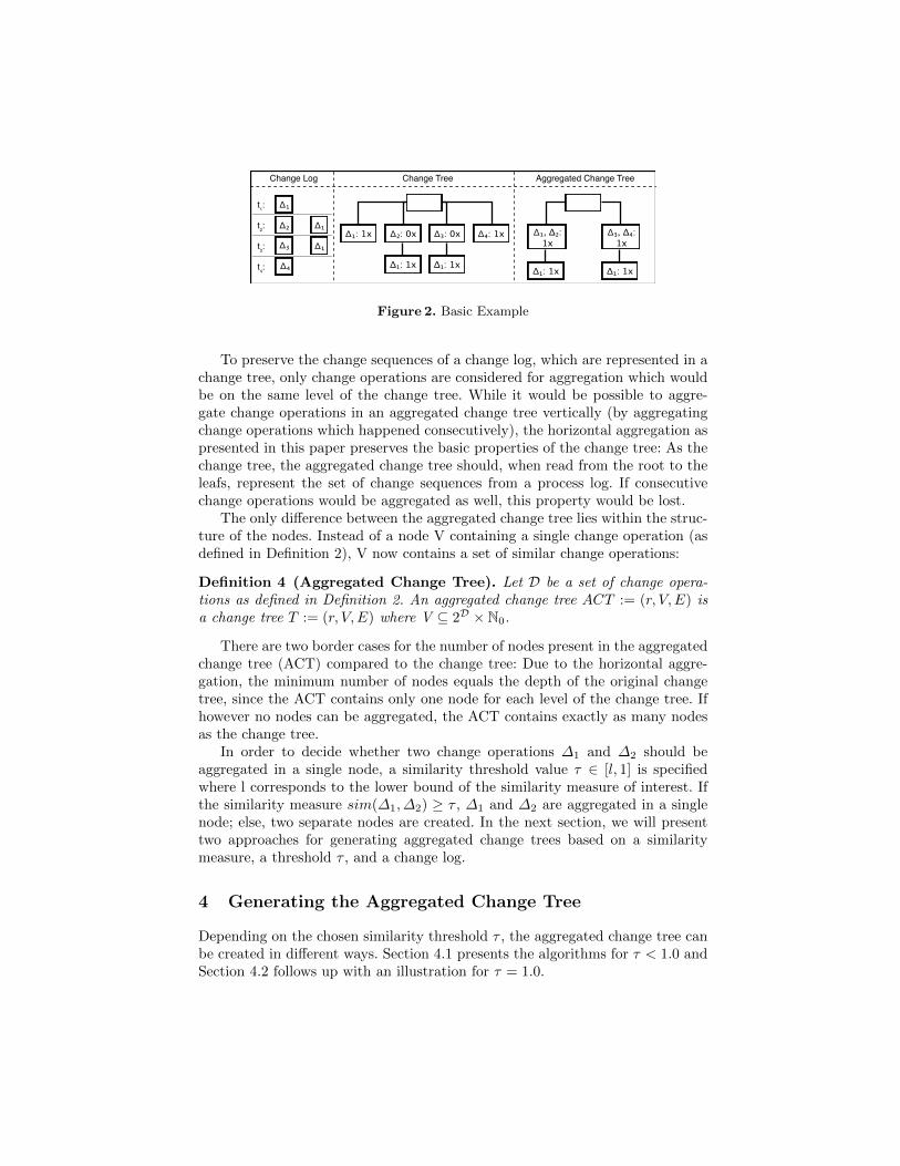
To discriminate between traditional change trees (based on label equivalence)and the change trees based on similarity measures as presented in this paper,we will refer to the latter by the term aggregated change tree. The term stemsfrom the fact that multiple similar change operations will be aggregated in asingle node. Figure 2 depicts an example of a change log, a change tree andan aggregated change tree. The middle pane shows a change tree according toDefinition 2 based on the change log in the left pane: It consists of two levels,where the first level contains the four change operations ∆1, ∆2, ∆3 and ∆4.The change traces t2 and t3 additionally contain a second change operation, ∆1.The right pane depicts the aggregated change tree. In the following sections, wewill discuss how this aggregated change tree is created.

Δ₁: 1x Δ₃: 0x

Δ₁: 1x

Δ₂: 0x

Δ₁: 1xΔ₁: 1x

Δ₄: 1x Δ₁, Δ₂: 1x

Δ₁: 1x

Δ₃, Δ₄: 1x

Change TreeChange Log Aggregated Change Tree

Δ₁t₁:

Δ₂ Δ₁t₂:

Δ₃ Δ₁t₃:

Δ₄t₄:

Figure 2. Basic Example

To preserve the change sequences of a change log, which are represented in achange tree, only change operations are considered for aggregation which wouldbe on the same level of the change tree. While it would be possible to aggre-gate change operations in an aggregated change tree vertically (by aggregatingchange operations which happened consecutively), the horizontal aggregation aspresented in this paper preserves the basic properties of the change tree: As thechange tree, the aggregated change tree should, when read from the root to theleafs, represent the set of change sequences from a process log. If consecutivechange operations would be aggregated as well, this property would be lost.

The only difference between the aggregated change tree lies within the struc-ture of the nodes. Instead of a node V containing a single change operation (asdefined in Definition 2), V now contains a set of similar change operations:

Definition 4 (Aggregated Change Tree). Let D be a set of change opera-tions as defined in Definition 2. An aggregated change tree ACT := (r, V,E) isa change tree T := (r, V,E) where V ⊆ 2D × N0.

There are two border cases for the number of nodes present in the aggregatedchange tree (ACT) compared to the change tree: Due to the horizontal aggre-gation, the minimum number of nodes equals the depth of the original changetree, since the ACT contains only one node for each level of the change tree. Ifhowever no nodes can be aggregated, the ACT contains exactly as many nodesas the change tree.

In order to decide whether two change operations ∆1 and ∆2 should beaggregated in a single node, a similarity threshold value τ ∈ [l, 1] is specifiedwhere l corresponds to the lower bound of the similarity measure of interest. Ifthe similarity measure sim(∆1, ∆2) ≥ τ , ∆1 and ∆2 are aggregated in a singlenode; else, two separate nodes are created. In the next section, we will presenttwo approaches for generating aggregated change trees based on a similaritymeasure, a threshold τ , and a change log.

4 Generating the Aggregated Change Tree

Depending on the chosen similarity threshold τ , the aggregated change tree canbe created in different ways. Section 4.1 presents the algorithms for τ < 1.0 andSection 4.2 follows up with an illustration for τ = 1.0.

4.1 Aggregation for Similar Process Change Operations

When aggregating similar change operations in one node, the similarity thresholdτ has to be reached for all similarity measures between the change operationsin the aggregation node. Figure 3 shows an example of such an aggregation: Inpane 1, a change log is depicted which contains three change traces consisting ofthe process change operations ∆1, ∆2 and ∆3. Pane 2 shows the similarity of thethree change operations: sim(∆1, ∆2) = 0.75, sim(∆2, ∆3) = 0.8 and sim(∆1,∆3) = 0.6. Pane 5 shows the change tree which would be generated based on labelequivalence (c.f. [3]). Depending on the chosen similarity threshold τ , differentchange operations can be aggregated in one node: If τ = 0.6, all three changeoperations can be aggregated in one node (c.f. aggregated change tree depictedin pane 6). If τ = 0.7, only change operations ∆1 and ∆2, or change operations∆2 and ∆3 can be aggregated in one node, but not ∆1, ∆2 and ∆3, since thesimilarity between∆1 and∆3 is below τ . The similarity measure is not transitive.Thus, for τ = 0.7, two aggregated change trees are possible (c.f. panes 7 and 8).These two change trees are the results of two different aggregation strategies,which are explained at the end of this section.

Δ₁ Δ₃Δ₂

Change Log Relations

sim = 0.8

sim = 0.75

sim = 0.6

1 2

Δ₃: 0x

Δ₁: 1x Δ₃: 1xΔ₃: 1x

Δ₁: 0x

Δ₂: 1x

Aggregated Change Tree 2Aggregated Change Tree 1 Aggregated Change Tree 3

Δ₁, Δ₂: 0x

Δ₁, Δ₂, Δ₃: 0x

Δ₁, Δ₂, Δ₃: 3x

Δ₂, Δ₃: 0x

Δ₁, Δ₂: 2x

76

3 4

5 8τ = 0.6 τ = 0.7 τ = 0.7

Δ₁t₁: Δ₂

Δ₂ Δ₁t₂:

Δ₃ Δ₃t₃:

Δ₁

Δ₃Δ₂

Change Similarity Graph 1 Change Similarity Graph 2

τ₁ = 0.7 τ₂ = 0.6

Δ₁

Δ₃Δ₂

Δ₁: 0x

Δ₁: 1x

Δ₃: 0x

Δ₃: 1x

Δ₂: 0x

Δ₂: 1x

Change Tree

Figure 3. Transitivity Example

The similarity measures between all change operations which can be aggre-gated in one node need to be above the threshold τ . In order to find the subsetof change operations for which this condition holds, we introduce the changesimilarity graph. (c.f. Definition 5).

Definition 5 (Change Similarity Graph). Let D be a set of change opera-tions, sim(∆i, ∆j) be a similarity measure, and τ the similarity threshold. TheChange Similarity Graph Γ := (D, E) is an undirected graph where E ⊆ D ×Ddenotes the set of edges. There exists an edge between change operations∆i, ∆j ∈ D, iff sim(∆i, ∆j) ≥ τ .

Pane 3 and 4 of Figure 3 show the similarity graphs for two thresholds τ1 =0.7 and τ2 = 0.6 for the process change operations ∆1, ∆2 and ∆3 from theexample given above. In the similarity graph for τ1 = 0.7, there exist only edgesbetween change operations ∆1 and ∆2, and between ∆2 and ∆3. There is noedge between ∆1 and ∆3, since its value lies below the threshold at 0.6.

Δ₄

Δ₃

Δ₂

Δ₄

Δ₃

Δ₂

Δ₁

Δ₄

Δ₃

Δ₂

Δ₁

Δ₄

Δ₃

Δ₂

Δ₁Δ₃

Δ₂

Δ₁

Similarity Graph Maximal Clique 1 Maximal Clique 2 Clique Set 1 Clique Set 2

1 2 3 54

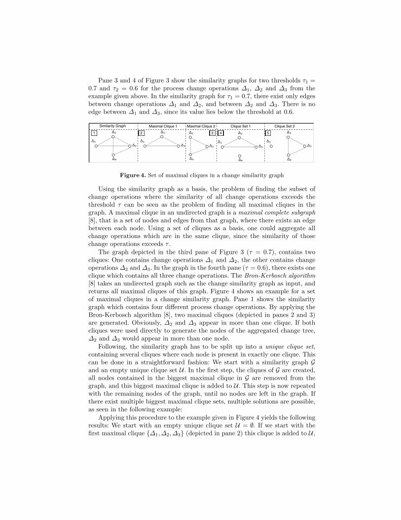
Figure 4. Set of maximal cliques in a change similarity graph

Using the similarity graph as a basis, the problem of finding the subset ofchange operations where the similarity of all change operations exceeds thethreshold τ can be seen as the problem of finding all maximal cliques in thegraph. A maximal clique in an undirected graph is a maximal complete subgraph[8], that is a set of nodes and edges from that graph, where there exists an edgebetween each node. Using a set of cliques as a basis, one could aggregate allchange operations which are in the same clique, since the similarity of thosechange operations exceeds τ .

The graph depicted in the third pane of Figure 3 (τ = 0.7), contains twocliques: One contains change operations ∆1 and ∆2, the other contains changeoperations ∆2 and ∆3. In the graph in the fourth pane (τ = 0.6), there exists oneclique which contains all three change operations. The Bron-Kerbosch algorithm[8] takes an undirected graph such as the change similarity graph as input, andreturns all maximal cliques of this graph. Figure 4 shows an example for a setof maximal cliques in a change similarity graph. Pane 1 shows the similaritygraph which contains four different process change operations. By applying theBron-Kerbosch algorithm [8], two maximal cliques (depicted in panes 2 and 3)are generated. Obviously, ∆2 and ∆3 appear in more than one clique. If bothcliques were used directly to generate the nodes of the aggregated change tree,∆2 and ∆3 would appear in more than one node.

Following, the similarity graph has to be split up into a unique clique set,containing several cliques where each node is present in exactly one clique. Thiscan be done in a straightforward fashion: We start with a similarity graph Gand an empty unique clique set U . In the first step, the cliques of G are created,all nodes contained in the biggest maximal clique in G are removed from thegraph, and this biggest maximal clique is added to U . This step is now repeatedwith the remaining nodes of the graph, until no nodes are left in the graph. Ifthere exist multiple biggest maximal clique sets, multiple solutions are possible,as seen in the following example:

Applying this procedure to the example given in Figure 4 yields the followingresults: We start with an empty unique clique set U = ∅. If we start with thefirst maximal clique {∆1, ∆2, ∆3} (depicted in pane 2) this clique is added to U ,

and these nodes are removed from the similarity graph. Following, the similaritygraph now only contains {∆4}, which is the last maximal clique left in the graph;thus, it is added to U , resulting in the unique clique set depicted in pane 4. Ifwe start with the second maximal clique set {∆2, ∆3, ∆4} (depicted in pane 3),{∆1} would be the second clique, and we would end up with the unique cliqueset depicted in pane 5. Thus, two unique clique sets are created.

These two unique clique sets can now be used to generate the change treenodes. Depending on the which set is chosen, either ∆1, ∆2 and ∆3 are aggre-gated in one node, and ∆4 is in the other node, or ∆2, ∆3 and ∆4 are aggregatedin a node, and ∆1 is in its own node. Two distinct features can be used as a basisfor deciding which process change operation should be aggregated in a node: (a)the most similar change operations should be aggregated or (b) the number ofnodes in the tree should be minimized.

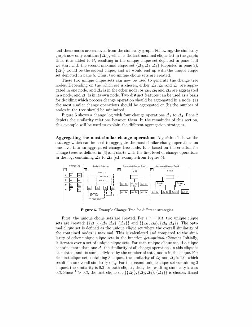
Figure 5 shows a change log with four change operations ∆1 to ∆4. Pane 2depicts the similarity relations between them. In the remainder of this section,this example will be used to explain the different aggregation strategies.

Aggregating the most similar change operations Algorithm 1 shows thestrategy which can be used to aggregate the most similar change operations onone level into an aggregated change tree node. It is based on the creation forchange trees as defined in [3] and starts with the first level of change operationsin the log, containing ∆1 to ∆4 (c.f. example from Figure 5).

Change Log Similarity Relations Aggregated Change Tree 1 Aggregated Change Tree 21

Δ₄: 1x

Δ₁ Δ₃ Δ₄Δ₂

sim = 1.0

sim = 0.2

sim = 0.2

sim = 0.3

sim = 0.2

sim = 0.3

2

Δ₂, Δ₃: 0x

3 4

Δ₁: 1x Δ₁, Δ₂: 2x

Δ₃, Δ₄: 2x

Δ₁: 1x Δ₁: 1xΔ₁: 1xΔ₄: 2x Δ₄: 1x Δ₁: 1x Δ₄: 1x

Δ₁t₁: Δ₁

Δ₄Δ₂t₂:

Δ₄Δ₃t₃:

Δ₄ Δ₁t₄:

τ = 0.3 τ = 0.3

Figure 5. Example Change Tree for different strategies

First, the unique clique sets are created. For a τ = 0.3, two unique cliquesets are created: {{∆1}, {∆2, ∆3}, {∆4}} and {{∆1, ∆2}, {∆3, ∆4}}. The opti-mal clique set is defined as the unique clique set where the overall similarity ofthe contained nodes is maximal. This is calculated and compared to the simi-larity of other unique clique sets in the function get-optimal-cliqueset. Initially,it iterates over a set of unique clique sets. For each unique clique set, if a cliquecontains more than one ∆, the similarity of all change operations in this clique iscalculated, and its sum is divided by the number of total nodes in the clique. Forthe first clique set containing 3 cliques, the similarity of ∆2 and ∆3 is 1.0, whichresults in an overall similarity of 1

3 . For the second unique clique set containing 2cliques, the similarity is 0.3 for both cliques, thus, the resulting similarity is also0.3. Since 1

3 > 0.3, the first clique set {{∆1}, {∆2, ∆3}, {∆4}} is chosen. Based

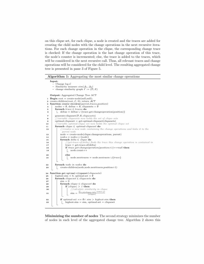
on this clique set, for each clique, a node is created and the traces are added forcreating the child nodes with the change operations in the next recursive itera-tions. For each change operation in the clique, the corresponding change traceis checked: If the change operation is the last change operation of this trace,the node’s counter is incremented; else, the trace is added to the traces, whichwill be considered in the next recursive call. Thus, all relevant traces and changeoperations will be considered for the child level. The resulting aggregated changetree is presented in pane 3 of Figure 5.

Algorithm 1: Aggregating the most similar change operations

Input:– Change log C– Similarity measure sim(∆1, ∆2)– change similarity graph Γ := (D, E)

Output: Aggregated Change Tree ACT

1 Begin root = create-node(null,null);2 create-children(root, C, 0); return ACT3 function create-children(parent,traces,position)4 nodes = ∅, deltas = ∅, cliquesets = ∅5 foreach trace ∈ traces do6 deltas = deltas ∪ {trace.get-changeoperation(position)}7 generate-cliqueset(D, ∅, cliquesets)8 //variable cliquesets now holds the set of clique sets9 optimal-cliqueset = get-optimal-cliqueset(cliquesets)

10 //variable optimal-clique set now holds the optimal clique set11 foreach clique ∈ optimal-cliqueset do12 //creates a new node containing the change operations and links it to the

parent node13 node = create-node(clique.changeoperations, parent)14 nodes = nodes ∪ {node}15 foreach delta ∈ clique do16 //get-trace-of(delta) finds the trace this change operation is contained in17 trace = get-trace-of(delta)18 if trace.get-changeoperation(position+1)==null then19 node.count++

20 else21 node.nexttraces = node.nextraces ∪{trace}

22 foreach node in nodes do23 create-children(node,node.nexttraces,position+1)

24 function get-optimal-cliqueset(cliquesets)25 highest-sim = 0, optimal-set = ∅26 foreach cliqueset ∈ cliquesets do27 sim = 028 foreach clique ∈ cliqueset do29 if |clique| > 1 then30 //calculate similarity in clique

31 sim =∑

i,j∈clique,i 6=j sim(i,j)

|clique|

32 if optimal-set == ∅∨ sim > highest-sim then33 highest-sim = sim, optimal-set = cliqueset

Minimizing the number of nodes The second strategy minimizes the numberof nodes in each level of the aggregated change tree. Algorithm 2 shows this

strategy. It replaces the function get-optimal-cliqueset with a different algorithmwhich prefers the unique clique set with the minimum number of cliques. Sinceeach clique is represented by a node in the aggregated change tree, this resultsin the lowest number of nodes per level. For the first call of the function in theexample given in Figure 5, this would return the clique set {{∆1, ∆2}, {∆3, ∆4}},thus resulting in the aggregated change tree depicted in pane 4.

Algorithm 2: Generating the minimum amount of nodes per level

1 function get-optimal-cliqueset(cliquesets)2 min-count = 0, optimal-set = ∅3 foreach cliqueset ∈ cliquesets do4 if optimal-set == ∅∨ min-count < |cliqueset| then5 min-count = |cliqueset|, optimal-set = cliqueset

Discussion: We have presented two strategies for aggregating similar changeoperations in change tree nodes. Which one should be used highly depends onthe structure of the change log: For most situations, aggregating the most similarchange operations in one node seems logical. In the nursing home, for example,one could aggregate the most similar therapy adaptations in a single change treenode. If however the resulting number of nodes would become very large dueto the structure of the change log, minimizing the number of change tree nodesinstead can enhance the tree’s readability, thus simplifying further analysis ofthe change log.

4.2 Aggregation for Equal Process Change Operations

For the aggregation of equal change operations (τ = 1.0), no change similaritygraph is required, since the equality relation is transitive (sim(∆1, ∆2) = 1.0∧ sim(∆2, ∆3) = 1.0 =⇒ sim(∆1, ∆3) = 1.0). The example we use to ex-plain the aggregation of equal change operations is based on the change log aspresented in Figure 21. While the middle pane shows the change tree based onlabel equivalence as defined in [3], the right pane shows the resulting aggregatedchange tree. Assume that sim(∆1, ∆2) = 1.0, sim(∆3, ∆4) = 1.0, and all othersimilarities < 1.0. The aggregated change tree is created as follows: First, anempty root node with no label and no parent is created. Next, each “column”in the change log is iterated over: The first column contains change operations∆1, ∆2, ∆3 and ∆4. The second column contains ∆1 (following ∆2 respectively∆3). For the first column, the similarities between all change operations arechecked: If sim(∆i, ∆j) = 1.0, the change operations are aggregated in one node- if not, they are split up in two nodes. In this example sim(∆1, ∆2) = 1.0 andsim(∆3, ∆4) = 1.0. All other similarities are smaller than 1. The same is donefor the second column. Note that the ∆1 of the second column cannot be aggre-gated in one node, since they have distinct parent nodes (one containing ∆1, ∆2,

1 The full version of the algorithm can be found on our project homepagehttps://cs.univie.ac.at/project/APES

and one containing ∆3, ∆4). Ultimately the aggregated change tree depicted inpane 3 of Figure 2 is created.

5 Evaluation

The approach presented in this paper is evaluated in an experiment which aimsat two goals, i.e., to analyze whether (a) the change tree can be used as a basisfor analyzing change sequences and (b) certain questions can be answered fasterby participants using an aggregated change tree, than using a change tree.

Method and Experiment Design The experiment is based upon a proto-typical implementation of the (aggregated) change tree, working in every mod-ern browser using HTML, CSS and JavaScript. This implementation serves as aproof of technical feasability, which can also be accessed without participatingin the experiment2.

The first draft of the experiment was refined using a two stage pretest: Duringstage one, the questions of the experiment were discussed with three peers whoare familiar with the concept of process change operations and change trees. Inthe second phase, persons from the target audience were asked to participate inthe experiment. The target audience of the aggregated change tree are personsfrom different fields of work, who do not necessarily have to be familiar with pro-cess change operations. Thus, the chosen participants were older than 18 years,and were not required to have any knowledge regarding process change opera-tions, or change trees. During the pretest, two major parts of the experimentwere optimized: First, the user interface was optimized to be more intuitive tousers who are not familiar with the setting, second, the wording of two questionsand their explanation was optimized.

The experiment consists of two parts: Part 1 addresses the question whetherthe change tree (CT) is a better representation of change logs than their rawXML format (XML). Specifically, we want to find out if certain questions re-garding the change log (e.g. How many resources have been used in this changelog? ) can be answered faster using a change tree than an XML based log file.The participants were split in two groups and had to answer the same questionsbased on those two representations. In each question, we measured the time un-til the (correct) answer was found. The questions for the two representationswere based on different, but similar log files to prevent bias due to the partic-ipants knowing the correct answer: While group 1 answered questions for theCT based on log A, and questions for XML based on log B, group 2 receivedthe CT questions based on log B, and the XML questions based on log A. Thissetup also helped us to mitigate the risk of a bias due to different log files: Ifthere was only one group who answered all CT questions based on log A, and allXML questions based on log B, the differences in speed and correctness couldbe due to the slight differences between those log files, and not due to their rep-resentation. To mitigate the risk of distortion due to a learning effect, the order

2 The prototype, the experiment including all questions, and all related data can befound at https://cs.univie.ac.at/project/APES

of the questions and representations was randomized. Part 2 of the experimentaddresses the usability of the aggregated change tree (ACT) in comparison tothe CT. The setup and the participants were the same as in Part 1; however,two log files C and D (different from those of Part 1) were used.

At the beginning of the experiment, the participants were introduced into thetopics of processes, process adaptations, change logs and (aggregated) changetrees. Following this 10 minute presentation, the participants had the possibilityto ask questions, and received a link to the experiment. They had three days toparticipate in the experiment. Such an uncontrolled experiment setup resemblesa realistic setting, in which aggregated change trees would be used, more closely.

Results: In total, 64 participants participated in the experiment. These par-ticipants were divided in two groups as described above. 31 participated in group1, and 33 participated in group 2. First, the data set was cleaned for participantswho obviously entered random numbers. The check was based on two parame-ters: (1) most of the answers were wrong, and (2) all answers were given in lessthan two seconds. Answers given that quickly can be seen as an indicator for aparticipant entering wrong answers on purpose. These patterns were found forone participant from group 1, resulting in 30 valid participants in group 1, and33 valid participants in group 2.

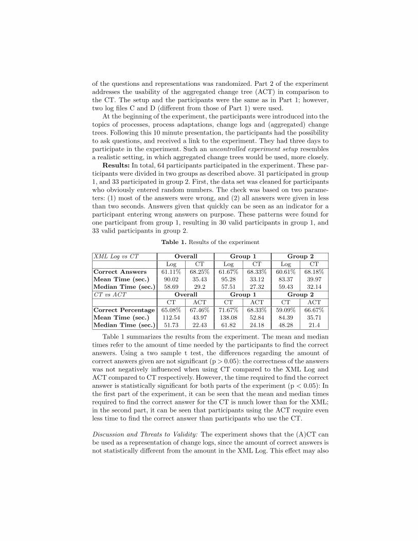
Table 1. Results of the experiment

XML Log vs CT Overall Group 1 Group 2

Log CT Log CT Log CT

Correct Answers 61.11% 68.25% 61.67% 68.33% 60.61% 68.18%Mean Time (sec.) 90.02 35.43 95.28 33.12 83.37 39.97Median Time (sec.) 58.69 29.2 57.51 27.32 59.43 32.14

CT vs ACT Overall Group 1 Group 2

CT ACT CT ACT CT ACT

Correct Percentage 65.08% 67.46% 71.67% 68.33% 59.09% 66.67%Mean Time (sec.) 112.54 43.97 138.08 52.84 84.39 35.71Median Time (sec.) 51.73 22.43 61.82 24.18 48.28 21.4

Table 1 summarizes the results from the experiment. The mean and mediantimes refer to the amount of time needed by the participants to find the correctanswers. Using a two sample t test, the differences regarding the amount ofcorrect answers given are not significant (p> 0.05): the correctness of the answerswas not negatively influenced when using CT compared to the XML Log andACT compared to CT respectively. However, the time required to find the correctanswer is statistically significant for both parts of the experiment (p < 0.05): Inthe first part of the experiment, it can be seen that the mean and median timesrequired to find the correct answer for the CT is much lower than for the XML;in the second part, it can be seen that participants using the ACT require evenless time to find the correct answer than participants who use the CT.

Discussion and Threats to Validity: The experiment shows that the (A)CT canbe used as a representation of change logs, since the amount of correct answers isnot statistically different from the amount in the XML Log. This effect may also

be due to the XML Log being very simple: For Part 1 of our experiment we chosea log with only four change operations in total, in order to not demoralize partic-ipants who had to work with the XML representations. Thus, the change log wasdesigned in favor of the XML representation, which may pose a threat to the va-lidity. However, even in such a setting, the time required for the correct answerswas statistically significantly lower for CT than for XML Log. For the ACT,the number of correct answers is not statistically significantly different from CT,but significantly less time is required to find a correct answer. Although the un-controlled setup of our experiment increases the resemblance of our experimentto a realistic setting in contrast to a controlled setup, this decision also poses athreat to validity, since participants have been able to communicate with eachother while participating. However, participants who completed the experimentdid not receive the correct answers to the questions, and such behavior may alsobe found in a realistic setting, where users would have to analyze change trees.Thus, the results can be seen as being more realistic, while the negative impactof the threat has been kept to a minimum.

6 Related Work

In [9], the authors present an overview over existing approaches to determinethe similarity of two process models. The presented approaches range from labelmatching similarity, over feature-based similarity estimations up to comparisonsof common nodes and edges in process model graphs. These approaches can alsobe interesting for change operation similarity measures, since they can be used tocompare attributes of change operations, like the schema, the applied fragment,or the position of the change. Van Dongen et al discuss causal footprints, whichis a collection of the essential behavioral constraints imposed by a process model[10] as a representation of a process model’s behavior. Using causal footprint’slook-back and look-ahead links, one could analyze and compare the positions ofprocess change operations.

The work presented in [11] provides similarity measures for process instances.To the best of our knowledge, [4] is the only approach dealing with process changesimilarity. This work exploits the measures proposed in [4], but any other changesimilarity measure can be used as well.

In contrast to change trees, change processes [2] are a different method toanalyze process change logs. Change processes focus on causal relations betweenprocess change operations. If a change operation ∆1 is followed by ∆2, it meansthat ∆2 may be caused by ∆1. For parallel change operations, such a conditioncannot be drawn from the change log.

While change logs provide a solid basis for analyzing conducted change op-erations and their consequences, they may not alwalys be available. Conceptdrift [12, 13] focuses on analyzing process execution logs to detect any executedchanges on the basic schema. By analyzing the activities present in the changelog over a long period of time, this approach can estimate if and which changeshave been applied to a process schema.

7 Conclusion and Future Work

In this paper we have discussed how process change operation similarity mea-sures, which calculate the similarity of two process change operations, can beextended to sets of change sequences, i.e. change logs. Change trees serve asa basis, since they provide a compact representation of change sequences. Ananalysis of the similarity of change sequences can provide interesting insightsfor many situations in different application domains: In the nursing home, forexample, nurses can compare sets of therapies which have been applied to dif-ferent patients over a long time. Using different similarity measures, differentfeatures of the change sequences can be analyzed, e.g. the diversity of requiredpersonnel, resources or time. The presented approach can be used with any sim-ilarity measure which returns a numeric value within a certain range; thus, it isvery flexible and extensible. In a practical setting, the choice of the similaritymetric has a huge impact on the information being displayed in a change tree.Thus, future work will analyze the impact of using different similarity notionsand aggregation strategies in practical settings.

Bibliography

1. Reichert, M., Weber, B.: Enabling Flexibility in Process-Aware Information Sys-tems - Challenges, Methods, Technologies. Springer (2012)

2. Gunther, C., Rinderle-Ma, S., Reichert, M., van der Aalst, W.: Using process min-ing to learn from process changes in evolutionary systems. International Journalof Business Process Integration and Management 3 (2008) 61–78

3. Kaes, G., Rinderle-Ma, S.: Mining and querying process change information basedon change trees. In: Service-oriented Computing, Springer (2015) 269–284

4. Kaes, G., Rinderle-Ma, S.: On the similarity of process change operations. In:Advanced Information Systems Engineering. (2017) 348–363

5. Allen, F.E.: Control flow analysis. ACM Sigplan Notices 5 (1970) 1–196. Ingvaldsen, J.E., Gulla, J.A.: Industrial application of semantic process mining.

Enterprise Information Systems 6 (2012) 139–1637. Rinderle-Ma, S., Reichert, M., Jurisch, M.: On utilizing web service equivalence

for supporting the composition life cycle. Int. J. Web Service Res. 8 (2011) 41–678. Bron, C., Kerbosch, J.: Algorithm 457: Finding all cliques of an undirected graph.

Commun. ACM 16 (1973) 575–5779. Becker, M., Laue, R.: A comparative survey of business process similarity measures.

Computers in Industry 63 (2012) 148 – 16710. van Dongen, B., Dijkman, R., Mendling, J.: Measuring similarity between business

process models. In: Advanced Information Systems Engineering. Volume 5074.(2008) 450–464

11. Pflug, J., Rinderle-Ma, S.: Process instance similarity: Potentials, metrics, appli-cations. In: On the Move to Meaningful Internet Systems. (2016) 136–154

12. Bose, R., van der Aalst, W., liobait, I., Pechenizkiy, M.: Handling concept drift inprocess mining. In: Advanced Information Systems Engineering. (2011) 391–405

13. Carmona, J., Gavalda, R.: Online techniques for dealing with concept drift inprocess mining. In: Advances in Intelligent Data Analysis XI. (2012) 90–102