UNIVERSIDADE DE LISBOAFACULDADE DE CIÊNCIAS

DEPARTAMENTO DE INFORMÁTICA

Implementation of an hybrid machine learning methodologyfor pharmacological modeling

Katarzyna Malgorzata Kwiatkowska

DISSERTAÇÃOMESTRADO EM BIOINFORMÁTICA E BIOLOGIA COMPUTACIONAL

ESPECIALIZAÇÃO EM BIOINFORMÁTICA

Dissertação orientada por:Prof. Andre Osorio Falcão

Prof. Lisete Maria Ribeiro de Sousa

2017

Resumo

Hoje em dia, especialmente na área biomédica, os dados contêm milhares de variáveis de fontesdiferentes e com apenas algumas instâncias ao mesmo tempo. Devido a este facto, as abordagens daaprendizagem automática enfrentam dois problemas, nomeadamente a questão da integração de dadosheterogéneos e a seleção das características. Este trabalho propõe uma solução eficiente para estaquestão e proporciona uma implementação funcional da metodologia híbrida. A inspiração para estetrabalho veio do desafio proposto no âmbito da competição AstraZeneca-Sanger Drug CombinationPrediction DREAM Challenge em 2016, e da solução vencedora desenvolvida por Yuanfang Guan.Relativamente a motivação do concurso, é observado que os tratamentos combinatórios para o cancrosão mais eficientes do que as terapias habituais de agente único, desde que têm potencial para superaras desvantagens dos outros (limitado espetro de ação e desenvolvimento de resistência). No entanto, oefeito combinatório de drogas não é obvio, produzindo possivelmente o resultado aditivo, sinérgico ouantagónico. Assim, o objetivo da competição era prever in vitro a sinergia dos compostos, sem teracesso aos dados experimentais da terapia combinatória. No âmbito da competição foram fornecidosficheiros de várias fontes, contendo o conhecimento farmacológico tanto experimental como obtidode ajustamento das equações, a informação sobre propriedades químicas e estruturais de drogas, e porfim, os perfis moleculares de células, incluindo expressão de RNA, copy variants, sequência emetilação de DNA. O trabalho referido envolveu uma abordagem muito bem sucedida de integraçãodos dados heterogéneos, estendendo o modelo com conhecimento disponível dentro do projeto TheCancer Cell Line Encyclopedia, e também introduzindo o passo decisivo de simulação que permiteimitar o efeito de terapia combinatória no cancro. Apesar das descrições pouco claras e dadocumentação da solução vencedora ineficiente, a reprodução da abordagem de Guan foi concluída,tentando ser o mais fiel possível. A implementação funcional foi escrita nas linguagens R e Python, e oseu desempenho foi verificado usando como referência a matriz submetida no concurso. Para melhorara metodologia, o workflow de seleção dos características foi estabelecido e executado usando oalgoritmo Lasso. Além disso, o desempenho de dois métodos alternativos de modelação foiexperimentado, incluindo Support Vector Machine and Multivariate Adaptive Regression Splines(MARS). Várias versões da equação de integração foram consideradas permitindo a determinação decoeficientes aparentemente ótimos. Como resultado, a compreensão da melhor solução de competiçãofoi desenvolvida e a implementação funcional foi construída com sucesso. As melhorias forampropostas e no efeito o algoritmo SVM foi verificado como capaz de superar os outros na resoluçãodeste problema, a equação de integração com melhor desempenho foi estabelecida e finalmente a listade 75 variáveis moleculares mais informativas foi fornecida. Entre estes genes, poderiam serencontrados possíveis candidatos de biomarcadores de cancro.

Palavras Chave: aprendizagem automática, modelo preditivo, seleção de características, integraçãode dados

Abstract

Nowadays, especially in the biomedical field, the data sets usually contain thousands of multi-sourcevariables and with only few instances in the same time. Due to this fact, Machine Learning approachesface two problems, namely the issue of heterogenous data integration and the feature selection. Thiswork proposes an efficient solution for this question and provides a functional implementation of thehybrid methodology. The inspiration originated from the AstraZeneca-Sanger Drug CombinationPrediction DREAM Challenge from 2016 and the winning solution by Yuanfang Guan. Regarding tothe motivation of competition, the combinatory cancer treatments are believed to be more effectivethan standard single-agent therapies since they have a potential to overcome others weaknesses(narrow spectrum of action and development of the resistance). However, the combinatorial drugeffect is not obvious bringing possibly additive, synergistic or antagonistic treatment result. Thus, thegoal of the competition was to predict in vitro compound synergy, without the access to theexperimental combinatory therapy data. Within the competition, the multi-source files were supplied,encompassing the pharmacological knowledge from experiments and equation-fitting, the informationon chemical properties and structure of drugs, finally the molecular cell profiles including RNAexpression, copy variants, DNA sequence and methylation. The referred work included very successfulapproach of heterogenous data integration, extending additionally the model with prior knowledgeoutsourced from The Cancer Cell Line Encyclopedia, as well as introduced a key step of simulationthat allows to imitate effect of a combinatory therapy on cancer. Despite unexplicit descriptions andpoor documentation of the winning solution, as accurate as possible, reproduction of Guan’s approachwas accomplished. The functional implementation was written in R and Python languages, and itsperformance was verified using as a reference the submitted in challenge prediction matrix. In order toimprove the methodology feature selection workflow was established and run using a Lasso algorithm.Moreover, the performance of two alternative modeling methods was experimented including SupportVector Machine and Multivariate Adaptive Regression Splines (MARS). Several versions of mergingequation were considered allowing determination of apparently optimal coefficients. As the result, theunderstanding of the best challenge solution was developed and the functional implementation wassuccessfully constructed. The improvements were proposed and in the effect the SVM algorithm wasverified to surpass others in solving this problem, the best-performing merging equation wasestablished, and finally the list of 75 most informative molecular variables was provided. Among thosegenes, potential cancer biomarker candidates could be found.

Keywords: machine learning, predictive model, feature selection, data integration

Resumo Alargado

Hoje em dia, especialmente na área biomédica, os dados contêm milhares de variáveis de fontesdiferentes e com apenas algumas instâncias ao mesmo tempo. Devido a este facto, as abordagens daaprendizagem automática enfrentam dois problemas, nomeadamente a questão da integração de dadosheterogéneos e a seleção das características. Este trabalho propõe uma solução eficiente para estaquestão e proporciona uma implementação funcional da metodologia híbrida. A inspiração para estetrabalho veio do desafio proposto no âmbito da competição AstraZeneca-Sanger Drug CombinationPrediction DREAM Challenge em 2016, e da solução vencedora desenvolvida por Yuanfang Guan.Relativamente a motivação do concurso, é observado que os tratamentos combinatórios para o cancrosão mais eficientes do que as terapias habituais de agente único, desde que têm potencial para superaras desvantagens dos outros (limitado espetro de ação e desenvolvimento de resistência). No entanto,o efeito combinatório de drogas não é obvio, produzindo possivelmente o resultado aditivo (seo resultado é equivalente aos efeitos somados de dois medicamentos), sinérgico (quando a respostaé exagerada e superior dos efeitos aditivos de dois produtos químicos) ou antagónico (com umaresposta inferior do efeitos somados do par de drogas). Assim, o objetivo da competição era preverin vitro a sinergia dos compostos, sem ter acesso aos dados experimentais da terapia combinatória.No âmbito da competição foram fornecidos ficheiros de várias fontes, contendo o conhecimentofarmacológico tanto experimental como obtido de ajustamento das equações, a informação sobrepropriedades químicas e estruturais de drogas, e por fim, os perfis moleculares de células, incluindoexpressão de RNA, copy variants, sequência e metilação de DNA. O trabalho referido envolveu umaabordagem muito bem sucedida de integração dos dados heterogéneos, estendendo o modelo comconhecimento disponível dentro do projeto The Cancer Cell Line Encyclopedia. No entanto, os dadosmoleculares são inúteis a menos que sejam simulados sob a droga, imitando o efeito de uma terapiacombinatória em células. Yuanfang Guan propôs uma abordagem baseada no conhecimento disponívelna base de dados Functional Networks of Tissues in Mouse (FNTM) e resumida no ficheiro externocontendo informações sobre as rede funcionais entre os genes e a probabilidade destas conexões.A ideia principal era alterar cada estado original atribuído às células cancerosas, de acordo coma probabilidade de ligação entre dois genes: o gene em consideração e o gene alvo para a drogaaplicada. De acordo com a implementação original, todas as fontes moleculares foram filtradase exclusivamente o conhecimento relacionado com o conjunto dos alvos foi considerado. Paraproduzir as previsões finais, foram construídos seis modelos: dois globais de dados moleculares e demonoterapia, um químico, um contando ficheiros, e mais dois locais de dados moleculares e demonoterapia. Os nomes deles indicam a fonte de dados utilizada na construção de vetores de variáveis.Posteriormente, as previsões obtidas de todos os modelos foram integradas usando média ponderada.Para determinar a ocorrência do efeito sinérgico para a combinação específica de par de drogas e dacélula, as previsões produzidas foram comparadas com a média total calculada para todasas instâncias. O efeito benéfico é esperado nos casos que representam o valor normalizado da sinergiasuperior da média global. Apesar das descrições pouco claras e da documentação da soluçãovencedora ineficiente, a reprodução da abordagem de Guan foi concluída, tentando ser o mais fielpossível. A implementação funcional foi escrita nas linguagens R e Python, e o seu desempenho foiverificado usando como referência a matriz submetida no concurso. Devido ao facto que os processoscomputacionalmente envolvidos na manipulação de dados moleculares foram intensos, uma filtraçãoadicional dos dados foi realizada. O objetivo era reduzir o número de variáveis selecionandounicamente as características informativas e relevantes. Baseando na informação contidana plataforma IntOGen, as mutações foram limitadas exclusivamente às localizadas nos oncogenes.A base de dados The Copy Number Variations in Disease foi usada para mapear genes de cancrosensíveis à dosagem e para selecionar os CNVs relevantes. Embora eficaz na redução do tamanho, este

passo de filtração tem o poder elevado de interferir com os dados porque limita o espaço das variáveisao conhecimento já bem estabelecido. Assim, a inferência de potenciais correlações ou implicaçõesestá inibida. Após o desenvolvimento da implementação funcional, a precisão e fidelidade dareprodução foram estimadas verificando o desempenho usando como referência a matriz de previsõessubmetida no concurso. Esta proeza permitiu o estabelecimento de uma base e a definição de pontosfracos do método, que no resultado indicou direções de melhoramento. Uma vez que o número devariáveis moleculares foi um desafio real na manipulação, processamento e interpretação, foi decididorealizar a seleção de características. Ao contrário da filtração anterior, esse método abre um espaçopara a inferência dos novos padrões e conexões. A importância e a relevância de uma variável sãoestimadas baseando nos dados experimentais que refletem o funcionamento de um sistema biológicointeiro e possivelmente nova compreensão pode ser surgir. Após várias tentativas, o workflow final foiestabelecido usando um algoritmo chamado Lasso. Em primeiro lugar, para cinco fontes de dadosmoleculares (exceto metilação devido ao processamento altamente intenso), os modelos forampreparados com um parâmetro λ indefinido, permitindo a observação do comportamento do erroquadrático médio (Mean Square Error, MSE) em função de lambda. A inspeção visual de gráficopermitiu a estimativa de λ correspondente ao minimo valor de MSE. Seguindo essa abordagem, paracada uma das fontes, o parâmetro foi estimado separadamente. Voltou-se construir os modelos delasso, mas desta vez com λ definido e em 60 iterações. Para cada fonte de dados moleculares foramselecionadas as variáveis com frequência de ocorrência superior de 30 em total das 60 corridase posteriormente foram todas incluídas numa única lista. O passo inicial foi repetido, mas desta vezexclusivamente para as características pré-selecionadas. Encontrando o parâmetro lambda máximopara o qual o número das variáveis é igual ou inferior a 60, realizou-se uma seleção final, extraindoapenas aquelas instâncias que entram no modelo com tal λ definido. Para verificar se os RFsoriginalmente aplicados são verdadeiramente o método de preferência para este conjunto de dados,dois outros algoritmos de modelação foram testados: Support Vector Machine and MultivariateAdaptive Regression Splines (MARS). Uma vez que não havia qualquer tipo de referência ouevidência que justificava a forma de combinação dos modelos separados criados ao longo daimplementação, foram testadas várias versões da mesma equação de integração, permitindoa determinação dos coeficientes aparentemente ótimos. Para tornar a avaliação de implementação finalmais confiável, foram usados como referência os valores de sinergia verdadeiras (em vez de previstaspor Yuanfang Guan). Formou-se novos conjuntos de treinamento e teste, a partir dos dados conhecidosdisponíveis no âmbito de concurso. Os subconjuntos reconstruíram as circunstâncias de modelaçãooriginais, o que na prática significa que eles foram totalmente disjuntas nos pares de drogas (como osoriginais) e foram equilibrados por tamanho contendo, respetivamente 30% e 70% de informação.Além disso, a matriz binária de predições foi melhorada e foi feita uma distinção entre 'sem sinergia'e 'dados indisponíveis', atribuindo valores respetivamente '0' e 'NA'. Isto garantiu que a avaliação foirealizada exclusivamente nas instâncias de teste, impedindo a excessiva representação de observaçõesverdadeiras negativas, como aconteceu durante a avaliação da implementação base. Como resultado,ao longo deste trabalho, a compreensão da melhor solução de desafio foi desenvolvidae a implementação funcional foi construída com sucesso. Foram propostas as melhorias nametodologia, em relação à seleção de características, modelação e aos passos de integração. No efeito,foi fornecida a lista de 75 variáveis moleculares de toda informação sobre expressão, mutaçõese CNVs. Entre estes genes, poderiam ser encontrados possíveis candidatos a biomarcadores do cancro,merecendo mais atenção e exploração. O algoritmo SVM foi verificado a superar os RFs na resoluçãodo problema de competição, e a equação de integração com o melhor desempenho foi estabelecida.A implementação final tornou-se um exemplo da abordagem que fornece uma solução eficiente paraos problemas de aprendizagem automática com os dados heterogéneos de muitas variáveis e poucasinstâncias.

8k

Acknowledgements

This work was performed with resources from research Project MIMED - Mining the Molecular MetricSpace for Drug Design (PTDC/EEI-ESS/4923/2014), sponsored by FCT - Fundação para a Ciênciae a Tecnologia.

In the first place I would like to thank to my both master thesis supervisors: Prof. André Osorio Falcão andProf. Lisete Maria Ribeiro de Sousa. Without the doubt, this work would never be accomplished if not theirsupport. I am especially grateful for their acceptance and openness to my curiosity, and for allowing me toexplore the Unknown on my way. Being guided by them through the Science is a huge honour anda pleasure for me.

I am especially grateful to Prof. Lisete Maria Ribeiro de Sousa for her trust in me and confidence in myskills. For infinite patience, the extraordinary positive attitude and a bright smile - that is what I really wishto thank her for.

After first week of putting hands on this project Prof. André asked me if I had fun. Indeed I had. Not onlyduring the first week but over all this time. For this priceless lesson, I want to express my special gratitude.

Further, to my main advisor, I would like to thank for the never-ending and contagious enthusiasm,for the understanding beyond the words, and finally for the absolutely right words in the exact moment.

I wish to acknowledge also my previous supervisor of my Master thesis in Biotechnologyat University of Aveiro, António Correia. He was the person who encouraged me to ask ‘why?’opening by this a door that I cannot close until now and hopefully will not do that never in the future.

To my LaSIGE collegues for makeing this journey together, in fabulous company. Especial thanksto Pati and Beatriz for the time and energy spend firstly on struggling trying to understand whatactually is in my head, and then turning it understandable to the portuguese part of the world.

I am very thankful to my great friend, amazing and inspiring researcher, Gautam Agarwal. He mustbe appreciated since without him this work would be definitely missing the section with results.

Thanks to objectT for all the firmware & software updates, backups, numerous defragmentations,technical and mute support.

Finally, I wish to express my gratitude to family, friends and all those who have contributed to thiswork and know their own names.

9

k

k

this work is dedicated to Pu

one of my very best friends

fighting against the cancer

with the most beautiful smile in the world

until the end

Contents1. Introduction........................................................................................................................................1

1.1. Problem......................................................................................................................................11.2. The wisdom of crowds................................................................................................................21.3. Work Progress............................................................................................................................3

2. The AstraZeneca-Sanger Drug Combination Prediction DREAM Challenge.....................................62.1. DREAM Challenge Data............................................................................................................7

2.1.1. Pharmacological Data.........................................................................................................72.1.2. Molecular Data.................................................................................................................102.1.3. Compound Data................................................................................................................12

2.2. Submission Form......................................................................................................................123. The Winning Solution.......................................................................................................................13

3.1. Outsourced Data.......................................................................................................................153.1.1. CCLE Expression.............................................................................................................153.1.2. CCLE CNVs.....................................................................................................................153.1.3. Functional Networks of Tissues in Mouse........................................................................15

3.2. Feature Vectors.........................................................................................................................163.2.1. Global Molecular..............................................................................................................16 3.2.2. Global Mono-therapy.......................................................................................................203.2.3. Chemical...........................................................................................................................223.2.4. File-counting....................................................................................................................223.2.5. Local Molecular and Mono-therapy.................................................................................23

3.3. Models......................................................................................................................................233.3.1. Global models...................................................................................................................243.3.2. Local models....................................................................................................................25

3.4. Predictions................................................................................................................................263.5. Merging....................................................................................................................................27

4. Implementation & Preliminary Results.............................................................................................284.1. Tools.........................................................................................................................................28

4.1.1. Python...............................................................................................................................284.1.2. R.......................................................................................................................................284.1.3. Random Forests................................................................................................................284.1.4. Server...............................................................................................................................29

4.2. Outsourced Data.......................................................................................................................294.2.1. IntOGen Mutations...........................................................................................................294.2.2. Copy Number Variation in Disease...................................................................................30

4.3. Pre-processing..........................................................................................................................304.2.1. Molecular Input................................................................................................................314.2.2. Pharmacological Input......................................................................................................324.2.2. Compound Input...............................................................................................................32

4.4. Modeling..................................................................................................................................334.5. Evaluation Metrics....................................................................................................................334.6. Results......................................................................................................................................34

5. Model Improvement.........................................................................................................................365.1. Feature Selection......................................................................................................................36

5.1.1. Tools.................................................................................................................................365.1.2. Methods............................................................................................................................375.1.3. Evaluation.........................................................................................................................42

5.2. Regression Modeling................................................................................................................435.2.1. Tools.................................................................................................................................435.2.2. Methods............................................................................................................................44

xi

5.3. Prediction-merging equation.....................................................................................................446. Results & Discussion........................................................................................................................467. Conclusions......................................................................................................................................50References............................................................................................................................................51Appendix 1...........................................................................................................................................55Appendix 2...........................................................................................................................................62

xii

List of TablesTable 3.1. GuanLab's 1st place submissions to DREAM Challenge.....................................................14Table 4.3. The partial result of evaluation of baseline implementation.................................................35Table 5.1. Values of lambda parameter established after the visual inspection of summarizing plots...40Table 5.2. Summary of the number of features selected on each data source with lasso algorithm, with the frequency of occurance at least 30 per 60 runs...............................................................................41Table 6.1. Summary of the final number of features selected on each data source with established and applied feature selection workflow.......................................................................................................46Table 6.2. The final result of evaluation of optimized implementation. Values are averages from three identical and individual runs.................................................................................................................46Table 6.3. The evaluation scores obtained by Yuanfang Guan in the 3rd submission, performed on the subchallenge 2 leaderboard...................................................................................................................47Table 6.4. Genes within features selected in optimization process which contribute to final model with more than one molecular characteristics...............................................................................................47

xiii

List of FiguresFigure 1.1. Plan of work and tasks realized in the project.......................................................................5Figure 2.1. Visualization of the concept of subchallenge 2.....................................................................6Figure 2.2. Tissue-of-origin of the samples in the study.........................................................................7Figure 2.3. Dosage-response curve fitting (Hill equation) for exemplar mono-therapy experiment for CHECK1 drug........................................................................................................................................8Figure 2.4. Dosage-response surface fitting. Example of combinatory therapy outcome for drug pair ATR4 and CHEK1, carried out on human bladder carcin.oma RT112 cell line......................................8Figure 2.5. Graphical representation of principle for computation of the extra-effect (S) distribution. . .9Figure 2.6. Structure of the .xls and .csv files storing information on combination and mono-therapy assays....................................................................................................................................................10Figure 2.7. Form of synergy prediction matrix accepted for final submission in subchallenge 2..........12Figure 3.1. Visualization of the pre-processing step applied to six molecular data sources according to baseline implementation.......................................................................................................................17Figure 3.2. Visualization of construction of partial feature vectors fvi, from uniform matrices holding molecular data, with a step of filtering target genes..............................................................................18Figure 3.3. Inspection of the head of source file containing information on probability of connections in functional network in mouse............................................................................................................18Figure 3.4. Inspection of the head of exemplar output file of a single branch modelling, holding information on cell line, drug pair combination and finally value of produced prediction....................24Figure 3.5. Visualization of 3D matrix with available data. All data points enter the global model to produce predictions..............................................................................................................................24Figure 3.6. Visual representation of global modelling procedure performed for mono-therapy branch 25Figure 3.7. Visualization of data subsets created for each of the drugs from the considered pair in [drugA.drugB.CL] combination, that serve for building of local model...............................................26Figure 3.8. Visualization of an example of observed effect obtained in combinatory therapy for a drug pair - cell line combination and scheme of synergy score decomposition.............................................27Figure 4.1. Cloud graph representing the most recurrently mutated cancer driver genes......................30Figure 5.1. Workflow of feature selection performed on molecular data sources applying Lasso algorithm..............................................................................................................................................38Figure 5.2. Graphical summary of example predictions produced by lasso models for gene expression data.......................................................................................................................................................39Figure 5.3. Visualization of predictions produced by lasso model on molecular data with features selected according to the established workflow....................................................................................40Figure 5.4. Visualization of predictions produced by lasso model on molecular data with features selected according to the established workflow....................................................................................41Figure 5.5. Histogram of minimum MSE values obtained in simulation of 500 runs...........................42Figure 5.6. Histogram of lambda parameter obtained for minimum MSE values produced in simulationof 500 runs............................................................................................................................................43Figure 6.1. Functional protein association network created with STRING after submitting a list of 72 unique genes from final selection.........................................................................................................48..............................................................................................................................................................24

xiv

1. Introduction

1.1. Problem

The aim of this work is to propose an efficient approach that provides a solution for machine learningproblems with thousands of multi-source variables and with only few instances in the same time. Thus,there are two separate but equally interesting aspects: heterogenous data integration and featureselection.

With the recent advance in technologies, production and acquisition of a data is not an issue any more.Every day, every minute, continuously there are giga-bytes, tera-bytes of diverse information beinggenerated [1]. The matter is how to turn it all efficiently to an useful knowledge that would truly bringa change to the world. The very first step on that pathway is a data integration that aims merging of thedata provided by different sources, having particular structures and manner of organization, finallyholding an information on various subjects [2]. The field of biomedical research is one of the caseswhich is abundant in data encompassing genomics, transcriptomics, metabolomics, proteomics andclinical records, and the efficient tools making a use of those are needed [3].

Recently a special attention has been given to the research on pattern recognition in a data withredundant and potentially irrelevant information among small set of samples [4]. All the methodstargetting this challenge has a principal idea in common, that is the identification and opting for asubset of predictors [5][6]. The advantages of feature selection are numerous and unquestionable:easing the visual representation and interpretation of data, facilitating its handling and storing, turningtraining and querying less time- and resources-consuming, and finally achieving a better performancethrough effective managing with the dimensionality [7]. The approaches widely proposed in scientificliterature differ in the focus, giving more attention to some aspects than to another, and one need toselect a solution according to the particular objectives and the problems faced with. The main questionto answer is to identify which features shall be selected: relevant or useful, because those, surprisingly,are not necessarily equal and it is crucial to understand the difference [8][9]. The set of usefulvariables includes only those which build good predictions, while in contrast, the list of relevantvariables contains factors highly correlated with the response that usually brings the suboptimalresult.

The inspiration to the present work, originated from the AstraZeneca-Sanger Drug CombinationPrediction DREAM Challenge from 2016 and the winning solution provided by an excellent scientist:Yuanfang Guan. Launching the competition, several institutions joined their efforts and ideas,including AstraZeneca, European Bioinformatic Institute, the Sanger Institute, Sage Bionetworks andfinally DREAM community [10]. The referred the best submission included very successful approachof heterogenous data integration encompassing among others chemical, experimental and multi-source

1

molecular data on RNA expression, copy variants, DNA sequence and methylation. Additionally, theauthor introduced a crucial simulation step that modeled the profiles of cell lines under the applicationof particular treatments.

Regarding to feature selection, the step was proposed and included within the optimization procedures.Beside the improvement of performance, this process allowed identification of potential molecularbiomarkers that could be important in predicting the synergy under the treatment.

The acquired knowledge was also hoped to bring an insight into determination of the behavior andoutcome of combinatory treatments with new compounds or new combinations and with extendedapplication to various diseases. The drug-pairs are already widely used as therapeutics in hepatitis Cvirus, malaria, pneumonia, asthma and others [11]. Their potential is still not evaluated in number ofclinical cases for example in neuropathologies or mood disorders.

1.2. The wisdom of crowds

The quotation above is wrong, as proved by Surowiecki in his book [12]. The knowledge that comesfrom a community is much more powerful than an individual idea. This concept became a principle ofany crowdsourcing effort, likewise of the initiator DREAM Challenge. Its objective is to examine abiological and medical questions by collective approach [13]. Each year a number of problems isbrought to the scientific community that joins the researches from different environments andbackgrounds like academical, technological, biotechnological or pharmaceutical, including companies,non-profit organization etc [14]. The participants are always provided with datasets on which theydevelope their methodologies, and additionally with the common benchmarks and standardizedperformance metrics that allow the evaluation and comparison after the realized submissions [15].

Despite of the impressing advance in medicine and pharmacology, cancer still continues to win manyfights for human lives. This is uncontrolled intense growth of cells driven by genetic factors that areinterconnected in complex network of interactions. The therapies commonly applied usually target anindividual cancer line and are not able to effieciently control the tumor development [16]. Thecombinatory cancer treatments are believed to be more effective than standard single-agent therapiessince they have a potential to overcome others weaknesses. Mainly, they shall present broaden rangeof activity, targeting simultaneously more than a single protein or biological pathway, and they shouldbring a solution to a resistance gain during the medication. This boost of the anticancer activity mustbe achieved obviously without consequences of increased toxicity [17]. While designing such atherapy, the very first property to be taken into consideration shall be a combinatorial drug effect thateventually can be:

1) Additive, if the final result is equivalent to summed outcomes of each drug;

2) Synergistic, when the response is exaggerated and beyond the additive effects of twochemicals;

3) Antagonisitic, with a reply beneath the summed effects of drug pair.

2

“No one in this world, so far as I know, has ever lost money by underestimating the intelligence of the great masses of the plain people.”

H. L. Mencken

Although the concept is simple and highly promising, it is an issue to accurately predict thecombinatory effect of drugs due to the lack of explicit understanding of underlying interactionmechanisms [18]. Thus, the assessment is mainly built on experimental measurements. However, inpractice and in laboratory it turns very complicated due to a very large number of possibilities of drugcombinations and their dosages. For this reason, the predictive models that would bring a support, areurgently sought for and became a problem brought by a DREAM to a research community.

The shared idea that united a board of referred already challenge, was to contribute to an expansion ofknowledge on synergy of drugs. Thus, the goal of competition was an exploration of crucial patternsthat drive the combinatory therapies of a cancer patients, leading to a particular response. Theparticipants were asked to determine a drug combination effects on a experimental data from mono-therapies. The main issue – how to infer a knowledge on the drug-pair synergy, basing on doseresponse observed for single compounds, was solved by organizers. They proposed a method able tocompute the combination effects and provided the participants with both: experimental mono-therapymeasurements and inferred synergy scores. The details on the introduced approach are presented insection 2.1.3. Pharmacological Data.

1.3. Work Progress

While achieving the goal of this work three keypoints were successfully completed:

1. Profund understanding of the original approach;

2. Functional reproduction of the methodology;

3. Introduction of improvements to the baseline.

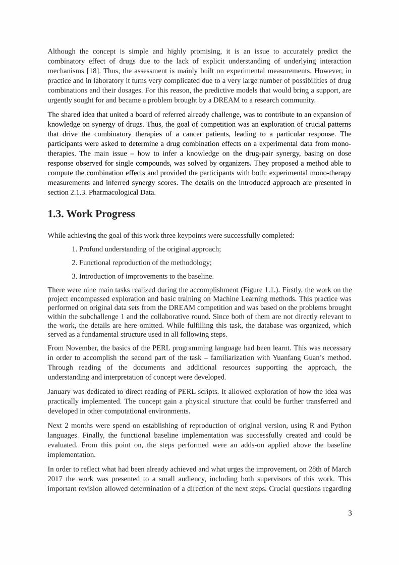
There were nine main tasks realized during the accomplishment (Figure 1.1.). Firstly, the work on theproject encompassed exploration and basic training on Machine Learning methods. This practice wasperformed on original data sets from the DREAM competition and was based on the problems broughtwithin the subchallenge 1 and the collaborative round. Since both of them are not directly relevant tothe work, the details are here omitted. While fulfilling this task, the database was organized, whichserved as a fundamental structure used in all following steps.

From November, the basics of the PERL programming language had been learnt. This was necessaryin order to accomplish the second part of the task – familiarization with Yuanfang Guan’s method.Through reading of the documents and additional resources supporting the approach, theunderstanding and interpretation of concept were developed.

January was dedicated to direct reading of PERL scripts. It allowed exploration of how the idea waspractically implemented. The concept gain a physical structure that could be further transferred anddeveloped in other computational environments.

Next 2 months were spend on establishing of reproduction of original version, using R and Pythonlanguages. Finally, the functional baseline implementation was successfully created and could beevaluated. From this point on, the steps performed were an adds-on applied above the baselineimplementation.

In order to reflect what had been already achieved and what urges the improvement, on 28th of March2017 the work was presented to a small audiency, including both supervisors of this work. Thisimportant revision allowed determination of a direction of the next steps. Crucial questions regarding

3

to missing values imputation, final test and trainig sets and optimization were decided, resulting in adefined improvement plan.

Contrary to expectations, at thas time, the true values of synergy scores in a challenge test set, still didnot become available to a public. Due to this fact, the test and training sets were generated fromknown data, reproducing as accurately as possible the modeling conditions created in DREAMchallenge.

One of the most laborious steps was the task 7 - feature selection. Different methodologies wereexperimented before establishing a workflow, for example Random Forests, Support Vector Machine,Generalized linear and additive models by likelihood based boosting (GAMBoost). The final result,accomplished with Lasso algorithm, provided a list of useful variables that shall be included in themodel to produce optimal outcome.

Finally, task 8 including the training of machine learning models and cross validations, allowedestablishment of the best performing workflow, for which the results are presented in this report.

4

Timeline

2016 2017

Tasks Sept. Oct. Nov. Dec. Jan. Feb. Mar. Apr. May June July Aug. Sept.

1. Familiarization with Machine Learnin methodologies

2. Familiarization with PERL and Yuanfang Guan’s approach

3. Decoding of original scripts

4. Establishment of baseline implementation

5. Definition of improvement plan

6. Re-establishment of training & test set

7. Feature selection

8. Cross validation, model optimization & evaluation

9. Report writing

Figure 1.1. Plan of work and tasks realized in the project.

5

2. The AstraZeneca-Sanger Drug Combination PredictionDREAM Challenge

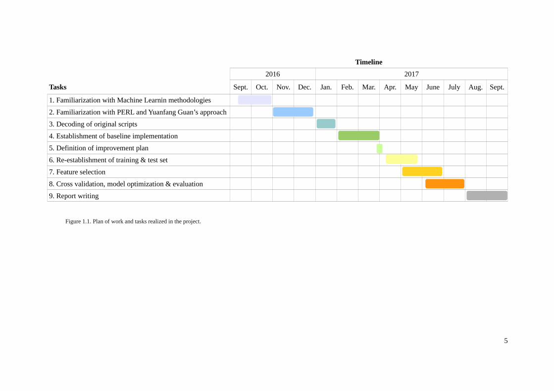
As stated before the goal of this challenge is to expand the understanding of drug synergy and toidentify biomarkers driving a patient’s response. Although the competition encompasses twosubchallenges, the focus of interest was only one of them - closer to the reality, so more interesting andimportant from this point of view. It reproduces the common situation in personalized medicine wherethe therapies must be determined and selected only on prior knowledge. Thus, the aim is to predict invitro drug synergy without the access to the combinational therapy training data. The effect needs tobe inferred from multi-sourced molecular data, compound information, experimental results of mono-therapies and/or any relevant prior knowledge and external datasets (Figure 2.1.).

Figure 2.1. Visualization of the concept of subchallenge 2 [19].

Along this work, the gene names and symbols are normalized according to standard defined by theHUGO Gene Nomenclature Committee at the European Bioinformatics Institute. The cellnomenclature is standard and common between worldwide laboratories, uniquely identifying the linesand their origin.

6

Dru

g co

mbi

nati

ons

Cell lines

2.1. DREAM Challenge Data

2.1.1. Pharmacological Data

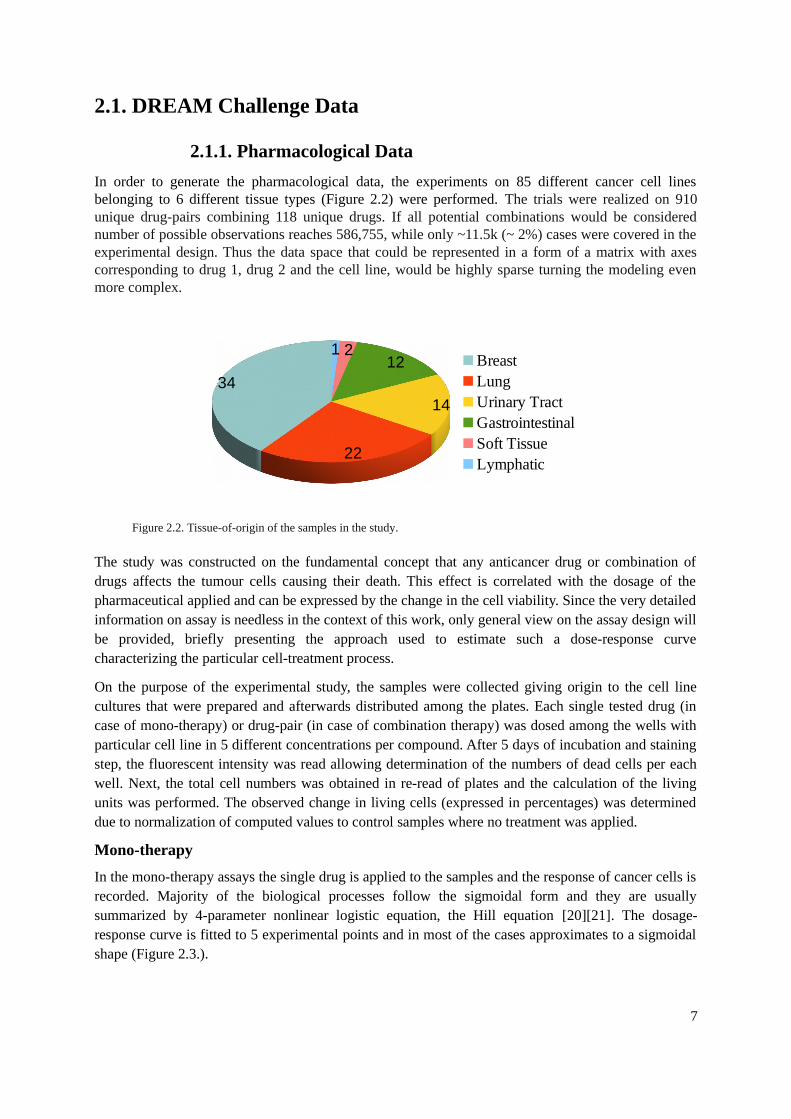
In order to generate the pharmacological data, the experiments on 85 different cancer cell linesbelonging to 6 different tissue types (Figure 2.2) were performed. The trials were realized on 910unique drug-pairs combining 118 unique drugs. If all potential combinations would be considerednumber of possible observations reaches 586,755, while only ~11.5k (~ 2%) cases were covered in theexperimental design. Thus the data space that could be represented in a form of a matrix with axescorresponding to drug 1, drug 2 and the cell line, would be highly sparse turning the modeling evenmore complex.

Figure 2.2. Tissue-of-origin of the samples in the study.

The study was constructed on the fundamental concept that any anticancer drug or combination ofdrugs affects the tumour cells causing their death. This effect is correlated with the dosage of thepharmaceutical applied and can be expressed by the change in the cell viability. Since the very detailedinformation on assay is needless in the context of this work, only general view on the assay design willbe provided, briefly presenting the approach used to estimate such a dose-response curvecharacterizing the particular cell-treatment process.

On the purpose of the experimental study, the samples were collected giving origin to the cell linecultures that were prepared and afterwards distributed among the plates. Each single tested drug (incase of mono-therapy) or drug-pair (in case of combination therapy) was dosed among the wells withparticular cell line in 5 different concentrations per compound. After 5 days of incubation and stainingstep, the fluorescent intensity was read allowing determination of the numbers of dead cells per eachwell. Next, the total cell numbers was obtained in re-read of plates and the calculation of the livingunits was performed. The observed change in living cells (expressed in percentages) was determineddue to normalization of computed values to control samples where no treatment was applied.

Mono-therapy

In the mono-therapy assays the single drug is applied to the samples and the response of cancer cells isrecorded. Majority of the biological processes follow the sigmoidal form and they are usuallysummarized by 4-parameter nonlinear logistic equation, the Hill equation [20][21]. The dosage-response curve is fitted to 5 experimental points and in most of the cases approximates to a sigmoidalshape (Figure 2.3.).

7

34

22

14

1221

BreastLungUrinary TractGastrointestinalSoft TissueLymphatic

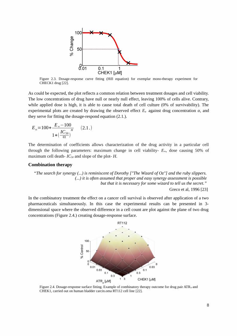
Figure 2.3. Dosage-response curve fitting (Hill equation) for exemplar mono-therapy experiment forCHECK1 drug [22].

As could be expected, the plot reflects a common relation between treatment dosages and cell viability.The low concentrations of drug have null or nearly null effect, leaving 100% of cells alive. Contrary,while applied dose is high, it is able to cause total death of cell culture (0% of survivability). Theexperimental plots are created by drawing the observed effect Eα against drug concentration α, andthey serve for fitting the dosage-respond equation (2.1.).

Eα=100+E∞−100

1+(IC50α )

H (2.1 .)

The determination of coefficients allows characterization of the drug activity in a particular cellthrough the following parameters: maximum change in cell viability- E∞, dose causing 50% ofmaximum cell death- IC50 and slope of the plot- H.

Combination therapy

Greco et al, 1996 [23]

In the combinatory treatment the effect on a cancer cell survival is observed after application of a twopharmaceuticals simultaneously. In this case the experimental results can be presented in 3-dimensional space where the observed difference in a cell count are plot against the plane of two drugconcentrations (Figure 2.4.) creating dosage-response surface.

Figure 2.4. Dosage-response surface fitting. Example of combinatory therapy outcome for drug pair ATR4 andCHEK1, carried out on human bladder carcin.oma RT112 cell line [22].

8

“The search for synergy (...) is reminiscent of Dorothy ["The Wizard of Oz"] and the ruby slippers.(...) it is often assumed that proper and easy synergy assessment is possible

but that it is necessary for some wizard to tell us the secret.”

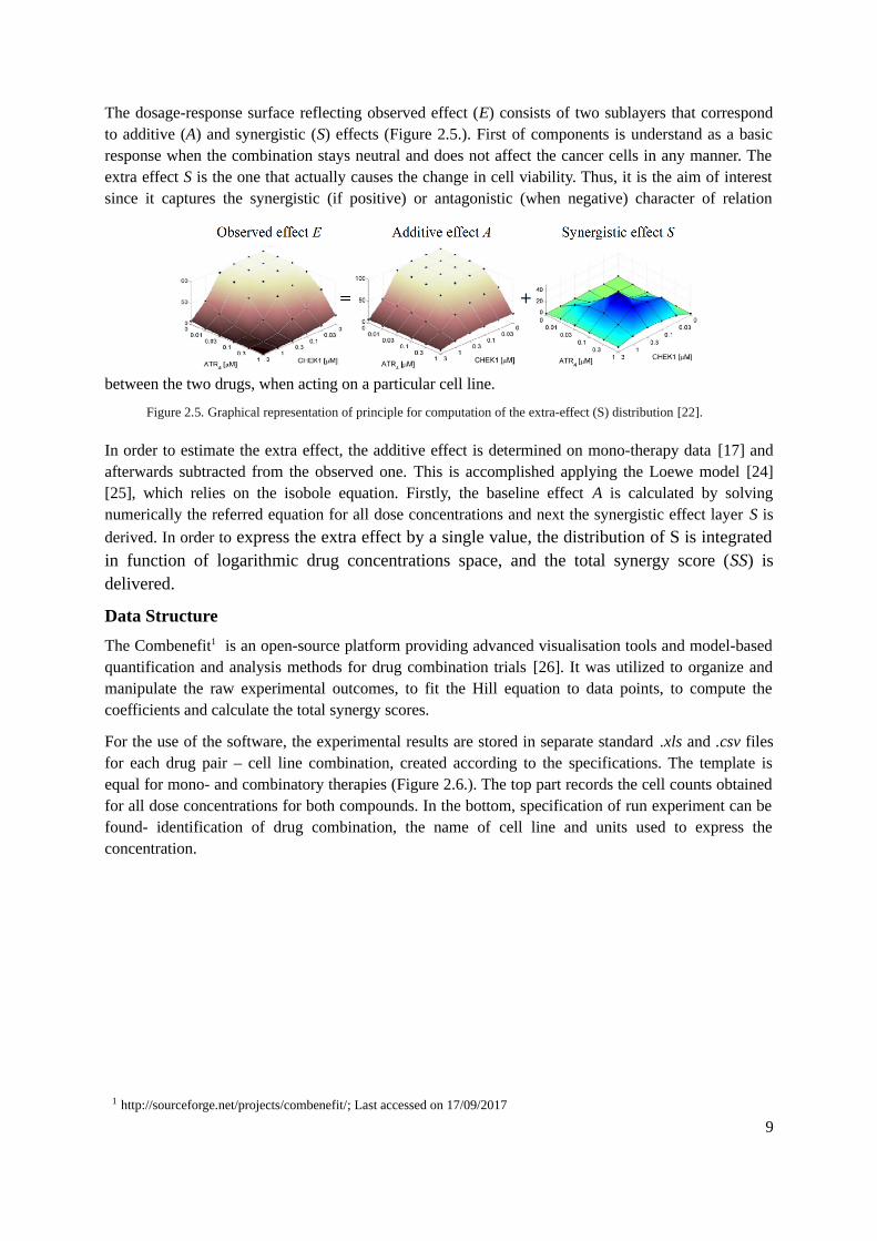
The dosage-response surface reflecting observed effect (E) consists of two sublayers that correspondto additive (A) and synergistic (S) effects (Figure 2.5.). First of components is understand as a basicresponse when the combination stays neutral and does not affect the cancer cells in any manner. Theextra effect S is the one that actually causes the change in cell viability. Thus, it is the aim of interestsince it captures the synergistic (if positive) or antagonistic (when negative) character of relation

between the two drugs, when acting on a particular cell line.

Figure 2.5. Graphical representation of principle for computation of the extra-effect (S) distribution [22].

In order to estimate the extra effect, the additive effect is determined on mono-therapy data [17] andafterwards subtracted from the observed one. This is accomplished applying the Loewe model [24][25], which relies on the isobole equation. Firstly, the baseline effect A is calculated by solvingnumerically the referred equation for all dose concentrations and next the synergistic effect layer S is

derived. In order to express the extra effect by a single value, the distribution of S is integratedin function of logarithmic drug concentrations space, and the total synergy score (SS) isdelivered.

Data Structure

The Combenefit1 is an open-source platform providing advanced visualisation tools and model-basedquantification and analysis methods for drug combination trials [26]. It was utilized to organize andmanipulate the raw experimental outcomes, to fit the Hill equation to data points, to compute thecoefficients and calculate the total synergy scores.

For the use of the software, the experimental results are stored in separate standard .xls and .csv filesfor each drug pair – cell line combination, created according to the specifications. The template isequal for mono- and combinatory therapies (Figure 2.6.). The top part records the cell counts obtainedfor all dose concentrations for both compounds. In the bottom, specification of run experiment can befound- identification of drug combination, the name of cell line and units used to express theconcentration.

9

1 http://sourceforge.net/projects/combenefit/; Last accessed on 17/09/2017

Figure 2.6. Structure of the .xls and .csv files storing information on combination and mono-therapy assays.* ‘Data’ - Numeric; Percentage of survivor tumour cells observed for each treatment.* ‘Data’ - as above; available only for combination therapy assays.

Some of the trials had to be repeated due to unsatisfactory level of quality of the measurements and allthe experiments are recorded in separate files. The duplicates and triplicates are identified by theadequate suffix in the file name, respectively: *.Rep2 and *.Rep3. In total there are 11,759 availablefiles corresponding to the mono-therapy assays and 6,731 storing the results of combinatoryexperiments.

After Combenefit manipulations, plotting and Hill’s equation fitting, the results are summarized andstored in a .csv file with 14 fields (Appendix 1A). Among the recorded information, there can be foundcombinatory effect coefficients, quality assessment, specification of a drug pair – cell line combinationand finally the total synergy score value.

2.1.2. Molecular Data

Three molecular data sources: gene expression, copy number variants and mutations in cancer celllines, were produced in a frame of one of the Sanger Institute projects, namely the Genomics of DrugSensitivity in Cancer (GDSC). The methylation data was generated by the Estseller group fromBellvitge Biomedical Research Institute (IDIBELL). All this molecular data provided within theDREAM challenge is available at COSMIC repository (COSMIC2012) in a format of .csv files. Thegene names and symbols used in the work are normalized according to standard defined by the HUGOGene Nomenclature Committee at the European Bioinformatics Institute. To allow easy transfer andsharing of information, the cell nomenclature is standard and common among worldwide laboratories,uniquely identifying the lines and their origin.

Gene Expression

Regarding to the data on RNA expression, it comes from a study performed using Affymetrix HumanGenome U219 Array Plates, available at ArrayExpress platform: E-MTAB-3610 [27]. The valuesprovided was obtained after processing the raw data in R utilizing tools implemented within theBioconductor [28]. Firstly, the package ‘makecdfenv’ [29] was applied to read Affymetrix chipdescription file (CDF) and allow mapping between probes and genes. Next, the values werenormalized with Robust Multi-array Average (RMA) algorithm employing R-package ‘affy’ [30]. The2-dimensional matrix holding processed values of a gene expression has 83 rows listing the cell linesand 17,419 columns corresponding to the genes. It also contains missing values due to the unavailabledata for two cell lines: MDA-MB-175-VII and NCI-H1437.

10

0,00 Dose 1 Dose 2 Dose 3 Dose 4 Dose 5 (=Agent 2)0,00 100,00 Data Data Data Data Data

Dose 1 Data Data Data Data Data DataDose 2 Data Data Data Data Data DataDose 3 Data Data Data Data Data DataDose 4 Data Data Data Data Data DataDose 5 Data Data Data Data Data Data(=Agent 1)Agent 1 Drug A nameAgent 2 Drug B nameUnit1 Concentrat ion (\muM)Unit2 Concentrat ion (\muM)Title Cell line name

Copy Number Variations

Another data set provides the knowledge on Copy Number Variations (CNVs). It was generatedemploying Affymetrix SNP6.0 microarrays and can be found at European Genome-phenome Archive:EGAS00001000978 [27]. The chromosomal alterations were identified using the PICNIC algorithm[31] with the reference to 38 human genome build (GRCh38). The data provided reveals the state ofchromosome at two levels: of the segment and gene. Since the approach presented in this work focuseson genes and simulates the posterior state on the gene level, exclusively the last source of CNVinformation was considered in the preparation of the model. The respective .csv file is a list of CNVsthat encompasses 29,158 observations for each of 85 cell lines (that is 2 478,430 unique records in

total) and contains 9 fields (Appendix 1B) revealing specifications of each gene alteration.

Mutations

In order to obtain detailed mutational profile for the cancer cell lines, the whole exome sequencingwas performed with the Agilent’s SureSelect on the Ilumina HiSeq 2000 platform. Raw BAM files areavailable on repository with mentioned above CNV data (EGAS00001000978 [27]). Two algorithmswere applied to identify mutations, namely the CaVEMan (Cancer Variants Through ExpectationMaximization) and PINDEL [32], allowing calling of the total 75,281 mutations for all 85 cell lines.The resulted output data was organized in a single .csv file with 32 fields (Aappendix 1C) including allthe specifications and details of detected mutation.

Methylation

One of a studies held at IDIBELL Institute and carried by the Esteller team provided the moleculardata on methylation. The project was performed at Illumina Infinium HumanMethylation450 v1.2BeadChip platform and the raw data is stored at a public Gene Expression Omnibus (GEO) repository:GSE68379 [27]. The methylation status can be expressed by two different parameters [33]:

- the betai methylation status of yi CpG site, which is a ratio of maximal methylated probeintensity versus the total sum of maximum methylated and unmethylated intensities (Eq. 2.2.);

beta i=max ( y i ,methylated ,0)

max ( yi ,methylated ,0)+max ( yi , unmethylated ,0)+α(2.2 .)

- value Mi, expressed as logarithm of ratio of maximum methylated and unmethylated probeintensities (Eq. 2.3.).

M i= log2 (max ( yi , methylated ,0)+α

max ( yi ,unmethylated ,0)+α) (2.3 .)

Both metrics are computed with correction through a coefficient α that is variable specific for theplatform used in the assay, in this case – one recommended for Illumina. Available beta and M scoresare defined per probe and CpG island. Thus, there are four datasets provided with methylation statusexpressed by beta and M metrics, probe- and island- wisely each. Following Yuanfang Guan,unlogged ratios assigned per probe were used as involving less transformations on raw values. Themethylation data is organized within the 2-dimensional matrix with 28,7450 rows referring to allunique probes included in the assay and 82 columns corresponding to the studied cell lines(unavailable data for MDA-MB-175-VII, KMS-11, SW620).

11

2.1.3. Compound Data

The data on chemical and structural properties for 118 unique drugs involved in the experiments isprovided in the .txt file with 8 fields (Appendix 1D). For each compound with anonymised name,chemical and structural properties are specified including the targets of action, specification on H-bond acceptors and donors (HBA and HBD), octanol-water partition coefficient (cLogP), number offulfilled Lipinski rules (Lipinski), SMILES or PubChem identificaton and molecular weight. Worth ofnoting is a fact that since the identity of all compounds is anonymized due to a confidentialityagreements, the information on drugs provided within this file is the one to rely on. The only possiblealternative to make a connection with a prior knowledge is throught the SMILE or PubChem ID,however this field is unavailable for 33% of instances.

2.2. Submission Form

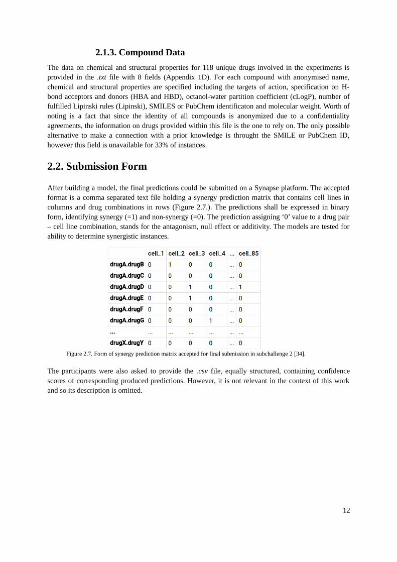
After building a model, the final predictions could be submitted on a Synapse platform. The acceptedformat is a comma separated text file holding a synergy prediction matrix that contains cell lines incolumns and drug combinations in rows (Figure 2.7.). The predictions shall be expressed in binaryform, identifying synergy (=1) and non-synergy (=0). The prediction assigning ‘0’ value to a drug pair– cell line combination, stands for the antagonism, null effect or additivity. The models are tested forability to determine synergistic instances.

Figure 2.7. Form of synergy prediction matrix accepted for final submission in subchallenge 2 [34].

The participants were also asked to provide the .csv file, equally structured, containing confidencescores of corresponding produced predictions. However, it is not relevant in the context of this workand so its description is omitted.

12

3. The Winning Solution

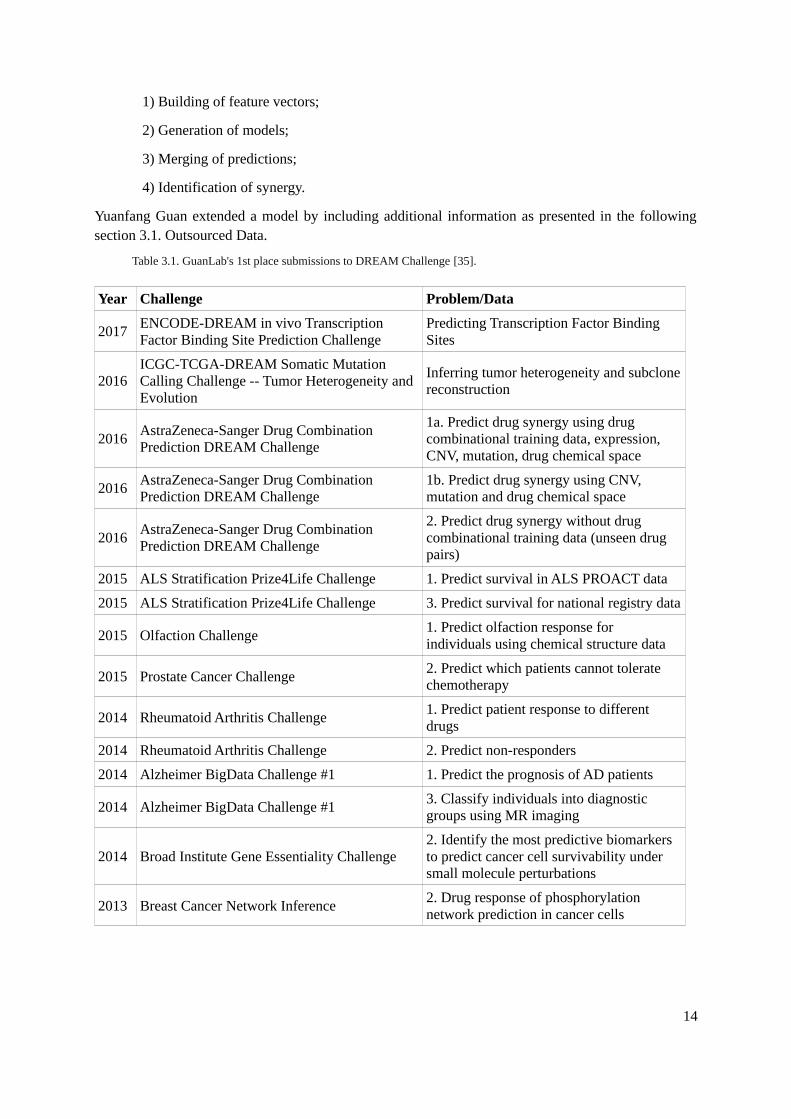
This work was inspired on the winning solution of the 2016 AstraZeneca-Sanger Drug CombinationPrediction DREAM Challenge. The implementation is provided by exceptional researcher YuanfangGuan from a Department of Computational Medicine and Bioinformatics at University of Michigan.Over last 4 years she with her team participated in 7 individual DREAM competitions, someconsisting of 2 or 3 subchallenges, always being recognized among the top performing teams. Fifteensubmissions of GuanLab became 1st place winning solutions (Table 3.1.), including challenges onvarious diseases (ex. cancers, Alzheimer, Rheumatoid Arthritis) and broad range of tasks to solve(classification, prediction, inferrence problems). This achievements prove the excelence and efficiencyof the built models. There is no doubt that general approach of problem solving developed by Guandeserves an attention and is a valuable lesson to learn.

Although each of submmissions is provided with script files and supporting documentation, usuallythe given explanations are not sufficient to easily understand and accurately reproduce themethodology. Exploration of Guan’s implementation requires careful examination and backtracking ofscripts, with simultaneous connecting it to the interpretation. Task become even more complicated dueto:

- absence of dockstrings and comments in scripts;

- unclean script writting, with remains of experimented commands;

- redundant programming - unnecessary manipulations, ghost-variables;

- presence of unutilized scripts – files are submitted but never called and run by wrappingscript;

- unclear origin of some input files;

- unknown pre-processing of original files.

Untill now some manipulations remain ambiguous but it was pretended to follow the indication of theproper author cited in the opening of this chapter. The effort was made to create a reconstruction ofprocedure as close to the original as possible.

The workflow of the baseline implementation include four main steps:

“Always try the easiest solution.And the common sense – first.”

Y. Guan

1) Building of feature vectors;

2) Generation of models;

3) Merging of predictions;

4) Identification of synergy.

Yuanfang Guan extended a model by including additional information as presented in the followingsection 3.1. Outsourced Data.

Table 3.1. GuanLab's 1st place submissions to DREAM Challenge [35].

Year Challenge Problem/Data

2017ENCODE-DREAM in vivo Transcription Factor Binding Site Prediction Challenge

Predicting Transcription Factor Binding Sites

2016ICGC-TCGA-DREAM Somatic Mutation Calling Challenge -- Tumor Heterogeneity and Evolution

Inferring tumor heterogeneity and subclonereconstruction

2016AstraZeneca-Sanger Drug Combination Prediction DREAM Challenge

1a. Predict drug synergy using drug combinational training data, expression, CNV, mutation, drug chemical space

2016AstraZeneca-Sanger Drug Combination Prediction DREAM Challenge

1b. Predict drug synergy using CNV, mutation and drug chemical space

2016AstraZeneca-Sanger Drug Combination Prediction DREAM Challenge

2. Predict drug synergy without drug combinational training data (unseen drug pairs)

2015 ALS Stratification Prize4Life Challenge 1. Predict survival in ALS PROACT data

2015 ALS Stratification Prize4Life Challenge 3. Predict survival for national registry data

2015 Olfaction Challenge1. Predict olfaction response for individuals using chemical structure data

2015 Prostate Cancer Challenge2. Predict which patients cannot tolerate chemotherapy

2014 Rheumatoid Arthritis Challenge1. Predict patient response to different drugs

2014 Rheumatoid Arthritis Challenge 2. Predict non-responders

2014 Alzheimer BigData Challenge #1 1. Predict the prognosis of AD patients

2014 Alzheimer BigData Challenge #13. Classify individuals into diagnostic groups using MR imaging

2014 Broad Institute Gene Essentiality Challenge2. Identify the most predictive biomarkers to predict cancer cell survivability under small molecule perturbations

2013 Breast Cancer Network Inference2. Drug response of phosphorylation network prediction in cancer cells

14

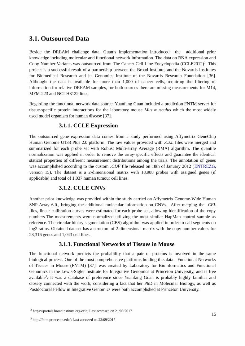
3.1. Outsourced Data

Beside the DREAM challenge data, Guan’s implementation introduced the additional priorknowledge including molecular and functional network information. The data on RNA expression andCopy Number Variants was outsourced from The Cancer Cell Line Encyclopedia (CCLE2012)2. Thisproject is a successful result of a partnership between the Broad Institute, and the Novartis Institutesfor Biomedical Research and its Genomics Institute of the Novartis Research Foundation [36].Althought the data is available for more than 1,000 of cancer cells, requiring the filtering ofinformation for relative DREAM samples, for both sources there are missing measurements for M14,MFM-223 and NCI-H3122 lines.

Regarding the functional network data source, Yuanfang Guan included a prediction FNTM server fortissue-specific protein interactions for the laboratory mouse Mus musculus which the most widelyused model organism for human disease [37].

3.1.1. CCLE Expression

The outsourced gene expression data comes from a study performed using Affymetrix GeneChipHuman Genome U133 Plus 2.0 platform. The raw values provided with .CEL files were merged andsummarized for each probe set with Robust Multi-array Average (RMA) algorithm. The quantilenormalization was applied in order to remove the array-specific effects and guarantee the identicalstatical properties of different measurement distributions among the trials. The annotation of geneswas accomplished according to the custom .CDF file released on 18th of January 2012 (ENTREZG,version 15). The dataset is a 2-dimensional matrix with 18,988 probes with assigned genes (ifapplicable) and total of 1,037 human tumour cell lines.

3.1.2. CCLE CNVs

Another prior knowledge was provided within the study carried on Affymetrix Genome-Wide HumanSNP Array 6.0., bringing the additional molecular information on CNVs. After merging the .CELfiles, linear calibration curves were estimated for each probe set, allowing identification of the copynumbers.The measurements were normalized utilizing the most similar HapMap control sample asreference. The circular binary segmentation (CBS) algorithm was applied in order to call segments onlog2 ratios. Obtained dataset has a structure of 2-dimensional matrix with the copy number values for23,316 genes and 1,043 cell lines.

3.1.3. Functional Networks of Tissues in Mouse

The functional network predicts the probability that a pair of proteins is involved in the samebiological process. One of the most comprehensive platforms holding this data - Functional Networksof Tissues in Mouse (FNTM) [37], was created by Laboratory for Bioinformatics and FunctionalGenomics in the Lewis-Sigler Institute for Integrative Genomics at Princeton University, and is freeavailable3. It was a database of preference since Yuanfang Guan is probably highly familiar andclosely connected with the work, considering a fact that her PhD in Molecular Biology, as well asPostdoctoral Fellow in Integrative Genomics were both accomplished at Princeton University.

152 https://portals.broadinstitute.org/ccle; Last accessed on 21/09/2017

3 http://fntm.princeton.edu/; Last accessed on 22/09/2017

In order to generate the network in mouse, diverse data sources needed to be integrated: geneexpression, tissue localization, phylogenetic and phenotypic profiles, data based on homology,physical interactions and gene-disease/phenotypic associations. According to the Yuanfang Guan [38]creating such a functional network in mammalian models is still challenging. Thus using the muchsimpler mouse network that could reveal major connections and relations between proteins could beapplicable in human models by inference.

In brief, according to the author, the procedure of determining the functional relations between thegenes and their connection probabilities encompasses five main steps [39]:

1) Pick all possible files with available data related to genes, for example microarrays, RNA-seq, phenotypes, sequences, homologies etc.

2) Compute correlations between genes and normalize them using z-transform.

3) Build a gold standard set using KEGG/GO.

4) Bin each into a number of bins.

5) Compute the Bayesian posterior with some regularization.

As could be expected this process is computationally highly intensive.

3.2. Feature Vectors

The final predictions are obtained by computing a weighted average from six separate models:

- global molecular,

- global mono-therapy,

- chemical,

- file-counting,

- local molecular,

- and local mono-therapy.

Each of those involves independent construction of feature vectors, for which different data sets serveas a sources and particular handling and manipulation steps are implicated.

3.2.1. Global Molecular

The molecular feature vector is based on six i data sources: gene expression, CNVs, mutations andmethylation that are described in details in the section 2.1.2., and additional outsourced CCLE datapresented in sections 3.1.1. and 3.1.2. The files selected to be used characterize a molecular profile ofcancer samples with regard to collection of genes. Each of them is transformed into unifrom two-dimensional matrix (Figure 3.1.) where the columns refers to the cell lines and rows- to genes. Theyare filled with vG1 – vGn values corresponding to an exact cell - gene instance, and expressing the assayresults provided with each original data source. Thus, in case of quantitative measurements, RNAexpression and methylation, they remain represented by respectively: logged intensities and level ofmethylation (ranging from 0 to 1 that corresponds to 0% – 100% of methylation). For qualitativeproperties like CNVs and mutations, those must be binarized assigning value '1' when the alteration ispresent and '0' contrary. All those matrices serve as input for the baseline script.

16

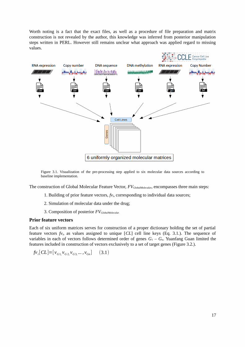
Worth noting is a fact that the exact files, as well as a procedure of file preparation and matrixconstruction is not revealed by the author, this knowledge was inferred from posterior manipulationsteps written in PERL. However still remains unclear what approach was applied regard to missingvalues.

Figure 3.1. Visualization of the pre-processing step applied to six molecular data sources according tobaseline implementation.

The construction of Global Molecular Feature Vector, FVGlobalMolecular, encompasses three main steps:

1. Building of prior feature vectors, fvi, corresponding to individual data sources;

2. Simulation of molecular data under the drug;

3. Composition of posterior FVGlobalMolecular.

Prior feature vectors

Each of six uniform matrices serves for construction of a proper dictionary holding the set of partialfeature vectors fvi, as values assigned to unique [CL] cell line keys (Eq. 3.1.). The sequence ofvariables in each of vectors follows determined order of genes G1 – Gn. Yuanfang Guan limited thefeatures included in construction of vectors exclusively to a set of target genes (Figure 3.2.).

fv i[CL ]=[vG1, vG 2, vG3, ... , vGn] (3.1)

17

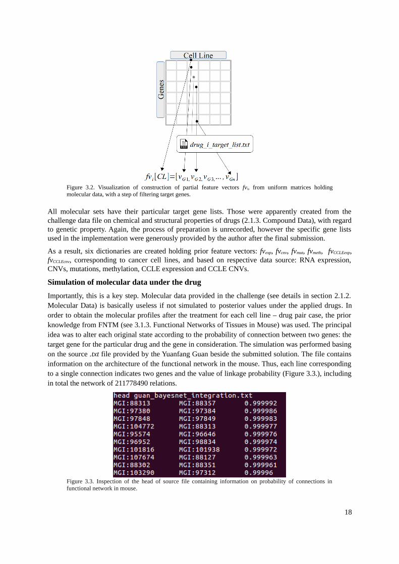
Figure 3.2. Visualization of construction of partial feature vectors fvi, from uniform matrices holdingmolecular data, with a step of filtering target genes.

All molecular sets have their particular target gene lists. Those were apparently created from thechallenge data file on chemical and structural properties of drugs (2.1.3. Compound Data), with regardto genetic property. Again, the process of preparation is unrecorded, however the specific gene listsused in the implementation were generously provided by the author after the final submission.

As a result, six dictionaries are created holding prior feature vectors: fvexp, fvcnv, fvmut, fvmeth, fvCCLEexp,fvCCLEcnv, corresponding to cancer cell lines, and based on respective data source: RNA expression,CNVs, mutations, methylation, CCLE expression and CCLE CNVs.

Simulation of molecular data under the drug

Importantly, this is a key step. Molecular data provided in the challenge (see details in section 2.1.2.Molecular Data) is basically useless if not simulated to posterior values under the applied drugs. Inorder to obtain the molecular profiles after the treatment for each cell line – drug pair case, the priorknowledge from FNTM (see 3.1.3. Functional Networks of Tissues in Mouse) was used. The principalidea was to alter each original state according to the probability of connection between two genes: thetarget gene for the particular drug and the gene in consideration. The simulation was performed basingon the source .txt file provided by the Yuanfang Guan beside the submitted solution. The file containsinformation on the architecture of the functional network in the mouse. Thus, each line correspondingto a single connection indicates two genes and the value of linkage probability (Figure 3.3.), includingin total the network of 211778490 relations.

Figure 3.3. Inspection of the head of source file containing information on probability of connections infunctional network in mouse.

18

As could be expected, the names of genes are expressed according to the official nomenclatureestablished by the International Comitee on Standardized Genetic Nomenclature for Mice that isavailable in the Mouse Genome Informatics Database4. In order to take advantage of this information,the MGI identificators require to be converted to HGNC nomenclature used as a standard. The filecalled by PERL script in order to accomplish the translation was not originally provided. It was foundthrought the search in the internet and downloaded from the GitHub repository5, thank to the nkiip userthat generously shared a file on the 15th of May 2016 and made it available.

The concept of simulation follows the common sense and reflect the simplified reality. The basicassumptions are:

1) The efficiency of treatments is ideal and once applied they totally turn off the genes that arethe drug targets.

2) The genes that are not targets for applied drug, neither connected to target genes: their stateremains unchanged (the treatment has no effect on them).

3) Treatment alterates the state of genes related to the drug targets according to the connectionprobability between those genes.

For the special attention deserves last of the rules. It cannot be applied automatically since the‘direction’ of alteration must be considered, i.e. if the molecular state promotes or limits thecarcinogenesis. The action of a drug is always directional: contra the tumour, what means that it shallpromote anticancer events and reduce those which are pro. Following the general rules stated above,particular cases can be considered.

Concerning expression, the gene state for each cell line is described by the log2 of measured intensityso the matrix is filled with continuous values. The expression of the gene that is a drug target for theapplied drug turns zero- reflecting the total silencing. Genes that are functionally linked to the targetreduce their intensities according to the connection probability (Eq. 3.2.). This simulation approach isvalid for both expression data sources – one provided within the challenge and other outsourced fromthe CCLE platform.

vGn[exp , posterior ]=vGn[exp , prior ]∗(1− pconnection) (3.2 .)

The information in a CNV matrix is binarized, expressing the gene states by discrete data. Accordingto the main concept, target genes turn zero because their activity is totally recovered under a treatment,and the copy number does not promote the growth of cancer any more. The activity of connectedgenes becomes partially normalized, their status reduces proportionally to the linkage with a target,and in consequence has less impact on tumorigenesis (Eq. 3.3.). The simulation of a CNVs posteriorstatus for a dataset outsourced from CCLE shares the same logic.

vGn[cnv , posterior ]=vGn[cnv , prior ]∗(1−pconnection) (3.3 .)

For mutations that are also organized in binary matrix, the assumption of ideal treatment would behigh to far unrealistic. This is an exception since the drugs applied nowadays are yet unable to fix thepro-cancer mutations in any manner. Thus, the state of target genes remains unchanged while valuesassigned to related genes are multiplied by the connection probability (Eq. 3.4.). Note, that in this casethe manipulation will always bring reduction of a molecular state: gene carrying mutation is assignedwith ‘1’ and if is connected to target, will turn < 1, according to a probability that is always below 1. Itcan be interpreted as although the target mutation cannot be fixed, the treatment will have still anindirect impact, improving other related processes.

vGn[mut , posterior ]=vGn[mut , prior ]∗(1− pconnection) (3.4 .)

194 http://www.informatics.jax.org/mgihome/nomen/; Last accessed on 22/09/2017;5 https://github.com/nkiip/GC2NMF/blob/master/0_origin_data/MGI_Gene.rpt; Last accessed on 25/09/2017;

In the case of methylation, matrix is filled with continues values that range between 0 and 1 and thatcorrespond to a percentage of methylation level. The simulation according to Yuanfang Guan ispractically proceeded as follows: the target genes become totally unmethylated while the related genesproportionally decrease their methylation level. However the script does not correspond to thedocumentation [39]. The author states that for both- target genes and those connected, status turnsbigger (proportionally to the connection probability in latter case, as usually).

Due to this discrepancy, the additional research was performed to understand the methylationprocesses underlying the carcinoma and decide on approach to implement. In cancer cell lines twophenomena are observed [40][41]:

- hypermethylation of CpG sites that causes the inactivation of tumor-suppressor genes,

- genome widespread hypomethylation that promotes the carcinogenesis and the tumorprogression.

Remembering that the data provided in challenge contains the measurements captured in CpG sites, itseems reasonable and convincing to define the process of simulation under the drug as followes: thetarget genes become totally unmethylated turning their status to zero (allowing tumor-suppressorgenes to fight against the cancer), while related genes reduce the methylation level according to theconnection probability (Eq. 3.5.). This approach, equal to included in PERL script, was proved toresult in more accurate model and so was decided to be implemented in this work.

vGn[met , posterior ]=vGn[met , prior ]∗(1− pconnection) (3.5 .)

Interestingly, Yuanfang Guan claims that the inclusion of methylation data apparently hurts theperformance [39]. This fact confirms the theory that proposed methodology of methyl simulationcould be imperfect and an alternative manner shall be applied.

Summarizing, each of prior feature vectors is processed and all vG1 – vGn values are substituted with anew state, generating simulated feture vectors, fv’i.

Posterior feature vectors

In order to generate the global molecular feature vectors FVGlobalMolecular, reflecting the molecularprofiles of samples, the simulated partial feature vectors are joined (Eq. 3.6.) according to their cellline annotation.

FV GlobalMolecular [CL ]=[ fv ' exp , fv ' cnv , fv 'mut , fv 'met , fv ' CCLEexp , fv ' CCLEcnv ] (3.6 .)

3.2.2. Global Mono-therapy

The idea of mono-therapy modeling is to produce the predictions basing on pharmacological sourceswith the experimental and curve-fitted variables. The feature vector is constructed from the originalcell counts observed in assays and estimated Hill model parameters. Due to a complexity of theprocedure it is convenient to define some common terminology for the purpose of this work, toprovide clearer and simpler description of the data manipulation.

Along this lines, denomination ‘yA1-5’ is used for cell counts obtained under the drug A for fivedifferent dosages. Similarly, ‘yB1-5’ stands for changes in cell viability observed for five concentrationsof drug B. Recalling the coefficients estimated by curve-fitting, the following designation of variablesis applied:

20

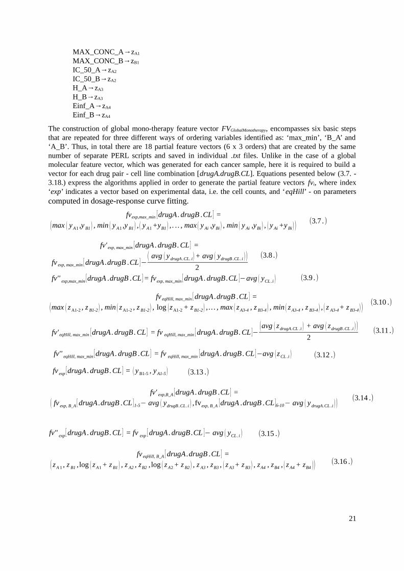
MAX_CONC_A→zA1 MAX_CONC_B→zB1

IC_50_A→zA2

IC_50_B→zA2

H_A→zA3

H_B→zA3

Einf_A→zA4

Einf_B→zA4

The construction of global mono-therapy feature vector FVGlobalMonotherapy, encompasses six basic stepsthat are repeated for three different ways of ordering variables identified as: ‘max_min’, ‘B_A’ and‘A_B’. Thus, in total there are 18 partial feature vectors (6 x 3 orders) that are created by the samenumber of separate PERL scripts and saved in individual .txt files. Unlike in the case of a globalmolecular feature vector, which was generated for each cancer sample, here it is required to build avector for each drug pair - cell line combination [drugA.drugB.CL]. Equations pesented below (3.7. -3.18.) express the algorithms applied in order to generate the partial feature vectors fvi, where index‘exp’ indicates a vector based on experimental data, i.e. the cell counts, and ‘eqHill’ - on parameterscomputed in dosage-response curve fitting.

21

fvexp,max_min [drugA . drugB .CL ] =

(max ( yA1 ,y B1 ) , min ( y A1 ,y B1 ) , ( y A1 +yB1 ) , . . . , max ( y Ai ,yBi ) , min ( y Ai ,yBi ) , ( y Ai +y Bi ) )(3.7 .)

(3.8 .)

fv'' exp,max_min [drugA .drugB .CL ] = fvexp, max_min [ drugA . drugB .CL ]−avg ( yCL . i ) (3.9 .)

fv eqHill, max_min [ drugA .drugB .CL ] =

(max ( zA1-2 , z B1-2 ) , min ( zA1-2 , z B1-2 ) , log (zA1-2 + z B1-2 ) , . . . , max ( zA3-4 , z B3-4 ) , min ( zA3-4 , z B3-4 ) , ( z A3-4+ z B3-4 ) )(3.10 .)

fv' eqHill, max_min [drugA . drugB . CL ] = fv eqHill, max_min [ drugA . drugB . CL ]−(avg ( z drugA.CL . i ) + avg ( zdrugB .CL . i ) )

2(3.11 .)

fv'' eqHill, max_min [drugA . drugB .CL ] = fv eqHill, max_min [drugA . drugB . CL ]−avg (zCL . i ) (3.12 .)

fv'' exp [ drugA . drugB . CL ] = fv exp [ drugA . drugB .CL ]− avg ( yCL . i )

fv exp [drugA . drugB . CL ] = ( y B1-5 , yA1-5 )

(3.15 .)

(3.14 .)

fv' exp, max_min [drugA . drugB . CL ] =

fv exp, max_min [ drugA .drugB .CL ]−( avg ( y drugA .CL. i) + avg ( ydrugB .CL .i ) )

2

(3.13 .)

fv eqHill, B_A [ drugA .drugB .CL ] =

( zA 1 , z B1 , log ( zA1 + z B1 ) , z A2 , zB2 , log ( zA2 + z B2 ) , z A3 , zB3 , ( zA3+ z B3 ) , zA4 , zB4 , ( zA4 + zB4 ))

fv' exp,B_A [drugA . drugB .CL ] =

( fv exp, B_A [ drugA .drugB .CL ]1-5− avg ( ydrugB .CL . i ) ,fvexp, B_A [drugA .drugB .CL ]6-10− avg ( y drugA.CL . i ) )

(3.16 .)

The process of generation of resting six partial feature vectors fvi, corresponding to ‘A_B’ ordering isanalogous to approach expressed by equations 3.13. – 3.18., just with a reversed sequence of variables.

Finally, the global mono-therapy feature vectors are generated by merging of all the produced partialvectors (Eq. 3.19.) regarding to a specific drug pair - cell line combination [drugA.drugB.CL]correspondence. Thus each of them includes 189 predictor variables.

FV GlobalMonotherapy [ drugA . drugB . CL ] = [ fvexp, max_min , fv' exp, max_min , fv'' exp, max_min , fv eqHill, max_min , fv' eqHill, max_min , fv'' eqHill, max_min , ...]

3.2.3. Chemical

One of the simplest and quickest to generate is the chemical feature vector, FVChemical. The file holdinginformation on specific properties of drugs (see 2.1.3. Compound Data) contains large amount ofmissing data: among 119 observations only 58 contain complete information. It is totally unclear howYuanfang Guan decided to deal with this issue since the direct input file entering the PERL script isnot provided, neither described by the author.

For each drug pair - cell line combination [drugA.drugB.CL], two chemical feature vectors are created.The difference between them is again in the order of variables. Thus one of the vectors consider the‘A_B’ order while another – reverse. They encompass five variables, characterizing each of drugs fromapplied pair (resulting in 10 in total), namely: number of H-bond acceptors and donors (HBA andHBD), calculated octanol-water partition coefficient (cLogP), the number of fulfilled Lipinski rules(Lipinski) and molecular weight (MW) (Eq. 3.20. and Eq. 3.21.).

FV Chemical [ drugA.drugB .CL ] = [HBAA , cLogP' A , HBDA ,Lipinski A , MW A , HBAB , cLogPB , HBDB , LipinskiB , MW B]

FV' Chemical [drugA.drugB .CL ] = [HBAB , cLogP' B , HBDB , LipinskiB , MW B , HBAA , cLogP A , HBDA , LipinskiA , MW A]

Since the prediction for each combination is doubled and based on original and reversed order ofdrugs, the model become immune for the fact which of compounds in a pair is indicated as a first, andwhich as a second.

3.2.4. File-counting

Putting it simple, the idea of file-counting branch is to build a model basing on the amount ofinformation available. That is important since the experiments were not equally performed - thenumber of assays carried on cancer samples differ among the cell lines (for some there are more dataavailable than for others). Also the drugs were not uniformly included in run tests and in the effect theknowledge on their action is not identical. In order to generate a fair final model this imbalance istaken into consideration.

22

fv' eqHill, B_A [ drugA .drugB .CL ] =

( fv eqHill, B_A [drugA . drugB .CL ]1,3,4,5− avg ( z drugA .CL . i) , fveqHill, B_A [ drugA . drugB .CL ]2,6,7,8− avg ( zdrugB .CL . i ) )

fv'' eqHill, B_A [drugA . drugB . CL ] = fv eqHill, B_A [ drugA . drugB .CL ]− avg (zCL . i )

(3.17 .)

(3.18 .)

(3.19 .)

(3.20 .)

(3.21 .)

No pre-processing is required in file-counting branch and the feature vector can be createdstraightforwardly. The PERL script run through all the experimental files that are available saving andanalysing their names. Since the denomination of files follows common pattern:drugA.drugB.CL.Rep[0-9].csv it is enough to extract the necessary information on drug pair and cellline used in assay. Passing all the names, the total counts of interest are produced:

- number of files corresponding to a particular cell line: # files[CL],

- number of files corresponding to a particular drug: # files[drugA] and # files[drugB],

- and number of files corresponding to a particular pair of cell and drug (considering drugAand drugB separately): # files[drugA.CL] and # files[drugB.CL].

Finally, for each drug pair - cell line combination, two file-counting feature vectors are created (Eq.3.22. and Eq. 3.23.). They encompass five variables: three are the direct counts obtained as described

above and additional two are the ratios created on base of direct counts.

Contrary to previously presented doubled feature vectors for chemical data, those two do not entertogether to the model building step. Separate predictions are produced basing on the informationcorresponding to the drugA and to the drugB, and averaged only afterwards giving the final output.

3.2.5. Local Molecular and Mono-therapy

Those two feature vectors are created as their global versions already described (see 3.2.1. GlobalMolecular and 3.2.2. Global Mono-therapy). The difference comes afterwards, only while building themodels. Due to this fact, more details on this mattter can be found in the following section.

3.3. Models

Following the approach of Yuanfang Guan, the random forest algorithm is applied to built thepredictive models. Original PERL scripts call the TreeBagger() function implemented in the MathLab[42]. The separate models are created for each future vectors, growing 200 trees for each, using allvariables as the sets of predictors. The response or outcome variable is the total synergy score, drugpair – normalized. The predictions obtained from each partial model, are saved in individual .txt fileswith a standard structure, where each line contains identification of a cell line, drug pair combinationand the predicted value (Figure 3.4.).

23

FV [drugA .drugB .CL] =

(# files [CL ] , # files [ drugA] , # files [ drugA .CL ] , # files [ drugA .CL ]

# files [ drugA], # files [ drugA .CL ]

# files [ CL ] )FV File-counting [drugA . drugB .CL ] =

(# files [CL ] , # files [ drugB ] , # files [ drugB .CL ] , # files [ drugB . CL ]

# files [drugB ], # files [drugB .CL ]

# files [CL ] )

(3.23 .)

(3.24 .)

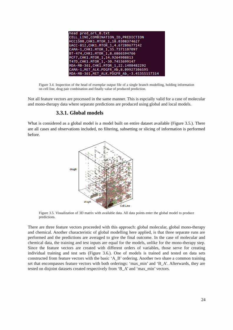
Figure 3.4. Inspection of the head of exemplar output file of a single branch modelling, holding informationon cell line, drug pair combination and finally value of produced prediction.

Not all feature vectors are processed in the same manner. This is espcially valid for a case of molecularand mono-therapy data where separate predictions are produced using global and local models.

3.3.1. Global models

What is considered as a global model is a model built on entire dataset available (Figure 3.5.). Thereare all cases and observations included, no filtering, subsetting or slicing of information is performedbefore.

Figure 3.5. Visualization of 3D matrix with available data. All data points enter the global model to producepredictions.

There are three feature vectors proceeded with this approach: global molecular, global mono-therapyand chemical. Another characteristic of global modelling here applied, is that three separate runs areperformed and the predictions are averaged to give the final outcome. In the case of molecular andchemical data, the training and test inputs are equal for the models, unlike for the mono-therapy step.Since the feature vectors are created with different orders of variables, those serve for creatingindividual training and test sets (Figure 3.6.). One of models is trained and tested on data setsconstructed from feature vectors with the basic ‘A_B’ ordering. Another two share a common trainingset that encompasses feature vectors with both orderings: ‘max_min’ and ‘B_A’. Afterwards, they aretested on disjoint datasets created respectively from ‘B_A’ and ‘max_min’ vectors.

24

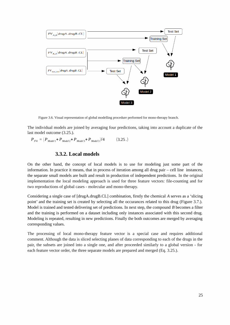
Figure 3.6. Visual representation of global modelling procedure performed for mono-therapy branch.

The individual models are joined by averaging four predictions, taking into account a duplicate of thelast model outcome (3.25.).

3.3.2. Local models

On the other hand, the concept of local models is to use for modeling just some part of theinformation. In practice it means, that in process of iteration among all drug pair – cell line instances,the separate small models are built and result in production of independent predictions. In the originalimplementation the local modeling approach is used for three feature vectors: file-counting and fortwo reproductions of global cases - molecular and mono-therapy.

Considering a single case of [drugA.drugB.CL] combination, firstly the chemical A serves as a ‘slicingpoint’ and the training set is created by selecting all the occurances related to this drug (Figure 3.7.).Model is trained and tested delivering set of predictions. In next step, the compound B becomes a filterand the training is performed on a dataset including only instances associated with this second drug.Modeling is repeated, resulting in new predictions. Finally the both outcomes are merged by averagingcorresponding values.

The processing of local mono-therapy feature vector is a special case and requires additionalcomment. Although the data is sliced selecting planes of data corresponding to each of the drugs in thepair, the subsets are joined into a single one, and after proceeded similarly to a global version - foreach feature vector order, the three separate models are prepared and merged (Eq. 3.25.).

25

(3.25 .)PFVi = ( PModel 1+ PModel 2+ PModel 3+ PModel 3 )/4

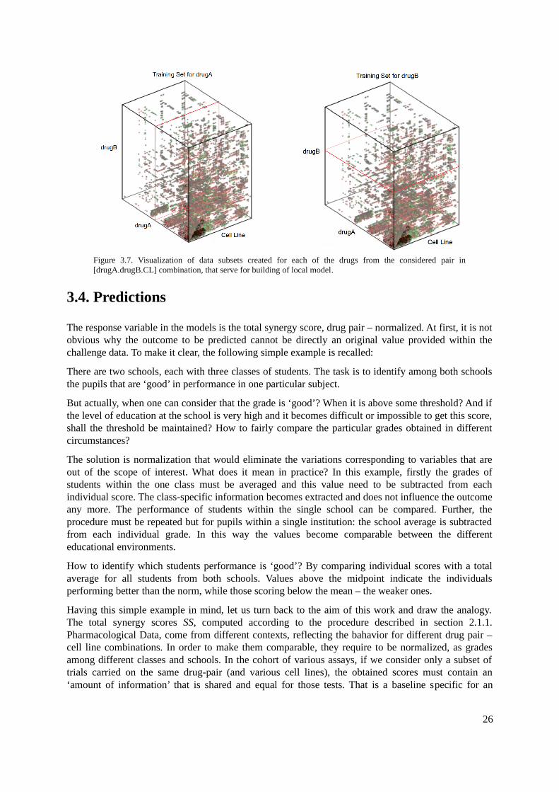
Figure 3.7. Visualization of data subsets created for each of the drugs from the considered pair in[drugA.drugB.CL] combination, that serve for building of local model.

3.4. Predictions

The response variable in the models is the total synergy score, drug pair – normalized. At first, it is notobvious why the outcome to be predicted cannot be directly an original value provided within thechallenge data. To make it clear, the following simple example is recalled:

There are two schools, each with three classes of students. The task is to identify among both schoolsthe pupils that are ‘good’ in performance in one particular subject.

But actually, when one can consider that the grade is ‘good’? When it is above some threshold? And ifthe level of education at the school is very high and it becomes difficult or impossible to get this score,shall the threshold be maintained? How to fairly compare the particular grades obtained in differentcircumstances?

The solution is normalization that would eliminate the variations corresponding to variables that areout of the scope of interest. What does it mean in practice? In this example, firstly the grades ofstudents within the one class must be averaged and this value need to be subtracted from eachindividual score. The class-specific information becomes extracted and does not influence the outcomeany more. The performance of students within the single school can be compared. Further, theprocedure must be repeated but for pupils within a single institution: the school average is subtractedfrom each individual grade. In this way the values become comparable between the differenteducational environments.

How to identify which students performance is ‘good’? By comparing individual scores with a totalaverage for all students from both schools. Values above the midpoint indicate the individualsperforming better than the norm, while those scoring below the mean – the weaker ones.

Having this simple example in mind, let us turn back to the aim of this work and draw the analogy.The total synergy scores SS, computed according to the procedure described in section 2.1.1.Pharmacological Data, come from different contexts, reflecting the bahavior for different drug pair –cell line combinations. In order to make them comparable, they require to be normalized, as gradesamong different classes and schools. In the cohort of various assays, if we consider only a subset oftrials carried on the same drug-pair (and various cell lines), the obtained scores must contain an‘amount of information’ that is shared and equal for those tests. That is a baseline specific for an

26

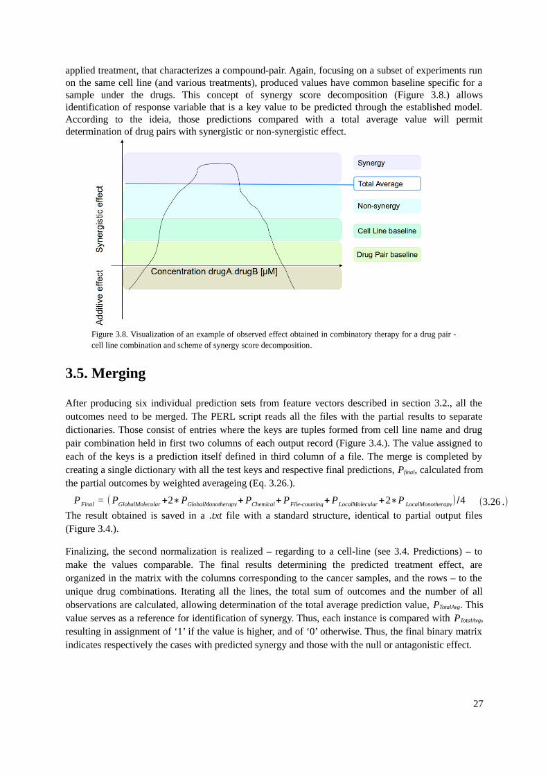
applied treatment, that characterizes a compound-pair. Again, focusing on a subset of experiments runon the same cell line (and various treatments), produced values have common baseline specific for asample under the drugs. This concept of synergy score decomposition (Figure 3.8.) allowsidentification of response variable that is a key value to be predicted through the established model.According to the ideia, those predictions compared with a total average value will permitdetermination of drug pairs with synergistic or non-synergistic effect.

Figure 3.8. Visualization of an example of observed effect obtained in combinatory therapy for a drug pair -cell line combination and scheme of synergy score decomposition.

3.5. Merging

After producing six individual prediction sets from feature vectors described in section 3.2., all theoutcomes need to be merged. The PERL script reads all the files with the partial results to separatedictionaries. Those consist of entries where the keys are tuples formed from cell line name and drugpair combination held in first two columns of each output record (Figure 3.4.). The value assigned toeach of the keys is a prediction itself defined in third column of a file. The merge is completed bycreating a single dictionary with all the test keys and respective final predictions, Pfinal, calculated fromthe partial outcomes by weighted averageing (Eq. 3.26.).

The result obtained is saved in a .txt file with a standard structure, identical to partial output files(Figure 3.4.).

Finalizing, the second normalization is realized – regarding to a cell-line (see 3.4. Predictions) – tomake the values comparable. The final results determining the predicted treatment effect, areorganized in the matrix with the columns corresponding to the cancer samples, and the rows – to theunique drug combinations. Iterating all the lines, the total sum of outcomes and the number of allobservations are calculated, allowing determination of the total average prediction value, PTotalAvg. Thisvalue serves as a reference for identification of synergy. Thus, each instance is compared with PTotalAvg,resulting in assignment of ‘1’ if the value is higher, and of ‘0’ otherwise. Thus, the final binary matrixindicates respectively the cases with predicted synergy and those with the null or antagonistic effect.

27

(3.26 .)PFinal = (PGlobalMolecular +2∗PGlobalMonotherapy+ PChemical+ PFile-counting+ PLocalMolecular+2∗P LocalMonotherapy)/4

4. Implementation & Preliminary Results

4.1. Tools

The implementation of the machine learning model was accomplished using basically twoprogramming languages namely Python and R. This work involved also acquiring of some knowledgeand familiarity with the PERL (Practical Extraction and Report Language) since this is the languageused in original scripts written by Yuanfang Guan. In submitted solution, the predictive models weregenerated applying the Random Forest algorithm by calling TreeBagger() function provided byMATLAB. The developed implementation used the same approach however it was adopted to Renvironment and employed with randomForest() function.

4.1.1. Python

Python is one of the high-level programming languages successfully combining efficiency andbeginner-friendliness. According to the main goals of its designer, Guido van Rossum, it was createdto be productive and readable. As broadly applicable (Web, GUI, scripting, etc.), interactive and open-source, it gains the popularity among all communities. It is portable and extensible, and allows object-oriented programming [43].

In this work, Python 2.7 was utilized to efficiently handle with large amount of information, especiallyon data pre-processing, simulation and integration steps.

4.1.2. R

R is a free programming language and environment, one of the most popular among statisticians, dataanalysts, researchers and market specialists. It provides utilities to retrieve, clean, analyze, visualizeand report data. It was designed to be intuitive and to mirror the way the user think. It is interactive,vector-oriented and highly flexible language. R provides efficient utilities to handle missing values,almost impossible to avoid when working with real data [44].

In this implementation R 3.3.3 was used in data pre-processing, modeling and optimization steps. Itwas found very convenient and efficient due to the diverse functions that perfectly complemented thecapabilities of the Python.

4.1.3. Random Forests

Random Forests (RFs) are powerful supervised prediction tool for classification and regressionproblems. The very first method of random decision forests approach was introduced in 1995 by Tin

28

Kam Ho and its increased accuracy was proved in the experiment on the recognition of handwritingdigits [45]. It was later extended by including “bagging” and random selection of features [46][47].

RFs is an ensemble method, generating multiple fits and after all combining them to deliver improvedresults. The technique uses as a principal algorithm the standard decision trees, that separate the datainto homogenous subsets, according to the most important splitter. The predicted feature is representedby terminal nodes or leaves, and the branches are particular sets of predictors driving to cohortdivision. In brief, the algorithm of growing decision trees takes all the root node data and scansthrough descriptors for the best splitter (that is: for the one providing the most pure children nodes).The one chosen divides the data and children nodes become parent nodes since the same growing stepcontinues starting from them. The process continues until the terminal nodes are reached and the leafsinclude only homogenous subsets. However the individual trees built in greedy way are imperfect andcan easily miss the optimal solutions (the splitting decisions are made locally, instantaneously withoutany general view on final outcome and without the possibility to change the past divisions).

Though the RFs idea is to take the collection of weak single tree fits, ensemble them and derive thefinal outcome by averaging or voting. There is a high probability that the obtained summarized modelwould be superior than any of the individual, and that it would be resistant to overfitting. Thealgorithm of generating RFs includes steps as follow. (1) Specification of the N number of iterations.(2) Bootstrap sample is picked from the original population with replacement. (3) Number of randomdescriptors is selected according to the value defined by user. (4) Independent, individual tree is grownon this subset. (5) Steps 1 – 4 are repeated N-times. (6) Collect all the trees and produce summarizedoutcome.

The RFs method was used in this work to create a baseline implementation reproducing the approachof Yuanfang Guan.

4.1.4. Server

This work was performed on server with Intel(R) Xeon(R) processor of number E5-1620V4. Theprocessor base frequency of device was 3.50GHz while de number of cores – 8. It was equipped withRAM of 16GiB.

4.2. Outsourced Data

An additional prior knowledge was used in order to reduce the input size and to limit the data to thepotentially most informative and relevant. It was achieved with catalog of the cancer driver genes andmap of dosage-sensitive cancer genes.

4.2.1. IntOGen Mutations

In the development of the cancer there can be two types of alterations distinguished: driver, thatcontribute to the oncogenesis or that are relevant to the phenotype of the cancer, and passenger whichaccumulate through DNA replication but are not related to tumorigenesis. The Web platform IntOGenMutations, provides a comprehensive tool for identification of cancer drivers. The database is built onthe results of the systematic analysis of most currently available large data sets encompassing 28tumor types among 6792 samples, including in the effect 1341752 somatic mutations [48][49]. There

29

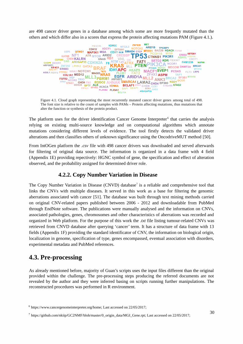
are 498 cancer driver genes in a database among which some are more frequntly mutated than theothers and which differ also in a scores that express the protein affecting mutations PAM (Figure 4.1.).

Figure 4.1. Cloud graph representing the most recurrently mutated cancer driver genes among total of 498.The font size is relative to the count of samples with PAMs – Protein affecting mutations, thus mutations thatalter the function or synthesis of the protein product.

The platform uses for the driver identification Cancer Genome Interpreter6 that carries the analysisrelying on existing multi-source knowledge and on computational algorithms which annotatemutations considering different levels of evidence. The tool firstly detects the validated driveralterations and then classifies others of unknown significance using the OncodriveMUT method [50].

From IntOGen platform the .csv file with 498 cancer drivers was downloaded and served afterwardsfor filtering of original data source. The information is organized in a data frame with 4 field(Appendix 1E) providing repectively: HGNC symbol of gene, the specification and effect of alterationobserved, and the probability assigned for determined driver role.

4.2.2. Copy Number Variation in Disease

The Copy Number Variation in Disease (CNVD) database7 is a reliable and comprehensive tool thatlinks the CNVs with multiple diseases. It served in this work as a base for filtering the genomicaberrations associated with cancer [51]. The database was built through text mining methods carriedon original CNV-related papers published between 2006 - 2012 and downloadable from PubMedthrough EndNote software. The publications were manually analysed and the information on CNVs,associated pathologies, genes, chromosomes and other characteristics of aberrations was recorded andorganized in Web platform. For the purpose of this work the .txt file listing tumour-related CNVs wasretrieved from CNVD database after querying ‘cancer’ term. It has a structure of data frame with 13fields (Appendix 1F) providing the standard identificator of CNV, the information on biological origin,localization in genome, specification of type, genes encompassed, eventual association with disorders,experimental metadata and PubMed references.

4.3. Pre-processing

As already mentioned before, majority of Guan’s scripts uses the input files different than the originalprovided within the challenge. The pre-processing steps producing the referred documents are notrevealed by the author and they were inferred basing on scripts running further manipulations. Thereconstructed procedures was performed in R environment.

30

6 https://www.cancergenomeinterpreter.org/home; Last accessed on 22/05/2017;

7 https://github.com/nkiip/GC2NMF/blob/master/0_origin_data/MGI_Gene.rpt; Last accessed on 22/05/2017;

4.2.1. Molecular Input

The objective of this step is to generate a set of six matrices corresponding to each molecular datasource, with an unform organization. The respective matrices were saved in output .txt files holdingthe cell lines in columns and gene names in rows. Each of the original files required slightly differenttreatments and procedures since they were not uniquely structured, they dealt with various problemsand demanded specific filtrations. Note, that this pre-processing steps are valid for both- global andlocal, molecular feature vectors.

RNA expression

While reading a .csv source file to a data frame in R, the attention must be paid since some slightautomatic changes may occure in column and row names, as in the case of expression data source.The alterations took place for the cell line identificators strating with a numerical characters (theyreceived a prefix ‘X’) and for those containing hyphen sign within the name (hyphen turned dot).Those alterations are not severe however prevents the correct recognition and so needed to be fixed.After dealing with this feilure, the data frame was transposed to the requested standard conformation.Finally, two instances holding NA values were bound to the matrix, preparing the entries for cell linesfor which expression data is missing (MDA-MB-175-VII, NCI-H1437) and would be imputedafterwards.

Copy number

According to the CNV definition in Genomics of Drug Sensitivity in Cancer8, in order to consider agene as amplified it needs to hold at least 8 copies, while to be recognized as deleted – no copy can beobserved (the homozygous deletion, on both alleles). Following this interpretation, after reading a fileto R working space, only the valid abberations listed in original CNV data source were selected. Inorder to avoid sex-dependent bias, additional filtering was performed and the alterations located on Ychromosome were excluded. Due to a large size of a data set and difficulties in handling, it wasdecided to limit the feature vector and include only the CNVs located in dosage-sensitive cancergenes. Those were determined using as areference the file outsourced from the Copy NumberVariation in Disease (CNVD) database (4.2.2. Copy Number Variation in Disease). The finalmolecular matrix was generated and the data was binarized assigning to each gene - cell linecombination a CNV status: ‘0’ corresponding to an absence of an aberration and ‘1’ standing for apresence of 1 or more CNVs.

DNA sequence

Again, preselection of relevant genes was necessary to achieve construction of realizableimplementation. Thus, only the mutations located in the driver genes were included in generation ofmolecular matrix. This filtering was performed according to the file outsourced from the IntoGenplatform (4.2.1. IntOGen Mutations). Secondly, the irrelevant mutations were excluded by removal ofthe instances assigned in the original source file with ‘PASSENGER/OTHER’ status in FATHMMprediction, and those identified as ‘Confirmed somatic variant’. The binary matrix was createdsimilarly to CNV case - by assignment of the mutation status to each gene - cell line: ‘0’corresponding to an absence of a variant and ‘1’ standing for a presence of 1 or more mutations.

DNA methylation

The pre-processing of the methylation data source initialized with the assignment of the genes to theprobes and removel of instances without genetic annotation. As in the case of expression file, the cellline names required corrections due to an automatic modifications introduced by R. Another issue –presence of multi-gene probes, was solved by multiplication of those instances by the number ofassigned genes and identification of each entry with a single gene annotation. The data frame was

318 http://www.cancerrxgene.org/; Last accessed on 27/09/2017;

transposed to create a matrix with a standard structure. It was extended by three instances holding NAvalues for missing cell lines (MDA-MB-175-VII, SW620, KMS-11) that served for future imputation.

CCLE RNA expression

In order to generate standard matrix summarizing expression data provided by CCLE, the instances inoriginal file were assigned with the genes and than filtered retaining only the probes with theannotations. The automatically introduced failures in cell line names were corrected turning theidentificators consistent with the Sanger nomenclature. The data was subset selecting only theinformation related to cancer samples included in experiments. Three instances holding NA valueswere introduced to the data frame, simulating the entries for missing cell lines: M14, MFM-223, NCI-H3122. One of the genes, TTL, was found to be assigned to two different probes. The issue wasovercome by keeping a single instance with a median value.

CCLE copy number

After the reading of an original file to a data frame in R, a correction step was required to obtainHGNC standarized cell line names. The instances corresponding to the cancer samples covered by thechallenge experiments were selected. As for CCLE expression data source, value for the same set ofcell lines is unavailable: M14, MFM-223, NCI-H3122. Thus, the molecular matrix is extended bythree entries holding NAs for posterior imputation.

Both datasets outsourced from CCLE required additional pre-processing step, run in Python,translating the internal nomenclature of sample to normalized primary cell line names. The conversionwas performed using as a reference .txt file outsourced from the CCLE platform, that contains cell-linemetadata from the cancer lines used in drug sensitivity screens.

4.2.2. Pharmacological Input

As one of the inputs for the mono-therapy feature vector serve the .csv files on the experimental resultsof the single-compound assays (see 2.1.1. Pharmacological Data). The number of files storing the datais higher than the number of drug pair - cell line combinations tested. The reason is that some of thetrials were repeated several times due to the problems in the performance. The accurate determinationof experimental file of origin for each of instances was a challenge. Different approaches wereundertaken: determination by quality score, by exclusion, by manual curve-fitting etc. but noneachieved to unequivocally identify the correct data source. The reproduction of dosage-response curvefitting performed automatically with Combenefit software was not attained. Due to this issue, it wasdecided to exclude the multi-source observations since those could introduce bias to the model. Thus,123 of total 2199 drug pair - cell line combinations were not included in further processing, andfeature vectors were constructed basing on 2076 unambiguous cases.

4.2.2. Compound Input

The input file holding information on chemical and structural drug characteristics (2.1.3. CompoundData) deals with large amount of missing data: among 119 observations only 58 contain completeinformation. Firstly, it was tempted to estimate the unavailable values basing on known measurementsof the most similar compounds, averaging them. However, this approach was not efficient and sincethe rfInput() function of R provides far easier solution and much better outcome, it becomeimplemented in script. No other pre-modelig steps were required for this data source.

32

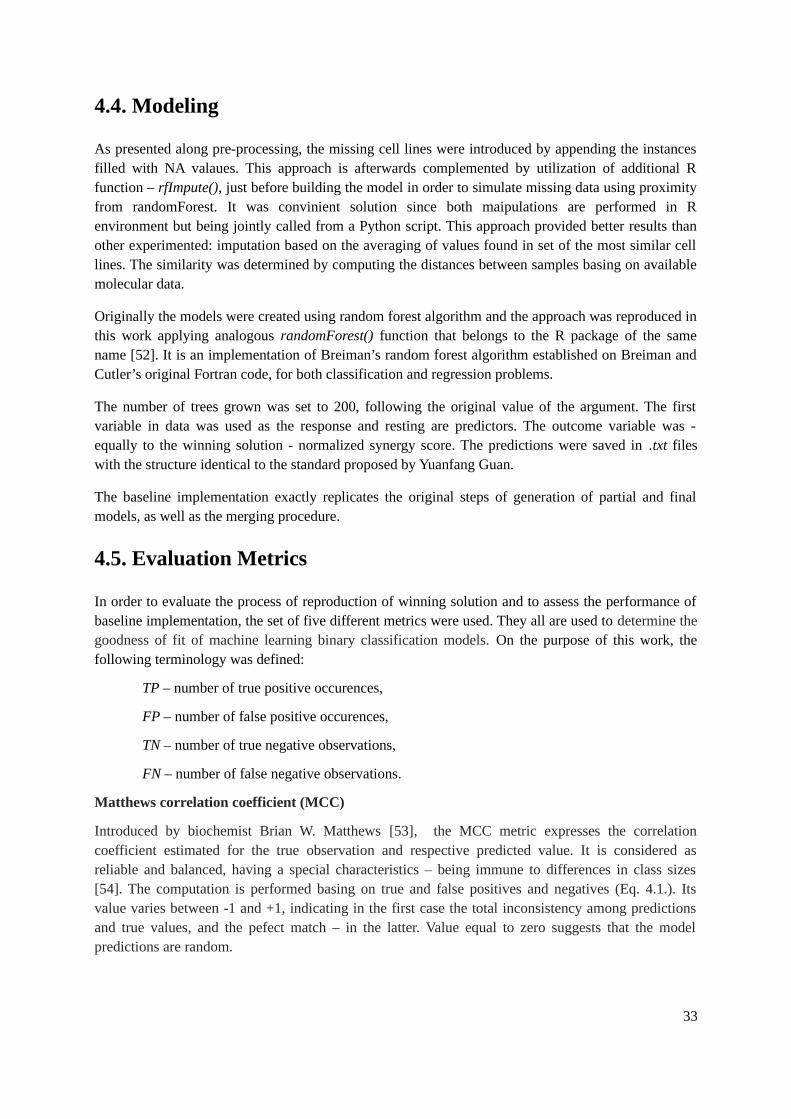
4.4. Modeling

As presented along pre-processing, the missing cell lines were introduced by appending the instancesfilled with NA valaues. This approach is afterwards complemented by utilization of additional Rfunction – rfImpute(), just before building the model in order to simulate missing data using proximityfrom randomForest. It was convinient solution since both maipulations are performed in Renvironment but being jointly called from a Python script. This approach provided better results thanother experimented: imputation based on the averaging of values found in set of the most similar celllines. The similarity was determined by computing the distances between samples basing on availablemolecular data.

Originally the models were created using random forest algorithm and the approach was reproduced inthis work applying analogous randomForest() function that belongs to the R package of the samename [52]. It is an implementation of Breiman’s random forest algorithm established on Breiman andCutler’s original Fortran code, for both classification and regression problems.

The number of trees grown was set to 200, following the original value of the argument. The firstvariable in data was used as the response and resting are predictors. The outcome variable was -equally to the winning solution - normalized synergy score. The predictions were saved in .txt fileswith the structure identical to the standard proposed by Yuanfang Guan.

The baseline implementation exactly replicates the original steps of generation of partial and finalmodels, as well as the merging procedure.

4.5. Evaluation Metrics

In order to evaluate the process of reproduction of winning solution and to assess the performance ofbaseline implementation, the set of five different metrics were used. They all are used to determine thegoodness of fit of machine learning binary classification models. On the purpose of this work, thefollowing terminology was defined:

TP – number of true positive occurences,

FP – number of false positive occurences,

TN – number of true negative observations,

FN – number of false negative observations.

Matthews correlation coefficient (MCC)

Introduced by biochemist Brian W. Matthews [53], the MCC metric expresses the correlationcoefficient estimated for the true observation and respective predicted value. It is considered asreliable and balanced, having a special characteristics – being immune to differences in class sizes[54]. The computation is performed basing on true and false positives and negatives (Eq. 4.1.). Itsvalue varies between -1 and +1, indicating in the first case the total inconsistency among predictionsand true values, and the pefect match – in the latter. Value equal to zero suggests that the modelpredictions are random.

33

Matthews CorrelationCoefficient MCC=TP∗TN −FP∗FN

√(TP+FP )∗(TP+FN )∗(TN +FP)(TN + FN )(4.1 .)

Sensitivity

This metric is also known as true positive rate, recall or probability of detection, depending on thefield where is applied. Its value represents the proportion of positive instances correctly dermined bythe model (Eq. 4.2.) [54]. The sensitivity can be interpreted as manner of quantification of avoiding offalse negatives.

Sensitivity=TP

TP+FN(4.2 .)

Specificity

Another popular denomination of this metric is true negative rate and it is just opposite to sensitivity. Itexpresses the proportion of negatives observations correctly indicated as such by the model (Eq. 4.3.)[54]. Analogously, it provides a manner of quantification of avoiding the false positives.

Specificity=TN

TN +FP(4.3 .)

Accuracy

The difference between a prediction and a true value can be expressed by accuracy. It is a ratio of allobservations correctly identified by model total number of instances (Eq. 4.4.) [54]. This metricreflects how close the estimations and observations are. Although, very informative, the accuracy issensitive to imbalances in classes sizes (that is a case of this work).

Accuracy=TP+TN

TP+TN +FP+FN(4.4 .)

Balanced Accuracy

In some circumstances accuracy estimate may become more optimistic then the reality is. Toovercome this issue more general metric may be used – balanced accuracy, that is simply the theaverage accuracy obtained on either class (4.5.) [55].

Balanced Accuracy BAC=(TP

TP+FN+

TNTN+FP

)/2 (4.5 .)

4.6. Results

As mentioned in the introduction, after establishing the functional baseline implementation, the workwas presented to a small public, in order to reflect on obtained results and to determine furtherdirections.

The model was evaluated including the specific feature vectors one by one. The reason for thisapproach was to monitor the behavior after single inclusions and to have an idea on impact that eachof the specific data source has on the overall outcome. Moreover, the generation of predictions was atime-consuming process, especially in the case of molecular data sources so the results were producedgradually. The predictions created on local molecular feature vectors were never obtained throught thebaseline implementation – the run was killed after 2 weeks of processing. The results are summarizedin table 4.3.

34

Table 4.3. The partial result of evaluation of baseline implementation.

Model MCC Sensitivity Specificity ACC

Global Molecular 0.62637 0.63212 0.97828 0.95589

+ Chemical 0.61702 0.63007 0.97683 0.95449

+ Global Mono-therapy 0.73367 0.74397 0.98353 0.96804

+ File-counting 0.71282 0.71780 0.98297 0.96581

+ Local Mono-therapy 0.74383 0.76398 0.98304 0.96887

+ Local Molecular n/a n/a n/a n/a

Some conclusions may be formed basing on the data presented above. Firstly, apparently the inclusionof chemical and file-counting data hurts the model causing a drop of all evaluation metrics. The bestscores are obtained after including the predictions originated from a local mono-therapy featurevectors – this step boost the model.

Generally the values are optimistically good. Investigating the reason of observation such high scores,the failures and imperfections of the experiment design were found. It must be reminded that thisresults were obtained testing a model on the original test set from the challenge. This fact implies that,since true values had not been published yet, the implementation was evaluated using as a referencematrix the final outcomes submitted by Yuanfang Guan, assumed as a ‘true’ on the purpose of thiswork. Moreover, the assessment was performed including all the possible combinations, while the ‘0’values indicating non-synergic effect were assigned also to the unknown cases. That means that thenumber of true negative is falsely elevated and the values obtained for specificity proves it.

According to this conclusions it was decided to on the purpose of this project construct a new trainingand test sets, from the available and known challenge data. The new subsets had to reconstruct theoriginal circumnstances what in practice meant that they had to be totally disjoint on drug pairs. Theywere balanced in size, holding 30% and 70% of data by respectively test and training sets.

It was decided that in order to obtain reliable evaluation scores the model assessment must beperformed exclusively on the test instances, neverthless that an entire matrix holding all possiblecombinations is produced. The alterations were introduced into the script and the unknown casesalthough still present in prediction matrix, they become to be assigned with NA values.

Furthermore, three directions of future work to be developed were defined:

1) Feature selection;

2) Alternative models;

3) Predictions-merging equation.

35

5. Model Improvement

Since the molecular data source deals with abundance of variables, the main point of the focus was toreduce the number of features included in the model selecting only the informative ones. The aim wasalso to determine the most important variables because those could be the potential biomarkers.

The baseline implementation follows the winning solution building the models with Random Forestsalgorithm. However there is no evidence provided by the Yuanfang Guan that this approach is the mostproper for the challenge problem. In this work an efforts were made to test the performance with twoothers methods: Support Vector Machine (SVM) and Multivariate Adaptive Regression Splines(MARS).

Moreover, the attempts were also directed at establishment of optimal merging equation since noinformation is available confirming that the version implemented in original script is the most accurateone. The establishment of used coefficients is not reported in the submission documentation, neither inPERL scripts.

5.1. Feature Selection

Feature selection in machine learning approaches is very often a requisite step for model building.Nowadays it is necessary to deal with large datasets with many variables since the production of thedata is rather not an issue anymore. This fact brings two complications:

1) most of the variables are not relevant, they do not contribute to the model or even can cause adecrease of accuracy. Those preferably should not be included in the feature set at all.

2) high technical requirements. Large datasets are demanding to deal with because they highly slowdown the process and may turn it impossible to run in reasonable time. Also they need many resourcesthat are often unreachable for one.

Thus it is preferable to select possibly the smallest set of variables that would ensure the optimalresults and manageable data size. It is necessary to find an approach that would identify all ofattributes with their relevance to the model, indicating those that shall be retained and included in theprocess.

5.1.1. Tools

Least Absolute Shrinkage and Selection Operator

Least Absolute Shrinkage and Selection Operator (LASSO) is a supervised regression machinelearning method using a shrinkage [56]. The approach generates simple and sparse models, especially

36

convenient in the case of high multicollinearity among variables where only most important featuresare selected.

The principle of the lasso is shrinkage that is in general bringing down of values to some central point.Since the method requires a constant threshold defining the maximum sum of the absolute modelparameters, it implies that some variable coefficients would be reduced to 0. In the effect the shrunkmodel will include fewer features, those for which the coefficients remain different from 0. Thefeatures selection step allows to determine the predictors highly associated with the respond variableand minimizing the error related to the outcome. Also, due to such a simplification, the interpretationof model becomes improved and user-friendly. The lasso is able to provide models of high accuracyand is especially useful when there are relatively low number of instances and high number ofpredictors.

The simplicity of lasso regression is also in a tuning by a single parameter λ, that controls strength ofthe penalty. The higher value of parameter, the more reduced model is obtained what means that morecoefficients are turned to 0.

Boruta

Boruta is an ‘all-relevant’ wrapper algorithm for feature selection through the variable importancemeasure (VIM) [57]. It identifies variables correlated with the response more than random ones. Bydefault it is built around the random forest classification but the function is able to work with any othermethod for which the importance metric is available. In short, Boruta selects the relevant featurescomparing their original importance with the random estimations from permuted copies. The search isrun top-down and irrelevant attributes are eliminated gradually.

The idea of approach was inspired on RFs methodology where the randomness is introduced to theanalysed system and the results are obtained from an enseble of samples picked by chance [58]. In thisway the added randomness reduces the tricking influence of casual variations and non significativecorrelations, and meanwhile it is supposed to expose the truly important features. The main steps ofalgorithm include: (1) The system is enriched with extra copies of all attributes (so called shadowfeatures). (2) The added variables are shuffled removing the random correlations. (3) The default RFsclassification algorithm (applied here due to its quickness, no need for parameter tunning and theoutput of numerical estimation of importance) is run and the VIM values are obtained for enricheddata (mean decrease accuracy by default). (4) For each attribute, the Z- score is compared with themaximum value observed among all its shadow features. If scoring significantly higher, the variable isrecognized as important and kept in data system, otherwise it is assigned as non-informative andpermanently eliminated. (5) The procedure is repeated untill all the attributes are identified withconfirmation/rejection status or when the limit of RFs runs is reached.

5.1.2. Methods

Overall, the establishing of feature selection approach for molecular data sources was one of the mostlaborious stages of the project. The workflow was changed and adjusted along the progress. The finalprocedure is visualized graphically on figure 5.1. and described in details within the followingsections.

The various attempts were performed to define the set of the most informative features with Borutaalgorithm. However, the methodology was found inconvenient in this work due to inconvinientrelative values expressing the importance and low reproducibility of results with such a high number

37

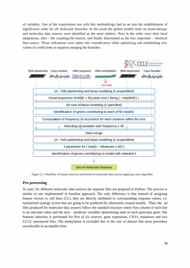
of variables. One of the experiments run with this methodology had as an aim the establishment ofsignificance order for all molecular branches. In the result the global models built on mono-therapyand molecular data sources were identified as the most relative. Next in the order were their localadaptations, after - the counting-file branch, and finally determined as the less important – chemicaldata source. Those indications were taken into consideration while optimizing and establishing newvalues of coefficients in equation merging the branches.

Figure 5.1. Workflow of feature selection performed on molecular data sources applying Lasso algorithm.

Pre-processing

To start, for different molecular data sources the separate files are prepared in Python. The process issimilar to one implemented in baseline approach. The only difference is that instead of assigningfeature vectors to cell lines [CL], they are directly attributed to corresponding response values, i.e.normalized synergy scores that are going to be predicted by afterwards created models. Thus, the .txtfiles produced for molecular data sources follow the standard structure where first column of each lineis an outcome value and the next – predictor variables determining state of each particular gene. Thefeatures selection is performed for five of six sources: gene expression, CNVs, mutations and twoCCLE outsourced files. The methylation is excluded due to the size of dataset that turns procedureunrealizable in acceptable time.

38

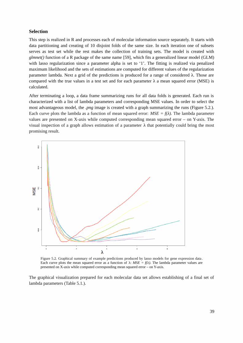
Selection

This step is realized in R and processes each of molecular information source separately. It starts withdata partitioning and creating of 10 disjoint folds of the same size. In each iteration one of subsetsserves as test set while the rest makes the collection of training sets. The model is created withglmnet() function of a R package of the same name [59], which fits a generalized linear model (GLM)with lasso regularization since a parameter alpha is set to ‘1’. The fitting is realized via penalizedmaximum likelihood and the sets of estimations are computed for different values of the regularizationparameter lambda. Next a grid of the predictions is produced for a range of considered λ. Those arecompared with the true values in a test set and for each parameter λ a mean squared error (MSE) iscalculated.

After terminating a loop, a data frame summarizing runs for all data folds is generated. Each run ischaracterized with a list of lambda parameters and corresponding MSE values. In order to select themost advantageous model, the .png image is created with a graph summarizing the runs (Figure 5.2.).Each curve plots the lambda as a function of mean squared error: MSE = f(λ). The lambda parametervalues are presented on X-axis while computed corresponding mean squared error – on Y-axis. Thevisual inspection of a graph allows estimation of a parameter λ that potentially could bring the mostpromising result.

Figure 5.2. Graphical summary of example predictions produced by lasso models for gene expression data .Each curve plots the mean squared error as a function of λ: MSE = f(λ). The lambda parameter values arepresented on X-axis while computed corresponding mean squared error – on Y-axis.

The graphical visualization prepared for each molecular data set allows establishing of a final set oflambda parameters (Table 5.1.).

39

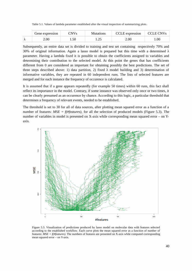
Table 5.1. Values of lambda parameter established after the visual inspection of summarizing plots.

Gene expression CNVs Mutations CCLE expression CCLE CNVs

λ 2.00 1.50 1.25 2.00 1.00

Subsequently, an entire data set is divided to training and test set containing respectively 70% and30% of original information. Again a lasso model is prepared but this time with a determined λparameter. Having a lambda fixed it is possible to obtain the coefficients assigned to variables anddetermining their contribution to the selected model. At this point the genes that has coefficientsdifferent from 0 are considered as important for obtaining possibly the best predictions. The set ofthree steps described above: 1) data partition, 2) fixed λ model building and 3) determination ofinformative variables, they are repeated in 60 independent runs. The lists of selected features aremerged and for each instance the frequency of occurence is calculated.

It is assumed that if a gene appears repeatedly (for example 50 times) within 60 runs, this fact shallreflect its importance in the model. Contrary, if some instance was observed only once or two times, itcan be clearly presumed as an occurence by chance. According to this logic, a particular threshold thatdetermines a frequency of relevant events, needed to be established.

The threshold is set to 30 for all of data sources, after plotting mean squared error as a function of anumber of features: MSE = f(#features), for all the selection of produced models (Figure 5.3). Thenumber of variables in model is presented on X-axis while corresponding mean squared error – on Y-axis.

Figure 5.3. Visualization of predictions produced by lasso model on molecular data with features selectedaccording to the established workflow. Each curve plots the mean squared error as a function of number offeatures: MSE = f(#features). The numbers of features are presented on X-axis while computed correspondingmean squared error – on Y-axis.

40

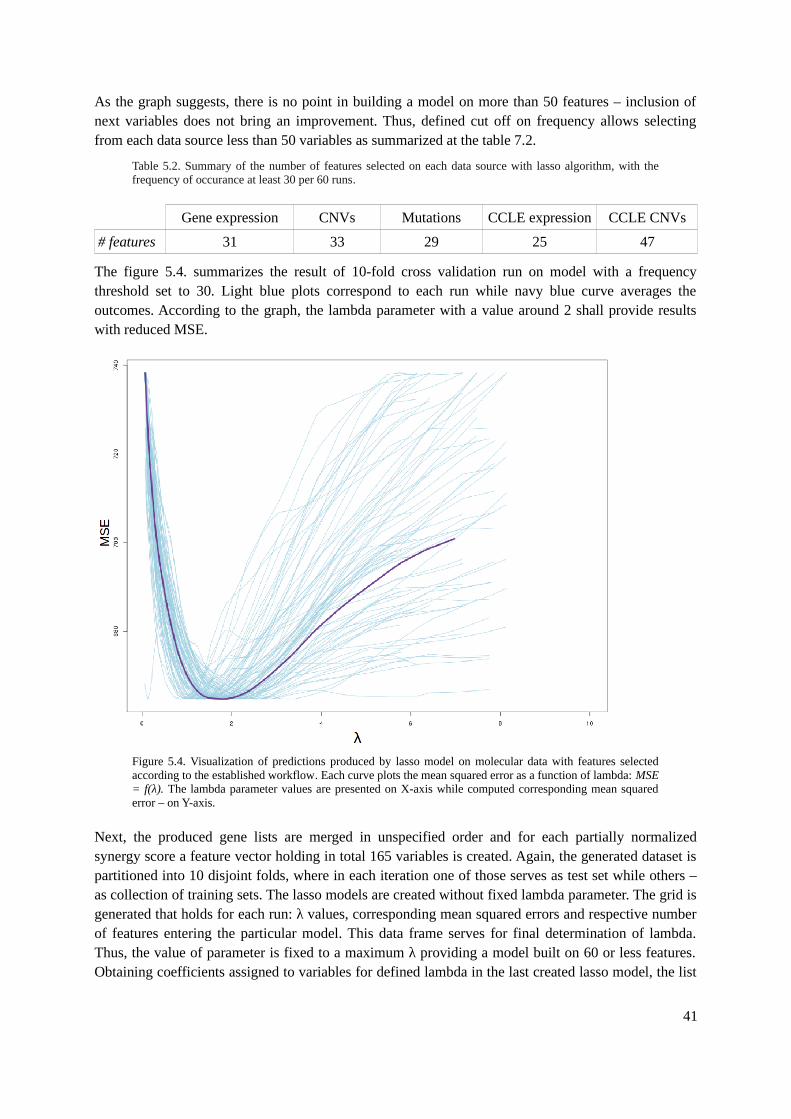
As the graph suggests, there is no point in building a model on more than 50 features – inclusion ofnext variables does not bring an improvement. Thus, defined cut off on frequency allows selectingfrom each data source less than 50 variables as summarized at the table 7.2.

Table 5.2. Summary of the number of features selected on each data source with lasso algorithm, with thefrequency of occurance at least 30 per 60 runs.

Gene expression CNVs Mutations CCLE expression CCLE CNVs

# features 31 33 29 25 47

The figure 5.4. summarizes the result of 10-fold cross validation run on model with a frequencythreshold set to 30. Light blue plots correspond to each run while navy blue curve averages theoutcomes. According to the graph, the lambda parameter with a value around 2 shall provide resultswith reduced MSE.

Figure 5.4. Visualization of predictions produced by lasso model on molecular data with features selectedaccording to the established workflow. Each curve plots the mean squared error as a function of lambda: MSE= f(λ). The lambda parameter values are presented on X-axis while computed corresponding mean squarederror – on Y-axis.

Next, the produced gene lists are merged in unspecified order and for each partially normalizedsynergy score a feature vector holding in total 165 variables is created. Again, the generated dataset ispartitioned into 10 disjoint folds, where in each iteration one of those serves as test set while others –as collection of training sets. The lasso models are created without fixed lambda parameter. The grid isgenerated that holds for each run: λ values, corresponding mean squared errors and respective numberof features entering the particular model. This data frame serves for final determination of lambda.Thus, the value of parameter is fixed to a maximum λ providing a model built on 60 or less features.Obtaining coefficients assigned to variables for defined lambda in the last created lasso model, the list

41

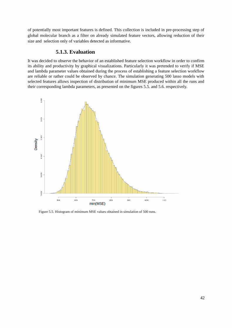
of potentially most important features is defined. This collection is included in pre-processing step ofglobal molecular branch as a filter on already simulated feature vectors, allowing reduction of theirsize and selection only of variables detected as informative.

5.1.3. Evaluation

It was decided to observe the behavior of an established feature selection workflow in order to confirmits ability and productivity by graphical visualizations. Particularly it was pretended to verify if MSEand lambda parameter values obtained during the process of establishing a feature selection workfloware reliable or rather could be observed by chance. The simulation generating 500 lasso models withselected features allows inspection of distribution of minimum MSE produced within all the runs andtheir corresponding lambda parameters, as presented on the figures 5.5. and 5.6. respectively.

Figure 5.5. Histogram of minimum MSE values obtained in simulation of 500 runs.

42

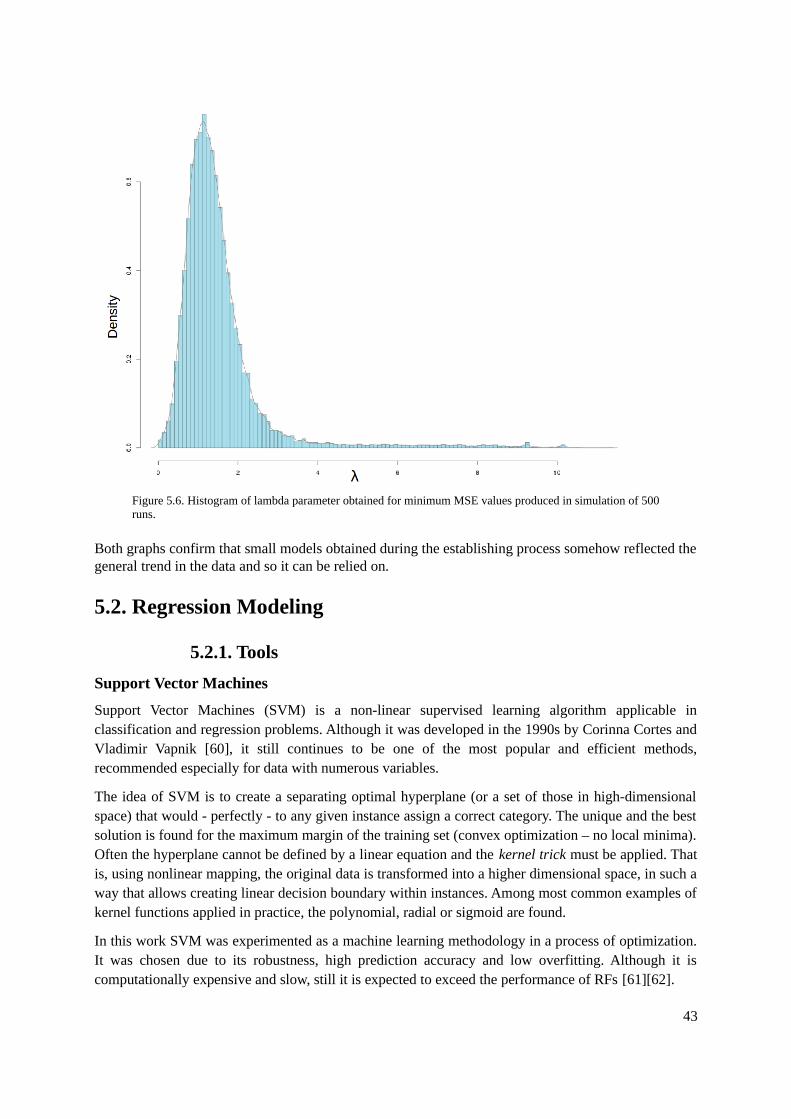
Figure 5.6. Histogram of lambda parameter obtained for minimum MSE values produced in simulation of 500runs.

Both graphs confirm that small models obtained during the establishing process somehow reflected thegeneral trend in the data and so it can be relied on.

5.2. Regression Modeling

5.2.1. Tools

Support Vector Machines

Support Vector Machines (SVM) is a non-linear supervised learning algorithm applicable inclassification and regression problems. Although it was developed in the 1990s by Corinna Cortes andVladimir Vapnik [60], it still continues to be one of the most popular and efficient methods,recommended especially for data with numerous variables.

The idea of SVM is to create a separating optimal hyperplane (or a set of those in high-dimensionalspace) that would - perfectly - to any given instance assign a correct category. The unique and the bestsolution is found for the maximum margin of the training set (convex optimization – no local minima).Often the hyperplane cannot be defined by a linear equation and the kernel trick must be applied. Thatis, using nonlinear mapping, the original data is transformed into a higher dimensional space, in such away that allows creating linear decision boundary within instances. Among most common examples ofkernel functions applied in practice, the polynomial, radial or sigmoid are found.

In this work SVM was experimented as a machine learning methodology in a process of optimization.It was chosen due to its robustness, high prediction accuracy and low overfitting. Although it iscomputationally expensive and slow, still it is expected to exceed the performance of RFs [61][62].

43

Multivariate Adaptive Regression Splines

Multivariate Adaptive Regression Splines (MARS) is a nonparametric supervised learning algorithmfor regression and classification problems, that does not require any assumption about relationshipbetween predictors and the dependent variable. The existing correlations and functions are derived onthe basis of the original data. The general idea is to divide total data space and obtain groups ofinstances for which the local regression equation may be determined [63][64]. This is s reason whyMARS is suitable for large inputs, overcoming limitations of many other machine learningmethodologies.

The algorithm includes following steps: (1) generation of simple model with the constant basisfunction; (2) exploration of basis function space, with all possible variables and knots; (3) selection ofsolutions that provide the best model (those with minimal prediction error); (4) repetition of search-select steps (3 and 4) until the pre-defined complexity limit is achieved; (5) pruning eliminatingsolutions with the least contribution to the total goodness of model [65].

MARS being very promising, especially in complex data mining problems, was chosen to beexperimented in the model optimization and compared to the RFs and SVMs performance.

5.2.2. Methods

Regarding to the Support Vector Machine, it generates the models using svm() function providedwithin ‘e1071’ R package [66], that is based on implementation by Chang et al. [67]. In general, theconcept follows a sequence of steps:

1) Class separation – having two classes, the optimal separating hyperplane is established,always aiming the maximization of the margin between the closest instances of the two sets;

2) Dealing with overlapping classes – the instances that are incorrectly classified with builthyperplane are weighted down in order to minimize their impact;

3) Handling the nonlinearity – if the instances initially are not linearly separable, they areprojected via kernel techniques into an higher-dimensional space, allowing construction oflinear separator;

4) Problem solution – known techniques are adopted to solve a final quadratic optimizationproblem. [60]

An another experiments were carried implementing a Multivariate Adaptive Regression Splines(MARS) approach for building a model. The earth() function from R package of the same name [68]was utilized and a regression model was generated basing on Friedman’s techniques [69].

Although both algorithms surpass a Random Forest approach, always the SVM methodology is in afavour and brings the improvement into the final model.

5.3. Prediction-merging equation

The merging step reconstructed on original implementation of Yuanfang Guan, follows the generalequation presented already in section 3.5. and recalled below:

Thus, the originally applied coefficients are set to 0.25 for four branches: global and local molecular,

44

PFinal = (PGlobalMolecular +2∗PGlobalMonotherapy+ PChemical+ PFileCounting+ PLocalMolecular+2∗P LocalMonotherapy)/4

chemical and file-counting, while they are equal to 0.5 for both mono-therapy data sources. In thiswork an attempts were undertaken to optimize the merging equation and different versions ofcomputations were performed varying coefficient values between 0 and 2, in various combinations.Observation of the parameters and their final outcomes for chosen SVM model, allows establishing ofthe most efficient values. The identified coefficients are summarized in the optimized equation 7.1.

45

P Final = (2∗PGlobalMolecular+0.25∗PGlobalMonotherapy+0.25∗PChemical+0.25∗P FileCounting+0∗PLocalMolecular+0.25∗PLocalMonotherapy )

(5.1 .)

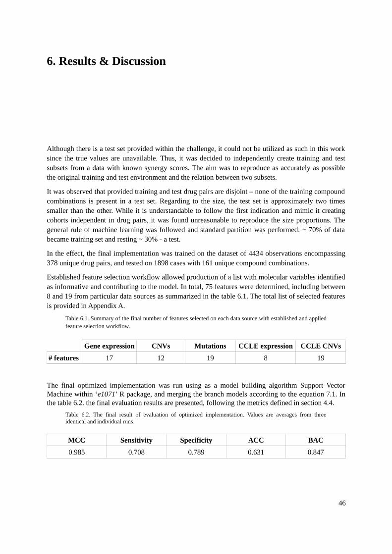
6. Results & Discussion

Although there is a test set provided within the challenge, it could not be utilized as such in this worksince the true values are unavailable. Thus, it was decided to independently create training and testsubsets from a data with known synergy scores. The aim was to reproduce as accurately as possiblethe original training and test environment and the relation between two subsets.

It was observed that provided training and test drug pairs are disjoint – none of the training compoundcombinations is present in a test set. Regarding to the size, the test set is approximately two timessmaller than the other. While it is understandable to follow the first indication and mimic it creatingcohorts independent in drug pairs, it was found unreasonable to reproduce the size proportions. Thegeneral rule of machine learning was followed and standard partition was performed: ~ 70% of databecame training set and resting ~ 30% - a test.

In the effect, the final implementation was trained on the dataset of 4434 observations encompassing378 unique drug pairs, and tested on 1898 cases with 161 unique compound combinations.

Established feature selection workflow allowed production of a list with molecular variables identifiedas informative and contributing to the model. In total, 75 features were determined, including between8 and 19 from particular data sources as summarized in the table 6.1. The total list of selected featuresis provided in Appendix A.

Table 6.1. Summary of the final number of features selected on each data source with established and appliedfeature selection workflow.

Gene expression CNVs Mutations CCLE expression CCLE CNVs

# features 17 12 19 8 19

The final optimized implementation was run using as a model building algorithm Support VectorMachine within ‘e1071’ R package, and merging the branch models according to the equation 7.1. Inthe table 6.2. the final evaluation results are presented, following the metrics defined in section 4.4.

Table 6.2. The final result of evaluation of optimized implementation. Values are averages from threeidentical and individual runs.

MCC Sensitivity Specificity ACC BAC

0.985 0.708 0.789 0.631 0.847

46

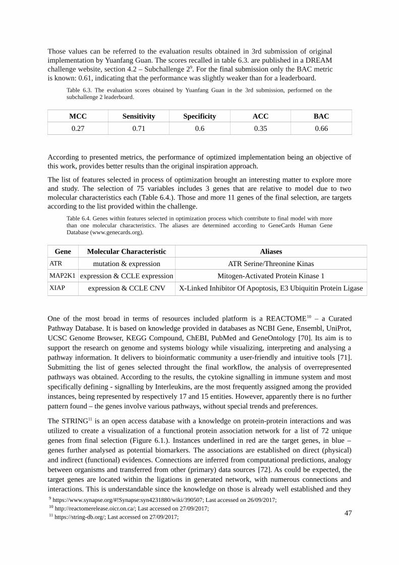
Those values can be referred to the evaluation results obtained in 3rd submission of originalimplementation by Yuanfang Guan. The scores recalled in table 6.3. are published in a DREAMchallenge website, section 4.2 – Subchallenge 29. For the final submission only the BAC metricis known: 0.61, indicating that the performance was slightly weaker than for a leaderboard.

Table 6.3. The evaluation scores obtained by Yuanfang Guan in the 3rd submission, performed on thesubchallenge 2 leaderboard.

MCC Sensitivity Specificity ACC BAC

0.27 0.71 0.6 0.35 0.66

According to presented metrics, the performance of optimized implementation being an objective ofthis work, provides better results than the original inspiration approach.

The list of features selected in process of optimization brought an interesting matter to explore moreand study. The selection of 75 variables includes 3 genes that are relative to model due to twomolecular characteristics each (Table 6.4.). Those and more 11 genes of the final selection, are targetsaccording to the list provided within the challenge.

Table 6.4. Genes within features selected in optimization process which contribute to final model with morethan one molecular characteristics. The aliases are determined according to GeneCards Human GeneDatabase (www.genecards.org).

Gene Molecular Characteristic Aliases

ATR mutation & expression ATR Serine/Threonine Kinas

MAP2K1 expression & CCLE expression Mitogen-Activated Protein Kinase 1

XIAP expression & CCLE CNV X-Linked Inhibitor Of Apoptosis, E3 Ubiquitin Protein Ligase

One of the most broad in terms of resources included platform is a REACTOME10 – a CuratedPathway Database. It is based on knowledge provided in databases as NCBI Gene, Ensembl, UniProt,UCSC Genome Browser, KEGG Compound, ChEBI, PubMed and GeneOntology [70]. Its aim is tosupport the research on genome and systems biology while visualizing, interpreting and analysing apathway information. It delivers to bioinformatic community a user-friendly and intuitive tools [71].Submitting the list of genes selected throught the final workflow, the analysis of overrepresentedpathways was obtained. According to the results, the cytokine signalling in immune system and mostspecifically defining - signalling by Interleukins, are the most frequently assigned among the providedinstances, being represented by respectively 17 and 15 entities. However, apparently there is no furtherpattern found – the genes involve various pathways, without special trends and preferences.

The STRING11 is an open access database with a knowledge on protein-protein interactions and wasutilized to create a visualization of a functional protein association network for a list of 72 uniquegenes from final selection (Figure 6.1.). Instances underlined in red are the target genes, in blue –genes further analysed as potential biomarkers. The associations are established on direct (physical)and indirect (functional) evidences. Connections are inferred from computational predictions, analogybetween organisms and transferred from other (primary) data sources [72]. As could be expected, thetarget genes are located within the ligations in generated network, with numerous connections andinteractions. This is understandable since the knowledge on those is already well established and they

47

9 https://www.synapse.org/#!Synapse:syn4231880/wiki/390507; Last accessed on 26/09/2017;10 http://reactomerelease.oicr.on.ca/; Last accessed on 27/09/2017;11 https://string-db.org/; Last accessed on 27/09/2017;

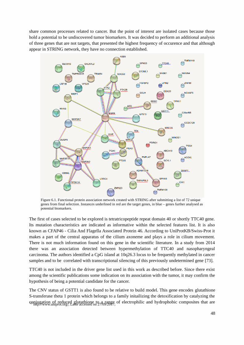
share common processes related to cancer. But the point of interest are isolated cases because thosehold a potential to be undiscovered tumor biomarkers. It was decided to perform an additional analysisof three genes that are not targets, that presented the highest frequency of occurence and that althoughappear in STRING network, they have no connection established.

Figure 6.1. Functional protein association network created with STRING after submitting a list of 72 unique genes from final selection. Instances underlined in red are the target genes, in blue – genes further analysed aspotential biomarkers.

The first of cases selected to be explored is tetratricopeptide repeat domain 40 or shortly TTC40 gene.Its mutation characteristics are indicated as informative within the selected features list. It is alsoknown as CFAP46 - Cilia And Flagella Associated Protein 46. According to UniProtKB/Swiss-Prot itmakes a part of the central apparatus of the cilium axoneme and plays a role in cilium movement.There is not much information found on this gene in the scientific literature. In a study from 2014there was an association detected between hypermethylation of TTC40 and nasopharyngealcarcinoma. The authors identified a CpG island at 10q26.3 locus to be frequently methylated in cancersamples and to be correlated with transcriptional silencing of this previously undetermined gene [73].

TTC40 is not included in the driver gene list used in this work as described before. Since there existamong the scientific publications some indication on its association with the tumor, it may confirm thehypothesis of being a potential candidate for the cancer.

The CNV status of GSTT1 is also found to be relative to build model. This gene encodes glutathioneS-transferase theta 1 protein which belongs to a family initailizing the detoxification by catalyzing theconjugation of reduced glutathione to a range of electrophilic and hydrophobic composites that are

48

12 http://www.uniprot.org/; Laste accessed on 27/09/2017;

potential toxins [74]. It is located on chromosome 22q11.2 and the product enzyme is expressed inhuman erythrocytes. The theta class of glutathione S-transferases is associated with carcinogenesis.Particularly GSTT1 is found to contribute to larynx cancer and mutagen sensitivity related tonasopharyngeal and colorectal carcinomas (http://www.genecards.org). This gene is haplotype-specificand is referred as absent in 38% of population. The observation of GSTT1 phenotypes in a largefamily suggests that the gene is passed through generations according to mendelian intermediaryinheritance, where due to the gene-dosage effect in the presence of 2 functional alleles the enzymeexpression is doubled [75].

There are various studies indicating GSTT1 contribution to detoxification processes. Patients withnonfunctionall GSTT1 allele have frequently decreased ability to metabolize environmental and/orendogenous carcinogens or toxins and may be at risk of developing pathologies. In the work of Chenet al. [76], the GSTT1 null genotype was observed among 46% of analysed cases withmyelodysplastic syndromes (MDS) while in the cancer-free controls – only among 16%. There areassociations found also with occurance of aplastic anemia [77] and with reduction in birth weightamong smoking mothers [78]. The explanation behind is common - a reduced capability to deal withtoxic factors.

According to the references, the GSTT1 gene is a strong biomarker candidate. Its association with acancer is broadly observed and documented but still there should be performed extra studies toconfirm its predictive power.

SKAP1, Src Kinase Associated Phosphoprotein 1, is identified as informative due to its CNV status.Its product is a T cell adaptor protein that belongs to a class of intracellular compounds carryingdomains with ability to recruit additional proteins [79]. Those molecules are incapable to perform anyintrinsic enzymatic activity and play a role in T cell receptor and Ras signaling pathways. SKAP1 isresponsible for for optimal conjugation between T-cells and antigen-presenting cells by enhancing theclustering of ITGAL integrin on the surface of T-cells. Moreover it may contribute to a high affinityimmunoglobulin epsilon receptor signaling in mast cells. The only indication on the association ofSKAP1 with a cancer found at this moment, is a list of dosage-sensitive cancer genes provided byCNVD and used in pre-processing of CNV data source. Thus, its potential on being a biomarkercandidate requires much further investigations.

49

7. Conclusions

The practical aim of this project, namely the implementation of an hybrid machine learningmethodology was achieved. The approach applied in the 2016 DREAM Challenge winning solution byYuanfang Guan was explored and comprehended. As the result of this work, the functional baselinescript flow reproducing the original methodology was produced using R and Python languages.Moreover, due to the optimizing manipulations, the imlementation was successfully improvedproviding higher evaluation scores.

Comparing a performance of different machine learning algorithms permitted gaining a practice andfamiliarity with the methodologies. The preferable approach for this prediction problem wasidentified, that is Support Vector Machine. Regarding to the merging equation, the optimization stepbrought improvement by the re-establishment of parameters. Although there was a trend observedamong the efficiency of methods and coefficients applied, the detected variances were not critical.However, according to the common law, through the small changes the final great result may beobtained.

The feature selection procedure allowed obtaining a list of potential cancer biomarkers. Thosecandidates varies in the level of confidence depending in general on the information available, studiescarried on the genes etc. Thus, the weaker preferably require much more profound and extendedverifications, including a high number of experimental analysis.

Finally the initial aims that caused this work to arise were successfully accomplished. The process ofimplementation development guaranteed high training on machine learning methods, broadening theknowledge on techniques and algorithms. The approach of multi-source data integration wassuccessfully explored opening new possibilities of application in a range of pharmacological modelingproblems.

50

References[1] Kannan, L., Ramos, M., Re, A., El-Hachem, N., Safikhani, Z., Gendoo, D.M.A., Davis, S., David,G.C.L., Castelo, R., Hansen, K.D., Carey, V.J., Morgan, M., Culhane, A.C., Haibe-Kains, B., Waldron,L., (2016), Public data and open source tools for multi-assay genomic investigation of disease,Briefings in Bioinformatics, 17, 603-615[2] Hieke, S., Benner, A., Schlenl, R. F., Schumacher, M., Bullinger, L., & Binder, H., (2016),Integrating multiple molecular sources into a clinical risk prediction signature by extractingcomplementary information, BMC Bioinformatics, 17(1), 327[3] Gligorijević, V. and Pržulj, N., (2015), Methods for biological data integration: perspectives andchallenges, Journal of the Royal Society, Interface, 12, [4] Rodrigues de Morais, S., (2008), A Novel Scalable and Data Efficient Feature Subset SelectionAlgorithm, Machine Learning and Knowledge Discovery in Databases: European Conference, ECMLPKDD 2008, Antwerp, Belgium, September 15-19, 2008, Proceedings, Part II, , 298-312[5] Peña, J.M., Nilsson, R., Björkegren, J., Tegnérab, J., (2007), Towards Scalable and Data EfficientLearningof Markov Boundaries, International Journal of Approximate Reasoning, 45(2), 211-232[6] Nilsson, R., Peña, J.M., Björkegren, J., Tegnér, J., (2007), Consistent Feature Selection for PatternRecognitionin Polynomial Time, The Journal of Machine Learning Research, 8, 589-612[7] Guyon, I., Elisseeff, A., (2003), An Introduction to Variable and Feature Selection, The Journal ofMachine Learning Research, 3, 1157-1182[8] Kohavi R., John G.H., (1997), Wrappers for feature subset selection, Artificial Intelligence, 97 (1-2), 273-324[9] Blum, A.L., Langley, P., (1997), Selection of relevant features and examples in machine learning,Artificial Intelligence, 97(1-2), 245-271[10] AstraZeneca-Sanger Drug Combination Prediction DREAM Challenge (syn4231880), (2015),doi:10.7303/syn4231880[11] Tan, X., Hu, L., Luquette, L.J., Gao, G., Liu, Y., Qu, H., … Elledge, S.J., (2012), SystematicIdentification of Synergistic Drug Pairs Targeting HIV, Nature Biotechnology, 30(11), 1125–1130[12] Surowiecki, J., (2006), The Wisdom of Crowds: Why the Many Are Smarter Than the Few andHow Collective Wisdom Shapes Business, Economics, Societies and Nations[13] Saez-Rodriguez, J., Costello, J.C., Friend, S.H., Kellen, M.R., Mangravite, L., Meyer, P.,Norman, T. & Stolovitzky, G., (2016), Crowdsourcing biomedical research: leveraging communities asinnovation engines, Nature Reviews Genetics, 17(8), 470-86[14] Marbach, D., Costello, J.C., Küffner, R., Vega, N.M., Prill, R.J., Camacho, D.M., Allison, K.R.,The DREAM5 Consortium, Kellis, M., Collins, J.J. & Stolovitzky, G., (2012), Wisdom of crowds forrobust gene network inference, Nature Methods, 9, 796–804[15] Stolovitzky, G., Monroe, D. & Califano, A., (2007), Dialogue on Reverse-EngineeringAssessment and Methods, Annals of the New York Academy of Sciences, 1115(1), 1-22[16] Green, M.R., Monti, S., Rodig, S.J., Juszczynski, P., Currie, T., O’Donnell, E., … Shipp, M.A.,(2010), Integrative analysis reveals selective 9p24.1 amplification, increased PD-1 ligand expression,and further induction via JAK2 in nodular sclerosing Hodgkin lymphoma and primary mediastinallarge B-cell lymphoma, Blood, 116(17), 3268–3277[17] Fitzgerald, J. B., Schoeberl, B., Nielsen, U. B., & Sorger, P. K. , (2006), Systems biology andcombination therapy in the quest for clinical efficacy., Nature chemical biology, 2, 458-466[18] Jia, J., Zhu, F., Ma, X., Cao, Z., Cao, Z.W., Li, Y., Li, Y.X., Chen, Y.Z., (2009), Mechanisms ofdrug combinations: interaction and network perspectives, Nature reviews. Drug Discovery, 8(2), 111-28[19] Synapse / Sage Bionetworks, (2015), AstraZeneca-Sanger Drug Combination Prediction DREAMChallenge / Challenge Questions. Available at https://www.synapse.org/#!Synapse:syn4231880/wiki/235650[20] Gadagkar, S. & Call, G., (2014), Computational tools for fitting the Hill equation to dose–response curves, Journal of pharmacological and toxicological methods, 71,

51

[21] Gesztelyi, R., Zsuga, J., Kemeny-Beke, A., Varga, B., Juhasz, B. & Tosaki, A., (2012), The Hillequation and the origin of quantitative pharmacology, Archive for History of Exact Sciences, 66, [22] Synapse / Sage Bionetworks, (2015), AstraZeneca-Sanger Drug Combination Prediction DREAMChallenge / Data Description. Available at https://www.synapse.org/#!Synapse:syn4231880/wiki/235651[23] Greco, W.R., Faessel, H., Levasseur, L., (1996), The Search for Cytotoxic SynergyBetweenAnticancer Agents: a Case of Dorothy and the Ruby Slippers?, Journal of the National CancerInstitute, 88(11), 699-700[24] Fitzgerald, J.B., Schoeberl, B., Nielsen, U.B. & Sorger, P.K. , (2006), Systems biology andcombination therapy in the quest for clinical efficacy., Nature chemical biology, 2, 458-466[25] Geary, N., (2013), Understanding synergy., American Journal of Physiology-Endocrinology andMetabolism, 304, 237-253[26] Di Veroli, G.Y., Fornari, C., Wang, D., Mollard, S., Bramhall, J.L., Richards, F.M., & Jodrell,D.I., (2016), Combenefit: an interactive platform for the analysis and visualization of drugcombinations, Bioinformatics, 32(18), 2866–2868[27] Iorio, F., Knijnenburg, T.A., Vis, D.J., Bignell, G.R., Menden, M.P., Schubert, M., … Garnett,M.J., (2016), A Landscape of Pharmacogenomic Interactions in Cancer, Cell, 166, 740-754[28] Gentleman, R., Carey, V., Huber, W., Irizarry, R., Dudoit, S., (2005), Bioinformatics andComputational Biology Solutions Using R and Bioconductor (Statistics for Biology and Health), , , [29] Irizarry, R.A., Gautier, L., Huber, W. & Bolstad, B., (2006), makecdfenv: CDF EnvironmentMaker. R package version 1.52.0.[30] Gautier, L., Cope, L., Bolstad, B.M. & Irizarry, R.A., (2004), affy—analysis of AffymetrixGeneChip data at the probe level, , 20, 307-315[31] Friedman, J.H., (1991), Multivariate Adaptive Regression Splines, Ann. Statist., 19, 1-67[32] Ye, K., Schulz, M.H., Long, Q., Apweiler, R., & Ning, Z., (2009), Pindel: a pattern growthapproach to detect break points of large deletions and medium sized insertions from paired-end shortreads, Bioinformatics, 25, 2865-2871[33] Du, P., Zhang, X., Huang, C.C., Jafari, N., Kibbe, W.A., Hou, L., & Lin, S.M., (2010),Comparison of Beta-value and M-value methods for quantifying methylation levels by microarrayanalysis, Bioinformatics, 11[34] Synapse / Sage Bionetworks, (2015), AstraZeneca-Sanger Drug Combination Prediction DREAMChallenge / Submitting Models. Available at https://www.synapse.org/#!Synapse:syn4231880/wiki/235659[35] Synapse / Sage Bionetworks, (2016), Synapse / Elements of Best-performing Algorithms, , , [36] Barretina, J., Caponigro, G., Stransky, N., Venkatesan, K., Margolin, A.A., Kim, S., … Garraway,L.A., (2012), The Cancer Cell Line Encyclopedia enables predictive modelling of anticancer drugsensitivity, Nature, 483(7391), 603–607[37] Goya, J., Wong, A.K., Yao, V., Krishnan, A., Homilius, M., & Troyanskaya, O.G., (2015), FNTM:a server for predicting functional networks of tissues in mouse, Nucleic Acids Research, 43(WebServer issue), W182–W187[38] Guan, Y., Myers, C.L., Lu, R., Lemischk , I.R., Bult, C.J., et al., (2008), A GenomewideFunctional Network for the Laboratory Mouse, PLOS Computational Biology, 4, [39] Guan, Y., (2016), GuanLab's solution to the 2016 AstraZeneca-Sanger Drug CombinationPrediction DREAM Challenge, Synapse Repository, Synapse ID: syn5614689, [40] Kulis, M., Esteller, M., (2010), DNA methylation and cancer, Advances in Genetics, 70, 27-56[41] Ehrlich, M., (2009), DNA hypomethylation in cancer cells, Epigenomics, 1(2), 239-259[42] MathWorks, (Accessed June 21, 2017), MathWorks / Documentation: TreeBagger. Available athttps://www.mathworks.com/[43] Python Software Foundation, (Accessed June 21, 2017), Python Language Reference, version 2.7.Available at http://www.python.org[44] Burns, P., (Accessed June 21, 2017), Burn Statistics Tutorial: Why use the R Language? Availableat http://www.burns-stat.com

52

[45] Ho, T.K., (1995), Random Decision Forests, Proceedings of the Third International Conferenceon Document Analysis and Recognition (Volume 1), , 278[46] Breiman, L., (2001), Random Forests, Machine Learning, 45, 5-32[47] Amit, Y., Geman, D., (1997), Shape Quantization And Recognition With Randomized Trees.,Neural Computation, 9, 1545-1588[48] Rubio-Perez, C., Tamborero, D., Schroeder, M.P., Antolín, A.A., Deu-Pons, J., Perez-Llamas, C.,Mestres, J., Gonzalez-Perez, A., Lopez-Bigas, N., (2015), In silico prescription of anticancer drugs tocohorts of 28 tumor types reveals novel targeting opportunities., Cancer Cell, 27, 382-396[49] Gonzalez-Perez, A., Perez-Llamas, C., Deu-Pons, J., Tamborero, D., Schroeder, M.P., Jene-Sanz,A., Santos, A. & Lopez-Bigas, N., (2013), IntOGen-mutations identifies cancer drivers across tumortypes, Nature Methods, 10, 1081-1082[50] Tamborero, D., Rubio-Perez, C., Deu-Pons, J., Schroeder, M., Vivancos, A., Rovira, A., Tusquets,I., Albanell, J., Rodon, J., Tabernero, J., Dienstmann, R., Gonzalez-Perez, A. & Lopez-Bigas, N. ,(2017), Cancer Genome Interpreter Annotates The Biological And Clinical Relevance Of TumorAlterations, bioRxiv[51] Qiu, F., Xu, Y., Li, K., Li, Z., Liu, Y. Duanmu, H., Zhang, S., Li, Z., Chang, Z., Zhou, Y., Zhang,R., Zhang, S., Li, C., Zhang, Y., Liu, M., Li, X., (2012), CNVD: Text mining-based copy numbervariation in disease database., Human Mutation, 33, 2375-2381[52] Breiman, L., Cutler, A., Liaw, A. & Wiener, M., (2015), randomForest: Breiman and Cutler'sRandom Forests for Classification and Regression, CRAN Repository[53] Matthews, B.W., (1975), Comparison of the predicted and observed secondary structure of T4phage lysozyme, Biochimica et Biophysica Acta (BBA) - Protein Structure, 405(2), 442-451[54] Powers, D.M.W., (2011), Evaluation: From Precision, Recall and F-Measure to ROC,Informedness, Markedness & Correlation, Journal of Machine Learning Technologies, 2(1), 37-63[55] Brodersen, K.H., Ong, C.S., Stephan, K.E. & Buhmann, J.M., (2010), The balanced accuracy andits posterior distribution, Pattern Recognition, International Conference[56] Tibshirani, R., (1996), Regression Shrinkage and Selectionvia the Lasso, Journal of the RoyalStatistical Society. Series B (Methodological), 58, 267-288[57] Kursa, M.B., Rudnicki, W.R., (2017), Package 'Boruta': Wrapper Algorithm for All RelevantFeature Selection, CRAN Repository[58] Kursa, Miron B., Rudnicki, Witold R., (2010), Feature Selection with the Boruta Package, Journalof Statistical Software, 36, 1-13[59] Friedman, J., Hastie, T., Simon, N., Qian, J., Tibshirani, R. , (2017),[60] Cortes, C. & Vapnik, V., (1995), Support-vector network, , 20, 1-25[61] Burges, C.J.C., (1998), A Tutorial on Support Vector Machines for PatternRecognition, DataMining and Knowledge Discovery, 2, 121-167[62] Dudek, A.Z., Arodz, T., Gálvez J., (2006), Computational Methods in Developing QuantitativeStructure-Activity Relationships (QSAR): A Review, Combinatorial chemistry & high throughputscreening, 9, 213-28[63] Friedman, J., (1991), Multivariate Adaptive Regression Splines, 1-141[64] Zhang, W. & Go, A.T.C., (2016), Multivariate adaptive regression splines and neural networkmodels for prediction of pile drivability, Geoscience Frontiers, 7, 45-52[65] StatSoft, Inc., (2013), Electronic Statistics Textbook. Multivariate Adaptive Regression Splines(MARSplines). Available at http://www.statsoft.com/textbook/[66] Meyer, D., Dimitriadou, E., Hornik, K., Weingessel, A., Leisch, F., Chang, C., Lin, C. , (2017),[67] Chang, C.C., Lin, C.J., (2011), LIBSVM: a library for support vector machines, 27:1 -- 27:27[68] Milborrow, S., Hastie, T. & Tibshirani, R., (2011), earth: Multivariate Adaptive RegressionSplines [R package earth version 4.5.1][69] J. Friedman, (1991), Multivariate Adaptive Regression Splines, 1-141[70] Croft, D., Mundo, A.F., Haw, R., Milacic, M., Weiser, J., Wu, G., … D’Eustachio, P., (2014), TheReactome pathway knowledgebase, Nucleic Acids Research, 42, D472–D477

53

[71] Fabregat, A., Sidiropoulos, K., Garapati, P., Gillespie, M., Hausmann, K., Haw, R., …D’Eustachio, P., (2016), The Reactome pathway Knowledgebase, Nucleic Acids Research, 44, D481–D487[72] Jensen, L.J., Kuhn, M., Stark, M., Chaffron, S., Creevey, C., Muller, J., … von Mering, C.,(2009), STRING 8—a global view on proteins and their functional interactions in 630 organisms,Nucleic Acids Research, 37, 412-416[73] Ayadi, W., Allaya, N., Frikha, H., Trigui, E., Khabir, A., Ghorbel, A., … Mokdad-Gargouri, R. ,(2014), Identification of a Novel Methylated Gene in Nasopharyngeal Carcinoma: TTC40, BioMedResearch International[74] Pemble, S., Schroeder, K. R., Spencer, S. R., Meyer, D. J., Hallier, E., Bolt, H. M., Ketterer, B.,Taylor, J. B., (1994), Human glutathione S-transferase theta (GSTT1): cDNA cloning and thecharacterization of a genetic polymorphism, Biochemical Journal, 300, 271-276[75] Wiebel, F.A., Dommermuth, A., Thier, R., (1999), The hereditary transmission of the glutathionetransferase hGSTT1-1 conjugator phenotype in a large family, Pharmacogenetics, 9, 251-256[76] Chen, H., Sandler, D.P., Taylor, J.A., Shore, D.L., Liu, E., Bloomfield, C.D., Bell, D.A., (1996),Increased risk for myelodysplastic syndromes in individuals with glutathione transferase theta 1(GSTT1) gene defect, Lancet, 347, 295-297[77] Lee, K.A., Kim, S.H., Woo, H.Y., Hong, Y.J., Cho, H.C., (2001), Increased frequencies ofglutathione S-transferase (GSTM1 and GSTT1) gene deletions in Korean patients with acquiredaplastic anemia, Blood, 98, 3483-3485[78] Wang, X., Zuckerman, B., Pearson, C., Kaufman, G., Chen, C., Wang, G., Niu, T., Wise, P.H.,Bauchner, H., Xu, X., (2002), Maternal cigarette smoking, metabolic gene polymorphism, and infantbirth weight, JAMA, 287, 195-202[79] Raab, M., Smith, X., Matthess, Y., Strebhardt, K., Rudd, C.E., (2011), SKAP1 protein PH domaindetermines RapL membrane localization and Rap1 protein complex formation for T cell receptor(TCR) activation of LFA-1, The Journal of Biological Chemistry, 286, 29663-70

54

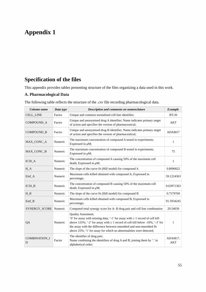
Appendix 1

Specification of the filesThis appendix provides tables presenting structure of the files organizing a data used in this work.

A. Pharmacological Data

The following table reflects the structure of the .csv file recording pharmacological data.

Column name Data type Description and comments on nomenclature Example

CELL_LINE Factor Unique and common normalised cell line identifier; BT-20

COMPOUND_A FactorUnique and anonymised drug A identifier; Name indicates primary target of action and specifies the version of pharmaceutical;

AKT

COMPOUND_B FactorUnique and anonymised drug B identifier; Name indicates primary target of action and specifies the version of pharmaceutical;

ADAM17

MAX_CONC_A NumericThe maximum concentration of compound A tested in experiments;Expressed in μM;

1

MAX_CONC_B NumericThe maximum concentration of compound B tested in experiments;Expressed in μM;

75

IC50_A NumericThe concentration of compound A causing 50% of the maximum cell death; Expressed in μM;

1

H_A Numeric The slope of the curve fit (Hill model) for compound A 0.8090022

Einf_A NumericMaximum cells killed obtained with compound A; Expressed in percentage;

59.1224363

IC50_B NumericThe concentration of compound B causing 50% of the maximum cell death; Expressed in μM;

9.63971363

H_B Numeric The slope of the curve fit (Hill model) for compound B 0.7579769

Einf_B NumericMaximum cells killed obtained with compound B; Expressed in percentage;

91.5934245

SYNERGY_SCORE Numeric Computed total synergy score for A- B drug pair and cell line combination 29.54039

QA Numeric

Quality Assesment;‘0’ for assay with missing data; ‘-1’ for assay with ≥ 1 record of cell kill above 125%; ‘-2’ for assay with ≥ 1 record of cell kill below -10%; ‘-3’ forthe assay with the difference between smoothed and non-smoothed fit above 25%; ‘1’ for assay for which no abnormalities were detected;

1

COMBINATION_ID

FactorThe identifier of drug pair;Name combining the identifiers of drug A and B, joining them by ’.’ in alphabetical order;

ADAM17.AKT

55

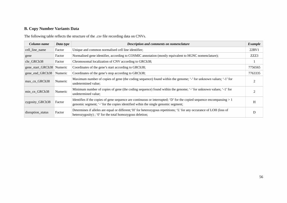
B. Copy Number Variants Data

The following table reflects the structure of the .csv file recording data on CNVs.

Column name Data type Description and comments on nomenclature Example

cell_line_name Factor Unique and common normalised cell line identifier; 22RV1

gene Factor Normalised gene identifier, according to COSMIC annotation (mostly equivalent to HGNC nomenclature); ZZZ3

chr_GRCh38 Factor Chromosomal localization of CNV according to GRCh38; 1

gene_start_GRCh38 Numeric Coordinates of the gene’s start according to GRCh38; 7756565

gene_end_GRCh38 Numeric Coordinates of the gene’s stop according to GRCh38; 7763335

max_cn_GRCh38 NumericMaximum number of copies of gene (the coding sequence) found within the genome; ‘-’ for unknown values; ‘-1’ for undetermined value;

2

min_cn_GRCh38 NumericMinimum number of copies of gene (the coding sequence) found within the genome; ‘-’ for unknown values; ‘-1’ for undetermined value;

2

zygosity_GRCh38 FactorIdentifies if the copies of gene sequence are continuous or interrupted; ‘D’ for the copied sequence encompassing > 1 genomic segment; ‘-’ for the copies identified wihin the single genomic segment;

H

disruption_status FactorDetermines if alleles are equal or different;‘H’ for heterozygous repetitions; ‘L’ for any occurance of LOH (loss of heterozygosity) ; ‘0’ for the total homozygous deletion;

D

56

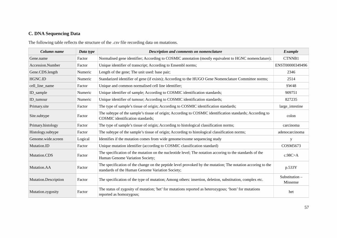
C. DNA Sequencing Data

The following table reflects the structure of the .csv file recording data on mutations.

Column name Data type Description and comments on nomenclature Example

Gene.name Factor Normalised gene identifier; According to COSMIC annotation (mostly equivalent to HGNC nomenclature); CTNNB1

Accession.Number Factor Unique identifier of transcript; According to Ensembl norms; ENST00000349496

Gene.CDS.length Numeric Length of the gene; The unit used: base pair; 2346

HGNC.ID Numeric Standarized identifier of gene (if exists); According to the HUGO Gene Nomenclature Committee norms; 2514

cell_line_name Factor Unique and common normalised cell line identifier; SW48

ID_sample Numeric Unique identifier of sample; According to COSMIC identification standards; 909751

ID_tumour Numeric Unique identifier of tumour; According to COSMIC identification standards; 827235

Primary.site Factor The type of sample’s tissue of origin; According to COSMIC identification standards; large_intestine

Site.subtype FactorThe subtype of the sample’s tissue of origin; According to COSMIC identification standards; According to COSMIC identification standards;

colon

Primary.histology Factor The type of sample’s tissue of origin; According to histological classification norms; carcinoma

Histology.subtype Factor The subtype of the sample’s tissue of origin; According to histological classification norms; adenocarcinoma

Genome.wide.screen Logical Identifies if the mutation comes from wide genome/exome sequencing study y

Mutation.ID Factor Unique mutation identifier (according to COSMIC classification standard) COSM5673

Mutation.CDS FactorThe specification of the mutation on the nucleotide level; The notation accoring to the standards of the Human Genome Variation Society;

c.98C>A

Mutation.AA FactorThe specification of the change on the peptide level provoked by the mutation; The notation accoring to the standards of the Human Genome Variation Society;

p.533Y

Mutation.Description Factor The specification of the type of mutation; Among others: insertion, deletion, substitution, complex etc.Substitution –

Missense

Mutation.zygosity FactorThe status of zygosity of mutation; 'het’ for mutations reported as heterozygous; ‘hom’ for mutations reported as homozygous;

het

57

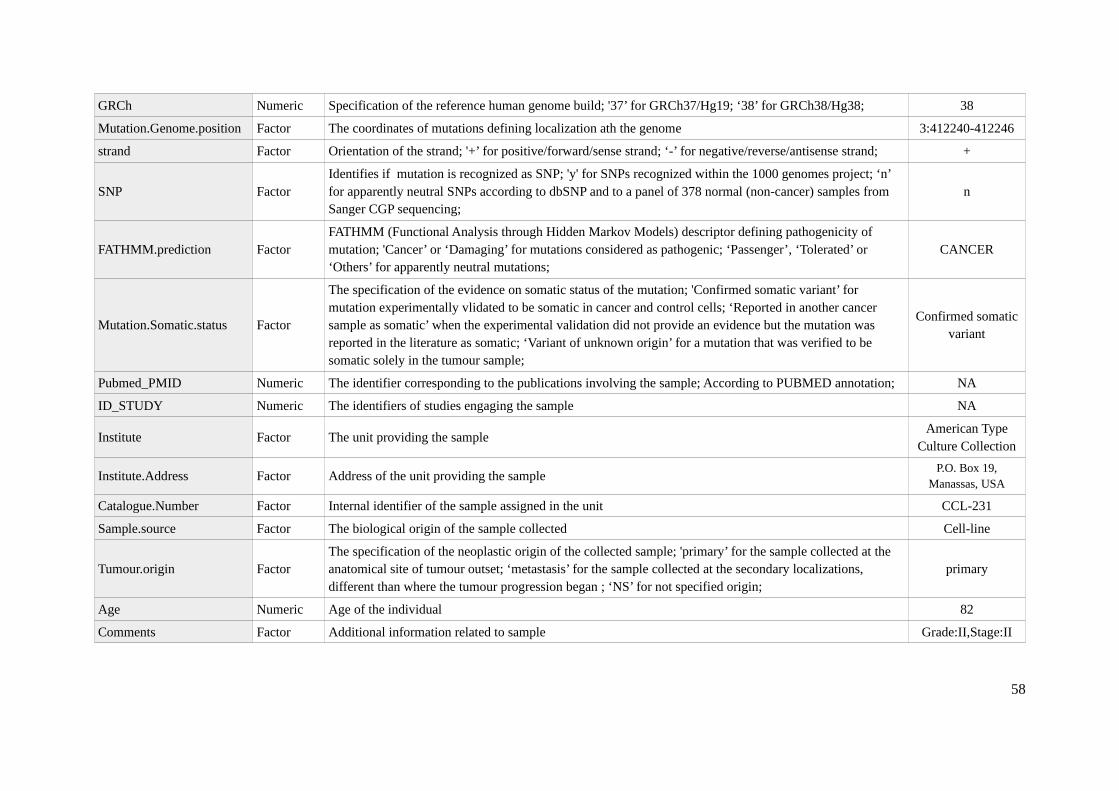
GRCh Numeric Specification of the reference human genome build; '37’ for GRCh37/Hg19; ‘38’ for GRCh38/Hg38; 38

Mutation.Genome.position Factor The coordinates of mutations defining localization ath the genome 3:412240-412246

strand Factor Orientation of the strand; '+’ for positive/forward/sense strand; ‘-’ for negative/reverse/antisense strand; +

SNP FactorIdentifies if mutation is recognized as SNP; 'y' for SNPs recognized within the 1000 genomes project; ‘n’ for apparently neutral SNPs according to dbSNP and to a panel of 378 normal (non-cancer) samples from Sanger CGP sequencing;

n

FATHMM.prediction FactorFATHMM (Functional Analysis through Hidden Markov Models) descriptor defining pathogenicity of mutation; 'Cancer’ or ‘Damaging’ for mutations considered as pathogenic; ‘Passenger’, ‘Tolerated’ or ‘Others’ for apparently neutral mutations;

CANCER

Mutation.Somatic.status Factor

The specification of the evidence on somatic status of the mutation; 'Confirmed somatic variant’ for mutation experimentally vlidated to be somatic in cancer and control cells; ‘Reported in another cancer sample as somatic’ when the experimental validation did not provide an evidence but the mutation was reported in the literature as somatic; ‘Variant of unknown origin’ for a mutation that was verified to be somatic solely in the tumour sample;

Confirmed somaticvariant

Pubmed_PMID Numeric The identifier corresponding to the publications involving the sample; According to PUBMED annotation; NA

ID_STUDY Numeric The identifiers of studies engaging the sample NA

Institute Factor The unit providing the sampleAmerican Type

Culture Collection

Institute.Address Factor Address of the unit providing the sampleP.O. Box 19,

Manassas, USA

Catalogue.Number Factor Internal identifier of the sample assigned in the unit CCL-231

Sample.source Factor The biological origin of the sample collected Cell-line

Tumour.origin FactorThe specification of the neoplastic origin of the collected sample; 'primary’ for the sample collected at the anatomical site of tumour outset; ‘metastasis’ for the sample collected at the secondary localizations, different than where the tumour progression began ; ‘NS’ for not specified origin;

primary

Age Numeric Age of the individual 82

Comments Factor Additional information related to sample Grade:II,Stage:II

58

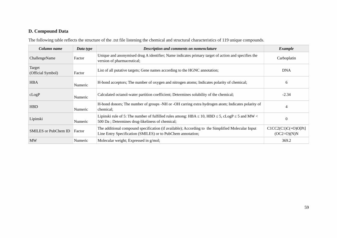
D. Compound Data

The following table reflects the structure of the .txt file listening the chemical and structural characteristics of 119 unique compounds.

Column name Data type Description and comments on nomenclature Example

ChallengeName FactorUnique and anonymised drug A identifier; Name indicates primary target of action and specifies the version of pharmaceutical;

Carboplatin

Target(Official Symbol) Factor

List of all putative targets; Gene names according to the HGNC annotation; DNA

HBANumeric

H-bond acceptors; The number of oxygen and nitrogen atoms; Indicates polarity of chemical; 6

cLogPNumeric

Calculated octanol-water partition coefficient; Determines solubility of the chemical; -2.34

HBDNumeric

H-bond donors; The number of groups -NH or -OH carring extra hydrogen atom; Indicates polarity of chemical;

4

LipinskiNumeric

Lipinski rule of 5: The number of fulfilled rules among: HBA ≤ 10, HBD ≤ 5, cLogP ≤ 5 and MW < 500 Da ; Determines drug-likeliness of chemical;

0

SMILES or PubChem ID FactorThe additional compound specification (if available); According to the Simplified Molecular Input Line Entry Specification (SMILES) or to PubChem annotation;

C1CC2(C1)C(=O)O[Pt](OC2=O)(N)N

MW Numeric Molecular weight; Expressed in g/mol; 369.2

59

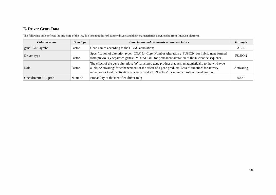
E. Driver Genes Data

The following table reflects the structure of the .csv file listening the 498 cancer drivers and their characteristics downloaded from IntOGen platform.

Column name Data type Description and comments on nomenclature Example

geneHGNCsymbol Factor Gene names according to the HGNC annotation; ABL2

Driver_typeFactor

Specification of alteration type; ‘CNA’ for Copy Number Alteration ; ‘FUSION’ for hybrid gene formed from previously separated genes; ‘MUTATION’ for permanent alteration of the nucleotide sequence;

FUSION

Role FactorThe effect of the gene alteration; ‘A’ for altered gene product that acts antagonistically to the wild-type allele; ‘Activating’ for enhancement of the effect of a gene product; ‘Loss of function’ for activity reduction or total inactivation of a gene product; ‘No class’ for unknown role of the alteration;

Activating

OncodriveROLE_prob Numeric Probability of the identified driver role; 0.877

60

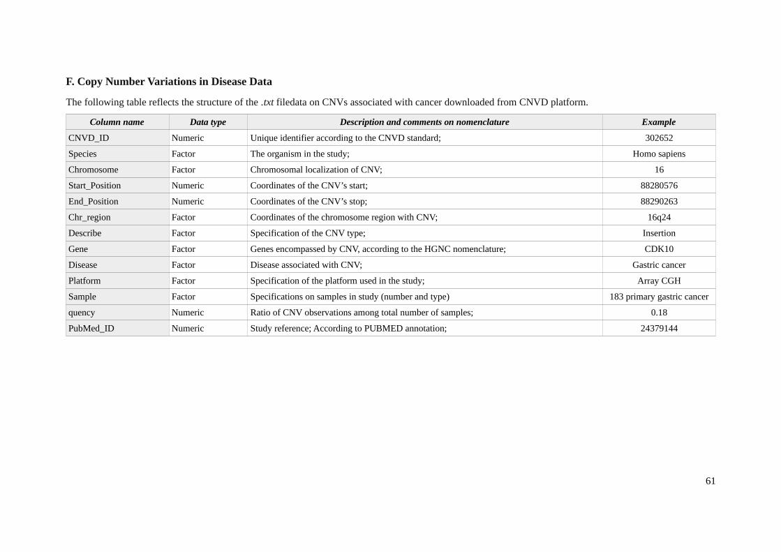
F. Copy Number Variations in Disease Data

The following table reflects the structure of the .txt filedata on CNVs associated with cancer downloaded from CNVD platform.

Column name Data type Description and comments on nomenclature Example

CNVD_ID Numeric Unique identifier according to the CNVD standard; 302652

Species Factor The organism in the study; Homo sapiens

Chromosome Factor Chromosomal localization of CNV; 16

Start_Position Numeric Coordinates of the CNV’s start; 88280576

End_Position Numeric Coordinates of the CNV’s stop; 88290263

Chr_region Factor Coordinates of the chromosome region with CNV; 16q24

Describe Factor Specification of the CNV type; Insertion

Gene Factor Genes encompassed by CNV, according to the HGNC nomenclature; CDK10

Disease Factor Disease associated with CNV; Gastric cancer

Platform Factor Specification of the platform used in the study; Array CGH

Sample Factor Specifications on samples in study (number and type) 183 primary gastric cancer

quency Numeric Ratio of CNV observations among total number of samples; 0.18

PubMed_ID Numeric Study reference; According to PUBMED annotation; 24379144

61

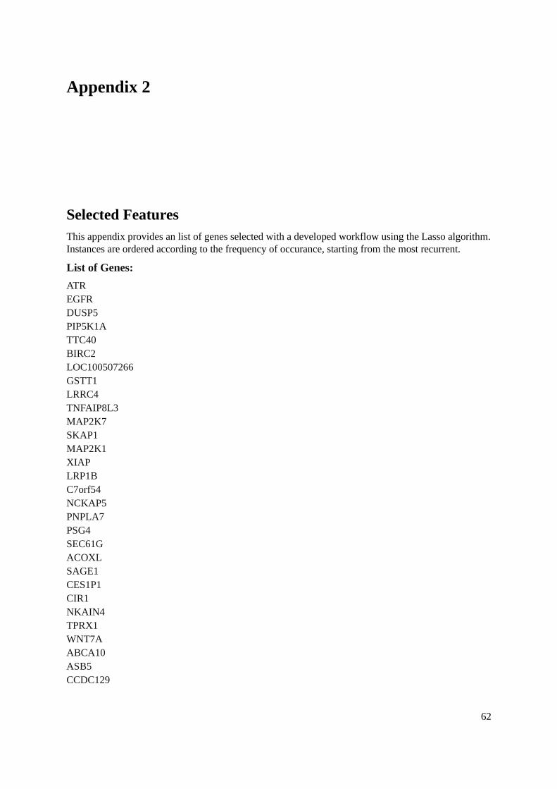
Appendix 2

Selected FeaturesThis appendix provides an list of genes selected with a developed workflow using the Lasso algorithm.Instances are ordered according to the frequency of occurance, starting from the most recurrent.

List of Genes:

ATREGFRDUSP5PIP5K1ATTC40BIRC2LOC100507266GSTT1LRRC4TNFAIP8L3MAP2K7SKAP1MAP2K1XIAPLRP1BC7orf54NCKAP5PNPLA7PSG4SEC61GACOXLSAGE1CES1P1CIR1NKAIN4TPRX1WNT7AABCA10ASB5CCDC129

62

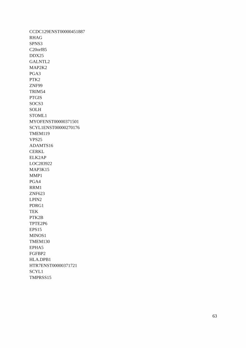
CCDC129ENST00000451887RHAGSPNS3C20orf85DDX25GALNTL2MAP2K2PGA3PTK2ZNF99TRIM54PTGISSOCS3SOLHSTOML1MYOFENST00000371501SCYL1ENST00000270176TMEM119VPS25ADAMTS16CERKLELK2APLOC283922MAP3K15MMP1PGA4RRM1ZNF623LPIN2PDRG1TEKPTK2BTPTE2P6EPS15MINOS1TMEM130EPHA5FGFBP2HLA.DPB1HTR7ENST00000371721SCYL1TMPRSS15

63