
Implementation and validation of ultra-fast dosimetric tools for ...
223
UNIVERSIDAD COMPLUTENSE DE MADRID FACULTAD DE CIENCIAS FÍSICAS Departamento de Física Atómica, Molecular y Nuclear TESIS DOCTORAL Implementation and validation of ultra-fast dosimetric tools for IORT Implementación y validación de herramientas de dosimetría ultra- rápida para IORT MEMORIA PARA OPTAR AL GRADO DE DOCTOR PRESENTADA POR Paula Beatriz Ibáñez Cuenca Director José Manuel Udías Moinelo Madrid, 2018 © Paula Beatriz Ibáñez Cuenca, 2017
-
Upload
khangminh22 -
Category
Documents
-
view
1 -
download
0
Transcript of Implementation and validation of ultra-fast dosimetric tools for ...

UNIVERSIDAD COMPLUTENSE DE MADRID FACULTAD DE CIENCIAS FÍSICAS
Departamento de Física Atómica, Molecular y Nuclear
TESIS DOCTORAL
Implementation and validation of ultra-fast dosimetric tools for IORT
Implementación y validación de herramientas de dosimetría ultra-rápida para IORT
MEMORIA PARA OPTAR AL GRADO DE DOCTOR
PRESENTADA POR
Paula Beatriz Ibáñez Cuenca
Director
José Manuel Udías Moinelo
Madrid, 2018
© Paula Beatriz Ibáñez Cuenca, 2017

UNIVERSIDAD COMPLUTENSE DE MADRID
FACULTAD DE CIENCIAS FÍSICAS
Departamento de Física Atómica, Molecular y Nuclear
TESIS DOCTORAL:
Implementation and validation of
ultra-fast dosimetric tools for
IORT
Implementación y validación de herramientas de dosimetría
ultra-rápida para IORT
Realizada por:
Paula Beatriz Ibáñez García
Director:
Dr. José Manuel Udías Moinelo

A mis padres
Por plantar la semilla de la
curiosidad en mi mente desde niña.


Felix, qui potuit rerumcognoscere causas.
Virgilio


Agradecimientos
Bueno, pues parece que ya está. Resulta que todos estos años, cuando los que ya habíanpasado por esto me decían parece imposible, pero acaba llegando, en el fondo no estabandesencaminados... Debe ser eso de hacerse doctor, que igual te hace un poquito más listo.
Ha sido un viaje largo y en ocasiones modivito, con sus triunfos (y sus correspondientes bailesde la victoria) y sus tropiezos (y sus ¾Y si monto una librería y me olvido de todo?). Pero alnal el esfuerzo ha tenido recompensa, y esta tesis lo demuestra.
Sois muchos los que habéis hecho posible esta tesis, ya sea por ayudarme en el ámbitoinvestigador o en el personal, y tenéis que saber que, sin vosotros, todo esto no habría salidoadelante.
En primer lugar debo darle las gracias a José Manuel. Él conó en mí a pesar de no tener elexpediente más brillante y me hizo ver que yo valía para la investigación. Si no hubiera sido poresa oportunidad que me dio en forma de beca de verano, esta aventura jamás habría ni siquieraempezado.
También quiero dar las gracias a la gente con la que he colaborado todos estos años. Alequipo de GMV, con Carlos Illana, Raúl Rodríguez, Manlio Valdivieso y Samuel Rodríguez.Sin ellos, radiance sería solamente una idea borrosa en la cabeza de algún oncólogo. A PedroGuerra, María Jesús Ledesma y Juan Ortuño, de la UPM, por su trabajo indispensable en esteproyecto.
Quiero agradecer también su ayuda a Laure Parent, Frank Schneider y, especialmente, a SvenClausen, por darme la oportunidad de ir a realizar medidas a sus centros y ayudarme en todo loque necesitaba cuando me encontraba perdida por los pasillos del hospital.
Y como no, un grandísimo gracias a Marie, mi franchutilla, la mejor compañera de batallasque alguien podía tener. Y a Elena, por ayudarme y enseñarme todo lo que sabía cuando erauna recién llegada.
Pero la lista acaba de empezar. Cuando llegué al GFN no sabía bien qué esperar. Nunca habíaestado en un grupo de investigación, así que me imaginaba muchos escenarios en mi cabeza (yos aseguro que tengo una gran imaginación). Pero lo que me encontré fue un grupo de genteestupendo, algo raritos pero maravillosos cada uno en su estilo. Estaba Jacobo, que vivía en
v
sus mundos de Cal, Vadym con sus liebres de 50 kg, Bruno, ese chico callado (al principio) quesiempre nos olvidábamos al bajar a comer, Pablo y sus bromas y concursos, Armando, nuestrometeorólogo con alma de nuclear, Elena, la pequeña dictadora con habilidad para hacer que IronMaiden sonara como los pitufos maquineros, Esteban, nuestro tico, Richichop, la persona conmás motes en la historia, Esther, la inauguradora de bares, Luis Mario y su bate, César, expertoen IPs, y Cris, que cada día intenta hacer del mundo un sitio un poquito más agradable.
Al poco de estar aquí llegaron Vicky con sus derrapes por el pasillo y May, acompañada de susrayos y centellas. Y con ellas surgió el gallinero, que pasó a ser el gallinero 2.0 con la incorporaciónde Marie y sus tirejas y parajitos. Quiero dar las gracias especialmente a mis nuclear hens, porhaber estado siempre ahí todos estos años, y porque, aunque cada una esté ahora en una partedistinta del mundo, nuestras reuniones hacen que no pase el tiempo. ½Os quiero!
Y pasaron los años, los más viejos se fueron y llegaron los nuevos (y no tan nuevos). Jaime,Víctor, Amaia, Pablo y Alex, que aunque no sepan cómo pegar un sello, son gente maja. Y Daniy Joaquín, los hijos pródigos que han vuelto al grupo. Gracias a todos por seguir haciendo delGFN un grupo tan divertido.
Y cómo olvidar a la gente que he conocido gracias a mis GFNitos: Edu, Borja Peropapi, Alex,Dimitri, Vincent 25, Simon, Tarek, Oli y Natalia. Con vosotros las cañas y los viajes se volvíanmucho más emocionantes.
También hay gente que le tengo que agradecer el haber estado siempre ahí. Y cuando digosiempre, es SIEMPRE. Desde niñas. Blanca, Agos y Rachel. Crecimos juntas y áun nos quedapor crecer mucho más, juntas, claro. Celes y Leti, mis hermanísimas favoritas y compañeras demil aventuras, Marion, echaré de menos nuestros cafés durante la tesis, y nuestra no tan nuevaadquisición, Angelita. Y Josus y Pumirris, porque aunque pasen los años hay cosas que nuncacambian.
Y no me quiero olvidar de mi familia swing. Vita, Estela, Eva, Isa (mis ladies), Urko, Adri,NachoS, Maite, AlbertoS y muchos más. Habéis hecho del miércoles mi día favorito de lasemana.
Y nalmente, mi mayor agradecimiento es para mi familia. A mis tíos, primos y a mi abuelo.A mi abuela, por todas esas velas que ha puesto durante años para que el trabajo fuera bien, ysobre todo, a mis padres. Gracias a ellos crecí rodeada de libros y curiosidad. Desde experimentos(a veces con nal desastroso) en la cocina, visitas casi semanales al museo de ciencias naturales,y preguntas infantiles incómodas que respondieron siempre con paciencia y veracidad. Ellos meenseñaron que la ciencia era algo asombroso y que la investigación era jugar siendo adulto. Mecontagiaron su pasión y sin ellos no estaría aquí. Muchas gracias.
En denitiva, a todos vosotros, y a los que me he olvidado, ½muchas gracias!
vi
Contents
Table of contents vii
Summary xi
Resumen en castellano xv
Motivation, objectives and outline of this thesis xix
1 Fundamentals of radiotherapy 11.1 The role of radiotherapy in oncology . . . . . . . . . . . . . . . . . . . . . . . . . 11.2 Interaction of radiation with matter . . . . . . . . . . . . . . . . . . . . . . . . . 3
1.2.1 Interaction of photons with matter . . . . . . . . . . . . . . . . . . . . . . 31.2.2 Interaction of electrons with matter . . . . . . . . . . . . . . . . . . . . . 5
1.3 Intraoperative radiation therapy (IORT) . . . . . . . . . . . . . . . . . . . . . . . 71.3.1 Intraoperative electron radiation therapy (IOERT) . . . . . . . . . . . . . 81.3.2 Low energy X-rays intraoperative radiation therapy (XIORT) . . . . . . . 9
1.4 Dose delivery in IORT . . . . . . . . . . . . . . . . . . . . . . . . . . . . . . . . . 101.4.1 Linear accelerators for IOERT . . . . . . . . . . . . . . . . . . . . . . . . . 101.4.2 Mobile devices for XIORT . . . . . . . . . . . . . . . . . . . . . . . . . . . 18
1.5 Dosimetry in an IORT treatment . . . . . . . . . . . . . . . . . . . . . . . . . . . 211.5.1 Ionization chambers . . . . . . . . . . . . . . . . . . . . . . . . . . . . . . 221.5.2 Radiochromic lms . . . . . . . . . . . . . . . . . . . . . . . . . . . . . . . 23
1.6 Dosimetric characteristics of electron beams . . . . . . . . . . . . . . . . . . . . . 261.6.1 Energy and angular distributions . . . . . . . . . . . . . . . . . . . . . . . 261.6.2 Depth dose proles . . . . . . . . . . . . . . . . . . . . . . . . . . . . . . . 271.6.3 Transverse dose proles . . . . . . . . . . . . . . . . . . . . . . . . . . . . 281.6.4 Isodose contours . . . . . . . . . . . . . . . . . . . . . . . . . . . . . . . . 29
1.7 Dosimetric characteristics of low energy X-rays . . . . . . . . . . . . . . . . . . . 301.7.1 Energy and angular distributions . . . . . . . . . . . . . . . . . . . . . . . 301.7.2 Depth dose proles . . . . . . . . . . . . . . . . . . . . . . . . . . . . . . . 311.7.3 Transverse dose proles . . . . . . . . . . . . . . . . . . . . . . . . . . . . 321.7.4 Isodose contours . . . . . . . . . . . . . . . . . . . . . . . . . . . . . . . . 33
1.8 Radiance R©, a treatment planning system for IORT . . . . . . . . . . . . . . . . . 33
vii
CONTENTS
1.9 Gamma evaluation . . . . . . . . . . . . . . . . . . . . . . . . . . . . . . . . . . . 36
2 Monte Carlo methods in radiotherapy 392.1 Introduction . . . . . . . . . . . . . . . . . . . . . . . . . . . . . . . . . . . . . . . 392.2 Monte Carlo technique. Basic concepts . . . . . . . . . . . . . . . . . . . . . . . . 40
2.2.1 Modeling of particle transport . . . . . . . . . . . . . . . . . . . . . . . . . 412.2.2 Random number generator . . . . . . . . . . . . . . . . . . . . . . . . . . 422.2.3 Probability distribution functions and sampling method . . . . . . . . . . 422.2.4 Error estimation . . . . . . . . . . . . . . . . . . . . . . . . . . . . . . . . 452.2.5 Monte Carlo optimization . . . . . . . . . . . . . . . . . . . . . . . . . . . 45
2.3 Main Monte Carlo codes in radiotherapy . . . . . . . . . . . . . . . . . . . . . . . 482.4 PENELOPE . . . . . . . . . . . . . . . . . . . . . . . . . . . . . . . . . . . . . . . 492.5 PenEasy . . . . . . . . . . . . . . . . . . . . . . . . . . . . . . . . . . . . . . . . . 51
2.5.1 Source models . . . . . . . . . . . . . . . . . . . . . . . . . . . . . . . . . . 522.5.2 Tallies . . . . . . . . . . . . . . . . . . . . . . . . . . . . . . . . . . . . . . 52
2.6 DPM . . . . . . . . . . . . . . . . . . . . . . . . . . . . . . . . . . . . . . . . . . . 532.6.1 Source model . . . . . . . . . . . . . . . . . . . . . . . . . . . . . . . . . . 542.6.2 Tallies . . . . . . . . . . . . . . . . . . . . . . . . . . . . . . . . . . . . . . 54
3 Detailed simulations of IORT systems 553.1 Introduction . . . . . . . . . . . . . . . . . . . . . . . . . . . . . . . . . . . . . . . 553.2 Intrabeam R© applicators . . . . . . . . . . . . . . . . . . . . . . . . . . . . . . . . 56
3.2.1 MC characterization of Intrabeam R© X-ray source . . . . . . . . . . . . . . 563.2.2 MC characterization of Intrabeam R© Spherical applicators . . . . . . . . . 603.2.3 Simulation of Intrabeam R© at and surface applicators . . . . . . . . . . . 63
3.3 Dedicated electron accelerators . . . . . . . . . . . . . . . . . . . . . . . . . . . . 653.3.1 LIAC R© . . . . . . . . . . . . . . . . . . . . . . . . . . . . . . . . . . . . . 653.3.2 NOVAC R© . . . . . . . . . . . . . . . . . . . . . . . . . . . . . . . . . . . . 673.3.3 MOBETRON R© . . . . . . . . . . . . . . . . . . . . . . . . . . . . . . . . . 69
3.4 Phase Space parameterization . . . . . . . . . . . . . . . . . . . . . . . . . . . . . 713.4.1 Parameterization of PHSP les in the IOERT accelerators . . . . . . . . . 713.4.2 Parameterization of PHSP les in the Intrabeam R© spherical applicators . 743.4.3 Parameterization of PHSP le in the Intrabeam R© at and surface applicators 77
3.5 Conclusion . . . . . . . . . . . . . . . . . . . . . . . . . . . . . . . . . . . . . . . . 79
4 Phase space optimization process 814.1 Introduction . . . . . . . . . . . . . . . . . . . . . . . . . . . . . . . . . . . . . . . 814.2 Database generation . . . . . . . . . . . . . . . . . . . . . . . . . . . . . . . . . . 83
4.2.1 Intrabeam R© applicators . . . . . . . . . . . . . . . . . . . . . . . . . . . . 834.2.2 IOERT accelerators . . . . . . . . . . . . . . . . . . . . . . . . . . . . . . 84
4.3 Optimization of energy spectrum . . . . . . . . . . . . . . . . . . . . . . . . . . . 844.3.1 Energy spectrum for Intrabeam R© applicators . . . . . . . . . . . . . . . . 854.3.2 Energy spectrum for IOERT accelerators . . . . . . . . . . . . . . . . . . . 864.3.3 Treatment of the experimental data . . . . . . . . . . . . . . . . . . . . . 87
viii
CONTENTS
4.4 PHSP weighting algorithm . . . . . . . . . . . . . . . . . . . . . . . . . . . . . . . 874.4.1 Weighting approach for DDPs with the same number of histories . . . . . 884.4.2 Weighting approach for DDPs with dierent number of histories . . . . . 89
4.5 Results . . . . . . . . . . . . . . . . . . . . . . . . . . . . . . . . . . . . . . . . . . 904.6 Conclusion . . . . . . . . . . . . . . . . . . . . . . . . . . . . . . . . . . . . . . . . 91
5 Validation of the phase space optimization process with experimental data 935.1 Introduction . . . . . . . . . . . . . . . . . . . . . . . . . . . . . . . . . . . . . . . 935.2 Validation for XIORT applicators . . . . . . . . . . . . . . . . . . . . . . . . . . . 94
5.2.1 Experimental measurements for Spherical applicators . . . . . . . . . . . . 945.2.2 Experimental measurements for Flat and surface applicators . . . . . . . . 995.2.3 Dose comparison for spherical applicators . . . . . . . . . . . . . . . . . . 1025.2.4 Dose comparison for at and surface applicators . . . . . . . . . . . . . . 105
5.3 Validation for IOERT accelerators . . . . . . . . . . . . . . . . . . . . . . . . . . 1085.3.1 Experimental measurements for IOERT accelerators . . . . . . . . . . . . 1085.3.2 Dose comparison for IOERT accelerators . . . . . . . . . . . . . . . . . . . 110
5.4 Conclusion . . . . . . . . . . . . . . . . . . . . . . . . . . . . . . . . . . . . . . . . 115
6 Hybrid Monte Carlo for dose calculation 1176.1 Introduction . . . . . . . . . . . . . . . . . . . . . . . . . . . . . . . . . . . . . . . 1176.2 MC simulations . . . . . . . . . . . . . . . . . . . . . . . . . . . . . . . . . . . . . 1196.3 Code description . . . . . . . . . . . . . . . . . . . . . . . . . . . . . . . . . . . . 120
6.3.1 Photoelectric eect . . . . . . . . . . . . . . . . . . . . . . . . . . . . . . . 1226.3.2 Compton eect . . . . . . . . . . . . . . . . . . . . . . . . . . . . . . . . . 1226.3.3 Study of the zero range approximation for electrons . . . . . . . . . . . . . 1246.3.4 Flow chart of the code . . . . . . . . . . . . . . . . . . . . . . . . . . . . . 124
6.4 Dose normalization . . . . . . . . . . . . . . . . . . . . . . . . . . . . . . . . . . . 1266.4.1 Calculation of the expected uence for spherical applicators . . . . . . . . 1286.4.2 Calculation of the expected uence for at and surface applicators . . . . 130
6.5 Validation of the Hybrid Monte Carlo against MC simulations . . . . . . . . . . . 1326.5.1 Hybrid Monte Carlo for spherical applicators . . . . . . . . . . . . . . . . 1326.5.2 Hybrid Monte Carlo for at and surface applicators . . . . . . . . . . . . . 1416.5.3 Validation in clinical situations . . . . . . . . . . . . . . . . . . . . . . . . 149
6.6 Conclusion . . . . . . . . . . . . . . . . . . . . . . . . . . . . . . . . . . . . . . . . 153
Conclusions of this thesis 155
A Appendix: Generation of the material list for the Hybrid Monte Carlo 161
Main contributions of this thesis 163
List of gures 171
List of tables 179
ix

CONTENTS
Bibliography 181
x

Summary
Introduction and objectives
Intraoperative Radiation Therapy (IORT) is a special modality for cancer treatment that deliversa single high dose of radiation directly to the exposed tumor bed during the tumor resectionsurgery [Palta et al., 1995, Beddar et al., 2006, Calvo et al., 1993, 2013, Lamanna et al., 2012].One of the main limitations in IORT lies in the diculties that the planning process entails,which limits the use of this technique [Lamanna et al., 2012, Pascau et al., 2012], and a treatmentplanning has not been available in IORT up to now. Recently, a new tool has been introduced:radiance R©, the rst Treatment Planning System (TPS) specically designed for IORT [Pascauet al., 2012, Valdivieso-Casique et al., 2015].
The main goal of this thesis has been the development, implementation and evaluation of adosimetric tool capable of providing a realistic dose distribution from any intraoperative electronradiotherapy (IOERT) dedicated accelerator or Intrabeam R© applicator that can be used for dosetreatment planning in the operating room (OR) during an IORT treatment.
This dosimetric tool has been separated in three phases. First, a database of monoenergeticphase space (PHSP) les and depth dose proles (DDPs) in water was computed with penEasy[Sempau et al., 2011, Badal Soler et al., 2008] from detailed simulations of each IOERT acceleratorand Intrabeam R© applicator. Then, the energy spectrum of these monoenergetic simulations wastuned for each device using simple experimental DDPs provided by the manufacturer to the user,obtaining an optimized PHSP le that reproduces the user's data [Ibáñez et al., 2015, Vidal et al.,2015]. Finally, dose was calculated from this optimized PHSP le with an accelerated versionof DPM [Sempau et al., 2000, Guerra et al., 2014] in the case of electrons, or with the HybridMonte Carlo (HMC) code we have developed [Vidal et al., 2014b,a, Udías et al., 2017b], in thecase of the Intrabeam R©.
xi

Summary
Materials and methods
Detailed simulations and database generation
We have simulated the most relevant dedicated accelerators employed in IOERT treatments (ie.NOVAC R©, LIAC R© and MOBETRON R©) with their corresponding applicators, and Intrabeam R©
needle, spherical, surface and at applicators. These simulations will represent a referenceaccelerator or applicator, and will be used to create a database of monoenergetic PHSP andDDPs in water that will be employed to generate a PHSP le tuned to each user machine in adose treatment planning procedure.
Phase space optimization process
First, a generic spectrum, whose general features were derived from the realistic MC simulations,is ne-tuned by means of a genetic algorithm [Fernandez-Ramirez et al., 2008] until itdescribes the experimental DDP provided by the user of any given applicator. Afterwards,the monoenergetic PHSP les are combined with weights given by the energy spectrum, to builda PHSP le optimized to describe the experimental dose distribution [Ibáñez et al., 2015, Vidalet al., 2015, Udías et al., 2017a].
Hybrid Monte Carlo
Dose with the Intrabeam R© device is calculated from the optimized PHSP le by means of anin-house developed code, the Hybrid Monte Carlo (HMC) [Vidal et al., 2014b,a, Udíaset al., 2017b]. This code calculates deposited dose within minutes, fully taking into account thedierent tissues and structures of the patient. It incorporates all the relevant physical processesat Intrabeam R© working energies, and the savings in calculation time are possible thanks to takingto the extreme some variance reduction techniques, such as the use of meta-histories, each onerepresenting the fate of many particles, or the dose normalization, which allows statistic noise-freedose distributions with a low number of initial meta-histories.
Results
Detailed simulations and database generation. We could compare dose distributions againstexperimental data and a good agreement was reached. The optimization process only ts theDDPs, which is why it is essential that the rest of the dose distribution behaves correctly. Bysimulating in detail the dierent accelerators we guarantee a precise shape of the transverseproles.
Phase space optimization process. We have done a broad validation of this process against
xii
Summary
experimental data in homogeneous and heterogeneous situations. For the validation ofdose distributions in water with spherical applicators, we found some discrepancies betweensimulations and measurements due to the anisotropy of the dose in the backward direction.However, the area presenting the anisotropy has no clinical interest. Regarding the dosedistributions in water with at and surface applicators, we found a good agreement for the casesstudied, with more than 95% of the voxels fullling the gamma criteria at the 2%-2 mm level.In the dose comparisons inside heterogeneous phantoms, either with Intrabeam R© applicatorsor IOERT accelerators, we reached a reasonable agreement at the 2%-2 mm level, speciallyconsidering the uncertainties in the measurements.
Hybrid Monte Carlo. We have validated the HMC against penEasy in homogeneous andheterogeneous phantoms. We have also compared dose distributions in clinical situations. Ingeneral, good results were obtained with the gamma evaluation with the 2%-1 mm criterion. Ina few cases we had to go to a 5%-1 mm criterion to achieve a good agreement. However, thegamma criteria for the Intrabeam R© has not been stipulated, and values of previous studies cango from 2%-1 mm [Nwankwo et al., 2013], 2%-2 mm [Clausen et al., 2012] to even 10%-1 mm[Chiavassa et al., 2014].
Conclusion
The phase space optimization process works correctly, reproducing dose distributions in clinicalsituations for both electrons or X-rays beams. It has proven to be fast, exible and preciseenough for IORT planning.
The HMC provides soft dose distributions accurately and within minutes. It can be used asa dose calculation tool in the operating room, as its high speed allows an on-the-y dosecalculation which includes the realistic eects of the beam in the dierent tissues within thepatient's body.
The phase space optimization process and the HMC have been integrated into radiance R©.
xiii

Resumen en castellano
Introducción y objetivos
La radioterapia intraoperatoria (IORT) es una modalidad de tratamiento que consiste en irradiardirectamente el lecho tumoral expuesto durante la cirugía con una dosis única y localizada [Paltaet al., 1995, Beddar et al., 2006, Calvo et al., 1993, 2013, Lamanna et al., 2012]. A pesar delas ventajas que ofrece esta técnica, hasta hace poco la IORT carecía de las herramientas deplanicación y dosimetría que se emplean regularmente en radioterapia externa. Para remediaresta carencia, se creó radiance R©, el primer planicador de tratamientos para IORT [Pascauet al., 2012, Valdivieso-Casique et al., 2015].
El principal objetivo de esta tesis ha sido el desarrollo, implementación y validación de unaherramienta de cálculo de dosis capaz de proporcionar una dosis realista de cualquier aceleradordedicado de IORT con electrones o con el sistema Intrabeam R© que pueda ser usada para planicarel tratamiento dentro del quirófano durante una intervención de IORT.
Esta herramienta dosimétrica se ha separado en tres fases. Primero, se ha generado una basede datos con penEasy [Sempau et al., 2011, Badal Soler et al., 2008] a partir de simulacionesdetalladas de aceleradores de electrones y aplicadores de Intrabeam R©, compuesta por espacios defase (PHSP) monoenergéticos y perles de dosis en profundidad (DDPs) en agua. Después, conun proceso de ajuste en el que necesitamos únicamente la DDP experimental de cada máquina,obtenemos un PHSP optimizado que reproduce la dosis experimental. Finalmente, la dosis secalcula a partir de este PHSP, bien con una versión acelerada de DPM [Sempau et al., 2000]en el caso de trabajar con electrones, o bien con el Monte Carlo Híbrido (HMC) que hemosdesarrollado [Vidal et al., 2014b,a, Udías et al., 2017b] para el Intrabeam R©.
Materiales y métodos
Simulaciones detalladas y generación de la base de datos
xv
Resumen en castellano
Hemos simulado los aceleradores dedicados para IORT de electrones más relevantes con susaplicadores correspondientes, así como los distintos aplicadores del R©. Estas simulacionesservirán para crear la base de datos de PHSP y DDPs monoenergéticos que alimentarán nuestroalgoritmo de optimización.
Proceso de optimización del espacio de fases
Primero, ajustaremos un espectro de energías genérico, derivado de las simulaciones detalladasde los aceleradores, mediante un algoritmo genético [Fernandez-Ramirez et al., 2008], hastaque describa la DDP experimental introducida por el usuario. Después usaremos el espectrooptimizado para pesar los PHSP monoenergéticos y obtener un espacio de fases que reproduzcala dosis experimental [Ibáñez et al., 2015, Vidal et al., 2015, Udías et al., 2017a].
Monte Carlo Híbrido
Para el cálculo de dosis con la máquina Intrabeam R© hemos desarrollado el Monte CarloHíbrido (HMC) [Vidal et al., 2014b,a, Udías et al., 2017b]. Este código calcula la dosisdepositada en minutos, y tiene en cuenta el efecto de los distintos tejidos y estructuras enel interior del paciente. Incorpora los procesos físicos relevantes a las energías de trabajo delIntrabeam R© y lleva al extremo técnicas de reducción de varianza para acelerar los cálculos, talescomo el uso de meta-historias, cada una de ellas representando el destino que miles de partículas,o la normalización de la dosis, que permite la obtención de dosis sin apenas ruido estadístico apartir de pocas meta-historias iniciales.
Resultados
Simulaciones detalladas y generación de la base de datos. Las distribuciones de dosis obtenidasse han comparado contra medidas experimentales y se ha observado un buen acuerdo entre ellas.El proceso de optimización del PHSP sólo ajusta la dosis a las DDP experimentales, por lo quees esencial que el resto de la dosis tenga la distribución adecuada. Al simular en detalle todoslos aceleradores, garantizamos que la forma de los perles transervales sea la correcta.
Proceso de optimización del espacio de fases. Se ha llevado a cabo una amplia validacióndel proceso con medidas experimentales en medios homogéneos y heterogéneos. Al realizar lacomparación de dosis con los aplicadores esféricos del Intrabeam R© en agua encontramos algunasdiscrepancias debidas a la anisotropía que presentan las medidas experimentales en la parte dedetrás del aplicador. Sin embargo, la localización de la anisotropía está en una zona sin interésclínico. En el caso de la comparación de dosis con los aplicadores planos y de supercie delIntrabeam R© en agua vimos que había buen acuerdo entre medidas y simulaciones, con más del95% de los vóxeles cumpliendo el criterio gamma con límites 2%-2 mm para todos los casos. Ylo mismo observamos al comparar las dosis en heterogeneidades tanto en IORT de electrones
xvi

Resumen en castellano
como en Intrabeam R©, donde el acuerdo es razonable, especialmente si tenemos en cuenta lasincertidumbres asociadas a la medida experimental.
Monte Carlo Híbrido. El HMC ha sido validado contra penEasy en maniquíes homogéneos yheterogéneos. También se han comparado las distribuciones de dosis en CTs de pacientes. Entérminos de criterio gamma, al nivel del 2%-1 mm se ha obtenido un buen acuerdo en generalentre ambos códigos, aunque en algunos casos se tuvo que aumentar a 5%-1 mm. Sin embargo,los límites del criterio gamma para las dosis del Intrabeam R© no se han establecido aún, y losvalores que se han usado en estudios previos pueden ir desde 2%-1 mm [Nwankwo et al., 2013],2%-2 mm [Clausen et al., 2012] hasta incluso 10%-1 mm [Chiavassa et al., 2014].
Conclusiones
El proceso de optimización de espacios de fase funciona correctamente, obteniendo PHSPque reproducen distribuciones de dosis experimentales tanto para electrones como para elIntrabeam R©. Se ha demostrado que es rápido, exible y sucientemente preciso para planicaciónen IORT.
El HMC proporciona distribuciones de dosis suaves y precisas en minutos. Puede usarse comoherramienta de cálculo de dosis en la sala de operaciones, ya que su alta velocidad permiterealizar un cálculo de dosis en el momento que además incluye los efectos realistas del haz alatravesar las distintas estructuras del cuerpo.
Tanto el proceso de optimización de espacios de fase como el Monte Carlo Híbrido han sidoincorporados en radiance R©.
xvii

Motivation, objectives and outline of
this thesis
Intraoperative radiotherapy (IORT) is a modality of cancer treatment that combines the eortof two disciplines, surgery and radiotherapy, in order to increment the rate of tumor control.In this treatment technique a high and localized dose of radiation is administrated directly tothe exposed tumor bed during the surgery performed to extract the tumor [Beddar et al., 2006,Lamanna et al., 2012, Calvo et al., 1993]. The direct visualization of the tumor allows a moreprecise denition of the volume that has to be irradiated and the protection of the surroundinghealthy tissues, by retraction of the tissue or by placing shields. Furthermore, IORT eliminatesthe time between surgery and radiotherapy and oers an alternative to those patients in whichexternal radiotherapy is not indicated. Finally, IORT is also used as the boost radiation ofmultidisciplinary treatment approaches, including external radiotherapy.
The rst reported IORT clinical treatments date back to the early 1900s, just a few years afterthe discovery of the X-rays, but the development of this technique really started in the late1960s with the incorporation of the high-energy electrons as the optimal radiation beam forIORT treatments [Calvo et al., 1993]. Since then, the technology involved in IORT has beenoptimized and several dedicated linear accelerators and X-rays devices, such as Intrabeam R© (CarlZeiss Meditec, Dublin, CA, USA) or Axxent R© (Xoft, San Jose, CA, USA) have been developed,and the number of institutions carrying out this treatment modality has been increasing in allcountries.
However, IORT is, in spite of the years that it has been around, still considered an experimentalprocedure. This is mostly due to the fact that no commercial or certied/approved solutionexisted covering the aspects that one is used to nd in conventional (external or brachytherapy)radiotherapy. Although treatment planning is a necessary step in external radiotherapy, thecorresponding procedure has not been available in IORT up to now. There are several reasonsto this: There is usually no image for therapy planning, and a basic planning is sketched basedon preoperatory imaging. There are a few places where intraoperatory image is available, thanksto magnetic resonance imaging (MRI) [Shah et al., 2012], in-room computed tomography (CT)imaging [Jones et al., 2014] or ultrasounds [Lindner et al., 2006], but it is not at all commonplace.
xix

Motivation, objectives and outline of this thesis
Moreover, the position where the applicator is going to be placed, its size and the possibleprotections are decided in situ, after examining the surgical results [Lamanna et al., 2012,Pascau et al., 2012, Beddar et al., 2006]. This means that there is a short time window toperform and/or tune the treatment plan. Furthermore, there is no actual record of the positionof the applicator, patient or shields during treatment, other than the memory of the peoplepresent, and pictures or videos of the intervention, from which one could only roughly infer thetreatment setup. This prevents the post study of treatments and complicates the quality control.In view of these inconveniences, planning has been based on isodose curves in water, measuredfor each applicator and energy, and from this information, oncologists and medical physics setthe radiotherapy plan.
The need of a tool that allows the radiation oncologist to plan an IORT treatment and to obtainan estimation of the dose distribution deposited in the volume of interest led the Unidad deMedicina y Cirugía Experimental and the Servicio de Oncología Radioterápica from the HospitalGeneral Universitario Gregorio Marañón (HGUGM) in Madrid into developing a tool capableof simulating an IORT process with electron beams from patient images. The Laboratorio deImagen Médica from the HGUGM developed a prototype of a treatment planning system (TPS)that allowed the positioning of the IOERT applicators superimposed on the patient's CT or MRIimages, and painted the isodose lines in water for each applicator diameter, bevel and energy[Desco et al., 1997]. The HGUGM contacted then with GMV company in order to transformthis prototype software into a commercial TPS for IOERT. As a result of this collaboration aproject was approved by the Ministry of Industry (FIT-300100-2007-53) to develop the rst TPSfor IORT: radiance R©.
radiance R© appeared in 2007. In its rst implementation, simple isodose curves in water werestill used, but radiance R© allowed to load a CT (or any other modality image) of the patient(either intra-, pre- or post-operatory). This image could be edited to reect better the surgicalndings and patient situation, and the applicator and energy of the electrons could be changedand the resulting water isodose could be seen on the screen, co-registered with the patient image,so that the doctors could then have a more clear picture of the setup and the radiation of thetumor bed and organs at risk. radiance R© made also possible a much more precise documentationof the procedure. However, although water measurements were a good starting point towardsproviding a planning tool to IORT, they did not take into account the behavior of electrons intissues with densities dierent than water.
Since 2009, a collaboration of several universities, companies and hospitals in Madrid have takenradiance R© to a new level, building a research consortium composed of private companies (GMV,Técnicas Radiofísicas), medical institutions (Hospital Universitario Gregorio Marañón, ConsorcioHospitalario Provincial de Castellón, Clínica La Luz, Hospital Ramón y Cajal) and universities(Universidad Politécnica de Madrid, Universidad Complutense de Madrid, Universidad Rey JuanCarlos, Universidad de Valencia, Universidad de Granada) [Valdivieso-Casique et al., 2015]. In2012 the project was extended to include low-energy X-rays intraoperative radiotherapy (IPT-2012-0401-300000) and early in 2016, radiance R©, including its MC TPS, obtained EU and
xx

Motivation, objectives and outline of this thesis
FDA marking and approval for use as TPS in human radiotherapy. Finally, in October 2016 thecompanies Carl Zeiss and GMV signed a commercial collaboration agreement, and now everyIntrabeam R© device is being sold with radiance R©, incorporating the codes described in thisthesis, fully taking into account patient's anatomy.
In the new version of radiance R©, intraoperative images are being obtained and incorporated, aswell as a fully registration of the patient and the radiotherapy applicator thanks to video camerasand reference marks in the OR, with real time visualization and oering the oncologist a similarcontrol as the one it is customarily achieved in external radiotherapy (ERT). Estimating dosefrom isodose curves in water was not longer sucient in this context. It was called for a TPStool of similar accuracy and precision as the ones available for ERT, and this means a full MonteCarlo (MC) based TPS.
Now this proved to be an extremely challenging goal. A MC TPS requires the two followingtasks to be accomplished:
• Detailed simulation of the accelerator and applicators to obtain a complete description ofthe radiation being applied to the patient. If repeatability among dierent units of thesame model is not good enough, the detailed simulations should be performed for eachaccelerator deployed on the eld. Commissioning of the unit must include the comparisonto measurements and the validation of the results. Ideally, commissioning has to be anapproach amenable to any user with little knowledge of MC simulations. And it shouldbe done in a very short time, hours at most. We have tackled this need employing phasespace (PHSP) les containing the complete description of the particles emitted by theaccelerator, meaning that the simulation of the accelerator and applicator does not needto be repeated for each case. With regards to tuning to the machine, the chosen procedureconsisted in the pre-computing of a number of virtual monochromatic accelerators, beingdescribed in Chapter 4 [Ibáñez et al., 2015, 2016, Vidal et al., 2015, Udías et al., 2017a].
• A fast calculation of the dose on the patient, taking into account the dierent tissues seenin the planning or intraoperative CT, once the PHSP le is given. Dose calculation must bevery fast because it should be possible to repeat the calculations once the patient situationafter surgery is known, and it should be even possible to compute the dose under dierentscenarios (energy, applicator size or angle, dierent shielding) so that the oncologist and themedical physicist can tune the setup within minutes, in order to not delay the procedureand allow an as fast as possible end of the surgical intervention. For the electron case,a modication of the DPM code [Sempau et al., 2000] was incorporated [Herranz et al.,2014, Guerra et al., 2014, Guerra Gutiérrez et al., 2012] in radiance R©. For Intrabeam R©'skilo-voltage X-rays, we have developed [Vidal et al., 2014b,a, Udías et al., 2017b] a newalgorithm for dose calculation aiming to preserve the accuracy of MC approaches, butavoiding as much statistical noise as possible. This is going to be described in Chapter 6.
This Ph.D. thesis has been carried out inside the Grupo de Física Nuclear from the Universidad
xxi
Motivation, objectives and outline of this thesis
Complutense de Madrid, which is a component of the radiance R© collaboration. The maingoal of this thesis has been the development, implementation and evaluation of a dosimetrictool capable of providing a realistic dose distribution from any IOERT dedicated accelerator orIntrabeam R© applicator that can be used for dose treatment planning in the OR during an IORTtreatment. To do this we have done two mayor contributions to the dose calculation algorithmsimplemented in radiance R©. First, we have developed a fast tuning tool to generate PHSP lesoptimized to any user's device providing as input only an experimental DDP in water. Second,we have developed a dose calculation code suitable for the Intrabeam R© working energies thatincludes the accuracy of a MC method and calculates dose distributions in a fraction of time.The combination of both contributions allows the user to obtain a dose distribution from a PHSPle tuned to reproduce his device within minutes.
The objectives of this thesis can be summarized as follows:
• Development of a complete database of detailed IOERT accelerators and Intrabeam R©
applicators by simulating in detail the dierent geometries of the devices and comparingdose distributions with experimental measurements to assure a correct behavior of everysimulation.
• Development of a phase space tuning procedure to generate a PHSP le that reproducesexperimental dose distributions from any given DDP in water.
• Validation of the previous procedure against experimental measurements for Intrabeam R©
applicators and IOERT accelerators.
• Development and validation of a dose computation tool, called Hybrid Monte Carlo, forthe Intrabeam R© applicators that calculates accurate dose distributions within minutes.
Therefore, in this thesis we describe the tools developed for the incorporation of realistic dosecalculations into radiance R©, taking into account the heterogeneous composition of the treatmentvolume. Such a complex project is the result of a collaboration between several researchers.However, the specic contributions of this PhD student to the radiance R© project are listedbelow:
• Elaboration of the detailed MC models with penEasy of the dierent IOERT accelerators,Intrabeam R© X-ray source and spherical, needle, at and surface applicators.
• Generation of the PHSP and DDP database for all IOERT and XIORT devices.
• Signicant contribution in the development of the HMC algorithm and the phase spaceoptimization tools.
xxii
Motivation, objectives and outline of this thesis
• Measurements with radiochromic lms for the spherical, at and surface Intrabeamapplicators in Mannheim and Toulouse.
• Complete validation of the phase space optimization process against reference simulationsand experimental measurements.
• Complete validation of the HMC against reference simulations.
This thesis is organized in six chapters:
In Chapter 1 we present the fundamentals of radiotherapy. First, we introduce the role of theradiotherapy in the treatment of cancer and the main modalities of administration. Then, wemake a brief introduction of the interaction of photons and electrons with matter, and afterwards,we focus on the intraoperative radiation therapy and its two modalities: Intraoperative electronradiotherapy (IOERT) and low energy X-rays intraoperative radiotherapy (XIORT). We describethe dedicated accelerators used in IOERT and the Intrabeam R© device, we introduce thedosimetric tools used in an IORT treatment, such as ionization chambers and radiochromiclms and we nally present the dosimetric characteristics of electrons and kilo-voltage photonbeams. We nally describe the main characteristics of radiance R©.
In Chapter 2 we summarize the main concepts of the Monte Carlo methods, as well as some oftheir mathematical and probabilistic bases. We present the main MC codes used in radiotherapyand we focus on the characteristics of the codes used in this thesis: penEasy, DPM, and themain MC code in which these two codes are based, PENELOPE.
In Chapter 3 we present the detailed simulations we have done to generate the database thatwill be used in Chapter 4. We describe the characteristics of each simulation and geometry,as well as the resulting dose distributions compared to experimental measurements. We startwith the Intrabeam R© device. We characterize the X-ray source and its energy spectrum, and weuse it to simulate all spherical, at and surface applicators. In the case of IOERT accelerators,we describe the geometries and source models for the LIAC R©, NOVAC R© and MOBETRON R©
dedicated accelerators. Finally we present the dierent parameterizations performed to the phasespace les of the simulations in order to make them easy to handle.
In Chapter 4 we describe the optimization method used to tune a PHSP le so it reproduces anygiven experimental dose. We explain the dierent parts of the optimization tool, starting withthe generation of the database with monochromatic PHSP les and DDPs from the detailedsimulations of the previous chapter, the optimization of the energy spectrum by means of agenetic algorithm and the nal PHSP weighting algorithm that generates the optimized PHSPle. We also include some of the results of the genetic algorithm, the comparison of the ttedDDPs against experimental data and the optimized energy spectra.
In Chapter 5 we perform a complete validation of the tting procedure described in the previous
xxiii
Motivation, objectives and outline of this thesis
chapter against experimental measurements. For the Intrabeam R© spherical applicators, wecompare against radiochromic lms that we measured in the Universitätsklinikum of Mannheimand for the Intrabeam R© at and surface applicators we compare against measurements we did inthe Institut Universitaire du Cancer in Toulouse. We describe the dierent experimental setupsand the calibration procedure, and we compare dose distributions in water and in heterogeneousphantoms. For the IOERT accelerators, we use experimental transverse proles measured with aNOVAC R© at the Universitätsklinikum in Düsseldorf, and we extend the validation to the LIAC R©
and MOBETRON R© against detailed simulations.
In Chapter 6 we present the Hybrid Monte Carlo (HMC) developed to calculate dose for thedierent Intrabeam R© applicators in a short period of time. We describe the physics incorporatedto the code and the accelerating approaches. We incorporate also a dose normalization to avoidartifacts and to generate statistical noise-free distributions with a low number of initial particles.We nally validate the HMC against penEasy simulations for all applicators, in homogeneousand heterogeneous media and in two clinical cases.
At the end we present the general conclusions of this thesis and the publications and conferenceproceedings derived from this work.
xxiv
Chapter 1
Fundamentals of radiotherapy
1.1 The role of radiotherapy in oncology
Nowadays, cancer is one of the leading causes of death worldwide, accounting for 8.2 milliondeaths in 2012 [World Health Organization, 2014]. Its high mortality, increasing incidence andaection to all humankind turn cancer into one of the diseases with higher social impact. WorldCancer Report 2014 [World Health Organization, 2014] highlighted the increasing incidence ofcancer from 12.7 million in 2008 to 14.1 million in 2012, and its trend is projected to continue,with the number of cancer cases close to 25 million over the next two decades. Furthermore,approximately 39.6 percent of men and women will be diagnosed with cancer at some point duringtheir lifetimes (based on 2010-2012 data) [World Health Organization, 2015]. These data justifythat ghting cancer has become one of the principal objectives in developed countries.
There has been a great improvement in cancer treatments during the last decades. Thanks toconstant investigation, important progress has been achieved in early diagnosis and treatment[Mackie et al., 2003, Mageras and Yorke, 2004, Herman, 2005, Jaray, 2005], increasing recoverexpectancy in cancer patients.
Fighting cancer is a multidisciplinary task of high complexity due to the increment of combinedtreatments. There are three main techniques which are used alone or in combination for treatingcancer: surgery, chemotherapy and radiotherapy. This last technique, radiotherapy, has anessential role in cancer treatment, specially for localized tumors. Around 50% cases of cancerwill receive radiotherapy at least once during the course of their illness [Delaney et al., 2005], foreither tumor control or palliative treatment.
Radiotherapy arose soon after the discovery of X-rays by Röntgen in 1895 when ionizing radiationwas established as a powerful therapeutic agent, and has been evolving since then together with
1
1. Fundamentals of radiotherapy
the advances in physics and oncology. This technique consists in the application of ionizingradiation on the tumor in such a way that the interaction of these particles within the mediummay kill or prevent the malignant cellular proliferation.
Ideally, a radiotherapy treatment would only irradiate tumor cells, leaving healthy tissueunaected. However, these two objectives cannot be fully achieved simultaneously, and acompromise between benecial and detrimental eects of radiation must be achieved. Therefore,in order to deliver the correct quantity of radiation dose, the oncologist must consider not only theeects of treatment on the tumor but also the consequences on normal tissues. For that, the nalobjective of radiotherapy is to deliver a lethal dose to the tumor while limiting radiation damageto healthy tissue. The development of new techniques to limit the radiotherapy eects in healthyareas is a constant challenge, where medicine, biology, physics and engineering meet.
Since the rst radiotherapy treatments until now, treatment techniques have become more andmore sophisticated [Jaray, 2005, Mackie et al., 2003, Halperin et al., 2008, Lamanna et al.,2012, Hogstrom and Almond, 2006, Sadeghi et al., 2010]. In order to obtain the best results,dierent types of radiation and dierent ways to deliver them are used. For example, certaintypes of radiation can penetrate more deeply into the body than others. In addition, some typesof radiation can be very nely controlled to treat only a small area without damaging nearbytissues and organs. Other types of radiation are better for treating larger areas. In general, thevarious radiotherapy techniques can be classied in the following two categories:
External beam radiotherapy or teletherapy: The radiation source is located at a certaindistance of the patient. Teletherapy is typically carried out in the radiation oncology unit of ahospital using photons or electrons from a linear accelerator (LINAC). The LINAC is a devicethat uses high-frequency electromagnetic waves to accelerate charged particles such as electronsto high energies (typically 5-25 MeV) through a linear tube [Sadeghi et al., 2010, Khan, 2009].The high-energy electron beam itself can be used for treating supercial tumors, or it can bemade to strike a target to produce X-rays for treating deep-seated tumors.
Internal radiotherapy or brachytherapy: Brachytherapy is a method of treatment inwhich sealed radioactive sources are used to deliver radiation at a short distance by interstitial,intracavitary, or supercial application. With this mode of therapy, a high radiation dose can bedelivered locally to the tumor with a rapid dose fall-o in the surrounding normal tissue [Sadeghiet al., 2010]. This involves placing implants in the form of seeds, wires or pellets directly intothe tumor. Such implants may be temporary or permanent depending on the implant and thetumor itself. The typically used radioactive sources are Iridium-192, Cesium-137, Iodine-125 andPalladium-103.
A special type of treatment is the intra-operative radiotherapy (IORT), considered halfway between external and internal radiotherapy. IORT treatment consists in directly irradiatingthe tumor bed with a high, localized dose during surgery. The tumor is removed surgically andthe radiation beam is directly delivered to the the tumor cavity, in order to kill residual cancer
2
1.2. Interaction of radiation with matter
cells to prevent recurrence. A high-dose radiation is given to the patient in only one fraction.Since the radiation is given directly to the tumor bed, the surrounding healthy tissues and organscan be protected and excluded. It can be either considered teletherapy, as the radiation sourceis located outside the patient, and brachytherapy, as the applicators are introduced inside thepatient or in direct contact.
This thesis presents an extensive study about this last technique, IORT, so its main characteristicsand applications will be described in detail in the following sections.
1.2 Interaction of radiation with matter
Ionizing radiations are characterized by their ability to excite and ionize atoms of matter withwhich they interact. Since the energy needed to cause a valence electron to escape an atomis of the order of 4-25 eV, radiations must carry kinetic or quantum energies in excess of thismagnitude to be called ionizing" [Attix, 2008].
Ionizing radiation may be classied into two main groups: Directly ionizing radiation andindirectly ionizing radiation [Attix, 2008, Knoll, 2010, Martin, 2006]. The rst group includes thecharged particle radiations that continuously interact with the electrons present in the mediumthrough the coulomb force, gradually losing their energy. On the other side, indirectly ionizingradiations are uncharged, so they undergo a probabilistic and catastrophic interaction thatradically alters the properties of the incident radiation. In a single encounter, these particlescan loose an important percentage of their energy, or all of it. In this case, the energy transferto the medium is a two-step process: The photons (or neutrons) transfer energy to the chargedparticles which are responsible of the bulk of the ionization eects.
1.2.1 Interaction of photons with matter
When a clinical photon beam goes through a medium, dierent interactions with matter takeplace. All these processes (except for the Rayleigh scattering) lead to the partial or completetransfer of the photon energy to electron energy. They result in sudden and abrupt changes in thephoton history, in which the photon either disappears or its scattered through a signicant angleand secondary charged particles are emitted. These resulting particles can produce ionizations,excitations or electromagnetic radiations in the medium.
We limit our considerations to the clinical energy range (keV-MeV), where the dominantinteraction processes are the photoelectric eect, coherent (Rayleigh) scattering, incoherent(Compton) scattering and electron-positron pair production (Figure 1.1).
3
1. Fundamentals of radiotherapy
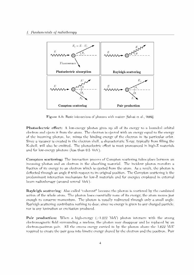
Figure 1.1: Basic interactions of photons with matter [Salvat et al., 2006].
Photoelectric eect: A low-energy photon gives up all of its energy to a bounded orbitalelectron and ejects it from the atom. The electron is ejected with an energy equal to the energyof the incoming photon, hν, minus the binding energy of the electron in its particular orbit.Since a vacancy is created in the electron shell, a characteristic X-ray, typically from lling theK-shell, will also be emitted. The photoelectric eect is most pronounced in high-Z materialsand for low-energy photons (less than 0.5 MeV).
Compton scattering: The interaction process of Compton scattering takes place between anincoming photon and an electron in the absorbing material. The incident photon transfers afraction of its energy to an electron which is ejected from the atom. As a result, the photon isdeected through an angle θ with respect to its original position. The Compton scattering is thepredominant interaction mechanism for low-Z materials and for energies employed in externalbeam radiotherapy (around several MeV).
Rayleigh scattering: Also called coherent because the photon is scattered by the combinedaction of the whole atom. The photon loses essentially none of its energy; the atom moves justenough to conserve momentum. The photon is usually redirected through only a small angle.Rayleigh scattering contributes nothing to dose, since no energy is given to any charged particle,nor is any ionization or excitation produced.
Pair production: When a high-energy (>1.022 MeV) photon interacts with the strongelectromagnetic eld surrounding a nucleus, the photon may disappear and be replaced by anelectron-positron pair. All the excess energy carried in by the photon above the 1.022 MeVrequired to create the pair goes into kinetic energy shared by the electron and the positron. Pair
4

1.2. Interaction of radiation with matter
production is predominantly conned to high-energy gamma rays.
The relative importance of Compton eect, photoelectric eect, and pair production depends onboth the photon quantum energy (E, = hν) and the atomic number Z of the absorbing medium.Figure 1.2 shows the relative importance of the three major types of photon interaction. Theline at the left represents the energy at which Compton scattering and photoelectric eect areequally probable as a function of the absorber atomic number. The line at the right representsthe energy at which pair production and Compton scattering are equally probable.
Figure 1.2: The three major types of photon interaction [Evans and Noyau, 1955].
1.2.2 Interaction of electrons with matter
An incident electron interacts with one or more electrons or with the nucleus of practically everyatom it passes. Most of these interactions transfer only a fraction of the incident particle's kineticenergy in each interaction, gradually losing its kinetic energy as they go through the medium (a1-MeV charged particle would typically undergo ∼105 interactions before losing all of its kineticenergy), so this mechanism is often called the continuous slowing-down approximation (CSDA).When electrons interact with other electrons, they produce excitations and ionizations. Wheninteracting with the atomic nuclei coulomb elds, they generate radiative collisions. In theseprocesses electrons undergo abrupt changes in their trajectories.
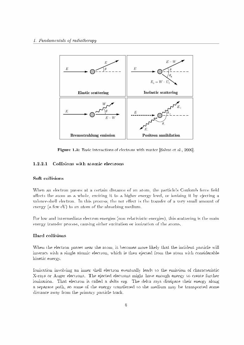
The possible interactions of electrons and positrons with the medium are, as shown in gure 1.3:elastic scattering, inelastic collisions and bremsstrahlung emission; positrons can also undergoannihilation, either in ight or at rest [Attix, 2008, Knoll, 2010, Martin, 2006, Cherry et al.,2012].
5
1. Fundamentals of radiotherapy
Figure 1.3: Basic interactions of electrons with matter [Salvat et al., 2006].
1.2.2.1 Collisions with atomic electrons
Soft collisions
When an electron passes at a certain distance of an atom, the particle's Coulomb force eldaects the atom as a whole, exciting it to a higher energy level, or ionizing it by ejecting avalence-shell electron. In this process, the net eect is the transfer of a very small amount ofenergy (a few eV) to an atom of the absorbing medium.
For low and intermediate electron energies (non relativistic energies), this scattering is the mainenergy transfer process, causing either excitation or ionization of the atoms.
Hard collisions
When the electron passes near the atom, it becomes more likely that the incident particle willinteract with a single atomic electron, which is then ejected from the atom with considerablekinetic energy.
Ionization involving an inner shell electron eventually leads to the emission of characteristicX-rays or Auger electrons. The ejected electrons might have enough energy to create furtherionization. That electron is called a delta ray. The delta rays dissipate their energy alonga separate path, so some of the energy transferred to the medium may be transported somedistance away from the primary particle track.
6

1.3. Intraoperative radiation therapy (IORT)
The probability of hard collisions depends of the nature of the incident particle, and althoughthese kind of collisions are less in number than the soft ones, the energy fraction of the primaryparticle lost in both processes is comparable.
1.2.2.2 Interactions with the external nuclear eld
These interactions occur when the incident particle actually penetrates the orbital electroncloud and interacts with its nucleus. In most of the cases (97%−98%) the electron is scatteredelastically, losing just a negligible amount of energy due to the nucleus recoil. Hence this is not amechanism for the transfer of energy to the absorbing medium (the electron does not emit X-raysor excite the nucleus), but it is the reason why the path of the electrons is very tortuous.
In the other 2-3 % of the cases in which the electron passes near the nucleus, an inelastic radiativeinteraction occurs in which an X-ray photon is emitted. The electron is not only deected inthis process, but gives a signicant fraction (up to 100%) of its kinetic energy to the photon,slowing down in the process. Such X-rays are called bremsstrahlung (German word for brakingradiation). The energy of the bremsstrahlung photons can range anywhere from nearly 0 (eventsin which the particle is only slightly deected) up to a maximum equal to the energy of theincident particle (events in which the particle is virtually stopped in the collision).
Bremsstrahlung is an important resource for dissipating energy in high Z media, but it is relativelyinsignicant for tissue-like (low Z) materials for electrons below 10 MeV.
1.2.2.3 Positron annihilation
When a positron is combined with an electron in an annihilation reaction, their masses areconverted into energy. This energy appears in the form of two 0.511 MeV annihilation photonsthat travel in opposite directions. However, if the annihilation takes place before the positronstops, the resulting photons may be emitted in directions slightly o the ideal.
1.3 Intraoperative radiation therapy (IORT)
Once described how the dierent types of radiation interact with matter, let's focus on describingthe main characteristics of intraoperative radiotherapy (IORT), because this treatment techniquewill be the main subject of this thesis.
Intraoperative radiation therapy is a special radiation modality that allows the administration
7
1. Fundamentals of radiotherapy
of a high localized dose (in the range of 10 to 25 Gy) in a single fraction during surgery, alone oras a boost technique [Calvo et al., 1993, Lamanna et al., 2012, Beddar et al., 2006, Abe, 1984,Rich, 1986, Gunderson et al., 2011, Debenham et al., 2013, Palta et al., 1995]. This modalitypermits direct visualization of the region to be irradiated after the removal of the lesion and itallows healthy tissue to be protected, by displacement or by shielding [Oshima et al., 2009, Russoet al., 2012, Martignano et al., 2007].
Although IORT was rst introduced as a treatment technique at the beginning of the XX century[Beck, 1909], it was not until the earlies 1970s and 1980s that modern IORT with electron beamswas developed [Abe et al., 1971, Abe and Takahashi, 1981]. Nowadays, IORT is widely usedand its benets in certain types of cancer (breast, gastrointestinal, prostate, pancreatic, brain,vertebral, etc) have been widely achieved [Calvo et al., 1993, Orecchia et al., 2003, Orecchia andVeronesi, 2005, Vaidya et al., 2001, Rich, 1986, Kraus-Tiefenbacher et al., 2005, Beatty et al.,1996, Bodner et al., 2003, Wenz et al., 2010, Schneider et al., 2011].
IORT can combine the benets of the surgery with the benets of the radiotherapy in thefollowing aspects:
• Reduction of the possibility of a residual tumor regeneration, eliminating the microscopictumor focal points.• Allowance of a better denition of the treatment area, minimizing the damage to thehealthy tissue.• Maximization of the radiobiological eect with a high, localized dose.• Fewer side eects, including rashes and skin irritation, that are commonly experiencedduring traditional radiation therapy.• Shortening of the external radiation therapy treatment time when combined with IORT.
IORT requires a complex organizing system specically designed for this treatment, that includesthe collaboration of a multidisciplinary team made up by surgeons, oncologists, radiotherapists,radiophysicists, anaesthetists, nursing sta and assistants, among others.
There are two dierent types of IORT treatment, depending of the radiation used: Intraop-erative electron radiation therapy (IOERT) and Low energy X-rays intraoperativeradiation therapy (XIORT).
1.3.1 Intraoperative electron radiation therapy (IOERT)
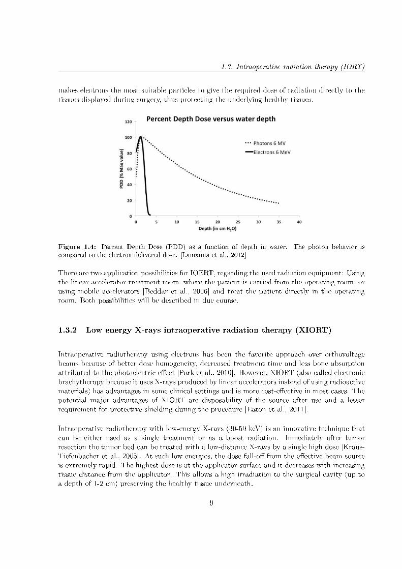
IOERT is the most common intraoperative radiation modality. Megavoltage electrons, whencomparing to megavoltage photons, release the maximum dose at a similar depth as the photons.However, while the dose of electrons is released in a few cm from the entry point, the dose ofphotons is released at greater depths, as shown in gure 1.4 [Lamanna et al., 2012]. This fact
8
1.3. Intraoperative radiation therapy (IORT)
makes electrons the most suitable particles to give the required dose of radiation directly to thetissues displayed during surgery, thus protecting the underlying healthy tissues.
Figure 1.4: Percent Depth Dose (PDD) as a function of depth in water. The photon behavior iscompared to the electron delivered dose. [Lamanna et al., 2012]
There are two application possibilities for IOERT, regarding the used radiation equipment: Usingthe linear accelerator treatment room, where the patient is carried from the operating room, orusing mobile accelerators [Beddar et al., 2006] and treat the patient directly in the operatingroom. Both possibilities will be described in due course.
1.3.2 Low energy X-rays intraoperative radiation therapy (XIORT)
Intraoperative radiotherapy using electrons has been the favorite approach over orthovoltagebeams because of better dose homogeneity, decreased treatment time and less bone absorptionattributed to the photoelectric eect [Park et al., 2010]. However, XIORT (also called electronicbrachytherapy because it uses X-rays produced by linear accelerators instead of using radioactivematerials) has advantages in some clinical settings and is more cost-eective in most cases. Thepotential major advantages of XIORT are disposability of the source after use and a lesserrequirement for protective shielding during the procedure [Eaton et al., 2011].
Intraoperative radiotherapy with low-energy X-rays (30-50 keV) is an innovative technique thatcan be either used as a single treatment or as a boost radiation. Inmediately after tumorresection the tumor bed can be treated with a low-distance X-rays by a single high dose [Kraus-Tiefenbacher et al., 2005]. At such low energies, the dose fall-o from the eective beam sourceis extremely rapid. The highest dose is at the applicator surface and it decreases with increasingtissue distance from the applicator. This allows a high irradiation to the surgical cavity (up toa depth of 1-2 cm) preserving the healthy tissue underneath.
9
1. Fundamentals of radiotherapy
XIORT is increasingly used since clinical results for breast cancer irradiation showed a similarlocal control [Veronesi et al., 2013], less toxicity, especially chronic skin toxicity [Sperk et al.,2012], and a overall survival benet [Vaidya et al., 2014] for patients treated with XIORT incomparison to patients treated with external beam radiotherapy.
There are currently two commercial devices dedicated to low energy X-rays IORT (XIORT)treatments: the Axxent R© Electronic Brachytherapy System (Xoft Inc., Fremont, California) andthe INTRABEAM R© device (Carl Zeiss Surgical Gmbh, Oberkochen, Germany). In this thesiswe will study the INTRABEAM R© device, so further description of this device can be found inthe next sections.
1.4 Dose delivery in IORT
1.4.1 Linear accelerators for IOERT
There are two IOERT types of linear accelerators (LINAC), as previously mentioned:Conventional linear accelerators and dedicated mobile accelerators. The main characteristicsof both systems will be found below.
1.4.1.1 Stationary linear accelerators
The available clinical linear accelerators can produce either photon or electron beams. In general,the generated radiation with this kind of devices is a high energy radiation with an energyspectrum from a few keV to several MeV, depending on the model.
A linear accelerator is a device that uses high radio-frequency (10-100 MHz) electromagneticwaves to accelerate charged particles (i.e. electrons) to high energies in a linear path, inside atube-like structure called the accelerator waveguide [Khan, 1994, Karzmark and Morton, 1981].The most basic conguration of a linear accelerator consists in using electron acceleration betweentwo electrodes by means of the electric gradient within them. The electron beam is accelerateduntil it reaches kinetic energies between 4 and 25 MeV.
The LINAC has two working modes depending on the particles used for the treatment (gure1.5):
In the X-ray therapy mode the electron beam hits a high-Z target, like tungsten. As a result,the electron energy is converted into a spectrum of X-ray energies with maximum energy equalto the incident electron energy.
10
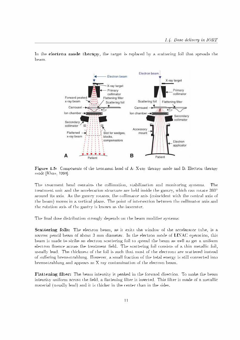
1.4. Dose delivery in IORT
In the electron mode therapy, the target is replaced by a scattering foil that spreads thebeam.
Figure 1.5: Components of the treatment head of A: X-ray therapy mode and B: Electron therapymode [Khan, 1994].
The treatment head contains the collimation, stabilization and monitoring systems. Thetreatment unit and the acceleration structure are held inside the gantry, which can rotate 360
around its axis. As the gantry rotates, the collimator axis (coincident with the central axis ofthe beam) moves in a vertical plane. The point of intersection between the collimator axis andthe rotation axis of the gantry is known as the isocenter.
The nal dose distribution strongly depends on the beam modier systems:
Scattering foils: The electron beam, as it exits the window of the accelerator tube, is anarrow pencil beam of about 3 mm diameter. In the electron mode of LINAC operation, thisbeam is made to strike an electron scattering foil to spread the beam as well as get a uniformelectron uence across the treatment eld. The scattering foil consists of a thin metallic foil,usually lead. The thickness of the foil is such that most of the electrons are scattered insteadof suering bremsstrahlung. However, a small fraction of the total energy is still converted intobremsstrahlung and appears as X-ray contamination of the electron beam.
Flattening lter: The beam intensity is peaked in the forward direction. To make the beamintensity uniform across the eld, a attening lter is inserted. This lter is made of a metallicmaterial (usually lead) and it is thicker in the center than in the sides.
11

1. Fundamentals of radiotherapy
Collimators: The emerging beam needs to be shaped to t the treatment area. This is doneby metallic jaws that change the beam area and size and focus the radiation.
IOERT applicators: All IOERT treatments need a specic collimator system [Nevelsky et al.,2010, Björk et al., 2000, Pimpinella et al., 2007]. Besides primary and secondary collimators,there are other systems called applicators that also collimate the beam.
Figure 1.6: Main components of an ELEKTA PRECISE device [Nevelsky et al., 2010]
An IOERT applicator has three main functions: Collimation of the electron beam, denition ofthe treatment volume and detraction of the healthy tissue [Björk et al., 2000].
The main characteristics of applicators (used in both stationary and mobile linear accelerators)are [Pimpinella et al., 2007, Björk et al., 2000]:
• Applicators have, in general, cylindrical shape, although some of them may be rectangular.• Applicators can be beveled or non-beveled.• They are usually made of PMMA or brass.• Applicator thickness varies between 3 mm and 8 mm.• They present dierent lengths (from 30 cm to more than 1 m) and diameters (5-10 cm ormore).
When a conventional accelerator is used for IOERT treatments, specic designed applicatorsmust be employed [Nevelsky et al., 2010]. A telescopic device is attached to the accelerator headto change the source-to-applicator-end distance in the range up to 100110 cm (gure 1.6).
The use of conventional accelerators for IOERT has several disadvantages. In this case, theanesthetized patient must be moved from the operating room (OR) to a sanitized treatment
12
1.4. Dose delivery in IORT
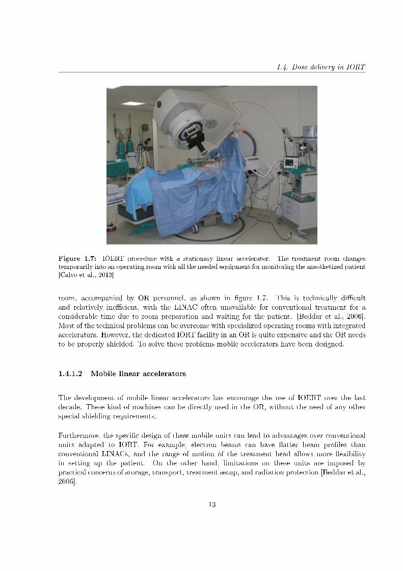
Figure 1.7: IOERT procedure with a stationary linear accelerator. The treatment room changestemporarily into an operating room with all the needed equipment for monitoring the anesthetized patient[Calvo et al., 2013]
room, accompanied by OR personnel, as shown in gure 1.7. This is technically dicultand relatively inecient, with the LINAC often unavailable for conventional treatment for aconsiderable time due to room preparation and waiting for the patient. [Beddar et al., 2006].Most of the technical problems can be overcome with specialized operating rooms with integratedaccelerators. However, the dedicated IORT facility in an OR is quite expensive and the OR needsto be properly shielded. To solve these problems mobile accelerators have been designed.
1.4.1.2 Mobile linear accelerators
The development of mobile linear accelerators has encourage the use of IOERT over the lastdecade. These kind of machines can be directly used in the OR, without the need of any otherspecial shielding requirements.
Furthermore, the specic design of these mobile units can lead to advantages over conventionalunits adapted to IORT. For example, electron beams can have atter beam proles thanconventional LINACs, and the range of motion of the treatment head allows more exibilityin setting up the patient. On the other hand, limitations on these units are imposed bypractical concerns of storage, transport, treatment setup, and radiation protection [Beddar et al.,2006].
13
1. Fundamentals of radiotherapy
Actually there are several types of mobile LINACs:
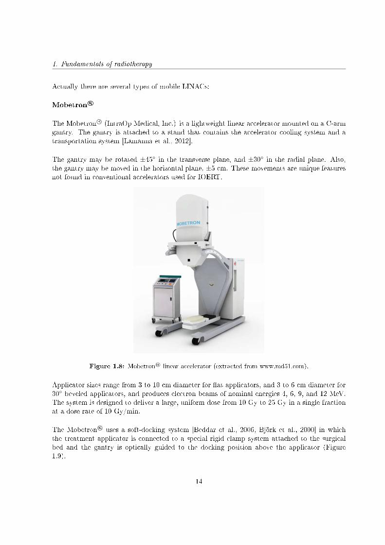
Mobetron R©
The Mobetron R© (IntraOp Medical, Inc.) is a lightweight linear accelerator mounted on a C-armgantry. The gantry is attached to a stand that contains the accelerator cooling system and atransportation system [Lamanna et al., 2012].
The gantry may be rotated ±45 in the transverse plane, and ±30 in the radial plane. Also,the gantry may be moved in the horizontal plane, ±5 cm. These movements are unique featuresnot found in conventional accelerators used for IOERT.
Figure 1.8: Mobetron R© linear accelerator (extracted from www.md51.com).
Applicator sizes range from 3 to 10 cm diameter for at applicators, and 3 to 6 cm diameter for30 beveled applicators, and produces electron beams of nominal energies 4, 6, 9, and 12 MeV.The system is designed to deliver a large, uniform dose from 10 Gy to 25 Gy in a single fractionat a dose rate of 10 Gy/min.
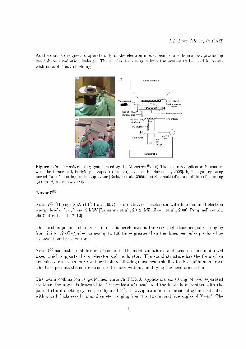
The Mobetron R© uses a soft-docking system [Beddar et al., 2006, Björk et al., 2000] in whichthe treatment applicator is connected to a special rigid clamp system attached to the surgicalbed and the gantry is optically guided to the docking position above the applicator (Figure1.9).
14
1.4. Dose delivery in IORT
As the unit is designed to operate only in the electron mode, beam currents are low, producingless inherent radiation leakage. The accelerator design allows the system to be used in roomswith no additional shielding.
Figure 1.9: The soft-docking system used by the Mobetron R©. (a) The electron applicator, in contactwith the tumor bed, is rigidly clamped to the surgical bed [Beddar et al., 2006].(b) The gantry beingmoved for soft docking to the applicator [Beddar et al., 2006]. (c) Schematic diagram of the soft-dockingsystem [Björk et al., 2000].
Novac7 R©
Novac7 R© (Hitesys SpA (LT) Italy 1997), is a dedicated accelerator with four nominal electronenergy levels: 3, 5, 7 and 9 MeV [Lamanna et al., 2012, Mihailescu et al., 2006, Pimpinella et al.,2007, Righi et al., 2013].
The most important characteristic of this accelerator is the very high dose-per-pulse, rangingfrom 2.5 to 12 cGy/pulse, values up to 100 times greater than the doses per pulse produced bya conventional accelerator.
Novac7 R© has both a mobile and a xed unit. The mobile unit is a stand structure on a motorizedbase, which supports the accelerator and modulator. The stand structure has the form of anarticulated arm with four rotational joints, allowing movements similar to those of human arms.The base permits the entire structure to move without modifying the head orientation.
The beam collimation is performed through PMMA applicators consisting of two separatedsections: the upper is fastened to the accelerator's head, and the lower is in contact with thepatient (Hard-docking system, see gure 1.11). The applicator's set consists of cylindrical tubeswith a wall thickness of 5 mm, diameter ranging from 4 to 10 cm, and face angles of 045. The
15
1. Fundamentals of radiotherapy
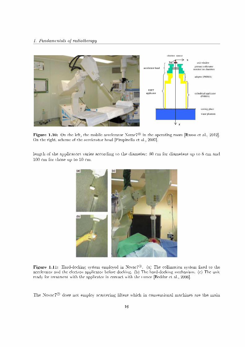
Figure 1.10: On the left, the mobile accelerator Novac7 R© in the operating room [Russo et al., 2012].On the right, scheme of the accelerator head [Pimpinella et al., 2007].
length of the applicators varies according to the diameter: 80 cm for diameters up to 8 cm and100 cm for those up to 10 cm.
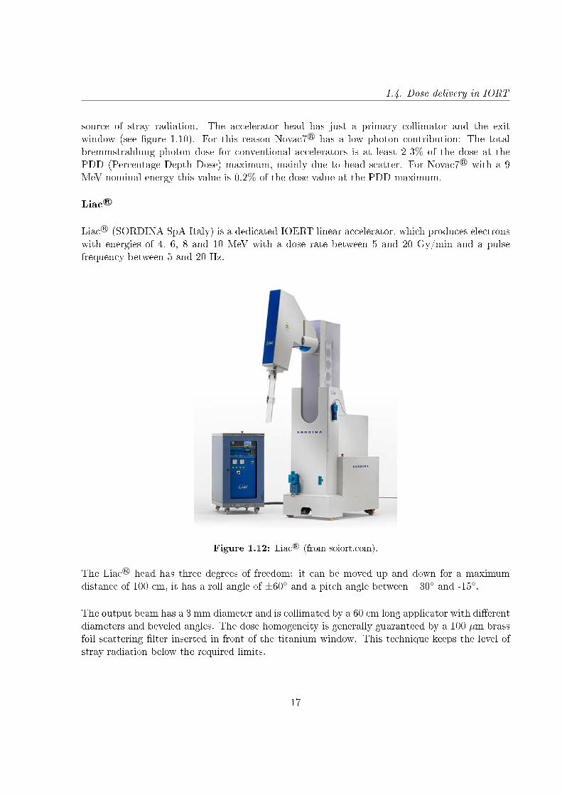
Figure 1.11: Hard-docking system employed in Novac7 R©. (a) The collimation system xed to theaccelerator and the electron applicator before docking. (b) The hard-docking mechanism. (c) The unitready for treatment with the applicator in contact with the tumor [Beddar et al., 2006].
The Novac7 R© does not employ scattering lters which in conventional machines are the main
16
1.4. Dose delivery in IORT
source of stray radiation. The accelerator head has just a primary collimator and the exitwindow (see gure 1.10). For this reason Novac7 R© has a low photon contribution: The totalbremmstrahlung photon dose for conventional accelerators is at least 2-3% of the dose at thePDD (Percentage Depth Dose) maximum, mainly due to head scatter. For Novac7 R© with a 9MeV nominal energy this value is 0.2% of the dose value at the PDD maximum.
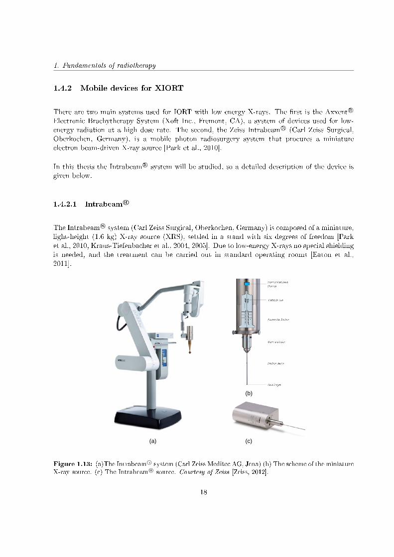
Liac R©
Liac R© (SORDINA SpA Italy) is a dedicated IOERT linear accelerator, which produces electronswith energies of 4, 6, 8 and 10 MeV with a dose rate between 5 and 20 Gy/min and a pulsefrequency between 5 and 20 Hz.
Figure 1.12: Liac R© (from soiort.com).
The Liac R© head has three degrees of freedom: it can be moved up and down for a maximumdistance of 100 cm, it has a roll angle of ±60 and a pitch angle between +30 and -15.
The output beam has a 3 mm diameter and is collimated by a 60 cm long applicator with dierentdiameters and beveled angles. The dose homogeneity is generally guaranteed by a 100 µm brassfoil scattering lter inserted in front of the titanium window. This technique keeps the level ofstray radiation below the required limits.
17
1. Fundamentals of radiotherapy
1.4.2 Mobile devices for XIORT
There are two main systems used for IORT with low energy X-rays. The rst is the Axxent R©
Electronic Brachytherapy System (Xoft Inc., Fremont, CA), a system of devices used for low-energy radiation at a high dose rate. The second, the Zeiss Intrabeam R© (Carl Zeiss Surgical,Oberkochen, Germany), is a mobile photon radiosurgery system that procures a miniatureelectron beam-driven X-ray source [Park et al., 2010].
In this thesis the Intrabeam R© system will be studied, so a detailed description of the device isgiven below.
1.4.2.1 Intrabeam R©
The Intrabeam R© system (Carl Zeiss Surgical, Oberkochen, Germany) is composed of a miniature,light-height (1.6 kg) X-ray source (XRS), settled in a stand with six degrees of freedom [Parket al., 2010, Kraus-Tiefenbacher et al., 2004, 2005]. Due to low-energy X-rays no special shieldingis needed, and the treatment can be carried out in standard operating rooms [Eaton et al.,2011].
(a)
(b)
(c)
Figure 1.13: (a)The Intrabeam R© system (Carl Zeiss Meditec AG, Jena) (b) The scheme of the miniatureX-ray source. (c) The Intrabeam R© source. Courtesy of Zeiss [Zeiss, 2012].
18

1.4. Dose delivery in IORT
The electrons are generated and accelerated to a potential of 50 kV in the main unit and travelvia the electron beam drift tube with 10 cm in length and 3.2 mm in diameter. At its end theaccelerated electrons strike a gold target resulting in a nearly isotropic bremsstrahlung X-raydistribution around the tip [Yanch and Harte, 1996, Beatty et al., 1996, Dinsmore et al., 1996].The scheme of the miniature X-ray source is shown in gure 1.13 (b).
The X-ray system produces low energy photons (up to 50 keV) with a steep dose fallo insoft tissue. This dose fallo in the tissue guarantees minimum exposure of the surroundingtissue.
Dierent cancer types can be treated with Intrabeam R©, using dierent applicators, which can beattached to the XRS. These applicators are optimized in shape, size and physical dose distributionaccording to the cancer type, shape and location within the body. There are several applicatorsavailable, such as spherical, needle, cylindrical, at and surface applicators (see gure 1.14).
(a) (b) (c)
(d) (e)
Figure 1.14: The Intrabeam R© applicators. (a) Spherical applicator. (b) Needle applicator. (c)Cylindrical applicator. (d) Surface applicator. (e) Flat applicator [Zeiss, 2012].
a) Spherical applicators
The most used applicator for Intrabeam R© is the Spherical, specially for irradiating the tumor
19
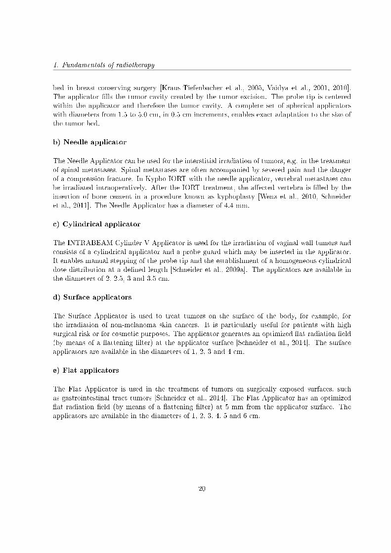
1. Fundamentals of radiotherapy
bed in breast-conserving surgery [Kraus-Tiefenbacher et al., 2005, Vaidya et al., 2001, 2010].The applicator lls the tumor cavity created by the tumor excision. The probe tip is centeredwithin the applicator and therefore the tumor cavity. A complete set of spherical applicatorswith diameters from 1.5 to 5.0 cm, in 0.5 cm increments, enables exact adaptation to the size ofthe tumor bed.
b) Needle applicator
The Needle Applicator can be used for the interstitial irradiation of tumors, e.g. in the treatmentof spinal metastases. Spinal metastases are often accompanied by severed pain and the dangerof a compression fracture. In Kypho-IORT with the needle applicator, vertebral metastases canbe irradiated intraoperatively. After the IORT treatment, the aected vertebra is lled by theinsertion of bone cement in a procedure known as kyphoplasty [Wenz et al., 2010, Schneideret al., 2011]. The Needle Applicator has a diameter of 4.4 mm.
c) Cylindrical applicator
The INTRABEAM Cylinder V Applicator is used for the irradiation of vaginal wall tumors andconsists of a cylindrical applicator and a probe guard which may be inserted in the applicator.It enables manual stepping of the probe tip and the establishment of a homogeneous cylindricaldose distribution at a dened length [Schneider et al., 2009a]. The applicators are available inthe diameters of 2, 2.5, 3 and 3.5 cm.
d) Surface applicators
The Surface Applicator is used to treat tumors on the surface of the body, for example, forthe irradiation of non-melanoma skin cancers. It is particularly useful for patients with highsurgical risk or for cosmetic purposes. The applicator generates an optimized at radiation eld(by means of a attening lter) at the applicator surface [Schneider et al., 2014]. The surfaceapplicators are available in the diameters of 1, 2, 3 and 4 cm.
e) Flat applicators
The Flat Applicator is used in the treatment of tumors on surgically exposed surfaces, suchas gastrointestinal tract tumors [Schneider et al., 2014]. The Flat Applicator has an optimizedat radiation eld (by means of a attening lter) at 5 mm from the applicator surface. Theapplicators are available in the diameters of 1, 2, 3, 4, 5 and 6 cm.
20
1.5. Dosimetry in an IORT treatment
1.5 Dosimetry in an IORT treatment
IORT treatments, as other modern radiotherapy techniques, have improved radiation delivery.But these techniques have also increased the complexity of the treatment planning and qualityassurance needs to be done.
Dosimetry for IOERT treatments:
The most commonly used dosimeters for calibration of photon and electron beams are exposure-calibrated ionization chambers [Khan et al., 1991, Almond et al., 1999]. However, IORTdosimetry requires particular procedures for beam dosimetry and characterization, specially whenusing dedicated LINACs, which are sometimes dierent from those used in conventional externalbeam radiotherapy.
The main dierence is related to the high dose per pulse of IOERT dedicated LINACs that doesnot allow the direct use of the ionization chamber as recommended in the IAEA 398 protocolfor the absolute dose determination because of ion recombination eects [Marrale et al., 2015].The direct use of ionization chambers could, in principle, lead to inaccurate measurements ofoutput factors (OF) when applied to electron beams with these features of dose rate and energyand angular distribution. However, Björk et al. [Björk et al., 2004] have shown that ionization-chamber-based international dosimetry protocols could be applied in direct manner for outputfactor measurement in IORT beam, with an uncertainty less than 0.3%.
Furthermore, the high dose gradients used in IORT require high spatial resolution detectors.Other conventional measuring systems such as semiconductors do not provide enough spatialresolution. Thermoluminescent detectors are hard to setup and time consuming to read. Silver-halide radiographic lm has large dierences in sensitivity to photon energies in the 10-200 keVregion, its properties of energy absorption and transfer do not match those of biological tissues,are sensitive to room light and require wet chemical processing [Niroomand-Rad et al., 1998,Fuss et al., 2007].
In contrast, radiochromic dosimeters provide high spatial resolution, have low spectral sensitivityvariation and does not require post-processing, which make them one of the most reliabledosimetry methods.
Dosimetry for XIORT treatments:
Kilovoltage X-ray beam dosimetry provides a number of challenges which are not present formegavoltage X-ray beams [Hill et al., 2014, Ebert et al., 2002, Ebert and Carruthers, 2003].
Due to the low beam energy, the dose falls rapidly (∼1/r3 in water, r being the distance to thecenter of the source [Armoogum et al., 2007]). Such a rapid fallo of the dose may complicate
21
1. Fundamentals of radiotherapy
dosimetry as dose can vary considerably across the volume of the detector when dose distributionsare being measured. For example, the recommended ionization chamber is a parallel-platechamber which has 1 mm width in the direction of the dose fallo (Type 23342, PTW, Freiburg,Germany), corresponding to a change in dose greater that 50% at 5 mm distance from the sourceat 50 kV [Ebert et al., 2002].
In addition, the energy spectrum is hardened quickly inside the water which can aect dosimetricparameters such as energy absorption coecients and tissue equivalence materials.
Another issue is that the response of the dosimeter is sensitive to the materials used in itsconstruction. For low energy X-ray beams, the photoelectric eect is a dominant interactionprocess and the photoelectric cross section has a strong dependence on the atomic number of thematerial.
The last challenge is that ionization chambers do not act as BraggGray cavities in the kilovoltageX-ray energy range and so cavity theory cannot be used for reference dosimetry.
In contrast, some of the required dosimetric characteristics are found in radiochromic lms[Avanzo et al., 2012, Ebert et al., 2009, Fletcher and Mills, 2008]:
• Intrabeam R© dose reaches a maximum of about 20 Gy around the applicator surface and fallsbelow 1 Gy at 3 cm depth in tissue. Gafchromic EBT3 (International Specialty Products,Wayne, NJ, USA) are recommended to be used in the range from 1 cGy to more than 40Gy.• Radiochromic lms have a high spatial resolution, necessary for measuring the rapidIntrabeam R© dose fallo.• As described before, one of the concerns of kilovoltage X-rays is the energy response of thedosimeter. Gafchromic EBT3 are energy-independent.• Regarding the dosimeter materials, these lms are near tissue-equivalent.
In this thesis, experimental measurements have been performed with the Intrabeam R© device.Two dierent dosimetric methods have been used: Ionization chambers and radiochromiclm.
1.5.1 Ionization chambers
A ionization chamber is a gas lled detector. As radiation passes through a gas it can ionize thegas molecules. The charge pairs can be made to move in opposite directions by the applicationof an external electric eld. The result is an electric pulse that can be measured by an associatedmeasuring device. Based on the applied bias voltage, a detector can be operated in a number ofmodes, which dier from one to another by the amount of charges produced and their movement
22
1.5. Dosimetry in an IORT treatment
inside the detector volume. In the ion chamber voltage region, all the charges that are beingproduced get collected.
Ionization chambers are widely used for absolute dose measurements in radiation therapy. Byapplying a certain detector specic calibration factor (e.g. Gy/C), the detector signal is relatedto a radiation dose value.
1.5.2 Radiochromic lms
The radiochromic lm consists of a radiation-sensitive dye embedded in an organic emulsion or aninert polymer. When an energetic photon or electron transfers its energy to the active layer, theactive monomer components present in the lm react to form a colored polymer [Niroomand-Radet al., 1998, Schneider et al., 2009b, Fuss et al., 2007].
These lms have very high spatial resolution and low energy dependence. Furthermore, they areinsensitive to visible light, and the direct coloration does not require chemical, optical or thermalprocessing or amplication.
In this work Gafchromic EBT3 (International Specialty Products, Wayne, NJ, USA) have beenused to perform absolute dosimetry. The lm structure is made of an active layer (28 µm thick),between two polyester substrates (125 µm thick) [Gafchromic-EBT3]. The active layer containsthe active component, a marker dye, stabilizers and other components giving the lm its nearenergy-independent response.
1.5.2.1 Data analysis. The three channel technique
After irradiation, radiochromic lms need to be scanned and converted to dose. The opticaldensity has to be determined and, by using the dose-optical density response curve, the scannedimage can be converted into dose (dose mapping). A multichannel atbed scanner is the bestoption, as it oers the selection of the red color channel for greater sensitivity at lower doses andthe blue and green color channel for higher doses.
Since the radiochromic lm provides a dierent response to each of the channels, scanned lmscan be separated and analyzed in two parts: one part which is dose-dependent, and anotherdose-independent part which contains information about the dierences in the lm or the scanner(thickness inhomogeneities, noise, dust particles, scanner artifacts, etc) [Micke et al., 2011]. Byseparating the independent-dose part from the image, the remaining information is more reliableand therefore more useful for dosimetry.
23
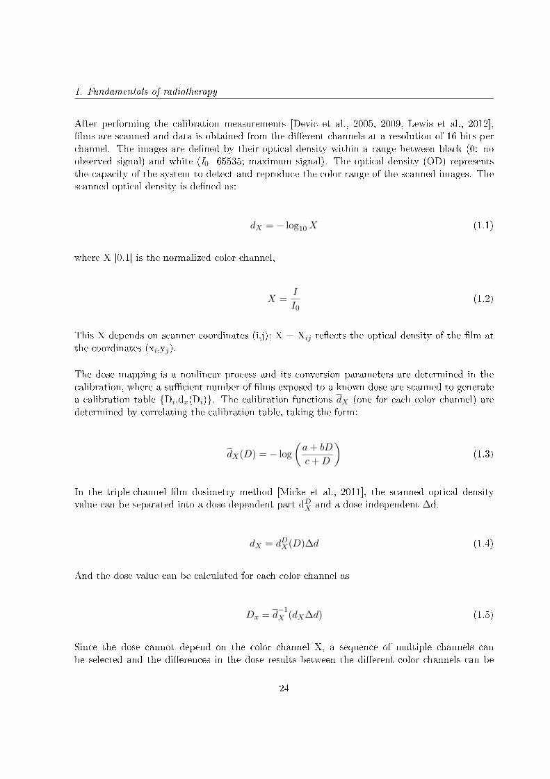
1. Fundamentals of radiotherapy
After performing the calibration measurements [Devic et al., 2005, 2009, Lewis et al., 2012],lms are scanned and data is obtained from the dierent channels at a resolution of 16 bits perchannel. The images are dened by their optical density within a range between black (0: noobserved signal) and white (I0=65535; maximum signal). The optical density (OD) representsthe capacity of the system to detect and reproduce the color range of the scanned images. Thescanned optical density is dened as:
dX = − log10X (1.1)
where X [0,1] is the normalized color channel,
X =I
I0(1.2)
This X depends on scanner coordinates (i,j); X = Xij reects the optical density of the lm atthe coordinates (xi,yj).
The dose mapping is a nonlinear process and its conversion parameters are determined in thecalibration, where a sucient number of lms exposed to a known dose are scanned to generatea calibration table Di,dx(Di). The calibration functions dX (one for each color channel) aredetermined by correlating the calibration table, taking the form:
dX(D) = − log(a+ bD
c+D
)(1.3)
In the triple-channel lm dosimetry method [Micke et al., 2011], the scanned optical densityvalue can be separated into a dose-dependent part dDX and a dose-independent ∆d.
dX = dDX(D)∆d (1.4)
And the dose value can be calculated for each color channel as
Dx = d−1X (dX∆d) (1.5)
Since the dose cannot depend on the color channel X, a sequence of multiple channels canbe selected and the dierences in the dose results between the dierent color channels can be
24

1.5. Dosimetry in an IORT treatment
Figure 1.15: Multichannel calibration curves [Micke et al., 2011]
minimized (gure 1.15).
Ω(∆d) =∑i 6=j
(DXi −DXj )2 → min
∆d(1.6)
This minimization is equivalent to nding the nearest color to the color path dR(D),dG(D),dB(D).The distance of a point from his color path represents the disturbance value ∆d, and the valueof the path parameter is the best dose value.
Figure 1.16: Dose map and disturbance map, and horizontal proles [Micke et al., 2011]
25
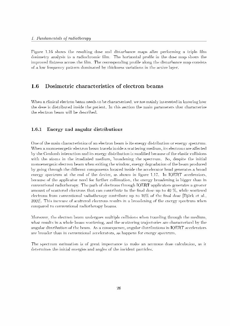
1. Fundamentals of radiotherapy
Figure 1.16 shows the resulting dose and disturbance maps after performing a triple lmdosimetry analysis to a radiochromic lm. The horizontal prole in the dose map shows theimproved atness across the lm. The corresponding prole along the disturbance map consistsof a low frequency pattern dominated by thickness variations in the active layer.
1.6 Dosimetric characteristics of electron beams
When a clinical electron beam needs to be characterized, we are mainly interested in knowing howthe dose is distributed inside the patient. In this section the main parameters that characterizethe electron beam will be described.
1.6.1 Energy and angular distributions
One of the main characteristics of an electron beam is its energy distribution or energy spectrum.When a monoenergetic electron beam travels inside a scattering medium, its electrons are aectedby the Coulomb interaction and its energy distribution is modied because of the elastic collisionswith the atoms in the irradiated medium, broadening the spectrum. So, despite the initialmonoenergetic electron beam when exiting the window, energy degradation of the beam producedby going through the dierent components located inside the accelerator head generates a broadenergy spectrum at the end of the device, as shown in gure 1.17. In IOERT accelerators,because of the applicator need for further collimation, the energy broadening is bigger than inconventional radiotherapy. The path of electrons through IOERT applicators generates a greateramount of scattered electrons that can contribute to the nal dose up to 40 %, while scatteredelectrons from conventional radiotherapy contribute up to 10% of the nal dose [Björk et al.,2002]. This increase of scattered electrons results in a broadening of the energy spectrum whencompared to conventional radiotherapy beams.
Moreover, the electron beam undergoes multiple collisions when traveling through the medium,what results in a whole beam scattering, and the scattering trajectories are characterized by theangular distribution of the beam. As a consequence, angular distributions in IOERT acceleratorsare broader than in conventional accelerators, as happens for energy spectrum.
The spectrum estimation is of great importance to make an accurate dose calculation, as itdetermines the initial energies and angles of the incident particles.
26
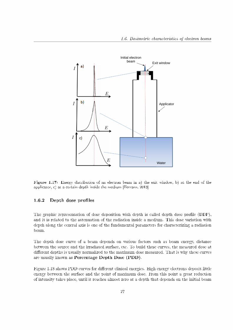
1.6. Dosimetric characteristics of electron beams
Initial electron beam Exit window
Applicator
Water
Figure 1.17: Energy distribution of an electron beam in a) the exit window, b) at the end of theapplicator, c) at a certain depth inside the medium [Herranz, 2013]
1.6.2 Depth dose proles
The graphic representation of dose deposition with depth is called depth dose prole (DDP),and it is related to the attenuation of the radiation inside a medium. This dose variation withdepth along the central axis is one of the fundamental parameters for characterizing a radiationbeam.
The depth dose curve of a beam depends on various factors such as beam energy, distancebetween the source and the irradiated surface, etc. To build these curves, the measured dose atdierent depths is usually normalized to the maximum dose measured. That is why these curvesare usually known as Percentage Depth Dose (PDD).
Figure 1.18 shows PDD curves for dierent clinical energies. High energy electrons deposit littleenergy between the surface and the point of maximum dose. From this point a great reductionof intensity takes place, until it reaches almost zero at a depth that depends on the initial beam
27

1. Fundamentals of radiotherapy
Figure 1.18: Percentage depth dose curves (PDD) for typical IOERT electron beams [Nevelsky et al.,2010].
energy. The rest of the dose contribution after this descending linear portion of the curve iscaused by bremsstrahlung X-rays.
Dierent parameters can be dened looking at the PDD (see gure 1.19 (a)) [Delgado et al.,2013]:
• Rmax: Depth where absorbed dose in the central axis reaches the maximum.• R90: Depth where dose reaches 90% of the maximum. The region between z=0 and R90 iscalled therapeutic range.• R50: Depth where dose reaches 50% of the maximum.• Rp: Depth of the point where the tangent to the descending linear portion of the curve(at the point of inection) intersects the extrapolated background. Also called PracticalRange.• Bremsstrahlung tail: X-ray contamination area. Dose measured in the central axis atd10 + 10 cm (d10 is the depth the dose reaches 10%) of the maximum.
1.6.3 Transverse dose proles
Depth dose curves have not enough information to describe completely the deposited dose, and3D dose distributions are necessary. To achieve this, dose measurements o-axis, also calledtransverse dose proles, are performed. These curves take into account the beam spatial variation,and are used to know how dose is distributed perpendicularly to the beam. By combining depthdose proles with o-axis data, 3D dose distribution can be reconstructed.
28
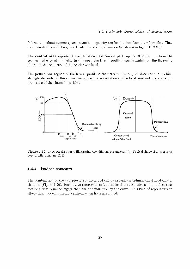
1.6. Dosimetric characteristics of electron beams
Information about symmetry and beam homogeneity can be obtained from lateral proles. Theyhave two distinguished regions: Central area and penumbra (as shown in gure 1.19 (b)).
The central area represents the radiation eld central part, up to 10 to 15 mm from thegeometrical edge of the eld. In this area, the lateral prole depends mainly on the atteninglter and the geometry of the accelerator head.
The penumbra region of the lateral prole is characterized by a quick dose variation, whichstrongly depends on the collimation system, the radiation source focal size and the scatteringproperties of the charged particles.
Dose %
Distance (cm)Geometrical edge of the field
Central area
PenumbraBremsstrahlungBremsstrahlung
tailtail
Rmax
R50
Rp
R90
PD
D (%
)
90
(a) (b)
Figure 1.19: a) Depth dose curve illustrating the dierent parameters. (b) Typical shape of a transversedose prole [Herranz, 2013].
1.6.4 Isodose contours
The combination of the two previously described curves provides a bidimensional modeling ofthe dose (Figure 1.20). Each curve represents an isodose level that includes spatial points thatreceive a dose equal or bigger than the one indicated by the curve. This kind of representationallows dose modeling inside a patient when he is irradiated.
29
1. Fundamentals of radiotherapy
Figure 1.20: Isodose contours of a 18 MeV electron beam [Nevelsky et al., 2010]
1.7 Dosimetric characteristics of low energy X-rays
As previously done with electrons, in this section we are going to describe the main parametersthat characterize the Intrabeam R© photon beam.
1.7.1 Energy and angular distributions
The Intrabeam R© source is a miniature X-ray source where electrons are accelerated up to 50 kVand hit a gold target. As a result, X-rays are emitted in all directions with a maximum energyof 50 keV. Therefore, the energy spectrum of the Intrabeam R© source will be a classical X-rayspectrum with characteristic X-rays and a bremsstrahlung background.
The energy spectrum of the Intrabeam R© X-ray source (XRS) can be seen in gure 1.21 (Left).The location of the prominent peaks correspond with the characteristic X-rays for gold and othermaterials of the source [Dinsmore et al., 1996, Beatty et al., 1996].
When an applicator is placed around the needle, the beam hardens as it passes through thedierent materials. As a result, there is a reduction of the characteristic X-rays and an increaseof the bremsstrahlung tail. The energy spectrum of a spherical applicator is shown in gure 1.21(Right).
Angular distribution of the Intrabeam R© needle has been studied in previous works [Dinsmoreet al., 1996]. It has been found (gure 1.22) that intensity is nearly isotropic, with an approxi-mately 10 % decrease perpendicular to the probe axis (due to photon self-absorption in the gold)and a 7% dip in the forward direction (origin unknown).
30
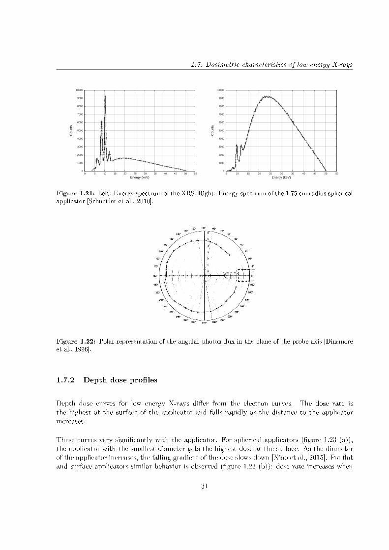
1.7. Dosimetric characteristics of low energy X-rays
0
1000
2000
3000
4000
5000
6000
7000
8000
9000
10000
0 5 10 15 20 25 30 35 40 45 50 55
Cou
nts
Energy (keV)
0
1000
2000
3000
4000
5000
6000
7000
8000
9000
10000
5 10 15 20 25 30 35 40 45 50 55
Cou
nts
Energy (keV)
Figure 1.21: Left: Energy spectrum of the XRS. Right: Energy spectrum of the 1.75 cm radius sphericalapplicator [Schneider et al., 2010].
Figure 1.22: Polar representation of the angular photon ux in the plane of the probe axis [Dinsmoreet al., 1996].
1.7.2 Depth dose proles
Depth dose curves for low energy X-rays dier from the electron curves. The dose rate isthe highest at the surface of the applicator and falls rapidly as the distance to the applicatorincreases.
These curves vary signicantly with the applicator. For spherical applicators (gure 1.23 (a)),the applicator with the smallest diameter gets the highest dose at the surface. As the diameterof the applicator increases, the falling gradient of the dose slows down [Xiao et al., 2015]. For atand surface applicators similar behavior is observed (gure 1.23 (b)): dose rate increases when
31
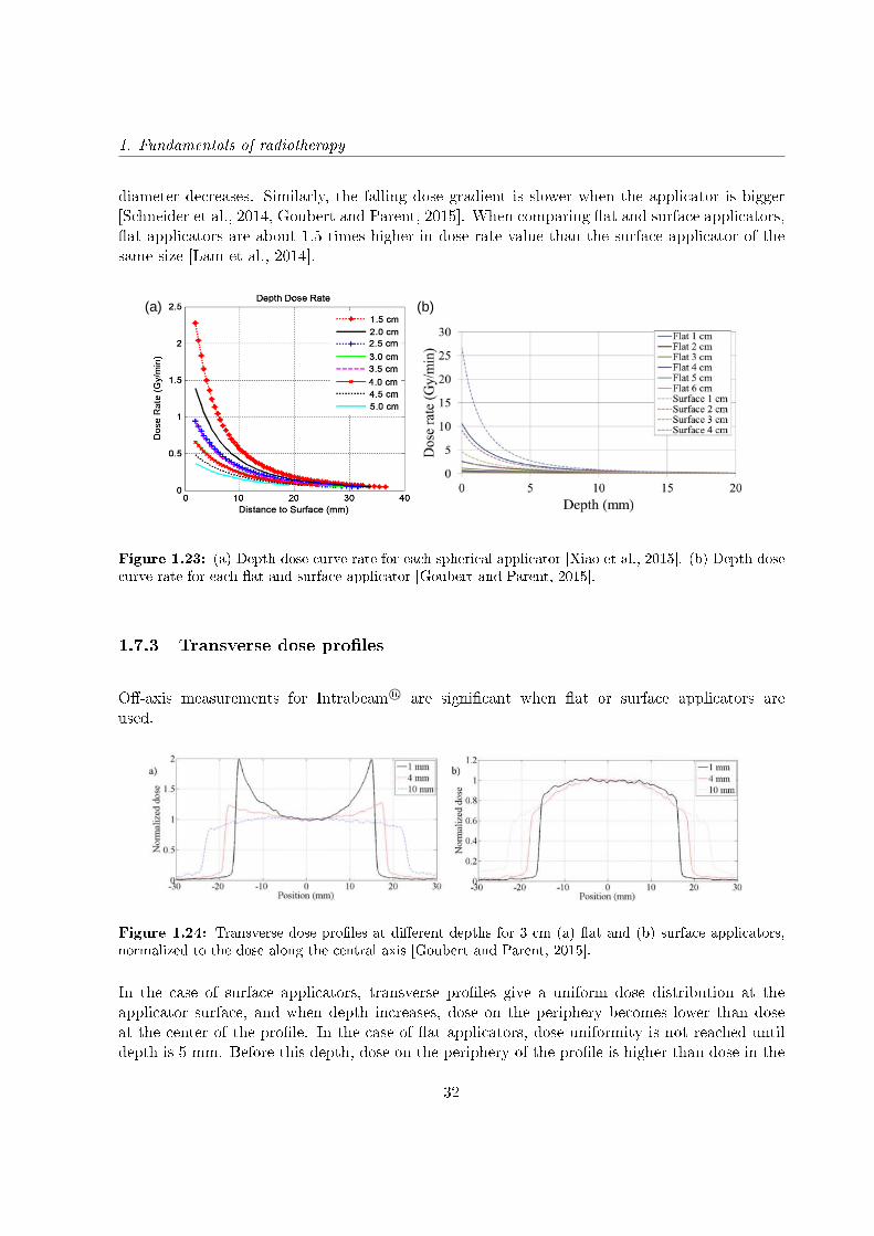
1. Fundamentals of radiotherapy
diameter decreases. Similarly, the falling dose gradient is slower when the applicator is bigger[Schneider et al., 2014, Goubert and Parent, 2015]. When comparing at and surface applicators,at applicators are about 1.5 times higher in dose rate value than the surface applicator of thesame size [Lam et al., 2014].
(a) (b)
Figure 1.23: (a) Depth dose curve rate for each spherical applicator [Xiao et al., 2015]. (b) Depth dosecurve rate for each at and surface applicator [Goubert and Parent, 2015].
1.7.3 Transverse dose proles
O-axis measurements for Intrabeam R© are signicant when at or surface applicators areused.
Figure 1.24: Transverse dose proles at dierent depths for 3 cm (a) at and (b) surface applicators,normalized to the dose along the central axis [Goubert and Parent, 2015].
In the case of surface applicators, transverse proles give a uniform dose distribution at theapplicator surface, and when depth increases, dose on the periphery becomes lower than doseat the center of the prole. In the case of at applicators, dose uniformity is not reached untildepth is 5 mm. Before this depth, dose on the periphery of the prole is higher than dose in the
32
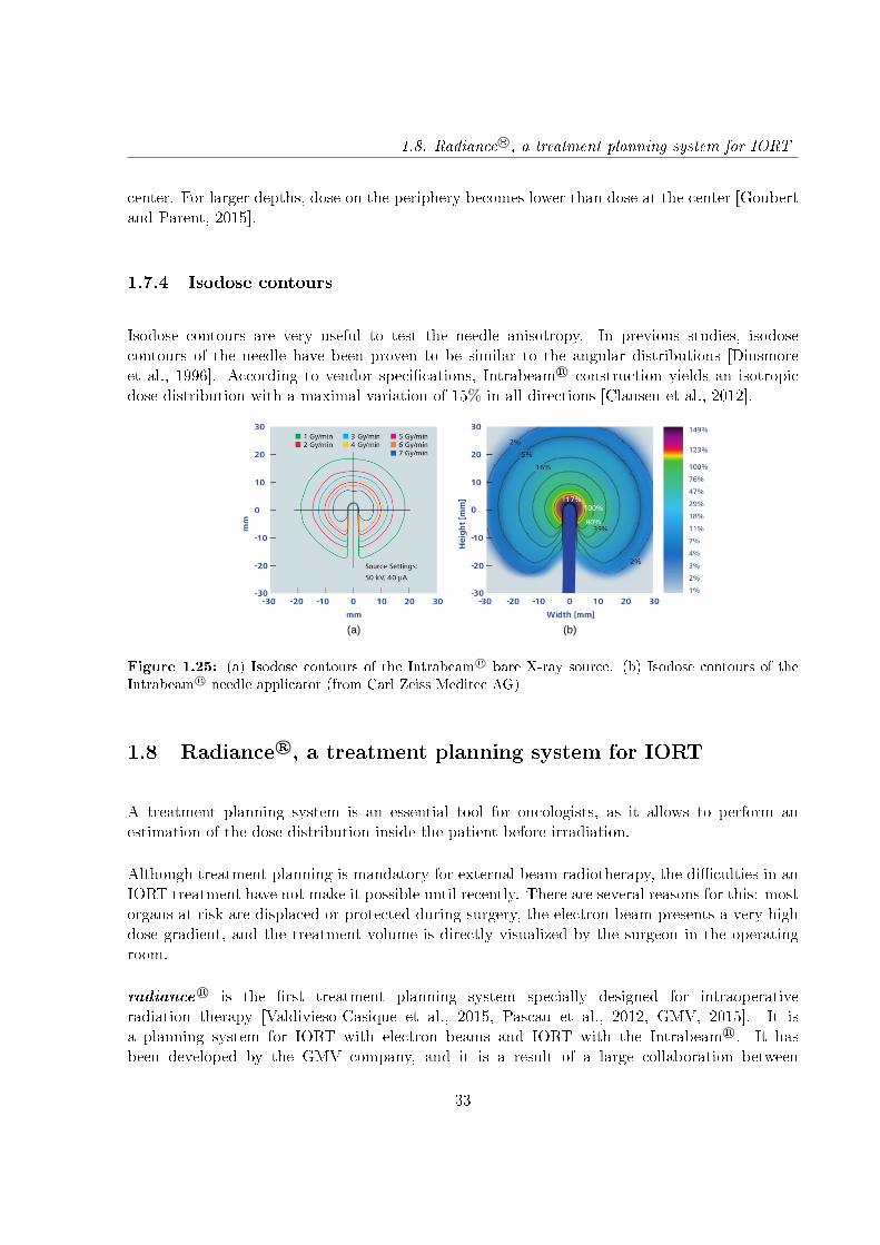
1.8. Radiance R©, a treatment planning system for IORT
center. For larger depths, dose on the periphery becomes lower than dose at the center [Goubertand Parent, 2015].
1.7.4 Isodose contours
Isodose contours are very useful to test the needle anisotropy. In previous studies, isodosecontours of the needle have been proven to be similar to the angular distributions [Dinsmoreet al., 1996]. According to vendor specications, Intrabeam R© construction yields an isotropicdose distribution with a maximal variation of 15% in all directions [Clausen et al., 2012].
(a) (b)
Figure 1.25: (a) Isodose contours of the Intrabeam R© bare X-ray source. (b) Isodose contours of theIntrabeam R© needle applicator (from Carl Zeiss Meditec AG)
1.8 Radiance R©, a treatment planning system for IORT
A treatment planning system is an essential tool for oncologists, as it allows to perform anestimation of the dose distribution inside the patient before irradiation.
Although treatment planning is mandatory for external beam radiotherapy, the diculties in anIORT treatment have not make it possible until recently. There are several reasons for this: mostorgans at risk are displaced or protected during surgery, the electron beam presents a very highdose gradient, and the treatment volume is directly visualized by the surgeon in the operatingroom.
radiance R© is the rst treatment planning system specially designed for intraoperativeradiation therapy [Valdivieso-Casique et al., 2015, Pascau et al., 2012, GMV, 2015]. It isa planning system for IORT with electron beams and IORT with the Intrabeam R©. It hasbeen developed by the GMV company, and it is a result of a large collaboration between
33
1. Fundamentals of radiotherapy
private companies (Técnicas Radiofísicas), medical institutions (Hospital Universitario GregorioMarañón, Consorcio Hospitalario Provincial de Castellón, Clínica La Luz, Hospital Ramón yCajal) and universities (Universidad Politécnica de Madrid, Universidad Complutense de Madrid,Universidad Rey Juan Carlos, Universidad de Valencia, Universidad de Granada).
radiance R© can be used in three dierent phases of the treatment:
• Pre-planning: Allows to try dierent positions of the applicator using CT images, and toselect the optimum parameters for each treatment (applicator diameter, bevel angle andelectron beam energy).• Intra-planning: During surgery, previous planning studies can be checked and updatescan be done if the situation requires it, checking the eects of these changes on the dosedistribution inside the patient.• Post-planning: After surgery, control CT studies combined with the simulation tool enableevaluation of the treatment.
Three dose calculation algorithms are implemented in radiance R©:
• A pencil beam (PB) algorithm [Hogstrom, 1985, López-Tarjuelo et al., 2010] for electrons.PB is very fast (running times up to 4 seconds). But this algorithm presents somelimitations when heterogeneities are present (such as bad backscattering modeling).However, these deciencies are covered by the Monte Carlo model.• AMonte Carlo (MC) algorithm for electrons which has been optimized for computationaleciency.• An Hybrid Monte Carlo algorithm capable of fast and accurate dose calculations withlow energy photons for the Intrabeam R© device.
Both Monte Carlo and Hybrid Monte Carlo implementations in the planning system havebeen possible thanks to the results presented in this thesis, that have been incorporated inradiance R©.
Two examples of treatment planning with radiance R© are shown in the gure 1.26.
34
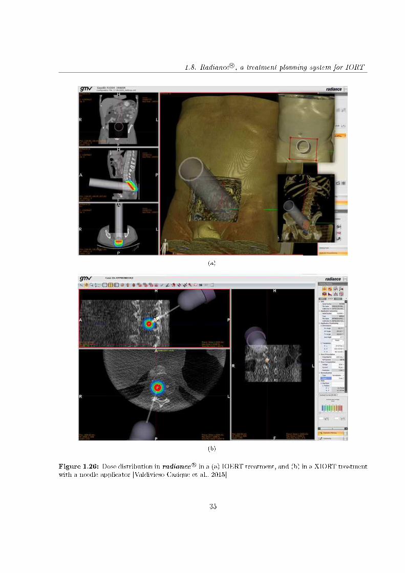
1.8. Radiance R©, a treatment planning system for IORT
(a)
(b)
Figure 1.26: Dose distribution in radianceR© in a (a) IOERT treatment, and (b) in a XIORT treatment
with a needle applicator [Valdivieso-Casique et al., 2015]
35
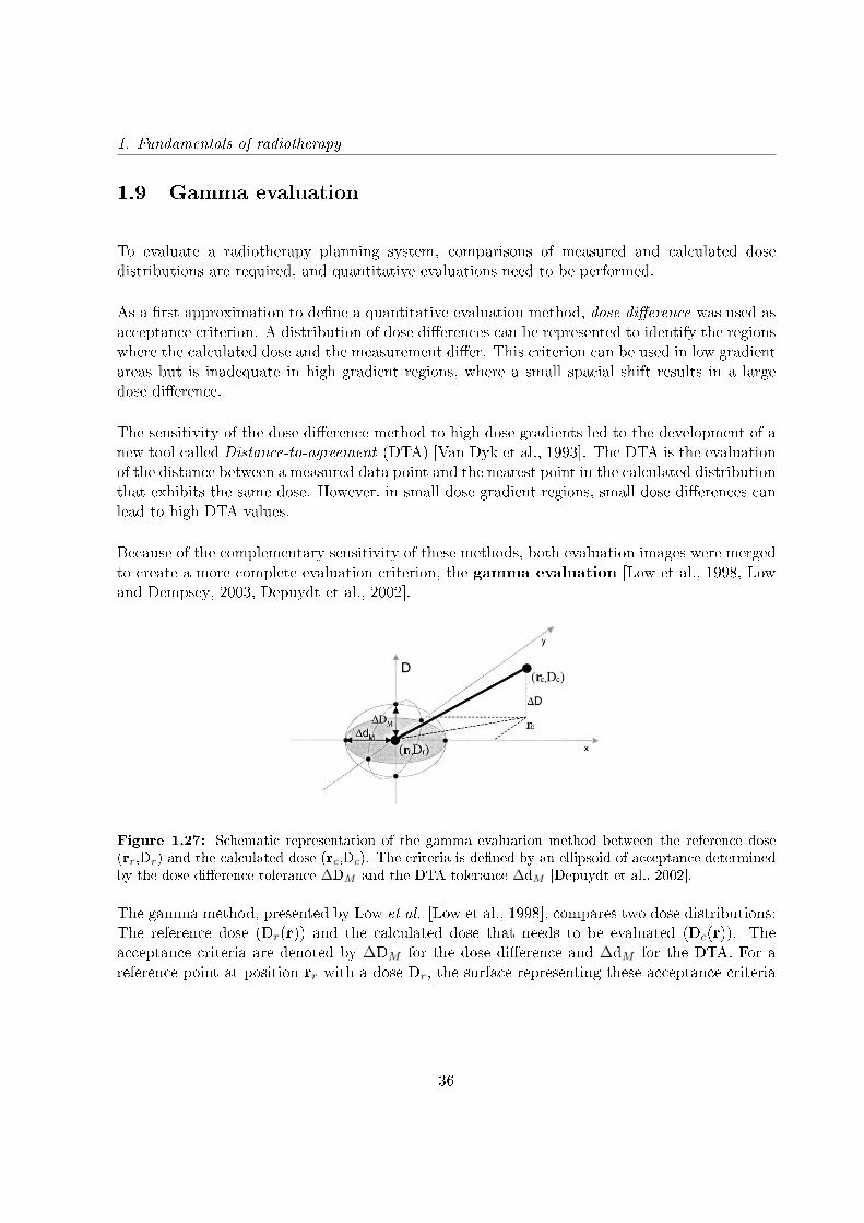
1. Fundamentals of radiotherapy
1.9 Gamma evaluation
To evaluate a radiotherapy planning system, comparisons of measured and calculated dosedistributions are required, and quantitative evaluations need to be performed.
As a rst approximation to dene a quantitative evaluation method, dose dierence was used asacceptance criterion. A distribution of dose dierences can be represented to identify the regionswhere the calculated dose and the measurement dier. This criterion can be used in low gradientareas but is inadequate in high gradient regions, where a small spacial shift results in a largedose dierence.
The sensitivity of the dose dierence method to high dose gradients led to the development of anew tool called Distance-to-agreement (DTA) [Van Dyk et al., 1993]. The DTA is the evaluationof the distance between a measured data point and the nearest point in the calculated distributionthat exhibits the same dose. However, in small dose gradient regions, small dose dierences canlead to high DTA values.
Because of the complementary sensitivity of these methods, both evaluation images were mergedto create a more complete evaluation criterion, the gamma evaluation [Low et al., 1998, Lowand Dempsey, 2003, Depuydt et al., 2002].
Figure 1.27: Schematic representation of the gamma evaluation method between the reference dose(rr,Dr) and the calculated dose (rc,Dc). The criteria is dened by an ellipsoid of acceptance determinedby the dose dierence tolerance ∆DM and the DTA tolerance ∆dM [Depuydt et al., 2002].
The gamma method, presented by Low et al. [Low et al., 1998], compares two dose distributions:The reference dose (Dr(r)) and the calculated dose that needs to be evaluated (Dc(r)). Theacceptance criteria are denoted by ∆DM for the dose dierence and ∆dM for the DTA. For areference point at position rr with a dose Dr, the surface representing these acceptance criteria
36

1.9. Gamma evaluation
is an ellipsoid dened as:
1 =
√∆r2
∆d2M
+∆D2
∆D2M
(1.7)
Where ∆r is the distance between the reference and the calculated point and ∆D is the dosedierence at the position rc relative to the reference dose Dr in rr.
∆r =| rr − rc | (1.8)
∆D = Dc(rc)−Dr(rr) (1.9)
The calculated dose will t the gamma evaluation if at least one point (rc, Dc) of its dosedistribution is contained inside the ellipsoid of acceptance showed in gure 1.27, ie. one pointfor which
Γr(rc, Dc) ≡
√∆r2
∆d2M
+∆D2
∆D2M
≤ 1 (1.10)
The pass-fail criterion becomes:
• γ(rr) ≤ 1, calculation passes.• γ(rr) > 1, calculation fails.
For example, if a 3%-3 mm criterion is considered, points passing this criterion will be theones located at 3 mm or less from a point in which dose dierence with the reference is 3% orless.
Gamma evaluation limits depend on the type of radiotherapy and the location of the tumor. Fora stereotactic brain treatment, with high precision systems and with organs at risk very close,it would be suitable a 1%-1 mm criterion. However, for IORT these precision requirements arenot so restrictive, because the surgeon limits the treatment area and protects the organs at risk.Therefore, in IOERT it is reasonable to consider suitable a dosimetric study when 95% of thepoints pass the 3%-3 mm limit [Alber et al., 2008]. Nevertheless, this approximation can not beconsidered in a dose evaluation for the Intrabeam R©, because of the rapid decrease of the dose.In this case, this limit can vary from 2%-1 mm [Nwankwo et al., 2013], to 2%-2 mm [Clausenet al., 2012] or even 10%-1 mm [Chiavassa et al., 2014]. In this thesis we have considered dierentlimits, depending on the voxel size used.
37

Chapter 2
Monte Carlo methods in
radiotherapy
2.1 Introduction
Determination of a dose distribution inside a patient or a phantom is of crucial importance tobe able to determine the eectiveness of a radiotherapy treatment and to evaluate the eectsof radiation in matter. Any dose measuring method will be only an estimation, because dosedeposition will depend on the irradiated medium, and by introducing any dosimetry system themedium will be modied. This estimation of the dose can be measured with dierent dosimetrytechniques (ionization chambers, radiochromic lms, etc.), or calculated with numerical methodsthat implement dierent models of the interaction of radiation with matter.
The use of calculation algorithms in dosimetry allows the estimation of absorbed dosedistributions inside irradiated volumes. These algorithms are based in radiation transport modelsthat describe the mechanisms responsible for the transport and the interaction of radiation withmatter. There are two main trends of dose calculation algorithms based in dierent mathematicalmodels of energy deposition: one is a deterministic strategy based in Boltzmann equation andthe other is based in Monte Carlo (MC) simulations.
In the deterministic approach, the model is built from a coupled set of equations (known asBoltzmann equation) that describe how a variety of dierent types of particles travel througha material. This technique works adequately in homogeneous media but has some problemswith heterogeneities [Wang et al., 1996, Ding et al., 2005], which are specially important inradiotherapy dosimetry.
39
2. Monte Carlo methods in radiotherapy
In the last years, Monte Carlo methods are becoming widely used. Monte Carlo simulation ofradiation transport uses the probability distributions governing the individual interactions ofelectrons and photons in materials to simulate the random trajectories or histories of individualparticles. These methods are more precise than the deterministic models, specially in complexmedia, but very time consuming.
In this chapter we will explain the basic concepts of MC methods and their application inradiotherapy. We will also describe the main MC codes used in radiation transport, specially theones that have been used in this thesis.
2.2 Monte Carlo technique. Basic concepts
The name "Monte Carlo" references a group of mathematical procedures or numerical methodsused to model complex systems by using the previously known probabilities of occurrence ofthe dierent events involved in the problem [Sobol, 1994, Kalos and Whitlock, 2008]. In theseprocesses random variables are used, and by calculating their expected value we can reach theapproximated solution of the problem. Therefore, a Monte Carlo simulation is a quantitativetechnique that uses statistics to mimic, by means of mathematic models, the behavior of a realsystem.
All processes involved in particle transport are stochastic, which means that we can not foreseewhat kind of interaction is going to happen next and where it is going to take place. We only canassign a probability to each possibility. However, the probability distributions associated at everyevent are well known, and, together with the use of a random number generator, they will be usedto sample parameter values for calculating a possible solution to the problem for a single historyor event. By simulating many histories, reliable average values can be obtained. Since the resultis an average, it is associated with a standard deviation that expresses the uncertainty due tothe fact that the simulated number of events is less than innite [Reynaert et al., 2006].
In a Monte Carlo dose calculation, the track of each individual ionizing particle through thevolume of interest is simulated. Along its way, the particle may interact with the matter throughwhich it is passing. Using a random number generator and probability distributions for thedierent types of interaction, the program samples the distance to the next interaction for everyparticle at a given position and with a certain direction. The particle is propagated to theinteraction location and next, the program chooses the type of interaction that will take place.After interaction, the same procedure is repeated with the remaining particle and secondaryparticles (if generated) [Reynaert et al., 2006]. Therefore, each history or trajectory of theparticles can be seen as a sequence of free paths that end with an interaction event where theparticle changes its direction, loses energy and can generate secondary particles.
All Monte Carlo codes have some components in common, regardless of its application eld.
40
2.2. Monte Carlo technique. Basic concepts
• Probability distribution functions: They contain all the information regarding thephysical processes. All the physics or mathematical models must be described by thesefunctions.• Random number generator: A tool to generate aleatory numbers uniformly distributedbetween 0 and 1.• Sampling method: A way to sample the variables of the probability distributionfunctions.• Scoring methods: All results must be stored for each variable of interest.• Error estimation: It is convenient to determine the error associated to the number ofhistories.
Furthermore, optimization tools can be found is most of the codes, such as:
• Variance reduction techniques: Methods introduced to increase the eciency of MCcalculations.• Parallelization techniques: Algorithms that increase the eciency by using the additiveproperty of MC calculations. They require the use of advanced computer architectures.
2.2.1 Modeling of particle transport
The physics models are usually hard-coded in the Monte Carlo software. In radiation transport,photons are transported in a similar manner as in a real medium. For example, to determine thescattering angle and energy of a secondary electron in a Compton scattering event, we make useof the Klein-Nishina cross section for Compton scattering [Rogers, 2002]. However, this is notpossible in the case of electrons because when an electron slows down in a material, it can undergohundreds or thousands of scattering events in which it is deected slightly but loses virtuallyno energy. Therefore, the simulation of each individual interaction is very time consuming andimpractical for radiotherapy applications [Reynaert et al., 2006]. To accelerate the simulations,so-called condensed history techniques have been introduced. In section 2.2.5.2 further detailsof condensed histories can be found.
The physics modeling can be also modied via a number of transport parameters, such as cut-oenergies or particles step length, that set thresholds when tracking a history. Depending on thevalues given to these parameters, the simulation can be accelerated, but they have to be handledwith care because accuracy can be lost. These transport parameters are explained in section2.2.5.1.
41
2. Monte Carlo methods in radiotherapy
2.2.2 Random number generator
A sequence of random numbers is one where next number in the sequence can not be predicted.The random numbers used in MC are not really random, as they are generated with a computeralgorithm, but pseudo-random, and they are the base of a Monte Carlo code. This pseudo-random nature of Monte Carlo simulations is what imitates the true stochastic or random natureof particle interactions. The pseudo-random number generators use an initial seed or number asa starting point for the sequence generation. The sequence will be suciently unpredictable andit will not be repeated in cycles. However, two sequences will be equal if the same initial seed isused.
These numbers must accomplish some characteristics:
• Good distribution. Generated random numbers must be uniformly distributed between[0,1].• The sequence generated must be suciently large to ensure non repeatability.• Reproducibility. If the simulation is repeated under the same circumstances, the resultmust be the same.
2.2.3 Probability distribution functions and sampling method
There are dierent kinds of sampling techniques. We will consider two of them.
2.2.3.1 Invertible cumulative distribution functions (direct method)
The direct method is the form used to calculate a particle's distance to an interaction in allMonte Carlo codes.
A probability distribution function, p(x) is a measure of the likelihood of observing x. Forexample, x could be the position at which a photon interacts via the Compton interaction.
In general, p(x) has some special properties that distinguishes it from other functions [Bielajew,2001]:
• p(x)≥0 since negative probabilities have no meaning.
• p(x) must be normalized to 1 ∫ xmax
xmin
p(x)dx = 1 (2.1)
42
2.2. Monte Carlo technique. Basic concepts
• xmin and xmax can be any real number as long as xmin is less than xmax.
Associated with each one-dimensional probability distribution function we nd its cumulativeprobability distribution function [Bielajew, 2001].
c(x) =∫ x
xmin
dx′p(x′) (2.2)
This cumulative function has the following properties:
• p(x) and c(x) are related by a derivative
p(x) =dc(x)dx
(2.3)
• c(x) is zero at the beginning of the range and one at the end of the range: c(x) is containedwithin the range [0,1].
• c(x) is a monotonically increasing function of x as a result of p(x) always being positive.
Cumulative probability distribution functions can be related to uniform random numbers toprovide a way for sampling these distributions. We can map the cumulative probabilitydistribution function onto the range of random variables, r, where 0≤r≤1 and r is distributeduniformly. That is, r=c(x).
Having mapped the random numbers onto the cumulative probability distribution function,we may invert the equation (all cumulative probability distribution functions are invertible)to give:
x = c−1(r) (2.4)
Then, by choosing r 's randomly over a uniform distribution and substituting them in the aboveequation, we generate x 's according to the proper probability distribution function.
In the case of a particle interaction, the probability distribution function will be:
p(z)dz = µe−µzdz (2.5)
Where µ is the interaction coecient needed to sample the distance to the next collision for a
43
2. Monte Carlo methods in radiotherapy
given type of particle with a given energy in a given material [Reynaert et al., 2006]. Data tableswith interaction probabilities of each type of interaction for each element are usually providedtogether with a Monte Carlo program.
The cumulative probability distribution will be:
r = c(z) = 1− e−µz (2.6)
Inverting it:
z = − 1µlog(1− r) (2.7)
If r is uniformly distributed over [0,1] then so is 1-r.
The invertible cumulative probability distribution function method is always possible, but it isoften impractical to calculate it because it may be exceedingly complicated mathematically ormay contain a structure that is dicult to control. Another approach is to use the rejectionmethod.
2.2.3.2 Rejection method
The procedure is the following:
• Scale the probability distribution function by its maximum value obtaining a newdistribution function, f(x)= p(x)/p(xmax).
• Choose a random number, r1, uniform in the range [0,1] and use it to obtain an x which isuniform in the probability distribution function's range [a,b] (by calculating x=a+(b-a)r1).
• Choose a second random number r2. If r2 < p(x)/p(xmax) then accept x, else, reject it andgo back to the second point.
This method only works if the probability distribution function is not innite anywhere and if itis not extremely dicult to determine the location of the maximum value. It is also restrictedto nite values of a and b.
44
2.2. Monte Carlo technique. Basic concepts
2.2.4 Error estimation
MC algorithms are statistical methods and, therefore, the results should be accompanied by thecorresponding error. In general, the associated error of a result is inversely proportional to
√N ,
where N is the number of simulated histories. Thus, if the uncertainty wants to the reduced bytwo, number of simulated histories must be increased by a factor four.
If we consider xi as one of the calculated and stored parameters of the simulation for a historyi, where 1≤i≤N, the mean value can be calculated as:
x =1N
N∑i=1
xi (2.8)
The variance associated to de xi distribution will be:
S2x =
1N − 1
N∑i=1
(xi − x)2 (2.9)
2.2.5 Monte Carlo optimization
The use in the clinic of the dose calculation systems requires a compromise between two maingoals: Accuracy and precision in the results and a reasonable calculation time. The last conditionis specially important in IORT, where the calculations must be done right after the surgery.
In MC methods the precision of the results can be improved by increasing the number of histories.However, by improving the precision there is an increasing in the simulation time. To solve this,some methods have been designed to reduce simulation time with dierent techniques.
In this section we will describe the most common optimization techniques. Some of them implya certain loss in the results quality because the use simplications in the physics model, in theinput data or incorporate some strategies inside the MC algorithm to reduce the amount ofneeded histories regardless the consequences in the dose results.
Other techniques reduce computation time without losing quality in the data. Normally, theykeep the physics of the model unaltered and change the calculation algorithm. These strategiesare the most used and can be found in the conguration input of most codes.
45
2. Monte Carlo methods in radiotherapy
2.2.5.1 Cut-o energies and step length
The mean free path of the particles (ie. the distance traveled between interactions) depends ontheir energy. Furthermore, the particle transfers energy to the medium in each interaction, untilits energy is so low that the particle is absorbed. Some programs introduce these two facts intheir code to accelerate simulation time.
The cut-o energy value is a threshold in energy. When the energy of a history goes below thecut-o energy value, the program stops following that particle. The particle is considered to beabsorbed at that point. There are dierent cut-o values for the energy depending on the typeof particle and the type of interaction.
The step length parameter denes the distance between interactions. The bigger the value is,the quicker the simulation.
The user may modify both of the mentioned parameters. They had to be handled carefully, assuch parameters may signicantly inuence a simulation and accuracy might be lost.
Some of the available programs that use these techniques are: PENELOPE [Salvat et al.,2006], EGS4 [Kawrakow and Rogers, 2000, Kawrakow et al., 2014] and VMC [Kawrakow et al.,1996].
2.2.5.2 Condensed histories
Another optimization technique of the MC simulations is the use of condensed histories [Bergeret al., 1963, Kawrakow and Bielajew, 1998]. It consists of replacing the calculation of a certainnumber of interactions (several thousands) by a single interaction whose eect will be the sumof all replaced particle eects.
A typical fast electron slowing down inside a medium undergoes of the order of 105-106 collisionswith surrounding matter, causing in most interactions only minor changes in the particle's energyand direction of ight. This large number of interactions makes very dicult to track everyelectron individually, and the computation time of doing this is very high. To circumvent thisdiculty, Berger [Berger et al., 1963] developed the condensed history technique. In this method,large numbers of transport and collision processes are condensed to a single electron step. Thecumulative eect of the individual interactions is taken into account by the appropriate changeof the particles energy and direction of motion at the end of the step.
This approximation has a limitation. In multiple dispersion theories, it is assumed that particlesmove in heterogeneous media and the distance they travel is bigger than their main free path. As
46

2.2. Monte Carlo technique. Basic concepts
a result, condensed history approximation can lead to artifacts in areas next to interfaces and,in general, in any object with a comparable size to the mean free path of the particles. Anotherlimitation of the condensed simulation is that this approximation cannot take into account thecatastrophic eects (ie. individual interactions that signicantly modify the energy or directionof the particles). To solve these limitations a mixed model can be implemented. In this model,condensed histories simulations are used to reproduce the soft interactions where the energy ordirection of the particles do not exceed an user-dened threshold, and the rest of the simulationsare calculated in detail (known as hard interactions) [Berger et al., 1963].
2.2.5.3 Variance reduction techniques
The variance reduction techniques may be used to make calculations more ecient. In somecases, these techniques require that no further approximations must be made to the transportphysics. In other cases, the gains in computing speed come at the cost of computing results thatmay be less accurate since approximations are introduced [Bielajew, 2001].
Lets introduce the most used variance reduction techniques.
The interaction forcing technique takes advantage of the fact that, usually, a high variancecomes from a low interaction rate. This is specially signicant for photons, where eciency maybe lost because photons leave the geometry of the simulation without interacting and time isspent tracking photons through a geometry that do not contribute to the score. This techniqueforces photons to interact within the geometry of interest. These photons will then be weightedby the probability that the photon would have had of interacting before leaving the geometry ofthe simulation.
The particle splitting technique is used in situations where interest is focused on a particularvolume inside the geometry. To increase interaction statistics within that area, a splittingtechnique can be used. It divides the particles with weight ω into a N smaller ones each with anew weight, ω' = ω/N.
Another technique is used when particle weights become very small. If this happens and thephoton is headed away from the region of interest it can be used the russian roulette technique.It selects a random number. If this random number lies above a threshold α, the photon isdiscarded without scoring any quantity of interest. If the random number turns out to be belowα the photon survives but with a new weight, ω' = ω/α.
All these techniques distort the simulation results because they modify the probabilitydistribution functions of the involved interactions. In order to minimize the alteration,parameters involved in these techniques must be chosen carefully.
47

2. Monte Carlo methods in radiotherapy
Now, we will describe a technique that accelerate the simulation without modifying the qualityof the results.
2.2.5.4 Pre-calculation of the source. Phase Space les
When a MC simulation of a treatment planning needs to be done, we need to simulate the detailedgeometry of the accelerator. But if in each treatment planning the simulation is performed bystarting the electrons at the beginning of the accelerator head, we will need a very long simulationto achieve a dose distribution with low variance.
This is because the particles, before entering the medium, go though a serial of materials, suchas collimators, attening lters, etc., as seen in Chapter 1. Most particles will interact in theaccelerator head, being absorbed or generating secondary particles, and following their trackswill slow down considerably the simulation, even though these interactions are not directlycontributing to the dose. But these elements, responsible of beam modication, are usuallyxed to the accelerator head and used in all treatments. By taking advantage of this property,some codes have developed a strategy that consist of saving the information of the particles in ale at a certain point, usually at the end of the collimation system. With this, a full simulationof each accelerator head can be done once, and the information of the particles coming outthe accelerator is recorded. Next time a simulation of that accelerator is required, instead ofgenerating again the detailed geometry of all the components of the accelerator, all the beaminformation coming out of the accelerator can be read from the stored le.
This le is known as Phase Space le. It contains all the information needed to characterize thebeam. This information includes type of particle, energy, position and direction of the particles,among other properties particular of each code.
2.3 Main Monte Carlo codes in radiotherapy
ETRAN (Electron TRANsport): First MC code designed for electrons and photons transportthrough simple geometries [Seltzer, 1991]. Its energy range is 1 keV-100 GeV.
EGS (Electron Gamma Shower): The actual version is called EGSnrc [Kawrakow and Rogers,2000, Kawrakow et al., 2014]. It is a code that simulates photon, electron and positron transportconsidering only electromagnetic interactions, with energies from 1 keV to 10 GeV. The geometrycan be built with a code called BEAMnrc [Rogers et al., 1995] that incorporates specic modulesdesigned for medical physics. It has been widely validated, as it is one of the most used MCcodes in medical physics. It is not an open code and may require that the user develops part ofthe code in MORTRAN language to dene complex geometries.
48
2.4. PENELOPE
FLUKA (FLUktuierendeKAskade): It is a code that reproduces the propagation in matter forup to 60 dierent particles, including electrons and photons (from 1 keV to 1000 TeV), hadrons(up to 20 TeV), neutrons and heavy ions [Ferrari et al., 2005]. It allows to reproduce complexgeometries. Its main code is written in FORTRAN77.
GEANT4 (Geometry ANd Tracking): It is a code that simulates the transport of all kind ofparticles inside an energy range between 250 eV and 10 TeV [Agostinelli et al., 2003]. It is verypowerful regarding the construction of complex geometries and can be used for a wide spectrumof applications: from high energy physics to medical physics. Part of the code must be developedby the user in C++ language. Its code is open source.
MCNP (Monte Carlo N-Particle): It is a code that simulates the transport of neutrons, photonsand electrons. Because its wide validation, it is considered the most reliable MC code for neutrontransport [Brown et al., 2002]. It is necessary a payment registration to use it.
MCNPX (Monte Carlo N-ParticleeXtended): It extends the application of the MCNP4C3 codeto almost all kind of particles in a wide energy range. The source code, written in FORTRAN90,is only available by a previous agreement with the developers.
PENELOPE (PENetration and EnergyLOss of Positrons and Electrons): It is an open sourcecode to simulate electrons, photons and positrons transport, in an energy range between 50eV and 1 GeV [Salvat et al., 2006]. Its main application eld is medical physics. Most of thecalculations done in this thesis are based in this code, so further description of PENELOPE canbe found in the next section.
2.4 PENELOPE
PENELOPE (PENetration and EnergyLOss of Positrons and Electrons) [Baro et al., 1995, Salvatet al., 1996, 2006, Sempau et al., 1997, 2003] is a Monte Carlo code of general purpose thatsimulates the transport of electrons, photons and positrons within an energy range from 50 eVto 1 GeV. It is formed by a package of subroutines written in FORTRAN77. It is an opensource code developed by the Universitat Politèctica de Catalunya (UPC) and distributed by theNuclear Energy Agency (NEA).
The main features of PENELOPE are the accurate description of particle transport throughinterfaces and the low-energy particles transport. It simulates with detail the transport ofphotons and applies a mixed-scheme for electron and positron transport.
The mechanisms responsible for particle transport are controlled by some user denedparameters. Elastic interactions are controlled by the parameters C1 and C2:
49

2. Monte Carlo methods in radiotherapy
• C1 denes the average angular deection produced by multiple elastic scattering throughthe mean free path between consecutive elastic events.• C2 sets an upper bound for the average fractional energy loss between consecutive elasticevents.
To ensure precision in the simulation, C1 and C2 must have small values. For both parameters,0.05 is recommended and the maximum recommended value would be 0.2. Beyond this point,the simulation will be quicker but precision will decrease.
User can also dene two parameters related to the energy values that delimit the distinctionbetween hard and soft interactions:
• WCC : Cuto energy value (in eV) for hard inelastic collisions.• WCR: Cuto energy value (in eV) for bremsstrahlung emissions.
Therefore, electron collisions whose energy loss is below WCC and inelastic radiative interactionswith energy loss below WCR are considered soft interactions and treated as condensed histories.The step length parameter for these soft interactions can also be controlled externally with thesmax parameter.
WCC and WCR cuto energies will aect the simulated energy distribution. If big values areused, the simulation time is reduced but energy distribution will be distorted. In real practice,energy distributions will not vary for dierent WCC and WCR values as long as these numbersare below the increment of energy used for energy distribution. Therefore, the desired energyresolution will determine the maximum value of these cuto energy values.
PENELOPE code is formed by a set of FORTRAN 77 subroutines which are invoked from amain program. The main codes included in PENELOPE are the following:
• penelope.f : Block of subprograms with the coupled electron-photon transport.
• material.f : Program which extracts atomic interaction data from the database and createsthe les with the physical information about each material.
• pengeom.f : Code that contains the geometry package. Any geometry is built fromhomogeneous bodies limited by quadric surfaces.
• penvared.f : Program that allows users to employ variance reduction techniques.
PENELOPE also includes other programs:
• GVIEW: Program used for displaying two- and three-dimensional images of the geometry.
50

2.5. PenEasy
• SHOWER: Program used to visualize particle tracks.• EMFIELDS: Block of subroutines to simulate particle transport in static electromagneticelds.• TABLES: Program to generate tables with the physical data of radiation transport.
2.5 PenEasy
PenEasy [Sempau et al., 2011, Badal Soler et al., 2008] is a modular, general-purpose mainprogram for PENELOPE that includes various source models and tallies. The goal of developingthis program was to provide a tool suitable for a wide spectrum of problems so that users wouldnot need to develop a specic code for each new application.
PenEasy is free and open software, and the source code is mostly written in FORTRAN77.
The code is structured in an initialization phase followed by three nested loops and the reportingof results. The skeleton of the main program is shown in gure 2.1. Uppercase namesdenote routines from PENELOPE, whereas lowercase subroutines are provided with the penEasypackage.
Figure 2.1: Basic structure of the FORTRAN version of the main program of penEasy. Calls to tallyingand other auxiliary subroutines have been removed for clarity [Badal Soler et al., 2008].
The main cycles are: history, particle and interaction. Each cycle of the loop named historyperforms the simulation of one primary particle and all its descendants. Inside the cycle history
51
2. Monte Carlo methods in radiotherapy
there is the loop particle that simulates a single photon, electron or positron. Finally, inside thisloop we can nd the cycle of interact that reproduces a single interaction, or the crossing of aninterface if the distance to the intersection is shorter than the distance to the next interaction.For calculating these interactions, inside this nal loop we nd an algorithm that essentiallyconsists of repeating the sequence of calls to subroutines JUMP, STEP and KNOCK: JUMPcomputes the distance to the next interaction event, returned through the variable ds; STEPdetermines if an interface is crossed before completing the step ds and displaces the particle; andKNOCK simulates the eect of the interaction and returns the energy lost by the particle. If aninterface is crossed (ncross not zero) the trajectory is truncated at the boundary, no interactiontakes place and a new interact cycle begins. The simulation of a particle ends when it leavesthe material system (mat is zero), or when its kinetic energy (e) falls below some user-denedabsorption energy (eabs), which may depend on the material and particle type.
PenEasy allows the use of quadric geometry (by invoking subroutines from PENELOPE'sstandard geometry package PENGEOM), voxelized geometry and a superposition of quadricobjects and voxelized regions (with the package penVOX).
2.5.1 Source models
PenEasy includes two types of source models [Sempau et al., 2011, Badal Soler et al., 2008].Their conguration parameters are set by the user through a global input le. Only one sourcecan be active in any given simulation.
The source called BIGS (Box Isotropic Gauss Spectrum) allows the denition of volumetricsources limited by quadric surfaces. The type of particle can be either a photon, electron orpositron with an arbitrary energy spectrum of emission or, alternatively, with the spectrumdened by means of a Gaussian function.
The source called PSF (Phase-Space File) reads the initial state of the particles from an externalle. Usually, this le is created by penEasy in a previous simulation with the PSF tally. Asexplained in section 2.2.5.4, the phase space le contains information to identify all particles,either primary or secondary, belonging to the same history (i.e., descendants of the same primaryparticle).
2.5.2 Tallies
PenEasy includes subroutines to score the most common quantities of interest. The talliesavailable are listed below.
52
2.6. DPM
• Section Tally Spatial Dose Distrib: Calculates absorbed dose per history scored inparallelepiped bins.• Section Tally Cylindrical Dose Distrib: Calculates absorbed dose per history in cylindricalshells.• Section Tally Spherical Dose Distrib: Calculates absorbed dose per history in sphericalshells.• Section Tally Voxel Dose: Calculates absorbed dose when voxelized geometries are used.• Section Tally Energy Deposition Pulse Spectrum: Determines the total deposited energyin the detection material per simulated history.• Section Tally Fluence Track Length: Calculates the uence spectrum per simulated historyin the detection material.• Section Tally Phase Space File: Stores the phase space le in the detection material.• Section Tally Particle Current Spectrum: Determines energy spectra and total number ofparticles of each type entering a certain material.• Section Tally Particle Track Structure: Allows the 3D representation of the particle tracks.
2.6 DPM
DPM (Dose Planning Method) [Sempau et al., 2000] is a MC code that share some of thePENELOPE characteristics and allows the simulation of the dose deposited by electronphotonshowers under radiotherapy conditions in a fraction time of a regular MC calculation, such aspenEasy. It can be used as an alternative to the analytical algorithms for treatment planning,as it gives an accurate dose in a very short time.
DPM employs the condensed history model for electron transport, and uses a mixed scheme forthe treatment of energy losses, treating large energy transfer collisions with a simplied model andusing the continuous slowing down approximation (CSDA) to model small-loss collisions.
The gain in performance time derives from a series of enhancements done to the algorithm[Sempau et al., 2000]:
• Employment and renement of a new step size independent multiple-scattering theory.• Use of new transport mechanics. DPM has adopted the `random hinge' scheme employedin PENELOPE.• Use of large electron transport steps, in which many voxels may be traversed beforesampling a multiple scattering angle.• DPM exploits the small dynamic range (in energy and material) of radiotherapy classproblems. Energies are limited to those between 100 keV and 20 MeV, and cross sectionsand distribution functions are determined by scaling them appropriately to computed datain water.
53
2. Monte Carlo methods in radiotherapy
DPM is formed by four main programs:
• material.f : Extracts from PENELOPE library the physical data of the materials.
• predpm.f : Program that allows the pre-calculation of cross sections and other calculationsthat DPM will use.
• genvoxel.f : Geometry program. The user can create a voxelized geometry or read a CTimage.
• dpm.f : Program that performs the MC simulation, considering the previously calculateddata from predpm.f
2.6.1 Source model
DPM generates the primary particles in the subroutine 'source'. In the original code, this routinegenerates unidirectional and monoenergetic electrons or photons that impact in a phantom. Thesource is centered in x=y=0 and its size can be dened in the conguration les.
However, DPM allows the user to write his own 'source' subroutine. In any case, the nal resultof this subroutine is to assign the particles the following variables:
• Kinetic energy of the particle in eV.• Unit direction vectors vx,xy,vz• Position coordinates of the particle in cm.• Particle type.
In this work the 'source' subroutine has been modied to read the initial particle state from aphase space le.
2.6.2 Tallies
Subroutine 'report' scores the deposited dose inside the region of interest dened in theconguration les. This dose is written in an ASCII le, but the subroutine has been modiedto include also a binary le.
54

Chapter 3
Detailed simulations of IORT
systems
3.1 Introduction
Monte Carlo (MC) simulations are considered to be the most accurate methods for radiotherapydose calculations in homogeneous and heterogeneous geometries [Rogers et al., 1995, Rogers,2006, Ma and Jiang, 1999, Siebers et al., 2000, McDermott et al., 2003], since all the relevanteects, such as material inhomogeneities, back-scatter and beam hardening can be modeled withreasonable accuracy. While MC methods are computationally demanding, the development of afew accelerated MC codes, such as DPM [Sempau et al., 2000], makes them more practical inclinical settings.
MC dosimetry requires a realistic and reliable description of the electron and/or photon beamsemployed in the radiotherapy procedure [Chetty et al., 2007]. A phase space (PHSP) lecontaining the information of energy, angular and spatial distributions of the particles comingfrom the electron or photon beam, has to be fed into the MC algorithm. A common approach tobuild these PHSP les consists of carrying out realistic simulations of the accelerator head andother elements involved in the radiotherapy procedure such as applicators and collimators [Maand Jiang, 1999, Capote et al., 2006, Faddegon et al., 1998].
Detailed MC modeling of IOERT accelerators and Intrabeam R© devices has been widely reported[Ma and Jiang, 1999, Hogstrom and Almond, 2006, Janssen et al., 2008, Bush et al., 2008,Clausen et al., 2012, Nwankwo et al., 2013, Verhaegen et al., 1999, Yanch and Harte, 1996] andgood results have been obtained with this method.
55

3. Detailed simulations of IORT systems
In this chapter we have simulated the most relevant dedicated accelerators employed in IOERTtreatments (ie. NOVAC R©, LIAC R© and MOBETRON R©) with their corresponding applicators,and Intrabeam R© needle, spherical, surface and at applicators. In most cases, the dierentcomponents of the devices have been extracted from literature, in other cases, such as for atand surface Intrabeam R© applicators, the geometry details have been provided by the vendor.These simulations will represent a reference accelerator or applicator, and will be used to createa database that will be employed to generate a PHSP le tuned to each user machine in a dosetreatment planning procedure explained in the following chapter.
From these simulations we will be interested especially in reproducing the shape of theexperimental transverse dose proles from the dierent machines. Our optimization procedurewill only tune the depth dose prole (DDP) to the experimental data, so having thecharacterization of the o-axis proles will be essential for an accurate dose distribution atthe end of the procedure.
3.2 Intrabeam R© applicators
3.2.1 MC characterization of Intrabeam R© X-ray source
The Intrabeam R© X-ray source (XRS) has been described in several works [Dinsmore et al., 1996,Beatty et al., 1996, Yanch and Harte, 1996, Clausen et al., 2012].
In the Intrabeam R© system X-rays are generated by a 50 keV electron beam that travels throughan evacuated tube (9 cm length and 3.2 mm diameter) and hits a 0.5 µm thick gold target atthe end of the tube [Yanch and Harte, 1996]. The most distal 1.6 cm of the tube consists ofberyllium. To make the XRS biocompatible, the target tube is coated on their outer surfacewith a nickel lm and a titanium nitrite (TiN) layer [Dinsmore et al., 1996]. This constructionyields an isotropic dose distribution with a maximal variation of 15% in all directions [Yanchand Harte, 1996].
In this thesis we have performed a detailed simulation of the XRS of the Intrabeam R© withpenEasy [Sempau et al., 2011, Badal Soler et al., 2008]. The objective was to test the accuracyof the penEasy code for kilo-voltage energies and to x the shape of the energy spectrum. Anexperimental spectrum of the XRS [Schneider et al., 2010] was used to compare and adjust thesimulation to the experiment.
56

3.2. Intrabeam R© applicators
Figure 3.1: Cross section through the beryllium window of the INTRABEAM X-ray source (XRS) withthe gold target [Beatty et al., 1996].
The geometry of the XRS was generated to t the experimental measurements of the spectrum.It is shown in gure 3.2. It was dened as:
1. A 1.6 cm length beryllium needle with 1.1 mm inner radius and thickness of 0.5 mm.2. A 0.5 µm layer of gold at the end of the probe.3. A 5 µm layer of nickel surrounding the beryllium needle.4. A 10 µm layer of TiN surrounding the nickel.5. PHSP plane surrounding all the structure.
Regarding the electron source impinging on the gold target, it was characterized with a Gaussianenergy distribution with a mean energy of 50 keV and a full width at half maximum (FWHM) of5 keV. The source was located 1.6 cm above the gold target. Concerning the spatial distributionof the source, it was dened as a circular foil of 0.1 mm diameter with a Gaussian distributioncentered at zero and a FWHM of 0.01 mm. The electron beam does not impact in all the targetsurface, but in a annular area between 0.6 and 0.8 mm radii [Clausen et al., 2012].
The dose was scored at the exit of the probe surface with 4·1010 initial particles in order toaccumulate more than 200 millions particles in the scoring plane and to fulll good statistics andreduce statistical uncertainty of the simulation to around 2%. The voxel size employed in thesimulation was 0.25 mm. This calculation was split up into 200 simulations running in parallelfor around 12 hours in a high capacity cluster.
57
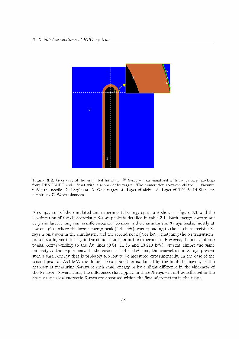
3. Detailed simulations of IORT systems
7
12
3
4
5
6
Figure 3.2: Geometry of the simulated Intrabeam R© X-ray source visualized with the gview2d packagefrom PENELOPE and a inset with a zoom of the target. The numeration corresponds to: 1. Vacuuminside the needle. 2. Beryllium. 3. Gold target. 4. Layer of nickel. 5. Layer of TiN. 6. PHSP planedenition. 7. Water phantom.
A comparison of the simulated and experimental energy spectra is shown in gure 3.3, and theclassication of the characteristic X-rays peaks is detailed in table 3.1. Both energy spectra arevery similar, although some dierences can be seen in the characteristic X-rays peaks, mostly atlow energies, where the lowest energy peak (4.41 keV), corresponding to the Ti characteristic X-rays is only seen in the simulation, and the second peak (7.54 keV), matching the Ni transitions,presents a higher intensity in the simulation than in the experiment. However, the most intensepeaks, corresponding to the Au lines (9.54, 11.53 and 13.240 keV), present almost the sameintensity as the experiment. In the case of the 4.41 keV line, the characteristic X-rays presentsuch a small energy that is probably too low to be measured experimentally. In the case of thesecond peak at 7.54 keV, the dierence can be either explained by the limited eciency of thedetector at measuring X-rays of such small energy or by a slight dierence in the thickness ofthe Ni layer. Nevertheless, the dierences that appear in these X-rays will not be reected in thedose, as such low energetic X-rays are absorbed within the rst micrometers in the tissue.
58
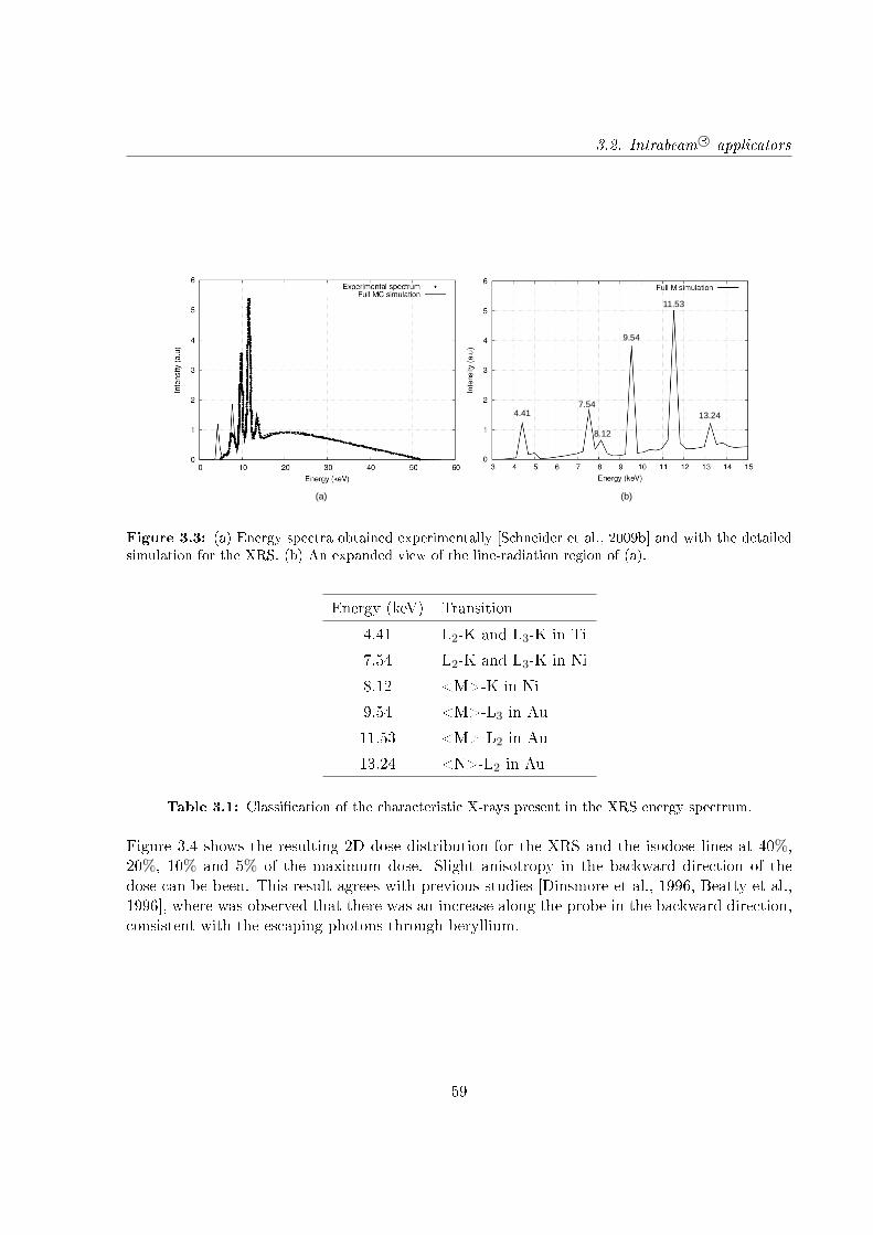
3.2. Intrabeam R© applicators
13.24
(a) (b)
4.417.54
8.12
9.54
11.53
Figure 3.3: (a) Energy spectra obtained experimentally [Schneider et al., 2009b] and with the detailedsimulation for the XRS. (b) An expanded view of the line-radiation region of (a).
Energy (keV) Transition
4.41 L2-K and L3-K in Ti
7.54 L2-K and L3-K in Ni
8.12 <M>-K in Ni
9.54 <M>-L3 in Au
11.53 <M>-L2 in Au
13.24 <N>-L2 in Au
Table 3.1: Classication of the characteristic X-rays present in the XRS energy spectrum.
Figure 3.4 shows the resulting 2D dose distribution for the XRS and the isodose lines at 40%,20%, 10% and 5% of the maximum dose. Slight anisotropy in the backward direction of thedose can be been. This result agrees with previous studies [Dinsmore et al., 1996, Beatty et al.,1996], where was observed that there was an increase along the probe in the backward direction,consistent with the escaping photons through beryllium.
59
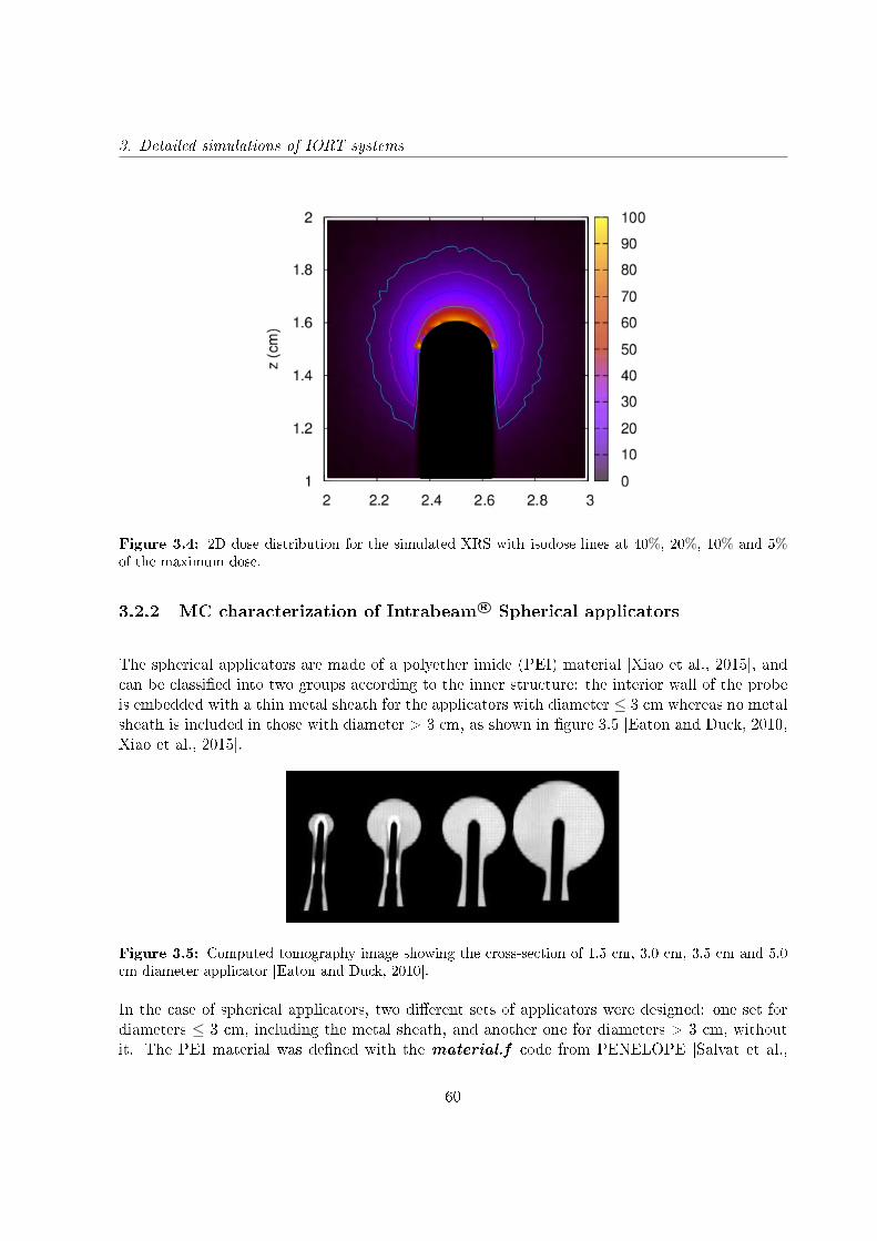
3. Detailed simulations of IORT systems
Figure 3.4: 2D dose distribution for the simulated XRS with isodose lines at 40%, 20%, 10% and 5%of the maximum dose.
3.2.2 MC characterization of Intrabeam R© Spherical applicators
The spherical applicators are made of a polyether imide (PEI) material [Xiao et al., 2015], andcan be classied into two groups according to the inner structure: the interior wall of the probeis embedded with a thin metal sheath for the applicators with diameter ≤ 3 cm whereas no metalsheath is included in those with diameter > 3 cm, as shown in gure 3.5 [Eaton and Duck, 2010,Xiao et al., 2015].
Figure 3.5: Computed tomography image showing the cross-section of 1.5 cm, 3.0 cm, 3.5 cm and 5.0cm diameter applicator [Eaton and Duck, 2010].
In the case of spherical applicators, two dierent sets of applicators were designed: one set fordiameters ≤ 3 cm, including the metal sheath, and another one for diameters > 3 cm, withoutit. The PEI material was dened with the material.f code from PENELOPE [Salvat et al.,
60
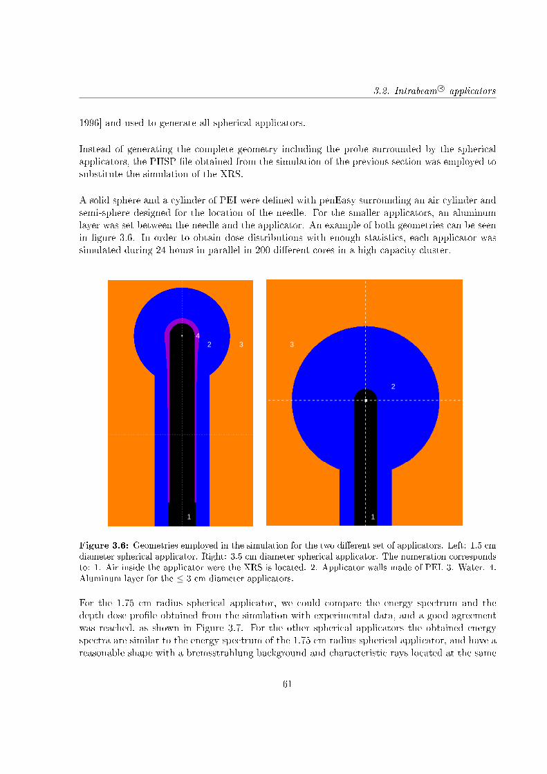
3.2. Intrabeam R© applicators
1996] and used to generate all spherical applicators.
Instead of generating the complete geometry including the probe surrounded by the sphericalapplicators, the PHSP le obtained from the simulation of the previous section was employed tosubstitute the simulation of the XRS.
A solid sphere and a cylinder of PEI were dened with penEasy surrounding an air cylinder andsemi-sphere designed for the location of the needle. For the smaller applicators, an aluminumlayer was set between the needle and the applicator. An example of both geometries can be seenin gure 3.6. In order to obtain dose distributions with enough statistics, each applicator wassimulated during 24 hours in parallel in 200 dierent cores in a high capacity cluster.
1 1
2
2
3 34
Figure 3.6: Geometries employed in the simulation for the two dierent set of applicators. Left: 1.5 cmdiameter spherical applicator. Right: 3.5 cm diameter spherical applicator. The numeration correspondsto: 1. Air inside the applicator were the XRS is located. 2. Applicator walls made of PEI. 3. Water. 4.Aluminum layer for the ≤ 3 cm diameter applicators.
For the 1.75 cm radius spherical applicator, we could compare the energy spectrum and thedepth dose prole obtained from the simulation with experimental data, and a good agreementwas reached, as shown in Figure 3.7. For the other spherical applicators the obtained energyspectra are similar to the energy spectrum of the 1.75 cm radius spherical applicator, and have areasonable shape with a bremsstrahlung background and characteristic rays located at the same
61
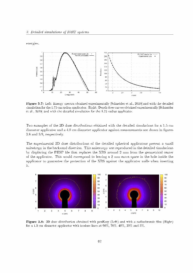
3. Detailed simulations of IORT systems
energies.
Figure 3.7: Left: Energy spectra obtained experimentally [Schneider et al., 2010] and with the detailedsimulation for the 1.75 cm radius applicator. Right: Depth dose curves obtained experimentally [Schneideret al., 2010] and with the detailed simulation for the 1.75 radius applicator.
Two examples of the 2D dose distributions obtained with the detailed simulations for a 1.5 cmdiameter applicator and a 4.0 cm diameter applicator against measurements are shown in gures3.8 and 3.9, respectively.
The experimental 2D dose distributions of the detailed spherical applicators present a smallanisotropy in the backward direction. This anisotropy was reproduced in the detailed simulationsby displacing the PHSP le that replaces the XRS around 2 mm from the geometrical centerof the applicator. This would correspond to leaving a 2 mm extra space in the hole inside theapplicator to guarantee the protection of the XRS against the applicator walls when insertingit.
Figure 3.8: 2D dose distribution obtained with penEasy (Left) and with a radiochromic lm (Right)for a 1.5 cm diameter applicator with isodose lines at 90%, 70%, 40%, 20% and 5%.
62

3.2. Intrabeam R© applicators
Figure 3.9: 2D dose distribution obtained with penEasy (Left) and with a radiochromic lm (Right)for a 4.0 cm diameter applicator with isodose lines at 90%, 70%, 40%, 20% and 10% of the maximumdose.
3.2.2.1 Approximation for Intrabeam R© needle and spherical applicators
In the previous section we have simulated in detail the spherical applicators, reaching a goodagreement with the experimental measurements. However, these detailed simulations required avery high resource usage to do the calculations, as each applicator needed to run over 24 hoursin parallel in a high capacity cluster in 200 dierent cores to obtain a dose distribution withenough statistics. If only one CPU had been used, the simulation of each applicator would haverun for about 7 months to achieve good enough statistics.
Consequently, for this work we have used a simplied version of the spherical and needleapplicators. We have considered a photon source emitting isotropically in a vacuum spherewith the radius of the real applicator. This way the simulation time needed to obtain a gooddose distribution is reduced up to several hours.
This approach may introduce some changes in the energy deposition distribution in depth.However, these dierences will be absorbed afterwards during the tting procedure explainedin the following chapter.
Regarding the anisotropy of the experimental measurements, it will not be reproduced with thisapproximation. Nevertheless, the area where the anisotropy is presented has not clinical interest,as it is behind the applicator, and we will take it into consideration in future works.
3.2.3 Simulation of Intrabeam R© at and surface applicators
For at and surface applicators characterization, the vendor provided the information of thegeometry, and therefore, the details are protected and can not be described in this work. Both
63
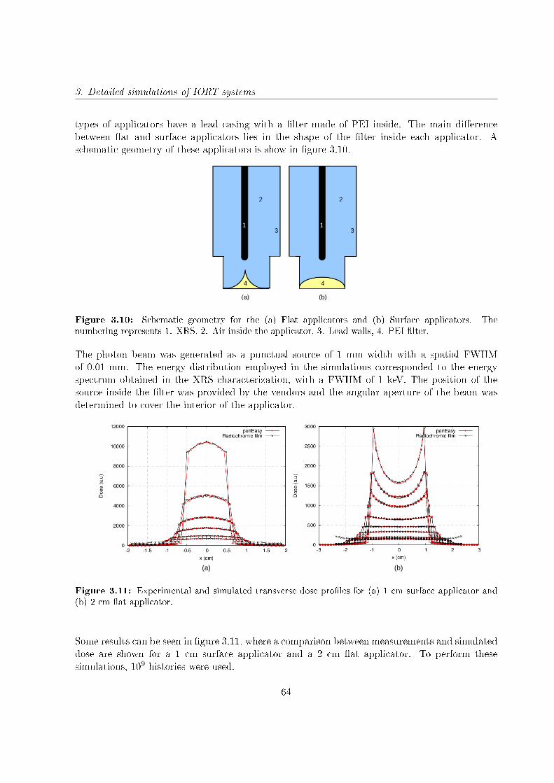
3. Detailed simulations of IORT systems
types of applicators have a lead casing with a lter made of PEI inside. The main dierencebetween at and surface applicators lies in the shape of the lter inside each applicator. Aschematic geometry of these applicators is show in gure 3.10.
Figure 3.10: Schematic geometry for the (a) Flat applicators and (b) Surface applicators. Thenumbering represents 1. XRS, 2. Air inside the applicator, 3. Lead walls, 4. PEI lter.
The photon beam was generated as a punctual source of 1 mm width with a spatial FWHMof 0.01 mm. The energy distribution employed in the simulations corresponded to the energyspectrum obtained in the XRS characterization, with a FWHM of 1 keV. The position of thesource inside the lter was provided by the vendors and the angular aperture of the beam wasdetermined to cover the interior of the applicator.
(a) (b)
Figure 3.11: Experimental and simulated transverse dose proles for (a) 1 cm surface applicator and(b) 2 cm at applicator.
Some results can be seen in gure 3.11, where a comparison between measurements and simulateddose are shown for a 1 cm surface applicator and a 2 cm at applicator. To perform thesesimulations, 109 histories were used.
64
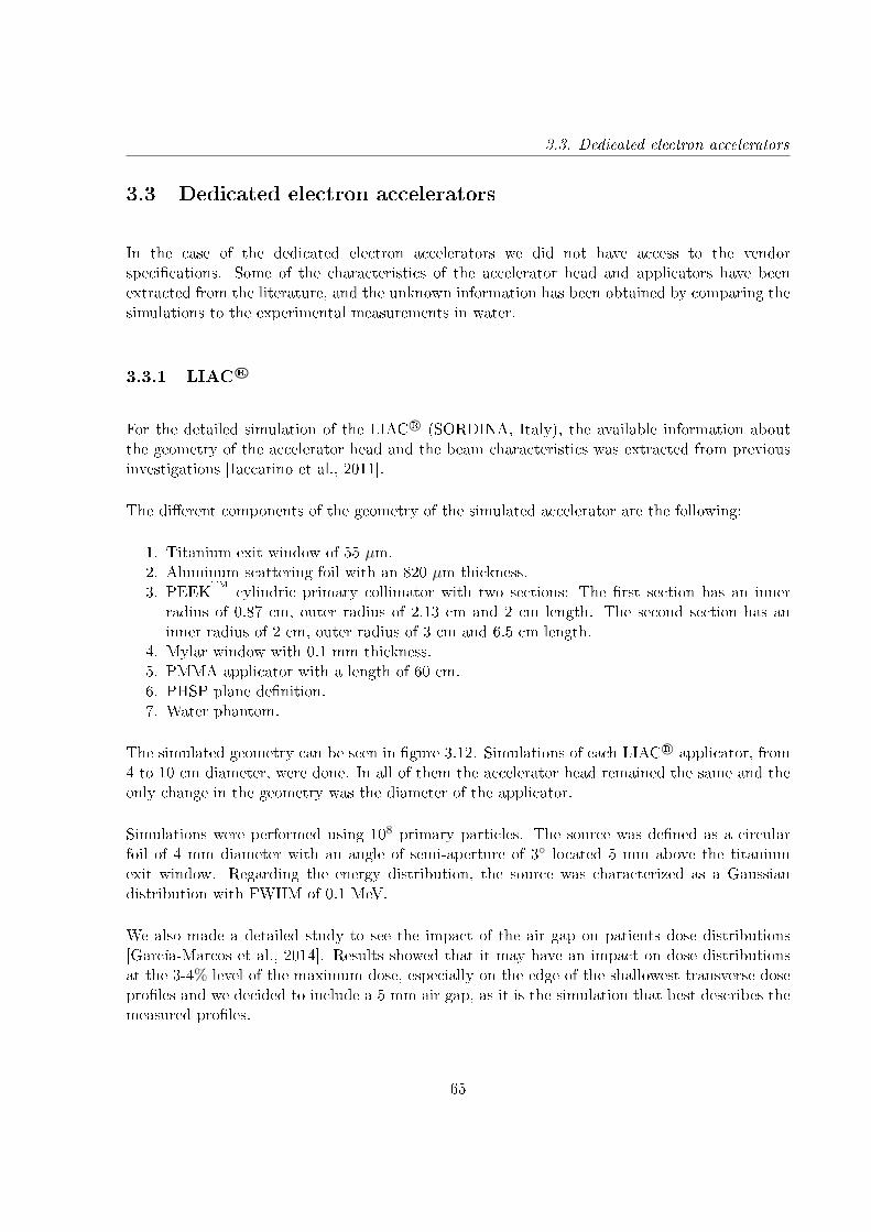
3.3. Dedicated electron accelerators
3.3 Dedicated electron accelerators
In the case of the dedicated electron accelerators we did not have access to the vendorspecications. Some of the characteristics of the accelerator head and applicators have beenextracted from the literature, and the unknown information has been obtained by comparing thesimulations to the experimental measurements in water.
3.3.1 LIAC R©
For the detailed simulation of the LIAC R© (SORDINA, Italy), the available information aboutthe geometry of the accelerator head and the beam characteristics was extracted from previousinvestigations [Iaccarino et al., 2011].
The dierent components of the geometry of the simulated accelerator are the following:
1. Titanium exit window of 55 µm.2. Aluminum scattering foil with an 820 µm thickness.3. PEEK
TM
cylindric primary collimator with two sections: The rst section has an innerradius of 0.87 cm, outer radius of 2.13 cm and 2 cm length. The second section has aninner radius of 2 cm, outer radius of 3 cm and 6.5 cm length.
4. Mylar window with 0.1 mm thickness.5. PMMA applicator with a length of 60 cm.6. PHSP plane denition.7. Water phantom.
The simulated geometry can be seen in gure 3.12. Simulations of each LIAC R© applicator, from4 to 10 cm diameter, were done. In all of them the accelerator head remained the same and theonly change in the geometry was the diameter of the applicator.
Simulations were performed using 108 primary particles. The source was dened as a circularfoil of 4 mm diameter with an angle of semi-aperture of 3 located 5 mm above the titaniumexit window. Regarding the energy distribution, the source was characterized as a Gaussiandistribution with FWHM of 0.1 MeV.
We also made a detailed study to see the impact of the air gap on patients dose distributions[García-Marcos et al., 2014]. Results showed that it may have an impact on dose distributionsat the 3-4% level of the maximum dose, especially on the edge of the shallowest transverse doseproles and we decided to include a 5 mm air gap, as it is the simulation that best describes themeasured proles.
65

3. Detailed simulations of IORT systems
12
3
4
5
6
7
8
Figure 3.12: Geometry of the simulated LIAC R©. The numeration, materials and dimensions correspondto the numbers shown in the description.
To validate the simulation and assure an accurate description of the accelerator, we comparedthe results of our simulation against transverse proles measured in water at the HospitalUniversitario Gregorio Marañón for energies of 6, 8, 10 and 12 MeV and the the dierentapplicators. A comparison of transverse dose proles is shown in gure 3.13.
66
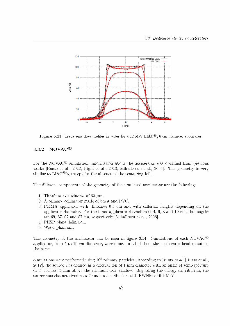
3.3. Dedicated electron accelerators
Figure 3.13: Transverse dose proles in water for a 12 MeV LIAC R©, 6 cm diameter applicator.
3.3.2 NOVAC R©
For the NOVAC R© simulation, information about the accelerator was obtained from previousworks [Russo et al., 2012, Righi et al., 2013, Mihailescu et al., 2006]. The geometry is verysimilar to LIAC R©'s, except for the absence of the scattering foil.
The dierent components of the geometry of the simulated accelerator are the following:
1. Titanium exit window of 60 µm.2. A primary collimator made of brass and PVC.3. PMMA applicator with thickness 0.5 cm and with dierent lengths depending on the
applicator diameter. For the inner applicator diameters of 4, 6, 8 and 10 cm, the lengthsare 69, 67, 67 and 87 cm, respectively [Mihailescu et al., 2006].
4. PHSP plane denition.5. Water phantom.
The geometry of the accelerator can be seen in gure 3.14. Simulations of each NOVAC R©
applicator, from 4 to 10 cm diameter, were done. In all of them the accelerator head remainedthe same.
Simulations were performed using 108 primary particles. According to Russo et al. [Russo et al.,2012], the source was dened as a circular foil of 1 mm diameter with an angle of semi-apertureof 3 located 5 mm above the titanium exit window. Regarding the energy distribution, thesource was characterized as a Gaussian distribution with FWHM of 0.1 MeV.
67
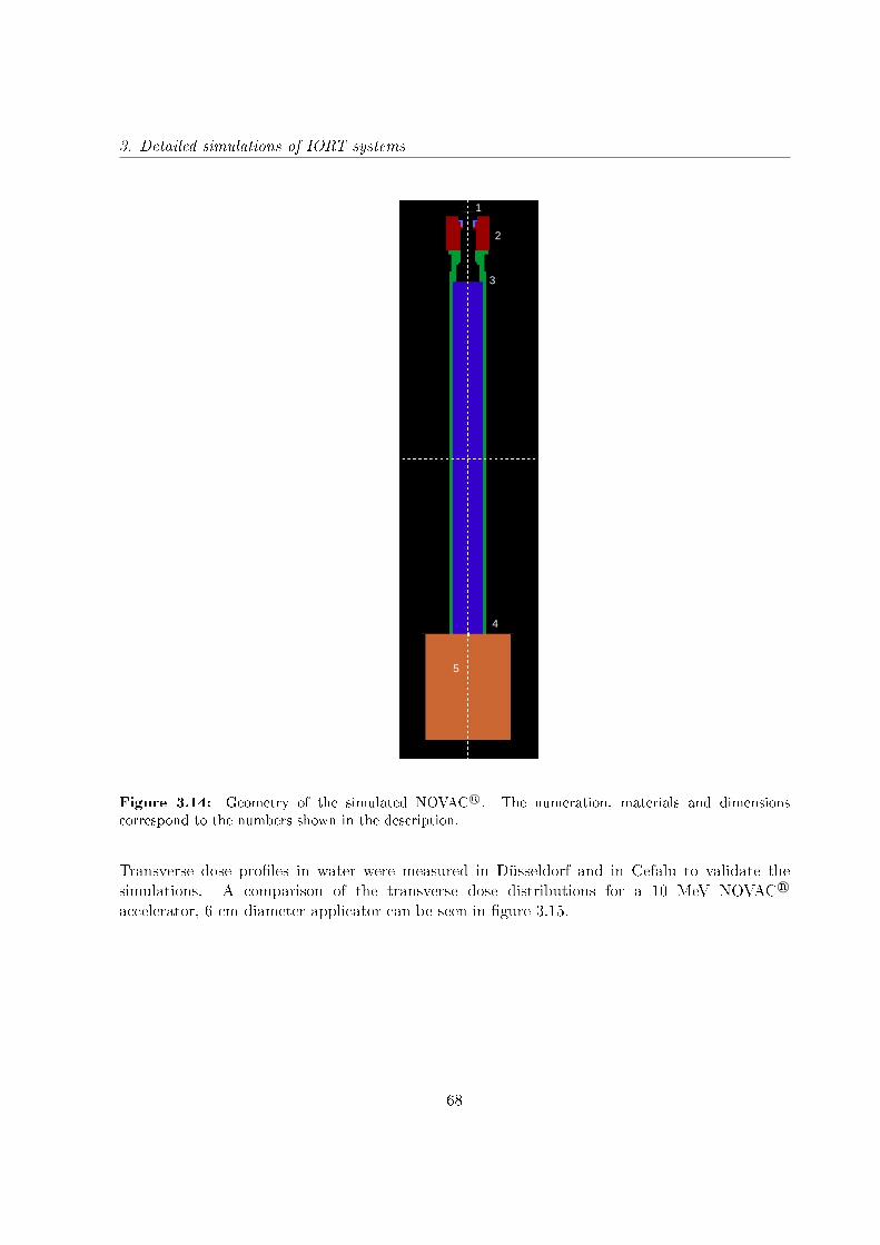
3. Detailed simulations of IORT systems
1
2
3
4
5
Figure 3.14: Geometry of the simulated NOVAC R©. The numeration, materials and dimensionscorrespond to the numbers shown in the description.
Transverse dose proles in water were measured in Düsseldorf and in Cefalu to validate thesimulations. A comparison of the transverse dose distributions for a 10 MeV NOVAC R©
accelerator, 6 cm diameter applicator can be seen in gure 3.15.
68
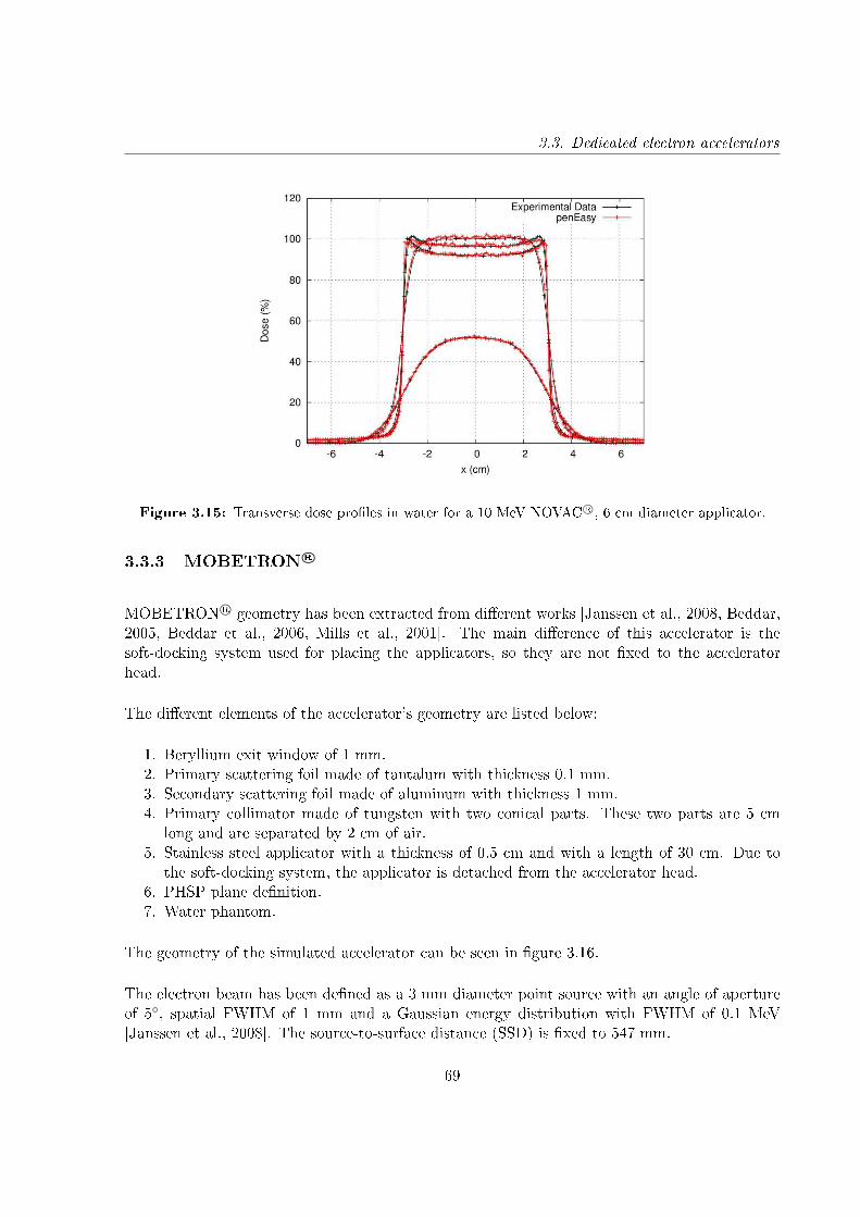
3.3. Dedicated electron accelerators
Figure 3.15: Transverse dose proles in water for a 10 MeV NOVAC R©, 6 cm diameter applicator.
3.3.3 MOBETRON R©
MOBETRON R© geometry has been extracted from dierent works [Janssen et al., 2008, Beddar,2005, Beddar et al., 2006, Mills et al., 2001]. The main dierence of this accelerator is thesoft-docking system used for placing the applicators, so they are not xed to the acceleratorhead.
The dierent elements of the accelerator's geometry are listed below:
1. Beryllium exit window of 1 mm.2. Primary scattering foil made of tantalum with thickness 0.1 mm.3. Secondary scattering foil made of aluminum with thickness 1 mm.4. Primary collimator made of tungsten with two conical parts. These two parts are 5 cm
long and are separated by 2 cm of air.5. Stainless steel applicator with a thickness of 0.5 cm and with a length of 30 cm. Due to
the soft-docking system, the applicator is detached from the accelerator head.6. PHSP plane denition.7. Water phantom.
The geometry of the simulated accelerator can be seen in gure 3.16.
The electron beam has been dened as a 3 mm diameter point source with an angle of apertureof 5, spatial FWHM of 1 mm and a Gaussian energy distribution with FWHM of 0.1 MeV[Janssen et al., 2008]. The source-to-surface distance (SSD) is xed to 547 mm.
69
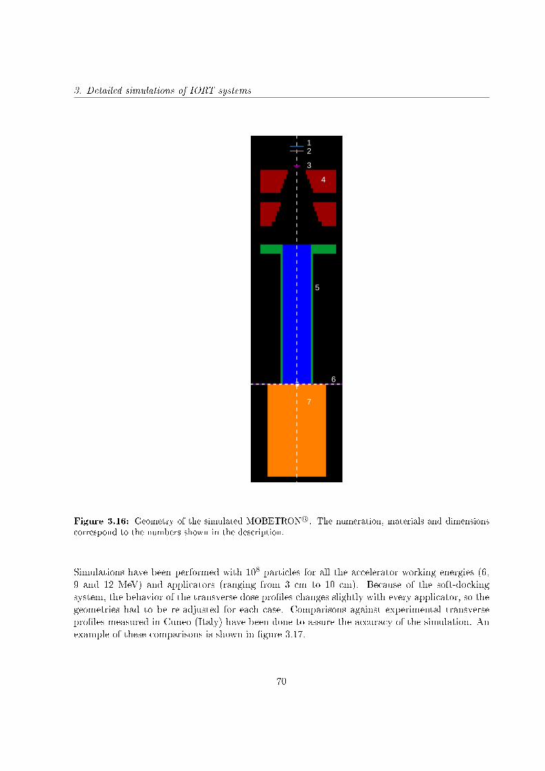
3. Detailed simulations of IORT systems
12
3
4
5
6
7
Figure 3.16: Geometry of the simulated MOBETRON R©. The numeration, materials and dimensionscorrespond to the numbers shown in the description.
Simulations have been performed with 108 particles for all the accelerator working energies (6,9 and 12 MeV) and applicators (ranging from 3 cm to 10 cm). Because of the soft-dockingsystem, the behavior of the transverse dose proles changes slightly with every applicator, so thegeometries had to be re-adjusted for each case. Comparisons against experimental transverseproles measured in Cuneo (Italy) have been done to assure the accuracy of the simulation. Anexample of these comparisons is shown in gure 3.17.
70
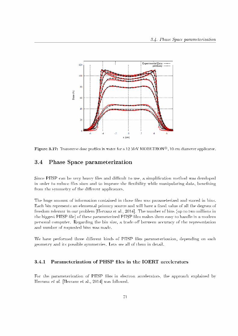
3.4. Phase Space parameterization
Figure 3.17: Transverse dose proles in water for a 12 MeV MOBETRON R©, 10 cm diameter applicator.
3.4 Phase Space parameterization
Since PHSP can be very heavy les and dicult to use, a simplication method was developedin order to reduce les sizes and to improve the exibility while manipulating data, benetingfrom the symmetry of the dierent applicators.
The huge amount of information contained in those les was parameterized and stored in bins.Each bin represents an elemental primary source and will have a xed value of all the degrees offreedom relevant in our problem [Herranz et al., 2014]. The number of bins (up to two millions inthe biggest PHSP le) of these parameterized PHSP les makes them easy to handle in a modernpersonal computer. Regarding the bin size, a trade-o between accuracy of the representationand number of requested bins was made.
We have performed three dierent kinds of PHSP les parameterization, depending on eachgeometry and its possible symmetries. Lets see all of them in detail.
3.4.1 Parameterization of PHSP les in the IOERT accelerators
For the parameterization of PHSP les in electron accelerators, the approach explained byHerranz et al. [Herranz et al., 2014] was followed.
71

3. Detailed simulations of IORT systems
Without loss of generality, it has been assumed that the PHSP le exiting a cylindrical applicatorpresents cylindrical symmetry. This assumption has been done considering that all the electronapplicators studied in this project present a cylindrical shape. This hypothesis also requires thatthe bevel of the applicator must be equal to 0. For those cases where a bevel of a certain angleis needed, which is a frequent situation in IOERT treatments, the PHSP plane is located atthe point where the applicator looses its cylindrical symmetry (see gure 3.18), and the bevel isincluded as an additional piece that is simulated together with the phantom.
Right angle applicator
Patient
PHSP plane
Bevel
Figure 3.18: Schematic view of the PHSP plane at the exit of the right angle applicator showing thesmall piece of beveled applicator included in the simulation to compute the dose for non-right applicators[Herranz et al., 2014].
Exploiting the cylindrical symmetry mentioned, the PHSP is fully dened by the distribution ofparticles in energy (E), distance to the applicator axis ρ, and two angles for the emission direction:θ, dened as the angle of the particle trajectory with the z axis, and φ, the azimuthal angle thatforms the plane containing the trajectory and the z axis. We assume azimuthal symmetry aroundthe applicator axis. In gure 3.19 the denition of these angles is shown.
This 4-dimensional representation was used to build a discretized nite set of up to a maximumof around 2.000.000 elementary sources or bins. Each bin represents a source with xed valuesof energy, radial distance to the applicator axis and trajectory angles.
The following ranges and binning widths (BW) were considered for the denition of theelementary sources:
• Type of particle (electron, photon).• Energy, ranging from 0 to 14 MeV (BW = 0.25 MeV).• Axial angle θ, ranging from 0 to 29 (BW = 0.64).• Azimuthal angle φ, ranging from 0 to 180 (BW = 20).• Radial position ρ ranging from 0 to 10 cm (BW = 0.2 cm).
72
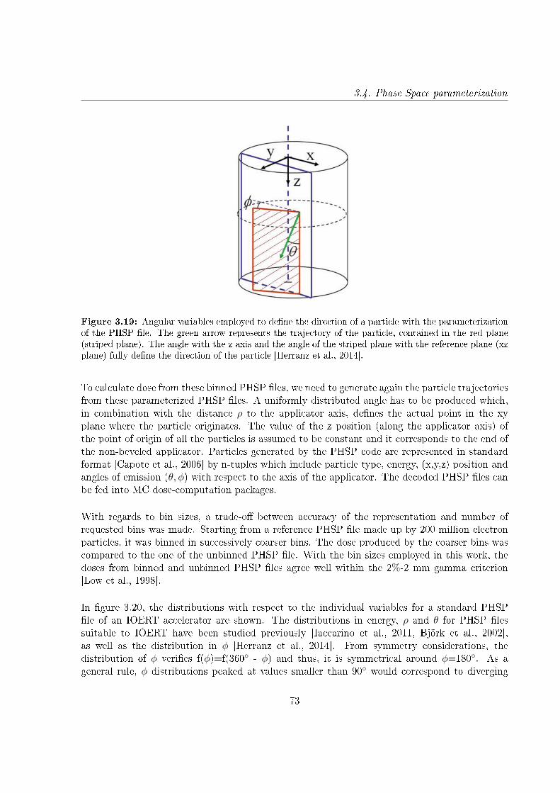
3.4. Phase Space parameterization
Figure 3.19: Angular variables employed to dene the direction of a particle with the parameterizationof the PHSP le. The green arrow represents the trajectory of the particle, contained in the red plane(striped plane). The angle with the z axis and the angle of the striped plane with the reference plane (xzplane) fully dene the direction of the particle [Herranz et al., 2014].
To calculate dose from these binned PHSP les, we need to generate again the particle trajectoriesfrom these parameterized PHSP les. A uniformly distributed angle has to be produced which,in combination with the distance ρ to the applicator axis, denes the actual point in the xyplane where the particle originates. The value of the z position (along the applicator axis) ofthe point of origin of all the particles is assumed to be constant and it corresponds to the end ofthe non-beveled applicator. Particles generated by the PHSP code are represented in standardformat [Capote et al., 2006] by n-tuples which include particle type, energy, (x,y,z) position andangles of emission (θ, φ) with respect to the axis of the applicator. The decoded PHSP les canbe fed into MC dose-computation packages.
With regards to bin sizes, a trade-o between accuracy of the representation and number ofrequested bins was made. Starting from a reference PHSP le made up by 200 million electronparticles, it was binned in successively coarser bins. The dose produced by the coarser bins wascompared to the one of the unbinned PHSP le. With the bin sizes employed in this work, thedoses from binned and unbinned PHSP les agree well within the 2%-2 mm gamma criterion[Low et al., 1998].
In gure 3.20, the distributions with respect to the individual variables for a standard PHSPle of an IOERT accelerator are shown. The distributions in energy, ρ and θ for PHSP lessuitable to IOERT have been studied previously [Iaccarino et al., 2011, Björk et al., 2002],as well as the distribution in φ [Herranz et al., 2014]. From symmetry considerations, thedistribution of φ veries f(φ)=f(360 - φ) and thus, it is symmetrical around φ=180. As ageneral rule, φ distributions peaked at values smaller than 90 would correspond to diverging
73
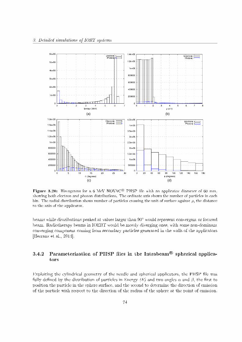
3. Detailed simulations of IORT systems
(a)
(c)
(b)
(d)
Figure 3.20: Histograms for a 6 MeV NOVAC R© PHSP le with an applicator diameter of 60 mm,showing both electron and photon distributions. The ordinate axis shows the number of particles in eachbin. The radial distribution shows number of particles crossing the unit of surface against ρ, the distanceto the axis of the applicator.
beams while distributions peaked at values larger than 90 would represent convergent or focusedbeam. Radiotherapy beams in IOERT would be mostly diverging ones, with some non-dominantconverging component coming from secondary particles generated in the walls of the applicators[Herranz et al., 2014].
3.4.2 Parameterization of PHSP les in the Intrabeam R© spherical applica-tors
Exploiting the cylindrical geometry of the needle and spherical applicators, the PHSP le wasfully dened by the distribution of particles in Energy (E) and two angles α and β, the rst toposition the particle in the sphere surface, and the second to determine the direction of emissionof the particle with respect to the direction of the radius of the sphere at the point of emission.
74
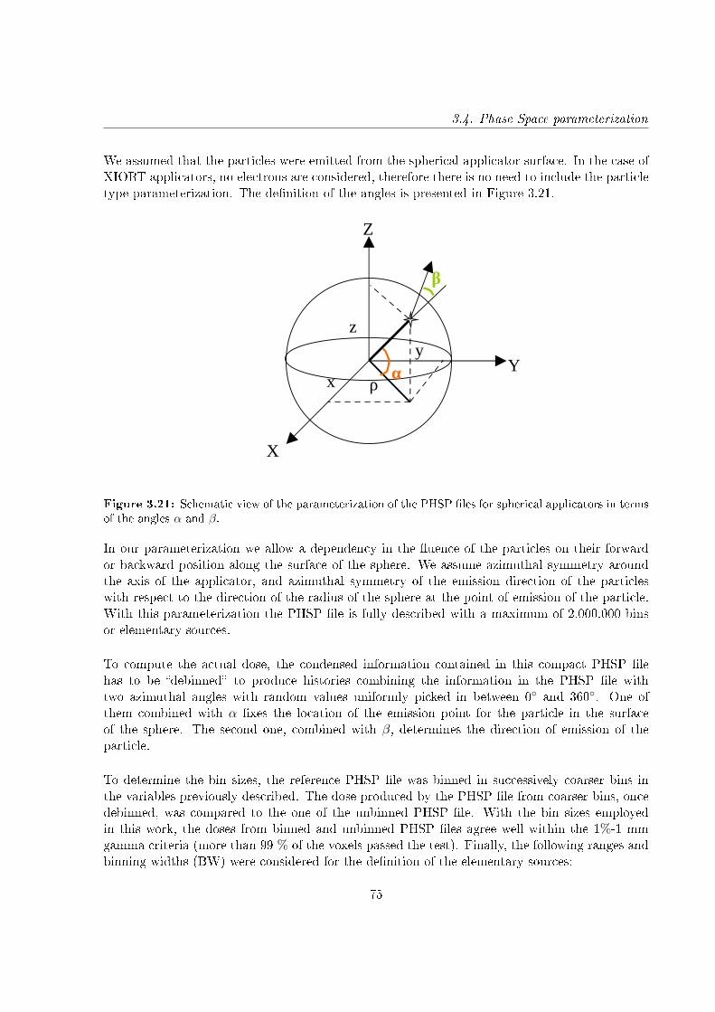
3.4. Phase Space parameterization
We assumed that the particles were emitted from the spherical applicator surface. In the case ofXIORT applicators, no electrons are considered, therefore there is no need to include the particletype parameterization. The denition of the angles is presented in Figure 3.21.
X
Y
Z
x
yz
ρα
β
Figure 3.21: Schematic view of the parameterization of the PHSP les for spherical applicators in termsof the angles α and β.
In our parameterization we allow a dependency in the uence of the particles on their forwardor backward position along the surface of the sphere. We assume azimuthal symmetry aroundthe axis of the applicator, and azimuthal symmetry of the emission direction of the particleswith respect to the direction of the radius of the sphere at the point of emission of the particle.With this parameterization the PHSP le is fully described with a maximum of 2.000.000 binsor elementary sources.
To compute the actual dose, the condensed information contained in this compact PHSP lehas to be debinned to produce histories combining the information in the PHSP le withtwo azimuthal angles with random values uniformly picked in between 0 and 360. One ofthem combined with α xes the location of the emission point for the particle in the surfaceof the sphere. The second one, combined with β, determines the direction of emission of theparticle.
To determine the bin sizes, the reference PHSP le was binned in successively coarser bins inthe variables previously described. The dose produced by the PHSP le from coarser bins, oncedebinned, was compared to the one of the unbinned PHSP le. With the bin sizes employedin this work, the doses from binned and unbinned PHSP les agree well within the 1%-1 mmgamma criteria (more than 99 % of the voxels passed the test). Finally, the following ranges andbinning widths (BW) were considered for the denition of the elementary sources:
75
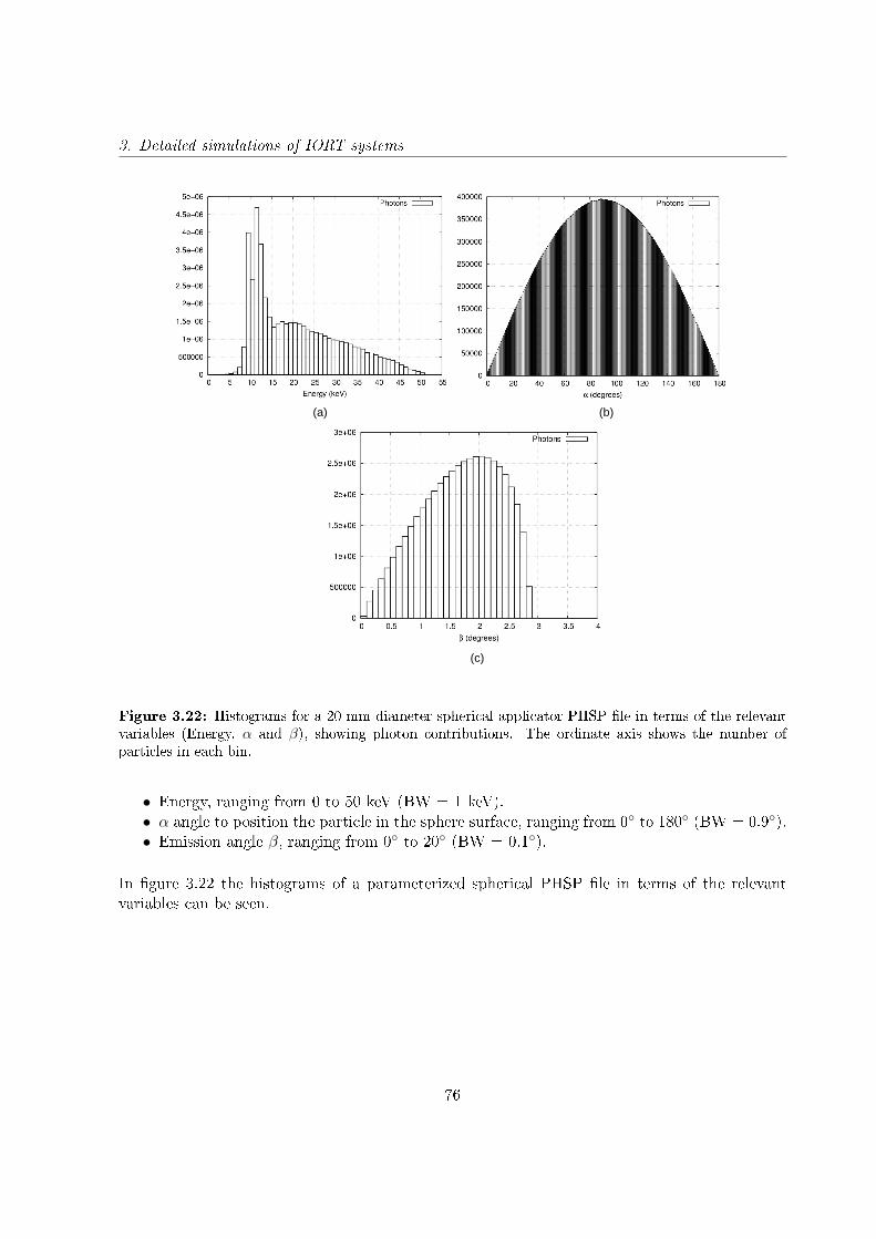
3. Detailed simulations of IORT systems
(a)
(c)
(b)
Figure 3.22: Histograms for a 20 mm diameter spherical applicator PHSP le in terms of the relevantvariables (Energy, α and β), showing photon contributions. The ordinate axis shows the number ofparticles in each bin.
• Energy, ranging from 0 to 50 keV (BW = 1 keV).• α angle to position the particle in the sphere surface, ranging from 0 to 180 (BW = 0.9).• Emission angle β, ranging from 0 to 20 (BW = 0.1).
In gure 3.22 the histograms of a parameterized spherical PHSP le in terms of the relevantvariables can be seen.
76
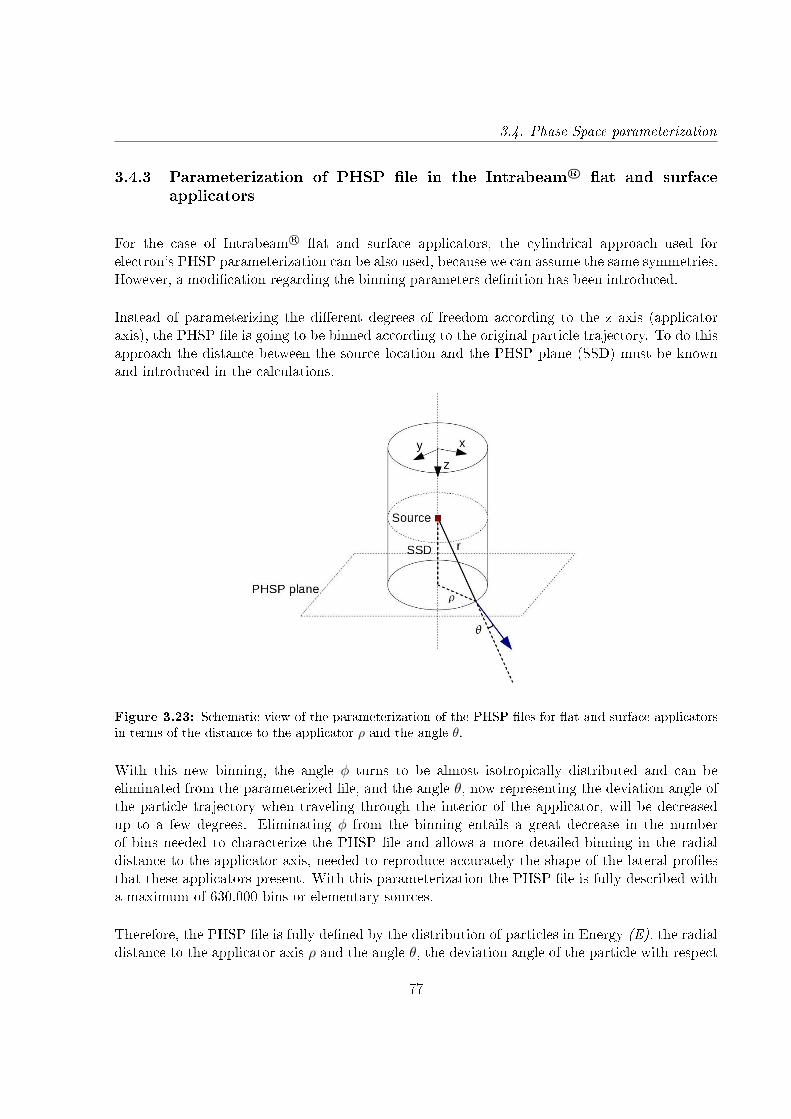
3.4. Phase Space parameterization
3.4.3 Parameterization of PHSP le in the Intrabeam R© at and surfaceapplicators
For the case of Intrabeam R© at and surface applicators, the cylindrical approach used forelectron's PHSP parameterization can be also used, because we can assume the same symmetries.However, a modication regarding the binning parameters denition has been introduced.
Instead of parameterizing the dierent degrees of freedom according to the z axis (applicatoraxis), the PHSP le is going to be binned according to the original particle trajectory. To do thisapproach the distance between the source location and the PHSP plane (SSD) must be knownand introduced in the calculations.
Figure 3.23: Schematic view of the parameterization of the PHSP les for at and surface applicatorsin terms of the distance to the applicator ρ and the angle θ.
With this new binning, the angle φ turns to be almost isotropically distributed and can beeliminated from the parameterized le, and the angle θ, now representing the deviation angle ofthe particle trajectory when traveling through the interior of the applicator, will be decreasedup to a few degrees. Eliminating φ from the binning entails a great decrease in the numberof bins needed to characterize the PHSP le and allows a more detailed binning in the radialdistance to the applicator axis, needed to reproduce accurately the shape of the lateral prolesthat these applicators present. With this parameterization the PHSP le is fully described witha maximum of 630.000 bins or elementary sources.
Therefore, the PHSP le is fully dened by the distribution of particles in Energy (E), the radialdistance to the applicator axis ρ and the angle θ, the deviation angle of the particle with respect
77
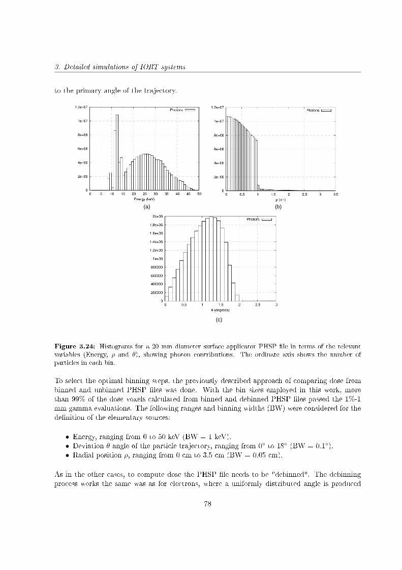
3. Detailed simulations of IORT systems
to the primary angle of the trajectory.
(a)
(c)
(b)
Figure 3.24: Histograms for a 20 mm diameter surface applicator PHSP le in terms of the relevantvariables (Energy, ρ and θ), showing photon contributions. The ordinate axis shows the number ofparticles in each bin.
To select the optimal binning steps, the previously described approach of comparing dose frombinned and unbinned PHSP les was done. With the bin sizes employed in this work, morethan 99% of the dose voxels calculated from binned and debinned PHSP les passed the 1%-1mm gamma evaluations. The following ranges and binning widths (BW) were considered for thedenition of the elementary sources:
• Energy, ranging from 0 to 50 keV (BW = 1 keV).• Deviation θ angle of the particle trajectory, ranging from 0 to 18 (BW = 0.1).• Radial position ρ, ranging from 0 cm to 3.5 cm (BW = 0.05 cm).
As in the other cases, to compute dose the PHSP le needs to be "debinned". The debinningprocess works the same was as for electrons, where a uniformly distributed angle is produced
78
3.5. Conclusion
which denes the position of the particle (x,y,z), in combination with the distance ρ to theapplicator axis.
In gure 3.24 are represented the histograms in terms of the variables used for theparameterization of the PHSP le.
3.5 Conclusion
In this chapter we have simulated in detail a large group of IOERT accelerators and Intrabeam R©
applicators that represent accurately the experimental dose distributions.
Furthermore, with the parameterization of the PHSP les we have turned these huge lescontaining all the information of the particle beam into an easy-to-manipulate le without lossof information. These binned PHSP les can be stored and used without storage issues. Andnally, with the debinning tool we can transform the simplied version of the PHSP le into theunbinned le.
The results from this chapter will be essential for the objectives of this thesis, because thesimulation results will be used as a pre-computed database that will be needed in the PHSPoptimization procedure explained in the following chapter. The binning and debinning tools willmake possible to handle and work with a large set of PHSP les.
79


Chapter 4
Phase space optimization process
4.1 Introduction
Accurate calculation of dose distribution in an inhomogeneous medium such as a human body is acomplicated task. To date, the Monte Carlo (MC) method is considered to be the most accuratealgorithm for dose calculation but it requires the greatest processing time. Apart from the MCmethod, all other methods make dierent degrees of approximation and simplication which leadto much faster calculations but also result in less accurate dose distributions when comparing tothe MC simulation [Chen et al., 2014]. The ideal planning system would be a calculation toolthat can provide accurate dose distributions in minutes by means of a MC algorithm.
As we explained in chapter 3, MC codes for dosimetry require a realistic and accurate descriptionof the electron and/or photon beam employed in the radiotherapy procedure [Chetty et al., 2007],and this information is included in the phase space (PHSP) le. The most common approach togenerate these PHSP les is by simulating in a realistic way the accelerator. To do this, we requirea detailed knowledge of the device and other elements, such as applicators. However, sometimesthis information is protected by the manufacturers, and even if the geometry is available, dosedistributions may vary slightly in dierent devices of the same model, so each specic acceleratorshould be tuned.
In the case of intraoperative electron radiotherapy, the development of new tools for MCsimulation of clinical linear accelerators, such a PRIMO [Rodriguez et al., 2013], can simplifythe simulation task as they include the geometry of some accelerators, but they still require afew hours of simulation for each applicator diameter, LINAC model and energy conguration,and the tuning of each specic accelerator is not contemplated.
A previous procedure [Herranz et al., 2014, Herranz, 2013, Ibáñez, 2012, Ibáñez et al., 2014, Pérez-
81
4. Phase space optimization process
Liva, 2012] developed in our group was done to characterize beams of medical linear acceleratorsfor intraoperative radiotherapy with electrons. This method relied on tting with an iterativeprocedure the relevant variables of a PHSP le (such as energy spectrum, spatial and angulardistributions of the particles) until it reproduced experimental dose measurements in water andin air. Despite this method could perform the machine-specic tuning within minutes, the userwas required to introduce several input data of water and air dose proles in the algorithm andthe accuracy of the tting depended strongly on the quality of the measurements.
The aim of this part of the thesis was to develop a fast and accurate phase space tuning tool whichcan be tted to the user's device with only an experimental depth dose prole (DDP) in water[Ibáñez et al., 2015, Vidal et al., 2015, Udías et al., 2017a], and which has been implementedinto a commercial treatment planning system for intraoperative electron radiotherapy (IOERT)and low energy X-rays radiotherapy (XIORT). The proposed process uses a parameterized phasespace model of the source dened at the surface of the treatment applicator and optimizes it tothe user's source characteristics, by means of an optimization procedure that relies on a simpleset of experimental measurements.
In chapter 3 we have characterized all mobile IOERT accelerators as well as the spherical, needle,at and surface Intrabeam R© applicators. We now will use these geometries to calculate a setof monoenergetic (also called monochromatic) PHSP les and DDPs in water and store them,in order to create a database to feed the PHSP optimization tool. After that, the optimizationmethod proposed in this thesis can be separated in two consecutive phases:
• In phase one, the set of monochromatic DDPs will be weighted and combined until thesum of all the contributions reproduces the experimental DDP. This will be done with agenetic algorithm and as a result of the tting process we will obtain an optimized energyspectrum created from the relative contribution of each DDP to the experimental dose.
• In phase two, we will use the energy spectrum from phase one to weight the monochromaticPHSP les stored in the database and generate an optimized PHSP le that will reproducethe experimental data.
These two phases have to be performed for each energy and applicator of every accelerator orIntrabeam R© that is going to be tuned, but the whole process takes only a few minutes, and oncethe PHSP le is obtained it can be stored and used any time is needed. A scheme of the processis shown in gure 4.1.
82
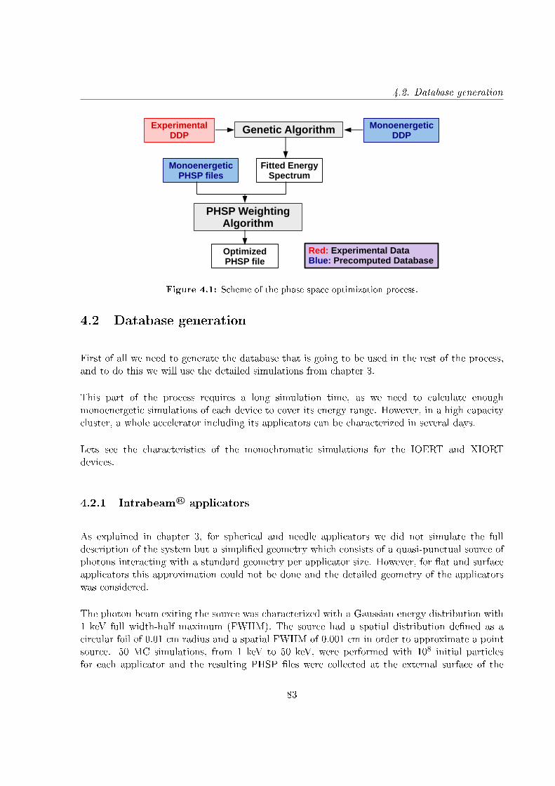
4.2. Database generation
Experimental DDP
Genetic Algorithm Monoenergetic DDP
Fitted Energy Spectrum
Monoenergetic PHSP files
PHSP Weighting Algorithm
Optimized PHSP file
Red: Experimental DataBlue: Precomputed Database
Figure 4.1: Scheme of the phase space optimization process.
4.2 Database generation
First of all we need to generate the database that is going to be used in the rest of the process,and to do this we will use the detailed simulations from chapter 3.
This part of the process requires a long simulation time, as we need to calculate enoughmonoenergetic simulations of each device to cover its energy range. However, in a high capacitycluster, a whole accelerator including its applicators can be characterized in several days.
Lets see the characteristics of the monochromatic simulations for the IOERT and XIORTdevices.
4.2.1 Intrabeam R© applicators
As explained in chapter 3, for spherical and needle applicators we did not simulate the fulldescription of the system but a simplied geometry which consists of a quasi-punctual source ofphotons interacting with a standard geometry per applicator size. However, for at and surfaceapplicators this approximation could not be done and the detailed geometry of the applicatorswas considered.
The photon beam exiting the source was characterized with a Gaussian energy distribution with1 keV full width-half maximum (FWHM). The source had a spatial distribution dened as acircular foil of 0.01 cm radius and a spatial FWHM of 0.001 cm in order to approximate a pointsource. 50 MC simulations, from 1 keV to 50 keV, were performed with 108 initial particlesfor each applicator and the resulting PHSP les were collected at the external surface of the
83
4. Phase space optimization process
applicator.
Since PHSP are huge les and therefore dicult to use, each one was parameterized in terms ofthe relevant variables to make them easy to manipulate, following the considerations described insection 3.4 of the previous chapter. All parameterized PHSP les were nally stored in a binaryformat to reduce even more their size.
Regarding the monochromatic depth dose proles (DDPs), they were either calculated withpenEasy at the same time as the PHSP les, or afterwards using a hybrid MC code specicallydeveloped to accelerate dose calculations for the Intrabeam R© photon beams. The codedescription is detailed in chapter 6.
4.2.2 IOERT accelerators
Geometries of the MOBETRON R©, LIAC R© and NOVAC R© described in chapter 3 were used togenerate the IOERT database.
The source was dened as circular, with a diameter of several millimeters (3-4 mm dependingon the accelerator) and with a Gaussian distribution centered at zero with 0.1 mm FWHM. 140simulations were performed for each applicator and each accelerator, from 1 MeV to 14 MeVwith 0.1 MeV FWHM. 108 histories were calculated, and the PHSP les were parameterized inthe type of particle, energy, axial angle and radial position each 107 histories to save computermemory. This part of the simulation took several days computation time (from 48 hours to 5days depending on the accelerator geometry on a 8 cores high capacity cluster).
Depth dose proles in water were obtained from these parameterized PHSP les with DPM[Sempau et al., 2000] and stored as well (1 hour computation time on a 8 cores high capacitycluster).
4.3 Optimization of energy spectrum
In the rst phase of the phase space optimization process, the monochromatic DDPs are goingto be adjusted to the experimental dose by means of a genetic algorithm [Fernandez-Ramirezet al., 2008].
A genetic algorithm is an optimization tool inspired by the process of natural selection. Thealgorithm creates a randomly generated population of possible solutions with a set of propertiesthat can be mutated. The evolution of this population follows an iterative process, where eachiteration is called a generation. In each generation, the more t individuals are selected, and
84

4.3. Optimization of energy spectrum
their properties are mutated to form another generation, which is used in the next iteration ofthe algorithm. The optimization ends when either a maximum number of generations have beenproduced or a certain tness level has been reached.
The genetic algorithm requires a tting function, and in this case this function will be ageneric energy spectrum. This way, the genetic algorithm will generate an optimized energyspectrum which weights the relative contributions of the monochromatic DDPs that reproducesthe experimental dose data.
The tting procedure will be the same for XIORT and for IOERT, but the shape of the initialenergy spectrum will dier. Both energy spectra are going to de dened by simple mathematicalfunctions describing the expected shape of the beam at the beginning of the accelerator head orat the exit of the Intrabeam R© X-ray source.
4.3.1 Energy spectrum for Intrabeam R© applicators
The energy spectrum of the Intrabeam R© X-ray source is dened as a function that describesthe Bremsstrahlung behavior of the energy spectrum and the characteristic rays. Based onKramers theory of the photons emitted when they hit a target (without taking into account thecharacteristic lines) [Kramers, 1923], equation 4.1 describes the bremsstrahlung background ofthe energy spectrum Sbackground in function of energy E:
Sbackground(E) = (E − E1)a(E0
E− 1)b
(4.1)
Where E0 is the maximal energy of the photon beam and E1 the cut-o energy. a and b are theltration parameter and the Kramers law adjustment parameter respectively.
The gold characteristic X-rays have been added to the background at energies of 9, 12 and 14keV, as measured by Schneider et al. at the probe surface [Schneider et al., 2010].
Sspectrum(E) = Sbackground(E) + c · Ip (4.2)
Where c is the mix parameter, xing the amplitude of the characteristic lines relative to thespectrum background intensity and Ip the intensity of the characteristic line with energy Erelative to the other two lines.
For each experimental DDP provided by the user, the parameters E1, E0, a, b and c are variedand the energy spectrum optimization results in a specic energy spectrum shape (with dierent
85

4. Phase space optimization process
bremsstrahlung backgrounds and characteristic lines intensities) reproducing each experimentalDDP.
4.3.2 Energy spectrum for IOERT accelerators
In the case of electrons, the initial electron beam entering the accelerator head is simulated asa combination of a Gaussian distribution with Kramers functions. For each central energy E0
of the Gaussian distribution, a Kramers function is generated. The sum of all combinations willgenerate the energy spectrum.
A set of Gaussian distributions from E0-3.5σ to E0+3.5σ will be generated, being E0 the centralenergy of the Gaussian distribution and σ its standard deviation:
ω(E) =1√
2πσ2e−
(E−E0)2
2σ2 (4.3)
These Gaussian distributions will be used to weight the 140 Kramers functions associated toeach monochromatic energy (Ec):
fKramers =(
E
(E − Ec) + ∆
)α(4.4)
Being ∆ a blurring parameter inserted to avoid dierences in the denominator between dierentenergies because of the energy binning that it is being used.
The energy spectrum will be the sum of all normalized Kramers functions weighted by theGaussian distributions:
Sspectrum(E) = ω(E)∑140
i=1 fKramers(E, i)normalization
(4.5)
For each experimental DDP provided by the user, the parameters E0, σ, α and ∆ will be variedand, as in the case of XIORT, the optimization will result in a specic energy spectrum shapereproducing each experimental DDP.
86

4.4. PHSP weighting algorithm
4.3.3 Treatment of the experimental data
To perform this tting, usually a previous treatment of the experimental DDP needs to beperformed. Specially in the case of electron doses, sometimes the experimental proles do nothave a soft shape and present some irregularities. This may aect the tting process as theseerrors are introduced in the algorithm. To avoid it and to guaranteer an accurate adjustment,a previous treatment is done to the DDP by approximating it to a general function with theform:
f(x) = A[e−Bx − Ce−Dx
]e−
Ex4+Fx2
G +H (4.6)
Figure 4.2 shows the treatment done to an experimental DDP from a NOVAC R© accelerator with9 MeV.
Figure 4.2: Experimental DDP and adjusted DDP for a 9 MeV NOVAC R© with 4 cm diameter.
4.4 PHSP weighting algorithm
Once the energy spectrum is optimized, we need to generate the tuned phase space le. To dothis, the monochromatic PHSP les are weighted with the optimized energy spectrum from thegenetic algorithm and merged to obtain the nal PHSP le. This le also needs to include a scalefactor that is going to be applied to the nal dose so that it is scaled to the input experimentalDDP.
87

4. Phase space optimization process
The genetic algorithm supplies a scale factor needed to scale the adjusted DDP to theexperimental one, and applies a normalization of the spectrum that will have to be consideredin the nal scale of the weighting procedure. However, this factor will not be sucient to scalethe problem, and we will need to introduce an extra scale factor derived from the number ofparticles used to calculate the monochromatic DDPs.
The nal scale factor will be a contribution of both factors:
f = fgenetic · fweighting (4.7)
The weighting procedure will depend on the way the monochromatic DDPs are generated.Dose distributions obtained with any MC algorithm are always dened as dose per primaryhistory. When the primary beam travels through the dierent elements of the accelerator heador the applicators, some of the original particles are absorbed or scattered and do not reach thePHSP recollection plane. The number of lost particles increases as the energy decreases, so themonochromatic PHSP les will not have information of the same number of particles for all theenergies. However, if the monochromatic DDPs are calculated in the same simulation as thePHSP les, these dose distributions will be all divided by the same number of histories, ie. theinitial primary histories of the simulations. But if these curves are obtained with other code,such as DPM or the hybrid MC algorithm described in chapter 6, they are going to be calculatedfrom the monochromatic PHSP les, and every curve will be divided by a dierent number ofprimary histories.
Therefore, two dierent approaches must be taken into consideration, depending on the procedureused for generating the monochromatic DDPs.
4.4.1 Weighting approach for DDPs with the same number of histories
If the monochromatic DDPs have been generated at the same time as the PHSP les, andtherefore they are all divided by the same number of primary histories, the optimized spectrumwill be used to directly weight the monochromatic PHSP les. The dose distribution obtainedwith the optimized PHSP le will be divided by the number of its primary histories, which inthis case will be sum of the number of histories of each monochromatic PHSP le multiplied bythe corresponding value of the energy spectrum:
[Emax∑i=1
PHSP (i) · spectrum(i)]→ dose∑Emaxi=1 [weightPHSP (i) · spectrum(i)]
(4.8)
88
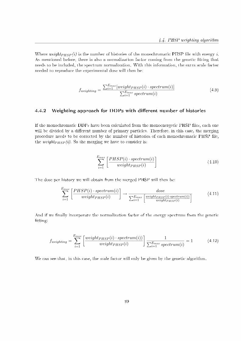
4.4. PHSP weighting algorithm
Where weightPHSP (i) is the number of histories of the monochromatic PHSP le with energy i.As mentioned before, there is also a normalization factor coming from the genetic tting thatneeds to be included, the spectrum normalization. With this information, the extra scale factorneeded to reproduce the experimental dose will then be:
fweighting =∑Emax
i=1 [weightPHSP (i) · spectrum(i)]∑Emaxi=1 spectrum(i)
(4.9)
4.4.2 Weighting approach for DDPs with dierent number of histories
If the monochromatic DDPs have been calculated from the monoenergetic PHSP les, each onewill be divided by a dierent number of primary particles. Therefore, in this case, the mergingprocedure needs to be corrected by the number of histories of each monochromatic PHSP le,the weightPHSP (i). So the merging we have to consider is:
Emax∑i=1
[PHSP (i) · spectrum(i)
weightPHSP (i)
](4.10)
The dose per history we will obtain from the merged PHSP will then be:
Emax∑i=1
[PHSP (i) · spectrum(i)
weightPHSP (i)
]→ dose∑Emax
i=1
[weightPHSP (i)·spectrum(i))
weightPHSP (i)
] (4.11)
And if we nally incorporate the normalization factor of the energy spectrum from the genetictting:
fweighting =Emax∑i=1
[weightPHSP (i) · spectrum(i))
weightPHSP (i)
]1∑Emax
i=1 spectrum(i)= 1 (4.12)
We can see that, in this case, the scale factor will only be given by the genetic algorithm.
89
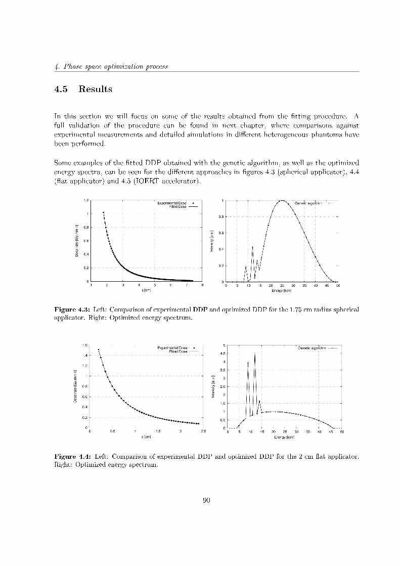
4. Phase space optimization process
4.5 Results
In this section we will focus on some of the results obtained from the tting procedure. Afull validation of the procedure can be found in next chapter, where comparisons againstexperimental measurements and detailed simulations in dierent heterogeneous phantoms havebeen performed.
Some examples of the tted DDP obtained with the genetic algorithm, as well as the optimizedenergy spectra, can be seen for the dierent approaches in gures 4.3 (spherical applicator), 4.4(at applicator) and 4.5 (IOERT accelerator).
Figure 4.3: Left: Comparison of experimental DDP and optimized DDP for the 1.75 cm radius sphericalapplicator. Right: Optimized energy spectrum.
Figure 4.4: Left: Comparison of experimental DDP and optimized DDP for the 2 cm at applicator.Right: Optimized energy spectrum.
90
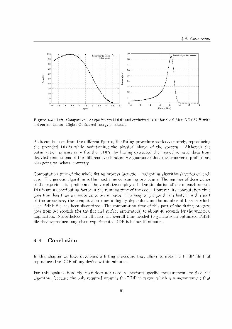
4.6. Conclusion
Figure 4.5: Left: Comparison of experimental DDP and optimized DDP for the 9 MeV NOVAC R© witha 4 cm applicator. Right: Optimized energy spectrum.
As it can be seen from the dierent gures, the tting procedure works accurately, reproducingthe provided DDPs while maintaining the physical shape of the spectra. Although theoptimization process only ts the DDPs, by having extracted the monochromatic data fromdetailed simulations of the dierent accelerators we guarantee that the transverse proles arealso going to behave correctly.
Computation time of the whole tting process (genetic + weighting algorithms) varies on eachcase. The genetic algorithm is the most time consuming procedure. The number of dose valuesof the experimental prole and the voxel size employed in the simulation of the monochromaticDDPs are a contributing factor in the running time of the code. However, its computation timegoes from less than a minute up to 6-7 minutes. The weighting algorithm is faster. In this partof the procedure, the computation time is highly dependent on the number of bins in whicheach PHSP le has been discretized. The computation time of this part of the tting progressgoes from 3-5 seconds (for the at and surface applicators) to about 40 seconds for the sphericalapplicators. Nevertheless, in all cases the overall time needed to generate an optimized PHSPle that reproduces any given experimental DDP is below 10 minutes.
4.6 Conclusion
In this chapter we have developed a tting procedure that allows to obtain a PHSP le thatreproduces the DDP of any device within minutes.
For this optimization, the user does not need to perform specic measurements to feed thealgorithm, because the only required input is the DDP in water, which is a measurement that
91
4. Phase space optimization process
has been previously done for each energy and applicator of the accelerator as it is mandatory forthe commissioning of the device.
By combining PHSP les and DDPs from realistic simulations and by using a realistic shape ofthe energy spectra we guarantee an accurate behavior of the dose distributions, not only of theDDP but also of the transverse proles.
In the next chapter we will validate this procedure by comparing dose distributions calculatedfrom optimized PHSP les to measurements in dierent scenarios, proving that the phase spacetuning process can be a powerful dosimetric tool.
92
Chapter 5
Validation of the phase space
optimization process with experimental
data
5.1 Introduction
In this chapter we present the validation and application of the phase space optimization processdescribed in the previous chapter using experimental measurements from clinical intraoperativeelectron radiotherapy (IOERT) accelerators and Intrabeam R© applicators used in low energyX-rays intraoperative radiotherapy (XIORT) [Ibáñez et al., 2015, 2016, Vidal et al., 2015].
For the validation of XIORT applicators, a set of measurements based on clinical situations hasbeen used, such as air gaps or bone inhomogeneities, and in the case of IOERT validation, theset of measurements were based on the ECWG (Electron Collaborative Working Group, AAPP)report [Shiu et al., 1992] and on the quality control protocol [Rodríguez et al., 2005] for treatmentplanning systems from the SEFM (Sociedad Española de Física Médica) [Ibáñez, 2012, Herranz,2013, Leoz Munté, 2015].
The set of measurements includes homogeneous and heterogeneous phantoms. Usually, therequired measurements for the characterization of any clinical machine include air and water dosedistributions. But when a patient is treated, the radiation beam travels through heterogeneousmedia, depositing its energy in a dierent way than in water or air. Therefore, dose distributionsin heterogeneous phantoms are also very valuable to verify any radiotherapy device.
Gafchromic EBT3 lms were used for performing all the dose measurements. This choice of
93
5. Validation of the phase space optimization process with experimental data
radiochromic lms is due to the high spatial resolution they present, as well as their low energydependence, which make them suitable for measuring dose distribution for both electron andlow-energy X-rays radiotherapy [Avanzo et al., 2012, Ebert et al., 2009, Fletcher and Mills,2008].
5.2 Validation for XIORT applicators
Before every session of measurements, the isotropy and dose rate of the source were checked.For this purpose, accessories of the Intrabeam R© were used: the photodiode array (PDA), whichcontains ve diodes at orthogonal positions in the front and side of the probe tip, to measureand adjust isotropy; the PAICH unit, which contains a light source to verify straightness of theprobe and a holder for a type 23342 chamber, to measure stability of the dose rate [Avanzo et al.,2012].
Films were marked for orientation, numbered, and were handled and stored in order to minimizeexposure to light. An Epson Expression 10000XL (US Epson, Long Beach, CA) atbed scannerwas used for scanning the lms. A scanning protocol was adopted that follows the modicationof Devic et al. protocol [Devic et al., 2005] described by Avanzo et al. where, instead of readingall the lms before and after exposure, only one piece of unirradiated lm was scanned and usedfor all lms [Avanzo et al., 2012].
The scanning was performed at least 24 hours after irradiation. For proper warming up of thescanner, ve preview scans were done before scanning the lms. The lms were scanned intransmission mode, in 48 bit RGB format, at a scanning resolution of 72 dpi (0.0847 mm=pixel)with the Epson Scan software, with all the lters and image corrections turned o. All lms werescanned in portrait orientation, one at a time, with the lm placed in the central area of thescanner. No inhomogeneity correction in scanner response was applied. Every lm was scannedtwo times consecutively [Aranda Escolástico, 2013].
Images were saved in uncompressed tagged image le format (TIFF). Film images were analyzedusing an in-house image manipulation routine written with MATLAB 7.6.0.324 (MathWorks,Natick, MA, USA) based in the three channel technique explained in chapter 1 [Lewis et al.,2012].
5.2.1 Experimental measurements for Spherical applicators
Measurements for all spherical applicators were done at the Universitätsklinikum Mannheim,Germany. The set of measurements includes depth dose proles (DDPs) in a water equivalentphantom and 2D dose distributions, dose measurements in an air-water step phantom and
94
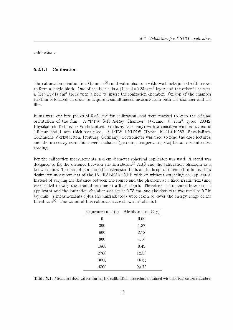
5.2. Validation for XIORT applicators
calibration.
5.2.1.1 Calibration
The calibration phantom is a Gammex R© solid water phantom with two blocks joined with screwsto form a single block. One of the blocks is a (14×14×0.25) cm3 layer and the other is thicker,a (14×14×1) cm3 block with a hole to insert the ionization chamber. On top of the chamberthe lm is located, in order to acquire a simultaneous measure from both the chamber and thelm.
Films were cut into pieces of 5×5 cm2 for calibration, and were marked to keep the originalorientation of the lm. A PTW Soft X-Ray Chamber (Volume: 0.02cm3, type: 23342,Physikalisch-Technische Werkstaetten, Freiburg, Germany) with a sensitive window radius of1.5 mm and 1 mm thick was used. A PTW UNIDOS (Type: 10001-010582, Physikalisch-Technische Werkstaetten, Freiburg, Germany) electrometer was used to read the dose lectures,and the necessary corrections were included (pressure, temperature, etc) for an absolute dosereading.
For the calibration measurements, a 4 cm diameter spherical applicator was used. A stand wasdesigned to x the distance between the Intrabeam R© XRS and the calibration phantom at aknown depth. This stand is a special construction built at the hospital intended to be used fordosimetry measurements of the INTRABEAM XRS with or without attaching an applicator.Instead of varying the distance between the source and the phantom at a xed irradiation time,we decided to vary the irradiation time at a xed depth. Therefore, the distance between theapplicator and the ionization chamber was set at 0.75 cm, and the dose rate was xed to 0.716Gy/min. 7 measurements (plus the unirradiated) were taken to cover the energy range of theIntrabeam R©. The values of this calibration are shown in table 5.1.
Exposure time (s) Absolute dose (Gy)
0 0.00
300 1.37
600 2.78
900 4.16
1800 8.49
2700 12.50
3600 16.63
4500 20.73
Table 5.1: Measured dose values during the calibration procedure obtained with the ionization chamber.
95

5. Validation of the phase space optimization process with experimental data
Figure 5.1: Left: Gammex R© solid water phantom employed in calibration measurements with theionization chamber and a EBT3 lm. Right: Experimental setup for the calibration measurements.
5.2.1.2 Experimental setup and phantom description
2D dose distributions in water
A Gammex R© phantom, specically created to measure 2D dose distributions along the applicatoraxis, was employed. It consists of two blocks made of solid water with an applicator-shaped hole.The lm is located between the two blocks and the applicator is placed in the phantom hole.This way, dose surrounding the applicator can be measured.
There are dierent types of solid water plates used in radiotherapy dosimetry, but not all materialsare water-equivalent at kilovoltage energies due to increased number of photoelectric interactions,which depends on the atomic number [Eaton and Duck, 2010]. Several authors have investigatedthe suitability of dierent materials in the kV energy range [Hermann et al., 1985, Meigooniet al., 1988, Hill et al., 2005, 2010]. In this study "Gammex" solid water was used because itseems to be the best suitable material for Intrabeam R© X-rays working energy.
Prescribed dose was set to 20 Gy at the surface, corresponding to the dose rate employed in abreast cancer treatment.
96

5.2. Validation for XIORT applicators
Figure 5.2: Gammex solid water phantoms employed in 2D dose distribution measurements.
Depth dose curves in water
Although Gammex is believed to be the best water-equivalent material for kV X-rays, in theclinic there were only a few Gammex phantoms for specic measurements. Therefore, in orderto perform dierent measurements, we were forced to use a CIRS Plastic Water R© solid waterphantom (Norfolk, VA).
To absorb possible dierences in dose due to the material type, DDPs were measured for allapplicators with this solid water material and were used as the input experimental DDP neededfor the tting process.
Ten lms were placed at dierent depths to reproduce the fall of the dose with distance.Measurements at 1, 2, 4, 6, 8, 10, 15, 20, 30 and 40 mm were taken. In gure 5.3 a viewof the setup with the location of the radiochromic lms is shown.
A comparison between the measured DDPs and the DDPs provided by Zeiss in water was doneto check the dierences of using the plastic water as reference. Figure 5.4 shows the comparisonfor all the spherical applicators of the measured DDPs described above (dots) and the DDPsprovided by Zeiss (solid lines). It can be seen that the behavior of the measured curves is verysimilar to the ones the provided by Zeiss.
97
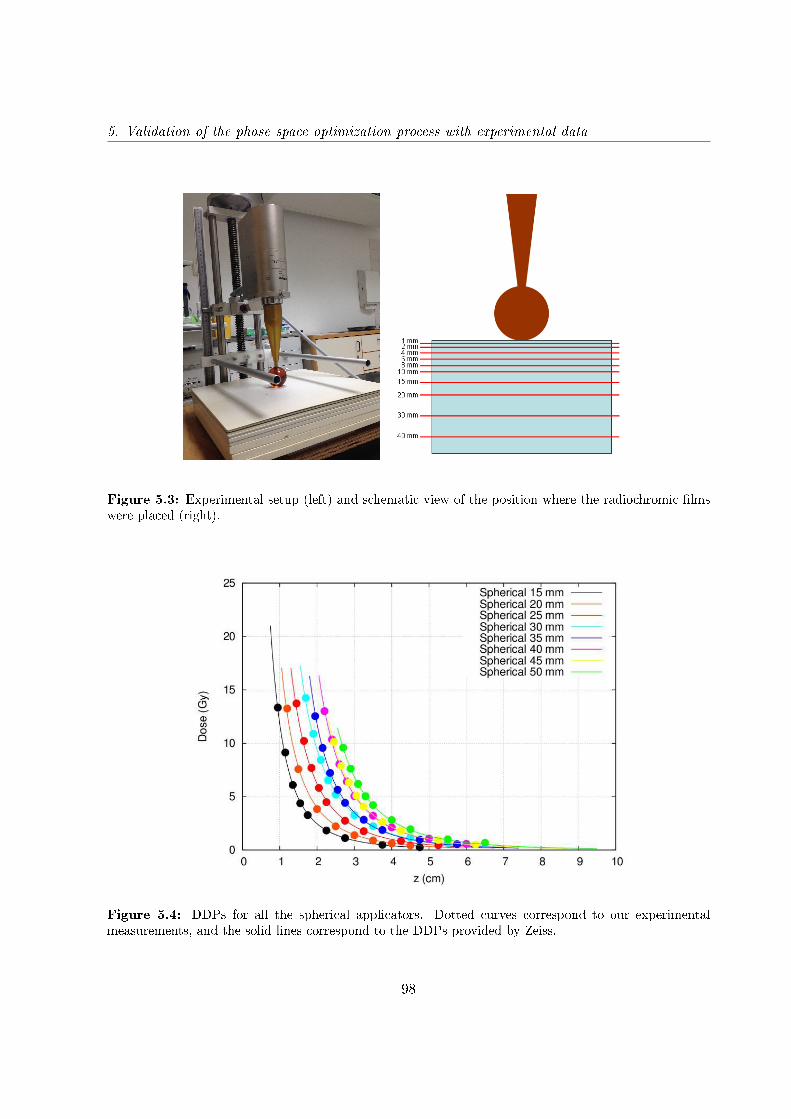
5. Validation of the phase space optimization process with experimental data
Figure 5.3: Experimental setup (left) and schematic view of the position where the radiochromic lmswere placed (right).
Figure 5.4: DDPs for all the spherical applicators. Dotted curves correspond to our experimentalmeasurements, and the solid lines correspond to the DDPs provided by Zeiss.
98
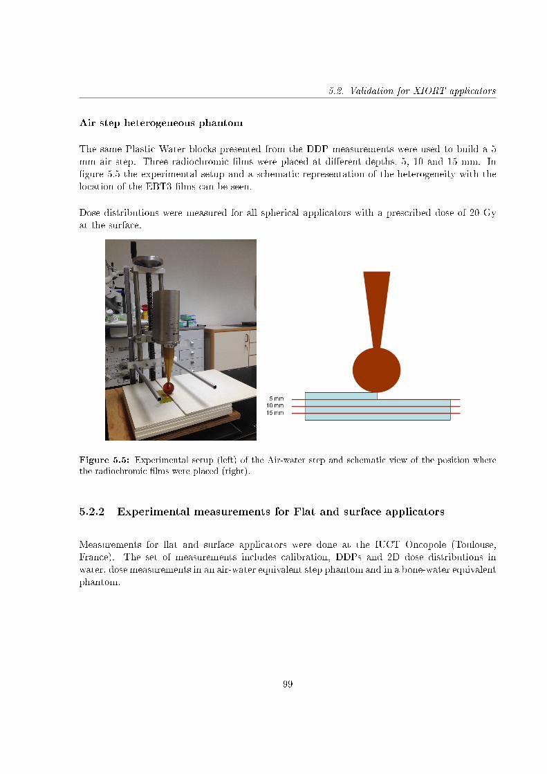
5.2. Validation for XIORT applicators
Air step heterogeneous phantom
The same Plastic Water blocks presented from the DDP measurements were used to build a 5mm air step. Three radiochromic lms were placed at dierent depths, 5, 10 and 15 mm. Ingure 5.5 the experimental setup and a schematic representation of the heterogeneity with thelocation of the EBT3 lms can be seen.
Dose distributions were measured for all spherical applicators with a prescribed dose of 20 Gyat the surface.
Figure 5.5: Experimental setup (left) of the Air-water step and schematic view of the position wherethe radiochromic lms were placed (right).
5.2.2 Experimental measurements for Flat and surface applicators
Measurements for at and surface applicators were done at the IUCT Oncopole (Toulouse,France). The set of measurements includes calibration, DDPs and 2D dose distributions inwater, dose measurements in an air-water equivalent step phantom and in a bone-water equivalentphantom.
99
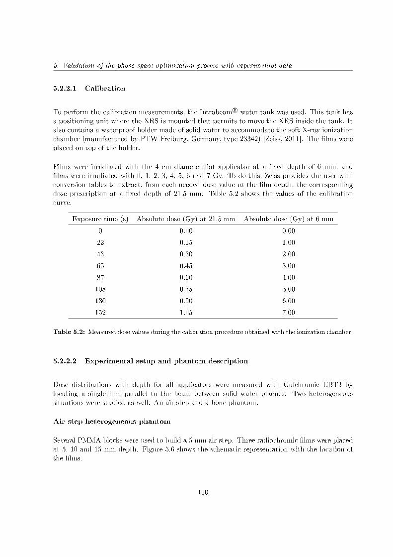
5. Validation of the phase space optimization process with experimental data
5.2.2.1 Calibration
To perform the calibration measurements, the Intrabeam R© water tank was used. This tank hasa positioning unit where the XRS is mounted that permits to move the XRS inside the tank. Italso contains a waterproof holder made of solid water to accommodate the soft X-ray ionizationchamber (manufactured by PTW Freiburg, Germany, type 23342) [Zeiss, 2011]. The lms wereplaced on top of the holder.
Films were irradiated with the 4 cm diameter at applicator at a xed depth of 6 mm, andlms were irradiated with 0, 1, 2, 3, 4, 5, 6 and 7 Gy. To do this, Zeiss provides the user withconversion tables to extract, from each needed dose value at the lm depth, the correspondingdose prescription at a xed depth of 21.5 mm. Table 5.2 shows the values of the calibrationcurve.
Exposure time (s) Absolute dose (Gy) at 21.5 mm Absolute dose (Gy) at 6 mm
0 0.00 0.00
22 0.15 1.00
43 0.30 2.00
65 0.45 3.00
87 0.60 4.00
108 0.75 5.00
130 0.90 6.00
152 1.05 7.00
Table 5.2: Measured dose values during the calibration procedure obtained with the ionization chamber.
5.2.2.2 Experimental setup and phantom description
Dose distributions with depth for all applicators were measured with Gafchromic EBT3 bylocating a single lm parallel to the beam between solid water plaques. Two heterogeneoussituations were studied as well: An air step and a bone phantom.
Air step heterogeneous phantom
Several PMMA blocks were used to build a 5 mm air step. Three radiochromic lms were placedat 5, 10 and 15 mm depth. Figure 5.6 shows the schematic representation with the location ofthe lms.
100
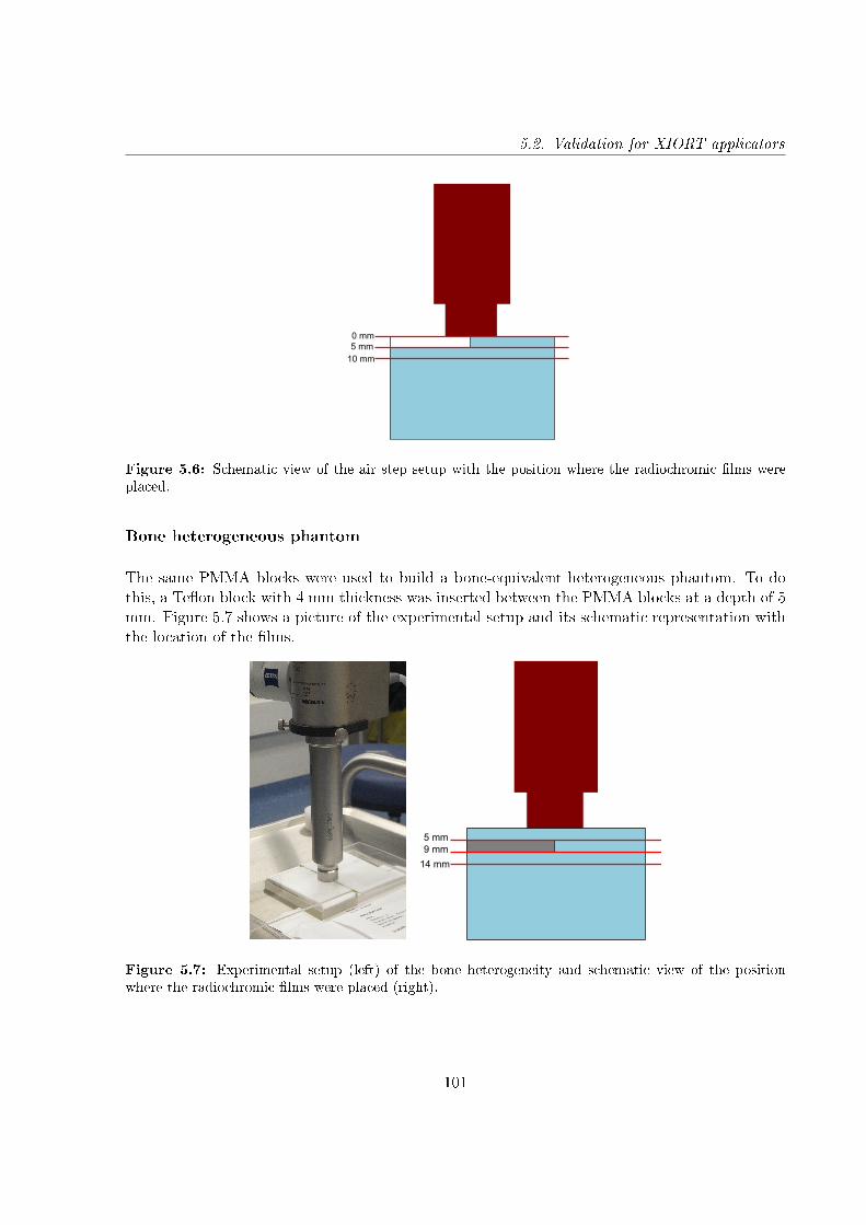
5.2. Validation for XIORT applicators
5 mm 10 mm
0 mm
Figure 5.6: Schematic view of the air step setup with the position where the radiochromic lms wereplaced.
Bone heterogeneous phantom
The same PMMA blocks were used to build a bone-equivalent heterogeneous phantom. To dothis, a Teon block with 4 mm thickness was inserted between the PMMA blocks at a depth of 5mm. Figure 5.7 shows a picture of the experimental setup and its schematic representation withthe location of the lms.
5 mm 9 mm
14 mm
Figure 5.7: Experimental setup (left) of the bone heterogeneity and schematic view of the positionwhere the radiochromic lms were placed (right).
101
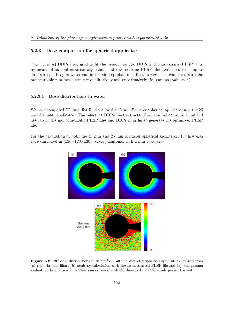
5. Validation of the phase space optimization process with experimental data
5.2.3 Dose comparison for spherical applicators
The measured DDPs were used to t the monochromatic DDPs and phase space (PHSP) lesby means of our optimization algorithm, and the resulting PHSP les were used to computedose with penEasy in water and in the air step phantom. Results were then compared with theradiochromic lm measurements qualitatively and quantitatively (ie. gamma evaluation).
5.2.3.1 Dose distributions in water
We have compared 2D dose distributions for the 40 mm diameter spherical applicator and the 25mm diameter applicator. The reference DDPs were extracted from the radiochromic lms andused to t the monochromatic PHSP les and DDPs in order to generate the optimized PHSPle.
For the calculation of both the 40 mm and 25 mm diameter spherical applicator, 109 historieswere simulated in (120×120×120) voxels phantoms, with 1 mm voxel size.
0
>1
Gamma 2%-2 mm
(a) (b)
(c)
Figure 5.8: 2D dose distributions in water for a 40 mm diameter spherical applicator obtained from(a) radiochromic lms, (b) penEasy calculation with the reconstructed PHSP le and (c), the gammaevaluation distribution for a 2%-2 mm criterion with 5% threshold. 83.82% voxels passed the test.
102
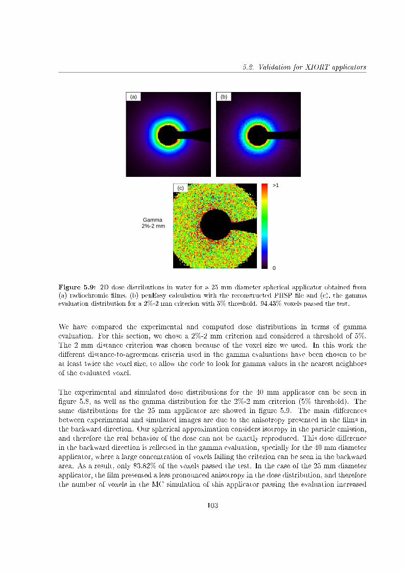
5.2. Validation for XIORT applicators
0
>1
Gamma 2%-2 mm
(a) (b)
(c)
Figure 5.9: 2D dose distributions in water for a 25 mm diameter spherical applicator obtained from(a) radiochromic lms, (b) penEasy calculation with the reconstructed PHSP le and (c), the gammaevaluation distribution for a 2%-2 mm criterion with 5% threshold. 94.43% voxels passed the test.
We have compared the experimental and computed dose distributions in terms of gammaevaluation. For this section, we chose a 2%-2 mm criterion and considered a threshold of 5%.The 2 mm distance criterion was chosen because of the voxel size we used. In this work thedierent distance-to-agreement criteria used in the gamma evaluations have been chosen to beat least twice the voxel size, to allow the code to look for gamma values in the nearest neighborsof the evaluated voxel.
The experimental and simulated dose distributions for the 40 mm applicator can be seen ingure 5.8, as well as the gamma distribution for the 2%-2 mm criterion (5% threshold). Thesame distributions for the 25 mm applicator are showed in gure 5.9. The main dierencesbetween experimental and simulated images are due to the anisotropy presented in the lms inthe backward direction. Our spherical approximation considers isotropy in the particle emission,and therefore the real behavior of the dose can not be exactly reproduced. This dose dierencein the backward direction is reected in the gamma evaluation, specially for the 40 mm diameterapplicator, where a large concentration of voxels failing the criterion can be seen in the backwardarea. As a result, only 83.82% of the voxels passed the test. In the case of the 25 mm diameterapplicator, the lm presented a less pronounced anisotropy in the dose distribution, and thereforethe number of voxels in the MC simulation of this applicator passing the evaluation increased
103
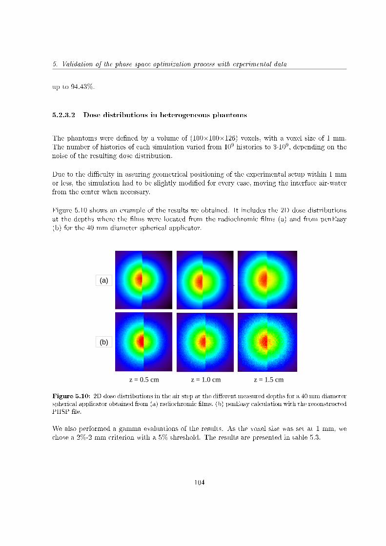
5. Validation of the phase space optimization process with experimental data
up to 94.43%.
5.2.3.2 Dose distributions in heterogeneous phantoms
The phantoms were dened by a volume of (100×100×126) voxels, with a voxel size of 1 mm.The number of histories of each simulation varied from 109 histories to 3·109, depending on thenoise of the resulting dose distribution.
Due to the diculty in assuring geometrical positioning of the experimental setup within 1 mmor less, the simulation had to be slightly modied for every case, moving the interface air-waterfrom the center when necessary.
Figure 5.10 shows an example of the results we obtained. It includes the 2D dose distributionsat the depths where the lms were located from the radiochromic lms (a) and from penEasy(b) for the 40 mm diameter spherical applicator.
(a)
(b)
z = 0.5 cm z = 1.0 cm z = 1.5 cm
Figure 5.10: 2D dose distributions in the air step at the dierent measured depths for a 40 mm diameterspherical applicator obtained from (a) radiochromic lms, (b) penEasy calculation with the reconstructedPHSP le.
We also performed a gamma evaluations of the results. As the voxel size was set at 1 mm, wechose a 2%-2 mm criterion with a 5% threshold. The results are presented in table 5.3.
104
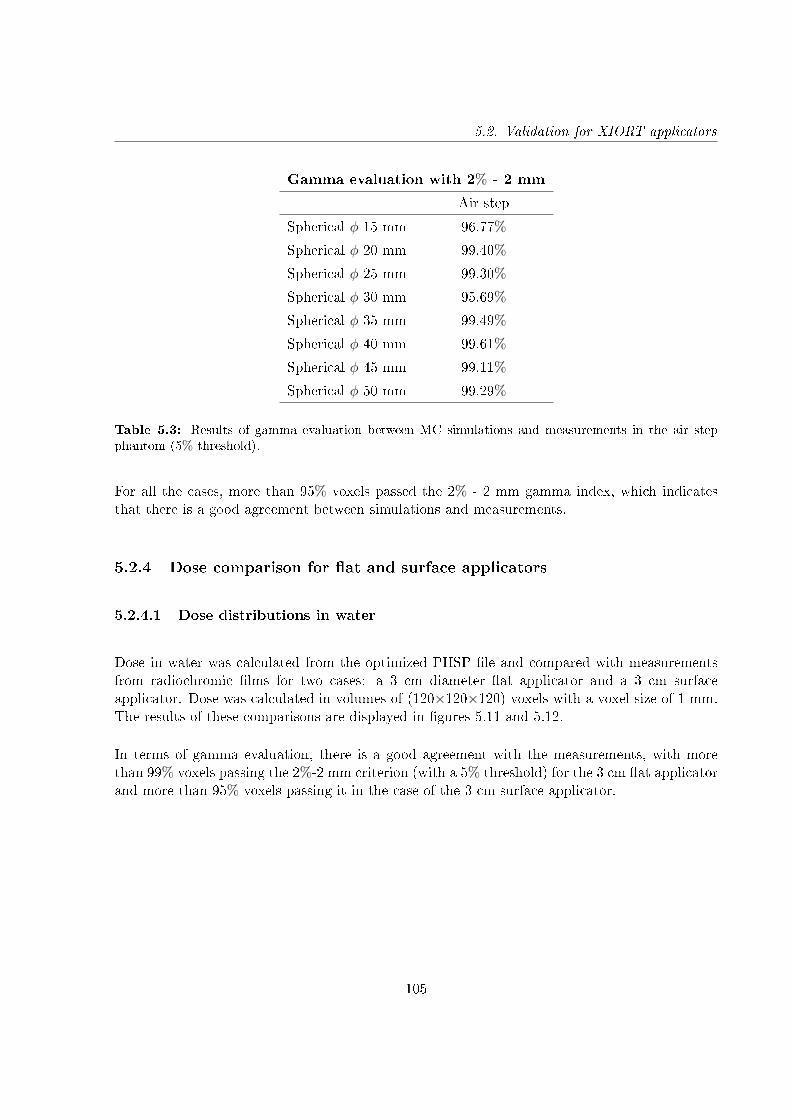
5.2. Validation for XIORT applicators
Gamma evaluation with 2% - 2 mm
Air step
Spherical φ 15 mm 96.77%
Spherical φ 20 mm 99.40%
Spherical φ 25 mm 99.30%
Spherical φ 30 mm 95.69%
Spherical φ 35 mm 99.49%
Spherical φ 40 mm 99.61%
Spherical φ 45 mm 99.11%
Spherical φ 50 mm 99.29%
Table 5.3: Results of gamma evaluation between MC simulations and measurements in the air stepphantom (5% threshold).
For all the cases, more than 95% voxels passed the 2% - 2 mm gamma index, which indicatesthat there is a good agreement between simulations and measurements.
5.2.4 Dose comparison for at and surface applicators
5.2.4.1 Dose distributions in water
Dose in water was calculated from the optimized PHSP le and compared with measurementsfrom radiochromic lms for two cases: a 3 cm diameter at applicator and a 3 cm surfaceapplicator. Dose was calculated in volumes of (120×120×120) voxels with a voxel size of 1 mm.The results of these comparisons are displayed in gures 5.11 and 5.12.
In terms of gamma evaluation, there is a good agreement with the measurements, with morethan 99% voxels passing the 2%-2 mm criterion (with a 5% threshold) for the 3 cm at applicatorand more than 95% voxels passing it in the case of the 3 cm surface applicator.
105
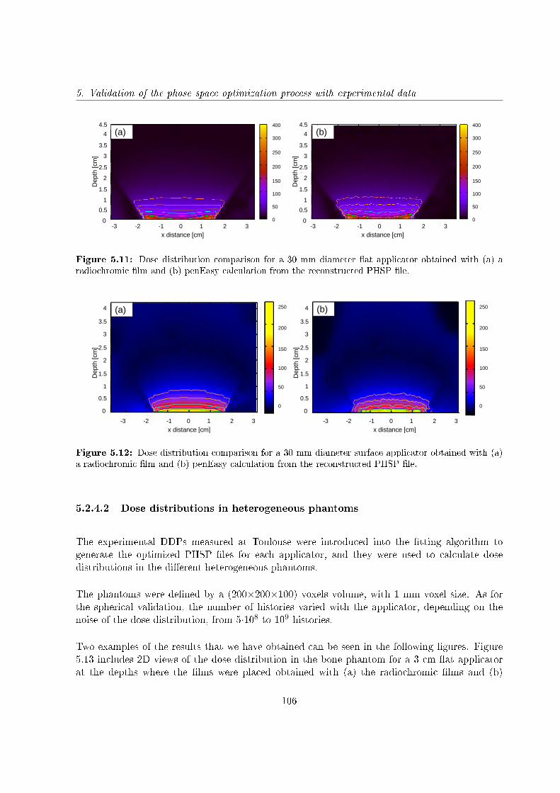
5. Validation of the phase space optimization process with experimental data
(a) (b)
-3 -2 -1 0 1 2 3-3 -2 -1 0 1 2 3
0.5
1.5
2.5
0
1
2
3
4
3.5
4.5
x distance [cm] x distance [cm]
0.5
1.5
2.5
1
2
3
4
3.5
4.5
0-3 -2 -1 0 1 2 3
0
50
100
150
200
250
300
400
0
50
100
150
200
250
300
400
Dep
th [c
m]
Dep
th [c
m]
(a) (b)
Figure 5.11: Dose distribution comparison for a 30 mm diameter at applicator obtained with (a) aradiochromic lm and (b) penEasy calculation from the reconstructed PHSP le.
0.5
1.5
2.5
0
1
2
3
4
3.5
0.5
1.5
2.5
0
1
2
3
4
3.5
Dep
th [c
m]
Dep
th [c
m]
-3 -2 -1 0 1 2 3 -3 -2 -1 0 1 2 3
x distance [cm] x distance [cm]
0
50
100
150
200
250
0
50
100
150
200
250(a) (b)
Figure 5.12: Dose distribution comparison for a 30 mm diameter surface applicator obtained with (a)a radiochromic lm and (b) penEasy calculation from the reconstructed PHSP le.
5.2.4.2 Dose distributions in heterogeneous phantoms
The experimental DDPs measured at Toulouse were introduced into the tting algorithm togenerate the optimized PHSP les for each applicator, and they were used to calculate dosedistributions in the dierent heterogeneous phantoms.
The phantoms were dened by a (200×200×100) voxels volume, with 1 mm voxel size. As forthe spherical validation, the number of histories varied with the applicator, depending on thenoise of the dose distribution, from 5·108 to 109 histories.
Two examples of the results that we have obtained can be seen in the following gures. Figure5.13 includes 2D views of the dose distribution in the bone phantom for a 3 cm at applicatorat the depths where the lms were placed obtained with (a) the radiochromic lms and (b)
106
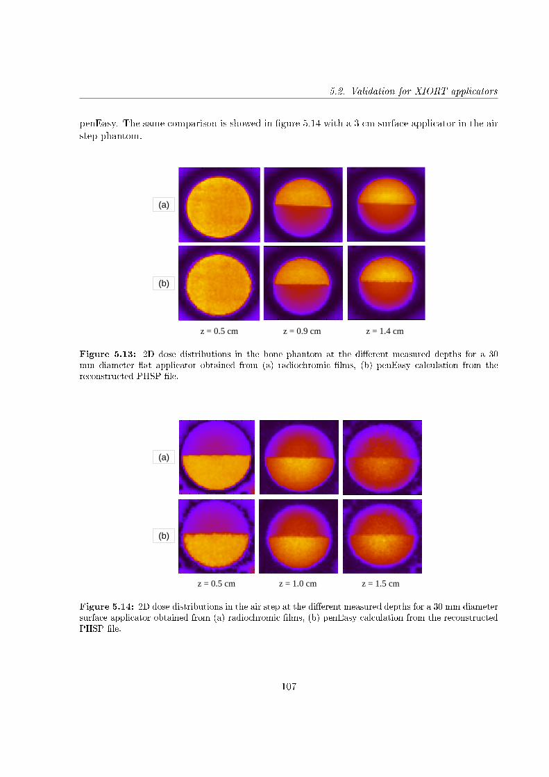
5.2. Validation for XIORT applicators
penEasy. The same comparison is showed in gure 5.14 with a 3 cm surface applicator in the airstep phantom.
(a)
(b)
z = 0.5 cm z = 0.9 cm z = 1.4 cm
Figure 5.13: 2D dose distributions in the bone phantom at the dierent measured depths for a 30mm diameter at applicator obtained from (a) radiochromic lms, (b) penEasy calculation from thereconstructed PHSP le.
(a)
(b)
z = 0.5 cm z = 1.0 cm z = 1.5 cm
Figure 5.14: 2D dose distributions in the air step at the dierent measured depths for a 30 mm diametersurface applicator obtained from (a) radiochromic lms, (b) penEasy calculation from the reconstructedPHSP le.
107
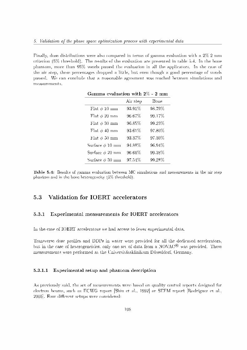
5. Validation of the phase space optimization process with experimental data
Finally, dose distributions were also compared in terms of gamma evaluation with a 2%-2 mmcriterion (5% threshold). The results of the evaluation are presented in table 5.4. In the bonephantom, more than 95% voxels passed the evaluation in all the applicators. In the case ofthe air step, these percentages dropped a little, but even though a good percentage of voxelspassed. We can conclude that a reasonable agreement was reached between simulations andmeasurements.
Gamma evaluation with 2% - 2 mm
Air step Bone
Flat φ 10 mm 93.91% 98.79%
Flat φ 20 mm 96.67% 99.17%
Flat φ 30 mm 96.85% 99.23%
Flat φ 40 mm 93.61% 97.80%
Flat φ 50 mm 93.37% 97.30%
Surface φ 10 mm 94.88% 96.94%
Surface φ 20 mm 96.66% 99.38%
Surface φ 30 mm 97.54% 99.28%
Table 5.4: Results of gamma evaluation between MC simulations and measurements in the air stepphantom and in the bone heterogeneity (5% threshold).
5.3 Validation for IOERT accelerators
5.3.1 Experimental measurements for IOERT accelerators
In the case of IOERT accelerators we had access to fewer experimental data.
Transverse dose proles and DDPs in water were provided for all the dedicated accelerators,but in the case of heterogeneities, only one set of data from a NOVAC R© was provided. Thesemeasurements were performed at the Universitätsklinikum Düsseldorf, Germany.
5.3.1.1 Experimental setup and phantom description
As previously said, the set of measurements were based on quality control reports designed forelectron beams, such as ECWG report [Shiu et al., 1992] or SEFM report [Rodríguez et al.,2005]. Four dierent setups were considered:
108
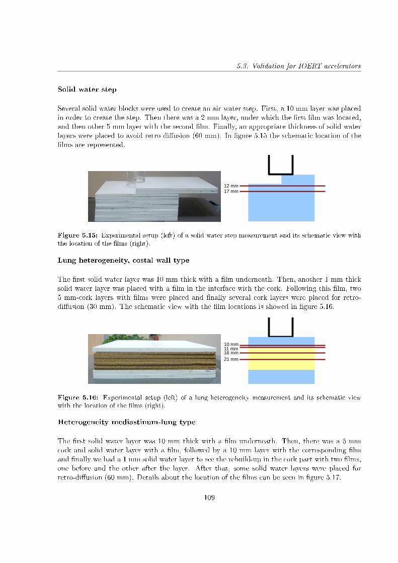
5.3. Validation for IOERT accelerators
Solid water step
Several solid water blocks were used to create an air-water step. First, a 10 mm layer was placedin order to create the step. Then there was a 2 mm layer, under which the rst lm was located,and then other 5 mm layer with the second lm. Finally, an appropriate thickness of solid waterlayers were placed to avoid retro-diusion (60 mm). In gure 5.15 the schematic location of thelms are represented.
12 mm17 mm
Figure 5.15: Experimental setup (left) of a solid water step measurement and its schematic view withthe location of the lms (right).
Lung heterogeneity, costal wall type
The rst solid water layer was 10 mm thick with a lm underneath. Then, another 1 mm thicksolid water layer was placed with a lm in the interface with the cork. Following this lm, two5 mm-cork layers with lms were placed and nally several cork layers were placed for retro-diusion (30 mm). The schematic view with the lm locations is showed in gure 5.16.
10 mm11 mm16 mm21 mm
Figure 5.16: Experimental setup (left) of a lung heterogeneity measurement and its schematic viewwith the location of the lms (right).
Heterogeneity mediastinum-lung type
The rst solid water layer was 10 mm thick with a lm underneath. Then, there was a 5 mmcork and solid water layer with a lm, followed by a 10 mm layer with the corresponding lmand nally we had a 1 mm solid water layer to see the rebuild-up in the cork part with two lms,one before and the other after the layer. After that, some solid water layers were placed forretro-diusion (60 mm). Details about the location of the lms can be seen in gure 5.17.
109
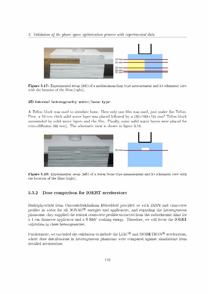
5. Validation of the phase space optimization process with experimental data
10 mm15 mm
25 mm30 mm31 mm
Figure 5.17: Experimental setup (left) of a mediastinum-lung type measurement and its schematic viewwith the location of the lms (right).
3D internal heterogeneity water/bone type
A Teon block was used to simulate bone. Here only one lm was used, just under the Teon.First, a 10 mm thick solid water layer was placed followed by a (30×160×10) mm3 Teon blocksurrounded by solid water layers and the lm. Finally, some solid water layers were placed forretro-diusion (60 mm). The schematic view is shown in gure 5.18.
20 mm
Figure 5.18: Experimental setup (left) of a water/bone type measurement and its schematic view withthe location of the lms (right).
5.3.2 Dose comparison for IOERT accelerators
Radiophysicists from Universitätsklinikum Düsseldorf provided us with DDPs and transverseproles in water for all NOVAC R© energies and applicators, and regarding the heterogeneousphantoms, they supplied the central transverse proles extracted from the radiochromic lms fora 4 cm diameter applicator and a 9 MeV working energy. Therefore, we will focus the IOERTvalidation in these heterogeneities.
Furthermore, we extended the validation to include the LIAC R© and MOBETRON R© accelerators,where dose distributions in heterogeneous phantoms were compared against simulations fromdetailed accelerators.
110
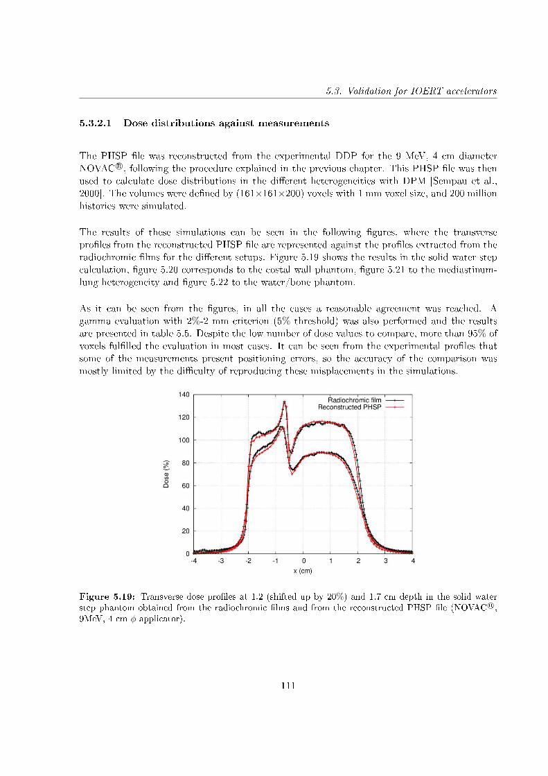
5.3. Validation for IOERT accelerators
5.3.2.1 Dose distributions against measurements
The PHSP le was reconstructed from the experimental DDP for the 9 MeV, 4 cm diameterNOVAC R©, following the procedure explained in the previous chapter. This PHSP le was thenused to calculate dose distributions in the dierent heterogeneities with DPM [Sempau et al.,2000]. The volumes were dened by (161×161×200) voxels with 1 mm voxel size, and 200 millionhistories were simulated.
The results of these simulations can be seen in the following gures, where the transverseproles from the reconstructed PHSP le are represented against the proles extracted from theradiochromic lms for the dierent setups. Figure 5.19 shows the results in the solid water stepcalculation, gure 5.20 corresponds to the costal wall phantom, gure 5.21 to the mediastinum-lung heterogeneity and gure 5.22 to the water/bone phantom.
As it can be seen from the gures, in all the cases a reasonable agreement was reached. Agamma evaluation with 2%-2 mm criterion (5% threshold) was also performed and the resultsare presented in table 5.5. Despite the low number of dose values to compare, more than 95% ofvoxels fullled the evaluation in most cases. It can be seen from the experimental proles thatsome of the measurements present positioning errors, so the accuracy of the comparison wasmostly limited by the diculty of reproducing these misplacements in the simulations.
Figure 5.19: Transverse dose proles at 1.2 (shifted up by 20%) and 1.7 cm depth in the solid waterstep phantom obtained from the radiochromic lms and from the reconstructed PHSP le (NOVAC R©,9MeV, 4 cm φ applicator).
111
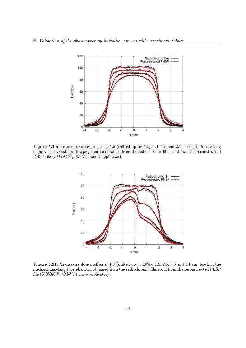
5. Validation of the phase space optimization process with experimental data
Figure 5.20: Transverse dose proles at 1.0 (shifted up by 5%), 1.1, 1.6 and 2.1 cm depth in the lungheterogeneity, costal wall type phantom obtained from the radiochromic lms and from the reconstructedPHSP le (NOVAC R©, 9MeV, 4 cm φ applicator).
Figure 5.21: Transverse dose proles at 1.0 (shifted up by 10%), 1.5, 2.5, 3.0 and 3.1 cm depth in themediastinum-lung type phantom obtained from the radiochromic lms and from the reconstructed PHSPle (NOVAC R©, 9MeV, 4 cm φ applicator).
112

5.3. Validation for IOERT accelerators
Figure 5.22: Transverse dose proles at 2.0 cm depth in the water/bone type phantom obtained fromthe radiochromic lms and from the reconstructed PHSP le (NOVAC R©, 9MeV, 4 cm φ applicator).
Gamma evaluation with 2% - 2 mm
NOVAC R©, 9 MeV, 4 cm φ
Step 96.19%
Costal wall 93.21%
Mediastinum 95.91%
Water/bone 96.92%
Table 5.5: Results of gamma evaluation between MC simulations and measurements in the dierentphantoms (5% threshold).
5.3.2.2 Dose distributions against simulations
We decided to include in the validation the LIAC R© and MOBETRON R© accelerators, but as wedid not have access to experimental data of these accelerators in heterogeneous phantoms, wecompared against simulations.
We used the detailed simulations from chapter 3 of the 6 cm diameter applicator LIAC R© and theMOBETRON R© with 9 cm diameter applicator and calculated dose distributions with a realisticenergy spectrum of 12 MeV (for the LIAC R©) and 9 MeV (for the NOVAC R©). We used the DDPsfrom these simulations as the input dose that feeds the genetic algorithm and the monochromatic
113
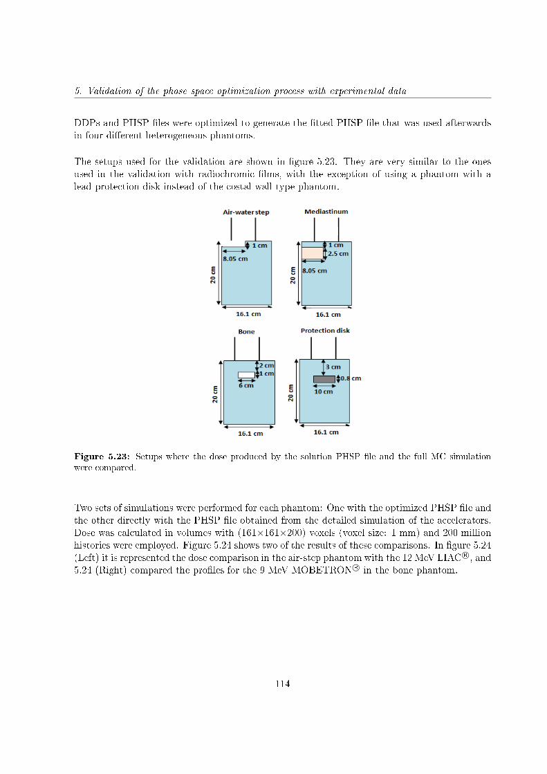
5. Validation of the phase space optimization process with experimental data
DDPs and PHSP les were optimized to generate the tted PHSP le that was used afterwardsin four dierent heterogeneous phantoms.
The setups used for the validation are shown in gure 5.23. They are very similar to the onesused in the validation with radiochromic lms, with the exception of using a phantom with alead protection disk instead of the costal wall type phantom.
Figure 5.23: Setups where the dose produced by the solution PHSP le and the full MC simulationwere compared.
Two sets of simulations were performed for each phantom: One with the optimized PHSP le andthe other directly with the PHSP le obtained from the detailed simulation of the accelerators.Dose was calculated in volumes with (161×161×200) voxels (voxel size: 1 mm) and 200 millionhistories were employed. Figure 5.24 shows two of the results of these comparisons. In gure 5.24(Left) it is represented the dose comparison in the air-step phantom with the 12 MeV LIAC R©, and5.24 (Right) compared the proles for the 9 MeV MOBETRON R© in the bone phantom.
114
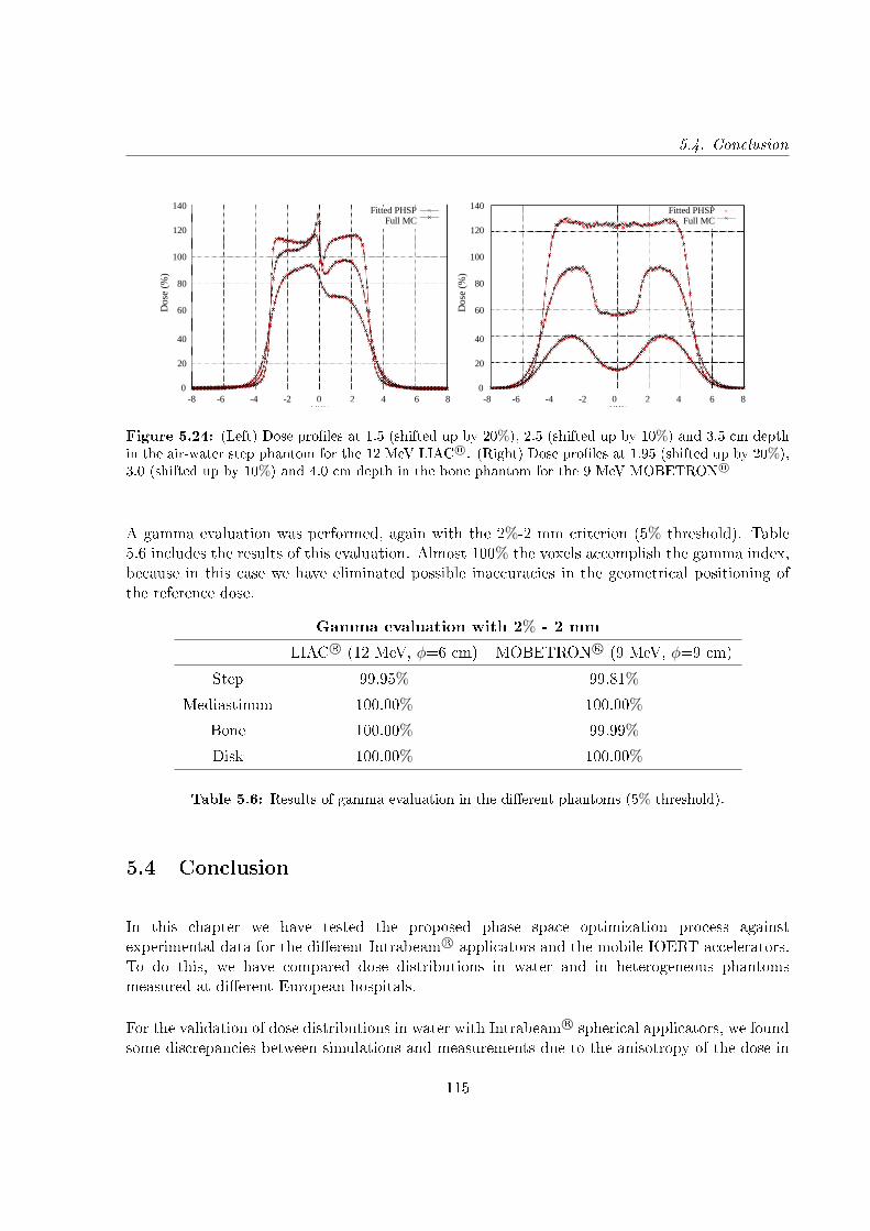
5.4. Conclusion
-8 -6 -4 -2 0 2 4 6 80
20
40
60
80
100
120
140
x (cm)
Dos
e (%
)
Fitted PHSPFull MC
-8 -6 -4 -2 0 2 4 6 80
20
40
60
80
100
120
140
x (cm)
Dos
e (%
)
Fitted PHSPFull MC
(a) (b)Figure 5.24: (Left) Dose proles at 1.5 (shifted up by 20%), 2.5 (shifted up by 10%) and 3.5 cm depthin the air-water step phantom for the 12 MeV LIAC R©. (Right) Dose proles at 1.95 (shifted up by 20%),3.0 (shifted up by 10%) and 4.0 cm depth in the bone phantom for the 9 MeV MOBETRON R©
A gamma evaluation was performed, again with the 2%-2 mm criterion (5% threshold). Table5.6 includes the results of this evaluation. Almost 100% the voxels accomplish the gamma index,because in this case we have eliminated possible inaccuracies in the geometrical positioning ofthe reference dose.
Gamma evaluation with 2% - 2 mm
LIAC R© (12 MeV, φ=6 cm) MOBETRON R© (9 MeV, φ=9 cm)
Step 99.95% 99.81%
Mediastinum 100.00% 100.00%
Bone 100.00% 99.99%
Disk 100.00% 100.00%
Table 5.6: Results of gamma evaluation in the dierent phantoms (5% threshold).
5.4 Conclusion
In this chapter we have tested the proposed phase space optimization process againstexperimental data for the dierent Intrabeam R© applicators and the mobile IOERT accelerators.To do this, we have compared dose distributions in water and in heterogeneous phantomsmeasured at dierent European hospitals.
For the validation of dose distributions in water with Intrabeam R© spherical applicators, we foundsome discrepancies between simulations and measurements due to the anisotropy of the dose in
115

5. Validation of the phase space optimization process with experimental data
the backward direction. The isotropic approach we considered for our spherical dose denitiondoes not reproduce completely the experiment. However, the area presenting the anisotropy isnext to the cone of applicator, which is an area without clinical interest, and in any case it shouldbe corrected by introducing an angular-dependent function in the X-rays beam uence, which isthe next approach we want to introduce in future work.
Regarding the dose distributions in water with Intrabeam R© at and surface applicators, wefound a good agreement for the two cases studied, with more than 95% of the voxels fulllingthe gamma criterion at the 2%-2 mm level.
In the dose comparisons inside heterogeneous phantoms, either with Intrabeam R© applicatorsor IOERT accelerators, we reached a reasonable agreement at the 2%-2 mm level, speciallyconsidering that a non-negligible contribution to the dose dierences is attributed to uncertaintiesin the measurements, such as asymmetries or displacements of the lms. When theseuncertainties disappear, the agreement increases substantially, something that has been seenin the validation of IOERT accelerators against simulations, where almost a 100% of the voxelspassed the 2%-2 mm level in all the phantoms.
Therefore, in view of the results of this chapter, we can conclude that the proposed optimizationmethod works accurately reproducing dose distributions in clinical situations. In fact, it hasalready been implemented for the tuning of the dierent IOERT and Intrabeam R© devices inradiance R© [Valdivieso-Casique et al., 2015, Pascau et al., 2012], the rst treatment planningsystem for intraoperative radiotherapy.
116
Chapter 6
Hybrid Monte Carlo for dose
calculation
6.1 Introduction
The use of intraoperative radiotherapy with low energy X-rays is increasing rapidly in the clinicaleld, as has been previously explained in this thesis.
However, this technique is currently limited by the inherent diculties associated with theplanning process and until recently there was no commercial tool for 3D planning of theIntrabeam R© system (Carl Zeiss Surgical Gmbh, Oberkochen, Germany) that allowed a fastan accurate dose deposition inside the patient. The commercial planning tool that users gotwith the device was based in isodose curves in water. Even if this procedure works correctlyin homogeneous tissues, inaccuracies appear when heterogeneous media are treated. In October2016 the companies Carl Zeiss and GMV signed a commercial collaboration agreement, and eversince every Intrabeam R© machine is being sold with the radiance R© treatment planning system(TPS), thus incorporating the TPS codes described in this thesis, fully taking into accountpatient's anatomy.
Detailed Monte Carlo simulations of miniature 50 keV accelerators have been performed in thepast. Simulations of a radiosurgery X-ray tube used to treat brain tumors were done [Yanchand Harte, 1996] with ITS 3.0 code. A Geant4/GATE code suitable to Intrabeam R© treatmentissues [Bouzid et al., 2015] was also developed, and the Intrabeam R© source was modeled withthe EGSnrc code [Ebert and Carruthers, 2003].
A high level of accuracy is reached with full Monte Carlo simulations, however it is still a time-
117
6. Hybrid Monte Carlo for dose calculation
consuming technique and it is not suitable to real-time planning in operating room.
The use of phase space (PHSP) les, as we have discussed previously, reduces the overallcomputation time because the radiotherapy device and applicators do not need to be simulatedfor every treatment. Therefore, in order to speed up dose calculation, Clausen et al. developeda Geant4-based source model using PHSP les and decreased computation time to 12 minutesfor a full gynecological treatment [Clausen et al., 2012]. However, the proposed technique wastested only for water dose calculations and simulation time would increase when applied to morecomplex geometries with heterogeneities. Moreover, PHSP les could have some disadvantageslike lack of exibility in manipulating the data, huge storage requirement and resources forreading-in the stored data during simulation.
Alternatively, Nwankwo et al. approximated PHSP les by a virtual source model to generatephotons for a specic Intrabeam R© source dened in Geant4 and a reasonable calculationuncertainty was achieved within 2 hours of simulation [Nwankwo et al., 2013]. Nevertheless,dose computation time is still too long for operating room irradiations or to be implemented in acommercial treatment planning system, and the proposed methods are not prepared for tuningeasily every actual X-ray source.
In chapter 4 the procedure to generate an optimized PHSP le tuned to a given Intrabeam R©
device, using as input just experimental DDP in water has been described. The accuracy of thismethod has been validated in chapter 5. In the case of IOERT, the DPM code [Sempau et al.,2000] gives an accurate deposited dose in a short time. However, we found that DPM would notbe an ecient and fast solution to describe photon interactions in the energy range from 1 to 50keV.
We thus decided to develop from scratch a new algorithm, named hybrid Monte Carlo(HMC), to calculate dose deposited by the Intrabeam R© device within minutes, fully takinginto account the dierent tissues and structures in the region of patient, i.e. as derived from aCT image.
HMC computes an accurate dose for both homogeneous and heterogeneous media [Vidal et al.,2014b,a, Udías et al., 2017b], as it incorporates all the relevant physics processes at Intrabeam R©
working energies. The savings in calculation time are possible thanks to taking to the extremesome variance reduction techniques. The HMC algorithm has been complemented with PHSPles generated for the needle, spherical, at and surface applicators.
To face the problem of fast dose calculation, lets rst analyze the specics of the radiotherapysituation we are dealing with, and of the MC simulations in general.
118

6.2. MC simulations
6.2 MC simulations
MC packages assume a stochastic approach to generate particles and to decide the fate ofthese radiation particles. Probability distributions of the dierent processes are taken fromcomputations, tables, etc. The particles are generated in random positions and emitted atrandom directions (following the known distributions) from the primary source in the simulateddevice. They are tracked by the code, and interaction and evolution of the particles are computed,stochastically, based upon assumed probabilities for dierent processes (Compton interactions,Rayleigh interactions, photoelectric eect, etc.) to happen.
The random nature of the variables dening every particle we generate introduces a statisticalnoise, due to the limited amount of particles (histories) we deal with in any actual simulation. Ingure 6.1 it is showed a representation of a pure random sampling in a XY plane. If the numberof points is very big, the sampling becomes homogeneous, but is the number of points is not bigenough, areas with high concentration of points are visible, as well as empty spaces in between,introducing statistical noise.
Figure 6.1: Randomly generated coordinates populating a XY plane.
The statistical noise of MC simulations bears no interest in radiotherapy (it is, however, veryimportant to keep it close to the actual statistical level of the real images, when simulatingmedical imaging devices), as the actual number of particles involved in any radiotherapytreatment, even in regions of low dose (say 5% of the dose at the maximum) is well in excessof 1012, for any realistic treatment. With this in mind, we have taken the idea of condensationof histories to compute the dose not from the number of histories reaching a region, but ratherfrom the relative change of weights of these histories when traveling through this region. We willdescribe the algorithm in detail in what follows.
119
6. Hybrid Monte Carlo for dose calculation
6.3 Code description
In the energy region, and with the geometry of the Intrabeam R© device, particle interactionsare not distributed very uniformly. Particularly for small applicators (the needle case being theextreme), depth dose proles show a very fast reduction of dose with the distance to the source,in part due to the solid angle eects, but also due to absorption of photons via photoelectriceect. Indeed, after traveling a couple of cm in water, in a typical MC calculation, most of thehistories we have produced at the source, and that are being tracked so expensively, will havedisappeared and will not contribute to statistical accuracy.
In a traditional MC, to keep a large number of histories in regions away from the source, wewould have to produce a very large number of histories at the source. The result would be anoversampling closer to the source, that is, we will have the best precision where we do not needit, and we would spend a lot of time in those regions that already have good precision, in orderto improve precision away from the source. The same happens when we include shieldings inthe simulation, if we want to obtain accurate readings of the dose after the protection, we mustsend many histories to the shield, most of which will die without contributing to the result inthe region we are interested.
Of course, there are several ways to improve the eciency of MC simulations under thesecircumstances, such as factorizing the problem in dierent regions, using particle splitting whenthe particles reach the region of interest or stop tracking the particles when the uence is belowa certain threshold. In our tool, we generalized this idea, without the need to adapt it todierent tissues or to enable a dierent detail of simulation when uences fall below a certainthreshold.
Summarizing what we have just said, a regular Monte Carlo will calculate millions of histories,even if they would barely interact or leave energy in the medium, increasing signicantly thesimulation time. Furthermore, small size, low energy photon sources present very high uencegradients, which implies high statistics next to the applicator, but very low statistics when thedistance to the source increases. Therefore, obtaining an accurate dose distribution with smallstatistical noise will require very long simulations. We want to improve this situation.
The algorithm we have developed, called Hybrid MC algorithm, or HMC algorithm,will include all the relevant physics of a Monte Carlo algorithm minimizing the contributionof statistical noise. The HMC algorithm takes into consideration photoelectric and Comptoninteractions. Rayleigh interactions are not included because they are not a relevant mechanismfor energy deposition at the energies considered here.
Condensed histories and particle splitting approximations will be generalized in this algorithm.We will use meta-histories (m-histories for short) to represent particles, each one of themrepresenting the fate of an arbitrary high number of photons N. Every m-history carries a
120
6.3. Code description
weight when it is generated at the source, proportional to the number of photons that shouldbe generated with the given characteristics (energy, position, emission angle). The probabilityof interaction of this m-history, either by photoelectric (PPE) or Compton eect (PCE), will becomputed in a continuum way as 1-e−µdx, where dx is the spatial displacement in the directionof the m-history since the last update and µ is the attenuation coecient for the photoelectricor the Compton eects, taken from the material tables of PENELOPE [Salvat et al., 1996], atthe spatial point where the updates of m-history position is being done. More information aboutthe material tables generation can be found in the appendix A.
In other words, instead of studying microscopically each interaction, which has a highcomputational cost, we will condensate many possible interactions into a single one with anaccumulated probability which will be the sum of all individual interactions. We will scorethe accumulated probability of interaction after moving a given step size. After each step,the new weights for the m-history will be computed, taking into account the lost weight byphotoelectric and Compton interactions. Moreover, new m-histories, corresponding to secondaryphotons coming from Compton interactions, can be generated with the corresponding weight,and stacked in the pile for calculating them in the same way as primary photons.
Thus, condensed histories (m-histories) of the photons at the source are generated from theinformation stored in the PHSP les, and transported throughout the volume in steps of xedlength dx, whose value is typically smaller than half the voxel size. At each step, a fraction of them-history will interact, being absorbed by photoelectric eect or being scattered by Comptoneect. Each condensed history updates its weight as it travels through matter, according to theweight lost until the moment.
This way, the number of m-histories remains constant along the volume, being only its weightreduced at each interaction, so that the number of m-histories does not decrease far from thesource due to photon absorption. Dose is computed not from the number of interactions or thenumber of photons who are absorbed in a region, but rather from the accumulated reduction ofthe weight of the m-histories as they travel through the region. Therefore, problems associatedwith low statistics are reduced, as we have always the same number of primary virtual histories, nomatter how much attenuation the material oers. Due to the fact that we follow in a detailed waythe trajectory of all m-histories and that we produce also secondary m-histories, our simulationwill be able to reproduce all the relevant phenomena related to interaction of radiation in mediasuch as backscatter, build-up or diraction.
Consequently, the following aspects are included in the simulation:
• The m-histories approximation. Every primary m-history represents the fate of manyphotons. The m-history can scatter or undergo photoelectric eect, with a given probability,and the weight of the m-history is shared among the dierent secondary particles that thism-history can produce. Weights are updated after each spatial time progression.• Photoelectric forced interaction. After each simulation step, a fraction of the energy of
121
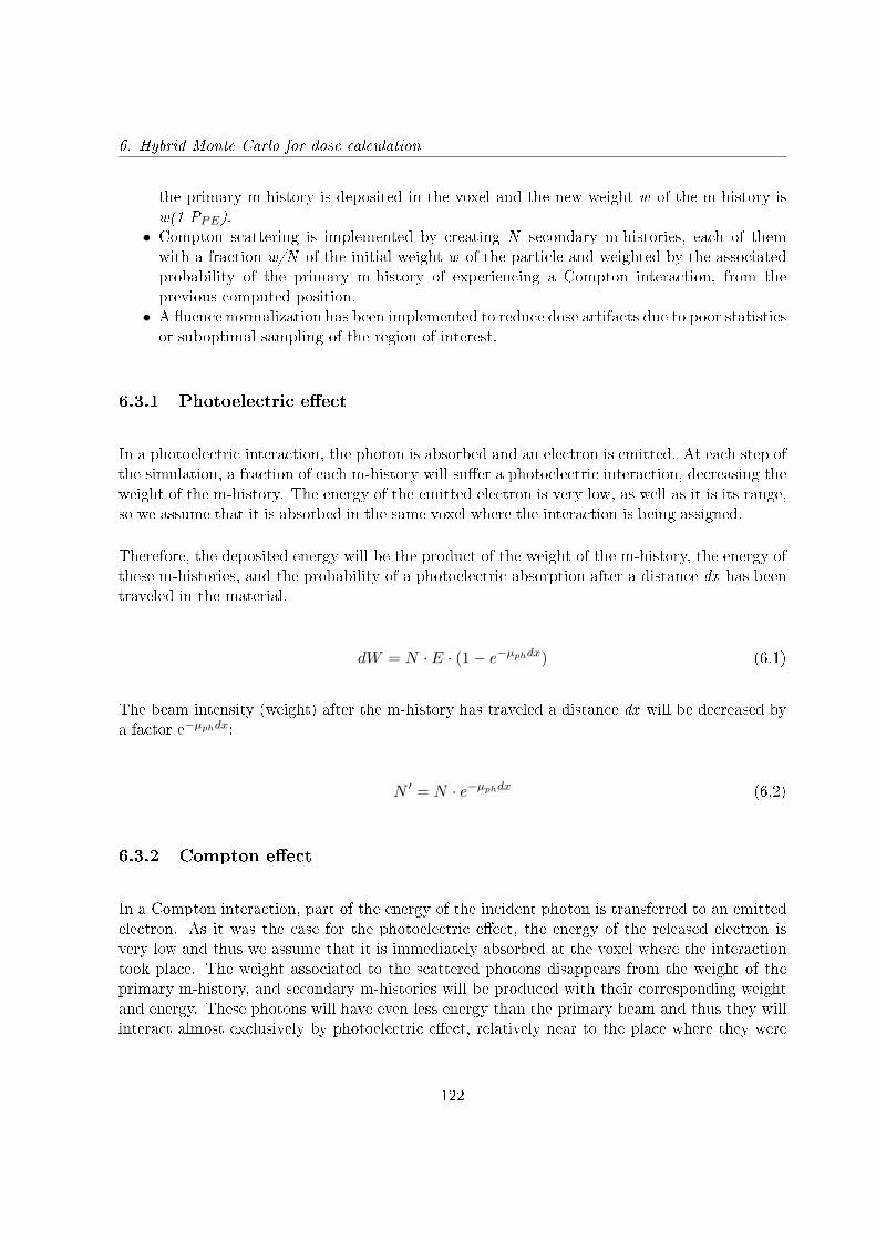
6. Hybrid Monte Carlo for dose calculation
the primary m-history is deposited in the voxel and the new weight w of the m-history isw(1-PPE).• Compton scattering is implemented by creating N secondary m-histories, each of themwith a fraction w/N of the initial weight w of the particle and weighted by the associatedprobability of the primary m-history of experiencing a Compton interaction, from theprevious computed position.• A uence normalization has been implemented to reduce dose artifacts due to poor statisticsor suboptimal sampling of the region of interest.
6.3.1 Photoelectric eect
In a photoelectric interaction, the photon is absorbed and an electron is emitted. At each step ofthe simulation, a fraction of each m-history will suer a photoelectric interaction, decreasing theweight of the m-history. The energy of the emitted electron is very low, as well as it is its range,so we assume that it is absorbed in the same voxel where the interaction is being assigned.
Therefore, the deposited energy will be the product of the weight of the m-history, the energy ofthese m-histories, and the probability of a photoelectric absorption after a distance dx has beentraveled in the material.
dW = N · E · (1− e−µphdx) (6.1)
The beam intensity (weight) after the m-history has traveled a distance dx will be decreased bya factor e−µphdx:
N ′ = N · e−µphdx (6.2)
6.3.2 Compton eect
In a Compton interaction, part of the energy of the incident photon is transferred to an emittedelectron. As it was the case for the photoelectric eect, the energy of the released electron isvery low and thus we assume that it is immediately absorbed at the voxel where the interactiontook place. The weight associated to the scattered photons disappears from the weight of theprimary m-history, and secondary m-histories will be produced with their corresponding weightand energy. These photons will have even less energy than the primary beam and thus they willinteract almost exclusively by photoelectric eect, relatively near to the place where they were
122
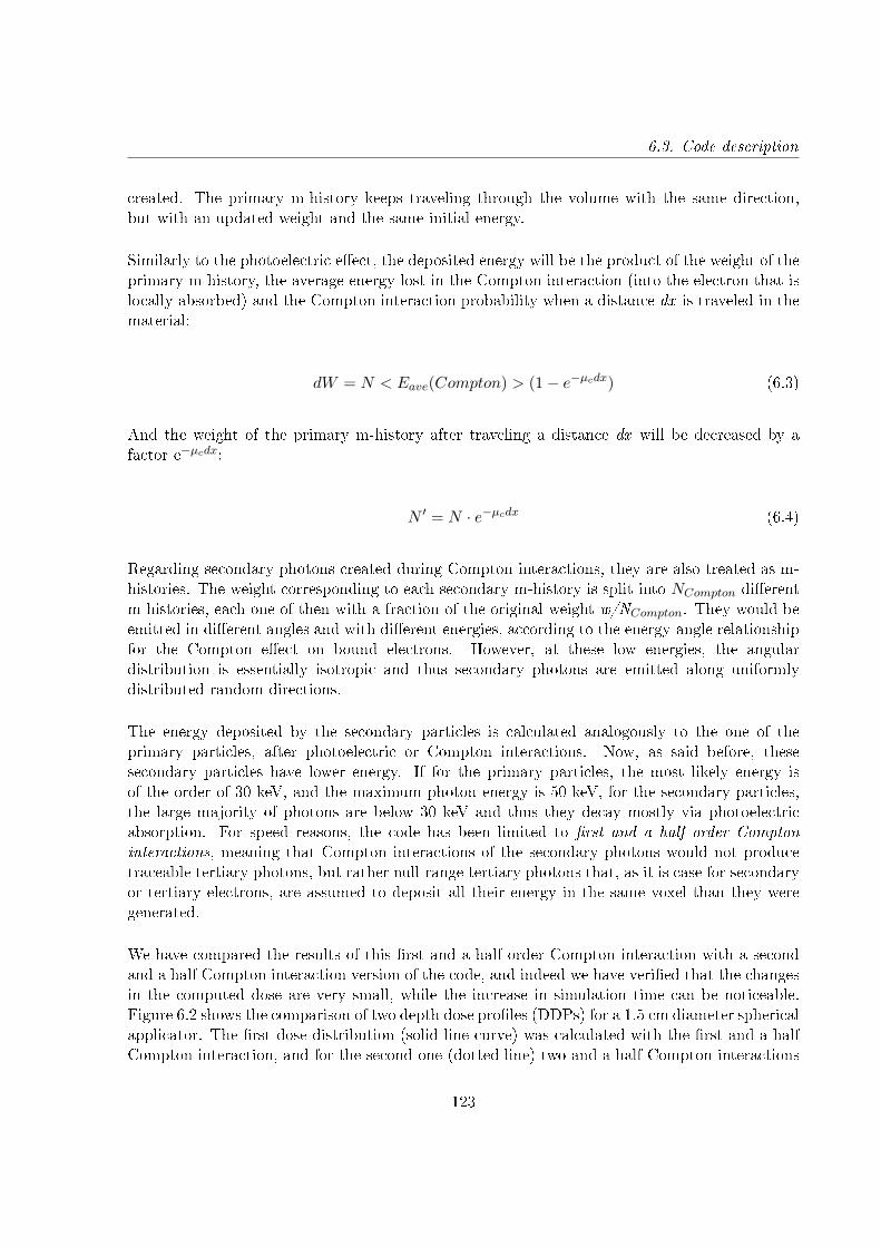
6.3. Code description
created. The primary m-history keeps traveling through the volume with the same direction,but with an updated weight and the same initial energy.
Similarly to the photoelectric eect, the deposited energy will be the product of the weight of theprimary m-history, the average energy lost in the Compton interaction (into the electron that islocally absorbed) and the Compton interaction probability when a distance dx is traveled in thematerial:
dW = N < Eave(Compton) > (1− e−µcdx) (6.3)
And the weight of the primary m-history after traveling a distance dx will be decreased by afactor e−µcdx:
N ′ = N · e−µcdx (6.4)
Regarding secondary photons created during Compton interactions, they are also treated as m-histories. The weight corresponding to each secondary m-history is split into NCompton dierentm-histories, each one of then with a fraction of the original weight w/NCompton. They would beemitted in dierent angles and with dierent energies, according to the energy-angle relationshipfor the Compton eect on bound electrons. However, at these low energies, the angulardistribution is essentially isotropic and thus secondary photons are emitted along uniformlydistributed random directions.
The energy deposited by the secondary particles is calculated analogously to the one of theprimary particles, after photoelectric or Compton interactions. Now, as said before, thesesecondary particles have lower energy. If for the primary particles, the most likely energy isof the order of 30 keV, and the maximum photon energy is 50 keV, for the secondary particles,the large majority of photons are below 30 keV and thus they decay mostly via photoelectricabsorption. For speed reasons, the code has been limited to rst and a half order Comptoninteractions, meaning that Compton interactions of the secondary photons would not producetraceable tertiary photons, but rather null-range tertiary photons that, as it is case for secondaryor tertiary electrons, are assumed to deposit all their energy in the same voxel than they weregenerated.
We have compared the results of this rst and a half order Compton interaction with a secondand a half Compton interaction version of the code, and indeed we have veried that the changesin the computed dose are very small, while the increase in simulation time can be noticeable.Figure 6.2 shows the comparison of two depth dose proles (DDPs) for a 1.5 cm diameter sphericalapplicator. The rst dose distribution (solid line curve) was calculated with the rst and a halfCompton interaction, and for the second one (dotted line) two and a half Compton interactions
123
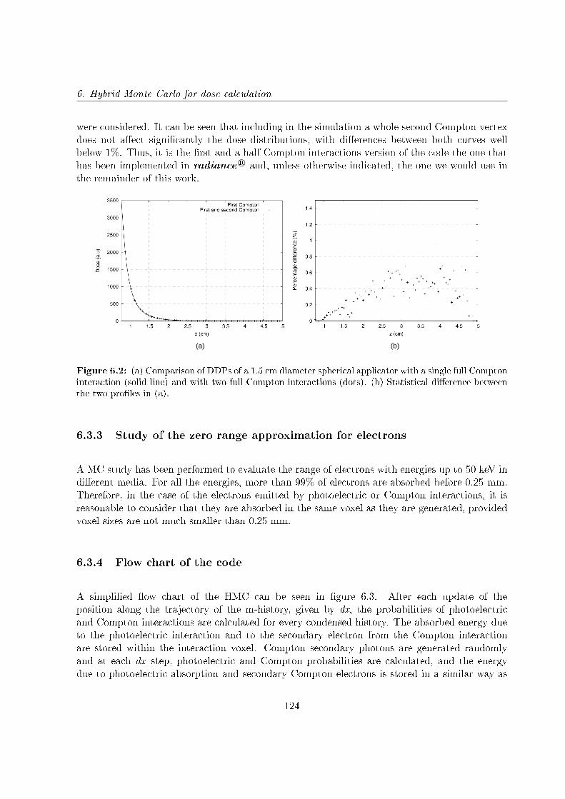
6. Hybrid Monte Carlo for dose calculation
were considered. It can be seen that including in the simulation a whole second Compton vertexdoes not aect signicantly the dose distributions, with dierences between both curves wellbelow 1%. Thus, it is the rst and a half Compton interactions version of the code the one thathas been implemented in radiance R© and, unless otherwise indicated, the one we would use inthe remainder of this work.
(a) (b)
Figure 6.2: (a) Comparison of DDPs of a 1.5 cm diameter spherical applicator with a single full Comptoninteraction (solid line) and with two full Compton interactions (dots). (b) Statistical dierence betweenthe two proles in (a).
6.3.3 Study of the zero range approximation for electrons
A MC study has been performed to evaluate the range of electrons with energies up to 50 keV indierent media. For all the energies, more than 99% of electrons are absorbed before 0.25 mm.Therefore, in the case of the electrons emitted by photoelectric or Compton interactions, it isreasonable to consider that they are absorbed in the same voxel as they are generated, providedvoxel sizes are not much smaller than 0.25 mm.
6.3.4 Flow chart of the code
A simplied ow chart of the HMC can be seen in gure 6.3. After each update of theposition along the trajectory of the m-history, given by dx, the probabilities of photoelectricand Compton interactions are calculated for every condensed history. The absorbed energy dueto the photoelectric interaction and to the secondary electron from the Compton interactionare stored within the interaction voxel. Compton secondary photons are generated randomlyand at each dx step, photoelectric and Compton probabilities are calculated, and the energydue to photoelectric absorption and secondary Compton electrons is stored in a similar way as
124
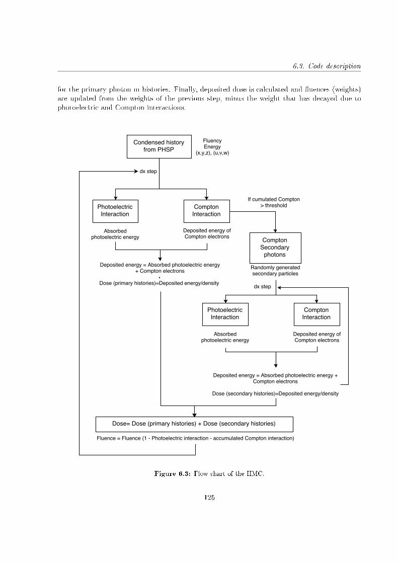
6.3. Code description
for the primary photon m-histories. Finally, deposited dose is calculated and uences (weights)are updated from the weights of the previous step, minus the weight that has decayed due tophotoelectric and Compton interactions.
Figure 6.3: Flow chart of the HMC.
125

6. Hybrid Monte Carlo for dose calculation
6.4 Dose normalization
The use of m-histories, each one of them representing a high number of photons, and the factthat these primary histories never die away, only their weight gets reduced, makes possible alarge reduction of the statistic noise, for the same number of primary particles, when comparingto a pure MC calculation. Statistical noise comes now almost exclusively from the fact that thenumber of secondary photons is nite and that the emission angles are random.
If the number of primary m-histories is not big enough, ray patterns may appear in the doseimage. This is due to, on the one hand, the stochastical procedure that is used to pick historiesinside the PHSP le. If only few histories are chosen, the initial angular distribution may not bejust homogeneous enough. And as typically seen in pure random sampling (see gure 6.1 withthe XY points where one can see clusters and empty spaces), it is likely that two m-historiesare produced very close to each other, thus producing a high-intensity ray-like artifact, whilethere are angular ranges left without any m-history, producing a low-intensity ray-like artifact.On the other hand, artifacts in dose computation may also appear due to the use of voxelizedgeometries and the subsequent subsampling leading to aliasing artifacts, more apparent if a verylow number of m-histories is used. The trajectories of the m-histories have dierent inclinationswithin a nite number of angles in the PHSP le. The angle of the history with respect to theorientation of the Cartesian grid has an impact in the path length of the history inside a givenvoxel. This makes that dierent voxels present an apparent higher number of interactions thanothers, even if they are at the same distance to the source.
In standard MC codes these patters are not appreciated, because the step taken to updateparticle position, their emission angles, and the resulting angles after interactions are purelystochastic. Statistical noise is clearly present in standard MC, and thus no ray-like patterns arevisible.
Figure 6.4 shows a comparison of dose distributions for a 40 mm spherical applicator withpenEasy and HMC using dierent number of (m-)histories. When using HMC, we can see thatthe streak or radial artifact decreases with the number of histories. When using penEasy, nopatterns are appreciated, but the dose is very noisy, even when 5 million histories are used (Figure6.4 (b)).
In order to solve this problem, a uence normalization for the primary histories has beenincorporated in the code. As m-histories never die inside the region considered, it is possible toknow the number of m-histories that have traveled through every voxel of the volume, and howmany interactions have taken place in each voxel. And this is independent on the materials theregion is made of. Dierent materials, thus dierent absorptions, would only aect the weights,but not the uence of the number of m-histories. Therefore, for a given source, the number ofm-histories in a region is identical if the region is made out of water or if it has heterogeneities.This means that this number of m-histories, and moreover, the number of interactions of these
126
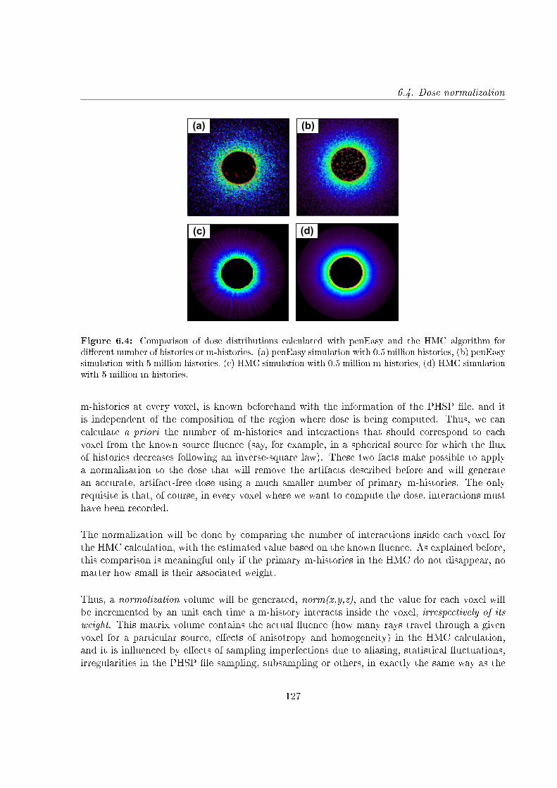
6.4. Dose normalization
(a) (b)
(c) (d)
Figure 6.4: Comparison of dose distributions calculated with penEasy and the HMC algorithm fordierent number of histories or m-histories. (a) penEasy simulation with 0.5 million histories, (b) penEasysimulation with 5 million histories, (c) HMC simulation with 0.5 million m-histories, (d) HMC simulationwith 5 million m-histories.
m-histories at every voxel, is known beforehand with the information of the PHSP le, and itis independent of the composition of the region where dose is being computed. Thus, we cancalculate a priori the number of m-histories and interactions that should correspond to eachvoxel from the known source uence (say, for example, in a spherical source for which the uxof histories decreases following an inverse-square law). These two facts make possible to applya normalization to the dose that will remove the artifacts described before and will generatean accurate, artifact-free dose using a much smaller number of primary m-histories. The onlyrequisite is that, of course, in every voxel where we want to compute the dose, interactions musthave been recorded.
The normalization will be done by comparing the number of interactions inside each voxel forthe HMC calculation, with the estimated value based on the known uence. As explained before,this comparison is meaningful only if the primary m-histories in the HMC do not disappear, nomatter how small is their associated weight.
Thus, a normalization volume will be generated, norm(x,y,z), and the value for each voxel willbe incremented by an unit each time a m-history interacts inside the voxel, irrespectively of itsweight. This matrix volume contains the actual uence (how many rays travel through a givenvoxel for a particular source, eects of anisotropy and homogeneity) in the HMC calculation,and it is inuenced by eects of sampling imperfections due to aliasing, statistical uctuations,irregularities in the PHSP le sampling, subsampling or others, in exactly the same way as the
127
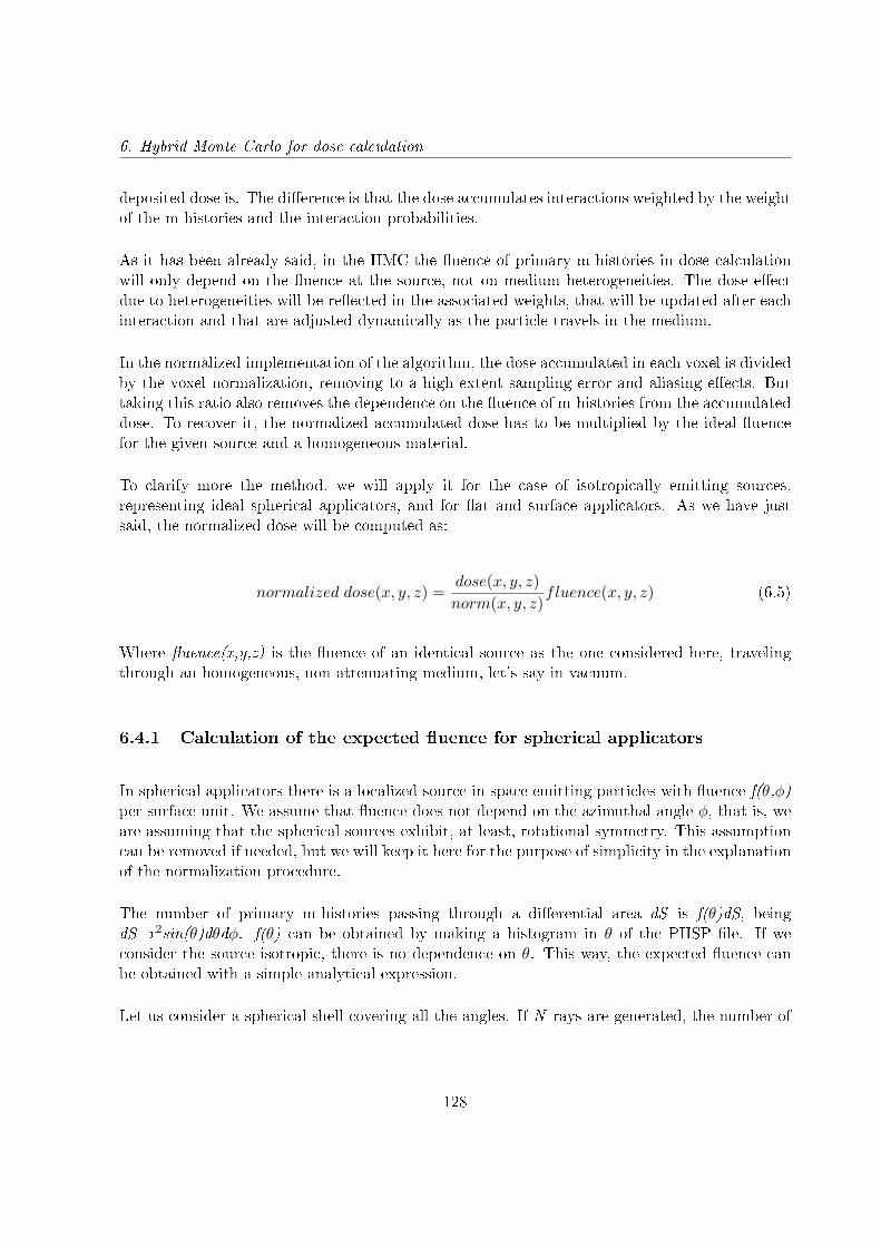
6. Hybrid Monte Carlo for dose calculation
deposited dose is. The dierence is that the dose accumulates interactions weighted by the weightof the m-histories and the interaction probabilities.
As it has been already said, in the HMC the uence of primary m-histories in dose calculationwill only depend on the uence at the source, not on medium heterogeneities. The dose eectdue to heterogeneities will be reected in the associated weights, that will be updated after eachinteraction and that are adjusted dynamically as the particle travels in the medium.
In the normalized implementation of the algorithm, the dose accumulated in each voxel is dividedby the voxel normalization, removing to a high extent sampling error and aliasing eects. Buttaking this ratio also removes the dependence on the uence of m-histories from the accumulateddose. To recover it, the normalized accumulated dose has to be multiplied by the ideal uencefor the given source and a homogeneous material.
To clarify more the method, we will apply it for the case of isotropically emitting sources,representing ideal spherical applicators, and for at and surface applicators. As we have justsaid, the normalized dose will be computed as:
normalized dose(x, y, z) =dose(x, y, z)norm(x, y, z)
fluence(x, y, z) (6.5)
Where uence(x,y,z) is the uence of an identical source as the one considered here, travelingthrough an homogeneous, non attenuating medium, let's say in vacuum.
6.4.1 Calculation of the expected uence for spherical applicators
In spherical applicators there is a localized source in space emitting particles with uence f(θ,φ)per surface unit. We assume that uence does not depend on the azimuthal angle φ, that is, weare assuming that the spherical sources exhibit, at least, rotational symmetry. This assumptioncan be removed if needed, but we will keep it here for the purpose of simplicity in the explanationof the normalization procedure.
The number of primary m-histories passing through a dierential area dS is f(θ)dS, beingdS=r2sin(θ)dθdφ. f(θ) can be obtained by making a histogram in θ of the PHSP le. If weconsider the source isotropic, there is no dependence on θ. This way, the expected uence canbe obtained with a simple analytical expression.
Let us consider a spherical shell covering all the angles. If N rays are generated, the number of
128
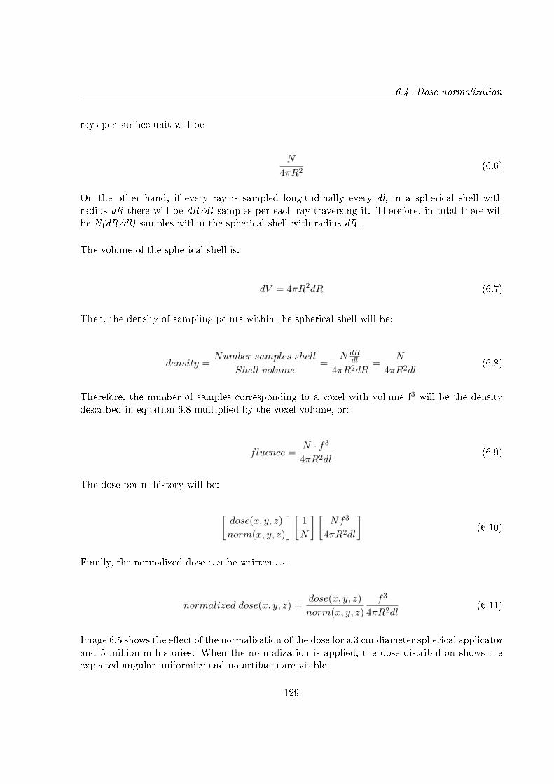
6.4. Dose normalization
rays per surface unit will be
N
4πR2(6.6)
On the other hand, if every ray is sampled longitudinally every dl, in a spherical shell withradius dR there will be dR/dl samples per each ray traversing it. Therefore, in total there willbe N(dR/dl) samples within the spherical shell with radius dR.
The volume of the spherical shell is:
dV = 4πR2dR (6.7)
Then, the density of sampling points within the spherical shell will be:
density =Number samples shell
Shell volume=
N dRdl
4πR2dR=
N
4πR2dl(6.8)
Therefore, the number of samples corresponding to a voxel with volume f3 will be the densitydescribed in equation 6.8 multiplied by the voxel volume, or:
fluence =N · f3
4πR2dl(6.9)
The dose per m-history will be:
[dose(x, y, z)norm(x, y, z)
] [1N
] [Nf3
4πR2dl
](6.10)
Finally, the normalized dose can be written as:
normalized dose(x, y, z) =dose(x, y, z)norm(x, y, z)
f3
4πR2dl(6.11)
Image 6.5 shows the eect of the normalization of the dose for a 3 cm diameter spherical applicatorand 5 million m-histories. When the normalization is applied, the dose distribution shows theexpected angular uniformity and no artifacts are visible.
129
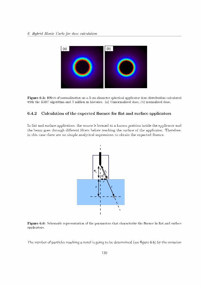
6. Hybrid Monte Carlo for dose calculation
(a) (b)
Figure 6.5: Eect of normalization on a 3 cm diameter spherical applicator dose distribution calculatedwith the HMC algorithm and 5 million m-histories. (a) Unnormalized dose, (b) normalized dose.
6.4.2 Calculation of the expected uence for at and surface applicators
In at and surface applicators, the source is located at a known position inside the applicator andthe beam goes through dierent lters before reaching the surface of the applicator. Therefore,in this case there are no simple analytical expressions to obtain the expected uence.
R0
rz
r0
Figure 6.6: Schematic representation of the parameters that characterize the uence in at and surfaceapplicators.
The number of particles reaching a voxel is going to be determined (see gure 6.6) by the emission
130

6.4. Dose normalization
angle α, that denes each particle's position with respect to the origin. Therefore, normalizationis going to depend on α and is going to decrease as 1/r2.
f(α)r2
0
r2(6.12)
With:
r0 =R0
cos(α)and r =
R0 + z
cos(α)(6.13)
The angle α needs to be corrected to remove the dependency of the number of particles with ρ.The normalization will have the following aspect:
f(α)ρ
R20
(R0 + z)2(6.14)
The angular uence factor is extracted from the PHSP le. Taking advantage of the symmetryof the reference dose, two normalization histograms are computed: One stores the volume ofthe number of interactions in Cartesian coordinates (norm(x,y,z)) that will be used to correctthe reference dose, and the other stores the 2D-surface containing the uence normalization incylindrical coordinates (norm(ρ,z)) that will be used to reintroduce the uence in the dose afternormalizing by the 3D-normalization volume.
The normalization in cylindrical coordinates contains the ideal uence of the photons emittedfrom the source, after going through the at and surface lters, and therefore we expect if to be arather smooth function with the angle, so we can lter the (ρ,z) 2D-histogram to avoid possiblepatterns that may still remain in it due to nite size of bins in ρ and z.
Finally we need to consider the number of interactions per unit of volume, which will be thevoxel volume (f 3) for the Cartesian normalization, and the volume of the ring between ρ andρ+dρ with a width dz for cylindrical normalization (π[(ρ+dρ)2-ρ2]dz ).
With all this, the normalized dose will be obtained from the following expression:
normalized dose(x, y, z) =
dose(x, y, z)norm(x,y,z)
f3
[ norm(ρ, z)π[(ρ+ dρ)2 − ρ2]dz
](6.15)
131
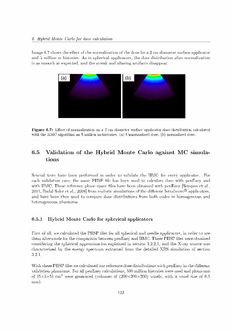
6. Hybrid Monte Carlo for dose calculation
Image 6.7 shows the eect of the normalization of the dose for a 2 cm diameter surface applicatorand 5 million m-histories. As in spherical applicators, the dose distribution after normalizationis as smooth as expected, and the streak and aliasing artifacts disappear.
(a) (b)
Figure 6.7: Eect of normalization on a 2 cm diameter surface applicator dose distribution calculatedwith the HMC algorithm an 5 million m-histories. (a) Unnormalized dose, (b) normalized dose.
6.5 Validation of the Hybrid Monte Carlo against MC simula-tions
Several tests have been performed in order to validate the HMC for every applicator. Foreach validation case, the same PHSP le has been used to calculate dose with penEasy andwith HMC. These reference phase space les have been obtained with penEasy [Sempau et al.,2011, Badal Soler et al., 2008] from realistic simulations of the dierent Intrabeam R© applicators,and have been then used to compare dose distributions from both codes in homogeneous andheterogeneous phantoms.
6.5.1 Hybrid Monte Carlo for spherical applicators
First of all, we calculated the PHSP les for all spherical and needle applicators, in order to usethem afterwards for the comparison between penEasy and HMC. These PHSP les were obtainedconsidering the spherical approximation explained in section 3.2.2.1, and the X-ray source wascharacterized by the energy spectrum extracted from the detailed XRS simulation of section3.2.1.
With these PHSP les we calculated our reference dose distributions with penEasy in the dierentvalidation phantoms. For all penEasy calculations, 500 million histories were used and phantomsof (5×5×5) cm3 were generated (volumes of (200×200×200) voxels, with a voxel size of 0.5mm).
132
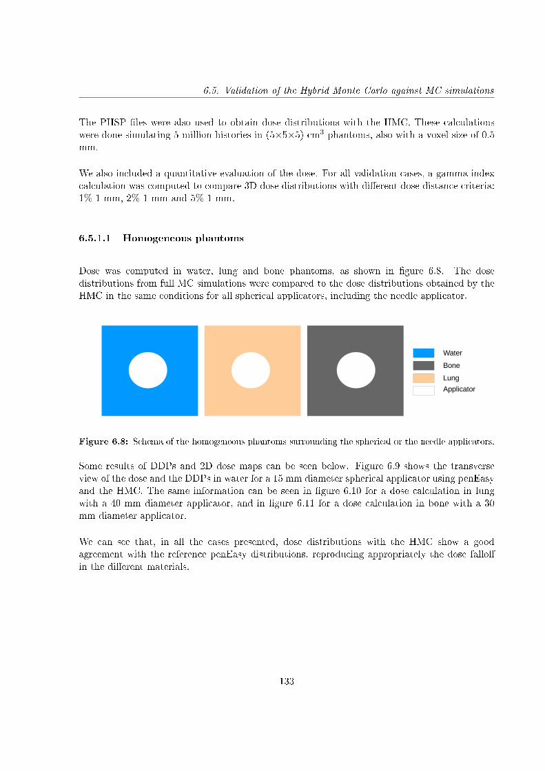
6.5. Validation of the Hybrid Monte Carlo against MC simulations
The PHSP les were also used to obtain dose distributions with the HMC. These calculationswere done simulating 5 million histories in (5×5×5) cm3 phantoms, also with a voxel size of 0.5mm.
We also included a quantitative evaluation of the dose. For all validation cases, a gamma indexcalculation was computed to compare 3D dose distributions with dierent dose distance criteria:1%-1 mm, 2%-1 mm and 5%-1 mm.
6.5.1.1 Homogeneous phantoms
Dose was computed in water, lung and bone phantoms, as shown in gure 6.8. The dosedistributions from full MC simulations were compared to the dose distributions obtained by theHMC in the same conditions for all spherical applicators, including the needle applicator.
Water
Bone
Lung
Applicator
Figure 6.8: Schema of the homogeneous phantoms surrounding the spherical or the needle applicators.
Some results of DDPs and 2D dose maps can be seen below. Figure 6.9 shows the transverseview of the dose and the DDPs in water for a 15 mm diameter spherical applicator using penEasyand the HMC. The same information can be seen in gure 6.10 for a dose calculation in lungwith a 40 mm diameter applicator, and in gure 6.11 for a dose calculation in bone with a 30mm diameter applicator.
We can see that, in all the cases presented, dose distributions with the HMC show a goodagreement with the reference penEasy distributions, reproducing appropriately the dose falloin the dierent materials.
133
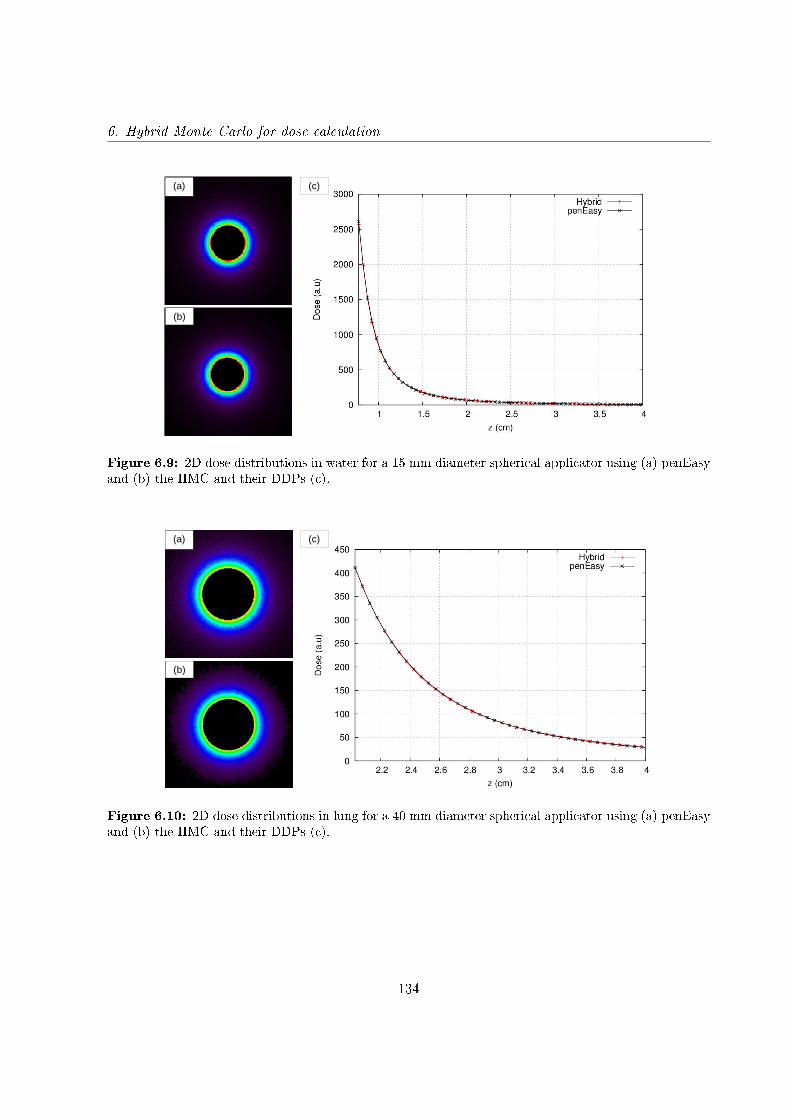
6. Hybrid Monte Carlo for dose calculation
(a) (b)
(a)
(b)
(c)
Figure 6.9: 2D dose distributions in water for a 15 mm diameter spherical applicator using (a) penEasyand (b) the HMC and their DDPs (c).
(a)
(b)
(c)
Figure 6.10: 2D dose distributions in lung for a 40 mm diameter spherical applicator using (a) penEasyand (b) the HMC and their DDPs (c).
134

6.5. Validation of the Hybrid Monte Carlo against MC simulations
(a)
(b)
(c)
Figure 6.11: 2D dose distributions in bone for a 30 mm diameter spherical applicator using (a) penEasyand (b) the HMC and their DDPs (c).
Gamma evaluations have been performed for all cases with 1%-1 mm, 2%-1 mm and 5%-1 mmcriteria. The results are presented in the following tables.
Gamma evaluation in water
1% - 1 mm 2% - 1 mm 5% - 1 mm
Needle 96.13% 98.50% 99.51%
Spherical φ 15 mm 95.81% 98.11% 99.40%
Spherical φ 20 mm 96.22% 98.84% 99.77%
Spherical φ 25 mm 96.47% 98.86% 99.75%
Spherical φ 30 mm 96.38% 99.25% 99.91%
Spherical φ 35 mm 95.69% 99.21% 99.97%
Spherical φ 40 mm 95.84% 99.04% 99.99%
Spherical φ 45 mm 97.02% 99.47% 99.98%
Spherical φ 50 mm 95.78% 99.23% 99.98%
Table 6.1: Results of gamma evaluation between MC simulations and HMC calculations in water (5%threshold).
135
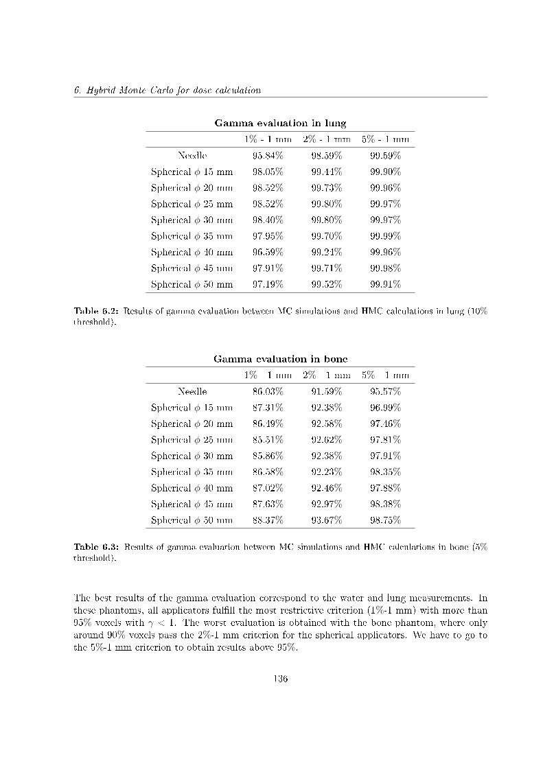
6. Hybrid Monte Carlo for dose calculation
Gamma evaluation in lung
1% - 1 mm 2% - 1 mm 5% - 1 mm
Needle 95.84% 98.59% 99.59%
Spherical φ 15 mm 98.05% 99.44% 99.90%
Spherical φ 20 mm 98.52% 99.73% 99.96%
Spherical φ 25 mm 98.52% 99.80% 99.97%
Spherical φ 30 mm 98.40% 99.80% 99.97%
Spherical φ 35 mm 97.95% 99.70% 99.99%
Spherical φ 40 mm 96.59% 99.24% 99.96%
Spherical φ 45 mm 97.91% 99.71% 99.98%
Spherical φ 50 mm 97.19% 99.52% 99.91%
Table 6.2: Results of gamma evaluation between MC simulations and HMC calculations in lung (10%threshold).
Gamma evaluation in bone
1% - 1 mm 2% - 1 mm 5% - 1 mm
Needle 86.03% 91.59% 95.57%
Spherical φ 15 mm 87.31% 92.38% 96.99%
Spherical φ 20 mm 86.49% 92.58% 97.46%
Spherical φ 25 mm 85.51% 92.62% 97.81%
Spherical φ 30 mm 85.86% 92.38% 97.91%
Spherical φ 35 mm 86.58% 92.23% 98.35%
Spherical φ 40 mm 87.02% 92.46% 97.88%
Spherical φ 45 mm 87.63% 92.97% 98.38%
Spherical φ 50 mm 88.37% 93.67% 98.75%
Table 6.3: Results of gamma evaluation between MC simulations and HMC calculations in bone (5%threshold).
The best results of the gamma evaluation correspond to the water and lung measurements. Inthese phantoms, all applicators fulll the most restrictive criterion (1%-1 mm) with more than95% voxels with γ < 1. The worst evaluation is obtained with the bone phantom, where onlyaround 90% voxels pass the 2%-1 mm criterion for the spherical applicators. We have to go tothe 5%-1 mm criterion to obtain results above 95%.
136
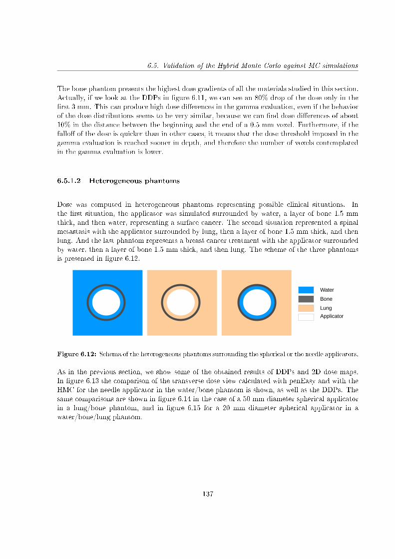
6.5. Validation of the Hybrid Monte Carlo against MC simulations
The bone phantom presents the highest dose gradients of all the materials studied in this section.Actually, if we look at the DDPs in gure 6.11, we can see an 80% drop of the dose only in therst 3 mm. This can produce high dose dierences in the gamma evaluation, even if the behaviorof the dose distributions seems to be very similar, because we can nd dose dierences of about10% in the distance between the beginning and the end of a 0.5 mm voxel. Furthermore, if thefallo of the dose is quicker than in other cases, it means that the dose threshold imposed in thegamma evaluation is reached sooner in depth, and therefore the number of voxels contemplatedin the gamma evaluation is lower.
6.5.1.2 Heterogeneous phantoms
Dose was computed in heterogeneous phantoms representing possible clinical situations. Inthe rst situation, the applicator was simulated surrounded by water, a layer of bone 1.5 mmthick, and then water, representing a surface cancer. The second situation represented a spinalmetastasis with the applicator surrounded by lung, then a layer of bone 1.5 mm thick, and thenlung. And the last phantom represents a breast cancer treatment with the applicator surroundedby water, then a layer of bone 1.5 mm thick, and then lung. The scheme of the three phantomsis presented in gure 6.12.
Water
Bone
Lung
Applicator
Figure 6.12: Schema of the heterogeneous phantoms surrounding the spherical or the needle applicators.
As in the previous section, we show some of the obtained results of DDPs and 2D dose maps.In gure 6.13 the comparison of the transverse dose view calculated with penEasy and with theHMC for the needle applicator in the water/bone phantom is shown, as well as the DDPs. Thesame comparisons are shown in gure 6.14 in the case of a 50 mm diameter spherical applicatorin a lung/bone phantom, and in gure 6.15 for a 20 mm diameter spherical applicator in awater/bone/lung phantom.
137
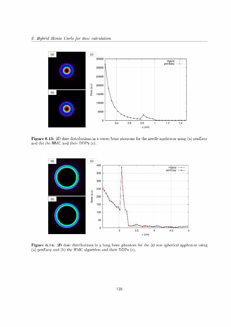
6. Hybrid Monte Carlo for dose calculation
(a)
(b)
(c)
Figure 6.13: 2D dose distributions in a water/bone phantom for the needle applicator using (a) penEasyand (b) the HMC and their DDPs (c).
(a)
(b)
(c)
Figure 6.14: 2D dose distributions in a lung/bone phantom for the 50 mm spherical applicator using(a) penEasy and (b) the HMC algorithm and their DDPs (c).
138
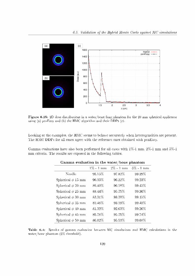
6.5. Validation of the Hybrid Monte Carlo against MC simulations
(a)
(b)
(c)
Figure 6.15: 2D dose distributions in a water/bone/lung phantom for the 20 mm spherical applicatorusing (a) penEasy and (b) the HMC algorithm and their DDPs (c).
Looking at the examples, the HMC seems to behave accurately when heterogeneities are present.The HMC DDPs for all cases agree with the reference ones obtained with penEasy.
Gamma evaluations have also been performed for all cases with 1%-1 mm, 2%-1 mm and 5%-1mm criteria. The results are exposed in the following tables.
Gamma evaluation in the water/bone phantom
1% - 1 mm 2% - 1 mm 5% - 1 mm
Needle 95.15% 97.82% 99.29%
Spherical φ 15 mm 90.33% 96.22% 99.23%
Spherical φ 20 mm 89.40% 96.18% 99.45%
Spherical φ 25 mm 88.44% 95.75% 99.36%
Spherical φ 30 mm 83.31% 93.70% 99.45%
Spherical φ 35 mm 82.48% 93.29% 99.40%
Spherical φ 40 mm 81.32% 92.63% 99.26%
Spherical φ 45 mm 85.78% 95.75% 99.74%
Spherical φ 50 mm 86.02% 95.53% 99.60%
Table 6.4: Results of gamma evaluation between MC simulations and HMC calculations in thewater/bone phantom (5% threshold).
139
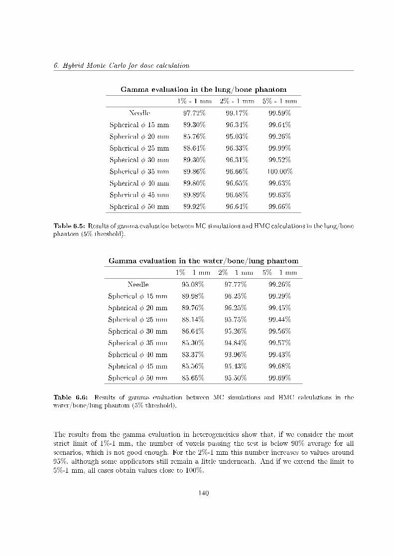
6. Hybrid Monte Carlo for dose calculation
Gamma evaluation in the lung/bone phantom
1% - 1 mm 2% - 1 mm 5% - 1 mm
Needle 97.72% 99.17% 99.59%
Spherical φ 15 mm 89.30% 96.34% 99.64%
Spherical φ 20 mm 85.76% 95.03% 99.26%
Spherical φ 25 mm 88.64% 96.33% 99.99%
Spherical φ 30 mm 89.30% 96.31% 99.52%
Spherical φ 35 mm 89.86% 96.66% 100.00%
Spherical φ 40 mm 89.80% 96.65% 99.63%
Spherical φ 45 mm 89.89% 96.68% 99.63%
Spherical φ 50 mm 89.92% 96.64% 99.66%
Table 6.5: Results of gamma evaluation between MC simulations and HMC calculations in the lung/bonephantom (5% threshold).
Gamma evaluation in the water/bone/lung phantom
1% - 1 mm 2% - 1 mm 5% - 1 mm
Needle 95.08% 97.77% 99.26%
Spherical φ 15 mm 89.98% 96.25% 99.29%
Spherical φ 20 mm 89.76% 96.25% 99.45%
Spherical φ 25 mm 88.14% 95.75% 99.44%
Spherical φ 30 mm 86.64% 95.26% 99.56%
Spherical φ 35 mm 85.30% 94.84% 99.57%
Spherical φ 40 mm 83.37% 93.96% 99.43%
Spherical φ 45 mm 85.56% 95.43% 99.68%
Spherical φ 50 mm 85.65% 95.50% 99.69%
Table 6.6: Results of gamma evaluation between MC simulations and HMC calculations in thewater/bone/lung phantom (5% threshold).
The results from the gamma evaluation in heterogeneities show that, if we consider the moststrict limit of 1%-1 mm, the number of voxels passing the test is below 90% average for allscenarios, which is not good enough. For the 2%-1 mm this number increases to values around95%, although some applicators still remain a little underneath. And if we extend the limit to5%-1 mm, all cases obtain values close to 100%.
140
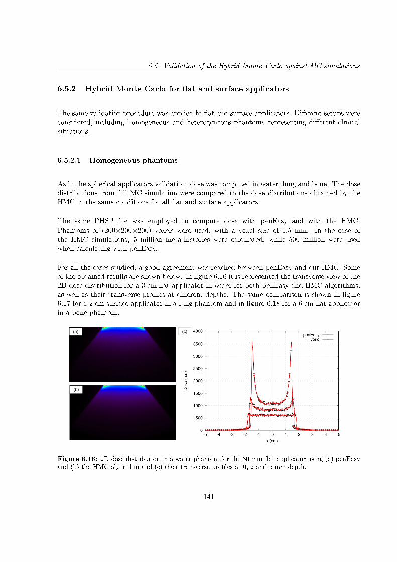
6.5. Validation of the Hybrid Monte Carlo against MC simulations
6.5.2 Hybrid Monte Carlo for at and surface applicators
The same validation procedure was applied to at and surface applicators. Dierent setups wereconsidered, including homogeneous and heterogeneous phantoms representing dierent clinicalsituations.
6.5.2.1 Homogeneous phantoms
As in the spherical applicators validation, dose was computed in water, lung and bone. The dosedistributions from full MC simulation were compared to the dose distributions obtained by theHMC in the same conditions for all at and surface applicators.
The same PHSP le was employed to compute dose with penEasy and with the HMC.Phantoms of (200×200×200) voxels were used, with a voxel size of 0.5 mm. In the case ofthe HMC simulations, 5 million meta-histories were calculated, while 500 million were usedwhen calculating with penEasy.
For all the cases studied, a good agreement was reached between penEasy and our HMC. Someof the obtained results are shown below. In gure 6.16 it is represented the transverse view of the2D dose distribution for a 3 cm at applicator in water for both penEasy and HMC algorithms,as well as their transverse proles at dierent depths. The same comparison is shown in gure6.17 for a 2 cm surface applicator in a lung phantom and in gure 6.18 for a 6 cm at applicatorin a bone phantom.
(a)
(b)
(c)
Figure 6.16: 2D dose distribution in a water phantom for the 30 mm at applicator using (a) penEasyand (b) the HMC algorithm and (c) their transverse proles at 0, 2 and 5 mm depth.
141
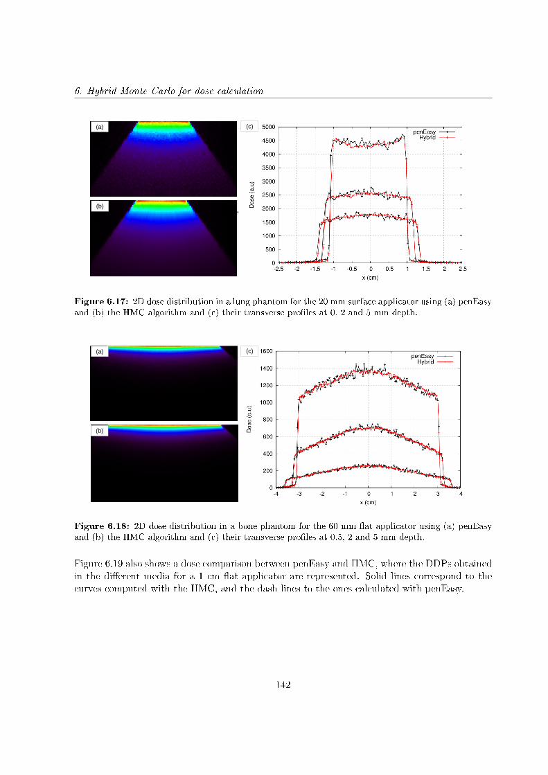
6. Hybrid Monte Carlo for dose calculation
(a)
(b)
(c)
Figure 6.17: 2D dose distribution in a lung phantom for the 20 mm surface applicator using (a) penEasyand (b) the HMC algorithm and (c) their transverse proles at 0, 2 and 5 mm depth.
(a)
(b)
(c)
Figure 6.18: 2D dose distribution in a bone phantom for the 60 mm at applicator using (a) penEasyand (b) the HMC algorithm and (c) their transverse proles at 0.5, 2 and 5 mm depth.
Figure 6.19 also shows a dose comparison between penEasy and HMC, where the DDPs obtainedin the dierent media for a 1 cm at applicator are represented. Solid lines correspond to thecurves computed with the HMC, and the dash lines to the ones calculated with penEasy.
142
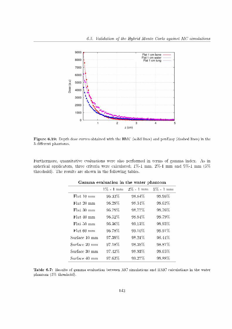
6.5. Validation of the Hybrid Monte Carlo against MC simulations
Figure 6.19: Depth dose curves obtained with the HMC (solid lines) and penEasy (dashed lines) in the3 dierent phantoms.
Furthermore, quantitative evaluations were also performed in terms of gamma index. As inspherical applicators, three criteria were calculated; 1%-1 mm, 2%-1 mm and 5%-1 mm (5%threshold). The results are shown in the following tables.
Gamma evaluation in the water phantom
1% - 1 mm 2% - 1 mm 5% - 1 mm
Flat 10 mm 96.33% 98.84% 99.56%
Flat 20 mm 96.29% 98.34% 99.62%
Flat 30 mm 96.79% 98.77% 99.76%
Flat 40 mm 96.52% 98.84% 99.79%
Flat 50 mm 96.36% 99.13% 99.93%
Flat 60 mm 96.78% 99.10% 99.91%
Surface 10 mm 97.39% 98.21% 98.44%
Surface 20 mm 97.18% 98.38% 98.81%
Surface 30 mm 97.42% 98.93% 99.65%
Surface 40 mm 97.63% 99.27% 99.88%
Table 6.7: Results of gamma evaluation between MC simulations and HMC calculations in the waterphantom (5% threshold).
143
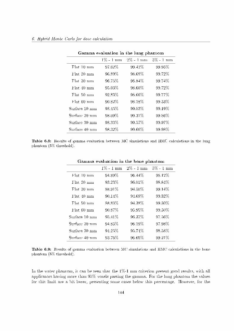
6. Hybrid Monte Carlo for dose calculation
Gamma evaluation in the lung phantom
1% - 1 mm 2% - 1 mm 5% - 1 mm
Flat 10 mm 97.62% 99.42% 99.95%
Flat 20 mm 96.89% 98.68% 99.72%
Flat 30 mm 96.75% 98.84% 99.74%
Flat 40 mm 95.03% 98.60% 99.72%
Flat 50 mm 92.83% 98.66% 99.77%
Flat 60 mm 90.82% 98.28% 99.53%
Surface 10 mm 98.45% 99.03% 99.19%
Surface 20 mm 98.09% 99.31% 99.86%
Surface 30 mm 98.33% 99.57% 99.97%
Surface 40 mm 98.32% 99.66% 99.98%
Table 6.8: Results of gamma evaluation between MC simulations and HMC calculations in the lungphantom (5% threshold).
Gamma evaluation in the bone phantom
1% - 1 mm 2% - 1 mm 5% - 1 mm
Flat 10 mm 94.89% 96.44% 98.12%
Flat 20 mm 93.23% 96.01% 98.84%
Flat 30 mm 88.91% 94.50% 99.14%
Flat 40 mm 90.14% 94.69% 99.32%
Flat 50 mm 88.83% 94.38% 99.30%
Flat 60 mm 90.87% 95.95% 99.50%
Surface 10 mm 95.41% 96.37% 97.56%
Surface 20 mm 94.85% 96.29% 97.98%
Surface 30 mm 94.25% 95.74% 98.58%
Surface 40 mm 93.76% 96.65% 99.21%
Table 6.9: Results of gamma evaluation between MC simulations and HMC calculations in the bonephantom (5% threshold).
In the water phantom, it can be seen that the 1%-1 mm criterion present good results, with allapplicators having more than 95% voxels passing the gamma. For the lung phantom the valuesfor this limit are a bit lower, presenting some cases below this percentage. However, for the
144
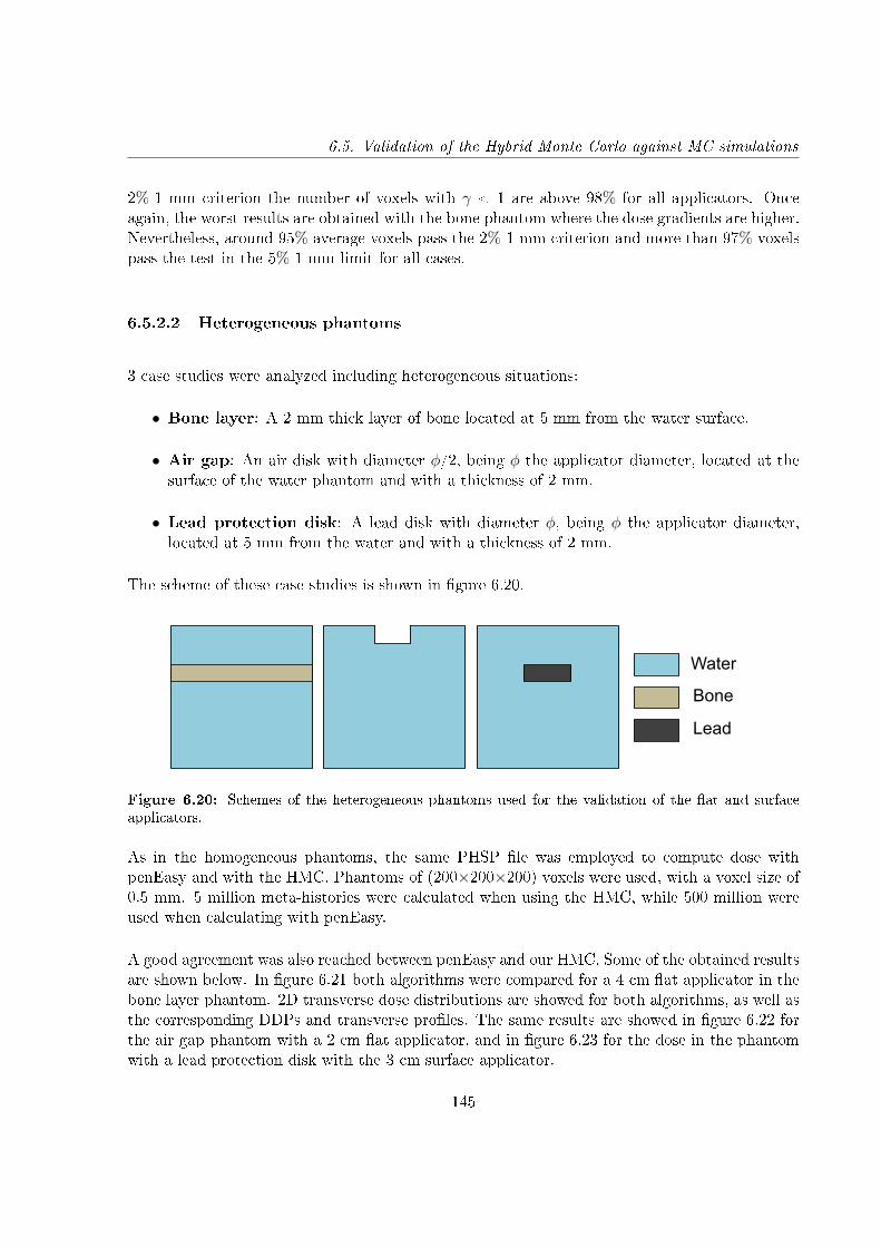
6.5. Validation of the Hybrid Monte Carlo against MC simulations
2%-1 mm criterion the number of voxels with γ < 1 are above 98% for all applicators. Onceagain, the worst results are obtained with the bone phantom where the dose gradients are higher.Nevertheless, around 95% average voxels pass the 2%-1 mm criterion and more than 97% voxelspass the test in the 5%-1 mm limit for all cases.
6.5.2.2 Heterogeneous phantoms
3 case studies were analyzed including heterogeneous situations:
• Bone layer: A 2 mm thick layer of bone located at 5 mm from the water surface.
• Air gap: An air disk with diameter φ/2, being φ the applicator diameter, located at thesurface of the water phantom and with a thickness of 2 mm.
• Lead protection disk: A lead disk with diameter φ, being φ the applicator diameter,located at 5 mm from the water and with a thickness of 2 mm.
The scheme of these case studies is shown in gure 6.20.
Water
Bone
Lead
Figure 6.20: Schemes of the heterogeneous phantoms used for the validation of the at and surfaceapplicators.
As in the homogeneous phantoms, the same PHSP le was employed to compute dose withpenEasy and with the HMC. Phantoms of (200×200×200) voxels were used, with a voxel size of0.5 mm. 5 million meta-histories were calculated when using the HMC, while 500 million wereused when calculating with penEasy.
A good agreement was also reached between penEasy and our HMC. Some of the obtained resultsare shown below. In gure 6.21 both algorithms were compared for a 4 cm at applicator in thebone layer phantom. 2D transverse dose distributions are showed for both algorithms, as well asthe corresponding DDPs and transverse proles. The same results are showed in gure 6.22 forthe air gap phantom with a 2 cm at applicator, and in gure 6.23 for the dose in the phantomwith a lead protection disk with the 3 cm surface applicator.
145
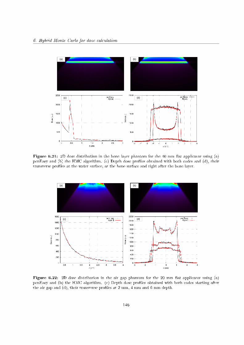
6. Hybrid Monte Carlo for dose calculation
(a) (b)
(c) (d)
Figure 6.21: 2D dose distribution in the bone layer phantom for the 40 mm at applicator using (a)penEasy and (b) the HMC algorithm. (c) Depth dose proles obtained with both codes and (d), theirtransverse proles at the water surface, at the bone surface and right after the bone layer.
(a) (b)
(c) (d)
Figure 6.22: 2D dose distribution in the air gap phantom for the 20 mm at applicator using (a)penEasy and (b) the HMC algorithm. (c) Depth dose proles obtained with both codes starting afterthe air gap and (d), their transverse proles at 2 mm, 4 mm and 6 mm depth.
146
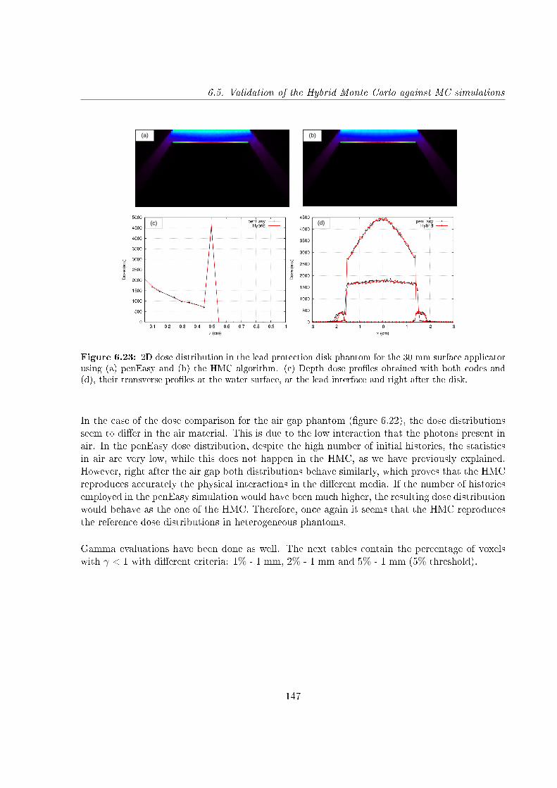
6.5. Validation of the Hybrid Monte Carlo against MC simulations
(a) (b)
(c) (d)
Figure 6.23: 2D dose distribution in the lead protection disk phantom for the 30 mm surface applicatorusing (a) penEasy and (b) the HMC algorithm. (c) Depth dose proles obtained with both codes and(d), their transverse proles at the water surface, at the lead interface and right after the disk.
In the case of the dose comparison for the air gap phantom (gure 6.22), the dose distributionsseem to dier in the air material. This is due to the low interaction that the photons present inair. In the penEasy dose distribution, despite the high number of initial histories, the statisticsin air are very low, while this does not happen in the HMC, as we have previously explained.However, right after the air gap both distributions behave similarly, which proves that the HMCreproduces accurately the physical interactions in the dierent media. If the number of historiesemployed in the penEasy simulation would have been much higher, the resulting dose distributionwould behave as the one of the HMC. Therefore, once again it seems that the HMC reproducesthe reference dose distributions in heterogeneous phantoms.
Gamma evaluations have been done as well. The next tables contain the percentage of voxelswith γ < 1 with dierent criteria: 1% - 1 mm, 2% - 1 mm and 5% - 1 mm (5% threshold).
147
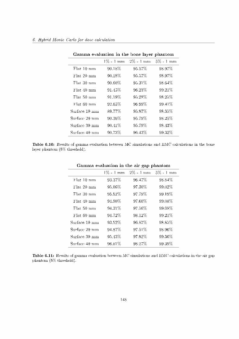
6. Hybrid Monte Carlo for dose calculation
Gamma evaluation in the bone layer phantom
1% - 1 mm 2% - 1 mm 5% - 1 mm
Flat 10 mm 90.18% 95.57% 98.97%
Flat 20 mm 90.18% 95.57% 98.97%
Flat 30 mm 90.60% 95.31% 98.64%
Flat 40 mm 91.45% 96.23% 99.21%
Flat 50 mm 91.19% 95.28% 98.25%
Flat 60 mm 92.65% 96.99% 99.41%
Surface 10 mm 89.77% 95.97% 98.35%
Surface 20 mm 90.36% 95.79% 98.25%
Surface 30 mm 90.41% 95.79% 98.43%
Surface 40 mm 90.73% 96.43% 99.32%
Table 6.10: Results of gamma evaluation between MC simulations and HMC calculations in the bonelayer phantom (5% threshold).
Gamma evaluation in the air gap phantom
1% - 1 mm 2% - 1 mm 5% - 1 mm
Flat 10 mm 93.37% 96.47% 98.84%
Flat 20 mm 95.06% 97.30% 99.02%
Flat 30 mm 95.52% 97.79% 99.19%
Flat 40 mm 94.90% 97.60% 99.08%
Flat 50 mm 94.31% 97.56% 99.08%
Flat 60 mm 94.72% 98.12% 99.21%
Surface 10 mm 93.52% 96.87% 98.85%
Surface 20 mm 94.87% 97.51% 98.96%
Surface 30 mm 95.43% 97.92% 99.36%
Surface 40 mm 96.01% 98.27% 99.39%
Table 6.11: Results of gamma evaluation between MC simulations and HMC calculations in the air gapphantom (5% threshold).
148
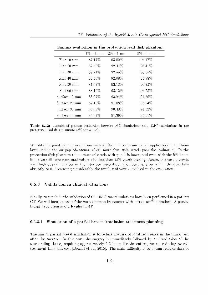
6.5. Validation of the Hybrid Monte Carlo against MC simulations
Gamma evaluation in the protection lead disk phantom
1% - 1 mm 2% - 1 mm 5% - 1 mm
Flat 10 mm 87.17% 93.82% 96.17%
Flat 20 mm 87.48% 92.44% 96.41%
Flat 30 mm 87.71% 92.55% 96.05%
Flat 40 mm 86.50% 92.08% 95.78%
Flat 50 mm 87.63% 93.13% 96.35%
Flat 60 mm 88.10% 93.12% 96.55%
Surface 10 mm 88.97% 93.24% 94.50%
Surface 20 mm 87.10% 91.08% 93.24%
Surface 30 mm 86.08% 90.48% 94.32%
Surface 40 mm 85.97% 91.36% 95.61%
Table 6.12: Results of gamma evaluation between MC simulations and HMC calculations in theprotection lead disk phantom (5% threshold).
We obtain a good gamma evaluation with a 2%-1 mm criterion for all applicators in the bonelayer and in the air gap phantoms, where more than 95% voxels pass the evaluation. In theprotection disk phantom the number of voxels with γ < 1 is lower, and even with the 5%-1 mmlimits we still have some applicators with less than 95% voxels passing. Again, this case presentsvery high dose dierences in the interface water-lead, and, besides, after 5 mm the dose fallsabruptly to 0, decreasing considerably the number of voxels involved in the evaluation.
6.5.3 Validation in clinical situations
Finally, to conclude the validation of the HMC, two simulations have been performed in a patientCT. We will focus on two of the most common treatments with Intrabeam R© nowadays: A partialbreast irradiation and a Kypho-IORT.
6.5.3.1 Simulation of a partial breast irradiation treatment planning
The aim of partial breast irradiation is to reduce the risk of local recurrence in the tumor bedafter the surgery. In this case, the surgery is immediately followed by an irradiation of thesurrounding tissue, requiring approximately 2-3 hours for the entire process, reducing overalltreatment time and cost [Bouzid et al., 2015]. The main diculty is to obtain reliable data of
149
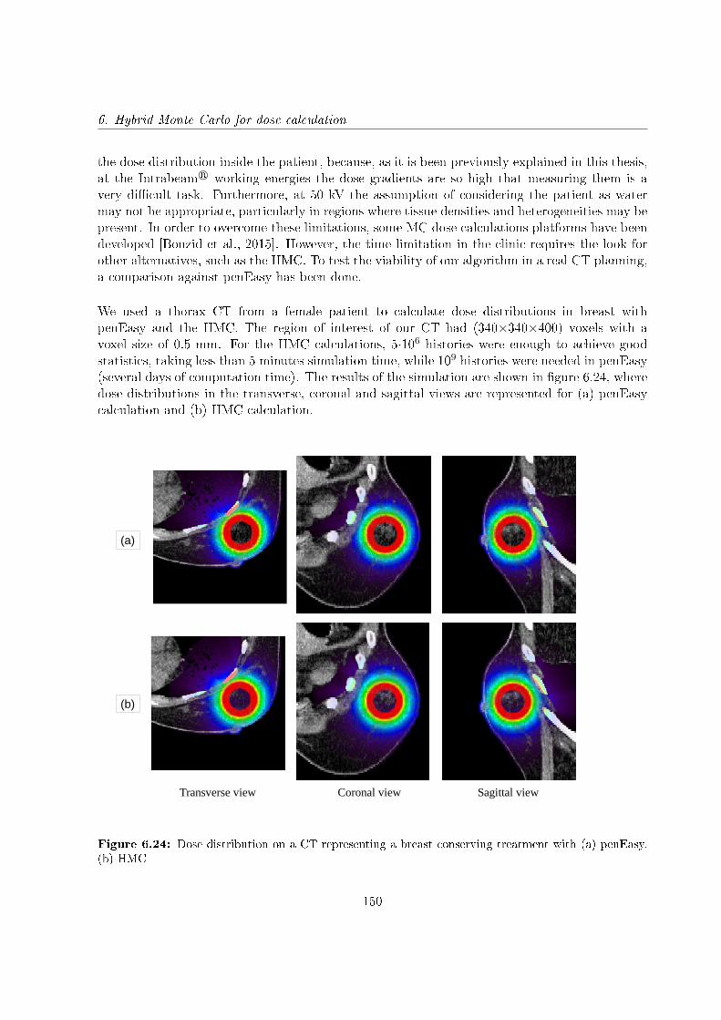
6. Hybrid Monte Carlo for dose calculation
the dose distribution inside the patient, because, as it is been previously explained in this thesis,at the Intrabeam R© working energies the dose gradients are so high that measuring them is avery dicult task. Furthermore, at 50 kV the assumption of considering the patient as watermay not be appropriate, particularly in regions where tissue densities and heterogeneities may bepresent. In order to overcome these limitations, some MC dose calculations platforms have beendeveloped [Bouzid et al., 2015]. However, the time limitation in the clinic requires the look forother alternatives, such as the HMC. To test the viability of our algorithm in a real CT planning,a comparison against penEasy has been done.
We used a thorax CT from a female patient to calculate dose distributions in breast withpenEasy and the HMC. The region of interest of our CT had (340×340×400) voxels with avoxel size of 0.5 mm. For the HMC calculations, 5·106 histories were enough to achieve goodstatistics, taking less than 5 minutes simulation time, while 109 histories were needed in penEasy(several days of computation time). The results of the simulation are shown in gure 6.24, wheredose distributions in the transverse, coronal and sagittal views are represented for (a) penEasycalculation and (b) HMC calculation.
Transverse view Coronal view Sagittal view
(a)
(b)
Figure 6.24: Dose distribution on a CT representing a breast conserving treatment with (a) penEasy,(b) HMC
150
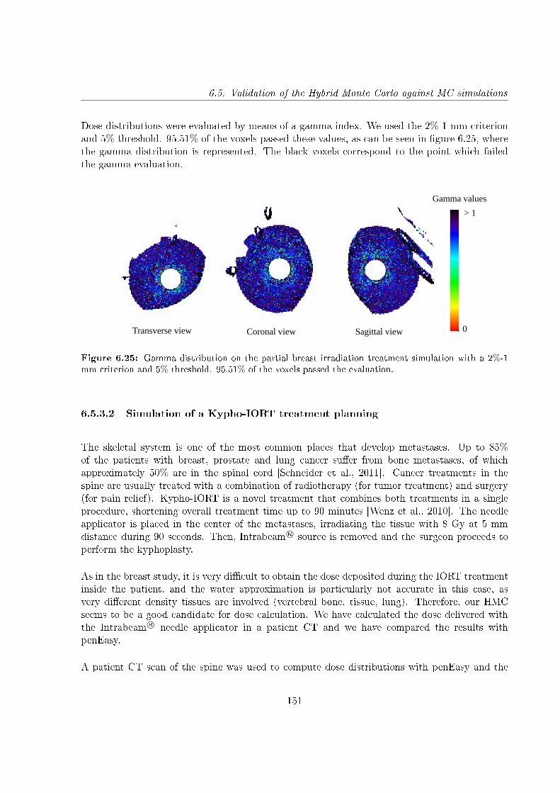
6.5. Validation of the Hybrid Monte Carlo against MC simulations
Dose distributions were evaluated by means of a gamma index. We used the 2%-1 mm criterionand 5% threshold. 95.51% of the voxels passed these values, as can be seen in gure 6.25, wherethe gamma distribution is represented. The black voxels correspond to the point which failedthe gamma evaluation.
0
> 1
Transverse view Coronal view Sagittal view
Gamma values
Figure 6.25: Gamma distribution on the partial breast irradiation treatment simulation with a 2%-1mm criterion and 5% threshold. 95.51% of the voxels passed the evaluation.
6.5.3.2 Simulation of a Kypho-IORT treatment planning
The skeletal system is one of the most common places that develop metastases. Up to 85%of the patients with breast, prostate and lung cancer suer from bone metastases, of whichapproximately 50% are in the spinal cord [Schneider et al., 2011]. Cancer treatments in thespine are usually treated with a combination of radiotherapy (for tumor treatment) and surgery(for pain relief). Kypho-IORT is a novel treatment that combines both treatments in a singleprocedure, shortening overall treatment time up to 90 minutes [Wenz et al., 2010]. The needleapplicator is placed in the center of the metastases, irradiating the tissue with 8 Gy at 5 mmdistance during 90 seconds. Then, Intrabeam R© source is removed and the surgeon proceeds toperform the kyphoplasty.
As in the breast study, it is very dicult to obtain the dose deposited during the IORT treatmentinside the patient, and the water approximation is particularly not accurate in this case, asvery dierent density tissues are involved (vertebral bone, tissue, lung). Therefore, our HMCseems to be a good candidate for dose calculation. We have calculated the dose delivered withthe Intrabeam R© needle applicator in a patient CT and we have compared the results withpenEasy.
A patient CT scan of the spine was used to compute dose distributions with penEasy and the
151
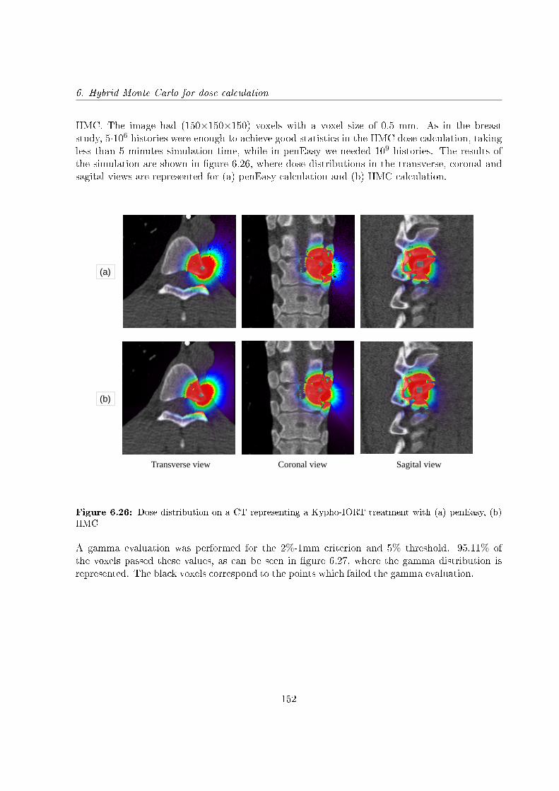
6. Hybrid Monte Carlo for dose calculation
HMC. The image had (150×150×150) voxels with a voxel size of 0.5 mm. As in the breaststudy, 5·106 histories were enough to achieve good statistics in the HMC dose calculation, takingless than 5 minutes simulation time, while in penEasy we needed 109 histories. The results ofthe simulation are shown in gure 6.26, where dose distributions in the transverse, coronal andsagital views are represented for (a) penEasy calculation and (b) HMC calculation.
Transverse view Coronal view Sagital view
(a)
(b)
Figure 6.26: Dose distribution on a CT representing a Kypho-IORT treatment with (a) penEasy, (b)HMC
A gamma evaluation was performed for the 2%-1mm criterion and 5% threshold. 95.11% ofthe voxels passed these values, as can be seen in gure 6.27, where the gamma distribution isrepresented. The black voxels correspond to the points which failed the gamma evaluation.
152
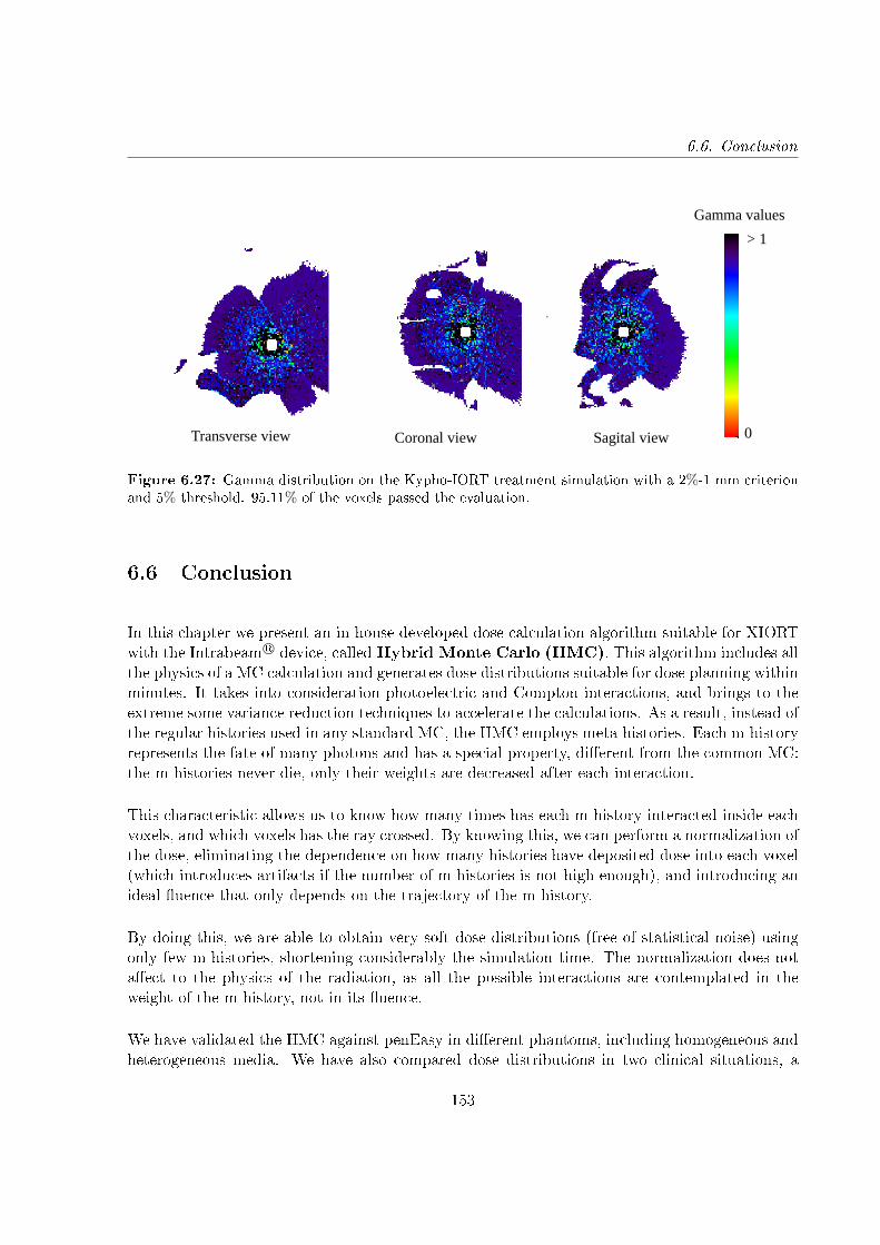
6.6. Conclusion
0
> 1
Transverse view Coronal view Sagital view
Gamma values
Figure 6.27: Gamma distribution on the Kypho-IORT treatment simulation with a 2%-1 mm criterionand 5% threshold. 95.11% of the voxels passed the evaluation.
6.6 Conclusion
In this chapter we present an in-house developed dose calculation algorithm suitable for XIORTwith the Intrabeam R© device, calledHybrid Monte Carlo (HMC). This algorithm includes allthe physics of a MC calculation and generates dose distributions suitable for dose planning withinminutes. It takes into consideration photoelectric and Compton interactions, and brings to theextreme some variance reduction techniques to accelerate the calculations. As a result, instead ofthe regular histories used in any standard MC, the HMC employs meta-histories. Each m-historyrepresents the fate of many photons and has a special property, dierent from the common MC:the m-histories never die, only their weights are decreased after each interaction.
This characteristic allows us to know how many times has each m-history interacted inside eachvoxels, and which voxels has the ray crossed. By knowing this, we can perform a normalization ofthe dose, eliminating the dependence on how many histories have deposited dose into each voxel(which introduces artifacts if the number of m-histories is not high enough), and introducing anideal uence that only depends on the trajectory of the m-history.
By doing this, we are able to obtain very soft dose distributions (free of statistical noise) usingonly few m-histories, shortening considerably the simulation time. The normalization does notaect to the physics of the radiation, as all the possible interactions are contemplated in theweight of the m-history, not in its uence.
We have validated the HMC against penEasy in dierent phantoms, including homogeneous andheterogeneous media. We have also compared dose distributions in two clinical situations, a
153
6. Hybrid Monte Carlo for dose calculation
partial breast irradiation and a Kypho-IORT. In general, good results were obtained with thegamma evaluation, for some situations even with the 1%-1 mm criterion. In a few cases we hadto go to a 5%-1 mm criterion to achieve a good agreement. However, the gamma limits forthe Intrabeam R© has not been stipulated, and values of previous studies can go from 2%-1 mm[Nwankwo et al., 2013], 2%-2 mm [Clausen et al., 2012] to even 10%-1 mm [Chiavassa et al.,2014].
Therefore, we can conclude that the HMC is a powerful tool that provides soft dose distributionsaccurately and within minutes. It can be used as a dose calculation tool in the operating room(OR), as its high speed allows an on-the-y dose calculation which includes the realistic eectsof the beam in the dierent tissues within the patient's body.
The HMC, in combination with the phase space optimization process described in chapter 4,provides dose distributions that reproduce the experimental data of any given Intrabeam R©'sapplicator in minutes, and both codes have been integrated into radiance R©.
154
Conclusions of this thesis
The main contributions and conclusions of the thesis are summarized in this chapter.
Detailed simulation of IORT systems
We have simulated the most relevant dedicated accelerators employed in IOERT treatments (ie.NOVAC R©, LIAC R© and MOBETRON R©) with their corresponding applicators, and Intrabeam R©
needle, spherical, surface and at applicators. In most cases, the dierent components ofthe devices have been extracted from literature, in other cases, such as for at and surfaceIntrabeam R© applicators, the geometry details have been provided by the vendor. Thesesimulations will represent a reference accelerator or applicator, and will be used to create adatabase that will be employed to generate a PHSP le tuned to each user machine in a dosetreatment planning procedure.
After characterizing each device, we used the geometries to calculate monoenergetic simulationsand store the PHSP les and DDPs. The PHSP les were parameterized in order to reduce thesize of the les. The monoenergetic simulations covered the energy range of the devices. Forthe IOERT accelerators, 140 simulations, from 1 MeV to 14 MeV were done. In the case ofIntrabeam R© applicators we calculated 50 simulations, from 1 to 50 keV.
The conclusions of this part are:
• Regarding the X-ray source study, a slight anisotropy in the backward direction of the dosecan be seen, which is consistent with previous studies [Dinsmore et al., 1996, Beatty et al.,1996], where an increase along the probe in the backward direction was observed from theescaping photons through beryllium.
• For the spherical applicators characterization, the backwards anisotropy seen in theexperimental measurements was reproduced by displacing the PHSP le that replaces theXRS around 2 mm from the geometrical center of the applicator, corresponding to leaving
155
Conclusions of this thesis
a 2 mm extra space in the hole inside the applicator to guarantee the protection of theXRS against the applicator walls when inserting it.
• In the simplied approach for the spherical applicators, while the possible dierences in theenergy deposition distribution with depth will be absorbed afterwards in the optimizationprocess, the anisotropy will not be reproduced.
• For the at and surface Intrabeam R© applicators, the detailed geometries provided by thevendor led to accurate dose distributions for all diameters.
• Regarding the electron beam dedicated accelerators, we were able to reproduce the dosedistributions by extracting the information from the literature and tuning the geometries.
• While for the LIAC R© and the NOVAC R© the same geometries were used to simulate all theapplicators and energies, for the MOBETRON R© we had to re-adjust slightly the geometriesfor each case, due to changes in the transverse proles with every applicator. This ispossibly a consequence of its soft-docking system.
• The parameterization performed to the PHSP les reduce the number of lines of each leup to a maximum of 2 million. Regarding the bin size, a trade-o between accuracy of therepresentation and number of requested bins was made.
Phase space optimization process and validation
We have developed a fast and accurate accelerator's tuning tool which can be optimized to theuser's device with only an experimental DDP in water [Ibáñez et al., 2015, Vidal et al., 2015,Udías et al., 2017a] for IOERT accelerators and Intrabeam R© applicators. This optimizationprocess will be possible thanks to the database of monochromatic PHSP les and DDPs inwater that has been obtained and stored from the detailed simulations that we have previouslydone.
A complete validation has been carried out against experimental measurements.
We have seen that:
• The procedure works accurately, reproducing the provided DDPs while maintaining thephysical shape of the spectra.
• Computation time of the whole optimization is below 10 minutes for all cases.
156

Conclusions of this thesis
• The optimization process only ts the DDPs, which is why it is essential that the rest ofthe dose distribution behaves correctly.
• By combining PHSP les and DDPs from realistic simulations and by using a realisticshape of the energy spectra we guarantee an accurate behavior of the dose distributions,not only of the DDP but also of the transverse proles.
• For the validation of dose distributions in water with spherical applicators, we found somediscrepancies between simulations and measurements due to the anisotropy of the dose inthe backward direction.
• The next step in the future work should be correcting these discrepancies due to theanisotropy by introducing an angular-dependent function in the X-rays beam uence.
• Regarding the dose distributions in water with at and surface applicators, we found agood agreement for the two cases studied, with more than 95% of the voxels fullling thegamma criterion at the 2%-2 mm level.
• In the dose comparisons inside heterogeneous phantoms, either with Intrabeam R©
applicators or IOERT accelerators, we reached a reasonable agreement at the 2%-2 mmlevel, specially considering that a non-negligible contribution to the dose dierences isattributed to uncertainties in the measurements, such as asymmetries or displacements ofthe lms.
• When these uncertainties disappear, the agreement increases substantially, something thathas been seen in the validation of IOERT accelerators against simulations, where almost a100% of the voxels passed the 2%-2 mm level in all the phantoms.
Hybrid Monte Carlo
We have developed a new dose computation algorithm for the Intrabeam R© applicators, namedhybrid Monte Carlo (HMC) [Vidal et al., 2014b,a, Udías et al., 2017b]. The HMC calculatesdose deposited by the Intrabeam R© device within minutes, fully taking into account the dierenttissues and structures in the region of patient, i.e. as derived from a CT image.
The HMC algorithm has been complemented with PHSP les generated for the needle, spherical,at and surface applicators and has been validated in dierent phantoms including clinicalsituations.
We can conclude:
157
Conclusions of this thesis
• HMC computes an accurate dose for both homogeneous and heterogeneous media, as itincorporates all the relevant physics processes at Intrabeam R© working energies.
• The savings in calculation time are possible thanks to taking to the extreme some variancereduction techniques.
• By not letting the meta-histories die inside the volume, we can normalize the dose,decreasing substantially the statistical noise of the distribution, and therefore, decreasingthe number of needed initial particles and consequently, the simulation time.
• The limitation of the number of Compton scatterings to one does not aect the nal dose,and the reduction of the simulation time is considerable.
• It can be considered that the electrons produced by the X-rays interactions inside themedia are absorbed in the same voxel as they are generated, provided voxel sizes not muchsmaller than 0.25 mm.
• Regarding the validation of the HMC, good results were obtained, in general, with thegamma evaluation, for some situations even with the 1%-1 mm criterion. In a few caseswe had to go to a 5%-1 mm criterion to achieve a good agreement. However, the gammacriteria for the Intrabeam R© has not been stipulated, and values of previous studies can gofrom 2%-1 mm [Nwankwo et al., 2013], 2%-2 mm [Clausen et al., 2012] to even 10%-1 mm[Chiavassa et al., 2014].
• For all the validations performed, we see that the worst results in terms of gamma evaluationappear when the dose gradients are higher, corresponding also to the cases were the numberof evaluated voxels is lower.
The nal conclusions of this thesis are:
• The proposed phase space optimization process works accurately reproducing dosedistributions in clinical situations for both electrons or X-rays beams. It has proven tobe fast, exible and accurately enough for IORT planning.
• The HMC provides soft dose distributions accurately and within minutes. It can be usedas a dose calculation tool in the operating room (OR), as its high speed allows an on-the-y dose calculation which includes the realistic eects of the beam in the dierent tissueswithin the patient's body.
• The HMC, in combination with the phase space optimization process, provides dosedistributions that reproduce the experimental data of any given Intrabeam R© in minutes,and both codes have been integrated into radiance R© [Valdivieso-Casique et al., 2015,
158

Conclusions of this thesis
Pascau et al., 2012].
159

Appendix A
Generation of the material list for the
Hybrid Monte Carlo
The Hybrid Monte Carlo extracts the photon's attenuation coecients for the dierent materialsfrom PENELOPE. One of the programs included in the distribution package is tables, whichgenerates tables with the physical information (physical properties, interaction cross sections,attenuation coecients, etc) from an input material data le. These material data les arecreated by means of the material program which extracts atomic interaction data from thePENELOPE database [Salvat et al., 2006].
Of all the physical information provided by the tables program for the dierent materials, we willbe interested in the photon mass attenuation coecients. This table includes the photoelectric,Compton, Rayleigh and pair production attenuation coecients for the selected material and fordierent energies. The attenuation table has to be interpolated to cover the energy range of theIntrabeam R©, from 1 keV to 50 keV (50 values for each material).
We have implemented 20 materials in the HMC code, covering dierent densities and materials(biologic and non-biologic):
• Air [Reference density (g/cm3): 1.21·10−3]• Water [Reference density (g/cm3): 1.00]• Solid Water [Reference density (g/cm3): 1.02]• Methacrylate [Reference density (g/cm3): 1.10]• Aluminum [Reference density (g/cm3): 2.70]• Brass [Reference density (g/cm3): 8.60]• Lead [Reference density (g/cm3): 11.35]• Copper [Reference density (g/cm3): 8.96]• Cork [Reference density (g/cm3): 2.40·10−1]
161
A. Appendix: Generation of the material list for the Hybrid Monte Carlo
• Teon [Reference density (g/cm3): 2.20]• PVC [Reference density (g/cm3): 1.40]• Dry Air [Reference density (g/cm3): 1.21·10−3]• Lung [Reference density (g/cm3): 3.00·10−1]• Adipose Tissue [Reference density (g/cm3): 9.20·10−1]• Muscle Striated [Reference density (g/cm3): 1.04]• Muscle [Reference density (g/cm3): 1.11]• Sacrum [Reference density (g/cm3): 1.29]• Rib [Reference density (g/cm3): 1.41]• B100 [Reference density (g/cm3): 1.45]• Cortical Bone [Reference density (g/cm3): 1.85]
162
Main contributions of this thesis
While this PhD. thesis was being carried out, partial results have been presented in publicationsin international journals and relevant conferences in the eld. The contributions of this thesisare presented in the following list.
Published articles in indexed international journals
1. E. Herranz, J. Herraiz, P. Ibáñez, M. Pérez-Liva, R. Puebla, J. Cal-González, P. Guerra,R. Rodríguez, C. Illana, and J.M. Udías. Phase space determination from measureddose data for intraoperative electron radiation therapy. Physics in Medicine and Biology,60(1):375-401, 2014
2. M. F. Valdivieso-Casique, R. Rodríguez, S. Rodríguez-Bescós, D. Lardíes, P. Guerra, M.J. Ledesma, A. Santos, P. Ibáñez, M. Vidal, J. M. Udías, et al. Radiance - a planningsoftware for intra-operative radiation therapy. Translational Cancer Research,4(2):196-209,2015
3. R. Lica , H. Mach, L. Fraile, A. Gargano, M. Borge, N. Marginean, C. Sotty, V. Vedia, A.Andreyev, G. Benzoni, P. Bomans, R. Borcea, L. Coraggio, C. Costache, F. De Witte, H.Flavigny, H. Fynbo, P. Ganey, P. Greenlees, L. Harkness-Brennan, M. Huyse, P. Ibáñez,S. Judson, J. Konki, A. Korgul, T. Kroll, et al. Fast-timing study of the l-forbidden 1/2+→3/2+ M 1 transition in Sn 129. Physical Review C, 93(4):044303 1-7, 2016
Articles submitted to indexed international journals
4. M. Vidal, P. Ibáñez, P. Guerra, M.F. Valdivieso-Casique, R. Rodríguez, C. Illana andJ.M. Udías. Fast optimized Monte Carlo phase-space based dose prediction for low energy
163
Main contributions of this thesis
X-rays Intra Operative Radiation Therapy. Physics in Medicine and Biology. Submitted.
Conference proceedings published in indexed international jour-nals
1. M. Vidal, P. Ibáñez, P. Guerra, E. Herranz, and J.M. Udías. Realistic on-the-y dosecalculation for low energy x-rays intra-operative radiation therapy. Radiotherapy andOncology, 110:S103-S104, 2014.
2. E. Herranz, J.M. Udías, P. Ibañez, J. Herraiz, M. Pérez-Liva, M. Vidal, and P. Guerra.Iterative reconstruction of clinical electron beam phase space for intra-operative radiationtherapy. Radiotherapy and Oncology, 110:S42, 2014
3. P. Ibáñez, M. Vidal, R. García Marcos, E. Herranz Muelas, P. Guerra Gutiérrez, C.Santiago, J. Agustín, M. Infante, M. Lavado, and J. M. Udías. Validation of a phase spacedetermination algorithm for intraoperative radiation therapy. Radiotherapy and Oncology,111(S1):331-331, 2014
4. R. G. Marcos, M. Vidal, P. Ibáñez, R. Ayala, R. Sendón, R. Polo, and J.M. Udías. Impactof patient-applicator air-gap in dedicated mobile accelerator for intra-operative radiationtherapy. Radiotherapy and Oncology, 111:S161-S162, 2014.
5. J.M. Udías, P. Ibáñez, M. Vidal, R. García-Marcos, G. Russo, C. Casarino, G. Candiano,G. Borasi, C. Messa, and M. Gilardi. A fast monte carlo-based calculation algorithm fora intra-operative radiation therapy TPS: A validation study. Radiotherapy and Oncology,111: S181-S182, 2014
6. M. Vidal, P. Ibáñez, J. Cal González, P. Guerra Gutiérrez, and J. M. Udías. Hybrid montecarlo dose algorithm for low energy x-rays intraoperative radiation therapy. Radiotherapyand Oncology, 111(S1):117-118, 2014
7. P. Ibáñez, M. Vidal, R. García-Marcos, P. Guerra and J.M. Udías. New geneticalgorithm-based procedure to determine phase space for intraoperative radiation therapy.Radiotherapy and Oncology, 115:S278-S279, 2015.
8. M. Perez-Liva, J. Herraiz, L. Medina-Valdés, J. Camacho, C. Fritsch, P. Ibáñez, and J.M.Udías. Ultrasound computed tomography for early breast cancer detection. Radiotherapyand Oncology, 115:S65, 2015
9. M. Vidal, P. Ibáñez, L. Parent, M. Goubert, R. Ferrand, P. Guerra, and J.M. Udias.
164
Main contributions of this thesis
Optimized monte-carlo intra-operative radiotherapy dose prediction for at and surfaceapplicators. Radiotherapy and Oncology, (115):S277-S278, 2015
10. P. Ibáñez, M. Vidal, P. Guerra, and J.M. Udías. Validation of an optimized MCdose prediction for low energy x-rays intraoperative radiation therapy. Radiotherapy andOncology, 119:S269-S270, 2016
Work presented in international or national conferences
Authors: E. Herranz, J. L. Herráiz, P. Ibáñez, M. Pérez-Liva, R. Puebla, J. Cal-González, P.Guerra, R. Rodríguez, C. Illana, J. M. UdíasTitle: Phase space determination of electron beam for intraoperative radiation therapy frommeasured dose dataType of presentation: OralCongress: Third European Workshop on Monte Carlo Treatment Planning (EW-MCTP)Place and date: Sevilla, Spain, 15-18 May, 2012.
Authors: E.Herranz, J.L. Herraiz, P. Guerra, J. Cal-González, P. Ibáñez, R. Rodríguez, C.Illana, M. J. Ledesma-Carbayo, M. A. Infante, M. E. Lavado, J. M. UdíasTitle:Iterative reconstruction of clinical electron beam phase space for intraoperative radiationtherapy from measured beam dose data.Type of presentation: PosterCongress: 7th International Conference of the International Society of Intraoperative RadiationTherapy (ISIORT)Place and date: Baveno, Italy, 22-24 June, 2012.
Authors: E. Herranz, J. L. Herráiz, P. Ibáñez, M. Pérez-Liva, R. Puebla, P. Guerra, J. M.Udías.Title:terative reconstruction of clinical electron beam phase space for intraoperative radiationtherapy from measured dose data.Type of presentation: PosterCongress: XXXIV Reunión Bienal de la Sociedad Española de FísicaPlace and date: Valencia, Spain, 15-18 July, 2013.
Authors: P. Ibáñez∗, E. Herranz, M. Pérez-Liva, R. Puebla, P. Guerra, C. Illana, R. Rodríguez,J.Calama, M. A. Infante, M. E. Lavado, J. M. Udías.Title: Vericación del algoritmo de determinación de espacios de fase para RadioterapiaIntraoperatoria (RIO) a partir de medidas experimentales.Type of presentation: Oral
∗presenting author
165
Main contributions of this thesis
Congress: XXXIV Reunión Bienal de la Sociedad Española de FísicaPlace and date: Valencia, Spain, 15-18 July, 2013.
Authors: M.Vidal, P. Ibáñez, E. Herranz, P. Guerra, J.M. UdíasTitle: Realistic on-the-y dose calculation for low energy X-rays Intra-Operative RadiationTherapyType of presentation: OralCongress: ICTR-PHEPlace and date: Geneva, Switzerland, 10-14 February, 2014.
Authors: E. Herranz, P. Ibáñez∗, J.L. Herraiz, M. Pérez Liva, M. Vidal, P. Guerra, J.M.UdíasTitle: Iterative Reconstruction of Clinical Electron Beam Phase Space for Intra-OperativeRadiation TherapyType of presentation: PosterCongress: ICTR-PHEPlace and date: Geneva, Switzerland, 10-14 February, 2014.
Authors: M. Vidal, P. Ibáñez, J. Cal-González, P. Guerra, J.M. UdíasTitle: Algorithme Monte Carlo hybride pour le calcul de dose de l'Intrabeam dans le système desimulation Radiance de GMVType of presentation: OralCongress: Zeiss Symposium, SFPM 53 conferencePlace and date: Deauville, France, 4-6 June, 2014.
Authors: P. Ibáñez∗, M. Vidal, R. García-Marcos, E. Herranz, P. Guerra, J.A. Calama, M.A.Infante, M.E. Lavado, J.M. UdíasTitle: Validation of a phase space determination algorithm for intra-operative radiationtherapyType of presentation: PosterCongress: ESTRO 33Place and date: Vienna, Austria, 4-8 April, 2014.
Authors: M. Vidal, P. Ibáñez, J. Cal González, P. Guerra, J.M. UdíasTitle: Hybrid Monte Carlo dose algorithm for low energy X-rays intra-operative radiationtherapyType of presentation: OralCongress: ESTRO 33Place and date: Vienna, Austria, 4-8 April, 2014.
Authors: J.M. Udías, P. Ibáñez∗, M. Vidal, R. García-Marcos, G. Russo, C. Casarino, G.C.
∗presenting author
166
Main contributions of this thesis
Candiano, G. Borasi, C. Messa, M.C. GilardiTitle: A fast Monte Carlo-based calculation algorithm for a Intra-Operative Radiation TherapyTPS : A validation studyType of presentation: PosterCongress: ESTRO 33Place and date: Vienna, Austria, 4-8 April, 2014.
Authors: R. García Marcos, M. Vidal, P. Ibáñez, R. Ayala, R. Sendón, R. Polo, J.M.UdíasTitle: Impact of patient-applicator air-gap in dedicated mobile accelerator for Intra-OperativeRadiation TherapyType of presentation: PosterCongress: ESTRO 33Place and date: Vienna, Austria, 4-8 April, 2014.
Authors: J. López, P. Ibáñez, J.M. Udías, E. Herranz, V. Morillo, A. Bouché, J. Bonaque, C.Ferrer, A. SantosTitle: Dosimetría con Monte Carlo de algunos casos prácticos en radioterapia intraoperato-ria.Type of presentation: PosterCongress: 4 Congreso conjunto SEFM/SEPRPlace and date: Valencia, Spain, 23-26 June, 2015.
Authors: P. Mur, P. Ibáñez, J.M. UdíasTitle: Development of a brachytherapy sources library for treatment planning with Monte CarloMethodsType of presentation: PosterCongress: 4 Congreso conjunto SEFM/SEPRPlace and date: Valencia, Spain, 23-26 June, 2015.
Authors: P. Ibáñez∗ , M. Vidal , R. García-Marcos, P. Guerra, J.M. UdíasTitle: Phase space determination for intraoperative electron radiation therapy with a geneticalgorithm-based procedureType of presentation: OralCongress: 4 Congreso conjunto SEFM/SEPRPlace and date: Valencia, Spain, 23-26 June, 2015.
Authors: A. Sethi, B. Chinsky, M. Vidal, P. Ibáñez, J.M Udías, C. IllanaTitle: Monte Carlo Modeling of IORT Dose Distributions in a Commercial Treatment PlanningSystemType of presentation: PosterCongress: 9th Intrabeam User Meeting
∗presenting author
167
Main contributions of this thesis
Place and date: Mannheim, Germany, 9-10 July, 2015.
Authors: M. Vidal, P. Ibáñez, P. Guerra, J. M. UdíasTitle: Optimized Monte-Carlo based dose computation for low energy X-rays IORT implementedin Radiance TPS.Type of presentation: OralCongress: 9th Intrabeam User MeetingPlace and date: Mannheim, Germany, 9-10 July, 2015.Note: This work was awarded with the best scientic contribution mention.
Authors: P. Ibáñez∗, M. Vidal, R. García-Marcos, P. Guerra, J.M. UdíasTitle: New genetic algorithm-based procedure to determine phase space for intraoperativeradiation therapyType of presentation: PosterCongress: 3rd ESTRO ForumPlace and date: Barcelona, Spain, 24-28 April, 2015.
Authors: M. Vidal, P. Ibáñez, L .Parent, M. Goubert, R. Ferrand, P.Guerra, J.M. Udías.Title: Optimized Monte-Carlo intra-operative radiotherapy dose prediction for supercial skincancers treatmentType of presentation: OralCongress: 3rd ESTRO ForumPlace and date: Barcelona, Spain, 24-28 April, 2015.
Authors: M. Perez-Liva, J.L. Herraiz, L. Medina-Valdés, J. Camacho, C. Fritsch, P. Ibáñez,J.M. Udías.Title: Ultrasound Computed tomography for early breast cancer detectionType of presentation: PosterCongress: 3rd ESTRO ForumPlace and date: Barcelona, Spain, 24-28 April, 2015.
Authors: P. Ibáñez∗, M. Vidal, L. Parent, M. Goubert, P. Guerra and J.M. Udías,Title: Optimized Monte Carlo dose calculation for supercial low energy X-rays intraoperativeradiation therapyType of presentation: OralCongress: XXXV Reunión Bienal de la Real Sociedad Española de FísicaPlace and date: Gijón, Spain, 13-17 July, 2015.
Authors: P. Ibáñez∗, M. Vidal, P. Guerra and J.M. UdíasTitle: Optimized Monte-Carlo based dose calculation for low energy X-rays intraoperativeradiation therapy
∗presenting author
168
Main contributions of this thesis
Type of presentation: OralCongress: I Jornadas RSEF / IFIMED de Física MédicaPlace and date: Valencia, Spain, 10-11 March, 2016.
Authors: P. Ibáñez∗, M. Vidal, P. Guerra and J.M. UdíasTitle:Validation of an optimized MC dose prediction for low energy X-rays intraoperativeradiation therapyType of presentation: PosterCongress: ESTRO 35Place and date: Turin, Italy, 29 April - 03 May, 2016.
Authors: J.M. Udías, P. Ibáñez, M. Vidal, J. Cal-Gonzélez, P. Guerra, MJ Ledesma, A. Santos,JE Ortuño, C. IllanaTitle: Cálculo acelerado de espacios de fases y dosis HMC en radioterapia intraoperatoria con elsistema IntrabeamType of presentation: OralCongress: VIII CPAN DAYSPlace and date: Zaragoza, Spain, 28-30 November, 2016.
169

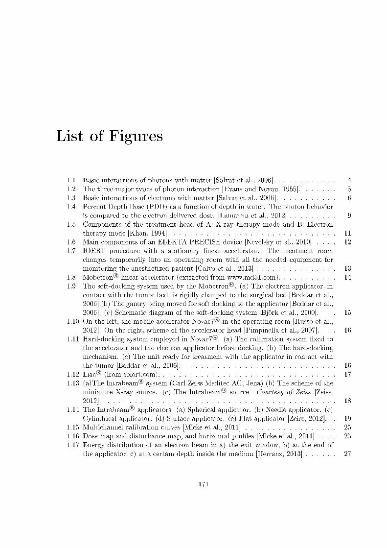
List of Figures
1.1 Basic interactions of photons with matter [Salvat et al., 2006]. . . . . . . . . . . . 41.2 The three major types of photon interaction [Evans and Noyau, 1955]. . . . . . . 51.3 Basic interactions of electrons with matter [Salvat et al., 2006]. . . . . . . . . . . 61.4 Percent Depth Dose (PDD) as a function of depth in water. The photon behavior
is compared to the electron delivered dose. [Lamanna et al., 2012] . . . . . . . . . 91.5 Components of the treatment head of A: X-ray therapy mode and B: Electron
therapy mode [Khan, 1994]. . . . . . . . . . . . . . . . . . . . . . . . . . . . . . . 111.6 Main components of an ELEKTA PRECISE device [Nevelsky et al., 2010] . . . . 121.7 IOERT procedure with a stationary linear accelerator. The treatment room
changes temporarily into an operating room with all the needed equipment formonitoring the anesthetized patient [Calvo et al., 2013] . . . . . . . . . . . . . . . 13
1.8 Mobetron R© linear accelerator (extracted from www.md51.com). . . . . . . . . . . 141.9 The soft-docking system used by the Mobetron R©. (a) The electron applicator, in
contact with the tumor bed, is rigidly clamped to the surgical bed [Beddar et al.,2006].(b) The gantry being moved for soft docking to the applicator [Beddar et al.,2006]. (c) Schematic diagram of the soft-docking system [Björk et al., 2000]. . . 15
1.10 On the left, the mobile accelerator Novac7 R© in the operating room [Russo et al.,2012]. On the right, scheme of the accelerator head [Pimpinella et al., 2007]. . . 16
1.11 Hard-docking system employed in Novac7 R©. (a) The collimation system xed tothe accelerator and the electron applicator before docking. (b) The hard-dockingmechanism. (c) The unit ready for treatment with the applicator in contact withthe tumor [Beddar et al., 2006]. . . . . . . . . . . . . . . . . . . . . . . . . . . . 16
1.12 Liac R© (from soiort.com). . . . . . . . . . . . . . . . . . . . . . . . . . . . . . . . . 171.13 (a)The Intrabeam R© system (Carl Zeiss Meditec AG, Jena) (b) The scheme of the
miniature X-ray source. (c) The Intrabeam R© source. Courtesy of Zeiss [Zeiss,2012]. . . . . . . . . . . . . . . . . . . . . . . . . . . . . . . . . . . . . . . . . . . 18
1.14 The Intrabeam R© applicators. (a) Spherical applicator. (b) Needle applicator. (c)Cylindrical applicator. (d) Surface applicator. (e) Flat applicator [Zeiss, 2012]. . 19
1.15 Multichannel calibration curves [Micke et al., 2011] . . . . . . . . . . . . . . . . . 251.16 Dose map and disturbance map, and horizontal proles [Micke et al., 2011] . . . . 251.17 Energy distribution of an electron beam in a) the exit window, b) at the end of
the applicator, c) at a certain depth inside the medium [Herranz, 2013] . . . . . . 27
171
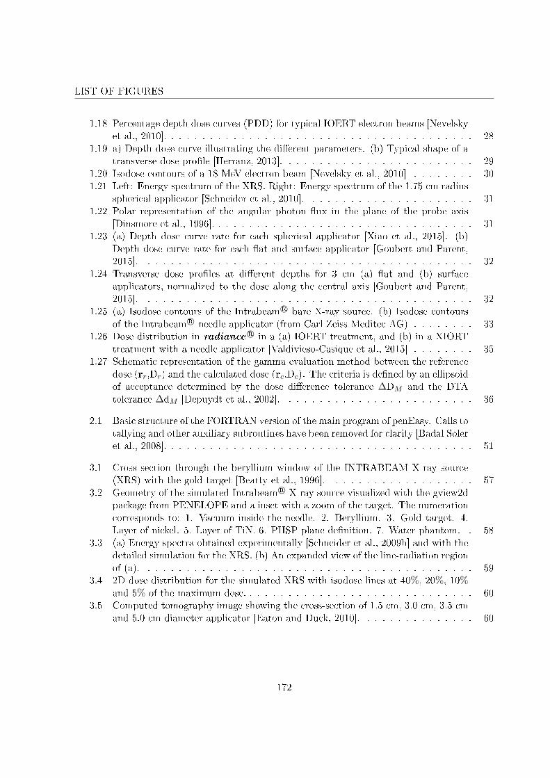
LIST OF FIGURES
1.18 Percentage depth dose curves (PDD) for typical IOERT electron beams [Nevelskyet al., 2010]. . . . . . . . . . . . . . . . . . . . . . . . . . . . . . . . . . . . . . . . 28
1.19 a) Depth dose curve illustrating the dierent parameters. (b) Typical shape of atransverse dose prole [Herranz, 2013]. . . . . . . . . . . . . . . . . . . . . . . . . 29
1.20 Isodose contours of a 18 MeV electron beam [Nevelsky et al., 2010] . . . . . . . . 301.21 Left: Energy spectrum of the XRS. Right: Energy spectrum of the 1.75 cm radius
spherical applicator [Schneider et al., 2010]. . . . . . . . . . . . . . . . . . . . . . 311.22 Polar representation of the angular photon ux in the plane of the probe axis
[Dinsmore et al., 1996]. . . . . . . . . . . . . . . . . . . . . . . . . . . . . . . . . . 311.23 (a) Depth dose curve rate for each spherical applicator [Xiao et al., 2015]. (b)
Depth dose curve rate for each at and surface applicator [Goubert and Parent,2015]. . . . . . . . . . . . . . . . . . . . . . . . . . . . . . . . . . . . . . . . . . . 32
1.24 Transverse dose proles at dierent depths for 3 cm (a) at and (b) surfaceapplicators, normalized to the dose along the central axis [Goubert and Parent,2015]. . . . . . . . . . . . . . . . . . . . . . . . . . . . . . . . . . . . . . . . . . . 32
1.25 (a) Isodose contours of the Intrabeam R© bare X-ray source. (b) Isodose contoursof the Intrabeam R© needle applicator (from Carl Zeiss Meditec AG) . . . . . . . . 33
1.26 Dose distribution in radiance R© in a (a) IOERT treatment, and (b) in a XIORTtreatment with a needle applicator [Valdivieso-Casique et al., 2015] . . . . . . . . 35
1.27 Schematic representation of the gamma evaluation method between the referencedose (rr,Dr) and the calculated dose (rc,Dc). The criteria is dened by an ellipsoidof acceptance determined by the dose dierence tolerance ∆DM and the DTAtolerance ∆dM [Depuydt et al., 2002]. . . . . . . . . . . . . . . . . . . . . . . . . 36
2.1 Basic structure of the FORTRAN version of the main program of penEasy. Calls totallying and other auxiliary subroutines have been removed for clarity [Badal Soleret al., 2008]. . . . . . . . . . . . . . . . . . . . . . . . . . . . . . . . . . . . . . . . 51
3.1 Cross section through the beryllium window of the INTRABEAM X-ray source(XRS) with the gold target [Beatty et al., 1996]. . . . . . . . . . . . . . . . . . . 57
3.2 Geometry of the simulated Intrabeam R© X-ray source visualized with the gview2dpackage from PENELOPE and a inset with a zoom of the target. The numerationcorresponds to: 1. Vacuum inside the needle. 2. Beryllium. 3. Gold target. 4.Layer of nickel. 5. Layer of TiN. 6. PHSP plane denition. 7. Water phantom. . 58
3.3 (a) Energy spectra obtained experimentally [Schneider et al., 2009b] and with thedetailed simulation for the XRS. (b) An expanded view of the line-radiation regionof (a). . . . . . . . . . . . . . . . . . . . . . . . . . . . . . . . . . . . . . . . . . . 59
3.4 2D dose distribution for the simulated XRS with isodose lines at 40%, 20%, 10%and 5% of the maximum dose. . . . . . . . . . . . . . . . . . . . . . . . . . . . . . 60
3.5 Computed tomography image showing the cross-section of 1.5 cm, 3.0 cm, 3.5 cmand 5.0 cm diameter applicator [Eaton and Duck, 2010]. . . . . . . . . . . . . . . 60
172
LIST OF FIGURES
3.6 Geometries employed in the simulation for the two dierent set of applicators.Left: 1.5 cm diameter spherical applicator. Right: 3.5 cm diameter sphericalapplicator. The numeration corresponds to: 1. Air inside the applicator were theXRS is located. 2. Applicator walls made of PEI. 3. Water. 4. Aluminum layerfor the ≤ 3 cm diameter applicators. . . . . . . . . . . . . . . . . . . . . . . . . . 61
3.7 Left: Energy spectra obtained experimentally [Schneider et al., 2010] and with thedetailed simulation for the 1.75 cm radius applicator. Right: Depth dose curvesobtained experimentally [Schneider et al., 2010] and with the detailed simulationfor the 1.75 radius applicator. . . . . . . . . . . . . . . . . . . . . . . . . . . . . . 62
3.8 2D dose distribution obtained with penEasy (Left) and with a radiochromic lm(Right) for a 1.5 cm diameter applicator with isodose lines at 90%, 70%, 40%,20% and 5%. . . . . . . . . . . . . . . . . . . . . . . . . . . . . . . . . . . . . . . 62
3.9 2D dose distribution obtained with penEasy (Left) and with a radiochromic lm(Right) for a 4.0 cm diameter applicator with isodose lines at 90%, 70%, 40%,20% and 10% of the maximum dose. . . . . . . . . . . . . . . . . . . . . . . . . . 63
3.10 Schematic geometry for the (a) Flat applicators and (b) Surface applicators. Thenumbering represents 1. XRS, 2. Air inside the applicator, 3. Lead walls, 4. PEIlter. . . . . . . . . . . . . . . . . . . . . . . . . . . . . . . . . . . . . . . . . . . . 64
3.11 Experimental and simulated transverse dose proles for (a) 1 cm surface applicatorand (b) 2 cm at applicator. . . . . . . . . . . . . . . . . . . . . . . . . . . . . . . 64
3.12 Geometry of the simulated LIAC R©. The numeration, materials and dimensionscorrespond to the numbers shown in the description. . . . . . . . . . . . . . . . . 66
3.13 Transverse dose proles in water for a 12 MeV LIAC R©, 6 cm diameter applicator. 673.14 Geometry of the simulated NOVAC R©. The numeration, materials and dimensions
correspond to the numbers shown in the description. . . . . . . . . . . . . . . . . 683.15 Transverse dose proles in water for a 10 MeV NOVAC R©, 6 cm diameter applicator. 693.16 Geometry of the simulated MOBETRON R©. The numeration, materials and
dimensions correspond to the numbers shown in the description. . . . . . . . . . . 703.17 Transverse dose proles in water for a 12 MeV MOBETRON R©, 10 cm diameter
applicator. . . . . . . . . . . . . . . . . . . . . . . . . . . . . . . . . . . . . . . . . 713.18 Schematic view of the PHSP plane at the exit of the right angle applicator showing
the small piece of beveled applicator included in the simulation to compute thedose for non-right applicators [Herranz et al., 2014]. . . . . . . . . . . . . . . . . . 72
3.19 Angular variables employed to dene the direction of a particle with theparameterization of the PHSP le. The green arrow represents the trajectoryof the particle, contained in the red plane (striped plane). The angle with the zaxis and the angle of the striped plane with the reference plane (xz plane) fullydene the direction of the particle [Herranz et al., 2014]. . . . . . . . . . . . . . . 73
3.20 Histograms for a 6 MeV NOVAC R© PHSP le with an applicator diameter of 60mm, showing both electron and photon distributions. The ordinate axis shows thenumber of particles in each bin. The radial distribution shows number of particlescrossing the unit of surface against ρ, the distance to the axis of the applicator. . 74
3.21 Schematic view of the parameterization of the PHSP les for spherical applicatorsin terms of the angles α and β. . . . . . . . . . . . . . . . . . . . . . . . . . . . . 75
173
LIST OF FIGURES
3.22 Histograms for a 20 mm diameter spherical applicator PHSP le in terms of therelevant variables (Energy, α and β), showing photon contributions. The ordinateaxis shows the number of particles in each bin. . . . . . . . . . . . . . . . . . . . 76
3.23 Schematic view of the parameterization of the PHSP les for at and surfaceapplicators in terms of the distance to the applicator ρ and the angle θ. . . . . . 77
3.24 Histograms for a 20 mm diameter surface applicator PHSP le in terms of therelevant variables (Energy, ρ and θ), showing photon contributions. The ordinateaxis shows the number of particles in each bin. . . . . . . . . . . . . . . . . . . . 78
4.1 Scheme of the phase space optimization process. . . . . . . . . . . . . . . . . . . . 834.2 Experimental DDP and adjusted DDP for a 9 MeV NOVAC R© with 4 cm diameter. 874.3 Left: Comparison of experimental DDP and optimized DDP for the 1.75 cm radius
spherical applicator. Right: Optimized energy spectrum. . . . . . . . . . . . . . 904.4 Left: Comparison of experimental DDP and optimized DDP for the 2 cm at
applicator. Right: Optimized energy spectrum. . . . . . . . . . . . . . . . . . . . 904.5 Left: Comparison of experimental DDP and optimized DDP for the 9 MeV
NOVAC R© with a 4 cm applicator. Right: Optimized energy spectrum. . . . . . . 91
5.1 Left: Gammex R© solid water phantom employed in calibration measurements withthe ionization chamber and a EBT3 lm. Right: Experimental setup for thecalibration measurements. . . . . . . . . . . . . . . . . . . . . . . . . . . . . . . . 96
5.2 Gammex solid water phantoms employed in 2D dose distribution measurements. . 975.3 Experimental setup (left) and schematic view of the position where the
radiochromic lms were placed (right). . . . . . . . . . . . . . . . . . . . . . . . . 985.4 DDPs for all the spherical applicators. Dotted curves correspond to our
experimental measurements, and the solid lines correspond to the DDPs providedby Zeiss. . . . . . . . . . . . . . . . . . . . . . . . . . . . . . . . . . . . . . . . . . 98
5.5 Experimental setup (left) of the Air-water step and schematic view of the positionwhere the radiochromic lms were placed (right). . . . . . . . . . . . . . . . . . . 99
5.6 Schematic view of the air step setup with the position where the radiochromiclms were placed. . . . . . . . . . . . . . . . . . . . . . . . . . . . . . . . . . . . . 101
5.7 Experimental setup (left) of the bone heterogeneity and schematic view of theposition where the radiochromic lms were placed (right). . . . . . . . . . . . . . 101
5.8 2D dose distributions in water for a 40 mm diameter spherical applicator obtainedfrom (a) radiochromic lms, (b) penEasy calculation with the reconstructed PHSPle and (c), the gamma evaluation distribution for a 2%-2 mm criterion with 5%threshold. 83.82% voxels passed the test. . . . . . . . . . . . . . . . . . . . . . . . 102
5.9 2D dose distributions in water for a 25 mm diameter spherical applicator obtainedfrom (a) radiochromic lms, (b) penEasy calculation with the reconstructed PHSPle and (c), the gamma evaluation distribution for a 2%-2 mm criterion with 5%threshold. 94.43% voxels passed the test. . . . . . . . . . . . . . . . . . . . . . . . 103
5.10 2D dose distributions in the air step at the dierent measured depths for a 40 mmdiameter spherical applicator obtained from (a) radiochromic lms, (b) penEasycalculation with the reconstructed PHSP le. . . . . . . . . . . . . . . . . . . . . 104
174
LIST OF FIGURES
5.11 Dose distribution comparison for a 30 mm diameter at applicator obtained with(a) a radiochromic lm and (b) penEasy calculation from the reconstructed PHSPle. . . . . . . . . . . . . . . . . . . . . . . . . . . . . . . . . . . . . . . . . . . . . 106
5.12 Dose distribution comparison for a 30 mm diameter surface applicator obtainedwith (a) a radiochromic lm and (b) penEasy calculation from the reconstructedPHSP le. . . . . . . . . . . . . . . . . . . . . . . . . . . . . . . . . . . . . . . . . 106
5.13 2D dose distributions in the bone phantom at the dierent measured depths for a30 mm diameter at applicator obtained from (a) radiochromic lms, (b) penEasycalculation from the reconstructed PHSP le. . . . . . . . . . . . . . . . . . . . . 107
5.14 2D dose distributions in the air step at the dierent measured depths for a 30 mmdiameter surface applicator obtained from (a) radiochromic lms, (b) penEasycalculation from the reconstructed PHSP le. . . . . . . . . . . . . . . . . . . . . 107
5.15 Experimental setup (left) of a solid water step measurement and its schematicview with the location of the lms (right). . . . . . . . . . . . . . . . . . . . . . . 109
5.16 Experimental setup (left) of a lung heterogeneity measurement and its schematicview with the location of the lms (right). . . . . . . . . . . . . . . . . . . . . . . 109
5.17 Experimental setup (left) of a mediastinum-lung type measurement and itsschematic view with the location of the lms (right). . . . . . . . . . . . . . . . . 110
5.18 Experimental setup (left) of a water/bone type measurement and its schematicview with the location of the lms (right). . . . . . . . . . . . . . . . . . . . . . . 110
5.19 Transverse dose proles at 1.2 (shifted up by 20%) and 1.7 cm depth in thesolid water step phantom obtained from the radiochromic lms and from thereconstructed PHSP le (NOVAC R©, 9MeV, 4 cm φ applicator). . . . . . . . . . . 111
5.20 Transverse dose proles at 1.0 (shifted up by 5%), 1.1, 1.6 and 2.1 cm depth inthe lung heterogeneity, costal wall type phantom obtained from the radiochromiclms and from the reconstructed PHSP le (NOVAC R©, 9MeV, 4 cm φ applicator). 112
5.21 Transverse dose proles at 1.0 (shifted up by 10%), 1.5, 2.5, 3.0 and 3.1 cm depthin the mediastinum-lung type phantom obtained from the radiochromic lms andfrom the reconstructed PHSP le (NOVAC R©, 9MeV, 4 cm φ applicator). . . . . . 112
5.22 Transverse dose proles at 2.0 cm depth in the water/bone type phantom obtainedfrom the radiochromic lms and from the reconstructed PHSP le (NOVAC R©,9MeV, 4 cm φ applicator). . . . . . . . . . . . . . . . . . . . . . . . . . . . . . . . 113
5.23 Setups where the dose produced by the solution PHSP le and the full MCsimulation were compared. . . . . . . . . . . . . . . . . . . . . . . . . . . . . . . . 114
5.24 (Left) Dose proles at 1.5 (shifted up by 20%), 2.5 (shifted up by 10%) and 3.5cm depth in the air-water step phantom for the 12 MeV LIAC R©. (Right) Doseproles at 1.95 (shifted up by 20%), 3.0 (shifted up by 10%) and 4.0 cm depth inthe bone phantom for the 9 MeV MOBETRON R© . . . . . . . . . . . . . . . . . . 115
6.1 Randomly generated coordinates populating a XY plane. . . . . . . . . . . . . . . 1196.2 (a) Comparison of DDPs of a 1.5 cm diameter spherical applicator with a single full
Compton interaction (solid line) and with two full Compton interactions (dots).(b) Statistical dierence between the two proles in (a). . . . . . . . . . . . . . . 124
6.3 Flow chart of the HMC. . . . . . . . . . . . . . . . . . . . . . . . . . . . . . . . . 125
175
LIST OF FIGURES
6.4 Comparison of dose distributions calculated with penEasy and the HMC algorithmfor dierent number of histories or m-histories. (a) penEasy simulation with0.5 million histories, (b) penEasy simulation with 5 million histories, (c) HMCsimulation with 0.5 million m-histories, (d) HMC simulation with 5 million m-histories. . . . . . . . . . . . . . . . . . . . . . . . . . . . . . . . . . . . . . . . . . 127
6.5 Eect of normalization on a 3 cm diameter spherical applicator dose distributioncalculated with the HMC algorithm and 5 million m-histories. (a) Unnormalizeddose, (b) normalized dose. . . . . . . . . . . . . . . . . . . . . . . . . . . . . . . . 130
6.6 Schematic representation of the parameters that characterize the uence in atand surface applicators. . . . . . . . . . . . . . . . . . . . . . . . . . . . . . . . . 130
6.7 Eect of normalization on a 2 cm diameter surface applicator dose distributioncalculated with the HMC algorithm an 5 million m-histories. (a) Unnormalizeddose, (b) normalized dose. . . . . . . . . . . . . . . . . . . . . . . . . . . . . . . . 132
6.8 Schema of the homogeneous phantoms surrounding the spherical or the needleapplicators. . . . . . . . . . . . . . . . . . . . . . . . . . . . . . . . . . . . . . . . 133
6.9 2D dose distributions in water for a 15 mm diameter spherical applicator using(a) penEasy and (b) the HMC and their DDPs (c). . . . . . . . . . . . . . . . . . 134
6.10 2D dose distributions in lung for a 40 mm diameter spherical applicator using (a)penEasy and (b) the HMC and their DDPs (c). . . . . . . . . . . . . . . . . . . . 134
6.11 2D dose distributions in bone for a 30 mm diameter spherical applicator using (a)penEasy and (b) the HMC and their DDPs (c). . . . . . . . . . . . . . . . . . . . 135
6.12 Schema of the heterogeneous phantoms surrounding the spherical or the needleapplicators. . . . . . . . . . . . . . . . . . . . . . . . . . . . . . . . . . . . . . . . 137
6.13 2D dose distributions in a water/bone phantom for the needle applicator using (a)penEasy and (b) the HMC and their DDPs (c). . . . . . . . . . . . . . . . . . . . 138
6.14 2D dose distributions in a lung/bone phantom for the 50 mm spherical applicatorusing (a) penEasy and (b) the HMC algorithm and their DDPs (c). . . . . . . . . 138
6.15 2D dose distributions in a water/bone/lung phantom for the 20 mm sphericalapplicator using (a) penEasy and (b) the HMC algorithm and their DDPs (c). . . 139
6.16 2D dose distribution in a water phantom for the 30 mm at applicator using (a)penEasy and (b) the HMC algorithm and (c) their transverse proles at 0, 2 and5 mm depth. . . . . . . . . . . . . . . . . . . . . . . . . . . . . . . . . . . . . . . 141
6.17 2D dose distribution in a lung phantom for the 20 mm surface applicator using(a) penEasy and (b) the HMC algorithm and (c) their transverse proles at 0, 2and 5 mm depth. . . . . . . . . . . . . . . . . . . . . . . . . . . . . . . . . . . . . 142
6.18 2D dose distribution in a bone phantom for the 60 mm at applicator using (a)penEasy and (b) the HMC algorithm and (c) their transverse proles at 0.5, 2 and5 mm depth. . . . . . . . . . . . . . . . . . . . . . . . . . . . . . . . . . . . . . . 142
6.19 Depth dose curves obtained with the HMC (solid lines) and penEasy (dashedlines) in the 3 dierent phantoms. . . . . . . . . . . . . . . . . . . . . . . . . . . . 143
6.20 Schemes of the heterogeneous phantoms used for the validation of the at andsurface applicators. . . . . . . . . . . . . . . . . . . . . . . . . . . . . . . . . . . . 145
176

LIST OF FIGURES
6.21 2D dose distribution in the bone layer phantom for the 40 mm at applicatorusing (a) penEasy and (b) the HMC algorithm. (c) Depth dose proles obtainedwith both codes and (d), their transverse proles at the water surface, at the bonesurface and right after the bone layer. . . . . . . . . . . . . . . . . . . . . . . . . 146
6.22 2D dose distribution in the air gap phantom for the 20 mm at applicator using(a) penEasy and (b) the HMC algorithm. (c) Depth dose proles obtained withboth codes starting after the air gap and (d), their transverse proles at 2 mm, 4mm and 6 mm depth. . . . . . . . . . . . . . . . . . . . . . . . . . . . . . . . . . 146
6.23 2D dose distribution in the lead protection disk phantom for the 30 mm surfaceapplicator using (a) penEasy and (b) the HMC algorithm. (c) Depth dose prolesobtained with both codes and (d), their transverse proles at the water surface,at the lead interface and right after the disk. . . . . . . . . . . . . . . . . . . . . . 147
6.24 Dose distribution on a CT representing a breast conserving treatment with (a)penEasy, (b) HMC . . . . . . . . . . . . . . . . . . . . . . . . . . . . . . . . . . . 150
6.25 Gamma distribution on the partial breast irradiation treatment simulation with a2%-1 mm criterion and 5% threshold. 95.51% of the voxels passed the evaluation. 151
6.26 Dose distribution on a CT representing a Kypho-IORT treatment with (a)penEasy, (b) HMC . . . . . . . . . . . . . . . . . . . . . . . . . . . . . . . . . . . 152
6.27 Gamma distribution on the Kypho-IORT treatment simulation with a 2%-1 mmcriterion and 5% threshold. 95.11% of the voxels passed the evaluation. . . . . . . 153
177

List of Tables
3.1 Classication of the characteristic X-rays present in the XRS energy spectrum. . 59
5.1 Measured dose values during the calibration procedure obtained with theionization chamber. . . . . . . . . . . . . . . . . . . . . . . . . . . . . . . . . . . . 95
5.2 Measured dose values during the calibration procedure obtained with theionization chamber. . . . . . . . . . . . . . . . . . . . . . . . . . . . . . . . . . . . 100
5.3 Results of gamma evaluation between MC simulations and measurements in theair step phantom (5% threshold). . . . . . . . . . . . . . . . . . . . . . . . . . . . 105
5.4 Results of gamma evaluation between MC simulations and measurements in theair step phantom and in the bone heterogeneity (5% threshold). . . . . . . . . . . 108
5.5 Results of gamma evaluation between MC simulations and measurements in thedierent phantoms (5% threshold). . . . . . . . . . . . . . . . . . . . . . . . . . . 113
5.6 Results of gamma evaluation in the dierent phantoms (5% threshold). . . . . . . 115
6.1 Results of gamma evaluation between MC simulations and HMC calculations inwater (5% threshold). . . . . . . . . . . . . . . . . . . . . . . . . . . . . . . . . . 135
6.2 Results of gamma evaluation between MC simulations and HMC calculations inlung (10% threshold). . . . . . . . . . . . . . . . . . . . . . . . . . . . . . . . . . 136
6.3 Results of gamma evaluation between MC simulations and HMC calculations inbone (5% threshold). . . . . . . . . . . . . . . . . . . . . . . . . . . . . . . . . . . 136
6.4 Results of gamma evaluation between MC simulations and HMC calculations inthe water/bone phantom (5% threshold). . . . . . . . . . . . . . . . . . . . . . . . 139
6.5 Results of gamma evaluation between MC simulations and HMC calculations inthe lung/bone phantom (5% threshold). . . . . . . . . . . . . . . . . . . . . . . . 140
6.6 Results of gamma evaluation between MC simulations and HMC calculations inthe water/bone/lung phantom (5% threshold). . . . . . . . . . . . . . . . . . . . 140
6.7 Results of gamma evaluation between MC simulations and HMC calculations inthe water phantom (5% threshold). . . . . . . . . . . . . . . . . . . . . . . . . . . 143
6.8 Results of gamma evaluation between MC simulations and HMC calculations inthe lung phantom (5% threshold). . . . . . . . . . . . . . . . . . . . . . . . . . . . 144
6.9 Results of gamma evaluation between MC simulations and HMC calculations inthe bone phantom (5% threshold). . . . . . . . . . . . . . . . . . . . . . . . . . . 144
179
LIST OF TABLES
6.10 Results of gamma evaluation between MC simulations and HMC calculations inthe bone layer phantom (5% threshold). . . . . . . . . . . . . . . . . . . . . . . . 148
6.11 Results of gamma evaluation between MC simulations and HMC calculations inthe air gap phantom (5% threshold). . . . . . . . . . . . . . . . . . . . . . . . . . 148
6.12 Results of gamma evaluation between MC simulations and HMC calculations inthe protection lead disk phantom (5% threshold). . . . . . . . . . . . . . . . . . . 149
180
Bibliography
M. Abe. Intraoperative radiotherapypast, present and future. International Journal ofRadiation Oncology* Biology* Physics, 10(10):19871990, 1984.
M. Abe and M. Takahashi. Intraoperative radiotherapy: the Japanese experience. InternationalJournal of Radiation Oncology* Biology* Physics, 7(7):863868, 1981.
M. Abe, M. Fukuda, K. Yamano, S. Matsuda, and H. Handa. Intra-operative irradiation inabdominal and cerebral tumours. Acta radiologica: therapy, physics, biology, 10(4):408416,1971.
S. Agostinelli et al. Geant4-a Simulation Toolkit, Nuclear Instruments and Methods in PhysicsResearch Section A: Accelerators, Spectrometers. Detectors and Associated Equipment, 506(3), 2003.
M. Alber, S. Broggi, C. De Wagter, I. Eichwurzel, P. Engström, C. Fiorino, D. Georg,G. Hartmann, T. Knöös, A. Leal, et al. Guidelines for the verication of IMRT. ESTRObooklet, 7, 2008.
P. R. Almond, P. J. Biggs, B. Coursey, W. Hanson, M. S. Huq, R. Nath, and D. Rogers. AAPM'sTG-51 protocol for clinical reference dosimetry of high-energy photon and electron beams.Medical physics, 26(9):18471870, 1999.
E. Aranda Escolástico. Análisis de películas radiocrómicas para su utilización en dosimetríamédica. Final Degree Project. Advisors: José Manuel Udías Moinelo y Marie Vidal.UniversidadComplutense de Madrid, 2013.
K. S. Armoogum, J. M. Parry, S. K. Souliman, D. G. Sutton, and C. D. Mackay. Functionalintercomparison of intraoperative radiotherapy equipmentPhoton Radiosurgery System.Radiation Oncology, 2(1):1, 2007.
F. H. Attix. Introduction to radiological physics and radiation dosimetry. John Wiley & Sons,2008.
181
BIBLIOGRAPHY
M. Avanzo, A. Rink, A. Dassie, S. Massarut, M. Roncadin, E. Borsatti, and E. Capra. In vivodosimetry with radiochromic lms in low-voltage intraoperative radiotherapy of the breast.Medical physics, 39(5):23592368, 2012.
A. Badal Soler et al. Development of advanced geometric models and acceleration techniques forMonte Carlo simulation in Medical Physics. PhD. thesis, 2008.
J. Baro, J. Sempau, J. M. Fernández-Varea, and F. Salvat. PENELOPE: an algorithm forMonte Carlo simulation of the penetration and energy loss of electrons and positrons inmatter. Nuclear Instruments and Methods in Physics Research Section B: Beam Interactionswith Materials and Atoms, 100(1):3146, 1995.
J. Beatty, P. Biggs, K. Gall, P. Okunie, F. Pardo, K. Harte, M. Dalterio, and A. Sliski. A newminiature x-ray device for interstitial radiosurgery: Dosimetry. Medical physics, 23(1):5362,1996.
C. Beck. On external Roentgen treatment of internal structures (eventration treatment). NYMed J, 89:621622, 1909.
A. S. Beddar. Stability of a mobile electron linear accelerator system for intraoperative radiationtherapy. Medical physics, 32(10):31283131, 2005.
A. S. Beddar, P. J. Biggs, S. Chang, G. A. Ezzell, B. A. Faddegon, F. W. Hensley, and M. D.Mills. Intraoperative radiation therapy using mobile electron linear accelerators: Report ofAAPM Radiation Therapy Committee Task Group No. 72. Medical physics, 33(5):14761489,2006.
M. J. Berger et al. Monte Carlo calculation of the penetration and diusion of fast chargedparticles. Methods in computational physics, 1:135215, 1963.
A. F. Bielajew. Fundamentals of the Monte Carlo method for neutral and charged particletransport. The University of Michigan, 2001.
P. Björk, T. Knöös, P. Nilsson, and K. Larsson. Design and dosimetry characteristics of asoft-docking system for intraoperative radiation therapy. International Journal of RadiationOncology* Biology* Physics, 47(2):527533, 2000.
P. Björk, P. Nilsson, and T. Knöös. Dosimetry characteristics of degraded electron beamsinvestigated by Monte Carlo calculations in a setup for intraoperative radiation therapy.Physics in medicine and biology, 47(2):239, 2002.
P. Björk, T. Knöös, and P. Nilsson. Measurements of output factors with dierent detector types
182
BIBLIOGRAPHY
and Monte Carlo calculations of stopping-power ratios for degraded electron beams. Physicsin medicine and biology, 49(19):4493, 2004.
W. R. Bodner, B. S. Hilaris, M. Alagheband, B. Safai, C. A. Mastoras, and S. Saraf. Use ofLow-Energy X-Rays in the Treatment of Supercial Nonmelanomatous Skin Cancers. Cancerinvestigation, 21(3):355362, 2003.
D. Bouzid, J. Bert, P.-F. Dupre, S. Benhalouche, O. Pradier, N. Boussion, and D. Visvikis.Monte-Carlo dosimetry for intraoperative radiotherapy using a low energy x-ray source. ActaOncologica, 54(10):17881795, 2015.
F. B. Brown, R. F. Barrett, T. E. Booth, J. S. Bull, L. J. Cox, R. A. Forster, T. J. Goorley, R. D.Mosteller, S. E. Post, R. E. Prael, E. C. Selcow, A. Sood, and J. Sweezy. MCNP VERSION5 Technical report LA-UR- 02-3935 Los Alamos National Laboratory. Technical report, 2002.
K. Bush, I. Popescu, and S. Zavgorodni. A technique for generating phase-space-based MonteCarlo beamlets in radiotherapy applications. Physics in medicine and biology, 53(18):N337,2008.
F. Calvo, C. Sole, R. Herranz, M. Lopez-Bote, J. Pascau, A. Santos, A. Muñoz-Calero, C. Ferrer,and J. Garcia-Sabrido. Intraoperative radiotherapy with electrons: fundamentals, results, andinnovation. Ecancermedicalscience, 7:339, 2013.
F. A. Calvo, B. Micaily, and L. W. Brady. Intraoperative radiotherapy: a positive view. Americanjournal of clinical oncology, 16(5):418, 1993.
R. Capote, R. Jeraj, C. Ma, D. Rogers, F. Sánchez-Doblado, J. Sempau, J. Seuntjens, andJ. Siebers. Phase-space database for external beam radiotherapy. IAEA, Nucl. Data Sec.Report INDC (NDS)-0484, International Atomic Energy Agency, Vienna, Austria, 2006.
W.-Z. Chen, Y. Xiao, and J. Li. Impact of dose calculation algorithm on radiation therapy.World journal of radiology, 6(11):874, 2014.
S. R. Cherry, J. A. Sorenson, and M. E. Phelps. Physics in nuclear medicine. Elsevier HealthSciences, 2012.
I. J. Chetty, B. Curran, J. E. Cygler, J. J. DeMarco, G. Ezzell, B. A. Faddegon, I. Kawrakow,P. J. Keall, H. Liu, C.-M. C. Ma, et al. Report of the AAPM Task Group No. 105: Issuesassociated with clinical implementation of Monte Carlo-based photon and electron externalbeam treatment planning. Medical physics, 34(12):48184853, 2007.
S. Chiavassa, C. Hervé, F. Buge, J. Rigaud, S. Supiot, A. Lisbona, and G. Delpon. Validation
183
BIBLIOGRAPHY
of a MC-based dose calculation environment for feasibility of IORT in prostate cancer withINTRABEAM. Radiotherapy and Oncology, 111:S68, 2014.
S. Clausen, F. Schneider, L. Jahnke, J. Fleckenstein, J. Hesser, G. Glatting, and F. Wenz. AMonte Carlo based source model for dose calculation of endovaginal TARGIT brachytherapywith INTRABEAM and a cylindrical applicator. Zeitschrift für Medizinische Physik, 22(3):197204, 2012.
B. J. Debenham, K. S. Hu, and L. B. Harrison. Present status and future directions ofintraoperative radiotherapy. The Lancet Oncology, 14(11):e457e464, 2013.
G. Delaney, S. Jacob, C. Featherstone, and M. Barton. The role of radiotherapy in cancertreatment. Cancer, 104(6):11291137, 2005.
J. M. Delgado, A. García, F. García, and E. Millán. Fundamentos de Física Médica, Volumen 4,Radioterapia externa II. Dosimetría clínica, algoritmos de cálculo, sistemas de planicación ycontrol de calidad. Sociedad Española de Física Médica ADI Servicios Editoriales, 2013.
T. Depuydt, A. Van Esch, and D. P. Huyskens. A quantitative evaluation of IMRT dosedistributions: renement and clinical assessment of the gamma evaluation. Radiotherapy andOncology, 62(3):309319, 2002.
M. Desco, J. López, F. A. Calvo, A. Santos, J. A. Santos, F. del Pozo, and P. García-Barreno.Simulated surgery on computed tomography and magnetic resonance images: an aid forintraoperative radiotherapy. Computer Aided Surgery, 2(6):333339, 1997.
S. Devic, J. Seuntjens, E. Sham, E. B. Podgorsak, C. R. Schmidtlein, A. S. Kirov, and C. G.Soares. Precise radiochromic lm dosimetry using a at-bed document scanner. Medicalphysics, 32(7):22452253, 2005.
S. Devic, N. Tomic, C. G. Soares, and E. B. Podgorsak. Optimizing the dynamic range extensionof a radiochromic lm dosimetry system. Medical physics, 36(2):429437, 2009.
G. X. Ding, J. E. Cygler, W. Y. Christine, N. I. Kalach, and G. Daskalov. A comparison ofelectron beam dose calculation accuracy between treatment planning systems using eithera pencil beam or a Monte Carlo algorithm. International Journal of Radiation Oncology*Biology* Physics, 63(2):622633, 2005.
M. Dinsmore, K. Harte, A. Sliski, D. Smith, P. Nomikos, M. Dalterio, A. Boom, W. Leonard,P. Oettinger, and J. Yanch. A new miniature x-ray source for interstitial radiosurgery: Devicedescription. Medical physics, 23(1):4552, 1996.
184
BIBLIOGRAPHY
D. Eaton and S. Duck. Dosimetry measurements with an intra-operative x-ray device. Physicsin medicine and biology, 55(12):N359, 2010.
D. Eaton, R. Gonzalez, S. Duck, and M. Keshtgar. Radiation protection for an intra-operativeX-ray device. The British journal of radiology, 2011.
M. Ebert and B. Carruthers. Dosimetric characteristics of a low-kV intra-operative x-ray source:implications for use in a clinical trial for treatment of low-risk breast cancer. Medical physics,30(9):24242431, 2003.
M. Ebert, B. Carruthers, P. Lanzon, A. Haworth, J. Clarke, N. Caswell, and S. Siddiqui.Dosimetry of a low-kV intra-operative X-ray source using basic analytical beam models.Australasian Physics & Engineering Sciences in Medicine, 25(3):119123, 2002.
M. Ebert, A. H. Asad, and S. A. Siddiqui. Suitability of radiochromic lms for dosimetry ofvery-low energy X-rays. Journal of applied clinical medical physics, 10(4), 2009.
R. D. Evans and A. Noyau. The atomic nucleus, volume 582. McGraw-Hill New York, 1955.
B. Faddegon, J. Balogh, R. Mackenzie, and D. Scora. Clinical considerations of Monte Carlo forelectron radiotherapy treatment planning. Radiation Physics and Chemistry, 53(3):217227,1998.
C. Fernandez-Ramirez, E. M. de Guerra, A. Udias, and J. M. Udias. Properties of nucleonresonances by means of a genetic algorithm. Physical Review C, 77(6):065212, 2008.
A. Ferrari, P. R. Sala, A. Fasso, and J. Ranft. FLUKA: A multi-particle transport code (Programversion 2005). Technical report, 2005.
C. L. Fletcher and J. A. Mills. An assessment of GafChromic lm for measuring 50 kV and 100kV percentage depth dose curves. Physics in medicine and biology, 53(11):N209, 2008.
M. Fuss, E. Sturtewagen, C. De Wagter, and D. Georg. Dosimetric characterization ofGafChromic EBT lm and its implication on lm dosimetry quality assurance. Physics inMedicine and Biology, 52(14):4211, 2007.
Gafchromic-EBT3. Gafchromic EBT3 Technical Specications. Technical report, Ashland.
R. García-Marcos, M. Vidal, P. Ibáñez, R. Ayala, R. Sendón, R. Polo, and J. M. Udías. Impactof patient-applicator air-gap in dedicated mobile accelerator for Intra-Operative RadiationTherapy. Radiotherapy and Oncology, 111:S161S162, 2014.
185
BIBLIOGRAPHY
GMV. Radiation treatment simulation platform for IORT suitable devices, White Paper, 2015.
M. Goubert and L. Parent. Dosimetric characterization of INTRABEAM R©miniature acceleratorat and surface applicators for dermatologic applications. Physica Medica, 31(3):224232, 2015.
P. Guerra, J. M. Udías, E. Herranz, J. A. Santos-Miranda, J. L. Herraiz, M. F. Valdivieso,R. Rodríguez, J. A. Calama, J. Pascau, F. A. Calvo, et al. Feasibility assessment of theinteractive use of a Monte Carlo algorithm in treatment planning for intraoperative electronradiation therapy. Physics in medicine and biology, 59(23):7159, 2014.
P. Guerra Gutiérrez, J. M. Udías Moinelo, A. d. Santos Lleo, E. Herranz Muelas, M. Valdivieso,C. Santiago, J. Agustín, C. Illana Alejandro, and M. J. Ledesma Carbayo. Optimization ofMonte Carlo code for clinical simulation of electron beams. International Journal of RadiationOncology, Biology, Physics, 84:S870, 2012.
L. L. Gunderson, C. G. Willett, F. A. Calvo, and L. B. Harrison. Intraoperative irradiation:techniques and results. Springer Science & Business Media, 2011.
E. C. Halperin, C. A. Perez, and L. W. Brady. Perez and Brady's principles and practice ofradiation oncology. Lippincott Williams & Wilkins, 2008.
M. G. Herman. Clinical use of electronic portal imaging. In Seminars in radiation oncology,volume 15, pages 157167. Elsevier, 2005.
K.-P. Hermann, L. Geworski, M. Muth, and D. Harder. Polyethylene-based water-equivalentphantom material for x-ray dosimetry at tube voltages from 10 to 100 kV. Physics in medicineand biology, 30(11):1195, 1985.
E. Herranz. Simulaciones Monte Carlo para radioterapia intraoperatoria con haces de electrones.PhD thesis, Advisors: José Manuel Udías and Joaquín López. Universidad Complutense deMadrid, 2013.
E. Herranz, J. Herraiz, P. Ibáñez, M. Pérez-Liva, R. Puebla, J. Cal-González, P. Guerra,R. Rodríguez, C. Illana, and J. M. Udías. Phase space determination from measured dosedata for intraoperative electron radiation therapy. Physics in medicine and biology, 60(1):375,2014.
R. Hill, L. Holloway, and C. Baldock. A dosimetric evaluation of water equivalent phantoms forkilovoltage x-ray beams. Physics in medicine and biology, 50(21):N331, 2005.
R. Hill, Z. Kuncic, and C. Baldock. The water equivalence of solid phantoms for low energyphoton beams. Medical physics, 37(8):43554363, 2010.
186

BIBLIOGRAPHY
R. Hill, B. Healy, L. Holloway, Z. Kuncic, D. Thwaites, and C. Baldock. Advances in kilovoltagex-ray beam dosimetry. Physics in medicine and biology, 59(6):R183, 2014.
K. Hogstrom. Evaluation of electron pencil beam dose calculations. InMedical physics, volume 12,pages 554554. Amer Inst Physics circulation fulllment Div, 500 Sunnyside Blvd, Woodbury,NY, 11797-2999, 1985.
K. R. Hogstrom and P. R. Almond. Review of electron beam therapy physics. Physics in medicineand biology, 51(13):R455, 2006.
G. Iaccarino, L. Strigari, M. D'Andrea, L. Bellesi, G. Felici, A. Ciccotelli, M. Benassi, andA. Soriani. Monte Carlo simulation of electron beams generated by a 12 MeV dedicatedmobile IORT accelerator. Physics in medicine and biology, 56(14):4579, 2011.
P. Ibáñez. Validación de modelos de aceleradores para radioterapia intraoperatoria. Master'sthesis, Advisor: José Manuel Udías, Universidad Complutense de Madrid, 2012.
P. Ibáñez, M. Vidal, R. García Marcos, E. Herranz Muelas, P. Guerra Gutiérrez, C. Santiago,J. Agustín, M. Infante, M. Lavado, and J. M. Udías. Validation of a phase space determinationalgorithm for intraoperative radiation therapy. Radiotherapy and Oncology, 111(S1):331331,2014.
P. Ibáñez, M. Vidal, R. García-Marcos, P. Guerra, and J. M. Udías. New genetic algorithm-basedprocedure to determine phase space for intraoperative radiation therapy. Radiotherapy andOncology, 115:S278S279, 2015.
P. Ibáñez, M. Vidal, P. Guerra, and J. M. Udías. Validation of an optimized MC dose predictionfor low energy x-rays intraoperative radiation therapy. Radiotherapy and Oncology, 119:S269S270, 2016.
D. A. Jaray. Emergent technologies for 3-dimensional image-guided radiation delivery. InSeminars in radiation oncology, volume 15, pages 208216. Elsevier, 2005.
R. W. Janssen, B. A. Faddegon, and W. J. Dries. Prototyping a large eld size IORT applicatorfor a mobile linear accelerator. Physics in medicine and biology, 53(8):2089, 2008.
R. Jones, B. Libby, S. L. Showalter, D. R. Brenin, D. D. Wilson, A. Schroen, M. Morris, K. A.Reardon, J. Morrison, and T. N. Showalter. Dosimetric comparison of 192 Ir high-dose-rate brachytherapy vs. 50 kV x-rays as techniques for breast intraoperative radiation therapy:Conceptual development of image-guided intraoperative brachytherapy using a multilumenballoon applicator and in-room CT imaging. Brachytherapy, 13(5):502507, 2014.
187

BIBLIOGRAPHY
M. H. Kalos and P. A. Whitlock. Monte carlo methods. John Wiley & Sons, 2008.
C. J. Karzmark and R. J. Morton. Primer on theory and operation of linear accelerators inradiation therapy. Technical report, Bureau of Radiological Health, 1981.
I. Kawrakow and A. F. Bielajew. On the condensed history technique for electron transport.Nuclear Instruments and Methods in Physics Research Section B: Beam Interactions withMaterials and Atoms, 142(3):253280, 1998.
I. Kawrakow and D. Rogers. The EGSnrc code system: Monte Carlo simulation of electron andphoton transport. 2000.
I. Kawrakow, M. Fippel, and K. Friedrich. 3D electron dose calculation using a Voxel basedMonte Carlo algorithm (VMC). Medical physics, 23(4):445457, 1996.
I. Kawrakow, A. Rogers D.W.O, Kling, F. J. Barao, M. Nakagawa, L. Tavora, and P. Vaz. TheEGSnrc system, a status report In: Advanced Monte Carlo for Radiation Physics, ParticleTransport Simulation and Applications: Proceedings of the Monte Carlo 2000 Conference,Lisbon, 2326 October 2000. Springer Science & Business Media, 2014.
F. Khan. The Physics of Radiation Therapy 2nd edn (Baltimore, MD: Williams and Wilkins).1994.
F. Khan. Handbook of the physics of radiation therapy. Baltimore: Williams and Wilkins, pages3653, 2009.
F. M. Khan, K. P. Doppke, K. R. Hogstrom, G. J. Kutcher, R. Nath, S. C. Prasad, J. A. Purdy,M. Rozenfeld, and B. L. Werner. Clinical electron-beam dosimetry: report of AAPM radiationtherapy committee task group No. 25. Medical physics, 18(1):73109, 1991.
G. F. Knoll. Radiation detection and measurement. John Wiley & Sons, 2010.
H. A. Kramers. XCIII. On the theory of X-ray absorption and of the continuous X-ray spectrum.The London, Edinburgh, and Dublin Philosophical Magazine and Journal of Science, 46(275):836871, 1923.
U. Kraus-Tiefenbacher, V. Steil, L. Bauer, F. Melchert, and F. Wenz. A novel mobile device forintraoperative radiotherapy (IORT). Oncology Research and Treatment, 26(6):596598, 2004.
U. Kraus-Tiefenbacher, A. Scheda, V. Steil, B. Hermann, T. Kehrer, L. Bauer, F. Melchert,and F. Wenz. Intraoperative radiotherapy (IORT) for breast cancer using the IntraBeam TMsystem. Tumori, 91:339345, 2005.
188
BIBLIOGRAPHY
S. C. Lam, Y. Xu, G. Ingram, and L. Chong. Dosimetric characteristics of INTRABEAM R© atand surface applicators. Translational Cancer Research, 3(1):106111, 2014.
E. Lamanna, A. Gallo, A. Soriani, F. Russo, L. Strigari, and R. Brancaccio. Intra-operativeradiotherapy with electron beam. INTECH Open Access Publisher, 2012.
N. Leoz Munté. Vericación del código de simulación Monte Carlo para Radioterapia. Análisis ycomparación de resultados teóricos y experimentales. Master's thesis, Advisors: José ManuelUdías Moinelo and Paula Ibáñez García. Universidad Complutense de Madrid, 2015.
D. Lewis, A. Micke, X. Yu, and M. F. Chan. An ecient protocol for radiochromic lm dosimetrycombining calibration and measurement in a single scan. Medical physics, 39(10):63396350,2012.
D. Lindner, C. Trantakis, C. Renner, S. Arnold, A. Schmitgen, J. Schneider, and J. Meix-ensberger. Application of intraoperative 3D ultrasound during navigated tumor resection.min-Minimally Invasive Neurosurgery, 49(04):197202, 2006.
J. López-Tarjuelo, M. Lardiés, A. García-Romero, J. R. Rodriguez, E. Lavado-Rodríguez,J. Calama-Santiago, M. Infante-Utrilla, C. Ferrer-Albiach, and E. Sanfeliu-Lucas. SU-GG-T-98: Pencil Beam for Electron Intraoperative Radiotherapy. Early Results from Prole andPercentage Depth Dose Modeling. Medical Physics, 37(6):32063207, 2010.
D. A. Low and J. F. Dempsey. Evaluation of the gamma dose distribution comparison method.Medical physics, 30(9):24552464, 2003.
D. A. Low, W. B. Harms, S. Mutic, and J. A. Purdy. A technique for the quantitative evaluationof dose distributions. Medical physics, 25(5):656661, 1998.
C.-M. Ma and S. B. Jiang. Monte Carlo modelling of electron beams from medical accelerators.Physics in medicine and biology, 44(12):R157, 1999.
T. R. Mackie, J. Kapatoes, K. Ruchala, W. Lu, C. Wu, G. Olivera, L. Forrest, W. Tome, J. Welsh,R. Jeraj, et al. Image guidance for precise conformal radiotherapy. International Journal ofRadiation Oncology* Biology* Physics, 56(1):89105, 2003.
G. S. Mageras and E. Yorke. Deep inspiration breath hold and respiratory gating strategies forreducing organ motion in radiation treatment. In Seminars in radiation oncology, volume 14,pages 6575. Elsevier, 2004.
M. Marrale, A. Longo, G. Russo, C. Casarino, G. Candiano, S. Gallo, A. Carlino, and M. Brai.Dosimetry for electron Intra-Operative RadioTherapy: Comparison of output factors obtained
189
BIBLIOGRAPHY
through alanine/EPR pellets, ionization chamber and Monte Carlo-GEANT4 simulations forIORT mobile dedicate accelerator. Nuclear Instruments and Methods in Physics ResearchSection B: Beam Interactions with Materials and Atoms, 358:5258, 2015.
A. Martignano, L. Menegotti, and A. Valentini. Monte Carlo investigation of breastintraoperative radiation therapy with metal attenuator plates. Medical physics, 34(12):45784584, 2007.
J. E. Martin. Physics for radiation protection: a handbook. John Wiley & Sons, 2006.
P. N. McDermott, T. He, and A. DeYoung. Dose calculation accuracy of lung planning with acommercial IMRT treatment planning system. Journal of Applied Clinical Medical Physics, 4(4):341351, 2003.
A. S. Meigooni, J. A. Meli, and R. Nath. A comparison of solid phantoms with water fordosimetry of 125I brachytherapy sources. Medical physics, 15(5):695701, 1988.
A. Micke, D. F. Lewis, and X. Yu. Multichannel lm dosimetry with nonuniformity correction.Medical physics, 38(5):25232534, 2011.
D. Mihailescu, M. Pimpinella, A. Guerra, and R. Laitano. Comparison of measured and MonteCarlo calculated dose distributions for the NOVAC7 R© linear accelerator. Romanian Journalof Physics, 51(7/8):729, 2006.
M. D. Mills, L. C. Fajardo, D. L. Wilson, J. L. Daves, and W. J. Spanos. Commissioning of amobile electron accelerator for intraoperative radiotherapy. Journal of Applied Clinical MedicalPhysics, 2(3):121130, 2001.
A. Nevelsky, Z. Bernstein, R. Bar-Deroma, A. Kuten, and I. Orion. Design and dosimetrycharacteristics of a commercial applicator system for intra-operative electron beam therapyutilizing ELEKTA Precise accelerator. Journal of Applied Clinical Medical Physics, 11(4),2010.
A. Niroomand-Rad, C. R. Blackwell, B. M. Coursey, K. P. Gall, J. M. Galvin, W. L. McLaughlin,A. S. Meigooni, R. Nath, J. E. Rodgers, C. G. Soares, et al. Radiochromic lm dosimetry:recommendations of AAPM radiation therapy committee task group 55. Medical physics, 25(11):20932115, 1998.
O. Nwankwo, S. Clausen, F. Schneider, and F. Wenz. A virtual source model of a kilo-voltageradiotherapy device. Physics in medicine and biology, 58(7):2363, 2013.
R. Orecchia and U. Veronesi. Intraoperative electrons. In Seminars in radiation oncology,
190
BIBLIOGRAPHY
volume 15, pages 7683. Elsevier, 2005.
R. Orecchia, M. Ciocca, R. Lazzari, C. Garibaldi, M. Leonardi, A. Luini, M. Intra, G. Gatti,P. Veronesi, J. Petit, et al. Intraoperative radiation therapy with electrons (ELIOT) in early-stage breast cancer. The Breast, 12(6):483490, 2003.
T. Oshima, Y. Aoyama, T. Shimozato, M. Sawaki, T. Imai, Y. Ito, Y. Obata, and K. Tabushi.An experimental attenuation plate to improve the dose distribution in intraoperative electronbeam radiotherapy for breast cancer. Physics in medicine and biology, 54(11):3491, 2009.
J. R. Palta, P. J. Biggs, J. D. Hazle, M. S. Huq, R. A. Dahl, T. G. Ochran, J. Soen,R. R. Dobelbower, and E. C. McCullough. Intraoperative electron beam radiation therapy:technique, dosimetry, and dose specication: report of task force 48 of the RadiationTherapy Committee, American Association of Physicists in Medicine. International Journalof Radiation Oncology* Biology* Physics, 33(3):725746, 1995.
C. C. Park, S. S. Yom, M. B. Podgorsak, E. Harris, R. A. Price, A. Bevan, J. Pouliot, A. A.Konski, P. E. Wallner, E. B. W. Group, et al. American Society for Therapeutic Radiologyand Oncology (ASTRO) emerging technology committee report on electronic brachytherapy.International Journal of Radiation Oncology* Biology* Physics, 76(4):963972, 2010.
J. Pascau, J. A. S. Miranda, F. A. Calvo, A. Bouché, V. Morillo, C. González-San Segundo,C. Ferrer, J. L. Tarjuelo, and M. Desco. An innovative tool for intraoperative electronbeam radiotherapy simulation and planning: description and initial evaluation by radiationoncologists. International Journal of Radiation Oncology* Biology* Physics, 83(2):e287e295,2012.
M. Pérez-Liva. Simulación de aceleradores para radioterapia intraoperatoria. Master's thesis,Advisor: José Manuel Udías, Universidad Complutense de Madrid, 2012.
M. Pimpinella, D. Mihailescu, A. Guerra, and R. Laitano. Dosimetric characteristics of electronbeams produced by a mobile accelerator for IORT. Physics in medicine and biology, 52(20):6197, 2007.
N. Reynaert, S. van der Marck, and D. Schaart. Monte Carlo Treatment PlanningAnIntroduction, Nederlandse Commissie Voor Stralingsdosimetrie, 2006.
T. A. Rich. Intraoperative radiotherapy. Radiotherapy and oncology, 6(3):207221, 1986.
S. Righi, E. Karaj, G. Felici, and F. Di Martino. Dosimetric characteristics of electron beamsproduced by two mobile accelerators, Novac7 and Liac, for intraoperative radiation therapythrough Monte Carlo simulation. Journal of Applied Clinical Medical Physics, 14(1), 2013.
191
BIBLIOGRAPHY
M. Rodríguez, S. E. de Física Médica, F. Vicente, and E. Cebrián. Protocolo para el control decalidad en sistemas de planicación de terapia con radiaciones ionizantes. Ramírez de ArellanoEditores, 2005. ISBN 9788493444815.
M. Rodriguez, J. Sempau, and L. Brualla. PRIMO: a graphical environment for the Monte Carlosimulation of Varian and Elekta linacs. Strahlentherapie und Onkologie, 189(10):881886, 2013.
D. Rogers. Monte Carlo techniques in radiotherapy. Physics in Canada, 58(2):6371, 2002.
D. Rogers. Fifty years of Monte Carlo simulations for medical physics. Physics in medicine andbiology, 51(13):R287, 2006.
D. Rogers, B. Faddegon, G. Ding, C.-M. Ma, J. We, and T. Mackie. BEAM: a Monte Carlo codeto simulate radiotherapy treatment units. Medical physics, 22(5):503524, 1995.
G. Russo, C. Casarino, G. Arnetta, G. Candiano, A. Stefano, F. Alongi, G. Borasi, C. Messa,and M. C. Gilardi. Dose distribution changes with shielding disc misalignments and wrongorientations in breast IOERT: a Monte CarloGEANT4 and experimental study. Journal ofApplied Clinical Medical Physics, 13(5), 2012.
M. Sadeghi, M. Enferadi, A. Shirazi, et al. External and internal radiation therapy: past andfuture directions. Journal of cancer research and therapeutics, 6(3):239, 2010.
F. Salvat, J. M. Fernandez-Varea, J. Baro, and J. Sempau. PENELOPE, an algorithm andcomputer code for Monte Carlo simulation of electron-photon showers. Informes TecnicosCIEMAT, 799, 1996.
F. Salvat, J. M. Fernández-Varea, and J. Sempau. PENELOPE-2006: A code system for MonteCarlo simulation of electron and photon transport. In Workshop proceedings, volume 7, 2006.
F. Schneider, H. Fuchs, F. Lorenz, V. Steil, F. Ziglio, U. Kraus-Tiefenbacher, F. Lohr, andF. Wenz. A novel device for intravaginal electronic brachytherapy. International Journal ofRadiation Oncology* Biology* Physics, 74(4):12981305, 2009a.
F. Schneider, M. Polednik, D. Wol, V. Steil, A. Delana, F. Wenz, and L. Menegotti.Optimization of the GafchromicTM EBT protocol for IMRT QA. Zeitschrift für medizinischePhysik, 19(1):2937, 2009b.
F. Schneider, F. Greineck, S. Clausen, S. Mai, U. Obertacke, T. Reis, and F. Wenz. Developmentof a novel method for intraoperative radiotherapy during kyphoplasty for spinal metastases(Kypho-IORT). International Journal of Radiation Oncology* Biology* Physics, 81(4):11141119, 2011.
192
BIBLIOGRAPHY
F. Schneider, S. Clausen, J. Thölking, F. Wenz, and Y. Abo-Madyan. A novel approach forsupercial intraoperative radiotherapy (IORT) using a 50 kV X-ray source: a technical andcase report. Journal of Applied Clinical Medical Physics, 15(1), 2014.
T. Schneider, M. Rouija, and H. J. Selbach. Absolute Dosimetry for Brachytherapy with theINTRABEAM miniature x-ray devices. Radiotherapy and Oncology, 96:S573, 2010.
S. M. Seltzer. Electron-photon Monte Carlo calculations: the ETRAN code. InternationalJournal of Radiation Applications and Instrumentation. Part A. Applied Radiation andIsotopes, 42(10):917941, 1991.
J. Sempau, E. Acosta, J. Baro, J. M. Fernández-Varea, and F. Salvat. An algorithm for MonteCarlo simulation of coupled electron-photon transport. Nuclear Instruments and Methods inPhysics Research Section B: Beam Interactions with Materials and Atoms, 132(3):377390,1997.
J. Sempau, S. J. Wilderman, and A. F. Bielajew. DPM, a fast, accurate Monte Carlo codeoptimized for photon and electron radiotherapy treatment planning dose calculations. Physicsin medicine and biology, 45(8):2263, 2000.
J. Sempau, J. M. Fernandez-Varea, E. Acosta, and F. Salvat. Experimental benchmarks of theMonte Carlo code PENELOPE. Nuclear Instruments and Methods in Physics Research SectionB: Beam Interactions with Materials and Atoms, 207(2):107123, 2003.
J. Sempau, A. Badal, and L. Brualla. A PENELOPE-based system for the automated MonteCarlo simulation of clinacs and voxelized geometriesapplication to far-from-axis elds.Medical physics, 38(11):58875895, 2011.
M. N. Shah, J. R. Leonard, G. Inder, F. Gao, M. Geske, D. H. Haydon, M. E. Omodon, J. Evans,D. Morales, R. G. Dacey, et al. Intraoperative magnetic resonance imaging to reduce the rateof early reoperation for lesion resection in pediatric neurosurgery: Clinical article. Journal ofNeurosurgery: Pediatrics, 9(3):259264, 2012.
A. S. Shiu, S. Tung, K. R. Hogstrom, J. W. Wong, R. L. Gerber, W. B. Harms, J. A. Purdy,R. K. Ten Haken, D. L. McShan, and B. A. Fraass. Verication data for electron beam dosealgorithms. Medical physics, 19(3):623636, 1992.
J. Siebers, P. Keall, A. Nahum, and R. Mohan. Converting absorbed dose to medium to absorbeddose to water for Monte Carlo based photon beam dose calculations. Physics in medicine andbiology, 45(4):983, 2000.
I. M. Sobol. A primer for the Monte Carlo method. CRC press, 1994.
193
BIBLIOGRAPHY
E. Sperk, G. Welzel, A. Keller, U. Kraus-Tiefenbacher, A. Gerhardt, M. Sütterlin, and F. Wenz.Late radiation toxicity after intraoperative radiotherapy (IORT) for breast cancer: resultsfrom the randomized phase III trial TARGIT A. Breast cancer research and treatment, 135(1):253260, 2012.
J. M. Udías, P. Ibáñez, and M. Vidal. Phase Space generator from dose data. Intellectual propertyregistration. Submitted, 2017a.
J. M. Udías, P. Ibáñez, and M. Vidal. Hybrid Monte Carlo. Intellectual property registration.Submitted, 2017b.
J. Vaidya, M. Baum, J. S. Tobias, D. P. D'Souza, S. Naidu, S. Morgan, K. Harte, A. Sliski,and E. Thomson. Targeted intra-operative radiotherapy (Targit): an innovative method oftreatment for early breast cancer. Annals of Oncology, 12(8):10751080, 2001.
J. S. Vaidya, D. J. Joseph, J. S. Tobias, M. Bulsara, F. Wenz, C. Saunders, M. Alvarado,H. L. Flyger, S. Massarut, W. Eiermann, et al. Targeted intraoperative radiotherapy versuswhole breast radiotherapy for breast cancer (TARGIT-A trial): an international, prospective,randomised, non-inferiority phase 3 trial. The Lancet, 376(9735):91102, 2010.
J. S. Vaidya, F. Wenz, M. Bulsara, J. S. Tobias, D. J. Joseph, M. Keshtgar, H. L. Flyger,S. Massarut, M. Alvarado, C. Saunders, et al. Risk-adapted targeted intraoperativeradiotherapy versus whole-breast radiotherapy for breast cancer: 5-year results for local controland overall survival from the TARGIT-A randomised trial. The Lancet, 383(9917):603613,2014.
M. F. Valdivieso-Casique, R. Rodríguez, S. Rodríguez-Bescós, D. Lardíes, P. Guerra, M. J.Ledesma, A. Santos, P. Ibáñez, M. Vidal, J. M. Udías, et al. RADIANCEA planningsoftware for intra-operative radiation therapy. Translational Cancer Research, 4(2):196209,2015.
J. Van Dyk, R. Barnett, J. Cygler, and P. Shragge. Commissioning and quality assurance oftreatment planning computers. International Journal of Radiation Oncology* Biology* Physics,26(2):261273, 1993.
F. Verhaegen, A. Nahum, S. Van De Putte, and Y. Namito. Monte Carlo modelling ofradiotherapy kV x-ray units. Physics in medicine and biology, 44(7):1767, 1999.
U. Veronesi, R. Orecchia, P. Maisonneuve, G. Viale, N. Rotmensz, C. Sangalli, A. Luini,P. Veronesi, V. Galimberti, S. Zurrida, et al. Intraoperative radiotherapy versus externalradiotherapy for early breast cancer (ELIOT): a randomised controlled equivalence trial. Thelancet oncology, 14(13):12691277, 2013.
194
BIBLIOGRAPHY
M. Vidal, P. Ibáñez, J. Cal González, P. Guerra Gutiérrez, and J. M. Udías. Hybrid MonteCarlo dose algorithm for low energy X-rays intraoperative radiation therapy. Radiotherapyand Oncology, 111(S1):117118, 2014a.
M. Vidal, P. Ibáñez, P. Guerra, E. Herranz, and J. M. Udías. Realistic on-the-y dose calculationfor low energy X-rays Intra-Operative Radiation Therapy. Radiotherapy and Oncology, 110:S103S104, 2014b.
M. Vidal, P. Ibáñez, L. Parent, M. Goubert, R. Ferrand, P. Guerra, and J. M. Udias. OptimizedMonte-Carlo intra-operative radiotherapy dose prediction for at and surface applicators.Radiotherapy and Oncology, (115):S277S278, 2015.
X. Wang, S. Spirou, T. LoSasso, J. Stein, C.-S. Chui, and R. Mohan. Dosimetric verication ofintensity-modulated elds. Medical physics, 23(3):317327, 1996.
F. Wenz, F. Schneider, C. Neumaier, U. Kraus-Tiefenbacher, T. Reis, R. Schmidt, andU. Obertacke. Kypho-IORT-a novel approach of intraoperative radiotherapy duringkyphoplasty for vertebral metastases. Radiation Oncology, 5(1):1, 2010.
World Health Organization. Fact sheet No 297. Technical report, 2015.
World Health Organization. World Cancer Report 2014. Technical report, ISBN: 978-92-832-0443-5, 2014.
Z. Xiao, O. Bin, Z. Wang, B. Huang, and B. Wen. The Dosimetric Characteristics and PotentialLimitation in Clinical Application of a Low Energy Photon Intra-Operative RadiotherapySystem. International Journal of Medical Physics, Clinical Engineering and RadiationOncology, 4(02):184, 2015.
J. Yanch and K. Harte. Monte Carlo simulation of a miniature, radiosurgery x-ray tube usingthe ITS 3.0 coupled electron-photon transport code. Medical physics, 23(9):15511558, 1996.
C. Zeiss. Intrabeam technical specication, Brochure, no. EN-30-010-0158IIs. Technical report,C. Zeiss, 2012.
C. Zeiss. INTRABEAM-Dosimetry. Technical report, Carl Zeiss Meditec AG, 2011.
195