Implementation and Simulation of Digital Control Compensators from Continuous Compensators Using...

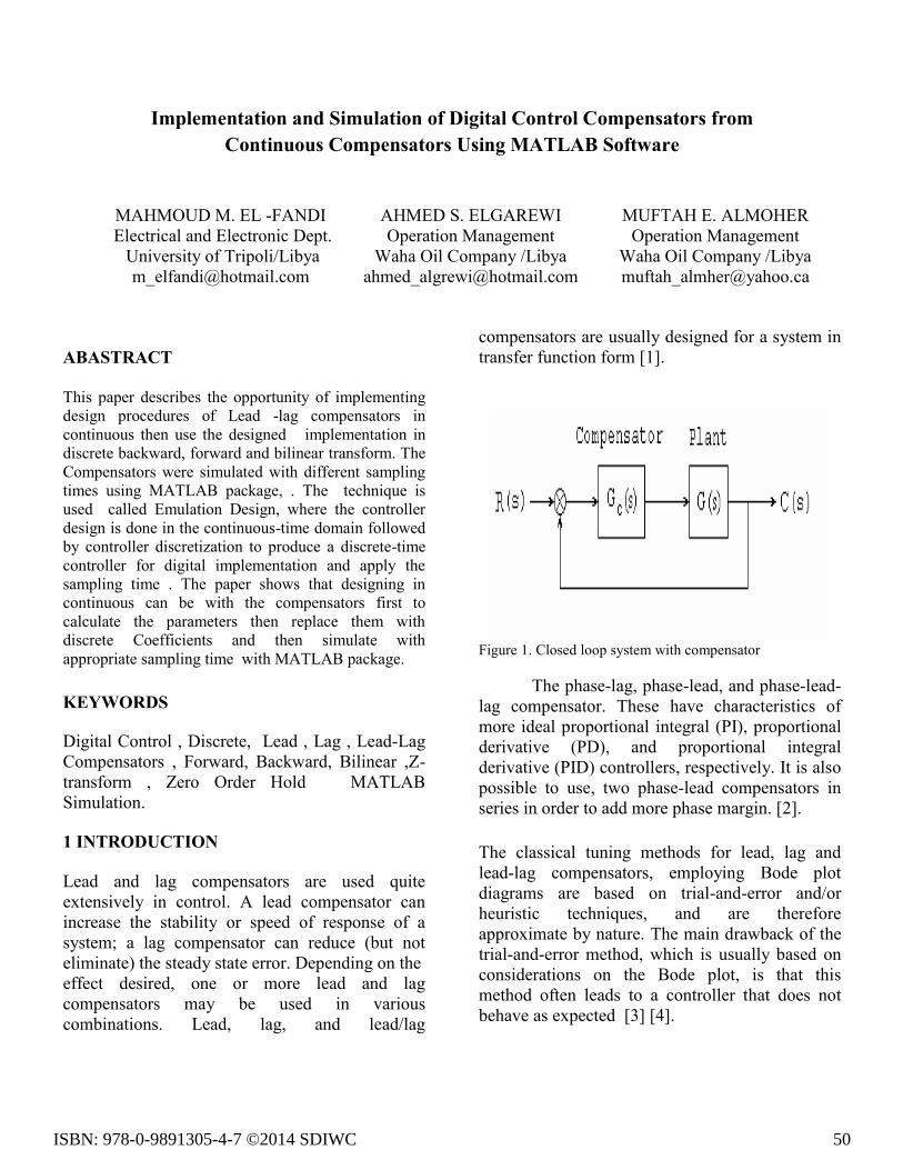
Implementation and Simulation of Digital Control Compensators from

Continuous Compensators Using MATLAB Software

MAHMOUD M. EL -FANDI

Electrical and Electronic Dept.

University of Tripoli/Libya

[email protected]

AHMED S. ELGAREWI

Operation Management

Waha Oil Company /Libya

[email protected]

MUFTAH E. ALMOHER

Operation Management

Waha Oil Company /Libya

[email protected]

ABASTRACT

This paper describes the opportunity of implementing

design procedures of Lead -lag compensators in

continuous then use the designed implementation in

discrete backward, forward and bilinear transform. The

Compensators were simulated with different sampling

times using MATLAB package, . The technique is

used called Emulation Design, where the controller

design is done in the continuous-time domain followed

by controller discretization to produce a discrete-time

controller for digital implementation and apply the

sampling time . The paper shows that designing in

continuous can be with the compensators first to

calculate the parameters then replace them with

discrete Coefficients and then simulate with

appropriate sampling time with MATLAB package.

KEYWORDS

Digital Control , Discrete, Lead , Lag , Lead-Lag

Compensators , Forward, Backward, Bilinear ,Z-

transform , Zero Order Hold MATLAB

Simulation.

1 INTRODUCTION

Lead and lag compensators are used quite

extensively in control. A lead compensator can

increase the stability or speed of response of a

system; a lag compensator can reduce (but not

eliminate) the steady state error. Depending on the

effect desired, one or more lead and lag

compensators may be used in various

combinations. Lead, lag, and lead/lag

compensators are usually designed for a system in

transfer function form [1].

Figure 1. Closed loop system with compensator

The phase-lag, phase-lead, and phase-lead-

lag compensator. These have characteristics of

more ideal proportional integral (PI), proportional

derivative (PD), and proportional integral

derivative (PID) controllers, respectively. It is also

possible to use, two phase-lead compensators in

series in order to add more phase margin. [2].

The classical tuning methods for lead, lag and

lead-lag compensators, employing Bode plot

diagrams are based on trial-and-error and/or

heuristic techniques, and are therefore

approximate by nature. The main drawback of the

trial-and-error method, which is usually based on

considerations on the Bode plot, is that this

method often leads to a controller that does not

behave as expected [3] [4].

ISBN: 978-0-9891305-4-7 ©2014 SDIWC 50

2 DISCRETE IMPLEMENTATION OF LEAD

COMPENSATO

For design lead compensator in equation (1) to

discrete using difference approximation methods

backward, forward and bilinear z-transformation

(1)

Where

β is phase lead compensator parameter

T is phase lead compensator time constant

2.1 - Lead Compensator with Backward

Approximation

Since

in Backward approximation

(2)

Where

is integration time.

(3)

Where

(4)

(5)

2.2 - Lead Compensator with Forward

Approximation

Since

in forward approximation

Where

(8)

(9)

2.3 - Lead Compensator with Bilinear

Approximation

Since

in bilinear approximation then

(10)

ISBN: 978-0-9891305-4-7 ©2014 SDIWC 51

(11)

Where

(12)

(13)

3-DISCRETE IMPLEMENTATION OF LAG

COMPENSATOR

For design lag compensator in equation (14) to

discrete using difference approximation methods

backward, forward and bilinear z-transformation

(14)

Where

α is phase lag compensator parameter

T is phase lag compensator time constant

3.1 - Lag Compensator with Backward

Approximation

Since

in Backward approximation

(15)

(16)

Where

(17)

(18)

3.2 - Lag Compensator with Forward

Approximation

Since

in forward approximation

(19)

(20)

Where

(21)

(22)

3.3 - Lag Compensator with Bilinear

Approximation

Since

in bilinear approximation

(23)

ISBN: 978-0-9891305-4-7 ©2014 SDIWC 52

(24)

Where

(25)

(26)

(27)

4-LEAD-LAG COMPENSATOR

A lead-lag compensator combines the effects of a

lead compensator with those of a lag compensator.

The result is a system with improved transient

response, stability, and steady-state error. To

implement a lead-lag compensator, first design the

lead compensator to achieve the desired transient

response and stability, and then design a lag

compensator to improve the steady-state response

of the lead-compensated system [5][6]

(28)

(29)

5-SIMULATION OF CONTINUOUS AND

DIGITAL COMPENSATORS

For digital design, after the continuous

system is designed with compensator in time

domain and the response is satisfactory, emulation

digital design take place for discretezation the

system using digital compensators, Backward,

Forward and Bilinear deference approximations,

with Zero Order Hold transform for the plant at

different sampling times in closed loop system

using MATLAB CODE

Figure 2. Continuous and digital closed loop systems with

compensators

EXAMPLE 1

For the second order system given in equation

(30).Design a compensator to meet the following

specification: overshot of 5% and steady state

error =0.02.

(30)

Figure 3. open loop unit step of equation (30)

The system as shown has large steady state error

and oscillating at high frequencies so by following

some steps compensator would by designed

First start to calculate the gain which satisfy the

steady state error using unit step response of

equation (31)

0 5 10 15 20 25 30 35 40 45 50 55 60 65 70 75 80 85 90 95 1000

0.05

0.1

0.15

0.2Step Response

Time (sec)

Am

plitu

de

ISBN: 978-0-9891305-4-7 ©2014 SDIWC 53

From the calculation the gain k=494.95

The step response in the figure below of

uncompensated system in equation (30) with gain

k to satisfy the steady state error of 0.02.

(32)

Figure 4. Closed loop response of uncompensated system

of equation (30)

5.1-LEAD DESIGN

Since the purpose of phase lead compensator

design in the frequency domain generally is to

satisfy specifications on steady-state accuracy and

phase margin. There may also be a specification

on gain crossover frequency or closed-loop

bandwidth. A phase margin specification can

represent a requirement on relative stability due to

pure time delay in the system, or it can represent

desired transient response characteristics that have

been translated from the time domain into the

frequency domain

From bode plot below the phase margin of the

uncompensated system is 0.153°.

Figure 5. Bode plot of uncompensated system of equation

(30)

The phase margin of the uncompensated system is

0.153o which cannot satisfy the value of ξ to have

overshot required. The required overshoot for

design is 5% since

From equation above to have OS=5% then ξ =0.69

Where

ξ is damping ratio

OS% is the percentage overshot

M is the phase margin required

Using equation (34) to find the phase margin

required, M =64.61o

The maximum phase shift of the compensator is:

Where 10o to 15o is a correction factor.

Using equation (35) to find β

Step Response

Time (sec)

Am

plitu

de

0 10 20 30 40 50 60 70 80 90 100 110 120 130 1400

0.2

0.4

0.6

0.8

1

1.2

1.4

1.6

1.8

2

System: sys

Final Value: 0.98

uncompensated system

10-1

100

101

102

-180

-135

-90

-45

0

Ph

ase (

deg

)

Bode DiagramGm = Inf dB (at Inf rad/sec) , Pm = 0.153 deg (at 31.8 rad/sec)

Frequency (rad/sec)

-40

-20

0

20

40

60

80

System: j

Frequency (rad/sec): 99.7

Magnitude (dB): -20

Mag

nit

ud

e (

dB

)

Uncompensated system

ISBN: 978-0-9891305-4-7 ©2014 SDIWC 54

The compensator magnitude is:

Compensator magnitude= 20 log

(36)

= 20.7dB.

At the gain crossover frequency the magnitude of

the compensator is 20.7dB, however the

magnitude of the compensated system should be 0

dB at this point so the magnitude of the

uncompensated system at this point should be

(-20.7dB.). The value of (- 20.7dB) in bode plot

figure (5) above the gain crossover frequency is

( max= 99.7 rad/sec)

To calculate the zero and pole of the compensator.

The compensator should have unity gain in order

to keep the steady state requirements as required.

(37)

The figure below shows the step response of the

compensator and the uncompensated system both

in close loop with unity feedback.

Figure 6. Step response of compensated system in

continuous

The system improved in transient characteristics

and steady state error very small .the lag

compensator is not needed for this system.

Figure 7. Bode plot of compensated and uncompensated

system equation (30)

The bode plot of figure (7) shows where the

compensator effected in the phase plot and phase

margin is 79o instead of 0.153

o.

For the digital design , after the system is

designed with lead- compensator and the response

was satisfactory, emulation digital design take

place for discretezation the system using three

approximation methods of compensators ,

Backward, Forward, Bilinear at different sampling

times in closed loop system

Figure 8. Step response of compensator in continuous,

digital forward, backward, bilinear with Z.O.H system at Ts

=0.001 sec”

Step Response

Time (sec)

Am

plitu

de

0 0.025 0.05 0.075 0.1 0.125 0.15 0.175 0.2 0.225 0.25 0.275 0.30

0.2

0.4

0.6

0.8

1

1.2

1.4

System: l3

Final Value: 0.999

System: l3

Peak amplitude: 1.08

Overshoot (%): 8.04

At time (sec): 0.0568

System: l3

Rise Time (sec): 0.0188

Compensated

Bode Diagram

Frequency (rad/sec)

10-1

100

101

102

103

104

105

-180

-135

-90

-45

0

45

Ph

ase (

deg

)

-200

-150

-100

-50

0

50

100

Mag

nit

ud

e (

dB

)

Uncompensated

Compensated

Step Response

Time (sec)

Am

plitu

de

0 0.025 0.05 0.075 0.1 0.125 0.15 0.175 0.2 0.225 0.25 0.275 0.3 0.325 0.35 0.375 0.4 0.425 0.45 0.475 0.5-0.25

0

0.25

0.5

0.75

1

1.25

1.5

1.75

2

2.25

Continuouse System

Forward Method Compensator

Backward Method Compensator

Bilinear method Compensator

ISBN: 978-0-9891305-4-7 ©2014 SDIWC 55

Figure 9. Step response of compensator in continuous,

digital forward, backward , bilinear with Z.O.H system at Ts

=0.002 sec”

As seen above, the forward and Bilinear methods

of the compensated system are sensitive to the

sampling time, at 0.001sec and 0.002 s and

identical to continuous with improvement in the

transient characteristics and steady state error ess.

For the backward method it is unstable and

compensator did not satisfy the appropriate

design

6-CONCLUSION

Discretizing the systems is very useful and

important since we can chose one of the many

digital transformations which can achieve the

needed requirements for implementations , they

are might not change the characteristics of the

system in the small sampling times in different

orders of systems , In closed loop another

parameter is added for designing which is the

sampling time Ts. The simulation of the

MATLAB package shows the forward and

Bilinear transformations systems have the same

behavior of the continuous but in backward system

is unstable at different sampling time.

7- MATLAB CODE

% Lead and Lag implementation from

Continues design to digital

implementation

% This Program is used for Lead, Lag,

and Lead-lag compensators in continuous

and digital.

% After designing all parameters needed

for each compensator, the program asks

to enter these parameters and uses step

response the system

%NOTE:

% 1- MAKE SURE TO ENTER THE ZERO AND

POLE VALUES OF THE COMPENSATORS AS

BELOW

% (s+1) the s= -1 BECAUSE OF USING (

zpk ) MATLAB command

% 2-Emulation digital design is used .

%For discrete Compensators, the program

uses the same parameters entered before

, and uses forward ,Backward or Bilinear

for the compensators .and Zero Order

Hold for the system

% 3- The sampling Time is the same for

system and the compensators

clc

s=tf('s');

fprintf('This Program is used for Lead,

Lag, and Lead-lag compensators in

continuous and digital.\n ');

%Transfer Function needed to be

transferred

H1=input('Enter Your TF Function of S :

\n')

h=figure(1);

hold;

%step(H1) %Step response of open-loop

system

Kc=input('Enter the Gain Of the TF to

Obtain the desired ess : \n')%Gain to

obtain reqiured steady state error

O=input('Choose a compensator\n 1-

Continuous Lead compensator ,\n 2-

Continuous Lag comensator ,\n3-

Continuous Lead-lag compensator\n')

if O==1

g_l=input('Enter the Gain value of

Lead Compensator : \n');

zl=input('Enter the zero value of


pl=input('Enter the pole value of


G_lead =zpk(zl,pl,g_l)

G_Fs=Kc*G_lead*H1;

GTs= feedback (G_Fs,1) %Closed Loop

System

step (GTs)

elseif O==2

g_g=input('Enter the Gain value of

Lag Compensator : \n');

zg=input('Enter the zero value of


Step Response

Time (sec)

Am

plitude

0 0.025 0.05 0.075 0.1 0.125 0.15 0.175 0.2 0.225 0.25 0.275 0.3 0.325 0.35-0.25

0

0.25

0.5

0.75

1

1.25

1.5

1.75

2

2.25

Continuous

Forward Method Compensator

Backward Method Compensator

Bilinear Method Compensator

ISBN: 978-0-9891305-4-7 ©2014 SDIWC 56

pg=input('Enter the pole value of


G_lag =zpk(zg,pg,g_g)

G_Fs=Kc*G_lag*H1;


System

step (GTs)

else

g_l=input('Enter the Gain value of


zl=input('Enter the zero value of


pl=input('Enter the pole value of


G_lead =zpk(zl,pl,g_l)

g_g=input('Enter the Gain value of


zg=input('Enter the zero value of


pg=input('Enter the pole value of


G_lag =zpk(zg,pg,g_g)

G_Fs=Kc*G_lead*G_lag*H1;


System

step (GTs)

end

T=input('\nEnter the sampling Time ');%

Sampling Time

Gz=c2d(H1,T,'zoh')

disp('The Zero Order Hold Method TF

above\n')

%step(Gz)

z=tf('z',T)

for r=1:3

O1=input('Enter the Method of

Approximation \n1-Forward Method

compensators \n2-Backward Method

compensators \n3-Bilinear Method

compensators\n4-Exite\n ');

if O1==1

disp('Now using Digital Forward Method

Approximation')

O=input('\n 1-Discrete Lead compensator

,\n2-Discrete Lag comensator ,\n3-

Discrete Lead-lag compensator')

if O==1

Gz_lead=g_l*(((z-1)/T)-zl)/(((z-

1)/T)-pl)

G_Fz=Kc*Gz_lead*Gz;

GTz= feedback (G_Fz,1) %Closed Loop

System

step (GTz)

elseif O==2

Gz_lag=g_g*(((z-1)/T)-zg)/(((z-

1)/T)-pg)

G_Fz=Kc*Gz_lag*Gz;


System

step (GTz)

else

Gz_lead=g_l*(((z-1)/T)-zl)/(((z-

1)/T)-pl)

Gz_lag=g_g*(((z-1)/T)-zg)/(((z-

1)/T)-pg)

G_Fz=Kc*Gz_lead*Gz_lead*Gz;


System

step (GTz)

end

elseif O1==2

disp('Now using Digital Backwaed Method

Approximation')

O=input('/n 1-Discrete Lead compensator

,2-Discrete Lag comensator ,3-Discrete

Lead-lag compensator')

if O==1

Gz_lead=g_l*(((z-1)/z*T)-zl)/(((z-

1)/z*T)-pl)

G_Fz=Kc*Gz_lead*Gz;


System

step (GTz)

elseif O==2

Gz_lag=g_g*(((z-1)/z*T)-zg)/(((z-

1)/z*T)-pg)

G_Fz=Kc*Gz_lag*Gz;


System

step (GTz)

else

Gz_lead=g_l*(((z-1)/z*T)-zl)/(((z-

1)/z*T)-pl)

Gz_lag=g_g*(((z-1)/z*T)-zg)/(((z-

1)/z*T)-pg)

G_Fz=Kc*Gz_lead*Gz_lead*Gz;


System

step (GTz)

end

elseif O1==3

disp('Now using Digital Bilinear Method

Approximation')

O=input('/n 1-Discrete Lead compensator

,2-Discrete Lag comensator ,3-Discrete

Lead-lag compensator')

if O==1

Gz_lead=g_l*((2*(z-1))/(T*(z+1))-

zl)/((2*(z-1))/(T*(z+1))-pl)

G_Fz=Kc*Gz_lead*Gz;


System

step (GTz)

elseif O==2

Gz_lag=g_g*((2*(z-1))/(T*(z+1))-

zg)/((2*(z-1))/(T*(z+1))-pg)

G_Fz=Kc*Gz_lag*Gz;

ISBN: 978-0-9891305-4-7 ©2014 SDIWC 57


System step (GTz) else Gz_lead=g_l*((2*(z-1))/(T*(z+1))-

zl)/((2*(z-1))/(T*(z+1))-pl) Gz_lag=g_g*((2*(z-1))/(T*(z+1))-

zg)/((2*(z-1))/(T*(z+1))-pg) G_Fz=Kc*Gz_lead*Gz_lead*Gz; GTz= feedback (G_Fz,1) %Closed Loop step (GTz) end else button = questdlg('Ready to quit?',

... 'Exit

Dialog','Yes','No','No'); switch button case 'Yes', disp('Exiting MATLAB'); %Save variables to

matlab.mat save case 'No', quit cancel; end end end

8- REFERENCES

[1] Katsuhiko Ogata, Modern Control Engineering, Prentice

Hall, Upper Saddle River, NJ, 4th edition, 2002.

[2] Moudgalya, Kannan M., Digital Control, John Wiley &

Sons, Published. Chichester, West Sussex, England;

Hoboken, NJ, USA: Wiley, c2007.

[3] Katsuhiko Ogata, Discrete-Time Control Systems,

Prentice Hall, 2nd Edition. Oxford University Press, June

1995

[4] Karl Johan °Astr¨om, Feedback Systems: An

Introduction for Scientists and Engineers, Department of

Automatic Control Lund Institute of Technology, and

Richard M. Murray, Control and Dynamical Systems,

California Institute of Technology, 2006.

[5] Partahmesh R. Vadhavkar, Mapping Controllers from s-

domain to z-domain using Magnitude inverse and Phase

inverse Methods, Bachelors of Electronic Engineering, Pune

University ,2004

[6] Les Fenical,Control Systems Technology, 1st Edition,

2006.

ISBN: 978-0-9891305-4-7 ©2014 SDIWC 58

Implementation and Simulation of Digital Control Compensators from Continuous Compensators Using...

Documents

Transcript of Implementation and Simulation of Digital Control Compensators from Continuous Compensators Using...