lable at ScienceDirect

Atmospheric Environment 45 (2011) 3078e3090

Contents lists avai

Atmospheric Environment

journal homepage: www.elsevier .com/locate/atmosenv

Impacts of emission changes on sulfate aerosols in Alaska

Trang T. Tran a, Greg Newbya, Nicole Mölders b,*

aArctic Region Supercomputing Center, PO Box 756020, Fairbanks, AK 99775, USAbUniversity of Alaska Fairbanks, College of Natural Science and Mathematics, Department of Atmospheric Sciences, 903 Koyukuk Dr., Fairbanks, AK 99775, USA

a r t i c l e i n f o

Article history:Received 20 October 2010Received in revised form23 February 2011Accepted 2 March 2011

Keywords:Long-range transportSulfate aerosolsEmissionsAlaska

* Corresponding author. Tel.: þ1 9074747910; fax:E-mail address: molders@gi.alaska.edu (N. Mölder

1352-2310/$ e see front matter � 2011 Elsevier Ltd.doi:10.1016/j.atmosenv.2011.03.013

a b s t r a c t

WRF/Chem simulations were performed using the meteorological conditions of January 2000 and alterna-tively the emissions of January 1990 and 2000 to examine whether increases in emissions may have causedthe increasing trends in observed sulfate-aerosol concentrations at coastal Alaska sites. The analysis focusedon six regions in Alaska that are exposed differently to the main emission sources. Meteorological obser-vations at 59 sites and aerosol measurements at three sites showed that WRF/Chem captured the meteo-rological situation over Alaska well and simulated the aerosol concentrations acceptably. Except for theregion adjacent to the Arctic Ocean that is influenced by local SO2-emissions, Alaska SO2 and SO4

2�-aerosoldistributions are affectedby long-range transport of SO2 fromship emissions and/or emissions inCanada andsouthern Siberia. Local changes in emissions between 1990 and 2000 are not the main cause for concen-trations changes in the six regions. The increases of SO4

2�-aerosols and SO42�-in-cloud along the Gulf of

Alaska are caused by increased ship or Canadian emissions. The study provides evidence that the increasedship and Canadian emissions during the last decades can cause increases in sulfate aerosols.

� 2011 Elsevier Ltd. All rights reserved.

1. Introduction

The long-term observations of the Interagency Monitoring ofProtected Visual Environment (IMPROVE) networks have shownnotable increases in sulfate-aerosol concentrations at coastal sitesof Alaska. On the contrary, decreases were observed at the inlandDenali National Park and Preserve site that is located between thetwo largest Alaskan cities (Mölders et al., 2011a).

Sulfate aerosols are induced into the atmosphere via biologicaldecay of dimethyl-sulphide (DMS) emitted from oceanic phyto-plankton or oxidation of sulfur dioxide (SO2) emitted in the gasphase from anthropogenic and natural sources. In Alaska, DMS-emissions and volcanic eruptions are natural sources of sulfateprecursors in the atmosphere. The number of volcanic eruptionshardly changed in the last decades (Mölders et al., in 2011a) andDMS-emissions are negligibly small in Alaska coastal waters(Thomas et al., 2010). Anthropogenic emissions occur mainly in theonly three cities and due to oil production on the North Slope. Overthe last decades, various policies reduced emissions in many areas.In some regions of Alaska, however, emissions increased due toincreased human activities. Ship emissions, for instance, on averageincreased since 1960 (Mölders et al., 2011a).

þ1 9074747379.s).

All rights reserved.

Studies on the sulfate-aerosol burden, long-range transport andthe interactions between meteorological conditions and sulfatedistributions focused on mid-latitudes or the global scale. In thenortheastern US, for instance, SO2-emissions correlate linearly withdownwind SO4

2�-concentrations (van Dutkiewicz et al., 2000). Theincreases of SO2-emissions from ships in the basin of southernCalifornia increased the SO4

2�-concentrations in the coastal areas,and at some California inland locations due to pollutant transport(Vutukuru and Dabdub, 2008). On the global scale, for instance, anychange in precipitation, cloud cover or atmospheric circulation wasfound to alter the sulfate burden (Ackerley et al., 2009).

Transport of pollutants permits the pollutants to spread overlarge areas and affect pristine regions far remote from emissionsources, even on an intercontinental scale. Long-range transport ofSO2, and SO4

2� from East Asia, for instance, contributes to the sulfurbudget in Europe; the plume of SO2 emitted in East Asia wasadvected across the North Pacific, North America and North Atlanticbefore reaching Europe (Fiedler et al., 2009). Analysis of satellite,aircraft, ground-based measurements over the North Pacific Oceanand western North America and chemical transport-model simu-lations indicated that 56% of the measured sulfate between 500and 900 hPa over British Columbia has East-Asian sources(van Donkelaar et al., 2008). In spring, anthropogenic sulfur emis-sions from East Asia increase the mean near-surface sulfateconcentrations inwestern Canada by 30% and account for 50% of theoverall regional sulfate burden between 1 and 5 km height.

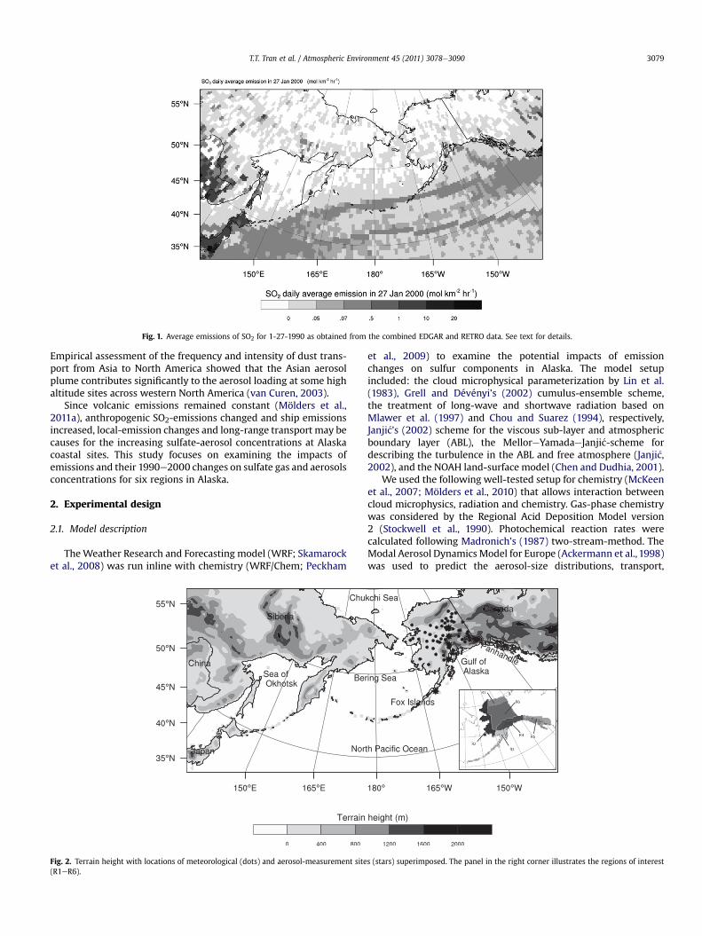
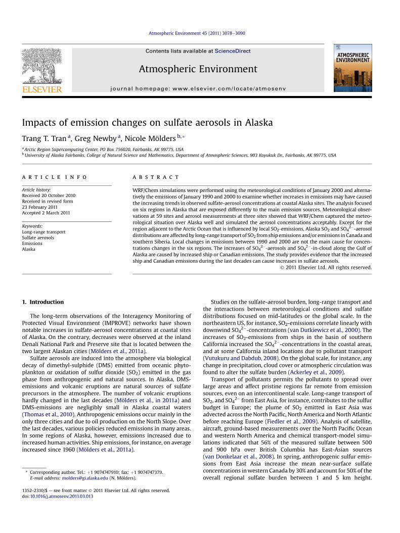
Fig. 1. Average emissions of SO2 for 1-27-1990 as obtained from the combined EDGAR and RETRO data. See text for details.

T.T. Tran et al. / Atmospheric Environment 45 (2011) 3078e3090 3079

Empirical assessment of the frequency and intensity of dust trans-port from Asia to North America showed that the Asian aerosolplume contributes significantly to the aerosol loading at some highaltitude sites across western North America (van Curen, 2003).

Since volcanic emissions remained constant (Mölders et al.,2011a), anthropogenic SO2-emissions changed and ship emissionsincreased, local-emission changes and long-range transport may becauses for the increasing sulfate-aerosol concentrations at Alaskacoastal sites. This study focuses on examining the impacts ofemissions and their 1990e2000 changes on sulfate gas and aerosolsconcentrations for six regions in Alaska.

2. Experimental design

2.1. Model description

TheWeather Research and Forecasting model (WRF; Skamarocket al., 2008) was run inline with chemistry (WRF/Chem; Peckham

Fig. 2. Terrain height with locations of meteorological (dots) and aerosol-measurement site(R1eR6).

et al., 2009) to examine the potential impacts of emissionchanges on sulfur components in Alaska. The model setupincluded: the cloud microphysical parameterization by Lin et al.(1983), Grell and Dévényi’s (2002) cumulus-ensemble scheme,the treatment of long-wave and shortwave radiation based onMlawer et al. (1997) and Chou and Suarez (1994), respectively,Janji�c’s (2002) scheme for the viscous sub-layer and atmosphericboundary layer (ABL), the MelloreYamadaeJanji�c-scheme fordescribing the turbulence in the ABL and free atmosphere (Janji�c,2002), and the NOAH land-surface model (Chen and Dudhia, 2001).

We used the following well-tested setup for chemistry (McKeenet al., 2007; Mölders et al., 2010) that allows interaction betweencloud microphysics, radiation and chemistry. Gas-phase chemistrywas considered by the Regional Acid Deposition Model version2 (Stockwell et al., 1990). Photochemical reaction rates werecalculated following Madronich’s (1987) two-stream-method. TheModal Aerosol DynamicsModel for Europe (Ackermann et al., 1998)was used to predict the aerosol-size distributions, transport,

s (stars) superimposed. The panel in the right corner illustrates the regions of interest

Fig. 3. Wind-roses for R1eR6 for January 11e31, 2000. The circles show frequency.

T.T. Tran et al. / Atmospheric Environment 45 (2011) 3078e30903080

nucleation, condensation, coagulation, dry deposition and chemicaltransformation processes including aqueous-phase reactions. Thephysical and chemical properties of secondary organic aerosolsincluding formation were simulated by the Secondary OrganicAerosol Model (Schell et al., 2001). Sulfates formed by oxidation ofSO2 in the gas phase and in the aqueous phase followed Stockwellet al. (1990) and Ackermann et al. (1998), respectively.

Dry deposition of pollutants followed Wesley (1989) with themodifications introduced by Mölders et al. (2011b). These modifi-cations include the treatment of dry deposition over snow in accordwith Zhang et al. (2003) and the lowering of the threshold at whichstomata close. In Alaska, stomata of coniferous trees are still openat �5 �C.

The background concentrations were modified to represent theconditions over the North Pacific in accord with Mölders et al.(2011b).

Table 1Mean and standard deviation, root-mean-square-error, standard deviation of error,bias and correlation for hourly averaged SLP, temperature, dew-point temperature,wind-speed (v) and direction (dir).

Quantity Simulated Observed RMSE SDE Bias R

SLP (hPa) 1005 � 16 1007 � 14 7.4 7.2 �2 0.922T (�C) �13.5 � 9.9 �13.9 � 15 11.6 11.5 0.4 0.638Td (�C) �15.9 � 10.6 �16.3 � 15.7 11.4 11.9 0.4 0.654v (m s�1) 6.0 � 3.5 1.7 � 2.6 5.7 3.7 4.3 0.295dir (�) 156 � 86 153 � 98 118.6 119.3 �3 0.166

2.2. Emissions

Biogenic emissions of isoprene, monoterpenes, and other vola-tile organic compounds from vegetation and nitrogen from soilbased on temperature and photosynthetic active radiation wereconsidered by the Model of Emissions of Gases and Aerosols fromNature (Guenther et al., 1994; Simpson et al., 1995).

We used the Emission Database for Global Atmospheric Research(EDGAR; http://www.mnp.nl/edgar/) data that comprises the annualanthropogenic emission inventories of carbon dioxide, methane,nitrous oxide, carbon monoxide, nitrogen oxide, and Non-MethaneVolatile Organic Compounds on a 1� � 1� grid. EDGAR providesinternational ship emissions, but no domestic ship emissions.

The Reanalysis of the Tropospheric (RETRO; http://retro.enes.org/data_emissions.shtml) chemical composition database providesboth monthly international and domestic ship-emission inventories

on a 1� � 1� grid, but no anthropogenic SO2-emissions. SO2-emis-sions, however, are essential for the formation of sulfate aerosols.Therefore, we merged the ship emissions of the EDGAR and RETROdata. We used the EDGAR international ship emissions and assignedthe RETRO ship-emission data to any grid-cell that has no EDGARship-emission data (Fig. 1). The emission data of EDGAR (anthropo-genic and international ship emissions) and RETRO (domestic shipemission) are annual and uniform monthly totals, respectively. Thus,the same monthly, weekly and hourly allocation functions were usedfor the EDGAR and RETRO data. Allocation functions for anthropo-genic emissions follow Mölders (2009) for Alaska, and Veldt (1991)else wise. For ship emissions, we used Wang et al.’s (2007) monthlyallocation functions for shipping in North America. Since theassumption of uniform ship-emission rates serves well in the absenceof high-temporal resolution emission datasets (Vutukuru andDabdub, 2008), we used uniform profiles for weekday/weekendand hourly variations. For a comparison of RETRO and EDGAR data seeButler et al. (2008).

2.3. Simulations

The model domain was centered at 59�N, 179�E with 30 kmspacing, 240� 120 grid points in the horizontal and 28 in the vertical

a b

c d

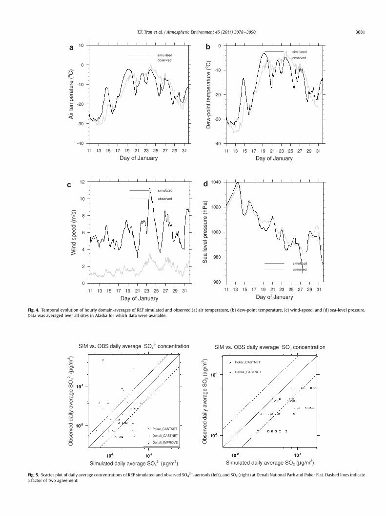
Fig. 4. Temporal evolution of hourly domain-averages of REF simulated and observed (a) air temperature, (b) dew-point temperature, (c) wind-speed, and (d) sea-level pressure.Data was averaged over all sites in Alaska for which data were available.

Fig. 5. Scatter plot of daily average concentrations of REF simulated and observed SO42�-aerosols (left), and SO2 (right) at Denali National Park and Poker Flat. Dashed lines indicate

a factor of two agreement.

T.T. Tran et al. / Atmospheric Environment 45 (2011) 3078e3090 3081

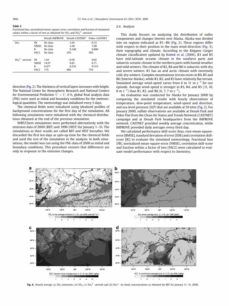
Table 2Fractional bias, normalized mean-square-error, correlation and fraction of simulatedvalues within a factor of two as obtained for SO2 and SO4

2�-aerosol.

Denali-IMPROVE Denali-CASTNET Poker-CASTNET

SO2 FB No data �1.03 �0.72NMSE No data 2.28 1.00R No data 0.348 0.800FAC2 No data 25% 50%

SO42�-aerosol FB 1.63 �0.50 0.02

NMSE 14.97 0.83 0.71R 0.477 0.232 0.315FAC2 17% 40% 75%

T.T. Tran et al. / Atmospheric Environment 45 (2011) 3078e30903082

direction (Fig. 2). The thickness of vertical layers increaseswith height.The National Center for Atmospheric Research and National Centersfor Environmental Prediction 1� � 1�, 6 h, global final analysis data(FNL) were used as initial and boundary conditions for the meteoro-logical quantities. The meteorology was initialized every 5 days.

The chemical fields were initialized using idealized profiles ofbackground concentrations for the first day of the simulation. Allfollowing simulations were initialized with the chemical distribu-tions obtained at the end of the previous simulation.

WRF/Chem simulations were performed alternatively with theemission data of 2000 (REF) and 1990 (HIST) for January 1e31. Thesimulations as their results are called REF and HIST hereafter. Wediscarded the first ten days as spin-up time for the chemical fieldsand used the rest of the simulation in the analysis. In both simu-lations, the model was run using the FNL-data of 2000 as initial andboundary conditions. This procedure ensures that differences areonly in response to the emission changes.

Fig. 6. Hourly average (a) SO2-emissions, (b) SO2, (c) SO42�-aerosol and (d) SO

2.4. Analysis

This study focuses on analyzing the distribution of sulfurcomponents and changes therein over Alaska. Alaska was dividedinto six regions indicated as R1eR6 (Fig. 2). These regions differwith respect to their position to the main wind-direction (Fig. 3),their topography and climate. According to the KöppeneGeigerclimate classification updated by Kottek et al. (2006), R3 and R5have mid-latitude oceanic climate in the southern parts andsubarctic oceanic climate in the northern parts with humidweatherandmild winters. The climate of R2, R4 and R6 is subarctic with dryand severe winters. R1 has an arid arctic climate with extremelycold, dry winters. Complexmountainous terrain exists in R4, R5 andR6 (Interior Alaska), while R1, R2, and R3 have relatively flat terrain.Simulated average wind-speed varies from 6 to 11 m s�1 for ourepisode. Average wind-speed is stronger in R3, R4, and R5 (11, 10,8 m s�1) than R1, R2, and R6 (6, 7, 7 m s�1).

An evaluation was conducted for Alaska for January 2000 bycomparing the simulated results with hourly observations oftemperature, dew-point temperature, wind-speed and direction,and sea-level pressure (SLP) that are available at 59 sites (Fig. 2). ForJanuary 2000, sulfate observations are available at Denali Park andPoker Flat from the Clean Air Status and Trends Network (CASTNET)campaign and at Denali Park headquarters from the IMPROVEnetwork. CASTNET provided weekly average concentration, whileIMPROVE provided daily averages every third day.

We calculated performance skill-score (bias, root-mean-square-error [RMSE], standard deviation of error [SDE] and correlation skill-score [R]) to evaluate the simulated meteorology. Fractional bias(FB), normalizedmean-square-error (NMSE), correlation skill-scoreand fraction within a factor of two (FAC2) were calculated to eval-uate model performance with respect to chemistry.

42�-in-cloud concentrations as obtained by REF for January 11e31, 2000.

Fig. 7. Potential temperature profiles as obtained by REF for R1eR6. The horizontal bars indicate the minimum and maximum values.

T.T. Tran et al. / Atmospheric Environment 45 (2011) 3078e3090 3083

Multi-correlation coefficients of regional average concentra-tions of SO2 or SO4

2�-aerosols versus SO2-emission or wind-speedat each grid-cell were calculated at various time-lags for R1eR6 toinvestigate the role of emissions and meteorological conditions forthe distributions of pollutants in Alaska.

We examined hourly average concentration differences (REF-HIST) of sulfur compounds to assess the impacts of emissionchanges on SO2 and SO4

2� in the gas phase, and SO42�-aerosol and

in-clouds. The discussion focuses on R1eR6, but results for otherregions are discussed where required to explain the situation in thesix regions. Student t-tests were performed to assess the agreementbetween model and observed data, and to test the hypothesis thatthe changes in Asian, Canadian and ship emissions can causechanges like those found for January by the IMPROVE network. Weused a confidence level of 95%.

We calculated the horizontal advection of SO2, SO42�-aerosol

and SO42�-in-cloud across the boundaries of each of the six regions

in and out of the regions. The advection was determined for theentire atmospheric column of each region. No vertical transportexists at the top of the model.

3. Results

3.1. Evaluation

On average over Alaska, WRF/Chem overestimates air temper-ature (T), dew-point temperature (Td) and wind-speed by 0.4 K,0.4 K, and 4.3 m s�1, respectively, while it slightly underestimatesSLP by 2 hPa (Table 1). The discrepancies in T and Td are strongest

after the passage of the cold fronts on January 13 and 16 (Fig. 4a, b,d). The temporal evolutions of T, Td, and SLP are captured acceptablyto well leading to correlation skill-scores of 0.638, 0.654, and 0.922,respectively.

According to the hourly mean values of simulated and observedwind-direction, the main wind-direction for Alaska for 1-11-2000to 1-31-2000 was south-southeast. WRF/Chem captures success-fully the overall wind-direction with a bias of 3�. However, WRF/Chem fails to capture the temporal behavior of wind-directionchanges to their full extend.

Despite an evaluation by only three sites is limited, we includedit for completeness. On average, WRF/Chem underestimates thesulfate concentrations at the Denali Park IMPROVE and Poker Flatsites, and overestimates them at the Denali Park CASTNET site;WRF/Chem overestimates SO2 at both SO2-sites (Fig. 5, Table 2). InDenali Park, 40% and 17% of the simulated concentrations fallwithin a factor of two for the CASTNET and IMPROVE observations,respectively. This different performance relates to the sites’ loca-tions. The IMPROVE site is close to a road that channels through themountains and passes a small community (Healy) with a powerplant, while the CASTNET site is in the park far away from anyanthropogenic emission sources. WRF/Chem fails to capture thechanneling of the dispersion plume from Healy to the monitoringsite because channeling through mountains is of subgrid-scale likein other mesoscale models.

WRF/Chem captures well the temporal evolution of SO2 forPoker Flat (R ¼ 0.800). Simulated and observed SO2 and sulfateconcentrations agree within a factor of two in 50 and 75% of thetime (Table 2).

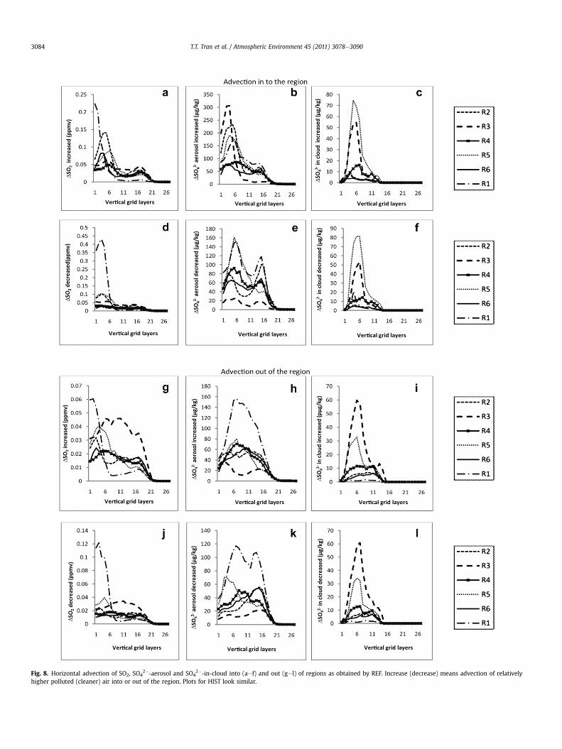
Fig. 8. Horizontal advection of SO2, SO42�-aerosol and SO4

2�-in-cloud into (aef) and out (gel) of regions as obtained by REF. Increase (decrease) means advection of relativelyhigher polluted (cleaner) air into or out of the region. Plots for HIST look similar.

T.T. Tran et al. / Atmospheric Environment 45 (2011) 3078e30903084

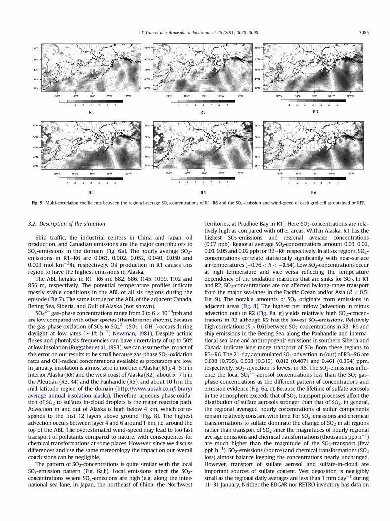
Fig. 9. Multi-correlation coefficients between the regional average SO2-concentrations of R1eR6 and the SO2-emission and wind-speed of each grid-cell as obtained by REF.

T.T. Tran et al. / Atmospheric Environment 45 (2011) 3078e3090 3085

3.2. Description of the situation

Ship traffic, the industrial centers in China and Japan, oilproduction, and Canadian emissions are the major contributors toSO2-emissions in the domain (Fig. 6a). The hourly average SO2-emissions in R1eR6 are 0.063, 0.002, 0.052, 0.040, 0.050 and0.003 mol km�2/h, respectively. Oil production in R1 causes thisregion to have the highest emissions in Alaska.

The ABL heights in R1eR6 are 682, 686, 1145, 1009, 1102 and856 m, respectively. The potential temperature profiles indicatemostly stable conditions in the ABL of all six regions during theepisode (Fig.7). The same is true for the ABL of the adjacent Canada,Bering Sea, Siberia, and Gulf of Alaska (not shown).

SO42� gas-phase concentrations range from 0 to 6� 10�4ppb and

are low compared with other species (therefore not shown), becausethe gas-phase oxidation of SO2 to SO4

2� (SO2 þ OH�) occurs duringdaylight at low rates (w1% h�1; Newman, 1981). Despite actinicfluxes and photolysis-frequencies can have uncertainty of up to 50%at low insolation (Ruggaber et al., 1993), we can assume the impact ofthis error on our results to be small because gas-phase SO2-oxidationrates and OH-radical concentrations available as precursors are low.In January, insolation is almost zero in northern Alaska (R1), 4e5 h inInterior Alaska (R6) and the west coast of Alaska (R2), about 5e7 h inthe Aleutian (R3, R4) and the Panhandle (R5), and about 10 h in themid-latitude region of the domain (http://www.absak.com/library/average-annual-insolation-alaska). Therefore, aqueous-phase oxida-tion of SO2 to sulfates in-cloud droplets is the major reaction path.Advection in and out of Alaska is high below 4 km, which corre-sponds to the first 12 layers above ground (Fig. 8). The highestadvection occurs between layer 4 and 6 around 1 km, i.e. around thetop of the ABL. The overestimated wind-speed may lead to too fasttransport of pollutants compared to nature, with consequences forchemical transformations at some places. However, since we discussdifferences and use the same meteorology the impact on our overallconclusions can be negligible.

The pattern of SO2-concentrations is quite similar with the localSO2-emission pattern (Fig. 6a,b). Local emissions affect the SO2-concentrations where SO2-emissions are high (e.g. along the inter-national sea-lane, in Japan, the northeast of China, the Northwest

Territories, at Prudhoe Bay in R1). Here SO2-concentrations are rela-tively high as compared with other areas. Within Alaska, R1 has thehighest SO2-emissions and regional average concentrations(0.07 ppb). Regional average SO2-concentrations amount 0.03, 0.02,0.03, 0.05 and 0.02 ppb for R2eR6, respectively. In all six regions, SO2-concentrations correlate statistically significantly with near-surfaceair temperatures (�0.76 < R< �0.54). Low SO2-concentrations occurat high temperature and vice versa reflecting the temperaturedependency of the oxidation reactions that are sinks for SO2. In R1and R2, SO2-concentrations are not affected by long-range transportfrom the major sea-lanes in the Pacific Ocean and/or Asia (R < 0.5;Fig. 9). The notable amounts of SO2 originate from emissions inadjacent areas (Fig. 8). The highest net inflow (advection in minusadvection out) in R2 (Fig. 8a, g) yields relatively high SO2-concen-trations in R2 although R2 has the lowest SO2-emissions. Relativelyhigh correlations (R> 0.6) between SO2-concentrations in R3eR6 andship emissions in the Bering Sea, along the Panhandle and interna-tional sea-lane and anthropogenic emissions in southern Siberia andCanada indicate long-range transport of SO2 from these regions toR3eR6. The 21-day accumulated SO2-advection in (out) of R3eR6 are0.838 (0.735), 0.568 (0.315), 0.812 (0.407) and 0.461 (0.354) ppm,respectively. SO2-advection is lowest in R6. The SO2-emissions influ-ence the local SO4

2�-aerosol concentrations less than the SO2 gas-phase concentrations as the different pattern of concentrations andemission evidence (Fig. 6a, c). Because the lifetime of sulfate aerosolsin the atmosphere exceeds that of SO2, transport processes affect thedistribution of sulfate aerosols stronger than that of SO2. In general,the regional averaged hourly concentrations of sulfur componentsremain relatively constant with time. For SO2, emissions and chemicaltransformations to sulfate dominate the change of SO2 in all regionsrather than transport of SO2 since the magnitudes of hourly regionalaverage emissions and chemical transformations (thousands ppb h�1)are much higher than the magnitude of the SO2-transport (fewppb h�1). SO2-emissions (source) and chemical transformations (SO2

loss) almost balance keeping the concentrations nearly unchanged.However, transport of sulfate aerosol and sulfate-in-cloud areimportant sources of sulfate content. Wet deposition is negligiblysmall as the regional daily averages are less than 1 mm day�1 during11e31 January. Neither the EDGAR nor RETRO inventory has data on

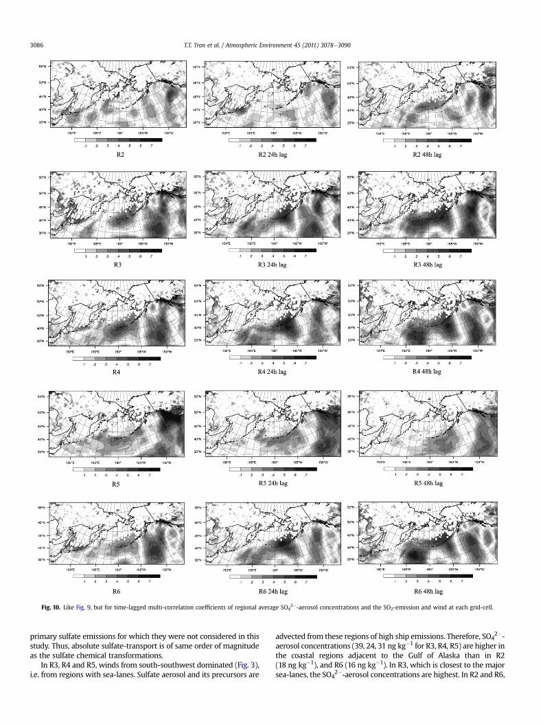
Fig. 10. Like Fig. 9, but for time-lagged multi-correlation coefficients of regional average SO42�-aerosol concentrations and the SO2-emission and wind at each grid-cell.

T.T. Tran et al. / Atmospheric Environment 45 (2011) 3078e30903086

primary sulfate emissions for which they were not considered in thisstudy. Thus, absolute sulfate-transport is of same order of magnitudeas the sulfate chemical transformations.

In R3, R4 and R5, winds from south-southwest dominated (Fig. 3),i.e. from regions with sea-lanes. Sulfate aerosol and its precursors are

advected from these regions of high ship emissions. Therefore, SO42�-

aerosol concentrations (39, 24, 31 ng kg�1 for R3, R4, R5) are higher inthe coastal regions adjacent to the Gulf of Alaska than in R2(18 ng kg�1), and R6 (16 ng kg�1). In R3, which is closest to the majorsea-lanes, the SO4

2�-aerosol concentrations are highest. In R2 and R6,

Fig. 11. Averaged differences of SO2-emissions and sulfur-compound concentrations between REF and HIST for January 11e31. Hatching indicates significant differences at the 95%confidence level.

T.T. Tran et al. / Atmospheric Environment 45 (2011) 3078e3090 3087

winds from southeast and southesoutheast, respectively, dominated,i.e. from regions with low SO2-emissions. Therefore, R2, and R6 havelower SO4

2�-aerosol concentrations than R3eR5. The relatively highSO4

2�-aerosol concentrations of R1 (24 ng kg�1) are due to high localSO2-emissions or emissions transported from the offshore oil fields atthe coast. Multi-correlation analysis (Fig. 10) shows that in R2eR6,SO4

2�-aerosol concentrations at breathing level are related to SO2from domestic ship emissions in the Bering Sea, along the Panhandle,the international sea-lanes in the Pacific Ocean and/or anthropogenicemissions in Canada (R > 0.6). The high correlations in the 1 d or2 d-time-lag indicate that SO2 from emissions outside the regions hasmore time to be transformed into sulfate before arriving in Alaska.The long transport times of the 1 d or 2 d-time-lag imply time forchemical reactions that is not available in the 0 d-time-lag. In R1, long-range transport does not affect SO4

2�-aerosol concentrations (R< 0.5at various time-lags; therefore not shown). Advection into (out) R2,R3 and R5 are high (low). Thus, the net advection increases the SO4

2�-aerosol concentration in R2, R3 and R5. On the contrary, advection outof R1 is higher than advection into R1. Advection into and out arerelatively equal for both R4 and R6. Note that R6 experiences thelowest advection of the six regions (Fig. 8b, h).

Sulfate-in-cloud concentrations (Fig. 6d) are high along themajor sea-lanes where clouds are present. The hourly regionalaverage SO4

2�-in-cloud concentrations in the regions along the Gulfof Alaska, R3eR5, are 0.48, 0.30, 0.31 ng kg�1, respectively. Theyexceed those of the inland region R6 (0.03 ng kg�1) and the coastalregions R1 (0.02 ng kg�1) and R2 (0.04 ng kg�1) that are far awayfrom high ship traffic. Advection of SO4

2�-in-cloud in/out of theregion is higher for R3, R4 and R5 than for R1, R2 and R6 (Fig. 8c, i).

Since the aqueous-phase oxidation reactions of SO2 to sulfateoccur in cloud droplets, cloud-water content affects sulfateproduction. The hourly regional vertically-averaged cloud-watercontent is 0.045 � 10�6, 0.603 � 10�6, 2.140 � 10�6, 1.679 � 10�6,2.099� 10�6, 0.302� 10�6 g m�3, respectively. Therefore, aqueous-phase oxidation reactions become more effective in R3, R4 and R5than in R1, R2 and R6.

3.3. Effects of emission changes

Compared with 1990, the SO2-emissions of 2000 increased inmost of the domain, especially along the sea-lanes, in Japan,northeast China and in some areas in Canada (Fig. 11a). Wide areasof Alaska experienced no emission changes. On regional average,accumulated anthropogenic emissions increased by 387.9,12.8, and1.7 mol km�2 in R1, R5, R6, while they decreased by 1.7, 0.5, and4.1 mol km�2 in R2, R3, and R4, respectively. R1 experienced thehighest increase in SO2-emissions due to the growth of the oilindustry in the 90s. The emissions of R2eR4 decreased due topollution-control policies implemented between 1990 and 2000.

The correlation coefficients between emission changes andconcentration changes of all sulfur components in the six regionsare approximately zero and insignificant. This indicates that local-emission changes are not the main cause for the concentrationchanges in the six regions.

In R1, SO2-emissions increased about five times whereas theaccumulated regional average of SO2-concentrations just increasedby 1.5, i.e. the increased local emissions contributed not only to SO2-increase inside, but also outside the region. In R2, SO2-emissions

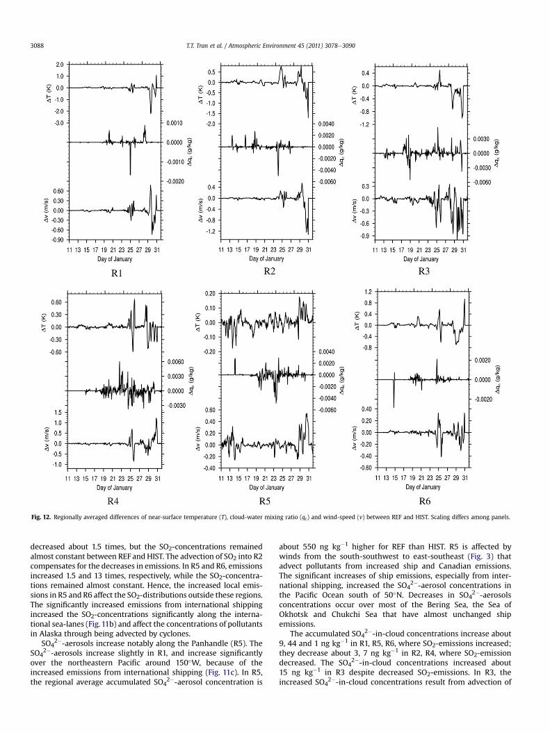
Fig. 12. Regionally averaged differences of near-surface temperature (T), cloud-water mixing ratio (qc) and wind-speed (v) between REF and HIST. Scaling differs among panels.

T.T. Tran et al. / Atmospheric Environment 45 (2011) 3078e30903088

decreased about 1.5 times, but the SO2-concentrations remainedalmost constant between REF and HIST. The advection of SO2 into R2compensates for the decreases in emissions. In R5 and R6, emissionsincreased 1.5 and 13 times, respectively, while the SO2-concentra-tions remained almost constant. Hence, the increased local emis-sions in R5 and R6 affect the SO2-distributions outside these regions.The significantly increased emissions from international shippingincreased the SO2-concentrations significantly along the interna-tional sea-lanes (Fig. 11b) and affect the concentrations of pollutantsin Alaska through being advected by cyclones.

SO42�-aerosols increase notably along the Panhandle (R5). The

SO42�-aerosols increase slightly in R1, and increase significantly

over the northeastern Pacific around 150�W, because of theincreased emissions from international shipping (Fig. 11c). In R5,the regional average accumulated SO4

2�-aerosol concentration is

about 550 ng kg�1 higher for REF than HIST. R5 is affected bywinds from the south-southwest to east-southeast (Fig. 3) thatadvect pollutants from increased ship and Canadian emissions.The significant increases of ship emissions, especially from inter-national shipping, increased the SO4

2�-aerosol concentrations inthe Pacific Ocean south of 50�N. Decreases in SO4

2�-aerosolsconcentrations occur over most of the Bering Sea, the Sea ofOkhotsk and Chukchi Sea that have almost unchanged shipemissions.

The accumulated SO42�-in-cloud concentrations increase about

9, 44 and 1 ng kg�1 in R1, R5, R6, where SO2-emissions increased;they decrease about 3, 7 ng kg�1 in R2, R4, where SO2-emissiondecreased. The SO4

2�-in-cloud concentrations increased about15 ng kg�1 in R3 despite decreased SO2-emissions. In R3, theincreased SO4

2�-in-cloud concentrations result from advection of

T.T. Tran et al. / Atmospheric Environment 45 (2011) 3078e3090 3089

polluted air with increased SO2 and/or SO42�-aerosol concentra-

tions stemming from increased international ship emissions.Since we used the same meteorology for REF and HIST, the

general pollution-distribution patterns of HIST and REF are quitesimilar (not shown). The multi-correlation analysis at various time-lags showed the same features for REF and HIST in all regions.Consequently, the regions identified in REF as main source regionsfor pollution are the main source regions in HIST too. However, inall six regions, the changed emissions altered the absoluteconcentrations. Since long-range transport hardly affects concen-trations in R1, the local-emission changes govern the concentrationchanges in R1. On the contrary, domestic and international shippingemissions and emissions in Canada and the changes therein affectR2eR6. Since R3eR5 are in the close downwind of ship emissions,these regions experience advection of stronger polluted air.Therefore, concentrations of sulfate aerosols are higher in REF thanHIST. The profiles for HIST show the same behavior as for REF withhighest advection around the top of the ABL except for marginal(<3%) changes in magnitude of 21-day accumulated amounts ofadvected pollutants (therefore not shown).

Despite REF and HIST used the same meteorological initial andboundary conditions, the cloud-water mixing ratio (qc), airtemperature and wind-speed marginally differ due to interactionbetween chemistry and physics (Fig. 12). The changes in SO4

2�-aerosol concentrations alter cloud properties, and modify temper-ature via radiative and thermal effects. Changes in wind-speedresult as secondary changes from altered interaction between cloudmicrophysics and dynamics. The highest temperature changes (upto �1 K) occur in R3 and R6. In R2, R3 and R4, wind-speed changesup to �1 m s�1 and exceeds the changes in R1, R5 and R6 (up to�0.6 m s�1). In R3, R4, and R5, cloud-water mixing ratios change upto �0.006 g kg�1, where the changes of SO4

2�-in-cloud concentra-tions are high. In R1, R2 and R6, changes of SO4

2�-in-cloudconcentrations are smaller than those in R3eR5.

4. Conclusions

WRF/Chem simulations were performed using the same mete-orological initial and boundary conditions of January 2000, butalternatively the emissions of 2000 (REF) and 1990 (HIST) toinvestigate whether emission changes may be the cause for theobserved changes in SO2 and SO4

2�-aerosol concentrations inAlaska. The analysis focused on the sulfur compounds in six regionsof Alaska (Fig. 3) that differ from each other with respect to theirposition to the main wind-direction, their topography and climate.

WRF/Chem captures well the temporal evolution of the mete-orological situation in Alaska. Here WRF/Chem, on average, over-estimates temperature, dew-point temperature and wind-speed,while it slightly underestimates SLP. The few available observationsof SO2 and sulfate aerosols suggest that WRF/Chem underestimatesSO2-concentrations and overestimates SO4

2�-aerosol concentra-tions. Performance is worst where WRF/Chem fails to capture thedispersion of pollutants in extremely complex mountainousterrain. WRF/Chem simulates the SO2 and sulfate concentrationswell at Poker Flat with 50 and 75% of the values being withina factor of two of the observations.

In all six regions, SO2-concentrations correlate strongly, nega-tively with temperature due to the temperature-dependent oxida-tion reactions that are the sinks for SO2. In R1, local SO2-emissionsgovern the SO2-concentrations. Here and in R2, long-range trans-port does not affect the SO2-concentrations. In the other regions,SO2-distributions are associated with advection from the sea-lanesor Canada. Due to the longer lifetime than SO2, SO4

2�-aerosols areless sensitive to local emissions than to long-range transport. Beingdownwind of the sea-lanes and the Canadian emissions, R3, R4 and

R5 have higher SO42�-aerosol and SO4

2�-in-cloud concentrationsthan R1, R2 and R6. In R2eR6, SO4

2�-aerosols are associated withemissions from domestic and international shipping or Canada.

Our analysis showed that local-emission changes between 1990and 2000 are not the main cause for the observed concentrationchanges in Alaska. The significantly increased emissions frominternational shipping increased significantly the SO2-concentra-tions along the sea-lanes. The notable increase of SO4

2�-aerosolconcentrations in R5 results from advection of stronger polluted airfrom the international sea-lanes and Canada where the emissionsincreased between 1990 and 2000. In R3, the increase of SO4

2�-in-cloud concentrations stems from advection of air with increasedSO2 and/or SO4

2�-aerosol concentrations from the sea-lanes.The changes in SO4

2�-aerosol concentrations in response to theemission changes caused marginal, insignificant changes in themeteorological conditions between REF and HIST via radiative,thermal and cloud microphysical effects. This means that thealtered emissions hardly affect climate. We conclude that theincreasing trends in sulfate aerosols observed at some Alaskamonitoring sites can be explained by the changes in ship emissionsand emissions in Canada during the last decades.

Acknowledgments

We thank C.F. Cahill, G. Kramm, H.N.Q. Tran and the anonymousreviewers for fruitful discussion. This research was in part sup-ported by a grant of HPC resources from the Arctic Region Super-computing Center at the University of Alaska Fairbanks as part ofthe Department of Defense High Performance ComputingModernization Program.

References

Ackerley, D., Highwood, E.J., Frame, D.J., Booth, B.B.B., 2009. Changes in the globalsulfate burden due to perturbations in global CO2 concentrations. Amer. Meteor.Soc. 22, 5421e5432.

Ackermann, I.J., Hass, H., Memmesheimer, M., Ebel, A., Binkowski, F.S., Shankar, U.,1998. Modal aerosol dynamics model for Europe: development and firstapplications. Atmos. Environ. 32, 2981e2999.

Butler, T.M., Lawrence, M.G., Gurjar, B.R., van Aardenne, J., Schultz, M., Lelieveld, J.,2008. The representation of emissions from megacities in global emissioninventories. Atmos. Environ. 42, 703e719.

Chen, F., Dudhia, J., 2001. Coupling an advanced land-surface/hydrology model withthe Penn State/NCAR MM5 modeling system. Part I: model description andimplementation. Mon. Wea. Rev. 129, 569e585.

Chou, M.-D., Suarez, M.J., 1994. An efficient thermal infrared radiation parameter-ization for use in General Circulation Models, NASA Tech. Memo. 104606, 85 pp.

Fiedler, V., Arnold, F., Schlager, H., Dornbrack, A., Pirjola, L., Stohl, A., 2009. EastAsian SO2 pollution plume over Europe e part 2: evolution and potentialimpact. Atmos. Chem. Phys. 9, 4729e4745.

Grell, G.A., Dévényi, D., 2002. A generalized approach to parameterizing convectioncombining ensemble and data assimilation techniques. Geophys. Res. Lett. 29,1693. doi:10.1029/2002GL015311.

Guenther, A., Hewitt, C., Erickson, D., Fall, R., Geron, C., Graedel, T., Harley, P., Klinger, L.,Lerdau, M., McKay,W., Pierce, T., Zimmerman, P.R., 1994. A global model of naturalvolatile organic compound emissions. J. Geophys. Res. 100D, 8873e8892.

Janji�c, Z.I., 2002. Nonsingular implementation of the MelloreYamada level 2.5scheme in the NCEP Meso Model, NCEP Office Note. 437, 61 pp.

Kottek,M.,Grieser, J.,Beck,C.,Rudolf,B.,Rubel, F.,2006.Worldmapof theKöppeneGeigerclimate classification updated. Meteorol. Z. 15, 259e263.

Lin, Y.-L., Rarley, R.D., Orville, H.D., 1983. Bulk parameterization of the snow field ina cloud model. J. Appl. Meteor. 22, 1065e1092.

Madronich, S., 1987. Photodissociation in the atmosphere, 1, actinic flux and theeffects of ground reflections and clouds. J. Geophys. Res. 92, 9740e9752.

McKeen, S.A., Chung, S.H., Wilczak, J., Grell, G.A., Djalalova, I., Peckham, S., Gong, W.,Bouchet, V., Moffet, R., Tang, Y., Carmichael, G.R., Mathur, R., Yu, S., 2007. Theevaluationof several PM2.5 forecastmodelsusingdata collectedduring the ICARTT/NEAQS 2004 field study. J. Geophys. Res. 112, D10S20. doi:10.1029/2006JD007608.

Mlawer, E.J., Taubman, S.J., Brown, P.D., Iacono, M.J., Clough, S.A., 1997. Radiativetransfer for inhomogeneous atmospheres: RRTM, a validated correlated-kmodel for the longwave. J. Geophys. Res. 102D, 16663e16682.

Mölders, N., Porter, S.E., Cahill, C.F., Grell, G.A., 2010. Influence of ship emissions onair quality and input of contaminants in southern Alaska National Parks andwilderness areas during the 2006 tourist season. Atmos. Environ. 44,1400e1413.

T.T. Tran et al. / Atmospheric Environment 45 (2011) 3078e30903090

Mölders, N., Porter, S.E., Tran, T.T., Cahill, C.F., Mathis, J., Newby, G.B., 2011a. Theeffect of unregulated ship emissions for aerosol and sulfur-dioxide concentra-tions in southwestern Alaska. In: Criddle, K., Eicken, H., Lovecraft, A., Metzger, A.(Eds.), North by 2020: Perspectives on a Changing North. Alaska UniversityPress, Fairbanks, 14 p.

Mölders, N., Tran, H.N.Q., Quinn, P., Sassen, K., Shaw, G.E, Kramm, G., 2011b. Assess-ment of WRF/Chem to capture sub-Arctic boundary layer characteristics duringlowsolar irradiation using radiosonde, SODAR, and station data. Atmos. Poll. Res..

Mölders, N., 2009. Alaska Emission Model (AkEM) Description Internal Report,Fairbanks, 10 p.

Newman, L., 1981. Atmospheric oxidation of sulfur dioxide: a review as viewed frompower plant and smelter plume studies. Atmos. Environ. 15, 2231e2239.

Peckham, S.E., Fast, J.D., Schmitz, R., Grell, G.A., Gustafson, W.I., McKeen, S.A.,Ghan, S.J., Zaveri, R., Easter, R.C., Barnard, J., Chapman, E., Salzmann, M.,Wiedinmyer, C., Freitas, S.R., 2009. WRF/Chem Version 3.1 User’s Guide. 78 p.

Ruggaber, A., Forkel, R., Dlugi, R., 1993. Spectral actinic flux and its ratio to spectralirradiance by radiation transfer calculations. J. Geophys. Res. 98, 1151e1162.

Schell, B., Ackermann, I.J., Hass, H., Binkowski, F.S., Ebel, A., 2001. Modeling theformation of secondary organic aerosol within a comprehensive air qualitymodel system. J. Geophys. Res. 106, 28275e28293.

Simpson, D., Guenther, A., Hewitt, C.N., Steinbrecher, R., 1995. Biogenic emissions inEurope 1. Estimates and uncertainties. J. Geophys. Res. 100D, 22875e22890.

Skamarock, W.C., Klemp, J.B., Dudhia, J., Gill, D.O., Barker, D.M., Duda, M.G.,Huang, X.-Y., Wang, W., Powers, J.G., 2008. A description of the AdvancedResearch WRF Version 3. NCAR/TN. 125 p.

Stockwell, W.R., Middleton, P., Chang, J.S., Tang, X., 1990. The second-generationregional acid deposition model chemical mechanism for regional air qualitymodeling. J. Geophys. Res. 95, 16343e16367.

Thomas, M.A., Suntharalingam, P., Pozzoli, L., Rast, S., Devasthale, A., Kloster, S.,Feichter, J., Lenton, T.M., 2010. Quantification of DMS aerosolecloudeclimateinteractions using ECHAM5-HAMMOZ model in current climate scenario.Atmos. Chem. Phys. 10, 3087e3127.

van Curen, R.A., 2003. Asian aerosols in North America: extracting the chemicalcomposition and mass concentration of the Asian continental aerosol plumefrom long-term aerosol records in the western United States. J. Geophys. Res.108, 4623e4639.

van Donkelaar, A., Martin, R.V., Leaitch, W.R., Macdonald, A.M., Walker, T.W.,Streets, D.G., Zhang, Q., Dunlea, E.J., Jimenez, J.L., Dibb, J.E., Huey, L.G.,Weber, R., Andreae, N.O., 2008. Analysis of aircraft and satellite measure-ments from the Intercontinental Chemical Transport Experiment (INTEX-B) toquantify long-range transport of East Asian sulfur to Canada. Atmos. Chem.Phys. 8, 2999e3014.

van Dutkiewicz, V.A., Das, M., Husain, L., 2000. The relationship between regionalSO2 emissions and downwind aerosol sulfate concentrations in the north-eastern US. Atmos. Environ. 34, 1821e1832.

Veldt, C., 1991. Emissions of SOx, NOx, VOC and CO from East European countries.Atmos. Environ. 25A, 2683e2700.

Vutukuru, S., Dabdub, D., 2008. Modeling the effects of ship emissions on coastal airquality: a case study of southern California. Atmos. Environ 42, 3751e3764.

Wang, C., Firestone, J., Corbett, J.J., 2007. Modeling energy use and emissions fromNorth American shipping: application of the ship traffic, energy, and environ-ment model. Environ. Sci. Technol. 41, 3226e3232.

Wesely, M.L., 1989. Parameterization of surface resistances to gaseous dry deposi-tion in regional-scale numerical models. Atmos. Environ. 23, 1293e1304.

Zhang, L., Brook, J.R., Vet, R., 2003. A revised parameterization for gaseous drydeposition in air-quality models. Atmos. Chem. Phys. 3, 2067e2082.