Impact of switching production to bioenergy crops: The switchgrass example

Impact of Switching Production to Bioenergy

Crops: The Switchgrass Example

Scott McDonald University of Sheffield

Sherman Robinson University of Sussex

and

Karen Thierfelder

U.S. Naval Academy *

Abstract This paper reports the results from simulations that evaluate the general equilibrium effects of substituting switchgrass, a biomass, for crude oil in USA petroleum production. The new production process is less efficient and USA GDP declines slightly. As switchgrass production expands, USA agriculture contracts and the world price of cereals increases. The world price of crude oil falls as USA import demand declines. The net effect of the price and income changes is a general decline in economic welfare. Moreover, the declines in welfare are proportionately greater for developing countries who produce small quantities of agricultural commodities whose prices increase.

Keywords: Biomass; Energy; Computable General Equilibrium; US agricultural policy.

JEL classification: Q42; Q43; D58; Q18. *Address for correspondence: Karen Thierfelder, Economics Department, U.S. Naval Academy, 589 McNair,Rd., Annapolis, MD 21402, USA. Email: [email protected]: (410) 293-6887 (direct line) or (410) 293-6899 (fax). The authors are grateful for helpful comments from Michael Taylor of Resources for the Future, Washington and for funding from the Global Affairs Program of the Hewlett Foundation. The authors are solely responsible for the content of this paper.

1

mailto:[email protected]

Introduction

The last 20 years has witnessed a growing level of concern about the role of carbon emissions

from the use of fossil fuels and the consequent implications for global warming. While there

remain doubts about the conclusiveness of the evidence linking fossil fuel use to global

warming, a broadly based consensus has emerged that the level of global use of fossil fuels is

dangerously high. The most visible manifestation of this consensus is the Kyoto agreement.

The analysis reported in this paper evaluates the effects of substituting a biomass product, in

this case switchgrass, for crude oil in the production of petroleum in the USA. Specifically the

analyses focus upon the global general equilibrium implications; this is achieved by using a

multi-region computable general equilibrium (CGE) model with detailed commodity markets.

If the USA adopts a policy of encouraging the substitution of crude oil by biomass

products this may have substantial effects upon the agricultural industry since an expansion of

switchgrass production will affect other agricultural sectors in the economy through factor

market, particularly land, linkages. Programs that expand biomass production may allow the

USA to adopt agricultural policies that provide support for farmers through avenues that

introduce a lower level of distortion to global agricultural markets. Indeed, since the USA is a

major exporter of agricultural commodities, an increase in biomass (e.g. switchgrass)

production may also involve a reduction in the production of traded agricultural commodities

that will affect global agricultural markets. Of particular interest are the implications for

developing countries that have arguably been most adversely affected by the agricultural

support policies of developed market economies.

A priori it might be expected that the withdrawal of land from conventional agricultural

production for use in biomass production would have beneficial effects upon developing

countries; provided it allows a reduction in agricultural support in the USA. Specifically a

reduction in the land area in the USA used for conventional agricultural production might be

expected to contribute to an increase in agricultural commodity prices, and thereby to welfare

gains in developing countries. However, substituting biomass for crude oil will have direct

effects on the market for crude oil, and may have indirect effects on the global markets for

agricultural products. It is this interaction between the markets for agricultural commodities

and crude oil upon which the analyses reported in this paper focus. The results indicate that

the general equilibrium effects realised through the crude oil market are substantial and that

2

they are typically sufficiently large as to overwhelm the initially positive price effects for

agricultural producers. But the welfare measures of gains and losses are based on changes in

household expenditures and therefore do not include the potential environmental gains from

reduction in global use of crude oil; rather they are indicative of the economic costs of

substitution crude oil with biomass.

The rest of the paper is organised as follows. The next section reviews the Global Trade

Analysis Project (GTAP) database used for this study and provides a series of descriptive

statistics that describe many of the key economic relationships. This is followed by a general

description of the global CGE model used to carry out the analyses, and then by an analysis

section that details the policy simulations carried out and summarises the main results. The

main body of the paper ends with a series of concluding comments. The paper also contains

an appendix that provides additional information about the data.

Database

The database used for these analyses is a Social Accounting Matrix (SAM) representation of

the Global Trade Analysis Project (GTAP) database version 5.4 (see McDonald and

Thierfelder, 2004a, for a detailed description of the core database). The GTA project produces

the most complete and widely available database for use in global computable general

equilibrium (CGE) modeling; indeed the GTAP database has become generally accepted as

the preferred database for global trade policy analysis and is used by nearly all the major

international institutions and many national governments. Hertel (1997) provides an

introduction to both the GTAP database and its companion CGE model1.

The precise version of the database used as the starting point for this study is a reduced

form global SAM representation of the GTAP data developed (McDonald and Thierfelder,

2004b, for a detailed description of the process and discussion of the advantages of using a

reduced form).

1 While Hertel (1997) remains the best single source for general descriptions of the GTAP database and

model it is now quite dated; for up to date descriptions of the database and the GTAP model it is necessary study a number of technical documents available from the GTAP web site.

3

Aggregation of the Global GTAP SAM

Global CGE models typically use aggregations of the GTAP database that reduce the number

of sectors and/or regions and/or factors. There are two key reasons for using aggregations;

first, they allow the modeller to focus upon the sectors and regions that are of particular

concern to the study in hand, and second, they ensure that the model has dimensions that are

amenable to the derivation of practical solution2. In this case the objective of the study

dictated the approach to aggregation: it was necessary to retain enough detail on agriculture

and food production to capture the effects upon food and agriculture while keeping enough

detail elsewhere to identify other effects – in particular it is necessary to have both crude oil

and petroleum sectors to capture the substitution effects of increasing the use of switchgrass

as a crude oil substitute. Furthermore so as to provide some insights into the potential range

of effects upon other sectors and regions it was necessary to keep enough sectoral detail

elsewhere in the model. The sectors in the model are identified in the first two columns of

Table 1, while the mappings from the GTAP database are reported in Appendix 1.

A similar rationale was applied to the choice of regional aggregation. The concern in

the study with the impact of an internal policy shift in the USA upon, particularly, developing

countries required the separate identification of the USA and several key developing country

regions – southern Africa, northern Africa, south Asia, east Asia – while maintaining a

balanced coverage of the world’s major economies. The regions in the model are identified in

the last two columns of Table 1, while the mappings from the GTAP database are reported in

Appendix 1.

Additions to the Database

The GTAP database does not record switchgrass as a separate commodity/activity account,

rather switchgrass is part of a larger aggregate that includes cereals and other similar field

crops. Since switchgrass is not traded and it is not envisaged that switchgrass production and

use will change elsewhere, there are no direct linkages with respect to switchgrass between

the regions in the model. All the inter-regional effects will be indirect—as switchgrass

production in the USA expands, it draws land from other agricultural sectors which contract.

2 In practice as the degree of aggregation decreases so the model size increases at an approximately

exponential rate.

4

These production changes affect trade and therefore other regions. Therefore, for purposes of

these analyses it is only necessary to add switchgrass commodity and activity accounts to the

SAM for the USA.

Since switchgrass is a member of the graminae family and is harvested only once per

year its input mix is similar to that of other cereal crops. However it is a perennial and

therefore only requires periodic planting and reduced usage of intermediate inputs. Based on

information in microeconomic studies, and in the absence of better information, it was

assumed that the primary input coefficients were the same as those for other US cereals and

that the intermediate input coefficients were 70 percent of those for cereals in the USA. All

output was assumed to be purchased as an intermediate input by the petroleum activity.

Descriptive Statistics

An overview of the database used in the study can be obtained by a brief review of some

descriptive statistics. Gross Domestic Product (GDP), from the values added side, indicates

the relative size of the regions in the global economy (see Figure 1). The USA, the EU and

Japan and Korea are by far the largest regions, both in terms of total GDP and GDP per

capita, moreover these three regions dominate global trade accounting for 60 percent and 61.5

percent of global imports and exports respectively (see Figure 2). Similar dominances by

these three regions are found for trade in cereals (58 and 53 percent of global exports and

imports, Figure 3), other crops (41 and 65 percent of global exports and imports, Figure 4)

and livestock (47 and 67 percent of global exports and imports, Figure 5). For crude oil

however the situation is very different, while these regions dominate import demand, 71

percent of global demand, they are responsible for only a small share of exports, 6 percent

(see Figure 6). When the other developed economies, Australia and New Zealand, Rest of

Europe and Rest of America are taken into account the extent of the dominance of world GDP

and trade is still more pronounced.

Combined the middle income regions, China, east Asia, south America and the rest of

the world, account for about 17 percent of global GDP, but are relatively slightly more open

to trade than the developed regions since they account for 23 percent of global import demand

and 22 percent of global export supply. The situation for agricultural commodity trade is

slightly more pronounced with trade in cereals (20 and 28 percent of global exports and

imports, Figure 3), other crops (31 and 19 percent of global exports and imports, Figure 4)

5

and livestock (21 and 22 percent of global exports and imports, Figure 5) demonstrating, on

average, a slightly greater degree of openness than found for the three economically largest

regions. For crude oil however the situation is very different, while these regions dominate

export supply, 62 percent of global supply, while only accounting for 17 percent of global

import demand (see Figure 6).

Consequently the developing country regions, southern Africa, northern Africa and

south Asia, are responsible for small proportions of global GDP, 3.7 percent, and global

import demand, 4 percent, and export supply, 3.4 percent. Their involvement in agricultural

commodity trade is equally small, with trade in cereals (2.7 and 9.7 percent of global exports

and imports, Figure 3), other crops (14.3 and 4 percent of global exports and imports, Figure

4) and livestock (3.3 and 2.2 percent of global exports and imports, Figure 5) demonstrating a

relatively high degrees of dependence on cereals imports and other crop exports. They are

also relatively substantial exporters of crude oil, 14.4 percent of global exports, but are less

prominent as importers, 4.2 percent of global imports (see Figure 6).

The differentials in the stage of development of the developed, middle income and

developing regions is also well illustrated by the relative importance of agricultural and food

commodities to these groups of regions (see Figure 7). In general terms there is an inverse

relationship between the state of development of regions and the production shares accounted

for by agricultural and food commodities. What is most noticeable however are the large

production shares for agricultural commodities in south Asia and the substantially lower

shares for the two African regions; indeed in southern Africa cereals production accounts for

a smaller share of total commodity production than found in most middle income regions.

Most importantly it emerges that developing regions are net importers of cereals and net

exporters of other crops.

The USA, the EU, and Japan and Korea are the three largest oil importing regions (see

Figure 6). More importantly from this perspective of this study is the extent to which the USA

imports crude oil from all regions in the model, with 30 percent coming from the Rest of

Americas (primarily from Mexico), 21 percent from the Rest of the World, and 20 percent

from South America (primarily from Venezuela), see Figure 8. This contrasts with the other

large oil importing regions whose sources of supply are less diversified.

6

Crude oil imports account for less than ten percent of total imports for all regions in the

model. The region Japan and Korea has the highest share of crude oil in total imports (7.4

percent); crude oil imports are also important for South Asia (7.1 percent of total imports).

For the USA, crude oil imports are 5.7 percent of total imports (see Table 2).

Since production and trade changes in the USA affect other regions in the model, it is

important to note which regions are heavily dependent on USA imports. The USA is the most

important import source for the Rest of the Americas, which gets 60 percent of its imports

from the USA. Other regions heavily dependent on the USA include South America (24.6

percent) and Japan and Korea (21 percent). Areas that are less dependent on the USA include

the EU (10.2 percent), South Asia (10 percent), and the rest of Europe (6.9 percent, see Table

2).

The MRT-Globe Model3

This model is a member of the class of computable general equilibrium (CGE) models that

are descendants of the approach to CGE modeling described by Dervis et al., (1982). The

implementation of this model, using the GAMS (General Algebraic Modeling System)

software, is a direct descendant and development of the single country models devised in the

late 1980s and early 1990s, particularly those models reported by Robinson et al., (1990),

Kilkenny (1991) and Devarajan et al., (1990), and the multi-country model developed by

Robinson and co-workers to analyse NAFTA in the early 1990s (see Lewis et al., 1995, for a

later application).

The model is a SAM based CGE model, wherein the SAM serves to identify the agents

in the economy and provides the database with which the model is calibrated. Since the model

is SAM based it contains the important assumption of the law of one price, i.e., prices are

common across the rows of the SAM. The SAM also serves an important organisational role

since the groups of agents identified by the SAM structure are also used to define sub-

matrices of the SAM for which behavioural relationships need to be defined. As such the

modeling approach has been influenced by Pyatt’s ‘SAM Approach to Modeling’ (Pyatt,

1987).

3 The description of the model provided here short and intended only to provide brief overview of the

model’s structure and operation. A detailed description is available in McDonald et al., (2005).

7

Trade

Trade is modeled using a treatment derived from the Armington ‘insight’; namely

domestically produced and consumed commodities are assumed to be imperfect substitutes

for both imports and exports. Import demand is modeled via series of nested constant

elasticity of substitution (CES) functions; imported commodities from different source

regions are assumed to be imperfect substitutes for each other and are aggregated to form

composite import commodities that are assumed to be imperfect substitutes for their

counterpart domestic commodities The composite imported commodities and their

counterpart domestic commodities are then combined to produce composite consumption

commodities. These are the commodities demanded by domestic agents as intermediate inputs

and for final demand by households, the government, and for investment.

Export supply is modeled via series of nested constant elasticity of transformation

(CET) functions; the composite export commodities are assumed to be imperfect ‘substitutes’

for domestically consumed commodities, while the exported commodities from a source

region to different destination regions are assumed to be imperfect ‘substitutes’ for each

other. The composite exported commodities and their counterpart domestic commodities are

then combined to produce composite production commodities. The properties of models using

the Armington ‘insight’ are well known (see de Melo and Robinson, 1989; Deverajan et al.,

1990), but it is worth noting here that this model differs from the GTAP model through the

use of CET functions for export supply; this ensures that domestic producers will adjust their

export supply decision in response to changes the relative prices of exports and domestic

commodities, which help to moderate the magnitude of the terms of trade effects in this class

of model.4

Production

The production structure is a two stage nest. Intermediate inputs are used in fixed proportions

per unit of output– Leontief technology. Primary inputs are combined as imperfect

substitutes, according to a CES function, to produce value added.

4 The terms of trade effects will prove to be important determinants of the results produced by the

simulations reported below.

8

In the current context it is useful to examine how changes in the use of switchgrass are

introduced to the production system. If the use of switchgrass as an input to the petroleum

producing industry increases at the ‘expense’ of crude oil the technology change can be

represented as an increase in the intermediate input coefficient for switchgrass and reduction

in the intermediate input coefficient for crude oil. Since the coefficients represent the

quantities of intermediate inputs used, on average, to produce a unit quantity of output it is

also necessary to determine the ratio by which switchgrass use must increase to achieve a unit

reduction in crude oil use. This is done in the simulations.

Final Consumption

Final demand by the government and for investment is modeled under the assumption that the

relative quantities of each commodity demand by these two institutions is fixed – this reflects

the absence of a clear theory that defines an appropriate behavioural response by these agents

to changes in relative prices. For the household there is however a well developed

behavioural theory; hence the model contains the assumption that households are utility

maximisers who respond to changes in relative prices and their incomes. In this version of the

model the utility functions for the private households are assumed to be Cobb-Douglas; this

has the advantage that with a standard, neoclassical, set of closure rules that changes in

household consumption expenditure can be interpreted as equivalent variations in welfare,

and hence provides a useful summary measure of the welfare effects of the policy

simulations.5

Analyses

Model Closure Rules

The closure rules adopted for these simulations are relatively straightforward. The foreign

exchange markets are cleared under the assumption that balances on the current accounts are

constant and the exchange rates adjust. This is a common specification in real trade models. It

is assumed that any changes in the trade balance are determined by macroeconomic forces

working mostly in asset markets which are not included in the model. The model is

investment driven with household savings rates flexible so as to maintain a constant level of

5 The closure rules are: consumer price index numéraire, fixed current account, flexible exchange rate,

fixed household savings rates and fixed tax rates.

9

investment; this ensure that adjustments to a new equilibrium do not take place through

changes in the volumes of investment. All the tax rates are fixed with constant government

spending and flexible government savings. The factor market closure is long run; all factors

are assumed to be fully employed and fully mobile across all sectors but are immobile across

regions. In the sensitivity analyses, the case of an endogenous supply of land at a constant

price is evaluated.

Policy Simulations

The policy change simulated in the model is the substitution of crude oil by switchgrass in the

technology of the petroleum activity. Clearly a wide range of degrees of input substitution

may be technologically feasible, although the realistic range of alternatives is likely to be

much more limited. The changes in the area of land used for switchgrass production and the

use of crude oil by the petroleum activity considered in this study are those implied by the

partial equilibrium studies into the use of switchgrass as a crude oil substitute (see De La

Torre Ugarte and Hellwinckel, 2004a and b); these studies indicate that if some 6 percent of

USA agricultural land were changed to switchgrass production there would be a reduction of

some 4 percent in the use of crude oil by the petroleum activity.6 The model is ‘calibrated’ to

achieve these targets by the derivation of a conversion factor this ensures that the increase in

land used for switchgrass and the reduction in the direct use of crude oil are consistent with

the changes derived from partial equilibrium studies.

The policy simulations are carried out in four stages so that the different effects of the

proposed policy change can be separated out:

1. Direct substitution of Crude Oil by Switchgrass – this involves a reduction in the

input-output coefficients for crude oil use by the petroleum activity and an equal

increase in the coefficient for switchgrass; this one-to-one substitution amounts

to an assumption that one unit of switchgrass substitutes for one unit of crude

oil. This simulation is called ‘One-to-One’ in the subsequent text.

2. Derivation of Switchgrass Conversion Factor – the first simulation produces

results where the land area in switchgrass is substantially less than indicated by

the partial equilibrium studies; this simulation produces an estimate of the units

6 Since a partial equilibrium model will not capture the multiplier effects the simulations in this study

assume that 4 percent is the target reduction in the use of crude oil per unit output of the petroleum activity.

10

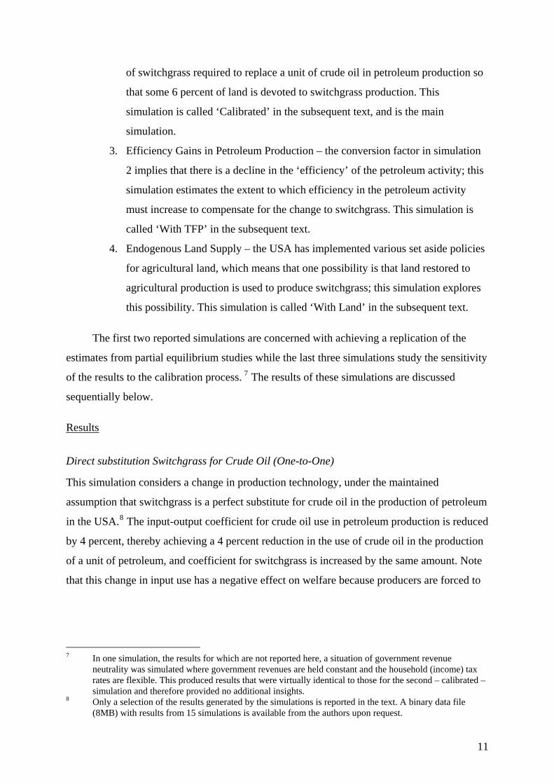
of switchgrass required to replace a unit of crude oil in petroleum production so

that some 6 percent of land is devoted to switchgrass production. This

simulation is called ‘Calibrated’ in the subsequent text, and is the main

simulation.

3. Efficiency Gains in Petroleum Production – the conversion factor in simulation

2 implies that there is a decline in the ‘efficiency’ of the petroleum activity; this

simulation estimates the extent to which efficiency in the petroleum activity

must increase to compensate for the change to switchgrass. This simulation is

called ‘With TFP’ in the subsequent text.

4. Endogenous Land Supply – the USA has implemented various set aside policies

for agricultural land, which means that one possibility is that land restored to

agricultural production is used to produce switchgrass; this simulation explores

this possibility. This simulation is called ‘With Land’ in the subsequent text.

The first two reported simulations are concerned with achieving a replication of the

estimates from partial equilibrium studies while the last three simulations study the sensitivity

of the results to the calibration process. 7 The results of these simulations are discussed

sequentially below.

Results

Direct substitution Switchgrass for Crude Oil (One-to-One)

This simulation considers a change in production technology, under the maintained

assumption that switchgrass is a perfect substitute for crude oil in the production of petroleum

in the USA.8 The input-output coefficient for crude oil use in petroleum production is reduced

by 4 percent, thereby achieving a 4 percent reduction in the use of crude oil in the production

of a unit of petroleum, and coefficient for switchgrass is increased by the same amount. Note

that this change in input use has a negative effect on welfare because producers are forced to

7 In one simulation, the results for which are not reported here, a situation of government revenue

neutrality was simulated where government revenues are held constant and the household (income) tax rates are flexible. This produced results that were virtually identical to those for the second – calibrated – simulation and therefore provided no additional insights.

8 Only a selection of the results generated by the simulations is reported in the text. A binary data file (8MB) with results from 15 simulations is available from the authors upon request.

11

use switchgrass which is more expensive than crude oil and therefore not initially chosen as

input.9

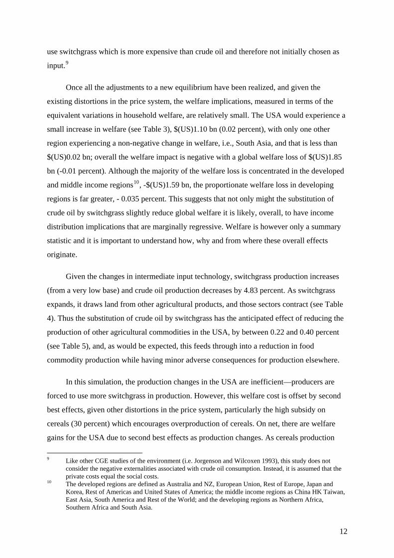
Once all the adjustments to a new equilibrium have been realized, and given the

existing distortions in the price system, the welfare implications, measured in terms of the

equivalent variations in household welfare, are relatively small. The USA would experience a

small increase in welfare (see Table 3), $(US)1.10 bn (0.02 percent), with only one other

region experiencing a non-negative change in welfare, i.e., South Asia, and that is less than

$(US)0.02 bn; overall the welfare impact is negative with a global welfare loss of $(US)1.85

bn (-0.01 percent). Although the majority of the welfare loss is concentrated in the developed

and middle income regions10, -$(US)1.59 bn, the proportionate welfare loss in developing

regions is far greater, - 0.035 percent. This suggests that not only might the substitution of

crude oil by switchgrass slightly reduce global welfare it is likely, overall, to have income

distribution implications that are marginally regressive. Welfare is however only a summary

statistic and it is important to understand how, why and from where these overall effects

originate.

Given the changes in intermediate input technology, switchgrass production increases

(from a very low base) and crude oil production decreases by 4.83 percent. As switchgrass

expands, it draws land from other agricultural products, and those sectors contract (see Table

4). Thus the substitution of crude oil by switchgrass has the anticipated effect of reducing the

production of other agricultural commodities in the USA, by between 0.22 and 0.40 percent

(see Table 5), and, as would be expected, this feeds through into a reduction in food

commodity production while having minor adverse consequences for production elsewhere.

In this simulation, the production changes in the USA are inefficient—producers are

forced to use more switchgrass in production. However, this welfare cost is offset by second

best effects, given other distortions in the price system, particularly the high subsidy on

cereals (30 percent) which encourages overproduction of cereals. On net, there are welfare

gains for the USA due to second best effects as production changes. As cereals production

9 Like other CGE studies of the environment (i.e. Jorgenson and Wilcoxen 1993), this study does not

consider the negative externalities associated with crude oil consumption. Instead, it is assumed that the private costs equal the social costs.

10 The developed regions are defined as Australia and NZ, European Union, Rest of Europe, Japan and Korea, Rest of Americas and United States of America; the middle income regions as China HK Taiwan, East Asia, South America and Rest of the World; and the developing regions as Northern Africa, Southern Africa and South Asia.

12

declines so the distortions for the subsidies decline. This positive effect is slightly enhanced

by the decline in livestock production, on which there is also a (small) subsidy (see Table 5).

The overall effect contributes to the marginal welfare gain in the USA.

The welfare changes in other regions can be explained by (1) price changes in other

markets, or terms of trade effects and by (2) exchange rate changes. The USA decreases

demand for imported crude oil, its total imports decline by 2.93 percent. Since the USA is a

large consumer of crude oil, a change in its demand affects the world market price for crude

oil, which declines by 0.46 percent (see Table 6). This change hurts crude oil exporters as the

price per unit sold drops and export revenue declines. Since the USA imports crude oil from

all regions except Japan and Korea and South Asia (see Figure 8), changes in USA demand

affect export revenue and therefore welfare in those regions. Crude oil importers benefit from

the price decline; regions that benefit the most are those with the highest share of crude oil in

total imports, namely South Asia (7.1 percent) and Japan and Korea (7.4 percent), see Table

2. Ceteris paribus, this price change would increase welfare. In the context of a single region

model, net crude oil exporters would be expected to lose out and net crude oil importers to

gain. But in the context of a global model, there are interdependence effects between regions

through trade and these independencies result in exchange rate effects, which are described in

more detail below.

World agricultural prices also change as the USA reduces output of cereals as

switchgrass production expands. The world price of cereal grains increase by 0.1 percent (see

Table 6). This price change hurts regions with high import shares in consumption of cereals,

particularly the region Japan and Korea which imports 40 percent of cereals consumed.

The negative welfare effects from production inefficiencies get transmitted from the

USA to other regions via exchange rate changes. All regions experience a depreciation of

their currency relative to the USA as the exchange rate (which measures domestic

currency/world currency) increases (see Table 7). Since the current account balances are held

constant in each region and oil imports by the USA decline due the exogenous change in

input use, then other regions must increase exports of other goods.11 The impact of the

exchange rate change depends on how important imports from the USA are, compared to

imports from other regions. Some regions such as the Rest of the Americas, South America,

13

Japan and Korea are quite dependent on the USA with import shares of 60 percent, 24.6

percent, and 21.2 percent, respectively (see Table 2). While crude oil imports increase

(because the world market price drops), all goods imported from the USA become more

expensive. The welfare change is the net effect of these changes. In all regions except South

Asia, which has a high share of crude oil in total imports and a low share of imports from the

USA, the exchange rate effect dominates.

The impact of these changes for food and agriculture in the developing regions

(southern Africa, northern Africa and south Asia) are illustrated by Figures 9, 10, 11 and 12.

For southern and northern Africa food and agricultural imports decline (Figure 9) while

exports increase (Figure 10). Production results are mixed, but for all regions the changes are

quite small. Cereal production increases in northern Africa by 0.03 percent and by 0.01

percent in south Asia. In southern Africa, production declines slightly, by 0.01 percent. All

developing regions have a slight increase in production of other crops (Figure 11). Production

increases are exported and sold to the domestic market. The net effect of a decrease in imports

and an increase in exports is that the total quantities supplied to the domestic market decline

(Figure 12). In all cases the proportionate changes are smaller, substantially less than 1

percent, and the declines in total supplies are very small, less than 0.1 percent. The situation

for south Asia is slightly different; although total supplies of cereals decline very marginally

the supplies of other food and agricultural commodities marginally increase. Overall the

implications for the African region are overwhelmingly negative, although very small, while

for south Asia the effects are marginally positive, although extremely small.

Calibrated Change in Switchgrass Production

The partial equilibrium estimates indicate that approximately 6 percent of land area should be

converted to switchgrass production; a one-to-one substitution of crude oil by switchgrass

results in 0.03 percent of land area to switchgrass. To increase the landshare, the amount of

switchgrass substituted for crude oil in the production of petroleum should increase.

Simulations indicate that the appropriate conversion factor is approximately 1.8, i.e., for each

0.01 reduction in the intermediate input coefficient for crude oil the coefficient for

11 Since the USA’s exchange rate is a numéraire in the model then this could symmetrically be described as

being a consequence of an appreciation of the USA’s exchange rate relative to all other regions.

14

switchgrass should increase by 0.018.12 In effect, the production of refined petroleum

becomes less efficient when switchgrass is substituted for crude oil.

As a result of the loss of productivity, household welfare declines by $(US) 2.02 bn (-

0.04 percent) in the USA and declines in all other regions except south Asia where it just

remains positive (see Table 3). The global welfare impact is a loss of $(US) 5.95 bn (-0.03

percent), which is overwhelmingly concentrated in the USA due to the decline in the USA’s

economic efficiency; this is manifested in the greater proportionate reductions in production

by most activities, especially crude oil that declines by a further percentage point, and by

increased production Gas (and Water) attributable to the changes in the relative prices of

competing energy products. Welfare declines for the other countries for the same reasons

described above.

Because there is an increased shift in land into switchgrass in the USA, the increases in

producer prices for food and agricultural commodities in the USA are substantially greater –

nearly twice as large. Even so the impacts upon producer prices in the developing regions

remain marginally negative, and are accompanied by further increases in exports and

decreases in imports of these commodities by the two Africa regions and further reductions in

supply while the smaller benefits to south Asia are further muted. Again, the fundamental

driving forces are (1) the exchange rate effects, which result in a further depreciation of the

exchange rates; (2) the role of the USA as major exporter of agricultural and food

commodities; and (3) the limited abilities of the developing regions to compensate for these

exchange rate movements. The biggest gainers, in terms of global market share, are two of the

developed regions, the EU and Japan-Korea, and the rest of America (a middle income

region).

Total Factor Productivity (TFP) Growth in Petroleum

The additional adverse implications for welfare of a decline in the efficiency of the USA’s

petroleum industry could be offset if there were a compensating increase the total factor

productivity (TFP) in petroleum production. A 30 percent increase in the efficiency with

which the petroleum industry uses its primary inputs – labour and capital - is sufficient to

generate a small positive welfare effect in the USA while retaining the 1.8 conversion factor

12 Note that because the conversion factor is derived from a general equilibrium solution it will differ from

the partial equilibrium estimate because it will take into account the second and lower order effects of substituting crude oil by switchgrass.

15

of switchgrass for crude oil and achieving the share of (USA) land devoted to switchgrass at 6

percent.13 While this may seem like a large TFP shock, it is important to note that petroleum

industry has a low share of value added in production (8 percent, see Table 5).

This change certainly ameliorates the adverse welfare implications for other regions and

returns them to the order of magnitude found in the first simulation. However, as reported in

Table 7 it makes no substantive difference to the relative depreciations in the exchange rates

or the changes in producer prices, see Figure 13, and consequently the welfare and structural

implications for the other regions are virtually unchanged.

Endogenous Land Supply

Agricultural policies in the USA have for some time made use of set-aside policies to restrain

production and thereby reduce the costs of domestic agricultural policy interventions.

Consequently one possible response would be for the USA to reduce the amount of land set-

aside by restoring it to use in the production of switchgrass. When that is the case, the welfare

change in the USA is marginally positive and although the changes in welfare are still

negative for all other regions except south Asia, they are marginally less negative than in the

calibrated case. Drawing land for switchgrass production from a ‘reserve’ of set-aside land

has substantial impacts upon food and agricultural commodity prices in the USA; indeed it

nullifies nearly all the increases in producer prices found with the earlier experiments (see

Figure 13). Nevertheless the impacts upon food and agricultural prices in developing regions

are virtually identical to those for the calibrated simulation although the effects are still

sufficient to produce small declines in food and agricultural production in southern Africa.

As before, the dominant effect is through the effect of the substitution of crude oil by

switchgrass upon demand for crude oil in the USA and the resulting appreciation of the

USA’s exchange rate. The provision of excess land for use in the production of switchgrass

marginally ameliorates the exchange rate effect, which confirms that a small part of the

adverse exchange rate effects originates from changes in agricultural land use, but further

strengthens the evidence that the effects within food and agriculture are dominated by those

taking place in the crude oil and petroleum sectors, i.e., that they are genuine general

equilibrium effects.

13 Since the intention with this simulation is indicative rather than predictive the model was not used to find

the precise magnitude of the TFP shock associated with no change in USA welfare. Such an exercise could be easily implemented but would risk implying an inappropriate degree of precision.

16

Concluding Comments

The paper reports results from a general equilibrium analysis of the effects of substituting

switch grass for crude oil in the production of petroleum in the USA. The modeling

framework accounts for the direct effect of an increase in demand for switchgrass and a

decrease in demand for crude oil. There are linkages to the domestic economy in the USA as

land is drawn out of other agricultural products, particularly cereals, and into switchgrass

production. Since the USA is a major exporter of agricultural products, there are changes in

production and trade in other regions as USA exports decline. Changes in the global market

for food and agricultural trade reduce production and imports in North Africa and South

Africa. Developed regions, particularly the EU and Japan-Korea, benefit from an increased in

export market share as the USA’s market share declines. An important qualification of the

results is the welfare measures do not account for the utility consumers derive from a cleaner

environment; that measure may offset the welfare cost associated with a productivity loss as

switchgrass replaces crude oil inputs.

The results for agricultural sectors are consistent with complementary partial

equilibrium analysis (see for example De La Torre Ugarte, D, and Hellwinckel, C., 2004b);

the world price of cereals increases slightly. However, dominant changes to the global

economy arise through the changes in the market for crude oil. As the USA, a major

consumer of crude oil, imports less, its exchange rate appreciates relative to the currency in

all other regions; it demands less foreign exchange because it consumes fewer imports.

Regions that depend on USA imports are hurt because these imports have become more

expensive. Also, as a large country in the global market for crude oil, the terms of trade

improve for the USA and deteriorate for crude oil exporters. Welfare declines for all other

regions (with the exception of south Asia which has a negligible gain) when the USA

substitutes switchgrass for crude oil in production largely due to changes in the global market

for crude oil. In the one-to-one simulation, the USA experiences a slight welfare gain through

second best effects of changes in oil prices and taxes as production changes. But welfare

declines for the USA when allowance is made for the quantity of switchgrass required to

replace a unit of crude oil in the production of petroleum since this involves a productivity

loss in the petroleum sector.

17

In addition, alternative scenarios are analysed by way of sensitivity analyses. They seek

to answer the question, “what changes in the economy would offset the welfare loss observed

when switchgrass is substituted for oil?” The results indicate that a 30 percent increase in

factor productivity in the petroleum sector would offset the productivity loss associated with

the substitution of switchgrass for crude oil. Likewise, an increase in switchgrass production

based upon land that was previously set aside would offset the welfare losses in the USA

increases.

18

References

de Melo, J. and Robinson, S., 1989, Product Differentiation and the Treatment of Foreign Trade in Computable General Equilibrium Models of Small Economies, Journal of International Economics, 27, 47-67.

Dervis, K., de Melo, J. and Robinson, S., 1982, General Equilibrium Models for Development Policy (World Bank, Washington D.C.).

Devarajan, S., Lewis, J.D. and Robinson, S., 1990, Policy Lessons from Trade-Focused, Two-Sector Models, Journal of Policy Modeling, 12, 625-657.

Hertel, T.W., 1997, Global Trade Analysis: Modeling and Applications (Cambridge University Press, Cambridge).

Jorgenson D., and Wilcoxen, P. 1993, Reducing U.S. Carbon Dioxide Emissions: An Assessment of Different Instruments, Journal of Policy Modeling, 15, 491-520.

Kilkenny, M.,1991, Computable General Equilibrium Modeling of Agricultural Policies: Documentation of the 30-Sector FPGE GAMS Model of the United States, USDA ERS Staff Report AGES 9125.

Kilkenny, M. and Robinson, S., 1990, Computable General Equilibrium Analysis of Agricultural Liberalisation: Factor Mobility and Macro Closure, Journal of Policy Modeling, 12, 527-556.

King, B.B., 1985, 'What is a SAM?', in: G. Pyatt, and J.I. Round, eds., Social Accounting Matrices: A Basis for Planning (World Bank, Washington D.C.).

Lewis, J.D., Robinson, S. and Wang, Z., 1995, 'Beyond the Uruguay Round: The Implications of an Asian Free Trade Area', China Economic Review, 6, 37-92.

McDonald, S., Robinson, S. and Thierfelder, K., 2005, ‘A SAM Based Global CGE Model using GTAP Data’, mimeo. (Forthcoming Sheffield Economics Research Paper 2005:001. The University of Sheffield.)

McDonald, S. and Sonmez, Y., 2004, ‘Augmenting the GTAP Database with Data on Inter-Regional Transactions’, Sheffield Economics Research Paper 2004:009. The University of Sheffield

McDonald, S., and Thierfelder, K., 2004a, ‘Deriving a Global Social Accounting Matrix from GTAP version 5 Data’, GTAP Technical Paper 23. Global Trade Analysis Project: Purdue University.

McDonald, S., and Thierfelder, K., 2004b, ‘Deriving Reduced Form Global Social Accounting Matrices from GTAP Data’, mimeo.

Pyatt, G., 1987, 'A SAM Approach to Modeling', Journal of Policy Modeling, 10, pp 327-352. Pyatt, G., 1991. 'SAMs, The SNA and National Accounting Capabilities', Review of Income

and Wealth, 37, 177-198.

19

Pyatt, G. and Round, J.I., 1977, 'Social Accounting Matrices for Development Planning', Review of Income and Wealth, 23, 339-364.

Reinert, K.A. and Roland-Holst, D.W., 1997, ‘Social Accounting Matrices’ in: J.F. Francois K.A. and Reinert, eds., Applied Methods for Trade Policy Analysis (Cambridge University Press, Cambridge)

Robinson, S., Kilkenny, M. and Hanson, K., 1990, 'USDA/ERS Computable General Equilibrium Model of the United States', Economic Research Service, USDA, Staff Report AGES 9049.

Sadoulet, E. and de Janvry, A., 1995, Quantitative Development Policy Analysis (John Hopkins University Press, Baltimore).

De La Torre Ugarte, D, and Hellwinckel, C., 2004a, The Economic Competitiveness and Impacts on the Agricultural Sector of Switchgrass as a Bioenergy Dedicated Crop, mimeo.

De La Torre Ugarte, D, and Hellwinckel, C., 2004b, Commodity and Energy Policies under Globalization, mimeo.

20

Appendix 1 Account Mappings

Model Sectors Code Description GTAP Sectors

Cer Cereals Paddy rice, Wheat, Cereal grains nec, Oil seeds Swgr Switchgrass Ocrp Other crops Vegetables fruit nuts, Sugar cane sugar beet, Plant based fibres, Crops nec, Forestry

Lstoc Livestock Bovine cattle sheep and goats horses, Animal products nec, Raw milk, Wool silk worm cocoons, Fishing

Mins Minerals Coal, Oil, Gas, Minerals nec

Fod Food ProcessingBovine cattle sheep and goat horse meat prods, Meat products nec, Vegetable oils and fats, Dairy products, Processed rice, Sugar, Food products nec, Beverages and tobacco products

Text Textiles Textiles, Wearing apparel, Leather products

Olman Other light manufacturing Wood products, Paper products publishing, Electronic equipment, Manufactures nec

Pet Petroleum etc Petroleum coal products Chem. Chemicals etc Chemical rubber plastic products

Hmanu Heavy manufacturing

Mineral products nec Ferrous metals, Metals nec, Metal products, Motor vehicles and parts, Transport equipment nec, Machinery and equipment nec

Cons Construction Construction Elec Electricity Electricity Gasw Gas and Water Gas manufacture distribution, Water

Trad Trade and Transport Trade, Transport nec, sea transport, Air transport, Communication

Serv Services Financial services nec, Insurance, Business services nec, Recreation and other services, PubAdmin Defence Health Educat, Dwellings

Model Regions Code Description GTAP Regions

Anz Australia and NZ Australia , New Zealand

Chin China HK Taiwan China, Hong Kong , Taiwan

Easia East Asia Indonesia , Malaysia, Philippines, Singapore , Thailand, Viet Nam

Eur European Union Austria, Denmark, France , Germany, United Kingdom, Greece , Ireland, Italy, Netherlands, Portugal, Spain, Sweden , Belgium, Luxembourg

Jkor Japan and Korea Japan, Korea Nafr Northern Africa Morocco, Rest of North Africa, Uganda , Rest of sub-Saharan Africa Rame Rest of Americas Canada , Mexico , Central America and the Caribbean

Reur Rest of Europe Finland, Switzerland, Rest of EFTA , Cyprus , Malta, Hungary, Poland , Bulgaria, Czech Republic, Romania, Slovakia, Slovenia, Croatia, Albania, Estonia, Latvia , Lithuania

Row Rest of the World

Russian Federation , Rest of Former Soviet Union , Turkey , Rest of Middle East, Rest of World

Same South America Colombia, Peru, Venezuela , Rest of Andean Pact, Argentina , Brazil , Chile, Uruguay, Rest of South America

Sasia South Asia Bangladesh, India, Sri Lanka , Rest of South Asia

Safr Southern Africa Botswana, South African Customs Union ex Botswana , Malawi , Mozambique, Tanzania, Zambia , Zimbabwe, Rest of southern Africa

Usa United States of America United States of America

21

Table 1 Model Sectors (Commodities and Activities) and Regions

Commodities/Activities Regions

Cereals Petroleum etc USA Japan and Korea

Other crops Chemicals etc European Union East Asia

Switchgrass Heavy manufacturing Rest of Europe Australia and NZ

Livestock Electricity Southern Africa South America

Crude oil Gas and Water Northern Africa Rest of Americas

Other minerals Construction South Asia Rest of the World

Food Processing Trade and Transport China HK Taiwan

Textiles Services

Light manufacturing

Table 2 Trade Dependence on Crude Oil and on USA

Crude imports as a share of total imports

Imports from USA as a share of total imports

USA 5.7 NAEU 3.0 10.2Rest of Europe 2.4 6.9S Africa 3.5 11.4N Africa 1.6 12.2S Asia 7.1 10.0China 2.0 14.5Japan and Korea 7.4 21.2E Asia 3.6 14.7Australia and NZ 3.5 20.1S America 2.8 24.6R of Americas 2.1 60.0Rest of World 2.6 14.4Source: GTAP/Model database.

22

Table 3 Household Welfare ($US billions)

Base Simulations

(Changes in welfare)

One-to-one Calibrated With

TFP With Land

USA 5,495.10 1.11 -2.02 0.70 0.19 EU 4,824.83 -0.79 -1.05 -0.82 -0.86 Rest of Europe 523.79 -0.07 -0.09 -0.07 -0.07 S Africa 108.38 -0.11 -0.14 -0.12 -0.14 N Africa 266.66 -0.16 -0.19 -0.17 -0.17 S Asia 357.46 0.02 0.01 0.01 0.02 China 689.73 -0.06 -0.11 -0.08 -0.04 Japan and Korea 2,769.95 -0.33 -0.53 -0.43 -0.21 E Asia 375.88 -0.03 -0.05 -0.02 -0.04 Australia and NZ 281.78 -0.02 -0.03 -0.02 -0.03 S America 1,022.46 -0.30 -0.33 -0.30 -0.32 Rest of Americas 712.41 -0.81 -1.06 -0.80 -0.97 Rest of World 949.12 -0.29 -0.36 -0.30 -0.30 Total 18,377.55 -1.85 -5.95 -2.43 -2.94

Source: Model simulation results.

23

Table 4 Proportions of Land in Different Agricultural Activities, USA

Base One-to-one Calibrated Cereals 0.63 0.61 0.60 Other crops 0.24 0.23 0.22 Switchgrass 0.00 0.03 0.06 Livestock 0.13 0.12 0.12


24

Table 5 Production Taxes, Value Added Shares, and Changes, USA

Base data Simulations Production (percent change)

Indirect tax

rate

Value added share of gross

output One-to-one Calibrated

Cereals -0.30 0.79 -0.28 -0.48 Other crops 0.01 0.55 -0.40 -0.69 Switchgrass 0.00 0.69 53,395.44 95,266.82 Livestock -0.01 0.18 -0.22 -0.40 Crude Oil 0.24 0.33 -4.83 -5.90 Other minerals 0.17 0.43 -0.06 -0.08 Food 0.00 0.32 -0.16 -0.30 Textiles 0.00 0.34 -0.07 -0.12 Light manufacturing

0.00 0.42 -0.10 -0.14

Petroleum 0.00 0.08 0.24 -0.64 Chemicals 0.00 0.39 -0.01 -0.05 Heavy manufacturing

0.00 0.40 -0.09 -0.11

Electricity 0.00 0.47 0.00 -0.02 Gas and water 0.00 0.56 0.10 0.17 Construction 0.00 0.46 -0.01 -0.01 Trade and transport

0.00 0.58 -0.01 -0.05

Services 0.00 0.69 -0.01 -0.03 Source: Model simulation results.

25

Table 6 World Price Changes in Agriculture and Crude Oil (percent change)

One-to-One Calibrated With TFP With Land Cereals 0.09 0.27 0.32 -0.23Other crops -0.15 -0.15 -0.09 -0.25Livestock -0.12 -0.12 -0.07 -0.22Crude oil -0.46 -0.57 -0.46 -0.55


26

Table 7 Exchange Rate Effects (percent change)

One-to-one Calibrated With TFP With Land

EU 0.20 0.25 0.19 0.22 Rest of Europe 0.21 0.26 0.21 0.24 S Africa 0.43 0.53 0.43 0.51 N Africa 0.42 0.50 0.41 0.49 S Asia 0.16 0.21 0.15 0.20 China 0.16 0.20 0.15 0.19 Japan and Korea 0.17 0.22 0.17 0.20 E Asia 0.16 0.21 0.16 0.20 Australia and NZ 0.18 0.23 0.17 0.22 S America 0.35 0.40 0.34 0.40 R of Americas 0.26 0.31 0.24 0.32 Rest of World 0.27 0.32 0.26 0.31


27

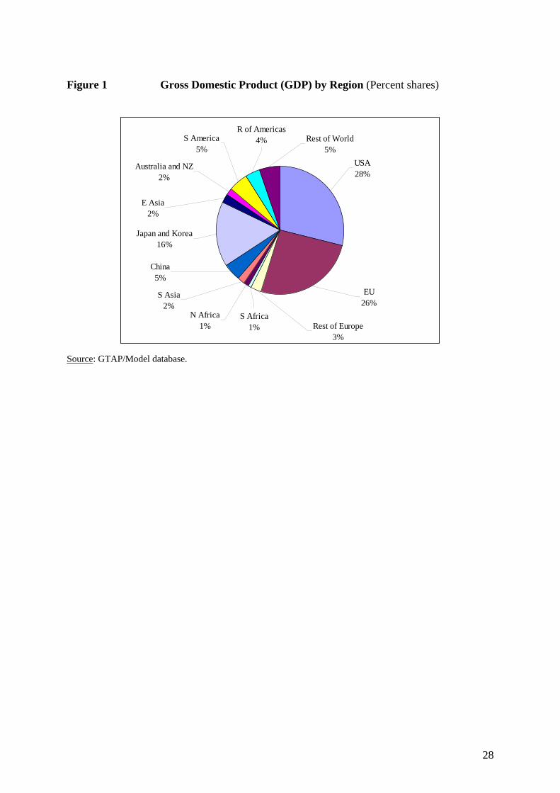
Figure 1 Gross Domestic Product (GDP) by Region (Percent shares)

S America5%

Australia and NZ2%

E Asia2%

Japan and Korea16%

China5%

Rest of Europe3%

S Africa1%

USA28%

Rest of World5%

R of Americas4%

EU26%

S Asia2%

N Africa1%

Source: GTAP/Model database.

28

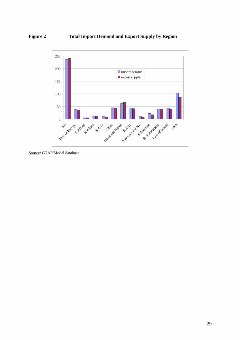
Figure 2 Total Import Demand and Export Supply by Region

0

50

100

150

200

250

EU

Rest of

Europe

S Afri

ca

N Afri

caS A

siaChin

a

Japan

and K

orea

E Asia

Austral

ia an

d NZ

S Ameri

ca

R of A

mericas

Rest of

Worl

dUSA

import demand export supply


29

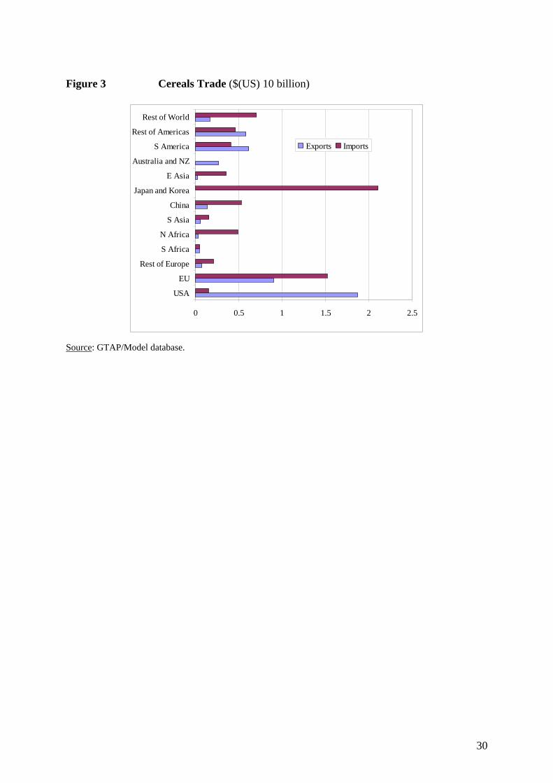
Figure 3 Cereals Trade ($(US) 10 billion)

0 0.5 1 1.5 2 2

USA

EU

Rest of Europe

S Africa

N Africa

S Asia

China

Japan and Korea

E Asia

Australia and NZ

S America

Rest of Americas

Rest of World

.5

Exports Imports


30

Figure 4 Other Crops Trade ($(US) 10 billion)

0 1 2 3 4 5 6

USA

EU

Rest of Europe

S Africa

N Africa

S Asia

China

Japan and Korea

E Asia

Australia and NZ

S America

Rest of Americas

Rest of World

Exports Imports


31

Figure 5 Livestock Trade ($(US) 10 billion)

0 0.5 1 1.5 2

USA

EU

Rest of Europe

S Africa

N Africa

S Asia

China

Japan and Korea

E Asia

Australia and NZ

S America

Rest of Americas

Rest of World

Exports Imports


Figure 6 Crude Oil Trade ($(US) 10 billion)

0 2 4 6 8 10 12 14

USA

EU

Rest of Europe

S Africa

N Africa

S Asia

China

Japan and Korea

E Asia

Australia and NZ

S America

Rest of Americas

Rest of World

Exports Imports


32

Figure 7 Production Shares of Agricultural Commodities by Region

0

0.02

0.04

0.06

0.08

0.1

0.12

EU

Rest of

Europe

S Afri

ca

N Afri

caS A

siaChin

a

Japan

and K

orea

E Asia

Austral

ia an

d NZ

S Ameri

ca

R of A

mericas

Rest of

Worl

dUSA

Cereals Other crops

Livestock Food Processing

Source: GTAP/Model database

Figure 8 USA Crude Imports by Source Region (Percent shares)

E Asia0.9%

Australia and NZ0.4%

Japan and Korea0.0%

China0.7%

S Asia0.0%

N Africa14.8%

S Africa5.3%

Rest of Europe2.9%

S America20.4%

R of Americas30.2%

EU2.9%

Rest of World21.6%


33

Figure 9 Food and Agricultural Imports by Developing Regions (percent

change)

-0.8

-0.7

-0.6

-0.5

-0.4

-0.3

-0.2

-0.1

0

0.1

0.2

S Africa

N A

frica

S Asia

S Africa

N A

frica

S Asia

S Africa

N A

frica

S Asia

S Africa

N A

frica

S Asia

Cereals Other crops Livestock Food Processing

One-to-oneCalibratedWith TFPWith Land


34

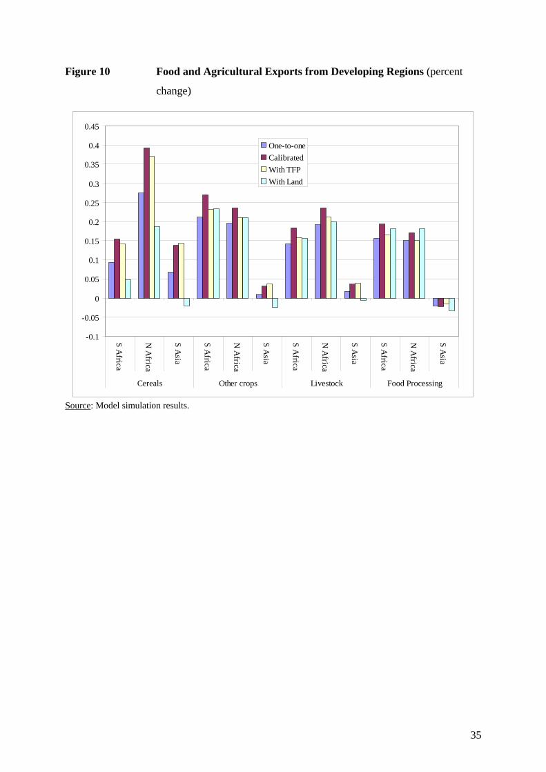
Figure 10 Food and Agricultural Exports from Developing Regions (percent

change)

-0.1

-0.05

0

0.05

0.1

0.15

0.2

0.25

0.3

0.35

0.4

0.45

S Africa

N A

frica

S Asia

S Africa

N A

frica

S Asia

S Africa

N A

frica

S Asia

S Africa

N A

frica

S Asia




35

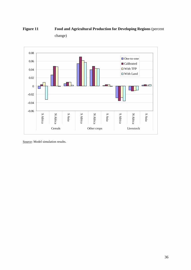
Figure 11 Food and Agricultural Production for Developing Regions (percent

change)

-0.06

-0.04

-0.02

0

0.02

0.04

0.06

0.08

S Africa

N A

frica

S Asia

S Africa

N A

frica

S Asia

S Africa

N A

frica

S Asia

Cereals Other crops Livestock



36

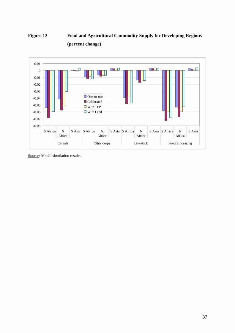
Figure 12 Food and Agricultural Commodity Supply for Developing Regions

(percent change)

-0.08

-0.07

-0.06

-0.05

-0.04

-0.03

-0.02

-0.01

0

0.01

S Africa NAfrica

S Asia S Africa NAfrica



S Asia




37

Figure 13 Producers Prices for Food and Agricultural Commodities – USA and

Developing Regions (percent change)

-0.5

0.0

0.5

1.0

1.5

2.0

usa

S A

fric

a

N A

fric

a

S A

sia

usa

S A

fric

a

N A

fric

a

S A

sia

usa

S A

fric

a

N A

fric

a

S A

sia

usa

S A

fric

a

N A

fric

a

S A

sia




38

Impact of switching production to bioenergy crops: The switchgrass example

Documents

Transcript of Impact of switching production to bioenergy crops: The switchgrass example