Impact of Notch Filtering on Tracking Loops for GNSS Applications
80
POLITECNICO DI TORINO Facoltà di Ingegneria dell’informazione Corso di Laurea in Ingegneria delle Telecomunicazioni Tesi di Laurea Specialistica Impact of Notch Filtering on Tracking Loops for GNSS Applications Relatori: prof. Mark Petovello - UoC dr. Daniele Borio - UoC prof.ssa Letizia Lo Presti - PoliTo prof. Fabio Dovis - PoliTo Candidato: Giorgio Giordanengo Gennaio 2009
Transcript of Impact of Notch Filtering on Tracking Loops for GNSS Applications
POLITECNICO DI TORINO
Facoltà di Ingegneria dell’informazione Corso di Laurea in Ingegneria delle Telecomunicazioni
Tesi di Laurea Specialistica
Impact of Notch Filtering on
Tracking Loops for GNSS
Applications
Relatori:
prof. Mark Petovello - UoC
dr. Daniele Borio - UoC
prof.ssa Letizia Lo Presti - PoliTo
prof. Fabio Dovis - PoliTo
Candidato:
Giorgio Giordanengo
Gennaio 2009
List of Figures
1.1 Frequency plan for the different Global Navigation Satellite System
(GNSS) systems. . . . . . . . . . . . . . . . . . . . . . . . . . . . . . 5
1.2 Clock misalignments in a GNSS system. . . . . . . . . . . . . . . . . 7
1.3 Example of a generic Direct Sequence Spread Spectrum (DSSS). . . . 8
1.4 Example of Auto Correlation Function (ACF) and Cross Correlation
Function (CCF) for a Gold code employed by the Global Positioning
System (GPS) C/A code. . . . . . . . . . . . . . . . . . . . . . . . . . 11
1.5 Ideal ACF of a GPS C/A code. . . . . . . . . . . . . . . . . . . . . . 13
1.6 General scheme of a GNSS receiver. . . . . . . . . . . . . . . . . . . . 13
1.7 Conceptual scheme of a tracking loop. . . . . . . . . . . . . . . . . . 15
1.8 Block scheme of a generic Delay Lock Loop (DLL). . . . . . . . . . . 16
1.9 Example of code correlation phase. . . . . . . . . . . . . . . . . . . . 17
1.10 Block scheme of a generic Phase Lock Loop (PLL) . . . . . . . . . . . 18
2.1 PSDs of a CWI and a GNSS signal. . . . . . . . . . . . . . . . . . . . 20
2.2 Notch Filter (NF) using the Overlapped FFT-based (OFFT) imple-
mentation. . . . . . . . . . . . . . . . . . . . . . . . . . . . . . . . . . 23
2.3 Notch Filter (NF) using the Filter Bank interference suppression im-
plementation. . . . . . . . . . . . . . . . . . . . . . . . . . . . . . . . 23
2.4 Adaptive Transversal Filter (ATF) scheme. . . . . . . . . . . . . . . . 24
2.5 Transfer function of the two-poles NF with different kα. . . . . . . . . 26
3.1 Simplified scheme of a GNSS receiver equipped with notch filter for
interference removal. . . . . . . . . . . . . . . . . . . . . . . . . . . . 28
3.2 Filtering distortions on the CCF for different modulations. . . . . . . 31
3.3 Particular of the CCF depicted in Figure 3.2. . . . . . . . . . . . . . 31
3.4 Approximation of the CCF for different modulations and different
front-end bandwidths. . . . . . . . . . . . . . . . . . . . . . . . . . . 34
I
3.5 Approximation of the CCF for different modulations, different front-
end bandwidths and in the presence of NF with bandwidth of 100
kHz and fc of 0.5 MHz. . . . . . . . . . . . . . . . . . . . . . . . . . . 37
3.6 RMS-Bandwitdh (βrms) for different modulations and different front-
end bandwidths. . . . . . . . . . . . . . . . . . . . . . . . . . . . . . . 38
3.7 Asymmetry Coefficient (fa) for different modulations and different
front-end bandwidths. . . . . . . . . . . . . . . . . . . . . . . . . . . 39
3.8 Bias for different modulations and different front-end bandwidths. . . 40
4.1 Simulation and analytical techniques for the analysis of a complex
system and their relative computational complexity. . . . . . . . . . . 42
4.2 Block scheme of a digital DLL . . . . . . . . . . . . . . . . . . . . . . 43
4.3 Equivalent representation of a digital DLL. The delay to be estimated
is represented along with its impact on the correlator outputs. . . . . 44
4.4 Tracking jitter for different E-L spacing as a function of the input
C/N0 under ideal conditions. . . . . . . . . . . . . . . . . . . . . . . . 48
4.5 Tracking jitter for different E-L spacing as a function of the input
C/N0 in the presence of front-end (Chebyshev, six taps, fco 24 MHz)
and notch (fc 0.5 MHz, bandwidth 100 kHz) filter. . . . . . . . . . . . 49
4.6 Jitter evaluated in different ways and for different chip spacing as a
function of the notch bandwidth and the central frequency. . . . . . . 51
4.7 Delay estimation for different filtering stages (front-end, fco 24 MHz,
notch filter, bandwidth 100 kHz, fc 0.5 MHz). . . . . . . . . . . . . . 52
4.8 Bias for different filtering stages and different chip spacing, (front-
end, fco 24 MHz, notch filter, bandwidth 100 kHz, fc 0.5 MHz). . . . 53
4.9 Delay estimated as a function of central frequency (fc) and spacing
(front-end, fco 24 MHz, notch filter, bandwidth 100 kHz). . . . . . . . 53
4.10 Bias introduced by the NF as a function of fc and bandwidth for
different chip spacing, (front-end, fco 24 MHz, notch filter, bandwidth
100 kHz). . . . . . . . . . . . . . . . . . . . . . . . . . . . . . . . . . 54
4.11 Comparison between the Asymmetry Coefficient (fa) and the bias
introduced by the Notch Filter. . . . . . . . . . . . . . . . . . . . . . 55
5.1 Scheme used for the data collection. . . . . . . . . . . . . . . . . . . . 57
5.2 Antenna used to collect data. . . . . . . . . . . . . . . . . . . . . . . 57
5.3 Front view of the NI-PXI-5660 front-end. . . . . . . . . . . . . . . . . 58
5.4 Novatel OEM4 GNSS receiver. . . . . . . . . . . . . . . . . . . . . . . 58
II
5.5 Information provided by the Novatel receiver (tracking status 5.5a
and satellites available 5.5b). . . . . . . . . . . . . . . . . . . . . . . . 59
5.6 Power Spectral Density of the GPS-L1 signal. . . . . . . . . . . . . . 60
5.7 C/N0 for two PRNs in the presence of notch filtering for different fcs. 61
5.8 Position estimated by the GSNRxTM in the absence and presence of
the Notch Filter. . . . . . . . . . . . . . . . . . . . . . . . . . . . . . 63
5.9 Error position evaluated for different central frequencies of the NF. . 63
5.10 Doppler error evaluated as the difference between the cases with and
without notch filter. . . . . . . . . . . . . . . . . . . . . . . . . . . . . 65
III
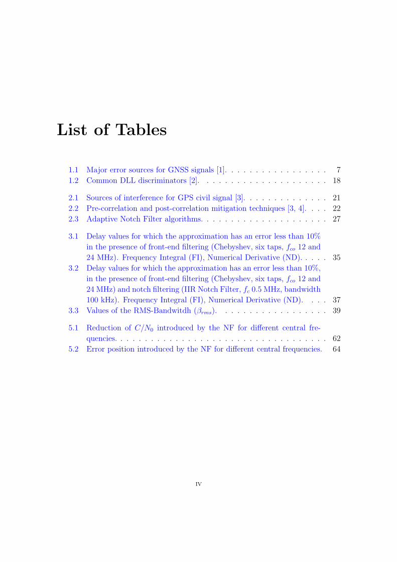
List of Tables
1.1 Major error sources for GNSS signals [1]. . . . . . . . . . . . . . . . . 7
1.2 Common DLL discriminators [2]. . . . . . . . . . . . . . . . . . . . . 18
2.1 Sources of interference for GPS civil signal [3]. . . . . . . . . . . . . . 21
2.2 Pre-correlation and post-correlation mitigation techniques [3, 4]. . . . 22
2.3 Adaptive Notch Filter algorithms. . . . . . . . . . . . . . . . . . . . . 27
3.1 Delay values for which the approximation has an error less than 10%
in the presence of front-end filtering (Chebyshev, six taps, fco 12 and
24 MHz). Frequency Integral (FI), Numerical Derivative (ND). . . . . 35
3.2 Delay values for which the approximation has an error less than 10%,
in the presence of front-end filtering (Chebyshev, six taps, fco 12 and
24 MHz) and notch filtering (IIR Notch Filter, fc 0.5 MHz, bandwidth
100 kHz). Frequency Integral (FI), Numerical Derivative (ND). . . . 37
3.3 Values of the RMS-Bandwitdh (βrms). . . . . . . . . . . . . . . . . . 39
5.1 Reduction of C/N0 introduced by the NF for different central fre-
quencies. . . . . . . . . . . . . . . . . . . . . . . . . . . . . . . . . . . 62
5.2 Error position introduced by the NF for different central frequencies. 64
IV

Acronyms
ACF Auto Correlation Function
ADC Analog to Digital Converter
ATF Adaptive Transversal Filter
AWGN Additive White Gaussian Noise
BOC Binary Offset Carrier
BPSK Binary Phase Shift Keying
βrms RMS-Bandwitdh
C/A Coarse Acquisition
CAF Cross Ambiguity Function
CCF Cross Correlation Function
CCIT Calgary Center for Innovative Technologies
CDMA Code Division Multiple Access
C/N0 Carrier-to-Noise density ratio
CW Continuous Wave
CWI Continuous Wave Interference
DLL Delay Lock Loop
DSSS Direct Sequence Spread Spectrum
EGNOS European Geostationary Overlay Service
1
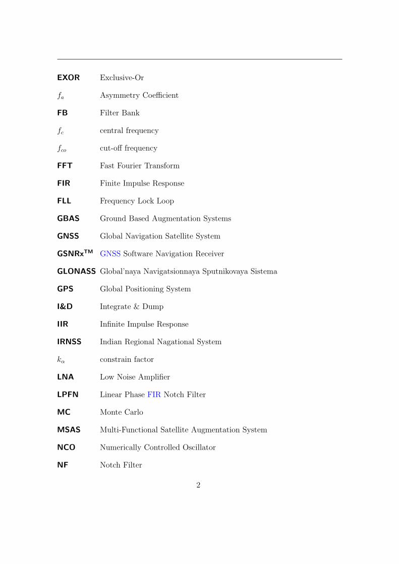
EXOR Exclusive-Or
fa Asymmetry Coefficient
FB Filter Bank
fc central frequency
fco cut-off frequency
FFT Fast Fourier Transform
FIR Finite Impulse Response
FLL Frequency Lock Loop
GBAS Ground Based Augmentation Systems
GNSS Global Navigation Satellite System
GSNRxTM GNSS Software Navigation Receiver
GLONASS Global’naya Navigatsionnaya Sputnikovaya Sistema
GPS Global Positioning System
I&D Integrate & Dump
IIR Infinite Impulse Response
IRNSS Indian Regional Nagational System
kα constrain factor
LNA Low Noise Amplifier
LPFN Linear Phase FIR Notch Filter
MC Monte Carlo
MSAS Multi-Functional Satellite Augmentation System
NCO Numerically Controlled Oscillator
NF Notch Filter
2
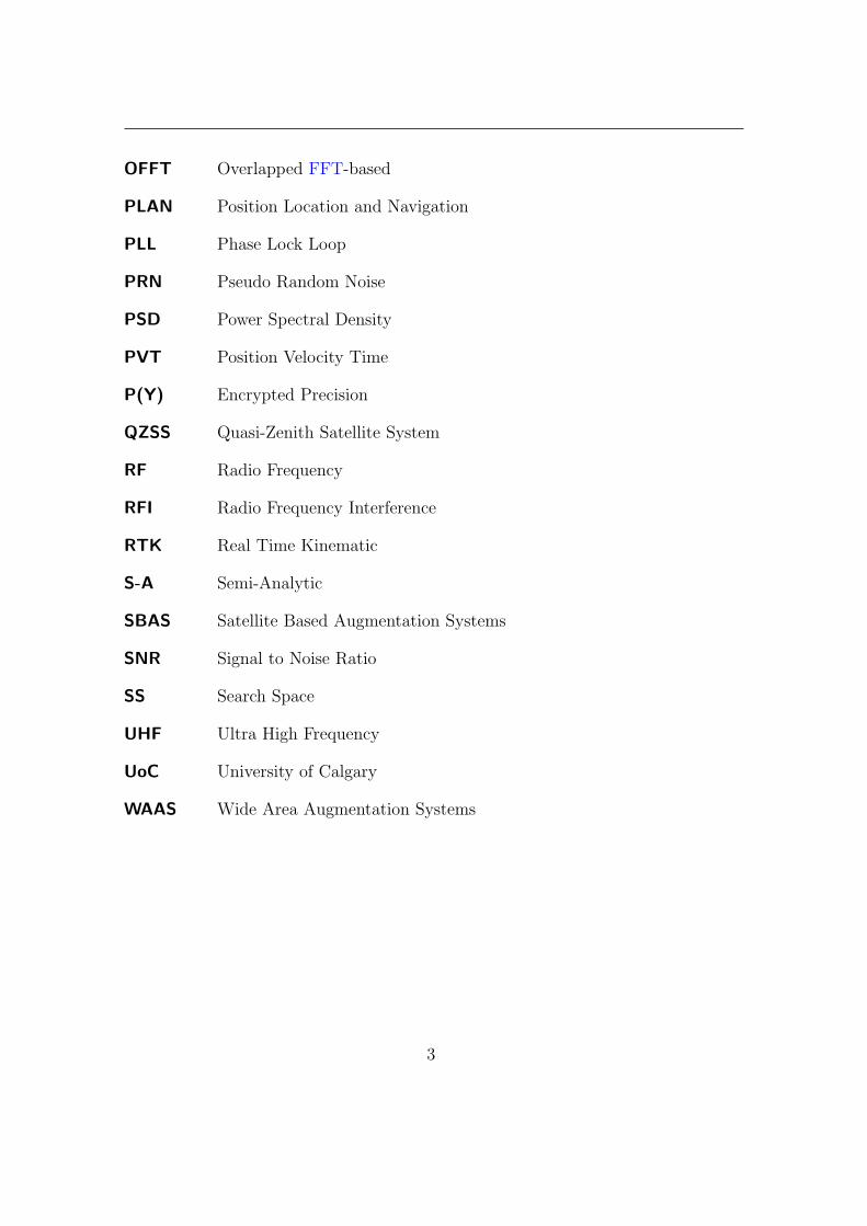
OFFT Overlapped FFT-based
PLAN Position Location and Navigation
PLL Phase Lock Loop
PRN Pseudo Random Noise
PSD Power Spectral Density
PVT Position Velocity Time
P(Y) Encrypted Precision
QZSS Quasi-Zenith Satellite System
RF Radio Frequency
RFI Radio Frequency Interference
RTK Real Time Kinematic
S-A Semi-Analytic
SBAS Satellite Based Augmentation Systems
SNR Signal to Noise Ratio
SS Search Space
UHF Ultra High Frequency
UoC University of Calgary
WAAS Wide Area Augmentation Systems
3
Contents
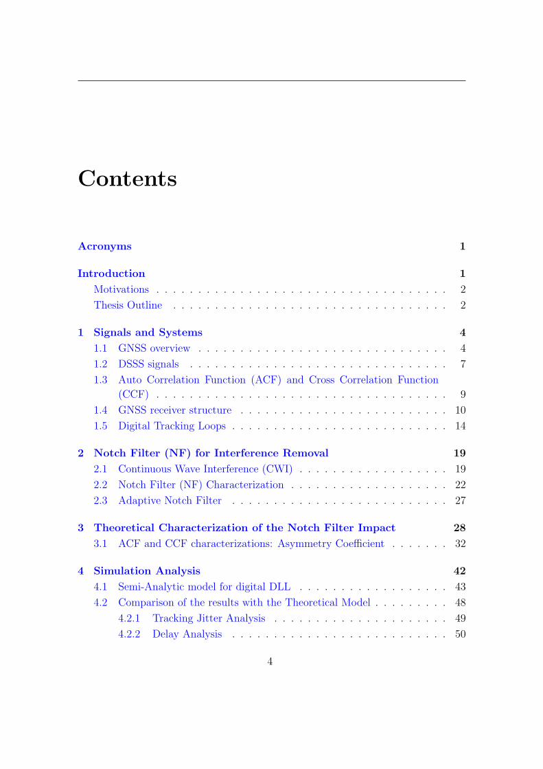
Acronyms 1
Introduction 1
Motivations . . . . . . . . . . . . . . . . . . . . . . . . . . . . . . . . . . . 2
Thesis Outline . . . . . . . . . . . . . . . . . . . . . . . . . . . . . . . . . 2
1 Signals and Systems 4
1.1 GNSS overview . . . . . . . . . . . . . . . . . . . . . . . . . . . . . . 4
1.2 DSSS signals . . . . . . . . . . . . . . . . . . . . . . . . . . . . . . . 7
1.3 Auto Correlation Function (ACF) and Cross Correlation Function
(CCF) . . . . . . . . . . . . . . . . . . . . . . . . . . . . . . . . . . . 9
1.4 GNSS receiver structure . . . . . . . . . . . . . . . . . . . . . . . . . 10
1.5 Digital Tracking Loops . . . . . . . . . . . . . . . . . . . . . . . . . . 14
2 Notch Filter (NF) for Interference Removal 19
2.1 Continuous Wave Interference (CWI) . . . . . . . . . . . . . . . . . . 19
2.2 Notch Filter (NF) Characterization . . . . . . . . . . . . . . . . . . . 22
2.3 Adaptive Notch Filter . . . . . . . . . . . . . . . . . . . . . . . . . . 27
3 Theoretical Characterization of the Notch Filter Impact 28
3.1 ACF and CCF characterizations: Asymmetry Coefficient . . . . . . . 32
4 Simulation Analysis 42
4.1 Semi-Analytic model for digital DLL . . . . . . . . . . . . . . . . . . 43
4.2 Comparison of the results with the Theoretical Model . . . . . . . . . 48
4.2.1 Tracking Jitter Analysis . . . . . . . . . . . . . . . . . . . . . 49
4.2.2 Delay Analysis . . . . . . . . . . . . . . . . . . . . . . . . . . 50
4

5 Real Data Analysis 56
5.1 Experimental setup . . . . . . . . . . . . . . . . . . . . . . . . . . . . 56
5.2 Comparison of the results in the presence and absence of Notch Filter:
impact of the notch central frequency . . . . . . . . . . . . . . . . . . 60
6 Conclusions 66
Bibliography 68
5
Introduction
The Global Navigation Satellite System (GNSS) users continue to demand location-
based services everywhere at any time. In this respect, GNSS services should be
available also in hostile environments such as in the presence of Radio Frequency
(RF) interference. One of the most common interference sources is represented by
a Continuous Wave (CW), that is, all those RF signals that can be represented as
pure sinusoids. Since CWI has a narrow spectrum concentrated around a specific
frequency, it can be effectively removed by using a NF. A NF is a linear device
able to remove only a small portion of spectrum of the signal at its input. This
portion is concentrated around a specific frequency whereas all the other components
of the spectrum are left almost unaltered. For this reason the NF is an effective
solution for removing CWI. The drawback of notch filtering is represented by the
fact that also a portion of the useful GNSS signal is removed. This can introduce
distortions, especially in the Auto Correlation Function (ACF), because the classical
form (a triangle), is distorted and changed a little bit. This fact can degrade the
accuracy of a GNSS receiver. In the literature, different classes of NFs have been
considered and analyzed [5, 6, 7, 8], but the analysis has been essentially limited to
the acquisition stage [9, 10]. However, acquisition represents only the first stage of
a GNSS receiver and further investigations are required for fully characterizing the
impact of NF. For these reasons, the main topic of this thesis is the evaluation of the
Notch Filter impact on the receiver processing chain. The impact on the tracking
stage is analyzed in detail and some insight is provided on the corresponding bias
and distortions introduced in the position domain.
1
Objectives and Motivations
As explained above this work investigates the performance of a GNSS receiver when
a NF is inserted in the receiver chain.
More specifically, the following points will be investigated:
• definition of suitable metrics for the analysis of notch filtering;
• theoretical analysis of the distortions introduced by the NF on the correlation
function of the received signal. A GNSS receiver is able to estimate the prop-
agation time of the received signal by correlating it with a locally generated
replica. NF alters the correlation function obtained, thus biasing the estima-
tion process. The analysis of the correlation function can provide some insight
on the distortions caused by NF;
• performance analysis of a digital DLL, in the presence of NF;
• use of real data and a customized version of the University of Calgary (UoC)
software receiver GNSS Software Navigation Receiver (GSNRxTM) [11] for
assessing the performance of a GNSS receiver in the presence of CWI and
notch filtering.
Thesis Outline
The thesis is organized as follows:
• Chapter 1 provides an overview of Global Navigation Satellite System and
GNSS receivers. A brief introduction to digital tracking loops is provided
and different metrics for their characterization introduced. The correlation
properties of GNSS signals and the importance of ACF in the receiver chain
is also discussed.
• Chapter 2 introduces the main subject of the thesis, i.e., the Notch Filter (NF).
At first, a general description of CWI is provided, highlighting its impact on
a GNSS receivers. Different types of NFs (different implementations) are also
discussed.
• Chapter 3 deals with the theoretical analysis of the NF impact: power losses,
delay and frequency are studied as a function of the different filter parameters.
The asymmetry coefficient is introduced for the evaluation of the asymmetry
2
introduced by the NF on the CCF. The concept of rms bandwidth [2] is also
introduced and used for further evaluating the NF impact. This parameter
corresponds to the Gabor bandwidth [12] of the signal after notch filtering and
plays a significant role in the evaluation of the code tracking jitter [13, 14].
• In Chapter 4 simulation results are provided; in particular a semi-analytic
model for the study of code delay tracking loop, is presented.
• Chapter 5 describes the results obtained by using the PLAN group software
receiver (GSNRxTM) [11], for the analysis of live GPS data in the presence
of NF. The analysis is made using BPSK signals (GPS C/A), but it is to be
hoped that the results are equally applicable to other signals (e.g., BOC).
• Finally, Chapter 6 presents some conclusions and possible future directions are
outlined.
3
Chapter 1
Signals and Systems
1.1 GNSS overview
The more general definition of Global Navigation Satellite System (GNSS) is given
by [15]: “A worldwide position and time determination system that includes one or
more satellite constellations, aircraft receivers and system integrity monitoring, aug-
mented as necessary to support the required navigation performance for the intended
operation”. As stated before, GNSS systems provide services for navigation and the
following general classification can be made [2, 16]:
• Truly global GNSS:
– Global Positioning System (GPS) (US);
– Global’naya Navigatsionnaya Sputnikovaya Sistema (GLONASS) (Rus-
sia);
– Galileo (EU);
– Compass (China).
• Other systems composed by:
– Ground Based Augmentation Systems (GBAS);
– Regional Satellite Based Argumentation Systems including Wide Area
Augmentation Systems (WAAS) (US), European Geostationary Overlay
Service (EGNOS) (EU), Multi-Functional Satellite Augmentation System
(MSAS) (Japan) and GAGAN (India);
4
1 – Signals and Systems
– Regional satellite navigation systems such as Quasi-Zenith Satellite System
(QZSS) (Japan) and Indian Regional Nagational System (IRNSS) (India);
– Regional GBAS such as CORS networks;
– Local GBAS typified by a single GPS reference station operating for Real
Time Kinematic (RTK) corrections.
For more details about the new or renewed systems refer to [2, 16].
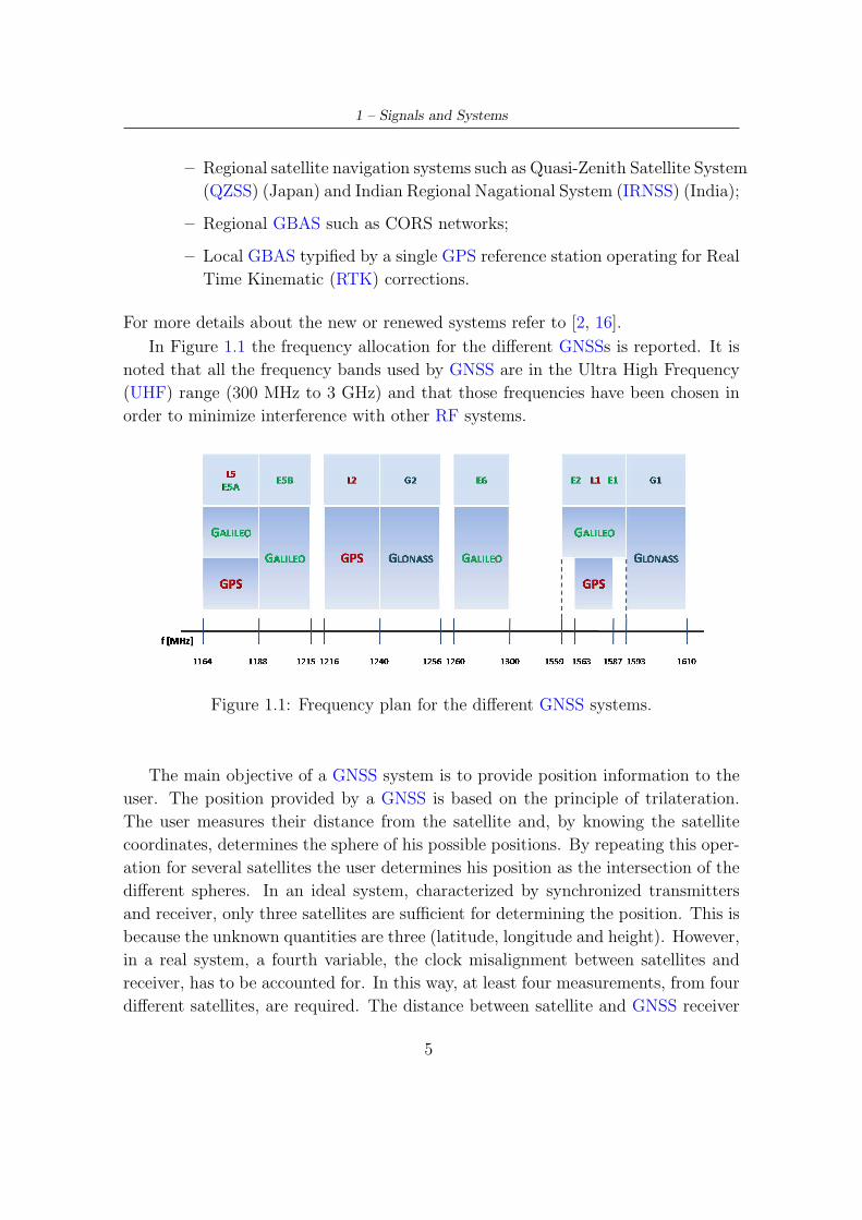
In Figure 1.1 the frequency allocation for the different GNSSs is reported. It is
noted that all the frequency bands used by GNSS are in the Ultra High Frequency
(UHF) range (300 MHz to 3 GHz) and that those frequencies have been chosen in
order to minimize interference with other RF systems.
Figure 1.1: Frequency plan for the different GNSS systems.
The main objective of a GNSS system is to provide position information to the
user. The position provided by a GNSS is based on the principle of trilateration.
The user measures their distance from the satellite and, by knowing the satellite
coordinates, determines the sphere of his possible positions. By repeating this oper-
ation for several satellites the user determines his position as the intersection of the
different spheres. In an ideal system, characterized by synchronized transmitters
and receiver, only three satellites are sufficient for determining the position. This is
because the unknown quantities are three (latitude, longitude and height). However,
in a real system, a fourth variable, the clock misalignment between satellites and
receiver, has to be accounted for. In this way, at least four measurements, from four
different satellites, are required. The distance between satellite and GNSS receiver
5
1 – Signals and Systems
can be evaluated as:
R = c τ (1.1)
where:
• R is the distance [m];
• c is the speed of light [m/s];
• τ is the transit time needed required by the signal transmitted by a satellite
to reach the GNSS receiver [s].
Since the receiver clock is not synchronous with the satellite clock, the receiver
can measure only a biased version of the transit time, τ . However, since all the
satellites of a GNSS are synchronous amongst themselves (after correction of their
clock errors), the bias affecting the transmit time is constants to all measurements
and can be determined by the receiver. In this way, a GNSS receiver is able to
measure what is usually referred to as pseudorange, and it is given by:
ρ = c [τ + (δtRx − δtS)] (1.2)
where δtRx and δtS are the clock bias of the receiver and the satellite with respect
a the reference time. δtS can be quite large, but the error over δtS is usually small
because a model can be used to predict this value. For this reason δtS can be
neglected. Moreover, clock corrections for δtS are continuously broadcast by the
satellite. Finally, Eq. 1.2 can be simplified as follows:
ρ = c [τ + δtRx]
= c τ + c δtRx
= R + ǫR. (1.3)
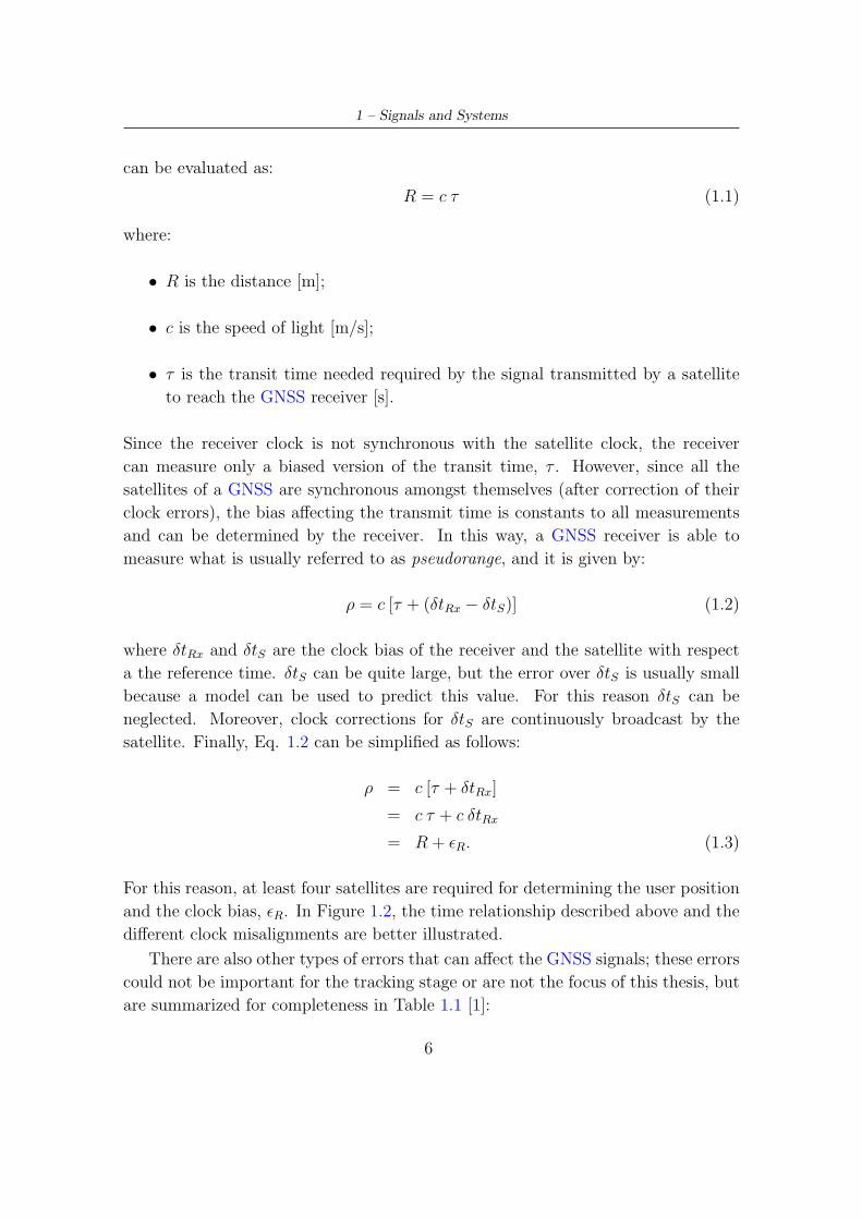
For this reason, at least four satellites are required for determining the user position
and the clock bias, ǫR. In Figure 1.2, the time relationship described above and the
different clock misalignments are better illustrated.
There are also other types of errors that can affect the GNSS signals; these errors
could not be important for the tracking stage or are not the focus of this thesis, but
are summarized for completeness in Table 1.1 [1]:
6
1 – Signals and Systems
Figure 1.2: Clock misalignments in a GNSS system.
Table 1.1: Major error sources for GNSS signals [1].
Major error sourcesSatellite Orbit & clock
PropagationIonosphere
Troposphere
Receiver
Code MultipathCode Noise
Carrier MultipathCarrier Noise
1.2 DSSS signals
GNSSs generally use a Direct Sequence Spread Spectrum (DSSS) modulation for the
transmission of the navigation signals. DSSS is a particular modulation where the
data message is multiplied by a Pseudo Random Noise (PRN) sequence (generally a
binary sequence). The duration of each element of the PRN is called a chip, whereas
the ratio between the duration of a data symbol of the navigation message and the
chip interval is called spreading factor. This type of transmission permits the signal
to occupy a bandwidth much larger than the one required by the data sequence; the
increase in bandwidth is equal to the spreading factor.
7
1 – Signals and Systems
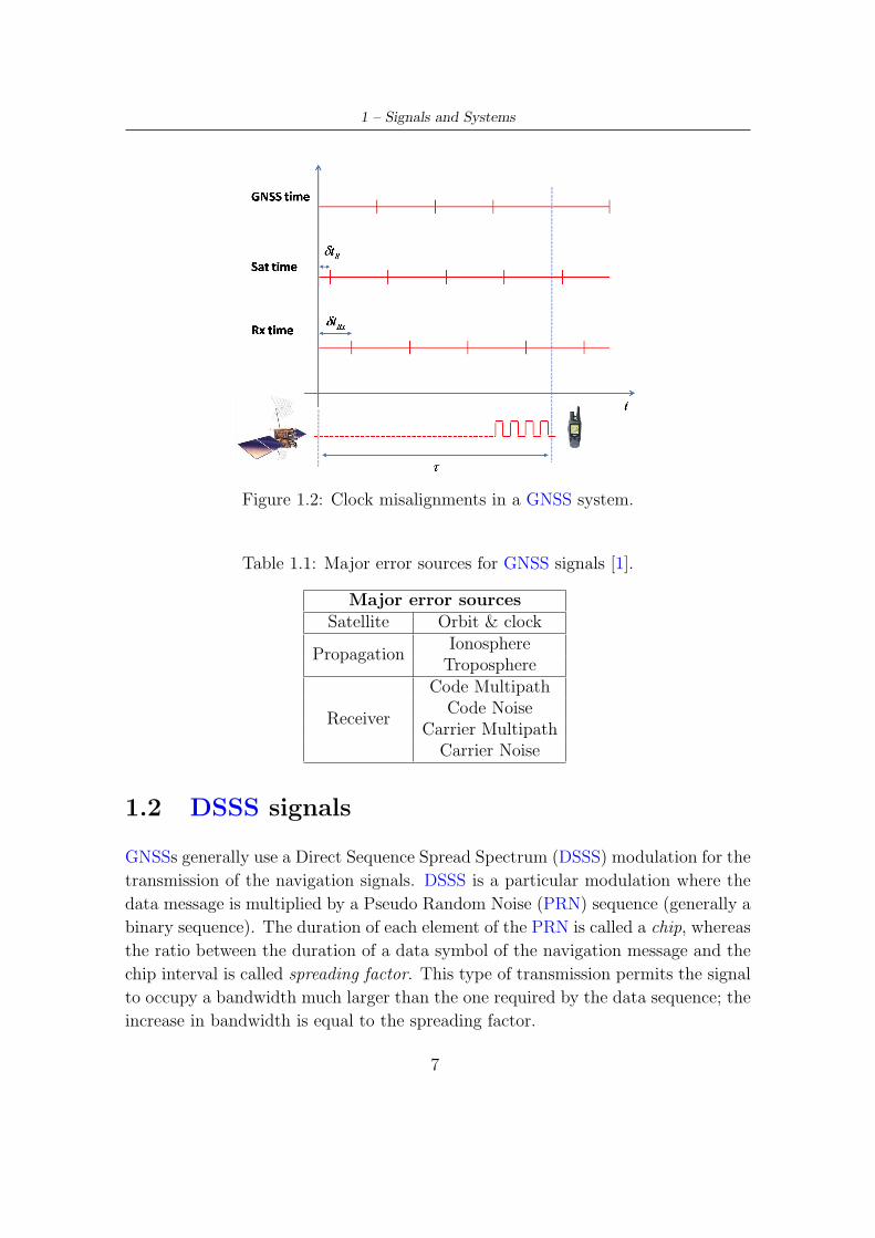
An example of DSSS modulation is shown in Figure 1.3. The first signal is the
data message that is multiplied by the the PRN sequence reported in the second
part of the figure. The last signal in Figure 1.3 is the result of the product of the
navigation message and PRN. This signal has the same rate and bandwidth of
the PRN sequence but it carries only the information provided by the navigation
message.
Figure 1.3: Example of a generic DSSS.
The advantages of employing DSSS modulations can be summarized as follows
[17]:
• since the signal is spread over a large frequency band, the signal Power Spectral
Density (PSD) becomes extremely low, reducing interference problems with
other communications systems;
• spreading and de-spreading makes the signal robust against Radio Frequency
Interference (RFI);
• since the bandwidth is much larger than the coherent bandwidth of the chan-
nel, the system is more robust to fading;
• finally there are some security aspects: without knowing the PRN, it is not easy
to recover the data sequence and besides, the signal may remain undetected
because the PSD is very low. This aspect is not applicable in GNSS because
the PRN sequences are known.
For more details about DSSS see [17].
8
1 – Signals and Systems
1.3 Auto Correlation Function (ACF) and Cross
Correlation Function (CCF)
Several operations performed by a GNSS receiver exploit the correlation properties
of PRN sequence. The correlation function measures how similar two different se-
quences or waveforms are. The Auto Correlation Function (ACF) and the Cross
Correlation Function (CCF) are two specific types of correlation and are defined as
follows [16]:
1. the ACF measures the similarity between a sequence and a shifted version of
itself:
Rx,x(τ) =1
N
N∑
n=0
x[n]x∗[n − τ ]; (1.4)
2. the CCF measures the similarity between two sequences for different relative
delays:
Rx,y(τ) =1
N
N∑
n=0
x[n]y∗[n − τ ]. (1.5)
In (1.4) and (1.5), (·)∗ denotes complex conjugate.
One of the main properties of PRN sequences is that their autocorrelation func-
tion is close to a Kronecker delta, i.e., it assumes a significant value only for a delay
equal to zero. Similarly, the cross-correlation of two sequences from the same family
is almost zero. These properties make PRN sequences suitable for measuring the
transit time, τ : the receiver generates a local replica of the transmitted PRN and
correlates it with the incoming signal. The transit time is estimate from the delay
that maximizes the correlation function.
The most commonly used PRN sequences are Gold codes [18], that present good
correlation properties. These codes were proposed in 1967/1968 by [18], and are
constructed by the Exclusive-Or (EXOR) of two maximum length sequences (m-
sequences) [19] of the same length. A family of Gold codes is obtained by combining
one of two sequences with all possible shifts of the other. The most important
characteristics of these codes are the excellent correlation properties [20]:
• the ACF for any Gold code sequence can assume only four values:
Rx,x(τ) ∈{
1,−1
L,−β(N)
L,β(N) − 2
L
}
(1.6)
9
1 – Signals and Systems
• the CCF between two different sequences can assume only three values:
Rx,y(τ) ∈{
−1
L,−β(N)
L,β(N) − 2
L
}
(1.7)
where
β(N) = 1 + 2
⌊N+2
2
⌋
.
L is the length of the Gold code and N is the size of the shift register used for the
generation of the m-sequences [19]. The CCF of an orthogonal code should be equal
to zero; these codes, instead, assume a value of CCF different from zero (even of
small). For this reason Gold codes are called quasi-orthogonal codes.
In the case of GPS, the Gold codes used for Coarse Acquisition (C/A) signal [2]
have the following properties:
• L equal to 1023 chips;
• shift registers of length N = 10.
The sequence for each satellite is chosen between the 1023 available and the values
of the CCF are:
Rx,y[n] =
{
−65
1023,−1
1023,
63
1023
}
.
These values are quite small, but different from zero (the ideal auto-correlation
function is zero outside the main peak) and the separation between the main and
the side peaks assume the values: ≈ −24, − 60, − 24 dB.
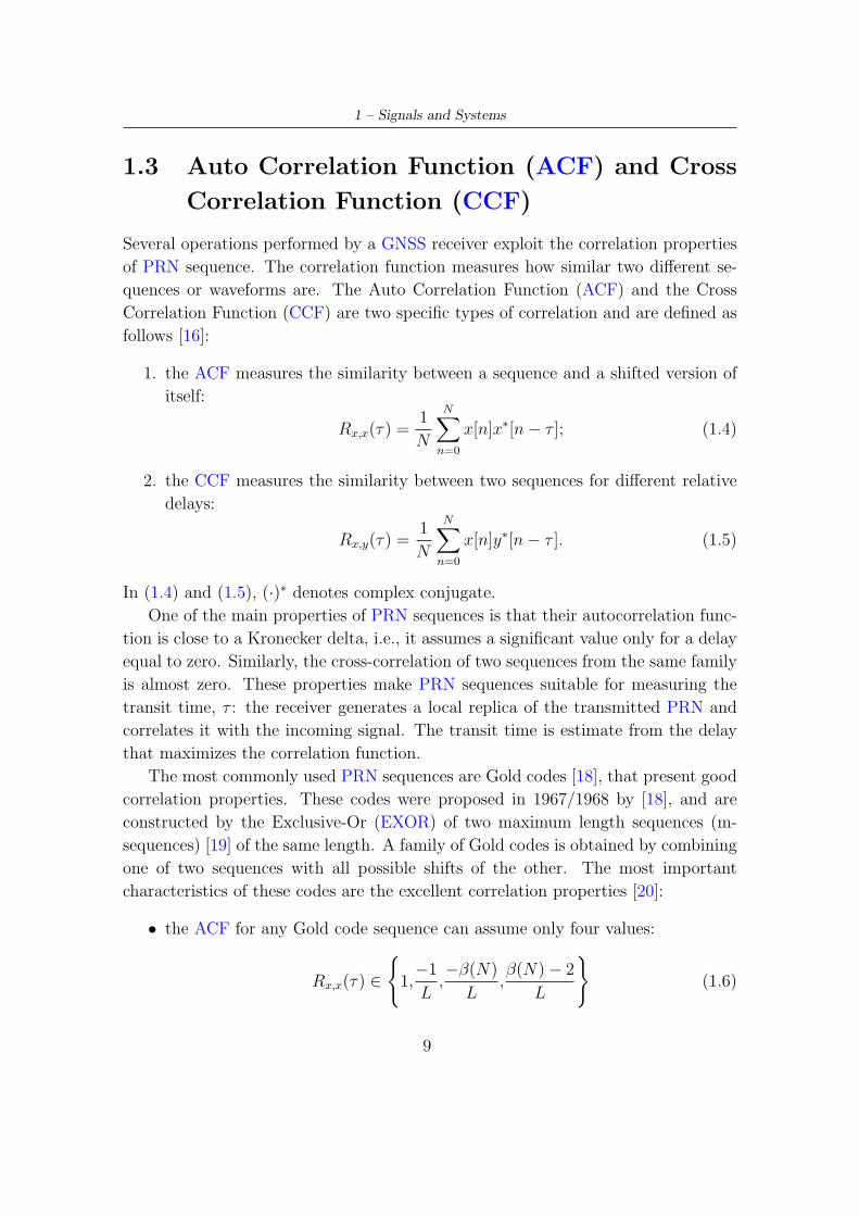
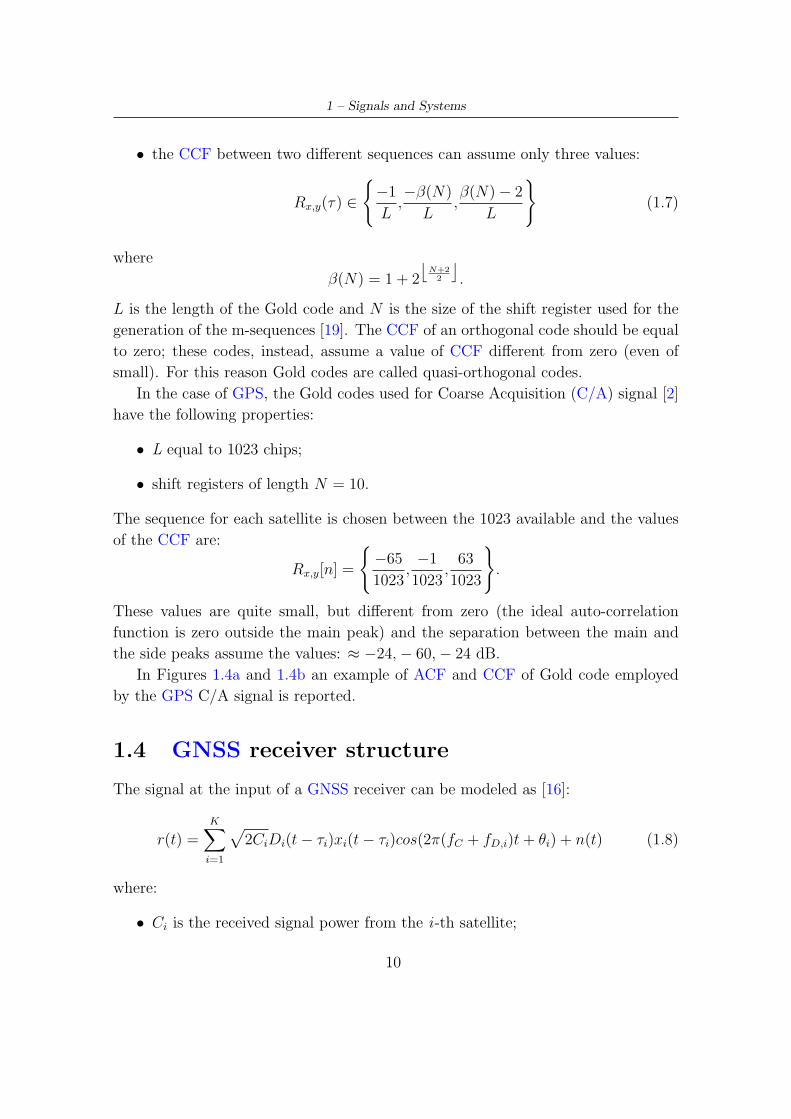
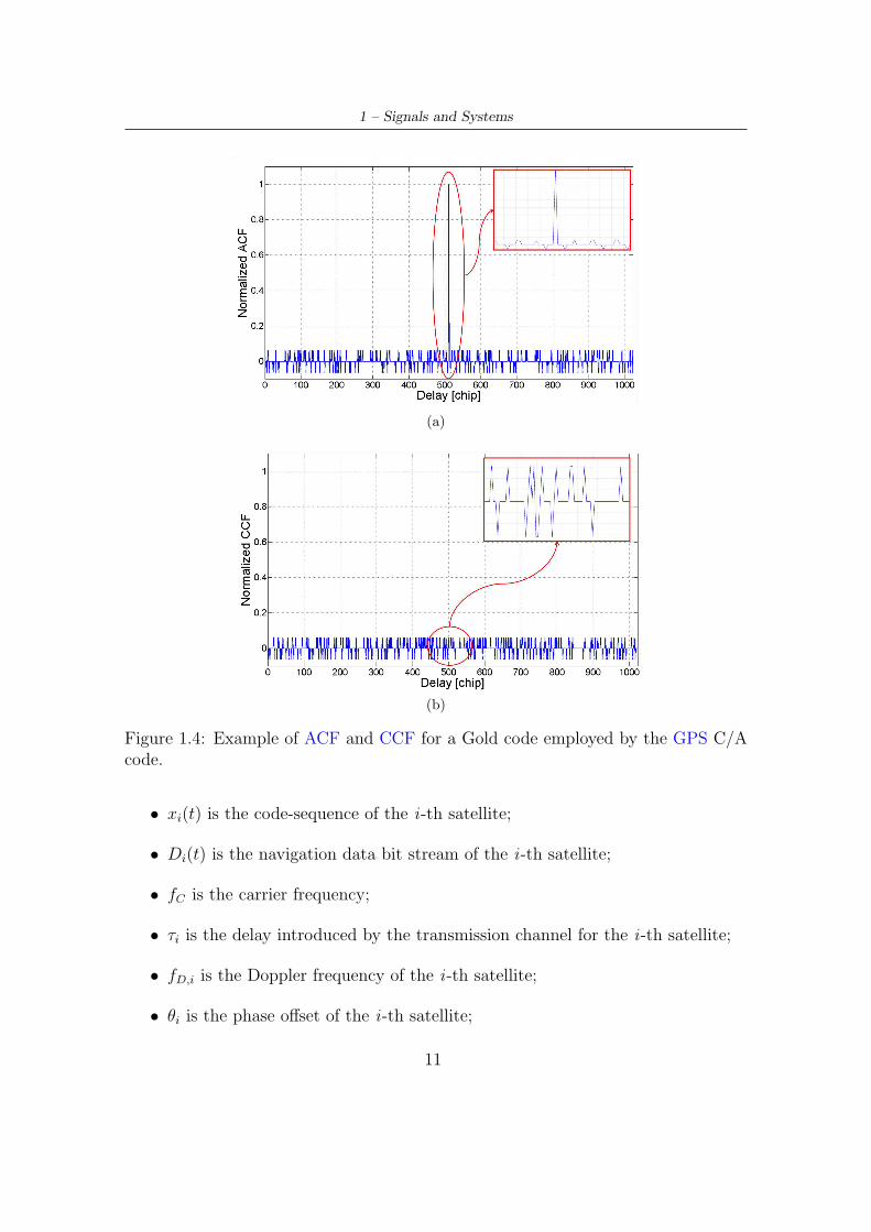
In Figures 1.4a and 1.4b an example of ACF and CCF of Gold code employed
by the GPS C/A signal is reported.
1.4 GNSS receiver structure
The signal at the input of a GNSS receiver can be modeled as [16]:
r(t) =K∑
i=1
√
2CiDi(t − τi)xi(t − τi)cos(2π(fC + fD,i)t + θi) + n(t) (1.8)
where:
• Ci is the received signal power from the i -th satellite;
10
1 – Signals and Systems
(a)
(b)
Figure 1.4: Example of ACF and CCF for a Gold code employed by the GPS C/Acode.
• xi(t) is the code-sequence of the i -th satellite;
• Di(t) is the navigation data bit stream of the i -th satellite;
• fC is the carrier frequency;
• τi is the delay introduced by the transmission channel for the i -th satellite;
• fD,i is the Doppler frequency of the i -th satellite;
• θi is the phase offset of the i -th satellite;
11
1 – Signals and Systems
• n(t) is the noise incoming into the receiver.
Due to the quasi-orthogonality of the PRN sequences a GNSS receiver is able to
process individually the signal transmitted by the different satellites. In this way
Eq. (1.8) can be simplified to consider a single satellite at a time, without loss of
generality, as follows:
y(t) =√
2CD(t − τ)x(t − τ)cos(2π(fC + fD)t + θ) + n(t) (1.9)
The signal x(t) is obtained from this sequence [16]:
x(t) =+∞∑
n=−∞
xnmodNSb(t − nTc)
=+∞∑
n=−∞
xnmodNδ(t − nTc)︸ ︷︷ ︸
gn
∗Sb(t) (1.10)
where:
• Tc is the chip period;
• gn is the periodic repetition of the PRN sequence;
• Sb is the sub-carrier.
The sub-carrier Sb determines the spectral characteristics of the signal and also the
form of the Auto Correlation Function (ACF). For example the GPS C/A code uses
Binary Phase Shift Keying (BPSK) to modulate the transmitted carrier such that
its sub-carrier can be expressed as [16]:
Sb(t) = ΠTc(t) (1.11)
where ΠTc(t) is the elemental chip waveform [2]:
ΠTc(t) =
{
1/√
Tc, −Tc/2 ≤ τ ≤ Tc/2
0, elsewhere.(1.12)
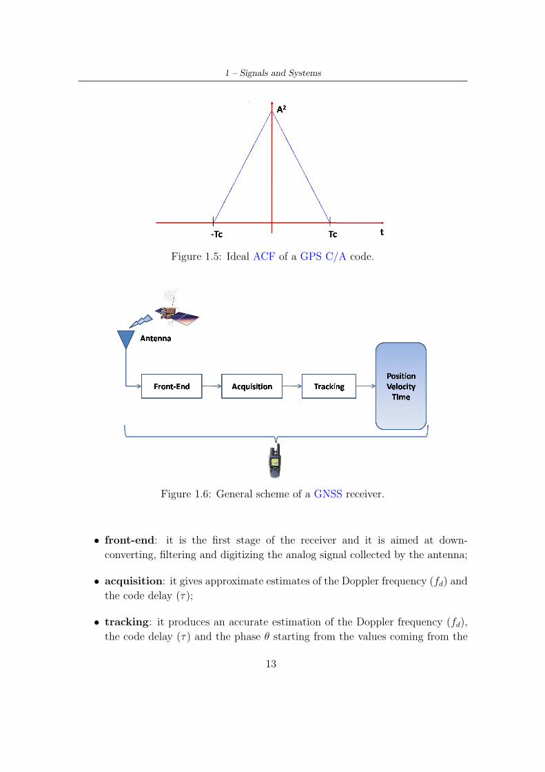
With this definition, the ACF assumes the classical form of a triangle (see Figure
1.5)
One of the main tasks of a GNSS receiver is to estimate the delay τ , the Doppler
frequency fD and the phase θ of the incoming signal. These operations are performed
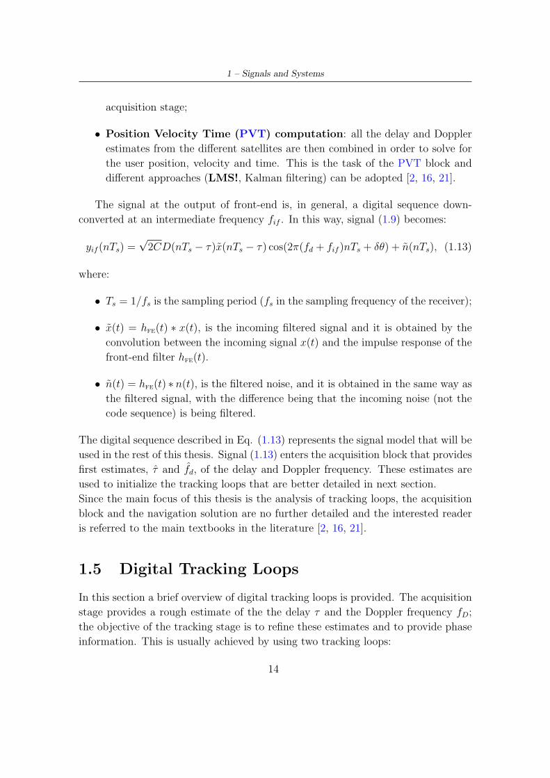
by several stages. The general structure of a receiver is shown in Figure 1.6. The
main functional blocks of a GNSS receiver can be summarized as follows:
12
1 – Signals and Systems
Figure 1.5: Ideal ACF of a GPS C/A code.
Figure 1.6: General scheme of a GNSS receiver.
• front-end: it is the first stage of the receiver and it is aimed at down-
converting, filtering and digitizing the analog signal collected by the antenna;
• acquisition: it gives approximate estimates of the Doppler frequency (fd) and
the code delay (τ);
• tracking: it produces an accurate estimation of the Doppler frequency (fd),
the code delay (τ) and the phase θ starting from the values coming from the
13
1 – Signals and Systems
acquisition stage;
• Position Velocity Time (PVT) computation: all the delay and Doppler
estimates from the different satellites are then combined in order to solve for
the user position, velocity and time. This is the task of the PVT block and
different approaches (LMS!, Kalman filtering) can be adopted [2, 16, 21].
The signal at the output of front-end is, in general, a digital sequence down-
converted at an intermediate frequency fif . In this way, signal (1.9) becomes:
yif (nTs) =√
2CD(nTs − τ)x(nTs − τ) cos(2π(fd + fif )nTs + δθ) + n(nTs), (1.13)
where:
• Ts = 1/fs is the sampling period (fs in the sampling frequency of the receiver);
• x(t) = hfe(t) ∗ x(t), is the incoming filtered signal and it is obtained by the
convolution between the incoming signal x(t) and the impulse response of the
front-end filter hfe(t).
• n(t) = hfe(t) ∗ n(t), is the filtered noise, and it is obtained in the same way as
the filtered signal, with the difference being that the incoming noise (not the
code sequence) is being filtered.
The digital sequence described in Eq. (1.13) represents the signal model that will be
used in the rest of this thesis. Signal (1.13) enters the acquisition block that provides
first estimates, τ and fd, of the delay and Doppler frequency. These estimates are
used to initialize the tracking loops that are better detailed in next section.
Since the main focus of this thesis is the analysis of tracking loops, the acquisition
block and the navigation solution are no further detailed and the interested reader
is referred to the main textbooks in the literature [2, 16, 21].
1.5 Digital Tracking Loops
In this section a brief overview of digital tracking loops is provided. The acquisition
stage provides a rough estimate of the the delay τ and the Doppler frequency fD;
the objective of the tracking stage is to refine these estimates and to provide phase
information. This is usually achieved by using two tracking loops:
14
1 – Signals and Systems
• Delay Lock Loop (DLL) that refines the code phase estimate and tracks its
changes by generating a local replica of the PRN and keeping it aligned with
the signal received from the satellite;
• Phase Lock Loop (PLL) refines the Doppler frequency estimate and provides
carrier phase information. In case of high dynamics the PLL is not able to
track the phase, so a Frequency Lock Loop (FLL) is required to lower the
frequency error.
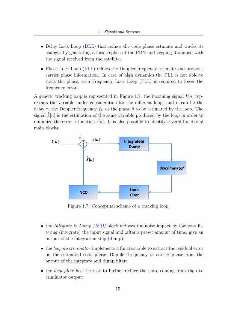
A generic tracking loop is represented in Figure 1.7; the incoming signal k[n] rep-
resents the variable under consideration for the different loops and it can be the
delay τ , the Doppler frequency fD or the phase θ to be estimated by the loop. The
signal k[n] is the estimation of the same variable produced by the loop in order to
minimize the error estimation ǫ[n]. It is also possible to identify several functional
main blocks:
Figure 1.7: Conceptual scheme of a tracking loop.
• the Integrate & Dump (I&D) block reduces the noise impact by low-pass fil-
tering (integrate) the input signal and ,after a preset amount of time, give an
output of the integration step (dump);
• the loop discriminator implements a function able to extract the residual error
on the estimated code phase, Doppler frequency or carrier phase from the
output of the integrate and dump filter;
• the loop filter has the task to further reduce the noise coming from the dis-
criminator output;
15
1 – Signals and Systems
• the NCO generates a local replica of carrier/code signal based on the informa-
tion provided by loop filter output.
This thesis is focused on the impact of notch filtering on tracking loops and in
particular on the loss and biases introduced on the delay domain, so below the DLL
and the PLL will be described, putting much more attention on the delay loop and
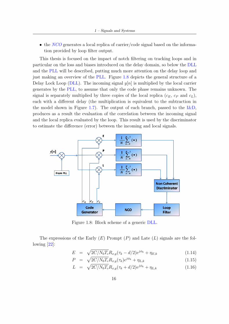
just making an overview of the PLL. Figure 1.8 depicts the general structure of a
Delay Lock Loop (DLL). The incoming signal y[n] is multiplied by the local carrier
generates by the PLL, to assume that only the code phase remains unknown. The
signal is separately multiplied by three copies of the local replica (cE, cP and cL),
each with a different delay (the multiplication is equivalent to the subtraction in
the model shown in Figure 1.7). The output of each branch, passed to the I&D,
produces as a result the evaluation of the correlation between the incoming signal
and the local replica evaluated by the loop. This result is used by the discriminator
to estimate the difference (error) between the incoming and local signals.
Figure 1.8: Block scheme of a generic DLL.
The expressions of the Early (E) Prompt (P ) and Late (L) signals are the fol-
lowing [22]:
E =√
2C/N0TcRx,y(τk − d/2)ejφk + ηE,k (1.14)
P =√
2C/N0TcRx,y(τk)ejφk + ηL,k (1.15)
L =√
2C/N0TcRx,y(τk + d/2)ejφk + ηL,k (1.16)
16
1 – Signals and Systems
where:
• CN0
is the Carrier-to-Noise density ratio;
• Tc is the integration time;
• Rx,y(τk) is the cross-correlation between the incoming signal and the local
replica;
• τk is the code phase at the k -th instant of time;
• d is the spacing between the local replicas in chips;
• φk is the residual phase error at the instant k;
• ηk are the complex noise samples.
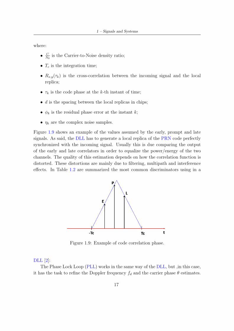
Figure 1.9 shows an example of the values assumed by the early, prompt and late
signals. As said, the DLL has to generate a local replica of the PRN code perfectly
synchronized with the incoming signal. Usually this is due comparing the output
of the early and late correlators in order to equalize the power/energy of the two
channels. The quality of this estimation depends on how the correlation function is
distorted. These distortions are mainly due to filtering, multipath and interference
effects. In Table 1.2 are summarized the most common discriminators using in a
Figure 1.9: Example of code correlation phase.
DLL [2]:
The Phase Lock Loop (PLL) works in the same way of the DLL, but ,in this case,
it has the task to refine the Doppler frequency fd and the carrier phase θ estimates.
17
1 – Signals and Systems
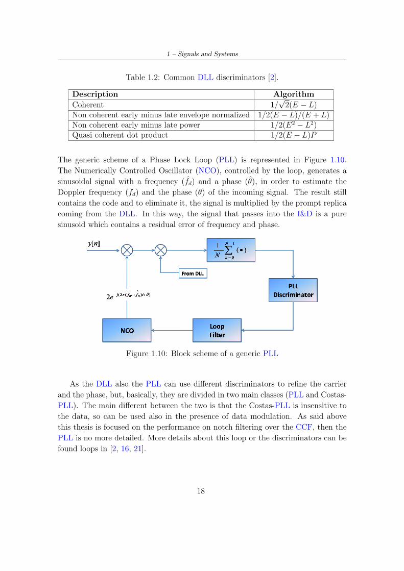
Table 1.2: Common DLL discriminators [2].
Description Algorithm
Coherent 1/√
2(E − L)Non coherent early minus late envelope normalized 1/2(E − L)/(E + L)Non coherent early minus late power 1/2(E2 − L2)Quasi coherent dot product 1/2(E − L)P
The generic scheme of a Phase Lock Loop (PLL) is represented in Figure 1.10.
The Numerically Controlled Oscillator (NCO), controlled by the loop, generates a
sinusoidal signal with a frequency (fd) and a phase (θ), in order to estimate the
Doppler frequency (fd) and the phase (θ) of the incoming signal. The result still
contains the code and to eliminate it, the signal is multiplied by the prompt replica
coming from the DLL. In this way, the signal that passes into the I&D is a pure
sinusoid which contains a residual error of frequency and phase.
Figure 1.10: Block scheme of a generic PLL
As the DLL also the PLL can use different discriminators to refine the carrier
and the phase, but, basically, they are divided in two main classes (PLL and Costas-
PLL). The main different between the two is that the Costas-PLL is insensitive to
the data, so can be used also in the presence of data modulation. As said above
this thesis is focused on the performance on notch filtering over the CCF, then the
PLL is no more detailed. More details about this loop or the discriminators can be
found loops in [2, 16, 21].
18
Chapter 2
Notch Filter (NF) for Interference
Removal
2.1 Continuous Wave Interference (CWI)
The impacts of an interference (unintentional or jamming) on a GNSS system are
manifold. First of all it is necessary to distinguish between wide-band and narrow-
band interference. The terms wide and narrow are referred to the bandwidth of the
GNSS signal, because, for example, an interference can be considered wide for the
C/A code, but, at the same time, narrow for the Encrypted Precision (P(Y)) code,
due to the different Power Spectral Densities PSDs. Another distinction is referred
to the magnitude of the interference, because, if the power of the interference can
be compared with the noise, then its impact can be neglected. Instead, if the
interference is strong, the impact depends on its duration and on its PSD. All
these Radio Frequency Interference (RFI) affect the GNSS receiver and produce as
a result a degradation in terms of acquisition and tracking accuracy, which means
less precision when the position is determined or, in the worst case, the loss of the
useful signal. As seen in Chapter 1, GNSS signals employ DSSS modulation, that
can improve slightly the robustness of the signal against interference.
One of the most common sources of interference is the so named Continuous
Wave Interference (CWI) and they can be modeled as a sinusoidal wave in time
[16]:
j(t) =√
2Pj cos(2πfj + θj) (2.1)
where:
• Pj is the power of the interference;
19
2 – Notch Filter (NF) for Interference Removal
• fj is the frequency where the CWI is centered;
• θj is the phase of the interference.
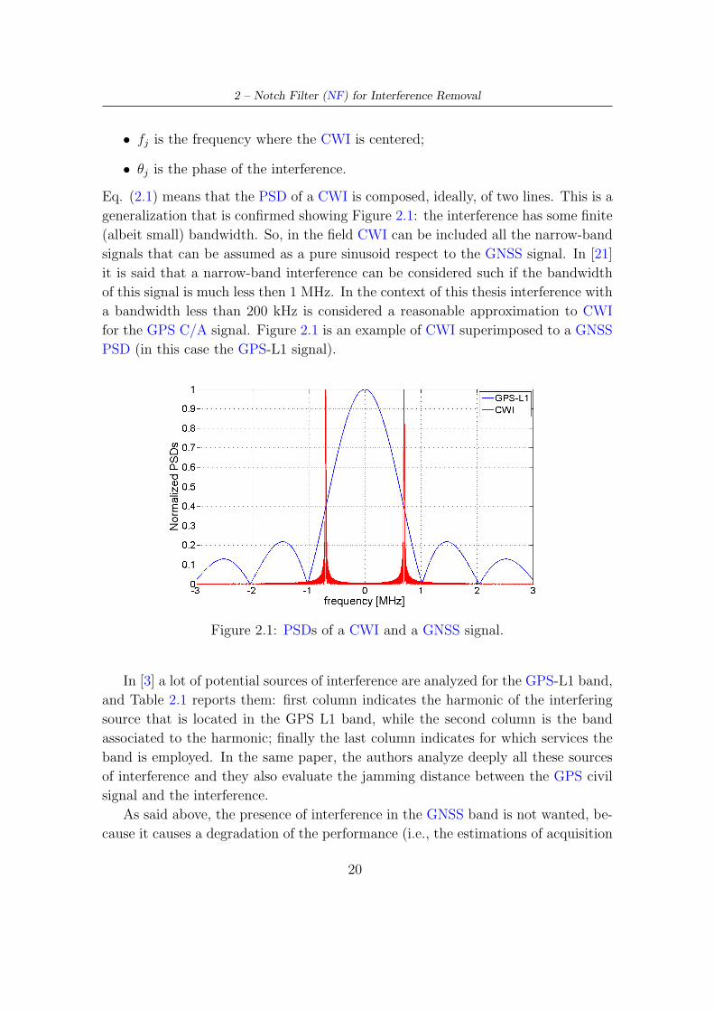
Eq. (2.1) means that the PSD of a CWI is composed, ideally, of two lines. This is a
generalization that is confirmed showing Figure 2.1: the interference has some finite
(albeit small) bandwidth. So, in the field CWI can be included all the narrow-band
signals that can be assumed as a pure sinusoid respect to the GNSS signal. In [21]
it is said that a narrow-band interference can be considered such if the bandwidth
of this signal is much less then 1 MHz. In the context of this thesis interference with
a bandwidth less than 200 kHz is considered a reasonable approximation to CWI
for the GPS C/A signal. Figure 2.1 is an example of CWI superimposed to a GNSS
PSD (in this case the GPS-L1 signal).
Figure 2.1: PSDs of a CWI and a GNSS signal.
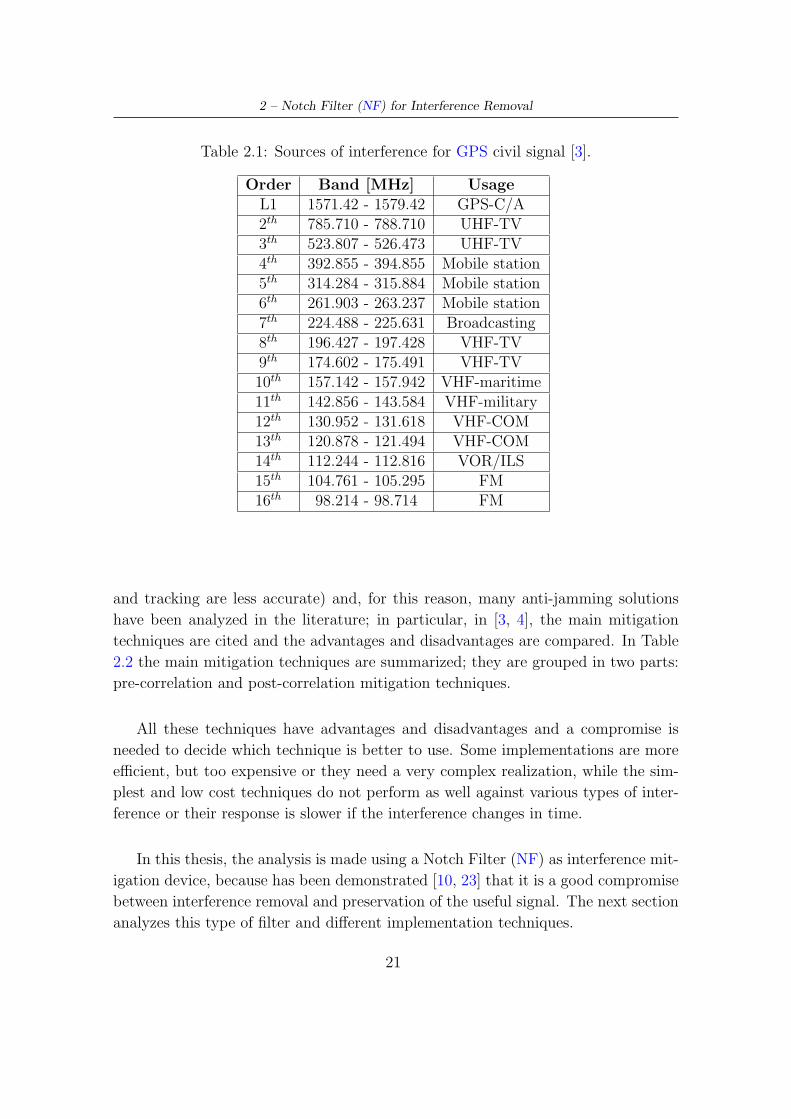
In [3] a lot of potential sources of interference are analyzed for the GPS-L1 band,
and Table 2.1 reports them: first column indicates the harmonic of the interfering
source that is located in the GPS L1 band, while the second column is the band
associated to the harmonic; finally the last column indicates for which services the
band is employed. In the same paper, the authors analyze deeply all these sources
of interference and they also evaluate the jamming distance between the GPS civil
signal and the interference.
As said above, the presence of interference in the GNSS band is not wanted, be-
cause it causes a degradation of the performance (i.e., the estimations of acquisition
20
2 – Notch Filter (NF) for Interference Removal
Table 2.1: Sources of interference for GPS civil signal [3].
Order Band [MHz] UsageL1 1571.42 - 1579.42 GPS-C/A2th 785.710 - 788.710 UHF-TV3th 523.807 - 526.473 UHF-TV4th 392.855 - 394.855 Mobile station5th 314.284 - 315.884 Mobile station6th 261.903 - 263.237 Mobile station7th 224.488 - 225.631 Broadcasting8th 196.427 - 197.428 VHF-TV9th 174.602 - 175.491 VHF-TV10th 157.142 - 157.942 VHF-maritime11th 142.856 - 143.584 VHF-military12th 130.952 - 131.618 VHF-COM13th 120.878 - 121.494 VHF-COM14th 112.244 - 112.816 VOR/ILS15th 104.761 - 105.295 FM16th 98.214 - 98.714 FM
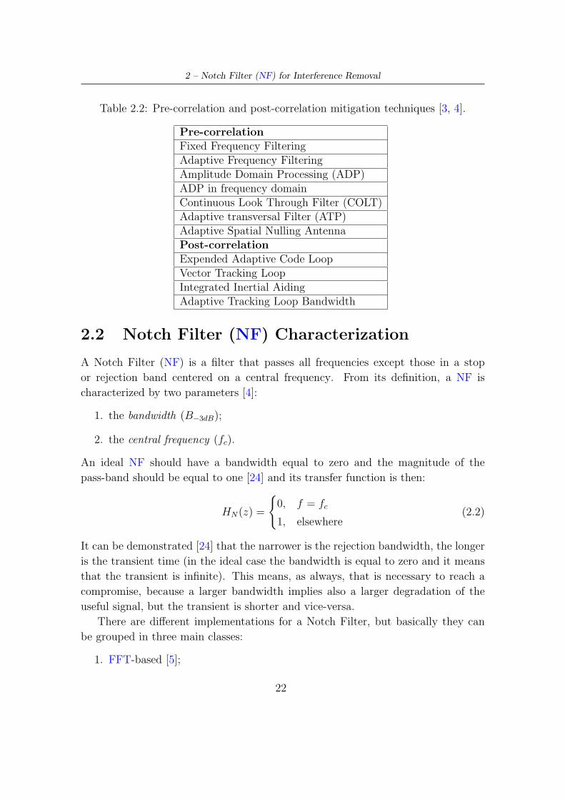
and tracking are less accurate) and, for this reason, many anti-jamming solutions
have been analyzed in the literature; in particular, in [3, 4], the main mitigation
techniques are cited and the advantages and disadvantages are compared. In Table
2.2 the main mitigation techniques are summarized; they are grouped in two parts:
pre-correlation and post-correlation mitigation techniques.
All these techniques have advantages and disadvantages and a compromise is
needed to decide which technique is better to use. Some implementations are more
efficient, but too expensive or they need a very complex realization, while the sim-
plest and low cost techniques do not perform as well against various types of inter-
ference or their response is slower if the interference changes in time.
In this thesis, the analysis is made using a Notch Filter (NF) as interference mit-
igation device, because has been demonstrated [10, 23] that it is a good compromise
between interference removal and preservation of the useful signal. The next section
analyzes this type of filter and different implementation techniques.
21
2 – Notch Filter (NF) for Interference Removal
Table 2.2: Pre-correlation and post-correlation mitigation techniques [3, 4].
Pre-correlationFixed Frequency FilteringAdaptive Frequency FilteringAmplitude Domain Processing (ADP)ADP in frequency domainContinuous Look Through Filter (COLT)Adaptive transversal Filter (ATP)Adaptive Spatial Nulling AntennaPost-correlationExpended Adaptive Code LoopVector Tracking LoopIntegrated Inertial AidingAdaptive Tracking Loop Bandwidth
2.2 Notch Filter (NF) Characterization
A Notch Filter (NF) is a filter that passes all frequencies except those in a stop
or rejection band centered on a central frequency. From its definition, a NF is
characterized by two parameters [4]:
1. the bandwidth (B−3dB);
2. the central frequency (fc).
An ideal NF should have a bandwidth equal to zero and the magnitude of the
pass-band should be equal to one [24] and its transfer function is then:
HN(z) =
{
0, f = fc
1, elsewhere(2.2)
It can be demonstrated [24] that the narrower is the rejection bandwidth, the longer
is the transient time (in the ideal case the bandwidth is equal to zero and it means
that the transient is infinite). This means, as always, that is necessary to reach a
compromise, because a larger bandwidth implies also a larger degradation of the
useful signal, but the transient is shorter and vice-versa.
There are different implementations for a Notch Filter, but basically they can
be grouped in three main classes:
1. FFT-based [5];
22
2 – Notch Filter (NF) for Interference Removal
2. Finite Impulse Response (FIR) implementations [5, 6];
3. Infinite Impulse Response (IIR) implementations [4, 23, 25, 26, 27];
In this thesis a NF belonging to the third class (IIR) will be used, so the first two
classes will be briefly described and more particulars can be found in the references.
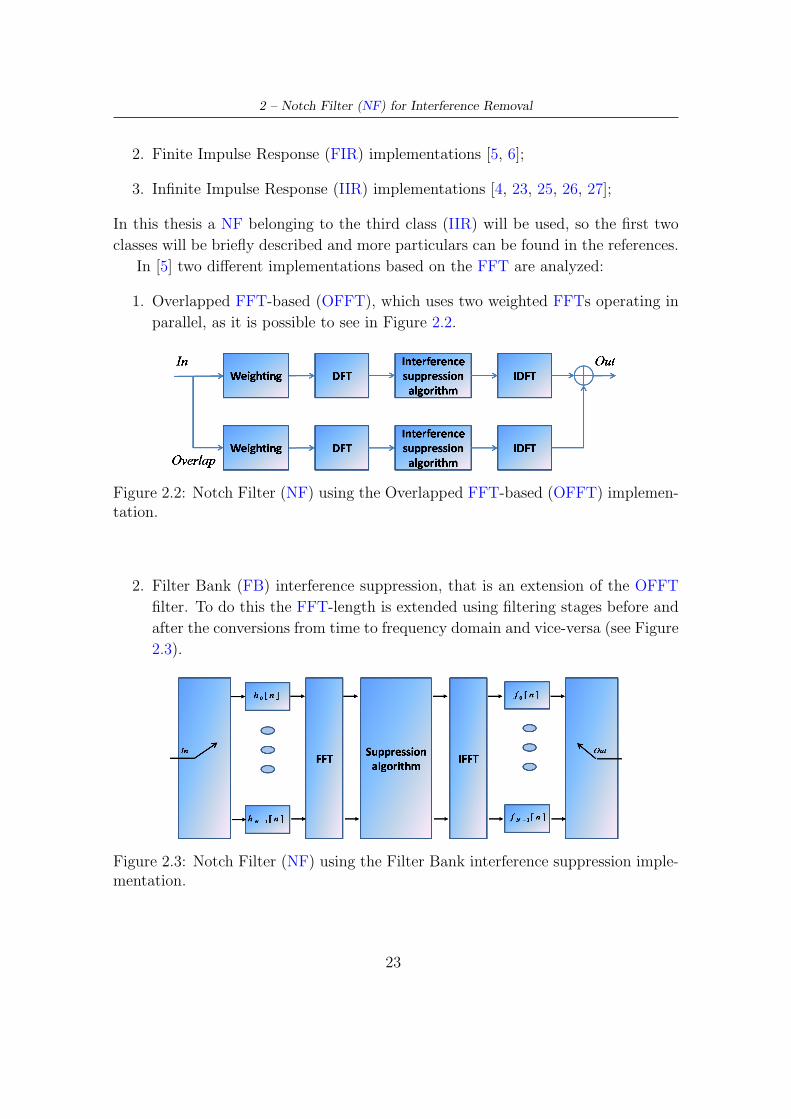
In [5] two different implementations based on the FFT are analyzed:
1. Overlapped FFT-based (OFFT), which uses two weighted FFTs operating in
parallel, as it is possible to see in Figure 2.2.
Figure 2.2: Notch Filter (NF) using the Overlapped FFT-based (OFFT) implemen-tation.
2. Filter Bank (FB) interference suppression, that is an extension of the OFFT
filter. To do this the FFT-length is extended using filtering stages before and
after the conversions from time to frequency domain and vice-versa (see Figure
2.3).
Figure 2.3: Notch Filter (NF) using the Filter Bank interference suppression imple-mentation.
23
2 – Notch Filter (NF) for Interference Removal
The functioning principle is the same for both the FFT-based techniques. The
excision of the interference is done setting to zero the frequency bins that pass
a certain threshold. The bins that remain under the threshold are unchanged.
The threshold is set by the suppression algorithm and it is usually proportional
to the mean noise in the absence of interference [5]. The difference between the two
algorithms is due to the fact that the second type (FB interference suppression) has
a lower implementation complexity given the same performance level, but it has a
low response time with respect to the OFFT technique.
The second class of filters (FIR implementation) has the advantage to not present
stability problems, but they are complicated to realize, because, for a very narrow-
band excision, they need a large number of taps, that means a large number of
additions and multiplications. Also for this type of filters there are different imple-
mentations:
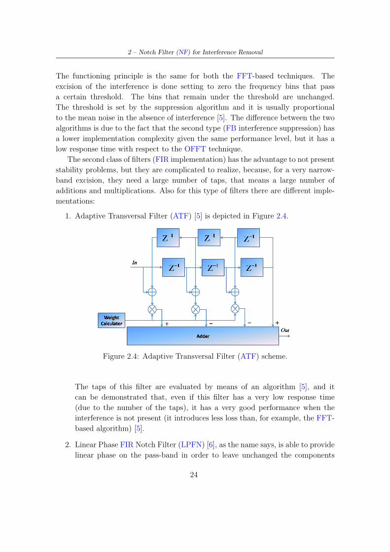
1. Adaptive Transversal Filter (ATF) [5] is depicted in Figure 2.4.
Figure 2.4: Adaptive Transversal Filter (ATF) scheme.
The taps of this filter are evaluated by means of an algorithm [5], and it
can be demonstrated that, even if this filter has a very low response time
(due to the number of the taps), it has a very good performance when the
interference is not present (it introduces less loss than, for example, the FFT-
based algorithm) [5].
2. Linear Phase FIR Notch Filter (LPFN) [6], as the name says, is able to provide
linear phase on the pass-band in order to leave unchanged the components
24
2 – Notch Filter (NF) for Interference Removal
outside the rejection bandwidth. In [6] three different approaches of the LPFN
are analyzed:
(a) The windowed Fourier series;
(b) The frequency sampling ;
(c) The optimal LPFN
In [6], the performance of these filters are compared and was found that the
best one is the optimal LPFN, but the simplest in terms of realization is the
windowed Fourier series.
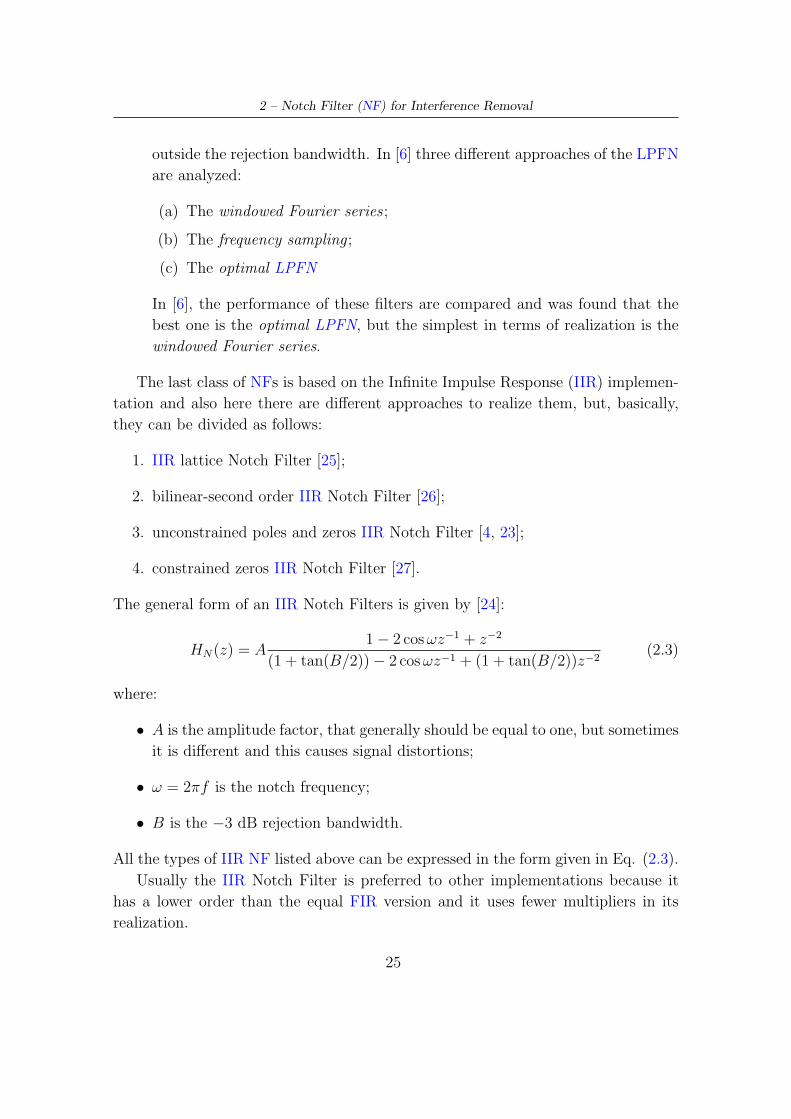
The last class of NFs is based on the Infinite Impulse Response (IIR) implemen-
tation and also here there are different approaches to realize them, but, basically,
they can be divided as follows:
1. IIR lattice Notch Filter [25];
2. bilinear-second order IIR Notch Filter [26];
3. unconstrained poles and zeros IIR Notch Filter [4, 23];
4. constrained zeros IIR Notch Filter [27].
The general form of an IIR Notch Filters is given by [24]:
HN(z) = A1 − 2 cos ωz−1 + z−2
(1 + tan(B/2)) − 2 cos ωz−1 + (1 + tan(B/2))z−2(2.3)
where:
• A is the amplitude factor, that generally should be equal to one, but sometimes
it is different and this causes signal distortions;
• ω = 2πf is the notch frequency;
• B is the −3 dB rejection bandwidth.
All the types of IIR NF listed above can be expressed in the form given in Eq. (2.3).
Usually the IIR Notch Filter is preferred to other implementations because it
has a lower order than the equal FIR version and it uses fewer multipliers in its
realization.
25
2 – Notch Filter (NF) for Interference Removal
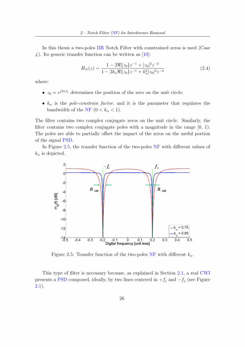
In this thesis a two-poles IIR Notch Filter with constrained zeros is used (Case
4 ). Its generic transfer function can be written as [10]:
HN(z) =1 − 2ℜ{z0}z−1 + |z0|2z−2
1 − 2kαℜ{z0}z−1 + k2α|z0|2z−2
(2.4)
where:
• z0 = ej2πfj determines the position of the zero on the unit circle;
• kα is the pole-constrain factor, and it is the parameter that regulates the
bandwidth of the NF (0 < kα < 1).
The filter contains two complex conjugate zeros on the unit circle. Similarly, the
filter contains two complex conjugate poles with a magnitude in the range [0, 1).
The poles are able to partially offset the impact of the zeros on the useful portion
of the signal PSD.
In Figure 2.5, the transfer function of the two-poles NF with different values of
kα is depicted.
Figure 2.5: Transfer function of the two-poles NF with different kα.
This type of filter is necessary because, as explained in Section 2.1, a real CWI
presents a PSD composed, ideally, by two lines centered in +fj and −fj (see Figure
2.1).
26
2 – Notch Filter (NF) for Interference Removal
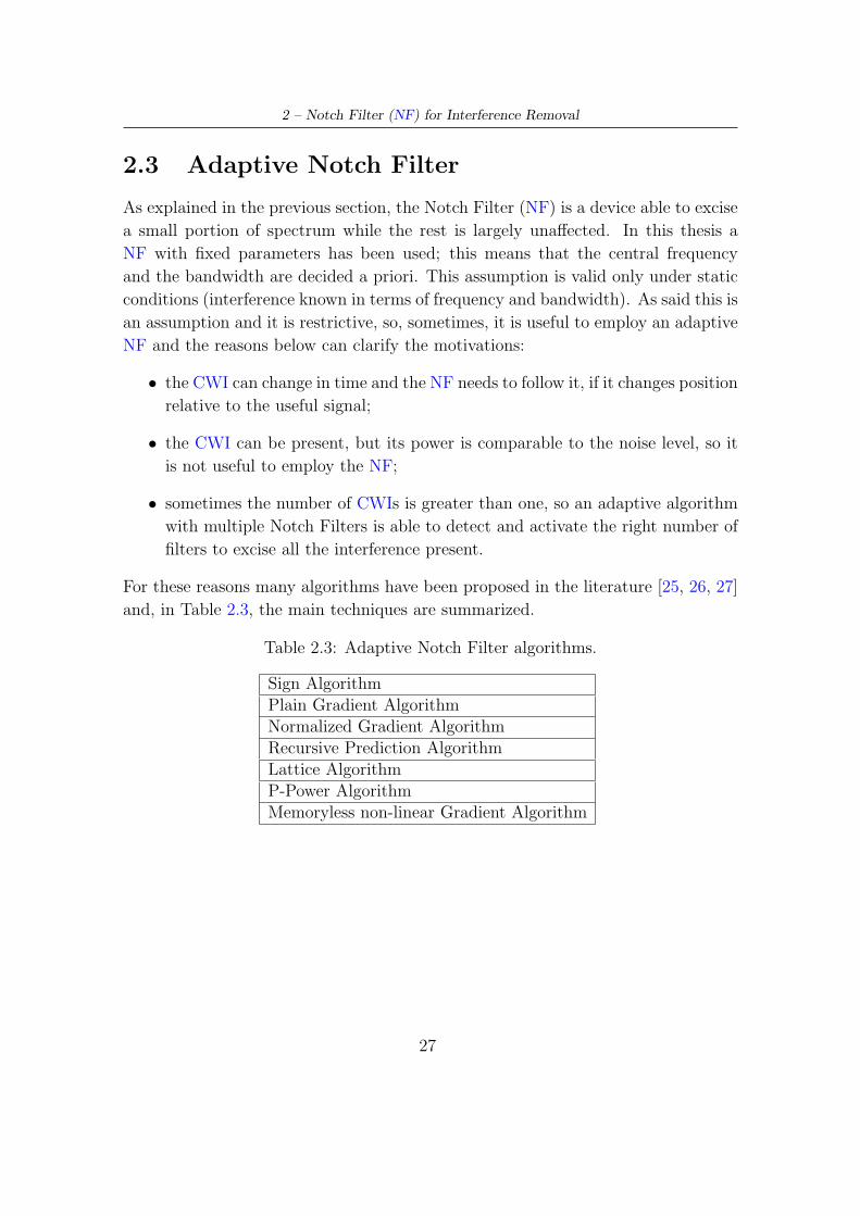
2.3 Adaptive Notch Filter
As explained in the previous section, the Notch Filter (NF) is a device able to excise
a small portion of spectrum while the rest is largely unaffected. In this thesis a
NF with fixed parameters has been used; this means that the central frequency
and the bandwidth are decided a priori. This assumption is valid only under static
conditions (interference known in terms of frequency and bandwidth). As said this is
an assumption and it is restrictive, so, sometimes, it is useful to employ an adaptive
NF and the reasons below can clarify the motivations:
• the CWI can change in time and the NF needs to follow it, if it changes position
relative to the useful signal;
• the CWI can be present, but its power is comparable to the noise level, so it
is not useful to employ the NF;
• sometimes the number of CWIs is greater than one, so an adaptive algorithm
with multiple Notch Filters is able to detect and activate the right number of
filters to excise all the interference present.
For these reasons many algorithms have been proposed in the literature [25, 26, 27]
and, in Table 2.3, the main techniques are summarized.
Table 2.3: Adaptive Notch Filter algorithms.
Sign AlgorithmPlain Gradient AlgorithmNormalized Gradient AlgorithmRecursive Prediction AlgorithmLattice AlgorithmP-Power AlgorithmMemoryless non-linear Gradient Algorithm
27
Chapter 3
Theoretical Characterization of
the Notch Filter Impact
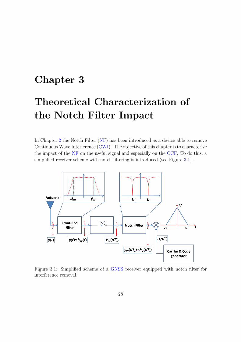
In Chapter 2 the Notch Filter (NF) has been introduced as a device able to remove
Continuous Wave Interference (CWI). The objective of this chapter is to characterize
the impact of the NF on the useful signal and especially on the CCF. To do this, a
simplified receiver scheme with notch filtering is introduced (see Figure 3.1).
Figure 3.1: Simplified scheme of a GNSS receiver equipped with notch filter forinterference removal.
28
3 – Theoretical Characterization of the Notch Filter Impact
In this analysis it is assumed that the parameters of the incoming signal are
known with the exception of the code delay; this means that the receiver is correctly
tracking the carrier phase and the Doppler frequency is properly removed. In Figure
3.1 several signals can be identified:
• y(t) is the incoming signal as expressed in Eq. (1.8);
• y(t) ∗ hFE(t) is the received signal after front-end filtering . In this case the
front-end is modeled using a Chebyshev filter with a certain cut-off frequency
(fco));
• yIF (nTs) is the digitalized and down-converted sequence as expressed in Eq.
(1.9);
• yIF (nTs) ∗ hN(nTs) is the intermediate-frequency signal filtered by a digital
Notch Filter (NF) with a certain central frequency (fc) and a certain band-
width;
• c(nTs) is the local code replica generated by the receiver.
The optimal strategy for recovering a RF signal in noise and transmitted over
a band-limited channel is represented by the matched filter [28]. In this respect,
acquisition and tracking are a sort of matched filter [10, 29], where the receiver tries
to produce a local replica of recovered signal. When the GNSS signal is corrupted by
a CWI, a NF is needed by the receiver to detect the useful signal. This filter removes
the interference, but introduces distortions and, for this reason, the correlation with
locally generated signal is no longer a matched filter. The distortions introduced
by the NF are usually preferable with respect to impact of the CWI and can be
summarized as follows:
1. Filtering loss or correlation loss [10], that measures the C/N0 degradation
introduced by filtering stages[30, 31]. This loss can be expressed as follows[10,
29]:
Lf =
∣∣∣
∫ fs/2
−fs/2GS(f)Hf (f)df
∣∣∣
2
∫ fs/2
−fs/2GS(f)
∣∣∣Hf (f)
∣∣∣
2
df(3.1)
where:
• fs is the sampling frequency;
• GS(f) is the Power Spectral Density (PSD) of the GNSS signal;
29
3 – Theoretical Characterization of the Notch Filter Impact
• Hf (f) is the transfer function of the input filters. For the case in exam
two filtering stages are considered: the front-end filtering and the notch
filtering (see Figure 3.1), so the composite transfer function assumes the
following form:
Hf (f) = HFE(f)HN(f) (3.2)
where HFE(f) is the transfer function of the front-end filter and HN(f)
is the transfer function of the NF.
These losses have been thoroughly examined in the literature [10, 29] and
won’t be further discussed in this thesis.
2. Correlation distortion: the notch filter distorts the correlation between the
input signal and the local code replica. The CCF is no longer a symmetric
function and some biases can introduced in the delay estimate.
Since this thesis is mainly focused on the analysis of the effect of notch filter
on tracking loops, this distortion on the Cross Correlation Function (CCF)
and its implications on the tracking loops is deeply analyzed. The distortion
introduced by the front-end filter is usually limited and consists of a smoothing
on the GNSS signal. Consequently, the CCF is also smoothed. The Notch
Filter (NF) introduces a distortion that depends on the central frequency and
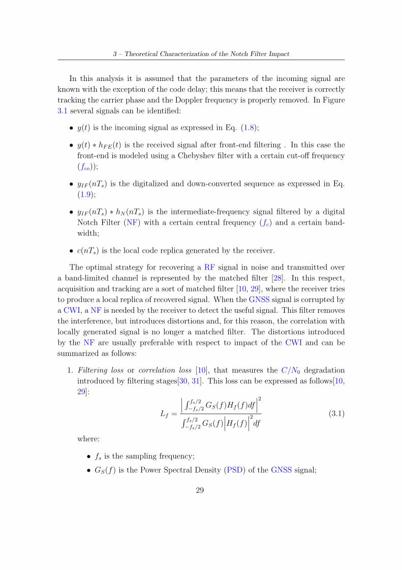
the bandwidth of the notch. In Figure 3.2 two cases of CCF distorted by NF
are depicted. In particular, Figures 3.2a and 3.2b are the PSDs of two different
GNSS modulations, the BPSK(1) used by GPS-L1 and the BOC(1,1) used by
Galileo-E1 signal. The transfer function of the notch filter is plotted over
the signal PSDs, showing the frequency components excised by the filter. In
Figures 3.2c and 3.2d the corresponding CCFs overlapping to the ideal cross-
correlation are shown.
The represented CCFs can be considered as worst cases, since the filter notch
is in the main lobe of the respective PSDs. In this way, a significant portion
of the GNSS signal is excised causing a high distortion on the CCF. If the
Notch Filter falls in a null of the PSD, the CCF distortions are marginal and
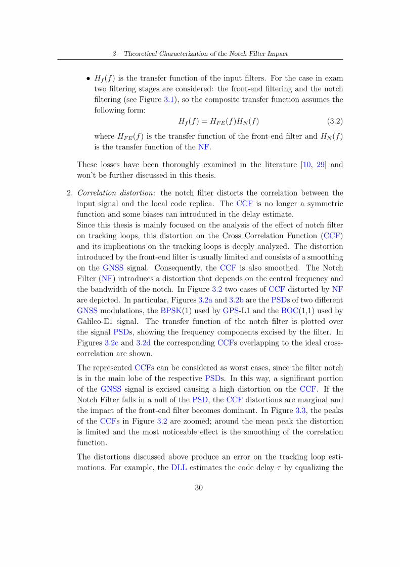
the impact of the front-end filter becomes dominant. In Figure 3.3, the peaks
of the CCFs in Figure 3.2 are zoomed; around the mean peak the distortion
is limited and the most noticeable effect is the smoothing of the correlation
function.
The distortions discussed above produce an error on the tracking loop esti-
mations. For example, the DLL estimates the code delay τ by equalizing the
30
3 – Theoretical Characterization of the Notch Filter Impact
(a) (b)
(c) (d)
Figure 3.2: Filtering distortions on the CCF for different modulations.
(a) (b)
Figure 3.3: Particular of the CCF depicted in Figure 3.2.
power of the early and late correlators (Chapter 1) and the quality of the delay
estimation is deeply related to the quality of the CCF: if the peak is distorted
or no longer symmetric, the estimate is no more accurate and some bias can
be introduced. Also the Early-Late spacing plays a fundamental role, since
the distortion is more significant at the correlation base (see Figure 3.2), a
31
3 – Theoretical Characterization of the Notch Filter Impact
larger spacing introduces a larger estimation error. This aspect will be further
analyzed in Chapter 4, where a semi-analytic model is used for evaluating the
DLL tracking jitter in the presence of notch filtering.
.
The next section aims at characterizing the Notch Filter impact exploiting the
correlation properties discussed in Chapter 1 and relating it to the NF parameters.
3.1 ACF and CCF characterizations: Asymmetry
Coefficient
Starting from the definitions of Auto Correlation Function (ACF) and Cross Corre-
lation Function (CCF) seen in Chapter 1, it is possible to re-write the CCF using
the definition of Fourier transform:
R(τ) =
∫ fs/2
−fs/2
Φ(f)ej2πfτdf. (3.3)
Φ(f) is the Fourier Transform of the CCF and, in the absence of filtering, it corre-
sponds to the normalized Power Spectral Density (PSD) of the recovered GNSS:
Φ(f) =Φ(f)
∫ fs/2
−fs/2Φ(f)df
. (3.4)
In Eq. (3.4), Φ(f) is the unnormalized signal PSD. The normalization (3.4), follows
from the condition R(0) = 1. The CCF in Eq. (3.3) can be approximated by its
Taylor expansion:
R(τ) = 1 + a1τ + a2τ2 + O(τ 3) (3.5)
and, depending on which type of function (symmetrical or asymmetrical) is consid-
ered, the above expansion assumes different forms:
1. Symmetrical function: the odd coefficients are zero and the expansion (3.5)
becomes:
R(τ) = 1 + a2τ2 + O(τ 4). (3.6)
The coefficient a2 can be evaluated as the second derivative of the CCF in Eq.
(3.3):
a2 =1
2
d2R(τ)
dτ 2
∣∣∣∣∣τ=0
(3.7)
32

3 – Theoretical Characterization of the Notch Filter Impact
leading to:
d2R(τ)
dτ 2
∣∣∣∣∣τ=0
=d2
dτ 2
∫ fs/2
−fs/2
Φ(f)ej2πfτdf
= −(2π)2
∫ fs/2
−fs/2
f 2Φ(f)ej2πfτdf. (3.8)
Since the CCF function is expanded around τ = 0, the value of the exponential
term is equal to 1, and Eq. (3.8) becomes:
d2R(τ)
dτ 2
∣∣∣∣∣τ=0
= −(2π)2
∫ fs/2
−fs/2
f 2Φ(f)df
︸ ︷︷ ︸
(βrms)2
. (3.9)
The term βrms is called RMS-Bandwitdh and is defined as follows[2]:
βrms =
√∫ β/2
−β/2
f 2Φ(f)df. (3.10)
In this way, the coefficient a2 of Eq. (3.7) can be written as:
a2 = −2(π)2β2rms (3.11)
and by substituting this result in Eq. (3.6), the final expression for the ap-
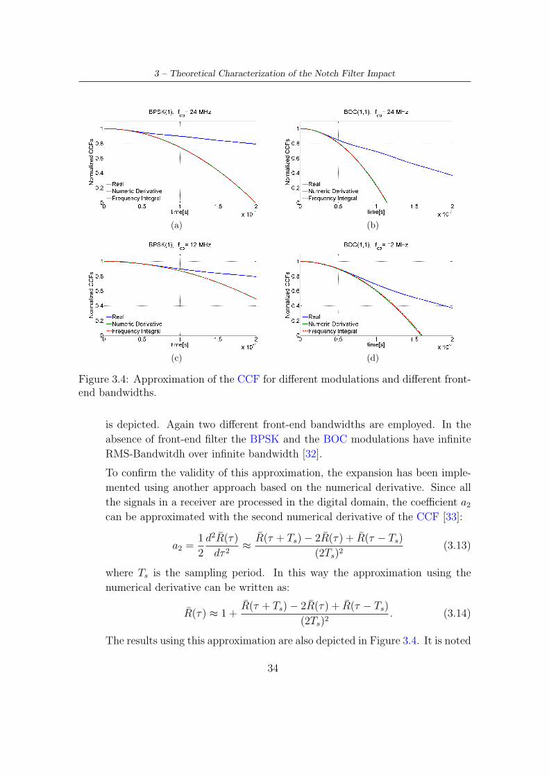
proximated CCF is:
R(τ) ≈ 1 − 2(π)2β2rmsτ
2. (3.12)
The term βrms indicates how much the CCF is peaked; this means that high
values of βrms indicate more accurate code tracking [2]. There is also another
interpretation of this coefficient: from a statistical point of view βrms corre-
sponds to the standard deviation when the normalized PSD is considered as a
probability distribution. Thus, βrms is an indicator of signal frequency spread.
The approximation in Eq. (3.12) has been implemented in Matlabr in order
to obtain the same results obtained by Betz in [32]. These results are depicted
in Figure 3.4.
Figures 3.4a and 3.4c show the approximation of the BPSK(1) CCF when
two different front-end bandwidths (24 and 12 MHz) of the front-end filter.
The filter employed is a Chebyshev filter with six taps and in-band ripple of
0.4 dB. In Figures 3.4b and 3.4d, the approximation for the BOC(1,1) CCF
33
3 – Theoretical Characterization of the Notch Filter Impact
(a) (b)
(c) (d)
Figure 3.4: Approximation of the CCF for different modulations and different front-end bandwidths.
is depicted. Again two different front-end bandwidths are employed. In the
absence of front-end filter the BPSK and the BOC modulations have infinite
RMS-Bandwitdh over infinite bandwidth [32].
To confirm the validity of this approximation, the expansion has been imple-
mented using another approach based on the numerical derivative. Since all
the signals in a receiver are processed in the digital domain, the coefficient a2
can be approximated with the second numerical derivative of the CCF [33]:
a2 =1
2
d2R(τ)
dτ 2≈ R(τ + Ts) − 2R(τ) + R(τ − Ts)
(2Ts)2(3.13)
where Ts is the sampling period. In this way the approximation using the
numerical derivative can be written as:
R(τ) ≈ 1 +R(τ + Ts) − 2R(τ) + R(τ − Ts)
(2Ts)2. (3.14)
The results using this approximation are also depicted in Figure 3.4. It is noted
34
3 – Theoretical Characterization of the Notch Filter Impact
that those curves are superimposed to the approximations obtained using the
frequency domain definition of the RMS-Bandwitdh. In Table 3.1, the delay
values for which the approximations have an error less then 10% are reported.
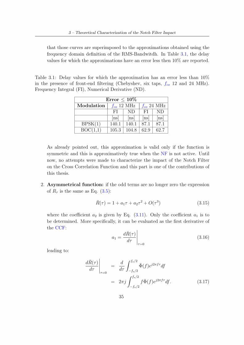
Table 3.1: Delay values for which the approximation has an error less than 10%in the presence of front-end filtering (Chebyshev, six taps, fco 12 and 24 MHz).Frequency Integral (FI), Numerical Derivative (ND).
Error ≤ 10%Modulation fco 12 MHz fco 24 MHz
FI ND FI ND[ns] [ns] [ns] [ns]
BPSK(1) 140.1 140.1 87.1 87.1BOC(1,1) 105.3 104.8 62.9 62.7
As already pointed out, this approximation is valid only if the function is
symmetric and this is approximatively true when the NF is not active. Until
now, no attempts were made to characterize the impact of the Notch Filter
on the Cross Correlation Function and this part is one of the contributions of
this thesis.
2. Asymmetrical function: if the odd terms are no longer zero the expression
of Rτ is the same as Eq. (3.5):
R(τ) = 1 + a1τ + a2τ2 + O(τ 3) (3.15)
where the coefficient a2 is given by Eq. (3.11). Only the coefficient a1 is to
be determined. More specifically, it can be evaluated as the first derivative of
the CCF:
a1 =dR(τ)
dτ
∣∣∣∣∣τ=0
(3.16)
leading to:
dR(τ)
dτ
∣∣∣∣∣τ=0
=d
dτ
∫ fs/2
−fs/2
Φ(f)ej2πfτdf
= 2πj
∫ fs/2
−fs/2
f Φ(f)ej2πfτdf. (3.17)
35
3 – Theoretical Characterization of the Notch Filter Impact
This function is evaluated in τ = 0 and the value of e(•) is equal to 1. In this
way, Eq. (3.17) becomes:
dR(τ)
dτ
∣∣∣∣∣τ=0
= 2π j
∫ β/2
−β/2
f Φ(f)df
︸ ︷︷ ︸
fa
(3.18)
where the term fa is called frequency average or asymmetry coefficient. This
coefficient was not introduced before in the GNSS community and can be used
to provide a qualitative idea about the bias introduced by the Notch Filter.
In the same way as the βrms, the fa can be interpreted from a statistical point
of view. In fact it plays a similar role of the mean of random variable and
indicates how much the mean of the PSD is far from zero. Ideally, fa should
be equal to zero since an ideal CCF should be symmetrical. Now it is possible
rewrite Eq. (3.5) as:
R(τ) ≈ 1 + 2πfaτ − 2(π)2β2rmsτ
2. (3.19)
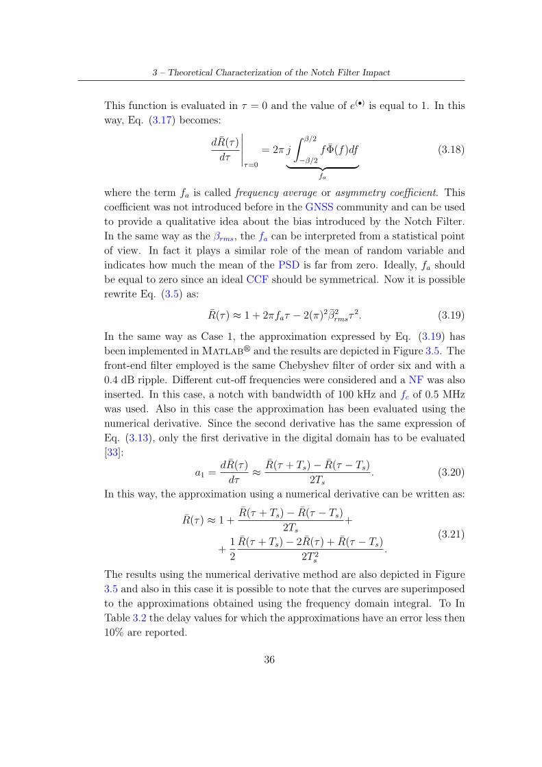
In the same way as Case 1, the approximation expressed by Eq. (3.19) has
been implemented in Matlabr and the results are depicted in Figure 3.5. The
front-end filter employed is the same Chebyshev filter of order six and with a
0.4 dB ripple. Different cut-off frequencies were considered and a NF was also
inserted. In this case, a notch with bandwidth of 100 kHz and fc of 0.5 MHz
was used. Also in this case the approximation has been evaluated using the
numerical derivative. Since the second derivative has the same expression of
Eq. (3.13), only the first derivative in the digital domain has to be evaluated
[33]:
a1 =dR(τ)
dτ≈ R(τ + Ts) − R(τ − Ts)
2Ts
. (3.20)
In this way, the approximation using a numerical derivative can be written as:
R(τ) ≈ 1 +R(τ + Ts) − R(τ − Ts)
2Ts
+
+1
2
R(τ + Ts) − 2R(τ) + R(τ − Ts)
2T 2s
.
(3.21)
The results using the numerical derivative method are also depicted in Figure
3.5 and also in this case it is possible to note that the curves are superimposed
to the approximations obtained using the frequency domain integral. To In
Table 3.2 the delay values for which the approximations have an error less then
10% are reported.
36
3 – Theoretical Characterization of the Notch Filter Impact
(a) (b)
(c) (d)
Figure 3.5: Approximation of the CCF for different modulations, different front-endbandwidths and in the presence of NF with bandwidth of 100 kHz and fc of 0.5MHz.
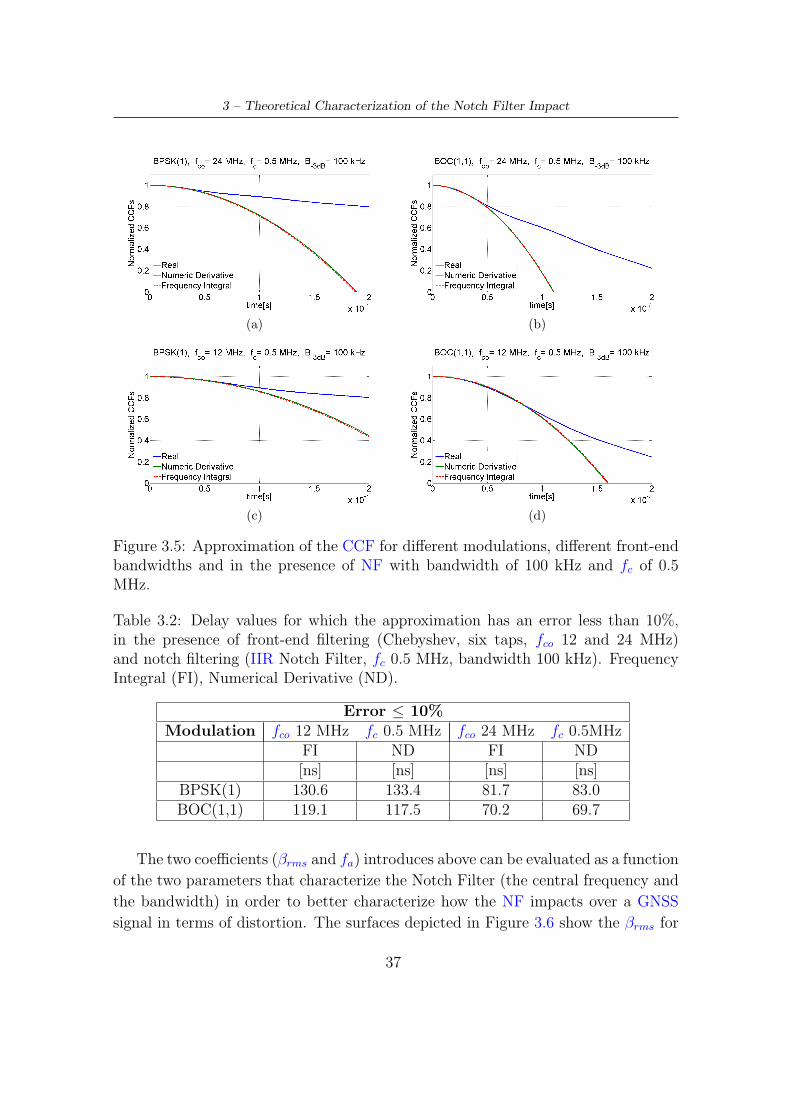
Table 3.2: Delay values for which the approximation has an error less than 10%,in the presence of front-end filtering (Chebyshev, six taps, fco 12 and 24 MHz)and notch filtering (IIR Notch Filter, fc 0.5 MHz, bandwidth 100 kHz). FrequencyIntegral (FI), Numerical Derivative (ND).
Error ≤ 10%Modulation fco 12 MHz fc 0.5 MHz fco 24 MHz fc 0.5MHz
FI ND FI ND[ns] [ns] [ns] [ns]
BPSK(1) 130.6 133.4 81.7 83.0BOC(1,1) 119.1 117.5 70.2 69.7
The two coefficients (βrms and fa) introduces above can be evaluated as a function
of the two parameters that characterize the Notch Filter (the central frequency and
the bandwidth) in order to better characterize how the NF impacts over a GNSS
signal in terms of distortion. The surfaces depicted in Figure 3.6 show the βrms for
37
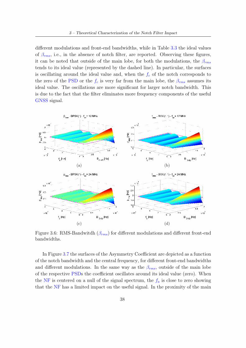
3 – Theoretical Characterization of the Notch Filter Impact
different modulations and front-end bandwidths, while in Table 3.3 the ideal values
of βrms, i.e., in the absence of notch filter, are reported. Observing these figures,
it can be noted that outside of the main lobe, for both the modulations, the βrms
tends to its ideal value (represented by the dashed line). In particular, the surfaces
is oscillating around the ideal value and, when the fc of the notch corresponds to
the zero of the PSD or the fc is very far from the main lobe, the βrms assumes its
ideal value. The oscillations are more significant for larger notch bandwidth. This
is due to the fact that the filter eliminates more frequency components of the useful
GNSS signal.
(a) (b)
(c) (d)
Figure 3.6: RMS-Bandwitdh (βrms) for different modulations and different front-endbandwidths.
In Figure 3.7 the surfaces of the Asymmetry Coefficient are depicted as a function
of the notch bandwidth and the central frequency, for different front-end bandwidths
and different modulations. In the same way as the βrms, outside of the main lobe
of the respective PSDs the coefficient oscillates around its ideal value (zero). When
the NF is centered on a null of the signal spectrum, the fa is close to zero showing
that the NF has a limited impact on the useful signal. In the proximity of the main
38
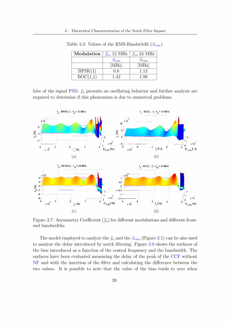
3 – Theoretical Characterization of the Notch Filter Impact
Table 3.3: Values of the RMS-Bandwitdh (βrms).
Modulation fco 12 MHz fco 24 MHzβrms βrms
[MHz] [MHz]BPSK(1) 0.8 1.13BOC(1,1) 1.42 1.98
lobe of the signal PSD, fa presents an oscillating behavior and further analysis are
required to determine if this phenomena is due to numerical problems.
(a) (b)
(c) (d)
Figure 3.7: Asymmetry Coefficient (fa) for different modulations and different front-end bandwidths.
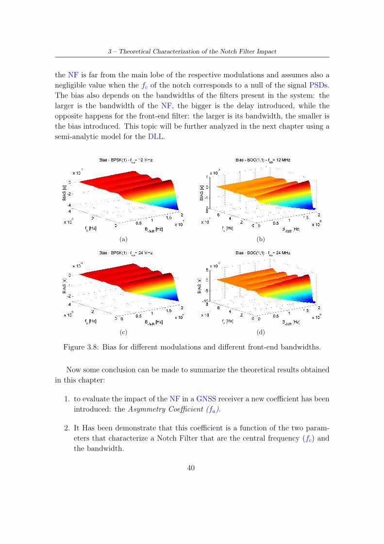
The model employed to analyze the fa and the βrms (Figure 3.1) can be also used
to analyze the delay introduced by notch filtering. Figure 3.8 shows the surfaces of
the bias introduced as a function of the central frequency and the bandwidth. The
surfaces have been evaluated measuring the delay of the peak of the CCF without
NF and with the insertion of the filter and calculating the difference between the
two values. It is possible to note that the value of the bias tends to zero when
39
3 – Theoretical Characterization of the Notch Filter Impact
the NF is far from the main lobe of the respective modulations and assumes also a
negligible value when the fc of the notch corresponds to a null of the signal PSDs.
The bias also depends on the bandwidths of the filters present in the system: the
larger is the bandwidth of the NF, the bigger is the delay introduced, while the
opposite happens for the front-end filter: the larger is its bandwidth, the smaller is
the bias introduced. This topic will be further analyzed in the next chapter using a
semi-analytic model for the DLL.
(a) (b)
(c) (d)
Figure 3.8: Bias for different modulations and different front-end bandwidths.
Now some conclusion can be made to summarize the theoretical results obtained
in this chapter:
1. to evaluate the impact of the NF in a GNSS receiver a new coefficient has been
introduced: the Asymmetry Coefficient (fa).
2. It Has been demonstrate that this coefficient is a function of the two param-
eters that characterize a Notch Filter that are the central frequency (fc) and
the bandwidth.
40
3 – Theoretical Characterization of the Notch Filter Impact
3. also the RMS-Bandwitdh (βrms) changes its values depending from the Notch
Filter parameters;
4. the two coefficients have quite the same trend and it is possible to assert that
outside from the main lobe of the GNSS PSDs the impact of the NF is not too
strong and this can be seen observing the values assumes by the coefficients,
that are very close to the ideal value (that in the case of the fa is zero).
5. Finally also a brief evaluation of the bias is reported to complete the analysis
of the NF impact over the Cross Correlation Function. Also in this case the
results are consistent with the others, so far from the main lobe of the GNSS
spectrum, the NF does not introduce bias and this can be also interpreted as
the fact that the distortions of the CCF are small.
41
Chapter 4
Simulation Analysis
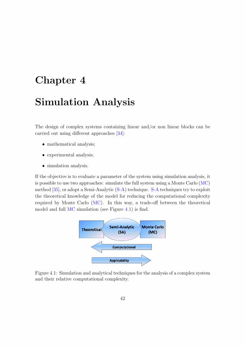
The design of complex systems containing linear and/or non linear blocks can be
carried out using different approaches [34]:
• mathematical analysis;
• experimental analysis;
• simulation analysis.
If the objective is to evaluate a parameter of the system using simulation analysis, it
is possible to use two approaches: simulate the full system using a Monte Carlo (MC)
method [35], or adopt a Semi-Analytic (S-A) technique. S-A techniques try to exploit
the theoretical knowledge of the model for reducing the computational complexity
required by Monte Carlo (MC). In this way, a trade-off between the theoretical
model and full MC simulation (see Figure 4.1) is find.
Figure 4.1: Simulation and analytical techniques for the analysis of a complex systemand their relative computational complexity.
42
4 – Simulation Analysis
MC simulations can, in general, be applied to almost every system, provided that
enough computational power is available. The main drawback of MC is the long
simulation time that they can require. On the other side, theoretical analysis is often
difficult when non-linear blocks are present and its applicability is quite limited. S-A
techniques are a mix of these two methods and combine their advantages, leading to
short simulation time. To do this, the following principle can be adopted: the linear,
time invariant part of the system is analyzed theoretically, while the remaining
part, composed by non-linear blocks, is studied using MC techniques. A S-A model
has been suggested by [36, 37] for the analysis of digital Delay Lock Loop (DLL).
This model has been adopted and modified for evaluating the impact of the Notch
Filter (NF) on the DLL.
4.1 Semi-Analytic model for digital DLL
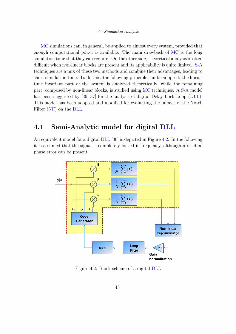
An equivalent model for a digital DLL [36] is depicted in Figure 4.2. In the following
it is assumed that the signal is completely locked in frequency, although a residual
phase error can be present.
Figure 4.2: Block scheme of a digital DLL
43
4 – Simulation Analysis
The incoming signal y[n] is the same used in Chapter 3 to evaluate the Cross
Correlation Function (CCF) in the presence of notch filtering, and it can be written
as:
y[n] = yIF [n] ∗ hFE[n] ∗ hN [n] (4.1)
where:
• yIF [n] is the intermediate-frequency signal;
• hFE[n] and hN [n] are the digital impulse responses of the front-end and notch
filter, respectively.
To simplify the notation, the following expression is used:
hf [n] = hFE[n] ∗ hN [n]. (4.2)
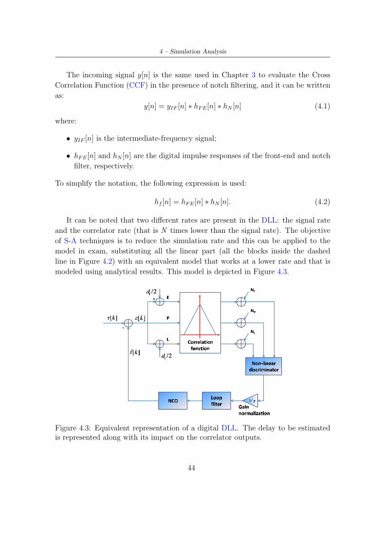
It can be noted that two different rates are present in the DLL: the signal rate
and the correlator rate (that is N times lower than the signal rate). The objective
of S-A techniques is to reduce the simulation rate and this can be applied to the
model in exam, substituting all the linear part (all the blocks inside the dashed
line in Figure 4.2) with an equivalent model that works at a lower rate and that is
modeled using analytical results. This model is depicted in Figure 4.3.
Figure 4.3: Equivalent representation of a digital DLL. The delay to be estimatedis represented along with its impact on the correlator outputs.
44
4 – Simulation Analysis
The discriminator used is a non-coherent early minus late (see Chapter 1) and
it is non-linear, so it will be evaluated using a MC simulation. A constant delay is
assumed at the system input. The loop tries to minimize the delay error generating,
at each instant, a new delay estimate. The noise component is analyzed separately
from the signal thanks to the linearity of the blocks and it is added after the corre-
lation block. The three components of the noise in Figure 4.3 are the early, prompt
and late components, as expressed in Eq. (1.14).
Knowing that the signal and the noise components can be analyzed separately,
the following considerations can be made [36]:
• the signal component is a complex base-band signal, which contains the delay
information coming from the acquisition stage and can be written as:
R(τ) =1
N
N−1∑
n=0
y[n]c[n − τ ]
=1
N(y[τ ] ∗ c[−τ ])
=1
N(c[τ ] ∗ c[−τ ]) ∗ hf [n]
=1
NR(τ) ∗ hf [n] (4.3)
where:
– R(τ) is the signal component as expressed in Eq. (1.14);
– y[n] is the signal of Eq. (4.1);
– c[n − τ ] is the local replica generated by the DLL;
Eq. (4.3) shows that the expression of the signal is a Cross Correlation
Function (CCF) convoluted with the impulse response of the filters.
• The noise component is a complex base-band signal with independent real
and imaginary parts, but the noise samples can be time correlated: the noise
processes are white in the time domain, but correlated along the delay direction
(correlation between the early, prompt and late). This correlation can be
45
4 – Simulation Analysis
written as a matrix [36]:
Ccelp =
1 Rc(ds/2) Rc(ds)
Rc(−ds/2) 1 Rc(ds/2)
Rc(−ds) Rc(−ds/2) 1
(4.4)
=
1 Rc(ds/2) Rc(ds)
Rc(ds/2) 1 Rc(ds/2)
Rc(ds) Rc(ds/2) 1
(4.5)
where Rc(•) is the correlation function of the code, that takes into account
the correlation of the noise processes in the delay domain:
Rc(τ) = hf [τ ] ∗ R(τ) ∗ hf [−τ ] (4.6)
Eq. (4.6) shows that every filter impacts twice on the correlation process of
the noise.
The model explained above has been simulated using Matlabr and the follow-
ing parameters have been adopted:
• BPSK-1 modulation;
• constant code delay;
• initial delay error (0.3Tc) from the acquisition block;
• 10 ms integration time;
• 1 Hz loop equivalent bandwidth;
• front-end modeled using a Chebyshev filter with six taps and a fco of 24 MHz;
• Notch Filter with different central frequency (generally between 0 and 4 MHz)
and bandwidth between 20 and 200 kHz.
To demonstrate the validity of this S-A model, the case under ideal conditions
is analyzed at first. This type of approach has been used in [38] to asses the perfor-
mance of a new discriminator and the results have been compared with full Monte
Carlo simulations. The same approach is used here for simulating the model under
ideal conditions and it consists in the generation of the signal without front-end and
notch filtering. The performance of this model are evaluated in terms of tracking
46
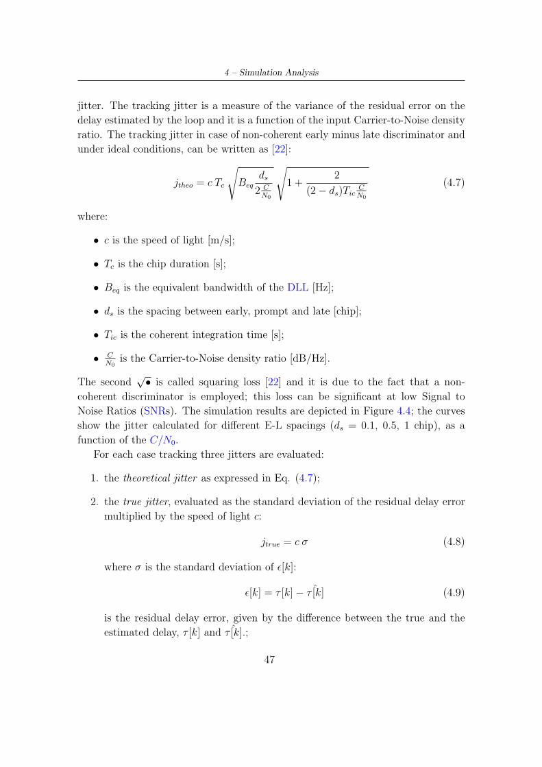
4 – Simulation Analysis
jitter. The tracking jitter is a measure of the variance of the residual error on the
delay estimated by the loop and it is a function of the input Carrier-to-Noise density
ratio. The tracking jitter in case of non-coherent early minus late discriminator and
under ideal conditions, can be written as [22]:
jtheo = c Tc
√
Beqds
2 CN0
√
1 +2
(2 − ds)TicCN0
(4.7)
where:
• c is the speed of light [m/s];
• Tc is the chip duration [s];
• Beq is the equivalent bandwidth of the DLL [Hz];
• ds is the spacing between early, prompt and late [chip];
• Tic is the coherent integration time [s];
• CN0
is the Carrier-to-Noise density ratio [dB/Hz].
The secondå is called squaring loss [22] and it is due to the fact that a non-
coherent discriminator is employed; this loss can be significant at low Signal to
Noise Ratios (SNRs). The simulation results are depicted in Figure 4.4; the curves
show the jitter calculated for different E-L spacings (ds = 0.1, 0.5, 1 chip), as a
function of the C/N0.
For each case tracking three jitters are evaluated:
1. the theoretical jitter as expressed in Eq. (4.7);
2. the true jitter, evaluated as the standard deviation of the residual delay error
multiplied by the speed of light c:
jtrue = c σ (4.8)
where σ is the standard deviation of ǫ[k]:
ǫ[k] = τ [k] − ˆτ [k] (4.9)
is the residual delay error, given by the difference between the true and the
estimated delay, τ [k] and ˆτ [k].;
47
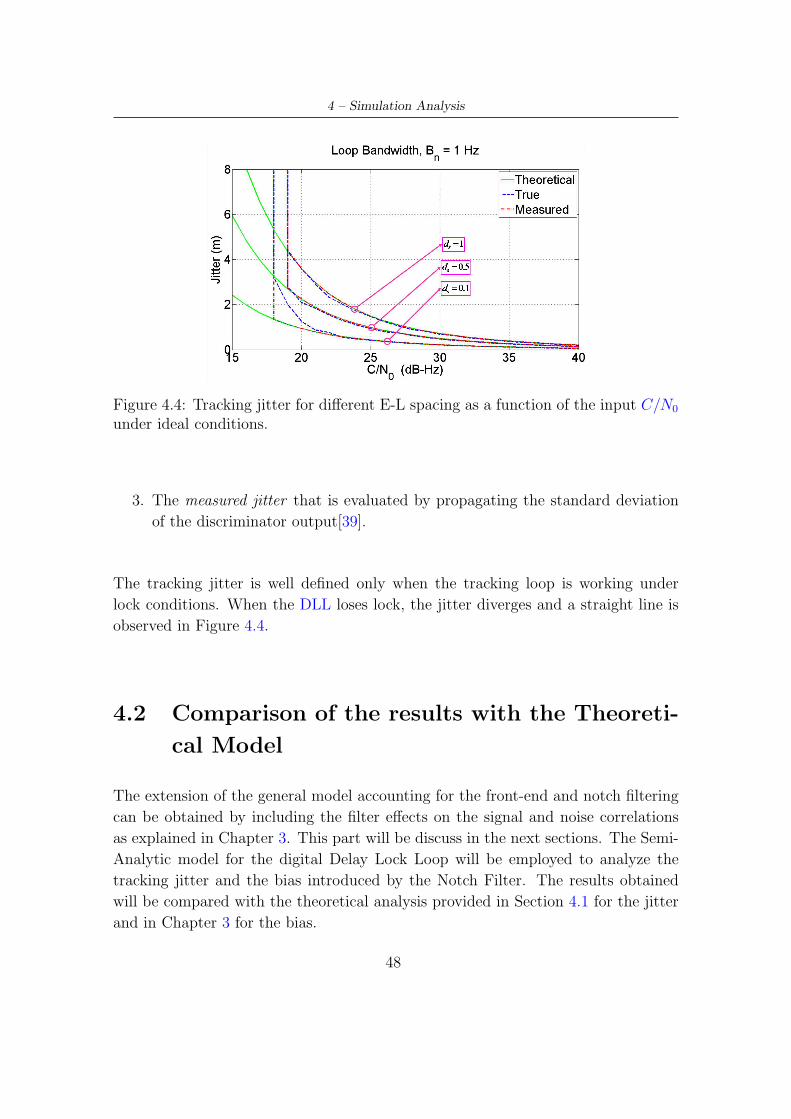
4 – Simulation Analysis
Figure 4.4: Tracking jitter for different E-L spacing as a function of the input C/N0
under ideal conditions.
3. The measured jitter that is evaluated by propagating the standard deviation
of the discriminator output[39].
The tracking jitter is well defined only when the tracking loop is working under
lock conditions. When the DLL loses lock, the jitter diverges and a straight line is
observed in Figure 4.4.
4.2 Comparison of the results with the Theoreti-
cal Model
The extension of the general model accounting for the front-end and notch filtering
can be obtained by including the filter effects on the signal and noise correlations
as explained in Chapter 3. This part will be discuss in the next sections. The Semi-
Analytic model for the digital Delay Lock Loop will be employed to analyze the
tracking jitter and the bias introduced by the Notch Filter. The results obtained
will be compared with the theoretical analysis provided in Section 4.1 for the jitter
and in Chapter 3 for the bias.
48
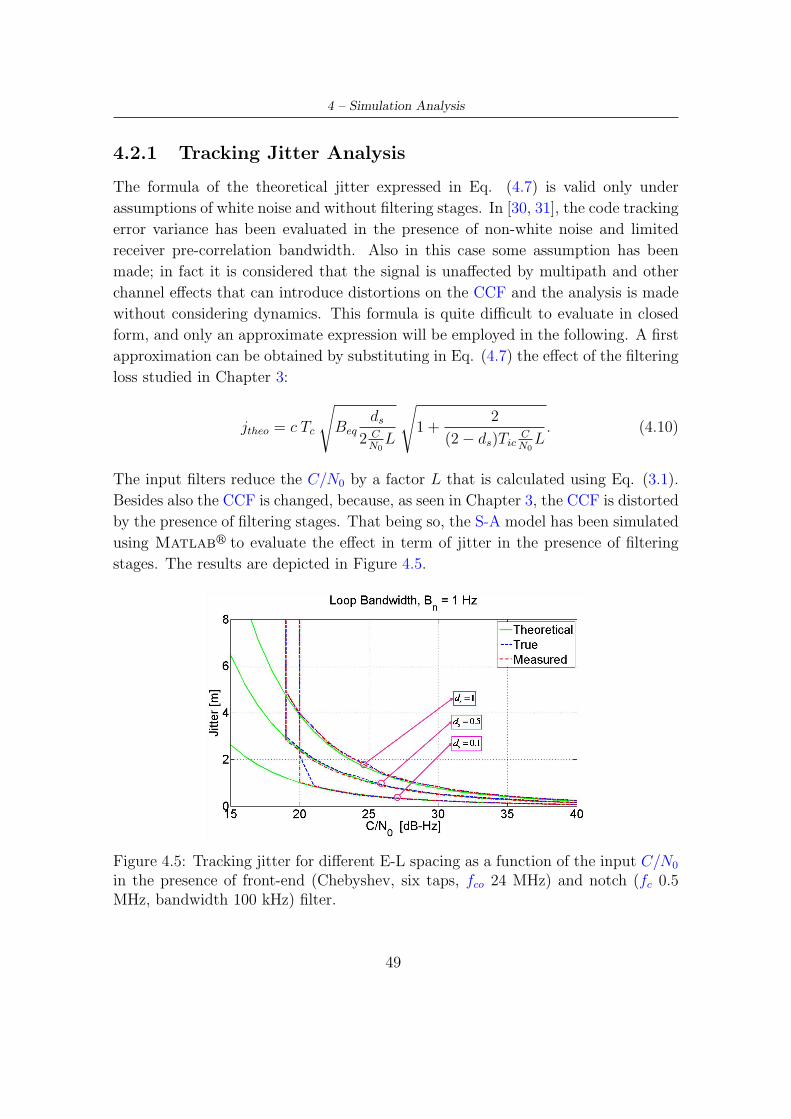
4 – Simulation Analysis
4.2.1 Tracking Jitter Analysis
The formula of the theoretical jitter expressed in Eq. (4.7) is valid only under
assumptions of white noise and without filtering stages. In [30, 31], the code tracking
error variance has been evaluated in the presence of non-white noise and limited
receiver pre-correlation bandwidth. Also in this case some assumption has been
made; in fact it is considered that the signal is unaffected by multipath and other
channel effects that can introduce distortions on the CCF and the analysis is made
without considering dynamics. This formula is quite difficult to evaluate in closed
form, and only an approximate expression will be employed in the following. A first
approximation can be obtained by substituting in Eq. (4.7) the effect of the filtering
loss studied in Chapter 3:
jtheo = c Tc
√
Beqds
2 CN0
L
√
1 +2
(2 − ds)TicCN0
L. (4.10)
The input filters reduce the C/N0 by a factor L that is calculated using Eq. (3.1).
Besides also the CCF is changed, because, as seen in Chapter 3, the CCF is distorted
by the presence of filtering stages. That being so, the S-A model has been simulated
using Matlabr to evaluate the effect in term of jitter in the presence of filtering
stages. The results are depicted in Figure 4.5.
Figure 4.5: Tracking jitter for different E-L spacing as a function of the input C/N0
in the presence of front-end (Chebyshev, six taps, fco 24 MHz) and notch (fc 0.5MHz, bandwidth 100 kHz) filter.
49
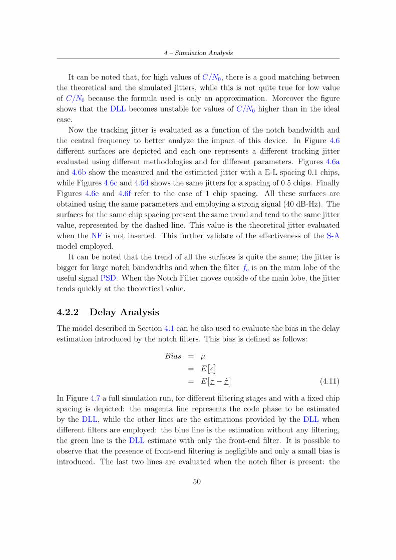
4 – Simulation Analysis
It can be noted that, for high values of C/N0, there is a good matching between
the theoretical and the simulated jitters, while this is not quite true for low value
of C/N0 because the formula used is only an approximation. Moreover the figure
shows that the DLL becomes unstable for values of C/N0 higher than in the ideal
case.
Now the tracking jitter is evaluated as a function of the notch bandwidth and
the central frequency to better analyze the impact of this device. In Figure 4.6
different surfaces are depicted and each one represents a different tracking jitter
evaluated using different methodologies and for different parameters. Figures 4.6a
and 4.6b show the measured and the estimated jitter with a E-L spacing 0.1 chips,
while Figures 4.6c and 4.6d shows the same jitters for a spacing of 0.5 chips. Finally
Figures 4.6e and 4.6f refer to the case of 1 chip spacing. All these surfaces are
obtained using the same parameters and employing a strong signal (40 dB-Hz). The
surfaces for the same chip spacing present the same trend and tend to the same jitter
value, represented by the dashed line. This value is the theoretical jitter evaluated
when the NF is not inserted. This further validate of the effectiveness of the S-A
model employed.
It can be noted that the trend of all the surfaces is quite the same; the jitter is
bigger for large notch bandwidths and when the filter fc is on the main lobe of the
useful signal PSD. When the Notch Filter moves outside of the main lobe, the jitter
tends quickly at the theoretical value.
4.2.2 Delay Analysis
The model described in Section 4.1 can be also used to evaluate the bias in the delay
estimation introduced by the notch filters. This bias is defined as follows:
Bias = µ
= E[ǫ]
= E[τ − τ
](4.11)
In Figure 4.7 a full simulation run, for different filtering stages and with a fixed chip
spacing is depicted: the magenta line represents the code phase to be estimated
by the DLL, while the other lines are the estimations provided by the DLL when
different filters are employed: the blue line is the estimation without any filtering,
the green line is the DLL estimate with only the front-end filter. It is possible to
observe that the presence of front-end filtering is negligible and only a small bias is
introduced. The last two lines are evaluated when the notch filter is present: the
50
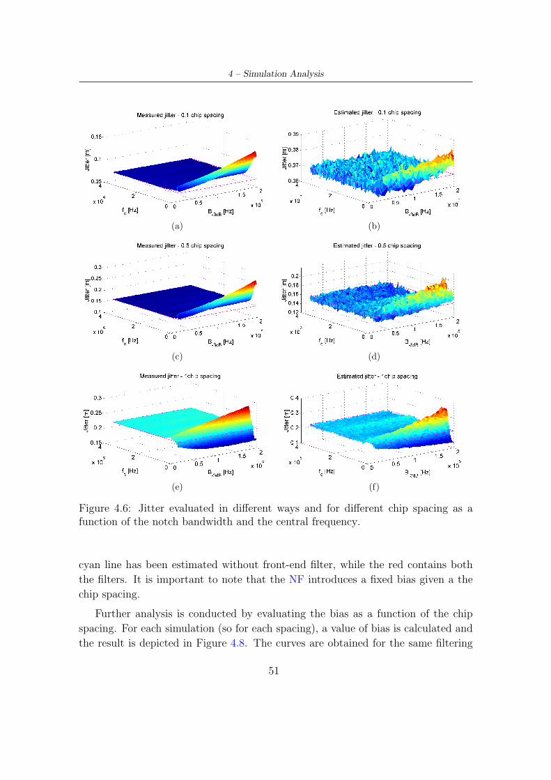
4 – Simulation Analysis
(a) (b)
(c) (d)
(e) (f)
Figure 4.6: Jitter evaluated in different ways and for different chip spacing as afunction of the notch bandwidth and the central frequency.
cyan line has been estimated without front-end filter, while the red contains both
the filters. It is important to note that the NF introduces a fixed bias given a the
chip spacing.
Further analysis is conducted by evaluating the bias as a function of the chip
spacing. For each simulation (so for each spacing), a value of bias is calculated and
the result is depicted in Figure 4.8. The curves are obtained for the same filtering
51
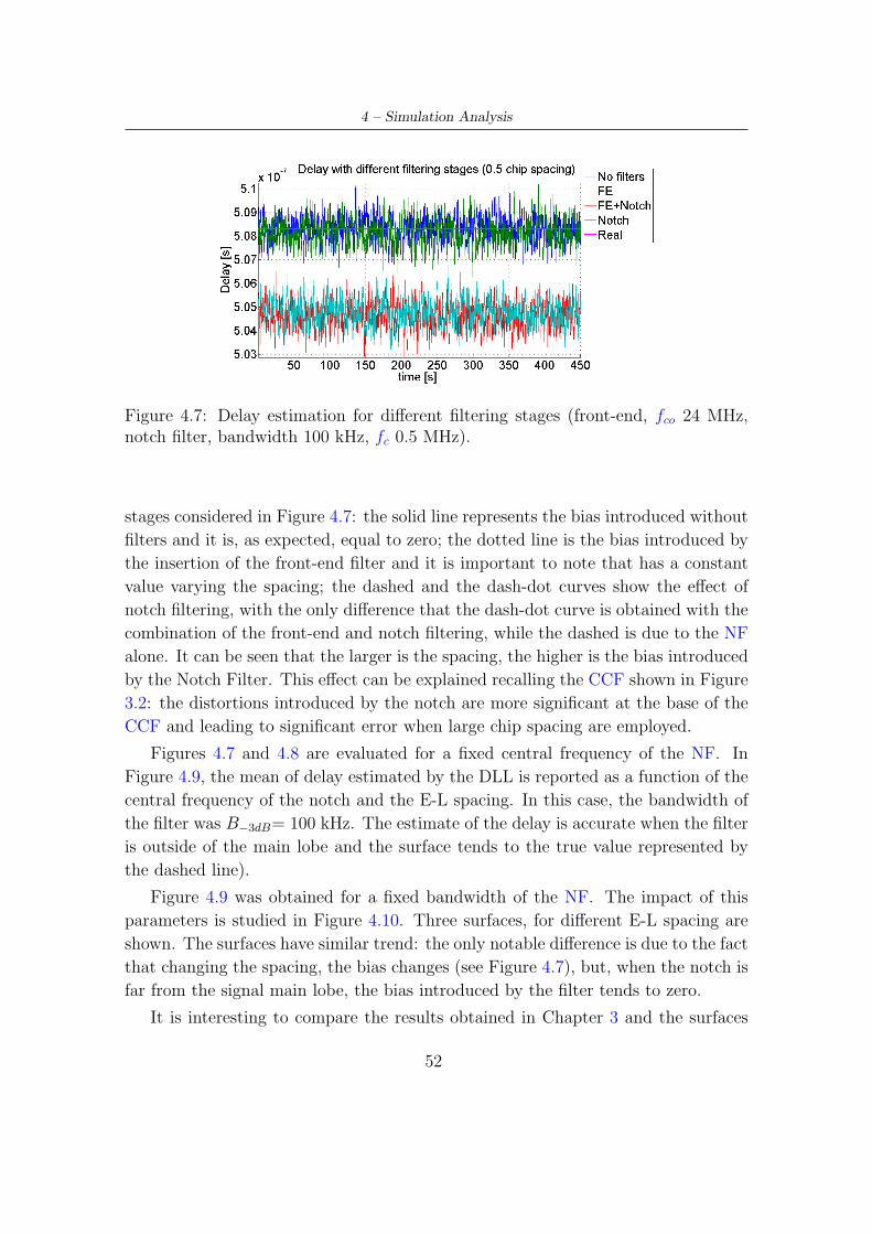
4 – Simulation Analysis
Figure 4.7: Delay estimation for different filtering stages (front-end, fco 24 MHz,notch filter, bandwidth 100 kHz, fc 0.5 MHz).
stages considered in Figure 4.7: the solid line represents the bias introduced without
filters and it is, as expected, equal to zero; the dotted line is the bias introduced by
the insertion of the front-end filter and it is important to note that has a constant
value varying the spacing; the dashed and the dash-dot curves show the effect of
notch filtering, with the only difference that the dash-dot curve is obtained with the
combination of the front-end and notch filtering, while the dashed is due to the NF
alone. It can be seen that the larger is the spacing, the higher is the bias introduced
by the Notch Filter. This effect can be explained recalling the CCF shown in Figure
3.2: the distortions introduced by the notch are more significant at the base of the
CCF and leading to significant error when large chip spacing are employed.
Figures 4.7 and 4.8 are evaluated for a fixed central frequency of the NF. In
Figure 4.9, the mean of delay estimated by the DLL is reported as a function of the
central frequency of the notch and the E-L spacing. In this case, the bandwidth of
the filter was B−3dB= 100 kHz. The estimate of the delay is accurate when the filter
is outside of the main lobe and the surface tends to the true value represented by
the dashed line).
Figure 4.9 was obtained for a fixed bandwidth of the NF. The impact of this
parameters is studied in Figure 4.10. Three surfaces, for different E-L spacing are
shown. The surfaces have similar trend: the only notable difference is due to the fact
that changing the spacing, the bias changes (see Figure 4.7), but, when the notch is
far from the signal main lobe, the bias introduced by the filter tends to zero.
It is interesting to compare the results obtained in Chapter 3 and the surfaces
52
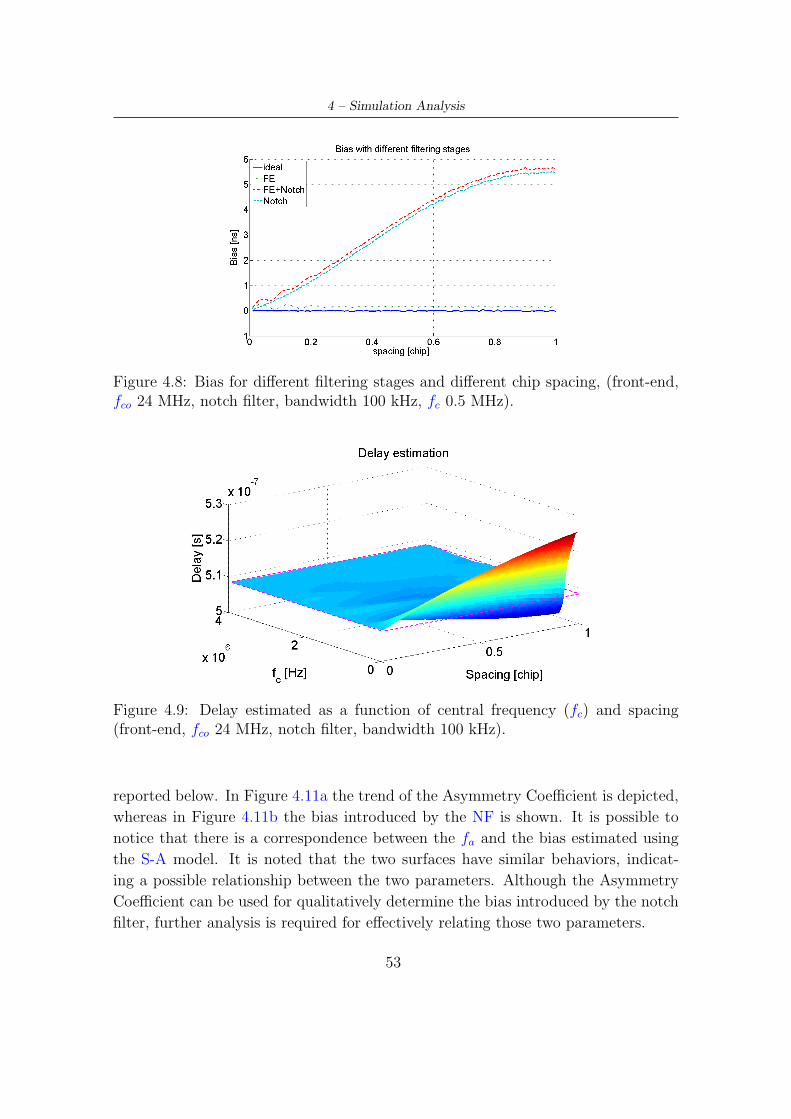
4 – Simulation Analysis
Figure 4.8: Bias for different filtering stages and different chip spacing, (front-end,fco 24 MHz, notch filter, bandwidth 100 kHz, fc 0.5 MHz).
Figure 4.9: Delay estimated as a function of central frequency (fc) and spacing(front-end, fco 24 MHz, notch filter, bandwidth 100 kHz).
reported below. In Figure 4.11a the trend of the Asymmetry Coefficient is depicted,
whereas in Figure 4.11b the bias introduced by the NF is shown. It is possible to
notice that there is a correspondence between the fa and the bias estimated using
the S-A model. It is noted that the two surfaces have similar behaviors, indicat-
ing a possible relationship between the two parameters. Although the Asymmetry
Coefficient can be used for qualitatively determine the bias introduced by the notch
filter, further analysis is required for effectively relating those two parameters.
53
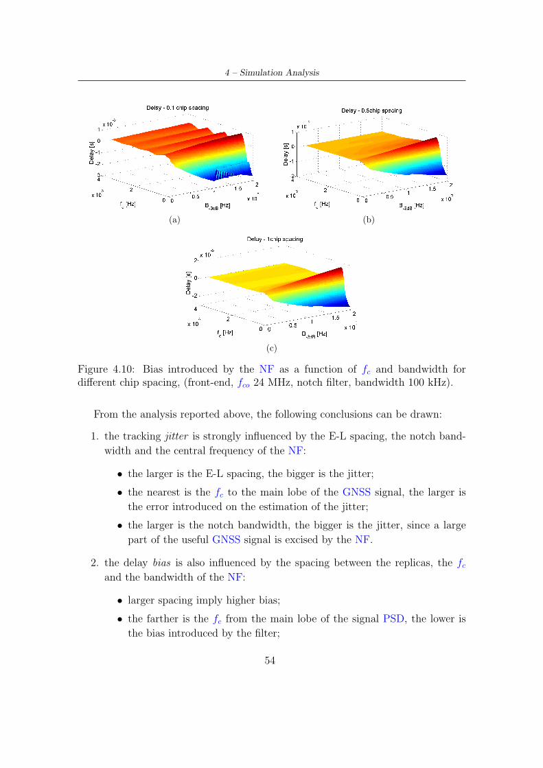
4 – Simulation Analysis
(a) (b)
(c)
Figure 4.10: Bias introduced by the NF as a function of fc and bandwidth fordifferent chip spacing, (front-end, fco 24 MHz, notch filter, bandwidth 100 kHz).
From the analysis reported above, the following conclusions can be drawn:
1. the tracking jitter is strongly influenced by the E-L spacing, the notch band-
width and the central frequency of the NF:
• the larger is the E-L spacing, the bigger is the jitter;
• the nearest is the fc to the main lobe of the GNSS signal, the larger is
the error introduced on the estimation of the jitter;
• the larger is the notch bandwidth, the bigger is the jitter, since a large
part of the useful GNSS signal is excised by the NF.
2. the delay bias is also influenced by the spacing between the replicas, the fc
and the bandwidth of the NF:
• larger spacing imply higher bias;
• the farther is the fc from the main lobe of the signal PSD, the lower is
the bias introduced by the filter;
54
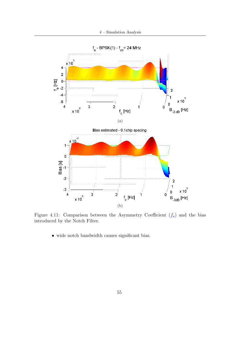
4 – Simulation Analysis
(a)
(b)
Figure 4.11: Comparison between the Asymmetry Coefficient (fa) and the biasintroduced by the Notch Filter.
• wide notch bandwidth causes significant bias.
55
Chapter 5
Real Data Analysis
In the previous chapters, the impact of the Notch Filter (NF) on tracking loops has
been analyzed using both a theoretical and a simulation approaches. In this chapter
the results already obtained are further validated using real data (in particular live
data from the GPS C/A signal).
In the first section of the chapter, the experimental setup used for the data collec-
tion is described, whereas the second section shows the results obtained by process-
ing the collected data with the University of Calgary Software Receiver (GSNRxTM)
[11]. This software receiver allows one to evaluate the effects of a NF on the tracking
loops and to determine the biases introduced in the position solution.
5.1 Experimental setup
In Figure 5.1 the experimental setup used for the data collection is depicted. The
data have been collected on the 30th of September 2008 using a fixed active antenna
positioned on the roof of the Calgary Center for Innovative Technologies (CCIT)
(see Figure 5.2). In this way, a strong signal, with a high C/N0, has been collected
under open sky conditions. This aspect is important since it allows one to better
evaluate the effects of the Notch Filter (NF) only, neglecting the effect of other
disturbance (i.e., multipath).
The antenna has been connected to a National Instrument NI-PXI-5660 signal
analyzer that is a customized device composed by three front-ends, each one formed
by a down-converter (NI-5600) and a digitizer (NI-5620) (see Figure 5.3). Each
front-end is able to collect signals with a 20 MHz bandwidth and using selectable
intermediate and sampling frequencies [40].
56
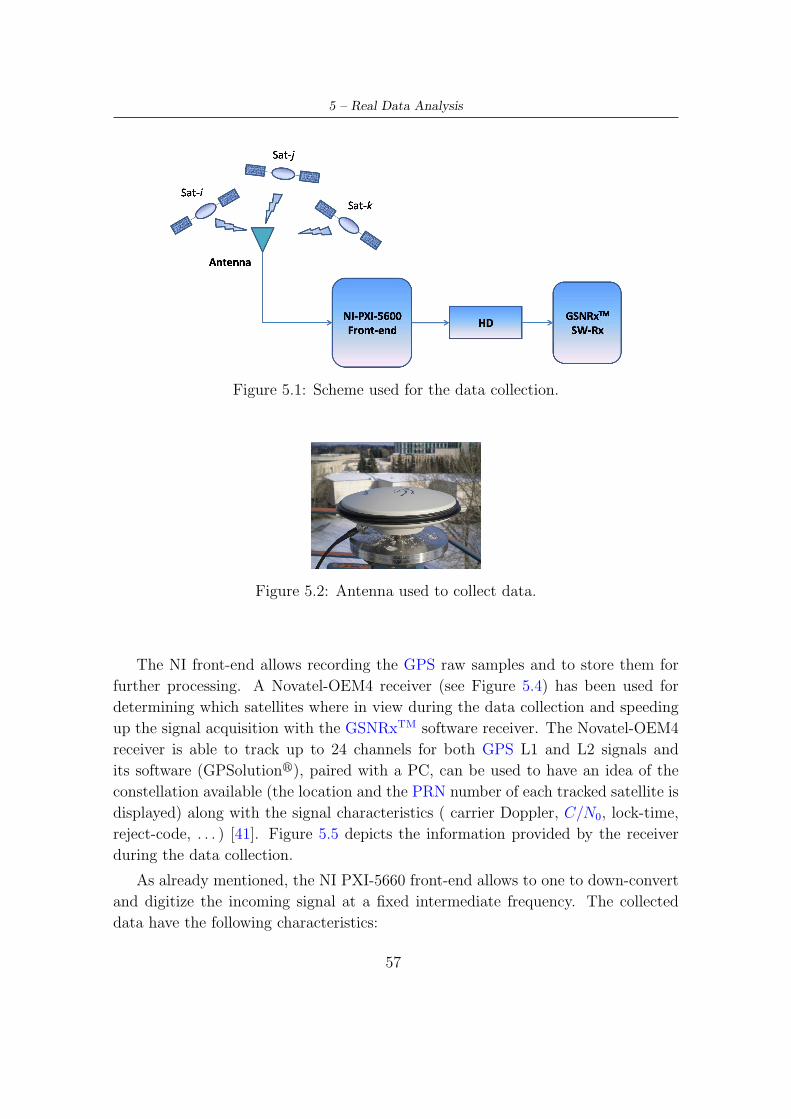
5 – Real Data Analysis
Figure 5.1: Scheme used for the data collection.
Figure 5.2: Antenna used to collect data.
The NI front-end allows recording the GPS raw samples and to store them for
further processing. A Novatel-OEM4 receiver (see Figure 5.4) has been used for
determining which satellites where in view during the data collection and speeding
up the signal acquisition with the GSNRxTM software receiver. The Novatel-OEM4
receiver is able to track up to 24 channels for both GPS L1 and L2 signals and
its software (GPSolutionr), paired with a PC, can be used to have an idea of the
constellation available (the location and the PRN number of each tracked satellite is
displayed) along with the signal characteristics ( carrier Doppler, C/N0, lock-time,
reject-code, . . . ) [41]. Figure 5.5 depicts the information provided by the receiver
during the data collection.
As already mentioned, the NI PXI-5660 front-end allows to one to down-convert
and digitize the incoming signal at a fixed intermediate frequency. The collected
data have the following characteristics:
57
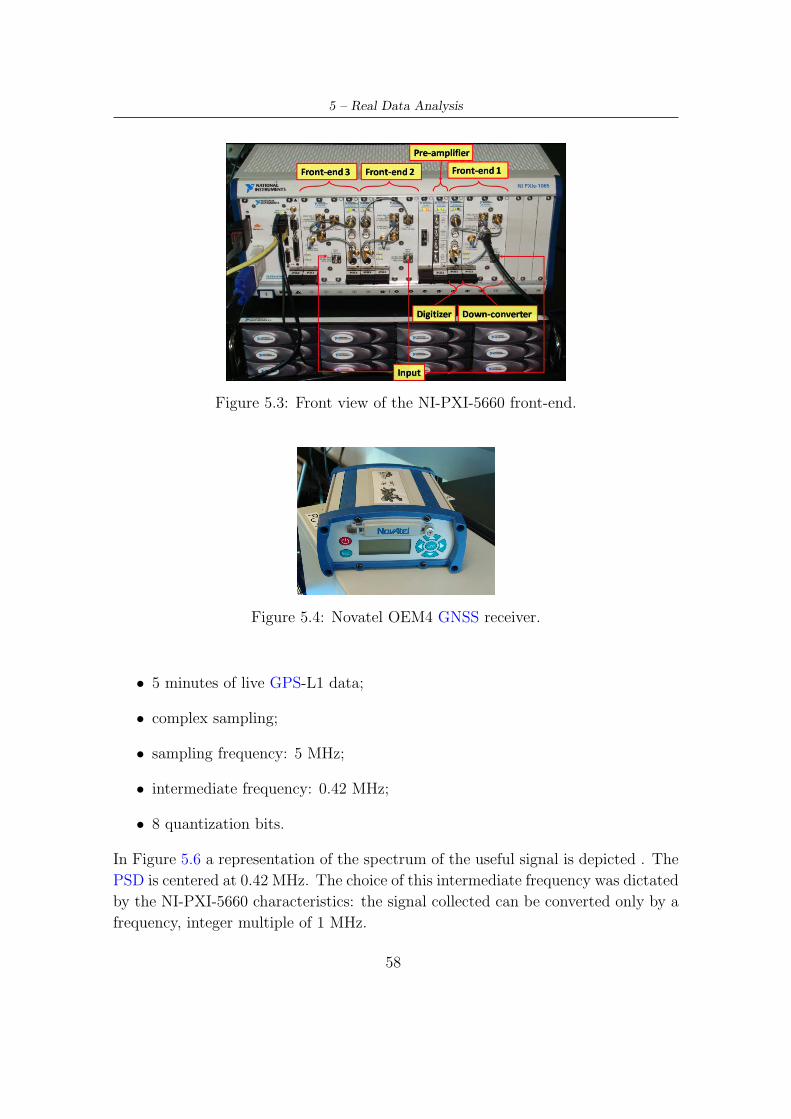
5 – Real Data Analysis
Figure 5.3: Front view of the NI-PXI-5660 front-end.
Figure 5.4: Novatel OEM4 GNSS receiver.
• 5 minutes of live GPS-L1 data;
• complex sampling;
• sampling frequency: 5 MHz;
• intermediate frequency: 0.42 MHz;
• 8 quantization bits.
In Figure 5.6 a representation of the spectrum of the useful signal is depicted . The
PSD is centered at 0.42 MHz. The choice of this intermediate frequency was dictated
by the NI-PXI-5660 characteristics: the signal collected can be converted only by a
frequency, integer multiple of 1 MHz.
58
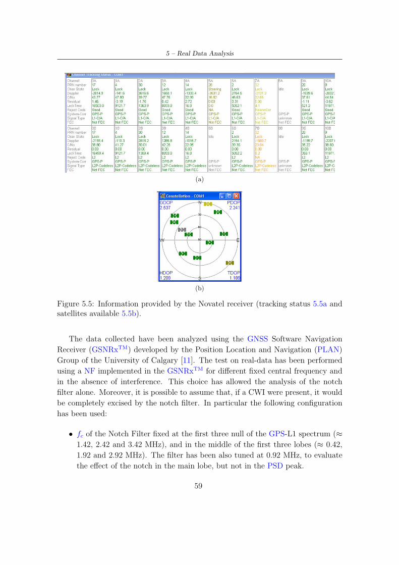
5 – Real Data Analysis
(a)
(b)
Figure 5.5: Information provided by the Novatel receiver (tracking status 5.5a andsatellites available 5.5b).
The data collected have been analyzed using the GNSS Software Navigation
Receiver (GSNRxTM) developed by the Position Location and Navigation (PLAN)
Group of the University of Calgary [11]. The test on real-data has been performed
using a NF implemented in the GSNRxTM for different fixed central frequency and
in the absence of interference. This choice has allowed the analysis of the notch
filter alone. Moreover, it is possible to assume that, if a CWI were present, it would
be completely excised by the notch filter. In particular the following configuration
has been used:
• fc of the Notch Filter fixed at the first three null of the GPS-L1 spectrum (≈1.42, 2.42 and 3.42 MHz), and in the middle of the first three lobes (≈ 0.42,
1.92 and 2.92 MHz). The filter has been also tuned at 0.92 MHz, to evaluate
the effect of the notch in the main lobe, but not in the PSD peak.
59
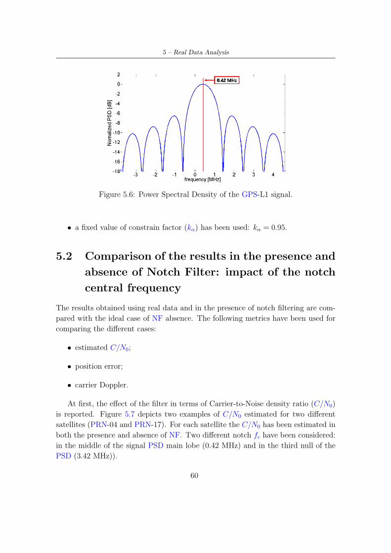
5 – Real Data Analysis
Figure 5.6: Power Spectral Density of the GPS-L1 signal.
• a fixed value of constrain factor (kα) has been used: kα = 0.95.
5.2 Comparison of the results in the presence and
absence of Notch Filter: impact of the notch
central frequency
The results obtained using real data and in the presence of notch filtering are com-
pared with the ideal case of NF absence. The following metrics have been used for
comparing the different cases:
• estimated C/N0;
• position error;
• carrier Doppler.
At first, the effect of the filter in terms of Carrier-to-Noise density ratio (C/N0)
is reported. Figure 5.7 depicts two examples of C/N0 estimated for two different
satellites (PRN-04 and PRN-17). For each satellite the C/N0 has been estimated in
both the presence and absence of NF. Two different notch fc have been considered:
in the middle of the signal PSD main lobe (0.42 MHz) and in the third null of the
PSD (3.42 MHz)).
60
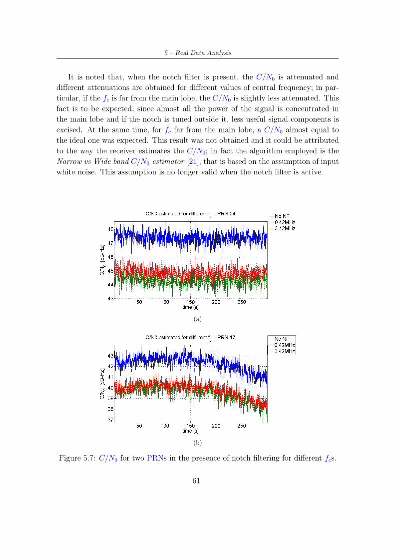
5 – Real Data Analysis
It is noted that, when the notch filter is present, the C/N0 is attenuated and
different attenuations are obtained for different values of central frequency; in par-
ticular, if the fc is far from the main lobe, the C/N0 is slightly less attenuated. This
fact is to be expected, since almost all the power of the signal is concentrated in
the main lobe and if the notch is tuned outside it, less useful signal components is
excised. At the same time, for fc far from the main lobe, a C/N0 almost equal to
the ideal one was expected. This result was not obtained and it could be attributed
to the way the receiver estimates the C/N0; in fact the algorithm employed is the
Narrow vs Wide band C/N0 estimator [21], that is based on the assumption of input
white noise. This assumption is no longer valid when the notch filter is active.
(a)
(b)
Figure 5.7: C/N0 for two PRNs in the presence of notch filtering for different fcs.
61
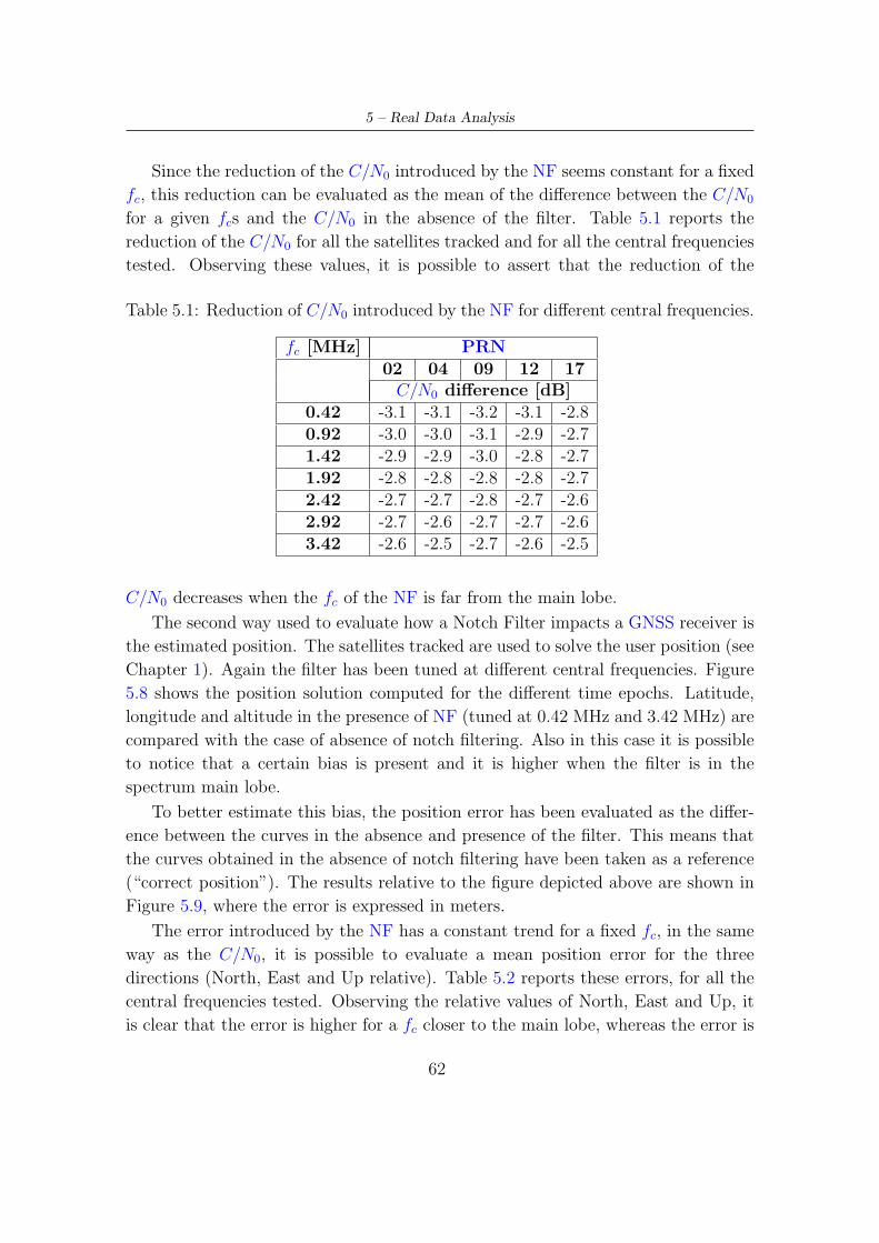
5 – Real Data Analysis
Since the reduction of the C/N0 introduced by the NF seems constant for a fixed
fc, this reduction can be evaluated as the mean of the difference between the C/N0
for a given fcs and the C/N0 in the absence of the filter. Table 5.1 reports the
reduction of the C/N0 for all the satellites tracked and for all the central frequencies
tested. Observing these values, it is possible to assert that the reduction of the
Table 5.1: Reduction of C/N0 introduced by the NF for different central frequencies.
fc [MHz] PRN02 04 09 12 17
C/N0 difference [dB]0.42 -3.1 -3.1 -3.2 -3.1 -2.80.92 -3.0 -3.0 -3.1 -2.9 -2.71.42 -2.9 -2.9 -3.0 -2.8 -2.71.92 -2.8 -2.8 -2.8 -2.8 -2.72.42 -2.7 -2.7 -2.8 -2.7 -2.62.92 -2.7 -2.6 -2.7 -2.7 -2.63.42 -2.6 -2.5 -2.7 -2.6 -2.5
C/N0 decreases when the fc of the NF is far from the main lobe.
The second way used to evaluate how a Notch Filter impacts a GNSS receiver is
the estimated position. The satellites tracked are used to solve the user position (see
Chapter 1). Again the filter has been tuned at different central frequencies. Figure
5.8 shows the position solution computed for the different time epochs. Latitude,
longitude and altitude in the presence of NF (tuned at 0.42 MHz and 3.42 MHz) are
compared with the case of absence of notch filtering. Also in this case it is possible
to notice that a certain bias is present and it is higher when the filter is in the
spectrum main lobe.
To better estimate this bias, the position error has been evaluated as the differ-
ence between the curves in the absence and presence of the filter. This means that
the curves obtained in the absence of notch filtering have been taken as a reference
(“correct position”). The results relative to the figure depicted above are shown in
Figure 5.9, where the error is expressed in meters.
The error introduced by the NF has a constant trend for a fixed fc, in the same
way as the C/N0, it is possible to evaluate a mean position error for the three
directions (North, East and Up relative). Table 5.2 reports these errors, for all the
central frequencies tested. Observing the relative values of North, East and Up, it
is clear that the error is higher for a fc closer to the main lobe, whereas the error is
62
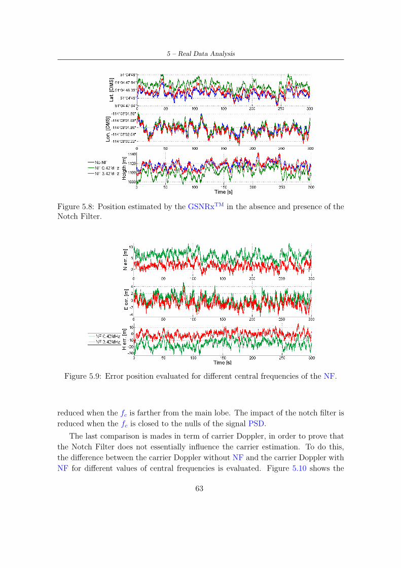
5 – Real Data Analysis
Figure 5.8: Position estimated by the GSNRxTM in the absence and presence of theNotch Filter.
Figure 5.9: Error position evaluated for different central frequencies of the NF.
reduced when the fc is farther from the main lobe. The impact of the notch filter is
reduced when the fc is closed to the nulls of the signal PSD.
The last comparison is mades in term of carrier Doppler, in order to prove that
the Notch Filter does not essentially influence the carrier estimation. To do this,
the difference between the carrier Doppler without NF and the carrier Doppler with
NF for different values of central frequencies is evaluated. Figure 5.10 shows the
63
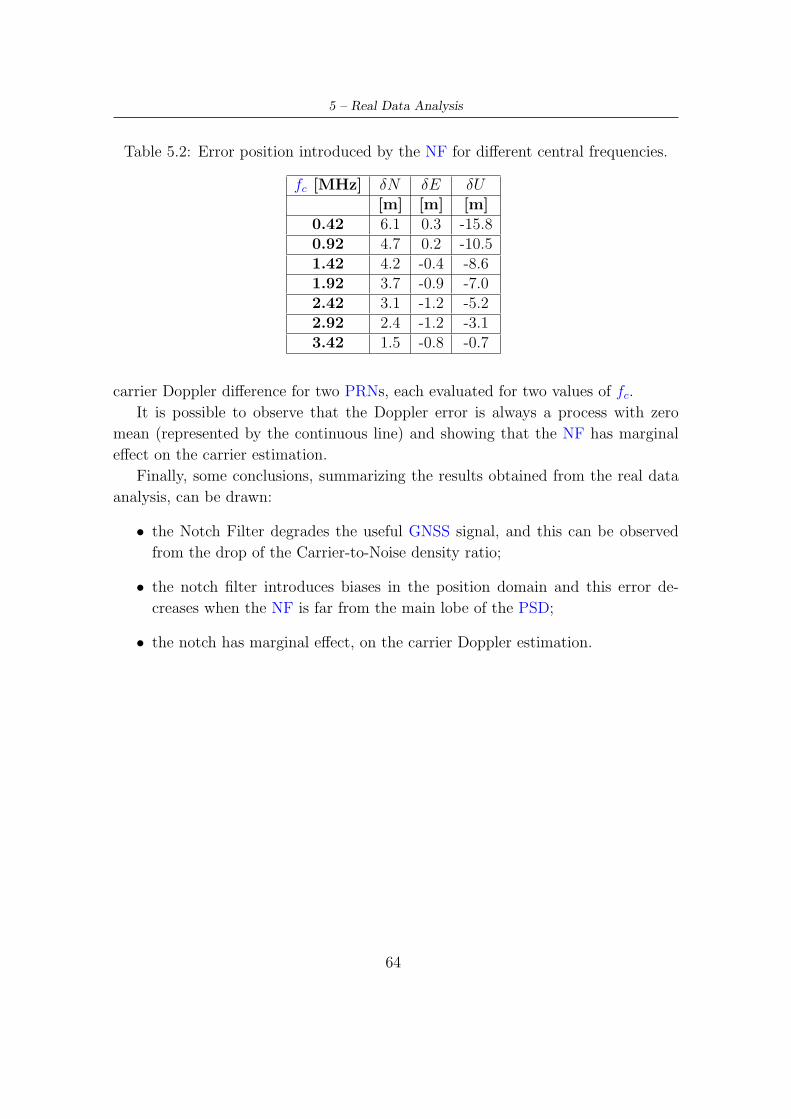
5 – Real Data Analysis
Table 5.2: Error position introduced by the NF for different central frequencies.
fc [MHz] δN δE δU[m] [m] [m]
0.42 6.1 0.3 -15.80.92 4.7 0.2 -10.51.42 4.2 -0.4 -8.61.92 3.7 -0.9 -7.02.42 3.1 -1.2 -5.22.92 2.4 -1.2 -3.13.42 1.5 -0.8 -0.7
carrier Doppler difference for two PRNs, each evaluated for two values of fc.
It is possible to observe that the Doppler error is always a process with zero
mean (represented by the continuous line) and showing that the NF has marginal
effect on the carrier estimation.
Finally, some conclusions, summarizing the results obtained from the real data
analysis, can be drawn:
• the Notch Filter degrades the useful GNSS signal, and this can be observed
from the drop of the Carrier-to-Noise density ratio;
• the notch filter introduces biases in the position domain and this error de-
creases when the NF is far from the main lobe of the PSD;
• the notch has marginal effect, on the carrier Doppler estimation.
64
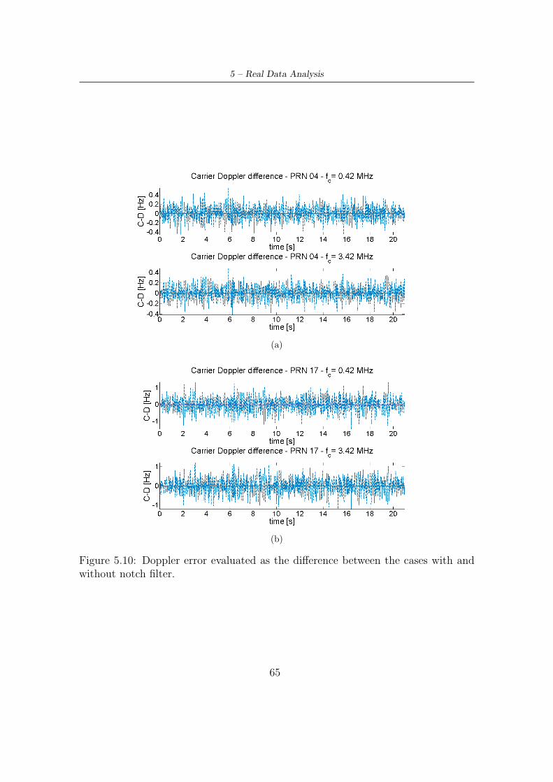
5 – Real Data Analysis
(a)
(b)
Figure 5.10: Doppler error evaluated as the difference between the cases with andwithout notch filter.
65
Chapter 6
Conclusions
The focus of this thesis was the evaluation of impact of notch filtering on tracking
loops for GNSS applications. In the following, the obtained results are summarized
and some conclusions are drawn.
At first, a theoretical analysis of the distortions introduced by the Notch Filter
(NF) on the correlation function has been provided. The distortions on the Cross
Correlation Function (CCF) have been evaluated as a function of the NF parameters:
the bandwidth and the central frequency (fc). The Asymmetry Coefficient (fa) has
been introduced in order to give a qualitative estimate of the bias introduced by
notch filtering. To the best of the author’s knowledge, this coefficient was not used
before for characterizing the notch filter distortion and represents one of the results
obtained in this work.
The second part of this thesis consisted in analyzing the NF impact on a Delay
Lock Loop (DLL) using a semi-analytic technique. The results obtained have been
compared with the case of the notch filtering absence in terms of tracking jitter
and delay bias. In particular, a correspondence between bias introduced and the
Asymmetry Coefficient has been highlighted. Further analysis, better quantifying
the relationship between those two parameters, is required and left for future works.
Finally, real data have been used to validate the theoretical and simulation re-
sults. The impact of notch filtering on a GNSS receiver has been evaluated in terms
of Carrier-to-Noise density ratio, position error and carrier Doppler. The results
obtained are consistent with the theoretical and the simulation analysis. In particu-
lar, it has been found that the Notch Filter has only marginal effects on the carrier
Doppler. All the analysis has been made using the NF alone, in the absence of
interference. This means that the NF parameters were fixed before processing the
signal and it has been assumed that, if a Continuous Wave Interference (CWI) were
66
6 – Conclusions
present, it would be completely excised by the filter. The analysis in the presence
of interference and/or using an adaptive Notch Filter is left as a future work. From
this analysis, it emerges that, when a notch filter is present, receiver performance
can be seriously degraded, depending on the filter bandwidth and central frequency.
Biases in the delay estimation and in the final position can be introduced by the
notch filter and it use should be evaluated with respect to the degradations caused
by the CWI jamming the GNSS signal.
67
Bibliography
[1] G. Lachapelle, “Advanced GNSS theory and applications,” 2008. Course
ENGO 625 - Fall 2008 semester.
[2] E. D. Kaplan and C. J. Hegarty, Understanding GPS: Principles and Applica-
tions. Artech House, second ed., 2006.
[3] R. J. Landry and A. Renard, “Analysis of potential interference sources and
assesment of present solutions for GPS/GNSS receivers,” in Proceedings 4th St.
Petersburg International Conference on INS, 1997.
[4] R. J. Landry, V. Calmettes, and M. Bousquet, “Impact of interference on a
generic GPS receiver and assessment of mitigation techniques,” IEEE, 1998.
[5] R. Rifkin and J. Vaccaro, “Comparison of narrowband adaptive filter technolo-
gies for GPS,” Mar. 2000. MITRE technical report.
[6] T. H. Yu, S. K. Mitra, and H. Babic, “Design of linear phase FIR notch filter,”
Sadhana, 2008.
[7] Y. V. Joshi and S. C. D. Roy, “Design of IIR digital notch filters,” IEEE, 1997.
[8] K. Hirano, S. Nishimura, and S. K. Mitra, “Design of digital notch filters,”
IEEE, 1973.
[9] D. Borio, L. Camoriano, and L. L. Presti, “Two pole and multi-pole notch
filters: A computationally effective solution for gnss interference detection and
mitigation,” IEEE Systems Journal, 2008.
[10] D. Borio, A Statistical Theory for GNSS Signal Acquisition. PhD dissertation,
Politecnico di Torino, Mar. 2008.
[11] M. G. Petovello, C. O’Driscoll, G. Lachapelle, D. Borio, and H. Murtaza, “Ar-
chitecture and benefits of an advanced GNSS software receiver,” in Proceedings
of the International Symposium on GPS/GNSS 2008, (Tokyo, Japan), pp. 212–
222, Nov. 2008.
[12] D. Gabor, “Theory of communication,” J.IEE (London), 1946.
[13] J. W. Betz and K. R. Kolodziejski, “Generalized theory of code tracking with
an early-late discriminator, part1: lower bound and coherent processing,” IEEE
68
Bibliography
Transactions on Aerospace and Electronic Systems, in press, 2008.
[14] J. W. Betz and K. R. Kolodziejski, “Generalized theory of code tracking with an
early-late discriminator, part2: non-coherent processing and numerical results,”
IEEE Transactions on Aerospace and Electronic Systems, in press, 2008.
[15] S. Blair, “Aeronatical Telecommunications, (Radio Navigations Aids),” in An-
nex 10, Volume 1, June 2006.
[16] P. Misra and P. Enge, Global Positiong System: Signals, Measurements and
Performance. Ganga-Jamuna Press, second ed., 2006.
[17] R. E. Ziemer, R. Pieterson, and D. E. Borth, Introduction to spread spectrum
communications. Prentice Hall, 1995.
[18] R. Gold, “Optimal binary sequences for spread spectrum multiplexing,” IEEE,
1967.
[19] S. W. Golomb, Shift register sequences. Aegean Park Press, 1981.
[20] D. W. Sarwate and M. B. Pursley, “Crosscorrelation properties of pseudoran-
dom and related sequences,” IEEE Systems Journal, 1980.
[21] B. W. Parkinson and J. J. S. Jr., Global Positioning System: Theory and Ap-
plications Volume I. AIAA, 1995.
[22] A. J. V. Dierendonck, P. Fanton, and T. Ford, “Theory and performance of
narrow correlator spacing in a GPS receiver,” Navigation, 1992.
[23] V. Calmettes, F. Pradeilles, and M. Bousquet, “Study and comparison of in-
terference mitigation techniques for GPS receiver,” in Proc. ION/GNSS, 2001.
[24] X. L. Wang, Y. J. Ge, J. J. Zhang, and Q. J. Song, “Discussion of -3db rejection
bandwidth of IIR notch filters,” IEEE, 2002.
[25] J. W. Choi and P. I. Cho, “Narrow-band interference suppression in direct
sequnce spread spectrum systems using a lattice IIR notch filter,” IEEE, 2001.
[26] T. Kwan and K. Martin, “Adaptive detection and enhancement of multiple
sinusoids using a cascade IIR filter,” IEEE, 1989.
[27] Y. Xiao, Y. Takeshita, and K. Shida, “Steady-state analysis of a plain gradient
algorithm for a second order adaptive IIR notch filter with constrained poles
and zeros,” IEEE, 2001.
[28] J. G. Proakis, Digital Communications. McGraw-Hill, fourth ed., 2001.
[29] D. Borio, L. Camoriano, L. L. Presti, and P. Mulassano, “Analysis of the one
pole notch filter for interference mitigation: Wiener solution and loss estima-
tion,” in Proc. ION/GNSS, 2006.
[30] J. W. Betz, “Effect of narrowband interference on GPS code tracking accuracy,”
in Proc. ION NTM, 2000.
69
Bibliography
[31] J. W. Betz, “Effect of partial-band interference on receiver estimation of c/n0:
theory,” in Proc. ION NTM, 2001.
[32] J. W. Betz, “Systems signals and received signal processing,” Sept. 2006.
Navtech GPS vol. 3.
[33] M. Abramowitz and I. A. Stegun, Handbook of mathematical functions, with for-
mulas, graphs, and mathematical tables. National Bureau of Standards, U.S.A.,
1965.
[34] M. Mondin, “Understanding simulations results.” Presentation, Apr. 2008. Di-
partimento di elettronica,Politecnico di Torino.
[35] N. Metropolis and S. Ulam, “The Monte Carlo Method,” Journal of the Amer-
ican Statistical Association, vol. 44, pp. 335–341, Sept. 1949.
[36] D. Borio and C. O’Driscoll, “Engo 625 lecture notes on GPS receiver,” Nov.
2008. PLAN Group UoC.
[37] J. S. Silva, P. F. Silva, A. Fernandez, J. Diez, and J. F. M. Lorga, “Factored
Correlator Model: A solution for fast, flexible, and realistic GNSS receiver
simulations,” in Proc. ION/GNSS, 2007.
[38] D. Borio, M. Fantino, L. L. Presti, and M. Pini, “Robust DLL discrimination
functions normalization in GNSS receivers,” IEEE, 2008.
[39] D. Borio, C. Mongrdien, and G. Lachapelle, “Collaborative code tracking of
composite GNSS signals,” IEEE, 2008.
[40] “2.7 GHz RF Vector Signal Analyzer with Digital Down-conversion, National
Instruments,” 2006. www.ni.com/pdf/products/us/4mi469-471.pdf.
[41] “Novatel OEM4 GPS receiver,” 2006. www.novatel.com/support/docupdates.htm.
70