
statement of additional information (sai) - IIFL Mutual Funds
Upload
khangminh22Category
view
4download
0

THE SCIENCE AND INFORMATION ORGANIZATION
www.thesa i .o rg | in fo@thesa i .o rg

(IJACSA) International Journal of Advanced Computer Science and Applications,
Vol. 4, No.2, 2013
(i)
www.ijacsa.thesai.org
Editorial Preface
From the Desk of Managing Editor…
It is our pleasure to present to you the February 2013 Issue of International Journal of Advanced Computer Science and
Applications.
Today, it is incredible to consider that in 1969 men landed on the moon using a computer with a 32-kilobyte memory
that was only programmable by the use of punch cards. In 1973, Astronaut Alan Shepherd participated in the first
computer "hack" while orbiting the moon in his landing vehicle, as two programmers back on Earth attempted to "hack"
into the duplicate computer, to find a way for Shepherd to convince his computer that a catastrophe requiring a
mission abort was not happening; the successful hack took 45 minutes to accomplish, and Shepherd went on to hit his
golf ball on the moon. Today, the average computer sitting on the desk of a suburban home office has more
computing power than the entire U.S. space program that put humans on another world!!
Computer science has affected the human condition in many radical ways. Throughout its history, its developers have
striven to make calculation and computation easier, as well as to offer new means by which the other sciences can be
advanced. Modern massively-paralleled super-computers help scientists with previously unfeasible problems such as
fluid dynamics, complex function convergence, finite element analysis and real-time weather dynamics.
At IJACSA we believe in spreading the subject knowledge with effectiveness in all classes of audience. Nevertheless,
the promise of increased engagement requires that we consider how this might be accomplished, delivering up-to-
date and authoritative coverage of advanced computer science and applications.
Throughout our archives, new ideas and technologies have been welcomed, carefully critiqued, and discarded or
accepted by qualified reviewers and associate editors. Our efforts to improve the quality of the articles published and
expand their reach to the interested audience will continue, and these efforts will require critical minds and careful
consideration to assess the quality, relevance, and readability of individual articles.
To summarise, the journal has offered its readership thought provoking theoretical, philosophical, and empirical ideas
from some of the finest minds worldwide. We thank all our readers for their continued support and goodwill for IJACSA.
We will keep you posted on updates about the new programmes launched in collaboration.
Lastly, we would like to express our gratitude to all authors, whose research results have been published in our journal, as
well as our referees for their in-depth evaluations.
We hope that materials contained in this volume will satisfy your expectations and entice you to submit your own
contributions in upcoming issues of IJACSA
Thank you for Sharing Wisdom!
Managing Editor
IJACSA
Volume 4 Issue 2 February 2013
ISSN 2156-5570 (Online)
ISSN 2158-107X (Print)
©2013 The Science and Information (SAI) Organization

(ii)
www.ijacsa.thesai.org
Editorial Board
Dr. Kohei Arai – Editor-in-Chief
Saga University
Domains of Research: Human-Computer Interaction, Networking, Information Retrievals,
Optimization Theory, Modeling and Simulation, Satellite Remote Sensing, Computer
Vision, Decision Making Methodology
Dr. Ka Lok Man
Xi’an Jiaotong-Liverpool University (XJTLU)
Domain of Research: Computer Science and Microelectronics
Dr. Sasan Adibi
Research In Motion (RIM)
Domain of Research: Security of wireless systems, Quality of Service
Dr. Zuqing Zuh
University of Science and Technology of China
Domains of Research : Optical Communication Systems, Optical network architecture
and design, Next generation Internet, Signal processing, Broadband access network,
such as cable access (DOCSIS) networks, passive optical networks (PON), fiber to the
home (FTTH), Energy-efficient network and green technologies
Dr. Sikha Bagui
University of West Florida
Domain of Research: Database, database modeling, ER diagrams, XML data, web
databases, data mining, association rule mining, data preprocessing
Dr. T. V. Prasad
Lingaya's University
Domain of Research: Bioinformatics, Natural Language Processing, Image Processing,
Robotics, Knowledge Representation
Dr. Mohd Helmy Abd Wahab
Universiti Tun Hussein Onn Malaysia
Domain of Research: Data Mining, Database, Web-based Application, Mobile
Computing
(IJACSA) International Journal of Advanced Computer Science and Applications,
Vol. 4, No.2, 2013

(IJACSA) International Journal of Advanced Computer Science and Applications,
Vol. 4, No.2, 2013
(iii)
www.ijacsa.thesai.org
Reviewer Board Members
A Kathirvel
Karpaga Vinayaka College of Engineering and
Technology, India
A.V. Senthil Kumar
Hindusthan College of Arts and Science
Abbas Karimi
I.A.U_Arak Branch (Faculty Member) & Universiti
Putra Malaysia
Abdel-Hameed A. Badawy
University of Maryland
Abdul Wahid
Gautam Buddha University
Abdul Hannan
Vivekanand College
Abdul Khader Jilani Saudagar
Al-Imam Muhammad Ibn Saud Islamic University
Abdur Rashid Khan
Gomal Unversity
Aderemi A. Atayero
Covenant University
Ahmed Boutejdar
Dr. Ahmed Nabih Zaki Rashed
Menoufia University, Egypt
Ajantha Herath
University of Fiji Ahmed Sabah AL-Jumaili
Ahlia University
Akbar Hossain
Albert Alexander
Kongu Engineering College,India
Prof. Alcinia Zita Sampaio
Technical University of Lisbon
Amit Verma
Rayat & Bahra Engineering College, India
Ammar Mohammed Ammar
Department of Computer Science, University of
Koblenz-Landau
Anand Nayyar
KCL Institute of Management and Technology,
Jalandhar
Anirban Sarkar
National Institute of Technology, Durgapur, India
Arash Habibi Lashakri
University Technology Malaysia (UTM), Malaysia
Aris Skander
Constantine University
Ashraf Mohammed Iqbal
Dalhousie University and Capital Health
Asoke Nath
St. Xaviers College, India
Aung Kyaw Oo
Defence Services Academy
B R SARATH KUMAR
Lenora College of Engineering, India
Babatunde Opeoluwa Akinkunmi
University of Ibadan
Badre Bossoufi
University of Liege
Balakrushna Tripathy
VIT University
Basil Hamed
Islamic University of Gaza
Bharat Bhushan Agarwal
I.F.T.M.UNIVERSITY
Bharti Waman Gawali
Department of Computer Science &
information
Bremananth Ramachandran
School of EEE, Nanyang Technological University
Brij Gupta
University of New Brunswick
Dr.C.Suresh Gnana Dhas
Park College of Engineering and Technology,
India
Mr. Chakresh kumar
Manav Rachna International University, India
Chandra Mouli P.V.S.S.R
VIT University, India
Chandrashekhar Meshram
Chhattisgarh Swami Vivekananda Technical
University
Chao Wang
Chi-Hua Chen
National Chiao-Tung University
Constantin POPESCU
Department of Mathematics and Computer
Science, University of Oradea
Prof. D. S. R. Murthy
SNIST, India.
Dana PETCU
West University of Timisoara
David Greenhalgh

(IJACSA) International Journal of Advanced Computer Science and Applications,
Vol. 4, No.2, 2013
(iv)
www.ijacsa.thesai.org
University of Strathclyde
Deepak Garg
Thapar University.
Prof. Dhananjay R.Kalbande
Sardar Patel Institute of Technology, India
Dhirendra Mishra
SVKM's NMIMS University, India
Divya Prakash Shrivastava
EL JABAL AL GARBI UNIVERSITY, ZAWIA
Dr.Dhananjay Kalbande
Dragana Becejski-Vujaklija
University of Belgrade, Faculty of organizational
sciences
Driss EL OUADGHIRI
Firkhan Ali Hamid Ali
UTHM
Fokrul Alom Mazarbhuiya
King Khalid University
Frank Ibikunle
Covenant University
Fu-Chien Kao
Da-Y eh University
G. Sreedhar
Rashtriya Sanskrit University
Gaurav Kumar
Manav Bharti University, Solan Himachal
Pradesh
Ghalem Belalem
University of Oran (Es Senia)
Gufran Ahmad Ansari
Qassim University
Hadj Hamma Tadjine
IAV GmbH
Hanumanthappa.J
University of Mangalore, India
Hesham G. Ibrahim
Chemical Engineering Department, Al-Mergheb
University, Al-Khoms City
Dr. Himanshu Aggarwal
Punjabi University, India
Huda K. AL-Jobori
Ahlia University
Iwan Setyawan
Satya Wacana Christian University Dr. Jamaiah Haji Yahaya
Northern University of Malaysia (UUM), Malaysia
Jasvir Singh
Communication Signal Processing Research Lab
Jatinderkumar R. Saini
S.P.College of Engineering, Gujarat
Prof. Joe-Sam Chou
Nanhua University, Taiwan
Dr. Juan Josè Martínez Castillo
Yacambu University, Venezuela
Dr. Jui-Pin Yang
Shih Chien University, Taiwan
Jyoti Chaudhary
high performance computing research lab
K Ramani
K.S.Rangasamy College of Technology,
Tiruchengode K V.L.N.Acharyulu
Bapatla Engineering college
K. PRASADH
METS SCHOOL OF ENGINEERING
Ka Lok Man
Xi’an Jiaotong-Liverpool University (XJTLU)
Dr. Kamal Shah
St. Francis Institute of Technology, India
Kanak Saxena
S.A.TECHNOLOGICAL INSTITUTE
Kashif Nisar
Universiti Utara Malaysia
Kavya Naveen
Kayhan Zrar Ghafoor
University Technology Malaysia
Kodge B. G.
S. V. College, India
Kohei Arai
Saga University
Kunal Patel
Ingenuity Systems, USA
Labib Francis Gergis
Misr Academy for Engineering and Technology
Lai Khin Wee
Technischen Universität Ilmenau, Germany
Latha Parthiban
SSN College of Engineering, Kalavakkam
Lazar Stosic
College for professional studies educators,
Aleksinac
Mr. Lijian Sun
Chinese Academy of Surveying and Mapping,
China
Long Chen
Qualcomm Incorporated
M.V.Raghavendra
Swathi Institute of Technology & Sciences, India.
M. Tariq Banday
University of Kashmir

(IJACSA) International Journal of Advanced Computer Science and Applications,
Vol. 4, No.2, 2013
(v)
www.ijacsa.thesai.org
Madjid Khalilian
Islamic Azad University
Mahesh Chandra
B.I.T, India
Mahmoud M. A. Abd Ellatif
Mansoura University
Manas deep
Masters in Cyber Law & Information Security
Manpreet Singh Manna
SLIET University, Govt. of India
Manuj Darbari
BBD University
Marcellin Julius NKENLIFACK
University of Dschang
Md. Masud Rana
Khunla University of Engineering & Technology,
Bangladesh
Md. Zia Ur Rahman
Narasaraopeta Engg. College, Narasaraopeta
Messaouda AZZOUZI
Ziane AChour University of Djelfa
Dr. Michael Watts
University of Adelaide, Australia
Milena Bogdanovic
University of Nis, Teacher Training Faculty in
Vranje
Miroslav Baca
University of Zagreb, Faculty of organization and
informatics / Center for biomet
Mohamed Ali Mahjoub
Preparatory Institute of Engineer of Monastir
Mohammad Talib
University of Botswana, Gaborone
Mohamed El-Sayed
Mohammad Yamin Mohammad Ali Badamchizadeh
University of Tabriz
Mohammed Ali Hussain
Sri Sai Madhavi Institute of Science &
Technology
Mohd Helmy Abd Wahab
Universiti Tun Hussein Onn Malaysia
Mohd Nazri Ismail
University of Kuala Lumpur (UniKL)
Mona Elshinawy
Howard University
Monji Kherallah
University of Sfax
Mourad Amad
Laboratory LAMOS, Bejaia University Mueen Uddin
Universiti Teknologi Malaysia UTM
Dr. Murugesan N
Government Arts College (Autonomous), India
N Ch.Sriman Narayana Iyengar
VIT University
Natarajan Subramanyam
PES Institute of Technology
Neeraj Bhargava
MDS University
Nitin S. Choubey
Mukesh Patel School of Technology
Management & Eng
Noura Aknin
Abdelamlek Essaadi
Om Sangwan
Pankaj Gupta
Microsoft Corporation
Paresh V Virparia
Sardar Patel University
Dr. Poonam Garg
Institute of Management Technology,
Ghaziabad
Prabhat K Mahanti
UNIVERSITY OF NEW BRUNSWICK
Pradip Jawandhiya
Jawaharlal Darda Institute of Engineering &
Techno
Rachid Saadane
EE departement EHTP
Raghuraj Singh
Raj Gaurang Tiwari
AZAD Institute of Engineering and Technology
Rajesh Kumar
National University of Singapore
Rajesh K Shukla
Sagar Institute of Research & Technology-
Excellence, India
Dr. Rajiv Dharaskar
GH Raisoni College of Engineering, India
Prof. Rakesh. L
Vijetha Institute of Technology, India
Prof. Rashid Sheikh
Acropolis Institute of Technology and Research,
India
Ravi Prakash
University of Mumbai
Reshmy Krishnan
Muscat College affiliated to stirling University.U
Rongrong Ji
Columbia University

(IJACSA) International Journal of Advanced Computer Science and Applications,
Vol. 4, No.2, 2013
(vi)
www.ijacsa.thesai.org
Ronny Mardiyanto
Institut Teknologi Sepuluh Nopember
Ruchika Malhotra
Delhi Technoogical University
Sachin Kumar Agrawal
University of Limerick
Dr.Sagarmay Deb
University Lecturer, Central Queensland
University, Australia
Said Ghoniemy
Taif University
Saleh Ali K. AlOmari
Universiti Sains Malaysia
Samarjeet Borah
Dept. of CSE, Sikkim Manipal University
Dr. Sana'a Wafa Al-Sayegh
University College of Applied Sciences UCAS-
Palestine
Santosh Kumar
Graphic Era University, India
Sasan Adibi
Research In Motion (RIM)
Saurabh Pal
VBS Purvanchal University, Jaunpur
Saurabh Dutta
Dr. B. C. Roy Engineering College, Durgapur
Sebastian Marius Rosu
Special Telecommunications Service
Sergio Andre Ferreira
Portuguese Catholic University
Seyed Hamidreza Mohades Kasaei
University of Isfahan
Shahanawaj Ahamad
The University of Al-Kharj
Shaidah Jusoh
University of West Florida
Shriram Vasudevan
Sikha Bagui
Zarqa University
Sivakumar Poruran
SKP ENGINEERING COLLEGE
Slim BEN SAOUD
Dr. Smita Rajpal
ITM University
Suhas J Manangi
Microsoft
SUKUMAR SENTHILKUMAR
Universiti Sains Malaysia
Sumazly Sulaiman
Institute of Space Science (ANGKASA), Universiti
Kebangsaan Malaysia
Sumit Goyal
Sunil Taneja
Smt. Aruna Asaf Ali Government Post Graduate
College, India
Dr. Suresh Sankaranarayanan
University of West Indies, Kingston, Jamaica
T C. Manjunath
HKBK College of Engg
T C.Manjunath
Visvesvaraya Tech. University
T V Narayana Rao
Hyderabad Institute of Technology and
Management
T. V. Prasad
Lingaya's University
Taiwo Ayodele
Lingaya's University
Tarek Gharib
Totok R. Biyanto
Infonetmedia/University of Portsmouth
Varun Kumar
Institute of Technology and Management, India
Vellanki Uma Kanta Sastry
SreeNidhi Institute of Science and Technology
(SNIST), Hyderabad, India.
Venkatesh Jaganathan
Vijay Harishchandra
Vinayak Bairagi
Sinhgad Academy of engineering, India
Vishal Bhatnagar
AIACT&R, Govt. of NCT of Delhi Vitus S.W. Lam
The University of Hong Kong
Vuda Sreenivasarao
St.Mary’s college of Engineering & Technology,
Hyderabad, India
Wei Wei
Wichian Sittiprapaporn
Mahasarakham University
Xiaojing Xiang
AT&T Labs
Y Srinivas
GITAM University
Yilun Shang
University of Texas at San Antonio Mr.Zhao Zhang
City University of Hong Kong, Kowloon, Hong
Kong
Zhixin Chen
ILX Lightwave Corporation
Zuqing Zhu
University of Science and Technology of China

(IJACSA) International Journal of Advanced Computer Science and Applications,
Vol. 4, No.2, 2013
(vii)
www.ijacsa.thesai.org
CONTENTS
Paper 1: Machine Learning for Bioclimatic Modelling
Authors: Maumita Bhattacharya
PAGE 1 – 8
Paper 2: Toward the Integration of Traditional and Agile Approaches
Authors: Hung-Fu Chang, Stephen C-Y.Lu
PAGE 9 – 13
Paper 3: Universal Learning System for Embedded System Education and Promotion
Authors: Kai-Chao Yang, Yu-Tsang Chang, Chien-Ming Wu, Chun-Ming Huang, Chin-Long Wey
PAGE 14 – 22
Paper 4: Diabetes Monitoring System Using Mobile Computing Technologies
Authors: Mashael Saud Bin-Sabbar, Mznah Abdullah Al-Rodhaan
PAGE 23 – 31
Paper 5: Detection and Correction of Sinkhole Attack with Novel Method in WSN Using NS2 Tool
Authors: Tejinderdeep Singh, Harpreet Kaur Arora
PAGE 32 – 35
Paper 6: Intelligent Collaborative Quality Assurance System for Wind Turbine Supply Chain Management
Authors: B.L.SONG, W.LIAO, J.LEE
PAGE 36 – 45
Paper 7: Introducing SMART Table Technology in Saudi Arabia Education System
Authors: Gafar Almalki, Professor Glenn Finger, Dr Jason Zagami
PAGE 46 – 52
Paper 8: SS-SVM (3SVM): A New Classification Method for Hepatitis Disease Diagnosis
Authors: Mohammed H.Afif, Abdel-Rahman Hedar, Taysir H.Abdel Hamid, Yousef B.Mahdy
PAGE 53 – 58
Paper 9: Comparison of the Information Technology Development in Slovakia and Hungary
Authors: Peter Sasvari, Zsuzsa Majoros
PAGE 59 – 64
Paper 10: Automated Localization of Optic Disc in Retinal Images
Authors: Deepali A.Godse, Dr.Dattatraya S.Bormane
PAGE 65 – 71
Paper 11: Neural Network Solution For Service Level Agreement
Authors: Sarmad Al-Aloussi
PAGE 72 – 80
Paper 12: IRS for Computer Character Sequences Filtration: a new software tool and algorithm to support the IRS at
tokenization process
Authors: Ahmad Al Badawi, Qasem Abu Al-Haija
PAGE 81 – 85

(IJACSA) International Journal of Advanced Computer Science and Applications,
Vol. 4, No.2, 2013
(viii)
www.ijacsa.thesai.org
Paper 13: A Simple Exercise-to-Play Proposal that would Reduce Games Addiction and Keep Players Healthy
Authors: Nael Hirzallah
PAGE 86 – 91
Paper 14: Segmentation of Ultrasound Breast Images using Vector Neighborhood with Vector Sequencing on KMCG and
augmented KMCG algorithms
Authors: Dr.H.B.kekre, Pravin Shrinath
PAGE 92 – 99
Paper 15: An Improved Scheme on Morphological Image Segmentation Using the Gradients
Authors: Pinaki Pratim Acharjya, Santanu Santra, Dibyendu Ghoshal
PAGE 100 – 104
Paper 16: Coordinated Resource Management Models in Hierarchical Systems
Authors: Gabsi Mounir, Rekik Ali, Temani Moncef
PAGE 105 – 109
Paper 17: Modeling and Simulation Multi Motors Web Winding System
Authors: Hachemi Glaoui, Abdeldjebar Hazzab, Bousmaha Bouchiba, Ismaïl Khalil Bousserhane
PAGE 110 – 115
Paper 18: The Visual Web User Interface Design in Augmented Reality Technology
Authors: Chouyin Hsu, Haui-Chih Shiau
PAGE 116– 121
Paper 19: E-Government Grid Services Topology Based On Province And Population In Indonesia
Authors: Ummi Azizah Rachmawati, Xue Li, Heru Suhartanto
PAGE 122 – 130
Paper 20: Performance Comparison of DCT and Walsh Transforms for Watermarking using DWT-SVD
Authors: Dr.H.B.Kekre, Dr.Tanuja Sarode, Shachi Natu
PAGE 131 – 141
Paper 21: Framework of Designing an Adaptive and Multi-Regime Prognostics and Health Management for Wind Turbine
Reliability and Efficiency Improvement
Authors: B.L.Song, J.Lee
PAGE 142 – 149
Paper 22: Automatic Detection Of Electrocardiogram ST Segment: Application In Ischemic Disease Diagnosis
Authors Duck Hee Lee, Jun Woo Park, Jeasoon Choi, Ahmed Rabbi, Reza Fazel-Rezai
PAGE 150 – 155
Paper 23: ZeroX Algorithms with Free crosstalk in Optical Multistage Interconnection Network
Authors: M.A.Al-Shabi
PAGE 156 – 160

(IJACSA) International Journal of Advanced Computer Science and Applications,
Vol. 4, No.2, 2013
(ix)
www.ijacsa.thesai.org
Paper 24: A Mixed Finite Element Method for Elasticity Problem
Authors: A.Elakkad, M.A.Bennani, J.EL Mekkaoui, A.Elkhalfi
PAGE 161 – 166
Paper 25: Omega Model for Human Detection and Counting for application in Smart Surveillance System
Authors: Subra mukherjee, Karen Das
PAGE 167 – 172
Paper 26: Integration of Automated Decision Support Systems with Data Mining Abstract: A Client Perspective
Authors: Abdullah Saad AL-Malaise
PAGE 173 – 176
Paper 27: Automatic Image Registration Technique of Remote Sensing Images
Authors: M.Wahed, Gh.S.El-tawel, A.Gad El-karim
PAGE 177 – 187
Paper 28: Indian Sign Language Recognition Using Eigen Value Weighted Euclidean Distance Based Classification
Technique
Authors: Joyeeta Singha, Karen Das
PAGE 188 – 195
Paper 29: Recognition of Facial Expression Using Eigenvector Based Distributed Features and Euclidean Distance Based
Decision Making Technique
Authors: Jeemoni Kalita, Karen Das
PAGE 196 – 202
Paper 30: Expensive Optimisation: A Metaheuristics Perspective
Authors: Maumita Bhattacharya
PAGE 203 – 209
Paper 31 GASolver-A Solution to Resource Constrained Project Scheduling by Genetic Algorithm
Authors: Dr Mamta Madan, Mr Rajneesh Madan
PAGE 210 – 217
Paper 32 Method for Image Portion Retrieval and Display for Comparatively Large Scale of Imagery Data onto Relatively
Small Size of Screen Which is Suitable to Block Coding of Image Data Compression
Authors: Kohei Arai
PAGE 218 – 222
Paper 33: E-governance justified
Authors: William Akotam Agangiba, Millicent Akotam Agangiba
PAGE 223 – 225
Paper 34: Method for Estimation of Aerosol Parameters Based on Ground Based Atmospheric Polarization Irradiance
Measurements
Authors: Kohei Arai
PAGE 226 –233
Paper 35: Visualization of Learning Processes for Back Propagation Neural Network Clustering
Authors: Kohei Arai
PAGE 234 – 238

(IJACSA) International Journal of Advanced Computer Science and Applications,
Vol. 4, No.2, 2013
(x)
www.ijacsa.thesai.org
Paper 36: Data Fusion Between Microwave and Thermal Infrared Radiometer Data and Its Application to Skin Sea
Surface Temperature, Wind Speed and Salinity Retrievals
Authors: Kohei Arai
PAGE 239 – 244
Paper 37: A Gaps Approach to Access the Efficiency and Effectiveness of IT-Initiatives In Rural Areas: case study of
Samalta, a village in the central Himalayan Region of India
Authors: Kamal Kumar Ghanshala, Durgesh Pant, Jatin Pandey
PAGE 245 – 250
Paper 38: An Efficient Algorithm for Resource Allocation in Parallel and Distributed Computing Systems
Authors: S.F.El-Zoghdy, M.Nofal, M. A.Shohla, A.A.El-sawy
PAGE 251 – 259
Paper 39: Reliable Global Navigation System using Flower
Authors: Daniele Mortari, Jeremy J.Davis, Ashraf Owis, Hany Dwidar
PAGE 260 – 266
Paper 40: Algorithm Selection for Constraint Optimization Domains
Authors: Avi Rosenfeld
PAGE 267 – 274
Paper 41: Reliable Network Traffic Collection for Network Characterization and User Behavior
Authors: Ali Ismail Awad, Hanafy Mahmud Ali, Heshasm F. A. Hamed
PAGE 275 – 279

(IJACSA) International Journal of Advanced Computer Science and Applications, Vol. 4, No. 2, 2013
1 | P a g e www.ijacsa.thesai.org
Machine Learning for Bioclimatic Modelling
Maumita Bhattacharya
School of Computing & Mathematics
Charles Sturt University
NSW, Australia – 2640
Abstract—Many machine learning (ML) approaches are
widely used to generate bioclimatic models for prediction of
geographic range of organism as a function of climate.
Applications such as prediction of range shift in organism, range
of invasive species influenced by climate change are important
parameters in understanding the impact of climate change.
However, success of machine learning-based approaches depends
on a number of factors. While it can be safely said that no
particular ML technique can be effective in all applications and
success of a technique is predominantly dependent on the
application or the type of the problem, it is useful to understand
their behavior to ensure informed choice of techniques. This
paper presents a comprehensive review of machine learning-
based bioclimatic model generation and analyses the factors
influencing success of such models. Considering the wide use of
statistical techniques, in our discussion we also include conventional statistical techniques used in bioclimatic modelling.
Keywords—Machine Learning; Bioclimatic Modelling;
Geographic Range; Artificial Neural Network; Evolutionary
Algorithm
I. INTRODUCTION
Understanding species’ geographic range has become all the more important with concerns over global climatic changes and possible consequential range shifts, spread of invasive species and impact on endangered species. The key methods used to study geographic range are bioclimatic models, alternatively known as envelope models (Kadmon et al., 2003), climate response surface models (Huntley, 1995), ecological niche models (Peterson & Vieglais, 2001) or species distribution models (Loiselle et al., 2003). Predictive ability lies at the core of such methods as it is the ultimate goal of ecology (Peters, 1991).
Machine Learning (ML) as a research discipline has roots in Artificial Intelligence and Statistics and the ML techniques focus on extracting knowledge from datasets (Mitchell, 1997). This knowledge is represented in the form of a model which provides description of the given data and allows predictions for new data. This predictive ability makes ML a worthy candidate for bioclimatic modelling. Many ML algorithms are showing promising results in bioclimatic modelling including modelling and prediction of species distribution (Elith et al., 2006).
There are diverse applications of ML algorithms in ecology. They range from experimenting bio-geographical, ecological, and also evolutionary hypotheses to modelling species distributions for conservation, management and future planning (e.g., Fielding, 1999; Recknagel, 2001, 2003; Cushing and
Wilson, 2005; Ferrier and Guisan, 2006; Park and Chon, 2007). Under the broad umbrella of Eco-informatics (Green et al., 2005) machine learning (ML) is a fast growing area which is concerned with finding patterns in complex, often nonlinear and noisy data and generating predictive models of relatively high accuracy. The increase in use of the ML techniques in ecological modelling in recent years is justified by the fact that this ability to produce predictive models of high accuracy does not involve the restrictive assumptions required by conventional, parametric approaches (Guisan and Zimmermann, 2000; Peterson and Vieglais, 2001; Olden and Jackson, 2002a; Elith et al., 2006).
It may be noted that there is no universally best ML method; choice of a particular method or a combination of such methods is largely dependent on the particular application and requires human intervention to decide about the suitability of a method. However, concrete understanding of their behavior while applied to bioclimatic modelling can assist selection of appropriate ML technique for specific bioclimatic modelling applications.
In this paper we present a concise review of application of machine learning approaches to bioclimatic modelling and attempt to identify the factors that influence success or failure of such applications. In our discussion we have also included popular applications of statistical techniques to bioclimatic modelling.
The rest of the paper is organized as follows: Section II provides an overview of the Machine Learning and statistical methods commonly used in bioclimatic modelling and their applications to bioclimatic modelling; Section III presents an investigation on factors which influence success of such applications; finally in Section IV, we present some concluding remarks.
II. ML & STATISTICAL TECHNIQUES AND THEIR
APPLICATION TO BIOCLIMATIC MODELLING
The inference mechanisms employed by Machine Learning (ML) techniques involve drawing conclusions from a set of examples. Supervised learning is one of the key ML inference mechanisms and is of particular interest in prediction of geographic ranges. In supervised learning the information about the problem being modeled is presented by datasets comprising of input and desired output pairs (Mitchell, 1997). The ML inference mechanism extracts knowledge representation from these examples to predict outputs for new
inputs. The ML inference mechanism is depicted in Fig. 1.

(IJACSA) International Journal of Advanced Computer Science and Applications, Vol. 4, No. 2, 2013
2 | P a g e www.ijacsa.thesai.org
The relatively more popular bioclimatic modelling applications of statistical and machine learning techniques and features of the relevant techniques are discussed next.
A. Statistical Approaches
1) Generalised Linear Model (GLM) Generalised linear models (GLM) (McCullagh and Nelder,
1989) are probably the most commonly used statistical method in the bioclimatic modelling community and have proven ability to predict current species distribution (Bakkenes et al., 2002).
Generalised linear model (GLM) is a flexible generalization of regular linear regression. In GLM the response variable is normally modeled as a linear function of the independent variables. The degree of the variance of each measurement is a function of its predicted value.
Logistic regression analysis has been widely used in many disciplines including medical, social and biological sciences (Hosmer and Lemeshow, 2000). Its bioclimatic modelling application is relatively straightforward where a binary response variable is regressed against a set of climate variables as independent variables.
2) Generalised Additive Model (GAM) Considering the limitations of Generalised Linear Models
in capturing complex response curves, application of Generalised Additive Models is being proposed for species suitability modelling (Austin and Meyers, 1996; Seone et al., 2004; Austin, 2007).
The Generalised Additive Model (GAM) blends the properties of the Generalised Linear Models and Additive models (Friedman et al., 1981). GAM is based on non-parametric regression and unlike GLM does not impose the assumption that the data supports a particular functional form (normally linear) (Hastie and Tibshirani, 1990). Here the response variable is the additive combination of the independent variables’ functions. However, transparency and interpretability are compromised to accommodate this greater flexibility.
GAM can be used to estimate a non-constant species’ response function, where the function depends on the location of the independent variables in the environmental space.
3) Climate Envelope Techniques There are a number of specialized statistics-based tools
developed for the purpose of bioclimatic modelling. Climate envelope techniques such as ANUCLAM, BIOCLIM, DOMAIN, FEM and HABITAT are popular and specialized bioclimatic modelling tools and thus deserve mention here. These tools usually fit a minimal envelope in a multidimensional climate space. Also, they use presence-only data instead of presence-absence data. This is highly beneficial as many data sets contain presence-only data.
Other statistical methods gaining popularity includes the Multivariate Adaptive Regression Splines (Elith et al., 2007).
B. Machine Learning Approaches
1) Evolutionary Algorithms (EA) Evolutionary Algorithms are basically stochastic and
iterative optimisation techniques with metaphor in natural evolution and biological sexual reproduction (Holland, 1975; Goldberg, 1989). Over the years several algorithms have been developed which fall in this category; some of the more popular ones being Genetic Algorithm, Evolutionary Programming, Genetic Programming, Evolution Strategy, Differential Evolution and so on. The most popular and extensive application of Evolutionary Algorithm and more specifically Genetic Algorithm (GA) to bioclimatic modelling has been through the software Genetic Algorithm for Rule-set Production (GARP) (Anderson et al., 2003; Peterson et al., 2001, 2002). Here, we shall restrict our discussion on application of Evolutionary Algorithm to bioclimatic modelling primarily to GARP.
Genetic Algorithm for Rule Set Production (Stockwell and Peters, 1999) is a specialised software based on Genetic Algorithm (Mitchell, 1999) for ecological niche modelling. The GARP model is represented by a set of mathematical rules based on environmental conditions. Each set of rules is an individual in the GA population. These rule sets are evolved through GA iterations. The model predicts presence of a species if all rules are satisfied for a specific environmental condition. The four sets of rules which are possible are: atomic, logistic regression, bio-climatic envelope and negated bio-climatic envelope (Lorena et al., 2011).
GARP is essentially a non-deterministic approach that produces Boolean responses (presence/absence) for each environmental condition. As in case of the climate envelope techniques, GARP also does not require presence/absence data and can handle presence-only data. However, as the “learning” in GARP is based on optimisation of a combination of several types of models and not of one particular type of model, ecological interpretability may be difficult.
Examples of applications of GARP for bioclimatic modelling include: the habitat suitability modelling of threatened species (Anderson and Martı´nez-Meyer, 2004) and that of invasive species (Peterson and Vieglais, 2001; Peterson, 2003; Drake and Lodge, 2006), and the geography of disease transmission (Peterson, 2001).
Other applications of Ganetic Algorithm to ecological modelling include: modelling of the distribution of cutthroat and rainbow trout as a function of stream habitat characteristics in the Pacific Northwest of the USA (D’Angelo et al., 1995) and modelling of plant species distributions as a function of both climate and land use variables (Termansen et al., 2006). McKay (2001) used Genetic Programming (GP) to develop spatial models for marsupial density. Chen et al. (2000) used GP to analyse fish stock-recruitment relationship, and Muttil and Lee (2005) used this technique to model nuisance algal blooms in coastal ecosystems. Newer approaches to use Evolutionary Algorithms for ecological niche modelling are being proposed such as the WhyWhere algorithm advocated by Stockwell (2006). EC has also been applied in conservation planning for biodiversity (Sarkar et al., 2006).

(IJACSA) International Journal of Advanced Computer Science and Applications, Vol. 4, No. 2, 2013
3 | P a g e www.ijacsa.thesai.org
Fig. 1. Steps Involved In The Machine Learning Inference Process
2) Artificial Neural Network (ANN) A relatively later introduction to species distribution
modelling is that of the Artificial Neural Network (ANN) (Manel et al., 1999; Olden et al., 2002b; Pearson et al., 2002; Thuiller, 2003).
Artificial Neural Networks are computational techniques with metaphor in the structure, processing mechanism and learning ability of the brain (Haykin, 1998). The processing units in ANN simulate biological neurons and are known as nodes.
These artificial neurons or nodes are organised in one or more layers. Simulating the biological synapses, each node is connected to one or more nodes through weighted connections. These weights are adjusted to acquire and store knowledge about data. There are many algorithms available to train the ANN.
Some of the noteworthy applications of ANN are as follows: species distribution modelling (Mastrorillo et al., 1997; O¨zesmi and O¨zesmi, 1999), species diversity modelling (Gue´gan et al., 1998; Brosse et al. 2001; Olden et al. 2006b), community composition modelling (Olden et al. 2006a), aquatic primary and secondary production modelling (Scardi and Harding 1999; McKenna 2005), species classification in appropriate taxonomic groups using multi-locus genotypes (Cornuet et al., 1996), modelling of wildlife damage to farmlands (Spitz and Lek , 1999), assessment of potential impacts of climate change on distribution of tree species in Europe (Thuiller, 2003), invasive species modelling (Vander Zanden et al. 2004), and pest management (Worner and Gevrey, 2006). Please see Olden et al. (2008) for further details.
The main advantages of ANNs are that they are robust, perform well with noisy data and can represent both linear and non-linear functions of different forms and complexity levels. Their ability to handle non-linear responses to environmental variables is an advantage.
However, they are less transparent and difficult to interpret. Inability to identify the relative importance and effect of the individual environmental variables is a limitation (Thuiller, 2003).
3) Decision Trees (DT) Decision Trees have also found numerous applications in
bioclimatic modelling. Decision Trees represent the knowledge extracted from data in a recursive, hierarchical structure comprising of nodes and branches (Quinlan, 1986). Each internal node represents an input variable or attribute. They are associated with a test or decision rule relevant to data classification. Each leaf node represents a classification or a decision i.e. the value of the target variable conditional to the value of the input variables represented by the root to leaf path. Predictions derived from a Decision Tree generally involve determination of a series of ‘if-then-else’ conditions (Breiman et al., 1984).
The two main types of Decision Trees used for predictions are: Classification Tree analysis and Regression Tree Analysis. The term Classification and Regression Tree (CART) analysis is the umbrella term used to refer to both Classification Tree analysis and Regression Tree analysis (Breiman et al., 1984).
Some of the relevant and relatively recent applications of Decision Trees are as follows: habitat models for tortoise species (Anderson et al. 2000), and endangered crayfishes (Usio, 2007); quantification of the relationship between frequency and severity of forest fires and landscape structure by Rollins et al. (2004); prediction of fish species invasions in the Laurentian Great Lakes by Mercado-Silva et al. (2006); species distribution modelling of bottlenose dolphin (Torres et al., 2003);development of models to assess the vulnerability of the landscape to tsunami damage (Iverson and Prasad, 2007). Olden et al. (2008) provides a more complete list.
The obvious advantage of the Decision Trees is that the ecological interpretability of the results derived from them is simple. Also there are no assumed functional relationships between the environmental variables and species suitability
Data set
Knowledge
Pre-processing Transformation Processing
by
ML Algorithm
Pre-processed
data
Transformed data Generated patterns
Interpretation of
patterns

(IJACSA) International Journal of Advanced Computer Science and Applications, Vol. 4, No. 2, 2013
4 | P a g e www.ijacsa.thesai.org
TABLE I. COMPARISON OF SOME OF THE RELEVANT CHARACTERISTICS
OF ML TECHNIQUES
Characteristic GLM DT ANN EA
Mixed data
handling
ability
Low High Low Moderate
Outlier
handling
ability
Low Moderate Moderate Moderate
Non-linear
relationship
modelling
Low Moderate High High
Transparency
of modelling
process
High Moderate Low Low
Predictive
ability Low Moderate High High
(De’Ath and Fabricius, 2000; Roguet et al., 2001; Vayssieres et al., 2000).
Despite their ease of interpretability, Decision Trees may suffer from over-fitting (Breiman et al., 1984; Thuiller, 2003).
Some relevant characteristics of different ML techniques are depicted in Table 1. Also see Olden et al. (2008).
III. FACTORS INFLUENCING SUCCESS OF ML APPROACHES
TO BIOCLIMATIC MODELLING
While it is not that straightforward to identify the causes of success or failure of applications of the Machine Learning techniques to bioclimatic modeling, in this section we attempt to outline some of the factors which may impact their performance broadly. However, this is not to undermine the fact that success or failure of any machine learning application is predominantly dependent on the specific application.
A. Very large data sets
Data sets with hundreds of fields and tables and millions of records are commonplace and may pose challenge to the ML processors. However, enhanced algorithms, effective sampling, approximation and massively parallel processing offer solution to this problem.
B. High dimensionality
Many bioclimatic modeling problems may require a large number of attributes to define the problem. Machine learning algorithms struggle when they are to deal with not just large data sets with millions of records, but with a large number of fields or attributes, increasing the dimensionality of the problem. A high dimensional data set pose challenges by increasing the search space for model induction. This also increases the chances of the ML algorithm finding invalid patterns. Solution to this problem includes reducing dimensionality and using prior knowledge to identify irrelevant attributes.
C. Over-fitting
Over-fitting occurs when the algorithm can model not only the valid patterns in the data but also any noise specific to the data set. This leads to poor performance as it can exaggerate minor fluctuations in the data. Decision Tress and also some of the Artificial Neural Networks may suffer from over-fitting.
Cross-validation and regularization are some of the possible solutions to this problem.
D. Dynamic environment
Rapidly changing or dynamic data makes it hard to discover patterns as previously discovered patterns may become invalid. Values of the defining variables may become unstable. Incremental methods that are capable of updating the patterns and identifying the patterns of changes hold the solution.
E. Noisy and missing data
This problem is not uncommon in ecological data sets. Data smoothing techniques may be used for noisy data. Statistical strategies to identify hidden variables and dependencies may also be used.
F. Complex dependencies among attributes
The traditional Machine Learning techniques are not necessarily geared to handle complex dependencies among the attributes. Techniques which are capable of deriving dependencies between variables have also been experimented in the context of data mining (Dzeroski, 1996; Djoko et al., 1995).
G. Interpretability of the generated patterns
Ecological interpretability of the generated patterns is a major issue in many of the ML applications to bioclimatic modeling. Applications of Evolutionary Algorithm and Artificial Neural Networks may suffer from poor interpretability. Decision Trees on the other hand scores high in terms of interpretability.
Other influencing factors, which are not directly related to the characteristic of Machine Learning techniques, are as below.
H. Choice of test and training data
Various reported applications of ML used the following three different means to choose test and training data: re-substitution – the same data set is used for both training and testing; data splitting – the data set is split into a training set and a test set; independent validation – the model is fitted with a data set independent of the test data set. Naturally, independent validation is the preferred method in most cases, followed by data splitting and then re-substitution. The results obtained by data splitting and re-substitution may be overly optimistic due to over-fitting (Jeschke and Strayer, 2008). However, the choice of one technique over the other is also problem dependent. Only a small segment of the reported studies seems to use independent validation.
I. Model evaluation metrics
The measure of model performance or the model evaluation technique should ideally be chosen based on the purpose of the study or the modeling exercise. It is thus perfectly understandable that different authors have used different evaluation metric for their specific studies. Pease see the following literature for further discussions on choice of evaluation metrics: Fielding & Bell (1997); Guisan & Zimmermann (2000); Pearce & Ferrier (2000); Manel et al. (2001); Fielding (2002); Liu et al. (2005); Vaughan &

(IJACSA) International Journal of Advanced Computer Science and Applications, Vol. 4, No. 2, 2013
5 | P a g e www.ijacsa.thesai.org
TABLE II. FACTORS INFLUENCING APPLICATION OF ML TECHNIQUES TO ECOLOGICAL MODELLING
Factor Impact on ML technique Possible solution
Very large data sets EC, ANN and DT all are adversely effected Enhanced algorithms, effective sampling,
approximation; massively parallel processing
High dimensionality EC, ANN and DT all are adversely effected
Reducing dimensionality; using prior knowledge to
identify irrelevant attributes
Over-fitting
DT and some of the ANNs are adversely effected
Cross-validation; regularization
Dynamic environment EC, ANN and DT all are adversely effected Incremental methods capable of updating the
patterns and identifying the patterns of changes
Noisy and missing data DT is better equipped to handle this problem
compared to others
Data smoothing; Statistical strategies to identify
hidden variables and dependencies
Complex dependencies among attributes
EC, ANN and DT all are effected; however,
handles better than traditional techniques such as
GLM
Interpretability of the generated patterns
EC = poor interpretability;
DT and ANN= moderate to high interpretability
Choice of test and training data Effects EC, ANN and DT Depends on goal of the study; however, generally
independent validation is better than others
Model evaluation metrics Effects EC, ANN and DT
Depends on goal of the study
Ormerod (2005); Allouche et al. (2006).
Table 2 summarises the factors influencing application of ML techniques to ecological modelling. Also see Jeschke et. al. (Jeschke and Strayer, 2008) for a list on comparative performances of ecological modelling techniques as observed in some of the selected studies found in the literature.
As can be seen, none of the modeling techniques is universally superior compared to other techniques across all applications. Comparative performances of the three traditional methods, namely, GLM, GAM and climate envelope model, shows GAM and GLM have comparable performances. Among the Machine Learning methods, the popular GARP technique produces moderate performance, while CART and ANN have shown mixed results. It may be noted that these examples did not include adequate number of applications of ANN. Jeschke and Strayer (2008) have reported, overall, ANN performs better among the ML techniques applied to this problem domain. Robustness is a characteristic often attributed to ANN. The findings by Jeschke and Strayer (2008) also validate this claim. The specialized climate envelope techniques such as BIOCLIM, FEM and DOMAIN show only moderate performance in general and often perform worse than the Machine Learning techniques. However, some of the relatively recent comparisons have claimed that newer techniques are likely to outperform more established techniques (e.g. the model-averaging random forests by Lawler et al. (2006) and Broennimann et al. (2007); the Bayesian weights-of-evidence model by Zeman & Lynen (2006)). However, as these methods have been used only in a handful of studies, claims about their predictive power is premature (Jeschke and Strayer, 2008). Finally, this comparative study reiterates the fact that success and failure of inductive, data-driven techniques such as the machine learning techniques are primarily dependent on the
application, including the complexity and representativeness of the data set and the goal of study.
IV. CONCLUSION
This paper presented a comprehensive review of applications of various Machine Learning techniques to bioclimatic modelling and broadly to ecological modelling. Some of the statistical techniques popular in this application domain have also been discussed. Factors influencing the performance of such techniques have been identified. It has been concluded that success or failure of application of the Machine Learning techniques to ecological modeling is primarily application dependent and none of techniques can claim superior performance as against other techniques universally. However, the identified factors or characteristics can be used as a guideline to select the ML techniques for such modeling exercises.
Some of the issues that future researches may consider are as follows:
Hybrid ML techniques have been successfully tried in various applications; this is still underutilized in bioclimatic modelling. Suitable hybrid methods may be useful in handling complexities such as the extreme variability, intermittence and long range correlation involved with the hydro-meteorological fields.
Goal of the research should be a key driver influencing the choice of the ML technique. For example: ANN would be a good choice where visualization is important; ANN also works well where the intent is to reveal the nature of relationships between the input (driver) and the output variables in the ecosystem; Adaptive agents can be used to predict the structure and

(IJACSA) International Journal of Advanced Computer Science and Applications, Vol. 4, No. 2, 2013
6 | P a g e www.ijacsa.thesai.org
behavior of emergent ecosystems in response to environmental changes.
Machine learning techniques are essentially data-driven techniques. It is important that the dataset is representative of the problem. This includes both the variables considered and the source of data. For example, modelling of species distribution may sometime require pooling of data from populations with very different demographic and ecological history.
Further research is required about transparency of the modelling process and more importantly the interpretability of the models for ML–based bioclimatic modelling.
Finally, in the bio-climatic modelling context, it is important to remember that the ML techniques are not meant to replace the human experts, but to provide them with powerful tools for prediction, explanation and interpretation of bio-climatic phenomena.
REFERENCES
[1] Allouche,O., A. Tsoar & R.Kadmon, Assessing the accuracy of species
distribution models: prevalence, kappa and the true skill statistic (TSS), J. Applied Ecology, Vol.43, 2006, pp.1223–1232.
[2] Anderson M. C., Watts J. M., Freilich J. E., Yool S. R., Wakefield G. I.,
McCauley J. F., Fahnestock P. B., Regression-tree modeling of desert tortoise habitat in the central Mojave desert. Ecological Applications,
Vol.10, No.3, 2000, pp.890 –900.
[3] Anderson R. P., Martı´nez-Meyer E., Modeling species’ geographic distributions for preliminary conservation assessments: an
implementation with the spiny pocket mice (Heteromys) of Ecuador, Biological Conservation, Vol.116, No.2, 2004, pp.167–179.
[4] Anderson, R.P., Lew, D., Peterson, A.T., Evaluating predictive models of species’ distributions: criteria for selecting optimal models,
Ecological. Modelling, Vol.162, 2003, pp.211–232.
[5] Austin M., Species distribution models and ecological theory: a critical assessment and some possible new approaches, Ecological Modelling,
Vol.200 (1–2): 2007, pp.1–19.
[6] Austin, M.P., Meyers, J.A., Current approaches to modelling the environmental niche of eucalyptus: implication for management of forest
biodiversity, Forest Ecology Management, Vol.85, 1996, pp.95–106.
[7] Bakkenes, M., Alkemade, J.R.M., Ihle, R., Leemans, R., Latour, J.B., Assessing effects of forecasting climate change on the diversity and
distribution of European higher plants for 2050, Global Change Biology, Vol.8, 2002, pp.390–407.
[8] Breiman, L., Friedman, J. H., Olshen, R. A., & Stone, C. J.,
Classification and regression trees, Monterey, CA: Wadsworth & Brooks/Cole Advanced Books & Software. ISBN 978-0412048418,
1984.
[9] Broennimann, O. et al., Evidence of climatic niche shift during biological invasion, Ecology Letters, Vol.10, 2007, pp.701–709.
[10] Brosse S., Lek S., Townsend C. R., Abundance, diversity, and structure of freshwater invertebrates and fish communities: an artificial neural
network approach, New Zealand Journal of Marine and Freshwater Research, Vol.35, No.1, 2001, pp.135–145.
[11] Chen D. G., Hargreaves N. B., Ware D. M., Liu Y. A fuzzy logic model
with genetic algorithm for analyzing fish stock-recruitment relationships, Canadian Journal of Fisheries and Aquatic Science, Vol.57, No.9, 2000,
pp.1878 –1887.
[12] Cornuet J. M., Aulagnier S., Lek S., Franck P., Solignac M., Classifying individuals among infraspecific taxa using microsatellite data and neural
networks, Comptes rendus de l’Acade´mie des sciences, Se rie III, Sciences de la vie, Vol.319, No.12, 1996, pp.1167–1177.
[13] Cushing J. B., Wilson T., Eco-informatics for 190 THE QUARTERLY
REVIEW OF BIOLOGY Volume 83 decision makers advancing a
research agenda, Data Integration in the Life Sciences: Second
International Workshop, DILS 2005, San Diego, CA, USA, July 20–22, 2005, Proceedings, Lecture Notes in Computer Science, Volume 3615,
edited by B. Luda¨scher and L. Raschid. Berlin (Germany): Springer-Verlag, 2005, pp.325–334.
[14] D’Angelo D. J., Howard L. M., Meyer J. L., Gregory S. V., Ashkenas L. R., Ecological uses for genetic algorithms: predicting fish distributions
in complex physical habitats. Canadian Journal of Fisheries and Aquatic Sciences, Vol.52, 1995, pp.1893–1908.
[15] De’Ath, G., Fabricius, K.E., Classification and regression treers: a
powerful yet simple technique for ecological data analysis. Ecology, Vol.81, 2000, pp.3178–3192.
[16] Djoko, S.; Cook, D.; and Holder, L. Analyzing the Benefits of Domain
Knowledge in Substructure Discovery, Proceedings of KDD-95: First International Conference on Knowledge Discovery and Data Mining,
Menlo Park, Calif.: American Association for Artificial Intelligence, 1995, pp.5–80.
[17] Drake J. M., Lodge D. M., Forecasting potential distributions of
nonindigenous species with a genetic algorithm. Fisheries, Vol.31, 2006, pp.9 –16.
[18] Dzeroski, S. 1996. Inductive Logic Programming for Knowledge
Discovery in Databases, Advances in Knowledge Discovery and Data Mining, eds. U. Fayyad, G. Piatetsky-Shapiro, P. Smyth, and R.
Uthurusamy, Menlo Park, Calif.: AAAI Press, 1996, pp.59–82.
[19] Elith J., Leathwick J., Predicting species distributions from museum and herbarium records using multiresponse models fitted with multivariate
adaptive regression splines. Diversity and Distributions, Vol.13, No.3, 2007, pp.265–275.
[20] Elith, J., Graham, C. H., Anderson, R. P., Dudk, M., Ferrier, S., Guisan, A., et al., Novel methods improve prediction of species’ distributions
from occurrence data, Ecography, Vol.29, 2006, pp.129–151.
[21] Ferrier S., Guisan A., Spatial modelling of biodiversity at the community level. Journal of Applied Ecology, Vol.43, No.3, 2006, pp.393– 404.
[22] Fielding A. H., editor. Machine Learning Methods for Ecological
Applications. Boston (MA): Kluwer Academic Publishers, 1999.
[23] Fielding, A.H. & J.F. Bell., A review of methods for the assessment of prediction errors in conservation presence/absence models.
Environmental Conservation, Vol.24, 1997, pp.38–49.
[24] Fielding, A.H., What are the appropriate characteristics of an accuracy measurement? In Predicting Species Occurrences: Issues of Accuracy
and Scale. J.M. Scott et al., Eds., Island Press. Washington, D.C., 2002, pp.271–280.
[25] Friedman, J.H. and Stuetzle, W., Projection Pursuit Regression, Journal
of the American Statistical Association, Vol.76, 1981, pp. 817–823.
[26] Goldberg D. E., Genetic Algorithms in Search, Optimization, and
Machine Learning. Reading (MA): Addison-Wesley, 1989.
[27] Green, J. L., Hastings, A., Arzberger, P., Ayala, F. J., Cottingham, K. L., Cuddington, K., Davis, F., Dunne, J. A., Fortin M.J., Gerber, L.,
Neubert, M., Complexity in ecology and conservation: mathematical, statistical, and computational challenges, BioScience, Vol.55, No.6,
2005, pp.01–510.
[28] Gue´gan J.-F., Lek S., Oberdorff T., Energy availability and habitat heterogeneity predict global riverine fish diversity. Nature, Vol.391,
1998, pp.382–384.
[29] Guisan A., Zimmermann N. E., Predictive habitat distribution models in ecology, Ecological Modelling, Vol.135 (2–3), 2000, pp.147–186.
[30] Haykin, S., Neural networks: A comprehensive foundation (2nd ed.).
Prentice Hall, 1998.
[31] Hernandez, P.A. et al., The effect of sample size and species characteristics on performance of different species distribution
modelingmethods. Ecography, Vol.29, 2006, pp. 773–785.
[32] Holland J. H., Adaptation in Natural and Artificial Systems: An
Introductory Analysis with Applications to Biology, Control, and Artificial Intelligence, Ann Arbor (MI): University of Michigan Press,
1975.
[33] Hosmer, D.W. and Lemeshow, S., Applied Logistic Regression, 2nd edn. Wiley. New York, 2000.

(IJACSA) International Journal of Advanced Computer Science and Applications, Vol. 4, No. 2, 2013
7 | P a g e www.ijacsa.thesai.org
[34] Huntley, B., Plant-species response to climate change—implications for
the conservation of European birds, Ibis, Vol.137, 1995, pp.S127—S138.
[35] Iverson L. R., Prasad A. M., Using landscape analysis to assess and model tsunami damage in Aceh province, Sumatra. Landscape Ecology,
Vol.22, No.3, 2007, pp.323–331.
[36] Jeschke, J.M. and Strayer, D.L., Usefulness of Bioclimatic Models for Studying Climate Change and Invasive Species, Annals of the New York
Academy of Sciences, Vol.1134, 2008, pp.1–24.
[37] Johnson, C.J. and Gillingham, M.P., An evaluation of mapped species distribution models used for conservation planning, Environ. Conserv.
Vol.32, 2005, pp.117–128.
[38] Kadmon, R., Farber, O., and Danin, A., 2003. A systematicanalysis of factors affecting the performance ofclimatic envelope models. Ecol.
Appl. Vol.13, 2003, pp.853–867.
[39] Lawler, J.J. et al. 2006. Predicting climate-induced range shifts: model differences and model reliability, Global Change Biology, Vol.12, 2006,
pp.1568–1584.
[40] Liu, C. et al., Selecting thresholds of occurrence in the prediction of species distributions. Ecography, Vol.28, 2005, pp.385–393.
[41] Loiselle, B.A. et al., Avoiding pitfalls of using species distribution models in conservation planning, Conservation. Biology, Vol.17, 2003,
pp.1591–1600.
[42] Lorena, A.C., Jacintho, L.F.O., Siqueira, M.F., Giovanni, R.D., Lohmann, L.G., Carvalho, A.C.P.L.F., and Yamamoto, M., Comparing
Machine Learning Classifiers in Potential Distribution Modeling, Expert Systems with Applications, Vol. 38, 2011, pp.5268–5275.
[43] Manel, S., Dias, J.-M., Ormerod, S.J., Comparing discriminant analysis,
neural networks and logistic regression for predicting species distributions: a case study with a Himalayan river bird, Ecology
Modellig, Vol.120, 1999, pp.337–347.
[44] Manel, S., Williams, H.C. & Ormerod, S.J., Evaluating presence-absence models in ecology: the need to account for prevalence, Journal
of Applied Ecology, Vol.38, 2001, pp.921–931.
[45] Mastrorillo S., Lek S., Dauba F., Belaud A., The use of artificial neural networks to predict the presence of small-bodied fish in a river,
Freshwater Biology, Vol.38, No.2, 1997, pp.237–246.
[46] McCullagh, P., Nelder, J.A., Generalized Linear Models, Chapman & Hall, London, 1989.
[47] McKay R. I., Variants of genetic programming for species distribution modelling—fitness sharing, partial functions, population evaluation,
Ecological Modelling, Vol.146 (1–3), 2001, pp.231–241.
[48] McKenna J. E., Jr., Application of neural networks to prediction of fish diversity and salmonid production in the Lake Ontario basin,
Transactions of the American Fisheries Society, Vol.134, No.1, 2005, pp.28–43.
[49] Mercado-Silva N., Olden J. D., Maxted J. T., Hrabik T. R., Vander
Zanden M. J., Forecasting the spread of invasive rainbow smelt in the Laurentian Great Lakes region of North America, Conservation Biology,
Vol.20, No.6, 2006, pp.1740 –1749.
[50] Meynard, C.N. and Quinn, J.F., Predicting species distributions: a critical comparison of the most common statistical models using
artificial species, Journal of Biogeography, Vol.34, 2007, pp.1455–1469.
[51] Mitchell, T., Machine learning. McGraw Hill, 1997.
[52] Muttil N., Lee J. H. W., Genetic programming for analysis and real-time
prediction of coastal algal blooms, Ecological Modelling, Vol.189(3–4), 2005, pp.363–376.
[53] O¨zesmi S. L., O¨ zesmi U. 1999. An artificial neural network approach to spatial habitat modelling with interspecific interaction, Ecological
Modelling, Vol.116, No.1, 1999, pp.15–31.
[54] Olden J. D., Jackson D. A., A comparison of statistical approaches for modelling fish species distributions, Freshwater Biology, Vol.47, No.10,
2002, pp.1976–1995.
[55] Olden J. D., Joy M. K., Death R. G., Rediscovering the species in community-wide modelling, Ecological Applications, Vol.16, No.4,
2006, pp.1449 –1460.
[56] Olden J. D., Poff N. L., Bledsoe B. P., Incorporating ecological
knowledge into ecoinformatics: an example of modeling hierarchically structured aquatic communities with neural networks, Ecological
Informatics, Vol.1, No.1, 2006, pp.33– 42.
[57] Olden, J.D., Jackson, D.A., Peres-Neto, P.R., Predictive models of fish
species distributions: a note on proper validation and chance prediction, Transactions of the American Fisheries Society, Vol.131, 2002, pp.329–
336.
[58] Olden, J.D., Lawler, J.J., Poff, N.L., Machine Learning Methods without Tears: A Primer for Ecologists, The Quarterly Review of Biology,
Vol.83, No.2, 2008, pp.171–193.
[59] Park Y.-S., Chon T.-S., Biologically-inspired machine learning implemented to ecological informatics, Ecological Modelling, Vol.203
(1–2), 2007, pp.1–7.
[60] Pearce, J. and Ferrier, S., Evaluating the predictive performance of habitat models developed using logistic regression. Ecology Modeling,
Vol.133, 2000, pp.225–245.
[61] Pearson, R.G. et al., Model-based uncertainty in species range prediction, Journal of Biogeography, Vol.33, 2006, pp.1704–1711.
[62] Pearson, R.G., Dawson, T.P., Berry, P.M., SPECIES: a spatial
evaluation of climate impact on the envelope of species, Ecological Modelling, Vol.154, 2006, pp.289–300.
[63] Peters R. H., A Critique for Ecology. Cambridge (UK): Cambridge University Press, 1991.
[64] Peterson A. T., Predicting species’ geographic distributions based on
ecological niche modelling, Condor, Vol.103, No.3, 2001, pp.599–605.
[65] Peterson A. T., Predicting the geography of species’ invasions via ecological niche modelling, Quarterly Review of Biology, Vol.78, No.4,
2003, pp.419–433.
[66] Peterson A. T., Vieglais D. A., Predicting species invasions using ecological niche modeling: new approaches from bioinformatics attack a
pressing problem, BioScience, Vol.51, No.5, 2001, pp.363–371.
[67] Peterson, A.T., Ortega-Huerta, M.A., Bartley, J., Sanchez-Cordero, V., Soberon, J., Buddemeier, R.H., Stockwell, D.R.B., Future projections for
Mexican faunas under global climate change scenarios, Nature, Vol.416, 2002, pp.626–629.
[68] Peterson, A.T., Sanchez-Cordero, V., Soberon, J., Bartley, J.,
Buddemeier, R.W., Navarro-Siguenza, A.G., Effects of global climate change on geographic distributions of Mexican Cracidae, Ecological
Modelling, Vol.144, 2001, pp.21–30.
[69] Quinlan, J. R., Induction of decision trees. Machine Learning, Vol.1,
No.1, 1986, pp.81–106.
[70] Randin, C.F. et al., Are niche-based species distribution models transferable in space?, J.ournal of Biogeography, Vol.33, 2006,
pp.1689–1703.
[71] Recknagel F., Applications of machine learning to ecological modelling, Ecological Modelling, Vol.146 (1–3), 2001, pp.303–310.
[72] Robertson, M.P., Villet, M.H. & Palmer, A.R., A fuzzy classification
technique for predicting species’ distributions: applications using invasive alien plants and indigenous insects, Diversity Distribution,
Vol.10, 2004, pp.461–474.
[73] Rollins M. G., Keane R. E., Parsons R. A., Mapping fuels and fire regimes using sensing, ecosystem simulation, and gradient modelling,
Ecological Applications, Vol.14, No.1, 2004, pp.75–95.
[74] Rouget, M., Richardson, D.M., Milton, S.J., Polakow, D., Predicting invasion dynamics of four alien Pinus species in a highly fragmented
semi-arid shrubland in South-Africa, Plant Ecology, Vol.152, 2001, pp.79–92.
[75] Sarkar S., Pressey R. L., Faith D. P., Margules C. R., Fuller T., Stoms D. M., Moffett A., Wilson K. A., Williams K. J., Williams P. H., Andelman
S, Biodiversity conservation planning tools: present status and challenges for the future, Annual Review of Environment and Resources,
Vol.31, 2006, pp.123–159.
[76] Scardi M., Harding L. W., Jr., Developing an empirical model of phytoplankton primary production: a neural network case study,
Ecological Modelling, Vol.120 (2–3), 1999, pp.213–223.
[77] Schussman, H. et al., Spread and current potential distribution of an alien grass, Eragrostis lehmanniana Nees, in the southwestern USA:

(IJACSA) International Journal of Advanced Computer Science and Applications, Vol. 4, No. 2, 2013
8 | P a g e www.ijacsa.thesai.org
comparing historical data and ecological niche models, Diversity
Distribution, Vol.12, 2006, pp.81–89.
[78] Seoane, J., Bustamante, J., Diaz-Delgado, R., Competing roles for
landscape, vegetation, topography and climate in predictive models of bird distribution. Ecological Modelling, Vol.171, 2004, pp.209–222.
[79] Spitz F., Lek S., Environmental impact prediction using neural network
modelling: an example in wildlife damage, Journal of Applied Ecology, Vol.36, No.2, 1999, pp.317–326.
[80] Stockwell D. R. B., Improving ecological niche models by data mining
large environmental datasets for surrogate models, Ecological Modelling, Vol.192 (1–2), 2006, pp.188–196.
[81] Stockwell, D. R. B., & Peters, D. P., The GARP modelling system:
Problems and solutions to automated spatial prediction, International Journal of Geographic Information Systems, Vol.13, 1999, pp.143–158.
[82] Termansen M., McClean C. J., Preston C. D., The use of genetic
algorithms and Bayesian classification to model species distributions, Ecological Modelling, Vol.192 (3–4), 2006, pp.410–424.
[83] Thuiller, W.,BIOMOD - optimising predictions of species distributions
and projecting potential future shifts under global change, Global Change Biology, Vol.9, 2003, pp.1353–1362.
[84] Torres L. G., Rosel P. E., D’Agrosa C., Read A. J., Improving management of overlapping bottlenose dolphin ecotypes through spatial
analysis and genetics, Marine Mammal Science, Vol.19, No.3, 2003, pp.502–514.
[85] Tsoar, A. et al., A comparative evaluation of presence-only methods for
modelling species distribution, Diversity Distribution, Vol.13, 2007, pp.397–405.
[86] Usio N., Endangered crayfish in northern Japan: distribution, abundance and microhabitat specificity in relation to stream and riparian
environment, Biological Conservation, Vol.134, No.4, 2007, pp.517–526.
[87] Vander Zanden M. J., Olden J. D., Thorne J. H., Mandrak N. E.,
Predicting occurrences and impacts of smallmouth bass introductions in north temperate lakes, Ecological Applications, Vol.14, No.1, 2004,
pp.132–148.
[88] Vaughan, I.P. & Ormerod, S.J., The continuing challenges of testing species distribution models. Journal of Applied Ecology, Vol.42, 2005,
pp.720–730.
[89] Vayssieres, M.P., Plant, R.E., Allen-Diaz, B.H., Classification trees: an alternative non-parametric approach for predicting speciers distributions,
Journal of Vegetation Science, Vol.11, 2000, pp.679–694.
[90] Worner S. P., Gevrey M., Modelling global insect pest species assemblages to determine risk of invasion, Journal of Applied Ecology,
Vol.43, No.5, 2006, pp.858–867.
[91] Zeman, P. & Lynen, G., Evaluation of four modelling techniques to predict the potential distribution of ticks using indigenous cattle
infestations as calibration data. Experimental and Applied Acarology, Vol.39,2006,pp.163–176.

(IJACSA) International Journal of Advanced Computer Science and Applications, Vol. 4, No. 2, 2013
9 | P a g e www.ijacsa.thesai.org
Toward the Integration of Traditional and Agile
Approaches
Hung-Fu Chang
Computer Science
University of Southern California
Los Angeles, United States
Stephen C-Y. Lu
Viterbi School of Engineering
University of Southern California
Los Angeles, United States
Abstract—The agile approach uses continuous delivery,
instead of distinct procedure, to work closer with customers and
to respond faster requirement changes. All of these are against
the traditional plan driven approach. Due to agile method’s
characteristics and its success in the real world practices, a
number of discussions regarding the differences between agile
and traditional approaches emerged recently and many studies
intended to integrate both methods to synthesize the benefits
from these two sides. However, this type of research often
concludes from observations of a development activity or surveys
after a project. To provide a more objective supportive evidence
of comparing these two approaches, our research analyzes the
source codes, logs, and notes. We argue that the agile and
traditional approaches share common characteristics, which can
be considered as the glue for integrating both methods. In our
study, we collect all the submissions from the version control
repository, and meeting notes and discussions. By applying our
suggested analysis method, we illustrate the shared properties
between agile and traditional approaches; thus, different
development phases, like implementation and test, can still be
identified in agile development history. This result not only
provides a positive result for our hypothesis but also offers a suggestion for a better integration.
Keywords—Source Code Analysis; Software Data Mining;
Agile Development
I. INTRODUCTION
Developing a modern software system becomes very challenging due to the increasing customer demands on more functions and higher quality. Especially, when software engineers face this challenge under very dynamic market, how to change their software or service in order to satisfy the need of faster delivery, better quality and lower cost rises many discussions [1, 2].
Recently, many suggestions for improving software development methods have come from real world practitioners. The main trend is the agile method. Unlike traditional development method, which requires a disciplined and distinct procedure, the agile development places the highest priority on satisfying the customer needs through continuous delivery [3, 4]. It emphasizes on rapidly iterations with the focus on working software so it can embrace closely customer collaboration by using faster responses to changing needs.
In addition, the theory behind the traditional methods is that all the requirements can be defined at the beginning of the system building process and a sequence of well-articulated
tasks like systems planning, analysis, architecture, design, development, and testing can be explicitly defined [5]. Therefore, the development process is systematic, and the boundary of each task can be clearly identified. On the other hand, the agile method is more chaotic. It contains the evolutionary delivery through short iterative cycles that blending planning, action, and testing activities within intense human collaboration.
Software industry found that agile process fits small and stand-alone projects better. Developers and managers have difficulties to scale up and to integrate agile practices into the organization that already has well-defined traditional process. Therefore, industry seeks a solution of integrating agile and traditional methods so their benefits can be synthesized [18].Past studies have discussed the agile method in the area of focusing on the integration of both traditional and agile developments or comparison of these two different methods [6]. Those suggested integration methods and the comparison studies are mostly inferred from the description of development activities or the review of the process. But, there are not any comparison research or any integration method, which has previously been published in the aspect of source code and design artifact’s data analysis. Therefore, one shortcoming of these studies is lacking of supportive evidences from scientific data analysis. To remedy this, we would like to investigate how the agile method is executed in practices and what their results or effects look like. We argued that agile and traditional developments should still share many similar characteristics although the whole agile development could be chaotic due to putting various tasks together in a single iteration. Once we identify different phases, such as requirement defining, implementation, and testing in the whole agile development history, how to integrate traditional and agile methods or how to compare them can be further developed.
In this paper, we investigate the history of a software project, which is developed by the agile approach. By cross-referencing the source code and analysis of development log and meeting notes, we identify several characteristics of the agile development. We find that agile project development is not so chaotic. It still demonstrates systematic aspects, like the traditional software development.
The rest of this paper will be organized as follows. Section 2 will explore the related research. Section 3 will discuss the detailed differences between agile and traditional software developments. Section 4 will explain the analysis method.

(IJACSA) International Journal of Advanced Computer Science and Applications, Vol. 4, No. 2, 2013
10 | P a g e www.ijacsa.thesai.org
Section 5 will show the analysis results and then discuss them. Finally, we will conclude our research and explain our future research.
II. RELATED WORK
Many past studies reveal the differences or contradictions between traditional and agile developments, tried to integrate both methods by applying the agile method to traditional approach. Parsons and Lai [7] discussed the hybrid approaches in the software quality perspective and argued the differences based on the statistics. Manhart and Schneider [8] showed the integration of agile and traditional methods an industrial case study. They claimed that both approaches shared the common developing goal but had different kinds of emphases. Armitage [9] described another hybrid approach that overlays the agile process with higher level design approaches in order to assist refactoring. Turner and Jain [10] researched the culture clash between the agile and Capability Maturity Model Integration (CMMI) processes. Lycett et al [11] suggested a situated process framework, in which, patterns are developed through a situated examination of contextual characteristics (e.g., project, product, or team)and expressed as Rational Unified Process (RUP) development cases. Alegria and Bastarrica [12] discussed the way to reach CMMI level 2’s certification by implementing agile methods like Scrum and Extreme Programming (XP).
Several previous reviews were also published to introduce characteristics of the agile method by comparing both agile and traditional approaches. Cohen et al.’s [13] explored the history of agile development, and particularly discusses relations between agile development and the Capability Maturity Model (CMM). Wang et al. introduced the contradictions in the agile development and used a paradoxical perspective to deal with them. Nerur et al. explored the differences and pointed out the challenges of changing to the agile method.
Most past research proposed their integrated approach by inserting the agile method into traditional development because their assumption is that the developer can treat traditional approach as an outline and then add the agile activities inside each major phase. However, the validation of this type of study lacks of the perspective of the data analysis about the delivered artifacts. With the implementation data analysis supports, the differences between agile and traditional development can become clearer and both methods’ benefits can be synthesized seamlessly.
III. AGILE AND TRADITIONAL SOFTWARE DEVELOPMENT
A. Agile vs Traditional software Development
One major reason to cause the failure of a software project is that the built software system cannot be delivered on time. Even if the software can be delivered on time, it may not satisfy all the customer’s expectations. As a result, agile software development is created to solve these problems. However, agile methods also face some critics, for example, insufficient architecture planning, over-emphasis on early results, and low levels of test coverage. These shortages can also be explicitly observed and understood while two development process models are compared.
In the traditional software development, each step in the process is clear. One must start only after the previous step is completed. On the other hand, software engineers who use the agile development do not wait for prior procedure to complete (see Fig. 1). Each iteration, engineers review their results, and then modify and test the product in the next iteration.
B. Observation of Source Code Changes
The implementation in traditional software process usually starts after a thought-through design. The amount of source codes usually increases largely during the early phase of development because most function has been implemented. After the main structure of the system becomes steady, the lines of source codes gradually increase or decrease. Thus, the source codes in the traditional method do not have dramatic dynamic changes (i.e., rapidly increase or decrease in a large amount) at anytime in the whole development.
Fig. 1. Agile Software Development Process
However, the agile method shows very differently. The key characteristic of the agile method is rapid iteration. After every time’s iteration, the release tries to meet customer’s requirements. If not, changes should immediately happen in the next iteration. The amount of source code change depends on customer’s review result. Due to no solid development planning, it is very possible to have changes about major structure adjustment. In addition, requirements during the whole development could change very often. As a result, the source codes change largely. However, we argue that the agile development can also demonstrate certain similar characteristics as traditional development. In our analysis, we would like to investigate this observation.
IV. ANALYSIS
A. Scope of Application
Our method targets the analysis of agile development project. The agile development team’s software release and team meeting is weekly. Although primary software releases
Initial Customer Needs and
Requirements
Iteration
1
Iteration
2
Iteration
N
Review
Review
Review
Iterations

(IJACSA) International Journal of Advanced Computer Science and Applications, Vol. 4, No. 2, 2013
11 | P a g e www.ijacsa.thesai.org
and weekly meetings are stored, between two weekly releases, there may still many development versions committed in the repository as well as many discussions, and documents are saved. Therefore, our analysis method will be applied to these data.
B. Data Analysis Method
There are three major stages in our analysis. We firstly collect data from the agile development project. In second stage, we eliminate insignificant versions from our collected dataset in order to reduce the efforts of the analysis. Lastly, we identify those phases, such as requirement, software architecture, implementation, or testing, as we define in the traditional development. Finding these phases is the key step in our justification of our source analysis hypothesis.
1) Data collection and engineering Three types of data are collected from the project: meeting
notes, source codes, and version logs. Two programs are written for collecting those data. The first program extracts all the source codes and version logs from Subversion (SVN) version control repository. Since the weekly meeting notes are written in the MS Power Point or Word formats and discussions are posted the internal wiki website. These textual data are first extracted by the other program and then are reorganized in to a time series structure. Using this time series structure can help us to specify various phases according to the project’s development timeline.
2) Identify key versions and development task Because many versions are only saved for records, their
modifications are small and cannot reflect structure altering, important designer’s decisions, or requirement changes. To avoid analyzing these trivial versions, one of our jobs is to identify the key versions in the development history. We use two ways to identify key versions - source code and text analyses.
a) Source code analysis One characteristic of key versions in the source code
analysis is that the amount of code change is substantial. Therefore, by comparing the number of source line of code (SLOC) in two sequential versions, those key versions can be identified. More importantly, in a source analysis diagram (e.g., SLOC VS version), the key version points can match the shape of the curve and capture the turning points.
To determine the key versions, we develop three methods to extract those versions that match significant changes. The first method calculates the slop change (SC) against three consecutive versions (see Fig. 2).
SC = (Vn+1 - Vn) / (Vn - Vn-1) (1)
Vn is the measured value (e.g., SLOC in the SLOC VS version diagram) at version n, Vn+1 represents is the measured value at version n+1, and Vn-1 represents is the measured value at version n-1.
This SC represents the angle between two tangents from two sequential versions. Once the SC exceeds the threshold, the key versions can be extracted.
Number of SLOC
or
Number of Classes
Vn-1
Version
Vn
Vn+1
SC
Fig. 2. The Calculation of the Slope Change
The second method extracts key versions based on the calculation of the relative difference RC between two sequential versions (see Fig. 3).We can also setup a threshold to determine if a version is the key version. The equation below is to calculate the relative changes RC.
RC = (Vn - Vn-1) / Vn-1 (
Vn is the measured value at version n (e.g., SLOC in the SLOC VS version diagram), and Vn-1 represents is the measured value at version n-1.
Number of SLOC
or
Number of ClassesVn-1
Version
Vn
RC
Vn – Vn-1
Vn-1
Fig. 3. The Calculation of the Relative Change
The third method is very similar to the second one. Instead of calculating the relative change, we compute the direct difference based on a normalized curve. The normalized values are calculated based on the measured value divided by the maximum value; for example, each number of SLOC divided by maximum number of SLOC. After we get the normalized values, we can direct calculate the difference using the formula below.
DC = (Vn - Vn-1) (3)
DC is direct change, Vn is the normalized value at version n, and Vn-1 represents the normalized value at version n-1.
To avoid missing any significant modifications or possible key version, the union of all the above three method’s results is the entire key version set.
b) Text analysis We applied text analysis in the developer’s meeting notes
and version logs. Since text analysis could be very time consuming, rather than analyzing every version’s log, only key version’s log is used.

(IJACSA) International Journal of Advanced Computer Science and Applications, Vol. 4, No. 2, 2013
12 | P a g e www.ijacsa.thesai.org
This method firstly detects the keywords according to its frequency, developer’s descriptive guideline, or common terminologies. For example, in the log “fixed the bug no 23”, “bug” and “fix” can be two keywords which represent correcting the program to satisfy the functional requirement. Then, we manually identify the description about requirements or development planning from meeting notes. After we analyze the meeting notes and version logs, we can decide which type of development task, such as debugging, building new function, or testing, is the major activity between two versions.
3) Identify different phases To identify different phases, we need to do cross-
referencing between the result of source code and text analysis. The source code analysis tells us that which versions are representative in the whole version history. The text analysis shows the type of development activity between two versions. With combining these two kinds of outcomes, we can further understand the major development activity within a period of time. In addition, the meeting note analysis result can also be used to verify if the phase that we identify is valid or not.
V. RESULTS AND DISCUSSIONS
A. Case Study Project Background
The agile project that we investigate is called Visualization of Attack Surfaces for Targeting (VAST). This is a tool that is developed based on the Eclipse plug-in framework. The VAST tool provides multi-column code viewer with bread crumb trail so that it helps code auditors to retrace their thought processes and shows source code overview in context of the software vulnerability. The tool is developed by a five developer’s product team in the Information Sciences Institute. The entire developing time is 18 months, and 841 versions are committed.
The team follows many methods that the agile practices proposed during entire development. First, their customer worked closely with the team, like one of the team members. The customer immediately clarifies their needs and identifies the priority. The team does not hold any meetings to layout the whole system structure; instead, customers reveal the expected user interfaces. Second, the tool is released weekly, an acceptance test is applied, and the customer discusses the expectation in the next release. Third, the team has daily meet like scrum to know each member’s obstacles and status. Lastly, the team keeps refactoring the code. In addition, team members also use an internal wiki site to maintain all the documents, discussions, learning, and meeting notes. Since there is a software release every week, in the initial stage of the project, the VAST team does not spend much time to work on the software architecture; instead, they quickly divide the task and start to build the software. The team expects the software will finally change while they have better understanding on design and customer’s needs after several iterations.
B. Key Version Extraction
We apply equation (1), (2), and (3) to all the version history in order to identify those key versions. In equation (1), (2), and (3), we use 0.2, 0.2, and 0.15 as thresholds, respectively. The entire key version is the union set of the results of all these three equations. In Fig. 3 and 4, we pick those key version points on the both original SLOC and Number of Classes
curves, respectively Then, we connect all the points to form a curve that matches the original graph. The matching curves in both Fig. 4 and 5 obviously still reserve the characteristics of the original curves. This shows that the matching curves should be able to have enough significance to represent the original curves. Therefore, we have confidence to use these key versions to do our next step analysis.
Fig. 4. Version VS SLOC and Its Matching Curve
Fig. 5. Version VS Number of Classes and Its Matching Curve
Fig. 6 shows the normalized matching curves of Number of Classes and Number of SLOC. All the versions in Fig. 6 are potentially the points that separate two different phases. Therefore, by investigating the meeting notes, documents, and discussions, we can validate separation points and detect different type of development stage. In our text analysis, except the logs of task assignment (e.g., developer X should work on task 1), three kinds of descriptions can be identified. They are functional, modification and testing or debugging descriptions. The log also tells the re-factored versions that are those sharp change points in matching curve. As well, in the meeting notes, we can find when customers stop to request modification of the system due to the stabilized needs. By knowing this time points and various types of descriptions in the logs, through a cross-
0
2000
4000
6000
8000
10000
12000
14000
0 200 400 600 800
Nu
mb
er
of
SLO
C
Version
SLOC Matching Curve
0
20
40
60
80
100
120
140
0 200 400 600 800
Nu
mb
er
of
Cla
sse
s
Version
Class Matching Curve

(IJACSA) International Journal of Advanced Computer Science and Applications, Vol. 4, No. 2, 2013
13 | P a g e www.ijacsa.thesai.org
reference between discussion, logs, and meeting notes, we can be divided the whole development history into four phases: (1) customer needs to requirements (from version 1 to 173) (2) developer’s learning and research (from version 174 to 264) (3) implementation and testing (from version 264 to 625) (4) debugging (from version 626 to the end of development - version 841).
Fig. 6. Normalized Matching Curves of Version VS Number of Classes and Version VS SLOC
Moreover, Fig. 6 also implies that the functional change should be less or adding function is completed when the development reaches a point where the whole system and requirements are more stable (i.e., the end of the second phase). After this point, the development activities turn to be focusing on testing and debugging.
VI. CONCLUSION AND FUTURE RESEARCH
The agile approach recently becomes a main trend in both industry and academia. Due to this, many studies try to understand the differences between this new and old development approaches to gain a balance between them, and then the benefits of these two methods can be synthesized. While there is no concrete data analysis of the implementation to support the integration of both methods from past research, our research particularly uses source code and design artifact analysis to complement the type of study.
In our source analysis method, we capture the characteristics of the SLOC VS version curve and then using this normalized skeleton curve to specify each development phase as traditional plan driven approach. From our case study result, we find that agile and traditional approaches share common features. The agile development has distinguished each phase like traditional process. This provides a data analysis evidence of the integration. We discover that the agile activities can be treated as the sub-activities in primary
development phase. Our research may lack of the suggestion from management’s point of view but we do provide another perspective to the agile approach.
Since our paper only contains one project data analysis, in the future, we should collect multiple projects’ data in order to strengthen our conclusion. In addition, we may also apply our source code analysis to enhance the software process improvement so that the integration can be more precise and seamless. Particularly, we would like to further research about offering good advices for managing a software project that could adopt the agile method.
REFERENCES
[1] J. Highsmith, and A. Cockburn, Agile Software Development: the Business of Innovation, 2001.
[2] B. Boehm, “Get ready for agile methods, with care,” IEEE Computer
1(35), 64–69, 2002.
[3] T. Dybå and T. Dingsoyr, “Empirical Studies of Agile Software
Development: A Systematic Review,” Information and Software Technology, Vol. 50, No. 9, August 2008, pp. 833-859.
[4] L Lindstrom and R. Jeffriess, “Extreme Programming and Agile
Software Development Methodologies,” Information Systems Management, pp. 41-52, 2004.
[5] S. Nerur, R. Mahapatra, and G. Mangalaraj, “Challenges of Migrating to
Agile Methodologies,” Communications of the ACM, Vol. 48, No. 5, pp. 72-78, May 2005.
[6] X. Wang, E. Ó Conchir, and R. T. Vidgen, “A Paradoxical Perspective
on Contradictions in Agile Software Development,” ECIS, pp. 470-481, 2008.
[7] D. Parsons and R. Lal, “Hybrid Agile Development and Software
Quality,” International Software Quality Management, 2006.
[8] P. Manhart and K. Schneider, "Breaking the Ice for Agile Development of Embedded Software: An Industry Experience Report," icse, pp.378-
386, 26th International Conference on Software Engineering (ICSE'04), 2004.
[9] J. Armitage, “Are agile methods good for design?” Interactions 11(1): 14-23, 2004.
[10] R. Turner and A. Jain, “Agile Meets CMMI: Culture Clash or Common
Cause?” XP/Agile Universe, pp.153-165, 2002.
[11] M. Lycett, R. D. Macredie, C. Patel and R. J. Paul, “Migrating Agile Methods to Standardized Development Practice,” Computer 36: 79–85,
2003.
[12] J. A. H. Alegria, M. C. Bastarrica, “Implementing CMMI using a Combination of Agile Methods,” CLEI Electron. J. 9(1), 2006.
[13] D. Cohen, M. Lindvall, P. Costa, An introduction to agile methods,
Advances in Computers, Advances in Software Engineering, Elsevier, Amsterdam, 2004.
[14] B. Shilpa1 and I. Maya, “Generalized Framework for Agile Software
Development Process,” International Journal of Recent Trends in Engineering, Vol 2, No. 4, November 2009.
[15] S. Augustine, B. Payne, F. Sencindiver, and S. Woodcock, “Agile Project Management: Steering from the Edges,” Communications,
ACM, Vol. 48 Issue 12, pp. 85-89, December, 2005.
[16] M. Pikkarainen and A. Mantyniemi, “An Approach for Using CMMI in Agile Software Development Assessments: Experiences from Three
Case Studies,” SPICE, May, 2006.
[17] L. Cao, K. Mohan, P. Xu, and B. Ramesh, “A framework for Adapting Agile Development Methodologies,” European Journal of Information
Systems 18, pp. 332–343, 2009.
[18] Boehm B. and Turner R., “Management challenges to implement agile processes in traditional development organizations”. IEEE Softw
22(5):30–38, 2005.
0
0.2
0.4
0.6
0.8
1
0 200 400 600 800
Version
Number of Classes Match Curve
SLOC Match Curve
(1) (2) (3) (4)

(IJACSA) International Journal of Advanced Computer Science and Applications, Vol. 4, No. 2, 2013
14 | P a g e www.ijacsa.thesai.org
Universal Learning System for Embedded System
Education and Promotion
Kai-Chao Yang, Yu-Tsang Chang, Chien-Ming Wu, Chun-Ming Huang, and Chin-Long Wey
National Chip Implementation Center
Hsinchu, Taiwan
Abstract—In this article, the idea of the universal learning
system for embedded systems is presented. The proposed system
provides a complete learning environment consisting of the
information collection center, preference estimation system,
Q&A center, forum, and virtual classroom. The skeleton of the
proposed system is a preference estimation system, which helps
users know the relationship between different hardware kits and
suggests suitable hardware kits to users to learn embedded
systems. Then, the proposed system provides the virtual
classroom and Q&A service for users to start their classes.
Besides, users can share design samples and experience, and join
discussions through the forum of the proposed system. For
demonstration, three embedded hardware platforms are
introduced and applied by the proposed learning system. The
results show that most students feel the proposed learning system can effectively help with their embedded software design.
Keywords—Embedded system; Distance learning; Computer
science education
I. INTRODUCTION
Due to the rapid development of electronic technology and requirements of electronic markets, electronic products tend to become smaller, faster, and more popular. In Europe, nearly 50% of the 100 biggest companies have invested in embedded systems research [1]. This implies the increasing requirements of the talents of embedded systems. More and more educators put emphasize on this area [2]-[9] as well. However, the great diversity of electronic products and applications also lead to inconvenience in education of embedded systems because it is difficult to learn all software design skills from the same embedded hardware platform.
Therefore, more and more embedded hardware platforms are developed and used in different courses for various applications, such as data sensing or video compression. When learning embedded software design, students usually encounter three difficulties. First, software resources are dispersive or unavailable on the Internet, so it is difficult for students to search for these resources. Second, the selection of embedded hardware platforms might not only confuse students but also educators. Third, time and locations for learning are confined. This might cause great inconvenience to students and thus restrict the growth of manpower.
Considering the above problems, the idea of the universal learning system is proposed in this article. The proposed
system is constructed and maintained by National Chip Implementation Center (CIC) [10] in Taiwan, a national research and service center supported by Taiwan government for IC education and promotion. The universal learning system contains five parts, the information collection center, preference estimation system, Q&A center, forum, and virtual classroom. The skeleton of the universal learning system is the preference estimation system, which helps users make comparisons and selections among different hardware kits. In the preference estimation system, the features of hardware kits are visualized and personalized according to the user preference. These features are mapped to points in a low-dimensional coordinate system, so a user can easily tell the relationship between the user preference and hardware kits. Finally the proposed system can suggest the most suitable hardware kit for the user. After a user selects the hardware kit to learn, he can take courses in the virtual classroom and search for relevant resources such as documents and design samples in the information collection center. Besides, the user can join discussions and share experience or resources in the forum. Moreover, the Q&A center in the proposed system can be viewed as a unified window between users and vendors. The experts in CIC help users answer questions or forward questions to the vendor. Therefore, the preference estimation system can provide a solution to let users learn embedded systems anytime and anywhere.
A case study is presented to demonstrate the performance of the universal learning system. Three embedded hardware platforms [11]-[13] are imported into the proposed system. For each hardware platform, a short course is carefully designed according to the features of this hardware platform. A user can choose the hardware platform and take the course according to the suggestion of the preference estimation system. The student feedback shows that most students agreed the proposed system could help their study in embedded software design.
This article is organized as follows. In the next section, we give an overview of the universal learning system. Then the preference estimation system is presented in Section 3. In Section 4, a case study is described. In the case study, three embedded hardware platforms are introduced and imported to the proposed system. Some discussions and student feedback are also given in the same section. In the last section, a summarization and future works are presented.

(IJACSA) International Journal of Advanced Computer Science and Applications, Vol. 4, No. 2, 2013
15 | P a g e www.ijacsa.thesai.org
II. OVERVIEW OF THE UNIVERSAL LEARNING SYSTEM
There are three kinds of participants in the universal learning system, Provider, Maintainer, and User. These participants share information together, such that the proposed system can work correctly. The role of each kind of participant is described as follows:
1) Provider: A provider provides information of hardware
kits to the universal learning system, and gets feedback from
users. A provider is usually the vendor providing hardware
kits, documents, design samples, and consulting. Besides, a
provider can be also an educator or learner that provides
experience and design samples.
2) Maintainer: The maintainer is in charge of maintenance
and update of the universal learning system, and transforms
information from the provider to helpful statistics for users.
For example, the maintainer delivers courses and evaluates
hardware kits in the universal learning system. Besides, the
maintainer also forward questions or suggestions of users to
the provider, so this role can be viewed as a unified window
between the provider and users. Therefore, the experts, rich
resources, and a good relationship with the provider are three
necessary conditions of the maintainer. As an IC research and
service center in Taiwan, CIC has sufficient resources and
enough experts supported by Taiwan government. Besides,
CIC also has a close relationship with both vendors and
universities. Thus CIC is very suitable for the role of the
maintainer.
3) User: A user is able to access information and get
suggestions of the universal learning system, take courses, join
discussions, ask questions, and share experience and design
samples. Besides, it is also important that the provider and
maintainer can get feedback from users. Students and teachers
are major users of the proposed system. The purpose of the universal learning system is to help
users select a suitable embedded hardware kits according to the requirements, and then provide a friendly learning environment to users. Based on the objective, the proposed system is categorized to five parts, as described below:
1) The information center collecting dispersed resources
together: While surveying hardware kits, a user usually faces a
problem: requested resources (i.e., documents, samples, etc.)
are unavailable or dispersed. This is because the resource
providers could be different organizations or users, so the user
must search for resources through different manners, such as
official website, attached CD of the hardware kits, forums,
classmates, etc. The universal learning system collects these
resources together, so every user can easily get required
resources and information on the proposed system.
2) The preference estimation system for hardware kits:
Another key problem that might be encountered by users is the
selection of hardware kits. Since there are numerous hardware
kits designed by different vendors for various purposes, the
wide diversity usually confuses users. Therefore, the
preference estimation system is proposed here to analyze the
user preference, compare the features of different hardware
kits, and then visualize the relationship between user
preference and features of hardware kits. Thus a user can
easily understand which hardware kits fulfill his requirements.
3) The Q&A center for responses of queries: Frequently
asked questions are collected in the question center. Besides,
the Q&A service is provided for users. Questions from users
will be answered by CIC experts or forwarded to the vendors.
Trough the universal learning system, a user can search for the
answer of questions and query anytime.
4) The forum sharing experience and feedback: The
proposed system also provides a forum for users to share their
learning experience and report bugs. Vendors can get user
responses as their reference to improve their products.
5) The virtual classroom for online learning: CIC experts
deliver embedded system courses every summer and winter
vacation. All video recorded courses can be accessed by users
from the universal learning system. Besides, virtual laboratory
such as virtual platforms or remote laboratory will be provided
in the virtual classroom as well, so that a user can learn both
knowledge and practical design experience in the virtual
classroom anytime and anywhere. In the future, every user can
register on-line as a lecturer or student. A lecturer could give
courses and recruit students. CIC will be responsible for the
quality of every course.
The architecture of the universal learning system is illustrated in Figure 1. From the selection of hardware kits, learning, laboratory, query, till discussion and sharing experience, the proposed system provides a complete learning environment to users. The arrows shown in Figure 1 represent several possible learning orders of users. For example, a user can have a survey in the information collection center first. Next, the preference estimation center help the user compare the relationship between user preference and hardware features, and then give a suggestion about suitable hardware kits for the user. After the user decides which hardware kit to use, he can take relevant courses in the virtual classroom and join discussion in the forum. The user can also ask questions in the Q&A center if he cannot get required information in the forum.
When a hardware kit and relevant resources are sent to CIC, CIC will start analyzing and evaluating the hardware kit. In the first step, experts of CIC have to understand how to use the hardware kit in depth. Then according to specifications and
Fig. 1. The Architecture of the Universal Learning System

(IJACSA) International Journal of Advanced Computer Science and Applications, Vol. 4, No. 2, 2013
16 | P a g e www.ijacsa.thesai.org
Fig. 2. The Steps To Visualize The Relationship Between Hardware Kits
user experience, the hardware features are extracted into the preference estimation system. After that, design samples will be collected or created by CIC experts in the information collection center. Next, CIC lecturers will deliver related courses. The courses content including lectures and teaching materials will be uploaded to the virtual classroom. The virtual platform is also going to be built up if the vendor is willing to provide detailed specification of the hardware kit to CIC. Meanwhile, an exclusive discussion board will be provided in the forum and question center, such that users can share experience and ask questions. In this article, we put emphasis on description of the preference estimation system because it is the most important part in the universal learning system.
III. PREFERENCE ESTIMATION SYSTEM
The spirit of the universal learning system is the preference estimation system. Before learning embedded systems, the most important thing is selecting a correct hardware kit that corresponds to the user requirements. In this section, we describe the components of the preference estimation system, which has several features:
Extraction of features from a hardware kit for users.
Visualization of the relationship between hardware kits.
Visualization of the user preference.
Suggestion of suitable hardware kits for users.
Figure 2 illustrates the flow chart of visualizing the hardware features and user preference. In the proposed system, every hardware kit is mapped to a point in a low dimensional coordinate system, such as a 3D cube, 2D plane, or even a 1D line, where the distance between two points illustrates how similar they are. For this purpose, we have to extract the features of every hardware kit first, and then transform these features to a feature vector. After normalization and weight scaling, these feature vectors are used to measure the distance between each other. Here the Euclidean distance is applied to represent the degree of similarity between two feature vectors. Then we can get a dissimilarity matrix describing the relationship between each pair of feature vectors. However, it is still inconvenient for users to search for relationship in this big matrix, so we use multidimensional scaling [14] to
transform the relationship to a low dimensional point, so that users can easily understand this relationship. In the following sub-sections, the details of every step are described.
A. Feature Extraction
In order to select a suitable hardware kit, a user may need to collect the specifications and spend much time comparing different hardware kits. It is a difficult task especially for a beginner. To help users make comparisons and decisions, the proposed system collects useful information and extract features for every hardware kit. These features can be classified as three categories, indicating the general information, complexity, and user experience of a hardware kit, respectively. Several objective and subjective feature factors are included to form a feature vector, listed as follows:
1) General Information: The general information shows
the brief specification of a hardware kit. This information let
users understand the global view and applicable area of a
hardware kit, such as the appearance, size, processor type,
peripheral information, etc. Thus the difference between
hardware kits becomes clearer and more transparent.
2) Complexity: The complexity includes several factors
that could influence the learning performance. Basically we
consider five factors in this category, but the factors could be
inserted, removed, or updated in practice according to the user
feedback. These factors are (1) degree of design transparency,
(2) number of design samples, (3) processor core speed, (4)
depth of Instruction Set Architecture (ISA), and (5) ease of use
of Board-level Support Package (BSP). The first factor
“degree of design transparency” means if the design of
hardware/software components provided by the vendor is
visible. For example, the codec inside a design sample is
released to all users without charge. Transparent design
benefits deep understanding of the foundational concepts
behind design ideas and also helps freeware development. The
second factor “number of design samples” means if enough
design references can be found. These design references can
be provided by vendors, CIC, or common users. More design
references means a user can be familiar with the hardware kit
more deeply and widely. The third and forth factors are related
to the core processor of the hardware kit because many users
select hardware kits depending only on the characteristic of a
core processor. The factor “core speed” denotes the processor
speed, which has significant impact on programming strategies.
High-speed cores can be used for complex and general-
purposed programming, but low-speed cores are only suitable
for simple programming or controlling. On the other hand,
high-speed cores usually cost more energy than low-speed
ones. In addition to the core speed, “ISA depth” indicating the
bit-depth of the instruction set is also important. A long
instruction set is usually more complex than a short instruction
set. The last factor “ease of use of BSP” means if the board-
level support package (BSP) is easy to use. The rating of this
factor is evaluated by CIC experts based on their experience.
The rated score depends on the user interface, function
supports, and integrity of BSP. Note that high complexity does

(IJACSA) International Journal of Advanced Computer Science and Applications, Vol. 4, No. 2, 2013
17 | P a g e www.ijacsa.thesai.org
not always imply high difficulty to learn this hardware kits.
They are just references for users to select a hardware kit
corresponding to the requirements.
3) User Experience: The above two categories are
considered from the view of the hardware kit, but it is also
important to consider the view of users, so that users can
realize how others think about the hardware kit. Therefore, the
proposed system allows users voting on-line and leaves
comments about every hardware kit. In fact, the user preference can be expressed by the above
factors as well. A user just needs to fill out the requirements of every feature factor. Then the proposed system will estimate the relationship between the user preference and hardware features. Our goal is to visualize this relationship, so that users can easily read the relationship.
In order to construct the relationship between hardware kits, how to represent these feature factors is very important. Since a hardware kit can be described by a feature vector consisting of the feature factors as mentioned above, we quantify these feature factors with numbers. For example, (core number, core speed, number of examples, user rating) can be treated as a feature vector with four feature factors. However, not every feature factor can be quantified. Some factors such as CPU type or peripheral type are only meaningful when they are expressed by text. This kind of feature factors will be excluded during the estimating process.
B. Dissimilarity Matrix
After the extraction of features, we can use a feature vector to describe a hardware kit. With these feature vectors, the relationship between hardware kits can be constructed. Here the relationship can be interpreted as the degree of similarity. Thus, if we let V1 = (v11, v12, …, v1n)
T and V2 = (v21, v22, …v2n)T
be two feature vectors, the simplest way to represent the relationship between V1 and V2 is the Euclidean Distance, as shown below:
2
21
2
2212
2
211121 )(...)()(),( nn vvvvvvVVD
The sub-index n indicates the number of learning indices. Apparently, a smaller D(V1,V2) means a higher degree of similarity between V1 and V2. However, the range of every feature factor vij is different. For example, “user rating” might be scored from 1 to 100, but “the number of design samples” might have only 30 levels. Due to this reason, we have to normalize each feature vector Vi to V’i = (v’i1, v’i2, …, v’in) before the measurement of the Euclidean Distance, such that
each V’i for i [1, n] has the same range. Therefore, the above formula becomes:
2
21
2
22122
2
2111121 )''(...)''()''()','(' nnn vvwvvwvvwVVD
In (2), wi is the weighting value indicating the importance of the i-th feature factor. It is configurable when a user prefers
one feature factor to others. In general cases, wi is set to 1 i [1, n].
Suppose the number of feature vectors is k. After (2) is applied to all pairs of feature vectors, the dissimilarity matrix D can be obtained as follows:
)','(')','('
)','('
)','(')','(')','('
1
12
12111
kkk
k
VVDVVD
VVD
VVDVVDVVD
D
As mentioned before, the dissimilarity matrix D consists of the degree of similarity between each pair of hardware kits. Through the dissimilarity matrix, the relationship among hardware kits becomes obvious.
C. Multidimensional Scaling
In the previous section, we use quantified feature vectors to construct the dissimilarity matrix, which shows the degree of similarity among different hardware kits. Nevertheless, a user still has to spend lots of time searching for the relationship
from this k k matrix, so a friendly interface to present this relationship is necessary, such that users can read this dissimilarity matrix with ease.
Multidimensional scaling (MDS) is a mathematical tool that uses proximities between objects, subjects, or stimuli to produce a spatial representation of these items. The proximities are defined as any set of numbers that express the amount of similarity or dissimilarity between pairs of objects, subjects or stimuli. It is a data reduction technique because it is concerned with the problem of finding a set of points in low dimension that represents the “configuration” of data in high dimension. Here the “configuration” can be viewed as our dissimilarity matrix D. Then D can be visualized in a low dimensional coordinate system, such as a 2D plane or a 3D cube. Figure 3 shows an example of multidimensional scaling from a dissimilarity matrix to 2D and 3D representation. Suppose there are seven items, noted as item 1 to item 7. In Figure 3, the distance between item i and item j is shown at location (i, j) of the dissimilarity matrix. After multidimensional scaling, the relative position of each item can be visualized in any low-dimensional coordinate systems. Figure 3 illustrates an example of 2D and 3D visualization of a dissimilarity matrix.
Fig. 3. An Example Of MDS From 77 Dissimilarity Matrix To 3D And 2D
Coordinating System

(IJACSA) International Journal of Advanced Computer Science and Applications, Vol. 4, No. 2, 2013
18 | P a g e www.ijacsa.thesai.org
In practice, there are many ways to implement the preference estimation system. For example, the feature factors could be divided to several classes, where each class is visualized by either an entire coordinate system or just an axis. In Figure 4 (a), a feature vector is divided to class 1 consisting of class 1-1 and class 1-2 as well as class 2 consisting of class 2-1 and class 2-2. Figure 4 (b) shows a hierarchical representation to visualize the features of all classes (Layer 1) and subclasses (Layer 2). Here a class or subclass is represented by an axis. Figure 4 (c) is another representation to illustrate class 1 and class 2. In this case, a class is represented by an entire coordinate system. The advantage of this kind of representation is that difference between classes or relationship in a class can be more easily compared. A detailed case study will be described in the next section.
IV. CASE STUDY
As mentioned before, more and more embedded hardware platforms have been developed and used in different courses for various applications. Thus it is unlikely to learn all design skills using one embedded hardware platform. In this case study, three hardware platforms with different features are adopted for embedded system curriculums. The three hardware platforms are imported into the universal learning system, so students can use the proposed system to understand the relationship between the user preference and other feature vectors. For each hardware platform, CIC lecturers deliver a short course, which has been carefully designed, such that the skills required for designing most popular electronic products can be covered in the course. Once a student decides the hardware platform according to the preference, he can take the course either in the CIC classroom or in the virtual classroom.
Besides, he can also join discussion in the forum and ask questions in the Q&A center.
In this section, the three embedded hardware platforms are first introduced. Then the steps to visualize features of the hardware platforms and the user preference are illustrated. Besides, for each hardware platform the course design strategy is described. Finally, student feedback is given for demonstration of the performance of the proposed system.
A. Hardware Platforms
The first hardware platform used in the system is Sunplus SPCE3200 [11], which is a highly integrated platform designed by Sunplus for multimedia applications, as shown in Figure 5 (a). The platform is composed of a domestic 32-bit SoC (S+Core), 128MB SDRAM, 64Mb NOR Flash, 128Mb NAN Flash, QVGA 3.5” TFT LCD, and rich peripherals. The SoC chip of SPCE3200 contains S+core CPU, Advanced High-Performance Bus (AHB) connecting with high-performance modules, and Advanced Peripheral Bus (APB) connecting with low-speed peripheral modules. High-performance modules include CMOS sensor interface (CSI), MPEG-4/JPEG encoding and decoding modules, LCD controller, TV signal encoding module, 2-channel 16-bit D/A converter, embedded 8KB RAM (LDM) and 32KB ROM, and memory interface controller. Low-speed peripheral modules include GPIO controller, SPI serial bus controller, SIO serial bus controller, I2C serial bus controller, I2S master/slave controller, UART controller, USB master/slave controller, Watchdog, SD controller, NAND flash controller, and 9-channel 12-bit A/D converter. A well-integrated development and debugging IDE environment as well as a ported eCOS system is offered with the platform, helpful for the Hardware-Dependent Software (HDS) and application developing. The core of SPCE3200 is S+Core7, a 32-bit and 7-stage pipeline RISC CPU, supporting
feature vector
Class 1
((Class 1-1, Class 1-2), (Class 2-1, Class 2-2))
Class 2
(a)
(b)
(c)
Fig. 4. An example of the preference estimation system
(a) (b)
(c)
Fig. 5. Three hardware platforms used in the courses: (a) Sunplus
SPCE3200, (b) ANDES Leopard, and (c) ITRI PAC-PMP

(IJACSA) International Journal of Advanced Computer Science and Applications, Vol. 4, No. 2, 2013
19 | P a g e www.ijacsa.thesai.org
16/32-bit mixed instruction set and working at 27~162 MHz. Since many applications can be implemented by hardware, it saves execution time of software programs, and thus achieves low energy cost and high efficiency. Therefore, SPCE3200 is suitable for low-power devices or the controller of devices, such as handheld devices, small household appliances, sensors, or controllers of robots. The architecture of SPCE3200 is shown in Figure 6.
The second hardware platform is ANDES Leopard [12], consisting of a 32-bit SoC, a SODIMM slot of SDRAM, 32MB Flash, QVGA 3.5” TFT LCD, Ethernet, UART, IIC, AC97, SD card, LED, LEDs, buttons, ICE port for on-line debug, and so on, as shown in Figure 5(b). Just like SPCE3200, there are AHB connecting with high-performance modules and APB connecting with low-speed peripheral modules. The core of ANDES Leopard is a 32-bit and 5-stage pipeline SoC, supporting 16/32-bit mixed instruction set. The maximum working frequency of the core can reach 500 MHz. Besides, the chip also contains controller of LCD, Flash, AHB, SDRAM, DMA, and so on. Moreover, Leopard offers a well-integrated development and debugging IDE environment and a well-ported Linux kernel. Since Leopard has a well-ported Linux
and a powerful CPU, it is suitable for developing general-purposed applications or applications that requires complex computations, such as Netbooks, mini-computers, or E-books. The architecture of Leopard is shown in Figure 7.
The third hardware platform is ITRI PAC-PMP [13] (Figure 5(c)). PAC (Parallel Architecture Core) is a high performance and low energy cost DSP developed by ITRI (Industrial Technology Research Institute of Taiwan). PAC-PMP (Parallel Architecture Core Portable Multimedia Player) is a heterogeneous dual-core hardware platform designed mainly for multimedia and parallel applications. The structure of PAC-PMP is shown in Figure 8. PAC-PMP has a dual-core SoC, 128MB SDRAM, 32MB Flash, VGA TFT LCD, and several interfaces, such as UART, Ethernet, USB, IIC, UART, IrDA, LEDs, IIS, SD card, ICE port for on-line debug, and so on. The core of PAC-PMP adopts the heterogeneous dual-core structure, consisting of ARM926EJ-S and a domestic DSP with 5-way VLIW for multimedia applications. Besides dual-core architecture, the other feature of PAC-PMP is multimedia hardware codec, supporting H.264/AVC hardware accelerator (motion estimation and entropy coding) and multimedia DMA and SDRAM controller. In addition, the SoC also includes the newest Dynamic Voltage Frequency Scaling (DVFS) technique, which can dynamically adjust voltage frequency to efficiently reduce energy cost. Due to the sufficient hardware supports and powerful computational ability, PAC-PMP focuses on high-quality multimedia applications and parallel computing, such as recording video and answering the phone simultaneously. However, the high complexity of its structure also increases the threshold to learn this platform, so PAC-PMP is more suitable for advanced software designer. The applicable area includes PDAs, smart phones, high-definition DVRs, and so on.
B. Preference Estimation
Before taking the courses, a student could provide his requirements (or preference) to the system, and give a weighting value to each feature factor. The requirements of students were treated as a feature vector, just like other hardware platforms. Then we extracted feature factors for each hardware platform. After that, the feature factors were divided into two parts, the ones that can be quantified or not.
Advanced Peripheral Bus (APB)
Advanced High-performance Bus (AHB)
A/D
converter
NAND-type
FlashSD
Timer
WatchdogI2SUARTUSB SIOI2C SPI
Memory
Interface
Flash
or ROM
SDRAM
ROM
APB bridge
And
DMA controller
GPIO
CD
Servo
TV
encoder
LCD
controller
D/A
converter
MPEG4
Codec/JPG
S+core7 CPU
162MHzCSI
Optical Device
(SPG Only)
SD cardNAND-type
FlashMicrophone
TVSTN / TFT
LCDSpeaker
CMOS image
sensor
Fig. 6. The Architecture Of Sunplus SPCE3200
N1213 CPU Bus ControllerUSB2.0
Device
WDT
MAC
10/100
Static
Memory
Controller
DMA
ControllerAHB to APB
Bridge
SDRAM
Controller
LCD
Controller
INTCGPIOPCPWM
CFBT
UARTPower
ManagerSSP
ST
UART
Timer RTC
I2S/AC97 SD/MMC
Advanced Peripheral Bus (APB)
Advanced High-performance Bus (AHB)
Fig. 7. The Architecture Of ANDES Leopard
PLLMPU
VIC
SDRAM
CtrLSMISMISMIMailboxDMACM1
M2
M3
DSP
VIC
MPU SRAM
FLASH SDRAM ME
Ethernet
PHY
ICM ICMPICMICM4-to2 ICMICM
ResCnt1
I2C
Timer1
Timer2
DVFS
ICMICMICMICMICM
M
Ethernet
MAC
M
USB2.0
OTG
SD/
MMC
M
Entropy
Codec
ICMAHB2
Monitor
AHB2
APB
AHB2
APB
Frame
Buffer
LCD
CtrL
CCIR
601LCD
Panel
USB2.0
PHY
SD
Card
ICM
DSPM
Frame
BufferAPB
48KB
128MB
128KB
STC
STC/CCU
3rd Parties
SoC Boundary
Fig. 8. The Architecture Of ITRI PAC-PMP

(IJACSA) International Journal of Advanced Computer Science and Applications, Vol. 4, No. 2, 2013
20 | P a g e www.ijacsa.thesai.org
Quantified factors were added into the feature vector, and others were listed by a table, as shown in TABLE I. Since the range of every feature factor is different, each factor is normalized to [1, 100] first. Next, every feature vector was adjusted according to the weighting values given by the user, so the result could more approximate the user requirements.
After all feature vectors were extracted and quantified, we categorized the feature vector into three classes, software information, hardware information, and user experience. Each class contains several feature factors. For example, the class of software information contains complexity of BSP, number of design examples, completeness of documents, and so on. The class of hardware information contains the core speed, core size, and some quantified hardware specifications. As for the user experience, it includes user ratings, ease of use, readability of documents, etc. Next, the Euclidean Distance between each pair of feature vectors is calculated to obtain the dissimilarity matrix. After multidimensional scaling of feature vectors in each class, the features of a hardware platform was reduced to three values, standing for software information, hardware information, and user experience, respectively. The three values are expressed by x, y, and z axis of a coordinate system, respectively. Eventually, there will be four points shown in a 3D coordinate system, standing for the feature of each platform and the preference of the user, respectively. Figure 9 shows an example of the preference of a student (U) and the corresponding visualized feature points of the three platforms (S, A, and P).
The distance between two points represents the degree of similarity. Since the distance between ‘S’ and ‘U’ is the shortest, the system suggests the student select SPCE3200. On the other hand, the user could consider from only one dimension (such as the hardware information dimension), so different suggestion might be provided.
C. Course Design
Since every selected hardware platform has different features and applicable areas, we design three short courses to teach these platforms so that students can learn different types
of design skills in different courses. Students could choose courses according to the suggestion of the user preference system.
The design strategy of courses basically follows ADDIE process [15], which is a systematic framework used for instructional design, and it is also used for helping create new research topics in learning technology. There are five phases in ADDIE process, analysis, design, development, implementation, and evaluation. We simplify these five phases to three steps, instructional objective, instructional strategy, and evaluation, as described in the following subsections.
First, we use ABCD model proposed by Mager [16] to describe our instructional objectives. In ABCD model, useful instructional objectives consist of four necessary components: Audience, Behavior, Conditions, and Degree. According to ABCD model, our instructional objective is defined as: Students (Audience) can learn embedded software design skills (Behavior) and finish 70% lab assignments (Degree) using the simulator and the hardware platform provided in the course (Condition). The details are described as follows:
1) Audience: Students are mainly graduated students with
basic knowledge of embedded systems, but the community is
also accepted to take the course.
2) Behavior: Students can learn skills of embedded
software design according to their requirements or abilities.
3) Condition: Students have to program using the
simulator and the hardware platform provided in the class.
4) Degree: Students have to finish 70% lab assignments in
the course, so that we can make sure how much the students
have learned. The position of the proposed courses is advanced learning
of embedded software design, so students are requested to have basic knowledge of embedded systems, operating systems, computer architecture, and C programming. All of the preliminary knowledge can be learned in the university.
Since teaching basic knowledge is omitted, the length of every short course can be curtailed to 15 hours. At beginning of every short course, the basic information of the platform is introduced, including specification of the hardware platform, development tools, peripheral devices and connectors, and
TABLE I. UNQUANTIFIED FEATURE FACTORS
SPCE3200 Leopard PAC-PMP
Processor Sunplus S+score ANDES N1213 PAC DSP +
ARM926EJ-S
Memory 128Mb SDRAM,
192Mb Flash
256MB SDRAM SO-
DIMM, 32MB NOR
Flash
128MB SDRAM,
32MB NOR
Flash
Communicati
on Interface
SPI, SIO, IIC,
UART, USB,
Ethernet, GPRS
Ethernet, UART, IIC Ethernet, USB,
IIC, UART, IrDA
Interaction
Interface
Joystick, Touch
panel, buttons,
LEDs
Touch panel, buttons,
LEDs
Touch panel,
buttons, LEDs
Multimedia
Interface
TV Out, LCD,
CMOS camera, IIS LCD, AC97 LCD, IIS
Other
Interface
SD card, SJTAG,
GPS
SD card, AHB, X-
Bus, MII SD card, AHB
Applicable
area
Peripheral
controlling, non-OS
programming
OS kernel
programming,
general-purposed
programming
DSP
programming,
multi-thread
programming
P
S
A
U
Software informationHardware
information
Use
r e
xp
eri
ence
Fig. 9. MDS From Three Hardware Platforms To A 3D Coordinating System,
Where S Means Sunplus SPCE3200, A Means ANDES Leopard, P Means ITRI PAC-PMP, And U Means User

(IJACSA) International Journal of Advanced Computer Science and Applications, Vol. 4, No. 2, 2013
21 | P a g e www.ijacsa.thesai.org
installation. After the introduction, there are specific topics for different applications in each class. TABLE II illustrates the overview of each course, and TABLE III shows specific topics in each course. For SPCE3200, we focus on design of controller to peripheral programming and low level non-OS device driver programming. For Leopard, the main topic is general purposed software development on Linux. For PAC-PMP, DSP programming and development of dual-core communications and applications are emphasized. Note that the difficulty to learn PAC-PMP is considered as the highest because many students are not familiar with the skills of parallel design and inter-process communication. Therefore, students are suggested to learn parallel programming design before PAC-PMP.
D. Evaluation
Dave addressed five stages composing Psychomotor Domain of Bloom’s Taxonomy [17]. The five stages are Imitation, Manipulation, Precision, Articulation, and Naturalization. These stages explained the importance of exercises. Besides, lab exercise is also one of the best ways to evaluate the learning efficiency of a student, so we emphasize on lab exercises in the courses. There are lab exercises assigned after the introduction of every topic. The assignments are designed in order to let students review the topics they just learned. In the first assignment, the teacher shows how to use IDE tools and simple programming skills, and students have to repeat these actions. As for the remaining assignments, the teacher just gives hints, and students have to finish assignments themselves.
In the final lab exercise, students design their own projects according to the given direction. The knowledge they have learned in the courses must be applied in their projects. In the summer courses of 2012, some students integrated their majors into the projects, such as a non-OS MP3 player using SPCE3200, a digital photo frame using ANDES Leopard, and a motion estimation accelerator using PAC-PMP.
As for the students taking the course in the virtual classroom, several virtual platforms are provided for lab exercise. Most functions on the hardware platform can be simulated by its virtual platform, although the performance might decrease significantly. Another problem is that the
student cannot ask question during the lab exercise, but he can join discussion in the forum or query in the Q&A center by email or hotline.
E. Student Feedback
At the end of the courses, we collected 69 questionnaires from students. Before the courses, only 57% students have basic knowledge of embedded systems. There are even 7% students had never touched embedded systems. This means about half of students did not really know their learning objective. After the courses, 98% students agreed the proposed system could more or less help their embedded software design in the future. Among these 98% students, 76% of them felt the proposed system is very helpful. Besides, 88% students believed the courses met their expectation. In ease of use, 100%, 90%, and 65% students agreed that it is easy to use SPCE3200, Leopard, and PAC-PMP, respectively. This result corresponds to our expectation because the preference estimation system reveals that the complex rank of the three hardware platforms is PAC-PMP > Leopard > SPCE3200. A complex hardware platform usually needs more effort to learn. Therefore, from the feedback, it can be concluded the proposed system helped students to select correct hardware platform. In addition, the proposed short courses also helped students to learn embedded software design for different applications.
We also collected the comments from the teachers after the courses. Some comments are quoted as follows:
1) The visualized interface might attract more students to
use the proposed suggesting system. The relation map looks
instinctive and easy.
2) The proposed system also helps teachers to determine
the instructional objectives. The teacher, for example, can
map the requirements of all students to coordinate points, and
classify students into groups by similarity. For different
groups, different assignments or objectives might be given, so
that every student could learn according to their requirements
and levels. However, the proposed system works only when the
student keys in correct user preference. If some students do
not really know what they need, the system output will lose
accuracy in this situation.
TABLE II. COURSE OVERVIEW
Course Outline
SPCE3200 Leopard PAC-PMP
S+core introduction ANDES introduction PAC-PMP SoC
overview
IDE tools
introduction
Software development using
AndesLive
Parallel architecture
core - PAC DSP + PAC
platform
SPCE3200 platform
introduction
AndesStar ISA Development tools of
ARM
SPCE3200 GPIO ANDES GPIO Development tools of
PAC DSP
SPCE3200 timer ANDES memory controller
SPCE3200 interrupt ANDES timer and interrupt
ANDES LCD and DMA
TABLE III. SPECIFIC TOPICS OF THE COURSES
Specific Topics
SPCE3200 Leopard PAC-PMP
Programming of
peripheral controller
Programming of general
purposed applications
DSP programming
Programming of non-
OS device driver
Program profiling and
optimization techniques
Dual-core project design
flow
Programming of tiny-
OS applications
Final Lab: Development
of applications on Linux
Dual-core project
execution flow
Final Lab:
Development of
applications on eCos
or non-OS
environments
Final Lab: Usage of AAC,
JPEG, and H.264/AVC
accelerators

(IJACSA) International Journal of Advanced Computer Science and Applications, Vol. 4, No. 2, 2013
22 | P a g e www.ijacsa.thesai.org
The main problem from the teachers is inaccurate user input. This error is unavoidable if the user input is inaccurate. Therefore, we suggest the user preference is determined by the feature vector of a platform that the user has used before. For example, in this case study, a user can use the feature vector of SPCE3200 as his preference if he used to use this hardware platform before. Then the system will suggest ANDES to the user because ANDES is more like SPCE3200 than PAC-PMP.
V. CONCLUSION
In this article, the idea of the universal learning system is proposed. The visualization of the dissimilarity matrix let users intuitively understand the relationship between the hardware platforms and user preference, and helps users select the most suitable hardware platform to learn embedded systems on-line. In addition to online courses and virtual platforms, users can also join discussion and ask questions using the proposed system. In the demonstration, we applied three hardware platforms used for embedded system education in Taiwan. The results show that users can easily select the most suitable hardware platform and take courses according to requirements. Therefore, the proposed system can help users learn embedded system anytime and anywhere.
However, there are still some problems in the proposed system. For example, there should be a well-organized management for the forum. Also, it is difficult to build up the virtual platform for each hardware platform. In the future, these issues will be taken into account gradually, such that the universal learning system can be more practical.
ACKNOWLEDGMENT
The CIC national program was supported in part by National Science Council of Taiwan. The authors wish to thank J.-R. Chang, C.-T. Kuo, and Y.-S. Lin for providing information of Sunplus SPCE3200, ANDES Leopard, and ITRI PAC-PMP.
REFERENCES
[1] ICT Results (2009). ICT and innovation: From micro-chips to macro-solutions [Online], available at
http://cordis.europa.eu/ictresults/index.cfm?section=news&tpl=brochuresreport.
[2] C.-S. Lee, J.-H. Su, K.-E. Lin, J.-H. Chang, and G.-H. Lin, “A project-based laboratory for learning embedded system design With Industry
Support,” IEEE Transactions on Education, vol. 53, no. 2, pp. 173-181, May 2010.
[3] S.H. Kim and J.W. Jeon, “Introduction for Freshmen to Embedded
Systems Using LEGO Mindstorms”, IEEE Transactions on Education, Vol 52, No 1, pp. 99-108.W.-K, Feb. 2009.
[4] M. Winzker and A. Schwandt, “Teaching embedded system concepts for technological literacy,” IEEE International Conference on
Microelectronic Systems Education, pp. 89-92, 2009.
[5] D.T. Rover, R.A. Mercado, Z. Zhang, M.C. Shelley, and D.S. Helvick, “Reflections on Teaching and Learning in an Advanced Undergraduate
Course in Embedded Systems”, IEEE Transactions on Education, Vol 51, No 3, pp. 400-412, Aug. 2008.
[6] J.-S. Chenard, Z. Zilic, and M. Prokic, “A Laboratory Setup and
Teaching Methodology for Wireless and Mobile Embedded Systems”, IEEE Transactions on Education, Vol 51, No 3, pp. 378-384, Aug. 2008.
[7] J. O. Hamblen, “Using a low-cost SoC computer and a commercial
RTOS in an embedded systems design course,” IEEE Transactions on Education, vol. 51, no. 3, pp. 356-363, August 2008.
[8] T. Tierens, P. Pelgrims, W. Dams, and P. V. Pelt, “Interdisciplinary
embedded system design in education,” IEEE International Conference on Microelectronic Systems Education, pp. 135-136, 2007.
[9] S. Nooshabadi and J. Garside, “Modernization of Teaching in Embedded
Systems Design – An International Collaborative Project”, IEEE Transactions on Education, Vol 49, No 2, pp. 254-262, May. 2006.
[10] National Chip Implementation Center, Taiwan. Available at http://www.cic.org.tw
[11] Sunplus Technology Co. Ltd., available at http://www.sunplus.com
[12] ANDES Technology Co. Ltd., available at
http://www.andestech.com
[13] Industrial Technology Research Institute, Taiwan, available at http://www.itri.org.tw
[14] I. Borg and P. Groenen, Modern Multidimensional Scaling: theory and
applications (2nd ed.), New York: Springer-Verlag, pp. 207–212, 2005.
[15] R. M. Branch, Instructional design: the ADDIE approach, New York: Springer, 2010.
[16] S. Smaldino, D. Lowther, and J. Russell, Instructional media and technologies for learning, 9th ed., Englewood Cliffs: Prentice Hall, Inc, 2007.
[17] R. H. Dave, Developing and writing behavioral objectives, R. J. Armstrong, ed., Tucson, Arizona: Educational Innovators Press, 197.

(IJACSA) International Journal of Advanced Computer Science and Applications, Vol. 4, No. 2, 2013
23 | P a g e
www.ijacsa.thesai.org
Diabetes Monitoring System Using Mobile
Computing Technologies
Mashael Saud Bin-Sabbar
Computer Science Department King Saud University
Riyadh, Saudi Arabia
Mznah Abdullah Al-Rodhaan
Computer Science Department King Saud University
Riyadh, Saudi Arabia
Abstract—Diabetes is a chronic disease that needs to
regularly be monitored to keep the blood sugar levels within
normal ranges. This monitoring depends on the diabetic
treatment plan that is periodically reviewed by the
endocrinologist. The frequent visit to the main hospital seems to
be tiring and time consuming for both endocrinologist and
diabetes patients. The patient may have to travel to the main city,
paying a ticket and reserving a place to stay. Those expenses can
be reduced by remotely monitoring the diabetes patients with the
help of mobile devices. In this paper, we introduce our
implementation of an integrated monitoring tool for the diabetes
patients.
The designed system provides a daily monitoring and monthly
services. The daily monitoring includes recording the result of
daily analysis and activates to be transmitted from a patient’s
mobile device to a central database. The monthly services require
the patient to visit a nearby care center in the patient home town
to do the medical examination and checkups. The result of this
visit entered into the system and then synchronized with the
central database. Finally, the endocrinologist can remotely
monitor the patient record and adjust the treatment plan and the insulin doses if need.
Keywords—Diabetes; Electronic Monitoring; Remote
Monitoring, Ubiquities Healthcare; T1DM, T2DM; Android
Monitoring System.
I. INTRODUCTION
Diabetes Mellitus (DM) is a chronic disease that is considered to be a metabolic disorder [1]. Diabetes is caused by either the absent of insulin or inability to utilize the produced insulin. Age, family history, body weight, and having previous gestational diabetes are some factors which make the person exhibition for diabetes. Diabetes classified within three categories: Type1 diabetes mellitus (T1DM); which is the result of not producing insulin, Type2 diabetes mellitus (T2DM); which is the result of ignoring insulin by the cells, and gestational diabetes which diagnosed in some pregnancies.
In fact, diabetes needs to be treated either by just modifying life style, or by medications and injections. This treatment is very important to prevent fatal complications. Also, patients who have diabetes need to measure their blood level daily using a glucose meter. In addition, they have to do the HA1c test every three to six months to guide the endocrinologist when evaluating the treatment plan.
Mobile computing can improve the quality of the patients' life by providing systems that help diabetes patients to monitor and control their diseases [2]. These applications can help the endocrinologist by providing a remote monitoring to the patient. Database technologies can be combined with communication technologies to present an integrated diabetes monitoring tool.
Nowadays, many researches are proposing different architectures and system designs for diabetes monitoring system. One of these proposed systems is SMARTDIAB [1] which is proposed by S.G. Mougiakakou et al. in 2010. They combine state of the art approaches in database technologies, communications, simulation algorithm and data mining. SMARTDIAB was consisting of two units: patient unit and patient management unit. The patient unit feed the system by passing information and gets a response regarding to that information.
In this paper, we will improve the SMARTDIAB by building a system of three units: patient unit, endocrinologist unit, and general physician unit. In addition, we increase the strength of our proposed system by concerning the HA1c test's result which helps the endocrinologist to efficiently evaluate the treatment plan. The accuracy of the data is achieved by depending on electronic data input for blood glucose levels' readings. And since the authority is a sensitive criterion in any health care monitoring system, we define three actors in the system with three associated access rights.
This paper is organized as the following: Section 2 discusses the existing work and shows the literature review. Then section 3 presents the problem statement and discusses the proposed system architecture. In Section 4, Patient side solution is presented. After that, in Section 5, we present the doctor side solution followed by discussion about the central database in section 6. In section 7, we show the system evaluation. And then, we show the system strength in section 8. Finally, we summarize our work and highlight some future works in section 9.
II. LITERATURE REVIEW
Diabetes is known as one of the most common diseases that has significant burden on patients and healthcare systems. Nowadays, there are lots of researches in the field of diabetes monitoring. These researches are coming as a sequence of evolutions. The first evolution in diabetes monitoring was the use the computers to manage patient data and save their

(IJACSA) International Journal of Advanced Computer Science and Applications, Vol. 4, No. 2, 2013
24 | P a g e
www.ijacsa.thesai.org
records which include personal information, treatment progress and historical information. Then, these monitoring systems were developed and become as dual sides systems. In this type of systems, diabetes can be controlled remotely by which called tele-monitoring and tele-medication. In such systems, the health care providers offer tele-support and monitoring services to patients through a desktop computer at home. Patient also can enter data about his daily intake food, activities, and medication and get a right advice about his condition. Later, with the huge growth in technology, a tele- monitoring system built for mobile phones and PDAs have appeared. These systems can support the patient while he is in move, and supply him with interactive conversation with the healthcare providers. This last type of evolution is now taking a considerable place in researches and markets. And if they well designed, they can provide a really prevention or improvement of diabetes.
In this section, we study the literature and application of diabetes monitoring systems with more details in the last evolution that is related to our work.
A. One-Side Desktop Diabetes Monitoring System
A system was developed by S. Pruna et al. to enable the monitoring of clinical care in the countries of the black sea[3]. The system improves the quality of diabetes services by providing the clinicians with a computerized diabetes registry. The clinicians have many options for the management of the creation, correction, and visualization of patients' records. The system was developed using a modular design and object oriented method approach and its architecture was based on the Good European Health Care Record (GEHR). They use a MS access related tables to store information in the database. Black Sea Tele Diab has two security levels: function level, which assigns specific functions to the user depending on his access right, and data level which restrict the access to the items depending on the user rights.
B. Dual-Side Desktop Diabetes Monitoring System
H. kwon et al. designed new diabetes monitoring system model online using the internet[4]. By using this system patients can contact physicians online, to provide them with information and receive recommendations. In this study, a randomized clinical trial involving 110 patients were conducted to do a comparison between patients who used the internet based blood glucose monitoring system and usual out patient who received the traditional out patient management system for the same period. They call these two groups intervention and control group respectively. Patients at intervention group could access the system via the internet and sent information about blood glucose level, drug information, medication intake, blood pressure and weight. Also, they could ask questions and post comments (e.g. diet exercise, hypoglycemic event). On the other hand, patients were able to see recommendations as well as laboratory data.
C. Mobile and PDA Diabetes Monitoring System
A study and a pilot testing of mobile based remote patient monitoring system was developed to improve blood-pressure (BP) control of hypertensive patient with diabetes [5]. The system was developed within two phases. The first one was to
design a home BP tele-management system. This involved a series of focus group meetings with patients and care providers to guide the development of the system. In the second phase, a pilot study of the system was done. Thirty three patients with type2 diabetes and uncontrolled ambulatory BP were chosen to be under the pilot test. The system was architected into the patient component, a data center and decision support system, and the care provider for physician for reporting and alerting components. Data from the BP monitor device were transmitted via Bluetooth to a programmed mobile phone. The phone securely transmits this data to sever to be stored in a central database. The system applies a set of clinical rules on the data then sends secure written progress messages automatically to the mobile phone.
A. Kollmann et al. [6] find that mobile phone can be used to provide a ubiquitous, easy-to-use, and cost efficient solution for management of diabetes mellitus type1 (T1DM). They do a feasibility study to see how much mobile phone-based data service could be accepted with diabetes mellitus type1 patients, and how much the services can assist T1DM patient on intensive insulin treatment. For this study, researchers had developed software called Diab-memory to support patients entering their information such as: blood-glucose level, injected insulin doses, food intake, well-being and physical activities. Then, data were remotely synchronized to a central database. The system was based on Java2 Mobile edition (J2ME) and built using state of the art internet technology. The study sample was 10 patients with T1DM. Mean age was 36.6 years (±11.0 years) being in the trail study for three months. The result was focused on patients' adherence to the therapy, availability of the monitoring system and the effects on metabolic status. As questionnaire shows, the system was accepted in general.
Another study was focusing on the difficulty of managing diabetes [6]. In this study, an appropriate diabetic treatment is needed to manage the diabetic's blood sugar level and prevent the future complications. Diabetes patients can send their information such as blood sugar level; blood pressure, food consumption, exercise and then the system manage the treatment by recommending food intake, physical activities, insulin dosage…etc. In order to have the best treatment recommendation, the system is based on rules and the k-Nearest Neighbor (KNN) classifier algorithm. Rule based interface select the knowledge similar to the human experts and it needs pervious knowledge to make rules. The KNN is a machine learning algorithm used in the system to classify results using given data by evaluate time, blood sugar, blood pressure, number of meals, amount of exercise and target caloric consumption. The system integrates the KKN and rule-based inference to generate decisions outside the strict rules. Also, a blood sugar monitoring system for diabetes patient is implemented using web services and Personal Digital Assistant (PDA) programmed in java.
A platform was designed to support the monitoring, management and treatment of Type1 Diabetes Mellitus (T1DM) patients. They call this platform "SMART DIAB" [1]. In order to provide the intelligent monitoring and management, "SMART DIAB" combine many approaches in the field of database and data mining technologies for

(IJACSA) International Journal of Advanced Computer Science and Applications, Vol. 4, No. 2, 2013
25 | P a g e
www.ijacsa.thesai.org
management of diabetes data, simulation algorithm for insulin treatment optimization, and communication technologies to implement a tele medicine platform either with wired or wireless capabilities. By combining the previous technologies, SMART DIAB allows intensive monitoring of glucose levels, diabetes treatment optimization, continuous medical care, and improvement of quality of life individuals with T1DM.
D.L. Katz and B. Nordwall state that self-care is efficient to controlling in chronic disease through patient empowerment and timely feedback [7]. They have built wireless system which provides a remote patient monitoring. The system was based on mobile phone technology. Patients are allowed to submit a new data daily and upon these data the server will generate and send feedback messages to the patients’ cell phones. The data accuracy ensured by reducing manual data input by integrating the phone with the glucose meter, blood pressure and weight measurement. This platform has some disadvantages as mentioned in [8] such as the limited scope to manually enter data about physical activities and intake food.
Pilot controlled trail were selected to evaluate the feasibility and efficiency of the system to manage type2 diabetes. The selected patients were divided into two groups; 15 patients were using the cell phone technology and 15 patients were in a control group. The study lasts for three months and the researchers collected some improvement feedbacks from the patient in order to apply these modifications to the system. All necessary improvements were done to the system.
III. PROBLEM STATEMENT AND PROPOSED SCHEMA
In this section we present the problem statement and the proposed scheme. First, we define the problem and present the real impact of diabetes on the human beings. We emphasize on the effort that rise from the regular medical examinations and tests. Next, we present our proposed scheme in details.
A. Problem Definition
Since diabetes mellitus is a chronic disease, it needs a regular monitoring to control blood sugar level. Seriously, this monitoring is very critical to prevent many fatal complications. According to the World Health Organization (WHO) [9], there are more than 220 million people worldwide having diabetes. In 2004, about 3.4 million people died from complications and consequences of high blood sugar. WHO expected that diabetes deaths will double between 2005-2030. For the economic side, diabetes mellitus economically has an impact on individuals, families, health systems, and countries.
Diabetes mellitus monitoring includes maintain healthy weight, physical activates, and regular medical examinations and tests. In fact, regular medical examinations and tests seem to be time consuming for both doctors and patients. Patients who live in neighboring villages face some difficulties to go down to the hospital in the city. They have to reserve a ticket or pass a road, reserve a place to stay in addition to the cost of the treatment if any.
Our proposed framework is to produce a diabetes monitoring system based on mobile platform. This system can assist diabetes mellitus patients to monitor their glucose level
according to the glucose level readings, intake food, medication, and physical activities. Our system based on electronic data input, as well as manual data input. This is for accomplish data accuracy and follow-up daily activities at the same time. In addition, clinician-to-patient interaction is allowed by exchanging messages.
The greatest achievement in our proposed system is Arabization. Most of the diabetes monitoring systems was available in English language only, where D.L. Katz and B. Nordwall were translated their system in Spanish [7]. Also we will allow an effective functionality to control the change in HbA1c Levels. Black sea tele Diab [3] was caring about this point, but it was a desktop based system specific for physicians.
B. Proposed System Architecture
The specification of our project is to deliver a smart medical system for diabetes monitoring based on mobile platform. The proposed architecture is consisting of three main units: the Patient Unit, the Center care Unit and the Hospital Unit. The Patient Unit is the starting point in the system. It contains the patient, the glucose meter, and the mobile device. The glucose level readings are electronically transmitted to the mobile device. Also, the patient can manually enter daily food intake, physical activities and information about some medications and injection. The system may alert the patient about injection time, special medicine reminder, date for medical examination and tests. The patient is able to do a conversation with his/her endocrinologist in emergency cases or for inquiries. These conversations are done via exchanging messages.
The Care Center Unit represents the medical center in the patient hometown where the patient can visit instead of the hospital in the main city to do regular checks and medical tests and examinations. The general physician in the medical center is allowed to enter results of the HA1c test.
The Hospital Unit is controlled by the endocrinologist who can remotely monitor the patients’ status, send advises, and take an action in urgent cases. The endocrinologist is the only actor who allowed modifying the insulin doses regarding to the daily glucose reading and the result of the HA1c test. These three units are integrated together forming a whole Diabetes Monitoring System. The interacting between these units is done by exchanging data. These three units are integrated together forming a whole Diabetes Monitoring System. The interacting between these units is done by exchanging data.
Our proposed system is consisting of three layers: Presentation Layer, Service Layer, and Data Repository Layer as shown in Figure 1. The Presentation Layer presents the system units' interface. The system user can access the system interface by logging to the system and assigned an access rights. The patient unit is provided by a patient's interface which can be accessed using a mobile device. The glucose readings are transmitted via Bluetooth adaptor to this interface. This patient's interface is presented to the patient by using a micro browser. The endocrinologist and the general physician are provided with a desktop interface. The interface

(IJACSA) International Journal of Advanced Computer Science and Applications, Vol. 4, No. 2, 2013
26 | P a g e
www.ijacsa.thesai.org
for these two system units will be presented by using an internet browser.
The Service Layer is the core of our system. It performs the services to the system units. It contains two main components: Report Extractor and Smart Analyzer. The Report Extractor service is inquired by the endocrinologist or the general physician. It accesses the Resource Layer and collect information from the requested database. Then, it formats this information and presents it to the requestor. The Smart Analyzer analyzes incoming data before sending it to the database. This Smart Analyzer is depending on some values such as: MIN_Glucose_LEVEL, MAX_Glucose_Level, and MAX_A1c. The analysis in this component is work as the following:
Once the glucose readings are transmitted from the
glucose meter to the mobile phone, they will be
compared with MIN_Glucose_LEVEL and
MAX_Glucose_Level values. Then, the patient will be
advised by the system to do something like: eat more,
have a walk, take insulin injection and so on.
When the general physician enters the test result of HA1c test, it will be compared with A1c critical value. If it is above the range, or below it, the endocrinologist will be alerted to make a decision and modify the insulin doses or the treatment plan if needed. His information and presents it to the requestor. The Smart Analyzer is responsible to analyze incoming data before send it to the database. This Smart Analyzer is depending on some values such as: MIN_Glucose_LEVEL, MAX_Glucose_Level, and HA1c value. Resource Layer contains the databases for the system. The system is connected on many databases such as: medical information's database, patients' database, and users' database.
Finally is the Resource Layer. It contains the databases for the system. The system is depends on four databases: knowledge database, medical information's database, patients' database, and users' database. The Knowledge database is used by the Smart Analyzer service. It will contain the information needed by this service to perform the analyses such as: MAX_Glucose_Level, MIN_Glucose_LEVEL and A1c. The Smart Analyzer uses this information to compare incoming reading and alert the endocrinologist about up normal or subnormal values. The patients' database holds the patients' personal information such as: patient name, Birth of date, address, telephone number and so on. The Medical Information database is designed to hold medical information for each patient. This medical information include: daily glucose levels, intake food and amount of activities in calories, insulin doses, medical checkups and examinations' results, and information about glucose injection. Finally, the users' database is needed for handling system users’ accounts and access rights. The database server is interacting with the web application server.
Fig. 1. Proposed System Architecture
IV. PATIENT SIDE IMPLEMENTATION
The Patient –Side Environment was implemented on the android using java programming language. Android SDK was used to setup the development tool and SDK add-ons. There are many reasons behind choosing android OS for the patient-side in our integrated system. We needed to develop a mobile application that can easily communicate with a central database without slowing down the application performance. Also, we needed the mobile to have ability that makes the patient implicitly sends SMS to another phone number and communicates with an external device via a Bluetooth adapter. Moreover, Android supports many libraries that contribute to the implementation process with our integrated environment such as, org.apache.http, org.json, android.bluetooth, android.telephony.SmsManager and java.util.Locale. In the following subsections we will overview some of the used android and java technologies and describe them in more details.
A. Patient side technologies
The first technology is the use of the virtual device configuration. We chose HTC Desire as a target platform and we set the virtual device configuration as SDK Platform Android 2.2, API8. After that, we were able to use the emulator as a virtual device to run our application. Second technology is Dual Language Support.

(IJACSA) International Journal of Advanced Computer Science and Applications, Vol. 4, No. 2, 2013
27 | P a g e
www.ijacsa.thesai.org
Our project implementation was designed to support two languages; English language and Arabic Language. Each Patient can set their preferred language. This preferred selection is saved in the database. Once the patient logged in to the system, the preferred language will be retrieved, and according to the preferred language the application will be launched with that language. The design of our system is flexible so it can support more languages in the future. In the database there may be two values for the language: "en" for English language support and "ar" for Arabic language support. After the patient logged in to the system, the Locale will set and configured with the language value. At any time the patient can go to the setting and change the preferred language. This will be updated in the database and the system will launched with the updated preferred language immediately. We built the interfaces labels and user prompt messages as an XML dictionary for each language. In this dictionary we declare the system interfaces variables and assign the value of this variable according to the target language. For example:
<string name="mysevices">My Services</string>
"myservices" is a variable for the Button led to patient services screen. Here we set the value as (My Services) for the English language support dictionary and (خدماتي) for the Arabic language support dictionary. This is done for all application interfaces' variables. This led to two dictionaries: en-value and ar-value with more than 27 variables for each.
Bluetooth Connectivity is another technology has been used in our system. The Android platform support exchanging data over a Bluetooth network stack. The Android application access the Bluetooth functionality through the Android Bluetooth APIs. These APIs allow point-to-point feature by performing the following: Query local Bluetooth adaptor, scan for neighbor Bluetooth devices, establish Radio Frequency channels between the local adapter and the selected device, and transfer data to and from other device [10]. Our selected glucose meter has an embedded Bluetooth sensor. It connects to the android application over a Synchronous Serial Port (SSP) profile with a well known Universally Unique Identifier (UUID). The SSP profile is a serial interface used for communication between two devices [11]. The android application communicates with the glucose meter by creating a Radio Frequency Communication (RFCOMM) socket using a well known UUID. And according to the UUID specification for the serial port, the used UUID is 00001101-0000-1000-8000-00805F9B34FB [12]. After RFCOMM socket is connected, the glucose meter is set in pair mode and the android application starts to get the glucose reading by exchanging commands with glucose meter. The outgoing command is written in a created output stream form the connected RFCOMM socket and the responses is read from an input stream created from the same RFCOMM socket.
Also, our system use remote communication with central database. The android application can handle communication with a remote MySQL database to authenticate patient log in information and also to retrieve/ update patient medical information in the database. The communication process with MySQL database is done by posting data using HttpRequest.
First, the application has to make a connection with a PHP script which located in the server. This is done by use HTTP protocol from the android application. PHP scripts are in the middle between the android application and MySQL database. There are many PHP files, each associated with a specific task in the android application such as: authenticate, inter glucose reading, change language…etc. These PHP files are used to call the remote server and POST/GET data to/from it. On the other hand, JSON object is used to handle incoming data from the MySQL database. JSON is Java Script Object Notation used as a data interchange language [13]. Once the query is executed in the PHP file, the result is encoded in string as a JSON representation format. Later, in the Android script, the returned value is handled in JSON array to be decoded and to extract the values from it. These values are used later in the Android application.
Finally, our system can send SMS. The patient can send SMS message to the endocrinologist through the Android application. This can be done by using SMS Manager that manages sending a text message. In the Android script, the endocrinologist's phone number will be retrieved from the MySQL database. Then, the SMS Manger will be called to get the default instance. After that, the function sendTextMessage will be called to send the SMS message.
B. Android Application Activities
In this section, we will preview the features of our implemented Android Application. Android deals with the project interfaces as Activities. The activity is an application component that provides view which users can interact with the application [14].
In our android application there are many activities as shown in Figure 2. The main Activity is named DiabMonSys.java. This activity is responsible to get the user log in information and authenticate this information. After successfully logged in, the patient will be allowed to choose from four features: My Services, My Information, Call Expert and Setting. Each of these features contains sub-functions in deep. My Services can run: GluoseReadingActivity.java, IntakeFoodActivity.java, PhysicalActivitiesActivity.java and GlucoseInjectionActivity.java.
The same is applied for My Information feature. It can run: MyDosesActivity.java, MyAppointment.java and GlucoseRanges.java. The Call Expert feature is an Activity in its own. We prefer to present it in the main screen because the patient may need it in urgent cases, so it has to be directly reachable.
Finally for the Setting feature, it contains two activities: ChangePasswordActivity.java and ChangeLanguageActivity.java. In the following sub-section we describe each activity in more details.
The Main Activity in our project launches log in screen with two data fields, user name and password. When the patient write his/her name in the fields, the Application will connect to the central database, authenticate the input information, and then if the patient authenticated, the patient id with his/her preferred language will be retrieved from the database. The patient id will be used in the next activities, and

(IJACSA) International Journal of Advanced Computer Science and Applications, Vol. 4, No. 2, 2013
28 | P a g e
www.ijacsa.thesai.org
the preferred language will be used to set the interfaces language.
Fig. 2. Patient-Side Android Application's Activities
In My Services Activity the patient can select from four sub-activities. First is 'Daily Glucose Reading Activity' which allows the patient to enter his/her daily readings. These readings can be entered either manually or via Bluetooth. After entering the glucose reading, the patient specifies whether this reading is pre-meal or post-meal. This is done because the application will analyze the glucose reading with the time situation and then advice the patient what to do. The analysis of glucose readings is based on standards of medical care in diabetes [15]-[19].
Another service here is 'Intake Food and Physical Activities'. These two activities are based on the patient entry. The patient can select from a menu what he/she was eaten and the amount. The calculation of the calories is based on Food and Nutrition Information Center [20]. After calculation is done, the patient will be advised about what to do e.g.: eat some fruit, drink something, have a walk and so on.
The final service in 'My Services Activity' is 'Glucose Injection'. As a treatment of hypoglycemia the patient have to take the glucose injection. If the patient takes this injection, the endocrinologist may decide to change the next few insulin doses for some time. So, our application allows the patient to enter this information and the endocrinologist will be alerted about that in order to modify the insulin doses if needed.
In My Information Activity, we allow the patient to preview the insulin doses, the appointments, and the average of his glucose readings. 'My Doses Activity' will retrieve the insulin doses from the MySQL database and present them to the patient. When the endocrinologist modifies these doses, the new values for these doses will be updated in the patient side as well. Also, the patient will receive the starting time to take this dose and the duration. 'My Appointment Activity' presents the patient with the next appointment. If the status of this appointment is 'urgent', he/she will be alerted about this appointment. The final activity is 'My Glucose Reading Rang'. This activity will show the patient average reading of the glucose for the last 7/14/21 days. This is to give the patient an overall vision about the glucose level.
In addition, sometimes the patient needs a quick advice from his/her endocrinologist. In our application, we allow the patient to send SMS message to the endocrinologist. In the MySQL, each patient is associated with an endocrinologist who follows his/her diabetes. Once the patient starts Call Expert Activity, the mobile number of this endocrinologist will be retrieved from the MySQL. And then, the text written by the patient will be sent by the android application to that number. After that, the endocrinologist advises the patient as needed.
Setting is the last activity in the patient side. The patient will be able either reset his/her account password or change the preferred language. If the patient tries to change the password, he/she will be prompted to enter the previous one. If they matched, he/she will be allowed to enter a new one and this new password will be stored in the MySQL database. Also, the patient can select the prefered language. These changes will be stored in the central database for future logins.
V. DOCTOR-SIDE IMPLEMENTATION
In this section we will discuss the implementation environment on the doctor-side Application. Also, we will introduce the system privileges that are supported by the doctor-side application and the functions available for each privilege. Finally we will discuss how we use Java Database Connector (JDBC) in our system to communicate with the central database.
A. Implementation Environment
This side of the application was implemented using java programming. Since this side is straight forward retrieving form the MySQL database and writing to it, the java programming was a good solution for that. The doctor-side application needs an extra library the JDK library which is default with any java application. The extra library is called mysql-conetor-java-x.x.x-bin.jar, where x.x.x is version number. This library is needed to facilitate communication with MySQL database. By using this java library, we can prepare SQL statements and execute it directly within the code. This eliminates the need of PHP scripts. But instead, we divided the functions that perform the tasks as web services. Each of which is specialized to do something in the database.
B. Application privileges
In the MySQL database, the doctor's information contains privilege field. This field may contain one of the two values: 'ENDO' for the endocrinologist and 'GP' for the general physician. If the doctor has 'ENDO' privilege which is the highest scope of functionality. The endocrinologist can have the following functions:
Preview patient record: shows record number, patient
name, patient ID, Date of birth, and phone number.
Glucose Injection: present the injection dose and
whether the patient took it or not. The Endocrinologist
has the ability to edit the glucose injection dose.
Physical Examination: shows the last examination date,
the hA1C result and physical examination result. The
Log in
My Services
Daily Gluose Reading
Intake Food
Activites
Glucose Injection
My Information
My Doses
My Appointments
My Gluose Level Ranges
Call Expert Setting
Change Password
Change Language

(IJACSA) International Journal of Advanced Computer Science and Applications, Vol. 4, No. 2, 2013
29 | P a g e
www.ijacsa.thesai.org
Endocrinologist has an ability to enter new test result
for a specific patient.
Appointments: shows the last visit, and the next visit.
Sometimes the endocrinologist needs to make an
urgent appointment according to some results, hA1C
result for example, so the endocrinologist will have authority to make an urgent appointment by specifying
the date and the priority for this appointment.
Insulin Doses: presents the doses for the insulin
injection, the start date for these doses and for how
many months. The endocrinologist has the ability to
edit these doses and accept the changes.
And as the main idea of the project was to add a general physician role to the system to balance the load with the endocrinologist, the general physician will have a preview privilege with an authority to insert new test examination. Each test examination result is associated with the doctor ID. So, the endocrinologist will know who did this examination for the patient.
C. Java Database Connector (JDBC)
The JDBC API is a java API that facilitates everyday access relational database [21]. By using JDBC the application can connect to MySQL database, send queries and update statements to the database, and retrieve results from the executed queries. In our application, we deal with the database as a separate class which we call "database". The constructor of this class receives the database host as a string variable. Then, a connection with the database will be established in order to be ready for the coming services. This can be done by calling the drive manager of JDBC as the following:
con = DriverManager.getConnection(Host, "root", "");
Where 'con' is variable connection, 'Host' is the transmitted parameter to the constructor. After that, whatever the services are there will be a function in this class to perform the task. Each service receives a query as a string and some needed parameters to execute the query or the update.
VI. CENTRAL DATA BASE
In our project, we build central databases between the patient-side application and the doctor-side application. These central databases are installed using Wamp Server to synchronies the information between the clients. We have two databases; 'accounts' database and 'dms' database. In our project, there are two databases: 'accounts' database and 'dms' database. 'Accounts' database contains the users log in information for the both application sides, e.g. patient-side application and doctor-side application. These data is used to authenticate users log in information. Once the application is authenticate the user, it will connect with the 'dms' database. The database contains all the system relational tables such as: patient, doctor, appointment and so on.
The databases are installed on a Wamp Server, which is a web development environment that allows creating MySQL databases and applications with PHP [22]. We use this server to build a MySQL relational database. In our project, there are
two databases: 'accounts' database and 'dms' database. 'Accounts' database contains the users log in information for the both application sides, e.g. patient-side application and doctor-side application. These data is used to authenticate users log in information. Once the application is authenticate the user, it will connect with the 'dms' database. It contains all the system relational tables such as: patient, doctor, appointment and so on. An early version of our design was published in [23].
VII. SYSTEM EVALUATION
This section will discuss the evaluation of the integrated system. Our project is considered to be e-health system. And in our evaluation, we will apply the criteria of e-health evaluation [24].
A. Areas of Evaluation
There are some important areas that have to be evaluated to ensure that the system is successful. First is to ensure that the system is useable so the users can achieve the target goal easily. The usability is important in e-health system because if the system is not useable, the patient will never get the benefit of the system. Cost implications are important in evaluation e-health applications [24].
B. Usability Evaluation
Since the target user for our mobile application is diabetes patients, our design should be easy to use and flexible. We put in our consideration that the patient may have vision problems, may be an elderly, or may have an urgent problem. So, in our user interfaces design, we try to follow the mobile application usability check list [25]. Table 1 shows these issues that we considered:
TABLE 1. CONSIDERED ISSUES
No. What is the Standard? How to ensue it in our project?
1 Clear and consistent way to go back on every screen
(Back) Button is applied in the activity to go one step back word.
(Home) Button is applied in the activity to go the select services home screen.
2 Labels and buttons text are clear and concise
We avoid using much word to explain labels and buttons.
We just use the simplest
word and well known to the public.
3 Retains overall consistency and behavior with
the mobile platform
As android phones are considered to be touchable. We take this consideration in our design and ensure that the touch are working well in our application.
4 Minimalist design - excess features removed
We do not offer more tasks than the minimums the application specification

(IJACSA) International Journal of Advanced Computer Science and Applications, Vol. 4, No. 2, 2013
30 | P a g e
www.ijacsa.thesai.org
needs.
This is to help the patient in urgent case that he/she is straight forward.
5 Content is concise and clear
We ensure that advises are understandable and easy to applied.
6 Provides feedback to the user of system status
Our system tells the patient is his/her SMS was send successfully or not.
Our system feeds the patient back about his/her glucose insertion in the database.
7 Number of buttons / links is reasonable
There are no buttons that have no significant reason to be.
8 UI elements provide visual feedback when
Pressed
The labels prompt the users about what to insert.
If the patient put invalid
input, he/she will also prompt about this.
9 Colors used provide good contrast
In our design, we put in our consideration the patient cases. We depend on only 4 colors with a blank background.
We repeat these colors in same sequence to help the patient self-remembering the task from the color.
10 Colors used provide good readability
We avoid using wooded, striped, nor dotted icons or buttons in our design.
11 Font size and spacing ensures good readability
As we mentioned before, the patient may have vision problems, so we adopt a medium font size that is easy to read.
12 If changes can be made, ensure there is a
Save button
In My services activities,
the patient can enter new values. In each activity there is a submit button that apply the changes and connect to the database to store the results.
13 Present users with a confirmation option when deleting.
The mobile application side seems to be feeding side, so there are no tasks that require delete operation.
14 Speak the users' language (not technical)
In our design, we use a
simple language that is understandable to the public.
Also, we present the application in two
supported language.
15 Error messages are free of technical language
We avoid using technical words to illustrate the errors. Instead we just inform the patient about the error exists
VIII. SYSTEM STRENGTH
Since our integrated system is design as client-server model, it has many strength points that make it better than some existing software. These strength points are:
Language independent: Our system interfaces is design
based on language dictionaries. Currently, we support
two languages. In future, it can contain many languages
just by building the XML language dictionary.
Shared Resources: The database in our application is
installed in Wamp Server. The resources in this
database are shared between the patient side
application as well as doctor side application.
Database isolation: Since the resources in the database
are very critical, we limit the insertion to the database
according to the authority. System administrator is the
one who is able to insert/edit/delete users and
equipments information, but not medical ones. The
Endocrinologist is the one who is responsible to
enter/update the critical medical information, such as: insulin doses, urgent appointments… etc. The GP
enters examination results only. This ensures the right
person is dealing with the right information.
Cost implication: As Android offers many mobiles
with variety in cost. The patient will be able to select a
smart phone that is within the budget. Currently, the
mobile-side application was tested on HTC Desire
which runs on Android 2.2. And regarding the glucose
meter, we use myglucohealth glucose meter/ wireless
kit, it costs about $89. This is a mediate cost between
the public.
IX. SUMMARY AND CONCLUSION
In this paper, we discuss our implementation of a diabetes monitoring system for managing and monitoring diabetes patients. The specification of our implemented project is based on Android platform. The architecture of the system is depends on three units: the patient unit, the endocrinologist unit, and the general physician unit. These three units are working together forming an integrated diabetes monitoring system.
The Presentation layer contains the actors of the system: the patient, the endocrinologist, and the general physician. The Presentation Layer is followed by the Service Layer: it contains the main two services provided by the system which are: the report extractor service and the smart analyzer service. The report extractor services are responsible for collecting the information and present them to the endocrinologist and the GP along with patients' record and medical history. The smart analyzer service is responsible to analyze the entered glucose

(IJACSA) International Journal of Advanced Computer Science and Applications, Vol. 4, No. 2, 2013
31 | P a g e
www.ijacsa.thesai.org
readings and HA1c test result in order to alert the endocrinologist about critical readings. Finally, there is a resource layer which handles the database repository.
Our implemented system provides the patient with many facilities to better monitoring diabetes. Also, the endocrinologist is another aim in our system that we try to reduce the amount of regular medical checkups and examinations done for every diabetes patient. We achieve this goal by adding a general physician who can do this medical checkups and examinations and feed the system with the results. The endocrinologist can access the system and request a report for a certain patient. The endocrinologist can modify the insulin doses and the treatment plan if needed.
Our Implemented system is divided into three environments: Patient-side, doctor-side and central database environments. The patient environment is implemented using Android SDK. In patient-side application, the patient is able to do many services. First, the patient is allowed to feed the system with information through My Services Activity. Patient can enters daily glucose reading, enter intake food, enter physical activities, and enter glucose injection information. Also, patients are allowed to preview their own information through My Information Activity and they can preview the insulin doses, the appointments, and the glucose level ranges. In addition, the patient can make an urgent call to the endocrinologist throw sending SMS message. We add two personal activities which are: change my password, and change my preferred language.
The doctor-side implementation is based on java programming. We use JDBC to facilitate communication with the database. In side Implantation, the interfaces in depending on doctor privilege. The doctor may have 'ENDO' authority which allows them to preview and edit patient record. On the other hand, they may have a 'GP' to preview patient record and enter physical examination results.
In our Implemented project, we use Wamp Server to create MySQL database. Our database is central between the patient-side application and the doctor-side application. We built an administer tool to manage the insert, update or delete users record in the database.
REFERENCES
[1] S.G. Mougiakakou et al. , SMARTDIAB: a communication and information technology approach for the intelligent monitoring,
management and follow-up of type 1 diabetes patients, IEEE Transactions on Information Technology in Biomedicine: A Publication
of the IEEE Engineering in Medicine and Biology Society, vol. 14, (May. 2010) , 622-633.
[2] M. Lee, T.M. Gatton, and K.-K. Lee, A Monitoring and Advisory
System for Diabetes Patient Management Using a Rule-Based Method and KNN, Sensors Magazine, vol. 10, (2010) , 3934-3953.
[3] S. Pruna, N. D. Harris, and R. Dixon, “Black Sea Tele Diab: building an information system for management of diabetes,” Proceedings 2000
IEEE EMBS International Conference on Information Technology Applications in Biomedicine, Arlington, VA , USA: 2000, pp. 284 - 289.
[4] C. Cobelli et al. , “Diabetes: Models, Signals, and Control,” Biomedical Engineering, IEEE Reviews, vol. 2, 2009, pp. 54-96.
[5] H.-S. Kwon et al. , “Establishment of Blood Glucose Monitoring System Using the Internet,” Diabetes Care, vol. 27, Feb. 2004, pp. 478 -483.
[6] A. Kollmann et al. , “Feasibility of a mobile phone-based data service for functional insulin treatment of type 1 diabetes mellitus patients,”
Journal of Medical Internet Research, vol. 9, 2007, p. e36. [7] D.L. Katz and B. Nordwall, “Novel interactive cell-phone technology
for health enhancement,” Journal of Diabetes Science and Technology, vol. 2, Jan. 2008, pp. 147-153.
[8] T. Malasanos, “ANALYSIS: mobile phones integrated into diabetes management: a logical progression,” Journal of Diabetes Science and
Technology, vol. 2, Jan. 2008, pp. 154-155. [9] "World Health Organization". Internet: http://www.who.int/en/ , 2011
[June, 7, 2011].
[10] Android Developers: Bluetooth. Internet: http://developers.android.com/guid/topics/wireless/bluetooth.html,
(2012) [January, 4, 2012].
[11] Microchip Synchronous Serial Port, Microchip technology Inc, (1997), 15-30.
[12] "Class UUID". Internet: http://www.avetana-gmbh.de/avetana-
gmbh/produkte/doc/javax/bluetooth/UUID.html, 2012 [January, 4, 2012].
[13] "Introducing JSON". Internet: http://www.json.org/, [January, 4, 2012]. [14] Android Developers: Activities. Internet:
http://developer.android.com/guide/topics/fundamentals/activities.html, (4 January 2012) [20, February, 2013].
[15] Standard of medical care in diabetes, Diabetes Care, vol 35,( January 2012), S11, S63.
[16] "National Diabetes Information Clearinghouse (NDIC)". Internet: http://diabetes.niddk.nih.gov/. 7 December 2011 [4 January 2012].
[17] "Living with Diabetes". Internet: http://www.diabetes.org/living-with-diabetes/ , 2011 [20, February, 2013].
[18] A. Rubin, "Diabetes for Dummies, 3rd
Edition", Welly Publishing, Inc., 2008.
[19] "Medicine Net: Hyperglycemia". Internet: http://www.medicinenet.com/hyperglycemia/page2.htm, 2012 [20,
February, 2013]. [20] Food and Nutrition Information Center. Internet:
http://fnic.nal.usda.gov/nal_display/index.php?info_center=4&tax_level=1 , 27 December 2011 [20, February, 2013].
[21] "JBDC database Access”. Internet: http://docs.oracle.com/javase/tutorial/jdbc/overview/index.html, 2011
[20, February, 2013]. [22] WAMP server. Internet: http://www.wampserver.com/en/, 2012 [20,
February, 2013]. [23] Mashael S. Bin-Sabbar and Mznah A. Al-Rodhaan “An Integrated
Monitoring System for Managing Diabetes Patients Using Mobile Computing Technology.” The World Congress on Engineering and
Computer Science (WCECS 2012), San Francisco, USA, October, 2012.
[24] Q. Le, Evaluation of E-health, Honors thesis, University of Tasmania, (2007).
[25] Mobile Application Usability Check List, Internet:
http://www.keepitusable.com/keepitusable-mobile-app-usability-checklist.pdf, (2011) [20, February, 2013].

(IJACSA) International Journal of Advanced Computer Science and Applications,
Vol. 4, No. 2, 2013
32 | P a g e
www.ijacsa.thesai.org
Detection and Correction of Sinkhole Attack with
Novel Method in WSN Using NS2 Tool
Tejinderdeep Singh
M-Tech Scholar, CSE
Sant Baba Bhag singh College of Engineering & Technology
Jalandhar, INDIA
Harpreet Kaur Arora
AP, CSE
Sant Baba Bhag singh College of Engineering & Technology
Jalandhar, INDIA
Abstract— Wireless Sensor Networks (WSNs) are used in many
applications in military, ecological, and health-related areas. These
applications often include the monitoring of sensitive information
such as enemy movement on the battlefield or the location of
personnel in a building. Security is therefore important in WSNs.
However, WSNs suffer from many constraints, including low
computation capability, small memory, limited energy resources,
susceptibility to physical capture, and the use of insecure wireless
communication channels. These constraints make security in WSNs
a challenge. In this article we discuss security issues in WSNs. In
this paper we are discussing a vulnerable sinkhole attack, its
implementation and correction.
Keywords— Wireless Sensor Networks (WSN); Intrusion
Detection (ID); Base Station (BS); Sinkhole (SH);Ad-hoc on demand
Distance Vector (AoDV).
I. INTRODUCTION
The pervasive interconnection of wireless sensor devices has given birth to a broad class of exciting new applications in several areas of our lives.
Fig. 1. A Wireless Sensor Network
However, as every network, sensor networks are exposed to security threats which, if not properly addressed, can exclude them from being deployed in the envisaged scenarios. Their wireless and distributed nature and the serious constraints in
node battery power prevent previously known security approaches to be deployed and has created a large number of vulnerabilities that attackers can exploit in order to gain access in the network and the information transferred within. Securing sensor networks against these threats is a challenging research area, necessary for commercially attractive deployments. Encryption and authentication mechanisms provide reasonable defence for mote-class outsider attacks. However, cryptography is inefficient in protecting against laptop class and insider attacks. It remains an open problem for additional research and development since the presence of insiders significantly lessens the effectiveness of link layer security mechanisms. This is because an insider is allowed to participate in the network and have complete access to any messages routed through the network and is free to modify, suppress, or eavesdrop on the contents. What makes it even easier for attackers is the fact that most protocols for sensor networks are not designed having security threats in mind. As a consequence, deployments of sensor networks rarely include security protection and little or no effort is usually required from the side of the attacker to perform the attack. So, it is very important to study realistic attacker models and evaluate the practicality and efficiency of certain attacks.[1][2]
This paper investigates one of the most severe routing attacks in sensor networks, namely the sinkhole attack, from the attacker’s point of view. Our goal is to describe the most effective ways to launch this attack and demonstrate them in practice. We reveal the weaknesses of the routing protocol that is used by the research community, hoping that this will lead to a better awareness of the threats and the study of more efficient security protocol. Then we propose some countermeasures against these threats in the direction of intrusion detection. Some first intrusion detection systems have started to appear for sensor networks, but rarely do they include specific detection rules. Rules against specific attacks, like the one we present here, if properly generalized could lead to better and more realistic IDS design. [5]
II. ROUTING PROTOCOL
Ad-hoc On-Demand Distance Vector (AODV) Routing Protocol is used for finding a path to the destination in an ad-hoc

(IJACSA) International Journal of Advanced Computer Science and Applications,
Vol. 4, No. 2, 2013
33 | P a g e
www.ijacsa.thesai.org
network. To find the path to the destination all mobile nodes work in cooperation using the routing control messages. Thanks to these control messages, AODV Routing Protocol offers quick adaptation to dynamic network conditions, low processing and memory overhead, low network bandwidth utilization with small size control messages. The most distinguishing feature of AODV compared to the other routing protocols is that it uses a destination sequence number for each route entry. The destination sequence number is generated by the destination when a connection is requested from it. Using the destination sequence number ensures loop freedom. AODV makes sure the route to the destination does not contain a loop and is the shortest path.
Route Requests (RREQs), Route Replay (RREPs), Route Errors (RERRs) are control messages used for establishing a path to the destination, sent using UDP/IP protocols. Header information of these control messages are explained in. When the source node wants to make a connection with the destination node, it broadcasts an RREQ message. This RREQ message is propagated from the source, received by neighbors (intermediate nodes) of the source node. The intermediate nodes broadcast the RREQ message to their neighbors. This process goes on until the packet is received by destination node or an intermediate node that has a fresh enough route entry for the destination.
III. PROBLEM FORMULATION
A sinkhole attack prevents the base station from obtaining complete and correct sensing data, and thus forms a serious threat to higher-layer applications. It is particularly severe for wireless sensor networks given the vulnerability of wireless links, and that the sensors are often deployed in open areas and of weak computation and battery power. Although some secure or geographic based routing protocols resist to the sinkhole attacks in certain level, many current routing protocols in sensor networks are susceptible to the sinkhole attack.
Fig. 2. A WSN Comprised Of Various Nodes
We consider a sensor network that consists of a base station (BS) and a collection of geographically distributed sensor nodes, each denoted by a unique identifier IDv. The sensor nodes continuously collect and send the sensed application data to the base station by forwarding packets hop-by-hop.
Fig. 3. Data sharing in WSN
As mentioned earlier, this commonly used many-to-one communication pattern is vulnerable to sinkhole attacks. In a sinkhole attack, an intruder usually attracts network traffic by advertising itself as having the shortest path to the base station. For example, an intruder using a wireless-enabled laptop will have much higher computation and communication power than a normal sensor node, and it could have a high-quality single-hop link to the base station (BS). It can then advertise imitated routing messages about the high quality route, thus spoofing the surrounding nodes to create a sinkhole (SH).
A sinkhole can also be performed using a wormhole, which creates a metaphorical sinkhole with the intruder being at the center. An example, where an intruder creates a sinkhole by tunneling messages received in one part of the network and replays them in a different part using a wormhole. We assume the sensor nodes are either good or malicious. The center of a sinkhole attack is a malicious node compromised by the intruder. Note that, even if there is only one compromised node providing a high quality route to the base station, it can affect many surrounding sensors. Furthermore, this intruder may also cooperate with some other malicious nodes in the network to interfere detection algorithms. In an extreme case, all the malicious nodes are colluding with the intruder. They may collaboratively cheat the base station by claiming a good node as the intruder (the victim, SH’), and thus hide the real one. In our work we implemented sinkhole attack in AODV routing protocol, that works on hop by hop method, means the request goes hop by hop till we reach the destination. The figures 2,3,4,5 shows nodes in wireless sensor networks comprised in which if
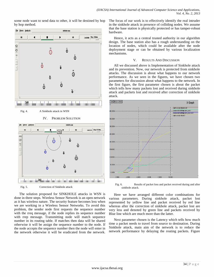
(IJACSA) International Journal of Advanced Computer Science and Applications,
Vol. 4, No. 2, 2013
34 | P a g e
www.ijacsa.thesai.org
some node want to send data to other, it will be destined by hop by hop method.
Fig. 4. A Sinkhole attack in WSN
IV. PROBLEM SOLUTION
Fig. 5. Correction of Sinkhole attack
The solution proposed for SINKHOLE attacks in WSN is done in three steps. Wireless Sensor Network is an open network as it has wireless nature. The security feature becomes less when we are working in a Wireless Sensor Networks. To avoid this problem, the sender node first requests the sequence number with the rreq message, if the node replies its sequence number with rrep message. Transmitting node will match sequence number in its routing table. If matches then data will be shared otherwise it will be assign the sequence number to the node. If the node accepts the sequence number then the node will enter in the network otherwise it will be eradicated from the network.
The focus of our work is to effectively identify the real intruder in the sinkhole attack in presence of colliding nodes. We assume that the base station is physically protected or has tamper-robust hardware.
Hence, it acts as a central trusted authority in our algorithm design. The base station also has a rough understanding on the location of nodes, which could be available after the node deployment stage or can be obtained by various localization mechanisms.
V. RESULTS AND DISCUSSION
All we discussed above is Implementation of Sinkhole attack and its prevention. Now, our network is protected from sinkhole attacks. The discussion is about what happens to our network performance. As we seen in the figures, we have chosen two parameters for discussion about what happens to the network. In the first figure, the first parameter chosen is about the packet which tells how many packets lost and received during sinkhole attack and packets lost and received after correction of sinkhole attack.
Fig. 6. Results of packet loss and packet received during and after
sinkhole attack.
Here we have arranged different color combinations for various parameters. During sinkhole attack, packet lost represented by yellow line and packet received by red line whereas after the correction of sinkhole attack, packet lost are very less and denoted by green line and packets received by Blue line which are much more than the latter.
Next parameter chosen is the Latency which tells how much time a packet needs to travel from source to destination. During Sinkhole attack, main aim of the network is to reduce the network performance by delaying the routing packets. Figure

(IJACSA) International Journal of Advanced Computer Science and Applications,
Vol. 4, No. 2, 2013
35 | P a g e
www.ijacsa.thesai.org
shows the results of routing time or the Latency during Sinkhole attack and after correction of Sinkhole attack.
Fig. 7. Comparison of routing time while and after sinkhole
attack.
Discussion ends by saying that performance of the network will be affected if there is any Sinkhole attack in the network.
VI. FUTURE WORK
Wireless sensor network is very vast topic for new research. It discovers various steps during data sharing. As we decided Sinkhole attack for research work, several other attacks will be chosen for future work. And if someone want to choose this selected topic, then the performance of the network will be measured by choosing different parameters like routing overhead, delay, or the same attack will be implemented by choosing other protocol.
REFRENCES
[1] C. Karlof and D. Wagner, “Secure routing in wireless sensor networks:Attacks and countermeasures,” AdHoc Networks Journal, vol. 1, no. 2–3,pp. 293–315, September 2003.
[2] R. Roman, J. Zhou, and J. Lopez, “Applying intrusion detection systems to wireless sensor networks,” in Proceedings of IEEE Consumer Communications and Networking Conference (CCNC ’06), Las Vegas, USA, January 2006, pp. 640–644.
[3] G. Werner-Allen, K. Lorincz, M. Welsh, O. Marcillo, J. Johnson, M. Ruiz, and J. Lees, “Deploying a wireless sensor network on an active volcano,” IEEE Internet Computing, vol. 10, no. 2, pp. 18–25, 2006.
[4] T. Schmid, H. Dubois-Ferri`ere, and M. Vetterli, “SensorScope: Experiences with a Wireless Building Monitoring Sensor Network,” in Proceeding of the Workshop on Real-World Wireless Sensor Networks (REALWSN ’05), Stockholm, Sweden, June 2005.
[5] S. Kim, S. Pakzad, D. Culler, J. Demmel, G. Fenves, S. Glaser, and M. Turon, “Wireless sensor networks for structural health monitoring,” in SenSys ’06: Proceedings of the 4th international conference on Embedded networked sensor systems, 2006, pp. 427–428.
[6] G. Werner-Allen, K. Lorincz, J. Johnson, J. Lees, and M. Welsh, “Fidelity and yield in a volcano monitoring sensor network,” in OSDI ’06: Proceedings of the 7th symposium on Operating systems design and implementation. Berkeley, CA, USA: USENIX Association, 2006.
[7] Hiren Kumar Dev Sharma, Ajit Kumar, Sikkim Manipal Institute of Technology ‘security threats in wireless sensor networks’ IEEE 2006.
[8] Piyush K. Shukla, S. Silakari. Sarita S. Bhadoria, RGVP Bhopal India ‘Network security scheme for wireless sensor network using efficient CSMA MAC layer protocol’, sixth international conference on Information Technology, 2009.
[9] Xiuli Ren, Norman University, Siping, China, ‘Security methods for Wireless Sensor networks’, International Conference on Mechatronics and Automation, June 25-28, 2006.
[10] Xiao Jiango Du, North Dakota State University ‘Security in Wireless Sensor Network’, IEEE August,2008 .
[11] Approaches to Wireless Sensor Network: Security Protocols, World of Computer Science and Information Technology Journal (WCSIT) ISSN: 2221-0741 Vol. 1, No. 7,302-306, 2011

(IJACSA) International Journal of Advanced Computer Science and Applications, Vol. 4, No. 2, 2013
36 | P a g e www.ijacsa.thesai.org
Intelligent Collaborative Quality Assurance System
for Wind Turbine Supply Chain Management
Intelligent Collaborative Quality Assurance System
for Wind Turbine Supply Chain Management
B. L. SONG, W.LIAO, J. LEE
National Science Foundation (NSF) Center for Intelligent Maintenance System (IMS)
Cincinnati, US
Abstract—To determine the root causes or sources of variance
of bad quality in supply chains is usually more difficult because
multiple parties are involved in the current global manufacturing
environment. Each component within a supply chain tends to
focus on its own responsibilities and ignores possibilities for
interconnectivity and therefore the potential for systematic
quality assurance and quality tracing. Rather than concentrating
on assigning responsibility for “recall” incidents, it would be
better to expend that energy on constructing a collaborative
system to assure product quality by employing a systematic view
for the entire supply chain. This paper presents a systematic
framework for intelligent collaborative quality assurance
throughout an entire supply chain based on an expert system for
implementing two levels of quality assurance: system level and
component level. This proposed system provides intelligent
functions for quality prediction, pattern recognition and data
mining. A case study for wind turbines is given to demonstrate
this approach. The results show that such a system can assure product quality improved in a continuous process.
Keywords—Wind turbine expert system; Supply chain
management; Collaborative quality assurance; Prediction; Pattern
recognition;
I. INTRODUCTION
Quality is a critical requirement for customers, especially in the case of expensive and complex products. In recent years, an increasing number of product recalls are occurring. Such product recall incidents have resulted in serious customer dissatisfaction and significant company losses in both image and business. Rather than argue who ought to apologize to the “recall” incidents, it would be better to expend that energy on constructing a collaborative system to assure product quality by employing a systematic view for the entire supply chain. A product supply chain can encompass multiple, diverse parties in the current global manufacturing environment. Each functional part in supply chain tends to focus on its own responsibilities, resulting in a lack of strong interconnected infrastructure to support systematic quality assurance, such as clear management structure and a quality tracing enabled data collection framework. It is therefore often difficult to identify or trace the exact reason for bad quality. How to ensure product quality collaboratively becomes a vital task for the companies along the supply chain.
Supply chain management (SCM) was defined as the management of a network of interconnected businesses involved in the ultimate provision of product and service packages required by the end customers. It spans all movement and storage of raw materials, WIP inventory and finished goods from point-of-origin to point-of-consumption. A good SCM is essential for companies to meet global competition. Nowadays, many manufacturers and service providers collaborate with their suppliers and upgrade their purchasing and supply management functions from a clerical role, to an integral part of SCM. In terms of possessing a systematic quality assurance function and a collaborative data collection framework for quality tracing, gaps still exist.
Quality assurance was defined as “a strategic management function concerned with the establishment of policies, standards and systems for the maintenance of quality”[1]. Later, as a result of benchmarking studies, Baines and Ryan determined that quality assurance could be identified as [2]:
1) A tool to demonstrate regulatory compliance;
2) A business efficiency tool to ensure product quality
and minimize hygienic risks;
3) A communication tool to customers and consumers,
wherever they are in the world. Quality assurance becomes increasingly important in
integrated SCM [3-4]. As for the methodologies, the majority of prior works tend to conduct failure testing or statistical control to improve quality assurance system [5-9]. Over the past thirty years, considerable advances have been made in computational intelligence. Various intelligent technologies and/or algorithms like artificial neural networks genetic algorithms, fuzzy/logic systems, learning algorithms, and metaheuristics have been developed for realizing intelligent control or expert systems [10]. Compared to traditional statistical control based quality assurance, computational intelligence technologies have advantages for making intelligent decisions such as quality prediction and pattern recognition for the situations with high complexity. If the quality can be predicted before production, it will greatly help avoid generating bad products. Designer can forecast the quality and thus optimize designed settings and tighter tolerance before releasing the design, while downstream parties, such as manufacturing, can optimize real settings in

(IJACSA) International Journal of Advanced Computer Science and Applications, Vol. 4, No. 2, 2013
37 | P a g e www.ijacsa.thesai.org
the similar way prior to production. And moreover, if the quality can be classified into several levels such as “good quality”, “average quality” and “bad quality,” products classified lower than “good quality” can be analyzed and traced back to the settings of the impact factors in order to determine the root cause of quality deficiencies. Through such analysis, the rules of best settings can be obtained, and the necessary changes in product or process design can be determined. Hence, providing intelligent functions such as quality prediction, pattern classification and data mining can improve quality by improving overall design; in addition, such functions can help optimize quality assurance for other downstream parties as well. Currently, there exists little research [11] on developing such intelligent systems for quality improvement in industry process. Extensive space could be explored to improve the performance of collaborative quality assurance.
With the consideration of the significance in closing above mentioned gaps, this paper will base on computational intelligence technologies to establish a collaborative quality assurance expert system for machinery products to ensure and improve their quality continuously.
This paper is structured as follows. In Section 2, the methodology of collaborative quality assurance in SCM is proposed. Section 3 takes wind turbine as a case to demonstrate the methodology. Finally, conclusions and future work are provided in Section 4.
II. METHODOLOGY FOR COLLABORATIVE QUALITY
ASSURANCE IN SCM
Methodology to develop the collaborative quality assurance expert system in SCM is provided in this section. Quality and quality assurance will be defined first. Three conceptual frameworks, including a management model, a technical model and a database management model, will be established to help guide the coordination of quality assurance along the whole supply chain. Intelligent functions such as quality prediction, pattern recognition and knowledge mining will be designed in the technical model to support two levels of collaborative quality assurance in SCM: system level and component level.
A. Problem formulation
1) Quality It is important to realize that quality is determined by the
intended users, clients or customers, not by society in general. 'Expensive' does not always mean 'high quality'. Even goods with low prices can be considered quality items if they meet a market’s requirements.
Quality ultimately is measured in terms of customer satisfaction. Customers may have various measurements, such as number of product recalls, number of maintenance fix requests per year, defects found after product delivery per function point, cost of defects (e.g. annual maintenance costs), costs of quality activities (e.g. costs of inspections, diagnostics, test execution, defect tracking, preventive measures and QA education), mean time between failure (MTBF), mean time to repair (MTTR), and so on, to check the
product quality characteristics like functionality, reliability, safety, efficiency, and maintainability.
For this paper, no matter what a customer’s requirements are, a product that is closest to meeting these requirements is considered to be of good quality.
2) Quality Assurance Quality Assurance, or QA for short, was described as a set
of activities intended to ensure that products (goods and/or services) satisfy customer requirements in a systematic, reliable fashion. QA can’t absolutely guarantee the production of quality products, unfortunately, but makes this more likely. Two objectives are therefore set for achieving the optimal QA (see Figure 1).
a) Objective 1: To optimize the design of product
Customer requirements will be translated by designers into parameters for what constitutes a high quality product. This paper assumes that designers will provide the optimal value setting and tolerance of all possible quality impact factors in advance, including raw material specification, product dimensions, manufacturing environment, machine statuses, delivery requirements and so on. The evaluation criterion of an optimal design is that the design can best meet customer-defined requirements. The objective 1 is identified as:
To Minimize Difference 1 = Design Setting - Customer Requirement
b) Objective 2: To maximize the compliance with design
Given an optimal design, quality assurance will attempt to make the real value setting of each quality impact factor along supply chain (e.g. raw material, manufacturing, delivery) in line with those of the design, so as to meet the functionality or the specifications of design. This objective can also be represented as minimizing the difference between real settings and design settings, that is:
To Minimize Difference 2 = Real Setting – Design Setting
The difference 2 is essentially the deviation of real settings from design settings. A maximum acceptable deviation from a nominal design setting is called tolerance.
The scales of the differences of different factors are not the same. A Compliance Index (CI) is defined to represent the degree of accuracy of the real setting in comparison to the design setting in a standardized scale from 0 to 1. A value of 0 means that the real setting matches design requirements perfectly, while a value of 1 means that real settings do not adequately match design requirements. These values can be obtained by
(1)
where R and D represent the real setting and design setting for a same impact factor, respectively. If the setting of certain input factors for the best design is zero, then the following
00
1
DRts
eCI D
DR
,..

(IJACSA) International Journal of Advanced Computer Science and Applications, Vol. 4, No. 2, 2013
38 | P a g e www.ijacsa.thesai.org
equation could be used to calculate the compliance index:
(2)
Objective 2 is therefore to “Minimize CI”.
Accordingly, QA includes two activities in this study: to design the best regulation of the quality related factors which rely on raw materials, assembly, components and overall products, as well as the services related to production, inspection and delivery processes; and to seek the maximum compliance between each real factor setting and their corresponding design factor settings.
3) Closed loop quality assurance improvement to
guarantee good An expert system based closed loop quality assurance
improvement process is proposed in Figure 1 to fulfill the above two objectives continuously. There are multiple factors (e.g. raw material factors, manufacturing environment factors, machine factors, assembly factors, delivery factors, etc) throughout supply chain that may influence product quality in various ways and in dynamic situations. The individual and combined influence of multiple factors on quality is unclear. The rules of knowledge base will be obtained from the intensive study of the impact of multiple factors on product quality by the expert system. The product quality will be predicted and patterns will be recognized. The features indicative of bad quality will be extracted and feedback to designers to determine, and improve upon, parameter settings and tolerances for bad quality. The deviation of real settings from nominal design settings on multiple factors will also be studied in order to provide knowledge for compliance improvement. Once the root causes for bad quality are determined, they will be delivered to appropriate personnel for quality improvement. The above improvement of design and compliance will be made in a continuous process.
Fig. 1. Closed Loop Improvement Method To Guarantee A Good Quality
Assurance In SCM.
The management-level method for guaranteeing the quality impact factor setting’s compliance with design is demonstrated in Section 2.2, while the expert system for studying multi-factor impacts on quality, providing intelligent functions such as prediction, pattern recognition, and generating the knowledge bases for above two objectives is presented in Section 2.3. The distributed database
management system proposed in Section 2.4 can help a user trace back the situation in which a quality issue has been discovered.
B. Management Structure for collaborative quality assurance
Assuming that a certain design is optimal, an order oriented collaborative quality assurance team management mode is proposed in order to assure the supply chain factor settings’ compliance with the design.
For the products of the same order, a quality assurance (QA) team will be organized among all the parties along the supply chain. The system supplier needs to take direct responsibility for delivering the product (a complete assembled system is defined as a product) to end users and it also needs to guarantee the quality of the components outsourced. The system supplier has a good connection to the end user and component suppliers. Considering these connections, the system supplier is the best party to lead the quality assurance team. Each quality related department, such as system level design, assembly process and delivery, component level design, raw material supply, manufacturing, and delivery will work together for QA.
After receiving the customer expectations of what they expect from a product, system level QA will design the optimal regulations (e.g. parameter value setting and tolerance setting for materials, manufacturing and delivery along supply chain) for the best quality product. The quality parameters for components will be delivered to each component QA as a customer requirement. Component QA will continue to update the optimal settings for a component if the customer requirements received need to be amended, or if new requirements are identified. The designed settings will then be passed to each party along the component supply chain.
Each downstream party will check the compliance of real settings with design settings after it completes its part. If the completed part passes the quality compliance check, then it will be delivered to its upstream party. If all parties, including those responsible for raw materials, manufacturing and delivery, have finished their check, a total quality assurance (TQA) will be carried out before the completed component is sent for system level assembly. System level QA will start after all component level QAs are completed. The same quality compliance check will be conducted for the system assembly process and its delivery path. The customer will do a TQA for the final assembled product. Those products which fail the TQA will be sent back for rework.
C. Two levels of quality assurance expert system in SCM
Ensuring a high level of quality for products throughout a supply chain is a much-needed perspective into the SCM due to the importance of quality in terms of improving system reliability and customer satisfaction. Various factors along a supply chain can influence the quality of a product. Determining the impact of multiple factors on product quality is of significant importance in providing useful information to improve quality assurance. Few quality assurance approaches can satisfy this need due to the complexity of the real situation. This section will propose a quality assurance expert system to close this gap. As the product (or system) and each
00
1
DRts
eCIDR
,..
Optimal Design
Knowledge base for
design improvement
Optimal Management to make each quality
impact factor setting along supply chain (e.g.
raw material, manufacturing, delivery) the most
compliant with design
Quality Assurance in Supply Chain Management
Continuous
Improvement
of design
Objective 1
Objective 2
Knowledge base
for compliance
improvement
Continuous
Improvement
of compliance
Quality
Pattern
Classification
Expert System
Quality
Prediction
Knowledge
Mining

(IJACSA) International Journal of Advanced Computer Science and Applications, Vol. 4, No. 2, 2013
39 | P a g e www.ijacsa.thesai.org
of its components have their own supply chains, the framework for the expert system is developed based on two levels: system-level quality assurance and component-level quality assurance.
1) System level quality assurance in SCM The procedure for conducting system level quality
assurance is illustrated in Figure 2. As indicated in the procedure, the supply chain of the product (or system) is identified first. The criteria for what constitutes system-level quality, such as reliability, based on the customer requirements, are then defined. Component level quality assurance is one important step for guaranteeing system level quality assurance. Theoretically speaking, quality assurance for each component will ensure the optimal result, in terms of quality, for the overall product. However in reality, it is not necessary to research each component, and it would be costly to do so. Thus, it becomes essential to balance the costs versus the benefit first. For the situation in which it is not cost effective to do quality assurance for each component, the critical component analysis and selection needs to be conducted. Subsequently, it is vital to define component-level quality for the chosen critical component(s) in order to conduct component-level quality assurance. The factors of the component that are most indicative of quality will be selected for studying their impact on the defined component-level quality. With this information, the component-level quality assurance expert system can be constructed. The comparison of component quality performance before and after applying the proposed system will be used for evaluation and to determine if improvements to the system can be made. The customer’s requirements are another criterion for making a quality determination. The order of using these two criteria can be adjusted according to the target of the quality improvement. Once the quality of all the studied components is improved to meet the defined requirements, the overall quality of the product will be evaluated to see whether it can meet the system requirements. If not, the prior steps should be revisited in order to continue improving the component-level quality. Therefore, through the procedure of system-level and component-level quality assurance, the quality of product can be better ensured.
2) Component level quality assurance in SCM A component-level quality assurance expert system has
been designed (Figure 3) for improving component quality based on the study of the impact of multiple factors on quality. For each component, the selection of factors from different parties along component supply chain, and the quality of the components produced, will be determined. The database system for data collection is presented in following section. Some samples will be selected from the database and input as training data for the expert system.
One major function of the expert system is to provide a scientific way for quality prediction and quality classification. For this purpose, quality forecasting and quality classification models will be built based on the training data. Inputting any test sample of impact factors, the forecasting model will predict the corresponding quality. For the predicted quality, the quality pattern recognition model will identify the pattern that it belongs to. The designer can use this system to test if
the design settings will result in a good or bad quality product before releasing the design to downstream parties. Downstream parties, such as manufacturing, can apply the proposed system to predict the quality of products to be produced based on simulated real settings. They are then able to optimize their real settings before production. With this intelligent measurement system, tremendous loss from incorrect design settings or incorrect real settings will be saved.
Fig. 2. System level quality assurance in SCM.
Fig. 3. Component level quality assurance in SCM
The expert system has another function: to generate knowledge bases for design improvement and compliance improvement for achieving the best quality assurance. For instance, a correlation study of the impact factors and their affect on quality will reveal the critical impact factors that have bigger influence on bad quality. Further data mining conducted on bad quality patterns, such as a histogram of each critical impact factor, is helpful to find the features (i.e. range of settings) that result in bad quality. The knowledge obtained
Identify the
supply chain of
the component
Identify the related
factors of the
selected
component
Define
component-
level quality
Identify the
critical
factors
N
Improve
component-
level quality
Identify the
related
components
Construct
component-
level quality
model
Identify the
supply chain of
the product
Define
system-level
quality
Component-level Quality Assurance
Evaluate the performance for component-level quality
assurance; Quality satisfied?
Y
End
Identify the
critical
components
Improve system-level quality
Evaluate the performance for system-level quality
assurance; Quality satisfied?
Y
N
If each critical component is improved?
Y
N
System-level Quality Assurance
Sampling quality related factors
and their impacts on quality
Patterns for
bad quality
Patterns for
good quality
Pattern ClassificationUse unsupervised learning method (e.g. Self-Organizing
Map) to classify quality patterns based on training data
Manufacturing Delivery
Component Supply Chain
Design Raw material
Patterns for
medium quality
Training data
Predicted quality value
Training data
Recognized quality pattern
Feedback it to the
relative department for
quality improvement
Feedback to
designer to avoid
design for bad quality
Quality Forecasting 1. Train forecasting model (e.g.Neural
Network ) based on training data
2. Predict quality given test sample
impact factors as input
Input
Test
Sample
Impact
Factors
Output
Predicted
Quality
Pattern RecognitionGiven a test sample, use supervised leaning method
(e.g. Mahalanobis distance) to determine which pattern
the predicted quality belongs to
Knowledge base for
Compliance Improvement
If it is a bad quality pattern,
improve its compliance setting by
learning from good quality pattern
Knowledge base for
Design Improvement
Critical
impact
factors
Features
for bad
quality
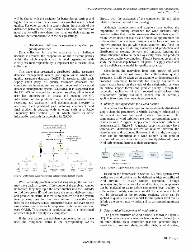
(IJACSA) International Journal of Advanced Computer Science and Applications, Vol. 4, No. 2, 2013
40 | P a g e www.ijacsa.thesai.org
will be shared with the designer for better design settings and tighter tolerances and hence avoid designs that result in bad quality. For other parties in a supply chain, the analysis of the difference between their input factors and those indicative of good quality will show them how to adjust their settings to improve their compliance with the design settings.
3) Distributed database management system for
quality assurance Data collection for quality assurance is a challenge
because it requires the cooperation of the different parties within the whole supply chain. A good organization with clearly assumed responsibility is important for successful data collection.
This paper thus presented a distributed quality assurance database management system (see Figure 4), in which one quality assurance database (QADB) is associated with each supply chain party, all quality assurance databases are connected via internet, and are under the control of a central database management system (CDBMS). It is suggested that the CDBMS be managed by the system supplier, while the end user has authorization to access and manage the QA information of the products they ordered. Consistent data recording and assessment and documentation integrity is necessary. Each produced part, including components and final product, is attached with an e-tag, such as a Radio Frequency Identification (RFID), which stores its basic information and path for accessing its QADB.
Fig. 4. Distributed quality assurance database management system.
When a quality problem occurs during usage, the end user may trace back its causes. If the source of the problem cannot be located, they may input the order number into the CDBMS to find the system ID and then trace the system delivery status and production status. If there is no problem with the system level process, then the user can continue to trace the issue back to the delivery status, production status and even to the raw material status for each component, with the assistance of each QADB. This process is conducted until it is determined at which stage the quality issue originated.
If the user knows the problem component, he can trace back the component status in the corresponding QADB
directly with the assistance of the component ID and other relative information read from its e-tag.
Although manufacturers and suppliers have noticed the importance of quality assurance for wind turbines, they usually confine their quality assurance efforts to their specific realm, which does not make use of potential opportunities for collaboration. For example, designers only focus on how to improve product design, while manufacturers only focus on how to ensure quality during assembly and production and distributers on storage, delivery and logistics. Ignoring the interrelationship between them may easily cause bad products due to poor quality coordination. Thus, it becomes essential to study the relationship between all parts in supply chain and build a collaborative model for quality assurance.
Considering the marvelous long term growth of wind turbine, and its utmost needs for collaborative quality assurance, it will be taken as an example to demonstrate the proposed systematic framework for quality assurance in supply chain based on the study of the relationship between the critical impact factors and product quality. Through the successful application of this proposed methodology, this collaborative quality assurance model can be certainly applicable to some other machinery products.
D. Identify the supply chain for a wind turbine
A wind turbine has a unique and internationally distributed supply chain the parameters of which is strongly influenced by the recent increase in wind turbine production. The components of wind turbines have their corresponding supply chains as well. A typical supply chain for a wind turbine is demonstrated in Figure 5. A general supply chain may have warehouses, distribution centers or retailers between the manufacturer and customer. However, in this study, the supply chain can be simplified as a wind turbine is the kind of customized products which is usually directly delivered from a wind turbine manufacturer to their customers.
Fig. 5. A typical supply chain for wind turbine.
Based on the framework in Section 2.3, first, system level quality for awind turbine can be defined as high reliability of wind turbine to ensure smooth operation. Through understanding the structure of a wind turbine, its components can be analyzed so as to define component level quality. A collaborative quality assurance model for component level will be discussed in the following sections, which can be applied as quality assurance model for the system level too by defining the system quality index and its corresponding impact factors.
E. Select critical components of wind turbine
The general structure of wind turbine is shown in Figure 6 [12]. The main parts of a wind turbine (as shown below ) are the rotor, blades, brake, controller, gear box, generator, high-speed shaft, low-speed shaft, nacelle, pitch, wind direction,
System Delivery QADBSystem Assembly QADB
System ID
Customer traces back causes
of bad quality product
Central database
management system
(CDBMS)
Order ID
Raw
Material
QADB
Raw
Material
QADB
Delivery
QADB
Manufacturing
QADB
Component 1 ID
Delivery
QADBManufacturing
QADB
Component 2 ID
Raw
Material
QADB
Delivery
QADBManufacturing
QADB
Component 3 ID
Component ID
Component ID (e.g. RFID)
Reader
Study the effect of different factors on product quality
Conclude reasons for product problems in different
situations and build up knowledge base for them
Establish Machine Learning Model to learn the
relationship between impact factors and product quality
Study the situation that quality defect is caused by raw material problem
Study the situation that quality defect is caused
by machine problem
Study the situation that quality defect is caused
by process problem
Study the situation that quality defect is caused
by design problem
Mining Reasons for Quality Defects
Diagnosis of product quality problem If a quality defect occurs, diagnose the root cause by mapping it to the situation/status in the knowledge
Given a set of factor statuses as input, predict the product quality
Prognosis of product quality problem
Making Decisions for Quality Assurance
Continuous learning &
enriching knowledge base
Monitor factors and collect impacts from
machine aspect
Monitor factors and collect impacts from
process aspect
Monitor factors and collect impacts from
design aspect
Monitor factors and collect impacts from raw material supplier
Pass the knowledge to designer for redesign
Design based Quality Assurance
Material-based Quality Assurance
Pass the knowledge to suppliers to improve
material quality
Machine based Quality Assurance
Pass the knowledge to machine supplier or operator to optimize machine setting or redesign machines
Process based Quality Assurance
Pass the knowledge to process manager for
optimal process control

(IJACSA) International Journal of Advanced Computer Science and Applications, Vol. 4, No. 2, 2013
41 | P a g e www.ijacsa.thesai.org
wind vane, yaw drive and yaw motor. Most turbines have either two or three blades. Wind blowing over the blades causes the blades to "lift" and rotate. Generally, the blades and the hub together are called the rotor. When the blades rotate, the gears rotate; the gears connect the low-speed shaft to the high-speed shaft and increase the rotational speeds from approximately 30 to 60 rotations per minute (rpm) to approximately 1000 to 1800 rpm, which is the rotational speed required by most generators to produce electricity. Generally, the gear box is the most costly part of a wind turbine.
Fig. 6. General structure of wind turbine.
Although a wind turbine is comprised of many components, it is more cost effective to focus on the critical components for quality assurance. In order to identify the critical components of a wind turbine, the typical way is to determine which component has the greatest influence on wind turbine breakdowns. In recent years, numerous failure surveys have been conducted on wind turbines. A downtime distribution was presented in [13], based on a population of German wind turbines. Braam and Tavner both provided recent studies on failure probabilities [14-16]. McMillan and Ault then selected four component categories from these multiple sources and illustrated their annual probability of failure on the same chart [17]. They further used this data to study reliability benchmarks [18]. This paper summarizes their researches in Figure 7 to illustrate the effect of both the failure probability and downtime distribution of four components of wind turbines, namely the electronics & controls, rotor blades, gearbox and generator. The X value is the downtime distribution data from Winstats Newsletter[13], meanwhile, while the Y value is the failure probability from the surveys for the same component [14-16]. It should be noted that each component has three samples marked in different colors. The plot area is divided into four quarters, namely quadrants 1 to 4, based on the high or low values of the axis. All gearbox & bearing samples, as well as all generator samples and some blades samples, fall in quadrant 4, which shows that all these components have a high downtime distribution with comparatively a low failure probability. Therefore, gearbox, generator and rotor blades are taken as more critical components.
Fig. 7. Wind Turbine Critical Components Selection Based On Integrated Failure Effect Study.
F. Define component level quality
Component level quality assurance will then be established for the component selected with its corresponding quality criteria (i.e. rules in quality assurance model) and impact factors. As shown in Figure 6, bearings are key sub-components in both gearboxes and generators, which are two critical components of wind turbines. It is thus taken as an example in the following sections to demonstrate the approach of building component level quality assurance model. This approach can be applied to other components.
Fig. 8. Fault of bearing.
TABLE I. PRIMARY TYPES OF QUALITY RELATED BEARING DAMAGES.
Bearing damage Caused by Bearing damage Caused by
wear abrasive particles flaking Preloading
inadequate lubrication oval compression
vibration axial compression
smearing rollers and raceways Misalignment
external surfaces Indentations
roller ends guide flanges Smearing
crack rough treatment deep seated rust
excessive drive-up fretting corrosion
smearing Fluting
Cage damage vibration corrosion deep seated rust
excessive speed fretting corrosion
wear indentation Overloading
blockage foreign particles
The primary types of bearing damages are necessary to be well researched before building the component level quality assurance model. Bearings as prominent parts among the most important components in the majority of machines sometimes, do not always meet their life expectancy due to damages from multiple sources for diverse reasons, such as heavier loading, careless handling, ineffective sealing or unsuitable fits. Each of these factors produces its own particular type of damage and leaves its own special impact on a bearing. Thus, it is
Study the effect of different factors on product quality
Conclude reasons for product problems in different
situations and build up knowledge base for them
Establish Machine Learning Model to learn the
relationship between impact factors and product quality
Study the situation that quality defect is caused by raw material problem
Study the situation that quality defect is caused
by machine problem
Study the situation that quality defect is caused
by process problem
Study the situation that quality defect is caused
by design problem
Mining Reasons for Quality Defects
Diagnosis of product quality problem If a quality defect occurs, diagnose the root cause by mapping it to the situation/status in the knowledge
Given a set of factor statuses as input, predict the product quality
Prognosis of product quality problem
Making Decisions for Quality Assurance
Continuous learning &
enriching knowledge base
Monitor factors and collect impacts from
machine aspect
Monitor factors and collect impacts from
process aspect
Monitor factors and collect impacts from
design aspect
Monitor factors and collect impacts from raw material supplier
Pass the knowledge to designer for redesign
Design based Quality Assurance
Material-based Quality Assurance
Pass the knowledge to suppliers to improve
material quality
Machine based Quality Assurance
Pass the knowledge to machine supplier or operator to optimize machine setting or redesign machines
Process based Quality Assurance
Pass the knowledge to process manager for
optimal process control

(IJACSA) International Journal of Advanced Computer Science and Applications, Vol. 4, No. 2, 2013
42 | P a g e www.ijacsa.thesai.org
essential to examine the damaged bearing and study the cause of the damage so as to provide support for quality assurance.
Based on the most prevalent types of bearing damage (see Table 2), it can be seen that most damage is caused by quality issues along the supply chain. Hence, the quality index and the major impact factors influencing bearing quality will be identified and their relationship will be well studied by using this proposed model.
As mentioned before, there exist various types of quality index according to customer requirement. Reliability is adopted in this section to represent the quality of the bearing. Other quality indices can also be considered in the same way, according to a customer’s requirements. In engineering, reliability is the ability of a system or component to perform its required functions under stated conditions for a specified
period of time. The traditional notation for reliability is ,
while here it is shown as one index of quality, and is denoted
as . Mathematically, reliability may be expressed as
(3)
where is the failure probability density function and is
the length of the period of time that is assumed to start from
time zero .
G. Identify quality impact factors for critical component
By analyzing bearing damages and its causes, 19 main quality impact factors which can cover the majority of the causes of damage are selected for study. Five of them are factors related to raw material, six of them are about machining, four of them are machine status factors, three are manufacturing environment factors, and one is the delivery condition. Those 19 impact factors and 1 quality index (i.e. reliability of bearing) are listed in Table 3.
As stated in the methodology section, the designed settings are assumed to be optimal. The quality assurance target of other parties is to make the real settings meet the designed settings. The deviations of real settings from design settings instead of the real setting values are studied because they can reflect the quality compliance level. The results of which can further help design tighter tolerances. As discussed in Section 2.1, CI is introduced to transfer the different scales of the deviations to a standardized range, from 0 to 1. In terms of the chosen standard value range, 0 means the difference between real settings and designed settings is the smallest, while 1 means the difference between them is the biggest. CI[Rlu] indicates the compliance index of lubricant in “Raw material” category. Equations (1) and (2) provide the method to calculate CI. The CIs of all selected impact factors are taken as the inputs of the quality assurance model. CI[Qre], the compliance index of reliability, is the output factor. CI[Qre] is calculated by , in order to make it comply with the
CI of the input factors. That is 0 means the perfect case with the best reliability, while 1 reflects the worst one.
H. Quality prediction and pattern recognition for critical
component
For the purpose of quality prediction and pattern recognition, many intelligent approaches can be used. In this study, two neural network models, called Feedforward neural network and self-organizing map neural network (SOM) are used. A Feedforward neural network is developed to predict the component quality and a self-organizing map (SOM) is built to classify the quality pattern, through learning the relationship between quality and its impact factors collected along the supply chain.
1) Quality prediction A Feedforward neural network is an artificial neural
network in which connections between the units do not form a directed cycle.
TABLE II. SELECTED IMPACT FACTORS AND QUALITY INDEX.
Factors Notation Range
of CI
Input
Raw material Lubricant Rlu [0,1]
mounting
pressure Rmp [0,1]
seating out of
alignment Rsa [0,1]
foreign particles Rfp [0,1]
material
containing Rmc [0,1]
Manufacturin
g
inner diameter Mid [0,1)
outer diameter Mod [0,1)
surface
roughness Msr [0,1)
chamfer Mch [0,1)
thickness Mth [0,1)
ball diameter Mbd [0,1)
Machine
Balance Aba [0,1]
Precision Apr [0,1]
Health index Ahi [0,1]
Vibration Avi [0,1]
Environment Temperature Ete [0,1]
Humidity Ehu [0,1]
Dust tolerance Edt [0,1]
Delivery Delivery
condition Ddc [0,1]
Output
Quality index Reliability QRe (0,1]
Note: CI range values have been standardized for all factors.
CI Value range in “Manufacturing” represents the difference between real
manufacturing setting and design requirements. 0 means no difference. The
closer to 1, the bigger difference it is. So 0=perfect case; 1=worst case
It is most commonly used with the back propagation algorithm that often has one or more hidden layers of sigmoid neurons followed by an output layer of linear neurons. In this network, the information moves in only one direction, forward, from the input nodes, through the hidden nodes and to the output nodes. There are no cycles or loops in this type if network. Multiple layers of neurons with nonlinear transfer functions allow the network to learn nonlinear and linear relationships between input and output vectors. A well learned network is often applied for function approximation or regression analysis tasks, including forecasting. Cost function
)(tR
reQ
t
re dxxftTPtRQ )()()(
)(xft
1 ( )R t
Study the effect of different factors on product quality
Conclude reasons for product problems in different
situations and build up knowledge base for them
Establish Machine Learning Model to learn the
relationship between impact factors and product quality
Study the situation that quality defect is caused by raw material problem
Study the situation that quality defect is caused
by machine problem
Study the situation that quality defect is caused
by process problem
Study the situation that quality defect is caused
by design problem
Mining Reasons for Quality Defects
Diagnosis of product quality problem If a quality defect occurs, diagnose the root cause by mapping it to the situation/status in the knowledge
Given a set of factor statuses as input, predict the product quality
Prognosis of product quality problem
Making Decisions for Quality Assurance
Continuous learning &
enriching knowledge base
Monitor factors and collect impacts from
machine aspect
Monitor factors and collect impacts from
process aspect
Monitor factors and collect impacts from
design aspect
Monitor factors and collect impacts from raw material supplier
Pass the knowledge to designer for redesign
Design based Quality Assurance
Material-based Quality Assurance
Pass the knowledge to suppliers to improve
material quality
Machine based Quality Assurance
Pass the knowledge to machine supplier or operator to optimize machine setting or redesign machines
Process based Quality Assurance
Pass the knowledge to process manager for
optimal process control

(IJACSA) International Journal of Advanced Computer Science and Applications, Vol. 4, No. 2, 2013
43 | P a g e www.ijacsa.thesai.org
is an important concept in learning, as it is a measure of how far away we are from an optimal solution to the problem that we want to solve. Learning algorithms search through the solution space in order to find a function that has the smallest possible cost. A commonly used cost is Mean Square Error (MSE) which tries to minimize the average squared error between the network's output and the target value over all the example pairs.
In this case study, for each selected impact factors and quality index, 1000 samples are collected and then their compliance indices are standardized into a range [0,1]. For each factor, 1000 standardized CI samples are stored in one factor vector, and 1000 quality index samples are in one quality index vector.
In the Feedforward neural network model, the input is the vector of 19 factor vectors, and the output is the quality index vector. Two layers are set and the Levenberg-Marquardt rule is chosen to train this neural network model. The epoch is set to be 1000. The Mean Square Error (MSE) is used to examine the prediction performance. The MSE <=0.01 is set as threshold to stop training. After training, Feedforward neural network model could be used to predict CI of quality index (i.e. reliability of bearing) given any test sample.
In Figure 9, the training results of the Feedforward neural network model, including the training state and the corresponding MSE (0.0068) are presented respectively. The results show that this Feedforward neural network model fits the samples to the degree that it is requested, which means this trained Feedforward neural network model can be used to predict the quality index based on the selected impact factors.
The following are two examples in which the proposed model is used to predict the quality index for two test samples:
Test sample vector of impact factors is: [0.32576;0.30902;0.30753;0.30937;0.28538;0.43926;0.44336;0.52081;0.45899;0.53185;0.48846;0.33633;0.3077;0.46696;0.35483;0.090269;0.044895;0.90836;0.77512]. Quality index is predicted to be: [0.2925]
Fig. 9. Training results of Feedforward neural network.
Test sample vector of impact factors is:
[0.8927;0.8942;0.9217;0.2920;0.1420;0.5032;0.4932;0.4675;0.5239;0.5061;0.5018;0.8447; 0.7880; 0.9724; 0.1794; 0.9296; 0.9256; 0.3489; 0.3816] Quality index is predicted to be: [0.9476]
2) Quality pattern recognition In addition to being able to predict a certain quality index
value, it would be advantageous to be able to determine the patterns of the whole values as well. For this purpose, SOM has been adopted to classify a certain quality index into various levels. If a certain pattern needs to be deeper studied, a specific analysis can be conducted for that.
SOM is another type of artificial neural network that is trained using unsupervised learning to produce a low-dimensional, discretized representation of the input space of the training samples. It produces a map to represent the input space of the training samples. It is different from other artificial neural networks in the sense that SOM uses a neighborhood function to preserve the topological properties of the input space. SOM has one layer with the neurons organized in a grid, which makes it useful for visualizing low-dimensional views of high-dimensional data, —this function is akin to multidimensional scaling.
SOM operates in two modes like most neural networks: training and mapping. Training builds the map using input samples. Mapping automatically classifies a new input vector. Training is a competitive process, also called vector quantization. Firstly, it will randomize the map's nodes' weight vectors, and then grab an input vector, traverse each node in the map, including the use of Euclidean distance formula to find similarity between the input vector and the map's nodes’ weight vector. It also includes the track of the best matching unit (BMU), the node that produces the smallest distance. Afterward, the nodes in the neighborhood of BMU will be updated by pulling them closer to the input vector. The whole procedure will be repeated till current iteration reaches the limit on time iteration.
In this study, 1000 samples of quality index are used as training data to build a SOM neural network for quality pattern classification. Within SOM one layer is set, and the Batch unsupervised weight/bias training algorithm is chosen.
In Figure 10, the results displayed by the developed of SOM are presented, in which 5 classes are obtained, after training. This means that the quality index can be classified into 5 levels: “very good quality”, “good quality”, “average quality”, “bad quality” and “very bad quality”, respectively.
This SOM model can then be used for recognizing the quality pattern given a certain quality index value. For instance, the predicted quality index, 0.2925, in the abovementioned sample test 1, is classified by the SOM into class 2, which is considered to be of “good quality”; the quality index in sample test 2, 0.9476, is classified by the SOM into class 5, which is considered to be of “very bad quality”.
Study the effect of different factors on product quality
Conclude reasons for product problems in different
situations and build up knowledge base for them
Establish Machine Learning Model to learn the
relationship between impact factors and product quality
Study the situation that quality defect is caused by raw material problem
Study the situation that quality defect is caused
by machine problem
Study the situation that quality defect is caused
by process problem
Study the situation that quality defect is caused
by design problem
Mining Reasons for Quality Defects
Diagnosis of product quality problem If a quality defect occurs, diagnose the root cause by mapping it to the situation/status in the knowledge
Given a set of factor statuses as input, predict the product quality
Prognosis of product quality problem
Making Decisions for Quality Assurance
Continuous learning &
enriching knowledge base
Monitor factors and collect impacts from
machine aspect
Monitor factors and collect impacts from
process aspect
Monitor factors and collect impacts from
design aspect
Monitor factors and collect impacts from raw material supplier
Pass the knowledge to designer for redesign
Design based Quality Assurance
Material-based Quality Assurance
Pass the knowledge to suppliers to improve
material quality
Machine based Quality Assurance
Pass the knowledge to machine supplier or operator to optimize machine setting or redesign machines
Process based Quality Assurance
Pass the knowledge to process manager for
optimal process control

(IJACSA) International Journal of Advanced Computer Science and Applications, Vol. 4, No. 2, 2013
44 | P a g e www.ijacsa.thesai.org
Fig. 10. Training results of self-organizing map.
The above two artificial neural network models constructs an intelligent measurement system which is capable of predicting the product quality and indentifying corresponding quality class for any given test sample. This method can also strongly help designers and other downstream parties conduct simulation based experiments to study the impact of designed settings or real settings on quality before real application. By comparing the values of the quality index generated on various simulated settings, the optimal setting could be found and applied before design regulation releases or before production starts.
I. Knowledge for design and compliance improvement
More data mining works, like correlation, distribution and comparison studies, can be conducted based on the above data, which help generate knowledge bases for optimizing quality assurance for both designers and other downstream parties.
1) Correlation study For determining the quality pattern, a correlation study of
the impact factors and quality change will reveal the critical impact factors that have bigger impact on quality. In probability theory and statistics, correlation (often measured as a correlation coefficient) indicates the strength and direction of a linear relationship between two random variables. A number of different coefficients are used for different situations. The best known is the Pearson product-moment correlation coefficient, which is obtained by dividing the covariance of the two variables by the product of their standard deviations, as shown below.
(4)
where or is correlation between two
random variables X and Y, means covariance
between X and Y, , are standard deviations, ,
are expected values, and is the expected value operator.
The correlation is 1 in the case of an increasing linear relationship, −1 in the case of a decreasing linear relationship,
and some value in between these two values in all other cases, indicating the degree of linear dependence between the variables. The closer the coefficient is to either −1 or 1, the stronger the correlation between the variables (see Table 4).
TABLE III. INTERPRETATION OF THE SIZE OF A CORRELATION.
Correlation Negative Positive
Small −0.3 to −0.1 0.1 to 0.3
Medium −0.5 to −0.3 0.3 to 0.5
Large −1.0 to −0.5 0.5 to 1.0
All 1000 samples were selected for this correlation study. The correlations of each impact factor and quality index are plotted in a Radar chart (see top left chart of Figure 11). The results reveal that seven factors have stronger correlation with quality for the samples studied. Three are raw material factors, namely, seating out of alignment (Rsa), mounting pressure (Rmp), and Lubricant (Rlu); two are machine status factors, namely, Health index (Ahi), Precision (Apr), and Balance (Aba); and two are manufacturing environment factors: Humidity (Ehu), and Temperature (Ete).
2) Distribution study As the quality index can be traced back to the original
collected impact factors data, for all bad quality indices, a further distribution analysis of the parameter settings of each critical factor can be conducted to illustrate that what range it is most in, which is very important information to posses for impact factor design.
The distribution of all settings of the impact factor Rsa in very bad quality class (i.e. Class 5) is shown on top right chart in Figure 11. The range of settings is one type of feature of the root causes of bad quality, and should be avoided in design.
3) Comparison study For such parties as material, manufacturing, and delivery,
they can simulate their real setting and predict the quality index before production using the proposed expert system. If the predicted quality is bad or very bad, then the system can do an analysis to check the difference between the impact factors settings of the bad quality predicted and those settings in a very good quality pattern.
The bottom chart on Figure 11 presents an example of comparison, where the mean and range of each impact factor setting in very good quality pattern are compared with the real setting of each factor in test sample 2, which generated a very bad quality. The differences will feedback to instruct people how to adjust their settings to improve the compliance with design.
J. System level quality assurance
The procedures introduced in Section 3.3 to 3.6 are applied to all critical components. After all component level quality improvements have been completed, the system level quality will be improved as well. Like the impact factors in the component level quality assurance model, the impact factors for the system level quality assurance model are the factors influencing the quality of the wind turbines received by customers. The system level quality index is defined by customer requirements. A system level quality assurance
YX
YX
YX
YX
YXEYXYXCorr
)))(((),cov(),( ,
),( YXCorr YX ,
),cov( YX
X Y Xu Yu
E
Study the effect of different factors on product quality
Conclude reasons for product problems in different
situations and build up knowledge base for them
Establish Machine Learning Model to learn the
relationship between impact factors and product quality
Study the situation that quality defect is caused by raw material problem
Study the situation that quality defect is caused
by machine problem
Study the situation that quality defect is caused
by process problem
Study the situation that quality defect is caused
by design problem
Mining Reasons for Quality Defects
Diagnosis of product quality problem If a quality defect occurs, diagnose the root cause by mapping it to the situation/status in the knowledge
Given a set of factor statuses as input, predict the product quality
Prognosis of product quality problem
Making Decisions for Quality Assurance
Continuous learning &
enriching knowledge base
Monitor factors and collect impacts from
machine aspect
Monitor factors and collect impacts from
process aspect
Monitor factors and collect impacts from
design aspect
Monitor factors and collect impacts from raw material supplier
Pass the knowledge to designer for redesign
Design based Quality Assurance
Material-based Quality Assurance
Pass the knowledge to suppliers to improve
material quality
Machine based Quality Assurance
Pass the knowledge to machine supplier or operator to optimize machine setting or redesign machines
Process based Quality Assurance
Pass the knowledge to process manager for
optimal process control

(IJACSA) International Journal of Advanced Computer Science and Applications, Vol. 4, No. 2, 2013
45 | P a g e www.ijacsa.thesai.org
model can be constructed in the same way as that at the component level. By using the Feedforward neural network and SOM methods, the quality index of a wind turbine system can then be predicted and the pattern of quality index can also be identified. Useful knowledge can be obtained from data mining. By continuously measuring the quality index, classifying its pattern and redefining the impact factors’ settings, quality can be improved at both the system level and the component level until the quality index reaches the pre-determined threshold.
III. CONCLUSION AND FUTURE WORK
The importance of performing quality assurance throughout an entire supply chain has been gradually gaining recognition by the decision makers in industry. In this study, the frameworks of collaborative quality assurance in a supply chain, including management model, technical model, and database model, were proposed so as to ensure high quality of products. In the wind turbine case study presented, bearings have been identified as an important component of wind turbines, and taken as an example to demonstrate the proposed component level quality assurance approach.
Fig. 11. Knowledge mining results in quality assurance expert system
The component quality assurance model acted as an intelligent measurement system, to predict quality and recognize the quality pattern given a set of quality impact factors. With these promising functions, designers can test whether the design settings will result in a good or bad quality product before releasing the design to downstream parties. Downstream parties, such as those responsible for manufacturing, can simulate different real settings to
determine which may generate the best quality before production. More knowledge is mined based on the results through statistical analysis, such as correlation, distribution, and comparison, and feedback to designers and downstream parties for optimizing settings and tighter tolerance. With this intelligent quality assurance model, potential losses from bad design settings or incorrect real settings will be saved, and product quality will be ensured.
REFERENCES
[1] R. Early, A Guide to Quality Management Systems for the Food
Industry. Blackie Academic and Professional, 1995, London.
[2] R. N. Baines and P. Ryan, Global trends in quality assurance. Trade Partners UK and Ministry of Agriculture “Modern Food Chain”
Seminar, 2002, Kuala Lumpur.
[3] J. C. Turner and W. P. Davies, The modern food chain: profiting from effective integration. Trade Partners UK and Ministry of Agriculture
‘Modern Food Chain’ Seminar, 2002, Kuala Lumpur.
[4] L. Manning, R. N. Baines and S. A. Chadd, Quality assurance models in the food supply chain. British Food Journal, 2006, 108(2), 91-104.
[5] D. H. Stamatis, Failure Mode and Effect Analysis: FMEA from Theory
to Execution, 2003, Hardcover.
[6] W. A. Shewhart, Economic control of quality of manufactured product. 1931, (D. Van Nostrand Company: New York).
[7] W. A. Shewhart, Statistical Method from the Viewpoint of Quality Control. 1939, (Dover: New York).
[8] G. Taguchi, Quality engineering (Taguchi methods) for the development
of electronic circuit technology. IEEE Transactions on Reliability (IEEE Reliability Society) 1995, 44 (2), 225-229.
[9] D. C. Montgomery, Introduction to Statistical Quality Control (6th
edition), John Wiley & Sons, 2008, New York.
[10] J. Behnamian, S.M.T. Ghomi, Fatemi and M. Zandieh, Development of a hybrid metaheuristic to minimize earliness and tardiness in a hybrid
flowshop with sequence-dependent setup times. International Journal of Production Research, 2009, 1-24, iFirst.
[11] X. Shi, P. Schillings, and D. Boyd, Applying artificial neural networks
and virtual experimental design to quality improvement of two industrial processes. International Journal of Production Research, 2004, 42(1),
101-118.
[12] J.A. Andrawus, J. Watson, and M. Kishk, Wind Turbine Maintenance Optimisation: principles of quantitative maintenance optimization, Wind
Engineering, 2007, 31 (2), 101-110.
[13] Winstats Newsletter, Section: Wind turbine data summary tables, 17,
2004.
[14] H. Braam, and L. Rademakers, Models to analyse operation and maintenance aspects of offshore wind farms. ECN Report, 2004.
[15] P. Tavner, G. V. Bussel, and F. Spinato, Machine and converter
reliabilities in wind turbines. PEMD 06, 2006, 127-130.
[16] P. Tavner, J. Xiang and F. Spinato, Reliability analysis for wind turbines. Wind Energy, 2007, 10, 1-18.
[17] D. McMillan, and G. W. Ault, Specification of Reliability Benchmarks
for Offshore Wind Farms. Proc. European Safety and Reliability, 2008.
[18] D. McMillan, and G. W. Ault, Condition monitoring benefit for onshore wind turbines: sensitivity to operational parameters. IET Renewable
Power Generation, 2008, 2, 60-72.

(IJACSA) International Journal of Advanced Computer Science and Applications, Vol. 4, No. 2, 2013
46 | P a g e www.ijacsa.thesai.org
Introducing SMART Table Technology in Saudi
Arabia Education System
Gafar Almalki
(School of Education and
Professional Studies)
Griffith University
Gold Coast, Australia
Professor Glenn Finger
(School of Education and
Professional Studies)
Griffith University
Gold Coast, Australia
Dr Jason Zagami
(School of Education and
Professional Studies)
Griffith University
Gold Coast, Australia
Abstract—Education remains one of the most important
economic development indicators in Saudi Arabia. This is evident
in the continuous priority of the development and enhancement
of education. The application of technology is crucial to the
growth and improvement of the educational system in Saudi
Arabia. Introducing SMART Table technology in the Saudi
Arabian education system is argued in this paper as being able to
assist teachers and students in the process of accommodating
both technological changes and new knowledge. SMART Tables
also can enhance the level of flexibility in the educational system,
thus improving the quality of education within a modern Saudi
Arabia. It is crucial to integrate technology effectively and
efficiently within the educational system to improve the quality of
student outcomes. This study will consider the potential benefits
and recommendations associated with the adoption of SMART Tables in Saudi Arabian education system.
Keywords—ICT; Smart Table; education; barrier;
implementation
I. INTRODUCTION – SMART TABLE TECHNOLGY
SMART Table technology referred to throughout this paper is the registered trademark of SMART Table collaborative learning centres (see, for example, http://smarttech.com/table). SMART Table represents a relatively new technology in the form of a multi-touch interactive learning centre that is designed for effective and efficient use for primary pupils.
The application of technology in the education system offers the opportunity for primary pupils to interact, discuss, and share information in the process of grasping vital knowledge from their teachers. SMART Table technology enables the pupils to collaborate, discuss, and enhance their knowledge through digital aspects of education. The students have the opportunity to explore digital lessons, participate in the educational games, and form teams as an element of working together in the search for relevant solutions. The technology is multi-user in its design to enable numerous pupils to participate in the interaction and discussion at the same time. The table provides unlimited opportunities for students in relation to enjoy learning and expressing elements of teamwork. The designing of the table makes it vital and relevant to the primary pupils and their teachers (Ghavifekr & Ghani 2011, p. 86).
The table is designed with a durable surface that is suitable for the requirements of the primary pupils in the pursuit of
education. The application of networking system in the form of wireless connections enables students to share during the learning process. Teachers also have the opportunity to design the learning objectives and activities within the table to enhance the process of transmitting information to the pupils. This is receiving positive acceptance from the teachers and students in Saudi Arabia, where it is being implemented, because of the ability to encourage connections between the learners and the teachers.
SMART Tables are also durable in their design in enabling education programs for a diverse range of students. A strength is the ease in which it can be used and has the capacity to support up to six users at a time. In addition, the table demonstrates numerous further benefits in relation to its implementation in the educational system of Saudi Arabia. This reflects development towards the achievement of quality education that would promote growth and development of the nation (Kian-sam 2011, p. 1279).
II. BENEFITS OF THE SMART TABLE TECHNOLOGY
SMART Tables being implemented in the educational system of Saudi Arabia provide the opportunity for the primary pupils to learn together and this is creative in nature since the pupils have the chance to express their knowledge with their peers. The pupils can make learning gains through the process of learning in the presence of other pupils.
Enjoyment for learning is enhanced through the implementation of the table as it enables the pupils to view the process of knowledge generation and acquisition as a game to be played. The learning process is creative, and has the ability to differentiate and personalize instructions with the aim of supporting a variety of learning styles in fun and engaging forms. The learning process is similar to playing environments whereby pupils interact with their teachers effectively and efficiently. This is vital towards the grasping of the crucial information from the between students and their teachers (Al-Fahad 2010, p. 67).
The teachers and students develop important collaborations thus creating a virtual environment to foster learning process. It is beneficial for students to grasp the fundamental aspects of knowledge at initial stages to promote their development as they progress within the educational system. Application of SMART Table provides the opportunity to ensure that each student has an equal chance of

(IJACSA) International Journal of Advanced Computer Science and Applications, Vol. 4, No. 2, 2013
47 | P a g e www.ijacsa.thesai.org
succeeding in the process of grasping essential knowledge. The table also enhances teamwork in the pursuit of education thus the opportunity to improve the creative environment.
A. SMART Table and English Language Learning
SMART Table also aims at minimizing the barriers that limit the ability of pupils to learn English language needed for their development through the learning process. The application of the table system in Saudi Arabia provides students with the opportunity to enjoy virtual aspect of knowledge, and this includes approaches which promote the ability to learn English language through using SMART Tables.
The interactive products play an important role in the development of virtual information to generate development and awareness of the students. It is also crucial for students to grasp the English language with minimal time possible to enhance further development. Further research is needed to determine if SMART Table can enable faster acquisition of English language proficiency. English language also develops through application of numerous products and interactive sessions using SMART Tables. The pupils develop the ability to communicate in English. The ability to learn collaboratively reduces anxiety in the pupils thus creates an environment to learn English language and relevant subject-area content. During the sessions, all students can engage in discussion and providing the opportunity to explain and share English words. There are substantial opportunities for students to see, listen, and interact with the available learning products or materials. This makes the learning process to be meaningful to the pupils hence the motivational aspect in relation to learning and participating in the classroom activities.
B. SMART Table and Enhancing Education
SMART Table enables the educational system in Saudi Arabia to create vibrant and meaningful lessons. This is possible through the application of the physical world into the classroom environment. This relationship makes the learning process interactive and user friendly, hence pupils understand the concepts with ease. The application of technology enables students to ask questions, discover, and collaborate with teachers thus the opportunity to explore and learn effectively and efficiently. Within the context of Saudi Arabia, SMART Table provides the opportunity for pupils to instill lifelong interest in science, technology, engineering, and mathematics. This can enable the educational system to improve academic achievement in relation to the pupils in need of knowledge. Teachers also play a critical role in encouraging pupils to participate in the learning process. This is possible through the provision of opportunities to hear, see, and touch the lesson products or materials.
C. SMART Table and Student Support
SMART Table is also useful in promoting accessibility through providing students with relevant support through visual, auditory, physical and mobility. These elements enable the student to satisfy their social and communication needs. This makes it easy for students to interact both academically and socially within the class environment. Creation of support in the pursuit of education is vital in the provision of equal
opportunity to students to enhance their understanding on the concepts. The students have the chance to express themselves, interact with relevant learning activities, and perceive appropriate concepts. The table is essential towards tailoring of instruction that relates to each student with the aim of creating ample environment to achieve academic and social goals.
D. SMART Table and Flexibility
SMART Table enhances flexibility in relation to the teaching style and content of the educational system in Saudi Arabia. SMART Table comes with a toolkit that enables teachers to create numerous activities within the learning centre. The toolkit is also essential in the customization of activities that are new and ready-made in nature. In the process of learning, it is critical to redesign activities with the aim of keeping students challenged or engaged. The students have the opportunity to interact with the teachers and fellow students equally and freely thus accurate and effective learning process.
SMART Table complements the application of SMART Board interactive whiteboard and other interoperable technologies. This leads to the accommodation of numerous teaching styles and is advantageous to student learning. The educational system in Saudi Arabia has the opportunity to develop interactive lessons between the whole-class or within the small learning groups. The modern students are often tech-savvy, and hence appreciate the application of SMART Table as an interactive learning centre. The horizontal and 360 degree surface provides the opportunity for students to enjoy the learning process and collaborate with each other.
The educational system in Saudi Arabia enables students to build cognitive, social, and acute motor skill. This is possible through implementation of SMART Table activities within the educational system. The system caters for students who are usually shy to participate effectively and demonstrate leadership abilities through the completion of group tasks. The table has different features that are engaging in the process of pursuing knowledge. The table system is accessible to all students including the pupils with exceptional needs.
E. SMART Table and IT Applications
SMART Table has the opportunity to integrate notebook and laptop software. This promotes the transfer of files and data from the main computer to the learning centre. The learning activities reflect on the table to provide students with prior information on the topic of concern. This is crucial towards the achievement of social and academic goals. The students also have the opportunity to capture the images through document camera. The captured images are applicable in the process of learning within the interactive centre (Karfash 2010, p. 67).
The Saudi government utilizes significant financial resources to enhance the education portfolio. For example, besides offering free education, the Saudi government provides its students with free learning tools, health services, and living expenses if necessary. As a result of its focus on education over the many years, the number of children at School increased from 547,000 students in 1970 to more than

(IJACSA) International Journal of Advanced Computer Science and Applications, Vol. 4, No. 2, 2013
48 | P a g e www.ijacsa.thesai.org
five million students in 2007, and the majority of these students attend nearly 32,000 public schools as shown in Table 1 (Vanderlinde, Braak & Tondeur, 2010).
TABLE I. SCHOOLS AND STUDENTS 1970-2007
Year Schools Girls Boys students
Number “000” “000” “000”
1970 3,282 135 412 547
1975 5,634 311 673 984
1980 11,070 511 951 1,462
1985 15,079 876 1,273 2,149
1990 16,609 1,310 1,624 2,934
1995 21,284 1,912 2,022 3,934
2000 22,770 2,369 2,404 4,774
2004 29,807 2,403 2,379 4,783
2007 31,798 2,496 2,522 5,019
As noted, this increase in students and the resources essential for their education places substantial strains on an education system which is still comparatively new and which needs considerable improvement in its standards to adhere to the needs of economic growth, a civil society, and international prospects. The aim of this paper is to make the case for the implementation of Smart Table technologies into Saudi Arabia Education System in order to meet those needs, and complement the use of other technologies in the learning and teaching environment.
F. Barriers to Implementing ICT and SMART Table
Technologies
SMART Table has a potential to enhance the methods of teaching and learning. However, there are some barriers that hinder the integration or rather the implementation of the SMART Table technology into the education system. Choy, Berkner, Yopper & Department of Education (ED) (2010) assert that, even though teachers accept the significance of ICT to enhance the education system, some challenges arise in the process of integrating these technologies. This section highlights several barriers on the implementation of both ICT and SMART Table technologies into the educational system.
While the integration of ICT and SMART Table into education may have the potential to generate positive changes in teaching and learning environments, this process is difficult. Barriers to ICT and SMART Table integration vary from case to case, depending on the existing environments of the country, society, education, school, teachers and conceivably the students. This section, therefore, seeks informed commentaries about issues which may relate to developing countries, and to Arab societies.
As mentioned above, there are many and various issues in integrating ICT and SMART Table in any given curriculum,
including both external and internal barriers to reform (Kian-Sam & Songan, 2011).
According to Bose (2010), the barriers comprise a lack of access to computers and software, inadequate time to plan instruction, lack of technical and administrative support and inadequate resources. Vanderlinde, Braak & Tondeur (2010) adds to these barriers the establishment and on-going costs of providing sufficient ICT for teachers. The external environment barriers include systems outside individual schools, for instance, educational districts, communities, and the larger society. There is a lot of criticism about Education having isolated itself from the local and the larger society. Societal involvement during technology planning with new pedagogy is an indispensable part of structuring a sustainable system (Kaveie, 2011). These barriers are discussed below as intrinsic and extrinsic barriers that impede implementation, and environmental issues.
A. Intrinsic Barriers
Intrinsic barriers refer to individual teacher dimensions, such as confidence, motivation and attitudes towards using technology. For example, Scott (2009) in a research study observing and interviewing teachers who attained different levels of ICT integration found that even though external barriers restrained all teachers' attempts in the school, individual teachers reacted in different ways to these external constraints, based largely in part on an individual teacher’s evaluation and design of efficient classroom practice. In another study, Scott (2009) stated that the affiliation between a lack of teacher self-assurance and teachers’ computer unease, and the lack of teacher competency were internal barriers or intrinsic factors, while the lack of access to ICT and resources were external barriers or extrinsic factors (see Figure 3).
As technology in education changes, pre-service teachers entering into the classroom may be the first in a school to initiate new techniques or take alternative paths to engaging students in learning experiences. SMART Table is an example of a new technology being introduced in modern education systems.
It is possible as well for some teachers to refuse to incorporate new technologies which might disrupt their historical approaches to curriculum design and implementation, based upon arguments that they achieved positive outcomes prior to the introduction of the new technologies. Caution is needed not to interpret this resistance to change may be “as anti-progressive or technophobia” Alenezi, Karim, & Veloo (2010). On the other hand, even when teachers are convinced that the new technology is worthwhile adopting, there may be numerous intrinsic factors that prevent teachers from using the SMART Table technology in their teaching. Kian-Sam & Songan (2011) indicate that the intensity of teachers’ training and skills are important factors that influence the implementation of ICT and SMART Table technologies. Also, Choy, Berkner, Lee Topper, & Department of Education (ED) (2009) note that opposing change relates to SMART Table strategy anxiety through several factors: psychological, sociological, and outfitted. There is perhaps a causal correlation between the

(IJACSA) International Journal of Advanced Computer Science and Applications, Vol. 4, No. 2, 2013
49 | P a g e www.ijacsa.thesai.org
external and internal barriers (Ghavifekr, Hussin, & Ghani, 2011).
To implement SMART Table effectively into the curriculum, teachers require proficiency in ICT skills as well as instructive knowledge of efficient ICT teaching practices. Intrinsic variables in ICT integration include positive teaching skills with computers; teacher’s confidence with computers; viewpoints supporting the use of computers as an educational tool; training; inspiration; support; and teaching efficiency Ghavifekr, Hussin, & Ghani, (2011) and Kian-Sam & Songan, (2011) found that quality of training and inadequate time as barriers that put off teachers from integrating SMART Table and ICT into the classroom.
Fig. 3. Integration Of SMART Table And ICT: Intrinsic And Extrinsic Factors
Source: Choy, Berkner, Lee Topper, & Department of Education (ED) (2009).
To implement ICT and SMART Table effectively into the education system, teachers require proficiency in ICT skills as well as pedagogical acquaintance of efficient ICT teaching practices. Intrinsic variables in computer assimilation comprise positive teaching skill with computers; teacher’s acquaintance with computers; beliefs supporting the use of computers as an educational tool; training; motivation; support; and teaching effectiveness. Choy, Berkner, Lee Topper, & Department of Education (ED) (2010) asserted that ineffective training and inadequate time are barriers that prevent teachers from integrating SMART Table and ICT into the education system. Scott (2009, p. 7) cited “numerous teachers with insufficient competence in ICT feel nervous about using in front of students who are perhaps acquitted to using it. Sub-standard ICT experience comprise factors that may include inadequate skills or insufficient pedagogical training. Moreover, the lack of ample time for teachers to
finish their work comprises inadequate time for preparation of the subject, for the discovery and practice of using ICT equipment, and for training; these are also considered significant barriers to the implementation of SMART Table. Ghavifekr, Hussin, & Ghani (2011) cited that science teachers’ motivation is an imperative aspect in introducing ICT, alluding to the inadequacy of time to obtain self-confidence with ICT, a science curriculum congested with content, and absence of subject-specific direction for using ICT to support learning.
1) Extrinsic Barriers Researchers cite that the external barriers that put off the
teacher from implementing SMART Table and ICT in the classroom are principally functional: inaccessibility to ICT and internet, inadequate time to build up courses, and unproductive training (Choy, Berkner, Lee Topper, & Department of Education (ED), 2010). Additional issues cited by authors Kaffash Kargiban, Kargiban & Ramezani (2010), and Hyland (2010) relate to inadequate organization and technical support, high costs of equipment, and that students lack skills. In addition, the barriers faced in Saudi Arabia, are similar as the ones faced by others in other countries that are the shortage of finance. As you know, technology is relatively expensive, and feasibility means balance between costs of inputs and outputs. The Ministry spares no effort to supply suitable finance, but there are a large number of schools for boys and girls.
Hyland (2010) cites practical issues of resources and access due to the “the lack of high-quality ICT resources in a school will not only prevent teachers from making good use of ICT in their teaching, but will as well have a negative effect on pupils’ success” (p. 11). These barriers are summarized in Figure 4.
Fig. 4. Issues Regarding Access to SMART Table and ICT Resources
Source: Ghavifekr, Hussin, & Ghani (2011).
Lack of access in
School
Inadequate
technical
support
Inaccessibility
Technical issues
Unconfident teachers
Incompetent
teachers
Fear of failing
Lack of skills
training
Lack of pedagogical training
Lack of training
Inaccessible homes
Lack of teacher’s school access
Classroom
management
Suites/clusters aspects
Age & reliability aspect
Sustainability issues
Lack of fitness for
purpose
Inadequate time
Absence of hardware
Poor management
Malfunction hardware
Unsuitable software used
Inaccessibility
Lack of teacher’s home access

(IJACSA) International Journal of Advanced Computer Science and Applications, Vol. 4, No. 2, 2013
50 | P a g e www.ijacsa.thesai.org
III. POTENTIAL SMART TABLE OUTCOMES
Application of SMART Table technology within the educational system of Saudi Arabia can result in potentially useful outcomes for the students and teachers. These outcomes are discussed in the following sections.
A. Increased engagement
A positive outcome is an increase in the level of engagement in the learning process. For example, Tondeur (2010) shared a view and illustrated the interrelationships between ICT, Policy and Management, in which teaching, learning and ICT are in the centre. In order to achieve implementation of the SMART Table strategy in teaching and learning, there should be connectedness and balance between management, and ICT and policy and their different aspects as shown in the following conceptualization.
Policy
Teaching,
Learning, and
ICT
Management
Inadequate
teacher support
ICT
Hardware
Software
Internet
Fig. 5. Interrelationships Between Policy, Management And ICT With Teaching, Learning And ICT
The students, through using SMART Tables, can participate effectively and efficiently in the learning process to enhance their social and academic development. All students can contribute with minimal fear since they develop quality collaboration with the teachers and fellow students. Even the shy students have the chance to participate and enhance their academic and social achievements. Application of SMART Table within the educational system in Saudi Arabia can enable the use of technology in relation to the curriculum.
B. Technological Application
Since the modern world is increasingly technology oriented, it is vital for students to be technologically confident to meet the requirements of the 21st Century. Technology also enables students to implement the physical world into relevant concepts that are understandable in the elementary aspects. The application of SMART Tables is also beneficial in the expression of learning activities in large formats. This provides the opportunity for students to see and participate during the learning process. This offers the chance for all students including the physically challenged pupils to
participate in the interactive learning process. Application of SMART Table can enhance the creation of visual images in the critical thinking of the students. This can assist the understanding process and thus the ability to grasp vital knowledge. The implementation of SMART Tables in the educational system of Saudi Arabia increases the pursuit of knowledge. This is possible since teachers have the opportunity to provide absentee students with relevant information on a previous topic (Khan 2011, p. 889). The notes are also available on the web to offer the chance to students and parents to access the lesson activities. This is elementary towards the development of teachers and students. Teachers reduce the elements of stress that might relate to the preparation of lesson plans and activities. The process enhances the productivity of the teachers in helping students achieve social and academic goals.
IV. DISCUSSION
This paper has provided an examination of the potential benefits as the barriers for the integration of SMART Table technology in the Saudi education system, and associated implications for teachers’ professional development. This discussion relates to the nature of online learning, and expected outcomes and issues pertaining to the introduction of ICT more widely in the classroom. In introducing ICT as a curriculum resource, interlinking enabling and mitigating factors need to be considered. Research elsewhere describes the potential for improved student outcomes (Ghavifekr & Ghani 2011, p. 86).
A. Implementation of SMART Table
In order to implement SMART Table and ICT in science education, it is imperative to first identify the specific purpose of that education and match the suitable use of such resources to the accomplishment of those purposes (Kian-sam 2011, p. 1279). Al-Fahad (2010) summarizes the use of ICT in education through three methods: first, learning about the computer with ICT literacy as the objective; second, learning by the computer, in which this type of technology ascertains learning across the curriculum; and the third approach is learning through the computer, incorporating ICT into the curriculum. Using these methods requires extensive professional development for teachers and corresponds to the main purposes of this research study. Developing this theme in a US study, (Kian-Sam & Songan (2011) accentuates the need for the study of the manner by which ICT integration occurs within schools, factors that increase its acceptance by instructors, and the lasting impacts that such technologies have on instructors and students. Noting its social and economic implications, Bose (2010) nominates four types of approach to using ICT:
a) As delivery: ICT can enhance the manner in which
instructional methods are delivered without linking
elementary change;
b) As the goal: ICT is the focus of learning new skills;
for student understanding: ICT can support students’ deep
understanding of subjects, as teams of students engage in
solving complex, real-world problems;

(IJACSA) International Journal of Advanced Computer Science and Applications, Vol. 4, No. 2, 2013
51 | P a g e www.ijacsa.thesai.org
c) As knowledge creation: knowledge creation and
technological innovativeness can lead to revolution of
education system and sustainability of economic and social
growth (Bose 2010).
These approaches are grounded in ICT-based methodologies in use today. Online learning, used often by educators and students for out-of-hours communications or distance learning is generally classified into two types: synchronous and asynchronous learning (Bose, 2010). In synchronous online learning, students and their instructors meet over the internet at given times to communicate; whereas with asynchronous online learning students and teachers do not interact live but access the ‘virtual’ classes from any location at their convenience (Bose). Educators, such as Vanderlinde, Braak & Tondeur (2010), cite that both types of online learning are powerful tools for teaching and learning. However, there are issues with online instruction; it can have limited capability to engage students unless learners are self-motivated and well organized in their learning habits (Ghavifekr, Hussin, & Ghani, 2011).
In Ghavifekr’s study, online learners also reported that ICT learning lacked the immediacy of group interchange and lacked empathy between learners and instructors. This factor influences learner satisfaction and learning absorption. Scott (2009) argues that delivering vivid learning experiences to online learners requires a sense of belonging, of immediacy, and a strong learning environment. There is a distinct difference between ICT-based learning opportunities in the developed countries and those of Saudi Arabia (Hyland, 2010). Internet services are limited in Arabic countries due to the government monopolies over the telecommunications sector, resulting in higher prices (Kian-Sam & Songan, 2011). The authors contend that a very small percent of internet users originate from Arab World, although the Arabic population is very small in comparison to the entire world population. Further, English is generally used for e-learning and most Arab users are not fluent in English, and do not have sufficient familiarity with the language to decipher discipline-based terms and acronyms, or to communicate using English. These factors can distance them from e-learning sources and educational courses. Lastly, social and cultural problems are reflected in varying levels of censorship by Arab governments, as the internet contains opinions that violate Islamic traditions and cultural values (Kian-Sam & Songan, 2011).
V. CONCLUSION AND RECOMMENDATIONS
This paper has argued that SMART Table technology has the potential to be a useful technology for enhancing the educational system in Saudi Arabia. The educational system provides students with equal opportunity to improve their understanding and grasping of relevant concepts. It is crucial for students to enjoy full benefits of the application of technology within the educational system in order to achieve both social and academic goals.
In summary, SMART Table technology enables the creation of learning environments that encourages creativity, teamwork, participation, and interaction between students and teachers. The technology is also essential in relating the
physical world to the classroom set-up. This is important for the overall development of the students in areas such as cognition and academic growth. SMART Table set-up also offers the opportunity for students to enhance their scope of pursuit of knowledge thus the perfect scenario to develop effectively and efficiently.
Since technology is essential in so many areas of life in the 21st Century and therefore it is important for new technologies to be integrated into learning environments, the implementation of SMART Tables within the Saudi Arabian educational system is worthy of serious consideration. As discussed in this paper, this can enhance the students’ participation in the learning activities, and it is recommended that SMART Tables should be applied in the illustration of complex concepts and collaborative learning within a range of learning areas. This would assist the process of students’ acquisition and generation of knowledge. It is also important to promote the adoption of the SMART Table in the educational system to assist teachers in their task of planning for the lessons for all students through catering for the diversity of student learning needs and learning styles (Boss 2010, p. 8).
REFERENCES
[1] Choy, S, Berkner, L, Lee, J, Topper, A, & Department of Education
(ED), O 2010, 'Academic Competitiveness and SMART Grant Programs: First-Year Lessons Learned', US Department of Education,
ERIC,EBSCOhost.Retrievedfrom: http://www2.ed.gov/rschstat/eval/highered/acsmartyear1/acsmart.pdf
[2] Ghavifekr, S, Hussin, S, & Ghani, M 2011, 'The Process of Malaysian
Smart School Policy Cycle: A Qualitative Analysis', Journal Of Research & Reflections In Education (JRRE), 5, 2, pp. 83-104,
Education Research Complete, EBSCOhost. Retrieved from: http://www.ue.edu.pk/jrre/articles/52002.pdf
[3] Scott, GA 2009, 'Recent Changes to Eligibility Requirements and Additional Efforts to Promote Awareness Could Increase Academic
Competitiveness and SMART Grant Participation', GAO Reports, p. 1, Master FILE Premier, EBSCOhost. Retrieved from:
http://www.gao.gov/assets/290/287473.pdf
[4] Hyland, NE 2010, 'Social Justice in Early Childhood Classrooms What the Research Tells Us', YC: Young Children, 65, 1, pp. 82-87, Education
Research Complete, EBSCOhost. Retrieved from: http://ucea.org/storage/jrle/pdf/specialissue2010/Christman_JRLE_34.p
df
[5] Student Access to Technology-Enabled Education Lags, Survey Finds. (Cover story)' 2010, Electronic Education Report, 17, 2, pp. 1-3,
Education Research Complete, EBSCOhost , viewed 8 October 2012.
[6] Options for Whiteboards Are on the Rise' 2010, Electronic Education Report, 17, 2, pp. 3-4, Education Research Complete, EBSCOhost. ,
viewed 8 October 2012.
[7] Kian-Sam, H, & Songan, P 2011, 'ICT in the changing landscape of higher education in Southeast Asia', Australasian Journal Of
Educational Technology, 27, 8, pp. 1276-1290, Education Research Complete, EBSCOhost.Retrievedfrom:
http://www.ascilite.org.au/ajet/ajet27/hong.pdf
[8] Bose, S 2010, 'Enabling Secondary Level Teachers to Integrate Technology through ICT Integrated Instructional System', Online
Submission, ERIC, EBSCOhost, viewed 8 October 2012.
[9] Kaffash, H, Kargiban, Z, Kargiban, S, & Ramezani, M 2010, 'A Close
Look in to Role of ICT in Education', Online Submission, ERIC, EBSCOhost. Retrieved from: http://www.e-
iji.net/dosyalar/iji_2010_2_4.pdf
[10] Kaveie, Z 2011, 'Application of ICT in distance education', Nature & Science, 9, 8, pp. 50-54, Academic Search Complete, EBSCOhost,
viewed 8 October 2012.

(IJACSA) International Journal of Advanced Computer Science and Applications, Vol. 4, No. 2, 2013
52 | P a g e www.ijacsa.thesai.org
[11] Vanderlinde, R, Braak, J, & Tondeur, J 2010, 'Using an online tool to
support school-based ICT policy planning in primary education', Journal Of Computer Assisted Learning, 26, 5, pp. 434-447, Education Research
Complete, EBSCOhost. Retrieved from: http://www.onderwijskunde.ugent.be/downloads/phd-
Ruben_Vanderlinde.pdf
[12] Al-Shehri, AM 2010, 'E-learning in Saudi Arabia: 'To E or not to E, that
is the question.'', Journal Of Family & Community Medicine, 17, 3, pp. 147-150, Academic Search Complete, EBSCOhost. Retrieved from:
http://www.jfcmonline.com/article.asp?issn=1319-1683;year=2010;volume=17;issue=3;spage=147;epage=150;aulast=Al-
Shehri
[13] Alenezi, A, Karim, A, & Veloo, A 2010, 'An Empirical Investigation Into The Role Of Enjoyment, Computer Anxiety, Computer Self-
Efficacy And Internet Experience In Influencing The Students' Intention
To Use E-Learning: A Case Study From Saudi Arabian Governmental
Universities', Turkish Online Journal Of Educational Technology, 9, 4, pp. 22-34, Education Research Complete, EBSCOhost. Retrieved from:
http://www.eric.ed.gov/PDFS/EJ908069.pdf
[14] Al-Fahad, Fahad N. "The Learners' Satisfaction toward Online E-
Learning Implemented In the College of Applied Studies and Community Service, King Saud University, Saudi Arabia: Can E-
Learning Replace the Conventional System of Education?" Turkish Online Journal of Distance Education (TOJDE) 11, no. 2 (April 2010):
61-72. Education Research Complete, EBSCOhost. Retrieved from: http://tojde.anadolu.edu.tr/tojde38/pdf/article_2.pdf
[15] Khan, I 2011, 'Professionalization of ELT in Saudi Arabia',
Interdisciplinary Journal Of Contemporary Research In Business, 3, 1, pp. 885-895, Business Source Complete, EBSCOhost, viewed 8 October
2012

(IJACSA) International Journal of Advanced Computer Science and Applications, Vol. 4, No. 2, 2013
53 | P a g e www.ijacsa.thesai.org
SS-SVM (3SVM): A New Classification Method for
Hepatitis Disease Diagnosis
Mohammed H. Afif, Abdel-Rahman Hedar, Taysir H. Abdel Hamid, Yousef B. Mahdy
Faculty of Computers & Information
Assiut Univ.
Assiut 71526, EGYPT
Abstract—In this paper, a new classification approach
combining support vector machine with scatter search approach
for hepatitis disease diagnosis is presented, called 3SVM. The
scatter search approach is used to find near optimal values of
SVM parameters and its kernel parameters. The hepatitis dataset
is obtained from UCI. Experimental results and comparisons
prove that the 3SVM gives better outcomes and has a competitive
performance relative to other published methods found in
literature, where the average accuracy rate obtained is 98.75%.
Keywords—Support Vector Machine; Scatter Search;
Classification; Parameter tuning
I. INTRODUCTION
The classification problem may be encountered in different domains, such as "disease diagnosis". Disease diagnosis usually depends on many symptoms and results of medical exams that demonstrate the presence or absence of the disease. Thus, disease diagnosis can be described as a classification problem.
Recently, many researchers try to propose new classification methods to improve or enhance the outcomes of existing methods. Several machine learning algorithms and data mining tools are employed; most studies are interested in proposing new methods that may be help in diseases diagnosis. The term hepatitis means an inflammation of the liver without determining a specific reason [28], [6]. There are more than two viruses that cause hepatitis, the serious of them are Hepatitis B virus (HBV) and Hepatitis C virus (HCV), where about 600000 and more than 350000 people died every year from HBC and HCV, respectively according to WHO (World Health Organization) statistic, Also, Countries with high rate from (HCV) are Egypt (22%), Pakistan (4.8%) and China (3.2%) [1]. This study concentrates on hepatitis disease due to its wide spread diseases around the world, as well as proposing a new method that may help the diagnosis of this serious disease.
The suggested method 3SVM combined support vector machine with scatter search (SS) approach. The SVM algorithm is used due to the following advantages: SVMs one of the most powerful classifiers and is applied to many different domains like pattern recognition [5], and bioinformatics [27], in the case separable datasets SVMs can find the optimal separation hyperplane, SVMs have ability to deal with very high dimensional data " means handle the curse of dimensionality well" [33], from computation perspective SVMs provide a fast training. Furthermore, SS methodology is
employed due to its promising performance when applied with machine learning algorithms.
Hepatitis datasets used are obtained from UCI repository. The main difference with other methods published in literature is the usage of SS approach to find near optimal values of SVM parameters and its kernel parameters. All features of the datasets are used without applying any reduction techniques, using SVMs classifier, in addition, two types of experiments are conducted using 10-fold cross validation method and holdout method for datasets partitioning with three different rates (50-50%,70-30%,80-20%), for training and testing, respectively. The obtained results are very promising where the accuracy is 98.75% in case of 10-fold method, while 92.5%, 95.83% and 100% for the three partition methods, respectively.
The paper is organized as follows. Next section gives an overview about the methods that are found in literature. Section 3 gives a brief description about datasets. Section 4 describes the 3SVM steps in details. Section 5 reports numerical experiments and results. Finally, the conclusions and future work make up Section 6
II. RELATED WORK
This section summarizes some works that found in literature. Plot and Günes in [28] present a new method called FS-AIRS with fuzzy resource allocation for hepatitis diagnosis. The method relies on a hybrid method that uses Feature Selection (FS) and Artificial Immune Recognition System (AIRS) with fuzzy resource allocation mechanism. The obtained results are very promising when compared with more than 20 approaches proposed in literature, where the average accuracy rate is 92.59%. Authors in [14] suggest a new method for classifying medical data, where a hybrid model is proposed by combining a case-based data clustering method and a fuzzy decision tree. The model is tested by using breast cancer wisconsin (diagnosis) and liver disorders datasets from UCI, where the produced accuracy rate is 98.4%and 81.6%, respectively. Researchers conclude that the proposed method could help doctors to extract effective conclusions in medical diagnosis. In [16], a new classification approach called FCS-ANTMINER is presented, where ant colony optimization is used to extract a set of fuzzy rules for diagnosis of diabetes disease; the accuracy rate is 84.24\%. Researchers in [7] present a new hybrid method called LFDA-SVM for hepatitis disease diagnosis; Local Fisher Discriminant Analysis (LFDA) and SVM are combined. The method employed LFDA for performing feature reduction to improve the performance of

(IJACSA) International Journal of Advanced Computer Science and Applications, Vol. 4, No. 2, 2013
54 | P a g e www.ijacsa.thesai.org
standard SVM algorithm. Datasets from UCI is used in testing, and the obtained accuracy rate is (96.77%) which is the best results when compared with other published approaches in literature. Also, a new intelligent method for hepatitis disease diagnosis called PCA-LSSVM, is suggested by [6]. The proposed method based on Principle Component Analysis (PCA) and Least Square SVM (LSSVM).The PCA is employed for feature extraction and reduction while LSSVM for classification, using Hepatitis datasets from UCI repository. The accuracy rate that produced is(95%). Furthermore, authors in [32] present a hybrid method based on SVM combined with Simulated Annealing (SA) for hepatitis disease diagnosis, also the method uses the same datasets which is used by previous studies in [7],[6]. The obtained accuracy is (96.25%), which the best accuracy rate when compared with other methods. In recent study presented by [4], the authors summarized the most works in the area of hepatitis disease diagnosis, and proposed a new method by employing Probabilistic Neural Network structure called PNN (10xFC), the results that obtained is 91.25%.
Classification results of the most previous methods may need to be enhanced or improve, especially when applied to critical applications, such as disease diagnosis. The diagnosis of some disease like hepatitis is very difficult task for a doctor, where doctor usually determines decision by comparing the current test results of patient with other one who has the same condition. All these reasons motivated for suggesting new methods to improve the outcomes of existing approaches, as well as to help a doctors and specialists to diagnose hepatitis diseases.
III. DESCRIPTION ABOUT DATASET
This study conducts experiments on hepatitis dataset, which is obtained from UCI machine learning repository. The dataset contains 155 instances distributed between two classes die with 32 instances and live with 123 instances. There are 19 features or attributes, 13 attributes are binary while 6 attributes with 6-8 discrete values. The goal of the dataset is to forecast the presence or absence of hepatitis virus. Table I lists information about the features.
TABLE I. INFORMATION ABOUT THE FEATURES OF THE HEPATITIS DATASET
Number Name of features The values of features
1 Age 10,20,30,40,50,60,70,80
2 Sex Male, Female
3 Steroid Yes, No
4 Antivirals Yes, No
5 Fatigue Yes, No
6 Malaise Yes, No
7 Anorexia Yes, No
8 Liver big Yes, No
9 Liver firm Yes, No
10 Spleen palpable Yes, No
11 Spiders Yes, No
12 Ascites Yes, No
13 Varices Yes, No
14 Bilirubin 0.39,0.80,1.20,2.00,3.00,4.00
15 Alk phosphate 33,80,120,160,200,250
16 SGOT 13,100,200,300,400,500
17 ALBUMIN 2.1,3.0,3.8,4.5,5.0,6.0
18 PROTIME 10,20,30,40,50,60,70,80,90
19 HISTOLOGY Yes, No
IV. THE PROPOSED METHODOLOGY
a) In this section, SVM and its parameters are defined. In addition, the steps of 3SVM are explained in details, as
illustrated in figure
b) Support Vector Machine and Solution Definition
Support Vector Machines (SVMs) one of the promising machine learning algorithms, which depends on statistical learning theory developed by Vapnik [10, 35, 11, 19, 2]. The main problems that are encountered in SVMs are how to find near optimal values for its parameters and select a SVMs kernel as well as tuning its parameter. The parameters that should be optimized are the complexity parameter C, epsilon ε and tolerance t and the kernel function parameters, such as γ for Gaussian kernel. The parameter C determines the trade-off between the fitting error minimization and model complexity [37, 29, 9, 24], where a bad choice of C leads to an imbalance between model complexity minimization and empirical risk minimization. The last two parameters ε, where its value indicates the error expectation in the classification process of the sample data, and it impacts the number of support vectors generated by the classifier [24], while t, is the tolerance parameter. In 3SVM the solution for finding the near optimal values of SVMs parameters and its kernel is represented as vector with dimensions equal to the number of trial solutions as in equation 1.
X= [P1, P2 ,P3, P4]
Where P1σis kernel parameter in range [0.0001, 33], while others are SVM parameters P2 C is Complexity and its range [0.1, 35000], P3 ε is epsilon [0.00001, 0.0001] and P4 t tolerance [0, 0.5]. These chosen values are based on the common settings in the literature [12, 36, 8]. As known, the classification process is divided into two phases: model building and model testing. In first phase, a learning algorithm runs over datasets to develop a model that could be employed in estimating an output. The aim of the model is to describe the relationship between the class and the predictor [15, 20, 13, 30]. The quality of the produced model is assessed in the model testing phase. Usually, accuracy measure is used for assessing the performance of the most classification methods, where it is calculated as in equation 2.
Accuracy=
where, TP (True Positive) is the positive cases that are classified correctly as positive, TN (True Negative ) is the negative cases that are classified correctly as Negative, while, FP (False Positive) are cases with negative class classified as positive, and FN ( False Negative) is the cases with positive class classified as negative [19, 21, 31]. Thus, the accuracy rate is used in this method to measure the quality of generated solutions, which is called the fittness function (fit). Furthermore, there are other performance measures employed, such as sensitivity. Sensitivity is the proportion of the cases with positive class that are classified as positive (true positive rate, expressed as a percentage); specificity is the proportion of cases with negative rate class, classified as negative (true negative rate, expressed as a percentage). Sensitivity and

(IJACSA) International Journal of Advanced Computer Science and Applications, Vol. 4, No. 2, 2013
55 | P a g e www.ijacsa.thesai.org
specificity reflect how well the classifier discriminates between case with positive and with negative class [19, 21]. They are calculated as in 3 and 4 equations as below:
Sensitivity=
Specificity=
c) Preprocessing Phase
To use SVM classifier all features of the datasets must be set in real number format. Therefore, the nominal features are converted into numerical data. After that, data normalization using equation 5 is performed. In order to prevent feature values in greater numeric ranges from dominating and to avoid numerical difficulties during the calculation. In addition, two methods are used in splitting dataset for training and testing phase. In first method is k-fold Cross Validation (CV), which is a popular strategy to estimate the performance of the classification methods, as well as to avoid trap in over-fitting problem, where the training sample is independent from the testing sample [3, 19, 2]. In k-fold CV the k value is usually set to 10. Therefore, the datasets are split into 10 parts. Nine data parts are applied in the training process, while the remaining one is utilized in the testing process. The program is run 10 times to enable each slice of data to take a turn as testing data. The accuracy rate for training process and testing process is calculated by summing the individual accuracy rates and error rates for each time of run, and then divided by 10. The second method is holdout. The datasets are split into two parts: one for training and the second for testing with various rates 50% - 50%, 70% - 30%, 80% - 20%, respectively. The major aim from using two methods for dataset split is evaluate the applicability of the method from more than one perspective.
XNormalization=
d) Applying Scatter Search Methodology
Scatter Search (SS) is one of meta-heuristics approaches classified as population-based algorithm, which is first suggested by F. Glover in the 1970's [18], due to his results in 1960's [17]. SS has more flexible framework than the other Evolutionary algorithms and uses a memory-type diversification procedure for more efficient globally search [22]. In addition, Glover in 1998 [26, 22] published the SS template, which presents an algorithmic description of the SS method. In addition, the SS is a promising meta-heuristic technique and has been applied to many different applications successfully. Some of these applications may be found in [22]. Furthermore, there are some studies that applied SS to machine learning algorithms as in [34], Authors suggest a hybrid procedure combining neural networks, and scatter searches to optimize the continuous parameter design of back-propagation neural network. Another method is suggested by [25] which constructed three scatter search-based algorithms to solve the feature-selection problem. In the area of parameter setting, a few works are done using SS. Lin et al. in [23] suggest an approach to determine the parameters and feature selection for C4.5 algorithm by employing SS meta-heuristics strategy. In
[8], researchers propose a method to enhance the classification accuracy by using SS approach to determine the parameters of three machine learning algorithms and performing feature selection for these algorithms. The SS depends on five steps which are:
Diversification Generation Method, An improvement Method, Reference Set Method, Subset Generation Method and Solution Combination.
1)- Diversification Generation Method:
After the preprocessing phase, the first method of scatter search is invoked in which a set of random solutions (value for parameters) are generated, based on the upper and, lower bound of every parameters defined in first section, and according to equation 6, the number of generated solutions is 30.
Solx= LWB[i] +(UPB[i] –LWB[i]) ×Rnd
where the LWB[i]: is the Lower Bound of the parameter number i, UPB: is the Upper Bound of the parameter number i and Rnd: is a random value in (0,1). After that, the model is training and testing using all solutions that are generated. After that, the initial Reference Set (RefSet) is develop by selecting the b solutions that produce the best accuracy rate b=5. After that, the subset generation, solution combination and Refset update steps, as described below, are repeated until one of the termination conditions is satisfied. This paper defines three termination conditions and if any condition of them is satisfied the process will be stopped. The conditions are: - First Condition: When the accuracy rate gets up to 100% for at least one solution.
-Second Condition: When I_max >= 75 , where I_max is the maximum iteration.
-Third Condition: When OldRefset= NewRefSet this means that no update is achieved.
2)- Subset Generation Method:
This method depends on or operates on the RefSet to generate all pairs of solutions, where the maximum number of subsets is (b2-b)/2. Means that 10 subsets are generated each subset is pair of solutions.
3)- Solution Combination Method:
In this method, a number of new solutions are generated from each subset of parents P1 and P2 as follows:
X1=P1 + ( P2 – P1) × r1
X2=P1 + ( P2 + P1) × r2
X3=P1 + P2 × r3
Where r1, r2and r3 are random numbers in (0,1). From this method, there are 30 new solutions are generated these solution will be used for training and testing the model. After that, solutions are put in pool together with solutions in the Refset in order from the best one to worst.

(IJACSA) International Journal of Advanced Computer Science and Applications, Vol. 4, No. 2, 2013
56 | P a g e www.ijacsa.thesai.org
4)- Solution Combination Method:
In this method, the Refset is updated to has the best b1= 4 solutions from the pool and the b2=1 diverse solutions, where b1+ b2 = b. Diverse solution is selected, which depends on calculating the Euclidean distance for each solution in the Refset and solutions in the pool. The b2 solution with the maximum distance is selected as diverse one.
V. NUMERICAL EXPERIMENTS
The 3SVM approach is implemented on PC with Core2Due 2.93 Ghz CPU, 2GB of RAM, and windows XP Professional OS. Visual Studio 2008-Visual C# and Accord.net framework are used in development.
A. Results and Discussion
The 3SVM approach performs two types of experiments: first one: uses k-fold cross validation method for splitting the dataset, and the second holdout method is used. Tables II and III list results of experiments, which are produce by using two different range for parameter C as in tables. Table II contains first row accuracy rate for testing (ACC.TS), and the remainder rows contained standard deviation for accuracy of testing (STDEV.TS), accuracy rate for training (ACC. TR), rate for training (ERR.TR), standard deviation for error rate of training phase (STDEV.Err.TR), sensitivity and specificity. While Table III contains in the first row the number of generation when the best is obtained (No.Gen.Best Sol.Obt.) and the rest of the rows contain the number of hitting the best solution (No.Hit.Best Sol.) and fitness function evaluation times (Fitness Fun.Eval). These factors reflect some performance aspects of the 3SVM method. All obtained results are very promising for various methods of experiments. The obtained accuracies are 98.75%, 93.75%, 91.66% and 87.5% for first range and 98.75%, 100%, 95.83% and 92.5% for the second range. The best results appear when using second range [0.1, 35000] for different methods of splitting dataset. In addition, figure 2 displays the accuracy rate for training data and testing data of various methods for splitting dataset. The differences between the accuracy rate for training and testing are reasonable for all splitting methods. This proves that the 3SVM method does not suffer from over-fitting and under-fitting problems, according to the fact that there is no large difference between the training and testing accuracy [23, 8]. Furthermore, the classification outcomes of 3SVM approach are compared with results of other published approaches. Table IV lists comparisons of 30 methods proposed in literature as listed in [6], [7], [23] and [4]. From comparisons, the 3SVM gives the better results than other methods proposed in literature, where the 3SVM enhances the performance of classification and the accuracy rate increases with 2.5%, 1.98% and 7.5% from the recently published methods [32], [7] and [4]. In addition, there are some major differences with other approaches in literature like some methods perform feature reduction, as well as using different training algorithms like neural network, using different implementation environments and different tools for SVM implementation. Finally, one may conclude that obtained results by 3SVM method is encouraged and gives the best performance when compared with methods that are published recently, [4], [6], [7] and [32], as summarized in Table IV. In addition, the
experimental results prove the efficiency of scatter search method for tuning SVM parameters. Therefore, the 3SVM method may be successfully employed to help doctors or specialists in diagnosis of hepatitis disease, providing them with some hints or indication that may help in making decision for disease diagnosis.
TABLE II. RESULTS
Measure Rang of C
parameter
The Method Used
10-fold 80-20% 70-30% 50-50%
ACC.TS
0.1-25000
98.75 93.75 91.66 87.5
STDEV.TS 0.0395 - - -
ACC.TR 99.16 100 100 100
ERR.TR 0.00833 0 0 0
STDEV.TR 0.0134 - - -
Sensitivity 100 100 95 96.87
Specificity 30 0 75 50
ACC. TS
0.1-35000
98.75 100 95.83 92.5
STDEV.TS 0.0395 - - -
ACC.TR 99.86 100 100 95
ERR.TR 0 0 0 0.05
STDEV.TR 0.00439 - - -
Sensitivity 98.57 100 95.45 100
Specificity 80 100 100 0
TABLE III. RESULTS
Measure Rang of C
Parameter
The Method Used
10-fold 80-20% 70-30% 50-50% No.Gen.Best Sol.Obt
0.1-25000 89 75 75 75
No.Hit.Best Sol. 286 0 0 0 Fitness Fun.Eval. 3410 2650 2650 2650
No.Gen.Best Sol.Obt 0.1-35000
82 2 75 75
No.Hit.Best Sol. 118 1 0 0
Fitness Fun.Eval. 3170 100 2650 2650
TABLE IV. RESULTS OF 3SVM
COMPARED WITH APPROACHED [6],[7],[32],[4],[7]
Author Method Accuracy
Adamczak MLP+BP(Tooldiag) 77.4
Adamczak RBF(Tooldiag) 79.0
Adamczak FSM with rotations 89.7
Adamczak FSM without rotations 88.5
Bascil and Temurtas MLNN(MLP) + LM 91.87
Bascil and Oztekin [4] PNN(10×FC) 91.25
Chen,Liu, et al [7] LDFA-SVM 96.77
Calisir and Dogantekin [6] PCA-LLSSVM 95
Dogantekin, Avci LDA-ANFIS 94.16
Grudzinski Weighted9NN 92.9
Grudzinski 18NN,stand.Manhattan 90.2
Grudzinski 15NN,stand.Euclidean 89.0
Jankowski IncNet 86.0
Ozyildirim, Yildirim et al MLP 74.37
Ozyildirim, Yildirim et al RBF 83.75
Ozyildirim, Yildirim et al GRNN 80.0
Polat and Gunes FS-AIRS with fuss res 92.59
Polat and Gunes PCA-AIRS 94.12
Stern and Dobnikar LDA 86.4
Stern and Dobnikar NaiveBayes and semi-NB 86.3
Stern and Dobnikar QDA 85.8
Stern and Dobnikar 1-NN 85.3
Stern and Dobnikar ASR 85
Stern and Dobnikar FDA 84.5
Stern and Dobnikar LVQ 83.2
Stern and Dobnikar CARC (DT) 82.7
Stern and Dobnikar ASI 82.0
Stern and Dobnikar LFC 81.9
Stern and Dobnikar MLP with BP 82.1

(IJACSA) International Journal of Advanced Computer Science and Applications, Vol. 4, No. 2, 2013
57 | P a g e www.ijacsa.thesai.org
Sartakhti, Zangooei et al
[32] SVM+SA 96.25
Our Method 3SVM 98.75
Fig. 1. Methodology Steps Flowchart
Fig. 2. The accuracy for Training and Testing Process
VI. CONCLUSIONS AND FUTURE WORK
This paper proposed a new method 3SVM, for hepatitis virus diagnosis, which combined SVM with scatter search. Experiments proved that 3SVM has very promising performance in classifying the living liver from the dead one, with accuracy rate 98.75%. Also, experiments demonstrated that the SS was a practical approach for tuning parameters of
SVM and its kernel parameters. A comparison of the obtained results with other published approaches found in literature demonstrated that the 3SVM given better results than others. However, the 3SVM method may be successfully used to help diagnosis of hepatitis disease. In future, the performance of the proposed method may be enhanced by performing feature reduction. In addition, more features will be added to existing datasets to enhance 3SVM to be able to forecast the treatment procedures according to the level of disease. Moreover, 3SVM will be applied to multiclass problems.
REFERENCES
[1] World heath organization (who). http://http://www.who.int, visted in Jul,
15, 2012.
[2] S. Abe. Support Vector Machines for Pattern Classification. Springer,2010.
[3] S. Arlot and A. Celisse. A survey of cross-validation procedures for model selection. Statistics Surveys, 4(1):40–79, 2009..
[4] M.S. Bascil and H. Oztekin. A study on hepatitis disease diagnosis using
probabilistic neural network. MEDICAL SYSTEMS, 36(3):1603–1606, 2012.
[5] C.J. Burges. A tutorial on support vector machines for pattern
recognition. Data Mining and Knowledge Discovery, 2:121–167, 1998.
[6] D. Calisir and E. Dogantekin. A new intelligent hepatitis diagnosis system: Pca-lssvm. Expert Systems with Applications, 38(8):10705–
10708, 2011.
[7] H-L. Chen, D-Y. Liu, B. Yang, J. Liu, and G. Wang. A new hybrid method based on local fisher discriminant analysis and support vector
machines for hepatitis disease diagnosis. Expert Systems with Applications, 38(9):11796–11803, 2011.
[8] S.C. Chen, S.W. Linb, and S.Y. Chou. Enhancing the classification
accuracy by scatter-based ensemble approach. Applied Soft Computing, p: 1–8, 2010.
[9] V. Cherkassky and Y. Ma. Pratical selection of svm parameters and noise estimation for svm regression. Neural Networks, 17:113–126,
2004.
[10] C. Cortes and V. Vapnik. Support vector networks. Machine Leaming, 20:273–297, 1995.
[11] N. Cristianini and J. Shawe-Taylor. An Introduction to Support Vector
Machines and Other Kernel-based Learning Methods. Cambridge University Press, 2000.
[12] D. DeCoste and K.Wagstaff. Alpha seeding for support vector machines.
Proceedings of Inernational Conference on Knowledge Discovery and Data Mining, 2000.
[13] R. O. Duda, P. E. Hart, and D. G. Stork. Pattern Classification, 2nd ed.
John Wiley and Sons Ltd, 2001.
[14] C-Y. Fan, P-C. Chang, J-J. Lin, and J.C. Hsieh. A hybrid model combining case-based reasoning and fuzzy decision tree for medical data
classification. Applied Soft Computing, 11(1):632–644, 2011.
[15] A.H. Fielding. Cluster and Classification Techniques for the
Biosciences. Cambridge University Press, 2007.
[16] M.F. Ganji and M.S. Abadeh. A fuzzy classification system based on ant colony optimization for diabetes disease diagnosis. Expert Systems with
Applications, 38(12):14650–14659, 2011.
[17] F. Glover. Surrogate constraints. Operations Research, 16(4):741 – 749,1968.
[18] F. Glover. Heuristics for integer programming using surrogate
constraints. Decision Sciences, 8(1):156 – 166, 1977.
[19] L. Hamel. Knowledge Discovery with Support Vector Machines. John Wiley and Sons Ltd, 2009.
[20] F. V. D. Heijden, R.P.W. Duin, D. de Ridder, and D.M.J. Tax.
Classification, Parameter Estimation and State Estimation: An Engineering Approach Using MATLAB. John Wiley and Sons Ltd,
2004.

(IJACSA) International Journal of Advanced Computer Science and Applications, Vol. 4, No. 2, 2013
58 | P a g e www.ijacsa.thesai.org
[21] C-L. Huang and C-J. Wang. A ga-based feature selection and parameters
optimization for support vector machines. Expert Systems with Applications, 31:231–240, 2006.
[22] M. Laguna and R. Marti. Scatter search methodology and implementations in C. Kluwer Academic, 2003.
[23] S-W. Lin and S-C. Chen. Parameter determination and feature selection
for c4.5 algorithm using scatter search approach. Soft Comput, 16(1):63–75, 2012.
[24] S. Liu and N. Jiang. Svm parameters optimization algorithm and its
application. In Proceedings of 2008 IEEE international conference mechatronics and automation, pages 509 – 513. 2008.
[25] F.G. Lopez, M.G. Torres, and B.M. Batista. Solving feature subset
selection problem by a parallel scatter search. Operational Research, 169:477–489, 2006.
[26] R. Marti, M. Laguna, and F.Glover. Principles of scatter search.
Operational Research, 169:359–372, 2006.
[27] W.S. Nobel. Support vector machine applications in computational biology. In B. Schoekkopf, K. Tsuda, and J.-P. Vert, editors, Kernel
Methods in Computational Biology, pages 71–92. MIT Press,Cambridge,MA, 2004.
[28] K. Polat and S. Gnes. Hepatitis disease diagnosis using a new hybrid system based on feature selection (fs) and artificial immune recognition
system with fuzzy resource allocation. Digital Signal Processing,16(6):889–901, 2006.
[29] Y. Ren and G. Bai. Determination of optimal svm parameters by using
GA/PSO. Journal of computers, 5(8):1160–1168, 2010.
[30] L. Rokach. Pattern Classification Using Ensemble Methods. World
Scientific Ltd, 2010.
[31] F. Samadzadegan, A. Soleymani, and R.A. Abbaspour. Evaluation of
genetic algorithm for tuning svm parameters in multi-class problems. pages 323 – 327. CINTI2010 - 11th IEEE international Symposium on
Computational Intelligence and Informatics, 2010.
[32] J.S. Sartakhti, M.H. Zangooei, and K. Mozafari. Hepatitis disease diagnosis using a novel hybrid method based on support vector
machineand simulated annealing (SVM-SA). computer methods and programs in biomedisine, -:1–10, 2011.
[33] R. Stoean, C. Stoean, M. Lupsor, H. Stefanescu, and R. Badea.
Evolutionary-driven support vector machines for determining the degree of liver fibrosis in chronic hepatitis c. Artificial Intelligence in
Medicine,51(1):53–65, 2011.
[34] C t. Su, M-C. Chen, and H-L. Chan. Applying neural network and scatter search to optimize parameter design with dynamic characteristics.
Operational Research Society, 56(10):1132–1140, 2005.
[35] V.N. Vapnik. Statistical Learing Theory. New York John Wiley& Sons.,1998.
[36] P. Williams, S. Li, J. Feng, and S. Wu. A geometrical method to
improve performance of the support vector machine. IEEE transactions On neural networks, 18(3):942–947, 2007.
[37] C-H. Wu, G-H. Tzeng, Y-J. Goo, and W-C. Fang. A real-valued genetic algorithm to optimize the parameters of support vector machine for
predicting bankrupcy. Expert Systems with Applications, 32:397–408, 2007.

(IJACSA) International Journal of Advanced Computer Science and Applications, Vol. 4, No. 2, 2013
59 | P a g e www.ijacsa.thesai.org
Comparison of the Information Technology
Development in Slovakia and Hungary
Peter Sasvari
Institute of Business Sciences, Faculty of Economics
University of Miskolc
Miskolc-Egyetemvaros, Hungary
Zsuzsa Majoros
Institute of Business Sciences, Faculty of Economics
University of Miskolc
Miskolc-Egyetemvaros, Hungary
Abstract— Nowadays the role of information is increasingly
important, so every company has to provide the efficient
procurement, processing, storage and visualization of this special
resource in hope to stay competitive. More and more enterprises
introduce Enterprise Resource Planning System to be able to
perform the listed functions. The article illustrates the usage of
these systems in Hungary and Slovakia, as well as tests the
following presumption: the level of Information Technology (IT)
development is lower in Hungary than our northern neighbor.
Keywords— Information society; Information Technology;
Slovakia, Hungary1
I. INTRODUCTION
The role of information has become more and more substantial in the economy recently, and information is regarded as an important resource since it is more difficult for companies to improve their market positions in the long term without having the appropriate amount of available information [5]. Globalization in the business world has brought about the possibility of getting a greater amount of information in much less time, which means that companies are forced to spend more time and energy on handling the increased information load [10] [17].
As information systems are designed to provide effective help in this process, they are becoming increasingly popular among companies due to the robust technological development [11]. This paper deals with the usage of business information systems among Hungarian enterprises and analyzes the following three key questions: how the usage of business information systems influences a company’s economic performance, what expenditure is required for an individual company to develop its information technology infrastructure and finally, to what extent information technology is considered important as a functional area within the organization of a company [2].
The aim of the research presented in this paper was to explore the current situation of Hungarian enterprises in terms of using business information systems, gaining a more thorough insight into the background of the decisions made on introducing such information systems, together with the
1 The described work was carried out as part of the TÁMOP-4.2.1.B-
10/2/KONV-2010-0001 project in the framework of the New Hungarian
Development Plan. The realization of this project is supported by the
European Union, co-financed by the European Social Fund.
possible problems related to their introduction and further usage [10].
The IT development of the two countries compared (Hungary (HUN) and Slovakia (SK)) may be corresponding with their economic status, so first we have analyzed some essential economic indicators.
TABLE I. ECONOMIC INDICATORS IN HUNGARY AND SLOVAKIA [27]
[28]
2008 2009 2010 2011
HUN SK HUN SK HUN SK HUN SK
GDP
(PPP)
EU=100
(%)
64 73 65 73 65 73 66 73
Unem-
ployment
rate (%)
7.8 9.6 10.0 12.1 11.2 14.4 10.9 13.5
Avarage
monthly
gross wage
(EUR)
705.5 723.0 708.5 744.5 718.4 769.0 755.6 786.0
The GDP /purchasing power parity/ indicate the quality of living standards; this data is constantly higher in Slovakia, while in Hungary we can see a slow development. The unemployment rate is lower in our country, so this indicator favors us. However the average monthly gross wage is greater in Slovakia.
In recent years the number of companies has multiplied across the EU, only the economic crisis has sat back this dynamism. Micro enterprises make up the most typical size both in Europe and in Hungary, this amount to 91.8% of all the companies. Since most jobs are created by SME-s, we cannot ignore researching them. In Hungary the number of SME-s per 1000 habitants is higher than the average in the EU. The reason of this is the existence of forced businesses, formed by the regulatory environment.
Hungary was the 49th in 2012 by the classification of the Doing Business Index, while Slovakia was the 46th. This indicator scans different parameters in the economies then shows their ease of doing business. In 2013 Slovakia keeps its position, but Hungary becomes only the 54th, because of the difficulty in access to credit, the deterioration in solving bankruptcies, and the hardness of starting business.

(IJACSA) International Journal of Advanced Computer Science and Applications, Vol. 4, No. 2, 2013
60 | P a g e www.ijacsa.thesai.org
Whereas these economic indicators show that Slovakia is in a more favorable economic position. Our purpose is to analyze that question of „which country is more developed by IT perspective”.
II. DEFINITION AND CLASSIFICATION OF INFORMATION
SYSTEMS
There are several definitions offered on business information systems in the literature. According to Burt and Taylor’s approach, “business information systems can be regarded as an information source in any combination thereof, or any access to and any recovery of their use or manipulation. Any business information system is designed to link the user to an appropriate source of information that the user actually needs, with the expectation that the user will be able to access the information satisfying their needs” [3]. Davis and Olson define business information systems as "an integrated user-machine system for providing information to support the operations, management, analysis, and decision-making functions in an organization. The system utilizes computer hardware and software, manual procedures, models for analysis, planning, control, and decision-making by using a database" [6].
"Information systems are a part of any organization that provides, generates, stores, separates, divides and uses information. They are made up of human, technical, financial and economic components and resources. In fact, they can be regarded as inherently human systems (organizations, manual systems) that may include a computer system, and automatizes certain well-defined parts and selected items of the system. Its aim is to support both the management functions and the daily operation of an organization." [7]
In a broader sense, a business information system is the collection of individuals, activities and equipment employed to collect, process and store information related to the company's environment, its internal activities, together with all transactions between the company and its environment. Beyond giving direct support to operations, its basic task is to provide decision-makers with the necessary information during the whole decision-making process. The system's main components are the following [9]:
Individuals carrying out corporate activities: the actual users of technical apparatus. Decision-makers also belong to this group, as leaders who receive information on the factors affecting business operations, and use business information systems to make decisions in relation to planning, implementation and monitoring business activities.
Information (also known as processed data on external and internal facts) which – due to its systematized form – can be used directly in the decision-making process.
Technical apparatus, nowadays usually a computer system that supports and connects the subsystems applied to achieve corporate objectives.
The computer system standardizes a significant part of the information and communication system, thus making it easier to produce and use information.
According to one definition proposed [4] "information systems are systems that use information technology to collect information, transmit, store, retrieve, process, display and transform information in a business organization by using information technology."
Raffai’s understanding of information systems is as follows: "it uses data and information as a basic resource for different processing activities in order to provide useful information for performing useful organizational tasks. It’s main purpose is the production of information, that is dedicated to creating messages that are new to the user, uncertainties persist, and their duties, to assist in fulfilling the decisions" [19].
The classification of business information systems is a difficult task because, due to the continuous development, it is hard to find a classification system that can present unanimously defined information system types. It occurs quite often that different abbreviations are used to refer to the same system or certain system types appear to be merged together. As a consequence, the classification of business information systems can be done in several ways, the lists of several groups of business information systems presented below just to show a few alternatives for classification [1].
Dobay [8] made a distinction between the following types:
Office Automation Systems (OAS): used for efficient handling of personal and organizational data (text, image, number, voice), making calculations and document management.
Communication systems: supporting the information flow between groups of people in a wide variety of forms.
Transaction-processing systems (TPS): used for receiving the initiated signals of transactions, generating and giving feedback on the transaction event.
Management Information Systems (MIS): used for transforming TPS-related data into information for controlling, management and analysis purposes.
Executive Information Systems (EIS): intended to give well-structured, aggregated information for decision-making purposes.
Decision support systems (DSS): applied to support decision-making processes with information, modelling tools and analytical methods.
Facility Management Systems (facility management, production management): used for directly supporting the value production process.
Group work systems: intended to give group access to data files, to facilitate structured workflows and the implementation of work schedules.
Another possible approach to defining categories is based on Raffai’s work [19]:
Implementation support systems: this group includes transaction processing systems (TPS), process control

(IJACSA) International Journal of Advanced Computer Science and Applications, Vol. 4, No. 2, 2013
61 | P a g e www.ijacsa.thesai.org
systems (PCS), online transaction processing systems (OLTP), office automation systems (OAS), group work support systems (GS), workflow management (WF), and customer relation management systems (CRM).
Executive work support systems: this category can include strategic information systems (SIS), executive information systems (EIS), online analytical processing systems (OLAP), decision support systems (DSS), group decision support systems (GDSS), and management information systems (MIS).
Other support systems: business support systems, (BIS), expert systems (ES), integrated information processing systems (IIS), and inter-organizational information systems (IOS) can be found in this category.
Based on Gábor’s [12] findings, information systems can also be examined by applying the following classification criteria.
According to organizational structure:
o functional systems such as reporting applications,
o comprehensive business systems such as corporate management systems used by the entire organization,
o inter-organizational systems such as reservation systems.
According to the field of application:
Depending on the scope of activities, systems used for accounting, finance, production, marketing or human resource management belong to this category. These systems are generally related to the various functions a company performs.
According to the type of support:
o TPS (Transaction Processing System) – it focuses on a particular purpose, its basic function is to serve as a supporting tool for data processing related to business activities.
o MIS (Management Information System) – it basically supports functional executive activities (O’Brien 1999).
o KMS (Knowledge Management System) – it facilitates the execution of tasks related to knowledge as a valuable corporate resource.
o OAS (Office Automation System) – it supports office document management, group work and communication.
o DSS (Decision Support System) – it supports decisions made by managers and analyses done by experts.
o EIS (Enterprise Information System) – it is designed to support the whole organization and its management.
o GSS (Group Support Systems) – it facilitates the cooperation between ad hoc and permanent work groups both within an organization and between different organizations.
o ISS (Intelligent Support System) – it is mainly designed to support the work of employees performing mental work.
o Applications supporting production activities: CAD/CAM (Computer Aided Design/Computer Aided Manufacturing) – they are designed to support planning and production processes by using information technology devices (Shaw 1991).
The information system connected to an organization, or a part of it, provides methods to fix, process and make the information available, thereby helping the company reach its goals.
The categorization of the information systems is a difficult task as there is no unified classification. Because of the continuous development we have to classify these systems according to different point of views. We will show some clustering methods below.
According to the supported function we can distinguish:
Office Automation Systems (OAS),
Communication Systems,
Transaction Processing Systems (TPS),
Management Information Systems (MIR, MIS),
Executive Information Systems (EIS),
Decision Support Systems (DSS),
Implementation Information Systems,
Collaboration Systems.
According to the roominess of the user groups we can separate:
Unique, special needs systems.
Public, complex systems with general purpose.
According to the role of the user, the below types can be delimited:
Implementation information system: creating those data, information, and documents which are necessary for doing routine tasks.
Management information system: handling information, which is necessary for the successful and efficient decision-making activities.
III. THE METHOD OF THE RESEARCH
The statements of the paper are based on a database of a primer survey research. The survey was carried out between May and December 2012.

(IJACSA) International Journal of Advanced Computer Science and Applications, Vol. 4, No. 2, 2013
62 | P a g e www.ijacsa.thesai.org
The questions of the questionnaire are scanning more areas by the companies, but we will focus on one major topic later. The introductory questions aim at the background information of the enterprises who filled in the questionnaire, then the IT infrastructure, internet usage habits, the practice of information management are also the subject of the inquiry. This article deals with the use of information systems and examines these questions of the questionnaire.
A. The presumption of the research
The purpose of our present survey is to justify our next assumption: the level of information development at Slovakian enterprises – considering every size classes – is higher than at Hungarian partners.
B. The combination of the sample
The target group of the survey included hundreds of micro-, small-, medium- and big enterprises. We received 94 pieces of questionnaires from Hungary and 86 pieces from Slovakia. The 21% of the Hungarian responder companies are micro-, 29% are small-, 29% are medium- and 21% are big enterprises. In spite of this more than half of the 86 Slovakian responders (51%) are micro-, 26% are small-, 15% are medium-, and only 8% are big companies. By the evaluation of the questionnaire this asymmetry in the size of the companies has not given rise to confusion, because we have compared the enterprises by countries and by size classes.
IV. COMPARISON OF THE IT DEVELOPMENT
The listed ERP systems in the questionnaire have been distinguished according to Dobay’s [8] typing. The enterprises could select between three options: the system is used; not used, introduction is planned; not used, and introduction is not planned either. Because of the low rate of the second option and the easier transparency we have compared graphically only the used systems. The 1st figure illustrates the result.
Fig. 1. Types of the applied information technology systems
The variegation of the first figure shows, that the companies use one of the listed IT systems almost in every category. However, the small and the bigger enterprises use different types by different frequency. An average micro enterprise has no need for an Executive Information System, Decision Support System or Management Information System, these do not appear on the Hungarian bar chart. The situation is different in Slovakia, the small companies also chose EIS, DSS or MIS. In the case of both countries we can say that the decision support and management systems get a higher emphasis by the increase of the company size, but this tendency is also true in every type of the systems. The Slovakian enterprises use the listed systems more often in three size classes.
The Transaction Processing Systems have been used more often by the Slovakian companies, the Hungarian data is higher only in the biggest size class. The Slovaks prefer the Office Automation Systems, while the Hungarian SME-s use the Management Information Systems more frequently than the Slovaks. The Executive Information Systems have been used more often by the Hungarian medium and large enterprises.
In case of the Decision Support Systems Hungary leads only on the medium size category. Besides the Intranet communication is more widespread among the domestic companies than in Slovakia. In total the most popular information technology systems are the Transaction Processing Systems, the Office Automation Systems and the Intranet communication, these are used by companies almost in every size class and in both countries.
Those enterprises, which use a sort of information technology systems typically, have bought ready-made systems, as you can see on the 2nd figure. This asymmetry toward the ready-made systems is the most conspicuous in Slovakia, but in Hungary only the micro size enterprises use own developed information systems mostly. The usage of the own developed systems has also appeared at the Slovakian micro companies, while the Hungarian medium and large companies use ready-made and own developed systems equally. The benefit of the latter is the customization, although the development costs are higher than in the case of the purchased systems.
Fig. 2. Ready-made and own developed information systems
0% 10% 20% 30% 40% 50% 60% 70% 80% 90%
Transaction Processing Systems (TPS)
Office Automation System (OAS)
Management Information System (MIS)
Executive Information System (EIS)
Decision Support System (DSS)
Intranet communication
Corporation SK Corporation HUN
Middle-sized enterprise SK Middle-sized enterprise HUN
Small-sized enterprise SK Small-sized enterprise HUN
Microenterprise SK Microenterprise HUN
0% 20% 40% 60% 80% 100%
Microenterprise HUN
Microenterprise SK
Small-sized enterprise HUN
Small-sized enterprise SK
Middle-sized enterprise HUN
Middle-sized enterprise SK
Corporation HUN
Corporation SK
Ready-made Own developed Both

(IJACSA) International Journal of Advanced Computer Science and Applications, Vol. 4, No. 2, 2013
63 | P a g e www.ijacsa.thesai.org
During the analysis of the information technology systems we should examine that in which area of the company operations the responders apply (at least once a week) the given software; the 3rd figure shows the result. We can see the correlation between the company size and the applied systems. The larger a company is, the more functional areas have access to the information systems. The Hungarian micro and small size enterprises use these applications in fewer areas, than the Slovaks. In contrast Hungary utilizes the software in more corporate functions in the category of medium and large companies. The most popular areas of applied information technology systems are accounting, finance and sales without reference to the company size. Logistics, marketing and senior management decision support functions also come into view by the growth of the company size.
Fig. 3. Application of the information technology systems under the company operations’ different areas
V. CONCLUSION
The purpose of writing this article was to find out if Slovakian enterprises are more developed informatically than Hungarians or not. We have applied the results of an empirical survey. The subjects of the questionnaire were nearly 100 per countries.
We have waited for a verification of our assumption from the evaluation, the questions verified it partly, but some of them denied it. In case of both countries we can say that the usage of the information technology systems becomes more frequent and varied by the increase of the company size. The Slovakian companies apply ready-made systems primarily, while in Hungary the rate of the own developed and ready-made systems is almost equal. This perception refers to a higher level of IT development. The larger a company is, the more functional areas have access to the information systems. Even though micro- and small companies utilize the IT softwares in more functional areas in Slovakia, in the category of medium- and large companies the Hungarian responders use these applications in a wider range of activities [20].
To sum up, according to the survey we can say that there is no significant difference between the IT development of Hungary and Slovakia. At the same time it seems that there is a directly proportional relationship between the company size and the willingness to use the information technology systems.
REFERENCES
[1] M. Aranyossy, “Business Value of IT Investment: The Case of a Low Cost Airline’s Website”. In: 20th Bled eConference eMergence:
Merging and Emerging Technologies, Processes, and Institutions, June 4 - 6, 2007, Bled, Slovenia
[2] B. Bencsik, “Az üzleti információs rendszerek használati szokásainak
elemzése a vállalkozások körében (Analysis of the usage practice of business information systems among the enterprises)”, Szakdolgozat
(MSC Thesis), Miskolc, 2011
[3] E. Burt, and John A. Taylor, “Information and Communication Technologies: Reshaping Voluntary Organizations?”, Nonprofit
Management and Leadership, Volume 11, Issue 2, pages 131–143, Winter 2000, 2003
[4] P. Csala, A. Csetényi, and B. Tarlós, “Informatika alapjai (Basis of
informatics)”, ComputerBooks, Budapest, 2003
[5] L. Cser, and Z. Németh, “Gazdaságinformatikai alapok (Basis of economic informatics)”, Aula Kiadó, Budapest, 2007
[6] G. B. Davis, and M. H. Olson, “Management information systems: Conceptual foundations, structure, and development”,. New York:
McGraw-Hill, 1985
[7] I. Deák, P. Bodnár, and G. Gyurkó, “A gazdasági informatika alapjai (Basis of economic informatics)”, Perfekt Kiadó, Budapest, 2008
[8] P. Dobay, “Vállalati információmenedzsment (Corporate information
management)”, Nemzeti Tankönyvkiadó, Budapest, 1997
[9] G. Drótos, K. Gast, P. Móricz, and G. Vas, “Az információmenedzsment fejlettsége és a versenyképesség. Versenyben a világgal 2004-2006
gazdasági versenyképességünk vállalati nézőpontból c. kutatás. Versenyképesség kutatások műhelytanulmány-sorozat (State of
development of information management and competitiveness. Research titled of ’Competition with the world, our economic competitiveness
from corporate point of view between 2004 and 2006’)”. 28. sz. műhelytanulmány. Budapest, 2006
[10] F. Erdős, “A kis- és közepes vállalkozások versenyképességének
növelése integrált vállalatirányítási rendszerek által (Increase of the small and middle-sized enterprises’ competitiveness by integrated
business management systems)”. Széchenyi István Egyetem, 2005
[11] Gy. Fülöp and G. I. Pelczné, “The SME-Sector Development Strategy in Hungary”, Global Management World Conference, Porto, Portugal,
2008
[12] A. Gábor, “Üzleti informatika (Business informatics)”, Aula Kiadó,
Budapest, 2007
[13] C. Harland, “Supply Chain Management, Purchasing and Supply Management, Logistics, Vertical Integration, Materials Management and
Supply Chain Dynamics”, Blackwell Encyclopedic Dictionary of Operations Management. UK: Blackwell, 1996
[14] J. Hughes, “What is Supplier Relationship Management and Why Does
it Matter?”, DILForientering, 2010
[15] L. Kacsukné Bruckner and T. Kiss, “Bevezetés az üzleti informatikába (Introduction into business informatics)”. Akadémiai Kiadó, Budapest,
2007
[16] P. Laudon, “Management Information Systems: Managing the Digital Firm”, Prentice Hall/CourseSmart, 2009
[17] A. Nemeslaki, “Vállalati internetstratégia (Corporate Internet Strategy)”,
Akadémiai Kiadó, Budapest, 2012
[18] J. O’Brien, “Management Information Systems – Managing Information
Technology in the Internetworked Enterprise”, Boston: Irwin McGraw-Hill, 1999
[19] M. Raffai, “Információrendszerek fejlesztése és menedzselése
(Development and management of information systems)”. Novadat Kiadó, 2003
0% 20% 40% 60% 80% 100%
Microenterprise HUN
Microenterprise SK
Small-sized enterprise HUN
Small-sized enterprise SK
Middle-sized enterprise HUN
Middle-sized enterprise SK
Corporation HUN
Corporation SK
Marketing, customer service Production, sales
Logistics Senior management decision support
Human resource management Accounting, finance

(IJACSA) International Journal of Advanced Computer Science and Applications, Vol. 4, No. 2, 2013
64 | P a g e www.ijacsa.thesai.org
[20] P Sasvari, “A Conceptual Framework for Definition of the Correlation
Between Company Size Categories and the Proliferation of Business Information Systems in Hungary”, Theory, Methodology, Practice, Club
of Economics in Miskolc, Volume 8: 2012, P 60-67, 2012
[21] R. Shaw, “Computer Aided Marketing and Selling”, Rbhp Trade Group,
ISBN 978-0750617079, 1991
[22] http://www.gazdasag.sk/szk-gazdasagi-fejlodes-mutatok, downloaded: 2012.10.22.
[23] Statisztikai tükör: A kis- és középvállalatok és a vállalkozás helyzete
(http://www.ksh.hu/docs/hun/xftp/stattukor/kkv.pdf, downloaded: 2012.10.26.)
[24] http://www.portfolio.hu/gazdasag/doing_business_ot_helyet_csuszott_le
_magyarorszag.174644.html, downloaded: 2012.10.30.
[25] http://users.iit.uni-miskolc.hu/ficsor/inftervseg/infrendsz1hand.pdf,
downloaded: 2012.10.27.
[26] M. Szepesné Stiftinger, Rendszertervezés 1., Az információrendszer fogalma, feladata, fejlesztése
(http://www.tankonyvtar.hu/hu/tartalom/tamop425/0027_RSZ1/ch01s03.html, downloaded: 2012.11.01.)
[27] http://www.gazdasag.sk, downloaded: 2012.10.27.
[28] Hungarian Central Statistical Office, http://www.ksh.hu, downloaded:
2012.10.27.

(IJACSA) International Journal of Advanced Computer Science and Applications,
Vol. 4, No. 2, 2013
65 | P a g e
www.ijacsa.thesai.org
Automated Localization of Optic Disc in Retinal
Images
Deepali A. Godse
Department of Information Technology
Bharati Vidyapeeth’s College of Engineering for Women
Pune, India
Dr. Dattatraya S. Bormane
Principal, Rajarshi Shahu College of Engineering
Pune, India
Abstract—An efficient detection of optic disc (OD) in colour
retinal images is a significant task in an automated retinal image
analysis system. Most of the algorithms developed for OD
detection are especially applicable to normal and healthy retinal
images. It is a challenging task to detect OD in all types of retinal
images, that is, normal, healthy images as well as abnormal, that
is, images affected due to disease. This paper presents an
automated system to locate an OD and its centre in all types of
retinal images. The ensemble of steps based on different criteria
produces more accurate results. The proposed algorithm gives
excellent results and avoids false OD detection. The technique is
developed and tested on standard databases provided for
researchers on internet, Diaretdb0 (130 images), Diaretdb1 (89
images), Drive (40 images) and local database (194 images). The
local database images are collected from ophthalmic clinics. It is
able to locate OD and its centre in 98.45% of all tested cases. The
results achieved by different algorithms can be compared when
algorithms are applied on same standard databases. This
comparison is also discussed in this paper which shows that the
proposed algorithm is more efficient.
Keywords—disease; healthy; optic disc; retinal image
I. INTRODUCTION
Study of colour fundus images is considered to be the best diagnostic modality available till date as it is reliable, non-invasive and easy to use. It allows recording the diagnostic data and enabling the ophthalmology consultation afterwards. For a particularly long time, automatic diagnosis of retinal diseases from digital fundus images has been an active research topic in the medical image processing community.
Fig. 1 shows the retinal fundus image with main anatomical structures. The retina is an interior surface of eye which acts as the film of eye. It converts light rays into electrical signals and sends them to the brain through the optic nerve. Optic nerve is the cable connecting the eye to the brain. OD is the bright region within the retinal image. It is the spot on the retina where the optic nerve and blood vessels enter the eye. Macula is responsible for our central vision and colour vision. The fovea is an indentation in the centre of the macula. This small part of our retina is responsible for our highest visual acuity. The vascular network is a network of vessels that supply oxygen, nutrients and blood to the retina.
An important prerequisite for automation is the accurate localization of the main anatomical features in the image. An accurate and efficient detection of these structures is a significant task in an automated retinal image analysis system.
Fig. 1. Retinal Fundus Image With Main Anatomical Structures
Once these locations are known, a frame of reference can be established in the image. The OD localization is important for many reasons. Some of them are mentioned here.
The automatic and efficient detection of the position of the OD in colour retinal images is an important and fundamental step in the automated retinal image analysis system [1], [2].To successfully find abnormal structures in a retinal image, it is often necessary to mask out the normal anatomy from the analysis. An example of this is the OD, an anatomical structure with a bright appearance, which should be ignored when detecting bright lesions. The attributes of OD are similar to attributes of hard exudates in terms of colour and brightness. Therefore it is located and removed during hard exudates detection process, thereby avoiding false positives.
OD detection is the main step while developing automated screening systems for diabetic retinopathy and glaucoma. OD boundary and localization of macula are the two features of retina necessary for the detection of exudates and also knowing the severity of the diabetic maculopathy [3]. In case of diabetic maculopathy lesions identification, masking the false positive OD region leads to improvement in the performance of lesion detection.
The OD has an inner portion called the optic cup. The optic cup is always smaller than the disc and the relative size of one to the other is called the cup disc ratio. The cup disc ratio (CDR) ranges from 0.1 to 0.5 [4], [5]. Specifically, this is an important indicator for glaucoma [6].
The distribution of the abnormalities associated with some retinal diseases (e.g. diabetic retinopathy) over the retina is not

(IJACSA) International Journal of Advanced Computer Science and Applications,
Vol. 4, No. 2, 2013
66 | P a g e
www.ijacsa.thesai.org
uniform; certain types of abnormalities more often occur in specific areas of the retina [7]. The position of a lesion relative to the major anatomy could thus be useful as a feature for later analysis. It is used as prerequisite for the segmentation of other normal and pathological features by many researchers. The position of OD can be used as a reference length for measuring distances in retinal images, especially for the location of macula. In case of blood vessel tracking algorithms, the location of OD becomes the starting point for vessel tracking.
The OD, fovea, blood vessel bifurcations and crosses can be used as control points for registering retinal images [8]. The registration of retinal images is an important step for super-resolution and image change detection. Unique feature points within image are used as control points for registration. OD is an unique anatomic structure within retinal image. These methods play major role in automatic clinical evaluation system. When feature based registration algorithms are used, the accuracy of the features themselves must be considered in addition to the accuracy of the registration algorithms [9]. OD acts as landmark feature in registration of multimodal or temporal images.
Location of the retinal OD has been attempted by several researchers recently. According to S. Sekhar et al., the OD is usually the brightest component on the fundus, and therefore a cluster of high intensity pixels will identify the OD location [10].
Sinthanayothin et al. [11] presented a method to detect the location of the OD by detecting the area in the image which has the highest variation in brightness. As the OD often appears as a bright disc covered in darker vessels, the variance in pixel brightness is the highest there. They also presented method for the detection of the macular centre. They used a template matching approach in which the template was a Gaussian blob. The search area was constricted by the fact that the macular centre was assumed to be in the darkest part of the image approximately 2.5 times the OD diameter from the OD [12]. In macula localization the approximate distance between OD and macula is used as a priori knowledge for locating the macula [13].
A method based on pyramidal decomposition and Handoff-distance based template matching was proposed by Lalonde et al. [14]. The green plane of the original image was sub-sampled and the brightest pixels in this sub-sampled image were selected as candidate regions. An edge detector was used on the candidate regions in the original image. Next, multiple circular templates were fit to each of the regions using the Hausdorff-distance as a distance measure. The centre of the fitted circular template was taken as the OD centre.
Sopharak et al. [15] presented the idea of detecting the OD by entropy filtering. After pre-processing, OD detection is performed by probability filtering. Binarization is done with Otsu’s algorithm [16] and the largest connected region with an approximately circular shape is marked as a candidate for the OD.
Hoover et al. [17] described a method based on a fuzzy voting mechanism to find the OD location. In this method the
vasculature was segmented and the vessel centrelines were obtained through thinning. After removal of the vessel branches, each vessel segment was extended at both ends by a fuzzy element. The location in the image where most elements overlap was considered to be the OD.
Ravishankar et al. [18] tried to track the OD by combining the convergence of the only thicker blood vessels initiating from it and high disk density properties in a cost function. A cost function is defined to obtain the optimal location of the OD that is a point which maximizes the cost function.
Niemeijer et al. [19] defines a set of features based on vessel map and image intensity, like number of vessels, average width of vessels, standard deviation, orientation, maximum width, density, average image intensity etc. The binary vessel map obtained [20] is thinned until only the centerlines of the vessels remain and all the centerline pixels that have two or more neighbors are removed. Next, the orientation of the vessels is measured by applying principal component analysis on each centerline pixel on both sides. Using the circular template of radius 40 pixels having manually selected OD center within the radius, all features are extracted for each sample location of the template including distance d to the true centre. To locate OD, a sample grid is overlaid on top of the complete field of view and features vector are extracted and location of OD is found containing pixels having lowest value of d.
Improved results on the same dataset were reported by Foracchia et al. [21]. They described a method based on the global orientation of the vasculature. A simple geometrical model of the average vessel orientation on the retina with respect to the OD location was fitted to the image.
Li et al. [22] presented a model based approach in which an active shape model was used to extract the main course of the vasculature based on the location of the OD. Next, the information from the active shape model was used to find the macular centre.
Huajun Ying et al. [23] utilized fractal analysis to differentiate OD area from other large and bright regions in retinal images due to the fact that the OD area is the converging point of all major vessels.
Hiuiqi, Chutatape [22], C. Sinthanayothin et al. [11] used PCA (Principal Component Analysis) method for OD detection. The accuracy of PCA algorithm is based on number of training images used for matching intensity pattern. Major drawback of PCA algorithm is that the time complexity of this algorithm is very high.
In most of the papers researchers considered the OD as the brightest region within retinal image. However, this criterion may not be applicable for retinal images those include other bright regions because of diseases such as exudates due to diabetic retinopathy. Some considered the OD as the area with highest variation in intensity of adjacent pixels. Both the criteria considered by many researchers are applicable for normal, healthy retinal images. M.D. Abramoff and M. Niemeijer clearly mentioned in the paper [2] that the approach in this paper has the potential to detect the location of the OD in retinal images with few or no abnormalities.

(IJACSA) International Journal of Advanced Computer Science and Applications,
Vol. 4, No. 2, 2013
67 | P a g e
www.ijacsa.thesai.org
This paper presents a novel algorithm for OD localization. The proposed algorithm ensembles the steps based on different principles and produces more accurate results. First we estimated threshold using green channel histogram and average number of pixels occupied by OD. Applying this threshold, all bright regions within image called clusters are detected. Then we applied two different criteria on these clusters, a: area criterion and b: density criterion. The details about this are discussed in further sections. Once the candidate cluster for OD is identified, the brightest oculus criterion is applied to locate the centre of OD.
The contribution of this work is that we propose an automatic system to locate an OD not only in normal, healthy images but also in images affected because of diseases such as diabetic retinopathy and images of poorer quality. There are more chances of false OD detection in images affected due to diseases and images of poor quality than desirable. The problem with retinal images is that the quality of the acquired images is usually not good. As the eye-specialist does not have complete control over the patient’s eye which forms a part of the imaging optical system, retinal images often contain artifacts and/or are of poorer quality than desirable [24]. Despite controlled conditions, many retinal images suffer from non-uniform illumination given by several factors: the curved surfaces of the retina, pupil dilation (highly variable among patients) or presence of disease among others [25]. However, our system avoids detecting false OD applying different criteria based on different principles. We tested proposed system on 453 retinal images which include normal (healthy) as well as abnormal (affected) retinal images. We are able to locate OD in 98.45% of all tested cases. Once the OD is located accurately, its centre is also located accurately.
II. MATERIAL AND METHODS
Database used for OD localization is as shown in Table I.
TABLE I DATABASE USED FOR OD LOCALIZATION
Sr. No. Test Database Number of Images
1 Diaretdb0 130
2 Diaretdb1 89
3 Drive 40
4 Walimbe Eye Clinic, Pune (M.S.),
India 34
5 Bhagali Clinic and Nursing Home,
Pune (M.S.), India 160
Thus, a set of 453 retinal images is studied for automated localization of OD and its centre.
A. Proposed Algorithm for Detection of Candidate Region for OD
Step 1: Estimate Threshold.
Step 2: Apply Threshold and identify bright regions.
Step 3: Select candidate regions which satisfy area
criterion.
Step 4: Select candidate region which satisfies density
criterion.
Step 5: If no candidate region is selected, reduce threshold.
Step 6: If threshold is greater than zero, apply steps 2
through 5.
Step 7: Stop.
The major steps in the algorithm are discussed in detail here.
1) Threshold estimation
In normal, healthy retinal images, OD is mostly the brightest region. However, in retinal images affected due to diseases such as diabetic retinopathy, there may exist other bright regions in addition to OD. So first we detected all bright regions within retinal images. In paper by Li and Chutatape [22], they used the highest 1% gray levels in intensity image to obtain threshold value to detect candidate bright regions. However, there is possibility of not detecting OD as candidate region if highest 1% gray levels are occupied by other bright regions within image.
Siddalingaswamy P.C. et al. [1] used iterative threshold method to estimate threshold for OD detection. This criterion is also not applicable to all types of retinal images.
Green channel image shows better contrast than red channel or blue channel image. It is observed that OD appears most contrasted in the green channel compared to red and blue channels in RGB image. Therefore, only the green channel image is used for the effective thresholding of the retinal image. So, we estimated threshold considering green channel histogram. Optimal thresholding method divides the pixels of the image in two groups: group A and group B such that group A contains pixels at least equal to the number of pixels occupied by the OD.
OD size varies from person to person. It is a vertical oval, with average dimensions of 1.76mm horizontally by 1.92mm vertically [26]. Its width and height are 1/8 and 1/7.33 of retinal image diameter, respectively [27]. Thus, it is possible to determine the number of pixels occupied by the OD as :
( ) ( ) (1)
where D is the diameter of the retinal image in pixels.
To obtain an optimal threshold, the histogram derived from the source image is scanned from highest intensity value to the lowest intensity value. The scanning stops at intensity level T when scanned pixels are greater than the estimated OD pixels and there is a 10% rise in pixel count between two consecutive intensity levels. Thus, the optimal threshold is calculated as follows :
Step1 : Initialize i = 255 and sum = 0
Step2: sum = sum + H[i]
Step3: i = i 1
Step4: if sum count or
[i-1] [i]
[ [i] 1 repeat steps 2 through 4
Step5: Threshold, T = i
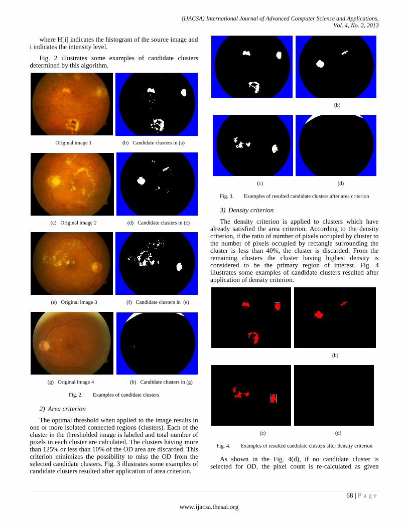
(IJACSA) International Journal of Advanced Computer Science and Applications,
Vol. 4, No. 2, 2013
68 | P a g e
www.ijacsa.thesai.org
where H[i] indicates the histogram of the source image and i indicates the intensity level.
Fig. 2 illustrates some examples of candidate clusters determined by this algorithm.
Original image 1 (b) Candidate clusters in (a)
(c) Original image 2 (d) Candidate clusters in (c)
(e) Original image 3 (f) Candidate clusters in (e)
(g) Original image 4 (h) Candidate clusters in (g)
Fig. 2. Examples of candidate clusters
2) Area criterion
The optimal threshold when applied to the image results in one or more isolated connected regions (clusters). Each of the cluster in the thresholded image is labeled and total number of pixels in each cluster are calculated. The clusters having more than 125% or less than 10% of the OD area are discarded. This criterion minimizes the possibility to miss the OD from the selected candidate clusters. Fig. 3 illustrates some examples of candidate clusters resulted after application of area criterion.
(b)
(c) (d)
Fig. 3. Examples of resulted candidate clusters after area criterion
3) Density criterion
The density criterion is applied to clusters which have already satisfied the area criterion. According to the density criterion, if the ratio of number of pixels occupied by cluster to the number of pixels occupied by rectangle surrounding the cluster is less than 40%, the cluster is discarded. From the remaining clusters the cluster having highest density is considered to be the primary region of interest. Fig. 4 illustrates some examples of candidate clusters resulted after application of density criterion.
(b)
(c) (d)
Fig. 4. Examples of resulted candidate clusters after density criterion
As shown in the Fig. 4(d), if no candidate cluster is selected for OD, the pixel count is re-calculated as given

(IJACSA) International Journal of Advanced Computer Science and Applications,
Vol. 4, No. 2, 2013
69 | P a g e
www.ijacsa.thesai.org
below to reduce the threshold and entire process is repeated with this threshold.
(2)
Fig. 5 shows the result of candidate cluster resulted after application of reduced threshold algorithm.
Fig. 5. Result of reduced threshold algorithm
B. Localization of Centre of an OD
The cluster which occupies OD is located in algorithm
discussed above. The centroid of this cluster is determined
using calculus method. A search area is defined around this
centroid such that this centroid is center of the search window.
This search window is a square window with side equal to
twice of OD diameter (ODD).
A circular window called an oculus of radius ODD/2 is
moved across the search area. This is illustrated in Fig. 6. The
maximum intensity oculus is identified using procedure given
here.
Fig. 6. Circular window for OD detection
Each pixel within the square window of side equal to ODD is tested for its distance (d) from the centre of the window. As shown in Fig. 7, if the distance, d is less than or equal to the radius r (radius of the oculus), it is considered as inside pixel. The total intensity of the oculus is calculated by adding squares of intensities of all inside pixels. It can be expressed mathematically as,
∑ ∑
where √( - ) (
- )
and
is the centre of an oculus
The centre of maximum intensity oculus is marked as a centre of OD.
Fig. 7. Pixel inside circle test
There may be more than one window of same maximum
total intensity. In this case, the central window amongst the
same intensity windows is the resultant window and the centre
of the resultant window is considered as a centre of an OD.
Fig. 8 illustrates some examples of centre of OD.
(b)
(c) (d)
Fig. 8. Examples of centre of OD
III. RESULTS
TABLE II RESULTS OF PROPOSED OD LOCALIZATION METHOD
Test database Images OD Detected % Accuracy
Diaretdb0 130 126 96.92
Diaretdb0 89 86 96.62
Drive 40 40 100
Walimbe Eye Clinic, Pune 34 34 100
Bhagali Clinic and
Nursing Home 160 160 100
Total 453 446 98.45
The outcome of OD localization is deemed true detection if obtained centre is within the OD area. Table II shows the accuracy of true OD detected retinal images.

(IJACSA) International Journal of Advanced Computer Science and Applications,
Vol. 4, No. 2, 2013
70 | P a g e
www.ijacsa.thesai.org
TABLE III COMPARISON OF RESULTS OBTAINED USING DIFFERENT METHODS
Test database Combined system Proposed method
Diretdb0 89.52% 77.56% 77.56% 95.29% 80.12% 96.79% 98.46%
Diaretdb1 88.99% 75.46% 75.46% 93.70% 76.41% 94.02% 96.62%
Drive 80.55% 97.22% 97.22% 98.61% 86.10% 100% 100%
Walimbe Eye Clinic, Pune - - - - - - 100%
Bhagali Clinic and Nursing Home
- - - - - - 100%
Total Average 87.95% 79.88% 76.12% 95.26% 79.78% 96.34% 98.45%
A. Comparison of results obtained using different methods
Rashid Jalal Qureshi et al. [28] discussed different OD detection algorithms and OD percentage detection rate in each case using standard databases. Table III summarizes the percentage accuracy achieved applying each algorithm discussed in this paper and proposed algorithm.
: Based on pyramidal decomposition [14]
: Based on edge detection [14]
: Based on feature vector and uniform sample grid
[19], [20]
: Based on entropy filter [15]
: Based on Hough transformation [18]
We can easily conclude observing Table III that proposed method gives better accuracy in localizing OD compared to other methods. Rashid Jalal Qureshi et al. [28] mentioned that performance of the methods listed in columns 2 through 6 of Table III is generally good, but each method has situations, where it fails. These methods fail on a difficult data set i.e., the diseased retinas with variable appearance of ODs in terms of intensity, colour, contour definition etc. The criteria used in the proposed algorithm are determined by considering abnormality of retinal images and hence provides better accuracy in localizing OD as shown in the last column of Table III.
IV. DISCUSSION AND CONCLUSION
An automated method has been presented which is able to locate an OD in retinal images. The results show that the system is able to locate the OD accurately in 98.45% of all tested cases. The percentage of successful detection of OD is increased using method presented in this paper.
The method of OD localization is tested on retinal images and qualitatively valuated by comparing the automatically segmented OD with manual ones detected by an experienced ophthalmologist. Original detection of OD leads towards the development of a fully automated retinal image analysis system to aid clinicians in detecting and diagnosing retinal diseases. Compared to the approaches by other researchers, our algorithm for OD detection has the advantage that it is applicable to all types of retinal images, healthy as well as abnormal, affected due to disease and/or acquisition process.
The work in this paper is carried out for control point detection which is an important step for registration of retinal images. As the OD and its centre are located accurately, macula and its centre can be detected accurately. OD, macula and vascular network are unique anatomical structures of retinal image. So centre of OD, centre of macula and bifurcation points of vascular network can be used as control points for registration of retinal images. The bifurcation points within retinal images which are to be registered can be co-related by checking their distances from centre of OD and centre of macula. The accurate registration of retinal images can be further used for retinal image change detection and super-resolution.
ACKNOWLEDGMENT
We are thankful to Dr. Tejaswini Walimbe, DO, DNB (OPHTH), FAEH, Consultant Eye Surgeon, Glaucoma and Medical Retina Specialist, Walimbe Eye Clinic and Dr. Meenakshi Bhagali, M.S., Eye Specialist, Bhagali Clinic and Nursing Home, Pune for providing retinal image database.
We are grateful to Dr. Deepa Mujumdar, Ophthalmologist, Bharati Hospital, Pune for her valuable guidance and suggestions.
REFERENCES
[1] Siddalingaswamy C , Gopalakrishna rabhu K , “Automatic localization and boundary detection of optic disc using implicit active contours”, Internation Journal of Computer Applications, vol. 1, no. 7, pp. 1-5, 2010.
[2] Michael D. Abramoff, Meindert Niemeijer, “The automatic detection of the optic disc location in retinal images using optic disc location regression”, Conf roc IEEE Eng Med Biol Soc , 1: pp 44 2- 4435, 2006.
[3] Jaspreet Kaur, Dr Sinha, “Automated localization of optic disc and macula from fundus images”, International Journal of Advanced Research in Computer Science and Software Engineering, vol. 2, Issue 4, pp. 242-249, April 2012.
[4] Healey PR, Mitchell P, Smith W, Wang JJ, “Relationship between cup-disc ratio and optic disc diameter”, the Blue Mountains Eye Study, Aust N Z J Ophthalmol.; 25 Suppl 1:S99-101, May 1997.
[5] The American Academy of Ophthalmology, The eye MD Association, San Francisco, CA 94120-7424.
[6] Gopal Datta Joshi, Jayanthi Sivaswamy, “Optic disc and cup boundary detection using regional information”, Arvind Eye Care System, Madurai, India.
[7] J Tang, S Mohr, YD Du and TS Kern, “Non-uniform distribution of lesions and biochemical abnormalities within the retina of diabetic humans”, Current Eye Res , vol.27, no.1, pp. 7-13, 2003.
[8] Mads Bo Christensen, Christian Bork Hardahl, Michael Munk Jakobsen,

(IJACSA) International Journal of Advanced Computer Science and Applications,
Vol. 4, No. 2, 2013
71 | P a g e
www.ijacsa.thesai.org
Toke Sonnenburg Ottesen and Sille Petersen, “Automatic algorithm for segmentation, registration and fusion of digital fundus retinal images from patients suffering from diabetic retinopathy”, Aalborg University, SEMCON, 21, Dec. 2007.
[9] R.J. Radke, Srinivas Andra, Omar Al-Kofahi, Badrinath Roysam, “Image change detection algorithms: A systematic survey”, IEEE Transactions on Image Processing, vol. 14, no. 3, March 2005.
[10] S. Sekhar, W. Al-Nuaimy and A K Nandi, “Automated localization of retinal optic disc using Hough transform”, pp 1577-1580, IEEE 2008.
[11] C. Sinthanayothin, J Boyce, Cook and T Williamson, “Automated localization of the optic disc, fovea and retinal blood vessels from digital color fundus images, Br J Ophthalmol, 83: pp. 902-910, Feb. 1999.
[12] Meindert Niemeijer, Michael D. Abramoff, Bram Van Ginneken, “Segmentation of the optic disc, macula and vascular arch in fundus photographs”, IEEE Transactions on medical Imaging, vol.26, no.1, pp. 116-127, January 2007.
[13] Siddalingaswamy C , Gopalakrishna rabhu K , “Automated detection of anatomical structures in retinal images”, 7th IEEE International Conference on computational intelligence and multi-media applications, vol. 3, pp. 164-168, 2007.
[14] M Lalonde, M Beaulieu and Langis Gagnon, “Fast and robust optic disc detection using pyramidal decomposition and Hausdorff-Based Template Matching”, vol. 20, No.11, pp. 1193-2001, Nov. 2001.
[15] Sopharak A., Thet New K., Aye Moe Y., N. Dailey M., Uyyanonvara B., “Automatic exudate detection with anaive bayes classifier”, International Conference on Embedded Systems and Intelligent Technology, Bangkok, Thiland, pp. 139-142,2008.
[16] N. Otsu, "A threshold selection method from gray-level histograms," IEEE Transactions on Systems. Man, and Cybernetics, vol. 9, pp 62-66, January 1979.
[17] A oover and M Goldbaum, “Locating the optic nerve in a retinal image using the fuzzy convergence of the blood vessels”, IEEE Trans Med. Image, vol. 22, no.8, pp. 951-958, Aug-2003.
[18] S Ravishankar, A Jain, A Mittal, “Automated feature extraction for early detection of diabetic retinopathy in fundus images”, IEEE Conference on Computer Vision and Pattern Recognition, pp. 210-217, 2009.
[19] M Niemeijer, M D Abramoff, B Van Ginneken, “ Fast detection of the optic disc and fovea in color fundus photographs, Medical Image Analysis, 13, pp. 859-870, 2009.
[20] M. Niemeijer, J.J. Staal, B. Van Ginneken, M. Loog, M.D. Abramoff, “Comparative study of retinal vessel segmentation methods on a new publically available database”, SPIE Medical Imaging, 5370, pp. 648-656, 2004.
[21] M. Foracchia, E. Grison and A. Ruggeri, “Detection of optic disk in retinal images by means of geometrical model of vessel structure”, IEEE Trans. Med. Image, vol. 23, no.10, pp. 1189-1195,Oct 2004.
[22] Li and O Chutatape, “Automated feature extraction in color retinal images by a model based approach”, IEEE Trans Biomed Eng , vol. 51, no.2, pp. 246-254, Feb 2004.
[23] Huajun Ying, Ming Zhang and Jyh-Charn Liu, “Fractal-based automatic localization and segmentation of optic disc in retinal images”, IEEE Proc. of the 29th Annual International conference of the IEEE EMBS, France.
[24] Geoff Dougherty, “Medical image processing techniques and applications”, Springer.
[25] Deepali A. Godse and Dr. Dattatraya S. Bormane, “Automated localization of centre of optic disc and centre of macula in retinal images”, CiiT International Journal of Biometrics and Bioinformatics, vol. 4, no. 16, pp. 896- 901, Nov 2012.
[26] Bob Zhang and Fakhry Karray, “Optic disc detection by multi-scale Gaussian filtering and with scale production and vessels directional match filter”, Medical Biometrics: Second International Conference, ICMB 2010, Hong Kong, pp. 173-180, 2010.
[27] Seng Soon Lee, Mandava Rajeswari and Dhanesh Ramachandram, “ reliminary and Multi Features Localisation of Optic Disc in Colour Fundus Images”, National Computer Science ostgraduate Colloquium, Malaysia, 2005
[28] Rashid Jalal Qureshi, Laszlo Kovacs, Balazs Harangi, Brigitta Nagy, Tunde eto, Andras ajdu, “Combining algorithms for automatic detection of optic disc and macula in fundus images”, Elsevier, Computer Vision and Image Understanding, vol. 116, Issue 1, pp. 138-146, Jan 2012.
AUTHORS PROFILE
Deepali A. Godse was born in Pune (M.S.) in India on March 20, 1971. She is a PhD student in Computer Engineering, Bharati Vidyapeeth Deemed University, Pune. She received her B.E. in Industrial Electronics from Pune University in 1992. She completed her M.E. in Computer Engineering in 2003. Her research interests include image processing, computer graphics and multimedia.
She is currently working as a Head of Information Technology Department in Bharati Vidyapeeth’s College of Engineering for Women affiliated to Pune University. She has 19 years experience in teaching as a Lecturer, Assistant Professor, Associate Professor and Head of Department. She has written books in the field of Computer graphics, Computer Organization and Digital Electronics. She is a life member of ISTE.
Dr. D. S. Bormane completed B.E. Electronics from Marathwada University, Aurangabad in 1987. He received his M.E. in Electronics from Shivaji University, Kolhapur. He is awarded PhD in Computer Engineering from Ramanand Tirth University, Nanded. His research interests include Digital Signal Processing, Communication Engineering and Image & Speech Processing. He has 22 years of experience in
teaching as a Lecturer, Assistant Professor, Professor and Head of Department. He is currently working as a Principal in Rajarshi Shahu College of Engineering Pune (M.S.) and as a Chairman, Board of Studies at University of Pune. He has 60 papers in National and International Conferences and Journals to his credit. He is a life member of ISTE and ISCEE, Fellow Member of IETE and senior member of IACS.

(IJACSA) International Journal of Advanced Computer Science and Applications, Vol. 4, No. 2, 2013
72 | P a g e www.ijacsa.thesai.org
Neural Network Solution For Service Level
Agreement
Sarmad Al-Aloussi,Researcher
AABFS Amman-Jordan
Abstract— Service Oriented Computing is playing an
important role in sharing the industry and the way business is
conducted and services are delivered and managed. This
paradigm is expected to have major impact on service economy;
the service sector includes health services, financial services,
government services, etc. This involves significant interaction
between clients and service providers[1]. This paper is pointed in
addressing the problem of enabling Service Level Agreement
(SLA) oriented resources allocation in data centers to satisfy
competing applications demand for computing services. A QoS
report designed to compare performance variables to QoS
parameters and indicate when a threshold has been crossed. This
paper was suggested a methodology which helps in SLA
evaluation and comparison. The methodology was found on the
adoption of policies both for service behavior and SLA
description and on the definition of a metric function for
evaluation and comparison of policies. In addition, this paper
contributes a new philosophy to evaluate the agreements between
user and service provider by monitoring the measurable and
immeasurable qualities to extract the decision by using artificial neural networks (ANN).
Keywords— Service Oriented Architecture; Service Level
Agreements; QoS; and Neural Network.
I. INTRODUCTION
Service-level agreements are, by their nature, "output" based the result of the service as received by the User is the subject of the "agreement." The (expert) service provider can demonstrate their value by organizing themselves with ingenuity, capability, and knowledge to deliver the service required, perhaps in an innovative way. Organizations can also specify the way the service is to be delivered, through a specification (a service-level specification) and using subordinate "objectives" other than those related to the level of service.
This type of agreement is known as an "input" SLA. This latter type of requirement is becoming obsolete as organizations become more demanding and shift the delivery methodology risk on to the service provider [2].
The development of SOA, organization is able to compose complex applications from distributed services supported by third party providers. Service providers and User negotiation based service level agreement (SLA) to determine different activities (security, cost, penalty,…..etc) on the achieved performance level. The service providers need to manage their resources to maximize the profits [3].
To maximize the SLA revenues in shared data environments, it can be formulated as the dual problem of minimizing the response time and maximizing throughput. That proposal considers the problem of hosting multiple web sites.
In service oriented architecture the problem is guaranteeing the "quality" of services to final users, in terms of functional and non-functional requisites like performance (measurable qualities) or security (immeasurable qualities). In general, a service provider is able to guarantee a predefined service level and a certain security level (supposing it can be measured).
II. THE EVALUATION METHODOLOGY
Having formalized and expressed SLAs by a policy form, in this paper we need an evaluation methodology to compare them and decide to request a service from the server or changing the server to provide the request service [1].
The proposed methodology is based on a Reference Evaluation Model (REM) to evaluate and compare different security policies and behavior policies, quantifying their security level by either value 0 (represent not existing sub provision for each immeasurable provisions) or value 1 (represent existing provisions) . The model will define how to express in a rigorous way the security policy (formalization), how to evaluate a formalized policy, and what is its service level. In particular the REM is made of three different components:
A. The policy formalization
The formalization policy is a way to express all the qualities parameters for SLA in a rigorous technique to define either the qualities exist or not, or for measurable qualities with defined values.
B. The evaluation technique
We propose REM includes the definition of a technique to compare and evaluate the policies; we have called this component the REM Evaluation technique. Different evaluation techniques represent and characterize the measurable and immeasurable level associated to a policy in different ways, for example with a numerical value, a fuzzy number [4][5] or a verbal judgment representing its security level.
C. The reference levels
The last component of the REM is the set of SLAs levels that could be used as a reference scale for the numerical

(IJACSA) International Journal of Advanced Computer Science and Applications, Vol. 4, No. 2, 2013
73 | P a g e www.ijacsa.thesai.org
evaluation of SLA. When references are not available, the REM could be used for direct comparison among two or more policies.
III. SLA STRUCTURE
The service providers and the users often negotiate by the qualities to base the Service Level Agreements (SLAs) by behavior aspects based on the achieved performance levels. The service provider needs to manage its resource to maximize its profits. The optimization approaches are commonly used to provide the service load balancing and to obtain the optimal classifications for quality of service levels. By the above are also used as guidelines and for realizing high level trends. One main issue of these systems is the high variability of the workload according to values of measurable and immeasurable qualities [6].
By such model, the service can dynamically be allocated among the service providers depending on the service availability. Fig. 1 shows the architecture of SLA model implementing an autonomic infrastructure. Service providers are allocated and de-allocated on demand on servers. The server level agreement model can monitor the qualities and by predictor phase, it can allocate the server to provide the service.
Fig. 1. SLA Architecture Of Data Center
The main components of the SLA model [7] include a monitor, a decision maker and a server allocator. The system monitors the qualities and performance matrices of each form, identifies requested classes and estimates requested service time. The decision maker can evaluate the system performance from the trace values. The allocator chooses the best system configuration [8].
IV. SERVICE LEVEL AGREEMENT CATEGORIES
SLA was defined as a contract between the users and service providers, and then the contract has many rules. Their rules can be established by different ways either manually or automatically. It can be either static, which means the system will be fixed without any modifications or upgrading all the service providing or the contract rules be dynamic and changing all the time, the SLA can be classified according to the inputs values collection way and the SLA, the inputs can define as qualities can classify as below:
D. Measurable Qualities
There are many measurable qualities; it can measure for each user, the definitions of the measurable qualities are shown below:
Accuracy is concerned with the error rate of the service. It is possible to specify the average number of errors over a given time period.
Availability is concerned with the mean time to failure for services, and the SLAs typically describe the consequences associated with these failures. Availability is typically measured by the probability that the system will be operational when needed. It is possible to specify the system’s response when a failure occurs − the time it takes to recognize a malfunction.
Capacity is the number of concurrent requests that can be handled by the service in a given time period. It is possible to specify the maximum number of concurrent requests that can be handled by a service in a set block of time.
Cost is concerned with the cost of each service request. It is possible to specify the cost per request the cost based on the size of the data − cost differences related to peak usage times.
Latency is concerned with the maximum amount of time between the arrival of a request and the completion of that request.
Provisioning-related time (e.g., the time it takes for a new client’s account to become operational).
Reliable messaging is concerned with the guarantee of message delivery. It is possible to specify how message delivery is guaranteed (e.g., exactly once, at most once) whether the service supports delivering messages in the proper order.
Scalability is concerned with the ability of the service to increase the number of successful operations completed over a given time period. It is possible to specify the maximum number of such operations.
E. Immeasurable Qualities
There are three main immeasurable qualities that can be defined by main provision and sub provision for each quality, in the following we define the immeasurable qualities:
Interoperability is concerned with the ability of a collection of communicating entities to share specific information and operate on it according to an agreed upon operational semantics. It is possible to specify the standards supported by the service and to verify them at runtime. Significant challenges still need to be overcome to achieve semantic interoperability at runtime.
Modifiability is concerned with how often a service is likely to change. It is possible to specify how often the service’s Interface changes or Implementation changes.
Security is concerned with the system’s ability to resist unauthorized usage, while providing legitimate users with access to the service. Security is also characterized as a system providing non-repudiation, confidentiality, integrity, assurance, and auditing. It is possible to specify the methods for
authenticating services or users
encrypting the data

(IJACSA) International Journal of Advanced Computer Science and Applications, Vol. 4, No. 2, 2013
74 | P a g e www.ijacsa.thesai.org
F. Policy Formalization
It will depend on measurable and immeasurable qualities which are mentioned is previous section. It will form two unsymmetrical matrices; first one describes the immeasurable qualities for n users, as well as the output matrix describe the decided output. The second matrix represent the measurable matrix, each row represent the provision and the state of each column represent if the sub provision exist or not, the output matrix represent the trace value of measurable matrix. Trace is the value of each matrix by maximum value of matrices.
Measurable Matrix
Output user = [Trace, Request, Delay Request, Wait, Change Provider, New User]
Immeasurable Matrix
Output= [Trace, Activated output]
V. MATHEMATICAL EVALUATION TECHNIQUE
To adopt WS-policy framework and to express policies for security-SLA the framework is structured as a hierarchical tree to express all sub provisions. We have started the formalization by considering the set of items proposed by [9].
Given the qualities matrices for measurable matrices as shown in section III, the evaluation process takes into account just the provisions of the policy which represent the sub provisions status for immeasurable qualities and the values of measurable qualities for each user.
With the formalization, each provision is represented by a real data type; the policy space "P" is defined as the vector product of all n provisions Ki
i.e. P = K1 x K2 x…... x Kn.
The policy space "P" has been transformed into an homogeneous one, denoted "PS" thanks to a family of threshold functions (F-functions) which allow us to associate a Local Security Level (LSL for short) to each provision. "PS" is represented by a n x 4 matrix whose n rows represent the single provisions Ki and 4 is the chosen number of LSLs admissible for each provision. For example, if the LSL associated to a provision is 3, the vector corresponding to its row in the matrix is: (1, 1, 1, 0).
The distance criteria for the definition of the metric space is the Euclidean distance among matrices, defined as:
d(A, B) =
Where: σ (A - B, A - B) =T r ( ( A - B ) ( A - B) T)
The T r ( ( A - B ) ( A - B) T) represents the trace value to know the invariant between any base and other qualities matrix. Below we show a sample of immeasurable matrix, the main provision was defined and sub-provisions were represented by existing status:
Provision Name 1 1 0 1
Digital Certificate Management 0 1 0 1
Policy applicability - - - -
Time between certificate request and issuance
- - - -
Notification of certificate issuance and revocation
- - - -
Local Registration Authorities (LRAs) - - - -
Repositories - - - -
SLA-P, SLA-X, and SLA-Y are supposed as different immeasurable matrices with the same provisions and different values of sub-provisions. SLA-X and SLA-Y; are supposed globally stronger than SLA-P since they have a lot of sub-provisions for each provision. Each policy in the example has just 10 provisions; this is just a simplification which does not affect the validity of the method.
Example 1: SLA-X is a policy that appears stronger than SLA-P, just looking at the levels of the single provisions; we first calculate the trace:
Tr((SLAX-SLAP)(SLAX-SLAP)T) = 6
Where: d(X, P) = d(X, P) is the distance among matrices
Where: σ (X - P, X - P) =T r ( ( X - P ) ( X - P) T)

(IJACSA) International Journal of Advanced Computer Science and Applications, Vol. 4, No. 2, 2013
75 | P a g e www.ijacsa.thesai.org
The distance between SLA-X and SLA-P is: d-2.45.That mirrors the fact that SLA-X is just a little stronger than SLA-P.
Example 2: SLA-Y is a policy that appears stronger than SLA-X and much stronger than policy SLA-P, while SLA-P is the same as that of the example 1; the trace is:
Tr((Y-P)(Y-P)T) = 19
The distance between SLA-Y and SLA-P is: d-4.36 .This result mirrors the evident difference between the two cases. These examples show how it is very simple to evaluate the distance between policies, once they have been represented as a matrix. The distance will be adopted to define the metric function.
VI. PROPOSED ANNSLA MODEL
In this section we will propose an artificial service level agreement model to be the base for qualities testing and comparing. The main idea of this model is to be able to decide if the services can supply by service provider or not depending on the value of the activated outputs. Because of this model was proposed depending on artificial neural network then the ANN needs to train by input and output data sets to be able to extract the outputs for other input data sets. Fig. 2 shows the general concepts of Neural Network Service Level Agreement in SOA.
Fig. 2. ANN Service Level Agreement
The training input and output data sets will be represented according to the mathematical models. The input sets of ANN represent the measurable and immeasurable matrices which are used in mathematical model while the output sets represents the extracted outputs for the traces and the activated outputs from the mathematical calculations model. To build the artificial service level agreement model, there are two phases should execute to extract the correct decision. In the following we will discuss the phases of ANNSLA model:
ANN Training phase: in this phase, the extracted data sets (formalized inputs and calculated outputs) from the SLA mathematical model will apply to ANN to train it. Section V.B will explain the simulation method of training phase for ANN. The training phase should apply for both part of ANNSLA model, measurable and immeasurable qualities and trained according for input/output matrices. It’s very important to notice when any changing happen for the
contact between the user and the service provider (i.e. the contract rules) will lead to change the SLA measurable and immeasurable qualities, the trace value will change directly as well as the outputs matrix may change. All those lead to reconfigure the ANN architecture and retrain it according to the new values of inputs/ outputs matrix values. From all the above we can consider the ANNSLA model is dynamic not static model and can be suitable for future extending, there are no limitations of users number or qualities number. The accuracy of output values ANNSLA depending on data sets and the training procedures. Fig. 3 shows the general ANNSLA model in the training phase. The ANN will train in 1st set of qualities and outputs. There are two training model one of them for measurable qualities ANN model and second one for immeasurable qualities ANN model, it can train separately because of the first one represent a logical model and the second one represent the behavior model between the user and service provider. The architecture of the ANN is very easy to build, for this reason we propose only one activated output for immeasurable formalization while there are more than one output for measurable formalization to mention that the ANN architecture may not be fixed and modifiable depending on the requirements and the rules in the contract between the user and the service providers [10].
Operation Phase: when the ANN trained correctly according to inputs/outputs data sets, it will be ready to use it as decision maker for different input sets to extract the trace value and activated output or outputs for either immeasurable qualities or measurable qualities. To evaluate the output values, it can compare the extracted outputs with calculated outputs from mathematical model, the evaluation will explain in details in 8. Fig. 4 shows the general trained ANNSLA model. By this model can extract the outputs for different inputs by applying it to trained ANN. As we mentioned in the training phase, the trained ANN be as a decision maker to extract the outputs. When applying the immeasurable or measurable matrices to trained ANN it can extract the trace and activated output or outputs. The operation phase can be fixed for long period except if there is any rules in the SLA contact will be changed, it will lead to go again to training phase to modify the ANN architecture according to new measurable and immeasurable qualities.
From the entire above if there is any modifications in input qualities or/and the active outputs will lead to reconfigure the ANN model and retrain it according to new values of the input qualities and outputs. The evaluation method will not change when the architecture of the ANN model changed because all the time we will calculate the difference between the calculated values and extracted outputs.
The process of ANNSLA will show in 6.1.The validation of the activated outputs and the reasons of defining activated outputs for both formalizations (measurable and immeasurable) will discuss in section VI. There are many limitations in ANNSLA operation phase, one of important operation phase limitation that can’t test this model online because of the

(IJACSA) International Journal of Advanced Computer Science and Applications, Vol. 4, No. 2, 2013
76 | P a g e www.ijacsa.thesai.org
servers’ operation restrictions and no experiments lab to evaluate this model practically.
Fig. 3. ANNSLA training phase
Fig. 4. ANNSLA operating phase
G. ANNSLA Process
The ANNSLA process for two parts of the model, the first part represents measurable part with their extracted and target outputs and the second part represents immeasurable part with their extracted and target outputs, each phase has many steps will discuss in the following:
The training phase process consist the following steps:
Define the ANN architecture, number of hidden layers, number of input nodes in input layer, and number of output nodes in output layer. The process initiated sets of measurable and immeasurable qualities as inputs for ANNSLA model. Formalize the inputs into measurable and immeasurable input matrices to apply it to ANN. The target outputs will define for the both measurable and immeasurable ANN. The training process will initiate to train the ANNs. The training process will continue till the extracted outputs reached to target outputs. When the error percent reached to acceptable value, the training process will stop and the ANN will consider trained.
The operation phase process consist the following steps:
The process initiated a set of measurable and immeasurable qualities as input for trained ANNSLA model. Formalize the input into measurable and immeasurable input matrices to apply it to ANN
Apply formalize measurable and immeasurable matrices to trained ANN. The trained ANN will run and stop when the ANN produces the outputs. The extracted outputs represent the outputs for both measurable and immeasurable parts.
From all the above, it consider that the ANNSLA model can modify the ANN architecture by changing the number of
inputs and/or the number of outputs, this will lead to repeat the ANNSLA process in both training and operation phases.
H. ANNSLA Simulation
The ANNSLA will build using ANN architecture, it’s very important to select the architecture by defining the number of layers (hidden layers), the number of input nodes in input layer, the output nodes in output layer, the values of inputs, the values of target outputs, and the error value. These architectures can be done by using MATHLAB package version 7.7.0. The simulation procedure will introduce the ANN architecture, the experimental data sets, training process and the running process of ANNSLA by MATHLAB model in next sections.
I. ANNSLA MATLAB Architecture
As we mentioned in the above sections the ANNSLA model architecture has two part one for measurable qualities and the second one for immeasurable qualities, this means there are two ANN.
The measurable ANN part consists the following: Input layer with consist 6 input neurons for each user. The inputs represent the measurable qualities which are the accuracy, availability, capacity, cost, related time, and scalability. The values of these inputs represent numeric value all the time ≤ 1 [11].One or two hidden layers to test the effect of increasing the hidden layers upon the performance of the architecture. The output layer consists either one neuron if we want to calculate trace of measurable matrix or five neurons represent the outputs (Request, Wait, Change, New Service, and Timer) for measurable part in ANNSLA model.
The immeasurable ANN part consists the following: Input layer with consist 40 input neurons for each user. The inputs represent the immeasurable qualities represent interoperability, modifiability, and security. All the values of these inputs will be represented either 1 (exist) or 0 (not exist).One or two hidden layers to test the effect of increasing the hidden layers upon the performance of the architecture. The output layer consist either one neuron if we want to calculate trace of immeasurable matrix or one neuron represents the activated output for immeasurable part in ANNSLA model[12].
The above ANN architecture can modify according to the measurable and immeasurable requirements in ANNSLA model.
VII. DATA COLLECTION AND EXPERIMENTAL RESULTS
In our test scenario, we used a sample of different matrices for measurable and immeasurable qualities; there are two experimental results as following: The trace and the distance for each matrix will calculate by mathematical model. The values of the mathematical traces will apply to train the ANNSLA. The ANN will train for input matrices and for target outputs. The trained ANN can run to extract the outputs when applying any new immeasurable or measurable matrices. Below we will mention the training input data sets and the target output which represent the trace vales and the activated output/outputs by applying it to trained ANN for both measurable and immeasurable parts for ANNSLA model. In next section, we will run the trained measurable and

(IJACSA) International Journal of Advanced Computer Science and Applications, Vol. 4, No. 2, 2013
77 | P a g e www.ijacsa.thesai.org
immeasurable ANN to extract the actual outputs for any data sets.
J. Immeasurable Experimental Results:
To train the immeasurable ANN to extract the trace value and activated output for each immeasurable matrix, the training data sets with target outputs (trace and activated output) will apply and train ANN by MATHLAB. TABLE I mentions the data sets of the immeasurable matrices with calculated trace (by mathematical SLA model which is mentioned in section IV) and the activated output (proposed simulation values).
These matrices are used to train the immeasurable ANN, it used as inputs while the calculated traces and the activated outputs are used as target outputs of immeasurable ANN. The trace ANN is used to extract the trace value for any measurable or immeasurable matrices. The trace value represents the invariant with respect to a change of basis. It means choosing a base matrix then by calculating distance between the choosing one with any other selected matrix. It easy to calculate the trace mathematically, and by applying the qualities to trained trace ANN (shows in Fig. 5) can extract the trace value, in the next section will show the comparison between the two values.
Fig. 5. Trace ANN Architecture
The trace value will extract by individual ANN represented in Fig. 5, the trace ANN should train by applying the immeasurable matrices as inputs and the target output is represented by calculated trace values. To train the ANN immeasurable ANN, the immeasurable qualities will apply with their target activated output; the number of training matrices is about 17. TABLE I shows the training set for immeasurable ANN. Fig. 6 shows the general ANN architecture for immeasurable ANN part, the number of input neurons is 40 neurons for each immeasurable matrix in input layer, and only one neuron in output layer represents the target output.
The values of the target output are representing the activated output values. To train the immeasurable ANN, we will apply 17 immeasurable matrices (M1, M2,……….Mn) with their proposed activated outputs. It represents 10 provisions with 4 sub-provisions for each provision; the provision represents some of security level tree structure, Interoperability, and Modifiability with their sub-provision. After training the immeasurable ANN, it will be ready to run and extract the activated output for any immeasurable matrix. Feed forward network architecture with back propagation momentum training algorithm was used. The back propagation algorithm was considered since it is the most successful algorithm for the design of multilayer feed forward networks
TABLE I. TRAINED IMMEASURABLE DATA SETS FOR THE TARGET
TRACE VALUE
Fig. 6. Immeasurable ANN Architecture
K. Measurable Experimental Results:
The measurable qualities can be represented by the measurable matrices as input and the target outputs (representing the values Accuracy, Availability, Capacity, Cost, Related Time, and Scalability) for each user, it already defined previously.
To train the measurable ANN part in ANNSLA, we will apply the measurable matrices as input data sets for the ANN and the activated outputs (Request, Delay Request, Wait, Change Provider, and New Customer) and trace as a target outputs for ANN. The values of simulation inputs are represented analogy; it’s all the time ≤1. The activated outputs are represented logically either 0 or 1. TABLE II shows the proposed activated outputs for each measurable matrix with calculated trace by mathematical model. These input data sets with proposed activated outputs and calculated trace will apply to train the measurable ANN part in ANNSLA.
Matrix No. Calculated Trace
Proposed Activated
Output
M1 3.581 0.5
M2 3.771 0.7
M3 4.123 0.6
M4 3.5541 0.9
M5 4.321 0.6
M6 3.5487 0.8
M7 4.242 0.65
M8 5.1832 0.75
M9 3.6111 0.8
M10 4.0231 0.5
M11 4.1101 0.7
M12 4.3465 0.85
M13 4.5732 0.7
M14 4.1021 0.55
M15 4.0231 0.65
M16 3.945 0.7
M17 4.1001 0.5

(IJACSA) International Journal of Advanced Computer Science and Applications, Vol. 4, No. 2, 2013
78 | P a g e www.ijacsa.thesai.org
TABLE II. TRAINED MEASURABLE DATA SETS FOR PROPOSED
ACTIVATED OUTPUTS AND TARGET TRACE VALUE
Matrix No. Activated Output
Calculated Trace
MM1 1,1,0,1,0 0
MM2 1,1,0,0,0 7.2621
MM3 1,0,1,1,0 8.3946
MM4 1,1,0,1,0 7.4403
MM5 1,1,0,1,0 6.6554
MM6 1,1,1,1,0 6.8806
MM7 1,0,1,1,0 6.5035
MM8 1,1,0,1,1 5.6391
MM9 1,1,1,1,0 7.1493
MM10 1,0,1,1,0 9.0777
MM11 1,1,0,1,1 5.6391
TMM1 1,0,1,1,0 6.5035
TMM2 1,1,0,1,1 5.6391
TMM3 1,1,1,1,0 7.1493
Fig 7. shows the general measurable ANN part for ANNSLA model, it represents the input, hidden, and output layers. To train the measurable ANN can be done by applying 12 inputs/outputs measurable qualities/ target outputs.
Fig. 7. Measurable ANN Architecture
VIII. SIMULATION RESULT DISCUSSION
After the trace, measurable and immeasurable ANNs in ANNSLA are trained, and then it can be operated as a decision maker. The scenario to run the trace and the immeasurable ANN, we apply 20 immeasurable matrices with by trace ANN, it can extract the trace value for each measurable matrix by ANN is shown in Fig. 5. The immeasurable ANN extracts the activated output for each matrix (ANN is shown in Fig. 6). In TABLE III the set of immeasurable tested matrices are shown, it shows the calculated trace and proposed activated output for each tested immeasurable matrices to compare the calculated
trace with extracted output from trace ANN and the proposed activated output with extracted activated output from immeasurable ANN.
The scenario to run the trace and the measurable ANN, we apply 3 measurable matrices with its activated outputs. By trace ANN and measurable ANN can extract the trace and the activated outputs for each matrix. TABLE IV shows the set of measurable tested matrices, the calculated trace, proposed activated output for each tested measurable matrices, and extracted activated outputs.
IX. RESULTS EVALUATION
From TABLEs III and IV, we can conclude that the error value between the calculated activated output and ANN activated output is about +/- 0.04 and the error between the calculated trace and extracted ANN trace is between 0.1141 and -0.0088 for both measurable and immeasurable ANN running, this means that ANNSLA can specify the SLA requirements specially the value of trace for measurable and immeasurable matrices. From the extracted trace value, by ANNSLA can decide the suitable SLA between the user and service providers. The activated outputs/output for measurable/immeasurable ANN can justify the SLA work flow.
From all the above, it can consider the ANN SLA can work properly as policy selector and as a decision maker between users and service providers. The figures below mention charts represent different comparison between the values which are extracted from ANNSLA and other calculated or supposed values. Fig. 8 shows the chart for calculated and ANN trace for different immeasurable qualities matrices, it shows the extracted values are very close to calculated values, the error as mentioned in above not more +/- 0.12. Fig. 9 shows the chart for activated and ANN output for immeasurable ANN part, the error between two values is between +/-0.04.
For measurable ANN part in ANNSLA model, Fig. 10 shows the chart for calculated trace and ANN trace for different measurable qualities matrices set.
From above, the ANNSLA model can use as a decision maker to extract the best policy and the suitable activated output/outputs value; it means, the ANNSLA can define the roles of the contract between the users and service providers.
The model can modify easily by reconstruct the ANN architecture to be suitable for the approximate number of the users and providers. It can very secure if each user has his key to be part of the immeasurable input qualities then the model can train to accept or refuse the user in other hand the model can accept or refuse the key for the provider.
The error value of the extracted outputs of the model was very small according to the testing sets; it’s very simple to modify the model. The ANN can be extended simply and the training rules are very efficient and know for different users.

(IJACSA) International Journal of Advanced Computer Science and Applications, Vol. 4, No. 2, 2013
79 | P a g e www.ijacsa.thesai.org
TABLE III. TESTING IMMEASURABLE MATRICES SETS
TABLE IV. TESTING MEASURABLE MATRICES SETS
Fig. 8. Calculated and ANN Trace Chart for immeasurable matrices
Fig. 9. Activated and ANN Output Chart for immeasurable matrices
Fig. 10. Calculated and Trace Chart for measurable matrices
The ANN takes the decision according to how the user train it and what the data types give to it, then the main important should manage carefully from the beginning before constructing the model is as the following:
Number of users.
Number of providers.
Define certain policy formalization for the qualities.
The main immeasurable and immeasurable qualities (it’s very important to define the security level for each user and providers).The architecture of trace, measurable, and immeasurable ANN. The presented approach aims to use the neural network as the intelligent part of service level agreement model. The global architecture will permit the provider to provide a new type methodology of providing a service by checking the system completely with all other users and service providers. This will help to reduce the cost while preserving the required QoS. The ANNSLA can provide monitoring of traffic for service request by service waiting or service reallocation to other service provider. Then the deployed architecture will be evaluated with respect to the mathematical model
X. CONCLUSION
In this research we have introduced a theoretical methodology to evaluate Service Level Agreement in SOA. The methodology is based on two fundamental features; the first one is the SLA formalization through the use of standard policy while the second one is the formalization of "qualifiable service levels" against which we could measure the SLA.
In particular, we have adopted a Reference Evaluation Model, developed for different methodology, to evaluate and compare different policies and quantifying their levels. The application of the methodology in different samples of measurable and immeasurable qualities and we adopted it in the integration of mathematical model and artificial model to guarantee the same perceived service level to the end-user. SLAs have been applied in service organizations in general, including IT organizations, to formalize the level of service between a service provider and service user. While SLAs are well understood in these domains, they are less understood for services in the SOA context.

(IJACSA) International Journal of Advanced Computer Science and Applications, Vol. 4, No. 2, 2013
80 | P a g e www.ijacsa.thesai.org
SOA enables the integration of automated services from multiple organizations. External providers may offer services that were not initially implemented to meet the quality attribute requirements of the service consumer organization. Defining an SLA and establishing SLA management mechanisms are important factors when clarifying the quality requirements for achieving the business and mission goals of SOA systems.
Standardized SLAs are going to be an important element for organizations moving to automation, SLA systems characterized by the dynamic discovery, composition, and invocation of services based on QoS and other contextual information.
There are efforts to standardize the SLAs for web services; it’s an effort to make SLAs machine adaptable. However, there is no established standard for SLA specification
REFERENCES
[1] AberdeenGroup "Enterprise Service Bus and SOA Middleware", Boston, AberdeenGroup Massachusetts, 2006.
[2] K.Alexander .and L. Heiko "The WSLA Framework: Specifying and
Monitoring Service Level Agreements for Web Services", Journal of Network and Systems Management,11(1), pp. 57-81,2003
[3] T. Luo and L. Meng, "SLA foundation template library: reusable-
component repository for SLA", Communication Technology Proceedings, ICCT 2003. International Conference on , 2 , ,pp. 1739 –
1743, 9-11 April, 2003.
[4] B. Wetzstein, D. Karastoyanova, and F. Leymann, "Towards
Management of SLA-Aware Business Processes Based on Key Performance Indicators", BPMDS'08, Institute of Architecture of
Application Systems, University of Stuttgart, Germany,Springer, June2008.
[5] Service Level Agreements in Service-Oriented Architecture Environments; http://www.slideshare.net/Zubin67/service-level-
agreements-in-serviceoriented-architecture
[6] M. Bishop "Developing Web Services" Proceedings 17th International Conference on Data Engineering, Los Alamitos CA : IEEE Computer
Society, pp. 477-481, 2003.
[7] C. Abrams and W. Roy "service-Oriented Architecture Overview and Guide to SOA Research", G00154463, Stamford: Gartner Research,
2008.
[8] K. Yuen, and H. Lau "A Distributed Fuzzy Qualitative Evaluation System", IAT '06 Proceedings of the IEEE/WIC/ACM international
conference on Intelligent Agent Technology, Hong Kong : IEEE, pp. 560-563,2006.
[9] IBM "WS-policy specification Web Services Policy Framework", IBM,
BEA Systems, Microsoft, SAP AG, Sonic Software, VeriSign,2006.
[10] N.A. Abdullah "An Architecture for Augmenting the SCORM Run-Time Environment As a Service", Phd, Learning Societies Group,2006.
[11] V.Caola, A. Mazzeo, N. Mazzocc and M. Rak"A SLA evaluation methodology in Service Oriented Architectures" Advances in
Information security’, Advances in Information Security,23, pp.119-130,2006.
[12] L.Lu "A Novel SOA-Oriented Federate SLA Management
Architecture", IEEC '09. International Symposium on Information Engineering and Electronic Commerce , Ternopil: IEEEE, pp. 630-
634,2009.

(IJACSA) International Journal of Advanced Computer Science and Applications, Vol. 4, No. 2, 2013
81 | P a g e www.ijacsa.thesai.org
IRS for Computer Character Sequences Filtration: a
new software tool and algorithm to support the IRS at
tokenization process
Ahmad Al Badawi
Department of Computers and Information Technology
Taif University
Taif, Saudi Arabia
Qasem Abu Al-Haija
Department of Electrical Engineering
King Faisal University
Alhasa, Saudi Arabia
Abstract—Tokenization is the task of chopping it up into
pieces, called tokens, perhaps at the same time throwing away
certain characters, such as punctuation. A token is an instance of
token a sequence of characters in some particular document that
are grouped together as a useful semantic unit for processing.
New software tool and algorithm to support the IRS at
tokenization process are presented. Our proposed tool will filter
out the three computer character Sequences: IP-Addresses, Web
URLs, Date, and Email Addresses. Our tool will use the pattern
matching algorithms and filtration methods. After this process,
the IRS can start a new tokenization process on the new retrieved text which will be free of these sequences.
Keywords—Information Retrieval; Tokenization; pattern
matching; and Sequences Filtration.
I. INTRODUCTION
People use search engines for instance to locate and buy goods, to choose a vacation destination, to select a medical treatment or to find background information on candidates of an election. It's necessary to build a searching system being able to support users expressing their searching by natural language queries is very important and opens the researching direction with many potential [7].
As a human nature, people prefer to search for their information using their natural language especially with the existence of huge amount of information these days. Thus, a good Information Retrieval System is on demand.
Information retrieval (IR) [1, 2] is finding material (usually documents) of an unstructured nature (usually text) that satisfies an information need from within large collections (usually stored on computers). An information retrieval system (IRS) [2] is a software program that stores and manages information on documents. This system assists users in finding the information they need. Designing an efficient IRS which tries to touch the optimal results in retrieving the relevant documents of information, that design will face a lot of parameters which are to be taken into account such as precision and recall [1]. There is always a trade of between precision and recall.
At the core of IRS immerges the tokenization process which is considered a primary part in IRSs. Tokenization [1] is the task of chopping character sequence up into pieces, called
tokens. Sounds good; but it's not as simple as its definition, many times the tokenizer should not split on some locations of the document.
Computer technology [1] has introduced new types of character sequences that a tokenizer should probably tokenize as a single token, including email addresses ([email protected]), web URLs (http://www.kfu.edu.sa), numeric IP addresses (192.168.0.1), and Date (16/07/1982).
Several methods and approaches where proposed to provide these services, but researches showed that many measures should be addressed to ensure complete the retrieving process.
The problem addressed in this proposal will focus on designing an IRS for Computer Character Sequences Filtration. Computer technology has introduced new types of character sequences that a tokenizer should probably tokenize as a single token. As we see from figure 1, our proposed work will focus on filtering email addresses, web URLs, date, and numeric IP addresses.
Fig. 1. Problem Statement Figure.
In this paper, we propose a new software tool and algorithm to support the IRS at tokenization process. Our proposed tool will filter out the three computer character Sequences: IP-Addresses, web URLs, and email addresses. Our tool uses the pattern matching algorithms [4, 5] and filtration methods [2, 3].
After this process, the IRS can start a new tokenization process on the new retrieved text which will be free of these sequences.

(IJACSA) International Journal of Advanced Computer Science and Applications, Vol. 4, No. 2, 2013
82 | P a g e www.ijacsa.thesai.org
II. RELATED WORKS
In the last years many classical solutions tried to address the tokenization process issues such as Computer Character Sequences Filtration. The most commonly used solution is the filtering and matching schemes [1].
Christopher D. Manning, Prabhakar Raghavan, Hinrich Schutze in [1] established the infrastructure for how to build IRSs by explaining all concepts and objects for several IRSs. They explained in details the tokenization process which sets at the core of the IR-Systems. They also discussed many of the challenges in the tokenization process such as the Computer Character Sequences (IP-Addresses, email addresses, date and web URLs), the use of the apostrophe for possession and contractions, hyphenation, foreign phrases, compound nouns and others.
Christos Faloutsos, Douglas Oard in [2] surveyed the major techniques for IRS. They provided an overview of some traditional IRSs (full text scanning, inversion, signature files and clustering) and discussed attempts to include semantic information (natural language processing, latent semantic indexing and neural networks.
Nicholas J. Belkin and W. Bruce Croft in [3] designed information filtering systems for unstructured or semi structured data, as opposed to database applications, which use very structured data. These systems also dealt primarily with textual information, but they may also entail images, voice, video or other data types that are parts of multimedia information systems.
Information filtering systems also involve a large amount of data and streams of incoming data, whether broadcast from a remote source or sent directly by other sources. Filtering is based on descriptions of individual or group information preferences, or profiles that typically represent long-term interests. Filtering also implies removal of data from an incoming stream rather than finding data in the stream; users see only the data that is extracted [1, 3].
Mary Elaine Califf, Raymond J. Mooney, in [4] presented an algorithm RAPIER, which uses pairs of sample documents and filled templates to induce pattern-match rules that directly extract fillers for the slots in the template. RAPIER is a bottom-up learning algorithm that incorporates techniques from several inductive logic programming systems. They have implemented the algorithm in a system that allows patterns to have constraints on the words, part-of-speech tags, and semantic classes present in the filler and the surrounding text. They presented encouraging experimental results on two domains.
Richard M. Karp, Michael O. Rabin, in [5] proposed randomized algorithms to solve the following string-matching problem and some of its generalizations. Given a string X of length n (the pattern) and a string Y (the text), find the first occurrence of X as a consecutive block within Y. The algorithms represent strings of length n by much shorter strings called fingerprints, and achieve their efficiency by manipulating fingerprints instead of longer strings. The algorithms require a constant number of storage locations, and essentially run in real time. They are conceptually simple and
easy to implement. The method readily generalizes to higher-dimensional pattern-matching problems.
Sumalatha Ramachandran Sujaya Paulraj Sharon Joseph Vetriselvi and Ramaraj in [8] showed that there is no guarantee for information correctness and lots of conflicting information is retrieved by the search engines and the quality of provided information also varies from low quality to high quality. The filtering of trustworthiness is based on 5 factors - Provenance, Authority, Age, Popularity, and Related Links.
All the previous methods have strong filtration pattern-matching for the IR-Systems. Our proposed work is to design a new software tool and algorithm to support the IRS at tokenization process for computer character sequences filtration.
III. MOTIVATIONS AND METHODOLOGY
The proposed research is motivated by many factors. First of all, the information retrieval which is a very important issue in real life applications as in banks, companies, hospitals, and at the personal level too. Second, previous studies showed that the tokenization process of IRS must leave some of the computer character sequences such as IP-Addresses, emails, web URLs, and date without any splitting operation; it should be treated as a single token. Our research will focus on the design and implementation of new software tool and algorithm to support the IRS at tokenization process. Another main reason to conduct this research is that IRSs are deemed world-wide hot research topic especially after the increasing demand on information and its applications.
The proposed methodology throughout this research consists of the following steps:
1) The approach for proceeding in the proposed solution
started by studying several Information Retrieval System (IRSs)
[1, 2] concepts.
2) Understanding the important parameters in each IRS
that can be helpful for solving the proposed problem.
3) Studying several information filtering systems [2, 3]
which are designed for unstructured data.
4) Studying the matching algorithms [4, 5] trying to
make some contribution to such algorithm. This will support
the IR systems and will be helpful in solving our proposed
problem. The proposed solutions were implemented and verified
using Java programming language.
IV. SIMULATION ENVIRONMENT
Our proposed work is to design a new software tool to support IRSs at the tokenization process to filter out some computer character sequences. Our proposed solution is programmed and implemented in Java programming language.
Java [6]; A simple, object-oriented, network-savvy, interpreted, robust, secure, architecture neutral, portable, high-performance, multithreaded, dynamic programming language. The Java programming language and environment is designed to solve a number of problems in modern programming practice. Java started as a part of a larger project to develop

(IJACSA) International Journal of Advanced Computer Science and Applications, Vol. 4, No. 2, 2013
83 | P a g e www.ijacsa.thesai.org
advanced software for consumer electronics. These devices are small, reliable, portable, distributed, and real-time embedded systems. When we started the project we intended to use C++, but encountered a number of problems. Initially they were just compiler technology problems, but as time passed more problems emerged that were best avoided by changing the language.
V. TESTS AND RESULTS
The proposed work has shown marvelous results in terms of performance and low text processing using many advanced and intelligent techniques. Some of these techniques are regular expressions which is an advanced efficient technique for pattern matching. Regular expressions have been used to detect the special character sequences. What makes this work unique is the ability to extend and modify the application so that it can detect more character sequence patterns.
Another technique is the use of XML hierarchal structure in the configuration of the application. This has shown great results in terms of performance and use. The application can be extended to handle more and more special character sequences and can be integrated with many IRSs to boost their operations.
As mentioned previously, our principle is simulated in Java programming language. We have adopted two interfacing techniques to satisfy deferent requirements. The first is Command Line Interface (CLI) which is harder to use and interact but better in terms of performance. The other is the Graphical User Interface (GUI), the easier to use while worse when the performance has utmost priority. Anyway, we focus here on the GUI to show our work and results simply and clearly. Figure 2 shows the basic interface which will be the user's guide through the tokenization process.
Here is a brief description about each component, augmented with snapshots to make everything concrete:
The "open" - shown in figure 3- button is used to load the ".txt" document that is intended to be tokenized. Upon clicking this button, open file dialog is popped up to the user to choose the desired document.
Fig. 2. The basic interface.
Fig. 3. The "open" button.
Once the desired document is opened, see figure 4, the user is supposed now to choose the desired special character sequences to be recognized as one token. This can be accomplished by clicking the "options" button, or go to menu -> Tokenize -> options. As seen in figure 5 below, four checkboxes appears so that the user can choose the desired options.
Fig. 4. Opened Document in the input pane.
As we can see, there are four special character sequences: IP address, Email address, URL address, and Date. These special character sequences can be treated as one token, which could be removed (i.e. reduce the size of the index) or indexed as semantic unified terms which in turn increases the precession and the versatility of the IRS.
Now, the user can initiate the tokenization process by clicking the tokenize button. The result of the tokenization will be saved in an output file (its path is configured) and will be shown to the user on the output text pane. Figure 5 below depicts this.
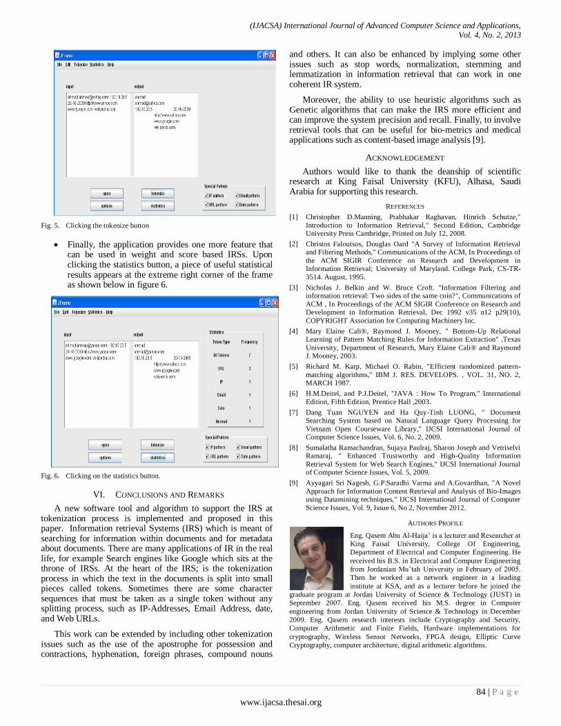
(IJACSA) International Journal of Advanced Computer Science and Applications, Vol. 4, No. 2, 2013
84 | P a g e www.ijacsa.thesai.org
Fig. 5. Clicking the tokenize button
Finally, the application provides one more feature that can be used in weight and score based IRSs. Upon clicking the statistics button, a piece of useful statistical results appears at the extreme right corner of the frame as shown below in figure 6.
Fig. 6. Clicking on the statistics button.
VI. CONCLUSIONS AND REMARKS
A new software tool and algorithm to support the IRS at tokenization process is implemented and proposed in this paper. Information retrieval Systems (IRS) which is meant of searching for information within documents and for metadata about documents. There are many applications of IR in the real life, for example Search engines like Google which sits at the throne of IRSs. At the heart of the IRS; is the tokenization process in which the text in the documents is split into small pieces called tokens. Sometimes there are some character sequences that must be taken as a single token without any splitting process, such as IP-Addresses, Email Address, date, and Web URLs.
This work can be extended by including other tokenization issues such as the use of the apostrophe for possession and contractions, hyphenation, foreign phrases, compound nouns
and others. It can also be enhanced by implying some other issues such as stop words, normalization, stemming and lemmatization in information retrieval that can work in one coherent IR system.
Moreover, the ability to use heuristic algorithms such as Genetic algorithms that can make the IRS more efficient and can improve the system precision and recall. Finally, to involve retrieval tools that can be useful for bio-metrics and medical applications such as content-based image analysis [9].
ACKNOWLEDGEMENT
Authors would like to thank the deanship of scientific research at King Faisal University (KFU), Alhasa, Saudi Arabia for supporting this research.
REFERENCES
[1] Christopher D.Manning, Prabhakar Raghavan, Hinrich Schutze,"
Introduction to Information Retrieval," Second Edition, Cambridge University Press Cambridge, Printed on July 12, 2008.
[2] Christos Faloutsos, Douglas Oard "A Survey of Information Retrieval and Filtering Methods," Communications of the ACM, In Proceedings of
the ACM SIGIR Conference on Research and Development in Information Retrieval; University of Maryland. College Park, CS-TR-
3514. August, 1995.
[3] Nicholas J. Belkin and W. Bruce Croft. "Information Filtering and information retrieval: Two sides of the same coin?", Communications of
ACM , In Proceedings of the ACM SIGIR Conference on Research and Development in Information Retrieval, Dec 1992 v35 n12 p29(10),
COPYRIGHT Association for Computing Machinery Inc.
[4] Mary Elaine Cali®, Raymond J. Mooney, " Bottom-Up Relational Learning of Pattern Matching Rules for Information Extraction" ,Texas
University, Department of Research, Mary Elaine Cali® and Raymond J. Mooney, 2003.
[5] Richard M. Karp, Michael O. Rabin, "Efficient randomized pattern-
matching algorithms," IBM J. RES. DEVELOPS. , VOL. 31, NO. 2, MARCH 1987.
[6] H.M.Deitel, and P.J.Deitel, "JAVA : How To Program," International
Edition, Fifth Edition, Prentice Hall ,2003.
[7] Dang Tuan NGUYEN and Ha Quy-Tinh LUONG, " Document Searching System based on Natural Language Query Processing for
Vietnam Open Courseware Library," IJCSI International Journal of Computer Science Issues, Vol. 6, No. 2, 2009.
[8] Sumalatha Ramachandran, Sujaya Paulraj, Sharon Joseph and Vetriselvi Ramaraj, " Enhanced Trustworthy and High-Quality Information
Retrieval System for Web Search Engines," IJCSI International Journal of Computer Science Issues, Vol. 5, 2009.
[9] Ayyagari Sri Nagesh, G.P.Saradhi Varma and A.Govardhan, "A Novel
Approach for Information Content Retrieval and Analysis of Bio-Images using Datamining techniques," IJCSI International Journal of Computer
Science Issues, Vol. 9, Issue 6, No 2, November 2012.
AUTHORS PROFILE
Eng. Qasem Abu Al-Haija’ is a lecturer and Researcher at
King Faisal University, College Of Engineering,
Department of Electrical and Computer Engineering. He
received his B.S. in Electrical and Computer Engineering
from Jordanian Mu’tah University in February of 2005.
Then he worked as a network engineer in a leading
institute at KSA, and as a lecturer before he joined the
graduate program at Jordan University of Science & Technology (JUST) in
September 2007. Eng. Qasem received his M.S. degree in Computer
engineering from Jordan University of Science & Technology in December
2009. Eng. Qasem research interests include Cryptography and Security,
Computer Arithmetic and Finite Fields, Hardware implementations for
cryptography, Wireless Sensor Networks, FPGA design, Elliptic Curve
Cryptography, computer architecture, digital arithmetic algorithms.

(IJACSA) International Journal of Advanced Computer Science and Applications, Vol. 4, No. 2, 2013
85 | P a g e www.ijacsa.thesai.org
Eng. Ahmad Al Badawi is a lecturer and Researcher at
Taif University, College Of Computers and Information
Technology, Department of Computer Engineering. He
received his B.S. in Electrical and Computer Engineering
from the Faculty of Engineering Technology, Al-Balqa
Applied University in June 2007. Then he worked as Sr.
Software Developer at Globitel, a leading Converged
Telecommunication Solutions provider, in Jordan before he joined the
graduate program at Jordan University of Science & Technology (JUST) in
September 2007. Eng. Ahmad received his M.S. degree in Computer
engineering from Jordan University of Science & Technology in March 2010.
Eng. Ahmad research interests include Particle Swarm Optimization,
Multiprocessor Scheduling, Parallel Processing, Information Security and
Cryptography, and Wireless Sensor Networks.

(IJACSA) International Journal of Advanced Computer Science and Applications, Vol. 4, No. 2, 2013
86 | P a g e www.ijacsa.thesai.org
A Simple Exercise-to-Play Proposal that would
Reduce Games Addiction and Keep Players Healthy
Nael Hirzallah
Software Engineering Department
Applied Science University
Amman, Jordan
Abstract—Games players usually get addicted to video
games in general and more specifically to those that are usually
played over the internet. These players prefer to stay at home
and play games rather than playing sports or outdoor games.
This paper presents a proposal that aims to implement a simple
way to let video games players exercise in order to play. The
proposal targets games where players virtually live inside a
certain area such as a forest, city or a war zone. Their aim is to
explore the area, capture, kill and avoid being killed by
something or someone. A costumed built treadmill acting as a
movement capture device is proposed to capture players’
commands for movements. These movements include Running,
walking, Stopping, and Turning. In that way, the players enjoy
exercising as well as playing the game. However, sooner or later,
the players get exhausted driving them to exit the game. That
way, we believe that such a proposal would keep players healthy, and reduce the chance of addiction.
Keywords—Virtual Reality; Gaming; Video Game.
I. INTRODUCTION
Computer and video games have come a long way since Space Invaders and Pac Man. Video games are becoming increasingly complex, detailed, and compelling to a growing international audience of players. Today's games are much more interesting, and the technology has advanced to the point where a gamer can become immersed in a multimedia-enabled 'virtual reality' or 'alternate world'. With better graphics, more realistic characters, and greater strategic challenges, it’s not surprising that some teens would rather play the latest video game than hang out with friends, play sports, or even watch television. Some games, especially online role playing games, can become a substitute for 'real life', and players can become immersed in the experience of living in an imaginary world. Some gamers report that they play games to escape things like family or personal problems – in a similar way to people who use drugs or alcohol to escape their problems.
Although gaming addiction is not yet officially recognized as a diagnosable disorder by the American Medical Association, there is increasing evidence that people of all ages, especially teens and pre-teens, are facing very real, sometimes severe consequences associated with compulsive use of video and computer games.
Thus, people can become addicted to games. Young gamers have shown similar symptoms to people who have drug or alcohol dependence – an inability to stop playing.
Of course, all gamers are not addicts – many teens can play video games a few hours a week, successfully balancing school activities, grades, friends, and family obligations. But for some, gaming has become an uncontrollable compulsion. Studies [1] estimate that 10 percent to 15 percent of gamers exhibit signs that meet the World Health Organization’s criteria for addiction. Just like gambling and other compulsive behaviors, teens can become so enthralled in the fantasy world of gaming that they neglect their family, friends, work, and school. Many children spend hours a day on computers, so much so that computers have become a primary source of entertainment for them, as well as a convenient baby-sitter for parents.
In reference [2] by Ricky Lam, many controversial cases in which addicted players commits suicide, murder, or robbery, caused death to negligence, or skipped school were listed. For instance, case number 2, a seventeen-year-old Daniel Petric murdered his mother and injured his father after they refused to let him play an online game named Halo 3. Also, just a week ago, among the ridiculous calls that people made to Emergency 999 in 2012 which the UK police revealed was a midnight call of a father to a 14 year old son who was ignoring his parents' pleas to switch a video game off and get some sleep [3].
In the following section, we will present few of the symptoms and injuries that addicted gamers usually start developing. Next in section 3, solutions proposed by literature and concerned centers will be presented. Section 4, will cover existing tools offered to players to capture real life movements and interpret them into games commands. Then, the costumed build treadmill will be proposed before we conclude.
II. SYMPTOMS AND POSSIBLE INJURIES
Addicted gamers usually try to be with the computer as much as possible, and in many cases, such gamers lose their confidence; they cannot involve with the social world in real time and they cannot communicate and compete with other people. When such thing happened, it means that they need video game addiction treatment as soon as possible.
In other words, computer game addiction can be diagnosed with a few easily spotted signs. They include but not restricted to:
School grades dropping
Avoiding other commitments in order to be with the computer (wagging school, stopping participation in sport)

(IJACSA) International Journal of Advanced Computer Science and Applications, Vol. 4, No. 2, 2013
87 | P a g e www.ijacsa.thesai.org
Not seeing friends
Not talking to parents/family
Being on the computer in most or all of your spare time.
Anxiousness to be with the computer.
Sleep and memory problems when playing an exciting game for 2 or 3 hours before bed
Family negligence
Furthermore, when playing video games, as with many activities, you may experience occasional discomfort in your hands, arms, shoulders, neck, or other parts of your body. Symptoms such as these can be associated with painful and sometimes permanently disabling injuries or disorders of the nerves, muscles, tendons, blood vessels, and other parts of the body. These musculoskeletal disorders (MSDs) include carpal tunnel syndrome, tendonitis, tenosynovitis, vibration syndromes, and other conditions. While researchers are not yet able to answer many questions about MSDs, there is general agreement that many factors may be linked to their occurrence, including: medical and physical conditions, stress and how one copes with it, overall health, and how a person positions and uses their body during work and other activities, including playing a video game.
RSI (Repetitive Strain Injury) for instance can be developed from playing games or sitting at the computer too long, or repeating certain movements, eg. clicking a mouse button. For gamers or heavy computer users, it's common to get RSI in the wrist. This results from the tendons in the arm and wrist being overworked, causing the tendons and the tissue covering the tendons to become inflamed and sore. Other overuse problems such as neck pains, tingling in the fingers, black rings in the skin under the eyes and muscular stiffness in the shoulders may also be developed from excessing playing.
To summarize, video games can cause injury and addiction. The following section presents solutions which specialists believe that may deal with the injury and addiction problems.
III. POSSIBLE SOLUTION
Many of the discussed injuries may be avoided by taking breaks while playing. This helps the player’s body to avoid MSDs. Also players must make sure that their positions when playing do not encourage discomfort. Whereas, to avoid addiction problems, we believe that there are three ways to approach this: through parents, through offering alternatives, and through exercising to play.
A. Parents’ supervision
Increase parental supervision and parental control may help in avoiding games addictions. Some Consoles like the PS3, Xbox360, Wii, and the PSP have parental control. Parental supervision and control can also be in the form of setting boundaries as to how long the child can be playing games/chatting on the computer. Furthermore, it is suggested that rewarding children with computer time for doing something, like completing an assignment, would make them feel like no one is trying to 'stop' them from using the computer as such, and thus helps.
B. Finding alternatives:
There are many alternatives to computer games and computers in general for entertainment. They include:
Playing a sport with friends
Going out often
Eating at a restaurant
Getting involved with a local recreational group
Drawing
C. Exercising while playing
So far, exercising while playing has been presented to the gamers as a way to increase the joy when playing, such as in MSE Weibull Virtual Theater. Giving gamers a feeling of the real world through virtual reality is an exciting challenge. Another reason for exercising while playing is to practice and improve certain physical skills of the player, such as in Tacx. Both examples will be addressed later. Regardless whether the reason for exercising is to enjoy the game more, or to improve certain physical skills, or to get the chance to play if one is prevented from playing by parents or self-control, players sooner or later will get exhausted, and consequently quit playing for the day. These three different reasons could be classified under playing while exercising, exercising while playing, and exercising to play.
As long as players do exercise, addition will not be of a concern. In what follows, we will give a history to the introduction of body interaction in games, and then we will present some recent tools or controllers that are used to interpret and perceive body motions. In section ??, we will propose our vision to a tool that could be used to reduce games addiction by exercising to play, before we state our conclusion.
IV. HISTORY TO BODY INTERACTIONS IN GAMES
In 1996, Mandala Gesture Xtreme (GX) System [4] became the first commercial arcade application using computer vision. Instead of a projector, the system used a large CRT display, which changed the player’s experience where the player could move with more confidence. In 2001, Intel®PlayTM Me2Cam Virtual Game System [5] was the first home product released. At the time, when an average PC screen was a 15” CRT display, it was difficult to play, due to the small screen size. It was hard to see the action on the screen. The recent commercial success of Sony PlayStation Eyetoy [6] and Nintendo Wii [7], which are not a “proper” full body interactive game, introduced the idea of a computer body interaction, full body interaction, and physically interactive games, i.e. games where the main interaction device is a user’s body. The user’s action was finally moved to take place in front of a large screen (i.e. TV display), where there was more space available for the physical gameplay.
Early design projects in full body interaction games such as those in [8] [9] presented principals for game design. Labanotation has been used in the interaction design context to evaluate Eyetoy Sony PlayStation games [10] and it provided a valuable foundation for the design of movement based interaction. Work of QuiQui Giant Bounce [11] and Kick Ass

(IJACSA) International Journal of Advanced Computer Science and Applications, Vol. 4, No. 2, 2013
88 | P a g e www.ijacsa.thesai.org
Kung-fu [12] focused around transforming the user movement into the gameplay.
Fairly new types of games called massively multiplayer online role-playing game, (MMORPG), have recently been developed and became very popular in a short time. A very large number of players interact with one another within a virtual game world. Players assume the role of a character (often in a fantasy world) and take control over many of that character's actions. MMORPGs are distinguished by the number of its players, and by the game's persistent world which continues to exist and evolve while the player is offline and away from the game. Worldwide revenues for MMORPGs exceeded half a billion dollars in 2005,[14] and Western revenues exceeded US$1 billion in 2006, [15]. In 2008, Western consumer spending on subscription MMOGs grew to $1.4 billion [16]. World of Warcraft, a popular MMORPG, has more than 10 million subscribers as of February 2012.[17] Star Wars: The Old Republic, released in 2011, became the world's 'Fastest-Growing MMO Ever' after gaining 1 million subscribers within the first three days of its launch[18,19].
In these games, the movement commands, which are walking and running, as well as in other similar games such as Runescape, Tibia, Call of duty, assassin's creed, Starcraft, Prius Online, Gears of War, Second Life, Legend of Mir, Halo, and Everquest, are controlled via one of the following methods:
A Mouse click on destination position in an overview map, such as in Runescape and World of Warcraft
A Keystroke or a joystick to indicate forward, backward, left and right directions to move, such as in Call of Duty, Hello, and Assasin’s creed.
Although, a small background application can be developed to convert one approach to another, the paper’s proposal works with only the second approach in which keystrokes or joysticks commands dictates the moving direction of the virtual player within the game.
V. OFF SHELF AND SPECIAL CONTROLLERS FOR MOTION
CAPTURE
In this section, we will introduce the most popular off shelf motion controllers that could be used for playing at home. PlayStation Move is a motion-sensing game controller platform for the PlayStation 3 (PS3) video game console by Sony Computer Entertainment (SCE). Based around a handheld motion controller wand, PlayStation Move uses the PlayStation Eye camera to track the wand's position, and inertial sensors in the wand to detect its motion. It was first revealed on 2 June 2009, [20]. Kinect is another controller but designed for Xbox 360. Kinect is a motion sensing input device by Microsoft for the Xbox 360 video game console and Windows PCs. Based around a webcam-style add-on peripheral for the Xbox 360 console, it enables users to control and interact with the Xbox 360 without the need to touch a game controller, through a natural user interface using gestures and spoken commands, [21]. It was aimed at broadening the Xbox 360's audience beyond its typical gamer base. It gives the experience of a controller-free gaming that involves a full body play.
Wii MotionPlus was developed by Nintendo in collaboration with game development tool company AiLive, [22]. The device incorporates a dual-axis [23] tuning fork gyroscope, [24] and a single-axis gyroscope which can determine rotational motion. The information captured by the angular rate sensor can then be used to distinguish true linear motion from the accelerometer readings. This allows for the capture of more complex movements.
In a different setup, MSE Weibull [26] offers system solutions within the sectors of production, test and training in civilian and military markets. The Virtual Theatre and the Omnidirectional treadmill link between the Live and Virtual domains. The Virtual Theatre from MSE is based on an omnidirectional floor, Figure 1.
It was shown to the public at ITEC 2011 for the first time. It facilitates omnidirectional unrestricted walking in the infinite virtual environment, within a finite real world footprint. The increased immersion is claimed to lead to a giant leap towards convergence of the real and the virtual world has been taken.
The WIZDISH™ locomotion platform, [27], is another controller similar to a treadmill but with no moving parts. It offers the navigation for Virtual Reality and Immersive Worlds. The users experienced when using wizdish [27] is claimed to be similar to a regular treadmill. The player stands on a slick concave disk, as shown in Figure 2, which minimizes friction under foot so the player can shuffle along in place, pretending to walk around.
Fig. 1. Mse Weibull Omnidirectional Treadmill
Fig. 2. WIZDISH
Although, all these controller or approaches may come close to satisfy our objective, which is to reduce games addiction, but not exactly. Players would stop playing their session once they get bored and not once they get tired. Thus, this may prevent them from using these controllers again. Our

(IJACSA) International Journal of Advanced Computer Science and Applications, Vol. 4, No. 2, 2013
89 | P a g e www.ijacsa.thesai.org
proposal aims to get players to sweat while playing. If one puts more efforts in each move, then the outcome would be different and shorter durations per session would make players get tired and have better chance to get back and use the same setup when play again.
Figure 3 shows another setup where players put greater efforts in the moves.
Tacx has created a video game to link cycling around the world and to offer a way to exercise at any time regardless to the weather situation. Tacx’ has become a household name for cyclists all over the world. They offered their customers Virtual Reality trainers through software programs and cycling films a unique experience in virtual worlds. They connect the bicycle to a rotation speed sensor as well as sensors for the left and right turnings. The cyclist then rides and starts playing or exercising. However, the main objective behind this is to exercise rather than play.
Finally, the closest to our proposal is Gamerunner [28]. It was an attempt to exhaust the player using a treadmill as a controller which was made available in February 2011. It was yet another way to blend exercise and gaming. As seen in the Figure 4, it was mounted by a joystick to control moving directions and other gamming tools. The Gamerunner is a person-powered treadmill that features 17 buttons and a handlebar that can be turned for looking or moving.
Fig. 3. Tacx Virtual Reality Cycling
Fig. 4. Gamerunner
VI. PROPOSAL
This paper proposes a controller that adopts the idea of exhausting the player while playing a video game to avoid long playing sessions; hence, neither reaching a state where the player may start feeling bored, nor playing for long which may lead to addiction.
We believe the presented earlier GameRunner is a good choice; however, keeping the players’ hands on the mounted handler all the time, is something that is not preferred by players. This would unfortunately reduce the feeling of excitement when playing the game; thus giving players more reasons for not getting back to the same setup when playing again.
Considering the Call of Duty game, for instance, this paper proposes modifications to the GameRunner in order to give the player more of a feeling to the convergence of the real and the virtual worlds. Keeping in mind that the player may sweat while playing, the addiction becomes of a no concern when playing video games.
The primary modification proposed is to make the fixed handler portable, or at least to split it into two pieces: one that is portable and another that is fixed. The portable handler could be in the form of a wireless joystick or fake machine gun (in case of a FPS, First Person Shooter, game) that includes few buttons which are responsible for the most frequent commands, such as Fire, Crouch, Stand, prone, and Jump as well as Looking left or right. That way, the player will have his/her hands off the treadmill and on the device that may resemble the virtual device being carried in the game.
The proposal classifies the commands offered by the game into three: Frequent, Motion based, and Optional. It distributes these commands over three devices. The frequent commands, such as those mentioned earlier, will be placed on the portable handler (or machine gun). The treadmill will include the motion based commands, such as Running, walking, and moving left or right. While the optional (or least used) commands such as Equipment and Inventory will be placed on the fixed handler, or added to the portable handler, if fixed handler is chosen not to exist. Moreover, the treadmill speed triggers, such as to increase or reduce as well as to come to a gradual full stop will be added to the frequent commands.
To implement the four Motion-based commands on the treadmill, namely: Running, Walking, and Moving left or right, first the rotation sensor similar to that used by Tacx will be used to indicate Running and walking.
This will basically translate the motor speed to the appropriate command based on a preset threshold. Second, for moving right and left, two concave slim switches are installed beneath the front sides of the rotating belt of the treadmill: one under the right-front, and another under the left-front corners, as shown in the Figure 5. Once a player steps on the center of any of these two switches, it will indicate moving left or right.
Each right or left switch press will represent a number of keystrokes used to control left or right movements depending on its sequence number, up to a specific maximum value. If the maximum is four, for instance, then the first step on a switch will represent one keystroke; the second will represent two keystrokes, and so on till either the switch is not stepped on it for some time that is long enough to break the sequence or a maximum of four keystrokes is reached. Breaking the sequence will result in the sequence reset.

(IJACSA) International Journal of Advanced Computer Science and Applications, Vol. 4, No. 2, 2013
90 | P a g e www.ijacsa.thesai.org
Fig. 5. Similar to Gamerunner but with portable Handler
The portable handler, in turn, is similar to a wireless keyboard providing the needed keystrokes to represent both frequent and optional commands (which also could include the right and left moving buttons, as alternatives to stepping on the switches). For the mouse pointer, which is used to look left or right, there are many ways to connect the portable handler with a wireless Motion sensing air mouse, such as Measy RC11 [29] or Flymouse Mouse [30]. We could also provide a webcam and object motion tracker software to detect motion produced by the head of the player or the tip of the portable handler. One example of such software that is available as a freeware is Camera Mouse 2013 [31]. A snapshot of the software settings is shown in Figure 6. That way, if the player turns his/her head left, the mouse will follow which consequently will be perceived as a look-left command in the Call of Duty game.
Fig. 6. Camera Mouse 2013 setting screen shot
VII. CONCLUSION
The paper has discussed the issue of games addiction that many players may be suffering from. Such a phenomenon has recently been bubbling up to the surface and becoming the concern of not only parents but also the society. The paper presented the symptoms that may appear on people who may be addicted to games or are becoming ones, as well as the possible injuries. The paper then drives the readers towards discussing possible solutions to avoid such a problem. It then focuses on one of these possible solutions by presenting the available tools and devices that could be used within the solution category. After discussing the drawback of them, it proposes one that is believed to have overcome most of these drawbacks, except one. The proposal of this paper suffers from
the same problem that most of the other pieces of gaming exercise equipment have suffered: its size. With the advent of more family friendly consoles, like the 360, that problem would grow. However, self or parental control would then be necessary to offer such a proposal as a way to allow players to play without imposing any time control, yet with the confidence that such a setup will lead to no addiction.
ACKNOWLEDGMENT
The author would like to acknowledge the financial support received from Applied Science University that helped in accomplishing the work of this article. He also would like to acknowledge the time and feedback provided by his son, Adam, who has helped him in verifying many of the issues as well as the feasibility concerning the proposal.
REFERENCES
[1] http://www.video-game-addiction.org/
[2] http://listverse.com/2010/11/07/top-10-cases-of-extreme-game-
addiction/
[3] “999? My son won't go to bed: Police reveal the ridiculous calls people make to emergency number” MailOnline Newsletter, Wednesday, Dec
26 2012
[4] Mandala Gesture Xtreme (GX) System [Hardware] (1996) Vivid Group Toronto, Canada
[5] Intel® Play™ Me2Cam* Virtual Game System [Software] (2001) Intel,
St Clara, CA, USA
[6] Eyetoy [Hardware] (2005) Sony Corporation In: Eyetoy. Available at
www.eyetoy.com, Accessed 20 Sep 2008
[7] Nintendo Wii [Hardware] (2007) Nintendo In: Nintendo. Available at www.nintendo.co.uk/NOE/en_GB/systems/about_wii_1069.html.
Accessed 20 Sep 2008
[8] D'Hooge H, Goldsmith M (2001) Game Design Principles for the Intel® Play™ Me2Cam* Virtual Game System. Intel Technology Journal
2001/4. pp. 1-9.
[9] Warren J (2003) Unencumbered Full Body Interaction in Video Games. In: Parsons School of Design. Available at
http://a.parsons.edu/~jonah/jonah_thesis.pdf. Accessed 2 Nov 2009
[10] Loke L, Larssen AT, Robertson T, Edwards J (2007) Understanding movement for interaction design: frameworks and approaches. Pers
Ubiquit Comput, 11/8. pp 691-701. doi:10.1007/s00779-006-0132-1
[11] QuiQui's Giant Bounce [Software] (2003). Höysniemi J, Hämäläinen P In: University of Tampere. Available at www.cs.uta.fi/kukakumma.
Accessed 2 Nov 2009
[12] Kick Ass Kung-Fu [Artwork] (2006) Hämäläinen P In: Kick Ass Kung-
Fu. Available at www.kickasskungfu.net. Accessed 2 Nov 2009
[13] Liu CC, Chiou WC, Tai SJ, Tsai CC, Chen GD, Jong CW et al (2006) Wristbands as Interaction Devices: a Vision-Based Interaction Space for
Facilitating Full-Body Learning. 4th IEEE International Workshop on Wireless, Mobile and Ubiquitous Technology in Education, (WMUTE
2006), Greece. pp. 171-173. doi:10.1109/WMTE.2006.261370
[14] Parks Associates (2005). "Online Gaming Revenues to Triple by 2009". Retrieved 2007-05-02.
[15] Harding-Rolls, Piers (PDF). Western World MMOG Market: 2006
Review and Forecasts to 2011. London, UK: Screen Digest. Archived from the original on 2007-06-04. Retrieved 2007-05-17.
[16] Harding-Rolls, Piers (PDF). Subscription MMOGs: Life Beyond World
of Warcraft. London, UK: Screen Digest. Archived from the original on 2009-12-25. Retrieved 2009-03-30.
[17] "Activision Blizzard Announces Record Fourth Quarter and Calendar
Year 2011 Earnings".Activision Blizzard.
[18] "Star Wars: The Old Republic Jumps to Light Speed (NASDAQ:EA)".
Investor.ea.com. 2011-12-23. Retrieved 2012-04-11.
[19] Rundle, Michael (2011-12-27). "Star Wars: The Old Republic Is 'Fastest-Growing MMO Ever' With 1m Users". Huffington Post.

(IJACSA) International Journal of Advanced Computer Science and Applications, Vol. 4, No. 2, 2013
91 | P a g e www.ijacsa.thesai.org
[20] "Sony Computer Entertainment America announces an unparalleled
software line up, launch of the PSP go system, and new services for PSP (PlayStation Portable) and PlayStation Network at E3 2009". Sony
Computer Entertainment. 2009-06-02. http://www.scei.co.jp/corporate/release/090603c_e.html. Retrieved
2009-06-03.
[21] "Project Natal" 101". Microsoft. June 1, 2009. Archived from the
original on June 1, 2009. http://blog.seattlepi.com/digitaljoystick/archives/169993.asp. Retrieved
June 2, 2009.
[22] "AILive Reveals LiveMove2 For Wii MotionPlus". Gamasutra.com. July 15, 2008. http://www.gamasutra.com/php-
bin/news_index.php?story=19432. Retrieved December 12, 2012.
[23] "INVENSENSE IDG-600 MOTION SENSING SOLUTION SHOWCASED IN NINTENDO'S NEW Wii MotionPlus
ACCESSORY". InvenSense. http://invensense.com/mems/gyro/documents/articles/071508.html.
Retrieved December 12, 2012.
[24] "MEMS Gyroscope Technology". InvenSense. Archived from the
original on April 16, 2008. http://web.archive.org/web/20080416215417/
http://www.invensense.com/company/technology.html. Retrieved Dec. 12, 2012.
[25] M. Zyda et al., “From Viz-Sim to VR to Games: How We Built a Hit Game-Based Simulation,” Organizational Simulation: From Modeling &
Simulation to Games & Entertainment, W.B. Rouse and K.R. Boff, eds., Wiley Press, 2005, pp. 553-590.
[26] http://www.mseab.se/ Retrieved 2012-06-03
[27] www.wizdish.com Retrieved 2013-01-03
[28] http://www.gamerunner.us/ Retrieved 2012-07-06
[29] http://www.measy.com.cn/product/showproduct48_en.htm Retrieved
2012-06-03
[30] http://www.airflymouse.com/air-mouse/air-mouse-iii.html Retrieved 2012-06-03
[31] http://www.cameramouse.org/ Retrieved 2011-09-20

(IJACSA) International Journal of Advanced Computer Science and Applications, Vol. 4, No.2, 2013
92 | P a g e www.ijacsa.thesai.org
Segmentation of Ultrasound Breast Images using
Vector Neighborhood with Vector Sequencing on
KMCG and augmented KMCG algorithms
Dr.H.B.kekre
Senior professor, Dept. of Computer Engineering
MPSTME, SVKM’s NMIMS University Mumbai, India.
Pravin Shrinath
Ph.D. Scholar
MPSTME, SVKM’s NMIMS University
Mumbai, India.
Abstract— B mode ultrasound (US) imaging is popular and
important modality to examine the range of clinical problems and
also used as complimentary to the mammogram imaging to detect
and diagnose the nature breast tumor. To understand the nature
(benign or malignant) of the tumor most of the radiologists focus
on shape and boundary. Therefore boundary is as important
characteristic of the tumor along with the shape. Tracing the
contour manually is a time consuming and tedious task.
Automated and efficient segmentation method also helps
radiologists to understand and observe the volume of a tumor
(growth or shrinkage). Inherent artifact present in US images,
such as speckle, attenuation and shadows are major hurdles in
achieving proper segmentation. Along with these artifacts,
inhomogeneous texture present in the region of interest is also a
major concern. Most of the algorithms studies in the literature
include noise removal technique as a preprocessing step. Here in
this paper, we are eliminating this step and directly handling the
images with high degree of noise. VQ based clustering technique
is proposed for US image segmentation with KMCG and
augmented KMCG codebook generation algorithms. Using this
algorithm images are divided in to clusters, further these clusters
are merged sequentially. A novel technique of sequential cluster
merging with vector sequencing has been used. We have also
proposed a technique to find out the region of interest from the selected cluster with seed vector acquisition.
Results obtained by our method are compared with our
earlier method and Marker Controlled Watershed transform.
With the opinion of the expert radiologist, we found that our method gives better results.
Keywords— codebook; seed vector; training set; vector
quantization
I. INTRODUCTION
B-Mode ultrasound (US) imaging is widely used diagnostic tool to examine the range of clinical problems because of its real-time image availability, non invasive nature and low cost of a scan. It has very low health risk to the patient during examination and image acquisition process relative to the other imaging modality [1, 2]. In the tissue characterization of the breast, US imaging is a complimentary method to the mammogram to distinguish between benign and malignant solid masses [3, 4]. Usually a malignant tumor has different characteristics, such as irregular shape, ill defined margins and heterogeneous echo texture as compare to benign
tumor. Round or oval shape with well defined boundary of a tumor is the most valuable information in the detection as benign and can be used to reduce the number of biopsies performed [5].
Segmentation of US images provides clinically valuable information for radiologists in terms of shape irregularity, boundary definition and quantitative measurement of lesion size. The accurate measurement of a lesion is basically used to monitor the tumor growth and also helps in treatment and planning for surgery [6]. Due to the limitation of acquisition process (dependence on expert radiologist) and technology, detection and measuring the size of tumor manually is difficult and time consuming process. However, with the improvement in the scanning devices (transducers), the inherent artifacts, such as speckle (which decrease signal-to-noise ratio), attenuation, shadows and signal dropout degrades the quality of the US images acquired. Many traditional segmentation algorithms are not suitable for such poor quality images, unless preprocessing steps to remove these artifacts has been used [7]. The artifact such as attenuation, which is causes by the gradual loss in the intensity of the ultrasound waves, generates inhomogeneous intensities within the same tissue type regions (i.e. tumor) and significant overlap between different class tissues (i.e. at the boundary). Blurred boundary and presence of tissue intensity variation in the region of interest are major constraints to achieve accuracy in the automated intensity based segmentation [8]. Some methods are discussed in the literature which handles this issue with the help of multiple images of the same region (sequence of images), but the processing of multiple images together is computationally inefficient [9, 10]. Other methods discussed in the literature for segmentation and classification such as, texture feature, thresholding [11,12], region growing and region merging [13,14], neural network, wavelet and watershed transform [15, 16], clustering [17, 18] etc, are strongly influenced by these inherent artifacts and involves steps to remove them to enhance the quality of images. The most usual artifact in US images is speckle and its degree is depends on human expertise, acquisition process and devices. This phenomenon highly affects the accuracy of segmentation and requires attention, so removal of noise has been extensively studied by the researchers and provides solutions [19-22]. Here, in this paper, we are demarking the boundary of the tumor in high degree noisy and attenuated US images

(IJACSA) International Journal of Advanced Computer Science and Applications, Vol. 4, No.2, 2013
93 | P a g e www.ijacsa.thesai.org
without involving any preprocessing (i.e. image enhancement) step. We are proposing Vector Quantization (VQ) based clustering with new computationally efficient codebook generation algorithm [23], i.e. Kekre’s Median Codebook Generation (KMCG) and augmented KMCG. Improved method of cluster merging with vector neighborhood is proposed on novel method of sequential merging of clusters [24] and compared with each other.
The other sections of this paper are organized as follows, in section II, vector quantization is discussed with encoding technique and its usability in segmentation. In section III, original VQ based KMCG codebook generation algorithm and augmented KMCG are discussed along with training set formation for horizontal and vertical division of the images. A novel technique of vector neighborhood with vector sequencing is described in section IV along with new technique for closing the holes in the clusters. In section V results are discussed followed by conclusion in section VI.
II. VECTOR QUANTIZATION
Vector Quantization (VQ) was initially developed and implemented for image compression, with the help of many codebook generation and quantization algorithms [25, 26, 27, 28], but now a days it has been extensively use in other applications, such as image segmentation [29], speech recognition [30], pattern recognition and face detection [31, 32], tumor demarcation in MRI and Mammogram images [33, 34], content based image retrieval [35, 36] etc. In this paper, this method has been used as clustering aid in demarcation of area of interest (cysts and tumor) in breast ultrasound images.
A two dimensional image I(X, Y) is converted into K dimensional vector space of size M, V = V1, V2, V3,……….., VM (training set). VQ is used as a mapping function to convert this K dimensional vector space to finite set CB = C1, C2, C3, C4,…….., CN. CB is a codebook of size N and each code vector from C1 to CN represents the specific set of vectors of the entire training set of dimensions K and size M. The codebook size is much smaller than size of the training set and it can represent entire training set. Here, in this paper, the work has been done in spatial domain and size of the codebook is limited to only eight codevectors, which are further used to forms eight clusters. As discussed in the section III A and B, KMCG and augmented KMCG are used as VQ based clustering algorithms and each cluster represents different regions of the image.
III. CLUSTER FORMATION USING CODEBOOK GENERATION
ALGORITHMS
A. Kekre’s Median Codebook Generation algorithm (KMCG)
This algorithm was proposed for data compression [37, 38, 39], but this VQ based algorithm, proved its potential and usefulness in various applications, such as segmentation of mammographic images[35], content based image retrieval, face recognition etc. Here, in this paper, this iterative algorithm has been explored for demarcation of tumor from the breast US images.
Initially, Image I, is divided into M non-overlapping blocks of size 2x2 and these blocks are further converted into
vectors of dimension 1 x K, (K=4) as shown in the Fig. 1(a). Let, V be the training set, i.e. V = V1, V2, V3,……….., VM, where V1 to VM are individual vectors of the training set. This entire training set (matrix) of dimension M x 4 is considered as first cluster and become the input to the KMCG algorithm. To divide this cluster further, during the first iteration of this algorithm, entire training set has been sorted with respect to first value of all vectors (i.e. first column) and obtained the median of this sorted column. This median is consider as first codevector, and then divide training set into two clusters with respect to this codevector ,as shown in Fig. 1(b). (i.e upper part including median is first cluster C1 and lower part is second cluster C2). In second iteration, clusters C1 and C2 are sorted separately with respect to second column (i.e. second value of all the vectors) of the training set and obtain the medians of C1 and C2. Further, cluster C1 and C2 are divided into four clusters by using these new medians, as shown in Fig. 1(c). Same procedure has been repeated till we obtained the desired number of clusters. In Fig. 1, cluster formations are shown up to second iteration with k = 4. After acquiring desired number of clusters, they are merged together sequentially as discussed in section IV.
V11 V12
. . .
. . .
V1k
V21 V22 V2k
V31 V32 V3k
.
.
.
VM1 VM2 VMK
V1
V2
V3
.
.
.
.
.
VM-1
VM
MED
.
.
.
MED
.
.
.
MED
C1
C2
C1
C3
C2
C4
(a) (b) (c)
Fig. 1. Clustering Using KMCG Algoritm (A) Entire Training Set Of Size M
X K (K=4) Obtained From Image. (B) Clusters C1 And C2 Obtained After
First Iteration W.R.T. First Column Shown By Arrow. (C) Four Cluster
Ontainned From C1 And C2 W.R.T. Second Column.
B. Augmented KMCG
KMCG algorithm has been augmented, to decrease the time require in the clustering process. In this method, vector size is increased to 6 columns, in which last four columns are used to store original gray levels obtained from 2 x 2 blocks of the image. Further, averages of each of these blocks are done separately and stored at the second column in the respective vectors. At the first column, sequence number of the respective vectors has been stored. Eventually, the size of the entire training set used for this method becomes M x 6. Therefore, unlike the original KMCG, sorting process is done only once on the second column and accordingly vectors of the entire training set are shuffled by keeping vector intact (i.e. vectors are arranged in the increasing order of their average values stored at second column). To make clusters, during the

(IJACSA) International Journal of Advanced Computer Science and Applications, Vol. 4, No.2, 2013
94 | P a g e www.ijacsa.thesai.org
process median value is obtained from the second column and entire training set is divided into two clusters. Further, these two clusters are handled separately and obtained median value from each of them from the same column. These median values further divides two clusters into four. This process is repeated until desired number of cluster has been formed. Since sorting process is applied only once on the second column (i.e. column of average gray values of the block), time require for clustering is drastically reduced as compared to original KMCG algorithm.
C. Training set formation with vector sequencing
Original KMCG and augmented KMCG algorithms are used to form clusters from the training set. Here, in this paper, two separate training sets are formed for each codebook generation algorithms, Fig. 2 shows training set used for augmented KMCG algorithm. First training set is created by dividing image I (X,Y) into 2x2 non overlapping blocks horizontally and sequence number of these blocks are added at the first location of respective vectors as the vector number as shown in Fig. 2, therefore, first column of the training set contains vector sequence number. Similarly, same image is divided into non overlapping blocks vertically and forms the second training set by adding sequence number of blocks at the first column of the vector. Same procedure has been followed to create two training sets for original KMCG algorithm, except calculation of average gray levels. Therefore, size of these training sets becomes M x 5 and clusters are created according to the method discussed in section III. A.
B2
B1
B3
1
2
3
.
.
M-1
MIMAGE
VSN AGL IGL
BM
(a) (b)
Fig. 2. (a) Original image, divided horizontaly into M nonoverlaping blocks
shown by red boxes. i.e. B1, B2, …., BM and stored at Last four column of the
respective vector. (b) Training set generated from Image shown in (a), where,
first column indicates sequence number of the block used as Vector Sequence
Number (VSN), Second column Indicates Average Gray Lavels (AGL)
calculated from Image Gray Levels (IGL) shown in last four column.
IV. CLUSTER MERGING AND SEED VECTOR ACQUISITION
A. Sequential cluster merging
As discussed in section III. C, pair of separate training sets is used for each codebook generation algorithms to make clusters. Initially, first training set (i.e. formed by horizontal division of image) from the pair is divided in to eight clusters using code book generation algorithms, similarly second training set (i.e. formed by vertical division of image) divided
in to another set of eight clusters by same algorithm. So pair of similar clusters is obtained for each algorithm. “Fig. 4”, shows cluster images obtained using KMCG algorithm. “Fig. 5”, shows cluster images obtained using augmented KMCG. These two sets of clusters are handled separately in segmentation process. Further these clusters are merged sequentially one-by-one and forms new sets of merged clusters. As shown in the “Fig. 6”, first cluster is added with second, resultant clusters is then added with third and resultant third cluster added with fourth and so on. Similarly clusters obtained by augmented KMCG are merged and shown in “Fig. 7”.
B. Seed vector and exploration of clusters with horizontal
and vertical sequencing
Images are divided horizontally and vertically into blocks and sequence of these blocks are used as vector sequence number (VSN) and added to the first column of the training set. After making eight clusters for these training sets, first cluster has been sorted by its vector sequence number (i.e. first column) and accordingly vectors are shuffled. Further median is acquired from the first column of the training set and vector which contains this median value is considered as seed vector as shown in “Fig. 3”. In most of the ultrasound images, gray level distribution is inhomogeneous but the pixels with lower gray value are concentrated at region of interest. Therefore after clustering, usually these gray levels are components of the first cluster in the form of vectors. Due to these characteristics of image, mostly seed vector obtained from the first cluster falls in the region of interest Therefore sequence number of the seed vector is used to gather neighboring vectors in the cluster. All the vectors in the cluster are searched with respect to sequence values of seed vector. Searching is done in both, right hand side and left hand side of the seed vector. Since cluster is in sorted order with respect to sequence number, it searches vectors only for consecutive sequence number, if any interlude occurs in between, it stops searching and marked all searched vectors as found and this vector line is considered as seed vector line as shown in “Fig. 3”. Obtained new seed vector by adding sequence number of the first seed vector with number of vectors present horizontally in the row (i.e. X/2). To explore other vectors in the region of interest, first this new vector is checked whether it is present or not in the cluster by using equation 1. If this new vector is present in the cluster then second line has been explored, this process is repeated and lines are explored and lower region is grown from the region of interest. Same procedure is repeated to explore the upper part of the original seed vector line, only difference is, instead of addition, subtraction is used to obtained new seed vector (sequence number of the original seed vector is subtracted from number of vectors present horizontally in the row). Furthermore all marked vectors from these clusters are preserved and other vectors are removed. As shown in the “Fig. 3” vectors which are representing noise are removed from the cluster, since they are not the neighbors of the seed vectors and this new cluster is converted to the original size image as shown in the “Fig. 8 (a)”. Similar procedure is followed to explore the cluster with vertical sequencing, except addition and subtraction of value (i.e. Y/2) is done with the vector sequence number every time to get the new seed vector. With addition of this value, right

(IJACSA) International Journal of Advanced Computer Science and Applications, Vol. 4, No.2, 2013
95 | P a g e www.ijacsa.thesai.org
hand side region is explored and with subtraction left hand side of the region is explored. This exploration has been stop similarly when newly generated vector does not present in the cluster. Cluster image for vertical indexing is shown in “Fig. 10 (a)”. Same procedure is applied for second merged cluster and third merged cluster after closing the opening as per discussed in the section IV C and cluster images are formed.
ROI
Seed
Vector
Seed
Vector
Line
Noise
openings
Fig. 3. Image Of First Cluster, Used To Obtain Seed Vector And Generate
Seed Vector Line. This Seed Vector Further Used To Acquire Region Of
Interest (ROI) By Vector Neighborhood With Vector Sequence Number.
C. Closing the opening of clusters
As discussed in the section IV-A, clusters are merged together one-by-one and sets of eight merged clusters are obtained for both horizontal and vertical sequencing. From this set desired merged cluster has been selected for closing the opening (Break in the sequence number of vector as shown in the “Fig. 3”. These vectors are not present in the cluster but they are part of region of interest). Here in this paper we proposed new technique to close the opening directly on cluster rather on cluster images. Here we select the certain threshold value, which indicates the number of vectors. Then selected cluster has been sorted with respect to its sequence number. This sorted cluster has been traversed sequentially from the first vector, if any consecutive interlude occur with respect to sequence number and it is less than or equal to threshold value then that many number of vector are added to the cluster with zero gray level. Sequence number of first newly added vector is stared from sequence number of the vector where the interlude has started plus one. After closing the opening of these clusters, they are converted into images of original size as shown in “Fig. 8(c)” and “Fig. 10(c)”. for horizontal and vertical sequencing respectively.
Cluster 1
Cluster 2
Cluster 3
Cluster 4
Cluster 5
Cluster 6
Cluster 7
Cluster 8
Fig. 4. Eight Cluster Images Obtained Using Original KMCG Algorithm For
Dimension K= 4. Cluster Images Obtained For Both Horizontal And Vertical Division Of Image Are Same.
Cluster 1
Cluster 2
Cluster 3
Cluster 4
Cluster 5
Cluster 6
Cluster 7
Cluster 8
Fig. 5. Eight Cluster Images Obtained Using Augmented KMCG Algorithm
For Dimension K= 4. Cluster Images Obtained For Both Horizontal And Vertical Division Of Image Are Same.
1
1+2
1+2+3
1+2+.+4
1+2+.+5
1+2+.+6
1+2+.+7
1+2+.+8
Fig. 6. Eight Sequentialy Merged Clusters Images Obtained From Clusters
Shown In “Fig. 4” Using KMCG For Both Horizontal And Vertical Division
1
1+2
1+2+3
1+2+..+4
1+2+..+5
1+2+..+6
1+2+..+7
1+2+..+8
Fig. 7. Eight Sequentialy Merged Clusters Images Obtained From Clusters
Shown In “Fig. 5” Using Augmented KMCG For Both Horizontal And Vertical Division

(IJACSA) International Journal of Advanced Computer Science and Applications, Vol. 4, No.2, 2013
96 | P a g e www.ijacsa.thesai.org
(A)
(B)
(C)
(D)
Fig. 8. Images Obtained From The Merged Clusters For Horizonatl
Direction Shown In “Fig. 6” (A) Image Obtained From The First Cluster
Generated By Using Seed Vector. (B) Image Obtained From Second Merged
Cluster Generated By Using Same Seed Vector Acquired From First Cluster.
(C) Image Obtained From Third Merged Cluster After Closing The Holes.
(D) Image Obtained From Third Cluster Shown In “Fig. 8(C) By Using Same Seed Vector
(a)
(b)
(c)
(d)
Fig. 9. Resultant Images Obtained By KMCG Algorithm With Horizontal
Division (A) Image Obtained By Merging Cluster Images Shown In “Fig. 8
(A),(B) And (D)” (B) Segmented Resultant Image (C) Original Breast US
Image With Tumor At The Center, Marked By Radiologist (D) Superimposed Image.
(a)
(b)
(c)
(d)
Fig. 10. Images Obtained From The Merged Clusters For Vertical Direction
Shown In “Fig. 6” (A) Image Obtained From The First Cluster Generated By
Using Seed Vector. (B) Image Obtained From Second Merged Cluster
Generated By Using Same Seed Vector Aquired From First Cluster. (C)
Image Obtained From Third Merged Cluster After Closing The Holes. (D)
Image Obtained From Third Cluster Shown In “Fig. 10(C)” By Using Same Seed Vector.
(a)
(b)
(c)
(d)
Fig. 11. Resultant Images Obtained By KMCG Algorithm With Vertical
Division Of Orignal Image. (A) Image Obtained By Merging Cluster Images
Shown In “Fig. 10 (A),(B) And (D)”. (B) Segmented Resultant Image (C)
Original Breast US Image With Tumor At The Center, Marked By Radiologist (D) Superimposed Image.
(a)
(b)
(c)
(d)
Fig. 12. Images Obtained From The Merged Clusters For Horizonatl
Direction Shown In “Fig. 7”. (A) Image Obtained From The First Cluster
Generated By Using Selected Seed Vector. (B) Image Obtained From Second
Merged Cluster Generated By Using Same Seed Vector Selected From First
Cluster. (C) Image obtained from third merged cluster after closing the holes.
(d) Image obtained from third cluster shown in “Fig. 12.(c) by selecting same
seed vector
(a)
(b)
(c)
(d)
Fig. 13. Resultant Images Obtained By Augmented KMCG Algorithm With
Horizontal Division Of Orignal Image. (A) Image Obtained By Merging
Cluster Images Shown In “Fig. 12 (A),(B) And (D)”. (B) Segmented
Resultant Image (C) Original Breast US Image With Tumor At The Center,
Marked By Radiologist (D) Superimposed Image
(a)
(b)
(c)
(d)
Fig. 14. Images Obtained From The Merged Clusters For Vertical Direction
Shown In “Fig. 7.” (A) Image Obtained From The First Cluster Generated
By Selecting Seed Vector. (B) Image Obtained From Second Merged Cluster
Generated By Using Same Seed Vector Selected From First Cluster. (C)
Image Obtained From Third Merged Cluster After Closing The Holes. (D)
Image Obtained From Third Cluster Shown In “Fig. 14.(C)” By Selecting Same Seed Vector.
(a)
(b)
(c)
(d)
Fig. 15. Resultant Images Obtained By Augmented KMCG Algorithm With
Vertical Division Of Orignal Image. (A) Image Obtained By Merging Cluster
Images Shown In “Fig. 14 (A),(B) And (D)”. (B) Segmented Resultant
Image (C) Original Breast US Image With Tumor At The Center, Marked By
Radiologist (D) Superimposed Image
(a)
(b)
(c)
(d)
Fig. 16. Segementation Results Obtained By KMCG Algorithm & Augmented
KMCG Algorithm. (A) Image Obtained By Taking INTERSECTION Of
Cluster Images Shown In “Fig. 9.(B)” With Cluster Image Shown In “Fig.
11.(B)” (Using KMCG) (B) Segmentation Results Superimposed On
Original Image. (C) Image Obtained By Taking INTERSECTION Of Cluster
Image Shown In “Fig. 13.(B)” With Cluster Image Shown In “Fig. 15.(B)” (Using Augmented KMCG). (D) Superimposed Image.
(a)
(b)
(c)
(d)

(IJACSA) International Journal of Advanced Computer Science and Applications, Vol. 4, No.2, 2013
97 | P a g e www.ijacsa.thesai.org
Fig. 17. Results Comparison (A) Results Of Marker Controlled Watershed
Algorithm (B) Results By VQ Based Clustering [24] (C) Result By Our
Method Shown In “Fig. 16.(B)”. (D) Results By Our Method Shown In “Fig. 16.(D)”.
(a)
(b)
(c)
(d)
Fig. 18. Resultant Images Obtained By KMCG Algorithm With Horizontal
And Vertical Division Of Orignal Image. (A) Segmented Image Obtained By
Horizontal Division. (B) Superimposed Image (C) Segmented Image Obtained By Vertical Division. (D) Superimposed Image
(a)
(b)
(c)
(d)
Fig. 19. Resultant Images Obtained By Augmented KMCG Algorithm With
Horizontal And Vertical Division Of Orignal Image. (A) Segmented Image
Obtained By Horizontal Division. (B) Superimposed Image (C) Segmented
Image Obtained By Vertical Direction. (D) Superimposed Image
(a)
(b)
(c)
(d)
Fig. 20. Resultant Images Obtained By Taking INTERSECTION Of Two
Images. (A) Image Obtained By INTERSECTION Of Images Shown In “Fig.
18.(A) And 18 (C)”. (B) Superimposed Image. (C) Image Obtained By
INTERSECTION Of Images Shown In “Fig. 19.(A) And 19 (C)”. (D) Superimposed Image
(a)
(b)
(c)
(d)
Fig. 21. Results Comparison (A) Results Of Marker Controlled Watershed
Transform (B) Results By VQ Based Clustering [24] (C) Result By Our
Method Shown In “Fig. 20.(B)”. (D) Results By Our Method Shown In “Fig.
20.(D)”.
(a)
(b)
(c)
(d)
Fig. 22. Resultant Images Obtained By KMCG Algorithm With Horizontal
And Vertical Division Of Orignal Image. (A) Segmented Image Obtained By
Horizontal Division. (B) Superimposed Image (C) Segmented Image Obtained By Vertical Division. (D) Superimposed Image
(a)
(b)
(c)
(d)
Fig. 23. Resultant Images obtained by augmented KMCG algorithm with
Horizontal and Vertical division of orignal image. (a) Segmented image
obtained by Horizontal division. (b) Superimposed image (c) Segmented image obtained by Vertical division. (d) Superimposed image
(a)
(b)
(c)
(d)
Fig. 24. Resultant Images Obtained By Taking INTERSECTION Of Two
Images. (A) Image Obtained By INTERSECTION Of Images Shown In “Fig.
22.(A) And 22 (C)”. (B) Superimposed Image. (C) Image Obtained By
INTERSECTION Of Images Shown In “Fig. 23.(A) And 23.(C)”. (D) Superimposed Image
(a)
(b)
(c)
(d)
Fig. 25. Results comparison (a) Results of Marker Controlled Watershed
transform (b) Results by VQ based clustering [24] (c) Result by our method, shown in “Fig. 24. (b)”. (d) Results by our method, shown in “Fig. 24. (d)”.
(a)
(b)
(c)
(d)
Fig. 26. Resultant Images Obtained By KMCG Algorithm With Horizontal
And Vertical Division Of Orignal Image. (A) Segmented Image Obtained By
Horizontal Division. (B) Superimposed Image (C) Segmented Image Obtained By Vertical Division. (D) Superimposed Image
(a)
(b)
(c)
(d)
Fig. 27. Resultant Images Obtained By Augmented KMCG Algorithm With
Horizontal And Vertical Division Of Orignal Image. (A) Segmented Image
Obtained By Horizontal Division. (B) Superimposed Image (C) Segmented
Image Obtained By Vertical Division. (D) Superimposed Image
(a)
(b)
(c)
(d)
Fig. 28. Resultant Images Obtained By Taking INTERSECTION Of Two
Images. (A) Image Obtained By INTERSECTION Of Images Shown In “Fig.
26.(A) And 26 (C)”. (B) Superimposed Image. (C) Image Obtained By
INTERSECTION Of Images Shown In “Fig. 27.(A) And 27.(C)”. (D)
Superimposed Image

(IJACSA) International Journal of Advanced Computer Science and Applications, Vol. 4, No.2, 2013
98 | P a g e www.ijacsa.thesai.org
(a)
(b)
(c)
(d)
Fig. 29. Results Comparison (A) Results Of Marker Controlled Watershed
Transform (B) Results By VQ Based Clustering [24] (C) Result By Our
Method, Shown In “Fig. 28.(B)”. (D) Results By Our Method, Shown In
“Fig. 28.(D)”.
V. RESULTS
Here, in this paper, KMCG and augmented KMCG codebook generation algorithms are implemented for clustering process and further improved cluster merging technique is used to get final segmentation results. These methods are tested on real US images, using MATLAB 7.0 and Intel Core2 Duo 2.20GHz processor with 1 GB RAM. Results of four different images are shown.
Using these algorithms, sets of clusters and merged clusters are obtained, for different images. But complete result (results of each and every stage) is displayed only for one image shown in “Fig. 9(c)” and for other original images final segmented results are shown directly. All the results are validated by expert radiologists with visual inspection. Final results are compared with other techniques such as Marker Controlled Watershed transform and our other method [24]. Our results are compared with other method’s results as shown in the “Fig. 17”, “Fig. 21”, “Fig. 25” and “Fig. 29” and best results are shown by red box drawn around the image. Marker controlled watershed transforms gives over segmentation and other method discussed in [24], boundary is not clear around the tumor.
VI. CONCLUSION
VQ based, KMCG and augmented KMCG algorithms are used for clustering and further it has been used to segment the ultrasound breast images. Here we used training set of size Mx5 and Mx6 for KMCG and augmented KMCG respectively. Since augmented KMCG algorithm requires sorting only once, it is computationally efficient than KMCG and on the basis of visual inspection by expert radiologist, it also having better segmentation results. Here in this paper we used vector indexing in the cluster formation process, which further helps to get the seed vector to grow the region of interest. Some images contains inhomogeneous texture within the tumor region, due to this openings may exist. This openings affects the accuracy of the segmentation, therefore we developed a new technique for closing. This technique is implemented directly on the clusters rather than cluster images.
Ultrasound images probably have smooth texture at the region of interest but course texture at the boundary of the normal tissue region and defected tissue region. Therefore tracing the boundary around the area of region is not remains a trivial task. Here in this paper we use US images with strong attenuation and high degree of noise without using any preprocessing task, because during preprocessing step, important information from the image could be lost. Our method focused on the computational efficiency as well as
accuracy of the segmentation. Results are compared with the recently developed marker control watershed transform and our newly developed method [24]. With the help of visual inspection and opinion of the expert radiologists, it is found that our results are improved and accurate
ACKNOWLEDGMENT
The authors would like to thank Dr. Wrushali More, Dr. Mushtak and Dr. Anita Sable for their valuable guidance and suggestions to understand the nature and shape of the tumor in ultrasound images and validity of the segmentation results
REFERENCES
[1] Thomas L Szabo, “Diagnostic Ultrasound Imaging: Inside out”, Elsevier
Inc., pp 19-23, Sept 2004.
[2] S. Michelle Biering, Anne Jones, “Accuracy and Cost Comparison of Ultrasound Versus Alternative Imaging Modalities, Including CT, MR,
PET, and Angiography”, Journal of Diagnostic Medical Sonography, vol. 25, no 3, pp 138-144, May 2009.
[3] Stavros AT, Thickman D, Rapp CL, Dennis MA, Parker SH, Sisney GA,
“Solid breast nodules: use of sonography to distinguish between benign and malignant lesions”, Radiology, pp 123-134, 196(1),1995.
[4] K. J. W. Taylor, C. Merritt, C. Piccoli, R. Schmidt, G. Rouse, B.
Fornage, E. Rubin, D. Georgian-Smith, F. Winsberg, B. Goldberg, and E. Mendelson, “Ultrasound as a complement to mammography and
breast examination to characterize breast masses,” Ultrasound Med. Biol., vol. 28, pp. 19–26, Jan. 2002.
[5] M.A. Dennis, S.H. Parker, A.J. Klaus, A.T. Stavros, T.I. Kaske, S.B. Clark, “Breast biopsy avoidance: the value of normal mammograms and
normal sonograms in the setting of a palpable lump”, Radiology vol. 219, no 1, pp 168–191. April 2001.
[6] K. Horsch, M.L. Giger, L.A. Venta, C.J. Vyborny, “Computerized
diagnostic of breast lesions on ultrasound”, Medical Physics, vol. 29, no.2, pp 157–164, Feb 2002.
[7] J. Alison Noble, Djamal Boukerroui, “Ultrasound Image Segmentation:
A Survey”, IEEE Transactions on Medical Imaging, Vol. 25, No. 8, pp 987-1010, Aug 2006
[8] Guofang Xiao, Michael Brady, J. Alison Noble, Yongyue Zhang,
“Segmentation of Ultrasound B-Mode Images With Intensity Inhomogeneity Correction, IEEE TRANSACTIONS ON MEDICAL
IMAGING, VOL. 21, NO. 1, pp 48-57, JANUARY 2002
[9] D.Boukerroui, O. Basset, A.Noble, and A. Baskurt, G´erard Gimenez, “A Multiparametric and Multiresolution Segmentation Algorithm of 3-D
Ultrasonic Data”, IEEE transactions on ultrasonics, ferroelectrics, and frequency control, Vol 48 , No1 pp 64-77, 2002.
[10] D.Boukerroui, O. Basset, A.Noble, and A. Baskurt, “Segmentation of
ultrasound images–– multiresolution 2D and 3D algorithm based on global and local statistics”, Pattern Recognition Letters Vol 24 , pp 779–
790, 2003, Elsevier, Science Direct, 2003.
[11] H.B.Kekre, Pravin Shrinath, “Tumor Demarcation by using Local
Thresholding on Selected Parameters obtained from Co-occurrence Matrix of Ultrasound Image of Breast”, International Journal of
Computer Applications, Volume 32– No.7, October 2011, Available at: http://www.ijcaonline.org/archives
[12] Dar-Ren Chen, Yu-Len Huang, Sheng-Hsiung Lin “Computer-aided
diagnosis with textural features for breast lesions in sonograms” Computerized Medical Imaging and Graphic, Elsevier, vol. 35, pp- 220–
226, 2011.
[13] X. Hao, C.J. Bruce, C. Pislaru, J.F. Greenleaf, Segmenting high-frequency intracardiac ultrasound images for myocardium into infarcted,
ischemic and normal regions, IEEE. Trans. Med. Imag. 20 (12) pp 1373–1383, 2001.
[14] A. Madabhushi, D.N. Metaxas, Combining low-, high-level and
empirical domain knowledge for automated segmentation of ultrasonic breast lesions, IEEE Trans. Med. Imag. 22 (2), pp155–169, 2003.
[15] D. R. Chen, R. F. Chang, W. J. Kuo, M. C. Chen, and Y. L.
Huang,“Diagnosis of breast tumors with sonographic texture analysis

(IJACSA) International Journal of Advanced Computer Science and Applications, Vol. 4, No.2, 2013
99 | P a g e www.ijacsa.thesai.org
using wavelet transform and neural networks,” Ultrasound Med. Biol.,
vol. 28, no. 10, pp. 1301–1310, Oct. 2002.
[16] Y. L. Huang and D. R. Chen, “Watershed segmentation for breast tumor
in 2-D sonography,” Ultrasound Med. Biol., vol. 30, no. 5, pp. 625–632, May 2004.
[17] Jin-Hua Yu, Yuan-Yuan Wang, Ping Chen, Hui-Ying Xu, “ Two-
dimensional Fuzzy Clustering for Ultrasound Image Segmentation”, published in the proceeding of IEEE International Conference on
Bioinformatics and Biomedical Engineering, pp 599-603,1-4244-1120-3, July 2007.
[18] Chang Wen Chen,”Image Segmentation via Adaptive k–Mean
Clustering and Knowledge-Based Morphological Operations with Biomedical Applications”, IEEE TRANSACTIONS ON IMAGE
PROCESSING, VOL. 7, NO. 12, PP 1673-1683, DECEMBER 1998
[19] R. F. Wagner, S. W. Smith, J. M. Sandrik, and H. Lopez, “Statistics of speckle in ultrasound B-scans,” IEEE Trans. Sonics Ultrasonics, vol.
SU-30, pp. 156–163, Mar. 1983.
[20] Y.J. Yu, S.T. Acton, ‘Speckle reducing anisotropic diffusion, IEEE Trans on Image Processing .,vol.11.no.11,pp.1260-1270,2002
[21] S.Sudha, G.R.Suresh and R.Sukanesh, “Speckle Noise Reduction in
Ultrasound Images by Wavelet Thresholding based on Weighted Variance”, International Journal of Computer Theory and Engineering,
Vol. 1, No. 1, pp 7-12, April 2009
[22] Peter C. Tay, Christopher D. Garson, Scott T. Acton, John A. Hossack ,
“ Ultrasound Despeckling for Contrast Enhancement”, IEEE TRANSACTIONS ON IMAGE PROCESSING, VOL. 19, NO. 7, pp
1847-1860, JULY 2010
[23] H. B. Kekre, Sudeep D. Thepade, Adib Parkar,“Performance Analysis of Kekre's Median Fast Search, Kekre's Centroid Fast Search and
Exhaustive Search Used for Colouring a Greyscale Image”, International Journal of Computer Theory and Engineering, Vol. 2, No. 4, August,
2010
[24] H. B. Kekre, Pravin Shrinath, “Tumor Demarcation by VQ based clustering and augmentation with KMCG and KFCG codebook
generation algorithms”,2nd
world congress of communication and information technology, IEEE conference, Trivendram.. pp 993-998,
978-1-4673-4806-5 IEEE, Oct 2012
[25] R. M. Gray, “Vector quantization”, IEEE ASSP Magazine., pp. 4-29, Apr.1984.
[26] Pamela C. Cosman, Karen L. Oehler, Eve A. Riskin, and Robert M.
Gray, “Using Vector Quantization for Image Processing”, Proceedings of the IEEE, pp- 1326-1341,Vol. 81, No. 9, September 1993
[27] W. H. Equitz, "A New Vector Quantization Clustering Algorithm,"
IEEE Trans. on Acoustics, Speech, Signal Proc., pp 1568-1575. Vol-37,No-10,Oct-1989.
[28] Huang,C. M., Harris R.W., “ A comparison of several vector quantization codebook generation approaches”, IEEE Transactions on
Image Processing, pp 108 – 112, Vol-2,No-1, January 1993.
[29] H. B. Kekre, Tanuja K. Sarode, Bhakti Raul, “Color Image Segmentation using Kekre’s Algorithm for Vector Quantization
International Journal of Computer Science (IJCS), Vol. 3, No. 4, pp. 287-292, Fall 2008. Available at: http://www.waset.org/ijcs.
[30] Chin-Chen Chang, Wen-Chuan Wu, “Fast Planar-Oriented Ripple
Search Algorithm for Hyperspace VQ Codebook”, IEEE Transaction on image processing, vol 16, no. 6, June 2007.
[31] Qiu Chen, Kotani, K., Feifei Lee, Ohmi, T., “VQ-based face
recognition algorithm using code pattern classification and Self-Organizing Maps”, 9th International Conference on Signal Processing,
pp 2059 – 2064, October 2008.
[32] C. Garcia and G. Tziritas, “Face detection using quantized skin color regions merging and wavelet packet analysis,” IEEE Trans. Multimedia,
vol. 1, no. 3, pp. 264–277, Sep. 1999.
[33] H. B. Kekre, Tanuja K. Sarode, Saylee Gharge, “Detection and Demarcation of Tumor using Vector Quantization in MRI images”,
International Journal of Engineering Science and Technology, Vol.1, Number (2), pp.: 59-66, 2009. Available online at:
http://arxiv.org/ftp/arxiv/papers/1001/1001.4189.pdf.
[34] H. B. Kekre, Dr.Tanuja Sarode, Ms.Saylee Gharge, Ms.Kavita Raut,
“Detection of Cancer Using Vecto Quantization for Segmentation”, Volume 4, No. 9, International Journal of Computer Applications (0975
– 8887), August 2010.
[35] H. B. Kekre, Ms. Tanuja K. Sarode, Sudeep D. Thepade, “Image
Retrieval using Color-Texture Features from DCT on VQ Codevectors obtained by Kekre’s Fast Codebook Generation”, ICGST-International
Journal on Graphics, Vision and Image Processing (GVIP), Volume 9, Issue 5, pp.: 1-8, September 2009. Available online at http://
www.icgst.com/gvip/Volume9/Issue5/P1150921752.html
[36] H.B.Kekre, Tanuja K. Sarode, Sudeep D. Thepade, “Color Texture Feature based Image Retrieval using DCT applied on Kekre’s Median
Codebook”, International Journal on Imaging (IJI), Available online at www.ceser.res.in/iji.html
[37] H. B. Kekre, Tanuja K. Sarode, ““Centroid Based Fast Search Algorithm
for Vector Quantization”, International Journal of Imaging and Robotics (IJIR), Volume 1, Number A08, pp. 73-83, Autumn 2008, available:
http://www.ceser.res.in/iji.html
[38] H. B. Kekre, Tanuja K. Sarode, “An Efficient Fast Algorithm to Generate Codebook for Vector Quantization”, First International
Conference on Emerging Trends in Engineering and Technology, IEEE Computer Society, pp 62-67, 978-0-7695-3267-7/08 2008 IEEE
[39] H. B. Kekre, Tanuja K. Sarode, “Fast Codebook Generation Algorithm
for, Color Images using Vector Quantization,” International Journal of Computer Science and Information Technology, Vol. 1, No. 1, pp: 7-12,
Jan 2009.
AUTHORS PROFILE
Dr. H. B. Kekre has received B.E. (Hons.) in Telecomm. Engineering. from Jabalpur University in 1958, M.Tech (Industrial Electronics) from IIT Bombay in 1960, M.S.Engg. (Electrical Engg.) from University of Ottawa in 1965 and Ph.D. (System Identification) from IIT Bombay in 1970 He has worked as Faculty of Electrical Engg. and then HOD Computer Science and Engg. at IIT Bombay. For 13 years he was working as a professor and head in the Department of Computer Engg. at Thadomal Shahani Engineering. College, Mumbai. Now he is Senior Professor at MPSTME, SVKM’s NMIMS University. He has guided 17 Ph.Ds, more than 100 M.E./M.Tech and several B.E./ B.Tech projects. His areas of interest are Digital Signal processing, Image Processing and Computer Networking. He has more than 450 papers in National / International Conferences and Journals to his credit. He was Senior Member of IEEE. Presently He is Fellow of IETE and Life Member of ISTE. 13 Research Papers published under his guidance have received best paper awards. Recently 5 research scholars have been conferred Ph. D. by NMIMS University. Currently 07 research scholars are pursuing Ph.D. program under his guidance.
Mr. Pravin Shrinath has received B.E. (Computer science and Engineering) degree from Amravati University in 2000. He has done Masters in computer Engineering in 2008. Currently pursuing Ph.D. from Mukesh Patel School of Technology Management & Engineering, NMIMS University, Vile Parle (w), Mumbai. He has more than 10 years of teaching experience and currently working as Associate Professor in Computer Engineering Department, MPSTME.

(IJACSA) International Journal of Advanced Computer Science and Applications, Vol. 4, No. 2, 2013
100 | P a g e www.ijacsa.thesai.org
An Improved Scheme on Morphological Image
Segmentation Using the Gradients
Pinaki Pratim Acharjya
Assistant Professor, CSE dept
BITM, Santiniketan,
Bolpur, West Bengal
Santanu Santra
Assistant Professor, CSE dept
BITM, Santiniketan,
Bolpur, West Bengal
Dibyendu Ghoshal
Associate Professor, ECE dept
National Institute of Technology
Agartala, Tripura
Abstract— An improved scheme for contour detection with
better performance measure has been proposed. It is based on
the response of human visual system during visualization of any
type of an image. The scheme consisted of two parts namely to
find the edge of the image by using the modified mask of
Laplacian of Gaussian edge operator and subsequent modulation
of the edge by using watershed algorithm. The method has been
applied to a digital image and better performance measure of
contour detection has been achieved.
Keywords— Contour detection; gradients; watershed algorithm.
I. INTRODUCTION
Contour detection [1-3] in real life images is a major problem to enable them for subsequent processing by machines. Contours are salient coarse edge which belongs to object and image boundaries in the image. Saliency of an edge is a subjective matter [4] and the perception about the contour of an image varies from one human being to another one. Contours are sparser than the edges of an image as detected by various edge detector operators [2] and following various lower and upper threshold values for edge detection. Thus, it can be apprehended that contour map is an efficient representation of an image as it possesses only salient information and thus provide more valuable information for high level computer vision and recognition tasks. Hence design of improved contour detection scheme is gaining gradual importance.
To perform image segmentation and edge detection tasks, there are many detection techniques [13-22]. Among them in mathematical morphology watershed algorithm using gradients is a popular one. The initial stage of this segmentation [4-7] method is to produce a gradient image from the actual image. It has been observed that the use of standard 5x5 mask of Laplacian of Gaussian edge detector for image segmentation does not also solve the main problem associated with the watershed transform: over-segmentation. In this paper a modified scheme of Laplacian of Gaussian operator with 9x9 mask for generating gradient images is proposed and produces greater accuracy and lesser over segmentation [5-6] in edge detection with subsequent modulation of the edge by using watershed algorithm. The entropy which is a statistical measure of randomness that can be used to characterize the texture of the input image is studied along with peak signal to noise ratio (PSNR), mean square ratio (MSE) and execution times are also studied in this paper.
The structure of this work is the following: Section 2 introduces conventional Laplacian of Gaussian edge detection operator for gradient images. Section 3 presents a brief description on gradients. Section 4 and 5 is devoted to the segmentation process for edge detection using watershed algorithm. Section 6 presents the proposed scheme of modified Laplacian of Gaussian moderator with9x9 mask. The results are discussed in section 7 and we finish this paper with some concluding remarks with section 8.
II. CONVENTIONAL LAPLACIAN OF GAUSSIAN OPERATOR
This detector finds edges by looking for zero crossings after filtering f(x, y) with a Laplacian of Gaussian filter. In this method, the Gaussian filtering is combined with Laplacian to break down the image where the intensity varies to detect the edges effectively. It finds the correct place of edges and testing wider area around the pixel. It have been observed and studied that the standard mask of Laplacian of Gaussian edge detector of 5x5mask can be modified and the scheme can be improved for generating masks of arbitrary size for gradient images for more accurate detections of object edges in a digital image. A 5x5 mask LOG filter has been shown in below.
III. MORPHOLOGICALGRADIENT CALCULATION
In contrast to classical area based segmentation, the watershed transform [2] was executed on the gradient image. A morphological gradient is the difference between the dilation and the erosion of a given image in mathematical morphology and digital image processing. It is an image where each pixel value (typically non- negative) indicates the contrast intensity in the close neighborhood of that pixel.
The morphological gradient m of a function f is defined by:
(1)

(IJACSA) International Journal of Advanced Computer Science and Applications, Vol. 4, No. 2, 2013
101 | P a g e www.ijacsa.thesai.org
Where, is the dilation of f at the
point x and is the erosion of f and S
would be the detection of obstacles but the main problem is structuring element applied on image.
IV. WATERSHED ALGORITHM
Fig. 1. Watershed segmentation-local minima yield catchment basins; local
maxima define the watershed lines.
Watershed algorithm is a tool for morphological image segmentation. A gray scale image can be interpreted as the topographic image of landscape. This is accomplished (the image intensity) as an altitude. Using the features of these images, the technique of digital image processing called Watershed Transform. It consists in placing a water source in each regional minimum (catchment basins), to flood the relief from sources, and build barriers when different sources are meeting. The resulting set of barriers constitutes a watershed by flooding, i.e., the set of pixels along which the gray levels changes sharply gives rise to a watershed edge.
V. MATHEMATICAL BACKGROUND OF WATERSHED
ALGORITHM
Assume, Mi where i= 1 to n be the set of coordinates points in the regional minima (catchment basins), of the image P(x,y) and C(Mi) be the coordinates points of catchment basins associated with the regional minima Mi
(2) Where,
T[n] = set of points in P(x,y) which are lying below the plane p(x,y) = n
min, max = minimum or maximum gray level value.
n = stage of flooding varies from min + 1 to max + 1 Let Cn(M1) be the set of points in the catchment basin
associated with M1 that are flooded at stage n.
(3) Where,
(4)
C[n] is the union of flooded catchment basin portions at the stage n.
Where,
(5) (6)
If the algorithm keeps on increasing flooding level then Cn(Mi) and T[n] will either remain constant or increase. Algorithm initializes , and then precedes recursively by assuming that at step n C [n - 1] has been constructed.
Let, G is a set of connected components in T[n] and for each connected component g G[n], there possibilities will arise.
1. g ∩ C[n - 1] is empty. 2. g ∩ C[n - 1] contains one connected component of C[n
- 1].
3. g ∩ C[n - 1] contains more than one connected component
of C[n - 1].
VI. PROPOSED SCHEME
In proposed scheme a modified 9x9 mask of Laplacian of Gaussian operator has been presented. After large number of trials using masks of larger dimensions, the size of the optimal mask was obtained and found to have 9x9 in dimensions. The modified mask is shown here.
0 0 0 1 1 1 0 0 0
0 1 3 4 4 4 3 1 0
0 2 3 2 2 2 3 2 0
1 4 2 -8 -14 -8 2 4 1
1 4 2 -14 -30 -14 2 4 1
1 4 2 -8 -14 -8 2 4 1
0 2 3 2 2 2 3 2 0
0 1 3 4 4 4 3 1 0
0 0 0 1 1 1 0 0 0
The flowchart of the proposed scheme is given in below. In initial stage a color image is converted into gray scale or black and white image. The gradient image is accrued from the grayscale image with the help of proposed modified mask of Laplacian of Gaussian edge detection operator. Finally the watershed algorithm is applied to detect the edges of the different objects within the image.

(IJACSA) International Journal of Advanced Computer Science and Applications, Vol. 4, No. 2, 2013
102 | P a g e www.ijacsa.thesai.org
VII. COMPARISON OF VARIOUS EDGE DETECTION
OPERATORS WITH THE PROPOSED SCHEME
Fig. 2. Grayscale image.
Fig. 3. Average.
Fig. 4. Disk.
Fig. 5. Gaussian.
Fig. 6. Laplacian.
Fig. 7. Log.

(IJACSA) International Journal of Advanced Computer Science and Applications, Vol. 4, No. 2, 2013
103 | P a g e www.ijacsa.thesai.org
Fig. 8. Motion.
Fig. 9. Prewitt.
Fig. 10. Sobel.
The proposed approach is applied on a natural image and shown in from figure 2 to figure 12 respectively. Figure 2 shows the original image. Figure 3 to figure 11 illustrates the segmented images with watershed algorithm using different gradient operators like Average, Disk, Gaussian, Laplacian, Laplacian of Gaussian , Motion, Prewitt, Sobel and Unsharp. The segmented image using watershed algorithm with proposed scheme which is a modified 9x9 mask of Laplacian of Gaussian operator is shown in figure 12. We obtained output images that consist of all edge information and regions about the objects of input image.
Fig. 11. Unsharp.
Fig. 12. Proposed scheme with modified 9x9 mask .
It have been observed by comparing the resultant images that the segmented images with watershed algorithm using conventional edge detection operators (figure 3 to figure 11) produces over segmentation and also the edges in the images are not very sharp. However the segmented image obtained by using the proposed scheme produces much better, accurate and sharp edges of different objects with less over segmentation. Statistical measurements of different segmented images are shown in table 1.
The entropies of the final segmented images using watershed algorithm through different edge detectors with watershed algorithm using gradients and the proposed scheme with modified log filter having 9x9 mask have been calculated and the values have been shown in the table 1.
VIII. CONCLUSION
The present work introduced the concept of edge detection with gradients and has used it to produce an effective watershed segmentation technique for natural images. The resultant image with the proposed scheme produces much higher accuracy to detect object edges compared with the other segmented images that is obtained by applying watershed algorithm using different edge detection operators for generating gradients images. Additionally, an improved scheme on morphological image segmentation with gradients

(IJACSA) International Journal of Advanced Computer Science and Applications, Vol. 4, No. 2, 2013
104 | P a g e www.ijacsa.thesai.org
has been implemented for better and accurate edge detection counteracts the problem of over-segmentation.
TABLE I. STATISTICAL MEASUREMENT
SEGMENTED IMAGE ENTROPY PSNR MSE
Watershed with average 2.5884 6.4471 14736
Watershed with disk 2.2669 5.7638 17246
Watershed with Gaussian 2.5808 6.8883 1 3312
Watershed with Laplacian 2.5519 7.0469 12835
Watershed with Laplacian of
Gaussian
2.5527 7.2787 12168
Watershed with Motion 2.5506 7.1162 12632
Watershed with Prewitt 2.5752 7.2311 12302
Watershed with Sobel 2.5662 7.2124 12355
Watershed with Unsharp 2.5166 7.9300 10473
Watershed with proposed
modified mask
2.5910 6.8776 13345
REFERENCES
[1] D. Ziou and S. Tabbone, "Edge detection techniques: An overview", International Journal of Pattern Recognition and Image Analysis,
8(4):537–559, 1998.
[2] W. Zhang and F. Bergholm, "Multi-scale blur estimation and edge type classification for scene analysis", International Journal of Computer
Vision, vol 24, issue 3, Pages: 219 – 250, 1997.
[3] T. Pajdla and V. Hlavac, "Surface discontinuities in range images," in Proc IEEE 4th Int. Conf. Comput. Vision, pp. 524-528, 1993.
[4] K. Haris,“Hybrid image segmentation using watersheds and fast region
merging,” IEEE Trans Image Processing, 7(12), pp. 1684-1699, 1998.
[5] Vicent L. Solille P, Watershed in digital spaces, “An efficient algorithm based immersion simulations”, IEEE Transections PAMI, pp. 538-598,
1991.
[6] S.Beucher, F.Meyer,―The morphological approach to segmentation: The
watershed transform‖, in Mathematical Morphology Image Processing, E. R. Dougherty, Ed. New York Marcel Dekker, vol. 12, pp. 433–481,
1993.
[7] Chen Pan, Congxun Zheng, Hao-Jun Wang, ―Robust Color Image Segmentation Based On Mean Shift And Marker-controlled
Watershed Algorithm‖, Second International Conference on Machine Learning and Cybernetics, 2-5 November 2003, Wan, pp. 2752-2756,
2003.
[8] Thilagamani, N.Shanthi, “A Novel Recursive Clustering Algorithm for
Image Oversegmentation”, European Journal of Scientific Research, Vol.52, No.3, pp.430-436, 2011.
[9] Peter Eggleston, “Understanding Oversegmentation and Region Merging”, Vision Systems Design, December 1, 1998.
[10] P. Jackway, “Gradient watersheds in morphological scalespace,” IEEE
Trans. Image Processing vol. l5, pp. 913–921, June, 1996.
[11] Rafael C. Gonzalez, Richard E. Woods, Steven L. Eddins, “Digital Image Processing Using MATLAB,” Second Edition, Gatesmark
Publishing, 2009.
[12] Dubrovin, B.A.; A.T. Fomenko, S.P. Novikov, Modern Geometry--Methods and Applications: Part I: The Geometry of Surfaces,
Transformation Groups, and Fields (Graduate Texts in Mathematics) (2nd ed.), Springer, pp. 14–17, 1991.
[13] S. Beucher, “Watershed, hierarchical segmentation and water fall
algorithm,” in Mathematical Morphology and Its Applications to Image Processing, Dordrecht, The Netherlands: Kluwer, 1994, pp. 69–76.
[14] Beucher, S., and Meyer, F. The morphological approach to
segmentation: the watershed transformation. In Mathematical Morphology in Image Processing, E. R. Dougherty, Ed. Marcel Dekker,
New York, ch. 12, pp. 433-481, 1993.
[15] Beucher, S., and Lantuejoul, C, “Use of watersheds in contour
detection”, In Proc. International Work-shop on Image Processing, Real-Time Edge and Motion Detection/Estimation, Rennes, pp.17-21, France,
September 1979.
[16] Vicent L. Solille P, Watershed in digital spaces, “An efficient algorithm based immersion simulations,” IEEE Transections PAMI,vol. 13.no6.
pp. 538-598, 1991.
[17] M. Couprie and G. Bertrand, “Topological grayscale watershed transformation,” in Proc. SPIE Vision Geometry V, vol. 3168, pp. 136-
146, 1997.
[18] C. Riddell, p. Brigger, R. E. Carson and S. L. Bacharach, “The watershed algorithm: a method to segment noisy PET transmission
images,” IEEE Trans. Nucl. Sci., vol. 46, no. 3, pp. 713-719, Mar, 1999.
[19] M. W. Hansen and W. E. Higgins, “Watershed-based maximum-homogeneity filtering,” IEEE Trans. Image Process., vol. 8, no. 7, pp.
982-988, jul. 1999.
[20] K. Haris,“Hybrid image segmentation using watersheds and fast region merging,” IEEE Trans Image Processing, vol. 7, no. 12, pp. 1684-1699,
1998.
[21] F. Meyer, S. Beucher, “Morphological Segmentation,” Journal of Visual
Communication and Image Representation,vol. 1, pp. 21-46, 1990.
[22] D. Wang, “Unsupervised video segmentation based on waterseds and temporal traking,” IEEE Trans. Circuits Syst. VideoTechnol., vol. 8, no.
5, pp. 539-546, May 1998.

(IJACSA) International Journal of Advanced Computer Science and Applications, Vol. 4, No. 2, 2013
105 | P a g e www.ijacsa.thesai.org
Coordinated Resource Management Models in
Hierarchical Systems
Gabsi Mounir
Department of Computer Sciences,
Higher Institute of Technological Studies, Nabeul,Tunisia
Rekik Ali
Department of Computer Sciences,
Higher Institute of Technological Studies, Sfax,Tunisia
Temani Moncef
University of Tunis, LI3 Laboratory,
IS
Abstract—In response to the trend of efficient global
economy, constructing a global logistic model has garnered much
attention from the industry .Location selection is an important
issue for those international companies that are interested in
building a global logistics management system.
Infrastructure in Developing Countries are based on the use of
both classical and modern control technology, for which the most
important components are professional levels of structure
knowledge, dynamics and management processes, threats and
interference and external and internal attacks. The problem of
control flows of energy and materials resources in local and
regional structures in normal and marginal, emergency operation
provoked information attacks or threats on failure flows are
further relevant especially when considering the low level of
professional ,psychological and cognitive training of operational
personnel manager. Logistics Strategies include the business
goals requirements, allowable decisions tactics, and vision
for designing and operating a logistics system .In this paper
described the selection module coordinating flow management
strategies based on the use of resources and logistics systems concepts.
Key-words- Strategy models; logistic system; resources
management; optimisation; routing; transport
I. INTRODUCTION
Large distributed real-time embedded systems [1] are often designed with static resource management strategies and tailored for specific goals or missions. These rigid resource allocation strategies are incapable of adapting to changing system goals, resource levels and operating environments. This inability to adapt can cause systems to fail to meet the end-to-end quality of service requirements when conditions change. Strategic management [2] often entails identifying the organization’s mission, vision, goals, policies, plans, projects and programs. It also involves defining and allocating resources to manage the organization. Strategic management is also described as an on-going process of assessing, and managing the business [3],watching competitors; reassessing each business regularly and determining the best way to make it succeed.
More effective approach[4], based on the concept of intelligent control, which includes the following components:
Receiving and processing data from the objects of measurement system;
Recognition situation in the state space object discrimination and classification;
Construction of decision tree splitting at the alternative target of the state space systems under the strategy achieving ;
Logic circuit, the team executive management mechanisms under tactics ;
Tracking the path system and forecast of possible situations;
Optimization and adaptation strategies goal-oriented behaviour.
The Company systems are characterised by central planning and control methods, which shows a wide range of weaknesses and cannot fulfil these demands. Conventional planning and control methods are based on simplified premises (predictable throughput times, fix processing times etc.), which lead to an inadequate and unrealistic description of the production system. In case of disturbances or fluctuating demand, centralised planning and control methods are insufficient to deal with the complexity of centralised systems. And this rises disproportionately to their size and heavily constrains the fault tolerance and the flexibility of the overall system. These weaknesses of conventional logistic planning and control systems require a fundamental reorganisation. Recently in scientific research the concept of autonomously controlled logistics systems as an innovative approach of a decentralised planning and control system is investigated, which meets the increasing requirements of a flexible and efficient order processing. To establish the logistic concept of autonomous control, adequate modelling methods are needed systematic models optimization strategy, coordination strategy which allows an exact description of autonomously controlled logistics processes.
II. EFFECTIVE STRATEGIC MODELS
Consider the diagram of the performance criteria process formation [5] based on the conception of logistics (Fig .1), as a strategic management function based on logistic criteria, which they are founded on:
Growth effect through changing the goals.
growth effect through optimization strategies;
changing logistics management structure of production and transport structure (PTS);
rational restructuring components of the logistics system;
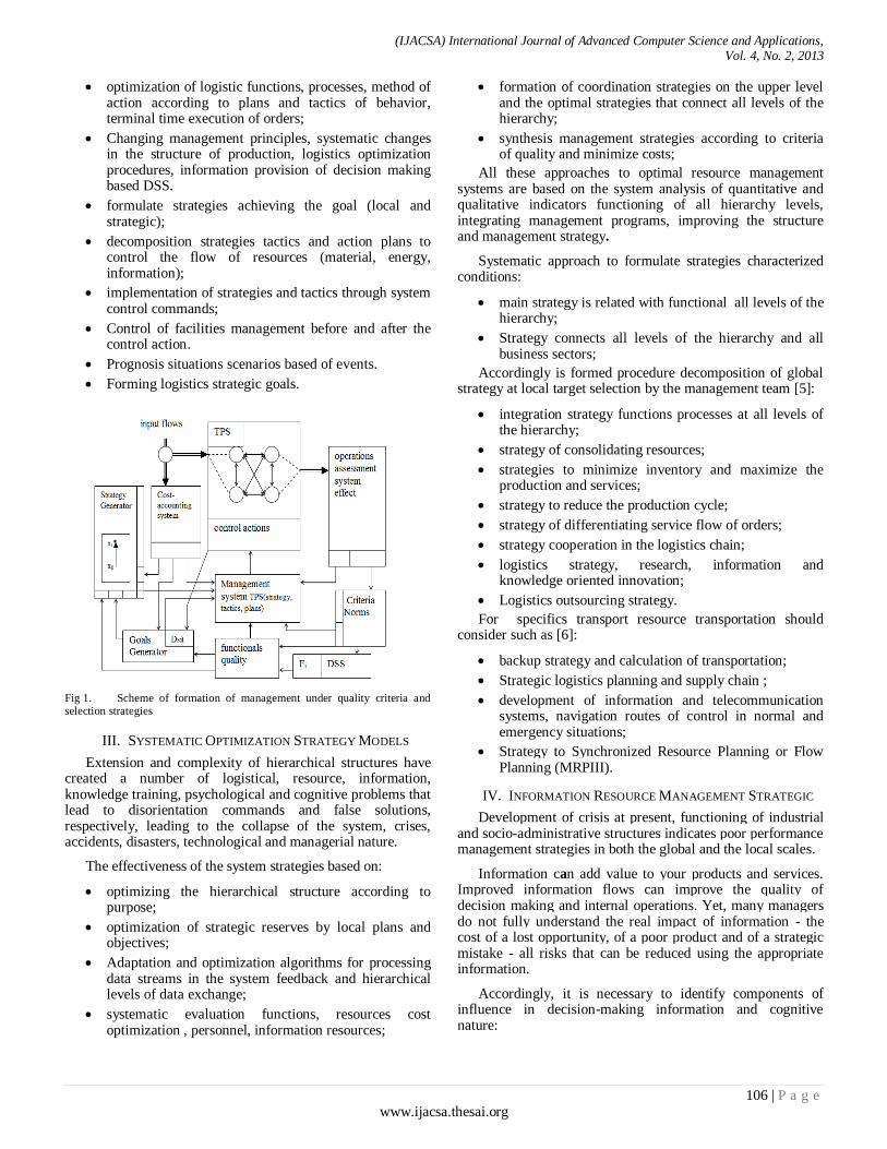
(IJACSA) International Journal of Advanced Computer Science and Applications, Vol. 4, No. 2, 2013
106 | P a g e www.ijacsa.thesai.org
optimization of logistic functions, processes, method of action according to plans and tactics of behavior, terminal time execution of orders;
Changing management principles, systematic changes in the structure of production, logistics optimization procedures, information provision of decision making based DSS.
formulate strategies achieving the goal (local and strategic);
decomposition strategies tactics and action plans to control the flow of resources (material, energy, information);
implementation of strategies and tactics through system control commands;
Control of facilities management before and after the control action.
Prognosis situations scenarios based of events.
Forming logistics strategic goals.
Fig 1. Scheme of formation of management under quality criteria and selection strategies
III. SYSTEMATIC OPTIMIZATION STRATEGY MODELS
Extension and complexity of hierarchical structures have created a number of logistical, resource, information, knowledge training, psychological and cognitive problems that lead to disorientation commands and false solutions, respectively, leading to the collapse of the system, crises, accidents, disasters, technological and managerial nature.
The effectiveness of the system strategies based on:
optimizing the hierarchical structure according to purpose;
optimization of strategic reserves by local plans and objectives;
Adaptation and optimization algorithms for processing data streams in the system feedback and hierarchical levels of data exchange;
systematic evaluation functions, resources cost optimization , personnel, information resources;
formation of coordination strategies on the upper level and the optimal strategies that connect all levels of the hierarchy;
synthesis management strategies according to criteria of quality and minimize costs;
All these approaches to optimal resource management systems are based on the system analysis of quantitative and qualitative indicators functioning of all hierarchy levels, integrating management programs, improving the structure and management strategy.
Systematic approach to formulate strategies characterized conditions:
main strategy is related with functional all levels of the hierarchy;
Strategy connects all levels of the hierarchy and all business sectors;
Accordingly is formed procedure decomposition of global strategy at local target selection by the management team [5]:
integration strategy functions processes at all levels of the hierarchy;
strategy of consolidating resources;
strategies to minimize inventory and maximize the production and services;
strategy to reduce the production cycle;
strategy of differentiating service flow of orders;
strategy cooperation in the logistics chain;
logistics strategy, research, information and knowledge oriented innovation;
Logistics outsourcing strategy.
For specifics transport resource transportation should consider such as [6]:
backup strategy and calculation of transportation;
Strategic logistics planning and supply chain ;
development of information and telecommunication systems, navigation routes of control in normal and emergency situations;
Strategy to Synchronized Resource Planning or Flow Planning (MRPIII).
IV. INFORMATION RESOURCE MANAGEMENT STRATEGIC
Development of crisis at present, functioning of industrial and socio-administrative structures indicates poor performance management strategies in both the global and the local scales.
Information can add value to your products and services. Improved information flows can improve the quality of decision making and internal operations. Yet, many managers do not fully understand the real impact of information - the cost of a lost opportunity, of a poor product and of a strategic mistake - all risks that can be reduced using the appropriate information.
Accordingly, it is necessary to identify components of influence in decision-making information and cognitive nature:

(IJACSA) International Journal of Advanced Computer Science and Applications, Vol. 4, No. 2, 2013
107 | P a g e www.ijacsa.thesai.org
Insufficient training of personnel manager, which leads to misunderstanding content change scenarios of events and incorrect actions.
inability to clearly logically build tactics and action plans under stress, crisis and conflicting situations;
global and local goals conflict and strategies for their implementation;
mobilization of intellectual and information resources through coordination management strategies at all levels of the hierarchy;
Ability to identify critical signs of crisis.
Formulation and subsequent implementation of coordination and sourcing agreement require appropriate conditions [1, 7], which include:
Availability of local and global strategy at all levels of the hierarchy and executions;
changes in the structure of production and transportation systems by logistics strategies;
vertical integration of logistics;
systematic structuring of resource flows and assessment of their dynamics and control;
compliance information systems processing data flow dynamics and dynamic situations in the system with the aim of forming correct states of the situations in the state space, target, terminal;
compliance management strategies tools and hardware and software management system processes in MTC;
Availability of suitably qualified personnel and mental goal-orientation;
presence of a strong base professional and fundamental knowledge;
A computer system supporting decision-making ;
Integration of computer software logistics processes and automated process control based <MRP, DRP, EDI> and <CAD, CAM, CIM, ACU>;
System integration processes for data collection at all levels of the hierarchy and displayed in 3D-space multimedia center operational management resource streams.
General functions of logistics information while preparing control solutions [15]:
organizing a network of communication between customers, suppliers and MTC;
planning operations by tactics and strategy;
Coordination of logistics;
monitoring of resource flows;
control of orders;
monitoring of external systems and evaluation of dynamic situations;
Under this approach, provides effective solutions suitable to the market situations and resources capable of withstanding crises and information attacks and ground creating information networks for the exchange of data flows in the hierarchy of the system and its environment.
V. INTEGRATION OF INFORMATION AND NAVIGATION
CARTOGRAPHIC SYSTEMS
To integrate in this, information systems must comply with the principles of [10]:
coordination of hardware and software modules;
synthesis ICS based deployment phases;
coordination places docking telecommunication and computer networks;
providing structural flexibility of the information system in AMS;
principle of access to information dialogue rules-based priorities;
harmonization of methods and means of data packets transmission;
Information coordination of local and strategic data networks;
Openness functioning ICT networks and satellite navigation systems.
In integrated systems [7] are updated requirements for the operational management of material resource flows, which requires support of parallelism in time material and information flows, the collection, processing and transmission flow and packets in real time based technologies (EDI) and identification (AI) .
An important effect of the functioning of the integrated systems is the ability to manage localized resources stocks selected according to coordinating strategies.
Openness information system for clusters of customers, suppliers, and operational agents helps to create an integrated logistics information system, which is the basis for management the logistics chain flow of resources and information flows for economic calculations. Information Logistics provides the functions of strategic management and coordination [1-8] resource and information flows in the hierarchy of the system connects the logistic chain into a single structure. Accordingly, it is the basis for logistics information structures (LIS).
SIF – System perturbing factors influence (F1…Fn) with stochastic dynamics , (SRV) – sources resources, TOM –technological object management , IMS – Information measuring system , ACS – Automated control system , SP– Storage products and resources ,UR – User resources ,FOsit(τi )– formation of situation state on time τi .
Phase of separation of the logistics activities systems, according to the strategic goals, can isolate building blocks [1-8]:
IACS - Integrated system of automated management;
block collection and storage of information;
block data processing and analysis of the content;
Informative block preparation decisions.
Accordingly, functional blocks of logistics infrastructure can be represented in the form (Fig .3).

(IJACSA) International Journal of Advanced Computer Science and Applications, Vol. 4, No. 2, 2013
108 | P a g e www.ijacsa.thesai.org
Fig 2. Scheme of structuring logistics information management schemes active resources.
VI. COORDINATION STRATEGIES
Coordination strategy is based on the verification of the situation according to the purpose of the system [8]:
the situation in the state space;
the situation in the target area;
the situation in the terminal area;
Evaluation and ranking of object trajectory in the state space;
Assessment coordinates the route and determine the distance to the target;
pattern matching situations in state space, target, terminal and their projection on the route map to determine the degree of approximation to the area of the target state based coordination strategy;
Evaluation criteria for effective routes held by strategic framework of region-based coefficient CV center of mass (center of influence) [5]:
1 1 1 1
[ ] / [ ]i
n m n m
V i i i i i i nT i i i i
optC D M d S M S C
where Di – distance to the i-th client,di – distance to the source resource, М – weight coefficient passengers number, Si – weight of traffic, Cn – normative coefficient, Ti – terminal time.
The optimization of transport cost is based on selected graph model with n-sources and m-sinks with models
m
jj
gn
ii xxij
11 ||
then [9]:
Fig 3. Formation Strategy Coordination
L-
A
L-
NXmin
Xmax
X0Xi
d(xi,xc)
Xc
α
P
Fig 4.
)(1
,
ji xx
ijij xxW
(1)
Where gij – bandwidth arcs, Wj – bandwidth vertices, ξij – flow from хі→xj.
The itinerary which will win at selected flow management strategy is evaluated by the formula [9], based on tree routes [13] :
Fxx Bxx
ijijMR
ji ji
ggSg),( ),(
/1)( (2)
Where F – the set of direct arcs, B - set of reverse arcs.
Optimization of transport cost in the integrity cards routing is based on the procedure of cycle traffic T(zi).

(IJACSA) International Journal of Advanced Computer Science and Applications, Vol. 4, No. 2, 2013
109 | P a g e www.ijacsa.thesai.org
],..1[),(
;
;
1
1
1 1 )(
MNji
Bbbx
Aaax
VxCVn
i
iiij
n
i
iiij
n
i
m
j
zT
ijijzizi
(3)
the performance conditions for volume and cost of each other operations Cij based on the balance of resource flows[12] :
n
i
n
j
ji ba1 1
(4)
To build route systems in cycles T(zk) k=1,e, route traffic based matrix and plan transportation problem arising from strategy traffic flows of resources. Used for that number of methods[16]:
Diagonal, lowest cost, potentials, integer methods [6] and conditionally optimal by criteria time, screen models, dynamic linear programming.
Accordingly problem solving scheduling traffic requires one side coordination sequence operations (logistics) and coordination time (synchronization) based scheduling with complete certainty requirements and objectives defined parameters: execution time of the transport operation, passing, expectations and delay.
Under the influence of factors, perturbation regime change and obtain the stochastic nature of the parameters that are probabilistic. For the duration of the transport, resource transactions have introduced mitigation strategies in the form:
n
i Tji
mijhDi
m
tRTttRStrat1 ,
)),((min]),([
(5)
Where DitR ),( – during the operation with a sequence of
actions ПDi on the terminal cycle Tm according to the plan of
operations. Optimization plan can be performed based on branch and
bound method [14] according to strategy of acceptable choice plan:
DxFxCfCUStrat DiiTiDi ,min),(:)|( (6)
),0(),(,,1,1
psDDDDkiGD ps
k
i
iDOi i
(7)
where D – partition into branches sets of plans targeted functional selection strategies, defined as [11]:
mT
mniiiDi optTdttFtFHtRstrI0
1 ))()...((]),([(
(8)
Where Fi( ) – Local criteria is forming operational decisions.
Then, the coordination task of integer programming, while the chosen management strategy is formed as:
;max)...( 10mT
NFFH (9)
];,1[,)...( 1 NmbFFH mNm (10)
],1[),( NiFQF ii (11)
Qi(F) – area of optimization functional quality.
VII. CONCLUSION
We have proposed models which evaluate the effectiveness of management strategies resource streams in decision making and internal operations in hierarchical distributed systems. Shown that the optimization procedures are formed on the basis of coordination strategies and structuring routes for resource flows are performed by logistic approach to management tasks. in the paper, there have been determined components, formulas and models logistical coordination strategy in optimization of the transport system company. In our future work, we will try to integrate these models into the system but trying to change the weight of each component of these models according to the strategies chosen by the manager. And we will try to integrate the intelligent agent which is necessary to manage all these models. This problem-solution approach of management resource flows is oriented to the developing countries (Asia, Africa, especially Tunisia).
REFERENCES
[1] L .A. Belady and C. J. Evangelisti, "System partitioning and its
measure," The Journal of Systems and Software, vol. 2, pp. 23-29, 1981.
[2] Karnani, A., "Generic Competitive Strategies," Strategic Management Journal, 5, 1985, pp. 367-80.
[3] Rumelt, Richard P., "Towards a Strategic Theory of the Firm," in R. B.
Lamb (ed.), Competitive Strategic Management. Englewood Cliffs, N.J.: Prentice-Hall, 1984, 556-570.
[4] Gabsi Mounir ,Sikora LS ,Model of active Management hierarchical
Systems" (CSIT’2009), 15-17 OCTOBER 2009, LVIV, UKRAINE.
[5] krukovski E.V. logistic. –lviv ,Intelligence-West ,2004 – 416 p.
[6] Simchi-Levi, D., P. Kaminski, and E. Simchi-Levi, 2003, Designing and
Managing the Supply Chain: Concepts, Strategies, and Case Studies, 2nd ed., New York: McGraw-Hill Irwin.
[7] krukovski E.V. Logistics management–Lviv.HNU, 2005. – 684 p.
[8] LS Sikora, Systematology decision making in complex technological
systems– lviv, kamenyar, 1999. – 380.
[9] Christofides N., Graph theory - the algorithmic approach, Moscow, "Mir",1978. – 431 p.
[10] Hu T. programming and flows seyyah - Moscou: Mir, 1974. - 519 p.
[11] Y Phillips, D., Garcia-Diaz A. Methods of analysis of networks -
Moscow: Mir, 1984. - 496 p. [12] Stepanek .J.B., Mathematical programming– .: high school, 1977. – 272
p.
[13] Fomin G.P., Mathematical methods and models in business: – M: the Finance and statistics, 2001. – 544 p.
[14] Karagodova O.O., Kihel V.P., Rojok V.D. operations Research – К.:
ЦУЛ, 2007. – 256 p.
[15] Kukushkin NS Conflicts and compromises - M.: Knowledge, 1986. - 31 p.
[16] Aliev, RA, MI Liberzon Methods and algorithms for the coordination of
industrial control systems - M.: Radio and communication. 1987. - 206.

(IJACSA) International Journal of Advanced Computer Science and Applications, Vol. 4, No. 2, 2013
110 | P a g e www.ijacsa.thesai.org
Modeling and Simulation Multi Motors Web Winding
System
Hachemi Glaoui, Abdeldjebar Hazzab, Bousmaha Bouchiba, Ismaïl Khalil Bousserhane
Laboratory of command, Analysis and Optimization of the Electro-Energizing Systems, Faculty of Sciences and
technology, Béchar University B.P. 417 Béchar, 08000, Algeria
Abstract— Web winding systems allow the operations of
unwinding and rewinding of various products including plastic
films, sheets of paper, sheets, and fabrics. These operations are
necessary for the development and the treatment of these
products. Web winding systems generally consist of the same
machine elements in spite of the diversity of the transported
products. Due to the wide rang variation of the radius and inertia
of the rollers the system dynamic change considerably during the
winding/ unwinding process. Decentralized PI controller for web
tension control and linear speed control are presented in this
paper. The PI control method can be applied easily and is widely
known, it has an important place in control applications.
Simulation results show the effectiveness of the proposed linear
speed and tension controller for web winding multi motors systems.
Keywords- Multi motors web winding system; PI controller;
tension control; linear speed control
I. INTRODUCTION
Many types of materials are manufactured or processed in
the form of a sheet or a web (textile, paper, metal, etc.) which
then couples the processing rolls and the associated motor
drives. The drives are required to work in synchronism to
ensure quality processing and rewinding of the product. Tension is a very important web manufacturing and process
setting. If severe tension variations occur, rupture of the
materiel during processing or degradation of product quality
can occur, resulting into significant economic losses due to
material loss and reduced production rate. Therefore, in order
to minimize the potential for loss, the need arises to adequately
control the tension within a predefined range in a moving web
processing section.
Henceforth, due to their importance in industry, tension
control problems have drawn the attention of many researchers.
One problem is the establishment of a proper mathematical model. In [1], a mathematical model of a web span is
developed, but this model does not predict the tension transfer.
This problem was addressed in [2] and [3], with the
assumption that the strain in the web is very small. However,
the form of the nonlinear and coupling terms in the model are
not always convenient for controller design so that other model
structures, with comparable precision, are desirable. Several
control strategies have been suggested to maintain quality and
reduce sensitivity to external disturbances, including
centralized multivariable control schemes for steel mill
applications [4][5] and an H∞ control strategy to decouple web
velocity and tension [3][6]. Also, for tension regulation in a
web transport system, [7] proposed a control method based on
a unique active disturbance rejection control (ADRC) strategy,
which actively compensates for dynamic changes in the system
and unpredictable external disturbances. In [8] and [9], Port-
Controlled Hamiltonian with Dissipation (PCHD) modeling is
considered to develop stabilization strategies with a physical
interpretation and motivation of the control action, interpreted as the realization of virtual dampers added to the system, which
resulted into a type of dual action controller with velocity
feedback and velocity error feedback terms. Some limited
improvements were obtained in disturbance rejection properties
and robustness with respect to some parameter variations. The
conventional PI control dominates industry, it is simple and
easy to implement [15]. Tuning of PI controllers is intuitive
and is well accepted by practitioners. PIs can at most achieve a
compromise in performance in terms of system response speed
and stability, and this approach becomes insufficient at the
increasingly high web velocities demanded by the industry and
with thin or fragile materials. Nonlinearities that appear at high velocities, disturbance rejection properties and robustness to
some parameter variations must be accounted for by the
controller. A decentralized nonlinear PI controller is proposed
to respond to this demand. The model of the winding system
and in particular the model of the mechanical coupling are
developed and presented in Section 2. Section 3 shows the
controllers design for winding system. Section 4 shows the
Simulation results using Matlab Simulink. Finally, the
conclusion is drawn in Section 5.
II. SYSTEM MODEL
In this system, the motor M1 carries out unreeling and M3 is used to carry out winding, the motor M2 drives two rollers
via gears “to grip” the band (Fig.1). The stage of pinching off
can make it possible to isolate two zones and to create a buffer
zone [8, 9]. The objective of these systems is to maintain the
linear speed constant and to control the tension in the band.
The used motors are five phase induction motors type
which each one is supplied by an inverter voltage controlled
with Pulse Modulation Width (PWM) techniques. A model
based on circuit equivalent equations is generally sufficient in
order to make control synthesis. The electrical dynamic model
of five-phase Y-connected induction motor can be expressed in the d-q synchronously rotating frame as [13]:

(IJACSA) International Journal of Advanced Computer Science and Applications, Vol. 4, No. 2, 2013
111 | P a g e www.ijacsa.thesai.org
lrc
qrdsdrqs
r
m
2
r
qr
r
rdrreqs
r
rmqr
drredr
r
rds
r
rmdr
qsqr2
r
rmrdr
r
mqsr
2
r
msdses
s
qs
dsrqr
r
mdr2
r
rmqsesdsr
2
r
ms
s
ds
T.J
P.
J
f.i.i.
J.L
L.P
dt
d
.L
R.i.
L
R.L
dt
d
..L
Ri.
L
R.L
dt
d
V.L
R.L..
L
Li.R.
L
LRi..L..
L.
1
dt
di
V..L
L.
L
R.Li..L.i.R.
L
LR.
L.
1
dt
di
(1)
Where is the coefficient of dispersion and is given by:
rs
m
LL
L2
1 (2)
The tension model in web transport systems is based on
Hooke’s law, Coulomb’s law, [8, 9] mass conservation law and
the laws of motion for each rotating roll.
A. Hooke’s law
The tension T of an elastic web is function of the web strain
0
0
L
LLESEST
(3)
Where E is the Young modulus, S is the web section, L is
the web length under stress and L0 is the nominal web length
(when no stress is applied).
B. Coulomb’s law
The study of a web tension on a roll can be considered as a
problem of friction between solids, see [8] and [9]. On
Fig. 1. Web Tension On The Roll
The roll, the web tension is constant on a sticking zone of
arc length a and varies on a sliding zone of arc length g (cf.
Fig.1, where Vk(t) is the linear velocity of the roll k). The web
tension between the first contact point of a roll and the first
contact point of the following roll is given by:
)(),( 1 ttx if ax (1.51)
)(
1 )(),( axettx if
gaxa
(1.52)
)(),( 2 ttx if tLxga
(1.53)
Where μ is the friction coefficient, And Lt = a + g
+ L. The tension change occurs on the sliding zone.
The web velocity is equal to the roll velocity on the
sticking zone.
(1.54)
C. Mass conservation law
Consider an element of web of length )1(0 LL
With a weight density ρ, under an unidirectional stress. The
cross section is supposed to be constant. According to the mass
conservation law, the mass of the web remains constant
between the state without stress and the state with stress
00SLSL
1
1
0
(4)
D. Tension model between two consecutive rolls.
The equation of continuity, cf. [8], applied to the web gives:
0)(
x
V
t
(5)
By integrating on the variable x from 0 to Lt (cf. Fig. 1),
taking into account (4), and using the fact that a + g << L, we
obtain
.111 2
2
1
1
2
VVL
dt
d
Therefore:
.)1(1
)1(22
1
2
21
2
VV
dt
dL
(6)
This equation can be simplified by using the approximation
11 21 and
)21)(1(1
)1(21
1
2
2
(7)
And using Hook’s law, we get:
.)2(
)(
1
1111
kkk
kkkkk
k
VVT
VTVVESdt
dTL
(8)
k = 2, 3, 4, 5.
where Lk−1 is the web length between roll k−1 and roll k,

(IJACSA) International Journal of Advanced Computer Science and Applications, Vol. 4, No. 2, 2013
112 | P a g e www.ijacsa.thesai.org
Tk is the tension on the web between roll k−1 and roll k, Vk is
the linear velocity of the web on roll k, Ωk is the rotational
speed of roll k, Rk is the radius of roll k, E is the Young
modulus and S is the web section.
E. Roll velocity calculation
The law of motion can be obtained with a torque balance:
fkkkk
kk CCemTTRdt
Jd
)(
)(1 (9)
Where kkk RV / , is the rotational speed of roll k
kCem is the motor torque (if the roll is driven) and Cf is the
friction torque.
F. Complete model of the five motors system
Fig.2 shows a typical five motors system with winder,
unwinder, and three tractors.
The complete model of this system is given by the
following equations:
.)( 3322233
2 VTVTVVESdt
dTL
.)( 4433344
3 VTVTVVESdt
dTL
.)( 5544455
4 VTVTVVESdt
dTL
(10)
1 11 2 1 1 1
( ( ) )( ) ( ) .em
d J tR t T C f t
dt
.)()()(
22223222
tfCTTR
dt
Jdem
.)()()(
333343
33
tfCTTRdt
Jdem
.)()()(
44445444
tfCTTR
dt
Jdem
Fig. 3. Electrical part of the five drive system
III. CONTROLLER DESIGN
A. Linear speed Controller Design
The speed controller permits to determine the reference
torque, the mechanical equation defined as
sJf
P
C cem
r
(10)
Fig. 2. Simple Web Winding System

(IJACSA) International Journal of Advanced Computer Science and Applications, Vol. 4, No. 2, 2013
113 | P a g e www.ijacsa.thesai.org
The diagram of speed controller as shown below
The parameters of the PI controller is
P
ρJK i
22
(11)
P
fJK c
p
2 (12)
B. Tension Controller Design
The proposed tension controller in the system permits to get
a linear speed of reference in relation with the strength tension. Thus, we can use (8) as follows:
)()(1
11 iiii
i TESVTESVLdt
dT
(13)
While achieving the linearization
)( 11 TESVVa
(14)
The eq (10) become
)(1
iia
i TESVVLdt
dT
(15)
While introducing the anticipatory term ba VUV where
)( iib TESVV then we gets
ULdt
dTi 1
(16)
This equation allows us to define the structure of controller
shows in the Fig 3. Note that this structure contains a
controller, an anticipation term as well as a linearization.
This equation allows us to define the structure of controller
shows in the Fig 5. Note that this structure contains a controller, an anticipation term as well as a linearization.
Where the parameters of the PI controller are
ρLKP
2 (17)
LρKI
22 (18)
In the sequel, the decentralized structure shown on (Fig.4)
will be considered. The control structure is composed of 5 elementary controllers associated respectively to each motor.
The cascade control configuration uses the tension as
primary measurement and velocity as secondary measurement.
The manipulated variable is the torque applied to the motors.
IV. SIMULATION RESULTS
The winding system we modeled is simulated using
MATLAB SIMULINK software and the simulation is carried
out on 10s. To evaluate system performance we carried out
numerical simulations under the following conditions:
Start with the linear velocity of the web of 5m / s.
The motor M1 has the role of Unwinder a roll radius R1
(R1 = 2.25 m).
The motors M2, M3, M4 are the role is to pinch the tape.
The motor M5 has the role of winding a roll of radius R5.
The aims of the STOP block is to stop at the same time the
different motors of the system when a radius adjust to a desired
value (for example R5 = 0.8 m), by injecting a reference speed
zero.
As shown in Fig (5, a b c d e), an improvement of linear
speed, moment of inertia, belt tension, torque, and radius of the
coil, and has follows the reference speed for PI controller after 1 sec, in all motors.
PI
Controller
V1
V1*
Cem1
Fig. 4. Linear Speed Controller
PI
Controller )(
1
1TES
T2
T2*
Vb
V1* +
+
Fig. 1. Tension Controller
Figure.4. Control structure of a winding system (PI)

(IJACSA) International Journal of Advanced Computer Science and Applications, Vol. 4, No. 2, 2013
114 | P a g e www.ijacsa.thesai.org
Fig. 5. a): Simulation results of the first motor
Fig. 5. b): Simulation Results Of The Second Motor
Fig. 5. c): Simulation Results Of The Third motor
Fig. 5. d): Simulation Results Of The Fourth Motor
Fig. 5. e): Simulation Results Of The Fifth Motor
Fig. 6. The Tension Of The Strip

(IJACSA) International Journal of Advanced Computer Science and Applications, Vol. 4, No. 2, 2013
115 | P a g e www.ijacsa.thesai.org
From the figures (6), we can say that: the tension follows
the reference tension with application of PI controller.
It appears clearly that the classical control with PI
controller in linear speed control and tension control offers
better performances in both of the overshoot control and the
tracking error. However is easy to apply.
V. CONCLUSION
The objective of this paper consists in developing a model
of a winding system constituted of five motors that is coupled
mechanically by a strap whose tension is adjustable and to
develop the methods of analysis and synthesis of the
commands robust and their application to synchronize the five
sequences and to maintain a constant mechanical tension
between the rollers of the system.
Computer simulations show the robustness and the
performance of the winding system with the PI controllers,
however PI control dominates industry and it is simple and
easy to implement.
REFERENCES
[1] D. P. Cambell, Process Dynamics, Wiley, 1958, pp.113-156
[2] G. Brandenburg, "New Mathematical Model For Web Tension and
Register Error,» Proceedings of the 3rd IFAC Conference on Instrumentation and Automation in The Paper, Rubber and Plastics, Vol.
1, May 1976, pp 411-438.
[3] H. Koç, D. Knittel, M de Mathelin and G. Abba , "Modeling and Robust Control of Winding Systems for Elastic Webs," IEEE Trans. Contr. Syst.
Technol., Vol. 10, March 2002, pp.197-208.
[4] J.E. Geddes and M. Postlethwaite, "Improvements in Product Quality in Tandem Cold Rolling Using Robust Multivariable Control," IEEE Trans.
Contr. System. Technology. Vol. 6, March 1998, pp. 257-267.
[5] S.H. Jeon, and al., "Decoupling Control of Bridle Rolls for Steel Mill Drive System» IEEE Trans. Ind. Application., Vol. 35, January/February
1999, pp. 119-125.
[6] D. Knittel, and al., "Tension Control for Winding Systems With Two-
Degrees of Freedom H∞ Controllers," IEEE Trans. Ind. Applicat. Syst., Vol. 39, January/February 2003, pp. 113-120.
[7] B.T. Boulter, Y. Hou, Z. Gao and F. Jiang., "Active Disturbance Rejection Control for Web Tension Regulation and Control," IEEE
Conference on Decision and Control, Orlando, USA, December 2001, pp. 4974- 4979.
[8] F. Mokhtari, P. Sicard, and N. Léchevin, "Damping Injection Control of
Winding System Based on controlled Hamiltonian Systems," 12th IFAC Symposium on Automation in Mining, Mineral and Metal Processing
(IFAC MMM’07). Québec, Canada, August 2007, pp. 243-248.
[9] F. Mokhtari, P. Sicard, and N. Léchevin, "Stabilizing Winding Systems by Injection Damping Control Based on controlled Hamiltonian
Systems," Proc. of IEEE International Electric Machines and Drives Conference (IEMDC’07), Antalya, Turquie, May 2007, pp. 95-100.
[10] Bousmaha Bouchiba, Abdeldejbar Hazzab, Hachemi Glaoui, FELLAH
Med-Karim, Ismaïl Khalil Bousserhane “Sliding Mode Speed Control for Multi-Motors System” JAMRIS journal Vol. 4 Nº 3 2010 page 50-54.
[11] Christian Thiffault Pierre Sicard Alain Bouscayrol, “Tension Control
Loop Using A LinearActuator Based On The Energetic Macroscopic Representation”, CCECE 2004- CCGEI 2004, Niagara Falls, May 2004
[12] S. Charlemagne, A. Bouscayrol, Slama Belkhodja, J.P. Hautier, "Flatness
based control of non-linear textile multimachine process", in Proc. of EPE'03, CD-ROM, Toulouse (France), September 2003.
[13] Adlane Benlatreche Dominique Knittel “State Feedback Control with Full or Partial Integral Action for Large Scale Winding Systems” Industry
Applications Conference, 2005. Vol. 2 page(s): 973- 978 Oct 2005
TABLE I. SYSTEM PARAMETERS
E 1.6e8 L1= L2= L3[m] 5
S [m2] 2.75e-3 n [Hz] 50
R1 [m] 1.25 T1ref= T2ref [N] 4
R2=R3 [m] 0.25 V2ref [m/s] 20
J01=J02=
J03[Kg.m2]
0.022 p 2

(IJACSA) International Journal of Advanced Computer Science and Applications, Vol. 4, No. 2, 2013
116 | P a g e www.ijacsa.thesai.org
The Visual Web User Interface Design in Augmented
Reality Technology
Chouyin Hsu
Department of Information Management
Overseas Chinese University
Taichung, Taiwan
Haui-Chih Shiau
Department of Information Technology
Overseas Chinese University
Taichung, Taiwan
Abstract—Upon the popularity of 3C devices, the visual
creatures are all around us, such the online game, touch pad,
video and animation. Therefore, the text-based web page will no
longer satisfy users. With the popularity of webcam, digital
camera, stereoscopic glasses, or head-mounted display, the user
interface becomes more visual and multi-dimensional. For the
consideration of 3D and visual display in the research of web user
interface design, Augmented Reality technology providing the
convenient tools and impressive effects becomes the hot topic.
Augmented Reality effect enables users to represent parts of the
digital objects on top of the physical surroundings. The easy
operation with webcam greatly improving the visual
representation of web pages becomes the interest of our research.
Therefore, we apply Augmented Reality technology for
developing a city tour web site to collect the opinions of users.
Therefore, the website stickiness is an important measurement.
The major tasks of the work include the exploration of
Augmented Reality technology and the evaluation of the outputs
of Augmented Reality. The feedback opinions of users are
valuable references for improving AR application in the work. As
a result, the AR increasing the visual and interactive effects of
web page encourages users to stay longer and more than 80% of
users are willing to return for visiting the website soon. Moreover,
several valuable conclusions about Augmented Reality
technology in web user interface design are also provided for
further practical references.
Keywords- Visual Represeantion; User Interface Design;
Augmented Reality; Google SketchUp
I. INTRODUCTION AND RESEARCH BACKGOUND
With the popularity of webcam, digital camera, stereoscopic glasses, or head-mounted display, the user interface becomes more visual and diverse. It's an interesting time to be working on the visual web user interface now. The web pages evolved from a text-based system to the current rich and interactive medium that supports images, 2D graphics, audio and video. There is no question of the coolness of Augmented Reality Technology. We have seen many world-class brands like Lego, Star Wars, and Avengers commercialize the technology. Many Enterprises start to pursue developing the web sites based on Augmented Reality technology.
It was in the late 60’s that researchers started to describe how and where people interacted with technology. The term ‘augmented reality,’ however, was not coined until the early 90’s, when airplane manufacturer Boeing started using
augmented reality goggles to assist engineers in the airplane assembling process. Recently, Augmented Reality enables you to represent parts of the digital world on top of the physical world. Augmented Reality is a hot topic that is growingly attracting attention of the developers of web user interface. This is sometimes reinforced by the fact that available tools for 3D UIs are toolkits, interface builders, rendering engines, etc. Moreover, rendering skill is mostly used in the work for increasing the visual representation. As a result, the user interaction and visual design in 3D are becoming more and more popular.
The research work increases the visual web page design in Augmented Reality. The purpose is to explore the feasibility of Augmented Reality in web page design. The web page design skill with text-based, image-based, flash-based design is no longer popular. With the extremely increasing new users of online games, the visual effect becomes an important element of web page design since the users are used to the visual representation on the screen. The research work builds a city tour web site in Augmented Reality tasks. We also do the evaluation for collecting the opinions of users for modifying the research direction. Therefore, the research result contains the skillful comments of Augmented Reality tools as well as the practical suggestion for further visual web page design.
II. RELATED WORK
The webcam and mobile phone and diverse devices have led to a complete redesign on the traditional User Interface (UI). There is a new emphasis on intuitive ease of use. Moreover, the development of 3D User Interfaces (UIs) mostly remains an art more than a principled-based approach.
Several methods have been introduced to decompose this life cycle into steps and sub-steps, but these methods rarely provide the design knowledge that should be typically used for achieving each step [1][9][17].
A. Visual User Interface Design
User interface design or user interface engineering is the design of computers, appliances, machines, mobile communication devices, software applications, and websites with the focus on the user's experience and interaction. Web user interface focuses on the web page design to link users and web content.
Visual user interfaces have been regarded as one of the most promising routes. They exploit powerful human vision

(IJACSA) International Journal of Advanced Computer Science and Applications, Vol. 4, No. 2, 2013
117 | P a g e www.ijacsa.thesai.org
and spatial cognition. Carefully designed visual user interfaces can shift the user's mental load from slow reading to faster perceptual processes such as visual pattern recognition. Visual interfaces should support information exploration and bring users’ attention [5][8].
Text-based web page is not suitable for the current modern users. Therefore, visual presentation is an important topic. More visual and interactive web operations are more crucial for web pages. With the stimulation of 3D tools, Augmented Reality tools are used for improving the presentation of web content. Unlike images or video, the user can operate and control the display of web objects. Therefore, more relative research topics become popular.
B. Augmetned Reality
The goal of Augmented Reality is to add information and meaning to a real object or place. The field of Augmented Reality (AR) has existed for just over one decade, but the growth and progress in the past few years has been remarkable. In 1997, the first author published a survey [1][2] and defined the field, described many problems, and summarized the developments up to that point. Since then, the field has grown rapidly.
Fig. 1. The Explanation Of Augmented Reality Effect
Unlike virtual reality, augmented reality does not create a simulation of reality. Instead, it takes a real object or space as the foundation and incorporates technologies that add contextual data to deepen a person’s understanding of the subject, as shown in Figure 1[26]. Many popular applications of AR successfully developed in various fields are explained as follows.
Advertising and marketing: Marketers started to use AR to promote products via interactive AR applications. From Toyota to Nivea to Disney, a diverse array of brands has applied AR bandwagon for creating hype interaction with consumer.
Task support: Complex tasks such as assembly, maintenance, and surgery can be simplified by inserting additional and useful information with AR technology. Some complicated repair works depend on AR information as well. Moreover, some restaurants provide the AR-enabled menu for users to ‘see’ the food first before they enjoy the food.
Product design: AR can simulate planned products, including architecture, machine, car and more objects for better design discussion in advance.
Navigation: AR can create virtual objects in museums and exhibitions, theme park attractions and books. The overlay between real and virtual worlds always makes novel navigation for users.
C. Redering Technique
Rendering is the final process of creating the actual 2D image or animation from the prepared scene. This can be compared to taking a photo or filming the scene after the setup is finished in real life. Several different, and often specialized, rendering methods have been developed. Rendering (computer graphics), generating an image from a model by means of computer programs. Many types of rendering are given as follows:
3D rendering, generating image or motion picture from virtual 3D models.
High dynamic range rendering allows preservation of details that may be lost due to limiting contrast ratios.
Non-photorealistic rendering, focuses on enabling a wide variety of expressive styles for digital art.
Scanline rendering, algorithm for visible surface determination.
Volume rendering, used to display a 2D projection of a 3D discretely sampled data set
Rendering engine has different types. Two major types are explained as follows.
Game engine, system designed for the creation and development of video games.
Web browser engine, software that takes information and displays the formatted content on the screen
D. Evaluation Method
The evaluation for user interface causes many discussions. From the perspectives of usability, the experts “inspect” your interfaces during formative evaluation and widely used in practice. Three major evaluation strategies which are considered to be used in the research are explained as follows:
Heuristic Evaluation - Heuristic evaluations were introduced by Nielsen and Molich in 1990 in the influential paper "Heuristic Evaluation of User Interfaces" and later assembled as part of a book [23][27]. Usability inspection method for computer software that helps to identify usability problems in the user interface (UI) design. It specifically involves evaluators examining the interface and judging its compliance with recognized usability principles (the "heuristics"). An additional practical problem is that multiple usability experts should be used. It can often be more expensive and difficult to find many usability professionals.
Cognitive Walkthroughs - A cognitive walkthrough is also a usability inspection method like heuristic evaluation but the emphasis is on tasks. The idea is basically to identify users' goals, how they attempt them in the interface, then meticulously identify problems

(IJACSA) International Journal of Advanced Computer Science and Applications, Vol. 4, No. 2, 2013
118 | P a g e www.ijacsa.thesai.org
users would have as they learn to use an interface. The method was also introduced at the same conference as Heuristic Evaluation (Lewis et al 1990). The cognitive walkthrough was an extension of earlier work by Polson and Lewis [15].
Pluralistic Walkthroughs - A pluralistic walkthrough is a usability inspection method whereby representative users (normally played by the evaluators), developers and usability experts, step through a scenario, discussing the usability issues associated with each scenario step. Also known as storyboarding, the method involves the development of a series of tasks, presented to a panel of users in the form of hard-copy panels; the panelists are then asked to write down the actions they would take to complete the task [4].
III. RESEARCH FLOW AND IMPLEMENTATION
A. Development Flow
The research development flow containing four phases is explained as follows.
The Concept phase - In the beginning, the concept of visual representation is the first idea. Then, the subject of web has to be decided. Not all the pages are suitable for visual effects. Therefore, the topic of city tour becomes the interesting work.
The Implementation and Content Development phase – Many web design tools and Augmented Reality tool are applied in the phase. Building models, rendering pictures, web page design and Augmented Reality effects are the major efforts in the phase. Google SketcUp and 3D Max are the tools for building models. It is pretty time consuming, but the output is really inspiring and exciting. The well-constructed models are helpful for generating good Augmented Reality effects.
The User Interaction Phase – With the identification card of Augmented Reality, the user can control the representation of Augmented Reality on the screen. The output of real world and virtual objects combing together is really interesting for users.
The Evaluation Phase - Heuristic evaluation is the most popular of the usability inspection methods. Heuristics Evaluations is done prior to and in addition to user-testing, not instead of user-testing. The feedback of evaluation is important for design improvement.
Fig. 2. The research development flow
B. The Augmented Reality Implement and Research Ouput
The index page of the web system is shown in Figure 3. It is the first image of the web to users. According to the opinions of users, the 3D-like, colorful and visual image brings lots of attention and they are attracted to stay on the site. The rendering technique is well applied for the effect. Rendering is the process of generating an image from a model, by means of computer programs. Many rendering software with SketchUp for rendering purposes are provided for different purposes, such light, motion or realism. There are Kerkythea, TrueSpace, Blender, Vue, and Podium are among the most popular rendering applications for SketchUp [28]. The rendering images used for the index page is one of successful designs in the work.
Fig. 3. The index page of the city tour web
Building models and make Augmented Reality effect are two major tasks. Googld Sketch Up and FLARTookit are used in the phases. Google SketchUp is a free, fun, easy-to-use 3D modeling application. Originally created for architects and designers, SketchUp is also a great tool for teaching geometry. FLARToolKit recognize the marker from input image, and calculate its orientation and position in 3D world. FLAToolKit has support for all major flash 3D graphics engine.
In order to explain the different effects of traditional 2D-like picture and 3D-like Augmented Reality technology, an example of the Mid-Lake Pavilion of Taichung Park is given below.
The picture of the Mid-Lake Pavilion shown in Figure 4 displays the ‘real’ outlook of the building. In the other hand, the model of the Pavilion built with Google SketcUp given is given in Figure 5. According to the users’ opinions, they spend more time to look the 3D-like model rather than picture. The model catches users’ eyes immediately after they browse the web. The visual effect works again. We collect many opinions from users for improving the built models and page design.
Furthermore, the user will like to pay more attention to operate the Augmented Reality function. Since the webcam is easy to setup with the PC, the user can easily play with the Augmented Reality card to view the Pavilion model, as shown in Figure 6. The user can control the direction of the identification card to view the model from different angles and directions. With the Augmented Reality operation, the attached introduction information will possibly get the attention of users, as shown in Figure 7. As long as the user read the introduction, the major function of city tour website is herein fulfilled.

(IJACSA) International Journal of Advanced Computer Science and Applications, Vol. 4, No. 2, 2013
119 | P a g e www.ijacsa.thesai.org
Fig. 4. The picture of the Mid-Lake Pavilion of Taichung Park
Fig. 5. The built model of the Mid-Lake Pavilion of Taichung Park
Fig. 6. The AR operation of the Mid-Lake Pavilion of Taichung Park
Fig. 7. The complete introduction web page of the Mid-Lake Pavilion of Taichung Park
Fig. 8. The AR operation of one famous building in Taichung
Fig. 9. The AR operation of the famous department building in Taichung
More famous buildings and parks are introduced with Augmented Reality effect on the web site, as shown in Figure 8 and Figure9. According to users’ opinions, the interesting operation givens they lots of fun. As playing with the Augmented Reality effect, they read lots of introduction pages and know more interesting information about the city.
Another visual example is given as follows. The introduction of famous Taiwan food is also introduced in the website. The example is given in Figure 10 and Figure11. The rending design increases the visual effect of the web page. Most of the users who really like the visual design stay much longer on the webpage for reading the introduction of local famous food.
Fig. 10. The visual representtion of famous Taiwn food

(IJACSA) International Journal of Advanced Computer Science and Applications, Vol. 4, No. 2, 2013
120 | P a g e www.ijacsa.thesai.org
Fig. 11. The AR operation of Taiwan snack
RESEARCH DISCUSSION
To please users is not an easy job, but it is an important for keeping the web stickiness. However, a good web page designer has to rapidly cause the attention of users since web surfers have so much information available to them that they often get bored. In order to keep the user’s attention, new technology is always a good try. Augmented Reality is such popular since the webcam and network become more convenient for PC users. The result is a rich combination of physical and virtual realities to increase the visual representation of web pages. The advantage is helpful for attracting the user’s attention and interest. Therefore, the user stays longer on the page and possibly reads the supplied information on the website.
The first conclusion is that Augmented Reality technology increasing the visual web page design helps to attract the users’ attention and increases the chance for users to read the information on the web pages. The visual representation in Augmented Reality is rapidly in progress currently and will become the main trend of mobile devices in the near future.
The second conclusion is that the 3D models have to be built closely to the real object. Do not cheat users with beautiful but fake models. Moreover, the third conclusion is that the easy operation of Augmented Reality technology is an important issue. Turn on the webcam automatically and shown the Augmented Reality effect quickly can help users continuously to enjoy the Augmented Reality application. Some users will give up since the system asks them to install the webcam or software.
During the research, we found the importance of attention management. Clear and concise graphics are the basic requirement of the web page design. Rendering design is such popular. However, some opinions imply that the 3D-like or visual model is sometimes embellished too much. It is easily cause the disapproval of users.
With Augmented Reality tasks the view of the real world behind the graphical annotations, and the interaction between the graphics and the real world, make Augmented Reality perception qualitatively different from anything previously studied. We will focus on the study of Augmented Reality technology for improving the representation skill. The user opinions are such important to increasing the opportunities of operations and business. Moreover, the application of Augmented Reality with smart phones is also interesting. To
increase the user interactive operations for different experiences is always the research direction in the future.
REFERENCES
[1] R. Azuma, “A Survey of Augmented Reality,” Presence: Teleoperators and Virtual Environments, August 1997, pp. 355–385.
[2] R. Azuma, Y. Baillot, R. Behringer, S. Feiner, S. Julier, and B.
MacIntyre, “Recent advances in augmented reality,” IEEE Computer Graphics and Applications, Vol.21, No.6, 2001, pp.34–47.
[3] D.A. Bowman and R.P. McMahan, “Virtual Reality: How Much
Immersion is Enough?,” IEEE Computer, Vol.40, No.7, 2007, pp.36-43.
[4] R. Bias, “The Pluralistic Usability Walkthrough: Coordinated Empathies,” in J. Nielsen & R. Mack Usability Inspection Methods,
John Wiley, 1994, pp.63-76
[5] K. Börner, and C Chen,. (eds.) Visual Interfaces to Digital Libraries. Springer Verlag, Lecture Notes in Computer Science, Vol. 2539, 2002.
[6] D. Bowman, E. Kruijff, , J. LaViola, and I. Poupyrev, 3D User
Interfaces: Theory and Practice, Addison Wesley, Boston, July 2004.
[7] D. Bowman, J. Chen, C. Wingrave, et al., “New Directions in 3D User
Interfaces,” International Journal of Virtual Reality, Vol.5, No.2, 2006, pp. 3-14.
[8] S. Card, J. Mackinlay, and B. Shneiderman(eds.), Readings in
Information Visualization: Using Vision to Think. Morgan Kaufmann, 1999.
[9] A. Celentano, and F. Pittarello, “A Content Centered Methodology for
Authoring 3D Interactive Worlds for Cultural Heritage,” in D. Bearman, F. Garzotto (eds.), Proc. of Int. Cultural Heritage Informatics Meeting
ICHIM’2001 (Milan, 3-7 September 2001), Cultural Heritage and Technologies in the Third Millennium, Vol. 2, 2001, pp. 315-324.
[10] T. Grossman, D. Wigdor and R. Balakrishnan, “Exploring and reducing
the effects of orientation on text readability in volumetric displays,” ACM CHI, 2007, pp. 483-492.
[11] J. L. Gabbard, J. E. Swan, D. Hix, S.-J. Kim, and G. Fitch, “Active text
drawing styles for outdoor augmented reality: A user-basedstudy and design implications,” Virtual Reality Conference, IEEE, 2007, pp.35–42.
[12] M. Hassenzahl, A. Beu and M. Burmester, “ Engineering Joy,” IEEE
Software, 2001.
[13] T. H¨ollerer, S. Feiner, T. Terauchi, G. Rashid,and D. Hallaway,
“Exploring MARS: Developing indoor and outdoor user interfaces to a mobile augmented reality system,” Computers and Graphics, Vol.23,
No.6, 1999, pp.779–785.
[14] C. Hsu, “The Feasibility of Augmented Reality on Virtual Tourism Website,” The 4th International Conference on Ubi-media Computing,
2011.
[15] C. Lewis, P. Polson, C. Wharton, and J. Rieman, “Testing a walkthrough methodology for theory-based design of walk-up-and-use interfaces,” In
Proceedings of CHI 1990, pp.235-242.
[16] A. Kulik, “Building on Realism and Magic for Designing 3D Interaction Techniques,” In IEEE Computer Graphics & Applications, Vol.29, No.6,
November/December 2009, pp. 22-33.
[17] F Liarokapis, “An augmented Reality Interface for Visualizing and Interacting with Virtual Content,” Virtual Reality, Vol.11, No.1, 2007,
pp. 23-43.
[18] W. Mackay and A. Fayard, “Designing Interactive Paper: Lessons from three Augmented,” Reality Projects, 1999.
[19] P. Milgram, H. Takemura, A. Utsumi, and F. Kishino, “Augmented Reality: A Class of Displays on the Reality-Virtuality Continuum,”
Proceedings of Telemanipulator and Telepresence Technologies, SPIE Vol. 2351, 1994, pp.282-292.
[20] H. Neale, and S. Nichols, “Designing and Developing Virtual
Environments: Methods and Applications,” in Proc. of Visualization and Virtual Environments Community Club VVECC’2001 Workshop,
Designing of Virtual Environments, 2001.
[21] J. Nielsen, and R. Molich, “Heuristic Evaluation of User Interfaces,” In Proceedings of ACM CHI’90 Conference on Human Factors in
Computing Systems, 1990, pp. 249-256.

(IJACSA) International Journal of Advanced Computer Science and Applications, Vol. 4, No. 2, 2013
121 | P a g e www.ijacsa.thesai.org
[22] J. Nielsen, “Heuristic Evaluation”, In Nielsen, J. and Mack, R. L. (Eds.),
Usability Inspection Methods, John Wiley and Sons, New York, 1994, pp. 25-62.
[23] J.-Y. Oh, W. Stuerzlinger and D. Dadgari, “Group Selection Techniques for Efficient 3D Modeling,” In IEEE Symposium on 3D User Interfaces,
2006, pp. 95-102.
[24] M. Rachel, “Augmented Reality Is Finally Getting Real,” Technology Review, 2 August 2012.
[25] F. Steve, “Augmented reality: a long way off?” AR Week. Pocket-lint.
Retrieved 3 March 2011.
[26] J. Vallino, Interactive Augmented Reality, PhD Thesis, Department of Computer Science, University of Rochester, 1998, New York, USA.
[27] C. Wingrave and J. LaViola, “Reflection on the Design and
Implementation of Virtual Environments,” In Special Issue of Presence: Teleoperators and Virtual Environments:Reflections on the Design and
Implementation of Virtual Environment Systems, Vol.19, No.2, 2010.
[28] Google Sketchup, http://www.sketchup.com/product/newin7.html
AUTHORS PROFILE
Chouyin Hsu received the M.S. degree in Computer Science in 1993 from Ohio University, USA and the Ph.D degree in information management in 2006 from National Chiao Tung University, Hsinchu, Taiwan. She is currently an Associate Professor in the Department of Information Management at Overseas Chinese University, Taichung, Taiwan. Her current research interests include Data Mining, Visual User Interface Design, Project Management and Enterprise Resource Planning.
Haui-Chih Shiau received the M.S. degree in Information Management in
2010 from Overseas Chinese University, Taichung, Taiwan. He is currently a second-year graduate student in the Department of Information Technology at Overseas Chinese University Taichung, Taiwan. Her interests include Augmented Reality, 3D Unity, Mobile phone Application.

(IJACSA) International Journal of Advanced Computer Science and Applications,
Vol. 4, No. 2, 2013
122 | P a g e
www.ijacsa.thesai.org
E-Government Grid Services Topology
Based On Province And Population In Indonesia
Ummi Azizah Rachmawati
Faculty of Information Technology
Yarsi University
Jakarta Indonesia
Xue Li
School of ITEE
University of Queensland
Brisbane Australia
Heru Suhartanto
Faculty of Computer Science
University of Indonesia
Depok Indonesia
Abstract— The e-Government Grid Service Model in
Indonesia is an adjustments based on the framework of existing e-Government and also the form of government in the country. Grid-based services for interoperability could be a solution for resource sharing and interoperability of e-Government systems. In previous study, we designed and simulated the topology of Indonesian e-Government Grid services based on function group from e-Government application solution map to connect the ministry/agency/department /institution. In this paper we analyse the result of e-Government services topology simulation based on the province and population in the country.
Keywords— e-Government; Grid Services; e-Government Grid
I. INTRODUCTION
Information and Communication Technologies (ICTs) has been pointed out as fundamental paths towards improving democracy and increasing people’s participation in the decision-making process. It forces government to make new management patterns that related to issues of transparency, accountability, efficiency, effectiveness, service and other public policies in order to respon the community aspiration.
Public management reform is influenced by management progress of ICT, called e-Government (e-Gov) which is the use of information technology to perform activities of government services to the public. It is a permanent commitment made by the government to improve the relationship between the private citizen and the public sector through enhanced, cost-effective, and efficient delivery of services, information and knowledge [1].
Chen, et al [1] proposed that one needs to consider some factors such as History and Culture, Technical Staff, Infrastructures, Citizens and Government officers for studying e-Government of a country. For Indonesian case, these factors are provided in Table I.
In Indonesia, e-Government is needed to support the government change towards a democratic governance practices and to support the application of authority balances between central and local government. Indonesian E-Government is also needed to facilitate communication between central and local governments, to gain openness and transformation towards information society era.
TABLE I. FACTORS FOR STUDYING E-GOVERNMENT IN INDONESIA
Indonesia
History and Culture
Indonesia is a Republic with a presidential system, and a unitary state with power concentrated in the national government.
Since 1945, Indonesia has been struggling with democracy and after reformation in 1998, Indonesia has been experiencing a democratic movement generated in a new political conditions.
Although there are some problems of poverty, health and infrastucture, Worldbank reported as of July 2012, Indonesia’s economy baseline outlook for growth is expected to be 6 percent in 2012 and increase to 6.4 percent in 2013 [2]
Technical Staff
Indonesia has a large number of in-house staff but since there is no policy standard of e-Government implementation, the current staff unable to define specific requirements.
Some provinces in Indonesia have an ability to implement e-Government because of good financial and staff, but others still face some problems to implement it.
Infrastructure
Since Indonesia has more than 17,000 islands and 33 provinces, in some areas with high population like Java island, there are superior current infrastructure and high internet access for employees and citizens, but in remote areas there are inferior current infrasturcture and low internet access for employees and citizens.
Citizens
In a big city like Jakarta, Surabaya and others, there are high Internet access and citizens are trust in online services; many citizens know how to operate computers, but in a small town, there are low Internet access and citizens are reluctant to trust online services; few citizens know how to operate computers
Since Indonesia has a new experience of democracy after 1998 reformation, citizens more actively participate in governmental policy-making process
Government Officers
Indonesia Government reported that in 2012 the number of Internet users in Indonesia significantly increased to 55 million, 25% of population in this country has access to computer and internet as well.

(IJACSA) International Journal of Advanced Computer Science and Applications,
Vol. 4, No. 2, 2013
123 | P a g e
www.ijacsa.thesai.org
Changes are expected to build clean and transparent government which is capable to respond the changes effectively, to build a new dimension into organization, management system and process, and soon to apply the transformation process towards e-Government.
Since Indonesia have not yet implemented Grid technology to conduct e-Government services, we propose the e-Government Grid services topology based on the province and population. A topology of our scenario is a schematic description of the arrangement of a network.
Our proposal will give a new perspective to develop e-Government in Indonesia to achieve a good governance and a clean government. As developing country, the practice of e-Government Grid Services in Indonesia is facing some challenges in particular encountered by government organizational. The application of e-Government Grid Services in the public officials needs to be supported by the policy and employees who understand technology well.
A. E-Government Implementation Strategy
The United States, as the largest developed country, has one of the most advanced e-Government Infrastructures in the world that focuses on increasing effectiveness and efficiency of government work and at the same time, reducing costs [1].
In 2012, US Government launches new Digital Government strategy, entitled “Digital Government: Building a 21st Century Platform to Better Serve the American People”. The Digital Government Strategy sets out to accomplish three things [3]:
1) Enable the American people and an increasingly
mobile workforce to access high-quality digital government
information and services anywhere, anytime, on any device.
For interoperability and openness, modernize our content
publication model, and deliver better, device-agnostic digital
services at a lower cost.
2) Ensure that as the government adjusts to this new
digital world, we seize the opportunity to procure and manage
devices, applications, and data in smart, secure and
affordable ways. Build a sound governance structure for
digital services, and do mobile “right” from the beginning.
3) Unlock the power of government data to spur
innovation across our Nation and improve the quality of
services for the American people. Enable the public,
entrepreneurs, and our own government programs to better
leverage the rich wealth of federal data to pour into
applications and services by ensuring that data is open and
machine-readable by default.
B. E-Government Development Stages
According to the United Nations E-Government Survey in 2012, Indonesia increased its world e-Government ranking from 109 in 2010 into 97 in 2012. It showed that Indonesia have made a tremendous effort to provide e-Government services to its people, despite the challenges faced by the country.
The United Nations Department of Economic and Social Affairs [4] conducted an assessment of e-Government in large countries by evaluating the information services developed by the Government such as websites to provide information on public policy, governance, laws, regulations, relevant documentation and types of government services provided. It is expected that the websites have links to ministries, departments and other branches of government.
The next stage is to asses whether the enhanced information service is available which is expected that the government websites deliver enhanced one-way or simple two-way e-communication between government and citizen. Citizens can download forms for government services and applications. The sites also have audio and video capabilities and are multi-lingual, among others.
The next stage is to asses whether the transactional services engaged in two-way communication between government with their citizens, including requesting and receiving inputs on government policies, programmes, regulations, etc. In this stage, some form of electronic authentication of the citizen’s identity is required to successfully complete the exchange. Government websites process financial and non-financial transactions.
And the last stage of e-Government in large countries is connected service where the government websites have changed the way governments communicate with their citizens from a government-centric to a citizen-centric approach.
C. E-Government in Indonesia
The Indonesian Central Government (called the Government) is the President and its supporting units which holds the power of the government as defined in the Constitution of the Republic of Indonesia Year 1945 [5]. To conduct governance, the Government uses the principle of Desentralisation, Deconsentration and Task Assistance [6]. Government in conducting the government affairs has a relationship with the local governments. This relationship includes the authority relationships, finances, public services, resource utilization, and other resources.
The initiative of e-Government in the country was introduced through President’s Instruction No. 6/2001 dated 24 April 2001 on Telematika (Telecommunication, Media, and Information) which states that government officials should use the technology of Telematika to support good governance and to accelerate democracy process. Furthermore, e-Government should be publicized for different objectives to the governmental offices. Public administration is one of areas in which Internet can be used to provide access for citizens who constitute basic service and to simplify the relations between citizens and government [7].
The initiative is then enhanced by Presidential Instruction No.3 Year 2003 on National Policy and Strategy of e-Government Development. It is an effort to build an electronic-based governance in order to improve the quality of public services effectively and efficiently. E-Government development means that management systems and work processes are reorganized within governmental agencies to optimize the utilization of information technology [8].

(IJACSA) International Journal of Advanced Computer Science and Applications,
Vol. 4, No. 2, 2013
124 | P a g e
www.ijacsa.thesai.org
Some factors to consider for developing e-Government in Indonesia were proposed in[8], they are:
1) Consistently approach to the citizens, businesses,
employees and local government in conducting a business
transaction with the central government.
2) Development a shared strategic vision at all levels to
build e-Government, including the technical architectures.
3) The design of standards-based approach to implement
e-Government
4) Cooperation and collaboration among all parties to
make e-Government policy. There have been various types and specifications of
technology that was implemented by each government agency. Determination to apply a particular technology on e-Government implementation will impact on the investment that has been expent by each agency. This can lead to enormous waste and state financial harm for the whole country. Access, infrastructure and basic applications is the key components to support the implementation of public services portal by information management and processing organization.
As the developing country, Indonesia has some strategic plans to develop e-Government as follows [9]:
1) To develop a good service system with reasonable cost.
The focus are to extend and improve the quality of information
and communication network, to build the information portals
and integrated public services, to build the electronic
document management system, standardization and
information security system;
2) To develop management system of central and local
government. The focus are to improve the quality of services
needed by the community, to manage the changes, to enforce
the leadership and to improve the product of the regulation.
3) To optimize the use of information technology. The
focus are on building the interoperability, standardization and
procedure of electronic document management system,
information security, basic application (e-billing, e-reporting)
and to develop inter government network.
4) To improve the participation of private sector and
information technology industry. The focus are to use the
expertise of the private sector, to encourage participation of
private sector and small industries.
5) To develop manpower capacity in the central and local
government. The objectives are to develop ICT culture in
government institutions, to optimize the use of ICT training
facilities, to extend the use of ICT for distant learning, and to
put ICT as input for school curriculum and to improve the
quality of teaching. Data and information integration is important among
government agencies in Indonesia. It needs to formulate methods and technology of collaboration. The requirements of a broader and comprehensive data interaction among government agencies, especially in the use of data and information together should be encouraged.
Interoperability concepts and strategies are crutial agenda of the national e-Government development to achieve
integrated, safe and efficient utilization of data and information. Interoperability is defined as system ability to share and integrate information and work processes using a set of standards. One of solutions to the interoperability problem is using Grid technology. Open grid services aim for the integration of services across distributed and heterogeneous virtual organizations with disparate resources and relationships [10].
E-Government interoperability can be addressed using a cross-organizational workflow [11][12][13][14] and semantic web or semantic driven [15][16][17].
Yang, et al [18] proposed a service-grid-based framework for Shanghai e-Government interoperability, named eGov Grid, which targets at facilitating among "horizontal" organizations and interoperability among "vertical" e-Government subsystems. Hereinafter, "horizontal" means cross-organizational application, and "vertical" means information system within one organization. According to Yang, et al [18], service grid [19] is a kind of combination of grid computing [20] and SOA technology, open up a new way for cross-organizational resources integrating and collaboration in e-Government. Service grid technologies can be used to build the platform resource sharing in e-Government system, and also bring new feature of better reusability, flexibility and scalability.
II. DESIGN AND SIMULATION OF E-GOVERNMENT GRID
SERVICES IN INDONESIA
Grid has proven resolve the problem of resources sharing on information that placed separately and dynamic including the sharing of data structures, databases, computational resources, storage resources, and other information using open-standard protocols. The use of open-source to meet the requirement of the e-Government that have already designed a set of middleware to support the E-government applications is necessary and it can reduce the cost of the government and fully utilize the IT resources existing in the government [21].
There have been various types and specifications of technology that was implemented by each government agency. Determination to apply a particular technology on e-Government implementation will impact on the investment that has been expended by each agency. This can lead to enormous waste and state financial harm for the whole country. Access, infrastructure and basic application is the key components to support the implementation of public services portal by information management and processing organization. We have proposed a function group based of Indonesian e-Government services topology as the result of the simulation using three different types of scenarios to see whether the effects of the formation or hierarchy of links and router configurations–which connect the ministry / agency / department / institution that have functions to serve the public/citizens (G2C), business groups (G2B), inter-agencies (G2G) and services to employees (G2E). Indonesia requires major infrastructure development hence a great amount of investment. The separation of basic application and function application make the interoperability processes easier because specific services are made in cluster. The division of the

(IJACSA) International Journal of Advanced Computer Science and Applications,
Vol. 4, No. 2, 2013
125 | P a g e
www.ijacsa.thesai.org
application also influences the development of e-Government Grid Services independently and gradually [22].
In this paper, we simulate scenarios based on province and population in Indonesia. Our topology and scenarios follow that of Suhartanto, et al [23] with some modification for e-Government purpose. In our topology, we considered the government of Indonesia data consisting of 33 provinces, 370 regencies and 95 municipals [24] and also the number of population of each province based on results of 2010 population cencus by Indonesian Statistics Office [25]. Although the Minister of Internal Affairs of Indonesia said the moratorium or suspend the expansion area will be in place until the end of 2012 but in fact, at October 22, the parliament of Indonesia and the Government agreed for the addition of new province in Indonesia, that is North Kalimantan which is the division of the province of East Kalimantan. It will take 3-5 years for the preparation of new province infrastructures, so we used the number of province that has been in operation and have an administrative service to the citizens.
These are given details in the Table II.
To evaluate and analyze the performance of a Grid system topology, the experiment must be repeatable and controlled. It will be hard to conduct heterogeneous and dynamic Grid system. In addition developing environment for testing Grid systems is very limited, expensive and time consuming and it also should handle administration different policy on each resource. Thus, it needs a simulation to study the behavior of Grid system and implement some complex scenarios to see the behavior of the system. Simulations can be performed on a single computer so that the cost, time of development and other barriers can be overcome. As our previous works, In the simulation, we also used GridSim of Buyya and Murshed [26].
We design the simulation that consists of three scenarios based on various configurations of the router and link connections. We use three different types of scenarios to see whether the effects of the formation or hierarchy of links and router configurations–which connect the province grouped by island and region. Simulations are performed using three scenarios based on the link connectivity and router configurations hierarchically to determine the effect of the configuration of the links and routers that are connected. The three scenarios will show the shortest processing time in the grid services. We use FIFO (First In First Out) scheduling algorithm and SCFQ (Self-cCocked Fair Queuing) scheduling algorithm.
A. First Scenario
The first scenario divides the country into three region according to its time division, namely west Indonesia consisting of Sumatera and Java islands, central Indonesia consisting of Kalimantan, Sulawesi, Bali and Lombok Islands, and east Indonesia consisting of Maluku and Papua islands. The scenario involves three types of routers that are configured hierarchically which consist of leaf routers, edge routers and core routers. The leaf router is a router that is connected directly to hosts on the network.
TABLE II. PROVINCE AND POPULATION IN INDONESIA
o Province Reg
ency Muni
cipal Populat
ion
1 Nanggroe Aceh
Darussalam 18 5
4,494,410
2 Sumatera Utara 21 7
12,982,204
3 Sumatera Barat 12 7
4,846,909
4 Riau 9 2
5,538,367
5 Jambi 9 1
3,092,265
6 Sumatera Selatan 11 4
7,450,394
7 Bengkulu 8 1
1,715,518
8 Lampung 9 2
7,608,405
9 Kep. Bangka
Belitung 6 1
1,223,296
10 Kepulauan Riau 4 2
1,679,163
11 DKI Jakarta 1 5
9,607,787
12 Jawa Barat 17 9
43,053,732
13 Jawa Tengah 29 6
32,382,657
14 Daista Yogyakarta 4 1
3,457,491
15 Jawa Timur 29 9
37,476,757
16 Banten 4 3
10,632,166
17 Bali 8 1
3,890,757
18 Nusa Tenggara
Barat 7 2
4,500,212
19 Nusa Tenggara
Timur 19 1
4,683,827
20 Kalimantan Barat 12 2
4,395,983
21 Kalimantan
Tengah 13 1
2,212,089
22 Kalimantan
Selatan 11 2
3,626,616
23 Kalimantan Timur 10 4
3,553,143
24 Sulawesi Utara 9 4
2,270,596
25 Sulawesi Tengah 9 1
2,635,009
26 Sulawesi Selatan 20 3 8,034,7

(IJACSA) International Journal of Advanced Computer Science and Applications,
Vol. 4, No. 2, 2013
126 | P a g e
www.ijacsa.thesai.org
76
27 Sulawesi Tenggara 10 2
2,232,586
28 Gorontalo 5 1
1,040,164
29 Sulawesi Barat 5 -
1,158,651
30 Maluku 7 2
1,533,087
31 Maluku Utara 6 2
1,038,087
32 Papua 20 1
2,833,381
33 Papua Barat 8 1 760,442
A host can be either a user's computer or resources on the Grid system and the function of the leaf router is to handle packets movements into or out of the host. The leaf routers are connected by an edge router that is situated in a central core router. A central core router is a router in the core network and serves the whole sub-network into a single large network. A baud rate for a link that connects a whole host with leaf router is set at 10 Mbps (megabits per second), while the baud rate for a link that connects the leaf router with edge router is set at 100 Mbps and the baud rate for the a link that connects all the edge router with central router is set at 1 Gbps (gigabit per second) because edge router have a function to forward packets in between networks. Core routers due to their role as internet backbone routers, support multiple telecommunication interfaces with high data throughput. A baud rate for link among core router is set at 500 Mbps.
Fig. 1 shows the network topology for the first scenario.
Central Core
Router
Sumatera Edge
Router
Sulawesi Edge
Router
Bali NTB NTT
Edge Router
Sumatera Leaf
Router
User
Banda Aceh
Server
Lampung
Server
User
10 Mbps
100 Mbps
1 Gbps
10
Mbps
10 Mbps
10
Mbps
1 Gbps
1 Gbps
1 Gbps
PROVINCE BASED
SCENARIO 1
Maluku
Egde Router
Kalimantan
Edge Router
User
Jakarta Server
User
10 Mbps
10 Mbps
10 Mbps
10 Mbps
East Java
Server
Java
Edge Router
Papua
Edge Router
PapuaLeaf
Router
UserUser
10 Mbps
10
Mbps
10
Mbps10
Mbps
Bali NTB NTT
Leaf Router
User
User
10 Mbps
Maluku Server
10
Mbps
10
Mbps
10 Mbps
Maluku Utara
Server
Papua
Server
Maluku
Leaf Router
Kalimantan
Leaf RouterSulawesi Leaf
Router
North Sulawesi
Server South Sulawesi
Server
10
Mbps
10 Mbps10
Mbps
10
Mbps
User
User
Central Kalimantan
Server
South
Kalimantan
Server
10 Mbps10
Mbps
10
Mbps
User
User
100 Mbps
100 Mbps
100 Mbps
100 Mbps
1 Gbps
1 Gbps
User
Bali Server
NTB Server
NTT Server
User
100 Mbps
10
Mbps10
Mbps
10
Mbps
10
Mbps10
Mbps10
Mbps Papua Barat
Server
Java
Leaf Router
100 Mbps
1 Gbps
West Core
Router
East Core
Router
500 Mbps
500 Mbps500 Mbps
Fig. 1. First Scenario
B. Second Scenario
The second scenario is almost similar to the first scenario. The difference is that this scenario involve two types of routers, they are leaf routers and edge routers which configured hierarchically. The leaf routers are connecting the hosts to edge router and all the edge routers are connected by high-speed network between routers. A baud rate for a link that connects all hosts with leaf router is set at 10 Mbps. A leaf router is responsible to gather group information. While the baud rate
for link that connects leaf router with edge router is set at 100 Mbps and the baud rate for link that connects edge router is set at 1 Gbps so that the edge router can forward packets in between networks faster.
Fig. 2 shows the network topology for the second scenario.
C. Third Scenario
The third scenario represents the whole province of the government structure. In this scenario, each province group by

(IJACSA) International Journal of Advanced Computer Science and Applications,
Vol. 4, No. 2, 2013
127 | P a g e
www.ijacsa.thesai.org
island/archipelago that coordinated by leaf router. The leaf router will receive the first packets from each province and gathering information from group. All the leaf routers are
connected by services with high-speed network among routers. Baud rate for link among leaf router is set at 100 Mbps.
Fig. 3 shows the network topology for the third scenario.
Sumatera Edge
Router Sulawesi Edge
Router
Bali NTB NTT
Edge Router
Sumatera Leaf
Router
User
Banda Aceh
Server
Lampung
Server
User
10 Mbps
100 Mbps
1 Gbps
10
Mbps
10 Mbps
10
Mbps
1 Gbps
1 Gbps
1 Gbps
PROVINCE BASED
SCENARIO 2
Maluku
Egde Router
Kalimantan
Edge Router
User
Jakarta Server
User
10 Mbps
10 Mbps
10 Mbps
10 Mbps
East Java
Server
Java
Edge Router
Papua
Edge Router
PapuaLeaf
Router
UserUser
10 Mbps
10
Mbps
10
Mbps10
Mbps
Bali NTB NTT
Leaf Router
User
User
10 Mbps
Maluku Server
10
Mbps
10
Mbps
10 Mbps
Maluku Utara
Server
Papua
Server
Maluku
Leaf Router
Kalimantan
Leaf RouterSulawesi Leaf
Router
North Sulawesi
Server South Sulawesi
Server
10
Mbps
10 Mbps
10
Mbps
10
Mbps
User
User
Central Kalimantan
Server
South
Kalimantan
Server
10 Mbps10
Mbps
10
Mbps
User
User
100 Mbps
100 Mbps
100 Mbps
100 Mbps
1 Gbps
1 Gbps
1 Gbps
User
Bali Server
NTB Server
NTT Server
User
100 Mbps
10
Mbps
10
Mbps
10
Mbps
10
Mbps10
Mbps10
Mbps Papua Barat
Server
Java
Leaf Router
100 Mbps
Fig. 2. Second Scenario
Sumatera Leaf
Router
User
Banda Aceh
Server
Lampung
Server
User
10 Mbps100 Mbps
10
Mbps
10 Mbps
10
Mbps
PROVINCE BASED
SCENARIO 3
User
Jakarta Server
User
10 Mbps
10 Mbps
10 Mbps
10 Mbps
East Java
Server
PapuaLeaf
Router
UserUser
10 Mbps
10
Mbps
10
Mbps10
Mbps
Bali NTB NTT
Leaf Router
User
User
10 Mbps
Maluku Server
10
Mbps
10
Mbps
10 Mbps
Maluku Utara
Server
Papua
Server
Maluku
Leaf Router
Kalimantan
Leaf Router Sulawesi Leaf
Router
North Sulawesi
Server South Sulawesi
Server
10
Mbps
10 Mbps
10
Mbps
10
Mbps
User
User
Central Kalimantan
Server
South
Kalimantan
Server
10 Mbps10
Mbps
10
Mbps
User
User
100 Mbps
100 Mbps
100 Mbps
100 Mbps
User
Bali Server
NTB Server
NTT Server
User
100 Mbps
10
Mbps
10
Mbps
10
Mbps
10
Mbps10
Mbps10
Mbps Papua Barat
Server
Java
Leaf Router
100 Mbps
Fig. 3. Third Scenario

(IJACSA) International Journal of Advanced Computer Science and Applications,
Vol. 4, No. 2, 2013
128 | P a g e
www.ijacsa.thesai.org
D. Result
We define three samples which based on three types of how the numbers of users are in each province where the total number of users in the country is set the same. In the first simulation, we assume that there is one user in each regency and municipal in each province and we label the sample as DS0. In the second simulation sample, DS1, we define the number of users in each province is proportional with the number of population in the province, however the total number of users in the country are the total number of users in DS0. Thus in each province the number of users is given as:
u = p/t x nd0 (1)
where:
u = number of user in each province
p = number of population in each province
t = total population in the country
nd0 = number of users of DS0
And for the third simulation, DS3, we use same number of users at each province as:
u = nd0 /np (2)
where:
u = number of user
nd0 = number of users of DS0
np = number of province
We round the number of users in each province in DS0, DS1 and DS2 to the nearest integer. Fig. 4 describes these samples:
Fig. 4. Number of users in each province based on various sample type
In each simulation using the above three scenarios S1, S2, and S3, and two algorithms FIFO and SCFQ, we introduce three Gridlets which define jobs in GridSim sent by each user successively to a resource and the resource will give a sign which Gridlet is ready to be processed. The computing time in each province is defined to be the average of these three
Gridlets response time, and the average computing time in the country is defined as the average computing time from all computing time in the provinces. The results are given in the Table III.
Where S1FIFO indicates the first scenario using FIFO algorithm, S1SCFQ indicates the first scenario using SCFQ, the same meaning applies to S2FIFO, S2SCFQ, S3FIFO, and S3SCFQ. Fig. 5 shows in general that sample DS1 is the most efficient one compared with DS0 and DS2.
Fig. 5. Result comparison of DS0, DS1, DS2
The results above show that Scenario 1 using SCFQ algorithm in DS1 gives the best processing time and Scenario 3 using FIFO algorithm in DS2 gives the worst processing time.
Scenario 1 using SCFQ scheduling algorithm in DS1 tends to make packet lifetime in routers with crowded traffic becomes shorter. As we see that more than 70% of population in Indonesia is in Java Island which is use West Core Router. Packet lifetime shows the difference between the enqueuing and dequeuing time of packets. This is because there are packet priority settings where the packets with higher priority will be served first, so the overall packet lifetime will be reduced. SCFQ algorithm can provide differentiated services for data traffics by changing the weight associated with traffic classes. The higher the weight of a traffic class, the better treatment of the class. Treatment here means the wider bandwidth allocation (bandwidth) so that the execution time would be smaller.
Scenario 3 using FIFO algorithm in DS2 gives the worst processing time because packet lifetime is higher. In FIFO mechanism, all packets are enqueued at the end of a queue, and the first packet located in the beginning of the queue will be dequeued first. The packets are unordered and no differentiated service will be provided.
The data above can be analyzed that in the development of e-Government Grid services in Indonesia using FIFO (First In First Out) scheduling algorithm, then the most suitable is the topology that allows data packets having a low number of hops. In this simulation, network with the lowest number of hops seen in the third scenario of DS1 using the population comparison as the number of user in each province.
0
20
40
60
80
100
1 4 7 10 13 16 19 22 25 28 31
DS0
DS1
DS2
225
230
235
240
245
250
255
260
S1FIFO S1SCFQ S2FIFO S2SCFQ S3FIFO S3SCFQ
DS0
DS1
DS2

(IJACSA) International Journal of Advanced Computer Science and Applications,
Vol. 4, No. 2, 2013
129 | P a g e
www.ijacsa.thesai.org
TABLE III. RESULT OF THE SIMULATION
Scenario
Simulation S1FIFO S1SCFQ S2FIFO S2SCFQ S3FIFO S3SCFQ
DS0 252.23357 247.72993 248.76200 252.34099 248.45325 251.00456
DS1 244.60348 237.48944 246.93003 251.68368 237.95047 240.34692
DS2 253.70659 241.51920 247.14717 241.07650 255.08733 253.06667
If using SCFQ (Self-Clocked Fair Queuing) scheduling algorithm, then the most suitable is the topology that makes the data packets with the same priority has small possibility to meet each other in a single router or link. In this simulation, topology that meet this condition is a topology on the first scenario of DS1 using the population comparison as the number of user in each province.
And we can see that DS1 give the best performance. So we can say that the most suitable for Grid topology in Indonesia is using the number of population comparison as the number of user in each province.
III. CONCLUSION
The research aim at modelling an e-Government Grid in Indonesia by performing a simulation using GridSim toolkit that is based on the Java programming language. Simulations carried out by testing three different types of topologies in terms of link and router configuration with FIFO and SCFQ algorithms and three types of number of users based on the province, population and same number of users in each province. The result is the average time processing that is used to obtain the most effective topology for each scheduling algorithm.
From the simulation results can be concluded that the SCFQ scheduling algorithm tends to create packets lifetime in the router with heavy traffic becomes shorter. Packet lifetime is the time of packet in the queue or the time difference between time the packet is enter into the queue and time the packet is out of the queue. It is due to packet priority setting where high-priority packet will be prioritized so that the overall packet lifetime will be reduced.
The proposed Grid arhitecture in this paper will be used as inputs for providing e-Government services and its implementation on a Cloud platform for the best performance. Comparing Grid services to Cloud services, we can see that Grid is about performance and Cloud is about scalability. In our next work, we will model the country e-Government Grid services based on Cloud Computing to test the scalability of the Grid system driven by economical scale considering some factors in existing practices done by the government.
ACKNOWLEDGMENT
Part of this works was done during the first author visit to School of ITEE-UQ in 2012 under the support of Indonesian Ministry of Education and Culture, Directorate General of Higher Education’s Sandwich Like grants No. 2954.6/E4.4/2012.
REFERENCES
[1] Y. Chen, HM. Chen, RKH. Ching, WW. Huang, “Electronic Government Implementation: A Comparison between Developed and Developing Countries”, International Journal of Electronic Government Research, Volume 3, Issue 2, 45-61, April-June 2007
[2] The World Bank, Indonesia Overview, Retrieved December 10, 2012, from http://www.worldbank.org/en/country/ indonesia/overview.
[3] Office of Management and Budget (OMB) and General Services Administration (GSA) US, “Digital Government: Building A 21st Century Platform to Better Serve The American People”, Retrieved December 20, 2012, from http://www.whitehouse.gov/digitalgov html5.
[4] United Nations, “E-Government Survey 2012: E-Government for the People”, Retrieved December 22, 2012, from http://www2.unpan.org/ egovkb/global_reports/12report.htm
[5] The 1945 Constitution of The Republic of Indonesia
[6] Law of The Republic of Indonesia No. 32/2004
[7] President Instruction No. 6/2001 dated 24 April 2001 on Telematika (Telecommunication, Media, and Information)
[8] President Instruction No. 3/2003 about National Policy and Strategy of E-Government.
[9] Blue Print National Information System (SISFONAS), Ministry of Communication and Informatics of Republic Indonesia (KOMINFO), Indonesia, 2004.
[10] V. Silva, Grid Computing for Developers, Charles River Media, Hingham, Massachusetts, 2005.
[11] D. Gouscos, G. Mentzas, and P. Georgiadis, “PASSPORT: A Novel Architectural Model for the Provision of Seamless Cross-Border e-Govemment Services”, In Proceeding of 12th International Conference on Database and Expert Systems Applications (DEXA 2001), Munich, IEEE Computer Society Press, September 2001, pp. 318-322.
[12] D. Verginadis, D. Gousco, M. Legal, G. Mentzas, “An Architecture for Integrating. Heterogeneous Administrative Services, into One-Stop e-Government, the eChallenges”, In Proceeding of Conference, Bologna 2003.
[13] E. Loukis and S. Kokolaki, “Computer Supported Collaboration in citizens Sector: The ICTE-PAN Project”, In Proceeding of EGOV 2003, LNCS 2739, 2003, pp. 181-186.
[14] D. Gouscos, G. Laskaridis, D. Lioulias, G. Mentzas, and P. Georgiadis, “An Approach to Offering One-Stop e-Government Services: Available Technologies and Architectural Issues”,In Proceeding of e-Government: State of the Art and Perspectives Conference (EGOV 2002), Aix-en-Provence, September 2002.
[15] R. Klischewski, “Semantic Web for e-Govemment”, In Proceedings of EGOV2003.
[16] L. Sabucedo and L. Rif, “A Proposal for a Semantic-Driven eGovernment Service Architecture”, In Proceeding of EGOV 2005, LNCS 3591, pp. 237-248, 2005.
[17] M. Jarvenpaa, M. Virtanen, A. Salminen, “Semantic Portal for LegislativeInformation”, In Proceeding of EGOV 2006, LNCS 4084, 2006, pp. 219-230,
[18] D. Yang, Y. Han, and J. Xiong, “eGov Grid: A Service-Grid-Based Framework for E-Government Interoperability”, in IFIP International Federation for Information Processing, Volume 252, Integration and Innovation Orient to E-Society Volume 2, eds. Wang, W., (Boston: Springer), 2007, pp. 364-372.

(IJACSA) International Journal of Advanced Computer Science and Applications,
Vol. 4, No. 2, 2013
130 | P a g e
www.ijacsa.thesai.org
[19] JB. Weissman and BD. Lee, “The Service Grid: Supporting Scalable Heterogeneous Services in Wide-Area Networks”, In Proceeding of Symp. Applications and the Internet, San Diego, CA, 2001: p. 95-104.
[20] I. Foster, C. Kesselman, and S. Tuecke, “The Anatomy of the Grid: Enabling Scalable Virtual Departments”, International Journal of Supercomputer Applications, 2001. 15(3)
[21] UA. Rachmawati, DI. Sensuse and H. Suhartanto, “Initial Model of Indonesian e-Government Grid Services Topology”, International Journal of Computer Theory and Engineering, Vol. 4, No. 4, August 2012.
[22] UA. Rachmawati, H. Suhartanto and DI. Sensuse, “Function Group Based of indonesian e-Government Grid Services Topology”, International Journal of Computer Science Issues, Vol. 9, Issue 2, No 2, March 2012.
[23] H. Suhartanto, IB. Nugroho and A. Herdiani, “Province Based Design and Simulation of Indonesian Education Grid Topology”, International Journal of Computer Science Issues, Vol. 9, Issue 1, No 2, January 2012.
[24] Directorate Generale of Population and Civil Registration, Ministry of Internal Affairs, Republic of Indonesia, 2012.
[25] Statics Indonesia, 2010 Population Cencus, Retrieved September 20, 2012, from http://bps.go.id.
[26] R. Buyya and M. Murshed, “Gridsim: A toolkit for the modeling and simulation of distributed management and scheduling for Grid computing”, The Journal of Concurrency and Computation: Practice and Experience 14, 2002, pp. 13-15.
AUTHORS’ PROFILE
Ummi Azizah Rachmawati holds B.Sc. from Informatics Engineering, Sepuluh Nopember Institute of Technology in 2000 and holds M.Sc. from Magister of Information Technology, University of Indonesia in 2003. She is currently a student of Doctoral Program, Department of Computer Science, University of Indonesia and an academic and research staff of Faculty of Information Technology, Yarsi University, Jakarta, Indonesia. She has won some research grants on e-Commerce, e-Leaning and e-Government.
Xue Li is an Associate Professor in the School of Information Technology and Electrical Engineering at the University of Queensland, Brisbane Australia. He obtained the Ph.D degree in Information Systems from Queensland University of Technology, Australia in 1997. He is also an Adjunct Professor of University of Electronic Science and Technology, China and a Guest Professor of Chongqing University. His major areas of research interest and expertise include Data Mining, Multimedia Data Security, Database Systems, and Intelligent Web Information Systems. He is a member of ACM, IEEE, and SIGKDD.
Heru Suhartanto is a Professor in Faculty of Computer Science, Universitas Indonesia (Fasilkom UI). He has been with Fasilkom UI since 1986. Previously he held some positions such as Post doctoral fellow at Advanced Computational Modelling Centre, the University of Queensland, Australia in 1998 – 2000; two periods vice Dean for General Affair at Fasilkom UI since 2000. He graduated from undergraduate study at Department of Mathematics, UI in 1986. He holds Master of Science, from Department of Computer Science, The University of Toronto, Canada since 1990. He also holds Ph.D in Parallel Computing from Department of Mathematics, The University of Queensland since 1998. His main research interests are Numerical, Parallel, Cloud and Grid computing.

(IJACSA) International Journal of Advanced Computer Science and Applications,
Vol. 4, No. 2, 2013
131 | P a g e
www.ijacsa.thesai.org
Performance Comparison of DCT and Walsh
Transforms for Watermarking using DWT-SVD
Dr. H. B. Kekre
Senior Professor
Computer Engineering Department
SVKM’s NMIMS (Deemed to be
University), Vileparle, Mumbai,
Dr. Tanuja Sarode
Associate Professor
Computer Department,
Thadomal Shahani Engg. College,
Bandra, Mumbai 50, India
Shachi Natu
Assistant Professor,
Information Technology Department
Thadomal Shahani Engg. College
Bandra, Mumbai 50, India
Abstract—This paper presents a DWT-DCT-SVD based
hybrid watermarking method for color images. Robustness is
achieved by applying DCT to specific wavelet sub-bands and then
factorizing each quadrant of frequency sub-band using singular
value decomposition. Watermark is embedded in host image by
modifying singular values of host image. Performance of this
technique is then compared by replacing DCT by Walsh in above
combination. Walsh results in computationally faster method and
acceptable performance. Imperceptibility of method is tested by
embedding watermark in HL2, HH2 and HH1 frequency sub-
bands. Embedding watermark in HH1 proves to be more robust
and imperceptible than using HL2 and HH2 sub-bands.
Keywords—Discrete Wavelet Transform (DWT); Discrete
Cosine Transform (DCT); Singular Value Decomposition (SVD);
watermarking.
I. INTRODUCTION
Advancement in technology has resulted in use of digital data which includes text, images, audio, video and multimedia data. Technology has also made it easy to duplicate/manipulate the contents of these data by various means. Piracy is a very good example of this. Thus authentication of data becomes obvious requirement before it is made available as digital data. Authentication includes information of owner of data within data itself to avoid taking undue credit as well as to prevent tampering of data. Digital watermarking is one of the most popular techniques used for digital data authentication.
Watermark is secret information which is embedded into a digital signal. Digital signal into which watermark is embedded is called as host signal or cover signal. Host signal can be text, image, audio or video data. Depending on the type of host signal, watermarking is classified as text watermarking, image watermarking, audio watermarking and video watermarking[1]. Image watermarking can be further classified into transform domain watermarking and spatial domain watermarking based on how the watermark is embedded into an image. Transform domain watermarking is one in which image is first transformed using appropriate transformation technique and then watermark is embedded into transformed coefficients of image. Spatial domain watermarking refers to directly modifying pixel values of an image to embed watermark into it. Transform domain watermarking is complex as compared to spatial domain
watermarking but it is more robust also. Watermarking technique is said to be robust with respect to transformations, if watermark embedded into digital image can be easily extracted even if any attempts are made to change the data contents thereby degrading the host image. Discrete Wavelet Transform[2],[8],[13] and Discrete Cosine Transform[3],[8],[13] are most popular transforms used for Transform domain watermarking. Singular Value Decomposition[4],[8] is yet another popular approach for the same. In this paper an attempt has been made to exploit strengths of all these techniques to provide robust and imperceptible watermarking technique. Other characteristics of a good watermarking technique are perceptibility and security. Perceptibility refers to the ability to notice existence of watermark into image. Low perceptibility is desirable. Security of watermarking algorithm refers to inability to extract data contents by unauthorised party even after knowing embedding and extraction algorithm.
II. RELATED WORK
In literature, various approaches have been tried out for digital watermarking using wavelet transform and singular value decomposition. Xi-Ping and Qing-Sheng Zhu [5] have proposed a wavelet based method using sub-blocks of image. Instead of applying wavelet transform on whole image, it was applied to local sub-blocks. These sub-blocks were randomly extracted from original image. Watermark was embedded into part of frequency coefficients of these sub-bands by computing their statistical characteristics. A Mansouri, A Mahmoudi Aznaveh, F Torkamani Azar [6] have proposed a method using Complex Wavelet Transform (CWT) and singular value decomposition (SVD). The watermark was embedded by combining singular values of watermark in LL band of transformed image. The method proposed by them is non-blind watermarking because singular values of original image are required in extraction phase. Rashmi Agarwal and K. Venugopalan [7] have proposed a SVD based method for watermarking of color images. Each plane of color image is separately treated for embedding and extracting process. Different scaling factors were used to test the robustness of their method. Satyanarayana Murty. P. and P. Rajesh Kumar[8] have proposed a hybrid DWT-DCT-SVD based approach. HL frequency band was selected by them for embedding purpose. Method proposed in this paper is

(IJACSA) International Journal of Advanced Computer Science and Applications,
Vol. 4, No. 2, 2013
132 | P a g e
www.ijacsa.thesai.org
motivated by their work. Satendra Kumar, Ashwini Kumar Saini, Papendra Kumar[9] have also proposed a watermarking scheme based on discrete wavelet transform and singular value decomposition. They have used three level wavelet transform and then by modifying singular values of cover image, watermark is embedded into it. Medium frequency bands i.e. HL3 and LH3 were preferred for embedding. PSNR and Normalized Cross Correlation (NCC) values were used to measure the effectiveness of the method. Krishnamoorthi and Sheba Kezia[10] proposed a watermarking technique based on orthogonal polynomial based transformation for copyright protection of digital images. A visual model was used to determine strength of watermarking. This visual model was used to generate Just Noticeable Difference (JND) by analyzing low level image characteristics like texture, edges and luminance of cover image in polynomial based transformation domain. Ko-Ming-Chan and Long-Wen Chang[11] have proposed a watermarking system which embeds two different watermarks –robust and fragile into spatial and frequency domain separately. Robust watermark is embedded in wavelet coefficients of LL band whereas fragile watermark is embedded in least significant bits of watermarked image. Advanced encryption standard- Rijndeal block cipher was used to make watermarking technique public. Veysel Atlantas, A Latif Dogan, Serkan Ozturk [12] proposed a DWT-SVD based watermarking scheme using Particle Swarm Optimizer (PSO). Singular values of each sub-band of cover image are modified by different scaling factors. Modifications were further optimized using PSO to obtain highest possible robustness.
III. DISCRETE WAVELET TRANSFORM, DISCRETE COSINE
TRANSFORM AND SINGULAR VALUE DECOMPOSITION
A. Discrete Wavelet Transform(DWT)[13]
Wavelets are special mathematical functions that represent scaled and shifted copies of finite length waveform. DWT is based on wavelets and analyzes the signal into its frequency components at multiple resolutions. Applying wavelet transform on two dimensional images divides image into four sub-bands LL, LH, HL and HH which consist of low frequency, middle frequency and high frequency components of an image. Maximum energy of an image is concentrated in LL sub-band whereas high frequency components in HH sub-band correspond to edges and textures [8]. Hence imperceptible watermarking can be achieved by using these high frequency components for embedding.
B. Discrete Cosinet Transform(DCT)
Discrete Cosine Transform converts the signal into its elementary frequency components. After applying DCT, most of the energy of a signal is concentrated into top left corner of an image. Due to this property, DCT is widely used in image compression. This property also helps in watermarking for selecting appropriate frequency coefficients to embed the watermark.
C. Singular Value Decomposition (SVD)
Singular Value Decomposition is a matrix factorization technique having many applications in image processing. Since digital image is a two dimensional matrix, SVD can be
applied to it. If I is a digital image of dimension M*N, then applying SVD on I decomposes it into three matrices U, S and V with following relationship.
I=USVT
Here U is a M*M unitary matrix, V is a N*N unitary matrix and S is M*N matrix whose first r diagonal values are Eigen values of positive definite matrix I
T * I. Coefficients of
matrix U, S or V can be appropriately selected and altered for watermark embedding.
IV. PROPOSED METHOD
In this paper a hybrid approach for watermark embedding and extraction has been proposed. Two combinations have been used to compare their performances. First combination is of DWT, DCT and SVD, whereas second combination is of DWT, Walsh and SVD. Thus main aim here is to compare performance of DCT and Walsh when combined with DWT and SVD. Further different frequency sub-bands (HL2, HH2 and HH1) of host image are tried for embedding purpose in order to observe the effect of frequency band selection on robustness and perceptibility. Experiments are carried out on 10 different color host images of size 256*256*8 by embedding five different color images / logos of size 128*128*8 into each host image. Let H be the host image and W be the watermark. WI refers to watermarked image. Embedding and Extraction algorithms given below are for HL2 Frequency sub-band. Same steps are conducted for HH2 and HH1 sub-band. For using HH1 frequency sub-band to embed watermark single level discrete wavelet transform is taken instead of two level DWT.
A. Embedding Algorithm
Embedding algorithm further can be subdivided into four sub-processes: a) Transformation of host image, b) Transformation of watermark, c) Embedding process and d) Generating stego image. Each of these are explained below.
a) Transformation of host image
1) Apply two level Discrete wavelet transform on host
image H separately on each plane. This gives us the wavelet
transformed image H’ of size 64*64*8. We also get an image
which can be distinguished into four different frequency bands
namely LL2, HL2, LH2 and HH2.
2) On HL2 sub-band of individual plane of wavelet
transformed image i.e. H’, apply DCT/WALSH transform. This
results into DCT/WALSH transformed image say H”.
3) Arrange H” in zigzag manner and then form four
quadrants out of it say Q1, Q2, Q3and Q4 of size 32*32*8
each.
b) Transformation of watermark
4) Repeat step 1 and step 2 on watermark image W to
get W” of size 32*32*8.
5) Apply Singular Value Decomposition on each
quadrant obtained in step 3. This decomposes each quadrant
into 3 matrices U, S and V. S is the singular value matrix used
for embedding purpose.

(IJACSA) International Journal of Advanced Computer Science and Applications,
Vol. 4, No. 2, 2013
133 | P a g e
www.ijacsa.thesai.org
6) Apply Singular Value Decomposition on W” obtained
in step 4. This decomposes W” into 3 matrices U’, S’ and V’.
c) Embedding watermark
7) Scale the S matrix of each quadrant of H” by value
say K using Equation (1) to get S”. Different values of scaling
factor k have been tried out to observe its effect on robustness
and perceptibility. (1)
d) Generating stego image
8) Using S”, reconstruct quadrants of H”. i.e. Qi’=
U*S”*V.
9) Rearrange these new quadrants by inversing the
zigzag procedure to get modified H”.
10) Take inverse DCT/WALSH of modified H” to get H’.
11) Take two- level inverse Discrete Wavelet Transform
of H’ obtained in Step 10 to get watermarked image WI.
B. Extraction Algorithm
Similar to embedding algorithm, extraction algorithm is divided into three sub-processes: a) Transformation of watermarked image, b) Extraction of watermark, c) Reconstruction of watermark. Each of these are explained below.
a) Transformation of host image
1) Apply two-level Discrete wavelet transform on
watermarked image WI separately on each plane. This gives
us the wavelet transformed image WI’ of size 64*64*8. This
image can be distinguished into four different frequency bands
namely LL2, HL2, LH2 and HH2.
2) On HL2 sub-band of individual plane of wavelet
transformed image i.e. WI’, apply DCT/WALSH transform.
This results into DCT/WALSH transformed image say WI”.
3) Arrange WI” in zigzag manner and then form four
quadrants out of it say Q1, Q2, Q3and Q4 of size 32*32*8
each.
4) Apply Singular Value Decomposition on each
quadrant obtained in step 3. This decomposes each quadrant
into 3 matrices U, S and V.
b) Extraction of watermark
5) Extract singular values from watermarked image
using modified and original singular values of R G B planes of
host image using Equation (2).
(2)
c) Reconstruction of watermark
6) These extracted singular values are then used to
construct DCT/Walsh transform coefficients of watermark say
W” from each quadrant.
7) Take inverse DCT/Walsh transform of W” to get W’.
8) Take inverse wavelet transform of W’ to get extracted
watermark EW. Table I below shows host images of size 256*256*8 used
for experimentation. Images from left to right and top to
bottom are Lena, Mandrill, Peppers, Balls, Puppy, Tiger, Flower, Ganesh, Titanic and Waterlili.
TABLE I. HOST IMAGES USED FOR EXPERIMENTATION
Table II below shows five different logos/images of size
128*128*8 used as watermark. Images from left to right and top to bottom are NMIMS, Austral, Bear, Logo and CCD.
TABLE II. WATERMARK IMAGES USED FOR EXPERIMENTATION
V. RESULTS
C. Results for embedding process using DCT and Walsh with
DWT-SVD
Table III on next page shows host image Lena after embedding watermark into its HL2, HH2 and HH1 frequency components using DCT. These results are for K=0.05(except HH1), 0.1, 0.2, 0.4 and 0.6. It can be seen that, as scaling factor is increased (0≤K≤1), quality of host image is degraded. This is due to considerable changes taking place into singular values of frequency components of host image with increased value of K. Table IV shows host image Lena after embedding watermark into its HL2, HH2 and HH1 frequency components using Walsh. Observations for Walsh are also similar to that of DCT.
Comparisons of results obtained for DWT-DCT-SVD and DWT-Walsh-SVD combinations are shown in following graphs. Fig. 1 shows comparison of Mean Absolute Error (MAE) between host image and watermarked image for different values of scaling factor K, when watermark is embedded in HL2 sub-band using DCT and Walsh with DWT-SVD.

(IJACSA) International Journal of Advanced Computer Science and Applications,
Vol. 4, No. 2, 2013
134 | P a g e
www.ijacsa.thesai.org
Fig. 1. Comparison of Mean Absolute Error (MAE) between host image
and watermarked image for different values of scaling factor K when watermark is embedded in HL2 sub-band using DCT and Walsh with DWT-
SVD.
From Fig.1 it can be observed that Walsh transform shows more imperceptibility than DCT for all scaling facto values. Fig. 2 and Fig. 3 show Mean Absolute Error between host and watermarked image for different scaling factor K when watermark is embedded in HH2 and HH1 sub-bands respectively with DWT-SVD.
Fig. 2. Comparison of Mean Absolute Error (MAE) between host image
and watermarked image for different values of scaling factor K when
watermark is embedded in HH2 sub-band using DCT and Walsh with DWT-SVD.
Fig. 2 clearly shows that Walsh transform with DWT-SVD for HH2 sub-band is more imperceptible than DCT with DWT-SVD.
Fig. 3. Comparison of Mean Absolute Error (MAE) between host image
and watermarked image for different values of scaling factor K when
watermark is embedded in HH1 sub-band using DCT and Walsh with DWT-
SVD.
Difference in imperceptibility for DCT and Walsh is more significant for HH1 sub-band as shown in Fig. 3.
To summarize, from Fig. 1, Fig. 2, and Fig. 3, it can be observed that distortion caused in host image due to embedding watermark is much less for Walsh as compared to DCT in all three frequency sub- bands, i.e. Walsh shows higher imperceptibility than DCT. It also indicates that, embedding watermark into high frequency components leads to higher imperceptibility which is a requirement for good watermarking technique. Though higher frequency components are more susceptible to various image processing attacks especially image compression, it is affordable in watermarking. The reason is that, main purpose of watermarking is to provide authentication of data contents which makes the image compression issue secondary. MAE can be directly related to perceptibility because it is the absolute difference between two images and hence noticeable by Human Visual System (HVS). Table VI shows result images for watermark extraction when no attacks are performed on watermarked image (K=0.6) for HL2, HH2, HH1 sub-band using DCT.

(IJACSA) International Journal of Advanced Computer Science and Applications,
Vol. 4, No. 2, 2013
135 | P a g e
www.ijacsa.thesai.org
TABLE III. WATERMARKED IMAGES FOR LENNA HOST IMAGE IN HL2, HH2 AND HH1 FREQUENCY SUB-BANDS FOR DIFFERENTVALUES OF SCALING
FACTOR K USING DWT-DCT-SVD
Scal
ing Factor (K) Watermarked Images (DWT-DCT-SVD) HL2 HH2 HH1
K=0.05
-
RMSE 9.8622 9.5669 - MAE 5.6053 5.0714 -
K=0.1
RMSE 10.754 9.6301 0.97263
MAE 6.7203 5.1099 0.56891
K=0.2
RMSE 13.755 9.8784 1.9453
MAE 9.6149 5.2676 1.1378
K=0.4
RMSE 21.985 10.814 3.8905
MAE 16.365 5.8456 2.2756
K=0.6
RMSE 31.2 12.214 5.8358
MAE 23.544 6.6577 3.4134
TABLE IV. WATERMARKED IMAGES FOR LENNA HOST IMAGE IN HL2, HH2 AND HH1 FREQUENCY SUB-BANDS FOR DIFFERENTVALUES OF SCALING
FACTOR K USING DWT-WALSH-SVD
Scal
ing Factor (K)
Watermarked Images (DWT-WALSH-SVD)
HL2 HH2 HH1
K=0.05
-
RMSE 9.6239
9.551
-
MAE 5.2354
5.062
-

(IJACSA) International Journal of Advanced Computer Science and Applications,
Vol. 4, No. 2, 2013
136 | P a g e
www.ijacsa.thesai.org
K=0.1
RMSE 9.8549
9.5669
0.48631
MAE 5.6192
5.0718
0.27981
K=0.2
RMSE 10.729
9.6302
0.97263
MAE 6.7407
5.1111
0.55963
K=0.4
RMSE 13.678
9.8785
1.9453
MAE 9.6179
5.269
1.1193
K=0.6
RMSE 17.522
10.279
2.9179
MAE 12.864
5.5206
1.6789
D. Attacks on watermarked images:
Generally attacks on digital image can be categorized into two groups. Attacks which affect the pixel values of image and which affect geometry of image [7]. In the work presented in this paper, five different types of attacks have been performed. These attacks are contrast stretching, image cropping, Gaussian noise, histogram equalization and image resizing. Table V below shows Lena image watermarked with ‘NMIMS’ image (K=0.6) after performing various attacks on it. Images in Fig. 4 from left to right and top to bottom correspond to contrast stretching, cropping, adding Gaussian noise (0.1 variance), histogram equalization, and resizing. Robustness plays an important role here because, watermark should survive the attacks performed on host image for successful authentication. Due to space constraints, results of watermark extraction without any attack are shown in Table VI only for K=0.6 for HL2, HH2 and HH1 sub-band with DWT-DCT-SVD. Table VII shows results of watermark extraction without any attack for K=0.6 for HL2, HH2 and HH1 sub-band with DWT-Walsh-SVD.
TABLE V. VARIOUS ATTACKS ON LENA IMAGE AFTER EMBEDDING
‘NMIMS’ IMAGE INTO IT (A) CONTRAST STRETCHING (B) CROPPING (C)
GAUSSIAN NOISE (D) HISTOGRAM EQUALIZATION (E) RESIZING
(a) (b) (c)
(d) (e)
E. Results of watermark extraction from HL2, HH2 and
HH1 sub-bands against various attacks using DCT with
DWT-SVD:
Fig. 4(a), (b), (c) and (d) below show performance comparison of different sub-bands against various attacks for K=0.1, 0.2, 0.4, 0.6 using DCT.

(IJACSA) International Journal of Advanced Computer Science and Applications,
Vol. 4, No. 2, 2013
137 | P a g e
www.ijacsa.thesai.org
Fig. 4. .(a) Mean Absolute Error between original and extracted NMIMS
watermark from HL2, HH2 and HH1 for K=0.1 and DCT
From Fig.4 (a), it can be noticed that for different attacks performed on watermarked image with K=0.1, HH1 sub-band gives smaller value of MAE than HL2 and HH2 sub-bands (except for Gaussian noise attak.). This in turn indicates more robustness when watermark is embedded in HH1 sub-band.
Fig. 4. (b) Mean Absolute Error between original and extracted
NMIMS watermark from HL2, HH2 and HH1 for K=0.2 and DCT.
However, from Fig. 4(b) it is observed that with K=0.2, for all attacks, HH1 gives smallest value of MAE. Also these MAE values are smaller as compared to MAE values for K=0.1in previous case.
Fig. 4. (c) Mean Absolute Error between original and extracted
NMIMS watermark from HL2, HH2 and HH1 for K=0.4 and DCT.
From Fig. 4.(c), we can say that HH1 is much better in robustness than HL2 and HH2 for K=0.4. MAE values are further reduced with increase in value of K.
Fig. 4. (d) Mean Absolute Error between original and extracted
NMIMS watermark from HL2, HH2 and HH1 for K=0.6 and DCT
This improvement in robustness for HH1 sub-bands continues for higher value of K(K=0.6) as shown in Fig.4 (d),
Thus it can be concluded that as we increase the value of scaling factor, watermark recovered from attack are closest to original watermark for HH1 sub-band. Similar results are observed for Walsh with DWT-SVD.
Further, for each sub-band, robustness of DCT and Walsh is compared by considering average MAE between original and extracted watermark for different attacks and for different values of K. For this, average MAE is computed over 10 host images for each attack in HL2, HH2 and HH1 sub-band separately. It is observed that robustness shown by Walsh transform is acceptable with less computational cost for each sub-band except for Gaussian noise in HH1 sub-band. This Comparison of robustness (MAE) for DCT and Walsh with K=0.6 is shown in Fig. 5(a)-(c). Watermarks extracted from each quadrant of HH1 sub-band for various attacks and K=0.6 using DWT-DCT-SVD and DWT-Walsh-SVD are shown in Table VIII and Table IX respectively.
Fig. 5. a) Comparison of average MAE for DCT and Walsh for HL2
sub-band (K=0.6, ‘NMIMS’ Watermark)
From Fig. 5(a), it is observed that MAE between original and extracted watermark from HL2 sub-band is slightly more for Walsh as compared to DCT and hence it is acceptable.

(IJACSA) International Journal of Advanced Computer Science and Applications,
Vol. 4, No. 2, 2013
138 | P a g e
www.ijacsa.thesai.org
Fig. 5. (b) Comparison of average MAE for DCT and Walsh for HH2
sub-band (K=0.6, ‘NMIMS’ Watermark)
From Fig. 5(b), it is observed that MAE between original and extracted watermark from HH2 sub-band is slightly increased for Walsh. It is still acceptable because
MAE for embedding process using Walsh is better than
DCT.
Fig. 5. (c) Comparison of average MAE for DCT and Walsh for HH1 sub-band (K=0.6, ‘NMIMS’ Watermark)
From Fig.5(c), it can be said that the performance of Walsh is acceptable for extraction from HH1 sub-band since MAE values are much smaller as compared to MAE values for HL2 and HH2 sub-band for watermark extraction process
TABLE VI. WATERMARKE EXTRACTED FROM FOUR QUADRANTS OF HL2, HH2 AND HH1 SUB-BAND OF LENA HOST IMAGE FOR K =0.6USING DWT-DCT-SVD WHEN NO ATTACK IS PERFORMED ON IT.
Extracted Watermark
Attacked Image Q1 Q2 Q3 Q4
RMSE=31.2 33.391 33.382 33.384 33.395
AME=23.544 19.403 19.37 19.379 19.375
(A) K=0.6, HL2 sub-band
RMSE=12.214 33.198 33.198 33.198 33.199
AME=6.657 18.793 18.792 18.792 18.804
(B) K=0.6, HH2 Sub-band
RMSE=5.835 0.0355 0.1074 0.1322 0.2004
MAE=3.413 0.0012614 0.011536 0.017476 0.04
(C) K=0.6, HH1 sub-band
TABLE VII. WATERMARKE EXTRACTED FROM FOUR QUADRANTS OF HL2, HH2,HH1 SUB-BAND OF LENA HOST IMAGE FOR K=0.6 USING DWT-
WALSH-SVD WHEN NO ATTACK IS PERFORMED ON IT.
Extracted Watermark
Attacked Image Q1 Q2 Q3 Q4

(IJACSA) International Journal of Advanced Computer Science and Applications,
Vol. 4, No. 2, 2013
139 | P a g e
www.ijacsa.thesai.org
RMSE=17.522
33.227 33.232 33.228 33.236
AME=12.864
18.977 19 18.981 18.993
(A) K=0.6, HL2 sub band
RMSE=10.279 33.196 33.197 33.197 33.196
AME=5.520 18.782 18.78 18.783 18.782 (B) K=0.6, HH2 sub-band
RMSE=2.917 0.0285 0.0433 0.0251 0.0406
AME=1.678 0.0008138 0.0018717 0.000631 0.00165
(C) K=0.6,HH1 sub-band
TABLE VIII. WATERMARKE EXTRACTED FROM FOUR QUADRANTS OF HH1 SUB-BAND OF LENA HOST IMAGE FOR K=0.6 USING DWT-DCT-SVD FOR (A)
CONTRAST STRETCHING, (B) CROPPING, (C) GAUSSIAN NOISE, (D) HISTOGRAM EQUALIZATION (E) IMAGE RESIZING ATTACKS.
Extracted Watermark
Attacked Image Q1 Q2 Q3 Q4
RMSE=29.29 5.5803 5.5303 5.983 6.8927
AME=25.048 2.8771 2.8503 3.0178 3.3298
(A) Contrast stretching
RMSE=55.921 0.62653 0.801 0.73025 0.46367
AME=18.936 0.22917 0.32019 0.3264 0.16331
(B) Cropping
RMSE= 10.8816 10.085 9.7701198 8.9896803
AME= 6.05751546 5.61658 5.4804688 5.09706624
(C) Gaussian noise

(IJACSA) International Journal of Advanced Computer Science and Applications,
Vol. 4, No. 2, 2013
140 | P a g e
www.ijacsa.thesai.org
RMSE=48.849 7.5344 7.5138 7.8871 8.7403
MAE=41.249 3.4099 3.3394 3.5149 3.8415
(D) Histogram Equalization
RMSE=10.883 10.561 11.349 12.644 15.791
MAE=6.171 4.7369 5.1686 5.8723 7.3549
(E) Resizing
TABLE IX. WATERMARKE EXTRACTED FROM FOUR QUADRANTS OF HH1 SUB-BAND OF LENA HOST IMAGE FOR K=0.6 USING DWT-WALSH-SVD
FOR (A) CONTRAST STRETCHING, (B) CROPPING, (C) GAUSSIAN NOISE, (D) HISTOGRAM EQUALIZATION (E) IMAGE RESIZING ATTACKS.
Extracted Watermark
Attacked Image Q1 Q2 Q3 Q4
RMSE=29.29 8.4939 8.7267 9.4209 10.946
AME=25.046 4.3429 4.5289 4.9218 5.3963
(A) Contrast stretching
RMSE=55.105 0.65387 0.81651 0.75272 0.55661
AME=18.937 0.24969 0.35659 0.32318 0.24801
(B) Cropping
RMSE=34.397 23.3019 21.934226 21.1316 20.0063
AME=28.388 13.0506 12.1854 11.779 11.2329
(C) Gaussian noise
RMSE=49.067 9.9075 10.48 11.655 12.931
MAE=41.454 4.6353 4.8488 5.468 5.9934
(D) Histogram Equalization

(IJACSA) International Journal of Advanced Computer Science and Applications,
Vol. 4, No. 2, 2013
141 | P a g e
www.ijacsa.thesai.org
RMSE=9.032 12.486 14.277 16.595 21.053
MAE=4.992 5.7634 6.8108 8.0143 9.9391
(E) Resizing
VI. CONCLUSION AND FURTHER WORK
Following conclusions can be drawn based on the work presented in this paper. As value of scaling factor increases, MAE between host image and watermark becomes significant thereby reducing imperceptibility. However, loss of perceptibility is less when watermark is embedded in high frequency components of host image. Since high frequency components of an image correspond to edges and borders of an image, embedding watermark causes distortion in images. But this distortion is affordable as compared to distortion in image caused by embedding watermark in HL or LH frequency components. Frequently, in image processing attacks, high frequency components are eliminated which results into loss of watermark information. However, such elimination is possible or can be of major concern in data compression. In watermarking, main emphasis is on protecting copyright information or content identification and not on data compression. Thus, it is acceptable to embed the watermark image in high frequency components rather than in low or medium frequency components. Walsh transform when used with DWT-SVD results in computationally faster watermarking scheme. Robustness and imperceptibility provided by Walsh is acceptable when compared with DWT-DCT-SVD.
Further work includes use of different orthogonal transforms like slant, Hartley, Kekre’s transform and wavelet transforms obtained from them for watermarking.
REFERENCES
[1] Smitha Rao, Jyothsna A. N, Pinaka Pani. R, “Digital watermarking: applications,techniques and attacks”, International Journal of Computer Applications Volume 44, No. 7, pp. 29-34, April 2012.
[2] Chih-chin lai, Cheng-chih Tsai, “Digital image watermarking using discrete wavelet transform and singular value decomposition”, IEEE Transaction on Instrumentation and Measurement, Vol. 59, No. 11, pp. 3060-3063.
[3] Basia Gunjal, R. Manthalkar,”An overview of transform domain robust digital image watermarking algorithms”, Journal of Emerging Trends in Computing and Information Science, Vol. 2, No. 1, 2010-11, pp.37–42.
[4] Harry Andrews,”Singular value decompositions and digital image processing”, IEEE Transactions on Acoustic, Speech and Signal Processing, Vol. 24, No. 1, 1976, pp. 26-53.
[5] Xi-Ping and Qing-Sheng Zhu, “A robust wavelet-domain watermarking algorithm for color image”, Proceedings of the Fifth International Conference on Machine Learning and Cybernetics, Dalian, pp.13-16 August 2006.
[6] A Mansouri, A Mahmoudi Aznaveh, F Azar, “SVD-based digital image watermarking using complex wavelet transform”, Sadhana, Vol. 34, Part 3, pp. 393-406, June 2009.
[7] Rashmi Agarwal, K. Venugopalan, “Digital watermarking of color images in the singular domain”, IJCA Special issue on “Computational Science- New Dimensions & Perspectives, pp. 144-149, 2011.
[8] S. Murty, Dr. Rajesh Kumar, “A Robust Digital Image Watermarking Scheme using Hybrid DWT-DCT-SVD Technique”, IJCSNS, Vol.10,No.10, pp. 185-192, Oct 2010.
[9] Satendra Kumar, Ashwini Saini, Papendra Kumar, “ SVD based Robust Digital Image Watermarking using Discrete Wavelet Transform”, IJCA, Vol. 45No. 10, pp.7-11, May 2012.
[10] R. Krishnamoorthi, Sheba Kezia,”Image Adaptive Watermarking with Visual Model in Orthogonal Polynomials based Transformation Domain”,IJICE, 5:2, pp. 146-153, 2009.
[11] Ko-Ming Chan, Long-wen Chang, “A Novel Public Watermarking System based on Advanced Encryption System”, IEEE Proc.of 18th International Conference on Advanced Information Networking and Application, 2004.
[12] Veysel Aslantas, A. Latif Dogan and Serkan Ozturk, “DWT-SVD based image watermarking using particle swarm optimizer”, Proc. Of IEEE International Conference on Multimedia and Expo, 2008 pp. 241-244.
[13] Yang Quianli, Cai Yanhong,”A digital watermarking algorithm based on DWT and DCT”,IEEE International Symposium on Information Technology in Medicine and Education, 2012, pp. 1102-1105.
AUTHORS PROFILE
Dr. H. B. Kekre has received B.E. (Hons.) in Telecomm. Engg. from Jabalpur University in 1958, M.Tech (Industrial Electronics) from IIT Bombay in 1960, M.S.Engg. (Electrical Engg.) from University of Ottawa in 1965 and Ph.D. (System Identification) from IIT Bombay in 1970. He has worked Over 35 years as Faculty of Electrical Engineering and then HOD Computer Science and Engg. at IIT Bombay. After serving IIT for 35 years, he retired in 1995. After retirement from IIT, for 13 years he was working as a professor and head in the department of computer engineering and Vice principal at Thadomal Shahani Engg. College, Mumbai. Now he is senior professor at MPSTME, SVKM’s NMIMS University. He has guided 17 Ph.Ds., more than 100 M.E./M.Tech and several B.E. / B.Tech projects, while in IIT and TSEC. His areas of interest are Digital Signal processing, Image Processing and Computer Networking. He has more than 450 papers in National / International Journals and Conferences to his credit. He was Senior Member of IEEE. Presently He is Fellow of IETE, Life Member of ISTE and Senior Member of International Association of Computer Science and Information Technology (IACSIT). Recently fifteen students working under his guidance have received best paper awards. Currently eight research scholars working under his guidance have been awarded Ph. D. by NMIMS (Deemed to be University). At present seven research scholars are pursuing Ph.D. program under his guidance.
Dr. Tanuja K. Sarode has received M.E. (Computer Engineering) degree from Mumbai University in 2004, Ph.D. from Mukesh Patel School of Technology, Management and Engg. SVKM’s NMIMS University, Vile-Parle (W), Mumbai, INDIA. She has more than 11 years of experience in teaching. Currently working as Assistant Professor in Dept. of Computer Engineering at Thadomal Shahani Engineering College, Mumbai. She is member of International Association of Engineers (IAENG) and International Association of Computer Science and Information Technology (IACSIT). Her areas of interest are Image Processing, Signal Processing and Computer Graphics. She has 137 papers in National /International Conferences/journal to her credit.
Ms. Shachi Natu has received M.E. (Computer Engineering) degree from Mumbai University in 2010. Currently pursuing Ph.D. from NMIMS University. She has 08 years of experience in teaching. Currently working as Assistant Professor in Department of Information Technology at Thadomal Shahani Engineering College, Mumbai. Her areas of interest are Image Processing, Database Management Systems and Operating Systems. She has 12 papers in International Conferences/journal to her credit.

(IJACSA) International Journal of Advanced Computer Science and Applications, Vol. 4, No. 2, 2013
142 | P a g e www.ijacsa.thesai.org
Framework of Designing an Adaptive and Multi-
Regime Prognostics and Health Management for
Wind Turbine Reliability and Efficiency
Improvement
B.L.Song, J.Lee
National Science Foundation (NSF) Center for Intelligent Maintenance System (IMS)
Cincinnati, US
Abstract—Wind turbine systems are increasing in technical
complexity, and tasked with operating and degrading in highly
dynamic and unpredictable conditions. Sustaining the reliability
of such systems is a complex and difficult task. In spite of
extensive efforts, current prognostics and health management
(PHM) methodologies face many challenges, due to the
complexity of the degradation process and the dynamic operating
conditions of a wind turbine. This research proposed a novel
adaptive and multi-regime prognostics and health management
(PHM) approach with the aim to tackle the challenges of
traditional methods. With this approach, a scientific and
systematic solution is provided for health assessment, diagnosis
and prognosis of critical components of wind turbines under
varying environmental, operational and aging processes. The
system is also capable of adaptively selecting the tools suitable for
a component under a certain health status and a specific
operating condition. The adopted relevant health assessment,
diagnosis and prognosis tools and techniques for wind turbines
are warranted by the intensive research of PHM models by the
IMS center for common rotary machinery components. Some
sub-procedures, such as information reconstruction, regime
clustering approach and the prognostics of rotating elements,
were validated by the best score performance in PHM Data
Challenge 2008 (student group) and 2009 (professional group).
The success of the proposed wind turbine PHM system would greatly benefit current wind turbine industry.
Keywords—PHM; Adaptive tool selection; Multi-regime
prognostics; Information reconstruction; Holo-coefficient
I. INTRODUCTION
Wind energy is an unlimited, renewable and clean energy source and makes it possible to establish a large number of Megawatts in a relatively short time. Wind energy has become a progressively more competitive source of energy. The American wind energy association reported that wind percentage in all the new capacity added increased from 2% in 2004 to 42% in 2008 (Figure 1). It is remarkable that the United States and China have now become the leaders in the wind power market industry in terms of newly installed capacity, surpassing Germany, the previous leader in wind power (Figure 2). The US market’s new wind energy converter installations, reaching up to 8.5 GW at the end of 2008, have increased the total wind power generating capacity by half when compared to the previous year. Such a notable
feat is due in part to the US Department of Energy’s 2008 report [1] purporting that the power that can be harvested from the country’s wind resources has the potential to supply 20% of its domestic demand for electricity.
Fig. 1. Percentage Of New Capacity Additions (Source: AWEA-Annual
Wind Industry Report 2009)[2]
Fig. 2. Total increased wind turbine capacity from 2005 to 2008
The increased reliance on wind energy as an energy source for the world makes the increased uptime and reliability of wind turbine systems become more critical issues. The degradation of wind turbine critical components’ health in the dynamic operating conditions could badly impact the wind energy generation efficiency. In recent years, increasing

(IJACSA) International Journal of Advanced Computer Science and Applications, Vol. 4, No. 2, 2013
143 | P a g e www.ijacsa.thesai.org
interests have been put on researching the condition monitoring and health management technologies based on the fact that the preventing the failure of critical equipments in advance could result in a significant amount of time and cost savings, and the overall improved reliability and safety of operations.
Ciang et al. provided a review of fault detection approaches for wind turbines, such as, acoustic emission events method, thermal imaging method, ultrasonic methods, various modal-based approaches, fiber optics method, laser Doppler vibrometer method, electrical-resistance based damage detection method, strain memory alloy method, x-radioscopy method and eddy current method [3]. The techniques surveyed focus more on physical models for structural health monitoring. In recent decade, with the spread of artificial intelligent and machine learning technologies, data driven methods, which base on the analysis of signals (e.g. vibration from accelerometers) to assess the asset’s health degradation status, diagnose current failure modes, and predict future health, have gained wide attention for their success in rotary machines [4][5][6].
In spite of extensive efforts by current prognostics and health management (PHM) methodologies, based on both data-driven and physical models, a successful deployment of these existing techniques to wind turbine applications still faces many challenges, such as, the complexity of the wind turbine health degradation and the dynamic operating conditions of a wind turbine. Wind turbine systems are increasing in technical complexity, and are tasked with operating in highly dynamic and unpredictable operating conditions.
Each component may degrade to various health statuses even under a same operating condition. Multi-regime approach is necessary to be researched to extend traditional health management techniques to consider the dynamic behavior of these components by segmenting the component health aging and operating conditions to various operating regimes. Moreover, considering the health management models may not have the same performance on different regimes, the selection of the proper model for a certain component under a specific application condition is significant. In practice, health representative data collected is a complicated and energy wide-range distributing signal. Only some parts of the signal related to the particular regime are of interest. In order to remove or reduce noise, a novel and effective information reconstruction method is desired to filter and reassemble the signal components without losing the information of interest.
An investigation of current industrial health management systems was conducted for the largest wind turbine manufacturers, namely GE Energy, Vestas and Siemens [7][8][9]. It is found that GE Energy’s system provides more advanced functionalities in diagnosis and fault detection for drive train components than the others. Nevertheless, some functions, such as, system degradation assessment and failure prediction based predictive condition monitoring, adaptive and multi-regime prognostics for dynamic conditions, are non-existent.
Fig. 3. Survey of critical components of wind turbines[10][11][12]
Numerous surveys conducted on faults experienced by wind turbine components have revealed that gearbox, generator and rotor blades have longer downtime once they fail. (Figure 3). Maintenance costs are estimated to make up approximately 15% of production costs in many industries. In the survey of the failure modes and hot spots of the critical component gearbox conducted by Musial [13], almost 100% of the 500 to 900 kW gearbox designs have had at least one retrofit/design change to the high speed bearing arrangement. More than half change happened on planet bearings and intermediate shaft locating bearings. A more accurate health estimation of critical components of wind turbines would be significant for their reliability improvement and breakdown cost reduction.
In order to minimize breakdown performance and associated maintenance and logistics costs, and improve efficiency of power generation and safety considerations, an adaptive and multi-regime prognostics and health management (AMPHM) approach is proposed in this paper. The proposed wind turbine AMPHM is a data driven method for health assessment, diagnosis and prognosis through the analysis of vibration signals from accelerometers. Its key technology was validated upon the research that resulted in the first place award in the international PHM Challenge in 2009. The proposed AMPHM system aims to provide an effective and systematic solution to improve the uptime and reliability of wind turbines working under the varying environmental, operational and aging processes, which will make a breakthrough for traditional PHMs.
This paper is structured as follows: the architecture of the adaptive and multi-regime wind turbine PHM system, which consists of data acquisition, health management, and health visualization, is firstly presented in section 2. The data acquisition is introduced in section 2 too. Health management details, including adaptive tool selection and multi-regime PHM, are explained in sections 3 and 4 respectively. Section 5 takes gearbox as an example to demonstrate the health visualization. A conclusion is made at the end section
II. ARCHITECTURE OF ADAPTIVE AND MULTI-REGIME
WIND TURBINE PHM SYSTEM
The architecture of adaptive and multi-regime wind turbine prognostics and health management system working in remote and online mode is proposed in Figure 4. Inside Nacelle, the

(IJACSA) International Journal of Advanced Computer Science and Applications, Vol. 4, No. 2, 2013
144 | P a g e www.ijacsa.thesai.org
up-tower data acquisition sub-system continuously collects signals, including both the operating conditions and the system behaviors, from installed sensors, as well as the wind turbine control system. Data files are transmitted through wind farm network from the nacelle to the remote health management database and server, where, the data files are downloaded and processed for health assessment, diagnosis and prognosis. The processing result will be visualized in a user-friendly human-machine interface (HMI) on client computer so that users can immediately understand and determine the health condition the critical components, and decision aid actions (e.g. predictive maintenance) can be taken on wind turbines timely, and accordingly.
Fig. 4. Architecture of adaptive and multi-regime wind turbine PHM
System
The proposed instrumentation plan for the up-tower condition monitoring sensor data acquisition (DAQ) for the critical components of wind turbine, gearbox and generator, is demonstrated in Figure 5. One low frequency PCB IEPE accelerometer, typically with sensitivity 500mV/g and frequency span 0.2-3000Hz, is placed on the main shaft (blade passing, main bearing) to collect vibration signals. Five PCB IEPE accelerometers with sensitivity 100 mv/g and frequency span of 0.5-15000Hz are positions on the gearbox and generator which have higher rotational speeds and gear mesh frequencies. One PCB laser tachometer is used to monitor the main bearing speed and synchronize the vibration. Three Compact DAQ NI USB 9234 (4 channels) are adapted for accelerometers and the tachometer signal collection. An industrial controller (NI 3110) is sitting in the Nacelle connected to NI USB 9234 to collect data continuously.
Fig. 5. Data acquisition solution (source: NI)
III. TECHNICAL APPROACH
Figure 6 illustrates the flow of the proposed wind turbine PHM which is conducted on health management server. As rotational components of a wind turbine work under dynamic conditions, an adaptive tool selection agent is designed to select the proper tool for a certain component under a specific situation. With the multiple operating regimes segmented, the health representative features are extracted and fed into the corresponding health assessment models. After health assessment, multi-dimensional features will be converted into a 1-Dimention health index between 0 and 1, with 1 indicating a perfect health condition and 0 indicating an unacceptable heath condition. The history of the health index can then be further processed for fault diagnosis and health prediction.
An illustrative example is presented in the following sections to demonstrate the procedure of the adaptive tool selection, multi-regime PHM approach, and the health visualization at users’ end as well.
Fig. 6. Flow of adaptive and multi-regime wind turbine PHM

(IJACSA) International Journal of Advanced Computer Science and Applications, Vol. 4, No. 2, 2013
145 | P a g e www.ijacsa.thesai.org
A. Adaptive Model Selection
Due to constantly changing operating conditions, such as wind speed and wind direction, as well as slow evolving environmental conditions such as temperature, the electrical and mechanical system of a wind turbine actually operates under highly dynamic conditions (Figure 7a). These operating conditions will be classified into different regimes in the following study. On each operating regime, wind turbine will experience different health statuses during degradation (Figure 7b). The combinations of various regimes and corresponding health statuses constitute the multiple application conditions. Considering a wind turbine has multiple components, and the performance of different PHM models may be sensitive to application conditions, the selection of the proper model for a certain component under a specific application condition is significant. An adaptive tool selection agent (Figure 7c) is designed for this purpose. This agent self adapts to the input of the customer requirements (e.g. implementation cost, human involvement, system knowledge, computation efficiency and signal sampling frequency, etc.) and application conditions, and automatically identifies a particular model that is suitable for that specific condition.
a) Multiple operating regimes
b) Multiple health degradation statuses under a certain operating regime
c) Adaptive Tool Selection Fig. 7. Operating regime and analyze tool
The expert knowledge of various situations that a particular model is suitable to use will be structured to initialize a model selection rules knowledge base.
Taking the customer requirements and applications conditions as inputs, and the models used in those situations as outputs, a reinforcement learning model will be trained to learn the model selection knowledge under different situations [14].
Formally, the basic reinforcement learning model
according to Wikipedia consists of:
1) a set of environment states S (i.e. a set of user
requirements and application conditions);
2) a set of actions A ( i.e. a set of models suitable for that
state); and
3) a set of scalar "rewards" in . The environment is typically formulated as a finite-state
Markov Decision Process (MDP). At each time t, the
reinforcement learning agent perceives its state and the
set of possible actions . It chooses an action
and receives from the environment the new state and a
reward .
Based on these interactions, the reinforcement learning agent must develop a policy which maximizes the
quantity for MDPs which have a terminal state, or the quantity.
The adaptive tool selection agent selects the most appropriate model for each application condition by choosing the largest Q-value for all the application condition /model pairs in the row of that application condition. The Q-value is determined by the sum of the (maybe discounted) reinforcements received when performing an action following a given policy.
Model selection rules will then be updated and structured into a knowledge base again. The reinforcement learning agent will iterate when receiving a new state.
B. Multi-regime Prognostics and Health Management
The changing operating conditions have significant influence on the baseline of a data-driven wind turbine PHM model. The relationship between the operating conditions and the model baseline is very hard to be established analytically or experimentally. To conquer the problem, it is proposed to use the operating regime approach [15] to employ multiple simple PHM models developed for static operating conditions to deal with dynamic operating conditions, which will be referred to as multi-regime PHM here.
The procedure of multi-regime prognostics is illustrated in Figure 8. First, the collected data, including those indicating system operating conditions and those indicating system behaviors, will be used to identify what regime the system is operating in. If the new measurement cannot fit to any of the existing patterns, a new operating regime will be learned. Once the operating regime is identified, the data will be fed into the corresponding PHM model that has either been established, or will have to be created for a newly-learned
)( tsA
1ts
1tr

(IJACSA) International Journal of Advanced Computer Science and Applications, Vol. 4, No. 2, 2013
146 | P a g e www.ijacsa.thesai.org
operating regime. The PHM models include sub-procedures, such as feature extraction, health assessment and fault diagnostics, which have been studied and applied intensively by the IMS center for common rotary machinery components. Finally, the health indices obtained from different operating regimes will be fused together to form a continuous time series of the system health, which will be used for health prediction.
Fig. 8. Multi-regime Wind Turbines Health Assessment and Prediction
1) Signal Processing Due to frequent environmental changes and unpredictable
wind turbulence, as well as the frequent stopping and starting of a wind turbine, recorded raw sensor data are not appropriate as direct input to various signal processing tools, even though they are continuous vibration or acoustic time series. In order to enhance data quality and improve signal processing efficiency, data preprocessing, such as de-noising and data segmentation, is a necessary preliminary step for signal processing. In order to remove or reduce noise and effects from other unrelated sources, de-noising can be performed by using noise smoothing filters or band pass filters, based on knowledge of the frequency distribution of wind turbine signals. Data segmentation can be performed by using working condition data to sift and retain the active vibration or acoustic time series.
To detect changes in the vibration signatures caused by abnormal behaviors, recorded data can be analyzed in the time domain. A number of simple signal metrics based on the time domain waveform, such as peak level, root mean square (RMS) value and kurtosis, have widespread applications in condition monitoring and fault detection for wind turbines. However, in order to gain more comprehensive knowledge and extract more reliable and effective health indicators for wind turbines, signals need to be observed in the frequency domain and time-frequency domain. Fast Fourier Transform (FFT) and cepstral analysis are applied for frequency domain analysis to decompose a signal into its component frequencies and amplitudes, and to isolate individual components of a complex signal for easier pattern identification. Spectral analysis of the electric power and of accelerations measured in the wind turbine system is performed effectively for stationary signal analysis where energy variation over time is
dispensable. For non-stationary, non-linear time series which can be observed from time to time in wind turbine systems under varying environmental and operating conditions, more advanced signal processing tools in time-frequency domain such as short-time Fourier Transform (STFT), Wigner-Ville distribution (WVD), Wavelet Transform (WT), and Hilbert-Huang transform (HHT) are applied. A time-frequency representation is a view of a signal represented over both time and frequency. In a wind turbine system, non-stationary, non-liner time series often appear during the transient period between different working conditions, and they usually carry abundant dynamic information of the system. The aforementioned advanced signal processing tools, especially WT and HHT methods, are able to capture the transient characteristics of non-stationery vibration data and are suitable for impact detection caused by a stroke of lightning, a collision with a large bird, or wave-induced tower oscillations of off-shore plants.
2) Feature Selection After signal processing, various features can be extracted
such as mean, peak, RMS in time domain, characteristic frequency, amplitude and phase in frequency domain and energy-time-frequency distribution in time-frequency domain. There may be, however, a lack of quality features, or there may be redundant features which increase feature dimension and affect the efficiency of the prognostics and health management activity. Feature selection has become the focus for applications in which tens or hundreds of variables are available. Appropriate feature selection can improve the data mining performance, help data visualization and reduce dimensionality and noise. For wind turbines, feature selection is further complicated by the fact that a wind turbine system is usually operating in varying environmental conditions, under diverse operating conditions and experiencing different aging processes. To establish an accurate and effective feature set to facilitate operation regime segmentation and health assessment of critical rotary components, it is necessary to identify operating condition parameters and select damage-sensitive features.
For feature selection, four methods are proposed; principal component analysis (PCA), fisher criterion, SVM-based feature selection and GA-based feature selection. PCA transforms a number of possibly correlated variables into a smaller number of uncorrelated variables, called principal components, and usually involves the calculation of the eigen-value decomposition of a data covariance matrix, or the singular value decomposition of a data matrix after mean centering the data for each attribute. Fisher criterion seeks the features that are efficient for discrimination to minimize the within-class distance and maximize the between-class distance. The objective of the SVM-based feature selection method is to find a subset of size r among d variables (r<d), which maximizes the performance of the classifier and predictor. This method is a backward sequential selection approach. It starts with all the features and removes one feature at a time until only r features are left, and until the performance of the classifier and predictor are maximized. In a GA-based approach, a given feature subset is represented as a binary string of length d, with a zero or one in position i

(IJACSA) International Journal of Advanced Computer Science and Applications, Vol. 4, No. 2, 2013
147 | P a g e www.ijacsa.thesai.org
denoting the absence or presence of feature i in the set. A population of chromosomes is maintained. Each chromosome is evaluated to determine its “fitness”. Based on a “fitness” threshold setting, an optimized binary string can be obtained to describe the feature selection result.
3) Information Reconstruction The mechanical drive-train of a wind turbine is a very
complex system that can generate vibrations from its various elements, such as gears, shafts, and bearings. Transmission path effect, signal coupling, and noise contamination can further induce difficulties in the development of a PHM system for wind turbines. In practice, vibration data collected by accelerometer is a complicated and energy wide-range distributing signal. But only some parts of the signal related to the particular machine condition are of interest. In order to remove or reduce noise and effects from other unrelated sources and further enhance signal components of interest, a novel information reconstruction method for filtering and reassembling the signal components to reconstruct signal without losing the information of interest is introduced. This method can also work for signal clustering and wind turbine diagnosis in varying operating conditions.
Fig. 9. Information Reconstruction
Firstly, the signal is transformed from time domain to frequency domain or time-frequency domain with FFT, WT, or HHT. Then, reconstruction filters are employed to sift the frequency components in FFT spectrum, to sift the decomposed band signals from WT analysis, or to sift the intrinsic mode functions (IMFs) from empirical mode decomposition (EMD) process of HHT. Next, sifted signal
components are reassembled together to reconstruct a new signal.
4) Regime Clustering Energy coefficients are then calculated for the
reconstructed energy index model, in which energy coefficients are selected to have certain classification power. The basic idea is to identify and further classify the data with similar attributes to the same specified group. Moreover, energy coefficients are also supposed to be comprehensible for the user or have physical meaning. This is necessary whenever the classified pattern is to be used for supporting a decision to be made. Knowledge comprehensibility can be achieved by using high-level knowledge representations from experts or historic data resources.
Then, correlation analysis (CA) and distance measurement (DM) techniques are utilized to cluster signals under diverse shaft speeds and loads. CA on two energy coefficient vectors is defined as
where • means dot product, |•| means the largest singular value of a vector. The result of CA ranges between zero and one, with higher CA signifying a higher correlation.
DM on two signals is
where ||•|| is the Euclidean distance, with lower DM signifying a higher similarity.
5) Diagnosis Finally, energy coefficients are used as health indicators in
holo-coefficients radar chart for the purpose of health assessment and prognostics of rotating elements in the wind turbine mechanical drivetrain. A holo-coefficients radar chart consists of all the energy coefficients. The multivariate coefficients are displayed in radar chart starting from the same point and in different equi-angular spokes, with each spoke representing one of the variables. The data length of a spoke is proportional to the magnitude of the variable. In the chart, the contribution rate of each coefficient can be revealed very clearly along with its variation with operating conditions. Figure 10 shows an example of using holo-coefficients radar chart to identify two patterns. In Pattern A, input shaft unbalance (radials 1 and 19) and bearing outer defect at input shaft output side (radial 21) are diagnosed. Figure 10 (b) shows the holo-coefficients radar chart of another pattern (Pattern B). It is determined that this pattern contains gear error defect at idler shaft 2 location (radials 8 and 26).
( ) / ( )Ei Ej Ei EjCA C C C C
Ei EjDM C C

(IJACSA) International Journal of Advanced Computer Science and Applications, Vol. 4, No. 2, 2013
148 | P a g e www.ijacsa.thesai.org
Fig. 10. Holo-coefficients Radar Chart of (a) Pattern A, (b) Pattern B
6) Prognosis The similarity-based prognostics (SBP) approach is
adopted from The Watchdog Agent® toolbox developed by the IMS Center for predicting future values of health indicator under dynamic operating conditions [16].
This similarity based prognostic technique was validated in the 2008 Prognostics and Health Management Society data challenge in which it produced the best prediction estimates and achieved number one overall in the competition [17]. By using multiple SBP models under different regimes, the given sensor data are fused into a single time series of health indices, which is then used in multi-regime SBP model.
IV. HEALTH VISUALIZATION
An illustrative example is taken to demonstrate the visualization of the detection of mechanical faults and prediction of future health for a generic gearbox using accelerometer data and information about bearing geometry. On the first step (Figure 11), the operating conditions are classified to different regimes, and the vibration signals collected from gearbox is segmented to corresponding regimes.
The second step in Figure 12 applies the adaptive tool selection approach and selects the time domain, frequency domain and wavelet analysis tools to process the raw data in different regimes and extract corresponding features. The third step, Figure 13, selects the principle features, reconstructs signals and generates energy coefficients, which are used as health indicators in holo-coefficients radar chart for the purpose of health assessment and diagnosis. A fault of chipped tooth problem in the first gear, for instance, is diagnosed. Also higher risk in high speed regime is alarmed. And the last step as in Figure 14, similarity based Match Matrix method is chosen to learn the health pattern based on the historical runs of similar gearboxes, and predict the future health.
The above mentioned information reconstruction and regime clustering approach, and the prognostics of rotating elements, were validated by the best score performance in the PHM Data Challenge Competitions 2008 (student group) and 2009 (professional group)[18].
Fig. 11. Step 1 of wind turbine PHM: regime segmentation
Fig. 12. Step 2 of wind turbine PHM: signal processing and feature
extraction
Fig. 13. Step 3 of wind turbine PHM: health diagnosis

(IJACSA) International Journal of Advanced Computer Science and Applications, Vol. 4, No. 2, 2013
149 | P a g e www.ijacsa.thesai.org
Fig. 14. Step 4 of wind turbine PHM: prognostics
V. CONCLUSION
The adaptive and multi-regime PHM system developed in this paper provides a more accurate health estimation, diagnosis and prognosis of critical components of wind turbines. The proposed research advances the understating of how to adaptively apply PHM to the various situations composed by dynamic operating conditions of wind turbines and the health condition of rotary components. This approach could be used in an intelligent and predictive maintenance program to minimize the time needed for inspection of components via on-line inspection, conducting remote site supervision and remote diagnosis, preventing catastrophic failures and secondary defects, preventing unnecessary replacement of components, allowing utility companies to be confident of power availability, improving designs and supporting further development of wind turbine. The reduction of maintenance risks and costs and improvement of reliability and efficiency will eventually make this green energy sector more competitive.
ACKNOWLEDGMENT
Great thanks should be given to research students and stuff in NSF IMS center, such as F.J. Wu, E.Lapira, H.Atat, L.X.Liao, T.Y.Wang, M.Abuali, D. Siegel, M. Ghaffari, and P.Johnson in National Instruments for their sharing and help in this research work.
REFERENCES
[1] U.S. Department of Energy report 20 Percent Wind Energy by 2030, “http://www1.eere.energy.gov/windandhydro/pdfs/41869.pdf."
[2] American wind energy association (AWES),
[3] http://www.awea.org/publications/reports/AWEA-Annual-Wind-Report-
2009.pdf.
[4] C.C. Ciang, J.R. Lee and H.J. Bang, Structural health monitoring for a wind turbine system: a review of damage detection methods.
Measurement Science and Technology 19 122001:20pp, 2008.
[5] H. Qiu, J. Lee, J. Ling, G. Yu, Robust Performance Degradation
Assessment Method for Enhanced Rolling Element Bearings Prognostics, Journal of Advanced Engineering Informatics, Vol. 17, pp.
127-140, 2003.
[6] J. Lee, J. Ni, D. Djurdjanovic, H. Qiu, and H. Liao, Intelligent Prognostics Tools and E-Maintenance, Computers in Industry 57 pp.
476–489, 2006.
[7] L. Liao, and J. Lee, Design of a reconfigurable prognostics platform for machine tools, Expert Systems with Applications, 2009.
[8] GE Energy,
[9] http://www.gepower.com/businesses/ge_wind_energy/en/index.htm;
http://www.gepower.com/prod_serv/products/oc/en/system_soft.htm.
[10] Vestas, http://www.vestas.com/en/wind-power-solutions/scada.aspx.
[11] Siemens, http://www.powergeneration.siemens.com/products-solutions
services/products-packages/wind-turbines/.
[12] P. Tavner, J. Xiang and F. Spinato, Reliability analysis for wind turbines, Wind Energy, vol. 10, pp. 1-18, 2007.
[13] P. Tavner, G. V. Bussel and F. Spinato, Machine and converter
reliabilities in wind turbines, PEMD 06, pp. 127–130, April 2006.
[14] H. Braam, and L. Rademakers, Models to analyse operation and maintenance aspects of offshore wind farms, ECN Report, 2004.
[15] W. Musial, S. Butterfield, B. McNiff, Improving Wind Turbine Gearbox
Reliability. 2007 European Wind Energy Conference, Milan, Italy, May 7–10, 2007.
[16] Reinforcement learning,
[17] http://en.wikipedia.org/wiki/Reinforcement_learning
[18] T. Wang, J. Lee, The operating regime approach for prediction health prognostics, Proceedings of 62th Meeting of the MFPT Society: Failure
Prevention for System Availability, pp. 87-98, 2008.
[19] J. Liu, D. Djurdjanovic, J. Ni, J. Casoetto and J. Lee, Similarity Based Method for Manufacturing Process Performance Predic
tionand Diagnosis, Computers in Industry, vol. 58(6), pp. 558-566, August 2007.
[20] T. Wang, J. Yu, D. Siegel, J. Lee, A Similarity-Based Prognostics
Approach for Remaining Useful Life Estimation of Engineered Systems, Proceedings of 2008 International Conference on PHM, pp. 1-6, 2008.
[21] PHM 2009 Data challenge Competition,
[22] http://www.phmsociety.org/competition/09.

(IJACSA) International Journal of Advanced Computer Science and Applications, Vol. 4, No. 2, 2013
150 | P a g e
www.ijacsa.thesai.org
Automatic Detection of Electrocardiogram ST
Segment: Application in Ischemic Disease Diagnosis
Duck Hee Lee1, Jun Woo Park
2, Jeasoon Choi
3, Ahmed Rabbi
1 and Reza Fazel-Rezai
1
1Department of Electrical Engineering, University of North Dakota, Grand Forks, North Dakota, USA 2Korea Artificial Organ Center, College of Medicine, Korea University, Seoul, South Korea
3Medical Engineering R&D Center, Asan Institute for Life Science, Asan Medical Center and
University of Ulsan College of Medicine, Seoul, South Korea
Abstract— The analysis of electrocardiograph (ECG) signal
provides important clinical information for heart disease
diagnosis. The ECG signal consists of the P, QRS complex, and
T-wave. These waves correspond to the fields induced by specific
electric phenomenon on the cardiac surface. Among them, the
detection of ischemia can be achieved by analysis the ST segment.
Ischemia is one of the most serious and prevalent heart diseases.
In this paper, the European database was used for evaluation of
automatic detection of the ST segment. The method comprises
several steps; ECG signal loading from database, signal
preprocessing, detection of QRS complex and R-peak, ST
segment, and other relation parameter measurement. The developed application displays the results of the analysis.
Keywords-Electrocardiogram (ECG); Ischemia; European ST-
T database; QRS complex ; ST segment.
I. INTRODUCTION
Electrocardiographic (ECG) signals information is derived from analysis of the information indirectly reflected on the surface ECG. The ECG signal is able to make of basic information for heart disease, indisposed of the autonomic nervous system and stress. The world Health Organization estimates that 17.5 million people died of cardiovascular disease. It is representing 30% of all global deaths. Out of these, 7.6 million were due to coronary artery disease (CAD)[1]. During the last few years, a lot of research has provided the solution of analysis and diagnosis in ECG by adopting new technologies and algorithms. Among them, ischemic heart disease constitutes one of the most common fatal diseases in the world. Myocardial ischemia is caused by a lack of sufficient blood flow to the contractile cells and many lead to myocardial information with its severe sequel of heart failure, arrhythmias and death [2]. The ischemic disease is usually identified in the standard ECG by changes in values of measured amplitudes, times and durations on the ST-T complex. The ST-T complex of the ECG reflects the time period from the end of active ventricular depolarization to the end of depolarization in the heart cycle [3-4]. Therefore, ST-segment changes are common ECG signal markers of important Myocardial ischemia [5]. The several methods for ischemia parameter detection (T wave and ST complex) have been proposed. In generally, all of them are based on the spectral estimation [6] and signal point from the ST segment better characterizes ischemic patterns [3, 7]. The various methods have been applied to the ECG for ischemia analysis and detection: used the First Fourier Transform (FFT) to
analyze the frequency component [8], fuzzy-logic, neural network, genetic algorithm, support vector machines (SVM), wavelet transform and many more [9]. However, most of the algorithms have sensitivity above the 80%. In this study we consider two applications of the ST segment detection and display program: Detection of ischemia episodes and monitoring PC programming. The modifications in the shape parameters have been used for ST segment measurement.
II. METHOD AND MATERIAL
A. European ST-T Database
The European ST-T database [10-11] is intended to be used for evaluation of algorithm for analysis of ST and T wave changes. It consists of three following files: 1) Header file has the patient’s information, lead, medication, clinical findings and recording equipment information. 2) Data file has an ECG data recording format that is of double-channel 2-hour length, resolution of 12bits and 250Hz sampling frequency, and data format of MIT-212 format. 3) Finally, annotation file contains data information (data beat, ST and T change start-peak-end, noise, rhythm). It includes numerous ischemic episodes of all types and thus it is very useful in evaluating ischemic detection algorithms.
B. Description of the detection system
This system is intelligent computer applications that provide decision support through acquisition and processing of human experts knowledge. In order to operate the plotting signal and detection algorithms through European ST-T database signal, we used a 2.5GHz Pentium processor, 2Gbyte of RAM and the MicrosoftTM Visual C++6.0 programming tools. Figure 1 show the block diagram of the automatic detection of ST change and segment system. This system comprises three separate parts: an ECG data loading and open from the database, signal parameter detection of ECG signal, and ST measurement of the ischemia disease.
C. Signal Preprocessing
The infinitesimal ECG signal have included for various noise. Accordingly, noise has to be reduced before the signal processing. The source of noise is encountered at every stage of data acquisition until the data is digitized. Power noise, muscular contract noise, electrode movement with signal wandering, and analog-to-digital converter noise all perturb the ECG signals [12].

(IJACSA) International Journal of Advanced Computer Science and Applications, Vol. 4, No. 2, 2013
151 | P a g e
www.ijacsa.thesai.org
Fig. 1. Automation Detection Of ST-Segment Block Diagram
Therefore, the signal future of detection and analysis need for noise removal method. Such as, signal filtering, rhythm and beat wandering canceling. In this paper, we used FIR (Finite Impulse Response) filter method in order to remove noise, which is cancelled for low and high frequency in signal. This filtering frequency default range was set at 5 to 15Hz. We also used dialog option for perform to control for user’s convenience and noise characteristic that it is able to filtering for variety noise band. The reduced noise signal for filter is as follows.
M
k
k kTnTxanTy0
)()( (1)
D. QRS complex and R-peak detection
Many algorithms and method have been applied in QRS-wave detection research. In fact, many systems have already been designed and implement to perform signal-processing tasks such as 12-lead off-line ECG analysis, Holter system analysis, and real-time patient monitoring. All these applications require an accurate detection of the QRS complex of the ECG [13]. Therefore, the precision detection of QRS complex and R-peak in the analysis of the ECG are very important and first step of signal analyze. The RR-Interval is the distance between two subsequent QRS complex and represent the Heart Rate (HR) variability. In our system, we used a robust real-time QRS detection algorithm popularly known as Pan-Tompkins algorithm [14] and added searchback compare method [7].
Pan-Tompkins algorithm has detection sensitivity for 99.3% that it has competence for real-time ECG signal parameter detection. The algorithm includes a series of six steps: ECG signal preprocessing, derivative, squaring,
integration, adaptive threshold and searchback. Figure 2 shows the block diagram for the QRS and R peak detection method.
Fig. 2. QRS complex and R peak detection of block diagram
After filtering, the derivative stage provides the slop information of the QRS complex and transfer function flows:
)]4(2)3()1()(2[8
1)( nxnxnxnxny
The integration operation intensifies the slope of the frequency response curve. The output of a derivative-based operation will exhibit multiple peaks within the duration of a single QRS complex. The equation 3 is this operation.
)](...))2(())1(([1
)( nxNnxNnxN
nd
QRS complex can be identified using general ECG parameter detection method. R-peak is easier to distinguish from noisy component since it has large amplitude [12]. So, already detected R-peak should pass verification. For deciding ultimate R-peak position by comparing to the maximum data value of a datum line in the front and rear each 10 msec range we have verified this.
The equation 4 shows this operation and figure 3 shows the detection of the R-peaks.
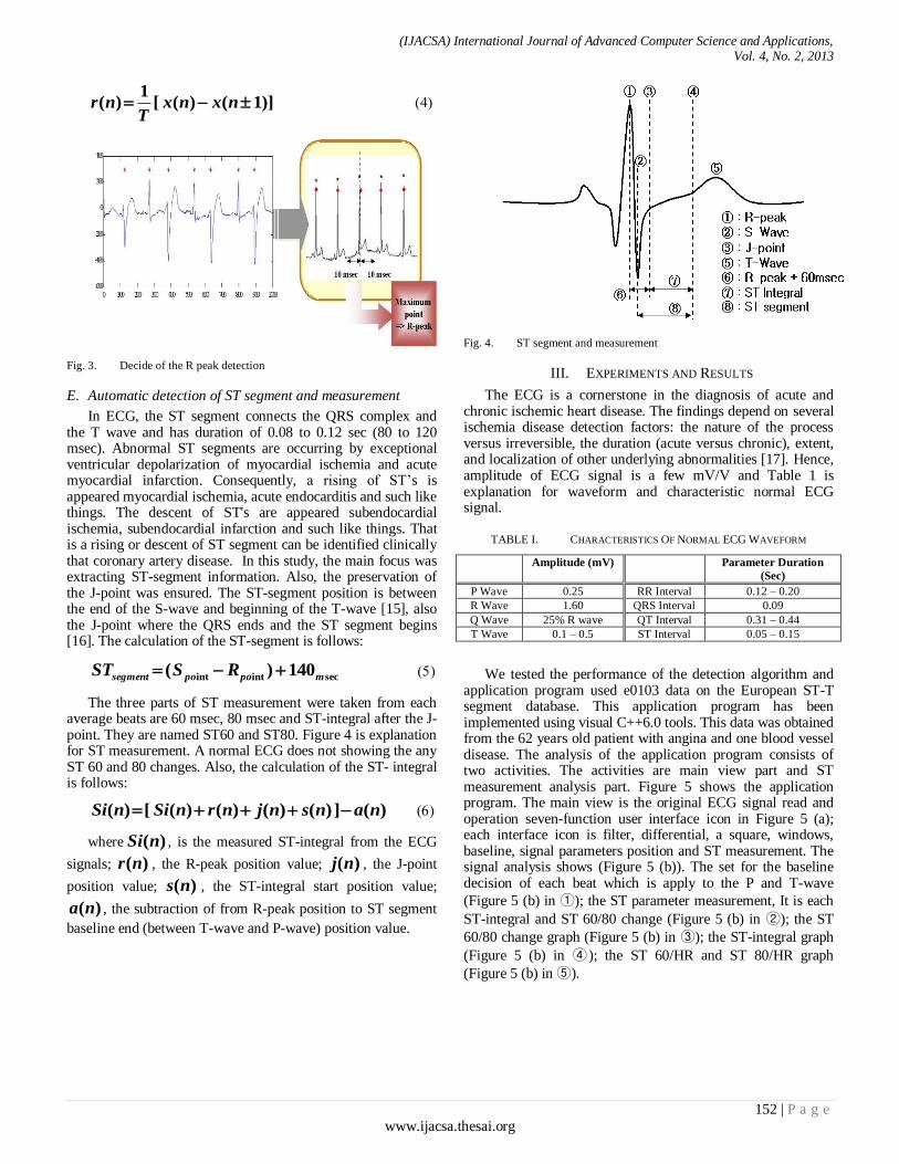
(IJACSA) International Journal of Advanced Computer Science and Applications, Vol. 4, No. 2, 2013
152 | P a g e
www.ijacsa.thesai.org
)]1()([1
)( nxnxT
nr
Fig. 3. Decide of the R peak detection
E. Automatic detection of ST segment and measurement
In ECG, the ST segment connects the QRS complex and the T wave and has duration of 0.08 to 0.12 sec (80 to 120 msec). Abnormal ST segments are occurring by exceptional ventricular depolarization of myocardial ischemia and acute myocardial infarction. Consequently, a rising of ST’s is appeared myocardial ischemia, acute endocarditis and such like things. The descent of ST's are appeared subendocardial ischemia, subendocardial infarction and such like things. That is a rising or descent of ST segment can be identified clinically that coronary artery disease. In this study, the main focus was extracting ST-segment information. Also, the preservation of the J-point was ensured. The ST-segment position is between the end of the S-wave and beginning of the T-wave [15], also the J-point where the QRS ends and the ST segment begins [16]. The calculation of the ST-segment is follows:
secintint 140)( mpoposegment RSST
The three parts of ST measurement were taken from each average beats are 60 msec, 80 msec and ST-integral after the J-point. They are named ST60 and ST80. Figure 4 is explanation for ST measurement. A normal ECG does not showing the any ST 60 and 80 changes. Also, the calculation of the ST- integral is follows:
)(])()()()([)( nansnjnrnSinSi
where )(nSi , is the measured ST-integral from the ECG
signals; )(nr , the R-peak position value; )(nj , the J-point
position value; )(ns , the ST-integral start position value;
)(na , the subtraction of from R-peak position to ST segment
baseline end (between T-wave and P-wave) position value.
Fig. 4. ST segment and measurement
III. EXPERIMENTS AND RESULTS
The ECG is a cornerstone in the diagnosis of acute and chronic ischemic heart disease. The findings depend on several ischemia disease detection factors: the nature of the process versus irreversible, the duration (acute versus chronic), extent, and localization of other underlying abnormalities [17]. Hence, amplitude of ECG signal is a few mV/V and Table 1 is explanation for waveform and characteristic normal ECG signal.
TABLE I. CHARACTERISTICS OF NORMAL ECG WAVEFORM
Amplitude (mV) Parameter Duration
(Sec)
P Wave 0.25 RR Interval 0.12 – 0.20
R Wave 1.60 QRS Interval 0.09
Q Wave 25% R wave QT Interval 0.31 – 0.44
T Wave 0.1 – 0.5 ST Interval 0.05 – 0.15
We tested the performance of the detection algorithm and application program used e0103 data on the European ST-T segment database. This application program has been implemented using visual C++6.0 tools. This data was obtained from the 62 years old patient with angina and one blood vessel disease. The analysis of the application program consists of two activities. The activities are main view part and ST measurement analysis part. Figure 5 shows the application program. The main view is the original ECG signal read and operation seven-function user interface icon in Figure 5 (a); each interface icon is filter, differential, a square, windows, baseline, signal parameters position and ST measurement. The signal analysis shows (Figure 5 (b)). The set for the baseline decision of each beat which is apply to the P and T-wave
(Figure 5 (b) in ①); the ST parameter measurement, It is each
ST-integral and ST 60/80 change (Figure 5 (b) in ②); the ST
60/80 change graph (Figure 5 (b) in ③); the ST-integral graph
(Figure 5 (b) in ④); the ST 60/HR and ST 80/HR graph
(Figure 5 (b) in ⑤).

(IJACSA) International Journal of Advanced Computer Science and Applications, Vol. 4, No. 2, 2013
153 | P a g e
www.ijacsa.thesai.org
(a)
(b)
Fig. 5. Results of the ST measurement and analysis: (a) application main view; (b) signal analysis and measurement view
IV. CONCLUSIONS
This paper presents a completely automatic algorithm and application program for component detection in ECG signal. The performance and the limitations of this method are discussed. The method and the various limits and the detection parameters used were test on just one patient’s data. The performance of the method must also be assessed for the value and position of all marker positions in ECG signal. In this work, this assessment is limited to the J-point, ST60/80 and ST-segment. This signal application program experimentation is an enough successful but we have a few improvement parts
and not real-time signal analysis, such as considering of the noise reduction, apply to the strong diagnostic algorithm, and totally measurement of the other physiological signals (e,g., Electromyography (EMG), Magnetoencephalography (MEG), Electroencephalography (EEG)).
Also, we would study real-time ECG signal analysis, using the algorithm for comparing the normal and abnormal ECG signals, elevation of environment design of the use interface system, testing on a long term data set, and system safety for clinical trials in a variety of conditions. Finally, the developed PC application can be useful for optimization of the already

(IJACSA) International Journal of Advanced Computer Science and Applications, Vol. 4, No. 2, 2013
154 | P a g e
www.ijacsa.thesai.org
available diagnosis algorithms and would assist of the early heart disease detection for medical doctors.
REFERENCES
[1] T. Rocha, S. Paredes, P. Carvalho, J. Henriques, M. Harris, J. Morais, and M. Antumes, “A lead dependent ischemic episodes detection
strategy using hermite functions,” Biomedical Signal Processing and Control, Vol. 5, No. 4, pp.271-281, 2010.
[2] J. Garcia, L. Sornmo, S. Olmos, and P. Laguna, “Automatic detection of
ST-T complex changes on the ECG using filtered RMS difference series: Application to ambulatory Ischemia monitoring,” IEEE
Transactions on Biomedical Engineering, Vol. 47, No. 9, pp.1195-1201, 2000.
[3] J. Garcia, P. Lander, L. L. Sornmo, S. Olmos, G. Wagner, and P.
Laguna, “Comparative study of local and Karhunen-Loe’ve-Based ST-T indexes in recordings from human subjects with induced myocardial
ischemia,” Computers and Biomedical Research, vol. 31, No. 4, pp.271-292, 1998.
[4] T. Barill, The Six Second ECG: A Practical Guidebook to Basic ECG
Interpretation, Nursecom Educational Technologies, 2003, chapter 4.
[5] B. R. Chaitman. “The changing role of the exercise electrocardiogram as a diagnostic and prognostic test for chronic ischemic heart disease,”
Journal of the American College of Cardiology, Vol. 8, No. 5, pp.1195-1210, 1986.
[6] J. P. Martinez, S. Olmos, and P. Laguna, “T wave alternans detection: A
simulation study and analysis of the European ST-T database,” Computers in Cardiology, Vol. 27, pp.155-158, 2000.
[7] P. Laguna, G. B. Moody, J. Garcia, A. L. Goldberger, and R. G. Mark, “Analysis of the ST-T complex of the electrocardiogram using the
Karhunen-Loe’ve transform: Adapative monitoring and alternans detection,” Medical and Biological Engineering and Computing, Vol.
35, No. 2, pp.175-189, 1999.
[8] D. S. Rosenbaum, L. E. Jackson, J. M. Smith, H. Garan, J. N. Ruskin, and R. J. Cohen, “Electrical alternans and vulnerability to ventricular
arrhythmias,” The New England Journal of Medicine, Vol. 330, No. 4, pp.235-241, 1994.
[9] S. Cerutti, “In the Spotlight: Biomedical Signal Processing,” IEEE
Reviews in Biomedical Engineering, Vol. 1, pp.1-5, 2008.
[10] A. Taddel, G. Distante, M. Emdin, P. Pisani, G. B. Moody, C. Zeelenbere, and C. Marchesi. “The European ST-T Database: standards
for evaluating systems for the analysis of ST-T changes on ambulatory electrocardigraphy,” European Heart Journal, Vol. 13, No. 9, pp.1164-
1172, 1992.
[11] Available: http://www.physionet.org
[12] D. H. Lee, A. Rabbi, J. Choi, and F. R. Reza. “Development of a mobile phone based e-health monitoring application,” International Journal of
Advanced Computer Science Applications, Vol. 3, No. 3, pp.38-43, 2012.
[13] V. X. Afonso, “ECG ARS detection,” in Biomedical Digital Signal Processing, W. J. Tompkins, Ed. Englewood Cliffs, NJ: Prentice-Hall,
1993.
[14] J. Pan, and W.J. Tompkins, “A Real-Time QRS Detection Algorithm,” IEEE Transactions on Biomedical Engineering, Vol. 32, No. 3, pp.230-
236, 1985.
[15] J. W. Hurst, “Abnormalities of the S-T segment-Part I,” Clinical Cardiology, Vol. 20, pp. 511-520, 1997.
[16] J. Brownfiels, and M. Herbert, “EKG criteria for fibrinolysis: What’s up
with the J point?,” Western Journal of Emergency Medicine, Vol. 9, No. 1, pp.40-42, 2008.
[17] A. L. Goldberger, Clinical Electrocardiography: A Simplified Approach,
7th Edition, 2006, Chapter 11.
[18] W. D. Rosamond, L. E. Chambless et al., “Trends in the Incidence of myocardial infarction and in mortality due to coronary heart disease,
1987 to 1994,” The New England Journal of Medicine, Vol. 339, No. 13, pp.861-867, 1998.
[19] D. Corrado, A. Biffi, C. Basso, A. Pelliccia, and G. Thiene, “12-lead ECG in the athlete: physiological versus pathological abnormalities,”
British Journal of Sports Medicine, Vol. 43, No. 9, pp.669-676, 2009.
[20] K. L. Part, K. J. Kim, and H. R. Yoon, “Application of a wavelet
adaptive filter to minimize distortion of the ST-segment,” Medical and Biological Engineering and Computing, Vol. 36, No. 5, pp.581-586,
1998.
[21] T. Stamkopoulos, K. Diamantaras, N. Maglaveras, and M. Strintzis,
“ECG analysis using nonlinear PCA neural networks for Ischemia detection,” IEEE Transactions on Signal Processing, Vol. 46, No. 11,
pp.3058-3067, 1998.
[22] R. V. Andreao, B. Dorizzi, J. Boudy, and J. C. M. Mota, “ST-segment analysis using hidden markov model beat segmentation: Application to
ischemia Detection,” Computer in Cardiology, Vol. 31, pp.381-384, 2004.
[23] C. Papaloukas, D. I. Fotiadis, A. P. Liavas, A. Likas, and L. K. Michalis,
“A knowledge based technique for automated detection of ischaemic wpisodes in long duration electrocardiograms,” Medical and Biological
Engineering and Computing, Vol. 39, No. 1, pp.105-112, 2001.
[24] M. Faezipour, A. Saeed, S. C. Bulusu, M. Nourani, H. Minn and L. S. Tamil, “A patient adaptive profiling scheme for ECG beat classification,”
IEEE Transactions on Information Technology in Biomedicine, Vol. 14, No. 5, pp.1153-1165, 2010.
[25] E. Pueyo, L. Sornmo, and P. Laguna, “ARS slops for detection and
characterization of myocardial ischemia,” IEEE Transactions on Biomedical Engineering, Vol. 55, No. 2, pp.468-477, 2008.
[26] Y. Birnbaum, I. Herz, S. Sclarovsky, B. Zlotikamien, A. Chetrit, L.
Olmer, and G. I. Barbash, “Prognostic signficance of the admission electrocardiogram in acute myocardial infarction,” Journal of the
American College of Cardiology, Vol. 27, No. 5, pp.1128-1132, 1996.
Authors Profile
Duck Hee Lee received the M.Sc degree in biomedical engineering from the Hanyang University, Seoul, South Korea in 2004. From 2005 to 2009, he worked at the Biomedical Engineering Division of the National Cancer Center (NCC), South Korea, developing a surgical robot system. In 2010, he was appointed Researcher of the University of North Dakota, Biomedical Signal Processing Laboratory, USA. Since 2004, he has worked on biomedical engineering research fields. His research interests include medical device and instrument, biomedical signal processing, and surgical robotics. He authored and co-authored more ten articles journals, conference proceedings and book chapter. He is a member of Korea Society for Medical and Biological.
Jun Woo Park received the Ph.D. degree in biomedical engineering from the Seoul National University, Seoul, South Korea in 2004. Since 2004, he has worked on biomedical engineering research fields. In 2009, he was appointed Research Professor of the Department of Biomedical Engineering, College of Medicine, Korea University, Seoul, South Korea. His research interests include medical device and instrument, vision-based force feedback, telesurgery and surgical robotics. He is a member of Korea Society for Medical and Biological Engineering, Institute of Electrical and Electronics Engineers (IEEE).
Jaesoon Choi received the Ph.D. degree in biomedical engineering from the Seoul National University, Seoul, South Korea in 2003. Since 2003, he has worked on biomedical engineering research fields. From 2007 to 2012, he was appointed Research Professor of the Korea Artificial Organ Center (KAOC), Seoul, South Korea. Currently, he is Assistant Professor at Medical Engineering R&D Center, Asan Institute for Life Science, Asan Medical Center and University of Ulsan College of Medicine, Seoul, South Korea. He was responsible for various national and international research projects focused on key components for surgery robot system. His research interests include medical device and instrument, medical fusion multi-modal simulation, Vision-Haptic-Integrated Control Mechanism, and surgical robotics. He authored and coauthored more than 30 articles and holds ten patents. He is a member of Korea Society for Medical and Biological, Institute of Electrical and Electronics Engineers (IEEE), and International Society for Pediatric Mechanical Cardiopulmonary Support
Ahmed Rabbi is currently he a Ph.D. student at the Department of Electrical
Engineering, University of North Dakota, USA. His research interests include
biomedical signal processing and pattern recognition, heart rate monitoring
using ECG, EEG movement artifacts detection and filtering, epileptic seizure
detection and prediction, and human cognitive performance assessment using
EEG/ECG signals, and biomedical instrumentation. He has participated as a
program committee member of an international conference (ICIEV). He has
published over ten articles in refereed journals, conference proceedings and

(IJACSA) International Journal of Advanced Computer Science and Applications, Vol. 4, No. 2, 2013
155 | P a g e
www.ijacsa.thesai.org
co-authored a book chapter. He is an active member of the IEEE and IEEE
Engineering in Medicine and Biology Society (EMBS).
Reza Fazel-Rezai received his BSc. and M.Sc. in Electrical Engineering and
Biomedical Engineering in 1990 and 1993, respectively. He received his Ph.D.
in Electrical Engineering from the University of Manitoba in Winnipeg,
Canada in 1999. From 2000 to 2002, he worked in industry as a senior
research scientist and research team manager. Then, he joined academia at
Sharif University of Technology and later the University of Manitoba as
Assistant Professor in 2002 and 2004, respectively. Currently, he is Assistant
Professor and the Director of Biomedical Signal Processing Laboratory at the
Department of Electrical Engineering, University of North Dakota, USA. His
research interests include biomedical engineering, signal and image
processing, brain computer interface, EEG signal processing, seizure
detection and prediction, neuro-feedback, and human performance evaluation
based on EEG signals.

(IJACSA) International Journal of Advanced Computer Science and Applications, Vol. 4, No. 2, 2013
156 | P a g e www.ijacsa.thesai.org
ZeroX Algorithms with Free crosstalk in Optical
Multistage Interconnection Network
M.A.Al-Shabi
Department of Information Technology, College of Computer, Qassim University, KSA.
Abstract— Multistage interconnection networks (MINs) have
been proposed as interconnecting structures in various types of
communication applications ranging from parallel systems,
switching architectures, to multicore systems and advances.
Optical technologies have drawn the interest for optical
implementation in MINs to achieve high bandwidth capacity at
the rate of terabits per second. Crosstalk is the major problem
with optical interconnections; it not only degrades the
performance of network but also disturbs the path of
communication signals. To avoid crosstalk in Optical MINs many
algorithms have been proposed by many researchers and some of
the researchers suppose some solution to improve Zero
Algorithm. This paper will be illustrated that is no any crosstalk
appears in Zero based algorithms (ZeroX, ZeroY and ZeroXY) in
using refine and unique case functions.
Through simulation modeling, the Zero based algorithm
approach yields the best performance in terms of minimal
routing time in and number of passes comparison to the previous algorithms tested for comparison in this paper.
Keywords— component; Optical multistage interconnection
networks (MINs); ZeroX Algorithm; crosstalk in Omega network.
I. INTRODUCTION
Multistage interconnection networks (MINs) have been proposed as interconnecting structures in various types of communication applications ranging from parallel systems [1]
, switching architectures [2], to multicore systems [3]. Advances in optical technologies have drawn the interest for optical implementation in MINs to achieve high bandwidth capacity at the rate of terabits per second. Optical MINs (OMINs) are an attractive solution that offers a combination of high bandwidth, low error probability, and large transmission capacity [4].
However, OMINs introduce optical crosstalk, which results from coupling two signals within a switching element (SE). Optical crosstalk degrades the performance of OMINs in terms of reduced signal-to-noise ratio and limits the size of the network [5]. Limited by the properties of optical signals, it is not possible to route more than one message simultaneously, without optical crosstalk, over a switching element in an OMIN. Reducing the effect of optical crosstalk has been a challenging issue considering trade-offs between aspects i.e. performance, hardware and software complexity.
There are three main approaches for solving optical crosstalk in OMINs namely the space [6], time [7] and wavelength [8][9] dilation approach. In this paper, the interest
is on the time dilation approach to solve the optical crosstalk problem in the omega networks, a class of self-routable networks, which is topologically equivalent to the baseline, butterfly, cube networks et[10]. The time dilation approach solves the crosstalk problem by ensuring that only one signal is allowed to pass through each switching element at a given time in the network [11][12]. Typical MINs consist of N inputs, N outputs and n stages with n=log N. Each stage is numbered from 0 to (n-1), from left to right and has N/2 Switching Elements (SE). Each SE has two inputs and two outputs connected in a certain pattern.
The critical challenges with optical multistage interconnections are optical loss, path dependent loss and optical crosstalk [13] [14]. Optical crosstalk is caused by coupling two signals within a switching element.
In this paper, the focus is illustrated that is no any crosstalk in ZeroX, ZeroY and ZeroXY if the refine and unique case apply in the given networks. And illustrate that is Fast ZeroX depends for that is some crosstalk still occurs in ZeroX without author used refine and unique case in ZeroX [15][16].
II. RELATED WORKS
There are various approaches available to reduce the problem of crosstalk like space domain, time domain and wavelength domain approach. In the present paper, our consideration is time domain approach [7]. Crosstalk is considered as a conflict in this approach. It is a good approach because it can make a balance between the electronic processor and Optical MINs [16][17]. It is not possible to send all the source addresses at the same time to their corresponding destination because it will create the switch and link conflict problem. Therefore, to route the data packets, Permutation and Semi-permutation is applied on the message groups. So that a conflict free route can be obtained for each group [4]. The source and destination address is combined to build combination matrix. On the basis of combination matrix message partitioning is performed so that some specific message should get their destination in the first pass and network remains crosstalk free. There are various techniques for message partitioning like Window Method [4][18], Improved Window Method[19] and Heuristic Routing Algorithms [19]. In this paper, the focus is to provide best message partitioning scheme so that a switch and link conflict free network can be obtained. Before describing our algorithms just have a look on the Window Method and Improved Window Method and Heuristic Routing Algorithm.

(IJACSA) International Journal of Advanced Computer Science and Applications, Vol. 4, No. 2, 2013
157 | P a g e www.ijacsa.thesai.org
A. Window Method
This method [4] [20] basically separates the messages, which have the same bit pattern so that crosstalk can be removed. If we consider the network size N x N, it shows that there are N source and N destination address. To get a combination matrix, it is required to combine the corresponding source and destination address. This matrix shows that the optical window size is M-1, where M=log2N and N is the size of the network. The first and last columns of the combination matrix are not considered in this method and all the processing is performed on the remaining columns. If the two messages having the same bit pattern then they will be routed in the different passes.
In our example, the window size will be two and the number of window will be three W0, W1 and W2 as shown in Figure 1.
Fig. 1. Three Optical Windows in an 8×8 OON
Then, we take the second and third columns as a matrix, where example messages 000 and 100 in this window have the same bit pattern of 00 inside the window and have a conflict. The bit patterns can be any of the four combinations of 00, 01, 10, and 11.
B. Conflict Matrix
A conflict matrix is the new proposed method proposed in
this research, it is a square matrix with NN entry, where N is the size of the network, it consist of the output of the window method , the propose definition of Conflict Matrix is the matrix
Mij with size NN where N is the size of network,
conflict if
otherwise
1
0ij M (1)
Where Mij is the entries of the Conflict Matrix.
Conflict matrix can be formed by assigning the value 1 when there is a conflict between the source and destination; otherwise the value 0 is assigned [4][20].
III. ZERO BASED ALGORITHMS
To avoid the crosstalk problem in omega network a new algorithm called Zero Based Algorithm is proposed and named it ZeroX algorithm, ZeroY algorithm and ZeroXY algorithm.
The following sections explain these algorithms.
A. ZeroX algorithm
This algorithm depends on taking the zero values from the row N+1(axis X) in conflict matrix and putting it in a new group. Then, the entries of this group are considered as having zero value in the matrix. After that, anew summation for the other entries of the matrix it will be done and collecting the zero values on row N+1 as a new group. These steps are to be repeated until the whole matrix becomes Zero. That means, all the entries of matrix are found to be in separate groups. Figure 2 illustrates the general flowchart of ZeroX algorithm [4] [20].
Initialization
A: Matrix N*N,
N: no. of the nodes, S: current node
AR: Reduced matrix contains the currently rows ri and columns, iG[k]
ri ,cj are the ith
row and jth
column where 0 ≤ i ≤ N-1, 0 ≤ j ≤ N-1
G: List of groups; k: group index
Input : conflict matrix A with size N*N
Output: (K and G[k]), k is the color number and G[k] is nodes at the color k
Begin
K: = 0; S: = 0 AR :=A;
While S < N do
Begin
For i = 1 to N do
For j = 1 to N do
Sum [i] = Sum [i] + AR [i,j];
// Sum [i] is the sum for all columns in matrix AR
For j: = 0 to N-1 do
// this loop to clustered the entries element in Current group called G[k]
Begin
If Sum[j] = 0 Then
Begin
Color[j]:= k; G[k]:= G[k] +j; S: = S+1;
End if
End for
If S = 1 then
// s =1 this mean the current group G[k] have only one entry equal zero
Call Unique_Case (AR, j, G[k], S) // function for Unique case
Call Refine (AR, G [k], S) // function for enhance the group
AR: = AR with rows rj and columns cj where j G[k]
K: = k+1
End While
Return (k, G[k])
Fig. 2. Pseudo Code of ZeroX Algorithm
To avoiding the crosstalk the algorithm must implement the refine Function and Unique Case Function. The refine function illustrated in Figure 3 is used to enhance the current groups by adding one or more entries in Matrix M the intersection with current group G equal to zero.
The unique function illustrated in figure 4 is only used to check whether the current group G consists of only one entry equals zero in order for the successor entry equals to zero to be added in the same row of the G and return for the main algorithm[4][20].
Authors' are use ZeroX algorithm without apply refine function and Unique case Function and decided that are some crosstalk still occur in ZeroX algorithm in papers [12][15] [16] [18].

(IJACSA) International Journal of Advanced Computer Science and Applications, Vol. 4, No. 2, 2013
158 | P a g e www.ijacsa.thesai.org
Function Refine (AR ,G[k],S) // rows of AR which only in G[k]
Begin //The Function Refine is used to add new elements to the current group.
For i = 1 to N do
For j = 1 to N do
Sum [i] = Sum [i]+ AR [i,j];
// Sum [i] is the summation for all columns in matrix AR
For j: = 0 to N-1 do
Begin
If Sum[j] =0 and (j G[k] ) Then
Begin
Color[j]:= k;
G[k]:= G[k] +m;
S: = S+1;
End if
End For
Return (G[k], S)
End Refine
Fig. 3. Refine Function in ZeroX Algorithm
Function Unique_Case (AR , j, G[k], S) // function for Unique
case
Begin
For m: = j+1 to N-1 do
Begin
If AR [j, m] = 0 then
Begin
G[k]:= G[k] +m;
S: = S+1;
Exit For
End if
End For
Return (G[k], S);
End Unique_Case
Fig. 4. Unique Case in ZeroX Algorithm
B. ZeroY Algorithm
ZeroY algorithm is another new algorithm proposed to avoid the crosstalk problem in Omega Network. It has the same steps of ZeroX algorithm, but with a difference in the first step where it considers the summation of rows instead of columns. The rest of the algorithm operates in the same way ZeroX algorithm does. In addition, the columns will be changed to rows an vice versa [ 4][20].
C. ZeroXY Algorithm
The ZeroXY algorithm is another new algorithm proposed to avoid the crosstalk problem in Omega network. The minimum number of passes between ZeroX and ZeroY algorithms is the output of the ZeroXY algorithm [20].
IV. UNIQUE CASE FUNCTION TO AVOIDING CROSSTALK IN
ZEROX
The unique case is only used to check whether the current group consists of only one entry equal zero in ZeroY algorithm then the previous entry equal to zero is added in the same column of the current group and the next step of the algorithm is continued. That also happened in ZeroX for the same reason, but in ZeroX the successor entry equal to zero is added in the same row of current group and the next steps of the algorithm is continued. This section provides an illustrate example that show how the unique case happens and explain that no any crosstalk occur in ZeroX or ZeroY algorithms.
Assuming that the source and the destination are randomly
generated and the size of the network is 8 8, the shuffle
exchange in Omega network for the unique case would be as shown in Table I.
TABLE I. SHUFFLE EXCHANGE IN OMEGA NETWORK FOR UNIQUE
CASE
Node No. Source Destination
0
1
2
3
4
5
6
7
000
001
010
011
100
101
110
111
011
001
010
000
100
101
110
111
The first column in Table 1 shows the node number of the
network while, the second and third columns present the sources and the destinations. Using the Window method, the generated conflict matrix would be as it is shown in Table II.
TABLE II. THE CONFLICT MATRIX IN UNIQUE CASE
Message 000 001 010 011 100 101 110 111
000 0 0 1 0 1 0 0 0
001 0 0 0 1 0 1 0 0
010 0 0 0 0 0 0 1 0
011 0 0 0 0 0 0 0 1
100 0 0 0 0 0 1 1 0
101 0 0 0 0 0 0 0 1
110 0 0 0 0 0 0 0 1
111 0 0 0 0 0 0 0 0
From Table II, upon completing the first step of the ZeroY
algorithm, the results would be as it is presented in Table III.
TABLE III. THE SUMMATION STEP IN ZEROY ALGORITHM
Table III shows that only one summation appears to be zero, which is the row (message) 111. If this unique case happened, the solution would be adding the previous entry equal to zero in the same column of the current group and then continuing the next step of the algorithm. As observed from this example, the only one entry which satisfies this condition
Message 000 001 010 011 100 101 110 11
1 Sum
000 0 0 1 0 1 0 0 0 2
001 0 0 0 1 0 1 0 0 2
010 0 0 0 0 0 0 1 0 1
011 0 0 0 0 0 0 0 1 1
100 0 0 0 0 0 1 1 0 2
101 0 0 0 0 0 0 0 1 1
110 0 0 0 0 0 0 0 1 1
111 0 0 0 0 0 0 0 0 0

(IJACSA) International Journal of Advanced Computer Science and Applications, Vol. 4, No. 2, 2013
159 | P a g e www.ijacsa.thesai.org
is entry 100. By adding this entry to the current group, the group will be including 2 entries 100, and 111, and then continue with the normal steps to get the rest of the nodes in the first group. Figure 5 illustrates the two passes (colors), acquired from the example after finishing the implementation of the whole ZeroY algorithm steps. The first color includes the nodes 000, 101, 011, and 110, and the second color includes the nodes 010, 001, 100 and 111.
Fig. 5. Two Colors in Unique Case
The Figure 5 illustrate that is no any crosstalk in this network like the authors says in papers [12] [15] [16][18].
V. COMPARATIVE ANALYSIS AND DISCUSSION
The comparison in this section is between the ZeroX algorithm with include refine and Unique Case functions and the routing algorithms, which includes the four heuristic algorithms namely; the Sequential up (Seq), the Sequential down (SeqDn), the Degree Ascending (Ascend), the Degree Descend (Descend), and the SA algorithm. The comparison depends on two parameters which are the average number of passes parameter and the execution time parameter using different values of the network size.
The average number of passes is shown in figures 6, and execution time shown in figures 7 respectively.
Fig. 6. Average number of Passes
From the results elaborated in figure 6 it is observed that the Degree-Ascending algorithm performs the worst in terms of the average number of passes. However, the Descend algorithm and ZeroX algorithm have the better performance. Seq algorithm and SeqDn algorithm perform better than Ascend algorithm and poorer than Descend. The Figure 6 illustrate that the SA Algorithm has been the best. The results obtained by ZeroX algorithms match closely those obtained by the Degree-Descending Algorithm. Therefore, the simulated
annealing is still considered to be more appropriate for finding the average number of passes for a given network.
In the execution time terms, the results of the different heuristic algorithms, SA algorithm and ZeroX algorithm are shown figure 7.
Fig. 7. Execution Time for ZeroX and Routing Algorithms
It is illustrated in figures 7 that the algorithms SA, Degree Ascend and Degree Descend perform the worst in terms of the execution time. Sequential and Sequential algorithm Down SeqDn algorithm perform better than SA, Ascend and Descend algorithms, but poorer than ZeroX algorithm. In addition, all the five routing algorithm in Figure 7 take the longest time to compute a solution compared the ZeroX algorithm in terms of the execution time. Therefore, the ZeroX algorithm can be considered more appropriate for finding the execution time for a given network. And finally the ZeroX algorithm includes refine and unique case function is free crosstalk for any given network.
REFERENCES
[1] Y. Yang, J. Wang and Y. Pan, “Routing Permutations with Link-Disjoint and Node-Disjoint Paths in a Class of Self-Routable Interconnects”.
IEEE Transactions on Parallel and Distributed Systems, Vol. 14, No. 4, pp. 383-393, 2003.
[2] D. Tustch and G. Hommel, “MLMIN: A Multicore Processor and
Parallel Computer Network Topology for Multicast”. Computers and Operations Research Journal, Elsevier, Vol. 35, No. 12, pp. 3807-3821,
2008.
[3] M. A. Al-Shabi and M. Othman, “A New Algorithm for Routing and Scheduling in Optical Omega Network”. International Journal of the
Computer, The Internet and Management, Vol. 16, No. 1, pp. 26-31, 2008.
[4] E. Lu and S. Q. Zheng, “High-Speed Crosstalk-Free Routing for Optical
Multistage Interconnection Networks”. Proceedings of the 12th International Conference on Computer Communications and Networks,
pp. 249-254, 2003.
[5] S. C. Chau, T. Xiao and A. W. C. Fu, “Routing and Scheduling for a Novel Optical Multistage Interconnection Networks”. Euro-Par 2005
Parallel Processing, Lecture Notes in Computer Science, Vol. 3648, pp. 984-993, 2005.
[6] Y. Pan, C. Qiao, and Y. Yang, Optical Multistage Interconnection Networks: New Challenges and Approaches, IEEE Communications
Magazine, Feature Topic on Optical Networks, Communication Systems and Devices, Vol 37, No. 2, 1999, pp: 50-56.
[7] C. Qiao and R. Melhem, A Time Domain Approach for Avoiding
Crosstalk in Optical Blocking Multistage Interconnection Networks, Journal of Lightwave Technology, Vol. 12. No. 10, 1994, pp. 1854-
1862.
[8] Enyue Lu and S. Q. Zheng, Parallel Routing and Wavelength Assignment for Optical Multistage Interconnection Networks,
Performance on different size network
0
1
2
3
4
5
6
7
1 2 3 4 5
Number of stage of OMIN=N+2
Ave
rage
Pas
ses
SeqUP
SeqDn
Degree
AscendDegree
DescendSA
ZeroX
Performance on different sizes of networks
0
500
1000
1500
2000
2500
3000
3500
4000
1 2 3 4 5
Number of stage of OMIN = N+2
Tim
e (M
illiS
ec) Seq
SeqDn
Degree
AscendDegree
DescendSA
ZeroX

(IJACSA) International Journal of Advanced Computer Science and Applications, Vol. 4, No. 2, 2013
160 | P a g e www.ijacsa.thesai.org
Proceedings of the 2004 International Conference on Parallel Processing
(ICPP 04), 2004.
[9] C. L. Wu, and T. Y. Feng, “On a Class of Multistage Interconnection
Networks”. IEEE Transactions on Computers, Vol. 29, No. 8, pp. 694-702, 1980.
[10] T.T. Lee and P. P. To, Non-blocking routing properties of Clos
networks, in Advances in switching networks (Princeton, NJ, 1997), Amer. Math. Soc., Providence, RI, 1998, pp. 181–195.
[11] X. Shen, F. Yang, and Y. Pan, Equivalent Permutation Capabilities
Between Time Division Optical Omega Networks and Non-Optical Extra-Stage Omega Networks, IEEE/ACM Transactions on Networking,
Vol. 9. No. 4, 2001, pp: 518-524.
[12] T. D. Shahida, M. Othman, M. Khazani, Routing Algorithms in Optical Multistage Interconnection Networks: Revisited, World Engineering
Congress 2007 (WEC 2007), August 2007.
[13] V.P. Bhardwaj, Nitin and V. Tyagi, An Algorithmic Approach to Minimize the Conflicts in an Optical Multistage Interconnection
Network, Proceedings of the 1st International Conference on Advances in Computing and Communications (ACC), Lecture Notes in Computer
Science (LNCS), Springer, Kerala, 2011.
[14] V.P. Bhardwaj, Nitin and V. Tyagi, Minimizing the Switch and Link Conflicts in an Optical Multi–stage Interconnection Network,
International Journal of Computer Science Issues, 8 (4) 1, ISSN: 1694–0814, 2011
[15] T. Shahida, M. Othman, M. Khazani, " A Fast and Efficient Crosstalk-Free Algorithm for Routing in Optical Multistage Interconnection
Networks", IEEE,2008.
[16] T. D. Shahida, M. Othman and M. K. Abdullah, Fast Zerox algorithm
for routing in optical Multistage interconnection networks, IIUM Engineering Journal, 11(1), pp. 28-39, 2010.
[17] A.K. Katangur, S. Akkaladevi and Y. Pan, Analyzing the performance of optical multistage interconnection networks with limited crosstalk,
Cluster Computing, 10, pp. 241-250.
[18] F. Abed and M. Othman, Fast method to find conflicts in optical multistage interconnection networks, International Journal of The
Computer, The Internet and Management, 16(1), pp. 18-25, 2008.
[19] M. Abdullah, M. Othman and R. Johari, An efficient approach for message routing in optical omega network, International Journal of The
Computer, the Internet and Management, 14(1), pp. 50- 60, 2006.
[20] M. A. Al-Shabi, “Zero Algorithms to avoid Crosstalk in Optical Multistage Interconnection Networks”. PhD Thesis, Universiti Putra
Malaysia, 2005.
AUTHOR PROFILE
Dr. M. A. Al-Shabi received his Bachelor degree (B.Sc. Computer Science) from Technology University at Iraq (1997). Post graduate Master (M. Sc. Computer Science from Putra Malaysia University at 2002) and PhD (Computer Network) from Putra Malaysia University, Malaysia (2006). He is currently an assistant professor of College of Computer at Qassim University. Kingdom of Saudi Arabia. Prior to joining Qassim University he worked
in the Faculty of computer at Sana’a University, Yemen. His research interests include: wireless security, cryptography, UML, Stenography Multistage interconnection network, parallel computing and Apply Mathematic.

(IJACSA) International Journal of Advanced Computer Science and Applications, Vol. 4, No. 2, 2013
161 | P a g e www.ijacsa.thesai.org
A Mixed Finite Element Method for Elasticity
Problem
A. Elakkad
Department of mathematics
Regional Centre for Professions of Education and Training, Fes, B.P: 243 Sefrou Morocco
M.A. Bennani, J. EL Mekkaoui and A.Elkhalfi
Mechanical engineering laboratory
Faculty of sciences and techniques-B.P. 2202 Route Imouzzer Fes
Abstract—This paper describes a numerical solution for plane
elasticity problem. It includes algorithms for discretization by
mixed finite element methods. The discrete scheme allows the
utilization of Brezzi - Douglas - Marini element (BDM1) for the
stress tensor and piecewise constant elements for the
displacement. The numerical results are compared with some
previously published works or with others coming from commercial code like ABAQUS.
keywords—Elasticity problem; Mixed Finite element method;
BDM1 approximation; ABAQUS
I. INTRODUCTION
Mixed finite element methods for linear elasticity are based on approximations of a stress- displacement system derived from the Hellinger-Reissner variational principle [7], in which both displacements and stresses were approximated simultaneously.
The mathematical analysis and applications of mixed finite element methods have been widely developed since the seventies. A general analysis for this kind of methods was first developed by Brezzi [8]. We also have to mention the papers by Babuska [14] and by Crouzeix and Raviart [15] which, although for particular problems, introduced some of the fundamental ideas for the analysis of mixed methods.
We also refer the reader to [16][17], where general results were obtained, and to the books [6][18][19].
Many mixed finite element methods have been developed for plane elasticity, and generally speaking, they can be grouped into two categories: methods that enforce the symmetry of the stress weakly, and methods that enforce the symmetry exactly (strongly). In the former category, the stress tensor is not necessarily symmetric, but rather orthogonal to anti-symmetric tensors up to certain moments. Weakly imposed stress symmetry methods also introduce a new variable into the formulation that approximates the anti-symmetric part of the gradient of u; see for example [2][3].On other hand, exactly symmetric stress methods have been much more difficult to construct. The first class of
inf_sup stable methods was the so called composite elements [4][5].
Section II presents the model problem used in this paper. The discretization by mixed finite elements described is in section III. Numerical experiments carried out within the framework of this publication and their comparisons with other results are shown in section IV.
II. GOVERNING EQUATIONS
The equilibrium equations and boundary conditions are
(1)
(2)
(3)
(4)
Where n is the unit outward normal. In the above, σ is the Cauchy stress, and f is the body force per unit volume.
The constitutive relation is given by Hooke’s law:
(5) Where C is the Hooke tensor, C is assumed here to
have constant coefficients. Its inverse (compliance tensor) will be denoted by E. Hence
(6) We consider small strains and displacements. The
kinematics equations therefore consist of the strain-displacement relation
(7)
Where
is the symmetric part of the
gradient operator, and the boundary condition
(8)

(IJACSA) International Journal of Advanced Computer Science and Applications, Vol. 4, No. 2, 2013
162 | P a g e www.ijacsa.thesai.org
Fig. 1. Body With Internal Boundary Subjected To Loads.
We set
;
.
(9)
(10)
(11)
Then the standard weak formulation of the equilibrium equations is the following:
Find and such that:
(12)
(13)
One can see that (12)-(13) practically coincide with the
variational formulation of the Hellinger-Reissner principle.
The use of this principle in the framework of finite elements
can be traced Back to the pioneering work of Herrmann [9]
and Hellan [10]. The interest in using the stress field σ as an independent variable is questionable in as simple a case as the
present one, but it is clear in more general and more
complicated problems involving nonlinearities, plasticity, and
so on. Let the bilinear forms a and b, and the linear forms l
and s such that:
(14)
(15)
(16)
(17)
The underlying weak formulation (12)-(13) may be restated as:
Find and such that:
(18)
(19)
THEOREM 1. Let E and Ψ be real Hilbert spaces, a bilinear form on E × E, and a bilinear form an E × Ψ. Set
(20)
And assume that:
(21)
(22)
Then for every l1 E′ and l2 Ψ′ there exist a unique
solution of the problem
(23)
(24)
REMARK 1. If problem (21)-(22) has a unique solution for every and then (20) holds and the bilinear form a(ξ1, ξ2) restricted to K, is nonsingular (in the sense that it induces an isomorphism from K onto K’). Clearly if one assumes that a (ξ1, ξ2) is symmetric and positive semi definite, then (21) and (22) are necessary and sufficient for the existence and uniqueness of the solution of (23)-(24).
REMARK 2. It is clear that if a (ξ1, ξ2) is symmetric;
the solution of (23)-(24) minimizes the functional
(25)
On the subspace of E,
(26)
And the formulation (23)-(24) corresponds to the
introduction in (25)-(26) of the Lagrange multiplier .
III. MIXED FINITE ELEMENT APPROXIMATION
Let , be a family of rectangulations of Ω. The edges of elements will be denoted (i=1, 2, 3 or
i=1, 2, 3, 4) in the two-dimensional case. Let us deal first with the abstract framework (23)-(24). Assume that we are

(IJACSA) International Journal of Advanced Computer Science and Applications, Vol. 4, No. 2, 2013
163 | P a g e www.ijacsa.thesai.org
given two sequences and of subspaces E and Ψ, respectively.
We set
. (27)
We have the following approximation theorem
THEOREM 2. Assume that
(28)
(29)
Then for every l1 E′ and l2 Ψ′, and for every h > 0, the discrete problem
(30)
(31)
Has a unique solution. Moreover, there exists a constant such that
(32)
The dependence of on and can be easy traced
[8]. Clearly if (21) and (22) hold with constants and independent of h, then (32) holds with a constant independent of h.
We define in general, for m integer ≥ 0,
(33)
Where
(34)
These derivatives being taken in the sense of distributions. On this space, we shall use the semi-norm
(35)
and the norm
(36)
We are now ready for the error estimates. THEOREM 3. If (σ, u) is the solution of (12)-(13) and
(σh, uh) is the solution of (30)-(31), there exist a constant C > 0 such that:
(37)
Discretization of the mixed formulations, for linear elliptic operators, many examples of successful discretization of (12)-(13) are known. The first ones were introduced by Raviart and Thomas in [11] and then re-elaborated and extended to more general cases by Nedelec [12]. Other families of possible discretization were introduced years later by Brezzi, Douglas, and Marini [1][13].
To give a more precise definition of our mixed finite element approximation we shall need a few definitions. Let us define on an element K.
Pk: the space of polynomials of degree ≤ k.
We shall also need polynomial spaces on the edges of the elements
. (38)
In the two-dimensional, for the triangular elements we have
(39)
(40)
(41)
Restricting to have a normal trace in yields a space larger than , but having essentially the same properties, that we denote
The dimension of is thus
dim =
(42) For the triangular case we thus have the following
inclusions between the spaces just defined
(43) We consider the space obtained basically from the
space of Brezzi-Douglas-Marini.
(44)
We have
(45)
dim = 6 (46)

(IJACSA) International Journal of Advanced Computer Science and Applications, Vol. 4, No. 2, 2013
164 | P a g e www.ijacsa.thesai.org
Fig. 2. . Brezzi - Douglas - Marini element, the element diagrams for the
stress and displacement elements.
The discrete scheme allows the utilization of BDM1 for the stress tensor and piecewise constant elements for the displacement.
We define, for choice of BDM1 (K), a space
(47)
(48)
We chose finite dimensional subspace
(div, Ω).
A mixed finite element approximation of (12)-(13) is defined
by Find and such that
(49)
. (50)
We obtain a system of linear equations
(51)
Where
The matrix associated for the system (51) is symmetric indefinite. We use the iterative methods Minimum Residual Method (MINRES) for solving the symmetric system.
IV. NUMERICAL SIMULATIONS
Example 1. Circular Void in a Finite Plate
Here a void of radius 0.3 is placed in the center of a plate of size 3 × 3 which is subjected to a unit stress in the y-direction.
The stress plot for σyy s is in excellent agreement with the expected 3σ stress concentration at the edges of the hole.
Fig. 3. Stress Solution Σxx By Mixed Finite Element Method (Left) And
Stress Solution (Right) Computed By ABAQUS.
Fig. 4. Stress Σxy By Mixed Finite Element Method (Left) And Stress
Solution (Right) Computed By ABAQUS.
Fig. 5. Stress Σyy By Mixed Finite Element Method (Left) And Stress
Solution (Right) Computed By ABAQUS.
Fig. 6. Curve Of The Displacement Ux And Uy Along Hole In A Finite
Plate

(IJACSA) International Journal of Advanced Computer Science and Applications, Vol. 4, No. 2, 2013
165 | P a g e www.ijacsa.thesai.org
Example 2. Circular Inclusion in a Finite Plate
Here an inclusion with E = 70gpa and and radius 0.5 is placed in the center of a plate of size 6 x 10 with E = 50gpa and which is subjected to a unit tension in the y-direction.
Fig. 7. Stress Σxx By Mixed Finite Element Method (Left) And Stress
Solution (Right) Computed By ABAQUS.
Fig. 8. Stress Σxy By Mixed Finite Element Method (Left) And Stress
Solution (Right) Computed By ABAQUS.
Fig. 9. Stress Σyy By Mixed Finite Element Method (Left) And Stress
Solution (Right) Computed By ABAQUS.
Fig. 10. Curve Of Displacement Ux And Curve Of Displacement Uy Along
Inclusion In A Finite Plate.
V. CONCLUSION
We were interested in this work in the numeric solution for equilibrium equations. It includes algorithms for discretization by mixed finite element methods. The discrete scheme allows the utilization of BDM1 for the
stress tensor and piecewise constant elements for the displacement. Our results agree with ABAQUS.
Numerical results are presented to see the performance of the method, and seem to be interesting by comparing them with other recent results.
ACKNOWLEDGMENTS
The authors would like to express their sincere thanks for the referee for his/her helpful suggestions.
REFERENCES
[1] F. Brezzi, J. Douglas, M. Fortin, L. Marini, Efficient rectangular mixed
finite elements in two and three variables, RAIRO Model. Math. Anal. Number. vol. 21, issue. 3, pp. 581-604, 1987.
[2] W. Qiu and L. Demkowicz, Mixed hp-finite element method for linear elasticity with weakly imposed symmetry: stability analysis,
SIAM J. Numer. Anal., vol. 49, n o . 2, pp. 619-641, 2011.
[3] J. Guzman, A unified analysis of several mixed methods for elasticity with weak stress symmetry, J. Sci. Comput., vol. 44, pp. 156-169, 2010.
[4] D.N. Arnold, J. Douglas Jr., C.P. Gupta, A family of higher order
mixed finite element methods for plane elasticity, Numer. Math., vol. 45, pp. 1-22, 1984.
[5] C. Johnson and B. Mercier, Some equilibrium finite element methods for
two-dimensional elasticity problems, Numer. Math., vol. 30, pp. 103-116, 1978.
[6] F. Brezzi, M. Fortin. Mixed and Hybrid Finite Element Method.
Springer Verlag; New York, 1991.
[7] Douglas N. Arnold, Jim Douglas, Jr., and Chaitan P. Gupta. A Family of Higher Order Mixed Finite Element Methods for Plane Elasticity.
Number. Math., vol. 45, pp. 1-22, 1984.
[8] F. Brezzi, On the existence uniqueness and approximation of saddle point
problems arising from Lagrangian multipliers, RAIRO, vol. 8-32, pp. 129-151, 1974.
[9] L.R. Herrmann, Finite element bending analysis for plates, J. Eng. Mech.
Div. ASCE EMS, vol. 93, pp. 49-83, 1967.

(IJACSA) International Journal of Advanced Computer Science and Applications, Vol. 4, No. 2, 2013
166 | P a g e www.ijacsa.thesai.org
[10] K. Hellan, Analysis of elastic plates in flexure by a simplified finite
element method, Acta Polytech. Scand. Math. Comput. Sci. Ser., vol. 46, 1967.
[11] P.A. Raviart and J.M. Thomas, A mixed finite element method for 2nd order elliptic problems, Mathematical Aspects of Finite Element Methods
(Proc. Conf., Consiglio Naz. delle Richerche, Rome, 1975), Lecture Notes in Math., vol. 606, Springer-Berlag, New York, pp. 292-315,
1977.
[12] J.C. Nedelec, Mixed finite elements in R3, Numer. Math., vol. 35, pp. 315-
341, 1980.
[13] F. Brezzi, J. Douglas, Jr., and L.D. Marini, Two families of mixed
finite elements for second order elliptic problems, Numer. Math., vol. 47, pp. 217-235, 1985.
[14] I. Babuska, The finite element method with lagrangian multipliers,
Numer. Math., vol. 20, pp. 179–192, 1973.
[15] M. Crouzeix and P.A. Raviart, Conforming and non-conforming finite element methods for solving the stationary Stokes equations, R.A.I.R.O.
vol. 7, pp. 33–76, 1973.
[16] R.S. Falk and J. Osborn, Error estimates for mixed methods,R.A.I.R.O. vol.4, pp. 249–277, 1980.
[17] M. Fortin, An analysis of the convergence of mixed finite element
methods, R.A.I.R.O. vol.11, pp. 341–354, 1977.
[18] J.E. Roberts and J. M. Thomas, Mixed and Hybrid Methods in Handbook of Numerical Analysis, Vol. II (P.G. Ciarlet and J.L. Lions, eds.), Finite
Element Methods (Part 1),North Holland, 1989.
[19] V. Girault and P.A. Raviart, Element Methods for Navier–Stokes
Equations, Springer, Berlin Heidelberg New York, 1986.

(IJACSA) International Journal of Advanced Computer Science and Applications, Vol. 4, No. 2, 2013
167 | P a g e www.ijacsa.thesai.org
Omega Model for Human Detection and Counting for
application in Smart Surveillance System
Subra mukherjee
Assam Don Bosco University
Guwahati, India
Karen Das
Assam Don Bosco University
Guwahati, India
Abstract— Driven by the significant advancements in
technology and social issues such as security management, there
is a strong need for Smart Surveillance System in our society
today. One of the key features of a Smart Surveillance System is
efficient human detection and counting such that the system can
decide and label events on its own. In this paper we propose a
new, novel and robust model: “The Omega Model”, for detecting
and counting human beings present in the scene. The proposed
model employs a set of four distinct descriptors for identifying
the unique features of the head, neck and shoulder regions of a
person. This unique head-neck-shoulder signature given by the
Omega Model exploits the challenges such as inter person
variations in size and shape of people’s head, neck and shoulder
regions to achieve robust detection of human beings even under
partial occlusion, dynamically changing background and varying
illumination conditions. After experimentation we observe and
analyze the influences of each of the four descriptors on the
system performance and computation speed and conclude that a
weight based decision making system produces the best results.
Evaluation results on a number of images indicate the validation of our method in actual situation.
Keywords - Omega Model; Human Detection; Surveillance;
Back ground Subtraction; Gaussian Mixture Model (GMM);
Mixture of Gaussians (MOG).
I. INTRODUCTION
The state-of-art of surveillance has made a quantum jump in recent years. However with the increase amount of video data to be processed it is becoming more and more unmanageable for human beings to monitor continuously. So if we could develop a surveillance system which could detect and classify objects, take decisions and label events autonomously, then a complete revolution can be brought in the current surveillance system. Vision based Human detection and counting is currently one of the most challenging tasks in the field of computer vision. The general surveillance cameras are like machines that can only see, but cannot decide or identify things or events on its own. So, keeping in mind the present day scenarios, it is important that we make our surveillance system intelligent and smart. Therefore, we propose to design a new framework to robustly and efficiently detect and count human beings, for application in surveillance. The proposed system would consist of: Background subtraction, boundary extraction, Head-neck-shoulder detection and, finally human/non-human classification and based on that, counting the number of human present in a scene. For these, we first intend to subtract the background and extract the foreground of any real time video. There are a
lot of techniques available for background subtraction. And Gaussian Mixture Model (GMM) is found to be more efficient in the literature. So we intend to use GMM for this purpose. Moreover some of the commonly faced problems in background subtraction are sudden changes in illumination, dynamic background, camouflage, etc. Hence we intend to design a robust adaptive GMM algorithm which can effectively deal with all these problems and produce a foreground mask. Secondly we intend to detect human presence in the scene by detecting the head and shoulder portion by using the Omega Model. We propose this model because the head-shoulder portion is the most unvarying part of human body. Based on the number of human beings detected we shall count the total number of human present in the scene. And hence the entire system could be used for application in an effective surveillance system.
The rest of the paper is organized as follows: In section II we discuss some of the related work in this field; in section III we give an overview of the method adopted for our work. In section IV our human detection and counting system is discussed giving a detailed description of our proposed Omega model explaining each of the descriptors and the algorithm. In section V we have explained results followed by conclusion and our future work in section VI.
II. RELATED WORK
There is an extensive literature on shape classification. Various approaches for shape based classification are discussed in [1-10].However different moving objects like bird, vehicle, etc may be present in the scene, so it is very important that we correctly distinguish humans from other moving objects. There are mainly two methods for classifying a moving object: shaped based detection and motion based detection [11]. In former one, human can be detected with the help of their shape information. This kind of a work was done in [12-14] where they used an SVM classifier to detect human beings based on finding people’s head by searching for circular patterns through a 2D correlation using a bank of annular patterns. Also it is a general fact that non articulated human motion exhibits certain periodicity. This property was used by many researchers to detect human beings based on their motion. In [14] based on the color object’s moving and background subtraction method, a color classifier based on the HS thresholds was proposed to detect moving object. In [15] edge-based features combined along with color and texture information was used for efficient human detection. In [16] human had been detected by detecting skin like pixels and

(IJACSA) International Journal of Advanced Computer Science and Applications, Vol. 4, No. 2, 2013
168 | P a g e www.ijacsa.thesai.org
locating each face like region. Also some researchers have employed model based human detection [17,18].In [17] such kind of work was done wherein they proposed a method for human detection by modeling human as flexible assemblies of parts represented by co-occurrence of local features. In [18] part detectors were learned by boosting a number of weak classifiers based on edgelet features. Recently in 2013 authors [19] have presented a method for human detection in range images captured from a vertically oriented camera by analysis of 3D range data.
III. OVERVIEW OF THE METHOD
This section gives an overview of the method adopted in our Human detection and Counting system. One of the major challenges in the field of object recognition is the ability to detect human beings irrespective of the variations in pose, body shape, clothing, illumination, moving cameras and changing background. So in this work we have developed the Omega model that could detect human beings under all this challenging scenarios. The methodology or the general flow diagram of our work is shown below:
Fig. 1. General Flow Diagram Of Our Human Detection And Counting
System.
The various steps involved are:
Acquiring real time video input from any video acquisation device
Background modelling using adaptive GMM
Background subtraction and shadow detection
Human detection and counting using the Omega Model.
IV. HUMAN DETECTION AND COUNTING SYSTEM
In this work, we first perform adaptive background modeling to extract the foreground region from a real time Surveillance video. Then we acquire a set of these foreground images from a surveillance video. As we know that the human head shoulder portion is the most unvarying part of human body, so we have used this dominant feature as the key information and developed the Omega Model for human detection.
A. Foreground Extraction
A good surveillance system requires an accurate segmentation of moving objects from a video sequence. Foreground extraction is generally done by using background subtraction, optical flow and frame differencing. However,
Background subtraction is one of the most efficient and widely used methods for segmenting dynamic scene in a video. The most common paradigm for background subtraction is to use an explicit model of the background. Background is generally modeled based on some regular statistical characteristics. Intruding objects are then detected by comparing the statistical parameters of the modeled background with that of the current frame. However this method does not work well in surveillance scenarios where the background is generally subjected to challenges like dynamic lightning conditions, long term scene changes, bimodal background, repetitive flickering motions etc. So, for application in surveillance it is important that the parameters of the background are also adaptive. Hence we have employed the adaptive GMM method proposed in [20] for modeling the background.
a) Gaussian mixture Model:
A Gaussian Mixture Model (GMM) is a parametric probability density function represented as a weighted sum of Gaussian component densities. GMMs are commonly used as a parametric model of the probability distribution of continuous measurements or features in a biometric system, such as vocal-tract related spectral features in a speaker recognition system. GMM parameters are estimated from training data using the iterative Expectation Maximization (EM) algorithm or Maximum A Posteriori (MAP) estimation from a well-trained prior model.
A Gaussian mixture model is a weighted sum of M component Gaussian densities as given by the equation,
where x is a D-dimensional continuous-valued data vector (i.e. measurement or features), wi, i=1, . . . ,M, are the mixture weights, and g(x|μi,Σi
), i = 1, . . . ,M, are the component
Gaussian densities. Each component density is a D-variate Gaussian function of the form,
with mean vector µi and covariance matrix Σi. The mixture
weights satisfy the constraint that i=1.
b) Parameter updates
The new pixel value Zt is checked against each Gaussian. A Gaussian is labeled as matched if
Then its parameters may be updated as follows:
)

(IJACSA) International Journal of Advanced Computer Science and Applications, Vol. 4, No. 2, 2013
169 | P a g e www.ijacsa.thesai.org
Where is the learning rate for the weights.
If a Gaussian is labeled as unmatched only its weight is decreased as
If none of the Gaussians match, the one with the lowest weight is replaced with Zt as mean and a high initial standard deviation.
The rank of a Gaussian is defined as w/σ. This value gets higher if the distribution has low standard deviation and it has matched many times. When the Gaussians are sorted in a list by decreasing value of rank, the first is more likely to be background. The first B Gaussians that satisfy (1) are thought to represent the background.
The Gaussian mixture model (GMM) is adaptive; it can incorporate slow illumination changes and the removal and addition of objects into the background. Further it can handle repetitive background changes like swaying branches, a flickering computer monitor etc. The higher the value of T in (1), the higher is the probability of a multi-modal background.
In our work we have modeled the background as a mixture of
three Gaussians.
B. Omega Model for Human Detection
Significant research has been devoted to detecting people in images and videos. Human detection is a challenging classification problem which has many potential applications in the field of machine vision. The main problems in detecting human beings are due to the variations in pose, body shape, clothing, illumination, moving cameras and changing background.
Therefore the main challenge is to find a set of unique features that characterizes human being in a scene, while remaining resistant to the above mentioned problems.
Thus in this work a new algorithm is presented to detect human beings in still images using a set of four descriptors. After the foreground extraction, the human beings have been detected by studying some of their invariant features like the head-neck- shoulder signature.
a) Outline of approach for Human Detection system:
The block diagram of the proposed Human detection system is as shown below in Fig2.
This approach uses a shape based representation of the extracted foreground contour for human detection. The advantages of this approach are:
It can detect human beings even in partial occlusion
(when legs are partially occluded).
It is tolerant to varying human pose.
It can detect human beings even if the person is not
facing the camera directly.
The final decision is weight based and depends on
multiple evidences obtained from descriptors.
Fig. 2. Flow chart for Omega model for human detection
In this approach, the boundary of the contour of the extracted foreground object has been examined experimentally to obtain some of the invariant features of human beings from the shape of the contour. Four descriptors have been designed to specifically analyze these invariant features and thereafter take a weight based decision to detect the presence of human beings in the scene.
b) Descriptors for Human Detection:
The choice of the distinguishing features for classification is a critical design step and depends on the characteristics of the problem domain. Having extracted the contour of the foreground objects, a set of invariant features have been chosen to detect the presence of human being in the scene. In this work we have developed four descriptors to classify the human beings from other non- human objects by using distinct features that are simple to extract as well as invariant to irrelevant transformations.
From the set of boundary points obtained, by processing the contour of the segmented objects, the main aim here is to develop descriptors that describe the ‘Omega’ shape (i.e. the shape of upper portion of human body) in the best possible manner.
The four Descriptors we use are as follows:
Descriptor 1 (Ω d) :( Head-neck- shoulder dimensions of Ω)
This shape based descriptor is firstly defined by its dimension given as shown in figure (3(b)):
Y max - Y min, X min - X max
A bounding box is designed to include the object of interest and whose axes are aligned with the image axes as shown in figure (d)
Based on the set of boundary points obtained, co-ordinates of the centroid are calculated.
From this obtained centroid, data for width of shoulder and neck is obtained.
The data obtained is then experimentally analyzed with a number of training images to obtain a threshold for

(IJACSA) International Journal of Advanced Computer Science and Applications, Vol. 4, No. 2, 2013
170 | P a g e www.ijacsa.thesai.org
describing the optimum ratio of these width and compare with the testing images.
Fig. 3. (a) original image, (b) image after background subtraction(c) dimensions of the image (d) Bounding box for the contour.
Based on this threshold (obtained experimentally) a decision is made if a human being is present in the scene or not.
Descriptor 2 (Ω m): (Radial Feature of Ω)
This descriptor particularly defines the radial feature of the human head.
Based on experimental analysis the upper (head) portion of the contour is extracted and a point (S’) lying somewhere between the neck and tip of head is obtained.
The radial distance between each of the points in the boundary and point S’ is calculated.
The pattern of occurrence of these distances is observed for human contours.
Based on the pattern a decision is taken if the extracted contour is that of human head or not.
Descriptor 3 (Ω k): (Curvature of Ω)
This descriptor classifies human based on the information of curvature of human head-neck-shoulder portion.
At each point in the boundary of the contour, curvature is estimated which is an indicator of the amount of bending of the curve that occurs at that position.
Based on the set of curvature values obtained for each of the boundaries of the contour, the patterns have been studied.
Analysis of these pattern shows that a specific number of local minimas occur if the contour under observation is that of human being.
Based on this experimental analysis, a threshold is obtained and decision is taken whether a human being is present in the scene or not.
Descriptor 4 (Ω s): (Convexity of Ω)
Here shape description is based upon the convex hulls of the set of boundary points obtained from the extracted contour.
The convex hull of the set of boundary points of the contour is the enclosing convex polygon with the smallest possible area.
So here we analyze the convexity of the head-shoulder portion of human body. We define convexity (Rs) as:
The ratio obtained above have been analyzed for a
number of test image and based on experimentation
a threshold have been obtained to detect the
presence of human being in the scene.
Weights are assigned to each of the descriptor based on the experimental analysis. Finally based on the decisions obtained from the four descriptors, a weight based decision is taken and if outcome is above a certain threshold than a human being is said to be present in the scene.
The complete algorithm for detecting human beings employing these four descriptors is given in the next sub-section.
c) Algorithm for Human Detection: The algorithm, that
have been designed for human detection is as described
below.
Each of the extracted contour present in an image is processed to find human beings based on the descriptors. Each of the descriptors has been assigned a weight depending on their performance analysis. Finally a weight based decision is taken and compared with a standard threshold (Ωth) obtained from experimental analysis and accordingly the human beings present in the scene is detected and counted.
V. EXPERIMENTAL RESULTS AND DISCUSIONS
The results obtained for human detection and counting are very satisfactory. Here after background subtraction, the contours present in the segmented foreground image is processed using the developed algorithm for Omega model. The resolution of the camera used in the work is 120X160, running in a 32 bit operating system, 2.00 GHz processor, and 2 GB RAM. The achieved speed of execution for foreground extraction is 21 fps. The developed algorithm was then tested on 100 frames, each consisting one or more number of human beings (including frames where the human is partially occluded i.e legs are occluded) and 50 frames that did not contain human beings. We have achieved a success rate of 95%. The time required to detect human in a frame is 18ms.Certain error arouse due to complete occlusion of the head shoulder portion. However our method is tolerant to changing background and also effectively deals with different poses of head- shoulder shape taken from different camera angles. A Matlab based tool with Graphical User Interface (GUI) has been developed for the ease of use by anyone to detect the number of human being present at a scene.
(a) (b)
(c) (d)

(IJACSA) International Journal of Advanced Computer Science and Applications, Vol. 4, No. 2, 2013
171 | P a g e www.ijacsa.thesai.org
When the tool is started, the user can browse and select any image containing contours of foreground object. The GUI shows the user a bounding box for each of the object present in the original image. Then the segmented contour for each of the object is also shown in the window and then using the algorithm it automatically generates the count of the number of human beings present in the image. A screen shot of the developed GUI is as shown below.
(i) Human count=3
Algorithm for Omega model for human detection:
Descriptor 1(Ωd) (Neck shoulder dimensions of Ω)
1. Get the boundary points xi, yi for each contour
obtained from background subtraction.
2. Find Ymin, Ymax, X min , X max values for each of the
boundaries obtained in step1.( refer fig.3(c) )
3. Obtain the height (h) and width (w) of the contour.
4. Find the co-ordinates of centroid (Cx, Cy) of the
contour.
5. Find distance, d= 1/3 of h and d’ =1/2 of d.
6. Obtain the following points:
(a) Xmin1, Xmax1 < Cx (b) Xmin2, Xmax2 > Cx
7. Define two variables ш1 (neck width) and ш2 (shoulder
width) such that:
(a) ш1 = Xmax1 - Xmin2
(b) ш2 = Xmax2 - Xmin1
8. Take a decision, [Ωd = 1 if ш1/ ш2 = Td,
=0 otherwise].
Descritor2 (Ωm): (Radial feature of Ω)
9. Obtain a point ‘S’ (from experimentation) lying between nose and neck in the y direction from Cy to Y
min.
10. Find the distance S’ between S and Y min.
11. Define a set of points S1’, S2
’ S3
’ S4
’ S5
’ S6
’ …………
Sn’ to all other points in the segmented boundary.
12. Take a decision such that:
[Ωm =1 if S’> S1’, S2
’ S3
’ S4
’ S5
’ S6
’
……………Sn’,
=0 otherwise].
Descriptor 3(Ω k): (Curvature of Ω)
13. Calculate the absolute values of curvatures Ci for the segmented boundary (1/3 of h) given as
14. Find the number of local minima for the segmented
upper contour. 15. Take a decision:
[Ω k= 1, if a1<C< a2 = 0 otherwise], where a1
and a2 are the thresholds for number of local minima.
Descriptor 4(Ω s) (Convexity of Ω)
16. Find the convex hull of the upper segmented boundary
of the contour.
17. Find the area (Ac) of the convex hull.
18. Find the area (Ar) of the rectangle bounding the upper
segmented contour. 19. Find the ratio: Rs = Ar/ Ac.
20. Take a decision:
[Ω s= 1, if r1< Rs < r2
= 0 otherwise],
where r1 and r2 are the thresholds values for Rs.
21. Finally take a weight based decision.
Define a function H (Ω) such that:
H(Ω) = SdΩd + SmΩm + SkΩk + Ss Ω s ,
where Sd ,Sm , Sk , Ss are the respective weights of descriptors.
An extracted contour is said to be that of human if
H (Ω) >= Ωth.

(IJACSA) International Journal of Advanced Computer Science and Applications, Vol. 4, No. 2, 2013
172 | P a g e www.ijacsa.thesai.org
(ii) Human count=5
(iii) Human count=0
Fig. 4. GUI shown for human count in images using the developed
algorithm.
VI. CONCLUSION AND FUTURE WORK
A method for human detection and counting has been presented in this paper. The key feature of our work is, we have employed four descriptors to detect four invariant and significant feature of human head-shoulder region to achieve our goal. We studied the influence of various descriptor parameters and conclude that none of them can individually detect human, hence we employed a weight based decision system for a good performance. Experiments performed on several images validate the effectiveness of our approach.
In our future work we shall focus on implementing the Omega Model in video, and hence develop a Real-time Smart Surveillance Systems that can decide and label events and give threat alerts for security conscious venues.
REFERENCES
[1] P. S. Hiremath and Jagadeesh Pujari, “Content Based Image Retrieval
using Color, Texture and Shape features,”Proceedings of the 15th International Conference on Advanced Computing and
Communications, 2007 IEEE computer Society.
[2] Kart-Leong Lim, Hamed Kiani Galoogahi, “Shape Classification Using Local and Global Features” proceedings of Fourth Pacific-Rim
Symposium on Image and Video Technology, 2010.
[3] Anuj Mohan, Constantine Papageorgiou, and Tomaso Poggio,
“Example-Based Object Detection in Images by Components”, IEEE Transactions on Pattern Analysis and Machine Intelligence, vol. 23, no.
4, APRIL 2001.
[4] Haibin Ling, David W. Jacobs, “Shape Classification Using the Inner-
Distance”- IEEE Transactions on Pattern Analysis and Machine Intelligence, vol. 29, NO. 2, 2007.
[5] Stanley Bileschi, Lior Wolf, “Image representations beyond histograms
of gradients: The role of Gestalt descriptors”, Proceedings of IEEE conference on Computer Vision and Pattern recognition, 2007.
[6] Xiang Bai Wenyu Liu Zhuowen Tu, “Integrating Contour and Skeleton
for Shape Classification”, proceedings of 12th IEEE International
conference on Computer Workshops(ICCV), 2009.
[7] Longbin Chen, Julian J. McAuley, Rogerio S. Feris, Tib´erio S. Caetano,
Matthew Turk, “Shape Classification Through Structured Learning of Matching Measures”,Proceedings of IEEE conference on Computer
Vision and Pattern Recognition (CVPR), 2009.
[8] Dengsheng Zhang, Guojun Lu, “Review of shape representation and description techniques”- Journal of the pattern Recognition Society,
Elsevier, Vol.37, Issue-1, 2004.
[9] Kang B. Sun and Boaz J. Super, “Classification of Contour Shapes Using Class Segment Sets”, Proceedings of IEEE Computer Society
Conference on Computer Vision and Pattern Recognition(CVPR), 2005.
[10] Hien Van Nguyen, Fatih Porikli, “Support Vector Shape: A Classifier
Based Shape Representation”, IEEE Transactions on Pattern Analysis and Machine Intelligence, vol. 35, Issue 4, pp-970-982.
[11] Liang Wang, Weiming Hu, Tieniu Tan, “ Recent developments in
human motion analysis”-Journal of pattern recognition Society,vol.36, pp-585-601, 2003.
[12] Huazhong Xu, Pei Lv, Lei Meng, “A People Counting System based on
Head-shoulder Detection and Tracking in Surveillance Video”, Proceedings of International Conference On Computer Design And
Appliations (ICCDA), 2010.
[13] Jorge Garcıa, Alfredo Gardel, Ignacio Bravo, Jos´e Luis L´azaro, Miguel Mart´ınez and David Rodr´ıguez, “ Directional People Counter based
on Heads Tracking”, IEEE transaction on Industrial Electronics, Vol.PP, Issue:99,2012.
[14] Liu Dong Xi Lin, “Monocular-Vision-Based Study on Moving Object
Detection and Tracking”, Proceedings of 4th International Conference on
New Trends in Information Science and Service Science (NISS), 2010.
[15] William Robson Schwartz, Aniruddha Kembhavi, David Harwood,
Larry S. Davis, “Human Detection Using Partial Least Squares Analysis”, proceedings of IEEE 12
th International Conference on
Computer Vision,pp-24-31, 2009.
[16] Yanjiang wang, Baozong Yuan, “A novel approach for Human Face
detection from color images under Complex Background”- Pattern Recognition, Elsevier, Volume 34, issue 10, pp- 1983-1992, 2010.
[17] Krystian Mikolajczyk, Cordelia Schmid, Andrew Zisserman, “Human
Detection based on a Probabilistic Assembly of Robust Part Detector”, Proceedings of 8
th European Conference on Computer Vision
(ECCV),pp-68-82, 2004.
[18] Bo Wu and Ram Nevatia “Detection and Tracking of Multiple, Partially Occluded Humans by Bayesian Combination of Edgelet based Part
Detectors”- International Journal of Computer Vision(Springer),Vol.75, Issue.2,pp-247-266, 2007.
[19] Rusi Antonov Filipov, Flavio Luis Cardeal Padua, Marco Aurelio Buono
carone, “Pylon grid: A fast method for human head detection in range images”,Journal of Neurocomputing(Elsevier),Vol.100, pp-74-85, 2013.
[20] Chris Stauffer W.E.L Grimson “Adaptive background mixture models
for real-time tracking”, Proceedings of IEEE Computer Society Conference on Computer Vision and Pattern Recognition, 1999.
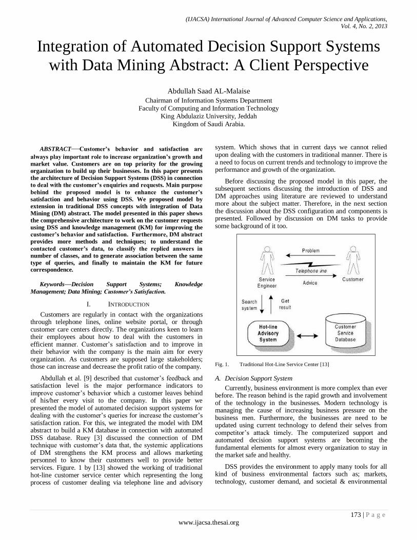
(IJACSA) International Journal of Advanced Computer Science and Applications, Vol. 4, No. 2, 2013
173 | P a g e www.ijacsa.thesai.org
Integration of Automated Decision Support Systems
with Data Mining Abstract: A Client Perspective
Abdullah Saad AL-Malaise
Chairman of Information Systems Department
Faculty of Computing and Information Technology
King Abdulaziz University, Jeddah
Kingdom of Saudi Arabia.
ABSTRACT—Customer’s behavior and satisfaction are
always play important role to increase organization’s growth and
market value. Customers are on top priority for the growing
organization to build up their businesses. In this paper presents
the architecture of Decision Support Systems (DSS) in connection
to deal with the customer’s enquiries and requests. Main purpose
behind the proposed model is to enhance the customer’s
satisfaction and behavior using DSS. We proposed model by
extension in traditional DSS concepts with integration of Data
Mining (DM) abstract. The model presented in this paper shows
the comprehensive architecture to work on the customer requests
using DSS and knowledge management (KM) for improving the
customer’s behavior and satisfaction. Furthermore, DM abstract
provides more methods and techniques; to understand the
contacted customer’s data, to classify the replied answers in
number of classes, and to generate association between the same
type of queries, and finally to maintain the KM for future correspondence.
Keywords—Decision Support Systems; Knowledge
Management; Data Mining; Customer’s Satisfaction.
I. INTRODUCTION
Customers are regularly in contact with the organizations through telephone lines, online website portal, or through customer care centers directly. The organizations keen to learn their employees about how to deal with the customers in efficient manner. Customer’s satisfaction and to improve in their behavior with the company is the main aim for every organization. As customers are supposed large stakeholders; those can increase and decrease the profit ratio of the company.
Abdullah et al. [9] described that customer’s feedback and satisfaction level is the major performance indicators to improve customer’s behavior which a customer leaves behind of his/her every visit to the company. In this paper we presented the model of automated decision support systems for dealing with the customer’s queries for increase the customer’s satisfaction ration. For this, we integrated the model with DM abstract to build a KM database in connection with automated DSS database. Ruey [3] discussed the connection of DM technique with customer’s data that, the systemic applications of DM strengthens the KM process and allows marketing personnel to know their customers well to provide better services. Figure. 1 by [13] showed the working of traditional hot-line customer service center which representing the long process of customer dealing via telephone line and advisory
system. Which shows that in current days we cannot relied upon dealing with the customers in traditional manner. There is a need to focus on current trends and technology to improve the performance and growth of the organization.
Before discussing the proposed model in this paper, the subsequent sections discussing the introduction of DSS and DM approaches using literature are reviewed to understand more about the subject matter. Therefore, in the next section the discussion about the DSS configuration and components is presented. Followed by discussion on DM tasks to provide some background of it too.
Fig. 1. Traditional Hot-Line Service Center [13]
A. Decision Support System
Currently, business environment is more complex than ever before. The reason behind is the rapid growth and involvement of the technology in the businesses. Modern technology is managing the cause of increasing business pressure on the business men. Furthermore, the businesses are need to be updated using current technology to defend their selves from competitor’s attack timely. The computerized support and automated decision support systems are becoming the fundamental elements for almost every organization to stay in the market safe and healthy.
DSS provides the environment to apply many tools for all kind of business environmental factors such as; markets, technology, customer demand, and societal & environmental

(IJACSA) International Journal of Advanced Computer Science and Applications, Vol. 4, No. 2, 2013
174 | P a g e www.ijacsa.thesai.org
factors to generate several choices and in the end to be selected optimal solution [2]. A DSS can have several phases to analyze the problem and take the decision. As Turban described a DSS must consider four phases for complete decision making process such as; Intelligent, Design, Choice and Implementation [2].
Industries build DSS for making themselves proactive and anticipative. The configuration of DSS can be based on data or model. The major classification of DSS are based on (i) Data Oriented DSS, (ii) Model Oriented DSS [2]. While some other scholars also categorized DSS into several categories such as; individual and group DSS, spreadsheet DSS, solver oriented DSS, etc.
Figure-2 [2] showed the basic model of DSS including linkages with its components. In this figure showing the four parts of DSS are; data, models, knowledge and user interface. In this paper we are applying the same concept with some integration in the model, discussed later in methodology section.
In the succeeding section presented the most common DM approaches and tasks which will describe more about the DM background.
Fig. 2. Components of DSS [2]
B. Data Mining Approaches
Data Mining, which also known as Knowledge Discovery in Databases (KDD), refers to the significant extraction of hidden, previously unknown and potentially useful information from data in databases. While DM and knowledge discovery in databases (or KDD) are frequently treated as synonyms, DM is actually part of the knowledge discovery process [5, 8]. Furthermore, Abdullah et. Al described the DM concept in connection with decision support systems (DSS), in decision support management terminology, DM can be consider as a decision support process in which decision maker is searching to generate rule for the help in decision making process [9, 7, 16]. There are several other fields where data mining techniques has been applied by researchers such as, medical database and ERP database [1, 14].
Mainly, DM tasks has been divided into descriptive and predictive methods. Classification, clustering and rule association mining are most common techniques use for predictive and descriptive analysis [10]. Therefore, mainly scholars describe DM in three major tasks. As Zaine [5] stated in his book chapter about major techniques of DM as follows:
a) Classification: Classification analysis is the organization of data in given classes. Also known as supervised classification, the classification uses given class labels to order the objects in the data collection
Classification consider as an important task of DM. Using this approach data must be already defined a class label (target) attribute. Firstly we divide the classified data into two sets; training and testing data [11]. Where each datasets contains others atrributes also but one of the attributed must be defined as class lable attribute. Jiawei Han [11] described classification task in two steps process; first is model construction and the second is model usage. The main target of this task is to build the model by using training dataset and then assign unseen records into a class by using the trained model as accurately as possible. While training data set is use to build the model on the other hand testing data set is use to validate the model [10].
b) Clustering: Similar to classification, clustering is the organization of data in classes. However, unlike classification, in clustering, class labels are unknown and it is up to the clustering algorithm to discover acceptable classes. Clustering is also called unsupervised classification.
Clustering is one of the major task has been applying for DM, work on unsupervised data (no predefined classes) [12]. Clustering is a collection of data objects, clustered by taking similar object to one another within the same cluster, and dissimilar to the objects related in other clusters. Cluster differentiate by using similarities between data according to the characteristics found in the data and grouping similar data objects into clusters [11].
c) Association: Association analysis is the discovery of what are commonly called association rules. It studies the frequency of items occurring together in transactional databases, and based on a threshold called support, identifies the frequent item sets.
Data can be use to find association between several attributes, generate rules from data sets, this task is known as association rule mining [12]. Given a set of transactions, find rules that will predict the occurrence of an item based on the occurrences of other items in the transaction. The goal of association rule mining is to find all rules having support ≥ minsup (minimum support) threshold and confidence ≥ minconf (minimum confidence) threshold [10].
Moreover, association rule mining can be viewed as a two-step process, first, find all frequent itemsets: items satisfying minimum support. Second, generate strong association rules from the frequent itemsets: these rules must satisfy minimum support and minimum confidence [11].
II. METHODOLOGY

(IJACSA) International Journal of Advanced Computer Science and Applications, Vol. 4, No. 2, 2013
175 | P a g e www.ijacsa.thesai.org
The main purpose of this paper is to discuss the enhancement of traditional customer’s dealing process by using current technology. Figure.1 presented above describe the traditionally customer’s dealing process. We presented the DSS model in this paper including DM abstract to generate new rules and patterns to maintain the KM. In order to reply on the customer requests, it will connect directly with KM which have managed all the previous given replies to the customers.
In addition, [15] presented the similar concept of combining the DSS and DM applications together to build joint application to solve evaluation and classification problem. Specially they presented hierarchical multi-attribute decision model which are generally use in decision analysis [17,18]. Basically, this concept attract our research presented in this paper where this research is not taking one techniques into consideration but we have designed a model which can work broadly with any kind of data mining in different phases of decision support system.
Therefore, this paper presents the extended model of the figure. 2 with the integration of DM abstract. The implementation of that model is from customer’s point of view which also known as customer relationship management (CRM). The major purpose of the CRM is to build good relations with the customer in the form customer satisfaction and behavior. Moreover, CRM will provide the facility to understand the customer by evaluating customer behavior, profile, customer segmentation, loyalty and profitability [3].
A. Explanation of the Proposed Model – (Figure-3)
Proposed model in figure. 3 is the extended model of DSS components model (figure. 2) presented above. According to figure. 2 the broad view of four components in the DSS connected to fulfill the requirements of DSS. The components
are; data, model, KM, and user interface. Our model in figure.3 is covering all the four major components of DSS with some integration of DM abstract and customer enquiry systems. Therefore, according to our proposed model we can divide them into four major parts again as per the requirements of DSS. The division is also described in table.1. The complete description of each part of the proposed model discussed in the subsections.
a) Part 1. Data: In the perspective of proposed model we are merging the DSS database with the DM abstraction. As DM tasks are more commonly use for data understanding and extraction new information from the data. In this scenario, firstly the queries will be asked from KM about suitable reply. If the decision is not available from KM, then it will proceed to DM abstract through DSS interface with selected data required for DM process. Afterwards, we can suppose that selected data is enough to produce some new patterns and rules. Simultaneously, the extracted information and rules will be saved in KM. Moreover, the DSS part 1. (DM) has some more methods to find and generate more alternatives for selecting best solution. As selecting the optimal solution is the major concern of DSS.
b) Part 2. Models: This part of DSS is to maintain the models generated while looking for new solutions. The proposed model has presented another aspect of the model generation which are known as DM models. Whenever DM tasks such as; Classification, clustering and association applied on the data, the tasks need to first build the model for data understanding and train the data. In addition of DSS own models, DM models will also be work and save in KM. These model can be available for the same type of request in future correspondence with the customer.
TABLE I. COMPARISON BETWEEN DSS MODEL AND PROPOSED MODEL
[COMPILED BY AUTHOR]
c) Part 3. Knowledge Management: This part considerably has more importance for improving customer’s behaviour and satisfaction with fast process of customer enquiries and complaints. KM is one of the types of database but the major purpose of building KM is to provide the facility to reply directly on customer queries (in current scenario) by using experienced data without contacting with DSS database.
While replying on customer queries, the DM models, rules & patterns, and DSS models will place in the KM for future correspondence with the customers. Those type of data placed in KM is also known as experienced data. As presented in the model firstly all customer’s request are connected with the decision box. Whereas decision box search the decision using KM to find the proper answer from experienced data
DSS Components According to DSS Model (Figure. 2) According to Proposed Model (Figure.3)
Part 1: Data
Data related with DSS Database DM Abstract; will provide more tasks to do on the saved data
Part 2: Models
DSS Model with Choices DM and DSS models; Association, Classification, and Clustering models
Part 3: Knowledge Management Only maintain DSS models, and Choices Maintained both DM and DSS models, patterns and rules
Part 4: User Interface
Any DSS Interface Customer Inquiry Interface

(IJACSA) International Journal of Advanced Computer Science and Applications, Vol. 4, No. 2, 2013
176 | P a g e www.ijacsa.thesai.org
(knowledge base data). If the decision will not available through KM then let the query will drag towards the DSS interface. At last if DSS need more understanding and some other operations to apply on data then it will be forwarded to the DM abstract. DM cannot initiate the working on customer queries directly. According to the model, DM abstract will work only if DSS abstract will forward any query with suitable data to apply any of the DM task. The solution/models generated either by DSS abstract or DM abstract will be transmitted to KM. Finally, the KM is only channel from where the answer will be post back to the asked customer.
d) Part 4. User Interface: In the model the user interface delegated for receiving and sending the customer requests online. According to the scenario detailed in the model a customer is the general term we use in this paper. Whereas a customer may be a type of user, purchaser, seller, influencer, or enquirer etc. Therefore, the raised query may also have several type such as; suggestions, requisitions, questionnaires, sales enquiries, and reclamations depend on the customer type. The major task of this model is to improve customer’s satisfaction and behavior. Therefore, we need to build a interface which can support both DSS and DM abstracts. Finally, both abstract must connect with same KM.
Fig. 3. Integrated Model of DSS with Data Mining Abstract [Proposed by
Author]
III. CONCLUSION AND FUTURE WORK
In conclusion, we proposed the extended version of the DSS model with new perspective of DM and KM. Working on customer’s query using DM and DSS abstract may work better than before. The concept of the model can also help to increase customer’s satisfaction, behavior and ultimately the growth of the organization. As customer’s plays significant role for making organization good will in the market. Therefore, the model may provide help for dealing with the customers in more efficient manner.
In future, the practical implementation of the proposed model with different attributed data may provide some fruitful results. Actually, each DM tasks deal with special attributed data. Model Implementation on real world data will guide more about the applicability of the model. Our future concerns is to apply this model using medical or student data for taking decision on student/patient online queries.
Reference
[1] Abdullah Saad ALMALAISE ALGHAMDI, “Efficient Implementation
of FP Growth Algorithm Data Mining on Medical Data”, International Journal of Computer Science and Network Security (IJCSNS)-2011.
[2] Efraim Turban, Ramesh Sharda, Dursun Delen, Decision Support and Business Intelligence, 9th Edition, published by Pearson Education,
Prentice Hall-2011. [3] Ruey-Shun Chen, Ruey-Chyi Wu and J. Y. Chen , "Data Mining
Application in Customer Relationship Management of Credit Card Business", Institute of Information Management,Taiwan.
[4] Hai Wang, Shouhong Wang, Medical Knowledge Acquisition through Data Mining, Proceedings of 2008 IEEE International Symposium on IT
in Medicine and Education. [5] Osmar R. Zaïane, "Chapter I: Introduction to Data Mining", CMPUT690
Principles of Knowledge Discovery in Databases, 1999. [6] Abdullah Al- Mudimigh, Farrukh Saleem, Zahid Ullah, The Effects Of
Data Mining In ERP-CRM Model – A Case Study Of MADAR, WSEAS Transaction, 2009
[7] Dr. Abdullah Al- Mudimigh, Farrukh Saleem, Zahid Ullah, The Role Of Data Mining In ERP-CRM Model”, International Conference on
Applied Computer & Applied Computational Science (ACACOS '09),
Hangzhou, China, 2009. [8] Abdullah s. Al- Mudimigh, Farrukh Saleem, Zahid Ullah, Fahad N. Al-
Aboud, Implementation of Data Mining Engine on CRM -Improve Customer Satisfaction”, IEEE / ICICT-2009, Third International
Conference on Information & Communication Technologies, Karachi, Pakistan, 2009.
[9] Dr. Abdullah Al- Mudimigh, Farrukh Saleem, Zahid Ullah, Efficient Implementation of Data Mining: Improve Customer's Behavior", The 7th
IEEE/ACS, International Conference on Computer Systems and Applications, Rabat, Morocco, to be held on May, 10-13, 2009.
[10] Pang-Ning Tan, Michael Steinbach & Vipin Kumar, "Introduction to Data Mining", Addison Wesley, 2005, ISBN 0321321367.
[11] Jiawei Han, Micheline Kamber, Jian Pei, “Data Mining: Concepts and Techniques”, 2nd edition, 2005, Morgan Kaufmann, ISBN 1558609016
[12] Farrukh Saleem, Areej Malibari, Data Mining Course In Information System Department–Case Study Of King Abdulaziz University, Ieee,
ICEED- 3rd International Congress on Engineering Education, 7th – 8th December, 2011.
[13] S.C. Hui, G. Jha, "Data Mining for Customer Service Support", Information & Management, Elsevier 2000.
[14] Abdullah Saad Almalaise Alghamdi, “Rules Generation from ERP Database: A Successful Implementation of Data Mining”, IJCSNS
International Journal of Computer Science and Network Security, VOL.12 No.3, March 2012.
[15] Marko Bohanec, Blaž Zupan, Integrating Decision Support and Data
Mining by Hierarchical Multi-Attribute DecisionModels, University of Ljubljana, Slovenia,
Baylor College of Medicine, Houston, U.S.A.
[16] Farrukh Saleem, Abdullah Saad Almalaise Alghamdi, “Implementation
of data mining approach for building automated decision support systems”, Information Society (i-Society), 2012 International
Conference, London, UK , pp. 127 – 130, June 2012.
[17] Angehm, A.A.: Supporting multi-criteria decision making. In: Holtham C. (ed.): Execu-tive Information
[18] Systems and Decision Support. Chapman & Hall (1992) Clemen, R.T.:
Making Hard Decisions: An Introduction to Decision Analysis. Duxbury Press (1996).

(IJACSA) International Journal of Advanced Computer Science and Applications, Vol. 4, No. 2, 2013
177 | P a g e www.ijacsa.thesai.org
Automatic Image Registration Technique of Remote
Sensing Images
M. Wahed, Gh.S. El-tawel
Computer Science Department
Suez Canal University
Ismailia, Egypt
A. Gad El-karim
Mathematics Department
Suez Canal University
Alarish, Egypt
Abstract— Image registration is a crucial step in most image
processing tasks for which the final result is achieved from a
combination of various resources. Automatic registration of
remote-sensing images is a difficult task as it must deal with the
intensity changes and variation of scale, rotation and
illumination of the images. This paper proposes image
registration technique of multi-view, multi- temporal and multi-
spectral remote sensing images. Firstly, a preprocessing step is
performed by applying median filtering to enhance the images.
Secondly, the Steerable Pyramid Transform is adopted to
produce multi-resolution levels of reference and sensed images;
then, the Scale Invariant Feature Transform (SIFT) is utilized
for extracting feature points that can deal with the large
variations of scale, rotation and illumination between images
.Thirdly, matching the features points by using the Euclidian
distance ratio; then removing the false matching pairs using the
RANdom SAmple Consensus (RANSAC) algorithm. Finally, the
mapping function is obtained by the affine transformation.
Quantitative comparisons of our technique with the related
techniques show a significant improvement in the presence of
large scale, rotation changes, and the intensity changes. The
effectiveness of the proposed technique is demonstrated by the experimental results.
Keywords— Image registration; Steerable Pyramid Transform;
SIFT; RANSAC
I. INTRODUCTION
Image registration is a fundamental task in image processing used to match two or more images which are taken at different time, from different sensors or different viewpoints [1]. The present image registration methods can be generally divided into two broad categories: area-based and feature-based methods [2]. Area-based methods deal with the images without detecting salient features, and adopt optimization algorithms. These methods are substantial to the intensity distribution. The feature-based methods do not directly work with image intensity values, but, instead, use salient features extracted from two images, which has been shown to be more suitable for such situations that intensity changes and complicated geometric deformations are encountered. Therefore, these feature-based methods have been widely used in remote-sensing image registration. Feature-based image registration consists of five steps: preprocessing, feature selection, feature correspondence, transformation and resampling. Among them, feature selection, correspondence and transformation require numerous manipulation techniques, where in the most difficult
one is the feature correspondence. If some correspondences are incorrect, they will produce an incorrect transformation function, which could yield totally wrong results, so a highly robust matching algorithm is needed. The process of image registration intersects with the following research areas: computer vision, pattern recognition, and remotely sensed data processing. In general, its applications can be divided into multi-view analysis, multi-temporal analysis and multimodal analysis according to the manner of the image acquisition.
In literature, there are several image registration techniques have been proposed, Xiangzeng and al. [3] Proposed multi-scale image registration technique based on steerable pyramid transform and Scale Invariant Feature Transform (SIFT) of remote sensing image. Nagham and al. [4] presented wavelet-based image registration technique that combined Scale Invariant Feature Transform (SIFT) with Mutual-Information (MI). Haidawati and al. [5] developed image registration approach based on a combination of Scale Invariant Feature Transform (SIFT), Belief Propagation (BP) for matching features and Random Sampling Consensus (RANSAC) adopted to filter out the mismatched points. Sang [6] introduced automatic coarse-to-fine image registration algorithm for satellite images, based on Haar Wavelet Transform (HWT) and the Speeded Up Robust Features (SURF) algorithm in the coarse registration, the normalized cross-correlation and RANdom SAmple Consensus (RANSAC) algorithm to achieve the fine registration. Mahmudul and al. [7] proposed a method to improve SIFT-based matching for multispectral image registration. Fatiha and al. [8] presented an efficient image registration algorithm that used the genetic algorithms and the cross-correlation similarity measure for matching within a multi-resolution framework based on the Non-Subsampled Contourlet Transform (NSCT).Yi and al. [9] presented an enhanced SIFT method for multi-spectral remote sensing image registration. Le and al. [10] developed a fully automatic and fast non-rigid image registration technique that coarsely aligned the input image to the reference image by automatically detecting their matching points by using the scale invariant feature transform (SIFT) method and an affine transformation model. Gang and Yun [11] introduced image registration technique, which is based on wavelet-based feature extraction technique, a normalized cross-correlation matching and relaxation-based image matching techniques. Leila and al. [12] presented efficient image registration algorithm of multi-temporal images with similar spectral responses based on modulus

(IJACSA) International Journal of Advanced Computer Science and Applications, Vol. 4, No. 2, 2013
178 | P a g e www.ijacsa.thesai.org
maxima of wavelet transform for point features extraction and a correlation based matching measure used in the matching process. Shirin and Kasaei [13] developed image registration method based on Contourlet Transform for extracting edge features from panchromatic satellite images and matching features by normalized cross-correlation.
In this paper we present automatic image registration technique of remote sensing image based on the Steerable Pyramid Transform and SIFT descriptors. This paper is organized as follows. Section 2 presents the proposed image registration technique. Experimental results and conclusions are given in Sections 3 and 4, respectively.
II. PROPOSED IMAGE REGISTRATION TECHNIQUE
In this section, we describe the proposed image registration technique which consists of six steps: preprocessing, decomposition by steerable pyramid transform, extract feature points using the Scale Invariant Feature Transform (SIFT), Find all matching pairs between two images ,remove false matching pairs, perform affine transformation and resampling to perform image registration. The work flow of the proposed technique is shown in Fig.1.
A. Preprocessing
Given two input images (the reference image and the sensed image), applying median filtering to the reference image and the sensed image in order to enhance the two input images.
B. Steerable Pyramid Transform
The steerable pyramid transform is a linear multi-scale, multi-orientation image decomposition that provides a useful front-end for image processing and computer vision applications [14]. It has been developed in order to overcome the limitations of orthogonal separable wavelet decompositions that were popular for image processing. The “steerable filter” refers to a class of filters, in which a filter of arbitrary orientation can be synthesized as a linear combination of a set of “basis filters”. For any function
is rotated through an angle about the origin. We call is steerable if it satisfies the
following equation:
Where are the interpolation functions .The basic functions of the steerable pyramid are directional derivative operators that come in different sizes and orientations, and the number of orientations may be adjusted by changing the derivative order. The structure of the steerable pyramid in the frequency domain is shown in Fig.2.The image is initially divided into high and low-pass sub-bands using filters and . The low-pass branch is then further divided into oriented band-pass portions using filters which ensure that the representation is rotation invariant and lower-pass portion using filter
.this lower-pass sub-band is sub-sampled by a factor of 2 in the X and Y directions. In order to ensure translation-
invariance, the outputs of the high-pass filter and of the band-pass filters are not sub-sampled. In addition, that portion of the signal, which is iteratively decomposed by the band-pass and the low-pass filters, does not contain the larger high frequency components and has been preprocessed by a low-pass filter, thus removing most aliased component, thus, to eliminate aliasing terms, is constrained as:
For
(2)
The recursive construction of a pyramid is achieved by inserting a copy of the shaded portion of the System diagram in Fig.2 at the location of the solid circle. The steerable pyramid performs a polar-separable decomposition in the frequency domain, thus allowing independent representation of scale and orientation. In order to cascade the system recursively, there should be
In the proposed technique we apply the steerable pyramid transform to the two input images to level three with one orientation band-pass component. Fig.3 shows three level of steerable pyramid decomposition with one orientation band-pass filter for the reference image and the sensed image, respectively.
C. SIFT Feature Point Extraction Algorithm
SIFT algorithm was proposed in [15] as a method to extract and describe feature points, which is robust to scale, rotation and change in illumination. There are four steps to implement the SIFT algorithm:
1) Scale-space Extrema Detection: The first stage
searches over scale space using a Difference of Gaussian
(DoG) function to identify potential interest points that are
invariant to scale and orientation. The scale space of an
image is defined as a function , which is produced
from the convolution of a variable-scale Gaussian with an input image :
To efficiently detect stable key-point locations in scale space using scale-space extrema in the difference-of-Gaussian function convolved with the image, which can be computed from the difference of two nearby scales separated by a constant multiplicative factor :
. (6)
2) Feature Point Localization: The location and the scale
of each candidate point are determined and the feature points
are selected based on measures of stability this information
allows points to be rejected that have low contrast (and are
therefore sensitive to noise) or are poorly localized along an
edge.

(IJACSA) International Journal of Advanced Computer Science and Applications, Vol. 4, No. 2, 2013
179 | P a g e www.ijacsa.thesai.org
Fig. 1. Work Flow of the Proposed Technique
Reference image
Image enhancement using
median filtering
Decomposition by Steerable
Pyramid Transform
Feature point extraction at
every decomposition level
using SIFT
Find all matching pairs between two
images by calculating the ratio of the Euclidian distance of descriptor vector from
closest neighbor to the distance of second
closest
Remove false matching pairs using
RANSAC algorithm
Using refined matching pairs, perform affine transformation
Resample sensed image according to
transformation parameters and perform
image registration
Sensed image
Image enhancement using
median filtering
Decomposition by Steerable
Pyramid Transform
Feature point extraction at
every decomposition level
using SIFT
2
3
4
5
1
6

(IJACSA) International Journal of Advanced Computer Science and Applications, Vol. 4, No. 2, 2013
180 | P a g e www.ijacsa.thesai.org
Fig. 2. System diagram for first derivative Steerable Pyramid
Fig. 3. Steerable Pyramid decomposition (l=3) for (a) reference image and (b) sensed image
3) Orientation Assignment: One or more orientations are
assigned to each feature point location based on local image
gradient directions. For each image sample at this
scale , the gradient magnitude and orientation
are precomputed using pixel differences:
(7)
4) Feature Point Descriptor: A feature descriptor is
created by first computing the gradient magnitude and
orientation at each image sample point in a region around the
feature point location, as shown on the left of Fig.4.These are
weighted by a Gaussian window, indicated by the overlaid
circle. These samples are then accumulated into orientation
histograms summarizing the contents over 4x4 sub-regions,
with 8 orientation bins. So each feature point has a 128-
element feature as shown on the right, with the length of each
arrow corresponding to the sum of the gradient magnitudes
near that direction within the region. The SIFT feature point
extraction for the reference image and the sensed image is
shown in Fig.5 and Fig.6.
D. The proposed Feature Points Matching Using Structural Information
SIFT algorithm at first detects feature points in scale-
space, feature points with low contrast and located at edges
are discarded. Then a 128-element feature descriptor is
generated for each feature point using statistics of the gradient
directions which are scale and rotation invariant. These
descriptors are used to find the corresponding feature points
by calculating the ratio of the Euclidian distance of descriptor
vector from closest neighbor to the distance of second closest.
To illustrate the issue, we show an example in Fig.7. SIFT matching is applied to images A and B. The bold line shows a
pair of matched featured points in the two images. The
dotted line shows the best match of another feature point
in image A, while the correct match should be point . In the
proposed technique is not selected as a matched feature
point for because the spatial distance between points and
is too large. Feature points and are matched while the
counterpart for neighboring feature point cannot be decided
because the SIFT descriptors for points and are almost
equally different from the SIFT descriptor of point . This
problem is made worse by the fact that a lot of similar
descriptors can be found in typical remote sensing images.
The idea to solve this problem is as follows. Still considering
the example in Fig.7, assume points and are already
matched with high confidence that the match is correct. We
can predict that the feature points around (shown in the
circular window) can be found around . So, for point we
only search the neighborhood of point for a matching
descriptor, which results in a correct match at point . For
better matching accuracy we suggest modifications to SIFT
matching by imposing a threshold on the Euclidian distance
ratio as follows: A descriptor of feature point in
image (reference image) is matched to a descriptor
in image (sensed image) only if
the Euclidian distance multiplied by threshold (set
(a) (b)

(IJACSA) International Journal of Advanced Computer Science and Applications, Vol. 4, No. 2, 2013
181 | P a g e www.ijacsa.thesai.org
to 1.5) is not greater than the distance of to all other
descriptors. SIFT matching result between the feature points
of the reference image and the sensed image is shown in Fig.8.
Fig. 4. Feature descriptor creation
Fig. 5. Feature points returned by SIFT for reference image
Fig. 6. Feature points returned by SIFT for sensed image
Fig. 7. a) Feature point matching results to points as correct match but no match found for b. (b) Euclidian distance of the descriptors of all the feature point on image B for the feature point on image .

(IJACSA) International Journal of Advanced Computer Science and Applications, Vol. 4, No. 2, 2013
182 | P a g e www.ijacsa.thesai.org
Fig. 8. Matching result between the reference image and sensed image in steerable domain.
E. RANSAC (Random Sample Consensus) Algorithm
In general there are all kinds of photometric and geometric transformations that can occur between two views of a scene. This means normalized cross-correlation will sometimes generate spurious correspondences. To robustly fit a model to the correspondences, we need to overcome the effect of these outliers. The RANdom SAmple Consensus (RANSAC) algorithm proposed by Martin and Robert [16] is a general parameter estimation approach designed to cope with a large proportion of outliers in the input data. There are two types of samples: contaminated, those that contain at least one outlier, and uncontaminated (all-inlier or outlier-free) samples. Only the latter ones are of interest, as the model parameters computed from data points including outliers are arbitrary. The number of iterations is chosen high enough to ensure that the probability (usually set to 0.99) that at least one of the sets of random samples does not include an outlier. Let represent the probability that any selected data point is an
inlier and – the probability of observing an outlier, iterations of the minimum number of points denoted are required, where
, and thus with some manipulation,
A RANSAC algorithm provides a general technique for model fitting in the presence of outliers and consists of the following steps:
1) Choose a model.
2) Determine the minimal number of points needed to
specify the model.
3) Define a threshold on the inlier count.
4) Fit the model to a randomly selected minimal subset
5) Apply the transformation to the complete set of
points and count inliers.
6) If the number of inliers exceeds the threshold, flag
the fit as good and stop.
7) Otherwise repeat steps 4 to 6.
In our technique we apply RANSAC algorithm to the putative correspondences to remove false matching point pairs, which are consistent with this estimate because many of the putative correspondences obtained in the previous step are incorrect.
F. Perform Affine Transformation and Resampling
Given the refined matching point pairs, build the mapping function and get the affine transformation parameters to resample the sensed image and perform image registration.
III. EXPERMENTAL RESULTS AND EVALUATION
A. Data Sets
The proposed technique is tested for ten different sets of remote sensing images. We present three different sets of images. The first set of images is Landsat TM images from different bands (12-band 0 and 8) (Fig. 9(a) and (b)) with large rotation variation, which are used to show the implementation and accuracy of our algorithm. Images of the second set are Agricultural images from Landsat TM (band 5) of Amazon region acquired at different times (Fig.10 (a) and Fig. 10(b)) .The third data set are QuickBird panchromatic and near-infrared band images (Fig.11 (a) and (b)) with large scale difference derived from Digital Globe, Inc; acquired on Jul. 4, 2005 over Boulder, USA .The near-infrared band has been shown to be effective for estimating moisture content and plant biomass in the 760–900 nm wavelength range. In addition, the panchromatic and multispectral images have 0.6 m and 2.4 m spatial resolution at nadir, respectively. Here, the near infrared band image of low spatial resolution is registered to the high resolution panchromatic image. The feature points information of the three data sets are shown in Table 1.

(IJACSA) International Journal of Advanced Computer Science and Applications, Vol. 4, No. 2, 2013
183 | P a g e www.ijacsa.thesai.org
Fig. 9. Reference image, sensed image, matching results, and registration results (Landsat TM images). (a) The reference image (Landsat TM 12-Band 0, 512 by 512); (b) the sensed image (Landsat TM 12 -Band 8, 512 by 512); (c) the matching results of (a) and (b); (d) the registration
results of (a) and (b).
Fig. 10. Agricultural images from Landsat TM (band 5). (a) The reference image (Landsat TM 400 by 400 acquired on September 9, 1990);
(b) the sensed image (Landsat TM 400 by 400 acquired on July 18, 1994.); (c) the matching results of (a) and (b); (d) the registration results of (a) and (b).
(a) (b) (c)
(d)
(a) (b) (c)
(d)

(IJACSA) International Journal of Advanced Computer Science and Applications, Vol. 4, No. 2, 2013
184 | P a g e www.ijacsa.thesai.org
Fig. 11. Reference image ,sensed image, matching results, and registration results of QuickBird panchromatic and near-infrared images (Image courtesy of Digital Globe) (a) The reference image (QuickBird panchromatic, 2048 by 2048); (b) the sensed image (QuickBird near-infrared, 937 by 915); (c) the matching results of (a) and (b); (d) the registration results of (a) and (b).
TABLE I. FEATURE POINTS INFORMATION (FIG.9—11)
Data sets
Feature points information
Level no. Image size(pixels) Number of feature points Number of initial
matched pairs
Number of refined
matched pairs using
RANSAC
Reference image Sensed image
Fig .9
1 512x512 6571 7502 244 161
2 256x256 3285 3498 420 270
Fig .10
1 400x400 4313 4192 174 108
2 200x200 1581 1519 169 102
Fig .11
1 2048x2048
937x915
19091 13261 578 505
2 1024x1024
465x 457
16538 10137 1630 1553
B. Evaluation
In order to evaluate the proposed image registration technique; First we apply the proposed technique to the three sets of images. Second, we compare our technique with other two related techniques on the accuracy of matching and registration. To evaluate the matching result between the two input images, Assume that the transformation between the point ( in the sensed image and its corresponding point ( in the reference image is affine transformation, we can use the root mean square error ( ) :
Where means the total number of matching points; are affine transformation parameters. The transformation parameters between the two input images of the three data sets and their root mean square error ( ) are shown in Table 2.
The test three sets of images include large rotation, translation, scale, and intensity changes. We use Fig.9 (a) as the reference image and Fig.9 (b) as the sensed image. Fig.9
(a) (b) (c)
(d)

(IJACSA) International Journal of Advanced Computer Science and Applications, Vol. 4, No. 2, 2013
185 | P a g e www.ijacsa.thesai.org
(c) and (d) shows the matching results and the registration results, respectively. In the second data set we use two Landsat TM (band5) images with translation differences; Fig.10 (a) and Fig.10 (b), are used as the reference image and the sensed image, respectively. Fig.10 (c) shows the matching results and Fig. 10 (d) shows the registration results .Fig.11 (a) and (b) are QuickBird panchromatic and near-infrared band images with large scale variations and intensity changes, which is used as the reference image and the sensed image, respectively. The matching results and registration results are shown in Fig.11 (c) and (d), respectively. To compare the registration accuracy, we consider the root mean square error of intensity ( ),the correlation (corr) between the overlapping areas of registered image pairs and Peak Signal to Noise Ratio(PSNR), which are defined as follows:
Where is the reference image, is the registered image, is the overlapping area between and , and is the number of pixels in . The accuracy of matching results and registration results for Fig.9, Fig.10, and Fig.11 are shown in Table3. Fig.12 shows the registration accuracy in four resolution levels for Fig.9.
Experiment have been carried out on the first set of images (Landsat TM images) in order to compare the registration accuracy of the proposed technique against other image registration techniques (Xiangzeng and al. [3]) and (Le and al. [10]); we consider is smaller and the is the larger which shows higher accuracy of registration. The comparisons of accuracy of matching results and registration results for Fig.9 are shown in Fig.13. From Fig.13, we can see both that and of the proposed technique are the smallest and of the proposed technique is the largest. From the above experimental results, we can see that the proposed technique performs better than the other two techniques when large scale variations, rotation, translation, and intensity changes exist between the two input image
TABLE II. THE TRANSFORMATION PARAMETERS AND THEIR RMSE (FIG.9—11)
Data sets
Transformation Parameters and RMSE
Fig .9 0.9626 -0.2551 -10.7779 0.2650 0.9757 264.9061 0.11
Fig .10 0.9872 -0.0006 69.6568 0.0005 1.0077 -60.8548 0.33
Fig .11 0.9914 -0.0001 -17.7040 0.0002 1.0276 -93.5854 0.17
TABLE III. THE ACCURACY OF MATCHING RESULTS AND REGISTRATION RESULTS (FIG.9—11)
Data sets
Matching error, Registration error, Correlation and Peak Signal to Noise Ratio
Fig.9 0.11 11.12 0.99 32.47
Fig.10 0.33 4.08 0.87 35.91
Fig.11 0.17 2.71 0.89 39.47

(IJACSA) International Journal of Advanced Computer Science and Applications, Vol. 4, No. 2, 2013
186 | P a g e www.ijacsa.thesai.org
Fig. 12. Registration accuracy ( in different resolution levels, (l=4) for Fig.9.
Fig. 13. Comparisons of the registration accuracy of the Proposed Technique against the two related Registration
Techniques for Fig.9.
0
0.1
0.2
0.3
0.4
0.5
0.6
1 2 3 4
RM
SE
Processing Level
Matching Error
10
11
12
13
14
1 2 3 4
RM
SE1
Processing Level
Registration Error
0.985
0.99
0.995
1
1 2 3 4
co
rr
Processing Level
Correlation
26
28
30
32
34
1 2 3 4
PS
NR
Processing Level
Peak Signal to Noise Ratio
0.11
0.2
0.36
0
0.1
0.2
0.3
0.4
Proposed
Technique
Registration
Technique[3]
Registration
Technique[9]
RM
SE
Matching Error
11.12
12.93 15.37
0
5
10
15
20
Proposed
Technique
Registration
Technique[3]
Registration
Technique[9]
RM
SE
1
Registration Error
0.99
0.98
0.86
0.75
0.8
0.85
0.9
0.95
1
Proposed
Technique
Registration
Technique[3]
Registration
Technique[9]
co
rr
Correlation

(IJACSA) International Journal of Advanced Computer Science and Applications, Vol. 4, No. 2, 2013
187 | P a g e www.ijacsa.thesai.org
IV. CONCLUSIONS
In this paper we have presented an automatic registration technique of multi-view, multi-temporal, and multi-spectral remote sensing images based on the Steerable Pyramid Transform and SIFT features that can deal with the large variations of scale, rotation and illumination between images. The median filtering is applied in order to enhance the two input images. The advantage of the proposed technique lies in its ability to increase the number of matched points using the developed SIFT neighborhood matching method and to overcome the outliers introduced in the matching using RANSAC algorithm and hence correctly estimate the transformation matrix. The experimental results show that the proposed technique returns better performance for large scale variations, rotation and intensity changes as compared to the two other related image registration techniques.
References
[1] D. Suma, S. Vikas, and Sh. Bhudev, “Remote sensing image registration techniques: a survey,” In: Proc ISISP, Vol. 6134.P. 103–12, 2010.
[2] Z. Barbra, and F. Jan, “Image registration methods: a survey,” Image and Vision Computing 21, 977–1000, 2003.
[3] L. Xiangzeng, T. Zheng, C. Chunyan, and F. Huijing, “Multiscale registrations of remote sensing image using robust SIFT features in
steerable-domain,” The Egyptian Journal of Remote Sensing and Space Sciences, 2011.
[4] M. Nagham, F. Abou-Chadi, and S. Kishk, “Wavelet-based image registration techniques: a study of performance,” IJCSNS International
Journal of Computer Science a 188 and Network Security, Vol.11 No.2, 2011.
[5] N. Haidawati, S. Vladimir, and M. Stephen, “Image registration for super resolution using scale invariant feature transform, belief
propagation, and random sampling consensus,” European Signal
Processing Conference (EUSIPCO-ISSN 2076-1465, 2010). [6] L. Sang, “A coarse-to-fine approach for remote-sensing image
registration based on a Local method,” International Journal on Smart Sensing and Intelligent Systems Vol. 3, No. 4, 2010.
[7] H. Mahmudul, J. Xiuping, R-K. Antonio, Z. Jun, P. Mark, “Multi-spectral remote sensing image registration via spatial relationship
analysis on SIFT keypoints,” IEEE 978-1-4244-9566-5. [8] M. Fatiha, El.M. Miloud, and T. Nasreddine, “A rigid image registration
based on the Nonsubsampled Contourlet transform and genetic algorithms,” Sensors 2010, 10, 8553-8571, doi: 10.3390/s100908553,
2010. [9] Z. Yi, C. Zhiguo, and X. Yang,” Multi-spectral remote image
registration based on SIFT,” IEEE Electronics Letter, Vol. 44, No. 2, pp. 107-108, 2008.
[10] Y. Le, Z. Dengrong, and H. Eun-Jung, “A fast and fully automatic registration approach based on point features for multi-source remote-
sensing images,” Computers and Geosciences 34. 838– 848, 2008. [11] H. Gang and Z. Yun, ”Wavelet-based image registration technique for
high resolution remote sensing images,” Computers & Geosciences 34.1708–1720, 2008.
[12] F. Leila, C. Max, K. Thales, C. Emiliano, and S. Felipe, “Multitemporal image registration based on multiresolution decomposition,” ISSN
1808-0936, 2008. [13] B. Shirin and Sh. Kasaei, “Contourlet-based edge extraction for image
registration,” Iranian Journal of Electrical &Electronic Engineering, Vol. 4, No. 1&2, 2008.
[14] F. William and A. Edward, “The design and use of steerable filters,” IEEE Transactions on Pattern Analysis and Machine Intelligence 13,
891–907, 1991. [15] L. David, “Distinctive image features form scale-invariant keypoints,”
International Journal of Computer Vision 60, 91–110, 2004. [16] F. Martin and B. Robert, “Random sample consensus: a paradigm for
model fitting with applications to image analysis and automated cartography,” Communications of the ACM, Vol. 24, No. 6, pp. 381-
395, 1981.

(IJACSA) International Journal of Advanced Computer Science and Applications, Vol. 4, No. 2, 2013
188 | P a g e www.ijacsa.thesai.org
Indian Sign Language Recognition Using Eigen
Value Weighted Euclidean Distance Based
Classification Technique
Joyeeta Singha
Dept. of Electronics and Communication Engineering
Assam Don Bosco University Guwahati, India
Karen Das
Dept. of Electronics and Communication Engineering
Assam Don Bosco University
Guwahati, India
Abstract—Sign Language Recognition is one of the most
growing fields of research today. Many new techniques have been
developed recently in these fields. Here in this paper, we have
proposed a system using Eigen value weighted Euclidean distance
as a classification technique for recognition of various Sign
Languages of India. The system comprises of four parts: Skin
Filtering, Hand Cropping, Feature Extraction and Classification.
24 signs were considered in this paper, each having 10 samples,
thus a total of 240 images was considered for which recognition rate obtained was 97%.
Keywords—Hand Gesture Recognition; Skin Filtering; Human
Computer Interaction; Euclidean Distance (E.D.); Eigen value;
Eigen vector.
I. INTRODUCTION
Sign Language is a well-structured code gesture, every gesture has meaning assigned to it. Sign Language is the only means of communication for deaf people. With the advancement of science and technology many techniques have been developed not only to minimize the problem of deaf people but also to implement it in different fields. Many research works related to Sign languages have been done as for example the American Sign Language, the British Sign Language, the Japanese Sign Language, and so on. But very few works has been done in Indian Sign Language recognition till date.
Finding an experienced and qualified interpreters every time is a very difficult task and also unaffordable. Moreover, people who are not deaf, never try to learn the sign language for interacting with the deaf people. This becomes a cause of isolation of the deaf people. But if the computer can be programmed in such a way that it can translate sign language to text format, the difference between the normal people and the deaf community can be minimized.
We have proposed a system which is able to recognize the various alphabets of Indian Sign Language for Human-Computer interaction giving more accurate results at least possible time. It will not only benefit the deaf and dumb people of India but also could be used in various applications in the technology field.
II. LITERATURE REVIEW
Different approaches have been used by different researchers for recognition of various hand gestures which were implemented in different fields. Some of the approaches were vision based approaches, data glove based approaches, soft computing approaches like Artificial Neural Network, Fuzzy logic, Genetic Algorithm and others like PCA, Canonical Analysis, etc. The whole approaches could be divided into three broad categories- Hand segmentation approaches, Feature extraction approaches and Gesture recognition approaches. Few of the works have been discussed in this paper.
Many researchers [1-11] used skin filtering technique for segmentation of hand. This technique separated the skin colored pixels from the non-skin colored pixels, thus extracting the hand from the background. Fang [12] used Adaptive Boost algorithm which could not only detect single hand but also the overlapped hands. In [13-15] external aid like data gloves, color gloves were used by the researchers for segmentation purpose.
Saengsri [13] in his paper Thai Sign Language Recognition used ‘5DT Data Glove 14 Ultra’ data glove which was attached with 14 sensors- 10 sensors on fingers and rest 4 sensors between the fingers which measures flexures and abductions respectively. But accuracy rate was 94%. Kim [14] used ‘KHU-1’ data glove which comprises of 3 accelerometer sensor, a Bluetooth and a controller which extracted features like joints of hand. He performed the experiment for only 3 gestures and the process was very slow. Weissmann [15] used Cyberglove which measured features like thumb rotation, angle made between the neighboring fingers and wrist pitch. Limitations were that the system could recognize only single hand gestures.
There have been wide approaches for feature extraction like PCA, Hit-Miss Transform, Principle Curvature Based Region detector (PCBR), 2-D Wavelet Packet Decomposition (WPD) etc. In [1][16-18] Principal Component Analysis (PCA) was used for extracting features for recognition of various hand gestures. Kong [16] segmented the 3-D images into lines and curves and then PCA was used to determine features like direction of motion, shape, position and size.

(IJACSA) International Journal of Advanced Computer Science and Applications, Vol. 4, No. 2, 2013
189 | P a g e www.ijacsa.thesai.org
Lamar [17] in his paper for American and Japanese alphabet recognition used PCA for extracting features like position of the finger, shape of the finger and direction of the image described by the mean, Eigen values and Eigen vectors respectively. The limitations were accuracy rate obtained was 93% which was low and the system could recognize gestures of only single hand. Kapuscinski [2] proposed Hit-Miss transform for extracting features like orientation, hand size by computing the central moments. Accuracy rate obtained was 98% but it lacks proper Skin filtering with changes in illumination. Generic Fourier descriptor and Generic Cosine Descriptor is used [19] for feature extraction as it is rotation invariant, translation invariant and scale invariant. Rotation of the input hand image leads to shifting of hand in polar space. Rotation invariance is obtained by only considering the magnitude of the Fourier coefficient. While using centroid as the origin translational invariance is achieved and finally ratio of magnitude to area scale invariance is obtained. Only 15 different hand gestures were considered in this paper. Rekha [9] extracted the texture, shape, finger features of hand in the form of edges and lines by PCBR detector which otherwise is a very difficult task because of change in illumination, color and scale. Accuracy rate obtained was 91.3%.
After the features were extracted, proper classifier were used to recognize the gestures. There are various gesture recognition approaches used by different researchers like Support Vector Machines, Artificial Neural Network (ANN), Genetic Algorithm (GA), Fuzzy Logic, Euclidean distance, Hidden Markov Model (HMM), etc. [13][17] used ANN for recognizing gestures. Saengsri [13] used Elman Back Propagation Neural Network (ENN) algorithm which consisted of input layer with 14 nodes similar to the sensors in the data glove, output layer with 16 nodes equal to the number of symbols and hidden layer with 30 nodes which is just the total of input and output nodes. Gesture was recognized by identifying the maximum value class from ENN. Recognition rate obtained was 94.44%. Difficulty faced in this paper was it considered only single gestured signs. Lamar [17] used ANN which comprises of input layer with 20 neurons, hidden and output layer each with 42 neurons. Back propagation algorithm was used and after the training of the neural network one output neuron was achieved, thus giving the proper recognized gesture. Gopalan [1] used Support Vector Machine for classification purpose. The linearly non separable data becomes separable when SVM was used as the data was projected to higher dimensional space, thus reducing error. Kim [20] in his paper of Recognition of Korean Sign Language used Fuzzy logic. Fuzzy sets were considered where each set were the various speeds of the moving hand. They were mathematically given by ranges like small, medium, negative medium, large, positive large, etc. Accuracy rate obtained was 94% and difficulty faced by them was heavy computation.
We have thus proposed a system that could overcome the difficulties faced by various. Our proposed system was able to recognize two hand gestures with an improved accuracy rate of 97%. Moreover, experiment was carried out with bare hands and computational time was also less thus removing the difficulties faced by use of the hand gloves with sensors.
III. THEORETICAL BACKGROUND
A. Eigen value and Eigen vector
Eigen values and Eigen vectors are a part of linear transformations. Eigen vectors are the directions along which the linear transformation acts by stretching, compressing or flipping and Eigen values gives the factor by which the compression or stretching occurs. In case of analysis of data, the Eigen vectors of the covariance are being found out. Eigenvectors are set of basis function which describes variability of data. And Eigen vectors are also a kind of coordinate system for which the covariance matrix becomes diagonal for which the new coordinate system is uncorrelated. The more the Eigen vectors the better the information obtained from the linear transformation. Eigen values measures the variance of data of new coordinate system. For compression of the data only few significant Eigen values are being selected which reduces the dimension of the data allowing the data to get compressed. Mathematically, it is explained in (1).
If x is a one column vector with n rows and A is a square matrix with n rows and columns, then the matrix product Ax will result in vector y. When these two vectors are parallel, Ax = λx, (λ being any real number) then x is an eigenvector of A and the scaling factor λ is the respective eigenvalue.
IV. PROPOSED SYSTEM
The block diagram of the proposed system is given in Fig. 1 which comprises of mainly four phases: Skin filtering, Hand cropping, Feature Extraction and Classification.
Fig. 1. Block Diagram Of The Proposed System
In our proposed system, we have considered 24 alphabets of Indian sign language, each with 10 samples thus a total of 240 images captured by camera. Some of the database images have been shown for each alphabet in Fig. 2.
Input Image
Skin Filtering
Hand cropping
Binary Image
Feature Extraction
Classifier
Output

(IJACSA) International Journal of Advanced Computer Science and Applications, Vol. 4, No. 2, 2013
190 | P a g e www.ijacsa.thesai.org
A
B
C
D
E
F
G
I
K
L
M
N
O
P
Q
R
S
T
U
V
W
X
Y
Z
Fig. 2. Some of the database images considered for the proposed system
A. Skin Filtering
The first phase for our proposed system is the skin filtering of the input image which extracts out the skin colored pixels from the non-skin colored pixels. This method is very much useful for detection of hand, face etc. The steps carried out for performing skin filtering is given in Fig. 3.
Fig. 3. Basic Block diagram of Skin Filtering
The input RGB image is first converted to the HSV image. The motive of performing this step is RGB image is very sensitive to change in illumination condition. The HSV color space separates three components: Hue which means the set of pure colors within a color space, Saturation describing the grade of purity of a color image and Value giving relative lightness or darkness of a color. The following Fig. 4 shows the different components of HSV color model.
Fig. 4. HSV color model
In our proposed system, the RGB is converted to HSV color model by the following mathematical calculations:
where MAX = max(R, G, B) and MIN = min(R, G, B).
Then the HSV image is filtered and smoothened and finally we get an image which comprises of only skin colored pixels. Now, along with the hand other objects in the surroundings may also have skin-color like shadows, wood, dress etc. Thus to eliminate these, we take the biggest binary linked object (BLOB) which considers only the region comprising of biggest linked skin-colored pixels. Results obtained after performing skin filtering is given in Fig. 5.
(a) (b) (c)
(d) (e) (f)
Fig. 5. a) RGB image, b) HSV image, c) Filtered image, d) Smoothened image, e) Binary image in grayscale, f) Biggest BLOB.
B. Hand Cropping
Next phase is the cropping of hand. For recognition of different gestures, only hand portion till wrist is required, thus the unnecessary part is clipped off using this hand cropping technique. Significance of using this hand cropping is we can detect the wrist and hence eliminate the undesired region. And once the wrist is found the fingers can easily be located as it will lie in the opposite region of wrist. The steps involved in this technique are as follows.
RGB to HSV color
space
Smoothened image
Binary image in
Grayscale
Biggest
BLOB
Output
image
Filtered image
Input
image

(IJACSA) International Journal of Advanced Computer Science and Applications, Vol. 4, No. 2, 2013
191 | P a g e www.ijacsa.thesai.org
The skin filtered image is scanned from all direction left, right, top, bottom to detect the wrist of the hand. Once the wrist is detected its position can be easily found out.
Then the minimum and maximum positions of the white pixels in the image are found out in all other directions. Thus we obtain Xmin, Ymin, Xmax, Ymax, one of which is the wrist position.
Then the image is cropped along these coordinates as used in [5].
Few images have been shown in Fig. 6 after performing hand cropping.
(a) (c)
(b) (d)
Fig. 6. Hand cropping: (a) and (b) showing the input image, (c) and (d)
showing cropped image respectively.
C. Feature Extraction
After the desired portion of the image is being cropped, feature extraction phase is carried out. Here, Eigen values and Eigen vectors are found out from the cropped image. The mathematical steps for finding out Eigen values and Eigen vectors in our proposed system are:
The input data is assumed to be X. Here, in our paper cropped image has been taken as the input image having a dimension 50 by 50.
The mean of the above vector X is found out as
Then the covariance matrix C of the above input vector X was found out. Mathematically, it was given by
The Eigen vectors and the Eigen values are computed from the covariance matrix C.
Finally the Eigen vectors are arranged in such a way that the corresponding Eigen values is in the decreasing order.
In our project, only five significant Eigen vectors out of 50 has been considered because the Eigen values were very small
after this and so can be neglected. This provides advantages like data compression, data dimension reduction without much loss of information, reducing the original variables into a lower number of orthogonal or non-correlated synthesized variables.
D. Classifier
Classifier was needed in order to recognize various hand gestures. In our paper, we have designed a new classification technique that is Eigen value weighted Euclidean distance between Eigen vectors which involved two levels of classification.
Classification based on Euclidean Distance: Euclidean distance was found out between the Eigen vectors of the test image and the corresponding Eigen vectors of the database image. As five Eigen vectors were considered, we get five Euclidean distances for each database image and then the minimum of each was found out. Mathematically,
where EV1 represents the Eigen vectors of the test image and EV2 represents the Eigen vectors of the database image.
Classification based on Eigen value weighted Euclidean distance: The difference of Eigen values of the test image and the Eigen values of the database image was found out. Then, it was multiplied with the Euclidean Distance obtained in the first level of classification given as C2 in equation below. Then sum of results obtained for each image were added and minimum of them was considered to be the recognized symbol. Mathematically,
where E1 and E2 are the Eigen values of the test images and database images respectively.
V. RESULTS AND DISCUSSIONS
Different images were tested and found that the new technique of classification was found to show 97% accuracy. Some images tested with other database images are given in the following table where 2 levels of classification were used to identify the gestures. Table I shows the Level 1 classification experimented for different test images and Table II shows the level 2 classification.
A comparison between the first level and second level of classification is being made in Table III and it is seen that the success rate has improved from 87% to 97% with the use of the Eigen value weighted Euclidean distance between Eigen vectors as a classification technique.

(IJACSA) International Journal of Advanced Computer Science and Applications, Vol. 4, No. 2, 2013
192 | P a g e www.ijacsa.thesai.org
TABLE I. CLASSIFICATION BASED ON EUCLIDEAN DISTANCE
Test image Image in
database
Euclidean
distance with
1st Eigen
vector
Euclidean
distance with
2nd
Eigen
vector
Euclidean
distance with
3rd
Eigen
vector
Euclidean
distance with
4th
Eigen
vector
Euclidean
distance with
5th
Eigen
vector
Recognized
symbol
A 0.1249 1.5691 1.2558 0.4792 0.8158
“A”
B 0.5533 0.5956 1.7043 1.4447 1.4507
C 0.7618 0.7394 1.0156 1.3916 1.3854
D 0.9854 1.2047 0.9849 1.5242 1.6026
E 0.5963 0.7418 1.6339 1.5727 1.6066
F 0.9521 1.0793 1.4544 1.5081 1.2504
G 1.1609 1.6549 1.7979 1.3987 1.7241
I 0.8485 0.8528 0.8169 1.2077 1.3014
K 0.9268 0.9928 0.5444 1.2782 1.0812
L 0.6364 1.9378 0.6811 0.8108 1.6678
M 0.3860 1.6395 1.4842 1.7437 1.3255
N 0.4770 1.1493 1.4225 1.7111 1.4469
O 0.6612 0.8577 1.4895 1.5931 1.3063
P 1.0740 1.0917 1.0965 1.3409 1.1151
Q 1.3458 1.4588 0.8631 1.7031 1.3686
R 1.1635 1.2585 1.1592 1.0778 1.6516
S 1.5031 1.1822 1.7871 0.8983 1.6370
T 0.9091 1.0428 0.8999 1.1844 1.2316
U 0.4152 1.0505 1.0741 1.1402 1.2867
V 0.4867 1.1147 1.3363 1.0399 1.4031
W 1.5046 1.2852 1.2904 1.6789 1.3340
X 1.4303 1.4346 1.6386 1.6693 1.3324
Y 1.5174 1.4646 1.1740 1.4543 1.5043
Z 1.4874 1.3243 0.9958 1.3852 1.4072

(IJACSA) International Journal of Advanced Computer Science and Applications, Vol. 4, No. 2, 2013
193 | P a g e www.ijacsa.thesai.org
TABLE II. CLASSIFICATION BASED ON EIGEN VALUE WEIGHTED EUCLIDEAN DISTANCE
Test image Image in
database
Eigen value
weighted
E.D. (1st
Eigen values)
Eigen value
weighted
E.D. (2nd
Eigen values)
Eigen value
weighted
E.D. (3rd
Eigen values)
Eigen value
weighted
E.D. (4th
Eigen values)
Eigen value
weighted
E.D. (5th
Eigen values)
Sum Recognized
symbol
A 0.0536 2.6397 0.1272 0.2379 0.1277 3.1861
“A”
B 2.0381 1.2870 0.4815 0.8599 0.2717 4.9382
C 0.9585 1.4476 0.0278 1.5120 0.0891 4.0350
D 2.4494 0.6792 0.0666 1.3786 0.0126 4.5864
E 0.7930 1.7588 1.3505 2.1545 0.0951 6.1519
F 1.5441 1.3513 1.2021 1.5735 0.0472 5.7182
G 0.6581 4.8827 3.2120 1.9195 0.3106 10.9829
I 3.5201 0.3021 0.2475 0.2014 1.0829 5.3540
K 7.0507 0.2316 0.3913 1.4674 0.0889 9.2299
L 2.6877 1.3673 0.1965 0.5769 0.5458 5.3742
M 0.4923 5.9935 0.3323 2.3351 0.0834 9.2366
N 0.6266 3.4768 0.2533 2.2766 0.0606 6.6939
O 1.2939 1.9144 1.2720 1.4887 0.3475 6.3165
P 0.8887 1.4092 1.8448 1.0864 0.3796 5.6087
Q 2.4164 0.1453 0.2031 0.5231 0.0593 3.3472
R 2.3273 2.4424 0.1145 0.8104 0.1669 5.8615
S 0.2087 0.9724 2.6583 0.3222 0.1852 4.3468
T 3.0581 0.3526 1.3615 1.7494 0.1140 6.6356
U 0.8202 2.0471 0.0857 0.3893 0.4308 3.7731
V 0.2843 2.6518 1.1536 0.2339 0.2783 4.6019
W 4.0941 0.8412 0.6467 2.4152 0.1949 8.1921
X 4.5624 0.4257 0.8330 2.8831 0.1120 8.8162
Y 1.8397 0.0949 0.5030 0.9159 0.6398 3.9933
Z 3.1385 2.5160 0.2507 1.4153 0.0757 7.3962

(IJACSA) International Journal of Advanced Computer Science and Applications, Vol. 4, No. 2, 2013
194 | P a g e www.ijacsa.thesai.org
TABLE III. SUCCESS RATES OF TWO LEVELS OF CLASSIFICATION
Symbol
Number of
images
experimented
Success rate
of Euclidean
distance
classification
Success rate of
Eigen value
weighted
Euclidean
distance
classification
A 10 100% 100%
B 10 90% 100%
C 10 100% 100%
D 10 70% 90%
E 10 90% 100%
F 10 90% 90%
G 10 100% 100%
I 10 90% 100%
K 10 90% 100%
L 10 90% 100%
M 10 70% 80%
N 10 70% 90%
O 10 100% 100%
P 10 80% 90%
Q 10 90% 100%
R 10 90% 100%
S 10 100% 100%
T 10 100% 100%
U 10 70% 90%
V 10 70% 90%
W 10 80% 100%
X 10 80% 100%
Y 10 80% 100%
Z 10 100% 100%
From the above experiments, we can say that we have designed a system that was able to recognize different alphabets of Indian Sign Language and we have removed difficulties faced by the previous works with improved recognition rate of 97%. The time taken to process an image was 0.0384 seconds. Table IV describes a brief comparative study between our works with the other related works.
VI. CONCLUSION AND FUTURE WORK
The proposed system was implemented with MATLAB version 7.6 (R2008a) and supporting hardware was Intel® Pentium® CPU B950 @ 2.10GHz processor machine, Windows 7 Home basic (64 bit), 4GB RAM and an external 2 MP camera. A system was designed for Indian Sign Language Recognition. It was able to handle different static alphabets of Indian Sign Languages by using Eigen value weighted Euclidean distance between Eigen vectors as a classification technique. We have tried to improve the recognition rate compared to the previous works and achieved a success rate of 97%. Moreover, we have considered both hands in our paper. As we have performed the experiments with only the static
images so out of the 26 alphabets ‘H’ and ‘J’ were not considered as they were dynamic gestures. We hope to deal with dynamic gestures in future. Moreover only 240 images were considered in this paper so in future we hope to extend it further.
TABLE IV. COMPARITIVE STUDY BETWEEN OUR WORK AND OTHER
APPROACHES
Name of the technique used
Success Rate Difficulties faced
Hit-Miss Operation, HMM [2]
97.83% Weak skin color detection
PCA, Gabor Filter and SVM [3]
95.2% Single hand gesture recognition
Perceptual color space [6]
100% Dealt with only 5 hand gestures
Contour based [8] 91%
Use of hand gloves
Single hand gesture recognition
ANN based [13] 94% Use of data gloves with 13 sensors
Kinematic Chain Theory based [14]
100%
3 simple hand gesture recognition
Use of Data gloves
Reduction in computation time
Our Work Success rate Advantages
Eigen value weighted
Euclidean Distance
based
97%
Less computation
time
Can recognize 2
hand gestures
Performed with
bare hands, thus
removing
difficulties of
using gloves
Can recognize 24
different gestures
with high success.
REFERENCES
[1] R. Gopalan and B. Dariush, “Towards a Vision Based Hand Gesture Interface for Robotic Grasping”, The IEEE/RSJ International
Conference on Intelligent Robots and Systems, October 11-15, 2009, St. Louis, USA, pp. 1452-1459.
[2] T. Kapuscinski and M. Wysocki, “Hand Gesture Recognition for Man-
Machine interaction”, Second Workshop on Robot Motion and Control, October 18-20, 2001, pp. 91-96.
[3] D. Y. Huang, W. C. Hu, and S. H. Chang, “Vision-based Hand Gesture
Recognition Using PCA+Gabor Filters and SVM”, IEEE Fifth International Conference on Intelligent Information Hiding and
Multimedia Signal Processing, 2009, pp. 1-4.
[4] C. Yu, X. Wang, H. Huang, J. Shen, and K. Wu, “Vision-Based Hand Gesture Recognition Using Combinational Features”, IEEE Sixth

(IJACSA) International Journal of Advanced Computer Science and Applications, Vol. 4, No. 2, 2013
195 | P a g e www.ijacsa.thesai.org
International Conference on Intelligent Information Hiding and
Multimedia Signal Processing, 2010, pp. 543-546.
[5] J. L. Raheja, K. Das, and A. Chaudhury, “An Efficient Real Time
Method of Fingertip Detection”, International Conference on Trends in Industrial Measurements and automation (TIMA), 2011, pp. 447-450.
[6] Manigandan M. and I. M Jackin, “Wireless Vision based Mobile Robot
control using Hand Gesture Recognition through Perceptual Color Space”, IEEE International Conference on Advances in Computer
Engineering, 2010, pp. 95-99.
[7] A. S. Ghotkar, R. Khatal, S. Khupase, S. Asati, and M. Hadap, “Hand Gesture Recognition for Indian Sign Language”, IEEE International
Conference on Computer Communication and Informatics (ICCCI), Jan. 10-12, 2012, Coimbatore, India.
[8] I. G. Incertis, J. G. G. Bermejo, and E.Z. Casanova, “Hand Gesture
Recognition for Deaf People Interfacing”, The 18th International
Conference on Pattern Recognition (ICPR), 2006.
[9] J. Rekha, J. Bhattacharya, and S. Majumder, “Shape, Texture and Local
Movement Hand Gesture Features for Indian Sign Language Recognition”, IEEE, 2011, pp. 30-35.
[10] L. K. Lee, S. Y. An, and S. Y. Oh, “Robust Fingertip Extraction with
Improved Skin Color Segmentation for Finger Gesture Recognition in Human-Robot Interaction”, WCCI 2012 IEEE World Congress on
Computational Intelligence, June, 10-15, 2012, Brisbane, Australia.
[11] S. K. Yewale and P. K. Bharne, “Hand Gesture Recognition Using
Different Algorithms Based on Artificial Neural Network”, IEEE, 2011, pp. 287-292.
[12] Y. Fang, K. Wang, J. Cheng, and H. Lu, “A Real-Time Hand Gesture
Recognition Method”, IEEE ICME, 2007, pp. 995-998.
[13] S. Saengsri, V. Niennattrakul, and C.A. Ratanamahatana, “TFRS: Thai
Finger-Spelling Sign Language Recognition System”, IEEE, 2012, pp. 457-462.
[14] J. H. Kim, N. D. Thang, and T. S. Kim, “3-D Hand Motion Tracking and
Gesture Recognition Using a Data Glove”, IEEE International Symposium on Industrial Electronics (ISIE), July 5-8, 2009, Seoul
Olympic Parktel, Seoul , Korea, pp. 1013-1018.
[15] J. Weissmann and R. Salomon, “Gesture Recognition for Virtual Reality Applications Using Data Gloves and Neural Networks”, IEEE, 1999, pp.
2043-2046.
[16] W. W. Kong and S. Ranganath, “Sign Language Phoneme Transcription with PCA-based Representation”, The 9th International Conference on
Information and Communications Security(ICICS), 2007, China.
[17] M. V. Lamar, S. Bhuiyan, and A. Iwata, “Hand Alphabet Recognition Using Morphological PCA and Neural Networks”, IEEE, 1999, pp.
2839-2844.
[18] O. B. Henia and S. Bouakaz, “3D Hand Model Animation with a New Data-Driven Method”, Workshop on Digital Media and Digital Content
Management (IEEE Computer Society), 2011, pp. 72-76.
[19] M. Pahlevanzadeh, M. Vafadoost, and M. Shahnazi, “Sign Language
Recognition”, IEEE, 2007.
[20] J. B. Kim, K. H. Park, W. C. Bang, and Z. Z. Bien, “Continuous Gesture Recognition System for Korean Sign Language based on Fuzzy Logic
and Hidden Markov Model”, IEEE, 2002, pp. 1574-1579.

(IJACSA) International Journal of Advanced Computer Science and Applications, Vol. 4, No. 2, 2013
196 | P a g e www.ijacsa.thesai.org
Recognition of Facial Expression Using Eigenvector
Based Distributed Features and Euclidean Distance
Based Decision Making Technique
Jeemoni Kalita
Department of Electronics and Communication Engineering
Assam Don Bosco University Guwahati, India
Karen Das
Department of Electronics and Communication Engineering
Assam Don Bosco University
Guwahati, India
Abstract—In this paper, an Eigenvector based system has
been presented to recognize facial expressions from digital facial
images. In the approach, firstly the images were acquired and
cropping of five significant portions from the image was
performed to extract and store the Eigenvectors specific to the
expressions. The Eigenvectors for the test images were also
computed, and finally the input facial image was recognized
when similarity was obtained by calculating the minimum
Euclidean distance between the test image and the different
expressions.
Keywords—Facial expression recognition; facial expressions;
Eigenvectors; Eigenvalues
I. INTRODUCTION
A human face carries a lot of important information while interacting to one another. In social interaction, the most common communicative hint is given by one’s facial expression. Mainly in psychology, the expressions of facial features have been largely considered. As per the study of Mehrabian [1], amongst the human communication, facial expressions comprises 55% of the message transmitted in comparison to the 7% of the communication information conveyed by linguistic language and 38% by paralanguage.
This shows that the facial expression forms the major mode of interaction between the man and machine. Since for communicating the non-verbal messages the face forms the basis, the ability to read the facial emotions becomes an important part of emotional intelligence [2].
In recent years, a lot of work has been done on the affective recognition of expressions which holds the major key in the human-machine interaction. The research on the facial emotions across different cultures points out that the recognition of expressions is universal and established as constant across cultures. The first suggestion of expression of emotions as universal was given by Charles Darwin in his contriving work build from his theory of evolution. Then the psychologist Ekman and Friesen showed in their cross culture studies that the six emotions “happiness, sadness, anger, surprise, disgust and fear” are interpreted in the same way and are universal across cultures, which are known as the six basic expressions [3] [12].
In this paper, a method has been presented to design an Eigenvector based facial expression recognition system. Eigenvector based features are extracted from the images. In the training phase, a set of 10 images for each basic expression is processed and Eigenvectors specific to the expressions are stored. In the testing phase, the Eigenvector of the testing image is computed and the Euclidean distance of the Eigenvector of the testing image and all the stored Eigenvector is computed. The testing image is classified as a particular facial expression if the Euclidean distance between the Eigenvectors of that expression and the Eigenvectors of the testing image is obtained minimum compared to the Eigenvectors of the other expressions. To make the system more efficient instead of the whole image being considered, segments of the image is processed. The detail of segmentation is discussed in section IV.
II. LITERATURE REVIEW
In 1977, Ekman and Friesen developed a famous and successful facial action coding system [4]. The Facial Action Coding System (FACS) identifies the facial muscles that cause changes in the facial expression thus enabling facial expression analysis. This system consists of 46 Action Units describing the facial behaviors. Gao, Leung, Hui, and Tananda [5] used the line based caricature of the facial expression for the line edge map (LEM) descriptor, measuring the line segment Hausdorff distance between the line caricature of the expression and the LEM of the test face. They achieved an optimal value of 86.6%, showing that the average recognition rate of females was 7.8% higher than that of males. In view of the color features, Lajevardi and Wu [6] presented a tensor based representation of the static color images. They achieved 68.8% accuracy at recognizing expression with different resolutions in CIEluv color space. A neural network is proposed in [7] that compresses the entire face region with 2-D discrete cosine transform. Ma and Khorasani [8] extended this image compression with the constructive one hidden layer neural network with the optimal block size to be 12 and the maximum number of hidden units to be 6, thus achieving the accuracy rate of nearly 93.75%.
Researchers have also used the MPEG-4 standard to provide the facial action parameters (FAPs) to represent the facial expressions. Aleksic and Katsaggelos [9] developed a

(IJACSA) International Journal of Advanced Computer Science and Applications, Vol. 4, No. 2, 2013
197 | P a g e www.ijacsa.thesai.org
facial expression recognition system utilizing these facial action parameters basically describing the eyebrow and the outer lip features, and classifying up to 93.66% of the test expressions by calculating the maximum likelihoods generated by the multistream hidden markov model (MS-HMM). Huang and He [10] presented a super resolution method to improve the face recognition of low resolution images. They applied canonical correlation analysis (CCA) to obtain the coherent features of the high resolution (HR) and low resolution (LR) images, and employed radial basis functions (RBFs) based non-linear mapping favoring the nearest neighbor (NN) classifier for recognition of single input low resolution image. The recognition rate of their method tested on the Facial Recognition Technology (FERET) face database was 84.4%, 93% for the University of Manchester Institute of Science and Technology (UMIST) database, and 95% for the Olivetti Research Laboratory (ORL) database.The approach of Eigenface method was given by Turk and Pentland [11]. Murthy and Jadon [12] enhanced this method to recognize the expression from the front view of the face, tested for the Cohn-Kanade (CK) Facial Expression database and Japanese female facial expression (JAFFE) database. Zhi, Flierl, Ruan, and Kleijn [13] applied the projected gradient method and developed the graph-preserving sparse non-negative matrix factorization (GSNMF) for extraction of feature verified on different databases. They achieved accuracy of 93.3% recognition for eyes occlusion, 94.0% for nose occlusion, 90.1% for mouth occlusion and 96.6% for images of spontaneous facial expression.
In recent years, automated recognition of facial expression has also gained popularity. Mase and Pentland [14] estimated the activity of the facial muscles using dense optical flow. In [15] this approach was extended combined with the face model, using recursive estimation and achieved an accuracy of 98%. Keith Anderson and Peter W. McOwan [16] used an enhanced ratio template algorithm to detect the frontal view of the face, and chose the multichannel gradient model (MCGM) for the motion of the face. They analyzed their recognition system using support vector machine classifier (SVM) and noted a recognition rate of 81.82%.In [17], the elastic graph matching (EGM) algorithm has been proposed and the analysis conducted for the feature extraction was a novel 2-class kernel discriminant analysis to improve the performance for the facial expression recognition. The recognition accuracy achieved for the Gabor-based elastic graph matching method was 90.5% whereas for the normalized morphological based elastic graph matching method was 91.8%. Facial expression recognition has been analyzed on visible light images, but [18] constructed a database for recognition of expression from both visible and infrared images. Gabor wavelets were also useful for recognition as it shows the enticing properties of specific spatial location and sparse object representation. Liu and Wechsler [19] presented a Gabor-Fisher based classification for face recognition using the Enhanced Fisher linear discriminant Model (EFM) along with the augmented Gabor feature, tested on 200 subjects. Zhang and Tjondronegoro [20] presented patch-based Gabor feature extraction from the automatically cropped images, in the form of patches. They matched the patches of the input image with the trained images by comparing the distance metrics and classification
carried out by four different kernels SVM. The results were seen for two databases, obtaining correct recognition rate of 92.93% for JAFFE database and 94.8% for CK database. Two novel methods were proposed in [21], first detecting the dynamic facial expressions directly and second, the facial action units based detection. The classification was performed using SVMs. The recognition rate of 99.7% and 95.1% were achieved for both the methods respectively.
III. THEORETICAL BACKGROUND
Eigenvectors and Eigenvalues are dependent on the concept of orthogonal linear transformation. An Eigenvector is basically a non-zero vector. The dominant Eigenvector of a matrix is the one corresponding to the largest Eigenvalue of that matrix. This dominant Eigenvector is important for many real world applications.
Steps used to find the features for expressions.
Organizing the data set- Consider the data having a set of M variables that are arranged as a set of N data vectors. Thus the whole data is put into a single matrix X of dimensions M x N.
Calculating the mean-
where is the mean of the matrix X; m and n are indices and m=1, 2… M and n=1, 2… N
Subtracting off the mean for each dimension-
(2)
The new matrix X comprises of the mean-subtracted data. The subtraction of mean is important, since it ensures that the first principal component indicates the direction of maximum variance.
Calculating the covariance matrix-
Covariance has the same formula as that of the variance. Assume we have a 3-dimensional data set (p, q, r), then we can measure the covariance either between p and q, q and r or r and p dimensions. But measuring the covariance between p and p, q and q, r and r dimensions gives the value of variance of the respective p, q, r dimension. Variance is measured on a single dimension whereas covariance on multi-dimensions.
For 1-dimension,
(3)
where Var is the variance matrix;
For 2-dimension say (x, y),
(4)
where Cov(x, y) is the covariance matrix; is the
mean of another matrix Y.
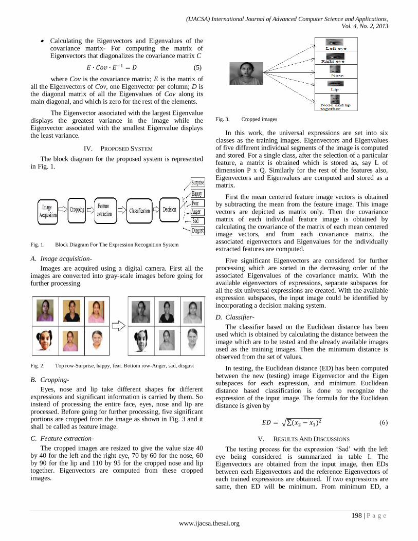
(IJACSA) International Journal of Advanced Computer Science and Applications, Vol. 4, No. 2, 2013
198 | P a g e www.ijacsa.thesai.org
Calculating the Eigenvectors and Eigenvalues of the covariance matrix- For computing the matrix of Eigenvectors that diagonalizes the covariance matrix C
(5)
where Cov is the covariance matrix; E is the matrix of all the Eigenvectors of Cov, one Eigenvector per column; D is the diagonal matrix of all the Eigenvalues of Cov along its main diagonal, and which is zero for the rest of the elements.
The Eigenvector associated with the largest Eigenvalue displays the greatest variance in the image while the Eigenvector associated with the smallest Eigenvalue displays the least variance.
IV. PROPOSED SYSTEM
The block diagram for the proposed system is represented in Fig. 1.
Fig. 1. Block Diagram For The Expression Recognition System
A. Image acquisition-
Images are acquired using a digital camera. First all the images are converted into gray-scale images before going for further processing.
Fig. 2. Top row-Surprise, happy, fear. Bottom row-Anger, sad, disgust
B. Cropping-
Eyes, nose and lip take different shapes for different expressions and significant information is carried by them. So instead of processing the entire face, eyes, nose and lip are processed. Before going for further processing, five significant portions are cropped from the image as shown in Fig. 3 and it shall be called as feature image.
C. Feature extraction-
The cropped images are resized to give the value size 40 by 40 for the left and the right eye, 70 by 60 for the nose, 60 by 90 for the lip and 110 by 95 for the cropped nose and lip together. Eigenvectors are computed from these cropped images.
Fig. 3. Cropped images
In this work, the universal expressions are set into six classes as the training images. Eigenvectors and Eigenvalues of five different individual segments of the image is computed and stored. For a single class, after the selection of a particular feature, a matrix is obtained which is stored as, say L of dimension P x Q. Similarly for the rest of the features also, Eigenvectors and Eigenvalues are computed and stored as a matrix.
First the mean centered feature image vectors is obtained by subtracting the mean from the feature image. This image vectors are depicted as matrix only. Then the covariance matrix of each individual feature image is obtained by calculating the covariance of the matrix of each mean centered image vectors, and from each covariance matrix, the associated eigenvectors and Eigenvalues for the individually extracted features are computed.
Five significant Eigenvectors are considered for further processing which are sorted in the decreasing order of the associated Eigenvalues of the covariance matrix. With the available eigenvectors of expressions, separate subspaces for all the six universal expressions are created. With the available expression subspaces, the input image could be identified by incorporating a decision making system.
D. Classifier-
The classifier based on the Euclidean distance has been used which is obtained by calculating the distance between the image which are to be tested and the already available images used as the training images. Then the minimum distance is observed from the set of values.
In testing, the Euclidean distance (ED) has been computed between the new (testing) image Eigenvector and the Eigen subspaces for each expression, and minimum Euclidean distance based classification is done to recognize the expression of the input image. The formula for the Euclidean distance is given by
V. RESULTS AND DISCUSSIONS
The testing process for the expression ‘Sad’ with the left eye being considered is summarized in table I. The Eigenvectors are obtained from the input image, then EDs between each Eigenvectors and the reference Eigenvectors of each trained expressions are obtained. If two expressions are same, then ED will be minimum. From minimum ED, a

(IJACSA) International Journal of Advanced Computer Science and Applications, Vol. 4, No. 2, 2013
199 | P a g e www.ijacsa.thesai.org
decision can be made of certain expression (in this case it is sad). Since five principal vectors are being considered, there will be five selections. In this case, out of the five vectors, the expression sad has been shown by two Eigenvectors and the expression fear has been shown by another two Eigenvectors.
In table II, the testing process for the expression ‘Sad’, with the right eye being considered is summarized. The Eigenvectors are computed from the input image and the EDs are calculated for the Eigenvectors of the input image and the Eigenvectors of the trained images. For the similar two expressions, their Euclidean distance will be minimum. Considering that, the particular expression can be decided. Since five significant vectors are taken into account, five selections are made and from table II, it is seen that the expression sad and disgust are selected most.
In table III, the testing process for the expression ‘Sad’, in view of the nose is summarized. The Eigenvectors of the input image are attained. The EDs of each Eigenvectors in reference to the trained expression’s Eigenvectors are obtained. The ED of the same two expressions will be minimum of all the EDs. The particular expression can be determined from the minimum ED. In this case, since five principal vectors have been considered, there will be five alternatives. From table III, it has been observed that expression sad and anger has been selected the most number of times.
In table IV, the testing process for the expression ‘sad’, the lip being considered is summarized. From the input image, the Eigenvectors are accomplished. The EDs are estimated for each Eigenvectors in relation to the Eigenvectors for the trained images. The minimum ED is obtained for the same two expressions and from this minimum ED, the specific expression can be accomplished. In this case, since five principal vectors have been considered, there will be five selections and from table IV, it is observed that expression sad is selected thrice of all the five EDs; hence the decided expression is ‘Sad’.
In table V, the testing process for the expression ‘Sad’ is summarized. The Eigenvectors are procured from the input image. Then EDs of each Eigenvectors are procured from the reference Eigenvectors of each trained expressions. The two expressions which are same, the value of their ED will be minimum and the preference of specific expression can be made. As five principal vectors are being considered, there will be five selections. And final decision is attained out of all the five selections. Taken into consideration the nose and the lip together, two of the Eigenvectors has exhibited the expression sad and the other two has exhibited the expression surprise.
The testing for the six basic expressions has been performed. Finally, the summarization of the values of the lowest Euclidean distance measured for the different features for the particular expression is given in table VI. The expression that gets selected more number of times is considered as the decided expression. From this table, it has been observed that the expression ‘sad’ has been selected the maximum number of times. Thus, a decision can be taken that the expression in the testing image is ‘Sad’.
TABLE I. EUCLIDEAN DISTANCE (ED) FOR THE MASKED LEFT
EYE
Testing
image
Training
image
ED1 ED2 ED3 ED4 ED5
Surprise
1.2676
1.8119
1.7794
1.1874
1.5855
Happy
1.4572
1.5182
1.5265
1.8055
1.6493
Fear
0.8267
1.2712
1.8443
1.3175
1.2972
Anger
0.9953
1.3782
1.7177
1.1334
1.4489
Sad
0.7931
1.5523
1.0986
1.3872
1.4326
Disgust
1.0762
1.6502
1.6997
1.5106
1.6576
Result
obtained
from
minimum
ED
Sad Fear Sad Anger Fear
TABLE II. EUCLIDEAN DISTANCE (ED) FOR THE MASKED
RIGHT EYE
Testing
image
Training
image
ED1 ED2 ED3 ED4 ED5
Surprise
1.4307
1.8186
1.1411
1.6590
1.6835
Happy
1.6744
1.2974
1.6189
1.6780
1.3144
Fear
1.1157
1.0956
0.8780
1.3808
1.5251
Anger
0.9820
1.7105
1.6698
1.4655
1.4475
Sad
1.7410
1.3809
1.6995
1.1275
1.2976
Disgust
0.3020
0.8777
1.3580
1.4427
1.5040
Result
obtained
from
minimum ED
Disgust Disgust Fear Sad Sad

(IJACSA) International Journal of Advanced Computer Science and Applications, Vol. 4, No. 2, 2013
200 | P a g e www.ijacsa.thesai.org
TABLE III. EUCLIDEAN DISTANCE (ED) FOR THE MASKED NOSE
Test-
ing
image
Training
image
ED1 ED2 ED3 ED4 ED5
Surprise
0.7883
1.7646
1.6823
1.1826
1.6365
Happy
1.8165
1.5430
1.3842
1.4952
1.5111
Fear
1.7987
1.6020
1.5370
1.4383
1.6254
Anger
1.0556
1.4425
1.2735
1.0630
1.6313
Sad
0.7850
1.2584
1.5923
1.4000
1.2754
Disgust
0.8231
1.2545
1.3076
1.4722
1.3457
Result
obtained
from
minimum
ED
Sad Disgust Anger Anger Sad
TABLE IV. EUCLIDEAN DISTANCE (ED) FOR THE MASKED LIP
Test-
ing
image
Training
image
ED1 ED2 ED3 ED4 ED5
Surprise
0.8594
1.7435
1.4553
1.3318
1.6708
Happy
1.6611
1.5389
1.4979
1.4459
1.4290
Fear
1.6277
1.5100
1.0623
1.3087
1.6064
Anger
1.2394
1.4300
1.5186
1.2620
1.3357
Sad
1.1744
0.8795
1.1459
1.2443
1.2540
Disgust
1.4730
1.5203
1.4403
1.3319
1.3884
Result
obtained
from
minimum
ED
Surp-
rise
Sad Fear Sad Sad
TABLE V. EUCLIDEAN DISTANCE (ED) FOR THE MASKED NOSE
AND LIP TOGETHER
Testing
image
Training
image
ED1 ED2 ED3 ED4 ED5
Surprise
0.3955
1.9696
1.3062
1.0205
1.7349
Happy
1.8522
1.4260
1.5798
1.4754
1.5429
Fear
0.8453
0.7654
1.4537
1.4948
1.4582
Anger
1.0770
1.5184
1.4441
1.2569
1.5348
Sad
0.7389
0.8601
1.1359
1.5248
1.1669
Disgust
0.5588
0.6722
1.8764
1.4028
1.5955
Result
obtained
from
minimum
ED
Surprise Disgust Sad Surprise Sad
In table VII, the success rate has been calculated and found to be 95% with the use of Euclidean distance based classification for 60 samples with various expressions. The time taken to process a set of image was obtained to be 0.0295 seconds.
A comparative study of our proposed work with few of the previous works performed for the recognition of facial expression has been shown in table VIII.
VI. CONCLUSION AND FUTURE WORK
The former work on Eigen face features considered the Eigen space of the whole face. In this paper, the objective was to amend the facial expression recognition system using the Eigenvector method, creating different Eigen subspace for a distinct expression. The system has been proposed using MATLAB version 7.6.0.324 (R2008a) and Intel(R) Core(TM) i3-2330M CPU @ 2.20 GHz processor machine, Windows 7 Ultimate (32 bit), 2 GB RAM and a 14 MP camera

(IJACSA) International Journal of Advanced Computer Science and Applications, Vol. 4, No. 2, 2013
201 | P a g e www.ijacsa.thesai.org
TABLE VI. TESTING RESULTS
Test image
Features
Number of votes for the selected features
Recognized
expression
Left eye
Surprise Happy Fear Anger Sad Disgust
Sad
0 0 2 1 2 0
Right eye 0 0 1 0 2 2
Nose 0 0 0 2 2 1
Lip 1 0 1 0 3 0
Nose and lip
together
2 0 0 0 2 1
Total votes 3 0 4 3 11 4
TABLE VII. SUCCESS RATE OF CLASSIFICATION
Expression Number of
images
experimented
Number of
correct
Recognition
Success rate
Surprise 10 10 100%
Happy 10 10 100%
Fear 10 8 80%
Anger 10 10 100%
Sad 10 9 90%
Disgust 10 10 100%
TABLE VIII. COMPARATIVE STUDY WITH THE PREVIOUS WORKS
Expression Tensor
perceptual
color
framework
[6]
Eigenspaces
[12]
HMM
[9]
Facial
movement
features
[20]
Our
work
Anger 62.08% 70% 70.6% 87.1% 100%
Disgust 57.54% 67% 97.3% 90.2% 100%
Fear 62.89% 77% 88.2% 92% 80%
Happy 75.13% 83% 98.4% 98.07% 100%
Sad 67.79% 73% 96.2% 91.47% 90%
Surprise 84.24% 80% 100% 100% 100%
The performance results show the efficacy of our suggested method, primarily used to recognize the six basic expressions. The recognition rate obtained for the proposed system is 95%.
As the humans can effortlessly recognize the facial expressions, the effectiveness of the machine doing the same performance without any delay is still a challenging job. Our future work is to develop a system to perform the same in real time videos.
REFERENCES
[1] A. Mehrabian, “Communication without words”, Psychology today, vol. 2, no. 4, pp. 53-56, September 1968.
[2] H. A. Elfenbein, A. A. Marsh, and N. Ambady, “Emotional Intelligence
and the Recognition of Emotion from Facial Expressions” in The Wisdom of Feelings: Processes Underlying Emotional Intelligence
[3] P. Ekman, E. R. Sorenson, and W. V. Friesen, “Pan cultural elements in
Facial displays of emotion” Science, New Series, vol. 164, no. 3875, pp. 86-88, April 4,1969
[4] P. Ekman and W.V. Friesen, “Manual for the Facial Action Coding
System,” Consulting Psychologists Press, 1977.
[5] Y. Gao, M. K. H. Leung, S. C. Hui, and M. W. Tananda, “ Facial
Expression Recognition From Line-Based Caricatures” IEEE Transactions on Systems, Man and Cybernetics-Part A:Systems and
Humans, vol. 33, no. 3, pp. 407-411, May 2003.
[6] S. M. Lajevardi and H. R. Wu, “Facial Expression Recognition in Perceptual Color Space” IEEE Transactions on Image Processing, vol.
21, no. 8, pp. 3721-3732, August 2012.
[7] M. Rosenblum, Y. Yacoob, and L. S. Davis, “Human expression recognition from motion using a radial basis function network
architecture,” IEEE Transactions on Neural Networks, vol. 7, pp. 1121–1138, Sept. 1996.
[8] L. Ma and K. Khorasani, “Facial Expression Recognition Using
Constructive Feedforward Neural Networks”, IEEE Transactions on Systems, Man and Cybernetics—Part B: Cybernetics, vol. 34, no. 3, pp.
1588-1595, June 2004
[9] P. S. Aleksic and A. K. Katsaggelos, “Automatic Facial Expression Recognition Using Facial Animation Parameters and Multistream
HMMs”, IEEE Transactions on Information Forensics and Security, vol. 1, no. 1, pp. 3-11, March 2006.
[10] H. Huang and H. He, “Super-Resolution Method for Face Recognition
Using Nonlinear Mappings on Coherent Features”, IEEE Transactions on Neural Networks, vol. 22, no. 1, pp. 121-130, January 2011.
[11] M. Turk and A. Pentland, “Eigenfaces for recognition,” Journal of Cognitive Neuroscience, vol.13, no. 1, pp. 71-86, 1991.
[12] G. R. S. Murthy and R. S. Jadon, “Effectiveness of Eigenspaces for
Facial Expressions Recognition” International Journal of Computer Theory and Engineering, vol. 1, no. 5, pp. 638-642, December 2009
[13] R. Zhi, M. Flierl, Q. Ruan, and W. B. Kleijn, “Graph-Preserving Sparse
Nonnegative Matrix Factorization with Application to Facial Expression Recognition”, IEEE Transactions on Systems, Man and Cybernetics—
Part B: Cybernetics, vol.41, no. 1 pp. 38-52, February 2011.
[14] K. Mase and A. Pentland, “Recognition of facial expression from optical flow,” IEICE Trans. E, vol. 74, pp. 408–410, 1991.
[15] I. Essa and A. Pentland, “Coding, analysis, interpretation, and
recognition of facial expressions,” IEEE Trans. Pattern Anal. Machine Intell., vol. 19, no. 7, pp. 757–763, Jul. 1997.
[16] K. Anderson and P. W. McOwan, “A Real-Time Automated System for
the Recognition of Human Facial Expressions” IEEE Transactions on Systems, Man and Cybernetics—Part B: Cybernetics, vol. 36, no. 1, pp.
96-105, February 2006.
[17] S. Zafeiriou and I. Pitas, “Discriminant Graph Structures for Facial
Expression Recognition”, IEEE Transactions on Multimedia, vol. 10, no. 8, pp. 1528-1540, December 2008.
[18] S. Wang, Z. Liu, S. Lv, Y. Lv, G. Wu, P. Peng, F. Chen, and X. Wang,
“A Natural Visible and Infrared Facial Expression Database for Expression Recognition and Emotion Inference”, IEEE Transactions on
Multimedia, vol. 12, no.7, pp. 682-691, November 2010.

(IJACSA) International Journal of Advanced Computer Science and Applications, Vol. 4, No. 2, 2013
202 | P a g e www.ijacsa.thesai.org
[19] C. Liu and H. Wechsler, “Gabor Feature Based Classification Using the
Enhanced Fisher Linear Discriminant Model for Face Recognition” IEEE Transactions on Image Processing, vol. 11, no. 4, pp. 467-476,
April 2002.
[20] L. Zhang and D. Tjondronegoro, “Facial Expression Recognition Using
Facial Movement Features”, IEEE Transactions on Affective
Computing, vol. 2, no. 4, pp. 219-229, October-December 2011.
[21] I. Kotsia and I. Pitas, “Facial Expression Recognition in Image
Sequences Using Geometric Deformation Features and Support Vector Machines”, IEEE Transactions on Image Processing, vol. 16, no. 1, pp.
172-187, November 2007

(IJACSA) International Journal of Advanced Computer Science and Applications, Vol. 4, No. 2, 2013
203 | P a g e www.ijacsa.thesai.org
Expensive Optimisation: A Metaheuristics
Perspective
Maumita Bhattacharya
School of Computing & Mathematics
Charles Sturt University
NSW, Australia - 2640
Abstract—Stochastic, iterative search methods such as
Evolutionary Algorithms (EAs) are proven to be efficient
optimizers. However, they require evaluation of the candidate
solutions which may be prohibitively expensive in many real
world optimization problems. Use of approximate models or
surrogates is being explored as a way to reduce the number of
such evaluations. In this paper we investigated three such
methods. The first method (DAFHEA) partially replaces an
expensive function evaluation by its approximate model. The
approximation is realized with support vector machine (SVM)
regression models. The second method (DAFHEA II) is an
enhancement on DAFHEA to accommodate for uncertain
environments. The third one uses surrogate ranking with
preference learning or ordinal regression. The fitness of the
candidates is estimated by modeling their rank. The techniques’
performances on some of the benchmark numerical optimization
problems have been reported. The comparative benefits and shortcomings of both techniques have been identified.
Keywords—Evolutionary Algorithm; Preference Learning;
Surrogate Modeling; Surrogate Ranking
I. INTRODUCTION
Evolutionary Algorithms (EAs) are biologically inspired iterative processes where a population of candidate solutions is evolved generation after generation. In a typical EA a number of new offspring candidate solutions are produced through mutation, recombination and selection. Individuals for producing offspring are chosen using a selection strategy after evaluating the fitness value of each individual in the selection pool. In many real world optimization problems this fitness evaluation can be very expensive.
The use of surrogates to reduce the expensive function evaluation is found to be orders of magnitude cheaper computationally [21, 9, and 18]. Incorporation of approximate models may be one of the most promising approaches to realistically use EA to solve complex real life problems, especially where: (i). Fitness computation is highly time-consuming, (ii). Explicit model for fitness computation is absent, (iii). Environment of the evolutionary algorithm is noisy etc. However, considering the obvious risk involved in such approach, an EA with efficient control strategy for the approximate model and robust performance is welcome.
There are different ways, in which a surrogate or approximation model can be incorporated in an EA [15]; some of which are as follows:
Problem level approximation. In this approach, the statement of the problem itself is replaced by a reduced one that is easier to solve. See [15] for some examples on this.
Functional approximation. As the name suggests, in this approach, an alternate and explicit expression is constructed for the objective function, for the purpose of reducing the cost of evaluation. A set of evaluated points are used to build the approximate fitness model. This model is used to predict the fitness of candidate solutions. Usually a fraction of individuals in the population are selected and evaluated within each generation or over a number of generations to generate training points and are added to the training set to update the surrogates to maintain a reliable surrogate during evolution. See [13, 14, and 15] for examples on this technique.
EA specific approximation. This approach is specific for evolutionary algorithms and utilizes the algorithm’s structural and functional aspects.
For a detailed review on use of approximation in EA, see [15].In this paper we investigate three different methods which use surrogates to reduce the number of actual function evaluations in EA [4].
In the first one, namely, Dynamic Approximate Fitness based Hybrid Evolutionary Algorithm (DAFHEA), Bhattacharya et. al [2, 3] use both “functional approximation” and “EA specific approximation”. It uses an approximation model to partially replace expensive fitness evaluations in evolutionary algorithm. DAFHEA uses an explicit control strategy (a cluster-based on-line learning technique) to improve reliability of using such approximate models to reduce expensive function evaluations. Also the approximate knowledge thus generated is exploited to avoid premature convergence (one of the major impediments of using evolutionary algorithm to solve complex real life optimization problems).
The second method, DAFHEA II [5] is an enhancement on DAFHEA to cover situations, where information from variable input dimensions and noisy data is involved. DAFHEA-II uses a multi-model regression approach. The multiple models are estimated by successive application of the SVM regression algorithm. Retraining of the model is done in a periodic fashion.
In the third method, Runersson [22] makes use of the EA feature that unlike classical optimization techniques, in rank based selection, selection of the best candidates requires only

(IJACSA) International Journal of Advanced Computer Science and Applications, Vol. 4, No. 2, 2013
204 | P a g e www.ijacsa.thesai.org
the rank or partial rank of the candidates. Here, the fitness of individuals is indirectly estimated by modeling their rank using surrogate. Preference learning or ordinal regression is used to implement a kernel-defined feature space.
The features and effectiveness of the above two surrogate-based methods have been investigated in this work. The above two methods have been selected for comparison as they are based on very different concepts and may reveal important characteristics which may be useful for specific problem cases.
Rest of the paper is organized as follows. Section II presents a brief review on use of surrogates in evolutionary computing. Section III outlines the features of the surrogate-based EA methods which we have investigated in this research. Section IV presents the experiment details and discussions on the findings. Finally, concluding remarks are summarized in Section V.
II. SURROGATE-BASED EVOLUTIONARY ALGORITHM
The use of an approximate model to speed up optimization dates all the way back to the sixties [8]. The most widely used models being Response Surface Methodology [17], Krieging models [23] and artificial neural network models [6]. As has been mentioned in Section 1, the concept of using approximate model varies in levels of approximation (Problem approximation, Functional approximation, and Evolutionary approximation), model incorporation mechanism and model management techniques [15].
In the multidisciplinary optimization (MDO) community, primarily response surface analysis and polynomial fitting techniques are used to build the approximate models [11, 27]. These models work well when single point traditional gradient-based optimization methods are used. However, they are not well suited for high dimensional multimodal problems as they generally carry out approximation using simple quadratic models.
In another approach, multilevel search strategies are developed using special relationship between the approximate and the actual model. An interesting class of such models focuses on having many islands using low accuracy/cheap evaluation models with small number of finite elements that progressively propagate individuals to fewer islands using more accurate/expensive evaluations [29]. This approach may suffer from lower complexity/cheap islands having false optima whose fitness values are higher than those in the higher complexity/expensive islands. Rasheed et al. in [19, 20], uses a method of maintaining a large sample of points divided into clusters. Least square quadratic approximations are periodically formed of the entire sample as well as the big clusters. Problem of unevaluable points was taken into account as a design aspect. However, it is only logical to accept that true evaluation should be used along with approximation for reliable results in most practical situations. Another approach using population clustering is that of fitness imitation [15]. Here, the population is clustered into several groups and true evaluation is done only for the cluster representative [16]. The fitness value of other members of the same cluster is estimated by a distance measure. The method may be too simplistic to be reliable, where the population landscape is a complex, multimodal one.
Jin et al. in [13, 14] analyzed the convergence property of approximate fitness based evolutionary algorithm. It has been observed that incorrect convergence can occur due to false optima introduced by the approximate model. Two controlled evolution strategies have been introduced. In this approach, new solutions (offspring) can be (pre)-evaluated by the model. The (pre)-evaluation can be used to indicate promising solutions. It is not clear however, how to decide on the optimal fraction of the new individuals for which true evaluation should be done [1]. In an alternative approach, the optimum is first searched on the model. The obtained optimum is then evaluated on the objective function and added to the training data of the model [19, 26, and 1]. Yet another approach as proposed in [14], a regularization technique is used to eliminate false minima.
III. THE INVESTIGATED METHODS
The main features of the three techniques investigated in this work, DAFHEA, DAFHEA II and the preference learning based EA are outlined below.
A. The DAFHEA Technique
The primary objectives of the proposed algorithm and their realization are as below.
1) The main objective of DAFHEA is to reduce the
number of actual fitness function evaluations to speed up the
search process. The proposed algorithm achieves this by
partially replacing actual function evaluation (as is required
in traditional genetic algorithm) by SVM based estimation.
The DAFHEA framework includes a global model of genetic
algorithm (GA), hybridized with support vector machine
(SVM) [28] as the approximation tool.
2) The related major objective is to minimize the
adverse effect of estimation. To this end explicit control
strategies are used for evolution control, leading to
considerable speedup without compromising heavily on
solution accuracy. The controlled use of estimation is the primary reason why
the proposed algorithm should be successful in reducing actual fitness function evaluation without heavily compromising on solution accuracy. The basic algorithm is as below.
Step One: Create a random population of cN individuals,
where, ac NN *5 and aN actual initial population size.
Step Two: Evaluate cN individual using actual expensive
function evaluation. Build the SVM approximate model using normalized expensive function evaluation values as training set for off-line training. (Use of normalized values in the training set appears to improve performance of meta-model, reducing effects of unnaturally high or low values). SVM hyper-parameters are initially tuned based on this training set.
Step Three: Select aN best individual out of cN
evaluated individuals to form the initial GA population.
Remarks: The idea behind using five times the actual EA population size (as explained in Step One) is to make the

(IJACSA) International Journal of Advanced Computer Science and Applications, Vol. 4, No. 2, 2013
205 | P a g e www.ijacsa.thesai.org
approximation model sufficiently representative at least
initially. Since initial EA population is formed with aN best
individuals out of these cN individuals, with high
recombination and low mutation rates, the EA population in first few generations is unlikely to drift much from its initial locality. Thus it is expected that large number of samples used in building the approximation model will facilitate better performance at this stage. Also using the higher fitness individuals, chosen out of a larger set should give an initial boost to the evolutionary process.
Step Four: Select parents using suitable selection operator and apply genetic operators namely recombination and mutation to create a new generation.
Step Five: Use SVM approximation model to compute fitness of new generation individuals based on approximate evaluation. Form m distance-based (considering spatial distribution of individuals) clusters in the new population
space. If for some n clusters, the standard deviation Predefined Threshold, rearrange solution space into nm
clusters. Compute a merit function )(xfm as below:
ijd
ix
afx
mf
21)()( is3
In the equation (1), )(xf a is the predicted fitness function
value. i is standard deviation (in terms of objective value) for
the thi cluster and ijd is the normalized minimum Euclidean
distance of thj point of
thi cluster from the all truly evaluated
points so far [22]. is is the sparseness of the thi cluster. 1 ,
2 and 3 are scaling factors for i , ijd and is respectively.
individualofDimension
iclusterinsindividualfoNosi
Step Six: Dynamically update the approximate model as below:
1) Identify the cluster containing the optimum based on
approximation.
2) Perform expensive evaluation for the approximate
optimum and its k nearest neighbors.
3) Also perform expensive evaluation for the centroid of
all other data clusters and their k nearest neighbors.
4) Expand neighborhood for true evaluation until a
point is found in each space dimension such that percentage
error Predefined threshold.
100
it
ipit
a
aa
In the equation (3), ita =True value of the thi neighbor and
ipa =Predicted value of the thi neighbor and max ki .
Add the newly evaluated points to approximate model training set to update model.
Step Seven: When termination/evolution control criteria are not met, repeat Step Four to Step Seven.
Remarks: It must be noted, the optimum is considered
based on the original predicted value )(xf a . For all other
purposes fitness based on the merit function )(xfm is
considered. Periodic parameter tuning of the SVM approximation model was incorporated, though no specific criterion was used.
Further details on the above method can be found in [2, 3].
B. The DAFHEA II Technique
As in the original DAFHEA framework, DAFHEA-II [5] includes a global model of genetic algorithm (GA), hybridised with support vector machine (SVM) as the approximation tool. Expensive fitness evaluation of individuals as required in traditional evolutionary algorithm is partially replaced by SVM approximation models (unlike the original DAFHEA, multi-model regression is used). Evolution control is implemented by periodic true evaluations, leading to considerable speedup without compromising heavily on solution accuracy. Also the approximate knowledge about the solution space generated is used to maintain population diversity to avoid premature convergence.
5) Functional Details The operational detail of DAFHEA-II [15] framework is as
described below:
Step One: Create a random population of cN individuals,
where, ac NN 5 and aN actual initial population size.
Step Two: Evaluate cN individual using actual expensive
function evaluation. Build the SVM approximate models using the candidate solutions as input and the actual fitness (expensive function evaluation values) as targets forming the training set for off-line training.
Step Three: Select aN best individual out of cN
evaluated individuals to form the initial GA population.
Remarks: The idea behind using five times the actual EA population size (as explained in Step One) is to make the approximation model sufficiently representative at least
initially. Since initial EA population is formed with aN best
individuals out of these cN individuals, with high
recombination and low mutation rates, the EA population in first few generations is unlikely to drift much from its initial locality. Thus it is expected that large number of samples used in building the approximation model will facilitate better performance at this stage. Also using the higher fitness individuals, chosen out of a larger set should give an initial boost to the evolutionary process.
Step Four: Rank the candidate solutions based on their fitness value.

(IJACSA) International Journal of Advanced Computer Science and Applications, Vol. 4, No. 2, 2013
206 | P a g e www.ijacsa.thesai.org
Step Five: Preserve the elite by carrying over the best candidate solution to the next generation.
Step Six: Select parents using suitable selection operator and apply genetic operators namely recombination and mutation to create children (new candidate solutions) for the next generation.
Step Seven: The SVM regression models created in Step two are applied to estimate the fitness of the children (new candidate solutions) created in Step six. This involves assignment of most likely or appropriate models to each candidate solution.
Step Eight: The set of newly created candidate solutions is ranked based on their approximate fitness values.
Step Nine: The best performing newly created candidate solution and the elite selected in Step five are carried to the population of the next generation.
Step Ten: New candidate solutions or children are created as described in Step six.
Step Eleven: Repeat Step seven to Step ten until either of the following condition is reached:
1. The predetermined maximum number of generations
has been reached; or
2. The periodic retraining of the SVM regression
models is due.
Step Twelve: If the periodic retraining of the SVM regression models is due, this will involve actual evaluation of the candidate solutions in the current population. Based on this training data new regression models are formed. The algorithm then proceeds to execute Step four to Step eleven.
Remarks: The idea behind using periodic retraining of the SVM regression models is to ensure that the models continue to be representatives of the progressive search areas in the solution space.
C. The Preference Learning Based EA
The second method is directly based on preference learning or ordinal regression based technique proposed by Runersson in [22] with the variation that we have used a genetic algorithm implementation instead of CMA-ES. This method is based on the assumption that in a stochastic and direct search method such as EA, ordinal regression should be able to offer adequate surrogates as only full or even partial ranking of the individuals or search points is sufficient for the selection process. Accordingly, the surrogate approach is considered as a
preference learning task, where a candidate point ix is preferred
over jx if ix has a higher fitness than jx . The training set for
the surrogate model is thus composed of pairs of points kji xx ,
and a corresponding label 1,1 kr , taking the value +1 or -1
depending on whether ix has a higher fitness than jx or vice
versa.
The technique used for preferential learning or ordinal regression is kernel based. See [Runersson] for details on the method of ordinal regression using kernel defined features.
Model selection in surrogate ranking involves appropriately choosing a suitable kernel and its parameters as well as the
regulation parameter C which controls the balance between model complexities and training errors. Choice of a suitable kernel is problem specific.
As the search progresses, different regions of the search space are sampled and the original surrogate ranking model may be insufficiently accurate for new regions of the search space. It is therefore extremely important to update the surrogate during evolution. We have followed the surrogate update method suggested by Runersson in [22]. The strategy involves estimating the ranking of a population of points using the current surrogate and identifying the highest ranking point. The point is then evaluated using the true fitness function and its rank is calculated. Accuracy of the surrogate is evaluated by comparing the estimated rank with the true rank. The point evaluated with true fitness function is added to the training set.
IV. EXPERIMENTS
A. Experiment Details for DAFHEA
It may be noted that the target problem domain for our proposed algorithm involves time consuming actual fitness function evaluation. This property or characteristic of the fitness function is external to the EA process. Hence, to verify DAFHEA’s effectiveness, it is sufficient to verify if DAFHEA can effectively reduce the number of actual function evaluations without compromising on accuracy for any set of standard test functions. Considering this, the performance of the proposed algorithm has been tested on five classical benchmark test functions: namely, Spherical, Ellipsoidal, Schwefel, Rosenbrock, and Rastrigin. Description of the test functions are as given in [3]. These benchmark functions in the test suit are scalable and are commonly used to assess the performance of optimization algorithms [30]. For Spherical and
Rastrigin the global minimum is 0xf at 0n
ix .
Rosenbrock has a global minimum of 0xf at 1n
ix .
All simulations were carried out using the following
assumptions: The population size of n10 was used for all the
simulations, where n is the number of variables for the problem; for comparison purposes three sets of input
dimensions are considered; namely, n 5, 10 and 20. For all cases, tenfold validation was done with the number of generations being 1000; the SVM regression models [8] were trained with five times the real GA population size initially.
All the simulation processes were executed using a
Pentium®
4, 2.4GHz CPU processor for both DAFHEA and the Preference Learning based EA.
B. Experiment Details for DAFHEA II
Both non-noisy and noisy versions of the chosen benchmark functions have been used to test DAFHEA II. The noisy versions of the functions have been obtained as follows.

(IJACSA) International Journal of Advanced Computer Science and Applications, Vol. 4, No. 2, 2013
207 | P a g e www.ijacsa.thesai.org
2,Nxfxf Noisy
Here, 2,N = Standard Normal (or Gaussian)
distribution with mean, = 0 and variance, 2 = 1. The
probability density function 2,; xf is defined as
follows.
2
2
2
2exp
2
1,;
xxf
All simulations were carried out using the following
experiment setup: The population size of n10 was used for all
the simulations, where n is the number of variables for the problem; for comparison purposes three sets of input
dimensions are considered; namely, 10,5n and 20. For all
three cases, tenfold validation was done with the number of iterations being 1000 for all non-noisy versions of the test problems; the SVM regression models were trained with five times the real EA (GA in this case) population size initially. However, in case of the noisy versions of the test functions much larger number of iterations has been used to obtain acceptable level of accuracy of results. All the simulation
processes were executed using a Pentium®
4, 2.4GHz CPU processor.
C. Experiment Details for Performance Learning Based EA
Following Runersson’s [22] method a 2-norm soft margin support vector machine (SVM) has been used and the technique has been implemented using a classical genetic algorithm. As mentioned earlier, choice of appropriate kernel is an important factor in the performance learning based EA. Runersson [22] has tried ordinal regression with different kernels and concluded that 4th order polynomial kernel produces the best results for the Rosenbrock’s function. For the sake of fair comparison we have used the same kernel for this test function. For the Spherical function, the 2nd order polynomial kernel performed best. Gaussian distribution with variance 0.12 has been used for the Rastrigin’s function.
Training points have been generated using a standard normal distribution centered about the origins (global minima) of the respective test functions. 1000 testing points were generated in the same manner. Using 60 randomly sampled training points the surrogate model has been estimated by
ordinal regression. The regulation parameter C has been
chosen as 1.0E6.
As the search zooms in on a local minimum, the search will benefit from use of different kernel [22]. As suggested by Runersson in [22] a Gaussian distribution with variance 0.12
was used in case of the Rosenbrock’s and the Spherical functions in similar situations.
The surrogate has been validated and updated as explained in Section 3.2, every second generation.
D. Results and Discussions
Performances of the three investigated methods on non-noisy versions of Spherical, Ellipsoidal, Schwefel, Rosenbrock, and Rastrigin functions with n 5, 10 and 20 have been demonstrated in Table I. We have not reported any information on the number of actual function evaluations required for DAFHEA II in Table I as by design this technique employs additional function evaluations to achieve better performance in noisy environment. To give an idea about its efficacy in the noisy environment, Table II presents the comparative performances of the canonical Genetic Algorithm, DAFHEA and DAFHEA II in terms of number of actual function evaluations required when tested on the noisy versions of the test functions.
As can be observed from these results, Preference Learning based EA seems to have an advantage in terms of “number of actual function evaluations” over DAFHEA. However, its performance in terms of “mean fitness” is just not comparable to that of DAFHEA in all nine test cases. Both methods found the classical Spherical function easier to tackle as compared to the Rosenbrock’s and the Rastrigin’s functions. For both algorithms the mean function values for the spherical functions were better than their Rosenbrock counterparts. However, it may appear that based on the number of function evaluations, the spherical function was much harder for DAFHEA to solve than its Rosenbrock counterpart of the same dimension. It must be noted that increase in number of iterations and thus increase in the number of actual function evaluation showed no improvement in case of the Rosenbrock’s function. In general, both models gained on performance with increase in training set size.
As can be anticipated, performances of both techniques deteriorated with increase in problem dimensions. However, this deterioration is much higher in case of the Preference Learning based EA, where the results are practically unusable except in case of Spherical function. Increase in the number of true function evaluations does not seem to improve the situation.
Other general observations are as below:
Both DAFHEA and Preference Learning based EA are applicable to situations where no explicit or computable fitness function is available. However, the concept of using preference learning based surrogate ranking may show more flexibility in such scenarios.
In the Preference Learning based EA, surrogate ranking has been realized using kernel based ordinal regression. That means the method is easily adaptable to any data types as long as a suitable kernel can be defined for the specific problem at hand. However, this is both an advantage and a disadvantage as this means, sufficient knowledge of the characteristics of the problem is required which may be difficult in real world scenarios.
The preference learning based EA benefits from selection of different kernel while the search zooms in on a local minimum. However, this switch may impose some additional computational as well as decisional overhead.

(IJACSA) International Journal of Advanced Computer Science and Applications, Vol. 4, No. 2, 2013
208 | P a g e www.ijacsa.thesai.org
Surrogate ranking with RBF kernel tended to suffer from overfitting and get stuck in local minima. Second order polynomial performed better in case of higher order Rosenbrock’s function.
The major drawback of the preference learning based surrogate ranking seems to be its inefficiency in handing higher dimensional problems, which is a common situation for most real world optimization problems.
TABLE I. PERFORMANCES OF THE DAFHEA TECHNIQUE (M1), THE
DAFHEA II TECHNIQUE (M2) AND THE PREFERENCE LEARNING BASED EA
(M3) AS IMPLEMENTED ON SPHERICAL, ELLIPSOIDAL, SCHWEFEL, ROSENBROCK, AND RASTRIGIN FUNCTIONS WITH n 5, 10 AND 20.
PERFORMANCE MEASURES HAVE BEEN EXPRESSED AS THE “MEAN FITNESS”
AND THE “NUMBER OF ACTUAL FUNCTION EVALUATIONS”.
Function Mean
Fitness
(M1)
Mean
Fitness
(M2)
Mean
Fitness
(M3)
No of
Actual
Function
Evaluations
(M1)
No of
Actual
Function
Evaluations
(M3) Rosenbrock(5) 1.789E-
41
1.998E-
38
1.1103E-
0.7
7015 1200
Rosenbrock(10) 1.991E-
39
1.918E-
26
1.0005 6990 4000
Rosenbrock(20) 2.313E-
36
1.901E-
19
2.1108 21170 17000
Spherical(5) 1.138E-
60
1.138E-
56
1.0102E-
7
21210 375
Spherical(10) 1.152E-
58
1.588E-
43
1.0081E-
5.5
77520 1200
Spherical(20) 1.58E-
55
1.388E-
35
1.0125E-
5.5
110420 2750
Ellipsoidal(5) 3.220E-
57
3.412E-
51
1.0000E-
6.1
18500 400
Ellipsoidal(10) 3.271E-
55
2.523E-
39
1.0100E-
5.5
65700 1500
Ellipsoidal(20) 2.209E-
52
1.323E-
32
1.0511E-
4.5
95510 2900
Schwefel(5) 1.198E-
54
1.911E-
48
1.0001E-
0.8
11500 2700
Schwefel(10) 1.199E-
51
2.971E-
38
0.9000 15000 5000
Schwefel(20) 1.023E-
48
1.989E-
31
2.0002 25100 18000
Rastrigin(5) 3.285E-
5
3.322E-
1
1.1901E-
0.8
4550 1700
Rastrigin(10) 3.089E-
3
3.388E-
1
0.9899 7175 5000
Rastrigin(20) 1.324E-
1
10.032 3.0011 28010 15000
V. CONCLUSIONS
Use of surrogates may be the most realistic answer to problems an iterative, stochastic search process like EA faces while dealing with situations, where, true fitness computation is highly expensive, or explicit model for fitness computation is absent, or environment of the evolutionary algorithm is noisy and so on. In this research, we have investigated three surrogate-based EA methods which aim at addressing some of these problems. While the first two methods, DAFHEA and DAFHEA II are based on “functional approximation” and “EA specific approximation” (see Section I), the second method uses surrogate ranking by ordinal regression or preference learning. Experiment results have shown, while Preference Learning based EA has some cost advantage in terms of number of true function evaluations, DAFHEA clearly should
be the choice where accuracy (mean fitness value) is of paramount importance. DAFHEA II that uses multi-model regression for surrogate generation, shows some advantage over original DAFHEA and Canonical GA when applied to noisy functions, in terms of solution accuracy (results have not been shown in this article). However, this comes at the expense of some extra overhead in terms of number of actual function evaluations.
TABLE II. PERFORMANCES OF THE CANONOCAL GA (M1), THE
DAFHEA TECHNIQUE (M2) AND THE DAFHEA II TECHNIQUE (M2) AS
IMPLEMENTED ON NOISY VERSIONS OF SPHERICAL, ELLIPSOIDAL, SCHWEFEL, ROSENBROCK, AND RASTRIGIN FUNCTIONS WITH n 5, 10 AND 20. THE
PERFORMANCE MEASURE HAS BEEN EXPRESSED AS THE “NUMBER OF ACTUAL
FUNCTION EVALUATIONS”.
Function No of
Actual
Function
Evaluations
(M1)
No of
Actual
Function
Evaluations
(M2)
No of
Actual
Function
Evaluations
(M3) Rosenbrock(5) 35,000 9500 9000
Rosenbrock(10) 100,000 71250 71000
Rosenbrock(20) 500,000 290,500 290,000 Spherical(5) 100,000 59000 58000
Spherical(10) 100,000 76000 75000
Spherical(20) 500,000 300,500 300,000 Ellipsoidal(5) 100,000 59000 58000
Ellipsoidal(10) 100,000 85000 84500
Ellipsoidal(20) 250,000 81550 81500 Schwefel(5) 100,000 69000 68000
Schwefel(10) 100,000 65000 64500 Schwefel(20) 300,000 200,050 200,000 Rastrigin(5) 100,000 5500 5100
Rastrigin(10) 100,000 20500 20000 Rastrigin(20) 500,000 410,500 410,000
REFERENCES
[1] Büche., D., Schraudolph, N., and Koumoutsakos, P., Accelerating
Evolutionary Algorithms Using Fitness Function Models, Proc. Workshops Genetic and Evolutionary Computation Conference,
Chicago, 2003.
[2] Bhattacharya, M., and Lu, G., DAFHEA: A Dynamic Approximate Fitness based Hybrid Evolutionary Algorithm, Proceedings of the IEEE
Congress on Evolutionary Computation, 2003, Vol.3, IEEE Catalogue No. 03TH8674C, ISBN 0-7803-7805-9, pp. 1879-1886.
[3] Bhattacharya, M., Surrogate Based EA for Expensive Optimization
Problem, Proceedings of the 2007 IEEE Congress on Evolutionary Computation (CEC 2007), Singapore, 1-4244-1340-0, 2007 IEEE Press.
[4] Bhattacharya, M., An Investigation on Two Surrogate-based EAs, Australian Journal of Intelligent Information Processing Systems, ISSN:
1321-2133, Vol 12. No. 2, 2010, pp. 7-12.
[5] Bhattacharya, M., Reduced Computation for Evolutionary Optimization in Noisy Environment, Proceedings of ACM Genetic and Evolutionary
Computation Conference 2008 (GECCO 2008), Atlanta, USA, ACM Press, ISBN: 978-1-60558-131-6, pp. 2117-2122.
[6] Bishop, C., Neural Networks for Pattern Recognition, Oxford Press,
1995.
[7] Cherkassky, V., and Ma, Y., Multiple Model Estimation: A New Formulation for Predictive Learning, under review in IEEE Transaction
on Neural Network.
[8] Dunham, B., Fridshal, D., Fridshal, R. and North, J., Design by natural selection, Synthese, 15, pp. 254-259, 1963.
[9] El-Beltagy, M. A., and Keane, A. J., Evolutionary optimization for
computationally expensive problems using Gaussian processes, Proc. Int. Conf. on Artificial Intelligence (IC-AI'2001), CSREA Press, Las
Vegas, pp. 708-714, 2001.

(IJACSA) International Journal of Advanced Computer Science and Applications, Vol. 4, No. 2, 2013
209 | P a g e www.ijacsa.thesai.org
[10] Gunn, S. R., Support Vector Machines for Classification and Regression,
Technical Report, School of Electronics and Computer Science, University of Southampton, (Southampton, U.K.), 1998.
[11] Hajela, P., and Lee, A., Topological optimization of rotorcraft subfloor structures for crashworthiness considerations, Computers and Structures,
vol.64, pp. 65-76, 1997.
[12] Hastie, T., Tibshirani, R., Friedman, J., The Elements of Statistical Learning: Data Mining, Inference, and Prediction, Springer Series in
Statistics, ISBN 0-387-95284-5.
[13] Jin, Y., Olhofer, M., and Sendhoff, B., A Framework for Evolutionary Optimization with Approximate Fitness Functions, IEEE Transactions
on Evolutionary Computation, 6(5), pp. 481-494, (ISSN: 1089-778X). 2002.
[14] Jin, Y., Olhofer, M., and Sendhoff, B., On Evolutionary Optimisation
with Approximate Fitness Functions, Proceedings of the Genetic and Evolutionary Computation Conference GECCO, Las Vegas, Nevada,
USA. pp. 786- 793, July 10-12, 2000.
[15] Jin, Y., Surrogate-assisted evolutionary computation: Recent advances and future challenges, Swarm and Evolutionary Computation, Vol 1,
pp.61-67, 2011.
[16] Kim, H. S., and Cho, S. B., An efficient genetic algorithm with less fitness evaluation by clustering, Proceedings of IEEE Congress on
Evolutionary Computation, pp. 887-894, 2001.
[17] Myers, R. and Montgomery, D., Response Surface Methodology, John
Wiley & Sons, 1985.
[18] Pierret, S., Three-dimensional blade design by means of an artificial neural network and Navier-Stokes solver, Proceedings of Fifth
Conference on Parallel Problem Solving from Nature, Amsterdam, 1999.
[19] Rasheed, K., An Incremental-Approximate-Clustering Approach for Developing Dynamic Reduced Models for Design Optimization,
Proceedings of IEEE Congress on Evolutionary Computation, 2000.
[20] Rasheed, K., Vattam, S., and Ni, X., Comparison of Methods for Using
Reduced Models to Speed Up Design Optimization, The Genetic and Evolutionary Computation Conference (GECCO'2002), 2002.
[21] Ratle, A., Accelerating the convergence of evolutionary algorithms by fitness landscape approximation, Parallel Problem Solving from Nature-
PPSN V, Springer-Verlag, pp. 87-96, 1998.
[22] Runersson, T. P., Constrained evolutionary optimization by approximate ranking and surrogate models, Parallel Problem Solving from Nature-
PPSN VII (PPSN-2004). Volume 3242 of LNCS., Springer-Verlag, pp. 401-410, 2004.
[23] Sacks, J., Welch, W., Mitchell, T., and Wynn, H., Design and analysis of
computer experiments, Statistical Science, 4(4), 1989.
[24] Schölkopf, B., Burges, J. and Smola, A., ed., Advances in Kernel Methods: Support Vector Machines, MIT Press, 1999.
[25] Smola, A. and Schölkopf, B., A Tutorial on Support Vector Regression,
NeuroCOLT Technical Report NC-TR-98-030, Royal Holloway College, University of London, UK, 1998.
[26] Torczon, V., and Trosset, M. W., Using approximations to accelerate
engineering design optimisation, ICASE Report No. 98-33. Technical report, NASA Langley Research Center Hampton, VA 23681-2199,
1998.
[27] Toropov, V. V., Filatov, A., and Polykin, A. A., Multiparameter
structural optimization using FEM and multipoint explicit approximations, Structural Optimization, vol. 6, pp. 7-14, 1993.
[28] Vapnik, V., The Nature of Statistical Learning Theory, Springer-Verlag,
NY, USA, 1999.
[29] Vekeria, H. D., and Parmee, I. C., The use of a co-operative multi-level CHC GA for structural shape optimization, Fourth European Congress
on Intelligent Techniques and Soft Computing – EUFIT’96, 1996.
[30] Won, K., Roy, T., and Tai, K., A Framework for Optimization Using Approximate Functions, Proceedings of the IEEE Congress on
Evolutionary Computation’ 2003, Vol.3, IEEE Catalogue No. 03TH8674C, ISBN 0-7803-7805-9.

(IJACSA) International Journal of Advanced Computer Science and Applications, Vol. 4, No. 2, 2013
210 | P a g e www.ijacsa.thesai.org
GASolver-A Solution to Resource Constrained Project Scheduling by Genetic Algorithm
Dr Mamta Madan Professor(Comp science)
Vivekananda Institute of Professional Studies, Affiliated to GGSIPU AU-Block Pitam PuraDelhi, India
Mr Rajneesh Madan Architect,
NIIT Technologies Ltd., Gurgaon-11
Abstract-The Resource Constrained Scheduling Problem (RCSP) represents an important research area. Not only exact solution but also many heuristic methods have been proposed to solve RCPSP (Resource Constrained Project Scheduling Problem). It is an NP hard problem. Heuristic methods are designed to solve large and highly Resource Constrained software projects. We have solved the problem of resource constrained scheduling problem and named as GASolver. It is implemented in C# using .net platform. We have used Dependency Injection to make the problem loosely coupled, so that other arena of scheduling like Time Cost Tradeoff (CT), Payment Scheduling (PS) etc can be merged with same solution in the future. We have implemented GASolver using Genetic Algorithm (GA).
Keywords-Genetic Algorithm; Dependency Injection; GASolver.Core; Resource Constrained Scheduling.
I. INTRODUCTION
The Resource Constrained Project Scheduling Problem represents an important research problem. Not only exact solution but also many heuristic methods have been proposed to solve RCPSP. It being an NP hard problem, Alcaraz and Maroto [5] mentioned that the optimal solution can only be achieved by exact solution procedures in small software projects, usually with less than 60 activities, which are not highly resource constrained.
Therefore heuristic methods are designed to solve large and highly Resource Constrained software projects. Mohring [6] mentioned that RCPSP is one of the most intractable problems in operations research and many latest optimization techniques and local search were applied to solve it. We have solved the problem of resource constrained scheduling problem and named as GASolver. It is implemented in C# using .net platform. We have used Dependency Injection (DI) to make the problem loosely coupled, so that other arena of scheduling like Time Cost Tradeoff, Payment Scheduling etc can be merged with same solution in the future. We have implemented GASolver using Genetic Algorithm. The problem statement is explained in the following section. Problem Statement for RCPSP (Resource Constrained Project Scheduling Problem)
What is the best way to assign the resources to the activities at specific times such that all of the constraints are satisfied and the best objective measures are produced?
II. GENETIC ALGORITHM
Genetic algorithms (GAs) are search algorithms that are conceptually based on the methods that living organisms adapt
to their environment. These methods, known as natural selection or evolution, combine the concept of survival of the fittest among string structures with a structured yet randomized information exchange to form a search algorithm with some of the innovative flair of human search. In each generation, a new set of string structures is created from (bits and pieces of) the fittest strings from the previous generation and occasionally a randomly altered new part. This process of exploiting historical data allows the GA to speculate on new search points that will improve performance thus producing better solutions. Genetic algorithms were initially developed by JohnH.Holland, a professor of psychology and computer science at the University of Michigan. As an optimization tool, the Genetic Algorithm attempts to improve performance leading to an optimal solution.
In this process, there are two distinct steps, (1) the process of improvement and (2) reaching the optimum itself. Of these two steps, the most important is the process of improvement. In complex systems, due to the potential high costs involved, reaching the optimum solution may not be justified as long as continuous improvement is being made and an optimal (desirable) solution can be found.
Genetic algorithm (GA) [1][2][3] is a pioneering method of metaheuristic optimization which originated from the studies of cellular automata of Holland in the 1970s. It is also known as an evolutionary algorithm and a search technique that copies from biological evolution. In Genetic Algorithm, a population of candidate solutions called individuals evolves toward better solutions from generation to generation.
ADVANTAGES OF GENETIC ALGORITHM
GA can quickly scan a vast solution set. Bad proposals do not affect the endSolution negatively as they are simply discarded.
The inductive nature of the GA means that it doesn’t have to know any rules of the problem - it works by its own internal rules. This is very useful for complex or loosely defined problems.
They efficiently search the model space, so they are more likely (than local optimization techniques) to converge toward a global minima.
There is no need of linearization of the problem. There is no need to compute partial derivatives. More probable models are sampled more frequently
than less probable ones

(IJACSA) International Journal of Advanced Computer Science and Applications, Vol. 4, No. 2, 2013
211 | P a g e www.ijacsa.thesai.org
III. RELATED WORK
In 1978, Stinson et al.[9] formulated the multiple resource-constrained scheduling problem as an integer programming problem and advanced a branch-and-bound algorithm for solving it. The algorithm they developed was similar to branch-and-bound algorithm with differences in the node selection heuristics employed and the number of resources handled (Johnson's algorithm allows for a single resource). In their algorithm, branching corresponds to creating new partial feasible schedules from given partial feasible schedules.
An experimental investigation was completed in 1988 by Dumond and Mabert[4]. They studied RCPSP in an environment where new software projects arrive continuously or randomly to a system in which software projects share common resources and receive completion deadlines. Dumond and Mabert tested the performance of four due date procedures and five scheduling heuristics with full control on the due date assignment. A second test was conducted to examine the performance of the due date procedures when deadlines were set externally. Their experimental results failed to indicate a rule that uniformly outperformed the others.
In 2006 an improved Particle Swarm Optimization (PSO) algorithm[10] for resource-constrained software project scheduling problem was proposed. Improvements based on the basic PSO include: the particle swarm is initialized by heuristic rule to improve the quality of particles; inertia weight was self-adapted with iteration of the algorithm to decelerate the speed of particles; crossover mechanism of genetic algorithm were applied to particle swarm to enable the exchange of good characteristics between two particles.
Computational results for software project instances of PSPLIB demonstrate that this improved PSO was effective as compared with other mataheuristic approaches
In 2007 YanLiu presented a fuzzy genetic algorithm for software project scheduling problem with resource constraints and uncertain activity duration [11]. The objective of this research was to minimize the fuzzy software project make span. Firstly, fuzzy set was used to represent the uncertainty of activity duration and the corresponding comparison method of fuzzy number called integral value approach was introduced. Second, three genetic operators were used to search for an approximate shortest software project make span. Therefore, this study provided another metaheuristic method for solving resource-constraint software project scheduling problem with uncertain activity duration.
In 2009 itself Mohammad Amin Rigi, Shahriar Mohammadi K. N. Toosi [8] proposed a new evolutionary approach to resource constrained software project scheduling problem. Hybrid genetic algorithm (GA)-constraint satisfaction problem (CSP) has been applied to solve resource constrained software project scheduling (RCPS). GA’s task was to find the best schedule. Their approach has used CSP in order to overcome the existing inconsistencies in activities precedence and resources conflicts. A full state CSP with min-conflict heuristic has been used for solving precedence conflicts and a simple iterative CSP is used to resolve the resource conflicts.
A more realistic resource-constrained software project-scheduling was solved in 2010[7]. A model that is applicable to real-world software projects, with discounted cash flows and generalized precedence relations is investigated under inflation factor such that a bonus–penalty structure at the deadline of the software project is imposed to force the software project not to be finished beyond the deadline. The goal was to find activity schedules and resource requirement levels that maximized the net present value of the software project cash flows. A Genetic Algorithm (GA) is designed using a new three-stage process that utilizes design of experiments and response surface methodology. The results of the performance analysis of the proposed methodology showed an effective solution approach to the problem.
IV. SOLUTION TO RESOURCE CONSTRAINED PROJECT
SCHEDULING PROBLEM
To implement RCPSP using GA we need to address the following objectives:-
A. method of specifying the relationships between the tasks.
B. description of resources, skill, salary to perform the tasks.
C. The representation of the chromosome.
D. Implementation of selection, crossover and mutation function.
E. Calculation of an objective function to evaluate the best schedule and optimal cost.
F. Class Diagram and Implementation Details of RCPSP.
A. A method of specifying the relationships between the tasks
A project is best represented as a Task Precedence Graph (TPG).A TPG is an acyclic directed graph consisting of a set of tasks and a set of precedence relationships. With the help of Task Precedence Graph we will be able to set the precedence for each task. The Task Precedence graph is shown below in the form of Table.
TABLE I. TASK PRECEDENCE GRAPH FOR RCPSP
The task precedence graph describes that Task T1 and T2 are not dependent on any task although for task T3 to finish, Task T1 should be completely finished. Similarly for task T4 to complete, Task T1 and T3 should finish and so on. Thus Task
T1 T2 T3 T4 T5 T6 T7 T8 T9 T10 T11 T12
T1 0 0 1 1 0 0 0 0 0 0 0 0
T2 0 0 0 0 1 0 0 0 0 0 0 0
T3 0 0 0 1 0 0 0 0 0 0 0 0
T4 0 0 0 0 0 0 1 0 0 0 0 0
T5 0 0 0 0 0 0 0 0 0 0 0 0
T6 0 0 0 0 0 1 0 1 1 0 0 0

(IJACSA) International Journal of Advanced Computer Science and Applications, Vol. 4, No. 2, 2013
212 | P a g e www.ijacsa.thesai.org
Precedence Graph enables us to set the precedence for various tasks and maintains the order of execution of tasks.
B. Description of resources, skills, salary to perform the tasks
Fig. 1. Data Descriptions for RCPSP
Figure 1 above demonstrates the description of relationship for Resource Constrained database.
C. Representation of the chromosome for RCPSP
Before Implementation any application with genetic algorithm, the most important part of genetic algorithm is to decide the structure for a genome. The genome is an essential part of genetic algorithm as it will be generated randomly. The genome for our problem is a two-dimensional array consisting of employees and tasks. We will randomly generate the employees who can work on these tasks as the random numbers generated between 0 and 1. The chromosome structure is shown below.
TABLE II. CHROMOSOME STRUCTURE FOR RCPSP
D. Design of operators for Genetic Algorithm
The three critical functions of genetic algorithm are selection, crossover and mutation. These are to be designed for a specific problem. We have designed these operators for RCPSP and they are explained below.
SELECTION: We initially generate a 2 dimensional array of the above
mentioned genome of employee who can work on various
tasks. First we check the validity of genome by checking the following
1) Have obeyed the task precedence relationship 2) Have fitness better than death fitness variable 3) Obeys employee skill matrix Here the death fitness variable signifies the fitness of the
genome. If the fitness of the genome is -1 , (value of death fitness) then the genome is an invalid genome. We calculate the fitness of the genome. We select only those genome which are good reproducers i.e. which can reproduce. If the fitness is better, only then it will reproduce otherwise it is removed from the genome list and if it is able to reproduce it will be added to the list of genomes which will be further utilized for crossover and mutation. This way we will be able to select the genomes which have the capability to reproduce further.
Crossover
The crossover operator mimics the way in which bisexual reproduction passes along each parents good genes to the next generation. Normally, two parents Genomes create two new offspring Genomes by combining their “genes” using one point crossover. Let’s take an example of two genomes which are successfully randomly generated and passed the first operator of genetic algorithm.
Before crossover
Randomly we have chosen two genomes from the list of selected genomes which can reproduce well. They are represented as Genome1 and Genome2.
TABLE III. GENOME 1
The crossover can be performed row wise as well as
column wise. Let’s take we have randomly generated the row wise crossover point as 2. So we will swap genome 1 and genome2 after T2, the two baby genomes will be as follows:
After Crossover
TABLE IV. GENOME 2
T1 T2 T3 T4
Emp1 0 1 0 1
Emp2 1 0 1 0
Emp3 1 0 0 1
Emp4 0 0 1 1
E1 E2 E3 E4 E5 E6 E7T1 1 0 0 0 0 0 0 T2 0 0 0 0 0 0 1 T3 1 0 0 0 0 0 1 T4 1 1 1 0 1 0 0 T5 1 1 1 0 1 0 0 T6 1 1 1 0 1 0 0
E1 E2 E3 E4 E5 E6 E7T1 1 0 0 0 0 0 0 T2 0 0 0 0 0 0 1 T3 1 0 0 0 0 0 1 T4 1 1 1 0 1 0 0 T5 1 1 1 0 1 0 0 T6 1 1 1 0 1 0 0

(IJACSA) International Journal of Advanced Computer Science and Applications, Vol. 4, No. 2, 2013
213 | P a g e www.ijacsa.thesai.org
TABLE V. BABY GENOME1
We have thus four genomes after crossover. They are Genome1, Genome2 and two 2 baby genomes. They will be sorted according to the fitness values and best of the two are stored in the list of genomes. We have used row wise crossover, we will also perform column wise crossover. We will generate a random number and based on that random we will decide for row wise or column wise crossover operator.
TABLE VI. BABY GENOME 2
MUTATION
Following the crossover operator the offspring may be mutated by the mutation operator. Mutation is basically to get some variation in the result. Similar to random mutation in the biological world, this function is intended to preserve the diversity of the population, thereby expanding the search space into regions that may contain better solutions. Here for problem of Resource Constrained Project Scheduling, we have a two dimensional array of genome.
TABLE VII. GENOME BEFORE MUTATION
TABLE VIII. GENOME AFTER MUTATION
We randomly pick a genome. We randomly generate an index value, pick any array value randomly, e.g. (4, 3). Presently the array value of this cell is one. We flip this value to zero. And index (5,4) which is 0 is flipped to 1. This way we can have variation in the genome results. After mutation we again calculate their fitness and put it in the final list of genomes.
E. Calculation of an objective function to evaluate the best schedule
Our objective is to find a schedule which should finish in minimum duration and should have an optimal cost. Another important objective is that no task should be undone. Our project will not be complete if any of the tasks is left incomplete, so we have maintained a check that no task is left, it should be managed by at least one of the employee. We have made functions like calculate project duration () that is to calculate the duration of the entire project which is shown below with the help of an example. Let say we have chosen this genome to calculate the project duration and project cost which is mentioned below.
TABLE IX. GENOME 1
TABLE X. TASK VS ESTIMATED DAYS
As mentioned earlier the task and Estimated man days are also stored in the above Table. Based on the Task and Estimate days, we have calculated the Task Duration of Genome as shown in Table 11.
E1 E2 E3 E4 E5 E6 E7
T1 1 0 0 0 0 0 0
T2 0 0 0 0 0 0 1
T3 1 0 0 0 0 0 1
T4 1 1 1 0 1 0 0
T5 1 1 1 0 1 0 0
T6 0 0 1 1 1 1 1
E1 E2 E3 E4 E5 E6 E7 T1 1 0 0 0 0 0 0 T2 0 0 0 0 0 0 1 T3 1 0 0 0 0 0 1 T4 1 1 1 0 1 0 0 T5 1 1 1 0 1 0 0 T6 1 1 1 0 1 0 0
E1 E2 E3 E4 E5 E6 E7 T1 1 0 0 0 0 0 0 T2 0 0 0 0 0 0 1 T3 1 0 0 0 0 0 1 T4 1 1 1 0 1 0 0 T5 1 1 1 0 1 0 0 T6 1 1 1 0 1 0 0
E1 E2 E3 E4 E5 E6 E7
T1 1 0 0 0 0 0 0
T2 0 0 0 0 0 0 1
T3 1 0 0 0 0 0 1
T4 1 1 0 0 1 0 0
T5 1 1 1 1 1 0 0
T6 1 1 1 0 1 0 0
E1 E2 E3 E4 E5 E6 E7 T1 1 0 0 0 0 0 0 T2 0 0 0 0 0 0 1 T3 1 0 0 0 0 0 1 T4 1 1 1 0 1 0 0 T5 1 1 1 0 1 0 0 T6 1 1 1 0 1 0 0
T1 T2 T3 T4 T5 T6
20 10 15 25 7 10

and
Baas
F.
Prinatproby F(xsucfitnobjfunmi
objdes
T1
T2
T3
T4
T5
T6
t1t2t3t4t5t6
TABLE XCHR
TABLE X
On the basisd shown in Ta
Thus the proased on the salthe summation
Fitness Func
Genetic Alginciple of natuturally suitaboblems are us some suitablx) is first deccessive genetness function cjective functionction and f(x)inimization pro
F(x)= 1/( 1+f
In our case jective functiscribed in the
Therefore
E1 E2
1 1 0
2 0 0
3 1 0
4 1 1
5 1 1
6 1 1
20
t1 1 0 2 0 3 0 4 0 5 0 6 0
20
XI. TASROMOSOME
XII. PRO
of Table 11, able 12.
oject Duration lary of varioun of these enti
ction
gorithm mimiure to make a sle for maximually transformle transformaterived from otic operations.can be on F(x) =f) is the oboblems:
f(x))
for RCPSP, ion ,the fitneabove equatio
E3 E4
0 0
0 0
0 0
1 0
1 0
1 0
10 7.5
t2 t3 0 1 0 0 0 0 0 0 0 0 0 0
10 27.5
SK DURATION FOR
OJECT DURATION
the project du
comes out tos skills, Projecire task cost.
ics the survisearch process
mization problmed into maxtion. In generobjective fun. For maximiz
considered tf(x). Where Fbjective fun
Since we havess function on.
E5 E6 E
0 0 0
0 0 1
0 0 1
1 0 0
1 0 0
1 0 0
6.25 1.7
t4 t51 0 0 1 1 0 0 0 0 0 0 0
33.75 11.7
(
ww
R RANDOM
uration is calcu
o be 36.25 Mact cost is calcu
ival of the s. Therefore, Glems, minimi
ximization proral fitness fun
nction and uszation problemto be the samF(x) is the f
unction.
ve to minimiz will be sam
7 Task Duratio
20
10
7.5
6.25
1.75
2.5
75 2.5
t6 0 0 0 1 0 0
75 36.25
(IJACSA) Intern
ww.ijacsa.thesa
ulated
andays ulated
fittest GAs is zation
oblems nction sed in ms, the me as fitness
For
ze the me as
w1
durmocandurfor
pregenbe con
A.
respselealsodifftheiGAesse
Fig.
conwor
looRC
on
national Journa
ai.org
Fitness= 1/1+
Where*projectdurati
Where w1 aration and projre crucial for
n decide the wration, the weicost also and
So we compvious genera
nerate variousachieved. Th
nsole applicatio
V. CLASS
GASolver.Cor
GASolver .Coponsible for iection, crossoo provides a ferent genomeir problem.
ASolver.Core. entially is coll
2. Class diagram
RCProjectSchntract IGenomrry about actua
Hence with tsely coupled
CProjectSchedu
al of Advanced C
+functionvalue
functionion+w2*projec
and w2 are tject cost respeour organizat
weights. If wght of durationvice versa.
pare the fitnated genome
generation anhe best fit genon.
DIAGRAM AN
re
ore is the mainimplementing
over and mutacontract IGe
es who wish t Following
It has a populection of simi
m for GASolver
hedulingGenomme, as shown
al implementa
the use of intand there i
ulingGenome
Computer Scien
e
n vctcost.
the weights aectively. Depetion whether ce have to givn will be incre
ness of this gand iterate
nd looks for bnome will be
ND IMPLEMENT
n component oall the three
ation on varioenome to bto use GASolg is the culation (generilar genomes.
me implemein Figure 2 b
ation of genom
terface IGenomis no direct and population
nce and ApplicaVol. 4, No. 2,
214 | P a
value
attached to prending on whicost or duratiove more weigeased and sim
genome, withthis process
best fitness thae displayed by
TATION DETAI
of the solutione operators naous generation
be implementelver for optimclass diagramration) class w
ents a combelow, it doe
me.
me, the soluticoupling betn class.
ations, , 2013
a g e
=
roject ich is
on we ght to
milarly
h the and
at can y the
LS
n. It is amely ns. It ed in
mizing m of which
mmon es not
ion is tween

Fig
creactRCactclacoudepov
Fig
B.
conRCIGmegentheRC
GARCinj
g. 3. RCProjectS
GASolver.Coeating collectiotual impCProjectSchedtual genome oass to that genuld not be pendency injeercome this pr
g. 4. GASolver’s
GASolver.RC
GASolver.RCnstrained
CProjectSchedGenome. This ethods for munome. RCPSPe connection CPSP database
Above diagraASolver.Core CProjectSchedection contain
chedulingGenom
ore populatioon of genomeplementation dulingGenomeobject since it nome implemeused for oth
ection object oroblem.
s Dependencies D
CPSP
CPSP is project
dulingGenomeclass is repr
utation, crossPDataConnectto database a
e.
am is dependec
dulingGenomener.
me Class
on class is as objects, it m
of . But we canwill tightly coentation and ther Genomes
oriented progra
Diagram
implementatioschedulin
class impresentation ofsover and caltion class is rand fetching d
ency graph of omponent using u
(
ww
also responsibmust know abo
IGenome nnot instantiatouple the poputhe populations. We have amming princi
on of Resng proplements intf genome anlculating fitneresponsible mdifferent data
GASolver solinsta
unity depen
(IJACSA) Intern
ww.ijacsa.thesa
le for out the
e.g te the
ulation n class
used iple to
source oblem. terface nd has ess of
making from
lution. antiate ndency
A.
the
Wechamad
hig
G
1
3
6
6
7
9
Fig.
Wedecvaryfor
B.
irre
WechamadDurThe
22222223
COST
national Journa
ai.org
V
Test Case 1
Find a valid duration of th
This is the fire had two vaanged the weigde to zero i.e.
Project Cost h or low. The
TABLE X
Generations
1
3
61
66
73
94
5. RCPSP-Cost
The above Fie can analyze creasing duringrying between Project Cost i
Test Case 2
Find a valiespective of the
This is the tese had two vaanged the weigde to zero i.e. ration is fully e results are sh
23000002400000250000026000002700000280000029000003000000
1
al of Advanced C
VI. TEST RESU
schedule that he Project.
rst test case in ariables in theght factor of cthe total focus
is fully optimresults are sho
XIII. OPTI
Project Du
t Optimization
igure 5 showsfrom the grapg higher generhigher and lo
is kept one.
id schedule e cost of the p
st case in whicariables in theght factor of dthe total focu
y optimized whhown below in
1 3 61GENER
COST O
Computer Scien
ULTS AND ANA
has lowest (P
which, we wise code, cost cost to one ans is on project
mized while down below in T
IMIZED PROJECT C
uration
65
65
31.67
51.67
47
29.35
s the graph ofph that Projectrations while ower values as
that has opproject.
ch, we wish toe code, cost duration to onus is on Projechile Cost may
n Table 14
66 73RATIONS
OPTIMIZATIO
nce and ApplicaVol. 4, No. 2,
215 | P a
ALYSIS
PC), irrespecti
sh to optimizeand duration
nd for durationcost.
duration may Table 13.
COST
Project cost
2910910
2810910
2795520
2710040
2664760
2545550
f cost optimizat Cost is constProject Duratis the weight f
ptimized dura
o optimize duraand duration
ne and for costct Duration. Pry vary high or
010203040506070
94
DURATION
ON
ations, , 2013
a g e
ive of
e cost. . We n it is
vary
0
0
0
0
0
0
ation. tantly ion is factor
ation,
ation. . We t it is roject r low.
cost
Duration

(IJACSA) International Journal of Advanced Computer Science and Applications, Vol. 4, No. 2, 2013
216 | P a g e www.ijacsa.thesai.org
TABLE XIV. RCPSP DURATION OPTIMIZATION
Generation Duration Cost
1 53.83 3153140
2 50.5 3109650
44 47.5 2758670
190 44.14 2589405
194 40.14 2565615
210 37.08 2702700
308 33 2667710
The Figure 6 below shows the graph of Duration Optimization. We can analyze from the graph that Project Duration is constantly decreasing during higher generations while Project Cost is varying between higher and lower values as the weight factor for Project duration is kept one and project cost is kept at zero.
Fig. 6. RCPSP Duration Optimization
C. Test Case 3
Find the optimum valid schedule, satisfying a composite function including cost and duration.
This is the test case in which, we wish to optimize Cost and Duration both. We had two variables in the code, Cost and Duration.
We changed the weight factor of cost to 0.5 and for Duration it is made to 0.5 i.e. focus is on optimizing both Cost and Duration. The results are shown below in Table 15.
The Figure 7 shows the graph of Cost and Duration Optimization. We can analyze from the graph that Project Duration and well as Project Cost both are constantly decreasing during higher generations as the weight factor for Project duration is kept at 0.5 and Project Cost is also kept at 0.5.
TABLE XV. RCPSP- DURATION AND COST OPTIMIZATION
Generation Project Duration Project Cost
1 72 3038030
5 68 3013045
8 73.75 3012420
13 73 2946170
127 41.67 2614705
137 40 2507620
157 44.17 2347185
Fig. 7. RCPSP- Duration and Cost Optimization
VII. CONCLUSION AND FUTURE DIRECTIONS
Resource Constrained Project scheduling is an important problem as studied in literature survey. We have implemented this with Genetic Algorithm using C#.net. Most of the solutions that existed earlier for RCPSP were not extendable. We have implemented GASolver .core using which any specific problem domain genome can be constructed. The fitness function is only to be specified by the project manager for their own specific domain. The same GASolver .core can be extended to other important research areas like Time Cost trade off, Payment Scheduling problem etc. Once all these areas will be part of GASolver, it will be the complete solution to project scheduling problems.
List of abbreviation:
RCSP - Resource Constrained Scheduling Problem
PS - Payment Scheduling
DI - Dependency Injection
CT - Cost Trade off
GA - Genetic Algorithm
PC - Project Cost
0
10
20
30
40
50
60
0
500000
1000000
1500000
2000000
2500000
3000000
3500000
1 2 44 190 194 210 308
DURATION
COST
GENERATIONS
DURATION OPTIMIZATION
Cost
0
10
20
30
40
50
60
70
80
0
500000
1000000
1500000
2000000
2500000
3000000
3500000
1 5 8 13 127 137 157
DURATION
COST
GENERATIONS
RESOURCE CONSTRAINT SCHEDULING‐PROJECT + COST OPTIMIZATION
ProjectCost
Duration

(IJACSA) International Journal of Advanced Computer Science and Applications, Vol. 4, No. 2, 2013
217 | P a g e www.ijacsa.thesai.org
REFERENCES
[1] Chambers LD (ed.) (1999) Practical handbook of genetic algorithms: complex coding
systems. CRC Press, Boca Raton
[2] David E. Goldberg “ Genetic Algorithm, in search Optimisation and Macine Learning
[3] Davis L (1991) Handbook of genetic algorithms. Van Nostrand Reinhold, New York
[4] Dumond, J. and Mabert, V.A., "Evaluating Software project Scheduling and Due Date Assignment Procedures: An Experimental Analysis", Management Science, Vol. 34 No. 1, 1988, pp. 101-18
[5] J.Alcaraz, C.Moroto, “ A Robust Genetic Algorithm for resource allocation in software project scheduling, Annals of operations Research 102(2001) 83-109.
[6] R.Mohring, A.Schulz, F.Stork, M.Uetz, “ Solving Software project scheduling problems by minimum cut computations, Management science 49 (3) (2003) 330-335
[7] Moslem Shahsavar a,1, Seyed Taghi Akhavan Niaki b,*, Amir Abbas
Najafi c,2 “An efficient Genetic Algorithm to maximize net present value of software project payments under inflation and bonus–penalty policy in resource investment problem”, 2010 Elsevier
[8] Mohammad Amin Rigi, Shahriar Mohammadi K. N. Toosi Finding a Hybrid Genetic Algorithm-ConstraintSatisfaction Problem basedSolution for ResourceConstrained Software project Scheduling University of Technology, Industrial faculty, IT group Tehran, Iran, 2009 International Conference on Emerging Technologies.
[9] Stinson, J.P., Davis, E.W. and Khumawala, B.M., "Multiple Resource-constrained Scheduling Using Branch-and-Bound", AIIE Transactions, Vol. 10 No. 3, 1978, pp. 252
[10] Xinggang Luo 1,2, Dingwei Wang 2, Jiafu Tang 2, Yiliu Tu 3Resource-Constrained Software project Scheduling Problem , Proceedings of the 6th World Congress on Intelligent Control and Automation, June 21 23, 2006, Dalian, China.
[11] Yan Liu1,2,Sheng-Li zharo2, Xi-Ping Zhang2, Guang-Qiandu2, A GA-Based Approach for solving fuzzy siftware project scheduling Proceedings of the Sixth International Conference on Machine Learning and Cybernetics, Hong Kong, 19-22 August 2007.

(IJACSA) International Journal of Advanced Computer Science and Applications, Vol. 4, No. 2, 2013
218 | P a g e www.ijacsa.thesai.org
Method for Image Portion Retrieval and Display for
Comparatively Large Scale of Imagery Data onto
Relatively Small Size of Screen Which is Suitable to
Block Coding of Image Data Compression Satellite image (and/or High Definition TV image) retrieval and display for mobile phones
Kohei Arai 1
Graduate School of Science and Engineering
Saga University
Saga City, Japan
Abstract— Method for image portion retrieval and display for
the relatively large scale of imagery data onto comparatively
small size of display is proposed. The method is suitable to the
data compression methods based on block coding. Through
experiments with satellite imagery data, it is found that the
proposed method is useful for the display onto small sized screen such as mobile phone display and so on.
Keywords-data compression; image retrieval; block coding
I. INTRODUCTION
There is a strong demand for displaying remote sensing satellite images onto mobile phone screen. Pixel size of the remote sensing satellite images, in general, is much greater than that of mobile phone screen. The pixel size of mobile phone is less than one million pixels while that of remote sensing satellite images is more than 10 million pixels, in general. On the other hands, the pixel size of High Definition of Television: HDTV1 is 1125 by 1080 pixels. Therefore, it is impossible to display HDTV image onto mobile phone screen. Thus scrolling or roaming of the displayed HDTV image or remote sensing satellite image on the mobile phone screen is required. It is obvious that it takes time or a time consumable processes are required to search and display most preferable portion of images on the mobile phone display.
On the other hands, data compression is desirable to reduce the time required for transmission and receiving relatively large size of HDTV images and remote sensing satellite images. One of the image data compression methods is block coding. JPEG2 data compression method is one of the well known and widely used block coding methods. JPEG is based on Discrete Cosine Transformation: DCT3 for the block which is composed with 8 by 8 pixels. Namely, images are divided with 8 by 8 pixels of block and DCT is applied to the block by block. DCT allows conversion from image space or time component to frequency component. By eliminating high frequency components, data
1 http://e-words.jp/w/HDTV.html
2 http://www.jpeg.org/
3 http://ja.wikipedia.org/wiki/DCT
compression can be done. Image portion retrieval and display method proposed here is to search the most preferable portion of images by block by block. Therefore, the proposed search and display method is suitable to block coding of data compression method. The examples of image portion search and display with remote sensing satellite images of Advanced Very High Resolution of Radiometer: AVHRR which onboard NOAA satellites4 is demonstrated.
There are a plenty of previous research works on the image retrieval methods. The first microcomputer-based image database retrieval system was developed [1]. Also, survey article documented progresses after 2007 [2]. The authors concentrate efficiency of image retrievals by using geophysical and spatial information of queries [3]-[5]. Also image portion retrieval method is proposed [6].
The following section describes proposed method for image portion retrieval and display method followed by some examples of image portion retrievals and display onto mobile phone screen. Then conclusion with some discussions is described.
II. PROPOSED METHOD
A. Process Flow of the Proposed Method
Process flow of the proposed image portion retrieval and display onto mobile phone screen is shown in Figure 1.
First, the relatively large scale of images such as HDTV, remote sensing satellite images are divided into blocks with 8 by 8 pixels of block. In this process, there two sets of divided blocks of images. The first block of the first divided sub-image starts from the first line/pixel coordinate of the original images while that of the second divided sub-image starts from fourth line/pixel coordinate of the original images as shown in Figure 2.
This image division is replaced and then sub-sub-images, and sub-sub-sub-images are created results in hierarchical
4 http://noaasis.noaa.gov/NOAASIS/ml/avhrr.html

(IJACSA) International Journal of Advanced Computer Science and Applications, Vol. 4, No. 2, 2013
219 | P a g e www.ijacsa.thesai.org
structure of the image database as shown in Figure 3. It looks like the well known coarse to fine retrieval method. Thus image portion can be retrieved fast as shown in Figure 4.
Figure 5 shows examples of portion image retrievals with sub-image and sub-sub-image. Namely, image portion retrievals can be done through the layer range from the bottom to the top which is shown in Figure 3.
Fig. 1. Process flow of the proposed image portion retrieval and display onto mobile phone screen
Fig. 2. Original image is divided into two sub-images which are composed
with 8 by 8 pixel blocks (the first block of the first sub-image starts from the
first line/pixel coordinate while the first block of the second sub-image starts from the fourth line/pixel coordinate)
The specific feature of the proposed image portion retrievals is to use the 50% overlapped area covers between two sub-image in the same layer. If the area of interest is situated in between two blocks, two adjacent blocks have to be retrieved for the conventional image portion retrievals method while only thing user has to do is to select one of two sub-image when they would like to search the areas for the proposed image portion retrieval method.
It makes retrievals based on the proposed method much faster than that for the conventional method.
Fig. 3. Hierarchical representation of image database for acceleration of image portion retrievals
Fig. 4. Examples of sub-sub-images (portion of sub-images)
B. Data Compression and Database
Second, DCT based JPEG data compression is applied to two sub-images by block by block which composed with 8 by 8 pixels. Then the compressed image data is saved in the image database.
Also, all the blocks in the sub-images are indexed. The blocks in two sub-images are overlapped with 50 %. Thus it is possible to retrieve potion of image much faster than the conventional retrieval method with single sub-image.

(IJACSA) International Journal of Advanced Computer Science and Applications, Vol. 4, No. 2, 2013
220 | P a g e www.ijacsa.thesai.org
Fig. 5. Examples of portion image retrievals with sub-image and sub-sub-image.
III. EXPERIMENTS
A. Data Used
Figure 6 shows the remote sensing satellite images of NOAA/AVHRR derived Sea Surface Temperature: SST which is acquired at 16:45 on November 30 2004 and at 17:11 on May 20 2002.
B. Portion Image Retrieval and Display onto Mobile Phone
Screen
Figure 7 shows two sub-images, A and B sub-images with the meshes. Users can display low resolution (top layer of image of Figure 3) of whole image onto mobile phone screen at first. Then user goes to search the area of interest through going down to the bottom direction of layer.
After that, users select one of two sub-images depends on their preference. Users can select one of those two sub-image by referencing the area of interest.
Figure 8 (a) shows main menu image of the proposed image portion retrieval system which is displayed onto mobile phone screen while Figure 8 (b) shows retrieved image portion of retrieved result. Users may input retrieval parameters, data product, acquisition time and date.
After that the proposed image portion retrieval system provides the top layered low resolution of whole image. Then users may go down the layer to the bottom layer of a small portion of image in accordance with users’ guidance with referencing to the area of interest. When users find out the area of interest is situated in between two adjacent blocks, users have to switch the sub-image from A to B, or B to A.
(a) SST at 16:45 on November 30 2004
(b) SST at 17:11 JST on May 20 2002
Fig. 6. Remote sensing satellite images used for experiments

(IJACSA) International Journal of Advanced Computer Science and Applications, Vol. 4, No. 2, 2013
221 | P a g e www.ijacsa.thesai.org
(a)A sub-image
(b)B sub-image
Fig. 7. shows two sub-images with the meshes.
IV. CONCLUSION
Method for image portion retrieval and display for the relatively large scale of imagery data onto comparatively small size of display is proposed. The method is suitable to the data compression methods based on block coding. Through experiments with satellite imagery data, it is found that the proposed method is useful for the display onto small sized screen such as mobile phone display and so on
It is found that the proposed image portion retrieval and display method and system works well in terms of the time required for retrievals. This is caused by using 50% overlapping two sub-images.
ACKNOWLEDGMENT
The author would like to thank Mr. Kazuo Kojima for his effort to conduct image portion retrieval experiments.
(a)Main menu of the proposed image portion retrieval system
(b)Displayed SST image as retrieved result
Fig. 8. Displayed image onto mobile phone screen.

(IJACSA) International Journal of Advanced Computer Science and Applications, Vol. 4, No. 2, 2013
222 | P a g e www.ijacsa.thesai.org
REFERENCES
[1] Prasad, B E; A Gupta, H-M Toong, S.E. Madnick, A microcomputer-based image database management system, IEEE Transactions on
Industrial Electronics IE-34, 1, 83–8, 1987.
[2] Datta, Ritendra; Dhiraj Joshi, Jia Li, James Z. Wang, Image Retrieval: Ideas, Influences, and Trends of the New Age, ACM Computing Surveys
40, 2, 1–60, 2008.
[3] K. Arai, H. Eto, T. Nishiyama, Remote sensing satellite image database system which alolows retrievals with fuzzy queries, Journal of Japan
Society of Photogrammetry and Remote Sensing, 38, 4, 47-52, 1999.
[4] K. Arai, M. Arakawa, H. Eto, Fuzzy retrievals of remote sensing satellite image database based on fuzzy theory utilizing geophysical and spatial
information related queries, Journal of Japan Society of Photogrammetry and Remote Sensing, 38, 4, 17-25, 1999.
[5] H. Eto, T.Yamamoto, K.Arai, Image indexing for image retrievals
utilizing spatial information of queries, Journal of Japan Society of Photogrammetry and Remote Sensing, 39, 3, 14-20, 2000.
[6] K. Arai, Image portion retrieval and display large size of images onto
small size of display, Report from the Science and Engineering Faculty, Saga University, 32, 2, 7-14, 2007.
AUTHORS PROFILE
Kohei Arai, He received BS, MS and PhD degrees in 1972, 1974 and 1982, respectively. He was with The Institute for Industrial Science, and Technology of the University of Tokyo from 1974 to 1978 also was with National Space Development Agency of Japan (current JAXA) from 1979 to 1990. During from 1985 to 1987, he was with Canada Centre for Remote Sensing as a Post Doctoral Fellow of National Science and Engineering Research Council of Canada. He was appointed professor at Department of Information Science, Saga University in 1990. He was appointed councilor for the Aeronautics and Space related to the Technology Committee of the Ministry of Science and Technology during from 1998 to 2000. He was also appointed councilor of Saga University from 2002 and 2003 followed by an executive councilor of the Remote Sensing Society of Japan for 2003 to 2005. He is an adjunct professor of University of Arizona, USA since 1998. He also was appointed vice chairman of the Commission “A” of ICSU/COSPAR in 2008. He wrote 30 books and published 332 journal papers.

(IJACSA) International Journal of Advanced Computer Science and Applications,
Vol. 4, No. 2, 2013
223 | P a g e
www.ijacsa.thesai.org
E-governance justified
William Akotam Agangiba
Department of Computer Science and Engineering
University of Mines and Technology
Tarkwa, Ghana
Millicent Akotam Agangiba
Department of Computer Science and Engineering
University of Mines and Technology
Tarkwa, Ghana
Abstract—Information and Communication Technology today
has become an indispensable part in our lives, gaining wide
application in human activities. This is due to the fact that, its use
is less expensive, more secure, and allows speedy information
transmission and access. It serves as a good base for the
development and success of today’s relatively young technologies.
It has relieved people of manual day-to-day activities in such
areas as businesses organizations, transport industry, teaching
and research, banking, broadcasting, entertainment amongst
other. This paper takes an overview study of e-governance, one of
the most demanding applications of information and
communication technology for public services. The paper
summarizes the concept of e-governance, its major essence and
some ongoing e-governance activities in some parts of the world.
Keywords—E-governance; Government; Human activities;
Information Technology (IT); Service delivery; citizen.
I. INTRODUCTION
E-Governance is the application of Information and Communication Technology (ICT) for delivering government’s services, exchange of information communication transactions, integration of various stand-alone systems and services between Government-to-citizens (G2C), Government-to-Business (G2B), Government-to-Government (G2G) as well as back office processes and interactions within the entire government frame work.
Through e-Governance,
government services are made available to the citizens in a convenient, efficient and transparent manner. Three main target groups that can be distinguished in governance concepts are governments, citizens and businesses/interest groups [5]. Three notable aspects to e-governance are (a) automation of government routine functions (b) Web-enabling government functions for access of the citizenry (c) Achievement of openness, accountability, effectiveness
and efficiency through improvement of government processes. E-governance promotes efficiency, reduces time delays, enforces accountability and brings transparency in the working of the governmental system. As a result, it
has become an integral part of democracy. All important government policies, acts, rules, regulations, notifications that are useful to the general public including land records, examination results, crime records, vehicle registration, birth and death registration, training and education, employment information, policies and legislation, telephone directory, etc. are made available on the Internet and can be accessed by the public free of cost. It is beneficial to the citizens as they can enjoy faster, effective and timely government services and also to the
government as it can become more integrated into the community and can focus its resources where they are needed the most. E-governance that involves technology, policies, infrastructure, training and funds is becoming popular around the world including India and other European and Western countries. E-Governance is not just about government web sites and e-mails. Neither is it just about service delivery over the Internet or digital access to government information or electronic payments. E-governance aims at changing how citizens relate to governments as well as how citizens relate to each other. It brings forth new concepts of citizenship, both in terms of needs and responsibilities [1],[2],[3],[4].
II. CONCEPT AND BENEFITS OF E-GOVERNANCE
The term e-governance emerged in the late 1990s and has become a viable concept as a result of the advancement and proven reliability of ICT. E-government is widely understood as the use of the information and communication technology (ICT) to achieve:
improved information and service delivery;
citizen participation in decision making process;
more accountable government;
effective and transparent governments.
E-governance means using ICTs as servants to the master of good governance, enabled route to
achieving good governance [9]. In its most ideal sense, e-governance is a practical concept meant to achieve all aspects of citizen-oriented governance; bringing the citizenry closer to the government and decision making process. Commitment to e-governance tends to transform how public servants work, relate to each other, do business, and engage citizens and others. E-government is a process that requires a sustained commitment of political will, resources and engagement among the government, private and public sectors [8].
The concept also seeks to improve the effectiveness and efficiency of service delivery between Government-to-citizens (G2C), Government-to-Business (G2B), Government-to-Government (G2G) as well as back office processes and interactions within the entire government frame work.
Governments all over the world are faced with the common challenge of improving their quality of services and gaining the confidence of their citizens. Citizen-centric service delivery has been identified as a key method to establish greater connections with the citizenry and build trust with them. This is to enable governments deliver better services to

(IJACSA) International Journal of Advanced Computer Science and Applications,
Vol. 4, No. 2, 2013
224 | P a g e
www.ijacsa.thesai.org
citizens more cost effectively. E-governance has been at the center of governments’ success in many developed countries today. Such countries benefit from cheaper and more effective delivery of public services resulting in efficient public administration which is a backbone of retrieving the maximum responsibility owed by citizens to government. Governments’ services, policies and strategies are availed at the door step of citizens while citizens’ responsibility to the government is duly fulfilled, hence maximizing the enforcement of government’s power in the state with high monitoring of affairs. Countries with well established system of e-governance correspondingly have a relatively better public service delivery [6],[7]. In the sections that follow, we take an overview study on the role of e-governance to development worldwide.
III. E-GOVERNANCE AS A DESIRABLE TOOL FOR
DEVELOPMENT.
A. E-governance as a means for effective citizen-government
relationship and corruption reduction tool
[14], researching under the hypothesis “e-Governance initiatives are positively related to government–citizen relationships and corruption reduction” the authors used a structured questionnaire, to explore the perceived role of e-Governance in reducing corruption amongst 400 respondents each from Fiji and Ethiopia. By their findings, e-Governance is positively related to improved government–citizen relationships and corruption reduction. The authors suggest that
e-governance initiatives can make important contributions to improving public services improving overall relationships between governments and the citizenry. The authors however state that, even though e-Governance initiatives cannot cure all the structural factors that breed corruption in states and societies, its strategic implementation can help improve the critical variable in combating corruption—government-citizen relationships.
Roumeen, Islam (2003) showed that there is a strong relationship between good information flow and good governance. The authors explored: i) The role of existence and free flow of information in good governance and ii) how often economic data is made accessible in countries around the world. Both indicators showed a positive relationship between better information and better quality of governance.
Regions with higher information accessibility had better knowledge concerning the available political choices and made better decisions in their votes. The citizenry need information concerning governments’ activity, on how decisions are being implemented.
B. E-governance as an effective managerial and
administrative tool through board portals in organizations.
[10], The role of board portals; online software-service solutions in the successful running and governance of business bodies is significant as it allows board members to store and retrieve information as well as connect with each other in real time. The wide range of board portals have a common aim of providing boards of directors a platform for achieving good,
efficient and transparent governance through document sharing, communication, and collaboration online through a web-based interface.
[11], the number of companies using board portals grew from 12 percent in 2005 to roughly 26 percent in 2007. More nonprofits are beginning to take notice of e-governance and to investigate the options available [12]. Even though e-governance is new in the nonprofit sector, organizations are testifying to the impact on their boards’ ability to govern well [10]. The implementation of board portals in the Enterprise Center (TEC) [10] has produced a number of positive effects including:
Saving of staff time and subsequent profitable reorganization of administrative staffing structure;
Elimination of costs for express delivery of documents, paper, and publishing.
Management estimate a 660 percent return on the annual investment.
Increase in organization’s transparency and ability to manage knowledge transfer
C. E-governance as an effective service delivery tool
Gradually, the positive influences of e-governance are being identified and enacted by governments all over the world with the aim of providing the best for their citizens. Advanced and developed countries like United States of America, Canada, United Kingdom and the Netherlands among others have taken the lead in e-governance and are doing really great in terms of public service delivery [13].
The developing countries on the other hand are putting up the necessary strategies to climb to achieve better status in e-governance in order to develop faster. [14], The governments of Ghana, India and South Africa for example have developed e-governance plans in which the provision of public services through local e-content is the main aim. Ghana and south Africa have prioritized the implementation of ICT infrastructure and processes for effective government-to-government governance while the government of India is simultaneously implementing government-to-government infrastructure and providing public services to citizens. [15],Promotion of e-government applications and government communication is one of the major aims of the e-Ghana project. The main concentration of this component of e-Ghana project is information sharing, communication and government database security. Other objectives like speedy delivery of government services, training of technical and information officers, development of interoperability standards are expected to be effected shared portal infrastructure to reduce costs. The Ministry of Communications has been charged with the responsibility of implementing the project.
The expected results of the e-Ghana project includes among others:
1) increase in ICT-based jobs by 200% over five years
with equal opportunities for women,
2) an increase in export-led revenues generated by
ICT/ITES industry by about US$90 million,

(IJACSA) International Journal of Advanced Computer Science and Applications,
Vol. 4, No. 2, 2013
225 | P a g e
www.ijacsa.thesai.org
3) an increase by 25% in satisfaction of users with
selected government services taken up for electronic delivery,
4) an increase by 10% in number of ICT SMEs
reporting increased revenues.
IV. DISCUSSION
E-governance is a medium meant to provide better services to the citizenry. A way of involving the people in policy making and gaining their confidence. With e-governance, a different paradigm of leadership is introduced. The attitude of leaders and government officials is citizen oriented. The concept of e-governance is not limited to be implemented in managing the affairs of countries only. The same concept can be used for the administrative purposes of organization and institutions. The base of good leadership is information. The more the flow of information, the easier the involvement of the citizens in policy making. The citizenry being up to date with policies in the country lays more solid foundation for good governance. We identify ICT as the most reliable medium to closing the bridge between the citizenry and the government by enhancing quicker and more reliable information access.
V. CONCLUSION
This paper is a summary of e-governance, its essence and e-governance recent activities in some parts of the world. We have made a modest effort to present e-governance as a concept and explore the most fundamental of its aims and objectives. We see that the good effects of e-governance can be applied in any organized body where people have to be managed through, information sharing and communication using the internet as a medium. We have also realized that, e-governance is the provision of more effective, efficient and transparent public services economically.
REFERENCES
[1] Zhiyuan Fang, “E-Government in Digital Era: Concept, Practice, and
Development”, School of Public Administration, National Institute of Development Administration (NIDA), Thailand.
[2] Preeti Mahajan, “E-governance initiatives in India with special Reference to Punjab”, Asia-Pacific Journal of Social Sciences, ISSN 0975-5942, Vol(1) January-June 2009, pp.142-155
[3] e-Governance Solutions and its importance. [online] Available at www.broadllyne. com/Whitepaper%20on%20e-Governance.pdf
[4] Keskinen, Auli & Kuosa, Tuomo, “Foundations for Citizenoriented eGovernance Models, in Anttiroiko, AriVeikko & Mälkiä, Matti (eds.)”, Encyclopedia of Digital Government, Ideagroup,USA, 2006 (PDF). [online] Available at http: // www. edemokratia. uta. fi/ haefile. php?f=224
[5] E-Governance [online].Available from: http://en.wikipedia.org/wiki/E-Governance (accessed 20 July 2011 1048am)
[6] Accenture, “Leadership in customer service: Delivering on promise”, Available from: http://nstore.accenture.com/acn_com/PDF/2007LCSDelivPromiseFinal.pdf (accessed: 23 August 2011)
[7] The 2007 e-readiness rankings. A white paper from the Economist Intelligence Unit. Available from: http://graphics.eiu.com/files/ad_pdfs/ 2007 Ereadiness_Ranking_WP.pdf (accessed: 23 August, 2011)
[8] Gurmeet Singh, R.D. Pathak, Rafia Naz, Rakesh Belwal, "E-governance for improved public sector service delivery in India, Ethiopia and Fiji". International Journal of Public Sector Management, Vol. 23 Iss: 3, pp.254 – 275. 2010
[9] N. S. Kalsi, Ravi Kiran and S. C. Vaidya. “Effective e-Governance for Good Governance in India”, International Review of Business Research Papers Vol.5 No. 1 January 2009 Pp. 212‐229.
[10] Ted Hart, James M. Greenfield, Steve MacLaughLin and Philip H. Geier Jnr, “Internet for nonprofits Management”, reprinted with permission by John Wiley & Sons Publishers, March 2011. Pp. 45-61.
[11] Matt Perkin, “Board Portals: No Assembly Required”, BusinessWeek, 2008.
[12] Linda Dixon, “Doing Board on the Web. Board”, Member 17, no. 2, 2008; John DiConsiglio, “Robo-Board,” Board Member 13, no. 7 (2004).
[13] United Nations Global E-government survey 2012. Available online at: http:// egovernments.wordpress.com [accessed: 1/09/2012 19:20 GMT].
[14] Towards effective e-governance. The delivery of public services through local e-content. Available at: http://www.cto.int/Portals/0/docs/research/towards-effective-egovernance/ Towards_ Effective_ eGovernance.pdf [accesse: 1/09/2012 19:32 GMT]
[15] e-Ghana project. Available at: http://www.worldbank.org/projects/ P093610/ eghana? lang=en [accessed: 1/09/2012 20:00 GMT]

(IJACSA) International Journal of Advanced Computer Science and Applications, Vol. 4, No. 2, 2013
226 | P a g e www.ijacsa.thesai.org
Method for Estimation of Aerosol Parameters Based
on Ground Based Atmospheric Polarization
Irradiance Measurements
Kohei Arai 1
Graduate School of Science and Engineering
Saga University Saga City, Japan
Abstract— Method for aerosol refractive index estimation
with ground based polarization measurement data is proposed.
The proposed method uses a dependency of refractive index on p
and s polarized down welling solar diffuse irradiance. It is much
easy to measure p and s polarized irradiance on the ground with
a portable measuring instrument rather than solar direct, diffuse
and aureole measurements. Through theoretical and simulation
studies, it is found that the proposed method show a good
estimation accuracy of refractive index using measured down
welling p and s polarized irradiance data with a measuring
instrument pointing to the direction which is perpendicular to the
sun in the principal plane. Field experimental results also show a
validity of the proposed method in comparison to the estimated
results from the conventional method with solar direct, diffuse and aureole measurement data.
Keywords- Degree of Polarization; aerosol refractive index; size
distribution
I. INTRODUCTION
The largest uncertainty in estimation of the effects of atmospheric aerosols on climate stems comes from uncertainties in the determination of their microphysical properties, including the aerosol complex index of refraction, which in turn determines their optical properties. The methods that allow estimation of refractive indices have being proposed so far (Shaw, G.E. 1976, Hoppel W.A., et al., 1990, Holben B.N. et al., 1991). Most of the methods use ground based direct, diffuse and aureole measurement data such as AERONET (Holben B.N. et al., 1998) and SKYNET Aoki, K. et al., 2005). The methodology for estimation of a complete set of vertically resolved aerosol size distribution and refractive index data, yielding the vertical distribution of aerosol optical properties required for the determination of aerosol-induced radiative flux changes is proposed (Reddemann, J. et al., 2000). The method based on the optical constants determined from the radiative transfer models of the Jovian atmosphere is also proposed (Clapp M.L. et al., 1996). Laboratory based refractive indices estimation methods with spectral extinction measurements are proposed (Eiden R., 1971, Thomas G.E., et al., 2005). Refractive index and size distribution as well as single scattering albedo, Angstrome exponent, volume spectrum are, in general, estimated with ground based solar direct, diffuse and aureole data together with measured optical depth. Instrument that allows
measurement is, in general, comparatively heavy and relatively large in comparison to the sun-photometer and polarized irradiance measuring instruments. They are not portable so that it is difficult to measure solar direct, aureole and diffuse irradiance at anywhere.
Measuring instrument for Degree of Polarization: DP, in turn, is portable and relatively light as well as comparatively small in comparison to the instrument. From optical depth measurement data in several atmospheric transparent wavelength channels, aerosol optical depth, and refractive index and size distribution are estimated. For instance, Junge parameter is estimated from Angstrome exponent derived from the optical depth measurement. DP, meanwhile, depends on molecule scattering (phase function of Rayleigh scattering) which is determined from atmospheric pressure and so on, aerosol scattering (phase function of Mie scattering) which is determined from refractive index and so on. Furthermore, it depends on surface reflectance so that surface reflectance, optical depth of molecule, aerosol and the other atmospheric components have to be known, then it might be possible to estimate DP results in estimation of refractive index and size distribution.
II. PROPOSED METHOD
A. Default Parameters
The proposed method utilizes a scattering angle dependency of DP on aerosol parameters, refractive index (Real: Re and Imaginary: Im) and size distribution. Junge parameter: Jp is chosen for size distribution model of which there are a variety of models, Junge, logarithmic normal, power of low, etc. (only one parameter is enough to represent size distribution). Obviously, scattering angle dependency of DP is highly related to the aerosol parameters so that it is possible to estimate the aerosol parameters with the measured DP of different scattering (observation) angle characteristics. In the principal plane composed with sun and the test site location, p and s polarized solar diffuse irradiance is measured with several different observation angles. Observation angle dependency of DP which is calculated with the measured p and s polarized irradiance is then compared to a previously calculated scattering angle dependency of DP with the possible parameters of Re, Im, and Jp which is shown in Table 1.

(IJACSA) International Journal of Advanced Computer Science and Applications, Vol. 4, No. 2, 2013
227 | P a g e www.ijacsa.thesai.org
TABLE I. POSSIBLE PARAMETERS FOR DP CALCULATIONS
(TYPICAL PARAMETER SET IS RE=1.5, IM=0.015, JP=3.0)
Re 1.35 1.40 1.45 1.50 1.55 1.60 1.65
Im 0.0001 0.005 0.010 0.015 0.020 0.025 0.030
Jp 2.4 2.6 2.8 3.0 3.2 3.4 3.6
In this case, step size of Re is 0.05 while that of Im is 0.005 and that of Jp is 0.2. After finding an initial parameter set of a combination of Re’, Im’, and Jp’, More accurate solution estimation is tried to find out a best-fit scattering angle dependency by using golden section method. Thus best-fit scattering dependency of DP in a least square mean is determined results in find out a most appropriate set of parameters, Re, Im, and Jp.
B. Sensitivity Analysis
In order to determine most appropriate observation angles, a
sensitivity analysis is conducted. Let (∂DP/∂x) be sensitivity of x to DP where x denotes Re, Im and Jp. Sensitivity for all the possible combinations of aforementioned parameters are estimated with the calculated DP derived from MODTRAN Mie code. Estimated sensitivities for Re, Im, and DP are shown in Figure 1.
(a) Real part of refractive index
(b) Imaginary part of refractive index
(c) Junge parameter
Fig. 1. Sensitivity Of Refractive Index: Re And Im And Junge Parameter:
Jp To Degree Of Polarization: DP
There two peaks in the sensitivity characteristics for Re, Im, and DP at around 90 and 170 degrees of scattering angles. The peak at 90 degree is relatively stable in comparison to that at 170 degree so that 90 degree of observation (scattering) angle (perpendicular to the sun) is more recommendable.
C. Single Scattering Albedo
In this calculation, single scattering albedo is also calculated. Figure 2 shows the single scattering albedo with the possible parameters. Obviously, single scattering albedo decreases in accordance with increasing of imaginary part. Also single scattering albedo increases in accordance with increasing of real part of refractive index.
Fig. 2. Single scattering albedo as functions of real and imaginary parts of
refractive index
D. DP Dependency on Aerosol Optical Depth, and Surface
Reflectance
DP decreases in accordance with increasing of aerosol optical depth due to the fact that multiple scattering increases with increasing of aerosol optical depth results in decreasing of DP. Meanwhile, DP decreases in accordance with increasing of surface reflectance due to the almost same reason for aerosol optical depth. Averaged DP sensitivity of

(IJACSA) International Journal of Advanced Computer Science and Applications, Vol. 4, No. 2, 2013
228 | P a g e www.ijacsa.thesai.org
aerosol optical depth and surface reflectance shows two peaks at 20 and 90 degrees for aerosol optical depth while at 35 and 90 degrees for surface reflectance so that it would be better to measure DP at the second peak at 90degree which is much sensitive to DP rather than 20 and or 35 degrees.
DP as function of aerosol optical depth and surface reflectance as well as DP sensitivity of aerosol optical depth and surface reflectance are shown in Figure 3.
(a) DP as a function of aerosol optical depth
(b) DP sensitivity of aerosol optical depth
(c) DP as a function of surface reflectance
(d) DP sensitivity of surface reflectance
Fig. 3. DP as function of aerosol optical depth and surface reflectance as
well as DP sensitivity of aerosol optical depth and surface reflectance.
E. Phase Function, DP and Sensitivity
Phase function of p and s polarized irradiance, DP as functions of aerosol refractive index and Junge parameter, and DP sensitivity of refractive index and Junge parameter are estimated. It is found that the sensitivities of real and imaginary parts of refractive index are greater than that of Junge parameter as is shown in Figure 4. Also it is found that there are two peaks in sensitivity at around 20 and 90 degrees of scattering angle. Therefore, it would be better to measure DP at the scattering angle of 90 degree for refractive index and Junge parameter estimation.
(a) Phase function of p polarized irradiance (real part)
(b) Phase function of s polarized irradiance

(IJACSA) International Journal of Advanced Computer Science and Applications, Vol. 4, No. 2, 2013
229 | P a g e www.ijacsa.thesai.org
(c) DP as a function of real part of refractive index
(d) DP sensitivity of real part of refractive index
(e) Phase function of p polarized irradiance (imaginary)
(f) Phase function of s polarized irradiance (imaginary)
(g) DP as a function of imaginary part of refractive index
(h) DP sensitivity of imaginary part of refractive index
(i) Phase function of p polarized irradiance (Junge parameter)
(j) Phase function of s polarized irradiance (Junge parameter)

(IJACSA) International Journal of Advanced Computer Science and Applications, Vol. 4, No. 2, 2013
230 | P a g e www.ijacsa.thesai.org
(k) DP as a function of Junge parameter
(l) DP sensitivity of Junge parameter
Fig. 4. Estimated phase function of p and s polarized irradiance, DP as
functions of aerosol refractive index and Junge parameter, and DP sensitivity
of refractive index and Junge parameter.
F. Estimation of refractive index and size distribution
Figure 5 shows the flowchart for refractive index and size distribution estimation. Using assumed Re, Im and Jp, p and s polarized phase function is estimated based on mie2new of software code included in MODTRAN. Then DP at 60, 70, 80, 90, 100, 110, and 120 degrees of scattering angles is
calculated. On the other hand, measured DP that is acquired at the corresponding scattering angles in the principal plane is compared to the calculated DP. To minimize the difference between both, Re, Im and Jp is changed by using golden section method. It is obvious that the golden section method of optimization cannot reach to a global optimum so that there is possibility to reach one of local minima.
III. VALIDATION
A. Test Sites
In order to validate the proposed method for refractive index and Junge parameter estimation with DP measurements, field campaigns were conducted at the test sites, Roach Lake in Nevada (35:38’N, 115:22’W) during from 8:00-8:20 on 3 December 2008 and Coyote Lake in California (35:04’N, 116:45’W) during 9:50-10:10 on 10 December 2008. Major characteristics of aerosol optical depth, molecule optical depth, surface reflectance (p and s polarizations), and solar zenith angle for both test sites are shown in Table 2.
TABLE II. MAJOR CHARACTERISTICS OF THE TEST SITES
(a) Roach Lake playa
Wave τaero τmol Refp Refs Sunθ
500nm 0.055 0.1630 0.364 0.354 63
675nm 0.026 0.0534 0.494 0.442 63
870nm 0.042 0.0127 0.580 0.549 63
(b) Coyote Lake playa
Wave Τaero Τmol Refp Refs Sunθ
500nm 0.033 0.135 0.309 0.249 63
675nm 0.011 0.0399 0.443 0.368 63
870nm 0.017 0.0143 0.430 0.309 63
Measured p and s polarized solar diffuse irradiance for the
test site at Roach Lake and calculated DP are shown in Figure 6 (a), (b), and (c) while those for Coyote Lake are also shown in Figure 6 (d), (e), and (f), respectively.
Fig. 5. Flowchart of the proposed method for refractive index and size distribution estimation process
DP for the scattering angle ranged from 60 to 120 at the wavelength of 500nm shows specific feature while that of scattering angle ranged from 0 to 60 and that of 870nm show unclear feature so that seven scattering angles of DP are used for aerosol refractive index and Junge parameter estimations.
B. Measured and Estimated DP
Figure 7 also shows the measured and the simulated DP. The simulated DP is calculated by means of MODTRAN with all the possible combination of refractive index and Junge
parameters. The numbers of parameters of real and imaginary parts of refractive index as well as Junge parameter are seven so that the number of combinations is 343. DP that is shown in Figure 7 is the most resemble, or most appropriate curve in least square means. From these measured DP, DP corresponding to the scattering angles from 60 to 120 is selected with 10-degree step for estimation of refractive index and Junge parameter more precisely.
MODTRAN
mei2new
Re
Im
Jp
p and s
irradiance, DP
calculation Phase function Compare Measured DP
Change Re,Im and Jp
Least square method minimizing seven
DP (60 to 120 deg. of scattering angles
with 10 deg. step) estimation errors

(IJACSA) International Journal of Advanced Computer Science and Applications, Vol. 4, No. 2, 2013
231 | P a g e www.ijacsa.thesai.org
There are seven DP data for each wavelength while unknown variables are three, real (Re) and imaginary (Im) parts of refractive index as well as Junge parameter (Jp) so that it is well posed problem. Least square method is applied, and then used for unknown variables estimation.
(a) Measured p polarized solar diffuse irradiance
(b) Measured s polarized solar diffuse irradiance
(c) Calculated DP
(d) Measured p polarized solar diffuse irradiance
(e) Measured s polarized solar diffuse irradiance
(f) Calculated DP
Fig. 6. Measured solar diffuse irradiance and calculated DP for the test
site of Roach Lake (a), (b), and (c) and Coyote Lake (d), (e), and (f) on
December 3 and 10 2008, respectively.
Table 3 shows the estimated Re, Im, and Jp for both test sites based on the proposed method with measured DP together with calculated Re, Im and Jp derived from skyradiometer data, solar direct, diffuse and aureole based on skyradpack which allows estimations of refractive index and size distribution (volume spectrum). Estimation error of

(IJACSA) International Journal of Advanced Computer Science and Applications, Vol. 4, No. 2, 2013
232 | P a g e www.ijacsa.thesai.org
imaginary part of refractive index is greater than the other two parameters due to the fact that imaginary part is essentially small.
(c) DP measured at Roach Lake on 3 December 2008
(d) DP measured at Coyote Lake on 10 December 2008
Fig. 7. Satellite images of the test sites, Roach Lake and Coyote Lake and
measured (REAL) and simulated (SIM) DP.
TABLE III. ESTIMATION ERRORS FOR REFRACTIVE INDEX AND
JUNGE PARAMETER AT 870 NM OF WAVELENGTH
Roach Lake on 3 December 2008 Coyote Lake on 10 December 2008
Param
eter
Skyradio
meter
Estim
ated
with
DP
Error
(%)
Param
eter
Skyradio
meter
Estim
ated
with
DP
Error
(%)
Re 1.5459 1.474
0
-
4.650
Re 1.5428 1.582
4
2.566
Im 0.00031 0.000
292
-
5.862
Im 0.00645
7
0.006
705
3.846
Jp 3.3718 3.365
3
3.653 Jp 5.2128 5.213
2
0.013
IV. CONCLUSION
It is found that the measured DP and calculated DP derived from MODTRAN show a good coincidence with below 10% of discrepancy. Also it is found that the estimated aerosol refractive index and size distribution (Junge parameter) based on the proposed method and those derived from the skyradiometer data of solar direct, diffuse, and aureole based
on skyradpack with below 6% of discrepancy. It is concluded that the proposed method is validated.
The estimated refractive index and size distribution using the proposed DP based method shows a good coincidence with the estimated those by the conventional skyradiometer (POM-01 which is manufactured by Prede Co.Ltd.), or aureole meter based method so that the proposed method does work well. The Junge parameter estimated by skyradiometer based method is derived from Angstrome exponent that is calculated with aerosol optical depth measured with skyradiometer while that by the proposed DP based method is derived from Angstrome exponent that is calculated with aerosol optical depth measured with polarized irradiance measuring instrument (MS720 which is manufactured by EKO Co.Ltd.). The difference between both is caused by the difference of gain/offset of the two instruments, POM-1 and MS720. On the other hand, the differences of estimated refractive index between skyradiometer based and the proposed DP based methods are mainly caused by the estimation methods, inversion of radiance to refractive index for skyradiometer based method while least square method minimizing the discrepancy between the actual and simulated DP at the seven different scattering angles based on MODTRAN.
It is obvious that skyradiometer and aureole meter is typically large and heavy in comparison to the polarized irradiance measuring instruments. It is possible to bring the polarized irradiance measuring instrument at anywhere easily. p and s polarized irradiance measurement at the seven different scattering angle takes around three minutes so that it has to be assumed that the atmosphere is stable for more than three minutes. p and s polarized irradiance is sensitive to the surface reflectance so that it is recommendable to use the proposed method for widely homogeneous ground cover targets.
ACKNOWLEDGMENT
The author would like to thank Mis. Yui Nishimura for her effort to conduct simulation
REFERENCES
[1] Aoki, K., T. Takamura, and T. Nakajima, Aerosol optical properties measured by SKYNET sky radiometer validation network. Proc. of the
2nd EarthCARE Workshop, 133-134, 2005.
[2] Clapp M.L., and R.E.Miller, Complex Refractive Indices of Crystalline Hydrazine from Aerosol Extinction Spectra, Icarus, 23, 2, 396-403(8),
1996.
[3] Eiden R., Determination of the complex index of refraction of spherical aerosol particles, Appl. Opt. 10, 749-757, 1971.
[4] Holben, B. N., et al., AERONET- A federated instrument network and
data achieve for aerosol characterization, Remote Sens., 12, 1147-1163, 1991.
[5] Holben, B.N., and Coauthors, AERONET-A federated instrument
network and data archive for aerosol characterization. Remote Sens. Environ., 66, 1-16. 1998.
[6] Hoppel, W. A., J. W. Fitzgerald, G. M. Frick, R. E. Larson, and E. J. Mack, Aerosol size distributions and optical properties found in the
marine boundary layer over the Atlantic Ocean, J. Geophys. Res., 95, 3659-3686, 1990.
[7] Redemann, J., R. P. Turco, K. N. Liou, P. B. Russell, R. W. Bergstrom,
B. Schmid, J. M. Livingston, P. V. Hobbs, W. S. Hartley, S. Ismail, R. A. Ferrare, E. V. Browell, Retrieving the vertical structure of the effective
aerosol complex index of refraction from a combination of aerosol in

(IJACSA) International Journal of Advanced Computer Science and Applications, Vol. 4, No. 2, 2013
233 | P a g e www.ijacsa.thesai.org
situ and remote sensing measurements during TARFOX, J. Geophys.
Res., 105, D8, 9949–9970, 2000.
[8] Shaw, G.E., Error analysis of multi-wavelength sunphotometry. Pure
Appl. Geophys., 114, 1, 1976.
[9] Thomas G.E., S. F. Bass, R. G. Grainger, and A. Lambert, Retrieval of aerosol refractive index from extinction spectra with a damped
harmonic-oscillator band model, Appl. Opt. 44, 1332-1341, 2005.Booth, N. and Smith, A. S., [Infrared Detectors], Goodwin House Publishers,
New York & Boston, 241-248 (1997).
[10] Davis, A., R., Bush, C., Harvey, J. C. and Foley, M. F., "Fresnel lenses in rear projection displays," SID Int. Symp. Digest Tech. Papers 32(1),
934-937 (2001).
[11] Van Derlofske, J. F., "Computer modeling of LED light pipe systems for uniform display illumination," Proc. SPIE 4445, 119-129 (2001).
[12] C. Jones (private communication).
[13] J. Rivers, http://awebsiteref.com
AUTHORS PROFILE
Kohei Arai, He received BS, MS and PhD degrees in 1972, 1974 and 1982, respectively. He was with The Institute for Industrial Science, and Technology of the University of Tokyo from 1974 to 1978 also was with National Space Development Agency of Japan (current JAXA) from 1979 to 1990. During from 1985 to 1987, he was with Canada Centre for Remote Sensing as a Post Doctoral Fellow of National Science and Engineering Research Council of Canada. He was appointed professor at Department of Information Science, Saga University in 1990. He was appointed councilor for the Aeronautics and Space related to the Technology Committee of the Ministry of Science and Technology during from 1998 to 2000. He was also appointed councilor of Saga University from 2002 and 2003 followed by an executive councilor of the Remote Sensing Society of Japan for 2003 to 2005. He is an adjunct professor of University of Arizona, USA since 1998. He also was appointed vice chairman of the Commission “A” of ICSU/COSPAR in 2008. He wrote 30 books and published 332 journal papers

(IJACSA) International Journal of Advanced Computer Science and Applications, Vol. 4, No. 2, 2013
234 | P a g e www.ijacsa.thesai.org
Visualization of Learning Processes for Back
Propagation Neural Network Clustering
Kohei Arai 1
Graduate School of Science and Engineering
Saga University
Saga City, Japan
Abstract—Method for visualization of learning processes for
back propagation neural network is proposed. The proposed
method allows monitor spatial correlations among the nodes as
an image and also check a convergence status. The proposed
method is attempted to monitor the correlation and check the
status for spatially correlated satellite imagery data of AVHRR
derived sea surface temperature data. It is found that the
proposed method is useful to check the convergence status and
also effective to monitor the spatial correlations among the nodes in hidden layer.
Keywords-neural network; error back propagation;
convergence process; spatial correlation
I. INTRODUCTION
Back Propagation Neural Network: BPNN is widely used method for machine learning and optimization method. One of the problems of BPNN is that it cannot ensure to find global optimum solution and can find one of local minima. Also it is difficult to check convergence status; residual error can be monitored though. Method for visualization of convergence processes and spatial correlation of nodes in hidden layer of BPNN is proposed.
II. PROPOSED METHOD
A. Back Propagation Neural Network
The activation is differentiable function of total input, given by equation (1) and (2),
(1)
(2)
where Wjk can be known as the weight of the connection from unit j to unit k. It is convenient to represent the pattern of connectivity in the network by a weight matrix whose elements are the weights Wik. In addition, the unit calculates the activity by using some function of the total weighted input. Typically we use the sigmoid function:
(3)
The error measure Ep is defined as the total quadratic error for pattern “p” at the output units:
(4)
where is the desired output for unit “o” when pattern “p” is clamped. We further set as the sum square error.
(5)
The error derivative of the weights is computed to recognize that how the error changes as each weight is increased or decreased slightly. We can write as equation (6),
(6)
Thus, the error signal for an output unit can be written as equation (7),
(7)
Also the error signal for a hidden unit is determined recursively in term of error signals of the units to which it directly connects and the weights of those connections which is shown in equation (8),
(8)
Therefore, the weights could be modified by using the past weights as follows,
(9)
The back propagation process can be explained as: when a set of desired input data and desired output data are ready, spare weights matrix which represent for the connection

(IJACSA) International Journal of Advanced Computer Science and Applications, Vol. 4, No. 2, 2013
235 | P a g e www.ijacsa.thesai.org
between “input layer and hidden layer” or “hidden layer and output layer”, will be created in random real numbers. While these matrixes are creating, the desired weights are also given define values.
When the preparation is finished, we will start learning process. In the beginning, the all actual input data will be given to equation (2), these results can be called the nets. The nets now can be used to figure out the actual output of the input nodes or actual input of hidden nodes through sigmoid equation (3) which is mentioned before. Equation (4) is useful for computing the error Ep which is the different between the actual output and the desired output. Follow the function is presented before; the error signal is able to calculate with equation (7) and (8). Thus then we have enough data to move to the next step which the weights can be changed by using equation (9).
The total error is able to compute by equation (5) above during the learning process. After the weights in neural network are changed, the total error will be compared with the value which is decided before. Therefore, if the total error is acceptable, the training process can be stopped. However, almost all the neural network can not finish its learning process after only several times. Thus, maybe it requires that we should train the network with a big enough number of times, and then the total error might be small enough to be acceptable.
B. Proposed All Node Linked Neural Network: ANLNN
In back propagation algorithms, an important consideration is the learning rate. If the learning rate is too small, it will take a long time to converge. However, when the learning rate is too large, we may end up bouncing around the error surface out of control, the algorithms diverges. This often ends with an overflow error.
Beside the learning rate, momentum also plays an important role in back propagation process. Adding the momentum, is one of the ways to avoid oscillation at large learning process and when no momentum term is used, it properly takes a long time before the global minimum has been reached with a low learning rate. Moreover, the number of hidden units is one of the reasons which cause effect on the network.
A large number of hidden units lead to a small error on the training set. However, even if increasing the number of hidden units can help the neural network escape from a trap at local minimum but it will not guarantee that neural network again can find the global minimum, when number of hidden units is over the demand. As the network trains, the weights can be adjusted to very large values. The total input of a hidden unit or output unit can therefore reach very high (positive or negative either) values and because of the activation function which we use in this research, is sigmoid function, the unit will have an activation very close to zero or very close to one. Thus, in the back-ward stage the error signal will be close to zero and the learning process can come to a virtual standstill. The answer for this problem is that the suitable momentum maybe select in order to support the process becomes normal.
We also use the other neural network which has a structure different from a typical one, with the purpose is able to clearly recognize the trend following weight’s images. A new structure
is described as: normally in typical structure neural network, all the nodes from one layer will completely link to all the other nodes of connected layer. The neural network which will be call All Nodes Linked Neural Network: ANLNN hereafter, does not have the same structure like a typical one, each node on a layer will only link to a specify node or specify nodes on connected layer. The nodes of a layer on the ANLNN is sorted like a matrix, from this matrix a smaller matrix will be picked up and linked to other specify nodes on the other layer whose nodes are also sorted in the same way.
The ANLNN and typical structure neural network will be tried to apply in recognizing integer numbers. Firstly, the desired input and desired output are selected from a set of integer numbers. The same problem happens like before, when the data is fed into neural network, nothing is done, neural network becomes virtual standstill. Thus, the data obviously has to normalize before it is given to a network. We know that all the integer numbers are 2 bytes digits, from this indication we can normalize the data by the same way which is mentioned above, like when we carried out the experiments with Multi Channel Sea Surface Temperature; MCSST data. All of the integer numbers will be divided into 1023 before they are brought to the neural network. The weight’s values are adjusted after each step is taken during the training process. Using these results, an image which displays how different the new weight’s values are, can be drawn. The initial values are absolutely free to choose between [-1, +1].
As we know, the highly correlated data which can be referred to AVHRR MCSST data or a set of integer numbers in turn from “0” until “9”, might be used in order to lead the weight’s images to the same trend if a global minimum is found when we keep changing the initial weight’s values for several times. Therefore, we can work out whether neural network converges at the local minimum or not by comparing the characteristic of the image.
We also use the other neural network which has a structure different from a typical one, with the purpose is able to clearly recognize the trend following weight’s images. A new structure is described as: normally in typical structure neural network, all the nodes from one layer will completely link to all the other nodes of connected layer. The neural network which will be call ANLNN neural network from now, does not have the same structure like a typical one, each node on a layer will only link to a specify node or specify nodes on connected layer. The nodes of a layer on the SL neural network are sorted like a matrix, from this matrix a smaller matrix will be picked up and linked to other specify nodes on the other layer whose nodes are also sorted in the same way.
The ANLNN neural network and typical structure neural network will be tried to apply in recognizing integer numbers. Firstly, the desired input and desired output are selected from a set of integer numbers. The same problem happens like before, when the data is fed into neural network, nothing is done, neural network becomes virtual standstill. Thus, the data obviously has to normalize before it is given to a network. We know that all the integer numbers are 2 bytes digits, from this indication we can normalize the data by the same way which is mentioned above, like when we carried out the experiments

(IJACSA) International Journal of Advanced Computer Science and Applications, Vol. 4, No. 2, 2013
236 | P a g e www.ijacsa.thesai.org
with MCSST data. All of the integer numbers will be divided into 1023 before they are brought to the neural network.
C. Visualization of Weighting Coefficients as an Image for
ANLNN
Layered structure of the proposed ANLNN is shown in Figure 1. Because all the input nodes are linked to the hidden layer nodes and the hidden layer nodes are linked to the output layer nodes, the number of weighting coefficients is n2 where n is the number of input layer nodes as well as the number of output layer nodes. Then weighting coefficients between input and hidden layers and those between hidden and output layers can be displayed as an image. AVHRR band 4 imagery data is assumed to be input data of the ANLNN while MCSST of imagery data is also assumed to be desired output for the output layer. Then learning process begins.
Although it is possible to take a look at residual error, it is still difficult to decide convergence situations. Because BPNN utilizes steepest descent method for learning process, it is not possible to reach a global optimum for weighting coefficients. Because the aforementioned reason, input data of neighboring nodes are highly correlated and output data of neighboring nodes are also highly correlated. That is same thing for weighting coefficients image. The weighting coefficients between input and hidden layers of neighboring nodes are highly correlated while the weighting coefficients between hidden and output layers of neighboring nodes are also highly correlated. Therefore, if we take a look at correlation among weighting coefficients, then it is possible to decide the convergence status.
Fig. 1. Layered structure of the proposed ANLNN
III. EXPERIMENTS
A. Data Used
The AVHRR MCSST data is given to the process in order to figure out the essence of neural network which is
acquired the back propagation algorithms. The data from band 4 and corresponding MCSST data are used this time.
MCSST can be estimated through regressive analysis with Advanced Very High Resolution Radiometer: AVHRR of Band 4 and 5 of thermal infrared images.
MCSST=a DN4 + b DN5 + c (1)
where MCSST, DN4 and DN5 denotes SST, Digital Number: DN of Band 4 and 5. Also a, b and c are regressive coefficients. If training samples, sets of MCSST, DN4 and DN5 are available, then a, b and c can be estimated. After that SST can be estimated with the regressive equation for another DN4 and DN5. Figure 2 and 3 show an example of AVHRR Band 4 and 5 and estimated MCSST images.
(a)AVHRR Band
(b) Band 5
Input Hidden Output Layer Layer Layer

(IJACSA) International Journal of Advanced Computer Science and Applications, Vol. 4, No. 2, 2013
237 | P a g e www.ijacsa.thesai.org
Fig. 2. An example of AVHRR Band 4 and 5 images of Kyushu which are
acquired on 20 May 2002
Fig. 3. SST estimated through a regressive analysis with sets of SST, DN4
and DN5 of training data
B. Node Images Derived from the Proposed Method
In the beginning, the experiment showed that there is no remarkable change in average error’s value or weight’s values either. The neural network becomes virtual standstill. After checking carefully all the steps, we realize that because the value of AVHRR MCSST data is quite big, thus it is necessary to normalize the data otherwise nothing will be done because almost all the results which are an output of hidden nodes or output nodes, error signal, will close to 0 or close to 1. As we know MCSST data is 10 bit data, therefore when we prepare a set of desired input and desired output, MCSST data can be normalized by dividing each MCSST data into 1023 which is means that totally there are 1024 elements, from 0 until 1023
We start to display weight images in order to confirm whether the initial image is different from the result image after learning process or not. As the images are shown below, we see that the initial image does not have anything special, it does not show any characteristic but the result image does. It is not difficult to recognize that through the training process, weight’s values are adjusted and they are modified with a remarkable amount because of shape and also the dark, bright color on the result image.
C. Experimental Resuts
Figure 4 shows weight coefficients image for between input and hidden layers at initial stage and convergence stages. Because the number of input nodes is 3 by 3 of AVHRR band 4 of data, the number of weighting coefficients is 81 by 81. Therefore, the weighting coefficients image of Figure 4 consists of 81 by 81, accordingly.
At the initial stage, all the weighting coefficients are determined with the random numbers derived from Mersenne
Twister random number generator. This is referred as comparatively isolated weighting coefficients. By using averaging filter, relatively correlated initial conditions of weighting coefficients are also determined. There is an initial condition dependency for convergence processes. That is because of preparation of two sets of initial weighting coefficients, relatively isolated and comparatively correlated initial conditions. The weight’s initial values of this network are in turn given -1, 0, 1 and random numbers while a set of desired input, output data also is tried with integer numbers and MCSST data. We suppose that if the network converges at the global minimum, all the weight’s images will show the same trend even the initial images or initial weight’s values are different. In addition, the momentum plays an important role in effecting weight’s values while desired input and desired output also decide the value of average error, the speed of neural network when it converges. These doubtful questions are proved when an experiment above is conducted.
Initial Stage Convergence stage
(a)ANLNN with relatively isolated initial condition
Initial Stage Convergence stage
(b)ANLNN with comparatively correlated initial condition
Fig. 4. Weight coefficients image of ANLNN with the different initial
conditions for weighting coefficients between input and hidden layers for 9 input nodes
Figure 5 shows example of convergence processes with residual error while Figure 6 shows the average correlation coefficient for all the weighting coefficients which situate in between input and hidden layers. In accordance with increasing of the iteration number, residual error goes down together with increasing of the averaged correlation coefficient. This is because there are high correlations among the input nodes. Therefore, it is possible to determine convergence of learning processes with referencing the averaged correlation coefficient rather than referring to the residual error. Furthermore, it is also

(IJACSA) International Journal of Advanced Computer Science and Applications, Vol. 4, No. 2, 2013
238 | P a g e www.ijacsa.thesai.org
possible to monitor convergence processes by looking at the weighting coefficients image.
Fig. 5. Residual errors in convergence process of the ANLNN
Fig. 6. Averaged correlation coefficient among the weighting coefficients
between input and hidden layer.
IV. CONCLUSION
Method for visualization of learning processes for back propagation neural network is proposed. The proposed method allows monitor spatial correlations among the nodes as an image and also check a convergence status. The proposed method is attempted to monitor the correlation and check the status for spatially correlated satellite imagery data of AVHRR derived sea surface temperature data. It is found that the proposed method is useful to check the convergence status and also effective to monitor the spatial correlations among the nodes in hidden layer
ACKNOWLEDGMENT
The author would like to thank Mr. Son Nguyen Xuan for his effort to conduct experiments.
REFERENCES
[1] Ben Krose, Patric Van Der Smagt, An introduction to neural network –– Eighth edition, November 1996.
[2] Colin Fyfe, Artificial neural network –– Department of computing and
information systems, the University of Paisley, Edition 1.1, 1996.
[3] Dave Anderson and George McNeill, Kaman, Artificial neural network technology – A Dacs state of the air report, August 20, 1992 - Sciences
Corporation.
[4]
[5] G. Eason, B. Noble, and I. N. Sneddon, “On certain integrals of Lipschitz-Hankel type involving products of Bessel functions,” Phil.
Trans. Roy. Soc. London, vol. A247, pp. 529–551, April 1955. (references)
[6] J. Clerk Maxwell, A Treatise on Electricity and Magnetism, 3rd ed., vol.
2. Oxford: Clarendon, 1892, pp.68–73.
[7] I. S. Jacobs and C. P. Bean, “Fine particles, thin films and exchange
anisotropy,” in Magnetism, vol. III, G. T. Rado and H. Suhl, Eds. New York: Academic, 1963, pp. 271–350.
[8] K. Elissa, “Title of paper if known,” unpublished.
[9] R. Nicole, “Title of paper with only first word capitalized,” J. Name
Stand. Abbrev., in press.
[10] Y. Yorozu, M. Hirano, K. Oka, and Y. Tagawa, “Electron spectroscopy studies on magneto-optical media and plastic substrate interface,” IEEE
Transl. J. Magn. Japan, vol. 2, pp. 740–741, August 1987 [Digests 9th Annual Conf. Magnetics Japan, p. 301, 1982].
[11] M. Young, The Technical Writer's Handbook. Mill Valley, CA:
University Science, 1989.
AUTHORS PROFILE
Kohei Arai, He received BS, MS and PhD degrees in 1972, 1974 and 1982, respectively. He was with The Institute for Industrial Science and Technology of the University of Tokyo from April 1974 to December 1978 also was with National Space Development Agency of Japan from January, 1979 to March, 1990. During from 1985 to 1987, he was with Canada Centre for Remote Sensing as a Post Doctoral Fellow of National Science and Engineering Research Council of Canada. He moved to Saga University as a Professor in Department of Information Science on April 1990. He was a councilor for the Aeronautics and Space related to the Technology Committee of the Ministry of Science and Technology during from 1998 to 2000. He was a councilor of Saga University for 2002 and 2003. He also was an executive councilor for the Remote Sensing Society of Japan for 2003 to 2005. He is an Adjunct Professor of University of Arizona, USA since 1998. He also is Vice Chairman of the Commission “A” of ICSU/COSPAR since 2008. He wrote 30
books and published 322 journal papers.

(IJACSA) International Journal of Advanced Computer Science and Applications, Vol. 4, No. 2, 2013
239 | P a g e www.ijacsa.thesai.org
Data Fusion Between Microwave and Thermal
Infrared Radiometer Data and Its Application to Skin
Sea Surface Temperature, Wind Speed and Salinity
Retrievals
Kohei Arai 1
Graduate School of Science and Engineering
Saga University Saga City, Japan
Abstract—Method for data fusion between Microwave
Scanning Radiometer: MSR and Thermal Infrared Radiometer:
TIR derived skin sea surface temperature: SSST, wind speed:
WS and salinity is proposed. SSST can be estimated with MSR
and TIR radiometer data. Although the contribution ocean depth
to MSR and TIR radiometer data are different each other, SSST
estimation can be refined through comparisons between MSR
and TIR derived SSST. Also WS and salinity can be estimated
with MSR data under the condition of the refined SSST.
Simulation study results support the idea of the proposed data fusion method.
Keywords-data fusion; simulataneous estimation
I. INTRODUCTION
Microwave Scanning Radiometer: MSR onboard remote sensing satellites allow estimations of salinity, soil moisture, ocean wind speed, precipitable water, rainfall rate, air temperature (profile), atmospheric pressure, and Skin Sea Surface Temperature: SSST. On the other hands, Thermal Infrared Radiometer: TIR onboard remote sensing satellites allow estimations of SSST [1]. There are remote sensing satellites which carries both MSR and TIR radiometers such as Tropical Rainfall Measurement Mission: TRMM/VIRS (Visible to Thermal Infrared radiometer) and TMI (TRMM Microwave Imager) [2]. It is possible to improve estimation accuracy by using both radiometer data which is known as data fusion.
There are some atmospheric and ocean surface models in the microwave wavelength region. Therefore, it is possible to estimate at sensor brightness temperature (microwave radiometer) with the geophysical parameters. The real and the imaginary part of dielectric constant of the calm ocean surface is modeled with the SST, salinity (conductivity). From the dielectric constant, reflectance of the ocean surface is estimated together with the emissivity (Debue, 1929 [3]; Cole and Cole, 1941 [4]). There are some geometric optics ocean surface models (Cox and Munk, 1954 [5]; Wilheit and Chang, 1980 [6]). According to the Wilheit model, the slant angle against the averaged ocean surface is expressed by Gaussian distribution function.
There is a relation between ocean wind speed and the variance of the Gaussian distribution function as a function of the observation frequency. Meanwhile the influence due to foams, white caps on the emissivity estimation is expressed with the wind speed and the observation frequency so that the emissivity of the ocean surface and wind speed is estimated with the observation frequency simultaneously. Meanwhile, the atmospheric absorptions due to oxygen, water vapor and liquid water were well modeled (Waters, 1976 [7]). Then atmospheric attenuation and the radiation from the atmosphere can be estimated using the models. Thus the at-sensor-brightness temperature is estimated with the assumed geophysical parameters.
Sea surface temperature estimation methods with AMSR data are proposed and published [8] while ocean wind retrieval methods with AMSR data are also proposed and investigated [9]. Furthermore, water vapor and cloud liquid estimation methods with AMSR data are proposed and studied [10]. The conventional geophysical parameter estimation method is based on regressive analysis with a plenty of truth data and the corresponding microwave radiometer data [11].
Both radiometers observe same sea surface through same atmosphere. Also atmospheric model and sea surface model for both thermal infrared wavelength region and microwave wavelength region are known. Therefore, both radiometer data can be used for improvement of the estimation accuracy. One of the well known week points is sea surface emissivity model. As is mentioned above, surface emissivity depends on dielectric constant of the sea water as functions of sea surface temperature, salinity, etc., ocean wave shape distribution, foams (white caps appears when ocean wind is greater than 7 m/s), and so on.
The proposed method of data fusion between thermal infrared and microwave radiometers is eliminate influences due to emissivity changes by ocean winds based on the aforementioned models. Through simulation studies using Community Radiative Transfer Model: CRTM [12] of atmospheric code which covers from visible to microwave wavelength regions, it is found that the proposed data fusion is useful.

(IJACSA) International Journal of Advanced Computer Science and Applications, Vol. 4, No. 2, 2013
240 | P a g e www.ijacsa.thesai.org
The following section describes the proposed data fusion method followed by simulation studies. Then conclusion is described together with some discussion.
II. PROPOSED METHOD
A. Process Flow of the Proposed Data Fusion Method
Process flow of the proposed data fusion method is shown in Figure 1. Assuming both of TIR and MSR radiometers are onboard same remote sensing satellite and observe the same sea surface through the same atmosphere.
Fig. 1. Process flow of the proposed data fusion method
B. Basic Idea of the Proposed Data Fusion Method
SSST is estimated with both TIR and MSR data separately. There is discrepancy between both SSST_TIR and SSST_MSR due to the fact that influences on emissivity due to ocean wind speed are difference between both. Emissivity in TIR wavelength region is affected by wind speed a little while that in microwave wavelength region is changed so much. Moreover emissivity in MSR wavelength region may change SSST and salinity (in relatively lower frequency below 10 GHz in particular). Therefore, such these influence might be possible to estimate by using the discrepancy between SSST_TIR and SSST_MSR. On the other hands, ocean wind speed can also be estimated with MSR data together with SSST. Therefore, wind speed can be refined using the discrepancy iteratively. Furthermore, salinity is estimated with estimated SSST as well as the refined wind speed.
C. Theoretical Background
Radiative transfer equation of MSR is expressed in equation (1).
(1)
The first term of equation (1) represent the contribution from the sea surface while the second term expressed the contribution from the atmosphere. The third term is the contribution from the reflected atmosphere and extraterrestrial contribution at the sea surface. In general, the first term is largest contribution followed by the second and the third term.
Sea surface reflectance for vertical and horizontal
polarizations is expressed in equation (2) and (3), respectively.
(2)
(3)
where θ denotes observation angle, or incident angle. The sea surface reflectance is illustrated in Figure 2 as a function of incident angle. Meanwhile, sea surface emissivity in vertical and horizontal polarizations is represented in equation (4).
(4)
Where εr denotes dielectric constant of sea water.
Fig. 2. Sea surface reflectance as a function of incident angle
III. SIMULATION STUDIES
A. Radiance
Simulation parameters are set as follows,
1) Wavelength: 11 micrometer for TIR, 5GHz for MSR
2) Atmospheric condition: US standard atmosphere 1976
3) Observation target: sea surface with 272K, 282K, 330K
of SSST
4) Observation zenith angle: 30 degree Figure 3 shows calculated radiance using CRTM
atmospheric software code while Figure 4 shows the radiance as a function of observation zenith angle.

(IJACSA) International Journal of Advanced Computer Science and Applications, Vol. 4, No. 2, 2013
241 | P a g e www.ijacsa.thesai.org
(a)TIR
(b)MSR1
(c)MSR2
Fig. 3. Calculated radiance for TIR and MSR wavelength regions as a function of wind speed
(a)TIR
(b)MSR1
(c)MSR2
Fig. 4. Calculated radiance for TIR and MSR wavelength region as a function of observation zenith angle

(IJACSA) International Journal of Advanced Computer Science and Applications, Vol. 4, No. 2, 2013
242 | P a g e www.ijacsa.thesai.org
TIR radiance at large observation zenith angle, limb darkening appears. Meanwhile, Figure 5 shows calculated radiance with the parameters of wind speed ranged from 0 to 16m/s.
(a)TIR
(b)MSR1
(c)MSR2
Fig. 5. Calculated radiance for TIR and MSR as parameters of wind speed ranged from 0 to 16 m/s
There is quite small difference among the calculated radiance for the different wind speed for TIR while that for MSR differ from each other, in particular for the 330K of sea surface temperature (Figure 5 (c)). The relations between observation zenith angle and radiance depend on SSST.
Figure 6 shows the calculated radiance for nadir viewing of observation zenith angle as a function of wind speed. The relations between wind speed and radiance depend on SSST.
(a)MSR1
(b)MSR2
Fig. 6. Calculated radiance for nadir viewing of observation zenith angle as a function of wind speed
Meanwhile, Figure 7 shows calculated radiance as a function of salinity. It is obvious that there is no change of the calculated radiance for TIR while there is a relatively large change for MSR, in particular for vertical polarization.

(IJACSA) International Journal of Advanced Computer Science and Applications, Vol. 4, No. 2, 2013
243 | P a g e www.ijacsa.thesai.org
(a)TIR
(b)Vertical polarization
(c)Horizontal polarization
Fig. 7. Calculated radiance as a function of salinity
In more detail, calculated radiance for the salinity ranged from 2 to 4 % is shown in Figure 8.
(a)Vertical polarization for 273 and 283K of SSST
(b)Vertical polarization for 273, 283, and 330 K of SSST
(c)Horizontal polarization for 273, 283K of SSST

(IJACSA) International Journal of Advanced Computer Science and Applications, Vol. 4, No. 2, 2013
244 | P a g e www.ijacsa.thesai.org
(d)Horizontal polarization for 273, 283, 330K of SSST
Fig. 8. Calculated radiance as a function of salinity
From these figure, it is found that salinity estimation is possible if the calculated radiance difference between horizontal and vertical polarization. Also it is promising that salinity is estimated for relatively large SSST, much greater than 330K.
IV. CONCLUSION
Method for data fusion between Microwave Scanning Radiometer: MSR and Thermal Infrared Radiometer: TIR derived skin sea surface temperature: SSST, wind speed: WS and salinity is proposed. SSST can be estimated with MSR and TIR radiometer data. Although the contribution ocean depth to MSR and TIR radiometer data are different each other, SSST estimation can be refined through comparisons between MSR and TIR derived SSST. Also WS and salinity can be estimated with MSR data under the condition of the refined SSST. Simulation study results support the idea of the proposed data fusion method. In particular, SSST and WS can be estimated with refined SSST. Furthermore, it also is promising that salinity estimation with MSR data.
ACKNOWLEDGMENT
The author would like to thank Mr.Choyo Taura for his simulation studies.
REFERENCES
[1] K.Arai, Fundamental Theory on Remote Sensing, Gakujutu Tosho Publishing Co., Ltd.,
[2] K.Arai, Lecture Note on Remote Sensing, Morikita Publishing Co. Ltd.,
[3] Debue, R. Polar Molecules, Chemical Catalog, New York, 1929.
[4] Cole, K.S., Cole, R.H. Dispersion and absorption in dielectrics. J. Chem.
Phys. 9, 341–351, 1941.
[5] Cox, C.S., Munk, W.H. Measurement of the roughness of the sea surface from photographs of the sun_s glitter. J. Opt. Sci. Am. 44, 838–850,
1954.
[6] Wilheit, T.T., Chang, A.T.C. An algorithm for retrieval of ocean surface and atmospheric parameters from the observations of the Scanning
Multichannel Microwave Radiometer (SMMR). Radio Sci. 15, 525–544, 1980.
[7] Waters, J.R. Absorption and emission by atmospheric gasses. in: Meeks, M.L. (Ed.), Methods of Experimental Physics, vol. 12B.Academic,
Orland, 1976 (Chapter 2.3).
[8] Dong, SF; Sprintall, J; Gille, ST, Location of the antarctic polar front from AMSR-E satellite sea surface temperature measurements,
JOURNAL OF PHYSICAL OCEANOGRAPHY, Nov 2006, 2075-2089.
[9] Konda, M., A. Shibata, N. Ebuchi, and K. Arai, An evaluation of the effect of the relative wind direction on the measurement of the wind and
the instantaneous latent heat flux by Advanced Microwave Scanning Radiometer, J. Oceanogr., vol. 62, no. 3, pp. 395-404, 2006.
[10] Cosh, M. H., T. J. Jackson, R. Bindlish, J. Famiglietti, and D. Ryu, A
comparison of an impedance probe for estimation of surface soil water content over large region, Journal of Hydrology, vol. 311, pp. 49-58,
2005.
[11] Wentz, F. AMSR Ocean Algorithm, second version of ATBD, NASA/GSFC, 2000.
[12] Yong Han, Paul van Delst1, Quanhua Liu1, Fuzhong Weng, Banghua
Yan, Russ Treadon and John Derber, JCSDA Community Radiative Transfer Model (CRTM) - Version 1, NOAA Technical Report NESDIS
122
AUTHORS PROFILE
Kohei Arai, He received BS, MS and PhD degrees in 1972, 1974 and 1982, respectively. He was with The Institute for Industrial Science, and Technology of the University of Tokyo from 1974 to 1978 also was with National Space Development Agency of Japan (current JAXA) from 1979 to 1990. During from 1985 to 1987, he was with Canada Centre for Remote Sensing as a Post Doctoral Fellow of National Science and Engineering Research Council of Canada. He was appointed professor at Department of Information Science, Saga University in 1990. He was appointed councilor for the Aeronautics and Space related to the Technology Committee of the Ministry of Science and Technology during from 1998 to 2000. He was also appointed councilor of Saga University from 2002 and 2003 followed by an executive councilor of the Remote Sensing Society of Japan for 2003 to 2005. He is an adjunct professor of University of Arizona, USA since 1998. He also was appointed vice chairman of the Commission “A” of ICSU/COSPAR in 2008. He wrote 30 books

(IJACSA) International Journal of Advanced Computer Science and Applications,
Vol. 4, No. 2, 2013
245 | P a g e
www.ijacsa.thesai.org
A Gaps Approach to Access the Efficiency and
Effectiveness of IT-Initiatives In Rural Areas: case
study of Samalta, a village in the central Himalayan
Region of India
Kamal Kumar Ghanshala
Chairman,Graphic Era University Dehradun, Uttarakhand, India
Durgesh Pant
Director, School of
ComputerScience & IT,
Uttarakhand Open University,
Haldwani, Uttarakhand, India
Jatin Pandey
J.R.F., Graphic Era University, Dehradun, Uttarakhand, India
Abstract:-This paper focuses on the effectiveness and
efficiency of IT initiatives in rural areas where topology creates
isolation to developmental activities. A village is selected for the
study and information is gathered through interviews of village
dwellers. These collected responses are then analyzed and a gaps
model is proposed.
Keywords: KDJ-Gaps Model; Efficiency; Effectiveness; IT-
Initiatives
I. INTRODUCTION
It is now an all accepted fact that computers have the potential of changing the world in a big way. The latter half of the previous century i.e. 20
th century saw an upsurge in the
adoption of computing technologies. The countries which embarked on the computing technologies and applications forged ahead in bringing about efficiency and effectiveness in their developmental programmes. All around the world what we witness today are technological interventions. The impact has been so overpowering that the world we are living in has become a techno-world. Information has become the most powerful tool and therefore, Information Technology has acquired unprecedented dimensions. We need technology to get the information as per our needs and requirement.
Over the years, it has blended seamlessly into our psyche, and there are hundreds of tasks that we do every day but do not think about it likewise making a simple phone call, answering an email, video chatting with someone from across the globe, paying bills, automating tasks, and finding information [1].
IT initiatives play an important role in formulating development strategies for a state, organization or country. The involvement of these initiatives in development is crucial. It may be for economic development, job-creation, rural development and poverty-alleviation etc. These initiatives have great potential to bring in the desired social transformation by enhancing its access to people, services, information and other technologies. Opportunities for the people can be enhanced by introducing IT applications by improving their access. Similarly citizens can be empowered by these initiatives through reaching out to them ensuring
social and financial inclusion [2]. These initiatives can elevate living standards in remote and rural areas by providing important commercial, social and educational benefits [3].
We wanted to study the level of IT at grass root level and identify what constraints the monsoon of IT to enter rural India and flourish it. We started with identification of the village and then using interviews to assess the factors.
II. SELECTION OF THE VILLAGE
The selection of village was done after a careful evaluation of
many factors.
1) Proximity to the technological hub: The village
should be near the capital Dehradun which is a thriving city of
educational institutes; the hub of policy making and a very
developed city of Uttarakhand. We wanted to see the
conditions in a nearby village and then move towards other
regions.
2) The hilly state: Uttarakhand being a hilly state the
choice of our village should reflect the difficult geographical
terrain as is the case with other villages of the state.
3) Agro based: The village should be agro based
Samalta satisfied all these conditions and hence was an ideal
choice for the study.
III. SCOPE OF THE STUDY
a) The study is carried out in Samalta Village
b) It uses the qualitative method of research
IV. OBJECTIVE
To identify the impact of Information technology in rural lives
V. RESEARCH QUESTIONS
1) What is the level of awareness with regards to IT?
2) What is the role of IT in Rural Areas?
3) Identification of Rural Needs for bottom up solutions
through IT

(IJACSA) International Journal of Advanced Computer Science and Applications,
Vol. 4, No. 2, 2013
246 | P a g e
www.ijacsa.thesai.org
4) Identifying possible visibility measures for rural
resources.
VI. METHODOLOGY
UNIT OF ANALYSIS
Individual residents of the village were interviewed.
DESIGN OF THE STUDY
The village ‘Samalta’ is a mixed populated village with a population of about 1500. It is located about 75 K.m. away from Dehradun in the tehsil of Kalsi. In most of the cases, one or two male members from each family work outside the village for gainful employment. Agriculture and livestock are the traditional prime occupations. Contracting has been another common occupation usually carried out by the males.
Initially we visited the Gram Pradhan to know about the village and conduct a preliminary study.
Keeping the social, political, interpersonal and economic aspects in mind the interview method was followed where descriptive answers were received. With the dimensions identified by interviews with many experts, few factors were shortlisted to carry out the study in this remote village to measure the influence of the IT on village folk.
A principle of full disclosure was followed in order to make them feel comfortable and put them at ease to answer the questions. Each person spent about 15 minutes of their time to share their experience on their transition prior to and after IT initiatives. A personal narrative method of qualitative study was carried out with interview being semi structured and open ended.
The elements of the research were to:
a) Identify the shared experience.
b) Explore the nature of the experience.
c) Examine the essence and the perspective of the
phenomenon
All the villagers shared their experience on the same phenomenon expressing their emotional, cognitive and gut feelings. The open-ended responses permit one to understand the world as seen by the respondents. We focused on use of open ended interviews to build up through personal narratives to determine if and how villagers see the role of IT. They were asked a series of questions about themselves, IT, their family and their household. In order to capture the actual words of the person being interviewed, their responses were recorded over the cell phone, Video camera and a few written notes. The recorded voice files enabled to give full attention to the respondents, build up eye contact and rapport and also be reflexive in terms of framing and reframing the questions in accordance with the responses. The villagers slowly shared their experiences, views and opinions and gradually revealed some of their innermost anguishes and aspirations in the course of the interviews.
Firstly, the recorded interviews which were in the local dialect of Hindi were transcribed and then translated into English and typed out. There were a few responses which
were not translatable and hence the words and phrases were retained along with the translated version, to give a full flavour to the responses. The responses were grouped into categories best captured and to which they could fit into. The repetitive phrases or words in the responses were identified by the themes culled out by knowing what, which, where and how of the data. Textural description giving an idea of what they experienced and a structural description of how they experienced totally depicting the essence of the phenomena was identified.
VII. FINDINGS
The important outcomes of the interviews are summarized in different headings
INFORMATION ABOUT IT
We found that none of them could totality define IT the closest one dealt with information exchange. They were though of the view that IT is and could be beneficial.
“IT is all about information exchange”-Resp. 2
They had very little information about IT and its uses. They were of a notion that IT is all about transferring information from one person to another.
LACK OF AWARENESS: THE BARRIER TO IT
REVOLUTION
We found that people especially above 25 years are not aware about many IT tools and Govt. initiatives. This factor sprang up through many respondents
“Here people are not aware about IT” –Resp. 1
They admitted the lack of awareness among people about IT and related issues. Many referred to themselves and the other village folk when acknowledging the unawareness to IT initiatives and tools.
“We lack in awareness here”-Resp. 2
They were highly unaware about IT and its various applications.
“I don’t have any knowledge about computer”-Resp. 4
They were of the view that there might be many tools and initiatives but also knew that the information would not reach them.
“People are not aware of the projects initiated by the Govt.”-Resp. 9
They had no idea about the various projects and schemes launched by the Government. Also they were of the view that the schemes only benefit and reach to the urban population.
ECONOMIC CONSTRAINTS: INHIBITOR OF IT WAVE:
Financing is a major problem to adopt IT. Even mobile is seen as convenient but expensive.
“Use of mobile can be a costly affair”-Resp. 7

(IJACSA) International Journal of Advanced Computer Science and Applications,
Vol. 4, No. 2, 2013
247 | P a g e
www.ijacsa.thesai.org
They all had a common notion that usability of mobile is a costly affair. The comparative wealth of village is perceived to be lower than the urban setup.
“Financial status of the people is not up to the mark here”-Resp. 9
Computer is still perceived to be a costly machine and its usage in nearer to nil.
“Computer is a costly affair”-Resp. 8
“Villagers are not in a condition to afford computers”-Resp. 9
Financial status of the people is not up to the mark in Samalta. Therefore they were of the view that they cannot afford computer and its maintenance.
DISFIGURED CONNECTIVITY: CRIPPLED LIFE OF IT
The connectivity wired and wireless is very poor and one of the major factor for stopping the free flow of information.
“There is a problem of internet connectivity here”-Resp. 2
“Connectivity is very poor here”-Resp. 9
They were of the view that connectivity is the major problem here and it hampers the free flow of communication.
Straddling a population of 740 million that logs in a GDP of over Rs. 600,000 cores, rural India presents enormous potential in thrusting India at the forefront of the most powerful nations of the 21st century. Connectivity is the key to harnessing the potential of its enormous human resources [4].
GEOGRAPHICAL CONDITIONS: PREVENTING IT
PENETRATION
We found that people of the village though being so close to the state capital find themselves isolated and deserted.
“We represent one of the remotest parts of Uttarakhand”- Resp. 1
A certain dissonance can be seen in people when they compare themselves to their urban counterparts, thus Geography has also induced this inferiority complex among villagers.
“We are still far behind when we compare ourselves to the metro cities and urban part of India” - Resp. 1
Because of the adverse geographical conditions, they are still forced to live in the absence of basic amenities. The pace of development has been slogging due to the difficult terrain and connectivity to this area.
“I think due to the geographical conditions of this region, the speed of IT revolution is very slow here” - Resp. 1
They also admitted that the geographical conditions of the area create an obstacle in the way to IT and related development.
India is a land of geographical diversities, WiMAX connectivity could play major role in improving the quality of
public services and could bring substantial improvement in rural areas [5].
RECEPTIVE AND OPTIMISTIC ABOUT IT: HOPES FOR
CHANGE
They are of the view that IT has the capability to change their lives and thus help in personal and societal progress.
“People are more enthusiastic here”-Resp. 2
Even elders have an urge to learn and share the benefits of IT
“Yes why not, I would like to learn computers”-Resp. 3
They were passionate about learning computers. Elders showed the great interest in learning new technologies. They see IT education and benefits to be pervasive and for everyone.
“I think everybody should have knowledge of computers”-Resp. 5
They were of the view that the knowledge of computer is of utmost importance.
“Yes I would like to use computers”-Resp. 7
They are willing to undergo training to be at par with their urban counterparts.
“We would like to be a part of any training initiative”-Resp. 8
They really wanted to learn computers. They were of the view that training programmes must be conducted for them. They realise that IT has the potential to change and elevate their living standards.
“The use of tech will definitely help us; people are passionate about learning new things” -Resp. 9
“IT is very beneficial” - Resp. 1
They agreed upon the importance and advantages of IT. They also acknowledged the power of IT as a change agent.
INITIAL FEAR OF IT: INERTIA FOR A CHANGE
The initial fear of using a new technology was evident in some cases.
“Before, I uses to be afraid of using mobile”-Resp. 4
The fear lowered after prolonged exposure to the IT device.
“I had to struggle a lot about its (computer) handling and I was scared at that time”-Resp. 5
Further research is recommended to provide a more holistic view of rural communities and their needs and of ways to develop ICT in these areas. Given the impact on attitudes to school and engagement with it as a result of the projects, research is also called for to explore how deep-seated antipathy to formal learning can be changed by community-based initiatives [6].

(IJACSA) International Journal of Advanced Computer Science and Applications,
Vol. 4, No. 2, 2013
248 | P a g e
www.ijacsa.thesai.org
IT THE TIME SAVER: QUICKNESS IS THE KEY
Mobile is seen as a portable source of communication and entertainment
“Yes, Mobile saves time”-Resp. 3
They agreed upon the view that mobile is a time saving device.
“Computer saves time and we can watch movies” Resp. 4
“Now we can talk to our relatives and dear ones through mobile and it saves lot of time”-Resp. 7
Those who use ATM see it as an easy and quick access to money.
“ATM saves lot of my time” -Resp. 9
“It helps us a lot .It saves our time it is beneficial in out day to day activities”-Resp. 5
Technology can help you save time, especially when you use the right technology and take the time to learn how to use it.
IT AS BOOSTER OF THEIR PROFESSION:
People of the area are mostly farmers and even though they are not using IT they are hopeful that it will aid in their professional development.
“We can spread awareness about our products through computers”-Resp. 4
The knowledge of computer can prove to be an aid in their professions.
“It can be of great use in agricultural field also, in this hilly region most of us are dependent on agriculture as our livelihood” - Resp. 1
They believe that if they are connected to their customers they can eliminate middlemen who suck up a lot of chunk of the profit.
“Connectivity will add to our business prospects” -Resp. 9
They were of the view that proper connectivity will enhance their business prospects.
And it will also add to their economic status. They look forward to training from the Govt. to improve and re-engineer their work practices.
“Govt. should provide proper training to upgrade our business”-Resp. 3
They were of the view that Government should take initiative to conduct training programmes for their professional elevation and socio-economic development. The main profession being agriculture in village IT for fields could be the need of the grass roots.
“IT will create awareness about various innovative techniques in agricultural development” - Resp. 1
The application of Information and Communication Technology (ICT) in agriculture is increasingly important-
Agriculture is an emerging field focusing on the enhancement of agricultural and rural development through improved information and communication processes. More specifically, e-Agriculture involves the conceptualization, design, development, evaluation and application of innovative ways to use information and communication technologies (IT) in the rural domain, with a primary focus on agriculture. E-Agriculture is a relatively new term and we fully expect its scope to change and evolve as our understanding of the area grows.
The Veterinary Department of Malaysia's Ministry of Agriculture introduced a livestock-tracking program in 2009 to track the estimated 80,000 cattle’s all across the country. Each cattle is tagged with the use of RFID technology for easier identification, providing access to relevant data such as: bearer's location, name of breeder, origin of livestock, sex, and dates of movement. This program is the first of its kind in Asia, and is expected to increase the competitiveness of Malaysian livestock industry in international markets by satisfying the regulatory requirements of importing countries like United States, Europe and Middle East. Tracking by RFID will also help producers meet the dietary standards by the halal market. The program will also provide improvements in controlling disease outbreaks in livestock [7].
IT AS MIGRATION PREVENTER: STOPS THE OUTFLOW
They believe that if IT enables them to get visibility they would love to stay in the village instead of moving out to the cities.
“If we get better opportunities here then I don’t think people will migrate to cities” - Resp. 1
The main reason of migration is lack of awareness and proper opportunities. They were of the view that people migrate in the absence of job prospects and better opportunities.
By 2030, India’s urban population is set to reach 590 million, an addition of approximately 300 million to India’s current urban population. Much of this growth will be due to rural-urban migration. The success of the Indian urbanization agenda will be hugely dependent on the poor migrants’ integration as urban citizens [8].
LACK OF RESOURCES: CURTAILING IT TO MASSES
The villagers are aware and disgruntled with the fact that lack of resources has kept them away from taking benefits of many IT tools and initiatives
“We lack in practical implementation of IT, we don’t have sufficient resources here” - Resp. 1
Electricity, Mobile coverage, roads etc. are major resources which are needed for IT to flourish but these are in deficiency here.
“No I have never made my reservation done here, there is a problem of electricity here” - Resp. 1
“We had to struggle for even basic necessities like electricity and transport”-Resp. 4

(IJACSA) International Journal of Advanced Computer Science and Applications,
Vol. 4, No. 2, 2013
249 | P a g e
www.ijacsa.thesai.org
They were of the notion that we had to even struggle for basic facilities like electricity, proper transportation facilities etc.
Despite several policy initiatives by the Government of India (GoI) and progress in extending the National grid, 56 % of rural households still do not have access to electricity. And even When they do, many have opted not to connect because of poor reliability and inadequate supply [9].
“Here we don’t have good facilities”-Resp. 9
Resource, knowledge, status and technology are important factors for the development of Rural India. Rural folk have largely been ignorant to this fact as they were either confined to their immediate livelihood incomes they have been gaining through manual labour [10].
GOVT.’S ROLE: WHAT SHOULD BE DONE?
Creating awareness and then usability could be seen as key challenges for Govt.; Good policy-making is only half of the solution. In the absence of proper execution or enforcement, it becomes mere eyewash, failing to help the most excluded.
“Govt. should help, motivate and make people aware here” - Resp. 1
Capacity building can be done through providing training to few who could impart it to others.
“There should a specialist to teach computers in schools” - Resp. 1
An important aspect of maintainability of a measure taken by Govt. is highlighted.
“I think proper implementation of policies is very important, after framing policy it must be maintained properly” - Resp. 1
They were of the view that there should be proper implementation of the policies designed by the Government. Uniformity in implementation of policies will plug in the discrepancies
“Policies framed by the govt. must be implemented uniformly and properly. Facilities must reach villages”-Resp. 2
Subsidised training and IT equipment can be very beneficial.
“Govt. should do something for BPL families”-Resp. 3
“We should be equipped with computer”-Resp. 4
“Govt. must educate us about new trends in technological developments”-Resp. 5
“Govt. should frame good policies for the development of villages”-Resp. 6
“Yes…Govt. should train us”-Resp. 7
The need of the training is quite visible. They had ample of enthusiasm about learning new things. Also they were of the view that good training programmes must be conducted for them.
“We want proper connectivity here” -Resp. 9
NEED FOR TRAINING: THE NEED OF THE HOUR
The need for training sprang up in many interviews; the bottom up demand from the grass roots can be cited as training and education.
“Yes…I see lots of benefits of training programmes and I think govt. must train villagers about new technologies and its use.”-Resp. 2
“We should be trained in IT and its use”-Resp. 3
Training is linked to the level of awareness and thus prospect of use.
“Yes…why not, Govt. must focus on training people here as it leads to awareness” - Resp. 1
“Govt. must educate and train us towards this”-Resp. 5
“Yes the Govt. must train us, it would be beneficial for us”-Resp. 6
They see training as an important enabler for IT to touch their lives.
“We can’t brush aside the importance of training”-Resp. 7
“Govt. should take initiative to start training program for us” -Resp. 9
VIII. CONCLUSION: PROPOSED GAPS MODEL
We identified many gaps between Govt and Public which are summarised below in the form of Gaps. A gap is evident only there is a mismatch between sending and receiving end. If there is a perfect match there will be no gap.
The KDJ1-Gaps model
GAP 1: THE GOVT.-PUBLIC GAP
We find that there is a huge gap between the expected policy by Govt. and how it is perceived by Public. Govt. expects a policy like Aadhar for social inclusion of the deprived but we found many of them see it as just substitute to Ration card.
1 KDJ refers to the authors’ initials
Expected Policy by Govt.
Perceived Policy by Public

(IJACSA) International Journal of Advanced Computer Science and Applications,
Vol. 4, No. 2, 2013
250 | P a g e
www.ijacsa.thesai.org
GAP 2: THE PUBLIC GOVT. GAP
Public expects policies to be tailored to their needs but Govt. due to lack of research perceives the need differently and designs mismatching policies which don’t benefit public at large.eg. Computers were provided at the village Samalta but no training on computers was provided either to villagers or teachers.
GAP 3: THINKING ACTION GAP
The conceptualization of a policy may be best but the execution makes it worst. The execution kills the essence of a policy.
GAP 4: MAINTAINABILITY GAP
The poor maintenance of the policy eventually leads to non-execution of the policy. We found in our study that the computers for the village school were dumped because they were not being maintained.
GAP 5: COMMUNICATION GAP
The distortion in communication or sometimes no communication has been major cause of low awareness towards IT initiatives.
We can conclude that the Govt.’s pull of policies towards public is not equal to the demand or pull by public and hence the cause of discrepancies.
Govt Push !=Public Pull
ACKNOWLEDGEMENT
We thank all the villagers of Samalta Village for their support during the course of the study.
REFERENCES
[1] Smith R,. Digit, July 2012, Page 1
[2] Cecchini, Simone and Christopher S. (2003). Can information and communications technology applications contribute to poverty reduction? Lessons from rural India, Information Technology for Development, 10(2) (2003): 73 – 84.
[3] Share, P. (1993). Telecommunication and rural remote development, Rural Society 3: 16.
[4] Jhunjhunwala, A. (2002). Challenges in rural connectivity for India. ASCI JOURNAL OF MANAGEMENT, Retrieved from journal.asci.org.in/Vol.31 (2002)/08. Jhunjhunwala.pdf
[5] Chaudhari, K., Dalal, U., & Rakesh, J. (2011). E-governance in rural India: Need of broadband connectivity using wireless technology. Wireless Engineering and Technology, Retrieved from www.scirp.org/journal/PaperDownload.aspx?paperid=5833
[6] Martin, L., Halstead, A., & Taylor, J. (2001).Learning in rural communities: fear of information communications technology leading to lifelong learning? Research in Post-Compulsory Education, 6(3), Retrieved from http://www.tandfonline.com/doi/pdf/10.1080/13596740100200107
[7] Malaysia-begins-rfid-enabled-livestock-tracking-program. (2009, April 06). RFID news. Retrieved from http://www.rfidnews.org/2009/04/06/malaysia-begins-rfid-enabled-livestock-tracking-program
[8] India in transition: Urban migration and exclusion. (2012, July 31). Business Line. Retrieved from http://www.thehindubusinessline.com/opinion/article3708079.ece
[9] Empowering rural India: Expanding electricity access by mobilizing local resources. (2010). Retrieved from http://www.google.co.in/url?sa=t&rct=j&q=&esrc=s&source=web&cd=4&cad=rja&ved=0CDUQFjAD&url=http://siteresources.worldbank.org/INDIAEXTN/Resources/empowering-rural-india-expanding-electricity-access-by-mobilizing-local-resources.pdf&ei=nJOHUMjpAoqPrgei9IH4BQ&usg=AFQjCNFHNMC0XQLXyIMjAYuau4G3-NyT-w&sig2=LtLWGPi4IPBAGhK2naa49w
[10] Rural resources: Decentralized development. (n.d.). Retrieved from http://www.hesco.in/rural.php
AUTHORS PROFILE
Prof. K.K. Ghanshala is the chairman of Graphic Era University, Dehardun, the capital of Uttarakhand, India. He founded Graphic Era in the year 1993 as one of his bold ventures towards providing quality educational inclusion to the society at large and people living in difficult geographies in particular.
Dr. Durgesh Pant is Professor of Computer Science, Department of computer science at Kumaun University, Nainital, Uttarakhand which he founded way back in 1989. Presently, he is working as Professor and Director of the School of Computer Science & IT at Uttarakhand Open University, Campus Dehradun, India. To Prof. Pant’s credit goes the distinction of taking computing & informatics to its
present level in this part of the world.
Jatin Pandey is working as J.R.F. in Graphic Era University, Dehradun. His research areas are multidisciplinary research in Management, Computer Science and Total Quality Management.
Public Policy Expectation
Govt.’s perception of Public Expectation
Govt. Policy Conceptualization
Govt. Policy Execution
Policy Execution
Policy Maintenance
Govt. policy
Communication of Policy Public

(IJACSA) International Journal of Advanced Computer Science and Applications, Vol. 4, No. 2, 2013
251 | P a g e www.ijacsa.thesai.org
An Efficient Algorithm for Resource Allocation in
Parallel and Distributed Computing Systems
S. F. El-Zoghdy
Computer Science Dep.,
College of Computers &
Information Technology,
Taif University, Taif, KSA
M. Nofal
Computer Engineering Dep.,
College of Computers &
Information Technology,
Taif University, Taif, KSA
M. A. Shohla
Computer Engineering Dep.,
College of Computers &
Information Technology,
Taif University, Taif, KSA
A. El-sawy
Computer Science Dep.,
College of Computers &
Information Technology,
Taif University, Taif, KSA
Abstract— Resource allocation in heterogeneous parallel and
distributed computing systems is the process of allocating user
tasks to processing elements for execution such that some
performance objective is optimized. In this paper, a new resource
allocation algorithm for the computing grid environment is
proposed. It takes into account the heterogeneity of the
computational resources. It resolves the single point of failure
problem which many of the current algorithms suffer from. In
this algorithm, any site manager receives two kinds of tasks
namely, remote tasks arriving from its associated local grid
manager, and local tasks submitted directly to the site manager
by local users in its domain. It allocates the grid workload based
on the resources occupation ratio and the communication cost.
The grid overall mean task response time is considered as the
main performance metric that need to be minimized. The
simulation results show that the proposed resource allocation
algorithm improves the grid overall mean task response time. (Abstract)
Keywords-grid computing; resource management; load
balancing; performance evaluation; queuing theory; simulation
models (key words)
I. INTRODUCTION
As a result of advances in wide-area network technologies and the low-cost of computing resources, currently, a wide variety of parallel and distributed computing systems are available to the user community. These varieties range from the traditional multiprocessor vector systems to clusters or networks of workstations and even the geographically dispersed meta-systems connected by high-speed Internet connections (Computing Grid). Computing Grid is hardware and software infrastructure that provides dependable, consistent, pervasive, and inexpensive access to high-end computational capabilities. It enables coordinated resource sharing within dynamic organizations consisting of individuals, institutions, and resources, for solving computationally intensive applications. Such applications include, but not limited to meteorological simulations, data intensive applications, research of DNA sequences, and nanomaterials. It supports the sharing and coordinated use of resources, independently of their physical type and location, in dynamic virtual organizations that share the same goal. Thus computing grid is designed so that users won't have to worry about where computations are being performed [1-4].
Basically, grid resources are geographically distributed computers or clusters (sites), which are logically aggregated to
serve as a unified computing resource. The primary motivation of grid computing system is to provide users and applications with pervasive and seamless access to vast high performance computing resources by creating an illusion of a single system image [1, 3, 5-7]. Grid Computing is becoming a generic platform for high performance and distributed computing due to the variety of services it offers such as computation services, application services, data services, information services, and knowledge services. These services are provided by the servers or processing elements in the grid computing system. The servers and the processing elements are typically heterogeneous in the sense that they have different processor speeds, memory capacities, and I/O bandwidths [5,8].
The recent development of grid computing technologies has provided us a means of using and sharing heterogeneous resources over local/wide area networks, and geographically dispersed locations. However, the Grid dynamic framework nature where resources are subjected to changes due to system performance degradation, node failure, allocation of new nodes in the infrastructure, etc. Hence, a grid resource management system (RMS) should be capable of adapting to these changes and take appropriate decisions to improve performance of users computing applications. A resource consumer is defined as an agent that controls the consumer. A RMS is defined as a service that is provided by a distributed computing system that manages a pool of named resources that is available for computing such that a system- or job-centric performance metric is optimized.
At the same time, the decisions for resource sharing should be made while maintaining the autonomy of their environments and geographical locations. Thus, the RMS should provide a highly scalable and configurable approach for sharing and securely accessing the resources [9].
To increase the system throughput, it is desired to allocate the tasks of a distributed (parallel) application program to the PEs to some objectives, ranging from the minimization of task execution time and communication cost [10–13], to the maximization of system reliability and safety [14-16]. Moreover, the system components (PEs and communication links) may be capacitated with limited amount of resources which constrains the demand of the allocated modules.
Resource allocation in heterogeneous parallel and distributed computing systems is the process of assigning (scheduling) tasks to processing elements (computers or

(IJACSA) International Journal of Advanced Computer Science and Applications, Vol. 4, No. 2, 2013
252 | P a g e www.ijacsa.thesai.org
processors) for execution such that some performance objective is optimized. For example, a common objective in resource allocation is to minimize the total response time required to complete a set of tasks [11, 12, 16, 17].
Basically, a Grid scheduler (GS) receives applications from Grid users, selects feasible resources for these applications according to acquired information from the Grid Information Service Module (GISM), and finally generates application-to-resource mappings, based on certain objective functions and predicted resource performance [18]. Unlike what happens in traditional parallel and distributed systems, GS usually cannot control Grid resources directly, but work like brokers. They are not necessarily located in the same domain with the resources which are visible to them.
In this paper, we propose a new resource allocation algorithm that would allow users to carry out their tasks by transparently accessing autonomous, distributed, and heterogeneous resources and improves the Grid computing performance in terms of mean task response time. The proposed algorithm takes into account the heterogeneity of the grid computational resources. It distributes the workload based on the resources occupation ratio and the communication cost. As in [19], we focus on the steady-state mode, where the number of tasks submitted to the grid is sufficiently large and the arrival rate of tasks does not exceed the grid overall processing capacity. The class of problems addressed by the proposed policy is the computation-intensive and totally independent tasks with no communication between them. A simulation model is built to evaluate the performance of the proposed policy. Through simulation, the performance of the proposed resource allocation algorithm is evaluated and compared with that of similar algorithms.
The rest of this paper is organized as follows: Section II presents related work. Section III describes the Grid computing model and assumptions. Section IV introduces the proposed resource allocation algorithm. Section V presents the simulation environment and results. Finally, Section VI summarizes this paper.
Related works and motivations
Resource allocation problem has been studied intensively in the traditional distributed systems literature for more than two decades. Various policies and algorithms have been proposed, analyzed, and implemented in a number of studies [20-22]. It is more difficult to achieve resource allocation in Grid computing systems than in traditional distributed computing ones because of the heterogeneity and the complex dynamic nature of the Grid systems [18--23].
Many papers have been published recently to address the problem of resource allocation in Grid computing environments. Some of the proposed algorithms for the Grid computing environments are modifications or extensions to the traditional distributed systems resource allocation algorithms. In [24], a decentralized model for heterogeneous grid has been proposed as a collection of clusters. In [17], the authors presented a tree-based model to represent any Grid architecture into a tree structure. The model takes into account the heterogeneity of resources and it is completely
independent from any physical Grid architecture. However, they did not provide any task allocation procedure. Their resource management policy is based on a periodic collection of resource information by a central entity, which might be communication consuming and also a bottleneck for the system. In [18], the authors proposed a ring topology for the Grid managers which are responsible for managing a dynamic pool of processing elements (computers or processors).The resource allocation algorithm was based on the real computers workload. In [25], the authors proposed a hierarchical structure for grid managers rather than ring topology to improve scalability of the grid computing system. They also proposed a task allocation policy which automatically regulates the job flow rate directed to a given grid manager. In [26], Aram proposes a resource allocation policy using reinforcement learning by creating multiple agents. In [27], the author presents dynamic resource allocation mechanisms by using service level agreement, best fit algorithm and process migration. In [28], Tibor introduces a resource allocation protocol for providing quality of service by using probability tree modeled as an AND/OR tree and the execution of a process is carried out through a search of a solution tree. In [29], Manpreet presents a resource oriented ant algorithm using ant colony as its key allocation strategy. In [30], Rouhollah and Hadi proposed an Analytic hierarchy process (ARA) by using Multi-Criteria Decision Making (MCDM), static and dynamic methods. In [31], Adil et al. proposed a bidding-based grid resource selection by applying a single reservation mechanism. In [32], Dawei, introduces an optimizing grid resource allocation by combining fuzzy clustering with application preference. He applied a novel heuristic, min-min algorithm and ACO (Ant Colony) algorithm.
In this paper, we developed a distributed task resource allocation algorithm that can cater for the following unique characteristics of practical Grid Computing environment:
Large-scale: As a grid can encompass a large number of high performance computing resources that are located across different domains and continents, it is difficult for centralized model to address communication overhead and administration of remote workstations.
Heterogeneous grid resources: The Grid resources are heterogeneous in nature, they may have different hardware architectures, operating systems, computing power, resource capacity, and network bandwidth between them.
Effects from considerable transfer delay: The communication overhead involved in capturing load information of local grid managers before making a dispatching decision can be a major issue negating the advantages of task migration. We should not ignore the considerable dynamic transfer delay in disseminating load updates on the Internet.
Tasks are non-preemptable: Their execution on a grid resource can't be suspended until completion.
Tasks are independent: There is no communication between tasks.

(IJACSA) International Journal of Advanced Computer Science and Applications, Vol. 4, No. 2, 2013
253 | P a g e www.ijacsa.thesai.org
Tasks are computation intensive (CPU-bounded): Tasks spend more time doing computations.
II. COMPUTING GRID MODEL
We consider a computing grid model which is based on a hierarchical geographical decomposition structure. It consists of a set of clusters or sites present in different administrative domains. For every local domain, there is a Local Grid Manager (LGM) which controls and manages a local set of sites (clusters). Every site owns a set of processing elements (PEs) and a Site Manager (SM) which controls and manages the PEs in that site. Resources within the site are interconnected together by a Local Area Network (LAN). The LGMs communicate with the sites in their local domains via the corresponding SMs using a High-Speed network. LGMs all over the world are connected to the global network or WAN by switches.
Grid users can submit their tasks for remote processing (remote tasks) through the available websites browsers using the Grid Computing Service (GCS) to the LGMs. This makes the job submission process easy and accessible to any number of clients. The Global Scheduler (GS) at the LGMs distributes the arriving tasks to the SMs according to a task allocation policy which is based on the available information about the SMs. Also, any local site or cluster user can submit his computing tasks (local tasks) directly to the SM in his domain. Hence, any SM will have two kinds of arriving tasks namely, remote tasks arriving from its associated LGM and local tasks submitted directly to the SM by the local users. We assume that local tasks must be executed at the site in which they have been submitted (i.e., they are not transferred to any other site). The Local Scheduler at the SM in turn distributes the arriving tasks on the PEs in its pool according to a task allocation policy which is based on the PE's load information. When the execution of the tasks is finished, the GCS notify the users by the results of their tasks.
A top-down three level view of the considered computing grid model is shown in Fig. 1. It can be explained as follows:
Level 0: Local Grid Manager (LGM) Every node in this level, called Local Grid Manager
(LGM), is associated with a set of SMs. It realizes the following functions:
1) It manages a pool of Site Managers (SMs) in its
geographical area (domain).
2) It collects information about its corresponding SMs.
3) New SMs can join the GCS by sending a join request
to register themselves at the nearest parent LGM.
4) LGMs are also involved in the task allocation and
load balancing process not only in their local domains but
also in the whole grid.
5) It is responsible for balancing the accepted workload
between its SMs by using the GS.
6) It sends the task allocation decisions to the nodes in
the level 1 (SMs).
Level 1: Site Manager (SM) Every node in this level, called Site Manager (SM), is
associated with a grid site (cluster). It is responsible for:
1) Managing a pool of processing elements (computers
or processors) which is dynamically configured (i.e.,
processing elements may join or leave the pool at any time).
2) Registering a new joining computing element to the
site.
3) Collecting information such as CPU speed, Memory
size, available software and other hardware specifications
about active processing elements in its pool and forwarding it
to its associated LGM.
4) Allocating the incoming tasks to any processing
element in its pool according to a specified task allocation
algorithm.
Level 2: Processing Elements (PE) At this level, we find the worker nodes (processing
elements) of the grid linked to their SMs. Any private or public PC or workstation can join the grid system by registering within the nearest parent SM and offer its computing resources to be used by the grid users. When a computing element joins the grid, it starts the GCS system which will report to the SM some information about its resources such as CPU speed, memory size, available software and other hardware specifications.
Every PE is responsible for:
1) Maintaining its workload information.
2) Sending instantaneously its workload information to
its SM upon any change.
3) Executing its load share decided by the associated
SM based on a specified task allocation policy

(IJACSA) International Journal of Advanced Computer Science and Applications, Vol. 4, No. 2, 2013
254 | P a g e www.ijacsa.thesai.org
Fig. 1. Computing Grid Model Architecture
As it could be seen from this decomposition, adding or removing SMs or PEs becomes very easy, flexible and serves both the openness and the scalability of proposed grid computing model. Also, the proposed model is a completely distributed model. It overcomes the bottleneck of the hierarchal models presented in [1, 33] by removing the Grid Manager or Global node which centralizes the global load information of the entire grid. The Grid manager node can be a bottleneck and therefore a point of failure in their models. The proposed model aims to reduce the overall mean response time of tasks and to minimize the communication costs.
Any LGM acts as a web server for the grid model. Clients (users) submit their computing tasks to the associated LGM using the web browser. Upon a remote task arrival, according to the available load information, the LGM accepts the incoming task for proceeding at any of its sites or immediately forwards it to the fastest available LGM. The accepted rate of tasks will be passed to the appropriate SM based on the proposed task allocation algorithm. The SM in turn distributes these computing tasks according to the available PEs load information to the fastest available processing element for execution.
A. System parameters
For each resource participating in the grid the following
parameters are defined which will be used later in the task
allocation process.
1) Task parameters: Every Task is represented by a task
Id, number of task instructions NTI, and a task size in bytes
TS.
2) PEs parameters: CPU speed, available memory,
workload index which can be calculated using the total
number of jobs queued on a given PE and its speed.
3) Processing Element Capacity (PEC): Number of
tasks per second a PE can process. It can be calculated using
the CPU speed and an average number of instructions per
task.
4) Total Site Manager Processing Capacity (TSMPC):
Number of tasks per second the site can process. It can be
calculated as the sum of the PECs of all the processing
elements of that site.
5) Total Local Grid Manager Processing Capacity
(LGMPC): Number of tasks that can be executed under the
responsibility of the LGM per second. The LGMPC can be
calculated by summing all the TSMPCs for all the sites
managed by the LGM.
6) Total Grid Processing Capacity (TGPC): Number of
tasks executed by the whole grid per second. The TGPC can
be calculated by summing all the LGMPCs for all the LGMs in
the grid.
7) Network Parameter: Bandwidth size
8) Performance Parameters: The overall mean task
response time is used as the performance parameter.
III. PROPOSED TASK RESOURCE ALLOCATION ALGORITHM
A two-level task resource allocation algorithm for the multi-cluster grid computing environment, where clusters are located in different local area networks, is proposed. This algorithm takes into account the heterogeneity of the computational resources. It distributes the system workload based on the fastest available processing elements load balancing policy. We assume that the tasks submitted to the grid system are totally independent tasks with no inter-process communication between them, and that they are computation intensive tasks. The FCFS scheduling policy is applied for tasks waiting in queues, both at Global scheduler and Local scheduler. FCFS ensures certain kind of fairness, does not require advance information about the task execution time, do not require much computational effort, and is easy to implement. Since the SMs and their PEs resources in a site are

(IJACSA) International Journal of Advanced Computer Science and Applications, Vol. 4, No. 2, 2013
255 | P a g e www.ijacsa.thesai.org
connected using a LAN (very fast), only the communication cost between the LGMs and the SMs is considered.
The proposed task allocation algorithm is explained at each level of the grid architecture as follows:
A. Local Grid Manager Level
A LGM is responsible of managing a group of SMs as well as exchanging its load information with the other LGMs. It has Global Information System (GIS) which consists of two information modules: Local Grid Managers Information Module (LGMIM) and the Sites Managers Information Module (SMIM). The LGMIM contains all the needed information about the other LGMs such as load information and communication bandwidth size. The LGMIM is updated periodically by the LGMs. Similarly, the SMIM has all the information about the local SMs managed by that LGM such as load information, memory size, communication bandwidth, and available software and hardware specifications. Also, the SMIM is periodically updated by the SMs managed by that LGM. Since the LGMs communicate using the global network or the WAN (slow internet links) while the LGM communicates with its SMs using a High Speed network (fast communication links), the periodical interval for updating LGMIM tG is set to be greater than the periodical interval for updating the SMIM (tS i.e., tG > tS) to minimize the communication overhead. The GS uses the information available in these two modules in taking the task allocation decisions.
When an external (remote) task arrives at ith LGM, its GS does the following steps:
Step 1: Workload Estimation
1) To minimize the communication overhead, based on
the information available at its SMIM which is more
frequently updated than the LGMIM (since TG>TS), the GS
accepts the task for local processing at the current LGMi if
that LGM is in the steady state (i.e., i <1) and goto step 2 else
begin else
a) Check the task size S in MB.
b) Based on the information available at the LGMIM,
for every LGMK, K≠i compute the following:
),( kiKK
LGMLGMLinkSpeed
SRC ,
K=(1,2,…,i-1,i+1,…,L)
where:
k
KK
NR
is the occupation ratio at the LGMK; where
KN is the total number of tasks at the LGMK, and K
is the total processing capacity of the LGMK.
),( ki LGMLGMLinkSpeed is the speed (in Mbps) of
communication link between the current LGMi, and the other LGMK, K≠i.
L is the number of LGMs in the whole grid.
a. Detecting the fastest available LGM to send the
task to it
1) Find the LGMK, K=1,2,…,i-1,i+1,…,L having the
lowest value of KC .
2) Forward the task immediately to the LGMK, update
the LGMIM at the GIS and goto step 1 for servicing a new
task.
end else Note: We assume that a transferred task from LGMi to
LGMK for remote processing receives its service at the LGMK and is not transferred to other LGMs (i.e., each task is forwarded at most once to minimize the communication cost).
Step 2: Distributing the workload accepted for processing at the LGMi on its SMs.
Based on the information available on the SMIM, for every SM number j managed by the LGMi, compute the following:
)21,),(
,…,m,j=(SMLGMLinkSpeed
SRC
jiijij
where:
S is the task size in MB.
ij
ij
ij
NR
is the occupation ratio at the jth SM managed
by the LGMi; where ijN is the total number of tasks at
the jth SM managed by the LGMi, and ij is the total
processing capacity of jth SM managed by the LGMi.
),( ji SMLGMLinkSpeed is the speed (in Mbps) of
communication link between the jth SM and the LGMi.
m is the number of SMs managed by the LGMi.
1) Find the SMj having the lowest value of ijC (fastest
available SM), j=1,2,.., m.
2) Schedule the task for processing at SMj.
3) Finally update the SMIM at GIS and goto step 1 for
servicing a new task.
B. Site Manager Level
As it is explained earlier, the SM or master node is responsible of monitoring a dynamic pool of heterogeneous processing elements (PEs) that are connected via a LAN and taking the task allocation decisions to distribute the workload on the PEs in its pool. It has Local Information System which handles all the information about all the PEs managed by that SM such as load information, memory size, and available software and hardware specifications. This information is stored in what is called Processing Elements Information Module (PEIM). Since the SM and the PEs within its site are interconnected via a LAN which is regularly very fast, the PEIM is instantaneously updated by the PEs when any change occurs in their state and the communication cost within a site is ignored.
To be close to reality, any local site or cluster user can submit its computing tasks (local tasks) directly to the SM. Hence, any SM will have two different kinds of arriving tasks namely, remote tasks arriving from the associated LGM and local tasks submitted directly to the SM by the local users. To

(IJACSA) International Journal of Advanced Computer Science and Applications, Vol. 4, No. 2, 2013
256 | P a g e www.ijacsa.thesai.org
limit the communication cost, we assume that local tasks will be executed at the site in which they have been submitted as long as the site is in the steady state otherwise, the LS forwards the exceeded rate to the associated LGM. The SM periodically updates the GIS at the LGM with its load and
resources information. The SM periodically updates the GIS at the LGM with its load and resources information. The LS at the SM will use a task allocation policy similar to that used by the GS at LGM. This means that the site workload will be distributed among its group of PES based on the fastest available PE policy. Using this policy, the utilization of PEs will be maximized, and hence their throughput will be improved which leads to improve whole system performance.
The LS schedules the arriving tasks, either remote or local, based on the FCFS policy. For any arriving task, the LS does the following:
Step 1: Workload Estimation
(i) Based on the information available at the PEIM, the
LS, for every PEK, k=1,2,…,n, computes the
occupation ratio:
ijk
ijk
ijk
NR
, j=1,2,…,m and k=1,2,…,n for m SMs.
where:
ijkN is the total number of tasks in the queue of the kth
PE at jth SM managed by ith LGM (LGMi).
ijk is the processing capacity of kth PE at jth SM
managed by ith LGM (LGMi). Step 2: Decision Making (Finding the fastest PE available
to process the task in it)
1) Find the PEK, K=1,2,…,n having the lowest value of
ijkR
2) Schedule the task for processing at that PEk and goto
step 1 to schedule a new task.
C. Performance Metrics
We refer to the length of time between the instant from the task arrival time to the grid and the instant when it leaves the grid, after all processing and communication are over as the task response time. Let rj be the response time of taskj, hence the overall mean response time RT is given by:
N
j
jrN
RT
1
1 , where N is the total number of processed
tasks.
IV. SIMULATION RESULTS AND DISCUSSION
A. Simulation Tool and Environment
Even though there are many available tools for simulating scheduling algorithms in Grid computing environments such as Bricks, OptorSim, SimGrid, GangSim, Arena, Alea, and GridSim, see [34] for more details, the simulation was carried out using the GridSim v4.0 simulator [35]. It provides facilities for modeling and simulating entities in grid computing environments such as heterogeneous resources,
system users, applications, and resource load balancers which are used in designing and evaluating load balancing algorithms. In order to evaluate the performance of the proposed task allocation algorithm, a heterogeneous grid environment was built using different resource specifications. The resources differ in their operating systems, RAM, and CPU speed. In GridSim, tasks are modeled as Gridlet objects which contain all the information related to the task and the execution management details. All the needed information about the available grid resources can be obtained from the Grid Information Service (GIS) entity that keeps track of all resources available in the grid environment.
B. Simulation Tool and Environment
Even though there are many available tools for simulating scheduling algorithms in Grid computing environments such as Bricks, OptorSim, SimGrid, GangSim, Arena, Alea, and GridSim, see [34] for more details, the simulation was carried out using the GridSim v4.0 simulator [35]. It provides facilities for modeling and simulating entities in grid computing environments such as heterogeneous resources, system users, applications, and resource load balancers which are used in designing and evaluating the task allocation algorithms. In order to evaluate the performance of the proposed algorithm, a heterogeneous grid environment was built using different resource specifications. The resources differ in their operating systems, RAM, and CPU speed. In GridSim, tasks are modeled as Gridlet objects which contain all the information related to the task and the execution management details. All the needed information about the available grid resources can be obtained from the Grid Information Service (GIS) entity that keeps track of all resources available in the grid environment.
All simulations experiments have been performed on a PC (Dual Core Processor, 3.2 GHz, 2GB RAM) running on Windows xp OS. The bandwidth speed between LGMs (low capacity link) was set to 10Mbps, and the bandwidth speed between LGMs and SMs (high capacity link) varies from 50Mbps to 100Mbps. All time units are in seconds.
C. Performance evaluation and Analysis
Both of the external (remote) tasks and local tasks arrive sequentially to the LGMs and the SMs respectively with inter-arrival times which are independent, identically, and exponentially distributed. Simultaneous arrivals are excluded. The service times of LGMs are independent and exponentially distributed. Task parameters (size and service demand) are generated randomly. Each result presented is the average value obtained from 5 simulation runs with different random numbers seeds.
Experiments 1: On a heterogeneous grid model consisting of 3 LGMs
having 4, 2, 1, 5 SMs respectively. The total grid processing capacity is set to 1000 task/second (t/s). For this model to be stable, total task arrival rate (remote arrivals plus local arrivals) must be less than 1000 t/s.
During experiments explanation, task allocation and load balancing are used interchangeably. In this experiment, we focused on the results related to objective parameter (i.e.,

(IJACSA) International Journal of Advanced Computer Science and Applications, Vol. 4, No. 2, 2013
257 | P a g e www.ijacsa.thesai.org
overall mean task response time) according to various numbers of tasks. During the experiment, 20 % from the total tasks arrived to the SMs are local tasks. In Fig. 3, we compare between the grid overall mean task response time obtained under the proposed load balancing (task allocation) policies (PLBPs) and that obtained without using any load balancing policies at all (No. LB). From that figure, we can see that as the number of tasks increases the overall mean task response time increases. The increase of grid overall mean task response time is less in PLBPs as compared to the increase in the grid overall mean task response time without using any load balancing policies.
Fig. 3. Grid Overall Mean Task Response Time Of Plbps Vs. No. LB
To evaluate how much improvement is obtained in the grid overall mean task response time as a result of applying the
PLBPs, we computed the improvement ratio NPN T/)T(T ,
where NT is the grid overall mean task response time without
using any balancing polices, and PT is the grid overall mean
task response time under PLBPs, see Fig. 4. From that figure, one can see that the improvement ratio gradually decreases as the grid workload increases, and it decreases rapidly as the grid workload approaches the saturation point (i.e., traffic intensity (λ/µ)≈1). The maximum improvement ratio is about 73% and is obtained when the grid workload is low. This result was anticipated since the PLBPs distribute the grid workload based on the resources occupation ratio and the communication cost which leads to maximizing grid resources utilization and as a result the grid overall mean task response time is minimized. In contrast, the distribution of the grid workload on the resources without using any loads balancing policies (No. LB.) leads to unbalanced workload distribution on the resources, which leads to poor resources utilization and hence, the grid performance is affected.
Experiments 2: In this experiment, the performance of the PLBPs is
compared with that of Random_GS and Random_LS policies described in [33], and Min_load and Min_cost policies described in [36]. Our model is limited to approach their models by reducing the number of LGMs to 1 and setting the Local Tasks Arrival Rate (LTAR) to 0 (i.e., no local arrivals is allowed). In this case the LGM represent the Grid Manager (GM) or Global Scheduler (GS) in their models. During the
experiment, we set the number of SMs to 4 with total processing capacity of 550 t/s.
Fig. 4. Grid overall mean task response time improvement ratio
For this model to be stable, external arrival rate must be less than 550 t/s. Each simulation ends after 550,000 tasks are completed. Fig. 5 shows the overall mean task response time obtained under the Random_GS and Random_LS, Min_Load and
Min_Cost, and the proposed load balancing policies. From that figure, we can see that the grid overall mean task response time obtained by all policies increases as the total arrival rate increases. Also from that figure, we can see that the PLBPs outperforms the Random_GS and Random_LS, and Min_Load and
Min_Cost policies in terms of grid overall mean task response time.
Fig. 5. Grid overall mean task response time of Random_GS and
Random_LS, Min_Load and Min_Cost, and the proposed load balancing policies.
To evaluate how much improvement is obtained in the grid overall mean task response time as a result of applying the PLBPs over the other policies, we computed the improvement
ratios RPR T/)T(T , and MPM T/)T(T where RT , MT , and
PT are the grid overall mean task response time obtained
using the Random_GS and Random_LS, Min_Load and Min_Cost, and the PLBPs, see Fig. 6. From that figure, one can see that the PLBPs outperforms the Random_GS and Random_LS, and Min_Load and Min_Cost policies in terms of grid overall mean task response time and the maximum improvement is bout 50% and 30% respectively. The improvement ratio gradually increases as the grid workload increases until the workload becomes moderate where the
0 5
10 15 20 25 30 35 40
100 200 300 400 500 600 700 800 900 1000
Ove
rall
Mea
n R
esp
on
se
Tim
e
Total Task Arrival Rate
No. LB. Proposed
0.5
0.55
0.6
0.65
0.7
0.75
100 200 300 400 500 600 700 800 900 1000
Ove
rall
Me
an T
ask
Re
spo
nse
Tim
e
Imp
rove
me
nt R
atio
Total Task Arrival Rate
0
5
10
15
20
100 150 200 250 300 350 400 450 500 550 Ove
rall
Mea
n T
ask
Res
po
nse
Tim
e
Total Task Arrival Rate
Random Min Proposed

(IJACSA) International Journal of Advanced Computer Science and Applications, Vol. 4, No. 2, 2013
258 | P a g e www.ijacsa.thesai.org
maximum improvement ratio is obtained and after that the improvement ratio decreases gradually as the grid workload increases approaching the saturation point (i.e., traffic intensity (λ/µ)≈1).
This result was anticipated since the PLBPs distribute the grid workload based on the resources occupation ratio which leads to maximizing the resources utilization and as a result, the grid overall mean response time is minimized. In contrast, the Random_GS and Random_LS load distribution policies distribute the workload on the resources randomly without putting any performance metric in mind which may lead to unbalanced workload distribution.
This situation leads to poor resources utilization and hence, the grid performance is degraded. Also, Min_Load and Min_Cost load balancing policies suffer from higher communication cost compared to the PLBPs. Notice that in the PLBPs, once a task is accepted by a LGM, it will be processed by any of its sites and it will not be further transferred to any other LGM. In contrast to the Min_Load and Min_Cost load balancing policies where a task may circulate between the grid resources leading to higher communication overhead. To be fair, we must say that according to the obtained simulation results, the performance of the Min_Load and Min_Cost load balancing policies is much better than that of the Random_GS and Random_LS distribution policies.
Fig. 6. Improvement ratio obtained by the proposed load balancing policies
over Random_GS and Random_LS, and Min_Load and Min_Cost policies.
Experiments 3: This experiment is done to study the effect of the local
arrival rate on the performance of the PLBPS. During the experiment, the same grid parameters setting of the second experiment is used, and we set the ratio of the LTAR=0% , LTAR=10% and 25% form the TTAR to the grid. As it can be seen form Fig. 7, the overall mean task response time decreases as the LTAR ratio from the TTAR increases. This result is obvious since the LTAR arrives directly to the SMs and don't suffer from any transmission delay at all.
Fig. 7. Grid overall mean task response obtained for different ratios of
LTAR from TTAR.
V. CONCLUSION AND FUTURE WORK
In this paper, we proposed a decentralized two-level task allocation algorithm for allocating the workload in a multi-cluster grid environment where clusters are located at administrative domains. The proposed algorithm takes into account the heterogeneity of the grid computational resources, and it resolves the single point of failure problem which many of the current policies suffer from. The task allocation decisions in this policy are taken at the local grid manager and at the site manager levels. The proposed policy allows to any site manager to receive two kinds of tasks namely, remote tasks arriving from its associated local grid manager, and local tasks submitted directly to the site manager by the local users in its domain, which makes this policy closer to reality and distinguishes it from any other similar policy. It allocates the workload based on the resources occupation ratio and the communication cost which leads to minimize the grid overall mean task response time. To evaluate the performance of the proposed task allocation policy a simulation model is built. In this model, the grid overall mean task response time is considered as the main performance metric that need to be minimized. The simulation results show that the proposed algorithm improves the grid performance in terms of overall mean task response time.
REFERENCES
[1] B. Yagoubi and Y. Slimani, "Task load balancing strategy for grid computing", J. of Computer Science, vol. 3, no. 3: pp. 186-194, 2007.
[2] I. Foster and C. Kesselman, The Grid2: Blueprint for a New Computing
Infrastructure, Morgan Kaufmann Puplishers, 2nd
edition, USA, 2004.
[3] K. Lu, R. Subrata, and A. Y. Zomaya, "On the performance-driven load
distribution for heterogeneous computational grids", J. of Computer and System Science, vol. 73, no. 8, pp. 1191-1206, 2007.
[4] P. Kumar, Load Balancing and Job Migration in Grid Environment, MS.
Thesis, Thapar University, 2009.
[5] K. Li, "Optimal load distribution in nondedicated heterogeneous cluster and grid computing environments", J. of Systems Architecture, vol. 54,
pp. 111–123, 2008.
[6] S. Parsa and R. Entezari-Maleki ," RASA: A new task scheduling algorithm in grid environment", World Applied Sciences J. (Special
Issue of Computer & IT), pp. 152-160, 2009
0
0.1
0.2
0.3
0.4
0.5
0.6
100 150 200 250 300 350 400 450 500 550
Ove
rall
Me
an
Ta
sk R
esp
on
se
Tim
e Im
pro
vem
en
t R
atio
Total Task Arrival Rate
(TR-TP)/TR (TM-TP)/TM
0
5
10
100 150 200 250 300 350 400 450 500 550
Ove
rall
Me
an T
ask
Re
spo
nse
Tim
e
Total Task Arrival Rate (TTAR)
LTAR=0% TTAR LTAR=10% TTAR
LTAR=25% TTAR

(IJACSA) International Journal of Advanced Computer Science and Applications, Vol. 4, No. 2, 2013
259 | P a g e www.ijacsa.thesai.org
[7] Y. Li, Y. Yang, M. Ma, and L. Zhou, "A hybrid load balancing strategy
of sequential jobs for grid computing environments", J. Future Generation Computer Systems, vol. 25, pp. 819-828, 2009.
[8] S. F. El-Zoghdy, "A capacity-based load balancing and job migration algorithm for heterogeneous Computational grids", Int. J. of Computer
Networks & Communications (IJCNC) vol.4, no.1, pp. 113-125, 2012.
[9] J. Pathak, J. Treadwell, R. Kumar, P. Vitale, F. Fraticelli, and P. Alto, "A framework for dynamic resource management on the grid", HPL-
2005-153, August, 2005.
[10] P.Yin, S. Yu, P. Wang, and Y. Wang, "Multi-objective task allocation in distributed computing systems by hybrid particle swarm optimization",
J. Applied Mathematics and Computation, vol. 184 , pp.407–420, 2007.
[11] C.H. Lee, K.G. Shin, "Optimal task assignment in homogeneous networks", IEEE Trans. on Parallel and Distributed Systems, vol. 8,
pp.119–129, 1997.
[12] A. Tom Pa, S. R. Murthy, "Optimal task allocation in distributed systems by graph matching and state space search", J. of Systems and Software,
vol. 46, pp. 59–75, 1999.
[13] A. Ernst, H. Hiang, M. Krishnamoorthy, "Mathematical programming approaches for solving task allocation problems", Proc. of the 16
th
National Conf. of Australian Society of Operations Research, 2001.
[14] S. Kartik, S. R. Murthy, "Task allocation algorithms for maximizing
reliability of distributed computing systems", IEEE Transactions on Computers, vol. 46 pp.719–724, 1997.
[15] S. Srinivasan, N.K. Jha, "Safety and reliability driven task allocation in
distributed systems", IEEE Trans. on Parallel and Distributed Systems, vol. 10, pp. 238–251,1999.
[16] C. Hsieh, "Optimal task allocation and hardware redundancy policies in
distributed computing systems", European J. of Operational Research, vol. 147, pp. 430–447, 2003.
[17] http://www.engr.uconn.edu/~lester/papers/Wseas04.pdf, A. M.
Mohamed, R. Ammar and L. Lipsky, "Efficient resource allocation for parallel and distributed systems"
[18] F. Dong and S. G. Akl, "Scheduling algorithms for grid computing: state
of the art and open problems", Tech. Report No. 2006-504, School of Computing, Queen’s University Kingston, Ontario, 2006.
[19] O. Beaumont, A. Legrand, L. Marchal and Y. Robert, "Steady-state
scheduling on heterogeneous clusters". Int. J. of Foundations of Computer Science, vol. 16, no.2, pp. 163-194, 2005.
[20] J. Regehr, J. Stankovic, and M. Humphrey, "The case for hierarchical schedulers with performance guarantees", Tech. Report No CS-2000-07,
University of Virginia, 2000.
[21] S. Zhou, X. Zheng, J. Wang, and P. Delisle, "Utopia: A load sharing facility for large, heterogeneous distributed computing systems", J. J.
Softw. Pract. Exper., vol. 23, no. 12, pp. 1305–1336, 1993.
[22] G. Banga, P. Druschel, J. Mogul,"Resource containers: A new facility for resource management in server systems", Proc. of the 3
rd USENIX
Symposium on Operating Systems Design and Implementation (OSDI 99), February 1999.
[23] K. Krauter, R. Buyya and M. Maheswaran, "A taxonomy and survey of
grid resource management systems for distributed computing", J. Softw. Pract. Exper., vol. 32, pp.135–164, 2002.
[24] P. Pazel, T. Eilam, L. Fong, M. Kalantar, K. Appleby, and G. Goldszmidt.”Neptune: A dynamic resource allocation and planning
system for a cluster computing utility”, 2nd
Int. Symp. on Cluster Computing and the Grid (CCGRID'02), Berlin, Germany, May 2002.
[25] S. Corsava and V. Getov, “ Intelligent architecture for automatic
resource allocation in computer clusters”, Int. Parallel and Distributed Processing Symposium, Nice, France, Apr 2003.
[26] G. Aram, C. Karl and L. Kristina," Resource allocation in the grid using
reinforcement learning", IEEE Comput. Soc., vol. 3, pp.1314-1315, 2004.
[27] I. Leila, B. Mills and A. Hennebelle, "A formal model of dynamic
resource allocation in grid computing environment", Proc. of the 9th
ACIS Int. Conference on Software Engineering, Artificial Intelligence,
Networking and Parallel/Distributed Computing (SNPD '08), IEEE Computer Society Washington, DC, USA, 2008.
[28] S. Manpreet, "GRAAA: Grid resource allocation based on ant
algorithm", .J. Adv. Inf. Technol., vol. 1, no. 3, pp. 133-135, 2010.
[29] G. Rouhollah, and S.S. Hadi,. "A grid resource allocation method based on analytic hierarchy process", 5
th Int. Sym. on Telecommunications
(IST'2010), 2010.
[30] Y. Adil, , A. A. Hanan, and A. A. Atahar, "A bidding-based grid
resource selection algorithm using single reservation mechanism", Int. J. Comp. Appl., vol. 16, no. 4, pp. 39-43, 2011..
[31] S. Dawei, C. Guiran, J. Lizhong and W. Xingwei, "optimizing grid
resource allocation by combining fuzzy clustering with application preference", Int Conf. on Advanced Computer Control (ICACC), pp:
22-27, 2010.
[32] G. Tibor, "A resource allocation protocol for providing quality of service in grid computing, using a policy-based approach", AICT-ICIW '06
Proc. of the Advanced Int'l Conf. on Telecommunications and Int'l Conf. on Internet and Web Applications and Services, IEEE Computer Society
Washington, DC, USA, 2006.
[33] S., Zikos, and H. D. Karatza, "Resource allocation strategies in a 2-level hierarchical grid system", Proc. of the 41
st Annual Simulation Symp.
(ANSS), April 13–16, IEEE Computer Society Press, SCS, pp. 157–164, 2008.
[34] Y. ZHU, "A survey on grid scheduling systems", Tech. Report,
Department of Computer Science, Hong Kong University of Science and Technology, 2003.
[35] R. Buyya, "A grid simulation toolkit for resource modelling and
application scheduling for parallel and distributed computing", www.buyya.com/gridsim/
[36] J. Balasangameshwara, and N. Raju, "A decentralized recent neighbour load balancing algorithm for computational grid", Int. J. of ACM
Jordan, vol. 1, no. 3, pp. 128-133, 2010.

Reliable Global Navigation System using FlowerConstellation
Daniele Mortari∗, Jeremy J. Davis†, Ashraf Owis‡ and Hany Dwidar§∗Professor, 746C H.R. Bright Bldg, Aerospace Engineering,
Texas A&M University, College Station,TX 77843-3141, Tel.: (979) 845-0734, Fax: (979) 845-6051,
AIAA Associate Fellow.E-mail: [email protected]†VectorNav Technologies,
LLC, Richardson, TX 75081,E-mail [email protected]
‡, Cairo, 13126 (Egypt)E-mail: [email protected]§, Cairo, 13126 (Egypt)
E-mail: [email protected]
Abstract—For many space missions using satellite constella-
tions, symmetry of satellites distribution plays usually a key role.
Symmetry may be considered in space and/or in time distribution.
Examples of required symmetry in space distribution are in
Earth observation missions (either, for local or global) as well
as in navigation systems. It is intuitive that to optimally observe
the Earth a satellite constellation should be synchronized with
the Earth rotation rate. If a satellite constellation must be
designed to constitute a communication network between Earth
and Jupiter, then the orbital period of the constellation satellites
should be synchronized with both Earth and Jupiter periods
of revolution around the Sun. Another example is to design
satellite constellations to optimally observe specific Earth sites or
regions. Again, this satellites constellation should be synchronized
with Earth’s rotational period and (since the time gap between
two subsequent observations of the site should be constant) also
implies time symmetry in satellites distribution. Obtaining this
result will allow to design operational constellations for observing
targets (sites, borders, regions) with persistence or assigned revisit
times, while minimizing the number of satellites required.
Constellations of satellites for continuous global or zonal Earth
coverage have been well studied over the last twenty years,
are well known and have been well documented [1], [2], [7],
[8], [11], [13]. A symmetrical, inclined constellation, such as a
Walker constellation [1], [2] provides excellent global coverage
for remote sensing missions; however, applications where target
revisit time or persistent observation are important lead to
required variations of traditional designs [7], [8]. Also, few results
are available that affect other figures of merit, such as continuous
regional coverage and the systematic use of eccentric orbit
constellations to optimize“hang time” over regions of interest.
Optimization of such constellations is a complex problem and the
general-purpose constellation design methodology used today is
largely limited to Walker-like constellations.
As opposed to Walker Constellations [1], [2], which were
looking for symmetries in inertial reference frame, Flower
Constellations [11] were devised to obtain symmetric distributions
of satellites on rotating reference frames (e.g., Earth, Jupiter,
satellite orbit). Since the theory of Flower Constellations has
evolved with time the next section is dedicated to the summary
of the theory up to the current status. The FCs solution space
has been recently expanded with the Lattice theory [13], [14],
encompassing all possible symmetric solutions.
I. FLOWER CONSTELLATIONS THEORY
The FC theory, devised and developed at Texas A&M [11],is a natural extension of the theory of compatible orbits. Whenan orbit is compatible, the satellite trajectory in the rotatingframe becomes a closed-loop trajectory. The original theorydefines a Flower Constellation a set of Ns satellites followingthe same (closed) trajectory with respect to a rotating referenceframe fixed to the Earth. This condition implies
1) The period of revolution, Tp, of each satellite about theEarth is a rational multiple of the period of rotation ofthe Earth, Td. That is, NpTp = NdTd for some positive(coprime) integers Nd and Np.
2) The orbital parameters a, e, i and ω are the same for allthe satellites.
3) The mean anomaly at epoch Mi and the right ascensionof the ascending node Ωi of the orbit of each satellitesatisfy NpΩi = −NdMi mod (2π).
The first item guarantees that the trajectory in the rotatingframe is closed (loop completed by the repetition period,Trep = Np To = Nd T⊕). In particular, in the Earth-CenteredEarth-Fixed (ECEF) rotating frame, the compatible orbit be-comes a repeating ground-track orbit.. The second and thirditem are necessary and sufficient conditions to have all thesatellites on the same trajectory (a complete proof of this factis given in [32]). To capture the key idea of FCs let’s considerFig. 1. This figure shows a FC made of 4 satellites moving in 8hr equatorial orbits with the four major axes orthogonal. Since24/8 = 3, each satellite passes through 3 apogees per day. Byjudicious phasing, the satellites all move on the same Earth-Fixed (EFEC) relative trajectory (red curve with the 3 apogees120 apart in Fig. 1). Furthermore, the three apogee loops inan ECEF frame are traversed very slowly with a hang time of
(IJACSA) International Journal of Advanced Computer Science and Applications, Vol. 4, No. 2, 2013
260 | P a g e www.ijacsa.thesai.org

Fig. 1. All 4 satellites are on the same space track (red trajectory; fixed inECEF).
about 5.3 hr for each satellite to traverse its 3 apogee loopsper day, therefore each of the 4 satellites spends about 2/3 ofa day near apogee. Notice these loops lie in a small region inECEF, and through intelligent design, 3 satellites are alwaysin the apogee loops, and the 4-th is en-route from perigeeto replace the satellite ready to exit the apogee loop. Thispattern of always having 3 satellites near apogee enables 24/7persistence over three regions with only 4 MEO satellites. Thisis one of an infinite family of possibilities, and optimizing overthese constellations is the first step of the proposed research.
A. From original theory to Lattice theory
In addition to a resonant period Tp =Nd
NpTd we can impose
the relation NpΩ = −NdM for all satellites. This conditiongives some degrees of freedom for selecting the locations ofthe satellites in the (Ω,M)-space, to get symmetries in spaceby using phasing parameters (Fn, Fd, and Fh). This procedureallows a maximum of NdFd/G satellites in a FC, where G =gcd(Nd, NpFn +FdFh). A FC with the maximum number ofsatellites allowed by the previous formula is called a HarmonicFC (HFC). The satellites in a HFC exhibit a shape-preservingdynamic, thus behaving like a true rigid body in space. Theuse of phasing parameters to design FC and HFC is simple,but some number-theoretic problems have been recently found[28] to generalize the theory. The following list describes someof these problems:
1) Equivalency Problem. Many combinations of input pa-rameters can give the same FC. For HFC a completesolution of this problem has been found [1]. It hasbeen shown that 3 invariants are sufficient to uniquelycharacterize them: the number of satellites per orbit Nso,the number of orbits No = Fd, and a configurationnumber, Nc. Formulas to compute these invariants areknown.
2) Similarity Problem. Two equivalent HFC with a differentNp/Nd ratio may have the same relative dynamics whilerotating at different velocities. Reference [1] provides acomplex algorithm to compute all similar (homotetic)HFC with given invariants (Nso, No, Nc).
3) Geometric properties of HFC. The number of perigeesand apogees of a HFC is time invariant. How to compute
these geometric invariants requires further research. Thisproblem is connected with the problem of computing thenumber of axial symmetries of rigid bodies.
4) Time and space uniform FC. The satellites of a FCare all located in a single closed-loop trajectory in therotating frame that depends only on the ratio Nd/Np.By dividing this relative orbit in equally spaced timeintervals, we obtain a FC whose time gap between 2subsequent observations of the same target is constant(time-uniform). This is achieved by introducing a newmean anomaly (Flower Anomaly) to map the (Ω,M)-space in time [1] by direct application of the ChineseRemainders Theorem. Space-uniform FCs for world-wide targets are obtained through optimization of theThompson problem (uniformly points distribution overa sphere).
All these problems have been addressed using the phasingparameters has and have been recently solved [9] with a newFC theory (Lattice FC). The new approach decouples thecompatibility condition and the shape parameters. The -spacesatellite locations (mathematically described as a torus) aregiven by all the solutions of a modular system of equations.
LPk =
a b
c d
Ωk
Mk
=
00
mod (2π)
The four integer parameters in these equations (a, b, c, d)give a new meaningful matrix associated with the FC. Thenumber of orbits NΩ, the number of satellite per orbits Nso,and the configuration number Nc can be derived from theLattice matrix (L) by computing it Smith-Hermite normal form
H =
NΩ 0Nc Nso
where H = LU, and U ∈ GL2(Z)
All the possible ratios Nd/Np for the FC come from thismatrix. With the new Lattice theory the solutions of problems1-3 are straightforward, and all the possible symmetric FC canbe defined with a given number of satellites.
II. CONSTELLATION DESIGN CONSIDERATIONS
The 2D Lattice theory has then evolved into a 3D Latticetheory [14] allowing to design satellite constellations at any
inclination using elliptical orbits and under the J2 effect. Thesatellites phasing is obtained as solution of the 3× 3 Hermitenormal form
No 0 0N
3c Nω 0
N1c N
2c N
so
Ωijk − Ω1
ωijk − ω1
Mijk −M1
= 2π
i
k
j
(1)
However, designing an 3D Lattice Flower Constellation(3D-LFC) requires more than selecting the six integer param-eters in Eq. (1). The semi-major axis (a), eccentricity (e), andinclination (i) that are in common to all satellites must beselected. Additionally, the RAAN (Ω1), argument of perigee(ω1), and mean anomaly (M1) of the first reference satellitecan also be selected arbitrarily without affecting the relativephasing within the constellation.
(IJACSA) International Journal of Advanced Computer Science and Applications, Vol. 4, No. 2, 2013
261 | P a g e www.ijacsa.thesai.org

Thus, an 3D-LFC requires six integer parameters and sixcontinuous parameters. Essentially, the six continuous param-eters define the orbit elements of the first satellite, and thesix integer parameters phase all other satellites relative to thatone. Each of the continuous parameters is subject to particularconsiderations as described in the following sections.
A. Semi-major axis and eccentricity
The orbit semi-major axis and eccentricity are commonamong all satellites in the constellation, and are typicallybounded by some minimum and maximum altitudes. Typicallythese bounds are a result of sensor or antennae limitations.Requiring hardware that can operate at varying altitudes is asignificant limitation on the use of elliptic orbits.
The semi-major axis can also be chosen to provide repeatingground-tracks as in the Walker or in the 2D-LFC theories.Satellites with the same argument of perigee can also be placedon the same repeating ground-track through judicious selectionof the parameters (Np, Nd).
B. Inclination
The inclination of the orbits has significant impact onthe coverage provided by a 3D-LFC. Even in circular orbitconstellations, certain inclinations result in satellites colliding,whereas others permit near perfect phasing as a satellite fromone plane passes directly between two satellites from anotherplane.
Considering two satellites in circular orbits with the samealtitude, the closest approach between the two satellites, ρmin,can be analytically computed from the equations [26]
∆F = ∆M − 2 arctan [− tan(∆Ω/2) cos i]cosβ = cos2 i+ sin2 i cos∆Ω
ρmin = 2
1 + cosβ
2sin
∆F
2
(2)
where ∆M and ∆Ω are the difference in orbit elements ofthe two satellites and i is the inclination angle common toboth. Note that ρmin must be scaled by the orbit radius tofind the physical approach distance. The minimum distanceencountered within a constellation of circular orbits can becomputed by calculating this approach distance for all pairsof satellites. Perfect juggling requires that no two satellitesare ever closer than half the distance between two consecutivesatellites in the same orbit. We can scale the minimum ap-proach distance such that zero corresponds to collision and onecorresponds to perfect juggling. Using this scaling, the resultsfor the 27/3/1 Walker constellation are plotted in Fig. 2 as afunction of inclination angle. Note the peak near an inclinationof 56, the chosen inclination for the Galileo GNSS system[27]. This clearly indicates that even though inclination istechnically a continuous parameter, there exist discrete valuesof inclination that maintain high levels of uniformity in thedistribution of satellites. Equation (2) only applies to circularorbits, but similar derivations can be made for elliptic orbitswith same value of perigee argument
Fig. 2. Minimum encounter distance in the 27/3/1 Walker constellation asa function of inclination.
C. Selecting Ω1, ω1, and M1
The values of (Ω1,ω1,M1) provide the three angular el-ements of the reference satellite (i, j, k) = (0, 0, 0). Thougheach of them could be drawn from [0, 2π), each can be furtherbounded by constellation considerations once the 6 integerparameters have been chosen.
Ref. ? has proven thal 3D-LFC can be described usingvalues of (Ω1, ω1, M1) in the ranges
Ω1 ∈0,
2π
No
ω1 ∈0,
2π
NoNωgcd(No, N
3c )
M1 ∈0,
2π
Nsgcd(NoNω, N
2cNo, NωN
1c −N
2cN
3c )
(3)All 3D-LFC can be described by values within these ranges
due to their uniform, symmetric nature. For general 3D-LFC with a global coverage mission, the design parameters(Ω1,ω1,M1) can simply be taken as zero. When zonal orregional coverage is required, these variables significantlyeffect coverage. Clearly, ω1 is significant for critically inclinedorbits, even when global coverage is considered, but has nomeaning when dealing with circular orbits.
If one is considering global coverage, these ranges maynot only be used for design purposes, they can also beused as limits on orbit propagations, thereby substantiallyreducing computation time. This is especially important giventhe rotation of the apsidal lines requires significantly morepropagation than required for circular orbits. The optimalbounds can reduce the computation time by a factor of No forω and a factor of NoNω for M for a total possible reductionfactor of N2
oNω . In the global navigation example of the nextsection, with 27 satellites in 3 orbital planes, the optimal
(IJACSA) International Journal of Advanced Computer Science and Applications, Vol. 4, No. 2, 2013
262 | P a g e www.ijacsa.thesai.org

bounds of Eq. (3) reduce propagation time by a factor of≈ 7.5 over these naive bounds when averaged over all 1173D-LFC tested. Some of those 117 3D-LFC see a reductionin propagation time of a factor of 81 (No = 3, Nω = 9). The150 3D-LFC with 25 satellites and 5 orbital planes improvepropagation times by a factor of ≈ 13.5 on average, with afew improving by a factor of 125 (No = 5, Nω = 5)!
To complete the picture with respect to other design meth-ods, Walker’s phasing parameter in Ref. [3] is equivalentto our M1. Dufour includes an ω1 in his elliptical Walkerconstellations that is a multiple of another integer parameterhe introduces, but the range of ω1 is limited to [−π/2,π/2]rather than the full allowable range of [−π,π] [24], [25]. Thecontinuous parameter used here clearly includes the discretevalues of Ref. [24], [25].
III. GLOBAL NAVIGATION SATELLITE SYSTEM
To examine the effectiveness of the 3D-LFC frameworkfor designing a global coverage constellation, we first usethe example of global navigation. Flower Constellations werefirst studied for use in GNSS by Park [19], who foundimprovements over the Galileo GNSS constellation by usinga combination of two Harmonic Flower Constellations foundby trial and error. Tonetti [22] ran a Genetic Algorithm(GA) to improve upon Park’s results. Both of these FlowerConstellations were designed for 30 satellites and utilizedlarge numbers of orbital planes (15 and 30 respectively),which is unattractive from a launch and operational standpoint.Alternatively, Bruccoleri [21] found a Harmonic Flower Con-stellation with 24 satellites that showed improved performanceover the GPS constellation. All three studies considered onlycircular orbits rather than be restricted to a critically inclinedFlower Constellation with elliptic orbits. In this paper, in orderto validate the proposed design methodology, we considerboth 27 and 25 satellite 3D-LFC. We have not consideredthe combination of two or more 3D-LFC into the sameconstellation, as was done in Ref. [19], but this may yieldadditional improved results.
A. Cost Function
As a cost function to drive these design studies, we considerthe Geometric Dilution Of Precision (GDOP), a measure of theaccuracy of a GNSS solution. The lower the value of GDOP,the more accurate is the GNSS solution. GDOP is dependententirely on the geometry of the satellites within view of aspecific ground site and relies on the visibility matrix, givenby
AT =
r1 r2 · · · rn1 1 · · · 1
(4)
where ri is the unit vector from ground site to the i-thsatellite and n is the number of visible satellites. We defineda minimum elevation angle of 10 to determine satellitevisibility in this simulation. We define the matrix H = A
TA.
GDOP can then be calculated
GDOP =
tr (H−1). (5)
This compact equation is simple, but requires a matrixinverse for every point (in time and space) that needs tobe evaluated, so here we derive a new equation with fastercomputation. Since the trace of a matrix is the sum of itseigenvalues, and the eigenvalues of a matrix inverse are theinverses of the original matrix eigenvalues, we can rewrite thecomputation of GDOP as
GDOP =
i
1
λi(6)
where λi are the eigenvalues of H . Note that
i λi = 2n. Thisalternate form of GDOP calculation reduced computation timein MATLAB by more than a factor of two.
To evaluate the accuracy of a given GNSS constellation,1,000 points were distributed uniformly around a sphericalEarth using an iterative electrostatic repulsion method (alsoknown as the Thomson problem). The constellation was propa-gated using an initial argument of perigee of zero with 5 stepsin mean anomaly, and GDOP was calculated for all groundsites at each of those times. The initial argument of perigeewas then rotated in 5 steps with mean anomaly propagationperformed at each step. This is a useful approximation of thebehavior of the constellation due to the low rate of rotation ofargument of perigee as compared to mean anomaly. The valuesof GDOP from all of these evaluations were then averaged,and we sought to minimize this mean GDOP value.
B. Design Study: 27 Satellites
In this paper, we compare performance to the Galileoconstellation, designed as a 27/3/1 Walker constellation at56 inclination and semi-major axis of 29,600 km [27], [28].Initial design studies based on a variety of performance andoperational considerations led to this particular selection ofthe number of satellites and number of orbital planes, sothose were held constant in this design paper. Once thosenumbers are fixed, the Walker constellation framework allowsfor just two design variables: the phasing parameter F and theinclination angle. The phasing parameter is restricted to just3 possible values. In contrast, the new 3D-LFC frameworkallows for 117 unique combinations of the parameters Nω ,N
so, N1
c , N2c , N3
c and permits eccentricity to vary in additionto the inclination angle. Additionally, elliptic orbits are cheaperto launch into than circular orbits of the same semi-major axis,so holding launch cost constant allows 3D-LFC with higheraltitudes. Thus, the search space is significantly expanded, yetstill contains the original Galileo constellation design.
Preliminary analysis to reduce the design space consistedof evaluating all 117 3D-LFC over four values of eccentricityand eleven values of inclination:
e ∈ [0.1, 0.2, 0.3, 0.4], and i ∈ [45, 47, · · · , 65].
Circular orbits were not considered because they all collapseto C-LFC/Walker constellations. The inclination range waschosen to place the Galileo optimal inclination of 56 in themiddle. The semi-major axis was held fixed at 29,655 km,
(IJACSA) International Journal of Advanced Computer Science and Applications, Vol. 4, No. 2, 2013
263 | P a g e www.ijacsa.thesai.org

corresponding to a repetition time of 17 orbits in 10 days. Asatellite was considered in view if it was at least 10 abovethe horizon (grazing angle).
The constellations were evaluated for both mean GDOP andmaximum GDOP encountered throughout the propagation. Asa first cut, only solutions with a maximum GDOP below 6were accepted (corresponding to the original requirements forthe GPS constellation [29], [30]). There were 9 3D-LFC outof the original 117 that satisfied this requirement at a varietyof inclinations and eccentricities, all of the form
No 0 0N
3c Nω 0
N1c N
2c N
so
=
3 0 0N
3c 9 0
N1c 0 1
All of the minima for mean GDOP occurred in the inclinationrange i ∈ [53, 59] over the full range of eccentricity.
This initial analysis was completed at a fixed altitude, butone advantage of elliptical orbits is their ability to launchinto larger orbits for the same launch cost. The GIOVE-Aand GIOVE-B satellites, launched as test vehicles for Galileo,launched into 190 km altitude circular parking orbits at aninclination of 51.8 [31]. They were then boosted into theirfinal orbit using a simple two-burn maneuver. Using thelimiting case of a 60 final inclination, a minimum eccentricityrequired to launch into an orbit of a given semi-major axis withthe same two-burn maneuver cost as Galileo can be calculated.
Following the design guidelines laid out by the Galileoconstellation design engineers, we seek a constellation witha repeating ground-track with repetition times between 5 and10 days. Shorter repetition times lead to the build up ofperturbations as the satellites pass over the same gravitationaldisturbances repeatedly, whereas longer repetition times poseoperational challenges. Given these limitations and the desireto keep the apogee below GEO, we selected nine values ofsemi-major axis. Table I shows the different values of semi-major axis, minimum eccentricity (for the same launch cost),and maximum eccentricity (for apogee below GEO). Onlyvalues of semi-major axis larger than the planned Galileosystem were considered because Ref. [28] shows that perfor-mance improves as altitude increases (though with diminishingreturns, and they considered only circular orbits).
TABLE IVALUES OF SEMI-MAJOR AXIS USED FOR GNSS OPTIMIZATION
Np Nd a (km) emin emax
17 10 29,655 0.045 0.42413 8 30,561 0.078 0.3828 5 30,878 0.089 0.36811 7 31,252 0.101 0.35114 9 31,464 0.107 0.34213 9 33,057 0.151 0.27710 7 33,302 0.157 0.2687 5 33,753 0.168 0.25111 8 34,161 0.177 0.236
For the second stage of the design study, another brute forcegrid search was completed with inclination selected from i ∈
[52, 53, · · · , 60], semi-major axis and e = emin selectedfrom Table I, and the 3D-LFC parameters selected from the 93D-LFC down-selected in the first stage.
After selecting the optimal inclination angle for each 3D-LFC at each altitude, one 3D-LFC outperformed all others atall altitudes:
No 0 0N
3c Nω 0
N1c N
2c N
so
=
3 0 02 9 00 0 1
As expected, the best performance occurred at the maximumaltitude with a = 34, 161 km and e = 0.177. The optimalinclination was the same as that of Galileo: 56. The meanGDOP of Galileo was calculated to be 2.32, whereas the meanGDOP of this 3D-LFC designed constellation is 2.24 - animprovement of 3.5%. Given an inclination of only 56 (asopposed to 60), the minimum eccentricity to achieve the samelaunch cost to this much larger orbit is 0.15. The mean GDOPvaries only slightly (by 0.005) over the allowable eccentricityrange, so eccentricity can be chosen based on other consid-erations. For instance, small eccentricity is attractive from anoperational perspective, whereas larger eccentricity increasesthe allowable on-orbit satellite dry mass.
This 3D-LFC exhibits an interesting property: the satellitesshare the same geometry of the Galileo constellation at alltimes, they simply vary in altitude over time. The geometry isnot an exact match, as the rotation of the argument of perigeeperturbs it somewhat, but the two constellations bear greatresemblance to one another. This “breathing” behavior, wherethe 3D-LFC mimics a C-LFC but with varying altitude, willoccur for any 3D-LFC of the form
No 0 0N
3c Nω 0
N1c N
2c N
so
=
No 0 0Nc Nso 00 0 1
where No, Nso, and Nc are the parameters of the associatedC-LFC.
The results of this study indicate that the Galileo constel-lation, at a semi-major axis of almost 30,000 km and 27satellites, is very nearly optimal. The original designers chosea design point near the knee of the curve where increasingnumber of satellites or altitude met with diminishing returns[27], which is why the 3D-LFC design could only slightlyimprove upon the original Galileo design.
C. Design Study: 25 Satellites
The ultimate goal of a constellation designer is a con-stellation that maximizes performance while minimizing totalsystem cost. Toward that end, reducing the number of satellitesin a constellation, thereby eliminating its hardware and launchvehicle costs is one of the most effective means of reducingcosts. We consider here the problem of designing an 3D-LFCwith 25 satellites, divided into 5 orbital planes, to see whatperformance can be achieved while reducing the number ofsatellites by two.
(IJACSA) International Journal of Advanced Computer Science and Applications, Vol. 4, No. 2, 2013
264 | P a g e www.ijacsa.thesai.org

The design approach is the same as in the previous section.For the 25 satellite, 5 plane case, there exist 150 unique 3D-LFC, and these were all studied over a range of eccentricitiesand inclinations at the original Galileo altitude. The maximumGDOPs encountered by the 25 satellite constellations weresignificantly higher than the original 27 satellite study, so theinitial results were pared down by requiring the mean GDOPto be less than 3 and the maximum GDOP to be less than16. This left 8 different 3D-LFC which were effective at avariety of eccentricities and inclinations. Table II shows theconfiguration parameters for these 8 3D-LFC, all of whichhad Nω = 5.
TABLE IIELLIPTICAL FLOWER CONSTELLATION PARAMETERS FOR 25 SATELLITE
GNSS
N1c N2
c N3c
0 2 33 2 24 2 23 3 44 3 33 4 34 4 24 4 4
When the altitude was allowed to vary as in the previoussection (with e = emin), the maximum altitude was again themost effective. Unlike the 27 satellite case, however, there wassignificant variation in GDOP as a function of eccentricity,so each of the 8 3D-LFC were analyzed over a range ofeccentricities at the maximum altitude.
The best 25 satellite constellation was found to be inclinedat 55 with an eccentricity of 0.207 and 3D-LFC parameters
No 0 0N
3c Nω 0
N1c N
2c N
so
=
5 0 04 5 04 4 1
The mean GDOP experienced with this constellation was2.49, compared to the 2.24 of the 27 satellite 3D-LFC inthe previous section. This 10% reduction in mean accuracyis significant, but may be warranted given the reduced costsof a 25 satellite constellation. Of course, if the spare satellitestrategy employed is to place one spare satellite in every orbitalplane, then both the 27 satellite, 3 plane constellation and this25 satellite, 5 plane constellation require 30 total satellites onorbit. The major shortcoming of the 25 satellite constellationis its maximum GDOP of 9.11, compared to a maximumGDOP of 3.87 for the 27 satellite 3D-LFC. A value above6 is considered unusable [29], so there are times at whichusers would be unable to get a fix using this system.
AcknowledgmentsThis project was supported financially by the Sci-
ence and Technology Development Fund (STDF),Egypt, Grant No 666.
REFERENCES
[1] Walker, J.“Some Circular Orbit Patterns Providing Continuous WholeEarth Coverage,” British Interplanetary Journal, Vol. Soc. 24, 1971, pp.369-384.
[2] Walker, J.“Satellite Constellations,” British Interplanetary Journal, Vol.Soc. 37, 1984, pp. 559-572
[3] Walker, J. “Continuous Whole-Earth Coverage by Circular Orbit SatellitePatterns,” Tech. Rep. 77044, Royal Aircraft Establishment, March 1977.
[4] J. Draim, “A Common Period Four-Satellite Continuous Coverage Con-stellation,” AIAA/AAS Astrodynamics Specialists Conference, Williams-burg, VA, August 1986.
[5] J. Draim, “A Six Satellite Continuous Global Double Coverage Constella-tion,” AIAA/AAS Astrodynamics Specialists Conference, Kalispell, MN,August 1987.
[6] J. Draim, “Continuous Global N-Tuple Coverage with (2N+2) Satellites,”Journal of Guidance, Control, and Dynamics, Vol. 6, Jan-Feb 1991, pp.17-23.
[7] Draim, J.“Elliptical Orbit MEO Constellations: A Cost-Effective Ap-proach for Multi-Satellite Systems,” Space Technology, Vol. 16, No. 1,1996
[8] Draim, J.E., Inciardi, R., Cefola, P., Proulx, R., and Carter,D.“Demonstration of the COBRA Teardrop Concept Using Two Smallsatsin 8-hr Elliptic Orbits,” USU Conference on Small Satellites, SSC01-II-3,2001
[9] J. Draim, “Satellite Constellations: The Breakwell Memorial Lecture,”Proceedings of the 55th International Astronautical Congress, Vancouver,Canada, 2004.
[10] J.L. Junkins, J.L. and Engels, R.C.“The Finite Element Approach inGravity Modelling,” Geodaetica (1979), Vol. 4, pp. 185-206
[11] Mortari, D., Wilkins, M.P., and Bruccoleri, C.“The Flower Constella-tions,” Journal of the Astronautical Sciences, Vol. 52, Nos. 1&2, Jan.-June2004, pp. 107-127.
[12] Avendano, M.E., Davis, J.J., and Mortari, D. “The Lattice Theory ofFlower Constellations,” Proceedings of the 2010 Space Flight MechanicsMeeting Conference, San Diego, CA, February 2010.
[13] Avendano, M.E., Davis, J.J., and Mortari, D. “The 2D Lattice Theory ofFlower Constellations,” Submitted to Celestrial Mechanics and Dynamic
Astronomy.[14] Davis, J.J., Avendano, M.E., and Mortari, D. “The 3D Lattice Theory of
Flower Constellations,” Submitted to Celestrial Mechanics and Dynamic
Astronomy.[15] Henderson, T.A., Mortari, D., Junkins, J.L., and no, M.E. “An Adaptive
and Learning Approach to Sampling Optimization,” 2009 Space FlightMechanics Meeting Conference, Savannah, GA, Feb. 9-12, 2009.
[16] Spratling, B. and Mortari, D.“The K-Vector ND and its Applicationto Building a Non-Dimensional Star-ID Catalog,” 2009 Space FlightMechanics Meeting, Savannah, GA, Feb. 9-12, 2009.
[17] D. Mortari“CASS: Responsive Space Using Flower Constellations andPeriodic Close Encounters,” AFRL contract. Dates: 06/01/08-05/30/09.
[18] M. Wilkins, C. Bruccoleri, and D. Mortari, “Constellation Design usingFlower Constellations,” Proceedings of the 2004 Space Flight MechanicsMeeting Conference, Maui, Hawaii, 2004.
[19] K. Park, M. Wilkins, and D. Mortari, “Uniformly Distributed FlowerConstellation Design Study for Global Positioning System,” Proceedingsof the 2004 Space Flight Mechanics Meeting Conference, Maui, HI, 2004.
[20] G. Dutruel-Lecohier and M. B. Mora, “ORION-A Constellation MissionAnalysis Tool,” Mission design and implementation of satellite constella-tions, Proceedings of the International Workshop, Toulouse, France, 1998.
[21] C. Bruccoleri, Flower Constellation Optimization and Implementation.PhD thesis, Texas A&M University, College Station, TX, December 2007.
[22] S. Tonetti, “Optimization of Flower Constellations: Applications inGlobal Navigation System and Space Interferometry,” Proceedings of the2009 AIAA Aerospace Sciences Meeting, Orlando, Florida, January 2009.
[23] D. Knuth, The Art of Computer Programming, Vol. 2. Reading, MA:Addison-Wesley, 1997.
[24] F. Dufour, “Coverage Optimization of Elliptical Satellite Constellationswith an Extended Satellite Triplet Method,” Proceedings of the 54thInternational Astronautical Congress, Bremen, Germany, October 2003.
[25] F. Dufour, “Optimal Continuous Coverage of the Northern Hemispherewith Elliptical Satellite Constellations,” Proceedings of the 2004 SpaceFlight Mechanics Meeting Conference, Maui, Hawaii, February 2004.
(IJACSA) International Journal of Advanced Computer Science and Applications, Vol. 4, No. 2, 2013
265 | P a g e www.ijacsa.thesai.org

[26] L. Speckman, T. Lang, and W. Boyce, “An Analysis of the Line of SightVector Between Two Satellites in Common Altitude Circular Orbits,”Proceedings of AIAA/AAS Astrodynamics Conference, Portland, OR,August 1990. AIAA-90-2988-CP.
[27] R. Piriz, B. Martin-Peiro, and M. Romay-Merino, “The Galileo Con-stellation Design: A Systematic Approach,” Proceedings of the 18thInternational Technical Meeting of the Satellite Division of the Instituteof Navigation, Long Beach, CA, September 2005.
[28] A. Mozo-Garcia, E. Herraiz-Monseco, A. Martin-Peiro, and M. Romay-Merino, “Galileo Constellation Design,” GPS Solutions, Vol. 4, April2001, pp. 9-15.
[29] B. Parkinson and J. Spilker, Global Positioning System: Theory and Ap-plications, Volume I. Washington, DC: American Institute of Aeronauticsand Astronautics, 1996.
[30] B. Parkinson and J. Spilker, Global Positioning System: Theory and Ap-plications, Volume II. Washington, DC: American Institute of Aeronauticsand Astronautics, 1996.
[31] “Flight ST 21 Launch Kit (GIOVE-B),”http://www.starsem.com/news/kits.htm [retrieved 4May 2010], April 2008.
[32] Avendano, M.E. and Mortari, D. “New Insights on Flower ConstellationsTheory,” IEEE Transactions on Aerospace and Electronic Systems, Vol.48, No. 2, April 2012.
(IJACSA) International Journal of Advanced Computer Science and Applications, Vol. 4, No. 2, 2013
266 | P a g e www.ijacsa.thesai.org

Algorithm Selection for Constraint Optimization Domains
Avi RosenfeldDepartment of Industrial Engineering
Jerusalem College of Technology, Jerusalem, Israel 9116001Email: [email protected]
Abstract—In this paper we investigate methods for selectingthe best algorithms in classic distributed constraint optimizationproblems. While these are NP-complete problems, many heuris-tics have nonetheless been proposed. We found that the bestmethod to use can change radically based on the specifics ofa given problem instance. Thus, dynamic methods are neededthat can choose the best approach for a given problem. Wefound that large differences typically exist in the expected utilitybetween algorithms, allowing for a clear policy. We present adynamic algorithm selection approach based on this realization.As support for this approach, we describe the results fromthousands of trials from Distributed Constraint Optimizationproblems that demonstrates the strong statistical improvementof this dynamic approach over the static methods they are basedon.
I. INTRODUCTION
When multiple agents operate within a joint envi-ronment, inter-agent constraints typically exist be-tween group members. Assuming these agents oper-ate within a cooperative environment, the team mustdecide how to coordinate satisfying as many of theseconstraints as possible [21]. Instances of such prob-lems are classic distributed planning and schedul-ing domains including specific applications such assupply chain management, disaster rescue manage-ment, Personal Data Assistant (PDA) scheduling,and military conflict planning [9], [19]. However,solving these real-world problems are challengingas they are known to be of NP-complete, or worse,complexities [10], [12], [19].
Despite the computational complexity inherentin these problems, a variety of algorithms havebeen suggested [4], [10], [11], [12], [15], [17],[21]. These algorithms differ in what and howagents communicate to attempt to find an optimalassignment. Each of these approaches have differentresource cost requirements (e.g., time, number ofmessages), and are often useful in different problemclasses. Thus, an important task for designers ofthese planning and scheduling systems is to find thealgorithm that will work best for a given probleminstance.
In this paper we claim that an algorithm selectionapproach is helpful in dictating which type of ap-proach to use. The key to this approach is that differ-ences between algorithms are typically quite large,and can be locally measured. This allows agents tolocally control what information to transfer to groupmembers. To demonstrate the effectiveness of thisapproach we study a general Distributed ConstraintOptimization Problem (DCOP) domain [10], [11],[21]. We performed thousands of trials involvinga variety team sizes and problem parameters andfound that the described algorithm selection ap-proach was effective in significantly outperformingthe static methods they were based on.
II. DOMAIN FORMALIZATIONAND ALGORITHMS DESCRIPTION
In this section, we formally present a general Dis-tributed Constraint Satisfaction and OptimizationProblem domain (DCSP and DCOP respectively).The goal within a DCSP or DCOP problem isfor distributed agents, each with control of somevariables, to either satisfy (in DCSP) or to optimize(in DCOP) a global utility function. DCOP is ageneralization of the DCSP problem as the goal isto minimize the number of non-fulfilled constraints,and is thus more suitable for most real-world prob-lems [9]. The DCOP problem has been previouslydefined as follows [4], [10]:
• A set of N agents A = A1, A2 . . . , AN
• A set of n variables V = x1, x2 . . . , xn
• A set of domains D = D1, D2 . . . , Dn wherethe value of xi is taken from Di. Each Di isassumed finite and discrete.
• A set of cost function f = f1, f2 . . . , fm whereeach fi is a function fi: Di,1 × . . . × Di,j →N ∪ ∞. Cost functions represent what mustbe optimized and are typically referred to asconstraints.
(IJACSA) International Journal of Advanced Computer Science and Applications, Vol. 4, No. 2, 2013
267 | P a g e www.ijacsa.thesai.org
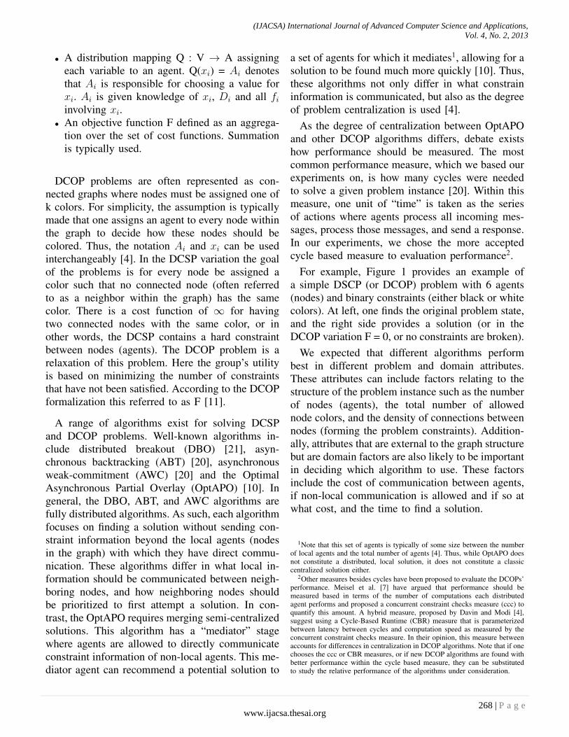
• A distribution mapping Q : V → A assigningeach variable to an agent. Q(xi) = Ai denotesthat Ai is responsible for choosing a value forxi. Ai is given knowledge of xi, Di and all fiinvolving xi.
• An objective function F defined as an aggrega-tion over the set of cost functions. Summationis typically used.
DCOP problems are often represented as con-nected graphs where nodes must be assigned one ofk colors. For simplicity, the assumption is typicallymade that one assigns an agent to every node withinthe graph to decide how these nodes should becolored. Thus, the notation Ai and xi can be usedinterchangeably [4]. In the DCSP variation the goalof the problems is for every node be assigned acolor such that no connected node (often referredto as a neighbor within the graph) has the samecolor. There is a cost function of ∞ for havingtwo connected nodes with the same color, or inother words, the DCSP contains a hard constraintbetween nodes (agents). The DCOP problem is arelaxation of this problem. Here the group’s utilityis based on minimizing the number of constraintsthat have not been satisfied. According to the DCOPformalization this referred to as F [11].
A range of algorithms exist for solving DCSPand DCOP problems. Well-known algorithms in-clude distributed breakout (DBO) [21], asyn-chronous backtracking (ABT) [20], asynchronousweak-commitment (AWC) [20] and the OptimalAsynchronous Partial Overlay (OptAPO) [10]. Ingeneral, the DBO, ABT, and AWC algorithms arefully distributed algorithms. As such, each algorithmfocuses on finding a solution without sending con-straint information beyond the local agents (nodesin the graph) with which they have direct commu-nication. These algorithms differ in what local in-formation should be communicated between neigh-boring nodes, and how neighboring nodes shouldbe prioritized to first attempt a solution. In con-trast, the OptAPO requires merging semi-centralizedsolutions. This algorithm has a “mediator” stagewhere agents are allowed to directly communicateconstraint information of non-local agents. This me-diator agent can recommend a potential solution to
a set of agents for which it mediates1, allowing for asolution to be found much more quickly [10]. Thus,these algorithms not only differ in what constraininformation is communicated, but also as the degreeof problem centralization is used [4].
As the degree of centralization between OptAPOand other DCOP algorithms differs, debate existshow performance should be measured. The mostcommon performance measure, which we based ourexperiments on, is how many cycles were neededto solve a given problem instance [20]. Within thismeasure, one unit of “time” is taken as the seriesof actions where agents process all incoming mes-sages, process those messages, and send a response.In our experiments, we chose the more acceptedcycle based measure to evaluation performance2.
For example, Figure 1 provides an example ofa simple DSCP (or DCOP) problem with 6 agents(nodes) and binary constraints (either black or whitecolors). At left, one finds the original problem state,and the right side provides a solution (or in theDCOP variation F = 0, or no constraints are broken).
We expected that different algorithms performbest in different problem and domain attributes.These attributes can include factors relating to thestructure of the problem instance such as the numberof nodes (agents), the total number of allowednode colors, and the density of connections betweennodes (forming the problem constraints). Addition-ally, attributes that are external to the graph structurebut are domain factors are also likely to be importantin deciding which algorithm to use. These factorsinclude the cost of communication between agents,if non-local communication is allowed and if so atwhat cost, and the time to find a solution.
1Note that this set of agents is typically of some size between the numberof local agents and the total number of agents [4]. Thus, while OptAPO doesnot constitute a distributed, local solution, it does not constitute a classiccentralized solution either.
2Other measures besides cycles have been proposed to evaluate the DCOPs’performance. Meisel et al. [7] have argued that performance should bemeasured based in terms of the number of computations each distributedagent performs and proposed a concurrent constraint checks measure (ccc) toquantify this amount. A hybrid measure, proposed by Davin and Modi [4],suggest using a Cycle-Based Runtime (CBR) measure that is parameterizedbetween latency between cycles and computation speed as measured by theconcurrent constraint checks measure. In their opinion, this measure betweenaccounts for differences in centralization in DCOP algorithms. Note that if onechooses the ccc or CBR measures, or if new DCOP algorithms are found withbetter performance within the cycle based measure, they can be substitutedto study the relative performance of the algorithms under consideration.
(IJACSA) International Journal of Advanced Computer Science and Applications, Vol. 4, No. 2, 2013
268 | P a g e www.ijacsa.thesai.org

Fig. 1. A sample DCSP problem with 6 nodes (N=6) and 2 colors. The original problem state is at left, with one possible solution at right.
III. USING PHASE TRANSITIONS TO AID ALGORITHMSELECTION
This paper focuses on developing an algorithmselection approach for constraint optimization prob-lems. Previously, Rice generally defined the algo-rithm selection problem as the process of choosingthe best algorithm for any given instance of a prob-lem from a given set of potential algorithms [16].We define the constraint optimization coordinationselection process used in this paper as follows:Let GR = a1, . . . , aN be a group on N agentsengaged in some cooperative behavior. Each agent,a, can choose out of a library of coordination al-gorithms, CA1 . . . CAk. We denote this selectionCAaj , where 1 ≤ aj ≤ k.
Using CAaj affects the group’s utility by a certainvalue, UT a(CAaj). UT a(CAaj) is composed of again, G(CAaj), that the group will realize by usingalgorithm CAaj , and the agent’s cost, C(CAaj), byusing that same algorithm. As this paper assumesthe agents within these problems are cooperative,the goal is to maximize
∑Na=1 UT
a(CAaj). Toachieve this, each agent must select the algorithmCAaj from the k possible algorithms in the librarywhose value G(CAaj) - C(CAaj) is highest.
One possible solution involves performing nolearning in advance and instead attempts to identifythe best algorithm exclusively during run-time. Forexample, Allen and Minton [1] suggest running
all algorithms CA1 . . . CAk in the portfolio fora short period of time on the specific probleminstance. Secondary performance characteristics arethen compiled from this preliminary trial to selectthe best algorithm. Gomes and Selman [5] suggestrunning several algorithms (or randomized instancesof the same algorithm) in parallel creating an al-gorithm portfolio. However, assuming running eachalgorithm incurs costs C(CA1) . . . C(CAk), theseapproaches are likely to be inefficient as the cu-mulative costs of running all algorithms are likelyto be higher than the potential gain of finding eventhe optimal choice.
Instead, we claim that the best algorithm withinthese problems can be quickly identified basedon finding phase transitions within these types ofproblem instances. The basis of this claim is theprevious findings that NP-complete problems arenot all equally difficult to solve [3], [13]. Manyinstances of NP-complete problems can still bequickly solved, while other similar instances ofproblems from the same domain cannot. They foundthat phase transitions are a well known phenomenonacross which problems display dramatic changes inthe computational difficulty and solution character[13].
The concept of phase transitions has been ap-plied to differentiate classes of these “easy” and“hard” NP-complete problem instances [13]. Withindistributed constraint satisfaction problems (DCSP),
(IJACSA) International Journal of Advanced Computer Science and Applications, Vol. 4, No. 2, 2013
269 | P a g e www.ijacsa.thesai.org

these problems can typically be broken into an easy-hard-easy pattern [11], [13]. The first set of easyproblems represent a category of under-constrainedproblems. All DCSP algorithms typically find anoptimal solution quickly for these instances. Atthe other extreme, the second easy category ofproblems are those that are over-constrained. Withinthese problems, the same algorithms can typicallydemonstrate that no solution exist, and thus these al-gorithms end in failure. The hardest DCSP problemsto solve are those within the phase transition goingfrom under to over-constrained problems, a categoryof problems also called “critically constrained”.These problems are the hardest to solve, with nosolution often being found [13].
One may view the DCOP problem as a generaliza-tion of the more basic DCSP decision form of theproblem. Again, in problems where there are fewcost constraints, the optimization requirements arelow, and an optimal solution can be quickly found.The “hard” problems exist where optimization re-quirements are high. However, debate exists if athird set of problems exist similar to the third “easy”problem set where DSCP problems can be quicklyshown to have no solution. It would seem that evenover-constrained DCOP instances cannot be easilyoptimized and still comprise “hard” problems [22].Consequently, DCOP problems should be dividedonly into Easy-Hard categories (instead of Easy-Hard-Easy) or those easy problems to solve beforethe problem’s phase transition, and “hard” problemsafter this point [14], [22]. Others have claimed[14] that certain optimization problems may in factfollow an easy-hard-easy distribution. However, thisdebate is not central to our thesis. According toboth opinions, problem clusters do exist, and thedifference of opinion revolves around the number ofthese clusters. If we follow the easy-hard model weshould expect to see two clusters of problems with atransitionary phase between the two, but followingthe easy-hard-easy model should yield three suchclusters with two transitionary phases.
Despite the computation complexity in solving allbut trivial DCOP problems, a variety of algorithmscan be used for attempting a solution in this do-main. These algorithms impact when constraints arecommunicated between agents, thus impacting howthe agents attempt to minimize F. We can formally
expand the classic DCOP model into an algorithmselection based model by modeling the selectionof algorithms CA1 . . . CAj that each agent canchoose in deciding what and how to communicatewhile attempting a solution. The intrinsically differ-ent approaches used by algorithms CA1 . . . CAjmakes them best suited for problems of differinglevels of complexity.
This realization significantly simplifies the pro-cess of finding those problems instances where agiven DCOP algorithm, CAaj , will be superior toother algorithms within CA1 . . . CAj. Based onthis knowledge, we expect to find attributes thatseparate between fundamentally different types ofproblems. Assuming each algorithm is best suitedfor different clusters of problems, a clear policywill be evident as to which algorithm to select,even when agents are confined to using only lo-cally available information. Instead of viewing alldomain problems as an enormous state space wherewe must map the relative effectiveness of algo-rithms CA1 . . . CAj, we instead focus on find-ing the problem attributes that differentiate thesealgorithms, significantly reducing the state space.After these attributes have been found, we expectto be able to further cluster problems as “easy” or“hard” types of interactions. One type of algorithmwill then be dominant within the easy problems,followed by phase shift(s)3 where differences be-tween algorithms are smaller and less apparent,followed by another large problem cluster where asecond algorithm becomes dominant. As a result,our research focuses on two important questions: 1.What are the attributes that differentiate betweenalgorithms CA1 . . . CAj? 2. At what attributevalues should one switch between algorithms?
IV. RESULTS
Our first step was to implement the algorithm li-brary of the ABT, AWC, DBO, and OptAPO withinthe previously defined DCOP domain. To do this,we used the Farm simulation environment [6] tocreate randomized instances of 3-color optimization
3We refer to differences in problem instance clusters as phase shifts insteadof phase transitions. This follows the distinction made by Brueckner andParunak [2] who reserve the term “phase transition” to clusters that have beenanalytically derived and refer to “phase shifts” to describe problem clustersthat have been emperically found. As this work derives these problem setsbased on emperical observation, we use the second term.
(IJACSA) International Journal of Advanced Computer Science and Applications, Vol. 4, No. 2, 2013
270 | P a g e www.ijacsa.thesai.org

Fig. 2. Graph coloring performance with ABT, AWC, DBO, and OptAPO algorithms with random graphs with 5-100 nodes (X-axis) and edges = 2.0n (left)and 2.7n (right). Each datapoint represents averaged results from 30 runs with 100 cycles per run.
Fig. 3. Graph coloring performance with ABT, AWC, DBO, and OptAPO algorithms with random graphs with 5-100 nodes (X-axis) and edges = 2.0n (left)and 2.7n (right). Each datapoint represents averaged results from 30 runs with 10 cycles per run.
problems. We first varied parameters such as thenumber of nodes (agents) and edges (which controlthe number of constraints) within these problems.Specifically, we studied “sparse” coloring graphproblems where the number of edges (m), is twotimes the number of nodes (n), and “dense” graphproblems with 2.7 times the number of edges (m)to nodes (n). Traditionally, these parameters werethought to control if a problem instance would be“easy” or “hard” [10].
Figure 2 represents the performance results of theABT, AWC, DBO, and OptAPO within probleminstances. We measured the number of non-fulfilledconstraints (F) after 100 cycles. The agents usingeach of the algorithms did not know in advance howmuch time would be available to reach a solution.As a result, after each cycle, the system wouldcheck if the global utility (F) had improved. If
it had, it created a snapshot of this solution, sothat the process could be interrupted at any time,and still return the best solution yet found. Thisallows for creating an interruptible anytime versionof these algorithms as per previous definitions ofanytime algorithms [23]. Note that in the easiestproblems (with 30 or less nodes in both problemsets), no significant differences existed betweenalgorithms as all algorithms were able to solve theseproblems equally (with the notable exception ofABT). Beyond this point, the OptAPO algorithmon average outperformed all other algorithms. Thisresult is consistent with previous finding demon-strating the effectiveness of the OptAPO algorithmin solving challenging DCOP problems regardlessof the number of nodes or constraints (edges) withinthe problem [10].
However, we found that the best algorithm to use
(IJACSA) International Journal of Advanced Computer Science and Applications, Vol. 4, No. 2, 2013
271 | P a g e www.ijacsa.thesai.org

also differed radically based on parameters such asthe time allotted to solve a problem instance. InFigure 3 we again ran the ABT, AWC, DBO, andOptAPO algorithms but allotted only 10 cycles ofruntime. Note how the APO algorithm performssignificantly worse than the other algorithms (inproblems with > 40 nodes) with the DBO algorithmperforming significantly better, especially in densegraphs with more than 60 nodes. This result is notsurprising as the OptAPO is fundamentally differentfrom other algorithms in the amount of problemcentralization used. Evidently, this algorithms needsan initialization period in order that its “mediator”nodes have enough information about non-localnodes in order to attempt an effective solution. Assuch, in these cases this algorithm underperformedthat of other purely localized algorithms that had nosuch overhead.
Communication costs can also radically affectwhich algorithm we should select. Recall that thegoal of our algorithm selection model is to maxi-mize
∑Na=1 UT
a(CAaj) where UT a(CAaj) is thegain G(CAaj) the group achieves by using thatalgorithm minus the cost, C(CAaj), paid by usingthe same algorithm. Again, the OptAPO algorithmis fundamentally different from other algorithms inthat it uses non-local communication, giving thisalgorithm a potential cost C(CAaj) not existent inother algorithms. Assuming such cost is significant– say because of privacy concerns or communicationlink cost, the OptAPO algorithm should also beavoided even if unlimited time exist to solve theseproblems. Indeed we found that the best of the breedof the localized algorithms, (such as the DBO orAWC algorithms), clearly outperforms OptAPO inthese types of problem instances.
Figure 4 demonstrates the impact of non-localcommunication cost on algorithm selection. In thisgraph we compared the performance of the OptAPOand DBO algorithms in dense graph problems with100 cycles allotted. When communication was freethe APO algorithm (APO-100 Cost 0) did signifi-cantly outperform DBO. However, once non-localcommunication had a cost of 0.02 quality units percommunication link, the DBO algorithm outperformOptAPO (APO-100 Cost 0.2)
Because of the radically different performanceof these algorithms, the selection policy is often
Fig. 4. The impact of non-local communication cost on algorithms studied
quite clear. Let us assume that agents are awareof performance limitations such as the time tocomplete the task, or the cost of non-local links. Aclear policy typically becomes immediately evident.For example, assume there is no communicationcost and agents need to find the best DCOP solutiongiven a relative long period of time (e.g. 100 cyclesor more). OptAPO is then clearly the best choice.Conversely, assuming communication is costly (e.g.cost of 0.02 or more), or only a very short periodof time is allocated (e.g. time of 10 cycles or less),the best of the local algorithms, e.g. DBO, wasselected. In cases with problem attributes betweenthose with a clearly defined policy (e.g. 50 cyclesof time to solve the problem), we considered twopossibilities. In the first possibility, a random selec-tion is taken between the borderline algorithms. Asecond possibility is to calculate the midpoint withinthe attribute space between these algorithms and tochoose the first algorithm for instances before themidpoint and use the second algorithm after thispoint. While random selection or midpoint heuris-tics will not likely form the optimal choice in manyof these instances, we hypothesized the differencebetween algorithms in these cases is not large asthis the transitional range for this attribute. Thus, thedifference between optimal and non-optimal choiceswithin these types of problems was not expected todeviate significantly from the optional choice.
Figure 5 demonstrates the effectiveness of theSelection algorithm just described. For comparison,we also display the average group utility (F) as takenfrom the the static DBO and OptAPO algorithms.We also created an Optimal group could run all
(IJACSA) International Journal of Advanced Computer Science and Applications, Vol. 4, No. 2, 2013
272 | P a g e www.ijacsa.thesai.org

Fig. 5. Comparing the effectiveness of the Selection algorithm policy versusthe static DBO and OptAPO algorithms
static algorithms without cost, and then accept thealgorithm that returned the highest utility. The re-sults in Figure 5 were generated from a total of100 DCOP 3-color graph problems with randomproblem attributes in the time to solve the problem,the number of nodes and edge constraints, andnon-local communication costs. As these problemsinstances were randomly selected, many of theseproblems had problem attributes fell within theproblem space where a clear policy existed. Suchinstances included: instances with long times tosolve the problem, very short times, or where non-local communication had a significant cost. In orderto strengthen the significance of this experiment, weensured that at least 25 percent of the problem in-stances were taken from the category when no clearpolicy existed. Notice that the Selection approachclosely approximated the optimal choice, and sig-nificantly outperformed statically choosing eitherDBO or OptAPO. In order to evaluate the statisticalsignificance of these findings, we performed a two-tailed t-test to compare the Selection approach to thestatic DBO and OptAPO methods. The resulting p-score was well below 0.05 (0.02), supporting thesignificance of the presented approach. Similarly,we compared the dynamic approach with the opti-mal selection policy and found only an insignificantdifference (p-score greater than 0.8) between thesevalues. This supports the claim that randomly se-lecting between algorithms in borderline cases doesnot significantly hurt performance.
V. CONCLUSION AND FUTURE WORK
In this work we present an algorithm selectionapproach for solving constraint optimization prob-lems. We focused on two factors: what attributesdifferentiate between the algorithms and how canwe build a selection policy based on those attributes.We present strong empirical evidence of the successof this approach in a general DCOP domain, sug-gesting the generality of this work.
For future work, several directions are possible.In this work, we manually found the attributes thatdifferentiated the coordination algorithms withinthe domains we studied. We hope to study howalgorithms can be created to automate this processso that novel interaction measures may be learnedfor quantifying coordination in other domains.
The success of our coordination selection ap-proach was rooted in the realization that differentclusters of problems can be created based on thehardness of different agent interactions. We drewupon the “phase transition” concept used to de-scribe some constraint satisfaction problems [13].However, following Brueckner and Parunak [2] wereserve the term “phase transition” to refer to a termused by physicists for mathematically describablebehavior within the system, and instead term theclusters of problems we empirically observed asphase shifts. We hope to study in the future whatformal models can be created that can predict whereand when these transitions should occur. We believethis study could strengthen the theoretical basis ofthe work we present.
REFERENCES
[1] John A. Allen and Steven Minton. Selecting the right heuristic algorithm:Runtime performance predictors. In Canadian Conference on AI, pages41–53, 1996.
[2] S. Brueckner and H. Parunak. Information-driven phase changes inmulti-agent coordination. 2003.
[3] Peter Cheeseman, Bob Kanefsky, and William M. Taylor. Where theReally Hard Problems Are. In IJCAI-91, pages 331–337, 1991.
[4] John Davin and Pragnesh J. Modi. Impact of problem centralizationin distributed constraint optimization algorithms. In AAMAS ’05, pages1057–1063, 2005.
[5] Carla P. Gomes and Bart Selman. Algorithm portfolios. ArtificialIntelligence (AIJ), 126(1-2):43–62, 2001.
[6] Bryan Horling, Roger Mailler, and Victor Lesser. Farm: A ScalableEnvironment for Multi-Agent Development and Evaluation. In Ad-vances in Software Engineering for Multi-Agent Systems, pages 220–237. Springer-Verlag, Berlin, February 2004.
[7] A. Meisels I. Razgon E. Kaplansky and R. Zivan. Comparing perfor-mance of distributed constraints processing algorithms. In Proc. AAMAS-2002 Workshop on Distributed Constraint Reasoning DCR, pages 86–93,July 2002.
273 | P a g e www.ijacsa.thesai.org
(IJACSA) International Journal of Advanced Computer Science and Applications, Vol. 4, No. 2, 2013

[8] V. Lesser, K. Decker, T. Wagner, N. Carver, A. Garvey, B. Horling,D. Neiman, R. Podorozhny, M. NagendraPrasad, A. Raja, R. Vincent,P. Xuan, and X.Q. Zhang. Evolution of the GPGP/TAEMS Domain-Independent Coordination Framework. Autonomous Agents and Multi-Agent Systems, 9(1):87–143, July 2004.
[9] Rajiv T. Maheswaran, Milind Tambe, Emma Bowring, Jonathan P.Pearce, and Pradeep Varakantham. Taking dcop to the real world:Efficient complete solutions for distributed multi-event scheduling. InAAMAS ’04, pages 310–317, 2004.
[10] Roger Mailler and Victor Lesser. Solving distributed constraint opti-mization problems using cooperative mediation. In AAMAS ’04, pages438–445, 2004.
[11] Roger Mailler and Victor Lesser. Using Cooperative Mediation to SolveDistributed Constraint Satisfaction Problems. In AAMAS ’04, pages 446–453, New York, 2004.
[12] Steven Minton, Mark D. Johnston, Andrew B. Philips, and PhilipLaird. Minimizing conflicts: A heuristic repair method for constraintsatisfaction and scheduling problems. Artificial Intelligence, 58(1-3):161–205, 1992.
[13] Remi Monasson, Riccardo Zecchina, Scott Kirkpatrick, Bart Selman,and Lidror Troyansky. Determining computational complexity fromcharacteristic “phase transitions”. Nature, 400(6740):133–137, 1999.
[14] H. Van Dyke Parunak, Sven Brueckner, John Sauter, and Robert Savit.Effort profiles in multi-agent resource allocation. In AAMAS ’02, pages248–255, 2002.
[15] David V. Pynadath and Milind Tambe. The communicative multiagentteam decision problem: Analyzing teamwork theories and models. JAIR,16:389–423, 2002.
[16] J. R. Rice. The algorithm selection problem. In Advances in Computers,volume 15, pages 118–165, 1976.
[17] Evan Sultanik, Pragnesh Jay Modi, and William C. Regli. On modelingmultiagent task scheduling as a distributed constraint optimizationproblem. In IJCAI, pages 1531–1536, 2007.
[18] Evan Sultanik, Pragnesh Jay Modi, and William C. Regli. On modelingmultiagent task scheduling as a distributed constraint optimizationproblem. In IJCAI, pages 1531–1536, 2007.
[19] Willem Jan van Hoeve, Carla P. Gomes, Bart Selman, and Michele Lom-bardi. Optimal multi-agent scheduling with constraint programming. InAAAI/IAAI, pages 1813–1818, 2007.
[20] Makoto Yokoo, Edmund H. Durfee, Toru Ishida, and KazuhiroKuwabara. The distributed constraint satisfaction problem: Formaliza-tion and algorithms. Knowledge and Data Engineering, 10(5):673–685,1998.
[21] Makoto Yokoo and Katsutoshi Hirayama. Distributed breakout algorithmfor solving distributed constraint satisfaction problems. In Victor Lesser,editor, ICMAS. MIT Press, 1995.
[22] Weixiong Zhang. Phase transitions and backbones of 3-SAT and max-imum 3-SAT. In Principles and Practice of Constraint Programming,pages 153–167, 2001.
[23] Shlomo Zilberstein. Using anytime algorithms in intelligent systems. AIMagazine, 17(3):73–83, 1996.
(IJACSA) International Journal of Advanced Computer Science and Applications, Vol. 4, No. 2, 2013
274 | P a g e www.ijacsa.thesai.org

Reliable Network Traffic Collection for NetworkCharacterization and User Behavior
Ali Ismail AwadElectrical Engineering Dept.,
Al Azhar University
Qena, Egypt
Email: [email protected]
Hanafy Mahmud AliElectrical Engineering Dept.,
Minia University
Minia, Egypt
Email: hanafy [email protected]
Heshasm F. A. HamedElectrical Engineering Dept.,
Minia University
Minia, Egypt
Email: [email protected]
Abstract—This paper presents a reliable and complete trafficcollection facility as a first and crucial step toward accuratetraffic analysis for network characterization and user behavior.The key contribution is to produce an accurate, reliable andhigh fidelity traffic traces as the valuable source of informationin the passive traffic analysis approach. In order to guarantee thetraces reliability, we first detect the bottlenecks of the collectionfacility, and then propose different monitoring probes startingfrom the ethernet network interface and ending at the packettrace. The proposed facility can run without stop for long timeinstead of one-shot periods, therefore, it can be used to drawa complete picture of network traffic that fully characterize thenetwork and user behavior. The laboratory experiments concludethat the system is highly reliable, stable and produces reliabletraces attached with different statistics reports that come fromthe installed monitoring probes.
I. INTRODUCTION
Presently, Internet supports wide variety of applications via
many protocol architecture instead of just data transfer. For
example, data, voice signals, images and videos are supported
by the same network infrastructure [1]. Due to the mixing
nature of network traffic with targeted high speed connections,
the understanding of the traffic behavior has become a difficult
task. Traffic collection and analysis is considered as the right
way for the network understanding and management [2].
Passively collected traffic traces include huge amount of
information that is useful for the measuring of almost all net-
work related activities. The analysis of packet traces provides
information from user, network and service perspectives. It
allows the identification and measurement of general trends
of many different metrics useful for engineering, management
and provisioning of the gigabit ethernet networks. The accu-
racy and reliability of the collected traffic traces have a direct
impact on the outcome of different trace-based operations
such as network characterization, traffic engineering [3], traffic
modeling and user behavior estimation [4].
The accuracy and the reliability are two key issues of pas-
sive traffic collection. Collecting reliable packet traces without
packet loss can be a difficult operation on gigabit ethernet
networks under the usage of commodity based hardware and
software. Conducting traffic analysis over incomplete and
unreliable traffic traces leads to inaccurate results unless data
losses are explicitly considered before the analysis process [5].
According to the resource constrains, the available collec-
tion facilities collect only one-shot of the network traffic that
does not contain enough amount of information that reflexes
the accurate characterization of the network. Additionally,
these collection systems do not provide any reliability reports
about the collected traces, and hence, the analysis results
of these traces may be inaccurate and unreliable. A reliable
packet capturing facility must be equipped with a mechanism
to accurately report the time and amount of packet loss during
the trace collection operation [6].
The usage of on-the-shelf hardware and software for packet
capturing on a high-speed (1 Gbps or higher) is sensible
to packet losses. Most of the carried out researches with
the commodity equipments is directed toward enhancing the
performance of packet capturing with respect to software [7],
and hardware [8] in order to cope the network line speed [9].
Data Acquisition and Generation (DAG) [10] is a dedicated
hardware solution for reliable packet capturing on high-speed
networks with high cost compared to the commodity solutions.
This paper focuses on the reliability of the collection
facility, and presents a reliable and complete traffic col-
lection facility using commodity hardware and softwares.
The efficient usage of the produced facility provides a very
useful information for different network users [4]. Network
users be categorized into Internet Service Providers (ISPs),
devices and hardware manufacturers, network administrations
and network researchers. ISPs use traffic analysis results for
billing their customers, identifying the dominant applications,
and hence they can build an accurate Service Level Agree-
ment (SLA)[11]. Moreover, ISPs can use the traffic analysis
for network management, provisioning and troubleshooting
recovery. Hardware providers use traffic analysis results for
measuring devices behavior under different conditions, and
hence they can make decisions to enhance or redesign the
current network devices. Traffic analysis will be useful for
network administrators to detect the up normal behavior of
the network traffic. Researchers use network traffic analysis
to understand and developing different traffic models.
The reminder part of this paper is organized as follows.
Section II demonstrates the structure of the generic collection
facility with bottleneck points, and emphasising the proposed
network interface monitoring approach. Section III explains
the implementation of the network interface monitoring ap-
proach. Section IV shows the exhaustive evaluation of the
reliable facility in terms of resources overhead and accuracy.
Conclusions and future work are reported in section V.
275 | P a g e www.ijacsa.thesai.org
(IJACSA) International Journal of Advanced Computer Science and Applications, Vol. 4, No. 2, 2013

Fig. 1. A Complete traffic collection facility with bottleneck points marked in circles. The bottlenecks diffuse in almost all system spaces.
II. RELIABLE NETWORK TRAFFIC COLLECTION
This research focuses on the passive traffic measurement
methodology to address the traffic collection and analysis
problem in the residential networks. However, it is not easy
to do continuous passive measurement, but on the other
hand, passive measurement provides a complete picture about
network traffic. Moreover, different traffic analysis phases can
be conducted on the traffic traces from different perspec-
tives. The performance metric of any passive collection is
the lossless packet capturing at link speed. Dropped packet
will produce problem in the next processes (anonymization,
analysis, etc.). Each component in the collection facility has
its own characteristics and limitations. Therefore, the bottle-
necks are distributed over all components. Fig. 1 shows the
bottlenecks through the packet journey through all collection
facility components.
A closed look at Fig. 1 shows that the traffic collection
facility suffers from many bottleneck points starting from
network interface, passing though kernel space, and ends with
the packet capturing applications in the user space. Every
system bottleneck point can lead to packet drops without
any feedback information to the system operator. Unreported
packet drops deteriorates the reliability of the traffic collection
facility especially at the 1 Gbps link speed.
The available solutions of the collection bottlenecks are
designed to overcome one point to enhance the collection
performance in terms of packet loss and scalability to link
speed. Those solutions can be divided into software-based such
as Driverdump [12] and Interrupt Coalescence (IC) technique
[13], kernel patching [14] and hardware-based solutions such
as Network Processor (NP) [8], [15], [16], and special purpose
DAG card [10]. Some solutions try to build special purpose
facilities, but those solutions are cost inefficient. The problem
with the previous solutions is that they have been designed for
special purpose or enhancing a particular point. Additionally,
the implementations of those solutions may become difficult
due to some coding problems or the high cost. We have built a
new solution for bottlenecks and insure the system reliability
by installing monitoring probe for each system bottleneck
using commodity based hardware and software. The most
important probe is the network interface monitoring approach.
A. Network Interface Monitoring Approach
Network interface card is the first contact point inside
the collection machine that can hold all packets including
the correct and the erroneous ones at 1 Gbps link speed.
Network interface monitoring approach uses network interface
capability to monitor all coming in and out packets to the
collection machine before its pumping up to the upper levels.
We could correlate the produced report with the trace file in
the post processing to detect the packet loss, and judging the
packet trace reliability for the collection session.
The idea behind monitoring the ethernet network interface
is considered as two folded process: (1) Open a socket for
direct communication with the network interface drivers, and
(2) Information exchange between network interface drivers
and the monitoring tool agent in the user interface. In order
to retrieve statistics directly from hardware, the proposed
monitoring approach takes advantage of the support provided
by the Ethtool Linux utility [17]. Ethtool is a GNU/Linux
tool that allows obtaining information and diagnostics about
ethernet card settings related to media, link status, and more.
Precisely, the ethtool_stats data structure provided by its
API enables dumping the network interface specific statistics
to the user space, and store them in a statistics file.
276 | P a g e www.ijacsa.thesai.org
(IJACSA) International Journal of Advanced Computer Science and Applications, Vol. 4, No. 2, 2013
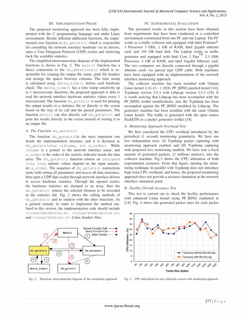
III. IMPLEMENTATION PHASE
The proposed monitoring approach has been fully imple-
mented with the C programming language and under Linux
environment. Beside different additional functions, the imple-
mented core function is do_gstats() which is responsible
for consulting the network interface hardware via its drivers,
open a User Datagram Protocol (UDP) socket and retrieving
back the available statistics.
The simplified interconnections diagram of the implemented
functions is shown in Fig. 2. The main() function has a
direct connection to the do_metatrace() which is re-
sponsible for creating the output file name, print file headers
and arrange the spaces between columns. The time stamp
is calculated using delta_time() before each hardware
check. The delta_time() has a time stamp sensitivity up
to 1 microsecond, therefore, the proposed approach is able to
read the network interface hardware statistics values every 1microsecond. The function do_print() is used for printing
the output results to a statistics file or directly to the screen
based on the way of its call and the passed parameters. The
function main() can also directly call do_gstats() and
print the results directly to the screen instead of writing it to
an output file.
A. The Function do_gstats()
The function do_gstats()is the most important one
inside the implementation structure, and it is declared as
do_gstats(char *ifname, int s_order). While
ifname is a pointer to the network interface name, and
s_order is the order of the statistic indicator inside the data
array. The do_gstats() function returns an unsignedlong long statistic values depend on the input parame-
ter s_order. The sequence of do_gstats() instructions
starts with setting all parameters and access all data structures,
then open a UDP data socket through network interface drivers
to access hardware statistics. Through the opened socket,
the hardware statistics are dumped to an array, then the
do_gstats() returns the selected element to be recorded
in the statistics file. Fig. 2 shows the calling methods of
do_gstats() and its relation with the other functions. As
a general remark, in order to implement the method out-
lined in this section, the implementation code should include
<linux/netdevice.h>, <linux/etherdevice.h>,
and <linux/ethtool.h> Linux headers files.
Fig. 2. Functions interconnection diagram of the monitoring approach
IV. EXPERIMENTAL EVALUATION
The presented results in this section have been obtained
from experiments that have been conducted in a controlled
environment constructed from one PC and one Laptop. The PC
works as a traffic collector and equipped with Intel Pentium R©
4 Processor 3 GHz, 1 GB of RAM, Intel gigabit ethernet
card, and 160 GB hard disk. The Laptop works as traffic
generator and equipped with Intel Core 2 DueTM
2.5 GHz
Processor, 4 GB of RAM, and Intel Gigabit Ethernet card.
The two computers are directly connected through a gigabit
ethernet cards via special type UDP cable. Both machines
have been equipped with an implementation of the network
interface monitoring approach.
The collector machine has been installed with Ubuntu
Linux kernel 2.16.18−1.2200, PF RING patched kernel [14],
Tcpdump version 3.9.4 with Libpcap version 0.9.4 [18]. It
is worth noticing that Libpcap has been recompiled with the
PF RING toolkit modifications, also the Tcpdump has been
recompiled against the PF RING modified by Libpcap. The
generator machine has been installed with the same Ubuntu
Linux kernel. The traffic is generated with the open source
PackETH as a packet generator toolkit [19].
A. Monitoring Approach Overhead Test
We first considered the CPU overhead introduced by the
periodical (1 second) monitoring granularity. We have run
two independent tests: (I) Tcpdump packet capturing with
monitoring approach enabled, and (II) Tcpdump capturing
with proposed loss monitoring enabled. We have sent a fixed
amount of generated packets, (2 millions packets), into the
collector machine. Fig.3 shows the CPU utilization of both
experimental scenarios. From that figure, running the moni-
toring technique in parallel with Tcpdump does not introduce
high extra CPU overhead, and hence, the proposed monitoring
approach does not provide a resource limitation at the network
interface saturation point.
B. Facility Overall Accuracy Test
This test is carried out to check the facility performance
with enhanced Linux kernel using PF RING explained in
[14]. Fig. 4 shows the generated packet rates for each packet
Fig. 3. CPU utilizations for one collection session with monitoring approach.
277 | P a g e www.ijacsa.thesai.org
(IJACSA) International Journal of Advanced Computer Science and Applications, Vol. 4, No. 2, 2013

Fig. 4. Packet generation rates measured in generator side.
sizes. The plotted data have been taken from the statistics file
produce by the monitoring approach in the traffic generator
side. Additionally, from the collector point of view, Fig. 5
shows the percentage of the collected packets for each packet
size. The figure proves the high packet losses at short packet
sizes. The overall accuracy can be predicted by finding the
difference between the generated and the collected packets.
Of course, the packet trace reliability is determined according
to the amount of dropped packets compared to the generated
ones. The dropped packets are directly reported by the moni-
toring approach (values in the statistic files). While the kernel
drops are measured as the difference between captured packets
and packets received by the network interface (deduced from
statistics information). From Fig. 6, the proposed monitor-
ing approach is always reporting the total generated packets
(received + erroneous) with 100% accuracy, and hence, the
reliability of the packet trace can be measured by correlating
the reported packets by the proposed approach and the actual
collected packets in the trace file.
C. Discussion
Although the related work shows many special purpose
hardware and software solutions for packet drop problem,
the presented results in this section prove the superiority of
using commodity based hardware and software in the proposed
solution with invented monitoring probes at every bottleneck
in the collection facility. The statistic files produced by each
monitoring probe can be correlated with the actual recorded
packets in the trace file, and hence, we get knowledge about
where and when the packet was dropped. The actual packet
trace is then sanitated further to remove the gaps of the
dropped packets which finally produces a reliable packet trace.
Fig. 5. Packet collection percentage (%) measured in collector side.
Fig. 6. The accuracy of the collection facility in terms of packet loss.
Once we got a reliable and accurate passively collected packet
trace with attached monitoring reports, the traffic analysis for
network characterization and user behavior will be the next
phase of this research.
V. CONCLUSION AND FUTURE WORK
This paper was directed toward enhancing the reliability of
traffic collection facility. It has presented a new network inter-
face monitoring approach in order to increase the reliability of
the collected packet trace. The evaluation results have proved
that the proposed mechanism is non-intrusive for the traffic
trace collection with respect to CPU consumption, packet
generation and packet collection. The experimental works
conclude that purposed monitoring approach is a feasible and
practical tool for reliable packet trace collection. As a future
work, the proposed approach can be extended for different
ethernet cards and implemented for wire and wireless network
interfaces on different Linux platforms.
ACKNOWLEDGEMENT
The initial design and implementation of this work has been
conducted in the laboratory of NetCom, Universitat Pompeu
Fabra, Barcelona, Spain. I would like to thank Professor
Dolors Sala for her advices during building the initial phase
of this research.
REFERENCES
[1] J. Goldman and P. Rawles, Local area networks: a business-orientedapproach, 2nd ed. John Wiley & Sons, 2000.
[2] J. Rubio-Loyola, D. Sala, and A. I. Ali, “Maximizing packet loss moni-toring accuracy for reliable trace collections,” in Proceedings of the 16th
IEEE Workshop on Local and Metropolitan Area Networks (LANMAN2008). Chij-Napoca, Romania: IEEE, 2008, pp. 61–66.
[3] B. Eriksson, P. Barford, and R. Nowak, “Network discovery from passivemeasurements,” Computer Communication Review, vol. 38, no. 4, pp.291–302, 2008.
[4] J. L. Jerkins and J. L. Wang, “A close look at traffic measurements frompacket networks,” in Global Telecommunications Conference, 1998.GLOBECOM 1998. The Bridge to Global Integration. IEEE, vol. 4,1998, pp. 2405–2411.
[5] A. I. Awad, H. M. Ali, and H. F. A. Hamed, “Toward highly reliablenetwork traffic traces,” in Proceedings of the First International Con-ference on Communications, Signal Processing, and their Applications,ICCSPA13. Sharjah, United Arab Emirates: IEEE, February 2013, p.To Appear.
[6] J. Rubio-Loyola, D. Sala, and A. I. Ali, “Accurate real-time monitoringof bottlenecks and performance of packet trace collection,” in Proceed-ings of the 33rd IEEE Conference onLocal Computer Networks (LCN2008). Montreal, Que, Canada: IEEE, 2008, pp. 884–891.
278 | P a g e www.ijacsa.thesai.org
(IJACSA) International Journal of Advanced Computer Science and Applications, Vol. 4, No. 2, 2013

[7] G. Iannaccone, C. Diot, I. Graham, and N. McKeown, “Monitoring veryhigh speed links,” in Proceedings of the 1st ACM SIGCOMM Workshopon Internet Measurement. San Francisco, California, USA: ACM, 2001,pp. 267–271.
[8] R. Ramaswamy, N. Weng, and T. Wolf, “A network processor basedpassive measurement node,” in Proceedings of the 6th internationalconference on Passive and Active Network Measurement (PAM’05).Boston, MA: Springer-Verlag, 2005, pp. 337–340.
[9] E. Weigle and W. chun Feng, “TICKETing high-speed traffic withcommodity hardware and software,” in Proceedings of the Third AnnualPassive and Active Measurement Workshop (PAM2002), 2002, pp. 156–166.
[10] “Data Acquisition and Generation (DAG).” [Online]. Available:http://www.endace.com/
[11] W. Stallings, Data & Computer Communications, six ed. Prentice Hall,1999.
[12] E. Anderson and M. Arlitt, “Full packet capture and offline analysis on1 and 10 gb/s networks,” Technical Report, HPL-2006-156 20061106,HP Labs, Tech. Rep., 2006.
[13] R. Prasad, M. Jain, and C. Dovrolis, “Effects of interrupt coalescenceon network measurements,” in The 5th anuual Passive & Active Mea-surement Workshop, (PAM 2004), Antibes, France, April 2004.
[14] L. Deri, “Improving passive packet capture: Beyond device polling,” inProceedings of SANE 2004, 2004.
[15] K. Mackenzie, W. Shi, A. Mcdonald, and I. Ganev, “An intel IXP1200-based network interface,” in Proceedings of the Workshop on Novel Usesof System Area Networks at HPCA (SAN-2 2003), 2003.
[16] T. Nguyen, M. Cristea, W. de Bruijn, and H. Bos, “Scalable networkmonitors for high-speed links: a bottom-up approach,” in ProceedingsIEEE Workshop on IP Operations and Management, 2004., Beijing,China, October 2004, pp. 16–22.
[17] “Free software directory. the ethtool resource: a net driver diagnostic andtuning tool.” [Online]. Available: http://directory.fsf.org/project/ethtool/
[18] “Berkley Packet Filter, Lawrence Berkeley National LaboratoryNetwork Research. TCPDump: the Protocol Packet Capture andDumper Program.” [Online]. Available: http://www.tcpdump.orgmp.org
[19] M. Jemec, “PackETH, Open Source Ethernet Packet Generator.”[Online]. Available: http://packeth.sourceforge.net/
279 | P a g e www.ijacsa.thesai.org
(IJACSA) International Journal of Advanced Computer Science and Applications, Vol. 4, No. 2, 2013
Copyright © 2022 FDOKUMEN