COMMISSION OF THE EUROPEAN COMMUNITIES

SCIENCE RESEARCH AND DEVELOPMENT

IIIOIITOR SPEAR

Economic Quantitative Methods for the Evaluation of the Impact

of R&D Programmes

A State-of-the-A·rt

Research evaluation EUR 14864 EN

!

Commission of the European Communities

Economic Quantitative Methods for ~ the Evaluation of the Impact

of R&D Programmes -A State-of-the-Art

Author H. CAPRON ,,

~ ~ 1 MONITOR/SPEAR}Coordinators C. DE LA TORRE

A. DUMORT

The opinions contained in this report are the sole responsability of the authors and do not necessarily reflect the official position of the Commission of the European Community

November 1992 EUR 14864 EN

Published by the COMMISSION OF THE EUROPEAN COMMUNITIES

Directorate-General Information Technologies and Industries, and Telecommunications

L-2920 LUXEMBOURG

LEGAL NOTICE

Neither the Commission of the European Communities nor any person acting on behalf of the Commission is responsible for the use which might be made of the following

information

Cataloguing data can be found at the end of this publication

Luxembourg: Office for Official Publications of the European Communities, 1993

ISBN 92-826-5646-2

© ECSC-EEC-EAEC Brussels • Luxembourg, 1993

Printed in Belgium

Table of Contents

Executive SuilllllalY .............................. · · · · · · · · · · · · · · · · · · · · · · · · · · · · · · · · · · · · · · · · · · · · · · · · · · · v

lntr<:xiuction ......................................................................................... . 1

Chapter 1. Technology Assessment : An Overview ............................................ . 5

1.1. How Can One Assess ? • . • . • . • . • • • • • • • . . . . . • • • • . • • • • • • . . • . . . . . . . . . . . . . • . . . . . . . . . . . . . . . . . . . 6

1. 2. Overview of Methods . . . . . . . . . . . . . . . . . . . . . . . . . . . . . . . . . . . . . . . . . . . . . . . . . . . . . . . . . . . . . . . . . . . . 12

1.2.1. Assessment by peers, questionnaires, interviews . . . . . . . . . . . . . . . . . . . . . . . . . . . . 12

1.2.2. Scoring methods . . . . . . .. . . . . . . . . . . . . . . . . . . . . . . . . . . . . . . . . . . . .. . . . . . . . . . . . . . . . . . . . . 14

1. 2. 3. Systemic approaches . . . . . . . . . . . . . . . . . . . . . . . . . . . . . . . . . . . . . . . . . . . . . . . . . . . . . . . . . . . . 17

1.2.4. Financial methoos . . . . . . . . . . . . . . . . . . . .. . . .. . . .. . . . . . .. . . . . . . . . . . . . . . . . . . . . . . . . . . . . 18

1.2.5. Technological forecasting methods . . .. .. . .. . . .. . . ... . .. . . .. . . . . . . . .. . . .. . . .. . . 21

1.2.6. Quantitative indicators . . .. . . .. . . . . . . .. . .. . . .. . . . . . . . . . . . . . .. . . . . . . . . . . . . . . . . . . . . . 22

1. 2. 7. Econometric methoo . . . . . . . . . . . . . . . . . . . . . . . . . . . . . . . . . . . . . . . . . . . . . . . . . . . . . . . . . . . . . 23

Chapter 2. The Economic Analysis of Technological Change . . . . . . . . . . . . . . . . . . . . . . . . . . . . . . . . . . 29

2.1. Technological Change and R & D. . . . . . . . . . . . • . . . . . . . . . . . . . . . . . . . . . . . . . . . . . . . . . . . . . . . . . . . 30

2.2. The Measurement of Technical Progress ..................... .............. .. ...... ... . 33

2. 3. The Applied Economics of Technical Change . . . . . . . . . . . . . . . . . . . . . . . . . . . . . . . . . . . . . . . . . 41

2. 3 .1. The exogenous disembodied technical change . . . . . . . . . . . . . . . . . . . . . . . . . . . . . . . . 41

2.3.2. The exogenous embodied technical change . . . .. . . .. . . . .. . . . .. . . . .. . . .. . . . .. . . 51

2.3.3. The induced technical change .. . .. ...... .. . . . . . . .. . . .. . . .. . . .. . . .. . . . . . . .. . . . . . . 58

2.3.4. The endogenous technical change ... . . .. .. .. . . .. . . .. . . . . . . . . . . . . . . . . . . . .. . . . .. . 60

Chapter 3. The Applied Economics of R & D . . . . . . . . . . . . . . . . . . . . . . . . . . . . . . . . . . . . . . . . . . . . . . . . . . . . 63

3.1. The Economics of R & D................................................................. 64

3.2. Econometric Studies in Retrospect .. . ... . .. . . .. . . .. . . .. . . . . .. .. . . .. . . .. . . .. . . . . . . . .. . . .. 75

3. 2. 1. Micro level studies . . . . . . . . . . . . . . . . . . . . . . . . . . . . . . . . . . . . . . . . . . . . . . . . . . . . . . . . . . . . . . . 7 6

3.2.2. Meso level studies . . . . . . . . . . . . . . . . . . . . . . . .. . . . . . . .. . . . . . .. . . . . . . .. . . . . . . . . . .. . . . . . 88

3. 2. 3. Macro level studies . . . . . . . . . . . . . . . . . . . . . . . . . . . . . . . . . . . . . . . . . . . . . . . . . . . . . . . . . . . . . . . 90

3.3. An Assessment of Econometric Studies ................ .. ..... ..... ... ... . . .. . . .. . ... . . 91

3.4. Adjustment Cost Models ................................................................. 100

III

Chapter 4. The Spillovers from R & D Investment .. .•.•...... .. . ... .. .. . . . ...... .. ... . . . . . . . . . 105

4.1. About Sonte Case Studies . . . . . . . . . . . . . . . . . . . . . . . . . . . . . . . . . . . . . . . . . . . . . . . . . . . . . . . . . . . . . . . . 1 06

4.2. The Inter-Industry Technology Flows Approaches . . . . . . . . . . . . . . . . . . . . . . . . . . . . . . . . . . . 1 OS

4.3. The Spillovers in the Technology Space................................................ 112

4.4. The Econontetric Measurement of Total Spillovers by Industry ..................... 115 117

4. 5. Tracing the Sources of Spillovers ...................................................... .

4. 6. More on the input -output approach . . . . • . • . . . . . . . . . . . . . . . . . . . . . . . . . . . . . . . . . . . . . . . . . . . . . . 1 29

4. 6 .1. Decomposition of growth in real output . . • . . . . . . . . . . . . . . . . . . . . . . . . . . . . . . . . . . . . l 2 9

4.6.2. The treatment of R & Din input-output tables . . . .. . . . .. .. ... . . . . . . . . .. . . . . . . . 132

Chapter 5. The Impact of Government-Financed R & D ........................................ 139

5 .1. Why to Evaluate the Economic Impact of Publicly-Funded R & D ? . . . . . . . . . . . . . . . . _140

5.2. How Productive is the Publicly-Financed R & D? .. .. ... . . ... ..... ... . . ... . . . . . . . .. . . 14.4

5.3. How Stimulating is the Publicly-Financed R & D? ................................... 15-5

5.4. How Effective is the Public Support toR & D Projects? ............................ 1 71

Chapter 6. Publicly-Funded R & D in a Competitive Environntent . . . . . . . . . . . . . . . . . . . . . . . . . . . 1 ~ 1.

6.1. Technological Rivahy and Public Incentive Policies . . . . . . . . . . . . . . . . . . . . . . . . . . . . . . . . . . 182

6.2. Mooels of R & D Strategy . . . . . . . . . . . . . . . . . . . . . . . . . . . . . . . . . . . . . . . . . . . . . . . . . . . . . . . . . . . . . . . . 191

6.3. Imitation, Purchase or Inducement: The Search for an Optimal Strategy .......... 203

6.4. Centres of Excellence and Agglomeration Economies ................................ 20'3

6.5. Technological Competition and R & D Policy in Oligopoly .......................... 21-2

Conclusion . . . . . . . . . . . . . . . . . . . . . . . . . . . . . . . . . . . . . . . . . . . . . . . . . . . . . . . . . . . . . . . . . . . . . . . . . . . . . . . . . . . . . . . . . 223

References . . . . . . . . . . . . . . . . . . . . . . . . . . . . . . . . . . . . . . . . . . . . . . . . . . . . . . . . . . . . . . . . . . . . . . . . . . . . . . . . . . . . . . . . . . . . 2 2 9

IV

Executive Summary

1. The Findings

The bases on which a nation can acquire competitive advantages in order to in­

crease its material welfare are manifold· and depend on its endowment with resources, its

stock of total capital and its institutional infrastructure. The stock of total capital is com­

posed of physical capital, knowledge capital and human capital. For a long time, know­

ledge capital and human capital have been treated by governments, at most, as second­

hand targets in the economic policy formation. Physical investment and labor were the

focus targets around which it was thought an efficient economic policy could be de­

signed. In the late seventies, the flagrant inefficiency of economic policies showed policy

makers that knowledge and human capital were really the active sources of economic

growth and competitiveness. This led them to review their conception of science and

technology policy as well as education and training policy and to adapt their institutional

system accordingly. In the search for a higher efficiency of the science and technology

policy, public managers increasingly view science and technology assessment as an inte­

gral component of policy management At the roots of the present science and technology

policies, there is the objective to stimulate innovative activities as a means of fostering

economic growth and strengthening competitiveness. Therefore, the ultimate question of

the policy evaluation process should be : what are the economic impacts of the science

and technology policy ? This questioning then leads them to try and find how to measure

these economic impacts and, in a further stage, when searching the toolbox of policy

makers, these wonder whether using econometric methods and models might be advis­

able.

Econometric methods are extensively used as an economic policy evaluation tool.

Nevertheless, its credibility and usefulness in the field of science and technology policy

is, to a large extent, subject to controversy. Main arguments against them are the identifi­

cation problem of the causal relationship between technological petfonnance and econo­

mic development, the time lag between knowledge investment and its economic impact,

the variability of results, the complexity and uncertain nature of innovation. Besides, lots

of evaluation studies point out that the evaluation processes are mainly focused on tech­

nological aspects and neglect economic impacts. When economic impacts are covered by

the evaluation process, the methods used are essentially case studies and sutveys. The

drawback of these methods is that results obtained from case studies cannot be easily

generalized and that sutveys may provide biased results. So, these methods have their

v

advantages and disadvantages. The modalities of their use are varied. They should be

simultaneously used in some cases in order to improve the reliability of observations and,

when the results are divergent, to reinforce the evaluation process by learning about

sources of divergence. Besides, they could be separately used depending on specific ob­

jectives. Yet, some criticisms against econometric methods are grounded. Hence, the

problems econometric techniques of impact evaluation are faced with are threefold : the

methodological drawbacks, the measurement issue and data availability.

The methodological drawbacks essentially follow from the treatment of technical

change in economic analysis. Indeed, technical change is conceived as an intrinsically

exogepous process in economic theory and, consequently, in economic models. It is

exogenous because assumed to depend exclusively on technical constraints. The empi­

rical consequence is that it is rudimentarily measured through a time trend. It is intrin­

sically exogenous because any attempts to grasp how it operates, as is the case for the

inducement and embodiment hypotheses, have not removed the exogeneity, and hence

the time dependence. Yet, in the past thirty years, a great amount of research has been

devoted to relaxing this hypothesis by introducing research and development (R & D) in

production functions. As long as R & D investment is only integrated as a production

factor without being itself, at least partially explained, by economic mechanisms, we have

only identified but not endogenized one of the sources of technical change. Nevertheless,

we may agree that it is a ftrSt important step towards endogenization.

Despite its limitations, the production function approach is presently the only

operational way of assessing the economic impact of R & D. This impact is measured by

estimating the relationship between R & D and productivity. The main attempts to

measure the impact of R & D on economic growth rely on the Cob)?: Douglas production

function and make use of two alternative theoretical frameworks. The first one is based

on the estimation of the R & D capital elasticity with respect to the output and the second

one on the estimation of the rate of return on R & D investment It is worth noting that the

interpretation of the estimated coefficients will differ depending on the level of data

aggregation. Indeed, empirical analyses can be performed at three levels: micro (i.e. on

firm data), meso (i.e. on industry data), macro (i.e. on nationwide data). At the micro

level, both coefficients only deal with the private effect of R & D. At the meso level, both

coefficients can be assumed to measure the intra-industry social effect of R & D. At the

macro level, both coefficients should provide an estimate of the nationwide social effect

of R & D. Furthermore, regression analyses can be alternatively petformed on time-series

data, cross-section data or both. The high variability observed in the estimates can, to a

large extent, be explained by data characteristics. When firm sales are used as output

measure the mean value of R & D elasticity is .05 for time-series data against .10 for

VI

cross-sections and the mean value of the rate of return is 15 percent. The use of value

added as output measure provides weaker estimates which often tum to be non-signifi­

cant. The estimates are higher when data are corrected for double counting and expensing

and in scientific sectors. At the industry level, the mean value of the rate of return is 22

percent and amounts to 35 percent when the fall observed in the rates of return during the

sixties is taken into account. At the nationwide level, the R & D elasticity noticeably

differs from one country to the other. The mean value is about .40. In recent years,

dynamic disequilibrium models have been applied to measure the contribution of R & D

to the changes in output. These adjustment cost models consider R & D as a quasi-fixed

factor which does not adjust instantaneously to its optimal level and which is endo­

genously determined by demand, input prices and inputs. At the nationwide level, the

estimates short-run elasticity ofR & D for the manufacturing sector is about .15 and the

net internal rate of return on R & D investment is about 13 percent. There is no major

contradiction between these estimates and the latter are strikingly compatible with results

obtained from case studies. So, these studies undoubtedly put forward the influence of R

& D activity on productivity. Nevertheless, this contribution varies from one sector to an

other. In the scientific sector, the R & D elasticity is higher than in other sectors, its mean

value being .13 for time-series against .18 for cross-sections. Regarding its rate of

return, it is 10 percent higher than in other sectors. Furthermore, as shown by case

studies, its impact changes over time and occurs with a variable lag depending ot:t the

orientation of research. Finally, econometric studies are faced with ·two categories of

problems : conceptual fuzziness and methodological drawbacks. The former principally

concerns the interpretation of estimates and data to be used and the latter, econometric

techniques implemented and data measurement.

There is a general agreement that the social return to R & D is higher than the

private return because the effects of R & D go beyond the fmn, the industry and the

country which perform the investment. Indeed, the returns to R & D may not be com­

pletely appropriable because knowledge produced by R & D investment performed in a

fmn is a public good which allows other fmns to develop new innovations with less R &

D efforts than otherwise. This spillover effect is a positive externality which causes the

social rate of return on R & D to be generally higher than the private rate of return, an

observation largely confirmed by empirical studies. The literature reports several methods

dealing with the measure of spillovers. A fmt method is to take into account the proximi­

ty between industries by giving weights to R & D stocks according to how close to each

other industries are. The different proximity measures which have been suggested are

successively : weights proportional to the flows of intermediate input purchases, to the

flows of patents or innovations or again to the firm's position in a technology space. A

second approach is to consider the outside pool of R & D stock globally. A last method is

VII

to enter separately into the production function the R & D stock of each potential source

of spillover. According to the inter-industry technology flow approaches, the rate of

return on external R & D should be around 50 percent Yet, the relationship between

external R & D and productivity varies across industry and over time. The use of inter­

mediate input purchases, patents or innovations in order to identify technology flows is

not free from criticisms. If intermediate input purchases may be assumed to be a good

proxy of embodied R & D, it is not necessarily a good measure of technological op­

portunities. On the other hand, when patents or innovations are used, they are assumed to

be equally important, which is far from being right. When technological proximity is

measured by characterizing the fmn's position in the technological space, patents are

made use of to distribute firms according to their research interests across technological

areas. The results obtained from this approach show that fmns in R & D intensive areas

have, on average, relatively more patents and a higher return toR & D though low R & D

intensity finns have lower return if their neighbors are R & D intensive. Further, firms

adjust their technological positions in response to technological opportunities. In the

approach considering the unweighted outside pool of R & D knowledge, the spillover

effects are measured by estimating a cost function which includes intraindustry and inter­

industry spillover variables. The empirical evidence based on this approach is very

limited. The findings suggest that interindustry spillovers cause unit costs to decline

substantially more than intra-industry spillovers. However, the contribution of the inter­

industry spillover to the social rate of return appears to be lower than the intraindustry

spillover effect. The latter contributes of about 10 percent against 2 percent for the

former. Not only is there a substantial difference between the social and private rates of

return but the spillover effects, to a large extent, differ across sectors. The latter ap­

proach, which separately enters the R & D stock of each potential source of spillover into

the cost function empirically demonstrates that tracing the sources and beneficiaries of

spillovers is econometrically feasible. However, only main spillover sources can be

significantly identified because of multicollinearity. Each producer is treated as a distinct

spillover source and the direction and magnitude of the interindustry spillovers can vary

across receiving industries so that the spillover network of senders and receivers can be

traced. The results obtained for the few empirical investigations show that all industries

are influenced by spillovers but not all are sender industries. All industries are charac­

terized by very high private rates of return, which, on average, amount to 25 percent.

Besides, the social rate of return greatly varies across industries and can be three to four

times as big as the private rate of return, as seems to be the case in the sectors of scientific

instruments, nonelectrical machinery and chemical products. R & D spillovers do not

only affect production characteristics but both output supply and input demand decisions.

Moreovet," spillovers are intertemporal externalities because they result from present and

past decisions about R & D investment process. Such features can be taken into account

VIII

by considering simultaneously cost and product demand functions in which R & D stocks

are defined as quasi-fixed factors of production which, because of adjustment costs, do

not adjust instantaneously. A last point is that it would be useful to extend the input­

output by treating R & D activities as an independent activity in the input-output structure.

As R & D investment is a strategic policy variable which increases the future production

potential and not principally the current production, it should be regarded as a final de­

mand component. Then, an R & D input-output matrix should be constructed in order to

have a disaggregation of R & D final demand between consumer sectors and producer

sectors.

Most efforts .. in the econometrics of R & D have been devoted to measuring the

impact of industrial R & D. Econometric methods are only marginally used as policy

evaluation tool in the field of science and technology. Yet, assessing economic impacts of

policy intervention is not an easy task because a variety of effects and causes may con­

tribute to specific outcomes. So far, only a few empirical pinpoint studies have en­

deavoured to estimate the economic impact of R & D policy. They principally make use

of two direct approaches. In the first one, the productivity approach, the respective ef­

fects of privately-funded and publicly-funded R & D expenditures on productivity are

me&Sured. These studies provide evidence of the output elasticity of public R & D or of

its rate of return. The second one, the investment approach, evaluates to what extent

publicly-funded R & D crowds out, complements or stimulates private R & D. Besides

these two conceptual approaches, probabilistic models which deal with qualitative data,

and a supply approach, which is an alternative indirect method to the productivity ap­

proach, are also used. Studies dealing with the impact on productivity of government­

funded R & D often fail to find evidence that public support to R & D is productive. Yet,

some studies show that the relationship between government R & D and productivity is

more subtle than the link between private R & D and productivity growth. The objectives

of public support, the rules that govern the allocation of public funds and the character of

use of government R & D are all elements which might strongly influence the

effectiveness of public R & D investments. So, defense-oriented R & D is not directly

aimed at furthering economic growth, basic research certainly sustains more long-term

economic growth than short-term objectives and the effectiveness of public support to

new economic products and processes produced by business enterprises strongly de­

pends on the recipient private enterprise's own economic effectiveness. Studies taking

into account some of these characteristics provide evidence that public support has a

positive and significant influence on productivity and also show that this productivity

effect cannot be generalized to the whole public R & D. Turning now to the impact of

public support on private R & D, studies, to a large extent, emphasize a marginally stimu­

lating effect of publicly-funded R & D on privately-funded R & D. Yet, here too, the

IX

effectiveness of public support depends on the characteristics of public intervention.

Furthermore, the impact largely differs from one country to the other. Unfortunately, like

the productivity approach, most of the evidence comes from the United States and shows

that the relationship between government-financed and company-fmanced R & D is more

subtle than suggested by global approaches. Although results are highly variable, the

studies support the complementary hypothesis. In other words, government R & D al­

locations to industry should not substitute for privately-financed R & D. This observation

is confmned by other approaches. All these approaches suffer from the same drawbacks

than studies on the impact of R & D on productivity. Moreover, a striking feature of these

studies is their lack of grounded theoretical framework. So, what are the theoretical links

between the productivity and investment approaches ? What is the behavior of the fmn

regarding public support ? How to explain the apparent divergence of results obtained

from alternative approaches ? Why should the impact of public support on productivity be

less effective than private R & D ? If the accumulated empirical evidence proves that eco­

nometric methods can be usefully used for policy evaluation, the theoretical background

of models should be improved and any analysis should be grounded on a reliable specifi­

cation of both causal relationships and the economic environment.

A fundamental distinction between science and technology policy and a large part

of other economic policies is that the former is largely motivated by strategic issues and is

designed to deal with a highly competitive technological environment. While, in recent

years, there has been an important literature dealing with both technological rivalry and

public R & D-incentive policies, in the present state-of-the-art, it has not led to clear-cut

recommendations on how to implement an efficient R & D policy. When a potential

strategic public policy is being designed, the endogenous characteristics of each industry

must be taken into account to use the most appropriate instruments. An effective policy in

an industry might be totally ineffective in another. So, it should be fruitful to learn about

how different industries might react to different instruments. The public policy should

also take into account the fact that its effectiveness is to a large extent conditioned by the

existence of critical mass. Technological opportunities, cumulativeness and the degree of

appropriability are characteristics which underlie sectoral and national technological per­

formances and may lead R & D to agglomerate. This phenomenon is also an important

component for the policy design. Coming back to a more general viewpoint, it is worth

emphasizing that R & D public policy is increasingly viewed as a strategic activity imple­

mented as a response to external challenges. R & D is a major determinant of non-price

competition and a primary means of gaining market shares. So, besides the productivity

approach, a demand approach might be suggested to study how successful R & D is in

generating greater demand and to what extent rivals are able to annihilate this demand

increase through R & D efforts.

X

In oligopolistic situations, firms are thought to react to rivals' decisions in order to

preserve and increase their market shares. Therefore, on the one hand, market share

models are well-suited to capture the interdependence among firms and, on the other

hand, reaction functions are able to provide evidence on how fmns move in response to

strategic actions undertaken by rivals. This approach could give information on the

magnitude of asymmetries firms are faced with and on the extent of submissive multiple

reactions which underlie the fmn's behavior. Furthermore, public policy considerations

might be integrated into the model to measure how R & D subsidies influence firms' reac­

tions and market shares and how strategic partnership affects economic performance.

While such a model still has to be developed, its advantage in comparison with the pre­

ceding ones""is to introduce the strategic component into the model and to evaluate how

both fmns' and governments' strategic behaviors are effective to increase market share.

2. The Appraisal

1. The economic quantitative methods, particularly econometric models, should be

viewed as an ex post quantitative evaluation tool of the economic impacts of science

and technology policy. They have their shortcomings and limits. They are an instru­

ment in the toolbox of policy evaluation which can be used for structured quantitative

analyses of the economic impact of R & D policy.

2. The economic analysis of technological change remains a fallow field impounded by

the neo-classical paradigm of exogenous technical change. Over the last thirty years,

empirical evidence has been accumulated on the economic impact of technical change

and recently new promising avenues have been opened for future research.

3. The applied economics of R & D has emphasized the link between R & D and pro­

ductivity. The experiments cover the micro-, meso- and macro-levels and the esti­

mates bear on the R & D elasticity with respect to output and the rate of return on R &

D. A large part of divergences observed in results can be explained by data character­

istics. Nevertheless, this approach is still faced with measurement problems and

conceptual inaccuracies.

4. The spillovers of R & D investment are very high due to the inability of fmns to

appropriate all the benefits of their own R & D. Several alternatives have been applied

to the measure of spillover effects. Besides the approaches based on proximity

measures, some recent econometric works have put forward that tracing sources and

XI

receivers of spillovers was feasible and that the social rate of return on R & D greatly varies across industries.

5. The economic impact of government-financed R & D might be evaluated by using

simultaneously existing pinpoint methods and extended macroeconometric models.

While existing pinpoint methods are numerous, the most commonly used ones are the

productivity and the investment approaches. Extended macroeconometric models

might be conceived by adapting present macromodels or developing adequate mo­

dules.

6. Public R & D policy is designed in a competitive environment so that the strategic grounding of science and teChnology policy needs to view the evaluation process of

the economic impacts of R & D programmes as a strategic activity. To deal with this

issue, competitive interaction models could be fruitfully used as a complement to the preceding approaches.

7. Econometric methods are suitable for policy evaluation but several techniques can be

used. The choice of a measurement method depends on four criteria : the objective of

the evaluation, the data availability, the time devoted to the evaluation and the imple­mentation cost.

8. The evaluation of the economic impact of R & D programmes provides an ultimate objective judgment of the science and technology policy and, to some extent, of the

complex, subjective and interactive technology assessment process. Its results should

serve as a discussion basis to improve policy design.

XII

Introduction

The economic turbulences of the seventies have disrupted the technological tra­jectories on which the industrialized countries had built their prosperity. The traditional

instruments of economic policy have proved to be ineffective to overcome the slackness

which Western economies are faced with. The process of creative destruction which goes

together with it reminds the industrial·countries that investment and employment are not

the only sources of growth. Indeed, they observe that any policy aiming at promoting

either of these variables only gives paltry results if it is not mixed with technological

mastery. The latter will be the real motor of growth. So, although investment and em­

ployment are conducive to growth, they are themselves boosted by technological change.

But technological change is not manna from heavens and requires some types of invest­ment, namely, investment in research and development but also investment in education

and on-the-job training, which are the main factors through which economic growth can be restored.

The sudden awareness of the central role played by technological change has led

governments to review their conception of science and technological policy and pay

particular attention to its interconnexion with economic policy. Yet, in lots of countries,

science and technology policies are implemented in a context of budgetary austerity which

obliges them to define priorities to look out for the efficiency of the system set up. Since

its resources are strongly limited, the Commission of European Communities is faced

with the same problem. In view of the lack of resources to finance R & D activities on the one hand, and of the increasing importance of these activities, on the other hand, a great

number of countries have become aware of the necessity of implementing procedures in

order to improve the efficiency of their science and technology system. To do that, public

authorities are incorporating evaluation into their research programmes. If the practice of

evaluation is not a new issue, its generalization is certainly a recent phenomenon.

Among the problems the evaluation must deal with, there is that of the economic

impacts of R & D programmes. The evaluation of these impacts raises the issue of their measurement, i.e. their quantification. So, the questions at stake are : What can quantita­

tive methods, and particularly econometric techniques, bring to the evaluation of the eco­

nomic impacts of R & D programmes ? What are their strengths and weaknesses ? In

what context and to what end could they be used ? Through this research, we have tried

to shed light on these questions.

Research on the state-of-the-art of economic quantitative methods for the assess­

ment of the impact of R & D programmes can be conducted in two ways. The first one is

to write a synthesis on quantitative methods and to think about their potential use in a

field such as the evaluation of science and technology policy. The second one is to review

how quantitative methods, particularly econometrics, are used to evaluate the economic

impact of R & D and to show what their results are. It is this alternative approach which

has been adopted here because, to a large extent, these methods speak by themselves and

the reader can easily deduce their advantages and disadvantages as well as the limits for

their use.

In their analytical synthesis on evaluation methods in use at the Commission of

European Communities, Bobe and Viala (1990) point out that substantial progress in

methodologies and instruments necessary for the evaluation of the socio-economic im­

pacts of R & D programmes should be made during the nineties. Despite the efforts

undertaken in the past forty years to highlight the mechanisms which underlie the rela­

tions between economic growth and technical change, the relative weakness of the ac­

cumulated knowledge in this field will lead anyone to consider such an agenda as an im­

possible challenge. Credibility and usefulness of economic quantitative methods in the

field of technology assessment is often questioned. Yet, the use of econometric tech­

niques in economic policy formation has become common place. Policy decisions in the

field of macroeconomic policy are now largely checked against a macroeconometric

model. While models are only an imperfect representation of economic reality, it is

generally admitted that it is more rational to test a potential policy decision by experiment­

ing through a model rather than to subject the real economy to the experience, which may

turn out to be a crash. Besides, the pervasive handling of the economic process by public

authorities and the questioning about its results have enhanced the need for a systematic -~

evaluation of their interventions. So, econometric methods are extensively used as a

policy evaluation tool for economic matters. To the extent that science and technology

policy deals with economic matters, technical expertise based on econometric modelling

may be considered to be a helpful guide in science and technology policy formation. For

example, econometric techniques are the only way to give information on the global eco­

nomic effects of a science and technology policy. They may also be used as a comple­

ment or an alternative to other methods when economic issues are under scrutiny.

The first chapter gives an overview of the main technology assessment methods

presently used. Its object is to emphasize that all these methods have their advantages and

their drawbacks and to position econometric methods in the tool box of evaluation tech­

niques. Lots of methods are directly concerned with scientific and technological matters.

The issue of the economic impacts of R & D policy often remains uncovered by evalua-

2

tion exercises because of methodological drawbacks and limits of economic quantitative

methods. As evaluation is a trial and error process, any method has its own deficiencies

and each of them contributes something to the evaluation process.

The economic analysis of technical change is the focus of the second chapter.

After defming main concepts and notions, we describe how technical change is taken into

account in production functions. In economic textbooks, technical change is regarded as a

black box in which no component except output is faced with economic rules. But even

the way in which this output is appraised, i.e. time, is ridiculously rudimentary when

compared with the high sophistication of economic theory and models.

Yet, over the past thirty years, experiments have been performed in order to sub­

stitute a better candidate as a proxy for technological change. Given the methodological

difficulties to define a clear output variable of the science and technology process, re­

searchers turned to an input variable to measure technological change, i.e. research and

development investment. The latter has then been introduced in models aiming at ex­

plaining productivity growth. It is to a review of this literature that chapter three has been

devoted.

While the R & D investment performed by a frrm, an industry or a country will

ftrstly benefit to its originator, the new knowledge so created may not be fully secured by

the innovator but spills over in the economy through improved equipment and new pro­

ducts. In recent years, there have been substantial efforts to measure these spillover ef­

fects. As these effects are not uniformly distributed among industries, some methods

have been developed to trace technology flows among industries. In chapter four, we

summarize the main attempts to measure these spillovers at the aggregate level as well as

when receiving industries are separately identified.

The issue of the quantitative measure of the economic impact of government fi­

nancing is dealt with in chapter five. Only studies dealing with direct public intervention

in the field of R & D are reviewed. More indirect subsidy instruments like tax deduction

and loans for R & D investment are not covered in this survey. Besides studies which

have introduced R & D investment into productivity growth models through sources of

financing (private versus public), an alternative approach has been developed which aims

at estimating what is the stimulus-response effect of public financing on private financ­

ing. Although the main amount of research has been devoted to these two approaches,

alternative methods have also been implemented in order to analyze some specific effects.

3

Some strategic considerations are discussed in the last chapter. Contrary to the

traditional economic policy, the design of an efficient science and technology policy is

directly conceived to help firms to adapt to technological competition. In the past few

years, several nonnative models of technological competitive behavior have been deve­

loped. After a rapid glance at these models regarding their possible empirical implementa­

tion, some empirical studies grappling with some strategic aspects are discussed. Finally,

a multiple competitive reaction model is considered. This approach, although exploratory,

might serve as an analytical framework to analyze the nature of technological competition

when both enterprises and governments are regarded as strategic oligopolists.

4

Chapter 1. Technology Assessment : An Overview

In a world in which capital, work, and technology determine the national produc­

tion limits, advanced economies resolutely attempt to organize the research process in

order to gain competitive edge, especially on the NIC's. Technological knowledge proves

to be the ultimate constraint of growth.

As research and development expenditures in the industrialized countries are sub­

stantial, as both the European Community and the member States are implementing re­

search and development programmes, which mobilize considerable resources, the time is

ripe for assessing their impact on the economy so as to justify the investments, direct later

choices, and define the productive potential of a technology. This is why a quantitative

analysis is useful.

Besides, the positive and negative effects of research on society and the environ­

ment have raised questions about how they can be anticipated. Besides, too budgetary

restrictions due to the crisis have required the definition of primary objectives and

projects. The staggeringly fast development of scientific and technical activities also

accounts for the interest taken in technology assessment methods.

As we have pointed out already, research finds its justification in the advantages

expected for the community. This same economic justification is required to buttress pro­

jects and programmes.

Actually, the question is what the economic performance would have been, if there

had not been any technological change. And in this respect, besides the research and de­

velopment expenditures made by enterprises, and the patenting costs, one should not for­

get the importance of the transfer of technological know-how between enterprises and in­

dustries through the market mechanisms or industrial liaisons.

An assessment is crucial because, through its diagnosis of the implemented policies

and the technological choices it implies, it conditions the satisfaction of individual and

collective needs. In fact, research and development investments affect all aspects of eco­

nomic and social life. Productivity, commercial performance, employment, investments,

income distribution, quality of goods, economic growth, inflation, environment, safety,

industrial structure of the economy, ... to name just a few, are variables influenced by

5

technical progress. Obviously, it is at the diffusion stage that those impacts are materiali­

zed. That is why, regarding that particular stage, numerous assessing methods have been

developed.

1.1. How Can One Assess ?

The idea of assessing technology first came up in the United States to comply with

the will to guide choices regarding R & D programmes. Value systems, technical and eco­

nomic approaches were to be taken into account

How can the profit actually derived from R & D investments be measured ? How

can the degree of accuracy of the measurement be defined if one cannot define the object

to be measured (some even speak of measurement of the intangible) ? How can one ex­

periment in this field ? Which model should be chosen ? How abstract is it realistic to be ?

Is a "closed" system relevant to represent an "open" system? These are a few questions

that arise when one analyzes the techniques and methods of technological assessment

A major feature of R & D investments is that, compared with traditional invest­

ments, they are mainly made up-stream. Although R & D expenditures are preeminently

creative investments, since they are aimed at generating products, technical procedures,

and new services, or at improving those already existing on the market, yet, they also

mean considerably lenghtening the production process. The average ripening time of an R

& D investment, even though it varies from one sector to another, is about one to three

years and even more in some industries (e.g. drugs and medecine) and some research

fields (e.g. basic research)l. So, in some cases, the decision to invest must therefore

often be taken some 10 years earlier, which does not always allow for letting oneself be

suitably guided by market reactions. Hence, the forecasts are long-term ones. The low

success rate of R & D projects, and the risk involved in them account for the fact that a

part of the R & D investments are financed with public funds. However, even though the

risk is high, this type of investment remains a strategic weapon in the competitive climate

that reigns between enterprises and countries.

1 The R & D gestation lag would be about 2 years [Pakes and Schankerman (1984a) Ravenscraft and Scherer (1982) ]. Mansfield (1991) reports an average time lag of 7 years between an academic research finding and its first commercial exploitation. It is also well-known that the lag between the discovery of a new potential product and its launching out to the market can reach fifteen years in the pharmaceutical industry.

6

As a concept, research assessment may mean quite different things : it may be a

simple observation, a systematic analysis, or a global examination of the extent to which

results meet earlier defined objectives, or even an assessment of the impacts of research

on the economic and social world. According to Gibbons (1984), the term "assessment"

should be reserved to the measurement of the extent to which activities have been modi­

fied following the adoption of a measure or a policy.

However this may be, several levels of assessment can be envisaged :

- assessment of individual projects;

- assessment of programmes;

- assessment of the national research and of it~ efficiency, which is, of course, the high-

est aggregation level. It is the macroeconomic level;

- assessment of research sectors such as university research or industrial research;

- , assessment of individual researchers;

- assessment of research institutions.

The last two points are beyond the scope of this analysis and will not further be

dealt with.

Finally, the evaluation process can also cover the different stages of research.

Generally, the three following phases are distinguished:

- ex ante evaluation : before launching the project;

- on going evaluation : during the research process;

- ex post evaluation : when the project has been completed;

The ex ante evaluation (done during the planning period) is closely linked to the

selection and implementation of the orientations of the research, and proves useful to de­

fine the research priorities, and, in some cases, alternatives (except at university level). It

can also allow to set standards for resources and outputs, and determine how resources

will be allocated. So, it proves necessary to assess and select innovation strategies.

The on going evaluation allows a permanent assessment of the situation which may

lead to re-calibrate the project or programme under way.

The ex post evaluation consists in analyzing to what extent the obtained results meet

the objectives initially set. It can prove useful to implement further programmes. It gives

an account of the outputs and of the resources used for them to be compared with the

7

standards estimated during the planning period. So, the performance is assessed, which

enables to take corrective actions, and to appreciate the impacts of technical progress on

the economic variables.

As Luukkonen-Gronow (1987) points out, the United States has mainly developed

the ex-ante approach, while Great-Britain and the EEC have favoured the ex-post one1.

R. Cordero (1990) suggests a systematic model to measure the performance of the

fmns' R & D investments. The fmns are to define exactly what Lltey want to measure

(outputs or inputs) as well as at which organizational level measuring is to take place

(global, technical (in the case of fundamental research) or commercial performance).

Measuring outputs allows to assess how effective R & D investments are, i.e. to what

extent they can meet objectives, while input evaluation is more particularly aimed at as­

sessing how efficient they are, i.e. whether minimum quantities of inputs are used.

The evaluation procedures are quite different from each other depending on the field

covered, the objective to be attained, and the criteria applied. As the social function of

science and the structure of the national research system have to be taken into account, it

seems a priori little feasible or irrelevant to draw lessons from experiments made in other

countries in order to sift out "the best technique". According to Luukkonen-Gronow

again, the choice of a method for a particular purpose or circumstance cannot be guided

with assurance.

Indeed, when assessing the effects of research, one is faced with several difficul-

ties :

1) The positive effects of research ~e uncertain and cannot always be measured

(this mainly hampers ex ante evaluation, but also ex post evaluation (especially with re­

gard to the consequences on society and on the environment).

2) The time-lags for effects to appear are often long.

3) For research to have positive effects on the economy, it has to result in innova­

tions. Yet, implementing the knowledge derived from research for product innovation

purposes is a complex process. So, if a scenario of this process is not integrated into the

input-output models, and one simply attempts to define the correlation between research

1 For a review of methods being used in several countries, cf. Auben (1989) as well as the special issue of Research Policy in 1989 (vol. 18, n°4) devoted to this subject

8

investment levels and other macro-economic results, the results obtained are unlikely to

be convincing [Gibbons and Georghiou (1987)].

Hence, economic effects can not easily be spotted effectively, which is why resort­

ing to evaluation by the user has to be considered.

For some years, the EEC has been trying to work out a strategy for the important

research fields. An ex-post evaluation by peers, carried out over a 6- to 8- month period,

is made about the technical and scientific results, the economic and social contribution of

actions whose costs are shared, i.e. undertaken by national or private laboratories and

substantially funded by the EEC. When the EEC's financial participation is smaller, a

simple evaluation on the basis of a three-day interview is made.

Let us again draw the attention to how important it is for an evaluation that the

scientific and socio-economic objectives of the programmes should be clearly defined be­

forehand. It is the evaluation of the socio-economic incidence that raises the biggest

methodological problems. With a view to remedying them, and in order to define the in­

cidence of R & D on the national variables, the EEC has ensured the collaboration of

users and specialists of the cost- effectiveness analysis to the evaluation groups. Al­

though this cannot but improve the quality of the assessment, one may wonder whether

this move can meet the requirements of quantification.

The issues are :

- determining the amount of funds to be devoted to R & D investment.

- choosing between the different R & D programmes.

- forecasting technological evolution. In this respect, two types of methods are usually

distinguished :

* the exploratory method, which is ill-adapted because it consists in an extrapolation

of the past trend, which implies some continuity, while technical progress is in es­

sence discontinuous.

* the normative methods which consist in setting a future objective to be attained at a

given term, and in finding the "critical path" to attain it.

- the impact of research and development expenditures on the economy. The aim is in

fact to evaluate to what extent the invested means meet the objectives defined, and the­

reby justify public funding.

9

Consequently, a systematic evaluation is a key element of an effective, common re­

search policy. It is a retroaction circuit for the decisions regarding future management

policies [Bobe and Viala, (1990)].

The methods developed hereunder are more particularly, or, sometimes, more ade­

quately suitable for one of these issues. This review of the literature is the obvious thing

to do in so far as a judicious combination of qualitative and quantitative methods would

allow to achieve an optimum quantitative evaluation. So, for instance, exogeneous

modifications of the parameters in a quantitative method could be introduced on the basis

of results provided by qualitative analyses.

Further in this chapter we will give a synthetic overview of the different techniques

for evaluating research activities, their advantages and drawbacks, as well as the fields in

which they can be applied.

Let us first notice that qualitative and quantitative methods can be more or less accu­

rately distinguished. The former are often aimed at selecting and sorting out the different

projects but prove to be little useful to evaluate the economic impact of investments in re­

search and development. The latter, fairly heterogeneous, are aimed at developing quanti­

tative analyses and measurements of evaluation. Their degree of quantification varies.

Most of these studies deal with the evaluation of R & D in terms of economic profits.

They are mainly indicators. Subjective evaluation methods have indeed been developed to

supplement the quantitative ones because, among other reasons, technical progress being

discontinuous, the quantitative methods did not seem suitable for making reliable techno­

logical forecasts I, which makes them less interesting for a long-term perspective. Yet, the

"subjective" methods do not seem to be more reliable for long-term evaluation. But

qualitative methods are above all used for more pragmatic objectives, particularly,

operational and strategic management of research. Both methods, qualitative and

quantitative, have their own advantages and drawbacks and are more complementary than

substitutable.

Figure 1 classifies the different types of studies which can be made. Let us specify

right away that socio-historical, technical, and theoretical economic studies are not co­

vered in this work. Yet, as it is difficult to remove all theoretical substratum from any ap­

proach made in terms of applied economics, some incursions into the theoretical econo­

mic foundations will prove necessary for a critical analysis of some methods. Among the

1 In this respect, let us, however, note that technical progress is unlikely to show sudden ruptures. Be­sides, to what extent don't the observed discontinuities partly result from economic fluctuations?

10

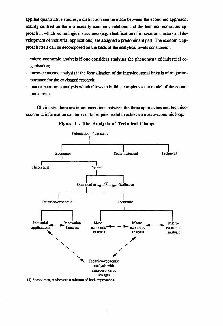
applied quantitative studies, a distinction can be made between the economic approach,

mainly centred on the intrinsically economic relations and the technico-economic ap­

proach in which technological structures (e.g. identification of innovation clusters and de­

velopment of industrial applications) are assigned a predominant part. The economic ap­

proach itself can be decomposed on the basis of the analytical levels considered :

- micro-economic analysis if one considers studying the phenomena of industrial or­

ganisation;

- meso-economic analysis if the formalisation of the inter-industrial links is of major im­

portance for the envisaged research;

- macro-economic analysis which allows to build a complete scale model of the econo­

mic circuit.

Obviously, there are interconnections between the three approaches and technico­

economic information can turn out to be quite useful to achieve a macro-economic loop.

Figure I - The Analysis of Technical Change

Orientation of the study

I I

I Economic Socio-historical

I I

Theoretical

I I Quantitative~OL ..... Qualitative

I I

Technico-economic

n Industrial._ ._!nnovation

applications bunches

'

I Economic

I I Meso-

economic~ analysis

Macro-~ - ..... economic

~ Technico-economic

analysis with macroeconomic

linkages

/ /

analysis

(1) Sometimes, studies are a mixture of both approaches.

11

I Technical

I _...,. Micro-

economic analysis

1.2. Overview of Methods

The literature reports plentiful methods of research evaluation but only a very small

part of them are really in use. This overview of the main methods does not deal with the

technical aspects of methods but with their more prominent characteristics in order to

emphasize their strengths and weaknesses and, hence, show that econometrics, rarely

referred as a research evaluation tool - and when, it is treated with suspicion - is certainly

no less credible than other methods. There is now an extensive literature reviewing and

surveying research evaluation methods to which we refer the interested readerl.

1.2.1. Assessment by Peers, Questionnaires, Interviews

a. Direct Assessment by Peers - This is an evaluation made by one or more

specialists of the same discipline to appreciate in particular the scientific value of the

research [Gibbons and Georghiou (1987)]. The drawbacks of this method are the

following:

- the subjectivity of the experts and of their diagnoses. This can be put down to :

* (intellectual or scientific) fashions which can be found both in the answers and in

the questions and prove difficult to get rid of. The solution to this problem is to re­

peat the assessment operation periodically. (Besides, the fashion bias can be evalua­

ted). However, there still is a risk that the experts may take the political and socio­

political objectives of the moment as forecasts;

* the experts being insufficiently trained to reason in the prospective mode;

* a lack of rigour,

* the fact that the maturation times required by some ideas are not sufficiently taken

into account;

* the desire to conform which impels into self-censorship;

* the experts not being independent, which makes it necessary to have recourse to an

anonymous questionnaire;

* the fact that researchers are involved in the evaluation which entails the risk that

their willingness to participate may be linked to the benefits they can derive from it

That is why some precautions have to be taken regarding the choice of experts,

which is a decisive criterion for the method to be valid. So, for instance, too close

1 Among others, see Saint-Paul and Teniere-Buchot (1974) and Vinck (1991) for a description of techniques and Luukkonen-Gronow (1987), Gibbons and Georghiou (1987) and Danila (1989) for a critical review of methods.

12

cooperative or polemical relations should be avoided, and experts should be chosen

that are as open-minded as possible with regard to their schools of thought and their

orientations.

- The partial character of the forecasts. Using cross-impact matrices somewhat allows to

remedy this problem.

- When the evaluation criteria bear upon the socio-economic impacts, non-scientific

members have to be included into the group of experts (for instance, clients or potential

users of the research, industrialists, economists, public authorities). This working

method, used by the EEC, is what is called assessment modified by peers.

- Assessing the social and economic effects of research activities is a challenge for expert

appraisements because their assessments are based on science-oriented criteria, which

are not appropriate to make an assessment of this kind.

- This method does not provide a sufficiently reliable basis to determine the global eco­

nomic impact of R & D expenditures.

b. Direct Assessment Modified by Peers - This is a direct assessment but whose

object is not only the scientific value of the research. So, other criteria, such as the

economic and social influence are taken into account. This type of evaluation requires

completing the group of experts for it to cover domains in which scientific competence is

not sufficient. Apart from this improvement, the advantages and drawbacks of this

approach are the same as for the preceding method.

c. Questionnaire Method and Interviews - This is a kind of assessment by peers

but more systematic, based on standardized questionnaires. This method allows to work

out quantitative indices provided the questions are phrased so that the answers can be

marked.

This method has the drawbacks of its advantages, i.e. :

- a reduced quantity of information since the prephrased questions limit the number of

possible answers, which can result in trivial information.

- The necessity of making up structured questionnaires in which the questions have to be

independent, accurate and quantifiable. Those who devise them have to combine their

technical expertise with a thorough knowledge of the subject, which requires using

complementary methods.

13

d. Direct-Systematic-Assesstnent-by-Peers Method - It cqnsists in sending a

closed questionnaire to a number of experts. A median opinion with an error margin and

quartiles is deduced from the answers. This result is returned to the specialists who are to

confirm or invalidate their estimates. After a number of iterations, the convergence gets

clearer, the objective being to reduce the interquartile interval while making the median

clearer [Schroeder, (1988)]. This method is often used to make technological forecasts

and select projects. The Delphi method has so far been one of the most used methods.

Among the methods based on consensus, we also find the Ringi method, used by the

Japanese decision-makers, and the Rule of Thumb method, with which managers are to

assess and estimate the risks and advantages of projects [Danila, (1989)].

The indirect-assessment-by-peers method is often used as well. It adds to the direct

assessment by peers a quantitative dimension and rests on the analysis of indicators. Be­

sides, it is a further systematization of the assessment-by-peers method.

The drawbacks of the method are the following :

- the method is not valid for comprehensive domains for it provides partial and incorrect

results.

The results are sensitive to radical changes.

- The Delphi method gives quite a satisfactory answer to the occurrence question, but

quite an unsatisfactory one to those bearing upon relevance (desirability for the enter­

prise or for the users), impact, and feasibility. The Probe and Soon techniques are an

attempt to improve on this method.

All the drawbacks mentioned earlier with regard to direct assessment by peers hold in

this case as well.

1.2.2. Scoring methods

a. Matrix Approaches -~There can be two kinds:

a.l. Analysis Matrices- They are applied for selecting and decision making.

This approach is closer to economic analysis. They help put into shape "research-re­

search" and "research-industry" matrices similar to the input-output tables of interindus­

trial relations per branch or sector.

Several stages can be distinguished, each of them leading to a matrix :

14

- evaluation of the economic impact of the researches on the other researches (research­

research matrix);

- evaluation of the economic impact of the researches on the industrial sectors (research­

industry matrix);

- multiplication of these two matrices, the product of which will give the impact of re­

search decisions on the rise of industries. Let us notice that by reversing this matrix,

one can determine which researches should be chosen to maximise industrial develop­

ment.

The main drawback of this method is that it is difficult, if not impossible, to collect

the data required to make a matrix of the interdependences between researches.

The BIPE (Bureau d'Information et de Prevision Economique), specialized in

technological "filieres", has oriented its researches towards isolating the motor vectors in

order to determine and quantify the consequences of technological innovations on the dif­

ferent industrial branches. It has thus developed channels comparable to relevance trees

whose different levels are the following : different research centres --> innovation --> functional sub-set --> basic technologies --> interested production enterprises. This

method can be supplemented with a preliminary qualitative analysis.

Among other methods, let us mention the Quest method, which is half-way bet­

ween analysis and decision-making matrices as it combines both subjectivity and matrix

calculation through the following stages :

- evaluating how much the technologies have contributed to achieving previously fixed

objectives by means of ordinal scales. Multiplying these scales by the weighted values

·of the missions involved provides a value index of the technologies.

- evaluating, by means of a similar process, how much the various scientific researches

made upstream (fundamental and applied) have contributed to the technologies. Questar

(Quantitative Utility Evaluation Suggesting Targets for the Allocation of Resources)

allows for instance to determine how much the R & D project has contributed to the

commercial value of the product.

An extension of this method which incorporates the notion of budget constraint has

been suggested, the Macro-R & D method. So, the research lump sum can be

determined, and the obtained selection can be j~stified.

a.2. Decision-Making Matrices- This method enables to arrange projects in

order of importance. It is closer to technological evaluation techniques. It is made up of

15

multicriteria appraisal grids (for instance, the Profile method 1 ). The stages of the method

are:

- detennining criteria and sub-criteria;

- marking the projects in function of those criteria;

- evaluating the correlation between the experts' answers with Spearman's formula and

showing off the experts whose answers diverge from the "standard ones".

Its advantages are that it systematizes decision making, rationalizes and simplifies

choosing. In this category let us also mention the Seer method (besides Proftle) and the

Trimatrix method (which combines Macro-Quest and Profile) which considers the socio­

political, technological, and economic viewpoints).

Its drawbacks are that it is subjective, lacks flexibility, and uses a substantial num­

ber of statistical information.

b. Multicriteria Analysis • This method consists in ranking and selecting the

projects according to several criteria weighted against each other. So, it can be used to

select projects under financial constraints.

The different stages of the method are the following :

- listing the criteria;

- formalizing the criteria : so, at each stage, the qualitative goals and the quantified ob-

jectives are inquired about;

- the different criteria are weighted.

Some methods allow to perform tests about the sensitiveness to one criterion or

another, or to iterate the procedure according to how far advanced the project is. This is,

for instance, the case of the Marsan-Electre method whose drawbacks are, on the one

hand, the necessity to have recourse to a specialized coordination and execution group,

and, on the other hand, the subjectivity involved in choosing the criteria and weighting

them. Its application field is mainly sorting out and selecting projects. When the projects

are characterized by a high dependence degree, the Electre-Oreste method proves more

appropriate.

1 The Profile method (Programmed Functional Indices for Laboratory Evaluation) is an example which attempts to sttucture the selection of R & D projects and to help manage them.

16

c. Relevance Trees • This is a combination of the decision theory and of the

operational research techniques. The aim of the method is not so much selecting projects,

but rather emphasizing the links between the different research projects, technology, and

the economy in order to detennine to what extent the project is relevant. The drawbacks

of this method are that it is very empirical, that working out a good tree is not an easy

matter, the fact that it is heavy, and that it is difficult to assign relative quantitative values

to how important it is to carry out those R & D projects. The advantage of this method is

basically that it provides lots of information to those who manage to implement it.l

1.2.3. Systemic Approaches

a. Systemic Analyses· They combine the advanJges of the multicriteria analysis and

of the relevance trees, and are the most advanced form of the methods providing aid to

decision making. The resulting information is very rich.

Regarding this type of analysis, two complementary methods can be mentioned :

1. the factor analysis whose purpose is to identify which elements form a system,

and, hence, select criteria to evaluate arid select research programs;

2. the structural analysis whose aim is to define the schedule and the control of the

research process.

System dynamics, which, among other things, studies the stability of systems,

could, according to some, be regarded as belonging to this category. Yet, because of its

specific characteristics, it has been classified separately.

b. Dynamic Modelling· According to Allen (1986), economics better agrees with a

concept of evolution than with one of equilibrium. Given the complexity and the

permanent evolution of the system in which we are living, innovation creation,

acceptation, diffusion cannot, according to him, be envisaged in purely economic terms

without taking elements into account such as history, culture, social and environmental

structures. Economic decisions as a whole must therefore be made within a broader

framework. Any action will have effects on different elements and feedback

phenomenona will develop as well. That is how a complex chain of actions and reactions

is formed which little fits in with a simple and intuitive assessment. Hence,

1 The methods Pattern (Planning Assistance Through Technical Evaluation of Relevance) and CPE (Centre de Prospective et d'Evaluation) are examples of implementation.

17

understanding technical change can only come from a better knowledge of the problem as

a whole.

The system theory is based on the idea that big aggregates evolve towards a state of

desequilibrium, phenomenon which alters the structures and induces qualitative changes.

Yet, with a view to discussing the concepts of a system, a classification and an aggre­

gation on that basis prove necessary in order to reduce its complexity. Allen also shows

that evolution does not necessarily lead to an optimal behaviour. Enterprises are thought

to be prompted to make new discoveries only because their present production planning

is imperfect. Besides, competition between fmns will lead to pro-active and retro-active

moves on their part in reply to technical and organizational changes. Obviously, this con­

stant evolution advantages individuals or fmns that can easily adapt and understand new

situations.

The advantage of this approach is that the whole process is taken into account.

Although the method may at ftrst seem very interesting because it considers all the aspects

of a system, the practical applications, however, are much less obvious. These works are

along the lines of the analysis of evolution processes [Prygogine and Stengers (1979)]

and of the dynamics of systems [Forrester (1973)]. The evolutionist approach with

regard to technical progress has been developed by Nelson and Winter (1982). Its object

is to identify and formalize the links between the elements which make up a dynamic

system in order to study its stability properties.

1.2.4. Financial Methods

This general name encompasses lots of methods worked out to define and quantify

the social and economic consequences of projects and their financial return as well as

their profitability and net social profit.

a. The Cost Benefit • Cost Effectiveness Analysis • It deals with the study of

the advantages and drawbacks of a project. This method provides, besides the net present

value, an estimate of the impact of the investment made on the annual profit of the com­

panies which have made it. Any modification while the project is under way is taken into

account in the form of sensitivity factors. The method usually consists in calculating the

ratio between the expected profit and the cost. With regard to the economic index, the cal­

culation of the profit includes the probability of obtaining one, and the cost sometimes

includes the capital; the most commonly used financial indices are the NPV (Net Present

18

Value) and the ROI (Return on Investment). The relative perfonnance is evaluated on the

basis of the past industrial research and development expenditure and sales. This measu­

rement, R. Cordero (1990) reminds us, is not that of a profit for it does not include the

resources used by the commercial units. Besides, it does not link the sales to the present

research and development expenses but to those of the past year. In this respect, it is

rather surprising, though that, usually, only the most recent information should be used,

while the maturation times are longer. Let us note as well that "average delays" are usual­

ly worked with; as investments in development usually involve more substantial amounts

of money than those in fundamental research, the average delay in question turns out to

be shorter. To determine the relative force of the "commercializable" outputs, one can

simply use market shares. Other measurements which allow to compare the output to

industrial means, to past outputs or to those of another firm are the number of new pro­

ducts developed in the past few years in the percentage of current sales, the number of I .. I

significant innovations during that period, the innovation output weighted by its impor-

tance as well as the success rate of a new product.

Besides this, there are the methods of return on investment which are suitable for

the selection of projects. A return index has to be determined, i.e. an interest rate so that

the actualized value of the monetary incomings should be equal to the outgoings (in terms

of mathematical expectation). One deduces thus the interest rate by equalizing the .incom­

ing and outgoing flows. H it is higher than the interest rate of the market, the ·project in

question is carried out.

Many methods of maximising the present net value of projects (internal profitability

rate, actualized self-financing) have been proposed in the literature (e.g. Disman, Hess,

Dean-Segupta, Daude methods). The advantage of these methods is that they take

expenses and receipts into account as they occur. Yet, their drawbacks are :

- the substantial number of statistical data required;

- the fact that strategical conditions are ignored;

- the fact that technical constraints are not analyzed;

- the fact that competition is not analyzed;

- evaluation difficulties similar to those encountered with the ratio method.

From a theoretical point of view, according to Gibbons and Georghiou (1987), the

method is valid. Other drawbacks usually mentioned are the cost and the difficulty of

gathering the required information as well as of choosing a realistic actualization rate.

This method does not allow either to clearly determine the external effects of research

works (not taken into account in the prices). Indeed, some effects or factors cannot be

19

measured and evaluated in financial terms. This difficulty mainly arises as far as outputs

are concerned. One can of course consider giving them an arbitrary value, but, in this

case, the method is not more relevant than an~ qualitative evaluation.

This problem affects almost all quantitative methods in so far as they require mak­

ing hypotheses, since some data on the research activities are not available. As for the re­

covering time method, inspired by similar concerns as those previously set out, it con­

sists in taking into account a compensation for the profits expected from research and de­

velopment and its costs, as well as those of production, commercialization, and capital.

Hence, an actualization rate, a success probability as well as the firm's level of experience

in the field have to be determined.

b. The Ratio Method - It deals with the evaluation of the value of the investment

compared to other items. The objective is not only to determine the financial lump sum to

be devoted to R & D investment but also to measure the ex-post profitability of the pro­

granunes. The numerous ratios considered usually establish the link between profit (sav­

ings, incomes, profits, cash flow) and cost ofR & D.

The drawbacks of this method are the following :

- the time-lag between the research and development expenditures and their economic re-

sults is difficult to quantify (the econometric method could help clarify this problem);

- it is not clear how many periods have to be taken into account;

- the results can be quite different depending on the periods considered;

- the result can be extremely hazardous.

The most obvious advantage is the simplicity of the instruments used.

The ratios have been generalized, using a technical or commercial criterion which

evaluates how likely the project is to be successful. These are the score or desirability in­

dexes. The most commonly used indices are the Olsen, Pacifico, Teal, and Texas Instru­

ments ones. This method has its own limits as well, among which :

- subjectivity when determining how likely success is: it is in fact a simple reduction co-

efficient and not a probability;

- the fact that the estimating error is unknown;

- sujectivity in the choice of criteria (simplistic and mechanistic aggregation);

- the traditional financial aspect of the mehod (at the expense of the technical or com-

mercial aspect or of the study of the economic impact as a whole).

20

3)

Besides, the ratio method provides us with purely descriptive information. The

economic impact it describes is only expressed in financial terms and is an evaluation cri­

terion inside the firm or sector only. Neither the impact on the economic variables, nor

the indirect effects, nor the spillover effects, nor the relations between frrms are taken into

account. The ratio for a firm may be very good in spite of an eviction effect on the other

firms, which cancels the positive effect at sectorial level.

The method can prove useful, though, since it provides a valuable analysis tool at

firm level, and could, provided a few modifications are made, be integrated with the

range of management tools for public projects.

c. The Hazard Profiles- It is a process by which projects are selected on the basis of

the investor's aversion to risk. They simultaneously take into a~count the hazards linked

to carrying out a project and the expected profitability.

d. Programming Models - These models maximise, for the whole set of evaluated

projects, the expected gross value in order to distribute the budget optimally between the

different projects selected. Others deal with the selection of R & D projects and the

allocation of manpower.

e. Portfolio Selection Models - Very developed in the financial world, they are

based on the definition of the usefulness of a project and on the expected value of the

same project as well as on estimates regarding occurrence probabilities.

1.2.5. Technological Forecasting Methods

a. Scenario Method - It is both a qualitative and quantitative analysis of heavy trends,

which consists in building coherent and complete scenarios. Compared to the Delphi

method, this method allows to reverse the "innovation-technology" causality chain and

takes social changes into account. It also allows to show how the different research fields

fit into one another. The drawbacks mentioned with regard to expert committees hold

here as well.

b. Cross-Impact Matrices (or interdependence matrices)- After events and/or trends

regarded as important have been identified, they are aimed at emphasizing the

interactions, i.e. the reciprocal influences between them, and at classifying them

21

\

\

according to their degree of influence. This method can be used in forecasting. It is again

an improvement on the Delphi method to make up for the bias resulting from the potential

links between the questions asked. So, it has the advantage of explicitly analyzing the

relations which may exist between the events to be forecast.

This method integrates both the a priori probabilities and the Monte Carlo methods,

and leads to real quantified scenarios. It then consists in transforming the a priori

probabilities into a posteriori probabilities thanks to a simulation of the stochastic type.

One can also measure how sensitive the result is to a modification of the a priori

probabilities. Although it remedies some of the subjectivity, the method does not

altogether ward it off.

c. Morphological Analysis - This method of technological forecasting combines

technological assessment methods and creativity techniques. Its discontinuous character

makes it different from the other methods. Its objective is no longer tracing the evolution

of situations or systems in time or forecasting an event but rather imagining what the as

yet still unknown event will be. With this procedure forecasting verges on inventing. It is

an inductive method.

1.2.6. Quantitative Indicators

a. Science and Technology Indicators - They have been developed for the ex-post

evaluation. Their aim is to evaluate R & D activities and technological change, and to

measure the effectiveness of the national R & D input at macroeconomic level. They rest

upon the theories about invention, innovation, technological change and international

competitiveness, and have recourse to measurements of the R & D investments of

innovations, of patents, of the balance of technological payments, of the technological

intensity of exchanges, and of the productivity growth. They also use bibliometrical

indicators. The indicators worked out are used to determine the direct technical,

economic, social, and environmental consequences at an aggregate level.

Their drawbacks are the following :

- the fact that the indirect effects, which are often noticeably bigger than the direct ones,

are not taken into account;

- the indicators are difficult to interpret;

- statistics may not be available or comparable;

22

- these indicators infer macroeconomic relations while they are based on data which des­

cribe technological change at microeconomic level.

b. Bibliometrics • It allows to construct quantitative indicators of the outputs of

scientific, mainly fundamental, research. It derives useful information from the analysis

of scientific periodicals. At the level of fundamental research this method can be justified

in three ways :

- The results of scientific research are often presented in articles.

- How frequently an article is referred to is a more or less reliable indicator of its quality.

- One gets accurate data about the activities described in the articles.

It is an ex-post method which is less suitable for evaluating the experimental deve­

lopment. The main drawback of this method is that the indicator it provides is a partial

one given the wide range of ways in which results can be diffused (such as oral, personal

communications and memos) and the secret which, for strategic reasons, may surround

some breakthroughs. Besides, there is a time-lag between the moment when results are

obtained, the moment when they are published, and the moment when they are quoted,

which reduces the effectiveness of the bibliometric method.

1.2. 7. Econometric Method

It is the only global method that is available to answer the question regarding how

much R & D contributes to growth and to globally measure the direct and indirect effects

of R & D programmes on the macroeconomic aggregates. Indeed, if the financial methods

seem easy to implement, they do not allow to take the indirect effects into account. Yet,

although the econometric approach seems able to estimate the main impact parameters,

there are many reasons for doubting the value of the results, among which :

- theoretical and methodological problems;

- measuring problems and the availability of statistics;

- is having recourse to the past relevant to analyze the present and make forecasts ? It can

only be a useful tool if production and technical progress keep on evolving as in the

past;

- the aggregation bias;

- some variables are omitted.

23

In a study about the evaluation of the economic effects of the Community's re­

search programmes, Toulemonde ( 1990) stresses that the econometric quantitative me­

thod could be a valid instrument only if the statistical adjustments suppose a causal rela­

tionship but they do not prove it. He adds that reverse causal relationships can be ima­

gined so that the (productivity) performances affect the level of research and development

expenditures by increasing the resources available for all items, including research. This

view seems somewhat severe, though, as it ignores phenomena which are well-known in

econometrics, namely the delay effects, the retroaction phenomena and the analysis of

simultaneous causality. He further rightly adds that the production functions sys­

tematically ignore non-measurable factors (which can have a substantial influence on pro­

Quctivity) such as the technology exchanges between fmns or countries, sociological re­

sistances to change, and the organization of the innovation process. With regard to taking

technology exchanges between firms or countries into account, a study based on the in­

put-output matrices could prove quite useful. As for sociological resistances to change

and the organization of the innovation process, one can consider combining econometric

methods with more subjective methods as well as making use of the firm organization

and management theory.

Case studies can prove useful to study the links existing between research and its

economic and social effects. The drawbacks of the method are that it concentrates on

specific fields, which biases the measurement of global impact, how much such studies

cost and how long they take. Supposing that making such a study has been opted for,

methodology has to be paid special attention to. This approach emphasizes how difficult

it is to economically justify fundamental and strategic research works, which leads to

pass a critical judgement on economic and other quantitative models. In the following

chapters we describe the advantages and drawbacks of these methods.

In a conference held at the EEC in 1982, Davignon insisted on clearly defining the

objectives, clearly evaluating the way in which the objectives are achieved, no matter

which instrument may be chosen to this endl. So, the issue is indeed evaluating the

programme in function of the objective defined at the start. But here is the whole problem

of ex ante defining a specific research objective given the degree of uncertainty linked to

the programme itself.

Three levels of research evaluation can be distinguished, namely :

- the scientific quality of the results;

1 Statement reported by Bob and Viala (1990).

24

- the programme management rules;

- the socio-economic impact

Although the first two points can be dealt with in a fairly adequate way thanks to

the peer review system and to qualitative measurements, it is largely admitted just as the

critical analysis by Bobe and Viala (1990) of ten years' technological evaluation of the

Community's R & D programmes, that those methods are not appropriate to tackle the

economic impact issue. It is from this point of view that an econometric quantitative study

can prove useful. So, the research productivity indicators must be improved and the

objectives of the European Community's research and development programmes must be

quantitatively defined in a more accurate way.

The synthesis presented in table 1.1 clearly shows that both the qualitative and

quantitative approaches are imperfect. Yet, some answer a particular question better than

others. Some quantitative measurements are complex and costly, and none encompasses

all outputs and inputs. Combining them remedies this shortcoming but that only increases

the cost. Besides, some characteristics are "non-quantifiable" even though they are

critically important (consequences on society, on the environment, product quality). That

is why qualitative measurements are often used to palliate problems encountered when

quantitative measuring instruments are used, but, as we have seen, these measurements

are sometimes lacking in objectivity, and prove less appropriate to measure output or eco­

nomic impact

A study by Booz and Allen [Rockwell and Particelli, (1982)] shows that in a

sample of 700 US manufacturing enterprises, 65% use formal measures to evaluate the

performance of new products. Schainblatt (1982), on his part, emphasizes that out of 34

enterprises, 20 use qualitative measures, the others quantitative ones. From an empirical

investigation of the French industry, Danila ( 1985) observes that only 20 % of 80 listed

methods are really used by firms.

The most commonly studied aspects are : the technical output quality and the extent

to which the objective has been attained. As no measurement is perfect, managers use se­

veral of them simultaneously. Besides, as they are not accurate, they use them as flexible

planning or control tools in order to reduce uncertainty. As these measurements are

costly, using them only makes sense if the benefits derived from them make up for the

costs. For instance, when the quantities of resources used are less substantial and there is

uncertainty as to the outputs, which is the case of fundamental research, qualitative me­

thods are preferred. In this case, planning and control will be less emphasized.

25

Conversely, when plenty of resources are used and there is more certainty as to the

outputs, the measurements used are more quantitative and complex and blanning and

control will be laid more emphasis on as well. Quantitative methods, and more

particularly econometric ones, used together with techniques such as the Delphi method,

relevance trees, decision-making analysis, can provide a useful evaluation tool.

Introducing technical change into econometric models through incorporating R & D

expenditures into production functions has so far given rise to much controversy. To

Saint-Paul and Teniere-Buchot (1974), the production function approach results in a sta­

lemate. This statement seems, however, somewhat forced and ungrounded, as recent

works in this field have shown. Indeed, the econometric approach is the only one that

allows an actual interaction between economic variables and the economic impacts of

technological evolutions. Examining the evaluation reports of the European Community's

various programmes shows that the main problem is how to evaluate the impacts on the

economic variables, or, simply, the modifications in the economic performance that are

due to research and development expenditures.

26

Tab

le 1

.1.

Syn

thes

is o

f E

valu

atio

n M

etho

ds -

Rel

evan

ce a

nd D

raw

back

s

Met

hod

Rel

evan

ce

Dra

w bo

cks

Fiel

d of

appl

icat

ion

a.

Ass

essm

ent b

y pe

ers,

que

stio

n--

Scre

ens o

f pro

ject

s an

d re

sear

ch

-Su

bjec

tivity

of e

xper

ts.

-Se

lect

ion

and

tech

nica

l eva

luat

ion.

na

ires a

nd in

terv

iew

s.

orie

ntat

ions

. -

Part

ial f

orec

asts

. -

Tec

hnol

ogic

al f

orec

astin

g.

-L

ack

of in

depe

nden

ce o

f exp

erts

. -

Doe

s no

t allo

w to

mea

sure

the

glob

al

econ

omic

impa

ct.

b.

Mat

rix a

ppro

ache

s :

-Ana

lysi

s m

abic

es.

-R

ich

info

rmat

ion.

-

Dif

ficu

lt, e

ven

impo

ssib

le to

col

lect

-

Eva

luat

ion

of th

e in

dusb

ial i

mpa

ct o

f th

e re

quire

d in

form

atio

n.

R &

D e

xpen

ditu

re.

-Dec

isio

n-m

akin

g m

abic

es

-D

ecis

ion-

mak

ing

proc

ess.

-

Subj

ectiv

ity.

-M

ultic

rite

ria

inte

rpre

tatio

n.

-R

atio

nalis

e an

d si

mpl

ify c

hoic

es.

-L

ack

of fl

exib

ility

. -

The

num

ber o

f sta

tistic

s re

quir

ed is

su

bsta

ntia

l. -M

ultic

rite

ria

anal

ysis

-

Prof

iles

proj

ects

and

R &

D p

lan-

-R

equi

res

cons

titut

ing

a sp

ecia

lized

-

Proj

ect s

elec

tion.

ni

ng.

grou

p.

-Su

bjec

tive

choi

ce o

f cri

teri

a an

d w

eigh

tings

. -R

elev

ance

tree

s -

Prov

ide

lots

of i

nfor

mat

ion.

-

Stro

ngly

em

piri

cal.

-E

mph

asiz

ing

the

links

bet

wee

n th

e -

Arb

ores

cenc

e.

diff

eren

t res

earc

h pr

ojec

ts, t

echn

olog

y -

Subj

ectiv

ity in

the

allo

catio

n o

f an

d th

e ec

onom

y.

auan

titat

ive

valu

es.

c. S

yste

mic

app

roac

hes:

-S

yste

mic

ana

lysi

s.

-C

an b

e us

ed to

impl

emen

t an

eval

ua-

-N

ot re

ally

sui

tabl

e fo

r ev

alua

ting

as

-Se

lect

ion

and

cont

rol.

tion.

su

ch.

-R

& D

str

ateg

ies.

-

App

ropr

iate

to s

elec

t pro

ject

s.

-Dyn

amic

mod

ellin

g.

-T

akes

the

evol

utio

nary

cha

ract

er o

f -

Ver

y di

ffic

ult t

o im

plem

ent.

-A

naly

sis

of th

e ev

olut

ion

of a

sys

-th

e ec

onom

y in

to a

ccou

nt.

tern

and

of i

ts a

dapt

abili

ty.

-In

clud

es s

ocia

l, hi

stor

ical

and

eco

lo-

gica

l stru

ctur

es.

-T

akes

feed

back

phe

nom

ena

into

ac-

coun

t.

N

00

d Fi

nanc

ial m

etho

ds :

-C

ost-b

enef

it I c

ost-e

ffec

tiven

ess

anal

yses

.

-Rat

ios

met

hods

.

-Ris

k pr

ofile

s.

- Pro

gram

min

g m

odel

s.

-Por

tfolio

mod

els.

e.

Tec

hnol

ogic

al fo

reca

stin

g m

etho

ds

-Sce

nario

met

hod.

-Cro

ss-i

mpa

ct m

atric

es.

-Mom

holO

Jric

al a

naly

sis.

f.

Qua

ntita

tive

indi

cato

rs

-Sci

ence

and

tech

nolo

gy in

dica

tors

.

-Bib

liom

etric

s

g.

Eco

nom

etric

s.

-M

easu

re m

arke

tabl

e ou

tput

s an

d co

mm

erci

al re

sour

ces.

-Si

mpl

e in

stru

men

ts.

-A

llow

s to

reve

rse

the

caus

ality

cha

in.

-T

akes

soc

ial t

rans

form

atio

ns in

to a

c-co

unt

-O

verc

ome

the

prob

lem

of i

nter

de-

pend

ence

s bet

wee

n qu

estio

ns.

-D

isco

ntin

uous

cha

ract

er.

-E

asy

mea

sure

men

t. -

Mea

sure

tech

nica

l res

ourc

es.

-B

uild

s up

fund

amen

tal r

esea

rch

indi

-ca

tors

.

-Th

e on

ly g

ener

al q

uant

itativ

e m

etho

d av

aila

ble

for e

valu

atin

g th

e ec

onom

ic

impa

ct o

f R &

D e

xpen

ditu

re.

-D

iffi

cult

to c

olle

ct th

e in

form

atio

n.

-F

inan

cial

eva

luat

ion

of a

pro

ject

. -

Som

e fa

ctor

s ca

nnot

be

mea

sure

d or

fm

anci

ally

ass

esse

d.

-T

he a

ctua

lisat

ion

rate

is d

iffi

cult

to

choo

se.

-D

o no

t allo

w to

take

R &

D e

xter

n-al

ities

into

acc

ount

-

Dif

ficu

lt to

est

imat

e tim

e-la

g be

t--

Mea

sure

men

t of t

he e

x-po

st re

turn

. w

een

rese

arch

and

dev

elop

men

t F

inan

cial

eva

luat

ion.

-

Num

ber o

f per

iods

to ta

ke in

to a

c--

Proj

ect s

elec

tion.

co

unt.

-D

eter

min

ing

the

finan

cial

lum

p su

m

-H

ighl

y va

riabl

e re

sults

. to

inve

st in

R &

D.

-Su

bjec

tivity

in th

e ch

oice

of t

he

succ

ess

prob

abili

ty a

nd o

f crit

eria

. -

Pure

ly f

inan

cial

asp

ects

.

-S

eea.

-

Sele

ctio

n an

d te

chni

cal e

valu

atio

n.

-T

echn

olog

ical

fore

cast

ing.

-Su

bjec

tivity

alw

ays

pres

ent.

-Se

lect

ion

and

tech

nica

l eva

luat

ion.

-

See

a.

-T

echn

olog

ical

fore

cast

ing.

-

Fore

cast

ing.

-Pu

rely

des

crip

tive.

-

Mea

surin

g ho

w e

ffic

ient

the

R &

D

-D

oes

not t

ake

the

indi

rect

eff

ects

into

in

put i

s at

the

mac

ro le

vel.

acco

unt

-M

icro

-mac

ro c

ross

-cut

ting.

-

Not

wel

l sui

ted

for e

valu

atin

g de

ve-

-A

naly

sis

of th

e ev

olut

ion

of a

sys

-lo

pmen

t. te

rn a

nd o

f its

ada

ptab

ility

. -

Par

tial i

ndic

ator

s.

-T

heor

etic

al a

nd m

etho

dolo

gica

l bac

k--

Eva

luat

ion

of th

e im

pact

of R

& D

gr

ound

. ex

pend

iture

upo

n th

e ec

onom

y.

-A

vaila

bilit

y of

stat

istic

al m

ater

ial.

-A

ggre

gatio

n bi

as.

-N

ot w

ell-s

uite

d fo

r for

ecas

ting.

Chapter 2. The Economic Analysis of Technological Change

Before moving on to the analysis of the interdependences between technical pro­

gress and macroeconomic dimensions, i.e. in particular to the evaluation of the impact of

R & D expenditure on the macroeconomic variables (i.e. production, growth, employ­

ment), it is useful to defme basic concepts such as technological change, technical pro­

gress and to see to what extent R & D expenses integrate into a general pattern. Such an

exercise will clarify the subject of the study and will delineate some of the limits of the

present formalization of the links between macroeconomics and R & D.

For a long time, economic theory has had some difficulty in dealing with techno­

logical change. The traditional growth theory emphasized the role of capital accumulation

rather than technological change as the major driving force of economic growth. In this

view, technological change, to a large extent, failed to fit into any formalized theoretical

framework because it essentially followed from the technical system and, therefore,

depended on technical compatibilities. Like manna from heavens, technical change exo­

genously boosted economic growth at a constant growth rate. With the exception of a few

theoretical major contributions, it was essentially on the side of applied economics that

evidence accumulated showing that technological change was really· a major source of

growth and was driven by economic forces. In the last ten years, a radical theoretical

breakthrough has been made with the development of a theory of growth which views

innovation activities as an endogenous process. What is now known as the new growth

theory legitimates, if need be, on the theoretical ground, forty years of forerunner works

on the applied economics of technological change. While important and certainly a fruitful

ferment for future econometric works, this approach is not tackled here because its empi­

rical fallouts remain limited.

Another major contribution to the economic theory of technological change is the

development of the evolutionary theory. More radical than but complementary to the new

growth theory, the evolutionary approach views technological change as the main source

of economic growth and as, at the same time, an interactive, cumulative, institutional and

disequilibrating process. It departs from the neoclassical theory in the sense that

producers adopt a satisficing behavior rather than an optimizing one due to bounded

rationality. Yet, this behavioral approach has not so far prompted on a new generation of

econometric studies.

29

2.1. Technological Change and R & D

To begin with, a difference has to be made between change of techniques and

change of technology. The distinction between these two notions usually proves to be

ambiguous and inaccurate, which is why authors often indifferently use either one or the

other.

The notion of technological change encompasses that of change of techniques. The

technological change concept is thus more comprehensive, more analytical as well.

Somehow it consists in penetrating the whole logic of the technical processes. It also

implies the necessity of taking into account all·the socio-economic structures which ac­

company the change of techniques.

According to Mansfield (1968), technology is the whole set of (technical or mana­

gerial) knowledge which enables to launch new products or processes. Technique differs

from technology in so far as the former is a production method at a given time which is

defined by the equipments and management methods used while the latter encompasses

the whole set of knowledge used in the production. The tenn "technique" can be reserved

for productive equipments and the work organisation they involve. Technology is a more

comprehensive concept which incorporates other functions such as management and

control which are grafted on to the technique. To Stoneman (1983), technical progress is

a process through which economies evolve in time as a function of the produced goods

and of the means to produce them.

Technological change is usually considered to count three stages :

Invention - It is the starting point of a new product, process or system which can

lead to a patent. So, Freeman (1982) defines it as "an idea, a sketch or model for a new

improved device, product process or system. Such inventions may often (not always) be

patented but they do not necessarily lead to technical innovation". It is somehow a

potential innovation 'Or a batch ·of potential innovations. Only when it practically opens on

an innovation does the invention become economically meaningful. So, as Stoneman

(1983) suggests, invention can be regarded either as a given ex-post resource, or as are­

source expected for the innovation process.

To Kennedy and Thirwall(1972), inventing is actually imagining new ways of at­

taining the same objective. Hence, the inventing activity encompasses not only the crea­

tion (thanks to the use of existent and "new" knowledge) of previously non-existent pro-

30

ducts, processes and systems but also an original exploitation of elements thaf have

always existed (such as penicillin, for instance). Funher, one may wonder whether

invention is autonomous or whether it is induced by the economic environment. In this

respect, it seems right to believe that it is a major factor in the economic activity and that it

is, to some extent, subject to the supply and demand forces. So, an invention market is

thought to exist Yet, the researches carried out in this field are mainly directed towards

theoretical microeconomic developments and, so far, have not easily lent themselves to a

macroeconomic globalisation.

Innovation - It is the commercial stage of invention. Schumpeter distinguishes

five main types of innovation :

1. product innovation : this is research and development expenditure aimed at improving on or creating new products;

2. process innovation : this is research and development expenditure directed towards perfecting the methods or obtaining new processes;

3. new markets and marketing methods;

4. legislation changes;

5. innovations with regard to organisation.

Referring again to Freeman (1982), "an innovation, in the economic sense, is

accomplished only with the first commercial transaction involving the new product,

process, system or device although the word is used also to describe the whole process".

Diffusion- It is the process through which innovation spreads out to the market.

The notion of appropriation of the scientific discovery follows from here. Unless one is

in a monopolistic situation, appropriation is never perfect, even if there is a patent or a

licence. The interest of the innovator, who wants to protect his right to exploit the inno­

vation, clashes with the general interest which requires a more intensive and competitive

exploitation of the innovations for these to be able to pass on to the whole economic

structure as effectively as possible. So, it is through the diffusion process that innova­

tions have an impact on the economy as a whole.

Innovation diffusion is not instantaneous over time and unifonn across space. The

timing and the magnitude of the diffusion process depend on the features of the new technologies, the behavior of economic agents, the characteristics of the environment and

the economic incentives. The diffusion process is a learning process which takes place

among users and producers and involves a reallocation of resources in favour of new

31

products and processes. After its introduction upon the market, the innovation can

receive incremental improvements which affect the pace of adoption. Its diffusion is also

often at the source of other successive innovations and leads to imitation. To a large

extent, diffusion is at the core of the process through which technical change boosts up

the economy as a whole.

Frascati's manual [OCDE (1976)] defmes experimental research and development

as a creative work undertaken systematically in order to increase the knowledge stock and

the use of it so as to achieve new applications. Research and development expenditure is

usually classified into three main categories:

Fundamental research which consists in experimental or theoretical works

mainly undertaken in order to acquire further knowledge of the foundations of observable

phenomena and facts, without considering any particular application or utilisation. The

expected result is mainly discovery.

Applied research which, like fundamental research, also consists in

experimental works aimed at acquiring further knowledge but it departs from it in so far

as it is directed towards an objective or towards particular goals. So, it includes research

into applications. The expected result is often invention.

Fundamental and applied researches only have economic implications if they have a

cost or if, in the short or long term, they allow a commercial exploitation.

Development which refers to systematic works based on existent knowledge ob­

tained through research and/or through practical experience, with a view to launching the

manufacture of new materials, products or devices, establishing new processes, systems

or services, or improving those that already exist. The expected result is information and

innovation through investment and experience.

It should, however, be noticed that the separation between the different stages of

technological change and of the R & D process is not as clear-cut as it may look at first

sight. Besides, in spite of the OECD's prescriptions, concepts are used so heteroge­

neously in international statistics that comparisons are rather hazardous.

Another distinction can be made between the research and development expenditure

funded privately or publicly, and between those made by enterprises or by other

organisations (e.g. universities and research institutes). This is a distinction we are

32

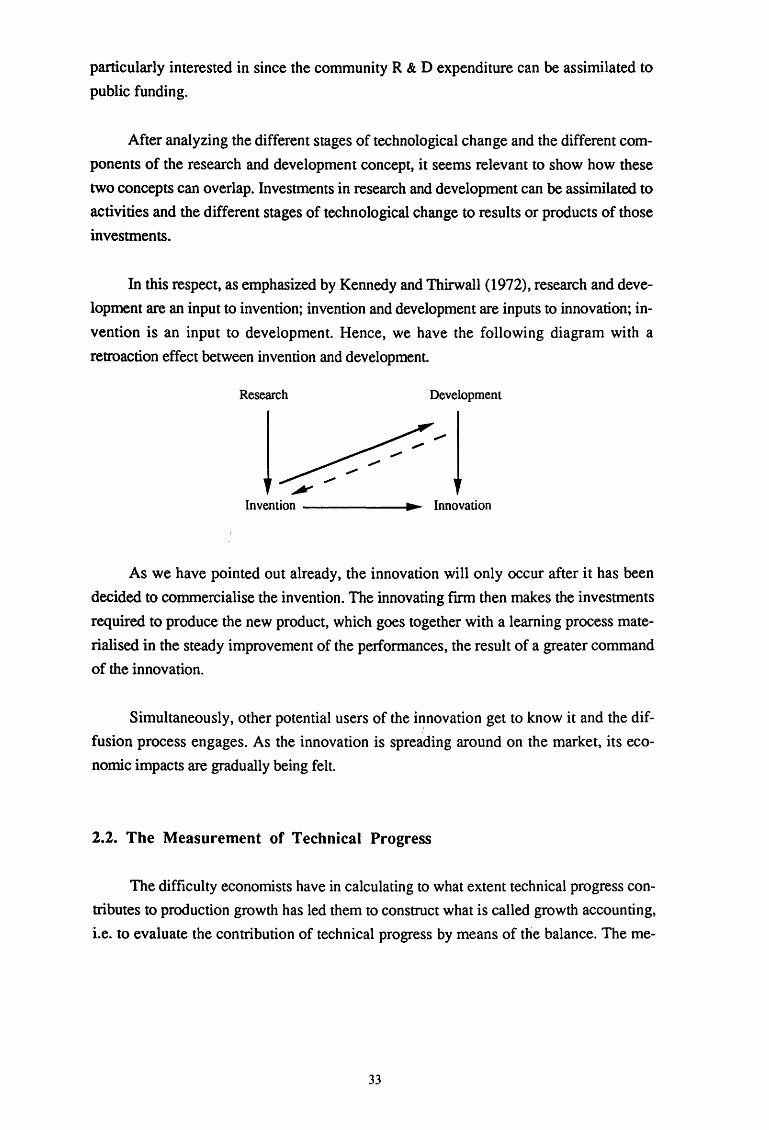
particularly interested in since the community R & D expenditure can be assimilated to

public funding.

After analyzing the different stages of technological change and the different com­

ponents of the research and development concept, it seems relevant to show how these

two concepts can overlap. Investments in research and development can be assimilated to

activities and the different stages of technological change to results or products of those

investments.

In this respect, as emphasized by Kennedy and Thirwall (1972), research and deve­

lopment are an input to invention; invention and development are inputs to innovation; in­

vention is an input to development. Hence, we have the following diagram with a

retroaction effect between invention and development.

Research Development

"""""' Invention ------11..,...~ Innovation

As we have pointed out already, the innovation will only occur after it has been

decided to commercialise the invention. The innovating frrm then makes the investments

required to produce the new product, which goes together with a learning process mate­

rialised in the steady improvement of the performances, the result of a greater command

of the innovation.

Simultaneously, other potential users of the innovation get to know it and the dif­

fusion process engages. As the innovation is spreading around on the market, its eco­

nomic impacts are gradually being felt.

2.2. The Measurement of Technical Progress

The difficulty economists have in calculating to what extent technical progress con­

tributes to production growth has led them to construct what is called growth accounting,

i.e. to evaluate the contribution of technical progress by means of the balance. The me-

33

thod has gone through considerable developments brought about by the identification of

the effects of the intermediary inputs as education, R & D and infrastructure. I

The contribution of technical progress to growth would thus be the part of product­

ivity growth rate that is not explained by the other factors, in other words, the residual

factor, whose measure is nothing but the measure of our ignorance. In fact, ftrst works

gave a residual of more than 80 percent, a challenging measure of our misunderstanding

of the real sources of growth. As Abramovitz (1956) pointed out "the indicated

importance of this element may be taken as some measure of our ignorance about the

causes of economic growth in the United States and some sort of indication of where we

need to concentrate our attention".

To allow an accurate and significant evaluation, this method implies from the outset

two major hypotheses :

1. all the other factors have to be exhaustively taken into account in the relation;

2. the contribution of those factors has to be calculated without any mistake.

Admittedly, meeting these two conditions is difficult.

Because formalising technical progress is difficult, the assumption has been made

that its growth rate was constant so that it has been represented by time. This approach is

not satisfactory in so far as technical progress is not a godsend [Kennedy and Thirwall

(1972)]. It results from actions directed towards creating new processes or products, and

for which substantial financial resources have been engaged. The growth rate of technical

progress is only constant in the process of time in so far as the technological innovations

are constant too.

Hence, to measure technical progress in a production function, it would better be

represented as being the technological innovations actually achieved in the economy. Yet,

as chronological series on innovations are hard to come by (indeed, how can innovations

be accounted since they do not necessarily have the same value?), one will somehow

work one's way up to the innovation so as to obtain indicators capable of representing it.

If one goes about it that way, one has to go back to the invention process since it

leads to innovation. In quantitative models one usually envisages two different ways of

grasping this process :

1 See the works of Maddison (1987), Denison (1984) and Kendrick (1976).

34

- through its inputs - i.e. the investments in research and development or the personnel

allocated to R & D;

- through its output - i.e. the number of patents taken out.

First of all, let us note that while the latter are outputs for invention, they are inputs

for innovation.

In view of the criticism voiced about these measurement instruments, it might be

more useful to regard them as complementary and non-substitutable sources of informa­

tion. Yet, in this case, causality and multicollinearity problems will arise.

The measurement of technical progress in terms of output is subject to much criti­

cism. Indeed :

- the quality of the patents can vary a great deal;

- a patent is not taken out for all inventions;

- the legislations regarding patents can vary a lot from one cmtntry to another and can be

modified regularly;

- patents do not always have a commercial value;

- enterprises have different tendencies to take out patents, which evolve in the course of

time, and differentiated protection strategies for their innovations.

However this may be, as emphasized by the OECD [OCDE (1986)], the data about

them can bel p assess the position of the different economies as technology producers.

Besides, the fact that there are international patent systems and patents taken out by

foreign companies in the national systems already provide indicators as to the place of the

different economies within the process of internatioilal diffusion of the techniques.

In practice, even if a stream aimed at promoting studies based on patent statistics is

developingl, input measures such as R & D expenditure or the personnel allocated toR &

D (as production factor of invention) are more frequently used. This measure is incom­

plete and imperfect as well, though. Indeed, if what is considered is the invention activi­

ty, the research and development expenditures exceed those made for invention since they

cover part of the innovating activity. On the contrary, if what is considered is the innova­

tion activity (and, hence, technical progress), the research and development expenditures

are readily found to cover only part of innovation and technical progress (presumably not

1 Cf., for example, the state-of-the-art written by Griliches (1990).

35

even half of it [Griliches (1979)]). Indeed, isolated inventors and accidental progress

have to be taken into account. In this respect, let us note that R & Dis increasingly a

structured organisational process, which implies that gradually this issue can be

investigated more and more accurately. Besides, it is obvious that there is an important

theoretical shift in moving from technical progress to growth induced by research and

development expenditures since the concepts of improvement of the educational level and

of organisational progress (i.e. infrastructure) are made light of. The technology transfer

should also be taken into account. Its features can be direct investments from abroad, the

purchase of foreign licences and patents or the importation of fixed high technology

capital. Technical progress is therefore not only a function of the nationwide R & D, but

also of the worldwide R & D, of accidental technical progress, of training and of in­

frastructure.

Boyer and Magrange (1989) have listed the various hypotheses made in the litera­

ture about the factors which can determine the innovation potential. The major factors

innovation potential originates from are successively:

-pressure on the profit rate between the innovation dynamism (measured by the

number of patents) and the evolution of profitability [Mensch (1979)] a 1

INNOt = 1 (1tt-i ... ) ~· < 0 t-1

where i is the average time lag

INNO is the innovation

This hypothesis, which was verified in several empirical studies, contrasts with the

Shumpeterian theses which argue that high transaction costs and market power incite

frrms to finance innovative efforts internally depending on how profitable their activities

are.

- growth of the markets corresponding to innovations [Schmookler ( 1966),

Mansfield (1972)]

INNOt = n (Qt, Qt-1 ... )

where Q is the output

a n d"Qt>O

This demand-pull hypothesis originally emphasized by Schmookler is challenged

by the technology-push hypothesis. According to this alternative view, a reverse causality

36

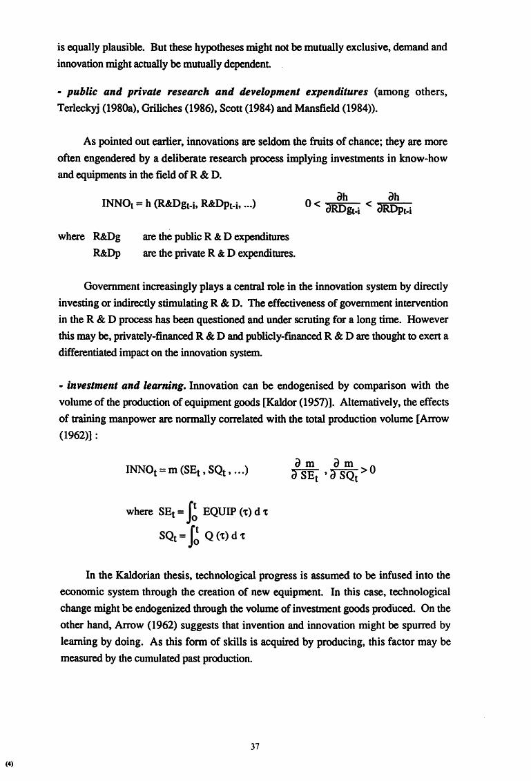
(4)

is equally plausible. But these hypotheses might not be mutually exclusive, demand and

innovation might actually be mutually dependent.

- public and private research and development expenditures (among others,

Terleckyj (1980a), Griliches (1986), Scott (1984) and Mansfield (1984)).

As pointed out earlier, innovations are seldom the fruits of chance; they are more

often engendered by a deliberate research process implying investments in know-how

and equipments in the field of R & D.

INNOt = h (R&Dgt-it R&DPt-it ... )

where R&Dg

R&Dp

are the public R & D expenditures

are the private R & D expenditures.

0 ah ah

< CJRDgt-i < CJRDpt-i

Government increasingly plays a central role in the innovation system by directly

investing or indirectly stimulating R & D. The effectiveness of government intervention

in the R & D process has been questioned and under scruting for a long time. However

this may be, privately-financed R & D and publicly-fmanced R & D are thought to exert a

differentiated impact on the innovation system.

-investment and learning. Innovation can be endogenised by comparison with the

volume of the production of equipment goods [Kaldor (1957) ]. Alternatively, the effects

of training manpower are normally correlated with the total production volume [Arrow

(1962)]:

INN01 = m (SEt, SQt, ... )

where SEt"' J! EQUIP ('t) d t

SQt"' J! Q ('t) d t

In the Kaldorian thesis, technological progress is assumed to be infused into the

economic system through the creation of new equipment. In this case, technological

change might be endogenized through the volume of investment goods produced. On the

other hand, Arrow ( 1962) suggests that invention and innovation might be spurred by

learning by doing. As this form of skills is acquired by producing, this factor may be

measured by the cumulated past production.

37

-infrastructure and Training [Freeman, Clark and Soe~e (1982)]

The development and diffusion of the innovations to the whole productive system

can only be envisaged through a minimum infrastructure conducive to the development of

the innovating action and through the educational system (particularly the technical and

scientific training).

As further factors we can add :

-components of R & D by character of use [Even~on (1984)] :

where B = basic research investment

A = applied research investment

D = development investment

~>~>~>0 a Dt-i a At-i () Bt-i

All the categories of R & D investment are not identically conducive to innovation.

They do not have the same properties while they ultimately improve the knowledge state.

Basic research serves as an essential input in applied research and applied research in

development. Although all three categories of research evolve in close interaction, their

innovation productivity is not the same, and the allocation of research resources will

therefore affect the performance of the innovation system.

- science-push and technological substitutability [Wyatt ( 1986) and Mowery

and Rosenberg (1979)]:

a z a z dTQ<O m>O

where j =activity sector

TQ = total output excluding sector j

SB = technological base

Mowery and Rosenberg (1979) disagree that market demand alone could influence

the innovative process, innovative activity also depends on the underlying science and

38

technology base on which the potential innovator can draw to develop new products and

processes.

This idea was implemented by Wyatt (1986) in a re-examination of Schmookler's

analysis. He also suggests that, if the technological base is sufficiently wide and flexible,

it can be used to create improvements in whatever area is desired and, therefore, there

should be high substitutability on the supply side between invention outputs in different

fields. While Wyatt only considers the interaction between sectoral patents, the

technological base might include technology transfers as a potential source of innovation.

Further, endogenising the volume of research and development expenditures could

be considered as well supposing the results are fairly homogeneous in terms of product­

ivity, demand, employment depending on the countries. In this case, the factors to be

taken into account would be :

- the profit rate :

* favourable effect : funding or access to credit means,

* unfavourable effect : firms innovate only when they are under pressure, under threat

of going bankrupt in a negative conjuncture;

- the estimate of the expected return;

- the past and anticipated growth rythms;

- the taxation methods governing this type of expenditures.

Several remarks can be made about this possibility of endogenising the research

and development expenditures : frrst of all, estimating such a complete equation is not an

easy task; besides, research and development expenditures are concentrated in a small

number of sectors, which can make the merely macroeconomic determinants i~sufficient.

Yet, in a complete model, this type of formalisation would have the advantage of partially

endogenising innovation and of examining what differentiates this formalisation from a

purely exogenous treatment of technical change.

Figure 2.1. summarizes the sequence of interactions between the components of

technological change. This diagram is an extension of a scheme originally suggested by

Rosegger (1980) and emphasizes the main factors which influence the innovation

process. Essentially, technological change is a dynamic process in which stocks of

knowledge accumulated by R & D activities are inputs in the generation of new

techniques and products which displace old techniques and products through adoption by

utility-maximizing economic agents. As technological change is a dynamic process of

39

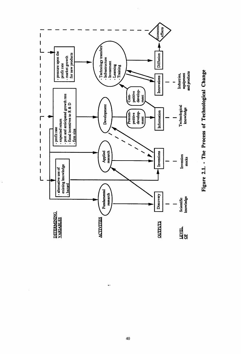
DET

ERM

ININ

G

VA

RIA

BLE

S

AC

TMTI

ES

Otr

fPU

TS

LEV

EL

QE

S

cien

tifi

c kn

owle

dge

r-------.--------r

-al

tern

ativ

e us

e o

f ex

isti

ng k

now

ledg

e -h

azar

d

Inve

ntio

n st

ocks

-pr

ofit

rate

-

expe

cted

retu

rn

-po

st a

nd a

ntic

ipat

ed g

row

th ra

te

-fiS

cal

ince

ntiv

es to

R &

D

-fm

n si

ze T

eclm

olog

ical

kn

owle

dge

' -

pres

sure

upo

n th

e pr

ofit

rat

e -

mar

ket g

row

th

for

new

pro

duct

s

Indu

stri

es,

equi

pmen

t an

d pr

oduc

ts

, ~-A

~~

Fig

ure

2.1.

· T

he P

roce

ss o

f T

echn

olog

ical

Cha

nge

creative destruction, there are feedback effects due to the competitive strengths which

permanently stimulate the search for new techniques and products.

2.3. The Applied Economics of Technical Change

2.3.1. The Exogenous Disembodied Technical Change

The traditional neoclassical specification of technical change considers an aggregate

production function (Q) whose production factors are labor (L) and capital (K) and where

time (t) is a proxy variable representing the state of technology :

Q = F (K, L, t)

From the analytical viewpoint, a less general but more functional form which

considers how technical change can affect the efficiency of production factors is largely

used in the literature. Indeed, it allows to categorize technical change with respect to the

way it alters the relative demands for inputs. Its formulation is :

where At and Bt are measures of efficiency gains resulting from technical

improvements in the utilization of both factors, capital and labor. On the basis of this

equation, a well-known set of results has been obtained about the different types of

technical progress. A worthwhile question is to know if inventions are labour-saving,

capital-saving or neutral. However, there is not a single definition of what is a neutral

technical progress. The three most popular types of neutrality are respectively :

- Hicks-neutrality when the marginal rate of substitution is left unchanged at a constant

capital-labor ratio (At = Bt);

- Harrod-neutrality when the capital-output ratio is left unchanged at a constant rate of

return to capital (At = 1 );

- Solow-neutrality when the labour-output ratio is left unchanged at a constant wage rate

<Bt = 1);

Any deviations from these particular kinds of neutrality are classified as technical

biases as shown in table 2.1. The analysis of the "biasedness" of technical change gives

indications about the directions of the bias, these directions being specific for each factor.

41

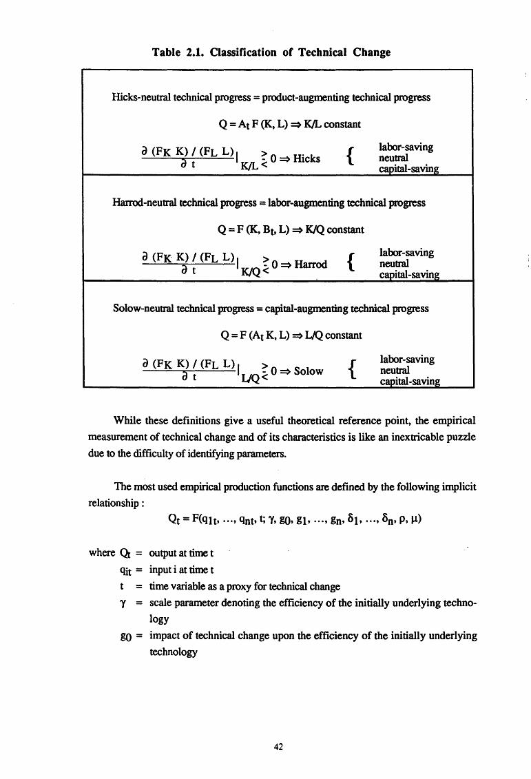
Table 2.1. Classification of Technical Change

Hicks-neutral technical progress = product-augmenting technical progress

Q =At F (K, L) ::> KJL constant

a (FK K) 1 <FL L> 1

> 0 8 . k

d t K/L <: ::> lC S { labor-saving neutral capital-saving

Harrod-neutral technical progress = labor-augmenting technical progress

Q = F (K, Bt, L) ==> KIQ constant

a (FK K)I(FL L)l ?o H od { a t KJQ< ==> arr

labor-saving neutral capital-saving

Solow-neutral technical progress = capital-augmenting technical progress

Q = F (At K, L) ==> UQ constant

a (FK K) 1 <FL L) 1

> 0

s 1 at uQ< ==> o ow {

labor-saving neutral capital-saving

While these definitions give a useful theoretical reference point, the empirical

measurement of technical change and of its characteristics is like an inextricable puzzle

due to the difficulty of identifying parameters.

The most used empirical production functions are defined by the following implicit

relationship :

where Q = output at time t

<lit = input i at time t

t = time variable as a proxy for technical change

'Y = scale parameter denoting the efficiency of the initially underlying techno­

logy

go = impact of technical change upon the efficiency of the initially underlying

technology

42

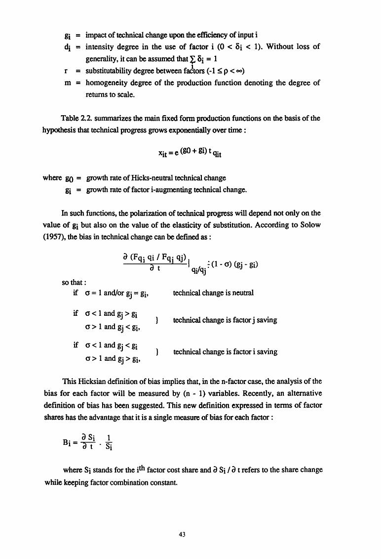
gi = dj =

r = m =

impact of technical change upon the efficiency of input i

intensity degree in the use of factor i (0 < 8i < 1). Without loss of

generality, it can be assumed that l: 8i = 1

substitutability degree between fa&tors ( -1 ::;; p < 00)

homogeneity degree of the production function denoting the degree of

returns to scale.

Table 2.2. summarizes the main fixed form production functions on the basis of the

hypothesis that technical progress grows exponentially over time :

Xit = e (gO + gi) t <lit

where go = growth rate of Hicks-neutral technical change

gi = growth rate of factor i-augmenting technical change.

In such functions, the polarization of technical progress will depend not only on the

value of gi but also on the value of the elasticity of substitution. According to Solow

(1957), the bias in technical change can be defined as :

so that: if a = 1 and/or gj = gj,

if a < 1 and gj > gi

a > 1 and gj < gh

if a < 1 and gj < gi

a > 1 and gj > gj,

technical change is neutral

) technical change is factor j saving

) technical change is factor i saving

This Hicksian definition of bias implies that, in the n-factor case, the analysis of the

bias for each factor will be measured by (n - 1) variables. Recently, an alternative

definition of bias has been suggested. This new definition expressed in terms of factor

shares has the advantage that it is a single measure of bias for each factor :

where Si stands for the ith factor cost share and a Si I a t refers to the share change

while keeping factor combination constant.

43

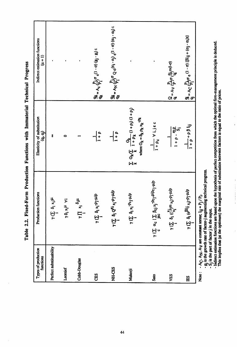
Tab

le 2

.2.

Fix

ed-F

orm

Pro

duct

ion

Fun

ctio

ns w

ith

Imm

ater

ial

Tec

hnic

al P

rogr

ess

Type

s of

pro

duct

ion

Prod

uctio

n fu

nctio

ns

Ela

stic

ity o

f sub

stitu

tion

Indi

rect

est

imat

ion

func

tions

fu

nctio

ns

(qj,

Qj)

(JJ. =

1)

Perf

ect s

ubst

ituab

ility

'Y

<I

8j X

j)J.l

00

-

i

Leo

ntie

f 'Y

8i X

jJ.l

'v' i

0 -

Cob

b-D

ougl

as

yfl

8·

).1

1 x·

1

-1

i

CE

S y [~

3i x

fP]-

J.l/P

_

1_

9i

t = Ac

(!j)

a e(l

-a)

(gj -

gi)

t I

1+

p

Qjt

pi

NH

-CES

y [~

3i (

/i x(

P]-J

.l/P

_1

_

9il= A

(~

)a Q

0.(

£i-E

j) e<

1. a

) (a

j. Q

j) t

I 1

+ p

Q

jt N

Pj

Muk

eJji

'Y [I

, ai

Xi ·P

t] -J

.l/p

I G

k/I

~(1 +

p·)

(1 +

Pj)

-

i k

k 1

+ P

k 1

whe

re G

k =

8Jc P

k xk

·Pk

Sa to

'Y

(I,

ac [~

Pcj X

j·Pc]

-P/P

c)-J

JIP

1 'v'

. .

-1

--

1,j

£ c

-

c JE

C +

Pc

VES

y

(I,

8· ((~

)m x·

)-P]-J

JIP

1 Q

= A

fi>a (

~m(l

-a)

i 1

Xj

1 1

+ p

-I!!

..Q.

Qi

Vp

<l

i S

· 1

IES

y £

I 3j

(eP

iij x

iYPr

J.liP

1

9i =

Ac (~)

a e

(1 -

a) [f

ilij +

(aj

-ai

)t]

--+

pfil

··

i 1

+ p

IJ

q·

P·

~ 1

Not

e:

-Ac

· AN

, Ay a

re c

onst

ant t

enns

; Iij

= Pj

/Pi·

-g

j is

the

grow

th ra

te o

f fac

tor-

j aug

men

ting

tech

nica

l pro

gres

s.

-Sj i

s th

e pa

rt o

f fac

tor j

in th

e ou

puL

-Ind

irect

est

imat

ion

func

tions

are

bas

ed u

pon

the

hypo

thes

is o

f per

fect

com

petit

ion

from

whi

ch th

e op

timal

fm

n-m

anag

emen

t prin

cipl

e is

ded

uced

. Th

is im

plie

s th

at (a

t the

opt

imum

) th

e m

argi

nal r

ate

of su

bstit

utio

n be

twee

n fa

ctor

s is

equ

al to

the

ratio

of p

rices

.

Abramovitz (1956), Solow (1957) and Fabricant (1954) were the first to develop

growth accounting exercices. The fonnal theoretical framework for this type of analysis

was provided by Solow along the line of the neoclassical model. Assuming a neutral

technical change, constant returns to scale and a perfect competitive environment, the following expression :

Q = AtF (K, L)

can be rewritten by taking proportional changes with respect to time:

• • • • Q A K L Q=A+£kK+£IL

where £k and £1 are respectively the output elasticities of capital and labor. Since under neoclassical assumptions these elasticities are equal to the share of factors in

output, we can write :

• • • • Q A K L Q = A + Sk K + Sl L

where Sk and sz are respectively the share of capital in output and the share of labor in

output.

This equation provides the theoretical justification for growth accounting and hence

a method of measuring technical progress. The index value of technical change is nothing

else that the indice of total-factor-productivity improvements :

• • • • A Q K L A = Q - Sk K - Sl L

An alternative way of measuring total factor productivity is the approach developed

by Kendrick ( 1961) who defines the level of total factor productivity as :

A = Q I (Sk K + sz L)

Solow's method. is referred to as the geometric method 1 of measuring technical

progress and Kendrick's method as the arithmetic method. These two methods are easily

generalized to take into account a higher number of production factors and were

I It is also largely called the Divisia index method. In this case, the total productivity index is defined as:

45

extensively used in empirical studies to measure the weight of technical progress in

productivity growth at the aggregate level. All the pioneer works in this field confirmed

the existence of a residual to growth 1.

In a survey article, Maddison (1987) draws up a list of the numerous variables that,

besides technical change, can explain the residual :

- changes in economic structure,

- effects of the process of convergence or "catching-up" of countries,

- volume of foreign trade,

- economies of scale at the national level,

- energy price,

- natural resource discovery,

- use of capacity effects,

- regulation,

- labor hoarding and dishoarding.

Despite efforts to reduce the size of the residual by taking into account additional

factors, an important residual remains. Furthermore, this approach has been criticized by

Nelson (1981) on grounds that the sources of growth are strongly interdependent so that

a growth of one input augments the marginal contribution of others and that if the factors

are highly complementary, it makes little sense to try to divide up the credit for growth.

In other respects, this decomposition method is based on an accounting caveat which

attributes to factor accumulation the causes of economic growth without really identifying

the propelling factors of growth. Finally, few of such studies attempted to directly

measure the contribution of R & D to economic growth. Using a 30 percent rate of return

toR & D, Griliches (1973) and the US Department of Labor (1989) found a contribution

of R & D that amounts to 0.2 percent of the productivity growth for various years over

the period 1960-1987 in the United States. Applying a higher rate of return to R & D,

Kendrick (1981) gives an estimation ranging from 0.60 to 0.85 for various subperiods

covering the years 1948-1978. In the last years, there ~as ~~a large ~ba~e about the ~ • '< ' L J -" • • \-

role of R & D expenditure in the productivity slowdown observed in the 1970's. How

can the apparent paradox of declining productivity growth in a period of accelerated

technological change be explained ? From the various attempts made at explaining this

1 Among the oldest ones, we refer the reader to Solow (1957), Kendrick (1964) and Schmookler (1966) who estimated an average total factor productivity growth rate of about 1% from 1870 to 1950 in the United States. A similar value was found by Fraumeni and Jorgenson (1980) for the period 1948-1976. As reported by Kennedy and Thirwall (1972), other country studies about Finland, Norway and United Kingdom also emphasized the importance of the residual factor. On the other hand, Gaathon (1961.) estimated that the physical capital was the prominent factor in the case of Israel.

46

slowdown, some of which have been summarized by Wolff (1984), it follows that

advances in knowledge cannot be charged with causing the decline in growth.

In the seventies, substantial advances in production theory were made with the

development of new functional forms providing a local approximation to any production

frontier. These functions are quite flexible in approximating arbitrary production

technologies and, as a consequence, are less restrictive in the sense that they include the

specific functional forms. These so-called transcendental production functions exploit the

duality between prices and quantities in the theory of production. The two most

commonly used flexible functional forms are the generalized Leontief and the translog

whose main characteristics are given in table 2.3.

All these functions have been largely used to measure the contribution of

technological change to economic growth. However, in such models the treatment of

technical change is very rudimentary :

- new technologies appear at a constant exponential rate;

- technical change is like a public good;

- technical change identically affects all inputs no matter how old they are;

- technical change is an exogenous phenomenon acting in a totally independent manner

upon the economic system.

This hypothesis of exogenous immaterial technical progress has been discussed in

Kennedy and Thirwall (1972)'s and Nadiri (1970)'s surveys. What is called technical

progress is in fact the combination of several elements, among which :

-the substitution between capital and labour,

- the returns to scale,

- the learning effects,

- the improvements in education and on-the-job training,

·- the changes in resources,

- the improvements in organization,

- the efficiency of production.

As the Cobb-Douglas production function has· been largely used in analyses, it is

useful to have a look at its limits and drawbacks compared with other alternative

specifications. The constraints associated with this function are:

47

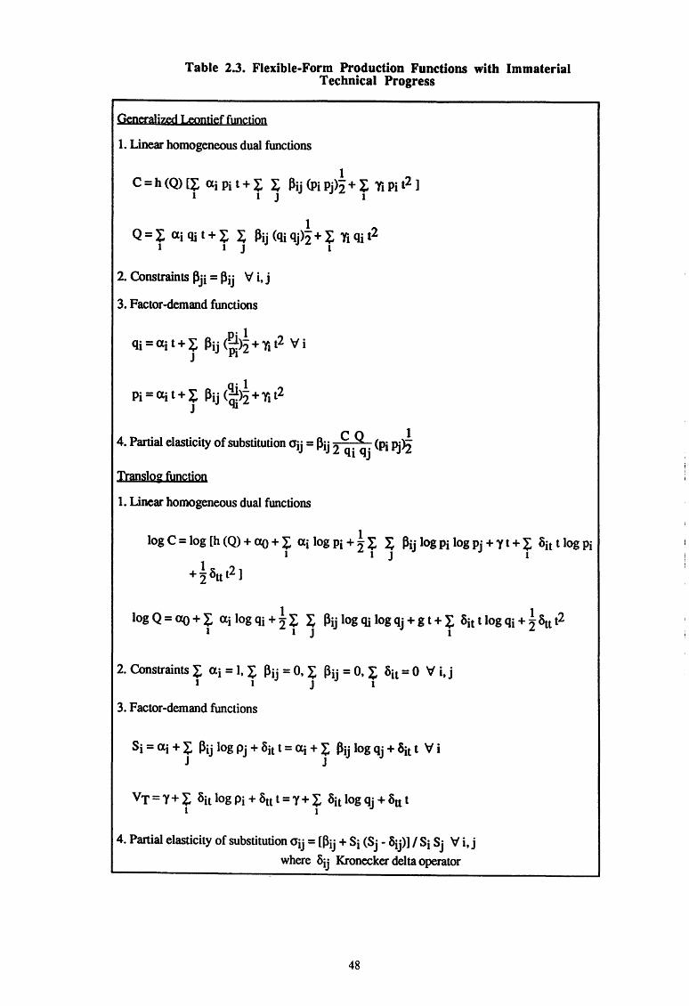
Table 2.3. Flexible-Form Production Functions with Immaterial Technical Progress

Generalized Leontief fliDCtion

1. Linear homogeneous dual functions

2. Constraints Pji = Pij v i, j

3. Factor-demand functions

q· 1 p· = a· t + ~ P· · (!1.)- + 'Yi t2

1 1 r 1J Qi 2 1

4 Partial elasticity of substitution a·· = A.· C Q (Pi p· J • lJ P1J 2 Qi Qj ]r.l

Translog fimction

1. linear homogeneous dual functions

1 log C = log [h (Q) + <X() + ~ ai log Pi + 2l: ~ Pij log Pi log Pj + 'Y t + l: ~it t log Pi

1 1 J 1

+ !~tt t2]

log Q = <X() + ~ ai log Qi + ! ~ ~ Pij log Qi log Qj + g t + ~ ~it t log Qi + ! ~tt t2 1 1 J 1

2. Constraints l: ai = 1, l: Pij = 0, l: Pij = 0, l: ~it = 0 V i, j 1 1 J 1

3. Factor-demand functions

Vr = 'Y + ~ ~it log Pi + au t = 'Y + ~ ~it log Qj + ~tt t 1 1

4. Partial elasticity of substitution <Jij = [Pij + Si (Sj - ~ij)] I Si Sj Vi, j

where aij Kronecker delta operator

48

- neutral technical progress,

- elasticity of substitution equal to unity,

-constant returns to scale,

- disembodied technical progress.

Neutral technical progress- According to Salter (1966), it should be a reasonable

hypothesis. Yet, David and van de Klundert ( 1965) gave clues that technical progress

might not be neutral. More striking is the impossibility theorem due to Diamond,

McFadden and Rodriguez (1978) demonstrating that it is not possible to identify the

nature of technical change without a priori infonnation about the production function. As

pointed out by Kennedy and Thirwall ( 1972), "while very considerable econometric

ingenuity has been used in order to distinguish bias in technical progress from factor

substitution, it remains doubtful whether the basic identification problem has been

entirely overcome. Even if it is possible to identify parameters for the "degree of bias"

and for the "elasticity of substitution" it is not clear that these parameters will necessarily

correspond to those which from an analytical point of view one would ideally want to

obtain".

Constant elasticity of substitution - An elasticity of substitution different from unity

can induce a bias in the estimate of technical change if capital and labor grow at different

rates. If !:1 K > A L and a < 1, there will be an over-estimate of the contribution of capital

to growth and an under-estimate of that of technical progress. The smaller the elasticity of

substitution, the more difficult it is 'to achieve increased output simply by increasing one

factor because diminishing returns set in strongly [Kennedy and Thirwall (1972)]. There

were several attempts to remove the restrictive features of both Cobb-Douglas and CES

production functions. This led to the development of the variable ·elasticity of substitution

production function (VES) [Diwan (1970), Tsang and Yeung (1976)], of the multifactor

generalized function [Muketji (1963)], of the nested-CES function [Sato (1967)] and of

the "induced"-CES function [Yeung and Roe (1978)]. In order to isolate the effect of

technical change from the scale effect, Sato ( 1977) has suggested a new type of

functions, the non-homothetic CES production functions. But all these production

functions only bring punctual improvements which impose stringent constraints on

production patterns (among which, separability, homotheticity and substitutability). The

flexible functional-form production functions which are able to approximate theoretically

consistent production functions satisfactorily were a radical theoretical breakthrough. In

essence, they allow interaction terms in the independent variables and represent second­

order approximation to any arbitrary function. The best known parametric forms are the

generalized Leontieffunctional form originated by Diewert (1971) and the transcendental

49

logarithmic functional form introduced by Christensen, Jorgenson and Lau (1973). They

overcome the limitations of the fixed functional forms by using the duality relation

between cost minimisation behavior and profit maximisation behavior to characterize the

production function by means of demand and supply functions based on prices without

imposing arbitrary constraints on production patterns. In other words, it allows to test

the validity of some restrictions such as separability, homotheticity, substitutability and

biasness of technical change 1. Yet, White ( 1980) rightly recalls that such functions have

their own limitations. They are only local approximation functions of any production

function and, as such, can induce erroneous intetpretations due to the inherent restrictions

in these functions 2.

Constant return to scale - If there are economies of scale and if the underlying

production function is homothetic, the effect of neutral technical change and the effects of

economies of scale cannot be detected empirically 3. H the linear homotheticity constraint

is imposed when there are real economies of scale, the growth rate of technical change

may be overestimated. Furthermore, a part of the economies of scale can be a result of

technical change, and from this standpoint, it is very difficult to disentangle economies of

scale due to technical progress from economies of scale resulting from the growth of

inputs. Finally, if the returns to scale are not constant, there is no reasons for thinking

that the production function is not of the Cobb-Doublas type [Griliches and Ringstad

(1971)].

Disembodied technical progress- The disembodiment hypothesis considers that

technological change affects all production factors in use identically, whatever their ages.

On the other hand, if technical change implies incremental improvements which make

new inputs more efficient than the old ones, it will be characterized by the implementation

of a more efficient production process for each generation of inputs.

Although the Cobb-Douglas function has its own limits, it is empirically very

useful indeed. The choice of other specifications is largely motivated by the objectives

pursued. As pointed out by Griliches (1979), the choice of a functional form is not very

important unless we are interested in the specific interaction of variables. Furthermore,

empirical studies seem to show that the complexity of the formulation rarely improves the

1 For a survey, see Jorgenson (1986). 2 According to Wales (1977), they are not necessarily representative of a cost minimisation-profit

maximisation behavior applying to the full sample. Furthermore, Anderson (1979) challenges the usefulness of these parametric forms for forecasting purposes. _

3 See the well-known Solow-Stigler controversy [Solow (1961), Stigler (1961)].

50

estimates significantly and that the form of the production function is of secondary

significance [Nadiri ( 1970)].

Yet, it must be kept in mind that such a function is only a first-order approximation

to any arbitrary function which imposes strong restrictions on the substitution

possibilities and consequently, is not adapted for the analysis of interaction phenomena.

It is now well-accepted that the criteria that must guide the selection of functional form are

[Lau (1986)] :

- the theoretical consistency : the functional form should heed the restrictions im­

posed by theory;

-the domain of applicability: the extent to which the functional form may be ex­

pected to perform satisfactorily should be well-known and satisfy the theoretical

requirements;

- the flexibility : the functional form should be able to satisfy the requirements of

the analysis;

- the computational facility : the choice of the functional form will be largely condi­

tioned by the following properties : linearity in parameters, explicit representabili­

ty, uniformity and parsimony;

- the factual conformity : the functional form should be consistent with known em­

pirical facts.

As, in practice, it is not possible to satisfy all these criteria simultaneously, some

trade-offs have to be made. According to Lau, the only area in which compromises may

be made is the domain of applicability.

2.3.2. The Exogenous Embodied Technical Change

Models with embodied technical change rest upon a distinction between the

different generations of investment intervening in the measure of capital stock. This way

of looking at technical progress gives a more realistic view of the role of capital in the

growth process. The idea underlying such an approach can be summarized as follows : if

technological knowledge can only be embodied in new capital goods, the more recent

51

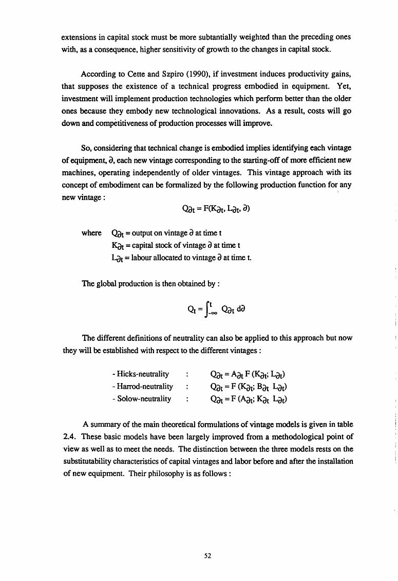
extensions in capital stock must be more subtantially weighted than the preceding ones

with, as a consequence, higher sensitivity of growth to the changes in capital stock.

According to Cette and Szpiro ( 1990), if investment induces productivity gains,

that supposes the existence of a technical progress embodied in equipment. Yet,

investment will implement production technologies which perform better than the older

ones because they embody new technological innovations. As a result, costs will go

down and competitiveness of production processes will improve.

So, considering that technical change is embodied implies identifying each vintage

of equipment, iJ, each new vintage corresponding to the starting-off of more efficient new

machines, operating independently of older vintages. This vintage approach with its

concept of embodiment can be formalized by the following production function for any

new vintage :

where Qat = output on vintage iJ at time t

Kat = capital stock of vintage iJ at time t

LiJt = labour allocated to vintage iJ at time t.

The global production is then obtained by :

)

The different definitions of neutrality can also be applied to this approach but now

they will be established with respect to the different vintages :

-Hicks-neutrality

- Harrod-neutrality

- Solow-neutrality

Oat = AiJt F <Kat; Lot)

Oat = F <Kat; BiJt LiJt)

Oat = F (Aat; KiJt Lat)

A summary of the main theoretical formulations of vintage models is given in table

2.4. These basic models have been largely improved from a methodological point of

view as well as to meet the needs. The distinction between the three models rests on the

substitutability characteristics of capital vintages and labor before and after the installation

of new equipment. Their philosophy is as follows :

52

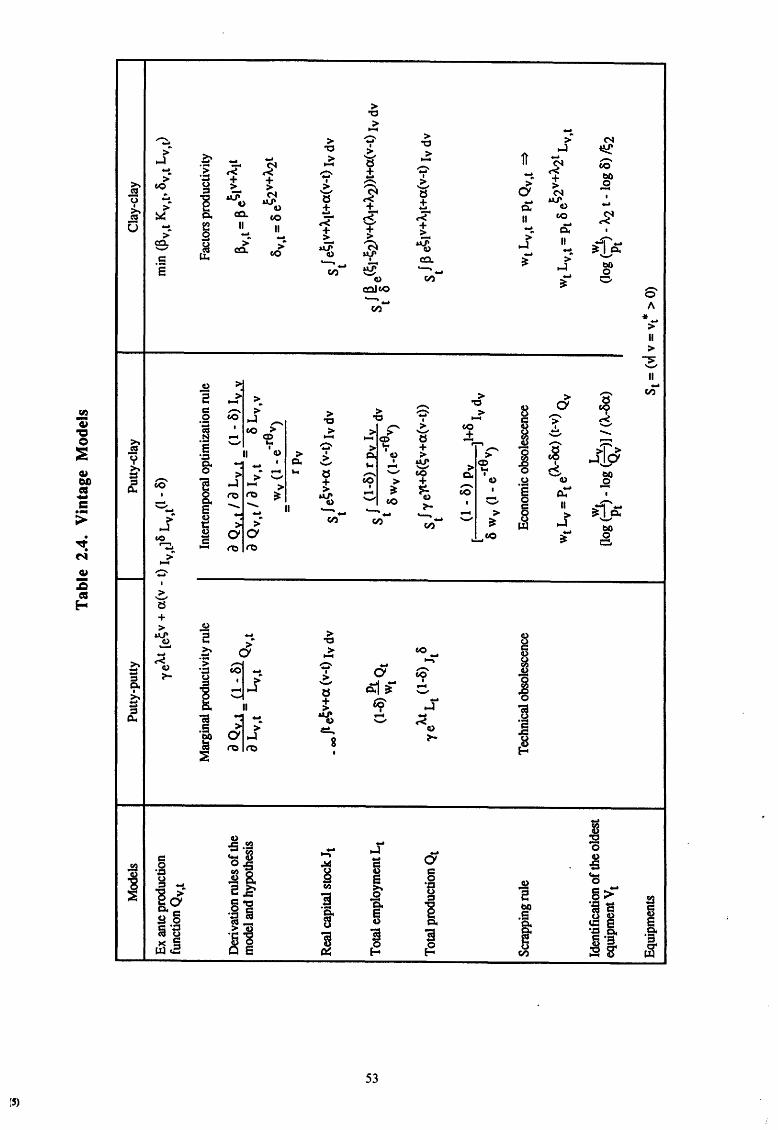
Mod

els

Ex a

nte

prod

uctio

n fu

nctio

n Q

v ,t

Der

ivat

ion

rule

s of

the

mod

el a

nd h

ypot

hesi

s

Rea

l cap

ital s

tock

lt

Tot

al e

mpl

oym

ent L

t

Tot

al p

rodu

ctio

n Q

t

Scra

ppin

g ru

le

Iden

tific

atio

n of

the

olde

st

equi

pmen

t V t

Equ

ipm

ents

Tab

le 2

.4.

Vin

tage

Mod

els

Putty

-put

ty

Putty

-cla

y

yeA

.t [e

~v +

a(v

-t)

I tlo

L

t(l-

a)

v,

v,

Mar

gina

l pro

duct

ivity

rule

_ 0

0 ft

e;v

+a

(v-t)

Iv

dv

(1-a

).&

.Q

Wt

t

A.t L

(1-

a) 1

a y

e

t t

Tec

hnic

al o

bsol

esce

nce

Inte

nem

pora

l opt

imiz

atio

n ru

le

a Qv.

t I a

Lv.t

_ (

1-

a) I

y.y

a Q v

, t 1

a I v

, t -

a L

v, v

-re

Wv

(1-

e V

) =

s I e;

v+

a (v

-t)

Iv d

v t

S I

(1-a

) rp

v I

v dv

t

a W

v (1

-e·r

8v)

S I 'Y

e'Yt+a(~v+a(v-t))

t

[ (1

-a)

Pv

]I+a

I

d -re

v

v 8

Wv

(1-

e V

)

Eco

nom

ic o

bsol

esce

nce

T

_ p

(A.-&

x) (

t-v)

Q

Wt-

v-

te

v

[log (~

) -lo

g (L

yQ )l

1 (A

.-oo)

Pt

v

Cla

y-cl

ay

Fact

ors

prod

uctiv

ity

S I e

~lv+A.tt+a(v-t)

Iv d

v t

S J ~

e~Iv+A.tt+a(v-t)

Iv d

v t

Wt L

v,t =

Pt Q

v,t

=>

Wt

(log

(---

)-A.

2 t -

log

a)

/E;2

Pt

VI ~

Def

initi

on o

f sym

bols

-T

he p

utty

-put

ty a

nd p

utty

-cla

y m

odel

s ar

e ba

sed

upon

an

assu

mpt

ion

of a

Cob

b-D

ougl

as te

chno

logy

, of c

onst

ant g

row

th r

ate

of te

chni

cal

prog

ress

, con

stan

t dep

reci

atio

n an

d co

nsta

nt re

turn

s to

sca

le.

-W

t =

nom

inal

wag

e at

tim

e l

-Pt

=

ou

tput

pri

ce.

-~

=

embo

died

tech

nica

l pro

gres

s.

-a

-A.

-1t

-St

-9

v,t

-Pv

= d

epre

ciat

ion

rate

.

= g

row

th ra

te o

f im

mat

eria

l tec

hnic

al p

rogr

ess.

= re

al c

apita

l sto

ck.

= e

quip

men

t set

use

d at

tim

e t.

= ex

pect

ed li

fe ti

me

of th

e in

vest

men

t.

= in

vest

men

tcos

t

-Pv

,h 'Y

v ,t =

resp

ectiv

ely

capi

tal a

nd la

bor p

rodu

ctiv

ities

for

an e

quip

men

t of v

inta

ge v

at t

ime

t.

-V

t =

the

olde

st e

quip

men

t yet

ope

ratio

nal.

-Putty-putty vintage model : substitution possibilities between capital and labor

exist both ex ante and ex post. Although the equipment of a vintage is fixed after the

installation, the entrepreneur can always allocate labor to this equipment according to the

rule of equalization of the real labor cost rate to its marginal product. The least realistic

characteristic of this model is certainly the hypothesis of ex post substitutability between

factors. Furthermore, in this model, capital vintages are only scrapped because of

technical obsolescence.

- Putty-clay vintage model : substitution possibilities only exist before the installa­

tion of the new vintage, when the equip~ent has been installed, labor requirements for

this vintage are definitively fiXed for the whole lifetime of the vintage. The choice of the

appropriate capital-labor ratio is made on the basis of the maximization of the expected

profits yielded by the equipment during its planned lifetime. A capital vintage will remain

in operation as long as its expected quasi-rent is positive.

- Clay-clay vintage model : substitution possibilities are excluded both before and

after the installation of the new capital vintage. The equipment of each generation is

characterized by a fixed capital-labor ratio that the entrepreneur cannot alter. Given the

labor productivity for each capital vintage, capital vintages whose real labor cost rates are

not compensated by their productivity will be scrapped. Consequently, the scrapping of

old equipment is ruled by both technical and economic obsolescences.

Among the numerous specifications of vintage models reported in the literature,

two very simple models have been suggested by Nelson (1964) and Solow (1959). The

first one is nothing else but a putty-putty Cobb-Douglas production function with a

Solow-neutral exogenous embodied technical change :

where It is the number of machines weighted by their quality (the new machines

having a more important weight) t

Pt is the disembodied technical change which does not take into account the

quality improvements of capital.

If technical development allows an increase in the quality of new machines of 100 AK% per year, one can write :

55

where Kat is the gross amount of capital of vintage a which is still in use at time t.

This equation shows that the growth of the effective capital stock is a function of 0

the growth of the actual capital stock, Kt, the average rate of its improvement, AK and the

effect of changes in its average age, which is itself a function of changes in the rate of

investment. Consequently, the approximated form to be estimated can be written :

0 0 0 0

(4 = Pt +a 4 + (1 -a) K + (1 - a) AK- (1 -a) AKA a

-where a is the average age of capital

A a is the change in the average age of capital and is assumed to be a

rough measure of the change in the gap between the average level

of technology and the best practice technology AK is the net growth per year of the average quality of capital.

In fact vintage models are almost exclusively physical capital vintage models which

ignore the improvements of labor in the use of the production potential. Why should

technical progress be exclusively embodied in physical capital and not in labor ?

Therefore, if the heterogeneity of capital stock in taken into account by the embodiment

hypothesis, the assumption of labor homogeneity certainly plays an important role in the

underestimation of the relationship between technical progress and labor growth. Labor

is not more malleable than physical capital. Not only does each physical capital vintage

generate a demand for some specific employment but increasingly, the ou.tput itself is

directly influenced by the level of labor qualification. Consequently, technological

progress will not happen if it is not materialized within physical capital and human

capital. So far, the vintage model approach has focussed the attention on the importance

of qualitative changes in the stock of physical capital in explaining how technological

change operates but it has largely neglected the real role of human capital vintages on

productivity growth.

An extended version of the Nelson-Solow model integrating quality improvements

in labour has been realized by Kennedy and Thirwall (1972) who suggest to rewrite their

equation as :

56

where Z represents the quality improvements in labour.

By analogy with the equation only including physical capital improvements, the

function adjusted for the change in both the quality of capital and that of labour may be

approximated by :

0 0 0 0

Qa: = P" +a L + (1 - a) K +a AL- (1 - a) AK- a ALAe

is the average rate per year of quality improvement in labour

A e is the change in the average age of labour.

It is interesting to observe that improvements in, both, physical and human capital

increase the output while an increase in the average age of these two categories of factor

has a negative impact on the output. However, there is an interaction between the rate of

improvements in factors and the average age of factors : the higher the rate of quality

improvements in factors, the faster the rate of obsolescence of factors will be and,

consequently, the lower the average age of factors will be. Otherwise, improvements in

labour quality will increase the efficiency of physical capital and the implementation of

new physical capital vintages will not be neutral with regard to the structure of

qualification required. Besides, a large part of improvements in labour quality is a result

of education which is intrinsically linked to technological progress. By stressing only the

role of generations of physical capital stock in the implementation of technical progress,

the present vintage models adopt a reductionist view of technological change.

Some authors are, skeptical about the ability of vintage models to capture

embodiment effects. So, Fellner (1970) argues that "all progress is necessarily

disembodied in the sense that new ideas must always be put into effect with reliance on

the initially given resources. This is an essential constraint under which all economies

operate. Improved production with the initially given resources then leads to more and

better capital goods ... and it yields more and better consumer goods. But all this

represents forward, not backward embodiment". Besides, he asks the following

fundamental question : " Why should the possibilities with a period's capital goods - a

given vintage - become exhausted during a specific period for which a specific level of

technological knowledge is defined?". Denison (1984) also sets out that "the gain in the

average quality of the capital stock that vintage models imagine to be derived from

57 .

additional new investment is not realized because the change in average age automatically

is largely offset by a reduction in the average amount of quality improvement

incorporated in new capital".

2.3.3. The Induced Technical Change

Models of induced technical change suggest that factor prices, goods prices and

market expansion are sources of technical change. This inducement hypothesis implies

that technical change is endogenous to the economic system and is a result of the interplay

of economic forces. Hence, the rate and direction of technical change would be

determined essentially by economic variables. According to Binswanger (1978) the term

induced innovation can be used "for all theories that are concerned with explaining rate

and biais of technical change as endogenous to the economic system".

Yet, at the basis of the inducement hypothesis, there is not necessarily a direct

functional relationship but the idea that changes in factor prices induce biases which save

the more expensive factor. Nevertheless, in some models, the biases of technical change

are endognized and depend on relative factors. This theory is very controversial.

According to Salter (1966), it must be rejected because "the enterpreneur is interested in

reducing costs in total, not particular costs such as labor costs or capital costs ... There is

no reason to assume that attention should be concentrated on labor-saving techniques,

unless, because of some inherent characteristic of technology, labor-saving knowledge is

easier to acquire than capital-saving knowledge". Nordhaus (1973) also shows himself

skeptical about this theory because it lacks a microeconomic background and he considers

that it must be at best considered to be a special case of how technical change takes place.

From the standpoint of the theoretical background of this model, Ahmad (1966) has

developed a model of price-induced technical change. He uses the concept of innovation

possibility curve which is nothing else than the envelope of all isoquants of the potential

inno~tions :which the .. producer may develop. Hence, each ·potential innovatio·n is

characterized by an isoquant whose elasticity of substitution is relatively small and

requires the use of a given quantity of labor and capital. He works by analogy with the

production theory to show that if the shift of the innovation possibility curve is neutral

over time, factor price movements will induce biased technical change.

The most direct test of this theory was run by Yeung and Roe (1978) in an analysis

of the development of Japanese agriculture from 1880 to 1940. They formulate a factor-

58

augmenting CES production function 1 in which the inputs are land and labor. As they

rightly point out about the classical CES production function, " because the source of

innovation is not specified, we cannot know whether a given technical change is induced

or autonomous". They, therefore, postulate that "the innovation is induced by relative

input price changes that reflect changes in relative input scarcities". In their production

functions, the factor-augmenting terms are a function of time and of ther relative factor

prices. Their estimates suggest that, during that period, technical change was biased in

the direction of saving labor and using land despite the fact that the price of labor declined

compared to the price of land. These results do not prove consistent with the Hicks­

Ahmad model of induced innovation.

Contrary to this direct approach, the measure of the bias of technical change is often

obtained as a residual from the estimation of a production function. Alternatively, time is

introduced into the production function to represent the level of technology. This

variable, specifically assigned to each input, measures the bias of productivity growth,

i.e. its coefficient indicates the effect of change in technology on the use of the concerned

input. This approach was adopted by Jorgenson (1984) in his analysis of the effect of

technological change on the US economy for the period 1958-1979. His production

model includes five inputs: capital, labor, electricity, non electrical energy and materials.

His analysis of 35 industrial sectors shows that the pattern of bias of technical change that

occurs most frequently is capital-using, labor-using, electricity-using, nonelectrical

energy-using and materials-saving technical change. Technical change proves to be

labor-saving for only 9 of the 35 industries and materials-saving for 27 industries. For

all other inputs, technical change is predominantly input-using.

These two illustrative studies provide evidence against the hypothesis of a labor­

saving technical change as suggested by models of induced innovation. If there is some

plausibility in the inducement theory, it is only an explanatory element of the innovation

dynamic which underlies technical change. This approach may certainly partly shed light

on some technological bias in the development of process innovation but it is not well­

suited to deal with product innovation. Hence, it may explain the development of energy­

saving technologies after the oil shocks but it cannot explain why countries with low

labor costs invest in capital-intensive techniques.

1 This production function is reproduced in table 2.1.

59

2.3.4. The Endogenous Technical Change

To some extent, the preceding approach already assumes that technical change is

endogenous to the economic process. Yet, it remains silent about the process according

to which the innovation production shifts over time depending on the resources allocated

to the search for new and improved techniques and products. The main characteristic of

the innovation production is to create new knowledge which increases stocks of basic and

applied knowledge. The latter are themselves inputs in the generation of production

processes.

These stocks of basic and applied knowledge do not accumulate exogenously to the

economic system. The accumulation process of knowledge is ruled by economic forces

and conditioned by technical contingencies. As we have seen, the most widespread

conception is based upon the postulate that technical change belongs to an autonomous

sphere with its own rationality and advancing independently of the social· and economic

environment If we have a look at this thesis, a contradiction immediately appears when

one looks into the problem of the effectiveness of a new technical system. Indeed, one

realizes that this apparaisal can only be made in economic tenns, the price system playing

the role of comparison unit. Moreover, technological innovation costs money, requires

material supports and, therefore, consumes resources that could otherwise be used for

other purposes. Consequently, technical change is endogenous, it is directed within the

economic system in accordance with the principle that economic agents behave rationally.

Technical change is the outcome of investment in knowledge, i.e. R & D

expenditures. These investments are a main source of improvements in the efficiency of

production structures, i.e. a main source of productivity growth. To measure the impact

of the stock of knowledge on productivity growth, it is treated as a production factor and

is introduced in production functions besides other traditional inputs. Hence, the

production function approach to the study of the relationship between knowledge

accumulation and productivity gains proves to be a logical way of proceeding. A major

conceptual issue is what is really the stock of knowledge ? The process of knowledge

accumulation may take several different forms including organized research, non­

organized research, education and on-the-job training. Another major issue is the

measurement problem. The stock of knowledg~ as a whole cannot be calculated

accurately, it can only be approximately valued through research activities. The two main

candidate variables are patenting activities, as output measure of the knowledge

production process, and R & D investment as input measure of the innovation process.

Yet, both measures have their advantages and drawbacks. Not all innovations are

60

patented and they are not all equally valuable. Besides patent regulations are not time

invariant and are difficult to compare at international level. Regarding R & D investment,

besides the fact that it is only an input measure there are the problems of gestation lag, of

effectiveness and efficiency. Not all new prices of knowledge are exclusively the results

of organized research. Despite the shortcomings of patent and R & D data, they are

extensively used as a measure of the stock of knowledge. From a production function

viewpoint, the use of R & D expenditures has the advantage of reflection both imitation

and innovation activity while patenting activity only reflects the innovation process.

Although there is a large agreement on the use of R & D data to study the

relationship between technological knowledge and productivity, this input factor in

production functions has some characteristics on its own which distinguish it from other

inputs. Contrary to other forms of capital accumulation, it is not subject to physical

obsolescence. Yet, as "its earning capacity erodes over time, both because better

products and processes become available and because its own knowledge begins to lose

its specificity" it is thought to be faced with a high rate of obsolescence [Griliches

(1979)]. In contradiction with that, it may be argued that R & D does not depreciate at all

as a source of productivity. Another characteristic is the substantial uncertainty that R &

D investment materializes by the creation or the improvement of new or existing products

and processes. As already mentioned, there is also a gestation lag in R & D investment.

A last prominent characteristic is that it is subject to large external economies. Not­

withstanding these difficulties, large efforts have been devoted to measure the impact of

R & D investment on productivity.

At most, this approach must be considered as a first step towards the endogeniza­

tion of technological change. A further step is to explain how economic mechanisms

affect R & D investment behavior to really endogenize technological change in economic

analysis. Hence, R & D investment must be viewed as constrained by the profit maxi­

misation criterion just like other investments. Profit opportunities for R & D investment

are directed by market demand, factor prices and competitive strengths. There is a long­

standing research tradition stressing the role of supply-side factors, market structure and

technological opportunity on R & D along the lines initially traced by Schumpeter. This

industrial organization approach has been extensively reviewed by Cohen and Levin

( 1988). Another approach, which is more in the line of the macroeconomic thought,

emphasizes the role of the demand side factors. The underlying hypothesis of this ap­

proach is that R & D is an input in the production process and therefore is a decision

variable for the producer who is assumed to select the R & D investment that minimizes

costs given factor prices and output demand. In the past few years, short-run disequi-

61

librium dynamic models of R & D investment demand incorporating spillover effects

have been developed, which represent an important contribution for the endogenization of

technological change in economic model.

62

Chapter 3. The Applied Economics of R & D

Over the past thirty years, evidence has been accumulated on the productivity

effects of R & D investment As total factor productivity growth is considered to be the

prime consequence of technological change, it is quite logical to investigate the impact of

R & D investment on productivity growth. Furthermore, since R & D expenditures are

investments aiming at the improvement of techniques and products, their most direct

effects should be on total factor productivity growth. This approach can be regarded as

the first step towards the endogenisation of technological change in economic modelling.

Most econometric studies dealing with this ftrst issue rely on the Cobb-Douglas

production function and generally treat R & D expenditure as a whole without looking at

how the shifts in the composition of R & D expenditures affect productivity growth.

In addition to this productivity approach, some recent researches have been devoted

to R & D demand functions. The underlying hypothesis of this demand approach is that

R & D, like investment in plant and equipment and labor, is ~~ input in the production

process and therefore is a decision variable for the producer. In these models, changes in

output, input prices and production factors are shown to influence R & D decisions.

Besides, the demand for the other inputs is also affected by R & D investments. While

the preceding approach assumes that all the inputs are given and measures the contribu­

tion of R & D to productivity growth, this approach investigates what are the determin­

ants of R & D investment. Besides, a more financial approach suggests that resources

devoted to R & D are faced with restrictions due to cash flow limitations and the potential

alternative use of funds. The R & D investments are submitted to the constraints of the

budgeting decision process of the firm and therefore, financial variables, like liquidity

and profitability, also determine the magnitude and pattern of R & D expenditures. This

second issue is a further step towards endogenisation of R & D investment While we are

here only concerned with these two issues, it is worth drawing attention to two other

important issues.

A third issue, largely examined in empirical works on industrial organisations bears

on the relationship between market structures and innovative activity. This literature is

focused on Schumpeter's hint that firm size and concentration influence the magnitude

and the appropriability of innovative efforts. So far, the empirical tests performed to

verify these hypotheses are at best inconclusive.

63

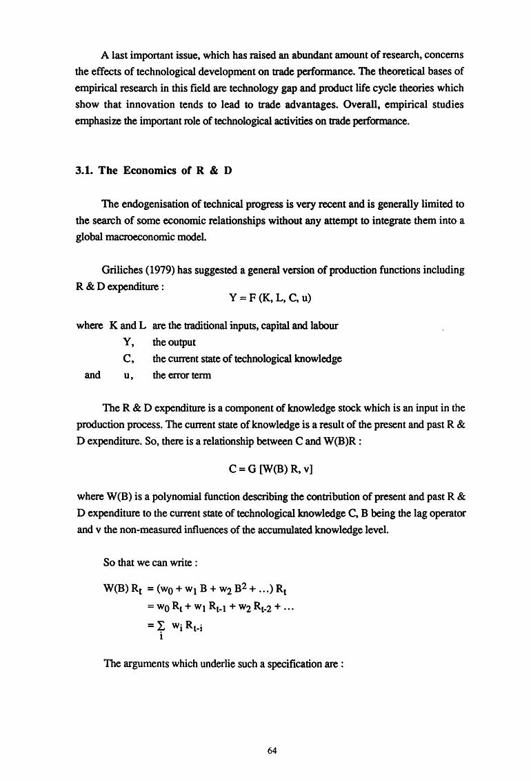
A last important issue, which has raised an abundant amount of research, concerns

the effects of technological development on trade performance. The theoretical bases of

empirical research in this field are technology gap and product life cycle theories which

show that innovation tends to lead to trade advantages. Overall, empirical studies

emphasize the important role of technological activities on trade performance.

3.1. The Economics of R & D

The endogenisation of technical progress is very recent and is generally limited to

the search of some economic relationships without any attempt to integrate them into a

global macroeconomic model.

Griliches (1979) has suggested a general version of production functions including

R & D expenditure : Y = F (K, L, C, u)

where K and L are the traditional inputs, capital and labour

Y, the output

C, the current state of technological knowledge

and u, the error term

The R & D expenditure is a component of knowledge stock which is an input in the

production process. The current state of knowledge is a result of the present and past R &

D expenditure. So, there is a relationship between C and W(B)R :

C=G [W(B) R, v]

where W(B) is a polynomial function describing the contribution of present and past R &

D expenditure to the current state of technological knowledge C, B being the lag operator

and v the non-measured influences of the accumulated knowledge level.

So that we can write :

W(B) Rt = (wo + w1 B + w2 B2 + ... ) Rt

=woRt+ WI Rt-1 + w2 Rt-2 + · · ·

= L wi Rt-i i

The arguments which underlie such a specification are :

64

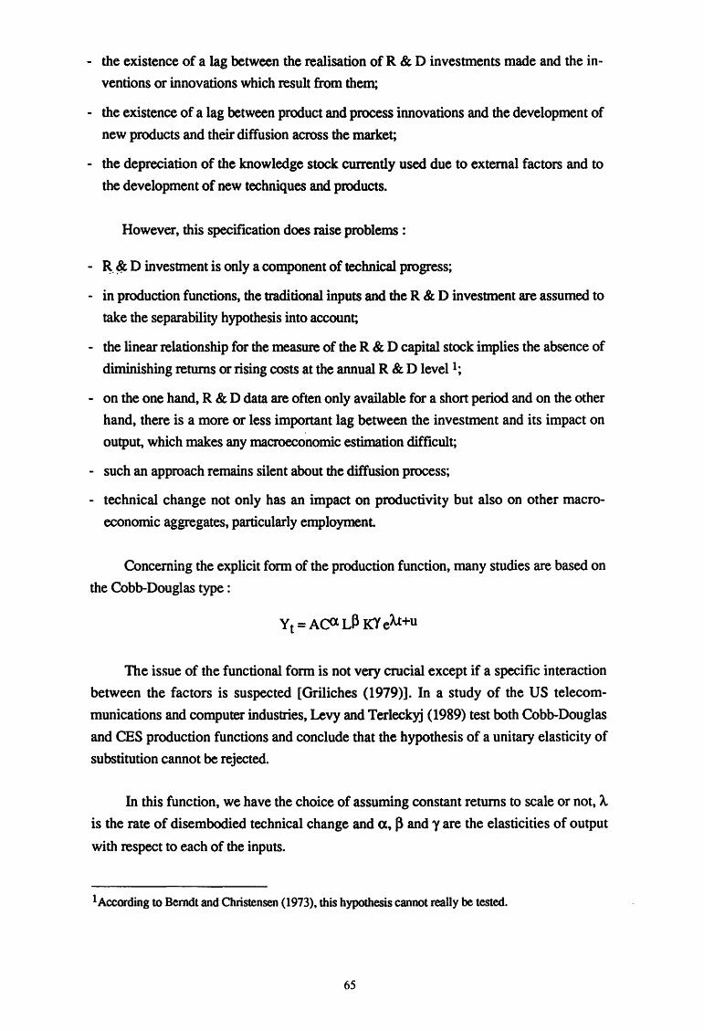
- the existence of a lag between the realisation of R & D investments made and the in­

ventions or innovations which result from them;

- the existence of a lag between product and process innovations and the development of

new products and their diffusion across the market;

- the depreciation of the knowledge stock currently used due to external factors and to

the development of new techniques and products.

However, this specification does raise problems :

- ~-~ D investment is only a component of technical progress;

- in production functions, the traditional inputs and the R & D investment are assumed to

take the separability hypothesis into account;

- the linear relationship for the measure of the R & D capital stock implies the absence of

diminishing returns or rising costs at the annual R & D Ievell;

- on the one hand, R & D data are often only available for a short period and on the other

hand, there is a more or less important lag between the investment and its impact on

output, which makes any macroeconomic estimation difficult;

- such an approach remains silent about the diffusion process;

- technical change not only has an impact on productivity but also on other macro-

economic aggregates, particularly employment

Concerning the explicit form of the production function, many studies are based on

the Cobb-Douglas type :

The issue of the functional form is not very crucial except if a specific interaction

between the factors is suspected [Griliches (1979)]. In a study of the US telecom­

munications and computer industries, Levy and Terleckyj (1989) test both Cobb-Douglas

and CES production functions and conclude that the hypothesis of a unitary elasticity of

substitution cannot be rejected.

In this function, we have the choice of assuming constant returns to scale or not, A. is the rate of disembodied technical change and a, (} and y are the elasticities of output

with respect to each of the inputs.

1 According to Berndt and Christensen (1973), this hypothesis cannot really be tested.

65

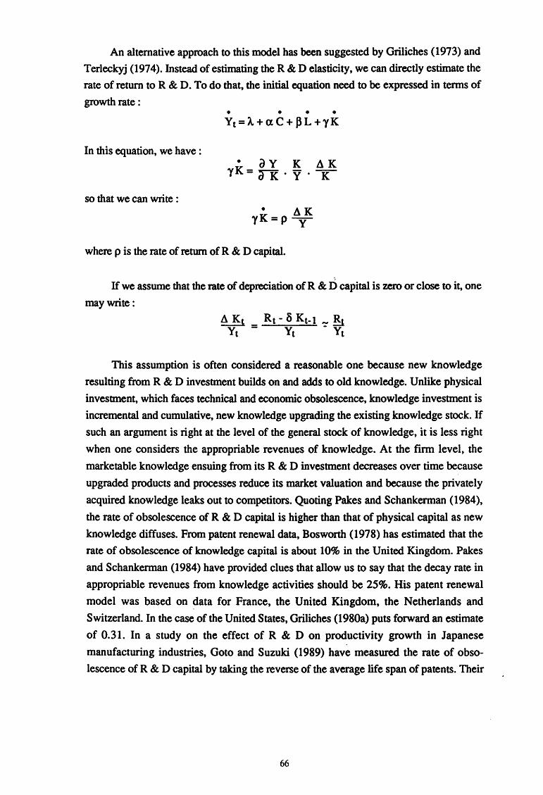
An alternative approach to this model has been suggested by Griliches (1973) and

Terleckyj (1974). Instead of estimating the R & D elasticity, we can directly estimate the

rate of return toR & D. To do that, the initial equation need to be expressed in terms of

growth rate : • • • • Y1=A.+aC+ PL+yK

In this equation, we have : • dY K IlK

yK=n·v·l{

so that we can write : • IlK

yK=p y

where p is the rate of return of R & D capital.

If we assume that the rate of depreciation of R & ti capital is zero or close to it, one

may write:

This assumption is often considered a reasonable one because new knowledge

resulting from R & D investment builds on and adds to old knowledge. Unlike physical

investment, which faces technical and economic obsolescence, knowledge investment is

incremental and cumulative, new knowledge upgrading the existing knowledge stock. If

such an argument is right at the level of the general stock of know ledge, it is less right

when one considers the appropriable revenues of knowledge. At the firm level, the

marketable knowledge ensuing from its R & D investment decreases over time because

upgraded products and processes reduce its market valuation and because the privately

acquired knowledge leaks out to competitors. Quoting Pakes and Schankerman (1984),

the rate of obsolescence of R & D capital is higher than that of physical capital as new

knowledge diffuses. From patent renewal data, Bosworth (1978) has estimated that the

rate of obsolescence of knowledge capital is about 10% in the United Kingdom. Pakes

and Schankerman (1984) have provided clues that allow us to say that the decay rate in

appropriable revenues from knowledge activities should be 25%. His patent renewal

model was based on ~ata for France, the United Kingdom, the Netherlands and

Switzerland. In the case of the United States, Griliches (1980a) puts forward an estimate

of 0.31. In a study on the effect of R & D on productivity growth in Japanese

manufacturing industries, Goto and Suzuki (1989) have measured the rate of obso­

lescence of R & D capital by taking the reverse of the average life span of patents. Their

66

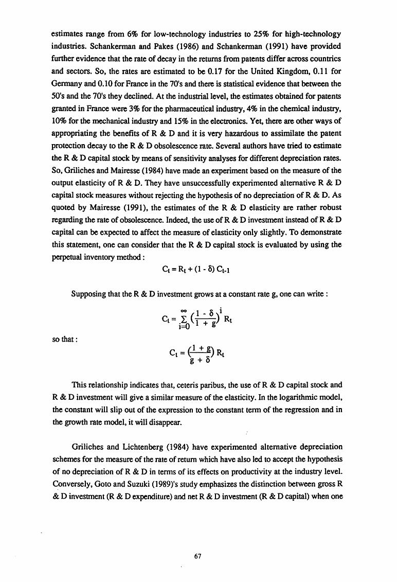
estimates range from 6% for low-technology industries to 25% for high-technology

industries. Schankerman and Pakes (1986) and Schankerman (1991) have provided

further evidence that the rate of decay in the returns from patents differ across countries

and sectors. So, the rates are estimated to be 0.17 for the United Kingdom, 0.11 for

Germany and 0.10 for France in the 70's and there is statistical evidence that between the

50's and the 70's they declined. At the industrial level, the estimates obtained for patents

granted in France were 3% for the pharmaceutical industry, 4% in the chemical industry,

10% for the mechanical industry and 15% in the electronics. Yet, there are other ways of

appropriating the benefits of R & D and it is very hazardous to assimilate the patent

protection decay to the R & D obsolescence rate. Several authors have tried to estimate

the R & D capital stock by means of sensitivity analyses for different depreciation rates.

So, Griliches and Mairesse ( 1984) have made an experiment based on the measure of the

output elasticity of R & D. They have unsuccessfully experimented alternative R & D

capital stock measures without rejecting the hypothesis of no depreciation of R & D. As

quoted by Mairesse (1991), the estimates of the R & D elasticity are rather robust

regarding the rate of obsolescence. Indeed, the use of R & D investment instead of R & D

capital can be expected to affect the measure of elasticity only slightly. To demonstrate

this statement, one can consider that the R & D capital stock is evaluated by using the

perpetual inventory method:

Supposing that the R & D investment grows at a constant rate g, one can write :

00 1 - a i Ct = .L ( 1 + g) Rt

1=0

so that:

This relationship indicates that, ceteris paribus, the use of R & D capital stock and

R & D investment will give a similar measure of the elasticity. In the logarithmic model,

the constant will slip out of the expression to the constant term of the regression and in

the growth rate model, it will disappear.

Griliches and Lichtenberg ( 1984) have experimented alternative depreciation

schemes for the measure of the rate of return which have also led to accept the hypothesis

of no depreciation of R & D in terms of its effects on productivity at the industry level.

Conversely, Goto and Suzuki (1989)'s study emphasizes the distinction between gross R

& D investment (R & D expenditure) and net R & D investment (R & D capital) when one

67

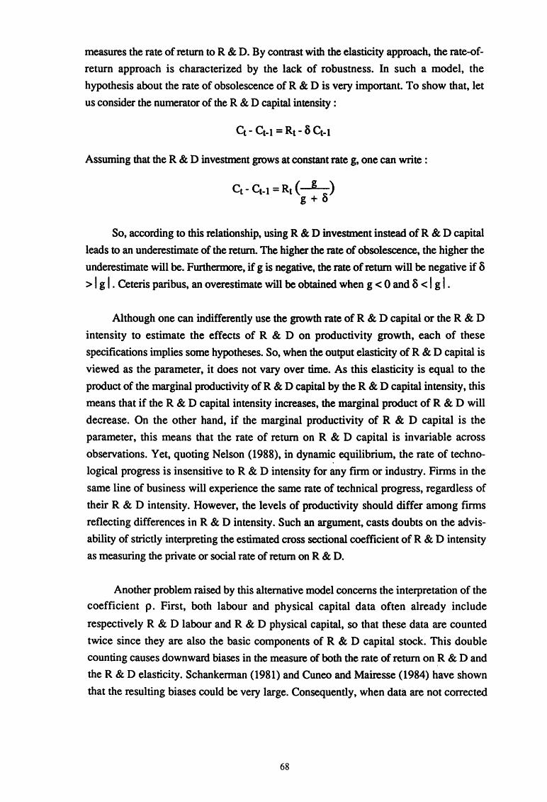
measures the rate of return toR & D. By contrast with the elasticity approach, the rate-of­

return approach is characterized by the lack of robustness. In such a model, the

hypothesis about the rate of obsolescence of R & D is very important. To show that, let

us consider the numerator of the R & D capital intensity :

Ct- Ct-1 = Rt- 8 Ct-1

Assuming that the R & D investment grows at constant rate g, one can write :

So, according to this relationship, using R & D investment instead of R & D capital

leads to an underestimate of the return. The higher the rate of obsolescence, the higher the

underestimate will be. Furthermore, if g is negative, the rate of return will be negative if o > I g I. Ceteris paribus, an overestimate will be obtained when g < 0 and o < I g I .

Although one can indifferently use the growth rate of R & D capital or the R & D

intensity to estimate the effects of R & D on productivity growth, each of these

specifications implies some hypotheses. So, when the output elasticity of R & D capital is

viewed as the parameter, it does not vary over time. As this elasticity is equal to the

product of the marginal productivity of R & D capital by the R & D capital intensity, this

means that if the R & D capital intensity increases, the marginal product of R & D will

decrease. On the other hand, if the marginal productivity of R & D capital is the

parameter, this means that the rate of return on R & D capital is invariable across

observations. Yet, quoting Nelson (1988), in dynamic equilibrium, the rate of techno­

logical progress is insensitive toR & D intensity for any firm or industry. Firms in the

same line of business will experience the same rate of technical progress, regardless of

their R & D intensity. However, the levels of productivity should differ among firms

reflecting differences in R & D intensity. Such an argument, casts doubts on the advis­

ability of strictly interpreting the estimated cross sectional coefficient of R & D intensity

as measuring the private or social rate of return on R & D.

Another problem raised by this alternative model concerns the interpretation of the

coefficient p. First, both labour and physical capital data often already include

respectively R & D labour and R & D physical capital, so that these data are counted

twice since they are also the basic components of R & D capital stock. This double

counting causes downward biases in the measure of both the rate of return on R & D and

the R & D elasticity. Schankennan ( 1981) and Cuneo and Mairesse ( 1984) have shown

that the resulting biases could be very large. Consequently, when data are not corrected

68

(6)

with respect to the R & D double counting, p is interpreted as being the excess rate of

return to R & D investment.

Consider that LK and CK are respectively the labour and physical capital

components included in the measure of the R & D capital. An approximation of the rate of return on R & D can be obtained by calculating a corrected value of p, PK· Assuming that

the variables are defined in value units, the time regression can be specified to measure

directly the rate of return of each production factor :

The estimated equation is :

Y• " ll C + ll CK ll L + ll LK ll K = A + PC y + PL y + p y

This adapted interpretation has been forcefully argued as being conceptually

incorrect by Schankerman (1981). He also points out the bias from R & D expensing out

when a value added measure is used for output. Material consumption components of R

& D investment are intermediate inputs and, consequently, are not accounted in the

measure of value added.

Taking the difference between these two equations, we obtain :

where PK, the rate of return on R & D capital is equal to the rate of return on R & D

capital in excess of the normal remuneration of its labour and physical capital components

plus the sum of the rates of return on labour and physical capital weighted by the

contribution of these factors to the net R & D investment.

Alternatively, as many studies combine the measure of the elasticities of labour and

physical capital with a measure of the excess rate of return on R & D physical capital, we

can adapt the preceding correction by combining these estimates :

A third correction can also be given for the measurement of R & D elasticity :

69

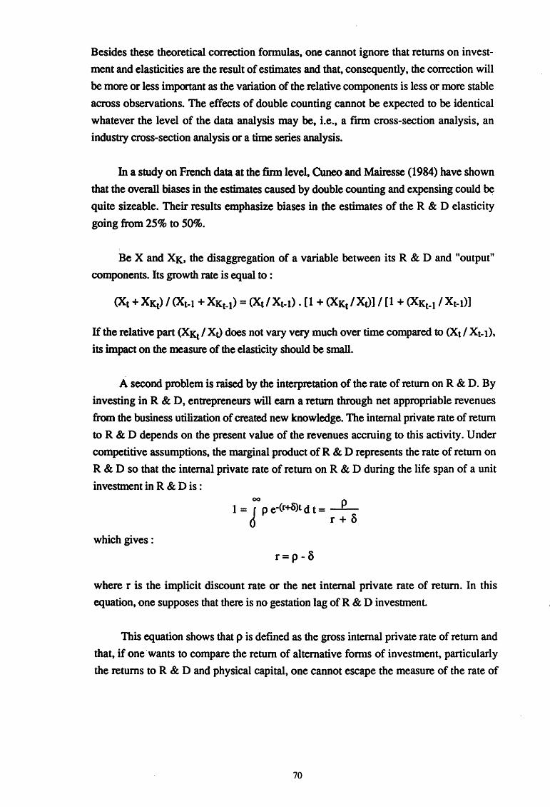
Besides these theoretical correction formulas, one cannot ignore that returns on invest­

ment and elasticities are the result of estimates and that, consequently, the correction will

be more or less important as the variation of the relative components is less or more stable

across observations. The effects of double counting cannot be expected to be identical

whatever the level of the data analysis may be, i.e., a fmn cross-section analysis, an

industry cross-section analysis or a time series analysis.

In a study on French data at the finn level, Cuneo and Mairesse (1984) have shown

that the overall biases in the estimates caused by double counting and expensing could ~

quite sizeable. Their results emphasize biases in the estimates of the R & D elasticity

going from 25% to 50%.

Be X and XK, the disaggregation of a variable between its R & D and "output"

components. Its growth rate is equal to :

(Xt + XKt) I (Xt-1 + XKt-1) = (Xt I Xt-1) . [1 + (XKt I Xt)] I [1 + (XKt-11 Xt-1)]

If the relative part (XKt I Xt) does not vary very much over time compared to <Xt I Xt-1),

its impact on the measure of the elasticity should be small.

A second problem is raised by the interpretation of the rate of return on R & D. By

investing in R & D, entrepreneurs will earn a return through net appropriable revenues

from the business utilization of created new knowledge. The internal private rate of return

toR & D depends on the present value of the revenues accruing to this activity. Under

competitive assumptions, the marginal product of R & D represents the rate of return on

R & D so that the internal private rate of return on R & D during the life span of a unit

investment in R & D is :

which gives :

1 = Joo p e-(r+a)t d t = _p­r+~

r=p-~

where r is the implicit discount rate or the net internal private rate of return. In this

equation, one supposes that there is no gestation lag of R & D investment

This equation shows that p is defined as the gross internal private rate of return and

that, if one·wants to compare the return of alternative forms of investment, particularly

the returns to R & D and physical capital, one cannot escape the measure of the rate of

70

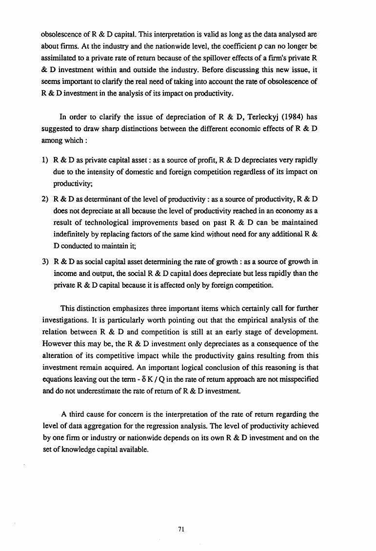
obsolescence of R & D capital. This interpretation is valid as long as the data analysed are

about firms. At the industry and the nationwide level, the coefficient p can no longer be

assimilated to a private rate of return because of the spillover effects of a frrm's private R

& D investment within and outside the industry. Before discussing this new issue, it

seems important to clarify the real need of taking into account the rate of obsolescence of

R & D investment in the analysis of its impact on productivity.

In order to clarify the issue of depreciation of R & D, Terleckyj (1984) has

suggested to draw sharp distinctions between the different economic effects of R & D

among which :

1) R & D as private capital asset : as a source of profit, R & D depreciates very rapidly

due to the intensity of domestic and foreign competition regardless of its impact on

productivity;

2) R & D as determinant of the level of productivity : as a source of productivity, R & D

does not depreciate at all because the level of productivity reached in an economy as a

result of technological improvements based on past R & D can be maintained

indefinitely by replacing factors of the same kind wjthout need for any additional R &

D conducted to maintain it;

3) R & D as social capital asset determining the rate of growth: as a source of growth in

income and output, the social R & D capital does depreciate but less rapidly than the

private R & D capital because it is affected only by foreign competition.

This distinction emphasizes three important items which certainly call for further

investigations. It is particularly worth pointing out that the empirical analysis of the

relation between R & D and competition is still at an early stage of development.

However this may be, the R & D investment only depreciates as a consequence of the

alteration of its competitive impact while the productivity gains resulting from this

investment remain acquired. An important logical conclusion of this reasoning is that

equations leaving out the term - S K I Q in the rate of return approach are not misspecified

and do not underestimate the rate of return of R & D investment.

A third cause for concern is the interpretation of the rate of return regarding the

level of data aggregation for the regression analysis. The level of productivity achieved

by one firm or industry or nationwide depends on its own R & D investment and on the

set of knowledge capital available.

71

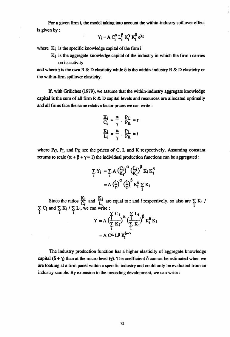
For a given fmn i, the model taking into account the within-industry spillover effect

is given by:

Yi =A GaLr ~., K~ eAt

where Ki is the specific knowledge capital of the finn i

K1 is the aggregate knowledge capital of the industry in which the fmn i carries

on its activity

and where y is the own R & D elasticity while 5 is the within-industry R & D elasticity or

the within-fmn spillover elasticity.

If, with Griliches (1979), we assume that the within-industry aggregate knowledge

capital is the sum of all firm R & D capital levels and resources are allocated optimally

and all finns face the same relative factor prices we can write :

where Pc, PL and Px are the prices of C, L and K respectively. Assuming constant

returns to scale (a + P + y = 1) the individual production functions can be aggregated :

Since the ratios ~ and ~ are equal tor and l respectively, so also are l: Ki I I ~ 1

l: Ci and l: Ki I~ Lj, we can write: 1 t 1 I, Ci I, Li

( i )a ( i )p ~ y = A l: K i l: K i KI KI

1 1

=A caLP ~8+y

The industry production function has a higher elasticity of aggregate knowledge

capital (8 + y) than at the micro level (y). The coefficient 8 cannot be estimated when we

are looking at a finn panel within a specific industry and could only be evaluated from an

industry sample. By extension to the preceding development, we can write :

72

• • • A K Y=A.+aC+PL+PI ~

where p measures the private rate of return to R & D while PI represents the social (in­

cluding private) rate of return. Compared to the elasticity approach which assumes a

common elasticity of output with respect to R & D stock when the relationship is

estimated across industries, which is not very likely given the large divergences in R & D

intensity, this alternative approach turns out to be more consistent with the optimal R & D

choice behavior 1. Given that R & D inputs are often already included into the

conventional factors, under the hypothesis that the discrepancy between social and private

returns is distributed randomly across industries, one can argue that the estimated

coefficient will be a consistent estimate of the average excess of social over private

returns [Griliches and Lichtenberg (1984)]. Generally, the estimated rates of return are a

mixture of private and social rates of return. For data at the fmn level, there is no doubt

that a variable like own R & D investment can only explore the magnitude of private

returns. At the industry level, only the private and within industry returns can be seized,

and hence only a part of the social rate of return. A complete measure of the social rate of

return on R & D conducted in a firm must cover the private rate of return, the social rate

of return on the within industry productivity and the social rate of return on the outside

industry productivity 2. The latter category of spillover effects is much more complicated

to evaluate. The extent to which an industry gains from the available pool of knowledge

of other industries depends on the economic and technological proximity of these

industries. In other words, for each industry, the spillover will be a weighted sum of the

R & D capital stocks of the other industries.

From a practical viewpoint, it is difficult to separate private and social return. The

extent of the gap between the social and the private rate of return on R & D is highly

dependent on the competitive environment, the orientation of the research and the nature

of the results. If the innovator is in a monopoly or oligopoly position, he will be able to

appropriate a proportion of the social benefits. When the competitive forces are stringent

the innovator will be in a less secure position to collect the social benefits. The degree of

appropriability will also differ according to whether the innovation deals with new

1 If the inputs are used at their competitive equilibrium levels, industries are unlikely to have the same output elasticities. The production technology being specific for each industry, industries will use different factor shares. A consequence of this is that a total productivity approach will be more relevant. 2conversely, for a firm the social rate of return on R & D will be equal to the private (or internal) rate of return (on own R & D) plus the external rate of return from the R & D conducted by other finns within both its own industry and other industries. It is worth noting that the external effects are not limited in space (e.g. a country) since a fmn also profits by the R & D conducted outside the country.

73

products or processes. Product innovations are likely to be under more intense

competitive pressures than process innovations. So, the discrepancy between social and

private returns could be larger for products than for processes. A last characteristic of the

discrepancy between social and private returns rests on the distinction between generic

and derived innovations. A radical innovation is more likely to be imitated quickly than

incremental innovations and, consequently, it will be very difficult for the originator of a

radical innovation to keep the benefits of his technological breakthrough.

On the other hand, when a new innovation comes onto the market place,

numerous economic variables come into action, which raises the issue of the

measurement of the social return on R & D and its distinction from private return. As

Griliches (1980a) points out : "Assuming that, on average, the outside world pays for

[new processes and] products what they are worth to it, using sales or value added as our

dependent variable does in fact capture the private returns to such research endeavors.

However, the observed private returns may underestimate the social returns because,

given the competitive structure of the particular industry, the market price of the new

product or process will be significantly below what consumers might have been willing

to pay for it. On the other hand, part of the increase in sales of an individual firm may

come at the expense of other firms and not as the result of the expansion of the market as

a whole. Also, some of the increase in prices paid for a particular new product may come

from changes in the market power of a particular firm induced by the success of the

research program. Moreover, some of the gains in productivity or in the sales of new

products may be based on the research results of other firms in the same or some other

industry. Such factors could result in the observed private returns overestimating the

social returns significantly. We cannot say much about the net impact of such forces on

the basis of [firm data]. It requires a detailed comparison of the individual firm results

with estimates based on industry and economy-wide returns to research[ ... ]. But since

expected private returns are presumably a determinant of private investment flows into

this activity, the estimates presented [on the basis of firm data] may be of some interest

even if they cannot answer the social-returns question unequivocally".

A last issue is which output variable should be introduced in the production

function : value added, sales or total factor productivity based on gross output or net

output. Conceptually, these alternative solutions rest on different hypotheses regarding

the production process and the optimality conditions. Their main impact on the

measurement of the rate of return, which is alternatively estimated by comparison with

net output or gross output, is that the latter provides higher estimates. This apparent

overestimate is understandable since the n1arginal product of R & D in terms of gross

74

output is logically higher than the marginal product of R & D in terms of net output. On

the other hand, the use of a value-added measure of output instead of sales will not result

in biased estimates. Yet, any measure based on gross output will be mispecified as long

as intermediate inputs are not taken into account besides primary inputs while any net

output measure must be connected with primary inputs only 1.

3.2. Econometric Studies in Retrospect

After discussing the main issues concerning the measurement of the impact of R

& D on productivity, we turn to the most significant studies investigating the relationship

between R & D and productivity. The literature in this field can be classified according to

the level of data aggregation. So, we can consider successively :

-studies at the micro level which are based on firm data (also called panal data) whose

main advantage is that they substantially increase the degrees of freedom. Further­

more, they provide evidence on the private rate of return on R & D investment;

- studies at the meso level whicQ use industry data and whose estimates can be

associated with the social rate of return on R & D. Yet, estimates will give at best a

partial measure of this social rate of return, i.e. an evaluation of the intra-industry

return;

- studies at the macro level which analyze economy-wide time series data in order to

measure the social rate of return on R & D. While such an approach can give an idea

of the domestic social return, we must keep in mind that, incomplete appropriability

property of R & D returns, which causes the social return to differ from the private

return, is not restricted by the existence of frontiers.

Besides, econometric analyses can also be classified according to :

- the dimensional extent : findings can be grounded on cross-sectorial or time-series

data or both;

- the econometric specification : th~ measure of the impact of R & D can be expressed

in terms of R & D elasticity or rate of return on R & D;

1 All variables having been beforehand corrected for double counting and expensing out

75

- the data measurement issue : sales, value-added or partial or total productivity can be

referred to as the explained variable, data can be corrected or not for R & D double

counting and expensing or R & D intensity can be defined with respect to sales or

value added.

This review is based on the classification of studies according to the level of data

aggregation and their econometric specification.

3.2.1. Micro Level Studies

Table 3.1. summarizes the main estimates of the R & D elasticity from finn panel

data. These estimates are performed within the framework of the Cobb-Douglas

production function except for Jaffe (1986)'s results which arise from the adjustment of a

profit function.

One of the fll'St studies to use finn data to estimate R & D elasticity was that by

Minasian (1969) performed on a small sample of chemical US ftrms. With the average

growth rate of value added as a dependent variable he experimented without firm

dummies and with firm dummies. These alternative approaches are respectively called

total regressions and within regressions. The latter can also be obtained by using the

deviations of variables from the individual fum means or by performing on growth rates.

Minasian finds R & D to have a positive and significant effect in the first case, an

observation which is not confumed by his second estimate. This result shows that biased

estimates can be obtained if not all finn-specific variables are included, which effect can

be picked up with finn dummies.

It is in the 1980's that the analyses at the firm level multiply. The first study of a

large number of fmns was realized by Griliches (1980a) who investigated 883 large US

manufacturing companies accounting for more than 90 % of all industrial R & D.

Working on both cross-section and time series, he obtains similar results for the two

types of regressions. Yet, estimates by industry give very different values ranging from

0.03 in aircraft to 0.14 in motor vehicles.

As already pointed out, Schankerman (1981) has forcefully argued that the

measured contribution of R & D to productivity improvements is often largely biased

downwards by failing to correct traditional inputs Oabor and physical capital) for double

counting as well as net output for R & D expensing (subtracted from value added as an

76

Tab

leau

3.1

. E

stim

ates

of

R &

D E

last

icit

y at

the

Fir

m L

evel

Stud

ies

Est

imat

ion

Sam

ple

Spec

ifica

tion

and

estim

atio

n pr

oced

ure

Ela

stic

ity o

f m

etho

d R

&D

Min

asia

n (1

969)

C

ross

-sec

tion

Uni

ted

Stat

es, C

hem

istry

, 17

fm

ns,

1948

-195

7.

Tot

al re

gres

sion

. 0.

26

(0.0

3)

Tim

e-se

ries

Uni

ted

Stat

es, C

hem

istry

, 17

fm

ns,

1948

-195

7.

With

in r

egre

ssio

n.

0.08

(0

.07)

Gril

iche

s (1

980a

) C

ross

-sec

tion

Uni

ted

Stat

es, 8

83 f

mns

, 19

63.

Indu

stry

dum

mie

s. 0.

07

(0.0

1)

Tim

e-se

ries

Uni

ted

Stat

es, 8

83 f

inns

, 19

57-1

963.

A

vera

ge g

row

th r

ate,

indu

stry

dum

mie

s.

0.08

(0

.01)

Scha

nker

man

(198

1)

Cro

ss-s

ectio

n U

nite

d St

ates

, 110

fmns

, Che

mis

try a

nd P

etro

leum

, D

ata

corr

ecte

d fo

r dou

ble

coun

ting

in R

& D

. 0.

16

1963

. (0

.04)

Cro

ss-s

ectio

n U

nite

d St

ates

, 11

0 fm

ns, C

hem

istry

and

Pet

role

um,

0.10

19

63.

(0.0

4)

Uni

ted

Stat

es, 1

01 f

inns

, Ele

ctric

Equ

ipm

ent,

1963

. 0.

03

(0.0

2)

Uni

ted

Stat

es, 1

01 f

inns

, Ele

ctric

Equ

ipm

ent,

1963

. D

ata

corr

ecte

d fo

r do

uble

cou

ntin

g in

R &

D.

0.23

(0

.03)

Uni

ted

Stat

es, 1

87 f

inns

, Met

als

and

Mac

hine

ry,

0.02

19

63.

(0.0

2)

Uni

ted

Stat

es, 1

87 f

inns

, Met

als

and

Mac

hine

ry,

Dat

a co

rrec

ted

for

doub

le c

ount

ing

in R

& D

. 0.

10

1963

. (0

.02)

Uni

ted

Stat

es, 3

4 fm

ns, M

otor

Veh

icle

s, 1

963.

0.

07

(0.0

5)

Uni

ted

Stat

es, 3

4 fi

nns,

Mot

or V

ehic

les,

196

3.

Dat

a co

rrec

ted

for d

oubl

e co

untin

g in

R &

D.

0.09

. (0

.05)

Uni

ted

Stat

es, 3

1 fr

rms,

Airc

raft,

196

3.

0.03

(0

.03)

Uni

ted

Stat

es, 3

1 fr

rms,

Airc

raft,

196

3.

Dat

a co

rrec

ted

for

doub

le c

ount

ing

in R

& D

. 0.

29

(0.0

5)

Uni

ted

Stat

es, 4

19 f

inns

, M

isce

llane

ous,

196

3.

0.04

(0

.01)

Uni

ted

Stat

es, 4

19 f

mns

, M

isce

llane

ous,

196

3.

Dat

a co

rrec

ted

for

doub

le c

ount

ing

in R

& D

. 0.

07

(0.0

1)

Gril

iche

s an

d M

aire

sse

Tim

e-se

ries

Uni

ted

Stat

es a

nd F

ranc

e, 3

43 a

nd 1

85 f

mns

, 19

73-

Ave

rage

gro

wth

rat

e.

0.02

(1

983)

19

78.

(0.0

3)

Gril

iche

s an

d M

aire

sse

Cro

ss-s

ectio

n U

nite

d St

ates

, 133

fin

ns,

1966

-197

7.

Tot

al re

gres

sion

, con

stan

t ret

urns

to s

cale

. 0.

07

(198

4)

(0.0

1)

Tot

al re

gres

sion

, fre

e re

turn

s to

sca

le.

0.05

(0

.01)

Cro

ss-s

ectio

n U

nite

d St

ates

, 77

scie

ntif

ic f

rrm

s, 19

66-1

977.

T

otal

regr

essi

on, c

onst

ant r

etur

ns to

sca

le.

0.22

(0

.01)

Tot

al r

egre

ssio

n, f

ree

retu

rns

to s

cale

. 0.

18

(0.0

1)

Tim

e-se

ries

Uni

ted

Stat

es, 1

33 f

inns

, 19

66-1

977.

Fr

ee r

etur

ns to

sca

le, w

ithin

reg

ress

ion.

0.

09

(0.0

2)

Con

stan

t ret

urns

to s

cale

, with

in r

egre

ssio

n.

0.16

(0

.02)

Cun

oo a

nd M

aire

sse

Cro

ss-s

ectio

n Fr

ance

, 18

2 fm

ns,

1972

-197

7.

Tot

al re

gres

sion

, dat

a co

rrec

ted

for R

& D

dou

ble

0.20

(1

984)

co

untin

g.

(0.0

1)

Cro

ss-s

ectio

n Fr

ance

, 98

fmns

, sci

entif

ic s

ecto

rs, 1

972-

1977

. T

otal

regr

essi

on, d

ata

corr

ecte

d fo

r R &

D d

oubl

e 0.

21

coun

ting.

(0

.01)

Tot

al re

gres

sion

. 0.

11

(0.0

1)

Tim

e-se

ries

Fran

ce, 1

82 f

irms,

197

2-19

77.

With

in re

gres

sion

, fre

e re

turn

s to

sca

le, d

ata

0.05

co

rrec

ted

for R

& D

dou

ble

coun

ting.

(0

.04)

With

in r

egre

ssio

n, c

onst

ant r

etur

ns to

sca

le, d

ata

0.11

co

rrec

ted

for R

& D

dou

ble

coun

ting.

(0

.04)

Mai

ress

e an

d C

uneo

C

ross

-sec

tion

Fran

ce, 2

96 fi

rms,

scie

ntifi

c se

ctor

s, a

vera

ge y

ear

With

out i

ndus

try d

umm

ies,

data

cor

rect

ed fo

r R &

D

0.16

(1

985)

19

74 a

nd 1

979.

do

uble

cou

ntin

g, b

etw

een-

finn

regr

essi

on.

(0.0

2)

Indu

stry

dum

mie

s, v

aria

ble

for

labo

ur q

ualif

icat

ion,

0.

10

corr

ecte

d da

ta, b

etw

een-

fum

regr

essi

on.

(0.0

2)

Tim

e-se

ries

Fran

ce, 3

90 f

irms,

1974

and

197

9.

Gro

wth

rate

bet

wee

n ex

trem

e ye

ars.

0.02

(0

.10)

Gril

iche

s (1

986)

C

ross

-sec

tion

Uni

ted

Stat

es, 4

91 f

mns

, 19

72.

Indu

stry

dum

mie

s, em

ploy

men

t cor

rect

ed.

0.11

(0

.02)

Cro

ss-s

ectio

n U

nite

d St

ates

, 491

fm

ns,

1977

. In

dust

ry d

umm

ies,

empl

oym

ent c

orre

cted

. 0.

09

(0.0

2)

Tim

e-se

ries

Uni

ted

Stat

es, 6

52 f

irms,

196

6-19

77.

Ave

rage

gro

wth

rate

, ind

ustry

dum

mie

s, co

nstra

ined

0.

12

elas

ticity

of l

abou

r. (0

.02)

Jaff

e (1

986)

C

ross

-sec

tion

Uni

ted

Stat

es, 4

32 f

mns

, 19

73 a

nd 1

979.

Pr

ofit,

tota

l reg

ress

ion,

labo

ur n

on in

clud

ed.

0.20

(0

.05)

Tim

e-se

ries

Uni

ted

Stat

es, 4

32 f

mns

, 19

73 a

nd 1

979.

Pr

ofit,

gro

wth

rat

e be

twee

n ex

trem

e ye

ars.

0.10

(0

.30)

Sass

enou

(19

88)

Cro

ss-s

ectio

n Ja

pan,

394

firm

s, 19

76.

-0.

10

(0.0

1)

Tim

e-se

ries

Japa

n, 3

94 f

mns

, 19

73-1

981.

W

ithin

regr

essi

on, c

onst

ant r

etur

n to

sca

le.

-0.0

1 (0

.01)

With

in re

gres

sion

, fre

e re

turn

to s

cale

. -0

.02

(0.0

1)

Ann

ual g

row

th r

ate,

con

stan

t ret

urn

to s

cale

. 0.

02

(0.0

2)

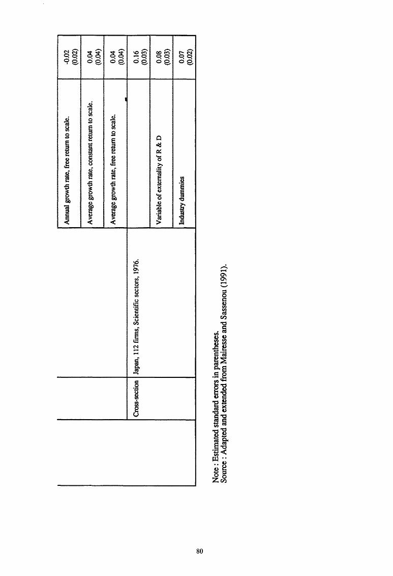
00

0

Cro

ss-s

ectio

n Ja

pan,

112

firm

s, S

cien

tific

sec

tors

, 19

76.

Not

e: E

stim

ated

sta

ndar

d er

rors

in p

aren

thes

es.

Sour

ce :

Ada

pted

and

ext

ende

d fr

om M

aire

sse

and

Sass

enou

(19

91).

-A

nnua

l gro

wth

rat

e, f

ree

retu

rn to

sca

le.

Ave

rage

gro

wth

rat

e, c

onst

ant r

etur

n to

sca

le.

Ave

rage

gro

wth

rat

e, f

ree

retu

rn t

o sc

ale.

-

Var

iabl

e of

exte

rnal

ity o

f R &

D

Indu

stry

dum

mie

s

-0.0

2 (0

.02)

0.04

(0

.04)

0.04

(0

.04)

0.16

(0

.03)

0.08

(0

.03)

0.07

(0

.02)

intermediate input). His estimates show that the downward bias varies from 50 percent

for chemicals and petroleum and motor vehicles to 800 percent for electric equipment and

aircraft. It is worth noting that the downward biases are largest in the two industries that

are most R & D intensive and most reliant on government funding, i.e. electrical

equipment and aircraft.

Cuneo and Mairesse (1984) arrive at a similar observation in their analysis of

French data. For scientific sectors, the downward bias amounts to 50%. From their

study it also appears that the hypothesis of constant returns to scale is not without

consequences on the estimates. When this assumption is relaxed, estimates of R & D

elasticities are lower and returns to scale appear to be decteasing. Large divergences are

also observed between estimates from total regressions and within regressions. The

within estimate under the hypothesis of free returns to scale gives a non-significant R &

D elasticity (except for scientific sectors). The order of magnitude of coefficients

obtained in this analysis is quite comparable to that reported by Griliches and Mairesse

(1984) for the United· States. Yet, in this study, within regressions give higher

coefficients than total regressions (except for the scientific sector). In a simultaneous

analysis of both American and French data, Griliches and Mairesse (1983) fail to find any

significant relationships between output growth rate and R & D investment.

In fact, we observe that time-series estimates of R & D elasticity provide more

controversial results than cross-section ones. In a large number of time series studies,

the estimated coefficient appears non-significant. But it is not the case for Griliches

(1980b, 1986)'s studies in which the estimated coefficients are close for the two types of

estimates. In the second study, a partial correction of data gives a higher estimate of R &

D coefficient while two additional variables about the share of R & D investment devoted

to basic research and privately financed research are introduced into the model, the latter

showing a high premium effect for these categories of research. The results obtained by

Jaffe (1986) from a profit equation are congruent with the observations made by

Griliches. A similar conclusion emerges from the estimates reported by Sassenou ( 1988)

for Japan. On the one hand, his coefficients are significant for the cross-section analysis,

but, on the other hand, these results are not confmned by the time series analysis.

According to Mairesse and Sassenou (1991) the high disparities between

estimates arising from the cross-section and the time-series analyses are likely to be due

to various causes. High collinearity of R & D capital with time, random measurement

errors in variables, inadequate specification of lags in the effects of R & D capital,

omission of variables reflecting short-term adjustments and the simultaneity of the

81

decision process regarding employment and production are all phenomena which may

explain why time-series estimates give poorer results than cross-sectional ones.

Models estimating the rate of return on R & D have been developed as an

alternative method to. the hypothesis of a constant R & D elasticiy. In this approach, the

marginal productivity of R & D capital, in other words, the rate of return on R & D, is

assumed to be constant. This hywthesis of a same rate of return on R & D for all firms

and industries is compatible with the competitive equilibrium conjecture all the more as

the measure bears on the private return and not on the social return. Although estimates

based on fmn data are generally seen as measuring the private return, the results may

also, to some extent, represent the social return depending on the analytical context. So,

it is the case when industry dummies are not included into the regression. Other practical

problems raised by this approach will be discussed throughout the review of the most

prominent studies whose results are gathered in table 3.2.

In their respective studies, Minasian (1962) and Mansfield (1980) provide some

clues to a very high rate of return on R & Din the chemical industry for the United

States. This result is not confirmed by Link (1981) for the shorter period covering the

beginning of the 70's. Yet, the rate of return for the chemical industry is significant

which is not the case for other industries, particularly those related to mechanical

manufacturing and transport equipment An estimate based on a sample of 302 firms for

the end of the 70's no longer provides any strong evidence of the rate of return on R & D

[Link (1983)].

As opposed to these disappointing experiments, Griliches and Mairesse (1983)

produce estimates of a significant rate of return in the United States and France with a

larger return for the latter. The use of industry dummies appreciably reduces the order of

magnitude of the estimated return. So, more attention should be paid to the construction

of variables in the measurement of the rate of return. The relationship between changes

in productivity and levels of R & D intensity can be evaluated by using alternatively sales

or value added as reference output. Generally, the measurements of the productivity

variable and the R & D intensity indicator are consistent with each other. Nevertheless,

one needs to be careful when comparing the returns on R & D provided by different

studies because estimates may sensitively diverge depending upon whether R & D

intensity is measured with respect to value added or sales. Consequently, the estimates

obtained by Minasian (1962), Mansfield (1980) and Link (1981) are not directly

comparable to those reported by Link (1983) and Griliches and Mairesse (1983), the

former being based on value added and the latter on sales. As the amount of sales is

82

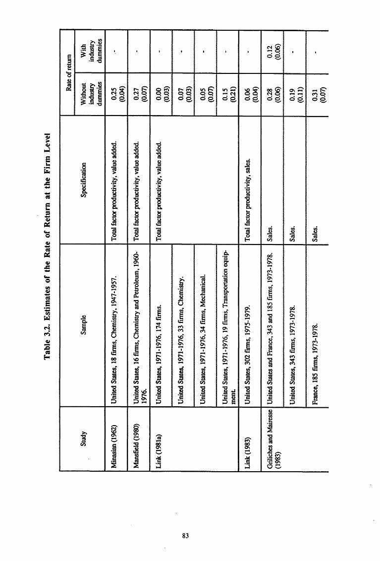
00

w

Stud

y

Min

asia

n (1

962)

Man

sfie

ld (1

980)

Lin

k (1

981a

)

Lin

k (1

983)

Gril

iche

s an

d M

aire

sse

(198

3)

Tab

le 3

.2.

Est

imat

es o

f th

e R

ate

of R

etur

n at

the

Fir

m L

evel

Sam

ple

Spec

ifica

tion

Uni

ted

Stat

es,

18 f

mns

, C

hem

istry

, 19

47-1

957.

T

otal

fact

or p

rodu

ctiv

ity, v

alue

add

ed.

Uni

ted

Stat

es,

16 fm

ns, C

hem

istry

and

Pet

role

um, 1

960-

Tot

al fa

ctor

pro

duct

ivity

, val

ue a

dded

. 19

76.

Uni

ted

Stat

es, 1

971-

1976

, 174

firm

s.

Tot

al fa

ctor

pro

duct

ivity

, val

ue a

dded

.

Uni

ted

Stat

es,

1971

-197

6, 3

3 fm

ns, C

hem

istry

.

Uni

ted

Stat

es,

1971

-197

6,34

firm

s, M

echa

nica

l.

Uni

ted

Stat

es, 1

971-

1976

, 19

firm

s, T

rans

porta

tion

equi

p-m

enL

Uni

ted

Stat

es, 3

02 f

mns

, 19

75-1

979.

T

otal

fact

or p

rodu

ctiv

ity, s

ales

.

Uni

ted

Stat

es a

nd F

ranc

e, 3

43 a

nd 1

85 f

irms,

1973

-197

8.

Sale

s.

Uni

ted

Stat

es, 3

43 f

mns

, 19

73-1

978.

Sa

les.

Fran

ce, 1

85 f

mns

, 19

73-1

978.

Sa

les.

Rat

e of

retu

rn

With

out

With

in

dust

ry

indu

stry

du

mm

ies

dum

mie

s

0.25

.-

(0.0

4)

0.27

-

(0.0

7)

0.00

-

(0.0

3)

0.07

-

(0.0

3)

0.05

-

(0.0

7)

0.15

-

(0.2

1)

0.06

-

(0.0

4)

0.28

0.

12

(0.0

6)

(0.0

6)

0.19

-

(0.1

1)

0.31

-

(0.0

7)

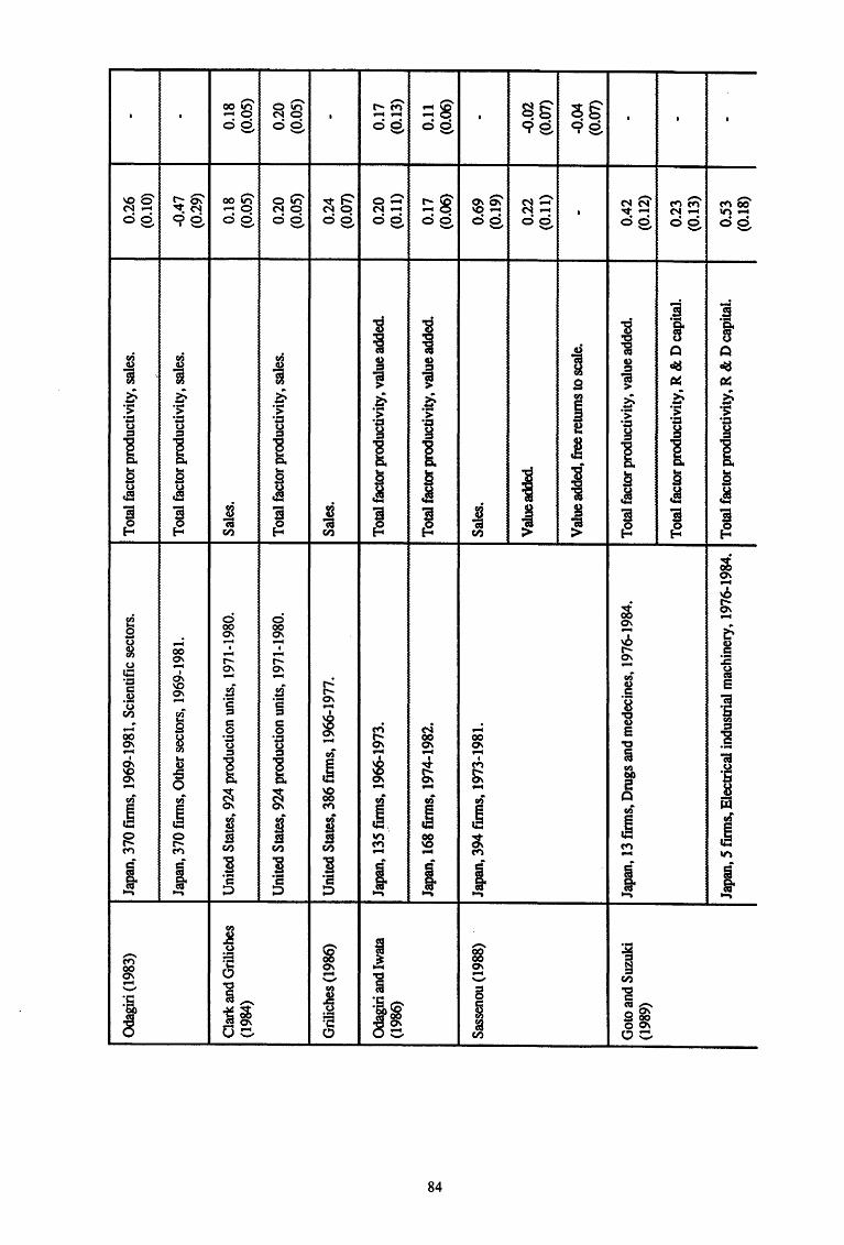
Oda

giri

(198

3)

Japa

n, 3

70 f

mns

, 19

69-1

981,

Sci

entif

ic s

ecto

rs.

Tot

al fa

ctor

pro

duct

ivity

, sal

es.

0.26

-

(0.1

0)

Japa

n, 3

70 f

mns

, Oth

er s

ecto

rs,

1969

-198

1.

Tot

al f

acto

r pr

oduc

tivity

, sal

es.

-0.4

7 -

(0.2

9)

Cla

rk a

nd G

rilic

hes

Uni

ted

Stat

es, 9

24 p

rodu

ctio

n un

its,

1971

-198

0.

Sale

s.

0.18

0.

18

(198

4)

(0.0

5)

(0.0

5)

Uni

ted

Stat

es, 9

24 p

rodu

ctio

n un

its,

1971

-198

0.

Tot

al fa

ctor

pro

duct

ivity

, sal

es.

0.20

0.

20

(0.0

5)

(0.0

5)

Gril

iche

s (1

986)

U

nite

d St

ates

, 386

fmns

, 19

66-1

977.

Sa

les.

0.

24

-(0

.07)

Oda

giri

and

Iwat

a Ja

pan,

135

_fm

ns, 1

966-

1973

. T

otal

fact

or p

rodu

ctiv

ity, v

alue

add

ed.

0.20

0.

17

(198

6)

(0.1

1)

(0.1

3)

Japa

n, 1

68 f

mns

, 19

74-1

982.

T

otal

fact

or p

rodu

ctiv

ity, v

alue

add

ed.

0.17

0.

11

(0.0

6)

(0.0

6)

Sass

enou

(198

8)

Japa

n, 3

94 f

mns

, 19

73-1

981.

Sa

les.

0.

69

-(0

.19)

Val

ue a

dded

0.

22

-0.0

2 (0

.11)

(0

.07)

Val

ue a

dded

, fre

e re

turn

s to

sca

le.

--0

.04

(0.0

7)

Got

o an

d Su

zuki

Ja

pan,

13

fmns

, Dru

gs a

nd m

edec

ines

, 197

6-19

84.

Tot

al f

acto

r pro

duct

ivity

, val

ue a

dded

. 0.

42

-(1

989)

(0

.12)

Tot

al f

acto

r pr

oduc

tivity

, R &

D c

apita

l. 0.

23

-(0

.13)

Japa

n, 5

fmns

, Ele

ctri

cal i

ndus

trial

mac

hine

ry,

1976

-198

4.

Tot

al f

acto

r pr

oduc

tivity

, R &

D c

apita

l. 0.

53

-(0

.18)

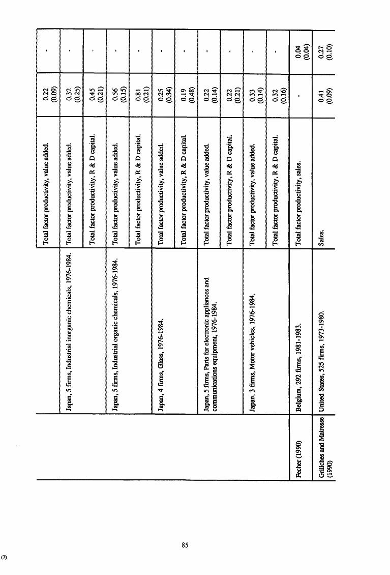
Tot

al f

acto

r pr

oduc

tivity

, val

ue a

dded

. 0.

22

-(0

.09)

Japa

n, 5

finn

s, I

ndus

tria

l ino

rgan

ic c

hem

ical

s, 1

976-

1984

. T

otal

fac

tor p

rodu

ctiv

ity, v

alue

add

ed.

0.32

-

(0.2

5)

Tot

al f

acto

r pr

oduc

tivity

, R &

D c

apita

l. 0.

45

-(0

.21)

Japa

n, 5

fmns

, Ind

ustri

al o

rgan

ic c

hem

ical

s, 1

976-

1984

. T

otal

fact

or p

rodu

ctiv

ity, v

alue

add

ed.

0.56

-

(0.1

5)

Tot

al f

acto

r pr

oduc

tivity

, R &

D c

apita

l. 0.

81

-(0

.21)

Japa

n, 4

fm

ns,

Gla

ss,

1976

-198

4.

Tot

al fa

ctor

pro

duct

ivity

, val

ue a

dded

. 0.

25

-(0

.34)

Tot

al f

acto

r pr

oduc

tivity

, R &

D c

apita

l. 0.

19

-(0

.48)

Japa

n, 5

fmns

, Par

ts f

or e

lect

roni

c ap

plia

nces

and

T

otal

fact

or p

rodu

ctiv

ity, v

alue

add

ed.

0.22

-

com

mun

icat

ions

equ

ipm

ent,

1976

-198

4.

(0.1

4)

Tot

al f

acto

r pr

oduc

tivity

, R &

D c

apita

l. 0.

22

-(0

.21)

Japa

n, 3

fum

s, M

otor

veh

icle

s, 1

976-

1984

. T

otal

fact

or p

rodu

ctiv

ity, v

alue

add

ed.

0.33

-

(0.1

4)

Tot

al f

acto

r pr

oduc

tivity

, R &

D c

apita

l. 0.

32

-(0

.16)

Fech

er (1

990)

B

elgi

um, 2

92 f

ums,

198

1-19

83.

Tot

al f

acto

r pro

duct

ivity

, sal

es.

-0.

04

(0.0

4)

Gril

iche

s an

d M

aire

sse

Uni

ted

Stat

es, 5

25 f

ums,

197

3-19

80.

Sale

s.

0.41

0.

27

(199

0)

(0.0

9)

(0.1

0)

00

"'

Japa

n, 4

06 f

irms,

197

3-19

80.

Lich

tenb

erg

and

Uni

ted

Stat

es, 5

240

firm

s, 19

72-1

985.

Si

egel

(19

91)

Kle

tte (1

991)

N

orw

ay, 1

396

plan

ts,

1977

-198

8

Not

e : E

stim

ated

sta

ndar

d er

rors

in p

aren

thes

es.

Sour

ce: A

dapt

ed a

nd e

xten

ded

from

Mai

ress

e (1

991)

.

Sale

s, f

ree

retu

rns

to s

cale

.

Sale

s.

Sale

s, f

ree

retu

rns

to s

cale

.

Tot

al f

acto

r pro

duct

ivity

, sal

es.

Tot

al f

acto

r pro

duct

ivity

, gro

ss o

utpu

t

-0.

25

(0.1

0)

0.56

0.

30

(0.2

3)

(0.2

1)

-0.

20

(0.2

1)

-0.

13

(0.0

2)

-0.

11

(0.0

3)

largely higher than the value added, the ratio of R & D to sales is expected to give higher

estimates than the R & D-value added ratio. The ratio of sales to value added being

superior to two, the estimates of Minasian and Mansfield appear very high when

compared to those obtained by Griliches and Mairesse.

The results reported by Clark and Griliches (1984) and Griliches (1986) are

roughly comparable to those obtained by Griliches and Mairesse. It is worth noting that

the introduction of industry dummies in their sample does not modify the estimates

obtained by Clark and Griliches and that the authors estimate a product-process mix

effect. Their mix coefficient indicates that the rate of productivity growth is lower when

the increase in R & D is product-oriented than when it is process-oriented. This is

explained by the fact that new products tend to be disruptive to established production

processes because their introduction involves a start-up and debugging phase. Moreover,

when new products are an important aspect of competition, businesses may sacrifice a

part of productivity to gain flexibility to avoid too rigid equipments and processes which

reduce the possibilities of adaptation.

If we tum to other estimates, we see that some studies show negative results. So,

Odagiri (1983) reports a positive and statistically significant return coefficient for the

scientific sector in Japan, but for other sectors, the coefficient is negative. This finding is

not isolated in the sense that detailed results published by other authors, like Link ( 1981)

for the United States and Fecher (1989) for Belgium, also yield negative estimates. Yet,

these astonishing findings are often only at most marginally significant.

Other studies of Japanese data by Odagiri and Iwata (1986), Sassenou (1988) and

Goto and Suzuki (1989) give more credible estimates. The estimates reported by

Sassenou ( 1988) show how different the return can be depending on whether the R & D

intensity is measured with respect to sales or value added as well as how the introduction

of industry dummies can affect the coefficients. The originality of Goto and Suzuki

(1989)'s study mainly lies in the fact that they emphasize the implications of disregarding

R & D depreciation in the measurement of R & D intensity. In some sectors, such as

pharmaceuticals, machinery, and chemicals, the corrected intensity measures give notice­

ably different estimates compared to those obtained with the uncorrected measure.

As pointed out by Mairesse and Sassenou (1991), the interpretation of dis­

crepancies between the estimates from corrected and uncorrected measures in terms of a

net rate of return versus a gross rate of return does not hold. What has to be· ~nderlined

87

from the estimates reported by Griliches and Mairesse (1990) is the fall in estimates when

both industry effects and free returns to scale are taken into account in the regressions.

Finally, Lichtenberg and Siegel (1989) and Klette (1991) carried out very large­

scale experiments for the United States and Norway respectively and their estimates of

the rate of return on R & Dare astonishingly very close.

3.2.2. Meso Level Studies

Besides these estimates obtained at the finn level, there are several studies which

have measured the rate of return on R & D at the industry level. The interpretation of the

rate of return estimated through such studies is different from that given for coefficients

estimated on the basis of panel data. What is measured through such an approach is the

excess gross social rate of return on R & D. It is an "excess" measure because data are

rarely corrected for double counting and expensing. The "gross" adjective results from

the fact that the R & D intensity measure used is based on gross R & D investment and

not net R & D investment. These two restrictions are not specific to industry level

analyses, they are also used in panel data analyses. The social characteristic of this rate

of return arises from the aggregation across fmns of R & D expenditures which causes

the coefficient to represent the return on industry R & D for the industry as a whole. Yet,

it does not give a full estimate of the social return because it is restricted to the R & D

performed inside the concerned industry. In other words, it is an internal rate of return or

a rate of return internal to the industry. Consequently, the meaning of the return at the

industry level is not clearer than at the fmn Ievell. Table 3.3 presents a synthesis of the

main estimates of the rate of return at the industry level. As in the case of firm level

analyses, the R & D intensity indicator is alternatively measured with respect to sales or

value added. Anticipating the following chapter, we have also summarized in this table

the studies measuring both the internal and the external rates of return. This external rate

of return measures what are for a given industry the external effects of the R & D realized

in the other industries.

1For recall, Griliches and Lichtenberg (1984) defme it as the average excess of the social gross rate of retwn. There is no reason to expect the social return to be equalized across industries but under the hypothesis that the discrepancy between social and private returns is distributed randomly across industries, the coefficient will give a consistent estimate of the average excess of social over private returns. It is a social return because it is based on output in constant prices rather than profit calculations. It is gross because it also includes a possible allowance for depreciation~ And it is excess because R & D expenditures are already included in conventional inputs at normal factor prices.

88

Table 3.3. Estimates of the Rate of Return at the Industry Level

Study Sample Data and Rate of return weighting matrix Internal External

Terleckyj United States Total factor productivity 0.37 -(1974) 20 industries Value added (0.11)

1948-1966 Transaction flow and 0.29 0.78 capital flow matrices (0.08) (0.21)

Terleckyj United States Total factor productivity (1980a) 20 industries Value added 0.20 1.83

1948-1966 Transaction flow and (0.31) (0.72) capital flow matrices

Scherer United States Labor productivity (1982)1 87 industries Sales

1964-1969 Patent flow matrix 0.13 0.64 (0.13) (0.35)

1973-1978 0.29 0.74 (0.14) (0.39)

Griliches- France Total factor productivity Mairesse 15 industries Sales (1983) 1964-1968, 0.33 -

1969-1973 (0.14)

United States 15 industries 1964-1968, 0.23 -1969-1973 (0.12)

Griliches- United States Total factor productivity Lichtenberg 27 industries Sales (1984a) 1959-1968 0.09 -

1964-1973 (0.05) 0.20 -

(0.06) 1969-1976 0.34 -

(0.08)

Griliches- United States Total factor productivity Lichtenberg 193 industries Interindustry transactions "(1984b)1 1964-1969 Sales 0.15 0.74

(0.08) (0.19) 1973-1978 Sales 0.28 0.50

(0.11) (0.25) 1964-1969 Value added 0.08 0.40

Value added (0.05) (0.10)

1973-1978 0.16 0.26 (0.06) (0.14)

Goto-Suzuki Japan Total factor productivity (1989) 50 industries Value added 0.26 0.80

1978-1983 Transaction flow and (0.14) (0.42) capital flow matrices

Leonard (1971) United States Sales 0.09 -16 industries 1957-1968

(0.04)

Griliches United States Total factor productivity 0.32 -(1973) 85 industries Value added (0.10)

1958-1963

Note: Estimated standard errors in parentheses. , 1. In these studies, the analyses are not based on a distinction between own and purchased R & D but between

own product R & D and own process and embodied R & D.

89

A frrst estimate made by Leonard ( 1971) gives a very weak rate of return on R &

D in the US industry. This result strongly contrasts with that obtained by Griliches

(1973) and is all the more disappointing as the frrst author makes use of sales and the

second one of value added. The estimates by Terleckyj (1974,1980a) are of the same

order of magnitude as the value reported by Griliches. The two types of results presented

by Terleckyj are based on alternative measurement methods of total factor productivity.

While the first measurement is derived from net output and net input, the second one uses

gross values and accounts for quality characteristics of inputs. This explains why in the

second case, the estimate of the rate of return on R & D is lower and non significant

Except for the first subperiod studied, Scherer (1982)'s results are comparable to

those obtained by Terleckyj. It is the same for results reported by Griliches and Mairesse

(1983) who provide evidence of a higher rate of return in France. Griliches and

Lichtenberg ( 1984a, 1984b) show how different the estimates may be depending on the

reference period and the R & D intensity indicator. The rate of return on R & D appears

to have increased over time. The estimates obtained by Goto and Suzuki (1989) are

comparable to those reported for the United States.

3.2.3. Macro Level Studies

Finally, let us close this review by having a glance at some studies estimating the

elasticity of R & D at the economy-wide level except for Capron (1990,1992b) who uses

total R & D expenditure. These studies only consider industrial R & D expenditure. All

the results gathered in table 3.4. show that there also exists a relationship between

productivity and R & D at the aggregate level.

The estimated elasticities are noticeably higher than the elasticities resulting from

panel experiments. Except for Italy, the private industrial R & D elasticity is lower than

the total industrial R & D elasticity. In the equations with total industrial R & D, the

elasticity of each type of R & D (private versus public) is equal to the estimated elasticity

weighted by the relative part of the corresponding type of R & D in total R & D.

Consequently, the lower level of private industrial R & D elasticities indicates that public

industrial R & D expenditure contributes to productivity growth. This finding is

particularly obvious for the United States, France and the United Kingdom where the

public contribution to industrial R & D expenditure is very high. It is worth noting that a

large part of this public intervention is not directed towards civil projects but is part of

defense objectives. By running the regression for two subperiods, Patel and Soete

90

(1988) tested whether the coefficients were significantly different in the two periods.

They find evidence that there was a break in the relationship between productivity and R

& Din the mid seventies in Canada, the UK, Sweden and Japan. While the impact of R

& D decreased in Canada and Sweden, it increased in the UK and Japan.

Table 3.4. Estimates of the Elasticity of R & D at the Aggregate Level

Study Sample Data characteristics Total Private Public R&D R&D R&D

Levy-Terleckyj United States Sales - 0.27 0.05 (1983) 1949-1981 No depreciation rate (0.07) (0.03)

Suzuki (1985) Japan Value added 1965-1982 Depreciation rate (0.10) 0.12 - -

imported technology (0.05) included

Patel-Soete United States Total factor productivity 0.61 0.34 -(1988) 1967-1985 Depreciation rate (0.15) (0.01) (0.02)

Canada 0.26 0.25 -1967-1985 (0.03) (0.03)

Japan 0.41 0.41 -1967-1985 (0.03) (0.03)

Germany 0.38 0.38 -1967-1985 (0.01) (0.01)

United Kingdom 0.82 0.62 -1967-1985 (0.06) (0.07)

France 0.43 0.37 -1967-1985 (0.01) (0.01)

Italy 0.56 0.61 -1967-1985 (0.04) (0.04)

Sweden 0.40 0.31 -1967-1985 (0.04) (0.03)

Capron ( 1990) Belgium Value added 0.76 - -1965-1985 Depreciation rate (0.15) (0.12)

A

Capron Belgium Value added - 0.58 0.24 (1992b) 1965-1985 Depreciation rate (0.15) (0.12) (0.04)

Note : Estimated standard errors in parentheses.

3.3. An Assessment of Econometric Studies

What can we conclude from this survey of econometric studies ? Like Mairesse

and Sassenou ( 1991 ), we think that the real issue is whether or not econometric studies

can characterise the relationship between productivity and R & D in a satisfactory and

useful manner. Studies are rarely con1parable with each other and there are large

91

disparities between parameters. The differences between estimates may be due to data

peculiarities : periods, industries, countries, data transformation and quality, estimation

methods and specification of models may, to some extent, explain the large range of

estimates reported in the literature. With a view to completing this qualitative evaluation,

a regression analysis has been conducted on the coefficients gathered in the preceding

tables. The objective of this regression analysis is to evaluate to what extent the main

data and regression characteristics play a prominent role in the explanation of the

observed disparities in estimates. The characteristics taken into account are the number of

enterprises covered by the sample, the periods considered, the industry sectors, reference

countries, regression methods and the nature of the output.

The regression analyses have been performed on the estimated coefficients

gathered in tables 3.1., 3.2. and 3.3. so that the samples of experiments are respectively :

- the estimates of the output elasticity of R & D capital at the frrm level : the regressions

are run on the total sample of 46 coefficients and alternatively on a subsample of 32

coefficients which does not include the estimates obtained for each industry

separately (i.e. by excluding Minasian's and Schankerman's studies).

- the estimates of the rate of return on R & D at the firm level : the number of

observations in this sample is of 47 coefficients in which the "abnormally" negative

coefficient reported by Odagiri as well as the result of Klette's study are not

included. Alternative results are also presented for a subsample of 28 coefficients

which does not include the estimates obtained for each industry separately (i.e. by

excluding Minasian's, Mansfield's, Link's and Goto and Suzuki's studies).

- the estimates of the internal rate of return on R & D at the industry level whose

sample is composed of 17 observations.

Two alternative estin1ation methods have been applied on these three samples of

coefficients. First, the explanatory power of data and regression characteristics have

been evaluated by running the ordinary least square method. Yet, this method is not

appropriate to obtain an unbiased estimate of the mean value of coefficients. The quality

of adjustment varies considerably from one experiment to the other and the ability to

measure the impact of R & D on productivity for each experiment is monitored by the

standard deviation of estimates. Consequently, an unbiased estimate of the mean value of

coefficients will be obtained by running a weighted least square regression on the

distribution of coefficients whose weights are the inverted variance of the estimated

92

coefficients. However, as the number of observations used in the studies may also have

something to do with the estimated coefficients, a second weighted least square

regression has been performed by using the number of firms or industries taken into

account in each experiment. By doing so, we give a higher weight to coefficients based

on a large sample whilst in the first weighted least square, it is the quality of adjustment

which sets the weight given to the coefficients.

The data and regression characteristics from which the explanatory variables have

been constructed are :

- the inverse of the number of observations taken into account in each experiment

(number of firms or industries) (lOBS);

- the average period of estimation defined as the average year covered by the sample

(mean year less 1950) (PER);

- a dummy variable taking the value one for the within industries estimation in cross­

section analyses and zero otherwise (Industry dummies);

-a dummy variable taking the value one for data corrected for double counting and

expensing and zero otherwise (corrected);

- a dummy variable taking the value one for cross-section analyses and zero otherwise

(cross-section);

- a dummy variable taking the value one for analyses based on sales as output variable

and zero otherwise (Sales);

-a dummy variable taking the value one for analyses bringing on Japanese data and

zero otherwise (Japan dummy);

- a dummy variable taking the value one for analyses bringing on scientific sectors and

zero otherwise (Scientific sector);

-a dummy variable taking the value one for studies bringing on the profit equation and

zero otherwise (7t);

93

- a dummy variable taking the value one for studies bringing on the total factor

productivity measured from sales and zero otherwise (TFPs);

- a dummy variable taking the value one for studies bringing on the total factor

productivity measured from value added and zero otherwise (TFPav);

- a dummy variable taking the value one for studies bringing on a production function

with value added as output measure (A V);

- a dummy variable taking the value one for studies whose the R & D intensity

indicator is based upon a measure of the R & D capital stock and zero otherwise

(STK);

- a dummy variable taking the value one for studies which measure both internal and

external rates of return on R & D and zero otherwise (External).

The regression results are listed in tables 3.5., 3.6. and 3. 7. The wideness in the

range of estimates is explained for about two third by data and regression characteristics.

About one third of disparities in the results is a consequence of data measurement

problems. As it could be thought, the output measurement issue is of prime importance.

The use of either sales or value added as dependent variable or as a basis for computing

productivity has significant effect on the regression results. The lack of corrections for R

& D double counting and expensing as well as for depreciation in the measure of R & D

intensity significantly affects the final result.

Another crucial issue in the lack of robustness between the estimates obtained

from time-series and cross-sections. Time-series estimates are generally very poor and

non significant, which is not the case for cross-sectional ones. Differences in the

specification of regressions are also at the source of significant deviations in the

estimates. So, the introduction of industry dummies reduces the estimated return on R &

D (but does not seem to affect the estimated elasticity significantly).

More specifically, the main results can be summarized as follows:

- frrstly, regarding the estimates of the output elasticities of R & D

94

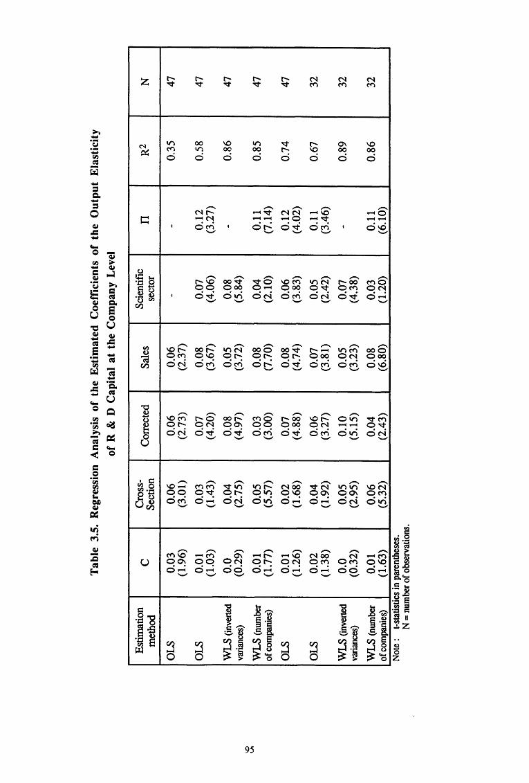
Tab

le 3

.5.

Reg

ress

ion

Ana

lysi

s of

the

Est

imat

ed C

oeff

icie

nts

of t

he O

utpu

t E

last

icit

y of

R &

D C

apit

al a

t th

e C

ompa

ny L

evel

Est

imat

ion

c C

ross

-C

orre

cted

Sa

les

Scie

ntifi

c n

R2

met

hod

Sect

ion

sect

or

OLS

0.

03

0.06

0.

06

0.06

-

-0.

35

(1.9

6)

(3.0

1)

(2.7

3)

(2.3

7)

OLS

0.

01

0.03

0.

07

0.08

0.

07

0.12

0.

58

(1.0

3)

(1.4

3)

(4.2

0)

(3.6

7)

(4.0

6)

(3.2

7)

WL

S (in

verte

d 0.

0 0.

04

0.08

0.

05

0.08

-

0.86

va

rianc

es)

(0.2

9)

(2.7

5)

(4.9

7)

(3.7

2)

(5.8

4)

WL

S (

num

ber

0.01

0.

05

0.03

0.

08

0.04

0.

11

0.85

of

com

pani

es)

(1.7

7)

(5.5

7)

(3.0

0)

(7.7

0)

(2.1

0)

(7.1

4)

OLS

0.

01

0.02

0.

07

0.08

0.

06

0.12

0.

74

(1.2

6)

(1.6

8)

(4.8

8)

(4.7

4)

(3.8

3)

(4.0

2)

OLS

0.

02

0.04

0.

06

0.07

0.

05

0.11

0.

67

(1.3

8)

(1.9

2)

(3.2

7)

(3.8

1)

(2.4

2)

(3.4

6)

WLS

(inv

erte

d 0.

0 0.

05

0.10

0.

05

0.07

-

0.89

va

rianc

es)

(0.3

2)

(2.9

5)

(5.1

5)

(3.2

3)

(4.3

8)

WL

S (

num

ber

0.01

0.

06

0.04

0.

08

0.03

0.

11

0.86

of

com

pani

es)

(1.6

3)

(5.3

2)

(2.4

3)

(6.8

0)

(1.2

0)

(6.1

0)

..

Not

e :

t-sta

usuc

s m

par

enth

eses

. N

= nu

mbe

r of o

bser

vatio

ns.

N

47

47

47

47

47

32

32

32

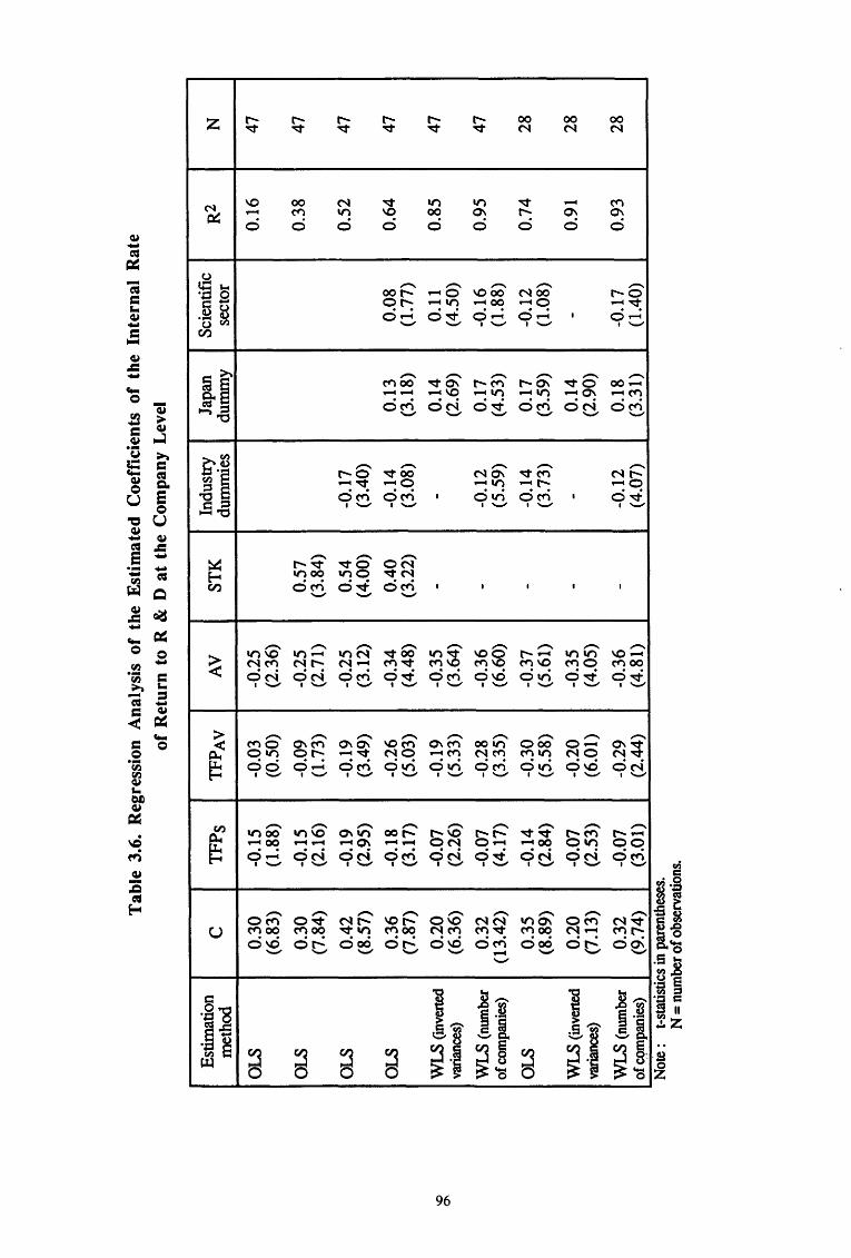
Tab

le 3

.6.

Reg

ress

ion

Ana

lysi

s of

the

Est

imat

ed C

oeff

icie

nts

of t

he I

nter

nal

Rat

e

of R

etur

n to

R &

D

at

the

Com

pany

Lev

el

Est

imat

ion

c TF

Ps

TFPA

v AV

ST

K

Indu

stry

Ja

pan

Scie

ntif

ic

met

hod

dum

mie

s du

mm

y se

ctor

OLS

0.30

-0

.15

-0.0

3 -0

.25

(6.8

3)

(1.8

8)

(0.5

0)

(2.3

6)

OLS

0.30

-0

.15

-0.0

9 -0

.25

0.57

(7

.84)

(2

.16)

(1

.73)

(2

.71)

(3

.84)

OLS

0.42

-0

.19

-0.1

9 -0

.25

0.54

-0

.17

(8.5

7)

(2.9

5)

(3.4

9)

(3.1

2)

(4.0

0)

(3.4

0)

OLS

0.36

-0

.18

-0.2

6 -0

.34

0.40

-0

.14

0.13

0.

08

(7.8

7)

(3.1

7)

(5.0

3)

(4.4

8)

(3.2

2)

(3.0

8)

(3.1

8)

(1.7

7)

WLS

(inv

erte

d 0.

20

-0.0

7 -0

.19

-0.3

5 -

-0.

14

0.11

va

rianc

es)

(6.3

6)

(2.2

6)

(5.3

3)

(3.6

4)

(2.6

9)

(4.5

0)

WLS

(nu

mbe

r 0.

32

-0.0

7 -0

.28

-0.3

6 -

-0.1

2 0.

17

-0.1

6 of

com

pani

es)

(13.

42)

(4.1

7)

(3.3

5)

(6.6

0)

(5.5

9)

(4.5

3)

(1.8

8)

OLS

0.35

-0

.14

-0.3

0 -0

.37

--0

.14

0.17

-0

.12

(8.8

9)

(2.8

4)

(5.5

8)

(5.6

1)

(3.7

3)

(3.5

9)

(1.0

8)

WLS

(inv

erte

d 0.

20

-0.0

7 -0

.20

-0.3

5 -

-0.

14

-va

rianc

es)

(7.1

3)

(2.5

3)

(6.0

1)

(4.0

5)

(2.9

0)

WLS

(nu

mbe

r 0.

32

-0.0

7 -0

.29

-0.3

6 -

-0.1

2 0.

18

-0.1

7 of

CQ

mpa

nies

) (9

.74)

(3

.01)

(2

.44)

(4

.81)

(4

.07)

(3

.31)

(1

.40)

N

ote

: t-s

taus

tics

in p

aren

thes

es.

N =

num

ber o

f obs

erva

tions

.

R2

N

0.16

47

0.38

47

0.52

47

0.64

47

0.85

47

0.95

47

0.74

28

0.91

28

0.93

28

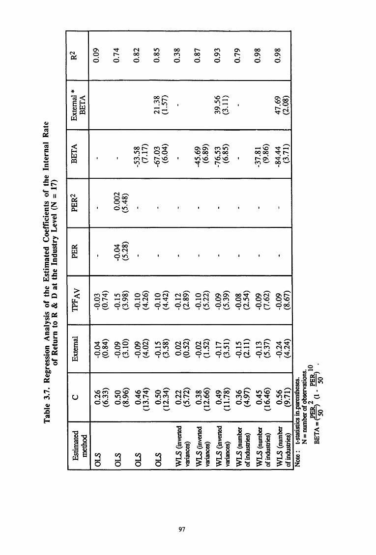
Tab

le 3

. 7.

Reg

ress

ion

Ana

lysi

s of

the

Est

imat

ed C

oeff

icie

nts

of t

he I

nter

nal

Rat

e of

Ret

urn

to R

&

D a

t th

e In

dust

ry L

evel

(N

= 17

)

Est

imat

ed

c E

xter

nal

1PF

AV

P

ER

P

ER

2 B

ET

A

met

hod

OLS

0.

26

-0.0

4 -0

.03

--

-(6

.33)

(0

.84)

(0

.74)

OLS

0.

50

-0.0

9 -0

.15

-0.0

4 0.

002

-(8

.96)

(3

.10)

(3

.98)

(5

.28)

(5

.48)

OLS

0.

46

-0.0

9 -0

.10

--

-53.

58

(13.

74)

(4.0

2)

(4.2

6)

(7.1

7)

OLS

0.

50

-0.1

5 -0

.10

--

-67.

03

(12.

34)

(3.5

8)

(4.4

2)

(6.0

4)

WLS

(in

verte

d 0.

22

0.02

-0

.12

--

-va

rianc

es)

(5.7

2)

(0.5

2)

(2.8

9)

WLS

(inv

erte

d 0.

38

-0.0

2 -0

.10

--

-45.

69

varia

nces

) (1

2.66

) (1

.52)

(5

.22)

(6

.89)

WLS

(in

verte

d 0.

49

-0.1

7 -0

.09

--

-76.

53

varia

nces

) (1

1.78

) (3

.51)

(5

.39)

(6

.85)

WLS

(nu

mbe

r 0.

36

-0.1

5 -0

.08

--

-of

indu

strie

s)

(4.9

7)

(2.1

1)

(2.5

4)

WLS

(num

ber

0.45

-0

.13

-0.0

9 -

--3

7.81

of

indu

strie

s)

(16.

46)

(5.3

7)

(7.6

2)

(9.8

6)

WLS

(nu

mbe

r 0.

56

-0.2

4 -0

.09

--

-84.

44

of in

dust

ries)

(9

.71)

(4

.24)

(8

.67)

(3

.71)

..

N

ote

: t-

stat

tsuc

s m

.par

enth

eses

. N

= n

umbe

r of o

bser

vatio

ns.

J>ER

.. 2

PE

R 1

0 B

ET

A=

{S()

J

(1-

SO

) .

Ext

erna

l*

R2

BE

TA

0.09

0.74

0.82

21.3

8 0.

85

(1.5

7)

-0.

38

0.87

39.5

6 0.

93

(3.1

1)

-0.

79

0.98

47.6

9 0.

98

(2.0

8)

- all things being otherwise equal, the mean value of output elasticity of R & D is

about .08 for sales and zero for value added when data have not been corrected for

double-counting and expensing;

- cross-section analyses show a measure of elasticity superior to .05 to that obtained

from time-series analyses;

- corrections for double-counting and expensing give a positive differential of elasticity

which amounts to .08;

- scientific sectors have a higher elasticity than other sectors, the differential being of

.07;

- estimates obtained from the profit equation give mitigated results (there is a positive

differential from OLS which becomes non significant when variances-based WLS is

used);

- the number of observations, the average period of estimation, the hypothesis of free

return to scale, the reference countty and the industty dummies do not significantly

influence the estimated elasticity of R & D;

- secondly, turning to the estimates of the rate of return on R & D at the fmn level :

- all things being otherwise equal, the mean value of the gross excess rate of return on

R & D is 0.20 when the return is measured with respect to sales and 0.13 when the

total factor productivity with respect to sales is used as dependent variable. Yet,

when the dependent variable is value added or total factor productivity with respect

to value added, the estimated return is not significantly different from zero;

- the use of R & D capital stock instead of R & D expenditure in the measure of R & D

intensity does not provide a significantly different return from that obtained in the

second case. The extra relative return of 40 percent emphasized by OLS results is

not conftrmed by WLS. This apparent discrepancy in the results may be explained

by the lack of statistical representativity of this approach in our sample.

Consequently, the approach calls for further investigations;

- the introduction of industty dummies significantly affects the estimates of the rate of

return (in opposition to the output elasticity of R & D) but without giving better

98

estimates of the rate of return as it seems to be suggested by the non significance of

this variable in the WLS with respect to variances;

- there is a significant premium to the Japanese R & D which amounts to 0.14;

- scientific sectors benefit by a significant premium on R & D of 0.11 (the non

significant result obtained for the subsample is explained by the fact that these

sectors are to a large extent excluded);

- the number of observations, the a~erage period of estimation and the hypothesis of

free return to scale do not significantly influence the estimated rate of return on R &

D;

-thirdly, concerning the estimates of the rate of return on R & D at the industry level:

- all things being otherwise equal, the mean value of the gross excess internal rate of

return on R & D is 0.22 when it is estimated with respect to sales and it is 0.10 when

estimates are run on the basis of value added, but these estimates are downward

biased due to the fall in the rates of return during the sixties.

- when this phenomenon is taken into account the mean values go up to 0.38 and 0.28

respectively. To grasp the decrease in the rate of return during the sixties, we

introduced as an explanatory variable into the model a quadratic function of the

average period of estimation (represented in the results by PER and PER2). Yet, as

such a function has infinite values at its extremes, we alternatively adjusted a Beta

distribution whose optimal values of the exponents were estimated by a search

procedure. According to these two approaches, the lowest rate of return was

attained in 1959-1960 with values equal to 0.18 and 0.08 respectively. The mean

values referred above are hit at the beginning of the seventies;

- taking value added instead of sales to measure R & D intensity shows a decrease in

the estimated rate of return of about 10 percent;

- the joint estimation of both internal and external rates of return decreases the estimate

of the internal rate of about 10 percent. Yet, as shown by the combined variable

External *BET A, this effect is less pronounced when the internal rate of return is

weak.

99

In a nutshell, the econometric evaluation of the impact of R & D on economic

growth allows to conclude that R & D investment is a significantly important source of

productivity gains. A large part of discrepancies between the coefficients estimated may

be explained by data and regression characteristics. To some extent, the discrepancies

explained by our regression analysis show that econometric studies of R & D are not so

imprecise and unreliable as it might be thought at first glance. Yet, plentiful

methodological and conceptual problems remain. In the last years, some very significant

improvements have been brought to the modelling of R & D and its spillover effects.

3.4. Adjustment Cost Models

So far, we have only considered static equilibrium models in which production

factors are always at ·their expected long-term level. These models can be made dynamic

in two ways:

- frrst, by considering that all or some factors only adjust partially to their short-run

equilibrium level;

- second, by envisaging a cost of adjustment model with a short-run disequilibrium

situation whose dynamic perspective presupposes the realisation of a long-term equili­

brium.

The adjustment cost models are based upon the hypothesis that firms face a

technology which uses variable factors (e.g., labor, energy and intermediary inputs) and

quasi-fixed factors (like physical capital and R & D capital). Some of the quasi-fixed fac­

tors cannot vary at short-term with respect to the equilibrium level and any change in the

level of these factors implies costs of adjustment

Mohnen and Nadiri ( 1985) developed cost of adjustment models including R & D

investments. They are assimilated to a production factor because they are at the origin of

new products and/or processes generating new sales and/or a reduction of production

costs. Both physical capital and R & D stock face costs of adjustment when their level

changes. These costs are caused by the instalment of new machines, the reorganisation of

production tasks and the familiarization with new working circumstances in the case of

capital; they also result from the difficulty in implementing and working out a research

project, and in marketing new products and processes. In this model, labor and

intermediary inputs are variable factors.

100

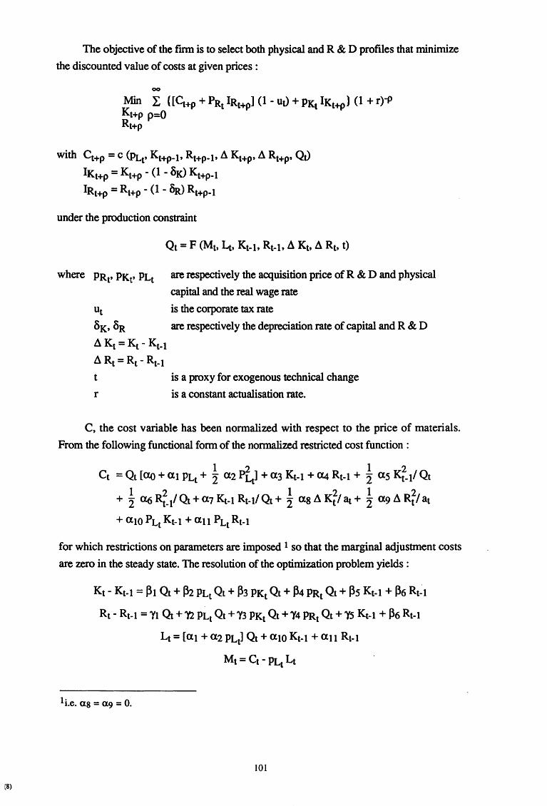
(8)

The objective of the finn is to select both physical and R & D profiles that minimize

the discounted value of costs at given prices :

00

with Ct+p = c (PLt' Kt+p-t, Rt+p-t, A Kt+P' A Rt+P' Qt)

IKt+p = Kt+p - (1 -OK) Kt+p-t

IRt+p = Rt+p- (1- ~) Rt+p-t

under the production constraint

where PRt' PKt' PLt are respectively the acquisition price of R & D and physical

capital and the real wage rate

ut is the corporate tax rate

OK, OR are respectively the depreciation rate of capital and R & D

A Kt = Kt - Kt-t

ARt= Rt- Rt-t t

r

is a proxy for exogenous technical change

is a constant actualisation rate.

C, the cost variable has been normalized with respect to the price of materials.

From the following functional form of the normalized restricted cost function :

1 2 1 2 Ct = Ot [<Xo +at PLt + 2 a2 PL11 + a3 Kt-t + <X4 Rt-t + 2 as Kt-tl Ot

1 2 1 2 1 2 + 2 Cl6 Rt-l Ot + a7 Kt-t Rt-tl Ot + 2 as A Ktl at+ 2 a9 ARt/ at

+ ato PLt Kt-t +au PLt Rt-t

for which restrictions on parameters are imposed 1 so that the marginal adjustment costs

are zero in the steady state. The resolution of the optimization problem yields :

Kt- Kt-t = ~t Ot + P2 PLt Ot + ~3 PK1 Qt + ~4 PR1 Qt + Ps Kt-t + ~6 Rt~t

Rt- Rt-t = 'Yt Qt + Yl PL1 Ot + 'Y3 PKt Qt + 'Y4 PR1 Qt + 'Y5 Kt-t + ~6 Rt-t

Lt =[at+ a2 PLt] Ot +a to Kt-t +au Rt-t

Mt = Ct - PLt Lt

1i.e. as = a9 = 0.

101

in which the ~i and 'Yi coefficients are linked to the ai by different constraints 1•

It is a similar model which was successfully estimated by Cardini and Mohnen

(1984), Mohnen and Nadiri (1985) and Mohnen, Nadiri and Prucha (1986) for the

Italian, American, Japanese, German and French cases. They observed that the

adjustment lags of R & D are noticeably more important than for physical capital2. While

the adjustment speed of capital is relatively identical among countries, the adjustment

speed of R & Dis faster in the United States. Furthermore, the internal rate of return

appears higher for R & D than for physical capital. The main results are summarized in

table 3.8.

Table 3.8. Impact of R & D in the Manufacturing Sector (1965-1978)

Dependent variable Parameter us Japan Genna- France Italy ny

Gross output Adjustment speed in fli'St .17 .11 .09 .02 -period

Short-run elasticity .16 .23 .20 .13 -Internal rate of return .11 .15 .13 - -

Contribution to labor .03 .03 .02 .04 productivity -

Value added Adjustment speed in fli'St .15 .26 .26 .07 .13 period

Short-run elasticity .18 .36 .35 .16 .18

Internal rate of return - - - .11 .12

Sources: Cardani and Mohnen (1984),Mohnen and Nadiri (1985) and Mohnen, Nadiri and Prucha ( 1986).

While the labor factor is still considered in a traditional way in this model, the in­

corporation of R & D expenditure as a quasi-fixed factor submitted to adjustment costs

makes this model an important step towards the endogenisation of technical change. It

could easily be extended to take into account human capital by distinguishing the skill

levels some of which are not readily malleable in the short run and face adjustment costs

resulting from the learning process inherent in the acquiring skills.

1For more details, cf. Mohnen and Nadiri (1985) and Mohnen, Nadiri and Prucha (1986) whose studies have inspired the simplified model developed here. 2 The mean lag for physical capital is about 3 years against five years and more for R & D capital.

102

This dual formulation based on the producer theory, which represents the techno­

logy of production by means of the cost function, is an important methodological step in

modelling producer behavior. The measurement of the rate of return on R & D in models

noticeably differs from the method used in Cobb-Douglas functions.

In the framework of the adjustment-cost model, it is assumed that the firm mini­

mizes the present value of expected production costs. This problem can be written as :

00

Min J e-Pt [c (pL, K, R, IK, IR, Q) + PK (p +OK) K + PR (p +OR) R] dt IK, IR 0

where the prices Pi (p + Oi) are the relative rental rates of the capital stocks, Oi, the rate of

depreciation and p, the real discount rate.

The internal gross rate of return on R & D is equal to :

• a c a c (p +OK) = (- aR + dJR) I PR

This equation shows that the internal net rate of return on R & D is nothing else that

the diminution of the production cost due to a marginal increase of R & D stock, net of

marginal adjustment cost and net of depreciation.

If the producer can immediately adapt his inputs to his level of production, the cost

minimisation problem amounts to minimizing the costs at each period :

Min [c (pL, K, R, Q) + PK (p +OK) K + PR (p +OR) R] IK, IR

so that in the static case, the internal gross rate of return on R & D is given by :

from which, compared to the dynamic case, the marginal adjustment cost has disap­

peared. So, the existence of costs of adjustment affects the rate of return on R & D.

103

Chapter 4. The Spillovers from R & D Investment

The effects of R & D go beyong the fmn, the industry and the country that perform

the R & D. The main feature of such an investment is that fmns which do it cannot

exclude others from obtaining a part of the benefits free in charge. In other words, spill­

overs arise because the returns of R & Dare not entirely appropriable. Only a perfectly

discriminant monopolist can appropriate quasi-rents from technical change and so escape

the diffusion of technological know-how to other enterprises. Von Rippel (1982) indica­

ted that, in the case where there is no monopoles and even if there exists a patent or

licence, there will not be perfect appropriability of the scientific discovery. There is to

some extent a contradiction between the social interest which suggests that the diffusion

of innovations should rapidly spread out throughout the economy and so boost the eco­

nomic growth and the private interest which checks the diffusion process in order to

maximise the private rent. Coming back to the seminal contribution of Arrow (1962),

technology is equivalent to information and as such characterized by indivisibilities. It

can be transmitted and rented without cost. Once produced, a new technology is like a

public good because it is available to everybody free of charge. At the two extremities of

the spectrum of appropriability opportunities, there is on one side the perfect monopolist

who can grab all the benefits from an innovation, and, on the other side, the producer

facing a perfect competititve market is not in a position to grab the welfare benefits from

the innovation. Along the spectrum, there are lots of situations which depend on the

market structures. This appropriability phenomenon corresponds to a first kind of spill­

overs emphasized by Griliches (1979). There are characterized by R & D intensive in­

puts purchased from other industries at less than their full quality price. Their produc­

tivity effects are not fully measured by official prices indexes because all quality im­

provements are not totally appropriated by the senders and are rarely incorporated into

official statistics. The second kind of spillovers deals with the real know ledge transmis­

sion. They result from discoveries and innovations in an industry whose some ideas of

which can be fruitfully borrowed in other industries to generate technological improve­

ments of products and processes in these industries. All these industries need not buy

from each other to benefit from this new knowledge and consequently, such spillovers

cannot adequately be trailed through the conventional interindustry relationships such as

input-output matrices.

So, these "knowledge" spillovers are more difficult to trace than the "economic"

spillovers because we do not have any grounded a priori information about the potential

beneficiaries of these researches. At the very most, it seems reasonable to assume that

105

for a given firm the major knowledge spillovers come from inside its own industry. For

the knowledge spillovers coming from outside its own industry, it is the concept of

technological proximity which must guide the search of source industries. The confusion

in the literature between these two kinds of spillovers is due to the fact that, in empirical

analyses, it is not an easy task to measure their effects separately. Regarding the

methods, the measure of any type of spillovers will be conveniently approximated but

one should bear in mind that, to some extent, the measure will also represent the effects

of the second type of spillovers.

While case studies are less general than econometric studies, they enable a more

acute measure of the real performance of specific innovations. However, their results

cannot be generalized and these studies often focus on successful innovations. They

usefully supplement the more aggregated approaches which deal with the full research

system at firm, industry or economy wide level. In order to have a larger view of the

extent of inter-industry spillovers, several approaches have been investigated in the

literature. A first method is to take into account the proximity between industries by

giving weights to R & D stocks according to how close to each other industries are. The

question here is to know what proximity measure to use to construct the weights. The

different proximity measures reponed in the literature are successively : weights

proportional to the flows of intermediate input purchases by using the input-output

coefficients, to the flows of patents or innovations by constructing a technology flow

matrix or to the firm's position in a technology space as measured by the uncentered

correlation of the patent distribution across technological areas. A second approach is to

consider the outside pool of R & D knowledge globally by adding up the R & D stocks of

other firms or industries. A strong assumption at the basis of this method is that the R &

D knowledge of other firms or industries is equally useful for the studied industry

whatever its characteristics. A last method is to enter separately into the production

function the R & D stock of each potential source of R & D spillover which constitutes an

extension of the preceding one.

4.1. About some Case Studies

In a case-study of 17 industrial innovations, Mansfield and al. (1977) calculated

both the private and the social rates of return from the investments in these innovations.

Their results indicate that the private rates have been much lower than the social ones.

The medium social rate of return was about 56 percent against a median private rate of

about 25 percent. Yet," there are very high variations in the private rates of return : six

106

innovations had a return inferior to 10 percent and five innovations a return superior to 40

percent. In this study, private benefits are measured by the net profits from the innovator

to the innovation. Social benefits are obtained by adding to the private benefits the

benefits derived by households and other ftrms from price reducing and imitation and

substracting the private costs, the unsuccessful R & D costs incurred by other ftrms and

environmental costs. Information was obtained from interviews with the relevant firms

and from published reports. The median values are consistent with the main estimates

obtained from econometric studies. Yet, this case-study shows that there can be very

wide differences between private and social rates of return, a result also consistent with

new econometric studies.

In a study of the spillovers from advances in general purpose computers to the

financial services, Bresnahan ( 1986) showed that the demand for high-speed computers

implied a very large social gain. The welfare gain that he measured is the reduction in the

price-performance ratio of computers not taken into account in real output indexes. The

basic idea is that, if an innovation only lowers the price of a consumption good, the area

under its demand curve measures the sum of the increased producer's surplus in the

downstream sectors plus the consumer's surplus of final demanders. Purchases of

computers by the financial services are treated as if this sector acted as an agent for its

customers and under this assumption, the welfare gains to the customers from service's

derived demand for computers are evaluated. From the calculations covering years 1958

and 1972, it appears that the spillover to adopters of computers and their customers has

been large comparatively to expenditures on computers. The size of the downstream

welfare gains resulting from the fall in the price-performance ratio of computers in the US

was at least five times the size of computer expenditures in 1972.

A method of constructing quality-adjusted price indices capturing the impact of

product innovations has been suggested by Trajtenberg (1989). This approach is based

on a two-stage estimate. First, discrete choice models are used to model the consumer

preference system and to derive the surplus function in order to measure the benefits from

innovation. Second, quality-adjusted price indices are constructed by using the estimates

of the social surplus function. The author applies the method to the case of Computed

Tomography Scanners, a highly sophisticated medical diagnostic technology first

introduced in the US in 1973. The evolution of this market was characterized by a fierce

competition between firms which brought about a breathtaking pace of technical advance.

The pace of innovation in CT scanners subsided in the mid-eighties as the technology

matured and new technological developments took over. His main finding is that the

quality-adjusted price of this product -went down from 10 000 to 7 from 1973 to 1982

107

(implying an average price reduction of 55 percent per year) while the unadjusted price

went up from 10 000 to about 26 000, (i.e. 2.6 times more expensive in 1982). The rate

of decline particularly staggered during the frrst years following the introduction of the

innovation. This example illustrates how inadequate conventional economic indicators

are to deal with the welfare consequences of technical advance.

4.2. The Inter-Industry Technology Flow Matrix Approaches

The frrst to propose the construction of an input-output matrix of invention flows

was Schmookler (1966) but it was only ten years later than his advice materialized with

the first attempt made by Terleckyj (1974). In a first analysis, Terleckyj combined R & D

data with conventional input-ouput tables to estimate the R & D borrowed by an industry

under the hypothesis that the higher the purchase of intermediate inputs of an industry

from an other industty is, the more knowledge the purchasing industry borrows from the

sending industry. He then regresses the total factor productivity growth rates of

manufacturing industries I on R & D performed in the industry and the R & D embodied

in inputs purchased from other industries. He also operates a distinction between

privately and publicly-fmanced R & D. The estimated excess rate of return for embodied

R & D was almost triple the rate of return on own R & D for private R & D while the

indirect effects from federally-financed R & D were not significant. His result as well as

the main ones of studies ·discussed below are reproduced in table 3.3. of the preceding

chapter .. :in a second study, Terleckyj (1980a) re-examines his results by exploiting new

data on total factor productivity growth which attempted to account for quality

improvements of inputs. The coefficient for privately-financed purchased R & D was

statistically significant and more than twice the estimate obtained with unadjusted data.

Griliches and Lichtenberg (1984b) reexamined this relationship between

productivity growth and R & D intensity using detailed data for US manufacturing

industries over various subperiods and breaking down R & D into own and purchased

product- and process-improvement-oriented components. According to them, the

productivity growth rate of an industry is affected by the R & D performance of

industries which supply it with intermediate inputs because of errors in the output

deflators of these supplying industries-errors which cause the materials deflators not to

accurately reflect changes in the user value of intermediate inputs. They add that the

extent of mismeasurement of the growth in a deflator depends on the extent of product­

oriented R & D activity in the supplying indusny and argue that "since process-oriented R

1 For non-manufacturing industries, only indirect returns are significant with a coefficient of 1.87.

108

& D does not alter the characteristics of products sold in inter-industry transactions, it

should not contribute to errors in the measurement of deflators corresponding to these

transactions". In their subsequent empirical analysis, these measurement errors are

assumed to be proportional to the product-oriented R & D intensity of supplying

industries. Their results are consistent with the assumption that the product-oriented R &

D of the origin industry has a lesser effect than own process-oriented and embodied

product-oriented R & D. This study is a re-assessment of Scherer (1982)'s study in

which the author gave "evidence of substantial returns on used R & D, i.e. from internal

process work and the purchase of R & D embodying products, but not . . . to the

performance of product R & D". In their study, Griliches and Lichtenberg showed that

the significance of the combined process and embodied R & D variable was largely due to

the process component

A similar study using an input-output table of transaction flows was realized by

Goto and Suzuki (1989) to examine the effects of R & Don the productivity growth of

Japanese manufacturing industries. They obtain comparable results to these obtained by

preceding analyses : the coefficient of the embodied R & D intensity is much larger than

that of own R & D intensity. They complete their study by an attempt to measure the

effect of electronics technology upon the productivity growth in industry through the

electronics-related embodied R & D and through the diffusion of technological

knowledge created by the electronics-related industries. The knowledge spillover

variable is a weighted sum of R & D by electronics-related industries where the weights

are the uncentered correlation coefficients between the R & D expenditures by product

areas realized by each industry and by the electronics-related industries. The results

suggest that the impact of electronics technology on the productivity growth of industries

is mainly achieved through the diffusion of technological knowledge rather than through

the electronics-related embodied R & D. This finding may be explained by the public

goods characteristics which permit industries to acquire these technologies through other

channels than through the transactions of intermediate or investment goods and exploit

them to develop new products and to improve their production processes.

The second way of constructing an inter-industry technology flow matrix, initiated

by Scherer (1982), is by classifying patent data according to industry of origin and

industries of use. The patent flow matrix is then used to attribute R & D data by industry

of origin to the industry of use. Patents with multiple or general uses were flowed out to

multiple using industries proportionally to their purchases from the origin industry. In

his matrix, row sums measure R & D by industry of origin, column sums R & D by

industry of use and the diagonal represents pure process R & D. Then, he uses these

new data to analyse the links between R & D and productivity growth by distinguishing

109

between the effects of origin and user industry R & D. Origin industry R & D concerns

own product R & D while user industry R & D combines own process and embodied R

& D. He finds little positive effect of origin industry R & D and a high positive effect of

user R & D and concludes that user R & D is the more appropriate measure. Yet,

whereas Scherer's results indicate an increase in both the size and the significance of the

coefficient on user R & D from 1964-69 to 1973-78, Griliches and Lichtenberg (1984b)

in their re-examination of Scherer's findings on the basis of a more disaggregated and

superior data set observe a secular decline in the effect of user R & D on productivity

growth. In contrast to Scherer, they also find own-product of R & D to be a significant

determinant of productivity growth except for the period from 1964-68 to 1969-73.

A more extensive similar study was realized by Englander, Evenson and Hanazaki

(1988) by pooling country data for the period 1970-1983. Their country sample includes

France, the United-States, the United-Kingdom, Germany, Japan, Canada and Italy. To

construct the user industry R & D stocks, their use the Canadian patent-based technology

flow matrix by assuming that the proximity between industries is the same for all the

countries. Then, they separately regress total factor productivity levels on user industry

R & D intensities and on origin industry R & D intensities for both manufacturing and

non-manufacturing industries. From their estimates, they conclude that productivity

levels are linked to user industry R & D, even more so in manufacturing than in non­

manufacturing, and that the extent of these links varies a lot across industries. The

effects are higher in the R & D intensive industries and the equation using user industry R

& D stocks instead of origin industry R & D stocks gives better results. In order to see if

the R & D potential had really changed over the period, alternative regressions were

realized in which the influence of R & D could modify after the period 1970-1973. Their

results give evidence that the R & D seems to be becoming less productive after this

period in a lot of industries. However, such an observation may be discussed because of

the weak significance of the estimated coefficients. It will also be noted that only seven

coefficients are significant and have the right sign in their analysis, four coefficients are

non-significant, the remaining ones are generally significantly negative. The authors do

not offer clear explanation for such divergences in results. The omission of important

explanatory variables for the non-manufacturing industries, the low user industry R & D

stocks for some industries and the distortions in the measure of the explanatory variable

may be at the origin of the mitigated results obtained.

On the one hand, the transaction approach assumes that the user industries of R &

D output originated in another industry are distributed proportionally to the purchases of

110

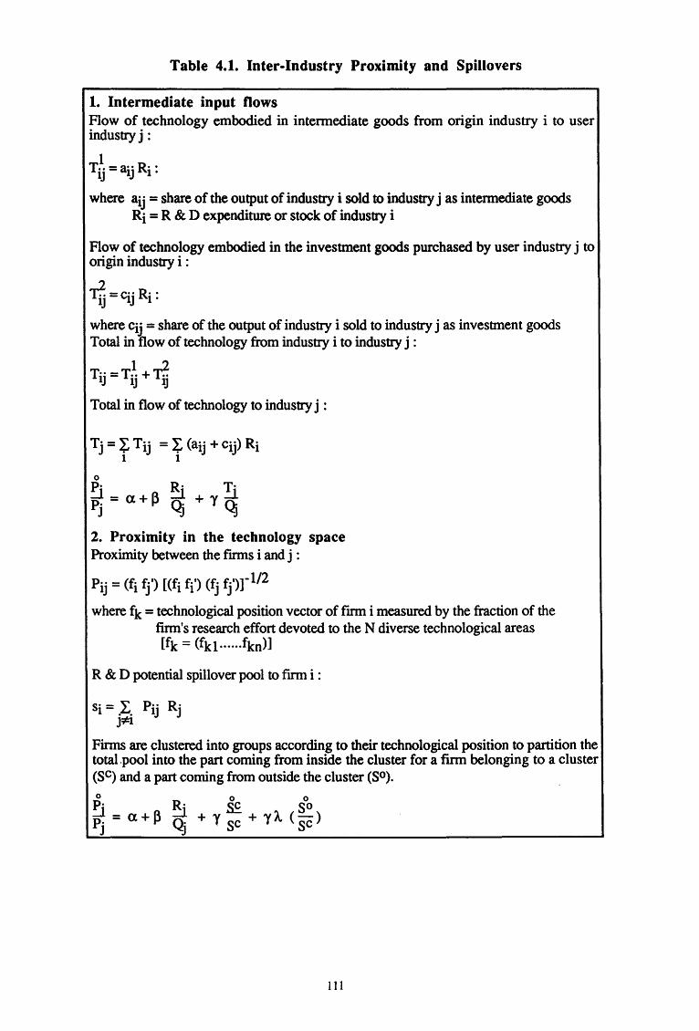
Table 4.1. Inter-Industry Proximity and Spillovers

1. Intermediate input flows Flow of technology embodied in intermediate goods from origin industry i to user industry j:

1 Tij = aij Ri:

where aij = share of the output of industry i sold to industry j as intermediate goods Ri = R & D expenditure or stock of industry i

Flow of technology embodied in the investment goods purchased by user industry j to origin industry i :

Tij = Ci.j Ri :

where Cij = share of the output of industry i sold to industry j as investment goods Total in flow of technology from industry i to industry j :

Til =T~- +~ ~ 1J 1J

Total in flow of technology to industry j :

2. Proximity in the technology space Proximity between the firms i and j :

P· · - (f· f·') [(f· f·') (f· f·')]-l/2 ~ - 1 J 1 1 J J

where fk = technological position vector of firm i measured by the fraction of the firm's research effort devoted to the N diverse technological areas [fk = (fkl······fkn)1

R & D potential spillover pool to firm i :

s·- L P·· R· 1-. . 1J J j:¢:1

Firms are clustered into groups according to their technological position to partition the total .pool into the part coming from inside the cluster for a firm belonging to a cluster (SC) and a part coming from outside the cluster (SO).

0 0 0 P· R· ~ so ~ = a + 13 ~ + 'Y sc + 'Y A. ( sc )

111

intermediate inputs and capital goods to this industry and, on the other hand, the patent

approach assumes that each industry has a same propensity to patent, all patents have a

same value inside an industry and patent data are representative of the innovative activity.

Each of these approaches has its own advantages and drawbacks. To overcome some

limits of the patent approach, it could directly be made use of the flows of innovations

from origin industries to user industries. It is the way adopted by Robson, Townsend

and Pavitt (1988) in a descriptive analysis of the sectoral patterns of production and use

of technology in the UK during the period 1945-1983. Unfortunately, this innovation­

based intersectoral technology flow analysis has not been continued by an econometric

estimation of the social rate of return of these innovations. In this descriptive study, the

information was collected through a survey of significant innovations commercialised in

the UK. Their sample covers more than 4 000 innovations which are identified with

respect to the innovating industry and the first user industry. Five "core .. sectors appear

to be at the origin of about two third of the innovations : chemicals, machinery,

mechanical engineering, instruments and electronics. The ratio of products to process

innovations is about four in the core sectors against two for the full sample. From a

comparison of their data with Scherer's, they observe that sectoral structures of

production and use of technology are very similar in the UK and US. A trend analysis in

the production and use of technology shows that there has been an increase in the

proportion of product innovations used outside manufacturing and considerable shifts in

the distribution of production within manufacturing where innovations increase in

instruments and electronics and decrease in chemicals and steel.

4.3. The Spillovers in the Technology Space

Alternatively, as summarized in table 4.1. one can also measure the technological

proximity between frrms by characterizing their positions in the technological space. It is

possible, for example, to use the distribution of the firm's patents over patent classes to

characterize their technological position. This approach was developed by Jaffe (1986).

He quantifies the effects of exogenous variations in the state of technology (technological

opportunities) and of the R & D spillovers on the R & D productivity of firms. He

observes that the R & D productivity is increased by the R & D of technologically

proximate firms though their R & D lowers the profits and market value of low-R & D­

in tensity firms. Firms appear to adjust the technological composition of their R & D in

response to technological opportunity. He defines the technological opportunity as the

exogenous variations in the cost and the difficulty of innovation in different technological

areas.

112

To look for the effects of technological opportunities and spillovers, he identifies

the technological areas of firms. The technological position of firms is captured through

the distribution of the fmns' patents over patent classes. Assuming that the existence of

technological spillovers implies that a finn's R & D success is affected by the research

activity of its neighbors in technology space, a potential spillover pool, which is the

weighted sum of other fmns' R & D, is measured. On the basis of position vectors, firms

are classified into technological groups. Firms whose technological focus is sufficiently

similar are assumed to face the same state of technological opportunity. In a second stage,

he relates the finn's patent applications, profits and market value to its R & D, the poten­

tial spillover pool, dummies for the technological opportunity, its capital stock, its market

share and the concentration ratio. The main results are presented in table 4.2. The patent

elasticity of R & D is .88 for the average fmn and increases with the value of the average

pool. The patent elasticity with respect to the R & D pool is about 1.1. This result shows

that more than one-half of R & D impact on patents comes from the spillover effect. The

results from the profit equation convey a gross rate of return on R & D of 27 percent

against 15 percent for physical capital. The profit elasticity of R & D is .18 and is in­

creased by the spillovers. Yet the direct effect of the pool is to lower profits. About one­

third of the net increase of profits due to R & D comes from the spillovers.

For firms with largely less R & D than the mean, the net effect of the pool is nega­

tive. While from a purely technological standpoint R & D spillovers constitute an unam­

biguous positive externality, they are potentially blurred with a negative competitive effect

of competitors' R & D. This competitive effect of the pool comes into play when we turn

to the economic return on R & D. Finally, the average elasticity of the ftrrn's market value

to the pool is about .05 and the pool effect is negative for firms with a low R & D-capital

ratio.

In a complementary study, Jaffe (1988) quantifies the effect of technological oppor­

tunity, market demand and R & D spillovers on R & D effort and productivity growth.

The elasticity of own R & D with respect to the research pool is statistically significant

and equal to .27. This result indicates that the technology position is an explanatory factor

of R & D investments. The fraction of cluster pool in total pool is also included to

estimate if there is a premium for the within-cluster firms. The absence of a cluster pre­

mium effect gives evidence that there is no further differential to the in-cluster firms. In

order to distinguish between demand-pull and technological opportunity effects, he intro­

duces in his model the fractions of sales going to distinct markets as indicators of market

position. This variable proves significant, which allows us to say that innovative activity

113

- - ~

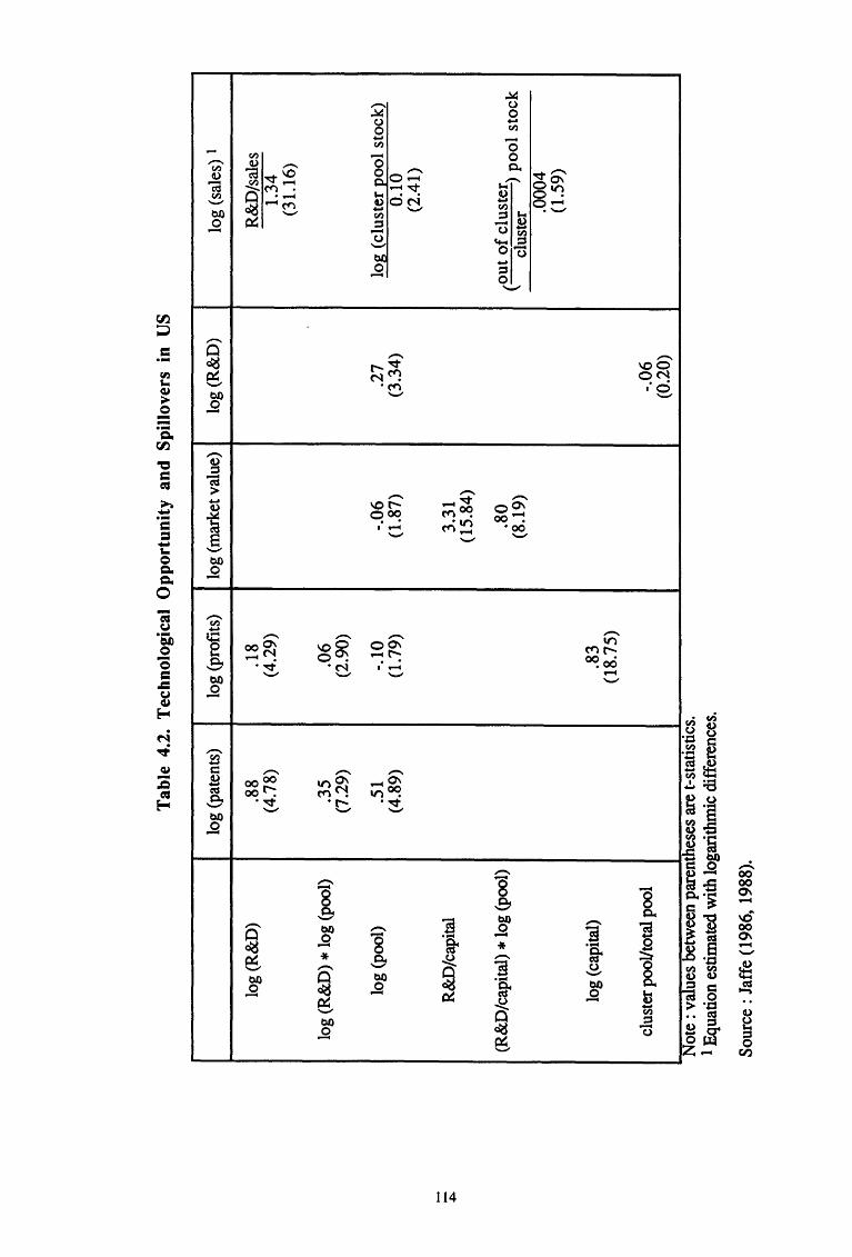
Tab

le 4

.2.

Tec

hnol

ogic

al O

ppor

tuni

ty a

nd S

pill

over

s in

US

log

(pat

ents

)

log

(R&

D)

.88

(4.7

8)

log

(R&

D)*

log

(poo

l)

.35

(7.2

9)

log

(poo

l)

.51

(4.8

9)

R&

D/c

apita

l

(R&

D/c

apita

l) *

log

(poo

l)

log

(cap

ital)

clus

ter p

ooV

tota

l poo

l

..

Not

e : v

alue

s be

twee

n pa

rent

hese

s ar

e t-

stat

tsttc

s.

1 E

quat

ion

esti

mat

ed w

ith lo

gari

thm

ic d

iffe

renc

es.

Sou

rce

: Jaf

fe (

198

6, 1

988)

.

log

(pro

fits

) lo

g (m

arke

t val

ue)

log

(R&

D)

.18

(4.2

9)

.06

(2

.90)

-.10

-.

06

.27

(1.7

9)

(1.8

7)

(3.3

4)

3.31

(1

5.84

)

.80

(8

.19)

.83

(18.

75)

-.06

(0

.20)

log

(sal

es)

1

R&

D/s

ales

1.

34

(31.

16)

log

(clu

ster

EO

Ol

stoc

k)

0.10

(2

.41)

(ou

t o

f cl

uste

r)

1 k

clus

ter

po

o

stoc

.000

4 (1

.59)

is the result of both the pull of market forces and the push of exogenous technological

factors on the supply side of innovation.

In his productivity function, both technological position and market position are not

significant. The measure of the growth excess return on R & D (data not having been

corrected for double counting) is significant and implies an annual rate of return of 27

percent (the initial coefficient being calculated over 5 years). The elasticity of the cluster

pool stock says that a 10 percent increase of the R & D pool yields 1 percent more output

of the fmn. The coefficient of the relative value of the out-of-cluster pool stock with

respect to the cluster pool stock is very small, which gives evidence of an apparently

localized effect of spillovers. So, R & D generated outside the cluster seems to

considerably influence the R & D of the firms belonging to a cluster but not directly their

productivity.

4.4. The Econometric Measurement of Total Spillovers by Industry

The measure of the spillover effects by considering the unweighted outside pool of

R & D knowledge was essentially initiated by Bernstein (1988) and Bernstein and Nadiri

(1989) in their analysis of both intra-industry and inter-industry spillovers in seven

Canadian industries and of intra-industry spillovers in four US industries. In the study

of the spillovers between Canadian industries the production technology is characterized

by a cost function with labour, materials, physical capital and R & D capital as variable

inputs and the R &D capital of all rival firms in the same industry and the R & D capital

of other industries as intra-industry and inter-industry spillover variables respectively.

From the estimates of a translog cost function and of cost share equations, the author

derived the elasticities on unit costs of production and factor demands with respect to the

spillover variables and the rates of return on R & D. His main findings are that :

-the estimates related to the spillover variables are generally significant;

- the inter-industry spillovers exert greater downward pressure on average production

costs compared to intra-industry spillovers;

- unit costs decrease more in response to an increase in the intra-industry spillover in

industries with relatively larger R & D cost shares and in the inter-industry spillover

in industries with relatively smaller R & D cost shares;

115

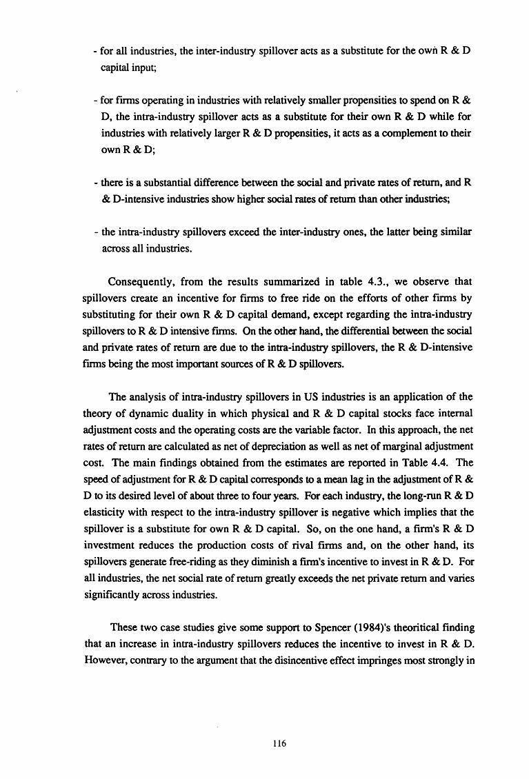
- for all industries, the inter-industry spillover acts as a substitute for the own R & D

capital input;

- for fmns operating in industries with relatively smaller propensities to spend on R &

D, the intra-industry spillover acts as a substitute for their own R & D while for

industries with relatively larger R & D propensities, it acts as a complement to their

own R&D;

- there is a substantial difference between the social and private rates of return, and R

& D-intensive industries show higher social rates of return than other industries;

- the intra-industry spillovers exceed the inter-industry ones, the latter being similar

across all industries.

Consequently, from the results summarized in table 4.3., we observe that

spillovers create an incentive for firms to free ride on the efforts of other firms by

substituting for their own R & D capital demand, except regarding the intra-industry

spillovers to R & D intensive fmns. On the other hand, the differential between the social

and private rates of return are due to the intra-industry spillovers, the R & D-intensive

fmns being the most important sources of R & D spillovers.

The analysis of intra-industry spillovers in US industries is an application of the

theory of dynamic duality in which physical and R & D capital stocks face internal

adjustment costs and the operating costs are the variable factor. In this approach, the net

rates of return are calculated as net of depreciation as well as net of marginal adjustment

cost. The main findings obtained from the estimates are reported in Table 4.4. The

speed of adjustment for R & D capital corresponds to a mean lag in the adjustment of R &

D to its desired level of about three to four years. For each industry, the long-run R & D

elasticity with respect to the intra-industry spillover is negative which implies that the

spillover is a substitute for own R & D capital. So, on the one hand, a firm's R & D

investment reduces the production costs of rival firms and, on the other hand, its

spillovers generate free-riding as they diminish a firm's incentive to invest in R & D. For

all industries, the net social rate of return greatly exceeds the net private return and varies

significantly across industries.

These two case studies give some support to Spencer (1984)'s theoritical finding

that an increase in intra-industry spillovers reduces the incentive to invest in R & D.

However, contrary to the argument that the disincentive effect impringes most strongly in

116

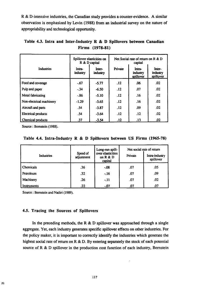
(9)

R & D-intensive industries, the Canadian study provides a counter-evidence. A similar

observation is emphasized by Levin ( 1988) from an industrial survey on the nature of

appropriability and technological opportunity.

Table 4.3. Intra and Inter-Industry R & D Spillovers between Canadian Firms (1978-81)

Spillover elasticities on Net Social rate of return on R & D R & Dcapital capital

Industries Intta- Inter- Private Intra- Inter-industry industry industry industry

spillover spjllover

Food and coverage -.67 -5.77 .12 .06 .02

Pulp and paper -.34 -6.50 .12 .07 .02

Metal fabricating -.86 -5.10 .12 .16 .02

Non-electrical machinery -1.29 -3.65 .12 .16 .02

Aircraft and parts .54 -3.87 .12 .09 .02

Electrical products .54 -3.64 .12 .12 .02

Chemical products .37 -3.54 .12 .13 .02

Source: Bernstein (1988).

Table 4.4. Intra-Industry R & D Spillovers between US Firms (1965-78)

Long-run spill- Net social rate of return

Industries Speed of over elasticities

Private Intra-industry adjustment on R&D capital spillover

Chemicals .36 -.08 .07 .05

Petroleum .32 -.16 .07 .09

Machinery .26 -.11 .07 .02

Instruments .22 -.07 .07 .07

Source : Bernstein and Nadiri (1989).

4.5. Tracing the Sources of Spillovers

In the preceding methods, the R & D spillover was approached through a single

aggregate. Yet, each industry generates specific spillover effects on other industries. For

the policy maker, it is important to correctly identify the industries which generate the

highest social rate of return on R & D. By entering separately the stock of each potential

source of R & D spillover in the production cost function of each industry, Bernstein

117

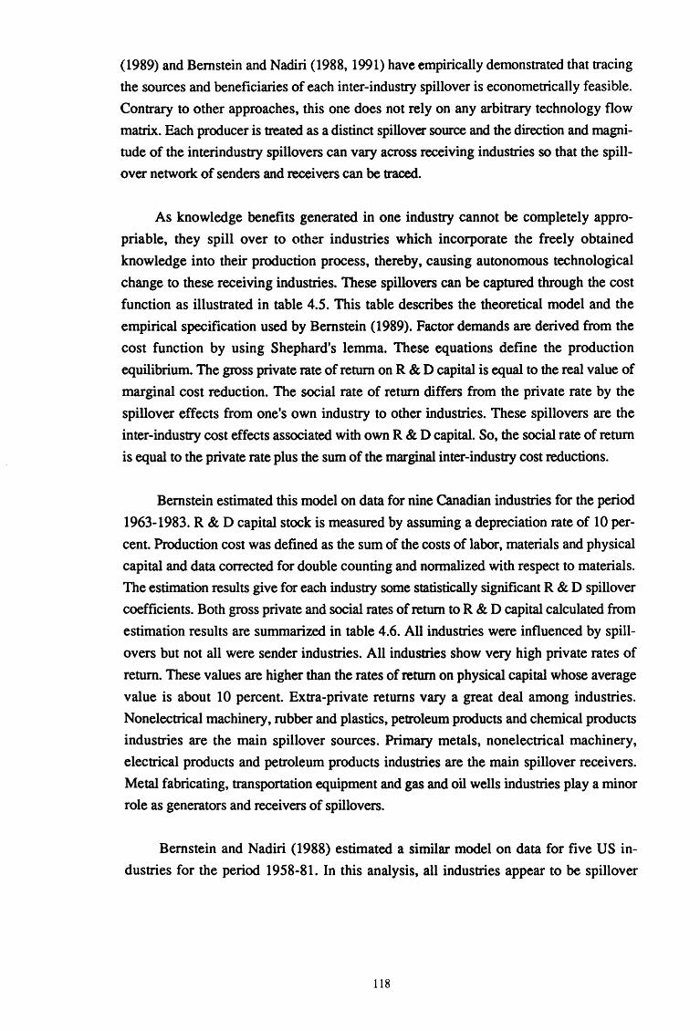
(1989) and Bernstein and Nadiri (1988, 1991) have empirically demonstrated that tracing

the sources and beneficiaries of each inter-industry spillover is econometrically feasible.

Contrary to other approaches, this one does not rely on any arbitrary technology flow

matrix. Each producer is treated as a distinct spillover source and the direction and magni­

tude of the interindustry spillovers can vary across receiving industries so that the spill­

over network of senders and receivers can be traced.

As knowledge benefits generated in one industry cannot be completely appro­

priable, they spill over to other industries which incorporate the freely obtained

knowledge into their production process, thereby, causing autonomous technological

change to these receiving industries. These spillovers can be captured through the cost

function as illustrated in table 4.5. This table describes the theoretical model and the

empirical specification used by Bernstein ( 1989). Factor demands are derived from the

cost function by using Shephard's lemma. These equations define the production

equilibrium. The gross private rate of return on R & D capital is equal to the real value of

marginal cost reduction. The social rate of return differs from the private rate by the

spillover effects from one's own industry to other industries. These spillovers are the

inter-industry cost effects associated with own R & D capital. So, the social rate of return

is equal to the private rate plus the sum of the marginal inter-industry cost reductions.

Bernstein estimated this model on data for nine Canadian industries for the period

1963-1983. R & D capital stock is measured by assuming a depreciation rate of 10 per­

cent. Production cost was defined as the sum of the costs of labor, materials and physical

capital and data corrected for double counting and normalized with respect to materials.

The estimation results give for each industry some statistically significant R & D spillover

coefficients. Both gross private and social rates of return to R & D capital calculated from

estimation results are summarized in table 4.6. All industries were influenced by spill­

overs but not all were sender industries. All industries show very high private rates of

return. These values are higher than the rates of return on physical capital whose average

value is about 10 percent. Extra-private returns vary a great deal among industries.

Nonelectrical machinery, rubber and plastics, petroleum products and chemical products

industries are the main spillover sources. Primary metals, nonelectrical machinery,

electrical products and petroleum products industries are the main spillover receivers.

Metal fabricating, transportation equipment and gas and oil wells industries play a minor

role as generators and receivers of spillovers.

Bernstein and Nadiri (1988) estimated a similar model on data for five US in­

dustries for the period 1958-81. In this analysis, all industries appear to be spillover

118

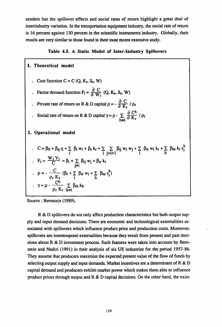
senders but the spillover effects and social rates of return highlight a great deal of

interindustry variation. In the transportation equipment industry, the social rate of return

is 16 percent against 130 percent in the scientific instruments industry. Globally, their

results are very similar to those found in their most ~ent extensive study.

Table 4.5. A Static Model of Inter-Industry Spillovers

1. Theoretical model

. Cost function C = C (Q, Kr, Sr, W)

. Factor demand function Fi = j ..2i (Q, Kr. Sr. W)

. Private rate of retmn on R & D capital p = -l ir I Pr

. Social rate of return on R & D capital 'Y = p - I, ~ KCh I Pr h;f:i r

2. Operational model

Source : Bernstein (1989).

R & D spillovers do not only affect production characteristics but both output sup­

ply and input demand decisions. There are economic and technological externalities as­

sociated with spillovers which influence product price and production costs. Moreover,

spillovers are intertemporal externalities because they result from present and past deci­

sions about R & D investment process. Such features were taken into account by Bern­

stein and Nadiri (1991) in their analysis of six US industries for the period 1957-86.

They assume that producers maximize the expected present value of the flow of funds by

selecting output supply and input demands. Market incentives are a determinant of R & D

capital demand and producers exhibit market power which makes them able to influence

product prices through output and R & D capital decisions. On the other hand, the exist-

119

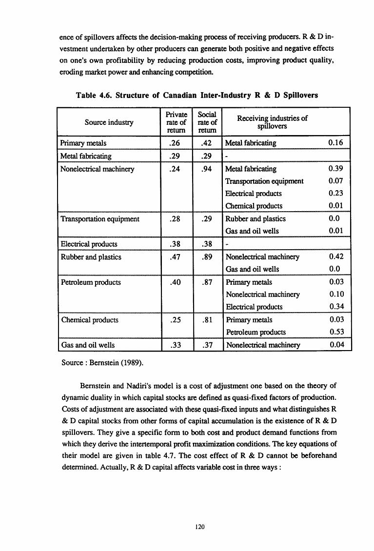
ence of spillovers affects the decision-making process of receiving producers. R & D in­

vestment undertaken by other producers can generate both positive and negative effects

on one's own profitability by reducing production costs, improving product quality,

eroding market power and enhancing competition.

Table 4.6. Structure of Canadian Inter-Industry R & D Spillovers

Private Social Receiving industries of Source industry rate of rate of spillovers return return

Primary metals .26 .42 Metal fabricating 0.16

Metal fabricating .29 .29 -Nonelectrical machinery .24 .94 Metal fabricating 0.39

Transportation equipment 0.07

Electrical products 0.23

Chemical products 0.01

Transportation equipment .28 .29 Rubber and plastics 0.0

Gas and oil wells 0.01

Electrical products .38 .38 -Rubber and plastics .47 .89 Nonelectrical machinery 0.42

Gas and oil wells 0.0

Petroleum products .40 .87 Primary metals 0.03

Nonelectrical machinery 0.10

Electrical products 0.34

Chemical products .25 .81 Primary metals 0.03

Petroleum products 0.53

Gas and oil wells .33 .37 Nonelectrical machinery 0.04

Source : Bernstein (1989).

Bernstein and Nadiri's model is a cost of adjustment one based on the theory of

dynamic duality in which capital stocks are defined as quasi-fixed factors of production.

Costs of adjustment are associated with these quasi-ftxed inputs and what distinguishes R

& D capital stocks from other forms of capital accumulation is the existence of R & D

spillovers. They give a specific form to both cost and product demand functions from

which they derive the intertemporal profit maximization conditions. The key equations of

their model are given in table 4. 7. The cost effect of R & D cannot be beforehand

determined. Actually, R & D capital affects variable cost in three ways :

120

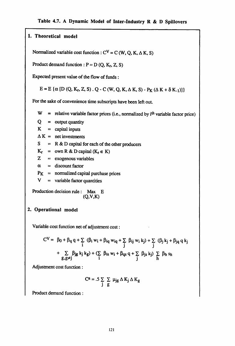
Table 4.7. A Dynamic Model of Inter-Industry R & D Spillovers

1. Theoretical model

Normalized variable cost function: cv = C (W, Q, K, ll K, S)

Product demand function: P = D (Q, Kr, Z, S)

Expected present value of the flow of funds :

E = E {a [D (Q, Kr, Z, S). Q- C (W, Q, K, ll K, S)- PI( (ll K + o K_t)]}

For the sake of convenience time subscripts have been left out.

w Q

K

IlK

s Kr

z a

PK v

= = = = = = = = = =

relative variable factor prices (i.e., normalized by ith variable factor price)

output quantity

capital inputs

net investments

R & D capital for each of the other producers

own R & D capital <Kr e K)

exogenous variables

discount factor

normalized capital purchase prices

variable factor quantities

Production decision rule : Max E (Q,V,K)

2. Operational model

Variable cost function net of adjustment cost :

CV = J3o + ~q q + ~ (~i Wi + ~iq Wiq + ~ ~ij Wi kj) + ~ (~j kj + {3jq q kj 1 J J

+ L . {3jg kj kg) + (~ f3is Wi + ~qs q + ~ f3js kj) L f3h Sh g,g;i:J 1 J h

Adjustment cost function :

Product demand function :

ca = .5 I, I, lljg ll Kj ll Kg j g

121

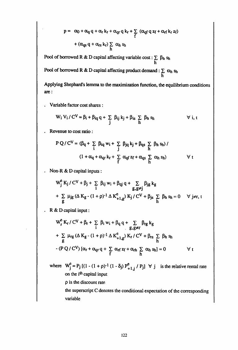
+ (<Xqs q +<Xes kr) L <Xh Sh h

Pool of borrowed R & D capital affecting variable cost : L f3h Sh h

Pool of borrowed R & D capital affecting product demand : L <Xh Sh h

Applying Shephard's lemma to the maximization function, the equilibrium conditions are:

. Variable factor cost shares :

'V i, t

. Revenue to cost ratio :

P Ql cv = ((3q + L f3iq Wi + L Pjq kJ· + f3qs L f3h Sh) I i j h

(1 + <Xq + <Xqr kr + L <Xqf Zf + CXqs L <Xh Sh) 'V t f h

. Non-R & D capital inputs :

wj Kj I cv + pj + ~ Pij Wi + pqj q + L 0 (3jg kg 1 g,g¢J

+ L Jljg (L\ Kg- (1 + p)-1 L1 K:1 g) Kj I cv + f3js L f3h Sh = 0 'V j:;t:r, t g ' h

. R & D capital input :

w; Kr I CV + Pr + ~ f3i Wi + Pq q + L Prg kg 1 _ g,g;tr

+ L Jlrg (d Kg- (1 + p)-1 A K~1 ,g) Kr I CV + f3rs L f3h Sh g h

- (P Q I CV) [ <Xr + <Xqr q + L <Xrf Zf + <Xrh L <Xh Sh] = 0 'V t f h

where wj = Pj [ (1 - ( 1 + p )-1 ( 1 - 8j) P~ 1 j I Pj] "V j is the relative rental rate

on the ith capital input

p is the discount rate

the superscript C denotes the conditional expectation of the corresponding

variable

122

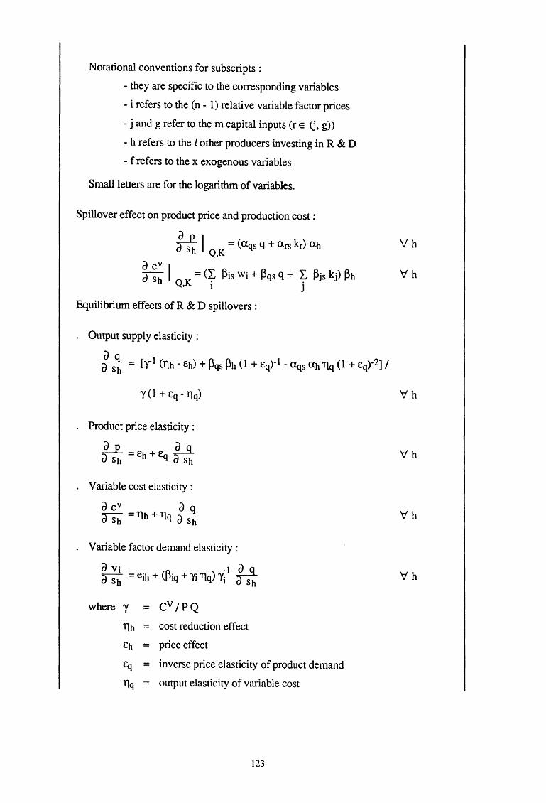
Notational conventions for subscripts :

- they are specific to the corresponding variables

- i refers to the (n- 1) relative variable factor prices

- j and g refer to them capital inputs (r e (j, g))

- h refers to the I other producers investing in R & D

- f refers to the x exogenous variables

Small letters are for the logarithm of variables.

Spillover effect on product price and production cost :

~aa I = (aqs q + ars kr) ah Sh Q,K

a cV I a Sh = (~ Pis Wi + Pqs q + ~ Pjs kj) Ph Q,K I J

Equilibrium effects of R & D spillovers :

. Output supply elasticity:

: s~ = [y1 (Tth- Eh) + ~qs ~h (1 + Eq)-l- !Xqs Uh llq (1 + Eq)-2]/

. Product price elasticity :

. Variable cost elasticity :

a CV _ + ~ ash -Tlh Tlq ash

Variable factor demand elasticity :

a Vi A ) -1 ~ a-- = eih + (piq + Yi Tlq 'Y· a Sh 1 Sh

where y = cv /PQ

Tlh = cost reduction effect

Eh = price effect

fq = inverse price elasticity of product demand

Tlq = output elasticity of variable cost

123

'v'h

'v'h

'v'h

'v'h

'v'h

'v'h

eih = spillover elasticity on conditional demand of ith variable factor

'Yi = cost share of ith variable factor

Net private rate of return on capital stocks :

Pj = P + L, lljg ~Kg (1 + p) I Pj g

Joint industry expected discounted flow of funds :

<I>= L, Eh h

where the superscript identifies each producer

Additional profit accruing from internalizing R & D spillovers :

Social rate of return on R & D capital stock :

f.=p~+(l-p) del>l/p~ a Kr

Source: Bernstein and Nadiri (1991).

V'j

V'j

V'j

- if R & Dis process-oriented, an increase in own R & D capital stock will reduce vari­

able costs. Yet, if R & Dis product-oriented, quality improvements will induce higher

costs;

- producers face adjustment costs when they divert variable factors to R & D investment

so that variable cost will increase;

- spillovers lead to cost reductions for the receiving producer.

Regarding product demand, R & D capital is a product quality indicator which

generally implies product price increases. However, spillovers can either generate posi­

tive or negative price effects. As R & D capital is not separated into process R & D and

product R & D, the product and process influences of R & D are measured through both

the variable cost and product demand functions.

In the production den1and function, spillovers affect output and R & D capital

through due parameters ( Clqs and <Xrs) and each spillover source generates a distinct effect

124

on product price (ah). Moreover, interaction terms are introduced between the spillovers

and factor prices, capital inputs and output quantity (~is, ~qs and ~js). Each borrowed R

& D generates a distinct effect on these variables (~h) and so one can test whether a given

producer is a source of spillover.

From the maximization of the expected present value of profits the equilibrium

conditions for the variable inputs, each variable factor cost share being directly affected

by the pool of borrowed R & D (~is). In equilibrium, the revenue to cost ratio is also in­

fluenced by spillovers through their impact on product price elasticity (<Xqs) and on vari­

able cost elasticity (~qs). Conditions for the non-R & D capital inputs imply that the mar­

ginal cost of a non-R & D capital input is offset by the expected marginal benefit at the

equilibrium and that R & D spillovers affect these equilibrium conditions (~js). A last

equilibrium condition concerns the R & D capital input which is influenced by conditions

ruling both variable cost and product price (i.e. both~ and a coefficients) and by the ex­

tent of spillovers (~hand <Xh). Under this condition, the marginal benefit from R & D

capital input is equal to the increase in marginal revenue net of changes in variable cost

and in adjustment cost.

As not all producers are a source of spillovers, the search of spillover sources is

based upon the idea that spillovers must generate a negative impact effect on variable

costs. This acceptance condition is compatible with some established facts :

- consistency with the assumption of free disposability in production :producers can

costlessly benefit from spillovers and avert them if they are cost increasing;

- capability to promote R & D investment : increasing total cost can result from supple­

mentary R & D investment engaged to absorb the spillovers;

- alteration of competitive strengths: R & D spillovers can freely affect product demand

and thereby generate various economic externalities.

From this model, we are able to evaluate the distinct influence of spillovers on pro­

duct price and production cost for receiving industries. Any increase in the product price

as a result of R & D spillovers will increase the revenue of the recipient industry and con­

versely. As a result of the acceptance condition, an increase of R & D spillovers will re­

duce variable factor cost. Furthermore, the measurement of the spillover elasticities of

output supply, product price, variable cost and variable factor demands emphasizes the

direct impact of spillovers on each of these variables and their indirect impact through

changes in output supply. In these elasticities, output expansion can cause variable cost to

increase, output growth effect outweighing the initial cost reduction due to spillovers. A

similar effect can be detected for product price and variable factor demands.

125

If we tum to the rate of return on R & D, private rate of return can differ from other

types of capital because th~'ipclude marginal adjustment costs which differ from one

type of capital to the other. In, equilibrium, the rate of return equals the discount rate plus

the capitalized value of marginal adjustment cost. The social rates of return are calculated

by considering that industries internalize the R & D spillovers. To do that, the joint indus­

try expected discounted flow of funds is maximized, so that the solution will take into ac­

count the additional profits earned by industries through their spillover effects. This addi­

tional profit equals the difference between the product price effect and the cost production

effect arising from the R & D spillovers. The social rate of return will differ from the net

private rate to the extent that an industry's R & D capital reduces both the product price

and the costs of other industries.

In their application of this model to six US industries, the authors consider as vari­

able factors, labor and intermediate inputs and as quasi-fixed factors, physical capital and

R & D capital. The depreciation rate of R & D capital is considered to be 10 percent. The

exogenous variable affecting product demands is the real gross domestic product net of

the industry output per capita.

The estimate of the model emphasizes the existence of adjustment costs. All the

own adjustment cost parameters are significant. The cost parameters are also significant

and positive, except for electrical products, which indicates that an increase in physical

capital increases adjustment cost of R & D capital. These adjustment costs imply the

existence of an intertemporal trade-off in the investment decisions.

The results, summarized in table 4.8., show that each industry is a receiver of R &

D spillovers and that only the fabricated metal industry is not a spillover source. For each

receiving industry, the spillover sources are concentrated in a few industries. This ob­

servation emphasizes the limits of more aggregated approaches. The sender-receiver net­

work is relatively narrow, links some enterprises through cross spillover effects and

points out the key role of scientific instruments, chemical products and nonelectrical

machinery industries as the main sources of spillovers. The cost reduction effect of spill­

over is generally higher than the product price effect and it is only in the case of chemical

products and scientific instruments that spillovers increase their product price. On the cost

reduction side, fabricated metal appears to be the main beneficiary of spillovers and

chemical products the one that benefits least. The output effect of spillovers is to expand

output. For the two industries where spillovers increase product price, the expansion

effect overcomes the price effect, causing product prices to fall.

126

Tab

le 4

.8.

Str

uctu

re o

f U

S In

ter-

Indu

stry

R &

D

Spi

llov

ers

Pri

vate

S

ocia

l rat

e R

ecei

ving

indu

stri

es o

f S

pill

over

retu

rn

Pro

duct

C

ost

Sou

rce

indu

stry

ra

te o

f o

f ret

urn

spil

love

rs

by ty

pe

pric

e re

duct

ion

retu

rn

Pro

duct

V

aria

ble

effe

ct

effe

ct

pric

e co

st

Che

mic

al p

rodu

cts

.22

.46

N

onel

ectr

ical

mac

hine

ry

-.23

.3

8 .0

5 -.

05

Sci

enti

fic

inst

rum

ents

.0

3

.06

Fab

rica

ted

met

al

.22

.2

2

--.

16

-.24

-N

onel

ectr

ical

mac

hine

ry

.25

.40

T

rans

port

atio

n eq

uipm

ent

-.2

0

.36

-.

06

-.12

N

-..

.J

Ele

ctri

cal p

rodu

cts

.27

.31

Sci

enti

fic

equi

pmen

t .0

2

.03

-.07

-.

12

Tra

nspo

rtat

ion

equi

pmen

t .2

3 .3

5 F

abri

cate

d m

etal

-.

12

.16

-.

05

-.11

Non

elec

tric

al m

achi

nery

-.

07

.12

Sci

enti

fic

inst

rum

ents

.0

1 .0

2

Sci

enti

fic

inst

rum

ents

.2

8 .8

7 C

hem

ical

pro

duct

s .2

6

.19

.0

3 -.

08

Ele

ctri

cal p

rodu

cts

-.36

.4

9

Sou

rce

: Ber

nste

in a

nd N

adir

i (1

991)

.

Figure 4.1. Traces of External Returns on R & D

1. Canada

Chemical products

Petroleum .53 --... ..-~ products

(j (.40)

.01

2. United States

.34 .. ~

+ Chemical products

(.22)

.16 Nonelectrical ... machinery (.25)

Primary .16 .. metals (.26)

.39 Electrical products

(.38)

l23 y Nonelectrical .07

machinery .. (.24)

~

.05

I .16 Transport

..... equipment (.23)

Scientific .03

instruments~--------------

(.28)

Electrical products

(.27)

Fabricated metals (.29)

.42

Transport equipment

(.28)

!.01 Gas and oil

wells (.33)

.04 .....

.0 ...

/

Fabricated metals (.22)

I Rubbers and

plastics (.47)

Note : The data between parentheses are the private rates of return and the others are the social rates of return per receiver.

Source: Bernstein (1989) and Bernstein and Nadiri (1991).

128

Figure 4.1. summarizes the distribution of spillovers between the different

industries for both the Canadian and American studies. In both cases, fabricated metals,

transport equipment and electrical products are not major sources of spillovers.

Chemicals, nonelectrical machinery and scientific instruments concentrate a large part of

external returns arising from spillovers. There is no important closed loop of R & D

externalities between industries. In the United States, there is a slight give and take

relationship between chemical products, scientific instruments and electrical products, on

the one hand, and between nonelectrical machinery and transport equipment, on the other

hand.

4.6. More on the Input-Output Approach 1

4.6.1. Decomposition of Growth in Real Output

The focus question is to decompose output growth into portions attributable to

changes in technology (represented by the changes in coefficients of the Leontief inverse

matrix) and to changes in final demand.

Induced output, X, is expressed by multiplying production technology, B, and

final demand, F. Therefore, any increment in induced output, dX, is expressed as fol­

lows:

dX = Xt- Xo = Bt pt- BO p0 = (BO +dB) (fO + dF)- BO p0

= BO p0 + p0 dB + BO dF + dB dF - BO pO

= B0dF + fOdB + dBdF

Thus, output growth can be decomposed into different components :

- first, the part of growth due to changes in final demand;

- second, the part resulting from technological change;

- third, the cross product term measuring the interdependencies between demand and

technology.

The increment in final demand, DF, can also be decomposed into three elements:

- the aggregate demand;

- its distribution into final demand components such as consumption and investment;

1 This section has largely been inspired by Uno (1989).

129

- the technical coefficients describing the industrial composition of a particular demand

item.

Consequently : F=cef

where f = aggregate final demand

c = technical coefficients (n x n)

e = composition ratios of final demand items (1 x n)

e = diagonal matrix of e.

Any increment in final demand, dF, is equal to:

dF = Fl - pO = ct et fl - cO eO fO =(cO+ de) (eO+ de) (fO + dt)- cO eO f{)

= c0 eO df + cO de f{) + de eO fO + cO de df + de eO df + de de f{)

+dcdedf

where cO eO df is attributable to changes in the aggregate level of final demand

cO de fO is attributable to changes in the components of final demand

de eo fO is attributable to changes in the technical coefficients

the cross product terms can be ignored because their impact is very weak.

(1)

The usefulness of input-output tables is strongly impaired by the fact that they are

rarely available annually and for a sufficiently long period. Furthermore, they are based

on very stringent hypotheses about the nature of production relationships :

- each industry produces only one good (no joint products or by-products);

- the production technology is identical for all the production levels of a good;

- the returns to scale are constant.

For the year of construction of the matrix, the data are supposed to give a satisfying

representation of the reality. It is hardly credible, though, that the technical coefficients

calculated for a specific year do not move over time. Several elements can influence the

matrix of technical coefficients :

- any change in the relative price of factors will entail to a reaction from fmns which will

tum to alternative production processes, thereby inducing a reallocation in the use of

factors.

130

- in some industries, short-term decreasing returns to scale may seem to be due to the

fact that the production capacity limits have been reached; in other sectors, increasing

returns to scale can result from an expansion of the production.

- technical change permanently affects technical coefficients.

In order to update and forecast input-output coefficients, one makes use of the RAS

method which is based on the following philosophy :

- the flow matrix is corrected for price changes between the two periods in order to ex­

press the technology of the initial period in the prices of the new period.

- in a second stage, a new correction of the matrix is operated in order to take into ac­

count the substitution effects between intermediate products which are due to technical

progress. This effect is supposed to materialize in the same way for all the sectors

using a same intermediary good. Furthermore, this effect will be greater than unity for

expanding products and less than unity for declining products.

- a last correction is applied to take into account that the manufacturing degree is liable to

change. The fabrication effect measures the extent to which the production makes use

of intermediary inputs. This effect will be greater than unity if the degree of fabrication

has decreased and less than unity if it has increased.

The new matrix so estimated can be written :

where Po is the diagonal matrix of prices in the initial period

p, the diagonal matrix of prices in the new period relatively to those of the initial

period

r, the diagonal matrix of substitution effects

s , the diagonal matrix of fabrication effects.

The matrices rands are iteratively estimated on the basis of the known sectoral

values of output, intermediate demand and intermediate input

This method has some drawbacks I:

- if an element of the matrix of coefficients is zero, its estimate in a future period will be

zero, which makes it difficult to take into account new products and processes which

combine inputs which are very different from those used in the preceding period.

1 Alternative methods of actualisation have been developed, they are surveyed by d'Alcantara (1986).

131

- due to the hypothesis of identical substitution effects, the rate of substitution of factors

is supposed the same in each production branch, which is not always very realistic.

- as there is an additivity constraint (total of both intermediate demand and intermediate

input being known), if an element is underestimated, an other will be overestimated.

- this method is unable to indicate if changes in the elements of the flow matrix are due to

a modification of the price structure or to technological change.

- when the results are used to analyse· further years, it is automatically assumed that

future periods face the same changes in the economic and technical environment than

the reference periods.

4.6.2. The Treatment of R & D in Input-Output Tables

Business services are production factors linked to economic activities which deal

with goods production. From this standpoint, research is a form of current service but it

cannot be assimilated to a current business service because it is the originator of know­

ledge production. Part of R & D expenditure is oriented towards the acquisition of basic

knowledge in science and technology and the operational implementation of new know­

ledge. As such, R & Dis an activity which extends the spectrum of production possibili­

ties, which distinguishes it from labor and capital factors.

According to Uno (1989), input-output tables do not adequately deal with R & D.

While European input-output tables do not takeR & D into account, the Japanese ones

include it. On the one hand, R & D conducted by the private sector for their own internal

use is integrated through the creation of a dummy sector where only the intermediate

inputs are accounted for. On the other hand, R & D by research institutions and

universities is fully endogenized. While for the private sector labor cost and the purchase

of tangible fixed assets are excluded, only the latter is excluded for research institutions

and universities. So, the treatment of R & D appears not to be homogenous within the

input-output framework. Furthermore, R & D expenditure is only partially accounted for.

Finally, as R & D activities are treated as an endogenous sector, any analysis of inter­

industry relationships of R & D activities is unfeasible.

Furthermore, such a treatment does not record the output of R & D activities. The

economy-wide impact of R & D escapes the analysis except for the indirect effect which

can be grasped by measuring the increase in production efficiency (i.e., through changes

in technical coefficients) or in the sales of a branch of production (i.e., increased

marketability of output). Consequently, the outcome of R & D may not be reflected in the

132

(10)

output of the industry in a pecuniary sense, as the output of this activity is the scientific

and technological knowledge. A specific method for recording the output of this activity

needs to be devised.

Another important aspect is that R & D activities are listed within the production

expenditures and not as an independent activity in the input-output structure so that any

increase in R & D activities would increase production cost. Yet, since R & D produces

scientific and technological knowledge, which increases the future production potential,

and not principally the production of the current period, it should be treated as final

demand. The input structure should include the costs in production and external R & D

changes should be treated separately. R & D investment is a strategic policy variable for

business firms and government whose level does not passively react to current

production but is determined by the decision to invest in production knowledge. Thus, R

& D activities cannot merely be regarded as an appendage to current directly productive

activities or as a technological adaptation cost (of adopting new technologies or of

imitating new technologies), they are a component of final demand as long as they are not

exclusively used in the production process.

In order to make up for the fact that the conventional input-output tables do not take

R & D into account, we can seek what would be the ideal treatment of such an activity.

This conceptual framework is considered without questioning the availability of empirical

statistics. The proposed scheme consists of nine layers as shown in figure 4.2 :

1 . a financing account which records the financial flows from financing sources to R

& D execution sectors. This would permit to highlight the role of public and private

organizations in the resource allocation.

2. an R & D expenditure account which records, for each execution sector, the R

& D expenditure by field or product. The expenditure items would be broken down

into tangible fixed assets, wages and salaries and material consumption in order to

identify the components of value-added, investment and consumption.

3. an R & D interindustry flow matrix which corresponds to an extended input­

output table including an R & D expenditure disaggregated account. The associated R

& D matrix would serve to establish the linkage with interindustry relations. In this

framework, R & D investment represents the expenditure on tangible fixed assets and

R & D consumption is defined as expenditure of materials and assimilated. The

wages and salaries and the depreciation of tangible fixed assets are components of

value-added. The R & D input consists of R & D labor cost, R & D capital depre-

133

ciation, user cost of existing knowledge and intermediate input, this last item being

treated as input to industry. The R & D output is recorded among the final demand

items, it is composed of R & D capital formation and R & D consumption. As current

expenditure for R & D is not an input to produce goods and services as defined in the

input-output framework, it would be more logical to treat it as fmal demand and not

as intermediate input. R & D spending is directed toward the knowledge acquisition

for future use and not toward immediate physical production. In order to distinguish

R & D components from other components of final demand, both R & D consump­

tion and investment are separated as an independent final demand item. The R & D

input-output table would be a disaggregation of R & D final demand be~ween con­

sumer sectors and producer sectors.

4. an R & D employment matrix which gives the industry-occupation employment

patterns and would help to analyze the impact of the changing industrial structure of

the varying levels of R & D expenditures on R & D employment.

5. an R & D capital stock account which gives information on the stock of fixed

tangible assets for R & D purposes in each sector and corresponds to the R & D capi­

tal formation. This correction departs from the defmition of R & D capital stock used

in econometric studies. To recall, in the latter, all R & D expenditures are taken into

account in the measure of R & D capital stock.

6. an R & D performance account which deals with the outcome of the research

activities. While the preceding table was concerned with the measurement of the R &

D capital stock, this account brings on the evaluation of the end results of R & D in

terms of R & D benefits, patents or publications. The appreciation of the performance

concept can highly vary accross research fields and so far there does not exist any

well-established standard indicator to appreciate performances inside a research field.

Consequently, the measurement of performances remains a tricky issue.

7. a knowledge capital stock account \vhich brings on the stock of scientific and ' \

technological knowledge. Although there are a variety of forms of knowledge stock,

this aggregate is alternatively approximated by the accumulated total R & D ex­

penditures, as is the case in econometric works or by the number of patent applica­

tions or patents granted. The main criticism against these approximations is that, on

the one hand, R & D expenditure is an input measure of the knowledge production

process and that, on the other hand, patents are only a rough measure because not all

knowledge is patented and not all patents are valuable.

134

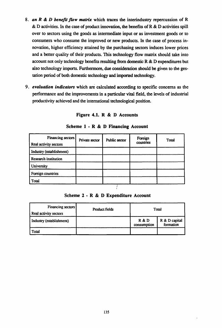
8. an R & D benefit flow matrix which traces the interindustry repercussion of R

& D activities. In the case of product innovation, the benefits of R & D activities spill

over to sectors using the goods as intermediate input or as investment goods or to

consumers who consume the improved or new products. In the case of process in­

novation, higher efficiency attained by the purchasing sectors induces lower prices

and a better quality of their products. This technol'?gy flow matrix should take into

account not only technology benefits resulting from domestic R & D expenditures but

also technology imports. Furthermore, due consideration should be given to the ges­

tation period of both domestic technology and imported technology.

9. evaluation indicators which are calculated according to specific concerns as the

performance and the improvements in a particular vital field, the levels of industrial

productivity achieved and the international technological position.

Figure 4.1. R & D Accounts

Scheme 1 • R & D Financing Account

Financing sectors Private sector Public sector Foreign Total

Real activity sectors countries

Industry (establishment)

Research institution

University

Foreign countries

Total

Scheme 2 • R & D Expenditure Account

Financing sectors Product fields Total

Real activity sectors

Industry (establishment) R&D R & D capital consumption formation

Total

135

Scheme 3 - R & D Interindustry Flow Matrix

Output Intenncdiate R&D c IP G E M

Input Industry

R&D con-

In~ediate Industry Intennediate sumption transactions & invest-

ment

R&D benefit

R&D Output Own R&D (b) R&D benefit

R&D in other sectors

Labor L R&DL

Value added Capital K R&DK

Scheme 4 - R & D Employment Matrix

Occupation

Industry Total by industry

Total by occupation Total

Scheme 5 - R & D Capital Stock Account

Technology fields

Industry Total by industry

Total by technology fields Total

136

Scheme 6 - Knowledge Capital Stock Account

Technology fields

Industry Total by industry

Total by technology fields Total

Scheme 7 - R & D Benefit Flow Matrix

Final demand

c G IP E

Industry engaged inR& D

Total benefit Benefit to industry Benefit to F-D accruing

Source: Uno (1989).

Uno investigated the empirical feasibility of this analytical schema in the case of

Japan. The linkage to the input-output framework is done using the aggregate data for R

& D consumption and investment. As converters are not available to transform these data

into demand for individual sectors, the intermediate input structure is used as an ap­

proximation. For R & D investment, the converters are assumed to be identical to those

calculated for private investment in plant and equipment. It is on this basis that he

estimates the input-output structure of the R & D activities. The stock of knowledge is

measured by combining the number of applications for both patents and utility models

and the average life expectancy of patents. The life expectancy of patents is defined as the

period during which a patent yielded returns from outside the firms or when the products

incorporating such patents yielded profits. Assuming that the economic value of patents

declines proportionally over time, the rate of depreciation of patents is given by the reci­

procal of the average life. To trace the technological flows among industries, R & D ex­

penditure is used rather than patent data. After estimating the time lag between R & D ex­

penditure and the implementation of new knowledge so created- in actual production on

the basis of information on gestation period, the flow of R & D benefits received by other

sectors through intermediate inputs is measured by the ratio of sales to intermediate

demand multiplied by the R & D expenditure in the producing sector. For the flow of R

& D benefits received by other sectors through purchase of investment gopds, a similar

procedure is applied by using the fixed capital formation matrix instead of intermediate

137

demand. Flow of R & D benefits to consumption and exports are estimated by the ratios

of sales to these final demand items respectively. A same measurement method is applied

for technology flows from new contracts of technology imports.

138

Chapter 5. The impact of Government-financed R&D

Assessing economic impacts of policy intervention by public authorities is a very

difficult task because a variety of effects as well as other causes may contribute to specific

outcomes. From this standpoint, the use of econometric models to evaluate the potential

impact of altemati~e sets of economic policy is now a current practice in economics.

Econometric models have asserted themselves as a tool of great value for improving our

understanding of the intricacies of economic phenomena. They play a role in the design

of economic policy both as a tool in the impact analysis in order to assess the global

economic fallouts of policy measures and as a tool in the decision making processes.

Yet, these methods are only very marginally used for the design of science and

technology policy. The exogenous status of technical change in macromodelling, the

scarcity of data in this field and the skepticism of experts regarding the usefulness of

econometric methods are certainly the three main reasons why econometric methods are

not regarded as a sufficiently efficient impact evaluation technique. Nevertheless, the

recent availability of better data, the multiplication of empirical and theoretical researches

on the interdependencies between economic growth and technological change and the

difficulty in appraising the economic impacts of science and technology policies when

only qualitative methods are used should lead to an increasing use of econometric

methods.

Most efforts in the econometrics of R & D have been devoted to measuring the impact

of overall and industrial R & D. The public R & D investment is often included in models

as an explanatory variable without the measure of its impact being the actual objective of

the undertaken analysis. Moreover, these estimates are only pinpoint approaches which

evaluate the impact of public R & D on an economic variable and not on the economic

system as a whole. In this field, the main evidence comes from U.S. case-studies.

Regarding this country, the apparent high variability of results can, to a large extent, be

explained by the data characteristics. Unfortunately, for other countries, the experiments

reported in the literature are not sufficient to draw clear conclusions.

139

5.1. Why to evaluate the Economic Impact of Publicly-Funded R & D ?

So, how science and technology resources should be allocated so as to have a maxi­

mum impact on economic growth has become an important focus for technology assess­

ment. The answer to such a question should be based on both qualitative criteria of eva­

luation and formalized quantitative methods. Although qualitative methods of evaluation

produce useful guidelines for the organization and implementation of R & D policy, they

are not suited to measure the economic impacts of public R & D programmes quantita­

tively. As pointed out by Roessner (1989), "efforts to evaluate government programs

intended to stimulate industrial innovation through various types of R & D subsidies are

confronted immediately with serious design and measurement challenges".

Although the need for more information about the economic effects of public support

of R & D activities has long been debated, the credibility of econometric methods as

evaluation tool is often questioned. The American Office of Technology Assessment

(1986) considers that quantitative methods "does not provide a useful practical guide to

improving Federal research decision making" and that the influential factors are too

complex and subjective "to allow quantitative models to take the place of mature,

informed judgement".

The mastery of technological change, and particularly technological innovation, is

increasingly viewed as a major driving force of economic growth and competitiveness. If

we glance at the normative literature on the economic analysis of technological change, it

appears that, in the present state of the art, although it provides a good understanding of

some basic factors, so far it has given practitioners little ground to build on. Hence,

some economists argue that governmental funding of R & D is likely to reduce private R

& D expenditure because firms may receive support from the public sector for projects

they would otherwise finance themselves. Taking an opposite stance, others say that

publicly-funded R & Dis complementary to and stimulates privately-funded R & D.

Futhermore, little is known about the efficiency of alternative forms of public inter­

vention. As a consequence, innovation policy may be said to be today more a matter of

faith than of understanding [Rothwell and Zegveld (1988)].

The R & D policy must rest on an appropriate set of actions aimed at influencing or

controlling factors which restrain the technological performances of finns. The fuzzy and

uncertain nature of R & D policy makes the assessment of the ~mpacts of the instruments

used a major analytical issue. Hence, if governmental action induces only small additional

140

private R & D expenditure, then, to justify public intervention the social return must be

relatively high. Conversely, if public subsidization results in high additionality and high

private return, but with weak positive externalities (the subsidized fmn appropriates most

of the benefits of the research), then the government must wonder whether its interven­

tion is meant to compensate for market failure and whether the overall economic benefits

outweigh the costs. Hence, the design of appropriate policy instruments should be based

on the following economic rationale :

- the support should be additional in the sense that the generated activity would not have

occurred in a similar form or at all without public intervention.

- the support should result in greater social benefits than otherwise.

- the support should provide higher extra benefits than its opportunity cost.

Given that these outcomes cannot be a priori guaranteed, the economic effects of R &

D policy actions have to be evaluated ex post. In case of ex ante impact assessment,

since the changes in the exogenous circumstances are unknown, it is difficult to define

the reference situation.

Science and technology policy is not implemented in order to achieve intrinsically

technological goals, or at least should not be viewed as such, but as a mean of action

aiming at improving the economic and social welfare. Its objective is not the search of

scientific and technological achievements for its own sake. This policy is ultimately

concerned with wealth creation and should be seen as part of economic policy dealing

with short-term and long-term economic growth.

The relevant questions for the design of a science and technology policy are :

What is the ultimate goal of a science and technology policy ?

What are the objectives to achieve ?

What are the targets aimed at ?

What instruments have been designed ?

How efficient have the policies implemented been ?

In accordance with the usual functions recognized to public policy, the goal should

primarily be to promote an efficient allocation of resources t. In order to attain this goal,

several objectives are fixed, among which fostering R & D activities, promoting the

1 It does not mean that science and technology policy is not concerned with other goals, i.e. stabilisa­tion and equity. For example, a science and technology policy aiming at fostering technological cap­abilities in lagging regions is, primarily, designed to satisfy the equity principle.

141

diffusion of new technologies and ensuring the access to technological opportunities as

well as to economic opportunities offered by the developments in science and technology.

Then, specific targets are chosen for each objective. For example, R & D activities can be

fostered by acting on private R & D investments. The instruments, which are the action

means, are under the control of public authorities. They can be general or selective and

principally bear on tax deductions, grants, loans, guarantees, purchases and investments.

Each of these components is vital for the design of an efficient policy. Besides, policy

assessment is also vital as it gives grounded recommendations to adapt the existing policy

or to implement future policies. In the process of policy assessment, ex post impact

assessment will give information on the changes in the targets caused by the implementa­

tion of instruments.

The purpose of impact assessment is to have information about the costs, the benefits

and the effectiveness of the implemented policy. The impact analysis may cover different

and complementary objectives :

- quantitative and qualitative effects on firms' R & D activities (spin-off effect).

- impact on the economic performance(s) of firms (productivity effect)

- impact on the economic performance(s) of industries (spillover effect).

- impact on the economy as a whole (global effect).

To date, only a few empirical studies have endeavoured to estimate the economic im­

pact of R & D policy. Three different types of economic assessment methods are used.

The first is the case study. Case studies always leave open the question of how repre­

sentative they are. Their results are often only valuable for a specific context and any

generalisation is a highly risky experiment. The second method consists in surveys con­

ducted among those who have been concerned by the policy. Surveys may provide de­

tailed information on factors influencing decision-making processes and on perceptions

of a subsidization policy. However, this method often suffers from lack of accuracy in

the way questionnaires are built and measurement errors, which may cause perceived

effects to be mistaken for actual ones. An other limitation of the frrst two methods is that

they usually cannot provide information about the effects on variables in a causal chain,

they are very costly and time consuming. The third method is the use of econometrics to

emphasize the relationship between subsidization and R & D intensity across firms as

well as between publicly-financed R & D and productivity performances of firms. This

method allows to estimate only direct effects of policy instruments on an impact variable.

All these methods belong to the class of micro-studies, they are complementary and they

are able, within their own limits, to add some pieces of information to our present puzzl~

142

of knowledge about the intricate interdependences between innovative activities and eco­

nomic performances.

The third method can also be used for two other types of studies : mesostudies and

macrostudies. Hence, it is useful to cluster the third method in micro-econometrics,

meso-econometrics and macro-econometrics. As far as mesostudies are concerned, input­

output models can be used to calculate the effects of technical change on production and

demand. Although input-output analysis is a very useful method of recording the effects

of public R & D policy, its usefulness is seriously limited by its rigid structure and the

scarcity of data. Conversely, macromodelling as a tool for macrostudies is not restricted

to recording transactions between industrial sectors. The causal chain of interdependen­

cies can be reproduced by introducing causal variables among the explanatory variables.

Only with such an approach can one measure the direct and indirect effects of public

policy, provided, however, data are available on a large number of variables. An alterna­

tive approach is to combine input-output analysis and macromodels, which is now largely

used in the existing macromodels. So far, there does not exist any macromodel that has

been designed to deal with public R & D policy. Developing such a model will imply

endogenizing private R & D investments and identifying their relationship with publicly­

funded R & D investments and the other economic variables. Despite many bottlenecks,

macromodels can be adapted so as to be used as a tool for ·the ex post assessment of R &

D public programmes. The outcomes of the econometric pin-point approaches can cer­

tainly be very helpful in the implementation of extended macromodels 1•

The efficiency of direct subsidization of private R & D by government and tax-credit

public policies is a very controversial subject. In a survey of the production function

approach, Griliches (1979) asked different questions concerning the real contribution of

publicly-funded R & D to productivity growth: are the returns to government-financed R

& D similar to those of company-financed R & D? Does Federal R & D substitute for or

complement private R & D investment? What are the spillover effects of government­

financed R & D ? As the rationale for government funding industrial R & D is more and

more questioned, it is of major importance that we should improve our knowledge of the

interaction between public and corporate funding of R & D and the contribution of public

funding of R & D to econon1ic growth. To date, a number of analyses give some pieces

of information on this issue.

The recent literature has essentially focussed on two direct approaches:

1 A taxonomy identifying the areas to be investigated for an extensive policy assessment is suggested by Capron (1992a).

143

- The productivity approach which measures the respective effects of privately-funded

and publicly-funded R & D expenses on the growth rate of output, so giving an evalua­

tion of the output elasticity of public R & D or of the rate of return on public R & D.

- The investment approach which measures to what extent public R & D allocations in­

fluence privately-funded R & D expenditures, the idea being to look at whether, by do­

ing its own R & D and funding private R & D, a government affects (positively, nega­

tively or not at all) the privately-funded R & D and the magnitude of the effect

Besides, econometric methods have also been used outside these two conceptual

approaches. It is the case of probabilistic models, which are required when data are not

quantitative but qualitative. On the other hand, a supply approach has been suggested as

an alternative to the productivity approach. Its advantage is to allow an indirect measure

of the internal rate of return on R & D as well as the marginal internal rate of return on R

&D.

5.2. How Productive is the Publicly-Financed R & D ?

In successive studies using alternative measures of total factor productivity growth,

Terleckyj (1974, 1980a, 1980b) found that privately-funded R & D was significantly

associated with industrial productivity growth but that government-financed R & D was

not. Besides the own sectoral R & D variables, he introduced a measure of borrowed R

& D investment obtained by crossing the own R & D expenditure and an input-output

matrix. His results show that the spillover effects of privately-financed R & D are very

important whereas the indirect effects from publicly-financed R & D are not significant.

In his analyses, he uses different measures of total factor productivity growth, i.e. based

on net and gross measures of output and inputs and taking into account or not quality

characteristics of inputs. For these different sets of productivity data, both direct and

indirect productivity effects of government-fmanced R & D are captured. In a comment

accompanying the paper, Globerman criticizes Terckelyj's observation of an apparent

inefficiency of government R & D by pointing out that, "to the extent that federally

financed R & D is primarily directed towards improvements in product quality as

opposed to cost reduction, the methodology used in deriving industry productivity

estimates could contribute to the finding that government-financed R & D is not

significantly related to productivity change. Furthermore, ... the time lag ... might be too

short to fully incorporate the effects of federally financed R & D which is presumably

aimed at effecting greater changes in underlying production conditions".

144

Tab

le 5

.1.

Impa

ct o

f R

& D

Cap

ital

Sto

ck o

n F

acto

r P

rodu

ctiv

ity

Stud

y Sa

mpl

e Sp

ecifi

catio

n an

d ad

ditio

nal v

aria

bles

Su

bsam

ples

and

T

otal

C

ompa

ny

Publ

ic

R2

othe

r det

ails

R

&D

R

&D

R

&D

Gri

liche

s (1

980a

) U

nite

d St

ates

-P

ania

l fac

tor

prod

uctiv

ity g

row

th

Pool

ed d

ata

.08

.06

-.1

1 19

57-6

5 -

App

roxi

mat

ed p

hysi

cal c

apita

l (5

.85)

(5

.25)

88

3 co

mpa

nies

C

hem

ical

s an

d .0

9 .0

9 -

.23

petro

leum

(2

.45)

(2

.37)

M

etal

s an

d m

achi

nery

.1

0 .0

9 -

.21

.(4.6

4)

(3.7

8)

Ele

ctric

equ

ipm

ent

.11

.06

-.4

1 (3

.53)

(2

.89)

M

otor

veh

icle

s .1

3 .1

4 -

.49

(1.8

0)

(2.6

0)

Airc

raft

.11

.03

-.2

3 (1

.39)

(0

.68)

O

ther

.0

5 .0

5 -

.56

(3.4

7)

(3.4

0)

Levy

-Ter

leck

yj

Uni

ted

Stat

es

- Pan

ial f

acto

r pr

oduc

tivity

G

over

nmen

t R &

D

-.2

7 .O

S -

(198

3)

1949

-81

-Une

mpl

oym

ent a

nd fi

xed

capi

tal

~~ent co

ntra

ct --·---~.L_ _

_ li:§

.:n.._

_ ----

--Pr

ivat

e bu

sine

ss

.27

.09

sect

or

R&

D

(4.1

0)

(21

3)

Oth

er g

over

nmen

t -

--.0

5 -

R&

D

(1.1

4)

Gri

liche

s ( 1

986)

U

nite

d St

ates

-P

rodu

ctio

n fu

nctio

n 19

67

.11

.19

-.3

9 19

66-7

7 -L

abor

, cap

ital s

ervi

ces

and

basi

c (4

.91}

(1

.96)

50

0-10

00 c

ompa

nies

re

sear

ch

1972

.1

4 .2

5 -

.39

-Alte

rnat

ive

resu

lts re

port

ed fo

r th

e ~m·

(5.1

9)

_Q.3

3)

.39

........

... pa

nial

pro

duct

ivity

gro

wth

and

the

gros

s .1

7 .0

7 -

prof

it ra

te in

dica

ting

a po

sitiv

e pr

emiu

m

(8.6

8)

(0.6

8)

on p

riva

tely

fin

ance

d R

& D

19

72

.13

.13

-.3

1 (6

.63)

(1

.51)

19

72

.12

.14

-.3

1 (6

.39)

(1

.57)

19

TI

.09

.04

-.2

9 (5

.23)

(0

.52)

Levy

-Ter

leck

yj

Uni

ted

Stat

es

-Pro

duct

ion

func

tion

--

.26

.04

.999

(1

989)

19

58-8

5 -L

abor

and

cap

ital

(7.2

0)

(220

) U

S te

1eco

mm

unic

a-lio

ns in

dust

rY

Not

e: V

alue

s be

twee

n pa

rent

hese

s ar

e t-

stat

istic

s.

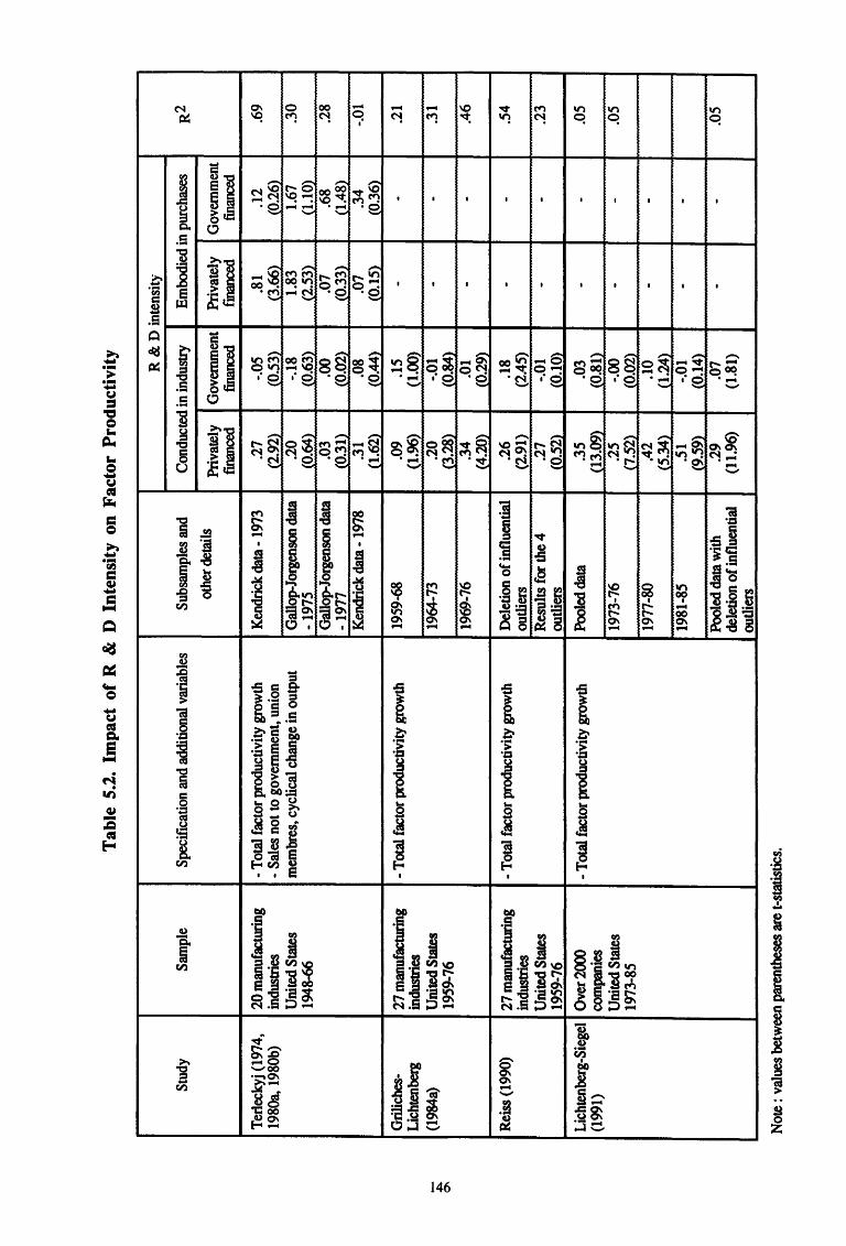
Tab

le 5

.2.

Impa

ct o

f R

&

D I

nten

sity

on

Fac

tor

Pro

duct

ivit

y

R &

D in

tens

ity

Stud

y Sa

mpl

e Sp

ecifi

catio

n an

d ad

ditio

nal v

aria

bles

Su

bsar

nple

s an

d C

ondu

cted

in in

dust

ry

Em

bodi

ed in

pur

chas

es

R2

othe

r det

ails

Pr

ivat

ely

Gov

ernm

ent

Priv

atel

y G

over

nmen

t fin

ance

d fin

ance

d fm

ance

d fin

ance

d

Ter

leck

yj (1

974,

20

man

ufac

turin

g -T

otal

fac

tor

prod

uctiv

ity g

row

th

Ken

dric

k da

ta -

1973

.2

7 -.0

5 .8

1 .1

2 .6

9 19

80a,

198

0b)

indu

strie

s -

Sale

s no

t to

gove

rnm

ent,

unio

n (2

.92)

(0

.53)

(3

.66)

(0

.26)

U

nite

d St

ates

m

embr

es, c

yclic

al c

hang

e in

out

put

Gal

lop-

Jorg

enso

n da

ta

.20

-.18

1.83

1.

67

.30

1948

-66

-197

5 (0

.64)

(0

.63)

(2

.53)

(1

.10)

G

allo

p-Jo

rgen

son

data

.0

3 .0

0 .0

7 .6

8 .2

8 -1

977

(0.3

1)

.(0.0

2)

(0.3

3)

(1.4

8)

Ken

dric

k da

ta -

1978

.3

1 .0

8 .0

7 .3

4 -.0

1 (1

.62)

(0

.44)

(0

.15)

(0

.36)

Gril

iche

s-27

man

ufac

turin

g -T

otal

fact

or p

rodu

ctiv

ity g

row

th

1959

-68

.09

.15

--

.21

Lic

hten

berg

in

dust

ri~

(1.9

6)

(1.0

0)

(198

4a)

Uni

ted

Stat

es

1964

-73

.20

-.01

--

.31

1959

-76

(3.2

8)

(0.8

4)

1969

-76

.34

.01

--

.46

(4.2

0)

(0.2

9)

Rei

ss (

1990

) 27

man

ufac

turin

g -T

otal

fact

or p

rodu

ctiv

ity g

row

th

Del

etio

n of

influ

entia

l .2

6 .1

8 -

-.5

4 in

dust

ries

outli

ers

(2.9

1)

(2.4

5)

Uni

ted

Stat

es

Res

ults

for

the

4 .2

7 -.0

1 -

-.2

3 19

59-7

6 ou

tlier

s (0

.52)

(0

.10)

Lic

hten

berg

-Sie

gel

Ove

r200

0 - T

otal

fac

tor p

rodu

ctiv

ity g

row

th

Pool

ed d

ata

.35

.03

--

.05

(199

1)

compani~

(13.

09)

(0.8

1)

Uni

ted

Stat

es

1973

-76

.25

-.00

-

-.0

5 19

73-8

5 (7

.52)

(0

.02)

19

77-8

0 .4

2 .1

0 -

-(5

.34)

(1

.24)

19

81-8

5 .5

1 -.0

1 -

-(9

.59)

(0

.14)

Po

oled

dat

a w

ith

.29

.07

--

.05

dele

tion

of in

fluen

tial

(11.

96)

(1.8

1)

outli

ers

Not

e : v

alue

s be

twee

n pa

rent

hese

s ar

e t-s

tatis

tics.

Contrary to Terleckyj, from a more extensive study, Griliches ( 1980a) concludes

that he was unable to discover any direct evidence of the superiority of company-financed

R & D as against federally-financed R & Din affecting the productivity growth. This

observation results from a comparison of estimates obtained by using alternatively total R

& D growth rate and company R & D growth rate by industry at the firm level. Yet, from

the relationship between company profitability and R & D investment and from the

elasticities obtained by estimating the production function, he derives the rate of return on

R & D and so observes that the two industries with the largest federal involvement in the

financing of R & D (electrical equipment and aircraft) yield the lowest rates of return.

His explanation is that in these industries the large federal support to R & D creates

externalities and restricts the appropriability opportunities, which drive down the private

rates of return below the prevailing rate in other industries.

A problem already emphasized by Leonard (1971) in a preceding study in which he

looks at the relationship between various measures of industry growth rates, company R

& D intensity and federal R & D fund intensity for sixteen US industries over the period

1957-63. He reports a highly positive correlation between industry growth rates and

company R & D intensity. For federal R & D intensity, the relationship with industry

growth rates only becomes significantly positive when aircraft and missiles and electrical

equipment industries are excluded. Yet, productivity reveals a poor association with

federal R & D intensity, a result which the author does not find surprising since federal R

& D is not aimed at discovering and applying productive processes which result in lower

unit costs. So, it is the disproportionate allocation of federal R & D funds to two

industries that impairs the contribution of these funds to growth. A possible explanation

is that the high concentration of federal funds in these industries may diminish returns on

R & D. A second hypothesis, i.e. that the low growth yield of federal R & D results

from its noncommercial objectives, does not seem verified as the contribution of federal

R & D to industrial growth is significant except for two industries. Concerning a third

hypothesis advanced by the author, i.e. that defense and space industries suffer from lack

orientation towards commercial markets and are less fit to exploit sales opportunities of

federal R & D than market-oriented industries, the results provide some support to the

idea that the extreme concentration of federal R & D resources in defense and space

industries yields excessive wastes.

In a more recent study, Griliches ( 1986) tested the hypothesis of a differentiated

impact of private and public R & D expenditure more directly. He found that privately­

financed R & D expenditure has a significantly larger effect on private productivity than

federally-financed R & D. This finding is based on estirrie;ites of both production

147

functions and gross profit rate regressions at the fmn level for several years. Amongst

the topics explored, he asks whether federal R & D and private R & D are equally patent

in generating productivity growth. To do that he introduces in his equation besides total

R & D capital stock the ratio of company-financed R & D stock on total R & D stock to

measure to what extent there is a premium on privately financed R & Dl. The results

indicate that there is a positive premium on privately financed R & D which amounts to

180 percent for the most older established firms. Yet, this variable does not appear

significant for the most extensive recent sample. He also estimates the existence of a

premium on the basis of growth rate of partial productivity. Here too the premium effect

is significantly positive but more cumbersome to calculate. In the gross profit rate

equations, the premium effect turns out to be insignificant once industry differences are

allowed for. Although he concludes that privately fmanced R & D expenditures are more

effective at the firm level than federally financed ones, his results are actually very

mitigated and unstable.

Wondering about the change in the relationship between the total factor productivity

growth and R & D stock observed by Griliches ( 1980b) during the 1970's, Griliches and

Lichtenberg (1984a) used new data to show that the relationship between productivity

intensity and R & D intensity did not really disappear but was obscured by the

productivity slowdown. They estimated a model of total factor productivity growth with

R & D intensity as the explanatory variable for several subperiods under alternative

assumptions about the rate of depreciation of R & D capital. They also considered two

variants of the model : one with total R & D and one with a distinction between privately­

financed R & D and federally-financed R & D. The best results were obtained for the

assumption of a rate of depreciation of zero percent and when the coefficients on the two

types of R & D are not constrained to be equal. For all the subperiods, the coefficients

on private R & D intensity are significant and do not give any evidence of a decline in the

potency of R & D. On the contrary, its value increases over time, so indicating that the

rates of return on R & D go up. Yet, if the intensity of private R & D expenditure was

found to be highly significant, there appeared to be no significant relationship between

the intensity of federal R & D expenditure and subsequent growth in productivity.

In a methodological paper about the search for outliers, Reiss ( 1990) reviewed

Griliches and Lichtenberg's results and provided clues as to why federal R & D has been

found non-significant. Furthermore, he argued that low estimates of the return to R & D

was principally due to the presence of outliers. From a selective analysis of outlier

1 He approximates the premium by the relation a log R + a a s where R is the total R & D stock, s is the company-financed R& D stock as a ratio to the total R & D stock, a the R & D elasticity and a the premium rate.

148

(llJ

diagnoses, he identified four outliers out of a sample covering 27 manufacturing

industries. These four outliers are respectively the industries of missiles and spacecraft,

engines and turbines, farm machinery and equipment and computers. Among these four

industries, the first one is the most highly federal R & D-intensive industry. The

regression results for the nonoutlying sample show how much the exclusion of these

anomalous observations dramatically affects parameter estimates. Indeed, his results

report a significant estimate of the social excess rate of return on private R & D equal to

26 percent (against 35 percent for the full sample) and a significant estimate of the social

excess rate of return on federal R & D equal to 18 percent (against a nonsignificant 1

percent for the full sample). For the four outlying industries, no coefficient is significant

This study illustrates how cautious one must be when one analyzes such flawed data as

total factor productivity growth. In the measurement of productivity, a better status is

allowed to traditional production factors than to knowledge investments. What the R & D

data are asked to do is explaining residuals, a real challenge.

In a recent paper, Lichtenberg and Siegel (1991) re-examined the relationship

between productivity growth and R & D using a large sample of firm-level data for three

subperiods covering the years 1973-1985. In their model, the R & D intensity is the

explanatory variable of productivity growth. Besides testing the returns by research

orientation (basic research, applied research and development), they discriminate R & D

by source of funds, i.e. company-funded versus federally-funded R & D. Their

estimates of the private rate of return on R & D are globally in accordance with Griliches

and Lichtenberg (1984a)'s findings. During the slowdown in productivity growth

observed in the 70's, the rate of return on R & D increased. Basic research appears to

provide higher rates of return than other types of research. The federally-funded R & D

does not appear to influence productivity growth significantly. As a possible

explanation, they point out the measurement problem: "In industries with relatively high

level of publicly-financed R & D, such as defense and space sectors, output is poorly

measured and price indices do not accurately reflect improvements in quality. A related

concern is that federal R & D may have an indirect positive impact on productivity which

is difficult to capture in our econometric framework. For example, federal R & D may

improve economic welfare as a result of a) stimulation of additional privately-financed R

& D or b) "spillovers" or benefits that accrue to industries or firms from R & D that is

performed outside a given firm or industry . . . At the present time, it is difficult to know

whether the standard econometric framework underestimates the impact of federal R & D

on economic growth". Yet, in their analysis, they examine how sensitive the full sample

regression results are to influential outliers. When the latter are discarded, th~ parameter

for private R & D declines and the one for federal R & D triples and becomes slightly

149

significant. The variation of the private R & D coefficient is of the same order of

magnitude as the alteration reported by Reiss. Although it is not the case for the federal R

& D coefficient, the direction of the modification is the same.

While studies discussed so far were based on cross-sectional data, the Levy­

Terleckyj (1983, 1989)'s analyses use a time series approach. The first study examines

the effects of R & D capital stock on output in the US business sector at the

macroeconomic level. The authors make a distinction between private and government R

& D and explore the effects of different types of government R & D, i.e. on the one

hand, government-financed R & D performed in industry and overhead allowances for

private R & D of the Defense and Space procurement contractors and, on the other hand,

government R & D outlays other than contract R & D on private R & D spending.

Assuming a six-year embodiment lag and no depreciation, they find a relatively large

coefficient for the private R & D capital stock and a relatively small and statistically

insignifiant coefficient for the total government R & D capital stock. When the

hypothesis of an equal effect of both government contract R & D and other R & D is

relaxed, the first variable is significantly positive and the second is insignificant and

negative. The magnitude of this effect, however, is much smaller than that of the private

R & D. According to the authors, .. the effect of government-contract R & D on private­

sector productivity which is observed here may represent either the direct effect on the

productivity of performing companies or the indirect effects of producer goods developed

as spillovers of government contract R & Don the productivity of the users of these

products ... Their second study deals with the problem of measuring physical returns toR

& D in which they report estimates for the US telecommunications and computer

industries. They estimate both Cobb-Douglas and CES production functions with and

without the restriction of constant returns to scale for the telecommunications industry.

The estimated impact of both public and private R & D are quite close in the two

equations but with high variability in their significance. However, the R & D elasticities

are very sensitive to the hypothesis about the returns to scale. Inside the traditional

Cobb-Douglas formulation, the government R & D proves to have a positive and

significant impact on output but less than the private R & D. Moreover, separating

physical returns to R & D from returns to scale turns out to be a very difficult task.

According to them another difficulty is in really measuring the effect on productivity

growth and price change of an industry of R & D performed in other industries. The full

effects of this outside R & D may not appear in an analysis of productivity growth

because they are fully internalized by the source industry. As an example, they show that

changes in the R & D capital stock in the computer industry explain a large part of the

decrease in the price of computers. Although government-funded R & D performed in

150

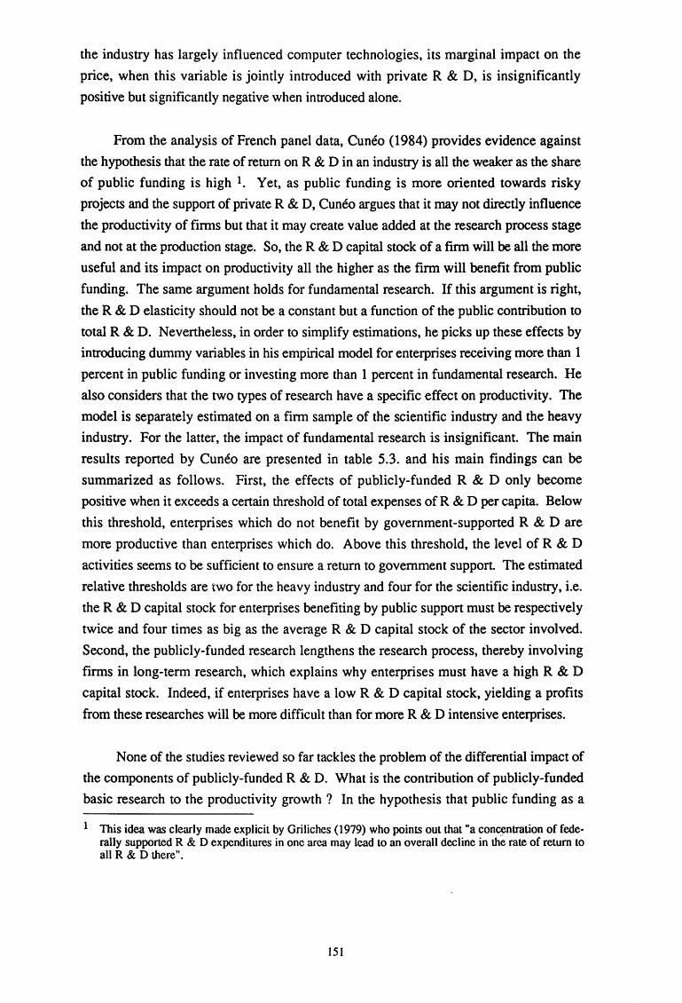
the industry has largely influenced con1puter technologies, its marginal impact on the

price, when this variable is jointly introduced with private R & D, is insignificantly

positive but significantly negative when introduced alone.

From the analysis of French panel data, Cuneo (1984) provides evidence against

the hypothesis that the rate of return on R & D in an industry is all the weaker as the share

of public funding is high 1. Yet, as public funding is more oriented towards risky

projects and the support of private R & D, Cuneo argues that it may not directly influence

the productivity of firms but that it may create value added at the research process stage

and not at the production stage. So, the R & D capital stock of a firm will be all the more

useful and its impact on productivity all the higher as the firm will benefit from public

funding. The same argument holds for fundamental research. If this argument is right,

the R & D elasticity should not be a constant but a function of the public contribution to

total R & D. Nevertheless, in order to simplify estimations, he picks up these effects by

introducing dummy variables in his empirical model for enterprises receiving more than 1

percent in public funding or investing more than 1 percent in fundamental research. He

also considers that the two types of research have a specific effect on productivity. The

model is separately estimated on a firm sample of the scientific industry and the heavy

industry. For the latter, the impact of fundamental research is insignificant. The main

results reported by Cuneo are presented in table 5.3. and his main findings can be

summarized as follows. First, the effects of publicly-funded R & D only become

positive when it exceeds a certain threshold of total expenses of R & D per capita. Below

this threshold, enterprises which do not benefit by government-supported R & D are

more productive than enterprises which do. Above this threshold, the level of R & D

activities seems to be sufficient to ensure a return to government support. The estimated

relative thresholds are two for the heavy industry and four for the scientific industry, i.e.

the R & D capital stock for enterprises benefiting by public support must be respectively

twice and four times as big as the average R & D capital stock of the sector involved.

Second, the publicly-funded research lengthens the research process, thereby involving

firms in long-term research, which explains why enterprises must have a high R & D

capital stock. Indeed, if enterprises have a low R & D capital stock, yielding a profits

from these researches will be more difficult than for more R & .D intensive enterprises.

None of the studies reviewed so far tackles the problem of the differential impact of

the components of publicly-funded R & D. What is the contribution of publicly-funded

basic research to the productivity growth ? In the hypothesis that public funding as a

1 This idea was clearly made explicit by Griliches (1979) who points out that "a con~ntration of fede­rally supported R & D expenditures in one area may lead to an overall decline in the rate of return to all R & D there".

151

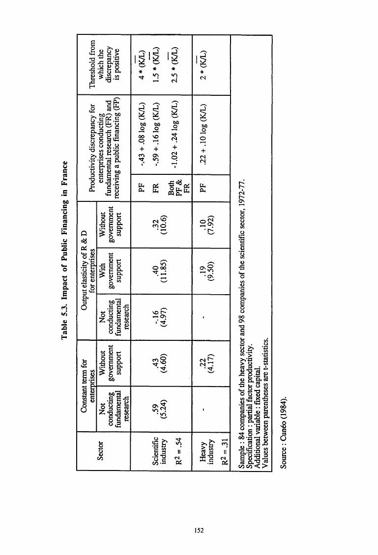
Tab

le 5

.3.

Impa

ct o

f P

ubli

c F

inan

cing

in

Fra

nce

Con

stan

t ter

m f

or

Out

put e

last

icity

of R

& D

en

ter '

rise

s fo

r en

terp

rise

s Pr

oduc

tivity

dis

crep

ancy

for

T

hres

hold

fro

m

Sect

or

Not

W

ithou

t N

ot

With

W

ithou

t en

terp

rise

s co

nduc

ting

whi

ch th

e co

nduc

ting

gove

rnm

ent

cond

uctin

g go

vern

men

t go

vern

men

t fu

ndam

enta

l res

earc

h (F

R)

and

disc

repa

ncy

fund

amen

tal

supp

ort

fund

amen

tal

supp

ort

supp

ort

rece

ivin

g a

publ

ic f

inan

cing

(F

P)

is p

ositi

ve

rese

arch

re

sear

ch

-P

F

-.43

+ .0

8log

(K

/L)

4 * (

K!L

) -

Scie

ntifi

c .5

9 .4

3 -.

16

.40

.32

FR

-.

59 +

.16l

og (K

/L)

1.5

* (K

!L)

indu

stry

(5

.24)

(4

.60)

(4

.97)

(1

1.85

) (1

0.6)

-

Bot

h -1

.02

+ .2

4log

(K

IL)

2.5

* (K

/L)

R2

=.5

4

PF

&

FR

--

VI

N

Hea

vy

-.2

2 -

.19

.10

PF

.2

2 +

.10

log

(K/L

) 2

* (K

/L)

indu

stry

(4

.17)

(9

.50)

(7

.92)

R2

= .3

1

Sam

ple

: 84

com

pani

es o

f the

hea

vy s

ecto

r and

98

com

pani

es o

f the

sci

entif

ic s

ecto

r, 19

72-7

7.

Spec

ific

atio

n : p

artia

l fac

tor p

rodu

ctiv

ity.

Add

ition

al v

aria

ble

: fix

ed c

apita

l. V

alue

s be

twee

n pa

rent

hese

s ar

e t-

stat

istic

s.

Sour

ce :

Cun

eo (

1984

).

Tab

le 5

.4.

Rat

e of

Ret

urn

on B

asic

Res

earc

h in

the

Uni

ted

Sta

tes

Bas

ic r

esea

rch

App

lied

rese

arch

St

udy

Sam

ple

Add

ition

al v

aria

bles

C

ompa

ny-

Gov

ernm

ent-

Com

pany

-G

over

nmen

t-R

2 fin

ance

d fin

ance

d fin

ance

d fin

ance

d

Man

sfie

ld (

1980

) 20

man

ufac

turin

g U

nion

izat

ion

1.33

0.

11

0.06

.6

3 in

dust

ries

(1

.51)

(0

.59)

(0

.80)

Uni

oniz

atio

n an

d ex

pect

ed

0.68

-0

.02

0.12

.8

7 R

&D

pay

off

(1

.27)

(0

.21)

(2

.88)

Lin

k (1

981)

51

man

ufac

turin

g U

nion

izat

ion

2.31

1.

17

0.19

-0

.0

.43

firm

s (3

.87)

(2

.13)

(1

.83)

(0

.31)

Not

e : v

alue

s be

twee

n pa

rent

hese

s ar

e t-s

tatis

tics.

whole is ineffective, we cannot conclude that all the components of publicly-funded R &

D are not potent. Only few studies have tried to shed light on this issue. Although not

directly investigating the issue of the effectiveness of public funding, Mansfield ( 1980)

has attempted to estimate the rate of return on basic research as opposed to applied

research and development. This analysis is an extension of Terleckyj's studies. In this

analysis, the sources of funds are considered separately for applied research and

development (privately financed versus publicly financed) but not for basic research. As

shown in table 5.4, all the variables are insignificant. Yet, an alternative result based on

total applied research and development expenditure gives significant coefficients of

respectively 1.49 for this variable and .07 for basic research. Another regression

introducing an expected R & D payoff variable (calculated as the percentage of the

industry's firms that expected their R & D expenditures to pay off in no less than six

years) shows a significant rate of return on publicly-financed applied research and

development but not on the privately-financed one. From complementary regression

results, Mansfield concludes that the productivity growth of an industry seems to be

directly and significantly related to the extent to which its R & D is long-term investment.

Yet, although the results are very mitigated, they throw a new light on Terleckyj's

negative findings about the real rate of return on publicly-fmanced R & D. An additional

evidence against the negative diagnoses about the effectiveness of publicly-funded R & D

is given by Li~ (198lb) from a more disaggregated analysis of finn data. In his model,

he separately introduces company-financed and government-financed basic research and

applied research plus development expenditures. In addition to results similar to

Mansfield's ones, his results suggest that government-financed basic research is also a

significant determinant of finn productivity growth but its impact is about half the value

observed for company-financed basic research as shown in table 5.4. The impact of

government-financed applied research plus development is near zero and insignificant.

On the other hand, the private applied research and development is marginally significant

and compared to basic research its impact its quantitatively marginal.

In a nutshell, the studies dealing with the impact on productivity of government

funded R & D generally lead to conclude that public support to R & D may be largely

unproductive1• Yet, some studies emphasize that the relationship between government R

& D support and productivity may be more subtle than the link between private R & D

and productivity growth. The objectives of public support (defense, prestige and

economic activity), the rules that govern the allocation of public funds to R & D

(competitive contracts, cost sharing) and the character of use of government R & D (basic

1 While not reporting his results, Klette (1991) also points out from the analysis of a_ large sample of Norwegian firms that his estimate of the private rate of return to publicly-financed R & D has turned

, ; . _ _out to be non-si~nifica~t..

154

research, applied research and development) are all elements which strongly influence the

effectiveness of public R & D investments. While the incentive of an enterprise to invest

in R & D may to a large extent come down to the profit maximization rule, the incentives

of public intervention are more complex and cannot easily be summarized in a single rule.

Defense-oriented R & D is not directly aimed at furthering economic growth, basic

research certainly sustains more long-term economic growth than short-term economic

growth and the effectiveness of public support to new economic products and processes

produced by business enterprises strongly depends on the own economic effectiveness of

recipient private enterprise. As pointed out by Mansfield (1988b) the higher effectiveness

of applied R & Din Japan compared to the US is to have been much faster and more

efficient imitators than American fmns. Yet, there is no evidence that Japanese firms

have been faster or more efficient innovators than American firms. He adds that

"American firms might respond by putting more resources into process R & D, which

would make it more difficult for Japanese ftrms and others to appropriate a large share of

the benefits from American product innovations. Also, American firms might increase

their own capacity to imitate quickly, efficiently, and creatively". This shows that if

public support is only an economically non-discriminant R & D support, the rate of return

on private R & D will to a large extent be the single mirror of its rate of return. The main

question regarding government support is perhaps more whether it is efficient than

whether it is effective. In other words, if public support toR & D only sustains the

private technological trends, its impact on productivity will be a duplication of the effect

of private R & D. What productivity studies shed light on is the relative inefficiency of

government support to R & D, not its ineffectiveness. In our view, the investment

approach is more appropriate to answer to the question of whether effective government

R & D support is, i.e. effective in promoting private R & D.

5.3. How Stimulating is the Publicly-Financed R & D ?

In an early attempt to measure the impact of publicly-funded R & D, Blank and

Stigler ( 1957) arrive to contradictory conclusions on the basis of two alternative

methodological approaches. The first one which rests on aggregate data for seventeen

industries in which firms are classified into two groups according to whether they are

engaged in government research or not, gives strong support to the substitution

hypothesis. They hypothesize that public R & D support is a substitute for private R & D

if the ratio to total employment of scientists and engineers engaged in private research is

higher for the first group of firms than for the second. This hypothesis is verified for

fifteen industries and for industry as a whole, which strongly buttresses the substitution

155

hypothesis. In the second approach they only consider firms that perform R & D and

only take their size into account Industries with high ratios of scientists and engineers in

private R & D also appear to have high ratios of scientists and engineers engaged in

government R & D. This observation is particularly apparent for large firms. These

findings lead the authors to conclude that public R & D is complementary to private R &

D. Their global comment from these contradictory results is that the substitution effect

derived from the aggregate data is grossly exaggerated in this type of approach.

However, this study used an indirect approach based on R & D manpower to

measure the effect of public R & D on private R & D. The recent literature covers a more

direct approach to analyzing to what extent public resources allocated to R & D modulate

privately-funded R & D expenditures, the investment function approach. Like the

production approach, the investment models may be classified as either based on

aggregate time-series, industry-level cross-sections or fmn-level cross-sections. While in

this approach, the interpretation of estimates is less ambiguous than in the production

function approach, the models greatly diverge according to the specification of models

and variables. Some models simply investigate the link between company-financed R &

D and government-financed R & D by either using or not using transformed data and

only controlling for industry- or fmn- fixed effects or demand shift Others are designed

in the Schumpeterian tradition and introduce additional relevant variables to measure

market structure effects. A last class of models are inspired by macroeconomics in that

they are derived from demand models in which changes in output and relative factor

prices, the adjustment process to equilibrium and/or the economic conditions are taken

into account. The main characteristics of these empirical models are summarized in tables

5.5 and 5.6. Only models dealing with the impact of publicly-financed R & Don private

R & D are reviewed. In table 5.5, the estimated coefficients are elasticities while in table

5.6 they are marginal effects.

Using a general disequilibrium demand model, Nadiri (1980) examines how

publicly-funded R & D capital stock influences privately-funded R & D capital stock in

three aggregated industries. The estimated effects noticeably differ according to the

industries considered. They are positive and statistically significant for total

manufacturing and in durables industries and significantly negative in non-durables

industries. His tests give some evidence that the effect of government financing is felt

within the year but he suspects that the aggregation of data could conceal the true timing

rel-ationship. The elasticities obtained are very small in all cases. Although it could be

concluded from this study that government support globally complements private R & D

156

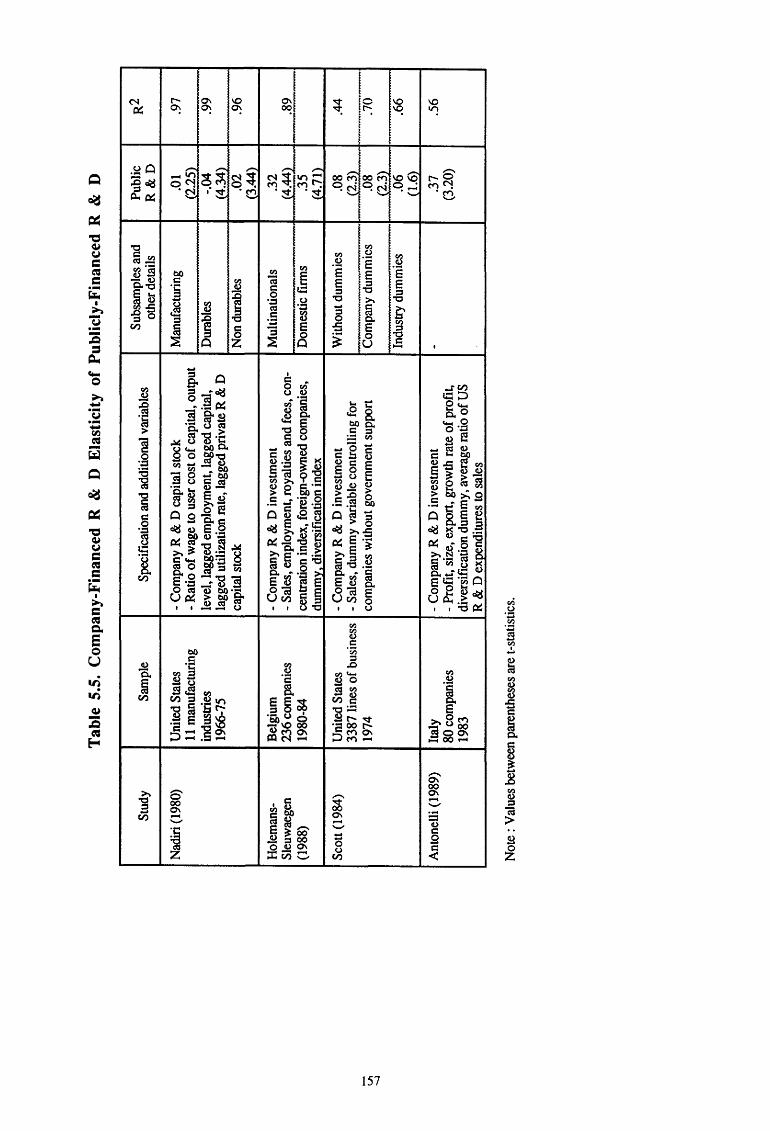
Tab

le 5

.5.

Com

pan

y-F

inan

ced

R &

D

Ela

stic

ity

of

Pu

bli

cly-

Fin

ance

d R

&

D

Stud

y Sa

mpl

e Sp

ecifi

catio

n an

d ad

ditio

nal v

aria

bles

Su

bsam

ples

and

Pu

blic

R

2 ot

her d

etai

ls

R&

D

Nad

iri (

1980

) U

nite

d St

ates

-C

ompa

ny R

& D

cap

ital s

tock

M

anuf

actu

ring

.01

.97

11 m

anuf

actu

ring

-Rat

io o

f wag

e to

use

r co

st o

f cap

ital,

outp

ut

(2.2

5)

indu

strie

s le

vel,

lagg

ed e

mpl

oym

ent,

lagg

ed c

apita

l, D

urab

les

-.04

.99

1966

-75

lagg

ed u

tiliz

atio

n ra

te, l

agge

d pr

ivat

e R

& D

(4

.34)

ca

pita

l sto

ck

Non

dur

able

s .0

2 .9

6 (3

.44)

Hol

eman

s-B

elgi

um

-C

ompa

ny R

& D

inve

stm

ent

Mul

tinat

iona

ls

.32

Sleu

wae

gen

236

com

pani

es

-Sal

es, e

mpl

oym

ent,

roya

lties

and

fees

, con

--·-

----

----

----

-~· !4

.44

L ...

._ ..... .

...:!9 _

__

(1

988)

19

80-8

4 ce

ntra

tion

inde

x, f

orei

gn-o

wne

d co

mpa

nies

, D

omes

tic f

irms

.35

dum

my.

div

ersi

ficat

ion

inde

x (4

.71)

Scot

t (19

84)

Uni

ted

Stat

es

-C

ompa

ny R

& D

inve

stm

ent

With

out d

umm

ies

.08

.44

3387

line

s of

bus

ines

s -S

ales

, dum

my

varia

ble

cont

rolli

ng fo

r (2

.3)

~~~·-

1974

co

mpa

nies

with

out g

over

nmen

t sup

port

C

ompa

ny d

umm

ies

.08

. 70

(2.3

) In

dust

ry d

umm

ies

.06

.66

(1.6

)

Ant

onel

li (1

989)

Ita

ly

-C

ompa

ny R

& D

inve

stm

ent

-.3

7 .5

6 80

com

pani

es

-Pro

fit,

size

, exp

ort,

grow

th r

ate

of p

rofi

t, (3

.20)

19

83

dive

rsifi

catio

n du

mm

y, a

vera

ge r

atio

of U

S R

& D

exp

endi

ture

s to

sal

es

Not

e : V

aloe

s be

twee

n pa

rent

hese

s ar

e t -s

tatis

tics.

Tab

le 5

.6.

Mar

gina

l Im

pact

of

Pub

licl

y-F

inan

ced

R &

D

on

Com

pany

-Fin

ance

d R

&

D

Stu

dy

Sam

ple

Spe

cifi

cati

on a

nd a

dditi

onal

var

iabl

es

Sub

sam

ples

and

M

argi

nal

R2

othe

r de

tail

s im

pact

Car

mic

hael

(19

81)

Uni

ted

Sta

tes

-C

ompa

ny R

& D

inv

estm

ent

Ful

l sa

mpl

e -.

08

.96

46

tran

spor

t com

pani

es

-Sal

es

(2.3

1)

1976

-77

Big

fir

ms

-.07

.9

5 (1

.42)

S

mal

l fi

rms

-.06

.5

9 (3

.39}

Lin

k (1

982)

U

nite

d S

tate

s -C

om

pan

y R

& D

int

ensi

ty

Pri

vate

R &

D

.09

.39

275

com

pani

es

-R

elat

ive

prof

its,

div

ersi

fica

tion

inde

x, c

on-

inte

nsit

y (2

.01)

19

77

cent

rati

on in

dex,

ow

ners

hip

dum

mie

s Pe

rcen

tage

allo

cate

d -.

08

.46

to b

asic

rese

arch

(1

.75)

Pe

rcen

tage

allo

cate

d -.0

1 .3

2 to

app

lied

rese

arch

(1

.59)

Pe

rcen

tage

all

ocat

ed

.09

.40

to d

evel

opm

ent

(2.3

1)

Levy

-T er

leck

yj

Uni

ted

Sta

tes

-C

ompa

ny R

& D

inv

estm

ent

Gov

ernm

ent

R &

D

.21

-(1

983)

P

riva

te b

usin

ess

sect

or

-O

utpu

t, ta

xes,

une

mpl

oym

ent,

wei

ghte

d (6

.97)

19

49-8

1 av

erag

e ag

e o

f th

e R

& D

sto

ck

Gov

ernm

ent c

ontr

act

.27

--VI

R&

D

.(8.

86).

0

0

Oth

er g

over

nmen

t .1

9 -

R&

D

(1.7

6)

Lev

in-R

eiss

(19

84)

Uni

ted

Sta

tes

-C

ompa

ny R

& D

int

ensi

ty

-.1

2 -

20 in

dust

ries

-

Rel

ativ

e ba

sic

R &

D e

xpen

ditu

res,

ind

ustr

y (2

.86)

19

67,

1972

, 19

77

age,

con

cent

rati

on in

dex,

new

and

im

prov

ed

Gov

ernm

ent

R &

D

2.69

-

prod

ucts

-ori

ente

d R

& D

(2

.68)

G

over

nmen

t R

& D

-2

4.08

-

conc

entr

atio

n in

dex

(_2.

61}

Sco

tt (

1984

) U

nite

d S

tate

s -

Com

pany

R &

D i

nten

sity

W

itho

ut d

umm

ies

.10

.03

3387

lin

es o

f bu

sine

ss

(9.9

) 19

74

Wit

h co

mpa

ny

.08

.36

dum

mie

s (5

8)

Wit

h in

dust

ry

.09

.34

dum

mie

s (6

2)

$wit

zer (

1985

) U

nite

d S

tate

s -

Com

pany

R &

D i

nves

tmen

t -

.08

.96

125

com

pani

es

-L

agge

d R

& D

, con

cent

rati

on in

dex,

cha

nge

(0.9

2)

1977

in

sal

es,_

fina

ncia

l va

riab

les

Ant

onel

li (

1989

) It

aly

-C

ompa

ny R

& D

inv

estm

ent

Rat

io o

f pu

blic

8.

27

.47

80 c

ompa

nies

-

Pro

fit,

siz

e, e

xpor

t, g

row

th r

ate

of

prof

it,

subs

idie

s to

tota

l (2

.94)

19

83

dive

rsif

icat

ion

dum

my,

ave

rage

rat

io o

f US

R

&D

R

& D

exp

endi

ture

s to

sal

es

Not

e : v

alue

s be

twee

n pa

rent

hese

s ar

e t-

stat

isti

cs.

the substitution effect obtained for non-durables manufacturing makes the analysis

inconclusive.

More conclusive were the tests made by Scott (1984) on the basis of a large sample

of observations on lines of business for 437 companies. He estimates two alternative

models. First, he regresses company R & D intensity on goverment-financed R & D

intensity with and without controlling for company and industry effects. His first result,

in which there is not control variable for fixed effects, shows that company R & D

intensity is greater in lines of business where government-financed R & dis greater. In

other words, government financing goes to firms that do a lot ofR & D. When company

indicators are introduced, the estimate remains significant which gives some evidence that

government funds do not principally go to firms that invest a lot in R & D. Instead of

controlling for differences across firms, one can verify how the results can be altered by

simply taking into account the industry effects. This will provide some information on

the possible concentration of public funds towards R & D intensive industries. The

amplitude of the estimated coefficient and its significance imply that of this hypothesis

has to be rejected. From a last regression in which both company and industry effects are

jointly intercepted, the author concludes that the significant impact of government

financing on company R & D expenditures obtained is not simply the result of

government funds going toR & D intensive firms in R & D intensive industries. Not

only does government financing appear to be a complement to private R & D but it also

stimulates R & D. An extra dollar spent by government in R & D generates an extra

investment in company R & D ·c,f eight to ten cents. Yet, these results may only be

spurious because sales are used in the construction of both the dependent and explanatory

variables. To confirm his results, he specifies an alternative model. In this second

model, logarithmic values of company-financed R & D are regressed with respect to

logarithms of sales and government-financed R & D and a control variable for companies

which do not receive any government support. Although far less significant than in the

preceding regression, the estimated coefficients are marginally significant and do not lead

to a rejection of the complementarity hypothesis. Moreover, in the margin, an increase in

public financing stimulates an extra private R & D expenditure.

In a comment on this paper, Link, referrring to his own works, insists on the

subtleties of the relationship between government-financed and company-financed R &

D. Indeed, government-financed R & D not only stimulates the company-financed R &

D but also affects the composition of R & D by category of use. An illustration of this is

given by Link (1982) in an analysis of the determinants of R & D expenditures by

character of use, i.e. basic research, applied research and development. The stimulus

159

coefficient of federal R & D intensity obtained from his firm-level data analysis is

significant and of the same order of magnitude as those reported by Scott. His regression

results on the composition of R & D, that is on the percentage of the company R & D

category of use, suggest that the impulse given to private R & D by an increase in federal

R & D is primarily directed away from basic research and towards development and only

very marginally influences applied research. In his discussion of results, he refers to

complementary tests based on a desaggregation of federal R & D data showing that the

positive relationship between federal R & D intensity and private R & D intensity and the

share of private funds allocated to development is primarily a result of federal applied

research plus development expenditures. In the case of the share of private funds

allocated to basic research, it is the federal basic allocations which is the determinant

factor.

Contrasting with Scott's and Link's findings, Carmichael (1981) reports empirical

evidence regarding the crowding-out hypothesis. He develops a capital asset pricing

model in which companies view R & D investments in terms of their risk and return

characteristics. The latter are altered by R & D investments through the expected profits

from sales and intra-frrm spillover. By public R & D contracting, companies are to some

extent able to separate these two sources of risk and return. In his model, the author

tends to demonstrate that while some public crowding-out of private R & D is likely, this

is almost certain to be incomplete. From the theoritical model, he deduces that private R

& D is an increasing function of the scale of the finn measured by sales and a decreasing

function of publicly-financed R & D. The application of this model to a sample of US

transport firms gives some support to the partial substitution hypothesis. Yet, this

hypothesis is more conclusive for small frrms than for large firms. By and large, this

model implies that each dollar spent by government in R & D adds around 92 cents to

total R & D spending, and decreases private R & D by 8 cents.

Schrieves (1978) analysis, whose results are summarized in table 5.7, also

suggests a crowding out of private R & D by federal R & D. In an analysis of the

relationship between market structure and the intensity of innovative effort, he regresses,

among other variables, the logarithm of privately-financed R & D employment on the

percentage of R & D activity financed by the federal government for a sample of 411

firms classified into four industry groups. For non-specialized producer durable goods

and specialized durable equipment the crowding-out hypothesis is accepted. For

materials, public financing marginally stimulates the R & D activity in this industry. The

complementarity hypothesis cannot be rejected for consumer goods. Yet, as the two

durables industries concentrate a large part of R & D activities, the crowding-out

160

hypothesis cannot be globally rejected. As these industries are heavily oriented towards

electronics, aerospace, mechanical and electro-mechanical fields, public support is

particularly intensive in these industries. So the government finances 26 percent of total

R & D in durables against 4 percent in other industries. The results show that the

marginal crowding-out effect is roughly about -.20 and the government R & D elasticity

-.04 for the industry as a whole. The government R & D elasticity is highest for

specialized durable equipment, its value is -.08. For durables, the elasticity is about the

same as that obtained by Nadiri, and for non durables, it is equal to zero.

In a funds flow approach of determinants of industrial R & D applied to firm-level

data, Switzer (1984) observes that government R & D expenditures do not significantly

influence private R & D and, therefore do not raise total R & D.

From a study reappraising the Schumpeter hypothesis that technological innova­

tions are more likely to be initiated by large rather than small firms, Rosenberg (1976)

tests the hypothesis that government R & D financing stimulates private R & D. His

dependent variable is defined as the percentage of total employment allocated to

professional R & D personnel and his proxy for government R & D is the fraction of the

firm's shipments originating in industries whose research is heavily subsidized by the

government. The estimates confirm the stimulus hypothesis as shown in table 5.7. Yet,

as his explanatory variable is contructed by accounting the ratio of firm's shipments to

government on total shipments from industries whose R & D is subsidized at more than

50 percent by government, the stimulus may arise from government R & D contracts as

well as from government non-R & D contracts.

In an examination of the simultaneous relationship between market structures and

research intensity, Levin and Reiss ( 1984) tests how government policy affects

technological opportunity and appropriability and how technological opportunity and

appropriability conditions influence government R & D decisions. In their model, R & D

intensity depends on the elasticity of unit cost with respect to own R & D, which is a

measure of technological opportunity, and on the elasticity of unit cost with respect to

industry wide R & D, which is a measure of technological appropriability multiplied by

the conjectural variation with respect to R & D and divided by the Herfindahl index of

concentration. On the one hand, the technological opportunity variable indicates the

responsiveness of cost to own research effort and on the other hand, the technological

appropriability variable represents how much a frrm benefits from an increase in the

common R & D pool. Among the determinants of opportunity, they assume that

161

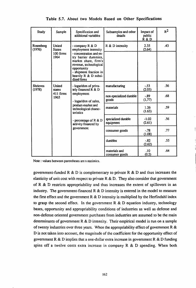
Table 5. 7. About two Models Based on Other Specifications

Study Sample Specification and Subsamples and other Impact of R2 additional variables details public

R&D

Rosenberg United - company R & D R & D intensity 2.35 .43 (1976) States employment intensity (2.64)

100 firms - concentration and en-1964 try barrier dummies,

market share, firm's revenue, technological opportunity - shipment fraction in heavily R & D subsi-dized fmns

Shrieves United - logarithm of priva- manufacturing -.53 .56 (1978) states tely financed R & D (2.05)

411 firms employment non-specialized durable -.89 .68 1965

- logarithm of sales, goods (1,77)

product-market and materials 1.26 .59 technological charac-

teristics (1.63)

- percentage of R & D specialized durable -1.02 .56

activity financed by equipment (2.61)

government consumer goods -.78 .77

(1.08)

durables -.82 .55 (2.62)

materials and .10 .64 consumer goods (0.2)

Note: values between parentheses are t-statistics.

government-funded R & D is complementary to private R & D and thus increases the

elasticity of unit cost with respect to private R & D. They also consider that government

of R & D restricts appropriability and thus increases the extent of spillovers in an

industry. The government-financed R & D intensity is entered in the model to measure

the first effect and the government R & D intensity is multiplied by the Herfindahl index

to grasp the second effect. In the government R & D equation industry, technology

bases, opportunity and appropriability conditions of industries as well as defense and

non-defense oriented government purchases from industries are assumed to be the main

determinants of government R & D intensity. Their empirical model is run on a sample

of twenty industries over three years. When the appropriability effect of government R &

D is not taken into account, the magnitude of the coefficient for the opportunity effect of

government R & D implies that a one-dollar extra increase in government R & D funding

spins off a twelve cents extra increase in company R & D spending. When both

162

opportunity and appropriability effects are accounted for, the extra increase is about

seventy-four cents. Yet, it seems that while government R & D stimulates private R & D

by increasing technological opportunities, it also increases technological appropriability

and so diminishes spillovers. The authors explain these contradictory results by the fact

that "much government funding supports R & D for large-scale, capital-intensive defense

systems which are not cheaply replicable despite mandatory licensing and technology

transfer provisions". Another explanation is that as government R & D funding

principally flows into industries with a high concentration rate, the technologifal

appropriability variable may also capture the diminushing return effect of public funding

on private R & D spending. In the government R & D equation, defense procurement is

the most significant variable. Technological opportunity appears to offer little incentive to

the government, which moreover seems to react with a substantial lag compared to

private industry. The extent of interindustry R & D spillovers appears to increase the

likelihood of government support.

Together with their analysis of the effects of government R & D funding on

productivity, Levy and Terleckyj (1983) studied at a macroeconomic level how effective

government funding was to generate additional private R & D investments. Besides the

total federally-funded R & D performance, they look at how the allocation of these funds

makes difference by distinguishing R & D contract from other categories of government

R & D spending. They find some evidence that total government R & D spending

stimulates an additional private R & D expenditure of 21 cents per dollar. However, this

indirect effect seems attributable to R & D contracts and not to other forms of government

R & D. The impulse effect of government R & D contracts is of 28 cents per dollar

against no effect for other government R & D. The search for a lag structure of R & D

contract has shown that the major impact occurs within the same year as the R & D

contract. Their explanation is that "the performing companies have learned to form

realistic expectations about future government support by developing R & D proposals

for the government in a way which takes into account their plans for future

complementary R & D funded with their own resources". For other federal R & D, an

average three-year lag was estimated. When this lagged effect is taken into account,

federal outlay for R & D performed outside industry appears to induce an additional

private R & D expenditure of 19 cents per dollar. However, this impact is only

marginally significant. These estimates of the effect of government R & Don private R

& D are largely higher than those obtained in the other studies. The authors'

interpretation of those divergences is that at the macroeconomic level, the estimates reflect

the cross effects of government contract R & D on private R & D expenditures in

companies other than those performing the R & D contracts.

163

Studies measuring the indirect effects of government R & D funding on private R &

Din other countries than the United States are not plentiful. Holemans and Sleuwaegen

( 1988) focused on the role of government support in stimulating private R & D

investment of foreign and domestic companies in Belgium. Their sample bears on time­

series of firm-level data. The other variables introduced in the model are sales and

employment which are shown not to be simply a substitute for size measures, as often

assumed in tests of the Schumpeterian hypothesis, but also to capture other effects.

Payments for royalties and fees are also included to measure to what extent foreign fmns

do less R & D than domestic firms due to a centralization of R & D functions within

multinational companies. Their estimates suggest complementarity between government­

financed R & D and privately-financed R & D and that the effects do not differ between

foreign and domestic companies. The elasticities are largely higher than those obtained

for the US but similar to those reported by Antonelli for Italy.

In his study, Antonelli ( 1989) investigates how declining profits and increasing

competition can stimulate innovative efforts. In his failure-inducement model, he

introduces, besides the profitability, the size of fmns, the export and a dummy for large

financial groups to explain the level of R & D expenditures for a sample of Italian firms.

He also takes into account the pressure of the international technological environment by

including the private R & D intensity of US f1rms. Concerning public subsidies, he

argues that they have helped Italian firms "to fund levels of R & D expenditures beyond

those allowed by short-term payback criteria". He respectively tests the linear and

multiplicative specifications of the model which tum out to adjust itself in a noticeably

similar way with regard to the ratio of public subsidies to total R & D expenditures.

According to the estimates, the marginal effect and the elasticity are very high, which

indicates a strong incentive effect of public subsidies on private R & D.

Levy (1990) argued that the absence of significant effect of government R & Don

productivity is due to the confusion of zero value of marginal product with zero marginal

physical product. If one supposes that government R & D can be employed without

private cost, it is a public good that a f1rm uses at zero wage and, therefore, in equi­

librium, the value of government financing's marginal product is zero. In other words,

the zero coefficient associated with government-financed R & Din the production ap­

proach results from the equalization by the f1rms of the value of the marginal product of

public R & D to their cost of utilizing this public R & D. This implies that the measure­

ment of the impact of government R & D on output cannot be directly evaluated when the

production is measured in value terms. Hence he suggests to use the indirect approach

164

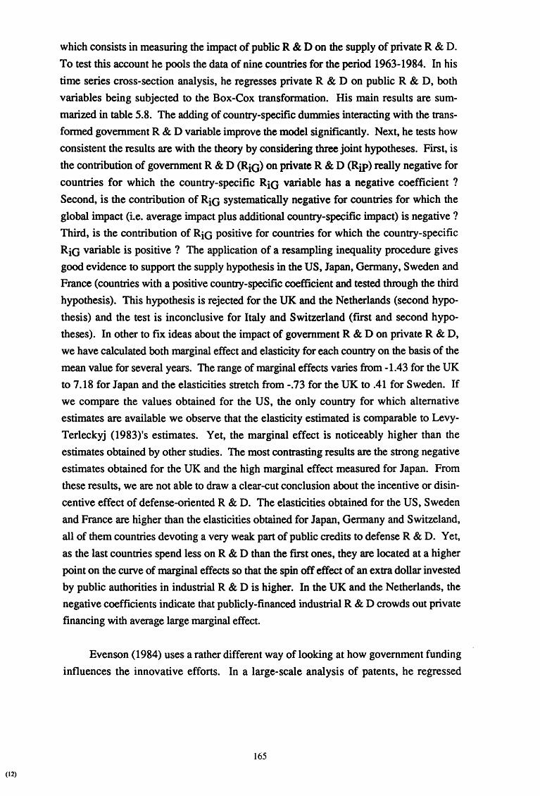
(12)

which consists in measuring the impact of public R & Don the supply of private R & D.

To test this account he pools the data of nine countries for the period 1963-1984. In his

time series cross-section analysis, he regresses private R & Don public R & D, both

variables being subjected to the Box-Cox transformation. His main results are sum­

marized in table 5.8. The adding of country-specific dummies interacting with the trans­

formed government R & D variable improve the model significantly. Next, he tests how

consistent the results are with the theory by considering three joint hypotheses. First, is

the contribution of government R & D (Rio) on private R & D (RiP) really negative for

countries for which the country-specific RiG variable has a negative coefficient ?

Second, is the contribution of Rio systematically negative for countries for which the

global impact (i.e. average impact plus additional country-specific impact) is negative ?

Third, is the contribution of RiG positive for countries for which the country-specific

RiG variable is positive ? The application of a resampling inequality procedure gives

good evidence to support the supply hypothesis in the US, Japan, Germany, Sweden and

France (countries with a positive country-specific coefficient and tested through the third

hypothesis). This hypothesis is rejected for the UK and the Netherlands (second hypo­

thesis) and the test is inconclusive for Italy and Switzerland (first and second hypo­

theses). In other to fix ideas about the impact of government R & Don private R & D,

we have calculated both marginal effect and elasticity for each country on the basis of the

mean value for several years. The range of marginal effects varies from -1.43 for the UK

to 7.18 for Japan and the elasticities stretch from -.73 for the UK to .41 for Sweden. If

we compare the values obtained for the US, the only country for which alternative

estimates are available we observe that the elasticity estimated is comparable to Levy­

Terleckyj (1983)'s estimates. Yet, the marginal effect is noticeably higher than the

estimates obtained by other studies. The most contrasting results are the strong negative

estimates obtained for the UK and the high marginal effect measured for Japan. From

these results, we are not able to draw a clear-cut conclusion about the incentive or disin­

centive effect of defense-oriented R & D. The elasticities obtained for the US, Sweden

and France are higher than the elasticities obtained for Japan, Germany and Switzeland,

all of them countries devoting a very weak part of public credits to defense R & D. Yet,

as the last countries spend less on R & D than the ftrst ones, they are located at a higher

point on the curve of marginal effects so that the spin off effect of an extra dollar invested

by public authorities in industrial R & D is higher. In the UK and the Netherlands, the

negative coefficients indicate that publicly-financed industrial R & D crowds out private

financing with average large marginal effect.

Evenson ( 1984) uses a rather different way of looking at how government funding

influences the innovative efforts. In a large-scale analysis of patents, he regressed

165

patents awarded to nationals in the US by industry over the period 1964-1978 on R & D

efforts, the proportion of government support, the proportion of basic research and the

proportion invested in development I. The introduction in the equation of the proportion

of different types of R & D besides total R & D investment allows to control for some

characteristics of the research system on patenting and provides a test similar to that

performed by Griliches (1986) in order to verify if private R & D and federal R & D were

equally potent. The potent elasticity of R & D is 1.23, which shows increasing returns of

R & D in patenting while one cannot really reject the hypothesis of constant returns. The

coefficient for government-funded R & D is 1.93, which indicates a large positive

premium on federal R & D of 150 percent. This result is very surprising given the often

emphasized argument that federal R & D carries restrictions on appropriability. The

coefficients of basic research and development are respectively 13.77 and 1.38, which

provides evidence of the less patentable character of basic research and of the near-the­

market character of experimental development.

In several successive articles, Lichtenberg ( 1984, 1987, 1988) has harshly

criticized studies which found that the federal R & D expenditure in the US has a positive

and significantly different from zero impact on private R & D expenditure. He argues

that studies of the relationship between federal and company R & D are generally upward

biased (Lichtenberg (1984)). First, the hypothesis of exogeneity of federal R & D

impulse on company R & D is largely unacceptable at the micro level because firm

characteristics play an important role in the allocation of federal R & D contracts. He

strongly suspects that the disregard for these firm characteristics causes an upward bias

of estimates. To obtain an unbiased estimate, he recommends to work on changes in the

variables over time. Second, he points out that deflating both company and federal

expenditures by the same error-ridden deflator to measure the real inputs devoted to R &

D induces spurious positive correlation between both variables, i.e. company and federal

R & D expenditures. As the bias is of unknown magnitude and direction, he suggests to

supplement data with an analysis of direct quantity indices of R & D input such as R & D

employment. Third, he underlines that the conventional practice of dividing both

·company and federal R & D by sales is likely to produce an upward bias in the estimates.

Subsequently, he reports estimates which support his arguments. Results of pooled

regressions of changes in privately-funded R & D expenditure and employment on

corresponding changes in federally-funded R & D at the industry level over the period

1963-1979 give an estimate insignificantly different from zero for the frrst measure and a

negative coefficient with the second n1easure, which implies a crowding-out effect of

federal-sponsored employment on con1pany-supported employment. He also presents a

1 He also includes industry indicators and some year dummies.

166

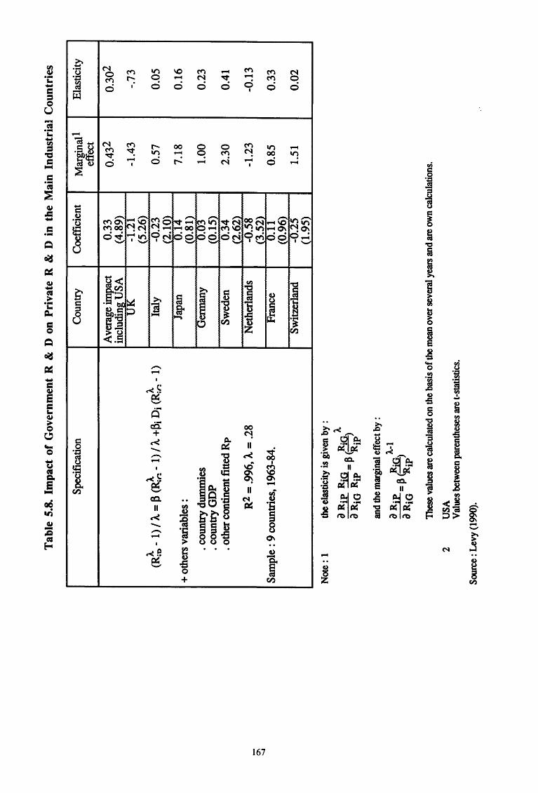
Tab

le 5

.8.

Impa

ct o

f G

over

nmen

t R

& D

on

Pri

vate

R &

D i

n th

e M

ain

Indu

stri

al C

ount

ries

Spe

cifi

cati

on

A

A

A

(R:D

-1)

I A.

= l3

(~('

!-1)

I A.

+ll

i Di

(R:I

'!-1)

+ o

ther

s va

riab

les

:

. cou

ntry

dum

mie

s . c

ount

ry G

DP

. o

ther

con

tine

nt fi

tted

Rp

R2

= .9

96, A.

= .2

8

Sam

ple

: 9 c

ount

ries

, 19

63-8

4.

Not

e: 1

th

e el

astic

ity is

giv

en b

y :

a Rip

&G

__

RiG

A

a Rio

Rip

-Ji

(Rip

)

and

the

mar

gina

l eff

ect b

y :

~-

&z:

A-1

a R

io-li ~i

P>

Cou

ntry

Ave

rage

impa

ct

incl

udin

g U

SA

U

K

Italy

Japa

n

Ger

man

y

Sw

eden

Net

herl

ands

Fra

nce

Sw

itze

rlan

d

Coe

ffic

ient

M

argi

nai1

ef

fect

0.33

0.

432

(4.8

9)

-1.2

1 -1

.43

(5.2

6)

-0.2

3 0.

57

(2.1

0)

0.1

4

7.18

(0

.81)

0.

03

1.00

(0

.15)

0

.34

2

.30

(2

.62)

-0

.58

-1.2

3 (3

.52)

0.

11

0.85

(0

.96)

-0

.25

1.51

(1

.95)

The

se v

alue

s are

cal

cula

ted

on th

e ba

sis

of th

e m

ean

over

seve

ral y

ears

and

are

ow

n ca

lcul

atio

ns.

2 U

SA

Val

ues

betw

een

pare

nthe

ses

are

t-sta

tistic

s.

Sour

ce :

Levy

(199

0).

Ela

stic

ity

0.30

2

-.73

0.0

5

0.1

6

0.2

3

0.41

-0.1

3

0.3

3

0.0

2

second analysis based on finn data in which he successively regresses the levels and the

changes in the R & D- sales ratios. From his results summarized in table 5.9, one can

observe for the level version a significant positive impact of federally-funded R & D in

1967 and 1972 whilst the estimated coefficient is negative for 1977. For the variation

version, all the coefficients are negative and highly significant. To conclude, he points

out that his findings "make heavier the burden of proof on those who would claim that

federal contract R & D makes a positive contribution to aggregate technical progress".

Another argument puts forward by Lichtenberg (1987) is that previous estimates

introducing sales or GNP as an explanatory variable are seriously upwardly biased

because they fail to control for shifts in the composition of final demand. This

misspecification is due to the existence of a correlation between the federal demand and

the federal R & D funding. He contests the a priori hypothesis that sales to each

customer identically affect the marginal returns on R & D and, therefore, that the

composition of final demand does not influence the equilibrium private R & D

expenditure. As we are primarily interested in a consistent estimate of the impact of

publicly-funded R & D, the restriction of identical coefficients for sales to the government

and to other customers cannot be maintained and this, for two reasons. First, an increase

in government purchases will tend to stimulate more private R & D investment than any

increase in purchases from other customers. Second, if the government is a major source

of R & D financing, it is also an important customer. So, not only the impact of

government purchases is likely to be substantially higher than the effect of other

purchases but government purchases are also expected to be strongly positively correlated

with government-financed R & D. If these propQsitions are right, part of the estimated

effect of public R & D support on private R & D is statistically spurious. The author

provides some empirical evidence by estimating both restricted and unrestricted models

for US aggregate time-series data and finn-level data. From his main results reproduced

in Table 5.10, on can observe that the federal R & D funding variable becomes

insignificant when federal purchases are separately introduced into the equations. So,

controlling for the components of sales inverts the finding of a positive significant effect

of federal R & D on private R & D and this, at both micro and macro levels. What has

been interpreted as the effect of federal R & D is nothing else than the effect of

government demand.

Continuing his analysis about the effectiveness of public R & D in promoting

private R & D, Lichtenberg (1988) gave further evidence by estimating regressions of

private R & D expenditure on the value of competitive and non-competitive R & D and

168

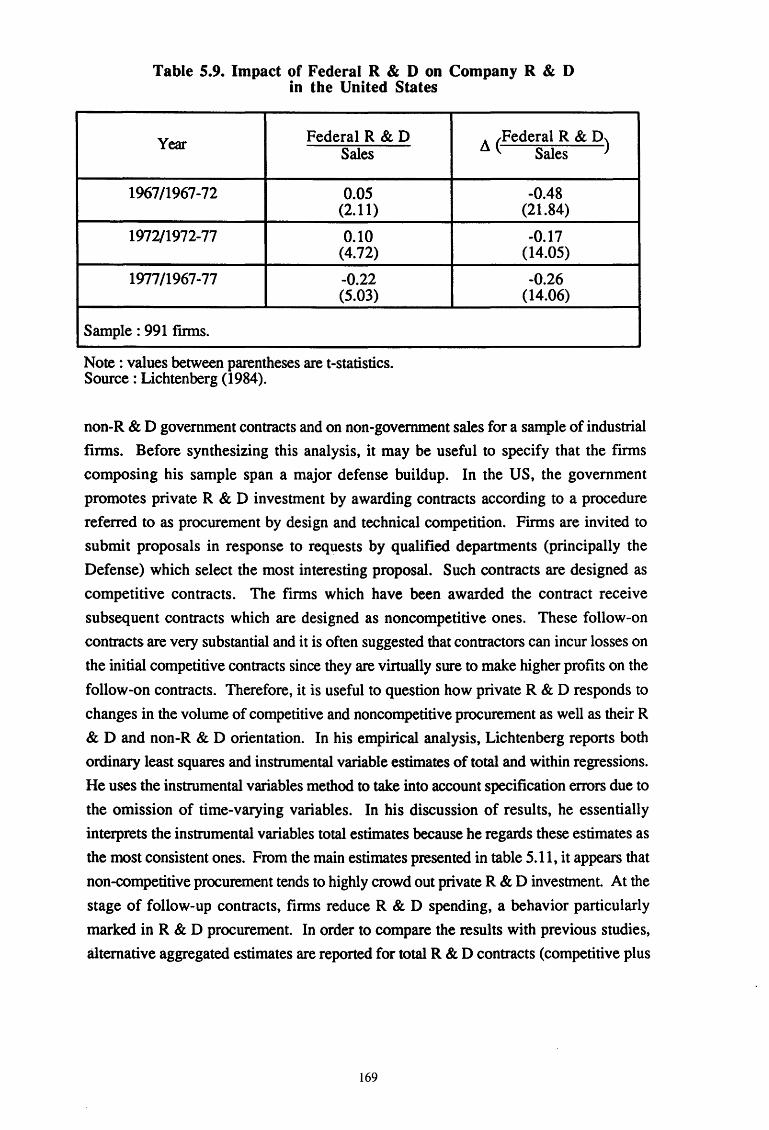
Table 5.9. Impact of Federal R & D on Company R & D in the United States

Year Federal R & D Sales

1967/1967-72 0.05 (2.11)

1972/1972-77 0.10 (4.72)

1977/1967-77 -0.22 (5.03)

Sample: 991 fmns.

Note: values between parentheses are t-statistics. Source : Lichtenberg (1984).

A (Federal R & D) Sales

-0.48 (21.84)

-0.17 (14.05)

-0.26 (14.06)

non-R & D government contracts and on non-government sales for a sample of industrial

firms. Before synthesizing this analysis, it may be useful to specify that the firms

composing his sample span a major defense buildup. In the US, the government

promotes private R & D investment by awarding contracts according to a procedure

referred to as procurement by design and technical competition. Finns are in vi ted to

submit proposals in response to requests by qualified departments (principally the

Defense) which select the most interesting proposal. Such contracts are designed as

competitive contracts. The firms which have been awarded the contract receive

subsequent contracts which are designed as noncompetitive ones. These follow-on

contracts are very substantial and it is often suggested that contractors can incur losses on

the initial competitive contracts since they are virtually sure to make higher profits on the

follow-on contracts. Therefore, it is useful to question how private R & D responds to

changes in the volume of competitive and noncompetitive procurement as well as their R

& D and non-R & D orientation. In his empirical analysis, Lichtenberg reports both

ordinary least squares and instrumental variable estimates of total and within regressions.

He uses the instrumental variables method to take into account specification errors due to

the omission of time-varying variables. In his discussion of results, he essentially

interprets the instrumental variables total estimates because he regards these estimates as

the most consistent ones. From the main estimates presented in table 5.11, it appears that

non-competitive procurement tends to highly crowd out private R & D investment At the

stage of follow-up contracts, firms reduce R & D spending, a behavior particularly

marked in R & D procurement. In order to compare the results with previous studies,

alternative aggregated estimates are reported for total R & D contracts (competitive plus

169

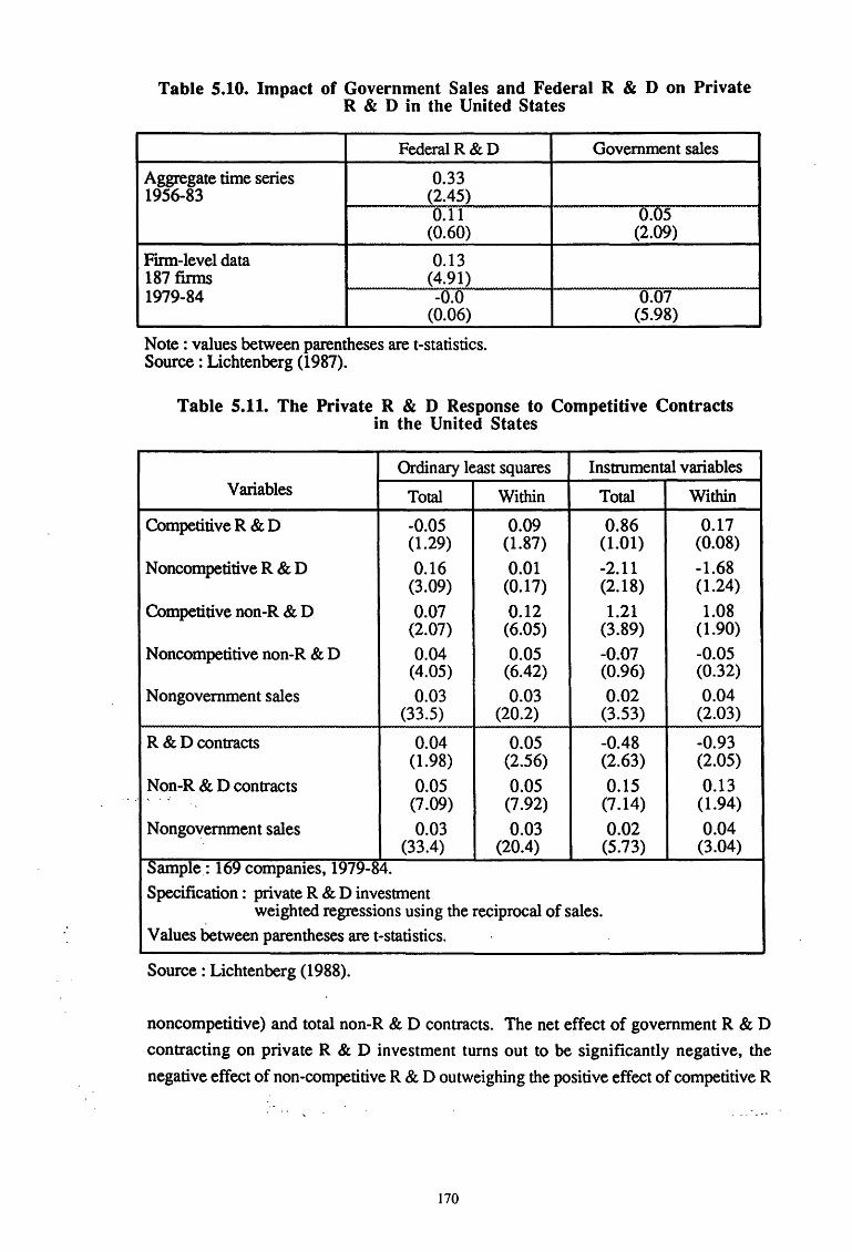
Table 5.10. Impact of Government Sales and Federal R & D on Private R & D in the United States

Federal R&D

Aggregate time series 0.33 1956-83 (2.45)

0.11 (0.60)

Flllll-level data 0.13 187 firms (4.91) 1979-84 -0.0

(0.06)

Note: values between parentheses are t-statistics. Source : Lichtenberg ( 1987).

Government sales

0.05 (2.09)

0.07 (5.98)

Table 5.11. The Private R & D Response to Competitive Contracts in the United States

Ordinary least squares Instrumental variables Variables Total Within Total Within

Competitive R & D -0.05 0.09 0.86 0.17 (1.29) (1.87) (1.01) (0.08)

Noncompetitive R & D 0.16 0.01 -2.11 -1.68 (3.09) (0.17) (2.18) (1.24)

Competitive non-R & D 0.07 0.12 1.21 1.08 (2.07) (6.05) (3.89) (1.90)

Noncompetitive non-R & D 0.04 0.05 -0.07 -0.05 (4.05) (6.42) (0.96) (0.32)

Nongovernment sales 0.03 0.03 0.02 0.04 (33.5) (20.2) (3.53) (2.03)

R & D contracts 0.04 0.05 -0.48 -0.93 (1.98) (2.56) (2.63) (2.05)

Non-R & D contracts 0.05 0.05 0.15 0.13 . . ' ... . ~

(7.09) (7.92) (7.14) (1.94)

Nongovernment sales 0.03 0.03 0.02 0.04 (33.4) (20.4) (5.73) (3.04)

Sample.: 169 companies, 1979-84.

Specification : private R & D investment weighted regressions using the reciprocal of sales.

Values between parentheses are t-statistics.

Source : Lichtenberg (1988).

noncompetitive) and total non-R & D contracts. The net effect of government R & D

contracting on private R & D investment turns out to be significantly negative, the

negative effect of non-competitive R & D outweighing the positive effect of competitive R

170

& D. In contrast, the net effects of non-R & D contracting is significantly positive,

which indicates that the positive effect of competitive non-R & D procurement outweighs

the negative effect of noncompetitive non-R & D contracts. As non-R & D procurements

are largely higher than other forms of procurement, the net effect of procurement as a

whole is positive and quantitatively important. Nevertheless, in contrast to previous

studies and in agreement with his preceding findings, Lichtenberg finds that the net effect

of R & D procurement on private R & D is negative. The important role that the US

government plays in the allocation of R & D resources is apparently stronger when it acts

as a purchaser of goods and services than when it directly stimulates private R & D via R

& D contracting. Hence, the relationship between government-financed and company­

financed R & Dis more subtle than suggested by global approaches. The allocation

process of publicly-funded R & D and market structures heavily influence the

effectiveness of directly and indirectly publicly-funded R & D programmes.

5.4. How Effective is the Public Support to R & D Projects ?

Another method was used by Meyer-Krahmer (1990) to evaluate the impact of

public incentives for the R & D and innovation activities of small and medium-sized

enterprises in Germany over the period 1979-1981. During the period, aid toR & D

personnel expenditures was granted by the German government to enterprises "without

regard to the field of technology concerned, the magnitude of the attendant risks, the

quality of the work or the prospects of economic success". The idea is to make a

comparison of R & D personnel expenditures between subsidized and unsubsidized

enterprises before and after the launching of the programme by regression analysis. He

considers that the incentives can change either the level of R & D or the R & D intensity

or both. If the government support changes the level of R & D, this effect can be

captured by a dummy variable which has the value 0 before and 1 after the governmental

action. The stimulus effect on R & D intensity, for its part, can be picked up by

measuring how the slope of the relationship between turnover and R & D expenditures

has changed. The explanatory variables of the model are turnover and time. The latter is

included in order to separate the conjunctural effect from the input of the incentives.

According to the author, the programme did not change the R & D intensity but it did

change the R & D level. The model was run for different subsamples of enterprises

grouped according to the branch to which they belonged and R & D intensity and fitted

better for branches and enterprises with a high R & D intensity than for those with a weak

R & D intensity. Although his results give evidence of a positive effect of government

171

support, he declares the model inappropriate to calculate accurately the additional R & D

expenditures caused by the government policy due to data heteroscedasticityl.

Although not based on the econometric approach, Mansfield and Switzer (1984)

gave some evidence of the complementarity effect of federal support by analyzing

answers of fmns to a questionnaire. Their sample covers 25 US fmns investing in

energy R & D. For each dollar increase in federal support these finns have, on average,

increased their own support of energy R & D by 6 cents in each of the first two years and

nothing from the third year. Conversely, for each dollar cut in federal support they

would reduce their own support by 25 cents in each of the fll'St two years and of 19 cents

in the third year. So, federal support appears to exert asymmetric effects on private R &

D. Any reduction has a higher impact on private R & D than any increase. Moreover,

these estimates are consistent with the complementarity effect detected by econometric

studies. They also tested the relationship between sales, R & D expenditures and federal

support without success. Another question tackled by Mansfield and Switzer is to what

extent finns receive government support for projects they would otherwise have financed

alone. To answer this question, they constructed a sample of 41 federally-funded energy

R & D projects carried out by eleven fmns. They evaluated that about 20 percent of the

work would have been carried out with the fum's funds if government support had not

been available. In addition, they observe that, on average, about 64 percent of the funds

allocated to the projects would have been spent on R & D if the projects had not been

carried out. A last question considered by the authors is how likely a project supported

by government is to spin off projects in which the firm invests its own funds2. This

topic is investigated by estimating a logit model giving the probability that a government­

financed R & D proj&t results in a spinoff. The explanatory variables are the originator

of the project (government or enterprise) and the degree of separation between

government-financed and company-financed R & D. With the fll'St binary variable, they

measure to what extent the contribution of the fmn to the formulation of the project is

likely to create spinoffs because the fmns can so orientate the proposals in a direction that

suits the commercial objectives of the fmn, which leads the firm to invest its own funds.

The second binary variable is concerned with the integration or the separation of the

project into or from the firm's R & D program because the interaction and coupling of

both financing sources are likely to promote spinoffs. Their results indicate that the

probability of a spinoff is about 20 to 30 percent lower if the project does not originate

within the firm. On the other hand, the separation of resources does not seem to impair

1 By comparing participating and non-participating enterprises, he nevertheless ascertains that 60 per­cent of public subsidies was invested in additional R & D expenditure.

2 See also Switzer (1985).

172

the likelihood that a government-financed project will lead to spin off of private R & D.

Finally, they observe that, because of spinoffs, the effect of government-financed R & D

on productivity is higher than its direct effect On average, the projects directly contribute

50 percent of what could have been achieved with the company's own funds. These

results are consistent with the econometric studies that have found that federal R & D has

a relatively weak impact on productivity. Yet, the federally-financed R & D to a large

extent generates further R & D into which the fmn invests its own funds. On a whole,

government support proves to be more a complement to private R & D than a substitute

for it.

A probabilistic approach was also used by Bhanich Supagol (1990) in his analysis

of a sample of 45 R & D contracts in the area of transportation in Canada. From a

contractor survey about these contracts, he observed that the commercial spinoffs were

greater for unsolicited projects than for government-initiated projects and for contracts

with property rights vested in the contractors. A project officer survey gave him a more

contrasted assessment in that no clear-cut divergence was detected about the spinoffs by

sources of project and with respect to property rights. This evidences how different the

perceptions can be depending on the person in charge who is being surveyed. A second

issue examined is the probability of making commercial benefits depending on contract

and contractor characteristics. Among the relevant explanatory variables, he introduces

an initiation indicator (i.e. industry or government), the proportion of government­

fmanced R & D, the squared term of the proportion of government-financed R & d and a

government utilization indicator (i.e. contract successfully used by the government or

not). He estimates a linear probability model but assumes that the relationship between

the probability of a spin-off and the proportion of government-financed R & Dis non­

linear. This is why the uses a squared term variable. His estimates confirm that the more

the contractor is engaged in the formulation of the project, the higher the likelihood of

commercial spinoffs is. The proportion of government-financed R & D negatively affects

the probability of commercial spinoffs. Yet, the existence of a non-linear relationship

cannot be excluded. His explanatory is "that a fmn with significant R & D dealing with

the government may have established a special unit or facility for managing government

research and bringing research results to their commercial applications". About the last

variable which concerns the government utilization of the contract, it does not provide

evidence of a possible trade-off between government and commercial benefits. Among

the other variables taken into account, the retrocession of property rights to the contractor

stimulates the private commercial exploitation. The probability of a spin-off is also all the

higher if the number of patents granted to the firm is high, if the size of the firm is large

173

and if the firm is young. The last result may be explained by a higher incentive in

younger fmns to pursue commercial spin-offs. Finally, foreign ownership and the use of

resources which otherwise would have been idle prove to affect the probability of spin­

offs negatively.

Seldon ( 1987) suggested an extension of the production function approach to

measure the rate of return on research investment in terms of consumer and producer

surpluses. He rightly underlines that in the traditional production function approach it is .

the marginal productivity or the value of the marginal product of R & D from which the

value of the marginal internal rate of return on R & D is derived but not the internal rate of

return. Both are different as the former is represented by the discount rate which equates

marginal benefits to marginal cost while the latter is the discount rate which equates total

benefits to total cost. The measures of the internal rate of return and of the marginal rate

of return allow to evaluate to what extent government underinvests or overinvests in R &

D. Indeed, according to the economic theory, the internal rate of return is maximized

when it is equal to the marginal internal rate of return. It increases when it is inferi~r to

the latter and decreases in the opposite case.

His development of the supply function approach is based on the estimation of a

production function for the industry from which the industry supply function is derived

by applying the rule of profit maximisation as illustrated in table 5.12. In the industry

production function, both private and government R & D efforts are assumed to have

separated lagged impacts on productivity. So, in this model, both private and government

R & D effects are considered not to influence the productivity immediately but after a

gestation period which differs according to the sources of fmancing. Moreover, these

effects are not punctual but assumed to decrease geometrically over time. Assuming

equilibrium in each period so that the maximum profit is zero, the supply function is

obtained by substituting the production function into the profit equation, solving the

profit maximization problem for traditional production factors and replacing the latter in

the zero profit equation. An industry demand function is then specified. On the basis of

these supply and demand functions, the changes in the producer and consumer surpluses

due to government R & D spending in any period are measured by keeping all other

variables at their initial levels and considering the convergence process to the equilibrium

price. The economic benefit as a whole is equal to the sum of producer plus consumer

surplus calculated at their present values. Subtracting R & D expenditures, the internal

rate of return in each period is given by the value of the discount rate which equates the

net economic benefit to zero. Besides, the marginal rate of return on government R & D

expenditures in any period is derived from the estimated production function.

174

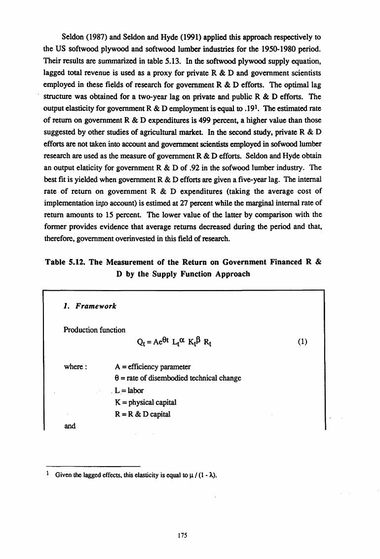
Seldon (1987) and Seldon and Hyde (1991) applied this approach respectively to

the US softwood plywood and softwood lumber industries for the 1950-1980 period.

Their results are summarized in table 5.13. In the softwood plywood supply equation,

lagged total revenue is used as a proxy for private R & D and government scientists

employed in these fields of research for government R & D efforts. The optimal lag

structure was obtained for a two-year lag on private and public R & D efforts. The

output elasticity for government R & D employment is equal to .191. The estimated rate

of return on government R & D expenditures is 499 percent, a higher value than those

suggested by other studies of agricultural market. In the second study, private R & D

efforts are not taken into account and government scientists employed in sofwood lumber

research are used as the measure of government R & D efforts. Seldon and Hyde obtain

an output elaticity for government R & D of .92 in the sofwood lumber industry. The

best fit is yielded when government R & D efforts are given a five-year lag. The internal

rate of return on government R & D expenditures (taking the average cost of

implementation in.to account) is estimed at 27 percent while the marginal internal rate of

return amounts to 15 percent. The lower value of the latter by comparison with the

former provides evidence that average returns decreased during the period and that,

therefore, government overinvested in this field of research.

Table 5.12. The Measurement of the Return on Government Financed R &

D by the Supply Function Approach

1. Framework

Production function

where:

and

A = efficiency parameter

a = rate of disembodied technical change

, L_=labor K = physical capital

R = R & D capital

1 Given the lagged effects, this elasticity is equal to J.1/ (1 - A.).

175

(1)

R = ; (G~. cu.)Ai-io i=io t-1-ko t-1

with : io = lag on the initial private effect

ko = difference between the public and private R & D lags

A = lag coefficient net of depreciation rate

G = government R & D

C = private R & D

Objective function of the firm

where:

where:

max 1tt = Pt Qt- Wt 4 -I\ Kt- Ct Lt;,Kt

P =price of the output

W=wagerate

R = user cost of capital

'Y = fraction of total revenue spent on private R & D

2. Derivation of demand and supply functions

(2)

(3)

Substituting (1) into (2), solving (2) for Land K, substituting (3) for C and solving

for 1t = 0 gives the supply equation :

00 • • • • -'\ '\ 1-1() au'l1-1o

Qt = B Pt a(a+~) e9t Wfaa Rfap 1t (l.."'~l\, G t:"'- ) (4) i=io t-1 t-1-ko

where B is a mixed constant term composed of the coefficients (a,(3,y,8)

a = (1 - a - (3)-1

Taking the log of (4) and subtracting A* Qt-1, we obtain the_ supply function to be

estimated:

qt = (1 -A) b + 8 (9t- A.et-1) +a (a+ (3) <Pt- APt-1> - 8a (Wt- AWt-1>

-a~ (rt- Art-1> + al>Ct-io + a~gt-io-ko + Mlt-1

176

where small letters represent logarithms of capitalized letters.

Similarly, the demand equation is defined as :

where z is a log-linear function of prices of outputs and costs of inputs to the

downstream industries so that the components of the derived demand from other

industries are taken into account.

Given an R & D level of G in period t, keeping all other variables at their levels at

time t except output price, the supply and demand system may be written :

where Q? and 0:, are the level terms of predetermined variables.

Calculated on the basis of these equations, the equilibrium price pE is equal to :

3. The internal rate of return on government R & D

The changes in the consumer and producer surpluses due to government R & D in

period t are respectively equal to :

177

where 11 = 8 (1 +e) I [e- 8 (a+ ~)]

The present values of the consumer and producer surpluses at time t due to

government R & D in period t are respectively approximated as :

where p = discount rate.

Net economic benefit from government R & D in period t is equal to :

where ~ is the ratio of the private cost of implementation of government-financed R

& D to government-financed R & D. The internal rate of return is de~ned as the value of

p which equates the equation NBt to zero.

4. Marginal product and marginal internal rate of return

The marginal internal rate of return of government-financed R & D in period t upon

the output in period t+n is calculated by estimating the value of the marginal product as :

aQt+n VMPt+n = Pt+n d Gt I (1 + p)n (1 + ~) \::1 n ~ io + ko

With the Cobb-Douglas specified above, we obtain :

VMPt+n = J,J.An-io-ko Pt+n Qt+nl Gt (1 + p)n (1 + ~)

The total value of the marginal product of R & D expenditures at time t is given by :·

178

= J.L Pt Qtl (1 + p- A.) (1 + p)io+ko-1 Gt (1 + ~)

Source: Seldon (1987), Seldon and Hyde (1991)

Table 5.13. Applications of the Supply Function Approach

Indus tty Private Government R&D R&D

Softwood plywood .066 .025 (3.03) (1.89)

Softwood lumber - .026 (1.73)

Note : values between parentheses are t-statistics.

Source: Seldon (1987) and Seldon and Hyde (1991).

A. lmplemen- Internal rate Marginal tation cost ofretmn internal rate

ratio of return

.869 .26 4.99 -(23.0)

.972 .09 .27 .15 (42.46)

In a recent paper, Leyden and Link ( 1991) have argued that infratechnology is the

critical link between governmental and private R & D and that the stimulus-response

effect is a consequence of technical complementarity at the production level between

funding, infratechnology and knowledge sharing.

In their model, they assume that the fmn engages in private R & D in order to

increase its profits and that it receives a governmental R & D allocation to engage in a

separate government-oriented R & D process. As a result, both R & D processes lead to

private technological knowledge and governmental technological knowledge respectively

through separate production functions. Nevertheless, the latter are assumed to share the

same infratechnology if conducted within the same fmn. Consequently, a proportion of

private and public funds will be devoted to the production of infratechnology which will

also depend on spillovers. These spillovers are represented by the level of the firm's

activity in sharing intellectual activities and the level of R & D activity of the firm's

competitors. Then, they consider that the firm maximizes its profits over its own

contribution to R & D activities and its knowledge sharing effects as decision variables.

Given that a governmental R & D allocation will increase the level of infratechnology at

no net cost, a firm will never refuse such a contract because it will increase profits. Then,

they define a third equation which represents the government's de~and for infra­

technology.

179

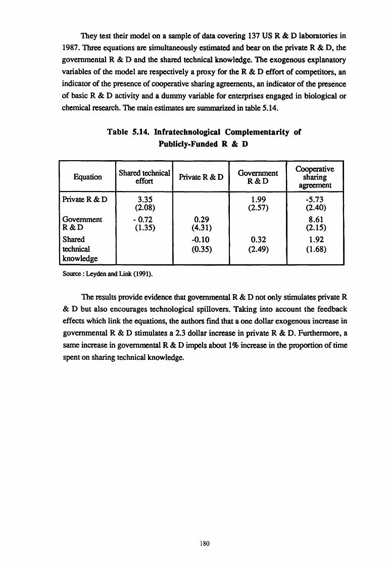
They test their model on a sample of data covering 137 US R & D laboratories in

1987. Three equations are simultaneously estimated and bear on the private R & D, the

governmental R & D and the shared technical knowledge. The exogenous explanatory

variables of the model are respectively a proxy for the R & D effort of competitors, an

indicator of the presence of cooperative sharing agreements, an indicator of the presence

of basic R & D activity and a dummy variable for enterprises engaged in biological or

chemical research. The main estimates are summarized in table 5.14.

Table 5.14. Infratechnological Complementarity of Publicly-Funded R & D

Shared technical Government Cooperative Equation effort Private R&D R&D sharing

agreement

Private R&D 3.35 1.99 -5.73 (2.08) (2.57) (2.40)

Government -0.72 0.29 8.61 R&D (1.35) (4.31) (2.15)

Shared -0.10 0.32 1.92 technical (0.35) (2.49) (1.68) knowledge

Source: Leyden and Link (1991).

The results provide evidence that governmental R & D not only stimulates private R

& D but also encourages technological spillovers. Taking into account the feedback

effects which link the equations, the authors find that a one dollar exogenous increase in

governmental R & D stimulates a 2.3 dollar increase in private R & D. Furthermore, a

same increase in governmental R & D impels about 1% increase in the proportion of time

spent on sharing technical knowledge.

180

3)

Chapter 6 - Publicly-Funded R & D in a Competitive Environment

Henri Capron and Olivier Debande

Since Arrow's major contribution emphasizing the incomplete appropriability of the

output of R & D activity, it has generally been accepted that public funding in this area

should correct market failure. Yet, while Arrow underlined that underinvestment in R &

D was likely, he also pointed out that "from the standpoint of efficiently distributing an

existing stock of information, the difficulties of appropriation are an advantage". Despite

works undertaken to improve our knowledge of R & D process on competitive markets,

economic theory is presently unable to give normative guidance for public policy in the

field of science and technology, which policy largely remains fuzzy and uncertain about

the real attainment of objectives.

At the roots of public funding, there are strategic issues which motivate government

action. The strategic issues of the technological race explain why public authorities have

reinforced their science and technology policy and thoroughly integrated it as a structural

competitiveness instrument of economic policy.

Strategic issues are vital in the design of science and technology policies because

their main concern is international competitiveness. Furthermore, governments often act

as strategic oligopolists in the design and the implementation of their policies. Only some

of these issues, which are presently covered by the theoretical and empirical literature,

will be discussed hereafter.

Some important theoretical papers dealing with both technological rivalry between

firms and public incentive policies promoting R & D investments have been developed in

recent years. Therefore, in the present state-of-the-art of the literature about strategic

issues, what can we learn from an approach like game-theoretic models in order to

implement appropriate R & D policies ? Another issue concerns the design of R & D

policies, which, among other components, must take into account the specificities of each

industry and international trends in R & D activities. Finally, a last issue investigated is

how advisable modelling strategic issues in policy assessment and impact evaluation is.

181

6.1. Technological Rivalry and Public Incentive Policies

As technology has become a competitive weapon, technology policy is increasingly

being viewed as a strategic activity. The role of governments in organizing, stimulating

and funding R & D investment clearly is of the utmost importance in shaping a favorable

environment and in channeling resources for technological innovation. Yet, enterprises

move in dynamic interactive economic surroundings where the decisions taken by public

authorities influence their allocation of resources. So, according to Weiss and Birnbaum

(1989), a technological strategy is a functional strategy, i.e. "a set of means and errors

chosen within a specific function within a business unit, which is a part of the overall

strategy of a business unit". Especially in the technological field, strategies are long-term

plans, created with a view to achieving general objectives, such as increasing the market

share in high-technology industry or becoming the leader on the international market for

specific products. However, the potential objectives and the behaviour differ with the

type of firm. For example, larger firms might be thought not to pursue the same objective

as small or medium-sized firms. Hence, they might have recourse to different instruments

to achieve their objectives and the efficiency of incentives might be different depending

on the size of the enterprises!.

Among the important strategic issues enterprises are faced with technological change

is a crucial one. Yet, technological change is not a homogeneous process and, therefore,

may be thought to be linked to different stages of the decision-making process inside the

enterprise depending on whether research is oriented toward product innovations and

processinnovations2:

- product innovation is developing specialized (radical innovation) or improved (incre­

mental innovation) products as part of establishing or protecting a competitive advan­

tage based on product differentiation and is more demand-oriented.

- process innovation aims at achieving cost or quality leadership within the product

markets and may be expected to affect supply.

1 Acs and Audretsch (1988) provide evidence that innovative activities in the small-and large-flfDls are likely to respond to different economic and technological conditions. In an industry, small-firms tend to perform better by using alternative strategies to those adopted by large firms. Regarding R & D policy effectiveness, FOister (1991) observes on the basis of a survey of Swedish firms, that small firms are more sensitive to subsidies than large flfDls.

2 While we agree with Baily and Chakrabarti (1988) that in some cases "since a typical new product is just a variant of an old product, the old products do have to compete with new products. The rapid productivity gains that occur for new products also had down the prices of old products and, hence, reduce the increase in the industry price index even if it excludes these new products ... New products do increase measured productivity, but the increase as now measured is understated relative to a true economic measure of productivity", we think that product innovations are driven by the potential demand and that they are a major component of actual demand to enterprises. Besides, PfOCe8S innova­tions mainly affect costs and only indirectly influence demand through price reductions and quality improvements.

182

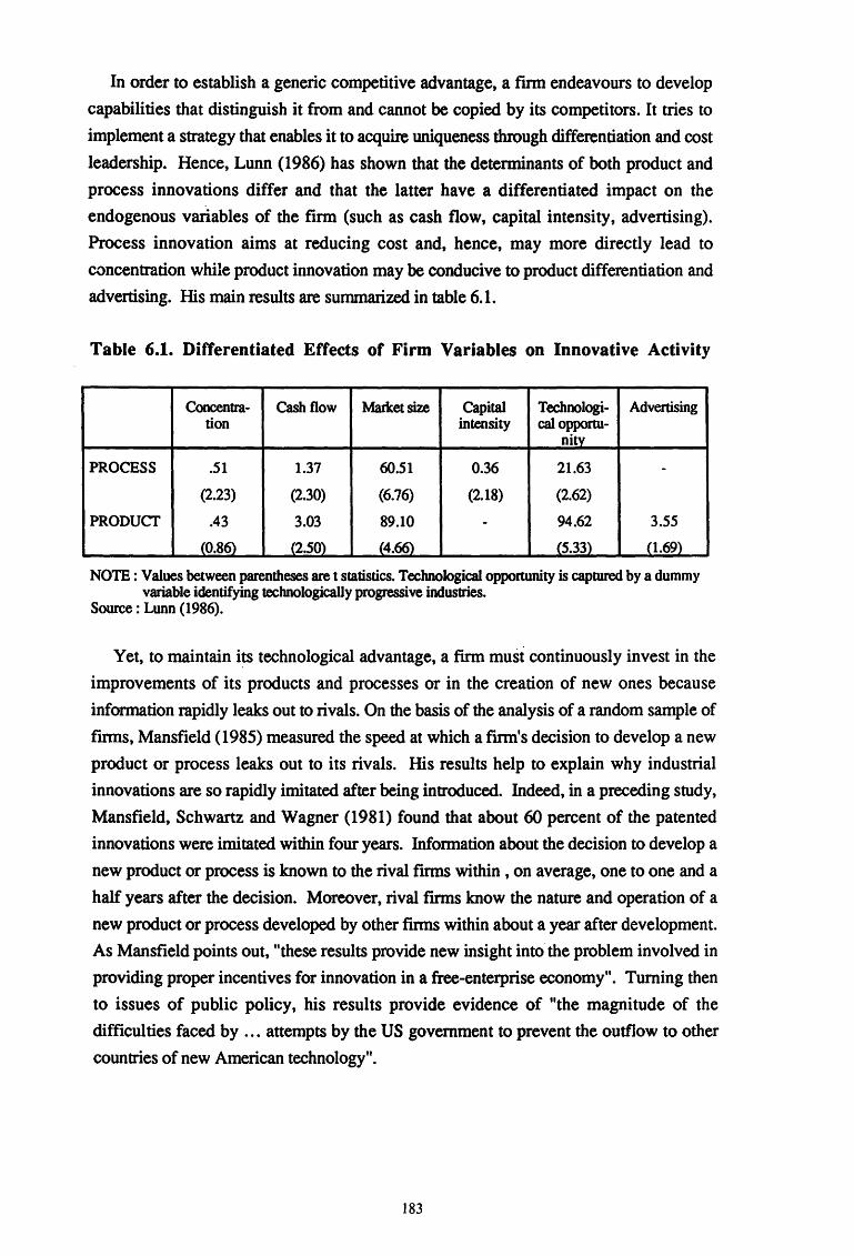
In order to establish a generic competitive advantage, a fmn endeavours to develop

capabilities that distinguish it from and cannot be copied by its competitors. It tries to

implement a strategy that enables it to acquire uniqueness through differentiation and cost

leadership. Hence, Lunn (1986) has shown that the determinants of both product and

process innovations differ and that the latter have a differentiated impact on the

endogenous variables of the firm (such as cash flow, capital intensity, advertising).

Process innovation aims at reducing cost and, hence, may more directly lead to

concentration while product innovation may be conducive to product differentiation and

advertising. His main results are summarized in table 6.1.

Table 6.1. Differentiated Effects of Firm Variables on Innovative Activity

Concentra- Cash flow Market size Capital Technologi- Advertising tion intensity cal opportu-

nitv

PROCESS .51 1.37 60.51 0.36 21.63 -(2.23) (2.30) (6.76) (2.18) (2.62)

PRODUCT .43 3.03 89.10 - 94.62 3.55

(0.86} (2.50} (4.66} (5.33) (1.69j

NOTE : Values between parentheses are t statistics. Technological opportunity is captured by a dummy variable identifying technologically progressive industries.

Source : Lunn (1986).

Yet, to maintain i~s technological advantage, a ftnn must continuously invest in the

improvements of its products and processes or in the creation of new ones because

information rapidly leaks out to rivals. On the basis of the analysis of a random sample of

fmns, Mansfield ( 1985) measured the speed at which a fmn's decision to develop a new

product or process leaks out to its rivals. His results help to explain why industrial

innovations are so rapidly imitated after being introduced. Indeed, in a preceding study,

Mansfield, Schwartz and Wagner (1981) found that about 60 percent of the patented

innovations were imitated within four years. Information about the decision to develop a

new product or process is known to the rival firms within , on average, one to one and a

half years after the decision. Moreover, rival fmns know the nature and operation of a

new product or process developed by other firms within about a year after development.

As Mansfield points out, "these results provide new insight into· the problem involved in

providing proper incentives for innovation in a free-enterprise economy". Turning then

to issues of public policy, his results provide evidence of "the magnitude of the

difficulties faced by ... attempts by the US government to prevent the outflow to other

countries of new American technology".

183

One way often put forward to in1prove technological capabilities is to promote

cooperation between firms through different research programmes. The debate on the

potential advantages or disadvantages of R & D cooperation is still largely open and it

might therefore be useful to recall some of the positive social welfare effects resulting

from cooperation. Jacquemin (1988) distinguishes between the private and public costs

or/ and benefits of cooperative R & D and, on the private side, he finds three potential

benefits to cooperation.

First, cooperative agreements can be used instead of pure market transactions or

complete integration into an economic entity. Pure market transactions may, indeed, be

costly and inefficient principally because, on the one hand, an R & D project requires

repeated and prolonged interaction between the different partners to exploit or develop

complementarities, and on the other hand, the market transactions in the R & D field hold

two main risks, moral hazard and adverse selection. A merger or a take-over is not

optimal to achieve an R & D project either. Indeed, an increasing size generates

diseconomies of scale due to rigidities in the corporate structure. The time-span required

for the research capabilities, strategies and partners to fit in with each other is too long.

The second advantage of R & D cooperation is that it accelerates the speed of invention

and innovation with less risk. Through cooperation, the money required to undertake an

R & D project can be gathered more rapidly. Moreover, the partners profit from the risk­

spreading advantage (i.e. sharing the benefits and the costs of the project) and the risk­

pooling advantage (i.e. realizing more risky projects). Thirdly, by pooling comple­

mentary resources in R & D, they can benefit by three main advantages: better conditions

on borrowed financial capital, sharing the high fixed and sunk costs of technological

development and the creation of synergetic effects by pooling R & D knowledge from

firms which may be located on different but connected technological trajectories.

Yet, if the potential benefits of R & D cooperation can be important, the

implementation of R & D agreements remains a difficult task. In the starting stage of

cooperation, an important impediment is the selection of partners. Because of imperfect

information about the level of technological knowledge of potential partners, the risk of

strengthening a competitor is real. An other restraint is the definition of a well-balanced

contribution, i.e. a trade-off between collaboration and independence, which is more

easily achieved in vertical agreements than in horizontal ones and which will often cause a

complicated organizational structure to be set up. In the operational phase, in order to

fully exploit the benefit of cooperative research, concerted manufacturing development

and cooperation in the marketing policy have to be implemented, which will riot be

without causing problems.

184

Jacquemin's conclusion is that "limiting cooperation to pure R & D or to the so-called

precompetitive level will then exercise a strong deterrent effect on the emergence of such

cooperative arrangements".

This description must be fitted to take into account the characteristics of each product

or process. The risk and necessity to cooperate at the competitive level will be different

depending on the innovation rate of the industry considered. With regard to the public

cooperative R & D, the problem that needs to be taken into account is whether there is

market failure or not, i.e. absence or not of complete appropriability of returns. With or

without substantial R & D spillovers, the potential benefit for the innovator firm will lead

to underinvestment compared to the socially optimal amount of R & D and to pricing R &

D results at a cost above the marginal cost of dissemination. Cooperative R & D can be

viewed as a means of internalizing the externalities created by significant R & D

spillovers and sharing information among firms more efficiently. Other side-effects are

generated through partial appropriation, among which, inefficiently low levels of

utilization by other firms, wasteful duplication of research and opportunism as well as

asymmetric information limiting the effectiveness of the market for R & D.

Katz and Ordover (1990) suggest different ways to correct the gap between private

and public returns to R & D investment and the insufficient sharing of the fruits of R & D

projects, i.e. direct or indirect subsidies to restore incentives, strengthening incentives to

engage in ex post cooperation and encouraging greater ex ante cooperation. Table 6.2.

gives an overview of the advantages and disavantages of these alternative policies. To

evaluate the impact of ex ante cooperation versus ex post cooperation, we must take into

account the induced effect (of the firms forming an R & D coalition) on the consumer

surplus as well as on the non-member firms' responses to changes in R & D levels.

Moreover, when evaluating the global positive or negative effect of cooperative

decision-making on the R & D investment, competitive and technological spillovers are to

be taken into account. Even with strong intellectual property rights protection, R & D in­

vestment by one firm may affect other fmns through competition in innovative activities

as well as on the market. Without technological spillovers, cooperative decision-making

reduces (increases) R & D incentives if the products are substitutes (complements). Yet,

the intensity of the spillovers is function of the quality of the protection effected by

intellectual property rights. When innovators are product-market competi~ors and

intellectual property rights are strong (weak), cooperative decision-making tends to

decrease (increase) R & D investment incentives.

185

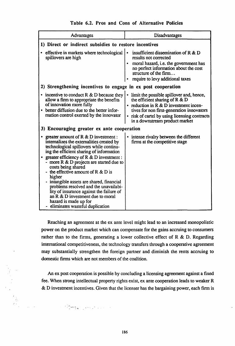
Table 6.2. Pros and Cons of Alternative Policies

Advantages Disadvantages

1) Direct or indirect subsidies to restore incentives

• effective in markets where technological • insufficient dissemination of R & D spillovers are high results not corrected

• moral hazard, i.e. the government has no perfect information about the cost structure of the fum ...

• require to levy additional taxes

2) Strengthening incentives to engage in ex post cooperation

• incentive to conduct R & D because they allow a fum to appropriate the benefits of innovation more fully

• better diffusion due to the better infor­mation control exerted by the innovator

• limit the possible spillover and, hence, the efficient sharing of R & D

• reduction in R & D investtnent incen­tives for non frrst-generation innovators

• risk of cartel by using licensing contracts in a downstream product market

3) Encouraging greater ex ante cooperation

• greater amount of R & D investtnent : internalizes the externalities created by technological spillovers while continu­ing the efficient sharing of information

• greater efficiency of R & D investtnent : - more R & D projects are started due to

costs being shared - the effective amount of R & D is

higher - intangible assets are shared, financial

problems resolved and the unavailabi­lity of insurance against the failure of an R & D investtnent due to moral hazard is made up for

- eliminates wasteful duplication

• intense rivalry between the different fnms at the competitive stage

Reaching an agreement at the ex ante level might lead to an increased monopolistic

power on the product market which can compensate for the gains accruing to consumers

rather than to the firms, generating a lower collective effect of R & D. Regarding

international competitiveness, the technology transfers through a cooperative agreement

may substantially strengthen the foreign partner and diminish the rents accruing to

domestic firms which are not members of the coalition.

An ex post cooperation is possible by concluding a licensing agreement against a fixed

fee. When strong intellectual property rights exist, ex ante cooperation leads to weaker R

& D investment incentives. Given that the licenser has the bargaining power, each firm is

186

motivated to conduct R & D in order to appropriate surplus that might otherwise accrue to

its rival. The collective R & D investment incentive under ex ante cooperation is lower

than the individual incentive under ex post cooperation. When the protection afforded by

secrecy is strong, when spillovers are high, ex post cooperation may be limited. The fact

that the ex post market power of firms can exceed their ex ante market power implies that

e' ante cooperation can lead to less severe monopolistic pricing distortions in the pricing

of R & D results.

Consequently, a potential strategic public policy is to implement cooperation in sectors

with some specific characteristics. These policies might for instance :

- meet the need to increase the international competitiveness of domestic firms;

- stimulate industries with a high spillover,

- induce precompetitive research which furthers long-run relationships between firms and

by-passes the problem of benefit sharing;

- implement programmes dealing with complementary products.

The technological positions of the different countries are not unalterable. The capacity

to innovate changes over tin1e. Since the Second World War, the US has been the refer­

ence level against which the technological positions of the industrial countries have been

evaluated. Any technological policy must build upon a check-up of innovative capabili­

ties, i.e. assessing the present situation and the possible modifications of the "country's

position" on a potential pe:rformance scale.

A study by Glismann and Horn (1988) looking at the invention performance of the

main industrialized countries on the basis of patents granted in the United States shows

that the heterogenous economic structures which characterize the main European

countries materialize in distinct technological advance rates.

Their analysis covers the innovation performances in France, Italy, Japan, United

Kingdom, the former USSR and West Germany, compared with the United States over

the past twenty years. Japan has filled the technology gap between itself and the United

States by using imitation as its strategy. Today, Japan and the United States are often

thought to be more successful in producing new technology than West European

countries. Glismann and Horn's analysis provides evidence of the position of the seven

countries in the technological race. To assess the innovative activities by country and

field of activity, they use the patents granted in the US between 1963 and 1983.

They consider respectively,

187

- the relative average invention performance of countries over time calculated as the

ratio of the number of patents granted to country j in field i to the number of patents

granted to the United States in field i:

i · 1 n Patents·

....J J RAlt'! =- l: · J n t= 1 Patents 1

us

- the estimated relative starting position of country j as measured by coefficient "a" in

the equation : i

Patentsj ----=.~-- = a.eb.t

1 Patentsus

- the estimated relative evolution of patent activity of countty j as measured by

coefficient "b" in the previous equation.

They observed that the number of non-US patents represented only 25 percent of the

number of patents granted to the United States with West-Germany and the United

Kingdom having a leading position. On the one hand, non-US patents per year rose six

percentage points faster than the United States patenting. On the other hand, Japan,

West-Germany and the USSR performed significantly better than the United States,

while France and Italy did only just a little less well. For its part, the United Kingdom

revealed a similar profile to that observed for the US. The US lost less in high­

technology fields than in average technologies. Regarding the highest country share of

patents granted to non-US citizens, West-Germany and Japan had a leading position and

only Japan in high-technology fields. They also emphasized a positive correlation

between the performance in technological activities and the countries' economic

performance and stressed the reduction of the technological gap between European

countries and the United States, an adjustment process highly contrasted for each

European country with West-Germany in a leading position and the development process

in the United Kingdom matching to the American business cycle. The heterogeneous

economic structures among European countries result in distinct rates of technological

advance.

An important factor determining the innovative performance and the catching-up pro­

cess is the increase in the level of investment devoted to inventive activities. Another

major factor is the institutional change. The development of the European Patent Office,

188

for instance, allows the European firms to develop innovation in a favourable context in

terms of appropriability conditions.

The working horizon and the cost constraints are also crucial factors to implement an

R & D program. Especially to develop technology, long-term investments that need not

meet very short-term perfonnance criteria have to be made.

So, Mansfield (1988a) showed that innovation time and innovation cost are central to

success. Japanese firms tend to develop and commercially introduce new products and

processes more quickly and cheaply than American fmns. As a consequence, there has

been a technological depreciation of American products. Here, it is worth noting that the

perception of American and Japanese products has been completely inverted in forty

years' time. This example illustrates how important a technology policy is to preserve and

improve competitiveness.

In his examination of the outcome of the technological race between Japan and the US

on a sample of American and Japanese firms he questions how quickly and economically

each nation's firms can develop and commercially introduce the new products and

processes and how essential it is for them to succeed. He looks at two variables of

innovation :

- the innovation time : which is the length of time elapsing from the beginning of

applied research by the innovator on a new product or process to the date of the new

product's or process's first commercial introduction;

- the innovation cost : which is all the costs involved in developing and introducing the

innovation, including R & D, plant and equipment, and startup costs.

The Japanese advantage is confined to external technologies (i.e. technologies

developed outside the innovating finn). In internal technology, developed within the

innovating frrm, there is no significant difference between both countries. Innovation

based on external technologies is an imitation process. The higher commercialization cost

in the US arises from the inability of American firms to improve significantly on the

imitated products and to reduce their production costs substantially. The process of

resource allocation differs between the US and Japan. The Japanese firms devote more

resources in the innovation process to tooling and manufacturing equipment and facilities,

which include preparation for manufacturing, design, construction, and acquisition of

manufacturing facilities for the new product, as well as tooling and equipment. The

189

American firms spend n1ore money on the manufacturing startup, which is linked to the

quality problem of their products. There has been a technological depreciation of the

American products over time. The US has now acquired a reputation for quality

problems that compels the US to offer its goods at a lower price than Japanese or German

manufacturers, for instance.

A recent study by van Hulst, Mulder and Soete (1991) emphasizes the narrow

relationship between a country's technological ability and its export performance. The

case of the US is relevant to look at the link between technology and competitiveness. In

1970, the US had a lead in technology over other industrial countries, which allowed it to

maintain a trade surplus in manufactured products in spite of higher unit labor costs in

most industries than elsewhere. But suffering from too high a currency and interest rate,

and above all from an upgrading of the products provided by Japanese and German

firms, US firms have lost market share in manufactured goods. The US advantage in

technology and quality has eroded a way and the US products have now acquired a

reputation for quality problems that compels the US to offer its goods at lower prices than

its rival manufactures. The American case shows how important it is to conduct a

technological policy that gives the home finns_the capacity to compete with foreign firms

and to increase their market shares in sectors with high added value.

The public policy has to take into account the original characteristics of each country.

Moreover it has to be oriented to create new comparative advantages. According to van

Hulst and al. (1991), "the degree to innovativeness of each country in any one particular

technology is explained through the complex interplay between (i) science-related

opportunities, (ii) country-specific and technology-specific institutions which foster/

hinder the emergence of new technologies and (iii) the nature and intensity of economic

stimuli, which stem from abundance of particular inputs, or, alternatively, critical

scarcities, specific patterns of demand as well as levels and changes in relative price".

In an analysis of the erosion of the American leadership, Nelson ( 1990) argues that it

will be investments in R & D and in physical and human capital, and perhaps particularly

the latter and not so much organizational differences, that will determine the classification

of countries regarding technological and economic levels. According to him, "technology

is only a public good for those who have made the investments to be able to tap in ... it is

differences in these that largely explain why Japan has done so well and the US recently

relatively poorly ... it is these latter investments (investments in new plant and

equipment, and in worker skills) that will largely determine who is in the best position to

develop and exploit technological developments, and relative national living standards".

190

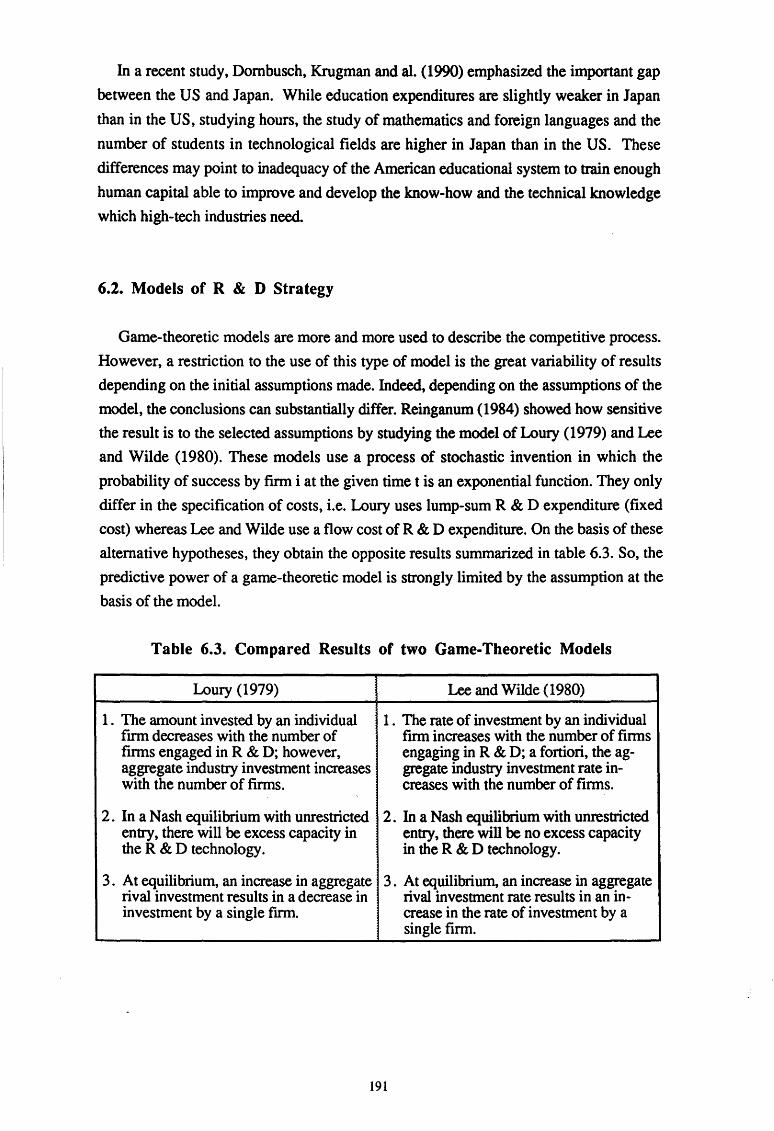
In a recent study, Dornbusch, Krugman and al. (1990) emphasized the important gap

between the US and Japan. While education expenditures are slightly weaker in Japan

than in the US, studying hours, the study of mathematics and foreign languages and the

number of students in technological fields are higher in Japan than in the US. These

differences may point to inadequacy of the American educational system to train enough

human capital able to improve and develop the know-how and the technical knowledge

which high-tech industries need.

6.2. Models of R & D Strategy

Game-theoretic models are more and more used to describe the competitive process.

However, a restriction to the use of this type of model is the great variability of results

depending on the initial assumptions made. Indeed, depending on the assumptions of the

model, the conclusions can substantially differ. Reinganum (1984) showed how sensitive

the result is to the selected assumptions by studying the model of Loury ( 1979) and Lee

and Wilde ( 1980). These models use a process of stochastic invention in which the

probability of success by firm i at the given time t is an exponential function. They only

differ in the specification of costs, i.e. Loury uses lump-sum R & D expenditure (fixed

cost) whereas Lee and Wilde use a flow cost of R & D expenditure. On the basis of these

alternative hypotheses, they obtain the opposite results summarized in table 6.3. So, the

predictive power of a game-theoretic model is strongly limited by the assumption at the

basis of the model.

Table 6.3. Compared Results of two Game-Theoretic Models

Loury (1979) Lee and Wilde ( 1980)

1 . The amount invested by an individual 1 . The rate of investment by an individual fmn decreases with the number of firm increases with the number of firms firms engaged in R & D; however, engaging in R & D; a fortiori, the ag-aggregate industry investment increases gregate industry investment rate in-with the number of firms. creases with the number of firms.

2. In a Nash equilibrium with unrestricted 2. In a Nash equilibrium with unrestricted entry, there will be excess capacity in entry, there will be no excess capacity the R & D technology. in the R & D technology.

3. At equilibrium, an increase in aggregate 3. At equilibrium, an increase in aggregate rival investment results in a decrease in rival investment rate results in an in-investment by a single fmn. crease in the rate of investment by a

single firm.

191

Table 6.4. gives a general overview of the main theoretical models of R & D

competition developed in the literature, which can be viewed as significant benchmarks of

this research field. Complementarily to this general description of models, one may add

the following comments :

1. Symmetric models give an appreciation of the extent to which rivalry and appropri­

ability interact to determine the incentives for individual fmn investment in R & D. The

main issues investigated are : what is the aggregate noncooperative investment in R & D

and how it is distributed across firms and across time ? How many firms enter the race

and what is the resulting equilibrium date of innovation ? The extent of appropriability

will guide the investment decision of fmns under entry. Finn will overinvest compared

to the cooperative optimum if rewards to innovation are appropriable and conversely

[Reinganum (1989)].

2. Asymmetric models are developed by referring to the auction and stochastic racing

paradigms. The choice of paradigm proves to be important because the associated

models are found to give opposite results. Under uncertainty, a firm with a large market

will invest at a lower rate than a potential entrant for an innovation promising the winner a

large market and conversely under a determinist scheme. As innovative activity may take

more or less time and money than expected and might not yield a worthwhile end­

product, the stochastic racing model seems more accurate while the auction model may

well be preferred for the analysis of the development phase as any substantial

technological uncertainties have already been resolved [Reinganum (1989)].

3. These models provide evidence of the existence of market failures, and hence

justify public intervention. Yet, they remain relatively silent on how government policy

may act to reduce market failures. When government action is taken into account in these

models, their counterfactual settings limit the practical range of results. Therefore, so far

they have not been able to guide an efficient R & D policy. For example, the next two

questions remain largely open : Where are the most prominent sources of market failure

in R & D ? How efficient is a public policy encouraging research joint ventures to correct

market failures ?

One difficulty, stressed by Cohen and Levin ( 1989), in testing the implications of

game-theoretic models of R & D rivalry is that they analyze behaviors in highly simplified

models, omitting important aspects of industrial competition. Moreover, the utilization of

game-theoretic tools implies that we must use unverifiable assumptions concerning the

192

- \0 w

Tab

le 6

.4.

An

Ove

rvie

w o

f S

trat

egic

Mod

els

of R

&

D

1) I

nnov

atio

n pr

oduc

tion

in

the

cont

ext

of

sym

met

ric

mod

els

Gen

eral

hy

poth

eses

: .

Sim

ulta

neou

s co

mpe

titio

n fo

r an

iden

tical

pot

entia

l in

nova

tion

Aut

hors

1)

Lou

ry (

1979

)

2) L

ee a

nd W

ilde

(198

0)

. G

loba

l and

inde

fini

te p

rote

ctio

n fr

om i

mita

tion

or d

uplic

atio

n fo

r th

e pa

tent

ed in

nova

tion.

.

Cos

t of i

nven

tion

bein

g a

decr

easi

ng c

onve

x fu

nctio

n of

the

time

prio

r to

inve

ntio

n.

Ass

umpt

ions

1)

The

suc

cess

pro

babi

lity

is a

n ex

pone

ntia

l tim

e fu

nctio

n.

2) R

&D

exp

endi

ture

s ar

e ftx

ed c

osts

. The

cos

ts

of ca

rryi

ng o

ut a

n in

vest

men

t pro

ject

may

be

rega

rded

as

know

n at

the

initi

al m

omen

t, in

de­

pend

ently

of s

ubse

quen

t dev

elop

men

ts.

1) C

f. L

oury

. 2)

R&

D e

xpen

ditu

res

are

flow

cos

ts i.

e. f

irms

are

able

to c

hoos

e a

rese

arch

inte

nsity

; onc

e th

is in

tens

ity is

fix

ed,

the

fmn

mus

t eith

er

sust

ain

this

leve

l of i

nves

tmen

t or c

ease

in­

vest

ing

alto

geth

er.

Res

ults

1)

The

equ

ilibr

ium

lev

el o

f frr

m R

&D

inve

st­

men

t dec

lines

as

the

num

ber o

f fm

ns in

the

indu

stry

incr

ease

s.

2) A

zer

o ex

pect

ed p

rofi

t ind

ustry

equ

ilibr

ium

w

ith in

itial

incr

easi

ng r

etur

ns t

o sc

ale

in t

he

R&

D te

chno

logy

and

with

a fm

ite n

umbe

r of

firm

s w

ill a

lway

s in

volv

e "e

xces

s ca

paci

ty"

in

the

R&

D t

echn

olog

y.

3) G

iven

a ft

xed

mar

ket s

truc

ture

, ind

ustry

equ

i­lib

rium

will

hav

e ea

ch f

irm i

nves

ting

mor

e in

R

&D

tha

n is

soc

ially

opt

imal

. 4)

With

incr

easi

ng in

itial

R&

D r

etur

ns to

sca

le,

com

petit

ive

entr

y le

ads

to m

ore

than

the

soci

al­

ly o

ptim

al n

umbe

r of

fmns

in t

he in

dust

ry,

each

of t

hem

inv

estin

g to

o lit

tle.

1) I

ncre

asin

g eq

uilib

rium

inve

stm

ent a

s th

e nu

mbe

r of f

mns

incr

ease

s.

2) In

indu

stry

equ

ilibr

ium

, hig

her

inve

stm

ent

mte

than

join

tly o

ptim

al f

or f

ixed

num

ber

of

fmns

. 3)

With

incr

easi

ng in

itial

R&

D r

etur

ns to

sca

le,

com

petit

ive

entr

y re

sults

in t

oo m

any

frrm

s,

with

too

hig

h an

inv

estm

ent r

ate.

Rem

arks

1)

Sym

met

ry b

etw

een

the

diff

eren

t firm

s.

2) E

xpon

entia

l ass

umpt

ion

to i

ncor

pore

stm

te­

gic

riva

ls im

plyi

ng n

o le

arni

ng b

y do

ing

or b

y us

ing.

3)

Inap

prop

riat

e in

vest

men

t pro

cess

ass

umin

g R

&D

exp

endi

ture

s co

mm

itted

up

fron

t. 4)

No

entr

y co

st.

1) C

f. L

oury

1).

2) C

f. L

oury

2).

3)

The

inst

anta

neou

s pr

obab

ility

of i

ntro

duci

ng

a ne

w t

echn

olog

y sh

ould

be

a fu

nctio

n o

f bot

h th

e cu

rren

t inv

estm

ent r

ate

and

the

stoc

k o

f kn

owle

dge.

4

) C

f. L

oury

4).

5)

Stm

tegi

c re

spon

se to

riv

al's

succ

ess

limite

d to

the

poss

ibili

ty o

f sto

ppin

g R

&D

inv

est­

men

t.

3) D

elbo

no a

nd D

enic

olo

1) cr

. Lee

and

Wild

e.

1) A

n in

crea

se in

the

num

ber o

f fm

ns m

ay r

e-C

ontin

uatio

n of

Lee

and

Wild

e's

mod

el.

(199

1a)

2) P

rize

to th

e w

inne

r dep

ends

on

the

num

ber

suit

in a

dec

reas

e in

the

equi

libri

um R

&D

eff

ort

of f

inns

(qu

antit

y -

setti

ng C

ourn

ot p

laye

rs in

of

each

fm

n an

d in

the

equi

libri

um t

otal

eff

ort.

the

prod

uct m

arke

t) an

d lo

sers

may

rea

p po

si-

2) I

n eq

uilib

rium

the

re m

ay b

e un

deri

nves

tmen

t tiv

e pr

ofits

in th

e po

st-i

nnov

atio

n eq

uilib

rium

. w

ith r

espe

ct to

the

soci

al o

ptim

um.

3) B

efor

e th

e in

nova

tion,

fm

ns m

ay m

ake

3) L

ee a

nd W

ilde'

s re

sult

still

hol

ds w

hen

the

posi

tive

prof

its, a

nd s

ocia

l and

pri

vate

ben

efits

po

st-in

nova

tion

mar

ket p

rofi

ts o

f the

win

ners

fr

om t

he in

nova

tion

diff

er.

as w

ell a

s th

ose

of th

e lo

sers

do

not d

epen

d on

th

e nu

mbe

r of f

mns

. 4)

Rei

ngan

um (

1982

) 1)

Flo

w e

xpen

ditu

res

dete

rmin

ing

the

likel

i-1)

In th

e no

-suc

cess

cas

e, th

e ex

pect

ed a

mou

nt

hood

of s

ucce

ss, w

ith k

now

ledg

e ac

cum

ula-

of ad

ditio

nal k

now

ledg

e is

inde

pend

ent o

f acc

u-tio

n.

mul

ated

kno

wle

dge.

2)

Fin

ns m

ay a

djus

t the

rat

e of

expe

nditu

re in

2)

For

PL

> P

f, a

n in

crea

se in

PL

stim

ulat

es

resp

onse

to e

laps

ed ti

me

and

stat

e va

riabl

es

each

fin

n to

acq

uire

kno

wle

dge

at a

hig

her r

ate,

w

hich

sum

mar

ize

riva

l pro

gres

s.

whi

le a

n in

crea

se in

PF

caus

es e

ach

fmn

to re

-3)

Impe

rfec

t pat

ent p

rote

ctio

n.

duce

its

equi

libriu

m ra

te o

f kno

wle

dge

acqu

isi-

4) L

eale

r's o

r inn

ovat

or's

payo

ff (P

I) ~ fo

l-tio

n.

low

er's

or im

itato

r's p

ayof

f {PJ

:).

3) F

or th

e ca

se o

f per

fect

pat

ent p

rote

ctio

n, a

n 5)

Fin

ite p

lann

ing

horiz

on.

incr

ease

in n

(num

ber o

f fm

ns)

incr

ease

s th

e 6)

The

val

ue o

f the

pat

ent i

s no

t con

stan

t ove

r eq

uilib

rium

rat

e of

inve

stm

ent f

or e

ach

fmn

and

time

and

may

dec

reas

e or

incr

ease

if a

dditi

onal

de

crea

ses

the

expe

cted

tim

e til

l inn

ovat

ion.

For

us

es a

re d

isco

vere

d.

the

case

of i

mpe

rfec

t pat

ent p

rote

ctio

n, th

e re

-7)

The

con

ditio

nal d

ensi

ty o

f suc

cess

dep

ends

su

it is

am

bigu

ous

and

func

tion

of th

e re

lativ

e on

ly o

n cu

rren

t inv

estm

ent.

payo

ffs

to in

nova

tors

and

imita

tors

. 8)

Use

the

conc

ept o

f Nas

h eq

uilib

ria

in f

eed-

back

stra

tegi

es.

5) R

eing

anum

(19

81)

1) C

oope

ratio

n am

ong

fmns

thr

ough

coo

rdi-

1) N

onco

oper

ativ

e ri

vals

will

(on

ave

rage

) su

e-1)

cr.

Lou

ry 1

). na

ting

rese

arch

stra

tegi

es a

nd e

xcha

nge

of

ceed

soo

ner t

han

coop

erat

ive

fmns

who

are

2)

App

ropr

iabi

lity

is ta

ken

into

acc

ount

by

know

ledg

e.

unab

le to

shar

e kn

owle

dge.

m

odul

atin

g th

e ef

fect

iven

ess

of th

e pa

tent

pro

-2)

Spi

llove

rs in

kno

wle

dge

are

com

plet

e.

2) A

ssum

ing

that

the

soci

al v

alue

of i

nnov

atio

n te

ctio

n. P

aten

ts a

re n

ot th

e m

ost e

ffec

tive

pro-

3) T

here

is a

ctua

lly n

o du

plic

atio

n.

exce

eds

half

priv

ate

valu

e, th

en th

e no

ncoo

pera

-te

ctio

n sy

stem

of i

nnov

atio

n. O

ther

dec

isio

n 4)

All

know

ledg

e is

tran

sfer

able

. tiv

e ra

te o

f kno

wle

dge

acqu

isiti

on is

less

than

is

varia

bles

are

mor

e po

wer

ful a

nd in

fluen

ce th

e so

cial

ly o

ptim

al. I

nnov

atio

n w

ill o

n av

erag

e be

st

rate

gic

beha

viou

r of t

he fi

rm.

dela

yed

com

pare

d to

the

soci

ally

opt

imal

dat

e.

3) N

o ef

fect

ive

publ

ic p

olic

y ab

out c

oope

rativ

e In

nova

tion

by N

ash

riva

ls w

ill o

n av

erag

e oc

cur

agre

emen

t la

ter t

han

the

coop

erat

ive

date

. 4)

cr.

Lou

ry 4

).

6) S

penc

er a

nd B

ran<

b'

1) T

wo-

stag

e ga

me

(R&

D a

nd o

utpu

t) pl

ayed

1)

Ove

ruse

of R

&D

in th

e ab

senc

e of

gov

ern-

1) C

ount

ries

are

sym

met

ric.

(198

3)

by tw

o co

mpe

ting

firm

s, lo

cate

d in

dif

fere

nt

men

t pol

icy.

2)

Res

ults

are

val

uabl

e fo

r any

kin

d of

inve

st-

coun

tries

. 2)

With

a si

ngle

gov

ernm

ent a

llow

ed to

sub

-m

ent a

nd n

ot o

nly

R&

D. T

he m

ajor

insi

ghts

2)

Int

rodu

ctio

n of

indu

stria

l stra

tegy

pol

icie

s in

si

dize

R&

D, t

he o

utco

me

is e

quiv

alen

t to

the

can

be o

btai

ned

by a

ny s

ubsi

dy p

olic

y ai

med

at

the

cont

ext o

f an

impe

rfec

tly c

ompe

titiv

e on

e ob

tain

ed in

the

lead

er-f

ollo

wer

equ

ilibr

ium

re

duci

ng c

osts

. w

orld

ca

se.

3) T

he C

oum

ot m

odel

im

plie

s th

at a

sub

sidy

3)

R&

D is

und

erta

ken

befo

re th

e as

soci

ated

3)

Whe

n bo

th g

over

nmen

ts a

re a

llow

ed t

o su

b-is

alw

ays

wor

thw

hile

bec

ause

it in

crea

ses

the

outp

ut is

pro

duce

d, w

ith f

irms

antic

ipat

ing

the

sidi

ze R

&D

, the

y do

it.

dem

and

for

the

dom

estic

firm

and

thus

its

pro-

effe

ct o

f R&

D o

n ho

w o

utpu

t sha

res

can

be

4) If G

over

nmen

t can

sub

sidi

ze b

oth

expo

rt an

d fit

s.

won

. R

&D

, it w

ill h

ave

an i

ncen

tive

to ta

x R

&D

4)

Gov

ernm

ent i

nter

vent

ions

take

diff

eren

t (e

ffic

ienc

y ob

ject

ive)

and

to su

bsid

ize

expo

rt fo

rms

: R&

D s

ubsi

diza

tion

and/

or e

xpor

t sub

-(m

arke

t sha

re o

bjec

tive)

. si

dies

. 5)

A G

over

nmen

t can

cre

dibl

y co

mm

it its

elf t

o

R&

D (o

r out

put)

subs

idie

s be

fore

the

R&

D d

e-ci

sion

s ar

e m

ade

by p

rivat

e fir

ms.

6) O

utPu

ts o

f eac

h fir

m a

re s

ubst

itute

s.

7) D

ixit

( 198

8)

1) C

ontin

uum

of f

mns

eng

aged

in th

e R

&D

1)

The

opt

imal

pol

icy

is t

o a

lter

the

appr

opri-

1) C

f. L

ee a

nd W

ilde.

co

mpe

titio

n.

able

ben

efit

of th

e w

inni

ng f

mn

by m

eans

of a

n 2)

Par

tial p

rogr

ess

in th

e R

&D

rac

e no

t con

-2)

A lu

mp-

sum

cos

t at t

he o

utse

t and

recu

rren

t aw

ard

(tax

) if

the

mar

ket i

s pr

ovid

ing

insu

ffi-

side

red.

flo

w c

osts

dur

ing

the

R&

D ra

ce.

cien

t (ex

cess

ive)

R&

D e

ffor

t acc

ordi

ng to

the

3) C

ontin

uum

of f

irms

in a

sym

met

ric

wor

ld.

3) S

ucce

ss in

depe

nden

t acr

oss

fmns

. ba

lanc

e be

twee

n ex

tern

aliti

es.

~

4) r

mn'

s ha

zard

rat

e in

depe

nden

t of t

ime

and

of

2) T

he la

rger

the

fmn,

the

mor

e it

will

inte

r-R

&D

flow

exp

endi

ture

s.

naliz

e ne

gativ

e ex

tern

aliti

es (i

.e. c

ompe

titio

n 5)

No

new

info

rmat

ion

durin

g th

e ra

ce.

for

the

inno

vatio

n le

adin

g to

a s

ocia

lly e

xces

-6)

Suc

cess

put

s an

end

to th

e co

mpe

titio

n.

sive

am

ount

of R

&D

inve

stm

ent).

2)

Inno

vati

on p

rodu

ctio

n in

the

con

text

of

asym

met

ric

mod

els

a) T

he d

iffe

renc

e am

ong

firm

s di

d no

t co

nfer

an

ex a

nte

adva

ntag

e up

on a

ny p

arti

cula

r fi

rm.

Aut

hors

8)

Rei

ngan

um (

1985

)

9) V

icke

rs (1

984)

Ass

umpt

ions

1)

Eac

h in

nova

tion

is d

rast

ic i

.e. o

ne w

hich

le

aves

the

inve

ntor

a m

onop

olis

t. 2)

An

incu

mbe

nt m

onop

olis

t com

pete

s w

ith (

n -

1) id

entic

al c

halle

nger

s fo

r a n

ew in

nova

tion.

3)

F'm

ns a

re s

ymm

etric

in a

ll ot

her r

espe

cts

i.e. t

hey

face

the

sam

e in

nova

tion

prod

uctio

n po

ssib

ilitie

s.

4) T

he e

quili

briu

m c

once

pt is

the

subg

ame

per­

fect

Nas

h eq

uilib

rium

. 5)

The

val

ue o

f win

ning

the

cur

rent

race

is

high

er th

an th

e va

lue

of lo

sing

it (t

rue

by in

­du

ctio

n).

6) T

here

alw

ays

exis

ts a

n in

vest

men

t lev

el f

or

a ch

alle

nger

for

whi

ch g

ross

pro

fits

exce

ed th

e va

lue

of lo

sing

imm

edia

tely

. 1)

A s

eque

nce

of n

ot-s

o-dr

astic

inno

vatio

ns is

co

nsid

ered

so

that

the

prof

it flo

ws

of th

e tw

o fir

ms

typi

cally

dep

end

upon

the

leve

ls o

f tec

h­no

logy

. 2)

The

tech

nolo

gica

l rac

e ta

kes

the

form

of a

si

mpl

e au

ctio

n.

3) F

irms

are

assu

med

not

to d

isco

unt t

he

futu

re.

Res

ults

1)

The

Nas

h eq

uilib

rium

in th

e cu

rren

t sta

ge is

sy

mm

etric

am

ong

the

chal

leng

ers

and

the

in­

cum

bent

inve

sts

less

than

eac

h ot

her c

halle

nger

. T

he la

tter c

oncl

usio

n gi

ves

rise

to a

turn

over

of

the

tech

nolo

gica

l lea

ders

hip

sim

ilar t

o Se

bum

­pe

ter's

"pr

oces

s of

cre

ativ

e de

stru

ctio

n".

2) E

ach

fmn

wou

ld p

refe

r to

be

the

incu

mbe

nt

in th

e cu

rren

t sta

ge ra

ther

than

a c

halle

nger

.

Whe

n th

e pr

oduc

t mar

ket i

s ve

ry c

ompe

titiv

e,

ther

e is

incr

easi

ng d

omin

ance

; in

othe

r cas

es,

ther

e is

a re

actio

n pr

oces

s.

Rem

arks

1)

In

this

mod

el, t

he m

onop

olis

t has

no

adva

n­ta

ge in

the

tech

nolo

gica

l pro

cess

. If t

he in

­cu

mbe

nt h

as s

ome

cost

adv

anta

ge, i

t may

hav

e a

high

er in

cent

ive

to in

vest

in R

&D

to a

void

en

try.

2) T

he q

uest

ion

of ap

prop

riabi

lity

is re

solv

ed

thro

ugh

the

notio

n of

dra

stic

inn

ovat

ion.

3)

The

re is

no

spill

over

eff

ect a

nd n

o le

arni

ng

effe

ct

4) S

ince

inno

vatio

n is

dra

stic

, the

pro

fit i

ncen

­tiv

e on

ly in

terf

ers

and

the

chal

leng

er h

as th

e gr

eate

st in

cent

ive

to in

nova

te.

Nei

ther

spi

llove

rs n

or le

arni

ng e

ffec

ts.

·--·

... --~-----------------------------------------------------

b)

The

nat

ure

of

the

asym

met

ry c

onfe

rs a

str

ateg

ic a

dvan

tage

upo

n on

e fi

rm.

1 0) F

uden

berg

and

al.

1) B

oth

frrm

s ar

e su

ffer

ing

from

info

rmat

ion

1) T

he r

esul

t is

cond

ition

ed b

y th

e la

g in

term

s 1)

Res

tric

tion

on t

he f

rrm

's ab

ilitie

s to

var

y it

s (1

983)

an

d/or

resp

onse

lags

rega

rdin

g th

e re

sear

ch

of a

ccum

ulat

ed e

xper

ienc

e be

twee

n th

e fJ

.tms.

If

rese

arch

inte

nsity

. ac

tiviti

es o

f the

ir ri

vals

. Thi

s fe

atur

e al

low

s th

ey a

re s

uffic

ient

ly c

lose

eac

h ot

her,

they

2)

The

res

ult c

ruci

ally

dep

ends

on

the

initi

al

frrm

s th

at a

re o

nly

slig

htly

beh

ind

to c

atch

up

choo

se a

hig

h ra

te to

try

to w

in t

he t

echn

olo-

lag

in e

xper

ienc

e.

befo

re th

e le

adin

g fir

m c

an a

ct to

pre

vent

it.

gica

l rac

e. I

n th

e ot

her c

ase,

it d

rops

out

of t

he

2) I

nven

tion

occw

s as

soo

n as

one

frrm

has

ac-

race

and

the

rem

aini

ng fr

rm c

hoos

es a

low

er

cum

ulat

ed e

noug

h kn

owle

dge

(tota

l res

earc

h ra

te.

and

deve

lopm

ent s

pend

ing)

. 2)

As

the

perio

d of

info

rmat

ion

lag

decr

ease

s,

3) V

aria

tion

in th

e ra

te o

f lea

rnin

g an

d th

e co

st

the

lag

in e

xper

ienc

e fo

r w

hich

the

follo

wer

of

lear

ning

are

str

ictly

con

vex.

st

ill c

ompe

tes

also

dec

reas

es.

4) W

ithin

the

curr

ent p

erio

d, e

ach

firm

mus

t ch

oose

its

rate

of k

now

ledg

e ac

quis

ition

with

-ou

t kno

win

g its

riv

al's

choi

ce.

5) B

oth

play

ers

valu

e th

e pa

tent

equ

ally

and

fa

ce th

e sa

me

cost

con

ditio

ns.

11) H

arris

and

Vic

kers

1)

The

two

firm

s m

ove

alte

rnat

ivel

y an

d th

e If

one

play

er is

far

eno

ugh

ahea

d, th

en th

e ot

her

1) T

his

mod

el is

a d

eter

min

istic

rac

e in

whi

ch

(198

5)

fJtS

t fm

n to

rea

ch a

goa

l, w

ins

the

priz

e.

give

s up

. The

not

ion

of d

ista

nce

corr

espo

nds

to

equi

libriu

m is

cha

ract

eriz

ed b

y al

l firm

s bu

t 2)

Pro

gres

s is

fun

ctio

n of

the

inve

sted

am

ount

. th

e va

lue

plac

ed o

n w

inni

ng a

nd th

e co

sts

of

one

exiti

ng th

e co

mpe

titio

n ri

ght a

t the

out

set.

3) T

he n

otio

n of

equi

libri

um is

sub

gam

e pe

r-ac

hiev

ing

a w

in. A

dis

tinct

ion

is o

pera

ted

bet-

The

equ

ilibr

ium

out

com

e is

a f

unct

ion

of t

he

feet

Nas

h eq

uilib

rium

. w

een

safe

ty a

nd tr

igge

r zon

es. I

n th

e fi

rst c

ase,

in

itial

dis

tanc

e, in

term

s of

addi

tiona

l un

its o

f 4)

Firm

s pl

ace

diff

eren

t val

ues

on th

e re

war

d th

e w

inne

r is

dete

rmin

ed a

nd p

roce

eds

as th

ough

kn

owle

dge,

whi

ch e

ach

frrm

is

face

d w

ith.

and

face

dif

fere

nt c

ost f

unct

ions

. no

riv

al e

xist

ed, t

his

riva

l inv

estin

g no

thin

g. I

n 2)

The

stra

tegi

c ad

vant

age

of e

ach

play

er is

th

e tr

igge

r zon

e, th

e fm

n w

hich

is a

llow

ed to

fu

nctio

n of

the

valu

atio

ns o

f the

pat

ent,

of t

he

mak

e th

e ftr

St m

ove

jum

ps im

med

iate

ly t

o its

va

lue

of th

e di

scou

nt fa

ctor

, of t

he e

ffic

ienc

y of

sa

fety

zon

e.

perf

orm

ing

R&

D a

nd o

f the

am

ount

of a

cqui

red

know

ledg

e an

d ex

perie

nce.

3)

The

re is

a p

lace

for p

ublic

inte

rven

tion

whi

ch m

ay s

peed

up

the

pre-

empt

ion

proc

ess.

12) G

ross

man

and

Sha

piro

1)

Ext

ensi

on o

f the

for

mul

atio

n of

Lee

and

1)

Com

petit

ion

is m

ost

inte

nse

whe

n bo

th

1) C

f. L

ee a

nd W

ilde

2).

(198

7)

Wild

e (1

980)

. fu

ms

are

even

and

eac

h ha

s co

mpl

eted

the

ini-

2) N

o sp

illov

er e

ffec

ts. T

he e

xist

ence

of t

wo

2) A

firm

win

s th

e ra

ce w

hen

it ha

s co

mpl

eted

tia

l pha

se o

f the

rese

arch

pro

jecL

st

ages

and

the

abili

ty o

f a fo

llow

er t

o ca

tch

up

the

two

equa

lly d

iffi

cult

phas

es o

f res

earc

h an

d 2)

Whe

n a

lagg

ing

fum

dra

ws

even

with

a ri

val

with

the

lead

er s

houl

d al

low

to in

trod

uce

thes

e de

velo

pmen

L th

at w

as f

orm

erly

ahe

ad in

the

race

, bot

h fu

ms

effe

cts.

3)

Ful

l inf

onna

tion

abou

t th

e po

sitio

n of

in

crea

se th

eir R

&D

eff

orts

. riv

als

durin

g th

e te

chno

logi

cal r

ace.

3)

Whe

n th

e tw

o fir

ms

are

at d

iffe

rent

sta

ges

in

4) F

our i

nves

tmen

t lev

els

are

spec

ified

rega

rd-

the

inno

vatio

n pr

oces

s, th

e on

e th

at is

ahe

ad

ing

the

posi

tion

of ea

ch f

um i

n th

e te

chno

lo-

has

a gr

eate

r inc

entiv

e to

inve

st in

R&

D th

an

gica

lrac

e.

the

one

that

is b

ehin

d.

5) T

he e

quili

briu

m c

once

pt is

the

subg

ame

per-

4) W

hen

ther

e is

room

for

agr

eem

ents

with

or

feet

Nas

h eq

uilib

rium

rat

es o

f inv

estm

enL

w

ithou

t pub

lic a

utho

ritie

s' in

terv

entio

n, a

ltern

a-liv

e fo

nns

of co

oper

atio

n ar

e m

ost l

ikel

y to

in-

crea

se jo

int e

xpec

ted

prof

its w

hen

com

petit

ion

-\0 be

twee

n no

n-co

oper

atin

g fu

ms

is in

tens

e.

00

13

) Jud

d (1

985)

1)

Fin

ns' s

trate

gic

adva

ntag

es a

re n

ot e

xoge

-1)

Non

-coo

pera

tive

equi

libri

um re

sults

in o

ver-

1) O

ne r

estr

ictio

n is

tha

t the

win

ner's

pri

ce is

no

us b

ut a

re a

cqui

red

endo

geno

usly

ove

r tim

e,

inve

stm

ent r

elat

ive

to th

e jo

int o

ptim

um a

nd

of ar

bitr

arily

sm

all v

alue

. th

roug

h th

e re

sear

ch p

roce

ss.

non-

coop

erat

ive

firm

s un

dert

ake

mor

e ris

k th

an

2) S

pillo

ver e

ffec

ts a

re n

ot ta

ken

into

acc

ounL

2)

Tw

o ty

pes

of p

roje

ct a

re c

onsi

dere

d w

ith

is jo

intly

opt

imal

, esp

ecia

lly i

f the

pri

ce e

qual

s re

gard

to th

e ris

k de

gree

. th

e so

cial

ben

efit.

3)

Fin

ns' c

hose

n re

sear

ch in

tens

ities

aff

ect t

he

2) If o

ne f

mn

adva

nces

in th

e re

sear

ch p

roce

ss,

likel

ihoo

d bu

t not

the

mag

nitu

de o

f the

resu

lt-th

e ot

her f

irm r

educ

es it

s R

&D

inte

nsity

on

the

ing

jum

ps.

risk

iest

pro

ject

and

may

incr

ease

its

R&

D in

-4)

Pri

ce a

nd s

ocia

l ben

efits

are

sm

all.

tens

ity o

f the

less

ris

ky p

roje

cL

3) I

n te

nns

of p

ublic

int

erve

ntio

ns, t

he o

ptim

al

way

i~

to a

llow

com

petit

ion

to p

roce

ed u

ntil

one

fmn

has

com

plet

ely

achi

eved

the

rese

arch

pr

oces

s.

14)

Bea

th, K

atso

ulac

os a

nd

1) D

uopo

listic

hom

ogen

eous

pro

duct

indu

stry

, 1)

R&

D e

xpen

ditu

res

will

be

grea

ter (

low

er)

in

1) C

f. L

oury

1),

2).

Ulp

h (1

988)

fa

cing

equ

al c

onst

ant u

nit c

osts

and

und

erta

k-a

rese

arch

join

t ven

ture

(RJV

) th

an u

nder

riv

alry

2)

In

cont

radi

ctio

n w

ith G

ross

man

and

Sha

-in

g R

&D

in o

rder

to r

educ

e th

eir

unit

cost

s.

whe

n im

itatio

n is

eas

y (d

iffi

cult)

. pi

ro's

mod

el (

1987

), th

ey s

uppo

se th

at t

he

2) T

he ti

me

until

a fm

n in

trod

uces

the

inno

va-

2) F

irms

pref

er a

n R

JV to

riv

alry

whe

n im

ita-

rew

ards

on

com

plet

ion

of th

e R

&D

pro

cess

are

lio

n is

dis

trib

uted

exp

onen

tially

. lio

n is

eas

y du

e to

the

high

er p

rese

nt v

alue

of

diff

eren

t in

an R

JV a

nd u

nder

riva

lry, d

ue to

3)

The

haz

ard

rate

sol

ely

depe

nds

on th

e fir

m's

the

expe

cted

pay

offs

. Firm

s pr

efer

riva

lry

whe

n th

e m

arke

t com

petit

ion

effe

ct.

curr

ent f

low

rat

e of

R&

D e

xpen

ditu

re.

imita

tion

is d

iffi

cult,

esp

ecia

lly w

hen

prod

uct

3) L

imita

tion

on th

e ty

pe o

f coo

pera

tion

: 4)

Inn

ovat

ion

is p

rote

cted

by

a pa

tent

impl

ying

m

arke

t com

petit

ion

is in

tens

e (m

arke

t com

peti-

ther

e ar

e no

eco

nom

ies

invo

lved

by

runn

ing

an

that

the

prof

it of

the

inno

vato

r is

hig

her

than

lio

n ef

fect

> c

oord

inat

ion

effe

ct).

RJV

rat

her

than

allo

win

g th

e fm

ns to

pro

ceed

th

e pr

ofit

of th

e lo

ser.

inde

pend

ently

and

the

RJV

inv

olve

s ru

nnin

g 5)

The

eas

ines

s of

imita

tion

is r

elat

ed to

the

th

e R

&D

labo

rato

ries

of a

ll fir

ms.

pr

otec

tion

offe

red

by th

e pa

tent

. 4)

The

re is

no

coop

erat

ion

on th

e pr

oduc

t m

arke

t, w

hich

can

rest

rain

the

attr

activ

enes

s of

su

ch R

JV a

nd m

oreo

ver,

the

prob

lem

of a

p-pr

opri

abili

ty o

f the

res

ult i

s no

t elu

cida

ted.

15) B

eath

, Kat

soul

acos

and

1)

Tw

o fm

ns e

ngag

ed in

a s

ingl

e on

e-st

age

Two

forc

es a

re in

act

ion

: the

pro

fit in

cent

ive

1) C

f. D

eath

and

al.

(198

8) 1

). U

lph

(198

9)

race

to b

e th

e fr

rst t

o in

nova

te.

and

the

com

petit

ive

thre

at T

he fo

nner

cor

res-

2) T

hey

have

a c

ompl

emen

tary

app

roac

h to

2)

Cf.

Dea

th a

nd a

l. (1

988)

2).

pond

s to

the

desi

re to

incr

ease

pro

fits

thro

ugh

Bra

nder

and

Spe

ncer

's m

odel

, allo

win

g to

de-

3) C

f. D

eath

and

al.

(198

8) 3

). th

e in

vest

men

t in

resp

ect o

f the

cos

t of i

nves

t-riv

e so

me

prel

imin

ary

conc

lusi

ons

abou

t an

4) A

finn

may

hav

e a

com

petit

ive

adva

ntag

e m

ent.

The

latte

r is

refle

cted

by

the

diff

eren

ce

optim

al s

ubsi

diza

tion

polic

y.

over

its

rival

s re

sulti

ng f

rom

a p

revi

ous

race

. be

twee

n th

e in

nova

tor's

and

the

non-

inno

vato

r's

3) T

he tw

o fo

rces

bei

ng a

t the

bas

is o

f any

5)

Cur

rent

pro

fits

and

the

prof

it of

win

ning

or

prof

its. A

maj

or d

eten

nina

nt o

f the

rela

tive

dyna

mic

adj

ustm

ent p

roce

ss, t

his

mod

el s

houl

d lo

sing

are

kno

wn

with

cer

tain

ty b

y bo

th.

mag

nitu

de o

f the

se tw

o fo

rces

is th

e ea

se o

f be

ext

ende

d ac

cord

ingl

y.

6) B

oth

fmns

fac

e th

e sa

me

inno

vatio

n te

chno

-im

itatio

n.

logy

and

dec

reas

ing

retu

rns.

1)

If i

mita

tion

is i

mpo

ssib

le, t

he c

ompe

titiv

e th

reat

dom

inat

es th

e pr

ofit

ince

ntiv

e an

d th

e le

ader

fmn

unde

rtake

s m

ore

R&

D th

an w

ould

tv

8

be o

ptim

al g

iven

the

prof

its it

wou

ld m

ake

if it

w

ere

sure

to b

e th

e w

inne

r. 2)

If i

mita

tion

is e

asy,

the

prof

it in

cent

ive

dom

inat

es th

e co

mpe

titiv

e th

reat

and

fin

ns a

re

prom

pted

to e

ngag

e le

ss in

R&

D a

nd w

ill in

-cr

ease

pro

fits

by fr

ee-r

idin

g.

3) In

the

case

of a

pub

lic s

ubsi

diza

tion

polic

y,

if th

e co

mpe

titiv

e th

reat

dom

inat

es th

e pr

ofit

ince

ntiv

e, a

sub

sidy

to th

e ho

me

finn

will

re-

suit

in a

n in

crea

se in

the

R&

D p

erfo

rmed

by

the

rival

firm

(ov

erin

vest

men

t).

4) I

n th

e ca

se o

f a p

ublic

sub

sidi

zatio

n po

licy,

if

the

prof

it in

cent

ive

dom

inat

es th

e co

mpe

ti-liv

e th

reat

, a s

ubsi

dy is

not

opt

imal

due

to

the

free

-rid

er p

robl

em.

16)

Del

bono

and

Den

icol

o 1)

Duo

polis

tic p

rodu

ct m

arke

t fac

ing

the

as-

1) U

nder

the

smoo

th te

chno

logy

, eith

er th

e pr

o-1)

cr.

Bea

th a

nd a

l. (1

988)

1).

(199

1b)

sum

ptio

ns 1

) to

5) o

f Bea

th a

nd a

l. (1

989)

. fit

inc

entiv

e or

the

com

petit

ive

thre

at m

ay p

re-

2) C

f. B

eath

and

al.

( 198

9) 3

). 2)

Tw

o di

ffer

ent p

ossi

bilit

ies

rega

rdin

g th

e va

il, d

epen

ding

on

the

ratio

bet

wee

n th

e di

s-3)

The

y de

rive

a la

rge

rnng

e of

dif

fere

nt b

ehav

-sp

ecif

icat

ions

of t

he R

&D

tech

nolo

gy :

co

unt r

ate

and

the

"pro

duct

ivity

" of

R&

D e

x-io

urs

whi

ch r

est o

n th

e pr

evio

us m

odel

of

-wel

l-beh

aved

R&

D te

chno

logy

exh

ibiti

ng

pend

iture

s. I

f the

dis

coun

t rat

e is

hig

h (lo

w)

Bea

th a

nd a

l. T

heir

mod

el is

lim

ited

to th

e sm

ooth

ly d

ecre

asin

g re

turn

s;

and/

or th

e pr

oduc

tivity

of R

&D

exp

endi

ture

is

inte

rfir

m c

ompe

titio

n w

ithou

t pub

lic i

nter

--i

ncre

asin

g re

turn

s m

odel

led

by a

ssum

ing

that

lo

w (

high

), th

en t

he p

rofi

t inc

entiv

e (t

he c

om-

vent

ion.

R

&D

act

ivity

is c

ompl

etel

y in

divi

sibl

e.

petit

ive

thre

at)

tend

s to

dom

inat

e.

2) U

nder

incr

easi

ng re

turn

s, th

e fm

n w

ith th

e hi

gher

pro

fit i

ncen

tive

inve

sts

in R

&D

at l

east

as

muc

h as

the

fmn

with

the

high

er c

ompe

ti-tiv

e th

reaL

In

equi

libri

um e

ither

the

fonn

er h

as

the

sam

e pr

obab

ility

as

the

latte

r to

win

the

pate

nt, o

r the

fon

ner

inno

vate

s w

ith p

roba

bilit

y on

e.

3) U

nder

qua

ntity

com

petit

ion

in th

e pr

oduc

t m

arke

t with

hig

h si

ze o

f the

mar

ket a

nd/o

r re-

duce

d co

st g

ap, b

oth

the

prof

it in

cent

ive

and

the

com

petit

ive

thre

at w

ork

in f

avou

r of t

he c

ur-

rent

ly h

igh

cost

fmn,

whi

ch th

eref

ore

has

a gr

eate

r pro

babi

lity

of in

nova

ting.

If t

he m

arke

t is

sm

all a

nd/o

r th

e co

st g

ap is

larg

e, p

rofi

t in-

cent

ive

and

com

petit

ive

thre

at g

o in

opp

osite

di

rect

ions

, whi

le th

e fo

rmer

wor

ks in

fav

our o

f th

e cu

rren

tly h

igh-

cost

fllD

l an

d th

e la

tter i

n fa

vour

of t

he c

urre

ntly

low

-cos

t fm

n (s

ame

con-

elus

ions

as

unde

r pri

ce c

ompe

titio

n).

distribution of inforn1ation, the identity of the decision variables and the sequence of

moves. Reinganun1 ( 1984) also questions the availability of data.

If theoretical developments yield statements which should be investigated empirically,

they are, as such, of little help. Basic hypotheses drastically condition the results of theo­

retical models and very often, a slight modification of hypotheses results in controversial

conclusions. However, the strategic game-theoretic approach is still in an early develop­

ment stage and future researches will certainly substantially improve our understanding of

finn behavior in the technological race framework. As Reinganum (1984) pointed out in

her survey article, "although individual models have unambiguous implications, the array

of existing models still generates considerable controversy ... In order to move in the

direction of empirical testing, we must both extend these models in more realistic direc­

tions to accommodate existing data, and attempt to gather the specific data required to test

directly such models of finn behavior". She also concludes from her survey [Reinganum

(1989)] that, so far, the analyses "have used stark models in order to identify the

significant characteristics of firms, markets and innovations which are likely to affect

incentives to invest and/or adopt. But since it is largely restricted to these special cases

(e.g. deterministic innovations, drastic innovations, two firms, symmetric firms) this

work has not yet had a significant impact on the applied literature in industrial organiza­

tion; its usefulness for policy purposes should also be considered limited. For these

purposes, one needs a predictive model which encompasses the full range of firm,

industry and innovation characteristics".

These different studies which use the game-theoretic approach have derived some

general results regarding an optimal subsidy policy. In general, they only look at the

effect of a subsidy at the R & D investment level and its direct effect on the market share,

the competitiveness of the home firm compared to rival firms. Yet, they remain silent

about the real design of public R & D policies. Regarding this point, Foister (1988) has

tried to make out an optimal structure for a subsidy. He suggests that the government

"can save public funds by supporting only projects that are socially valuable and that

firms would not conduct of own initiative". But identifying research projects that are

socially worthwhile in order to subsidize only projects that firms would not conduct with­

out subsidies, on the one hand, and, on the other hand, in order to prompt firms to be­

have efficiently, requires quite a lot information.

The incentive subsidy requires no ex ante judgement by the public authorities because

the exact size of the subsidy is determined after the project has been conducted. This ex

post judgemen~ allows to have a more accurate assessment of social and private values of

....... '!'-._ --

202

research projects. The incentive subsidy contains different elements that directly affect the

cost function of the firm :

- compensation for a loss due to the project,

- tax on the profit made on the project,

-reward equal to a fraction of the social value of the project

Such a policy implies that a firm does not apply for subsidies on the basis of a project

that has an expected negative social value. According to Foister, the incentive subsidy

policy is socially more efficient than the normal subsidy policy or conditional loans. The

arguments that support the incentive subsidy as a superior alternative are summarized in

table 6.5.

6 • 3 • Imitation, Purchase or Inducement : The Search for an Optimal Strategy

When a potential strategic public policy is being designed, the endogenous character­

istics of each industry must be taken into account to use the most appropriate instruments.

Indeed, different innovative contexts will induce different effects of R & D policies. The

firm's behaviour will be different depending on whether it is part of a high-, stable- or

low-technology industrial sector. In the case of high-technology industries like aero­

space, chemicals, pharmaceuticals, computers or other electronic and electrical industries,

firms' incentives to promote internal R & D can be higher if the environment is rich in

opportunities for appropriation by the frrm and spill-over into other projects. If it is not

the case, the frrm may prefer to imitate or purchase in order to minimise the risks. More­

over, high technology industries are unstable, which property decreases the possibility of

creating lasting advantage in these sectors. The alternative potential ways of acquiring

innovations are : imitation, purchasing, internal R & D. The cost-benefit characteristics of

these innovation routes is presented in table 6.6. As can be seen, each way has its own

advantages and disadvantages and the choice between these alternative roads must be the

result of a technological audit of the investigated sector. · ..

By subjecting the amount of subsidies granted to the R & D strategy adopted by a

firm, i.e. by granting a certain amount of subsidies if, for instance, a fmn imitates and a

different amount if the fmn purchases a licence, public authorities have a powerful tool to

induce firms to improve their R & D's. This selective approach incorporates the specific

203

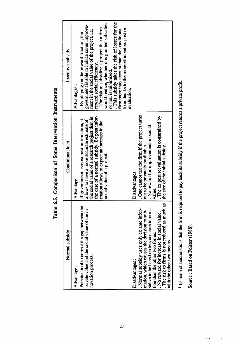
Tab

le 6

.5.

Com

pari

son

of S

ome

Inte

rven

tion

Ins

trum

ents

Nor

mal

sub

sidy

C

ondi

tiona

l loa

n 1

Ince

ntiv

e su

bsid

y

Adv

anta

ge:

Adv

anta

ge:

Adv

anta

ges

: Po

tent

ial t

ool t

o co

rrec

t the

gap

bet

wee

n th

e If

gov

ernm

ent u

ses

ex p

ost i

nfor

mat

ion,

it

. By

play

ing

on th

e re

war

d fr

actio

n, t

he

priv

ate

valu

e an

d th

e so

cial

val

ue o

f the

in-

allo

ws

to h

ave

a m

ore

accu

rate

est

imat

e o

f go

vern

men

t is

able

to in

duce

som

e im

prov

e-no

vatio

n pr

oces

s.

the

soci

al v

alue

of a

rese

arch

pro

ject

than

in

men

t in

the

soci

al v

alue

of t

he p

roje

ct, i

.e.

the

case

of a

nor

mal

sub

sidy

. Ex

post

info

r-re

war

d so

cial

eff

icie

ncy.

m

atio

n al

low

s to

exp

ect a

n in

crea

se in

the

. The

risk

to s

ubsi

dize

a p

roje

ct th

at a

frrm

so

cial

val

ue o

f a p

roje

ct.

wou

ld re

aliz

e, w

heth

er it

is g

rant

ed s

ubsi

dies

or

not

, is

min

imiz

ed .

. Thi

s su

bsid

y ta

kes

the

risk

of

loss

es f

or th

e fi

nn m

ore

into

acc

ount

than

the

con

ditio

nal

loan

than

ks to

the

mor

e ef

fici

ent e

x po

st re

-ev

alua

tion.

D

isad

vant

ages

: D

isad

vant

ages

: . N

orm

al s

ubsi

dy u

ses

only

ex

ante

inf

or-

. One

can

not t

ax t

he f

inn

if th

e pr

ojec

t tur

ns

mat

ion,

whi

ch c

ause

s th

e de

cisi

on to

sub

-ou

t to

be p

riva

tely

pro

fita

ble.

si

dize

to b

e ba

sed

on le

ss a

ccur

ate

info

nna-

. No

rew

ard

for

impr

ovem

ent i

n so

cial

tio

n th

an th

e ot

her

two

form

s.

valu

e.

. No

rew

ard

for

incr

ease

in s

ocia

l val

ue.

. The

ex

post

ree

valu

atio

n is

con

stra

ined

by

. The

risk

to f

mns

is n

ot re

duce

d as

muc

h as

th

e si

ze o

f the

ini

tial s

ubsi

dy .

with

the

othe

r tw

o m

eans

.

1 Its

mai

n ch

arac

teri

stic

is th

at th

e fi

nn

is r

equi

red

to p

ay b

ack

its s

ubsi

dy if t

he p

roje

ct re

turn

s a

priv

ate

prof

it.

Sour

ce :

Bas

ed o

n F

oist

er (1

988)

.

N

0 Vl

1) P

urch

ase

2) I

mita

tion

3) In

tern

al R

& D

(or

in

itia

ting

tec

hnol

ogy)

Tab

le 6

.6.

Cos

t-B

enef

it C

hara

cter

isti

cs o

f E

ach

Inno

vati

on C

hann

el

Cos

ts

Ben

efit

s

. Pur

chas

e pr

ice

of

the

tech

nolo

gy.

. Les

s te

chno

logi

cal

unce

rtai

nty.

In

the

inno

vati

on p

ro-

. The

fm

n's

spec

ific

req

uire

men

ts h

ave

to b

e m

et. A

n ce

ss, u

ncer

tain

ty a

rise

s be

caus

e an

abs

trac

t ide

a m

ust

adap

tativ

e pr

oces

s m

ust b

e im

plem

ente

d to

inte

grat

e be

tra

nsla

ted

into

a w

orka

ble

proc

ess

desi

gn.

By

con-

the

new

tec

hnol

ogy

into

the

prod

ucti

on p

roce

ss o

f the

tr

ast,

in t

he c

ase

of t

echn

olog

y tr

ansf

er, i

f th

e tr

ansf

er

firm

. S

ome

addi

tion

al t

rain

ing

may

be

nece

ssar

y to

al-

proc

ess

is e

ffic

ient

ly m

anag

ed, i

t can

ind

uce

a te

chno

-lo

w th

e m

anpo

wer

to a

ssim

ilat

e th

e ne

w p

roce

ss.

logy

mas

tery

dyn

amic

that

cou

ld le

ad to

inno

vati

on a

nd

. The

org

aniz

atio

nal

stru

ctur

e o

f the

firm

has

to

be

diff

usio

n .

mod

ifie

d to

ens

ure

an e

ffic

ient

inte

rnal

tran

smis

sion

of

the

requ

ired

info

rmat

ion,

...

. T

he f

mn

bec

omes

dep

ende

nt o

n ex

tern

al te

chno

logy

. T

he p

urch

ase

of t

echn

olog

ies

mus

t be

inco

rpor

ated

into

a

long

term

str

ateg

y ai

med

at a

cqui

ring

one

's o

wn

tech

-no

logy

.

. Ent

ails

dep

ende

nce

and

requ

ires

ada

ptat

ion

tim

e.

. Les

s te

chno

logi

cal u

ncer

tain

ty b

ecau

se t

he m

ain

cha-

. Ada

ptat

ion

cost

s ar

e hi

gher

than

in

the

purc

hase

cas

e ra

cter

isti

cs o

f the

mos

t app

ropr

iate

pro

cess

des

ign

are

beca

use

the

mar

ket o

nly

prov

ides

impe

rfec

t inf

orm

a-kn

own.

tio

n (m

oral

haz

ard,

adv

erse

sel

ecti

on)

and

ther

e is

litt

le

. Nee

d no

t be

bou

ght.

in

form

atio

n ab

out t

he c

hara

cter

isti

cs o

f the

imit

ated

. I

mpr

ovem

ent o

f the

ori

gina

l pro

duct

and

pro

duct

ion

tech

nolo

gy. T

he d

evel

opm

ent o

f a t

echn

olog

y in

volv

es

at a

low

er c

ost.

le

arni

ng b

y tr

ial

and

erro

r, w

hich

is

mor

e or

less

ard

u-ou

s de

pend

ing

on th

e ab

ilit

y an

d sk

ill o

f the

inno

vato

r fi

nn. T

hese

ele

men

ts a

re im

port

ant t

o m

aste

r a te

chno

-lo

gy a

nd n

ot re

adil

y tr

ansf

erab

le (

key

pers

onne

l or

labo

rato

ries

) .

. Cos

t of t

he i

nfor

mat

ion

rela

ted

to th

e kn

owle

dge

of

all t

he a

vail

able

tech

nolo

gy .

. Dir

ect c

ost o

f res

earc

h hi

gher

than

the

sal

e pr

ice

of a

. T

he r

esul

ts o

f th

e re

sear

ch p

roce

ss m

eet

the

firm

's

purc

hase

d te

chno

logy

. se

t of r

equi

rem

ents

and

firm

s ca

n so

met

imes

app

ro-

. Unc

erta

inty

of

the

rese

arch

pro

cess

. pr

iate

som

e ad

diti

onal

tech

nica

l kno

wle

dge

acqu

ired

. I

mpe

rfec

t app

ropr

iabi

lity

of t

he r

esul

t. du

ring

the

inno

vati

on p

roce

ss .

. R &

D i

nves

tmen

t enh

ance

s th

e fi

rm's

abi

lity

to

as-

sim

ilat

e an

d ex

ploi

t exi

stin

g in

form

atio

n.

technological trajectory of each indusny by allowing fmns to choose between several op­

tional ways of improving technological efficiency : imitation, purchase and R & D initia­

tion. Besides, they can also choose not to engage in R & D at all.

If the fmn is rational, i.e. makes choices that maximize its expected benefits, the ex­

pected welfare that firms get from a specific choice can be measured by the income flow.

This income flow can be decomposed into different variables. On the one hand, we have

variables that are functions of the selected option and, on the other hand, we have vari­

ables which are independent of the selected option. For the former, the main variables are

expected profits, subsidies and/or tax credit from public authorities. For the latter, the

structural characteristics of the firm which are not affected by any alternative have to be

considered. To model and assess the determinant of alternative choices whose impact on

the fmns can be assumed to be constant, it is preferable to resort to conditionallogit

rather than multinomiallogit 1 [Hoffman and Duncan (1988)]. A mixed conditionallogit

should be used because some explanatory variables are sectoral characteristics and the

other variables are characteristics related to the selected alternatives i.e. varying from one

option to another. The function associated to the fmn i under the option j is, then, defined

as the following latent variable :

Ve {Pe S·· T .. X·} 2 " .. , IJ' IJ' 1 IJ IJ

where P~ IJ

Sij

Tij

Xi

expected profits of fmn i under the option j

subsidies to finn i under the option j

tax credit to fmn i under the option j

structural characteristics vector associated to fmn i.

In fact, Vij stands for the value of alternative j to firm i. Such models are especially

well suited for the analysis of situations in which the government policy affects the attrac­

tiveness of an alternative by changing some relevant characteristics. Obviously, to assess

the effect of government policies such as a subsidy policy, when possible, the policy

parameters have to be directly included in the choice structure.

Assuming that the indirect utility function is additive, we have :

1 By contrast, the multinomiallogit model hypothesizes that the explanatory variables (individual cha­racteristics) are constant across the alternatives. So, it measures the specific impact of these character­istics (across individuals) on each choice.

2 Other variables can be used such as the level of R & D expenditures which differs across industries and alternatives. The variables selected here are only a potential representation which must be modified ac­cording to the amount of available information.

206

I

where ~' "(, a, a j unknown parameters

Eij residual that captures the effect of unmeasured variables and the

imperfection in the optimization program.

The mixed conditionallogit is based on the assumption that the error terms in Vij fol­

low an extreme value distribution and are independent across alternatives. This independ­

ence assumption is crucial because any other assumption leads to substantial computa­

tional difficulties involving the computation of multivariate integrals.

With a set of n firms facing m options, we can defme :

- Cij = 1 if the ith fmn makes the jth choice

i.e. vij =max {Vi~' ... ,Vi~)

- Cij = 0 otherwise.

j = 1, ... , m i = 1, ... , n

If we assume that Eij are independently and identically distributed with an extreme­

value distribution, then the probability Pij that the firm i chooses alternative j, in the

mixed conditionallogit, is :

Pij = Prob (Cij = 1) e I

= Exp (~ pij + 'Y Sij + a Tij + aj Xi) I m I

L, Exp (~ P.ek + 'Y Sik + a Tik + 9k Xi) k=1 1

The estimation of the structural parameters of this equation through a maximum likeli­

hood procedure allows to simulate the different policies and determine the consequence of

policy changes on the rate of R & D effort of each alternative. The expected profits Pij

can be obtained by using questionnaires or sound estimates based on past profits.

Another possible application of this sort of model is to classify the ftrms in respect of

their R & D expenditure. Once again, using subsidy as an explanatory variable, we can

study the effect of a modification in the subsidy level on the R & D expenditure of the

firm. However, to measure the impact of the subsidy on the technological efficiency, it

might be preferable to use a measure of output such as the number of patents issued.

207

6. 4. Centres of Excellence and Agglomeration Economies

Through setting-up R & D programmes a country can avail itself of strategies that go

beyond the subsidy policy. So, a potential alternative policy is to develop European

centres of excellence in research and innovation.

The creation of a centre of excellence is a cumulative process if decisions taken pre­

viously increase the likelihood of locating a research facility in a European centre. Hence,

repeated investments in these centres strengthen their international position and their R &

D ability, so creating agglomeration effects. These agglomeration effects may result from

the user-producer interaction. Indeed, users' sophisticated requirements support the re­

search facilities of the technology producers and the ensuing feedback and joint testing

procedure leads to incremental technological improvement. In addition, such centres of

excellence improve the diffusion process and make a wider range of technological pro­

ducts available to the users. However, a major potential cause of failure is that these

centres are 'locked in' to a path of technological development.

At the European level, the creation of centers of excellence, which go beyond the na­

tional boundaries, allows to develop and reorganize a network of research facilities. It is -.

important to strengthen the interaction between the different centers and to organize the

participation of the European countries in function of their technological ability in a spe­

cific field and not in function of political considerations of balanced representation.

Cantwell (1991) tested the significance of such a proposition on the basis of the pre­

vious argument that research tends to agglomerate geographically. He showed that the

geographical concentration of technological activity has risen outside the U.S. and that

Japan has increased its share. His analysis emphasizes the fact that many sectors show an

agglomerative consolidation of their comparative (dis)advantages 1.

In his empirical study, he draws up an index of the revealed technological advantages

(RTA) of locations in the following way :

where Pij : number of US patents granted in sector i attributable to research in country j.

1 He also assessed the contribution of foreign-owned research facilities to technological agglomeration and concluded that the location of foreign-owned research has, in general, contribtited to technical ag­glomeration but not in a significant way.

208

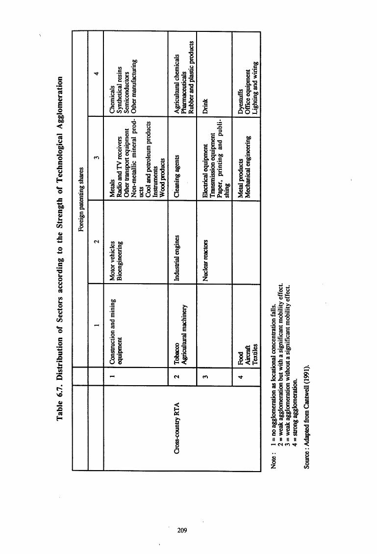
Tab

le 6

.7.

Dis

trib

utio

n of

Sec

tors

acc

ordi

ng t

o th

e S

tren

gth

of T

echn

olog

ical

Agg

lom

erat

ion

1

1 C

onst

tuct

ion

and

min

ing

equi

pmen

t

Cro

ss-c

ount

ry R

TA

2

Tob

acco

A

gric

ultu

ral m

achi

nery

3 4 Fo

od

Airc

mft

Tex

tiles

Not

e :

1 =

no a

gglo

mer

atio

n as

loca

tiona

l con

cent

ratio

n fa

lls.

2 =

weak

agg

lom

erat

ion

but w

ith a

sig

nifi

cant

mob

ility

eff

ect

3 =

weak

agg

lom

erat

ion

with

out a

sig

nifi

cant

mob

ility

eff

ect.

4 =

stron

g ag

glom

erat

ion.

Sour

ce :

Ada

pted

from

Can

twel

l (19

91).

2

Mot

or v

ehic

les

Bio

engi

neer

ing

Indu

stri

al e

ngin

es

Nuc

lear

~tors

Fore

ign

pate

ntin

g sh

ares

3 4

Met

als

Che

mic

als

Rad

io a

nd T

V re

ceiv

ers

Synt

hetic

al r

esin

s O

ther

tran

spor

t equ

ipm

ent

Sem

icon

duct

ors

Non

-met

alli

c m

iner

al p

rod-

Oth

er m

anuf

actu

ring

ucts

C

ool a

nd p

etro

leum

pro

duct

s In

stru

men

ts

Woo

d pr

oduc

ts

Cle

anin

g ag

ents

A

gric

ultu

ral c

hem

ical

s Ph

arm

aceu

tical

s R

ubbe

r and

pla

stic

pro

duct

s

Ele

ctri

cal e

quip

men

t D

rink

Tra

nsm

issi

on e

quip

men

t P

aper

, pr

inti

ng a

nd

publ

i-sh

ing

Met

al p

rodu

cts

Dye

stuf

fs

Mec

hani

cal e

ngin

eerin

g O

ffic

e eq

uipm

ent

Lig

htin

g an

d w

irin

g

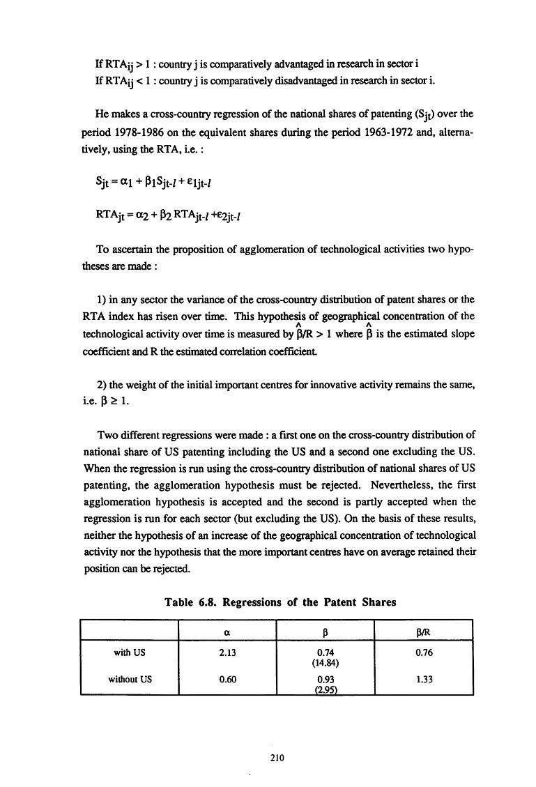
If RT Aij > 1 : country j is comparatively advantaged in research in sector i

If RTAij < 1 : country j is comparatively disadvantaged in research in sector i.

He makes a cross-country regression of the national shares of patenting (Sjt) over the

period 1978-1986 on the equivalent shares during the period 1963-1972 and, alterna­

tively, using the RT A, i.e. :

Sjt =at + Pt Sjt-1 + £tjt-l

RTAjt = a2 + P2 RTAjt-1 +£2jt-l

To ascertain the proposition of agglomeration of technological activities two hypo­

theses are made :

1) in any sector the variance of the cross-country distribution of patent shares or the

RTA index has risen over time. This hypothesis of geographical concentration of the 1\ 1\

technological activity over time is measured by PIR > 1 where P is the estimated slope

coefficient and R the estimated correlation coefficient

2) the weight of the initial important centres for innovative activity remains the same,

i.e. p ~ 1.

Two different regressions were made : a firSt one on the cross-country distribution of

national share of US patenting including the US and a second one excluding the US.

When the regression is run using the cross-country distribution of national shares of US

patenting, the agglomeration hypothesis must be rejected. Nevertheless, the first

agglomeration hypothesis is accepted and the second is partly accepted when the

regression is run for each sector (but excluding the US). On the basis of these results,

neither the hypothesis of an increase of the geographical concentration of technological

activity nor the hypothesis that the more important centres have on average retained their

position can be rejected.

Table 6.8. Regressions of the Patent Shares

a ~ ~IR

with US 2.13 0.74 0.76 (14.84)

without US 0.60 0.93 1.33 (2.95)

210

Table 6.7 ., which summarizes Cantwell's results shows that the trend towards

agglomeration is higher when patenting shares are used than when RTA is the reference

measure. Such an observation is only the consequence that patent shares are similar at an

absolute value of technological advantage while RTA is a relative value measuring

comparative technological advantages. The first four quadrants show the sectors for

which no agglomeration effect was detected. The four following quadrants show the

sectors characterized by a reinforcement of spatial concentration in foreign patenting

shares combined with a weakening of comparative technological advantages. This

contrasted finding is explained by the high weight of small countries in the measurement

of the RTA for these sectors which is not reflected by the patent shares. Some of these

sectors also correspond to cases in which Japan made strong absolute but not relative

gains. The next four lower quadrants represent the sectors for which the spatial

concentration in patent shares becomes more dispersed and the concentration in terms of

RTA rises. So, in these sectors, while the patent shares come closer to each other, the

leader countries strengthen their initial technological position. The last four quadrants

give the sectors for which both types of measurement provide evidence of strong

agglomeration effects. Only two high-technology sectors belong to this category : office

equipment and electrical equipment. The other high technology sectors, such as

bioengineering, instruments, semiconductors and pharmaceuticals, do not seem to be

faced with a strong agglomeration trend. Yet, the trend towards a higher concentration of

these sectors in absolute value might be the source of future RTA. Finally, it is worth

noting that the analysis of patent shares does not include the US. The map of sectors

presented in table 6.7. would certainly have been different if the US had been included.

Indeed, as shown in table 6.8., the results of total regressions with and without the US

are noticeably different.

However this may be, this analysis stresses that technological concentration exists and

that the Japanese position is stronger, both in absolute and in comparative terms. The

U.S. position is weaker and the European situation is relatively contrasted. One

observes, however, a positive correlation between the technological position of a country

and its industrial competitiveness. The poor performance of the U.K. points to the weak

performance in its industrial sector whereas Germany affrrms its dominant position both

in absolute and in comparative advantage terms. The existence of a European network of

centres of excellence requires the availability of research professionals, i.e. a highly

skilled human capital. Once again, a manpower that is highly skilled in the scientific and

engineering field is a crucial factor to increase competitiveness. Besides, a favorable insti­

tutional environment, both on the labour market and on the capital market, should be

211

created. In this respect, the completion of the European internal market offers the possi­

bility to generate an environment conducive to R & D investment.

The existence of critical mass is the main reason why R & D tends to agglomerate.

The subsidization of R & D at one location will benefit R & D at the location and will

attract researchers from other locations. It will be beneficial as long as domestic scale

economies are available and can induce an international redistribution of research

activities. Such a policy strategy has clear advantages at the European level where lots of

research centres do not reach the critical mass. Yet, its disadvantages are threefold. First,

it may depress research activities in some regions and countries. Second, if other

governments adopt a similar strategy, a large part of the redisnibutive effect may be lost.

Third, the implementation of a selective subsidy policy will encourage the beneficiaries to

lobby for more and divert subsidies for non-innovative activities [Casson (1991)].

6.5. Technological Competition and R & D Policy in Oligopoly

R & D is a non-price competitive element and requires to be associated with all the

other elements of the fmn's strategy. The issue of a fmn's optimal levels for all decision

instruments has received considerable attention in the marketing literature. These exten­

sions of the profit maximisation rule have nied to take into account other decision-making

process variables than just the price. All these normative models have been developed

along the lines defined by Dorfman and Steiner (1954)'s theorem for monopolistic com­

petition.

Following the original contribution of Dorfman and Steiner, Hay and Morris ( 1991)

have recently presented a basic model of innovation. Besides the frrm's own decision

variables, they also include the rival's decision variables as determinant of the firm's

demand.

The demand curve for firm i is a function of its own price Pi and its own expenditure

on R & D, Xit and of Pj and Xj vectors of prices and R & D expenditures of other firms.

The expenditure Xi shifts the demand curve, () Qi I a Xi > 0, but at a diminishing rate.

The first order conditions can be obtained from the profit maximization process 1ti :

where c ( Qi) is the production cost.

212

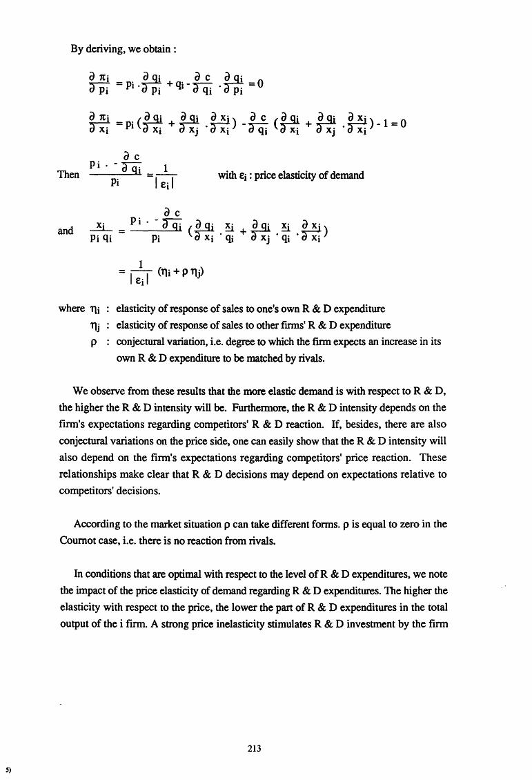
S)

By deriving, we obtain:

1_. 1+. 1_ ax· ~· a c ~· dpj - Pt . Pi q1 - dqi . Pi - 0

a c Then Pi. - dQi __ 1_

Pi -I ed with Ei : price elasticity of demand

a c

and _!j_ =Pi. - aQi (~ !i + ~ 5 ~ Xj) Pi qi Pi a xi · ~ a Xj · qi · Xi

1 = leJ (1li + p 'llj)

where 1li elasticity of response of sales to one's own R & D expenditure

1lj elasticity of response of sales to other firms' R & D expenditure

p conjectural variation, i.e. degree to which the firm expects an increase in its

own R & D expenditure to be matched by rivals.

We observe from these results that the more elastic demand is with respect toR & D,

the higher the R & D intensity will be. Furthermore, the R & D intensity depends on the

finn's expectations regarding competitors' R & D reaction. If, besides, there are also

conjectural variations on the price side, one can easily show that the R & D intensity will

also depend on the finn's expectations regarding competitors' price reaction. These

relationships make clear that R & D decisions may depend on expectations relative to

competitors' decisions.

According to the market situation p can take different forms. p is equal to zero in the

Coumot case, i.e. there is no reaction from rivals.

In conditions that are optimal with respect to the level of R & D expenditures, we note

the impact of the price elasticity of demand regarding R & D expenditures. The higher the

elasticity with respect to the price, the lower the part of R & D expenditures in the total

output of the i finn. A strong price inelasticity stimulates R & D investment by the firm

213

due to the fact that non-price instruments are more efficient to obtain important market

shares.

This analysis can be extended to include the effects of a public incentive to private R &

D. Suppose the subsidy be equal to a fraction a of the private R & D so that the profit is

equal to:

withOSa<l

In such a case, the R & D intensity equation becomes :

which shows that the higher a is, the higher R & D intensity will be.

However; this model is too simple to express a real situation. Considering zero con­

jectural variations is inealistic. But the definition of rational conjectural variations is not

easy due to, for instance, the great part of uncertainty associated with R & D investment

Moreover, each different non-zero conjectural variation implies a different type of reac­

tion function and, therefore, another equilibrium.

Lambin and al. (1975) have derived an optimal marketing behavior model that is more

consistent for the analysis of oligopolistic competition. We can extend this model to in­

corporate R & D and obtain an expression in terms of market share.

In the process of maximization, a firm can use a set of decision variables, among

which the level of R & D expenditure, the purpose being to determine the conditions in

which each decision variable is likely to yield maximum profit

We can derive the optimality conditions, considering first the company profit function

for the case of monopolistic competition :

1t = q . [p - c (q, o)] - x

where p price

o organizational cost

x R & D expenditure.

214

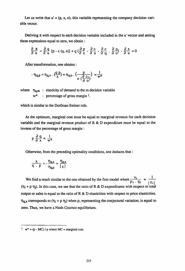
Let us write that u' = (p, x, o), this variable representing the company decision vari­

able vector.

Deriving 1t with respect to each decision variable included in the u' vector and setting

these expressions equal to zero, we obtain :

a x Pu <fJ a c a c Q_q) a x --r:-:- = [p - c (q o >l + q -~ - -a . a -~ = o ou u ' u ou q u ou

Mter transformation, one obtains :

-llq,p = llq,x · fl!) = llq,o · { 9 Ci ) o <a o)

1 =w*

where n ••q,m

w*

elasticity of demand to the m decision variable

percentage of gross margin 1.

which is similar to the Dorfman-Steiner rule.

At the optimum, marginal cost must be equal to marginal revenue for each decision

variable and the marginal revenue product of R & D expenditure must be equal to the

inverse of the percentage of gross margin :

Otherwise, from the preceding optimality conditions, one deduces that :

_x_ _ llg,x _ llg,x q . p - - llq,p - I E I

We find a result similar to the one obtained by the first model where p. Xi q. = 1

1 • 1 I Ei I (lli + p llj). In this case, we see that the ratio of R & D expenditures with respect to total

output or sales is equal to the ratio of R & D elasticities with respect to price elasticities.

llq,x corresponds to (lli + p llj) when p, representing the conjectural variation, is equal to

zero. Thus, we have a Nash-Coumot equilibrium.

1 w* = (p- MC) I p where MC =marginal cost.

215

The preceding relation shows that the higher the percentage of gross margin w* is, the

lower the marginal product of R & D expenditure is and the higher the profitable level of

R & D expenditure is since we expect diminishing returns on R & D expenditure. We

know that ~* = I e I . Hence, the previous situation implies a low price elasticity, i.e. the

possibility for the frrm to charge high prices.

A competitive situation is characterized by strong interdependences between rival

fmns. In parallel with the concept of conjectural variations, one can express two different

forms of interdependence. First, the performances of any fmn depend on the level of its

rivals' decision variables, in particular R & D expenditure. Second, if a firm modifies its

R & D expenditure, other rival firms will react.

To extend the model, let us decompose the Eq,u vector of total sales elasticities into

three components which are :

1) the industry sales or output effect;

2) the direct partial effect in the company market share due to a change in the company

decision variables 1;

3) the indirect partial effect in the company market share due to modifications in rival

fmns' decision variables, i.e. brought about by a change in the competitive mix pres­

sure of rival firms.

By definition:

m. _ _q_ ,-Qr

where mi market share of the company

q company sales

Qr industry sales.

1 The company market share can be represented as :

ki p ~1 X ~2 0 ~3 1 1 1

mi = e e e L ki p . 1 X • 2 0 • 3 • 1 1 1 1

where the ej are the market share sensitivities with respect to each decision variable and for each frrm the numerator of this relationship can be defined as the competitive mix pressure of the firm. The elasticity of the market share to each variable is defined as :

Ej = Cj (1 - ffij)

216

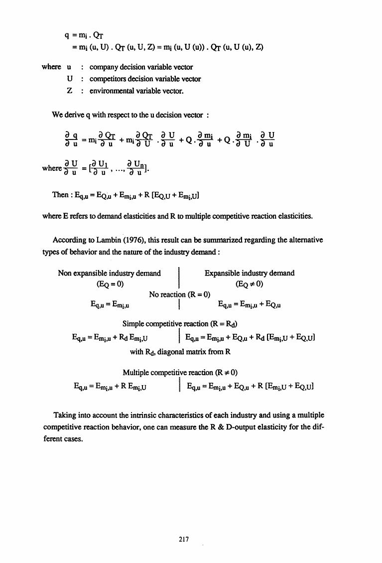
q =mi. Qr

= mi (u, U) . Qr (u, U, Z) = mi (u, U (u)) . Qr (u, U (u), Z)

where u

u z

company decision variable vector

competitors decision variable vector

environmental variable vector.

We derive q with respect to the u decision vector :

~ a Qr a Qr a u ~mi a mj a u d u =midU +midl) ·du +Q. u +Q.dlf ·du

d U [d U1 dUn] wheredu = LdU, ... , dU .

where E refers to demand elasticities and R to multiple competitive reaction elasticities.

According to Lambin (1976}, this result can be summarized regarding the alternative

types of behavior and the nature of the industry demand :

Non expansible industry demand (EQ=O)

Expansible industry demand (EQ¢0)

No reaction (R = 0) I Eq,u = Emj,u + EQ,u

Simple competitive reaction (R = Rd)

Eq,u = Emj,u + R<t Emj,U I Eq,u = Emj,u + EQ,u + R<t £Emj.U + EQ,u]

with R(i, diagonal matrix from R

Multiple competitive reaction (R :1: 0)

Eq,u = Emj,u + R Emj,U I Eq,u = Emj,u + EQ,u + R [Emj,U + EQ,U]

Taking into account the intrinsic characteristics of each industry and using a multiple

competitive reaction behavior, one can measure the R & D-output elasticity for the dif­

ferent cases.

217

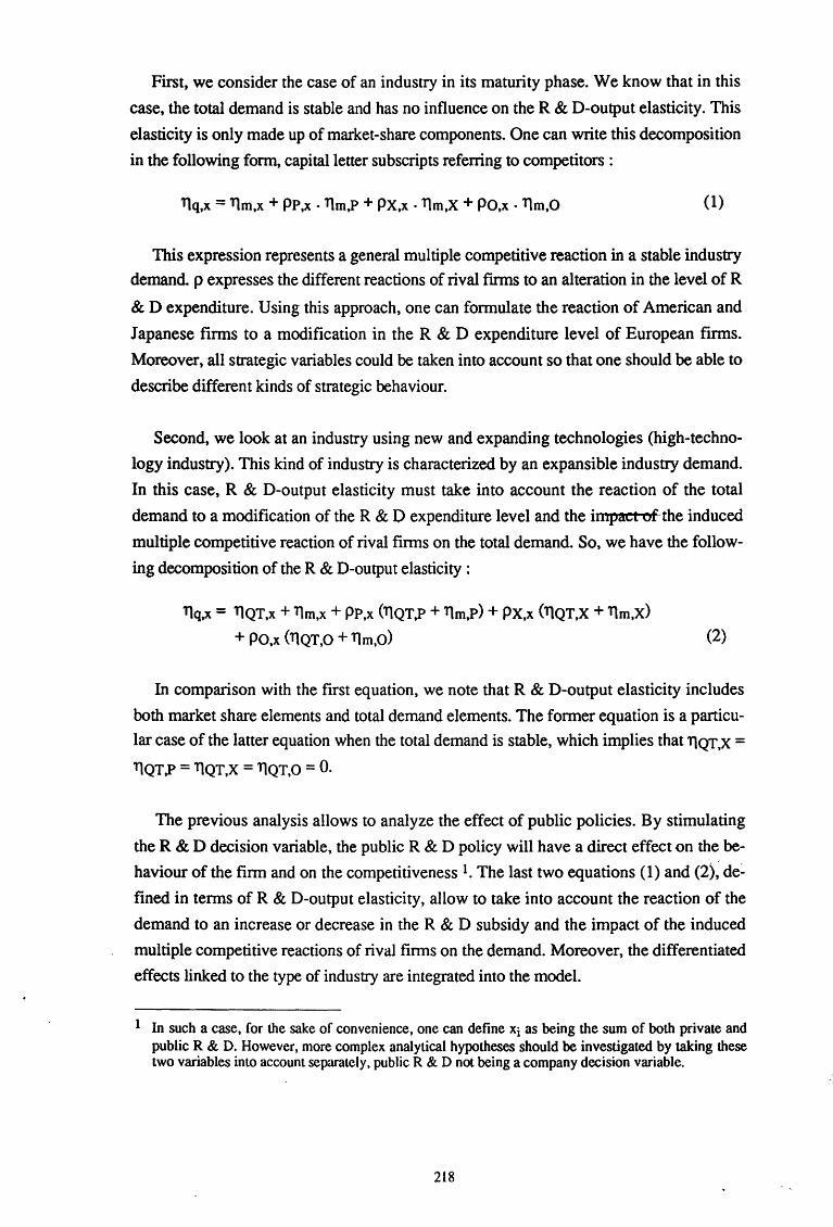
First, we consider the case of an industry in its maturity phase. We know that in this

case, the total demand is stable and has no influence on the R & D-output elasticity. This

elasticity is only made up of market-share components. One can write this decomposition

in the following form, capital letter subscripts referring to competitors:

Tlq,x = Tlm,x + PP,x · Tlm,P + PX,x · Tlm,X + PO,x · Tlm,O (1)

This expression represents a general multiple competitive reaction in a stable industry

demand. p expresses the different reactions of rival fums to an alteration in the level of R

& D expenditure. Using this approach, one can formulate the reaction of American and

Japanese firms to a modification in the R & D expenditure level of European firms.

Moreover, all strategic variables could be taken into account so that one should be able to

describe different kinds of strategic behaviour.

Second, we look at an industry using new and expanding technologies (high-techno­

logy industry). This kind of industry is characterized by an expansible industry demand.

In this case, R & D-output elasticity must take into account the reaction of the total

demand to a modification of the R & D expenditure level and the hnpaet of the induced

multiple competitive reaction of rival firms on the total demand. So, we have the follow­

ing decomposition of the R & D-output elasticity :

Tlq,x = 11QT,x + llm,x + PP,x (11QT,P + Tlm,P) + PX,x (11QT,X + Tlm,x)

+ PO,x (11QT,O + llm,O) (2)

In comparison with the first equation, we note that R & D-output elasticity includes

both market share elements and total demand elements. The former equation is a particu­

lar case of the latter equation when the total demand is stable, which implies that 11QT,X = 11QT ,P = 11QT,X = 11QT,O = 0.

The previous analysis allows to analyze the effect of public policies. By stimulating

the R & D decision variable, the public R & D policy will have a direct effect on the be­

haviour of the firm and on the competitiveness 1. The last two equations (1) and (2), de~

fined in terms of R & D-output elasticity, allow to take into account the reaction of the

demand to an increase or decrease in the R & D subsidy and the impact of the induced

multiple competitive reactions of rival firms on the demand. Moreover, the differentiated

effects linked to the type of industry are integrated into the model.

1 In such a case, for the sake of convenience, one can define Xi as being the sum of both private and public R & D. However, more complex analytical hypotheses should be investigated by taking these two variables into account separately. public R & D not being a company decision variable.

218

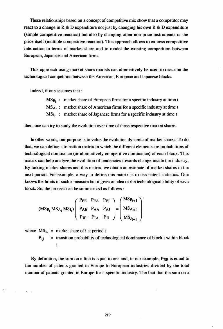
These relationships based on a concept of competitive mix show that a competitor may

react to a change in R & D expenditure not just by changing his own R & D expenditure

(simple competitive reaction) but also by changing other non-price instruments or the

price itself (multiple competitive reaction). This approach allows to express competitive

interaction in terms of market share and to model the existing competition between

European, Japanese and American firms.

This approach using market share models can alternatively be used to describe the

technological competition between the American, European and Japanese blocks.

Indeed, if one assumes that :

MSE1 : market share of European firms for a specific industry at time t

MS At : market share of American firms for a specific industry at time t

MSJt : market share of Japanese fmns for a specific industry at timet

then, one can try to study the evolution over time of these respective market shares.

In other words, our purpose is to value the evolution dynamic of market shares. To do

that, we can define a transition matrix in which the different elements are probabilities of

technological dominance (or alternatively competitive dominance) of each block. This

matrix can help analyze the evolution of tendencies towards change inside the industry.

By linking market shares and this matrix, we obtain an estimate of market shares in the

next period. For example, a way to define this matrix is to use patent statistics. One

knows the limits of such a measure but it gives an idea of the technological ability of each

block. So, the process can be summarized as follows :

(

PEE PEA PEJ ) MSEt+t

(MSE1 MSA1 MSJt) PAE PAA PAJ = MSAt+l

PJE · PJA Pn MSJt+t

where MSit = market share of i at period t

Pij = transition probability of technological dominance of block i within block

J.

By definition, the sum on a line is equal to one and, in our example, PEE is equal to

the number of patents granted in Europe to European industries divided by the total

number of patents granted in Europe for a specific industry. The fact that the sum on a

219

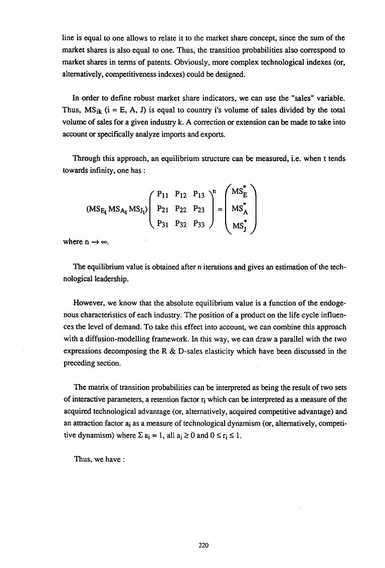
line is equal to one allows to relate it to the market share concept, since the sum of the

market shares is also equal to one. Thus, the transition probabilities also correspond to

market shares in terms of patents. Obviously, more complex technological indexes (or,

alternatively, competitiveness indexes) could be designed.

In order to define robust market share indicators, we can use the "sales" variable.

Thus, MSik (i = E, A, J) is equal to country i's volume of sales divided by the total

volume of sales for a given industry k. A correction or extension can be made to take into

account or specifically analyze imports and exports.

Through this approach, an equilibrium structure can be measured, i.e. when t tends

towards infinity, one has :

* ( Pu

P12 P13 J MSE

* (MSEt MSAt MSJt) P21 P22 P23 = MSA

P31 P32 P33 * MS1

where n ~ oo.

The equilibrium value is obtained after n iterations and gives an estimation of the tech­

nological leadership.

However, we know that the absolute equilibrium value is a function of the endoge­

nous characteristics of each industry. The position of a product on the life cycle influen­

ces the level of demand. To take this effect into account, we can combine this approach

with a diffusion-modelling framework. In this way, we can draw a parallel with the two

expressions decomposing the R & D-sales elasticity which have been discussed in the

preceding section.

The matrix of transition probabilities can be interpreted as being the result of two sets

of interactive parameters, a retention factor ri which can be interpreted as a measure of the

acquired technological advantage (or, alternatively, acquired competitive advantage) and

an attraction factor ai as a measure of technological dynamism (or, alternatively, competi­

tive dynamism) where .'E ai = 1, all ai ~ 0 and 0 ~ ri ~ 1.

Thus, we have :

220

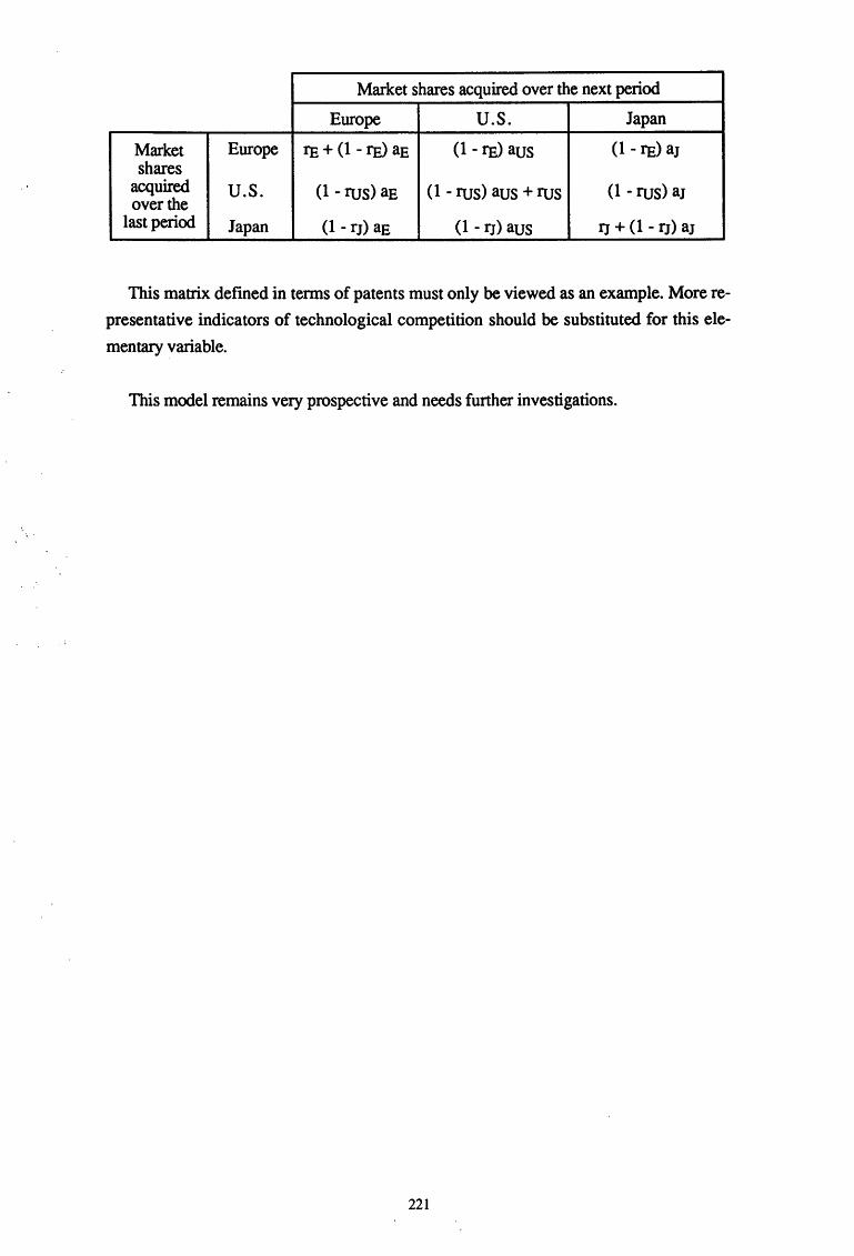
Market shares acquired over the next period

Europe u.s. Japan

Market Europe fE + (1 - fE) aE (1- fE) aus (1 - fE) aJ shares

acquired over the

u.s. (1- rus) aE (1- rus) aus + rus (1 - rus) aJ

last period Japan (1 - rJ) aE (1 - rJ) aus I) + ( 1 - rJ) a]

This matrix defined in terms of patents must only be viewed as an example. More re­

presentative indicators of technological competition should be substituted for this ele­

mentary variable.

This model remains very prospective and needs further investigations.

221

Conclusion

While econometric methods are extensively used as a tool for the evaluation of

economic policy, its credibility and usefulness in the field of science and technology

policy is very controversial, if not contested. The main arguments invoked against these

techniques are the problem of causality links, the time lag structure, the variability of

results, the complexity and uncertain nature of the innovation process which rend eco­

nometric investigations difficult. On the other hand, lots of evaluation studies point out

that the evaluation processes are mainly focused on technological aspects and do not

deal with the economic impacts. When the latter are covered, methods used are essen­

tially case studies and surveys. Yet, these methods have their own shortcomings and, in

any case, only consider some direct and partial economic impacts. What must take the

lead in the choice of a method is the issue at stake. As the evaluation process is funda­

mentally a heuristic and subjective process, there is seldom a clear-cut definitive

answer. In order to avoid costly erroneous decisions, any experiment should be, if pos­

sible, complemented by another one performed on the basis of an alternative method.

Theoretical and empirical studies of the relationship between technical change

and improvements in economic performance are principally based on the concept of

production function. While the production theory is well developed, the treatment of

technical change is still very abstract. This abstraction results from the neo-classical

paradigm of exogenous technical change. In empirical works, despite their large efforts

to analyze how technical change affects the production process, the way in which it

works is not analytically dealt with.

The most commonly used approach to materialize technical change in produc­

tion functions is to use R & D investment as a proxy and to treat it as a production fac­

tor. Although this variable is only an input measure of the knowledge production pro­

cess, output measures, like inventions and patents, are considered to be less appropriate

to grapple with the full spectrum of knowledge activities. The accumulated empirical

expertise about the relationship between R & D investment and productivity empha­

sizes the significant impact of R & Don productivity growth. Two types of measure

can be captured by the productivity approach, the R & D elasticity with respect to out­

put and the rate of return on R & D. The apparent diversity of results can be, to a large

extent, explained by data characteristics. Yet, this approach suffers from some pro­

blems, among which, the interpretation of the rate of return (distinction between gross

or net, private or social, in excess or not rate of return), data measurement (distinction

223

between gross output, net output and total factor productivity), the specification of

models (distinction between total regression, within regression, regressions with dum­

my variables and on average values) and choice of variables (distinction between R &

D investment and R & D stock). So far, studies have essentially been concentrated on

the measure of the impact of total R & D expenditure. More efforts should be devoted

to the analysis of the time lag structure of the R & D effects on productivity growth and

on the effects of R & D by character of use (basic research, applied research, develop­

ment, R & Don processes, R & Don products), the simultaneity between the firm's

decisions and data improvements. The simultaneity problem has been considered in

some studies making use of an adjustment cost model from which the input demand

functions are derived. These studies provide evidence that R & D investments respond

to changes in demand, prices and other inputs and that there are interactive adjustments

between inputs. The latter model represents an important methodological step in the

formalization of relationships between R & D, output, prices, employment and physical

investment.

The measure of the impact of research efforts of a fmn or an industry on the

productivity growth of this firm or this industry only provides a piece of information on

the economic impact of research efforts. As research results are not fully appropriable,

they spill over to other firms and industries. These spillover effects which make the dif­

ference between the social and private rate of return on R & D are generally very high

but greatly vary across industries. Several methods have been suggested to measure

these spillovers. A first category includes the approaches based on a proximity measure.

The main drawback of these approaches is that the proximity weights are derived from

intermediate input, patent or innovation flows, which are only able to capture a part

of knowledge transmission. The second category distinctively considers industries as

sources or receivers of R & D spillovers whose rates of return are estimated by specify­

ing cost or cost and demand functions of industries in a static or dynamic frarnework.

The advantages of this approach are to capture the diversity of spillover effects across

industries and to trace the flows of these effects by identifying the source- and receiver­

industries and to measure what is the magnitude of spillovers for each source- and

receiver-industry. It provides evidence that the spillovers are circumscribed in some

industries. Furthermore, a recent model based on the dynamic duality theory showed

that spillovers affect both costs and demand and that adjustments are not instantaneous.

A further extension of this model should be to emphasize how international competition

affects both cost and demand functions by taking into account the spillover effects of

foreign R & D.

224

An important issue in the analysis of the economic impact of R & D is the issue

of the differentiated effects of components of R & D investment. A disaggregation of

interest is the distinction between privately-financed R & D and government-financed

R & D. Empirical investigations showed that the impacts on productivity growth of

both types of investment were largely different. On the one hand, government-financed

R & D appears to influence at most marginally productivity growth while, on the other

hand, privately-financed R & D significantly affects productivity growth. Yet, regard­

ing government-financed R & D, some studies showed that its relationship with pro­

ductivity growth was more subtle than for privately-financed R & D. A peculiarity of

government-financed R & D is that it affects not only productivity growth but that it

may also stimulate private R & D. So, concurrently to the productivity approach, an in­

vestment approach has been developed in order to measure to what extent government­

financed R & D crowds out, complements or stimulates private R & D. The empirical

observations showed that publicly-financed R & D might only marginally crowd out

private R & D in some cases but that, in a majority of cases, it stimulates private R &

D. Yet, some studies have emphasized that specification problems might greatly affect

the evaluation. Indeed, what is captured as a stimulation effect of government-financed

R & D might simply be the stimulation effect of government purchases or the result of

spurious correlation. These studies show that results obtained from the investment must

be cautiously interpreted but, in any case, do not support the crowding-out hypothesis.

The implementation of science and technology policy is, to a large extent,

guided by strategic considerations. Technology is a non-price competitive weapon on

which governments act by developing their science and technology policy. Not only

technological rivalry between frrms leads them to engage in a strategic race to innovate

but also governments adopt a strategic behavior in the design of their policies. In the

past few years, some nonnative models of technology rivalry have been developed but,

so far, this new theoretical modelling approach has not provided clear-cut prescriptions

about the guidance of R & D policy. Besides, some more pragmatic studies which con­

sider certain strategic issues show how difficult it is to implement an efficient R & D

policy because of, among other things, the existence of agglomeration economies, the

differences among industries, the outflow outside national borders of new knowledge,

the specificities of the different types of R & D. As government actions in the field of

science and technology are increasingly prompted by strategic issues, the evaluation of

the economic impact of R & D policy should take this dimension into account. Future

empirical investigations might consider models of competitive behavior in oligopolistic

markets. In this approach, the frrm's behavior is captured by estimating a market share

model to measure how sensitive the market share of a frrm is to the competitive mix of

rival fmns and competitive reaction models to evaluate how a frrm moves in reaction to

225

a shift of the competitive mix of rivals. These models might be extended by including

public policy variables and by modelling government behavior to evaluate to what ex­

tent government strategies are designed under oligopolistic behavior.

The methodological choice for the conduct of the analysis has been to review

the available methods for the evaluation of the economic impacts of R & D program­

mes, asking oneself how empirical economics deal with technical change. This way of

proceeding has drastically reduced the field of investigation since it considers methods

really in use. Yet, there are other candidate methods which might be fruitfully imple­

mented. They are measurement methods which can be implemented in a large variety of

contexts and whose use is conditioned by four interdependent criteria : the objective of

the evaluation, the data availability, the time to be devoted to the evaluation and the

implementation cost. The measurement methods can be split into four large categories.

A first category concerns quasi-experimental methods. In the field of policy

formation, real controlled experiments are rarely performed because they are practically

unfeasible and when they are, they are cost- and time-intensive. An alternative way is to

conduct quasi-experiments by surveying a sample of firms affected by the policy in­

strument or by comparing some relevant variables obtained for the fmns affected by the

policy to those characterizing a control group. This method can only cover a limited

number of variables, only provides information on the direct effects of the programmes

and may suffer from a bias between the actual effects and the perceived ones.

In a second category, there are intervention analysis methods which consist in

modelling a target variable in order to estimate by means of interrupted time series

analysis techniques to what extent the evolution of the target variable has been in­

fluenced by the policy. In this analysis, the prepolicy variable is distinguished from the

postpolicy variable on which the policy has exerted its impact and the time series data

structures can bear on a single time series design or a time series panel design. Policy

interventions can produce a wide array of effects, which leads to consider some alterna­

tive intervention models depending upon the duration of the impact. Three response

patterns to a policy variable are generally contemplated. So, the impact is transcent if

there are one-time shifts in the observations, permanent if the effect remains constant

throughout the postintervention series or dampened if the initial effect declines over

time toward the intervention level. This approach can be used when only some target

variables or both target variables and the policy variable are known and other relevant

explanatory variables are missing. Its main disadvantage is to only allow an evaluation

of the direct impact of the policy on the target variable.

226

Single multivariate methods represent a third category which essentially differs

from the preceding one by the availability of information on the other relevant explana­

tory variables for the modelling of the target variable. In these models, the impact ana­

lysis is performed by distinguishing between policy-on and policy-off periods and in­

troducing the policy variable as additional explanatory variable. These two last ap­

proaches are single equation impact models. If there are several targets, a single equa­

tion impact model can be specified for each target variable. Yet, if there are interde­

pendencies between target variables, the estimated impact effects can be biased.

The general multivariate methods allow to cope with interdependencies and cau­

sality links between target variables, policy variables and explanatory variables and to

estimate both the direct and indirect effects of the policy instruments implemented.

Input-output analysis and macroeconometric modelling are the two main classes of j I

methods dealing with these problems. While largely used by policy makers as a tool for

economic policy formation, these methods are regarded suspiciously in the field of

science and technology policy. The main reason is their difficulty in dealing with tech­

nical change, and, concretely, the fact that they do not include target variables of

science and technology policy. In order to increase their credibility as a science and

technology policy tool, R & D investments should be endogenized in macromodels.

If R & D subsidies are regarded as an instrument to recover technological lea­

dership or to promote knowledge production for its own sake, as the latter are not

actually economic objectives, the measurement of their economic impacts is not a vital

element in the evaluation process as only technological performances are at stake. On

the other hand, if the objective is to improve the efficiency of production structures, any

evaluation of the efficiency of R & D policy cannot dodge the issue of the measurement

of its economic impacts. The economic quantitative methods may help to cover this

issue. The recourse to these methods and the choice of an appropriate method will de­

pend on the question under scruteny and, in any case, the results should be only viewed

as a piece of information in the evaluation process.

227

i)

References

Abramovitz, M. (1956), "Resource and Output Trends in the United States Since 1870", American Economic Review, 46 (2), pp. 5-23.

Acs, Z. and Audretsch, D. (1988), "Innovation in Large and Small Finns: An Empirical Analysis", American Economic Review, 78 (4), pp. 678-90.

Ahmad, S. (1966), "On the Theory of Induced Innovation", Economic Journal, 16 (302), pp. 344-57.

Allen, P. (1986), Evolution, Innovation and Economics, IFIAS Workshop on Technical Change and Economic Theory, Lewes, Sussex, October.

Anderson, R. (1979), On the Accurency of Estimated Factor Demand Elasticities in Flexible Functional Form Demand Models, Michigan State, University, Workshop Paper 7906.

Antonelli, C. (1989), "A Failure-Inducement Model of Research and Development Ex­penditure, Italian Evidence from the Early 1980s", Journal of Economic Behavior and Organization, 12 (2), pp. 159-80.

Arrow, K. (1962), "The Economic Implications of Learning by Doing", Review of Eco­nomic Studies, 29 (2), pp. 155-73.

Aubert, J. (1989), "Evaluation des Politiques et Programmes Scientifiques et Technolo­giques- L'Experience des Pays de l'OCDE: Un Choix d'Exemples", STI Revue, n° 6, pp. 159-94.

Baily, M. and Chakrabarti, A. (1988), Innovation and the Productivity Crisis, Brookings Institution, Washington.

Beath, J., Katsoulacos, Y. and Ulph, D. (1988), "R & D Rivalry vs R & D Cooperation under Uncertainty, Recherches Economiques de Louvain, 54 (4), pp. 373-84.

Beath, J., Katsoulacos, Y. and Ulph, D. (1989), "Strategic R & D Policy", Economic Journal, 99 (395), pp. 74-83.

Berndt, E. and Christensen, L. (1973), "The Internal Structure of Functional Relation­ships: Separability, Substitution, and Agregation", Review of Economic Studies, 40 (2), pp. 403-10.

Bernstein, J. (1988), "Costs of Production, Intra and Interindustry R & D Spillovers : Canadian Evidence", Canadian Journal of Economics, 21 (3), pp. 324-47.

Bernstein, J. (1989), "The Structure of Canadian Interindustry R & D Spillovers and the Rates of Return toR & D", Journal of Industrial Economics, 32 (3), pp. 315-28.

Bernstein, J. and Nadiri, I. (1988), "Interindustry R & D Spillovers, Rates of Return and Production in High-Tech Industries", American Economic Review, 78 (3), pp. 429-34.

Bernstein, J. and Nadiri, M. (1989), "Research and Development and Intraindustry Spill­overs : An Empirical Application of Dynamic Duality", Review of Economic Studies, 56 (2), pp. 249-69.

Bernstein, J. and Nadiri, I. ( 1991 ), Product Demand, Cost of Production, Spillovers, and the Social Rate of Return to R & D, Working Paper n° 3625, NBER.

229

,.,. ' .

Bhanich Supapol, A. ( 1990), "The Commercialization of Government. Sponsored Tech­nologies: Canadian Evidence", Research Policy, 19 (4), pp. 369-78.

Binswanger, H. (1978), "Induced Technical Change: Evolution of Thought", in Bins­wanger, H., Ruttan, V. and al. (eds), Induced Innovation Technology, Institutions and Development, Johns Hopkins University Press, Baltimore, pp. 13-44.

Blank, D. and Stigler, G. (1957), The Demand and Supply of Scientific Personal, NBER, New York.

Bobe, B. and Viala, H. (1990), Une Decennie d'Evaluation de Ia R & D ala Commission des Communautes Europeennes ( 1980-1990), Commission des Communautes Europeen­nes, Bruxelles, EUR 13097 FR.

Bosworth, D. (1978), ''The Rate of Obsolescence of Technical Knowledge- A Note", Journal of Industrial Economics, 26 (3), pp. 273-79.

Boyer, R. and Malgrange, P. (1989), "Formalisation du Long Terme, Revue de Littera­ture, CEPREMAP, Working Paper 8906.

Bresnahan, T. (1986), "Measuring the Spillovers from Technical Advance", American Economic Review, 16 (4), pp. 742-55.

Cantwell, J. (1991), "The International Agglomeration of R&D", in Casson M. (ed.), Global Research Strategy and International Competitiveness, Basil Blackwell, Oxford, pp. 104-32.

Capron, H. (1988), "Towards Global Macroeconomic Models with Technological Change", in T. Khalil, A. Bayraktar and J. Edisomwan (eds), Technology Management I, lnterscience Enterprises Ltd., Geneve, pp. 651-9.

J~apron, H. (1990), "Implementation of Macromodels with Endogenous Technological ~hange", in T. Khalil and A. Bayraktar (eds), Management of Technology II, the Key for Global Competitiveness, Industrial Engineering and Management Press, Georgia, pp. 535-44.

Capron, H. ( 1992a), "State-of-the-Art of Quantitative Methods for the Assessment of R & D Programs", in T. Khalil and A. Bayraktar (eds), Management ofTechnology Ill, In­dustrial Engineering and Management Press, Georgia, pp. 1195-204.

Capron, H. (1992b), "The Applied Econometrics ofR & D Public Funding: What's That For?", in Capron H. (ed.), The Quantitative Evaluation of the Impact of R & D Pro­grammes, Commission of the European Communities, Brussels, pp. 90-126.

Carmichael, J. (1981), "The Effects of Mission Oriented Public R&D Spending on Pri­vate Industry, Journal of Finance, 36 (3), pp. 617-27.

Casson, M. ( 1991 ), Global Research Strategy and International Competitiveness, Basil Blackwell, Oxford.

Cette, G. and Szpiro, D. (1990), "L'Influence de l'Investissement sur la Productivite via le Progres Technique", Economie et Statistique, n° 237-8, pp. 87-98.

Christensen~ L., Jorgenson, D. and Lau, L. (1973), "Transcendental Logarithmic Pro­duction Frontiers", The Review of Economics and Statistics, 55 (1), pp. 28-45.

Clark, B. and Griliches, Z. (1984), "Productivity Growth and R & D at the Business Level: Results from the PIMS Data Base", in Z. Griliches (ed.), R & D, Patents and Productivity, University of Chicago Press, Chicago, pp. 393-416.

230

Cohen, W. and Levin, R. (1988), "Empirical Studies of Innovation and Market Struc­ture", in Schmalensee R. and Willig R. (eds.), Handbook of Industrial Organization, North-Holland, Amsterdam, pp. 1059-1107.

Cohen, W. and Levin, R. (1989), "Empirical Studies of Innovation and Market Struc­ture", in R. Schmalensee and R. Willig (eds.), Handbook of Industrial Organization, North-Holland, Amsterdam, pp. 1059-1107.

Cohen, W. and Levinthal, D. (1986), The Endogeneity of Appropriability and R & D In­vestment, Mimeo.

Cohen, W. and Levinthal, D. (1989), "Innovation and Learning: the Two Faces of R & D", Economic Journal, 99 (397), pp. 569-96.

Cordero, R. ( 1990), "The Measurement of Innovation Performance in the Firm : An Overview", Research Policy, 20 (2), pp. 185-92.

Cuneo, P. (1984), "L'Impact de Ia Recherche et Developpement sur la Productivite In­dustrielle", Economie et Statistique, n° 164, pp. 3-18.

Cuneo, P. and Mairesse, J. (1984), "Productivity and R & D at the Firm Level in French Manufacturing", in Z. Griliches (ed.), R & D, Patents and Productivity, University of Chicago Press, Chicago, pp. 37 5-92.

D'Alcantara, G. (1985), Technology and Macroeconomics, FAST Occasional Papers, Commission of the European Communities, Brussels.

Danila, N. (1985), Pratique Fran~aise des Strategies Technologiques, FNEGEIIDMP, Paris.

Danila, N. (1989), "Strategic Evaluation and Selection ofR & D Projects", R & D Mana­gement, 19 (1), pp. 47-62.

David, P. and Van de Klunden (1965), "Biased Efficiency Growth and Capital- Labor Substitution in the US, 1899-1960", American Economic Review, 55 (3), pp. 357-94.

Delbono, F. and Denicolo, V. (1991a), "Incentives to Innovate in a Coumot Oligopoly", Quarterly Journal of Economics, 106 (3), pp. 951-61.

Delbono, F. and Denicolo, V. (1991b), "Firms with Different Incentives to Innovate", Recherches Economiques de Louvain, 57 (2), pp. 103-23.

Denison, E. (1984), "Accounting for Slower Economic Growth: An Update",Jn J. Ken­drick (ed.), International Comparisons of Productivity and Causes of the. Slowdown, Ballinger Publishing Company, Cambridge, pp. 1-46.

Diamond, P., Mac Fadden, D. and Rodriguez, M. (1978), "Measurement of the Elas­ticity of Factor Substitution and Bias of Technical Change"~ in Fuss M. and Me Fadden D. (eds.) (1978), Production Economics :A Dual Approach to Theory and Applications, North Holland, Amsterdam.

Diewen, W. (1971), "An Application of the Shepard Duality Theorem: A Generalized Leontief Production Function", Journal of Political Economy, 79 (3), pp. 481-505.

Diwan, R. (1970), "About the Growth Path of Firms", American Economic Review, 60 (1), pp. 30-43. \

Dixit, A. (1988), "A General Model of R & D Competition and Policy", Rand Journal of Economics, 19 (3), pp. 317-26.

Dorfman, R. and Steiner, P. (1954), "Optimal Advertising ~d Optimal Quality", Ameri­can Economic Review, 44 (5), pp. 826-36.

\

231 \.

Dornbusch, R., Krugman, P., Park, Y. and Chandler, C. (1990), Meeting World Chal­lenges: U.S. Manufacturing in the 1990s, MIT, Cambridge.

Englander, A., Evenson, R. and Hanazaki, M. (1988), "Recherche, Developpement, In­novation et Flechissement de la Productivite Totale des Facteurs ", Revue Economique de l'OCDE, n° 11, pp. 7-47.

Evenson, R. ( 1984 ), "International Invention : Implications for Technology Market Ana­lysis", in Z. Griliches (ed.), R & D, Patents and Productivity, University of Chicago Press, Chicago, pp. 89-126.

Fabricant, S. (1954), Economic Progress and Economic Growth, 34th Annual Report of the National Bureau of Economic Research, New York.

Fecher, F. (1990), "Effets Directs et Indirects de Ia R & D sur Ia Productivite: Une Ana­lyse de l'Industrie Manufacturiere Beige", Cahiers Economiques de Bruxelles, n° 128, pp. 459-82.

Fellner, W. (1970), "Trends in Activities Generating Technological Progress", American Economic Review, 60 (1), pp. 1-29.

Foister, S. (1988), "The "Incentive Subsidy" for Government Support of Private R&D", Research Policy, 17 (2), pp. 105-12.

Foister, S. (1991), The An of Encouraging Invention- A New Approach to Government Innovation Policy, Industrial Institute for Economic and Social Research, Stockholm.

Forrester, J. (1973), World Dynamics, MIT Press, Cambridge.

Fraumeni, B. and Jorgenson, D. (1980), "The Role of Capital in US Economic Growth, 1948-76", in Von Furstenberg G. (ed.), Capital, Efficiency and Growth, Ballinger Publishing Company, Cambridge, pp. 9-250.

Freeman, C. (1982), The Economics of Industrial Innovation, Frances Pinter, London.

Freeman, C., Clark, J. and Soete, L. (1982), Unemployment and Technical Innovation: A Study of Long Waves and Economic Development, Frances Pinter, London.

Fudenberg, D., Gilbert, R., Stiglitz, J. and Tirole, J. (1983), "Preemption, Leapfrog­ging and Competition in Patent Races", European Economic Review, 22 (1 ), pp. 3-31.

Gaathon, A. (1961), Capital Stock, Employment and Output in lsrae/1950-1959, Bank of Israel, Jerusalem.

Gibbons, M. (1984), Methods for the Evaluation of Research in OCDE, Programme on Institutional Management in Higher Education, Paris, 3-5 December.

Gibbons, M. and Georghiou, L. (1987), Evaluation de la Recherche. Un Choix de Prati­ques en Vigueur, OCDE, Paris.

Glismann, H. and Hom, E. (1988), "Comparative Invention Performance of Major In­dustrial Countries : Patterns and Explanations", Management Science, 34, (10), pp. 1169-87.

Goto, A. and Suzuki, K. (1989), "R & D Capital, Rate of Return on R & D Investment and Spillover of R & Din Japanese Manufacturing Industries", Review of Economics and Statistics, 71 (4), pp. 555-64.

Griliches, Z. (1973), "Research Expenditures and Growth Accounting", in Williams Z. (ed.), Science and Technology in Economic Growth, Macmillan, London, pp. 59-95.

232

Griliches, Z. (1979), "Issues in Assessing the Contribution of Research and Develop­ment to Productivity Growth", Bell Journal of Economics, 10 (1), pp. 92-116.

Griliches, Z. (1980a), "Returns to Research and Development Expenditures in the Private Sector", in J. Kendrick and Vaccara (eds), New Developments in Productivity Mea­surement and Analysis, University of Chicago Press, Chicago, pp. 419-54.

Griliches, Z. (1980b), "R & D and the Productivity Slowdown", American Economic Review, 70 (2}, pp. 343-8.

Griliches, Z. ( 1986), "Productivity, R & D and Basic Research at the Firm Level in the 1970", American Economic Review, 76 (1), pp. 141-54.

Griliches, Z. (1990), "Patents Statistics as Economic Indicators: A Survey", Journal of Economic Literature, 28 (4), pp. 1661-707.

Griliches, Z. and Lichtenberg, F. (1984a), "R&D and Productivity Growth at the Industry Level: Is there Still a Relationship?", in Z. Griliches (ed.), R&D, Patents and Productivity, Chicago, University of Chicago Press, pp. 465-96.

Griliches, Z. and Lichtenberg, F. (1984b), "Interindustry Technology Flows and Pro­ductivity Growth: A Reexamination", Review of Economics and Statistics, 66 (2), pp. 324-29.

Griliches, Z. and Mairesse, J. (1983), "Comparing Productivity Growth, an Explanation of French and US Industrial and Firm Data", European Economic Review, 21 (1/2}, pp. 89-119.

Griliches, Z. and Mairesse, J. (1984 ), "Productivity and R & D at the Firm Level", in Z. Griliches (ed.), R & D, Patents and Productivity, University of Chicago Press, Chicago, pp. 339-74.

Griliches, Z. and Mairesse, J. (1990), "R & D and Productivity Growth : Comparing Japanese and US Manufacturing Firms", in Hulten C. (ed.), Productivity Growth in Japan and the United States, University of Chicago Press, Chicago, pp. 317-48.

Griliches, Z. and Ringstad, V. (1971 ), Economics of Scale and the Form of the Produc­tion Function, North Holland, Amsterdam.

Grossman, G. and Shapiro, C. (1987), "Dynamic R & D competition", Economic Jour­nal, 91 (386), pp. 372-87.

Harris, C. and Vickers, J. (1985), "Perfect Equilibrium in a Model of a Race", Review of Economic Studies, 52 (2), pp. 193-209.

Hay, A.D. and Morris, D.J. (1991), Industrial Economics and Organization :Theory and Evidence, Oxford University Press, Oxford.

Hoffman, S. and Duncan, G. (1988), "Multinomial and Conditional Logit Discrete­Choice Models in Demography", Demography, 25 (3), pp. 415-29.

Holemans, B. and Sleuwaegen, L. (1988), "Innovation Expenditures and the Role of Government in Belgium", Research Policy, 17 (4), pp. 375-9.

Jacquemin, A. (1988), "Cooperative Agreements in R & D and European Antitrust Poli­cy", European Economic Review, 32 {2/3}, pp. 551-60.

Jaffe, A. (1986), "Technological Opportunity and Spillovers of R & D", American Economic Review, 16 (5), pp. 984-1001.

Jaffe, A. (1988), "Demand and Supply Influences in R & D Intensity and Productivity Growth", Review of Economics and Statistics, 10 (3), pp. 431-37.

233

Jorgenson, D. (1984), "The Role of Energy in Productivity Growth", in J.W. Kendrick (ed.), International Comparisons of Productivity and Causes of the Slowdown, Ballinger Publishing Company, Cambridge, pp. 279-334.

Jorgenson, D. (1986), "Econometric Methods for Modeling Producer Behavior", in Gri­liches Z. and Intriligator M. (eds.), Handbook of Econometrics, North-Holland, Amster­dam, pp. 1841-916.

Judd, K. (1985), "Closed-Loop Equilibrium in a Multi-Stage Innovation Race", Discussion paper n° 647, Center for Mathematical Studies in Economics and Management Science, Northwestern University.

Kaldor, N. (1957), "A Model of Economic Growth", Economic Journal, 67 (267), pp. 591-624.

Kamien, M. and Schwartz, N. (1975), "Market Structure and Innovation- A Survey", Journal of Economic Literature, 13 (1), pp. 1-37.

Katz M. and Ordover J. (1990), "R & D Cooperation and Competition", Brookings Pa­pers on Economic Activity, Microeconomics, pp. 137-203.

Kendrick, J. (1961), Productivity Trends in the United States, Princeton University Press, Princeton. ·

Kendrick, J. (1961), Productivity Trends in the United States, NBER, New York.

Kendrick, J. (1976), The Formation and Stocks of Total Capital, Columbia University Press and NBER, New York.

Kendrick, J. (1981), "Why Productivity Growth Rates Change and Differ", in Giersch H. (ed.), Towards an Explanation of Economic Growth, Mohr and Siebeck, Tiibingen.

Kennedy, C. and Thirwall, A. (1972), "Surveys in Applied Economics- Technical Pro­gress", Economic Journal, 82 (325), pp. 11-72.

Klette, T. (1991), On the Importance of R&D and Ownership for Productivity Growth. Evidence from Norwegian Micro-Data 1976-85, Discussion Paper n° 60, Central Bureau of Statistics, Norway. ,I

Lambin J. (1976), Advertising, Competition and Market Conduct in Oligopoly over Time, North-Holland, Amsterdam.

Lambin, J., Naert, P. and Bultez, A. (1975), "Optimal Marketing Behaviour", European Economic Review, 6 (2), pp. 105-28.

Lau, L. (1988), "Functional Forms in Econometric Model Building", in Griliches Z. and Intriligator M. (eds), Handbook of Econometrics, North-Holland, Amsterdam, pp. 1515-66.

Lee, T. and Wilde, L. (1980), "Market Structure and Innovation : a Reformulation", Quarterly Journal of Economics, 94 (2), pp. 429-36.

Leonard, W. (1971), "Research and Development in Industrial Growth", Journal of Poli­tical Economy, 79 (2), pp. 232-56.

Levin, R. (1988), "Appropriability, R & D Spending, and Technological Performance", American Economic Review, 78 (2), pp. 425-28.

Levin, R. and Reiss, P. (1984), "Tests of Shumpeterian Model of R & D and Market Structure", in Z. Griliches (ed.), R & D, Patents and Productivity, University of Chicago Press, Chicago, pp. 175-208.

234

Levy, D. (1990), "Estimating the Impact of Government R&D", Economics Letters, 32 (2), pp. 169-73.

Levy, D. and Terleckyj, N. (1983), "Effects of Government R&D on Private R&D In­vestment and Productivity: A macroeconomic Analysis", Bell Journal of Economics, 14 (4), pp. 551-61.

Levy, D. and Terleckyj, N. (1989), "Problems Identifying Returns to R&D in an Indus­try", Managerial and Decision Economics, Special Issue, n° 1-2, pp. 43-9.

Leyden, D. and Link, A. (1991), "Why Are Governmental R & D and Private R & D Complements?", Applied Economics, 23 (10), pp. 1673-82.

Lichtenberg, F. (1984), "The Relationship Between Federal Contract R&D and Company R&D", American Economic Review, 74 (2), pp. 73-8.

Lichtenberg, F. (1987), "The Effect of Government Funding on Private Industrial Re­search and Development: A Re-Assessment", Journal of Industrial Economics, 36 (1), pp. 97-104.

Lichtenberg, F. (1988), "The Private R & D Investment Response to Federal Design and Technical Competitions", American Economic Review, 78 (3), pp. 550-60.

Lichtenberg, F. and Siegel, D. (1991), "The Impact of R&D Investment on Productivity -New Evidence Using Linked R&D- LRD Data", Economic Inquiry, 29 (2), pp. 203-28.

Link, A. (1981a), Research and Development Activity in US Manufacturing, Praeger, New York.

Link, A. (1981b), "Basic Research and Productivity Increase in Manufacturing: Addi­tional Evidence", American Economic Review, 71(5), pp. 1111-2.

Link, A. (1982), "An Analysis of the Composition of R&D Spending", Southern Eco­nomic Journal, 49 (2), pp. 342-9.

Link, A. (1983), "Inter-firm Technology Flows and Productivity Growth", Economics Letters, 11 (2), pp. 179-84.

Loury, G. (1979), "Market Structure and Innovation", Quarterly Journal of Economics, 93 (3), pp. 395-410.

Lunn, J. (1986), "An Empirical Analysis of Process and Product Patenting: a Simulta­neous Equation Framework", The Journal of Industrial Economics, 34 (3), pp. 319-30.

Luukkonen-Gronow, T. (1987), "Scientific Research Evaluation: A Review of Methods and Various Contexts of their Application", R & D Management, 17 (3), pp. 207-21.

Maddison, A. (1987), "Growth and Slowdown in Advanced Capitalist Economies : Techniques of Quantitative Assessment", Journal of Economic Literature, 25 (2), pp. 649-98.

Mairesse, J. and Cuneo, P. (1985), "Recherche-Developpement et Performances des Entreprises: Une Etude Econometrique sur Donnees lndividuelles", Revue Economique, 36 (5), pp. 1 ()() 1-42.

Mairesse, J. and Mohnen, P. (1990), "Recherche-Developpement et Productivite- Un Survol de Ia Litterature Econometrique", Economie et Statistique, n° 237-8.

Mairesse, J. and Sassenou, M. (1991), "Recherche-Developpement et Productivite: Un Panorama des Etudes Econometriques sur Donnees d'Entreprises", Sf/ Revue, n° 8, pp. 9-45.

235

Mansfield, E. (1968), Industrial Research and Technological Innovation, Norton, New York.

Mansfield, E. (1972), "Contribution of R & D to Economic Growth in the US", Science, n° 175, pp. 477-86.

Mansfield, E. (1980), "Basic Research and Productivity Increase in Manufacturing", American Economic Review, 10 (5), pp. 863-73.

Mansfield, E. (1984), "R & D and Innovation: Some Empirical Findings", in Z. Gri­liches (ed.), R & D, Patents and Productivity, University of Chicago Press, Chicago, pp. 127-55.

Mansfield, E. (1985), "How Rapidly Does New Industrial Technology Leak Out?", Journal of Industrial Economics, 34 (2), pp. 217-23.

Mansfield, E. (1988a), "The Speed and Cost of Industrial Innovation in Japan and the United States :External vs Internal Technology", Management Science, 34 (10), pp. 1157-68.

Mansfield, E. (1988b), "Industrial R & Din Japan and the United States: A Comparative Study", American Economic Review, 18 (2), pp. 223-8.

Mansfield, E. (1991), "Academic Research and Industrial Innovation", Research Policy, 20 (1), pp. 1-12.

Mansfield, E., Rapoport, J., Romeo, A. and al. (1977), "Social and Private Rates of Return from Industrial Innovations", Quarterly Journal of Economics, 91 (2), pp. 221-40.

Mansfield, E., Schwartz, H. and Wagner, S. (1981), "Imitation Costs and Patents: An Empirical Study", Economic Journal, 91 (364), pp. 907-18.

Mansfield, E. and Switzer, L. (1984), "Effects of Federal Support of Company Financed R&D: The Case of Energy", Management Science, 30 (5), pp. 562-71.

Mensch, G. (1979), Stalemate in Technology: Innovation Overcome Depression, Bal­linger Publishing Company, Cambridge.

Meyer-Krahmer, F. (1990), "The Determinants of Investment in R&D and the Role of Public Policies: an Evaluation", in Deiaco, E., Hornell, E. and Vickery, G. (eds.), Tech­nology and Investment, London, Pinter Publishers, pp. 167-84.

Minasian, J. (1962), "The Economics of Research and Development", in Nelson R. (ed.), The Rate and Direction of Inventive Activity :Economic and Social Factors, Princeton University Press, Princeton, pp. 93-142.

Minasian, J. (1969), "Research and Development, Production Functions, and Rates of Return", American Economic Review, 59 (2), pp. 80-85.

Mohnen, P. (1990), "New Technologies and Interindustry Spillovers", STI Review, n° 7, pp. 131-47.

Mohnen, P. and Nadiri, M. (1985), "Demande de Facteurs et Recherche et Developpe­ment- Estimations pour les Etats-Unis, le Japon, l'Allemagne et Ia France", Revue Eco­nomique, 36 (5), pp. 943-73.

Mohnen, P., Nadiri, M. and Prucha, I. (1986), "R & D, Production Structure and Rates of Return in the US, Japanese and German Manufacturing Sectors, A Non Separate Dynamic Factor Demand Model", European Economic Review, 30 (4), pp. 749-71.

236

Mowery, D. and Rosenberg, N. (1979), "The Influence of Market Demand upon Innovation: A Critical Review of Some Recent Empirical Studies", Research Policy, 8 (2), pp. 102-53.

Mukerji, V. (1963), "A Generalized SMAC Function with Constant Ratios of Elasticities of Substitution", Review of Economic Studies, 30 (3), pp. 233-6.

Nadiri, I. (1970), "Some Approaches to the Theory and Measurement of Total Factor Productivity: A Survey", Journal of Economic literature, 8 (3), pp. 1137-77.

Nadiri, I. (1980), "Contributions and Detenninants of Research and Development Ex-. penditures in the U.S. Manufacturing Industries", in von Furstenberg, G. (ed.), Capital, Efficiency, and Growth, Ballinger Publishing Company, Cambridge, pp. 361-92.

Nelson, R. (1964), "Aggregate Production Functions and Medium Range Growth Pro­jections", American Economic Review, 54 (5), pp. 575-606.

Nelson, R. (1981), "Research on Productivity Growth and Productivity Differences : Dead Ends and New Departures", Journal of Economic Literature, 19 (3), pp. 1029-64.

Nelson, R. (1988), "Modelling the Connections in the Cross Section between Technical Progress and R&D Intensity", Rand Journal of Economics, 19 (3), pp. 478-85.

Nelson, R. (1990), "U.S. Technological Leadership : Where Did it Come from and Where Did it Go?, Research Policy, 19 (2), pp. 117-32.

Nelson, R. and Winter, S. (1982), An Evolutionary Theory of Economic Change, Har­vard University Press, Cambridge.

Nordhaus, W. (1973), "Some Skeptical Thoughts on the Theory of Induced Innovation", Quarterly Journal of Economics, 87 (2), pp. 209-19.

OCDE (1976), Manuel de Frascati- La Mesure des Activites Scientifiques et Techniques, OCDE, Paris.

OCDE (1986), lndicateurs de Ia Science et de la Technologie: R-D, Invention et Compe­titivite, n° 2, OECD, Paris.

Odagiri, H. (1983), "R & D Expenditures, Royalty Payments and Sales Growth in Japa­nese Manufacturing Corporation", Journal of Industrial Economics, 32 (1), pp. 61-71.

Odagiri, H. and Iwata, H. (1986), "The Impact of R & Don Productivity Increase in Japanese Manufacturing Companies", Research Policy, 15 (1), pp. 13-9.

Office of Technology Assessment ( 1986), "Research Funding as an Investment : Can We Measure the Returns", U.S. Congress, Office of Technology Assessment, OTA-TM­SET-36, Washington.

Pakes, A. and Schankerman, M. ( 1984 ), "The Rate of Obsolescence of Patents, Re­search Gestation Lags, and the Private Rate of Return to Research Resources", in Gri­liches Z. (ed.), R & D, Patents, and Productivity, University of Chicago Press, Chicago, pp. 73-88.

Patel, P. and Soete, L. (1988), "L'Evaluation des Effets Economiques de Ia Technolo­gie", ST/ Revue, n° 4, pp. 133-83.

Pavitt, K., Robson, M. and Townsend, J. (1989), "Technological Accumulation, Diver­sification and Organization in UK Companies, 1945-1983", Management Science, 35 (1), pp. 81-99.

Prigogine, F. and Stengers, I. (1979), La Nouvelle Alliance, Gallimard, Paris.

Ravenscraft, D. and Scherer, F. (1982), "The Lag Structure of Returns to Research and Development", Applied Economics, 14 (6), pp. 603-20.

237

Reinganum, J. (1981), "Dynamic Games of Innovation", Journal of Economic Theory, 25 (1), pp. 21-41 [(1985), Corrigendum, 35 (1), pp. 196-7].

Reinganum, J. (1982), "A Dynamic Game of Rand D: Patent Protection and Competi­tive Behaviour", Econometrica, 50 (3), pp. 671-88.

Reinganum, J. (1984), "Practical Implications of Game Theoretic Models of R & D", American Economic Review, 14 (2), pp. 61-7.

Reinganum, J. (1985), "Innovation and Industry Evolution", Quarterly Journal of Eco­nomics, 100 (1), pp. 81-99.

Reinganum, J. (1989), "The Timing of Innovation : Research, Development and Diffu­sion", in R. Schmalensee and R. Willig (eds.), Handbook of Industrial Organization, Amsterdam, North-Holland, pp. 849-908.

Reiss, P. (1990), "Detecting Multiple Outliers with an Application to R&D Productivity", Journal of Econometrics, 43 (2), pp. 293-315.

Robson, M., Townsend, J. and Pavitt, K. (1988), "Sectoral Patterns of Production and Use of Innovations in the U.K.- 1945-1983", Research Policy, 17 (1), pp. 1-14.

Rockwell, J. and Particelli, M. (1982), "New Product Strategy :How the Pros Do It", Industrial Marketing, May, pp. 49-60.

Roessner, J. (1989), "Evaluation of Government Innovation Programs: Introduction", Research Policy, 18 (4), pp. 309-12.

Rosegger, G. (1980), The Economics of Production and Innovation :An Industrial Pers­pective, Pergamon Press, New York.

Rosenberg, J. (1976), "Research and Market Share: A Reappraisal of the Schumpeter Hypothesis", Journal of Industrial Economics, 25 (2), pp. 101-12.

Rothwell, R. 'apd Zegveld, W. (1988) "An Assessment of Government Innovation Poli­cy", in Roessner, J. (ed.), Government Innovation Policy : Design, Implementation, Evaluation, St. Martin's, New York.

Saint-Paul, R. and Teniere-Buchot, P. (1974), Innovation et Evaluation Technologiques, Entreprise Moderne d'Edition, Paris.

Salter, W. (1966), Productivity and Technical Change, Cambridge University Press, Cambridge.

Sassenou, M. (1988), Recherche-Developpement et Productivite dans les Entreprises J aponaises : U ne Etude Econometrique sur Donnees de Panel, These de Doctorat, Ecole des Hautes Etudes en Sciences Sociales, Paris.

Sato, R. (1967), "Two-Level Constant-Elasticity-of-Substitution Production Function", Review of Economic Studies, 34 (3), pp. 201-18.

Sato, R. (1977), "Homothetic and Non Homothetic CES Production Functions", Ameri­can Economic Review, 61 (4), pp. 559-69.

Schankerman, M. (1981), "The Effects of Double-Counting and Expensing on the Mea­sured Returns to R&D", Review of Economics and Statistics, 63 (3), pp. 454-8.

Schankerman, M. (1991), "Les Statistiques sur les Renouvellements de Brevets : Un Moyen pour Mesurer Ia Valeur de Ia Protection par Brevet ainsi que Ia Production de l'Activite Inventive", ST/ Revue, n° 8, pp. 107-32.

238

Schankerman, M. and Pakes, A. (1986), "Estimates of the Value of Patent Rights in European Countries During the Post-1950 Period", Economic Journal, 96 (384), pp. 1052-76.

Scherer, F. (1982), "Interindustry Technology Flows and Productivity Growth", Review of Economics and Statistics, 64 (4), pp. 627-34.

Scherer, F. (1990), "Using Linked Patent and R & D Data to Measure Interindustry Technology Flows", in Z. Griliches (ed.), R & D, Patents and Productivity, University of Chicago Press, pp. 417-61.

Schmeder, G. (1988), "Prevision Technologique, Retrospective Critique", Futuribles, September, pp. 3-27.

Schmookler, J. (1966), Invention and Economic Growth, Harvard University Press, Cambridge.

Schrieves, R. (1978), "Market Structure and Innovation: A New Perspective", Journal of Industrial Economics, 26 (4), pp. 329-47.

Scott ( 1984 ), "Firm Versus Industry Variability in R & D Intensity", in Z. Griliches (ed.), R & D, Patents and Productivity, University of Chicago Press, Chicago, pp. 233-48.

Seldon, B. (1987), "A Nonresidual Estimation of Welfare Gains from Research: The Case of Public R&D in a Forest Product Industry", Southern Economic Journal, 54 (2), pp. 64-80.

Seldon, B. and Hyde, W. (1991), "The Productivity and Welfare Effects of Government R&D in the U.S. Softwood Lumber Industry", Annals of Public and Cooperative Econo­mics, 62 (2), pp. 239-62.

Solow, R. (1957), "Technical Change and the Aggregate Production Function", Review of Economics and Statistics, 39 (3), pp. 312-20.

Solow, R. (1959), "Investment and Technical Progress", inK. Arrow, S. Karlini and P. Supper (eds.), Mathematical Methods in the Social Sciences, Stanford University Press, Stanford, pp. 89-104.

Solow, R. (1961), "Comment on Stigler", in Output, Input and Productivity Measurement, Income and Wealth Series, Princeton University Press, Princeton, pp. 47-59.

Spencer, A. (1984), "Cost Reduction, Competition and Industry Performance", Econo­metrica, 52 (1), pp. 101-21.

Spencer, B. and Brander, J. (1983), "International R & D Rivalry and Industrial Stra­tegy", Review of Economic Studies, 50 (4), pp. 707-22.

Stigler, G. (1961), "Economic Problems in Measuring Changes in Productivity"; in Output, Input and Productivity Measurement, Income and Wealth Series, Princeton University Press, Princeton, pp. 60-63.

Stoneman, P. (1983), The Economic Analysis ofTechnological Change, Oxford Univer­sity Press, Oxford.

Stoneman, P. (1991), "The Use of Levy/Grant System as an Alternative to Tax Based Incentives to R&D", Research Policy, 20 (2), pp. 195-201.

I

Suzuki, K. (1985), "Knowledge (}apital and Private Rate of Return toR & Din Japanese Manufacturing Industries", International Journal of Industrial Organization, 3 (2), pp. 293-306.

239

Switzer, L. (1984), "The Detenninants of Industrial R&D : A Funds Flow Simultaneous Equation Approach", Review of Economics and Statistics, 66 (1), pp. 163-6.

Switzer, L. (1985), The Financing ofTechnological Change, UMI Research Press, Ann Arbor.

Terleckyj, N. (1974), Effects of R & Don the Productivity Growth of Industries: An Exploratory Study, National Planning Association, Washington.

Terleckyj, N. (1980a), "Direct and Indirect Effects of Industrial Research and Develop­ment on the Productivity Growth Industries", in Kendrick, W. and Vaccara, B. (eds.), New Developments in Productivity Measurement and Analysis, The University of Chi­cago Press, Chicago, pp. 359-85.

Terleckyj, N. (1980b), "What Do R & D Numbers Tell us about Technological Change", American Economic Review, 70 (2), pp. 55-61.

Terleckyj, N. (1984), "Comment", in Griliches Z. (ed.), R & D, Patents, and Produc­tivity, University of Chicago Press, Chicago, pp. 496-501.

Toulemonde, J. (1990), L'Evaluation des Effets Economiques des Programmes de Re­cherche de Ia Communaute Europeenne, Commission des Communautes Europeennes, Bruxelles, CD-NA-13146-FR-C.

Trajtenberg, M. (1989), "The Welfare Analysis of Product Innovations, with an Applica­tion to Computed Tomography Scanners", Journal of Political Economy, 97 (2), pp. 444-79.

Tsang, H. and Yeung, A. (1976), "A Generalized Model for CES-VES Family of Pro­duction Function", Metroeconomica, 28 (1), pp. 107-18.

Uno, K. (1989), Measurement of Services in an Input-Output Framework, North-Hol­land, Amsterdam.

U.S. Department of Labor ( 1989), The Impact of Research and Development on Pro­ductivity Growth, Bureau of Labor Statistics, Bulletin 2331, Washington.

van Hulst, N ., Mulder, R. and Soete, L. ( 1991 ), "Exports and Technology in Manufact­uring Industry", Weltwirtschaftliches Archiv, 127 (2), pp. 246-64.

Vickers, J. (1984), "Notes on the Evolution of Market Structure when there is a Se­quence of Innovations", mimeo.

Vinck, D. (1991), Gestion de Ia Recherche: Nouveaux Problemes, Nouveaux Outils, De Boeck, Bruxelles.

Von Hippel, E. (1982), "Appropriability of Innovation Benefit as a Predictor of the Source of Innovation", Research Policy, 11 (3), pp. 95-115.

Wales, T. (1977), "On the Flexibility of Flexible Functional Forms, an Empirical Ap­proach", Journal of Econometrics, 30 (1), pp. 183-93.

Weiss, A. and Birnbaum, P. (1989), "Technological Infrastructure and the Implementa­tion of Technological Strategies", Management Science, 35 (8), pp. 1014-26.

White, H. (1980), "Using Least Squares to Approximate Unknown Regression Func­tions", International Economic Review, 21 (1), pp. 149-63.

Wilson, R. (1984), Resultats d'Etudes Econometriques de Fonctions de Production, OCDE, DSTUICCP/84.12.

240

Wolff, E. (1984), "Comment", in Kendrick J. (ed.), International Comparisons of Pro­ductivity and Causes of the Slowdown, Ballinger Publishing Company, Cambridge, pp. 47-58.

Wyatt, G. (1986), The Economics of Invention :A Study of the Determinants of Inven­tive Activity, Harvester Press, Brighton.

Yeung, P. and Roe, T. (1978), "A CES Test of Induced Technical Change : Japan", in Binswanger H., Ruttan V. and al. (eds.), Induced Innovation, Technology, Institutions, and Development, Johns Hopkins University Press, Baltimore, pp. 243-60.

241

Commission of the European Communities

EUR 14864- Economic Quantitative Methods for the Evaluation of the Impact of R&D Programmes- A State-of-the-Art.

H. Capron

Luxembourg: Office for Official Publications of the European Communities

1993- XII, 242 pp. - 21.0 x 29.7 em

Science and Technology policy series

ISBN 92-826-5646-2

Price (excluding VAT) in Luxembourg: ECU 26.50

This report is one of a series of studies related to the methodology for the evaluation of the socio-economic effects of R&D programmes and for providing a solid discussion basis for policy design. In this case, Prof. Capron·makes a critical review of existing economic quantitative cases, the availability of data and time and their cost of implementation, as well as the conceptual problems. The main recommen­dation is that competitive interaction models could be fruitfully used ~s a complement of more classical approaches. However, there is still room for improvement and more research work is needed.

Venta y suscripciones • Salg og abonnement • Verkauf und Abonnement • nwAflo&•c; KOI ouvl5potJtc; Sales and subscriptions • Vente et abonnements • Vendita e abbonamenti

BELGIQUE I BELGI!:

Moniteur beige I Belgisch Staatsblad

Rue de Louvain 42 I Leuvenseweg 42 1 000 Bruxelles I 1 000 Brussel Tel. (02) 512 oo 26 Fax 511 01 84 CCP I Postrekening 000-2005502-27

Autres distributeurs I Overige verkooppunten

Librairie europeenne/ Europese Boekhandel Avenue Albert Jonnart 50 I Albert Jonnartlaan 50 1200 Bruxelles I 1200 Brussel Tel. (02) 734 02 81 Fax 735 08 60

Jean De Lannoy

Avenue du Roi 202 IKoningslaan 202 1 060 Bruxelles I 1 060 Brussel TeL (02) 538 51 69 Telex 63220 UNBOOK B Fax (02) 538 08 41

CREDOC

Rue de Ia Montagne 34 I Bergstraat 34 Bte 11 I Bus 11 1 000 Bruxelles I 1 000 Brussel

DAN MARK

J. H. Schultz Information A/S

EF-Publikationer

Ottiliavej 18 2500 Valby Tlf. 36 44 22 66 Fax 36 44 01 41 Girokonto 6 00 08 86

BR DEUTSCHLAND

Bundesanzeiger Verlag

Breite StraBe Postfach 1 0 80 06 5000 Koln 1 Tel. (02 21) 20 29-0 Fernschreiber: ANZEIGER BONN 8 882 595 Fax 20 29 278

GREECE

G.C. Eleftheroudakis SA

International Bookstore Nikis Street 4 1 0563 Athens Tel. (01) 322 63 23 Telex 219410 ELEF Fax 323 98 21

ESPANA

Boletln Oficial del Estado

Trafalgar, 27 28010 Madrid Tel. (91) 44 82 135

Mundi-Prensa Libros, S.A.

Castell6, 37 28001 Madrid Tel. (91) 431 33 99 (Libras)

431 32 22 (Suscripciones) 435 36 37 (Direcci6n)

Telex 49370-MPLI-E Fax (91) 575 39 98

Sucursal:

Librerfa lnternacional AEDOS Consejo de Ciento, 391 08009 Barcelona Tel. (93) 301 86 15 Fax (93) 317 01 41

Verkoop en abonnementen • Venda e assinaturas

Llibreria de Ia Generalitat de Catalunya

Rambla dels Estudis , 118 (Palau Moja) 08002 Barcelona Tel. (93) 302 68 35

302 64 62 Fax 302 12 99

FRANCE

Journal officiel Service des publications des Communautes europeennes

26, rue Desaix 75727 Paris Cedex 15 Tel. (1) 40 58 75 00 Fax (1) 40 58 75 74

IRELAND

Government Publications Sales Office

Sun Alliance House Molesworth Street Dublin 2 Tel. 71 03 09

or by post

Government Stationery Office

EEC Section

6th floor Bishop Street Dublin 8 Tel. 78 16 66 Fax 78 06 45

IT ALIA

Licosa Spa

Via Benedetto Fortini, 120110 Casella postale 552 50125 Firenze Tel. (055) 64 54 15 Fax 64 12 57 Telex 570466 LICOSA I CCP 343 509

Subagenti:

Libreria scientific& Lucio de Biasio - AEIOU

Via Meravigli, 16 20123 Milano Tel. (02) 80 76 79

Herder Editrice e Libreria

Piazza Montecitorio, 11 7-120 00186 Roma Tel. (06) 679 46 281679 53 04

Libreria giuridica

Via XII Ottobre, 1721R 16121 Genova Tel. (010) 59 56 93

GRAND-DUCHE DE LUXEMBOURG

Abonnements seulement Subscriptions only Nur fi.ir Abonnements

Messageries Paul Kraus

11 , rue Christophe Plantin 2339 Luxembourg TeL 499 88 88 Telex 2515 Fax 499 88 84 44 CCP 49242-63

NEDERLAND

SOU Overheidsinformatie

Externe Fondsen Postbus 20014 2500 EA 's-Gravenhage Tel. (070) 37 89 911 Fax (070) 34 75 778

PORTUGAL

lmprensa Nacional

Casa da Maeda, EP Rua D. Francisco Manuel de Melo, 5 P-1092 Lisboa Codex Tel. (01) 69 34 14

Distribuidora de Livros Bertrand, Ld. •

Grupo Bertrand, SA

Rua das Terras dos Vales, 4-A Apartado 37 P-2700 Amadora Codex Tel. (01) 49 59 050 Telex 15798 BERDIS Fax 49 60 255

UNITED KINGDOM

HMSO Books (PC 16)

HMSO Publications Centre 51 Nine Elms Lane London SW8 5DR Tel. (071) 873 9090 Fax GP3 873 8463 Telex 29 71 138

Sub-agent:

Alan Armstrong Ltd

2 Arkwright Road Reading, Berks RG2 OSO Tel. (0734) 75 18 55 Telex 849937 AAALTD G Fax (0734) 75 51 64

OSTER REICH

Manz'sche Verlags-und Universitatsbuchhandlung

Kohlmarkt 16 1014 Wien Tel. (0222) 531 61-0 Telex 11 25 00 BOX A Fax (0222) 531 61-81

SVERIGE

BTJ

Box 200 22100 Lund Tel. (046) 18 00 00 Fax (046) 18 01 25

SCHWEIZ I SUISSE I SVIZZERA

OSEC

StampfenbachstraBe 85 8035 ZOrich Tel. (01) 365 51 51 Fax (01) 365 54 11

MAGYARORSzAG

Agroinform

Kozpont:

Budapest 1., Attila ut 93. H-1012

Levelcim:

Budapest, Pf.: 15 H-1253 Tel. 36 (1) 56 82 11 Telex (22) 4717 AGINF H-61

POLAND

Business Foundation

ul. Wsp61na 113 PL-00-529 Warszawa Tel. 48 (22) 21 99 93121 84 20 Fax 48 (22) 28 05 49

YUGOSLAVIA

Privredni Vjesnik

Bulevar Lenjina 171/XIV 11 070 - Beograd Tel. 123 23 40

TORKIYE

Pres Dagitim Ticaret ve sanayi A.$.

Narlibahqe Sokak No. 15 Cagaloglu Istanbul Tel. 512 01 90 Telex 23822 DSVO-TR

AUTRES PAYS OTHER COUNTRIES ANDERE lANDER

Office des publications officielles des Communautes europeennes

2, rue Mercier L-2985 Luxembourg Tel. 49 92 81 Telex PUBOF LU 1324 b Fax 48 85 73 cc bancaire BIL 8-10916003noo

CANADA

Renouf Publishing Co. Ltd

Mail orders - Head Office:

1294 Algoma Road Ottawa, Ontario K1 B 3W8 Tel. (613) 741 43 33 Fax (613) 741 54 39 Telex 0534783

Ottawa Store:

61 Sparks Street Tel. (613) 238 89 85

Toronto Store:

211 Yonge Street Tel. (416) 363 31 71

UNITED STATES OF AMERICA

UN I PUB

4611-F Assembly Drive Lanham, MD 20706-4391 Tel. Toll Free (800) 274 4888 Fax (301) 459 0056

AUSTRALIA

Hunter Publications

58A Gipps Street Collingwood Victoria 3066

JAPAN

Kinokuniya Company Ltd

17-7 Shin juku 3-Chome Shinjuku-ku Tokyo 160-91 Tel. (03) 3439-0121

Journal Department

PO Box 55 Chitose Tokyo 156 Tel. (03) 3439-0124

NOTICE TO THE READER

All scientific and technical reports published by the Commission of the European Communities are announced in the monthly periodical 'euro abstracts'. For subscription (1 year: ECU 118) please write to the address below.

Price (excluding VAT) in Luxembourg: ECU 26.50 ISBN 92-826-5646-2

.-:a;. *,:, ... * * .........

OFFICE FOR OFFICIAL PUBLICATIONS OF THE EUROPEAN COMMUNITIES

L-2985 Luxembourg Ulllllllllllllllll ~

9 789282 656464 >

-Cl1

~ I -~ ... m z I (j