U1\JIVERSITÉ DU QUÉBEC À MONTRÉAL

IDENTIFICATION DES FACTEURS DE STRESS IMPLIQUÉS DANS LE

DÉCLIN ET LA MORTALITÉ DE L'ÉRABLE À SUCRE APRÈS COUPE DE

JARDINAGE

ÉTUDE DE LA CROISSANCE, DE LA VIGUEUR ET DE L'ÉTAT HYDRIQUE

DES ARBRES

THÈSE

PRÉSENTÉE

COMME EXIGENCE PARTIELLE

DU DOCTORAT EN BIOLOGIE

PAR

HENRIK HARTMANN

NOVEMBRE 2008

UNIVERSITÉ DU QUÉBEC À MONTRÉAL Service des bibliothèques

Avertissement

La diffusion de cette thèse se fait dans le respect des droits de son auteur, quia signé le formulaire Autorisation de reproduire et de diffuser un travail de recherche de cycles supérieurs (SDU-522 - Rév.01-2006). Cette autorisation stipule que "conformément à l'article 11 du Règlement no 8 des études de cycles supérieurs, [l'auteur] concède à l'Université du Québec à Montréal une licence non exclusive d'utilisation et de publication de la totalité ou d'une partie importante de [son] travail de recherche pour des fins pédagogiques et non commerciales. Plus précisément, [l'auteur] autorise l'Université du Québec à Montréal à reproduire, diffuser, prêter, distribuer ou vendre des copies de [son] travail de recherche à des fins non commerciales sur quelque support que ce soit, y compris l'Internet. Cette licence et cette autorisation n'entraînent pas une renonciation de [la] part [de l'auteur] à [ses] droits moraux ni à [ses] droits de propriété intellectuelle. Sauf entente contraire, [l'auteur] conserve la liberté de diffuser et de commercialiser ou non ce travail dont [il] possède un exemplaire.»

REMERCIEMENTS

Je tiens à remercier, en premier lieu, mon directeur de thèse, Christian Messier. Son rôle

a largement dépassé celui d'un superviseur. Il a été un ami, un collègue, un modèle et parfois

même comme un père pour moi. J'ai appris beaucoup de lui et je profiterai de son influence

toutau long de mon cheminement futur.

Je remercie également MariJou Beaudet pour ses conseils et son soutien, elle a été ma

référence scientifique par excellence. La minutie dont elle a fait preuve lors de la révisioll des

divers proposés de recherche et manuscrits m'a marqué sans doute. Je me souhaiterais de

devenir aussi soigneux qu'elle ... un jour.

Merci également aux nombreuses personnes qui m'ont donné des conseils personnels et

scientifiques. Je voudrais souligner la contribution de Catherine Malo à l'exécution des

travaux de terrain. Elle a pris les tâches à cœur comme pour son propre projet et à aucun

moment je n'ai été inquiet pour la qualité de son travail. Même après un accident grave de la

route en forêt, elle a repris son travail avec discipline et rigueur. Elle a été un véritable 'ange

des forêts'.

Merci à Lionel Humbert de m'avoir initié à R, un outil puissant d'analyses statistiques,

qui m'a permis d'entreprendre des analyses sophistiquées de mes données. Je tiens également

à remercier les professionnels de recherche du CEF, notamment Stéphane Daigle pour ses

consei Is en statistiques, Pierre Racine pour son aide avec les divers problèmes de traitements

informatiques, Bill Parsons pour la révision linguistique des manuscrits et Mélanie

Desrochers pour son aide avec le traitement de données spatiales.

Merci également à Pierre Bernier du Service canadien des forêts pour son soutien

logistique lors de la préparation d'échantillons et à Christian Wirth, du Max-Planck Institut

for Biogeochemistry à Jena, Allemagne, pour sa contribution à la réalisation des analyses

isotopiques du quatrième chapitre. Je remercie également Frank Berninger pour ses conseils

concernant les aspects physiologiques de ce dernier chapitre.

En dernier lieu, mais pas en moindre mesure, je tiens à remercier toute ma famille, ma

femme, mes enfants et mes parents pour leur soutien et leur endurance lors de ce long trajet

III

scolaire. Merci, Savoyane, pour croire en moi et pour m'encourager dans les phases de 'vol

en basse altitude' qui apparaissaient régulièrement au cours de mon cheminement. Merci

aussi à mes amis qui m'ont accueilli chaleureusement dans leur famille pour des séjours de

rechargement émotionnel et inspirateur.

Merci également à ceux et celles qui n'ont pas été mentionnés ici. Ce n'est pas dû à un

manque d'appréciation de leur contribution mais faute de mémoire.

En dernier mais pas en moindre mesure, j'aimerais remercier tous les partenaires

finaciers. Personnellement, j'ai profité d'un financement en forme de bourse d'études du

CRSNG et du FQRNT ainsi que de la chaire en aménagement forestier durable (AFD). Le

projet a été financé partiellement par le FQRNT, le ministère des Ressources naturelles et de

la Faune, le réseau de gestion durable des forêts ainsi que Tembec Inc au Témiscamingue.

AVANT-PROPOS

Cette thèse comprend quatre chapitres. Les travaux de terrain pour l'ensemble de ces

chapitres ont été effectués dans l'érablière à bouleau jaune de l'Ouest au Témiscamingue,

près de la ville de Témiscaming. Durant deux étés (2004 et 2005), ces travaux ont été

exécutés par moi-même avec J'aide de quatre assistants de terrain. La mesure des cernes de

croissance a été effectuée majoritairement par Catherine Malo, qui faisait aussi partie de mes

assistants de terrain et dont j'ai supervisé étroitement le travail. En 2006, un bref séjour au

Témiscamingue a été nécessaire pour récolter des échantillons pour les analyses isotopiques

du quatrième chapitre. J'ai récolté les arbres moi-même mais avec le soutien de Lionel

Humbert, lui-même étudiant au doctorat à l'UQAM.

J'ai entièrement assumé la rédaction de la présente thèse et de toutes ses parties dans tous

ses aspects inc luant les analyses statistiques. Pour les chapitres sous forme d'article, j'ai

entrepris la rédaction en collaboration avec les coauteurs en me basant sur leurs

commentaires aux versions préliminaires. Pour les premiers deux chapitres, les révisions de

ma codirectrice Marilou Beaudet ont été essentielles afin d'at1eindre la qualité qu'ils

possèdent maintenant. Pour le troisième chapitre, j'ai profité surtout des commentaires de

mon directeur Christian Messier. Le chapitre quatre constitue une coJlaboration avec

Christian Wirth (Max-Planck Institute for Biogeochemistry, Jena, Allemagne), Christian

Messier et Frank Berninger, dans l'ordre d'importance.

L'ordre des auteurs des quatre manuscrits correspond à l'ordre spécifié sur les pages titre

des chapitres. Le premier chapitre a été publié en 2007 dans 'Canad ian Journal of Forest

Research', les chapitres deux à quatre en 2008 dans 'Forest Ecology and Management',

'Annals ofBotany' et 'Tree Physiology'.

TABLE DES MATIÈRES

Page

AVANT-PROPOS iv

LISTE DES FIGURES vii

LISTE DES TABLEAUX x

RÉSUMÉ ; xii

INTRODUCTION GÉNÉRALE 1

1. IMPROVING TREE MORTALITY MODELS BY ACCOUNTING FOR

ENVIRONMENTAL INFLUENCES 15

1.1 Abstract 16

1.2 Résumé 17

1.3 Introduction 18

1.4 Material & methods 22

1.5 Resu1ts 29

1.6 Discussion 32

1.7 Acknow1edgements 36

1.8 References 37

rr. USING LONGITUDINAL SURVrVAL PROBABILITfES TO TEST FIELD

VIGOUR ESTIMATES IN SUGAR MAPLE (Acer saccharum Marsh.) 40

2.1 Abstract 41

2.2 Résumé 42

2.3 Introduction 43

2.4 Material & methods 46

2.5 Resu1ts 54

2.6 Discussion 61

VI

2.7 Acknowledgements 66

2.8 References 67

III. THE ROLE OF FOREST TENT CATERPILLAR DEFOLIATIONS AND

HARVEST DISTURBANCE IN SUGAR MAPLE DECLINE AND DEATH.... 71

3.1 Abstract 72

3.2 Résumé 73

3.3 Introduction 74

3.4 Materials & methods 76

3.5 Results 85

3.6 Discussion 93

3.7 Acknowledgements 97

3.8 References 98

IV. EFFECTS OF ABOVE AND BELOW GROUND PARTIAL HARVEST

DISTURBANCE ON RESIDUAL SUGAR MAPLE (Acer saccharum Marsh.)

GROWTH AND WATER STRESS 104

4.1 Abstract 105

4.2 Résumé 106

4.3 Introduction 107

4.4 Material & methods 109

4.5 Resu1ts 119

4.6 Discussion 129

4.7 Acknowledgements 134

4.8 References 135

CONCLUSION GÉNÉRALE 139

RÉFÉRENCES 148

ANNEXE 1: Analyses de corrélation et de fonction de réponse complémentaires au

chapitre quatre 155

LISTE DES FIGURES

Page

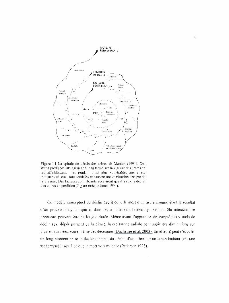
Figure 1.1 La spirale de déclin des arbres de Manion (1991). Des stress préd isposants agissent à long terme sur la vigueur des arbres en les affaiblissant, les rendant ainsi plus vulnérables aux stress incitants qui, eux, sont soudains et causent une diminution abrupte de la vigueur. Des facteurs contribuants accélèrent quant à eux le déclin des arbres en perdition (Figure tirée de Innes 1994) 5

Figure 1.1 Recent radial growth series and computed growth variables for live (black line) and dead (grey line) individuals. Lines with open symbols indicate the slope of the last ten years of growth for dead (0, 1986-1995) and 1ive (/1,. 1986-1995; 0, 1995-2004) trees, sol id symbols indicate the 5-yr median of 'recent growth'. Note the change in both median and slope when different time frames are used to compute the growth variables of the live tree 20

Figure 1.2 Average chronologies for live (black line) and dead (grey line) tree growth series (l950-end of series) and sample size of dead individllals (dotted line). Sample size of live tl'ees = 30 throughollt the pel'iod. Figure lettering corresponds to data set identification for the different data sets (A to E), see Table 1.1 and text for details 23

Figure 2.1 Median annual ring-width (a), sample sizes (b), and standard errors (SE) of means (c) from 1930 to 2003 for vigorous (R), growing (C), declining (S), moribllnd (M) and dead (D) adult sugar maple trees. Ring-widths were measured to 0.001 mm precision. Note the strong decline in sample size of dead trees due to mortality related drop-out. 58

Figure 2.2 Survival probabilities (a, b) and their standard errors (c) from 1970 to 2003. Panel a shows survival probabilities of vigorous (R), growing (C), declining (S), moribund (M), and dead (D) trees; panel b excludes dead trees. Asterisks (*) above the curves in (a) indicate the years of significant differences (P < 0.05, ANOVA) between de ad and live (ail vigour classes), in (b) asterisks indicate the years of significant differences (P <0.05) between vigollr classes based on Tukey's HSD tests for years with significant (P <0.05) annual ANOV As. Vigour classes that were significantly different from each other are listed in panel (b), with a dash separating significantly different groups 59

Figure 3.1 (a) Average ring-width (mm, lines) and sample size (tl'ees, symbols) chronologies (1910-2003) of undisturbed (by harvest) live (solid line) and dead (dotted line) trees. (b) Average grüwlh index chronologies (1910 - 2003) or undisturbed (by harvest) live (solid line) and dead (dotted line) sllgar maple trees. Arrows ind icate the year of the se lection harvest. 86

Figure 3.2 (a) Averaged ring-width indices (1910 - 2003) of und istllrbed (by harvest) sugar maple trees (n=134, same as in Fig. 3.lb) and rescaJed indices (RI) of yellow birch trees (n=20), a non-host species of the forest tent caterpillar. (b) Corrected ring-width indices of sugar maple trees obtained by subtracting RI in (a) from the host species (su gal' maple) indices in (a). Cress hatched areas in (b)

VUl

are periods of inferred (grey block arrows) or docllmented (black block arrows) FTC defol iations (see text for detai Is). The down faci ng arrow in (b) ind icates the year of the selection harvest... 87

Figure 3.3 Average surv ival probabilities of 1ive and dead sugar maple trees from 1960 - 2003. Table inset specifies years of significant differences (P <0.05) between pairs of disturbance classes and dead trees and among disturbance classes. Arrows indicate the most severe years of FTC olltbreaks (1974-1976, 1986-\992) and the partial harvest ([ 993). The horizontal! ine ind 'cates a critica! probabil ity threshold (P[Y= 1] =0.987) for a definite vigour dec 1ine (see text for deta ils) 91

Figure 3.4 Mean summer (April-August) monthly precipitation (solid line with stars) and temperature (dotted line with crosses) computed from climate data covering the years 1910-2003. Horizontal lines indicate the long-term mean precipitation and temperature across these years. The vertical line indicates the year of the partial harvest (1993) 92

Figure 4.1 Average ring-width indices (upper panel) and average Ol3C (lower panel) from 1983 - 2003 of the four disturbance classes. The horizontal lines indicate the pooled average of aIl 1983-2003 values. Note the negative impact of the forest tent caterpi Ilar (FTC) outbreak on ring-width ind ices of ail disturbance classes 120

Figure 4.2 Average rescaled ring-width indices (upper panel) and standard errors of rescaled ring-width indices (Iower panel) from 1983 - 2003 of the four disturbance classes. The horizontal 1ines ind icate the pooled average of ail rescaled pre-harvest (1983-\993) ring-width indices or standard errors. Note the negative impact of the forest tent caterpillar (FTC) olltbreak on standardized ring-width of al! disturbance classes 122

Figure 4.3 Average rescaled 013C (upper panel) and standard errors of Ol'C (Iower panel) from 1983 - 2003 of the four disturbance classes. The horizontal lines indicate pooled average (ail disturbance classes) of rescaled pre-harvest (1983­1993) 013C 123

Figure 4.4 Mean monthly summer (April-August) precipitation (sol id line with stars) and temperature (dotted line with crosses) computed from cl imate data covering the years 1910-2003. Horizontal lines indicate the Jong-term mean precipitation and temperature across these years. Vertical lines indicate the year of the beginning of the growth and 013C sampling period (1983) and the year of the partial harvest (1993) 124

Figure 4.5 Correlation (bars) and response function (lines) analysis of rescaled ring­width indices and climate data. Monthly precipitation (Ieft) and temperature (right) from prior (upper case) September ta current (Iower case) September (1'983-1994) were used to explain variance in rescaled ring-width indices of trees in the four disturbance classes. Sign ificant correlation and response function coefficients (P<0.05) are indicated with dark grey bars and white circles, respectively 125

Figure 4.6 Correlation (bars) and response function (Iines) analysis of rescaled Ol3C and climate data. Monthly precipitation (left) and temperature (right) from prior (upper case) September to current (lower case) September (1983-1994) were used to explain variance in rescaled D13C of trees in the four disturbance classes.

IX

Significant correlation and response function coefficients (P<O.OS) are indicated with dark grey bars and white circles, respectively 126

Figure 4.7 Penetration ratios (inch/blow) as an estimate of soil compaction, taken II years after harvest across skidding trails or on the undisturbed forest floor. Measurement points on skidding trails 1 and 5 were off-trail, points 2 and 4 on wheel tracks, and point 3 on the inter-wheel space. Points 1 through 5 on undisturbed forest floor were spaced at -1 m equidistance. Filled circles indicate significant differences (P<O.05, Wi1coxon rank sum test) between skidding trail and forest floor measurements at a given point. 130

Figure C.1 Modèle conceptuel du déclin des arbres de Manion (199]). Chaque ligne représente un arbre, la différence entre les niveaux de vigueur découle de l'impact d'un stress prédisposant sur celle-ci. Le stress incitant ne cause qu'un creux temporel de la vigueur dans l'arbre en 'santé' (ligne continue) mais déclenche un déclin vers la mort (e) dans l'arbre affaibli (ligne pointillée) par le stress prédisposant. Un stress contribuaf\!: agit sur la pente du déclin vers la mort (Figure adaptée de Pedersen 1998) 145

LISTE DES TABLEAUX

Page

Table 1.1 Growth series identification, location, growth pattern, tree size (D8H), last entire year of growth and range of year of death of the data sets used as modelling scenarios 24

Table 1.2 Most significant variables, selected variables, and associated internai predictive and discriminative measures (R/ and Dxy) of the 5 data sets used in the modell ing procedure based on truncated and untruncated live tree growth series. Parameter estimates are given in parentheses 30

Table 1.3 External validation: predictive and discriminative measures (R/ and Dxy) of untruncated (UT) and truncated (T) models developed on different training data sets when applied to the various test data sets 31

Table 2.1 Growth JeveJ, growth trend and growth sensitivity variables computed for different time windows used for logistic regression analysis of survjval probabilities. Shown are variable names and their respective number of observations, including live and dead measurements. Number of observations of dead measurements are constant across growth variables and equal the number of dead trees (n=56) 51

Table 2.2 Parameter estimates, bootstrapped 95% confidence intervals (CI), AIC, and optimism-corrected OXY of logistic mortality models. Models in bold are the 'best' univariate or bivariate models 55

Table 2.3 Sample sizes (n), mean values and standard errors (SE) of the predictor variables av3-log [ln(3-year average growth(flm/yr)+ J)] and slp5 [5-year regression slope (flm/yr)] of live trees in different vigour classes and dead trees ......... 56

Table 2.4 Number of trees per defect type and their respective percentage distribution within each vigour class 57

Table 3.1 Parameter estimates, bootstrapped 95% confidence intervals (Cr), Aue (ROC) and optimism-corrected OXY of the logistic survival probability mode!. 81

Table 3.2 Behrens-Fisher tests on relative effect estimates of ring-width ind ices (1990 - 2003) between disturbance classes using a non parametric simultaneous rank lest procedure. Only significant (P<O.OS) tests are shown 89

Table 3.3 Mean, standard error (SE) and range of averaged corrected indices du ring FTC outbreak (1986 - 1992) and harvest disturbances (J 994 - 1998). P values refer to a Wilcoxon signed-rank test between periods. Negative values are in parentheses 90

Table 4.1 Minimum, maximum and mean Iree diameter at breast heighl (dbh, mm) and tree height (m) and average tree density pel' species in the sample plots 110

Table 4.2 Mean diameter (mm), soil disturbance (%), light change ratio, height (m), and sample size (n) oftrees in the four disturbance classes. Values in parenthesis are minima and maxima. Light change ratios are light availability after harvest/before harvest; a value of one indicates no change in light availability 119

XI

Table 4.3 Annual permanova table for years with significant or marginally significant differences in rescaled ring-width indices and multi-comparisons among disturbance treatments with significant differences within these years using permutation tests based on 4999 resamples 127

Table 4.4 T-tests of differences between post-harvest - pre-harvest levels in rescaled ring-width indices and rescaled SJ)C within treatments 128

Table Al Complementary correlation (COR) and response function (RF) anaJysis of resca.led ring-width indices and c!imate data (see chapter 4, Figure 6) for the previous year (May to September). Bold values indicate significant (p< 0.05, 95% percentile range of the bootstrapped distribution) correlation coefficients or response function parameter estimates 156

RÉSUMÉ

Le modèle conceptuel de déclin des arbres de Manion (1991) stipule que des stress dits prédisposants, d'impact modéré et agissant à long terme (ex. pollution atmosphérique), diminuent la vigueur des arbres et les rendent plus vulnérables à des stress subséquents. Ces arbres ainsi affaiblis seraient par la suite davantage atfectés par des stress incitants, ces derniers ayant un impact plus prononcé et soudain (ex. défoliations d'insectes). Ceux-ci les entraîneraient alors dans une spirale de déclin vers la m011. La progression dans ce processus de déclin pouvant elle-même être accélérée par des facteurs contribuants tels les pathogènes fongiques.

La coupe de jardinage vise une amélioration de la qualité des peuplements par l'enlèvement progressif, sur plusieurs rotations, d'arbres de faible qualité et de faible vigueur, diminuant ainsi le taux de m0l1alité des peuplements résiduels. Récemment, l'observation d'un taux élevé de mortalité après coupe de jardinage dans la forêt publique québécoise a suscité inquiétudes et interrogations, nous incitant à entreprendre une étude afin d'identifier les causes potentielles et les processus précurseurs de la mortalité des arbres, afin de mieux comprendre ce phénomène.

Nous avons étudié près de 400 érables à sucre (Acer saccharum Marsh.) vivants et morts dans des érablières à bouleau jaune au Témiscamingue, Québec. Les peuplements sous étude avaient subi une coupe de jardinage en 1993-94 et tout en étant régulièrement soumis à des épidémies de la livrée des forêts (Malacosoma disstria Hubner).

Nous avons d'abord testé si le système de classification utilisé pour sélectionner les arbres pour la récolte pourrait être en cause dans les taux élevés de mOl1alité. Si le système en question ne permet pas de cibler adéquatement les arbres non vigoureux afin d'en prioriser la récolte, un mauvais choix d'arbres peut s'en suivre augmentant ainsi la proportion d'arbres non vigoureux dans le peuplement résiduel. Puisque de tels arbres sont plus susceptibles de mourir, le taux de mortalité augmenterait dans les peuplements résiduels. Nous avons comparé la probabilité de survie des arbres (évaluée à pal1ir de leur croissance radiale récente), comme indicateur de leur vigueur réelle, entre les quatre classes de vigueur du système de classification. Nos résultats indiquent que ce système reflète assez bien la vigueur réelle des arbres et ne semble donc pas être la cause d'un mauvais choix d'arbres ni de la mortalité élevée observée après coupe.

Par la suite, nous avons évalué l'impact des perturbations associées à la coupe sur les arbres résiduels en assumant que ces pel1urbations pourraient imposer des stress hydriques aux arbres résiduels par les mécanismes suivants: (1) la machinerie cause de la compact ion du sol et des dommages aux racines fines des arbres à proximité des sentiers de débardage ce qui pourrait engendrer, respectivement, une diminution de la disponibilité en eau dans le sol et une diminution de la capacité des arbres à puiser l'eau du sol; (2) l'ouverture de la canopée augmente la disponibiJ ité de lumière pour les arbres, ceux-ci répondant avec un accroissement du taux photosynthétique et de transpiration ce qui intensifierait la demande en eau. Nous avons comparé les croissances radiales, les probabilités de survie et le ratio d'isotope stable de carbone (\J C/ 12C) entre des arbres appal1enant à quatre classes de

XIII

perturbation: (1) aucune perturbation, (2) perturbation de machinerie seu lement, (3) augmentation de lumière seulement et (4) perturbation de machinerie et augmentation de lumière. Nos résultats montrent que les perturbations de la coupe n'ont pas eu d'impact négatif sur la croissance, la vigueur ou l'état hydrique des arbres résiduels. Au contraire, L1ne augmentation de lumière engendrait une hausse de la croissance. La comparaison des croissances radiales entre une période de défoliation et la période suivant la coupe de jardinage démontrait que la croissance radiale était beaucoup plus faible lors de la défoliation que lors de la période suivant la coupe et ceci pour n'importe quelle combinaison de perturbations associées à la coupe.

Nous avons de plus utilisé les croissances radiales d'érables à sucre morts pour caractériser la dynamique de leur déclin. Ces arbres ont été prédisposés par une première défoliation qui les a rendu plus vulnérable à une deuxième défoliation. Une perte de vigueur importante lors de la deuxième défoliation a déclenché leur déclin final, celui-ci ayant été accéléré lors de la période après coupe. Le déclin des érables sous étude a perduré pour environ 30 ans et s'est déroulé selon le modèle de Manion (1991) : la première défol iation étant le stress prédisposant, la deuxième le stress incitant et les perturbations associées à la coupe agissant comme stress contribuants.

L'ensemble de nos résultats nous permet de conclure que les perturbations associées à la coupe de jardinage ne semblent pas expliquer le taux élevé de mortalité dans le contexte de notre étude. Toutefois, les cond itions c li matiques estivales favorables (températures douces, précipitations abondantes) qui ont prévalu dans les premières années après les coupes de jardinage de 1993-94 pourraient avoir empêché le développement d'un stress hydrique et ainsi avoir atténué l'impact sur les arbres résiduels des perturbations associées à la coupe.

Notre étude apporte des contributions importantes à notre compréhension de la mortalité chez les arbres. Ainsi, nous avons identifié la nature du stress prédisposant dans le déclin d'érables à sucre dans des peuplements jard inés, un aspect souvent négl igé dans les études de la mortalité des arbres. De plus, notre étude a permis de démontrer que Je rôle d'un stress ne dépend pas de la nature du vecteur (ex. pollution atmosphérique, insectes défoliateurs) mais plutôt de l'impact que ce stress exerce sur la vigueur de l'arbre. Au niveau méthodologique, notre étude a contribué à améliorer les estimations de probabilités de mortalité (chapitre I)et à tester une méthode simple et efficiente d'estimation de conditions de croissance (disponibilité de lumière, chapitre 3) pour des études rétrospectives.

Notre étude soulève aussi certaines questions. Par exemple, on peut se demander quel serait l'impact des perturbation's associées à la coupe sur les arbres résiduels sous des conditions climatiques moins favorables que celles ayant prévalu dans notre étude (ex. étés chauds et secs dans les années suivant la coupe)? Ou sur des sites ayant des sols différents? Pourquoi les défoliations de la livrée n'ont pas eu le même impact sur tous les arbres, causant seulement un déclin temporaire chez certains arbres mais un déclin sévère menant à la mort chez d'autres individus? Est-ce que les arbres survivants ont pu mieux se défendre contre ou encore éviter complètement les défoliations? Ces questions devraient faire l'objet d'études supplémentaires afin d'approfondir notre compréhension de la mortalité des arbres.

Mots-clés: Acer saccharum Marsh., mortalité, stress, vigueur, probabil ité de survie

XIV

Except during the nine months beJore he draws his first breath, no man manages his affairs as weil as a tree does.

George Bernard Shaw

Ofal! the wonders ofnature, a tree in summer is perhaps the most remarkable; with the possible exception ofa moose singing "Embraceable You" in spats.

Woody Allen

fNTRODUCTION GÉNÉRALE

A. Préambule

Cette étude a été effectuée dans des érablières à bouleau Jaune au Témiscaminguc

(Québec). Ces peuplements sont soumis à des défoliations par la livrée des forêts

(Malacosoma disstria Hubner) à des intervalles régu liers et ont, de plus, subi une coupe de

jardinage en 1993/1994. Notre étude vise à mieux comprendre le phénomène de la mortalité

chez les arbres par l'identification des facteurs qui sont impliqués dans le processus de la

mortalité de l'érable à sucre et la caractérisation de leur mode d'action en interaction.

Comme nous le verrons dans les sections suivantes, les perturbations en forêt constituent

des vecteurs de stress qui agissent sur la santé des arbres. La coupe de jardinage, un type de

coupe partielle, provoque plusieurs modifications à l'environnement qui peuvent constituer

des facteurs potentiels de stress pour les arbres résiduels. En premier lieu, la coupe augmente,

par l'ouverture de la ca nopée, la disponibilité en lumière pour les arbres dégagés. Cette

augmentation peut entraîner, pour certains arbres, une hausse soudaine et importante de la

demande en eau dû à un accroissement marqué de la transpiration. Ceci pourrait donc

perturber l'équilibre établi entre la biomasse foliaire et racinaire et engendrer un stress

hydrique. De plus, l'utilisation de la machinerie forestière lors des opérations de récolte cause

des perturbations du sol (ex. compaction) et des dommages aux systèmes racinaires des

arbres ce qui peut réduire la disponibilité en eau dans le sol et la capacité d'absorption d'eau

des arbres. Finalement, les perturbations naturelles, notamment les épisodes de défoliation

par la livrée des forêts, peuvent être sources de stress importants pour les arbres en réduisant

significativement et de façon récurrente leur biomasse foliaire et donc, par le fait même, leur

potentiel photosynthétique, ce qui se traduit le plus souvent par une diminution notable de la

croissance radiale.

Notre étude examine l'impact des perturbations soit naturelles ou humaines (par la

coupe) sur la santé des arbres. En utilisant une approche rétrospective et en s'appuyant sur

des données dendrochronologiques, cette étude nous a permis de caractériser la dynamique

2

entre ces facteurs de stress et d'obtenir un aperçu de l'effet cumulatif des divers stress sur la

santé des arbres à l'étude.

Dans cette introduction nous allons revoir le concept de maladie et de déclin des arbres,

ce qui sera suivi par un bref aperçu des mesures utilisées pour quantifier la vigueur des

arbres. Nous allons aussi définir la problématique sous-jacente à notre étude en la plaçant

dans son contexte théorique et pratique. Par la suite, les objectifs généraux et spécifiques de

l'étude, sa structure et l'approche méthodologique seront présentés.

B. La maladie et le déclin des arbres

Les arbres sont des organismes exceptionnels. Ils atteignent des tailles impressionnantes,

dépassant largement toute autre forme de vie, et peuvent vivre plus longtemps que tout autre

type d'organisme. L'arbre vivant le plus âgé, un pin de Bristlecone (Pinus longaeva [O.K.

BaileyJ), a été daté à 4723 ans en 1957 (Schulman 1958). De plus, par le biais de la

reproduction végétative, certaines espèces d'arbre peuvent éviter la mort de l'individu (défini

par son assemblage génétique) apparemment indéfiniment. Par exemple, le peuplier faux­

tremble (Populus tremuloides [Michx.J) peut former des colonies clonales (ramets) de grande

superficie et de grand âge. Le ramet 'Pando' de cette espèce, situé dans l'état de l'Utah (E.­

U.), compte plus de 47000 tiges (ortets) sur plus de 77 hectares et son âge a été estimé à plus

d'un million d'années (Mitton & Grant 1996).

Mais mêmes les arbres les plus longévifs ne vivent pas éternellement. Quoique le concept

de sénescence ne semble pas s'appliquer à certaines espèces d'arbres comme le pin de

Bristlecone (Lanner et Connor 2001) ou le Thuja occidentalis (L.) (Larson 2001), des

évènements catastrophiques tels des feux de forêt, des épidémies d'insectes ou encore des

chablis peuvent affecter de grandes étendues de forêt et causer la mortalité à grande échelle

(ex. Solomon et al. 2003, Bouchard et al. 2005, Peterson & Pickett 1995). De plus, les arbres

individuels peuvent être soumis à des stress externes qui détériorent leur état de santé,

causent des maladies et mènent à leur mort. La maladie, au sens large, constitue une

cond ition anormale de l'organisme qui perturbe son fonctionnement.

3

Quoique des pathogènes soient souvent des vecteurs de malad ie, c'est une interaction de

plusieurs facteurs qui mène à la maladie et à la mort d'un arbre et ces divers facteurs ne

peuvent pas être facilement séparés les uns des autres (Franklin et al. 1987). Souvent la cause

ultime de la mort d'un arbre, un déséquilibre entre le gain et les dépenses de produits

photosynthétiques, peut être initialement déclenchée par une défoliation d'insectes (export de

carbone par l'enlèvement de l'appareil photosynthétiq ue) mais par la suite résulter d'un

affaiblissement (ex. épuisement de réserves de carbone) de l'arbre à long terme (Franklin et

al. 1987). Ainsi, le déclin des arbres est un processus complexe et graduel qui comprend

plusieurs facteurs et vecteurs de stress (Waring 1987).

Manion (1991) a décrit le développement d'une maladie chez un arbre comme résultant

d'une relation triangulaire entre l'hôte (arbre), les pathogènes et l'environnement.

L'environnement et les pathogènes exercent des stress sur l'hôte, ce qui a pour conséquence

de réduire sa vigueur. Une fois affaibli, l'hôte devient plus vulnérable à d'autres stress qui

l' affaibl issent davantage et qui peuven t l'entraîner dans une spira le de déci in irréversible.

Le concept de vigueur est quelque peu ambigu et souvent utilisé comme synonyme au

concept de vitalité (voir Dobbertin 2005). Selon Shigo (1986), la vitalité d'un arbre est son

état de santé à un moment donné, découlant d'une interaction dynamique entre l'arbre et son

environnement, notamment les stress, tandis que la vigueur d'un arbre est sa capacité

génétique à survivre à de tels stress. Cette définition de vigueur est théorique et difficile,

voire impossible à quantifier. Manion (1991) utilise le terme vigueur avec la signification de

vitalité et cette utilisation du terme a été reprise par d'autres auteurs (ex. Kaufmann 1996,

Pedersen 1998). Dans notre étude, nous adoptons la définition de vigueur de Manion (1991)

afin de quantifier, à tout moment dans la vie d'un arbre, son état de santé comme une réponse

à des stress environnementaux.

Selon le modèle conceptuel du déclin des arbres de Manion (1991), des stress

prédisposants, ayant un impact modéré et agissant à long terme, diminuent la vigueur

initiale des arbres. Par exemple, la pollution atmosphérique près de centres industriels a des

effets toxiques sur les processus physiologiques végétaux et réduit le taux de croissance des

arbres (Ashby & Fritts 1972, Pandey & Pandey 1994, Bressan 1998). Une réduction de

croissance est généralement associée à une baisse de la mise en réserve de carbone sous

4

forme d'amidon. Chez les arbres, la mise en réserve d'amidon constitue une priorité

d'allocation moins élevée que la croissance (Oliver & Larson 1996) et on suppose que seul le

carbone non utilisé pour la croissance est disponible pour la mise en réserve (Le Roux et al.

2001). Ainsi, le déclin de la vigueur des arbres est généralement relié à un épuisement des

réserves de carbone (Liu & Tyree 1997). Suite à une telle réduction des réserves de carbone,

les arbres ne peuvent produire suffisamment de composés de défense contre des herbivores

(Dunn et al. 1987) ou refaire le feuillage consommé par des herbivores (Renaud & Mauffette

1991 ).

Les arbres ainsi affaiblis sont plus vulnérables aux stress subséquents tels des épidémies

d'insectes défoliateurs. Des défoliations répétées diminuent continuellement les réserves de

carbone (Parker & Houston 1971, Gregory & Wargo 1986, Renaud & Mauffette 1991),

permettant aux stress contribuants, tels les champignons, de vaincre les mécanismes de

défense de l'hôte, accélérant ainsi son déclin (Wargo & Houston 1974) et l'entraînant dans

une spirale vers la mort (Fig. 1.1).

- ----

5

FACTEURS PREDISPDSANTS

(lf:.IIJlJf:t"'T).:':1 FACTEURS

) INCITANTS 1 -'

;' V/ FACTEURS ,." CONTRIBUANTS." ,,,.,,,'"

.--,. d,'l,.,.,-'

) <,

,..... .--- -­1 l'llh~rr~la 'li- L:l1

/ /r' 1'~1'1.,IUlJl~ \ , '. Ct"-Yl:1"'11l'H \ ,1I1."":l;n: 1 1\111",11;" (1 •. " - 'Jill'. \

, ... l, 1 ....... · \

, _MORT ." , !',""""" 1

\ 'i" '~', .~b1r:tw'~I1· : ... \ ~T:.j l, ,., 1

',"':'V"l;F. - ' P:mr:l!:~' / ,W·r,l.

/....· ...·------·--z-··..

r;;,) ,~ 1.1H.' ç:HJ:Ii:~l!

I~: H'J"1~:(;1I t:ll edlJ

'---- ..... ' Sel

Figure I.l La spirale de déclin des arbres de Manion (1991), Des stress prédisposants agissent à long terme sur la vigueur des arbres en les affaiblissant, les rendant ainsi plus vulnérables aux stress incitants qui, eux, sont soudains et causent une diminution abrupte de la vigueur, Des facteurs contribuants accélèrent quant à eux le déclin des arbres en perdition (Figure tirée de Innes 1994),

Ce modèle conceptuel du déclin décrit donc la mort d'un arbre comme étant le résultat

d'un processus dynamique et dans lequel plusieurs facteurs jouent un rôle interactif, ce

processus pouvant être de longue durée. Même avant l'apparition de symptômes visuels de

déclin (ex. dépérissement de la cime), la croissance radiale peut subir des diminutions sur

plusieurs années, voire même des décennies (Duchesne et ai. 2003). En effet, il peut s'écouler

un long moment entre le déclenchement du déclin d'un arbre par un stress incitant (ex, une

sécheresse) jusqu'à ce que la mort ne survienne (Pedersen 1998),

6

C. Comment quantifier la vigueur des arbres?

Il existe une panoplie de mesures pour quantifier l'état de santé d'un arbre, comme par

exemple la taille des aiguilles, l'émission de luminescence ou de composés gazeux par les

feuilles, ou la résistance électrique du cambium (voir Gehrig 2004). Toutefois, ces mesures

sont coüteuses, difficiles à effectuer sm le teïïain et ne décrivent que l'état actuel d'un arbre,

ne se prêtant donc pas aux études rétrospectives.

Les cernes de croissance offrent, par contre, une source de données à résolution annuelle

et peuvent donc fournir de manière retrospective des informations au sujet des conditions

environnementales qui prévalaient et de ['état physiologique des arbres au moment de la

formation du cerne (Saurer et al. 1997, McCarro Il & Loader 2004).

La quantité de réserves de carbone contenues dans le tronc (cernes) ou les racines semble

corrélée à la vigueur des arbres (Wargo 1999), mais les réserves de carbone sont difficiles à

quantifier et relativement peu utilisées dans les études sur le déclin et la mortalité des arbres.

Par contre, les cernes de croissance des arbres constituent une information sensible de la

vigueur des arbres car la priorité d'allocation de carbone aux cernes du tronc est inférieure à

la priorité d'allocation aux autres fonctions vitales telles la respiration, la croissance des

racines fines, la reproduction et la croissance primaire (en élongation) (Waring 1987, Oliver

& Larson 1996). Ainsi, la croissance secondaire (radiale) est habituellement l'une des

premières fonctions affectées par une diminution du budget de carbone de l'arbre (Givnish

1988) et elle constitue donc un indicateur précoce d'une perte de vigueur globale de l'arbre.

Il est reconnu qu'il existe un lien entre la croissance radiale et le risque de mortalité des

arbres (Wyckoff & Clark 2000). Ce lien a aussi été utilisé pour estimer des probabilités de

mortalité (Monserud 1976) et a été intégré dans des modèles de simulation forestière (ex.

Botkin 1993, Pacala & Hurtt 1993, Pacala et al. 1993 & 1996, Loehle & LeBlanc 1996). De

plus, piusieurs études ont évalué à j'aide de cernes de croissance l'impact de stress

environnementaux sur les arbres (ex. Pedersen 1998& 1999, Ogle et al. 2000, Suarez et al.

2004) et l'estimation de probabilités longitudinales l de mortalité a été utilisée pour prédire

1 Une étude longitudinale mesure une caractéristique chez un individu (ou un groupe d'individus) à différents moments dans le temps. Ainsi, l'étude longitudinale de séries de croissances radiales permet d'estimer des probabilités de survie à différents moments de la vie d'un arbre contrairement aux études

7

l'incidence de la mort des arbres (Bigler & Bugmann 2004). Dans le cadre de la présente

étude, nous utilisons la croissance radiale dans le but d'estimer la probabilité longitudinale de

survie des arbres afin de quantifier leur vigueur.

D. Contexte de j'étude

Cette étude vise à améliorer la compréhension du phénomène de la mortalité des arbres

suite à la coupe partielle (coupe de jardinage). La coupe de jardinage, appliquée en Europe

depuis plus de deux siècles (Rohrig & Gussone 1990), a été introduite graduellement au

Québec au début des années 1990 (mais en 1983 dans un contexte expérimental) dans le but

de pallier les effets dégradants de la coupe à diamètre limite sur la qualité et la vigueur des

peuplements feuillus et mixtes (Majcen et al. 1990). Ce type de coupe, effectuée dans des

peuplements de structure inéquienne, réunit les caractéristiques de plusieurs traitements

sylvico les (cou pe de régénération, éclaircie, réco Ite) dans une seule intervention (Smith et al.

1(96). La coupe de jardinage a pour objectif, en outre, l'amélioration de la qualité du

peuplement résiduel en récoltant des arbres de moindre vigueur et elle vise également à

diminuer les 'pertes' dues à la mortalité et donc le taux de mortalité avant la prochaine

intervention.

Le rendement de la coupe de jardinage, en terme de croissance et de taux de mortalité, a

été établi à partir de données récoltées dans des dispositifs de recherche gouvernementaux.

Toutefois, puisque les coupes effectuées dans ces dispositifs l'ont été avec plus de soins que

lors d'opérations forestières industrielles normales, une extrapolation de leurs résultats à des

forêts sous aménagement industriel ne semble pas valide (Majcen 1996). Un dispositif de

suivi a été installé pour vérifier le rendement réel de la coupe de jardinage dans un contexte

industriel et les résultats de ce suivi ont révélé que le rendement cinq ans après la coupe

(accroissement annuel périodique net) n'atteignait que 40% des prédictions basées sur les

données des dispositifs expérimentaux. Ce faible accroissement serait dû à un taux de

transversales qui sont ponctuelles et produisent des estimations seulement pour un instant donné de la vie d'un arbre.

8

mortalité deux fois plus élevé que dans les dispositifs de recherche (Bédard et Brassard

2002).

E. Causes potentielles des forts taux de mortatlié enregistrés

a. Mauvais choix d'arbres pour la récolte

Il a été suggéré que les normes de sélection des arbres à récolter lors de la coupe de

jardinage déterminant le choix des arbres à récolter pourraient être trop vagues ou ne pas être

basées sur des critères adéquats, permettant ainsi aux aménagistes de récolter des arbres

vigoureux en laissant une proportion importante d'arbres non vigoureux dans les

peuplements (Meunier et al. 2002). Évidemment, ces arbres résiduels peu vigoureux seraient

alors plus susceptibles de mourir, ce qui pourrait expliquer le taux élevé de mortalité

enregistré après jardinage. Bien que semblant intuitivement justifiée, cette explication est

difficile, voire impossible à vérifier rétrospectivement et n'apporte pas d'éléments à la

compréhension des mécanismes de mortalité. Toutefois, afin d'exclure le mauvais choix de

tiges comme explication des forts taux de mortalité, nous allons vérifier si le système de

classification des arbres actuellement en usage permet réellement de choisir des arbres à

récolter selon leur vigueur.

b. Les perturbations d'arbres résiduels par la coupe partielle

La coupe partielle modifie l'environnement des arbres résiduels et ceux-ci peuvent être

perturbés par ces modifications soudaines des conditions environnementales. Les

modifications des cond itions environnementales résu Itant de coupes partielles sont de

plusieurs types et incluent notamment les perturbations du sol par la machinerie et l'ouverture

soudaine de la voûte forestière:

• Perturbations par la mach inerie forestière

La machinerie forestière exerce, selon sa masse opérationnelle, le type et les dimensions

du système de traction, des pressions importantes sur le sol (Deschênes 1989) auxquelles

s'ajoutent des forces de cisaillement et de vibration (Gjedtjernet 1995, Kozloswki 1999). Ces

9

forces causent une réduction de la porosité du sol, augmentant ainsi sa densité, détruisent la

structure du sol en diminuant sa conductivité hydrique (voir revue dans Kozlowski 1999 et

Lipiec & Hatano 2003) et peuvent mener à une capacité réduite de rétention d'eau dans les

sols à texture fine (Souch et al. 2004). Quoique la sévérité de l'impact de ces forces varie

selon les caractéristiques du sol (Assouline et al. 1997), elles réduisent généralement

l'infiltration d'eau, le drainage et J'aération du sol (Taylor & Brar 1991, Herbauts et al. 1996,

Starsev & McNabb 2001) et résultent, dû à une résistance à la pénétration plus élevée, en la

formation de systèmes racinaires réduits et superficiels (Wronski 1984) menant à une

absorption réduite d'eau au niveau de la plante (Lipiec & Hatano 2003). L'impact négatif sur

le sol se produit en grande partie après un seul passage (Williamson & Neilsen 2000) et peut

causer des stress hydriq ues et une réduction de croissance chez les arbres (Helms &Hipkin

1986, Clayton et al. 1987, Smith & Wass 1994, Tardieu 1994, Souch et al. 2004). De plus, la

compaction du sol, en réduisant la capacité d'absorption de l'eau par les racines fines, réduit

la capacité de transpiration des arbres (Komatsu et al. 2007) ce qui peut entraîner une

diminution de la photosynthèse et éventuellement de la croissance des arbres (Law et al.

2002).

Puisque les études sur les systèmes racmalres étant fastidieuses et coûteuses, les

connaissances demeurent limitées concernant les impacts directs (dommages mécaniques) de

l'équipement forestier sur les racines (ex. Rbnnberg 2000) ou leur impact sur la croissance

globale des arbres (Waesterlund 1989, Gjedtjernet 1995), mis à part quelques évidences

indirectes et anecdotiques (ex. Wronski 1984, voir aussi revue dans Trame & Harper 1997).

Lagegren & Lindroth (2004) ont démontré que des arbres situés à proximité de sentiers de

débardage avaient des accroissements en surface terrière moins élevés que les arbres ailleurs

dans un peuplement de Pinus sy/vestris (L.) et Picea abies (L.[Karst]) mais sans établir la

relation entre la distance au sentier et la croissance des arbres. Ouimet et al. (2005) ont quant

à eux trouvé une relation significative entre la distance des arbres par rapport à des tranchées

d'excavation (pour l'enfouissement de tubulures de transport de sève d'érable) et la

croissance radiale de J'érable à sucre quand cette distance était inférieure à un seuil critique

(:S 6 cm pour chaque cm de diamètre à la hauteur de poitrine, Ouimet et al. 2005).

10

L'impact des dommages racinaires sur la santé des arbres a été évalué surtout sur des

plants d'arbres. Par exemple, Deans et al. (1990) et McKay & Milner (2000) ont démontré

que des dommages racinaires causés par une manutention indél icate (ex. échappement sur le

sol) de plants peut ralentir leur développement ou même entraîner leur mort (Kauppi 1984,

McKay et al. 1993). En forêt, les forces mécaniques dans le sol par mouvement de masse lors

d'un gel ont été tenues responsables pour des dommages et la mortalité de racines fines

(Tierney et al. 2001).

Nadezhdina et al. (2006) ont démontré que le passage de la machinerie lourde à

proximité des arbres diminue la conductivité hydrique et endommage le système racinaire.

Quoique la régénération des racines fines soit un processus assez rapide dans des sols non

perturbés (Hendrick et Pregitzer 1992), la compaction du sol par la machinerie peut nuire à

cette régénération en limitant le taux de croissance racinaire (Lipiec & Hatano 2003)

entraînant ainsi une contrainte persistante à l'absorption d'eau.

• Ouverture soudaine de la voûte forestière

L'éclaircie d'un peuplement forestier réduit la densité des arbres dans le but de

concentrer les ressources (eau, lumière, minéraux, espace) sur un nombre réduit d'arbres

résiduels (Smith et al. 1996). Bien que l'augmentation de la disponibilité en lumière puisse

être bénéfique aux arbres résiduels, le fait que cette augmentation soit forte et soudaine peut

perturber l'équilibre entre les racines et le feuillage (Kneeshaw et al. 2002) et avoir des effets

sur l'efficacité d 'uti lisation ,de l'eau (Warren et al. 2001). Des semis sous la canopée,

acclimatés à une faible luminosité, réagissent à une augmentation de la radiation avec un taux

plus élevé de photosynthèse après une brève période d'inhibition (Lovelock et al. 1994,

Krause et al. 2003) et une augmentation du taux photosynthétique a été également constatée

pour des érables à sucre matures à proximité de trouées d'éclaircie (Jones et Thomas 2007).

Toute augmentation du taux photosynthétique nécessite forcément une augmentation de la

conductance stomataJe afin de faciliter la diffusion de COz dans les feuilles. Ceci entraîne

également une augmentation de la transpiration et des besoins en eau de j'arbre (Bréda et al.

1995). Évidemment, si l'augmentation de la demande en eau est jumelée à une réduction de

l'absorption d'eau, par l'intermédiaire de la compact ion et/ou des dommages aux racines

Il

fines, les arbres affectés pourraient éprouver un déséqui 1ibre entre demande et

approvisionnement en eau et subir un stress hydrique.

c. Les perturbations naturelles: défoliations par la livrée des forêts

Pour la région et l'espèce sous étude, une des perturbations naturelles importantes est due

aux défoliations par la livrée des forêts. Ces épisodes de défoliation surviennent selon un

cycle d'environ 9 ans et plus (MRNFPQ 2002). L'érable à sucre est l'essence-hôte préférée

parmi les espèces présentes dans les peuplements sous étude (Fitzgerald 1995).

Les œufs de la livrée éclosent tôt au printemps au moment de j'ouverture des bourgeons

et les larves commencent immédiatement à consommer les jeunes feuilles. Habituellement,

l'impact d'une défoliation sur un arbre vigoureux est peu menaçante pour la survie de l'arbre

mais des défoliations répétées sur plusieurs années peuvent réduire la croissance radiale des

arbres affectés et même causer la mort de branches et de rameaux (CfS 2001). Les arbres

défoliés rétablissent habituellement leurs cimes au cours de l'été mais ceci cause un

épuisement des réserves de carbone (Wargo et al. 1972, Wargo 1981) ce qui entraîne des

réductions de la croissance radiale (Gross 1991) et rend les arbres affectés plus vulnérables à

des stress subséquents (Renaud & Mauffette 1991).

F. Les mécanismes anticipés

En résumé, les perturbations du sol par la machinerie lors des opérations de récolte sont

susceptibles de causer une diminution de la disponibilité en eau dans le sol et d'engendrer

une contrainte à l'absorption de l'eau par les racines. D'autre part, l'ouverture de la canopée

est susceptible de causer une augmentation de la transpiration et donc un accroissement du

besoin en eau des arbres. Les impacts de ces deux perturbations sont potentiellement additifs

et sont susceptibles de causer des déficits hydriques chez les arbres affectés. NOliS avons donc

avancé l'hypothèse que ces perturbations pourraient, surtout quand elles sont jumelées,

causer des stress hydriques assez sévères pour déclencher un décI in et potentiellement la mort

des arbres affectés.

12

N'oublions pas qu'à ces perturbations s'ajoutent les impacts des défoliations de la livrée.

Selon Je modèle de Manion (1991), les défoliations pourraient, selon leur sévérité, agir

comme facteur de stress dans le déclin des arbres. Alors, la réponse des arbres aux

perturbations de la coupe devrait être plus négative s'ils ont été affectés par une défoliation

peu de temps auparavant, durant ou après la coupe. Puisque les défoliations diminuent la

quantité de réserves de carbone, les arbres défoliés devraient être moins en mesure de contrer

les impacts des perturbations associées à la coupe, par exemple pour rétablir et/ou augmenter

leur réseau de racines fines afin d'assurer un approvisionnement en eau suffisant.

G. Objectifs généraux de la thèse

Cette thèse vise deux principaux objectifs. Le premier est d'identifier les causes

potentielles du taux de mortalité élevé observé dans des peuplements dominés par l'érable à

sucre et suite à des coupes de jardinage. Le deuxième est de décrire les interactions entre les

perturbations associées à la coupe, les perturbations naturelles et la vigueur des arbres et ce

afin d'acquérir une meilleure compréhension des mécanismes et processus de la mortalité des

arbres.

H. Objectifs spécifiques de la thèse

• Développer et tester la performance d'une méthode de traitement de données

dendrochronologiques permettant de tenir compte de l'influence des conditions

environnementales sur les estimations de la probabilité de mortalité comme mesure

de vigueur.

• Vérifier la concordance entre la vigueur établ ie à partir d'un système de classi fication

de la vigueur basé sur des défaults externes des arbres et la vigueur 'réelle' de

l'érable à sucre établie à partir de probabilités de survie longitudinales basées sur des

données dendrochronologiques.

• Évaluer et comparer l'impact des perturbations associées à la coupe de jardinage à

l'impact d'épisodes de défoliation par la livrée des forêts sur la croissance radiale et

13

la vIgueur de l'érable à sucre, et évaluer l'interaction entre ces deux sources

potentielles de stress.

• Vérifier si les perturbations asso'ciées à la coupe de jardinage (perturbations du sol,

augmentation de la disponibilité de lumière) causent un stress hydrique chez les

arbres résiduels.

1. Approche méthodologique et structure de la thèse

La thèse comporte quatre chapitres. Afin de tenir compte des délais qui peuvent s'écouler

entre l'incidence d'un stress et la réaction de l'arbre, nOLIs avons choisi d'entreprendre l'étude

dans des peuplements ayant subi une coupe de jardinage Il ans avant J'échantillonnage,

assumant que les impacts de la coupe sur l'état de santé des arbres devraient se manifester au

cours de cette période.

Le premier chapitre est de nature méthodologique et a été élaboré afin de répondre à

une lacune observée dans plusieurs études visant à estimer la probabilité de mortalité des

arbres à partir de leur croissance récente. Ce premier chapitre présente et teste une

méthodologie de traitement de données dendrochronologiques pour l'estimation de

probabilités de mortalité par régression logistique. Cette méthodologie vise à éliminer

l'impact potentiel des conditions environnementales sur les estimations de probabilité de

mortalité les rendant ainsi plus robustes pour des applications générales (ex. modélisation).

Le chapitre deux vise à déterminer si la vigueur établie à partir de défaults externes des

arbres corrrespond à la vigueur estimée à partir de données dendrochronologiques. Ainsi, ce

chapitre vise à tester le système de classification des arbres utilisé pour la sélection des arbres

à récolter. Ce système a été introduit par le Ministère des Ressources naturelles et de la faune

du Québec (Boulet et al. 2005) et vise à estimer la vigueur et l'espérance de survie des arbres

dans le but de sélectionner pour la récolte les arbres moins vigoureux et avec un plus grand

risque de mortalité. Dans ce chapitre, nous testons si les classes de vigueur du système de

classification reflètent la vigueur réelle des arbres telle qu'exprimée par les probabi lités

longitudinales de survie. Ce chapitre nous permet donc de vérifier si le système de

classification pourrait permettre un mauvais choix des arbres pour la récolte.

14

Au chapitre tl"Ois, nous vérifions si certaines perturbations associées à la coupe (i.e., la

circulation de la machinerie à proximité des arbres et l'augmentation forte et soudaine de la

disponibilité de lumière) affectent la croissance et la vigueur des arbres. Par un design

expérimental factoriel, nous évaluons séparément l'impact de l'une ou l'autre des

perturbations ainsi que l'impact de la combinaison des deux perturbations sur la croissance et

la vigueur des arbres. De plus, nous comparons l'impact des perturbations associées à la

coupe avec l'impact des perturbations naturelles (défoliations) sur la croissance et la vigueur

des arbres et nous caractérisons la dynam ique temporelle des interactions entre les diverses

perturbations. En utilisant à la fois les données d'arbres vivants et morts, nous serons en

mesure de décrire le déroulement temporel du déclin des arbres. Ce chapitre nous permettra

donc d'identifier les facteurs de stress agissant sur l'état de santé des arbres ainsi que de

vérifier si le déclin des arbres se déroule selon le modèle conceptuel de Manion (1991).

Le chapitre quatre présente une étude dans laquelle nous avons eu recours à l'analyse

d'isotopes stables de carbone dans les cernes de croissance afin de vérifier si les traitements

de coupe ont causé un stress hydrique chez les arbres résiduels. En ayant recours à un design

expérimental factoriel, nous testons pour la présence d'un stress hydrique pour chaque

perturbation de coupe individuellement et pour la combinaison des deux perturbations.

1. IMPROVING TREE MORTALITY MODELS BY ACCOUNTING FOR

ENVIRONMENTAL INFLUENCES

Hemik Hartmann, Christian Messier & Marilou Beaudet

Article publié dans la Revue canadienne de recherche forestière 37 : 2106-2114.

16

1.1 Abstract

Tree-ring chronologies have been widely used in studies oftree mortality where variables of recent growth act as an indicator of tree physiological vigour. Comparing recent rad ial growth of live and dead trees thus allows estimating probabilities of tree mortality. Sampling of mature dead trees usuaHy provides death-year distributions that may span over years or decades. Recent grovvth of dead trees (prior to death) is then computed during a numbcr of periods, whereas recent growth (prior to sampling) for live trees is computed for identical periods. Because recent growth of live and dead trees is then computed for different periods, external factors such as disturbance or climate may influence growth rates and, th us, mortality probability estimations. To counteract this problem, we propose the truncating of live-growth series to obtain similar frequency distributions of the "Iast year of growth" for the populations of live and dead trees.

In this paper, we use different growth scenarios from several tree species, from several geographic sources, and from trees with different growth patterns to evaluate the impact of truncating on predictor variables anà their selection in logistic regression analysis. Also, we assess the ability of the resulting models to accurately predict the status of trees through internai and external validation.

Our results suggest that the truncating of live-growth series helps decrease the influence of external factors on growth comparisons. By doing so, it reinforces the growth-vigour 1ink of the mortality model and enhances the model 's accuracy as weil as its general applicability. Hence, if mode! parameters are to be integrated in simulation models of greater geographical extent, truncating may be used to increase mode! robustness.

17

1.2 Résumé

La dendrochronologie été largement utilisée dans les études portant sur la mortalité des arbres où des variables de croissance récente sont uti 1isées comme ind icateur de la vigueur physiologique des arbres. La comparaison de la croissance radiale récente d'arbres vivants et morts permet donc d'estimer la probabilité de mortalité des arbres. L'échantillonnage d'arbres matures morts fournit généralement la distribution des années de mortalité qui peuvent s'étendre sur pl usieurs années ou décennies. La croissance récente des arbres morts (avant leur mort) est ensuite calculée pour un certain nombre de périodes alors que celle des arbres vivants (avant leur échantillonnage) est calculée pour des périodes identiques. Puisque la croissance récente des arbres vivants et morts est ensuite calculée pour des périodes différentes, des facteurs externes tels les perturbations ou le climat peuvent influencer le taux de croissance et, par conséquent, l'estimation de la probabilité de mortalité. Pour résoudre ce problème, nous proposons de tronquer les séries de croissance des arbres vivants de façon à obtenir des distributions de fréquence similaires de « la dernière année de croissance» pour les populations d'arbres vivants et morts.

Dans cette étude, nOliS utilisons différents scénarios de croissance à partir de plusieurs espèces d'arbre et de plusieurs origines géographiques ainsi que différents patrons de croissance pour évaluer l'impact des séries tronquées sur les variables de prédiction et sur leur sélection dans les analyses de régression logistique. De plus, nous évaluons la capacité des modèles qui en résultent à préd ire avec exactitude le statut des arbres à l'aide d'une validation interne et externe.

Nos résultats indiquent que les senes de croissance tronquées des arbres vivants contribuent à diminuer l'influence des facteurs externes sur les comparaisons de croissance. De ce fait, elles renforcent le lien entre la croissance et la vigueur dans le modèle de mortalité et améliorent l'exactitude et l'applicabilité générale du modèle. Par conséquent, si les paramètres du modèle doivent être intégrés dans des modèles de simulation à plus grande portée géographique, les séries tronquées peuvent être utilisées pour augmenter la robustesse du modèle.

18

1.3 Introduction

Tree mortality is a critical component of forest dynamics. Since the early 1980's, there

has been a marked increase of publications related to tree mortality (e.g., Waring 1987,

Franklin et al. 1987). During this period some of the earlier studies focLised on predicting

individual tree mortality in an empirical manner using stem diameter and diameteï inCïement

as predictor variables (e.g., Monserud 1976, Buchman 1983, Buchman and Lentz (984).

Generally, a tree dies when it cannot acquire or mobilize enough resources to repair

damage, overcome stress or otherwise sustain its 1ife (Waring 1987). There are many

potential physiological causes for a tree's decline in vigor (Franklin et al. 1987). Tree vigor is

a somewhat ambiguolls concept aiming to describe a tree's vitality. Tree vigor can be

estimated in the field with a visual assessmenl of the social position of trees and

morphological and pathological qualities of the tree stem, crown or bark (e.g., Ouellet and

Zarnovican 1988, Millers et al. 1991, OMNR 2004) but also with measures of physiological

processes (e.g., photosynthesis) or vital functions such as radial growth (Gehrig 2004).

Manion 's (1981) described a conceptual tree decline model in which the downward spiral

towards death is often triggered by sorne form of disturbance or by the interacting effects of

environmental factors and pathogens. If the underlying physiological processes do not yield

sllfficient synthate to sustain ail essential vital functions, tree vigor declines. Oliver and

Larson (1996) provided sorne insight into this concept by ranking the vital functions of a tree

in order of allocation priority where maintenance of live tissue, fine root production and

reproduction precede height and diameter growth. Since radial growth has a low priority in

carbon allocation, it is sensitive to the overall carbon balance of a tree, and is considered to

be positively correlated with tree vigor (Waring and Pitman 1985, Pedersen 1998a, 1998b).

Since tree vigor itself is expected to be negatively correlated with tree mortality, radial

growth has been successfully used to predict mortality probabilities (e.g., Ogle et al. 2000,

Bigler and Bugmann 2003, 2004a, 2004b).

Low growth rates in dying trees is therefore information that can be used for estimating

mortality probabilities using measures of 'recent radial growth' of live and dead trees

(Wyckoff and Clark 2000). A tree's last year of growth, or the average growth over sorne

period prior to death, can then be used as a predictor variable in, for example, a logistic

19

regression model (e.g., Flewelling and Monserud 2002, van Mantgem 2003). To account for

the fact that trees with slow but steady growth can survive over long periods whereas trees

with initially rapid but then decreasing growth levels often die, some authors also included

growth trend variables as predictors for tree mortality models (Bigler and Bugmann 2003,

Bigler and Bligmann 2004a).

When using logistic models, the prediction of individual-tree mortality probabilities

requires live and dead tree growth series, from which variolls predictor variables, such as

those mentioned above, can be computed. However, since the death of individual trees is a

relatively rare event in the absence of severe or large-scale disturbance, samples of dead trees

usually comprise trees that have died over a more or less wide range of years. On the other

hand, the last year of growth of live individuals usually corresponds to the year of sampling

or, if growth has not ceased by the time of sampling, the year prior to sampling. The anchor

point for predictor variable computations (death year or last year of growth) therefore varies

between live and dead individuals. This means that computed growth variables for dead trees

correspond ta different time windows whereas growth variables of ail live individual are

camputed for the same period. If growing conditions change through time due to the

influence of external factors (e.g. disturbance, climate) the recent growth of live trees might

be subjected ta the influence of factors that will not necessarily have affected the growth of

dead trees, priar to their death. One can therefore expect that the difference in growth (levels

and/or trends) between live and dead trees might be over-or under-estimated relative to what

it would have been if it had been evaluated at corresponding periods (Fig. 1.1). Therefore,

under some circumstances, the resulting estimates of mortality probabilities might be

inaccurate. Other researchers have addressed this issue by explicitly modelling environmental

variations and intervention occurrences (i.e. inciting stresses) that are common to ail trees at a

particular site and then using only estimated parameters of "vigor-related" growth variations

(e.g., Pedersen J 998b). However, by relying completely on madel estimates th is method may

be prone to add further modelling uncertainty (i.e. through model assumptions and parameter

estimate uncertainti~s) ta the resulting mortality mode!. Truncating constitlltes a more direct

method and shauld yield growth variables that reflect more accurately the difference in vigor

betvveen live and dead individuals, rather than the difference in growing conditions between

different time windows. The resulting model is therefore expected to better reflect the

20

biological differences occurring between live and dead trees, reducing the need for empirical

calibration (Hawkes 2000).

2000 l Ê E

...-- 1500 0 0 1:....­

~ 1000 o Ol

'2(ij 500 0:

O+-__r---,-----,----r----.--,-----r-__r-----r---,---,

1950 1960 1970 1980 1990 2000

Tirne

Figure 1.1 Recent radial growth series and computed growth variables for live (black line) and dead (grey line) individuals. Lines with open symbols indicate the slope of the last ten years of growth for dead (0, 1986-1995) and 1ive (l::;., 1986-1995; 0, 1995-2004) trees, solid symbols indicate the 5-yr median of 'recent growth'. Note the change in both median and slope when different time frames are used to compute the growth variables of the live tree.

[n this paper, our objective was to determine if truncating (right-censoring) the growth

series of each live tree to the death year of a paired dead individual would affect the

discriminative ability of a logistic individual-tree mortality mode!. More specifically, we

wanted to evaluate the magnitude, if an y, of the effect that might be introduced when the

proposed procedure (truncating) is not performed, and identify situations where it might be

especially important to take into account. To do so, we compare models based on truncated

live series with those based on untruncated data using predictor choice and validation

measures as evaluation criteria.

The overall hypothesis is that the impact oftruncating depends on the underlying growth

dynamics of the training and validation data sets (where the training data is used to

parameterize the model, while the validation data is an independent data set used to test the

21

model performance). Two types of validation will be performed: internaI and externa1.

Internai validation uses a resample (e.g., bootstrap sample) of the original (training) data

whereas external validation is based on a completely independent data set which does not

come from the same sample population (Harrel! 2001). We evaluate the model on its

discriminative ability, i.e. its ability to correctly predict the status (live or dead) of the trees

from their growth history. We predict that, (i) an untruncated model should generally have a

higher discriminative and predictive ability in internaI validation if, during the years when

their growth is being compared, the growth of live and dead trees shows a diverging trend

over time. Here, truncating wou Id reduce the values of growth level variables of live trees,

and therefore also reduce the differential between live and growth trees. When live and dead

tree growth series approach over time (merging trend), (i i) truncating shou Id increase the

internaI predictive ability of the model since it causes an increase in gïOwth level differences.

Since we wish our testing to be as stringent as possible, we also use external validation. Here

(iii) truncated models should have a better discriminative ability in most cases. Since

truncating possibly eliminates growth variation due to data-specific external factors (e.g.,

disturbance, climate), it is expected to make these models more indicative of the biological

processes of vigor decline preceding death which is the overal! assumption of aIl mortality

models based on radial growth.

22

lA Material & methods

DATA SOURCES

The three hypotheses were tested using five data sets corresponding to vanous tree

species from different geographic areas: (A) White spruce (Picea glauca [Moench] Voss)

from the Abitibi region in northwestern Quebec, Canada (48°30' N,79° l' W) (Senecal et al.

2004); (B) sugar maple from the Temiscaming area (46°43' N, 79°04' W) (Hartmann, H.

unpublished data); (C) balsam fir (Abies balsamifera (L.) P. MilL), (D) black spruce (Picea

mariana (P. Mill.) B.S.P.) from the lower North Shore in eastern Quebec (49°36' N,

68°39' W) (DeGrandpré, L., unpublished data); and (E) Norway spruce (Picea abies [L.]

Karst.) from Pallas Yllas Tunturi in north western Finland (67°56' N, 23°44' E) (Caron, M.­

N., unpublished data). These stands were of different age structures (uneven-aged, even­

aged) and of different ages (approximately 70 to 150 years). The stands represented by these

data sets underwent di fferent disturbances (e.g. defol iation, drought), wh ich produced

different growth dynamics (Fig. 1.2).

23

------~O .C{)

A:ilo

­

'0 'N

io 1~

1 o [ o ~ r

-:;=~~~-;;--;;;';=-""""""".".-':o"" 1960 1970 1980 1990 2000 1"'95=0-1=96=0----;-;;19"'70,.....-;-;19""'80,......-;c19=90~20""06·0

E .,.... Ba a 0

a o 0

Ê

êlVW 1:.~: ÀAn _0 ~ ~ . ri vy \tlÎ <"l (1)..c j'-­~ gL a '0 "Q.

:il'N Eo <DI , eu 0) "-

rU)eu Or 0 N[ N

g L .~_~oTI

eu 1950 1990 2000 1960 1970 1980 1990 2000

0::: Time 0 g,

:1O'

'" J: 0­<D

0 1

j;0 ,0

" j;? 00 N

.-0 1950 1960 19'70 1980 1990 2000

Time

Figure 1.2 Average chronologies for live (black 1ine) and dead (grey line) tree growth series (19S0-end of series) and sample size of dead individuaIs (dotted line). Sampie size of live trees = 30 throughout the period. Figure lettering corresponds ta data set identi fication for the different data sets (A to E), see Table 1.1 and text for details.

In A and C the growth of live and dead trees diverges over time (at least if one considers

the last 15-20 years) whereas in D and E, 1ive and dead tree growth series show a merging or

non-diverging trend. As for B, the average grov.rth level of dead trees is lower than that of

live trees before 1978 (corresponding to a spruce budworm epidemic) but shows a marked

release afterwards, leading to a cross-over of live and dead tree growth series. The average

number ofyears since death for dead trees varied from 3.9 yrs (A) to 22.9 yrs (E) (Table 1.1).

24

Table 1 1 GroWlh series identi lication, location, growlh pallern. tree size (DBH), last entire year of grow!h and rang~ of year of death or

the data sets used as modelling scenarios

Data set

Location Growlh pattern

-15 - 20yrs prior

DBH range (cm)

Last emire year of growth

(live Irees)

Range of year of dealh (average lime since

death)

A T~miscaming, Quebec, Canada Diverging 19 ­ 42 2003 1994-2003

(3.9)

B Lower St.-Lawrence, Quebec, Canada

Cross-over 12 - 44 1999 1974-1999

(183)

C Lower St.-Lawrence, Quebec, Canada

Diverging 13 - 37 2000 1963-2000

(10.7)

D Abitibi, Quebec, Canada Merging nia 2000 1979-1999

(124)

E Pallas Yllas Tunturi, Finland Merging nia 2005 1938-2001

(229)

DATA TREATA4ENT

Among the sam pIed trees available in each data set we only used trees with diameters

between 19 cm and 49 cm in DBH (diameter at breast height) as to avoid heavily suppressed

(=smaller diameters) and senescent (=larger diameters) trees. Trees were selected so that the

sample was evenly distributed within these diameter limits. Live trees were sampled using an

increment borer at DBH whereas for dead trees, cross sections were taken at the same heighl.

Radial increment was measured using a computer-assisted micrometer (0.001 mm precision)

equipped with a microscope. Live tree growth series were used to construct a master

chronology using COFECHA (Holmes 1983) and visual examination of marker years which

pennitted crossdating of dead individuals. Some of the growth series cou Id not be crossdated

with absolute certainty so they were excluded from our analyses. These series were mostly

from heavily suppressed trees with very low growth rates and little growth variation.

However, the remaining trees showed c1ear evidence for some kind of cyclic disturbance (i.e.

spruce budworm [A, C, D] or forest tent caterpillar [B]) or very cold summer temperatures

([E]) and the associated growth declines served as reliable marker years. Based on these

visual datings, COFECHA was used to detect missing or false rings which would then be

identified on the cores or cross sections. After adding or removing these measurements,

COFECHA was used agall1 ta verify the crossdating which usually yielded satisfactorily

results.

The original data sets had varying sample sizes and, in most cases, at least two increment

cores (live) or two radii on cross sections (dead) were available per tree. These tree-Ievel

25

measurements were averaged to account for intra-tree variability of radial Increment due to

growing conditions or leaning (Kienholz 1930, Peterson and Peterson 1995). However, ail the

tests were run on data sets with an equal number of live and dead individuals to minimize the

influence of sample size on predictive ability (Fielding and Bell 1997). To do so, we

randomly selected 30 dead and 30 live individuals from each data set. As the goal of this

study was not to estimate absolute mortality probabilities but rather to compare changes in

discriminative ability induced by truncating within each data set, we assume that the

differences in sampi ing strategies (e.g., coring height, use of cores vs. cross sections) do not

affect the general conclusions.

Thirty live and thirty dead trees were randomly selected form each data set and paired

using tree size classes as grouping factor (i.e., DBH classes: 19.\ - 29.0 cm, 29.\ - 39.0 cm

and 39.1 - 49.0 cm) when information on tree size was available (sugar maple, black spruce,

balsam fir). The use of these coarse classes, while controlling for diameter related growth

differences, reduces the risk that live trees, after truncating and therefore reducing diameters,

were paired with consistently larger dead trees. The model comparisons should still be valid

even where tree size distributions cou Id not be homogenized across live and dead trees since

the same data set was used to compare the truncated with the untruncated mode!.

Truncating was done by snipping the growth series of a live tree to the year of death of its

paired dead individual. Each of the resulting data sets contained 30 dead tree growth series

and 30 live tree gmwth series, the latter as both truncated and untruncated series. A number

of variables were computed to describe the recent growth history for each growth series:

growth level variables included the medians over 3, 5, and 1°years of 'recent' growth

(Med_3, Med_5, and Med_10, respectively), and growth trend variables which included the

slopes calculated over 3, 5, 10,25, and 35 years of 'recent' growth (SLP_3, SLP_5, SLP_10,

SLP_25 and SLP_35, respectively). Considering that the logistic regression analyses lIsed

gïOwth level and trend variables, we did not standardize radial growth series nor did we apply

any detrending methods. Each of these data treatments would have eliminated, at least

partially, the desired information.

26

STrlTfSTfCAL ANALYSIS

We used logistic regression to estimate mortality probabilities as a function of 'recent'

radial growth variables. This method is adequate for estimating a binary dependent variable

(e.g. live or dead status) from a vector of discrete or continuous variables (Hosmer and

Lemeshow 2000). The logistic model is:

where P(Y=I) is the probability that an individual tree dies given the combination of

independent variables (GL: growth level and Gr: growth trend) and their coefficients, a.. and ~

(Hosmer and Lemeshow 2000, Quinn and Keough 2002).

Logistic regression analysis was performed in two steps for each data set. The purpose of

the first step was to determine which of the many alternative univariate models, each

containing one growth level variable (Gd, would provide the best fit. Parameter estimation

was performed using maximum log-likelihood, and the model yielding the highest likelihood

ratio was selected for further analysis. In the second step, growth trend variables (Gr) were

added individually to the best univariate mode l, and a likelihood ratio test (LRT) was

performed to determine whether the bivariate model yielded a statistically significant

(p<0.05) improvement to the maximized likelihood over the nested univariate model

(Venables and Ripley 2004). In any case, only one growth trend and one growth level

variable was allowed to remain in the final mode!. Ali regression and validation analyses

were performed using the statistical computing environment and language 'R' (R

Development Core Team 2005).

Once a logistic model has been developed and parameters estimated using measures of

'goodness of fit' and statistical significance as decision criteria, care should be taken to

further evaluate the model by assessing prediction errOi" (Fielding and Bell 1997). Solely

reporting positive and negative predictive powers of a model can yield a misleading model

evaJuation because such measures are sensitive to the prevalence (i.e. the relative frequency

of the positive outcome) in the data as weil as to the threshold used to determine the binary

outcome (Manel et al. 2001). More rigorous measures such as the 'receiver operating

27

characteristics' (ROC) plot, developed from signal detectiol1 theory (Mason 1982), can be

applied in ecological studies (Guisan and Zimmermann 2000). Hence, we used some of these

measures from Harrell's (2001) contributed S-Plus libraries (Design and Hmisc) (see

below) for model assessment.

When model performance IS internally evaluated, I.e. uSll1g the training

(parameterization) data, estimates of the model's predictive accuracy are usually optimistic

(Copas 1983, Efron 1983, Van Houwelingen and Le Cessie 1990). This optimism can be

accounted for using a bootstrap procedure. First, validation indices are computed on the

original data set. Then, at each iteration, these indices are recomputed on the bootstrap

sample. Each of the bootstrap indices minus the original indices provides an estimate of the

(overfitting-induced) optimism of the original fitting process. The optimism indices are

averaged over the number of iterations and subtracted from the original indices, yielding a

bias-corrected estimate of the predictive accuracy. The bootstrap procedure is a very efficient

means of validation since no data is withheld from the model fitting process (Steyerberg et al.

2001).

However, external validation is the most stringent means for testing the general

applicability of a model to a new data set and data from a different geographic area may be

used to do so (Han'ell 2001). To achieve this, the models are first developed and validated

with the above mentioned internai methods and the resulting best model is then 'frozen' and

applied to an externat data set not reJated to the training data.

We validated the final 'best' model internally using the bootstrap validation procedure

validate ,lrm available in the Design library (version 2.0-12, Harrell 2005), using

Somer's Dxy index as criteria of model discriminative ability (Somer 1962). The latter is

closely related to the area under the curve (AUC) of the ROC plot (Engelmann et al. 2003)

and is, as such, independent of prevalence and classification threshold (Swets 1988). The

AUC (and thus Somer's Dxy ) is a good indicator in ecological research of responses that are

naturally dichotomous, like the occurrence or non-occurrence of events such as death

(Murtaugh 1996). Dxy va lues range from -1 (perfect status misclassification where the model

classifies ail live trees as dead and vice-versa) to 1 (perfect status classification). Values> 0.6

indicate a usefuJ modelling application according to Manel et al. (1999). However, we added

28

Nagelkerke's RN2 as a measure of discriminative strength to have more information for model

comparisons (Harrell 2001).

This internai validation was performed to obtain an unbiased (from overfitting) measure

of the discriminative ability of the developed models. However, bootstrapping does not

eliminate the underlying growth dynamics in each data set. Hence, external validation on an

independent data set was performed to more rigorously test model discriminative abilities.

Although we used data set from other tree species, the purpose was only to validate our

models on other independent data sets. This external validation should be regarded only as a

stringent form of model testing (Harrell 2001) and not an attempt to test whether the model is

universally applicable across species. We used the val. prob procedure from the Desgin

library to perform this validation. Predicted and observed probabilities were used to compute

several discrimination measures (e.g., Dxy) where the selected model of one data set is

applied with its original calibration to another.

29

1.5 Results

Truncating synchronizes the distribution of the last year of growth of live trees with the

distribution of the year death of dead trees allowing growth comparisons of live and dead

individuals ta be based on variables computed over the same time period. Depending on the

data set, truncating may increase (8) or decrease (E) values of the prcdictor variables but

often no consistent pattern within a data set emerges (data not shown).

For each of the five datasets, the predictor selection of the final truncated model was

different From that of the final untruncated model, but there was no obvious pattern in

predictor selection (Table 1.2). There was also no clear pattern in variable selection;

truncating did not yield models with either consistently longer or shorter median or trend

intervals than untruncated models. In two models (C untruncated, E truncated) only the

growth level variable was retained in the final mode!. In ail other cases, the regression

analyses yielded bivariate models. Similarly, parameter estimates showed no obvious pattern,

truncating neither consistently increased nor decreased estimates (Table 1.2).

Internai validation also showed variable patterns in predictive (RN2) and discriminative

(Dxy) ability depending on the situation. For the two data sets with diverging growth

chronologies (A, C) and the data set where chronologies crossed over (8), truncating lowered

RN2 and Dxy values (Table 1.2). However, for the two other data sets with merging growth

trends, truncated models were of better predictive and discriminative strength (Table 1.2).

30

Table 1.2 MOSl significanl variables, selecled variables, and associaled internai predictive and discriminative measures (Ri and D.Il )

oflhe 5 data sets used in lhe modelling procedure based on truncated and unlruncaled live trce growlh series Parameler estimates arc given in parentheses

Unrruncated Truncaled

Dalasets Final mode! R./ DI'( Final model R/ DIT

A Med_IO + Slp_25 0.572 0.806 Med_3 + Slp_J 0536 0.761

(-0.001917) (-0050886) (-0002641) (-0.004504)

B Med_3 + Slp_25 0.645 0.1120 Med_5 + Slp_35 0.296 0.517

(0.00422) (-0.14174) (00002561) (-00723448)

C Med_3 0.770 0.912 Med_IO + Slp_35 0.740 0.883

(-001923) (-001596) (0.16283)

D Med_5 + Slp_35 0.513 0.719 Med_3 + Slp_3 0.648 0.85~

(-0003828) (0028764) (-0003527) (-0012734)

E Mcd_IO + Slp_25 0.670 0.850 Med_IO 0.722 0.897

(-0.08507) (0.71304) (-008957)

Note: Bold values indicate lhe highesl score of Dxy and associaled R/ values between the IInal lruncaled and untruncated model

External validation showed that truncating increased the predictive-discriminative

strength of the models when they were applied to data sets with different growth patterns

(Table 1.3). Truncated models based on A and C (both merging) performed better on 0 and E

(both diverging) than the untruncated models. However, the cross-over growth trend from B

did not yield a single good model, Le. ail models had Dxy values < 0.6 whether or not they

were applied to similar (diverging) or dissimilar (merging) data. Untruncated models had

higher discriminative ability when run on data with similar growth patterns. Good predictive­

discriminative ability (Dxy > 0.6) was observed when the untruncated model from A was run

on B or C or when the untruncated model of C was run on A (Table 1.3, columns 1 to 3).

Also, the C model performed poorly on only B even though the higher Dxy and RN2 values of

the llntrllncated model seems to indicate that llntruncated models are more discriminative

when used on data of similar growth dynamics (Table 1.3, colllmn 3).

31

Table 1.3 External validation: predictive and discriminative measures (R/ and D.\T) ofuntruncated (UT) and truncated (T)

models developed on differenttraining data sets when applied 10 the various test data sets

Training data set 1 2 3 4 5

A (merging) B (cross-over) C (merging) D (diverging) E (diverging) Test data set UT T UT T UT T UT T UT T A (merging)

Dxy R Jv

0.376 0144

OA57 0.166

0.731 0.372

0334 0.179

0.540 0.274

0.708 0.518

OA33 0.203

0.631 0.311

B DIT 0.706 0.260 0.406 0.099 0158 0.271 0.163 0.209 (cross-over) R/ 0.430 0.105 0178 0.00\ 0.039 0.097 0.019 0.069

C DIT 0.880 0830 0.184 0163 0.900 0.553 0729 0.862 (merging) R./ 0.709 0.651 0028 0.002 0.754 0.320 0.493 0.695

D DIT 0.162 0.821 0.3 83 0.380 0.252 0.471 0603 0.683 (diverging) R/ 0.039 0.642 0.177 0.144 0.091 0.202 0294 0.452

E D.IT 0.568 0.823 0.559 0.116 0.741 0.891 0.813 0.691 (diverging) RvJ 0.294 0.526 0.330 0.025 0.419 0.739 0.582 0.393

Nole: Bold values indicate the best (truncated vs. unlruncated) model's discriminalivc ability (D.\"}') with associated predictive power (R/) when Dxy >0.6.

External validation of models based on the diverging growth chronologies (D and E)

showed somewhat less obvious results (Table 1.3). Truncated models from E performed

better when run on dissimilar A and C (Table 1.3, column 5). However, truncated models of

D performed better when run on dissimilar A, but this was not the case when run on C,

although the latter is also dissimilar. Similarly, the untruncated 0 model exhibited higher

predictive-discriminative values when run on E, but vice-versa the truncated model had a

slightly higher, albeit not very impressive (OXy = 0.683), predictive-discriminative ability

(Table 1.3). Models based on these data (0 and E) did not, whether truncated or not, have

acceptable values (i.e., > 0.6) of predictive-discriminative ability wh en run on the cross-over

growth pattern (Table 1.3, columns 4 and 5).

32

l.6 Discussion

Truncating affected the values of predictor variables computed from live tree growth

series (Fig. J. J) and thus influenced the selection of variables in the models (Table 1.2).

Consequently, truncating also affected parameter estimates (Table 1.2) and was therefore a

data treatment with considerable impact on thc modclling proccss of trcc mortal ity

probabi lities.

The impact of truncating on a model's predictive-discriminative ability depended on the

underlying growth patterns of the training and test data. In general, untruncated models had

higher discriminative ability when applied to the same populations from which the models

had been derived, or when the test (or application) population showed a similar growth

pattern. In these cases, higher discriminative abilities stem from the fact that growing

conditions have improved since dead individuals died, thereby leading to an increase in the

growth levels of live trees. However, when such models were tested on data sets with

dissim ilar growth patterns, the truncated mode Is were of better pred ictive-d iscrim inative

strength.

Logistic regression uses the difference bet\veen groups in the values of predictor

variables to predict the probabilities of a binary outcome (e.g., live or dead status). The

greater the difference in the predictor variable values, the higher the predictive-discriminative

capacity of the resulting mode!. Here lies one of the reasons why growth trends (e.g.

diverging vs. merging) determine the impact of truncating on the model performance. In

situations of diverging chronologies, truncating tends to lower the difference in the predictor

variable values computed for the live and dead tree populations. The procedure is thus

expected to lower the predictive-d iscriminative strength of the model, whereas the opposite is

true when chronologies show a merging trend.

Although a high predictive-discriminative strength IS desirable when one wants to

estimate mortality probabilities, the use of untruncated data in situations where external

factors (e.g., d isturbance, cl imate) may ha ve had a potentially strong influence on the recent

growth oftrees gives this strength a somewhat artificial nature. This would not be the case for

dead trees if many of them had already died before the onset of the external influence.

33

External factors such as disturbance or climate very often influence tree growth (Lorimer

1985, Nowacki and Abrams 1997) and this may lead to biased mortality models. The use of

untruncated data will then confound c1imate or disturbance growth signals with tree vigor­

related growth responses and will lead to high data specificity through the fitting of data­

specifie noise and thus to overfitted models (Harrell 2001). Truncating may alleviate this

probiem as is suggested by their superior external predictive-discriminative ability.

Our results suggest that truncating reduces the influence of external factors (e.g.,

disturbance, climate) on mortality probability estimations which translates into more accurate

models with greater general applicabilit'j. Such a procedure is therefore expected to bring the

model closer to its original intent, that is, to predict mortality probabilities from radial growth

as a surrogate measure of tree vigor (Waring and Pitman 1985, Pedersen 1998a, 1998b).

Whether our approach succeeds better in doing so than other approaches such as the explicit

modelling of climate signal and intervention occurrences in growth series (Pedersen 1998b)

has not been tested in our analyses and is beyond the scope of this paper. However,

truncating has the advantage of being a simple method that does not rely on statistical

assumptions and that is therefore not intluenced by parameter esti mation uncertainties.

If one uses growth variables to estimate mortality probabilities in trees, the general use of

truncating is indicated. Truncating has shown to improve or, at worst, have little impact on

model predictions. However, even lower predictive-d iscriminative strength in truncated

models would promote truncating since these models more realistically reflect the underlying

tree vigor relationships between live and dead trees.

The poor performance of the C models in discriminating tree status in other data sets, and

the poor perfOl"mance of other models in predicting C outcomes, highlights the need for

cautious parameterization of mortality models. As indicated by the growth inversion

following disturbance (Fig. 1.2B), vigorolls and dominant trees were most severely .affected

by the disturbance agent which was, in this case, the spruce budworm (Chorisloneura

fumiferana) (C is data from balsam tir, the preferred host of the budworm). The subsequent

decline and death of the overstory will enhance growth of suppressed and less vigorous trees.

Since this species responds very weil to release, even after extended periods of suppressio,?

(Frank 1990), and repetitively attacked overstory trees die in high proportions (So lomon et al.

34

2003), the disturbance caused a rapid shift in tree vigor from the dominant canopy trees to the

lower strata. This prevented the typical negative growth trend to develop in declining trees

and since some of the trees died even though they maintained high radial growth rates (Fig.

I.2B), neither growth trend nor growth level variables from the C are good pred ictors of

mortality probabilities in other scenarios.

Tree size, where available, was used as a pairing factor to match live and dead trees to

determine the year in which individual live series had to be truncated. Whilst this might be

adequate in most situations, other potential confound ing factors, such as tree vigor classes or

crown position, could be uscful in situations where, as in the C, vigorous, dominant trees

show an abrupt decrease in growth before their death. ln this instance, their dominant

position may be closely linked to their decline (Batzer et Popp 1985).

Truncated models generally performed better than untruncated models when the growth

pattern of the testing data was differerit. More data, spanning an even wider gradient of

patterns would be necessary to conduct a more thorough analysis and to pinpoint the causes

and extent of this behavior. Resampling procedures producing confidence intervals of the

predictive-discriminative measures could facilitate this task through formai hypothesis testing

but such procedures are currently unavailable (Harrell, F., personal communication). Also,

simulated data might be helpful to further investigate the statistical behavior of truncated

models under a variety of scenarios including multiple disturbances. Such investigations

could be useful even for applications where tree mortality probabilities are estimated 111 a

longitudinal ('on-time') approach (Bigler and Bugmann 2üü4b).

Overall, truneating has been shown to be an efficient data treatment in the context of

morta!ity probability estimations. Although more studies may be necessary to fUlther test the

impact of truncating on model selection and performance and - in studies where probability

estimations are the actual aim - on parameter estimations, it has been demonstrated that

truncating can reduce the influence of external factors on the modelling process. When

mortality algorithms are to be integrated in forest simulation models of general applicability,

truncating will give the predictors (radial growth variables) more biological sense (Hawkes

2000) and could allow more process-(vigor-) oriented model parameterization which is an

35

important feature of mortality algorithms especially in a world of accelerated environmental

change (Keane et al. 2001).

In simulation models (e.g. JABOWA, Botkin et al. 1972) where mortality occurs when

growth becomes lower than a given threshold, and where model parameters (i.e., the

threshold growth level in the case of mortality prediction) are derived from 'intelligent'

guesses (Hawkes 2000), truncating does not apply since no empirical parameter estimation is

undertaken. However, these models usually assume that mortality algorithm parameters are

constant across species which is an unrealistic assumption (Kobe et al. 1995, Pacala et al.

1996, Wyckoff and Clark 2002). To counteract these shortcomings, a mortality algorithm has

to be parameterized by comparing growth of live and dead trees (Wyckoff and Clark 2000)

and in these situations truncating will make the parameter estimates more realistic.

However, we do not propose truncating as a means to develop a general mortality model

spanning across species and geographic regions. Mortality probability models derived from

field data are empiricaJ in nature and remain dependent on parameterization. Still, this does

not diminish the benefits of truncating: making a model as robust as possible where

robustness is desired.

36

1.7 Acknowledgements

Many thanks to Lionel Humbert for introducing me to the powerful world of the R

environment. We gratefully acknowledge the support from Louis De Grandpré, Dominic

Sénécal, and Marie-Noëlle Caron who provided access to their data sets. Comments and

suggestions from Christof Bigler on a previous version of the paper ',vere greatly appreciated.

We also thank two anonymous reviewers for improving the scientific and Lana Ruddick for

improving the linguistic quality of the manuscript.

37

1.8 References

Batzer, H.a. and Popp, M.P. 1985. Forest succession folJowing a spruce budworm outbreak in Minnesota. For. Chrono 61 (2): 75-80.

Bigler, C. and Bugmann, H. 2003. Growth-dependent mortality models based on tree rings. Cano J. For. Res. 33: 210-221.

Bigler, C. and Bugmann, H. 2004a. Assessing the performance of theoretical and empirical tree mortality models using tree-ring series of Norway spruce. Ecol. Model. 174: 225­239.

Bigler, C. and Bugmann, H. 2004b. Predicting the time of tree death using dendrochronological data. Ecol. Appl. 14(3): 902-914.

Botkin, D.B., Janak, J.F. and Wallis, J.R. 1972. Some ecological consequences ofa computer model of forest growth. J. Ecol. 60: 849-872.

Buchman, R. G. 1983. Surviva! predictions for major lake states tree species. USDA For. SerY. Res. P. NC-RP-233: 7p.

Buchman, R. G., and Lentz, E. 1. 1984. More lake states tree survival predictions. USDA For. Sery. Res. N. NC-RN-3] 2: 6p.

Copas, J.B. 1983. Regression, prediction and shrinkage. J.R. Statist. Soc. B. 45(3): 311-354. Efron, B. ]983. Estimating the error rate of a prediction rule: some improvements on cross­

validation. J. Am. Stat. Assoc. 78: 316-331. Engelmann, B., Hayden, E. and Tasche, D. 2003. Testing rating accuracy. Risk 16( 1): 82-86. Fielding, A.H. and Bell, J.F. 1997. A review of methods for the assessment of prediction

errors in conservation presence/absence models. Envir. Conserv. 24: 38-49. FlewelJing, J. W. and Monserud, R. A. 2002. Comparing methods for modelling tree

mortality. In: Proceeding of the second forest vegetation simulator conference, February 12-14,2002; Fort Collins, CO. Edited by Crookston, N.L. and Havis, R.N. USDA Forest Service. pp. ]68-177.

Frank, R.M. ]990. Balsam fir. In: Burns, R.M. and Honkala, B.H. (tech. coords.) 1990. Silvics of North America: 1. Conifers; 2. Hardwoods. Agriculture Handbook 654, Vol.2. USDA For. Serv. Washington, DC. 877p.

Franklin, J.F., Shugart, H.H. and Harmon, M.E. 1987. Tree death as an ecoJogical process. BioScience 37 (8): 550-556.

Gehrig, M. 2004. Methoden zur VitaJitiitsbeurteilung von Baümen. Vergleichende Untersuchungen mit visuellen, nadelanalytischen und bioelektrischen Verfahren. Dissertation. No. ]5341, ETH Zürich.

Guisan, A. and Zimmermann, N.E. 2000. Predictive habitat distribution models in ecology. Ecol. Model. 135: ]47-186.

Harrell, F.E. 2001. Regression modeling strategies with applications to linear models, logistic regression, and survival analysis. Springer, New York. 568p.

Harrell, F.E. 2005. The design package. Version 2.0-12. Contributed R package. Available from: http://biostat.me.vanderbilt.edu/s/Design and http://biostat.l1lc.vanderbilt.edu/nns.

Hawkes, C. 2000. Woody plant mortality algorithms: description, problems, and progress. Ecol. Model. 126: 225-248.

Holmes, R.L. 1983. Computer assisted quality control in tree-ring dating and measurement. Tree-Ring Bulletin 43: 69-78.

38

Hosmer, D.W. and Lemeshow, S. 2000. Applied logistic regression. 2nd edition. John Wiley & Sons. 392p.

Keane, R. E., Austin, M., Dahlman, R., Field, C., Huth, A., Lexer, M. J., Peters, D., Solomon, A., and Wyckoff, P. 2001. Tree mortality in gap models: application to climate change. Clim. Change 51: 509-540.

Kienholz, R. 1930. The wood structure of a "pistol-butted" mountain hemlock. Am. l Bot. 17(8): 739-764.

Kobe, R.K., Pacala, S.W., Canham, C.D. and Silander, lA.l 1995. Juveni!e tree survivorship as a component of shade tolerance. Ecol. Appl. 5(2): 517-532.

Lorimer, CG. 1985. Methodological considerations in the analysis of forest disturbance history. Can. 1. For. Res. 15(1): 200-213.

Manel, S., Dias, J-M. and Ormerod, SJ. 1999. Comparing discriminant analysis, neural networks and logistic regression for predicting species distributions: a case study with a Himalayan river bird. Ecol. Model. 120(2-3): 337-347.

Manion, P. 1981. Tree disease concepts. Prentice Hall Inc. Englewood Cliffs, N.1. 389p. Mason, r. 1982. A model for assessment of weather forecasts. Aust. Meteorol. Mag. 30: 291­

303. Millers, 1., Lachance, D., Burkman, W.D. and Allen, D.C. 1991. North American sugar

maple decline project: organization and field methods. USDA For. SerY. GTR NE-154. 26p.

Monserud, R. A. 1976. Simulation offorest tree mortality. For. Sei .. 22(4): 438-444. Murtaugh, P.A. 1996. The statistical evaluation of ecological indicators. Ecol. Appl. 6( 1):

132-139. Nowacki; GJ. and Abrams, M.D. 1997. Radial-growth averaging criteria for reconstruction

disturbance histories from presettlement-origin oaks. Ecol. Monogr. 67(2): 225-249. Ogle, K. Whitham., T.G. and Cobb, N.S. 2000. Tree-ring variation in pinyon predicts

likelihood of death following severe drought. Ecology 81: 3237-3243. Oliver, CD. and Larson, B.C. 1996. Forest stand dynamics. Updated edition. John Wiley &

Sons, Inc. 520p. OMNR (Ontario Ministry of Natural Resources). 2004. Ontario tree marking guide, version

1.1. Queen's Printer for Ontario. Toronto. 252p. Ouellet, D. and Zarnovican, R. 1988. Cultural treatment of young yeliow birch (Betula

alleghaniensis Britton) stands: tree classification and stand structure. CanJ .For.Res. 18: 1581-1586.

Pacala, S. W., Canham, C.D., Saponara, 1., Silander, 1.A.l, Kobe, R.K. and Ribbens, E. 1996. Forest models defined by field mesurements: estimation, error analysis and dynamics. Ecol. Monogr. 66( 1): 1-43.

Pedersen, B.S. 1998a. Modeling tree mortality in respoose to short- and long-term environmental stresses. Ecol. Model. 105: 347-351.

Pedersen, B.S. 1998b. The role of stress in the mortality of midwestern oaks as indicated by growth prior to death. Ecology 79: 79-93.

Peterson, D.W. and Peterson, D.L. 1995. Climatic influences on radial growth of subalpine larch in the North Cascade Mountains. In: Ecology and management of larix forests: A look ahead, USDA For. Serv., GTR-INT-319. pp. 268 - 271.

Quinn, G.P. and Keough, MJ. 2002. Experimental design and data analysis for biologists. Cambridge University Press, UK. 537p.

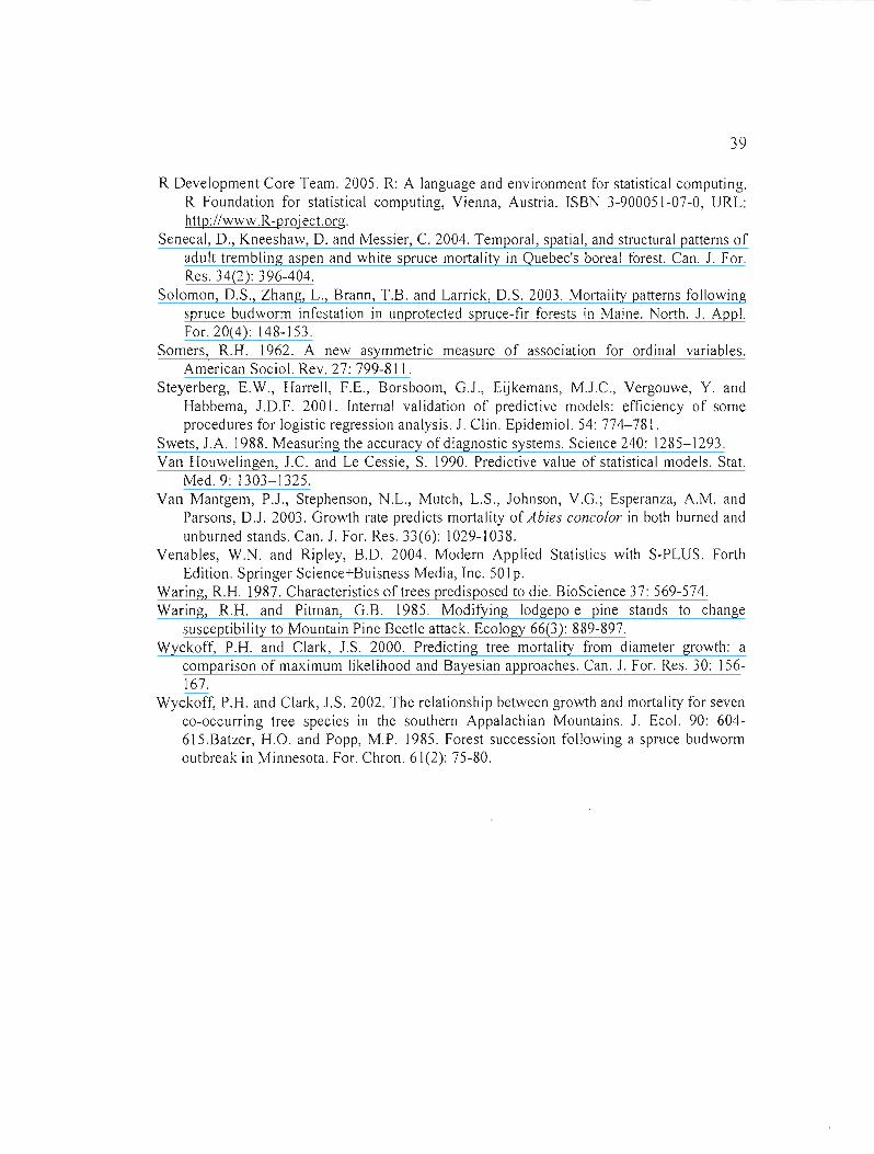
39

R Development Core Team. 2005. R: A language and environment for statistical computing. R Foundation for statistical computing, Vienna, Austria. ISBN 3-900051-07-0, URL: http://www.R-project.org.

Senecal, D., Kneeshaw, O. and Messier, C. 2004. Temporal, spatial, and structural patterns of adult trembling aspen and white spruce mortality in Quebec's boreal forest. Cano 1. For. Res. 34(2): 396-404.

Solomon, O.S., Zhang, L., Brann, T.B. and Larrick, O.S. 2003. Mortality patterns foJlowing spruce bud\.'iorm infestation in unprotected spruce-fir forests in Maine. North. 1. Appl. For. 20(4): 148-153.

Somers, R.H. 1962. A new asymmetric measure of association for ordinal variables. American Sociol. Rev. 27: 799-811.

Steyerberg, E.W., Harrell, F.E., Borsboom, G.J., Eijkemans, M.J.C., Vergouwe, y. and Habbema, J.D.F. 2001. Internai validation of predictive models: efficiency of sorne procedures for logistic regression analysis. 1. Clin. Epidemiol. 54: 774-781.

Swets, lA. 1988. Measuring the accuracy of diagnostic systems. Science 240: 1285-1293. Van Houwelingen, J.c. and Le Cessie, S. 1990. Predictive value of statistical models. Stat.

Med.9: 1303-1325. Van Mantgem, P.J., Stephenson, l'IL, Mutch, L.S., Johnson, V.G.; Esperanza, A.M. and

Parsons, O.J. 2003. Growth rate predicts rnortaJity of Abies conca/or in both burned and unburned stands. Cano J. For. Res. 33(6): 1029-1038.

Venables, W.N. and Ripley, B.D. 2004. Modern Applied Statistics with S-PLUS. Forth Edition. Springer Science+Bu isness Media, Inc. 501 p.

Waring, R.H. 1987. Characteristics of trees predisposed to die. BioScience 37: 569-574. Waring, R.H. and Pitrnan, G.B. 1985. Modifying lodgepole pine stands to change

susceptibility to Mountain Pine Beetle attack. Ecology 66(3): 889-897. Wyckoff, P.H. and Clark, J.S. 2000. Predicting tree mortality from diameter growth: a

cornparison of maximum likelihood and Bayesian approaches. Cano 1. For. Res. 30: 156­167.

Wyckoff, P.H. and Clark, 1.S. 2002. The relationship between growth and mortality for seven co-occurring tree species in the southern AppaJachian Mountains. 1. Ecol. 90: 604­615.Batzer, H.a. and Popp, M.P. 1985. Forest succession following a spruce budworrn outbreak in Minnesota. For. Chrono 61(2): 75-80.

II. USTNG LONGITUDINAL SURVJVAL PROBABJUTIES TO TESt FJELD

VIGOUR ESTIMATES IN SUGAR MAPLE

(Acer saccharum Marsh.)

Henrik Hartmann, Marilou Beaudet & Christian Messier

Article publié dans Forest Eco!ogy and Management 256: 1771-1779.

41

2.1 Abstract

Tree mortality is a major force driving forest dynamics. To foresters, however, tree mortaJity is often considered a loss in productivity. To reduce tree mortality, silvicultural systems, such as selection cuts, aim at removing trees that are more likely to die. In order to identify trees with higher risks of mortality, field classifications are employed that assess vigour based on external characteristics of trees.

We used a novel longitudinal approach for estimating survival probabilities based on ring-width measurements, initialJy developed by Bigler and Bugmann (2004), to parameterize a survival probability model for sugar maple (Acer saccharum Marsh.) and to test whether field-assessed tree vigour classes are corroborated by survival probabilities determined from radial growth histàry. Data from 56 dead and 321 live sugar maples were colJected in stands in western Quebec (Canada) that had undergone a selection eut ~ 10 years prior to sampling.

Our resu Its showed that tree vigour established from external defects and pathological symptoms, using the classification of Boulet (2005), is partially corroborated by growth­driven survival probabilities. Moribund trees had lower survival probabilities than vigorous trees over several years in the period prior to vigour assessment. Intermediate vigour classes showed less obvious tendencies, but this may be due to the growth-independent nature of sorne defects used for their classification.

Although the timing of tree death may not be correctly predicted by the vigour classi fication (i.e., our resu Its suggest that time of death generally was overestimated), its general agreement with survival probabilities determined from growth series make it a useful tool for tree selection in sugar maple stands under selection management.

Key words: Selection eut, radial growth, survival model, logistic mode!.

42

2.2 Résumé

La mortalité des arbres est une composante importante de la dynamique forestière. Toutefois, pour les forestiers la mortalité constitue sOLlvent L1ne perte de productivité. Afin de réduire cette perte, des traitements sylvicoles, telle la coupe de jardinage, visent à enlever les arbres susceptibles de mourir. Ainsi, pour identifier ces arbres en forêt, les forestiers utilisent des systèmes de classification de vigueur des arbres qui sont basés sur des caractéristiques externes (défauts) des arbres.

Nous avons recours à une nouvelle approche d'estimation de probabilité de survie, basée sur la croissance radiale des arbres et développée par Bigler & Bugmann (2004), pour paramétriser un modèle de probabilité de survie pour l'érable à sucre (Acer saccharum Marsh.). Nous utilisons ces probabilités longitudinales de survie comme estimée de la vigueur des arbres et nous les comparons avec les estimées de vigueur obtenues en forêt. Nous avons échantillonné 56 arbres morts et 321 arbres vivants dans des peuplements d'érables au Québec occidental (Canada). Ces peuplements avaient subi une coupe de jardinage ~ la ans avant l'échantillonnage.

Nos résultats montrent que le système de classification sous étude (Boulet 2005) et les probabilités de survie donnent des estimées de vigueur similaires pour les classes extrêmes (arbres moribonds et arbres vigoureux). Les arbres mori bonds avaient des probabi 1ités de survie inférieures aux arbres vigoureux pour plusieurs années avant l'échantillonnage. Toutefois, le classes de vigueur intermédiaires du système de classification de terrain ne coïncident pas nettement avec les probabilités de survie ce qui semble être dû à la nature des critères d'évaluation sur le terrain.

Quoique le système de classification de vigueur testé dans cette étude ne peut pas prédire l'incidence de la mort des arbres correctement (le temps jusqu'à la mort est sous-estimé), sa concordance générale avec les probabilité de survie lui accorde lin potentiel intéressant comme outil pour la sélection d'arbres dans les érablières sous aménagementjardinatoire.

Mots clés: Coupe de jardinage, croissance radiale, modèle de probabilité de survie, modèle logistique.

43

2.3 Introduction

Tree mortality is a major force driving forest dynamics and succession (Franklin el al.

1987, Pacala et al. 1996). It influences species composition, together with the size and age­

structure of forest stands (Oliver and Larson 1996), and is a key process in nutrient and

biomass cycling (Brown and Schroeder 1999). Knowledge of mOi1ality rates is necessary for

developing sustainable forest management practices (Davis et al. 2001). However, our

understanding of the processes underlying tree mortality remains limited and warrants further

investigation (Manion and Lachance 1992, Hawkes 2000).

ln young stands undergoing canopy closure, trees die through self-thinning when

increasing population densities limit resources for particular individuals (Yoda et al. 1963).

Suppressed trees decrease their growth rates, which in turn reduces their competitive capacity

under conditions of limited resources (Oliver and Larson 1996). In mature stands, tree

mortality rates may be indicators of environmental stresses (Brooks 1994, Pedersen 1999,

Dobbertin 2005), such as insect defoliation or drought, which may weaken individual trees

unti 1they die (Manion 1981).

In forest management, tree mortality is often seen as a loss in forest productivity, and

standing dead trees (snags) are considered a potential danger during logging operations,

although more recently their ecological role has been recognized (e.g., DellaSala et al. 1995,

Hunter 1999). Nevertheless, most partial harvests, such as the selection system, attempt to

remove low-vigour trees (Smith et al. 1997), thereby reducing future mortality losses while

liberating resources for the residual trees. The residual stand therefore is expected to have a

higher proportion of 'healthy' trees than before harvest, and to offer better growth conditions

for residual trees, which Should translate into lower mortality rates. However, to achieve this

goal of decreasing post-harvest stand-Jevel mortality rates, individual-Ievel tree vigour must

be adequately assessed in the field prior to harvesting under operational cond itions.

Several tree classification systems have been developed to assess tree vigour based on

social, morphological and pathological qualities of the target trees (e.g., Ouellet and

Zarnovican 1988), crown characteristics (Miliers et al. 1991) or bark characteristics (OrvrNR

2004). Although these indicators may be adequate tools for tree selection, their use may have

44

unintended consequences. For example, it has been observed that stands under industrial

management had mortality rates five years after selection harvest that were higher than

expected, based on previous experimental studies (Bédard and Brassard 2002). These higher­

than-expected mortal ity rates, which occurred among trees without obvious harvest damage

(skidding wounds, crown damage from felling, etc.), might be a consequence of ambiguous

or ineffective marking guidel ines (Meunier et al. 2002) that rely on visual assessments of tree

vigour. If inadequate criteria are used, low-vigour trees may be retained to in harvested

stands. However, the link between tree classification and future mortaJity occurrence has not

been empirically tested.

Other approaches for assessing tree vigour are based on measures of photosynthesis, gas

exchange or nutrient content in leaves, transport rates of water or ions, as weil as

measurements of tree vital function such as radial groWlh (Gehrig 2004). Radial growth of

tree stems is assumed to be a low priority in carbon allocation; it varies with growth

conditions (e.g., soil, climate, and competition) and has been used as a sensitive surrogate

measure of the carbon balance of trees (Kobe et al. 1995, Kobe 1997). It is also a potentially

usefuJ indicator of stress and tree vigour (Waring and Pitman 1985, Pedersen 1998). Radial

groWlh increment has been used to assess survival probabilities of individual trees by

comparing growth of live and dead trees (e.g., Monserud 1976, Hamilton 1986) and is

considered a viable approach to assess tree vigour.

To date, most studies of tree mortality probabilities are based on a cross-sectional

approach where the data consist of a single measurement of recent growth per tree. These

data can take the form, for example, of the ring-width or basal area increment in the year

prior to sampling or prior to the year of death, or sorne derived variable such as the mean

growth rate over a given period of recent growth (e.g., Bigler and BlIgmann 2003). With this

approach, predictions of tree status (dead or alive) are accurate only at one single point in

time, namely, the year when groWlh measurements are taken or the period for which the

predictor variable was computed. Therefore, the cross-sectional approach cannot be lIsed to

predict mortality probabilities for other periods in a tree's life. More recent studies have used

a longitud inal approach to model the probabil ity of mortality over time, for example, for the

entire life span oftrees (Bigler and Bugmann 2004, Bigler et al. 2004).

45

Unfortunately, radial increment cannot be easily measured in the field, since it requires

repeated diameter measurements or increment core sampling. This repeated measurement

precludes its use as a tool for vigour assessment and tree selection on an operational basis.

However, radial growth can provide a powerflll validation of existing vigour classifications

by comparing survival probabilities oftrees of different vigour classes (Bigler et al. 2004).

[n this study, radial growth rates of sugar maple (Acer saccharum Marsh.) were used to

parameterize a survival probability model for empirically estimating tree vigour. These

survivaJ probabilities were compared to field estimations of tree vigour using the

classification system described in Boulet (2005). Sugar maple was selected for our study

because it is a major, ecologically important North American tree species. It is shade tolerant

and forms uneven-aged stands of great geographical extent spanning the northeastern USA

and eastern Canada (Godman et al. 1990).

The objectives of this study were to: (1) develop a longitudinal survival probability

model lIsing radial growth series from sugar maple trees from stands in western QlIebec,

Canada, and (2) use this model to determine whether survival probabil ities corroborate the

visual classification of tree vigour used for tree marking.

46

2.4 Material & methods

STUD y AREA

The study sites are located in the Abitibi-Temiscamingue reglon of western Quebec,

about 60 km southeast of the city of Temiscaming (46°43' north, 79°04' west). The region is

part of the western sugar maple-yellow birch bioclimatic domain (Robitaille and Saucier

1998). Mean annual temperature varies from 2.5 to 5.0°C; growing season extent is 170 to

180 days, and mean annual precipitation ranges from 800 to 1000 mm, with about 25% of

total precipitation falling as snow (Gosselin et al. 2000). Soils are derived principally from

glacial till, with the remainder originating from fluvio-glacial deposits in the large valley

bottoms, and peat-bogs in poorly drained depressions (Robitaille and Saucier 1998).

In 2004 and 2005, 19 plots (26 m x 56 m) were established in uneven-aged sugar maple

stands that had been harvested by selection cuts in 1993 or 1994. The studied stands had an

average pre-harvest basal area of 27 m2/ha, which was reduced by harvesting to an average

21 m2/ha. On average, maximum canopy height reached 25-28 m. The entire area

experienced two forest tent caterpillar (Malacosoma disslria Hubner) outbreaks (1971 and

1988), which caused heavy defoliation in sugar maple (MRi\lFP 2002, MRNF 2005), one of

its hast species (Fitzgerald 1995).

In our plots, sugar maple made up 68% of total basal area, yellow birch (Belula

alleghaniensis Britton) about 18%, red oak (Quercus rubra L.) 3.5%, and American beech

(Fagus grandifolia Ehrh.), eastern white cedar (Thuja occidenlalis L.), and eastern hemlock

(Tsuga canadensis [L.] Carr.) each constituting roughly 1.5% of the total. Other species such

as balsam fir(Abies balsamea [L.] P. MilL), white spruce (Picea glauca [Moench] Voss), and

red ma pie (Acer rubrum 1.) occurred in minor proportions « 1% of total basal area).

Plots were established at locations where site characteristics were corisidered

representative of the greater region, i.e., on level ground or on gentle slopes with good to

moderate drainage, and on podzols of glacial origin. In these plots the diameter at breast

height (dbh, 1.3 m above ground level) and crown class (dominant, codominant, intermediate,

suppressed) ofall trees >10.0 cm dbh was determined. Also, tree vigour was assessed using a

visual classification system (see below) and three increment cores for each live tree between

47

19.1 cm and 49.0 cm dbh were taken as a retrospective measure of radial stem growth. Trees

<19.lcm and >49.0cm were excluded from sampling to avoid heavily suppressed or

senescent individuals.

TREE VIGOUR CLASSIFICATION

The tree vigour classification that we used has been developed by the Quebec Ministry of

Natural Resources (Boulet 2005), and relies on pathological symptoms (e.g., presence of

cankers and fungi), mechanical damage (e.g., cracks, leaning) and other visible features (e.g.,

improper branch shedding, crown openness) to assign trees to 200+ vigour codes, which are

then grouped into four main vigour classes. The classification system is considered a

thorough framework for tree vigour assessment and, since it is based on symptoms of

physiological vigour decJine, can be regarded as an indicator of tree vigour beyond the

geographical boundaries of where it was developed. The vigour classification takes into

account wood properties, but also assigns tree survival probabilities until the next harvest

entry, typically scheduled every 20-25 years (MRN 1997).

The four vigour classes are described as follows. Trees of reserve stock (class 'R') are

free of any symptoms of disease or damage and are considered 'healthy' trees with the

highest probability of survival. Growing trees (class 'C') have minor defects but are not

biologically declining and are expected to survive until the next harvest without risk of

imminent wood decay. Low quality or defective trees (class 'S') are considered to be

declining in terms of vigour, wood quality and volume increment, and are not expected to

survive until the next harvest. Moribund trees (class'M') show signs of either lethal

pathological infection or severe damage with high risk of trunk breakage. Moribund trees are

biologicalJy declining (decreasing vigour, wood decay) and are assumed to have a high

probability of mortality before the next harvest entry.

The vigour classification system has a hierarchical structure based on the assumed

severity of observed defects. When assessing a tree's vigour, one should first determine

whether the tree shows signs or symptoms of fLlngal infection (sporocarps, stroma) and, if

present, this observation determines the vigour code. If the tree is free of fungal infection,

then signs or symptoms of cambium nec roses (cambial diseases) should be determined and, if

48

present, they wi Il determine the vigour code. The stepwise assessment procedure continues

further using various types of criteria, in the following order: bole defects and bark

mechanical injuries, root and butt wounds, bark fissures and bole cracks, woodworm and

woodpecker damage (wood dust and bird-pecks), crown defects, and finally, branching

defects.

Listing aIl poss ible defects for vigour classi fication is beyond the scope of this paper.

However, typical fungal infections for sugar maple involve the northern tooth fungus

(Climacodon septentrionalis [Fr.] P. Karst.), which causes severe crown dieback. In al! cases,

sugar maples showing signs of this fungal infection arc classified as moribund. However, the

mere presence of a pathogen does not automatically relegate the infected tree to moribund

status. For example, latent stump decay incurred by the mossy maple conk (Oxyporus

populinus [Schumach.] Donk, [1933]) only leads to a 'c' code if present at or below 60 cm

from the base of the stump. If the same pathogen is encountered higher on the trunk and is

associated with necroses, cracks, and heart rot, the tree would be given an 'M' code. Similar

complex ratings apply to necroses. For example, the presence of cankers such as Neonectria

sp., Eutypella sp., or Sirococcus sp. would rate a 'c' code, if no or only superficial wood

decay is visible. If heart wood decay (> 5 cm in depth) is present but the necroses covers less

than one apparent side of the trunk, the associated code is 'S.' However, if the necrosis spans

over more than one apparent side of the trunk, the tree is then classified as moribund.

Other classification criteria, such as trunk deformations, bark cracks, and root or crown

damage are more straightforward to identify than pathogen infections, but their inclusion

adds to overall classification complexity as weil. More details of the rating system can be

found in the field guide (Boulet 2005).

TREE GROWTH DATA

While ail growth data for live trees were obtained from increment cores taken from trees

inside the study plots, the number of dead trees in the plots was insufficient for our analyses.

We therefore had to extensively search for dead trees througl1Out the entire area of the 1993

and 1994 harvest blacks. However, we only sampled dead trees that were on sites and within

stands similar to those where the initial live tree plots were located. Also, only trees with

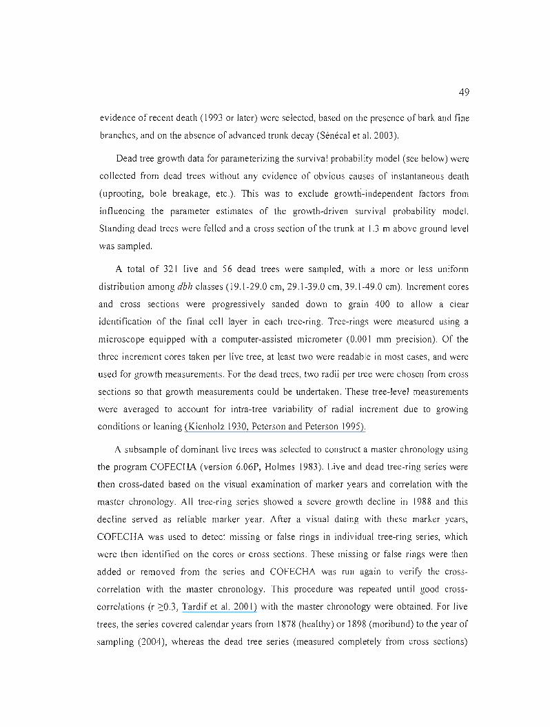
49

evidence of recent death (1993 or later) were selected, based on the presence of bark and fine

branches, and on the ab'sence of advanced trunk decay (Sénécal et al. 2003).

Dead tree growth data for parameterizing the survival probability model (see below) were

collected from dead trees without any evidence of obvious causes of instantaneous death

(uprooting, bole breakage, etc.). This was to exclude growth-independent factors from

influencing the parameter estimates of the growth-driven survival probability mode!.

Standing dead trees were felled and a cross section of the trunk at 1J m above ground level

was sampled.

A total of 321 live and 56 dead trees were sampled, with a more or less uniform

distribution among dbh classes (19.1-29.0 cm, 29.1-39.0 cm, 39.1-49.0 cm). Increment cores

and cross sections were progressively sanded down to grain 400 to allow a clear

identification of the final cell layer in each tree-ring. Tree-rings were measured using a

microscope equipped with a computer-assisted micrometer (0.001 mm precision). Of the

three increment cores taken per live tree, at least two were readable in most cases, and were

used for growth measurements. For the dead trees, two radii per tree were chosen from cross

sections so that growth measurements could be undertaken. These tree-Ievel measurements

were averaged to account for intra-tree variability of radial increment due to growing

conditions or leaning (Kienholz 1930, Peterson and Peterson 1995).

A subsample of dominant live trees was selected to construct a master chronology using

the program COFECHA (version 6.06P, Holmes 1983). Live and dead tree-ring series were

then cross-dated based on the visual examination of marker years and correlation with the

master chronology. Ail tree-ring series showed a severe growth decline in 1988 and this

decline served as reliable marker year. After a visual dating with these marker years,

COFECHA was used to detect missing or false rings in individual tree-ring series, which

were then identified on the cores or cross sections. These missing or false rings were then

added or removed from the series and COFECHA was run again to verify the cross­

correlation with the master chronology. This procedure was repeated until good cross­

correlations (r ~0.3, Tardif et al. 2001) with the master chronology were obtained. For live

trees, the series covered calendar years from 1878 (healthy) or 1898 (moribund) to the year of

sampling (2004), whereas the dead tree series (measured completely from cross sections)

50

covered calendar years 1848 to 2003 or earlier, depending on the year of death of individual

trees.

From the 321 live trees sam pied in our plots, 56 individuals (i.e., a nllmber equivalent to

the sample size of dead trees) were randomly selected and lIsed to parameterize the survival

probability mode!. To assure that growth of selected trees (and the resulting survival

probability model) had not been negatively influenced by direct harvest disturbance, live

trees were selected only when our field assessment indicated absence of obvious harvest

disturbance (i.e., trees not close to skid trails and not heavily thinned).

LOGISTIC REGRESSION

Logistic regression was used to model survival probabilities as a function of radial

growth, in the following form (Bigler and Bugmann 2003):

flX e [eq. lJ P(Y=l)=-­

1+ eflX

where P(Y = 1) is the probability that an individual tree survives given the matrix of

independent variables X. The latter include three types of growth variables: (i) growth level

(average growth over a specified period), (ii) growth trend (regression slopes of growth over

a specified period) and (iii) growth sensitivity (average growth variability over the preceding

5 years, see below for details). The vector j3 of regression parameters is estimated in the

analysis (Hosmer and Lemeshow 2000, Quinn and Keough 2002).

A manual stepwise procedure was used in the modelling process. First, only one growth

level variable was included at a time. The growth level predictor variables that we considered

were the log-transforms of the arithmetic mean over the preceding 3,5 and 10 years ofradial

growth (Table 2.1). The log-transformation was applied to lower the weight of very high

growth values. Using the Akaike Information Criterion (AIC, Burnham and Anderson 2002),

the Dxy and bootstrapped confidence intervals (see below) were used as the main decision

criteria for selecting the 'best' univariate mode l, which was then used for further analysis.

Second, growth trend variables were added individually to the best univariate mode!. The

51

growth trend variables that we considered were the coefficients of the local linear regression

over the preceding 3, 5, 10, and 25 years (Table 2.1).

Table 2.1 Growth level, growth trend and gro\\1h sensitivity variables computed for different time windows used for

logistic regression analysis ofsurvival probabilities. Shown are variable names and lheir respective number of observations, including live and dead measurements. Number of observations of dead measurements are

constant across growth variables and equal the number of dead (rees (n=56)

Types of growth variables

Leve)' Trend Sensitiviry No. of tree·rings to Variable Variable Variable corn pute variable name n name n name n

1 r\V-log 9727

3 av3-log 9722 slp3 9727

5 av5-log 9512 slp5 9504 sens5 9727

10 avlO·log 9286 slp 10 9283

25 slp25 8723

• log transfonmed

To avoid redundancy, only one growth trend and one growth level variable was allowed

in the final mode!. Last, the mean sensitivity over the preceding 5 years was added to the best

bivariate mode!. This variable represents the responsiveness of individuals to environmental

signaIs, such as climate (Fritts 1976). High sensitivity values have been associated with tree

vigour decline because dying trees may exhibit higher variability in past growth rates (Ogle

et al. 2000, Suarez et al. 2004). Interannual sensitivity was defined as (Fritts 1976):

abs(rw, - rW'_1 )[eg.2]

abs(rw, + rwl

_ l )

where SI is the sensitivity in the year l, and rw is the ring width measurement in the year

t. We used the average sensitivity of the most recent 5 years, assuming that decl ining trees

would exhibit growth variability during the period close to Lheir death.

Parameter estimation was done with R software (version 2.4.0, R Development Core

Team 2006), using maximum log-likelihood. The model with the lowest AIC was retained for

further analysis. Non-parametric confidence intervals for parameter estimates were computed

using a bootstrap resamp1ing procedure (bootcov) with 1000 repetitions and applying the 25 1h

52

and the 975 1h quantile as interval limits. Longitudinal data from tree-rings are interannually

correlated and, therefore, are not independent within an individual tree-ring series. This

violation of independence will underestimate the true variance and confidence interval width.

To correct for within-cluster (i.e., within-tree) correlation of the responses, the boolcov

function was used, which allows substituting cluster sampling with replacement for the usual

simple sampling with replacement. The resulting parameter estimates therefore can be

regarded as unbiased and were considered significant when the confidence interval did not

include zero; otherwise the model was rejected even if it had a lower AIC.

To obtain additional information on the gain in model performance when variables were

added, Somer's Dxy index was used as another decision criterion (Somers 1962). Dxy is

indicative of the model's discriminative ability and is closely related to the area under the

curve (AUC) of a receiver operating characteristic (ROC) plot (Engelmann et al. 2003) and,

as such, is independent of prevalence and classification thresholds (Swets 1988). It ranges

from -1 (indicating perfect status misclassification, where ail live trees are classified as dead

or vice-versa) to 1 (perfect status classification); values >0.6 indicate good discrimination

(see Manel et al. 1999). To account for over-optimistic classification measures when

validating the model on the training data (data specificity), the bootstrap resampling

procedure validale.lrm from the R Design library (Harre Il 2005) was used. This procedure

eliminates the optimism of the Dxy due to overfitting and produces a more conservative

estimate of the model's discriminative ability (HarreIl2001).

LONGITUDINAL SUR VIVA L PROBABILITY EST/i'vIATfONS

Survival probabilities were estimated following a longitudinal approach to logistic

regression developed by Bigler and Bugmann (2004). This method uses tree-ring data from

live and dead trees to estimate surviva! probabilities over the life span of a tree. To do so,

growth data from the entire life span of the trees must enter the modelling process. First, tree

growth variables (e.g., mean values and trend coefficients over different periods) are

computed as predictor variables. Variables containing the last year of growth of a dead

individual are marked as 'dead' measurements. Ali measurements of dead trees, excluding

those from the year of death, and ail live tree-ring measurements are marked as 'live'

53

measurements. The logistic regression model is then fitted to data points from the entire 1ife

span of aIl trees.

COlv/PAR/SONS OF SURVIVAL PROBABlLITlES

Among the available tree growth series (321 live, 56 dead), the data were divided into

five distinct groups according to the status (live or dead) and vigour code of live trees.

Individual survival probabilities were computed for vigorous ('R', n = 160), growing ('C, n

= 87), declining ('S', n = 31), moribund ('M', n = 43) and dead ('D', n = 56) trees, and

compared among groups. A series of annual ANOVAs was applied ta determine whether

within-year differences in survival probabilities varied statistically (P <0.05) among these

five groups. For years with significant differences, Tukey's HSO adjustment for multiple

comparisons was applied to obtain adjusted P-values for unplanried comparisons between

pairs of groups (Quinn and McKeough 2002).

54

2.5 Results

ln the tirst step of the regression analysis, the univariate model with the best fit (Iowest

AIC) contained the log-transformed averages over the last 3 years of growth (model 2, Table

2.2). Although the log-transformed annual measurement (rw-Iog, model 1) yielded a model

with a higher Dxy (0.772) than model 2 (0.715), its Ale was markedly highcr (587.1) than

that ofmodel2 (545.9, Table 2.2). The addition of the growth trend variable yielded bivariate

models with consistently lower AICs than univariate models. However, the inclusion of 10­

year slopes and 25-year slopes decreased the Dxy to 0.707 and 0.710, respectively (Table

2.2). Among the two models with lower AICs and higher Dxy values, the addition of the

trend over 5 years yielded an ArC (513.5) weil below the model including the 3-year slope

(519.5, Table 2.2). Therefore model 6 (Dxy=0.783) was considered for further analysis even

if the Dxy was slightly greater for model 5 (0.798). The addition of the sensitivity variable to

this model caused a slight decrease in the ArC (510.0) and little improvement in the Dxy

(0.793), but the confidence interval of the parameter estimate spanned across zero, so this

predictor was rejected as being signiflcant (Table 2.2).

55

Table 2.2 Parame ter estimates, booLStrapped 95% conlïdenœ intervals (CI), AIC, and optimism-corrected Dxy of logistic mortality

models Models in bold are Ihe 'best' univariate or bivariate models

CI (95%)

lndependenl variables Estimate Lower Upper AIC D.w

Univariate models

Modell Intercept -1.740 -5379 0.053 587.1 0.772

f',v-Iog 1.093 0.799 1ni

Model2 fnlercepl -6.589 -8.422 -4.724 545.9 0.715

av3-log 1.872 1.567 2.193

Model3 Intercept -7.088 -9.397 -4.424 5671 0.634

av5-Jog 1.923 1476 2335

Model4 Inlercept -8153 -II 121 -4.974 5863 0.563

av la-log 2.052 l.547 2.551

Bivariate models

Model5 Inlercept -7623 -9.555 -5792 519.5 0.798

av3-log 2.082 1.779 2.440

slp3 0.004 0.002 0.005

Model6 Inlerccpl -7.115 -8.974 -S.337 513.5 0.783

av3-log 2.017 1.7i3 2.375

slpS 0.006 0.004 0.007

Model7 Intercept -6.278 -8393 -4.242 540.9 0707

av3-log 1.826 IA93 2.202

slp la 0003 -0005 0008

Model8 Intercept -5.820 -7943 -4.018 534.4 0.710

av3-log \.756 IA55 2.132

slp25 0.008 -0007 0017

Trivariate model

Model9 [ntercept -5.951 -8.414 -3.508 510.0 0.793

av3-log 1.904 1536 2302

slp5 0.005 0003 0.007

sensSyr -2.622 -S.154 0.420

Means of the growth level variable were similar among the intermediate vigour classes,

which in turn differed significantly (P < 0.00/) from the means for vigour class R and the

dead trees (Table 2.3). Mean log-transformed growth over three years (av3-Jog) of live trees

varied between 6.893 (vigour class M) and 6.999 (R) but was only 6.742 for dead trees

(Table 2.3). S/opes over 5 years showed a direct relationship with vigour; mean regression

slopes decreased with vigour and ranged from positive (5.654, R) to negative values (-4.956,

56

M, Table 2.3). However, slopes were statistically different only between vigour class Rand

M (P <0.05) and vigour class Rand 0 (P <0.00 \). Interestingly, regresslon slopes of

moribund and dead trees (-4.570) were quite similar (Table 2.3).

Table 2.3 Sample sizes (n), me an values and standard errors (SE) of the predictor variables av3-log [ln(3­

year average growthÜun/yr)+ 1)1and slp5 [5-year regression slope (I-un/yr) J of live Irees in different vigour classes and dead trees

Prediclors

av3-log slp5

Vigour class n Mean SE Mean SE

Live R 160 6.999 A 0627 5.654' 183 167 C 87 6920 B 0657 2170" 177333 S 31 6.918 B 0.698 2.651 " 183.857 M 43 6.893 " 0.645 -4.956 bd 201.980

Oead 0 56 6.742 c 0.679 -4570 c, 142.456

Upper case letters, if different between vigour classes, indicate a signiticant differenee at P <0.001, lower case at P <0.05, Tukey's HSO.

More than 80% of vigorous trees had no defects, while the reminder had cracks (5.0%),

bole (4.4%), root and butt defects (3.8%), or bird pecks and branching defects (bath 3.\%,

Table 2.4). These defective trees showed no signs of decay. Most defects of growing trees

were bole cracks lacking signs of decay or bird pecks, which together affected more than

75% of trees in this class (Table 2.4). Declining trees were mostly affected by bole defects

(25.8%), bird pecks (22.6%) and cambium necroses (19.4%). There was evidence of fungal

infection in one individual in this class (Table 2.4). Moribund trees were mostly affected by

sporocarps and stromata (26.6%), together with cambium nec roses (52.4%) and decayed

cracks (\4.3%), which characterized more than 90% oftrees in this class (Table 2.4).

57

Table 2.4 Number of trees per defect type and their respective percentage distribution within each vigour class

Vigour class

R (vigorous) C (growillg) S (declining) rv1 (moribund)

Defect N % N % % N %

None 129 80.6 0 00 0 0.0 0 0.0

Sporocarps 0 0.0 3 34 1 32 II 25.6 ~oNecroses 0 00 0 0.0 6 19.4 "-0 535

Bole 7 4.4 8 9.2 8 25.8 1 23

Root&butt 6 3.8 3 34 0 0.0 1 23

Cracks 8 5.0 36 414 4 129 6 14.0

Bird pecks 5 3.1 31 35.6 7 22.6 1 23

Crown 0 0.0 2 23 1 3.2 0 0.0

Branchillg 3.1 4 4.6 4 12.9 0 00

Total 160 100.0 87 100 31 100 43 \00

For all vigour classes, there was a strong growth decline apparently due to disturbance in

1971 and 1988 (Fig. 2.la). Average annual growth rates of vigorous trees (R) were

consistentJy higher than growth rates of trees in other vigour classes, at least from the 1960's

onwards, but showed a similar pattern (Fig. 2.1 a). On the other hand, growth of dead trees

(D) showed a distinct pattern ofsteady decline from 1960 onwards, with a small increase in

the 1ast year (Fig. 2.\ a). Th is apparent recovery is 1ikeJy due to the continued decrease in

sample size of dead trees (Fig 2.1 b) and associated higher variability in dead tree data

towards the end of the series (Fig. 2.1 c).

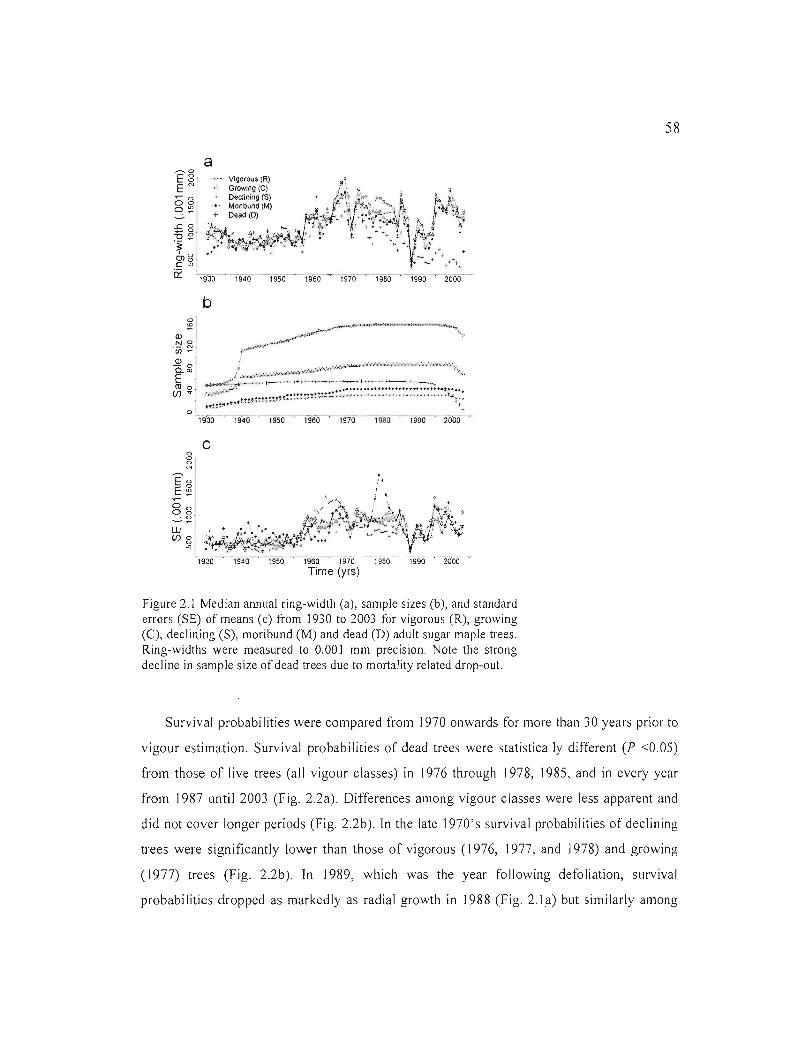
58

a

b

.~._. """'..... ,.~ •.,''''P.,..."··'''".,><.o'··,,···>··,,~,,·"·~,.·><.o',····~·,~· ..\

,....":1

. /1

w (/)0

o

"'

Figure 2.1 Median annual ring-width (a), sample sizes (b), and standard errors (SE) of means (c) from 1930 to 2003 for vigorous (R), growing (C), declining (S), moribund (M) and dead (D) adult sugar maple trees. Ring-widths were measured to 0.001 mm precision. Note the strong decline in sample size of dead tTees due ta mortality related drop-out.

Survival probabilities were compared from 1970 onwards for more than 30 years prior ta

vigour estimation. Survival probabilities of dead trees were statistically different (P <0.05)

from those of live trees (ail vigour classes) in 1976 through 1978, 1985, and in every year

from 1987 until 2003 (Fig. 2.2a). Differences among vigour classes were less apparent and

did not caver longer periods (Fig. 2.2b). In the late 1970's survival probabilities of declining

trees were significantly lower than those of vigorous (1976, 1977, and 1978) and growing

(1977) trees (Fig. 2.2b). In 1989, which was the year following defoliation, survival

probabilities dropped as markedly as radial growth in 1988 (Fig. 2. la) but similarly among

59

vigour classes. Another decline occurred in 1993-1994, the yea'rs when harvesting took place,

but this trend was followed by a quick recovery (Fig, 2.2b).

a ....... 'IIr *"'kk"'kk**"'**k*/t'* ....

....·""'....---.......r~~t,};..,.II;,·~"lI:;--~f, ......---.............--lh'*, e-- Vigorous (R) • + - - + •• + •

Cl Growing (C) Declining (5)

.+- Moribund (M) Dead (0)

1970 1975 1980 1985 1990 1995 2000

b rn :;: u. u

mmrna: a: a: ~t.I 0::0::

:;::;:a: a:

::<a:. ::<::<

a: a:

c

l ,

1975 1980 1985 1990 1995 2000 Time (yrs)

Figure 2.2 Survival probabilities (a, b) and their standard errors (c) From 1970 to 2003. Panel a shows survival probabilities of vigorous (R), growing (C), declining (S), moribund (M), and dead (0) trees; panel b excludes dead trees. Asterisks (*) above the curves in (a) indicate the years of significant differences (P < 0.05, ANOV A) between dead and IiYe (ail vigour classes), in (b) asterisks indicate the years of significant differences (P <0,05) between vigour classes based on Tukey's HSO tests for years with significant (P <0.05) annual ANOV As, Vigour classes that were significantly different From each other are Iisted in panel (b), with a dash separating significantly different groups.

60

Survival probabilities of vigorous trees were significantly higher than those of moribund

trees in 1980, 1987, 1988, 1995, 200 l, and 2002, and higher than those of growing trees in

1981 (Fig. 2.2b). Aiso in 2002, survival probabilities of growing trees were higher than those

of moribund trees (Fig. 2.2b). Standard errors of the means were large for moribund (1983­

1984, 1988), declining (1987) and vigorous (1992) trees, but low for most of the time before

and especially after these brief periods (Fig. 2.2c).

61

2.6 Discussion

L!NK/NG FJELD V/GOUR ESTft'v/ATES Ta RETROSPECTIVE SUR V/VAL PROSAS/LIT/ES

We used radial tree-ring series to estimate retrospectively survival probabilities for the

entire life span of trees and used these probabilities to test the validity of a field vigour

classification system. Whilst the former methodology has been proven adequate (Bigler and

Bugmann 2004), the latter is more ambiguous especially if vigour was estimated at the very

end of the tree-ring series. It is obvious that tracing back vigour estimates through time is

challenging. At what point in time has a tree entered a vigour class estimated in 2004 and

how did this influence radial growth rates?

Trees that were showing signs or symptoms of advanced lethal pathogen infection in

2004 (e.g., presence of perennial conks) had been already und el' attack for some time, in the

case of the tinder fungus (Fomes fomentarius [L.] J.J. Kickx) up to 30 or more years

(Schmidt 2006). Also, it has been observed that pine trees (Pinus mugo Turra) were infected

and killed by Armillaria spp only ifthey were weakened by competition and this weakening

translated into a graduai, severa! decades lasting decline of radial growth prior to death

(Cherubini et al. 2002). These low growth rates were estimated as preconditioning to fungal

attack and not as its result (Cherubini et al. 2002). Similarly, Pedersen (1998) found that oak

trees (Quercus spp) died several decades after an inciting drought stress and that these trees

had lower growth rates than surviving trees during this period. Lower growth rates of dead

trees prior to drought were considered ind icative of the preconditioning of these trees to

further decl ine (Pedersen 1998). On the other hand, Davis et al. (1997) observed that heavi Iy

cankered (Cryphonectria parasitica [Murrill] Barr) scarlet oak trees (Querais coccinea

Münchh.) had higher growth rates (basal area increment) than moderately cankered

ind ividuals, but their growth rates were sti Il lower than non-can kered trees. Potential

mechanisms for this growth stimulation were attributed to callus formation close to the sites

of infection and sampling, and thus, were considered worthy of further investigation (Davis et

al. 1997). Whether or not slow growth rates are the cause or the consequence of fungal

infection may still be an open question, but both phenomena often coincide. Also, declines

due to fungal infection or other sources of stress are slow processes, which may last decades.

Signs (sporocarps, stromata, cankers) or symptoms (wood decay, crown dieback) of fungal

62

infection therefare can be assumed to be reliable criteria for estimating tree vigour in the field

and can be linked to survjval probabilities estimated From past radial growth rates.

Similarly, severe crown dieback, if chranic or induced by competition or drought,

classifies a tree as moribund when >26% of the crown is dead in suppressed individuals and

>51 % of the canopy of trees with open, chlorotic and dwarf-Ieaved crowns is dead (Boulet

2005). Although severe crown dieback (i.e., >40%) cannot not be sllpported by trees for very

long periods (Gross 1991), our data show (Fig. 2.1 a) that a single severe crown defoliation

caused by a forest tent caterpillar outbreak (1971) initiated severe declines in growth rates

that persisted over decades in less vigorolls trees. Similar reSlIlts have been observed in

trembling aspen (Populus tremuloides Michx.) where crown defoliations reduced radial

growth rates and predisposed trees to attack by wood-boring insects and fungal pathagens

(Hogg et al. 2002).

Structural defects, such as butt defects, bole cracks or strong leaning, reduce survival

probabilities by increasing the risk of mechanical failure. The presence of deep cracks

decreases the tree's mechanica! resistance to external forces, such as wind, and increases the

tree's risk ta fall over (Smiley et al. 2007). These risks are unlikely to show in radial growth

rates but the vigour classification system assigns a moribllnd code only to major structural

defects (e.g., crack> 1.5 m) that are accompanied by profound wood decay caused by fungal

activity (Boulet 2005). However, because fungal infections in this instance are a result of

mechanical damage rather than one of reduced vigour, their linkage to radial growth rates

may be difficult to detect. This decreases the potential of survival probabilities inferred fram

radial growth to reflect vjgour classification in these cases.

VAL/DAT/NG THE FIELD V/GOUR EST/MATES W/TH GROWTH-DEPENDENT SURV/VAL

PROBAB/L1T1ES

ln this study, radial growth of dead and, to a lesser extent, moribund trees diverged From

that of vigorous trees shortly after 1971 and onwards (Fig.2.1 a). Th is and a subsequent

growth decline in 1988 can be linked ta forest tent caterpillar defoliation, a disturbance

recurring over about a 9-year cycle in the study region (MRNFP 2002, MRNF 2005). A

comparison of growth rates in sugar maple (a host species) and yellow birch (a non-hast

63

species) clearly showed that birch did not incur the same growth reduction as sugar maple (H.

Hartmann, unpubl ished data), supporting the hypothesis that the growth decrease observed

among maples resulted from tent caterpillar defoliation and not from other disturbances (e.g.,

drought). Growth declines prior to death are consistent with Manion's tree decline model

(Manion 1981), where predisposing stresses reduce tree vigour and inciting factors cause a

final decline and death. For dying trees, the first defoliation (although not a long-term stress,

as stated in Manion's model) reduced tree vigour, i.e., growth rates and survival probabilities,

and predisposed these trees to a second, more intense forest tent caterpillar defoliation, which

led to an accelerated growth decline and to death (Fig. 2.1 a). Average growth rates during

these defoliations were (although not significantly) higher in vigorous than in moribund trees,

possibly indicating that their greater carbon reserves allowed for quick foliage replacement

and growth recovery (Mc Laugh 1in et al. 1980).

Surviyal probabilities corroborate, at least partially, the yisual tree Yigour classification

used for tree marking. The different vigour classes that are used in Quebec (Boulet 2005) are

supposed to broadly predict tree survival probabilities. It is assumed that moribund trees will

1ikely die before the next harvest (over the next 20 to 35 years), whereas dec lining trees

shou Id survive until the next harvest despite their decreasing vigour (and hence, sury ival

probability). Growing and vigorous trees are assumed to have unconstrained life expectancy.

Although the average 5-year slope of moribund and now dead trees was negative (Table

2.3), survival probabilities of moribund trees showed no monotonie negative growth trend

over the most recent 30 years (Fig. 2.2a), as has been observed in other studies (Bigler et al.

2004). This may be due to the fact that, in this study, vigour estimates were based on external

signs and symptoms related to vigour but not on any actual measures of physiological

activity. Bigler et al. (2004, p.185) used cambial vitality, a measure that "correlated

signiflcantly with the number of cells produced by the cambium", for Yigour estimations in

European silver fir (Abies alba MilL). Obyiously, the number of cells produced by the

cambium correlates weil with tree-ring width. However, vigorous, growing and declining

trees in this study had higher (positive) average growth trends computed over the entire tree­

ring series than those of moribund and dead trees (negative, Table 2.3), indicating that

moribund and now dead trees showed an overaJJ growth decline over their life span.

64

In this study, mean survival probabilities of vigorous trees were greater than those of

moribund or declining trees for most years from 1970 onwards, although not consistently

throughout this period (Fig. 2.2a). The growth-driven survival probability model used in this

study may not correctly predict survival probabilities in trees affected by gro\vth-independent

defects, such as bole cracks, which accounted for roughly 14% of moribund trees. Similarly,

most growing (:::::90%) and declining (:::::61%) trees were classified based on bole injuries, root

butt defects, cracks or bird pecks (Table 2.4). None ofthese defects is directly linked to radial

gro\vth rates, and therefore, their effects on tree vigour would be difficult to relate to survival

probabi lity estimated from retrospective growth series. This may also expia in why no

significant differences in survival probabilities between intermediate vigour classes have

been detected.

IMPLICATIONS FOR FOREST MANAGEMENT

The results of this study highJight the strengths and weaknesses of an elaborate visual

field vigour classification system. In a context where pal1ial harvesting is used, vigour

estimation is a crucial step in assigning harvest priorities for tree marking if stand

improvement is sought (OMNR 2004). Tree classification systems have a long tradition,

dating back to the 1840s (Rosznyay 1979). Early classifications, sllch as that propsed by

Kraft (1884), described trees in terms of their social position, and were later amended to

include qualitative measures of bole quality (Heck 1931). In 1956, Leibundgut defined the

IUFRO (International Union of Forest Research Organizations) tree classification system,

which combines social position, harvest priority and tree quality in a numeric code

(Leibundgut 1956).

On Iy much later did Wari ng et al. (1980) defi ne a quantitative measure of tree vigour as

the ratio of basal area growth to sapwood basal area representing the amount of stemwood

produced pel' square meter of foliage. Instead of describing trees by visually evaluating their

external condition, the 'Waring vigour' index described their overall vitality. Assuming that

stem growth has a low priority in carbon allocation, the amount of stemwood produced,

weighted by the size of a tree's photosynthetic apparatus, was considered indicative of tree

vigour (Waring et al. 1980). Other vigour measures, such as crown transparency (Millers et

65

al. 1991), nutrient content of need les or sapwood (Joos 1997), electric cambial resistance

(Torell i et al. 1996) or ch lorophyll fluorescence (Lichtenthaler and Rinderle 1988), aIso

aimed at describing tree vigour (see Gehrig 2004 for a comprehensive review). Among these

vigollr-based measures, only crown transparency can be easily assessed in the field.

However, crown openness can be caused by several agents and stresses (Innes 1993) that

vary temporally, especially in broad-Ieafed trees, and therefore, it may not be adeqllate as a

criterion for tree removal.

The vigour classification used in this study may overestimate the time-to-tree death. If

moribund trees were to die within 20-25 years following vigour estimation, one would expect

their sllrviva! probabilities to decline in a fashion similar to those of dead trees. However,

survival probabilities of dead trees were significantly lower than those of ail vigour classes in

most years from ]970 onwards and in every year from 1987 to 2003 (Fig. 2.2a). This

indicates that moribund trees were not declining as rapidly as dead trees were prior to their

death, at least for the most recent 16 years. It is therefore doubtful that these trees would die

within the predicted period.

The classification system used in Qllebec, which is based on vigollr-related defects in

trees, has the practicality of classical tree classifications and was able to discriminate between

moribund and vigorous trees, the two extreme vigour classes. It did not discriminate among

the intermediate vigollr classes, which sllggests that the various criteria used did not affect

diameter growth. However, such field vigollr classifications cOllld not adeqllately predict the

timing oftree death with any accuracy.

66

2.7 Acknowledgements

We thank Catherine Malo for her help during the long weeks of field work and

dendrochronological analyses. We also thank Mr. Denis Boileau of the Quebec Ministry of

Natural Resources for his help in exp!aining historical tree growth disturbances and Ronnie

Drever for reviewing an earlier draft of this paper. We aiso thank Lana RuJJick alld Biil

Parsons for improving the linguistic quality of the manuscript. We would also like to thank

Christof Bigler, an anonymous reviewer, and the Special issue guest editor for their thorough

reviews and helpfuJ suggestions. Financial support was provided by FQRNT (Programme des

actions concertées) through a research grant to C.M., M.B. and colleages, and by NSERC

through a scholarship to H.H.

67

2.8 References

Bédard, S. and Brassard, F. 2002. Les effets réels des coupes de jardinage dans les forèts publiques du Québec en 1995 et 1996. Ministère des ressources naturelles du Québec, Gouvernement du Québec. 15 p.

Bigler, e. and Bugmann, H. 2003. Growth-dependent mortality models based on tree rings. Cano J. For. Res. 33: 210-221.

Bigler, C. and Bugmann, H. 2004. Predicting the time of tree death using dendrochronological data. Eco!. App!. 14(3): 902-914.

Bigler, e., Gricar, J., Bugmann, Rand Cufar, K. 2004. Growth patterns as indicators of impending tree death in silver fir. For. Eco!. Manag. 199: 183-190.

Boulet, B. 2005. Défauts externes et indices de la carie des arbres: guide d'interprétation. Publication du Québec, Sainte-Foy, Quebec. 291 p.

Brooks, R.T 1994. A regional- scaJe survey and analysis of forest growth and mortality as affected by site and stand factors and acidic deposition. For. Sci 40(3): 543-557.

Brown; S.L. and Schroeder, P.E. 1999. Spatial patterns of aboveground production and mortality of woody biomass for eastern U.S. forest. Ecol. Appl. 9(3): 968-980.

Burnham, K.P. and Anderson, D.R. 2002. Model selection and multimodel inference: a practical information-theoretic approach. Springer, New York. 496 p.

Cherubini, P., Fontana, G., Rigling, D., Dobbertin, M., Brang, P. and Innes, lI. 2002. Tree­life history prior to death: two fungaJ root pathogens affect tree-ring growth differently. l Ecol. 90: 839-850.

Davis, D.D., Torsello, M.L., and McClenahen, J.R. 1997. Influence of Cryphonectria parasitica basal cankers on radial grow1h of scarlet oak in Pennsylvania. Plant Dis. 81: 369-373.

Davis, L.S., Johnson, K.N., Bettinger, P.S. and Howard, TE. 2001. Forest management: to sustain ecological, economic and social values (4th edition). McGraw-Hi Il, NY. 816 p.

DellaSala, D.A., OIson, D.M., Barth S.E., Crane, S.L. and Primm, S.A. 1995. Forest health: moving beyond rhetoric to restore healthy landscapes in the Inland Northwest. Wildlife Soc. B. 23(3): 346-356.

Dobbertin, M. 2005. Tree gro'W1h as indicator of tree vitality and of tree reaction to environmental stress: a review. Eur. J. For. Res. 124: 319-333.

Engelmann, B., Hayden, E. and Tasche, D. 2003. Testing rating accuracy. Risk 16(1): 82-86. Fitzgerald, TD. 1995. The tent caterpillars. Cornell University Press, Ithaca, NY. 303 p. Franklin, J.F., Shugart, H.H. and Harmon, M.E. 1987. Tree death as an ecological process.

BioScience 37(8): 550-556. Fritts, Re. 1976. Tree rings and climate. Academic Press, London. 567 p. Gehrig, M. 2004. Methoden zur Vitalitatsbeurteilung von Baümen. Vergleichende

Untersuchungen mit visuelJen, nadelanalytischen und bioelektrischen Verfahren. Dissertation. No. 15341, ETH Zürich. 254 p.

Godman, R.M., Yawney, H.W. and Tubbs, e.H. 1990. Sugar maple. pp. 194-215. ln. Burns, KM., and Honkala, B.H. (tech. coords.). Silvics of North America: 2. Hardwoods. Agriculture Handbook 654. U.S. Department of Agriculture, Forest Service, Washington, De. 877 p.

Gosselin, 1., Grondin, P. and Saucier, l-P. 2000. Programme de connaissance des écosystèmes forestiers du Québec méridional. Rapport de classification écologique:

68

érablière à bouleau jaune de l'ouest. Ministère des Ressources naturelles. Direction des inventaires forestiers. 186 p. [RN99-3065].

Gross, HL 1991. Dieback and growth loss of sugar maple associated with defoliation by forest tent caterpillar. For. Chrono 67: 33-42.

Hami Iton, D.A. 1986. A logistic regression model of mortality in thinned and unthinned mixed conifer stands of northern Idaho. For. Sei. 32(4): 989-1000.

Harrell, F.E. 2001. Regression modeling strategies with applications to linear models, logistic regression, and survivaI analysis. Springer, New York. 568 p.

Harrell, F.E. 2005. The design package. Version 2.0-12. Contributed R package. Available at: http://biostat.mc.vanderbilt.edu/s/Design and http://biostat.mc. vandcrbi lt.edu/rll1s.

Hawkes, C. 2000. Woody plant mortality algorithms: description, problems and progress. Eco!. Mode!. 126: 225-248.

Heck, C.R. ]931. Handbuch der freien Durchforstung: mit Beitragen zum forstlichen Versuchswesen. Stuttgart: Schwe izerbart, 348 S.

Hogg, E.H., Brandt, J.P. and Kochtubajda, B. 2002. Growth and dieback of aspen forests in northwestern Alberta, Canada, in relation to climate and insects. Cano J. For. Res. 32: 823-832.

Holmes, R.L. 1983. Computer assisted quality control in tree-ring dating and measurement. Tree-Ring Bull: 43: 69-78.

Hosmer, D.W. and Lemeshow, S. 2000. Applied 10gistic regression. 2nd edition. John Wiley & Sons, New York. 392 p.

Hunter, M.L. Jr. (ed.) 1999. Maintaining biodiversity in forest ecosystems. Cambridge University Press, Cambridge, UK. 698 p.

Innes, J.L. 1993. Forest health: its assessment and status. CAB International, Wallingford, UK.677p.

Joos, K. 1997. Untersuchung der Zusammenhange zwischen Nadeldichte, Zuwachsleistung und Nahrstoffversorgung bei der Fichte unter besonderer BerLicksichtigung des Ionentransportes im Splintsaft. Diss. ETH, No. 12117, ETH ZLirich.

Kienho1z, R. 1930. The wood structure of a "pistol-butted" mountain hemlock. Am. J. Bot. 17(8): 739-764.

Kobe, R.K. 1997. Carbohydrate allocation to storage as a basis of interspecific variation in sapling survivorship and growth. Oikos 80(2): 226-233.

Kobe, R.K., Pacala, S.W., Canham, C.D. and Silander, J.A.J. 1995. Juvenile tree survivorship as a component of shade tolerance. Ecol. App!. 5(2): 517-532.

Kraft, G. ]884. Beitrage zur Lehre von den Durchforstungen, Sch lagstellungen und Lichtungshieben, Hannover, Germany. 147p.

Leibundgut, H. 1956. Empfehlungen fur die Baumklassenbildung und Methodik über die Wirkung von Waldpflegemassnahmen. 12. IUFRü Congress. Section 23.10. Report in German (French summary).

Lichtenthaler, H.K. and Rinderle, U. 1988. The role of chlorophyll fluorescence in the detection of stress cond itions in plants. J. Plant Physiol. 148: 4-! 4.

Manel, S., Dias, J.-M. and Ormerod, SJ. 1999. Comparing discriminant analysis, neural networks and logistic regression for predicting species distributions: a case study with a Himalayan river bird. Ecol. Model. 120(2-3): 337-347.

Manion, P.D. ]981. Tree disease concepts. Prentice HaJJ Inc. Englewood Cliffs, NJ. 389 p.

69

Manion, P.D. and Lachance, D. 1992. Forest decline concepts: an overview. pp. 181-190. ln: Manion, P.D. and Lachance, D. (eds.). 1992. Forest decline concepts. APS Press, Saint Paul, MN. 249 p.

McLaughlin, S.B., McConathy, R.K., Barnes, R.L. and Edwards, N.T. 1980. Seasonal changes in energy allocation by white oak (Quercus a/ba). Cano l For. Res.: 10:379-388.

Meunier, S., Patry, A., Lessard, G., Blouin, D. and Legault, 1. 2002. Projet d'amélioration des travaux de jardinage réalisés sur terres publiques. CERFO (Centre d'enseignement et de recherche en foresterie de Sainte-Foy inc.). Rapport 2002-03. 77 p. Available online at: http://www.mrn.gou V. qC. calforets/amena gementlamenage ment-ame1ioration.j sp.

Millers, L, Lachance, D., Burkman, W.D. and Allen, D.C. 1991. North American sugar maple decline project: organization and field methods. GTR NE-154. USDA Forest Service, NE. Forest Experiment Station, Radnor, PA. 26 p.

Monserud, R.A. 1976. Simulation of forest tree mortality. For. Sci. 22: 438-444. MRN (Ministère des Ressources naturelles du Québec). 1997. Manuel d'aménagement

forestier. 3e Edition. Direction des programmes forestiers. Gouvernement du Québec. 122 p.

MRNF (Ministère des ressources naturelles et de la Faune du Québec). 2005. Aires infestées par la livrée des forêts, au Québec, en 1988. Available online at: I1llp://\\'\\'\I'. mm l'p.gou v.qc.ca/publ ical ions/lorelS Iii mnq/ins~clcs/li vredl ivrec 1988 P.pd l'. Webpage visited on November 26, 2006.

MRNFP (Ministère des Ressources naturelles, de la Faune et des Parcs du Québec). 2002. Fréquence des épidémies de la livrée des forêts de 1938 à 2002, région 08. Available on 1ine at: btto://www.mrnfo.gouv.qc.ca/publications/forets/fimag/L1V ROSA. PDF. Webpage visited on January 8, 2007.

Ogle, K., Whitham, T.C. and Cobb, N.S. 2000. Tree-ring variation in Pinyon predicts likelihood of death following severe drought. Ecology 81: 3237-3243.

Oliver, C.D. and Larson, B.C. 1996. Forest stand dynamics. Updated edition. John Wiley & Sons, New York. 520 p.

OMNR (Ontario Ministry of Natural Resources). 2004. Ontario tree marking guide, version 1.1. Ont. Min. Nat. Resour. Queen's Printer for Ontario. Toronto, ON. 252 p.

Ouellet, D. and Zarnovican, R. 1988. Cultural treatment of young yellow birch (Belu/a alleghaniensis Britton) stands: tree classification and stand structure. Cano J. For. Res. 18: 1581-1586.

Pacala, S.W., Canham, C.D., Saponara, J., Silander, lA., Jr., Kobe, R.K. and Ribbens, E. 1996. Forest models defined by field measurements: estimation, error analysis and dynamics. Eco!. Monogr. 66(1): 1-43.

Pedersen, B.S. 1998. The raIe of stress in the mortality of midwestern oaks as indicated by growth prior to death. Ecology 79: 79-93.

Pedersen, BS. 1999. The mortality of midwestern overstory oaks as a bioindicator of environmental stress. Eco!. App!. 9: 1017-1027.

Peterson, D.W. and Peterson, D.L. 1995. Climatic influences on radial growth of subalpine larch in the North Cascade Mountains. ln: Ecology and management of Larix forests: a look ahead. USDA For. Serv., GTR-fNT-3 19, Ogden, UT. pp. 268-271.

Quinn, G.P. and Keough, M.J. 2002. Experimental design and data analysis for biologists. Cambridge University Press, Cambridge, UK. 537 p.

70

R Development Core Team. 2005. R: A language and environment for statistical computing. R Foundation for Statistical Computing, Vienna, Austria. ISBN 3-900051-07-0, URL: http://www.R-project.org.

Robitaille, A. and Saucier, J.-P. 1998. Paysages régionaux du Québec méridional. Les Publications du Québec. Sainte-Foy, Quebec. 213 p.

Rosznyay, Z. 1979. Forstgeschichtliche Betrachtungen zur Entstehung der Kraft'schen Baumklassen. Allg. Forst Jagdztg. 126: 65-67.

Schmidt. O. 2006. Wooù and lree fungi: biology, damage, protection, and use. Springer­Verlag, Berlin Heidelberg. 334 p.

Sénécal, D., Messier, e. and Poulin, J. 2003. Revue de littérature: principales causes de mortalité chez les arbres adultes et clé d'identification des arbres morts ligneux. Report presented to Tembec, Inc. Groupe de recherche en écologie forestière interuniversitaire, UQAM. April 2003.

Smiley, E., Fraedrich, B. and Fengler, P. 2007. Hazard tree inspection, evaluation, and management. pp. 277-294. ln: Kuser, J.E. (Ed.). Urban and communÎty forestry in the Northeast. 2nd edition, Springer Verlag, New York. 487 p.

Smith, D.M., Larson, B.e., Kelty, M.J. and Ashton, P.M.S. 1997. The practice of silviculture: applied forestecology, 91h edition. John Wiley & Sons, New York. 560p.

Somers, R.H. 1962. A new asymmetric measure of association for ordinal variables. Amer. Sociol. Rev. 27: 799-811.

Suarez, M.L., Ghermandi, L. and Kitzberger, T. 2004. Factors predisposing episodic drought­induced tree mortality in Nothojagus - site, climatic sensitivity and growth trends. 1. Ecol. 92: 954-966.

Swets, J.A. 1988. Measuring the accuracy of diagnostic systems. Science 240: 1285-1293. Tardif, J., Brisson, 1. and Bergeron, Y. 2001. Dendroclimatic analysis of Acer saccharum,

Fagus grandifolia, and Tsuga canadensis from an old-growth forest, southwestern Quebec. Can. J. For. Res. 31: 1491- J501.

Torelli, N., êfar, K. and Oyen, P. 1996. Bioelectrical characterization oftree conditions and slime cells in the bark as possible symptoms of silver fil' decline. Phyton-Ann. Rei Bot. 36: 35-38.

Waring, R.H. and Pitman, G.B. 1985. Modifying lodgepole pine stands to change susceptibility to mountain pille beetle attack. EcoJogy 66: 889-897.

Waring, R.H., Thies, W.G. and Muscato, D. 1980. Stem growth pel' unit of leaf area: a measure of tree vigor. For. Sci.26( 1): 112-1 17.

Yoda, K., Tira, T. Ogawa, H. and Hozumi, K. 1963, Self-thinning in overcrowded pure stands under cultivated and natural conditions (intraspecific competition among higher plants XI). Journal of the Institute of Polytechnics, Osaka City University, Series D 14: 107-129.

III. THE ROLE OF FOREST TENT CATERPILLAR DEFOLIATIONS AND

HARVEST DISTURBANCE IN SUGAR MAPLE DECLINE AND DEATH

Henrik Hartmann & Christian Messier

Article publié dans Annals ofBotany 102: 377-387.

72

3.1 Abstract

Natural and anthropogenic disturbances may act as stresses on tree vigour according ta Manion's (1981) conceptual tree disease mode!. According ta this model, initial vigour of trees is decreased by predisposing factors that render these trees more vu 1nerable ta severe inciting stresses, which may then cause a final vigour decline and tree death. We tested the validity of Manion's tree disease model in sugar maple (Acer saccharum Marsh.) by characterising the raie ofnatural and anthropogenic disturbances in tree decline and death.

Radial growth data from ;::300 sugar maple trees that had undergone bath defoliations by insects and partial harvest disturbances were used ta estimate longitudinal survival probabilities as a proxy for tree vigour. Radial growth rates and survival probabilities were compared among trees of different disturbance classes, between periods of defoliation and the period of harvest disturbance, and between live and dead trees.

Manion's tree disease model correctly accounts for vigour decline and tree death in sugar maple. Tree growth and vigour were negatively affected by a first defoliation, predisposing dead trees to a second insect outbreak that initiated a final vigour decline. This was accelerated during the post-harvest period. Even the most severe anthropogenic disturbances from partial harvest did not cause, unlike insect defoliation, any growth or vigour declines in live sugar maple.

Natural disturbances acted as predisposing and inciting stresses in tree sugar maple decline and death. Anthropogenic disturbances from a partial harvest at worst accelerated a decline in trees that were already weakened by predisposing and inciting stresses (repeated insect defoliations). However, under severe climatic constraints (i.e., hot and dry summers) duri ng the post-harvest period, anthropogenic disturbances from partial harvest may cause negative impacts on tree growth and vigour.

Keywords: Manion, Tree disease model, Disturbance, Acer saccharum (Marsh.), Tree mortality, Tree vigour.

73

3.2 Résumé

Selon le modèle conceptuel du déclin des arbres de Manion (1991), les perturbations naturelles et anthropogéniques peuvent imposer des stress et diminuer la vigueur des arbres. Ainsi, la vigueur initiale des arbres est atteinte par des facteurs prédisposants ce qui les rend plus vulnérables à des stress subséquents. Des stress incitants peuvent déclencher un déclin sévère de vigueur et la mort. Nous avons testé ce modèle avec des données d'érable à sucre (Acer saccharum Marsh.) en caractérisant le rôle des perturbations naturelles et anthropogéniques dans le déclin et la mort des arbres.

À l'aide de données de croissance radiale d'environ 300 érables à sucre, ayant été soumis à une coupe partielle et des défoliations répétées d'insecte, nous avons estimé des probabilités longitudinales de survie comme indicateur de vigueur physiologique. Nous avons comparé les croissances radiales et les probabilités de survie entre des classes de perturbations de coupe et entre périodes de défoliation et après coupe partielle ainsi qu'entre arbres vivants et arbres morts.

Le modèle de Manion prédit correctement la dynamique du déclin et la mort des érables à l'étude. La croissance et la vigueur ont été diminuées par une première défoliation, rendant les arbres plus vulnérables à une deuxième défoliation qui, elle, a déclenché un déclin final, accéléré durant la période après coupe. Même les perturbations anthropogéniques les plus sévères n'ont pas diminué la croissance ou la vigueur des arbres dans les arbres vivants,

Les perturbations naturelles ont joué le rôle de stress prédisposant et incitant dans le déclin et la mort d'érable à sucre. Les perturbations anthropogéniques par contre ont seulement accéléré le déclin dans les arbres déjà affaiblis et en déclin final. Toutefois, en présence de conditions climatiques très contraignantes (ex. étés chauds et secs) après coupe, les perturbations de la coupe pourraient avoir des impacts négatifs sur la croissance et la vigueur des arbres. .

Mots-clés: Manion, modèle de déclin, perturbation, Acer saccharum (Marsh.), mortalité, vigueur.

74

3.3 Introduction

Tree decline is a graduai process and may require several years or even decades before

tree death occurs (Pedersen, 1998b). Manion (1981) developed a conceptual tree disease

model, which relates initial tree condition (i.e., tree vigour) to stress vulnerability and tree

decline. According to this mode! long-lasting predisposing factors (e.g., sail compaction,

genetic potential, air pollutants) reduce initial tree vigour and predispose affected trees, now

less resistant against further disturbance, to more severe inciting stresses (e.g., defoliating

insects, drought). These stresses cause sharp and irreversible vigour declines. Contributing

stresses, such as secondary pathogens, may accelerate this process and act as the 'coup de

grâce' for declining trees, but their role in decline may not be essential (Muller-Dumbois,

1987; Pedersen, 1998b).

However, tree vigour is an arbitrary concept describing a tree's genetic capacity to

survive stress but is often used synonymously with tree vitality, the status of tree health at

any one time in response to environ mental stresses (Shigo, 1986). Generally, tree vigour is

estimated in the field based on visual criteria, such as crown condition, stem characteristics or

pathological symptoms (Ouellet and Zarnovican, 1988; Millers el al., 1991; OMNR, 2004).

ln a more empirical approach, radial growth rates can be interpreted as an integrative measure

of tree physiological condition (Gehrig, 2004), carbon balance (Givnish, 1988) and tree

vigour (Dobbertin, 2005) and tree-ring chronologies can be used to estimate survival

probabilities for the entire lifespan of trees (Bigler and Bugmann, 2004). Because

longitudinal survival probabilities are estimated for the entire period covered by the tree-ring

chronology they are a valuable tool to evaluate the impact of past stresses on tree vigour.

Stress factors in sugar maple decline, an ecologically and economically important tree

species in north-eastern North America (Godman et al., 1990) can result From natural

disturbances, such as droughts or insect defol iations (A lien et al., 1992; Parshall, 1995; Kolb

and McCormick, 1993; Payette et al., 1996). Sugar maple is among the principal host species

of the forest tent caterpillar (FTC, Malacosoma disstria Hubner) whose eggs hatch in the

early spring about the time of bud break and caterpi llars start feed ing immed iately on

unfolding leaves (Fitzgerald, 1995). Repeated heavy defoliations over two or more years can

cause a severe reduction in radial gro\o'lth, branch and twig mortality, and weaken trees by

75

exhausting carbon reserves for refoliation (Wargo et al., 1972; Wargo, 1981). This makes

trees more susceptible to other stresses, such as droughts (Renaud and Mauffette, 1991; CFS,

2001) or pathogens (Wargo and Houston, 1974).

While the impact of natural stresses on sugar maple gro\Vth and survival has been stud ied

by several authors (e.g., Gross, 1991; Payette et al., 1996; Duschesne et al., 2002,2003),

studies on the impact of harvest disturbance are limited to investigations of growth release or

tree physiology (e.g., Bréda et al., 1995; Singer and Lorimer, 1997; Jones and Thomas, 2004,

2007) and do not consider tree survival or vigour. However, residual trees that are close to

skid trails cao experience disturbance in the form of root damage (Rbnnberg, 2000; Ouimet et

al., 2005; Nadezhdina et al., 2006) and soil compaction (Kozlowski, 1999) during partial

harvesting. This which may lead to decreased water availability in soils (Starsev and

McNabb, 2001; Komatsu et al., 2007) and reduced root development (Taylor and Brar, 1991)

which, in tum, may cause reductions in tree growth and survival (Murphy, 1983; Helms and

Hipkin, 1986). Heavy thinning disturbs the established root-shoot equilibrium (Kneeshaw et

al., 2002) and the sudden opening of the canopy will cause higher photosynthetic rates (Jones

and Thomas, 2007) and higher transpiration rates (Bréda et al., 1995). A combination of soil

compaction (reducing soil water availability) and root damage (reducing tree water uptake)

with sudden canopy opening (increasing tree water use), may have an additive effect on tree

water status and may cause severe post-disturbance water stress. This stress may act upon the

vigour of residual trees and cou Id be an important stress-inciting factor causing mortality.

The aim of this study was to investigate the influence of insect defoliation and harvest

disturbance on radial growth and tree vigour of live sugar Impie (Acer saccharum Marsh.).

We addressed the following questions in our study. (1) [s observed tree decline driven, as

predicted by Manion 's (1981) conceptual model, by an interaction of predisposing, inciting

and contributing stresses, and can these stresses be associated with growth declines and

decreases in survival probability? (2) How is growth and vigour of residual trees affected by

disturbances from partial harvests? (3) Have FTC defoliations and harvest disturbances a

similar impact on tree radial growth and vigour? (4) Can these anthropogenic and natural

factors act as predisposing, inciting or contributing stresses in vigour decline and tree death?

76

3.4 Materials & methods

STUDY REG/ON

Sugar maple trees were studied in forest stands near Temiscaming in western Quebec,

Canada (46°43' north, 79°04' west). The forests of this region are part of the western sugar

maple-yellow birch bioclimatic domain (Robitail1e and Saucier, 1998). Mean annual

temperatures range from 2.5-5.0°C, the growing season spans 170-180 days, and mean

annual precipitation is 800-]000 mm, with snowfall comprising roughly 25% of total

precipitation (Gosselin el al., 2000). Soils of the region originate mainly from glacial tills

(Robitaille and Saucier, ]998).

STUDY PLOTS

In 2004 and 2005, ]9 plots (26 x 56 m) were established in stands that !lad undergone a

selection eut in either 1993 or 1994. The selection eut aimed at removing individual trees of

low growth potential by reducing average pre-harvest stand density of 27 ml/ha to an average

21 m2/ha. Sugar maple was the most abundant species (~ 68% of total post-harvest basal

area), follwed by yellow birch (Belula alleghaniensis Britton, ~ 18%), and red oak (Quercus

rubra L., ~ 3.5%), and sorne other species (e.g., Fagus grandifolia Ehrh., Thuja occidenla/is

L., Tsuga canadensis [L.] Carr., Abies balsamea [L.] P. Mil1., Picea glauca [Moench] Voss,

and Acer rubrum L.) occurred in smaller proportions.

In these plots we measured the diameter and mapped the position of ail live and dead

trees >9.1 cm in diameter at breast height (dbh, ].3 m above ground), together with all

stumps (diameter at stump height, dsh, ;::::; 0.5 m above ground), from the 1993/1994 harvest.

Mapping was achieved by laying out a virtual grid on the forest floor. The plot center line

provided the y-coordinates and perpendicular distances from this line to the trees (x­

coordinates) were measured using a HagloffVertex m® hypsometer (HagiOf Sweden AB).

We also mapped skidding trail networks from the 1993/1994 harvest using soil

disturbance, tree positions and regeneration as indicators for the original path. Path width was

assumed to be 4 m, a conservative estimate of the original skid trail width.

77

TREECROWTH DATA

Growth data for live trees were obtained from increment cores (three per tree at 1.3 m

above ground) taken from trees within the 19 plots. However, due to their rarity, recently

dead trees (1993 or later) had to be searched for throughout the entire area harvested in 1993

and 1994. We used presence of bark and fine branches and absence of advanced trunk decay

as selection criteria for recently dead trees (Sénécal et al. 2003).

To preclude growth-independent factors from influencing the parameter estimates of the

growth-driven survival probabi1ity model (see below), cross sections of tree trunks at 1.3 m

above ground Jevel were collected only from dead trees without any evidence of obvious

causes of instantaneous death (uprooting, bole breakage, etc.).

A total of 323 live and 56 dead trees were growth-sampled, and were distributed roughly

uniformly among three dbh classes (19.1-29.0 cm, 29.1-39.0 cm, 39.1-49.0 cm). These

diameter limits (~19.0 cm and ::s49.0 cm) were imposed to prevent heavily suppressed (i.e.,

smaller diameter) and senescent (i.e. larger diameter) trees from being sampled. Because both

suppression and senescence can have a strong influence on growth rates, impacts of

defol iation and harvest disturbance on growth may have obscured in very small and very

large trees.

Increment cores and cross-sections were progressively sanded to make the final cell layer

in each tree-ring clearly visible. Tree-rings were then measured using a microscope equipped

with a computer-assisted micrometer (0.001 mm precision). In most cases, at least two cores

pel' tree were readable. For the dead trees, two radii per tree were chosen from cross sections

for radial growth measurements. We averaged these tree-Ievel measurements ta account for

intra-tree variability of radial increment due ta growing conditions or leaning (Kienholz,

1930; Peterson and Peterson, 1995). This yielded a single growth chronology pel' tree.

We took a subsample of dominant live trees to construct a master chronology by

progressively adding highly correlated tree-ring series (using the program COFECHA,

Holmes, 1983) to the already existing ones. We considered l'-values ~0.3 as good cross­

correlations with the master chronology (Tardif et al., 2001), which hac! a final overall cross­

correlation coefficient of 0.479 among the 29 individual tree chronologies.

78

We cross-dated (matching of tree-rings with calendar years) live and dead tree-ring series

based on (1) visual examination of marker years (mainly a severe growth decline in 1971 and

1988) and (2) using cross-correlation coefficients of chronology segments with the master

chronology. COFECHA assisted in detecting missing or false rings in individual segments of

'tree-ring series. In suspect cases, we identified false or missing rings on the cores or cross­

sections, and added or removed these from the series. Corrected series were then l'un again in

COFECHA to verify the cross-correlation with the master chronology. We also collected data

From 90 live yellow birch trees from within the plots and constructed a yelJow birch

chronology by the same means as described above. The resulting chronology contained data

from 20 individual trees and had a cross-correlation coefficient of 0.392.

Tree-ring series were standardised by divid ing each ind ividual tree-ring series by its

growth trend estimate, using a cubic smoothing spline. This procedure was done after

visually checking the adequacy of the growth trend estimate (close match of growth trend

estimate with growth chronology) and produced dimensionless ring-width indices that can be

more adequately compared among trees at different ages and from different sites.

Standardising was done using the i. detrend function from the contributed R package

dplR (Bunn, 2007) in the R software environment for statistical computing and graphies

(version 2.6.0; R Development Core Team, 2007).

NATURAL DISTURBANCES

We identified periods of FTC outbreaks by subtracting a non-host (yellow birch)

chronology of growth indices from chronologies of growth indices of the host species, sugar

maptes (Swetnam et al., 1985). Residuals from the mean of the yellow birch (By) series are

first rescaled to the variance of the host series that yielded predicted residual indices (PRI),

which were then subtracted from the raw sugar maple (Ms) indices to produce the corrected

sugar maple indices (CI, Swetnam and Lynch, 1989):

PRf = SDM , *(Index - Mean )3D liy liy 8y (1)

CI = IndexMs - PRf (2)

79

We considered periods as inferred insect outbreaks when corrected indices were negative

for at least 3 consecutive years because FTC outbreaks are known to last about 2 to 4 years

(Fitzgerald, 1995). Also, at least one of these indices was to be at least one standard deviation

below the mean of the series. This allowed a close match of the inferred outbreak frequency

with the observed approximate average frequency of FTC outbreaks in this region (9+ years,

MRt'J"FPQ, 2002).

MEASURES OF ANTHROPOGENIC D1STURBANCE

Disturbance from logging (i.e., machinery traffic caus lOg soil compaction and root

damage or major canopy removal) did not occur until the 1993/1994 selection cut in the

stands under investigation (D Boileau, MRNFQ, Canada, 'pers. comm.').

Sudden exposure to higher light levels due to partial cutting

Because harvesting was done 11 years prior to our field work, we cou Id not measure

changes in light levels directly and therefore used simulation. To achieve this, dsh

measurements of tree stumps were converted to dbh using existing conversion tables

(MRNFPQ, 2003). These dbh estimates were then used to virtually resurrect harvested trees

(see below). The resulting pre-harvest dbh maps were then entered into the simulation model

SORTIE to estimate light availability for individual trees (Pacala et al., 1993, 1996).

SORTIE was parameterised with regional parameters 0 f tree species allometry and

species-specific light extinction coefficients (Canham et aL, 1994; Poulin and Messier, 2007;

Lefrançois et al., 2008; M Beaudet, UQAM, Montreal, Canada, 'unpubl. l'es.'). Based on

these parameters, SORTIE modelied tree and crown dimensions of each tree and then

computed light availability for each tree as the seasonally averaged percentage of full sun

(Canham, 1988). This routine was l'un initially on the plots, with the inclusion harvested and

recently dead trees, and then with residual trees only, viz., the actual post-harvest plots. We

estimated Jight availability individually for each tree in the centres of the simulated crowns at

0.75*crown height. The ratio of post- over pre-harvest light availability was then computed

as our measure of changes in light conditions.

Soi! disturbance in the proximity oftrees

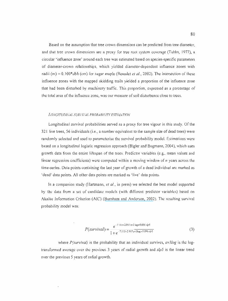
80

Based on the assumption that tree crown dimensions can be predicted from tree diameter,

and that tree crown dimensions are a proxy for tree root system coverage (Tubbs, 1977), a

circular 'influence zone' around each tree was estimated based on species-specific parameters

of diameter-crown relationships, which yielded diameter-dependent influence zones with

radii (m) = 0.1 OO*dbh (cm) for sugar maple (Beaudet et al., 2002). The intersection of these

influence zones with the mapped skidding trails yielded a proportion of the influence zone

that had been disturbed by machinery traffic. This proportion, expressed as a percentage of

the total area of the influence zone, was our measure of soil disturbance close to trees.

LO/v'GITUDl/'v'AL SURVIVAL PROBABILlTY ESTlivlATlO/'v'

Longitudinal survÎval probabilities served as a proxy for tree vigour in this study. Of the

321 live trees, 56 individuals (i.e., a number equivalent to the sample size of dead trees) were

random ly selected and used to parameterise the survival probability mode!. Estimations were

based on a longitudinal logistic regression approach (Bigler and Bugmann, 2004), which uses

growth data from the entire lifespan of the trees. Predictor variables (e.g., mean values and

linear regression coefficients) were computed within a moving window of n years across the

time-series. Data points containing the last year of growth of a dead individual are marked as

'dead' data points. Ali other data points are marked as 'live' data points.

In a companion study (Hartmann, et al., in press) we selected the best model supported

by the data from a set of candidate models (with different predictor variables) based on

Akaike Information Criterion (AIC) (Burnham and Anderson, 2002). The resulting survÎval

probability model was:

. e-7115+2.017av3Iog+0.006slp5

P(surv/val) = ,_ (3). 1+ e-711 5+2017uvJ!ug T0006.,/p)

where P(survival) is the probability that an individual survives, av3log is the log­

transformed average over the previous 3 years of radial growth and slp5 is the 1inear trend

over the previous 5 years of radial growth.

81

Parameter estimation was undertaken within R (version 2.6.0; R Development Core

Team, 2007), using maximum likelihood. Non-parametric confidence intervals for the

parameter estimates were computed with the bootcov bootstrap resampl ing procedure

from the Des ign library (Harrell, 2005), based on 1000 repetitions, with the 25 lh and the

975 th quantiJes serving as interval limits. Ta correct for underestimation of the true variance

and confidence interval width due to the interannual correlation of longitudinal tree-ring data,

the bootcov function substitutes cluster (= within tree) sampling with replacement for the

usual simple (= among trees) sampling with replacement. This modification resulted in

parameter estimates that can be regarded as unbiased.

Model performance was estimated with Somer's Dxy index (Somers, 1962), which is

indicative of the model's discriminative ability and is closely related to the area under the

curve (AUC) of a receiver operating characteristic (ROC) plot (Engelmann et al., 2003). The

Design bootstrap resampling procedure validate .lrm (Harrell, 2005) was used to

account for over-optimistic classification measures when validating models on training data

(data specificity). The validate. lrm procedure eliminates overfitting-induced optimism

of Dxy and produces a more conservative estimate of the modeJ's discriminative ability

(Harrell, 2001). The model used in this study had a Dxy value of 0.783, which corresponded

to an AUe of 0.892 and indicated excellent model performance (Manel et al., 1999, Table

3.1 ).

Table 3.1 Parameter estimates. bootslrapped 95% confidence intervals

(CI), AUC (ROC) and optimism-corrected Oxy of the logislic survival probability model

CI (95%)

Variables ESlimale Lower Upper Oxy AUC

Intercept -7.115 -8.974 -5337 0.783 0.892

av3-log 2.017 1.713 2375

slr5 0.006 0.004 0.007

82

Interpretation ofsurviva! probabilities

The above described procedure led to a very unbalanced data distribution (i.e., many 1ive

data points and few dead data points) and yields, using logistic regression, survival

probability estimates biased towards the more abundant group (Fielding and Bell, 1997).

Hence, survival probability estimates were ail very close to one and could not be interpreted

directly, i.e. as absolute measure of probability of survival, unless adjustments for the

unbalanced data distribution were undertaken. However, in our study, survival probabilities

were interpreted only as a relative measure of tree vigour among disturbance classes of trees

(see below), so threshold adjustments were unnecessary.

COt'vlPARlSON OF GROWTH INDICES AND SURVIVAL PROBABILITIES AMONG DISTURBANCE

CLASSES AND DEAD TREES

Live trees with available growth data were grouped into 4 anthropogenic disturbance

classes: (1) trees with neither machinery disturbance in their proximity nor a substantial

(>50%) increase in post-harvest 1ight levels (N = no disturbance, n= 134), (2) trees with

machinery disturbance in their proximity, but no substantial increases in light levels (M =

machinery, n=71); (3) trees with a substantial (>50%) increases in post-harvest light levels,

but no machinery disturbance (L = light, n=28); and (4) trees with both substantial (>50%)

increases in post-harvest light levels and with machinery disturbance (L&M = light and

machinery, n=16).

Of the 321 live trees, 249 fe11 within these classes, while the remainder contained trees

with either no machinery disturbance but light increases :s50% (n=51), or trees with

machinery disturbance but with light increases :s50% (n=21). Because de ad trees (D, n=56)

had to be searched for outside our sampling plots, we could compute disturbance levels for

these trees.

Since ring-width measurement and survival probabilities are usually not normally

distributed, we used the non-parametric Kruskal-Wallis test for annual comparisons of ring­

width indices among disturbance classes and with dead trees in the years prior to and

following harvest (1990-2004). We employed a non-parametric simultaneous rank test

83

procedure for multi-comparisons using the npmc function From the R package npmc (Helms

and Munzel, 2008). This procedure is based on estimations of simultaneous relative effects

and variance among pairs, does not assume continuity of the underlying distribution functions

(as Wilcoxon or other ranking procedures do) thereby allowing arbitrary ties. The procedure

can be applied to ail relevant multiple testing problems in the one-way layout and derives the

test statistic (I-V,:;) and P-values with the Behrens-Fisher test (Munzel and Hothorn, 2001).

Survival probabilities were analysed with the same procedure described above.

To test for differences between FTC defoliation and harvest disturbances, we used

corrected growth indices because these are assumed to be free of the effects of climate and

other environmental factors on growth rates (Swetnam et a1., 1985). We selected the 1986­

1992 FTC outbreak, which had the strongest influence on growth rates among ail inferred and

documented FTC outbreaks. We compared the averaged (within individual trees) growth

indices over this period with those over the i994-1998 post-harvest period (and just before

the onset of the next FTC outbreak in 1999), within each disturbance class and within dead

trees. Since we compared observations within growth chronologies of the same trees, we used

a Wilcoxon signed-rank test. This test requires equal sample sizes between the two groups, a

condition that was not met for dead trees for the 1994-1998 period due to mortality dropout.

We therefore compared data from this period with a random subsample (without

replacement) of the 1986-1992 period, applied a Wilcoxon signed-rank test on this balanced

sample, repeated this procedure 1000 times and averaged test P-values.

DEFINITION OF STRESSES ON TREE GROWTH AND VIGOUR

According to Manion's (1981) conceptual tree disease model, predisposing factors, such

as genetic potential or soil compaction, can determine initial tree vigour and, therefore, a

tree's vulnerability to further stresses. These factors are difficult or even impossible to assess

since an unambiguous benchmark for the absence of stress would have to be defined.

However, predisposing factois have a diffuse impact on tree vigour, allowing trees to survive

but with modified vital functions (Waring, 1987). In this study, predisposing factors are

defined as stresses with a moderate impact on tree vitality, i.e., on tree vital functions as

84

measured by radial growth. These stresses decrease radial growth levels but do not lead

ultimately and directly (without further stress) to tree death.

In contrast, according to Manion (1981), inciting factors are severe stresses, such as

defoliations or drought, which cause severe vigour declines and ultimately lead to tree death.

We used this definition with respect to radial growth and survival probabilities. [n an

accompanying study (H. Hartmann, unpublished data), trees with surviva! probabilities

permanently below 0.987 eventually died (data not shown). Hence, this value can be

considered a threshold for definite vigour decline and a benchmark for inciting stresses.

Contributing stresses may not play an essential l'ole in tree decline (Muller-Dumbois,

1987, Pedersen, 1998b) but can act as the 'coup de grâce' for declining trees by accelerating

their dec!ine. We defined contributing stresses as decreases in survival probabilities when

these had already fallen below the threshold of definite vigour decline.

SUMAdER CL/MATE DATA AS INDICATOR OF GROWTH CONDITIONS

We computed mean summer monthly precipitation and temperature (April-August) as an

indicator of climatic growth conditions from monthly climate data of the two closest nearby

(~60 km) weather stations (Environment Canada, http://climate.weatheroffice.ec.gc.ca).

85

3.5 Results

GROWTH DYNAtl4fCS OF UNDfSTURBED TREES

A comparison of average growth rates from 1910 to 2004 for undisturbed (by han'est)

live versus dead sugar maple trees showed that they both experienced a sudden increase in

growth rates in the late 1950's (Fig. 3.1 a). Shortly after this increase, growth rates of dead

trees started to deviate from those of live trees (about 1960). In ]971, a major drop in growth

rates of both live and dead trees occurred, which was followed by a continuous decline in

both groups. This decline was followed, in 1988, by another major drop in growth rates of

both live and dead trees (Fig. 3.la). The 199311994 harvest (indicated by the arrow in Fig.

3.1 a) caused a temporal increase in growth rates of dead trees, which then declined and died.

In live trees, the growth decline in 1988 was followed by an increase in growth to levels prior

to 1988, which were then maintained unti1 2004 (Fig. 3.1 a).

Average ring-width indices do not show the difference betWeen live and dead tree growth

patterns as clearly, at least for earlier years. Until 1965, standardised growth rates of de ad

trees were more variable and oscillated around live tree grovrth indices (Fig. 3.lb). From

1965 to 1995, growth indices of live and dead trees were almost identical and both groups

experienced a major drop in 1988, followed byan increase. From 1995 onwards, shortly after

the 199311994 harvest (indicated by the arrow in Fig. 3.1 b), growth indices of dead trees

declined whereas those of live trees maintained increases in growth levels until 2004 (Fig.

3.1 b).

86

o N

'EcoE ~

'-' .r:::. ..... a"'0 . .~ ~

1 Cl C co

Il:: 0

a ci

1910 1925 1940 1955 1970 1985 2000

2.0 b

1.5 Cf) Q)

.210-0 . c

05

00

1910 1925 1940 1955 1970 1985 2000 Time (years)

Figure 3.1 (a) Average ring-width (mm, lines) and sample size (trees, symbols) chronologies (1910-2003) of undisturbed (by harvest) live (solid line) and dead (dotted line) trees. (b) Average growth index chronologies (l9! 0 - 2003) of undisturbed (by harvest) live (solid line) and dead (dotted line) sugar maple trees. Arrows indicate the year of the se lection harvest.

Rescaled indices of yellow birch showed a growth pattern different From that of sugar

maple during several periods, especially in the 1930's, 1940's and 1960's (Fig. 3.2a).

Corrected sugar maple ring-width indices showed that growth of dead trees was affected

more than that of live trees by FTC defoliations from the 1930's until the mid-1940's, but

dead trees exhibited higher growth rates from about 1945 until 1965 (Fig. 3.2b). Decreases in

growth rates of dead trees lasted longer than those of live trees during the 1986-1992

outbreaks (see area LInder the curve in Fig. 3.2b). Although dead trees achieved a brief and

small increase in growth rates in 1994 and 1995, growth decJined again shortly after harvest

in 1996 (indicated by the thin arrow in Fig. 3.2b) and trees died shortly afterwards.

87

o N a

Indices (Ms) RI (By)

<J) (j)

.~ 0 -0 C

'"o

.' ',' . . ' ...

",'" :/". .... "

1 1 1 ) , 1 1 1 1 1 i i 1 Iii 1

1910 1925 1940 1955 1970 1985 2000

20i b

i"110

8 0511 0.0 -,.---r,-r,,,-----.,-'.-T,-r,,,-----.,"r-r,--r,--.-,'"r-r,-'.-T'­

1910 1925 1940 1955 1970 1985 2000

Time (years)

Figure 3.2 (a) Averaged ring-width indices (1910 - 2003) of undisturbed (by harvest) sugar maple trees (n= 134, same as in Fig. 3.1 b) and rescaled indices (RI) of yellow birch trees (n=20), a non-host species of the forest tent caterpillar. (b) Corrected ring-width indices of sugar maple trees obtained by subtracting RI in (a) from the host species (sugar maple) indices in (a). Cress hatched areas in (b) are periods of inferred (grey block arrows) or documented (black block arrows) FTC defoliations (see text for details). The down facing arrow in (b) indicates the year of the selection harvest.

We identified eight insect outbreaks during the period from 1910 to 2004 which

translated into an average outbreak cycle length of Il.75 years and an average outbreak

length of 4.6 years (data not shown). Ail but the 1957-1960 FTC outbreak could be

confirmed by MRNFQ survey data available for 1938-2002. However, the ministry survey

indicated a continuolls occurrence of FTC defoliations from 1950 until 1956, suggesting that

both the 1950-1954 and 1957-1960 growth dec1ines were caused by this single FTC outbreak.

88

GROWTf-f D YNA MfCS OF DfSTURBED TREES

To evaluate the impact of harvest disturbance on radial growth, we examined growth

ind ices for the 1990 - 2004 period, i.e., th.ree years prior to until 10 years after partia 1harvest.

In 1990, growth indices of dead trees were significantly different from those of und isturbed

live trees only (Table 3.2). From 1991 until 1994, there were no significant differences in

growth indices among disturbance classes. Indices of dead trees were srgnificantly different

from ail live trees in 1998, 2001, and 2003, from L, M, and N trees in 1999 and 2000, from L

and L&M trees in 1995, 1996, and 1997, and from N trees in 1995 (Table 3.2). Among live

trees only, the growth indices of L trees were different from those of M trees in 1995, 1997,

and 1997 and from N trees in 1995 (Table 3.2).

The 1986-92 FTC defol iation had a greater impact on corrected growth indices of live

sugar maple than any of the harvest disturbance types, but this was not the case for dead

sugar ma pie. Means of the averaged corrected indices during defoliation varied between

0.627 for L trees and 0.727 for N trees (Table 3.3). Duri ng the post-harvest period (1994­

1998), corrected indices were consistently higher for ail trees, ranging from 0.809 (D) to

1.267 (L) (Table 3.3). Differences in average corrected indices between periods of natural

and anthropogenic disturbance were highly significant (P <0.001) within disturbance classes

of ail live trees, but not significant for dead trees (Table 3.3).

89

Table 3.2 Behrens-Fisher tests on relative efTecl eSlimales of ring-width indices (1990 - 2003) bet\veen disturbance classes using a non paramelric simultaneous rank test procedure. Only significanl

(P<0.05) lests are shawn

Year

1990

ComparISon

D vs. N

n

189

Erfect

0.648

Relative effecl estimate CI CI

(Iower) (upper) Var.

0.518 0.778 0382

SE 0.045

WB!" N

1290

P

0.021

1995 D vs. L

Dvs. L&M

D vs. N

L vs. M

L vs. N

78

66

184

99

162

0.759

0.7 J9

0.669

0.296

0.281

0.592

0.531

0.506

0.106

0091

0927

0.906

0832

OA87

OA7 J

0.251

0.267

0.563

OAI3

0.671

0.057

0.064

0.055

0.065

0.064

4.571

3A41

1057

-1 l55

-3A03

0.002

0.019

0040

0.035

0.020

1996 D vs. L

D vs. L&M

71

59

0.694

0725

0.512

0.524

0.877

0.926

0.273

0275

0.062

0.068

3.133

3.J0 1

0.034

0024

1997 D vs L

D vs. L&M

L vs. M

69

57

99

0.748

0.729

0302

0.575

0537

0.112

0.921

0920

OA92

0.242

0.245

OA20

0.059

0.066

0.065

4.189

3A85

-3.035

0003

0015

0.039

1998 D vs. L

Dvs. L&M

D vs. ivI

D vs. N

L vs. ivI

67

55

110

172

99

0.799

0.747

0.681

0.729

0.259

0.638

0551

0502

0.566

0.082

0960

0.942

0.861

0.893

OA35

0.202

0.244

OAI2

0.534

0359

0.055

0.067

0.061

0.056

0.060

5A55

3.705

2.965

4.115

-4.012

0.000

0.010

0.047

0.004

0.005

1999 D vs. L

D vs. ivI

D vs. N

62

105

165

0.777

0.692

0.715

0593

0502

0.534

0.962

0883

0.895

0.242

OA37

0.615

0.062

0.065

0.061

4A41

2979

1519

0.002

0.047

0.016

2000 D vs. L

D vs. ivI

D vs. N

55

99

159

0749

0.737

0.728

0.545

0543

0.540

0.953

0.932

0917

0.261

OA28

0.646

0.069

0.066

0.064

3.611

3610

3584

0.014

0.013

0.014

2001 D vs. L

D vs. L&M

D vs. ivI

D vs. N

45

34

89

141

0749

0.754

0.767

0.758

0.520

0.503

0557

0.550

0978

1.005

0977

0.965

0.267

0243

0.445

0.688

0.077

0085

0.071

0070

3.234

3.009

3.775

3688

0.030

0.046

0.010

0.012

2003 D vs. L

D vs. L&M

D vs. ivI

D vs. N

30

20

72

113

0.872

0.880

0.845

0.870

0572

0.556

0.558

0.629

1.172

1.204

1.132

1.111

0.168

0130

0368

OA07

0.075

0.081

0072

0060

4.973

4.708

4822

6.174

0.022

0.027

0.024

0.009

90

Table 33 Mean, standard error (SE) and range of averaged corrected indices during FTC outbreak (1986­

1992) and harvest disturbances (1994 - 1998). P values refer 10 a Wilcoxon signed-rank tesl between periods. Negative values are in parentheses

Natural disturbance Harvest disturbance Disturbance class Mean SE Range Mean SE Range P

N 0.727 0.185 0.260 ­ 1281 \.033 0.255 0.561 - 2.048 <0001

M 0704 0.177 0.329 ­ 1.230 0.972 0.248 0.260 - 1.664 <0 001

L 0.627 0.234 0.223 ­ 1022 1.267 0.372 0495 ­ 2.047 <0.001

L&M 0.687 0151 0.283 - 0876 1156 0.292 0.614 - 1.752 <0.001

D 0.688 0.247 (0.189) ­ 1.252 0.809 0.419 0.132 ­ 1859 0352

Dead trees exJlibited the first signs ofvigour decline in 1977 (Fig. 3.3) following the FTC

outbreak in 1974-1976. Vigour of dead trees was lower before the 1986-1992 FTC olltbreak

than vigollr of live trees and was followed by a greater vigour decline dllring the 1986-1992

FTC outbreak than in live trees. Dead trees never regained their pre-FTC olltbreak vigour

levels and their vigour stayed below levels of live trees (Fig. 3.3). Multiple comparisons

(Behrens-Fisher tests) indicated that sllrvival probabilities of dead trees were significantly

different from those of ail four disturbance classes from J992 until 2002 (Fig. 3.3, Table

inset). In the post-harvest period (1994 onwards), no differences of sllrvival probabilities

among disturbance classes were detected (Fig. 3.3).

91

0 C!

.t'~ + 'y ~ ,~~~t x, A>. OJ <, r~

:!:: OJ \~,' ~ / \

15 0 \~f '.;, '.l, ii fil 't {/ ~ , \

.D -<>-- ~Jo ~ l' ~ ~ 0 L.. 00 -8- M3Chrn~ry _ \D.- Ol .+. \

0 LI;Jht 1(ij ._}f.- \Lj;lht&lv'êCI-j n~ry \f.::: 1..+- [J~:o:l ,r--.è OJ \

::J D·L 1977 193. 1~9J.2JO !(fJ ci D-L&N 1977 1970 IS9J.2J02 D·M '970 ISnn79 IS82-1388 .S91·J:)0" D·h ISlS-1379 IS82·1387 1939 ~92·.llJ2

ID LN 197J 1974 19JO Ol 0

1960 197D 1980 1990 2000

Time

Figure 3.3 Average survival probabilities of live and dead sugar maple trees from 1960 - 2003. Table inset specifies years of significant differences (P <0.05) between pairs of disturbance classes and dead trees and among disturbance classes. Arrows indicate the most severe years of FTC outbreaks (1974-1976, 1986-1992) and the partial harvest (1993). The horizontal 1ine indicates a crilical probabi 1ity threshold (P[Y= 1] =0.987) for a definite vigour decline (see text for details).

Mean summer temperatures were only slightly above the long-term average (1910-2003)

tn the years following harvest (1994-1997) and mean summer precipitation was above

average in 1994, on average in 1995 and again above average in 1996 (Fig. 3.4).

92

~

(Il

E 0

E '" ::J en --+. Temperature c (\j ---lib- Precipitation (Il

2 0 0 0 0 0 0 0 0 0 0

N N M M <D <D ..... ..... Ci) <Xl cr> cr> 0 0 '" '" '" '" '" '" '" '" '" '" cr> cr> cr> cr> cr> cr> cr> 0 0 " " '" '" ~ ~ ~ ~ ~ ~ ~ ~ ~ ~ ~ ~ ~ ~ ~ N N~

Time (yrs)

Figure 3.4 Mean summer (April-August) monthly precipitation (sol id line with stars) and temperature (dotted line with crosses) computed From climate data covering the years 1910-2003. Horizontal lines indicate the long-term mean precipitation and temperature across these years. The veltical 1ine indicates the year of the partial harvest (1993).

93

3.6 Discussion

THE NATURE OF PREDISPOSING AND INCITING STRESSES AND THEIR INTERACTION

In our study, dead trees were predisposed to inciting stresses by a first FTC defol iation in

1974-76 which decreased their initial vigour. The 1986-1992 FTC defoliation acted then as

an inciting stress having a longer lasting and more severe negative effect on growth rates and

vigour of dead trees than the 1974-76 outbreak. Although growth rates and survival

probabiJities of dead trees temporarily recovered shortly after harvest, their decline resumed

and accelerated drastically From 1997 onwards (Fig. 3.3). Harvest disturbances may have

contributed ta this acceleration as a contributing stress in these already weakened trees.

Successive defoliation events that can readily weaken more sensitive trees and trigger

sugar maple decline (Kolb and McCormick, 1993; Payette et 01., 1996). Carbon reserves of

dead trees may have been already reduced From repeated previous defoliations (Parker and

Houston, 1971) and the 1986-1992 severe defoliation may then have acted as inciting stress

in the decline of already weakened trees (Horsley et al., 2002). In live trees, more abundant

carbon reserves may explain their greater potentiaJ for recovery, which allowed to quickly

rebuild leaf area and subsequently, their photosynthetic apparatus (Landhausser and Lieffers,

2002).

Sugar maple tree decline and death was driven by an interaction between predisposing

and inciting stresses, as suggested by Manion's (1981) conceptual tree disease mode!.

Similarly, Hogg et al. (2002) found that FTC defoJiations combined with other environmental

stresses led ta reduced growth and crown dieback in trembling aspen (Populus Iremufoides

Michx.). Our results are in general agreement with those of other researchers who identified

defoliating insects (Payette et al. 1996), fungal pathogens (Cherubini et 01., 2002; Marçais

and Bréda, 2006) or drought (Pedersen, 1998a; Suarez et al., 2004) as inciting stresses in tree

decline and death.

94

fl'v/PACT OF ANTHROPOCENIC DISTURBANCES FROid PARTIAL HARVEST ON TREE CROWTH AND

V/COUR

Radial growth rates of live trees in ail harvest disturbance classes quickly regained or

even surpassed pre-disturbance growth levels after harvest disturbances and did not show a

growth stagnation known as 'thinning shock' (e.g., Staebler, 1956; Harrington and Reukema,

1983). On the contrary, trees with strong increases in light levels showed the greatest 'post­

disturbance growth increases lasting until 1998 (Table 3.2). A\thollgh photoinhibitive effects

of significant and sudden increases in light levels have been observed in seedlings of shade­

tolerant beech (faglls sylvatica L.; Tognetti et aL, 1997) and in saplings of shade-tolerant

sugar maple (Naidu and DeLucia, 1997), this does not seem ta be the case for adult sugar

maple trees in our study, even though mean increases in light levels were remarkably high

(> 600%, data not shown). Instead, acclimatisation of shade leaves in the lower canopy ta

higher light availability close to canopy gaps seemed to have increased photosynthetic rates

(Jones and Thomas 2007) and this translated into higher growth rates (Jones and Thomas

2004). Hence, sudden changes in light availability from partial harvest did not have the

potential to act as a stress causing growth declines but rather improved tree vitality.

Soil disturbance is thought to negatively impact radial growth of trees (Clayton et aL,

1987) through its effects on soil physical properties (Kozlowski, 1999) or potential damage ta

the root system (Waesterlund, 1992) but also through potentially resulting fungal infections

of the tree root system (Nadezhdina et aL, 2006). However, growth indices of trees that

experienced machinery disturbance were only lower than those of trees with increased light

levels, but not significantly different from those of undisturbed trees (Table 3.2). This is

surprising since these trees had a mean sail disturbance of 34.7 % (Table 3.\). The sail

texture in the study plots (which was either sandy, sandy loam or, in one plot, rocky) may

explain the absence of negative effects of machinery disturbance on growth. Coarse-textured

soi!s are not easily compacted (Horn, 1988; McBride and Joosse, 1996) and the dense root

network in the humus layer, formed by the abundant woody understory vegetation in the

studied maple stands (mostly tree regeneration, beaked hazel [Cary/us cornuta Marsh.], and

hobblebush [Viburnum lantanoides Michx.]), may increase soil strength and th us resistance

ta mechanical forces from logging equipment (Waesterlllnd, 1989). Machinery disturbance

95

apparently did also not cause fungal infections of the tree root systems and associated severe

growth declines as has been observed, for example, in trees infected with root rot (Mallet and

Volney, 1999; Cherubini et al., 2002).

COMPARING fivlPACTS OF INSECT OUTBREAKS AND HARVEST DISTURBANCES ON RADIAL

GROWTH AND TREE VIGOUR

Average corrected growth indices were lower during natural disturbance than during the

post-harvest period (Tab le 3.3), ind icating that FTC defo 1iation had a stronger negative effecl

on growth rates than any harvest disturbance. These results show that disturbances From

partial harvest, even in their most severe form, have no significant negative effect on tree

growth. It may be noted, however, that we did not sample trees that had incurred obvious

damage From harvest (uprooting, bole breakage, girdling, etc.). This type of 'disturbance'

would most probably cause growth reduction and has been found to cause high post-harvest

tree mortality (Nyland, 1994).

96

3.7 Conclusions

Our findings showed that disturbances From partial harvest, at worst, can act as

contributing stresses in trees that are already greatly weakened by predisposing and inciting

stresses, in our study FTC defoliations. Since the whole range of disturbance severity caused

bya partial harvest was sampled in this study, we must conclude that harvest disturbances did

not contribute to maple decline and death. However, favourable climatic conditions did not

impose severe constraints on tree growth in the post-harvest period. Hence, the impact of

harvest disturbance may have been different if climatic conditions, especially precipitation,

had been less favourable for growth (Hanson et al., 2001). The sud den exposure to su ni ight

From thinning may then impose an additive constraint on tree water status (Warren et al.,

2001) and this may impose a stress that not only decreases radial growth rates but may act as

inciting stresses in tree decline and death (Pedersen, 1998b).

97

3.7 Acknowledgements

We thank Catherine Malo for her help with the field work and dendrochronological

measurements, and Denis Boileau and Louis Deschamps for their help on identifying

disturbance history. Lana Ruddick and Bill Parsons have greatly improved the linguistic

qualit'j of the manuscript. Also, we greatly appreciated the comments of Virginie Angers and

two anonymous reviewers on an earlier draft of this paper.

98

3.8 References

Allen OC, Barnett CJ, Millers, land Lachance D. 1992. Temporal change (1988-1990) in su gal' maple health, and factors associated with crown condition. Canadian Journal of Forest Research 22: 1776-1784.

Beaudet M, Messier C and Canham CD. 2002. Predictions of understorey light conditions in northern hardwood forests following parameterization, sensitivity analysis, and tests of the SORTIE light mode!. Forest Ecology and Management 165: 235-248.

Bigler C and Bugmann H. 2004. Predicting the time of tree death using dendrochronological data. Ecological Applications 14: 902-914.

Bréda N, Granier A and Aussenac G. 1995. Effects of thinning on sail and tree water relations, transpiration and growth in an oak forest (Quercus petraea (Matt.) Liebl.). Tree Physiology 15: 295-306.

Bunn A. 2007. The dplR package. Version 1.0. Contributed R package. Available at: http://cran.r-project.org/web/packages/dplRJdpIR.pdf. (25 Apri 12008)

Bumham KP and Anderson DR. 2002. Model selection and multimodel inference: a practical information-theoretic approach. Springer, New York.

Canham CD. 1988. Growth and canopy architecture of shade-tolerant trees: response to canopy gaps. Ecology 69: 786-793.

Canham CD; Finzi AC; Pacala SW and Burbank OH. 1994. Causes and consequences of resource heterogeneity in forests: interspecific variation in light transmission by canopy trees. Canadian Journal ofForest Research 24: 337-349.

CFS (Canadian Forest Service) 2001. Forest tent caterpillars. Frontline Express Bulletin No. 9. Hel' Maj esty the Queen in Right of Canada. Available at: http://cfs.nrcan.gc.calnews/262. (25 April 2008).

Cherubini P, Fontana G, Rigling D, Dobbertin M, Brang P and Innes J1. 2002. Tree-life history prior to death: two fungal pathogens affect tree-ring growth differently. Journal ofEcology 90: 839-850.

Clayton JL, Kellogg Gand Forrester N. 1987. Soi! disturbance-tree growth relations in central Idaho cfearcuts. USDA Forest Service, Ogden, UT. Research Note fNT-372.

Dobbertin M. 2005. Tree growth as indicator of tree vitality and of tree reaction ta environmental stress: a review. European Journal ofForest Research 124: 319-333.

Duchesne L, Ouimet R and Houle D. 2002. Basal area growth of sugar maple in relation to acid deposition, stand health, and sail nutrients. Journal of Environmental Quality 31: 1676-1683.

Duchesne L, Ouimet Rand Momeau C. 2003. Assessment of sugar maple health based on basal area growth pattern. Canadian Journal ofForest Research 33: 2074-2080.

Engelmann B, Hayden E and Tasche D. 2003. Testing rating accuracy. Risk 16: 82-86. Fielding AH and Bell JF. 1997. A review of methods for the assessment of prediction errors

in conservation presence/absence models. Environmental Conservation 24: 38-49. Fitzgerald TD. 1995. The Tent Caterpillars. Cornell University Press, Ithaca, NY. Gehrig M. 2004. Methoden zur Vitalitatsbeurteilung von Baumen. Vergleichende

Untersuchungen mit visuellen, nadelanalytischen und bioelektrischen Verfahren. Ph.D. thesis. ETH Zürich, Switzerland.

99

Givnish TJ. 1988. Adaptation to sun and shade: a whole-plant perspective. Australian Journal ofPlant Physiology 15: 63-92.

Godman RW, Yawney HW and Tubbs CH. 1990. Sugar maple (Acer saccharum Marsh.) In: Burns RM., Honkala B.H. (technical coordinators) Silvics of North America. vol. 2. Hardwoods. Agriculture Handbook 654. Washington, D.C.: United States Department of Agricul ture Forest Service, 78-91.

Gosselin J, Grondin P and Saucier J-P 2000. Programme de connaissance des écosystèmes forestiers du Québec méridional. Rapport de classification écologique: érablière à bouleau jaune de l'ouest. [RN99-3065]. Ministère des Ressources naturelles du Québec, Québec Direction des inventaires forestiers. Québec.

Gross HL. 1991. Dieback and growth loss of sugar ma pie associared with defol iation by forest tent caterpillar. Forestry Chronicle 67: 33-42.

Hanson PJ, Todd DE Jr and Amthor JS. 2001. A six-year study of sapling and large-tree growth and mOltality responses to natural and induced variability in precipitation and throughfall. Tree Physiology 21: 345-358.

Harrell FE. 2001. Regression modeling strategies with applications ta linear models, logistic regression. and survival analysis. Springer, New York.

Harrell FE. 2005. The design package. Version 2.0-12. Contributed R package. Available at: http://biostat.mc.vanderbilt.edu/s/Design (25 April 2008)

Harrington CA and Reukema DL. 1983. Initial shock and long-term stand development following thinning in a Douglas-fir plantation. Forest Science 29: 33-46.

Helms J and Munze1 V. 2008. The npmc package. Version 1.0-6. Contributed R package. Availab le at: http://cran.r-projecLorg/web/packages/npmc/npmc.pdf (25 Apri 12008)

He1ms JA and Hipkin C. 1986. Effects of soil compaction on tree volume in a California ponderosa pine plantation. Western Journal ofApplied Forestry 1: 121-124.

Hogg EH, Brandt JP and Kochtubajda B. 2002. Growth and dieback of aspen forests in northwestern Alberta, Canada, in relation to climate and Însects. Canadian Journal of Forest Research 32: 823-832.

Holmes RL. 1983. Computer assisted quaJity control in tree-ring dating and measurement. Tree-Ring Bulletin 43: 69-78.

Horn R. 1988. Compressibility of arable land. Catena suppl. II: 53-71. Horsley SB, Long RP, Bailey SW, Hallet RA and Wargo PM. 2002. Health of eastern North

American sugar maple forests, and factors affecting decline. Northern Journal ofApplied Forestry 19: 34-44.

Jones TA and Thomas SC. 2004. The time course of diameter increment responses to selection harvest in Acer saccharum. Canadian Journal of Forest Research 34: 1525­1533.

Jones TA and Thomas SC. 2007. Leaf-Ievel acclimation to gap creation in mature Acer saccharum trees. Tree Physiology 27: 281-290.

Kienholz R. 1930. The wood structure of a "pistol-butted" mountain hemlock. American Journal ofBotany: 17: 739-764.

Kneeshaw DO, Williams H, Nikinmaa E and Messier C. 2002. Patterns of above- and below­ground response of understory conifer release 6 years after partial cutting. Canadian Journal ofForest Research 32: 255-265.

Ko1b TE and McCormick LH. 1993. Etio1ogy of sugar maple decline in four Pennsylvania stands. Canadian Journal ofForest Research 23: 2395-2402.

100

Kolb TE and McCormick LH. 1993. Etiology of sugar mapie decline in four Pennsylvania stands. Canadian Journal ofForest Research 23: 2395-2402.

Komatsu H, Katayama A, Hirose S, Kume A, Higashi N, Ogawa Sand Otsuki K. 2007. Reduction in soil water avai labi 1ity and tree transpiration in a forest with pedestrian trampling. Agricultural and Forest Meteorology 146: 107-114.

Kozlowski, TT 1999. Soil compaction and growth of woody plants. Scandinavian Journal ofForest Research 14: 596-619.

Landhausser SM and Lieffers VJ. 2002. Leaf area renewal, root retention and carbohydrate reserves in a clonai tree species following above-ground disturbance. Journal ofEcology 90: 658-665.

Lefrançois M.-L, Beaudet M and Messier C. 2008. Crown openness as influenced by tree and site characteristics for yellow birch, sugar maple and eastem hemlock. Canadian Journal ofForest Research 38: 488-497.

Mallett KI and Volney WJA. 1999. The effect of Armillaria root disease on lodgepole pine tree growth. Canadian Journal ofForest Research 29: 252-259.

Manel S, Dias J-M and Ormerod SJ. 1999. Comparing discriminant analysis, neural networks and logistic regression for predicting species distributions: a case study with a Himalayan river bird. Ecological Modelling 120: 337-347.

Manion, P. 1981. Tree disease concepts. Prentice Hall Inc. Englewood Cliffs, NJ. Marçais Band Bréda N. 2006. Role of an opportunistic pathogen in the decl ine of stressed

oak trees. Journal ofEcology 94: 1214-1223. McBride RA. and Joosse P1. 1996. Overconsolidation in agricultural soils: II. Pedotransfer

functions for estimating preconsolidation stress. Soil Science Society ofAmerica Journal 60: 373-380.

Millers l, Lachance D, Burkman WD and Allen DC. 1991. North American sugar maple decline project.· organization and field methods. USDA Forest Service. GTR NE-154, Radnor, PA.

MRNFPQ (Ministère des Ressources naturelles, de la Faune et des Parcs du Québec) 2002. Fréquence des épidémies de la livrée des forêts de 1938 à 2002, région 08. Available at: http://www.mrnfp.gouv.qc.ca/publicatiolls!forets/fimaq/LIV R08A. PDF (25 April 2008).

MRNFPQ 2003. Méthodes d'échantillonnage pour les inventaires d'intervention (inventaire avant traitement) et pour les suivis des interventions forestières (après martelage, après coupe et années antérieures). [ISBN 2-550-41221-6] Forêt Québec. Direction de l'assistance technique. Division des traitements sylvicoles, Ste-Foy.

Muller-Dumbois D. 1987. Natura1 dieback in forests. BioScience 37: 575-583. Munzel U and Hothorn LA. 2001. A unified approach to simultaneous rank test procedures in

the unba1anced one-way layout. Biometrical Journal 43: 553-559. Murphy G. 1983. Pinus radiata surviva1, growth and form four years after planting off and

on skid trai Is. New Zealand Journal ofForestry 28: 184-193. Nadezhdina N, Cermak J, Neruda J, Prax A, Ulrich R, Nadezhdin V, Gasparek J and Pokorny

E. 2006. Roots under the load of heavy machinery in spruce trees. European Journal of Forest Research 125: 111-128.

Naidu SL and DeLucia EH. 1997. Acclimation of shade-deve10ped leaves on saplings exposed to late-season canopy gaps. Tree Physiology 17: 367-376.

101

Nyland, R.D. 1994. Careful logging in northern hardwoods. In: Rice, JA (ed.). Logging damage: the problems and practical solutions. Ontario Ministry of Natural Resources Forest Research Report 117. Sault Ste. Marie, 29-51.

OMNR (Ontario Ministry of Natural Resources) 2004. Ontario tree marking guide, version 1.1. Ontario Ministry ofNatural Resources. Queen's Printer for Ontario, Toronto.

Ouellet 0 and 2arnovican R. 1988. Cultural treatment of young yellow birch (Betula alleghaniensis Brirton) stands: tree classification and stand structure. Canadian Journal ofForest Research 18: 1581-1586.

Ouimet R Guay S and Lang P. 2005. Évaluation de la distance minimale à respecter entre une tranchée et les arbres pour éviter la perte de vigueur des érables dans les érablières. Ministère des ressources naturelles et de la faune du Québec. Direction de la recherche forestière. Note de recherche forestière nO 130, Québec.

Pacala SW, Canham CD and Silander JA Jr. 1993. Forest models defined by field measurements: r. The design of a nnorth-eastern forest simulator. Canadian Journal of Forest Research 23: 1980-1988.

Pacala SW, Canham CD, Saponara J, Silander JA Jr, Kobe RK and Rjbbens E. 1996. Forest models defined by field measurements: estimation, error analysis and dynamics. Ecological Monographs 66: 1-43.

Parker JS and Houston DR. 1971. Effects of repeated defoliation on mot and root collar extractives of sugar maple trees. Forest Science 17: 91-95.

Parshall T. 1995. Canopy mortality and stand-scale change in a northern hemlock-hardwood forest. Canadian Journal ofForest Research 25: 1466-1478.

Payette S, FOltin MJ and Morneau C. 1996. The recent sugar maple decline in southern Quebec: probable causes deduced from tree rings. Canadian Journal ofForest Research 26: 1069-1078.

Pedersen BS. 1998a. Modeling tree mortality in response to short- and long-term environmental stresses. Ecological Modelling 105: 347-351.

Pedersen BS. 1998b. The role of stress in the mOltality of midwestern oaks as indicated by growth prior to death. Ecology 79: 79-93.

Peterson DW and Peterson DL. 1995. Climatic influences on radial growth of subalpine larch in the North Cascade Mountains. In: Schmidt, WC and McDonald, KJ (eds.). Ecology and management of Larix forests' a look ahead. USDA Forest Service, GTR­INT-319, Ogden, 268-271.

Poulin J and Messier C. 2007. Rapport de paramétrisation du modèle de simulation de la dynamique forestière SORTIE-ND pour la forêt boréale et sub-boréale de l'ouest du Québec. Available at: http://www.cef-cfr.ca/uploads/CEF/parametrisation.pd f (25 Avril 2008)

R Development Core Team. 2007. R: a language and environmentfor statistical computing. R Foundation for Statistical Computing, Vienna, Austria. Available at: http://www.R­project.org. (25 April 2008)

Renaud J-P and Mauffette Y. 1991. The relationships of crown dieback with carbohydrate content and growth of sugar maple (Acer saccharum). Canadian Journal of Forest Research 21: 1111-1118.

Robitaille A and Saucier J-P 1998. Paysages régionme( du Québec méridional. Les Publications du Québec, Sainte-Foy.

102

Ronnberg J. 2000. Logging operations damage to roots of clear-felled Picea abies and subsequent spore infection by Heterobasidion annosum. Silva Fennica 34: 29-36.

Sénécal D, Messier C and Poulin 1. 2003. Revue de littérature : principales causes de mortalité chez les arbres adultes et clé d'identification des arbres morts lignent. Groupe de recherche en écologie forestière interuniversitaire, UQAM, Montréal.

Shigo AL. 1986. A new tree biology dictionary: tenns, topics and treatments for trees and their problems and proper care. Shigo & Trees Associates, Durham, N.H.

Singer MT and Lorimer CG. 1997. Crown release as a potential old-growth restoration approach in northern hardwoods. Canadian Journal ofForest Research 27: 1222-1232.

Smith DM, Larson BC, Kelty MJ and Ashton PMS. 1997. The practice of si/viculture: appliedforest ecology, 9th edition. John Wiley and Sons, New York.

Somers RH. 1962. A new asymmetric measure of association for ordinal variables. American Sociological Reviews 27: 799-811.

Staebler GR. 1956. Evidence of shock fol!owing thinning of young Douglas-fir. Journal of Forestry 54: 339.

Startsev AD and McNabb DH. 2001. Skidder traffic effects on water retention, pore-size distribution, and van Genuchten parameters ofboreal forest soils. Soil Science ofAmerica Journal 65 224-231.

Suarez ML, Ghermandi Land Kitzberger T. 2004. Factors predisposing episodic drought­induced tree mortality in Nothofagus: site, climate and growth trends. Journal of Ecology 92: 954-966.

Swetnam TW and Lynch AM. ]989. A tree-ring reconstruction of western spruce budworm outbreaks in the Southern Rocky Mountains. Forest Science 35: 962-986.

Swetnam TW, Thompson MA and Sutherland EK. 1985. Using dendrochronology to measure radial growth ofdefoliated trees. USDA Forest Service, Agriculture Handbook 639. Washington, De.

Tardif J, Brisson J and Bergeron Y. 2001. Dendroclimatic analysis of Acer saccharum, Fagus grandifolia, and Tsuga canadensis from an old-growth forest, southwestern Quebec. Canadian Journal ofForest Research 31: 1491-1501.

Tognetti R, Johnson JD and Michelozzi M. 1997. Ecophysiological responses of Fagus sylvatica seedlings to changing light conditions. 1. Interactions between photosynthetic acclimation and photoinhibition during simulated canopy gap formation. Physiologia Plantarum lOI: 115-123.

Tubbs CH. 1977. Root-crown relations ofyoung sugar maple and yellow birch. USDA Forest Service, Research Note, NC-225. St. Paul, MN.

Wargo PM and Houston DR. 1974. Infection of defoliated sugar maple trees by Armillaria mettea. Phytopathology 64: 817-822.

Wargo PM Parker J and Houston DR. 1972. Starch content in roots of defoliated sugar maple. Forest Science 18: 203-204.

Wargo PM. 1981. Effects of defoliation on trees and stands, individual tree relationships: measuring response of trees to defoliation stress. In: Doane CC, McManus ML (eds.). The gypsy moth: research toward integrated pest management. USDA Forest Service, Science and Education Agency Technical Bulletin 1584. Washington, DC, 248- 267.

Waring RH. 1987. Characteristics oftrees predisposed to die. BioScience 37: 569-574. Warren CR, McGreath JF and Adams MA. 2001. Water availability and carbon isotope

discrimination in conifers. Oecologia 127: 476-486.

103

Wasterlund I. 1989. Strength components in the forest floor restricting maximum tolerable machine forces. Journal of Terramechanics 26: 177-182.

Wasterlund 1. 1992. Extent and causes of site damage due to forestry traffic. Scandinavian Journal ofForest Research 7: 135-142.

IV. EFFECTS OF ABOVE AND BELOW GROUND PARTIAL HARVEST

DISTURBANCE ON RESIDUAL SUGAR MAPLE (Acer saccharum Marsh.)

GROWTH AND WATER STRESS

Henrik Hartmann, Christian Wirth, Christian Messier & Frank Berninger

Article publié dans Tree Physiology 28: 1851-1862.

105

4.1 Abstract

Partial harvesting is known to modify both above and below-ground resource availability but may also induce sorne direct and indirect stress to residual trees due to machinery traffic and sudden changes in light levels. We studied sugar mapJe (Acer saccharum Marsh.) trees in stands that had undergone a selection han'est Il years prior to sampling to veritY whether sudden increases in light availability and soil disturbance from machinery would influence growth rates and could lead to water stress.

We selected trees that had experienced either no disturbance from partial harvest, soil disturbance only, sudden increases in light avaiJability only or both disturbances. We analyzed stem radial growth rates and stable carbon isotope composition (ol3C) of stem wood with an annual resolution from 10 years prior to until 10 years after partial harvest.

Our results showed that disturbances from partial harvest did not have a negative influence on growth rates or on mapJe water status. Although trees that experienced increases in light availability had higher o13e after harvest (indicating water use efficiency) increased growth rates suggest that these trees did not experience any water stress. Also, trees with soil disturbance did not show any signs of water stress. These results may partly be due to favorable climatic conditions (abundant precipitation and mild temperature) in the years following harvest and could be different under more severe climatic conditions.

Keywords: Selection cut, light availability, soil disturbance, tree water status.

106

4.2 Résumé

La coupe partielle redistribue des ressources du mi 1ieu (Ium ière, eau, nutriments) et améliore ainsi les conditions de croissance pour un nombre restreint d'arbres résiduels. Une plus grande interception de lumière augmente le taux de photosynthèse et la croissance à l'échelle de l'arbre mais également la conductivité stomatale et la demande en eau. Cette demande est habituellement contrebalancée par une plus grande disponibilité en eau par l'éclaircie du peuplement, mais la circulation de la machinerie près des arbres peut causer une compaction du sol et des dommages aux racines et ces perturbations peuvent ainsi réduire la disponibilité en eau au sol et / ou l'absorption d'eau par les arbres affectés.

Nous avons étudié l'érable à sucre (Acer saccharum Marsh.) dans des peuplements ayant subi une coupe partielle Il ans avant l'échantillonnage afin de vérifier si l'augmentation soudaine de la lumière jumelée à des perturbations du sol par la machinerie influence la croissance radiale et cause un stress hydrique.

Nous avons sélectionné des arbres échantillons selon quatre classes de perturbation: (1) aucune perturbation, (2) perturbation de la machinerie à proximité seulement, (3) augmentation de la lumière seulement et (4) les deux perturbations simultanément. Nous avons analysé la croissance radiale et le ratio isotopique (OIlC) des cernes de croissance à résolution annuelle de 10 ans avant jusqu'à 10 ans après coupe partielle.

Nos résultats montrent que les perturbations de la coupe n'ont pas eu d'impact négatif sur la croissance ni l'état hydrique des arbres. Quoique les arbres ayant vécu une augmentation de la lumière démontraient une augmentation de OIlC après la coupe (probablement due à une augmentation du taux photosynthétique), cette augmentation a été accompagnée par une hausse de la croissance radiale indiquant l'absence d'un stress hydrique. Similairement, les ratios isotopiques des arbres avec perturbation du sol n'ont pas ind iqué aucun signe de stress hydrique. Toutefois, ces résultats pourraient être dus, au moins en partie, à des conditions météorologiques estivales favorables (précipitation abondante, température modérée) dans les années suivant la coupe. Sous conditions plus contraignantes dans les années suivant la coupe (étés secs et chauds) les résultats de cette étude pourraient être différents.

Mots-clés: Coupe de jardinage, disponibilité de lumière, perturbation du sol, état hydrique des arbres

107

4.3 Introduction

Partial harvests remove varying proportions of canopy and understory trees to liberate

resources and, therefore, improve growth conditions of the released residual trees (Smith et

al. 1997). According1y, growth rates of residual trees foJlowing partial harvest have increased

in trees of different species and ages (e.g., Drew and Flewe11ing 1979, Bodner 1984,

Kneeshaw et al. 2002, Jones and Thomas 2004).

Partial harvest causes higher growth rates of residua1 canopy trees through increases in

light interception of exposed tree crowns (Wyckoff and Clark 2005) whose lower-canopy

leaves adjust to higher maximum area-based photosynthetic rates and higher stomatal

conductance (Jones and Thomas 2007)..Hence, increases in light interception increase

photosynthetic rates but also increase water demand for transpiration.

Residual trees close to skid trai1s may also experience root damage (Réinnberg 2000,

Guimet et al. 2005) and soil compaction (Kozlowski 1999) and this may impair root

development (Taylor & Brar 1991). Lower water availability in compacted soils (Starsev &

McNabb 2001) and decreased water uptake by damaged root systems both reduce the water

supply of affected trees. To mitigate the impact of water shortage and drought stress to the

whole organism trees can down regulate their transpiration rates by decreasing their canopy

leaf area or by reducing the stomatal conductance of their canopy (Sperry 2000, Sperry et al.

2002).

Experimental studies oftree physiological responses to stand thinning are often limited to

few measurements and 1 - 2 growing seasons only (e.g. Bréda et al. 1995, Stoneman et al.

1997, Jones and Thomas 2007). Instead, tree-rings provide an integrated archive of the

environmental conditions at the time when the wood was deposited (Saurer et al. 1997). They

can serve to trace back the growth responses but also the photosynthetic behavior of trees for

thousands of years with an annual resolution (McCarrol and Loader 2004). Fluctuations in

stable carbon isotope ratios of tree-rings have been used to reconstruct past climate

conditions (e.g. Lipp et al. 1991) but also in ecophysio10gical studies reJating climatic

variables to physiological processes such as respiration (e.g. Beminger et al. 2000, Bowling

et al. 2002&2003, Fessenden and Ehleringer 2003).

lOS

However, variations in o13e can also be caused by increases in photosynthetic activity at

constant stomatal conductance. Scheidegger et al. (2000) used information on evaporative

enrichment in the 018 0 of plant matter to distinguish between biochemical and stomatal

limitations to photosynthesis in response to changes in environmental conditions (e.g.,

precipitation). Saurer et al. (1997) proposed linking growth rates with variations in o13e to

indicate whether photosynthetic activity or stomatal conductance caused variations in o13e in

response to environmental conditions: (1) If enhanced photosynthetic activity at constant

stomatal conductance (= no water stress) increases oDe growth rates should increase

simultaneously. (2) If increased stomatal conductance (= decreasing water stress) increases

e02 supply, oDe becomes more negative along with higher growth rates indicating higher

photosynthetic activity. (3) o13e may stay constant if the plant controls stomataJ conductance

and photosynthetic capacity simultaneously. In this situation growth rates may vary

depending on the tree's ability to adjust to prevailing growth conditions (i.e. irradiance, water

supply). Similarly, a constant photosynthetic rate under reduced stomatal conductance (due to

reduced water supply) will yield higher o13e and Jower growth rates.

In this study, we investigated the responses of radial growth rates and stable carbon

isotope discrimination in stem wood of residuaJ sugar maple trees (Acer saccharum Marsh.)

following partial harvest. Trees were classified according to the degree of impact (soil

disturbance, light increases) from harvest. To interpret changes in radial growth and 13 e discrimination in response to harvest disturbance the application of the theoretical framework

of Saurer et al. (1997) allowed us to formulate the following hypotheses (sensu Saurer et al.

1997): (1) completely undisturbed trees (no light increase, no soil disturbance) should show

no sign ificant changes in neither growth rates nor ol3e following harvest (constant

photosynthetic rate at constant stomatal conductance and no water stress); (2) trees with

strongly increased light levels but with no soil disturbance should show higher growth rates

and less negative o13 e values following harvest; (3) trees with no increase in light levels but

with much soil disturbance should have constant (or decreasing) growth rates and less

negative o13 e values following harvest, and (4) trees with strongly increased light levels and

with much soil disturbance should have decreased growth levels and much less negative oDe values following harvest.

109

4.4 Material & methods

STUDY SITE

The study sites are located in western Quebec (Canada, 46°43' north, 79°04' west). The

region has a mean an nuai temperature varying from 2.5 to 5.0°C, the growing season extents

over 170 to 180 days and the mean annual precipitation ranges from 800 to 1000 mm, with

snowfall comprising roughly 25% of total precipitation (Gosselin et al. 2000). Soils are

podzols with sandy to loamy texture derived principally from glacial tills or fluvio-glacial

deposits (Robitaille and Saucier 1998).

STUDY PLOTS

In 2004 and 2005, 19 plots (26 m x 56 m) were established in sllgar maple stands on level

ground or on gentle slopes with good to moderate drainage. In 1988 the stands had

experienced a severe forest tent caterpillar (Malacosoma diSSlria Hllbner, FTC) outbreak and

had been harvested by selection cuts in 1993 or 1994 wh ich redllced pre-harvest basal area

from an average 27 m2/ha to an average 21 m2/ha.

In the plots, sugar maple was, on average, the most frequent species (almost 70% of total

basal area), followed by yellow birch (Belula alleghaniensis Britton, 18%), red oak (Quercus

rubra L., 3.0%). American beech (Fagus grandifolia Ehrh., 2.3%), eastern hemlock (Tsuga

canadensis [L.] Carr., 1.8%), eastern white cedar (ThuJa occidentalis L., 1.6%), and red

maple (Acer rubrum L., 1.5%). Other species, such as balsam tir [Abies balsamea (L.) P.

MilL] and white spruce [Picea glauca (Moench) Voss], occllrred in minor proportions (:S 1%

of total basal area) (Table 4.1). Average post-harvest diameter at breast height (dbh, 1.3 m

above ground) varied between 155 mm for balsam tir and 422 mm for eastern hemlock.

Canopy height reached 19.2 m in eastern white cedar and up to 23.8 min red oak (Table 4.1).

110

Table 4.1 Minimum, maximum and mean trce diameler at breas! height (dbh, mm) and trec heighl (m) and

average lree density per species in the sample plais

Tree dbh Tree height Average density (mm) (m)

Species min max mean min max mcan (tree/ha) m'/ha

Yellow birch 92 849 271 5.8 31.1 193 49 18.0

Red oak 91 685 405 112 30.8 238 4 30

White spruce 91 370 196 6.1 25.7 15.2 6 0.9

Red maple 93 720 299 7.1 333 21.9 3 1.5

Sugar maple 91 792 230 53 35.8 183 269 69.9

American Beech 91 542 203 4.9 31.0 15.4 Il 23

Eastern hemlock 225 631 422 14.9 243 20 1 3 1.8

Balsam tir 91 270 155 6.1 19.6 12.4 10 1.0

Eastern white cedar 173 575 416 2.5 26.4 19.2 2 1.6

Within the plots, the diameter of ail live and dead trees >9.1 cm dbh and of ail stumps

(dsh, ::::: 0.5 m above ground) from the 19931\994 harvest was measured and their position

was mapped. We achieved mapping by laying out a virtual grid on the forest floor for which

the plot center line served as y-coordinate. X-coordinates were determined by measuring

(using a Hagloff Vertex m® hypsometer, Haglof Sweden AB) the perpendicular distances of

tree positions from the center line. Orientation (magnetic azimuth) of the plot center line was

measured with a standard forester's compass.

Skidding traits from the 199311994 harvest were also measured. However because

regeneration dynamics and litter accumulation since harvest (::::: Il years) made skidding trail

identification difficult, we used severa 1 ind icators as evidence: (1) 1inear opening in the

canopy, (2) ruts and tire (or skidding) wounds at the basis of trees, (3) dense undergrowth of

light and soil disturbance-dependent species (e.g. yellow birch, pin cherry [Prunus

pensylvanica L.f.], poplars [Populus spp.]), (4) stumps in the proximity, (5) absence of

obstacles (boulders, escarpments etc.), (6) conformity with machinery constraints (e.g.

turning radius), and (7) general concordance with the trail network and stand features. Only

when aIl ofthese criteria were satisfied, skidding trails were considered for further analysis.

We drew the skidding trait paths as the estimated center of skidding trails on the tree

maps using tree positions as landmarks. We could not directly measure traiJ width because of

forest floor vegetation and litter accumulation. We therefore estimated original trail width

III

with an approximate but realistic machinery width (4 m). Hence, skidding trails were

assumed to be 2 m wide from either side of the central trail path.

We evaluated the impact of machinery traffic on soil bulk density by measuring

penetration resistance with adynamie penetrometer (PEM-l, Roctest Inc., Montreal,

Quebec). In each of the plots, we took five measurements at -1 m intervals across each three

transects on skidding trails and three on the undisturbed forest floor. For trail measurements

we selected only trail sections with c1early defined trail features (wheel tracks, inter-wheel

space, off trail). Transect locations were chosen randomly and the five measurements on skid

trails were placed so that measurement 1 and 5 were off-trail, measurement 2 and 4 on wheel

tracks, and measurement 3 in the inter-wheel space.

TREE-RING DATA

In the mapped plots increment cores (3 cores pel' tree) were taken of ail trees between

19.1 cm and 49.0 cm dbh as a retrospective measure of radial growth. Trees <19.1 cm were

not sampled to avoid the juvenile effect in 13C discrimination (Freyer 1979, Francey and

Farquhar 1982) and to avoid trees with heavi Iy suppressed growth rates. Trees >49.0 cm were

not sampled to avoid trees with declining growth rates due to senescence. We sampled a total

of 321 sugar maple trees.

Increment cores were progressively sanded down to grain 400 to allow unambiguolls

identification of tree-rings. We measured tree-rings with a microscope equipped with a

computer-assisted micrometer (0.001 mm precision). At least two cores per tree were

readable in most cases and we averaged ring-width measurements among cores to account for

intra-tree variability of radial increment due to growing conditions or leaning (Kienholz

1930, Peterson and Peterson 1995). This then yielded a single growth chronology pel' tree.

We took radial growth measurements of dominant canopy trees to construct a master

chronology by adding progressively highly correlated (l'-values 2:0.3, Tardif et al. (2001))

tree-ring series to the already existing ones and obtained a final master chronology containing

29 ind ividual tree-ring series with ail overail cross-correlation coefficient of 0.479.

112

We cross-dated (matching of tree-rings with calendar years) the remaining tree-ring

series based on (1) visual examination of marker years (severe growth declines in 1971 and

1988) and (2) cross-correlation coefficients of chronology segments with the master

chronoJogy. We ran COFECHA to detect missing or false rings in individual segments of

tree-ring series and, in suspect cases, we identified false or missing rings on the cores or cross

sections and added tree-rings with zero width or removed these from the series. We then run

COFECHA again on theses series to veritY improvements of the cross-correlations with the

master chronology.

Only trees whose ring-width series showed strong cross-correlations (r> 0.4) with the

master chronology were retained for further analysis. Because we wanted to exclude harvest

disturbance not related to sudden light increases or soil disturbance from influencing growth

and carbon isotope responses, we withheld data from trees with obvious and severe

mechanical damages from harvest (uprooting, bole breakage, etc.) from further analysis.

We standardized these tree-ring series by dividing each individual tree-ring series by its

Jong-term growth trend, estimated with a cubic smoothing spline over the entire series.

Resulting dimensionless ring-width indices cOllld be more adequately compared among trees

at different ages and from different sites. This standardization procedure was done using the

i.detrend function from the contriQuted R package dplR (Bunn 2007) in the R software

environment for statistical compllting and graphies (version 2.6.0, R Development Core

Team 2007).

Becallse stable carbon analysis was limited to the period 1983 - 2003 (see below) the

growth series were truncated for further analysis at these years. In order to reduce inter-tree

differences in ring-width indices before harvest we rescaled each series individually by

divid ing each ring-width series by its pre-harvest (1983-1993) average. These resca led val ues

could be more adequately compared and averaged over treatment groups than series of raw

ring-width indices.

113

ME"J.SURES OF HARVEST OfSTURBANCE

Sudden changes in light conditions

Because the harvest took place Il years prior to sampling, changes in light conditions

cou Id not be measured directly and had to be estimated retrospectively. Using spatial

information on trees and stumps of the Jast harvest, we were able to simulate pre-harvest

stand conditions. To achieve this, we converted dsh measurements oftree stumps to dbh with

existing conversion tables (MRNFP 2003) and these were then considered dbh measurements

of cut trees before harvest. When external criteria of dead trees such as the presence of bark

and fine branches, stem wood decay or crown deterioration (Sénécal et al. 2003) indicated

that these trees died only after harvest we considered these trees as being alive in the pre­

harvest stands (2.9% of ail trees). The dbh measllrements and estimates of aIl trees present

before harvest (live trees + cut trees + trees dead :s Il years) were then loaded into the forest

dynamics simulator SORTIE to estimate light availability for individual trees (a

comprehensive overview of SORTIE's structure and simulation procedure can be found in

Deutschman el al. (1997) at: http://www.sciencemag.orglfeatllre/data/delltschman

/index.htm).

We parameterized SORTIE with regional parameters of tree species allometry and tree

canopy light extinction coefficients (Lefrançois et aL, in press). Based on these parameters,

SORTIE models tree dimensions and estimates light availability for each individual tree in

the stand as the seasonally averaged percentage of full sun (Canham 1988). Estimations of

light avaiJability for each individual tree, in the centre of simuJated crowns at 0.75*crown

height, were done for pre- and post-harvest plots. Dividing post-hal-vest light availability by

pre-harvest light availabiJity yielded our measure of changes in light conditions.

Sail dislurbance at tree proximity

Assuming that tree crown dimensions can be predicted from tree diameter, and that tree

crown dimensions are a proxy for tree root system coverage (TlIbbs 1977), a circular

'influence zone' was estimated around each tree based on species specifie parameters of

diameter-crown relationships. This yielded a diameter-dependent influence zones with radii

(m) for sugar maple = 0.1 OO*dbh (cm) (Bealldet et al. 2002). By intersecting the influence

zones of the mapped trees with the mapped skidding trails we obtained an estimate of the

114

proportion of the influence zone that had been disturbed by machinery traffic. The ratio of the

area of the influence zone disturbed by machinery traffic divided by the total area of the

influence zone served as our measure of soil disturbance at tree proximity.

Dislurbance classes

Ali retained trees were grouped into 4 disturbance classes: (1) trees withollt slldden

increases in light levels or soil disturbance (no disturbance treatment), (2) trees with strong

sudden increases (> 100%) in Iight levels following harvest but without soil disturbance (Iight

treatment); (3) trees with no sudden increase in light levels but with soil disturbance (>30%

ofintluence zone (soil treatment), and (4) trees with both strong sudden increase (>100%) in

light levels following harvest and with soil disturbance (>30% of influence zone (Iight and

soil treatment). For each of the 4 disturbance classes we selected randomly 5 trees for both

growth and stable carbon isotope analysis. Sample sizes were limited because of the large

number of carbon isotope analysis (20 trees x 21 years = 420 analyses) and associated costs.

The threshold for soil disturbance for these four classes had been set assuming that

disturbance >30% of the forest floor surrounding trees should have an affect on tree growth

and water status through the impact of soil compaction and root damage (Kozlowski 1999,

Ronnberg 2000, Ouimet el al. 2005). For sudden increases in light levels we chose> J00%

because increases up to -40% have been found to still allow a graduai acclimation of leaf­

level photosynthetic activity in mature sugar maple trees (Jones and Thomas 2007).

STABLE CARBON ISOTOPE ANALYSIS

The isotopie composition of a carbon compound (ol3C), the proportional deviation of the

1Je/2e ratio from the Vienna Peedee belemnite (VPDB) carbonate standard is defined as:

(1 )

In plant organic matter the IJe/le ratio (op) is depleted in 1Je compared to the

atmospheric 13e composition (oa)' This discrimination (L'-.) against 13e can be expressed as:

115

(2)

Discrimination of 13C over 12C results from two processes. Firstly, 13C0 2 diffuses more

slowly in air (and thus through stomata) into the intercellular spaces of the leaves due to its

heavier molecular mass. Secondly, the enzyme-catalyzed fixation of CO2 itself (Rubisco

carboxylation) causes a further discrimination against I3C0 2. Considering only C3 plants (as

ail trees are), we can express the fractionation process as follows (Farquhar et al. 1989):

6=a Pu -P, +b.!l.=a+(b-a)Jl Pa Pa Pli (3)

where 6 is the 13C discrimination and a and b are the parameters describing, respectively,

the fractionation due to diffusion of CO2 in air (4.4%0, a theoretical value) and by the enzyme

Rubisco (22%0 to 34%0). The parameters Pa and Pi represent partial pressures of CO2 in the

ambient air and the interce lIu laI' air spaces, respectively.

The trees selected for further analysis were cut down and cross sections of the trunk were

taken at 1.3 m height. To avoid carbon contamination from chain saw lubricants sma!1

rectangular pieces were cut from the interior of these cross sections with a band saw. The

sections were then further cut to coyer a 10-year period before and after the year of harvest

which yielded a sampling period spanning from 1983 to 2003.

Although the actual fractionation processes of the heavier 13C02 are beyond active

control by plants Pi inside the leaf is influenced by stomatal aperture as follows. Under

conditions of limited water supply, plants reduce the leaf stomatal conductance through

partial or complete stomata closure in an attempt to use water more efficiently, i.e. to fix

more carbon for each unit of water transpired. Since stomata closure also limits diffusion of

CO2 into the leaf, the intercellular concentration ofC02drops with continued photosynthesis.

From equation (3) it is obvious that this will decrease 6. Hence, higher water use efticiency is

therefore associated with decreases in f":" (Farquhar and Richards 1984) and this makes stable

carbon isotope ratios a useful measure for plant water relations (Francey and Farquhar 1982,

Farquhar et al. 1989).

116

To prevent mobile substances and handl ing contaminations from interfering with stable

carbon isotope measurements the wood sections were extracted with a 2: 1 (v/v)

toluene:methanol solution for several hours in a heated ultrasonic bath and oven-dried at

70°C overnight (Loader et al. 1997). Single tree-rings were th en shaved from the wood

sections with a surgical scalpel. These shavings were milled in a baIl mixer mitl MM 200®

(Reisch GmbH, Haan, Germany) to ascertain a homogeneous distribution of late and early

wood in the sample. Three of the wood section had tree-rings so tightly spaced that shaving

with an nuaI precision and subsequent milling was not feasible. These sections were therefore

eut to dimensions that allowed their measurement in a 'laser ablation combustion gas

chromatography isotope ratio mass spectrometry' (LA-C-GC-IRMS) (Schulze et al. 2004).

Ali other milled wood samples were weighted in tin cups and processed with a conventional

'elemental analyzer' (EA)-IRMS. Since the laser ablation technique necessitated the use of

whole wood sections, conventional isotope ratio analysis was also based on whole wood

samples. Moreover, it has been shown by others that undecayed whole wood and extracted

cellulose had very coherent ODC signatures with whole wood samples having slightly less

negative 0DC va lues (Loader et al. 2003). Laser trajectories spanned across the entire ring

width so that ablated wood material contained both early and late wood and that averaged

o13C val ues cou Id be considered representative for entire tree-rings.

Sequential isotopie analyses of milled wood samples were done using a Finnigan MAT

DeltaPlus XL EA-IRMS coupled to an autosampler. For the laser ablation technique a

frequency quadrupled Nd:YAG 266 nm UV-laser (New Wave Research Merchantek) was

used for ablating wood dust from the samples. After combustion of the ablated wood dust

CO2 was separated from other combustion gases and analyzed with a Finnigan DeltaPlus XL

EA-IRMS. Measurement precision of o'JC analyses was < 0.1 %0 for milled wood samples

and < 0.25%0 for the laser ablation technique, based on measurements of an internai lab

standard (NBS 22: -30.03%0 vs. VPDB scale). Ali isotope measurements were done in the

Iso-Lab of the Max-Planck-Institute for Biogeochemistry in Jena.

For consistency with ring-width measurements and to reduce differences in 013C between

individual trees, we rescaled ol3e values by dividing individua! time series by their pre­

harvest (1983-1993) average. This rescaling implies that values below 1 are indicative of

117

post-harvest increases in 013C (less negative) and are therefore indicative of constrained post­

harvest water status. Values above 1 indicate improvements in water supply or decreases in

water use and are therefore indicative of releases of the pre-harvest water status of trees.

We did not correct Ol3C values for time trends due to CO2 enrichment of the atmosphere

because time series spanned across 21 years only and comparisons were undertaken between

treatment groups for which the atmospheric enrichment was identical.

CLIMATE-CROWTH AND CLIMATE-O/ 3C RELATIONSHfPS

Monthly mean climate data (precipitation, temperature) were obtained From the Canadian

National Climate Data and Information Archive, operated and maintained by Environment

Canada (http://climate.weatheroffice.ec.gc.ca) Weather stations closest to our study sites (­

60 km) were Barrage Temiscaming (46° 42.600'N, 79° 6.000' W, elevation 181.40 m) and

Rapide des Joachims (46° 12.000' N,77° 42.000' W elevation 137.20 m). Monthly climate

data From Barrage Temiscaming were discontinued from 1995 onwards so we amended the

data set by adding data From Rapide des Joachims and averaged values in overlapping years

(1983-1995).

To quantify the climate-growth and the climate-ô l3 C relationships, we performed a

correlation and response function analyses with the program Dendrocl im2002 (Biondi and

Waikul, 2004). The correlation function gives univariate estimates of Pearson's product

moment correlation between ring-width indices (or o13C indices) and climate variables,

whereas the response function is a principal component regression model of the multivariate

climate data with ring-width indices (or Ôl3C indices) as the response variable. To account for

multicollinearity in climate data and to add more accuracy to the correlation and the response

function analysis, Dendroclim2002 computes bootstrapped confidence intervals of the

parameter estimates for both functions (Biondi and Waikul, 2004). Only climate variables

with consistently positive or negative parameter estimates within the 95% bootstrapped

confidence interval are considered significant.

118

STATfSTfCAL ANALYSfS

We tested for di fferences of rescaled ring-width ind ices and of rescaled o13 e between

treatments on an annual basis. Due to smal! sample sizes (5 frees per treatment for 4

treatments per year = 20 measurements per year) and because of heteroscedasticity of the

variances among groups we avoided the use of ANOVA. Instead we used a permutational

analysis of variance (Anderson 2001, McArdle and Anderson 200!) with the free statistical

program PERMANOVA (Anderson 2005). PERMANOVA tests assume only that individual

observations can be exchanged under a true null hypothesis. The program provides a

partitioning of variation, based on distance measures, according to treatment factors and uses

permutations to test for differences between groups (factor levels). First, the program

estimates a distribution of the test statistic F under a true null hypothesis (i.e., no differences

between groups) by randomly shuffling group labels among observations. For each

permutation PERMANOVA computes the test statistic F*. Probabilities for the tests under a

true null hypothesis are computed as the proportion of aIl permutational F* values that are

greater than or equal to the value of F observed for the real data (Anderson 2005). Similarly,

painvise comparisons are based on the permutational test statistic t* and probabilities for the

test under a true null hypothesis are estimated as the proportion of ail permutation al t* va lues

that are greater than or equal to the value of t observed for the real data.

For both test procedures we used 4999 permutations to estimate F* and t* distributions as

recommended by the authors of the program (Anderson 2005). Signifïcance levels of

permutational ANOVA was 0.05 but were adjusted for multiple comparisons using the Tukey

correction which, for six comparisons, yields an (J. threshold of 0.0085.

We used contrasts of pre- vs. post-harvest levels in rescaled ring-width indices and in

rescaled o13 e within treatments to test whether harvest caused a change in these variables

within a given treatment. Significance tests of these contrasts were done with t-tests after

confirming normality of the sample distributions with Kolmogorov-Smirnov tests.

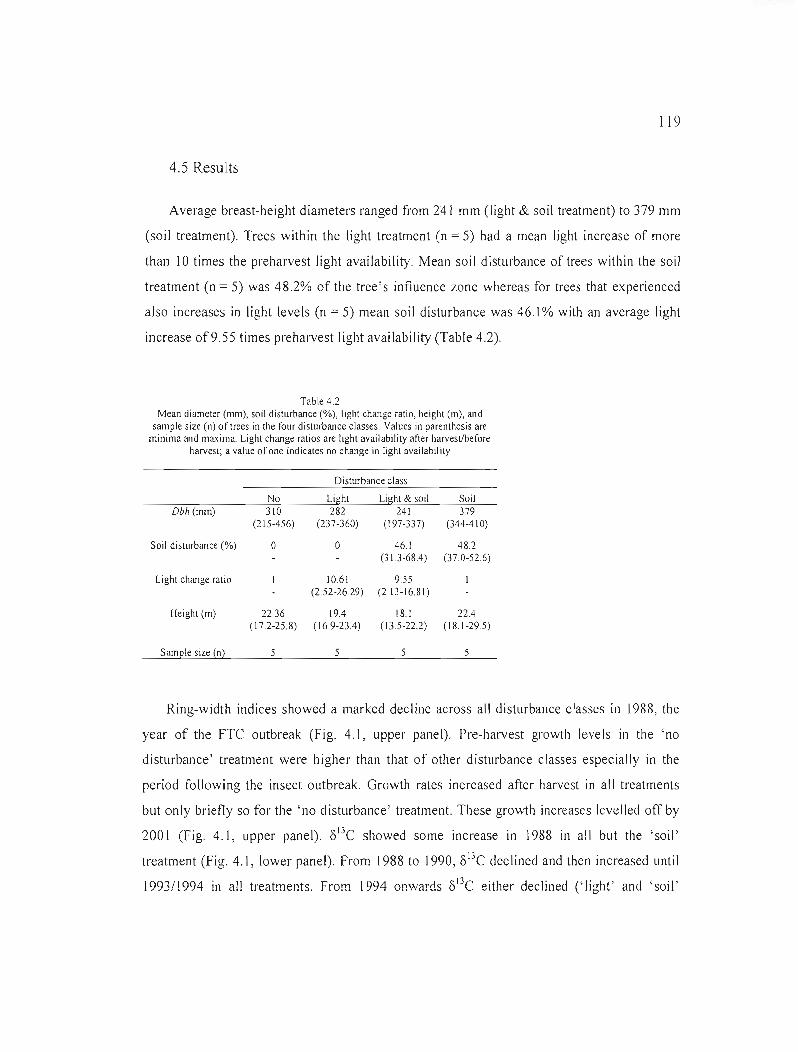
119

4.5 Resu1ts

Average breast-height diameters ranged from 241 mm (Iight & soil treatment) to 379 mm

(soil treatment). Trees within the light treatment (n = 5) had a mean light increase of more

than \0 times the preharvest light availability. Mean soil disturbance of trees within the soil

treatment (n = 5) was 48.2% of the tree's influence zone whereas for trees that experienced

aJso increases in light levels (n = 5) mean soil disturbance was 46.1 % with an average light

increase of9.55 times preharvest light availability (Table 4.2).

Table 4.2 Mean diameter (mm), soil disturbance (%), lighl change ratio, heighl (m), and

sample size (n) OrlreeS in the l'our disturbance classes. Values in parenlhesis are minima and maxima. Lighl change ralios are lighl availability arter harvesLlbefore

harvesl; a value of one indicales no change in Iighl availability

Disturbance class

No Lighl Lighl & soil Soil Dbh (mm) 310 282 241 379

(215-456) (237-360) (197-337) (344-410)

Soil dislurbance (%) 0 0 46.1 48.2 (313-68.4) (37.0-526)

Lighl change ratio 10.61 9.55 (2.52-26.29) (213-16.81)

Heighl (m) 2236 19.4 18.1 22.4 ( 172-25.8) (169·23.4) (135-22.2) (18.1-295)

Sample size (n) 5

Ring-width indices showed a marked decline across ail disturbance classes in 1988, the

year of the FTC outbreak (Fig. 4.1, upper panel). Pre-harvest growth levels in the 'no

disturbance' treatment were higher than that 0 f other disturbance classes especiaJly in the

period following the insect outbreak. Growth rates increased after harvest in ail treatments

but only briefly so for the 'no disturbance' treatment. These groyy1h increases levelled off by

200\ (Fig. 4.\, upper panel). S13C showed some increase in \988 in ail but the 'soil'

treatment (Fig. 4.\, lower panel). From \988 to \990, S13C declined and then increased until

1993!!994 in ail treatments. From \994 on'Nards S13C either declined ('Iight' and 'soil'

120

treatment) or remained constant ('no' and 'Iight & soil' treatment) over time until 2003 (Fig.

4. t, lower panel).

01 N 1­

a 0' '--­

1984 1988 1992 1996 2000

CD <;'

~

'" <;'""00 <;'

<Jl <;'

1984 1988 1992 1996 2000

Time (yrs)

Figure 4.1 Average ring-width indices (upper panel) and average (iDe (Iower panel) From J983 - 2003 of the four disturbance classes. The horizontal lines indicate the pooled average of all J983-2003 values. Note the negative impact of the forest tent caterpillar (FTC) outbreak on ring-width indices of ail disturbance classes.

RescaJed ring-width indices showed two declines within the 1983-2003 period dropping

below the pooled (ail treatments) pre-harvest average. In 1988, the year of the FTC outbreak

rescaled growth indices of ail disturbance treatments declined below the 1983-1993 average

(Fig. 4.2, upper panel). However, trees of different disturbance classes responded differently

to harvest. Mean rescaled ring-width indices oftrees in the 'Iight' and in the 'light & soil'

121

treatment increased and stayed above pre-harvest levels until 2003 (except for 2002 where

the 'Iight' treatment fel! briefly and slightly below the mean). Mean rescaled ring-width

indices of the 'soil' treatment showed a one-year lag in response but increased in 1995 and

stayed above pre-harvest mean until 2002. 'No disturbance' trees showed only a brief

increase in 1995 but feU below the pre-harvest mean right after and remained there until2003

(Fig. 4.2, upper panel). Standard deviations of rescaled ring-width indices increased from

harvest onwards and were similar among trees in the 'no', 'Iight', and 'soil' treatment but

Were highest in the 'Iight & soil' treatment (Fig. 4.2, lower panel).

122

1984 1988 1992 1996 2000

o N

1984 1988 1992 1996 2000

Time (yrs)

Figure 4.2 Average rescaled ring-width indices (upper panel) and standard errors of rescaled ring-width indices (Iower panel) From 1983 - 2003 of the four disturbance classes. The horizontal lines indicate the pooled average of ail rescaled pre-harvest (1983-1993) ring-width indices or standard errors. Note the negative impact of the forest tent caterpillar (FTC) outbreak on standardized ring-width of aIl disturbance classes.

From 1993 om,vards, rescaled o13e stayed below the pre-harvest mean for ail d isturbance

classes but the 'soil' treatment for which they increased above the pre-harvest mean from

1998 onwards (Fig. 4.3, upper panel). Below-average levels in rescaled o13 e are equivalent to

post-harvest increases ol3e (i .e. Jess negative) relative to pre-harvest levels and are therefore

indicative of water stress. ThllS average rescaled post-harvest o13 e are indicative of water

stress in the 'Iight' and 'Iight & soil' treatment until 1998 which then levelled off. Rescaled

post-harvest ol3e of the 'no' treatment were quite stationary throughollt the period and the

123

'sail' treatment even showed increases (i.e. release of water stress) from 1998 onwards.

Standard errors of rescaled Sl3e are generally higher in the post-harvest period except for the

soil treatment for which standard errors were higher at the beginning and at the end of the

1983-2003 period and lower in between (Fig. 4.3, lower panel).

(]'> • '" al L

1984 1988 1992 1996 2000

<Xl a a

ü<D M a -~o

'0 al

TI3 ~a

u.J (/JN

a a

a a o

1984 1988 1992 1996 2000

Time (yrs)

Figure 4.3 Average rescaled 0lJe (upper panel) and standard elTors of ol3e (Iower panel) From 1983 - 2003 of the four disturbance classes. The horizontal lines indicate pooled average (ail disturbance classes) of rescaled pre-harvest (1983­1993) 613 e.

Summer precipitation was quite variable in the study region throughout the period 1910­

2003 with a long-term mean of 78.10 mm. Most abundant mean summer precipitation was

received in 1970 and the driest summer was in 1975 (Fig. 4.4). During the period of growth

124

and b13 C sampling (1983-2003), the forests received a maximum of almost 120 mm of

precipitation per summer month in 1984 and monthly mean sllmmer precipitation was lower

than averages in 1987, 1989, 1999, and 2001, and lowest in 2002 (Fig. 4.4). Average monthly

mean summer temperature \Vas above the long-term mean (l3.65°C) for almost the entire

1983-2003 period except in 1984 and 1992. However, in the years following partial harvest

monthly mean sllmmer temperatures were very close to the long-term mean (Fig. 4.4).

ô 0'

CD ~I~j / _ +c - t: : ..r -1+ t :: t - ~ o '. ++. + T -j,': .' " .. of" ::J:;:; +i: : + .~ _:* .tt:li- :: + + -Ij., #:rf: .+: ,::t<Il a ... -.,,-, .... -----t,+-Tt,::r.•.,~*+-.-i*:"-- l_f'---="'.'~,-.----.: -lt-+-f-- " - -~ - ~ +: ..p-: ,+ + "l"'-f" '.-:+- +,'-f"t','+ .,:+ :. <1l'6.. +:. ~,' +:,' +:;:j.~. :'ci- -+

"'0. .~ ~ + ''-1\..-l>i- + -ï- + - E 0.- <1l

0 ­

- >­>­ :c:c ~ ë <Xlë

o H-:&-l+ttH:-\t'k--,.fl----ljHffl-ttlfli"tHt-hd--t/--\Hif'lf'*"ft+-i CD ~ E 12

Q)Ci> E " EE .,.,a E

::J::J'" Cf)(/) --+.. Temperature c

~ --7IE- Precipitation eu o Q)<1l

L.-,--,----r---,--------r-,-,---,--,------,---.---,-----,---------,--,-~--,-----r--r- 22 a .,., 0 .,., a a .,., a 0 .,., a a .,., a a co co .,. .,. <0 CD .... .... <Xl <Xl cr> Cl a 0 "' "' "' "' "' cr> cr> cr> cr> Q) cr> cr> a 0 '" ~ '" ~ ~ ~ ~ ~

.,., - "'- - - - ~ ~ ~ ~ ~ '" '" Time (yrs)

Figure 4.4 Mean monthly summer (April-August) precipitation (solid line with stars) and temperature (dotted tine with crosses) computed From climate data covering the years 1910-2003. Horizontal lines indicate the long-term mean precipitation and temperature across the se years. Verticallines indicate the year of the beginning of the growth and o13 e sampling period (1983) and the year of the partial harvest (1993).

Climate-growth relationships of trees were quite similar across disturbances classes (Fig.

4.5). Both correlation and response function coefficients showed a similar pattern in current

year's precipitation although the significant positive correlation of July precipitation with

growth in the 'no distllrbance' trcatment \lv'as not significant in othcr treatmcnts. Surprisingly,

August precipitation was negatively correlated to growth and had significant regression

parameters in the 'no disturbance' and the 'soil' treatment. This tendency also showed in the

125

other treatments but coefficients were not sîgn ificant. Prior fall and winter (November and

January) precipitation had a positive influence on growth in the 'no' treatment but not in the

other treatments for which prior October precipitation had a negative influence on growth

(Fig. 4.5, left panel). Prior October temperature had a significant positive effect on growth of

ail disturbance classes and June temperature was positively correlated with growth in the

'light' and 'light & soil' treatment (Fig. 4.5, right panel).

Precipitation

~I~ q -- ­

c

~i ~ A\ l , :ltLyVV' q._-----­

Figure 4.5 Correlation (bars) and response function (lines) anaJysis of rescaled ring-width indices and climate data. Monthly precipitation (left) and temperature (right) From prior (upper case) September to current (Iower case) September (1983-1994) were used to explain variance in rescaled ring-width indices of trees in the four disturbance classes. Significant correlation and response function coefficients (P<ü.ü5) are indicated with dark grey bars and white circles, respectively.

Climate-ùlJC relationships were less obvious. No clear pattern established for

precipitation correlation or regression coefficients in the 'no disturbance' treatment (Fig. 4.6).

Although one would expect rescaled ODC values to be consistently positively correlated to

126

any form of precipitation (i.e. precipitation causes post-harvest o"e to be lower, more

negative than the pre-harvest mean) this was not necessarily the case. Although winter

(December) and spring (March) precipitation were positively correJated with rescaled oUe in

the 'light' treatment and summer (June) precipitation in the 'soil' treatment no significant

relationship could be detected in the 'Iight & soil' treatment (Fig. 4.6, left panel).

Temperature was not correlated with rescaled Ù13C in the 'no disturbance' treatment. In the

'Iight & soil' and the 'soil' treatment December temperatures were negatively correlated with

rescaled ù13e and had significant regression parameters whereas June temperatures were

negatively correlated with rescaled Ùl3C in the 'Iight' treatment. On the other hand February

temperature was positive Iy correlated with rescaled b13C in the' light' and the' soi l' treatment

and April temperature in the 'light' and 'light & soil' treatment (Fig. 4.6, right panel).

<Q Precipitation Temperature;1 No disl. ~:

i'l~il q L. __ • _

~11I9hl ~I ~ H_14r

! ~rr~ :n-9 -'r l i ~ ~. o ..---.---­u u •

~~lugh'~SOi' ;;)~i il :11 1 :'1 ~~ g. - \:?" .L.,­

ro .) 9

q" ---- q '"- -_.

~ : Soil ~ 1;: - ~ _=! ;I M r~-I~ vnl ~ I-qr-rr:r'~: IY- ~ ~~~.__. ç ç .--~-

~ g ~ ~ ~ ~ 1 ~ § ~ ~ 1 ~ mg ~ ~ ~ ~ ~ ~ § ~ ~ 1 & Time of year (month)

Figure 4.6 Correlation (bars) and response function (lines) analysis of rescaled S13C and climate data. Monrhly precipitation (Ieft) and temperature (right) /Tom prior (upper case) September to current (Iower case) September (1983-1994) were used to explain variance in rescaled olJC of trees in the four disturbance classe~. Significant correlation and responsc function coefficients (P<O.OS) are indicated with dark grey bars and white circles, respectively.

127

PERMANOVA analysis indicated that rescaled ring-width indices were significantly

different between treatments in 2000 (p =0.0036),2001 (p = 0.0324) and 2003 (p = 0.0302).

Multi-comparisons based on permutation tests in these years were, after Tukey correction,

sign ificantly different only between the 'no disturbance' and the '1 ight' treatment and th is

only in 2003 (P = 0.0054). However, rescaled ring-width indices were also significantly

d ifferent between the 'no disturbance' and the' light treatment in 199 J and 1998 (both

P = 0.0054) even though PERMANOVA did not indicate significant difference overall

(Table 4.3). Rescaled 013C values were not statistically different in any of these years or in

any other years from 1983 to 2003.

Table 4.3 Annual permanova table for years with significanl or marginally significant

difrerences in rescaled ring·width indices and multi·comparisons among dislUrbance treatments wilh significant differences within Ihese years using permutation leslS

based on 4999 resamples

Multiple comparisons

L vs. No

Source df SS MS r- P(perm) p(mc)

1991 dist.class 3 04337 0.1446 2.3208 0.1112 2.6129 0.005.t

Residual 16 0.9967 0.0623

Talai 19 14304

1998 dist.c1ass 3 3.2861 1.0954 1.4785 0.2254 14097 0.0054

Residual 16 Il.8539 0.7409

Talai 19 15.14

2000 dist.c1ass 3 2.1691 0.723 6.7271 0.0036 3.3896 0.0128

Residual 16 1.7197 0.1075

Total 19 3.8888

2001 dist.class 3 1.5103 0.5034 3.1188 0.0324 10287 0.0128

Residual 16 2.5827 0.1614

Total 19 4.0929

2003 dist.class 3 2.7749 0.925 3.9047 0.0302 4.313 0.0054

Residual 16 3.7901 0.2369

Total 19 6.565

Contrasting pre- (1983-1993) vs. post-harvest (1994-2003) levels ofrescaled ring-width

indices within disturbance classes showed statistically significant increases in growth rates in

the 'light' (P<O.OOJ), the 'Iight & soil' (P<O.OOJ) and in the 'soil' treatment (p = 0.025)

but not in the 'no disturbance' treatment (P = 0.256, Table 4.4). Rescaled (l 13e decreased

128

significantly in the 'Iight' CP < 0.001) and 'Iight & sail treatment' (p = 0.008) but not in the

'no disturbance' treatment (p = 0.290) but increased, albeit not statistically significantly, III

the 'soil' treatment (p = 0.126, Table 4.4).

Table 4.4 T-teslS of differences belWeen post-harvest - pre-harvest levels in rescaled ring-width indices and rescaled

ô"e within treatmenls

Rescaled ring-width Rescaled olle Treatment Difference df p-value Di fference df p-value

No -0.085 1 142 95.847 0.256 -0.007 10626 96.764 0290

Lighl 0514 -5.678 90.106 <0001 -0.026 4.239 88283 <0001

Lighl $ Soil 0.745 -4.474 61367 <0001 -0.018 2.718 102335 0008

Soil 0.219 -2273 83. 57 5 0.025 0.009 -1.542 92.289 0126

129

4.6 Discussion

Our data supports hypothesis one and hypothesis two which state respectively that

undisturbed trees would not experience any changes in growth rates or olJe and that trees

with strongly increased light levels but no soil disturbance would show higher growth rates

and less negative oDe values foJlowing harvest. However, we have to reject hypothesis three

that trees with soil disturbance would experience increases in o13e and decreases in growth

rates as weIl as hypothesis four, i.e. the 'Iight & soil' treatment would cause significant

decreases in growth rates and significant increases in olJe indicating water stress, needs to be

rejected.

Growth and stable carbon isotope analysis following partial harvest indicated no negative

impact of harvest disturbance on growth rates or on water status of residual sugar maple

trees. Rescaled growth indices increased after harvest in ail but the 'no disturbance' treatment

(Fig. 4.2, Table 4.4) whereas rescaled o13 e were decreased only with sudden increases in

light availability but increased slightly with soil disturbance 5 years after harvest (Fig. 4.3,

Table 4.4). Our results indicate that none of the studied disturbances from partial harvest

caused water stress in residual sugar maple trees.

We are aware of the potential pitfalls that come with limited sample sizes in factorial

analytical designs. Also, we are aware that our light availability estimation using SORTIE

implies oversimplifications of the complex canopy structure in uneven-aged deciduous

forests. Similarly, our measure of soil disturbance is indirect and relies on severa!

assumptions (e.g., negative impact of machinery traffic on soil bulk density and tree root

systems, uniform distribution root systems within influence zones) which are, especially

about the distribution of tree root systems, unavoidable in a retrospective study. We estimated

the impact of machinery traffic on soil bulk density using penetrometer measurements. Even

Il years after haniest penetration ratios (soil penetration pel' blow) is significantly lower in

wheel tracks and in the inter-wheel space than off-trail or in the undisturbed forest floor (Fig.

4.7) indicating persistence ofsoil compaction from machinery traffic for at least 11 years.

130

~ o ~ ~ ~~_- x------------ x------------ x ------------;

i e ~.~.~/ 2 ~ •

9i :0-.. , J'--r_-&--- ~-__ _tra_il_----, ----, --.­~ _ S_k_id,d_in_Forest noor a.

Sample point

Figure 4.7 Penetration ratios (inch/blow) as an estimate of soi 1 compaction, taken Il years after harvest across skidding trails or on the undisturbed forest fioor. Measurement points on skidding trails 1 and 5 were off-trail, points 2 and 4 on wheel tracks, and point 3 on the inter­wheel space. Points 1 through S on undisturbed forest floor were spaced at -1 m equidistance. Filled circ les indicate significant differences (P<O.OS, Wilcoxon rank sum test) between skidding trail and forest floor measurements at a given point.

In addition, our results on growth responses to harvest disturbances are corroborated by

findings from Hartmann & Messier (in review) who analyzed the impact of insect defoliation

and harvest disturbances on radial growth and survival probabilities of residual sugar maple

trees using the same disturbance measures but greater samples sizes pel' disturbance class.

They found that harvest disturbances had either no impact (soil disturbance) or a positive

(sudden exposure to higher light levels) impact on growth compared to the control ('no

disturbance') treatment (Hartmann & Messier, in review). The observed increases in growth

as response to estimated higher light levels corroborate our method of estimating light

availability with SORTIE.

In our study, harvest disturbances also did not have a strong influence on the climate­

growth relationships except that in ail trees affected by harvest disturbance the positive

correlation of prior November and prior January precipitation on growth vanished. lnstead

prior October precipitation was significantly negatively correlated with growth in aH but the

'no disturbance' treatment (Fig. 4.5). The positive correlation ofcurrent Janual)' precipitation

with growth may linked to a better protection of fine roots against freezing damage from

131

higher snow cover (Tierney et al. 2001) but the shift in correlation from prior October and

prior November precipitation to CUITent January precipitation is not clear. Several other

studies on climate-growth relationship of sugar maple did not detect these correlations (e.g.,

Ryan & Allen 1994, Yin et al. 1994, He et al. 2005) or did not try to explain causal

relationships (Goldblum & Riggs 2005). The absence of correlation between summer

precipitation and growth rates may be linked to the humid climate of our research area and

variations in summer precipitation may not explain much of the variation in growth rates.

The positive correlation of prior October temperature with growth indices may also be

linked to freezing damage. Yin et al. (1994) used regression analysis to identify a 'peak

temperature' of the prior average October precipitation on sugar maple growth indices. They

argued that temperatures below this peak (6.4°C) may expose trees to frost damage whereas

temperatures above this peak may result in high maintenance respiration (Yin et al. 1994)

both of which may reduce the amount of carbon reserves for the upcoming season's vernal

growth (Wong et al. 2003).

In our study current June temperature was positively correlated with growth indices in the

'Iight' and the 'Iight & soil' treatment (Fig. 4.5). The positive correlation of cllrrent June

temperature with growth seems indicative of favorable growth condition Trees with

increased crown exposure from thinning ('light' and 'light & soil' treatment) took advantage

of higher irrad iance with increased growth rates which was not the case for trees withollt

changes in crown exposure ('no disturbance' and 'soil' treatment).

Although Ô13C variations have been shown to be correlated with climate variables, such

as air temperature and precipitation (e.g., Manzany et al. 1980, Saurer et al. 1995, Robertson

et al. 1997, Hemming et al. 1998) or with light intensities and radiation (e.g., Smith et al.

1976, Leavitt & Long 1986, Gessler et al. 2001, Jaggi et al. 2002). We did not find a

consistent and intuitive pattern in the climate-8 13e re1ationship of our data. Summer

precipitation should have a strong negative effect on 813e (i.e., more precipitation causes

more negative Ô13C values, in our case causing higher rescaled 8uC indices) but this was not

the case in our study, not even in trees with increased Iight availability ('Iight' and 'Iight &

soil' trcatment) or with assumed reduced water avai labi 1ity/uptake (' soi l' treatment).

132

McDowel1 et al. (2003) obseryed that carbon isotope discrimination increased in Pinus

ponderosa (c. Lawson) following stand thinning through increases in water ayailability.

Maximum discrimination took place only 6 years after thinning (McDowell et al. 2003). It is

possible that post-haryest decreases in rescaled sugar maple 013C in the 'Iight' and 'Iight &

soil' treatment were mitigated by increases in water ayailability through thinning so that no

differences could haye been detected between treatments in indiyidual years immediately

after haryest. AIso, Vesala et al. (2005) did not find much influence of thinning on the

transpiration of pine trees. Abundant growing season precipitation and moderate summer

temperatures in the immediate post-haryest period (1994-1996) could haye intensified this

effect and may haye contributed to further mitigating OIJC responses to disturbance.

The absence of response in 013C to the 'soil' treatment may be explained by an interplay

of root turnover and, again, fayourable growth conditions. Fine root tu moyer rates in nOlthern

hardwoods haye been estimated to be -8 mo in the uppermost soillayer «30 cm) and 5.5 mo

in deeper soil horizons (>30 cm, Hendrick & Pregitzer 1992). Considering the stimulating

effect of root pruning on root growth (Geisler & Feree 1984, Hipps et al. 1999), potential root

damage From machinery trafflc may haye accelerated the replacement of damaged roots.

Abundant precipitation during the post-haryest period and rapid root replacement following

disturbance may haye mitigated water deficits of trees with soil disturbance and thereby

preyented substantial increases in 013C (i .e. sign ificant decreases in rescaled 013C).

Interestingly, 013C increased in 1988 (Fig. 4.1) despite abundant summer precipitation

(Fig. 4.4). The Forest tent caterpillar outbreak reached its climax in 1988 and reallocation of

reseryes for refoliation of defoliated crowns may haye caused this Încrease. Starch reseryes

stored in woody tissue during winter are enriched in 1Je compared to other synthates such as

sucrose and hexoses and their mobilization during heterotrophic leaf deyelopment in spring

has been found to cause increases in stem wood 013C (Helle & Schleser 2004). Similarly, 13 e.refoliation following herbiyory predation should haye the same effect on o

133

4.7 Conclusions

Our results indicate that the redistribution of resources for individual trees following

partial harvest is balanced, i.e. increases in water availability through thinning outweigh

higher water demands from higher light interception. This may counteract potential decreases

in water avaiiability/uptake from soil compaction or root damage, respectively, and prevent a

water deficit in affected trees. However, it should be noted that average growing season

precipitation and temperatures were favourable for growth for at least 3 years following

partial harvest in the studied stands (Fig. 4.4). Effects of harvest disturbances on the climate­

growth relationship could be different if climatic conditions in the first few years following

harvest would have been less favourable and could cause the redistribution of resources from

partial harvest to become out of balance.

134

4.7 Acknowledgements

We thank Catherine Malo for her help during fieldwork, Petra Linke and Willy Brandt

from the Max-Planck Institute of Biogeochemisty in Jena for their technical advice and

seemingly unlimited support during wood sample preparation and carbon isotope analysis.

We are also thankful for statistical advice from Stéphane Daigle and for the linguistic

improvement of the manuscript by Bi Il Pearsons, both of whom are members of the Centre of

Forest Research.

135

4.8 References

Anderson, M.1. (2001) A new method for non-parametric multivariate analysis of variance. Austral Ecology, 26, 32-46.

Anderson, M.1. (2005) PERMANDVA: a FDRTRAN computer program for permutational multivariate analysis ofvariance. Department of Statistics, University of Auckland, New Zea1and.

Beaudet, M., Messier, C. & Canham, C.D. (2002) Predictions of understorey light conditions in northern hardwood forests following parameterization, sensitivity analysis, and tests of the sortie light mode!. Forest Ecology and Management, 165,235-248.

Berninger F., Sonninen E., Aalto T., & Lloyd 1. (2000) Modelling I3 C discrimination in tree rings. Global Biogeochemical Cycles, 14,213-223.

Biondi, F. & Waikul, K. (2004) DENDROCLlM2002: A C++ program for statistical calibration of climate signais in tree-ring chronologies. Computers & Geosciences, 30, 303-311.

Bodner, J. (1984) Effect of thinning and fertilization on wood properties and intra-ring characteristics in young Douglas-fir. Holzforshung Holzverwertung, 36, 5-11.

Bowling, D.R., McDowell, N .G., Bond, B.1., Law, B.E. & Ehleringer, J.R. (2002) Carbon 13 content of ecosystem respiration is linked to precipitati"on and va pOl' pressure deficit. Decologia, 131,113-124.

Bowling, D.R., Pataki, D.E. & Ehleringer, J.R. (2003) Critical evaluation of micrometeorological methods for measuring ecosystem atmosphere isotopie exchange of C02. Agricultural and Forest Meteorology, 116, 159-179.

Bréda, N., Granier, A. & Aussenac, G. (1995) Effects of thinning on soil and tree water relations, transpiration and growth in an oak forest (Quercus petraea (Matt.) Liebl.). Tree Physiology, 15,295-306.

Drew, T.J. & Flewelling J.W. (1979) Stand density management: an alternative approach and its application to Douglas-fil' plantations. Forest Science, 25, 518-532.

Farquhar, G.D. & Richards, R.A. (1984) Isotopie composition of plant carbon correlates with water-use efficiency of wheat genotypes. Australian Journal of Plant Physiology, 11, 539-552.

Farquhar, G.D., Ehleringer, J .R. & Hubick, KT (1989) Carbon isotope discrimination and photosynthesis. Annual Review of Plant Physiology and Plant Molecular Biology, 40, 503-537.

Fessenden, lE. & Ehleringer, J.R. (2003) Temporal variation in 13C of ecosystem respiration in the Pacifie Northwest: Links to moisture stress. Decologia, 136, 129-136.

Francey, R.1. & Farquhar, G.D. (1982) An explanation of 13C/l2C variations in tree rings. Nature, 297, 28-3 1.

Freyer, B.D. (1979) On the I3C record in tree rings. Part 1. Variations in northem hemispheric trees during the last 150 years. Tel/us, 31, 124-137.

Geisler, D. & Feree, D.C. (1984) Response ofplants to root pruning. Horticultural Review, 6, 155-188.

Gef3!er, A., Schrempp, S., Matzarakis, A., Mayer, H., Rennenberg, H. & Adams, M.A. (2001) Radiation modifies the effect of watel' availabiJity on the carbon isotope composition of beech (Fagus sylvatica). New Phytologist, 150,653-664.

136

Goldblum, D. & Rigg, L.S. (2005) Tree growth response to climate change at the deciduous/boreal forest ecotone, Ontario, Canada. Canadian Journal of Forest Research, 35,2709-2718.

Gosselin, J., Grondin, P. and Saucier, J.-P. 2000. Programme de connaissance des écosystèmes forestiers du Québec méridional. Rapport de classification écologique: érablière à bouleau jaune de l'ouest. Ministère des Ressources naturelles. Direction des inventaires forestiers, Quebec. 186 p. [RN99-3065].

Hartmann, H. & Messier, C. (In review) Role of natural and anthropogenic stresses in tree decline and death. Submitted to Ecological Applications, February, 28, 2008.

He, J.S., Zhang, Q.-B. & Bazzaz, F.A (2005) Differentiai drought responses between samplings and adult trees in four co-occurring species of New England. Trees-Structure and Function, 19,442-450.

Helle, G. & Schleser, G.H. (2004) Beyond COrfixation by Rubisco-an interpretation of 13C/2C variations in tree rings from novel intra-seasonal studies on broad-Ieaf trees. Plant Cell Environ, 27, 367-380.

Hemming, D.L., Switsur, V.R., Waterhouse, J.S., Heaton, T.H.E. & Carter, AH.C. (1998) Climate variation and the stable carbon isotope composition of tree ring cellulose: an intercomparison of Quercus robur, Fagus sylvatica and Pinus silvestris. Tellus, 50B, 25­33.

Hendrick, R.L. & Pregitzer, K.S. (1992) The demography of fine roots in a northern hardwood forest. Ecology, 73, 1094-1104.

Hipps, N.A., Higgs, K.H. & Collard, L.G. (1999) Effects of root wrenching on the growth and water relations of Prunus avium and Castanea sativa seedlings in nursery beds and after outplanting. Canadian Journal ofForest Research, 29, 696-704.

Holmes, R.L. (1983) Computer assisted quality control in tree-ring dating and measurement. Tree-Ring Bulletin, 43, 69-78.

Jaeggi, M., Saurer, M., Fuhrer, J. & Siegwolf, R. (2002) The relationship between the stable carbon isotope composition of need le buJk material, starch, and tree rings in Picea abies. Oecologia, 131,325-332.

Jones, T.A. & Thomas, S.c. (2004) The time course of diameter increment responses to selection harvest in Acer saccharum. Canadian Journal of Forest Research, 34, 1525­1533.

Jones, T.A & Thomas, S.c. (2007) Leaf-leve1 acclimation to gap creation in mature Acer saccharum trees. Tree Physiology, 27, 281-290.

Kneeshaw, 0.0., Williams, H., Nikinmaa, E. & Messier, C. (2002) Patterns of above- and below-ground response of understory conifer release 6 years after partial cutting. Canadian Journal ofForest Research, 32, 255-265.

Kozlowski, TT. (1999) Soil compaction and growth of woody plants. Scandinavian Journal ofForest Research, 14,596-619.

Leavitt, S.W. & Long, A. (1986) Stable-carbon isotope variability in tree foliage and wood. Ecology, 67, 1002-10.10.

Lipp, J., Trimborn, P., Fritz, P., Moser, H., Becker, B. & Frenzel, B. (1991) Stable isotopes in tree ring cellulose and climatic change. Tel/us, 43B, 322-330.

Loader, N.J., Robertson, 1. & McCarroll, D. (2003) Comparison of stable carbon isotope ratios in the wholewood, cellu 10se and lignin of oak tree-rings. Palaeogeography. Palaeoclimatology, Palaeoecology, 196,395-407.

137

Loader, NJ., Robertson, 1., Barker, A.C., Switsur, V.R. & Waterhouse, J.S. (1997) An improved technique for the batch processing of small wholewood samples to a-cellulose. Chemical Geology, 136, 313-317.

Mazany, T., Lerman, J.C. & Long, A. (1980). Carbon-13 in tree-ring ce llulose as an indicator of past climates. Nature, 287, 432-435.

McArdle, B.H. & Anderson, MJ. (2001) Fitting multivariate models to community data: a comment on distance-based redundancy analysis. Ec%gy, 82,290-297.

McCaïOlI, D. & Loader, NJ. (2004) Stable isotopes in tree rings. Quaternary Science Reviews, 23, 771-801.

McDowell, N.G., Brooks, J.R., Fitzgerald, S.A. & Bond, BJ. (2003) Carbon isotope discrimination and growth response of old Pinus ponderosa trees to stand density reductions. Plant, Cel! and Environment, 26,631-644.

MRNFPQ (2003) Méthodes d'échantillonnage pour les inventaires d'intervention (inventaire avant traitement) et pour les suivis des interventions forestières (après martelage, après coupe et années antérieures). Ministère des Ressources naturelles, de la Faune et des Parcs du Québec Forêt Québec. Direction de l'assistance technique. Division des traitements sylvicoles. Québec. 283 p.

Ouimet, R. Guay, S. & Lang, P. (2005) Évaluation de la distance minimale à respecter entre une tranchée et les arbres pour éviter la perte de vigueur des érables dans les érablières. Note de recherche forestière na 130. Ministère de ressources nature Iles et de la faune du Québec, Québec. 12 p.

Pacala, S.W., Canham, C.D. & Silander, lA., Jr. (1993) Forest models defined by field measurements: I. the design of a northeastern forest simu lator. Canadian Journal of Forest Research, 23, 1980-1988.

Pacala, S.W., Canham, C.D., Saponara, 1., Silander, J.A., Jr., Kobe, R.K. & Ribbens, E. (1996) Forest models defined by field measurements: estimation, error analysis and dynamics. Ecological Monographs, 66, 1-43.

Robertson, I., Rolfe, J., Switsur, V.R., Carter, A.H.C., Hall, M.A., Barker, A.C. & Waterhouse, J.S. (1997) Signal strength and climate relationships in 13C;12C ratios of tree ring cellulose from oak in east England. Journal of Geophysical Research, 102, 19,507­19,516.

Robitaille, A. & Saucier, l-P. (1998) Paysages régionaux du Québec méridional. Les Publications du Québec, Sainte-Foy. 213 p.

Ronnberg, J. (2000) Logging operations damage to roots of clear-felled Picea abies and subsequent spore infection by Heterobasidion annosum. Si/va Fennica, 34,29-36.

Ryan, D.AJ., Allen, O.B., McLaughlin, D.L. & Gordon, A.M. (1994) Interpretation of sugar maple (Acersaccharum) ring chronologies from central and southern Ontario using a mixed linear mode!. Canadian Journal ofForest Research, 24, 568-575.

Saurer, M., Borella, S., Schweingruber, F. & Siegwolf, R. (1997) Stable carbon isotopes in tree rings of beech: climatic versus site-related influences. Trees, 11,291-297.

Saurer, M., Siegenthaler, U. & Schweingruber, F. (1995) The climate-carbon isotope relationship in tree rings and the significance ofsite conditions. Te1lus, 47B, 320-330.

Scheidegger, Y., Saurer, M., Bahn, M. & Siegwolf, R. (2000) Linking stable oxygen and carbon isotopes with stomatal. Oecologia, 125,350-357.

138

Schulze, B., Wirth, e., Linke, P., Brand, W.A., Kul1lmann, 1., Horna, V. & Schulze, E.-O. (2004) Laser Ablation Combustion GC-IRMS - A new method for online analysis of intra-annua/ variation of 13C in tree rings. Tree Physiology, 24, 1193-1201.

Smith, B.N., Oliver, J. & McMillan, e. (1976) Influence of carbon source, oxygen concentration, light intensity, and temperature on 13C112C ratios in plant tissues. Botanical Gazette, 137,99-104.

Smith, O.M., Larson, B.C., Kelty, MJ. & Ashton, P.M.S. (1997) The practice ofsilviculture. appliedforest ecology. (9 th edition) John 'vViley&Sons, New York. 560 p.

Sperry, J.S. (2000) Hydraulic constraints on plant gas exchange. Agricultural and Forest Meteorology, 104, 13-23.

Sperry, J.S., Hacke, U.G. Oren, R. & Comstock, J.P. (2002) Water deficits and hydraulic limits to leafwater supply. Plant Cell and Environment, 25, 251-263.

Startsev, A.D. & McNabb, D.H. (2001) Skidder traffic effects on water retention, pore-size distribution, and van Genuchten parameters of boreal forest soils. Sail Science Society of America Journal, 65, 224-23 1.

Stoneman, G.L., Crombie, O.S., Whitford, K., Hingston, FJ., Giles, R., Portlock, C.e., Galbraith, J.H. & Dimmock, G.M (1997) Growth and water relations of Eucalyptus marginata Uarrah) stands in response to thinning and fertilization. Tree Physiology, 17, 267-74.

Taylor, H.M. & Brar, G.S. (1991) Effects of soil compaction on root development. Sail & Tillage Research, 19, 111-119.

Tierney, G.L., Fahey, T.J., Groffman, P.M., Hardy, J.P. Fitzhugh, R.D. & Oriscoll, CT (2001) Soil freezing alters fine root dynamics in a northern hardwood forest. Biogeochemistry, 56, 175-190.

Tubbs, C.H. (1977) Root-crown relations of young sugar maple and yellow birch. USOA Forest Service, Research Note, NC-225, St. Paul, MN. 4 p.

Vesala, T., Suni, T., Rannik, U., Keronen, P., Markkanen, T., Sevanto, S., Gronholm, T., Smolander, S., Kulmala, M., I1vesniemi, H., Ojansuu, R., Uotila, A., Levula, J., Makela, A., Pumpanen, J., Kolari, P., Kulmala, L., Altimir, N., Berninger, F., Nikinmaa, E. & Hari, P. 2005: Effect of thinning on surface fluxes in a boreal forest. Global Biochemical Cycles. 19: Art. No. GB2001.

Wong, B.L., Baggett, K.L. & Rye, A.H. (2003) Seasonal patterns of reserve and soluble carbohydrates in mature sugar maple (Acer saccharum). Canadian Journal ofBotany, 81, 780-788.

Wyckoff, P.H. & Clark, J.S. (2005) Tree growth prediction using size and exposed crown area. Canadian Journal ofForest Research, 35, 13-20.

Yin, X., Foster, N.W., Morrison, IX., & Arp, P.A. (1994) Tree-ring based growth analysis for a sugar maple stand: relations to local climate and transient soil properties. Canadian Journal ofFores! Research, 24, 1567-1574.

CONCLUSION GÉNÉRALE

A. Principaux résultats pratiques

Le premier chapiire de la thèse illustre comment le simple tronquage des données

dendrochronologiques peut améliorer nettement les estimations de la probabilité de mortalité.

Le tronquage de séries dendrochronologiques de croissances radiales diminue l'influence des

conditions environnementales - qui peuvent varier depuis la mort des arbres échantillonnés et

le moment de l'échantillonnage - sur les estimations des probabilités transversales2 de

mortalité. Les estimations deviennent alors plus robustes, une qualité intéressante surtout

quand on vise une paramétrisation d'un modèle de simulation forestière avec les paramètres

estimés. Quoique d'autres méthodes existent pour tenir compte des influences

environnementales sur les estimations de probabilités, ces méthodes utilisent de la

modél isation (ex. Pedersen 1998) et introduisent ainsi davantage d' incertitude dans les

estimations. L'étude sur le tronquage au chapitre un constitue une contribution importante

à la discipline puisque cette méthode s'avère une approche simple qui permet une évaluation

plus robuste de la probabilité de mortalité chez les arbres.

Le deuxième chapitre confirme que le système de classification des arbres développé au

Québec à des fins de sélection de tiges pour la coupe de jardinage permet de bien caractériser

la vigueur physiologique des arbres. Ainsi, ce chapitre apporte des informations esseniielles

pour les aménagistes de la forêt feuillue québécoise mais les résultats obtenus peuvent être

adaptés à d'autres mi 1ieux forestiers. Nous avons en effet trouvé une bonne correspondance

entre les différentes classes proposées par le système de classification basé sur les défaults

externes des arbres et notre mesure de la vigueur des arbres basée sur les probabilités

longitudinales de survie. Toutefois, le classement des arbres situés entre les deux extrêmes,

c'est-à-dire les arbres vigoureux mais avec défauts et les arbres en déclin 'modeste', est plus

ambigü. Évidemment, les probabilités longitudinales de survie comme mesure de vigueur ne

peuvent refléter que les défauts pathologiques, c'est-à-dire, les malad ies qui se traduisent en

2 Contrairement aux estimations longitudinales de probabilité de mortalité, les estimations transversales sont ponctuelles et produisent des estimés valides à un moment donnée d'une série chronologique.

140

une diminution de la croissance radiale. Toutefois, dans le cas des deux classes

intermédiaires, les critères de classification ne sont pas toujours de cette nature ce qui peut

expliquer l'ambiguïté de la classification.

Aux chapitres trois et quatre, nous avons démontré que la proximité aux sentiers de

débardage et le degré d'ouverture du couvert associés aux perturbations de la coupe n'ont pas

d'impact négatif sur la croissance et la vigueur des arbres et ne causent pas de stress hydrique

détectable chez les arbres résiduels. Par contre, les épisodes de défoliation par la livrée des

forêts ont provoqué des diminutions importantes de la croissance et de la vigueur et elles ont

vraisemblablement eu un rôle de facteurs prédisposants et incitants dans le déclin et la mort

de l'érable à sucre suite à la coupe de jardinage. Également, les défoliations ont causé la

mobilisation de réserves de carbone pour refaire le feuillage consommé par les insectes tel

qu'exprimé par une diminution de b13 C.

Ces deux derniers chapitres constituent des apports importants à nos connaissances car

ils ont démontré que le rôle d'un vecteur de stress ne dépend pas de sa durée, tel que stipulé

par Man ion (1991) mais seu lement de sa séverité. Les études de la mortalité des arbres basées

sur le modèle de Manion (1991) assument généralement qu'un facteur prédisposant agit de

manière diffuse et à long terme, comme la compétition ou la pollution atmosphérique (ex.

Pedersen 1998, van Mantgem et al. 2003). Notre étude montre clairement que l'action peut

être' ponctuelle et sa sévérité ne dépend pas de la nature du vecteur mais plutôt de la capacité

de l'arbre de répondre à cette action.

De manière générale, ces deux chapitres fournissent des informations intéressantes

quant à ]' impact de la coupe sur le mi lieu forestier. La circulation de la machinerie ne semble

pas avoir causé de dommages sévères aux racines fines ou celles-ci ont pu être rapidement

renouvelées grâce aux conditions climatiques favorables. Aussi, la compaction observée

même Il ans après coupe n'a pas entravé la capacité d'absorption des arbres au point de

causer des diminutions de croissance. En fait, les perturbations de la coupe n'ont pas eu

d'impact négatif sur]' état hydrique des arbres.

Un aspect intéressant de notre étude a été l'utilisation de SORTIE pour les estimations

rétrospectives de la lumière. Nos résultats, l'augmentation observée de la croissance des

arbres associée à l'augmentation estimée de la disponibilité de lumière, confirment la

141

validité de cette méthode. Notre étude contribue donc à ouvrir la voie pour des études

rétrospectives de la mortalité d'arbres où la disponibilité de lumière joue un rôle dans le

déclin comme, par exemple, par l'intermédiaire de la compétition.

B. Interprétation des résultats

Notre étude avait comme objectifs (1) d'investiguer des pistes d'exp lication pour les taux

élevés de mortalité observés dans des érablières après coupe de jardinage et (2) améliorer la

comptréhension des mécanismes et processus de la mortalité chez les des arbres en général.

Nos résultats nous permettent de répondre aux questions de recherche énoncées dans

l'introduction.

Plus spécifiquement, nos résultats indiquent qu'il est peu probable que le système de

classification présentement en vigueur au Québec soit la source d'une mortalité élevée des

arbres laissés sur pied suite à la coupe. Par contre, ce n'est pas ce système de classification

qui a été utilisé dans les peuplements affectés par des taux élevés de mOltalité. Étant donné

qu'il a été impossible de classifier rétrospectivement les arbres récoltés lors de la coupe en

1993-94, cette question demeura inévitablement sans réponse. Toutefois, considérant

l'ambiguïté de l'ancien système de classification (Meunier et al. 2002), il est concevable

qu'une partie de cette mortalité découle d'une mauvaise sélection d'arbres. Ceci semble

d'autant plus vraisemblable que l'ensemble de nos résultats ne donne pas d'autres indications

sur les vecteurs potentiels de cette mortalité liée à la coupe. Toutefois, ladite ambigüité était

également la raison pour laquelle nous n'avons pas inclus l'ancienne classification dans nos

analyses.

Toutefois, même dans le cas des arbres moribonds, la classification sous-estime

l'espérance de vie des arbres. Il est donc important de considérer la classification comme un

outil valable pour le choix de tiges en ce qui concerne leur potentiel de résister à d'autres

stress. Mais, quand le choix des arbres vise à éliminer les 'pertes potentielles' qui pourraient

survenir dues à la mortalité des arbres avant la prochaine intervention (habituellement à tous

les 20 à 25 ans), la classification ne peut pas donner des indications valables. Il ne serait

certainement pas justifié de récolter les arbres moribonds seulement pour éviter leur perte

142

prématurée due à une mortalité imminente. De plus, ces arbres peuvent, malgré leur vigueur

pl us fai ble, encore jouer un rôle important en aménagement forestier. Par exemple, ces arbres

pourraient servir pour plusieurs années comme arbres semenciers afin d'assurer la

régénération du peu plement. Ainsi, l'enlèvement systématique d'arbres de la classe des

moribonds n'est certainement pas souhaitable et devrait être évalué avec jugement par un

forestier d'expérience.

Les perturbations associées à la coupe, même pour des arbres fortement perturbés, n'ont

pas engendré d'impacts négatifs sur la croissance ou la vigueur des arbres, du moins sous les

conditions environnementales rencontrées dans cette étude. L'absence d'une telle réponse

chez les arbres et dans les sites à l'étude pourrait être reliée aux conditions météorologiques

favorables qui ont prévalu dans les années suivant la coupe de jardinage de 1993-94 (Fig.

3.4). La croissance radiale d'essences feuillues peut être 2 à 3 fois plus élevée dans les années

de forte précipitation par rapport aux années plutôt sèches (Hanson et al. 2001) et ces bonnes

conditions de croissance pourraient se traduire par un rétablissement rapide du système

racinaire et un contre-balancement des impacts négatifs de la machinerie chez les arbres

affectés. Le taux de renouvellement des racines fines dans des érablières au Michigan a été

estimé à 5,5 à 8 mois (Hendrick & Pregitzer 1992). Sous de bonnes conditions de croissance,

le renouvellement de racines endommagées par la machinerie ou l'augmentation de la densité

de racines fines en réponse à un appel d'eau plus fort par l'ouverture soudaine de la canopée

pourrait être ainsi réalisé dans la première saison de croissance suivant la coupe. Selon nos

données de croissance radiale, tout changement de l'approvisionnement en eau (compaction

du sol, dommages au racines) ou de la demande en eau (exposition soudaine à la lumière)

semble être contrebalancé dans l'année suivant la coupe: les croissances augmentent, pour

les arbres ayant subi les deux perturbations, légèrement en 1994 (rétablissement des racines

fines) et fortement en 1995 (meilleure croissance car plus de lumière mais maintenant sans

contraintes hydriq ues).

Basé sur nos résu Itats des analyses isotopiques, nous pouvons conclure que la circulation

de la machinerie n'a pas causé de contraintes hydriques à la croissance des arbres. Ainsi, les

perturbations par la machinerie n'ont pas diminué la disponibilité en eau dans le sol ni

l'absorption d'eau par les arbres à un niveau nuisible pour leur croissance. Quoique des

143

mesures de la résistance à la pénétration du sol nous indiquent la persistance de la

compaction du sol même II ans après la coupe (Fig. 4.7), cette compaction ne semble pas

avoir des impacts négatifs sur la croissance des arbres contrairement à ce qui a été observé

ailleurs (Wronski 1984, Helms &Hipkin 1986, Clayton et al. 1987, Smith & Wass 1994,

Souch et al. 2'004, mais voir aussi Miller et al. 1996, Ares et al. 2005).

Nos résultats montrent également que l'augmentation soudaine de la lumière n'entraîne

pas de 'choc d'éclaircie' comme il a été observé dans de jeunes arbres après éclaircie (ex.

Staebler 1956, Harrington & Reukema 1983). Les érables dans notre étude n'ont pas

manifesté de réponses retardées à l'éclaircie (Jones & Thomas 2004) mais plutôt une

augmentation immédiate de la croissance radiale. Cette augmentation semble intuitivement

liée à une augmentation du taux photosynthétique du feuillage d'ombre dégagé par la coupe

(Jones & Thomas 2007) mais pourrait être causé également par la libération d'autres

ressources édaphiques tels l'eau ou des nutriments (Aussenac 2000). Toutefois, l'interaction

entre la libération des ressources édaphiques par la coupe et l'augmentation de la croissance

est encore mal connue (Singer & Lorimer 1997).

L'impact positif de l'augmentation de la disponibilité de lumière sur les croissances

radiales débute dans la deuxième année après la coupe et persiste pour environ quatre ans. La

fermeture graduelle de la canopée (Runkle & Yetter 1987, Choi et al. 2001) semble causer un

rétablissement de la compétition pour les ressources (eau, nutriments, espace) après cette

période ce qui pourrait expliquer l'atténuation de l'augmentation de la croissance radiale.

La combinaison des perturbations (machinerie + lumière) n'a pas engendré de diminution

de croissance ou de vigueur, ni de stress hydrique. Évidemment, un effet additif pourrait se

développer seulement quand les deux perturbations exercent des impacts négatifs sur l'état

hydrique des arbres. Quoique l'augmentation de la lumière ait eu tendance à causer des

contraintes hydriques à la croissance (Fig. 4.J), les perturbations du sol n'ont pas entravé

l'approvisionnement en eau suffisamment pour réduire le taux photosynthétique tel

qu'indiqué par l'augmentation de la croissance suivant la coupe (Fig. 4.1 & Fig. 4.2).

Les défoliations par la livrée des forêts, notamment la défoliation de 1988, ont eu un

impact important sur la vigueur des arbres, indiqué par la diminution sévère des probabilités

de survie lors de la période de défoliation. Nos résultats concordent alors avec ceux de Gross

144

(1991) qui a lié des diminutions de croissance radiale et le dépérissement de la cime d'érable

à sucre aux défoliations par cet insecte mais également avec Payette et al. (1996) qui ont 1ié

le déclin massif de l'érable à sucre observé dans les années 1980 à une interaction entre les

défoliations et des sécheresses.

Une première défoliation par la livrée des forêts a causé, dans les années 1970, une

diminution de la vigueur de certains arbres. Ces arbres ainsi aftàiblis ont été plus vulnérables

à d'autres stress. Une deuxième défoliation (1986-92) a par la suite causé un déclin sévère de

leur vigueur. Ces arbres ne se sont jamais remis de ce déclin et les perturbations associées à

la coupe semblent avoir contribué à une accélération de leur déclin vers la mort (Fig. 3.3).

Cette dynamique de déclin concorde parfaitement avec le modèle conceptuel de déclin

des arbres de Manion (1991). Pour les érables à J'étude, la défoliation de 1974-76 ajoué le

rôle d'un stress prédisposant qui a réduit la vigueur initiale de certains arbres et les a rendus

plus vulnérables à des stress plus sévères, à des stress incitants (Fig. CI). Les perturbations

de la coupe ont accéléré ce déclin en agissant comme stress contribuants.

145

Stress incïtant

1 /

:;1 _.. _.._--_._-v <1.> • :::s \ Cl 5

\

Temps

Figure C.l Modèle conceptuel du déclin des arbres de Manion (1991). Chaque ligne représente un arbre, la différence entre les niveaux de vigueur découle de l'impact d'un stress prédisposant sur celle-ci. Le stress incitant ne cause qu'un creux tempore1de la vigueur dans l'arbre en 'santé' (ligne continue) mais déclenche un déclin vers la mort (.) dans l'arbre affaibli (ligne pointillée) par le stress prédisposant. Un stress contribuant agit sur la pente du déclin vers la mOlt (Figure adaptée de Pedersen 1998).

Notre étude ajoute donc une composante importante aux études antérieures portant sur la

mortalité des arbres: l'identification de la nature d'un stress prédisposant. Quoique Pedersen

( 1998) ait trouvé une dynamique de déclin similaire chez des chênes (Quercus spp. L.), van

Mantgem et al. (2003) chez Abies conc%r ([Gord. & Glend.] Lindl.) ainsi que Cherubini et

al. (2002) chez Pinus mugo (Turra), dans ces cas seul les stress incitants avaient été

identifiés. Ceux-ci correspondaient respectivement à des sécheresses, au passage du feu

(roussissement de la cime) et aux infections fongiques de Heterobasidion annosum ([Fr.]

Bref.). Toutefois, dans ces études, la nature des stress prédisposants n'avait pas été identifiée

mais seulement assumée comme étant des perturbations diffuses, agissant à long terme, telles

la pollution atmosphérique ou la compétition (Fig. 1.1).

Notre étude montre qu'un seul agent de perturbation (livrée des forêts) causant des

perturbations ponctuelles et distinctes (épisodes de défoliation) peut agir comme stress

prédisposant mais également comme stress incitant. Ce n'est donc pas la nature du vecteur ni

la durée de son effet, tel que stipulé par le modèle conceptuel de Manion (1991), qui

146

déterminent son rôle dans le déclin des arbres mais plutôt la réponse individuelle des arbres à

une perturbation. Dans notre étude, seuls certains érables ont été affaiblis et donc prédisposés

à d'autres stress par la défoliation de 1974-76, ce qui découlait probablement de leur faible

capacité à se remettre de cette perturbation. La quantité de réserves de carbone pourrait y

jouer un rôle causal (Parker & Houston 1971) ce qui sign ifie que seuls les arbres ayant

amplement de réserves seraient capables de recouvrer complètement leur état de santé après

la défoliation. Puisque l'épuisement des réserves de carbone diminue la capacité des arbres à

se défendre contre d'autres attaques et les rend davantage vulnérables à d'autres défoliations

(Dunn et al. 1987, Renaud & Mauffette 1991), la défoliation de 1974-76 a seulement agit

comme stress prédisposant sur les arbres qui, pour des raisons inconnues (ex. capacité de

défense des arbres, variabilité spatiale de la densité de population d'insecte), n'ont pas réussi

à refaire leur réserves épuisées. Par la suite, la défoliation plus sévère de 1986-92 a fortément

réduit la vigueur de tous les arbres mais seulement pour les arbres prédisposés, cette

défoliation avait l'effet d'un stress incitant.

Dans notre étude, le déclin des arbres, du déclenchement par le stress prédisposant

jusqu'à leur mort, a duré environ 30 ans (Fig. 3.3). L'impact négatif des défoliations sur la

croissance radiale a été, en moyenne, d'une durée de 4,6 ans (Tableau 3.2). Basé sur la durée

moyenne des épidémies de la livrée, estimée à deux à trois ans (Fitzgerald 1995), et sur la

comparaison entre les périodes de détection de la livrée des forêts lors des recensements

gouvernementaux avec la durée des diminutions de croissance radiale (Fig. 3.2, Tableau 3.2)

il semble que les arbres vigoureux absorbent l'impact des défoliations assez rapidement, soit

au cours de deux à quatre ans après la fin de l'épidémie.

C. Sommaire et perspectives

Quoique notre étude a mis en lum ière plusieurs aspects de la mortalité des arbres, nous ne

pouvons pas expliquer, basé sur nos résultats, les forts taux de mortatlité enregistrés pour

l'ensemble de la province. Toutefois, il est important de mentionner ici que le rapport

dévoilant les taux de mOltaJité n'a pas spécifié les taux par région. Il serait donc possible que

147

la région sous étude n'a pas été affectée par ce phénomène et, par ce fait, notre étude ne

pouvait pas identifier ses causes.

Néanmoins, nous avons pu démontrer que le déclin suit le modèle conceptuel de Manion

(1991) et constitue un processus progressif d'une durée de quelques décennies. Des facteurs

de stress interagissaient avec les arbres en diminuant graduellement leur vigueur, certains

arbres pouvant recouvrer leur vigueur initiale alors que pour d'autres, le déclin se poursuivait

jusqu'à leur mort.

Les défoliations par la livrée des forêts ont eu un impact beaucoup plus sévère sur la

croissance et [a vigueur des arbres et ont été responsables du déclin et à la mort de certains

érables. Les perturbations de la coupe n'ont eu soit aucun impact ou un impact positif sur la

croissance et la vigueur des arbres. Toutefois, nous avons également démontré que l'absence

d'impact de la coupe sur l'état hydrique des arbres pourrait découler des conditions

climatiques favorables. Ainsi, il serait intéressant d'étudier la contribution des conditions

climatiques sur les résultats obtenus. Quel impact les perturbations de la coupe auraient-elles

si la coupe avait eu lieu au cours d'une année suivie d'une sécheresse estivale?

Similairement, nous avons indiqué au chapitre trois que les caractéristiques des sols (i.e., sols

sablonneux peu susceptibles à la compaction) dams la région d'étude pourraient expliquer

l'absence d'impact de la circulation de machinerie sur les croissances radiales. Alors, est-ce

que les résultats obtenus seraient différents dans des régions ayant des sols différents?

Également, pourquoi certains arbres se sont échappés de l'impact négatif des défol iations

de la livrée des forêts? Pourquoi ces défoliations ont-elles déclenché le déclin seulement dans

certains arbres? Est-ce que ces arbres ont été capables de se défendre activement en

synthétisant des produits de défense (Barbehenn et al. 2005)? Ou est-ce que les arbres ont

échappés à la défoliation par une désynchronisation entre l'ouverture des bourgeons et

l'éclosion des œufs de la livrée (Tikkanen & Julkunen-Tiitto 200J)?

Ces questions devraient être abordées afin de clarifier davantage tes processus de la

mortalité de l'érable à sucre mais également pour mieux comprendre le déclin et la mortalité

des arbres en général.

RÉFÉRENCES

Ares, A., Terry, T.A., Miller, R.E., Anderson, H. W. & Flaming, B.L. (2005) Ground-based forest harvesting effects on soil physical properties and Oouglas-fir growth. Soil Science Society of America Journal 69: 1822-1832.

Ashby, W.C. & Fritts, H.C. (1972) Tree growth, air pollution, and climate near LaPorte, Ind. Bulletin of the American Meteorological Society 53: 246-251.

Assouline, S., Tavares-Filho, J. & Tessier, O. (1997) Effects of soil compact ion on soil physical and hydraulic properties: experimental results and modeling. Soil Science Society of America Journal 61: 390-398.

Aussenac, G. (2000) Interactions between forest stands and microclimate: ecophysiological aspects and consequences for silviculture. Annals of Forest Science 57: 287-30\.

Barbehenn, R.Y., Cheek, S., Gasperut, A., Lister, E. & Maben, R. (2005) Phenolic compounds in red oak and sugar maple leaves have prooxidant activities in the midguts of Malacosoma disstria and Orgyia leucostigma caterpillars. Journal of Chemical Ecology 31: 969-988.

Bédard, S. & Brassard, F. (2002) Les effets réels des coupes de jardinage dans les forêts publiques du Québec en 1995 et 1996. Ministère des ressources naturelles du Québec, Gouvernement du Québec. 15 p.

Bigler, C. & Bugmann, H. (2004) Predîcting the time oftree death using dendrochronological data. Ecological Applications 14: 902-914.

Botkin, O.B. (1993) JABOWA-II: A computer model of forest growth. Oxford University Press, N.Y.

Bouchard, M., Kneeshaw, D. & Bergeron, Y. (2005) MOItality and stand renewal patterns following the last spruce budworm outbreak in mixed forests of western Quebec. Forest Ecology and Management 204: 297-313.

Boulet, B. (2005) Défauts externes et indices de la carie des arbres: guide d'interprétation. Publication du Québec, Sainte-Foy, Quebec. 291 p.

Bréda, N., Granier, A. & Aussenac, G. (1995) Effects of thinning on soil and tree water relations, transpiration and growth in an oak forest (Quercus petraea (Matt.) Liebl.). Tree Physiology 15: 295-306.

Bressan, R.A. (1998) Stress physiology. pp. 725-757. ln: Taiz, L. & Zeiger, E. (eds.) Plant physiology. 2nd edition. Sinauer Associates, Inc. MA. 792 p.

CFS (Canadian Forest Service) (2001) Forest te nt caterpillars. Frontline Express Bulletin No 9. Her Majesty the Queen in Right of Canada. Available online at: http://cfs.nrcan.gc.ca/news/262.

Cherubini, P., Fontana, G., Rigling, D., Bobbertin, M., Brang, P. & Innes, J.L. (2002) Tree­life history prior to death: two fungal pathogens affect tree-ring growth differently. Journal of Ecology 90: 839-850.

Choi, J., Lorimer, C.G., Yanderwerker, J., Cole, W.G. & Martin, G.L. (2001) A crown model for simulating long-term stand and gap dynamics in northern hardwood forests. Forest Ecology and Management 152: 235-258.

Clayton, J.L., Kellogg, G. & Forrester, N. (1987) Soil disturbance - tree growth relations in central Idaho clearcuts. USDA Forest Service, Research Note INT-372.

149

Deans, J.D., Lundberg, c., Tabbush, P.M., Canne Il, M.G.R., Sheppard, L.J. & Murray, M.B. (1990) The influence of desiccation, rough handling and cold storage on the quality and establishment of Sitka spruce planting stock. Forestry 63: 129-141.

Deschênes, C. (1989) Pression exercée sur le sol par la machinerie forestière. Edition 1989­1990. Ministère de l'Énergie and des Ressources. Gouvernement du Québec. 28 p.

DiGregorio, L.M., Krasny; M.E. & Fahey, T.J. 1999. Radial growth trends of sugar maple (Acer saccharum) in an Allegheny northern hardwood forest affected by beech bark disease. Journal of the Torrey Botanical Society 126: 245-254.

Dobbertin, M. 2005. Tree growth as indicator of tree vitality and of tree reaction to environmental stress: a review. European Journal of Forest Research 124: 319-333.

Duchesne, L., Ouimet, R. & Morneau, C. (2003) Assessment of sugar maple health based on basal area growth pattern. Canadian Journal of Forest Research 33: 2074-2080.

Dunn, J. P., Kimmerer, T. W. and Potter, D. A. (1987) Winter starch reserves ofwhite oak as a predictor of attack by the two lined chestnut borer, Agrilus bilineatus (Weber) (Coleoptera: Buprestidae). Oecologia 74: 352-355.

Fitzgerald, T.D. (1995) The tent caterpillars. Cornell University Press, Ithaca, NY. 303 p. Franklin, J.F., Shugart, H.H. and Harmon, M.E. 1987. Tree death as an ecological process.

BioScience 37: 550-556. Gehrig M. 2004. Methoden zur Vitalitatsbeurteilung von Baumen. Vergleichende

Untersuchungen mit visuellen, nadelanalytischen und bioelektrischen Verfahren. Diss. No. J534 l, ETH Zürich.

Givnish T.J. (1988) Adaptation to sun and shade: a whole-plant perspective. Australian Journal of Plant Physiology 15: 63-92.

Gjedtjernet, A.M.F. (1995) Forest operations and environmental protection. Water, Air & Soi l Pollution 82: 35-41.

Gregory, R.A. & Wargo, P.M. (1986) Timing of defoliation and its effect on bud development, starch reserves, and sap sugar concentration in sugar maple. Canadian Journal of Forest Research: 16: 10-17.

Gross, HL (1991) Dieback and growth loss of sugar maple associated with defoliation by forest tent caterpillar. Forestry Chronicle 67: 33-42.

Hanson, P.J., Todd, D.E., Jr. & Amthor, J.S. (2001) A six-year study ofsapling and large-tree growth and mortality responses to natural and induced variability in precipitation and throughfall. Tree Physiology 21: 345-358.

Harrington, c.A. & Reukema, D.L. (1983) Initial shock and long-term stand development following thinning in a Douglas-tir plantation. Forest Science 29: 33-46.

Helms, J.A. & Hipkin, C. (1986) Effects of soil compaction on tree volume in a California ponderosa pine plantation. Western Journal of Applied Forestry 1: 121-124.

Hendrick, R.L. & Pregitzer, K.S. (1992) The demography of fine fOots in a northern hardwood forest. Ecology 73: 1094-1 104.

Hendrick, R.L. & Pregitzer, K.S. (1996) Temporal and depth-related patterns of tine fOot dynamics in northern hardwood forests. Journal of Eco 1ogy 84: 167-176.

Herbauts, J., El Bayad, 1. & Gruber, W. (1996) Influence of logging traffic on the hydromorphic degradation of acid forest soils developed on loessic loam in middle Belgium. Forest Ecology and Management 87: 193-207.

Innes, L. 1994. Principales maladies des arbres du Québec. Publications du Québec. Ste-Foy. 78p.

150

Jones, T.A. & Thomas, S.C. (2004) The time course of diameter increment responses ta selection harvest in Acer saccharum. Canadian Journal of Forest Research 34: 1525­]533.

Jones, T.A. & Thomas, S.c. (2007) Leaf-Ievel acclimation ta gap creation in mature Acer saccharum trees. Tree Physiology 27: 281-290.

Kaufmann M.R. (1996) To live fast or not: growth, vigor and longevity of old-growth ponderosa pine and lodgepole pine trees. Tree Physiology 16: 139-144.

Kauppi, P. (1984) Stress, strain and injury: Scots pine transplants From lifting to acclimation on the planting site. Acta Forestalia Fennica 185: 1-49.

Kneeshaw, D.D., Williams, H., Nikinmaa, E. & Messier, C. (2002) Patterns of above- and below-ground response of understory conifer release 6 years after partial cutting Canadian Journal of Forest Research 32: 255-265.

Komatsu, H., Katayama, A., Hirose, S., Kume, A., Higashi, N., Ogawa, S. & Otsuki, K. (2007) Reduction in soil water availabi lity and tree transpiration in a forest with pedestrian trampling. Agricultural and Forest Meteorology 146: 107-114.

Kozlowski, T.T. (1999) Sail compaction and growth of woody plants. Scandinavian Journal of Forest Research 14: 596-619.

Krause, G.H., Grube, E., Virgo, A. & Winter, K. (2003) Sudden exposure ta solar UV-B radiation reduces net C02 uptake and photosystem 1 effïciency in shade-acclimated tropical tree seed lings. Plant Phys iology 13 1: 745-752.

Lagergren, F., & Lindroth, A. (2004) Variation in sapfiow and stem growth in relation ta tree size, competition and thinning in a mixed forest of pine and spruce in Sweden. Forest Ecology and Management 188: 51-63.

Lanner, R. M. and Connor, K. F. 2001 Does bristlecone pine senesce? Experimental Gerontology 36: 675-685.

Larson, D.W. 2001. The parada x of great longevity in a short-lived species. Experimental Gerontology 36: 65] -673.

Law, B.E., Falge, E., Gu, 1., Baldocchi, D.D., Bakwin, P., Berbigier, P., Davis, K., Dolman, A.J., Falk, M., Fuentes, J.D., Goldstein, A., Granier, A., Grelle, A., Hollinger, D., Janssens, I.A., Jarvis, P. Jensen, N.O., Katul, G., Mahli, Y., Matteucci, G., Meyers, T., Manson, R., Munger, W., Oechel, W., Oison, R., Pilegaard, K., Paw U, K.T., Thorgeirsson, H., Valentini, R., Verma, S., Vesala, T., Wilson, K. & Wofsy, S. (2002) Environmental contrais over carbon dioxide and water vapour exchange of terrestrial vegetation. Agricultural and Forest Meteorology 113: 97-120.

Le Roux, X., Lacointe, A., Escobar-Gutiérez, A. & Le Dizès, S. (2001) Carbon-based models of. individual tree growth: a critical appraisal. Annals of Forest Science 58: 469-506.

Lipiec, J. & Hatano, R. (2003) Quantification of compact ion effects on sail physical properties and crop growth. Geoderma 116: 107-136.

Liu, X. & Tyree, MT (1997) Root carbohydrate reserves, minerai nutrient concentrations and biomass in a healthy and a declining sugar maple (Acer saccharum) stand. Tree Physiology 17: 179-185.

Loehle, C. & LeBlanc, D. (1996) Model-based assessments of climate change effects on forests: a critical review. Ecological Modeling 90: 1-31.

Lovelock, C.E., Jebb, M., & Osmond, C.B. (1994) Photoinhibition and recovery in tropical plant species-response ta disturbance. Oecologia 97: 297-307.

151

Majcen, Z. (1996) Coupe de jardinage et coupe de succession dans cinq secteurs forestiers. Accroissement quinquennal en surface terrière et état de la régénération. Ministère des Ressources naturelles, Direction de la recherche forestière. Note de recherche forestière n070, 20 p. [RN96-3057].

Majcen, Z., Richard, Y., Ménard, M. & Grenier, Y. (1990) Choix des tiges à marquer pour le jardinage d'érablières inéquiennes. Guide technique. Mémoire n096. Direction de la recherche et du développement. Ministère de l'Energie et des Ressources (Forêts). 96 p.

Manion, P.D. (1991) Tree disease concepts. 2nd edition. Prentice Hall, Englewood Cliffs, NJ. 402 p.

McCaroll, D. & Loader, NJ. (2004) Stable isotopes in tree rings. Quaternary Science Reviews 23: 771-801.

McKay, H.M. & Milner, A.D. (2000) Species and seasonal variability in the sensitivity of seedling conifer roots to drying and tough handling. Forestry 73: 259-270.

McKay, H.M., Gardiner, B.A, Mason, W.L., Nelson, D.G. & Hollingsworth, M.K. (1993) The gravitational forces generated by dropping plants and the response of Sitka spruce seedlings to dropping. Canadian Journal of Forest Research 23: 2443-2451.

Meunier, S., Patry, A, Lessard, G., Blouin, D. & Legault, 1. (2002) Projet d'amélioration des travaux de jardinage réalisés sur terres publiques. CERFO (Centre d'enseignement et de recherche en foresterie de Sainte-Foy inc.). Rapport 2002-03. 77 p.

Miller, R.C., Scott, W. & Hazard, J.M. (1996) Soil compaction and conifer growth after tractor yarding at three coastal Washington locations. Canadian Journal of Forest Research 26: 225-236.

Mitton, J.B. & Grant, M.e. (1996) Genetic variation and natural history of quaking aspen. BioScience 46: 25-31.

Monserud, R.A (1976) Simulation of forest tree mortality. Forest Science 22: 438-444. MRNFPQ (Ministère des Ressources naturelles, de la Faune et des Parcs du Québec) (2002)

Fréquence des épidémies de la livrée des forêts de 1938 à 2002, région 08. Available online at: http://www.mrnfp.gouv.qc.ca/publications/forets/fimaq IllY_R08A.PDF.

Nadezhdina, N., Cermâk, J., Neruda, J., Prax, A., Ulrich, R., Nadezhdin, V., Gaspârek" 1. & Pokorny, E. (2006) Roots under the load of heavy machinery in spruce trees. European Journa 1of Forest Research 125: [11-128.

OgJe, K., Whitham, T.G. & Cobb, N.S. (2000) Tree-ring variation in pinyon predicts likelihood of death following severe drought. Ecology 81: 3237-3243.

Oliver, e.D. & Larson, B.e. (1996) Forest stand dynamics. Updated edition. John WiJey & Sons, Inc. 520 p.

Ouimet, R. Guay, S. & Lang, P. (2005) Évaluation de la distance minimale à respecter entre une tranchée et les arbres pour éviter la perte de vigueur des érables dans les érablières. Note de recherche forestière n° 130.12 p.

Pacala, S.W. & Hurtt, G.C. (1993) Terrestrial vegetation and climate change: Integrating models and experiments. pp. 57-74. In: P.M. Kareiva, J.G. Kingsolver & R.B. Huey (eds.). Biotic Interactions and Global Change, Sinauer Associates Inc., Sunderland, MA.

Pacala, S.W., Canham, e.D., Saponara, J. & Silander, AJ. (1993) Forest models defined by field measurements: 1. The design of a northeastern forest simulator. Canadian Journal of Forest Research 23: 1980-1988.

152

Pacala, S.W., Canham, C.D., Saponara, J., Silander, J.AJ., Kobe, R.K. & Ribbens, E. (1996) Forest models defined by field mesurements: estimation, error analysis and dynamics. Ecological Monographs 66: 1-43.

Pandey, J. & Pandey, U. (1994) Eval uation of air pollution phytotoxicity in a seasonally dry tropical urban environment. Environmental Monitoring and Assessment 33: 195-213.

Parker J.S. & Houston, D.R. (1971) Effects of repeated defoliation on root and root collar extractives of sugar maple trees. Forest Science 17: 91-95.

Payette, S., Fortin, M.-J. & Morneau, C. (1996) The recent sugar maple decline in southern Quebec: probable causes deduced from tree rings. Canadian Journal of Forest Research 26: 1069-1078.

Pedersen, B.S. (1998) The role of stress in the mortality of Midwestern oaks as indicated by growth prior to death. Ecology 79: 79-93.

Pt:dersen, B.S. (1999) The mortality of miuwestern overstory oaks as a bioindicator of environmental stress. Ecological Applications 9: 1017-1027.

Peterson, CJ. & Pickett, S.T.A. (1995) Forest reorganization: a case study in an old-growth forest catastrophic blow-down. Ecology 76: 763-774.

Renaud, J.-P. & Mauffette, Y. (1991) The relationships of crown dieback with carbohydrate content and growth of sugar maple (Acer saccharum). Canadian Journal of Forest Research 21: 1111-1118.

Ronnberg, J. (2000) Logging operations damage to roots of clear-felled Picea abies and subsequent spore infection by Heterobasidion annosum. Si Iva Fennica 34: 29-36.

Rohrig, E. & Gussone, H.A. 1990. Waldbau auf okologischer Grundlage. 2. Band. Baumartenwahl, Bestandesbegründung and Bestandespflege. Yerlag Paul Parey, Hamburg und Berlin. 314p.

Runkle, J.R. & Yetter, T.C. (1987) Treefalls revisited: gap dynamics in the southern Appalachians. Ecology 68: 417-424.

Saurer, M., Borella, S., Schweingruber, F. & Siegwolf, R. (1997) Stable carbon isotopes in tree rings of beech: climatic versus site-related influences. Trees II: 291-297.

Schulman, E. 1958. Bristlecone Pine, oldest known living thing. National Geographic 113: 355-372.

Shigo, A.L. 1986. A new tree biology dictionary: terms, topics and treatments for trees and their problems and proper care. Shigo & Trees, Associates, Durham, N.H. 132 p.

Singer, MT. & Lorimer, c.G. (1997) Crown release as a potential old-growth restoration approach in northern hardwoods. Canadian Journal of Forest Research 27: 1222-1232.

Smith, D.M., Larson, B.C., Kelty, M.l & Ashton, P.M.S. (1996) The practice ofsilviculture: applied forest ecology, 91h edition. John Wiley & Sons, New York. 560 p.

Smith, R.B. & Wass, E.F. (1994) Impacts of skidroads on properties of a calcareous, loamy soil and on planted seedling performance. Canadian Forest Service, Pacific Forest Centre. Information Report BC-X-346.

Solomon, O.S., Zhang, L., Brann, T.B. & Larrick, O.S. (2003) Mortality patterns following spruce budworm infestation in unprotected spruce-fir forests in Maine. Northern Journal of Appl ied Forestry 20: 148-153.

Souch, C.A., Martin, P.J., Stephens, W. & Spoor, G. (2004) Effects of soil compaction and mechanical damage at harvest on growth and biomass production of short rotation coppice willow. Plant & Soi1263: 173-182.

153

Staebler, G.R. (1956) Evidence of shock following thinning of young Douglas-fir. Journal of Forestry 54: 339.

Startsev, A.D. & McNabb, D.H. (2001) Skidder traffic effects on water retention, pore-size distribution, and van Genuchten parameters of boreal forest soils. Soil Science Society of America Journal 65: 224-231.

Suarez, M.L., Ghermandi, L. & Kitzberger, T. (2004) Factors predisposing episodic drought­induced tree mortality in Nothofagus - site, climatic sensitivity and growth trends. Journal of Ecology 92: 954-966.

Tardieu, F. (1994) Growth and functioning of roots and of root systems subjected to soil compaction: towards a system with multiple signalling? Soil & Tillage Research 30: 217­243.

Taylor, H.M. & Brar, G.S. (1991) Effect of soit compaction on root development. Soil & Tillage Research 19: 111-119.

Tierney, G.L., Fahey, T.J., Groffman, P.M., Hardy, J.P., Fitzhugh, R.D. & Driscoll, CT (2001) Soil freezing alters fine root dynamics in a northern hardwood forest. Biogeochemistry 56: 175-190.

Tikkanen, O.-P. & Julkunen-Tiitto, R. (2003) Phenological variation as protection against defoliating insects: the case of Quercus robur and Operophtera brumata. Oecologia 136: 244-251.

Trame, A. & Harper, M. (1997) Potential military effects on selected plant communities in the southeastern United States. US Army Corps of Engineers USACERL Technical Report 97/115.

van Mantgem, P., Stephenson, N.L., Mutch, L.S., Johnson, v.G., Esperanza, A.M. & Parsons, D.J. (2003) Growth rate predicts mortality of Abies conca/or in both burned and unburned stands. Canadian Journal of Forest Research 33: 1029-1038.

Wargo, P.M. & Houston, D.R. (1974) Infection of defoliated sugar maple trees by Armillaria mettea. Phytopathology 64: 817-822.

Wargo, P.M. (1981) Effects' of defoliation on trees and stands, individual tree relationships: measuring response of trees to defoliation stress. pp. 248-267. ln: Doane, c.c., and McManus. M.L. (eds.). The gypsy moth: research toward integrated pest management. USDA Forest Service, Science and Education Agency Technical Bulletin 1584. Washington, OC.

Wargo, P.M. (1999) Integrating the role of stressors through carbohydrate dynamics. pp. 107-112. In: Sugar Maple Ecology and Health: Proceedings of an International Symposium, 2-4 June 1998, Warren, Pa. Hors1ey, S.B. & Long, R.P. (eds.). USDA Forest Service, General Technical Report NE-261 .

Wargo, P.M., Parker, 1. & Houston, D.R. (1972) Starch content in roots of defoliated sugar maple. Forest Science 18: 203-204.

Waring, R.H. (1987) Characteristics oftrees predisposed to die. BioScience 37: 569-574. Warren C.R., McGreath, J.F. & Adams, M.A. (2001) Water availability and carbon isotope

discrimination in conifers. Oecologia 127: 476-486. Wasterlund, I. (1989) Strength components in the forest floor restricting maximum tolerable

machine forces. Journal ofTerramechanics 26: 177-182. Williamson, J.R. & Neilsen, W.A. (2000) The influence of forest site on the rate and extent

of soil compaction and profile disturbance of skid trails during ground-based harvesting. Canadian Journal of Forest Research 30: 1196-1205.

154

Wronski, E.B. (1984) Impact of tractor thinning operations on soils and tree roots in a karri forest, Western Austral ia. Australian Forest Research 14: 319-332.

Wyckoff , P.H. & Clark, 1.S. (2000) Predicting tree mortality from diameter growth: a comparison of approaches. Canadian Journal of Forest Research 30: 156-167.

ANNEXE 1: Analyses de corrélation et de fonction de réponse complémentaires au

chapitre quatre

Tel que suggéré par le président du Jury, le Dr. Yves Bergeron, nous avons effectué une

analyse complémentaire au chapitre quatre. Selon ces suggestions, la considération des

cond itions cl imatique de l'année précédente à la période de croissance pourrait avoir une

influence sur la croissance des arbres. Cette suggestion est basée sur le fait que les séries de

données dendïOchronologiques sont souvent caractérisées par une autocorrélation (i.e.,

corrélation inter-annuelle). Cette autocorrélation découlerait de la mise en réserve de produits

de la photosynthèse lors de la saison de croissance et de la mobilisation de ces réserves au

printemps subséquent afin d'approvisonner le débourrement des bourgeons et la croissance

printanière avec du carbone.

Toutefois, notre analyse initiale au chapitre quatre a été contrainte par le nombre

d'années de croissance sous analyse (le nombre de mois doit être égale ou supérieur à 1,5 fois

le nombre de prédicteurs, c.-à-d., le nombre de mois), alors une analyse complète couvrant

les deux saisons de croissance a été impossible. Dans notre cas, le nombre de mois ne pouvait

pas dépasser 13 (20 années communes de données de croissance et de climat). Alors nous

avons décidé de faire les analyses de corrélation et de fonction de réponse complémentaires

séparément pour l'année précédente.

Le tableeau A1 montre que les ind ices de croissance ajustés ("rescaled") ont été

significativement corrélés avec la température en juin précédent pour le 'Iight & soil

treatment' et avec la précipitation en juillet précédent pour le 'soil treatment' (pour ce

dernier, le paramètre de la fonction de réponse a été également significatif). Ces résultats sont

intuitivement logiques: la température en juin peut être limitante à la croissance au moment

que les sols sont encore saturés d'eau. Ainsi, des températures en juin sont positivement

corrélées avec la croissance. En juillet, après l'épuisement des réserves d'eau du sol, la

précipitation devient limitante à la croissance. Ces relations sont particulièrement déterminant

pour les deux traitements affichant des augmentations importantes de croissance radiale suite

à la coupe (Figure 4.2).

156

Table AI Complementary correlation (COR) and response tùnction (RF) analysis of rescaled ring-width indices and climate data (see chapter 4, Figure 6) for the previous year (May la September). Bold values

indicate signiticant (p< 0.05,95% percentile range of the bootstrapped distribution) correlation coefficients or response function parameter eslimales.

Treatment

No Light Light & soil Soil

Monlh COR RF COR RF COR RF COR RF Temperature

MAY -0.120 -0.094 -0.273 -0.230 -0.110 -0.125 -0.035 -0.055

JUN -0.073 -0.064 0.326 0.298 0.421 0.357 0184 0.198

JUL -0.077 -0.050 0.005 -0.033 0.026 -0.029 -0.309 -0.244

AUG -0.058 -0.007 -0.090 -0119 -0.062 -0.090 -0.218 -0 144

SEP -0223 -0.153 0.147 0.103 0013 0.013 -0.213 -0.127

Precipitation

MAY 0261 0.138 -0.009 0.000 -0.051 -0.030 0.067 0.009

JUN 0313 0.243 0.270 0190 0.210 0.153 0.161 0.131

JUL 0322 0.209 0.148 0.168 0.129 0.153 0.468 0.417

AUG 0.185 0.174 -0.191 -0.159 -0.195 -0.169 -0.118 -0.106

SEP -0.034 -0.029 0.190 0.215 0.195 0213 0.202 0.244